Modeling Indian Wheat and Rice Sector Policies Marta Kozicka Center for Development Research (ZEF), University of Bonn Indian Council for Research on International Economic Relations (ICRIER) [email protected] Matthias Kalkuhl Center for Development Research (ZEF), University of Bonn [email protected] Shweta Saini Indian Council for Research on International Economic Relations (ICRIER) [email protected] Jan Brockhaus Center for Development Research (ZEF), University of Bonn [email protected] Selected Paper prepared for presentation at the Agricultural & Applied Economics Association’s 2014 AAEA Annual Meeting, Minneapolis, MN, July 27-29, 2014. Copyright 2014 by M. Kozicka, M. Kalkuhl, S. Saini, J. Brockhaus. All rights reserved. Readers may make verbatim copies of this document for non-commercial purposes by any means, provided that this copyright notice appears on all such copies.

Welcome message from author
This document is posted to help you gain knowledge. Please leave a comment to let me know what you think about it! Share it to your friends and learn new things together.
Transcript

Modeling Indian Wheat and Rice Sector Policies
Marta Kozicka
Center for Development Research (ZEF), University of Bonn
Indian Council for Research on International Economic Relations (ICRIER)
Matthias Kalkuhl
Center for Development Research (ZEF), University of Bonn
Shweta Saini
Indian Council for Research on International Economic Relations (ICRIER)
Jan Brockhaus
Center for Development Research (ZEF), University of Bonn
Selected Paper prepared for presentation at the Agricultural & Applied Economics Association’s 2014 AAEA Annual Meeting, Minneapolis, MN, July 27-29, 2014. Copyright 2014 by M. Kozicka, M. Kalkuhl, S. Saini, J. Brockhaus. All rights reserved. Readers may make verbatim copies of this document for non-commercial purposes by any means, provided that this copyright notice appears on all such copies.
1
Contents
List of Figures ......................................................................................................................................................... 2
List of Tables .......................................................................................................................................................... 3
Acknowledgments ................................................................................................................................................. 4
Abstract ................................................................................................................................................................. 5
1. Introduction and problem statement ............................................................................................................ 6
2. Literature review ........................................................................................................................................... 8
3. Conceptual framework and methods used ................................................................................................. 10
4. Policies and their measures and outcomes ................................................................................................. 14
a. Prices ....................................................................................................................................................... 14
b. Production ............................................................................................................................................... 18
c. Procurement ............................................................................................................................................ 24
d. Demand and TPDS/OWS .......................................................................................................................... 26
e. Stocks and OMSS (Domestic and Exports) ............................................................................................... 32
f. Private stocks ........................................................................................................................................... 37
g. Trade ........................................................................................................................................................ 41
h. Fiscal costs ............................................................................................................................................... 45
i. Seasonal dynamics of prices and stock in- and out-flows ........................................................................ 51
5. Summary and Conclusions ........................................................................................................................... 54
Bibliography ......................................................................................................................................................... 56
Appendix 1 Price series constriction ................................................................................................................... 59
Appendix 2 Estimation results’ details ................................................................................................................ 61
Appendix 3 Regional heterogeneity of prices ..................................................................................................... 62
2
List of Figures Figure 1 Food Subsidy as paid by the Government of India .................................................................................. 7
Figure 2 Model Framework of the Indian Food Policy ........................................................................................ 11
Figure 3 Wheat producer prices (real, in INR per quintal) .................................................................................. 16
Figure 4 Rice (in paddy) producer prices (real, in INR per quintal) ..................................................................... 16
Figure 5 Wheat production, marketed surplus and procurement (as part of production) - in million tons ...... 19
Figure 6 Rice production, marketed surplus and procurement (as part of production) - in million tons ........... 19
Figure 7 Wheat CIP and wholesale price – WPI deflated (in INR/qtl) ................................................................. 27
Figure 8 Rice CIP and wholesale price – WPI deflated (in INR/qtl) ..................................................................... 27
Figure 9 Offtakes from the public stocks for the (T)PDS and OWS (million tons, within the financial years) .... 28
Figure 10 Wheat marketing year and harvest time price averages, CPI and WPI deflated (in INR/qtl, right axis),
and quantity of the grain retained on farm (in million tons, left axis) ................................................................ 29
Figure 11 Rice marketing year and harvest time price averages, CPI and WPI deflated (in INR/qtl, right axis),
and quantity of the grain retained on farm (in million tons, left axis) ................................................................ 29
Figure 12 Wheat stock change as estimated from equation 4 and change in actual stock within the FY – Mar to
Mar (in million tons) ............................................................................................................................................ 33
Figure 13 Rice stock change as estimated from equation 4 and change in actual stock within the FY – Mar to
Mar (in million tons) ............................................................................................................................................ 34
Figure 14 Wheat stocks, offtakes for OMSS - D and exports (in million tons) and prices (in INR per ton, real the
WPI deflated) ....................................................................................................................................................... 35
Figure 15 Rice stocks, offtakes for OMSS - D and exports (in mln tons) and prices (in INR per ton) .................. 36
Figure 16: Public and private wheat marketing year ending stocks according to the different sources ............ 38
Figure 17: Public and private rice marketing year ending stocks according to the different sources ................ 38
Figure 18 Total trade of wheat in India (at 2010 real prices) .............................................................................. 42
Figure 19 Total trade of rice in India (at 2010 real prices) .................................................................................. 42
Figure 20 Total estimated cost and revenue and food subsidy actual and estimated (in real terms – 2001/02 =
100, INR) .............................................................................................................................................................. 48
Figure 21 Stocks of wheat and rice ..................................................................................................................... 49
Figure 22 Wheat and rice procurement and total offtakes* .............................................................................. 50
Figure 23 Composition of estimated food subsidy costs (INR, real terms) ......................................................... 50
Figure 24 Composition of estimated food subsidy revenues (INR, real terms) .................................................. 51
Figure 25 Seasonal pattern of wheat procurement, offtakes, stocks and prices ................................................ 52
Figure 26 Seasonal pattern of rice procurement, offtakes, stocks and prices .................................................... 53
Figure 27 Paddy WPI and major producing states production weighted price average ..................................... 59
Figure 28 Wheat WPI and major producing states production weighted price average .................................... 60
Figure 29 Wheat production actual, predicted and confidence intervals for regression 1, Table 2 (in million
tons) ..................................................................................................................................................................... 61
Figure 30 Rice production actual, predicted and confidence intervals for regression 4, Table 3 (in million tons)
............................................................................................................................................................................. 61
Figure 31 Wheat procurement actual, predicted and confidence intervals for the results in Table 4 (in million
tons) ..................................................................................................................................................................... 61

3
Figure 32 Rice procurement actual, predicted and confidence intervals for the results in Table 4 (in million
tons) ..................................................................................................................................................................... 61
Figure 33 Wheat wholesale prices in selected markets ...................................................................................... 62
Figure 34 Rice wholesale prices in selected markets .......................................................................................... 62
List of Tables
Table 1. Correlation of different prices for wheat and rice (nominal first differences between the consecutive
years) ................................................................................................................................................................... 17
Table 2. Regressions for wheat production......................................................................................................... 21
Table 3 Regressions of rice production ............................................................................................................... 22
Table 4 Procurement regression estimates ........................................................................................................ 25
Table 5 Regressions of wheat demand ............................................................................................................... 31
Table 6 Regressions of rice demand .................................................................................................................... 31
Table 7: Results of the instrumental variable regression using the MSP as instrument for the government
closing stocks. Robust standard errors were applied. ........................................................................................ 40
Table 8 Foreign trade regression estimates ........................................................................................................ 43
Table 9 Categories as included in the Fiscal Cost equation ................................................................................ 46

4
Acknowledgments
The research leading to this publication has been funded by the German Federal Ministry for Economic
Cooperation and Development (BMZ) within the research project “Commodity Price Volatility, Trade
Policy and the Poor” and by the European Commission within the “Food Secure” research project.
We would like to thank Dr. Ashok Gulati, Prof. Joachim von Braun and Mr. Anwarul Hoda for their
guidance and highly insightful and valuable comments.
5
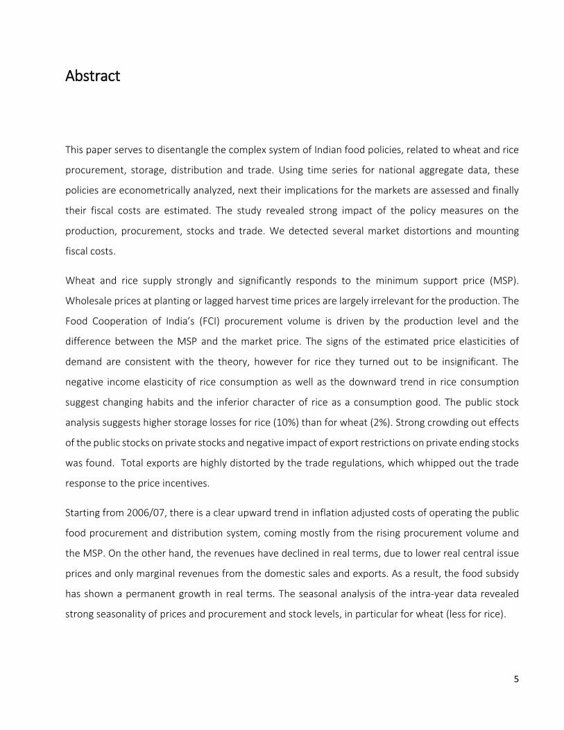
Abstract
This paper serves to disentangle the complex system of Indian food policies, related to wheat and rice
procurement, storage, distribution and trade. Using time series for national aggregate data, these
policies are econometrically analyzed, next their implications for the markets are assessed and finally
their fiscal costs are estimated. The study revealed strong impact of the policy measures on the
production, procurement, stocks and trade. We detected several market distortions and mounting
fiscal costs.
Wheat and rice supply strongly and significantly responds to the minimum support price (MSP).
Wholesale prices at planting or lagged harvest time prices are largely irrelevant for the production. The
Food Cooperation of India’s (FCI) procurement volume is driven by the production level and the
difference between the MSP and the market price. The signs of the estimated price elasticities of
demand are consistent with the theory, however for rice they turned out to be insignificant. The
negative income elasticity of rice consumption as well as the downward trend in rice consumption
suggest changing habits and the inferior character of rice as a consumption good. The public stock
analysis suggests higher storage losses for rice (10%) than for wheat (2%). Strong crowding out effects
of the public stocks on private stocks and negative impact of export restrictions on private ending stocks
was found. Total exports are highly distorted by the trade regulations, which whipped out the trade
response to the price incentives.
Starting from 2006/07, there is a clear upward trend in inflation adjusted costs of operating the public
food procurement and distribution system, coming mostly from the rising procurement volume and
the MSP. On the other hand, the revenues have declined in real terms, due to lower real central issue
prices and only marginal revenues from the domestic sales and exports. As a result, the food subsidy
has shown a permanent growth in real terms. The seasonal analysis of the intra-year data revealed
strong seasonality of prices and procurement and stock levels, in particular for wheat (less for rice).
6
1. Introduction and problem statement
The food market in India is characterized by the high degree of government involvement, especially in
two staple food grain markets – rice and wheat. The overall policy comprises of policies governing
production, procurement, storage, distribution and trade of food grains. The widespread presence of
the state resulted in the dual nature of the system – the simultaneous occurrence of public and private
sectors with the former strongly influencing (often crowding out) the latter. As a result, these sectors
are shaped by the interplay of the two forces – private and public. What is more, the system, with all
the interventions, regulations and at the same time informal and illegal transactions (like grain
diversion) has become very complex and difficult to understand and manage.
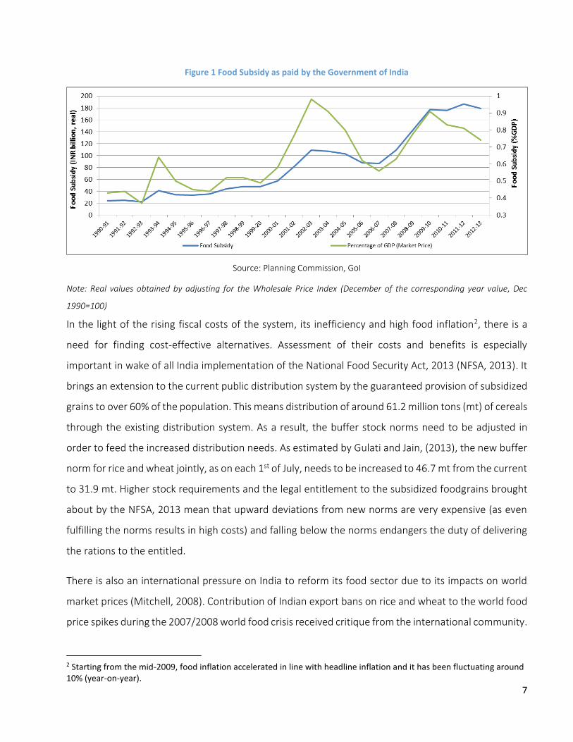
The government’s official food subsidy bill has been rising steadily from less than 0.4% in the early
1990s to around 0.8% of the GDP in the recent years (Figure 1). Apart from this direct cost, there are
additional costs that go unaccounted in the form of leakages, illegal diversion of food grains, and
significant wastage due to poor storage and transport facilities1 (Shreedhar, Gupta, Pullabhotla,
Ganesh-Kumar, & Gulati, 2012). Food, fertilizer, power and irrigation subsides together accounted for
15.1% of agricultural GDP in 2009–10 up from 7.8% of the same in 1995–96 (Ganguly & Gulati, 2013).
The Indian government is also actively involved in regulating international trade, e.g. by imposing
selective export bans and zero import duties, which fuels international food price volatility. In fact, this
trade policy may also harm Indian farmers – the domestic price, especially of rice, has been often much
lower than the international price, indicating a net taxation of Indian farmers and adding to the ‘bill’
the foregone benefits from trade (see also Anderson, 2013).
1 As computed by Swaminathan (2009) in years 2004-2005 in some states more than 20% of rural poor were excluded from the PDS (in Bihar this number amounted to 32.1%) and more than 30% of non-poor were included in the system (41.6% in Andhra Pradesh). According to Government of India estimates (GoI, 2005), in 2001 about 57% of subsidized grains did not reach the targeted group. Currently, the estimates for leakage are close to 40% (Mukherjee, 2014). This might be one of the reasons that despite staples being highly subsidized, nutrition levels of the poor remain low and a cause for much concern (von Grebmer et al., 2013).
7
Figure 1 Food Subsidy as paid by the Government of India
Source: Planning Commission, GoI
Note: Real values obtained by adjusting for the Wholesale Price Index (December of the corresponding year value, Dec
1990=100)
In the light of the rising fiscal costs of the system, its inefficiency and high food inflation2, there is a
need for finding cost-effective alternatives. Assessment of their costs and benefits is especially
important in wake of all India implementation of the National Food Security Act, 2013 (NFSA, 2013). It
brings an extension to the current public distribution system by the guaranteed provision of subsidized
grains to over 60% of the population. This means distribution of around 61.2 million tons (mt) of cereals
through the existing distribution system. As a result, the buffer stock norms need to be adjusted in
order to feed the increased distribution needs. As estimated by Gulati and Jain, (2013), the new buffer
norm for rice and wheat jointly, as on each 1st of July, needs to be increased to 46.7 mt from the current
to 31.9 mt. Higher stock requirements and the legal entitlement to the subsidized foodgrains brought
about by the NFSA, 2013 mean that upward deviations from new norms are very expensive (as even
fulfilling the norms results in high costs) and falling below the norms endangers the duty of delivering
the rations to the entitled.
There is also an international pressure on India to reform its food sector due to its impacts on world
market prices (Mitchell, 2008). Contribution of Indian export bans on rice and wheat to the world food
price spikes during the 2007/2008 world food crisis received critique from the international community.
2 Starting from the mid-2009, food inflation accelerated in line with headline inflation and it has been fluctuating around 10% (year-on-year).
8
Also the recent prorogation of implementation of the WTO Agreement on Agriculture (AoA), which
limits support for farmers to 10% of the value of production, is only a temporary solution and indicates
the inevitable change of the political paradigm to more market oriented approaches (R. Kumar, Bagaria,
& Santra, 2014).
This study serves to disentangle the major linkages between the policies and the markets of the wheat
and rice sector and to quantify the impacts of the former on the latter (and sometimes vice versa). The
policies studied are procurement, storage and distribution (with market sales and exports) policies and
the major variables of interest are stock levels, market prices and the fiscal costs.
2. Literature review
Analysis of Indian rice and wheat sector policies didn’t receive much attention in the last years. A few
studies analyzed the particular aspects or policies with isolation from the rest of the system. For
example, Sharma (2012) focused on the cost of the system – the food subsidy as generated by the Food
Cooperation of India (FCI) after 1991. The results suggest that despite the growing total cost of the food
subsidy, there have been improvements in the operational efficiency of the FCI. Also, an earlier study
on the FCI performance by Swaminathan (1999) found that the FCI improved its efficiency3 during the
90s and in many states it was more competitive4 than the private sector. A broader scope of policy
analysis, with evaluation of the effects on production productivity, accumulation of stocks, prices and
exports, was conducted by Gaiha and Kulkarni (2005). This study is much more critical of the
governmental action. The authors found, among others, that the agricultural subsidies hindered food
grain productivity growth by constraining public investments in agriculture. They also found a positive
impact of the minimum support prices (MSP) on procurement and stocks of wheat and rice. What is
more, a higher MSP increases the wholesale price, which in turn transmits to the consumer prices. The
earlier study by Gulati and Sharma (1990) analyzed the impact of the procurement price on open
market prices, procurement and output. The authors found that the procurement prices are the major
3 Two indicators were used to identify operational efficiency of the FCI – the ratio of the economic cost to procurement price and the ratio of the subsidy to procurement price. 4 The economic costs of the FCI were lower than the wholesale market price.
9
factor driving the market prices and the procurement volume to be driven by the output level and the
difference between the procurement and the market prices.
There are several works studying the demand and supply response to price changes. Mythili (2008)
used a dynamic panel data model for analyzing the supply response of the major crops before and after
the reforms in the early 90s. The study revealed that after 1990 the production response to prices
(farm-gate prices were taken into consideration) has increased and that farmers are more elastic in
their non-acreage inputs. Most of the food grain demand analysis in India is based on the household
consumption data estimates based on the National Sample Survey (NSS) data, collected by the Ministry
of Statistics and Programme Implementation. Kumar et al. (2011) analyzed price and expenditure
elasticities of demand for several goods in different income groups in India. They reported that the
expenditure elasticity of cereals consumption is very high among the very poor consumers – it is on
average equal to 0.5. This number decreases along with the higher income and turns negative for the
high income group. The average income elasticity for all income groups for rice was found to be 0.024
and for wheat 0.075, so rather low. The own price elasticities for all groups were estimated to be -0.247
for rice and -0.340 for wheat. The comprehensive study of wheat and rice demand and supply can be
found in Ganesh-Kumar et al. (2012). The demand model was also estimated based on the NSS data,
finding that the expenditure elasticity of demand for wheat and rice is negative. Production was
modeled in two ways - as aggregate with the Cobb-Douglas production function and as a product of
separately modeled yield and acreage. In both approaches the relative own to competing crop price
was one of the explanatory variables.
As in the last few years food inflation has been persistently high, there were a few studies analyzing the
sources of rising food prices in the light of food price stabilizing policies. Dasgupta et al. (2011)
conducted econometric analysis of wheat price formation in India. The results suggest that the
domestic price is only “moderately” affected by the international prices and in addition, the public
stocks have virtually no impact on wheat prices in India. The authors conclude that “public stocks are
rarely used effectively to stabilize wholesale market prices of wheat in India”. Gulati and Saini (2013)
found a significant impact of the fiscal deficit, rising farm wages and international prices on high food
inflation in India.
10
Several simulation models implemented the Indian wheat and rice sector in order to analyze the impact
of various policies. Krishna and Chhibber (1983) built a partial equilibrium model for the wheat sector
to study the consequences of the dual price policy. The model was used to simulate output,
procurement, offtakes, imports, stocks and market prices of wheat under different scenarios. They
showed a very high price sensitivity of wheat production and demand and strong response of
procurement to production level changes. Schiff (1993) is another important study which examined
the impact of the dual pricing of wheat, rice and sugar for producers and consumers with a partial
equilibrium model. He distinguished three groups of actors affected by the pricing policy – urban rich,
urban poor and the farmers and two trade regimes – free trade and closed economy. He found that
the effect of dual pricing has, under certain assumptions, a negative impact on prices and harms
farmers, although it has a positive short-run impact on the urban poor. However, as the setup of Indian
economy has changed a lot since the publication of these two papers, their results may not be
applicable anymore.
A series of more recent analysis of the sector policies within the partial equilibrium model was
conducted by Jha and Srinivasan (for example Jha & Srinivasan, 1999) and jointly with Landes the
authors published a report (Jha, Srinivasan, & Landes, 2007) with extensive sector analysis and policy
recommendations. Authors opt for more liberal, market-oriented price policies with greater reliance
on international markets.
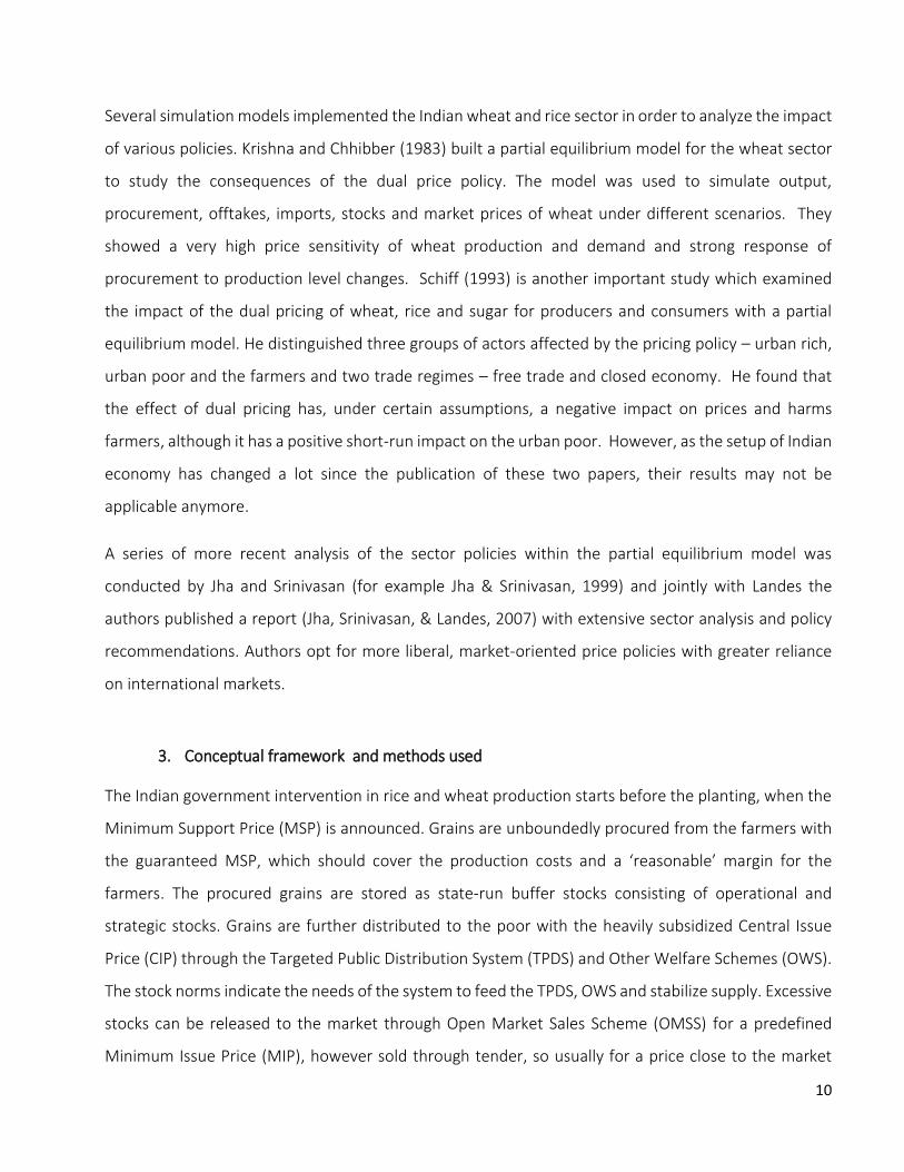
3. Conceptual framework and methods used
The Indian government intervention in rice and wheat production starts before the planting, when the
Minimum Support Price (MSP) is announced. Grains are unboundedly procured from the farmers with
the guaranteed MSP, which should cover the production costs and a ‘reasonable’ margin for the
farmers. The procured grains are stored as state-run buffer stocks consisting of operational and
strategic stocks. Grains are further distributed to the poor with the heavily subsidized Central Issue
Price (CIP) through the Targeted Public Distribution System (TPDS) and Other Welfare Schemes (OWS).
The stock norms indicate the needs of the system to feed the TPDS, OWS and stabilize supply. Excessive
stocks can be released to the market through Open Market Sales Scheme (OMSS) for a predefined
Minimum Issue Price (MIP), however sold through tender, so usually for a price close to the market
11
price; or exported, with exports and imports being concessional. Most of the operations are conducted
by the parastatal agency Food Corporation of India (FCI)5. There are also trade regulations and private
stock limitations6 used ad hoc to increase the domestic availability, isolate domestic prices from the
international prices or boost the public procurement.
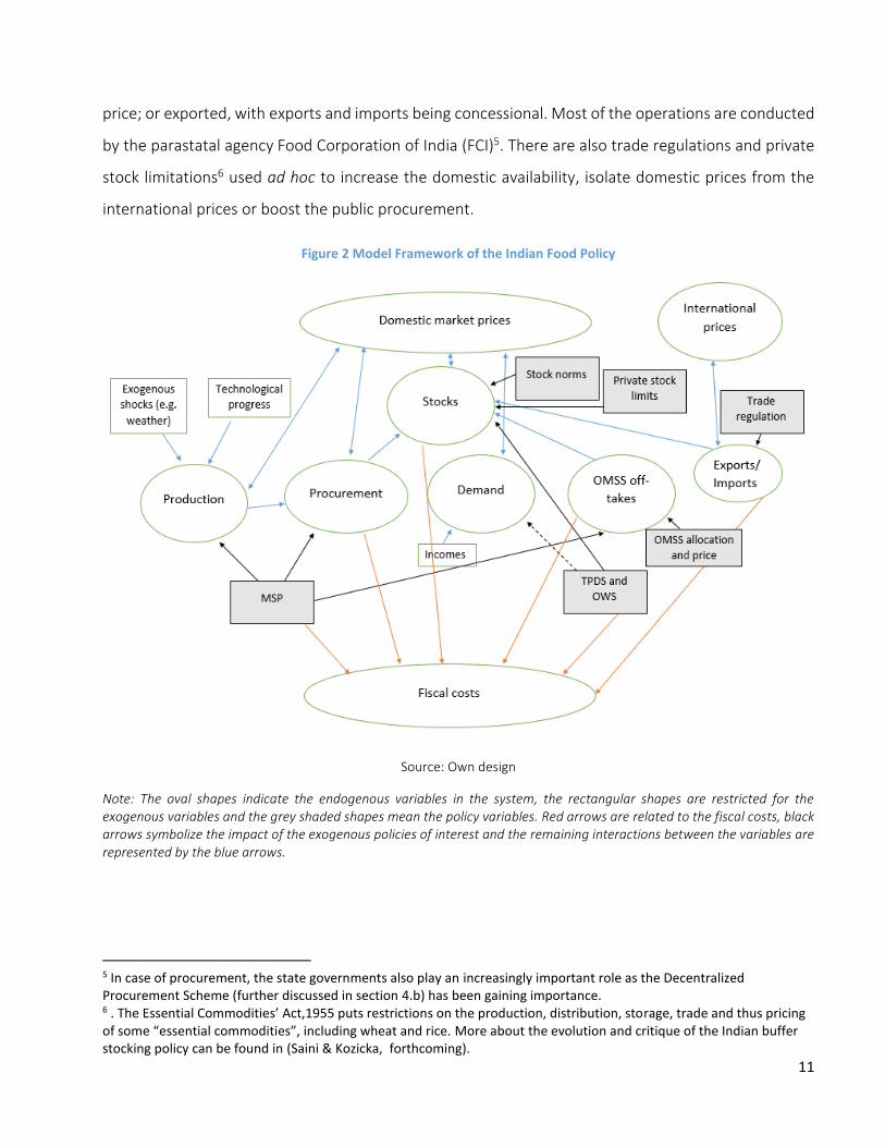
Figure 2 Model Framework of the Indian Food Policy
Source: Own design
Note: The oval shapes indicate the endogenous variables in the system, the rectangular shapes are restricted for the exogenous variables and the grey shaded shapes mean the policy variables. Red arrows are related to the fiscal costs, black arrows symbolize the impact of the exogenous policies of interest and the remaining interactions between the variables are represented by the blue arrows.
5 In case of procurement, the state governments also play an increasingly important role as the Decentralized Procurement Scheme (further discussed in section 4.b) has been gaining importance. 6 . The Essential Commodities’ Act,1955 puts restrictions on the production, distribution, storage, trade and thus pricing of some “essential commodities”, including wheat and rice. More about the evolution and critique of the Indian buffer stocking policy can be found in (Saini & Kozicka, forthcoming).
12
Figure 2 shows a graphical representation of our modeling approach of the Indian wheat and rice
sector. As it was mentioned before, even after the necessary simplification, the system is still very
complex. The main variables of interest – prices, stocks and fiscal costs are influenced by several
endogenous and exogenous variables and directly as well as indirectly by the policy measures.
The current study includes description and analysis of the different fragments of the system, with the
aim of explaining the endogenous components of Figure 2. Our aim is to empirically investigate the
relationships between the different elements on the macro-level. Identifying key drivers of prices,
demand, supply and costs will allow already an important qualitative assessment of current policies.
The empirical analysis serves, however, also another goal: By determining the functional forms and the
corresponding parameters, we can use these findings for simulating the quantitative impacts of several
policies within a partial equilibrium model at a later stage. As this model requires a consistent
representation of the macro-variables of the Indian food sector which is close to the Indian reality, we
focus on national aggregate variables from 1990 to 2013. Hence, our basic method of analysis will be
time-series analyses of these economy-wide variables which are indicated as ovals in Figure 2.7
The model, as described by equations, has a following structure:
• Production
ln 𝑄𝑡,𝑖 = 𝛼0 + γln 𝑄𝑡−1,𝑖 + 𝛼1 ln 𝑝𝑡,𝑖𝑀𝑆𝑃+ 𝛼4ln𝑡 + 𝛼5𝑅𝑡 + 휀𝑡,𝑖,
where 𝑄𝑡,𝑖 is a yearly production quantity of the i-th crop, 𝑝𝑖𝑀𝑆𝑃 is a real MSP, t is a trend variable, R is
a total yearly rainfall, 휀𝑡,𝑖 is a stochastic shock.
• Demand
𝑙𝑛 𝐷𝑡,𝑖𝑛𝑒𝑡 𝑐𝑎𝑝
= 𝛼0 + 𝛼1 ln 𝑝𝑡,𝑖 + 𝛼2 ln 𝑝𝑡,𝑖𝑐𝑟𝑜𝑠𝑠 + 𝛼3 ln 𝑃𝐷𝑆𝑡,𝑖
𝑐𝑎𝑝+ 𝛼4 ln 𝐼𝑛𝑐𝑜𝑚𝑒𝑡
𝑐𝑎𝑝+ 𝛼5 𝑡,
where 𝐷𝑡,𝑖𝑛𝑒𝑡 𝑐𝑎𝑝
is a per capita yearly consumption for the i-th crop net of consumption from the (T)PDS
and OWS (PDS), 𝑝𝑡,𝑖 is a yearly average of the own price of the i-th crop and 𝑝𝑡,𝑖𝑐𝑟𝑜𝑠𝑠 is price average of
the other crop (cross price), both in real terms. 𝐼𝑛𝑐𝑜𝑚𝑒𝑡𝑐𝑎𝑝 is a disposable income per capita and 𝑡 is
a time trend. The variable 𝑃𝐷𝑆𝑡,𝑖𝑐𝑎𝑝 is a per capita offtake for PDS.
7 Using cross-sectional household data would allow microeconomic analyses of household’s demand and supply dynamics. These data, however, do hardly cover economic activities beyond the household level (like trade, commercial storage, processing) and are only available for very few years which impedes the consideration of large developments of policies and temporal shocks.

13
• Procurement
𝐷𝑡,𝑖𝐹𝐶𝐼
𝑄𝑡,𝑖= 𝛼0 + 𝛼1
𝑝𝑡,𝑖
𝑝𝑡,𝑖𝑀𝑆𝑃 + 𝛼2𝑡,
where 𝐷𝑡,𝑖𝐹𝐶𝐼 is the yearly procurement level of the i-th crop, 𝑝𝑡,𝑖. Thus, on the left hand side of the
equation there is the share of public procurement in total production and on the right hand side, there
is ratio of market price and the MSP and the trend.
• Private stocks
𝑋𝑡,𝑖𝑝𝑟𝑖𝑣
𝐷𝑡,𝑖𝑡𝑟𝑒𝑛𝑑 = 𝛼0 + 𝛼1
𝑆𝑡,𝑖
𝐷𝑡,𝑖𝑡𝑟𝑒𝑛𝑑 + 𝛼2𝐵𝑡,𝑖 + 𝛼3
𝑋𝑡,𝑖
𝐷𝑡,𝑖𝑡𝑟𝑒𝑛𝑑,
where 𝑋𝑡,𝑖𝑝𝑟𝑖𝑣 is a private stocks of the i-th crop in the marketing year t, 𝐷𝑡,𝑖
𝑡𝑟𝑒𝑛𝑑 is a consumption trend,
𝑆𝑡,𝑖 is a total market supply calculated as 𝑆𝑡,𝑖 = 𝑄𝑡,𝑖 + 𝑋𝑡−1,𝑖𝑝𝑟𝑖𝑣 and 𝐵𝑡,𝑖 is an export ban dummy.
• Exports
𝐸𝑥𝑝𝑡,𝑖
𝑄𝑡,𝑖= 𝛼0 + 𝛼1∆𝐺𝐷𝑃𝑡 + 𝛼2𝐵𝑡−1,𝑖 + 𝛼3
𝑝𝑡−1,𝑖
𝑝𝑡−1,𝑖𝑖𝑛𝑡 ,
where 𝐸𝑥𝑝𝑡,𝑖 is a total volume of exported in a financial year, ∆𝐺𝐷𝑃𝑡 is a first difference of the GDP of
the major importers of Indian wheat and rice, 𝐵𝑡−1,𝑖 is a lagged export ban dummy, 𝑝𝑡−1,𝑖
𝑝𝑡−1,𝑖𝑖𝑛𝑡 is a lagged
price ratio – domestic wholesale to international, converted to INR.
• Fiscal costs
𝐹𝐶𝑡,𝑖 = (𝑐𝑡,𝑖𝑝 + 𝑝𝑡,𝑖
𝑀𝑆𝑃)𝐷𝑡,𝑖𝐹𝐶𝐼 + 𝑐𝑡,𝑖
𝑑 𝑃𝐷𝑆𝑡,𝑖 + 𝑘𝑡𝑋𝑡,𝑖 − 𝑝𝑡,𝑖𝑃𝐷𝑆𝑃𝐷𝑆𝑡,𝑖 − 𝑝𝑡,𝑖𝑂𝑀𝑆𝑆𝑡,𝑖 − 𝑝𝑡,𝑖
𝐸𝑋𝑁𝐸𝑋𝑡,𝑖𝑝𝑢𝑏 ,
where 𝐹𝐶𝑡,𝑖 are yearly fiscal costs related to the i-th crop, (𝑐𝑡,𝑖𝑝 + 𝑝𝑡,𝑖
𝑀𝑆𝑃)𝐷𝑡,𝑖𝐹𝐶𝐼 are acquisition costs,
𝑐𝑡,𝑖𝑑 𝑃𝐷𝑆𝑡,𝑖 are distribution costs, 𝑘𝑡𝑋𝑡,𝑖 buffer carrying cost (where 𝑋𝑡,𝑖 is an average in the financial year
buffer stock of wheat and rice in the central pool) and 𝑝𝑡,𝑖𝑃𝐷𝑆𝑃𝐷𝑆𝑡,𝑖 + 𝑝𝑡,𝑖𝑂𝑀𝑆𝑆𝑡,𝑖 + 𝑝𝑡,𝑖
𝐸𝑋𝑁𝐸𝑋𝑡,𝑖𝑝𝑢𝑏 are
sales realizations (revenues) from sales from PDS, OMSS and net public exports offtakes.
• Public stocks – identity equation
𝑋𝑡,𝑖 = (1 − 𝛿𝑖)𝑋𝑡−1,𝑖 + 𝐷𝑡,𝑖𝐹𝐶𝐼 − 𝑂𝑀𝑆𝑆𝑡,𝑖 − 𝑇𝑃𝐷𝑆𝑡,𝑖 − 𝑁𝐸𝑋𝑡,𝑖
𝑝𝑢𝑏,
where 𝛿𝑖 is a public stock deterioration rate.
The following chapter includes the analysis of the endogenous variables and estimation results.

14
4. Policies, their measures and outcomes
a. Prices
In order to understand what determines demand, supply and storage, we need to find out which prices
are paid and received by different actors in the market. Regulated prices like the MSP, the MIP and the
CIP are usually set on the central level and differ only slightly on the state level8. They influence,
however, market prices due to the high level of government involvement. The market prices include
farm-gate prices, wholesale prices and retail prices. Regulated and market prices can be grouped as
follows: the MSP with farm-gate price as producer prices, MIP and wholesale price (Wholesale Price
Index (CPI) component) as trader prices and finally CIP and retail price (Consumer Price Index (CPI)
component) as consumer price.
Market prices differ a lot (price time series from selected markets can be found in the Appendix 3) due
to the state specific environment (like the efficiency of the procurement or state-specific bonuses to
the MSP and taxes) and weak market integration (Acharya, Chand, Birthal, Kumar, & Negi, 2007; Baylis,
Jolejole-Foreman, & Mallory, 2013). This is important for analyzing the relationships between the
variables, as the production and consumption levels in different states vary significantly. But for the
purpose of our analysis, which deals with the all-India yearly aggregates, we need to consider a
weighted price average which reflects the market forces and influences the decisions of the different
actors. This price needs to represent prices faced by consumers, producers and traders and at the same
time it needs to consider the shares of different markets in the country. We therefore use a commodity-
specific Wholesale Price Index, which captures the overall demand and supply conditions of the food
market. Its components are trade weighted averages, collected on many markets and it is available on
a monthly basis. Based on this monthly index, we calculate average price dynamics for different periods,
corresponding with the times when our endogenous variables are determined. For example, to analyze
8 Unfortunately these state-level differences are difficult to track, especially in a historical perspective. For example, bonuses to the MSP are sometimes used by the local governments but data on them is rarely available. Even bigger issues are the institutional differences between the states – like the almost universal coverage of the TPDS in Kerela, or extremely high level of leakages in Bihar. Furthermore, the procurement efficiency of the FCI/ state level procurement agencies is not uniform in all the states across the country. It is relatively better functioning in a few states (Punjab, Haryana, parts of Andhra Pradesh, and in recent years also in Chattisgarh) but is mostly ineffective in others (Bihar, Orissa, etc.). As the purpose of this study is to assess the impact of the central policies on the all India aggregate outcomes, considering these state-wise differences would bring too much complexity in the analysis and the model would become intransparent.
15
the production determinants, we used averages for harvest months, planting months and marketing
year, which are different for wheat and rice. Marketing year averages are also important for the
demand analysis.
Wheat and rice components of the WPI are indices, which makes them difficult to compare with the
price levels, like the MSP or farm-gate prices. In order to obtain a representative for the whole India
wholesale price, these monthly indexes were adjusted to match the average price level at the end of
the sample period – so they were multiplied by the last available four-year production weighed average
price from the major markets. The WPI index is less volatile than the wholesale price index constructed
with the market prices form the major grain-producing states (see Appendix 1 for comparison of the
price averages). Then, for different purposes, different annual averages were created: for production,
the prices during the harvest months were considered which, in the case of rice, were weighted
according to the production share in Kharif and Rabi seasons. For consumption, the marketing year
average price was used. The WPI is a trade weighted average. The farm gate price is a state-wise
production weighted harvest time price average. As the representative international price, the
International Monetary Fund quoted prices were used. For wheat ‘No.1 Hard Red Winter, ordinary
protein, FOB Gulf of Mexico, US$ per metric ton’ and for rice ‘5 percent broken milled white rice,
Thailand nominal price quote, US$ per metric ton’. Both were converted to INR with the current
exchange rate.
In order to obtain the real prices, all nominal prices are WPI deflated. CPI is positively correlated with
prices, which is most probably due to the high share of wheat and rice in the CPI. The share of the
‘cereals and products’ group in the CPI agricultural laborer basket is more than 40%. In the WPI the
share of wheat and rice is less than 3% jointly. Also Krishna and Chhibber (1983) used the WPI deflated
prices in their modeling of Indian grain market.
The comparison of the derived price time series is presented in Figure 3 and Figure 4. The wheat farm
gate price and the MSP were quite closely connected, especially starting from the late 90’s. An
interesting trend observed both on the wheat and rice markets is the narrowing gap between the MSP
and the wholesale prices. It is also clear that the Indian domestic prices were successfully protected
from the international price fluctuations, avoiding the up- and down-swings in the mid - 90’s and during

16
and after the 2007/2008 food crisis. Wheat domestic prices, except for the few years of world price
spikes, were above the international prices, whereas rice domestic prices for most of the time remained
below the international quotes.
Figure 3 Wheat producer prices (real, in INR per quintal)
Source: Own design based on data from indiastat.com, RBI, DFPD, eands.dacnet.nic.in, IMF
Figure 4 Rice (in paddy) producer prices (real, in INR per quintal)
Source: Own design based on data from indiastat.com, RBI, IMF

17
Wheat wholesale market price changes (both at harvest time and yearly average) are only slightly
correlated with MSP changes (Table 1). The MSP changes are highly correlated with the farm gate price
changes, which in turn are somewhat linked to the harvest time market prices. This is due to the
seasonality in production and prices of wheat in India. For rice, all three price dynamics, i.e. the MSP,
and the two market averages are strongly correlated, which can be attributed to the more stable
monthly pattern of rice market arrivals and little seasonality in prices.
Table 1. Correlation of different prices for wheat and rice (nominal first differences between the consecutive years)
Wheat Rice
MSP Farm-gate
price
WPI marketing
year
WPI harvest
time
MSP WPI marketing
year
WPI harvest
time
MSP 1 1
Farm-gate price 0.66 1
WPI marketing year 0.13 0.18 1 0.8 1
WPI harvest time 0.25 0.43 0.5 1 0.74 0.88 1
Source: Own design based on MOSPI, DAC, DFPD.
WPI – wheat and rice components of the wholesale price index; based on harvest time9 average (for rice these are the production weighted averages in the two seasons) and marketing year average; farm-gate prices for rice are missing due to changing rice varieties and unclear season quotes.
The CIP has been very low and it was changed very rarely. Is has been kept constant in nominal terms
for the Below Poverty Line (BPL) and Above Poverty Line (APL) cardholders from July 2002 and for the
group of ‘poorest of the poor’ (AAY) from beginning of 2001.
These different dynamics and changing relationships between the prices, especially the regulated and
the market prices, as well as our particular interest in the impact of the policies on the market outcomes
resulted in decision to estimate the independent system equations (presented in the chapter 3), as
opposed to the simultaneously solved system of equations. This also allowed us test for the relevance
of different period price averages for the farmers’ decision making. The endogeneity problems were
solved with the instrumental variables estimation techniques.
9 Harvest months for wheat are March – May and for rice, October – December for the Kharif season and March – June for the Rabi season.
18
b. Production
The government uses both input subsidies and output price support (MSP) to boost production. The
MSP serves also for farmers’ income stabilization. The MSP for rice and wheat, ”which along with other
factors, takes into consideration the cost of various agricultural inputs and the reasonable margin for
the farmers for their produce” (FCI web portal, n.d.), is announced before the planting of each of the
two seasons – Rabi and Kharif.
Rice is sown and harvested in two seasons. The major (Kharif) season sowing lasts from June till
September and harvesting follows in the three consecutive months. Right after harvesting starts sowing
of the Rabi crop which is harvested from March to June. Thus, market arrivals of rice happen with some
fluctuations but throughout the year. This is one of the important differences between the rice and the
wheat sector.
Wheat and rice usually do not compete for area – they are in majority produced in different regions -
wheat dominantly in the north and rice in the south10. Wheat, as compared to rice, is more often
produced by commercial farmers, whereas rice in majority is cultivated by small-scale farmers11. The
wheat sector shows higher investments and irrigation – the latter has risen from 81% in 1990-1991 to
above 91% currently, as compared to rice with growth from 45.5% to 58% (DAC, Ministry of
Agriculture). As a result, rice production is highly dependent on the rainfall and is characterized by
greater yield variability.
Public procurement plays a very important role in both sectors. Rice is procured directly from farmers
in the form of paddy at the MSP (open end procurement) or from millers/traders (with obligatory levy12
currently ranging from 30% to 75% depending on the state) at the ‘levy’ price, which is the MSP plus
the milling cost. Wheat is procured directly from producers at the MSP. The dominant share of the
government’s involvement, especially in the recent years, can be traced by the procurement levels (see
Figure 5 and Figure 6). For both crops share of the public procurement in the total production has been
10 For wheat the major competing crops are chickpea (gram), rapeseed and mustard and for rice mostly sugarcane. 11 Indian agriculture in general is characterized by high degree of fragmentation - 80% of farms are of small or marginal size. 12 This is an indirect taxation on rice millers/traders who are required to deliver rice to the government agencies at the prices derived from the minimum support price of paddy, before selling the remaining rice in the open market.

19
close or even above 30%. But when we take into consideration only the marketed grains, the share
increases to around 50%, which means that about half of the grains which are sold by the farmers go
to the FCI.
Figure 5 Wheat production, marketed surplus and procurement (as part of production) - in million tons
Source: Own design based on data from indiastat.com database
Figure 6 Rice production, marketed surplus and procurement (as part of production) - in million tons
Source: Own design based on indiastat.com database
0
10
20
30
40
50
60
70
80
90
100
Farm Market FCI
20
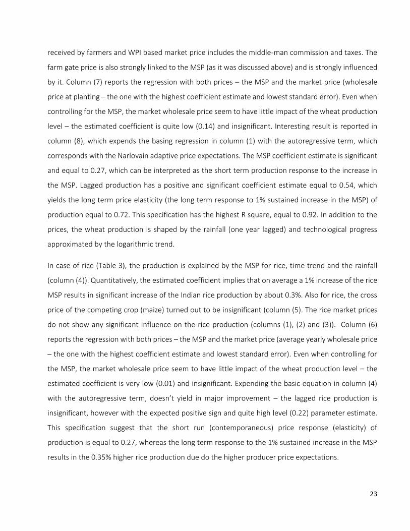
This strong governmental involvement is reflected in a high correlation of the market price with the
MSP, as it was discussed in section a. As we will see, it has also serious implications for the production
determination: not only has the MSP the largest impact on the production level, but also it has wiped
out the market impact on the farmer’s production decisions. Neither do the input market prices
influence the production decisions as the agricultural inputs are heavily subsidized and their nominal
prices change very rarely.
The general equation for describing production is given by:
1 ln 𝑄𝑡,𝑖 = 𝛼0 + γln 𝑄𝑡−1,𝑖 + 𝛼1 ln 𝑝𝑡,𝑖𝑀𝑆𝑃 + 𝛼2 ln 𝑝𝑡,𝑖 + 𝛼3 ln 𝑝𝑡,𝑗 + 𝛼4ln𝑡 + 𝛼5𝑅𝑡 + 휀𝑡,𝑖,
where 𝑄𝑡,𝑖 is yearly production quantity of the i-th crop (USDA data), 𝑝𝑖𝑀𝑆𝑃 is a real MSP (WPI deflated)
and 𝑝𝑡,𝑖 is a market price of the i-th crop (WPI deflated). The contemporaneous MSP is considered
because farmers know the MSP before planting and there is little uncertainty related to receiving this
price. As the representatives of the market price, lagged harvest time and planting time, as well as
lagged marketing year price averages were taken into consideration. The lag structure of the market
price reflects the assumption of naïve price expectation - the farmers expect the current year price to
be the same as the previous year’s price (harvest time and the yearly average prices) or alternatively
the price they observed at planting. Later, we econometrically test, whether they really do. We also
incorporated the Nerlovian (Nerlove, 1956) price expectation model with the adaptive expectations by
including the lagged production as the explanatory variable. Also cross prices 𝑝𝑡,𝑗 of respective crops
were used as explanatory variables – gram for wheat and maize for rice13. t is a trend variable, R is a
total yearly (calendar year) rainfall (IMD data14). Using ordinary least square method and data for 1990-
2012 gives the following results for different specifications:
13 Wheat and rice do not compete in production. 14 http://www.imd.gov.in/

21
Table 2. Regressions for wheat production
Dependent variable: log wheat production
(1) (2) (3) (4) (5) (6) (7) (8)
Lag log wheat
production
0.54**
(2.65)
Log MSP 0.49***
(3.25)
0.47***
(3.15)
0.46**
(2.78)
0.33**
(2.29)
Lag log WPI price
(harvest)
-0.03
(-0.09)
Lag log WPI price
(yearly)
0.28
(0.68)
Log WPI price (planting) 0.30
(1.61)
0.14
(0.79)
Log WPI cross price
(wheat planting time
gram price)
-0.08
(1.20)
Lag log farm-gate price 0.41***
(3.48)
Log time trend 0.15***
(8.52)
0.23***
(11.75)
0.15***
(8.65)
0.22***
(10.34)
0.23***
(8.89)
0.19***
(8.27)
0.16***
(6.39)
0.07**
(1.96)
Lag log rainfall 0.35*
(2.81)
0.23
(1.14)
0.35**
(2.67)
0.17
(0.78)
0.32*
(2.00)
0.26**
(2.29)
0.39***
(3.68)
0.45***
(4.22)
Constant 1.21
(1.32)
1.91
(1.22)
1.25***
(1.31)
2.59
(1.65)
0.67
(0.51)
1.79**
(2.14)
0.57
(0.70)
-1.50
(-1.25)
N 23 22 23 22 23 21 22 22
R² 0.89 0.80 0.9 0.79 0.83 0.84 0.89 0.92
Note. *,**,*** indicates significance levels at 10, 5 and 1%, respectively with the robust standard error estimation. In
brackets t-values are given. Error terms do not show a clear non-stationarity pattern.
22
Table 3 Regressions of rice production
Dependent variable: log rice production
(1) (2) (3) (4) (5) (6) (7)
Lag log rice production 0.22
(1.41)
Log MSP 0.31**
(2.32)
0.26*
(2.01)
0.30**
(2.43)
0.27**
(2.07)
Lag log WPI price (harvest) 0.07
(0.42)
Lag log WPI price (yearly) 0.23
(1.06)
0.01
(0.06)
Log WPI price (planting) 0.14
(0.50)
Log WPI cross price (kharif
planting maize price)
0.1
(0.97)
Log time trend 0.17***
(4.83)
0.19***
(4.32)
0.15***
(6.38)
0.12***
(6.32)
0.13***
(6.28)
0.14***
(3.57)
0.10***
(4.04)
Log rainfall 0.48*
(1.83)
0.51*
(1.95)
0.45
(1.69)
0.55**
(2.32)
0.56**
(2.32)
0.57**
(2.3)
0.63***
(2.43)
Constant 0.69
(0.36)
-0.16
(-0.07)
0.51
(0.21)
0.24
(0.14)
0.16
(0.09)
-0.03
(-0.01)
-1.24
(-0.57)
N 21 21 22 22 22 22 21
R² 0.71 0.72 0.71 0.78 0.79 0.78 0.79
Note. *,**,*** indicates significance levels at 10, 5 and 1%, respectively with the robust standard error estimation. In
brackets t-values are given. Error terms do not show a clear non-stationarity pattern.
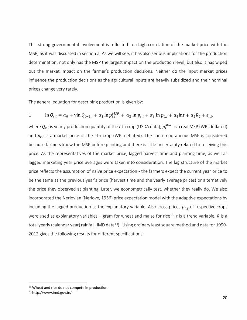
Table 2 presents our estimates of the average price elasticities of wheat production in India. Column
(1) shows estimates where the wheat production is explained by the contemporaneous MSP, the lagged
rainfall and a time trend. Column (3) adds to this regression the price (average at wheat planting period)
of competing crop, gram (chickpea), which gives slightly negative, however insignificant impact of this
variable on wheat production. In both cases the impact of the wheat MSP on wheat production is strong
and significant, implying that on average a 1% increase of the MSP significantly increases the wheat
production in the same marketing year by about 0.5%. Columns (2), (4), (5) and (7) suggest that the
wholesale market prices don’t play a significant role for the wheat production in India. On the contrary,
the lagged farm gate price (column (6) has a strong significant influence on wheat production, similar
to the MSP effect. This is an intuitive result as the farm gate price is the actual producer price, as
23
received by farmers and WPI based market price includes the middle-man commission and taxes. The
farm gate price is also strongly linked to the MSP (as it was discussed above) and is strongly influenced
by it. Column (7) reports the regression with both prices – the MSP and the market price (wholesale
price at planting – the one with the highest coefficient estimate and lowest standard error). Even when
controlling for the MSP, the market wholesale price seem to have little impact of the wheat production
level – the estimated coefficient is quite low (0.14) and insignificant. Interesting result is reported in
column (8), which expends the basing regression in column (1) with the autoregressive term, which
corresponds with the Narlovain adaptive price expectations. The MSP coefficient estimate is significant
and equal to 0.27, which can be interpreted as the short term production response to the increase in
the MSP. Lagged production has a positive and significant coefficient estimate equal to 0.54, which
yields the long term price elasticity (the long term response to 1% sustained increase in the MSP) of
production equal to 0.72. This specification has the highest R square, equal to 0.92. In addition to the
prices, the wheat production is shaped by the rainfall (one year lagged) and technological progress
approximated by the logarithmic trend.
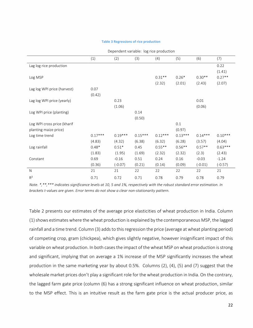
In case of rice (Table 3), the production is explained by the MSP for rice, time trend and the rainfall
(column (4)). Quantitatively, the estimated coefficient implies that on average a 1% increase of the rice
MSP results in significant increase of the Indian rice production by about 0.3%. Also for rice, the cross
price of the competing crop (maize) turned out to be insignificant (column (5). The rice market prices
do not show any significant influence on the rice production (columns (1), (2) and (3)). Column (6)
reports the regression with both prices – the MSP and the market price (average yearly wholesale price
– the one with the highest coefficient estimate and lowest standard error). Even when controlling for
the MSP, the market wholesale price seem to have little impact of the wheat production level – the
estimated coefficient is very low (0.01) and insignificant. Expending the basic equation in column (4)
with the autoregressive term, doesn’t yield in major improvement – the lagged rice production is
insignificant, however with the expected positive sign and quite high level (0.22) parameter estimate.
This specification suggest that the short run (contemporaneous) price response (elasticity) of
production is equal to 0.27, whereas the long term response to the 1% sustained increase in the MSP
results in the 0.35% higher rice production due do the higher producer price expectations.

24
The price elasticity of rice production is smaller for rice than for wheat, which can be explained by the
big share of small-scale farmers in rice producers and more commercial character of wheat production.
49% and 31% price elasticities of production are considerably high – relatively to estimates of the
market price elasticities in other countries. For example in the FAPRI database15 the price elasticities of
rice supply are usually close to 0.2, with the value of 0.25 in Bangladesh and 0.16 in China (0.11 in India).
The same database quotes price elasticities of wheat area response are slightly higher, averaging for
example to 0.33 in Australia, 0.43 in Brazil and 0.09 in China (0.29 in India). The high MSP-elasticity in
India might be explained by the low risk related to the MSP.
Gulati and Sharma (1990) used slightly different specification of the output equation for Indian wheat
and rice production. They used lagged output, lagged relative wholesale price, rainfall and irrigation to
explain wheat and rice production in India. Also the estimation was based on data from 1969 to 1986,
so before the structural change in the 90-ties. They found a significant and strong impact of the market
price, with the short term (one year) elasticity 0.28 for wheat and 0.25 for rice. The long term (three-
year) elasticities were 0.83 for wheat and 0.72 for rice. Mythili (2008) found lower short run price
(relative price) elasticity of wheat and rice supply. In post reform period (1990/91-2004/05), the
estimated short run price elasticity of wheat supply is 0.17 (and 0.16 with the alternative specification)
and of rice supply is 0.28 (and 0.18 with the alternative specification). Also in this study the long run
supply response was estimated, with wheat long run elasticity equal to 0.36 (0.29 with the alternative
specification) and rice 0.7 (0.51 with the alternative specification). Neither of these studies used the
MSP as an explanatory variable.
c. Procurement
The share of wheat procurement in total production has been fluctuating between 11% and 33% since
the beginning of the 90s, with the steep increase in the last years (see Figure 5). Rice procurement has
been characterized by a more stable trend – from less than 14% in 1991 to average 34% in the last five
years (see Figure 6). These tendencies are strongly coinciding with the MSP dynamics, especially in
relation to the market price. The MSP was oscillating around 70% of the wholesale price until the 2007.
15 http://www.fapri.iastate.edu/tools/elasticity.aspx
25
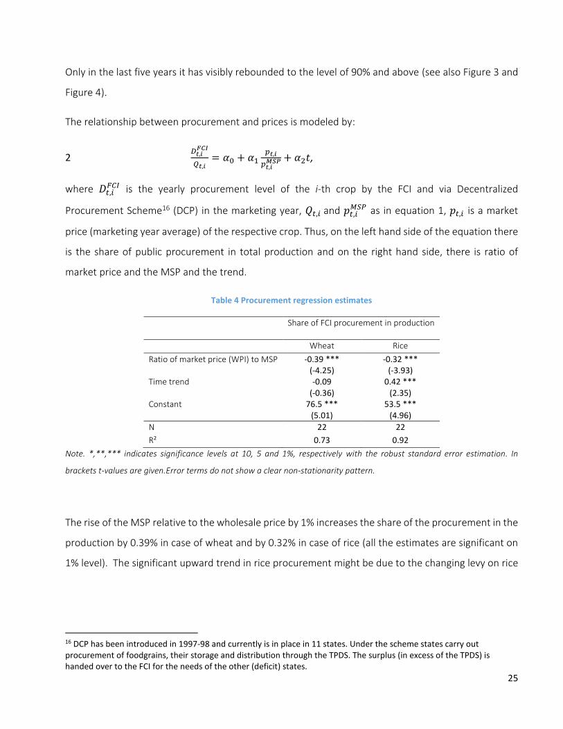
Only in the last five years it has visibly rebounded to the level of 90% and above (see also Figure 3 and
Figure 4).
The relationship between procurement and prices is modeled by:
2 𝐷𝑡,𝑖
𝐹𝐶𝐼
𝑄𝑡,𝑖= 𝛼0 + 𝛼1
𝑝𝑡,𝑖
𝑝𝑡,𝑖𝑀𝑆𝑃 + 𝛼2𝑡,
where 𝐷𝑡,𝑖𝐹𝐶𝐼 is the yearly procurement level of the i-th crop by the FCI and via Decentralized
Procurement Scheme16 (DCP) in the marketing year, 𝑄𝑡,𝑖 and 𝑝𝑡,𝑖𝑀𝑆𝑃 as in equation 1, 𝑝𝑡,𝑖 is a market
price (marketing year average) of the respective crop. Thus, on the left hand side of the equation there
is the share of public procurement in total production and on the right hand side, there is ratio of
market price and the MSP and the trend.
Table 4 Procurement regression estimates
Share of FCI procurement in production
Wheat Rice
Ratio of market price (WPI) to MSP -0.39 *** (-4.25)
-0.32 *** (-3.93)
Time trend -0.09 (-0.36)
0.42 *** (2.35)
Constant 76.5 *** (5.01)
53.5 *** (4.96)
N 22 22
R² 0.73 0.92
Note. *,**,*** indicates significance levels at 10, 5 and 1%, respectively with the robust standard error estimation. In
brackets t-values are given.Error terms do not show a clear non-stationarity pattern.
The rise of the MSP relative to the wholesale price by 1% increases the share of the procurement in the
production by 0.39% in case of wheat and by 0.32% in case of rice (all the estimates are significant on
1% level). The significant upward trend in rice procurement might be due to the changing levy on rice
16 DCP has been introduced in 1997-98 and currently is in place in 11 states. Under the scheme states carry out procurement of foodgrains, their storage and distribution through the TPDS. The surplus (in excess of the TPDS) is handed over to the FCI for the needs of the other (deficit) states.
26
millers/traders. It could also be caused by decreasing transportation costs due to better infrastructure
in rice growing areas which gives farmers more incentive to sell to FCI.
Also Gulati and Sharma (1990) estimated a similar procurement equation, however allowing for an
additive impact of the production level. Their results indicate strong procurement response to the
production, with the elasticity equal 1.37 for wheat and 1.1 for rice. The relative price elasticity
(procurement to market price ratio) was estimated 0.85 for wheat and 0.59 for rice. However, these
numbers cannot be compared with our estimates due to different equation specification.
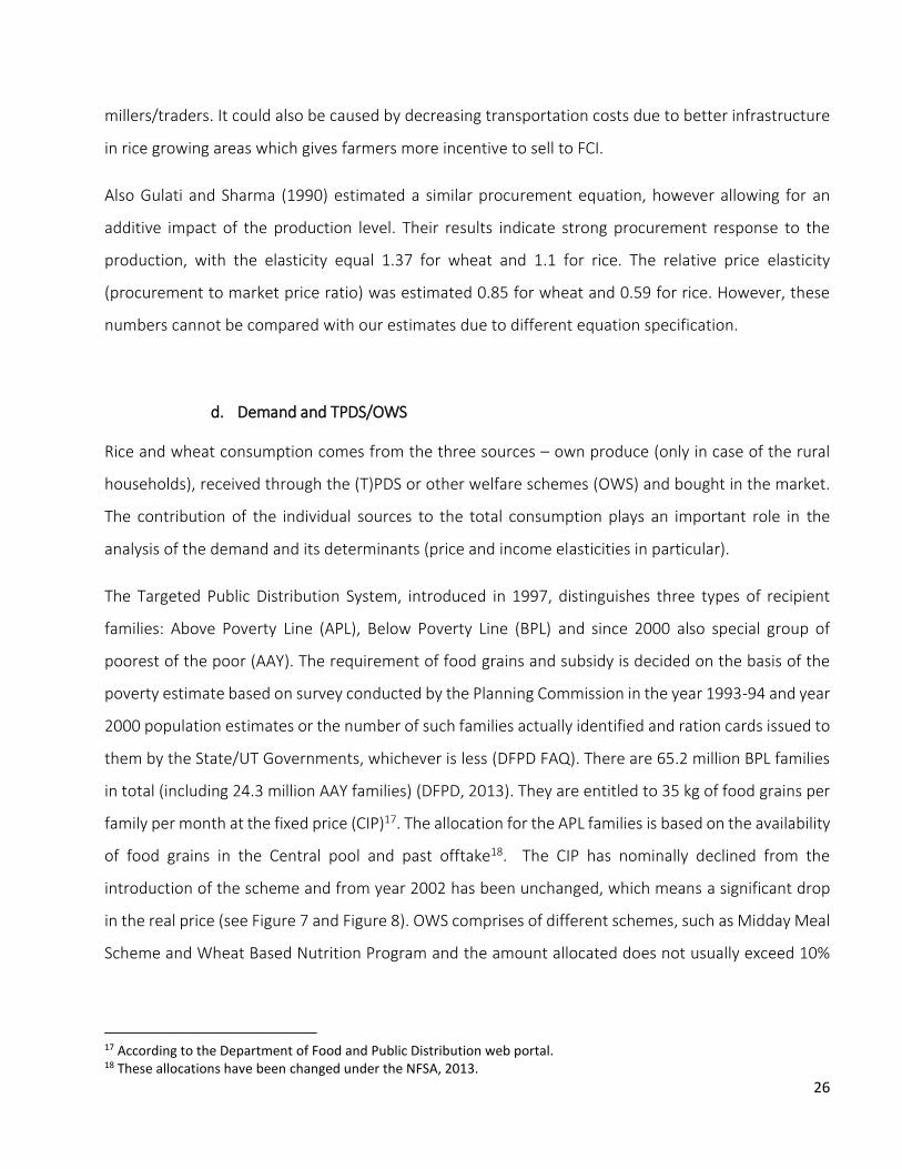
d. Demand and TPDS/OWS
Rice and wheat consumption comes from the three sources – own produce (only in case of the rural
households), received through the (T)PDS or other welfare schemes (OWS) and bought in the market.
The contribution of the individual sources to the total consumption plays an important role in the
analysis of the demand and its determinants (price and income elasticities in particular).
The Targeted Public Distribution System, introduced in 1997, distinguishes three types of recipient
families: Above Poverty Line (APL), Below Poverty Line (BPL) and since 2000 also special group of
poorest of the poor (AAY). The requirement of food grains and subsidy is decided on the basis of the
poverty estimate based on survey conducted by the Planning Commission in the year 1993-94 and year
2000 population estimates or the number of such families actually identified and ration cards issued to
them by the State/UT Governments, whichever is less (DFPD FAQ). There are 65.2 million BPL families
in total (including 24.3 million AAY families) (DFPD, 2013). They are entitled to 35 kg of food grains per
family per month at the fixed price (CIP)17. The allocation for the APL families is based on the availability
of food grains in the Central pool and past offtake18. The CIP has nominally declined from the
introduction of the scheme and from year 2002 has been unchanged, which means a significant drop
in the real price (see Figure 7 and Figure 8). OWS comprises of different schemes, such as Midday Meal
Scheme and Wheat Based Nutrition Program and the amount allocated does not usually exceed 10%
17 According to the Department of Food and Public Distribution web portal. 18 These allocations have been changed under the NFSA, 2013.
27
of the TPDS. Also special additional allocations of food grains are made, depending on the grain
availability (based on DFPD Foodgrains Bulletins from different years).
Figure 7 Wheat CIP and wholesale price – WPI deflated (in INR/qtl)
Source: Own design based on DFPD data
Figure 8 Rice CIP and wholesale price – WPI deflated (in INR/qtl)
Source: Own design based on DFPD data
0
100
200
300
400
500
600
700
800
900
CIP wheat BPL CIP wheat APL CIP wheat AAY Market wheat price
28
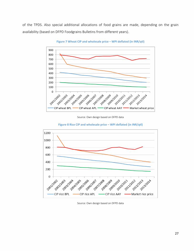
Leakages19 from the TPDS are the major challenge in estimating the ‘market’ consumption of wheat
and rice. The ‘leaked’ grains are sold on the market at the market price or exported to the neighboring
countries, e. g. Bangladesh. 22% (1.2 kg/capita/month) of total consumption of rice and 12.3% (0.5
kg/capita/month) of wheat came from the TPDS in 2009/10 (NSS data). These numbers have increased
from 1999 (13.1% and 4.5% respectively). This can be attributed to the lesser leakages (there is no
consistent historical data on leakages from the TPDS available) and increased TPDS allocations and
offtakes (Figure 9). However, it is still much less than the TPDS entitlements (discussed above) and per
capita offtakes – 1.9 kg/capita/month of rice and 1.5 kg/capita/month of wheat.
Figure 9 Offtakes from the public stocks for the (T)PDS and OWS (million tons, within the financial years)
Source: Own design based on Food Grain Bulletin data, dfpd.nic.in
25% and 37% (1.2 kg and 1.5 kg per capita per month) of rice and wheat respectively of total
consumption of the rural households came from the home grown stock in 2009/10 and 30% and 40%
in 2004/05, which was the drought year (NSS data). As it has been discussed earlier in this paper, rice
is mostly produced by the small-holders, whereas wheat is a more commercial crop. This fact has its
19 Currently, the estimates for leakage are close to 40% (Mukherjee, 2014).
0
5
10
15
20
25
30
35
19
90
/19
91
19
91
/19
92
19
92
/19
93
19
93
/19
94
19
94
/19
95
19
95
/19
96
19
96
/19
97
19
97
/19
98
19
98
/19
99
19
99
/20
00
20
00
/20
01
20
01
/20
02
20
02
/20
03
20
03
/20
04
20
04
/20
05
20
05
/20
06
20
06
/20
07
20
07
/20
08
20
08
/20
09
20
09
/20
10
20
10
/20
11
20
11
/20
12
PDS wheat offtakes PDS rice offtakes
29
reflection not only in production function, but also in the quantity of grains retained on farm (and
marketed surplus) in response to the price changes.
Figure 10 Wheat marketing year and harvest time price averages, CPI and WPI deflated (in INR/qtl, right axis), and
quantity of the grain retained on farm (in million tons, left axis)
Source: Own design based on http://agricoop.nic.in/agristatistics.htm and RBI data
Figure 11 Rice marketing year and harvest time price averages, CPI and WPI deflated (in INR/qtl, right axis), and
quantity of the grain retained on farm (in million tons, left axis)
Source: Own design based on http://agricoop.nic.in/agristatistics.htm and RBI data
30
Wheat reacts more like a cash crop (Figure 10); it is highly sensitive to the producer price – the WPI
deflated harvest time average wheat WPI – with the correlation equal to -0.54. This might mean that
farmers decide to sell more in times of high market prices during the harvest. What is interesting, they
also retain more (consume more from the home production, when the yearly CPI deflated price is high).
The correlation is equal to 0.32.
In case of rice (Figure 11), the higher the market prices, the more is consumed from the own produce.
The yearly average CPI deflated price (relevant from the consumer perspective) has the highest
correlation with the quantity retained – almost 0.4. This is probably driven by the poorest farmers, for
whom rice may be a Giffen good20. When the harvest time average, WPI deflated price is taken into
consideration, the correlation becomes even slightly negative, which means that the farmers decide to
sell more with the higher price.
The general equation for describing demand is given by:
3 ln 𝐷𝑡,𝑖𝑐𝑎𝑝 = 𝛼0 + 𝛼1 ln 𝑝𝑡,𝑖 + 𝛼2 ln 𝑝𝑡,𝑖
𝑐𝑟𝑜𝑠𝑠 + 𝛼3 ln 𝑃𝐷𝑆𝑡,𝑖𝑐𝑎𝑝 + 𝛼4 ln 𝐼𝑛𝑐𝑜𝑚𝑒𝑡
𝑐𝑎𝑝 + 𝛼5 𝑡,
where 𝐷𝑡,𝑖𝑐𝑎𝑝 is a yearly (marketing year) per capita yearly consumption for the i-th crop (based on the
USDA data for domestic utilization), 𝑝𝑡,𝑖 is a yearly (marketing year) average of the own price of the i-
th crop and 𝑝𝑡,𝑖𝑐𝑟𝑜𝑠𝑠 is price average of the other crop (cross price), both in real terms. 𝐼𝑛𝑐𝑜𝑚𝑒𝑡
𝑐𝑎𝑝 is a
disposable income per capita and 𝑡 is a time trend. The variable 𝑃𝐷𝑆𝑡,𝑖𝑐𝑎𝑝 is a per capita offtake for the
(T)PDS and OWS (PDS), which is treated in two different ways. First, it is assumed that grains from the
PDS are imperfect substitutes of the grains available in the market (due to sometimes lower quality of
the PDS grains and more difficult way of acquisition – through the Fair Price Shops). In this case, the
constant portion21 of the PDS grains is subtracted from the total consumption (left hand side of the
equation) and the total PDS offtake used as an explanatory variable. Second, it is assumed that grains
20 As it was found to be the case in China (Jensen & Miller, 2008). 21 This constant portion should represent the actually delivered through PDS grains, so offtake minus leakage. In reality, the leakage portions fluctuates, however this number is a controversial matter and differs significantly subject do the source. The reliable estimates are based on the comparison of actually consumed grains from the PDS, based on the National Sample Survey results, and the offtake, as reported by the FCI. However the survey is not conducted yearly and in addition the PDS consumption question has been asked only in a few recent rounds, as a result there are only three available observations. The portion of the leaked grains used in a study is an average of these numbers, which is 25% for wheat and 61% for rice.
31
from the PDS are a perfect substitute for the market gains. In this case only the total consumption is
considered and 𝛼3 is set equal to zero.
Because the market price is endogenous to consumption, instrumental variable (two stage least square
estimation method) regressions were used in order to estimate equation 3. MSP, rainfall and
international price (in years without the export ban) were used as instruments for the market price.
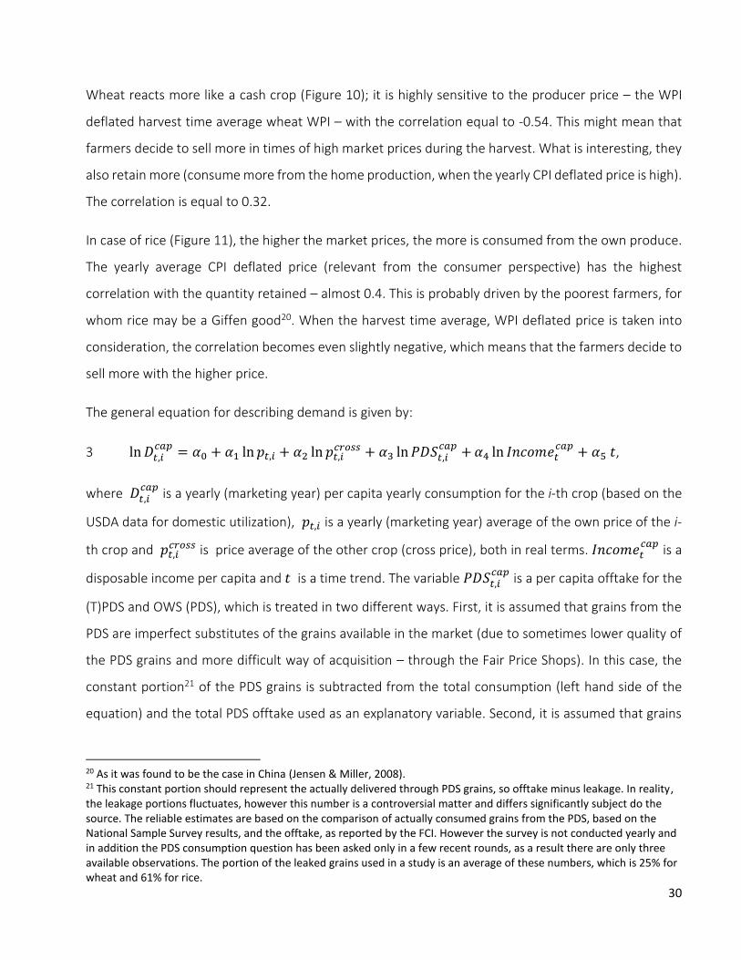
Table 5 Regressions of wheat demand
Log per-capita wheat demand
(1) (2) (3)
Log market price own -0.434*
(-1.88)
-0.633**
(-2.01)
0.236
(1.05)
Log market price cross 0.211
(1.41)
0.325*
(1.91)
0.083
(0.52)
Log PDS per capita offtakes -0.183***
(-4.14)
-0.216***
(-4.43)
Log income per capita 0.045
(1.01)
-0.036
(-1.20)
Time trend 0.005
(1.46)
Constant -3.378***
(-22.82)
-13.973*
(-1.94)
-3.186***
(-22.39)
N 20 21 20
p-value of underidentification LM statistic
p-value of Hansen J statistic
0.034
0.358
0.041
0.412
0.09
0.148
Note. *,**,*** indicates significance levels at 10, 5 and 1%, respectively with the robust standard error estimation. In
brackets t-values are given. For column (1) and (2) PDS consumption is assumed to be an imperfect substitute (subtracted
from the per-capita consumption); in column (3) PDS consumption is a perfect substitute.
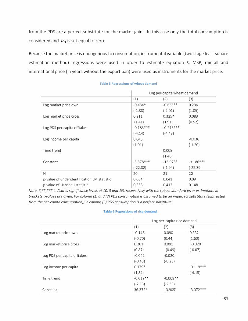
Table 6 Regressions of rice demand
Log per-capita rice demand
(1) (2) (3)
Log market price own -0.148
(-0.70)
0.090
(0.44)
0.332
(1.60)
Log market price cross 0.201
(0.87)
0.091
(0.49)
-0.020
(-0.07)
Log PDS per capita offtakes -0.042
(-0.43)
-0.020
(-0.23)
Log income per capita 0.179*
(1.84)
-0.119***
(-4.15)
Time trend -0.019**
(-2.13)
-0.008**
(-2.33)
Constant 36.372* 13.905* -3.072***

32
(1.95) (1.86) (-19.04)
N 20 22 20
p-value of underidentification LM statistic
p-value of Hansen J statistic
0.154
0.191
0.071
0.178
0.196
0.170
Note. *,**,*** indicates significance levels at 10, 5 and 1%, respectively with the robust standard error estimation. In
brackets t-values are given. For column (1) and (2) PDS consumption is assumed to be an imperfect substitute (subtracted
from the per-capita consumption); in column (3) PDS consumption is a perfect substitute.
In case of wheat, market prices have significant impact on consumption (Table 5): they are negative for
the own price and positive for the cross price (rice). Own price elasticity estimate is equal to -0.63 and
cross price elasticity to 0.33 (regression 2). Also the PDS grains seem to be a significant substitute for
the market consumption, with the elasticity (with respect to the amount of wheat consumed from the
PDS) equal to -0.22. In case of rice, the consumption seems to be mostly driven by the negative trend
(changing tastes) and income (elasticity equal to 0.18), which has a significant positive impact on
consumption (Table 6, regression 1). In a specification, where the PDS is assumed to be a perfect
substitute (regression 3), income has a significant negative impact on rice consumption, with the
elasticity -0.12. As it was discussed before, rice may be inferior good in India.
Kumar et al. (2011) and Ganesh-Kumar et al. (2012) analyzed price and expenditure elasticities of
demand for several goods in India based on the household survey data (NSS). Their results are difficult
to compare with those reported above as our dependent variable is a total domestic utilization and, on
the contrary to the NSS consumption data, includes grains bought in a processed form, consumed in
canteens and restaurants and also used for other than consumption purposes (e.g. feed). The average
income elasticity for rice was found 0.024 and for wheat 0.075 in the former study and food
expenditure elasticity equal -0.21 for rice and -0.13 for wheat in the latter study. The own price
elasticities were estimated in Kumar et al. (2011) -0.247 for rice and -0.340 for wheat.
e. Stocks and OMSS (Domestic and Exports)
The public stock level (𝑋𝑡,𝑖 is end of marketing year t stock level) is a result of the carryover stocks (less
the deterioration rate 𝛿), the grain inflow from the domestic procurement (𝐷𝑡,𝑖𝐹𝐶𝐼), imports and outflows
to the (T)PDS/OWS, OMSS for domestic market (OMSS D) and exports:
4 𝑋𝑡,𝑖 = (1 − 𝛿𝑖)𝑋𝑡−1,𝑖 + 𝐷𝑡,𝑖𝐹𝐶𝐼 − 𝑂𝑀𝑆𝑆𝑡,𝑖 − 𝑇𝑃𝐷𝑆𝑡,𝑖 − 𝑁𝐸𝑋𝑡,𝑖
𝑝𝑢𝑏.
33
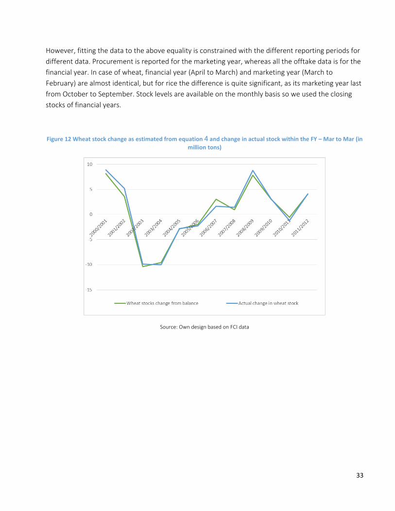
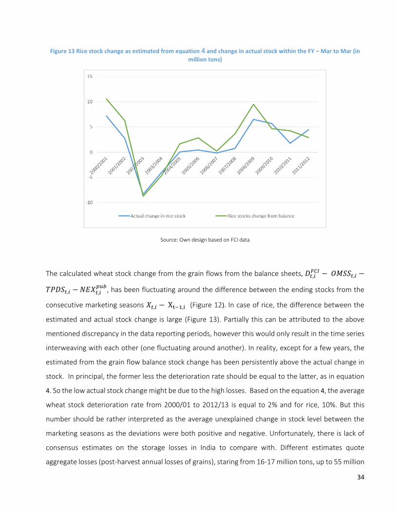
However, fitting the data to the above equality is constrained with the different reporting periods for
different data. Procurement is reported for the marketing year, whereas all the offtake data is for the
financial year. In case of wheat, financial year (April to March) and marketing year (March to
February) are almost identical, but for rice the difference is quite significant, as its marketing year last
from October to September. Stock levels are available on the monthly basis so we used the closing
stocks of financial years.
Figure 12 Wheat stock change as estimated from equation 4 and change in actual stock within the FY – Mar to Mar (in
million tons)
Source: Own design based on FCI data
34
Figure 13 Rice stock change as estimated from equation 4 and change in actual stock within the FY – Mar to Mar (in
million tons)
Source: Own design based on FCI data
The calculated wheat stock change from the grain flows from the balance sheets, 𝐷𝑡,𝑖𝐹𝐶𝐼 − 𝑂𝑀𝑆𝑆𝑡,𝑖 −
𝑇𝑃𝐷𝑆𝑡,𝑖 − 𝑁𝐸𝑋𝑡,𝑖𝑝𝑢𝑏, has been fluctuating around the difference between the ending stocks from the
consecutive marketing seasons 𝑋𝑡,𝑖 − Xt−1,i (Figure 12). In case of rice, the difference between the
estimated and actual stock change is large (Figure 13). Partially this can be attributed to the above
mentioned discrepancy in the data reporting periods, however this would only result in the time series
interweaving with each other (one fluctuating around another). In reality, except for a few years, the
estimated from the grain flow balance stock change has been persistently above the actual change in
stock. In principal, the former less the deterioration rate should be equal to the latter, as in equation
4. So the low actual stock change might be due to the high losses. Based on the equation 4, the average
wheat stock deterioration rate from 2000/01 to 2012/13 is equal to 2% and for rice, 10%. But this
number should be rather interpreted as the average unexplained change in stock level between the
marketing seasons as the deviations were both positive and negative. Unfortunately, there is lack of
consensus estimates on the storage losses in India to compare with. Different estimates quote
aggregate losses (post-harvest annual losses of grains), staring from 16-17 million tons, up to 55 million

35
tons, so roughly 7% to 23% of the total production (Artiuch & Kornstein, 2012). FCI reports are much
below any of these numbers – quoting around 0.3 million tons of wheat and rice wasted in storage and
transit in the recent years (as reported by on http://fciweb.nic.in/). Approximately half of this amount
was lost in storage, which gives not more than 0.4% of the average stock level in the central pool in the
corresponding years.
The buffer stock norms define the amount required to feed the public distribution system and different
governmental welfare schemes (operational stocks) and to stabilize supply and ‘insure food security’
(strategic stocks). The open-end character of the procurement, relatively high MSP and trade
limitations (e.g. temporary export bans) result in very high stock levels – periodically exceeding the
norms manifold.
Figure 14 Wheat stocks, offtakes for OMSS - D and exports (in million tons) and prices (in INR per ton, real the WPI deflated)
Source: Own calculation based on FCI data, IMF and indiastat.com

36
Figure 15 Rice stocks, offtakes for OMSS - D and exports (in mln tons) and prices (in INR per ton)
Source: Own calculation based on FCI data, IMF and indiastat.com
OMSS (D) for wheat is mostly used to stabilize market supply and release stocks before the new harvest
arrival (Figure 14). For rice, the seasonality of supply is almost absent, so OMSS was usually not used
(Figure 14). However, in the last years, small amounts were allocated for the OMSS (D) but they were
mostly not absorbed by the market (offtakes were lower than allocations).
Both OMSS (D) and export allocations are ad hoc decisions. Although they are correlated with the stock
levels against the stock norms, there are no rules for this. The issue price of the grains – the Minimum
Issue Price (MIP), is usually based on acquisition cost22 from the previous marketing year (plus the
freight), but sometimes it is lower than that (however it is newer below the current MSP as it could lead
to ‘reselling’ of the grains by the traders). It is sold through tenders, so the actual price received is close
to the market price. Also the amount actually released through these channels is not a simple outcome
of difference between the market price and the CIP as there are several limitations – sometimes the
22 Acquisition cost consists of cost of grains, statutory taxes, storage and interest charges etc. at acquisition stage.
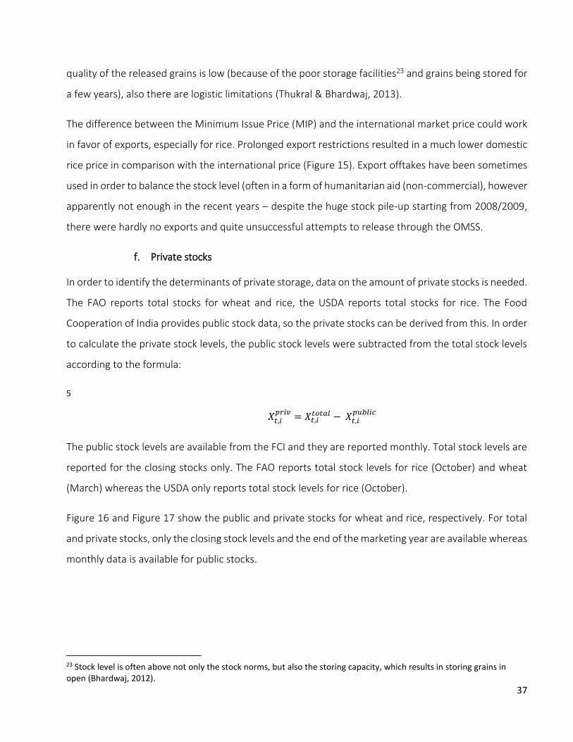
37
quality of the released grains is low (because of the poor storage facilities23 and grains being stored for
a few years), also there are logistic limitations (Thukral & Bhardwaj, 2013).
The difference between the Minimum Issue Price (MIP) and the international market price could work
in favor of exports, especially for rice. Prolonged export restrictions resulted in a much lower domestic
rice price in comparison with the international price (Figure 15). Export offtakes have been sometimes
used in order to balance the stock level (often in a form of humanitarian aid (non-commercial), however
apparently not enough in the recent years – despite the huge stock pile-up starting from 2008/2009,
there were hardly no exports and quite unsuccessful attempts to release through the OMSS.
f. Private stocks
In order to identify the determinants of private storage, data on the amount of private stocks is needed.
The FAO reports total stocks for wheat and rice, the USDA reports total stocks for rice. The Food
Cooperation of India provides public stock data, so the private stocks can be derived from this. In order
to calculate the private stock levels, the public stock levels were subtracted from the total stock levels
according to the formula:
5
𝑋𝑡,𝑖𝑝𝑟𝑖𝑣
= 𝑋𝑡,𝑖𝑡𝑜𝑡𝑎𝑙 − 𝑋𝑡,𝑖
𝑝𝑢𝑏𝑙𝑖𝑐
The public stock levels are available from the FCI and they are reported monthly. Total stock levels are
reported for the closing stocks only. The FAO reports total stock levels for rice (October) and wheat
(March) whereas the USDA only reports total stock levels for rice (October).
Figure 16 and Figure 17 show the public and private stocks for wheat and rice, respectively. For total
and private stocks, only the closing stock levels and the end of the marketing year are available whereas
monthly data is available for public stocks.
23 Stock level is often above not only the stock norms, but also the storing capacity, which results in storing grains in open (Bhardwaj, 2012).
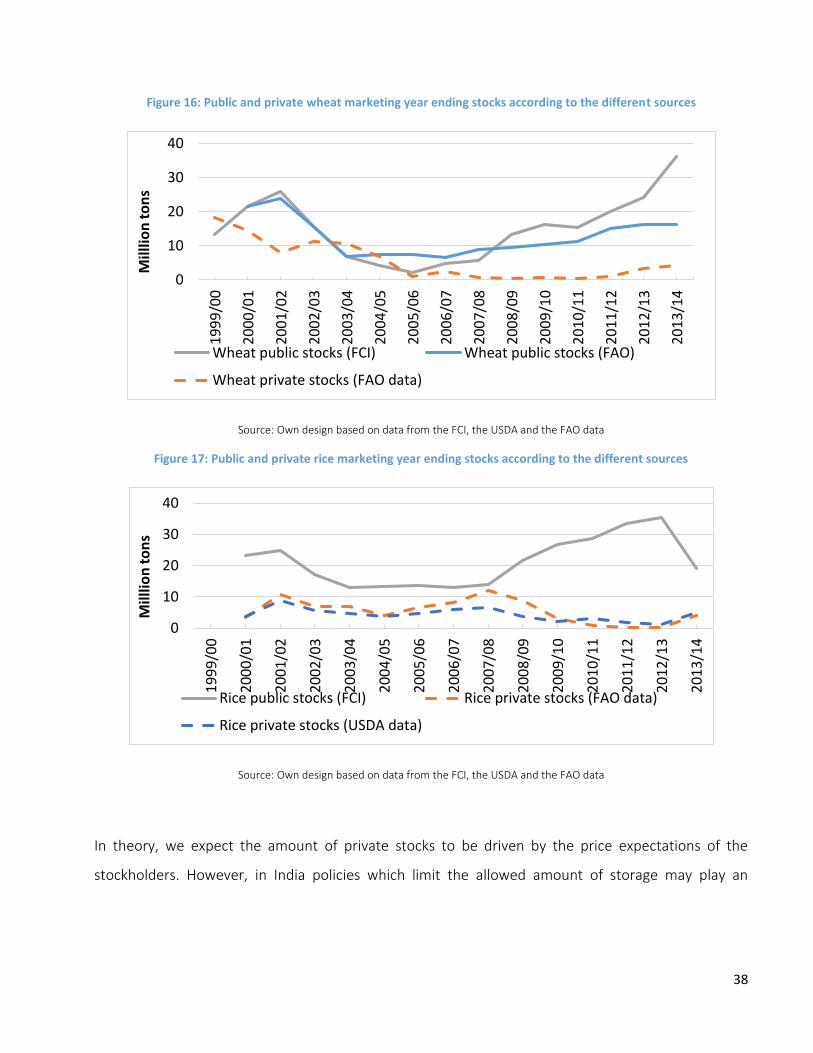
38
Figure 16: Public and private wheat marketing year ending stocks according to the different sources
Source: Own design based on data from the FCI, the USDA and the FAO data
Figure 17: Public and private rice marketing year ending stocks according to the different sources
Source: Own design based on data from the FCI, the USDA and the FAO data
In theory, we expect the amount of private stocks to be driven by the price expectations of the
stockholders. However, in India policies which limit the allowed amount of storage may play an
0
10
20
30
40
19
99
/00
20
00
/01
20
01
/02
20
02
/03
20
03
/04
20
04
/05
20
05
/06
20
06
/07
20
07
/08
20
08
/09
20
09
/10
20
10
/11
20
11
/12
20
12
/13
20
13
/14
Mill
lion
to
ns
Wheat public stocks (FCI) Wheat public stocks (FAO)
Wheat private stocks (FAO data)
0
10
20
30
40
19
99
/00
20
00
/01
20
01
/02
20
02
/03
20
03
/04
20
04
/05
20
05
/06
20
06
/07
20
07
/08
20
08
/09
20
09
/10
20
10
/11
20
11
/12
20
12
/13
20
13
/14
Mill
lion
to
ns
Rice public stocks (FCI) Rice private stocks (FAO data)
Rice private stocks (USDA data)
39
important role.24 Nevertheless, it is complicated to control for these effects which is why they are not
considered here. The price expectations themselves are – if rational expectations apply – based on the
fundamentals, i.e. the total supply and demand. Therefore, we consider the production, last year’s
private closing stocks, the export opportunities – to meet the demand on the world market – as well
as the public ending stocks (of the same marketing year) to be the relevant drivers of private closing
stocks. The public storage can be important because large amounts may increase government’s OMSS
offtakes, PDS distribution and exports from public stocks and may therefore impact the price
expectations of private stockholders.
For our analysis, we applied a Hodrick-Prescott time-series filter to the USDA demand data in order to
obtain a smooth demand trend. Afterwards, the production (USDA), last year’s private stocks, and the
same year’s public closings stocks were de-trended by the demand trend and then used as explanatory
variables. Last year’s private stocks and production were then combined to the “total supply”. To
account for the export opportunities, an export ban dummy was used. As the public closing stocks were
considered for the same marketing year as the estimated private closing stocks, endogeneity problems
may arise. This is why, the regressions were estimated using the instrumental variables technique (two-
stage least square estimation method). The public closing stocks were instrumentalized by the
exogenous MSP, which is responsible for the procurement level (see section c) – the main driver of the
public stock change (see section e). An underidentification test as well as a weak identification test
were conducted to ensure that the MSP is a valid instrument.
The general equation describing the private stocks is given by:
6
𝑋𝑡,𝑖𝑝𝑟𝑖𝑣
𝐷𝑡,𝑖𝑡𝑟𝑒𝑛𝑑 = 𝛼0 + 𝛼1
𝑆𝑡,𝑖
𝐷𝑡,𝑖𝑡𝑟𝑒𝑛𝑑 + 𝛼2𝐵𝑡,𝑖 + 𝛼3
𝑋𝑡,𝑖
𝐷𝑡,𝑖𝑡𝑟𝑒𝑛𝑑 ,
where 𝑋𝑡,𝑖𝑝𝑟𝑖𝑣 is a private stocks of the i-th crop in the marketing year t, 𝐷𝑡,𝑖
𝑡𝑟𝑒𝑛𝑑 is a consumption trend,
𝑆𝑡,𝑖 is a total market supply calculated as 𝑆𝑡,𝑖 = 𝑄𝑡,𝑖 + 𝑋𝑡−1,𝑖𝑝𝑟𝑖𝑣 and 𝐵𝑡,𝑖 is an export ban dummy.
24 Data on state governments stockholding limits for traders is currently collected and might be added to the analysis at a later stage.
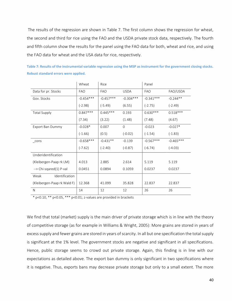
40
The results of the regression are shown in Table 7. The first column shows the regression for wheat,
the second and third for rice using the FAO and the USDA private stock data, respectively. The fourth
and fifth column show the results for the panel using the FAO data for both, wheat and rice, and using
the FAO data for wheat and the USA data for rice, respectively.
Table 7: Results of the instrumental variable regression using the MSP as instrument for the government closing stocks.
Robust standard errors were applied.
Wheat Rice Panel
Data for pr. Stocks FAO FAO USDA FAO FAO/USDA
Gov. Stocks -0.454*** -0.457*** -0.304*** -0.341*** -0.244**
(-2.98) (-5.49) (6.55) (-2.75) (-2.49)
Total Supply 0.847*** 0.445*** 0.193 0.630*** 0.518***
(7.34) (3.22) (1.48) (7.48) (4.67)
Export Ban Dummy -0.028* 0.007 0 -0.023 -0.027*
(-1.66) (0.5) (-0.02) (-1.54) (-1.83)
_cons -0.658*** -0.431** -0.139 -0.567*** -0.465***
(-7.62) (-2.40) (-0.87) (-6.74) (-4.03)
Underidentification
(Kleibergen-Paap rk LM) 4.013 2.885 2.614 5.119 5.119
--> Chi-sqared(1) P-val 0.0451 0.0894 0.1059 0.0237 0.0237
Weak Identification
(Kleibergen-Paap rk Wald F) 12.368 41.099 35.828 22.837 22.837
N 14 12 12 26 26
* p<0.10, ** p<0.05, *** p<0.01; z-values are provided in brackets
We find that total (market) supply is the main driver of private storage which is in line with the theory
of competitive storage (as for example in Williams & Wright, 2005): More grains are stored in years of
excess supply and fewer grains are stored in years of scarcity. In all but one specification the total supply
is significant at the 1% level. The government stocks are negative and significant in all specifications.
Hence, public storage seems to crowd out private storage. Again, this finding is in line with our
expectations as detailed above. The export ban dummy is only significant in two specifications where
it is negative. Thus, exports bans may decrease private storage but only to a small extent. The more
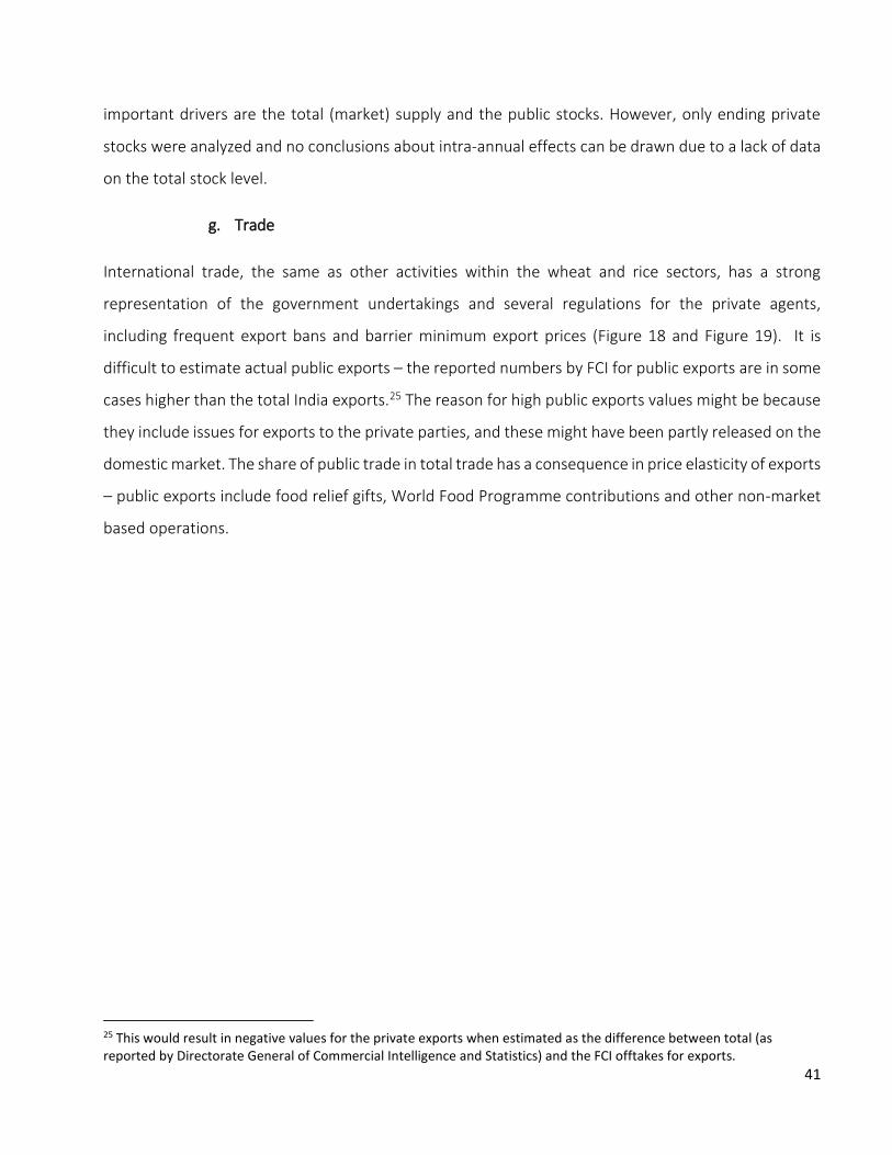
41
important drivers are the total (market) supply and the public stocks. However, only ending private
stocks were analyzed and no conclusions about intra-annual effects can be drawn due to a lack of data
on the total stock level.
g. Trade
International trade, the same as other activities within the wheat and rice sectors, has a strong
representation of the government undertakings and several regulations for the private agents,
including frequent export bans and barrier minimum export prices (Figure 18 and Figure 19). It is
difficult to estimate actual public exports – the reported numbers by FCI for public exports are in some
cases higher than the total India exports.25 The reason for high public exports values might be because
they include issues for exports to the private parties, and these might have been partly released on the
domestic market. The share of public trade in total trade has a consequence in price elasticity of exports
– public exports include food relief gifts, World Food Programme contributions and other non-market
based operations.
25 This would result in negative values for the private exports when estimated as the difference between total (as reported by Directorate General of Commercial Intelligence and Statistics) and the FCI offtakes for exports.
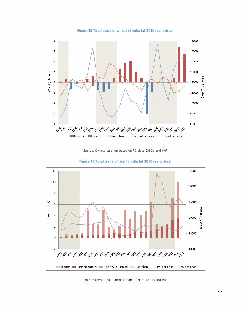
42
Figure 18 Total trade of wheat in India (at 2010 real prices)
Source: Own calculation based on FCI data, DGCIS and IMF
Figure 19 Total trade of rice in India (at 2010 real prices)
Source: Own calculation based on FCI data, DGCIS and IMF

43
As a result, the relationship between export volume and the domestic vs. international price ratio has
become positive, which means that the rise in the domestic price with respect to the international price
can be associated with higher exports. The regressions results, which explain the total wheat and rice
exports as a share of production with the major importing countries GDP, domestic to international
price ratio and the export bans confirms this hypothesis.
The following regressions were estimated:
𝐸𝑥𝑝𝑡,𝑖
𝑄𝑡,𝑖= 𝛼0 + 𝛼1∆𝐺𝐷𝑃𝑡 + 𝛼2𝐵𝑡−1,𝑖 + 𝛼3
𝑝𝑡−1,𝑖
𝑝𝑡−1,𝑖𝑖𝑛𝑡
where 𝐸𝑥𝑝𝑡,𝑖 is a total volume of exported in a financial year, 𝑄𝑡,𝑖 is a production of the respective
grain, ∆𝐺𝐷𝑃𝑡 is a first difference of the GDP of the major importers of Indian wheat and rice – Nepal,
Bangladesh, SA and UAE (population weighted average, in USD, constant prices), 𝐵𝑡−1,𝑖 is a lagged
export ban dummy, 𝑝𝑡−1,𝑖
𝑝𝑡−1,𝑖𝑖𝑛𝑡 is a lagged price ratio – domestic wholesale to international, converted to
INR. The lags of export bans and price ratios are due to the delay in realization of export contracts and
price expectation formation (in this way, we assume naïve price expectations). The estimation results
are presented in Table 8 below.
Table 8 Foreign trade regression estimates
Share of total exports in production
Wheat Rice
Lagged ratio of market price (WPI) to international price
0.035** (2.37)
0.010 (0.67)
Lagged export ban -0.017** (-2.12)
-0.022** (-2.89)
First difference of importer’s GDP -0.000 (-0.38)
0.003 (1.58)
Constant -0.017 (-1.12)
0.028 (1.61)
N 21 21
R² 0.317 0.463
Note. *,**,*** indicates significance levels at 10, 5 and 1%, respectively with the robust standard error estimation. In
brackets t-values are given.
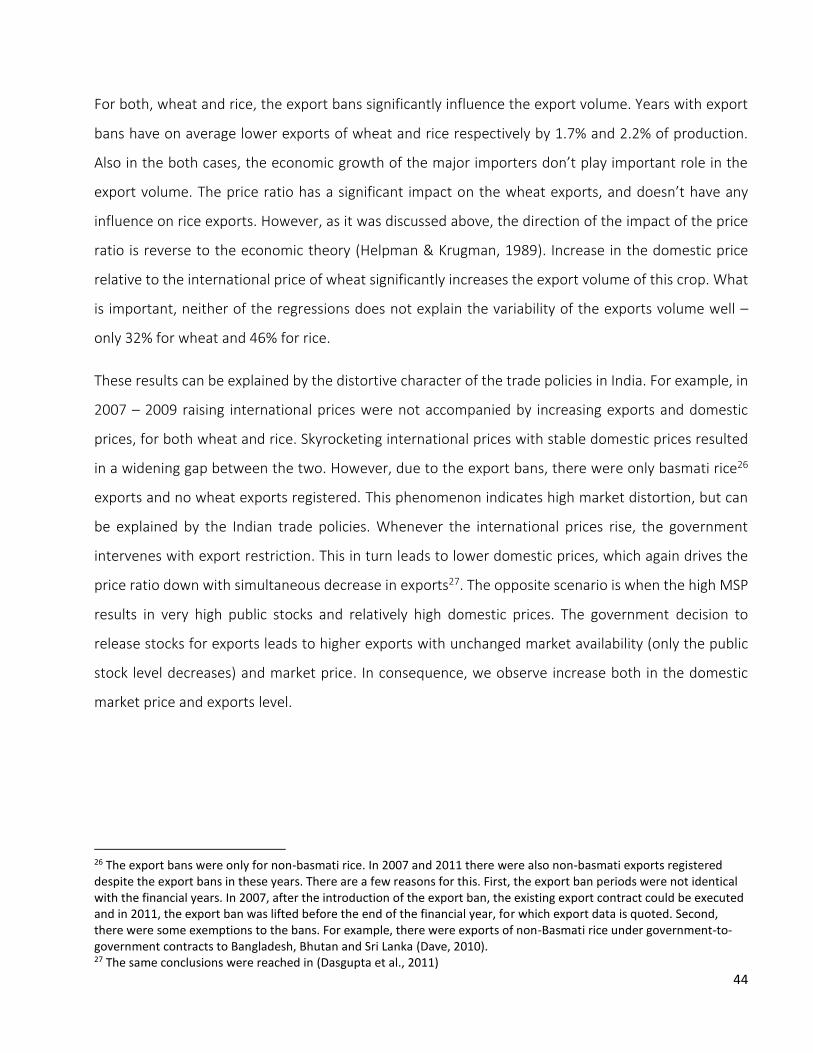
44
For both, wheat and rice, the export bans significantly influence the export volume. Years with export
bans have on average lower exports of wheat and rice respectively by 1.7% and 2.2% of production.
Also in the both cases, the economic growth of the major importers don’t play important role in the
export volume. The price ratio has a significant impact on the wheat exports, and doesn’t have any
influence on rice exports. However, as it was discussed above, the direction of the impact of the price
ratio is reverse to the economic theory (Helpman & Krugman, 1989). Increase in the domestic price
relative to the international price of wheat significantly increases the export volume of this crop. What
is important, neither of the regressions does not explain the variability of the exports volume well –
only 32% for wheat and 46% for rice.
These results can be explained by the distortive character of the trade policies in India. For example, in
2007 – 2009 raising international prices were not accompanied by increasing exports and domestic
prices, for both wheat and rice. Skyrocketing international prices with stable domestic prices resulted
in a widening gap between the two. However, due to the export bans, there were only basmati rice26
exports and no wheat exports registered. This phenomenon indicates high market distortion, but can
be explained by the Indian trade policies. Whenever the international prices rise, the government
intervenes with export restriction. This in turn leads to lower domestic prices, which again drives the
price ratio down with simultaneous decrease in exports27. The opposite scenario is when the high MSP
results in very high public stocks and relatively high domestic prices. The government decision to
release stocks for exports leads to higher exports with unchanged market availability (only the public
stock level decreases) and market price. In consequence, we observe increase both in the domestic
market price and exports level.
26 The export bans were only for non-basmati rice. In 2007 and 2011 there were also non-basmati exports registered despite the export bans in these years. There are a few reasons for this. First, the export ban periods were not identical with the financial years. In 2007, after the introduction of the export ban, the existing export contract could be executed and in 2011, the export ban was lifted before the end of the financial year, for which export data is quoted. Second, there were some exemptions to the bans. For example, there were exports of non-Basmati rice under government-to-government contracts to Bangladesh, Bhutan and Sri Lanka (Dave, 2010). 27 The same conclusions were reached in (Dasgupta et al., 2011)

45
h. Fiscal costs
Analysis of the fiscal costs is based on data starting from 2001 because there were major changes in
1997, when the TPDS came into life and in 2001, when the AAY group was defined and introduced.
The fiscal costs, as we define them in our framework (further fiscal costs), are based on the amount of
wheat and rice which was handled by the FCI and states under the DCP within the fiscal year28. We use
costs and volumes of the procurement, storage and distribution as reported by the FCI. However, it is
impossible to compare the estimated fiscal cost with the food subsidy incurred by the FCI. ‘The Food
Subsidy provided to FCI by the Ministry is in the form of Consumer Subsidy and Buffer Subsidy. For the
quantity distributed, the difference between the acquisition cost and distribution cost incurred by FCI
and the CIP realized is reimbursed as Consumer Subsidy. As per the instructions issued, three months29
average sales quantity is treated as operational stock. Stock over and above the operational stock is
treated as buffer stock. For buffer stocks, the cost of holding and maintenance of the stock (i.e. interest,
storage etc.) is reimbursed in the form of Buffer Subsidy.’ (FCI) So the food subsidy is calculated for the
grains distributed, not handled (doesn’t capture the total cost of procurement in the current year – it
is claimed only after releasing these grains). As a result, the fiscal costs and food subsidy refer to
different volumes of grains. For the further simulation purposes we need to endogenize the fiscal costs
and for the clarity of the procedure, we need to define the cost of operating the system based on the
procurement, stock and distribution level within the same financial year. The per unit costs of these
operations are approximated by the FCI reported numbers. ` The formula for the fiscal costs is given
below.
7
𝐹𝐶𝑡 = ∑ (𝑐𝑡,𝑖𝑝 + 𝑝𝑡,𝑖
𝑀𝑆𝑃)𝐷𝑡,𝑖𝐹𝐶𝐼 + 𝑐𝑡,𝑖
𝑑 𝑃𝐷𝑆𝑡,𝑖 + 𝑘𝑡𝑋𝑡,𝑖 − 𝑝𝑡,𝑖𝑃𝐷𝑆𝑃𝐷𝑆𝑡,𝑖 − 𝑝𝑡,𝑖𝑂𝑀𝑆𝑆𝑡,𝑖 − 𝑝𝑡,𝑖
𝐸𝑋𝑁𝐸𝑋𝑡,𝑖𝑝𝑢𝑏
𝑖 ,
28 The exception is the amount of grains procured as it is related to the marketing year. In case of wheat, financial year (April to March) and marketing year (March to February) are almost identical, but for rice the difference is quite significant, as its marketing year last from October to September. However, the majority of rice is normally procured from October to March, so within the financial year the cost of the residual procurement from the previous rice marketing year and the major part of the current rice marketing year is captured. As a result, the consequence for the fiscal costs is negligible in case of wheat and for rice is means small deviations of the estimated cost from the actual cost. 29 The currently used definition of the operational stock uses 4 month offtake (CAG, 2013). Further, we will be using this definition in our estimates.

46
where 𝐹𝐶𝑡 are yearly fiscal costs, (𝑐𝑡,𝑖𝑝 + 𝑝𝑡,𝑖
𝑀𝑆𝑃)𝐷𝑡,𝑖𝐹𝐶𝐼 are acquisition costs30 (proportional to the
procurement level, includes the MSP) of the i-th crop, 𝑐𝑡,𝑖𝑑 𝑃𝐷𝑆𝑡,𝑖 are distribution costs31 (proportional
to the amount distributed through the PDS and OWS) of the i-th crop, 𝑘𝑡𝑋𝑡,𝑖 buffer carrying cost (where
𝑋𝑡,𝑖 is a buffer stock, so an average in the financial year stock of wheat and rice in the central pool minus
the operational stock, which is part of the distribution cost) and 𝑝𝑡,𝑖𝑃𝐷𝑆𝑃𝐷𝑆𝑡,𝑖 + 𝑝𝑡,𝑖𝑂𝑀𝑆𝑆𝑡,𝑖 +
𝑝𝑡,𝑖𝐸𝑋𝑁𝐸𝑋𝑡,𝑖
𝑝𝑢𝑏 are sales realizations (revenues) from sales with the average CIP and market price for
OMSS (D) and net exports. Most of the components of the equation come from the FCI reports (see
Table 9).
Table 9 Categories as included in the Fiscal Cost equation
Variable FCI Category Source Unit
𝑐𝑡,𝑖𝑝
Procurement incidentals (as
proportional to the procurement
level)
FCI (can be also estimated
as 21% of the MSP)
INR/quintal, WPI deflated
𝐷𝑡,𝑖𝐹𝐶𝐼 Total procurement FCI Million tons
𝑝𝑡,𝑖 𝑀𝑆𝑃 MSP FCI INR/quintal, WPI deflated
𝑐1 Distribution cost FCI INR/quintal, WPI deflated
𝑃𝐷𝑆𝑡,𝑖 TPDS and OWS offtakes FCI Million tons
𝑘𝑡 Annual rate of buffer carrying cost FCI INR/quintal, WPI deflated
𝑋𝑡,𝑖 Buffer stock Estimated based on
reported monthly stock
positions in the Central Pool
Million tons
𝑝𝑡,𝑖𝑃𝐷𝑆 CIP Estimated CIP weighted by
offtake for different
categories (APL, BPL, AAY
and OWS) average
INR/quintal, WPI deflated
𝑝𝑡,𝑖 Market price Based on the WPI index INR/quintal, WPI deflated
𝑂𝑀𝑆𝑆𝑡,𝑖 OMSS offtakes FCI Million tons
𝑝𝑡,𝑖𝐸𝑋 Export price Estimated as international
price
INR/quintal, WPI deflated,
converted from the USD to
the INR with the
simultaneous exchange
rate
30 As incurred by the FCI it consists of freight, interest, handling and storage charges, transit and storage losses and administrative overheads. (FCI) 31 As incurred by the FCI it comprises of freight handling expenses, storage charges for the operational stock, interest charges, transit shortages, storage shortages, establishment charges and wage revision arrears. (FCI)

47
𝑁𝐸𝑋𝑡,𝑖𝑝𝑢𝑏
Total net offtakes for exports FCI Million tons
Source: Own design
Acquisition costs consist of the two components – the MSP plus a bonus (pooled cost of grain)32 and
procurement incidentals. Acquisition costs are the additional costs like statutory charges,
transportation charges and labor charges. The rest of the cost – distribution costs and buffer carrying
costs are also approximated by the past reported by the FCI cost per unit, multiplied by the PDS offtakes
and stock levels.
Total grain cost (acquisition, distribution and buffer caring cost) in real terms have risen in the last seven
years in comparison to the period 2000-2006, mostly due to higher acquisition costs. Rice acquisition
costs rose from an average 919 INR/qtl in 2000-2006 to 1032 INR/qtl in 2007-2013 (in real terms),
whereas for wheat the increase was from 696 INR/qtl to 777 INR/qtl, so by around 12% in both cases.
Distribution costs and buffer carrying cost for both grains decreased in real terms, so the total grain
cost increase was subdued to 4% for wheat and 5.4% for rice. After 2007/08, the total cost started
rising dramatically (Figure 20). This is due to both growing procurement levels and stock levels.
On the revenue side, there are three components – the OMSS, the TPDS with the OWS and net exports.
Both the OMSS allocation quantity and the MIP are ad hoc policy decisions, which are difficult to
model33. However, the OMSS is sold through tenders, so we use the market price as a proxy for the
price received for the OMSS grains. Revenues from the OMSS were estimated by multiplying (estimated
or reported) quantity released by the market price. TPDS and OWS revenues were approximated by the
quantities offtaken for the different programs (income groups – APL, BPL, AAY) with the adequate CIP
(both quantity and the CIP as reported by the FCI). The difficulty is that there are usually additional
allocations, like flood reliefs or festival allocations, sold with the different prices. So the difference
between the total PDS offtakes and offtakes for the APL, BPL and AAY is sold with heterogeneous prices.
It was assumed, that on average, this price was equal to the APL CIP. Finally, the net exports revenues
32 The FCI definition of the pooled cost of grain slightly differs – in their method it is a weighted average cost of opening stock at previous years’ MSP and procurement of current year’s crop at current year MSP. 33 Even the authority making the decision has not been constant over time – sometimes it is the Ministry of CAF & PD and sometimes HLC of the FCI (information obtained from the Ministry of Agriculture).

48
were calculated based on the reported net export quantity and the international price. However, this
method must have upward bias as a big share of the public exports was in a form of humanitarian aid
and transportation costs for exports are not considered. In general, the estimation of the revenue side
is based on several assumptions and is subject to errors. However, our goal is to produce a simple and
transparent but detailed enough method for assessing the total cost of the implementation of the set
of policy measures.
Figure 20 Total estimated cost and revenue and food subsidy actual and estimated (in real terms – 2001/02 = 100, INR)
Source: Own calculation based on FCI data
The estimated fiscal cost has risen dramatically in the real terms from the financial year 2001/02 (even
more as compared to the value in 2002/03, which seems to be an outlier though) – by 235% till 2012/13
(Figure 20). This number seems to be large as compared with the only 80% increase in the TPDS and
OWS offtakes in the same period. In 2001/02 the fiscal cost incurred per 1 ton of distributed grains
(wheat and rice on average) was 7654 INR and in 2012/13 it rose to 14204 INR (in Dec 2000 prices). In
the same period, the average stock level in the central pool has increased by 35% and procurement
volume by 69%. Also food subsidy has increased quite significantly – by 141% in real terms.
10
110
210
310
410
510
610
710
810
910
Bill
ion
IN
R (
real
)
Food Subsidy Incurred by FCI Estimated fiscal costsEstimated fiscal costs with the FCI stock Total costTotal revenue

49
The estimated total fiscal cost has been usually above the food subsidy incurred by the FCI (Figure 20).
Except for the year 2002/03 and 2003/04, the fiscal cost fluctuates between 13% in 2001/02 and 109%
above the food subsidy. This difference can have several sources. One is the way the buffer stock
carrying cost was accounted by the FCI. The average buffer stock, as reported by the FCI in its annual
reports has been always much below our estimates based on the monthly stock levels as reported by
the FCI (Figure 21). Estimation of the fiscal costs with the FCI reported buffer stock slightly decreased
the figure, however the difference is quite small (Figure 20).
Figure 21 Stocks of wheat and rice
Source: Own calculation based on FCI data
Note: The FCI stock is own and held by the state governments under the DCP.
Second, the food subsidy as reported by the FCI related to the grains released, not operated, as it was
already discussed. And the procurement levels were usually higher than the total offtakes (Figure 22),
especially after 2006/07, which corresponds with the rising difference between the estimated fiscal
costs and claimed food subsidy. This might mean that the cost of the higher procurement than
distribution will be reported in the next years, when the excessive stocks will be released.
0
10
20
30
40
50
60
70
2002-03 2003-04 2004-05 2005-06 2006-07 2007-08 2008-09 2009-10 2010-11 2011-12
Mill
ion
to
ns
Buffer stock as audited by the FCI
Average stock in the central pool
Total stock minus 4-month requirenment for issues
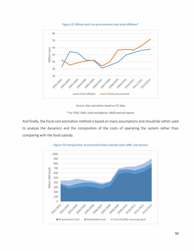
50
Figure 22 Wheat and rice procurement and total offtakes*
Source: Own calculation based on FCI data
* For TPDS, OWS, relief and defense, OMSS and net exports
And finally, the fiscal cost estimation method is based on many assumptions and should be rather used
to analyze the dynamics and the composition of the costs of operating the system rather than
comparing with the food subsidy.
Figure 23 Composition of estimated food subsidy costs (INR, real terms)
20
30
40
50
60
70
80
Mill
ion
to
ns
Total offtakes Total procurement
0
100
200
300
400
500
600
700
800
900
1000
Bill
ion
INR
(re
al)
Procurement cost Distribution cost Cost of buffer carrying stock
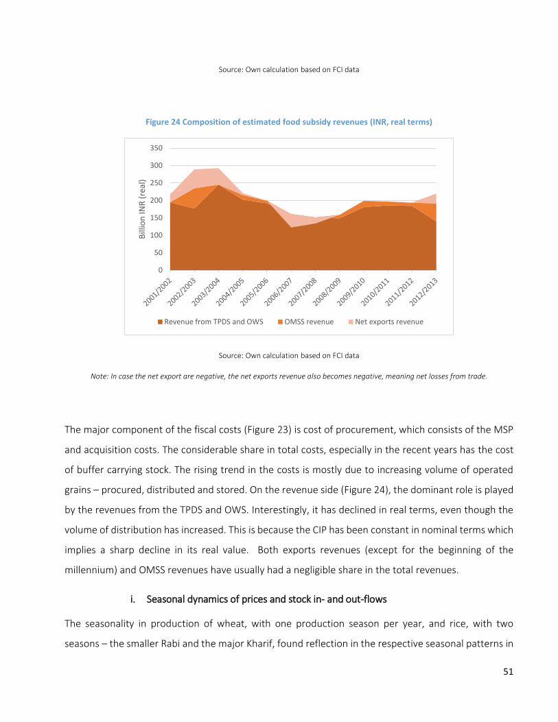
51
Source: Own calculation based on FCI data
Figure 24 Composition of estimated food subsidy revenues (INR, real terms)
Source: Own calculation based on FCI data
Note: In case the net export are negative, the net exports revenue also becomes negative, meaning net losses from trade.
The major component of the fiscal costs (Figure 23) is cost of procurement, which consists of the MSP
and acquisition costs. The considerable share in total costs, especially in the recent years has the cost
of buffer carrying stock. The rising trend in the costs is mostly due to increasing volume of operated
grains – procured, distributed and stored. On the revenue side (Figure 24), the dominant role is played
by the revenues from the TPDS and OWS. Interestingly, it has declined in real terms, even though the
volume of distribution has increased. This is because the CIP has been constant in nominal terms which
implies a sharp decline in its real value. Both exports revenues (except for the beginning of the
millennium) and OMSS revenues have usually had a negligible share in the total revenues.
i. Seasonal dynamics of prices and stock in- and out-flows
The seasonality in production of wheat, with one production season per year, and rice, with two
seasons – the smaller Rabi and the major Kharif, found reflection in the respective seasonal patterns in
0
50
100
150
200
250
300
350B
illio
n IN
R (
real
)
Revenue from TPDS and OWS OMSS revenue Net exports revenue
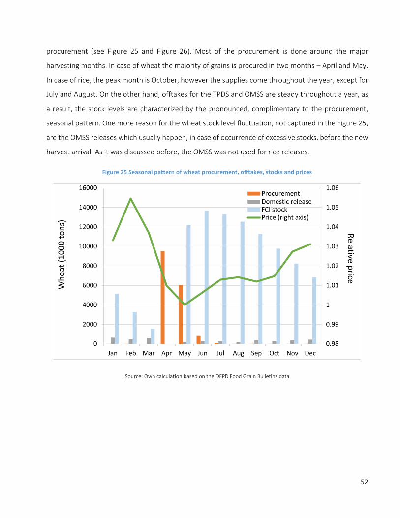
52
procurement (see Figure 25 and Figure 26). Most of the procurement is done around the major
harvesting months. In case of wheat the majority of grains is procured in two months – April and May.
In case of rice, the peak month is October, however the supplies come throughout the year, except for
July and August. On the other hand, offtakes for the TPDS and OMSS are steady throughout a year, as
a result, the stock levels are characterized by the pronounced, complimentary to the procurement,
seasonal pattern. One more reason for the wheat stock level fluctuation, not captured in the Figure 25,
are the OMSS releases which usually happen, in case of occurrence of excessive stocks, before the new
harvest arrival. As it was discussed before, the OMSS was not used for rice releases.
Figure 25 Seasonal pattern of wheat procurement, offtakes, stocks and prices
Source: Own calculation based on the DFPD Food Grain Bulletins data
0.98
0.99
1
1.01
1.02
1.03
1.04
1.05
1.06
0
2000
4000
6000
8000
10000
12000
14000
16000
Jan Feb Mar Apr May Jun Jul Aug Sep Oct Nov Dec
ProcurementDomestic releaseFCI stockPrice (right axis)
Wh
eat
(10
00
to
ns)
Relative p
rice

53
Figure 26 Seasonal pattern of rice procurement, offtakes, stocks and prices
Source: Own calculation based on the DFPD Food Grain Bulletins data
Note. Seasonal dynamics based on X12-Arima RSA3 filter using Demetra Plus software. Figure shows the
normalized (to minimum value adjusted) seasonal component. For wheat and rice prices: Log-transformed
monthly WPI prices for 1990 to 2013 have been used; FCI stocks from 2000 to 2012; domestic release (i.e. sum of
off-takes for TPDS, welfare schemes and OMSS open tender sales) for 2000 to 2006 (only wheat); procurement
for 1998 to 2002
The described above seasonality in procurement and stocks has found its reflection in seasonal
fluctuation of prices. Along with the new harvest arrival, coinciding with the lowest public stock level,
market prices drop and later gradually rise throughout the year: Wheat prices before harvest are more
than 5% higher than after harvest; for rice the gap is almost 4%34. This price dynamics may indicate that
the public interventions are not effective in stabilizing the market prices throughout the marketing
year.
34 Note that these figures underestimate the seasonality as the underlying commodity WPI shows less fluctuations than the weighted average of wholesale market prices (see Appendix 1).
0.98
0.99
1
1.01
1.02
1.03
1.04
1.05
1.06
0
1000
2000
3000
4000
5000
6000
7000
8000
Jan Feb Mar Apr May Jun Jul Aug Sep Oct Nov Dec
ProcurementFCI stockPrice (right axis)
Ric
e (1
00
0 t
on
s)
Relative p
rice
54
5. Summary and Conclusions
The main findings of this study are as follows. The extensive market interventions resulted in the duality
of the wheat and rice sectors with the coexistence of public and private sectors and dual – regulated
prices and market prices, with the former strongly influencing the letter. Also the former strongly
influencing the real processes. Wheat and rice supply strongly and significantly responds to the MSP.
This result is robust with different specifications. In case of wheat the price elasticity is even higher,
which might be due to more commercial character of this crop production. The price elasticities are
high compared to acreage and yield elasticities for other countries which can be explained by the low
price risks due to the minimum prices. Also the farm-gate prices for wheat have a significant impact on
its production level, however consideration of the MSP results in a better explanatory power of the
regression. Wholesale prices at planting or lagged harvest time prices are largely irrelevant.
The FCI procurement volume is driven by the production level and the difference between the MSP and
the market price. For rice, there is also an upward trend in the share of the procured grains in total
production.
The demand equation estimation turned out to be challenging due to the endogeneity of the market
price and also because of the difficulty in accounting for the consumption from the PDS (due do
fluctuating and mostly unknown leakages from the PDS). Eventually, the instrumental variable
regression was used to assess the impact of the market price on the wheat and rice consumption. PDS
grains were considered both as a perfect and imperfect substitute for the market grains. The signs of
the estimated price elasticities are consistent with theory, however for rice they turned out to be
insignificant. The negative income elasticity of rice consumption as well as the downward trend in rice
consumption suggests changing habits and the inferior character of rice as a consumption good.
Public stock analysis reviled higher storage losses in case of rice than wheat – 10% and 2% respectively.
These numbers are difficult to compare with other studies’ estimates due to high variance in results
and differences in methodology. OMSS allocations were usually made in case of wheat due to higher
seasonality of production and prices. The actual offtakes for the OMSS were much below the
allocations.
55
The analysis of private stocks was challenged by poor data availability and strong time- and state-
varying regulations to private stockholding. However, the estimation results are consistent with the
theory of competitive storage and suggest strong crowding out effects of the public stocks on private
stocks. Export restrictions also tend to reduce private ending stocks. Data quality was also a major issue
for analyzing international trade, particularly due to the difficulty to distinguish public and private
exports. As a result the total exports were analyzed. Trade policies, like export bans seem to react to
national and international prices, diluting ‘normal’ market dynamics (i.e. the higher the international
prices, the lower the exports).
The accounting of fiscal costs based on the FCI reports gives figures which are permanently above the
food subsidy incurred by the FCI. There might be a few reasons behind it – different accounting
methods and financing from the other sources (credits). Starting from 2006/07, there is a clear upward
trend in inflation adjusted costs of operating the system, coming mostly from the rising procurement
volume and the MSP. On the other hand, the revenues have declined in real terms, due to lower real
CIP and only marginal revenues from the OMSS (D) and exports. As a result, the fiscal costs have shown
a permanent growth in real terms and growth of the real fiscal costs relative to the amount of grains
released through the TPDS and the OWS .
The seasonal analysis of the intra-year data revealed strong seasonality of prices and procurement, in
particular for wheat (less for rice). Offtakes for the PDS are non-seasonal. As a result, the stock level
fluctuations are characterized by a strong seasonal patterns, which are accounted for in the buffer stock
norms.
High involvement of the government in wheat and rice production, trade and storage resulted in several
market distortions. The large government interventions resulted in mounting fiscal costs that seem to
be higher than officially accounted by the government. Further research should be focused on
developing and evaluating alternative policies, like switching from the PDS to the food subsidies or from
the MSP to the deficiency subsidies, which would be less distortive and less costly. For this purpose we
suggest a simulation model.

56
Bibliography
Acharya, S. S., Chand, R., Birthal, P. S., Kumar, S., & Negi, D. S. (2007). Market Integration and Price Transmission in India: A Case of Rice and Wheat with Special Reference to the World Food Crisis of 2007/08. Rome.
Anderson, K. (2013). Agricultural Price Distortions: Trends and Volatility, Past and Prospective. Retrieved from http://papers.ssrn.com/abstract=2210256
Artiuch, P., & Kornstein, S. (2012). Sustainable Approaches to Reducing Food Waste in India.
Baylis, K., Jolejole-Foreman, M. C., & Mallory, M. L. (2013). Impact of Wheat and Rice Export Ban on Indian Market Integration. Washington DC.
Bhardwaj, M. (2012). As Crops Rot , Millions Go Hungry in India. Reuters. Retrieved October 03, 2013, from http://in.reuters.com/article/2012/07/02/india-wheat-food-malnutrition-crops-idINDEE86101620120702
CAG. (2013). Performance Audit Report on Storage Management and Movement of Food Grains in FCI. New Delhi.
Dasgupta, D., Dubey, R. N., & Sathish, R. (2011). Domestic Wheat Price Formation and Food Inflation in India.
Dave, D. (Ed.). (2010). The Rice Crisis; Markets, Policies and Food Security. FAO.
DFPD. (2013). Foodgrains Bulletin December, 2013. New Delhi. Retrieved from http://dfpd.nic.in/fcamin/bulletion/december-2013.pdf
FCI web portal. (n.d.). Procurement in Details. Food Corporation of India. Retrieved October 02, 2013, from http://fciweb.nic.in/procurements/view/20
Gaiha, R., & Kulkarni, V. S. (2005). Foodgrain Surplaces, Yields and Prices in India. Paris.
Ganesh-Kumar, A., Mehta, R., Pullabhotla, H., Prasad, S., Ganguly, K., & Gulati, A. (2012). Demand and Supply of Cereals in India 2010-2025 (No. 01158). New Delhi.
Ganguly, K., & Gulati, A. (2013). The political economy of food price policy The case study of India (No. 2013 / 034). Helsinki.
GoI. (2005). Performance Evaluation of Targeted Public Distribution System ( TPDS ). New Delhi.
Gulati, A., & Jain, S. (2013). Buffer Stocking Policy in the Wake of NFSB : Concepts, Empirics, and Policy Implications (No. 6). New Delhi.
Gulati, A., & Saini, S. (2013). Taming Food Inflation in India (No. 4). New Delhi.
Gulati, A., & Sharma, P. K. (1990). Prices , Procurement and Production. Economic and Political Weekly, A36–A47.
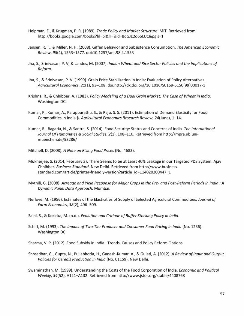
57
Helpman, E., & Krugman, P. R. (1989). Trade Policy and Market Structure. MIT. Retrieved from http://books.google.com/books?hl=pl&lr=&id=BdGJE2o6oLUC&pgis=1
Jensen, R. T., & Miller, N. H. (2008). Giffen Behavior and Subsistence Consumption. The American Economic Review, 98(4), 1553–1577. doi:10.1257/aer.98.4.1553
Jha, S., Srinivasan, P. V, & Landes, M. (2007). Indian Wheat and Rice Sector Policies and the Implications of Reform.
Jha, S., & Srinivasan, P. V. (1999). Grain Price Stabilization in India: Evaluation of Policy Alternatives. Agricultural Economics, 21(1), 93–108. doi:http://dx.doi.org/10.1016/S0169-5150(99)00017-1
Krishna, R., & Chhibber, A. (1983). Policy Modeling of a Dual Grain Market: The Case of Wheat in India. Washington DC.
Kumar, P., Kumar, A., Parappurathu, S., & Raju, S. S. (2011). Estimation of Demand Elasticity for Food Commodities in India §. Agricultural Economics Research Review, 24(June), 1–14.
Kumar, R., Bagaria, N., & Santra, S. (2014). Food Security: Status and Concerns of India. The International Journal Of Humanities & Social Studies, 2(1), 108–116. Retrieved from http://mpra.ub.uni-muenchen.de/53286/
Mitchell, D. (2008). A Note on Rising Food Prices (No. 4682).
Mukherjee, S. (2014, February 3). There Seems to be at Least 40% Leakage in our Targeted PDS System: Ajay Chhibber. Business Standard. New Delhi. Retrieved from http://www.business-standard.com/article/printer-friendly-version?article_id=114020200447_1
Mythili, G. (2008). Acreage and Yield Response for Major Crops in the Pre- and Post-Reform Periods in India : A Dynamic Panel Data Approach. Mumbai.
Nerlove, M. (1956). Estimates of the Elasticities of Supply of Selected Agriculural Commodities. Journal of Farm Economics, 38(2), 496–509.
Saini, S., & Kozicka, M. (n.d.). Evolution and Critique of Buffer Stocking Policy in India.
Schiff, M. (1993). The Impact of Two-Tier Producer and Consumer Food Pricing in India (No. 1236). Washington DC.
Sharma, V. P. (2012). Food Subsidy in India : Trends, Causes and Policy Reform Options.
Shreedhar, G., Gupta, N., Pullabhotla, H., Ganesh-Kumar, A., & Gulati, A. (2012). A Review of Input and Output Policies for Cereals Production in India (No. 01159). New Delhi.
Swaminathan, M. (1999). Understanding the Costs of the Food Corporation of India. Economic and Political Weekly, 34(52), A121–A132. Retrieved from http://www.jstor.org/stable/4408768
58
Swaminathan, M. (2009). Neo-Liberal Policy and Food Security in India: Impact on the Public Distribution System (Vol. 06). Conference Paper for international conference on’'The Crisis of Neo-liberalism in India: Challenges and Alternatives''organised by Tata Institute of Social Sciences (TISS), Mumbai and International Development Economics Associates (IDEAs).
Thukral, N., & Bhardwaj, M. (2013). India’s Grain Mountain Grows Despite Push for Exports. Reuters In.reuters.com. Singapore/New Delhi. Retrieved from http://in.reuters.com/article/2013/02/25/india-grains-glut-bumper-crop-storage-idINDEE91O0IA20130225
Von Grebmer, K., Headey, D., Olofinbiyi, T., Wiesmann, D., Fritschel, H., Yin, S., & Yohannes, Y. (2013). 2013 Global Hunger Index The Challenge of Hunger: Building Resilience to Achieve Food and Nutrition Security. Bonn/Washington, DC/Dublin.
Williams, J. C., & Wright, B. D. (2005). Storage and Commodity Markets (Vol. 2005, p. 520). Cambridge University Press.
59
Appendix 1 Price series constriction
The monthly price is calculated by weighting the state-wise prices by the latest harvest share of that
state. This is done for the four consecutive years. Then the monthly conversion factor is calculated and
the average over the four years is taken to use it as the final conversion factor. The stronger seasonality
of the production weighted prices goes into the conversion factor. The fluctuations of the conversion
factor are the rationale why we cannot just use one single month to scale the WPI
Figure 27 Paddy WPI and major producing states production weighted price average
Source: Own calculation based on http://www.dacnet.nic.in/
9000
10000
11000
12000
13000
14000
15000
16000
17000
10
.20
09
1.2
010
4.2
010
7.2
010
10
.20
10
1.2
011
4.2
011
7.2
011
10
.20
11
1.2
012
4.2
012
7.2
012
10
.20
12
1.2
013
4.2
013
7.2
013
INR
/to
n
Weighted avarage price WPI constructed price

60
Figure 28 Wheat WPI and major producing states production weighted price average
Source: Own calculation based on http://www.dacnet.nic.in/
9000
10000
11000
12000
13000
14000
15000
16000
17000
4.2
008
7.2
008
10
.20
08
1.2
009
4.2
009
7.2
009
10
.20
09
1.2
010
4.2
010
7.2
010
10
.20
10
1.2
011
4.2
011
7.2
011
10
.20
11
1.2
012
INR
/to
n
Weighted avarage price WPI constructed price
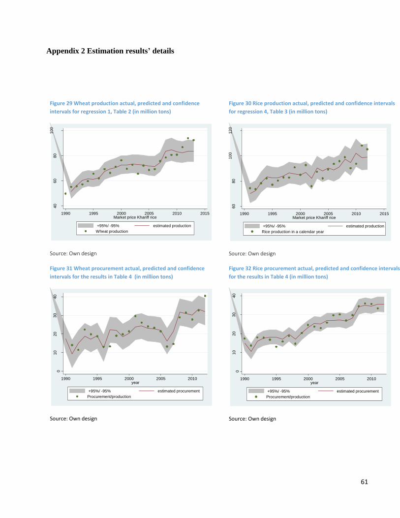
61
Appendix 2 Estimation results’ details
Figure 29 Wheat production actual, predicted and confidence
intervals for regression 1, Table 2 (in million tons)
Source: Own design
Figure 30 Rice production actual, predicted and confidence intervals
for regression 4, Table 3 (in million tons)
Source: Own design
Figure 31 Wheat procurement actual, predicted and confidence
intervals for the results in Table 4 (in million tons)
Source: Own design
Figure 32 Rice procurement actual, predicted and confidence intervals
for the results in Table 4 (in million tons)
Source: Own design
40
60
80
10
0
1990 1995 2000 2005 2010 2015Market price Khariff rice
+95%/ -95% estimated production
Wheat production60
80
10
012
0
1990 1995 2000 2005 2010 2015Market price Khariff rice
+95%/ -95% estimated production
Rice production in a calendar year
010
20
30
40
1990 1995 2000 2005 2010year
+95%/ -95% estimated procurement
Procurement/production
010
20
30
40
1990 1995 2000 2005 2010year
+95%/ -95% estimated procurement
Procurement/production
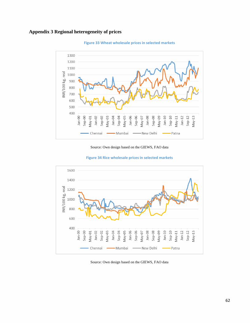
62
Appendix 3 Regional heterogeneity of prices
Figure 33 Wheat wholesale prices in selected markets
Source: Own design based on the GIEWS, FAO data
Figure 34 Rice wholesale prices in selected markets
Source: Own design based on the GIEWS, FAO data
Related Documents