DISCRETE AND CONTINUOUS Website: http://aimSciences.org DYNAMICAL SYSTEMS SERIES B Volume 9, Number 1, January 2008 pp. 103–128 MODELING GROUP DYNAMICS OF PHOTOTAXIS: FROM PARTICLE SYSTEMS TO PDES Doron Levy Department of Mathematics and Center for Scientific Computation and Mathematical Modeling (CSCAMM) University of Maryland College Park, MD 20742, USA Tiago Requeijo Department of Mathematics Stanford University Stanford, CA 94305-2125, USA (Communicated by Benoit Perthame) Abstract. This work presents a hierarchy of mathematical models for de- scribing the motion of phototactic bacteria, i.e., bacteria that move towards light. Based on experimental observations, we conjecture that the motion of the colony towards light depends on certain group dynamics. This group dy- namics is assumed to be encoded as an individual property of each bacterium, which we refer to as ’excitation’. The excitation of each individual bacterium changes based on the excitation of the neighboring bacteria. Under these as- sumptions, we derive a stochastic model for describing the evolution in time of the location of bacteria, the excitation of individual bacteria, and a surface memory effect. A discretization of this model results in an interacting sto- chastic many-particle system. The third, and last model is a system of partial differential equations that is obtained as the continuum limit of the stochastic particle system. The main theoretical results establish the validity of the new system of PDEs as the limit dynamics of the multi-particle system. 1. Introduction. Bacteria live in environments that can be often limiting for growth. As a result, they have evolved sophisticated mechanisms in order to sense changes in environmental parameters such as light and nutrients. Under certain conditions, such changes will initiate a motion of an individual bacteria (or even of an entire colony) in order to increase the resources availability. In this work we are interested in the motion of Cyanobacteria, that are a lineage of ancient, ubiquitous photosynthetic microbes. Cyanobacteria track light direction and quality to optimize conditions for photosynthesis. The motility toward a light source is called “phototaxis” and requires a photoreceptor, a signal transduction event, and a motility apparatus. In a series of experiments reported in [7], time- lapse video microscopy was used to monitor the movement of individual cells and groups of cells. These movies suggest that in addition to the ability of single cells 2000 Mathematics Subject Classification. Primary: 92C17; Secondary: 92C80, 82C22, 65C35. Key words and phrases. Phototaxis, Chemotaxis, Group Dynamics, Stochastic Particle Systems. 103

Welcome message from author
This document is posted to help you gain knowledge. Please leave a comment to let me know what you think about it! Share it to your friends and learn new things together.
Transcript
DISCRETE AND CONTINUOUS Website: http://aimSciences.orgDYNAMICAL SYSTEMS SERIES BVolume 9, Number 1, January 2008 pp. 103–128
MODELING GROUP DYNAMICS OF PHOTOTAXIS:
FROM PARTICLE SYSTEMS TO PDES
Doron Levy
Department of Mathematicsand
Center for Scientific Computation and Mathematical Modeling (CSCAMM)University of Maryland
College Park, MD 20742, USA
Tiago Requeijo
Department of MathematicsStanford University
Stanford, CA 94305-2125, USA
(Communicated by Benoit Perthame)
Abstract. This work presents a hierarchy of mathematical models for de-scribing the motion of phototactic bacteria, i.e., bacteria that move towardslight. Based on experimental observations, we conjecture that the motion ofthe colony towards light depends on certain group dynamics. This group dy-namics is assumed to be encoded as an individual property of each bacterium,which we refer to as ’excitation’. The excitation of each individual bacteriumchanges based on the excitation of the neighboring bacteria. Under these as-sumptions, we derive a stochastic model for describing the evolution in timeof the location of bacteria, the excitation of individual bacteria, and a surfacememory effect. A discretization of this model results in an interacting sto-chastic many-particle system. The third, and last model is a system of partialdifferential equations that is obtained as the continuum limit of the stochasticparticle system. The main theoretical results establish the validity of the newsystem of PDEs as the limit dynamics of the multi-particle system.
1. Introduction. Bacteria live in environments that can be often limiting forgrowth. As a result, they have evolved sophisticated mechanisms in order to sensechanges in environmental parameters such as light and nutrients. Under certainconditions, such changes will initiate a motion of an individual bacteria (or even ofan entire colony) in order to increase the resources availability.
In this work we are interested in the motion of Cyanobacteria, that are a lineageof ancient, ubiquitous photosynthetic microbes. Cyanobacteria track light directionand quality to optimize conditions for photosynthesis. The motility toward a lightsource is called “phototaxis” and requires a photoreceptor, a signal transductionevent, and a motility apparatus. In a series of experiments reported in [7], time-lapse video microscopy was used to monitor the movement of individual cells andgroups of cells. These movies suggest that in addition to the ability of single cells
2000 Mathematics Subject Classification. Primary: 92C17; Secondary: 92C80, 82C22, 65C35.Key words and phrases. Phototaxis, Chemotaxis, Group Dynamics, Stochastic Particle
Systems.
103
104 DORON LEVY AND TIAGO REQUEIJO
to move directionally, the overall time-evolution is determined by means of a groupdynamics. For example, even when a directional light is continuously present, ittakes a significant time for the cells to initiate a motion towards light. It is alsoobserved that individual cells are less likely to move towards light while cells thatare grouped together are more likely to move. Some surface memory effects arealso observed, i.e., it seems to be easier for bacteria to travel on surfaces that werepreviously visited by other bacteria. Overall, the various patterns of movement thatwe observe appear to be a complex function of cell density, surface properties andgenotype. Almost nothing is known about the nature of the interactions betweenthese parameters for Cyanobacteria.
In this work we derive several mathematical models for the motion of phototaxisthat take into account certain assumptions about the nature of the group dynamics.More specifically, we assume that every bacteria has an internal property, which werefer to as its ’excitation’. The excitation of any bacterium is a time-dependentquantity that is adjusted based on the excitation of the neighboring bacteria. Theexcitation of a bacteria must exceed a pre-determined threshold for it to initiate amotion in the direction of light.
In that spirit, our first model is a stochastic model in which we track in time thelocations of the individual bacteria, their excitation, and their trajectories in space.Numerical simulations of this stochastic model show a qualitative behavior that issimilar to the observed experimental data.
Our second model is a stochastic particle model that is obtained from a dis-cretization of Model I. In this model all three quantities (bacteria, excitation, andsurface) are converted into particles. Rules of motion as well as birth/death rulesfor all particles determine their dynamics. In particular, excitation particles areassumed to move together with their associated bacteria, but since excitation forany individual bacterium can change in time, excitation particles are allowed togive birth and die. Finally, our last model, is a continuous model that is writtenas a system of PDEs for the evolution of the densities of bacteria, excitation, andthe surface memory effect. Most of this paper deals with establishing the limit ofthe particle system as the system of PDEs. The techniques we use follow the worksof Oelschlager [14] for reaction-diffusion equations, and of Stevens [18] for chemo-taxis. When compared with the work of Stevens, the inclusion of the “excitation”property, does require us to make some additional assumptions and to adjust someof the estimates.
Over the past several decades, there has been a lot of activity in the mathemat-ical community in studying mathematical models for chemotaxis (i.e. motion inthe direction of a chemical attractant), starting with the pioneering work of Pat-lack [16], and the similar Keller and Segel model [12]. Most of the recent researchefforts concentrate on studying finite-time blowup for the Keller-Segel model or onpreventing such a blowup using various regularizations. Since at this point, thesestudies have very little connection to the focus of our present work, we do not pro-vide a list of references. We rather refer the interested reader to the recent workof Hillen, Painter, and Schmeiser, that contains a comprehensive overview of thestate-of-the-art studies of the Patlack-Keller-Segel model [11].
In spite the interest of the mathematical community in chemotaxis, phototaxismodels are almost nowhere to be found. Few examples include [19] and [21], noneof which considers the group dynamics as a mechanism that is important to themotion. This paper is the first attempt in that direction. Finally, we note that
GROUP DYNAMICS OF PHOTOTAXIS 105
(a) (b)
Figure 1. Bacteria motion when the density is high. The snap-shots were taken at increasing times. The light comes from the leftof the domain.
we have introduced the stochastic model and its simulations in a recent conferenceproceedings [4]. An extensive simulation study of the stochastic model has beenconducted in a separate publication [5]. For completeness we do include in this paperexamples of the numerical simulations that can be obtained using the stochasticmodel.
The structure of this paper is as follows: Our first model, the stochastic model,is introduced in Section 2. The presentation starts with a summary of experimen-tal observations, proceeds with the mathematical framework, and concludes withnumerical simulations. The other two models, the many-particle system, and thelimit system of PDEs are introduced in Section 3. We start with the particle sys-tem in Section 3.1. The densities that will be used in the continuous descriptionare defined in Section 3.2. The dynamics of the particles is described in Section 3.3.The formal derivation of the limit dynamics as a system of PDEs is carried out inSection 3.4. The limit theorems that establish that limit are given in Section 3.5.Section 4 is devoted to the proof of Theorem 3.2. Concluding remarks are given inSection 5.
2. A Stochastic Model for Phototaxis.
2.1. Experimental Observations. In [7] Bhaya and Burriesci used time-lapsevideo microscopy to track the movement of cells. An analysis of these videos hasled us to the following observations regarding the characteristics of the motion:
1. Delayed motion. Even when the light is on, it will typically take a long amountof time (minutes to hours) for the bacteria to make a decision to start movingtowards the light. When such a motion is initiated, it always starts in areasof a high-density of bacteria. Individual bacteria will almost never initiate amotion towards light.
2. High density motion. When the density of the cells is high, bacteria tend tomove towads the light in one group (see Fig. 1).
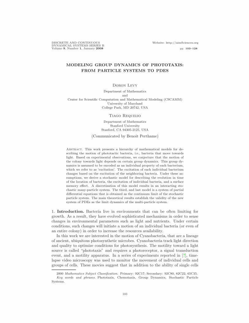
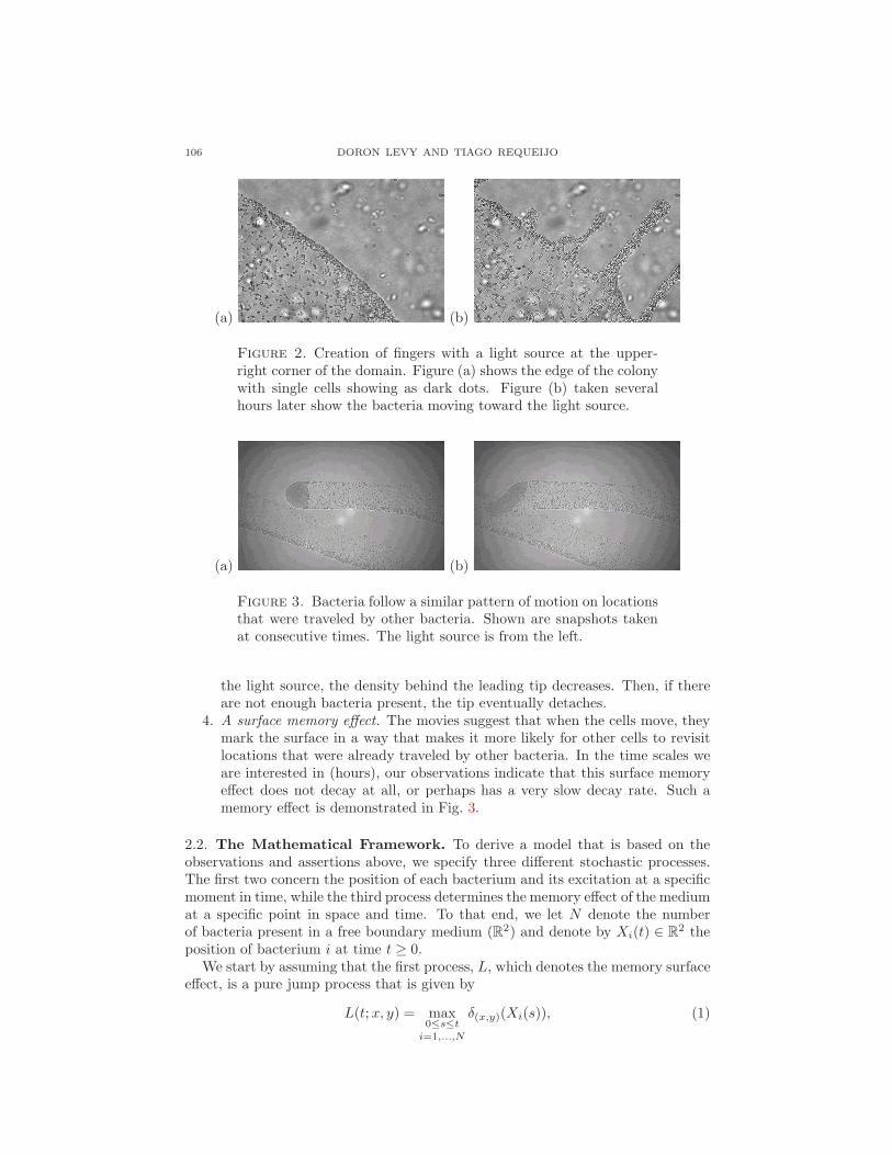
3. Fingering. In areas of low-density, bacteria tend to remain still, while whenthe density of bacteria is high, cells tend to move faster. Such a “competition”between the inhomogeneously populated regions results with fingers such asthose that can be seen in Fig. 2. Bacteria that end up being on the edgesof these fingers stop moving (or move very slowly). In some cases it is evenpossible to observe a pinching. This happens when the density of cells is highenough to form a finger but as the finger is formed and bacteria move towards
106 DORON LEVY AND TIAGO REQUEIJO
(a) (b)
Figure 2. Creation of fingers with a light source at the upper-right corner of the domain. Figure (a) shows the edge of the colonywith single cells showing as dark dots. Figure (b) taken severalhours later show the bacteria moving toward the light source.
(a) (b)
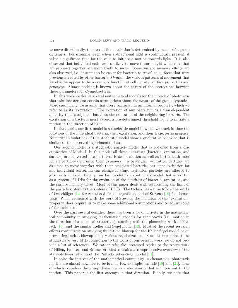
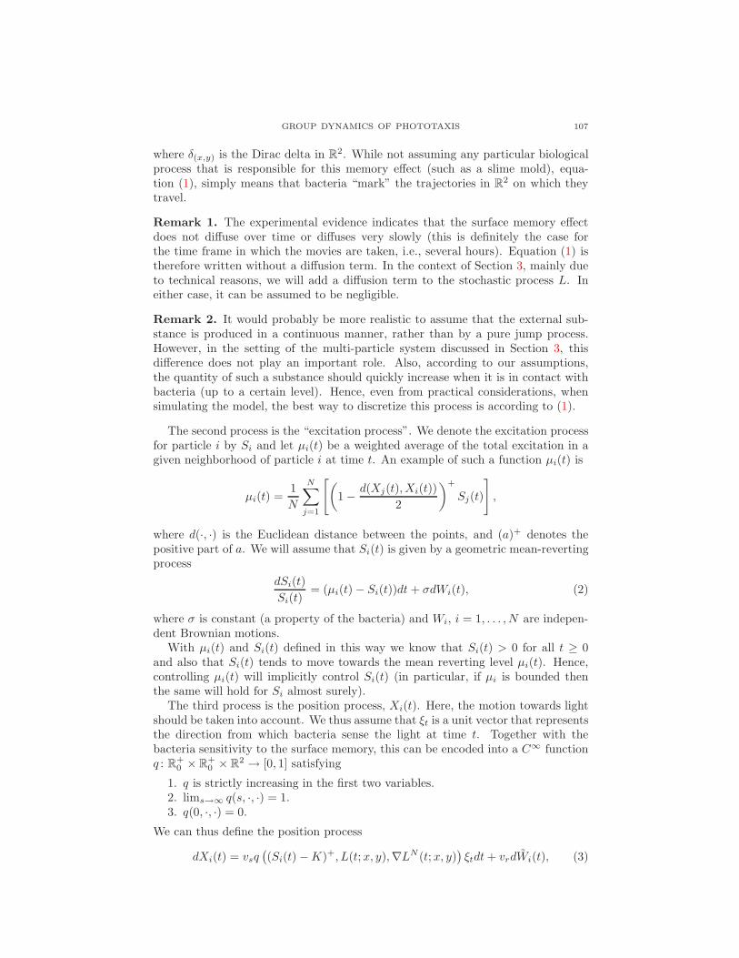
Figure 3. Bacteria follow a similar pattern of motion on locationsthat were traveled by other bacteria. Shown are snapshots takenat consecutive times. The light source is from the left.
the light source, the density behind the leading tip decreases. Then, if thereare not enough bacteria present, the tip eventually detaches.
4. A surface memory effect. The movies suggest that when the cells move, theymark the surface in a way that makes it more likely for other cells to revisitlocations that were already traveled by other bacteria. In the time scales weare interested in (hours), our observations indicate that this surface memoryeffect does not decay at all, or perhaps has a very slow decay rate. Such amemory effect is demonstrated in Fig. 3.
2.2. The Mathematical Framework. To derive a model that is based on theobservations and assertions above, we specify three different stochastic processes.The first two concern the position of each bacterium and its excitation at a specificmoment in time, while the third process determines the memory effect of the mediumat a specific point in space and time. To that end, we let N denote the numberof bacteria present in a free boundary medium (R2) and denote by Xi(t) ∈ R
2 theposition of bacterium i at time t ≥ 0.
We start by assuming that the first process, L, which denotes the memory surfaceeffect, is a pure jump process that is given by
L(t;x, y) = max0≤s≤t
i=1,...,N
δ(x,y)(Xi(s)), (1)
GROUP DYNAMICS OF PHOTOTAXIS 107
where δ(x,y) is the Dirac delta in R2. While not assuming any particular biological
process that is responsible for this memory effect (such as a slime mold), equa-tion (1), simply means that bacteria “mark” the trajectories in R
2 on which theytravel.
Remark 1. The experimental evidence indicates that the surface memory effectdoes not diffuse over time or diffuses very slowly (this is definitely the case forthe time frame in which the movies are taken, i.e., several hours). Equation (1) istherefore written without a diffusion term. In the context of Section 3, mainly dueto technical reasons, we will add a diffusion term to the stochastic process L. Ineither case, it can be assumed to be negligible.
Remark 2. It would probably be more realistic to assume that the external sub-stance is produced in a continuous manner, rather than by a pure jump process.However, in the setting of the multi-particle system discussed in Section 3, thisdifference does not play an important role. Also, according to our assumptions,the quantity of such a substance should quickly increase when it is in contact withbacteria (up to a certain level). Hence, even from practical considerations, whensimulating the model, the best way to discretize this process is according to (1).
The second process is the “excitation process”. We denote the excitation processfor particle i by Si and let µi(t) be a weighted average of the total excitation in agiven neighborhood of particle i at time t. An example of such a function µi(t) is
µi(t) =1
N
N∑
j=1
[
(
1 −d(Xj(t), Xi(t))
2
)+
Sj(t)
]
,
where d(·, ·) is the Euclidean distance between the points, and (a)+ denotes thepositive part of a. We will assume that Si(t) is given by a geometric mean-revertingprocess
dSi(t)
Si(t)= (µi(t) − Si(t))dt+ σdWi(t), (2)
where σ is constant (a property of the bacteria) and Wi, i = 1, . . . , N are indepen-dent Brownian motions.
With µi(t) and Si(t) defined in this way we know that Si(t) > 0 for all t ≥ 0and also that Si(t) tends to move towards the mean reverting level µi(t). Hence,controlling µi(t) will implicitly control Si(t) (in particular, if µi is bounded thenthe same will hold for Si almost surely).
The third process is the position process, Xi(t). Here, the motion towards lightshould be taken into account. We thus assume that ξt is a unit vector that representsthe direction from which bacteria sense the light at time t. Together with thebacteria sensitivity to the surface memory, this can be encoded into a C∞ functionq : R
+0 × R
+0 × R
2 → [0, 1] satisfying
1. q is strictly increasing in the first two variables.2. lims→∞ q(s, ·, ·) = 1.3. q(0, ·, ·) = 0.
We can thus define the position process
dXi(t) = vsq(
(Si(t) −K)+, L(t;x, y),∇LN (t;x, y))
ξtdt+ vrdWi(t), (3)
108 DORON LEVY AND TIAGO REQUEIJO
where Wi(t) are independent 2-dimensional Brownian motions and vs, vr are themaximum velocity components for 1) excitation and sensitivity to external sub-stance, 2) the random phenomena. For each N > 0, LN is the stochastic processobtained from L by a convolution with a mollifier. Equation (3) is designed in away that guarantees that bacteria tend to move in the direction of light only ifthe excitation exceeds the predetermined threshold K. In such cases, the surfacememory effect is also taken into account in the overall motion towards light. If theexcitation of an individual bacterium does not pass the threshold K, the only mech-anism that controls its motion is a random phenomenon. This model thus accountsfor sensitivity to the extra substance, sensitivity to light, and random phenomena.
Remark 3. In order to take into account the possibility of time periods withoutany light, the processes Si(t) can be changed by either making them decay fastwhen the light source is not present or even by making them jump to values belowthe threshold K at the moment the light source vanishes.
Remark 4. The main difference between our model of phototaxis and the chemo-taxis model of Stevens [18] resides in the existence of the excitation quantity, whichis an internal property of each bacteria. Equation (2) has the desired effect that anindividual’s excitation will evolve towards a surrounding neighborhood trend (givenby µi(t)). The excitation serves as a mechanism for taking into account the groupdynamics. The threshold that the excitation must pass in order to initiate a motiontoward light serves as a way for encoding the observed delay in the response of thebacteria to light.
2.3. Numerical Simulations. We used the model described in Section 2.2 to sim-ulate the behavior of a bacteria population. The simulation is done by discretizing(1), (2) and (3) for small time increments. The functions and parameters that wereused in our simulations are: ∆t = 0.1, σ = 0.3, K = 0.1, vs = 3.0, vr = 0.05, andq(s, w, v) = α(w, v)
(
1− exp(−s))
, where α(w, v) = max{w, v · ξt, 0.2}. For the sakeof brevity, we refer to [5] for the details of the discretizations of the model equations.
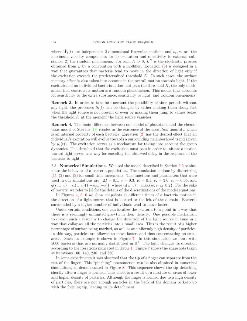
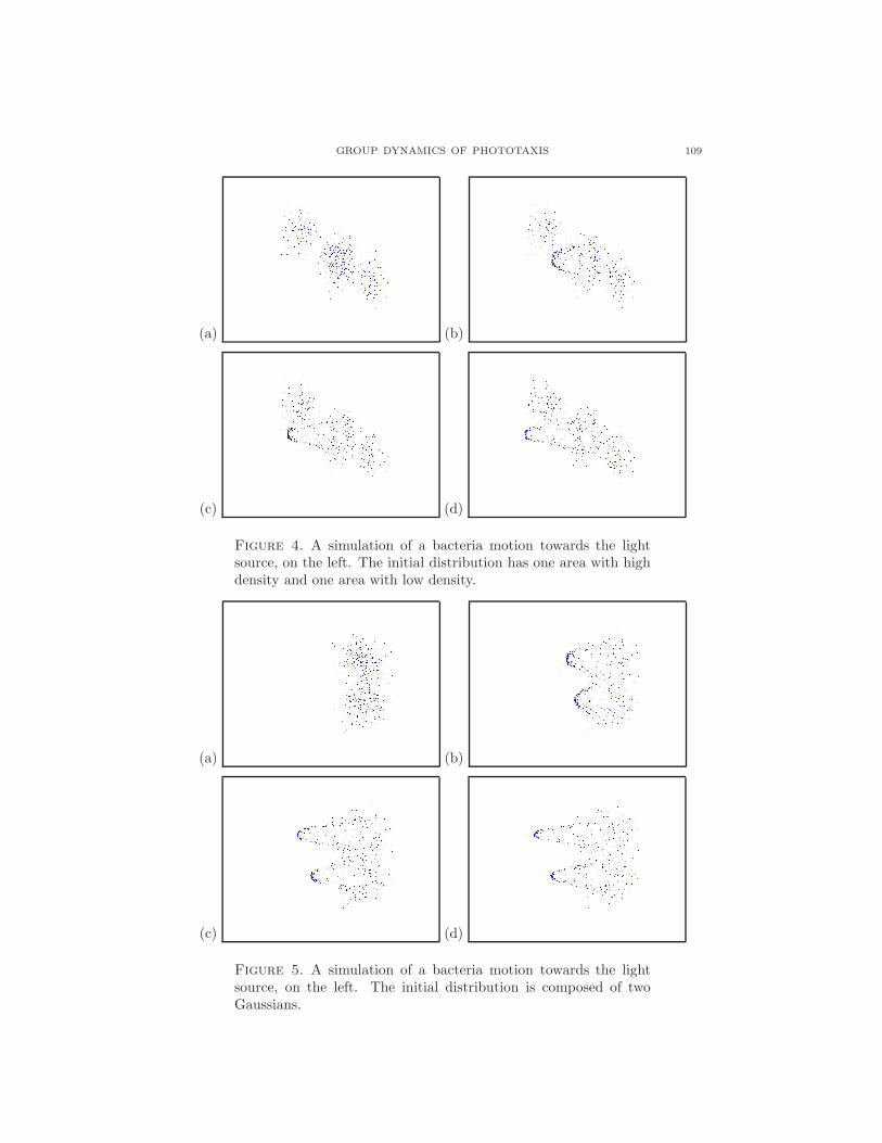
In Figures 4, 5, 6 we show snapshots at different times of a bacteria motion inthe direction of a light source that is located to the left of the domain. Bacteriasurrounded by a higher number of individuals tend to move faster.
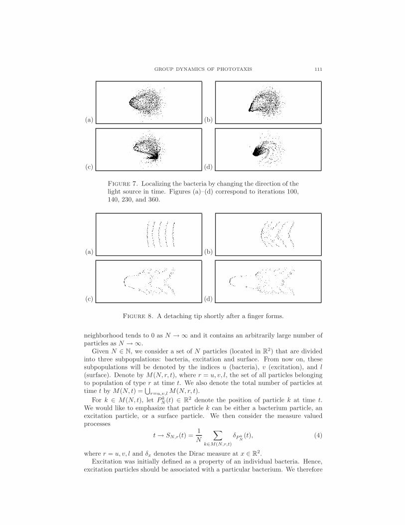
Under certain conditions, one can localize the bacteria to a point in a way thatthere is a seemingly unlimited growth in their density. One possible mechanismto obtain such a result is to change the direction of the light source in time in away that collapses all the particles into a small area. This is the result of a higherpercentage of surface being marked, as well as an uniformly high density of particles.In this way, particles are allowed to move faster, and thus concentrating on smallareas. Such an example is shown in Figure 7. In this simulation we start with5000 bacteria that are normally distributed in R
2. The light changes its directionaccording to the iterations indicated in Table 1. Figure 7 shows the snapshots takenat iterations 100, 140, 230, and 360.
In some experiments it was observed that the tip of a finger can separate from therest of the finger. This “pinching” phenomenon can be also obtained in numericalsimulations, as demonstrated in Figure 8. This sequence shows the tip detachingshortly after a finger is formed. This effect is a result of a mixture of areas of lowerand higher density of particles. Although the finger is formed due to a high densityof particles, there are not enough particles in the back of the domain to keep upwith the forming tip, leading to its detachment.
GROUP DYNAMICS OF PHOTOTAXIS 109
(a) (b)
(c) (d)
Figure 4. A simulation of a bacteria motion towards the lightsource, on the left. The initial distribution has one area with highdensity and one area with low density.
(a) (b)
(c) (d)
Figure 5. A simulation of a bacteria motion towards the lightsource, on the left. The initial distribution is composed of twoGaussians.
110 DORON LEVY AND TIAGO REQUEIJO
iteration 0 − 100 − 140 − 230 − 280 − 330 − 370 − 400
direction | ← | ↓ | → | ↑ | ← | ↓ | → |
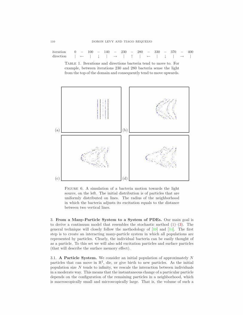
Table 1. Iterations and directions bacteria tend to move to. Forexample, between iterations 230 and 280 bacteria sense the lightfrom the top of the domain and consequently tend to move upwards.
(a) (b)
(c) (d)
Figure 6. A simulation of a bacteria motion towards the lightsource, on the left. The initial distribution is of particles that areuniformly distributed on lines. The radius of the neighborhoodin which the bacteria adjusts its excitation equals to the distancebetween two vertical lines.
3. From a Many-Particle System to a System of PDEs. Our main goal isto derive a continuum model that resembles the stochastic method (1)–(3). Thegeneral technique will closely follow the methodology of [18] and [14]. The firststep is to create an interacting many-particle system in which all populations arerepresented by particles. Clearly, the individual bacteria can be easily thought ofas a particle. To this set we will also add excitation particles and surface particles(that will describe the surface memory effect).
3.1. A Particle System. We consider an initial population of approximately Nparticles that can move in R
2, die, or give birth to new particles. As the initialpopulation size N tends to infinity, we rescale the interaction between individualsin a moderate way. This means that the instantaneous change of a particular particledepends on the configuration of the remaining particles in a neighborhood, whichis macroscopically small and microscopically large. That is, the volume of such a
GROUP DYNAMICS OF PHOTOTAXIS 111
(a) (b)
(c) (d)
Figure 7. Localizing the bacteria by changing the direction of thelight source in time. Figures (a)–(d) correspond to iterations 100,140, 230, and 360.
(a) (b)
(c) (d)
Figure 8. A detaching tip shortly after a finger forms.
neighborhood tends to 0 as N → ∞ and it contains an arbitrarily large number ofparticles as N → ∞.
Given N ∈ N, we consider a set of N particles (located in R2) that are divided
into three subpopulations: bacteria, excitation and surface. From now on, thesesubpopulations will be denoted by the indices u (bacteria), v (excitation), and l(surface). Denote by M(N, r, t), where r = u, v, l, the set of all particles belongingto population of type r at time t. We also denote the total number of particles attime t by M(N, t) =
⋃
r=u,v,lM(N, r, t).
For k ∈ M(N, t), let P kN (t) ∈ R
2 denote the position of particle k at time t.We would like to emphasize that particle k can be either a bacterium particle, anexcitation particle, or a surface particle. We then consider the measure valuedprocesses
t→ SN,r(t) =1
N
∑
k∈M(N,r,t)
δP k
N
(t), (4)
where r = u, v, l and δx denotes the Dirac measure at x ∈ R2.
Excitation was initially defined as a property of an individual bacteria. Hence,excitation particles should be associated with a particular bacterium. We therefore
112 DORON LEVY AND TIAGO REQUEIJO
have to be particularly careful with the numbering of the excitation particles in theset M(N, v, t). To that end, define Mw(N, v, t) ⊂M(N, v, t) as the set of excitationparticles that are associated with bacterium w ∈ M(N, u, t). For any bacteriumw ∈M(N, u, t) we can then define the measure valued process
t→ SN,v,w(t) =∑
k∈Mw(N,v,t)
δP k
N
(t). (5)
Equation (5) is the sum over all the excitation particles that are associated withthat bacterium. Note that since {Mw(N, v, t)}w∈M(N,u,t) is a partition ofM(N, v, t),
then SN,v(t) = 1N
∑
w∈M(N,u,t) SN,v,w(t).
3.2. Densities. We now introduce smoothed versions of the empirical processesabove. For a fixed symmetric and sufficiently smooth function W1 (see [14] fortechnical conditions on this function), let
WN (x) = α2NW1(αNx), WN (x) = α2
NW1(αNx),
where αN = Nα/2 and αN = N α/2 for fixed scaling exponents α and α. We alsointroduce a sequence δN = N−δ. Given an arbitrarily small ρ > 0, we assume thatα, α, and δ satisfy
α ≤δ
3and 2δ(1 + 2ρ) < α <
2
5. (6)
We are now ready to define for r = u, v, l
sN,r(t, x) = (SN,r(t) ∗WN ∗WN )(x),
sN,r(t, x) = (SN,r(t) ∗WN ∗ WN )(x),(7)
and, for w ∈M(N, v, t),
sN,v,w(t, x) = (SN,v,w(t) ∗WN ∗WN )(x),
sN,v,w(t, x) = (SN,v,w(t) ∗WN ∗ WN )(x).(8)
The functions defined in (7) and (8) formally represent the density or concen-tration of each subpopulation near x at time t. We introduce two density versionsof each type (s and s) for technical reasons that will be made clear later. A morethorough discussion and technical details can be found in [14]. Finally, we definethe following auxiliary functions that will play a major role in the analysis below
VN (x) = (WN ∗WN ) (x),
hN,r(t, x) = (SN,r(t) ∗WN ) (x),(9)
for r = u, v, l. Note that the definition (9) implies that sN,r(t, x) = (hN,r(t)∗WN )(x)
and sN,r(t, x) = (hN,r(t) ∗ WN )(x).
3.3. Dynamics. Existing particles can move (in R2), and they can also cause dis-
continuous changes to the population, i.e., they can die or give birth to new particles.We start with describing the motion of particles. In what follows, {W k(t)}k∈M(N,t)
are independent 2-dimensional Brownian motions. For the bacteria particles we let(for t ≥ 0)
dP kN (t) =g
(
sN,v,k(t, P kN (t)), sN,l(t, P
kN (t)),∇sN,l(t, P
kN (t))
)
dt+√
2µdW k(t)
:=gkN
(
t, P kN (t)
)
dt+√
2µdW k(t), ∀k ∈M(N, u, t).(10)
GROUP DYNAMICS OF PHOTOTAXIS 113
Here, gkN(t, x) = g (sN,v,k(t, x), sN,l(t, x),∇sN,l(t, x)) (compare with (3)). The exci-
tation particles move together with the bacterium they are associated with. Hence,we impose
dP kN (t) = dPw
N (t), ∀k ∈Mw(N, v, t). (11)
Finally, for the surface memory particles, we have
dP kN (t) =
√
2ηdW k(t), ∀k ∈M(N, l, t), (12)
We assume that η is a small positive constant, so that the surface memory effectdiffuses at a slow rate.
We assume that any bacteria particle k ∈M(N, u, t) at position P kN (t) = y may
induce discontinuous changes in the excitation (v) and surface (l) subpopulations;namely they give birth to surface (type l) particles, with intensity λN (t, y), andthey give birth to excitation (type v) particles, with intensity βN,k(t, y). We alsoassume that any excitation particle, k ∈ M(N, v, t) at position P k
N (t) = y, maycause the death of excitation particles, with intensity γN,k(t, y). (This is equivalentto saying that the death rate of the excitation particles is proportional to the densityof these particles). These intensities are assumed to depend on the densities of theN -particle system, i.e.,
βN,k(t, x) = β(sN,v,k(t, x), sN,u(t, x), sN,v(t, x)),
γN,k(t, x) = γ(sN,v,k(t, x), sN,u(t, x), sN,v(t, x)),
λN (t, x) = λ(sN,u(t, x), sN,l(t, x)).
(13)
These birth and death processes are given as
βkN (t) = Qβ,k
N
(∫ t
0
1M(N,u,τ)(k)βN,k(τ, P kN (τ))dτ
)
,
γkN (t) = Qγ,k
N
(∫ t
0
1M(N,v,τ)(k)γN,k(τ, P kN (τ))dτ
)
, (14)
λkN (t) = Qλ,k
N
(∫ t
0
1M(N,l,τ)(k)λN (τ, P kN (τ))dτ
)
,
where Q·
N are independent standard Poisson processes. The point processes βkN (t),
γkN (t), λk
N (t) for a jump of size 1 at time t, have intensities 1M(N,u,τ)(k)βN,k(t, P kN (t)),
1M(N,u,t)(k)γN,k(t, P kN (t)), and 1M(N,u,t)(k)λN (t, P k
N (t)).
3.4. The Limit Dynamics. In this section we present a heuristic derivation of thelimit dynamics of the particle system (10)–(14). The idea is to use Ito’s formula onthe processes (10), (11) and (12) to obtain integral systems for SN,r(t), r = u, v, l.At this point we take the limit when N → ∞ and arrive at an integral system forthe densities r(t, ·) corresponding to SN,r(t). The phototaxis system follows afterintegrating by parts the limit integral system. At this stage, the transition to thelimit densities will be formal. This connection will be rigorously established in thefollowing sections.
114 DORON LEVY AND TIAGO REQUEIJO
Using Ito’s formula on (10), we obtain for f ∈ C1,2b (R+ × R
2) and bacteriumk ∈M(N, u, t),
f(
t, P kN (t)
)
=f(
0, P kN (0)
)
+
∫ t
0
√
2µ∇f(
τ, P kN (τ)
)
· dW k(t)
+
∫ t
0
[
∇f(
τ, P kN (τ)
)
· gkN
(
τ, P kN (τ)
)
+ ∂τf(
τ, P kN (τ)
)
+ µ∆f(
τ, P kN (τ)
)
]
dτ.
(15)
In order to simplify (15) we define the functional T kN : C1,2
b (R+ × R2) → R by
T kN(ϕ) = ∇ϕ
(
τ, P kN (τ)
)
· gkN
(
τ, P kN (τ)
)
+ ∂τϕ(
τ, P kN (τ)
)
+ µ∆ϕ(
τ, P kN (τ)
)
. (16)
Thus, (15) reads
f(
t, P kN (t)
)
= f(
0, P kN(0)
)
+
∫ t
0
T kN (f)dτ +
∫ t
0
√
2µ∇f(
τ, P kN (τ)
)
· dW k(t). (17)
Let 〈µ, f〉 =∫
R2 f(x)µ(dx) for any measure µ and real-valued function f in R2.
In order to study the limit behavior of the bacteria particles, we are interested incomputing 〈SN,r(t), f(t, ·)〉. Since there are no births or deaths of type u particles,
〈SN,u(t), f(t, ·)〉 = 〈SN,u(0), f(0, ·)〉 +1
N
∫ t
0
∑
k∈M(N,u,τ)
T kN(f)dτ
+1
N
∫ t
0
∑
k∈M(N,u,τ)
√
2µ∇f(
τ, P kN (τ)
)
· dW k(t)
(18)
For the excitation particles, i.e., k ∈M(N, v, t), we have to take into account birthand decay. The motion of the excitation particles follows the motion of the bacteriaparticles (see (11)). Thus
〈SN,v(t), f(t, ·)〉 =1
N
∑
k∈M(N,v,t)
f(
t, P kN (t)
)
+ birth/decay terms
=1
N
∑
k∈M(N,u,t)
SN,v,w(τ)(
P kN (τ)
)
f(
t, P kN (t)
)
+ birth/decay terms.
(19)
Hence,
GROUP DYNAMICS OF PHOTOTAXIS 115
〈SN,v(t), f(t, ·)〉
= 〈SN,v(0), f(0, ·)〉
+1
N
∫ t
0
∑
k∈M(N,u,τ)
SN,v,w(τ)(
P kN (τ)
)
T kN (f)dτ
+1
N
∫ t
0
∑
k∈M(N,u,τ)
SN,v,w(τ)(
P kN (τ)
)√
2µ∇f(
τ, P kN (τ)
)
· dW k(t) (20)
+1
N
∫ t
0
∑
k∈M(N,u,τ)
f(
τ, P kN (τ)
)
βkN (dτ)
−1
N
∫ t
0
∑
k∈M(N,v,τ)
f(
τ, P kN (τ)
)
γkN (dτ).
Finally, for the surface particles we have (see (12)):
〈SN,l(t), f(t, ·)〉 = 〈SN,l(0), f(0, ·)〉 +1
N
∫ t
0
∑
k∈M(N,l,τ)
T kN(f)dτ
+1
N
∫ t
0
∑
k∈M(N,l,τ)
√
2η∇f(
τ, P kN (τ)
)
· dW k(t)
+1
N
∫ t
0
∑
k∈M(N,u,τ)
f(
τ, P kN (τ)
)
λkN (dτ).
(21)
To deal with the random components of the dynamics, we introduce the processes
MNr (t, f) =
1
N
∫ t
0
∑
k∈M(N,r,t)
√
2µ∇f(
τ, P kN (τ)
)
· dW k(t), r = u, v, l,
MNv,γ(t, f) =
1
N
∫ t
0
∑
k∈M(N,u,τ)
f(
τ, P kN (τ)
) (
γkN (dτ) − γN,k
(
τ, P kN (τ)
)
dτ)
,
MNv,β(t, f) =
1
N
∫ t
0
∑
k∈M(N,v,τ)
f(
τ, P kN (τ)
) (
βkN (dτ) − βN,k
(
τ, P kN (τ)
)
dτ)
,
MNl,λ(t, f) =
1
N
∫ t
0
∑
k∈M(N,u,τ)
f(
τ, P kN (τ)
) (
λkN (dτ) − λN
(
τ, P kN (τ)
)
dτ)
.
(22)
The processes defined in (22) are martingales with respect to the natural filtrationgenerated by the processes t →
(
P kN (t),1M(N,r,t)(k)
)
1kN (t) where 1
kN (t) is the in-
dicator function of the lifetime of individual k. If we assume that the quadraticvariation of these martingales tends to 0 as N → ∞, they can be neglected whenpassing to the limit dynamics.
From Section 3.2, we see that in the sense of distributions,
limN→∞
WN = limN→∞
WN = δ0.
For r = u, v, l and t ≥ 0 we assume that in some sense (similarly to [18] and [14]),
limN→∞
SN,r(t) = Sr(t),
116 DORON LEVY AND TIAGO REQUEIJO
where the measures Sr(t) have a smooth density r(t, ·). It follows that
limN→∞
sN,r(t, ·) = limN→∞
sN,r(t, ·) = r(t, ·),
and
limN→∞
∇sN,r(t, ·) = limN→∞
∇sN,r(t, ·) = ∇r(t, ·).
Let u0(·), v0(·) and l0(·) be the densities of Su(0), Sv(0) and Sl(0). Defineλ∞(τ, x) = λ(u(τ, x), l(τ, x)) as the growth rate of surface memory at x ∈ R
2 attime τ . In order to define g∞, β∞ and γ∞, we assume that as N → ∞, the totalexcitations of bacteria (w and w) that are close with respect to the size of theinteraction domain should be close to each other. That is, if |Pw
N (t) − P wN (t)| is
small compared to the domain of interaction then
|Mw(N, v, t)| ≃ |Mw(N, v, t)|.
Thus, in the limit as N → ∞, SN,v,w(t) should be approximated by the number ofexcitation particles at Pw
N (t) divided by the number of bacteria particles at PwN (t),
i.e.
SN,v,w(t)(PwN ) ≃
∑
k∈Sv(N,t) δP k
N
(PwN )
∑
k∈Su(N,t) δP k
N
(PwN )
=SN,v(t)(P
wN )
SN,u(t)(PwN )
,
which, in turn, implies that
limN→∞
sN,v,x(t) =v(t, x)
u(t, x).
Hence, we get
g∞(τ, ·) = g
(
v(τ, ·)
u(τ, ·),∇l(τ, ·),∇u(τ, ·)
)
,
γ∞(τ, ·) = γ
(
v(τ, ·)
u(τ, ·), u(τ, ·), v(τ, ·)
)
,
β∞(τ, ·) = β
(
v(τ, ·)
u(τ, ·), u(τ, ·), v(τ, ·)
)
.
We can now formally take the limit and obtain
〈u(t, ·), f(t, ·)〉 = 〈u0(·), f(0, ·)〉
+
∫ t
0
⟨
u(t, ·),∇f(τ, ·) · g∞ (τ, ·) + ∂τf(τ, ·) + µ∆f(τ, ·)⟩
dτ
〈v(t, ·), f(t, ·)〉 = 〈v0(·), f(0, ·)〉
+
∫ t
0
⟨
v(t, ·),∇f(τ, ·) · g∞ (τ, ·) + ∂τf(τ, ·) + µ∆f(τ, ·)⟩
dτ
+
∫ t
0
〈u(t, ·), β∞(τ, ·)f(τ, ·)〉 dτ −
∫ t
0
〈v(t, ·), γ∞(τ, ·)f(τ, ·)〉dτ
〈l(t, ·), f(t, ·)〉 = 〈l0(·), f(0, ·)〉
+
∫ t
0
⟨
l(t, ·), ∂τf(τ, ·) + η∆f(τ, ·)⟩
dτ
+
∫ t
0
〈u(t, ·), λ∞(τ, ·)f(τ, ·)〉 dτ.
(23)
GROUP DYNAMICS OF PHOTOTAXIS 117
Integrating (23) by parts we obtain the system
∂tu =µ∆u−∇ ·(
g(v/u, l,∇l)u)
,
∂tv =µ∆v −∇ ·(
g(v/u, l,∇l)v)
+ β(v/u, u, v)u− γ(v/u, u, v)v,
∂tl =η∆l + λ(u, l)u,
(24)
which we rewrite as
∂tu =µ∆u−∇ ·(
g(u, v, l,∇l)u)
,
∂tv =µ∆v −∇ ·(
g(u, v, l,∇l)v)
+ β(u, v)u − γ(u, v)v,
∂tl =η∆l + λ(u, l)u.
(25)
with a new function g that replaces the function g in (24). From now on, we willrefer to the system (25) as the phototaxis system.
Remark 5. The structure of the system (25) is not surprising, We expect the rateof change on bacteria density u to be given by a diffusion part (originating fromthe Brownian motion) plus an advection term that captures the sensitivity to lightand the external substance. Similarly, the excitation density v, can be expectedto follow the same motion pattern as u and hence an identical velocity, with theaddition of birth and decay terms. The surface is marked proportionally to themotion of the bacteria, with a weak diffusion term.
Remark 6. The phototaxis system (25) is similar to the classical chemotaxis system
{
∂tu =µ∆u −∇ ·(
χ(u, v)u∇v)
∂tl =η∆l + λ(u, l)u− κ(u, l)l(26)
where u is the bacteria density and v is the density of chemo-attractant. The maindifference in our case is the existence of an internal property, which shows up in thesystem (25) as a quantity that closely follows the dynamics of the bacteria u (plusthe additional birth and decay terms).
Remark 7. Our derivation is based on the assumption that, as N → ∞,|Mw(N, v, t)| ≃ |Mw(N, v, t)| if Pw
N (t) = P wN (t). That is, as N → ∞, our model
looks like a reaction-diffusion system, which allows us to use the methods discussedin [18] and [14]. As mentioned above, when rescaling the interaction in a moder-ate way, we are looking at neighborhoods that are microscopically large. Hence,as N → ∞, we expect to have an arbitrarily large number of individuals in suchneighborhoods.
Remark 8. Comparing with the model introduced in Section 2.2, arriving at pos-sible functions for g and λ is fairly easy. In fact one can use the function q withminor modifications in place of g. For β and γ one needs to be somewhat carefulas these functions regulate the dynamics of v. In particular β and γ must lead to v
ubounded, and well-defined as u approaches 0. A possible choice is β(u, v) = 0 when-ever v > Cu for some fixed constant C, and γ(u, v) large enough when u approacheszero in order to guarantee the smoothness of v
u . This choice for β guarantees theboundedness of v
u , while the choice for γ ensures that v approaches zero sufficientlyfast when u approaches zero.
118 DORON LEVY AND TIAGO REQUEIJO
3.5. Limit Theorems. In this section we proceed with the formal approach corre-sponding to the description given in Sec. 3.4. This approach follows closely the workof Stevens [18], and Oelschlager [14]. The idea is to consider an intermediate system(see (27) below), and show that the solution for this system is in some sense closeto both the solution for the phototaxis system and the limit of SN,r as N → ∞.The precise statements are given in Theorems 3.1, 3.2, and 3.3. Theorem 3.1 as-serts that the solution for (27) converges to the solution of the phototaxis systemin the | · |[0,T ] introduced below. Theorem 3.2 shows that the difference between the
solution for (27) and a smoothed version of the processes SN,r is approaching zeroas N → ∞. Finally, Theorem 3.3 combines the results from the previous theoremsto conclude the desired result.
Before stating the main results, we will outline some technical assumptions. Weassume that W1 is a symmetric probability density (as in [18]). This is a reasonableassumption as a Gaussian probability density satisfies it. Since sN,r and sN,r are
given by a convolution with WN and WN , we have the estimate∣
∣
∣
∣
∣
∣
∣
∣
∂k1+k2
(∂x1)k1(∂x1)k2
sN,r
∣
∣
∣
∣
∣
∣
∣
∣
C0
≤ C(k1, k2)〈SN (t), 1〉α2+k1+k2
N ,
where k1, k2 ∈ N, t ≥ 0.We also assume that the following quantities are positive, µ, η, σ > 0; that the
function g is continuously differentiable and bounded together with its derivatives;that β, γ, λ are continuously differentiable and bounded together with their deriva-tives; and that u0, v0, l0 ∈ C∞
b (R2) with 〈u0, ψ〉, 〈v0, ψ〉, 〈l0, ψ〉 ≤ C for ψ(x) =log(2+x2), x ∈ R
2. The form of this function is identical to the one in [18]. Finally,we assume that for some T > 0, the phototaxis system (24) has a unique positivesolution u, v, l ∈ C∞
b ([0, T ] × R2,R) ∩ C0([0, T ], L2(R
2)) such that v/u is also inC∞
b ([0, T ] × R2,R) ∩ C0([0, T ], L2(R
2)).Denote by ||·||2 the L2-norm in R
2 and define
|f |[0,T ] = supt≤T
||f ||22 +
∫ T
0
||∇f ||22 dt,
for any function f ∈ C0([0, T ], L2(R2)) ∩ L2([0, T ], L2(R2)). We also define for allpositive measures ν1, ν2 on R
2,
d(ν1, ν2) = sup{〈ν1 − ν2, f〉 : f ∈ C1b (R2), ||f ||C0 + ||∇f ||C0 ≤ 1}.
We are now ready to consider the system
∂tuN =∇ ·(
µ∇uN − gN uN
)
,
∂tvN =∇ ·(
µ∇vN − gN vN
)
+ βN uN − γN vN ,
∂t lN =η∆lN + λN uN ,
(27)
subject to the initial data uN (0, x) = uN0(x), vN (0, x) = vN0(x), and lN (0, x) =
lN0(x). Here, gN(t, x) = g(
(uN (t, ·) ∗ WN )(x), (vN (t, ·) ∗ WN )(x), (lN (t, ·) ∗ WN )(x),
∇(uN (t, ·) ∗ WN )(x))
, βN (t, x) = β(
(uN (t, ·) ∗ WN )(x), (vN (t, ·) ∗ WN )(x))
, andγN (t, x), λN (t, x) are defined in a similar way. We assume that the system (27)
has a unique positive solution uN , vN , lN ∈ C1,∞b ([0, T ]×R
2,R)∩C0([0, T ], L2(R2))
such that vN/uN also belongs to C1,∞b ([0, T ] × R
2,R) ∩ C0([0, T ], L2(R2)). Under
these conditions, the theorems from [18] that were formulated for the chemotaxissystem hold also for the phototaxis system:
GROUP DYNAMICS OF PHOTOTAXIS 119
Theorem 3.1. If uN0, vN0, lN0 ∈ C∞b (R2) and
limN→∞
||uN0 − u0||22 + ||vN0 − v0||
22 + ||lN0 − l0||
22 = 0, (28)
then the solutions for (27) are uniformly bounded with respect to N in the associated
norm and
limN→∞
|uN − u|[0,T ] + |vN − v|[0,T ] + |lN − l|[0,T ] = 0. (29)
Theorem 3.2. Assume that the initial distributions of particles are converging
limN→∞
P[
||hN,u(0, ·) − uN0||22 + ||hN,v(0, ·) − vN0||
22 (30)
+||hN,l(0, ·) − lN0||22 ≥ δ1+2ρ
N
]
= 0,
and that the number of particles grows in a controlled way, i.e.,
limn→∞
supN∈N
P [〈SN (0), 1〉 ≥ n] = 0. (31)
Then
limN→∞
P[
|hN,u − uN |[0,T ] + |hN,v − vN |[0,T ] + |hN,l − lN |[0,T ] ≥ δN
]
= 0, (32)
where uN , vN , lN is the unique solution for (27).
Theorem 3.3. Assume that the initial distribution of particles is controlled in the
limit
limn→∞
supN∈N
P [〈SN,u(0), ψ2〉 + 〈SN,v(0), ψ2〉 + 〈SN,l(0), ψ2〉 ≥ n] = 0, (33)
where ψ(x) = log(2 + x2). Then SN,r converge in probability to the corresponding
densities, i.e., for δ > 0,
limN→∞
P
[
supt≤T
d(SN,u(t), u(t, ·)) + supt≤T
d(SN,v(t), v(t, ·)) (34)
+ supt≤T
d(SN,l(t), l(t, ·)) ≥ δ
]
= 0.
Theorem 3.3 gives us the desired result, i.e., the phototaxis system (24) is thelimit as N → ∞ for the particle systems whose dynamics is defined by (10), (11),and (12).
The proofs of these theorems follow the arguments in [18]. The main differenceis in the proof of Theorem 3.2. This proof requires adjustments to some of theestimates in [18]. In Section 4 we sketch the proof of Theorem 3.2. We do notprovide the proofs for Theorems 3.1 and 3.3 . The proof of Theorem 3.1 is similarto the one for Theorem 3.2, where estimates to |rN − r|[0,T ] are obtained in the same
way as in Sec. 4.2. Theorem 3.3 is a consequence of the first two theorems, and itsproof can be repeated by following the arguments in [18] with minor modifications.
4. A Sketch of the Proof of Theorem 3.2. Generally, the proof follows thearguments of [18] with some necessary adjustments that are outlined below. Fortechnical reasons, we will need to consider the following system
∂tuN =∇ ·(
µ∇uN − gNuN
)
,
∂tvN =∇ ·(
µ∇vN − gNvN
)
+ βNuN − γNvN ,
∂tlN =η∆lN + λNuN ,
(35)
120 DORON LEVY AND TIAGO REQUEIJO
subject to the initial data uN (0, x) = uN0(x), vN (0, x) = vN0(x), and lN (0, x) =lN0(x). Here, gN (t, x) = g (sN,v(t, x)/sN,u(t, x),∇sN,l(t, x),∇sN,u(t, x))and βN(t, x), γN (t, x), and λN (t, x) are defined analogously. Note that gN , βN ,γN , and λN do not depend directly on uN , vN , or lN . This is the phototaxis sys-tem with frozen nonlinearities. We assume that this system has a unique regularsolution uN , vN , lN .
The system (35) will be used to show that for a suitable stopping time TN ,
limN→∞
P[
|hN,u − uN |[0,TN ] + |hN,v − vN |[0,TN ] + |hN,l − lN |[0,TN ] ≥ δ1+ρN
]
= 0.
We will also determine that
limN→∞
P
[
|uN − uN |[0,TN ] + |vN − vN |[0,TN ] + |lN − lN |[0,TN ] ≥δN2
]
= 0,
and using a triangle inequality, conclude with the desired result of Theorem 3.2.Following our previous assumptions, we assume that the difference between
sN,v,u(t, x), sN,v(t, x)/sN,u(t, x), and v(t, x)/u(t, x) converge to zero sufficiently fastwhen N → ∞. A consequence of this assumption is that
|(gkN − gN )(t, x)| ≤ AN (t, x) ||∇g||C0 , (36)
where ||AN ||2 → 0 sufficiently fast as N → ∞. The same estimate holds when g issubstituted for β or γ. Another consequence of such assumption is that the quantityv(t, x)/u(t, x) is bounded and goes to zero as u(t, x) goes to zero. In particular, wemust have
∣
∣
∣
∣
∣
∣
∣
∣
v(t, x)
u(t, x)−v(t, y)
u(t, y)
∣
∣
∣
∣
∣
∣
∣
∣
2
2
≤ C ||u(t, x) − u(t, y)||22 . (37)
We assume that this behavior is valid for both systems (27) and (35). Essentially,such an assumption is reasonable as one expects the excitation to tend to zero (ata certain rate) in locations where the density of bacteria also tends to zero.
Due to the hypothesis (31) and the fact that β is a bounded function, we have
limn→∞
supN∈N
P [supτ≤T
〈SN (τ), 1〉 ≥ n] = 0. (38)
This means that the number of particles is in some sense controlled up to time T .Note that the quantity 〈SN (τ), 1〉 is the total number of particles at time τ dividedby N , so that (38) really means that the ratio between the number of particles forthe N -system and N is bounded almost surely.
Based on (38), it is natural to consider the following stopping times
T nN (ω) = inf
{
τ > 0∣
∣
∣supσ≤τ
〈SN (σ), 1〉(ω) > n
}
.
Note that (38) is valid if one substitutes T with any T <∞. In particular, defining1
T nN := T ∧ T n
N , one has limn→∞ P [T nN > T ] = 1, so we just need to show that
limN→∞
P[
|hN,u − uN |[0,T n
N] + |hN,v − vN |[0,T n
N] + |hN,l − lN |[0,T n
N] ≥ δN
]
= 0, (39)
in order to conclude with (32). To that end consider the hitting time
tN (ω) ={
τ > 0∣
∣
∣
(
|hN,u − uN |[0,τ ] + |hN,v − vN |[0,τ ] + |hN,l − lN |[0,τ ]
)
(ω) ≥ δN
}
.
1the notation ∧ means a ∧ b = min{a, b}
GROUP DYNAMICS OF PHOTOTAXIS 121
For any stopping time T0 = T0(ω), denote [0, T0] = {τ ∧ T0 : τ ≥ 0}. With thisnotation and from the definition of tN we have
P[
|hN,u − uN |[0,T n
N] + |hN,v − vN |[0,T n
N] + |hN,l − lN |[0,T n
N] ≥ δN
]
=P[
|hN,u − uN |[0,T n
N∧tN ] + |hN,v − vN |[0,T n
N∧tN ] + |hN,l − lN |[0,T n
N∧tN ] ≥ δN
]
≤P[
|hN,u − uN |[0,T n
N∧tN ] + |hN,v − vN |[0,T n
N∧tN ] + |hN,l − lN |[0,T n
N∧tN ] ≥ δ1+ρ
N
]
+ P
[
|uN − uN |[0,T n
N∧tN ] + |vN − vN |[0,T n
N∧tN ] + |lN − lN |[0,T n
N∧tN ] ≥
δN2
]
.
(40)
The inequality above comes from using the triangle inequality and from noting that
for N large, δ1+ρN = N−δ(1+ρ) < N−δ
2 = δN
2 . We need to estimate the right side of(40) in order to achieve (39). Those estimates rely on uniform boundedness withrespect to N of supt≤T n
N∧tN
||sN,r(t, ·)||C2 . This is a consequence of Theorem 3.1
and was done in [18].We note that (40) brings the system (35) into play. As mentioned above, the
idea for the proof is to show the solution of (35) is close to hN,r and also to thesolution to (27). We first look at the first term on the right-hand side of (40). Inwhat follows, t ≤ T n
N ∧ tN .
4.1. Estimates for |hN,r − rN|[0,Tn
N∧tN]. In order to obtain an estimate for the
first term on the right-hand side of (40), we will first look at ||hN,r(t, ·) − rN (t, ·)||22,for r = u, v, l. We have
||hN,r(t, ·) − rN (t, ·)||22 = 〈hN,r(t, ·), hN,r(t, ·)〉 − 2 〈hN,r(t, ·), rN (t, ·)〉
+ 〈rN (t, ·), rN (t, ·)〉 .(41)
We first note that
〈hN,r(t, ·), hN,r(t, ·)〉 =1
N2
∑
k,l∈M(N,r,t)
VN (P kN (t) − P l
N (t))
+terms resulting from discontinuitiesin the size of population r,
(42)
and look at each of the populations u, v, and l. Following the arguments of [18]with the necessary adjustments due to the new terms of the form gk
N − gN , for thebacteria particles (type-u) one can obtain the upper bound
supt≤T∧T n
N∧tN
||hN,u(t, ·) − uN (t, ·)||22
≤ ||hN,u(0, ·) − uN (0, ·)||22
− 2
∫ T∧T n
N∧tN
0
µ∣
∣
∣
∣
∣
∣∇(
hN,u(τ, ·) − uN (τ, ·))∣
∣
∣
∣
∣
∣
2
2dτ
(43)
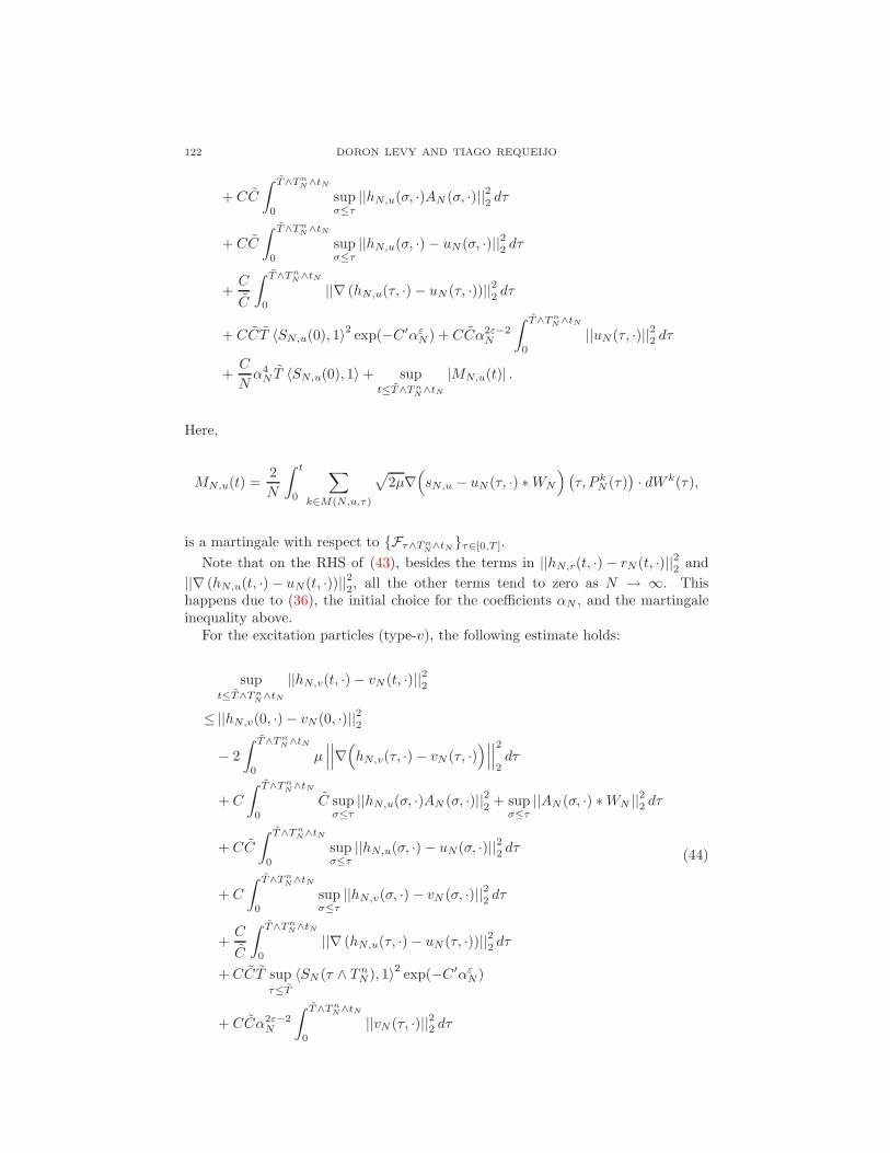
122 DORON LEVY AND TIAGO REQUEIJO
+ CC
∫ T∧T n
N∧tN
0
supσ≤τ
||hN,u(σ, ·)AN (σ, ·)||22 dτ
+ CC
∫ T∧T n
N∧tN
0
supσ≤τ
||hN,u(σ, ·) − uN (σ, ·)||22 dτ
+C
C
∫ T∧T n
N∧tN
0
||∇ (hN,u(τ, ·) − uN (τ, ·))||22 dτ
+ CCT 〈SN,u(0), 1〉2exp(−C′αε
N ) + CCα2ε−2N
∫ T∧T n
N∧tN
0
||uN(τ, ·)||22 dτ
+C
Nα4
N T 〈SN,u(0), 1〉 + supt≤T∧T n
N∧tN
|MN,u(t)| .
Here,
MN,u(t) =2
N
∫ t
0
∑
k∈M(N,u,τ)
√
2µ∇(
sN,u − uN(τ, ·) ∗WN
)
(
τ, P kN (τ)
)
· dW k(τ),
is a martingale with respect to {Fτ∧T n
N∧tN
}τ∈[0,T ].
Note that on the RHS of (43), besides the terms in ||hN,r(t, ·) − rN (t, ·)||22 and
||∇ (hN,u(t, ·) − uN (t, ·))||22, all the other terms tend to zero as N → ∞. This
happens due to (36), the initial choice for the coefficients αN , and the martingaleinequality above.
For the excitation particles (type-v), the following estimate holds:
supt≤T∧T n
N∧tN
||hN,v(t, ·) − vN (t, ·)||22
≤ ||hN,v(0, ·) − vN (0, ·)||22
− 2
∫ T∧T n
N∧tN
0
µ∣
∣
∣
∣
∣
∣∇(
hN,v(τ, ·) − vN (τ, ·))∣
∣
∣
∣
∣
∣
2
2dτ
+ C
∫ T∧T n
N∧tN
0
C supσ≤τ
||hN,u(σ, ·)AN (σ, ·)||22 + sup
σ≤τ||AN (σ, ·) ∗WN ||
22 dτ
+ CC
∫ T∧T n
N∧tN
0
supσ≤τ
||hN,u(σ, ·) − uN(σ, ·)||22 dτ
+ C
∫ T∧T n
N∧tN
0
supσ≤τ
||hN,v(σ, ·) − vN (σ, ·)||22 dτ
+C
C
∫ T∧T n
N∧tN
0
||∇ (hN,u(τ, ·) − uN (τ, ·))||22 dτ
+ CCT supτ≤T
〈SN (τ ∧ T nN), 1〉
2exp(−C′αε
N )
+ CCα2ε−2N
∫ T∧T n
N∧tN
0
||vN (τ, ·)||22 dτ
(44)
GROUP DYNAMICS OF PHOTOTAXIS 123
+C
Nα4
N T supτ≤T
〈SN (τ ∧ T nN ), 1〉 + C
α2N
NT sup
τ≤T
〈SN,v(τ ∧ TnN), 1〉
+ supt≤T∧T n
N∧tN
|MN,v(t)| + supt≤T∧T n
N∧tN
∣
∣
∣Mβ,0
N,v(t)∣
∣
∣+ sup
t≤T∧T n
N∧tN
∣
∣
∣Mβ,1
N,v(t)∣
∣
∣
+ supt≤T∧T n
N∧tN
∣
∣
∣Mγ,0
N,v(t)∣
∣
∣+ sup
t≤T∧T n
N∧tN
∣
∣
∣Mγ,1
N,v(t)∣
∣
∣.
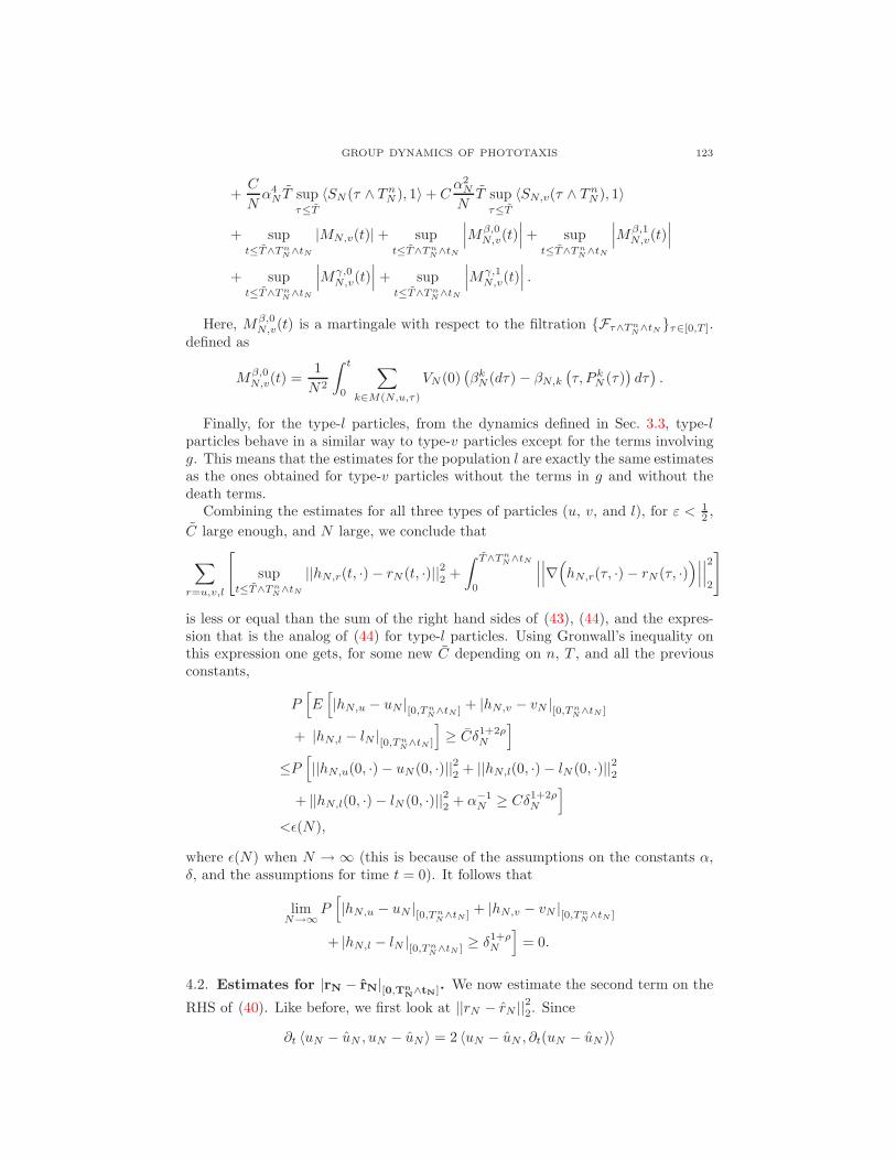
Here, Mβ,0N,v(t) is a martingale with respect to the filtration {Fτ∧T n
N∧tN
}τ∈[0,T ].defined as
Mβ,0N,v(t) =
1
N2
∫ t
0
∑
k∈M(N,u,τ)
VN (0)(
βkN (dτ) − βN,k
(
τ, P kN (τ)
)
dτ)
.
Finally, for the type-l particles, from the dynamics defined in Sec. 3.3, type-lparticles behave in a similar way to type-v particles except for the terms involvingg. This means that the estimates for the population l are exactly the same estimatesas the ones obtained for type-v particles without the terms in g and without thedeath terms.
Combining the estimates for all three types of particles (u, v, and l), for ε < 12 ,
C large enough, and N large, we conclude that
∑
r=u,v,l
[
supt≤T∧T n
N∧tN
||hN,r(t, ·) − rN (t, ·)||22 +
∫ T∧T n
N∧tN
0
∣
∣
∣
∣
∣
∣∇(
hN,r(τ, ·) − rN (τ, ·))∣
∣
∣
∣
∣
∣
2
2
]
is less or equal than the sum of the right hand sides of (43), (44), and the expres-sion that is the analog of (44) for type-l particles. Using Gronwall’s inequality onthis expression one gets, for some new C depending on n, T , and all the previousconstants,
P[
E[
|hN,u − uN |[0,T n
N∧tN ] + |hN,v − vN |[0,T n
N∧tN ]
+ |hN,l − lN |[0,T n
N∧tN ]
]
≥ Cδ1+2ρN
]
≤P[
||hN,u(0, ·) − uN(0, ·)||22 + ||hN,l(0, ·) − lN (0, ·)||
22
+ ||hN,l(0, ·) − lN (0, ·)||22 + α−1
N ≥ Cδ1+2ρN
]
<ǫ(N),
where ǫ(N) when N → ∞ (this is because of the assumptions on the constants α,δ, and the assumptions for time t = 0). It follows that
limN→∞
P[
|hN,u − uN |[0,T n
N∧tN ] + |hN,v − vN |[0,T n
N∧tN ]
+ |hN,l − lN |[0,T n
N∧tN ] ≥ δ1+ρ
N
]
= 0.
4.2. Estimates for |rN − rN|[0,Tn
N∧tN]. We now estimate the second term on the
RHS of (40). Like before, we first look at ||rN − rN ||22. Since
∂t 〈uN − uN , uN − uN 〉 = 2 〈uN − uN , ∂t(uN − uN )〉
124 DORON LEVY AND TIAGO REQUEIJO
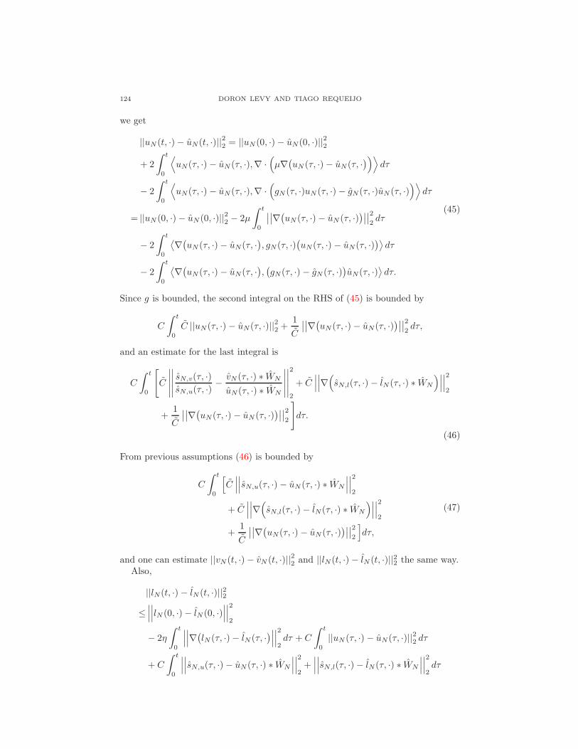
we get
||uN (t, ·) − uN(t, ·)||22 = ||uN(0, ·) − uN(0, ·)||
22
+ 2
∫ t
0
⟨
uN(τ, ·) − uN (τ, ·),∇ ·(
µ∇(
uN (τ, ·) − uN(τ, ·)
)⟩
dτ
− 2
∫ t
0
⟨
uN(τ, ·) − uN (τ, ·),∇ ·(
gN (τ, ·)uN (τ, ·) − gN(τ, ·)uN (τ, ·))⟩
dτ
= ||uN (0, ·) − uN (0, ·)||22 − 2µ
∫ t
0
∣
∣
∣
∣∇(
uN (τ, ·) − uN (τ, ·))∣
∣
∣
∣
2
2dτ
− 2
∫ t
0
⟨
∇(
uN (τ, ·) − uN(τ, ·)
, gN(τ, ·)(
uN(τ, ·) − uN(τ, ·))⟩
dτ
− 2
∫ t
0
⟨
∇(
uN (τ, ·) − uN(τ, ·)
,(
gN(τ, ·) − gN (τ, ·))
uN(τ, ·)⟩
dτ.
(45)
Since g is bounded, the second integral on the RHS of (45) is bounded by
C
∫ t
0
C ||uN(τ, ·) − uN(τ, ·)||22 +
1
C
∣
∣
∣
∣∇(
uN (τ, ·) − uN(τ, ·))∣
∣
∣
∣
2
2dτ,
and an estimate for the last integral is
C
∫ t
0
[
C
∣
∣
∣
∣
∣
∣
∣
∣
∣
∣
sN,v(τ, ·)
sN,u(τ, ·)−vN (τ, ·) ∗ WN
uN (τ, ·) ∗ WN
∣
∣
∣
∣
∣
∣
∣
∣
∣
∣
2
2
+ C∣
∣
∣
∣
∣
∣∇(
sN,l(τ, ·) − lN (τ, ·) ∗ WN
)∣
∣
∣
∣
∣
∣
2
2
+1
C
∣
∣
∣
∣∇(
uN(τ, ·) − uN (τ, ·))∣
∣
∣
∣
2
2
]
dτ.
(46)
From previous assumptions (46) is bounded by
C
∫ t
0
[
C∣
∣
∣
∣
∣
∣sN,u(τ, ·) − uN (τ, ·) ∗ WN
∣
∣
∣
∣
∣
∣
2
2
+ C∣
∣
∣
∣
∣
∣∇(
sN,l(τ, ·) − lN(τ, ·) ∗ WN
)∣
∣
∣
∣
∣
∣
2
2
+1
C
∣
∣
∣
∣∇(
uN(τ, ·) − uN (τ, ·))∣
∣
∣
∣
2
2
]
dτ,
(47)
and one can estimate ||vN (t, ·) − vN (t, ·)||22 and ||lN(t, ·) − lN (t, ·)||22 the same way.Also,
||lN(t, ·) − lN (t, ·)||22
≤∣
∣
∣
∣
∣
∣lN (0, ·) − lN (0, ·)
∣
∣
∣
∣
∣
∣
2
2
− 2η
∫ t
0
∣
∣
∣
∣
∣
∣∇(
lN (τ, ·) − lN (τ, ·)
∣
∣
∣
∣
∣
∣
2
2dτ + C
∫ t
0
||uN (τ, ·) − uN(τ, ·)||22 dτ
+ C
∫ t
0
∣
∣
∣
∣
∣
∣sN,u(τ, ·) − uN(τ, ·) ∗ WN
∣
∣
∣
∣
∣
∣
2
2+∣
∣
∣
∣
∣
∣sN,l(τ, ·) − lN(τ, ·) ∗ WN
∣
∣
∣
∣
∣
∣
2
2dτ
GROUP DYNAMICS OF PHOTOTAXIS 125
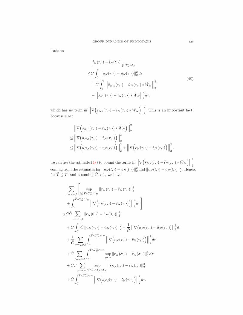
leads to
∣
∣
∣lN (t, ·) − lN(t, ·)
∣
∣
∣
[0,T n
N∧tN ]
≤C
∫ t
0
||uN(τ, ·) − uN (τ, ·)||22 dτ
+ C
∫ t
0
∣
∣
∣
∣
∣
∣sN,u(τ, ·) − uN(τ, ·) ∗ WN
∣
∣
∣
∣
∣
∣
2
2
+∣
∣
∣
∣
∣
∣sN,l(τ, ·) − lN(τ, ·) ∗ WN
∣
∣
∣
∣
∣
∣
2
2dτ,
(48)
which has no term in∣
∣
∣
∣
∣
∣∇(
sN,l(τ, ·) − lN (τ, ·) ∗ WN
)∣
∣
∣
∣
∣
∣
2
2. This is an important fact,
because since
∣
∣
∣
∣
∣
∣∇(
sN,r(τ, ·) − rN (τ, ·) ∗ WN
)∣
∣
∣
∣
∣
∣
2
2
≤∣
∣
∣
∣
∣
∣∇(
hN,r(τ, ·) − rN (τ, ·))∣
∣
∣
∣
∣
∣
2
2
≤∣
∣
∣
∣
∣
∣∇(
hN,r(τ, ·) − rN (τ, ·))∣
∣
∣
∣
∣
∣
2
2+∣
∣
∣
∣
∣
∣∇(
rN (τ, ·) − rN (τ, ·))∣
∣
∣
∣
∣
∣
2
2,
we can use the estimate (48) to bound the terms in∣
∣
∣
∣
∣
∣∇(
sN,l(τ, ·) − lN (τ, ·) ∗ WN
)∣
∣
∣
∣
∣
∣
2
2
coming from the estimates for ||uN (t, ·) − uN(t, ·)||22 and ||vN (t, ·) − vN (t, ·)||
22. Hence,
for T ≤ T , and assuming C > 1, we have
∑
r=u,v,l
[
supt≤T∧T n
N∧tN
||rN (t, ·) − rN (t, ·)||22
+
∫ T∧T n
N∧tN
0
∣
∣
∣
∣
∣
∣∇(
rN (τ, ·) − rN (τ, ·))∣
∣
∣
∣
∣
∣
2
2dτ
]
≤CC∑
r=u,v,l
||rN (0, ·) − rN (0, ·)||22
+ C
∫ t
0
C ||uN (τ, ·) − uN(τ, ·)||22 +
1
C
∣
∣
∣
∣∇(
uN (τ, ·) − uN(τ, ·))∣
∣
∣
∣
2
2dτ
+1
C
∑
r=u,v,l
∫ T∧T n
N∧tN
0
∣
∣
∣
∣
∣
∣∇(
rN (τ, ·) − rN (τ, ·))∣
∣
∣
∣
∣
∣
2
2dτ
+ C∑
r=u,v,l
∫ T∧T n
N∧tN
0
supσ≤τ
||rN (σ, ·) − rN (σ, ·)||22 dτ
+ CT∑
r=u,v,l
supt≤T∧T n
N∧tN
||sN,r(t, ·) − rN (t, ·)||22
+ C
∫ T∧T n
N∧tN
0
∣
∣
∣
∣
∣
∣∇(
sN,l(τ, ·) − lN (τ, ·))∣
∣
∣
∣
∣
∣
2
2dτ.
126 DORON LEVY AND TIAGO REQUEIJO
Thus for for C large, one gets using Gronwall’s inequality,
P
∑
r=u,v,l
|rN (t, ·) − rN (t, ·)|[0,T n
N∧tN ] >
δN2
≤P
[
CeCT n
N
(
∑
r=u,v,l
||rN (0, ·) − rN (0, ·)||22
+∑
r=u,v,l
supt≤T n
N∧tN
||sN,r(t, ·) − rN (t, ·)||22
+
∫ T∧T n
N∧tN
0
∣
∣
∣
∣
∣
∣∇(
sN,l(τ, ·) − lN (τ, ·))∣
∣
∣
∣
∣
∣
2
2dτ
)
>δN2
]
≤P
[
CeCT n
N
(
∑
r=u,v,l
||rN (0, ·) − rN (0, ·)||22
+∑
r=u,v,l
|sN,r(t, ·) − rN (t, ·)|[0,T n
N∧tN ]
)
>δN2
]
.
From the result in 4.1 and the assumptions for t = 0, this quantity goes to zero asN → ∞. Thus the second term of (40) is valid and (32) follows.
5. Conclusion. In this paper we have derived a hierarchy of models for describingthe motion of phototactic bacteria. The novelty of our approach was in assumingthat the motion of the colony of bacteria strongly depends on group dynamics,rather on decisions made by individual bacteria. The postulated group dynamics(whose existence is evident in the experimental data) was incorporated into themodels through the excitation property.
The phototaxis system (24) we obtained, resembles the known chemotaxis sys-tem. The main differences between both systems are related to both the existenceof an internal property, and to the restrictions imposed on the parameter functions.For example, in the phototaxis system it is assumed that the velocity is bounded.This is not the case with the chemotaxis system.
While the analysis presented in this paper closely follows the methods of [14, 18]the additional excitation property, which is a property of the individual bacterium,adds another layer of difficulty to the analysis. From an analytical point of view, thephototaxis system does pose several difficulties as there is a system-wide dependenceon v/u and g depends on ∇l in a nonlinear manner.
The method used in this paper works only for a diffusing surface memory effect.The details of the analysis as presented here do not allow the sensitivity function gto depend on any derivative besides ∇l. It would be interesting to study the effectsof adding such terms into the phototaxis system, i.e., a system of the form
∂tu =µ∆u −∇ ·(
g(u, v, l,∇u,∇l)u)
,
∂tv =µ∆v −∇ ·(
g(u, v, l,∇u,∇l)v)
+ β(u, v)u − γ(u, v)v,
∂tl =λ(u, l)u.
Such a system will allow, e.g., to directly consider a motion of the bacteria thattends towards areas of a large density of bacteria.
GROUP DYNAMICS OF PHOTOTAXIS 127
An extensive simulation study of the stochastic model to determine the depen-dency of the results on the values of the different parameters and on the choice ofthe response functions is separately reported in [5].
Finally, it will be very interesting to see if the phototaxis system (24) does supportthe formation of some of the structures that are observed experimentally, such asthe fingers and the pinching. This may depend on the choice of parameter functions,such as g, β, and γ. Such a study is beyond the scope of this introductory paperand is left to a future work.
Acknowledgments. The work of D. Levy was supported in part by the NSF underCareer Grant DMS-0133511. We would like to thank Devaki Bhaya and MatthewBurriesci for generating the images and movies and for their guidance.
REFERENCES
[1] J. P. Armitage, Bacterial tactic responses, Adv. Microb Physiol., 41 (1999), 229–289.[2] D. Bhaya, Light matters: Phototaxis and signal transduction in unicellular cyanobacteria,
Mol. Microbiol., 53 (2004), 745–754.[3] D. Bhaya, N. R. Bianco, D. Bryant, and A. R. Grossman, Type IV pilus biogenesis and motility
in the cyanobacterium Synechocystis sp. PCC6803, Mol. Microbiol., 37 (2000), 941–951,[4] D. Bhaya, D. Levy and T. Requeijo, Group Dynamics of Phototaxis: Interacting Stochastic
Many-Particle Systems and their Continuum Limits, To appear in Proceedings of HYP 2006,Lyon.
[5] D. Levy and T. Requeijo, Stochastic Models for Phototaxis, submitted.[6] D. Bhaya, A. Takahashi, and A. R. Grossman, Light regulation of TypeIV pilus-dependent
motility by chemosensor-like elements in Synechocystis PCC 6803, Proc. Natl. Acad. Sci.U.S.A., 98 (2001), 7540–7545.
[7] M. Burriesci and D. Bhaya, Tracking the motility of single cells and groups of Synechocystis
sp. strain PCC6803 during phototaxis, in preparation.[8] B. Chopard, P. Luthi, and A. Masselot, Cellular automata and lattice boltzmann techniques:
An approach to model and simulate complex systems, Adv. Complex Syst., 5 (2002), 103–246.[9] B. Davis, Reinforced Random Walks, Probability Theory Related Fields, 84 (1990), 203–229.
[10] A. Friedman, “Partial Differential Equations of Parabolic Type,” Robert E. Krieger PublishingCompany, Malabar, FL, 1983.
[11] T. Hillen, K. Painter, and C. Schmeiset, Global Existence for Chemotaxis with Finite Sampling
Radius, Disc. Cont. Dyn. Sys. B, 7 (2007), 125–144.[12] E. F. Keller and L. A. Segel, Traveling band of chemotactic bacteria: a theoretical analysis,
J. Theor Biology, 30 (1971), 235–248.[13] L. L. McCarter, Regulation of flagella, Curr Opin Microbiol., 9 (2006), 180–186.[14] K. Oelschlager, On the derivation of reaction-diffusion equations as limit dynamics of systems
of moderately interacting stochastic processes, Probability Theory Related Fields, 82 (1989),565–586.
[15] B. Øksendal, “Stochastic Differential Equations: An introduction with applications,” Sixthedition, Springer-Verlag, Berlin, 2003.
[16] C. S. Patlack, Random walk with persistence and external bias, Bull. Math. Biophys, 15
(1953), 311–338.[17] A. Stevens, A stochastic cellular automaton modeling gliding and aggregation of myxobacteria,
SIAM Journal of Applied Mathematics, 61 (2000), 172–182.[18] A. Stevens, The derivation of chemotaxis equations as limit dynamics of moderately inter-
acting stochastic many-particle systems, SIAM Journal of Applied Mathematics, 61 (2000),183–212.
[19] S. Childress and M. Levandowsky and E. Spiegel, Pattern formation in a suspension of
swimming microorganisms: equations and stability theory, Journal of Fluid Mechanics, 63
(1975), 591[20] S. Childress and M. Levandowsky and E. Spiegel and S. Hunter, A Mathematical Model of
Pattern Formation by Swimming Microorganisms, J. Protozool., 22 (1975).
128 DORON LEVY AND TIAGO REQUEIJO
[21] A. Maree and A. Panfilov and P. Hogeweg, Phototaxis during the slug stage of Dictyostelium
discoideum: a model study, Proc. R. Soc. Lond., B (1999) 266, 1351–1360.[22] T. Nutsch and W. Marwan and D. Oesterhelt and E. Gilles Signal Processing and Flagellar
Motor Switching During Phototaxis of Halobacterium salinarum, Genome Res., 13 (2003),2406–2412
Received April 2007; revised August 2007.
E-mail address: [email protected]
E-mail address: [email protected]
Related Documents