Modeling Gas-Grain Chemistry in Dark Cloud Conditions

Modeling Gas-Grain Chemistryin Dark Cloud Conditions

Dissertation

zur

Erlangung des Doktorgrades (Dr. rer. nat.)

der

Mathematisch-Naturwissenschaftlichen Fakultat

der

Rheinischen Friedrich-Wilhelms-Universitat Bonn

vorgelegt von

Fujun Du

aus

Chongqing, China

Bonn 2012

Angefertigt mit Genehmigung der Mathematisch-Naturwissenschaftlichen Fakultat derRheinischen Friedrich-Wilhelms-Universitat Bonn

1. Gutachter: Prof. Dr. Karl M. Menten

2. Gutachter: Prof. Dr. Pavel Kroupa

Tag der Promotion: August 20, 2012

Erscheinungsjahr: 2012

Diese Dissertation ist auf dem Hochschulschriftenserver der ULB Bonn unterhttp://hss.ulb.uni-bonn.de/diss_online elektronisch publiziert.

Abstract

I first wrote a gas phase chemical code, which solves for the gas phase composition of aninterstellar cloud as a function of time. We used this code to study the abundance ratiosbetween the H+

3 isotopologues, since in this case the interaction between processes in thegas phase and on the dust grain surface can be treated in a simplified way.

Grain chemistry is necessary to explain the formation of many interstellar molecules.My first investigation on grain chemistry is from the mathematical side, by looking deepinto the difficulties posed by its stochasticity and discreteness. After writing a Monte Carlocode to serve as a benchmark, I developed a new method called “hybrid moment equation”(HME) approach, which gives results that are more accurate than those obtained withthe usual rate equation approach, and it runs much faster than the Monte Carlo methodfor a medium-to-large-sized reaction network. Improvements in this HME approach areneeded if a very large surface network is to be used.

Following the recent detection of hydrogen peroxide (H2O2) in the ρOphiuchus A cloudcore, I modeled its formation with a gas-grain network. Its observed abundance, togetherwith the abundances of other species detected in the same source can be reproduced in ourmodel. These molecules are mainly driven into the gas phase from the dust grain surfaceby the heat released in chemical reactions. Our model predicted the presence of O2Hmolecule in the gas phase, which has indeed been detected recently. Further investigationsare needed to answer whether H2O2 is widespread in the interstellar medium.

I then studied the chemistry involving species containing one or more deuterium atomswith a gas-grain-mantle three-phase model, which takes into account recent experimentalresults on the key reactions. The observed fractionated deuterium enhancement in wa-ter, methanol, and formaldehyde is reproduced in our models. I demonstrated that theexistence of abstraction reactions for methanol and formaldehyde is the main reason forthese species to be more prone to deuterium enhancement than water. The observed low[D2O/H2O] ratio suggests that water is mainly formed through H2+OH −−→ H2O+H onthe dust grain surface. Our model also gives a range of ice mantle compositions for thedust grains that agree with the observations in different sources.

Contents

1 Introduction 11.1 Interstellar environments . . . . . . . . . . . . . . . . . . . . . . . . . . . . 11.2 From molecular clouds to stars . . . . . . . . . . . . . . . . . . . . . . . . 21.3 The role of modeling in astrochemistry . . . . . . . . . . . . . . . . . . . . 51.4 Beyond simple molecules? . . . . . . . . . . . . . . . . . . . . . . . . . . . 71.5 Outline of this thesis . . . . . . . . . . . . . . . . . . . . . . . . . . . . . . 7

2 Gas phase chemistry 92.1 Gas phase reactions . . . . . . . . . . . . . . . . . . . . . . . . . . . . . . 9

2.1.1 Gas phase reaction networks . . . . . . . . . . . . . . . . . . . . . 92.1.2 Calculating the reaction rates . . . . . . . . . . . . . . . . . . . . . 122.1.3 Different types of reactions, and their properties . . . . . . . . . . 14

2.2 The chemical rate equation . . . . . . . . . . . . . . . . . . . . . . . . . . 202.2.1 Solving a stiff system of equations . . . . . . . . . . . . . . . . . . 212.2.2 The gas phase chemical code . . . . . . . . . . . . . . . . . . . . . 232.2.3 Application of the gas phase code to study H2D

+ and D2H+ . . . 25

3 Grain chemistry 273.1 General facts about interstellar dust grains . . . . . . . . . . . . . . . . . 273.2 Why do we study grain chemistry . . . . . . . . . . . . . . . . . . . . . . . 293.3 Rates of processes in grain chemistry . . . . . . . . . . . . . . . . . . . . . 30

3.3.1 Adsorption rates . . . . . . . . . . . . . . . . . . . . . . . . . . . . 303.3.2 Evaporation rates . . . . . . . . . . . . . . . . . . . . . . . . . . . 323.3.3 Surface migration rates . . . . . . . . . . . . . . . . . . . . . . . . 353.3.4 Two-body reaction rates on the surface . . . . . . . . . . . . . . . 37

3.4 Mathematical framework for surface chemistry . . . . . . . . . . . . . . . 383.4.1 Why the rate equation may fail for surface chemistry . . . . . . . . 383.4.2 The chemical master equation . . . . . . . . . . . . . . . . . . . . . 403.4.3 Monte Carlo method . . . . . . . . . . . . . . . . . . . . . . . . . . 42

4 The hybrid moment equation (HME) approach 474.1 Introduction . . . . . . . . . . . . . . . . . . . . . . . . . . . . . . . . . . . 484.2 Description of the hybrid moment equation (HME) approach . . . . . . . 50

4.2.1 The chemical master equation and the moment equation (ME) . . 504.2.2 The MEs and REs for a set of reactions . . . . . . . . . . . . . . . 524.2.3 The HME approach . . . . . . . . . . . . . . . . . . . . . . . . . . 54

4.3 Benchmark with the Monte Carlo approach . . . . . . . . . . . . . . . . . 55

iv

CONTENTS v

4.3.1 Test of the HME approach truncated at the second order on a largegas-grain network . . . . . . . . . . . . . . . . . . . . . . . . . . . . 57

4.3.2 Test of the HME approach truncated at the third order on a smallsurface network . . . . . . . . . . . . . . . . . . . . . . . . . . . . . 63

4.4 Discussion . . . . . . . . . . . . . . . . . . . . . . . . . . . . . . . . . . . . 654.A A method to generate the moment equations based on the generating function 664.B The surface reaction network we used to test our code . . . . . . . . . . . 69

5 H2O2 formation on dust grain surface 715.1 Introduction . . . . . . . . . . . . . . . . . . . . . . . . . . . . . . . . . . . 725.2 Chemical model . . . . . . . . . . . . . . . . . . . . . . . . . . . . . . . . . 735.3 Results and discussions . . . . . . . . . . . . . . . . . . . . . . . . . . . . 76

5.3.1 Modeling ρ Oph A . . . . . . . . . . . . . . . . . . . . . . . . . . . 765.3.2 Chemical age versus dynamical time scale . . . . . . . . . . . . . . 805.3.3 Effects of changing the energy barrier of the surface reaction H +

O2 → HO2 . . . . . . . . . . . . . . . . . . . . . . . . . . . . . . . 815.3.4 Effects of changing the diffusion energy barriers . . . . . . . . . . . 825.3.5 Dependence on the temperature and density . . . . . . . . . . . . . 835.3.6 Discussions and limits of the model . . . . . . . . . . . . . . . . . . 85

5.4 Conclusions . . . . . . . . . . . . . . . . . . . . . . . . . . . . . . . . . . . 915.A An explanation of the spike-like features in the evolution curves . . . . . . 915.B The surface reaction network used in this work . . . . . . . . . . . . . . . 965.C Enthalpies of the surface species . . . . . . . . . . . . . . . . . . . . . . . 99

6 Deuterium chemistry on dust grain surfaces 1016.1 Why is deuterium special . . . . . . . . . . . . . . . . . . . . . . . . . . . 1016.2 Previous studies . . . . . . . . . . . . . . . . . . . . . . . . . . . . . . . . 1036.3 Preparation for the gas phase reaction network . . . . . . . . . . . . . . . 106

6.3.1 Reducing the gas phase reaction network . . . . . . . . . . . . . . 1066.3.2 Deuterating the gas phase reaction network . . . . . . . . . . . . . 108

6.4 The grain surface chemistry . . . . . . . . . . . . . . . . . . . . . . . . . . 1126.4.1 Coverage of H and D on the surface . . . . . . . . . . . . . . . . . 1136.4.2 Addition and abstraction reactions of formaldehyde . . . . . . . . 1166.4.3 Abstraction reactions of methanol . . . . . . . . . . . . . . . . . . 1206.4.4 Hydrogenation/deuteration of CO . . . . . . . . . . . . . . . . . . 1246.4.5 The formation of water . . . . . . . . . . . . . . . . . . . . . . . . 1266.4.6 The formation of CO2 through OH+ CO . . . . . . . . . . . . . . 1286.4.7 Other reactions in the surface reaction network . . . . . . . . . . . 1316.4.8 The zero-point energy issue for the evaporation and surface migra-

tion rates . . . . . . . . . . . . . . . . . . . . . . . . . . . . . . . . 1316.5 The three-phase gas-surface-mantle model . . . . . . . . . . . . . . . . . . 133

6.5.1 Accretion onto the dust grain . . . . . . . . . . . . . . . . . . . . . 1346.5.2 Evaporation of grain material . . . . . . . . . . . . . . . . . . . . . 1356.5.3 The complete set of equations . . . . . . . . . . . . . . . . . . . . . 136

6.6 Results and discussions . . . . . . . . . . . . . . . . . . . . . . . . . . . . 1376.6.1 Ice mantle composition . . . . . . . . . . . . . . . . . . . . . . . . 139

vi CONTENTS

6.6.2 Deuterium fractionation . . . . . . . . . . . . . . . . . . . . . . . . 1536.6.3 Comparison with observations . . . . . . . . . . . . . . . . . . . . . 171

6.7 Conclusions . . . . . . . . . . . . . . . . . . . . . . . . . . . . . . . . . . . 178

7 Summary and outlook 1817.1 Summary . . . . . . . . . . . . . . . . . . . . . . . . . . . . . . . . . . . . 1817.2 Outlook . . . . . . . . . . . . . . . . . . . . . . . . . . . . . . . . . . . . . 182

A Comparison of different approaches for surface chemistry 184A.1 With the rate equation approach . . . . . . . . . . . . . . . . . . . . . . . 185A.2 The master equation approach . . . . . . . . . . . . . . . . . . . . . . . . 186

B Formal solution to the master equation 192

Acknowledgements 208

Curriculum Vitae 209

Chapter 1

Introduction— Chemistry in astronomical environments

Since ancient times, the formation of complex structures from simple components hasalways been one of the central themes in natural science. The very existence of a vastnumber of different molecules on Earth, when contrasted with the primordial “hot soup”state of the early Universe, where nothing except for elementary particles (such as protons,neutrons, and electrons, depending on which specific stage we are talking about) existed,indicates that formation processes of these molecules must have occurred in the past. Thediscovery of more than one hundred different molecules (including ions and radicals) ininterstellar space suggests that such processes have started in the interstellar environment,where the physical conditions are completely different from those we are familiar with hereon Earth.

1.1 Interstellar environments

By the terrestrial standards, interstellar space is essentially empty. The average densityof visible matter in our Milky Way galaxy—even if the stars are counted in—is merelyabout 100 protons cm−3, which may be compared with the air density of our atmosphereat sea level, being approximately 7×1020 protons cm−3. But in our Galaxy, the stars arethe major mass component of the visible mass[1], and the total mass of the interstellarmedium (ISM) is only about 5% of the total stellar mass (Lequeux et al. 2005), so theactual average density of interstellar space, not counting the stars, is much lower, about afew protons cm−3; this is somewhat similar to the density of interplanetary space (Prolss2004). The typically low density of the ISM does not mean that nothing interesting canoccur; rather it only suggests that the relevant time scales may be much longer thanwhat we are used to on Earth. These time scales are literally “astronomical”! On theother hand, the low density of the ISM makes the existence of non-negligible amounts ofreactive radical and charged species possible, because the rates to destruct them throughtwo-body chemical reactions are low.

In fact, the interstellar space is highly inhomogeneous, both in physical condition

[1]For the Galaxy as a whole, most of the mass is generally believed to be in the form of the so-called“dark matter”, whose nature is still a mystery.

1

2 Introduction

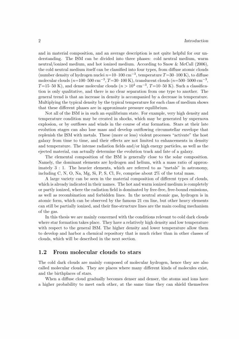
and in material composition, and an average description is not quite helpful for our un-derstanding. The ISM can be divided into three phases: cold neutral medium, warmneutral/ionized medium, and hot ionized medium. According to Snow & McCall (2006),the cold neutral medium itself can be classified into four types, from diffuse atomic clouds(number density of hydrogen nuclei n=10–100 cm−3, temperature T=30–100 K), to diffusemolecular clouds (n=100–500 cm−3, T=30–100 K), translucent clouds (n=500–5000 cm−3,T=15–50 K), and dense molecular clouds (n > 104 cm−3, T=10–50 K). Such a classifica-tion is only qualitative, and there is no clear separation from one type to another. Thegeneral trend is that an increase in density is accompanied by a decrease in temperature.Multiplying the typical density by the typical temperature for each class of medium showsthat these different phases are in approximate pressure equilibrium.

Not all of the ISM is in such an equilibrium state. For example, very high density andtemperature condition may be created in shocks, which may be generated by supernovaexplosion, or by outflows and winds in the course of star formation. Stars at their lateevolution stages can also lose mass and develop outflowing circumstellar envelope thatreplenish the ISM with metals. These (more or less) violent processes “activate” the hostgalaxy from time to time, and their effects are not limited to enhancements in densityand temperature. The intense radiation fields and/or high energy particles, as well as theejected material, can actually determine the evolution track and fate of a galaxy.

The elemental composition of the ISM is generally close to the solar composition.Namely, the dominant elements are hydrogen and helium, with a mass ratio of approx-imately 3 : 1. The heavier elements, which are referred to as “metals” in astronomy,including C, N, O, Na, Mg, Si, P, S, Cl, Fe, comprise about 2% of the total mass.

A large variety can be seen in the material composition of different types of clouds,which is already indicated in their names. The hot and warm ionized medium is completelyor partly ionized, where the radiation field is dominated by free-free, free-bound emissions,as well as recombination and forbidden lines. In the neutral atomic gas, hydrogen is inatomic form, which can be observed by the famous 21 cm line, but other heavy elementscan still be partially ionized, and their fine-structure lines are the main cooling mechanismof the gas.

In this thesis we are mainly concerned with the conditions relevant to cold dark cloudswhere star formation takes place. They have a relatively high density and low temperaturewith respect to the general ISM. The higher density and lower temperature allow themto develop and harbor a chemical repository that is much richer than in other classes ofclouds, which will be described in the next section.

1.2 From molecular clouds to stars

The cold dark clouds are mainly composed of molecular hydrogen, hence they are alsocalled molecular clouds. They are places where many different kinds of molecules exist,and the birthplaces of stars.

When a diffuse cloud gradually becomes denser and denser, the atoms and ions havea higher probability to meet each other, at the same time they can shield themselves

1.2 From molecular clouds to stars 3

better from external radiation fields[2]. This provides a shelter for the molecules to beproduced. Observationally, it has been shown that the molecular H2 becomes more andmore dominant over atomic H as the visual extinction grows.

Observational studies on the molecules in the cold ISM are mostly based on their emis-sion lines. Molecular line emission can be divided into three types: electronic emission,which is due to transition between different electronic states; vibrational emission, dueto transition between different vibration states; and rotational emission due to transitionbetween different rotation states. The typical energy released in each type (hence theirtypical frequency) decreases by a factor of roughly[3]

√mp/me∼40, the square root of the

mass ratio between proton and electron, from one type to another in the above sequence.Thus the electronic transitions usually fall in the UV or optical band, the vibrationaltransitions fall in the infrared band, and the rotational transitions fall in the radio band.

Only a few simple molecules have their electronic transitions in the optical band, andmany molecules detected in this type have their transitions in the UV band (Lequeuxet al. 2005), which is not readily available from the ground due to atmosphere absorption.More importantly, in cold dark clouds, the temperature is generally too low to excitethe vibration levels (a temperature of 10 K corresponds to a wavelength of 1 mm), letalone electronic levels. Hence the detection of molecules relies predominantly on radioobservations of the rotational lines. For the H2 molecule, due to its small size and smallmass, even the non-ground rotation energy levels[4] are too high to populate in coldconditions, and its column density (particles per cm2) is usually traced by other molecules(such as CO), or dust emission/absorption.

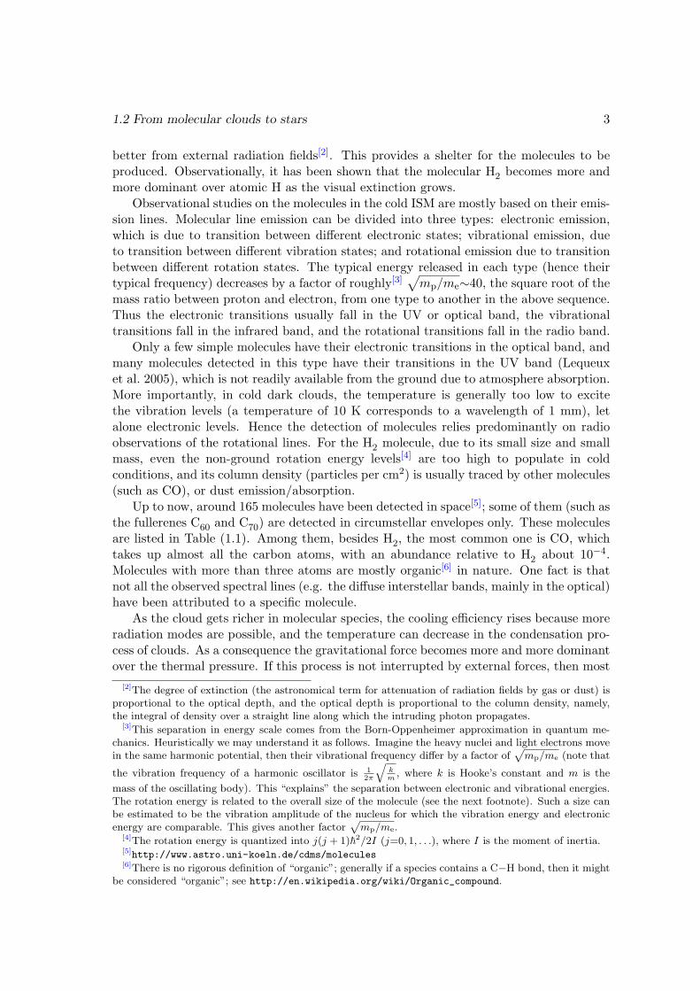
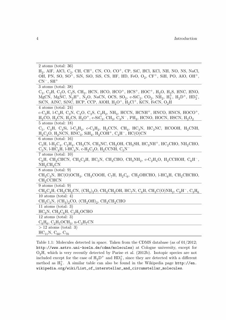
Up to now, around 165 molecules have been detected in space[5]; some of them (such asthe fullerenes C60 and C70) are detected in circumstellar envelopes only. These moleculesare listed in Table (1.1). Among them, besides H2, the most common one is CO, whichtakes up almost all the carbon atoms, with an abundance relative to H2 about 10−4.Molecules with more than three atoms are mostly organic[6] in nature. One fact is thatnot all the observed spectral lines (e.g. the diffuse interstellar bands, mainly in the optical)have been attributed to a specific molecule.

As the cloud gets richer in molecular species, the cooling efficiency rises because moreradiation modes are possible, and the temperature can decrease in the condensation pro-cess of clouds. As a consequence the gravitational force becomes more and more dominantover the thermal pressure. If this process is not interrupted by external forces, then most

[2]The degree of extinction (the astronomical term for attenuation of radiation fields by gas or dust) isproportional to the optical depth, and the optical depth is proportional to the column density, namely,the integral of density over a straight line along which the intruding photon propagates.

[3]This separation in energy scale comes from the Born-Oppenheimer approximation in quantum me-chanics. Heuristically we may understand it as follows. Imagine the heavy nuclei and light electrons movein the same harmonic potential, then their vibrational frequency differ by a factor of

√mp/me (note that

the vibration frequency of a harmonic oscillator is 12π

√km, where k is Hooke’s constant and m is the

mass of the oscillating body). This “explains” the separation between electronic and vibrational energies.The rotation energy is related to the overall size of the molecule (see the next footnote). Such a size canbe estimated to be the vibration amplitude of the nucleus for which the vibration energy and electronicenergy are comparable. This gives another factor

√mp/me.

[4]The rotation energy is quantized into j(j + 1)~2/2I (j=0, 1, . . .), where I is the moment of inertia.[5]http://www.astro.uni-koeln.de/cdms/molecules[6]There is no rigorous definition of “organic”; generally if a species contains a C−H bond, then it might

be considered “organic”; see http://en.wikipedia.org/wiki/Organic_compound.

4 Introduction

2 atoms (total: 36)H2, AlF, AlCl, C2, CH, CH

+, CN, CO, CO+, CP, SiC, HCl, KCl, NH, NO, NS, NaCl,OH, PN, SO, SO+, SiN, SiO, SiS, CS, HF, HD, FeO, O2, CF

+, SiH, PO, AlO, OH+,CN – , SH+

3 atoms (total: 38)C3, C2H, C2O, C2S, CH2, HCN, HCO, HCO+, HCS+, HOC+, H2O, H2S, HNC, HNO,MgCN, MgNC, N2H

+, N2O, NaCN, OCS, SO2, c-SiC2, CO2, NH2, H+3 , H2D

+, HD+2 ,

SiCN, AlNC, SiNC, HCP, CCP, AlOH, H2O+, H2Cl

+, KCN, FeCN, O2H

4 atoms (total: 24)c-C3H, l-C3H, C3N, C3O, C3S, C2H2, NH3, HCCN, HCNH+, HNCO, HNCS, HOCO+,H2CO, H2CN, H2CS, H3O

+, c-SiC3, CH3, C3N– , PH3, HCNO, HOCN, HSCN, H2O2

5 atoms (total: 18)C5, C4H, C4Si, l-C3H2, c-C3H2, H2CCN, CH4, HC3N, HC2NC, HCOOH, H2CNH,H2C2O, H2NCN, HNC3, SiH4, H2COH+, C4H

– , HC(O)CN

6 atoms (total: 16)C5H, l-H2C4, C2H4, CH3CN, CH3NC, CH3OH, CH3SH, HC3NH+, HC2CHO, NH2CHO,C5N, l-HC4H, l-HC4N, c-H2C3O, H2CCNH, C5N

–

7 atoms (total: 10)C6H, CH2CHCN, CH3C2H, HC5N, CH3CHO, CH3NH2, c-C2H4O, H2CCHOH, C6H

– ,NH2CH2CN

8 atoms (total: 9)CH3C3N, HC(O)OCH3, CH3COOH, C7H, H2C6, CH2OHCHO, l-HC6H, CH2CHCHO,CH2CCHCN

9 atoms (total: 9)CH3C4H, CH3CH2CN, (CH3)2O, CH3CH2OH, HC7N, C8H, CH3C(O)NH2, C8H

– , C3H6

10 atoms (total: 4)CH3C5N, (CH3)2CO, (CH2OH)2, CH3CH2CHO

11 atoms (total: 3)HC9N, CH3C6H, C2H5OCHO

12 atoms (total: 3)C6H6, C2H5OCH3, n-C3H7CN

> 12 atoms (total: 3)HC11N, C60, C70

Table 1.1: Molecules detected in space. Taken from the CDMS database (as of 01/2012;http://www.astro.uni-koeln.de/cdms/molecules) at Cologne university, except forO2H, which is very recently detected by Parise et al. (2012b). Isotopic species are notincluded except for the case of H2D

+ and HD+2 , since they are detected with a different

method as H+3 . A similar table can also be found in the Wikipedia page http://en.

wikipedia.org/wiki/List_of_interstellar_and_circumstellar_molecules.

1.3 The role of modeling in astrochemistry 5

likely at a certain stage the gravitation instability will set in, and the cloud will collapse.Depending on the initial configuration, a central protostar and a surrounding accretiondisk can be formed. The central star gains mass through accretion and becomes moreluminous over time. Its radiation field and wind act in the reverse direction of gravity,blowing out the surrounding material. Finally, the environment becomes clear of gas anddust, and a newly born star is visible to distant observers. As a bonus, a planet system(like our solar system) may have also formed (and may still be evolving) in the accretiondisk. This is an important bonus, since we are residing in such a system.

The above a picture is an oversimplification. Many details of these processes are notknown for sure, or are yet to be discovered. For example, what actually triggers theconversion from the diffuse phase to dense phase for interstellar clouds? How do theseprocesses determine the statistical distribution of the resulting stellar masses? How is theprestellar material transported to the final planetary system? Many such questions canbe asked. However, they are not the topic of this thesis.

1.3 The role of modeling in astrochemistry

Any modeling study in astronomy is based on the rationale that the physical laws (in-cluding chemistry) at the place of the celestial objects, no matter how far away they are,are the same as in any laboratory on Earth. Thus the goal of any modeling effort is tryingto understand the interstellar processes in terms of our local understanding of physics (aswell as chemistry and mathematics).

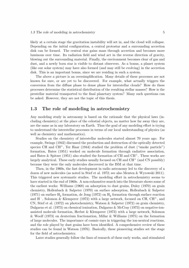
Studies on the chemistry of interstellar molecules started almost 70 years ago. Forexample, Swings (1942) discussed the production and destruction of the optically detectedspecies CH and CH+, Ter Haar (1944) studied the problem of dust (“smoke particle”)formation, Bates (1951) worked on molecule formation through radiative association,and Bates & Spitzer (1951) also studied the formation of CH and CH+. These works arelargely analytical. These early studies usually focused on CH and CH+ (and CN possibly)because they were the only molecules discovered in the ISM at that time.

Then, in the 1960s, the fast development in radio astronomy led to the discovery of adozen of new molecules (as noted in Stief et al. 1972; see also Menten & Wyrowski 2011).This triggered new systematic studies. The modeling effort in astrochemistry seems tohave started in the end of 1960s. A non-exhaustive search into the literature shows some ofthe earliest works: Williams (1968) on adsorption to dust grains, Duley (1970) on grainchemistry, Hollenbach & Salpeter (1970) on surface adsorption, Hollenbach & Salpeter(1971) on surface H2 formation, de Jong (1972) on H2 formation through surface reactionand H – , Solomon & Klemperer (1972) with a large network, focused on CH, CH+, andCN, Stief et al. (1972) on photochemistry, Watson & Salpeter (1972) on grain chemistry,Dalgarno et al. (1973) on chemical ionization, Dalgarno & McCray (1973) on negative-ion-assisted molecule formation, Herbst & Klemperer (1973) with a large network, Solomon& Woolf (1973) on deuterium fractionation, Millar & Williams (1975) on the formationof large molecules. The importance of cosmic-rays in triggering the ion-neutral reactions,and the role played by dust grains have been identified. A comprehensive review of thesestudies can be found in Watson (1976). Basically, these pioneering studies set the stagefor the field of astrochemistry.

Later studies generally follow the lines of research of these early works, and stimulated

6 Introduction

by interaction between several fields, have proliferated into more branches focusing ondifferent types of objects, such as dark clouds (Millar & Nejad 1985), hot cores and corinos(Hassel et al. 2008), proto-planetary disks (Aikawa et al. 1997), photon-dominated regions(Tielens & Hollenbach 1985), shocks (Gusdorf et al. 2008), circumstellar envelopes aroundevolved stars and planetary nebulae (Glassgold 1996), etc. Among them, a specific topic ofinterest to us is the phenomenon of deuterium fractionation, in which the observed [D/H]ratios in certain species appear much higher (Parise et al. 2002, 2004; Bergman et al.2011a) than the cosmic value of ∼10−5, and the degree of [D/H] enhancement can differfor different species. This topic has been investigated since the early times and continuesto be an intriguing phenomenon to study (Millar et al. 1989; Roberts & Millar 2000b).One chapter of this thesis is devoted to it, emphasizing the role of surface processes ondeuterium fractionation.

As more and more molecules are discovered observationally, more questions arise re-garding their formation mechanism. For many of the detected molecules in Table (1.1),it is not completely clear[7] how they are produced, especially for the complex ones; theformation channels that are proposed for a species cannot always account for its observedabundance (though it is not always possible to get an accurate abundance observationallyeither). Sometimes, when the gas phase processes are unable to explain the abundancesof certain species, grain chemistry is resorted to. Though once being ironically describedas “the last refuge of the scoundrel” (Charnley et al. 1992), grain chemistry is commonlyagreed to be essential for astrochemistry, and besides its role in explaining existent ob-servations, it also has a predictive power in some sense. This is discussed in this thesis.

Besides gas phase species, many molecules have also been detected in solid form in theice mantles of dust grains (van Dishoeck 2004). The most abundant is water ice, followedtypically by CO, CO2, CH3OH, H2CO, and NH3, etc. These ice species may have formedin situ on the dust grains or they are first formed in the gas phase and then accreted tothe grain mantle. It is one of the major goals of astrochemistry to explain their absoluteand relative abundances, and how they mix together (which can be inferred from theirspectral features; Tielens et al. 1991). The formation of grain ice mantles is touched uponin this thesis.

Observers who are interested in the dynamics of the ISM and star formation (either onthe cloud scale or on the galactic scale) care about molecular tracers, which are indicativeof the local physical conditions. The performance of a tracer is related to its chemistry andradiative transfer properties. Ideally the abundance of a tracer should be constant. It isnot always straightforward for chemical modelers to determine which molecules are goodtracers, since chemistry is intrinsically complex[8], and the trend seems to be that it willnot get simpler in the future. Besides this complexity, the uncertainties in the models (ini-tial condition, reaction rates, physical parameters, and evolution history) often make theinterpretation of the modeling results ambiguous. But such a situation has to be acceptedand faced up, since nature is complex by itself, especially when we talk about fields suchas chemistry (and biology, economics, etc.). Nevertheless the advances in our understand-ing of the chemical processes—mainly gained from experimental/theoretical studies, and

[7]Hence Einstein’s famous quote “it is the theory which decides what can be observed” does not appar-ently apply here.

[8]Note that a chemical system is a nonlinear dynamical system containing hundreds of variables, whilethose dynamical systems studied by mathematicians usually contain only a few variables.

1.4 Beyond simple molecules? 7

partly from observations and innovative thinking, together with improvements in com-putation and analysis power enable us to extract insights from a complicated chemicalnetwork, as will be shown in the latter half of this thesis.

1.4 Beyond simple molecules?

Table (1.1) shows that some of the detected molecules are quite complex, such as ethylformate (C2H5OCHO) and n-propyl cynanide (C3H7CN), both of which were detectedin Sagittarius B2 (close to the Galactic center) by Belloche et al. (2009). Anothermolecule, amino acetonitrile (NH2CH2CN), which is likely a direct precursor of glycine(NH2CH2COOH, the simplest amino acid), has also been detected in the same source byBelloche et al. (2008). It is clear that a lot of effort and patience is required for iden-tifying the spectral lines of these and even more complex species—such as amino acidsand nucleobases—since their structures are so complex that many internal motions arepossible, which produce exceedingly rich spectra.

Grain chemistry is believed to be pivotal in producing the observed abundances ofmany complex molecules. In cold conditions, most species except for the lightest ones(such as H, D, H2) on the grains are immobile, and complex organic molecules with morethan three heavy atoms cannot form effectively under such conditions. However, as willbe shown in the latter part of this thesis, precursors to the complex molecules, such asformaldehyde (H2CO) and methanol (CH3OH), can indeed accumulate to a high amounton the grain even at very low temperature. They can be broken into fragments by thecosmic-ray induced photons, and when the cloud core gets warmed up, these fragmentscan combine with each other and form complex species, either in the gas phase, or onthe grain surface (Garrod et al. 2008). The protonation of these precursor moleculesafter desorption in the warm-up phase also leads to the formation of complex molecules(Charnley et al. 1992). However, the formation of complex species is not a topic of thepresent thesis.

1.5 Outline of this thesis

Chapter 2 contains an overview of the gas phase reactions and their rate parameters,followed by a description of the methods and our code to solve the rate equations governingthe evolution of a gas phase system. An application of this code to study deuterated H+

3

is briefly discussed.Chapter 3 begins with a description of a few general facts about interstellar dustgrains, followed by a brief discussion of the necessity of grain chemistry for astrochemicalstudy. Then the rates of various processes related to grain chemistry are shown in detail.Finally the mathematical framework, specifically the master equation and the MonteCarlo approach for gas-grain chemistry are presented.Chapter 4 is about the hybrid moment equation approach we developed for calculatingthe gas-grain chemical evolution, aimed at a faster speed than the Monte Carlo method,while the stochastic and discrete nature of grain surface chemistry are still properly ac-counted for. Its relation with previous approaches is discussed. It has been benchmarkedwith the Monte Carlo method.

8 Introduction

Chapter 5 contains a gas-grain chemical study for the formation of the interstellarH2O2 molecule. The observed abundance of H2O2 in ρ Ophiuchus A can be reproducedat a certain stage of the chemical evolution. Desorption of surface species by the heatreleased in surface chemical reactions plays a vital role in producing gas phase H2O2. Theabundances of other gas phase species, such as O2, H2O, and O2H from our model arealso presented.Chapter 6 is about a gas-grain-mantle chemical model with deuterium included. Itis the longest chapter. The special role of deuterium in the general physics context andin astrochemistry is discussed, followed by a description of the procedures by which wecompile our network. Some technical issues regarding extracting information from exper-imental results on surface chemistry are included. The way we implement the three-phasemodel is described in detail. The ice mantle composition and the deuterium fractionationin various species are finally presented.Chapter 7 includes a summary and a discussion on possible extensions of my work.Appendix A contains a comparison of different methods for calculating the surfaceformation rate of H2.Appendix B contains a mathematical discussion on the formal solution of the chemicalmaster equation.

Chapter 2

Gas phase chemistry

Contents

2.1 Gas phase reactions . . . . . . . . . . . . . . . . . . . . . . . . . . . . . 9

2.2 The chemical rate equation . . . . . . . . . . . . . . . . . . . . . . . . . 20

About 99% of the mass of the ISM is in gas phase, so gas phase processes deservefirst consideration in any study on interstellar chemistry. Although in this thesis we em-phasize processes on dust grains, the coupling between gas phase chemistry and grainsurface chemistry is important for a consistent model, hence we cannot neglect gas phasechemistry. There are also cases in which the two regimes can be taken as decoupled,which allows adopting a simple gas phase model; one such example is the deuteriumfractionation in the H+

3 isotopologues, which will be discussed in the last section of thischapter. Historically, gas phase processes received more consideration, partly due to thedominance of gas over dust in mass, partly due to the relative mathematical simplicity ofgas phase models, and partly due to the fact that the rate parameters of gas phase reac-tions seem to be easier to obtain experimentally or theoretically[1]. In addition, the actualphysical constitution of dust grains, in particular of their surface is poorly constrainedand adds uncertainty. In the following, an overview of gas phase chemistry is first givenin the context of ISM, then our code for gas phase chemistry is described, followed by anapplication of this code.

2.1 Gas phase reactions

2.1.1 Gas phase reaction networks

A chemical system contains more than one species. These species are related to eachother through reactions, forming a network structure. The details of these reactions areusually stored in a chemical network file, which is usually a plain text file containing a

[1]By “theoretically” we mean to calculate the rate parameters using quantum chemical methods (by thechemists). The modeling work we have done in this thesis sometimes may also be regarded as “theoretical”,but the meaning is different, since we don’t calculate the rate parameters by ourselves, instead we makeuse of these parameters taken from various sources and see how the whole system evolves.

9

10 Gas phase chemistry

list of reactions and their rate parameters, together with possibly other descriptive tags(reaction type, reference, etc.) for each reaction. A chemical network is the startingpoint of any chemical modeling. Here I give a brief non-exhaustive description of severalchemical networks for astrochemical study compiled (and maintained) by different groupsin the world.

The OSU network

This network is maintained by the astrochemistry group lead by Eric Herbst at Ohio StateUniversity[2]. One of its latest version (OSU09)[3] contains 6046 (6039 after removingduplicate entries) reactions and 468 species.

One feature of this network is the inclusion of a rich anion chemistry (Walsh et al.2009). The anions included are of the form C−

n (n=3–10), CnH− (n=4–10), and CnN

−

(n=3, 5). They are mainly formed by combining of Cn with an electron (the Cn itselfis formed from C + Cn−1H), accompanied by emission of a photon, and they are mainlydestroyed by reacting with other atoms or cations. The work of Walsh et al. (2009) showedthat the anions do not have a dramatic effect on the chemistry of other species: the speciesmostly affected are the carbon-chain molecules. The reason to include anions is becausethey have been detected in space, e.g., in the carbon star IRC+10216 (McCarthy et al.2006; Cernicharo et al. 2007), the Taurus molecular cloud (McCarthy et al. 2006), andthe low mass star forming region L1527 (Agundez et al. 2008). The possible existence ofanions in the ISM had been theoretically predicted by Herbst (1981).

Another recent network provided by the OSU group is described in Harada et al.(2010) [4], which is mainly targeted at conditions with higher temperatures up to 800 K,AGN (active galactic nucleus) accretion disk for example. They approximate the X-rayionization by modifying the cosmic-ray ionization rates. More accurate treatment wouldinvolve using different ionization cross sections for each species in X-ray ionization thanin cosmic-ray ionization.

The UMIST RATE06 network

This network has several predecessors. The oldest one seems to be RATE90 (Millar et al.1991), followed by RATE95 (Millar et al. 1997), RATE99 (Le Teuff et al. 2000), andRATE06[5] (Woodall et al. 2007). The most recent one, RATE06, contains 420 species[6]

and 4606 reactions. Species with up to ten carbon atoms are included.One feature of the RATE06 network is that each reaction is assigned a temperature

range in which the rate parameters work best, together with a quality mark indicating towhat extent the parameters are accurate. The same reaction may have multiple entries,

[2]Now Prof. Herbst has moved to the University of Virginia[3]The reaction file can be downloaded at http://www.physics.ohio-state.edu/~eric/research_

files/osu_01_2009, and the species included in this network can be downloaded at http://www.physics.ohio-state.edu/~eric/research_files/List_species_01_2009.dat.

[4]Downloadable at http://www.physics.ohio-state.edu/~eric/research_files/osu_09_2010_ht[5]Downloadable at http://www.udfa.net/.[6]They have made alterations to the chemical formulae of some species with respect to their previous

versions. There is a table in the paper of Woodall et al. (2007) which lists the new and old chemicalformulas of these species. However, in the downloaded reaction file, old formulae are still used for somespecies, for example, C7H4 (it should be CH3C6H).

2.1 Gas phase reactions 11

each has its own temperature range[7], with different rate parameters. This is due tothe fact that at different temperatures the rates of some reactions are best described bydifferent parameters, and the maintainers of this network intend to make the networkapplicable for a wider temperature range (cold clouds and shocked gas). Care must betaken to use the correct one when calculating the rates. The temperatures at which therate parameters change are usually quite high (∼300 K) by the standard of cold darkcloud conditions, so those redundant reactions that are applicable at higher temperaturesare unimportant for our purpose.

Another feature of the RATE06 network is that reactions have negative activationbarriers. This is because in certain temperature ranges the experimentally measured ratesare best fit with a negative barrier. These experiments are usually done at relatively hightemperatures (&100 K), so that assuming negative barriers are likely inappropriate forlower temperatures, and indeed they can cause a big problem if blindly used. For thestudy of cold interstellar environments, these reactions are usually discarded.

The RATE06 network has two versions: one is the non-dipole case, another is dipole-enhanced. The difference between the two is, a temperature dependence T−1/2 is includedfor ion-neutral reactions in which the neutral has a large dipole moment in the dipole case,but not in the non-dipole case.

The H2 formation reaction H+H −−→ H2 on dust grains is not included in the file, soit needs to be added manually. The sample run presented in the accompanying papers ofthe UMIST network seems to have used a formation rate of 9.5×10−18nn(H) cm−3 s−1

(explicitly stated in Millar et al. 1991, but not in Woodall et al. 2007).

KIDA

KIDA (KInetic Database for Astrochemistry) is a relatively new database, mainted by V.Wakelam at the University of Bordeaux. It has a more “modern” web interface[8] thanthe previous two. Chemists are invited to submit new data to this database, which arethen checked by the experts.

The KIDA database is planned to contain reactions for the study of ISM for a temper-ature range of 10–300 K, as well as for planetary atmospheres and circumstellar envelopes.

Other miscellaneous networks

• The NIST (National Institute of Standards and Technology) Chemistry WebBook[9]

is a general-purpose database, which contains chemical kinetic and thermal chem-istry data (and many other types of data) for many species. However, not all thesedata have been carefully scrutinized by experts. Another chemical database hostedby NIST is the CCCBDB database[10], which stands for Computational ChemistryComparison and Benchmark Database. Its focus is on thermochemical data (for-mation enthalpies, entropies, etc.), instead of chemical kinetic data.

[7]It has been tried to ensure that the temperature ranges of the same reaction do not overlap; but inpractice several reactions do have overlapping temperature ranges.

[8]http://kida.obs.u-bordeaux1.fr/[9]http://webbook.nist.gov/

[10]http://cccbdb.nist.gov/

12 Gas phase chemistry

• The network provided by the Meudon PDR code group [11] (Le Petit et al. 2006) isrelatively simple one; species containing a single deuterium atom are also included.Their code, aimed at modeling photon dominated regions, deals with a stationaryplane-parallel slab of gas and dust, taking into account the illumination by the inter-stellar radiation field. Radiative transfer, as well as heating and cooling processes,are included.

• Various relatively small networks have been used in the past to study a specialclass of problems. For example, the completely depleted network by Walmsleyet al. (2004) and Flower et al. (2004) contains no elements heavier than He; itssmallness leaves room for multiply deuterated species, and for the ortho/para/metadiscrimination of the H+

3 and H2 isotopologues.

2.1.2 Calculating the reaction rates

Denote the density of species X by n(X). Its abundance [X] is usually defined to berelative to the total hydrogen nuclei density,

[X] ≡ n(X)/nH,

where nH is the total hydrogen nuclei density, which is approximated by

nH = n(H)+2n(H2).

Note that sometimes the abundance is defined to be relative to the H2 density, which maycause confusion when making comparison between different studies.

The rate of a reaction describes how frequently a reaction can occur, either expressedin terms of density, or in terms of abundance, of the species that are involved in thisreaction.

The chemical reactions of interest in astrochemistry are mainly one-body or two-body reactions. Three body reactions are rarely included, due to the low density of theinterstellar environment. In the following the mathematical form for the contribution tothe evolution rate of a species from one- and two-body reactions are described.

Reaction rates

• For an one-body reaction, suppose A is the only reactant, we have

∂tn(A) = −kn(A). (2.1)

The rate coefficient k has the dimension of the inverse of time, and is usually pro-vided with the unit of s−1. It sets the time scale for the consumption of A. Dividingboth sides by the total hydrogen density nH, the equation becomes

∂t[A] = −k[A]. (2.2)

Thus for one-body reactions, the evolution equation for the density of a species isthe same as the equation for the relative abundance. The abundances of all theproducts get increased by the same amount.

[11]http://pdr.obspm.fr/PDRCode/Chemistry/Drcnosd.chi

2.1 Gas phase reactions 13

• For a two-body reaction, suppose A and B are the two reactants, we have

∂tn(A) = −kn(A)n(B). (2.3)

k is usually provided in the unit cm3 s−1. Dividing both sides by the total hydrogendensity nH, the equation becomes

∂t[A] = −knH · [A][B]. (2.4)

Now knH has the unit of s−1. The abundances of all the products get increased bythe same amount.

• The reaction H + H → H2 for the formation of H2 on dust grains is a bit special.Although it appears to be a two-body reaction, however, in gas phase models,which do not consider the surface processes in detail, usually it is treated in a verysimplified way, by assuming the formation rate of H2 takes the form

∂tn(H2) = knHn(H); (2.5)

thus∂t[H2] = knH[H], (2.6)

which is similar to the expression for one-body reactions. The underlying assump-tion is that all (or a fixed fraction of) the hydrogen atoms hitting a dust grain arequickly converted into H2 molecules. So the formation rate of H2 is essentially half(a fixed fraction of) the adsorption rate of H.

However, if deuterium is included in the chemistry, then the above simplified ex-pressions cannot be directly extended to calculate the formation rate of HD andD2, because one cannot assume all the H and D atoms are converted into H2 or D2

anymore, and one has to find a way to arrange the adsorbing H and D atoms intodifferent possible products.

Arrhenius equation for rate coefficient

The rate coefficient k as a function of temperature T is usually conveniently expressed ina form with three parameters

k = α

(T

300 K

)β

exp [−γ/T ] . (2.7)

This is called modified Arrhenius equation, while the original form does not contain thepower-law part. That the temperature is scaled by 300 K seems to come from the factthat reaction rates are commonly measured at room temperature. γ has the physicalmeaning of an activation barrier that has to be crossed in the reaction path.

Not all the rate coefficients of reactions of any type can be expressed in the Arrheniusform, and sometimes more than three parameters are needed. In the RATE06 network, asdescribed in Woodall et al. (2007), the γ parameters they give do not always correspondto activation energy, but can also mean the efficiency for the dissociation by cosmic-ray induced photons, or a parameter to correct for the dust extinction at ultravioletwavelengths based on the visual extinction AV; see the description of different types ofreactions in the next section.

14 Gas phase chemistry

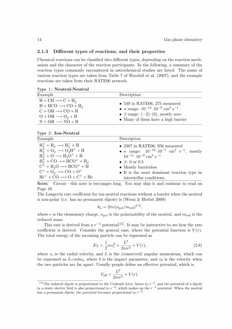
2.1.3 Different types of reactions, and their properties

Chemical reactions can be classified into different types, depending on the reaction mech-anism and the character of the reaction participants. In the following, a summary of thereaction types commonly encountered in astrochemical studies are listed. The name ofvarious reaction types are taken from Table 7 of Woodall et al. (2007), and the examplereactions are taken from their RATE06 network.

Type 1: Neutral-Neutral

Example Description

H + CH −−→ C+H2

H+HCO −−→ CO+H2

C+OH −−→ CO+HO+OH −−→ O2 +HN+OH −−→ NO+H

• 549 in RATE06, 275 measured• α range: 10−13–10−9 cm3 s−1

• β range: (−2)–(8), mostly zero• Many of them have a high barrier

Type 2: Ion-Neutral

Example Description

H+2 +H2 −−→ H+

3 +HH+

2 +O2 −−→ O2H+ +H

H+3 +O −−→ H2O

+ +HH+

3 +CO −−→ HCO+ +H2

C+ +H2O −−→ HCO+ +HC+ +O2 −−→ CO+O+

He+ +CO −−→ O+C+ +He

• 2387 in RATE06, 956 measured• α range: 10−19–10−7 cm3 s−1, mostly

10−11–10−9 cm3 s−1

• β: 0 or 0.5• Mostly barrierless• It is the most dominant reaction type in

interstellar conditions.

Notes: Caveat—this note is two-pages long. You may skip it and continue to read onPage 16.The Langevin rate coefficient for ion-neutral reactions without a barrier when the neutralis non-polar (i.e. has no permanent dipole) is (Woon & Herbst 2009)

kL = 2πe(αpol/mred)1/2,

where e is the elementary charge, αpol is the polarizability of the neutral, and mred is thereduced mass.

This rate is derived from a r−4 potential[12]. It may be instructive to see how the ratecoefficient is derived. Consider the general case, where the potential function is V (r).The total energy of the incoming particle can be expressed as

ET =1

2mv2r +

L2

2mr2+ V (r), (2.8)

where vr is the radial velocity, and L is the (conserved) angular momentum, which canbe expressed as L=mbv0, where b is the impact parameter, and v0 is the velocity whenthe two particles are far apart. Usually people define an effective potential, which is

Veff =L2

2mr2+ V (r).

[12]The induced dipole is proportional to the Coulomb force, hence to r−2, and the potential of a dipolein a static electric field is also proportional to r−2, which makes up the r−4 potential. When the neutralhas a permanent dipole, the potential becomes proportional to r−2.

2.1 Gas phase reactions 15

Note that L is related to the kinetic energy of the incoming particle at infinity, byE0=L2/(2mb2).

A chemical reaction occurs if the incoming particle is captured. What does “cap-ture” mean? Since the total energy is positive and conserved, we should not expect thetwo-particle system to become bound by acquiring a negative total energy unless certainenergy release processes are explicitly accounted for (and for chemical reactions such anexpectation is wrong, simply due to the fact that endothermic reactions exist). However,these complications are unnecessary (at least in the present rudimentary discussion). Thekey is explained in the following.

The effective potential varies as one particle moves from far away towards anotherparticle. If the Veff decreases indefinitely as r decreases, then there will be no obstacle forthe two particles to come close to each other and merge (react). In reality Veff may havea local maximum at certain radius, or may increase with decreasing r when r is smallerthan a certain value.

Let’s only consider the case in which Veff has a local maximum at radius rp. Theeffective potential at this point is Veff(rp). If Veff(rp)>E0, then the particle won’t be ableto reach this peak point, which means that the inter-molecular distance has no chance tobecome smaller than rp, and the reaction cannot occur. In contrast, when Veff(rp)<E0,the radial velocity vr at rp is still nonzero, and must still be pointed towards the center(i.e. dr/dt<0), because for r>rp the corresponding |vr| must be larger (due to the con-servation of energy and the fact that rp is the peak position of Veff), hence vr can neverbe zero or positive since initially vr<0.

So we have arrived at a criterion for a capture event to occur (for simplicity we mayassume a capture event always leads to a chemical reaction, though this may not be true):

Veff|r=rp < E0, (2.9)

where rp is defined so that ∂rVeff|r=rp=0. Note that the left side is a function of boththe impact parameter b and initial kinetic energy E0. The critical impact parameter bc isdefined such that both sides of Eq. (2.9) are equal.

Assuming a power-law attractive potential V (r)=− κr−n, we have

Veff =L2

2mr2− κr−n,

rp =(nmκ

L2

)1/(n−2),

and

Veff|r=rp =n− 2

2κ−2/(n−2)

(L2

nm

)n/(n−2)

. (2.10)

The critical impact parameter for capture can thus be solved for. It is

bc =

(κ

E0

)1/n

·(

n

n− 2

)1/2(n− 2

2

)1/n

. (2.11)

For the ion-neutral reaction involving a non-polar neutral, n=4, κ=αpole2/2, hence

bc=(2αpole2/E0)

1/4,

16 Gas phase chemistry

and the rate coefficient is

k = πb2cv = 2πe(αpol

m

)1/2= 2.3× 10−9 cm3 s−1

( αpol

10−24 cm3

)1/2( m

mH

)−1/2

,

which is called Langevin rate. A typical value for αpol can be found in Duley & Williams(1984). k has no temperature dependence, so that extrapolating experimental resultsobtained usually at room temperature to low temperatures becomes a simple task.

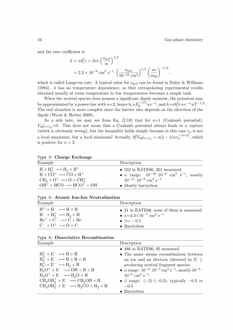
When the neutral species does possess a significant dipole moment, the potential may

be approximated by a power-law with n=2, hence bc∝E−1/20 ∝v−1, and k=πb2cv∝v−1∝T−1/2.

The real situation is more complex since the barrier also depends on the direction of thedipole (Woon & Herbst 2009).

As a side note, we may see from Eq. (2.10) that for n=1 (Coulomb potential),Veff|r=rp<0. This does not mean that a Coulomb potential always leads to a capture(which is obviously wrong), but the inequality holds simply because in this case rp is not

a local maximum, but a local minimum! Actually, ∂2rVeff|r=rp = n(2− n)κr

−(n+2)p , which

is positive for n < 2.

Type 3: Charge Exchange

Example Description

H + H+2 −−→ H2 +H+

H+CO+ −−→ CO+H+

CH2 +O+ −−→ O+CH+2

OH+ +HCO −−→ HCO+ +OH

• 552 in RATE06, 201 measured• α range: 10−16–10−8 cm3 s−1, mostly

10−11–10−9 cm3 s−1

• Mostly barrierless

Type 4: Atomic Ion-Ion Neutralization

Example Description

H+ +H – −−→ H+HH – +H+

2 −−→ H2 +HHe+ +C – −−→ C+HeC – +O+ −−→ O+C

• 31 in RATE06, none of them is measured• α=2.3×10−7 cm3 s−1

• β=− 0.5• Barrierless

Type 5: Dissociative Recombination

Example Description

H+2 + E – −−→ H+H

H+3 + E – −−→ H+H+H

H+3 + E – −−→ H2 +H

H3O+ + E – −−→ OH+H+H

H3O+ + E – −−→ H2O+H

CH3OH+2 + E – −−→ CH3OH+H

CH3OH+2 + E – −−→ H2CO+H2 +H

• 486 in RATE06, 95 measured• The name means recombination between

an ion and an electron (denoted by E – ),producing neutral fragment species.

• α range: 10−9–10−4 cm3 s−1, mostly 10−8–10−6 cm3 s−1

• β range: (−3)–(−0.3); typically −0.3 or−0.5

• Barrierless

2.1 Gas phase reactions 17

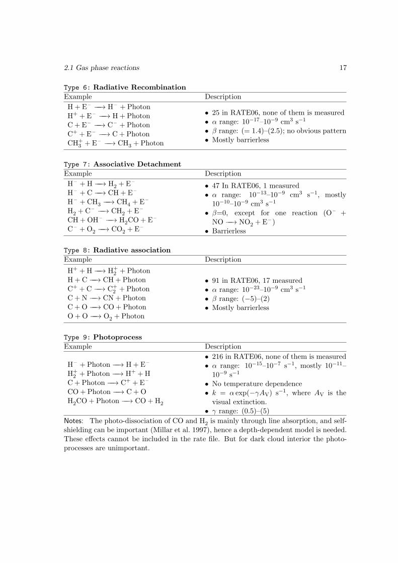
Type 6: Radiative Recombination

Example Description

H + E – −−→ H – + PhotonH+ + E – −−→ H+ PhotonC + E – −−→ C – + PhotonC+ + E – −−→ C+ PhotonCH+

3 + E – −−→ CH3 + Photon

• 25 in RATE06, none of them is measured• α range: 10−17–10−9 cm3 s−1

• β range: (= 1.4)–(2.5); no obvious pattern• Mostly barrierless

Type 7: Associative Detachment

Example Description

H – +H −−→ H2 + E –

H – +C −−→ CH+ E –

H – +CH3 −−→ CH4 + E –

H2 +C – −−→ CH2 + E –

CH+OH – −−→ H2CO+ E –

C – +O2 −−→ CO2 + E –

• 47 In RATE06, 1 measured• α range: 10−13–10−9 cm3 s−1, mostly

10−10–10−9 cm3 s−1

• β=0, except for one reaction (O – +NO −−→ NO2 + E – )

• Barrierless

Type 8: Radiative association

Example Description

H+ +H −−→ H+2 + Photon

H + C −−→ CH+ PhotonC+ +C −−→ C+

2 + PhotonC + N −−→ CN+ PhotonC + O −−→ CO+ PhotonO +O −−→ O2 + Photon

• 91 in RATE06, 17 measured• α range: 10−23–10−9 cm3 s−1

• β range: (−5)–(2)• Mostly barrierless

Type 9: Photoprocess

Example Description

H – + Photon −−→ H+ E –

H+2 + Photon −−→ H+ +H

C+ Photon −−→ C+ + E –

CO+ Photon −−→ C+OH2CO+ Photon −−→ CO+H2

• 216 in RATE06, none of them is measured• α range: 10−15–10−7 s−1, mostly 10−11–

10−9 s−1

• No temperature dependence• k = α exp(−γAV) s−1, where AV is the

visual extinction.• γ range: (0.5)–(5)

Notes: The photo-dissociation of CO and H2 is mainly through line absorption, and self-shielding can be important (Millar et al. 1997), hence a depth-dependent model is needed.These effects cannot be included in the rate file. But for dark cloud interior the photo-processes are unimportant.

18 Gas phase chemistry

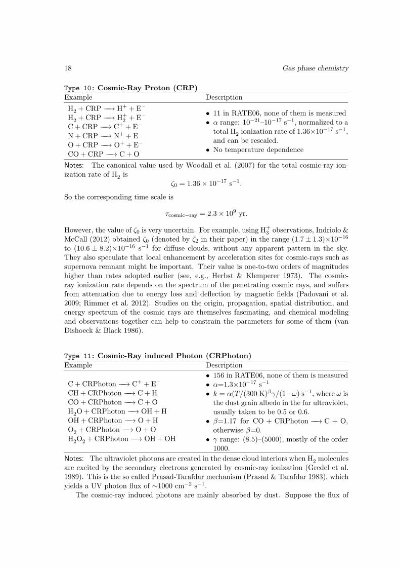
Type 10: Cosmic-Ray Proton (CRP)

Example Description

H2 +CRP −−→ H+ + E –

H2 +CRP −−→ H+2 + E –

C+ CRP −−→ C+ + E –

N+CRP −−→ N+ + E –

O+CRP −−→ O+ + E –

CO+CRP −−→ C+O

• 11 in RATE06, none of them is measured• α range: 10−21–10−17 s−1, normalized to a

total H2 ionization rate of 1.36×10−17 s−1,and can be rescaled.

• No temperature dependence

Notes: The canonical value used by Woodall et al. (2007) for the total cosmic-ray ion-ization rate of H2 is

ζ0 = 1.36× 10−17 s−1.

So the corresponding time scale is

τcosmic−ray = 2.3× 109 yr.

However, the value of ζ0 is very uncertain. For example, using H+3 observations, Indriolo &

McCall (2012) obtained ζ0 (denoted by ζ2 in their paper) in the range (1.7± 1.3)×10−16

to (10.6 ± 8.2)×10−16 s−1 for diffuse clouds, without any apparent pattern in the sky.They also speculate that local enhancement by acceleration sites for cosmic-rays such assupernova remnant might be important. Their value is one-to-two orders of magnitudeshigher than rates adopted earlier (see, e.g., Herbst & Klemperer 1973). The cosmic-ray ionization rate depends on the spectrum of the penetrating cosmic rays, and suffersfrom attenuation due to energy loss and deflection by magnetic fields (Padovani et al.2009; Rimmer et al. 2012). Studies on the origin, propagation, spatial distribution, andenergy spectrum of the cosmic rays are themselves fascinating, and chemical modelingand observations together can help to constrain the parameters for some of them (vanDishoeck & Black 1986).

Type 11: Cosmic-Ray induced Photon (CRPhoton)

Example Description

C + CRPhoton −−→ C+ + E –

CH+ CRPhoton −−→ C+HCO+CRPhoton −−→ C+OH2O+CRPhoton −−→ OH+HOH+CRPhoton −−→ O+HO2 +CRPhoton −−→ O+OH2O2 +CRPhoton −−→ OH+OH

• 156 in RATE06, none of them is measured• α=1.3×10−17 s−1

• k = α(T/(300 K)βγ/(1−ω) s−1, where ω isthe dust grain albedo in the far ultraviolet,usually taken to be 0.5 or 0.6.

• β=1.17 for CO + CRPhoton −−→ C + O,otherwise β=0.

• γ range: (8.5)–(5000), mostly of the order1000.

Notes: The ultraviolet photons are created in the dense cloud interiors when H2 moleculesare excited by the secondary electrons generated by cosmic-ray ionization (Gredel et al.1989). This is the so called Prasad-Tarafdar mechanism (Prasad & Tarafdar 1983), whichyields a UV photon flux of ∼1000 cm−2 s−1.

The cosmic-ray induced photons are mainly absorbed by dust. Suppose the flux of

2.1 Gas phase reactions 19

these photons is Fγ , we have

FγσGnG(1− ω) = 0.15ζ0nH,

which gives

Fγ =0.15ζ0nH

σGnG(1− ω)=

0.15ζ0σG(1− ω)

,

where σG'2×10−21 cm2 is the absorption cross section of the dust grains per hydrogennucleus (Sternberg et al. 1987), and nG is the dust density. This gives Fγ'1700 cm−2 s−1.The factor 0.15 comes from the impact excitation efficiency of H2 by an electron with en-ergy 30 eV.

Note that the γ value for these reactions are a factor of two smaller than those calcu-lated by Gredel et al. (1989), due to a difference in whether it is scaled to the total cosmicionization rate of H2 or H.

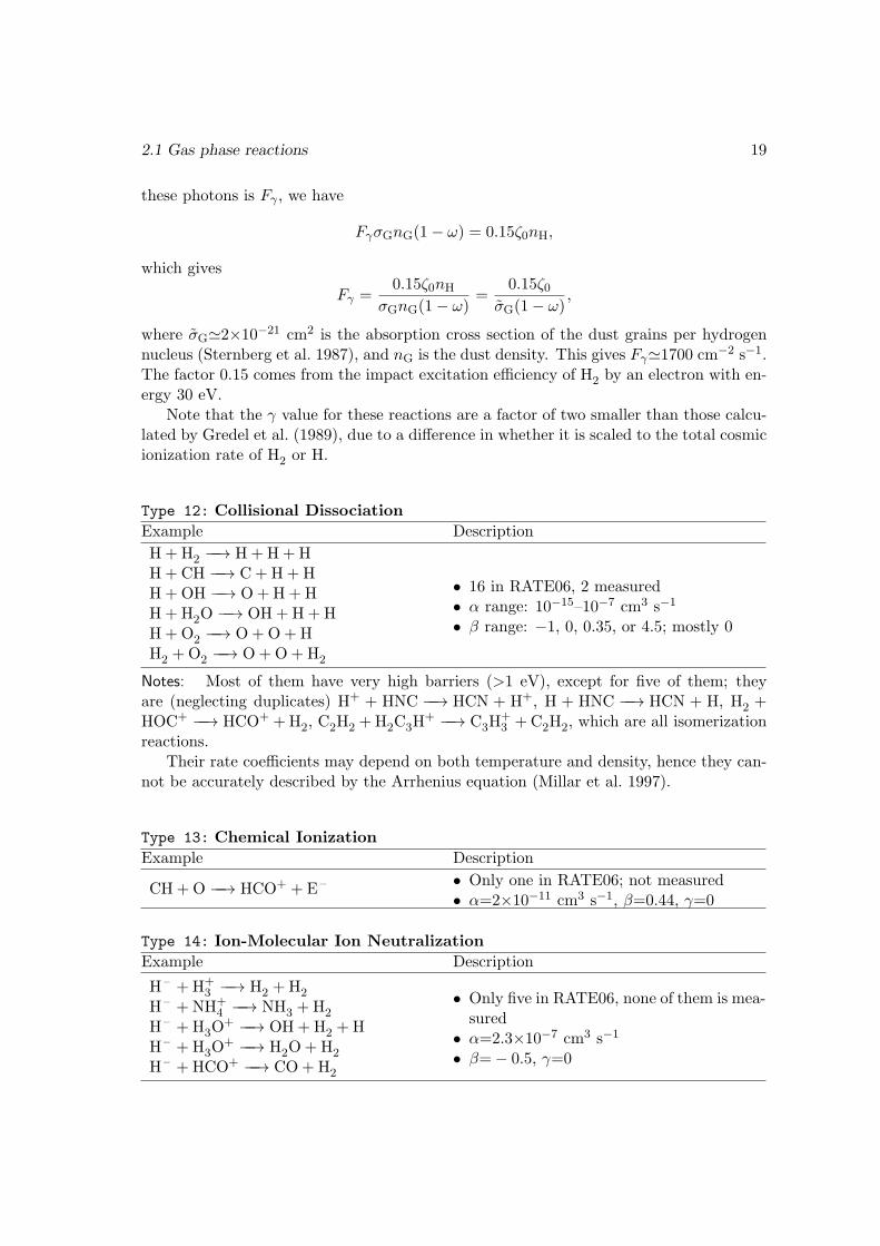
Type 12: Collisional Dissociation

Example Description

H + H2 −−→ H+H+HH+CH −−→ C+H+HH+OH −−→ O+H+HH+H2O −−→ OH+H+HH+O2 −−→ O+O+HH2 +O2 −−→ O+O+H2

• 16 in RATE06, 2 measured• α range: 10−15–10−7 cm3 s−1

• β range: −1, 0, 0.35, or 4.5; mostly 0

Notes: Most of them have very high barriers (>1 eV), except for five of them; theyare (neglecting duplicates) H+ + HNC −−→ HCN + H+, H + HNC −−→ HCN + H, H2 +HOC+ −−→ HCO+ +H2, C2H2 +H2C3H

+ −−→ C3H+3 +C2H2, which are all isomerization

reactions.Their rate coefficients may depend on both temperature and density, hence they can-

not be accurately described by the Arrhenius equation (Millar et al. 1997).

Type 13: Chemical Ionization

Example Description

CH +O −−→ HCO+ + E – • Only one in RATE06; not measured• α=2×10−11 cm3 s−1, β=0.44, γ=0

Type 14: Ion-Molecular Ion Neutralization

Example Description

H – +H+3 −−→ H2 +H2

H – +NH+4 −−→ NH3 +H2

H – +H3O+ −−→ OH+H2 +H

H – +H3O+ −−→ H2O+H2

H – +HCO+ −−→ CO+H2

• Only five in RATE06, none of them is mea-sured

• α=2.3×10−7 cm3 s−1

• β=− 0.5, γ=0

20 Gas phase chemistry

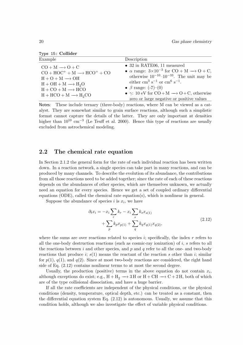
Type 15: Collider

Example Description

CO +M −−→ O+CCO+HOC+ +M −−→ HCO+ +COH+O+M −−→ OHH+OH+M −−→ H2OH+CO+M −−→ HCOH+HCO+M −−→ H2CO

• 32 in RATE06, 11 measured• α range: 3×10−3 for CO + M −−→ O + C,

otherwise 10−10–10−33. The unit may beeither cm3 s−1 or cm6 s−1.

• β range: (-7)–(0)• γ: 10 eV for CO+M −−→ O+C, otherwise

zero or large negative or positive values

Notes: These include ternary (three-body) reactions, where M can be viewed as a cat-alyst. They are somewhat similar to grain surface reactions, although such a simplisticformat cannot capture the details of the latter. They are only important at densitieshigher than 1010 cm−3 (Le Teuff et al. 2000). Hence this type of reactions are usuallyexcluded from astrochemical modeling.

2.2 The chemical rate equation

In Section 2.1.2 the general form for the rate of each individual reaction has been writtendown. In a reaction network, a single species can take part in many reactions, and can beproduced by many channels. To describe the evolution of its abundance, the contributionsfrom all those reactions need to be added together; since the rate of each of these reactionsdepends on the abundances of other species, which are themselves unknown, we actuallyneed an equation for every species. Hence we get a set of coupled ordinary differentialequations (ODE), called the chemical rate equation(s), which is nonlinear in general.

Suppose the abundance of species i is xi, we have

∂txi = −xi∑r

kr − xi∑s

ksxs(1)

+∑p

kpxp(1) +∑q

kqxq(1)xq(2),(2.12)

where the sums are over reactions related to species i; specifically, the index r refers toall the one-body destruction reactions (such as cosmic-ray ionization) of i, s refers to allthe reactions between i and other species, and p and q refer to all the one- and two-bodyreactions that produce i; s(1) means the reactant of the reaction s other than i; similarfor p(1), q(1), and q(2). Since at most two-body reactions are considered, the right handside of Eq. (2.12) contains nonlinear terms to at most the second degree.

Usually, the production (positive) terms in the above equation do not contain xi,although exceptions do exist; e.g., H+H2 −−→ 3H or H+CH −−→ C+ 2H, both of whichare of the type collisional dissociation, and have a huge barrier.

If all the rate coefficients are independent of the physical conditions, or the physicalconditions (density, temperature, optical depth, etc.) can be treated as a constant, thenthe differential equation system Eq. (2.12) is autonomous. Usually, we assume that thiscondition holds, although we also investigate the effect of variable physical conditions.

2.2 The chemical rate equation 21

Since different spatial points may have different chemical composition, the most gen-eral form of the evolution equation should contain partial derivatives over the spatialcoordinate, to take into account the convection and diffusion effects. In cold dark cloudsthe diffusion through thermal motions should be very slow. Turbulent mixing might beimportant, but it works only locally, where the gradient in chemical composition is small.Hence we may neglect the convection effect, and put the explicit form of the physicalparameters as a function of time into Eq. (2.12) through the rate coefficients.

In a completely self-consistent model, the chemical rate equations should be coupledwith the dynamical equations. This means that not only the evolution in the densityand temperature can affect the chemical evolution, but that the compositional variationscaused by the chemical processes can also affect the dynamical evolution by changing theheating and cooling rates (Neufeld et al. 1995) or by changing the interaction betweenmatter and magnetic fields through the degree of ionization (see, e.g. Tassis et al. 2011).However, in models of this class, the chemistry considered is usually relatively simple,where only the key species (such as the major coolants) are included. Since our goal isnot to give a comprehensive chemical-dynamical model of cloud evolution, we don’t takethe coupling and feedback effect into account; namely, our emphasis is on the chemicalpart, isolated from complications from the dynamics.

The solutions to Eq. (2.12) can be divided into two types. The first type is to solveonly the steady-state equations, which means to solve a set of algebraic equations bysetting ∂txi = 0, for all i. This is usually done with a Newton-Raphson scheme (LeBourlot 1991), and is adopted for studies on chemical bi-stability[13] (Le Bourlot et al.1993; Charnley & Markwick 2003). Another type is the time-dependent solution, in whichthe evolution of the abundances of all the species are calculated as a function of time froma given initial condition. Sometimes this type of solution is called pseudo-time-dependent,since the physical conditions are kept constant. Note that the second type of solution canindeed be viewed as an iterative way to obtain the steady-state solution, though this maynot be as efficient as the Newton-Raphson method for this kind of problem.

In our work we always obtain the time-dependent solution of Eq. (2.12). In thefollowing I give a description of the problems encountered in solving the chemical rateequation and the way to deal with them. Then I describe a code I wrote for obtainingthe solutions, based on a general-purpose solver.

2.2.1 Solving a stiff system of equations

The chemical rate equation is a stiff system[14], meaning that a large range of time scalesare involved. For example, the cosmic-ray dissociation time scale is of the order 109 yr,while the time scale for the dissociative recombination reactions can be as short as severalyears. Since we are usually interested in time scales that are not too short, the existence

[13]The chemical bi-stability is a phenomenon in which there are two (maybe more in the general case)stable solutions for the steady state, for certain physical conditions. It is related to the bifurcationphenomenon, in which the continuous variation of one controlling parameter (density for example) canlead to the appearance or disappearance of one of the two steady states. Whether this theoreticallydiscovered behavior has any observational significance seems to be unanswered (Charnley & Markwick2003; Boger & Sternberg 2006).[14]The word “stiff” in the name seems to be related to the motion of spring systems with large spring

constants.

22 Gas phase chemistry

of a large range of time scales means that we have to deal with those very fast processesoccurring in time intervals much shorter than the time scales we care about.

This stiffness causes problems when trying to solve the equations numerically with anexplicit method. For example, if the following equation

y′ = −cy (c > 0) (2.13)

is solved using the explicit forward Euler scheme

yn+1 = yn + hy′n = (1− ch)yn = (1− ch)ny1, (2.14)

where h is the time step, then its long-time behavior (i.e. when n is large) is correct onlyif |1−ch| < 1, which requires h < 2/c. This is because if h is so large that (1−ch) < −1,the solution Eq. (2.14) will be oscillating between positive and negative values. So whenc is large, a very small time step is needed for the numerical solution to converge to zero,although the exact analytical solution vanishes exponentially. A similar problem appearsin the general case of a nonlinear set of equations (rather than only one equation), wherethe right hand side can be linearized and analyzed similarly.

For these stiff equations, it is impractical to avoid the instability problem by adoptingvery small integration intervals, since—if such an approach is taken—extremely smallinterval (in comparison to the time scales we are interested in) will be necessary, leadingto a huge number of integration steps.

The solution to this stiffness problem is to use implicit methods. The form in Eq. (2.14)is explicit, as its right hand side involves only quantities at step n, and the calculationinvolved is straightforward. In contrast, in the implicit approach the right hand side ofan integration step contains quantities that need to be solved for. For example, one maysimply replace Eq. (2.14) by

yn+1 = yn + hy′n+1 = yn − chyn+1, (2.14′)

which gives

yn+1 =yn

1 + ch=

y1(1 + ch)n

. (2.15)

Since both c and h are positive, the above form is always stable; no oscillatory behaviorwill appear.

The fact that unknown quantities appear in both sides of each integration step in theimplicit method requires solution of a set of (nonlinear) algebraic equations, similar towhat we did to get Eq. (2.15) from Eq. (2.14′).

The method used in solving these algebraic equations are usually based on Newton’smethod, i.e., by linearizing these equations and iterating until the solution has converged.The linearization step may be done by numerical differencing, or, probably more efficiently,by making use of the Jacobian matrix.

For a set of differential equations with the form

∂txi = fi(x1, x2, . . . , xn; t), (2.16)

each element of the associated Jacobian matrix at each time is defined to be

Jij =∂fi∂xj

, (2.17)

2.2 The chemical rate equation 23

which is easy to evaluate based on the rate equations Eq. (2.12).For a large chemical network, the Jacobian matrix is most likely very sparse, meaning

that most of its elements are zero at all time. For example, when species j does not reactwith species i, and does not participate in any reactions producing i, then Jij = 0. Thisproperty should be utilized in the solver.

The ODE solver we use

We did not write an ODE solver by ourselves, rather we use the 2003 version of theDLSODES solver of the ODEPACK package[15] (Hindmarsh 1983; Radhakrishnan & Hind-marsh 1993), which is written in FORTRAN77. The name of the solver means “the doubleprecision version of the Livermore Solver for Ordinary Differential Equations with generalSparse Jacobian matrix”. The ODEPACK package contain 9 solvers, each of which suitsdifferent class of problems. The one we use is best suited for stiff and sparse problems; itsupersedes and improves upon the older GEARS package.

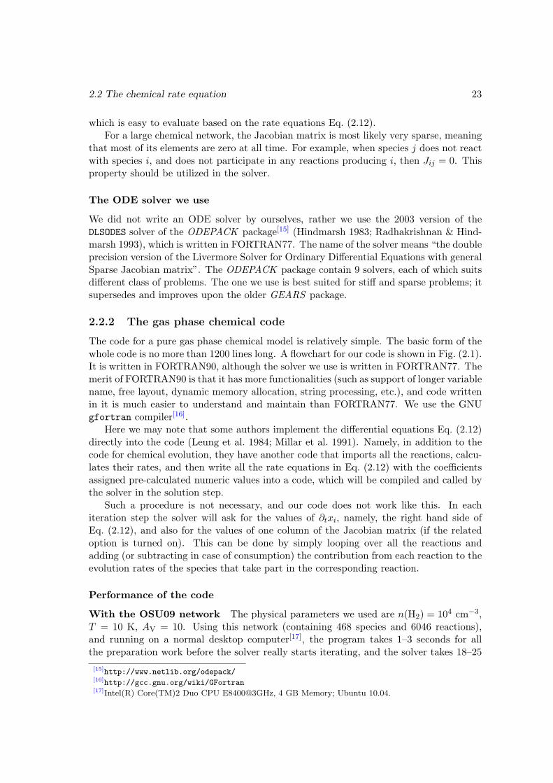
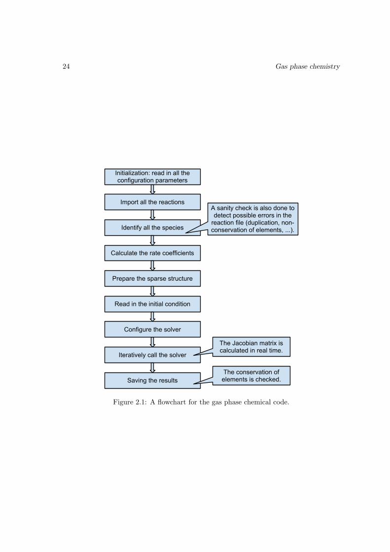
2.2.2 The gas phase chemical code

The code for a pure gas phase chemical model is relatively simple. The basic form of thewhole code is no more than 1200 lines long. A flowchart for our code is shown in Fig. (2.1).It is written in FORTRAN90, although the solver we use is written in FORTRAN77. Themerit of FORTRAN90 is that it has more functionalities (such as support of longer variablename, free layout, dynamic memory allocation, string processing, etc.), and code writtenin it is much easier to understand and maintain than FORTRAN77. We use the GNUgfortran compiler[16].

Here we may note that some authors implement the differential equations Eq. (2.12)directly into the code (Leung et al. 1984; Millar et al. 1991). Namely, in addition to thecode for chemical evolution, they have another code that imports all the reactions, calcu-lates their rates, and then write all the rate equations in Eq. (2.12) with the coefficientsassigned pre-calculated numeric values into a code, which will be compiled and called bythe solver in the solution step.

Such a procedure is not necessary, and our code does not work like this. In eachiteration step the solver will ask for the values of ∂txi, namely, the right hand side ofEq. (2.12), and also for the values of one column of the Jacobian matrix (if the relatedoption is turned on). This can be done by simply looping over all the reactions andadding (or subtracting in case of consumption) the contribution from each reaction to theevolution rates of the species that take part in the corresponding reaction.

Performance of the code

With the OSU09 network The physical parameters we used are n(H2) = 104 cm−3,T = 10 K, AV = 10. Using this network (containing 468 species and 6046 reactions),and running on a normal desktop computer[17], the program takes 1–3 seconds for allthe preparation work before the solver really starts iterating, and the solver takes 18–25

[15]http://www.netlib.org/odepack/[16]http://gcc.gnu.org/wiki/GFortran[17]Intel(R) Core(TM)2 Duo CPU E8400@3GHz, 4 GB Memory; Ubuntu 10.04.

24 Gas phase chemistry

Figure 2.1: A flowchart for the gas phase chemical code.

2.2 The chemical rate equation 25

seconds to reach 1.2×108 years, with an absolute tolerance of 10−50, a relative tolerance[18]

of 10−6, and a user-provided iteration number 710 (which is the number of output datapoints, not the number of internal iteration steps of the solver). About one second isneeded to save the results. The total abundance of each element varies by no more thana factor of 10−10 between the initial and final states, which means at least in this sensethe code is working fine.With the UMIST RATE06 network As this network is smaller than the OSU09network, containing 420 species and 4605 reactions, the program takes ∼9 seconds toreach 108 years, with a relative tolerance of 10−6, and an absolute tolerance of 10−50.

Since the RATE06 network is accompanied by a paper (Woodall et al. 2007), whichcontains a benchmark model, we compared the results from our model with theirs (Table 9in Woodall et al. 2007). The agreement is generally good, with relative differences of theorder 1% (the values in their Table 9 contains only three digits). The differences mayoriginate from different treatment of some of the reactions with negative energy barriers,or maybe slightly different physical conditions have been used.With the depleted network This network is based on the completely depleted networkof Walmsley et al. (2004) and Flower et al. (2004), which contains no elements heavier thanHe, supplemented by Pagani et al. (2009) and Hugo et al. (2009), compiled by B. Parise.With 28 species, 389 reactions, and with relative tolerance set to 10−6, absolute toleranceset to 10−90, the run time needed to reach 108 years is about 0.1 second. If the relativetolerance is set to 10−2, then the time needed becomes 0.04 second, with essentially nochange in the results.

2.2.3 Application of the gas phase code to study H2D+ and D2H

+

In Parise et al. (2011) a spatially extended distribution of D2H+ was for the first time

firmly detected in the H-MM1 prestellar core in the L1688 cloud. The exact temperatureand density of this source has not been derived, but the temperature is constrained to be<13 K based on the velocity width. Together with data on H2D

+, the ratio between para-D2H

+ and ortho-H2D+ is constrained to be ∼1–10, depending on the assumed density and

kinetic temperature of the source that are needed for the non-LTE[19] radiative transfermodeling.

The ortho- and para- (and possibly meta-) designations are used to distinguish differ-ent nuclear spin states of a molecule that contain two or more equivalent H or D atoms.The fact that the H nucleus is a fermion while the D nucleus is a boson exerts requirementson the symmetry of possible spatial wave functions of the molecule, specifically the rota-tion states, which determine the rotation energy levels. The transition between differentnuclear spin states is forbidden, hence two molecules with the same chemical structure

[18]The absolute tolerance and relative tolerance are setup parameters for the solver, which set themaximum allowable absolute and relative errors for the abundances. A very small absolute tolerance isused merely to let the solver proceed, since, if the absolute tolerance is set to zero, then for a species withvery low abundance, the allowed error determined from the relative tolerance may be too small to achieve.[19]LTE: Local thermodynamic equilibrium. For non-LTE conditions, in which the gas density is not

high enough to thermalize the distribution of the occupation number in each energy level of a moleculebecause the radiative cascade is relatively fast, the kinetic temperature of the gas (which describes thethermal velocity of a molecule) and the Boltzmann equation cannot be used to describe the energy levelpopulation.

26 Gas phase chemistry

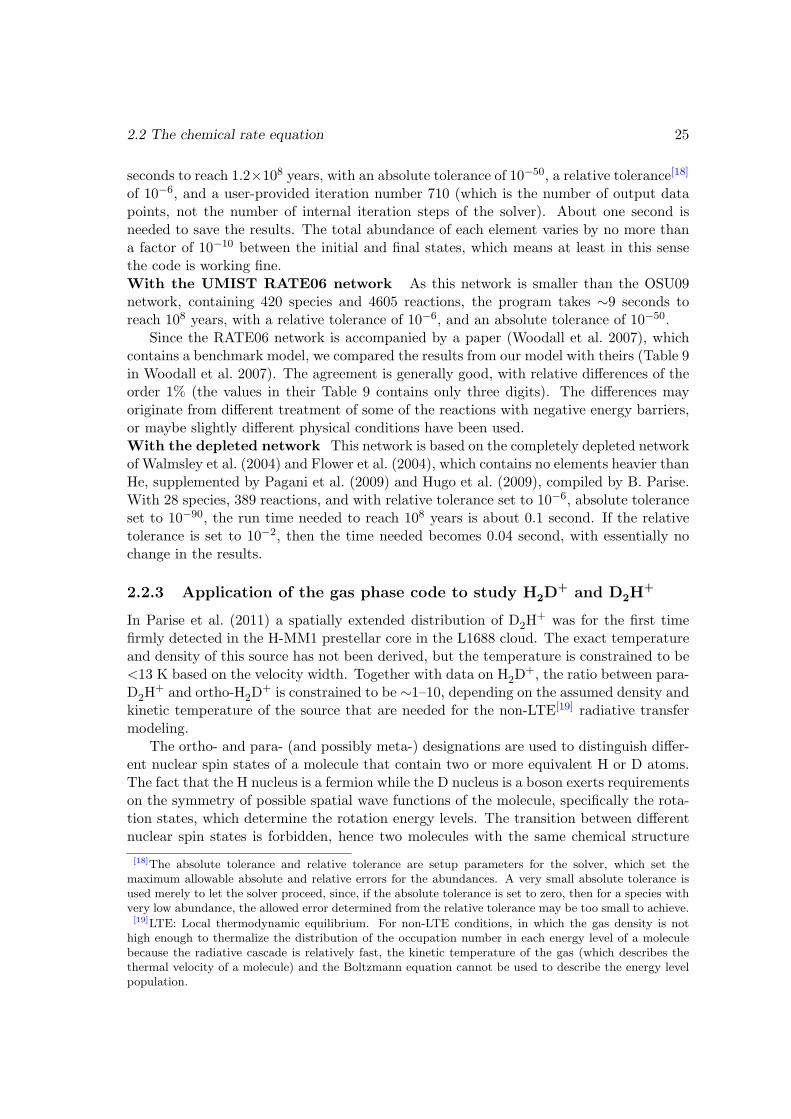
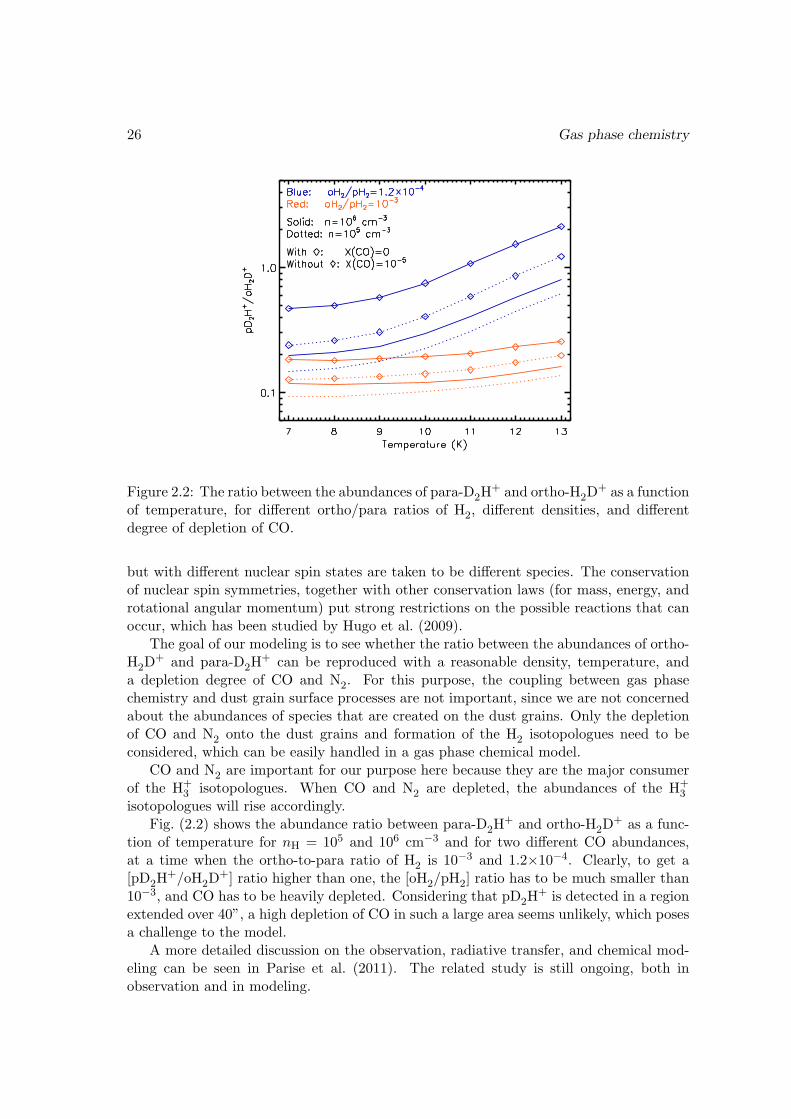
Figure 2.2: The ratio between the abundances of para-D2H+ and ortho-H2D

+ as a functionof temperature, for different ortho/para ratios of H2, different densities, and differentdegree of depletion of CO.

but with different nuclear spin states are taken to be different species. The conservationof nuclear spin symmetries, together with other conservation laws (for mass, energy, androtational angular momentum) put strong restrictions on the possible reactions that canoccur, which has been studied by Hugo et al. (2009).

The goal of our modeling is to see whether the ratio between the abundances of ortho-H2D

+ and para-D2H+ can be reproduced with a reasonable density, temperature, and

a depletion degree of CO and N2. For this purpose, the coupling between gas phasechemistry and dust grain surface processes are not important, since we are not concernedabout the abundances of species that are created on the dust grains. Only the depletionof CO and N2 onto the dust grains and formation of the H2 isotopologues need to beconsidered, which can be easily handled in a gas phase chemical model.

CO and N2 are important for our purpose here because they are the major consumerof the H+

3 isotopologues. When CO and N2 are depleted, the abundances of the H+3

isotopologues will rise accordingly.Fig. (2.2) shows the abundance ratio between para-D2H

+ and ortho-H2D+ as a func-

tion of temperature for nH = 105 and 106 cm−3 and for two different CO abundances,at a time when the ortho-to-para ratio of H2 is 10−3 and 1.2×10−4. Clearly, to get a[pD2H

+/oH2D+] ratio higher than one, the [oH2/pH2] ratio has to be much smaller than

10−3, and CO has to be heavily depleted. Considering that pD2H+ is detected in a region

extended over 40”, a high depletion of CO in such a large area seems unlikely, which posesa challenge to the model.

A more detailed discussion on the observation, radiative transfer, and chemical mod-eling can be seen in Parise et al. (2011). The related study is still ongoing, both inobservation and in modeling.

Chapter 3

Grain chemistry

Contents

3.1 General facts about interstellar dust grains . . . . . . . . . . . . . . . . 27

3.2 Why do we study grain chemistry . . . . . . . . . . . . . . . . . . . . . 29

3.3 Rates of processes in grain chemistry . . . . . . . . . . . . . . . . . . . 30

3.4 Mathematical framework for surface chemistry . . . . . . . . . . . . . . 38

In the previous chapter, the gas phase chemical reactions and the networks that arerelevant for interstellar clouds, together with their mathematical formulation, have beendescribed. The vast majority of the interstellar mass resides in the gas phase; only aroundone percent of the mass is in mesoscopic solid form, which we call dust grains. Thoughbeing tiny, this dust material has an impact on astronomy that cannot be overestimated.Dust affects the dynamical evolution of the ISM in many aspects. From a chemical point ofview, it can act as a reservoir of gas phase molecules, a factory and catalyst for producingmolecules, and, can enrich the gas phase composition by partially or completely beingfragmented.

In this chapter I first give a brief review of the general aspects of dust properties, thenstate the reasons why do we need to study grain chemistry, followed by an investigationof the basic processes involved in grain chemistry. A mathematical formalism that isneeded to model these processes is then presented. Finally, one method (Monte Carlosimulation) to model the grain chemistry is described. Another method (hybrid momentequation method) that is developed by us will be presented in the next chapter.

3.1 General facts about interstellar dust grains

The existence of dust in the interstellar space is not a trivial fact even when viewed inretrospect. In the early times astronomers noticed dark regions in the sky in which thenumber of stars is much lower than their neighborhood (mentioned in Greenberg 1963 andBergin & Tafalla 2007); that these dark regions are not really empty but rather containa lot of gas and dust is unveiled by observations in the optical and infrared band. Lightrays passing through these clouds are absorbed and scattered by the dust grains. This so-called extinction demonstrates the existence of opaque material between the observer and

27

28 Grain chemistry

the stars, and can be used to quantitatively study the physical properties (composition,size, morphology, etc.) of the dust grains.

Most of our knowledge about interstellar dust comes from its interaction with elec-tromagnetic fields. The degree of extinction as a function of wavelength can be used toconstrain the size and material composition of the dust grains, and the polarized lightfrom the dust indicates their non-spherical shape, the existence of a magnetic field (witha strength greater than a few µG), via the alignment of the dust grains with respect tothe magnetic field (Davis & Greenstein 1951). Besides absorption features, the emissionspectra from dust provide independent and complementary information on the dust com-position, leading to the discovery of PAH (Polycyclic Aromatic Hydrocarbon) moleculesin the interstellar space (Li & Draine 2001; Tielens 2008).

The infrared light scattered by the interstellar dust (leading to the so-called “cloud-shine” and “coreshine”) can also be used as a proxy to study the dust grain sizes and thehost cloud cores (Pagani et al. 2010). This is somewhat similar to the case in our solarsystem, where the presence of zodiacal light indicates the condensation of dust particlestowards the ecliptic plane.

The interstellar dust grains contain a core, usually composed of refractory materials,such as carbonaceous compounds (graphite, PAH, etc.) and silicates (containing Si, O,Fe, and Mg) (Draine 2003). The core may also be chemically differentiated due to itsformation process. In cold conditions the grain core will be covered with an ice mantle,mainly composed of solid water, CO, CO2, CH3OH, and some other species. The size ofa dust grain can be described by the famous MRN power-law distribution (Mathis et al.1977), dn/dr ∝ r−3.5, for 0.005 µm<r<1 µm. It gives a mean radius of about 0.008 µm.Grain chemistry models typically adopt a larger radius of 0.1 µm, considering the growthof dust in cold dense conditions.

Dust particles in the interplanetary space close to Earth can be directly captured byballoons or airplanes flying in the stratosphere[1], or by satellites (such as MIDAS onboard Rosetta, the aerogel collector of Stardust, and VBSDC on board New Horizons).The dust grains that have been captured and directly imaged by scanning electron mi-croscope(Bradley et al. 1992) usually appear as a porous and heterogeneous mixture ofparticles with different compositions (refractory or organic). Dust fallen onto the Earthin the pristine continent of Antarctica (where contamination from terrestrial sources arereduced as much as possible) can also be collected (Hodge 1981). They are visually clas-sified into several types, such as opaque or transparent spherules, and irregular particles;chemically they are rich in iron or silicon (Schmidt & Keil 1966). The isotopic ratio inthese particles can be used to confirm their extraterrestrial origin. Most of the interplan-etary dust are fragments of comets or ejecta produced in asteroid collisions, and only aminor part may come from the interstellar space.

The interstellar dust grains have their origins in the ejecta of old stars or in supernovaexplosions. It is not clear which contributes more by now. The detailed mechanism forthe formation of dust particles from atoms and molecules (e.g., how the atomic silicon cancombine with other elements such as oxygen, magnesium, . . . , to form clusters) in theseconditions is still under active investigation (see, e.g., Goumans & Bromley 2012). In theirjourney from the circumstellar envelopes to the diffuse ISM, to the dense dark clouds, and

[1]See, e.g., http://www.spaceref.com/news/viewpr.html?pid=28009

3.2 Why do we study grain chemistry 29

then finally to newly formed stars and planets (and other cometary and asteroid bodies),the dust grains must have been heavily altered by radiation field and particle encounters.A dust particle can gain material by accumulating gas phase molecules, or by mergingwith other dust particles upon close encounter. But if the collision with an incomingparticle is too fierce, it may lose mass by sputtering (Draine & Salpeter 1979; Draine1979; Tielens et al. 1994), or it may get reshaped. If the collision is energetic enough,the dust particle may be hot enough to restructure itself (crystallization or glassification).Energetic photons or cosmic rays can also change the dust composition by evaporatingsurface molecules (Purcell 1976) or by initiating chemical reactions.

Among the researches on interstellar dust, the work of Hoyle & Wickramasinghe seemsto be a heresy (Wickramasinghe 2011). Although their early work (Hoyle & Wickramas-inghe 1962) is in the mainstream, which studied the extinction caused by dust grains madeof graphite (graphite flake), and their polarizing effect, later these authors conjecturedthe presence of prebiotic or even biotic materials on the dust grains (Hoyle & Wickra-masinghe 1977, 1979) based on the extinction features and the presence of amino acidsin carbonaceous chondrites. It is not our objective to defend or dispute such a radicalviewpoint here, but the formation and accumulation of a vast variety of organic materials(see, e.g. Garrod et al. 2008) on the dust grains does make the idea about the existenceof biotic material in the interstellar space not too far-fetched.

3.2 Why do we study grain chemistry

The reason grain chemistry was introduced to astrochemical study may be two-folds.First, certain species that are observed to be abundant cannot be accounted for by gasphase chemistry. The most important species of this kind is molecular hydrogen (H2).Simple addition of two gas-phase H atoms does not work because the excess energy cannotbe released through radiation efficiently since the H−H system has zero dipole moment;the H−H system can indeed stabilize through electronic or vibrational transition, butas estimated by Duley & Williams (1984), the rates are too low, being about 10−31–10−29 cm3 s−1. Another possible route is

H + H+ −−→ H+2 + Photon,

H+2 +H −−→ H2 +H+.

The H2 formation rate from this route is about 10−18n(H)n(H+), hence it is too low. Yetanother possibility is to form H2 through the anion H – ,

H + H− −−→ H2 + E-,

with rate coefficient 1.3×10−9 cm3 s−1. This route requires a high H – abundance, whichmay indeed be satisfied at a relatively high temperature (Duley & Williams 1984). Ingeneral, grain chemistry is the most efficient way to produce H2.

Another molecule that cannot be efficiently produced in the gas phase is methanol(CH3OH), which was proposed to form through (Bates 1983)

CH+3 +H2O −−→ CH3OH+

2 + Photon,

30 Grain chemistry

followed by (Millar et al. 1988)

CH3OH+2 + E− −−→ CH3OH+H.

However, this latter dissociative recombination reaction has other branches, such as CH3+OH+H and CH2+H+H2O, which are measured to be dominant over the one producingCH3OH (Geppert et al. 2006), hence the amount of CH3OH that can be produced in thegas phase is very low, at most 10−11 relative to H2 (Garrod et al. 2006), even lower thanthe typically detected abundance of 10−9 in cold regions (Friberg et al. 1988; Gomez et al.2011), and much lower than 10−6 in warm regions (Menten et al. 1986). The inabilityof gas phase chemistry to reproduce the observed abundance of CH3OH points to grainchemistry.

The reasons why dust grains can enhance the production of some molecules can beheuristically understood as follows: (i) They can act as a third body, absorbing excessenergies of the intermediate reaction complex. (ii) They can alter the reaction barrier ofcertain reactions. (iii) They can prolong the time for two reactants to stay together, byconfining them on the surface, or even in the same site on the surface.

Finally, we may argue that grain chemistry is important not just because it helps tosolve some of the problems encountered in pure gas phase chemistry, but rather becausewe believe important processes are occurring on dust grain surfaces, which deserve tobe studied. The observed grain mantle composition requires an explanation. Reactionsbetween the mantle species, when they become mobile and reactive in the warm-up phase,may lead to the formation of molecules with much higher complexity, some of which areeven prebiotic. However, only the fundamentals of grain chemistry will be discussed inthis chapter.

3.3 Rates of processes in grain chemistry

At least four basic processes are encountered in grain chemistry. Namely, accretion[2]

of gas phase species onto the grain surface, desorption of surface species from the grainsurface, migration of surface species on the grain surface, and reaction between two speciesupon meeting. In the following the rates of these processes will be discussed.

3.3.1 Adsorption rates

Strictly speaking, the adsorption process is not a surface process, but rather an interactionbetween the surface and gas phase. When a gas phase molecule encounters a dust grain,it has a probability to be captured by the latter. Such a process is called adsorption.The particle being adsorbed is called an adsorbate, and the surface material is calledan adsorbent. Adsorption is different from absorption, in that the word “adsorption”emphasizes the incoming particles are captured and stored on a surface, while in thelatter process the incoming particles are dissolved into bulk material.

The theory of adsorption, pioneered by Langmuir (Langmuir 1918), is based on severalassumptions (Moore 1972):

[2]We use the words “accretion” and “adsorption” interchangeably in this thesis. Also the words “evap-oration” and “desorption” are equivalent for our purpose.

3.3 Rates of processes in grain chemistry 31

(i) The surface contains a fixed number of adsorption sites. (ii) Each site canhold one and only one molecule, (iii) All the sites have a binding energy, whichdoes not depend on the surface coverage. (iv) The molecule residing in onesite does not affect molecules in other sites.

Furthermore, it was also assumed by Langmuir that, when a molecule attacks a surfacesite already occupied, it will be rejected, and the molecule in that site is not affected. Thisis called Langmuir rejection. However, this rejection mechanism will not be included inour model, since the interaction (in contrast to rejection) between the dust grain materialand the incoming particles is essential for the grain chemistry.

Two types of adsorption are generally considered: chemisorption and physisorption.In chemisorption the adsorbate is attached to the adsorbent through covalent bonds, whilein physisorption the adsorbate is attracted to the surface by the van der Waals force. Thebinding energy Ebind/k (k is the Boltzmann constant) due to chemisorption can be morethan 104 K, which is much stronger than physisorption, whose binding energy is typically∼1000 K. Some species can also form hydrogen bond with the surface, the strength ofwhich is roughly .5000 K, stronger than physisorption but weaker than chemisorption.

The accretion rate for species X can be written as

kacc(X) = ηn(X)v(X)σ, (3.1)

where n(X) is the gas phase density of X, v(X) is its thermal velocity, η is the stickingcoefficient, usually taken to be unity (or a fractional value of order unity), and σ is thecross section area of a dust grain. kacc(X) is the number of X particles that are accretedonto a single dust grain in unit time. Note that usually v(X) is taken to be the averagevelocity of a Maxwell distribution,

v(X) =

√8kT

πmX, (3.2)

and σ should be taken to be the cross section area πr2, not the total surface area 4πr2,where r is the dust grain radius.

Numerically, we have

kacc(X) = 1.44× 10−5 s−1[' 1.24 day−1 ' 454 yr−1

]×(η1

)( n(X)

1 cm−3

)(T

10 K

)1/2(mH

mX

)1/2( r

0.1 µm

)2

.(3.3)

Thus we see that for the typical physical parameters written in the parentheses, approx-imately one X particle is adsorbed onto a dust grain per day.

The decreasing rate of the gas phase density of species X is

∂tn(X) = −kacc(X)/V (3.4)

where V is the average gas phase volume containing a single dust grain:

V =1

nHRG,n, (3.5)

32 Grain chemistry

where nH is the total number density of hydrogen nuclei, which is essentially 2n(H2) sincemost of the hydrogen nuclei are in molecular form; RG,n is the dust-to-gas number ratio,which can be calculated from the dust-to-gas mass ratio:

RG,n = RG,mmpµmol4π3 r3ρG

, (3.6)

where RG,m is the dust-to-grain mass ratio, usually taken to be 0.01; mp is the protonmass, and µmol is the mean molecular weight of the interstellar gas, usually taken to be1.4. ρG is the mass density of the dust material, usually taken to be 2–3 g cm−1.

Hence we have

∂tn(X) = −n(X)× ηnHv(X)RG,mmpµmol4r3 ρG

' −n(X)× 1.3× 10−4 yr−1

×(η1

)( nH

105 cm−3

)( T

10 K

)1/2(mH

mX

)1/2

(0.1 µm

r

)(RG,m

0.01

)(2 g cm−3

ρG

).

(3.7)

So the time scale for depleting the gas phase molecules is of the order 104–105 yr fortypical dark cloud densities. This may be compared with the free-fall time scale of auniform cloud,

tff =

(3π

32Gρ

)' 105 yr

( nH

105 cm−3

)−1/2, (3.8)

where ρ is the cloud mass density. Hence for molecules such as CO, when the gas densityis higher than ∼105 cm−3, the depletion time scale will be shorter than the free-fall timescale, and a shortage of gaseous CO should be observable (see, e.g., Kramer et al. 1999;Bacmann et al. 2002; Caselli et al. 1999).

3.3.2 Evaporation rates

The thermal evaporation rate of species X is simply

keva(X) = νX exp [−Ebind(X)/T ] , (3.9)

where νX is a frequency characteristic of the vibrational motion of the species in a di-rection perpendicular to the dust surface. Usually it is taken to be the same as thecharacteristic frequency in the plane of the surface, and calculated through the followingformula (Hasegawa et al. 1992)

νX =(2ρSEbind/π2mX)

1/2

=2.4× 1012 Hz( ρS1015 cm−2

)1/2( Ebind

350 K

)1/2(mX

mH

)−1/2

,(3.10)

where ρS is the number density of surface sites, typically taken to be around 1015 cm−2.It is not clear which is the original source for the above formula. It seems to be related

3.3 Rates of processes in grain chemistry 33

to the Debye frequency[3] of a crystal, and resembles the frequency characteristic for thecollision within a repulsive potential as shown in equation (11) of Hollenbach & Salpeter(1970).

The binding energy Ebind depends on the type of the bond between the adsorbate andadsorbent, and is usually taken to be ∼400 K for species such as H, D, HD, H2, ∼800 Kfor C, N, O atoms, ∼1200 K for CO, O2, and CH4, and to be of a much higher value∼5000 K for H2O and CH3OH on water ice. These values are all based on the assumptionthat these species are physisorbed or confined by hydrogen bonds, not by chemical bond.

Each species has a zero-point vibrational energy, which should in principle be added tothe (negative) potential barrier. A higher zero-point energy makes it easier for a speciesto evaporate. Different species have different zero-point energies, which can be a source ofthe differences in their evaporation rates. But such an effect is of secondary importance,given that the binding energies of most species are poorly constrained experimentally.However, in Chapter 6 we consider this effect for the atomic and molecular hydrogenisotopologues (H, D, H2, HD, and D2).

Cosmic-ray desorption of surface species

Under dark cloud conditions, photo-desorption can be neglected because UV radiationis heavily attenuated. But cosmic-rays can still penetrate deep into the cloud and maycontribute to the desorption of surface species. Hasegawa & Herbst (1993a) assumed thateach time a cosmic-ray particle hits a dust grain, the temperature of the grain immediatelyrises to 70 K[4], and cools down in a short time by evaporating the dominant mantle species(CO for example). Thus the contribution of cosmic-rays to the desorption rate is

keva,cosmic(X) = ζ(70 K) · νX exp [−Ebind(X)/(70 K)] , (3.11)

where ζ(70 K) is the “duty cycle” fraction of the cosmic rays, which is the ratio betweenthe time for the dust grain to stay at around 70 K after being hit by a cosmic-ray particle,and the time interval between two successive cosmic-ray collisions (∼106 yr). Hasegawa& Herbst (1993a) estimated the time for a dust grain to stay at around 70 K to bethe evaporation time of CO ice at such a temperature, which can be calculated to be1/[(1012 s−1) exp(−1210/70)

]'3.2×10−5 s, where 1210 (K) is the binding energy of CO.

Hence ζ(70 K)'10−18. The value used by Hasegawa & Herbst (1993a) is 3.16×10−19.Hence, in the case of CO, the evaporation rate due to cosmic-rays is roughly

keva,cosmic(CO) = 3× 10−14 s−1 = 10−6 yr−1. (3.12)

This means the time scale of cosmic-ray desorption is 106 yr. But we have to note thatthe derivation of this number involves quite some uncertainties. For example, in such a

[3]The Debye frequency is

νDebye = vs

(3ρn4π

)1/3

,

where vs is the sound speed of the crystal, and ρn is the crystal number volume density.[4]They assume that a relativistic Fe nucleus with energy in the range 20–70 MeV deposits 0.4 MeV to

each dust grain. Then the temperature of the mantle will rise by an amount that can be estimated to

be ∼46 K(

108

Nm

), where Nm is the number of mantle species that are promptly heated by the cosmic-ray

particle. The number 108 corresponds to 100 mantle layers, each layer containing 106 particles. This maybe an overestimate of the number of layers affected by the cosmic-ray particle.

34 Grain chemistry

treatment the effect of each cosmic-ray particle, which takes action for a very brief time(∼10−5 s−1) only, is smoothed out over a time scale as long as 106 yr. This seems to beinequivalent to a scenario in which dust particles are striped off the ice mantle (assumingthat a cosmic-ray particle can destroy the whole mantle) randomly (namely, treated as aPoisson process with average time interval ∼106 yr), episodically driving the newly-madeice mantle species into the gas phase and enriching the gas phase chemistry.

Equilibrium between adsorption and evaporation when Langmuir rejection isincluded

Although we will not consider Langmuir rejection in our modeling, this process has onesimple but interesting application in astrochemistry that will be described below.

Consider a very simple system with only a single species that can be adsorbed onto asurface and can evaporate from it, with rate coefficients kacc and keva, respectively. Denoteits surface coverage by θ (the fraction of surface area that is covered by the species beingconsidered), and assume no surface recombination reaction. We have

∂tθ = kacc(1− θ)− kevaθ, (3.13)

where the (1− θ) term accounts for the Langmuir rejection. For the steady state, we getthe so-called Langmuir isotherm

θ =kacc

keva + kacc. (3.14)

Now inserting the expression for keva (Eq. (3.9)) yields

θ =1

1 + keva/kacc=

1

1 + ν/kacce−Ebind/T, (3.15)

which mimics the Fermi-Dirac distribution in quantum statistics, where the average oc-cupation number of a non-degenerate state is written as

1

1 + e(E−µ)/T, (3.16)

where µ is the chemical potential. Note that the potential energy of a molecule confinedto the surface should be considered as negative when making the analogy. We also seethat the chemical potential µ=− T ln [ν/kacc].

Is this resemblance merely a coincidence? Maybe not. The Langmuir rejection prin-ciple explicitly requires that each surface site can accommodate at most one molecule ateach time. This is similar to the Pauli exclusion principle, saying that identical fermionscannot be in the same quantum state at the same time, which is fundamental to theFermi-Dirac distribution. The surface coverage θ can be interpreted as the probabilitythat a randomly-picked surface site is occupied, which closely resembles the probabilitythat a single quantum state is occupied in the Fermi-Dirac statistics. The Pauli exclusionprinciple is a very deep result of theoretical physics, which seems to have no intuitiveexplanation, while the Langmuir rejection mechanism is understandable by practicallyeveryone, nevertheless the two have a very similar mathematical form when applied tostatistics.

3.3 Rates of processes in grain chemistry 35

Amiaud et al. (2006) and Kristensen et al. (2011) have used such a formulation instudying the surface binding of H2 and its isotopologues. They assume the binding energyof different surface sites can take different values, described by a power-law distributionof the form (E0 − Ebind)

b. For each site, they assume the probability that it is occupiedtakes the form of Eq. (3.16). At first sight it may be surprising that quantum statisticsis involved in this apparently “classical” problem (meaning that the adsorption and des-orption processes can be understood easily in a classical picture; whereas calculating therates require quantum mechanics; see Section 3.3.3.), but as discussed before, this merelyreflects the fact that the Langmuir rejection mechanism is being incorporated.

3.3.3 Surface migration rates

In principle, because of the low temperature and small scales involved, the surface mi-gration of a molecule should be studied using quantum random walk theory. Hollenbach& Salpeter (1970) used a model based on the spreading-out of wave packet on a zero-temperature perfect lattice surface to derive that the time scale for a particle to diffusen steps away is nt0, where t0'4~/∆Ebind, ∆Ebind being the width of the ground energyband. However, that the particle diffuses n steps away does not necessarily mean thatit has covered a surface area of the order n2. How does this result make itself into thereaction rate equation is not clear.

The problem with quantum random walk is that dust grain surfaces cannot be ex-pected to be of perfect crystalline configuration; rather they should be quite amorphousor fractal. The surface imperfections make the quantum wave function incoherent, andthe migration of a particle should behave classically.

In classical random walk theory, a theorem in Dvoretzky & Erdos (1951) claims thatthe average number of different points visited by a particle during n steps in a two-dimensional random walk is N'πn/ lnn, from which we get n∼N lnN/π, which approx-imates the average number of steps required to cover N different points. Note that thelattice structure is square. A different configuration may lead to a different numeric factor(Montroll 1969).

However, rigorously speaking, the question about the number of steps needed to covera given finite region with N points is not exactly the inverse problem of finding the numberof different points visited in an infinite lattice after n steps. Nemirovsky et al. (1990) gavesemi-empirical formulae for the number of jumps required to cover a D-dimensional torus,and in the 2-D case it is ∼0.33N (lnN)2, while for 3-D or higher dimensions it is AN lnN ,where A is a constant of order one.

Thus the time needed to cover the whole surface containing NS sites is of the orderNSln

2(NS)t0/3. The time interval t0 between successive steps can be determined eitherclassically or quantum-mechanically.

It might be meaningful to consider the fact that interstellar dust grains are likelyfractal in nature, which is determined by the slow growth process by accretion (althoughheating of the dust grains may restructure and crystallize them.). Rammal (1984) sum-marized some results regarding random walk on fractal structure, and it seems no radicalmodifications have to be made to our usual understanding in the 2-dimensional case.Furthermore, the dust grain surface in reality is not only fractal in shape, the physicalproperties of the binding sites can also vary from one to another, which may have a larger

36 Grain chemistry

impact on chemistry than the morphology.

Thermal hopping rate and quantum tunneling rate

Classically, the time needed to jump to a neighboring site is

t0,C = ν−1 exp(Ediff/T ), (3.17)

where Ediff is the barrier against surface migration, usually taken to be a fixed fraction(0.3–0.8) of Ebind, and ν is the characteristic frequency, which is usually fixed to a valueof the order 1012 s−1 or calculated with Eq. (3.10). We can interpret ν−1 as the timescale for a particle with kinetic energy Ebind to travel a distance 1/

√ρS, where ρS is the

number of surface sites per unit surface area.For the quantum-mechanical version of t0, there are several different formulae. One

is the t0 parameter in Hollenbach & Salpeter (1970) as already mentioned before,

t0,1 = 4~/∆Ebind = 3× 10−12 s

(10 K

∆Ebind

). (3.18)

According to Hollenbach & Salpeter (1970), ∆Ebind=5 K for H2 molecules on H2O ice,and 20 K for H atoms on H2O ice. Another quantum tunneling time scale is (Hasegawaet al. 1992)

t0,2 =ν−1 exp[2a

~√

2mEdiff]

=ν−1 exp

[4

(a

1 A

)(m

mH

)1/2( Ediff

100 K

)1/2],

(3.19)

with no temperature dependence. This form is derived from the WKB (Wentzel-Kramers-Brillouin) approximation (Gould & Salpeter 1963; Watson 1976). A third form is (Le Petitet al. 2009)

t0,3 =ν−1

[1 +

E2diff

4E(Ediff − E)sinh2(a/λDB)

]'ν−1

[1 +

Ediff

16Eexp(2a/λDB)

],

(3.20)

where in the last step it is assumed that EEdiff and a&λDB, with E being the kineticenergy of the tunneling particle and a being the barrier width. The de Broglie wavelengthλDB is

λDB = ~/√

2m(Ediff −E) ' 0.5 A(mH

m

)1/2(100 K

Ediff

)1/2

, (3.21)

where it has been assumed that EEdiff. The term in the bracket of equation (3.20) is theinverse of the transmission coefficient of a particle with total energy E across a rectangularpotential barrier Ediff (Ediff>E) with width a (Eisberg 1961). A fourth form[5] is due to

[5]This form was cited by Dash to be also from the quantum-mechanical treatment of a particle crossing arectangular barrier, just as the form of t0,3. The author referred to pages 94, 95 of Schiff (1949). However,pages 94, 95 of Schiff (1949) apparently do not lead to the form of t0,4. On the other hand, t0,3 is aconsequence of equation (17.7) on page 95 of Schiff (1949).

3.3 Rates of processes in grain chemistry 37

Dash (1968)

t0,4 =τ02exp

[a~√

2m(Ediff − E)]

'1.3× 10−10 s

(m

mH

)(a

1 A

)2

exp [a/λDB] ,(3.22)

where τ0'ma2/h. Dash (1968) also gives the criteria for tunneling to be important,namely, the temperature should be below ∼~/(kt0,4).

Equation (3.19) is not a special form of (3.20), and in general the two gives differentresults, but the difference should not be much more than one order of magnitude. Fort0,1–t0,4, roughly we may have

t0,1 . t0,2 ∼ t0,3 . t0,4. (3.23)

In literature most frequently the form of t0,2 (equation 3.19) is used for quantumtunneling. For a given Ediff, the temperature at which t0,C=t0,2 is

T0 =~2a

(Ediff

2m

)1/2

= 24.6 (K)

(1 A

a

)(Ediff

100 K

)1/2 (mH

m

)1/2. (3.24)

Below this temperature, the quantum tunneling rate is dominant over the thermal hop-ping rate. However, if the criterion of Dash (1968) is used, then quantum tunneling isunimportant at any practical temperature of astrochemistry.

The surface migration rate of species X is defined to be the rate at which an X jumpsfrom one surface site to another, hence

kmig,X = 1/t0, (3.25)

where the time interval t0 between successive jumps can be calculated with the thermalhopping time scale t0,C or each of the quantum tunneling time scales t0,1–t0,4. We takeeither t0,C or t0,2, depending on which one leads to a higher kmig,X.

3.3.4 Two-body reaction rates on the surface

For a surface reaction A + B −−→ C+D+ · · ·, the rate at which A is consumed is

∂tN(A) = −(kmig,A + kmig,B)pA,BN(A)N(B)

NS, (3.26)

where N(A) is the number of species A on the surface of a dust grain, and pA,B is theprobability for A and B to cross over the reaction barrier upon meeting at the same site; italso accounts for the fact that the reaction may have several exit channels. The migrationrates kmig,A and kmig,B controls how frequently the two reactants meet each other. NS isthe number of surface sites, NS=ρS×σ, where σ is the surface area of a dust grain, andρS is the density of surface sites (see Eq. (3.10) on page 32). N(B)/NS is the probabilityfor a randomly chosen site to contain a B molecule in it.

The reaction probability pA,B can be determined either by the thermal rate using theBoltzmann formula, or by the quantum tunneling efficiency

ptun = exp

[−2a

~√

2mtunEa

], (3.27)

38 Grain chemistry

which is similar to Eq. (3.19), except that the factor before the exponential function isdropped. The barrier width a, tunneling mass mtun, and the activation barrier Ea arespecific to each reaction.

In the quantum tunneling case pA,B does not depend on the temperature. Thus ifone can get the pA,B parameter for a specific temperature, it can be applied to othertemperatures within a certain range. In the case of thermal crossing-over, pA,B doeshave a temperature dependence, but it does not depend on the barrier width, thus onlyone parameter is needed, namely, the barrier height, which is obtainable from theoreticalcalculation. In summary, for calculating the rate of a surface two-body reaction, all weneed are: (1) The surface migration rate of A and B; (2) the branching ratios for the exitchannels; (3) the barrier height and width.

Garrod & Pauly (2011) and Chang et al. (2007) enhanced the reaction rates by re-placing Eq. (3.26) with

∂tN(A) = −(kmig,A + kmig,B)νpA,B

νpA,B + kmig,A + kmig,B

N(A)N(B)

NS, (3.28)

based on the competition between reaction and migration of surface species, where ν is thevibrational frequency of either A or B. The idea behind the above expression is that thetwo reactants of a reaction mediated by a barrier—even if they do not react immediately—can stay in the same surface site for a long time, hence can make many reaction attemptsbefore they depart through migration. We may also understand this by imaging thatan intermediate complex AB∗ is formed when A and B meet. AB∗ may proceed to theproduct channel to yield C + D + · · ·, or it may be destructed due to the migration (orevaporation, which is less important here) of A or B. The steady-state solution to thecorresponding rate equations will give Eq. (3.28). We note that the validity of such aformalism really depends on the microscopic picture of how surface reaction proceeds,and choose not to include it at the moment.

3.4 Mathematical framework for surface chemistry

3.4.1 Why the rate equation may fail for surface chemistry

In the previous section we have discussed various chemical processes of surface chemistry.In the present section a general mathematical framework describing the kinetics of grainchemistry will be developed.

Why does grain chemistry need a special mathematical framework? Why not use thesame rate equation approach as gas phase chemistry? There can be two reasons, and theframework described in the following copes with only one of them.

The first reason for the possible failure of the rate equation approach is related to thesmallness of interstellar dust grains. For a small grain size, the number of reactants ofa specific reaction on the surface at any time can be very small—if averaged over time(or over an ensemble of grains), this number can be much smaller than one, which meansmost of the time no reactants are present on the surface. The smallness itself does notcause a problem; however, it causes the chemical reactions to have strong correlationsbetween under-abundant species. This invalidates the rate equation, because the latter isbased on the assumption that the concentrations of the reactants are uncorrelated.

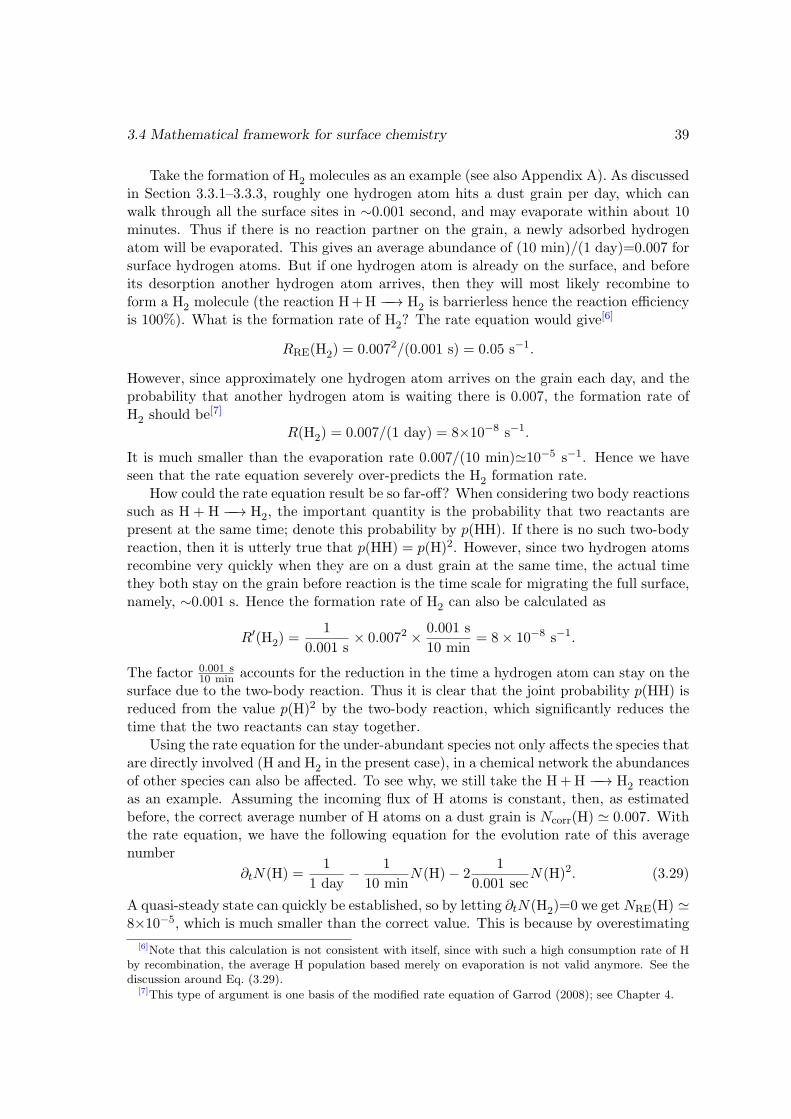
3.4 Mathematical framework for surface chemistry 39

Take the formation of H2 molecules as an example (see also Appendix A). As discussedin Section 3.3.1–3.3.3, roughly one hydrogen atom hits a dust grain per day, which canwalk through all the surface sites in ∼0.001 second, and may evaporate within about 10minutes. Thus if there is no reaction partner on the grain, a newly adsorbed hydrogenatom will be evaporated. This gives an average abundance of (10 min)/(1 day)=0.007 forsurface hydrogen atoms. But if one hydrogen atom is already on the surface, and beforeits desorption another hydrogen atom arrives, then they will most likely recombine toform a H2 molecule (the reaction H+H −−→ H2 is barrierless hence the reaction efficiencyis 100%). What is the formation rate of H2? The rate equation would give[6]

RRE(H2) = 0.0072/(0.001 s) = 0.05 s−1.

However, since approximately one hydrogen atom arrives on the grain each day, and theprobability that another hydrogen atom is waiting there is 0.007, the formation rate ofH2 should be[7]

R(H2) = 0.007/(1 day) = 8×10−8 s−1.

It is much smaller than the evaporation rate 0.007/(10 min)'10−5 s−1. Hence we haveseen that the rate equation severely over-predicts the H2 formation rate.

How could the rate equation result be so far-off? When considering two body reactionssuch as H + H −−→ H2, the important quantity is the probability that two reactants arepresent at the same time; denote this probability by p(HH). If there is no such two-bodyreaction, then it is utterly true that p(HH) = p(H)2. However, since two hydrogen atomsrecombine very quickly when they are on a dust grain at the same time, the actual timethey both stay on the grain before reaction is the time scale for migrating the full surface,namely, ∼0.001 s. Hence the formation rate of H2 can also be calculated as

R′(H2) =1

0.001 s× 0.0072 × 0.001 s

10 min= 8× 10−8 s−1.

The factor 0.001 s10 min accounts for the reduction in the time a hydrogen atom can stay on the

surface due to the two-body reaction. Thus it is clear that the joint probability p(HH) isreduced from the value p(H)2 by the two-body reaction, which significantly reduces thetime that the two reactants can stay together.

Using the rate equation for the under-abundant species not only affects the species thatare directly involved (H and H2 in the present case), in a chemical network the abundancesof other species can also be affected. To see why, we still take the H+H −−→ H2 reactionas an example. Assuming the incoming flux of H atoms is constant, then, as estimatedbefore, the correct average number of H atoms on a dust grain is Ncorr(H) ' 0.007. Withthe rate equation, we have the following equation for the evolution rate of this averagenumber

∂tN(H) =1

1 day− 1

10 minN(H)− 2

1

0.001 secN(H)2. (3.29)

A quasi-steady state can quickly be established, so by letting ∂tN(H2)=0 we getNRE(H) '8×10−5, which is much smaller than the correct value. This is because by overestimating

[6]Note that this calculation is not consistent with itself, since with such a high consumption rate of Hby recombination, the average H population based merely on evaporation is not valid anymore. See thediscussion around Eq. (3.29).

[7]This type of argument is one basis of the modified rate equation of Garrod (2008); see Chapter 4.

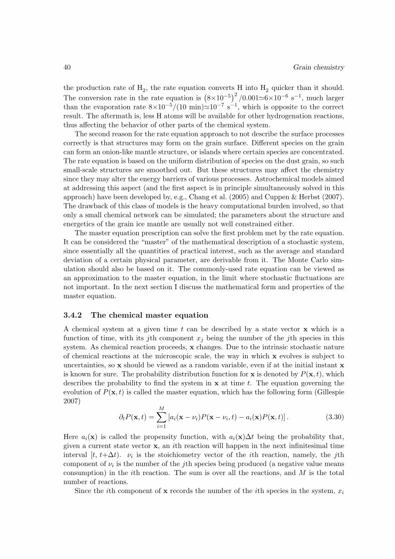
40 Grain chemistry

the production rate of H2, the rate equation converts H into H2 quicker than it should.

The conversion rate in the rate equation is(8×10−5

)2/0.001'6×10−6 s−1, much larger

than the evaporation rate 8×10−5/(10 min)'10−7 s−1, which is opposite to the correctresult. The aftermath is, less H atoms will be available for other hydrogenation reactions,thus affecting the behavior of other parts of the chemical system.

The second reason for the rate equation approach to not describe the surface processescorrectly is that structures may form on the grain surface. Different species on the graincan form an onion-like mantle structure, or islands where certain species are concentrated.The rate equation is based on the uniform distribution of species on the dust grain, so suchsmall-scale structures are smoothed out. But these structures may affect the chemistrysince they may alter the energy barriers of various processes. Astrochemical models aimedat addressing this aspect (and the first aspect is in principle simultaneously solved in thisapproach) have been developed by, e.g., Chang et al. (2005) and Cuppen & Herbst (2007).The drawback of this class of models is the heavy computational burden involved, so thatonly a small chemical network can be simulated; the parameters about the structure andenergetics of the grain ice mantle are usually not well constrained either.

The master equation prescription can solve the first problem met by the rate equation.It can be considered the “master” of the mathematical description of a stochastic system,since essentially all the quantities of practical interest, such as the average and standarddeviation of a certain physical parameter, are derivable from it. The Monte Carlo sim-ulation should also be based on it. The commonly-used rate equation can be viewed asan approximation to the master equation, in the limit where stochastic fluctuations arenot important. In the next section I discuss the mathematical form and properties of themaster equation.

3.4.2 The chemical master equation

A chemical system at a given time t can be described by a state vector x which is afunction of time, with its jth component xj being the number of the jth species in thissystem. As chemical reaction proceeds, x changes. Due to the intrinsic stochastic natureof chemical reactions at the microscopic scale, the way in which x evolves is subject touncertainties, so x should be viewed as a random variable, even if at the initial instant xis known for sure. The probability distribution function for x is denoted by P (x, t), whichdescribes the probability to find the system in x at time t. The equation governing theevolution of P (x, t) is called the master equation, which has the following form (Gillespie2007)

∂tP (x, t) =

M∑i=1

[ai(x− νi)P (x− νi, t)− ai(x)P (x, t)] . (3.30)

Here ai(x) is called the propensity function, with ai(x)∆t being the probability that,given a current state vector x, an ith reaction will happen in the next infinitesimal timeinterval [t, t+∆t). νi is the stoichiometry vector of the ith reaction, namely, the jthcomponent of νi is the number of the jth species being produced (a negative value meansconsumption) in the ith reaction. The sum is over all the reactions, and M is the totalnumber of reactions.

Since the ith component of x records the number of the ith species in the system, xi

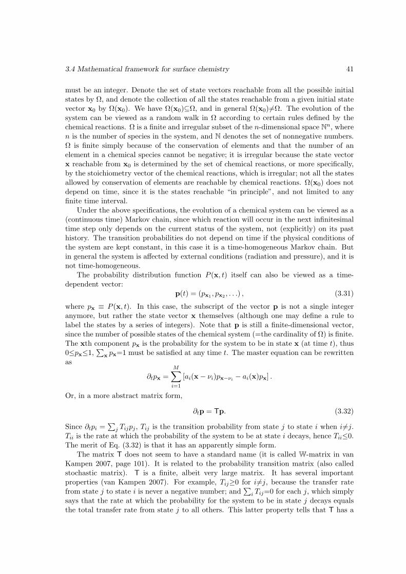
3.4 Mathematical framework for surface chemistry 41

must be an integer. Denote the set of state vectors reachable from all the possible initialstates by Ω, and denote the collection of all the states reachable from a given initial statevector x0 by Ω(x0). We have Ω(x0)⊆Ω, and in general Ω(x0)6=Ω. The evolution of thesystem can be viewed as a random walk in Ω according to certain rules defined by thechemical reactions. Ω is a finite and irregular subset of the n-dimensional space Nn, wheren is the number of species in the system, and N denotes the set of nonnegative numbers.Ω is finite simply because of the conservation of elements and that the number of anelement in a chemical species cannot be negative; it is irregular because the state vectorx reachable from x0 is determined by the set of chemical reactions, or more specifically,by the stoichiometry vector of the chemical reactions, which is irregular; not all the statesallowed by conservation of elements are reachable by chemical reactions. Ω(x0) does notdepend on time, since it is the states reachable “in principle”, and not limited to anyfinite time interval.

Under the above specifications, the evolution of a chemical system can be viewed as a(continuous time) Markov chain, since which reaction will occur in the next infinitesimaltime step only depends on the current status of the system, not (explicitly) on its pasthistory. The transition probabilities do not depend on time if the physical conditions ofthe system are kept constant, in this case it is a time-homogeneous Markov chain. Butin general the system is affected by external conditions (radiation and pressure), and it isnot time-homogeneous.

The probability distribution function P (x, t) itself can also be viewed as a time-dependent vector:

p(t) = (px1 , px2 , . . .) , (3.31)

where px ≡ P (x, t). In this case, the subscript of the vector p is not a single integeranymore, but rather the state vector x themselves (although one may define a rule tolabel the states by a series of integers). Note that p is still a finite-dimensional vector,since the number of possible states of the chemical system (=the cardinality of Ω) is finite.The xth component px is the probability for the system to be in state x (at time t), thus0≤px≤1,

∑x px=1 must be satisfied at any time t. The master equation can be rewritten

as

∂tpx =

M∑i=1

[ai(x− νi)px−νi − ai(x)px] .

Or, in a more abstract matrix form,

∂tp = Tp. (3.32)

Since ∂tpi =∑

j Tijpj , Tij is the transition probability from state j to state i when i6=j.Tii is the rate at which the probability of the system to be at state i decays, hence Tii≤0.The merit of Eq. (3.32) is that it has an apparently simple form.

The matrix T does not seem to have a standard name (it is called W-matrix in vanKampen 2007, page 101). It is related to the probability transition matrix (also calledstochastic matrix). T is a finite, albeit very large matrix. It has several importantproperties (van Kampen 2007). For example, Tij≥0 for i6=j, because the transfer ratefrom state j to state i is never a negative number; and

∑i Tij=0 for each j, which simply

says that the rate at which the probability for the system to be in state j decays equalsthe total transfer rate from state j to all others. This latter property tells that T has a

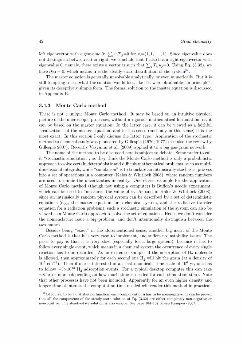
42 Grain chemistry

left eigenvector with eigenvalue 0:∑

i viTij=0 for vi=(1, 1, . . . , 1). Since eigenvalue doesnot distinguish between left or right, we conclude that T also has a right eigenvector witheigenvalue 0; namely, there exists a vector u such that

∑j Tijuj=0. Using Eq. (3.32), we

have ∂tu = 0, which means u is the steady-state distribution of the system[8].The master equation is generally unsolvable analytically, or even numerically. But it is

still tempting to see what the solution would look like if it were obtainable “in principle”,given its deceptively simple form. The formal solution to the master equation is discussedin Appendix B.

3.4.3 Monte Carlo method

There is not a unique Monte Carlo method. It may be based on an intuitive physicalpicture of the microscopic processes, without a rigorous mathematical formulation, or, itcan be based on the master equation. In the latter case, it can be viewed as a faithful“realization” of the master equation, and in this sense (and only in this sense) it is themost exact. In this section I only discuss the latter type. Application of the stochasticmethod to chemical study was pioneered by Gillespie (1976, 1977) (see also the review byGillespie 2007). Recently Vasyunin et al. (2009) applied it to a big gas-grain network.

The name of the method to be discussed here is subject to debate. Some prefer to callit “stochastic simulation”, as they think the Monte Carlo method is only a probabilisticapproach to solve certain deterministic and difficult mathematical problems, such as multi-dimensional integrals, while “simulation” is to translate an intrinsically stochastic processinto a set of operations in a computer (Kalos & Whitlock 2008), where random numbersare used to mimic the uncertainties in reality. One classic example for the applicationof Monte Carlo method (though not using a computer) is Buffon’s needle experiment,which can be used to “measure” the value of π. As said in Kalos & Whitlock (2008),since an intrinsically random physical system can be described by a set of deterministicequations (e.g., the master equation for a chemical system, and the radiative transferequation for a radiation problem), such a stochastic simulation of the system can also beviewed as a Monte Carlo approach to solve the set of equations. Hence we don’t considerthe nomenclature issue a big problem, and don’t intentionally distinguish between thetwo names.

Besides being “exact” in the aforementioned sense, another big merit of the MonteCarlo method is that it is very easy to implement, and suffers no instability issues. Theprice to pay is that it is very slow (especially for a large system), because it has tofollow every single event, which means in a chemical system the occurrence of every singlereaction has to be recorded. As an extreme example, if the adsorption of H2 moleculeis allowed, then approximately for each second one H2 will hit the grain (at a density of105 cm−3). Then if one is interested in an “astronomical” time scale of 106 yr, one hasto follow ∼3×1013 H2 adsorption events. For a typical desktop computer this can take∼8 hr or more (depending on how much time is needed for each simulation step). Notethat other processes have not been included. Apparently for an even higher density andlonger time of interest the computation time needed will render this method impractical.

[8]Of course, to be a distribution function, each component of u has to be non-negative. It can be provedthat all the components of the steady-state solution of Eq. (3.32) are either completely non-negative ornon-positive. The steady-state solution is also unique. See page 104–107 of van Kampen (2007).

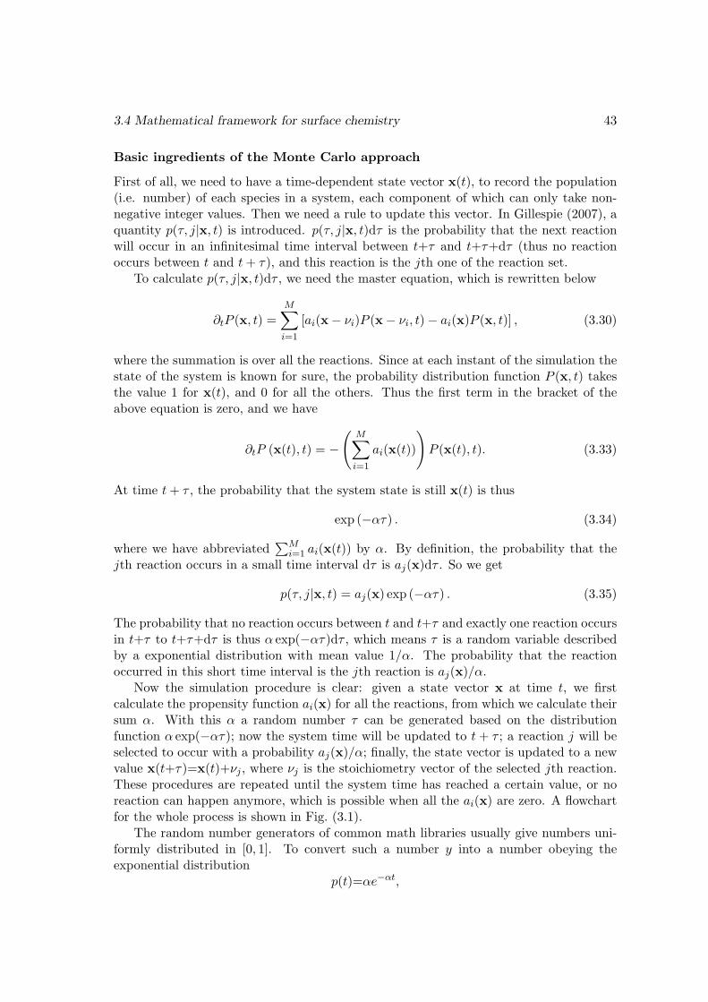
3.4 Mathematical framework for surface chemistry 43

Basic ingredients of the Monte Carlo approach

First of all, we need to have a time-dependent state vector x(t), to record the population(i.e. number) of each species in a system, each component of which can only take non-negative integer values. Then we need a rule to update this vector. In Gillespie (2007), aquantity p(τ, j|x, t) is introduced. p(τ, j|x, t)dτ is the probability that the next reactionwill occur in an infinitesimal time interval between t+τ and t+τ+dτ (thus no reactionoccurs between t and t+ τ), and this reaction is the jth one of the reaction set.

To calculate p(τ, j|x, t)dτ , we need the master equation, which is rewritten below

∂tP (x, t) =

M∑i=1

[ai(x− νi)P (x− νi, t)− ai(x)P (x, t)] , (3.30)

where the summation is over all the reactions. Since at each instant of the simulation thestate of the system is known for sure, the probability distribution function P (x, t) takesthe value 1 for x(t), and 0 for all the others. Thus the first term in the bracket of theabove equation is zero, and we have

∂tP (x(t), t) = −

(M∑i=1

ai(x(t))

)P (x(t), t). (3.33)

At time t+ τ , the probability that the system state is still x(t) is thus

exp (−ατ) . (3.34)

where we have abbreviated∑M

i=1 ai(x(t)) by α. By definition, the probability that thejth reaction occurs in a small time interval dτ is aj(x)dτ . So we get

p(τ, j|x, t) = aj(x) exp (−ατ) . (3.35)

The probability that no reaction occurs between t and t+τ and exactly one reaction occursin t+τ to t+τ+dτ is thus α exp(−ατ)dτ , which means τ is a random variable describedby a exponential distribution with mean value 1/α. The probability that the reactionoccurred in this short time interval is the jth reaction is aj(x)/α.

Now the simulation procedure is clear: given a state vector x at time t, we firstcalculate the propensity function ai(x) for all the reactions, from which we calculate theirsum α. With this α a random number τ can be generated based on the distributionfunction α exp(−ατ); now the system time will be updated to t+ τ ; a reaction j will beselected to occur with a probability aj(x)/α; finally, the state vector is updated to a newvalue x(t+τ)=x(t)+νj , where νj is the stoichiometry vector of the selected jth reaction.These procedures are repeated until the system time has reached a certain value, or noreaction can happen anymore, which is possible when all the ai(x) are zero. A flowchartfor the whole process is shown in Fig. (3.1).

The random number generators of common math libraries usually give numbers uni-formly distributed in [0, 1]. To convert such a number y into a number obeying theexponential distribution

p(t)=αe−αt,

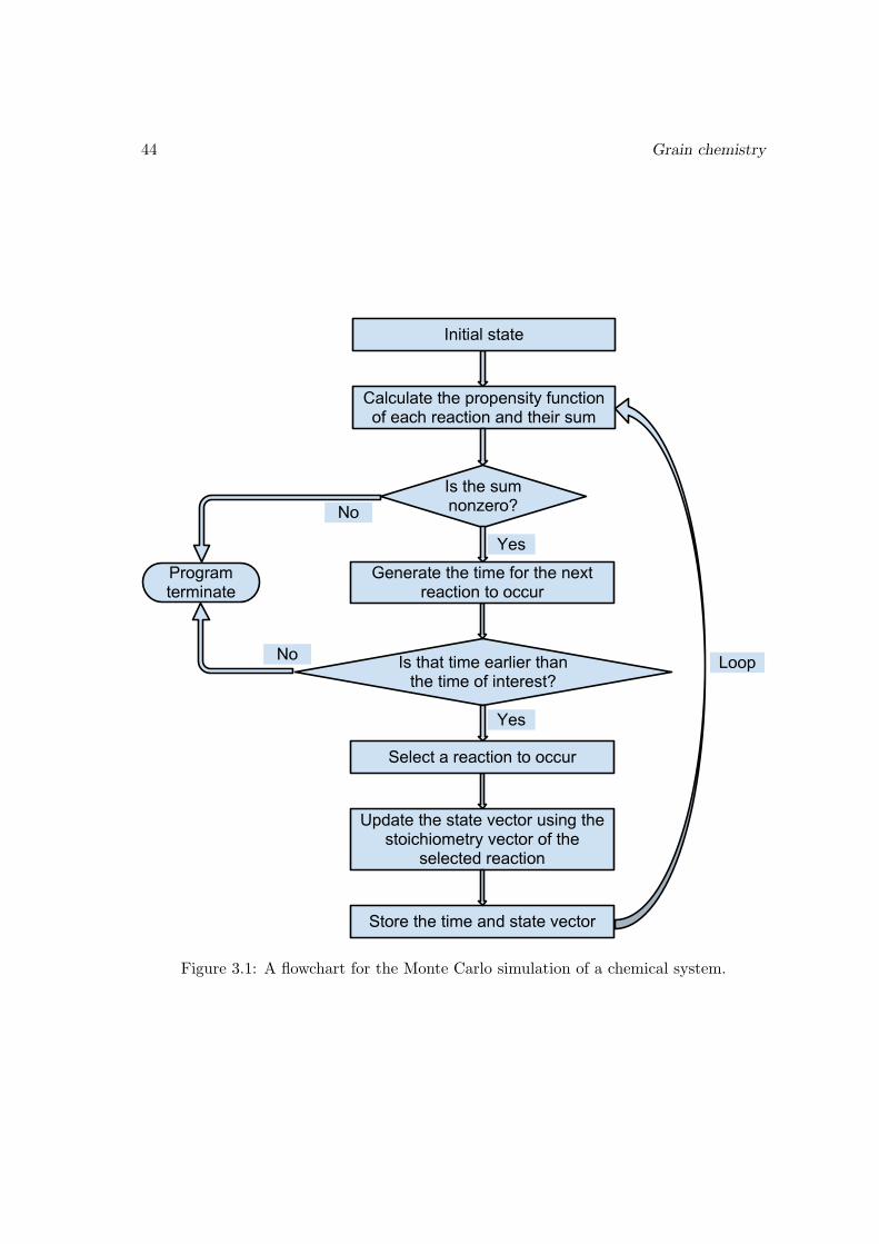
44 Grain chemistry

Figure 3.1: A flowchart for the Monte Carlo simulation of a chemical system.

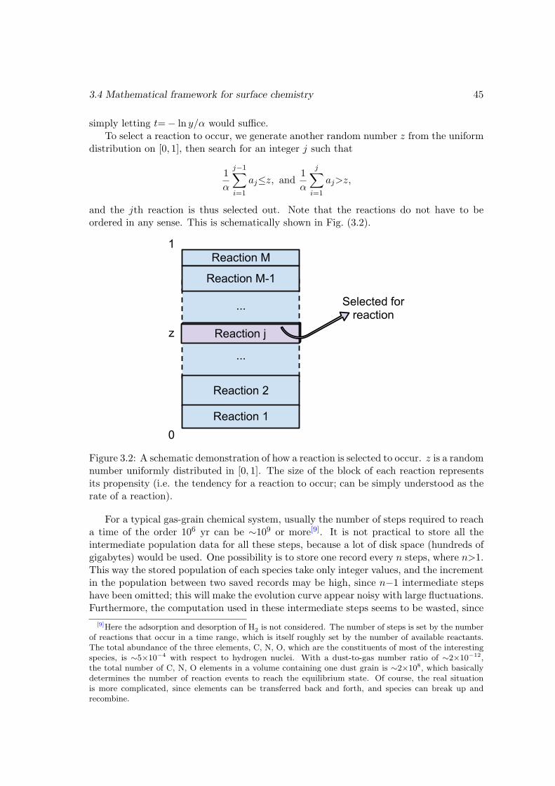
3.4 Mathematical framework for surface chemistry 45

simply letting t=− ln y/α would suffice.To select a reaction to occur, we generate another random number z from the uniform

distribution on [0, 1], then search for an integer j such that

1

α

j−1∑i=1

aj≤z, and1

α

j∑i=1

aj>z,

and the jth reaction is thus selected out. Note that the reactions do not have to beordered in any sense. This is schematically shown in Fig. (3.2).

Figure 3.2: A schematic demonstration of how a reaction is selected to occur. z is a randomnumber uniformly distributed in [0, 1]. The size of the block of each reaction representsits propensity (i.e. the tendency for a reaction to occur; can be simply understood as therate of a reaction).

For a typical gas-grain chemical system, usually the number of steps required to reacha time of the order 106 yr can be ∼109 or more[9]. It is not practical to store all theintermediate population data for all these steps, because a lot of disk space (hundreds ofgigabytes) would be used. One possibility is to store one record every n steps, where n>1.This way the stored population of each species take only integer values, and the incrementin the population between two saved records may be high, since n−1 intermediate stepshave been omitted; this will make the evolution curve appear noisy with large fluctuations.Furthermore, the computation used in these intermediate steps seems to be wasted, since

[9]Here the adsorption and desorption of H2 is not considered. The number of steps is set by the numberof reactions that occur in a time range, which is itself roughly set by the number of available reactants.The total abundance of the three elements, C, N, O, which are the constituents of most of the interestingspecies, is ∼5×10−4 with respect to hydrogen nuclei. With a dust-to-gas number ratio of ∼2×10−12,the total number of C, N, O elements in a volume containing one dust grain is ∼2×108, which basicallydetermines the number of reaction events to reach the equilibrium state. Of course, the real situationis more complicated, since elements can be transferred back and forth, and species can break up andrecombine.

46 Grain chemistry

their data are discarded. A better way of storing the data is to take the average populationof n successive steps and store it; now the average population will not take integer valueanymore. The time stamp associated with each average population should also be theaverage occurring time of these n steps. In this way the fluctuations can be greatlyreduced, resulting a much smoother evolution curve.

Another issue with the Monte Carlo approach is that, to get the average behavior of asystem, in principle many instances of simulations have to be carried out. The reason isthe following. Let’s assume the average population of a species (called A) is a constant,for example, 0.1. Then we may expect that if we look at the system at ten different timeintervals, A will show up in one of them. However, it can also be that if we look at tendifferent realizations of the same system, A will always show up in one of them at anytime, but never show up in all the others. This is the case in which a time-average is notequivalent to an ensemble average. The real situation may be a mixture of the two. Itis not straightforward to determine whether a system has such a behavior before runningthe simulations.

In our work, the Monte Carlo approach is not used as a major tool, because it is tooslow in the general case; rather it is utilized to set a benchmark (see Chapter 4), andthe results of other methods should comply with it. So here I only show, in Fig. (3.3),a sample Monte Carlo calculation (ten realizations with identical condition) for the H2

formation on dust grains, using typical parameters as discussed in Section 3.4.1. It canbe seen that the surface population of H atoms and the production rate of H2 agree quitewell with the values estimated there.

Figure 3.3: Monte Carlo simulation of the H + H −−→ H2 problem. Ten realizations areplotted.

Other methods have also been proposed to solve the gas-grain chemical problem,including one developed by us, which is the topic of the next chapter, where a briefreview on those previous methods is also included.

Chapter 4

The hybrid moment equation(HME) approach

The content of this chapter is based on:Du, F., & Parise, B. 2011, A&A, 530, A131+

Contents

4.1 Introduction . . . . . . . . . . . . . . . . . . . . . . . . . . . . . . . . . 48

4.2 Description of the hybrid moment equation (HME) approach . . . . . . 50

4.3 Benchmark with the Monte Carlo approach . . . . . . . . . . . . . . . . 55

4.4 Discussion . . . . . . . . . . . . . . . . . . . . . . . . . . . . . . . . . . 65

4.A A method to generate the moment equations based on the generatingfunction . . . . . . . . . . . . . . . . . . . . . . . . . . . . . . . . . . . . 66

4.B The surface reaction network we used to test our code . . . . . . . . . . 69

In addition to gas phase reactions, the chemical processes on the surfaces of interstellardust grains are important for the energy and material budget of the ISM. The stochasticityof these processes requires special care in modeling. Previously methods based on themodified rate equation, the master equation, the moment equation, and Monte Carlosimulations have been used.

In this chapter, a systematic and efficient way is developed to model the gas-grainchemistry with a large reaction network as accurately as possible. We name our method“hybrid moment equation approach”. It is a general and automatic method where thegenerating function is used to generate the moment equations. For large reaction networks,the moment equation is cut off at the second order, and a switch scheme is used whenthe average population of certain species reaches 1. For small networks, the third ordermoments can also be utilized to achieve a higher accuracy.

For physical conditions in which the surface reactions are important, our method pro-vides a major improvement over the rate equation approach, when both are benchmarkedagainst the rigorous Monte Carlo results. For either very low or very high temperatures,or large grain radii, results from the rate equation are similar to those from our new

47

48 The hybrid moment equation (HME) approach

approach. Our method is faster than the Monte Carlo approach, but slower than the rateequation approach.

The hybrid moment equation approach with a cutoff and switch scheme is potentiallya powerful way to solve gas-grain chemistry. It is applicable to medium-to-large gas-grainnetworks, and is demonstrated to have a degree of accuracy high enough to be used forastrochemistry studies. Further work should be done to investigate how to cut off thehybrid moment equation selectively to make the computation faster, more accurate, andmore stable, how to make the switch to rate equation more mathematically sound, andhow to make the errors controllable. The layered structure of the grain mantle could alsobe incorporated into this approach, although a full implementation of the grain micro-physics appears to be difficult.

4.1 Introduction

The chemistry of the ISM can be roughly divided into two types: gas phase chemistryand grain surface chemistry. The two types of chemistry are coupled by the adsorptionand desorption processes. Species adsorbed on the grain surface migrate in a randomwalk manner, and they may react with each other upon encounter at the same site (alocal potential minimum). The products can be released back to the gas phase throughcertain desorption mechanisms. In addition to the gas phase chemistry, grain chemistryis important for the material and energy budget of the ISM. For example, besides H2,molecules such as methanol are believed to be formed on the grain surfaces (Garrod et al.2007), because its relatively high abundance (see, e.g., Menten et al. 1988) cannot bereproduced by gas phase chemistry.

Several methods have been used to model the gas-grain chemistry. In the rate equation(RE) approach (see, e.g., Hasegawa et al. 1992), the surface processes are treated the sameway as the gas phase processes. This works fine when the number of reactants on a singlegrain is large (under the assumption that the system is well stirred; see Gillespie (2007)),but might not be accurate enough when the average populations[1] of some reactants ona single grain is small. This failure of the rate equation is related to the treatment oftwo-body reaction. For the REs to be applicable, the probability of one reactant beingpresent should be independent of that of another being present. This is not always true,especially when the average populations of both reactants are low, in which case theymight be highly correlated. The flaws in employing the RE for grain-surface chemistrywere pointed out by Charnley et al. (1997) and Tielens & Charnley (1997).

To remedy this problem, modification schemes based on some empirical, heuristic,and/or physical reasoning have been applied to the RE approach (Caselli et al. 1998;Stantcheva et al. 2001), and are called modified rate equation (MRE) approach. Thevalidity of this method has been questioned (Rae et al. 2003). A modification scheme de-veloped by Garrod (2008) uses different functional forms for different surface populations,taking various competition processes and refinements into account. It has been shown towork very well, even for very large reaction networks (Garrod et al. 2009).

[1]Here by “population” we mean the number of a species in a volume of interest, and by “average” wemean an ensemble average (i.e. average over many different realizations of the same system setup). Hence“population” can only take non-negative integer values, while “average population” is a non-negative realnumber.

4.1 Introduction 49

Mathematically, the gas-grain system should be viewed as a stochastic chemical sys-tem (see, e.g., McQuarrie 1967; Gillespie 1976; Charnley 1998), being described by aprobability distribution P (x, t), which is the probability that the system has a popula-tion vector x at time t, with xi being the number of the ith species in the system. Theevolution equation of P (x, t) is the so-called master equation, whose form is determinedby the reaction network.

Many sophisticated methods have been proposed (mainly outside the astro-chemicalcommunity; see, e.g., the operator method described in Mattis & Glasser (1998), or thevariational approach used by Ohkubo (2008)) to solve the master equation. However,these methods work fine only when either the chemical network is small or some specialassumptions are made in the derivation, thus their validity in the general case shouldbe questioned. It is unclear whether these methods can be generalized to large complexnetworks.

The numerical solution of the master equation has also been performed (Biham et al.2001; Stantcheva et al. 2002; Stantcheva & Herbst 2004). To limit the number of variablesin the set of differential equations and to separate the deterministic and stochastic species,usually a priori knowledge of the system is required in these studies. The steady statesolution of the master equation can also be obtained analytically in some very simplecases, such as the formation of H2 molecules on the grain surface (Green et al. 2001;Biham & Lipshtat 2002).

On the other hand, the master equation prescription can be “realized” through astochastic simulation algorithm (SSA), proposed by Gillespie (1976) (see also Gillespie(1977) and Gillespie (2007)). In this approach, the waiting time for the next reaction tooccur, as well as which specific reaction will occur are random variables that are completelydetermined by the master equation, so this approach should be considered the mostaccurate. In principle, multiple runs are needed to average out the random fluctuations,but in practice this is unnecessary if one only cares about the abundant species. Thisapproach has been applied successfully to astrochemical problems (Charnley 1998, 2001;Vasyunin et al. 2009), even in the case of very large networks (Vasyunin et al. 2009).Besides providing results that are accurate, this approach is very easy to implement.However, it requires a very long run time for large networks if a long evolution track isto be followed, although some approximate accelerated methods do exist (e.g. Gillespie2000).

The SSA described above is somewhat different from a Monte Carlo (MC) approachwhich has also been applied to astrochemistry (e.g. Tielens & Hagen 1982); however,this approach is not rigorously consistent with the master equation (see the comment byCharnley 2005), and can lead to a reaction probability higher than 1 (Awad et al. 2005)in certain cases. The nomenclature of these two approaches is not always consistent in theastrochemical literature[2]. For example, the SSA used by Vasyunin et al. (2009) is calledthe Monte Carlo approach in their paper. Hereafter, we use the term “Monte Carlo”when referring to the rigorous stochastic simulation approach of Gillespie.

By taking various moments of the master equation, the so-called moment equation(ME) is obtained (Lipshtat & Biham 2003; Barzel & Biham 2007a,b). This set of equationsdescribes the evolution of both the average population of each species and the average

[2]For a discussion about the relations and differences between “stochastic simulation” and “MonteCarlo”, see Kalos & Whitlock (2008) and Ripley (2008).

50 The hybrid moment equation (HME) approach

value of the products of the population of a group of species, usually cut off at the secondorder moments. Its formulation is similar to that of the RE, so it is relatively easyto implement. Furthermore, in this approach the gas phase chemistry and grain surfacechemistry can be coupled together naturally. It has been tested on small surface networks.

In the present paper, we propose yet another approach to modeling gas-grain chem-istry, named the hybrid moment equation (HME) approach. The goal is to find a system-atic, automatic, and fast way to modeling gas-grain chemistry as accurately as possible.Our method is based on the ME approach. Different approximations are applied to theMEs at different time depending on the overall populations at that specific time. It is hy-brid in the sense that the RE and the ME are combined together. The basic modificationand competition scheme presented in Garrod (2008) can be viewed as a semi-steady-stateapproximation to our approach (by assuming that the time derivatives of certain secondorder moments are equal to zero), while our approach can also be viewed as a combinationof the ME approach of Barzel & Biham (2007a) and the RE. In our approach, the MEsare generated automatically with the generating function technique, and in principle MEsup to any order can be obtained this way. We benchmark our approach against the exactMC approach (i.e. the SSA of Gillespie).

The remaining part of this paper is organized as follows. In section 4.2, we review thechemical master equation and ME, then describe the main steps of the HME approach. Insection 4.3, we benchmark the HME approach with a cutoff at the second order and theRE approach against the MC approach with a large gas-grain network; we also tested theHME approach with a cutoff at the third order with a small network. In section 4.4, wediscuss the performance of the HME, and its relation with previous approaches, as well aspossibilities for additional improvements. Our way of generating the MEs is described inAppendix 4.A. A surface chemical network we used for benchmark is listed in Appendix4.B.

4.2 Description of the hybrid moment equation (HME) ap-proach

In this section, we first review both the chemical master and moment equations. Althoughthis content can be found in many other papers (e.g., Charnley 1998; Gillespie 2007), wepresent them here as they are the basis of our HME approach. We then describe theMEs and REs for a simple set of reactions as an example, to demonstrate how the HMEapproach naturally arise as a combination of ME and RE. Finally we show the main stepsof the HME approach.

4.2.1 The chemical master equation and the moment equation (ME)

A chemical system at a given time t can be described by a state vector x which changeswith time, with its jth component xj being the number of the jth species in this system.As a chemical system is usually stochastic, x should be viewed as a random variable,whose probability distribution function P (x, t) evolves with time according to the masterequation, which has been discussed in Chapter 3 (see Eq. (3.32)), and will be repeated

4.2 Description of the hybrid moment equation (HME) approach 51

here:

∂tP (x, t) =

M∑i=1

[ai(x− νi)P (x− νi, t)− ai(x)P (x)], (4.1)

where ai(x) is called the propensity function, ai(x)∆t is the probability that given acurrent state vector x an ith reaction will happen in the next infinitesimal time interval∆t, and νi is the stoichiometry vector of the ith reaction. The sum is over all the reactions,and M is the total number of reactions.

The ME is derived by taking moments of the master equation. For example, forthe first order moment 〈xj〉, which is simply the average number of species j, 〈xj〉 ≡∑

x P (x, t)xj , its evolution is determined by (Gillespie 2007)

∂t〈xj〉 =∑x

∂t[P (x, t)]xj

=

M∑i

∑x

xj [ai(x− νi)P (x− νi, t)− ai(x)P (x)]

=

M∑i

∑x

[(xj + νij)ai(x)P (x, t)− xjai(x)P (x)] (4.2)

=M∑i

∑x

νijai(x)P (x, t) =M∑i

νij〈ai(x)〉,

where νij is the jth component of the stoichiometry vector of the ith reaction, i.e. thenumber of jth species produced (negative when being consumed) by the ith reaction. Forhigher order moments, their corresponding evolution equations can be similarly derived,although the final form will be more complex. In Appendix 4.A, we present anothermethod based on the generating function technique to derive the MEs, which is moresuitable for programming.

For the simplest network, in which all the reactions are single-body reactions, ai(x) isa linear function of x. In this case the ME is closed and can easily be solved. However,when two-body reactions are present, this is no longer true, as 〈ai(x)〉 might be of a form〈xk(xk − 1)〉 or 〈xkxl〉, which is of order two and cannot be determined in general bythe lower order moments. Hence additional equations governing their evolution should beincluded, i.e., they should be taken to be independent variables. The evolution equationof these second order moments may also involve moments of order three, and this processcontinues without an end, thus the ME is actually an infinite set of coupled equations(although in principle they are not completely independent if the chemical system beingconsidered is finite, which leads to a finite-dimensional space of state vectors). Theequation cannot be solved without a compromise, e.g., a cutoff procedure, except for thesimplest cases in which an analytical solution is obtainable in the steady state. Such asituation is common in many other fields which deals with objects with a certain degreeof stochastic nature, and the problem is called a “moment closure” problem in general.Thus our work can be viewed as an option for moment closure.

52 The hybrid moment equation (HME) approach

4.2.2 The MEs and REs for a set of reactions

We take the following symbolic reactions as an illustrative example

Adsorption: akad−−→ A, (4.3)

Evaporation: Akevap−−−→ a, (4.4)

Surface reaction: A+BkAB−−→ C +D, (4.5)

Surface reaction: A+AkAA−−→ E, (4.6)

where the ks are the reaction rates of each reaction, A – E are assumed to be surfacespecies that are distinct from each other, and “a” is the gas phase counterpart of A.

In the following we first write down the MEs and REs for this system, then discuss therelations and differences between them, as well as the relation between a cutoff of MEsand a cutoff of master equations in previous studies. These discussions will be essentialto developing our HME approach.

The MEs for this system

The propensity functions for the above four reactions are kada, kevapA, kABAB, andkAAA(A− 1), respectively. Here for convenience we use the letter “A” to represent boththe name of a species and the population of the corresponding species.

For the first order moments, we have

∂t〈A〉 =kad〈a〉 − kevap〈A〉 − kAB〈AB〉 − 2kAA〈A(A− 1)〉, (4.7)

∂t〈C〉 =kAB〈AB〉, (4.8)

∂t〈E〉 =kAA〈A(A− 1)〉. (4.9)

Other similar equations are omitted. The symbol 〈∗〉 is used to represent the averagepopulation of “*” in the system; the average should be understood as an ensemble average.The second order moments 〈AB〉 and 〈A(A−1)〉 have their own evolution equations, whichare

∂t〈AB〉 =kad〈aB〉 − kevap〈AB〉− kAB[〈A(A− 1)B〉+ 〈AB(B − 1)〉+ 〈AB〉] (4.10)

− 2kAA〈A(A− 1)B〉,

∂t〈A(A− 1)〉 =2kad〈aA〉 − 2kevap〈A(A− 1)〉− 2kAB〈A(A− 1)B〉 (4.11)

− 2kAA[2〈A(A− 1)(A− 2)〉+ 〈A(A− 1)〉].

For this simple example set of reactions (equation (4.3 – 4.6) ), the above equations canbe easily obtained from the master equation (see, e.g., Lipshtat & Biham 2003, page 8).In the general case (e.g., when A – E are not completely distinct from each other), anautomatic way of obtaining the MEs is described in Appendix 4.A. The method described

4.2 Description of the hybrid moment equation (HME) approach 53

there is also applicable to moments with any order, and to all the common reaction typesin astrochemistry.

In general, the third order moments in the above equations cannot be expressed asa function of the lower order moments, so they need their own differential equations. Inthe case of a cutoff at the second order, the chain of equations, however, stops here. Wedescribe the method required to evaluate them in section 4.2.3.

The REs for this system

When using REs, equations (4.7 – 4.11) are replaced by

∂t〈A〉 = kad〈a〉 − kevap〈A〉 − kAB〈A〉〈B〉 − 2kAA〈A〉2, (4.7′)

∂t〈C〉 = kAB〈A〉〈B〉, (4.8′)

∂t〈E〉 = kAA〈A〉2. (4.9′)

∂t[〈A〉〈B〉] = kad〈a〉〈B〉 − kevap〈A〉〈B〉− kAB[〈A〉2〈B〉+ 〈A〉〈B〉2] (4.10′)

− 2kAA〈A〉2〈B〉,∂t[〈A〉2] = 2kad〈a〉〈A〉 − 2kevap〈A〉2

− 2kAB〈A〉2〈B〉 − 4kAA〈A〉3. (4.11′)

The equations for 〈A〉〈B〉 and 〈A〉2 are of course not needed in the RE approach but aresimply derived from equation (4.7′) (and an omitted similar equation for 〈B〉) using thechain rule of calculus.

The relation between MEs and REs

The differences between the MEs (equation 4.7 – 4.11) and the REs (equation 4.7′ – 4.11′)in the present case are as follows: All the 〈AB〉 are replaced by 〈A〉〈B〉, all the 〈A(A−1)〉are replaced by 〈A〉2, all the 〈A(A − 1)B〉 are replaced by 〈A〉2〈B〉, the 〈AB(B − 1)〉is replaced by 〈A〉〈B〉2, and the 〈A(A − 1)(A − 2)〉 is replaced by 〈A〉3. Furthermore,the term kAB〈AB〉 in equation (4.10) and the term kAA〈A(A − 1)〉 in equation (4.11)disappear in the RE (4.10′) and (4.11′).

These differences make clear why the REs are accurate when the involved species areabundant (namely when 〈A〉1 and 〈B〉1). This is because, in this case, 〈AB〉 can beapproximated well by[3] 〈A〉〈B〉, and 〈A(A− 1)〉 can be approximated well by 〈A〉2.

The RE approach will be erroneous when 〈A〉 or 〈B〉 are smaller than 1 because,in this case, the correlation between A and B might cause 〈AB〉 to differ considerablyfrom 〈A〉〈B〉, and the fluctuation in A might cause 〈A(A− 1)〉 to differ considerably from〈A〉2. It can also be viewed like this: in equation (4.10′) and equation (4.11′) that governthe evolution of second order moments, the omitted term kAB〈AB〉 might be much larger

[3]Assuming Poisson statistics, we have

|〈AB〉 − 〈A〉〈B〉|〈A〉〈B〉 .

√1

〈A〉 +1

〈B〉 1.

54 The hybrid moment equation (HME) approach

than the retained terms such as 〈A〉2〈B〉 or 〈A〉〈B〉2, and the omitted term kAA〈A(A−1)〉might be much larger than the retained term 〈A〉3.

The relation between a cutoff of MEs and a cutoff of possible states in previousmaster equation approaches

In Eqs. (4.7 – 4.11) we do not write terms such as 〈A(A − 1)〉 in the split form 〈A2〉 −〈A〉. We keep terms such as 〈A(A − 1)B〉 and 〈A(A − 1)(A − 2)〉 in their present formsintentionally. One reason for this is that terms such as 〈A(A − 1)〉 look more succinctand follow naturally from our way of deriving them (see Appendix 4.A). When 〈A〉 1,〈A(A−1)〉 and 〈AB〉 can be directly replaced by 〈A〉2 and 〈A〉〈B〉, respectively, to obtainthe RE formulation.

More importantly, this formulation can be directly connected to the cutoff schemesin the previous master equation approaches (e.g., Biham et al. 2001; Stantcheva et al.2002). For example, in a scheme in which no more than two particles of A are expectedto be present on a single grain at the same time, we have P (A>2) = 0. In this case,〈A(A − 1)(A − 2)〉 =

∑∞A=3 P (A)A(A − 1)(A − 2) = 0. Thus we see that a cutoff at a

population of two in the master equation approach corresponds naturally to assigning azero value to moments containing A more than twice, as far as the moments are definedin the form presented above.

4.2.3 The HME approach

The HME approach is a combination of the ME and RE approaches. The basic ideais that, for deterministic (average population >1) species, the REs are used, while forstochastic (average population <1) species, the stochastic effects are taken into accountby including higher order moments in the equations. Since a deterministic species maybecome stochastic as time goes by, and vice versa, the set of ODEs governing the evolutionof the system also changes with time, and is determined dynamically. A flow chart of ourHME code is shown in Fig. 4.1.

We first set up all potentially needed MEs (using the procedure described in Ap-pendix 4.A), with a cutoff of moments at a prescribed order (usually two). After this andsome other initialization work, the program enters the main loop.

Since the system of MEs is a set of ordinary differential equations (ODEs), the mainloop contains an ODE solver, for which we use the one from the ODEPACK package[4].

Not all MEs and moments are used at all times; which ones are used is determineddynamically. In each iteration of the main loop, we verify whether some surface specieshave changed from stochastic to deterministic, or from deterministic to stochastic. Thegas phase species are always treated as deterministic, regardless of how small their av-erage populations are. In either of these two cases, we re-examine all the moments, anddetermine the way to treat them. There are four cases:

1. All the first order moments are treated as independent variables.

2. If a moment consists of only stochastic species, and its order is no larger than theprescribed highest allowed order, it will be treated as an independent variable, and

[4]Downloaded from www.netlib.org

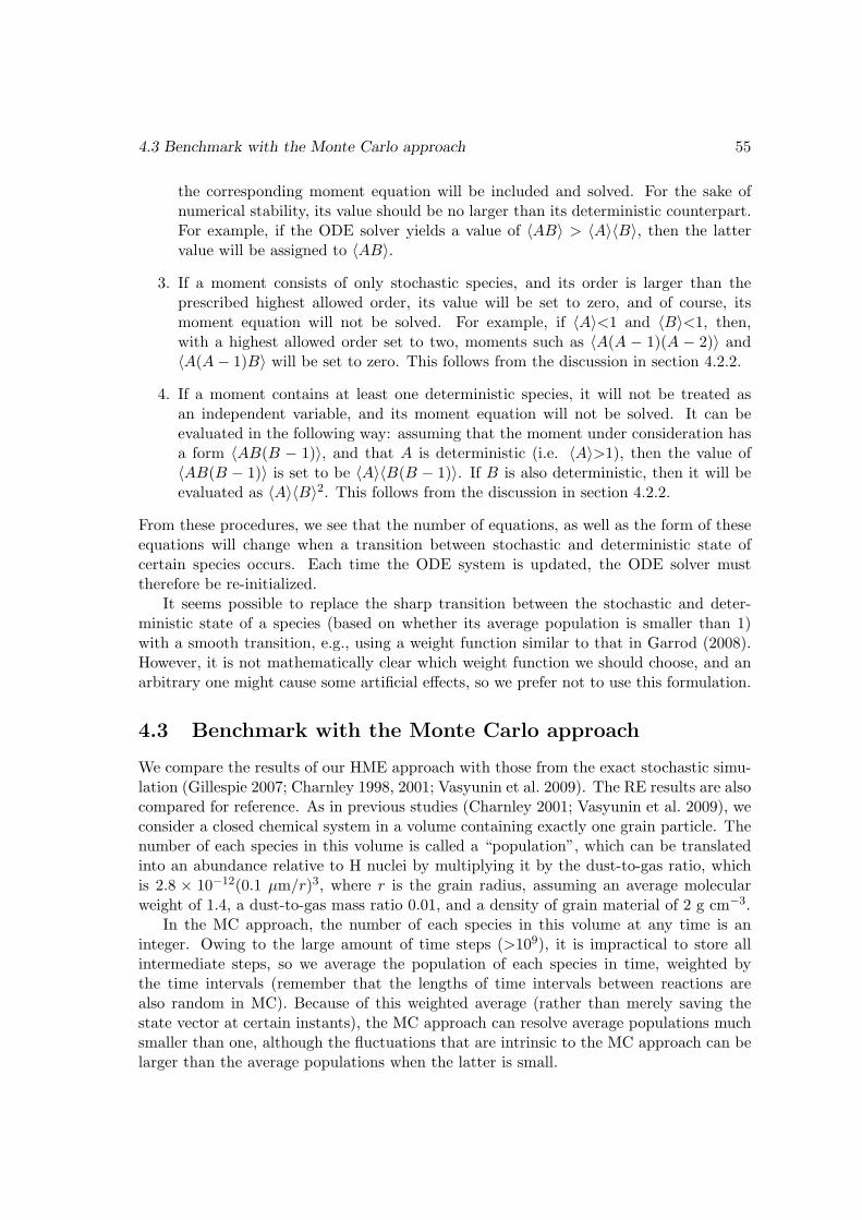
4.3 Benchmark with the Monte Carlo approach 55

the corresponding moment equation will be included and solved. For the sake ofnumerical stability, its value should be no larger than its deterministic counterpart.For example, if the ODE solver yields a value of 〈AB〉 > 〈A〉〈B〉, then the lattervalue will be assigned to 〈AB〉.

3. If a moment consists of only stochastic species, and its order is larger than theprescribed highest allowed order, its value will be set to zero, and of course, itsmoment equation will not be solved. For example, if 〈A〉<1 and 〈B〉<1, then,with a highest allowed order set to two, moments such as 〈A(A − 1)(A − 2)〉 and〈A(A− 1)B〉 will be set to zero. This follows from the discussion in section 4.2.2.

4. If a moment contains at least one deterministic species, it will not be treated asan independent variable, and its moment equation will not be solved. It can beevaluated in the following way: assuming that the moment under consideration hasa form 〈AB(B − 1)〉, and that A is deterministic (i.e. 〈A〉>1), then the value of〈AB(B − 1)〉 is set to be 〈A〉〈B(B − 1)〉. If B is also deterministic, then it will beevaluated as 〈A〉〈B〉2. This follows from the discussion in section 4.2.2.

From these procedures, we see that the number of equations, as well as the form of theseequations will change when a transition between stochastic and deterministic state ofcertain species occurs. Each time the ODE system is updated, the ODE solver musttherefore be re-initialized.

It seems possible to replace the sharp transition between the stochastic and deter-ministic state of a species (based on whether its average population is smaller than 1)with a smooth transition, e.g., using a weight function similar to that in Garrod (2008).However, it is not mathematically clear which weight function we should choose, and anarbitrary one might cause some artificial effects, so we prefer not to use this formulation.

4.3 Benchmark with the Monte Carlo approach

We compare the results of our HME approach with those from the exact stochastic simu-lation (Gillespie 2007; Charnley 1998, 2001; Vasyunin et al. 2009). The RE results are alsocompared for reference. As in previous studies (Charnley 2001; Vasyunin et al. 2009), weconsider a closed chemical system in a volume containing exactly one grain particle. Thenumber of each species in this volume is called a “population”, which can be translatedinto an abundance relative to H nuclei by multiplying it by the dust-to-gas ratio, whichis 2.8 × 10−12(0.1 µm/r)3, where r is the grain radius, assuming an average molecularweight of 1.4, a dust-to-gas mass ratio 0.01, and a density of grain material of 2 g cm−3.

In the MC approach, the number of each species in this volume at any time is aninteger. Owing to the large amount of time steps (>109), it is impractical to store allintermediate steps, so we average the population of each species in time, weighted bythe time intervals (remember that the lengths of time intervals between reactions arealso random in MC). Because of this weighted average (rather than merely saving thestate vector at certain instants), the MC approach can resolve average populations muchsmaller than one, although the fluctuations that are intrinsic to the MC approach can belarger than the average populations when the latter is small.

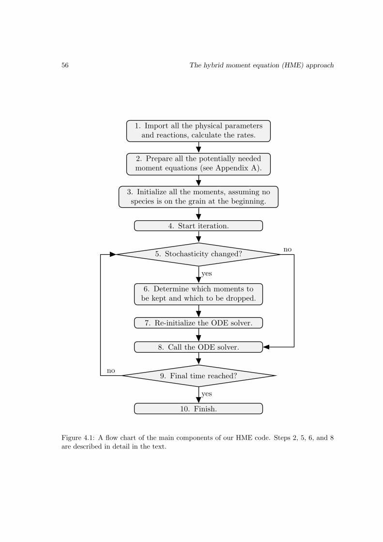
56 The hybrid moment equation (HME) approach

1. Import all the physical parametersand reactions, calculate the rates.

2. Prepare all the potentially neededmoment equations (see Appendix A).

3. Initialize all the moments, assuming nospecies is on the grain at the beginning.

4. Start iteration.

5. Stochasticity changed?

6. Determine which moments tobe kept and which to be dropped.

7. Re-initialize the ODE solver.

8. Call the ODE solver.

9. Final time reached?

10. Finish.

yes

no

yes

no

Figure 4.1: A flow chart of the main components of our HME code. Steps 2, 5, 6, and 8are described in detail in the text.

4.3 Benchmark with the Monte Carlo approach 57

We first demonstrate how our method works for a large gas-grain network. We thenshow that for a small surface network, third order moments can also be included toimprove the accuracy.

4.3.1 Test of the HME approach truncated at the second order on alarge gas-grain network

We use the “dipole-enhanced” version of the RATE06 gas phase reaction network[5]

(Woodall et al. 2007), coupled with a surface network of Keane (1997) (see Appendix4.B). The surface network contains 44 reactions between 43 species, which is basically areduced and slightly revised version of the network of Tielens & Hagen (1982), containingthe formation routes of the most common grain mantle species, such as H2O, CH3OH,CH4, NH3, etc. This surface network is not really large in comparison with some of theprevious works, such as that used by Garrod et al. (2009). However, it is already essentialfor the most important species. The energy barriers for thermal desorption and diffusionare taken from Stantcheva & Herbst (2004). Diffusion of H atoms on the surface throughquantum tunneling is included. Desorption by cosmic rays is taken into account followingthe approach of Hasegawa & Herbst (1993a). The rate coefficients of the gas phase reac-tions are calculated according to Woodall et al. (2007), while the rate coefficients of thesurface reactions are calculated following Hasegawa et al. (1992). The initial condition isthe same as in Stantcheva & Herbst (2004).

We assumed a dust-to-gas mass ratio of 0.01. The grain mass density is taken to be 2 gcm−3, with a site density 5×1013 cm−2. Two grain sizes have been used: 0.1 µm and 0.02µm. A cosmic ray ionization rate of 1.3×10−17 s−1 is adopted. Four different temperatures(10, 20, 30, 50 K) and three different densities (103, 104, 105 cm−3) have been used. Intotal, the comparison has been made for 24 different sets of physical parameters. Theseconditions are commonly seen in translucent clouds and cold dark clouds.

As in Garrod et al. (2009), we make a global comparison between the results of MC,HME, and RE. For each set of physical parameters, the comparisons are made at a timeof 103, 104, and 105 years. We calculate the percentage of species for which the agreementbetween MC and HME/RE is within a factor of 2 or 10. Only species with a population(either from MC or from HME/RE) larger than 10 are included for comparison. This isbecause for species with smaller populations, the intrinsic fluctuation in the MC resultscan be significant. For several different sets of physical parameters, we repeated the MCseveral times to get a feeling for how large the fluctuation magnitude would be, althoughthis is impractical for all the cases.

The comparison results are shown in Table 4.1 (grain radius = 0.1 µm) and Table 4.2(grain radius = 0.02 µm). The HME approach always has a better global agreement (orthe same for several cases) than the RE approach in the cases we tested. The typical timeevolution of certain species is shown in Fig. 4.2. In each panel of the figure, the specieswith a name preceded with a “g” means it is a surface species.

The poorest agreement of HME (Fig. 4.3) is at t = 103 year for T=20 K, nH = 105

cm−3, and grain radius = 0.02 µm. This is mostly because at the time of comparisonthe populations of certain species were changing very rapidly, so a slight mismatch intime leads to a large discrepancy. This mismatch is probably caused by the truncation

[5]http://www.udfa.net/

58 The hybrid moment equation (HME) approach

of higher-order terms in the HME (see section 4.3.2). For gN2 in Fig. 4.3, its populationseems to be systematically smaller in HME than in MC during the early period, althoughthe HME result matches the one from MC at a later stage (after 3× 103 years).

The RE is as effective as the HME in several cases, when the temperature is eitherrelatively low (∼10 K) or high (∼ 50 K) (see also Vasyunin et al. 2009), and generallyworks better for a grain radius of 0.1 µm than of 0.02 µm. When the temperature isvery low, many surface reactions with barriers cannot happen (at least in the consideredtimescales). On the other hand, when the temperature is high, the surface species evapo-rate very quickly and the surface reactions are also unable to occur. In these two extremecases, the surface processes are inactive, and the RE works fine.

The RE becomes problematic in the intermediate cases, when the temperature is highenough for many surface reactions to occur, but not too high to evaporate all the surfacespecies; in these cases the HME represents a major improvement over the RE. For asmaller grain radius, the population of each species in a volume containing one grain willbe smaller, thus the stochastic effect will play a more important role, and the RE willtend to fail.

We note that, in the HME approach, there is no elemental leakage except those causedby the finite precision of the computer. In all the models that we have run, all the elements(including electric charge) are conserved with a relative error smaller than 5×10−14. Thereason why elemental conservation is always guaranteed is that either the rate equationsor the moment equations for the first order moments conserve the elements exactly.

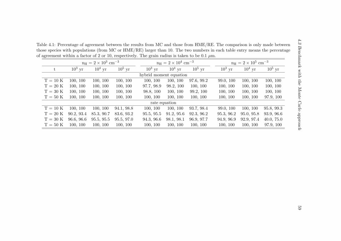
4.3

Benchmark

with

theMon

teCarlo

approach

59Table 4.1: Percentage of agreement between the results from MC and those from HME/RE. The comparison is only made betweenthose species with populations (from MC or HME/RE) larger than 10. The two numbers in each table entry means the percentageof agreement within a factor of 2 or 10, respectively. The grain radius is taken to be 0.1 µm.

nH = 2× 103 cm−3 nH = 2× 104 cm−3 nH = 2× 105 cm−3

t 103 yr 104 yr 105 yr 103 yr 104 yr 105 yr 103 yr 104 yr 105 yr

hybrid moment equation

T = 10 K 100, 100 100, 100 100, 100 100, 100 100, 100 97.6, 99.2 99.0, 100 100, 100 100, 100T = 20 K 100, 100 100, 100 100, 100 97.7, 98.9 98.2, 100 100, 100 100, 100 100, 100 100, 100T = 30 K 100, 100 100, 100 100, 100 98.8, 100 100, 100 99.2, 100 100, 100 100, 100 100, 100T = 50 K 100, 100 100, 100 100, 100 100, 100 100, 100 100, 100 100, 100 100, 100 97.9, 100

rate equation

T = 10 K 100, 100 100, 100 94.1, 98.8 100, 100 100, 100 93.7, 98.4 99.0, 100 100, 100 95.8, 99.3T = 20 K 90.2, 93.4 85.3, 90.7 83.6, 93.2 95.5, 95.5 91.2, 95.6 92.3, 96.2 95.3, 96.2 95.0, 95.8 93.9, 96.6T = 30 K 96.6, 96.6 95.5, 95.5 95.5, 97.0 94.3, 96.6 98.1, 98.1 96.9, 97.7 94.9, 96.9 92.9, 97.4 40.0, 75.0T = 50 K 100, 100 100, 100 100, 100 100, 100 100, 100 100, 100 100, 100 100, 100 97.9, 100

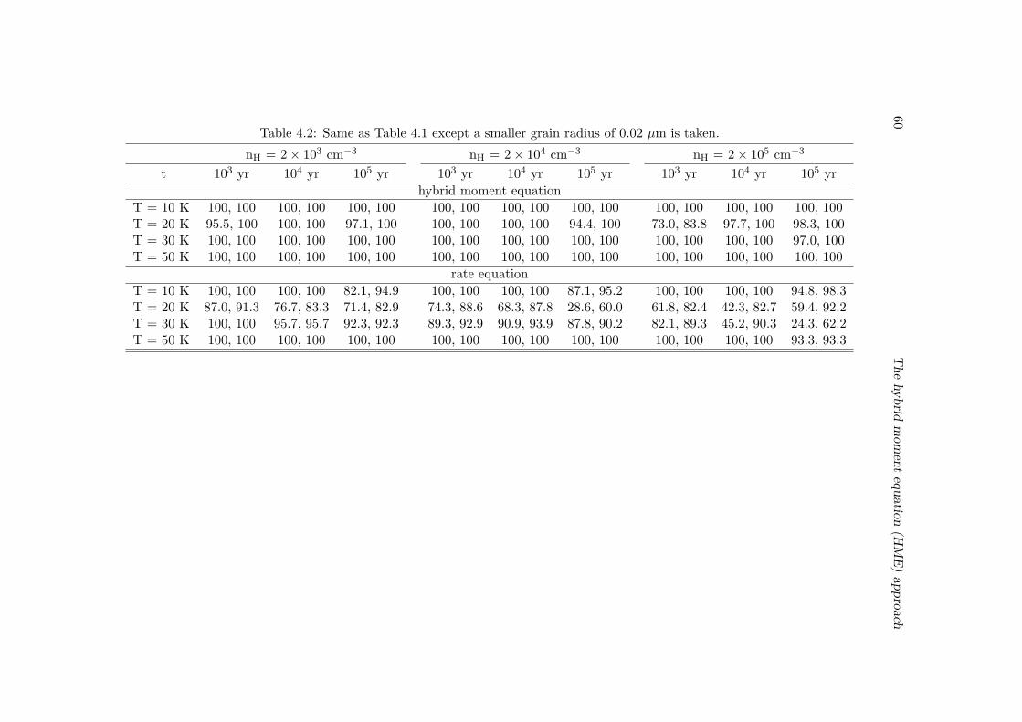
60

Thehybrid

mom

entequation

(HME)ap

proach

Table 4.2: Same as Table 4.1 except a smaller grain radius of 0.02 µm is taken.

nH = 2× 103 cm−3 nH = 2× 104 cm−3 nH = 2× 105 cm−3

t 103 yr 104 yr 105 yr 103 yr 104 yr 105 yr 103 yr 104 yr 105 yr

hybrid moment equation

T = 10 K 100, 100 100, 100 100, 100 100, 100 100, 100 100, 100 100, 100 100, 100 100, 100T = 20 K 95.5, 100 100, 100 97.1, 100 100, 100 100, 100 94.4, 100 73.0, 83.8 97.7, 100 98.3, 100T = 30 K 100, 100 100, 100 100, 100 100, 100 100, 100 100, 100 100, 100 100, 100 97.0, 100T = 50 K 100, 100 100, 100 100, 100 100, 100 100, 100 100, 100 100, 100 100, 100 100, 100

rate equation

T = 10 K 100, 100 100, 100 82.1, 94.9 100, 100 100, 100 87.1, 95.2 100, 100 100, 100 94.8, 98.3T = 20 K 87.0, 91.3 76.7, 83.3 71.4, 82.9 74.3, 88.6 68.3, 87.8 28.6, 60.0 61.8, 82.4 42.3, 82.7 59.4, 92.2T = 30 K 100, 100 95.7, 95.7 92.3, 92.3 89.3, 92.9 90.9, 93.9 87.8, 90.2 82.1, 89.3 45.2, 90.3 24.3, 62.2T = 50 K 100, 100 100, 100 100, 100 100, 100 100, 100 100, 100 100, 100 100, 100 93.3, 93.3

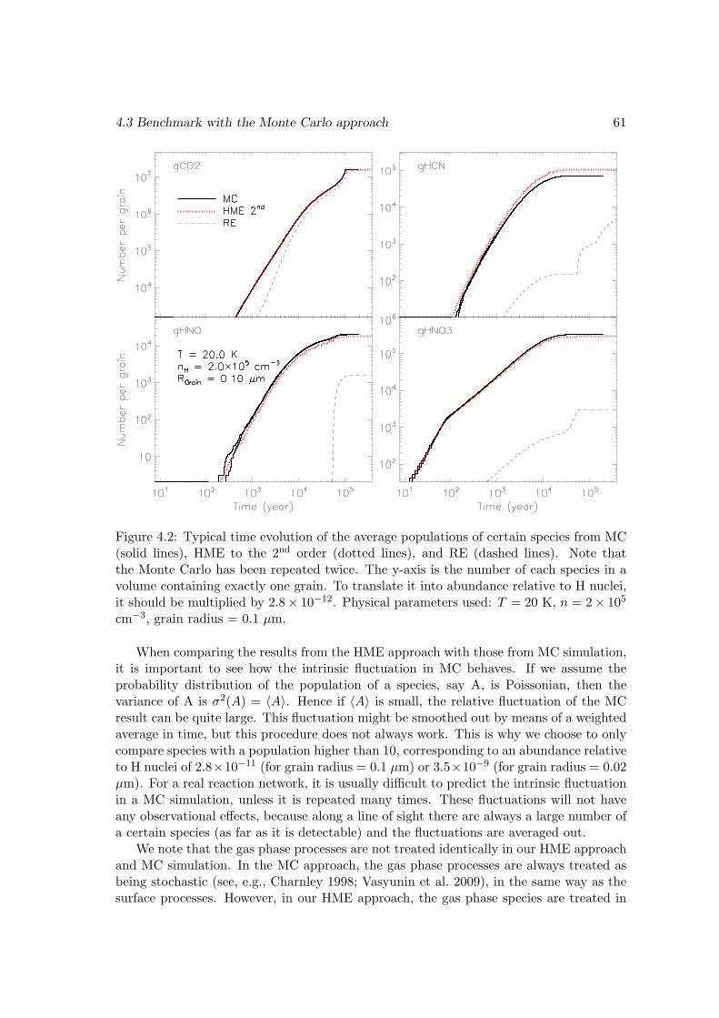
4.3 Benchmark with the Monte Carlo approach 61

Figure 4.2: Typical time evolution of the average populations of certain species from MC(solid lines), HME to the 2nd order (dotted lines), and RE (dashed lines). Note thatthe Monte Carlo has been repeated twice. The y-axis is the number of each species in avolume containing exactly one grain. To translate it into abundance relative to H nuclei,it should be multiplied by 2.8× 10−12. Physical parameters used: T = 20 K, n = 2× 105

cm−3, grain radius = 0.1 µm.

When comparing the results from the HME approach with those from MC simulation,it is important to see how the intrinsic fluctuation in MC behaves. If we assume theprobability distribution of the population of a species, say A, is Poissonian, then thevariance of A is σ2(A) = 〈A〉. Hence if 〈A〉 is small, the relative fluctuation of the MCresult can be quite large. This fluctuation might be smoothed out by means of a weightedaverage in time, but this procedure does not always work. This is why we choose to onlycompare species with a population higher than 10, corresponding to an abundance relativeto H nuclei of 2.8×10−11 (for grain radius = 0.1 µm) or 3.5×10−9 (for grain radius = 0.02µm). For a real reaction network, it is usually difficult to predict the intrinsic fluctuationin a MC simulation, unless it is repeated many times. These fluctuations will not haveany observational effects, because along a line of sight there are always a large number ofa certain species (as far as it is detectable) and the fluctuations are averaged out.

We note that the gas phase processes are not treated identically in our HME approachand MC simulation. In the MC approach, the gas phase processes are always treated asbeing stochastic (see, e.g., Charnley 1998; Vasyunin et al. 2009), in the same way as thesurface processes. However, in our HME approach, the gas phase species are treated in

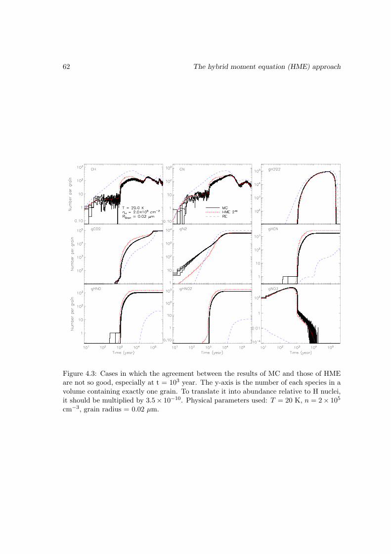
62 The hybrid moment equation (HME) approach

Figure 4.3: Cases in which the agreement between the results of MC and those of HMEare not so good, especially at t = 103 year. The y-axis is the number of each species in avolume containing exactly one grain. To translate it into abundance relative to H nuclei,it should be multiplied by 3.5× 10−10. Physical parameters used: T = 20 K, n = 2× 105

cm−3, grain radius = 0.02 µm.

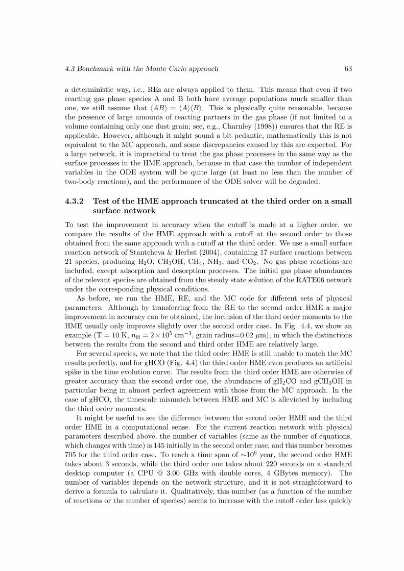
4.3 Benchmark with the Monte Carlo approach 63

a deterministic way, i.e., REs are always applied to them. This means that even if tworeacting gas phase species A and B both have average populations much smaller thanone, we still assume that 〈AB〉 = 〈A〉〈B〉. This is physically quite reasonable, becausethe presence of large amounts of reacting partners in the gas phase (if not limited to avolume containing only one dust grain; see, e.g., Charnley (1998)) ensures that the RE isapplicable. However, although it might sound a bit pedantic, mathematically this is notequivalent to the MC approach, and some discrepancies caused by this are expected. Fora large network, it is impractical to treat the gas phase processes in the same way as thesurface processes in the HME approach, because in that case the number of independentvariables in the ODE system will be quite large (at least no less than the number oftwo-body reactions), and the performance of the ODE solver will be degraded.

4.3.2 Test of the HME approach truncated at the third order on a smallsurface network

To test the improvement in accuracy when the cutoff is made at a higher order, wecompare the results of the HME approach with a cutoff at the second order to thoseobtained from the same approach with a cutoff at the third order. We use a small surfacereaction network of Stantcheva & Herbst (2004), containing 17 surface reactions between21 species, producing H2O, CH3OH, CH4, NH3, and CO2. No gas phase reactions areincluded, except adsorption and desorption processes. The initial gas phase abundancesof the relevant species are obtained from the steady state solution of the RATE06 networkunder the corresponding physical conditions.

As before, we run the HME, RE, and the MC code for different sets of physicalparameters. Although by transferring from the RE to the second order HME a majorimprovement in accuracy can be obtained, the inclusion of the third order moments to theHME usually only improves slightly over the second order case. In Fig. 4.4, we show anexample (T = 10 K, nH = 2×105 cm−3, grain radius=0.02 µm), in which the distinctionsbetween the results from the second and third order HME are relatively large.

For several species, we note that the third order HME is still unable to match the MCresults perfectly, and for gHCO (Fig. 4.4) the third order HME even produces an artificialspike in the time evolution curve. The results from the third order HME are otherwise ofgreater accuracy than the second order one, the abundances of gH2CO and gCH3OH inparticular being in almost perfect agreement with those from the MC approach. In thecase of gHCO, the timescale mismatch between HME and MC is alleviated by includingthe third order moments.

It might be useful to see the difference between the second order HME and the thirdorder HME in a computational sense. For the current reaction network with physicalparameters described above, the number of variables (same as the number of equations,which changes with time) is 145 initially in the second order case, and this number becomes705 for the third order case. To reach a time span of ∼106 year, the second order HMEtakes about 3 seconds, while the third order one takes about 220 seconds on a standarddesktop computer (a CPU @ 3.00 GHz with double cores, 4 GBytes memory). Thenumber of variables depends on the network structure, and it is not straightforward toderive a formula to calculate it. Qualitatively, this number (as a function of the numberof reactions or the number of species) seems to increase with the cutoff order less quickly

64 The hybrid moment equation (HME) approach

Figure 4.4: Comparison of the results from MC, HME to the 2nd order, HME to the 3rd

order, and RE. The y-axis is the number of each species in a volume containing exactlyone grain. To translate it into abundance relative to H nuclei, it should be multipliedby 3.5× 10−10. Physical parameters used when running these models include T = 10 K,nH = 2× 105 cm−3, grain radius = 0.02 µm.

4.4 Discussion 65

than exponential growth. However, such a “mild” increase affects the behavior of theODE solver quite significantly. This is partly because the solver contains operations(such as matrix inversion) that become slower as the number of variables become larger.An increase in the number of variables might also increase the stiffness of the problem, letalone the memory limitation of the computer. For the larger reaction network describedin the previous section, the third order HME would involve about 5000 variables and hasnot been tested successfully.

4.4 Discussion

In our HME approach, we have used a general and automatic way to derive the MEs. Forlarge gas-grain networks, the MEs are cut off at the second order. For small networks, acutoff at the third order is possible and higher accuracy can be obtained. We incorporatea switching scheme between the ME and RE when the average population of a speciesreaches 1.

The results from HME are more accurate than those from the RE in the cases wehave tested, when benchmarked against the exact MC results. The abundances of almostall the abundant species (&2.8×10−11 for a grain radius of 0.1 µm and &3.5×10−9 for agrain radius of 0.02 µm) from HME are accurate to within a factor of two, especially atlater stages of the chemical evolution, while in some cases nearly 40% of the results fromRE are incorrect by a factor of at least ten.

In terms of computation time, our approach usually takes several tens of minutes toreach a evolution time span of 106 years, so it is slower than the RE, but faster than theMC approach (which usually takes from several hours to days). Our approach may alsobe slower than the MRE approach of Garrod (2008), because more variables (namely themoments with orders higher than one) are present in our method, and the ODE system inHME is usually stiffer. For example, for a moderate temperature many surface reactionscan be much faster than any gas phase reactions, and yield a very large coefficient in someof the MEs. However, this is not the case in the stochastic regime of the MRE approach,because when a competition scheme is used in MRE, such a large coefficient does notappear. In this sense, we also advocate the MRE approach of Garrod (2008).

Mathematically, our approach is partially equivalent to the master equation approachof Stantcheva & Herbst (2004) in two respects. 1) They separated stochastic and deter-ministic species, which is similar to our adopting RE for the abundant species. 2) Theyset a cutoff for the possible states of the stochastic species. This is in essence equivalent toletting moments containing these species with order higher than a certain number equalto zero.

Our approach can also be viewed as a combination of some of the ideas of Garrod(2008) and Barzel & Biham (2007a). The basic modification and competition scheme inGarrod (2008) can be derived from the MEs, with a semi-steady state assumption for thesecond order moments. Barzel & Biham (2007a) used the MEs, but they did not include aswitch scheme, and their way of deriving the MEs is different from the one in the presentpaper.

There are still many possibilities for improvement. Although in principle momentswith any order can be included, the number of equations grows quite quickly with thecutoff order, which makes the system of equations intractable with a normal desktop

66 The hybrid moment equation (HME) approach

computer. It is unclear whether it is possible to include the moments selectively. Itis unclear whether there are better, and more mathematically well founded strategiesthan the switch at an average population of 1. The present approach is usually stablenumerically. However, this is not always guaranteed, especially if higher order momentsare to be included. The behavior of the numerical solution also depends on other factors,such as the ODE solver being used and the tunable parameters for it, while the MCapproach does not have such issues. In this sense, the MC approach is the most robust.

Even in the accurate MC approach described above, the detailed morphology of thegrain surface and the detailed reaction mechanism is not taken into account. One stepin this direction would be to take into account the layered structure of the grain mantle.This was done by Charnley (2001) (see also Charnley & Rodgers (2009)) by means ofstochastic simulation. It could also be included in the HME approach, as far as theunderlying physical mechanism could be described by a master equation.

However, a microscopic MC approach has also been used to study the grain chemistry(see, e.g., Chang et al. 2005; Cuppen & Herbst 2007). In this approach, the morphologyof the grain mantle and the interaction between species are modeled in detail. As far aswe know, this approach is only practical when the network is small. It remains unclearwhether it is possible to incorporate these details into the current HME approach.

In some cases, errors caused by uncertainties in the reaction mechanism and rate pa-rameters might be larger than those introduced by the modeling method (Vasyunin et al.2008). Hence, further experimental study and a more sophisticated way of interpretingthose results would be indispensable.

4.A A method to generate the moment equations based onthe generating function

We describe our means of getting the MEs. Our method is automatic, and can be easilycoded into a computer program. It is applicable to moments of any order and all thecommon astrochemical reactions. It makes use of the probability generating function.While preparing the present paper, we noted that Barzel & Biham (2011) also proposeda binomial formulation of ME, which in essence is partly equivalent to our approachpresented here, although our way of deriving the MEs is quite different from theirs.

For a probability distribution P (x, t), the corresponding generating function is definedas (van Kampen 2007)

f(z1, z2, . . . , t) =∑x

P (x, t)zx11 zx2

2 · · · . (4.12)

Here all the zis should be thought of as merely symbols without any physical meaning,and they have a one-to-one correspondence with the xis.

It is obvious that f(z = 1, t) ≡ 1, which is just the normalization condition forprobability. It is also easy to see that the average population of the ith species is

〈xi〉 = ∂zif(z1, z2, . . . , t)|z=1. (4.13)

The right hand side of the above equation means taking the partial derivative first, thenassigning a value one to all the zis.

4.A A method to generate the moment equations based on the generating function 67

For the second order moment between two distinct species i and j, we have

〈xixj〉 = ∂zi∂zjf(z1, z2, . . . , t)|z=1. (4.14)

If i equals j in the above equation, then what we actually get is

〈xi(xi − 1)〉 = ∂2zif(z1, z2, . . . , t)|z=1. (4.15)

In general, we have

〈xixjxk · · · 〉 = ∂zi∂zj∂zk · · · f(z1, z2, . . . , t)|z=1. (4.16)

If several of the subscripts are the same in the left hand side of the above equation, say,i = j = k, then the second should be understood as (xj − 1), while the third should beunderstood as (xk − 2), and so on.

From the master equation in Eq. (4.1), it seems possible to get an equation for theevolution of f(z, t) in the general case. However, if the propensity functions ai(x) (seeEq. (4.1)) are allowed to take any functional form, then this is not straightforward.Fortunately, in practice ai(x) usually has a very simple form. On the other hand, we notethat in the right hand side of the master equation in Eq. (4.1) the contributions from allthe reactions are added linearly. Hence the contribution of each reaction to the evolutionof generating function can be considered independently of each other.

We assume there is only one reaction in the network, which has a form

x1 + x2 + · · ·+ xnk−→ y1 + y2 + · · ·+ ym, (4.17)

where the xis and yis represent the reactants and products, which do not have to bedifferent from each other. We also use these symbols to represent the populations of thecorresponding species. If, given a population of x1, x2, . . . , xn, the probability that theabove reaction will happen in a unit time is kx1x2 · · ·xn (namely, the propensity functiona(x) = kx1x2 · · ·xn; the product should be understood as explained in the sentencefollowing Eq. (4.16)), then the generating function[6] will evolve according to

∂tf = k(y1y2 · · · ym − x1x2 · · ·xn)∂x1∂x2 · · · ∂xnf. (4.18)

It is not difficult to derive the above equation from the master equation and the definitionof generating equation and our assumption about the propensity function.

We note that equation (4.18) has a very simple pattern that is easy to remember: (a)The constant coefficient is the rate coefficient; (b) In the parenthesis, the symbols of allthe products are multiplied together, with a coefficient +1, while the symbols of all thereactants are multiplied together, with a coefficient −1; (c) In the differential part, all thereactants are present as they are in the left hand side of equation (4.17), while none ofthe products appear.

We now attempt to derive the ME. We obtain the evolution equation of each moment(as defined in Eq. (4.16)) by simply differentiating both sides of equation (4.18) withrespect to the relevant components in the moment, then setting all the symbols to a valueof one.

[6]Instead of using zis as symbols for the independent variables of the generating function f , we use xisand yis instead. This will not cause any confusion.

68 The hybrid moment equation (HME) approach

For example, for the reaction A+Bk−→ C+D, the evolution equation of the generating

function f is∂tf = k(CD −AB)∂A∂Bf.

For 〈AB〉, we differentiate both sides of the above equation by A and B. We obtain

∂t∂A∂Bf =k[(CD −AB)∂2A∂

2Bf

−A∂2A∂Bf −B∂A∂

2Bf − ∂A∂Bf ].

Next we assign a value of one to all the symbols (A – D) appearing in the resultingexpressions, and “translate” the remaining terms into moments (recalling the remarkabout equation (4.16)), obtaining

∂t〈AB〉 = −k[〈A(A− 1)B〉+ 〈AB(B − 1)〉+ 〈AB〉].

Although the above derivation involves differentiations, these operations can be easilytranslated into some combinatorial rules and written as a computer program. A recursiveprocedure is needed to generate all the potentially needed moments up to a given order.

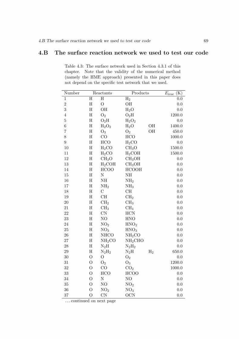
4.B The surface reaction network we used to test our code 69

4.B The surface reaction network we used to test our code

Table 4.3: The surface network used in Section 4.3.1 of thischapter. Note that the validity of the numerical method(namely the HME approach) presented in this paper doesnot depend on the specific test network that we used.

Number Reactants Products Ereac (K)

1 H H H2 0.02 H O OH 0.03 H OH H2O 0.04 H O2 O2H 1200.05 H O2H H2O2 0.06 H H2O2 H2O OH 1400.07 H O3 O2 OH 450.08 H CO HCO 1000.09 H HCO H2CO 0.010 H H2CO CH3O 1500.011 H H2CO H2COH 1500.012 H CH3O CH3OH 0.013 H H2COH CH3OH 0.014 H HCOO HCOOH 0.015 H N NH 0.016 H NH NH2 0.017 H NH2 NH3 0.018 H C CH 0.019 H CH CH2 0.020 H CH2 CH3 0.021 H CH3 CH4 0.022 H CN HCN 0.023 H NO HNO 0.024 H NO2 HNO2 0.025 H NO3 HNO3 0.026 H NHCO NH2CO 0.027 H NH2CO NH2CHO 0.028 H N2H N2H2 0.029 H N2H2 N2H H2 650.030 O O O2 0.031 O O2 O3 1200.032 O CO CO2 1000.033 O HCO HCOO 0.034 O N NO 0.035 O NO NO2 0.036 O NO2 NO3 0.037 O CN OCN 0.0

. . . continued on next page

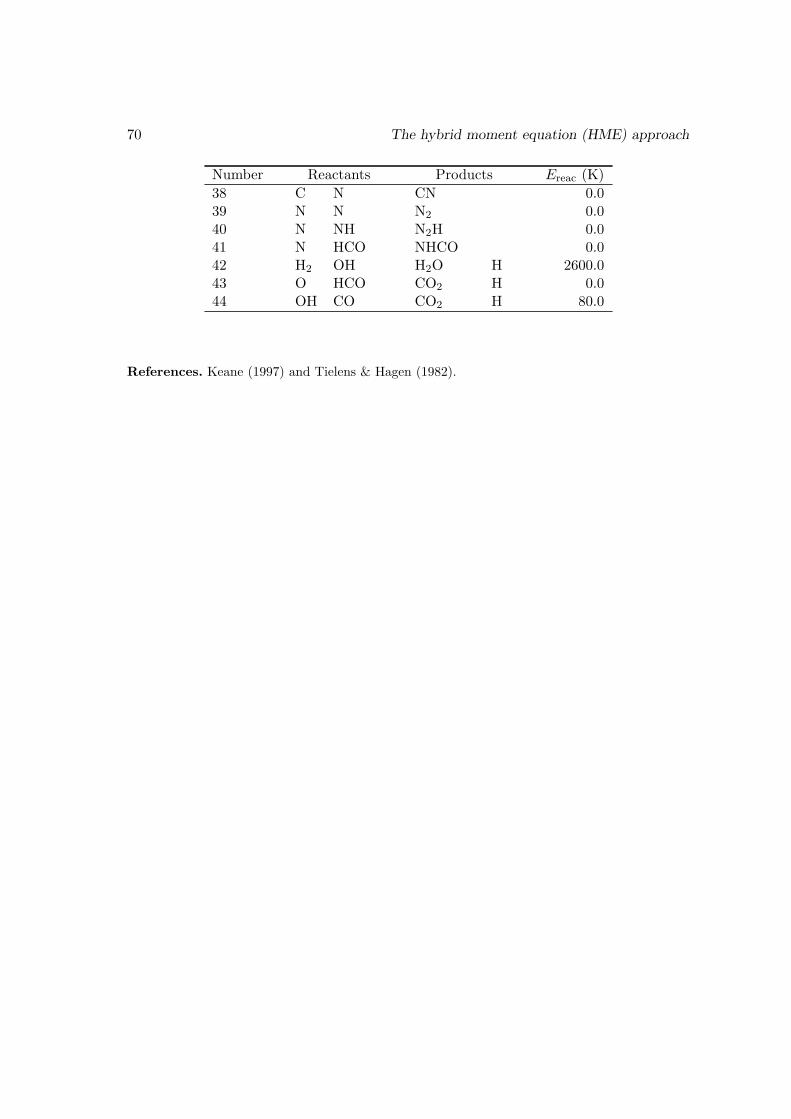
70 The hybrid moment equation (HME) approach

Number Reactants Products Ereac (K)

38 C N CN 0.039 N N N2 0.040 N NH N2H 0.041 N HCO NHCO 0.042 H2 OH H2O H 2600.043 O HCO CO2 H 0.044 OH CO CO2 H 80.0

References. Keane (1997) and Tielens & Hagen (1982).

Chapter 5

Production of interstellarhydrogen peroxide (H2O2) on thesurface of dust grains

The content of this chapter is based on:Du, F., Parise, B., & Bergman, P. 2012, A&A, 538, A91

Contents

5.1 Introduction . . . . . . . . . . . . . . . . . . . . . . . . . . . . . . . . . 72

5.2 Chemical model . . . . . . . . . . . . . . . . . . . . . . . . . . . . . . . 73

5.3 Results and discussions . . . . . . . . . . . . . . . . . . . . . . . . . . . 76

5.4 Conclusions . . . . . . . . . . . . . . . . . . . . . . . . . . . . . . . . . 91

5.A An explanation of the spike-like features in the evolution curves . . . . 91

5.B The surface reaction network used in this work . . . . . . . . . . . . . . 96

5.C Enthalpies of the surface species . . . . . . . . . . . . . . . . . . . . . . 99

The formation of water on the dust grains in the ISM may proceed with hydrogenperoxide (H2O2) as an intermediate. Recently gas-phase H2O2 has been detected in ρOph A with an abundance of ∼10−10 relative to H2.

The study presented in this chapter is aimed at reproducing the observed abundanceof H2O2 and other species detected in ρ Oph A quantitatively.

For this purpose, we make use of a chemical network that includes gas phase reactions,as well as processes on the grains. We also include the desorption mechanism triggeredby the heat released in chemical reactions. We run the model for a range of physicalparameters.

The modeling results show that the abundance of H2O2 can be best reproduced at∼6×105 yr, which is close to the dynamical age of ρ Oph A. The abundances of otherspecies detected in the same source such as H2CO, CH3OH, and O2 can also be reasonablyreproduced at this time. In the early time, the gas-phase abundance of H2O2 can be muchhigher than the currently detected value. We predict a gas phase abundance of O2H at

71

72 H2O2 formation on dust grain surface

the same order of magnitude as H2O2, and an abundance on the order of 10−8 for gasphase water in ρ Oph A. A few other species of interest are also discussed.

The main conclusion is, H2O2 can be produced on the dust grains and released intothe gas phase through nonthermal desorption via surface exothermic reactions. The H2O2

molecule on the grain is an important intermediate in the formation of water. The factthat H2O2 is over-produced in the gas phase for a range of physical conditions suggeststhat its destruction channel in the current gas phase network may be incomplete.

5.1 Introduction

Oxygen is the most abundant “metal” element in the cosmos (Savage & Sembach 1996;Asplund et al. 2009). In the cold dense interstellar clouds, gas-phase chemical modelspredict that oxygen mainly resides in CO and O2 molecules (Herbst & Leung 1989; Millar& Herbst 1990; Wakelam et al. 2006). However, although CO is ubiquitously distributedin the ISM, O2 is not. The latter is only detected very recently in ρ Oph A at a lowabundance (relative to molecular hydrogen) of 5×10−8 (Larsson et al. 2007), and in Orionat an abundance of (0.3 – 7)×10−6 (Goldsmith et al. 2011). On the other hand, theobserved water (gas or ice) abundance can be as high as 10−4 (van Dishoeck 2004). Thusit seems that water, instead of O2, is a main reservoir of oxygen in addition to CO. Whenonly gas phase chemistry is included, the H2O abundance can be on the order 10−7 atmost (see, for example, Bergin et al. 2000; Roberts & Herbst 2002) for typical dark cloudconditions. That O2 is overproduced and H2O is underproduced in gas phase chemistrysuggests that adsorption onto the grain surfaces and the reactions on the surfaces mayplay important roles.

On the grain surface, H2O can form through successive additions of hydrogen atomsto an oxygen atom:

H + O → OH, (5.1)

H + OH → H2O, (5.2)

both of which are barrierless (Allen & Robinson 1977). It can also form via hydrogenaddition to molecular oxygen:

H + O2 → O2H, (5.3)

H + O2H → H2O2, (5.4)

H + H2O2 → H2O+OH. (5.5)

Reaction (5.3) was assumed to have an activation barrier of 1200 K in Tielens & Hagen(1982). However, based on experimental results, Cuppen et al. (2010) have recentlyconcluded that it is barrierless. Other possible formation pathways of water include thereaction between H2 and OH and the route with O3 as an intermediate (Tielens & Hagen1982).

In the second route described above (Eqs. (5.3) – (5.5)), hydrogen peroxide (HOOH,also written as H2O2, which is adopted in this paper) appears as an intermediate product.Thus if this route is indeed important, a significant amount of H2O2 might form onthe grain, and its gas phase counterpart could also be detectable if effective desorptionmechanisms exist.

5.2 Chemical model 73

In the current mainstream gas phase reaction networks for astrochemistry, H2O2 isnot efficiently formed in the gas phase. For example, in the 2009 version of the OSUnetwork[1], the only two reactions leading to the formation of H2O2 are

H2 +O2H → H2O2 +H,

OH+OH → H2O2 + hν.

The first one has a large activation barrier of 104 K, rendering it inactive at low temper-atures. H2O2 is mainly consumed by

H2O2 + hν → OH+OH,

OH+H2O2 → H2O+O2H,

the first of which is dissociation by cosmic-ray induced radiation. Other destructionchannels by reacting with H and O are ineffective due to large activation barriers. At atemperature of 10 K and an H2 density of 104 cm−3, the steady-state abundance of H2O2

can be approximated by

X(H2O2) ' 103X2(OH) ' 5× 10−12.

At a higher density, the abundance of H2O2 will be even less because OH is less abundantin this case. With the UMIST RATE06 network the abundance of H2O2 is essentiallyzero (Woodall et al. 2007). Thus if a substantial amount of H2O2 can be detected in theISM, then it must have been synthesized on the dust grains, rather than in the gas phase.This would also provide information and constraints on the formation route of H2O.

It has indeed recently been detected (for the first time) in the ρ Oph A cloud byBergman et al. (2011b), at an abundance of ∼10−10, which is well above what would bepredicted by the gas phase chemistry, indicating that chemical processes on the grainsare responsible for this detection. Why this molecule has not been detected in the pastseems to be a puzzle and will be discussed later. Previously Clancy et al. (2004) detectedH2O2 in the atmosphere of Mars.

In the present work we aim at modeling the gas phase abundance of H2O2 at a phys-ical condition relevant to ρ Oph A, to demonstrate whether the grain chemistry is ableto explain its observed abundance. The model is also required to give consistent abun-dances for other species detected earlier in this region. Also, ice and gas-phase abundancepredictions for previously undetected species are made.

The remaining part of this paper is organized as follows. In section 5.2 we describe thechemical model used in this work. In section 5.3 we present the results of our modeling.The conclusions are in section 5.4. Appendix 5.A contains an explanation to a spike-likefeature in the evolution curves of some species. The surface reaction network we use islisted in Appendix 5.B, and the enthalpies of the surface species, which are needed in thechemical desorption mechanism (see section 5.2) are listed in Appendix 5.C.

5.2 Chemical model

For the gas phase chemistry, we use a subset of the UMIST RATE06 network[2] (Woodallet al. 2007). Species containing Fe, Na, Mg, and Cl are excluded. In total 284 gas phase

[1]http://www.physics.ohio-state.edu/∼eric/research files/osu 01 2009[2]http://udfa.net

74 H2O2 formation on dust grain surface

species and 3075 gas phase reactions are included. The cosmic-ray ionization rate is takento be the canonical value of 1.36×10−17 s−1 (Woodall et al. 2007).

The surface chemical network is a combination of a selection of the reactions in Allen& Robinson (1977), Tielens & Hagen (1982), and Hasegawa et al. (1992), with the ratesof a few reactions updated according to the recent experimental results and/or theoret-ical calculations. In total 56 surface species and 151 surface reactions are included (seeappendix 5.B).

The binding energies of the surface species are either taken from Hasegawa & Herbst(1993a) or estimated from the value of a similar species as in Garrod et al. (2008). Thesevalues are applicable to bare grains, i.e., grains without an ice mantle. A grain will becovered by ice (typically water) as adsorption and reaction proceeds, thus these valuesare not always appropriate. Ideally, they should be varied according to the real-timecomposition of the grain. The water ice mantle mainly affects the binding energies ofspecies with a hydrogen bond, such as OH and H2O. The effect of this should be minorfor our purpose, because most of the reactions involving a species with a hydrogen bondare primarily mediated by another reaction partner that does not have a hydrogen bond.

The barriers against surface diffusion are taken to be a fixed fraction of the bindingenergies. A range of values have been used for this fraction in the past, from 0.3 (Hasegawaet al. 1992) through 0.5 (Garrod et al. 2008) to 0.77 (Ruffle & Herbst 2000). We use avalue of 0.77, based on the analysis of Katz et al. (1999). Because our model is mainly fora relatively high temperature (∼20 K) in comparison with most of the previous models(predominantly for a temperature of ∼10 K), a low diffusion barrier for the surface specieswould lead to an unrealistic ice mantle composition. The effect of changing this parameteris discussed later. We allow H and H2 on a dust grain to migrate through quantumtunneling or thermal hopping, depending on which is faster. All the heavier species areonly allowed to move by thermal hopping. The quantum tunneling and thermal hoppingrates are calculated using the formulation of Hasegawa et al. (1992). For calculating ofthe quantum tunneling rates, we use a barrier width of 1 A. The exact value of thiswidth depends on the composition and structure of the surface, which has not been fullyquantified.

About the activation barrier of reaction (5.3), as there is a big discrepancy betweenthe value adopted in the past and the value proposed recently based on experiments(Cuppen et al. 2010), we adopt an intermediate value of 600 K. However, the effect ofvarying this parameter is also tested during the modeling, and will be discussed later.Reaction (5.5) has a barrier of 1400 K in Tielens & Hagen (1982), while in Cuppen et al.(2010) this reaction is found to be about 20 times slower than reaction (5.4), suggesting anon-negligible barrier[3]. We adopt the latter result, which can be translated into a barrierheight of ∼92 K for a barrier width of 1 A; a more detailed discussion on this reaction ison page 127.

Surface reactions with an activation barrier are allowed to proceed thermally orthrough quantum tunneling, depending on whichever is faster. The formula used tocalculate the rates is also the same as in Hasegawa et al. (1992), and the reaction barriersare assumed to have a width of 1 A, although different values are possible (Garrod &Pauly 2011).

[3]Our original publication Du et al. (2012) contains an error here, saying that reaction (5.5) is barrierless,though our conclusions are not affected.

5.2 Chemical model 75

The reaction rate of a two-body surface reaction

A + B → C+ · · ·

is[kdiff(A) + kdiff(B)]N(A)N(B)/NS,

if A 6= B. Here NS is the number of reaction sites of a grain, kdiff(A) and kdiff(B) are thediffusion rates of A and B, and N(A) and N(B) are the number of species A and B on asingle grain. If A = B, then the reaction rate should be

kdiff(A)N(A)(N(A)− 1)/NS.

With a number density of reaction sites being 1015 cm−2, a dust grain with radius 0.1 µmhas an NS of about 106.

As we are mainly concerned with the gas phase abundances of several species, theirdesorption mechanism must be treated carefully, especially if they are mainly producedon the grains. Besides the normal thermal desorption, species can also get evaporatedepisodically when a cosmic-ray hits a grain. This is treated in the same manner as inHasegawa & Herbst (1993a). Furthermore, the nonthermal desorption mechanism viaexothermic surface reactions (for brevity we call it “chemical desorption”) proposed byGarrod et al. (2006; see also Watson & Salpeter 1972; Garrod et al. 2007; Cazaux et al.2010) is also included. Here the products of the exothermic reactions on the grain havea probability of being directly ejected into the gas phase. The rate of such a desorptionmechanism depends on the exoergicity of the reaction, as well as on the desorption energyof the products. A parameter characterizing the efficiency of this mechanism (the “a”parameter in Garrod et al. 2007) is introduced, which we take to be 0.1. The yield ofchemical desorption is directly proportional to this “a” parameter, although it is not wellconstrained. The value we adopt here gives a good match to the observational results.See section 5.3.6 for further discussion. The exoergicities of these reactions are estimatedfrom the enthalpies of the reactants and products in the same manner as in Allen &Robinson (1977) (their equations (3) and (4)), and the enthalpies of the species involvedin these reactions are taken from Binnewies & Milke (1999), from the NIST chemistryweb book[4], or from some other sporadic sources (see appendix 5.C).

However, the desorption mechanisms described above are not always sufficient to pro-vide enough gas phase abundances for some species, especially at late times. Even if alarge amount of a species is produced on the grain and released into the gas phase atearly times, it would later be accreted back to the grain surface. If at this later time itsproduction is no longer active (due to the exhaustion of the precursor species), its gasphase abundance cannot be maintained. Dust sputtering (Tielens et al. 1994) and pho-todesorption (Oberg et al. 2007) might help release them to the gas phase, both of whichshould not be very important in a quiet cold dark cloud. Another possible mechanismis that cosmic-ray induced radiation can dissociate the species on the grain, and whenthe fragments recombine, the products can possibly be ejected into the gas phase directlybecause of the energy release of the reaction, as described before. We implement thismechanism in the same way as in Ruffle & Herbst (2001a) and Garrod & Pauly (2011)

[4]http://webbook.nist.gov/chemistry/

76 H2O2 formation on dust grain surface

(see also Cuppen & Herbst 2007), namely, the cosmic-ray induced photodissociation ratesfor the surface species are taken to be the same as in the gas phase. Several dissociationbranches from Garrod et al. (2008) (their Table 1) are included.

In our model the numbers of all the species on a single grain are solved with thehybrid moment equation (HME) approach (Du & Parise 2011). It has been shown in Du& Parise (2011) that the rate equation method can be inaccurate in some cases, and theHME approach provides a major improvement over the rate equation method. Since theHME approach is relatively new, in several cases we also benchmarked our HME resultswith the exact Monte Carlo method (similar to the one of Vasyunin et al. 2009) as in Du& Parise (2011), and the agreement is satisfactory. It is impractical to run all the modelswith the Monte Carlo method because the run time would be too long.

At present the layered structure of the grain mantle is not incorporated into our model.Such a structure might be more realistic, and it is important for retaining some of theice species. However, it is also possible that the interstellar dust grains may have anamorphous structure, which renders the layered structure an inaccurate description. Onthe other hand, particles landing on a grain are able to penetrate the interior by severalto tens of layers, as demonstrated by experiments (see, e.g., Ioppolo et al. 2010), thusalthough a model neglecting the layered structure is not accurate, one that deactivatesall the layers below the outermost surface does not reflect the whole reality either. Infact, for the H-addition reactions, whether the layered structure is taken into account onlyplays a minor role in determining the reaction rates in the accretion limit (i.e. when theaccretion and evaporation processes are much slower than the reactions; Garrod 2008),because the species involved in these reactions never build up a full layer.

5.3 Results and discussions

5.3.1 Modeling ρ Oph A

We ran the chemical model for the physical parameters that are appropriate for ρ OphA, where H2O2 has first been detected by Bergman et al. (2011b). In Fig. 5.1 we showthe abundances of several species as a function of time. In this model, a temperature of21 K and a hydrogen density of 6×105 cm−3 have been assumed, which are determinedfor ρ Oph A observationally by Bergman et al. (2011a,b). The dust temperature and gastemperature are assumed to be the same. A fixed value of 15 for the visual extinction AV

has been adopted. We assume a canonical grain size of 0.1 µm and a reaction site densityof 1015 cm−2. The dust-to-gas mass ratio is set to 0.01, and the dust grain material isassumed to have a mass density of 2 g cm−3. We also assume that the ratio between thediffusion barrier and the binding energy is 0.77, which is at the higher end of the valuesused in the past, to give a reasonable ice composition. The initial condition is atomicexcept for H2. The elemental abundances are the same as in Garrod & Pauly (2011).

The observed abundance of gas phase H2O2 is ∼10−10 relative to H2 (Bergman et al.2011b). This value is best matched at a time of ∼6×105 yr. In the early time, beforeabout 2×105 years, the gas phase H2O2 abundance can be as high as ∼5×10−7. At latetimes, the H2O2 abundance decreases to a very low value, due to the exhaustion of O2 onthe grain and a full conversion of H2O2 into H2O.

H2O2 is mainly formed through reaction (5.4) on the grain, followed by immediate

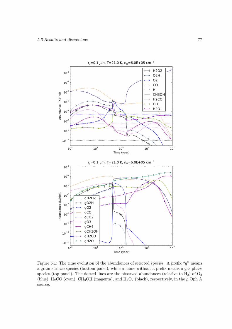
5.3 Results and discussions 77

103 104 105 106 107

Time (year)

10-10

10-9

10-8

10-7

10-6

10-5

10-4

10-3

Abun

danc

e ([

X]/[H

])rg=0.1 m, T=21.0 K, nH=6.0E+05 cm3

H2O2O2HO2COHCH3OHH2COOHH2O

103 104 105 106 107

Time (year)

10-11

10-10

10-9

10-8

10-7

10-6

10-5

10-4

10-3

Abun

danc

e ([

X]/[H

])

rg=0.1 m, T=21.0 K, nH=6.0E+05 cm3

gH2O2gO2HgO2gCOgCO2gO3gCH4gCH3OHgH2COgH2O

Figure 5.1: The time evolution of the abundances of selected species. A prefix “g” meansa grain surface species (bottom panel), while a name without a prefix means a gas phasespecies (top panel). The dotted lines are the observed abundances (relative to H2) of O2

(blue), H2CO (cyan), CH3OH (magenta), and H2O2 (black), respectively, in the ρ Oph Asource.

78 H2O2 formation on dust grain surface

desorption of the product into the gas phase caused by the reaction heat. About 7% ofthe produced H2O2 is released this way. Its gas phase abundance is determined by theadsorption and chemical desorption processes. The dissociation of gas phase H2O2 bycosmic-ray-induced photons is unimportant in consuming it, compared to adsorption.

Ioppolo et al. (2008) modeled the abundance of H2O2 ice briefly, giving a value of10−14 – 10−10 relative to molecular hydrogen, depending on which energy barriers ofseveral relevant reactions were used. Our major goal is to model the gas phase H2O2

abundance, rather than the H2O2 ice. In our model results, the gas phase abundance ofH2O2 is much higher than its ice counterpart. The H2O2 ice does not have a significantabundance in the later stage, being well below the upper limit (5.2% with respect toH2O ice) given by Boudin et al. (1998), because it is constantly transformed into H2Oby reacting with the accreted H atoms. However, by irradiating thin water ice film withlow energy ions, Gomis et al. (2004) found that it is possible to obtain an H2O2 to H2Oratio in the solid phase up to a few percent. This direct processing of the grain mantleby cosmic rays is not included in our model. The production of H2O2 inside water icein an O2-rich environment triggered by UV radiation (Shi et al. 2011) should also beof little importance here. We notice in Fig. 5.1 (bottom panel) that in the early stage(before ∼5×104 yr) the H2O2 ice can achieve a rather high abundance, ∼5×10−6 relativeto H nucleus or ∼10% relative to H2O. During this early period the water formation onthe grain mainly proceeds through reaction (5.5) with H2O2 as an intermediate, which isresponsible for about half of the final water ice repository on the grain mantle. In thelater stage, reaction (5.2) takes over. In the results of Ioppolo et al. (2008) (their Fig. 4),we do not see a similar feature (i.e. a high abundance of H2O2 ice in the early stage). Inour current model the layered structure of the grain mantle is not taken into account. Itis possible that, if such a structure is considered, the inner layers with a relatively highH2O2 content might be maintained, which would give a value of a few percent for theH2O2-to-H2O ratio in the solid phase.

Methanol (CH3OH) and formaldehyde (H2CO) are also detected in the ρ Oph A SM1core (Bergman et al. 2011a), at an abundance of ∼2×10−9 and ∼5×10−9, respectively.Their abundances are also reproduced very well at a time of ∼6×105 yr in our model.At early times, both CH3OH and H2CO have a high abundance. Their abundances alsohave a peak in the period between 2×105 yr to 107 yr. In our current network, CH3OHis mainly formed on the grains, and mainly through the addition of H atom to CH2OH,while the latter is mainly produced from the reaction between C and OH to form HOCfollowed by successive H additions. Thus the abundance of CH3OH decreases at very latetimes due to the depletion of atomic C (which is mainly in CH4 ice in the late stage).The normal formation channel through successive hydrogenation of CO is important ataround 5×105 – 2×106 yr. The gas phase H2CO mainly forms in the gas phase in theearly stage (< 105 yr), and mainly through the reaction CH3 +O → H2CO+H. Later itis mainly formed through successive hydrogenation of CO on the grain surface followedby chemical desorption. The abundance of methanol and formaldehyde ice relative towater ice can be as high as ∼20% at their peaks at a time of ∼2×106 yr, but falls to avery low value in the late times. The late-time abundances are consistent with the upperlimit derived for quiescent environment and low-mass young stellar objects in Gibb et al.(2004). However, in Pontoppidan et al. (2004) a much higher abundance of CH3OH iceis observed along the line-of-sight of SVS4 (a dense cluster of pre-main sequence stars),

5.3 Results and discussions 79

which is close to a class 0 protostar, and this is consistent with the peak abundances inour model.

From Fig. 5.1 (top panel) it can be seen that the abundance of gaseous O2 at anintermediate time of 6×105 year is ∼6×10−9, which is within one order of magnitude ofthe observed abundances of 5×10−8 for O2 (Larsson et al. 2007). The late-time abundanceof O2 drops to a very low value, while its observed abundance is best matched at a timeof ∼2×105 yr. We notice that during the period ∼(0.6 – 2)×105 yr, the abundance of O2

ice has a prominent bump, reaching a peak abundance of ∼10−5 relative to H2. At thesame time, the gas phase O2 also reaches an abundance of ∼(1 – 5)×10−7. These valuescan be compared with the recent detection of gas phase O2 at an abundance of (0.3 –7)×10−6 in Orion by Herschel (Goldsmith et al. 2011). Warm-up of the dust grain at thisstage may release a large amount of O2 molecule into the gas phase.

As a precursor of H2O2, O2Hmainly forms from the reaction between O and OH (whichdoes not have a barrier according to Hasegawa et al. 1992) on the grain at an early stage(<5×104 yr), and through reaction H + O2 at a later stage. The ratio between the gasphase O2H and H2O2 is almost constant throughout the evolution, being approximately3. Thus in our current network, the gas phase O2H also has a remarkable abundance,which might be detectable in the future[5].

Except at very early times, the grain mantle is mainly composed of water ice. Theabundances of CO and CO2 are comparable at an intermediate time of (0.3–1)×106 yr,being about 40–60% of water ice. This is in rough agreement with the ice composition forintermediate-mass YSOs (Gibb et al. 2004) (see also Oberg et al. 2011), and is also in linewith the suggestion of An et al. (2011) that CO2 ice is mixed with CH3OH ice (the latteris about 10% of the former in our model). Water ice mainly forms from reaction (5.5) inthe early time, and from reaction (5.2) in the late time. The gas phase formation routeof water only plays a minor role. In contrast, the CO ice mantle is mainly from accretionof CO molecules formed in the gas phase. For the CO2 ice, it is mainly accreted from itsgas phase counterpart in the early time, and its abundance is increased further throughthe reaction OH + CO → CO2 + H in the late stage. At late times (> 3×106 yr), mostof the carbon resides in the form of CH4 ice, with the latter about half of the water ice.However, as far as we know, such a high abundance of CH4 ice (see also Garrod & Pauly2011) has not been observed in the ISM.

The gas phase CO is heavily depleted, with an abundance ∼10−6 relative to the Hnucleus or ∼1% relative to its ice counterpart, at an intermediate time (105 – 106 yr).Its abundance is mainly determined by the balance between the adsorption and cosmic-ray induced evaporation processes. At late times the CO ice abundance drops to a verylow value. This is because CO is continuously hydrogenated into H2CO or CH3OH, andthe dissociation of CH3OH by cosmic-ray induced photons produces CH3, which quicklybecomes CH4 by hydrogenation. Taking the layered structure of grain mantle into accountcan retain a fair amount of CO ice.

The abundance of gas phase H2O in the intermediate to late time is on the order 10−8.At these times, its grain surface production route (5.2) followed by chemical desorptionand the gas phase production route H3O

+ + e− → H2O+ H plays a similarly importantrole. H3O

+ itself is mainly formed from successive protonation of atomic oxygen at this

[5]O2H has been recently detected in the same source by Parise et al. (2012a), with an abundance of∼10−10, close to the prediction here.

80 H2O2 formation on dust grain surface

stage.The hydroxyl radical (OH) has an abundance ∼10−8 – 10−9 in the gas phase at the

intermediate-to-late times. These values are comparable to the observed abundance of∼(0.5 – 1)×10−8 in the envelope around the high-mass star-forming region W3 IRS 5obtained with HIFI onboard Herschel (Wampfler et al. 2011). The physical condition inthis source is different from ρ Oph A. However, since OH is readily produced and recycledin the gas phase by the reactions H3O

+ + e− → OH+ 2H and H+3 +OH → H2O

+ +H2,grain processes will not play a dominant role in determining its abundance, especiallywhen the temperature is not too low. However, Goicoechea et al. (2006) detected a muchhigher abundance (0.5 – 1)×10−6 of OH in the Orion KL outflows, which seems to requireother formation pathways (e.g. shock destruction of H2O ice).

A relatively high abundance (∼10−7 and ∼10−5) of gas phase and grain surface ozone(O3) is also obtained for t . 105 yr. However, these values should be treated with caution,because the chemistry of O3 is very incomplete in our current model: neither the OSUgas phase network nor the UMIST RATE06 network includes it. Possible gas phasedestruction pathways involving atomic O and S (according to the NIST chemistry webbook; see footnote [4]) may lower its gas phase abundance significantly, but its ice mantleabundance should not be severely affected.

The abundance of atomic hydrogen in the gas phase is quite high at late times asseen from Fig. 5.1, which seems to be at odds with the usual results. In many gas phasechemical models, the abundance of atomic hydrogen in the gas phase is determined by thebalance between its adsorption onto the dust grains and the dissociation of H2 moleculesby cosmic rays. The adsorption process is thought to have a sticking coefficient close tounity, and evaporation is assumed not to occur (which is appropriate at low temperatures).In such a framework it can be found that the gas phase atomic hydrogen will always havea fixed density on the order of 1 cm−3. However, in our case with a temperature of 21K, evaporation is very fast and cannot be neglected. Furthermore, the dissociation of icemantle by cosmic-ray induced photons generates atomic hydrogen, which enhances its gasphase abundance significantly in the late stage.

We note that, at a time of about 5×104 years, the abundances of several species changevery quickly, and the abundances of some other species show a spike-like feature. At firstsight this may resemble an erroneous behavior caused by the differential equation solver,so we ran the model with the same parameters using a Monte Carlo code (also used forbenchmark purpose in Du & Parise 2011), which is free of such problems, and it turnsout that these features are genuine. A semi-quantitative explanation of this feature is inappendix 5.A.

5.3.2 Chemical age versus dynamical time scale

As noted before, the time of the closest agreement between our modeling results andthe observational results of Bergman et al. (2011a,b) is at ∼6×105 year. Interestingly,this time scale is quite close to those derived in Andre et al. (2007) (their Table 7). Forexample, the evolution time scale for ρ Oph A as estimated to be three times the free-falltime is (0.5 – 2)×105 years, which is close to the statistically estimated age, while thecollisional time scale of 5.5×105 years and the cross time scale of 8×105 years are alsowithin the same order of magnitude.

5.3 Results and discussions 81

It is important to define the starting point when talking about age. In the chemicalevolution model described above, the whole system starts to evolve from a simple initialstate where all the elements except for hydrogen are in atomic form, and the grainsare bare. How relevant is such an initial condition when we talk about the dynamicalevolution of a cloud condensation? At a density of ∼103 cm−3, a temperature of ∼20 K,and a visual extinction of 2, which are typical of diffuse or translucent molecular clouds,a chemical model starting from an atomic initial condition (except for H2) reaches steadystate for most of the species in several 103 years. Because such a time scale is much shorterthan the dynamical time scale of a cloud, it should not make much difference for a time-dependent model (i.e. one in which temperature and density etc. vary with time) to useeither atomic or molecular initial conditions. For a time-independent cloud model (suchas the one we are using) with constant physical conditions, adopting an atomic initialcondition and a high density is equivalent to assuming that the cloud was compressedfrom the diffuse ISM very quickly. Converging flows in the ISM might play such a role,although this seems unlikely in ρ Oph A because only a very small velocity gradient wasobserved (Andre et al. 2007).

However, the time of best match and the predicted abundances may also be verydependent on the value adopted for some of the modeling parameters that are not very wellconstrained. It is necessary to see how the results would be changed if these parametersare varied.

5.3.3 Effects of changing the energy barrier of the surface reaction H+O2 → HO2

The activation barrier of reaction (5.3) was set to 1200 K in Tielens & Hagen (1982),which was taken from the theoretical calculation by Melius & Blint (1979) for the gasphase case. Cuppen et al. (2010) conclude that this reaction has a negligible barrier. Wechoose to use an intermediate value for the energy barrier of reaction (5.3), namely, 600 Kfor the modeling. Here we study how the uncertainties in this parameter would affect theabundances of several species of interest.

In Fig. 5.2 the abundances of several species at the best-match time (6×105 yr) areplotted as a function of the activation energy barrier of reaction (5.3). The temperatureand density are fixed at 21 K and 6×105 cm−3, and the ratio between the diffusion energybarrier and the binding energy is set to 0.77.

The abundance of gas phase O2 is not affected by changing the energy barrier ofreaction (5.3) because its abundance is mainly determined by the gas phase productionprocess O + OH → O2 +H and adsorption. However, the abundance of grain surface O2

increases by five orders of magnitude as the barrier changes from 0 to 1200 K, becausereaction (5.3) is one of the main reactions for the consumption of grain O2. However, evenwith a barrier of 1200 K for reaction (5.3), the abundance of O2 on the grain at a late stageis too low to be detected. Although the rate coefficient of reaction (5.3) is reduced by sixorders of magnitude when its barrier changes from 0 to 1200K, the abundance of O2H onthe grain does not change significantly. The reason is that when reaction (5.3) becomesslower, more O2 will build up on the grain, compensating for the effect of increasing thebarrier of reaction (5.3). The abundance of gas phase H2O2 does not change much either,as its abundance is mainly determined by accretion onto the grain, and production by

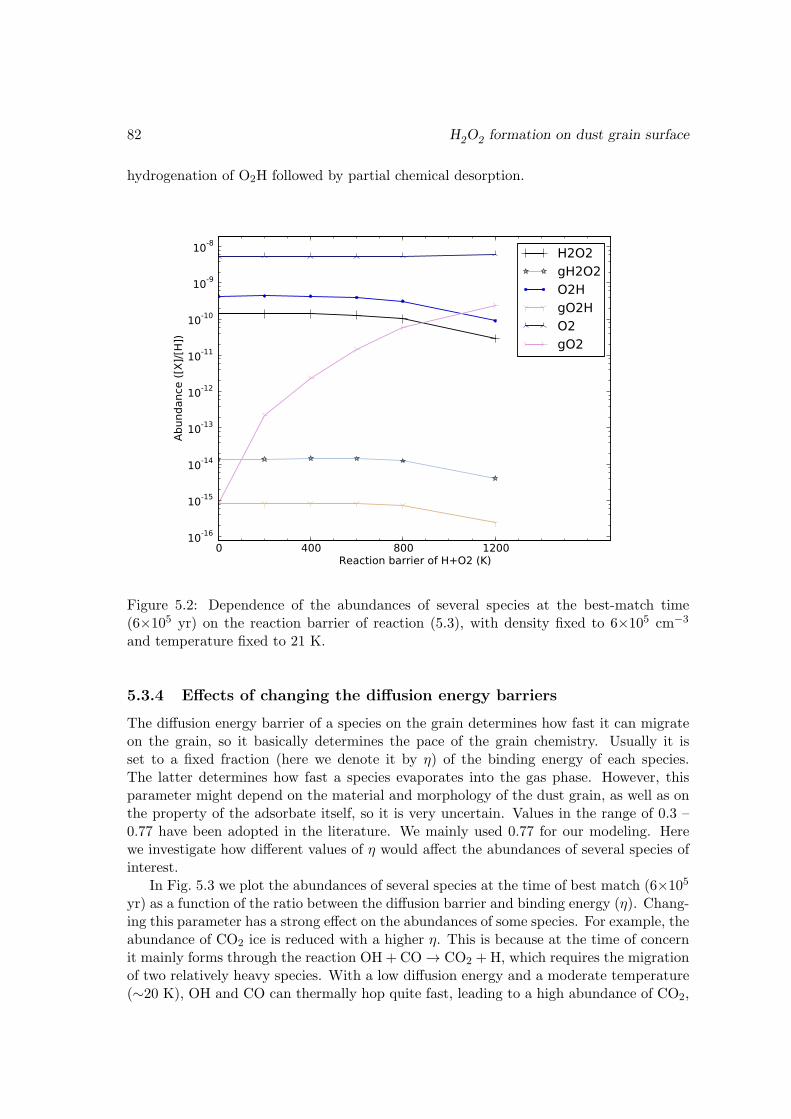
82 H2O2 formation on dust grain surface

hydrogenation of O2H followed by partial chemical desorption.

0 400 800 1200Reaction barrier of H+O2 (K)

10-16

10-15

10-14

10-13

10-12

10-11

10-10

10-9

10-8

Abun

danc

e ([

X]/[H

])

H2O2gH2O2O2HgO2HO2gO2

Figure 5.2: Dependence of the abundances of several species at the best-match time(6×105 yr) on the reaction barrier of reaction (5.3), with density fixed to 6×105 cm−3

and temperature fixed to 21 K.

5.3.4 Effects of changing the diffusion energy barriers

The diffusion energy barrier of a species on the grain determines how fast it can migrateon the grain, so it basically determines the pace of the grain chemistry. Usually it isset to a fixed fraction (here we denote it by η) of the binding energy of each species.The latter determines how fast a species evaporates into the gas phase. However, thisparameter might depend on the material and morphology of the dust grain, as well as onthe property of the adsorbate itself, so it is very uncertain. Values in the range of 0.3 –0.77 have been adopted in the literature. We mainly used 0.77 for our modeling. Herewe investigate how different values of η would affect the abundances of several species ofinterest.

In Fig. 5.3 we plot the abundances of several species at the time of best match (6×105

yr) as a function of the ratio between the diffusion barrier and binding energy (η). Chang-ing this parameter has a strong effect on the abundances of some species. For example, theabundance of CO2 ice is reduced with a higher η. This is because at the time of concernit mainly forms through the reaction OH + CO → CO2 +H, which requires the migrationof two relatively heavy species. With a low diffusion energy and a moderate temperature(∼20 K), OH and CO can thermally hop quite fast, leading to a high abundance of CO2,

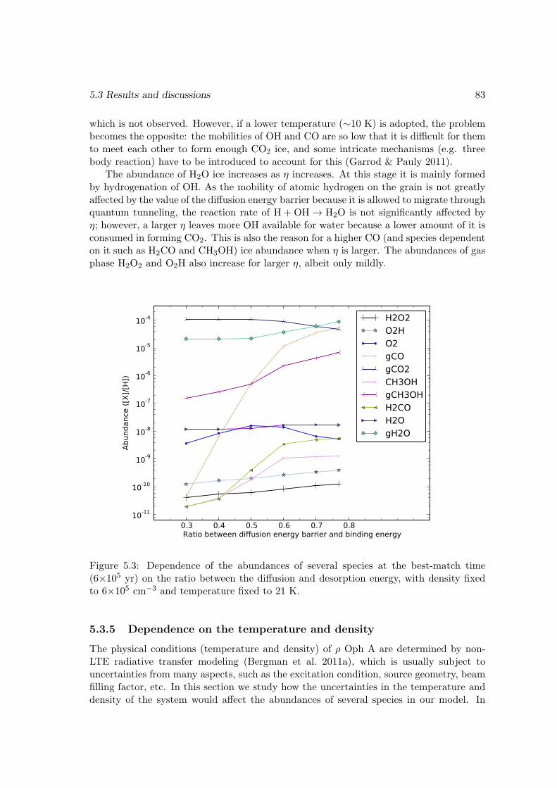
5.3 Results and discussions 83

which is not observed. However, if a lower temperature (∼10 K) is adopted, the problembecomes the opposite: the mobilities of OH and CO are so low that it is difficult for themto meet each other to form enough CO2 ice, and some intricate mechanisms (e.g. threebody reaction) have to be introduced to account for this (Garrod & Pauly 2011).

The abundance of H2O ice increases as η increases. At this stage it is mainly formedby hydrogenation of OH. As the mobility of atomic hydrogen on the grain is not greatlyaffected by the value of the diffusion energy barrier because it is allowed to migrate throughquantum tunneling, the reaction rate of H + OH → H2O is not significantly affected byη; however, a larger η leaves more OH available for water because a lower amount of it isconsumed in forming CO2. This is also the reason for a higher CO (and species dependenton it such as H2CO and CH3OH) ice abundance when η is larger. The abundances of gasphase H2O2 and O2H also increase for larger η, albeit only mildly.

0.3 0.4 0.5 0.6 0.7 0.8Ratio between diffusion energy barrier and binding energy

10-11

10-10

10-9

10-8

10-7

10-6

10-5

10-4

Abun

danc

e ([

X]/[H

])

H2O2O2HO2gCOgCO2CH3OHgCH3OHH2COH2OgH2O

Figure 5.3: Dependence of the abundances of several species at the best-match time(6×105 yr) on the ratio between the diffusion and desorption energy, with density fixedto 6×105 cm−3 and temperature fixed to 21 K.

5.3.5 Dependence on the temperature and density

The physical conditions (temperature and density) of ρ Oph A are determined by non-LTE radiative transfer modeling (Bergman et al. 2011a), which is usually subject touncertainties from many aspects, such as the excitation condition, source geometry, beamfilling factor, etc. In this section we study how the uncertainties in the temperature anddensity of the system would affect the abundances of several species in our model. In

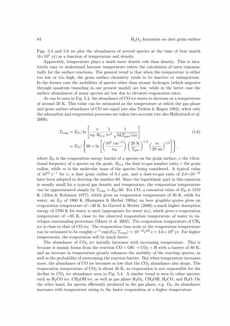
84 H2O2 formation on dust grain surface

Figs. 5.4 and 5.6 we plot the abundances of several species at the time of best match(6×105 yr) as a function of temperature and density.

Apparently, temperature plays a much more drastic role than density. This is intu-itively easy to understand because temperature enters the calculation of rates exponen-tially for the surface reactions. The general trend is that when the temperature is eithertoo low or too high, the grain surface chemistry tends to be inactive or unimportant.In the former case the mobilities of species other than atomic hydrogen (which migratesthrough quantum tunneling in our present model) are low, while in the latter case thesurface abundances of many species are low due to elevated evaporation rates.

As can be seen in Fig. 5.4, the abundance of CO ice starts to decrease at a temperatureof around 20 K. This value can be estimated as the temperature at which the gas phaseand grain surface abundance of CO are equal (see also Tielens & Hagen 1982), when onlythe adsorption and evaporation processes are taken into account (see also Hollenbach et al.2009):

Tevap = ED/ ln

[ν

nH RG,n

1

πr21√

8kTgas/πm

](5.6)

' ED/

60 + ln

[(105 cm−3

nH

)(20 K

Tgas

)1/2 ( m

28 au

)1/2],

where ED is the evaporation energy barrier of a species on the grain surface, ν the vibra-tional frequency of a species on the grain, RG,n the dust-to-gas number ratio, r the grainradius, while m is the molecular mass of the species being considered. A typical valueof 1012 s−1 for ν, a dust grain radius of 0.1 µm, and a dust-to-gas ratio of 2.8×10−12

have been adopted in deriving the number 60. Since the logarithmic part in this equationis usually small for a typical gas density and temperature, the evaporation temperaturecan be approximated simply by Tevap ' ED/60. For CO, a canonical value of ED is 1210K (Allen & Robinson 1977), which gives an evaporation temperature of 20 K, while forwater, an ED of 1860 K (Hasegawa & Herbst 1993a) on bare graphite grains gives anevaporation temperature of ∼30 K. In Garrod & Herbst (2006) a much higher desorptionenergy of 5700 K for water is used (appropriate for water ice), which gives a evaporationtemperature of ∼95 K, close to the observed evaporation temperature of water in en-velopes surrounding protostars (Maret et al. 2002). The evaporation temperature of CH4

ice is close to that of CO ice. The evaporation time scale at the evaporation temperaturecan be estimated to be roughly ν−1 exp(ED/Tevap) ' 10−12e60 s ' 3.6×106 yr. For highertemperature, the evaporation will be much faster.

The abundance of CO2 ice initially increases with increasing temperature. This isbecause it mainly forms from the reaction CO +OH → CO2 +H with a barrier of 80 K,and an increase in temperature greatly enhances the mobility of the reacting species, aswell as the probability of overcoming the reaction barrier. But when temperature increasesmore, the abundance of CO ice becomes so low that the CO2 abundance also drops. Theevaporation temperature of CO2 is about 40 K, so evaporation is not responsible for thedecline in CO2 ice abundance seen in Fig. 5.4. A similar trend is seen in other species,such as H2CO ice, CH3OH ice, as well as gas phase H2O2, CH3OH, H2CO, and H2O. Onthe other hand, for species efficiently produced in the gas phase, e.g. O2, its abundanceincreases with temperature owing to the faster evaporation at a higher temperature.

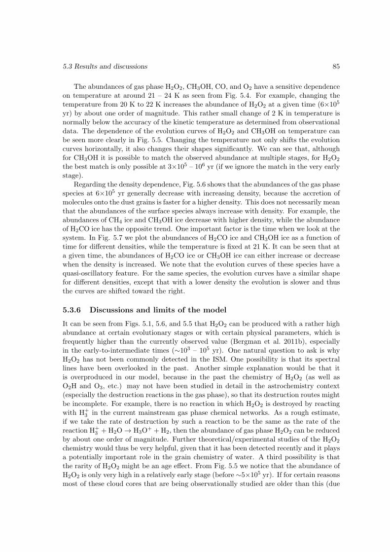
5.3 Results and discussions 85

The abundances of gas phase H2O2, CH3OH, CO, and O2 have a sensitive dependenceon temperature at around 21 – 24 K as seen from Fig. 5.4. For example, changing thetemperature from 20 K to 22 K increases the abundance of H2O2 at a given time (6×105

yr) by about one order of magnitude. This rather small change of 2 K in temperature isnormally below the accuracy of the kinetic temperature as determined from observationaldata. The dependence of the evolution curves of H2O2 and CH3OH on temperature canbe seen more clearly in Fig. 5.5. Changing the temperature not only shifts the evolutioncurves horizontally, it also changes their shapes significantly. We can see that, althoughfor CH3OH it is possible to match the observed abundance at multiple stages, for H2O2

the best match is only possible at 3×105 – 106 yr (if we ignore the match in the very earlystage).

Regarding the density dependence, Fig. 5.6 shows that the abundances of the gas phasespecies at 6×105 yr generally decrease with increasing density, because the accretion ofmolecules onto the dust grains is faster for a higher density. This does not necessarily meanthat the abundances of the surface species always increase with density. For example, theabundances of CH4 ice and CH3OH ice decrease with higher density, while the abundanceof H2CO ice has the opposite trend. One important factor is the time when we look at thesystem. In Fig. 5.7 we plot the abundances of H2CO ice and CH3OH ice as a function oftime for different densities, while the temperature is fixed at 21 K. It can be seen that ata given time, the abundances of H2CO ice or CH3OH ice can either increase or decreasewhen the density is increased. We note that the evolution curves of these species have aquasi-oscillatory feature. For the same species, the evolution curves have a similar shapefor different densities, except that with a lower density the evolution is slower and thusthe curves are shifted toward the right.

5.3.6 Discussions and limits of the model

It can be seen from Figs. 5.1, 5.6, and 5.5 that H2O2 can be produced with a rather highabundance at certain evolutionary stages or with certain physical parameters, which isfrequently higher than the currently observed value (Bergman et al. 2011b), especiallyin the early-to-intermediate times (∼103 – 105 yr). One natural question to ask is whyH2O2 has not been commonly detected in the ISM. One possibility is that its spectrallines have been overlooked in the past. Another simple explanation would be that itis overproduced in our model, because in the past the chemistry of H2O2 (as well asO2H and O3, etc.) may not have been studied in detail in the astrochemistry context(especially the destruction reactions in the gas phase), so that its destruction routes mightbe incomplete. For example, there is no reaction in which H2O2 is destroyed by reactingwith H+

3 in the current mainstream gas phase chemical networks. As a rough estimate,if we take the rate of destruction by such a reaction to be the same as the rate of thereaction H+

3 +H2O → H3O+ +H2, then the abundance of gas phase H2O2 can be reduced

by about one order of magnitude. Further theoretical/experimental studies of the H2O2

chemistry would thus be very helpful, given that it has been detected recently and it playsa potentially important role in the grain chemistry of water. A third possibility is thatthe rarity of H2O2 might be an age effect. From Fig. 5.5 we notice that the abundance ofH2O2 is only very high in a relatively early stage (before ∼5×105 yr). If for certain reasonsmost of these cloud cores that are being observationally studied are older than this (due

86 H2O2 formation on dust grain surface

15 20 25 30Temperature (K)

10-13

10-12

10-11

10-10

10-9

10-8

10-7

10-6

10-5

10-4

10-3

Abun

danc

e ([

X]/[H

])

H2O2O2HO2H2OCOCH3OHH2COHOH

15 20 25 30Temperature (K)

10-10

10-9

10-8

10-7

10-6

10-5

10-4

Abun

danc

e ([

X]/[H

])

gH2OgCOgCH3OHgH2COgCO2gCH4

Figure 5.4: Dependence of the abundances of several species at the time of best match(6×105 yr) on temperature, with density fixed to 6×105 cm−3. Top panel: gas phasespecies; bottom panel: surface species.

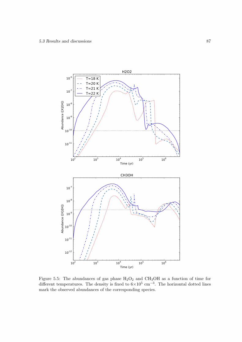
5.3 Results and discussions 87

102 103 104 105 106

Time (yr)

10-11

10-10

10-9

10-8

10-7

10-6

Abun

danc

e ([

X]/[H

])

H2O2

T=18 KT=20 KT=21 KT=22 K

102 103 104 105 106

Time (yr)

10-12

10-11

10-10

10-9

10-8

10-7

Abun

danc

e ([

X]/[H

])

CH3OH

Figure 5.5: The abundances of gas phase H2O2 and CH3OH as a function of time fordifferent temperatures. The density is fixed to 6×105 cm−3. The horizontal dotted linesmark the observed abundances of the corresponding species.

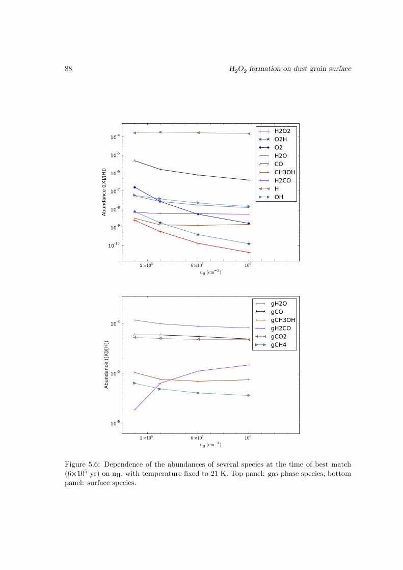
88 H2O2 formation on dust grain surface

2105 6105 106

nH (cm3 )

10-10

10-9

10-8

10-7

10-6

10-5

10-4

Abun

danc

e ([

X]/[H

])

H2O2O2HO2H2OCOCH3OHH2COHOH

2105 6105 106

nH (cm3 )

10-6

10-5

10-4

Abun

danc

e ([

X]/[H

])

gH2OgCOgCH3OHgH2COgCO2gCH4

Figure 5.6: Dependence of the abundances of several species at the time of best match(6×105 yr) on nH, with temperature fixed to 21 K. Top panel: gas phase species; bottompanel: surface species.

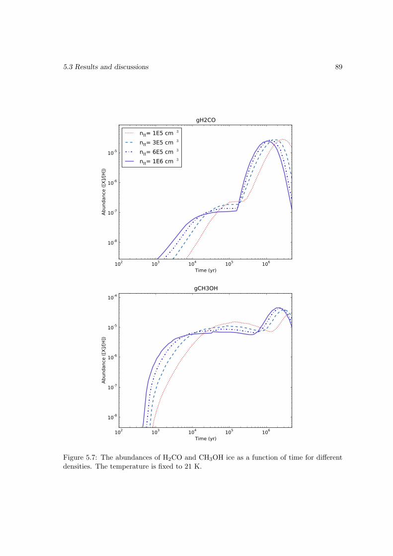
5.3 Results and discussions 89

102 103 104 105 106

Time (yr)

10-8

10-7

10-6

10-5

Abun

danc

e ([

X]/[H

])

gH2CO

nH= 1E5 cm3

nH= 3E5 cm3

nH= 6E5 cm3

nH= 1E6 cm3

102 103 104 105 106

Time (yr)

10-8

10-7

10-6

10-5

10-4

Abun

danc

e ([

X]/[H

])

gCH3OH

Figure 5.7: The abundances of H2CO and CH3OH ice as a function of time for differentdensities. The temperature is fixed to 21 K.

90 H2O2 formation on dust grain surface

to some selection effects), then the H2O2 abundance in these objects would be too lowto detect. Basically, at least three physical parameters are relevant, namely age, density,and temperature. A probability distribution of these three parameters of the cloud coreswould help to give the detection probability of H2O2 (and any other molecules). Thus ρOph A may be considered special in the sense that it has a relatively high density (∼106

cm−3) and temperature (20 – 30 K), while most dark clouds with a high density (&104

cm−3) tend to be very cold (.15 K) (Bergin & Tafalla 2007). An inhomogeneous physicalcondition would make the situation more complex, which may require a self-consistentdynamical-chemical model. However, a thorough study of these possibilities has to be leftto future work.

On the other hand, although CH3OH has been studied quite extensively in the past, wenotice that the gas phase reactions associated with it contain some important (althoughnot decisive) differences between the OSU09 network and the UMIST RATE06 network.For example, the reaction between CH and CH3OH to form CH3 and H2CO has a rate2.49×10−10(T/300)−1.93 in the UMIST RATE06 network, but it does not exist in theOSU09 network. One possible problem is that the temperature of cold ISM (at mostseveral tens of Kelvins) is out of the indicated valid range for many reactions in RATE06,and it is not clear how to extrapolate these reaction rates correctly, although we haveclosely followed the instructions in Woodall et al. (2007). In our modeling we have beenusing the RATE06 network.

The energy barriers for the hydrogenation of CO and H2CO on the grain are both takento be 2500 K. Woon (2002) calculated the barrier heights of these two reactions, givinga value of ∼2740 K and 3100 K in the case three water molecules are present, with zero-point energy corrections added. If these values are adopted, then the observed abundancesof H2CO and CH3OH can only be reproduced within one order of magnitude at best.However, Goumans (2011) gives a lower barrier height (∼2200 K) for the hydrogenationof H2CO, which would give better agreement with the observational results than if Woon(2002) were used in our model.

The chemical desorption is very important for the abundances of the gas phase H2O2

and CH3OH. However, the efficiency of this mechanism (the “a” parameter in Garrodet al. 2007) is uncertain. Garrod & Pauly (2011) adopt a low value of 0.01 for it, to avoidoverproduction of some gas phase species (Garrod et al. 2007). We use a value of 0.1in our study, and the abundances of H2CO and CH3OH are not overproduced, exceptpossibly in the early stages of the evolution. We note that the temperature and densityof major concern in our study is around 20 K and 6×105 cm−3, while in Garrod et al.(2007) the temperature is set to 10 K and density to 2×104 cm−3. As a test we ranour model with the latter physical condition, and in this case CH3OH and H2CO areindeed overproduced by about one order of magnitude. Thus it seems that the efficiencyof chemical desorption depends on the temperature of the dust grain, in the sense that athigher temperature the probability that the product of a surface exothermic reaction getsejected to the gas phase is higher. However, a detailed study of this possibility is beyondthe scope of the present paper.

Regarding the formation of water ice, Bergin et al. (1998) propose an interestingmechanism in which water is first formed in the high-temperature shocked gas, and thengets adsorbed onto the dust grains in the post-shock phase. This mechanism may actas an alternative or supplement to the grain chemistry route. It is not our aim here to

5.4 Conclusions 91

discuss to what extent this mechanism contributes to the water ice budget. However, wepoint out that even with a temperature 1000 – 2000 K, the amount of H2O2 produced ina pure gas phase chemistry (using the UMIST RATE06 network) is still much lower thanthe detected level.

5.4 Conclusions

• With a gas-grain chemical model that properly takes the desorption of grain surfacespecies by the heat released by chemical reactions into account, we reproduced theobserved abundances of H2O2 in ρ Oph A at a time of ∼6×105 yr. The solid phaseH2O2 abundance is very low at this stage. However, a H2O2 to H2O ratio of a fewpercent might be obtained in the solid phase if the layered structure of grain mantleis considered.

• The abundances of other species such as H2CO, CH3OH, and O2 detected in thesame object can also be reasonably reproduced at a time of ∼6×105 yr. Such atime scale is consistent with the evolution time scale estimated through dynamicalconsiderations.

• The O2H radical is a precursor of H2O2 on the dust grain, and we predict that ithas a gas-phase abundance with the same order-of-magnitude of H2O2 and shouldthus be detectable. Observational searches for it are under way.

• For physical conditions relevant to ρ Oph A, water is mainly in solid form, beingthe dominant grain mantle material. Its gas phase abundance is only on the orderof 10−8 according to our model.

• We note that the abundance of gas-phase H2O2 in our model results can be muchhigher than the current observed level for a range of physical conditions. This maysuggest that its gas-phase destroying channels are incomplete. Due to the potentiallyimportant role played by H2O2 in the formation of water, its reaction network needsto be studied more thoroughly in the future.

Other uncertainties in our modeling include the ratio between the diffusion energybarrier to the binding energy of a species on the grain surface, the activation en-ergy barriers of certain key reactions, and the efficiency of the chemical desorptionmechanism. In the present work we mainly make use of their canonical values or ofvalues that give good matches to the observational results, and we also vary themto see the effects on the resulting abundances, which are significant in many cases.

5.A An explanation of the spike-like features in the evolu-tion curves

In Fig. 5.1 we note that at a time of∼5×104 yr a spike-like feature appears in the evolutioncurves of some species (e.g. gas phase H2O2 and CH3OH), while the abundances of someother species (e.g. H2O2 and O2 on the grain) change very rapidly at the same time.These features might appear to be caused by faults in the program for solving the set

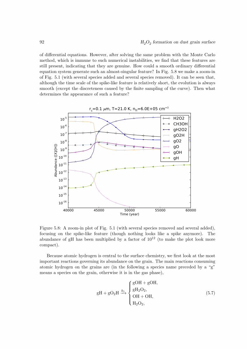
92 H2O2 formation on dust grain surface

of differential equations. However, after solving the same problem with the Monte Carlomethod, which is immune to such numerical instabilities, we find that these features arestill present, indicating that they are genuine. How could a smooth ordinary differentialequation system generate such an almost-singular feature? In Fig. 5.8 we make a zoom-inof Fig. 5.1 (with several species added and several species removed). It can be seen that,although the time scale of the spike-like feature is relatively short, the evolution is alwayssmooth (except the discreteness caused by the finite sampling of the curve). Then whatdetermines the appearance of such a feature?

40000 45000 50000 55000 60000Time (year)

10-16

10-15

10-14

10-13

10-12

10-11

10-10

10-9

10-8

10-7

10-6

10-5

Abun

danc

e ([

X]/[H

])

rg=0.1 m, T=21.0 K, nH=6.0E+05 cm3

H2O2CH3OHgH2O2gO2HgO2gOgOHgH

Figure 5.8: A zoom-in plot of Fig. 5.1 (with several species removed and several added),focusing on the spike-like feature (though nothing looks like a spike anymore). Theabundance of gH has been multiplied by a factor of 1012 (to make the plot look morecompact).

Because atomic hydrogen is central to the surface chemistry, we first look at the mostimportant reactions governing its abundance on the grain. The main reactions consumingatomic hydrogen on the grains are (in the following a species name preceded by a “g”means a species on the grain, otherwise it is in the gas phase),

gH + gO2Hk1−→

gOH + gOH,

gH2O2,

OH+OH,

H2O2,

(5.7)

5.A An explanation of the spike-like features in the evolution curves 93

gH + gH2O2k2−→

gH2O+ gOH,

H2O+OH,(5.8)

while others such as the reactions with gO3 and gCH2OH are relatively unimportant inthe early times. It is mainly produced by

Hk3−→ gH, (5.9)

gOH + gCOk4−→ gCO2 + gH, (5.10)

gH2Ok5−→ gOH + gH. (5.11)

As the abundance of atomic H in the gas phase and the abundance of gCO and gH2Ochange relatively smoothly, they can be viewed as constant on a short time scale. Themain reactions for the consumption and production of gOH are

gO + gOHk6−→

gO2H,

O2H,(5.12)

gCO + gOHk7−→

gCO2 + gH,

CO2 +H,(5.13)

gH + gO2Hk8−→ gOH + gOH, (5.14)

gH + gH2O2k9−→ gH2O+ gOH, (5.15)

gH2Ok10−−→ gH + gOH. (5.16)

From the above reaction list we may write the evolution equation of gH and gOH as[6]

∂tgH =− k1gHgO2H− k2gHgH2O2

+ k3H+ k4gOHgCO+ k5gH2O, (5.17)

∂tgOH =− k6gOgOH− k7gCOgOH

+ 2k8gHgO2H+ k9gHgH2O2 + k10gH2O, (5.18)

or in a more succinct form

∂tgH =κ1gH + κ2gOH + b1,

∂tgOH =κ3gH + κ4gOH + b2, (5.19)

where

κ1 =− k1gO2H− k2gH2O2,

κ2 =k4gCO,

κ3 =2k8gO2H+ k9gH2O2,

κ4 =− k6gO− k7gCO,

b1 =k3H+ k5gH2O,

b2 =k10gH2O.

[6]Here for brevity we use the name of a species to denote its average population on a single grain; forexample, if gCO=100, it means on average there are 100 CO molecules on a single grain.

94 H2O2 formation on dust grain surface

If we view κ1 – κ4, as well as b1 and b2, as constants (of course they are not), then Eq.(5.19) can be solved exactly; the solution contains an exponential part and a constant part.The amplitude of the exponential part will be inversely proportional to the determinantof the coefficient matrix

det(κ) =

(κ1 κ2κ3 κ4

).

Since κ1 – κ4 are not really constant in our problem, we expect that when they becomesuch that det(κ) is close to zero, a spike-like or jump-like behavior would appear. Namely,we require

κ1κ4κ2κ3

=(k1gO2H+ k2gH2O2)(k6gO + k7gCO)

(k4gCO)(2k8gO2H+ k9gH2O2)

' gO2H/gH2O2 + 1

1.2gO2H/gH2O2 + 1×(2.5× 108gO/gCO + 1

)'1. (5.20)

The actual value of the parameters have been inserted in the second line of the aboveequation. These parameters depend on the physical conditions.

To satisfy this condition (at least approximately), gO/gCO should be very small. InFig. 5.9 the ratio (κ1κ4)/(κ2κ3) and the value of 2.5×108gO/gCO are plotted as a functionof time. The abundances of O, gO, gO2, gH, and gOH are also plotted for reference (notto scale). It can be seen that the (κ1κ4)/(κ2κ3) ratio does decrease, and it approaches avalue of unity before the time of the spike/jump feature, and the gO/gCO ratio drops toa very low value monotonically.

The above mathematical argument can also be understood intuitively. When the gOabundance is so low that reaction (5.12) can be neglected, gOH is only destroyed byreaction (5.13). Each time a gOH radical is consumed, one gH is created (if we neglectthe desorption process), and this gH will quickly react with gH2O2 or gO2H to create oneor two gOHs. There will then be a net gain in the gOH abundance, leading to its fastgrowth, and the gH abundance will increase accordingly. Thus we see that reaction (5.14)is crucial in that it produced two gOH radicals by consuming only one gH.

Therefore for such a spike-like feature to occur, the abundance of gO must decrease to alow value such that the reaction between gOH and gO becomes unimportant for consuminggOH. Namely, we require [gO] . [gCO] k7/k6 ' 5 × 10−13. The abundances of atomicoxygen in the gas phase and on the grain surface are related by O/gO ' kevap(gO)/kad(O)' 3×106, so equivalently we require [O] < 1.5× 10−6 (i.e., about a factor of 200 less thanthe initial O abundance) at the time of the spike-like feature. Atomic oxygen is mainlyconsumed on the grain surface by reacting with another gO to form gO2 (for t . 103 yr) orby reacting with gOH to form gO2H. Only the latter is relevant here. As the abundance ofgOH does not change much before the spike-like feature, the time scale for the consumptionof atomic oxygen can be estimated to be ln 200× (O/gO)/(k6gOH) ' 105 yr, which is onthe same order of magnitude as the time of occurrence of the spike-like feature.

The time scale for the endurance of the spike-like feature itself can be estimated to bethe time scale for the exhaustion of gO2H or gH2O2 (so that Eqs. (5.17) and (5.18) donot hold anymore) by reacting with gH, which is

1/(k1gH) ' 103 yr,

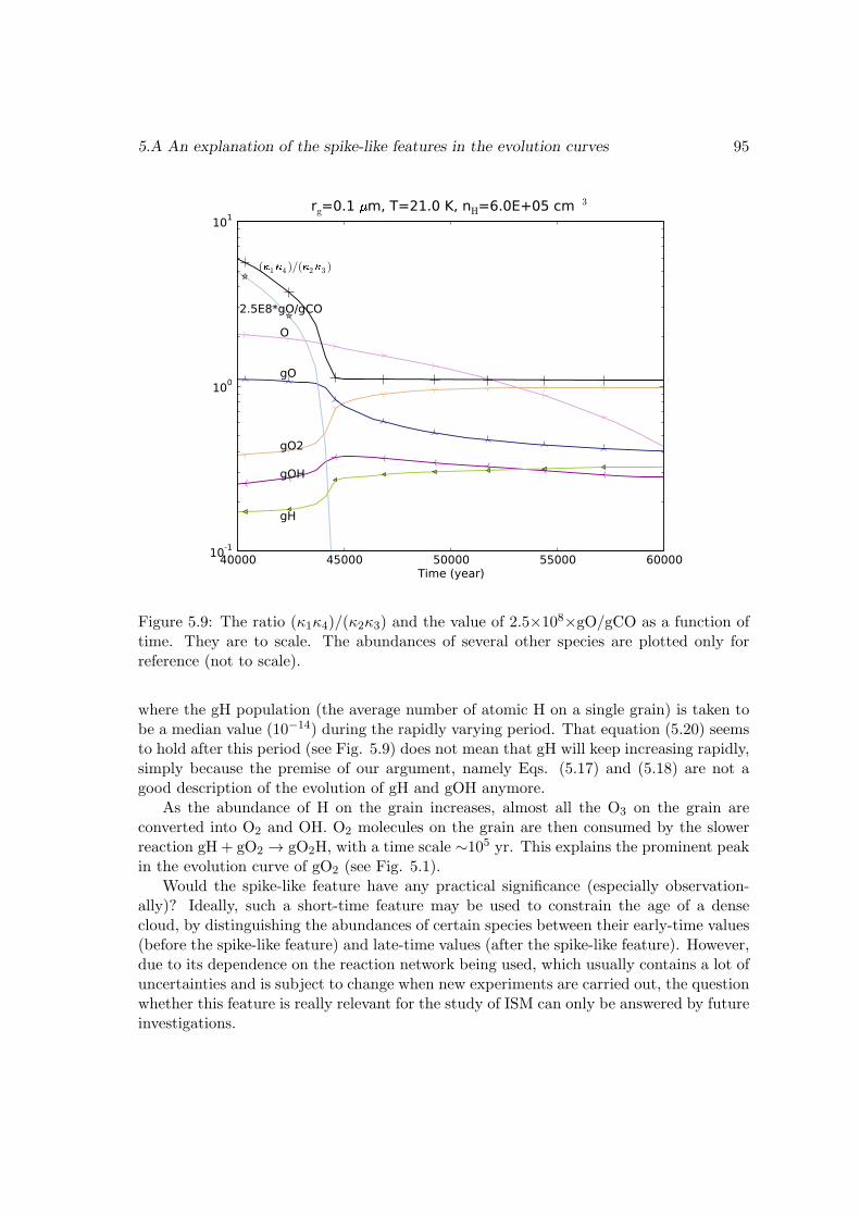
5.A An explanation of the spike-like features in the evolution curves 95

40000 45000 50000 55000 60000Time (year)

10-1

100

101

(14 )/(23 )

2.5E8*gO/gCO

gOH

gO

gO2

gH

O

rg=0.1 m, T=21.0 K, nH=6.0E+05 cm3

Figure 5.9: The ratio (κ1κ4)/(κ2κ3) and the value of 2.5×108×gO/gCO as a function oftime. They are to scale. The abundances of several other species are plotted only forreference (not to scale).

where the gH population (the average number of atomic H on a single grain) is taken tobe a median value (10−14) during the rapidly varying period. That equation (5.20) seemsto hold after this period (see Fig. 5.9) does not mean that gH will keep increasing rapidly,simply because the premise of our argument, namely Eqs. (5.17) and (5.18) are not agood description of the evolution of gH and gOH anymore.

As the abundance of H on the grain increases, almost all the O3 on the grain areconverted into O2 and OH. O2 molecules on the grain are then consumed by the slowerreaction gH + gO2 → gO2H, with a time scale ∼105 yr. This explains the prominent peakin the evolution curve of gO2 (see Fig. 5.1).

Would the spike-like feature have any practical significance (especially observation-ally)? Ideally, such a short-time feature may be used to constrain the age of a densecloud, by distinguishing the abundances of certain species between their early-time values(before the spike-like feature) and late-time values (after the spike-like feature). However,due to its dependence on the reaction network being used, which usually contains a lot ofuncertainties and is subject to change when new experiments are carried out, the questionwhether this feature is really relevant for the study of ISM can only be answered by futureinvestigations.

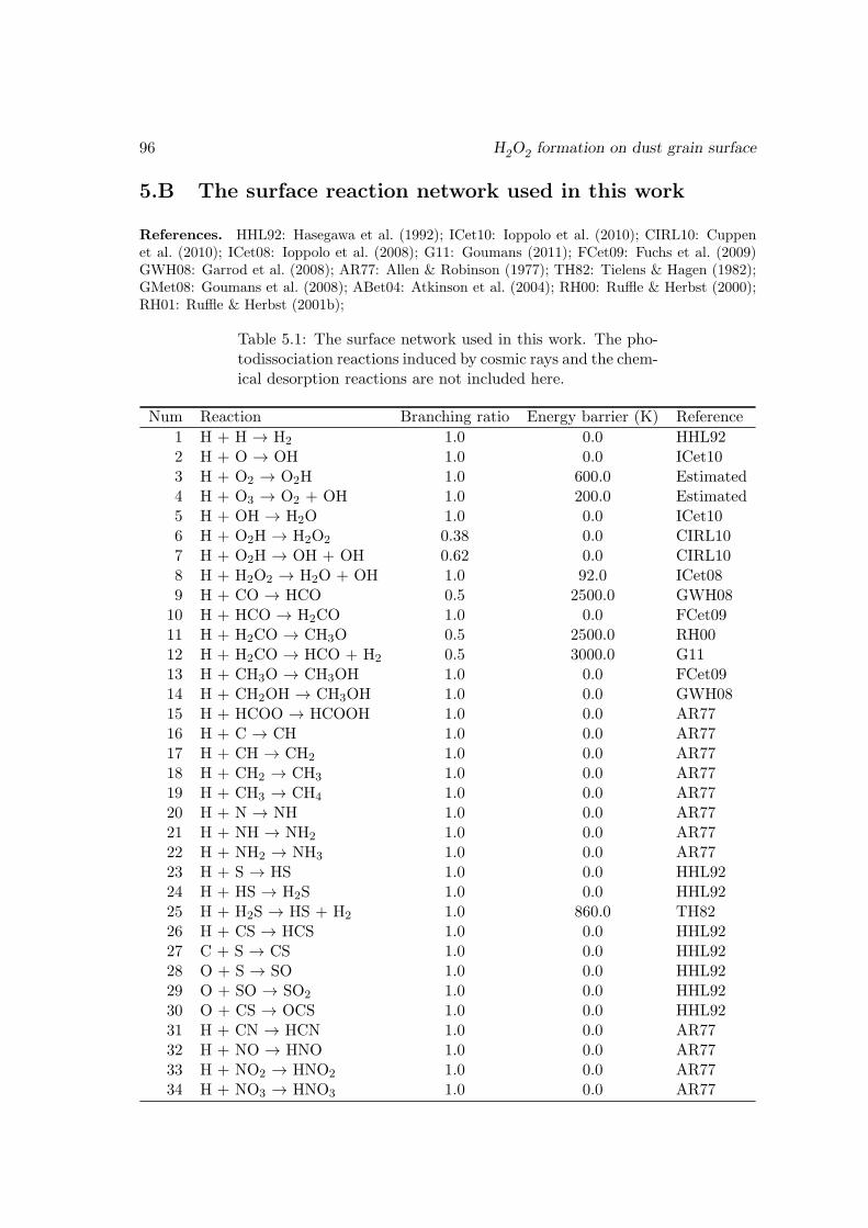
96 H2O2 formation on dust grain surface

5.B The surface reaction network used in this work

References. HHL92: Hasegawa et al. (1992); ICet10: Ioppolo et al. (2010); CIRL10: Cuppenet al. (2010); ICet08: Ioppolo et al. (2008); G11: Goumans (2011); FCet09: Fuchs et al. (2009)GWH08: Garrod et al. (2008); AR77: Allen & Robinson (1977); TH82: Tielens & Hagen (1982);GMet08: Goumans et al. (2008); ABet04: Atkinson et al. (2004); RH00: Ruffle & Herbst (2000);RH01: Ruffle & Herbst (2001b);

Table 5.1: The surface network used in this work. The pho-todissociation reactions induced by cosmic rays and the chem-ical desorption reactions are not included here.

Num Reaction Branching ratio Energy barrier (K) Reference

1 H + H → H2 1.0 0.0 HHL922 H + O → OH 1.0 0.0 ICet103 H + O2 → O2H 1.0 600.0 Estimated4 H + O3 → O2 + OH 1.0 200.0 Estimated5 H + OH → H2O 1.0 0.0 ICet106 H + O2H → H2O2 0.38 0.0 CIRL107 H + O2H → OH + OH 0.62 0.0 CIRL108 H + H2O2 → H2O + OH 1.0 92.0 ICet089 H + CO → HCO 0.5 2500.0 GWH0810 H + HCO → H2CO 1.0 0.0 FCet0911 H + H2CO → CH3O 0.5 2500.0 RH0012 H + H2CO → HCO + H2 0.5 3000.0 G1113 H + CH3O → CH3OH 1.0 0.0 FCet0914 H + CH2OH → CH3OH 1.0 0.0 GWH0815 H + HCOO → HCOOH 1.0 0.0 AR7716 H + C → CH 1.0 0.0 AR7717 H + CH → CH2 1.0 0.0 AR7718 H + CH2 → CH3 1.0 0.0 AR7719 H + CH3 → CH4 1.0 0.0 AR7720 H + N → NH 1.0 0.0 AR7721 H + NH → NH2 1.0 0.0 AR7722 H + NH2 → NH3 1.0 0.0 AR7723 H + S → HS 1.0 0.0 HHL9224 H + HS → H2S 1.0 0.0 HHL9225 H + H2S → HS + H2 1.0 860.0 TH8226 H + CS → HCS 1.0 0.0 HHL9227 C + S → CS 1.0 0.0 HHL9228 O + S → SO 1.0 0.0 HHL9229 O + SO → SO2 1.0 0.0 HHL9230 O + CS → OCS 1.0 0.0 HHL9231 H + CN → HCN 1.0 0.0 AR7732 H + NO → HNO 1.0 0.0 AR7733 H + NO2 → HNO2 1.0 0.0 AR7734 H + NO3 → HNO3 1.0 0.0 AR77

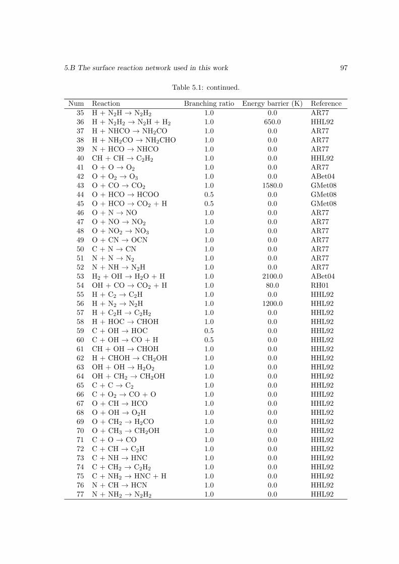
5.B The surface reaction network used in this work 97

Table 5.1: continued.

Num Reaction Branching ratio Energy barrier (K) Reference

35 H + N2H → N2H2 1.0 0.0 AR7736 H + N2H2 → N2H + H2 1.0 650.0 HHL9237 H + NHCO → NH2CO 1.0 0.0 AR7738 H + NH2CO → NH2CHO 1.0 0.0 AR7739 N + HCO → NHCO 1.0 0.0 AR7740 CH + CH → C2H2 1.0 0.0 HHL9241 O + O → O2 1.0 0.0 AR7742 O + O2 → O3 1.0 0.0 ABet0443 O + CO → CO2 1.0 1580.0 GMet0844 O + HCO → HCOO 0.5 0.0 GMet0845 O + HCO → CO2 + H 0.5 0.0 GMet0846 O + N → NO 1.0 0.0 AR7747 O + NO → NO2 1.0 0.0 AR7748 O + NO2 → NO3 1.0 0.0 AR7749 O + CN → OCN 1.0 0.0 AR7750 C + N → CN 1.0 0.0 AR7751 N + N → N2 1.0 0.0 AR7752 N + NH → N2H 1.0 0.0 AR7753 H2 + OH → H2O + H 1.0 2100.0 ABet0454 OH + CO → CO2 + H 1.0 80.0 RH0155 H + C2 → C2H 1.0 0.0 HHL9256 H + N2 → N2H 1.0 1200.0 HHL9257 H + C2H → C2H2 1.0 0.0 HHL9258 H + HOC → CHOH 1.0 0.0 HHL9259 C + OH → HOC 0.5 0.0 HHL9260 C + OH → CO + H 0.5 0.0 HHL9261 CH + OH → CHOH 1.0 0.0 HHL9262 H + CHOH → CH2OH 1.0 0.0 HHL9263 OH + OH → H2O2 1.0 0.0 HHL9264 OH + CH2 → CH2OH 1.0 0.0 HHL9265 C + C → C2 1.0 0.0 HHL9266 C + O2 → CO + O 1.0 0.0 HHL9267 O + CH → HCO 1.0 0.0 HHL9268 O + OH → O2H 1.0 0.0 HHL9269 O + CH2 → H2CO 1.0 0.0 HHL9270 O + CH3 → CH2OH 1.0 0.0 HHL9271 C + O → CO 1.0 0.0 HHL9272 C + CH → C2H 1.0 0.0 HHL9273 C + NH → HNC 1.0 0.0 HHL9274 C + CH2 → C2H2 1.0 0.0 HHL9275 C + NH2 → HNC + H 1.0 0.0 HHL9276 N + CH → HCN 1.0 0.0 HHL9277 N + NH2 → N2H2 1.0 0.0 HHL92

98 H2O2 formation on dust grain surface

Table 5.1: continued.

Num Reaction Branching ratio Energy barrier (K) Reference

78 O + NH → HNO 1.0 0.0 HHL92

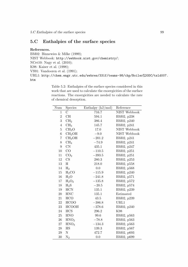
5.C Enthalpies of the surface species 99

5.C Enthalpies of the surface species

References.BM02: Binnewies & Milke (1999);NIST Webbook: http://webbook.nist.gov/chemistry/;NCet10: Nagy et al. (2010);K98: Kaiser et al. (1998);VS91: Vandooren et al. (1991);URL1: http://chem.engr.utc.edu/webres/331f/teams-98/chp/Boiler%20DC/tsld007.htm

Table 5.2: Enthalpies of the surface species considered in thiswork that are used to calculate the exoergicities of the surfacereactions. The exoergicities are needed to calculate the rateof chemical desorption.

Num Species Enthalpy (kJ/mol) Reference

1 C 716.7 NIST Webbook2 CH 594.1 BM02, p2383 CH2 386.4 BM02, p2404 CH3 145.7 BM02, p2415 CH3O 17.0 NIST Webbook6 CH2OH −9.0 NIST Webbook7 CH3OH −201.2 BM02, p2418 CH4 −74.9 BM02, p2419 CN 435.1 BM02, p247

10 CO −110.5 BM02, p25111 CO2 −393.5 BM02, p25112 CS 280.3 BM02, p25313 H 218.0 BM02, p55814 H2 0.0 BM02, p56815 H2CO −115.9 BM02, p24016 H2O −241.8 BM02, p57117 H2O2 −135.8 BM02, p57218 H2S −20.5 BM02, p57419 HCN 135.1 BM02, p23920 HNC 135.1 Estimated21 HCO 43.5 BM02, p23922 HCOO −386.8 URL123 HCOOH −378.6 BM02, p24024 HCS 296.2 K9825 HNO 99.6 BM02, p56326 HNO2 −78.8 BM02, p56327 HNO3 −134.3 BM02, p56328 HS 139.3 BM02, p56729 N 472.7 BM02, p69330 N2 0.0 BM02, p699

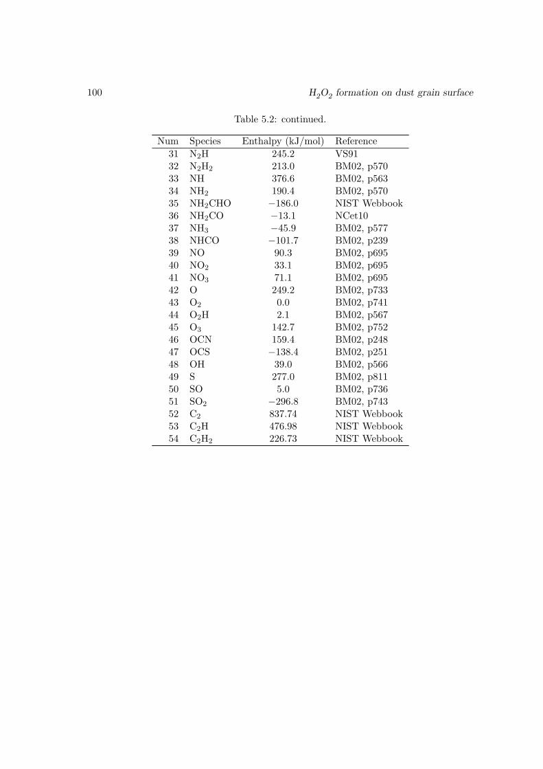
100 H2O2 formation on dust grain surface

Table 5.2: continued.

Num Species Enthalpy (kJ/mol) Reference

31 N2H 245.2 VS9132 N2H2 213.0 BM02, p57033 NH 376.6 BM02, p56334 NH2 190.4 BM02, p57035 NH2CHO −186.0 NIST Webbook36 NH2CO −13.1 NCet1037 NH3 −45.9 BM02, p57738 NHCO −101.7 BM02, p23939 NO 90.3 BM02, p69540 NO2 33.1 BM02, p69541 NO3 71.1 BM02, p69542 O 249.2 BM02, p73343 O2 0.0 BM02, p74144 O2H 2.1 BM02, p56745 O3 142.7 BM02, p75246 OCN 159.4 BM02, p24847 OCS −138.4 BM02, p25148 OH 39.0 BM02, p56649 S 277.0 BM02, p81150 SO 5.0 BM02, p73651 SO2 −296.8 BM02, p74352 C2 837.74 NIST Webbook53 C2H 476.98 NIST Webbook54 C2H2 226.73 NIST Webbook

Chapter 6

Deuterium chemistry on dustgrain surfaces

Part of the content of this chapter will be submitted to Astronomy & Astrophysics forpublication.

Contents

6.1 Why is deuterium special . . . . . . . . . . . . . . . . . . . . . . . . . . 101

6.2 Previous studies . . . . . . . . . . . . . . . . . . . . . . . . . . . . . . . 103

6.3 Preparation for the gas phase reaction network . . . . . . . . . . . . . . 106

6.4 The grain surface chemistry . . . . . . . . . . . . . . . . . . . . . . . . 112

6.5 The three-phase gas-surface-mantle model . . . . . . . . . . . . . . . . 133

6.6 Results and discussions . . . . . . . . . . . . . . . . . . . . . . . . . . . 137

6.7 Conclusions . . . . . . . . . . . . . . . . . . . . . . . . . . . . . . . . . 178

This chapter is about our modeling study on the chemistry of species containing one ormore deuterium atoms (we call these species “deuterated”). I begin with a discussion onthe uniqueness of deuterium in a general context, followed by a brief review on previousstudies on deuterium chemistry. Then I describe how we compile the gas and grainchemical network with deuterium included, and how we implement the “three-phase”gas-grain-mantle prescription. Finally the results and conclusions are presented.

6.1 Why is deuterium special

Besides the major isotope (denoted by 1H and sometimes called protium), hydrogen hastwo other isotopes: deuterium (2H) and tritium (3H). Deuterium is stable, while tritiumis radioactive with a half-life of ∼12.3 yr and decay products 3

2He+ + e – + νe (Simpson1987). It is easier for the deuterium and tritium nuclei than the hydrogen nuclei to fusewith other light nuclei, because the presence of more neutrons in the nuclei increasesthe attractive strong force when they are close by, while the repulsive electrostatic forceremains the same. Thus in the stars deuterium is the first to ignite (Clayton 1968).Except for the primordial nucleosynthesis at the beginning of the Universe through the

101

102 Deuterium chemistry on dust grain surfaces

reaction p+n −−→ D+γ (Weinberg 2008), it is commonly believed that there is no efficientnatural process to produce deuterium, so its overall abundance can only decrease withtime. However, Mullan & Linsky (1999) challenged this idea by proposing that deuteriumcan be produced in stellar atmospheres (during a stellar flare for example), which assuggested by these authors might be one reason for the inhomogeneity and enhancementof the deuterium abundance.

The total abundance of deuterium in the early Universe would thus be expected to behigher than its current value if the mainstream assumption about its evolution is correct,i.e. the suggestion of Mullan & Linsky (1999) is disregarded for the moment. Fumagalliet al. (2011) measured the abundance of deuterium using absorption lines towards thesightlines of high-z quasars, obtaining [D/H] ' 2.78×10−5, providing a constraint on thebaryon density parameter (Ωb) in cosmology, which is consistent with an independentconstraint from measurements of the anisotropies in the cosmic microwave background.Linsky et al. (2006) argued that the atomic [D/H] ratio representative of the region within1 kpc[1] of the Sun ≥2.3×10−5. By analyzing the solar wind composition, Geiss & Reeves(1972) estimated that the [D/H] ratio ' 2.5×10−5 in the proto-solar gas. In Jupiter andSaturn, the [D/H] ratio of H2 molecules was measured with the Infrared Space Observatory(ISO) by Lellouch et al. (2001) to be ∼2.3×10−5 and ∼1.7×10−5, respectively. The [D/H]ratio in comet water was measured to be of the order (1.5–3)×10−4 (depending on thebirth places of these comets) (Hartogh et al. 2011). In Earth’s ocean the [D/H] ratio is∼1/6700'1.5×10−4 (Friedman 1953), and varies slightly from place to place[2]. Accordingto the review of Robert (2003), the overall [D/H] ratio in carbonaceous chondrites lies inthe range (1.2–3)×10−4, and peaks at ∼1.5×10−4.

Studies on the isotopic ratio of hydrogen and of many other elements in different typesof terrestrial and celestial bodies play a vital role in understanding the origin and evolu-tion of objects with vast diversity, from Earth’s water, the Earth itself, the origin of bioticmatter, to the origin of the solar system, and even to the origin of the Universe. For exam-ple, people use tritium (generated by nuclear weapon tests) to trace ocean circulation andventilation (Jenkins & Smethie 1996); the 13C/12C ratio can be used to study the effectsof human activities have on the Earth’s atmosphere based on the discrimination against13C in plants (Ghosh & Brand 2003); the organic matter in chondrite meteorites was sug-gested by Sephton & Gilmour (2000) to have originated in interstellar space because ofthe 13C and deuterium abundances; finally, the [D/H] ratio at an early cosmological ageis a crucial parameter to constrain the baryon density of the Universe (see, e.g., Weinberg2008).

The observed deuterium enrichment in many species (see the next section) is generallybelieved to be due to chemical fractionation, in which H and D atoms behave differentlyin chemical reactions. The effects of chemical fractionation can be distinguished from thatof an overall increase in the deuterium abundance due to the mechanisms suggested byMullan & Linsky (1999). In chemical fractionation, the [D/H] ratio of a species stronglydepends on its formation route, while an overall increase in the deuterium abundancewould not have such a dependence; thus if the observed deuterium enrichment is chem-ical in nature, one would expect different species to have different degrees of deuterium

[1]1 pc ' 3.1× 1018 cm[2]In the “Vienna Standard Mean Ocean Water”, the [D/H] ratio is 1.5576×10−4; see http://en.

wikipedia.org/wiki/Vienna_Standard_Mean_Ocean_Water.

6.2 Previous studies 103

enhancement, and the total deuterium abundance would be more or less the same fordifferent regions of the interstellar space (if the consumption of deuterium in the stars isproperly accounted for).

The chemical fractionation of the two stable isotopes of hydrogen (H and D) is specialwhen compared to other elements because of their large mass ratio of 2, which is thelargest among all elements. Such a large ratio leads to a large difference in the zero-pointvibrational energies of deuterium and hydrogen, which is vital at very low temperatures.The difference in mass also causes a difference in their migration and tunneling rates onthe dust grain surface, which affects their surface reaction rates. Replacing a hydrogenatom by a deuterium atom in a molecule can also change its energy levels and transitionprobabilities; for example, H2 and CH4 have no electric dipole moment, but HD andCH3D do.

In this chapter I present a chemical model that takes into account both gas phaseprocesses and reactions occurring on dust grain surfaces. The goal is to investigate towhat extent can chemical processes lead to the differentiated distribution of deuteriumatoms in various species in the ISM, specifically in dark cloud conditions. Note thatthe possibility that the atomic deuterium abundance might be enriched by processes instellar atmosphere (Mullan & Linsky 1999) is not considered in the present work. InSection 6.2 I give a brief overview of previous studies on deuterium fractionation. InSection 6.3 I describe the gas phase reaction network, which is a subset of the UMISTRATE06 network[3] (Woodall et al. 2007) with deuterium added in, then in Section 6.4I discuss the surface reaction network, especially on the key reactions for formaldehyde,methanol, and water. Our dust grain model takes into account the mantle structure,which is described in detail in Section 6.5. The results and conclusions are presented inSection 6.6.

6.2 Previous studies

Deuterium-containing molecules have been studied in the interstellar space for quite sometime. The first one detected beyond our solar system was DCN (Jefferts et al. 1973; Wilsonet al. 1973), observed in the Orion molecular cloud. These authors derived a [D/H] ratio of∼6×10−3, which they attributed to chemical fractionation. In particular they mentionedthat the zero-point vibrational energy of DCN is much lower than that of HCN, which cancause deuterium enrichment, either in the gas phase or on dust grain surfaces, especiallyat low temperatures. Solomon & Woolf (1973) discussed the deuterium fractionation ofHCN with the exchange reactions HD+HCN −−−− H2+DCN and D+HCN −−−− DCN+H,based only on energetic considerations. Namely, they claim (for the first reaction)

[DCN]

[HCN]=

[HD]

[H2]exp

(456

T

)=

2[D]

[H]exp

(456

T

),

where the number 456 (K) is the exothermicity of the first reaction. Also based on such anenergy argument, they inferred the possible enhancement of the ratio [HD]/[H2] relativeto [D]/[H]. However, their arguments have been questioned by Watson (1974) and Brown(1977) due to the presence of activation barriers in those reactions. We may also note that

[3]http://udfa.net/

104 Deuterium chemistry on dust grain surfaces

Watson (1973) proposed another mechanism to enhance the atomic [D/H] ratio (whichcan then be transferred to HCN and DCN), in which the HD molecule is more likelyto be photo-dissociated (into H and D atoms) due to its lower degree of self-shieldingthan H2. Such a mechanism may indeed be at work in certain situations. Finally, thelower [DCN/HCN] ratio towards the Galactic center relative to other regions was usedby Penzias et al. (1977) to argue against the possibility that the observed deuteriumenhancement is due to stellar processes.

DCO+ was first detected by Hollis et al. (1976) and Guelin et al. (1977) in darkclouds. Watson (1977) and Watson et al. (1978) discussed the possibility of constrainingthe electron abundance in the ISM by measuring [DCO+/HCO+]. This idea is based onthe assumption that DCO+ is formed from H2D

+ +CO, hence the ratio [DCO+/HCO+]reflects the ratio [H2D

+/H+3 ], which is directly related to the electron abundance (hence

to the degree of ionization). In this example we can see that the formation route of aspecific molecule may provide useful information on certain physical parameters. Dalgarno& Lepp (1984) gave a similar discussion on [DCO+/HCO+] and used this ratio to givelower and upper limits on the overall [D/H] ratio.

The HD molecule was first detected by Spitzer et al. (1973) in UV absorption. Deuter-ated water (HDO) was first detected by Turner et al. (1975) in Orion KL, at an abun-dance of ∼10−8 relative to H2, and deuterated ammonia (NH2D) was first detectedby Rodriguez Kuiper et al. (1978) also in this source. The first multiply-deuteratedmolecule discovered in the ISM is D2CO, detected by Turner (1990) in the compact ridgecomponent of Orion KL, with a relative abundance of [D2CO]/[HDCO] ' 0.02, while[HDCO]/[H2CO] ' 0.1. Based on simple equilibrium analysis, Turner concluded thatH2CO and its deuterated counterparts can be formed on dust grain surface. van der Taket al. (2002) detected triply deuterated ammonia (ND3) in NGC 1333 with an abundanceof 3×10−12–10−11.

In a survey van Dishoeck et al. (1995) detected more than 40 molecules in the lowmass proto-binary source IRAS 16293−2422, including many deuterated species, suchas DCO+, DCN, DNC, CCD, HDS, HDO, CH3OD, etc. This source has a remarkablyrich deuterium chemistry. For example, Ceccarelli et al. (1998), Loinard et al. (2000)and Ceccarelli et al. (2001) found high [HDCO/H2CO] and [D2CO/HDCO] ratios in it.Parise et al. (2002, 2004) detected doubly and triply deuterated methanol (CHD2OH andCD3OH) in this source, with abundances a few to ten percent of the main isotopologue.It has also been found that the D atom has a preference over the CH3 group than theOH group in this source, so CH2DOH is much more abundant than CH3OD. The degreeof deuteration of water is relatively low in comparison with methanol and formaldehyde.For example, the [HDO/H2O] ratio in IRAS 16293−2422 was constrained by Parise et al.(2005) to be 3% in the inner hot region and ≤0.2% in the outer envelope, and Liu et al.(2011) found a similar [HDO/H2O] ratio (&1%) for the inner region of the low-massprotostar NGC1333-IRAS2A.

Besides the qualitative analysis in the early times, theoretical studies on deuteriumchemistry include the gas phase models of Millar et al. (1989), Roberts & Millar (2000b),Roberts & Millar (2000a), Turner (2001), Roberts et al. (2003), Roberts et al. (2004),Roueff et al. (2007), and grain chemical models of Tielens (1983), Brown & Millar (1989),Caselli et al. (2002), Stantcheva & Herbst (2003), and the recent work of Albertsson et al.(2011) and Taquet et al. (2012). The gas phase part of the chemistry is essential, since all

6.2 Previous studies 105

the species on dust grains are from the gas phase, and the “driving force” of deuteriumfractionation is in the gas phase. This is because at low temperatures only H and D(and possibly the H2 isotopologues and light atoms such as C, N, O, though much lessmobile than H and D) are mobile on the grain surface, which are the active participants ofsurface processes. Thus to get a high deuterium fractionation ratio on the grain surface,the [D/H] ratio in the H and D fluxes accreted on the dust grains should not be too low.The gas phase chemistry serves to provide the H and D fluxes in a self-consistent way.This is different from some of the previous studies, e.g. Stantcheva & Herbst (2003) andCaselli et al. (2002), in which the H and D flux ratio was assumed arbitrarily.

D atoms are extracted from HD molecules through cosmic-ray ionization of H2 andthe accompanying ion-neutral and dissociative recombination reactions:

H2 +CRP −−→ H+2 + E−, (6.1)

H2 +H+2 −−→ H+

3 +H, (6.2)

H+3 +HD −−→ H2D

+ +H2 + 220 K, (6.3)

H2D+ +HD −−→ HD+

2 +H2 + 187 K, (6.4)

HD+2 +HD −−→ D+

3 +H2 + 234 K, (6.5)

H2D+ + E− −−→ D+ 2H, (6.6)

HD+2 + E− −−→ 2D + H, (6.7)

D+3 + E− −−→ 3D. (6.8)

Note that the reactions extracting D from HD by the H+3 isotopologues are exothermic

by about 200 K, so at low temperatures the reactions in the reverse direction will be veryslow. For example, at 10 K an exothermicity of 200 K will render the reverse reaction10−9 times slower than the forward direction. Thus a low temperature tends to enhancethe [H2D

+/H+3 ], [HD

+2 /H

+3 ], and [D+

3 /H+3 ] ratios, hence the atomic [D/H] ratio, and the

degree of such an enhancement is temperature-sensitive.Another aspect is, when other abundant heavy molecular species (such as CO and

N2) exist, H+3 and its isotopologues are mainly consumed by protonating (or deuterating)

them, through reactions such as

H2D+ +CO −−→ HCO+ +HD or DCO+ +H2, (6.9)

to form species such as HCO+, DCO+, N2H+, and N2D

+, returning the deuterium atomback to the HD molecule at the same time. Hence to make the above mechanism forenhancing the atomic [D/H] ratio really work we require the depletion of these heavymolecules from the gas phase. A lower temperature (and a higher density) tends tosuppress the evaporation of molecules adsorbed on the dust grains, also pushing thesystem towards the direction of atomic D enrichment.

Besides the H+3 isotopologues, the deuterated isotopologues of CH+

3 are also believedto play a role in deuterium fractionation at higher temperatures because of the higherexothermicity involved in their deuteration reactions.

These reactions are included in the gas phase part of our network. Our model containsa complete network for species with astrochemical interest, such as H2O, CH3OH, andH2CO, and many others, as well as their deuterated variants, both in the gas phase andon the dust grains. The details of the network are described in the following sections.

106 Deuterium chemistry on dust grain surfaces

6.3 Preparation for the gas phase reaction network

Both gas phase reactions and dust grain surface reactions are included in our model. Thecoupling between gas phase chemistry and surface chemistry is important, because thelatter is driven by the species accreted from the gas phase, and this accretion process canin turn affect the behavior of the gas phase chemistry significantly.

The gas phase chemical networks publicly available usually do not include deuterium[4].Hence we have to devise an algorithm to add deuterium atom to the network in a “ra-tional” way. One problem is, when deuterium is being added, the number of reactionsgrows very quickly. This can be understood by a simple example. Given the reactionH2 +H2O

+ −−→ H3O+ +H, its singly deuterated version can be

HD + H2O+ −−→ H2DO+ +H,

HD+H2O+ −−→ H3O

+ +D,

H2 +HDO+ −−→ H2DO+ +H, and

H2 +HDO+ −−→ H3O+ +D.

(6.10)

We can see that even if only one deuterium is included, one single reaction proliferatesinto 1+4 = 5 reactions. Allowing more deuterium atoms will enlarge the network further.For the UMIST RATE06 network, which contains more than 4000 reactions, allowing thesimultaneous presence of four deuterium atoms in each reaction will generate a reactionset with ∼27000 reactions. Although a network with such size can still be handled withinthe rate equation framework, it becomes very slow if the surface reactions are added, andespecially if the moment equation approach is adopted.

Thus we need to reduce the size of the gas phase reaction network without sacrificingthe accuracy too much. The procedure is described in Section 6.3.1. In Section 6.3.2 wedescribe the procedure for adding deuterium into the gas phase network.

6.3.1 Reducing the gas phase reaction network

There are several previous papers dedicated to the topic of reducing a chemical network(Rae et al. 2002; Ruffle et al. 2002; Wiebe et al. 2003; Semenov et al. 2004; Grassi et al.2012). Their motivation is to speed up the chemical evolution code, which may be coupledwith a magneto-hydrodynamic code. This purpose leads them to mainly address the ion-ization degree of the chemical system, and species that are potentially important coolants(such as the CO molecule). This is different from our purpose, namely, to calculate theabundances of a set of molecules of interest that are not necessarily important for thedynamics and energetics of the cloud.

A straightforward approach to reduce the network would be to remove reactions oneby one, and if the results obtained with the reduced network deviated too much, to addback the previously removed reaction, and try removing another reaction. Although thisseems to be a secure way, it is too time consuming, since the code has to be run as manytimes as the number of equations in the reaction network, which may take hours to finish.

[4]One exception may be the chemistry file of the Meudon PDR code, available at http://pdr.obspm.fr/PDRcode_Chemistry.html. But it is not suitable for our purpose: only one deuterium atom is allowedin each species at most. The format of this network is also different from the one we are usually dealingwith.

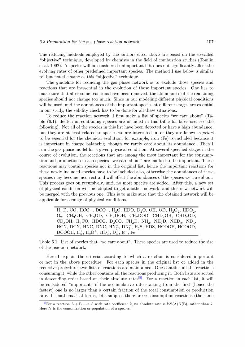
6.3 Preparation for the gas phase reaction network 107

The reducing methods employed by the authors cited above are based on the so-called“objective” technique, developed by chemists in the field of combustion studies (Tomlinet al. 1992). A species will be considered unimportant if it does not significantly affect theevolving rates of other predefined important species. The method I use below is similarto, but not the same as this “objective” technique.

The guideline for reducing the gas phase network is to exclude those species andreactions that are inessential in the evolution of those important species. One has tomake sure that after some reactions have been removed, the abundances of the remainingspecies should not change too much. Since in our modeling different physical conditionswill be used, and the abundances of the important species at different stages are essentialin our study, the validity check has to be done for all these situations.

To reduce the reaction network, I first make a list of species “we care about” (Ta-ble (6.1); deuterium-containing species are included in this table for later use; see thefollowing). Not all of the species in this list have been detected or have a high abundance,but they are at least related to species we are interested in, or they are known a priorito be essential for the chemical evolution; for example, iron (Fe) is included because itis important in charge balancing, though we rarely care about its abundance. Then Irun the gas phase model for a given physical condition. At several specified stages in thecourse of evolution, the reactions that are among the most important for the consump-tion and production of each species “we care about” are marked to be important. Thesereactions may contain species not in the original list, hence the important reactions forthese newly included species have to be included also, otherwise the abundances of thesespecies may become incorrect and will affect the abundances of the species we care about.This process goes on recursively, until no more species are added. After this, a new setof physical condition will be adopted to get another network, and this new network willbe merged with the previous one. This is to make sure that the obtained network will beapplicable for a range of physical conditions.

H, D, CO, HCO+, DCO+, H2O, HDO, D2O, OH, OD, H2O2, HDO2,O2, CH3OH, CH3OD, CH2DOH, CH2DOD, CHD2OH, CHD2OD,CD3OH, H2CO, HDCO, D2CO, CH3D, NH3, NH2D, NHD2, ND3,HCN, DCN, HNC, DNC, HN+

2 , DN+2 , H2S, HDS, HCOOH, HCOOD,

DCOOH, H+3 , H2D

+, HD+2 , D

+3 , E

– , Fe

Table 6.1: List of species that “we care about”. These species are used to reduce the sizeof the reaction network.

Here I explain the criteria according to which a reaction is considered importantor not in the above procedure. For each species in the original list or added in therecursive procedure, two lists of reactions are maintained. One contains all the reactionsconsuming it, while the other contains all the reactions producing it. Both lists are sortedin descending order based on their absolute rates[5]. For a reaction in each list, it willbe considered “important” if the accumulative rate starting from the first (hence thefastest) one is no larger than a certain fraction of the total consumption or productionrate. In mathematical terms, let’s suppose there are n consumption reactions (the same

[5]For a reaction A + B −−→ C with rate coefficient k, its absolute rate is kN(A)N(B), rather than k.Here N is the concentration or population of a species.

108 Deuterium chemistry on dust grain surfaces

for production reactions) for species A in the unreduced network, and denote the absoluterate of the ith fastest reaction for the consumption of species A by Ci. Note that Ci isa function of the abundances of species in the network, which vary with time; it can alsohave explicit time dependence. Hence the ordering of the reactions may be different atdifferent times. The jth fastest reaction will be considered important if

j∑i=1

Ci ≤ f

n∑i=1

Ci. (6.11)

The f parameter can be tuned, and is taken to be 0.8 for the first iteration (i.e. for thespecies we care about), and 0.5 for newly added species. These parameters are chosen sothat the number of reactions are small while guaranteeing the abundances of the specieswe care about do not vary by more than a factor of two before and after the reduction.To further limit the number of reactions being added, the f parameter is varied accordingto the relative importance of the species newly added. New species are added becausenew reactions are included, which may lead to the inclusion of species that had notbeen included before. A species being added due to a slower reaction is considered lessimportant than a species being part of a faster reaction.

Furthermore, reactions with a time scale longer than 109 yr are excluded, and specieswith too small abundances and/or too many metal atoms are not included. These numberscan be tuned, balancing between limiting the number of reactions to be included, andkeeping the discrepancies in the abundances of the important species small.

By requiring that the resulting network be applicable for a range of temperatures(10–50 K), and a range of densities (104–106 cm−3), the UMIST RATE06 network isreduced to contain 650 reactions, while abundances of the species we care about do notvary by more than a factor of two for all these physical conditions and for a time rangeof 102–107 yr (except for H2S, which varies by a factor less than three).

6.3.2 Deuterating the gas phase reaction network

By “deuterating” a network, I mean adding deuterium atoms to a reaction network thatdoes not contain deuterium yet. The procedure has two steps, one is to replace the oneor more hydrogen atoms in each species by deuterium atoms, based on certain rules,assuming the reactions rates are the same as the undeuterated ones, except for a possiblebranching ratio based on statistical weights. Another is to include a “driving network”,which includes important deuterium transfer reactions, whose inverse reactions usuallyhave a significant endothermicity, and thus are inactive at very low temperatures. Hencethese reactions drive the degree of deuteration into one direction, leading to deuteriumenhancement in many species.

For the first step, namely, to incorporate deuterium into the gas phase network in anautomatic way, I follow the rules listed below:

1. For each reaction, a new reaction obtained by replacing the same number of hy-drogen atoms on both sides (reactants and products) by deuterium atoms is alwaysconsidered viable. Namely, we assume “complete scrambling”.

2. For a given set of deuterated reactants, there will likely be several product channels.

6.3 Preparation for the gas phase reaction network 109

Their relative branching ratios are obtained by assuming all the hydrogen atoms inthe products have equal probability to be replaced by a deuterium atom.

3. The total reaction rate (summed over all the product branches) is assumed to bethe same as for the original reaction.

These rules are not necessarily correct from the point of view of theoretical chemistry.It may be utterly true that in a reaction a deuterium atom in a species could not betransferred from one functional group to another. This depends on our knowledge aboutthe detailed reaction mechanism. The “complete scrambling” assumption is based on apicture that when two reactants collide, they merge to form an activated complex in achaotic way so that the information on their initial configuration is lost, hence a deuteriumatom is able to change its location among functional groups.

Take the dissociative recombination reaction CH3OH+2 + E – −−→ CH3OH + H as an

example[6] (here E – means an electron). In one of its singly deuterated versions, the lefthand side is CH2DOH+

2 +E – . Without the complete scrambling assumption, the productscould only be CH2DOH + H. This is based on the picture that an electron is combinedwith a proton affiliated with the hydroxyl (OH) group of methanol, to neutralize thecharge. The attractive force between one hydrogen nucleus of the OH2 group and themain part of the molecule disappears due to this neutralization, and one hydrogen atomis thus ejected. But assuming complete scrambling, there are several possible productchannels, leading to the products:

CH2DOH+H,

CH3OD+H,

CH3OH+D.

(6.12)

The second and third channel may appear contradictory to our “chemical intuition”, butthey are nevertheless not impossible. Whether these channels really proceed in reality canonly be determined by careful experiments and/or sophisticated theoretical calculations,both of which are out of the scope of our study. So the complete scrambling assumptioncan be viewed as a “working hypothesis”. Another reason to make this assumption isdue to a practical challenge in programing: it is not straightforward to determine whichpart of a sequence of letters such as “CH2DOH2+” can be called a “functional group”,and to determine which groups are conserved in a reaction, and which groups have beenfragmented or have merged with other reactants. This problem can be illustrated withthe reaction CH3OH+

2 +E – −−→ H2CO+H2+H. One may imagine that the two hydrogenatoms connected to O are ejected as a H2 molecule, while one hydrogen atom in the CH3

group is also ejected. This picture is not necessarily correct. Before this type of picturesare well-justified, it is not urgent to devise an algorithm to implement it.

Regarding the second rule, a deuterium atom may actually prefer to stay in onefunctional group of a chemical compound than in another (this will be emphasized inSection 6.4 about the surface chemistry network). But since theoretical or experimentalstudies on most of the deuterated reactions that are needed in our study are not availableyet, the best we can do is to assume that all the positions are equally possible. Based

[6]There are another two product channels CH3 + OH + H and H2CO + H2 + H, which are neglectedhere.

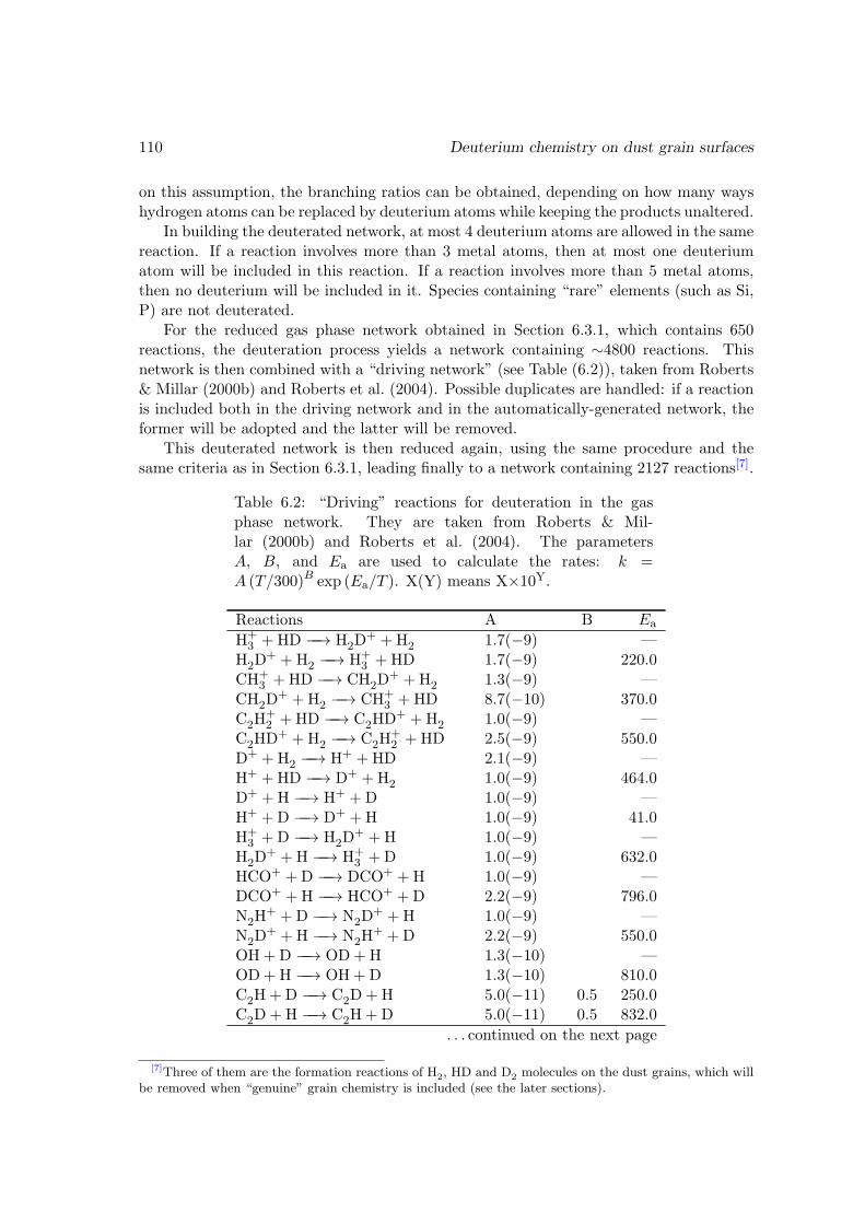
110 Deuterium chemistry on dust grain surfaces

on this assumption, the branching ratios can be obtained, depending on how many wayshydrogen atoms can be replaced by deuterium atoms while keeping the products unaltered.

In building the deuterated network, at most 4 deuterium atoms are allowed in the samereaction. If a reaction involves more than 3 metal atoms, then at most one deuteriumatom will be included in this reaction. If a reaction involves more than 5 metal atoms,then no deuterium will be included in it. Species containing “rare” elements (such as Si,P) are not deuterated.

For the reduced gas phase network obtained in Section 6.3.1, which contains 650reactions, the deuteration process yields a network containing ∼4800 reactions. Thisnetwork is then combined with a “driving network” (see Table (6.2)), taken from Roberts& Millar (2000b) and Roberts et al. (2004). Possible duplicates are handled: if a reactionis included both in the driving network and in the automatically-generated network, theformer will be adopted and the latter will be removed.

This deuterated network is then reduced again, using the same procedure and thesame criteria as in Section 6.3.1, leading finally to a network containing 2127 reactions[7].

Table 6.2: “Driving” reactions for deuteration in the gasphase network. They are taken from Roberts & Mil-lar (2000b) and Roberts et al. (2004). The parametersA, B, and Ea are used to calculate the rates: k =A (T/300)B exp (Ea/T ). X(Y) means X×10Y.

Reactions A B Ea

H+3 +HD −−→ H2D

+ +H2 1.7(−9) —H2D

+ +H2 −−→ H+3 +HD 1.7(−9) 220.0

CH+3 +HD −−→ CH2D

+ +H2 1.3(−9) —CH2D

+ +H2 −−→ CH+3 +HD 8.7(−10) 370.0

C2H+2 +HD −−→ C2HD

+ +H2 1.0(−9) —C2HD

+ +H2 −−→ C2H+2 +HD 2.5(−9) 550.0

D+ +H2 −−→ H+ +HD 2.1(−9) —H+ +HD −−→ D+ +H2 1.0(−9) 464.0D+ +H −−→ H+ +D 1.0(−9) —H+ +D −−→ D+ +H 1.0(−9) 41.0H+

3 +D −−→ H2D+ +H 1.0(−9) —

H2D+ +H −−→ H+

3 +D 1.0(−9) 632.0HCO+ +D −−→ DCO+ +H 1.0(−9) —DCO+ +H −−→ HCO+ +D 2.2(−9) 796.0N2H

+ +D −−→ N2D+ +H 1.0(−9) —

N2D+ +H −−→ N2H

+ +D 2.2(−9) 550.0OH +D −−→ OD+H 1.3(−10) —OD+H −−→ OH+D 1.3(−10) 810.0C2H+D −−→ C2D+H 5.0(−11) 0.5 250.0C2D+H −−→ C2H+D 5.0(−11) 0.5 832.0

. . . continued on the next page

[7]Three of them are the formation reactions of H2, HD and D2 molecules on the dust grains, which willbe removed when “genuine” grain chemistry is included (see the later sections).

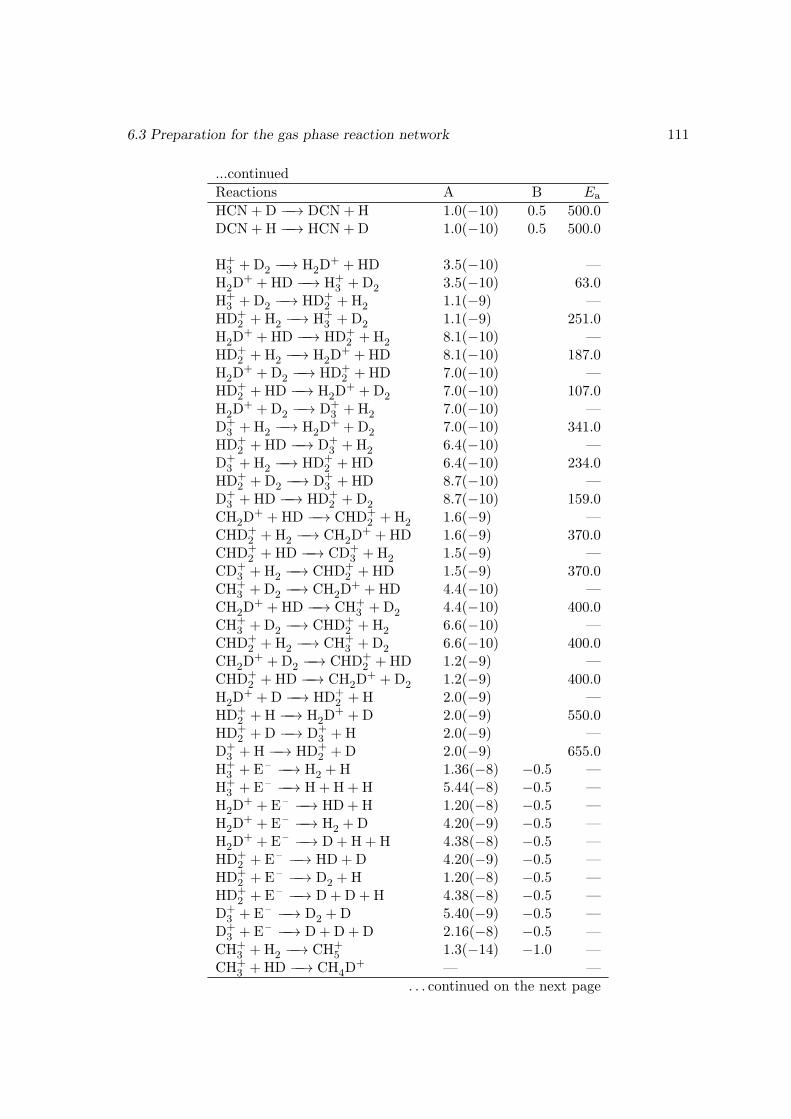
6.3 Preparation for the gas phase reaction network 111

...continued

Reactions A B Ea

HCN+D −−→ DCN+H 1.0(−10) 0.5 500.0DCN+H −−→ HCN+D 1.0(−10) 0.5 500.0

H+3 +D2 −−→ H2D

+ +HD 3.5(−10) —H2D

+ +HD −−→ H+3 +D2 3.5(−10) 63.0

H+3 +D2 −−→ HD+

2 +H2 1.1(−9) —HD+

2 +H2 −−→ H+3 +D2 1.1(−9) 251.0

H2D+ +HD −−→ HD+

2 +H2 8.1(−10) —HD+

2 +H2 −−→ H2D+ +HD 8.1(−10) 187.0

H2D+ +D2 −−→ HD+

2 +HD 7.0(−10) —HD+

2 +HD −−→ H2D+ +D2 7.0(−10) 107.0

H2D+ +D2 −−→ D+

3 +H2 7.0(−10) —D+

3 +H2 −−→ H2D+ +D2 7.0(−10) 341.0

HD+2 +HD −−→ D+

3 +H2 6.4(−10) —D+

3 +H2 −−→ HD+2 +HD 6.4(−10) 234.0

HD+2 +D2 −−→ D+

3 +HD 8.7(−10) —D+

3 +HD −−→ HD+2 +D2 8.7(−10) 159.0

CH2D+ +HD −−→ CHD+

2 +H2 1.6(−9) —CHD+

2 +H2 −−→ CH2D+ +HD 1.6(−9) 370.0

CHD+2 +HD −−→ CD+

3 +H2 1.5(−9) —CD+

3 +H2 −−→ CHD+2 +HD 1.5(−9) 370.0

CH+3 +D2 −−→ CH2D

+ +HD 4.4(−10) —CH2D

+ +HD −−→ CH+3 +D2 4.4(−10) 400.0

CH+3 +D2 −−→ CHD+

2 +H2 6.6(−10) —CHD+

2 +H2 −−→ CH+3 +D2 6.6(−10) 400.0

CH2D+ +D2 −−→ CHD+

2 +HD 1.2(−9) —CHD+

2 +HD −−→ CH2D+ +D2 1.2(−9) 400.0

H2D+ +D −−→ HD+

2 +H 2.0(−9) —HD+

2 +H −−→ H2D+ +D 2.0(−9) 550.0

HD+2 +D −−→ D+

3 +H 2.0(−9) —D+

3 +H −−→ HD+2 +D 2.0(−9) 655.0

H+3 + E – −−→ H2 +H 1.36(−8) −0.5 —

H+3 + E – −−→ H+H+H 5.44(−8) −0.5 —

H2D+ + E – −−→ HD+H 1.20(−8) −0.5 —

H2D+ + E – −−→ H2 +D 4.20(−9) −0.5 —

H2D+ + E – −−→ D+H+H 4.38(−8) −0.5 —

HD+2 + E – −−→ HD+D 4.20(−9) −0.5 —

HD+2 + E – −−→ D2 +H 1.20(−8) −0.5 —

HD+2 + E – −−→ D+D+H 4.38(−8) −0.5 —

D+3 + E – −−→ D2 +D 5.40(−9) −0.5 —

D+3 + E – −−→ D+D+D 2.16(−8) −0.5 —

CH+3 +H2 −−→ CH+

5 1.3(−14) −1.0 —CH+

3 +HD −−→ CH4D+ — —

. . . continued on the next page

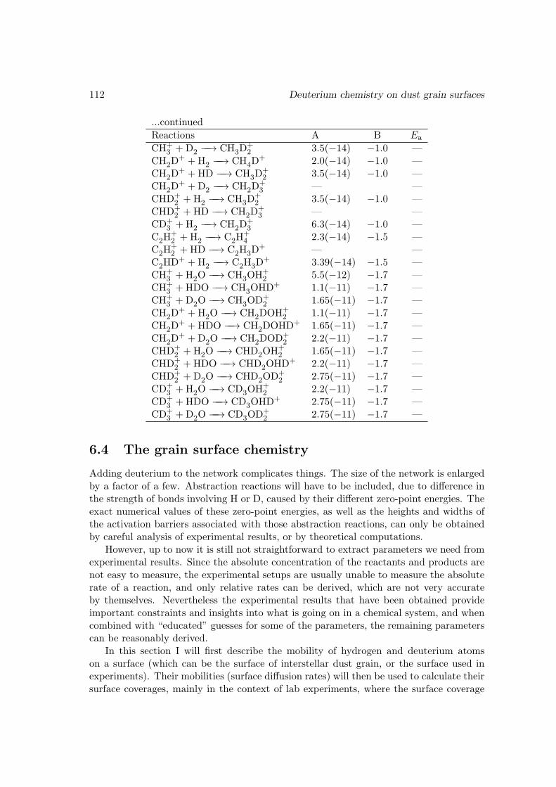
112 Deuterium chemistry on dust grain surfaces

...continued

Reactions A B Ea

CH+3 +D2 −−→ CH3D

+2 3.5(−14) −1.0 —

CH2D+ +H2 −−→ CH4D

+ 2.0(−14) −1.0 —CH2D

+ +HD −−→ CH3D+2 3.5(−14) −1.0 —

CH2D+ +D2 −−→ CH2D

+3 — —

CHD+2 +H2 −−→ CH3D

+2 3.5(−14) −1.0 —

CHD+2 +HD −−→ CH2D

+3 — —

CD+3 +H2 −−→ CH2D

+3 6.3(−14) −1.0 —

C2H+2 +H2 −−→ C2H

+4 2.3(−14) −1.5 —

C2H+2 +HD −−→ C2H3D

+ — —C2HD

+ +H2 −−→ C2H3D+ 3.39(−14) −1.5 —

CH+3 +H2O −−→ CH3OH+

2 5.5(−12) −1.7 —CH+

3 +HDO −−→ CH3OHD+ 1.1(−11) −1.7 —CH+

3 +D2O −−→ CH3OD+2 1.65(−11) −1.7 —

CH2D+ +H2O −−→ CH2DOH+

2 1.1(−11) −1.7 —CH2D

+ +HDO −−→ CH2DOHD+ 1.65(−11) −1.7 —CH2D

+ +D2O −−→ CH2DOD+2 2.2(−11) −1.7 —

CHD+2 +H2O −−→ CHD2OH+

2 1.65(−11) −1.7 —CHD+

2 +HDO −−→ CHD2OHD+ 2.2(−11) −1.7 —CHD+

2 +D2O −−→ CHD2OD+2 2.75(−11) −1.7 —

CD+3 +H2O −−→ CD3OH+

2 2.2(−11) −1.7 —CD+

3 +HDO −−→ CD3OHD+ 2.75(−11) −1.7 —CD+

3 +D2O −−→ CD3OD+2 2.75(−11) −1.7 —

6.4 The grain surface chemistry

Adding deuterium to the network complicates things. The size of the network is enlargedby a factor of a few. Abstraction reactions will have to be included, due to difference inthe strength of bonds involving H or D, caused by their different zero-point energies. Theexact numerical values of these zero-point energies, as well as the heights and widths ofthe activation barriers associated with those abstraction reactions, can only be obtainedby careful analysis of experimental results, or by theoretical computations.

However, up to now it is still not straightforward to extract parameters we need fromexperimental results. Since the absolute concentration of the reactants and products arenot easy to measure, the experimental setups are usually unable to measure the absoluterate of a reaction, and only relative rates can be derived, which are not very accurateby themselves. Nevertheless the experimental results that have been obtained provideimportant constraints and insights into what is going on in a chemical system, and whencombined with “educated” guesses for some of the parameters, the remaining parameterscan be reasonably derived.

In this section I will first describe the mobility of hydrogen and deuterium atomson a surface (which can be the surface of interstellar dust grain, or the surface used inexperiments). Their mobilities (surface diffusion rates) will then be used to calculate theirsurface coverages, mainly in the context of lab experiments, where the surface coverage

6.4 The grain surface chemistry 113

of hydrogen and deuterium is much higher than on interstellar dust grains under normalconditions (though still much less than 100%). After this I describe how information on theactivation barrier for abstraction reactions of formaldehyde and methanol can be obtainedby considering the experimental results and theoretical calculations simultaneously. Thesurface formation routes for water are also discussed. Finally, I give a brief overview ofother reactions in the surface network.

6.4.1 Coverage of H and D on the surface

In lab experiments H or D atoms are injected onto layers of deposited species, to investi-gate the reaction mechanism and to measure (if possible) the rates of the key reactions.The reactions determining the pace of the process usually have a barrier (that is the veryreason that these reactions are of interest to the experimentalists), hence they are slow.The incoming H or D atoms are mainly consumed by recombination with themselves,to form H2 or D2 molecules. Their surface coverage can be determined by the balancebetween the influx and recombination process.

Mobilities of hydrogen and deuterium atoms

At low temperatures, essentially only atomic and molecular hydrogen and deuterium onthe dust grain surface are able to migrate across the surface sites. Their mobilities arethus a very important controlling parameter of surface chemistry.

With TPD (Time-Programed Desorption) experiments and rate equation modeling,Katz et al. (1999) obtained the binding energies of H atoms on olivine and amorphouscarbon dust, being 370 and 660 K, respectively. The diffusion barriers are 290 and 510 K.The binding energies for H2 molecule are 310 and 540 K, respectively. Quantum tunnelingis not included in their modeling.

Using a similar method, Perets et al. (2005) obtained the binding energy and diffusionenergy barriers of H on low density water ice, ∼610 K and 520 K, respectively, and ∼720and 640 K for high density water ices (the two types of ice are prepared by differentmethods). The D atoms are assumed to have the same binding energy and barrier as H.The binding sites for HD and D2 molecules on low density ice are modeled to have threetypes with different depths, which are in the range 470–760 K. Only one binding energyis assumed for high density ice, 800 K for HD and 835 K for D2.

Matar et al. (2008) studied the mobility of D atoms on porous amorphous water icesurfaces. O2 molecules (to be used as an auxiliary tracer) are deposited on a porousamorphous water ice substrate, then D atoms are deposited onto the surface at 10 K. Thediffusion energy barrier of D is found to be ∼260 K. They suggest the discrepancy withthe Perets et al. (2005) result may be related to the assumed surface coverage of D.

Using classical trajectory methods, Al-Halabi & van Dishoeck (2007) calculated thesticking coefficient, η, and the binding energy, Eb, for H atoms hitting amorphous solidwater ice (ASW). The sticking coefficient is shown to be a function of the incident energyη=exp(−Ei/300). The binding energies Eb for H atoms on ASW and on crystalline iceare shown to have an average of ∼650 K and ∼400 K, respectively, with a dispersion of195 and 111 K, respectively (i.e. in their model Eb does not assume a single value). TheH atoms with an initial energy of 100 K landing on the ice surface can travel a distance

114 Deuterium chemistry on dust grain surfaces

of 30 A before being thermalized. The diffusion coefficient, d, of H atoms for a surfacetemperature of 10 K is found to be ∼10−5 cm2 s−1.

The diffusion coefficient, d, is not what we usually need in modeling surface chemistry.What we need are the barrier height and width against surface diffusion. So it would beinteresting to see what can be inferred about these parameters from the calculation ofAl-Halabi & van Dishoeck (2007). The d parameter is defined to be[8] d≡(rf − r0)

2/3t intheir paper, where r0 and rf are the initial and final position of a diffusing particle, andt is the time needed for such a trajectory. For a discrete random walk with step length L(i.e. the distance between successive jumps), (rf − r0)

2=NL2, and t=N∆t, where N isthe number of steps in such a trajectory, and ∆t is the time interval between each step.Thus d=L2/3∆t. Since ∆t is related to the characteristic frequency ν and barrier heightagainst diffusion Ediff by ∆t=1/[ν exp(−Ediff/T )], assuming no quantum tunneling, wehave

d = L2ν exp(−Ediff/T )/3, (6.13)

With L=1 A and Ediff=100 K, we have ν'6×1015 s−1. However, using formula (3) ofHasegawa et al. (1992), namely, ν = (2ρSEbind/π

2m)1/2 (see also Eq. (3.10)), where ρSis the number density of surface sites, Ebind is the binding energy, and m is the mass ofthe surface species being considered, we have only ν'2×1012 s−1, lower by three ordersof magnitude. If we instead assume quantum tunneling for surface diffusion (Hasegawaet al. 1992), then

d = L2ν exp[−2(a/~)(2mEdiff)1/2]/3. (6.14)

Assuming a=L=1 A and Ediff=100 K, we have ν'2×1013 s−1, which agrees better withthe value calculated from the formula in Hasegawa et al. (1992), although it is still toohigh. However, Al-Halabi & van Dishoeck (2007) used classical trajectory methods, whichby itself should not have quantum tunneling inside. Thus it seems that the effectiveenergy barrier against diffusion has to be very low (.50 K) in this scenario, which is veryuncommon.

The diffusion coefficient d can be related to the two-body surface reaction rate. Takethe formation of H2 molecule as an example. Let θH be the surface coverage of H atoms(i.e. the area covered by H atoms divided by the total area). Its evolution equation(derived later in this section; see Eq. (6.18)) is

∂tθH = FH/ρS − 2kH,Hθ2H − keva,HθH,

where FH is the influx of H, ρS is the surface sites density, and keva,H is the evaporationrate of H. The parameter kH,H is related to the diffusion coefficient d by

kH,H ' 3ρSd. (6.15)

With ρS=1015 cm−2, and d'10−5 cm2 s−1 from Al-Halabi & van Dishoeck (2007), wehave kH,H'3× 1010 s−1. This is close to the commonly used value (∼1010 s−1).

In summary, the diffusion energy barriers obtained with the TPD method tend to bequite high. If quantum tunneling is not included, then no active surface reaction canhappen at 10 K. The time scale for a hydrogen atom to cover the whole grain surface

[8]This definition is slightly different from that in Chandrasekhar (1943), where the definition of d isequivalent to d≡(rf − r0)

2/6t.

6.4 The grain surface chemistry 115

through migration would be of the order one month up to millions of years, if the energybarrier against diffusion were as high as 300–500 K. The fact that these values givegood fits to the experimental data might indicate some intrinsic shortcomings in the TPDmethod, in that this method may not be very sensitive to the low temperature behavior ofthe surface species. The diffusion coefficient obtained by Al-Halabi & van Dishoeck (2007)is consistent with the two-body reaction rate calculated with the formulae in Hasegawaet al. (1992). However, for a reasonable characteristic frequency and energy barrier againstsurface diffusion, quantum tunneling must be assumed in the calculations.

Surface coverage of H and D

In dark clouds the density of hydrogen atoms is usually ∼1 cm−3, determined by thebalance between cosmic-ray ionization of H2 and adsorption onto the dust grains to formH2. At a kinetic temperature of 10 K, the influx of hydrogen atoms onto the dust grainsurface is ∼104 cm−2 s−1. On the contrary, in experiments the flux are usually in therange 1012–1015 cm−2 s−1. Considering the small size of the interstellar dust grains, theaverage number of hydrogen atoms on a dust grain is usually much smaller than one(meaning that most of the time the dust grain contains no free hydrogen atom). Thisis different from the situation in typical lab experiments, where the surface coverage canbe much higher (though still considerably smaller than 100%), otherwise the experimentswould take too long a time to finish.

Suppose the total number of adsorption/reaction sites on the experimental surface isNS, the total number of H atoms on the surface is NH, the reaction rate coefficient for Hrecombination is kH,H, the evaporation rate of H is keva, H, then the evolution equation forthe number of H atoms on the surface due to adsorption, recombination, and evaporationis

∂tNH = αn(H)v(H)σ − 2kH,HNH(NH − 1)/NS − keva, HNH, (6.16)

where α is a coefficient . 1, n(H) and v(H) are the gas phase density and velocity ofthe H atoms, and σ is the surface area in the experimental setup. The factor 2 is dueto the fact that each H + H −−→ H2 reaction consumes two H atoms, and the “−1” inthe (NH − 1) term accounts for the fact that each H atom has NH − 1 potential reactionpartners. In the laboratory NH 1, so the “−1” can be neglected in the above equation.Note that in the experiments we are going to consider, H and D atoms are never injectedsimultaneously in the same setup, so we don’t have to include both H and D in the sameequation. The coverage of H atoms is mainly determined by the recombination (to formH2) and evaporation processes, because the coverages of other reactants are low and/orthe reaction rates with these other species are low.

Define the surface coverage of H by

θH = NH/NS, (6.17)

which is the fraction of surface sites that are covered by H atoms. Then we have for theevolution of θH,

∂tθH = FH/ρS − 2kH,Hθ2H − keva,HθH, (6.18)

where we have replaced αn(H)v(H) with FH (the incoming flux of H atoms); ρS is thesurface density of the reaction sites: ρS≡NS/σ. From equation (6.18) we get the steady

116 Deuterium chemistry on dust grain surfaces

state coverage for H

θH =2FH/ρS

keva +√

k2eva + 8kH,HFH/ρS. (6.19)

For the coverage of D the formula is the same.The coverages of H and D will be used in the next section to calculate the barrier

parameters for the addition and abstraction reactions of formaldehyde by combining the-oretical and experimental results in the literature. The parameters needed for calculatingthe coverages are either taken from the experimental settings as reported in the corre-sponding literature, or, for parameters not determinable in those experiments, taken tobe their canonical values used in astrochemical modeling.

To get a feeling of the typical H and D coverage in experiments, we may assume theirbinding energy Ebind to be 350 K. The diffusion barrier, Ediff, is usually taken to be afixed fraction of Ebind in the range 100 – 270 K. Such values are canonically used andare in the lower range of the experimental results described in Section 6.4.1. Since thecombination reaction of H atoms has no barrier, kH,H is equal to the migration rate ofhydrogen atom, kmig,H. In the case of quantum tunneling (Hasegawa et al. 1992) it is

kH,H = kmig,H = νHe−2a/~

√2mHEdiff,H = νH10

−1.8( a1 A

)(

Ediff,H100 K

)1/2

, (6.20)

where νH is the vibration frequency of H, while a and Ediff,H are the barrier width andheight for surface diffusion. The characteristic frequency νH can be calculated withEq. (3.10) on page 32 to be 2.4×1012 s−1, which is independent of temperature. Hencewe have

kH,H = (0.3–4)× 1010 s−1.

The evaporation rate of H atoms is

keva,H = νHe−Ebind,H/T .

For a temperature of 15 K, the evaporation rate is keva,H = 176 s−1. Thus evaporationis unimportant in consuming the surface H atoms unless θH is less than ∼10−9. TakeρS=1015 cm−2, FH=2×1014 cm−2 s−1 (Hidaka et al. 2009), we have for the surface coverageof atomic hydrogen

θH = (0.2–0.6)× 10−5.

The coverage of D can be estimated in a similar way. The typical values are:

νD = 1.7× 1012 s−1,

kD,D = kmig,D = (0.1–5.3)× 109 s−1,

θD =√

FD/ρS/2/kD,D = (0.6–4.5)× 10−5.

The surface coverage of D is higher than that of H due to its lower surface mobility.

6.4.2 Addition and abstraction reactions of formaldehyde

The pathways leading to the formation and deuteration of formaldehyde and methanolon the dust grain surface starting from CO are shown in Fig. (6.26) on page 170. The

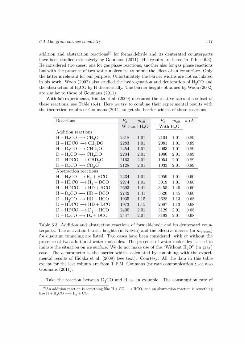
6.4 The grain surface chemistry 117

addition and abstraction reactions[9] for formaldehyde and its deuterated counterpartshave been studied extensively by Goumans (2011). His results are listed in Table (6.3).He considered two cases: one for gas phase reactions, another also for gas phase reactionsbut with the presence of two water molecules, to mimic the effect of an ice surface. Onlythe latter is relevant for our purpose. Unfortunately the barrier widths are not calculatedin his work. Woon (2002) also studied the hydrogenation and deuteration of H2CO andthe abstraction of H2CO by H theoretically. The barrier heights obtained by Woon (2002)are similar to those of Goumans (2011).

With lab experiments, Hidaka et al. (2009) measured the relative rates of a subset ofthese reactions; see Table (6.4). Here we try to combine their experimental results withthe theoretical results of Goumans (2011) to get the barrier widths of these reactions.

Reactions Ea meff Ea meff a (A)

Without H2O With H2OAddition reactionsH + H2CO −−→ CH3O 2318 1.01 2104 1.01 0.89H + HDCO −−→ CH2DO 2283 1.01 2081 1.01 0.89H + D2CO −−→ CHD2O 2254 1.01 2063 1.01 0.89D + H2CO −−→ CH2DO 2204 2.01 1980 2.01 0.89D + HDCO −−→ CHD2O 2163 2.01 1954 2.01 0.89D + D2CO −−→ CD3O 2128 2.01 1933 2.01 0.89

Abstraction reactionsH + H2CO −−→ H2 +HCO 2234 1.01 2959 1.01 0.60H + HDCO −−→ H2 +DCO 2274 1.01 3019 1.01 0.60H + HDCO −−→ HD+HCO 2693 1.41 3455 1.45 0.60H + D2CO −−→ HD+DCO 2742 1.41 3520 1.45 0.60D + H2CO −−→ HD+HCO 1935 1.15 2628 1.13 0.68D + HDCO −−→ HD+DCO 1973 1.15 2687 1.13 0.68D + HDCO −−→ D2 +HCO 2400 2.01 3129 2.01 0.68D + D2CO −−→ D2 +DCO 2447 2.01 3192 2.01 0.68

Table 6.3: Addition and abstraction reactions of formaldehyde and its deuterated coun-terparts. The activation barrier heights (in Kelvin) and the effective masses (in mproton)for quantum tunneling are listed. Two cases have been considered: with or without thepresence of two additional water molecules. The presence of water molecules is used toimitate the situation on ice surface. We do not make use of the “Without H2O” (in gray)case. The a parameter is the barrier widths calculated by combining with the experi-mental results of Hidaka et al. (2009) (see text). Courtesy: All the data in this tableexcept for the last column are from T.P.M. Goumans (private communication); see alsoGoumans (2011).

Take the reaction between D2CO and H as an example. The consumption rate of

[9]An addition reaction is something like H + CO −−→ HCO, and an abstraction reaction is somethinglike H + H2CO −−→ H2 +CO.

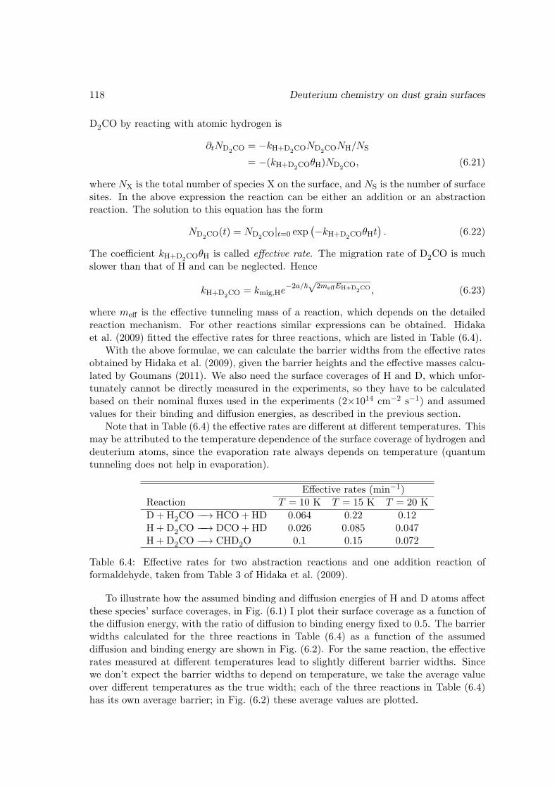
118 Deuterium chemistry on dust grain surfaces

D2CO by reacting with atomic hydrogen is

∂tND2CO = −kH+D2COND2CONH/NS

= −(kH+D2COθH)ND2CO, (6.21)

where NX is the total number of species X on the surface, and NS is the number of surfacesites. In the above expression the reaction can be either an addition or an abstractionreaction. The solution to this equation has the form

ND2CO(t) = ND2CO|t=0 exp(−kH+D2COθHt

). (6.22)

The coefficient kH+D2COθH is called effective rate. The migration rate of D2CO is muchslower than that of H and can be neglected. Hence

kH+D2CO = kmig,He−2a/~

√2meffEH+D2CO , (6.23)

where meff is the effective tunneling mass of a reaction, which depends on the detailedreaction mechanism. For other reactions similar expressions can be obtained. Hidakaet al. (2009) fitted the effective rates for three reactions, which are listed in Table (6.4).

With the above formulae, we can calculate the barrier widths from the effective ratesobtained by Hidaka et al. (2009), given the barrier heights and the effective masses calcu-lated by Goumans (2011). We also need the surface coverages of H and D, which unfor-tunately cannot be directly measured in the experiments, so they have to be calculatedbased on their nominal fluxes used in the experiments (2×1014 cm−2 s−1) and assumedvalues for their binding and diffusion energies, as described in the previous section.

Note that in Table (6.4) the effective rates are different at different temperatures. Thismay be attributed to the temperature dependence of the surface coverage of hydrogen anddeuterium atoms, since the evaporation rate always depends on temperature (quantumtunneling does not help in evaporation).

Effective rates (min−1)Reaction T = 10 K T = 15 K T = 20 K

D+H2CO −−→ HCO+HD 0.064 0.22 0.12H + D2CO −−→ DCO+HD 0.026 0.085 0.047H + D2CO −−→ CHD2O 0.1 0.15 0.072

Table 6.4: Effective rates for two abstraction reactions and one addition reaction offormaldehyde, taken from Table 3 of Hidaka et al. (2009).

To illustrate how the assumed binding and diffusion energies of H and D atoms affectthese species’ surface coverages, in Fig. (6.1) I plot their surface coverage as a function ofthe diffusion energy, with the ratio of diffusion to binding energy fixed to 0.5. The barrierwidths calculated for the three reactions in Table (6.4) as a function of the assumeddiffusion and binding energy are shown in Fig. (6.2). For the same reaction, the effectiverates measured at different temperatures lead to slightly different barrier widths. Sincewe don’t expect the barrier widths to depend on temperature, we take the average valueover different temperatures as the true width; each of the three reactions in Table (6.4)has its own average barrier; in Fig. (6.2) these average values are plotted.

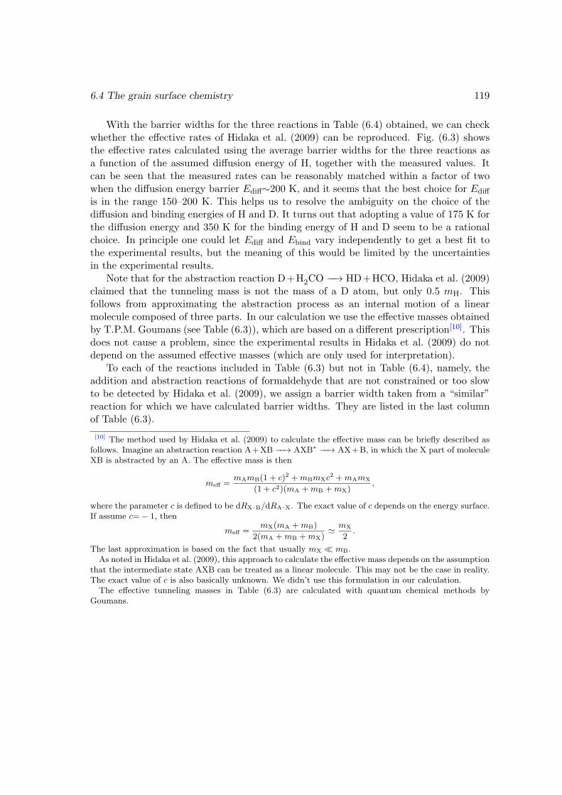
6.4 The grain surface chemistry 119

With the barrier widths for the three reactions in Table (6.4) obtained, we can checkwhether the effective rates of Hidaka et al. (2009) can be reproduced. Fig. (6.3) showsthe effective rates calculated using the average barrier widths for the three reactions asa function of the assumed diffusion energy of H, together with the measured values. Itcan be seen that the measured rates can be reasonably matched within a factor of twowhen the diffusion energy barrier Ediff∼200 K, and it seems that the best choice for Ediff

is in the range 150–200 K. This helps us to resolve the ambiguity on the choice of thediffusion and binding energies of H and D. It turns out that adopting a value of 175 K forthe diffusion energy and 350 K for the binding energy of H and D seem to be a rationalchoice. In principle one could let Ediff and Ebind vary independently to get a best fit tothe experimental results, but the meaning of this would be limited by the uncertaintiesin the experimental results.

Note that for the abstraction reaction D+H2CO −−→ HD+HCO, Hidaka et al. (2009)claimed that the tunneling mass is not the mass of a D atom, but only 0.5 mH. Thisfollows from approximating the abstraction process as an internal motion of a linearmolecule composed of three parts. In our calculation we use the effective masses obtainedby T.P.M. Goumans (see Table (6.3)), which are based on a different prescription[10]. Thisdoes not cause a problem, since the experimental results in Hidaka et al. (2009) do notdepend on the assumed effective masses (which are only used for interpretation).

To each of the reactions included in Table (6.3) but not in Table (6.4), namely, theaddition and abstraction reactions of formaldehyde that are not constrained or too slowto be detected by Hidaka et al. (2009), we assign a barrier width taken from a “similar”reaction for which we have calculated barrier widths. They are listed in the last columnof Table (6.3).

[10] The method used by Hidaka et al. (2009) to calculate the effective mass can be briefly described asfollows. Imagine an abstraction reaction A+XB −−→ AXB∗ −−→ AX+B, in which the X part of moleculeXB is abstracted by an A. The effective mass is then

meff =mAmB(1 + c)2 +mBmXc

2 +mAmX

(1 + c2)(mA +mB +mX),

where the parameter c is defined to be dRX–B/dRA–X. The exact value of c depends on the energy surface.If assume c=− 1, then

meff =mX(mA +mB)

2(mA +mB +mX)' mX

2.

The last approximation is based on the fact that usually mX mB.As noted in Hidaka et al. (2009), this approach to calculate the effective mass depends on the assumption

that the intermediate state AXB can be treated as a linear molecule. This may not be the case in reality.The exact value of c is also basically unknown. We didn’t use this formulation in our calculation.

The effective tunneling masses in Table (6.3) are calculated with quantum chemical methods byGoumans.

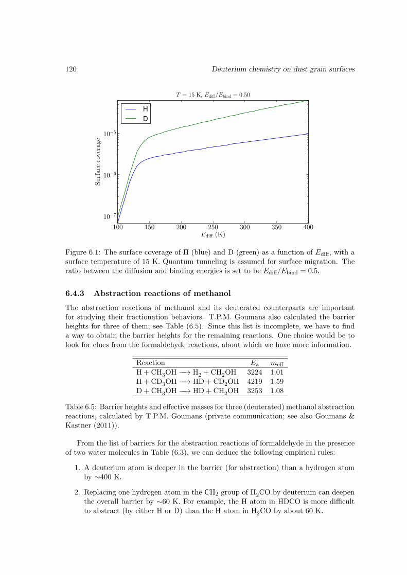
120 Deuterium chemistry on dust grain surfaces

Figure 6.1: The surface coverage of H (blue) and D (green) as a function of Ediff, with asurface temperature of 15 K. Quantum tunneling is assumed for surface migration. Theratio between the diffusion and binding energies is set to be Ediff/Ebind = 0.5.

6.4.3 Abstraction reactions of methanol

The abstraction reactions of methanol and its deuterated counterparts are importantfor studying their fractionation behaviors. T.P.M. Goumans also calculated the barrierheights for three of them; see Table (6.5). Since this list is incomplete, we have to finda way to obtain the barrier heights for the remaining reactions. One choice would be tolook for clues from the formaldehyde reactions, about which we have more information.

Reaction Ea meff

H+ CH3OH −−→ H2 +CH2OH 3224 1.01H + CD3OH −−→ HD+CD2OH 4219 1.59D + CH3OH −−→ HD+CH2OH 3253 1.08

Table 6.5: Barrier heights and effective masses for three (deuterated) methanol abstractionreactions, calculated by T.P.M. Goumans (private communication; see also Goumans &Kastner (2011)).

From the list of barriers for the abstraction reactions of formaldehyde in the presenceof two water molecules in Table (6.3), we can deduce the following empirical rules:

1. A deuterium atom is deeper in the barrier (for abstraction) than a hydrogen atomby ∼400 K.

2. Replacing one hydrogen atom in the CH2 group of H2CO by deuterium can deepenthe overall barrier by ∼60 K. For example, the H atom in HDCO is more difficultto abstract (by either H or D) than the H atom in H2CO by about 60 K.

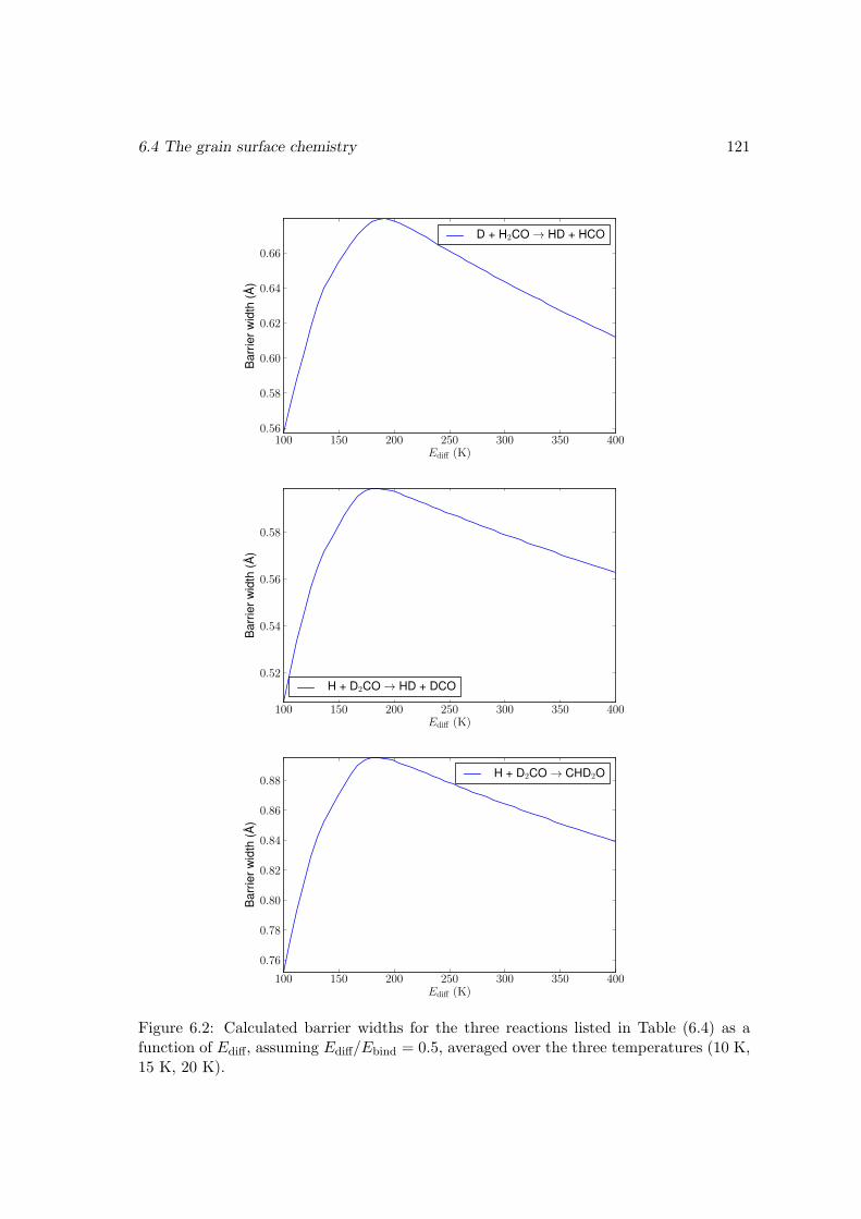
6.4 The grain surface chemistry 121

Figure 6.2: Calculated barrier widths for the three reactions listed in Table (6.4) as afunction of Ediff, assuming Ediff/Ebind = 0.5, averaged over the three temperatures (10 K,15 K, 20 K).

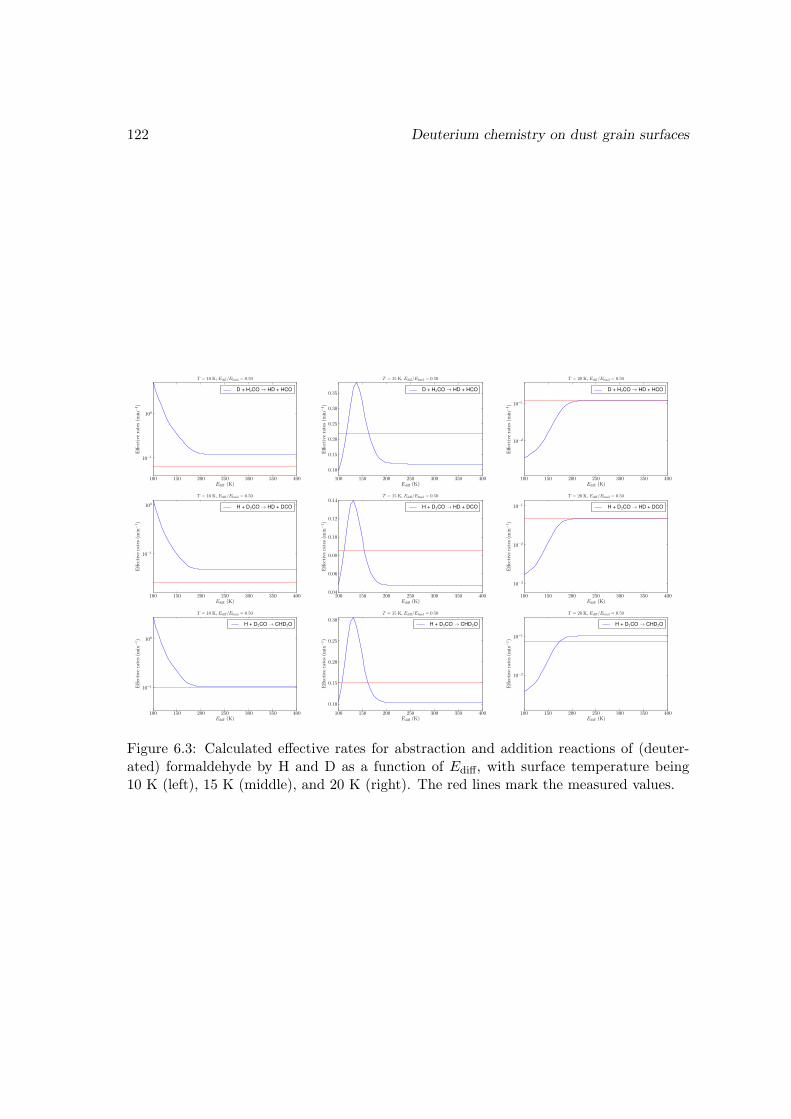
122 Deuterium chemistry on dust grain surfaces

Figure 6.3: Calculated effective rates for abstraction and addition reactions of (deuter-ated) formaldehyde by H and D as a function of Ediff, with surface temperature being10 K (left), 15 K (middle), and 20 K (right). The red lines mark the measured values.

6.4 The grain surface chemistry 123

3. An incoming abstracting hydrogen atom experiences a barrier ∼300 K higher thanan abstracting deuterium atom.

If the barrier height of only one abstraction reaction of formaldehyde is known, these rulesenable us to obtain the approximate barrier heights of all the other possible abstractionreactions. Let’s first test whether these rules really work for formaldehyde.

For example, suppose we are only given the barrier of the reaction H2CO+H −−→ H2+HCO, being 2960 K, we can get the barrier of other abstraction reactions of H2CO step bystep in the following way (the numbers in parenthesis are the exact theoretical values fromGoumans, and the middle column shows the detailed addition and subtraction operationsinvolved):Reaction Calculation step Estimated Ea (exact Ea)

H2CO+H −−→ H2 +HCO — 2960 KH2CO+D −−→ HD+HCO 2960 K − 300 K 2660 K (2628 K)HDCO+H −−→ H2 +DCO 2960 K + 60 K 3020 K (3019 K)HDCO+H −−→ HD+HCO 3020 K + 400 K 3420 K (3455 K)HDCO+D −−→ HD+DCO 3020 K − 300 K 2720 K (2687 K)HDCO+D −−→ D2 +HCO 2720 K + 400 K 3120 K (3129 K)D2CO+H −−→ HD+DCO 3420 K + 60 K 3480 K (3520 K)D2CO+D −−→ D2 +DCO 3480 K − 300 K 3180 K (3192 K)

The rules for the effective masses (in unit of mproton) in these abstraction reactionsare:

• H abstracting H: 1.01;

• H abstracting D: 1.45;

• D abstracting H: 1.13;

• D abstracting D: 2.01.

We can see that the barriers obtained with the three rules approximate the exactvalues quite well. Thus we may apply the same rules to the abstraction of methanol and itsisotopologues, since not all of them have been calculated by Goumans. However, from theknown barriers of three abstraction reactions (Table 6.5) of the methanol isotopologues,it seems that the third rule in the case of formaldehyde does not hold anymore. Namely,an incoming H or D atom experiences very similar barrier heights (the Ea for the firstand third reaction in Table (6.5) are almost the same).

Moreover, since the barrier height of H + CD3OH −−→ HD+ CD2OH is 995 K higherthan that of H+CH3OH −−→ H2+CH2OH, in contrast to the case of formaldehyde, wherethe barrier height of H+D2CO −−→ HD+DCO is higher than that of H+H2CO −−→ H2+HCO by 561 K, for the methanol abstraction reactions we have to scale up the parameterscompared to the formaldehyde abstraction reactions to account for such a difference.Denote by x the increase in barrier height due to replacing one H in the CH3 group byD, and by y the difference in the zero point energies of H and D in the same group. Thenwe have

3x+ y = 4219− 3224 = 995,

x : y = 60 : 400,

124 Deuterium chemistry on dust grain surfaces

where the ratio 60 : 400 results from rule 1 and 2 for formaldehyde. Hence x=103, andy=686.

Hence we may have the following two rules for the barrier heights of the methanolabstraction reactions:

1. A deuterium atom is ∼686 K deeper in the barrier than a hydrogen atom in theCH3 group of methanol.

2. Replacing one hydrogen atom in the CH3 group by a deuterium atom can deepenthe overall barrier in the same group by 103 K.

And for the effective tunneling masses:

1. H abstracting H: 1.01;

2. H abstracting D: 1.59;

3. D abstracting H: 1.08;

4. D abstracting D: 2.01.

The first three are taken from Table (6.5), while the fourth one is taken from Table (6.3).From these rules we can derive the barrier heights and effective masses for abstracting

methanol and its isotopologues by H and D. We assume that the methyl group (CH3)is not affected should the hydroxyl group (OH) be deuterated, though this is not well-studied. The parameters for the abstraction of methanol and its deuterated counterpartsare listed in Table (6.6). The barrier widths are taken to be the same as the barrierwidths for the abstraction reactions of formaldehyde by H and by D (0.6 and 0.68 A inTable 6.3).

Nagaoka et al. (2007) measured the relative rates for three of the methanol abstractionreactions D + CH3OH −−→ HD + CH2OH, D + CH2DOH −−→ HD + CHDOH, and D +CHD2OH −−→ HD+CD2OH, which are

1 : 0.69 : 0.52. (6.24)

Using the barrier parameters in Table (6.6), we can calculate these relative rates (sinceonly D atoms are involved, the absolute coverage of D atoms on the surface is not neededfor the calculation), which are:

1 : 0.77 : 0.59. (6.25)

The agreement is not bad.

6.4.4 Hydrogenation/deuteration of CO

The reactions we consider here are H + CO −−→ HCO and D+CO −−→ DCO. They havebeen studied theoretically by Woon (2002) with ab initio quantum mechanical calcula-tions. In the presence of three water molecules (to simulate the effect of an ice surface), theformer has a barrier height of 5.45 kcal mol−1 = 2740 K, in which 0.68 kcal mol−1 is con-tributed by zero-point energy (thus the potential part of the barrier is 4.77 kcal mol−1).For the latter reaction the total barrier height is 5.13 kcal mol−1 = 2579 K in Woon(2002), however, in the presence of only two water molecules.

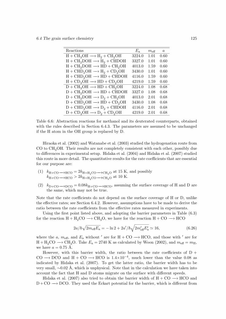
6.4 The grain surface chemistry 125

Reactions Ea meff a

H+ CH3OH −−→ H2 +CH2OH 3224.0 1.01 0.60H + CH2DOH −−→ H2 +CHDOH 3327.0 1.01 0.60H + CH2DOH −−→ HD+CH2OH 4013.0 1.59 0.60H + CHD2OH −−→ H2 +CD2OH 3430.0 1.01 0.60H + CHD2OH −−→ HD+CHDOH 4116.0 1.59 0.60H + CD3OH −−→ HD+CD2OH 4219.0 1.59 0.60

D + CH3OH −−→ HD+CH2OH 3224.0 1.08 0.68D + CH2DOH −−→ HD+CHDOH 3327.0 1.08 0.68D + CH2DOH −−→ D2 +CH2OH 4013.0 2.01 0.68D + CHD2OH −−→ HD+CD2OH 3430.0 1.08 0.68D + CHD2OH −−→ D2 +CHDOH 4116.0 2.01 0.68D + CD3OH −−→ D2 +CD2OH 4219.0 2.01 0.68

Table 6.6: Abstraction reactions for methanol and its deuterated counterparts, obtainedwith the rules described in Section 6.4.3. The parameters are assumed to be unchangedif the H atom in the OH group is replaced by D.

Hiraoka et al. (2002) and Watanabe et al. (2003) studied the hydrogenation route fromCO to CH3OH. Their results are not completely consistent with each other, possibly dueto differences in experimental setup. Hidaka et al. (2004) and Hidaka et al. (2007) studiedthis route in more detail. The quantitative results for the rate coefficients that are essentialfor our purpose are:

(1) kH+CO−−→HCO = 2kH+H2CO−−→CH3Oat 15 K, and possibly

kH+CO−−→HCO > 2kH+H2CO−−→CH3Oat 10 K.

(2) kD+CO−−→DCO = 0.08kH+CO−−→HCO, assuming the surface coverage of H and D arethe same, which may not be true.

Note that the rate coefficients do not depend on the surface coverage of H or D, unlikethe effective rates; see Section 6.4.2. However, assumptions have to be made to derive theratio between the rate coefficients from the effective rates measured in experiments.

Using the first point listed above, and adopting the barrier parameters in Table (6.3)for the reaction H + H2CO −−→ CH3O, we have for the reaction H + CO −−→ HCO

2a/~√

2meffEa = − ln 2 + 2a′/~√2m′

effE′a ' 16, (6.26)

where the a, meff, and Ea without ′ are for H + CO −−→ HCO, and those with ′ are forH+H2CO −−→ CH3O. Take Ea = 2740 K as calculated by Woon (2002), and meff = mH,we have a = 0.75 A.

However, with this barrier width, the ratio between the rate coefficients of D +CO −−→ DCO and H + CO −−→ HCO is 1.4×10−4, much lower than the value 0.08 asindicated by Hidaka et al. (2007). To get the latter ratio, the barrier width has to bevery small, ∼0.02 A, which is unphysical. Note that in the calculation we have taken intoaccount the fact that H and D atoms migrate on the surface with different speeds.

Hidaka et al. (2007) also tried to obtain the barrier width of H + CO −−→ HCO andD+CO −−→ DCO. They used the Eckart potential for the barrier, which is different from

126 Deuterium chemistry on dust grain surfaces

the usually assumed rectangular form, though this should not make a big difference. Theirresults (for the tunneling length) lie in the range 0.5–1.3 A, depending on which barrierheight is used. However, in their calculation they implicitly assumed that the mobilitiesof H and D are the same, which may not be the case. Using the formulae in Section 6.4.1,one can find that the ratio of the migration rate of D and H is kmig,D/kmig,H ' 0.08 (whichis close to the ratio between the effective rates of the two reactions), and the coverageratio θD/θH ' 1.2. Thus the coverages of H and D are indeed very similar, as assumedby Hidaka et al. (2007), but their mobilities are quite different. However, if only thermalhopping is allowed for surface diffusion, then the mobilities of H and D will be the sameagain. So here we face the dilemma that we may assume equal reaction probability forthe two reactions and attribute their different effective rates to the different mobilities ofH and D and, or, we may assume H and D diffuse on the surface only through thermalhopping to arrive at a “normal” barrier width.

For the following I assume a barrier width of 0.75 A obtained with the first approach.If quantum tunneling does not play a role in surface migration (but still works for surfacereactions), then the ratio between the effective rates of the two reactions D + CO andH+CO is consistent with a barrier width of 0.3 A. This value is different from the valueobtained by Hidaka et al. (2007) because they used a different formalism. The effect ofdisallowing quantum tunneling for surface migration (even if the tunneling rate calculatedwith the usual formula is higher than the thermal hopping rate) may be investigated later.

6.4.5 The formation of water

There are mainly three different routes to surface water formation:

1. Starting from O: O + H −−→ OH, OH +H −−→ H2O;

2. Starting from O2: O2 +H −−→ O2H, O2H+H −−→ H2O2, H2O2 +H −−→ H2O+OH;

3. Starting from O and O2: O + O2 −−→ O3, O3 +H −−→ O2 +OH, OH +H −−→ H2O.

Besides the reaction OH + H −−→ H2O, OH can also be hydrogenated into H2O throughOH+H2 −−→ H2O+H.

The first reaction chain is barrierless, hence needs not to be discussed. The remainingroutes do possibly have a barrier. But they are still potentially important since largeabundances of O2 and H2 might be accumulated on the dust grain surface, at least insome situations. They will be discussed in the following.

The O2 route

Miyauchi et al. (2008) exposed solid O2 (with a thickness of 8 monolayers) to H and Datoms, and fitted the effective reaction rate constants for the reactions O2 +H −−→ O2H,H+H2O2 −−→ H2O+OH, O2+D −−→ O2D, and D+D2O2 −−→ D2O+OD, for temperaturesof 10 K and 15 K. They compared these rate constants to those of the two reactionsH+CO −−→ HCO and D+CO −−→ DCO. The experimental conditions of this experimentwere quite different from those of the investigation by Hidaka et al. (2009), so a directquantitative comparison is not possible. It seems that surface migration is not importantin the study of Miyauchi et al. (2008), because the surface is completely covered by the

6.4 The grain surface chemistry 127

deposited O2 molecules. Rather the penetration of H and D atoms deep into the iceinterior might be more important (the authors divide the ice mantle into three parts:the deepest part containing only O2 and having no reaction, the middle part where onlyhydrogenation of O2 into H2O2 is possible, and the topmost part where the conversion ofH2O2 into H2O also occurs).

Information about the reaction barriers can still be obtained from the ratio betweenthe rates of hydrogenation and deuteration reactions. The effective rate constants forO2+H −−→ O2H and O2+D −−→ O2D are almost the same (∼12 min−1), indicating bothreactions have negligible barriers. On the other hand, H+H2O2 −−→ H2O+OH is aboutone order of magnitude faster than D+D2O2 −−→ D2O+OD (3.9 versus 0.49 min−1), thusthey are mediated by an activation barrier. Miyauchi et al. concluded that an activationenergy of 3.6–4.3 kcal/mol (=1800–2200 K) from calculation for the gas phase (Koussaet al. 2006) is consistent with such a ratio. But if a typical barrier width of 0.6–1 A isassumed, then the barrier height should more likely lie in the range 200–500 K.

The ratio between the rates of H + H2O2 −−→ H2O + OH and H + O2H −−→ H2O2 isabout 0.05 in Cuppen et al. (2010). Taking into account the fact that the latter hasanother branch, H + O2H −−→ 2OH, the ratio between the reaction rates of H + H2O2

and H+O2H is about 0.02. As the latter reaction has no barrier, their ratio can be usedto estimate the reaction barrier of the former. Combining the results of the two studies(Miyauchi et al. 2008; Cuppen et al. 2010), one gets

exp[−2a

~√

2mHEa] = 0.02,

exp[−2a

~√

2Ea(√mD −

√mH)] = 0.13.

(6.27)

The value 0.13 (=0.49/3.9) in the above equation is the ratio between the effective reactionrates of D+D2O2 and H+H2O2. The tunneling masses are taken to be the mass of eitherH or D, and the barrier heights is taken to be the same for H and D.

Unfortunately, the above two equations cannot be used to solve for a and Ea, thebarrier width and activation energy, respectively, of the reaction H+H2O2 −−→ H2O+OH;but both of the two equations are consistent with(

a

0.68 A

)(Ea

200 K

)1/2

' 1. (6.28)

Since the O2+H −−→ O2H reaction is also likely barrierless in addition to the reactionH + O2H −−→ H2O2, we can get another constraint based on the relative rate betweenH + H2O2 −−→ H2O+H and O2 +H −−→ O2H, which is 3.9/12.8 = 0.3 in Miyauchi et al.(2008). This leads to

exp[−2a

~√

2mHEa] = 0.3, (6.29)

which is equivalent to (a

0.21 A

)(Ea

200 K

)1/2

' 1. (6.30)

This is quite different from Eq. (6.28).The main assumption used in the above calculation is that the two reactions H +

O2 −−→ O2H and H + O2H −−→ H2O2 are barrierless. Although this may be true, the

128 Deuterium chemistry on dust grain surfaces

uncertainties in these experiments might have caused the above apparent contradiction.To resolve this, I simply set the barrier height to a value of 200 K, and the barrier widthto the average of Eq. (6.28) and Eq. (6.30), namely, 0.5 A.

The O3 route

The reaction H + O3 −−→ O2 + OH was assumed to have a barrier of 450 K in Tielens& Hagen (1982). Romanzin et al. (2011) experimentally studied this reaction with solidO3 ice and concluded that it does play a role in water formation, although detailedinformation regarding the activation barrier cannot be extracted from this study. Mokraneet al. (2009) studied the reaction D+O3 −−→ O2 +OD, with O3 deposited on non-porousamorphous water ice and arrived at a similar conclusion; a barrier of 450 K is consistentwith their results. Due to the limited information on this reaction, I take as a workingassumption that this reaction has a barrier of 450 K with a width of 0.5A.

The OH+H2 −−→ H2O+H reaction

This reaction received more study than the previous one. In the gas phase it has a barrierof ∼2100 K (Atkinson et al. 2004) or higher (Nguyen et al. 2011). Oba et al. (2012) studiedthis reaction and its deuterated counterparts, finding that it does possess a barrier, asevidenced by the isotopic effect on the relative reactions rates. Since the theoretical studyabout the barrier heights has not converged, here I will take the canonic value 2100 K.

To estimate the barrier width, as before, we may make use of the relative reactionefficiency roughly obtained by Oba et al. (2012). In their Table (2) it is shown that therate of OH+D2 −−→ HDO+D is 10% that of OH+H2 −−→ H2O+H. Taking the tunnelingmass of the two reactions to be the mass of a deuterium atom and a hydrogen atom, wehave

exp[−2a

~√

2Ea(√mD −

√mH)] = 0.1, (6.31)

which is equivalent to (a

0.3 A

)(Ea

2100 K

)1/2

' 1. (6.32)

So a barrier width of 0.3 A will be adopted. If we assume the effective mass formula usedby these authors (or Hidaka et al. 2009; see page 119), then a slightly larger width willresult[11].

The full set of reactions and their parameters for the formation of water and itsdeuterated counterparts are listed in Table (6.7).

6.4.6 The formation of CO2 through OH+CO

For the formation of CO2, Garrod & Pauly (2011) implemented a three-body mechanism,H + O+ CO −−→ CO2 +H, which is inspired by the two-body reaction OH + CO (whichby itself does not occur at low temperatures because both OH and CO are immobile).

[11]We may note that the implicit “mental picture” based on which to calculate the effective mass withthis formula is, for reaction OH + H2 −−→ H2O + H, an H atom in H2 is abstracted (“grabbed”) by anOH radical. Whether this is true depends on the detailed energy surface and reaction path, which affectthe exact effective mass.

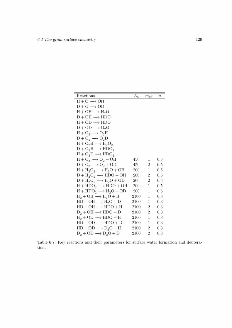
6.4 The grain surface chemistry 129

Reactions Ea meff a

H+O −−→ OHD+O −−→ ODH+OH −−→ H2OD+OH −−→ HDOH+OD −−→ HDOD+OD −−→ D2OH+O2 −−→ O2HD+O2 −−→ O2DH+O2H −−→ H2O2

D+O2H −−→ HDO2

H+O2D −−→ HDO2

H+O3 −−→ O2 +OH 450 1 0.5D + O3 −−→ O2 +OD 450 2 0.5H + H2O2 −−→ H2O+OH 200 1 0.5D + H2O2 −−→ HDO+OH 200 2 0.5D + H2O2 −−→ H2O+OD 200 2 0.5H + HDO2 −−→ HDO+OH 200 1 0.5H + HDO2 −−→ H2O+OD 200 1 0.5H2 +OH −−→ H2O+H 2100 1 0.3HD +OH −−→ H2O+D 2100 1 0.3HD +OH −−→ HDO+H 2100 2 0.3D2 +OH −−→ HDO+D 2100 2 0.3H2 +OD −−→ HDO+H 2100 1 0.3HD +OD −−→ HDO+D 2100 1 0.3HD +OD −−→ D2O+H 2100 2 0.3D2 +OD −−→ D2O+D 2100 2 0.3

Table 6.7: Key reactions and their parameters for surface water formation and deutera-tion.

130 Deuterium chemistry on dust grain surfaces

Namely, when an H atom arrives at a surface site occupied by an O atom, and if this Oatom is on top of a CO molecule, then a CO2 molecules is assumed to be formed. This issimilar to the Eley-Rideal mechanism, in which a gas phase molecule reaching the surfacedirectly react with a molecule attached to the surface.

Since the adsorption energy of OH is 2850 K, much higher than the barrier height(80 K) of the reaction OH+CO −−→ CO2 +H, it is reasonable to assume that the newlyadsorbed OH can overcome such a barrier and react with CO to form CO2. Note thatthe adsorption energy of OH quoted here is for amorphous water ice, while we are talkingabout an OH arriving on top of a CO molecule. But even if the adsorption energy of OHon CO ice is lower, it should still be larger than the small barrier of 80 K.

Besides the adsorption process, we may assume that, in general, each time an OHradical is formed, and if it is on top of a CO molecule, a CO2 molecule will be immediatelyformed. This is because all the surface reactions that are of interest at the low temperatureof dark clouds are exothermic, and the energy released in each reaction should be muchhigher than the small activation barrier.

Mathematically, this amounts to taking away a fraction of the surface OH formationrate and adding it to the formation rate of CO2. Namely,

∂tN(OH) = P (OH) [1− θ(CO)]− · · · ,∂tN(CO) = −P (OH)θ(CO) + · · · ,∂tN(CO2) = P (OH)θ(CO) + · · · ,

∂tN(H) = P (OH)θ(CO) + · · · ,

(6.33)

where P (OH) is the production rate of OH, and θ(CO) is the surface coverage of CO,

θ(CO) ≡ N(CO)/NS, (6.34)

where NS is the total number of surface sites, and N(CO) is the number of CO moleculeson the surface of single dust grain.

The production rate of OH contains terms like N(H)N(O), so the term P (OH)θ(CO)contains a product of the abundances of three species, hence we are practically consideringthree-body reactions.

However, the above prescription is susceptible to numerical instabilities. This is be-cause, in the first line of Eq. (6.33), the negative term for OH is not proportional toN(OH), which causes the loss of self-correction in the numeric evolution. Hence theθ(CO) term in these equations should be replaced by min(1, θ(CO)).

In coding this mechanism, to be “fair”, the two reactants will be treated the sameway. That is to say, not only P (OH)θ(CO), but also P (CO)θ(OH) will be added to theformation rate of CO2, even if the latter is not as important.

To allow more flexibility, a “pre-factor” is also included. So the actual contributionadded to the CO2 formation rate is fpreP (OH)θ(CO). Such a pre-factor is in principle afree parameter. It may be used to account for the possibility that an OH radical sittingon a CO molecule may evaporate or hop away before the reaction occurs. In this case,we have

fpre =kreac

kreac + khop + keva. (6.35)

6.4 The grain surface chemistry 131

Here kreac is ν exp[−Ea/T ], where ν is the characteristic frequency. The exponentialpart may be replaced by a quantum tunneling version, depending on whichever is faster.Note that the above form is similar to, but not the same as equation (6) in Garrod &Pauly (2011), which was used to enhance the reaction rate by considering the compe-tition between reaction, hopping, and evaporation processes. We don’t include such anenhancement for normal surface reactions.

6.4.7 Other reactions in the surface reaction network

Other reactions included in our model are basically the same as those used in our previousstudy on the formation of H2O2, except that deuterium is included. Basically, besidesformaldehyde, methanol, and water that have been described in the previous sections, weinclude the formation of methane (CH4), ammonia (NH3), H2S, HCOOH, HCN, HNC,etc., and their deuterated counterparts (if applicable). They are listed in Table (6.8);deuterated reactions are not included for simplicity.

6.4.8 The zero-point energy issue for the evaporation and surface mi-gration rates

For an oscillatory system, quantum mechanics predicts that the energy of its lowest energystate is not zero, but has a finite value hν/2, where h is Planck’s constant, and ν is thefrequency of the system. If the system has more than one independent vibrational modes,then the total zero-point energy is the sum of the zero-point energy of all these modes. Wenote that in classical physics (with the exception of general relativity) only the differencesbetween energies really enter the dynamical equations.

In surface evaporation processes, the rate is determined by ν exp [−Ebind/T ], where νis the characteristic frequency for the vibration of a species on the surface. If the sameamount is subtracted from the binding energies Ebind of all the species, then their relativeevaporation rates won’t change. However, all the rates would have to be scaled by acommon factor, which has an observable consequence (in principle), because it wouldlead to a different absolute time scale. Furthermore, since different species have differentcharacteristic vibrational frequencies, they also have different zero-point energies. Henceincluding the zero-point energy also has a measurable change to the relative evaporationrates.

The effect due to difference in vibrational frequencies is most obvious between differ-ent isotopologues of the same species. Since the electronic structure of two isotopologuesshould be very similar, they experience very similar energy potentials[12]. For example,the zero point energy corresponding to the characteristic frequency of H (∼2.4×1012 Hz)is ∼58 K, while for D (∼1.7×1012 Hz) is ∼41 K; together with the difference in vibra-tional frequencies (a factor of 1.4), H evaporates about 7 times faster than D at 10 K.The characteristic frequency of H2 molecule is ∼1.94×1012 Hz, for HD molecule it is∼1.58×1012 Hz, while for D2 it is ∼1.37×1012 Hz (calculated with Eq. (3.10)). The

[12]In principle, the differences in the dipole moments of different isotopologues can also contribute tothe variation in binding energy by changing the bond strength.

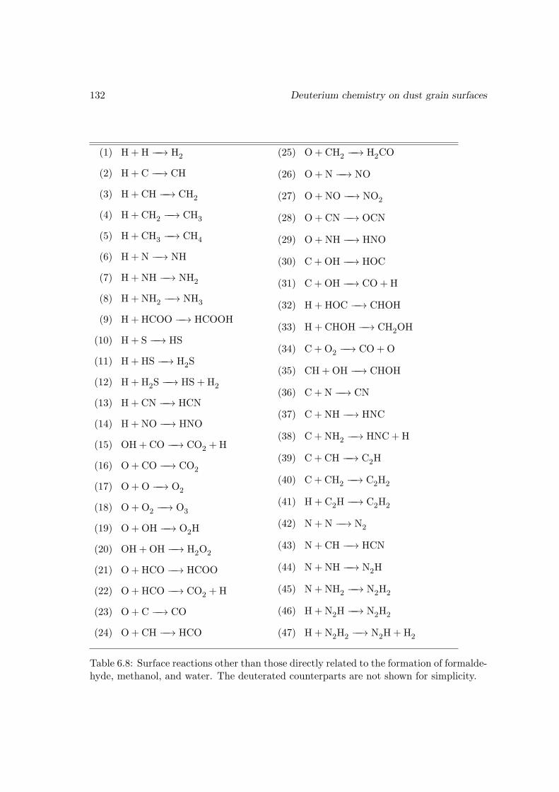
132 Deuterium chemistry on dust grain surfaces

(1) H + H −−→ H2

(2) H + C −−→ CH

(3) H + CH −−→ CH2

(4) H + CH2 −−→ CH3

(5) H + CH3 −−→ CH4

(6) H + N −−→ NH

(7) H + NH −−→ NH2

(8) H + NH2 −−→ NH3

(9) H + HCOO −−→ HCOOH

(10) H + S −−→ HS

(11) H + HS −−→ H2S

(12) H + H2S −−→ HS + H2

(13) H + CN −−→ HCN

(14) H + NO −−→ HNO

(15) OH + CO −−→ CO2 +H

(16) O + CO −−→ CO2

(17) O + O −−→ O2

(18) O + O2 −−→ O3

(19) O + OH −−→ O2H

(20) OH +OH −−→ H2O2

(21) O + HCO −−→ HCOO

(22) O + HCO −−→ CO2 +H

(23) O + C −−→ CO

(24) O + CH −−→ HCO

(25) O + CH2 −−→ H2CO

(26) O + N −−→ NO

(27) O + NO −−→ NO2

(28) O + CN −−→ OCN

(29) O + NH −−→ HNO

(30) C + OH −−→ HOC

(31) C + OH −−→ CO+H

(32) H + HOC −−→ CHOH

(33) H + CHOH −−→ CH2OH

(34) C + O2 −−→ CO+O

(35) CH +OH −−→ CHOH

(36) C + N −−→ CN

(37) C + NH −−→ HNC

(38) C + NH2 −−→ HNC+H

(39) C + CH −−→ C2H

(40) C + CH2 −−→ C2H2

(41) H + C2H −−→ C2H2

(42) N + N −−→ N2

(43) N + CH −−→ HCN

(44) N + NH −−→ N2H

(45) N + NH2 −−→ N2H2

(46) H + N2H −−→ N2H2

(47) H + N2H2 −−→ N2H+H2

Table 6.8: Surface reactions other than those directly related to the formation of formalde-hyde, methanol, and water. The deuterated counterparts are not shown for simplicity.

6.5 The three-phase gas-surface-mantle model 133

differences in zero-point energies are

EZPE(H2)− EZPE(HD) ' 8 K,

EZPE(H2)− EZPE(D2) ' 14 K.

At 10 K the evaporation rate of D2 will be e−1.4'0.25 time slower than that of H2.This can enhance the surface abundance of D2 relative to H2, which might play a role indetermining the deuteration of water through the reaction channel H2+OH −−→ H2O+H.

In our code, the zero-point energy of each surface species is subtracted from its “pure”potential energy. The zero-point energy itself is calculated with the characteristic fre-quency of each species. Then the total energy is used to calculate the evaporation rate,and a fraction (a free parameter of the code, usually taken to be in the range of 0.3–0.8) ofit is used to calculate the surface diffusion rate. Such a treatment is subject to uncertain-ties. Moreover, the evaporation of a species corresponds to the vertical vibrational modeof its motion on the surface, which may have a different frequency from the horizontalmodes. Calculating the vibrational frequencies is a highly nontrivial task by itself (Groß2009, page 243), since in principle the details of the potential energy surface should beknown for such a calculation. Hence our implementation of the zero-point energy shouldbe only viewed as a hypothetical trial.

6.5 The three-phase gas-surface-mantle model

In our previous treatment of grain chemistry, all the species on the grain are allowed toparticipate in chemical reactions. In reality, one may imagine that species on the surfacelayer can be covered by incoming molecules and become inert to chemical changes. Insuch a manner an ice mantle is formed for each grain, which serves as a reservoir for theproducts of gas phase and surface chemistry. When the temperature of the dust grain rises,the mantle material evaporates and returns to the gas phase, liberating their rotationalmotions so that they may be observed at radio and (sub)millimeter wavelengths.

There are several types of chemical models for dust grains, depending on to whatextent the details of the grain structure are captured. Models with the least details donot distinguish between surface and mantle layers, and only a distinction between thegas phase and grain surface is made—these are called “two phase” models. The so-called“three-phase” models distinguish between the surface and mantle layers; see Fig. (6.4) fora schematic view. All the layers below the surface layer and above the dust core are calledmantle, and are treated as a whole. Thus we see that such a “three-phase” model stillcannot describe the detailed distribution of different species inside the grain mantle[13].Only models in the style of Chang et al. (2005) and Cuppen & Herbst (2007) maintainthese details. However, for a reaction network large enough for astrochemical study, suchan approach is too demanding in computational resources and impractical, since one hasto keep track of the position of each species in the grain mantle and the chemical reactionshave to be simulated one by one.

Here we adopt the “three-phase” model of grain structure. We neglect the possibilitythat an incoming atom (such as H or D) may penetrate into the mantle layers and react

[13]In this sense the “three-phase model” should not be called a “multi-layer” model, since essentiallyonly two layers are considered on the grain.

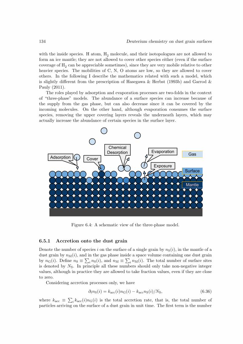
134 Deuterium chemistry on dust grain surfaces

with the inside species. H atom, H2 molecule, and their isotopologues are not allowed toform an ice mantle; they are not allowed to cover other species either (even if the surfacecoverage of H2 can be appreciable sometimes), since they are very mobile relative to otherheavier species. The mobilities of C, N, O atoms are low, so they are allowed to coverothers. In the following I describe the mathematics related with such a model, whichis slightly different from the prescription of Hasegawa & Herbst (1993b) and Garrod &Pauly (2011).

The roles played by adsorption and evaporation processes are two-folds in the contextof “three-phase” models. The abundance of a surface species can increase because ofthe supply from the gas phase, but can also decrease since it can be covered by theincoming molecules. On the other hand, although evaporation consumes the surfacespecies, removing the upper covering layers reveals the underneath layers, which mayactually increase the abundance of certain species in the surface layer.

Figure 6.4: A schematic view of the three-phase model.

6.5.1 Accretion onto the dust grain

Denote the number of species i on the surface of a single grain by nS(i), in the mantle of adust grain by nM(i), and in the gas phase inside a space volume containing one dust grainby nG(i). Define nS ≡

∑i nS(i), and nM ≡

∑i nM(i). The total number of surface sites

is denoted by NS. In principle all these numbers should only take non-negative integervalues, although in practice they are allowed to take fraction values, even if they are closeto zero.

Considering accretion processes only, we have

∂tnS(i) = kacc(i)nG(i)− kaccnS(i)/NS, (6.36)

where kacc ≡∑

i kacc(i)nG(i) is the total accretion rate, that is, the total number ofparticles arriving on the surface of a dust grain in unit time. The first term is the number

6.5 The three-phase gas-surface-mantle model 135

of species i arriving on a dust grain in unit time, and the second term accounts for the factthat each surface site has a probability of kacc/NS to be covered by an incoming particlein unit time.

If the gas phase concentration of species i can be approximated to be constant, thenthe solution of Eq. (6.36) can be written as

nS(i, t) = NSkacc(i)nG(i)∑j kacc(j)nG(i)

[1− e−kacct/NS

], (6.37)

which is proportional to the accretion rate of species i, and never becomes greater thanNS, which is expected.

The total number of particles in the surface layer as a function of time is

nS = NS

[1− e−kacct/NS

], (6.38)

which is essentially a constant (=NS) at a late stage. This is trivially correct, of course.For the mantle component, we have

∂tnM(i) = kaccnS(i)/NS, (6.39)

which is simply a result of conservation of material. Its time evolution can also be obtainedif the gas phase concentration of species i is fixed:

nM(i, t) = kacc(i)nG(i) t− nS(i)|t→∞

[1− e−kacct/NS

]. (6.40)

In the limit t → +∞, nM(i, t) → kacc(i)nG(i) t−nS(i)|t→∞, which is intuitively obtainableby simple counting.

6.5.2 Evaporation of grain material

Consider evaporation process only, we have

∂tnS(i) = −keva(i)nS(i) + kevanM(i)/max(nM, nS), (6.41)

where keva ≡∑

i keva(i)nS(i) is the total evaporation rate, namely, the total number ofparticles that are evaporated from a dust grain in unit time. The max() function in thedenominator accounts for the fact that, when the number of mantle species is less than thenumber of surface sites, removing a surface particle does not necessarily reveal a mantleparticle, since the particle being removed may be located on top of the dust core material,rather than on mantle material. In contrast, when the number of mantle species is greaterthan the number of surface sites, removing a surface particle must lead to the exposureof one mantle particle, due to our simplified assumption that all the mantle material isuniformly distributed over the dust grain core (hence presenting only one “phase”).

It is evident that the mantle material is considered as a whole in this treatment of theevaporation process. Each species in the grain mantle has equal probability to be exposedto external space when a surface molecule is removed, regardless of its depth in the dustgrain. The mantle composition is uniform, regardless of depth. Such a description isan approximation to the real situation, where molecules buried deep in the mantle are

136 Deuterium chemistry on dust grain surfaces

evaporated later than those in shallower layers. Nevertheless it is arguably better thanthe two-phase model.

For the mantle component, we have

∂tnM(i) = −kevanM(i)/max(nM, nS), (6.42)

which is simply a result of conservation of material.Suppose there is only one single species on the dust grain, then nM=nM(i), and suppose

there are many layers on the dust grain initially, we have

nM(t) =

nM|t=0 − keva t, when t < t0,

NSe−keva(i)(t−t0), when t ≥ t0;

(6.43)

nS(t) =

NS, when t < t0,

NSe−keva(i)(t−t0) [keva(i)(t− t0) + 1] , when t ≥ t0.

(6.44)

In the above equation t0 ≡ (nM|t=0 −NS)/keva.

6.5.3 The complete set of equations

The full set of equations describing the evolution of surface and mantle species can bewritten as

∂tnS(i) =∑j,k

kjknS(j)nS(k)−∑j

kijnS(i)nS(j)

+ kacc(i)nG(i)− kaccnS(i)/NS

+ kevanM(i)/max(nM, nS)− keva(i)nS(i),

(6.45)

∂tnM(i) =kaccnS(i)/NS − kevanM(i)/max(nM, nS). (6.46)

The first two terms in Eq. (6.45) are the direct contribution from chemical reactions.The total accretion rate kacc and evaporation rate keva include contributions from surfacereactions.

Ordinary differential equations of the above form are stable by themselves (as far asa good implicit solver is used). This can be inferred from the exact solutions for thesimple cases in Section 6.5.1 and Section 6.5.2, which involve only exponential and linearfunctions. The stability is also confirmed in practical model runs.

Besides adsorption and evaporation, in principle surface reactions can also alter thesurface coverage and mantle composition. For example, each time the reaction A+B −−→ Coccurs, the number of surface particles decreases by one, thus one surface site will becomeempty, and one mantle particle is exposed to the gas phase. The chemical desorption (seeChapter 5) of surface particle also leaves at least one surface site empty, thus liberatingone mantle particles.

To take this effect into account, I divide the surface reactions into two types: thoseleading to the decrease in total surface population, and those leading to the increase ofthe surface coverage. The former are treated as if they were evaporation reactions (only incalculating the surface-mantle transfer, of course), and the latter is treated as if they wereadsorption reactions. Surface reactions involving no mantle species (such as H+H −−→ H2)

6.6 Results and discussions 137

are not considered. Only the total absolute rates of these two types of reactions enter theequations governing the transfer between surface and mantle populations. Including suchan effect is optional.

Another issue is whether to allow the interconversion between surface mantle specieseven when the mantle is still growing. Such a situation is possible when the concentrationof a species inside the mantle is higher than in the surface layer. This can be seen fromequation Eq. (6.46): even if the total accretion rate is higher than the evaporation rate(kacc>keva), in case

nS(i)

NS<

kevakacc

nM(i)

nM,

∂tnM(i) can be negative. It is not clear whether such a scenario is realistic. One optionis to disallow the conversion of mantle species into surface species when kacc>keva. Thiscan be done by redefining k′acc = kacc − keva, and k′eva = 0.

In grain chemistry models the radius of a grain particle is canonically taken to be 0.1µm. It will gain in size by adsorbing gas phase particles. With the usual gas-to-dust massratio of 100, and an estimated metal-to-gas mass ratio[14] of ∼0.006, the mass of a typicaldust grain can increase by about 60% at most, and the increase in radius can be 20% atmost (assuming uniform density), if all the metals are assimilated into the dust grains. Ifthe mass density of the mantle layer is assumed to be lower, then the increase in radiuscan be ∼60% (Walmsley et al. 2004). Hence the accretion rate can increase by a factorof 1.4–2.5. Such a change in accretion rate is insignificant and will not be included in ourmodel.

6.6 Results and discussions

As can be seen from previous sections, the model contains a lot of parameters. Someof them may be considered free, while others are not completely free but are not wellconstrained either. Table (6.9) is a list of parameters that we vary during the modeling ina reasonable interval to see how the behavior of the model changes. For a specific source,some of the parameters (mainly temperature and density) can usually be constrainedrelatively well observationally. Table (6.10) is a list of parameters that are fixed duringthe modeling.

(1) Gas density nH;(2) Gas temperature Tgas and dust temperature Tdust: we always

assume Tdust = Tgas;(3) The binding energies of H and D;(4) We tested whether to include the H2 + OH channel for water

formation, and whether to allow the abstraction reactions ofCH3OH and H2CO.

Table 6.9: List of parameters that are varied in our model.

[14]Based on the elemental abundance of the metals usually assumed in the initial conditions of chemicalmodels. Here all the elements heavier than helium are called metal.

138 Deuterium chemistry on dust grain surfaces

(1) Elemental abundances; mainly taken from Garrod & Pauly(2011); included in table Table (6.11) for reference;

(2) Initial condition; we always use the abundances obtained witha gas phase chemistry at t = 107 yr with all the grain reactionsturned off except for the formation of H2 isotopologues;

(3) The rate parameters of many reactions are not known for sure;here we take their canonical values, or constrain them withexperimental and theoretical results;

(4) We allow CO2 formation through the three-body reaction H+O+CO, though this mechanism is still largely hypothetical;

(5) Dust-to-gas mass ratio: ηm = 0.01;(6) Dust material density ρG = 2 g cm−3;(7) Dust grain radius rgrain = 0.1 µm;(8) Cosmic-ray ionization rate: ζ = 1.36× 10−17 s−1;(9) Cosmic-ray desorption rate: 3.16×10−19 s−1; assume a cosmic-

ray can heat the dust grain to 70 K; cf. Page 33;(10) Chemical desorption efficiency is fixed to 0.01 except for one

case; unlike the previous chapter on H2O2 formation, for thepresent study we are not very concerned with the release ofsurface species into the gas phase;

(11) We disallow dissociation by cosmic-ray-induced photons; thisis allowed in the previous chapter;

(12) Albedo of dust grains: 0.6;(13) Density of surface sites: 1015 cm−2;(14) Width of barriers against surface diffusion: 1 A;(15) Height of barriers against surface diffusion: Ediff = 0.5Ebind;(16) Binding energy of each species (Ebind): taken from literature

and fixed (except for H and D); cf. Page 33.(17) We always include the contribution of zero-point energies to

the desorption and surface migration processes;(18) We disallow exposure of mantle species if the accretion rate is

higher than the evaporation rate.

Table 6.10: List of parameters that are fixed in our model.

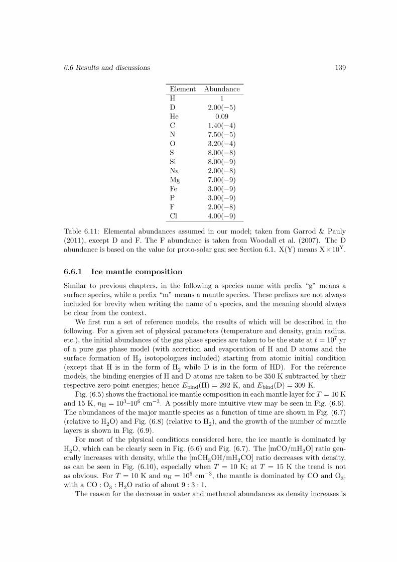
6.6 Results and discussions 139

Element Abundance

H 1D 2.00(−5)He 0.09C 1.40(−4)N 7.50(−5)O 3.20(−4)S 8.00(−8)Si 8.00(−9)Na 2.00(−8)Mg 7.00(−9)Fe 3.00(−9)P 3.00(−9)F 2.00(−8)Cl 4.00(−9)

Table 6.11: Elemental abundances assumed in our model; taken from Garrod & Pauly(2011), except D and F. The F abundance is taken from Woodall et al. (2007). The Dabundance is based on the value for proto-solar gas; see Section 6.1. X(Y) means X×10Y.

6.6.1 Ice mantle composition

Similar to previous chapters, in the following a species name with prefix “g” means asurface species, while a prefix “m” means a mantle species. These prefixes are not alwaysincluded for brevity when writing the name of a species, and the meaning should alwaysbe clear from the context.

We first run a set of reference models, the results of which will be described in thefollowing. For a given set of physical parameters (temperature and density, grain radius,etc.), the initial abundances of the gas phase species are taken to be the state at t = 107 yrof a pure gas phase model (with accretion and evaporation of H and D atoms and thesurface formation of H2 isotopologues included) starting from atomic initial condition(except that H is in the form of H2 while D is in the form of HD). For the referencemodels, the binding energies of H and D atoms are taken to be 350 K subtracted by theirrespective zero-point energies; hence Ebind(H) = 292 K, and Ebind(D) = 309 K.

Fig. (6.5) shows the fractional ice mantle composition in each mantle layer for T = 10 Kand 15 K, nH = 103–106 cm−3. A possibly more intuitive view may be seen in Fig. (6.6).The abundances of the major mantle species as a function of time are shown in Fig. (6.7)(relative to H2O) and Fig. (6.8) (relative to H2), and the growth of the number of mantlelayers is shown in Fig. (6.9).

For most of the physical conditions considered here, the ice mantle is dominated byH2O, which can be clearly seen in Fig. (6.6) and Fig. (6.7). The [mCO/mH2O] ratio gen-erally increases with density, while the [mCH3OH/mH2CO] ratio decreases with density,as can be seen in Fig. (6.10), especially when T = 10 K; at T = 15 K the trend is notas obvious. For T = 10 K and nH = 106 cm−3, the mantle is dominated by CO and O3,with a CO : O3 : H2O ratio of about 9 : 3 : 1.

The reason for the decrease in water and methanol abundances as density increases is

140 Deuterium chemistry on dust grain surfaces

because a higher gas density (for T = 10 K) means a lower atomic hydrogen abundancein the gas phase (see the following), while the abundance of CO in the gas phase (whenaccretion has not started) does not have a strong dependence on density. This can beseen in Fig. (6.11) for the T = 10 K case, where the initial abundances of H, D, andCO (obtained from a pure gas phase chemistry) are plotted as a function of gas density.As the [H/CO] ratio becomes lower at higher density, there will not be enough H atomsavailable to produce water, or to hydrogenate CO into CH3OH, which leads to the higher[CO/H2O] and [H2CO/CH3OH] ratios at a higher density.

The reason for the abundance of gas phase atomic hydrogen to decrease with densityis explained in the following. The gas phase density of H, n(H), is usually ∼1 cm−3 inde-pendent of temperature and the overall gas density in dark clouds. Hence its abundance,[H], which is defined to be the ratio between its density and the total density[15] of hy-drogen nuclei nH, varies with nH as [H] ∝ n−1

H . The fact that n(H) is constant is basedon the assumption that the gas phase atomic hydrogen is mainly produced by cosmic-rayionization of H2 molecules, and mainly consumed by adsorption onto the dust grains.Namely, we may assume H is mainly formed in the following reaction chain

H2 +CRPkcos−−→ H+

2 + E−,

H+2 +H2

k1−→ H+3 +H,

H+3 + E− k2−→ 3H,

gHkeva−−→ H,

(6.47)

and consumed through

Hkacc−−→ gH. (6.48)

These yield the following equations

∂tn(H+2 ) = kcosn(H2)− k1n(H2)n(H

+2 ),

∂tn(H+3 ) = k1n(H2)n(H

+2 )− k2n(H

+3 )n(E

−),

∂tn(H) = k1n(H2)n(H+2 ) + 3k2n(H

+3 )n(E

−) + kevan(gH)− kaccn(H),

(6.49)

where the density of H2 is assumed to be constant. Using Eq. (3.4) on page 31, whichindicates that

kacc = ηv(H)σnHRG,n, (6.50)

where η is the sticking coefficient (we assume η = 1), σ is the dust grain cross section,and RG,n is the dust-to-gas number ratio, we have for the steady-state (i.e. ∂tn(X) = 0)solution

n(H) =kcos4n(H2) + kevan(gH)

kacc' 2kcos

v(H)σRG,n, (6.51)

where in the last step the evaporation of surface H has been neglected. The above ex-pression does not depend on the total gas density, and indeed has a typical value of∼1 cm−3.

[15]For molecular clouds the total density of hydrogen nuclei can be approximated very well by two timesthe density of H2 molecule.

6.6 Results and discussions 141

Why is the steady-state abundance of CO in gas phase chemistry roughly indepen-dent of gas density? This is simply because practically all the carbon atoms have beenconverted into CO molecules (note that the abundance of oxygen is about two times theabundance of C) in steady state, so the abundance of CO is just the elemental abundanceof carbon, which is widely considered constant.

Then, can we say that it is impossible to form a large amount of water and methanolice at very high gas density (& 106 cm−3, for example) because in these cases the [H/CO]ratio will be low? Seemingly not, since it can be clearly seen in Fig. (6.5)–Fig. (6.8)that in the T = 15 K case the water and methanol ice can still be present with a highabundance at nH = 106 cm−3.

The fact is that at T = 15 K the evaporation of surface H atoms becomes important.Note that for a binding energy of 300 K for H, the evaporation rate at 15 K is aboute10 ' 2×104 times faster than at 10 K. This is a significant difference. As can be seen inthe right panel of Fig. (6.11), the initial abundances of gas phase H and D for T = 15 Kare much higher than for T = 10 K, especially when nH > 103 cm−3, and they are almostindependent of density at 15 K.

This independence on density is due to the fact that we set the initial abundances ofthe gas-grain model to be the abundances of a gas phase model at t = 107 yr, and whenthe surface evaporation rate of H is too high, the steady state has not been reached at thistime. This is because a high evaporation rate means H2 cannot be efficiently formed onthe grain, and the H2 molecules will be continuously converted into H atoms by cosmic-rayionization. The latter process is quite slow, with a time scale of ∼2.6×109 yr.

Hence the apparently very different results at T = 10 K and 15 K for nH = 106 cm−3

are due to our way of setting the initial abundances, and to the low binding energies ofH and D atoms. To confirm this, we tried higher values for the binding energies for Hand D, 618 K for H and 642 K for D, which are obtained from a common value of 700 Ksubtracted by their corresponding zero-point energies. In this case their evaporation ratesbecome negligible (the evaporation time scales are hundreds of years). The resulting icemantle compositions are shown in Fig. (6.12). Now the differences between the T = 10 Kand 15 K case are much smaller than before, though still noticeable.

On the other hand, the presence of “dry” CO ice (i.e. not mixed with water ice) in ourreference model and in the one with higher binding energies for H and D at nH = 106 cm−3

is consistent with the existence of non-polar CO ice suggested by observations. By observ-ing the absorption band of solid CO toward 18 protostars, Tielens et al. (1991) discoveredthat at least two independent grain mantle compositions are needed to explain the spec-tra: a polar mixture component rich in H2O and a nonpolar component dominated byCO. Our modeling results suggest that in cold dense (& 106 cm−3) environments nonpolargrain mantles tend to be formed, while at lower densities or higher temperatures (which,however, must still be lower than the evaporation temperature of the heavy species) water-rich ice mantles tend to be formed. This is similar to the suggestion of Pontoppidan et al.(2008).

We may note that, accompanying the formation of CO-dominated ice, a relativelyhigh abundance of O3 can also be accumulated on the grain mantle, which may serve asa test of our model. However, the formation of O3 is subject to uncertainties, since it issensitive to the surface mobility of O atoms (while the water formation is not). If O isimmobile, then O3 cannot be formed, at least in the Langmuir-Hinshelwood mechanism.

142 Deuterium chemistry on dust grain surfaces

One may also invoke the Eley-Rideal mechanism to form O3, in which an O atom fromthe gas phase hitting a surface O2 molecule can directly react with it to form O3, similarto the formation of CO2 through a three-body reaction mechanism.

Our modeling results may be compared with the observational results, as compiled inTable (6.12), where the abundances of a few major ice species expressed relative to H2Oare listed. Due to the intrinsic complexity of the ISM, where the dust can be processedby various processes, such as shock sputtering and heating, radiative evaporation anddissociation, collision with high-energy particles, etc., one should not expect that a singlemodel can reproduce all the observational results. Furthermore, we should not expect thatthe dust is formed in the environments where it is currently observed either; evolution intime, as well as transportation in space are likely to be common for the interstellar matter.Observationally, the abundance ratios of those major ice species can vary from source tosource significantly, even for sources within the same class. However, our modeling resultscan already match the observed abundances of most of them reasonably well, if differentphysical conditions for the formation of grain mantles are assumed.

The CO abundance is the easiest to match, which is typically 10%–50% with respectto water except for the extreme case of T = 10 K and nH = 106 cm−3, where littlewater ice is present; see Fig. (6.7) and Fig. (6.10). For CO2, the [CO2/H2O] ratio isaround 10%–30% at T = 10 K and nH = 104 cm−3, which are also consistent with theobservational results in Table (6.12). In the nonpolar case where water is deficient the[CO2/H2O] ratio can be up to 40%.

The CH3OH and H2CO abundances seem to be more challenging. For T = 10 K,only with a low density (103 cm−3) can the [CH3OH/H2O] ratio be higher than 20%,and for nH = 104 cm−3 the ratio is a few percent. Similar for the [H2CO/H2O] ratio,though it is typically higher by a factor of a few to ten than the [CH3OH/H2O] ratioat higher densities. The [CH4/H2O] ratio can be about 1%–2% at most in our referencemodel, while the [NH3/H2O] ratio is normally a few percent, and can be up to 10%. Ourmodel produces CH4 and NH3 at lower quantities than observed. This is understandable,since in the initial conditions of our model practically all the carbon is in CO and all thenitrogen is in N2.

From Figs. (6.5), (6.6) and (6.9) we may notice that the number of mantle layers atsteady state is different for different physical conditions, and it seems to be larger at ahigher temperature, and that for T = 10 K, the number of layers at nH = 106 cm−3 issmaller than at 105 cm−3. Though apparently counterintuitive, since we might think thatat lower temperature or higher density more species can be adsorbed, the reason alsolies in the abundance of H atoms. A higher flux of H atoms injected on the dust graintends to hydrogenate the heavy molecules (atoms) on the surface, instead of letting themcombine with each other. For example, on the surface oxygen atoms can combine to formO2 and O3 molecules, which will be stored in the mantle layer and become unavailablefor hydrogenation. If the hydrogen flux is high, they may be converted into water icebefore being covered. Note that one layer of O3, if completely converted into H2O, will becounted as three layers. The same holds for CO2, where one layer of CO2, if divided intoO and CO, will be counted as two layers. When the hydrogen flux is high, the probabilityfor the three-body reaction H+O+CO −−→ CO2 becomes lower, because O and CO willmost likely directly react with an incoming H atom; but when the hydrogen flux is low,the accumulation of surface O and CO makes this reaction much more likely.

6.6 Results and discussions 143

The total number of layers can be estimated by assuming all the oxygen and carbonatoms have been converted into H2O and CO ices. The elemental abundance of O isadopted to be 3.2×10−4 relative to H. With a dust-to-gas number ratio of 2.8×10−12, thenumber of O atoms that can accumulate on one dust grain is 3.2×10−4/(2.8×10−12) ' 108,which gives a total layer number of ∼100, since the number of surface sites on a dust grainis ∼106. The elemental abundance of nitrogen is about 1/4 that of oxygen, and if it ismainly in the form of N2, it constitutes only about 1/8 of the mantle volume.

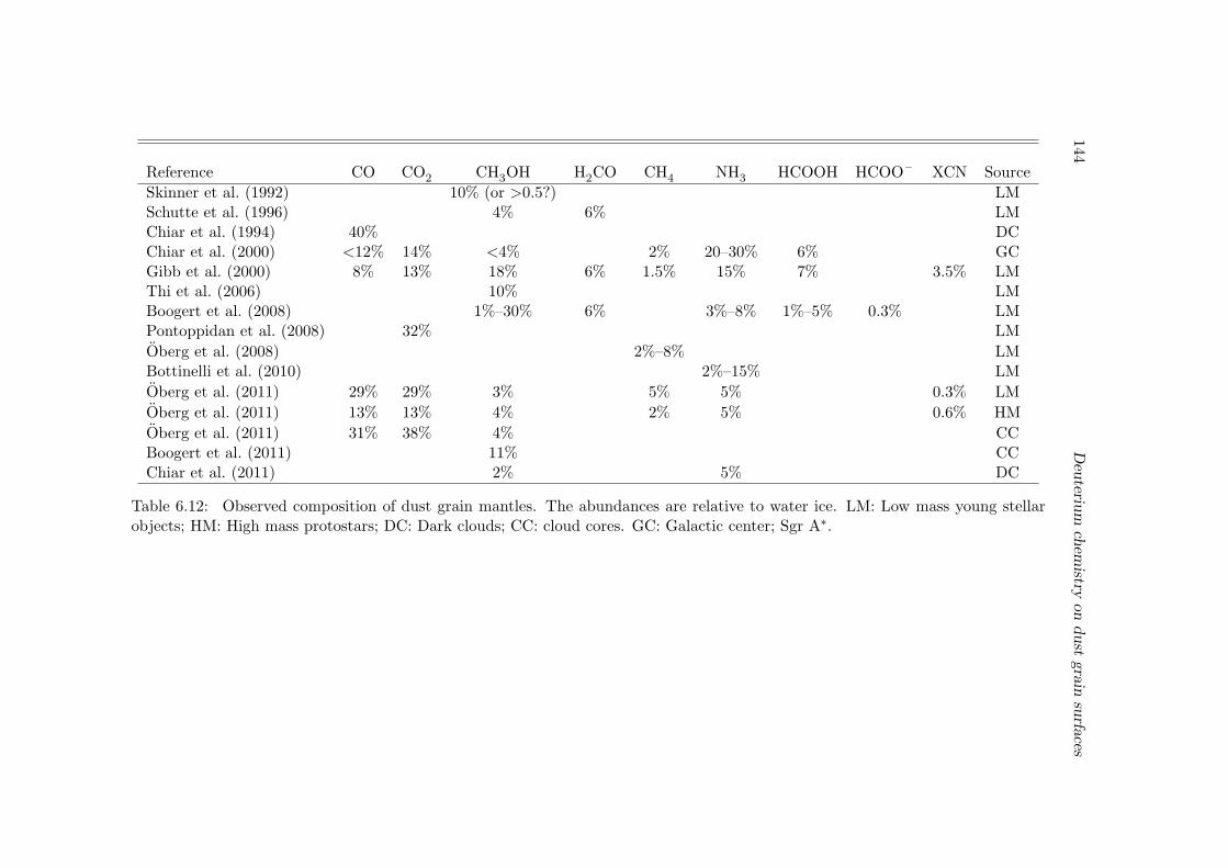
144

Deuteriu

mchem

istryon

dust

grainsurfaces

Reference CO CO2 CH3OH H2CO CH4 NH3 HCOOH HCOO – XCN Source

Skinner et al. (1992) 10% (or >0.5?) LMSchutte et al. (1996) 4% 6% LMChiar et al. (1994) 40% DCChiar et al. (2000) <12% 14% <4% 2% 20–30% 6% GCGibb et al. (2000) 8% 13% 18% 6% 1.5% 15% 7% 3.5% LMThi et al. (2006) 10% LMBoogert et al. (2008) 1%–30% 6% 3%–8% 1%–5% 0.3% LMPontoppidan et al. (2008) 32% LM

Oberg et al. (2008) 2%–8% LMBottinelli et al. (2010) 2%–15% LM

Oberg et al. (2011) 29% 29% 3% 5% 5% 0.3% LM

Oberg et al. (2011) 13% 13% 4% 2% 5% 0.6% HM

Oberg et al. (2011) 31% 38% 4% CCBoogert et al. (2011) 11% CCChiar et al. (2011) 2% 5% DC

Table 6.12: Observed composition of dust grain mantles. The abundances are relative to water ice. LM: Low mass young stellarobjects; HM: High mass protostars; DC: Dark clouds; CC: cloud cores. GC: Galactic center; Sgr A∗.

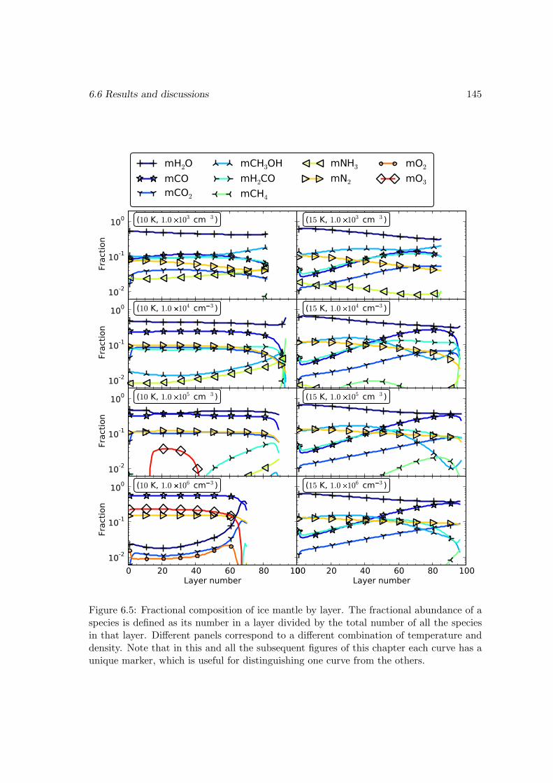
6.6 Results and discussions 145

10-2

10-1

100

Frac

tion

(10 K, 1.0103 cm3 )

mH2OmCOmCO2

mCH3OHmH2COmCH4

mNH3

mN2

mO2

mO3

10-2

10-1

100

Frac

tion

(10 K, 1.0104 cm3 )

10-2

10-1

100

Frac

tion

(10 K, 1.0105 cm3 )

0 20 40 60 80 100Layer number

10-2

10-1

100

Frac

tion

(10 K, 1.0106 cm3 )

(15 K, 1.0103 cm3 )

(15 K, 1.0104 cm3 )

(15 K, 1.0105 cm3 )

0 20 40 60 80 100Layer number

(15 K, 1.0106 cm3 )

Figure 6.5: Fractional composition of ice mantle by layer. The fractional abundance of aspecies is defined as its number in a layer divided by the total number of all the speciesin that layer. Different panels correspond to a different combination of temperature anddensity. Note that in this and all the subsequent figures of this chapter each curve has aunique marker, which is useful for distinguishing one curve from the others.

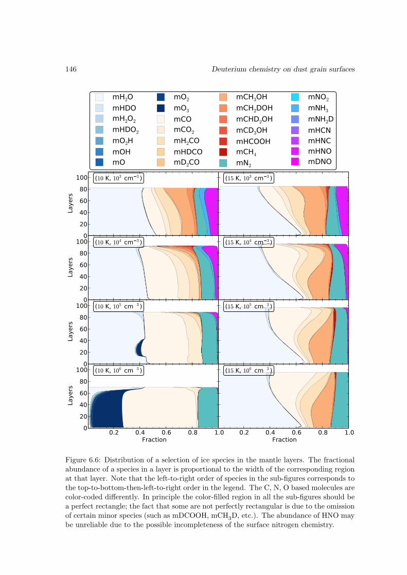
146 Deuterium chemistry on dust grain surfaces

0

20

40

60

80

100

Laye

rs

(10 K, 103 cm3 )

mH2OmHDOmH2O2

mHDO2

mO2HmOHmO

mO2

mO3

mCOmCO2

mH2COmHDCOmD2CO

mCH3OHmCH2DOHmCHD2OHmCD3OHmHCOOHmCH4

mN2

mNO2

mNH3

mNH2DmHCNmHNCmHNOmDNO

0

20

40

60

80

100

Laye

rs

(10 K, 104 cm3 )

0

20

40

60

80

100

Laye

rs

(10 K, 105 cm3 )

0.2 0.4 0.6 0.8 1.0Fraction

0

20

40

60

80

100

Laye

rs

(10 K, 106 cm3 )

(15 K, 103 cm3 )

(15 K, 104 cm3 )

(15 K, 105 cm3 )

0.2 0.4 0.6 0.8 1.0Fraction

(15 K, 106 cm3 )

Figure 6.6: Distribution of a selection of ice species in the mantle layers. The fractionalabundance of a species in a layer is proportional to the width of the corresponding regionat that layer. Note that the left-to-right order of species in the sub-figures corresponds tothe top-to-bottom-then-left-to-right order in the legend. The C, N, O based molecules arecolor-coded differently. In principle the color-filled region in all the sub-figures should bea perfect rectangle; the fact that some are not perfectly rectangular is due to the omissionof certain minor species (such as mDCOOH, mCH3D, etc.). The abundance of HNO maybe unreliable due to the possible incompleteness of the surface nitrogen chemistry.

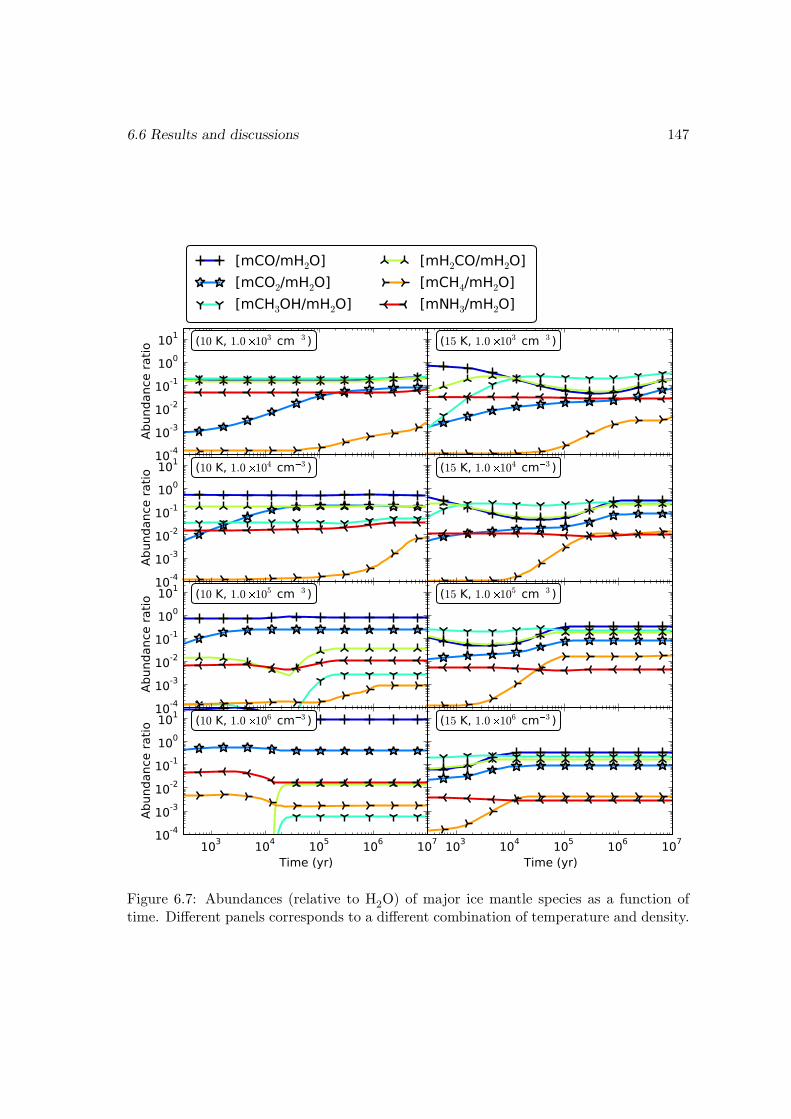
6.6 Results and discussions 147

10-4

10-3

10-2

10-1

100

101

Abun

danc

e ra

tio

(10 K, 1.0103 cm3 )

[mCO/mH2O][mCO2/mH2O][mCH3OH/mH2O]

[mH2CO/mH2O][mCH4/mH2O][mNH3/mH2O]

10-4

10-3

10-2

10-1

100

101

Abun

danc

e ra

tio

(10 K, 1.0104 cm3 )

10-4

10-3

10-2

10-1

100

101

Abun

danc

e ra

tio

(10 K, 1.0105 cm3 )

103 104 105 106 107

Time (yr)

10-4

10-3

10-2

10-1

100

101

Abun

danc

e ra

tio

(10 K, 1.0106 cm3 )

(15 K, 1.0103 cm3 )

(15 K, 1.0104 cm3 )

(15 K, 1.0105 cm3 )

103 104 105 106 107

Time (yr)

(15 K, 1.0106 cm3 )

Figure 6.7: Abundances (relative to H2O) of major ice mantle species as a function oftime. Different panels corresponds to a different combination of temperature and density.

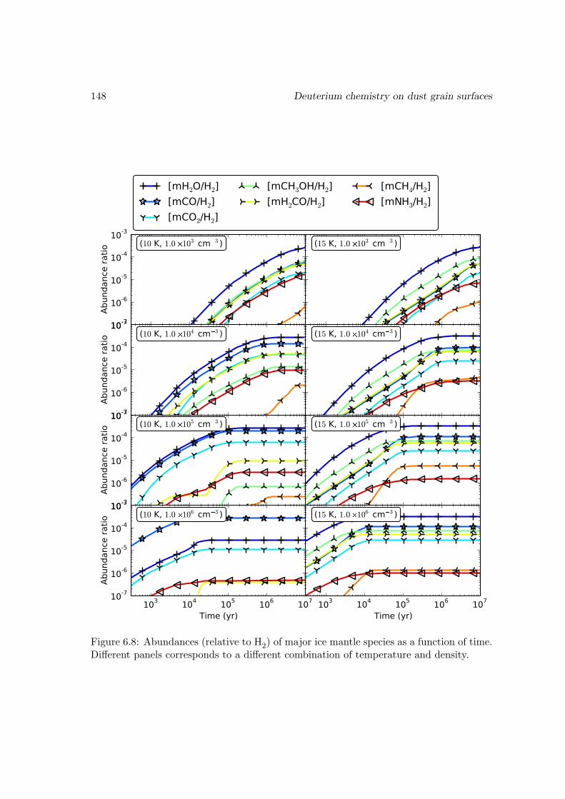
148 Deuterium chemistry on dust grain surfaces

10-7

10-6

10-5

10-4

10-3

Abun

danc

e ra

tio

(10 K, 1.0103 cm3 )

[mH2O/H2][mCO/H2][mCO2/H2]

[mCH3OH/H2][mH2CO/H2]

[mCH4/H2][mNH3/H2]

10-7

10-6

10-5

10-4

10-3

Abun

danc

e ra

tio

(10 K, 1.0104 cm3 )

10-7

10-6

10-5

10-4

10-3

Abun

danc

e ra

tio

(10 K, 1.0105 cm3 )

103 104 105 106 107

Time (yr)

10-7

10-6

10-5

10-4

10-3

Abun

danc

e ra

tio

(10 K, 1.0106 cm3 )

(15 K, 1.0103 cm3 )

(15 K, 1.0104 cm3 )

(15 K, 1.0105 cm3 )

103 104 105 106 107

Time (yr)

(15 K, 1.0106 cm3 )

Figure 6.8: Abundances (relative to H2) of major ice mantle species as a function of time.Different panels corresponds to a different combination of temperature and density.

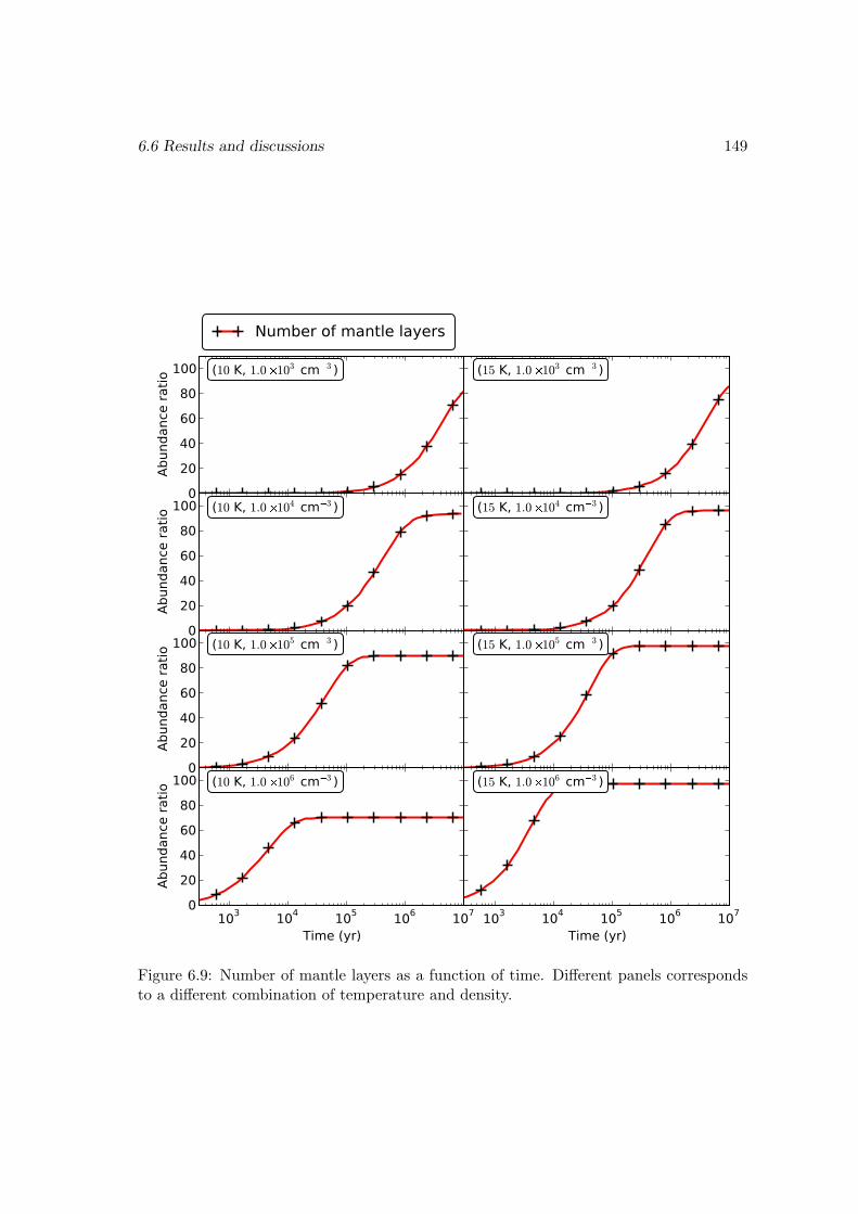
6.6 Results and discussions 149

0

20

40

60

80

100

Abun

danc

e ra

tio

(10 K, 1.0103 cm3 )

Number of mantle layers

0

20

40

60

80

100

Abun

danc

e ra

tio

(10 K, 1.0104 cm3 )

0

20

40

60

80

100

Abun

danc

e ra

tio

(10 K, 1.0105 cm3 )

103 104 105 106 107

Time (yr)

0

20

40

60

80

100

Abun

danc

e ra

tio

(10 K, 1.0106 cm3 )

(15 K, 1.0103 cm3 )

(15 K, 1.0104 cm3 )

(15 K, 1.0105 cm3 )

103 104 105 106 107

Time (yr)

(15 K, 1.0106 cm3 )

Figure 6.9: Number of mantle layers as a function of time. Different panels correspondsto a different combination of temperature and density.

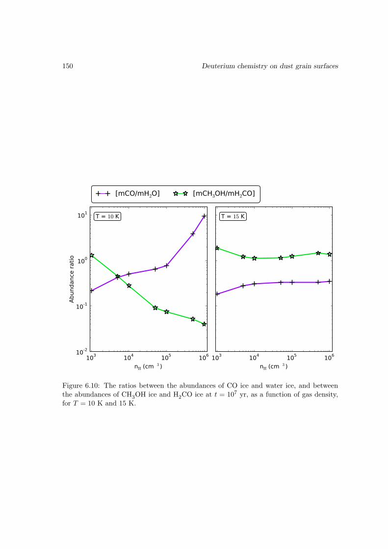
150 Deuterium chemistry on dust grain surfaces

103 104 105 106

nH (cm3 )

10-2

10-1

100

101

Abun

danc

e ra

tio

T = 10 K

[mCO/mH2O] [mCH3OH/mH2CO]

103 104 105 106

nH (cm3 )

T = 15 K

Figure 6.10: The ratios between the abundances of CO ice and water ice, and betweenthe abundances of CH3OH ice and H2CO ice at t = 107 yr, as a function of gas density,for T = 10 K and 15 K.

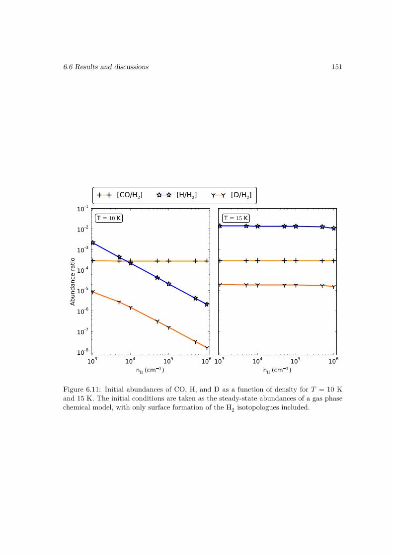
6.6 Results and discussions 151

103 104 105 106

nH (cm3 )

10-8

10-7

10-6

10-5

10-4

10-3

10-2

10-1

Abun

danc

e ra

tio

T = 10 K

[CO/H2] [H/H2] [D/H2]

103 104 105 106

nH (cm3 )

T = 15 K

Figure 6.11: Initial abundances of CO, H, and D as a function of density for T = 10 Kand 15 K. The initial conditions are taken as the steady-state abundances of a gas phasechemical model, with only surface formation of the H2 isotopologues included.

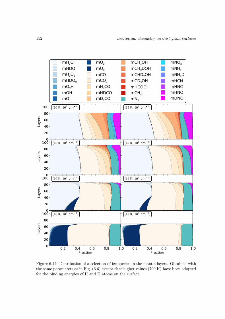
152 Deuterium chemistry on dust grain surfaces

0

20

40

60

80

100

Laye

rs

(10 K, 103 cm3 )

mH2OmHDOmH2O2

mHDO2

mO2HmOHmO

mO2

mO3

mCOmCO2

mH2COmHDCOmD2CO

mCH3OHmCH2DOHmCHD2OHmCD3OHmHCOOHmCH4

mN2

mNO2

mNH3

mNH2DmHCNmHNCmHNOmDNO

0

20

40

60

80

100

Laye

rs

(10 K, 104 cm3 )

0

20

40

60

80

100

Laye

rs

(10 K, 105 cm3 )

0.2 0.4 0.6 0.8 1.0Fraction

0

20

40

60

80

100

Laye

rs

(10 K, 106 cm3 )

(15 K, 103 cm3 )

(15 K, 104 cm3 )

(15 K, 105 cm3 )

0.2 0.4 0.6 0.8 1.0Fraction

(15 K, 106 cm3 )

Figure 6.12: Distribution of a selection of ice species in the mantle layers. Obtained withthe same parameters as in Fig. (6.6) except that higher values (700 K) have been adoptedfor the binding energies of H and D atoms on the surface.

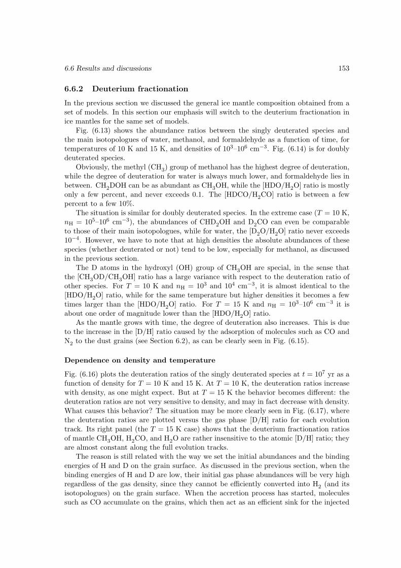
6.6 Results and discussions 153

6.6.2 Deuterium fractionation

In the previous section we discussed the general ice mantle composition obtained from aset of models. In this section our emphasis will switch to the deuterium fractionation inice mantles for the same set of models.

Fig. (6.13) shows the abundance ratios between the singly deuterated species andthe main isotopologues of water, methanol, and formaldehyde as a function of time, fortemperatures of 10 K and 15 K, and densities of 103–106 cm−3. Fig. (6.14) is for doublydeuterated species.

Obviously, the methyl (CH3) group of methanol has the highest degree of deuteration,while the degree of deuteration for water is always much lower, and formaldehyde lies inbetween. CH2DOH can be as abundant as CH3OH, while the [HDO/H2O] ratio is mostlyonly a few percent, and never exceeds 0.1. The [HDCO/H2CO] ratio is between a fewpercent to a few 10%.

The situation is similar for doubly deuterated species. In the extreme case (T = 10 K,nH = 105–106 cm−3), the abundances of CHD2OH and D2CO can even be comparableto those of their main isotopologues, while for water, the [D2O/H2O] ratio never exceeds10−4. However, we have to note that at high densities the absolute abundances of thesespecies (whether deuterated or not) tend to be low, especially for methanol, as discussedin the previous section.

The D atoms in the hydroxyl (OH) group of CH3OH are special, in the sense thatthe [CH3OD/CH3OH] ratio has a large variance with respect to the deuteration ratio ofother species. For T = 10 K and nH = 103 and 104 cm−3, it is almost identical to the[HDO/H2O] ratio, while for the same temperature but higher densities it becomes a fewtimes larger than the [HDO/H2O] ratio. For T = 15 K and nH = 103–106 cm−3 it isabout one order of magnitude lower than the [HDO/H2O] ratio.

As the mantle grows with time, the degree of deuteration also increases. This is dueto the increase in the [D/H] ratio caused by the adsorption of molecules such as CO andN2 to the dust grains (see Section 6.2), as can be clearly seen in Fig. (6.15).

Dependence on density and temperature

Fig. (6.16) plots the deuteration ratios of the singly deuterated species at t = 107 yr as afunction of density for T = 10 K and 15 K. At T = 10 K, the deuteration ratios increasewith density, as one might expect. But at T = 15 K the behavior becomes different: thedeuteration ratios are not very sensitive to density, and may in fact decrease with density.What causes this behavior? The situation may be more clearly seen in Fig. (6.17), wherethe deuteration ratios are plotted versus the gas phase [D/H] ratio for each evolutiontrack. Its right panel (the T = 15 K case) shows that the deuterium fractionation ratiosof mantle CH3OH, H2CO, and H2O are rather insensitive to the atomic [D/H] ratio; theyare almost constant along the full evolution tracks.

The reason is still related with the way we set the initial abundances and the bindingenergies of H and D on the grain surface. As discussed in the previous section, when thebinding energies of H and D are low, their initial gas phase abundances will be very highregardless of the gas density, since they cannot be efficiently converted into H2 (and itsisotopologues) on the grain surface. When the accretion process has started, moleculessuch as CO accumulate on the grains, which then act as an efficient sink for the injected

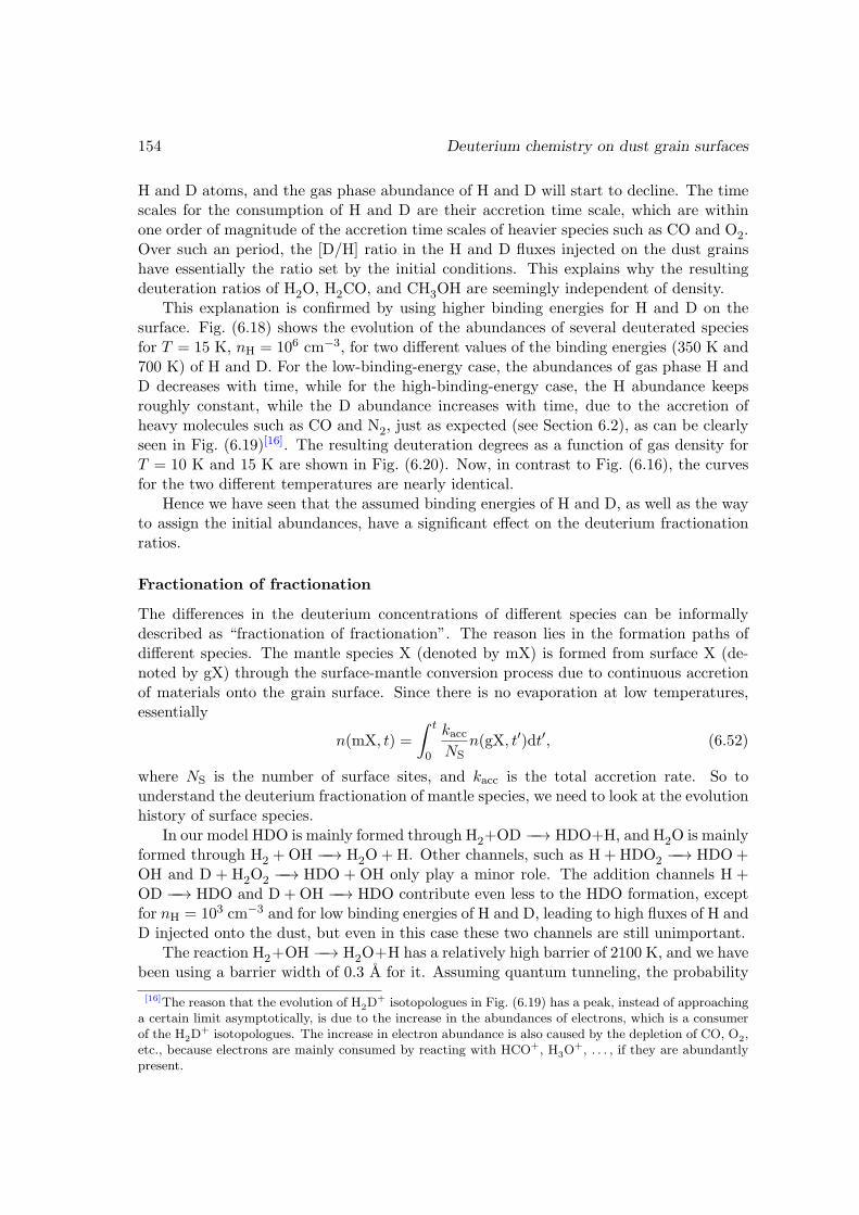
154 Deuterium chemistry on dust grain surfaces

H and D atoms, and the gas phase abundance of H and D will start to decline. The timescales for the consumption of H and D are their accretion time scale, which are withinone order of magnitude of the accretion time scales of heavier species such as CO and O2.Over such an period, the [D/H] ratio in the H and D fluxes injected on the dust grainshave essentially the ratio set by the initial conditions. This explains why the resultingdeuteration ratios of H2O, H2CO, and CH3OH are seemingly independent of density.

This explanation is confirmed by using higher binding energies for H and D on thesurface. Fig. (6.18) shows the evolution of the abundances of several deuterated speciesfor T = 15 K, nH = 106 cm−3, for two different values of the binding energies (350 K and700 K) of H and D. For the low-binding-energy case, the abundances of gas phase H andD decreases with time, while for the high-binding-energy case, the H abundance keepsroughly constant, while the D abundance increases with time, due to the accretion ofheavy molecules such as CO and N2, just as expected (see Section 6.2), as can be clearlyseen in Fig. (6.19)[16]. The resulting deuteration degrees as a function of gas density forT = 10 K and 15 K are shown in Fig. (6.20). Now, in contrast to Fig. (6.16), the curvesfor the two different temperatures are nearly identical.

Hence we have seen that the assumed binding energies of H and D, as well as the wayto assign the initial abundances, have a significant effect on the deuterium fractionationratios.

Fractionation of fractionation

The differences in the deuterium concentrations of different species can be informallydescribed as “fractionation of fractionation”. The reason lies in the formation paths ofdifferent species. The mantle species X (denoted by mX) is formed from surface X (de-noted by gX) through the surface-mantle conversion process due to continuous accretionof materials onto the grain surface. Since there is no evaporation at low temperatures,essentially

n(mX, t) =

∫ t

0

kaccNS

n(gX, t′)dt′, (6.52)

where NS is the number of surface sites, and kacc is the total accretion rate. So tounderstand the deuterium fractionation of mantle species, we need to look at the evolutionhistory of surface species.

In our model HDO is mainly formed through H2+OD −−→ HDO+H, and H2O is mainlyformed through H2 +OH −−→ H2O+H. Other channels, such as H + HDO2 −−→ HDO+OH and D + H2O2 −−→ HDO + OH only play a minor role. The addition channels H +OD −−→ HDO and D +OH −−→ HDO contribute even less to the HDO formation, exceptfor nH = 103 cm−3 and for low binding energies of H and D, leading to high fluxes of H andD injected onto the dust, but even in this case these two channels are still unimportant.

The reaction H2+OH −−→ H2O+H has a relatively high barrier of 2100 K, and we havebeen using a barrier width of 0.3 A for it. Assuming quantum tunneling, the probability

[16]The reason that the evolution of H2D+ isotopologues in Fig. (6.19) has a peak, instead of approaching

a certain limit asymptotically, is due to the increase in the abundances of electrons, which is a consumerof the H2D

+ isotopologues. The increase in electron abundance is also caused by the depletion of CO, O2,etc., because electrons are mainly consumed by reacting with HCO+, H3O

+, . . . , if they are abundantlypresent.

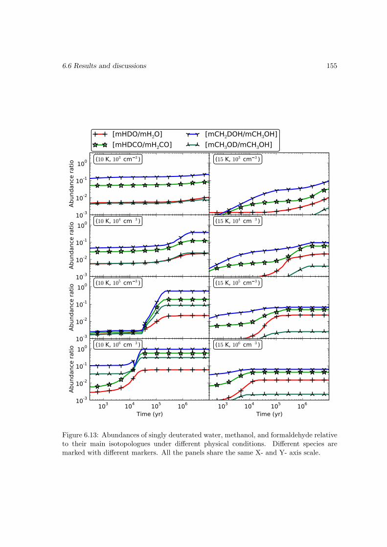
6.6 Results and discussions 155

10-3

10-2

10-1

100

Abun

danc

e ra

tio

(10 K, 103 cm3 )

[mHDO/mH2O][mHDCO/mH2CO]

[mCH2DOH/mCH3OH][mCH3OD/mCH3OH]

10-3

10-2

10-1

100

Abun

danc

e ra

tio

(10 K, 104 cm3 )

10-3

10-2

10-1

100

Abun

danc

e ra

tio

(10 K, 105 cm3 )

103 104 105 106

Time (yr)

10-3

10-2

10-1

100

Abun

danc

e ra

tio

(10 K, 106 cm3 )

(15 K, 103 cm3 )

(15 K, 104 cm3 )

(15 K, 105 cm3 )

103 104 105 106

Time (yr)

(15 K, 106 cm3 )

Figure 6.13: Abundances of singly deuterated water, methanol, and formaldehyde relativeto their main isotopologues under different physical conditions. Different species aremarked with different markers. All the panels share the same X- and Y- axis scale.

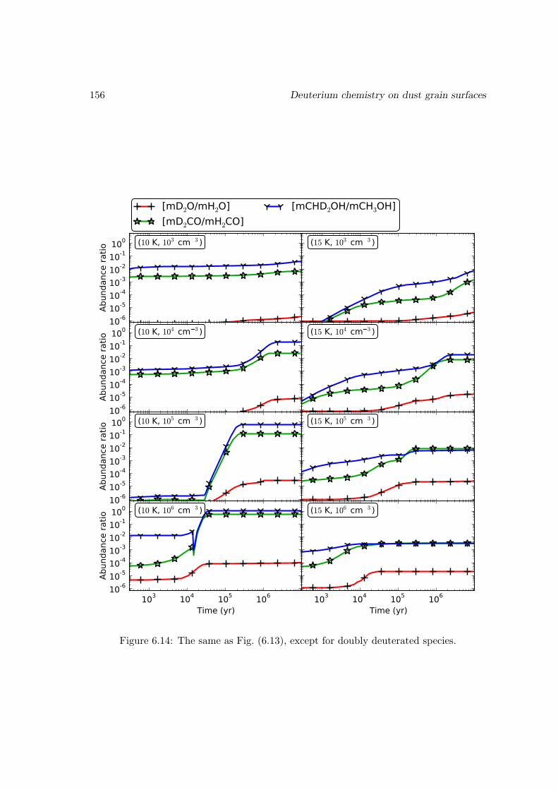
156 Deuterium chemistry on dust grain surfaces

10-610-510-410-310-210-1100

Abun

danc

e ra

tio

(10 K, 103 cm3 )

[mD2O/mH2O][mD2CO/mH2CO]

[mCHD2OH/mCH3OH]

10-610-510-410-310-210-1100

Abun

danc

e ra

tio

(10 K, 104 cm3 )

10-610-510-410-310-210-1100

Abun

danc

e ra

tio

(10 K, 105 cm3 )

103 104 105 106

Time (yr)

10-610-510-410-310-210-1100

Abun

danc

e ra

tio

(10 K, 106 cm3 )

(15 K, 103 cm3 )

(15 K, 104 cm3 )

(15 K, 105 cm3 )

103 104 105 106

Time (yr)

(15 K, 106 cm3 )

Figure 6.14: The same as Fig. (6.13), except for doubly deuterated species.

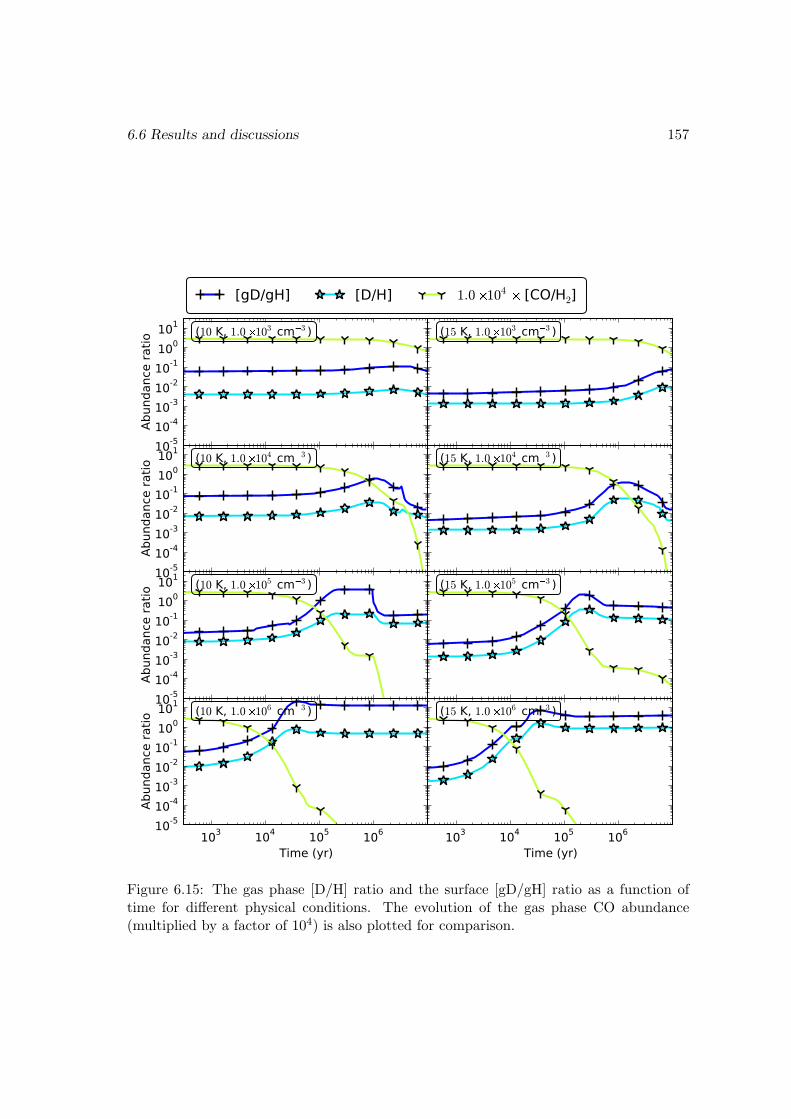
6.6 Results and discussions 157

10-510-410-310-210-1100101

Abun

danc

e ra

tio

(10 K, 1.0103 cm3 )

[gD/gH] [D/H] 1.0104 [CO/H2]

10-510-410-310-210-1100101

Abun

danc

e ra

tio

(10 K, 1.0104 cm3 )

10-510-410-310-210-1100101

Abun

danc

e ra

tio

(10 K, 1.0105 cm3 )

103 104 105 106

Time (yr)

10-510-410-310-210-1100101

Abun

danc

e ra

tio

(10 K, 1.0106 cm3 )

(15 K, 1.0103 cm3 )

(15 K, 1.0104 cm3 )

(15 K, 1.0105 cm3 )

103 104 105 106

Time (yr)

(15 K, 1.0106 cm3 )

Figure 6.15: The gas phase [D/H] ratio and the surface [gD/gH] ratio as a function oftime for different physical conditions. The evolution of the gas phase CO abundance(multiplied by a factor of 104) is also plotted for comparison.

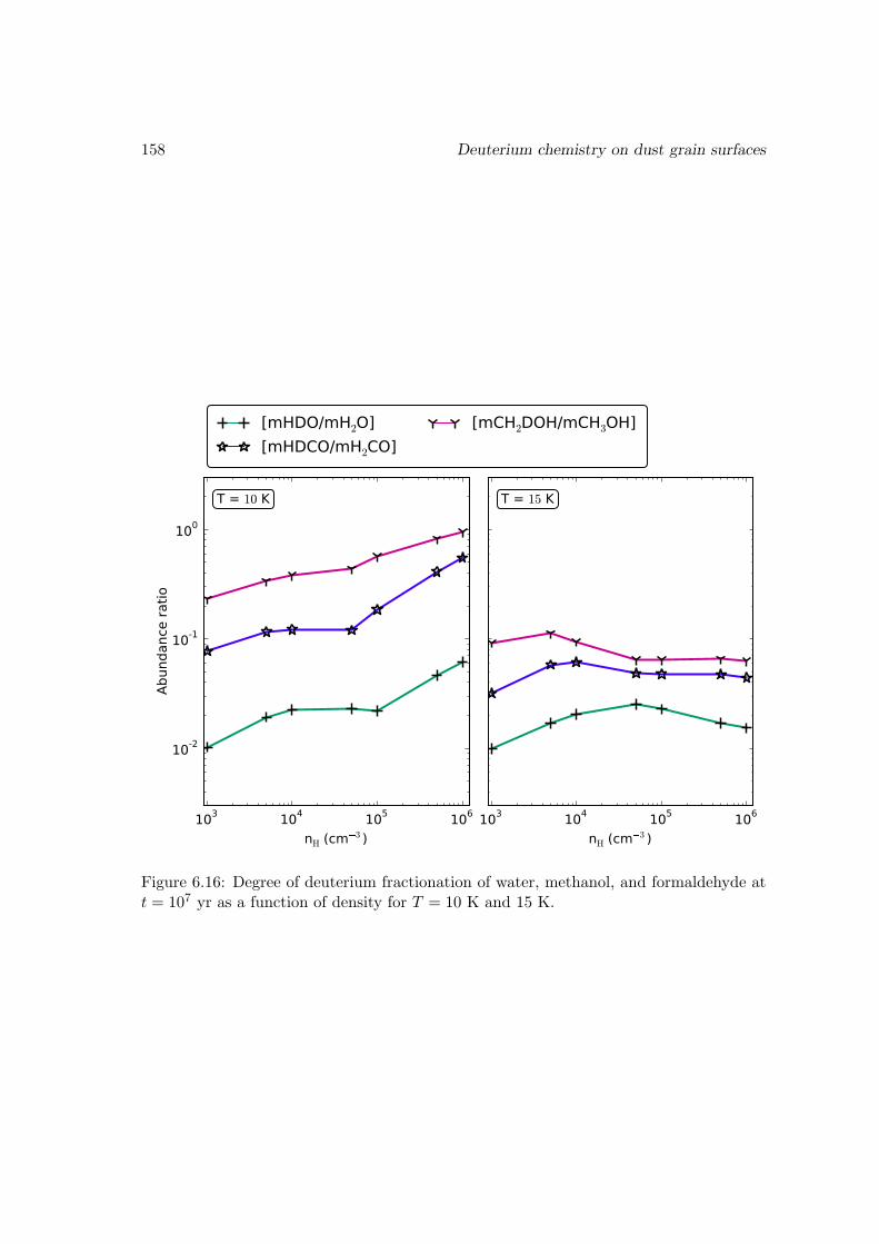
158 Deuterium chemistry on dust grain surfaces

103 104 105 106

nH (cm3 )

10-2

10-1

100

Abun

danc

e ra

tio

T = 10 K

[mHDO/mH2O][mHDCO/mH2CO]

[mCH2DOH/mCH3OH]

103 104 105 106

nH (cm3 )

T = 15 K

Figure 6.16: Degree of deuterium fractionation of water, methanol, and formaldehyde att = 107 yr as a function of density for T = 10 K and 15 K.

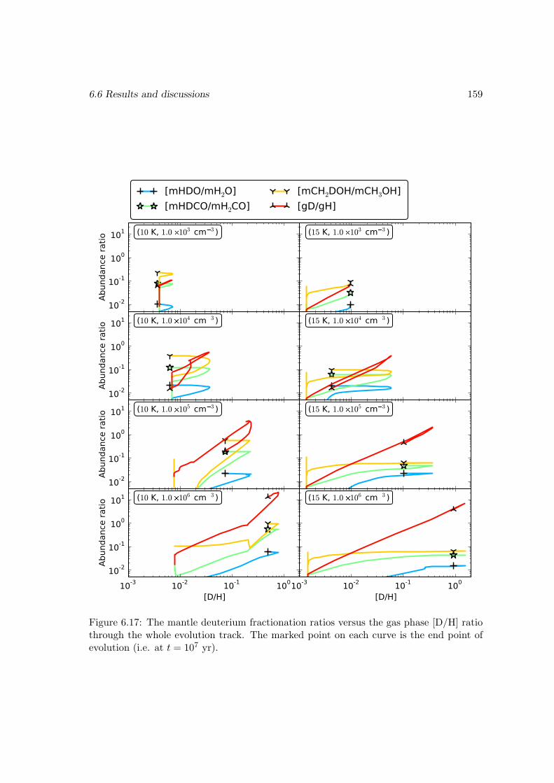
6.6 Results and discussions 159

10-2

10-1

100

101

Abun

danc

e ra

tio

(10 K, 1.0103 cm3 )

[mHDO/mH2O][mHDCO/mH2CO]

[mCH2DOH/mCH3OH][gD/gH]

10-2

10-1

100

101

Abun

danc

e ra

tio

(10 K, 1.0104 cm3 )

10-2

10-1

100

101

Abun

danc

e ra

tio

(10 K, 1.0105 cm3 )

10-3 10-2 10-1 100

[D/H]

10-2

10-1

100

101

Abun

danc

e ra

tio

(10 K, 1.0106 cm3 )

(15 K, 1.0103 cm3 )

(15 K, 1.0104 cm3 )

(15 K, 1.0105 cm3 )

10-3 10-2 10-1 100

[D/H]

(15 K, 1.0106 cm3 )

Figure 6.17: The mantle deuterium fractionation ratios versus the gas phase [D/H] ratiothrough the whole evolution track. The marked point on each curve is the end point ofevolution (i.e. at t = 107 yr).

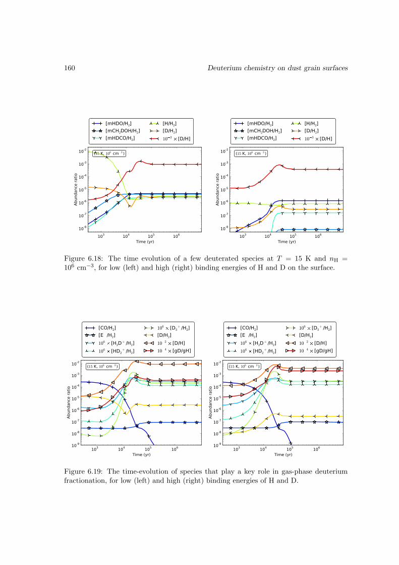
160 Deuterium chemistry on dust grain surfaces

103 104 105 106

Time (yr)

10-8

10-7

10-6

10-5

10-4

10-3

10-2

Abun

danc

e ra

tio

(15 K, 106 cm3 )

[mHDO/H2][mCH2DOH/H2][mHDCO/H2]

[H/H2][D/H2]103 [D/H]

103 104 105 106

Time (yr)

10-8

10-7

10-6

10-5

10-4

10-3

10-2

Abun

danc

e ra

tio

(15 K, 106 cm3 )

[mHDO/H2][mCH2DOH/H2][mHDCO/H2]

[H/H2][D/H2]103 [D/H]

Figure 6.18: The time evolution of a few deuterated species at T = 15 K and nH =106 cm−3, for low (left) and high (right) binding energies of H and D on the surface.

103 104 105 106

Time (yr)

10-9

10-8

10-7

10-6

10-5

10-4

10-3

10-2

Abun

danc

e ra

tio

(15 K, 106 cm3 )

[CO/H2][E /H2]106 [H2D+ /H2]106 [HD2

+ /H2]

106 [D3+ /H2]

[D/H2]102 [D/H]104 [gD/gH]

103 104 105 106

Time (yr)

10-9

10-8

10-7

10-6

10-5

10-4

10-3

10-2

Abun

danc

e ra

tio

(15 K, 106 cm3 )

[CO/H2][E /H2]106 [H2D+ /H2]106 [HD2

+ /H2]

106 [D3+ /H2]

[D/H2]102 [D/H]104 [gD/gH]

Figure 6.19: The time-evolution of species that play a key role in gas-phase deuteriumfractionation, for low (left) and high (right) binding energies of H and D.

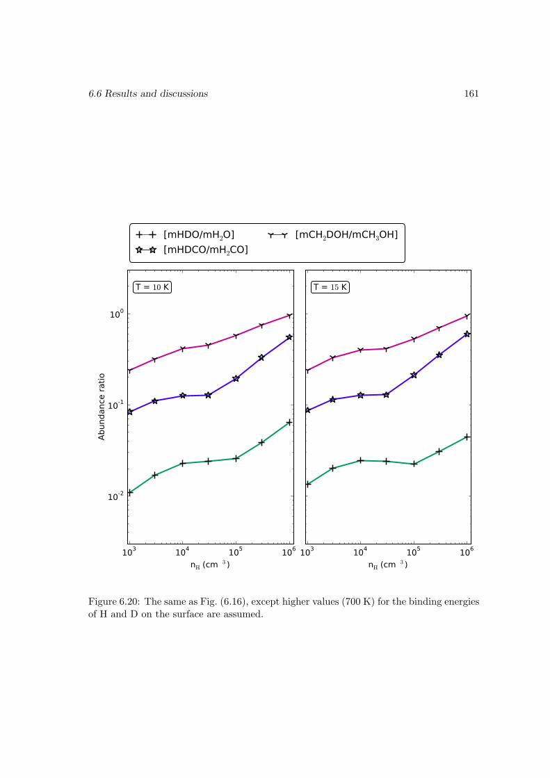
6.6 Results and discussions 161

103 104 105 106

nH (cm3 )

10-2

10-1

100

Abun

danc

e ra

tio

T = 10 K

[mHDO/mH2O][mHDCO/mH2CO]

[mCH2DOH/mCH3OH]

103 104 105 106

nH (cm3 )

T = 15 K

Figure 6.20: The same as Fig. (6.16), except higher values (700 K) for the binding energiesof H and D on the surface are assumed.

162 Deuterium chemistry on dust grain surfaces

for an H2 (HD) and an OH (OD) molecule to react upon meeting is 10−4–10−3, dependingon whether an H or D atom is being transferred. Due to its higher mass, the mobilityof H2 on a grain surface is about 30 times lower than that of H. Considering the highpopulation of H2 on the surface, which can be up to a few 10%, and the extremely lowcoverage of atomic H, which is around ten orders of magnitude lower than that of H2, thedominance of the H2 +OH reaction over the H + OH reaction is thus understandable.

The surface [HDO/H2O] ratio is approximately equal to the surface [OD/OH] ratioat the time when H2O and HDO are being formed. See Fig. (6.21) for an example. Thesurface [OD/OH] ratio is roughly proportional to the surface [D/H] ratio, the formerbeing lower by a factor of around ten. So even if the surface [D/H] ratio can becomequite high (which can be higher than one in Fig. (6.21)), the [HDO/H2O] ratio cannotbe very high. Another fact is, the surface [D/H] ratio (hence the [OD/OH] ratio) onlybecomes very high at a late stage when most of the H2O ice has already formed; this canbe seen from the vertical line in Fig. (6.21), which marks the time when 90% of water icehas formed (and it is about the same time when 90% of the gas phase CO, O2, etc., havebeen adsorbed onto the dust grains). So a late-time high surface [D/H] ratio cannot betransferred to water.

Since both the H + OH −−→ H2O channel and the H2 + OH −−→ H2O + H channelinvolve OH as an intermediate, and since the [HDO/H2O] ratio is determined by thesurface [OD/OH] ratio in the formation stage of water ice, would it make a difference inthe deuteration ratio of water if OH is turned into water by reacting with H instead ofH2? To address this, I switch off the reaction H2 +OH −−→ H2O+ H and its deuteratedcounterparts completely, while other parameters are unchanged. The resulting ice mantlecomposition is shown in Fig. (6.22), where evidently water is still the dominant speciesexcept for T = 10 K and nH = 106 cm−3; the reason for this has been explained before.Hence a model without the H2 +OH reaction seems to be viable, at least in the sense ofbeing able to produce enough water ice. Here our focus is on deuteration ratios, whichfor the singly deuterated species are shown in Fig. (6.23). Clearly H2O is still the least-deuterated species, which never has a fractionation ratio higher than 10% except for thecases when it is not abundant (for T = 10 K, nH = 105 and 106 cm−3), while CH3OH hasthe highest deuteration ratio, which can be up to order unity, and H2CO is still in theintermediate.

A comparison between Fig. (6.13) and Fig. (6.23) indicates that excluding the H2+OHchannel can indeed increase the deuteration degree of H2O by a factor of about two (moreat higher densities). The reason is that, with the H+OH channel, HDO can be formed viatwo reactions, H +OD −−→ HDO or D+OH −−→ HDO, while with the H2 +OH channel,only the H2 + OD −−→ HDO + H reaction works efficiently; the HD + OH −−→ HDO + Hchannel is much less efficient due to its higher tunneling mass and the lower mobility ofHD compared to H2 (and the [HD/H2] ratio is much lower than [OD/OH] anyway).

To see the difference in the surface [HDO/H2O] ratio caused by the two routes morequantitatively, in the following we list the relevant reactions (again, a prefix “g” is includedfor the surface species to distinguish them from the gas phase species)

gH2 + gOHk1−→ gH2O+ gH,

gH2 + gODk1−→ gHDO+ gH,

(6.53)

6.6 Results and discussions 163

and

gH + gOHk2−→ gH2O,

gH + gODk2−→ gHDO,

gD + gOHk3−→ gHDO.

(6.54)

Hence we have for the H2+OH channel (neglecting the term for converting surface speciesinto mantle species):

∂tn(gH2O) = k1n(gH2)n(gOH),

∂tn(gHDO) = k1n(gH2)n(gOD),(6.55)

which leads ton(gHDO)

n(gH2O)=

n(gOD)

n(gOH). (6.56)

For the H + OH channel,

∂tn(gH2O) = k2n(gH)n(gOH),

∂tn(gHDO) = k2n(gH)n(gOD) + k3n(gD)n(gOH),(6.57)

which givesn(gHDO)

n(gH2O)=

n(gOD)

n(gOH)+

k3k2

n(gD)

n(gH). (6.58)

The last term in the last equation is roughly the ratio between the consumption rate ofsurface D and H, which can be estimated to be the ratio between their accretion fluxes(under the quasi-steady-state approximation), namely,

k3k2

n(gD)

n(gH)' 1√

2

n(D)

n(H), (6.59)

where the factor 1√2accounts for the mass ratio between D and H, and n(D)

n(H) is the

abundance ratio of gas phase D and H. So we finally get

n(gHDO)

n(gH2O)' n(gOD)

n(gOH)+

1√2

n(D)

n(H). (6.60)

Thus it is clear that the H + OH channel gives a higher deuteration ratio for water thanthe H2 +OH channel.

Note that the mantle abundance of any species is an integral over time of its surfaceabundance weighted by the accretion flux of heavy mantle-making species (cf. Eq. (6.52)),so the final [mHDO/mH2O] ratio will lie somewhere in between the maximum and mini-mum of the [gHDO/gH2O] ratio.

In contrast to singly deuterated water, a vast change in the abundance of doublydeuterated water can be seen by comparing Fig. (6.24) with Fig. (6.14). When the H2+OHchannel is turned off, the [D2O/H2O] ratio increases by 2–3 orders of magnitude relativeto the case when the H2+OH channel is on. The reason is easily understood: on the dustgrain surface the reactions forming D2O are D + OD −−→ D2O, HD + OD −−→ D2O + H,

164 Deuterium chemistry on dust grain surfaces

D2 + OD −−→ D2O + D, and D2 + OH −−→ D2O + H; the latter ones cannot give a highfractionation ratio for D2O because the [HD/H2] and [D2/H2] ratios never get very high.So we may consider the D + OD −−→ D2O reaction only. When the H2 + OH channel isallowed, a D atom has to compete with the very abundant H2 molecules to react withOD, which renders the D + OD reaction practically impossible; in fact, in this case thesurface D2O molecules are mainly from the gas phase. Without the H2 + OH channel,the competitor of D is mainly atomic H, which is much less abundant than H2, hence theD + OD reaction can proceed to produce much more D2O than the previous case. Weremark that a low [D2O/H2O] ratio (∼10−5) when water is mainly formed through theH2 +OH channel is consistent with the value obtained by Butner et al. (2007) in the lowmass protostar IRAS 16293-2422 (and it seems up to now D2O is only detected in thissource).

By comparing Figs. (6.6) and (6.22) one may also note that, for T = 10 K andnH = 105 cm−3, when the H2 + OH channel is removed, the O3 abundance (occupying∼10% of the mantle volume) in the ice mantle is much higher than when the H2 + OHchannel is included, where O3 only occupies about 1% of the mantle volume. This isdue to the fact that removing the H2 +OH channel means a higher consumption rate ofsurface H, which leaves more O and O2 on the surface free to form O3 to be stored in themantle.

Since H2+OH −−→ H2O+H being the major channel to produce water in our previousmodels seems not to be the main reason for the lower deuterium fractionation ratio ofwater in comparison to formaldehyde and methanol, then the question becomes why thelatter two species are more prone to deuterium enhancement. One apparent reason is theirabstraction and the associated addition reactions, which do not exist for water. So I madea test by turning off all the abstraction reactions related to H2CO and CH3OH, and theresults are shown in Fig. (6.25). Now the prevalence of CH3OH and H2CO in deuterationhave disappeared. In most cases the fractionation ratios of H2CO and CH3OH are almostthe same, and can be either greater than or lower than that of H2O. Hence we mayconclude that the existence of differentiating abstraction reactions for H2CO and CH3OH,in which the efficiencies to abstract H and D are different due to the different tunnelingmasses and barrier heights, is the main reason for their higher deuterium fractionationratios. The reason for CH3OH to have a higher deuteration ratio than H2CO is thatCH3OH has more such abstraction channels. The addition and abstraction pathwaysrelated to them are shown in Fig. (6.26).

Why do abstraction reactions such as H+H2O −−→ OH+H2 not exist for water? Thevery fact that one major formation channel of H2O is OH+H2 −−→ H+H2O means thatthe abstraction reaction H + H2O −−→ OH + H2 must be endothermic. A search in theNIST database[17] indicates that the endothermicity of this reaction is around 1 eV. Thiscan also be verified by calculating the enthalpy change of this reaction using Table (5.2)on page 99. We find that the total enthalpy of the products is higher than that of thereactants, indicating the reaction is endothermic. Hence it cannot occur on cold dust grainsurfaces. Neither can it for its deuterated counterparts, because the differences in the zero-point energies of H and D won’t be able to compensate for such a big endothermicity.Enthalpy calculations using Table (5.2) also confirm that the abstraction of the H atoms

[17]http://kinetics.nist.gov/kinetics/rpSearch?cas=7732185. Look for “H + H2O” within this page.

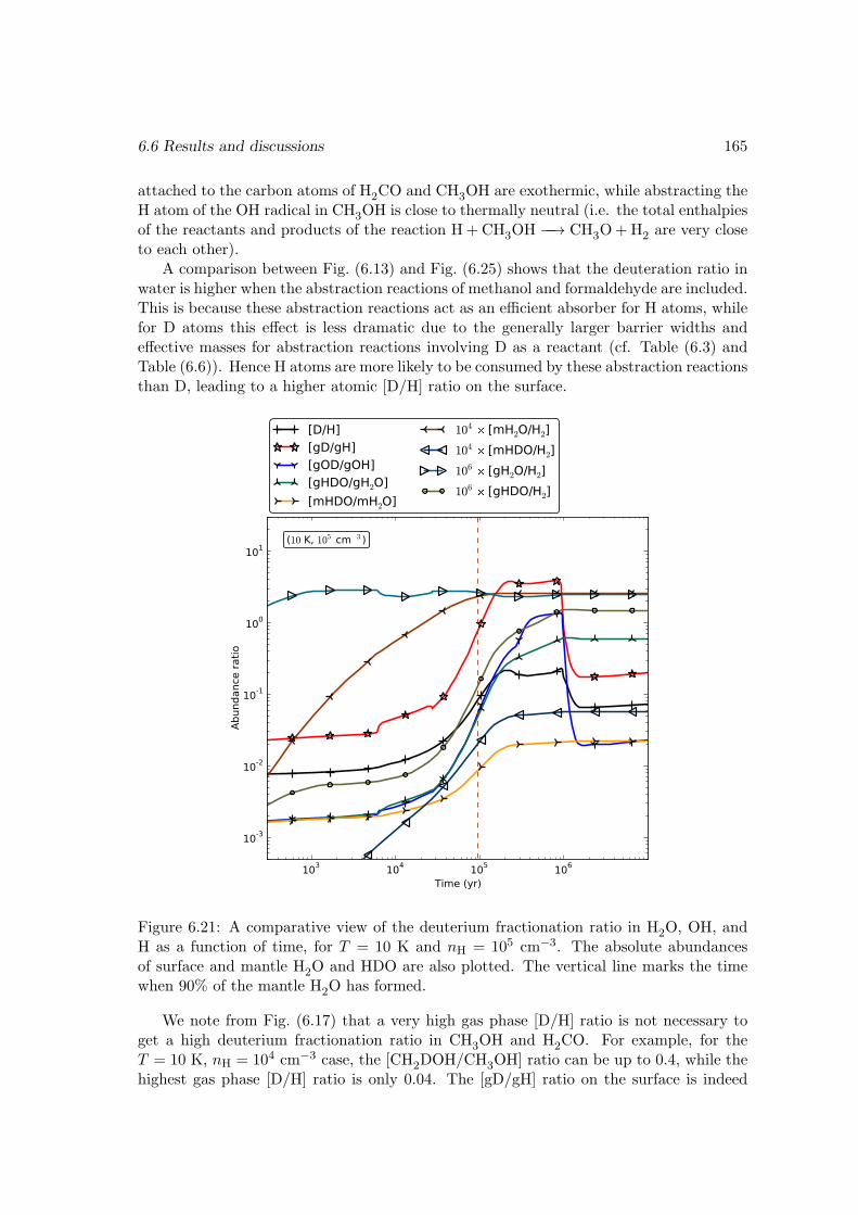
6.6 Results and discussions 165

attached to the carbon atoms of H2CO and CH3OH are exothermic, while abstracting theH atom of the OH radical in CH3OH is close to thermally neutral (i.e. the total enthalpiesof the reactants and products of the reaction H+CH3OH −−→ CH3O+H2 are very closeto each other).

A comparison between Fig. (6.13) and Fig. (6.25) shows that the deuteration ratio inwater is higher when the abstraction reactions of methanol and formaldehyde are included.This is because these abstraction reactions act as an efficient absorber for H atoms, whilefor D atoms this effect is less dramatic due to the generally larger barrier widths andeffective masses for abstraction reactions involving D as a reactant (cf. Table (6.3) andTable (6.6)). Hence H atoms are more likely to be consumed by these abstraction reactionsthan D, leading to a higher atomic [D/H] ratio on the surface.

103 104 105 106

Time (yr)

10-3

10-2

10-1

100

101

Abun

danc

e ra

tio

(10 K, 105 cm3 )

[D/H][gD/gH][gOD/gOH][gHDO/gH2O][mHDO/mH2O]

104 [mH2O/H2]104 [mHDO/H2]106 [gH2O/H2]106 [gHDO/H2]

Figure 6.21: A comparative view of the deuterium fractionation ratio in H2O, OH, andH as a function of time, for T = 10 K and nH = 105 cm−3. The absolute abundancesof surface and mantle H2O and HDO are also plotted. The vertical line marks the timewhen 90% of the mantle H2O has formed.

We note from Fig. (6.17) that a very high gas phase [D/H] ratio is not necessary toget a high deuterium fractionation ratio in CH3OH and H2CO. For example, for theT = 10 K, nH = 104 cm−3 case, the [CH2DOH/CH3OH] ratio can be up to 0.4, while thehighest gas phase [D/H] ratio is only 0.04. The [gD/gH] ratio on the surface is indeed

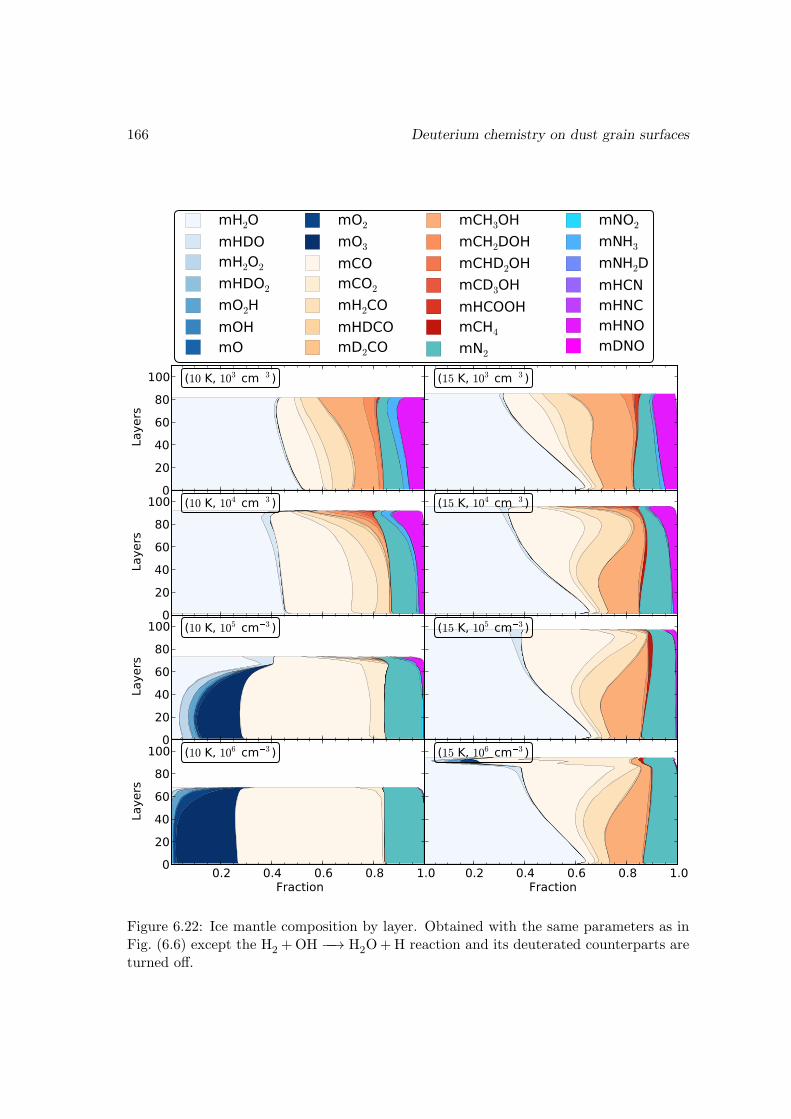
166 Deuterium chemistry on dust grain surfaces

0

20

40

60

80

100

Laye

rs

(10 K, 103 cm3 )

mH2OmHDOmH2O2

mHDO2

mO2HmOHmO

mO2

mO3

mCOmCO2

mH2COmHDCOmD2CO

mCH3OHmCH2DOHmCHD2OHmCD3OHmHCOOHmCH4

mN2

mNO2

mNH3

mNH2DmHCNmHNCmHNOmDNO

0

20

40

60

80

100

Laye

rs

(10 K, 104 cm3 )

0

20

40

60

80

100

Laye

rs

(10 K, 105 cm3 )

0.2 0.4 0.6 0.8 1.0Fraction

0

20

40

60

80

100

Laye

rs

(10 K, 106 cm3 )

(15 K, 103 cm3 )

(15 K, 104 cm3 )

(15 K, 105 cm3 )

0.2 0.4 0.6 0.8 1.0Fraction

(15 K, 106 cm3 )

Figure 6.22: Ice mantle composition by layer. Obtained with the same parameters as inFig. (6.6) except the H2 +OH −−→ H2O+H reaction and its deuterated counterparts areturned off.

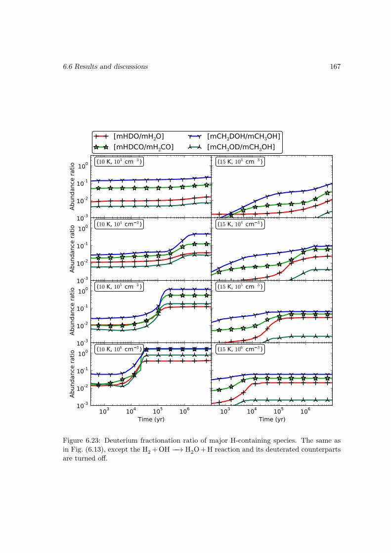
6.6 Results and discussions 167

10-3

10-2

10-1

100

Abun

danc

e ra

tio

(10 K, 103 cm3 )

[mHDO/mH2O][mHDCO/mH2CO]

[mCH2DOH/mCH3OH][mCH3OD/mCH3OH]

10-3

10-2

10-1

100

Abun

danc

e ra

tio

(10 K, 104 cm3 )

10-3

10-2

10-1

100

Abun

danc

e ra

tio

(10 K, 105 cm3 )

103 104 105 106

Time (yr)

10-3

10-2

10-1

100

Abun

danc

e ra

tio

(10 K, 106 cm3 )

(15 K, 103 cm3 )

(15 K, 104 cm3 )

(15 K, 105 cm3 )

103 104 105 106

Time (yr)

(15 K, 106 cm3 )

Figure 6.23: Deuterium fractionation ratio of major H-containing species. The same asin Fig. (6.13), except the H2+OH −−→ H2O+H reaction and its deuterated counterpartsare turned off.

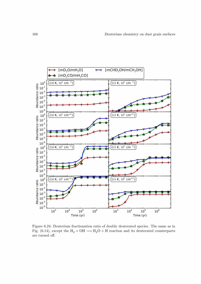
168 Deuterium chemistry on dust grain surfaces

10-610-510-410-310-210-1100

Abun

danc

e ra

tio

(10 K, 103 cm3 )

[mD2O/mH2O][mD2CO/mH2CO]

[mCHD2OH/mCH3OH]

10-610-510-410-310-210-1100

Abun

danc

e ra

tio

(10 K, 104 cm3 )

10-610-510-410-310-210-1100

Abun

danc

e ra

tio

(10 K, 105 cm3 )

103 104 105 106

Time (yr)

10-610-510-410-310-210-1100

Abun

danc

e ra

tio

(10 K, 106 cm3 )

(15 K, 103 cm3 )

(15 K, 104 cm3 )

(15 K, 105 cm3 )

103 104 105 106

Time (yr)

(15 K, 106 cm3 )

Figure 6.24: Deuterium fractionation ratio of doubly deuterated species. The same as inFig. (6.14), except the H2 + OH −−→ H2O + H reaction and its deuterated counterpartsare turned off.

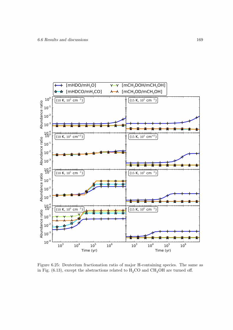
6.6 Results and discussions 169

10-4

10-3

10-2

10-1

100

Abun

danc

e ra

tio

(10 K, 103 cm3 )

[mHDO/mH2O][mHDCO/mH2CO]

[mCH2DOH/mCH3OH][mCH3OD/mCH3OH]

10-4

10-3

10-2

10-1

100

Abun

danc

e ra

tio

(10 K, 104 cm3 )

10-4

10-3

10-2

10-1

100

Abun

danc

e ra

tio

(10 K, 105 cm3 )

103 104 105 106

Time (yr)

10-4

10-3

10-2

10-1

100

Abun

danc

e ra

tio

(10 K, 106 cm3 )

(15 K, 103 cm3 )

(15 K, 104 cm3 )

(15 K, 105 cm3 )

103 104 105 106

Time (yr)

(15 K, 106 cm3 )

Figure 6.25: Deuterium fractionation ratio of major H-containing species. The same asin Fig. (6.13), except the abstractions related to H2CO and CH3OH are turned off.

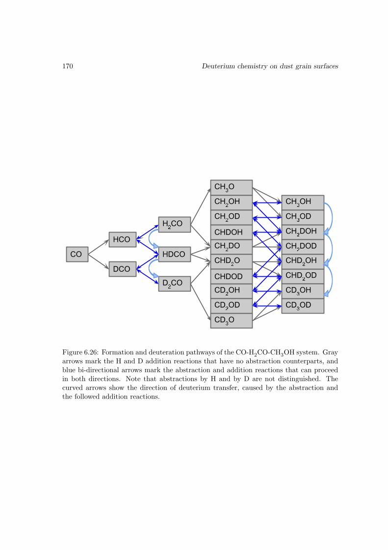
170 Deuterium chemistry on dust grain surfaces

Figure 6.26: Formation and deuteration pathways of the CO-H2CO-CH3OH system. Grayarrows mark the H and D addition reactions that have no abstraction counterparts, andblue bi-directional arrows mark the abstraction and addition reactions that can proceedin both directions. Note that abstractions by H and by D are not distinguished. Thecurved arrows show the direction of deuterium transfer, caused by the abstraction andthe followed addition reactions.

6.6 Results and discussions 171

high, due to the slower evaporation and reaction rate of surface D caused by its highermass and lower zero-point energy in comparison with H.

6.6.3 Comparison with observations

Table (6.13) lists the deuterium fractionation ratio for methanol, formaldehyde, and water,observed for different sources. In general, low mass and cold sources have higher deuteriumfractionation ratios than the hot high mass sources, and methanol and formaldehyde havehigher deuterium fractionation ratios than water, which are qualitatively in agreementwith our modeling results as has been discussed in previous sections. A quantitativematch is more challenging because, after all, the observational results usually have largeuncertainties, and vary from one source to another considerably. Each source is unique,with its own environment and evolution, and detailed modeling following the time evolu-tion is necessary, though the initial condition and external action are usually unknown.

In the next two small sections a more detailed analysis of two recent observationalresults is presented in the context of our modeling results.

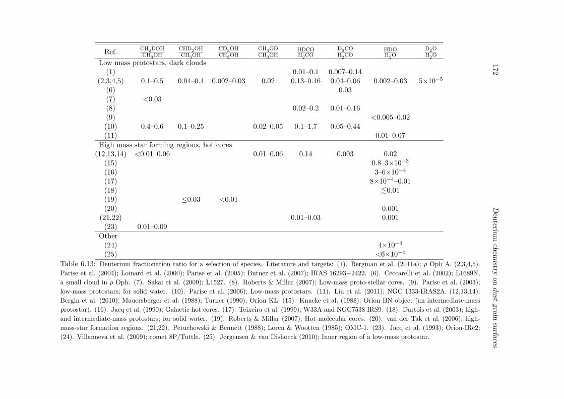
172

Deuteriu

mchem

istryon

dust

grainsurfaces

Ref.CH2DOHCH3OH

CHD2OHCH3OH

CD3OHCH3OH

CH3ODCH3OH

HDCOH2CO

D2COH2CO

HDOH2O

D2OH2O

Low mass protostars, dark clouds(1) 0.01–0.1 0.007–0.14

(2,3,4,5) 0.1–0.5 0.01–0.1 0.002–0.03 0.02 0.13–0.16 0.04–0.06 0.002–0.03 5×10−5

(6) 0.03(7) <0.03(8) 0.02–0.2 0.01–0.16(9) <0.005–0.02(10) 0.4–0.6 0.1–0.25 0.02–0.05 0.1–1.7 0.05–0.44(11) 0.01–0.07

High mass star forming regions, hot cores(12,13,14) <0.01–0.06 0.01–0.06 0.14 0.003 0.02

(15) 0.8–3×10−3

(16) 3–6×10−4

(17) 8×10−4–0.01(18) .0.01(19) ≤0.03 <0.01(20) 0.001

(21,22) 0.01–0.03 0.001(23) 0.01–0.09

Other(24) 4×10−4

(25) <6×10−4

Table 6.13: Deuterium fractionation ratio for a selection of species. Literature and targets: (1). Bergman et al. (2011a); ρ Oph A. (2,3,4,5).

Parise et al. (2004); Loinard et al. (2000); Parise et al. (2005); Butner et al. (2007); IRAS 16293−2422. (6). Ceccarelli et al. (2002); L1689N,

a small cloud in ρ Oph. (7). Sakai et al. (2009); L1527. (8). Roberts & Millar (2007); Low-mass proto-stellar cores. (9). Parise et al. (2003);

low-mass protostars; for solid water. (10). Parise et al. (2006); Low-mass protostars. (11). Liu et al. (2011); NGC 1333-IRAS2A. (12,13,14).

Bergin et al. (2010); Mauersberger et al. (1988); Turner (1990); Orion KL. (15). Knacke et al. (1988); Orion BN object (an intermediate-mass

protostar). (16). Jacq et al. (1990); Galactic hot cores. (17). Teixeira et al. (1999); W33A and NGC7538 IRS9. (18). Dartois et al. (2003); high-

and intermediate-mass protostars; for solid water. (19). Roberts & Millar (2007); Hot molecular cores. (20). van der Tak et al. (2006); high-

mass-star formation regions. (21,22). Petuchowski & Bennett (1988); Loren & Wootten (1985); OMC-1. (23). Jacq et al. (1993); Orion-IRc2;

(24). Villanueva et al. (2009); comet 8P/Tuttle. (25). Jørgensen & van Dishoeck (2010); Inner region of a low-mass protostar.

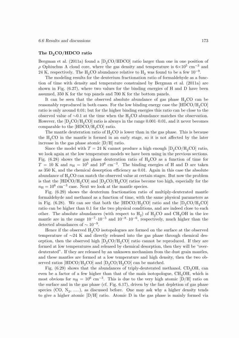
6.6 Results and discussions 173

The D2CO/HDCO ratio

Bergman et al. (2011a) found a [D2CO/HDCO] ratio larger than one in one position ofρ Ophiuchus A cloud core, where the gas density and temperature is 6×105 cm−3 and24 K, respectively. The H2CO abundance relative to H2 was found to be a few 10−9.

The modeling results for the deuterium fractionation ratio of formaldehyde as a func-tion of time with density and temperature constrained by Bergman et al. (2011a) areshown in Fig. (6.27), where two values for the binding energies of H and D have beenassumed, 350 K for the top panels and 700 K for the bottom panels.

It can be seen that the observed absolute abundance of gas phase H2CO can bereasonably reproduced in both cases. For the low binding energy case the [HDCO/H2CO]ratio is only around 0.01; but for the higher binding energies this ratio can be close to theobserved value of ∼0.1 at the time when the H2CO abundance matches the observation.However, the [D2CO/H2CO] ratio is always in the range 0.001–0.01, and it never becomescomparable to the [HDCO/H2CO] ratio.

The mantle deuteration ratio of H2CO is lower than in the gas phase. This is becausethe H2CO in the mantle is formed in an early stage, so it is not affected by the laterincrease in the gas phase atomic [D/H] ratio.

Since the model with T = 24 K cannot produce a high enough [D2CO/H2CO] ratio,we look again at the low temperature models we have been using in the previous sections.Fig. (6.28) shows the gas phase deuteration ratio of H2CO as a function of time forT = 10 K and nH = 105 and 106 cm−3. The binding energies of H and D are takenas 350 K, and the chemical desorption efficiency as 0.01. Again in this case the absoluteabundance of H2CO can match the observed value at certain stages. But now the problemis that the [HDCO/H2CO] and [D2CO/H2CO] ratios become too high, especially for thenH = 106 cm−3 case. Next we look at the mantle species.

Fig. (6.29) shows the deuterium fractionation ratio of multiply-deuterated mantleformaldehyde and methanol as a function of time, with the same physical parameters asin Fig. (6.28). We can see that both the [HDCO/H2CO] ratio and the [D2CO/H2CO]ratio can be higher than 0.1 for the two physical conditions, and are indeed close to eachother. The absolute abundances (with respect to H2) of H2CO and CH3OH in the icemantle are in the range 10−7–10−5 and 10−8–10−6, respectively, much higher than thedetected abundances of ∼ 10−9.

Hence if the observed H2CO isotopologues are formed on the surface at the observedtemperature of ∼24 K and directly released into the gas phase through chemical des-orption, then the observed high [D2CO/H2CO] ratio cannot be reproduced. If they areformed at low temperatures and released by chemical desorption, then they will be “over-deuterated”. If they are released by an unknown mechanism from the dust grain mantles,and these mantles are formed at a low temperature and high density, then the two ob-served ratios [HDCO/H2CO] and [D2CO/H2CO] can be matched.

Fig. (6.29) shows that the abundances of triply-deuterated methanol, CD3OH, caneven be a factor of a few higher than that of the main isotopologue, CH3OH, which ismost obvious for nH = 106 cm−3. This is due to the very high atomic [D/H] ratio onthe surface and in the gas phase (cf. Fig. 6.17), driven by the fast depletion of gas phasespecies (CO, N2, . . . ), as discussed before. One may ask why a higher density tendsto give a higher atomic [D/H] ratio. Atomic D in the gas phase is mainly formed via

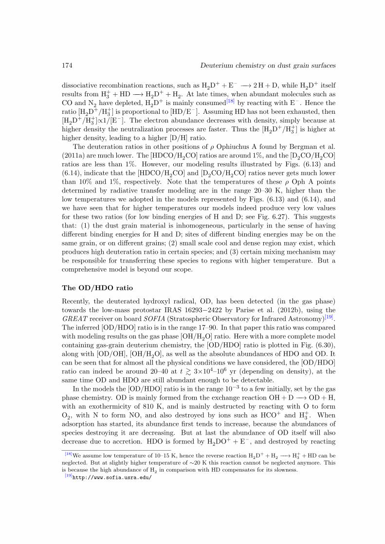
174 Deuterium chemistry on dust grain surfaces

dissociative recombination reactions, such as H2D+ +E – −−→ 2H +D, while H2D

+ itselfresults from H+

3 +HD −−→ H2D+ +H2. At late times, when abundant molecules such as

CO and N2 have depleted, H2D+ is mainly consumed[18] by reacting with E – . Hence the

ratio [H2D+/H+

3 ] is proportional to [HD/E – ]. Assuming HD has not been exhausted, then[H2D

+/H+3 ]∝1/[E – ]. The electron abundance decreases with density, simply because at

higher density the neutralization processes are faster. Thus the [H2D+/H+

3 ] is higher athigher density, leading to a higher [D/H] ratio.

The deuteration ratios in other positions of ρ Ophiuchus A found by Bergman et al.(2011a) are much lower. The [HDCO/H2CO] ratios are around 1%, and the [D2CO/H2CO]ratios are less than 1%. However, our modeling results illustrated by Figs. (6.13) and(6.14), indicate that the [HDCO/H2CO] and [D2CO/H2CO] ratios never gets much lowerthan 10% and 1%, respectively. Note that the temperatures of these ρ Oph A pointsdetermined by radiative transfer modeling are in the range 20–30 K, higher than thelow temperatures we adopted in the models represented by Figs. (6.13) and (6.14), andwe have seen that for higher temperatures our models indeed produce very low valuesfor these two ratios (for low binding energies of H and D; see Fig. 6.27). This suggeststhat: (1) the dust grain material is inhomogeneous, particularly in the sense of havingdifferent binding energies for H and D; sites of different binding energies may be on thesame grain, or on different grains; (2) small scale cool and dense region may exist, whichproduces high deuteration ratio in certain species; and (3) certain mixing mechanism maybe responsible for transferring these species to regions with higher temperature. But acomprehensive model is beyond our scope.

The OD/HDO ratio

Recently, the deuterated hydroxyl radical, OD, has been detected (in the gas phase)towards the low-mass protostar IRAS 16293−2422 by Parise et al. (2012b), using theGREAT receiver on board SOFIA (Stratospheric Observatory for Infrared Astronomy)[19].The inferred [OD/HDO] ratio is in the range 17–90. In that paper this ratio was comparedwith modeling results on the gas phase [OH/H2O] ratio. Here with a more complete modelcontaining gas-grain deuterium chemistry, the [OD/HDO] ratio is plotted in Fig. (6.30),along with [OD/OH], [OH/H2O], as well as the absolute abundances of HDO and OD. Itcan be seen that for almost all the physical conditions we have considered, the [OD/HDO]ratio can indeed be around 20–40 at t & 3×104–106 yr (depending on density), at thesame time OD and HDO are still abundant enough to be detectable.

In the models the [OD/HDO] ratio is in the range 10−3 to a few initially, set by the gasphase chemistry. OD is mainly formed from the exchange reaction OH+D −−→ OD+H,with an exothermicity of 810 K, and is mainly destructed by reacting with O to formO2, with N to form NO, and also destroyed by ions such as HCO+ and H+

3 . Whenadsorption has started, its abundance first tends to increase, because the abundances ofspecies destroying it are decreasing. But at last the abundance of OD itself will alsodecrease due to accretion. HDO is formed by H2DO+ + E – , and destroyed by reacting

[18]We assume low temperature of 10–15 K, hence the reverse reaction H2D+ +H2 −−→ H+

3 +HD can beneglected. But at slightly higher temperature of ∼20 K this reaction cannot be neglected anymore. Thisis because the high abundance of H2 in comparison with HD compensates for its slowness.[19]http://www.sofia.usra.edu/

6.6 Results and discussions 175

103 104 105 106 107

Time (yr)

10-6

10-5

10-4

10-3

10-2

10-1

100

101

Abun

danc

e ra

tio

(24 K, 6.0105 cm3 )

[HDCO/H2CO][D2CO/H2CO]109 [H2CO/H2]

103 104 105 106 107

Time (yr)

10-6

10-5

10-4

10-3

10-2

10-1

100

101

Abun

danc

e ra

tio

(24 K, 6.0105 cm3 )

[mHDCO/mH2CO][mD2CO/mH2CO]105 [mH2CO/H2]

103 104 105 106 107

Time (yr)

10-6

10-5

10-4

10-3

10-2

10-1

100

101

Abun

danc

e ra

tio

(24 K, 6.0105 cm3 )

[HDCO/H2CO][D2CO/H2CO]109 [H2CO/H2]

103 104 105 106 107

Time (yr)

10-6

10-5

10-4

10-3

10-2

10-1

100

101

Abun

danc

e ra

tio

(24 K, 6.0105 cm3 )

[mHDCO/mH2CO][mD2CO/mH2CO]105 [mH2CO/H2]

Figure 6.27: Deuterium fractionation ratio of formaldehyde as a function of time, withT = 24 K and nH = 6×105 cm−3, which is relevant for ρ Ophiuchus A. The chemicaldesorption efficiency is set to 0.1. Left: gas phase; right: mantle. Top: the bindingenergies of H and D are set to a low value of 350 K; Bottom: the binding energies of Hand D are set to a high value of 700 K.

176 Deuterium chemistry on dust grain surfaces

10-6

10-5

10-4

10-3

10-2

10-1

100

101

Abun

danc

e ra

tio

(10 K, 105 cm3 )

[HDCO/H2CO][D2CO/H2CO]109 [H2CO/H2]

103 104 105 106 107

Time (yr)

10-6

10-5

10-4

10-3

10-2

10-1

100

101

Abun

danc

e ra

tio

(10 K, 106 cm3 )

Figure 6.28: The deuterium fractionation ratio of H2CO in the gas phase as a functionof time for T = 10 K and nH = 105 and 106 cm−3. The binding energies of H and D areassumed to be 350 K, and the chemical desorption efficiency is taken as 0.01.

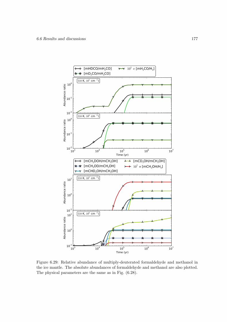
6.6 Results and discussions 177

10-2

10-1

100

Abun

danc

e ra

tio

(10 K, 105 cm3 )

[mHDCO/mH2CO][mD2CO/mH2CO]

105 [mH2CO/H2]

103 104 105 106 107

Time (yr)

10-2

10-1

100

Abun

danc

e ra

tio

(10 K, 106 cm3 )

10-1

100

101

Abun

danc

e ra

tio

(10 K, 105 cm3 )

[mCH2DOH/mCH3OH][mCH3OD/mCH3OH][mCHD2OH/mCH3OH]

[mCD3OH/mCH3OH]107 [mCH3OH/H2]

103 104 105 106 107

Time (yr)

10-1

100

101

Abun

danc

e ra

tio

(10 K, 106 cm3 )

Figure 6.29: Relative abundance of multiply-deuterated formaldehyde and methanol inthe ice mantle. The absolute abundances of formaldehyde and methanol are also plotted.The physical parameters are the same as in Fig. (6.28).

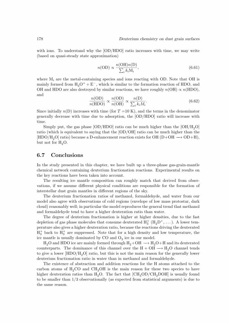
178 Deuterium chemistry on dust grain surfaces

with ions. To understand why the [OD/HDO] ratio increases with time, we may write(based on quasi-steady state approximation)

n(OD) ∝ n(OH)n(D)∑i kiMi

, (6.61)

where Mi are the metal-containing species and ions reacting with OD. Note that OH ismainly formed from H3O

+ +E – , which is similar to the formation reaction of HDO, andOH and HDO are also destroyed by similar reactions, we have roughly n(OH) ∝ n(HDO),and

n(OD)

n(HDO)∝ n(OD)

n(OH)∝ n(D)∑

i kiMi. (6.62)

Since initially n(D) increases with time (for T =10 K), and the terms in the denominatorgenerally decrease with time due to adsorption, the [OD/HDO] ratio will increase withtime.

Simply put, the gas phase [OD/HDO] ratio can be much higher than the [OH/H2O]ratio (which is equivalent to saying that the [OD/OH] ratio can be much higher than the[HDO/H2O] ratio) because a D-enhancement reaction exists for OH (D+OH −−→ OD+H),but not for H2O.

6.7 Conclusions

In the study presented in this chapter, we have built up a three-phase gas-grain-mantlechemical network containing deuterium fractionation reactions. Experimental results onthe key reactions have been taken into account.

The resulting ice mantle composition can roughly match that derived from obser-vations, if we assume different physical conditions are responsible for the formation ofinterstellar dust grain mantles in different regions of the sky.

The deuterium fractionation ratios of methanol, formaldehyde, and water from ourmodel also agree with observations of cold regions (envelope of low mass protostar, darkcloud) reasonably well; in particular the model reproduces the general trend that methanoland formaldehyde tend to have a higher deuteration ratio than water.

The degree of deuterium fractionation is higher at higher densities, due to the fastdepletion of gas phase molecules that consume deuterated H+

3 (H2D+, . . . ). A lower tem-

perature also gives a higher deuteration ratio, because the reactions driving the deuteratedH+

3 back to H+3 are suppressed. Note that for a high density and low temperature, the

ice mantle is usually dominated by CO and O3 ice in our model.H2O and HDO ice are mainly formed through H2+OH −−→ H2O+H and its deuterated

counterparts. The dominance of this channel over the H + OH −−→ H2O channel tendsto give a lower [HDO/H2O] ratio, but this is not the main reason for the generally lowerdeuterium fractionation ratio in water than in methanol and formaldehyde.

The existence of abstraction and addition reactions for the H atoms attached to thecarbon atoms of H2CO and CH3OH is the main reason for these two species to havehigher deuteration ratios than H2O. The fact that [CH3OD/CH2DOH] is usually foundto be smaller than 1/3 observationally (as expected from statistical arguments) is due tothe same reason.

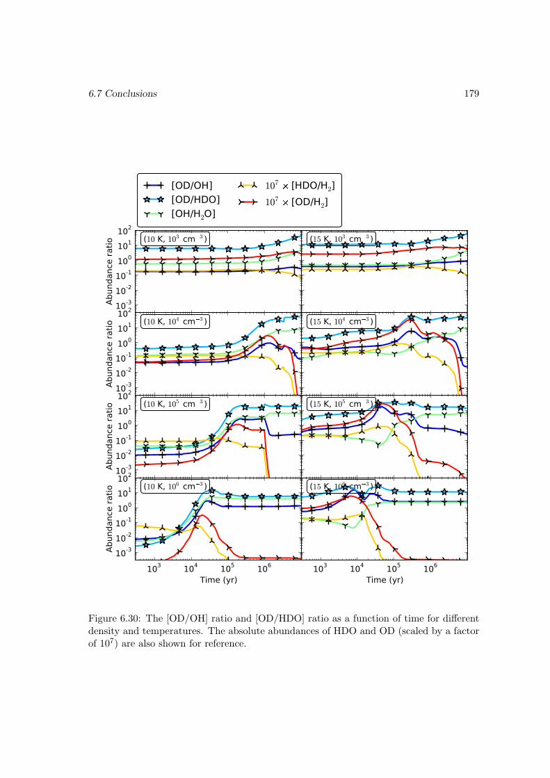
6.7 Conclusions 179

10-310-210-1100101102

Abun

danc

e ra

tio

(10 K, 103 cm3 )

[OD/OH][OD/HDO][OH/H2O]

107 [HDO/H2]107 [OD/H2]

10-310-210-1100101102

Abun

danc

e ra

tio

(10 K, 104 cm3 )

10-310-210-1100101102

Abun

danc

e ra

tio

(10 K, 105 cm3 )

103 104 105 106

Time (yr)

10-310-210-1100101102

Abun

danc

e ra

tio

(10 K, 106 cm3 )

(15 K, 103 cm3 )

(15 K, 104 cm3 )

(15 K, 105 cm3 )

103 104 105 106

Time (yr)

(15 K, 106 cm3 )

Figure 6.30: The [OD/OH] ratio and [OD/HDO] ratio as a function of time for differentdensity and temperatures. The absolute abundances of HDO and OD (scaled by a factorof 107) are also shown for reference.

180 Deuterium chemistry on dust grain surfaces

The [D2O/H2O] ratio is very sensitive to whether water is formed through the H+OHchannel or the H2+OH channel. The former channel gives a [D2O/H2O] ratio 2–3 ordersof magnitude higher than the latter channel. The low observed [D2O/H2O] ratio supportsthe H2 +OH channel for water formation on dust grains.

There are a few caveats (the generic ones will be listed in the next chapter) we needto be aware of.

We found that the way we set the initial abundances and the binding energies of Hand D on the grain surface affect the overall behavior of the system abruptly, by changingthe fluxes of H and D injected onto the dust grains. It is not clear to what extent ourinitial setting approximates the real conditions of interstellar molecular clouds.

The zero-point energies of H and D affect their relative surface coverage. We calculatedthe zero-point energies by simply using their characteristic vibrational frequency on thesurface, which is not guaranteed to be accurate.

We take single values for the binding and diffusion energies of each surface species. Areal dust grain surface may actually contain sites with different characteristics. This mayspecifically be important for the surface binding and migration of H2, which is responsiblefor water formation.

The high coverage of H2 at low temperatures may alter the binding energy of otherspecies, an effect that has not been included in our models.

There are uncertainties in the surface reaction network. Many of the reaction parame-ters are not well-constrained. Even for those we have discussed in detail, the experimentalresults should be considered semi-quantitative at best. Further input from the chemicalcommunity would be very helpful.

Chapter 7

Summary and outlook

7.1 Summary

This thesis contains the major part of the work I have done during my doctoral studies.I first wrote a code for solving the time-evolution of a gas phase chemical system underinterstellar conditions, which has been applied to the study of the ortho and para forms ofdeuterated H+

3 , where the interaction between gas phase and dust grain surface processescan be simplified. This is described in Chapter 2. Common types of reactions are alsodescribed there.

Then I studied the grain surface chemistry by first looking at the necessity of incor-porating it, identifying the basic processes that are involved, and then digging into itsmathematical formulation based on the master equation. Following this, I wrote a MonteCarlo code, which is based on the stochastic simulation approach proposed by Gillespie(1976). All this is discussed in Chapter 3. The Monte Carlo code mainly serves as abenchmark, and is not used for studying astrochemical problems.

Grain surface chemistry is stochastic in nature due to the small sizes of dust grainsand the discreteness of the surface reactions. This renders the rate equation approachusually adopted for gas phase chemistry inaccurate in some cases. The master equationprescription is accurate but difficult to solve. The Monte Carlo approach is easy toimplement but it is slow. Hence we developed a new method to solve the coupled gas-grain chemistry, named the “hybrid moment equation” approach that is based on themoment equations that are derivable from the master equation. By benchmarking withthe Monte Carlo method, we demonstrated that this HME approach is superior to therate equation approach in the sense of producing accurate results. The main drawback ofthe HME approach is that for very large surface networks its speed degrades significantly.This is the topic of Chapter 4.

Inspired by the recent detection of hydrogen peroxide (H2O2) in the interstellarmedium by Bergman et al. (2011b), we modeled its formation through gas-grain chemistry.It is found that the resulting gas phase H2O2 abundance, together with the abundances ofH2CO and CH3OH, can match the observed values at a certain stage, which agrees withthe dynamical time scale of the source constrained observationally. This is the content ofChapter 5. The O2H molecule predicted by our model has actually been detected veryrecently in the same source.

Finally we build up a gas-grain-mantle model to study the deuterium fractionation

181

182 Summary and outlook

processes. Our model can produce a range of ice mantle compositions that are consis-tent with observations of different regions in space. The general trend that methanoland formaldehyde have a higher deuterium fractionation ratio than water is also repro-duced. The abstraction reactions of methanol and formaldehyde are vital in differen-tiating them from water in their deuterium enhancement, while the dominance of theH2+OH −−→ H2O+H channel over the H+OH −−→ H2O channel plays only a minor rolein lowering the [HDO/H2O] ratio. On the other hand, the [D2O/H2O] ratio is sensitiveto the route through which water is formed, and the observed low value for this ratiostrongly suggests that water is mainly formed through H2 +OH −−→ H2O+H. All this isdiscussed in Chapter 6.

7.2 Outlook

There are several aspects of our work that can be continued or improved.One feature that is obviously missing from the modeling work presented here is that the

time evolution of the physical parameters is not included. An explicitly time-dependentdensity and temperature is relatively straightforward to implement, and has actually beenused in a small study contained in Parise et al. (2012b).

What is more challenging is to couple the chemical and physical evolution. Theabundances of gas phase species such as CO and H2O can alter the cooling efficiency,which in turn affects the dynamical evolution of the cloud. The ionization degree is alsorelated to the chemical processes, hence the coupling between matter and magnetic fieldcan also be affected by chemistry.

For the surface chemistry, we have assumed that the surface sites are homogeneous,meaning that all the sites have the same characteristics. A more realistic treatmentmay assume a distribution for certain parameters describing surface sites. An even moredetailed approach would take into account the micro-physics of dust grain surface (andpossibly the mantle layers), using a Monte Carlo method. It is still not clear how tocouple such an approach to a large gas phase network.

Our modeling of H2O2 formation can explain the abundances of H2O2 and otherspecies in the source where H2O2 is detected. The time-evolution of the H2O2 abundanceshows that it can be very abundant at an early stage. However, at present it has onlybeen detected in a single source, namely, ρ Ophiuchus A, by Bergman et al. (2011b). Wenote that the position in ρ Oph A, toward which H2O2 was detected has a very high H2

column density of 3×1022 cm−2, which is 3 times higher than the value in the canonicaldark cloud TMC-1 (Frerking et al. 1982). Given the H2O2 abundance determined byBergman et al. (2011b), these authors would not have detected H2O2 were the H2 columndensity a few times lower. Alternatively, limitations of our modeling and/or the naturalevolution of interstellar clouds combined with certain observational selection effects mayalso be responsible for the rarity of H2O2 detections, and more work will be needed toinvestigate this.

Regarding deuterium chemistry in the gas phase, it is not completely clear whetherincluding the ortho/para discrimination of species such as the H2 and H+

3 isotopologuescan alter the degree of deuteration appreciably. This is an issue because the different spinstates have different rotational energy levels, which may be high enough to overcome thebarriers of certain reactions that act in the reverse direction of deuterium enhancement

7.2 Outlook 183

in some species.The surface chemistry involving deuterium also has large room of improvement. Many

(if not most) of the parameters of the reactions related to water, formaldehyde, andmethanol are not well-constrained, and certain “educated guesses” had to be made. Afterthe arrival of new quantitative experimental results, it may be necessary to check how thedeuterium fractionation for the species of interest is affected.

Finally some technical remarks on the code. Generally speaking, prospective improve-ments should be in the software side, rather than in the hardware side. Parallelizationof the code is not an urgent requirement for astrochemical studies, unless, of course, thechemistry is to be coupled with a parallelized hydrodynamical code. Usually a “poorman’s parallelization” would suffice, in which the code is arranged to run on differentcomputers at the same time using different physical parameters.

Our hybrid moment equation (HME) approach is faster than the Monte Carlo methodfor a medium-to-large-sized system. But for a system involving many surface reactionsthat need to be treated stochastically, especially when the number of surface reactionsapproaches 1000, it also becomes very slow or even stops integration if its internal iterationdoes not converge. Including the three-phase gas-surface-mantle structure can furtherdegrade its behavior. On the other hand, the Monte Carlo method, no matter how slow itmay be, never gets stuck, because by design it does not involve solving any equations, andonly simple algebraic operations (plus evaluation of exponential functions) are needed[1].

There are two possibilities to mitigate this situation. With the moment equation,many terms involving the second-order (or higher order depending on the accuracy re-quired) moments have to be taken as indeterminate variables and need to be solved, whichincreases the size of the differential equation system significantly and slows down the code.Hence reducing the size of the system by eliminating some of the high order terms canincrease the speed. This requires some “moment closure” method, namely, a systematicway to express the higher order moments in terms of lower order ones.

The next possibility is related to the solver for the differential equations. I use theDLSODES solver taken from the ODEPACK package, which is implicit in nature. The gen-eral consensus on solving a stiff system (a generic chemical system is stiff) of differentialequations is that an implicit method must be used to guarantee stability. An implicitmethod involves solving a set of nonlinear algebraic equations, which is done with theNewton iteration method by linearization. The iteration process does not necessarilyconverge to the correct solution due to the potential sensitivity on the starting point, andthis is the most time-consuming part of the code. Recently Guidry et al. (2011) claimedthat an explicit method can actually be used for stiff systems, specifically for reactionnetwork problems (chemical or nuclear), by stabilizing the integration with certain alge-braic methods. Though this approach is still preliminary, it may turn out to be usefulfor solving a large system of equations as in the case of our HME approach, or for a largechemical network coupled with dynamics.

Another technical issue is related to the fact that a chemical model usually involvesmany parameters, some of which are free while others are not. A thorough and quickunderstanding of how the system behavior depends on these parameters requires novelanalysis and visualization methods.

[1]Unfortunately, the Monte Carlo method cannot be parallelized to boost its speed, at least in its presentform, because the evolution of a chemical system has to be followed step by step.

Appendix A

A comparison of differentapproaches for surface chemistry— the case of H2 formation ondust grain surfaces

As a concrete demonstration of the utility of grain surface chemistry, here I show twodifferent approaches to the formation of H2, including a description of how this processis implemented in usual gas phase chemistry. The first one is based on the rate equation,and the second is based on the master equation.

In many purely gas phase chemical models, no surface processes are included, but theformation of H2 is nevertheless accounted for, in a somewhat “handwaving” way, althoughfor normal dark cloud conditions, the efficiency of H2 formation is actually unimportant.This is because most of the hydrogen is usually assumed to be in molecular form in theinitial condition. The destruction of H2 by cosmic rays is very slow, with a typical timescale of 109 yr. Even if no formation channel for H2 is included, the gas phase chemistrywill not be affected much, since the H2 abundance is essentially constant for time spans ofastrochemical interest. Even the surface chemistry will not be affected much by neglectingthe surface formation of H2 either, due to the presence of a lot of heavy molecules (suchas CO and O2) on the surface. An H atom landing on the dust grain surface will almostalways combine with one of these heavy molecules, with an extremely low chance to keepfree before evaporation and react with another incoming H atom to form an H2 molecule.Thus the H2 formation is not competitive with other hydrogenation reactions. However,when the active surface reactions have ceased, and when a long time scale is of interest,the surface formation of H2 becomes important.

Only three reactions will be involved in the following discussion:

Hkacc−−→ gH, (A.1)

gHkeva−−→ H, and (A.2)

gH + gHkH,H−−−→ gH2. (A.3)

Here the “g” in gH means that the atomic H is on the grain surface. Such a distinction

184

A.1 With the rate equation approach 185

between the symbols for gas phase and grain surface species is not always necessary, sincethe meaning can be easily judged from the context.

A.1 With the rate equation approach

Usually we are interested in the production rate of H2 in terms of the change rate of itsgas phase density n(H2). With the rate equation, the production rate of H2 is

R(H2) ≡ ∂tn(H2)|prod =kH,H

NSVN2

H, (A.4)

where NH is the number of H atoms on the surface of one dust grain, NS is the numberof reaction sites on the surface of this dust grain, kH,H is the surface reaction rate of Hatoms, and V is the gas volume containing one dust grain (see Eq. (3.5) on page 31; notto be confused with the volume of a dust grain).

The evolution equation of NH is (cf. Eq. (6.16))

∂tNH = αn(H)v(H)σ − 2kH,HN2H/NS − keva, HNH,

where αn(H)v(H) is the flux of H atoms accreted onto the grain surface, the α factorbeing related to the surface shape and sticking coefficient, σ is the surface area of a dustgrain, and keva,H is the evaporation rate of surface H atoms. With a Maxwell distributionfor the gas phase velocity, we have α = 1/4 (assuming unity sticking coefficient), andv(H) = (8kT/πmH)

1/2.Assuming steady state has been reached, then NH can be solved for from the above

equation (cf. Eq. (6.19)):

NH =2αn(H)v(H)σ

keva +√

k2eva + 8kH,Hαn(H)v(H)σ/NS

. (A.5)

In gas phase chemical models, the formation rate of H2 on the dust grains is usuallyexpressed as (Le Petit et al. 2009)

R(H2) = β(H2)n(H)nH. (A.6)

The parameter β(H2) may be called formation rate coefficient. We have

β(H2) =kH,H

NSVN2

H/ [n(H)nH]

=kH,H

NSV nH

4α2n(H)v2(H)σ2(keva +

√k2eva + 8kH,Hαn(H)v(H)σ/NS

)2 . (A.7)

If keva is so small that it can be neglected (so that all the H atoms arriving on the dustgrain surface recombine to form H2 molecules), then

β(H2) 'αv(H)σ

2V nH=

1

2αv(H)σRG,n

=1.44×10−17 cm3 s−1

×(

T

10 K

)1/2(RG,m

0.01

)(0.1 µm

rgrain

)(2 g cm−3

ρG

),

(A.8)

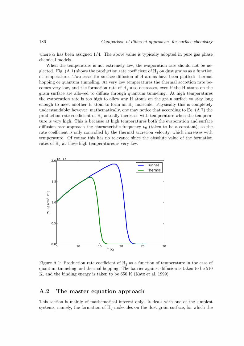
186 Comparison of different approaches for surface chemistry

where α has been assigned 1/4. The above value is typically adopted in pure gas phasechemical models.

When the temperature is not extremely low, the evaporation rate should not be ne-glected. Fig. (A.1) shows the production rate coefficient of H2 on dust grains as a functionof temperature. Two cases for surface diffusion of H atoms have been plotted: thermalhopping or quantum tunneling. At very low temperatures the thermal accretion rate be-comes very low, and the formation rate of H2 also decreases, even if the H atoms on thegrain surface are allowed to diffuse through quantum tunneling. At high temperaturesthe evaporation rate is too high to allow any H atoms on the grain surface to stay longenough to meet another H atom to form an H2 molecule. Physically this is completelyunderstandable; however, mathematically, one may notice that according to Eq. (A.7) theproduction rate coefficient of H2 actually increases with temperature when the tempera-ture is very high. This is because at high temperatures both the evaporation and surfacediffusion rate approach the characteristic frequency ν0 (taken to be a constant), so therate coefficient is only controlled by the thermal accretion velocity, which increases withtemperature. Of course this has no relevance since the absolute value of the formationrates of H2 at these high temperatures is very low.

5 10 15 20 25 30T (K)

0.0

0.5

1.0

1.5

2.0

(H2) (

cm3

s

1)

1e17

TunnelThermal

Figure A.1: Production rate coefficient of H2 as a function of temperature in the case ofquantum tunneling and thermal hopping. The barrier against diffusion is taken to be 510K, and the binding energy is taken to be 650 K (Katz et al. 1999)

A.2 The master equation approach

This section is mainly of mathematical interest only. It deals with one of the simplestsystems, namely, the formation of H2 molecules on the dust grain surface, for which the

A.2 The master equation approach 187

(steady-state) master equation can be solved analytically.For the master equation, we let the probability distribution function P (n, t) describe

the probability that there are n H atoms on the surface of one specific dust grain at timet. For brevity I denote it by P (n). Its evolution equation (the master equation) is

∂tP (n) = kacc[P (n− 1)− P (n)]

+ keva[P (n+ 1)(n+ 1)− P (n)n]

+ kH,H[P (n+ 1)(n+ 2)(n+ 1)− P (n)n(n− 1)],

(A.9)

where kacc, keva, and kH,H are the accretion rate, evaporation rate, and surface reactionrate, respectively.

The corresponding generating function (see Section 4.A on Page 66) is

f(x) =

∞∑n=0

P (n)xn. (A.10)

Since the probability must sum up to unity, we have f(1) = 1; and f(0) = P (0); ingeneral,

P (n) = f (n)(0)/n!. (A.11)

The evolution equation of f(x) is

∂tf(x) =

∞∑n=0

∂tP (n)xn

= kacc

∞∑n=0

[P (n− 1)− P (n)]xn

+ keva∑

[P (n+ 1)(n+ 1)− P (n)n]xn

+ kH,H

∑[P (n+ 1)(n+ 2)(n+ 1)− P (n)n(n− 1)]xn,

(A.12)

which can be simplified into

∂tf(x) = (x− 1) [kaccf − keva∂xf − kH,H(x+ 1)∂xxf ] . (A.13)

At steady state, ∂tf(x) = 0, hence

kaccf − keva∂xf − kH,H(x+ 1)∂xxf = 0. (A.14)

If kH,H = 0, i.e. there is no surface reaction, then

f(x) = exp

[kacckeva

(x− 1)

], (A.15)

where the condition f(1) = 1 has been used. In this case the probability that there are nH atoms on the grain surface is

P (n) =exp [−kacc/keva]

n!

(kacckeva

)n

, (A.16)

188 Comparison of different approaches for surface chemistry

which is simply the Poisson distribution, with average number kacc/keva. It is interestingto see that the Poisson distribution can be derived this way.

Eq. (A.14) has a closed-form solution (Green et al. 2001), though it is somewhatcomplicated. Define a≡kacc/kH,H, b≡keva/kH,H, then

f(x) =2−(1−b)/2

I[−(1− b), 2√2a]

(1 + x)(1−b)/2I[−(1− b), 2√

a(1 + x)], (A.17)

where I is the Bessel I-function:

I[ν, z] =(z2

)ν ∞∑k=0

1

k!Γ(ν + k + 1)

(z2

4

)k

. (A.18)

Hence f(x) can also be written as

f(x) =

∑∞k=0

ak

k!(1+x)k

Γ(k+b)∑∞k=0

ak

k!2k

Γ(k+b)

. (A.19)

From the above equations and using the relation Eq. (A.11), with some algebra wecan also have

P (n) =1

n!2−(1−b)/2an/2

I[−(1− b) + n, 2√a]

I[−(1− b), 2√2a]

=1

n!

∑∞k=n

ak

(k−n)!1

Γ(k+b)∑∞k=0

ak

k!2k

Γ(k+b)

=an

n!

∑∞k=0

ak

k!1

Γ(k+n+b)∑∞k=0

ak

k!2k

Γ(k+b)

.

(A.20)

The average occupation number of H atoms on a single grain 〈n〉 can be calculated by∂xf(x)|x=1:

〈n〉 = a ·∑∞

k=01k!

1Γ(k+b+1)(2a)

k∑∞k=0

1k!

1Γ(k+b)(2a)

k

'

a

b+2a = kacc2kacc+keva

, when a 1 and b 1,ab = kacc

keva, when b 1,√

a2 =

√kacc2kH,H

, when a 1 and b 1.

(A.21)

and 〈n(n− 1)〉 can be calculated by ∂2xf(x)|x=1:

〈n(n− 1)〉 = a2 ·∑∞

k=01k!

1Γ(k+b+2)(2a)

k∑∞k=0

1k!

1Γ(k+b)(2a)

k

'

a2

b+2a = k2acckH,H(2kacc+keva)

, when a 1 and b 1,

a2

b2= k2acc

k2eva, when b 1,

a2 = kacc

2kH,H, when a 1 and b 1.

(A.22)

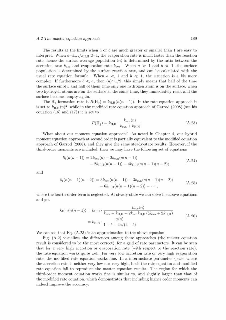
A.2 The master equation approach 189

The results at the limits when a or b are much greater or smaller than 1 are easy tointerpret. When b=keva/kH,H 1, the evaporation rate is much faster than the reactionrate, hence the surface average population 〈n〉 is determined by the ratio between theaccretion rate kacc and evaporation rate keva. When a 1 and b 1, the surfacepopulation is determined by the surface reaction rate, and can be calculated with theusual rate equation formula. When a 1 and b 1, the situation is a bit morecomplex. If furthermore b a, then 〈n〉'1/2; this simply means that half of the timethe surface empty, and half of them time only one hydrogen atom is on the surface; whentwo hydrogen atoms are on the surface at the same time, they immediately react and thesurface becomes empty again.

The H2 formation rate is R(H2) = kH,H〈n(n − 1)〉. In the rate equation approach itis set to kH,H〈n〉2, while in the modified rate equation approach of Garrod (2008) (see hisequation (16) and (17)) it is set to

R(H2) = kH,H · kacc〈n〉keva + kH,H

. (A.23)

What about our moment equation approach? As noted in Chapter 4, our hybridmoment equation approach at second order is partially equivalent to the modified equationapproach of Garrod (2008), and they give the same steady-state results. However, if thethird-order moments are included, then we may have the following set of equations

∂t〈n(n− 1)〉 = 2kacc〈n〉 − 2keva〈n(n− 1)〉− 2kH,H〈n(n− 1)〉 − 4kH,H〈n(n− 1)(n− 2)〉,

(A.24)

and

∂t〈n(n− 1)(n− 2)〉 = 3kacc〈n(n− 1)〉 − 3keva〈n(n− 1)(n− 2)〉− 6kH,H〈n(n− 1)(n− 2)〉 − · · · ,

(A.25)

where the fourth-order term is neglected. At steady-state we can solve the above equationsand get

kH,H〈n(n− 1)〉 = kH,H · kacc〈n〉keva + kH,H + 2kacckH,H/(keva + 2kH,H)

= kH,H · a〈n〉1 + b+ 2a/(2 + b)

.

(A.26)

We can see that Eq. (A.23) is an approximation to the above equation.Fig. (A.2) visualizes the differences among these approaches (the master equation

result is considered to be the most correct), for a grid of rate parameters. It can be seenthat for a very high accretion or evaporation rate (with respect to the reaction rate),the rate equation works quite well. For very low accretion rate or very high evaporationrate, the modified rate equation works fine. In a intermediate parameter space, wherethe accretion rate is neither very low nor very high, both the rate equation and modifiedrate equation fail to reproduce the master equation results. The region for which thethird-order moment equation works fine is similar to, and slightly larger than that ofthe modified rate equation, which demonstrates that including higher order moments canindeed improve the accuracy.

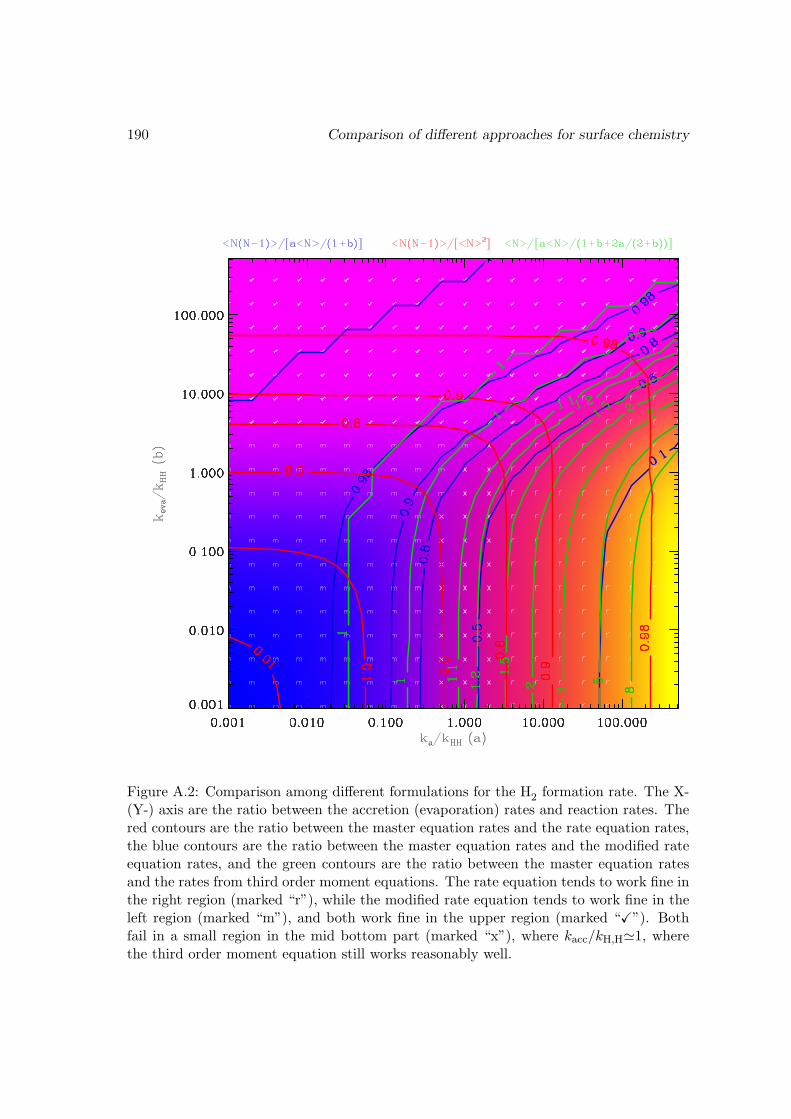
190 Comparison of different approaches for surface chemistry

Figure A.2: Comparison among different formulations for the H2 formation rate. The X-(Y-) axis are the ratio between the accretion (evaporation) rates and reaction rates. Thered contours are the ratio between the master equation rates and the rate equation rates,the blue contours are the ratio between the master equation rates and the modified rateequation rates, and the green contours are the ratio between the master equation ratesand the rates from third order moment equations. The rate equation tends to work fine inthe right region (marked “r”), while the modified rate equation tends to work fine in theleft region (marked “m”), and both work fine in the upper region (marked “X”). Bothfail in a small region in the mid bottom part (marked “x”), where kacc/kH,H'1, wherethe third order moment equation still works reasonably well.

A.2 The master equation approach 191

Finally, we remark that the master equation Eq. (A.9) in the steady-state case canalso be solved with continued fractions (Biham & Lipshtat 2002). The starting point is arecurrence relation that can be derived from Eq. (A.9)

P (n) =n+ 1

aP (n+ 1)

[(n+ b) + (n+ 2)

P (n+ 2)

P (n+ 1)

]. (A.27)

The derivation involves summing over n from 1 to N (such a procedure is commonly usedin reducing a set of linear equations) to get

− aP (0) + aP (N) + bP (1)− b(N + 1)P (N + 1) + 2P (2)

−N(N + 1)P (N + 1)− (N + 1)(N + 2)P (N + 2) = 0, (A.28)

and making use of the relation

2P (2) = aP (0)− bP (1), (A.29)

which is obtained by setting n = 1 in Eq. (A.9).Define

q(n)≡ aP (n)

(n+ 1)P (n+ 1),

then Eq. (A.27) becomes

q(n) = n+ b+a

q(n+ 1), (A.30)

which can be solved using continued fraction

q(n) = n+ b+a

n+ 1 + b+a

n+ 2 + b+a

n+ 3 + b+ · · ·

, (A.31)

and P (n) can be expressed as

P (n) =a

nq(n− 1)P (n− 1) =

an

n!

1

q(n− 1) · · · q(0)P (0), (A.32)

which is indeed related to the continued fraction expansion of the ratio between two BesselI-functions (Biham & Lipshtat 2002)[1].

[1]See also http://people.math.sfu.ca/~cbm/aands/page_363.htm.

Appendix B

Formal solution to the masterequation

We introduced the chemical master equation in Section 3.4.2 on page 40. The master equa-tion can rarely be solved analytically due to its complex structure and large size. Oneknown exception is the H2 formation problem in the steady-state case; see Appendix A.Here we discuss if the master equation is analytically solvable in principle, what formwould the solution take. Note that the following investigation is mainly out of mathe-matical curiosity, and it does not seem to ease the difficulties in numerically solving thereal-life stochastic problem underlying the master equation.

Symbolically, the solution to Eq. (3.32) can be written as

p(t) = exp [Tt]p|t=0, (B.1)

where exp [Tt] is to be understood as

exp [Tt] ≡∞∑n=1

tn

n!Tn.

If one can somehow obtain the spectrum of matrix T, namely, all the eigenvectors andtheir corresponding eigenvalues, and if these eigenvectors form a complete system, thenone may decompose the initial vector p0≡p|t=0 into a superposition of the eigenvectors,and the solution of the master equation would be obtained immediately. That is, if wehave Tvi=λivi, and vi (i=1, 2, . . . , Np, Np being the dimension of p) form a complete

set, then the initial probability distribution vector can be expressed as p|t=0=∑Np

i civi.Putting this expansion into Eq. (B.1), we have

p(t) =

∞∑n=1

tn

n!Tn

Np∑i=1

civi =

∞∑n=1

Np∑i=1

tn

n!ciλ

ni vi

=

Np∑i=1

ci exp (tλi)vi.

(B.2)

However, the eigensystem of the matrix operator T is not always complete, that isto say, the number of linearly independent eigenvectors of T may be smaller than its

192

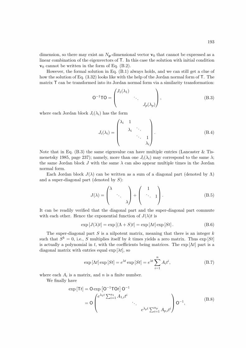
193

dimension, so there may exist an Np-dimensional vector v0 that cannot be expressed as alinear combination of the eigenvectors of T. In this case the solution with initial conditionv0 cannot be written in the form of Eq. (B.2).

However, the formal solution in Eq. (B.1) always holds, and we can still get a clue ofhow the solution of Eq. (3.32) looks like with the help of the Jordan normal form of T. Thematrix T can be transformed into its Jordan normal form via a similarity transformation:

O−1TO =

J1(λ1). . .

Jp(λp)

, (B.3)

where each Jordan block Ji(λi) has the form

Ji(λi) =

λi 1

λi. . .. . . 1

λi

. (B.4)

Note that in Eq. (B.3) the same eigenvalue can have multiple entries (Lancaster & Tis-menetsky 1985, page 237); namely, more than one Ji(λi) may correspond to the same λ;the same Jordan block J with the same λ can also appear multiple times in the Jordannormal form.

Each Jordan block J(λ) can be written as a sum of a diagonal part (denoted by Λ)and a super-diagonal part (denoted by S):

J(λ) =

λ. . .

λ

+

1. . . 1

. (B.5)

It can be readily verified that the diagonal part and the super-diagonal part commutewith each other. Hence the exponential function of J(λ)t is

exp [J(λ)t] = exp [(Λ + S)t] = exp [Λt] exp [St] . (B.6)

The super-diagonal part S is a nilpotent matrix, meaning that there is an integer ksuch that Sk = 0, i.e., S multiplies itself by k times yields a zero matrix. Thus exp [St]is actually a polynomial in t, with the coefficients being matrices. The exp [Λt] part is adiagonal matrix with entries equal exp [λt], so

exp [Λt] exp [St] = eλt exp [St] = eλtn∑

i=1

Aiti, (B.7)

where each Ai is a matrix, and n is a finite number.We finally have

exp [Tt] = O exp[O−1TOt

]O−1

= O

eλ1t∑n1

i=1A1,iti

. . .

eλpt∑np

i=1Ap,iti

O−1,(B.8)

194 Formal solution to the master equation

where O is a constant invertible matrix, and each Aj,i is a matrix.Thus the general solution of the master equation is no more than a superposition

of many simple exponential functions (if the corresponding eigenvalue is an imaginarynumber, then the exponential function becomes a trigonometric function) multiplied bypolynomials in t. Such a solution describes the evolution of the probability distributionfunction. What we usually care about is the abundance (or population) of each species ina system, which can be obtained by taking the moments of the probability distribution(see Chapter 4). Since the operation of taking moments is also a linear operation (withconstant coefficients), the abundance of each species as a function of time is also inprinciple a superposition of many functions of the form tneλt. This might seem to be asurprise at first glance, since the evolution curve of a species can be quite complex; thetruth is that a linear superposition of many simple exponential functions of the form e−λt

can indeed appear very complex.The formal solution presented in Eq. (B.2) or Eq. (B.8) indicates that the eigenvalues

of the stochastic matrix T must have certain special properties. For example, none ofthem can be positive, otherwise the solution p(t) would grow without limit. They cannotbe all negative either, otherwise p(t) would vanish as time goes by. So the largest of theλis should be zero. Another strong constraint is that the sum of all the components ofp(t) should always equal one because of probability conservation.

Unfortunately, the above derivation only has theoretical value. In practice, the di-mension of the state vector Np is extremely large and impossible to enumerate (evencalculating the value of Np is quite non-trivial), let alone to solve the eigenvalue problemassociated with T (which is a matrix of dimension Np×Np).

Bibliography

Agundez, M., Cernicharo, J., Guelin, M., et al. 2008, A&A, 478, L19

Aikawa, Y., Umebayashi, T., Nakano, T., & Miyama, S. M. 1997, ApJ, 486, L51

Al-Halabi, A., & van Dishoeck, E. F. 2007, MNRAS, 382, 1648

Albertsson, T., Semenov, D. A., & Henning, T. 2011, ArXiv e-prints

Allen, M., & Robinson, G. W. 1977, ApJ, 212, 396

Amiaud, L., Fillion, J. H., Baouche, S., et al. 2006, The Journal of Chemical Physics,124, 094702

An, D., Ramırez, S. V., Sellgren, K., et al. 2011, ApJ, 736, 133

Andre, P., Belloche, A., Motte, F., & Peretto, N. 2007, A&A, 472, 519

Asplund, M., Grevesse, N., Sauval, A. J., & Scott, P. 2009, ARA&A, 47, 481

Atkinson, R., Baulch, D. L., Cox, R. A., et al. 2004, Atmospheric Chemistry & Physics,4, 1461

Awad, Z., Chigai, T., Kimura, Y., Shalabiea, O. M., & Yamamoto, T. 2005, ApJ, 626,262

Bacmann, A., Lefloch, B., Ceccarelli, C., et al. 2002, A&A, 389, L6

Barzel, B., & Biham, O. 2007a, ApJ, 658, L37

—. 2007b, J. Chem. Phys., 127, 144703

—. 2011, Physical Review Letters, 106, 150602

Bates, D. R. 1951, MNRAS, 111, 303

—. 1983, ApJ, 270, 564

Bates, D. R., & Spitzer, Jr., L. 1951, ApJ, 113, 441

Belloche, A., Garrod, R. T., Muller, H. S. P., et al. 2009, A&A, 499, 215

Belloche, A., Menten, K. M., Comito, C., et al. 2008, A&A, 482, 179

Bergin, E. A., Neufeld, D. A., & Melnick, G. J. 1998, ApJ, 499, 777

195

196 BIBLIOGRAPHY

Bergin, E. A., & Tafalla, M. 2007, ARA&A, 45, 339

Bergin, E. A., Melnick, G. J., Stauffer, J. R., et al. 2000, ApJ, 539, L129

Bergin, E. A., Phillips, T. G., Comito, C., et al. 2010, A&A, 521, L20

Bergman, P., Parise, B., Liseau, R., & Larsson, B. 2011a, A&A, 527, A39+

Bergman, P., Parise, B., Liseau, R., et al. 2011b, A&A, 531, L8+

Biham, O., Furman, I., Pirronello, V., & Vidali, G. 2001, ApJ, 553, 595

Biham, O., & Lipshtat, A. 2002, Phys. Rev. E, 66, 056103

Binnewies, M., & Milke, E. 1999, Thermochemical data of elements and compounds(Wiley-VCH)

Boger, G. I., & Sternberg, A. 2006, ApJ, 645, 314

Boogert, A. C. A., Pontoppidan, K. M., Knez, C., et al. 2008, ApJ, 678, 985

Boogert, A. C. A., Huard, T. L., Cook, A. M., et al. 2011, ApJ, 729, 92

Bottinelli, S., Boogert, A. C. A., Bouwman, J., et al. 2010, ApJ, 718, 1100

Boudin, N., Schutte, W. A., & Greenberg, J. M. 1998, A&A, 331, 749

Bradley, J. P., Humecki, H. J., & Germani, M. S. 1992, ApJ, 394, 643

Brown, P. D., & Millar, T. J. 1989, MNRAS, 240, 25P

Brown, R. D. 1977, Nature, 270, 39

Butner, H. M., Charnley, S. B., Ceccarelli, C., et al. 2007, ApJ, 659, L137

Caselli, P., Hasegawa, T.I., & Herbst, E. 1998, ApJ, 495, 309

Caselli, P., Stantcheva, T., Shalabiea, O., Shematovich, V. I., & Herbst, E. 2002,Planet. Space Sci., 50, 1257

Caselli, P., Walmsley, C. M., Tafalla, M., Dore, L., & Myers, P. C. 1999, ApJ, 523, L165

Cazaux, S., Cobut, V., Marseille, M., Spaans, M., & Caselli, P. 2010, A&A, 522, A74+

Ceccarelli, C., Castets, A., Loinard, L., Caux, E., & Tielens, A. G. G. M. 1998, A&A,338, L43

Ceccarelli, C., Loinard, L., Castets, A., et al. 2001, A&A, 372, 998

Ceccarelli, C., Vastel, C., Tielens, A. G. G. M., et al. 2002, A&A, 381, L17

Cernicharo, J., Guelin, M., Agundez, M., et al. 2007, A&A, 467, L37

Chandrasekhar, S. 1943, Reviews of Modern Physics, 15, 1

BIBLIOGRAPHY 197

Chang, Q., Cuppen, H., & Herbst, E. 2005, A&A, 434, 599

Chang, Q., Cuppen, H. M., & Herbst, E. 2007, A&A, 469, 973

Charnley, S. B. 1998, ApJ, 509, L121

—. 2001, ApJ, 562, L99

—. 2005, Adv. Space Res., 36, 132

Charnley, S. B., & Markwick, A. J. 2003, A&A, 399, 583

Charnley, S. B., & Rodgers, S. B. 2009, in ASP Conf. Ser., ed. K. J. Meech, J. V. Keane,M. J. Mumma, J. L. Siefert, & D. J. Werthimer, Vol. 420, 29

Charnley, S. B., Tielens, A. G. G. M., & Millar, T. J. 1992, ApJ, 399, L71

Charnley, S. B., Tielens, A. G. G. M., & Rodgers, S. D. 1997, ApJ, 482, L203

Chiar, J. E., Adamson, A. J., Kerr, T. H., & Whittet, D. C. B. 1994, ApJ, 426, 240

Chiar, J. E., Tielens, A. G. G. M., Whittet, D. C. B., et al. 2000, ApJ, 537, 749

Chiar, J. E., Pendleton, Y. J., Allamandola, L. J., et al. 2011, ApJ, 731, 9

Clancy, R. T., Sandor, B. J., & Moriarty-Schieven, G. H. 2004, Icarus, 168, 116

Clayton, D. 1968, Principles of Stellar Evolution and Nucleosynthesis: With a New Preface(University of Chicago Press)

Cuppen, H., & Herbst, E. 2007, ApJ, 668, 294

Cuppen, H. M., Ioppolo, S., Romanzin, C., & Linnartz, H. 2010, Physical ChemistryChemical Physics (Incorporating Faraday Transactions), 12, 12077

Dalgarno, A., & Lepp, S. 1984, ApJ, 287, L47

Dalgarno, A., & McCray, R. A. 1973, ApJ, 181, 95

Dalgarno, A., Oppenheimer, M., & Berry, R. S. 1973, ApJ, 183, L21

Dartois, E., Thi, W.-F., Geballe, T. R., et al. 2003, A&A, 399, 1009

Dash, J. G. 1968, J. Chem. Phys., 48, 2820

Davis, Jr., L., & Greenstein, J. L. 1951, ApJ, 114, 206

de Jong, T. 1972, A&A, 20, 263

Draine, B. T. 1979, ApJ, 230, 106

—. 2003, ARA&A, 41, 241

Draine, B. T., & Salpeter, E. E. 1979, ApJ, 231, 77

198 BIBLIOGRAPHY

Du, F., & Parise, B. 2011, A&A, 530, A131+

Du, F., Parise, B., & Bergman, P. 2012, A&A, 538, A91

Duley, W., & Williams, D. 1984, Interstellar chemistry (Academic Press)

Duley, W. W. 1970, JRASC, 64, 331

Dvoretzky, A., & Erdos, P. 1951, in Second Berkeley Symposium on Mathematical Statis-tics and Probability, ed. J. Neyman, 353–367

Eisberg, R. 1961, Fundamentals of modern physics (Wiley)

Flower, D. R., Pineau des Forets, G., & Walmsley, C. M. 2004, A&A, 427, 887

Frerking, M. A., Langer, W. D., & Wilson, R. W. 1982, ApJ, 262, 590

Friberg, P., Hjalmarson, A., Madden, S. C., & Irvine, W. M. 1988, A&A, 195, 281

Friedman, I. 1953, Geochim. Cosmochim. Acta, 4, 89

Fuchs, G. W., Cuppen, H. M., Ioppolo, S., et al. 2009, A&A, 505, 629

Fumagalli, M., O’Meara, J. M., & Prochaska, J. X. 2011, Science, 334, 1245

Garrod, R. 2008, A&A, 491, 239

Garrod, R., Park, I. H., Caselli, P., & Herbst, E. 2006, Faraday Discussions, 133, 51

Garrod, R., Vasyunin, A., Semenov, D., Wiebe, D., & Henning, T. 2009, ApJ, 700, L43

Garrod, R., Wakelam, V., & Herbst, E. 2007, A&A, 467, 1103

Garrod, R. T., & Herbst, E. 2006, A&A, 457, 927

Garrod, R. T., & Pauly, T. 2011, ApJ, 735, 15

Garrod, R. T., Weaver, S. L. W., & Herbst, E. 2008, ApJ, 682, 283

Geiss, J., & Reeves, H. 1972, A&A, 18, 126

Geppert, W. D., Hamberg, M., Thomas, R. D., et al. 2006, Faraday Discussions, 133, 177

Ghosh, P., & Brand, W. A. 2003, International Journal of Mass Spectrometry, 228, 1

Gibb, E. L., Whittet, D. C. B., Boogert, A. C. A., & Tielens, A. G. G. M. 2004, ApJS,151, 35

Gibb, E. L., Whittet, D. C. B., Schutte, W. A., et al. 2000, ApJ, 536, 347

Gillespie, D. 1976, J. Comp. Phys., 22, 403

—. 1977, J. Phys. Chem, 81, 25

—. 2007, Annu. Rev. Phys. Chem., 58, 35

BIBLIOGRAPHY 199

Gillespie, D. T. 2000, J. Chem. Phys., 113, 297

Glassgold, A. E. 1996, ARA&A, 34, 241

Goicoechea, J. R., Cernicharo, J., Lerate, M. R., et al. 2006, ApJ, 641, L49

Goldsmith, P. F., Liseau, R., Bell, T. A., et al. 2011, ApJ, 737, 96

Gomez, L., Wyrowski, F., Pillai, T., Leurini, S., & Menten, K. M. 2011, A&A, 529, A161

Gomis, O., Leto, G., & Strazzulla, G. 2004, A&A, 420, 405

Gould, R. J., & Salpeter, E. E. 1963, ApJ, 138, 393

Goumans, T. P. M. 2011, MNRAS, 413, 2615

Goumans, T. P. M., & Bromley, S. T. 2012, Monthly Notices of the Royal AstronomicalSociety, no

Goumans, T. P. M., & Kastner, J. 2011, The Journal of Physical Chemistry A, 115, 10767

Goumans, T. P. M., Uppal, M. A., & Brown, W. A. 2008, MNRAS, 384, 1158

Grassi, T., Bovino, S., Gianturco, F. A., Baiocchi, P., & Merlin, E. 2012, ArXiv e-prints

Gredel, R., Lepp, S., Dalgarno, A., & Herbst, E. 1989, ApJ, 347, 289

Green, N., Toniazzo, T., Pilling, M., et al. 2001, A&A, 375, 1111

Greenberg, J. M. 1963, ARA&A, 1, 267

Groß, A. 2009, Theoretical Surface Science: A Microscopic Perspective (Springer)

Guelin, M., Langer, W. D., Snell, R. L., & Wootten, H. A. 1977, ApJ, 217, L165

Guidry, M. W., Budiardja, R., Feger, E., et al. 2011, ArXiv e-prints

Gusdorf, A., Pineau Des Forets, G., Cabrit, S., & Flower, D. R. 2008, A&A, 490, 695

Harada, N., Herbst, E., & Wakelam, V. 2010, ApJ, 721, 1570

Hartogh, P., Lis, D. C., Bockelee-Morvan, D., et al. 2011, Nature, 478, 218

Hasegawa, T., Herbst, E., & Leung, C. M. 1992, ApJS, 82, 167

Hasegawa, T. I., & Herbst, E. 1993a, MNRAS, 261, 83

—. 1993b, MNRAS, 263, 589

Hassel, G. E., Herbst, E., & Garrod, R. T. 2008, ApJ, 681, 1385

Herbst, E. 1981, Nature, 289, 656

Herbst, E., & Klemperer, W. 1973, ApJ, 185, 505

Herbst, E., & Leung, C. M. 1989, ApJS, 69, 271

200 BIBLIOGRAPHY

Hidaka, H., Kouchi, A., & Watanabe, N. 2007, The Journal of Chemical Physics, 126,204707

Hidaka, H., Watanabe, M., Kouchi, A., & Watanabe, N. 2009, ApJ, 702, 291

Hidaka, H., Watanabe, N., Shiraki, T., Nagaoka, A., & Kouchi, A. 2004, ApJ, 614, 1124

Hindmarsh, A. C. 1983, IMACS Transactions on Scientific Computation, 1, 55

Hiraoka, K., Sato, T., Sato, S., et al. 2002, ApJ, 577, 265

Hodge, P. 1981, Interplanetary dust (Gordon and Breach Science Publishers)

Hollenbach, D., Kaufman, M. J., Bergin, E. A., & Melnick, G. J. 2009, ApJ, 690, 1497

Hollenbach, D., & Salpeter, E. E. 1970, J. Chem. Phys., 53, 79

—. 1971, ApJ, 163, 155

Hollis, J. M., Snyder, L. E., Lovas, F. J., & Buhl, D. 1976, ApJ, 209, L83

Hoyle, F., & Wickramasinghe, C. 1979, Ap&SS, 66, 77

Hoyle, F., & Wickramasinghe, N. C. 1962, MNRAS, 124, 417

—. 1977, Nature, 266, 241

Hugo, E., Asvany, O., & Schlemmer, S. 2009, J. Chem. Phys., 130, 164302

Indriolo, N., & McCall, B. J. 2012, ApJ, 745, 91

Ioppolo, S., Cuppen, H. M., Romanzin, C., van Dishoeck, E. F., & Linnartz, H. 2008,ApJ, 686, 1474

—. 2010, Physical Chemistry Chemical Physics (Incorporating Faraday Transactions), 12,12065

Jacq, T., Walmsley, C. M., Henkel, C., et al. 1990, A&A, 228, 447

Jacq, T., Walmsley, C. M., Mauersberger, R., et al. 1993, A&A, 271, 276

Jefferts, K. B., Penzias, A. A., & Wilson, R. W. 1973, ApJ, 179, L57

Jenkins, W. J., & Smethie, W. M. 1996, Oceanus, http://www.whoi.edu/oceanus/

viewArticle.do?id=2330

Jørgensen, J. K., & van Dishoeck, E. F. 2010, ApJ, 725, L172

Kaiser, R. I., Ochsenfeld, C., Head-Gordon, M., & Lee, Y. T. 1998, Science, 279, 1181

Kalos, M. H., & Whitlock, P. A. 2008, Monte Carlo Methods: Second Revised and En-larged Edition (Wiley-VCH Verlag)

Katz, N., Furman, I., Biham, O., Pirronello, V., & Vidali, G. 1999, ApJ, 522, 305

BIBLIOGRAPHY 201

Keane, J. 1997, PhD thesis, Rijks Univ., Leiden, (1997)

Knacke, R. F., Larson, H. P., & Noll, K. S. 1988, ApJ, 335, L27

Koussa, H., Bahri, M., Jadane, N., & Lakhdar, Z. B. 2006, Journal of Molecular Structure:THEOCHEM, 770, 149

Kramer, C., Alves, J., Lada, C. J., et al. 1999, A&A, 342, 257

Kristensen, L. E., Amiaud, L., Fillion, J., Dulieu, F., & Lemaire, J. 2011, A&A, 527,A44+

Lancaster, P., & Tismenetsky, M. 1985, The Theory of Matrices: With Applications,Computer Science and Applied Mathematics (Academic Press)

Langmuir, I. 1918, Journal of the American Chemical Society, 40, 1361

Larsson, B., Liseau, R., Pagani, L., et al. 2007, A&A, 466, 999

Le Bourlot, J. 1991, A&A, 242, 235

Le Bourlot, J., Pineau des Forets, G., Roueff, E., & Schilke, P. 1993, ApJ, 416, L87

Le Petit, F., Barzel, B., Biham, O., Roueff, E., & Le Bourlot, J. 2009, A&A, 505, 1153

Le Petit, F., Nehme, C., Le Bourlot, J., & Roueff, E. 2006, ApJS, 164, 506

Le Teuff, Y. H., Millar, T. J., & Markwick, A. J. 2000, A&AS, 146, 157

Lellouch, E., Bezard, B., Fouchet, T., et al. 2001, A&A, 370, 610

Lequeux, J., Falgarone, E., & Ryter, C. 2005, The Interstellar Medium, Astronomy andAstrophysics Library (Springer)

Leung, C. M., Herbst, E., & Huebner, W. F. 1984, ApJS, 56, 231

Li, A., & Draine, B. T. 2001, ApJ, 554, 778

Linsky, J. L., Draine, B. T., Moos, H. W., et al. 2006, ApJ, 647, 1106

Lipshtat, A., & Biham, O. 2003, A&A, 400, 585

Liu, F.-C., Parise, B., Kristensen, L., et al. 2011, A&A, 527, A19

Loinard, L., Castets, A., Ceccarelli, C., et al. 2000, A&A, 359, 1169

Loren, R. B., & Wootten, A. 1985, ApJ, 299, 947

Maret, S., Ceccarelli, C., Caux, E., Tielens, A. G. G. M., & Castets, A. 2002, A&A, 395,573

Matar, E., Congiu, E., Dulieu, F., Momeni, A., & Lemaire, J. L. 2008, A&A, 492, L17

Mathis, J. S., Rumpl, W., & Nordsieck, K. H. 1977, ApJ, 217, 425

202 BIBLIOGRAPHY

Mattis, D., & Glasser, M. 1998, Rev. Mod. Phys., 70, 3

Mauersberger, R., Henkel, C., Jacq, T., & Walmsley, C. M. 1988, A&A, 194, L1

McCarthy, M. C., Gottlieb, C. A., Gupta, H., & Thaddeus, P. 2006, ApJ, 652, L141

McQuarrie, D. A. 1967, J. Appl. Probab., 4, 413

Melius, C. F., & Blint, R. J. 1979, Chemical Physics Letters, 64, 183

Menten, K. M., Walmsley, C. M., Henkel, C., & Wilson, T. L. 1988, A&A, 198, 253

Menten, K. M., Walmsley, C. M., Henkel, C., et al. 1986, A&A, 169, 271

Menten, K. M., & Wyrowski, F. 2011, in Interstellar Molecules, ed. Yamada, K. M. T.and Winnewisser, G., 27

Millar, T. J., Bennett, A., & Herbst, E. 1989, ApJ, 340, 906

Millar, T. J., Bennett, A., Rawlings, J. M. C., Brown, P. D., & Charnley, S. B. 1991,A&AS, 87, 585

Millar, T. J., Defrees, D. J., McLean, A. D., & Herbst, E. 1988, A&A, 194, 250

Millar, T. J., Farquhar, P. R. A., & Willacy, K. 1997, A&AS, 121, 139

Millar, T. J., & Herbst, E. 1990, MNRAS, 242, 92

Millar, T. J., & Nejad, L. A. M. 1985, MNRAS, 217, 507

Millar, T. J., & Williams, D. A. 1975, MNRAS, 173, 527

Miyauchi, N., Hidaka, H., Chigai, T., et al. 2008, Chemical Physics Letters, 456, 27

Mokrane, H., Chaabouni, H., Accolla, M., et al. 2009, ApJ, 705, L195

Montroll, E. W. 1969, Journal of Mathematical Physics, 10, 753

Moore, W. 1972, Physical chemistry, Prentice-Hall chemistry series (Prentice-Hall)

Mullan, D. J., & Linsky, J. L. 1999, ApJ, 511, 502

Nagaoka, A., Watanabe, N., & Kouchi, A. 2007, The Journal of Physical Chemistry A,111, 3016

Nagy, B., Csontos, J., Kallay, M., & Tasi, G. 2010, The Journal of Physical Chemistry A,114, 13213

Nemirovsky, A. M., Martin, H. O., & Coutinho-Filho, M. D. 1990, Phys. Rev. A, 41, 761

Neufeld, D. A., Lepp, S., & Melnick, G. J. 1995, ApJS, 100, 132

Nguyen, T. L., Stanton, J. F., & Barker, J. R. 2011, The Journal of Physical ChemistryA, 115, 5118

BIBLIOGRAPHY 203

Oba, Y., Watanabe, N., Hama, T., et al. 2012, ApJ, 749, 67

Oberg, K. I., Boogert, A. C. A., Pontoppidan, K. M., et al. 2008, ApJ, 678, 1032

Oberg, K. I., Boogert, A. C. A., Pontoppidan, K. M., et al. 2011, ArXiv e-prints

Oberg, K. I., Fuchs, G. W., Awad, Z., et al. 2007, ApJ, 662, L23

Ohkubo, J. 2008, J. Chem. Phys., 129, 044108

Padovani, M., Galli, D., & Glassgold, A. E. 2009, A&A, 501, 619

Pagani, L., Steinacker, J., Bacmann, A., Stutz, A., & Henning, T. 2010, Science, 329,1622

Pagani, L., Vastel, C., Hugo, E., et al. 2009, A&A, 494, 623

Parise, B., Belloche, A., Du, F., Gusten, R., & Menten, K. M. 2011, A&A, 526, A31

Parise, B., Bergman, P., & Du, F. 2012a, A&A, 541, L11

Parise, B., Castets, A., Herbst, E., et al. 2004, A&A, 416, 159

Parise, B., Ceccarelli, C., Tielens, A. G. G. M., et al. 2006, A&A, 453, 949

Parise, B., Simon, T., Caux, E., et al. 2003, A&A, 410, 897

Parise, B., Ceccarelli, C., Tielens, A. G. G. M., et al. 2002, A&A, 393, L49

Parise, B., Caux, E., Castets, A., et al. 2005, A&A, 431, 547

Parise, B., Du, F., Liu, F.-C., et al. 2012b, A&A, 542, L5

Penzias, A. A., Wannier, P. G., Wilson, R. H., & Linke, R. A. 1977, ApJ, 211, 108

Perets, H. B., Biham, O., Manico, G., et al. 2005, ApJ, 627, 850

Petuchowski, S. J., & Bennett, C. L. 1988, ApJ, 326, 376

Pontoppidan, K. M., van Dishoeck, E. F., & Dartois, E. 2004, A&A, 426, 925

Pontoppidan, K. M., Boogert, A. C. A., Fraser, H. J., et al. 2008, ApJ, 678, 1005

Prasad, S. S., & Tarafdar, S. P. 1983, ApJ, 267, 603

Prolss, G. 2004, Physics Of The Earth’s Space Environment: An Introduction (Springer)

Purcell, E. M. 1976, ApJ, 206, 685

Radhakrishnan, K., & Hindmarsh, A. C. 1993, LLNL report UCRL-ID-113855

Rae, J. G. L., Bell, N., Hartquist, T. W., Pilling, M. J., & Ruffle, D. P. 2002, A&A, 383,738

Rae, J. G. L., Green, N. J. B., Hartquist, T. W., Pilling, M. J., & Toniazzo, T. 2003,A&A, 405, 387

204 BIBLIOGRAPHY

Rammal, R. 1984, Journal of Statistical Physics, 36, 547

Rimmer, P. B., Herbst, E., Morata, O., & Roueff, E. 2012, A&A, 537, A7

Ripley, B. D. 2008, Stochastic Simulation (John Wiley & Sons, Inc.)

Robert, F. 2003, Space Sci. Rev., 106, 87

Roberts, H., & Herbst, E. 2002, A&A, 395, 233

Roberts, H., Herbst, E., & Millar, T. J. 2003, ApJ, 591, L41

—. 2004, A&A, 424, 905

Roberts, H., & Millar, T. J. 2000a, A&A, 364, 780

—. 2000b, A&A, 361, 388

—. 2007, A&A, 471, 849

Rodriguez Kuiper, E. N., Kuiper, T. B. H., & Zuckerman, B. 1978, ApJ, 219, L49

Romanzin, C., Ioppolo, S., Cuppen, H. M., van Dishoeck, E. F., & Linnartz, H. 2011,J. Chem. Phys., 134, 084504

Roueff, E., Parise, B., & Herbst, E. 2007, A&A, 464, 245

Ruffle, D. P., & Herbst, E. 2000, MNRAS, 319, 837

—. 2001a, MNRAS, 322, 770

—. 2001b, MNRAS, 324, 1054

Ruffle, D. P., Rae, J. G. L., Pilling, M. J., Hartquist, T. W., & Herbst, E. 2002, A&A,381, L13

Sakai, N., Sakai, T., Hirota, T., & Yamamoto, S. 2009, ApJ, 702, 1025

Savage, B. D., & Sembach, K. R. 1996, ARA&A, 34, 279

Schiff, L. I. 1949, American Journal of Physics, 17, 453

Schmidt, R. A., & Keil, K. 1966, Geochimica et Cosmochimica Acta, 30, 471

Schutte, W. A., Gerakines, P. A., Geballe, T. R., van Dishoeck, E. F., & Greenberg, J. M.1996, A&A, 309, 633

Semenov, D., Wiebe, D., & Henning, T. 2004, A&A, 417, 93

Sephton, M. A., & Gilmour, I. 2000, ApJ, 540, 588

Shi, J., Raut, U., Kim, J.-H., Loeffler, M., & Baragiola, R. A. 2011, ApJ, 738, L3+

Simpson, J. J. 1987, Phys. Rev. C, 35, 752

BIBLIOGRAPHY 205

Skinner, C. J., Tielens, A. G. G. M., Barlow, M. J., & Justtanont, K. 1992, ApJ, 399,L79

Snow, T. P., & McCall, B. J. 2006, ARA&A, 44, 367

Solomon, P. M., & Klemperer, W. 1972, ApJ, 178, 389

Solomon, P. M., & Woolf, N. J. 1973, ApJ, 180, L89

Spitzer, L., Drake, J. F., Jenkins, E. B., et al. 1973, ApJ, 181, L116

Stantcheva, T., Caselli, P., & Herbst, E. 2001, A&A, 375, 673

Stantcheva, T., & Herbst, E. 2003, MNRAS, 340, 983

Stantcheva, T., & Herbst, E. 2004, A&A, 423, 241

Stantcheva, T., Shematovich, V., & Herbst, E. 2002, A&A, 391, 1069

Sternberg, A., Dalgarno, A., & Lepp, S. 1987, ApJ, 320, 676

Stief, L. J., Donn, B., Glicker, S., Gentieu, E. P., & Mentall, J. E. 1972, ApJ, 171, 21

Swings, P. 1942, ApJ, 95, 270

Taquet, V., Ceccarelli, C., & Kahane, C. 2012, ApJ, 748, L3

Tassis, K., Willacy, K., Yorke, H. W., & Turner, N. J. 2011, ArXiv e-prints

Teixeira, T. C., Devlin, J. P., Buch, V., & Emerson, J. P. 1999, A&A, 347, L19

Ter Haar, D. 1944, ApJ, 100, 288

Thi, W.-F., van Dishoeck, E. F., Dartois, E., et al. 2006, A&A, 449, 251

Tielens, A., & Hagen, W. 1982, A&A, 114, 245

Tielens, A. G. G. M. 1983, A&A, 119, 177

—. 2008, ARA&A, 46, 289

Tielens, A. G. G. M., & Charnley, S. B. 1997, OLEB, 27, 23

Tielens, A. G. G. M., & Hollenbach, D. 1985, ApJ, 291, 722

Tielens, A. G. G. M., McKee, C. F., Seab, C. G., & Hollenbach, D. J. 1994, ApJ, 431,321

Tielens, A. G. G. M., Tokunaga, A. T., Geballe, T. R., & Baas, F. 1991, ApJ, 381, 181

Tomlin, A. S., Pilling, M. J., Turnyi, T., Merkin, J. H., & Brindley, J. 1992, Combustionand Flame, 91, 107

Turner, B. E. 1990, ApJ, 362, L29

206 BIBLIOGRAPHY

—. 2001, ApJS, 136, 579

Turner, B. E., Fourikis, N., Morris, M., Palmer, P., & Zuckerman, B. 1975, ApJ, 198,L125

van der Tak, F. F. S., Schilke, P., Muller, H. S. P., et al. 2002, A&A, 388, L53

van der Tak, F. F. S., Walmsley, C. M., Herpin, F., & Ceccarelli, C. 2006, A&A, 447,1011

van Dishoeck, E. F. 2004, ARA&A, 42, 119

van Dishoeck, E. F., & Black, J. H. 1986, ApJS, 62, 109

van Dishoeck, E. F., Blake, G. A., Jansen, D. J., & Groesbeck, T. D. 1995, ApJ, 447, 760

van Kampen, N. 2007, Stochastic processes in physics and chemistry, 3rd edn. (NorthHolland)

Vandooren, J., Sarkisov, O. M., Balakhnin, V. P., & van Tiggelen, P. J. 1991, ChemicalPhysics Letters, 184, 294

Vasyunin, A., Semenov, D., Henning, T., et al. 2008, ApJ, 672, 629

Vasyunin, A., Semenov, D., Wiebe, D., & Henning, T. 2009, ApJ, 691, 1459

Villanueva, G. L., Mumma, M. J., Bonev, B. P., et al. 2009, ApJ, 690, L5

Wakelam, V., Herbst, E., & Selsis, F. 2006, A&A, 451, 551

Walmsley, C. M., Flower, D. R., & Pineau des Forets, G. 2004, A&A, 418, 1035

Walsh, C., Harada, N., Herbst, E., & Millar, T. J. 2009, ApJ, 700, 752

Wampfler, S. F., Bruderer, S., Kristensen, L. E., et al. 2011, A&A, 531, L16+

Watanabe, N., Shiraki, T., & Kouchi, A. 2003, ApJ, 588, L121

Watson, W. D. 1973, ApJ, 181, L129

—. 1974, ApJ, 188, 35

—. 1976, Reviews of Modern Physics, 48, 513

Watson, W. D. 1977, in Astrophysics and Space Science Library, Vol. 67, CNO Isotopesin Astrophysics, ed. J. Audouze, 105–114

Watson, W. D., & Salpeter, E. E. 1972, ApJ, 174, 321

Watson, W. D., Snyder, L. E., & Hollis, J. M. 1978, ApJ, 222, L145

Weinberg, S. 2008, Cosmology (Oxford University Press)

Wickramasinghe, N. C. 2011, ArXiv e-prints

BIBLIOGRAPHY 207

Wiebe, D., Semenov, D., & Henning, T. 2003, A&A, 399, 197

Williams, D. A. 1968, ApJ, 151, 935

Wilson, R. W., Penzias, A. A., Jefferts, K. B., & Solomon, P. M. 1973, ApJ, 179, L107

Woodall, J., Agundez, M., Markwick-Kemper, A., & Millar, T. 2007, A&A, 466, 1197

Woon, D. E. 2002, ApJ, 569, 541

Woon, D. E., & Herbst, E. 2009, ApJS, 185, 273

Acknowledgements

First of all, I owe great thanks to my supervisor, Doctor Berengere Parise, who offered methe opportunity to study in her new group, from which I have gained immeasurably. I amgrateful for her patience in reading my papers and thesis and pointing out many potentialproblems in the models, and for her concern about her students in various aspects. I alsoenjoyed the time we spent in her and her husband’s house.

I am grateful to Professor Tielens, for the vivid discussions with him and for hissupport in my application for a postdoc position.

I thank Professor Menten for his suggestions as a thesis committee member of mine,for his support during my postdoc application, and for his careful reading of this thesis.

I also benefit from the suggestions from my other thesis committee members, ArnaudBelloche and Professor Kroupa.

Thanks are also directed to all the referees who will be reading my thesis.My room mates, the perfect couple Guangxing Li and Xun Shi, have shared with me

many interesting stuffs. I would also like to thank my office mates, especially Felipe for hishelp during my starting days in Bonn, Laura for her knowing practically everything, andFangchun for her delicious Taiwan food. Regarding food, I must also acknowledge ZhiyuZhang for his master cooking skills, and another perfect couple, Kejia Li and YingzhengLi for the nice dinners we had at their home. I have also learnt a lot in discussions withthem, and also with Keping Qiu, Yiping Ao, Lijing Shao, Yuanwei Wu, and Jie Gu. Ithank Xinzhong Er for his kindness and help during my early days in Germany.

I thank our institute secretaries for their assistance in many respects.Finally I would like to acknowledge my “tools”. They include (probably incom-

plete) screen, vim, gfortran and the ODEPACK package, python and its numpy andmatplotlib packages, and of course, LATEX, especially its mhchem package that makestyping chemical formulas much easier. All the flowcharts in this thesis (except the onein the HME chapter, which is made with the TikZ and PGF package) are made with theonline Google Document toolkit, which is very simple to use. During certain period ofmy study I also used the GILDAS package, the IDL software, and Mathematica (to get theanalytical form of certain generating functions). The ADS database, the Google searchengine (and Google Scholar), as well as Wikipedia and Scholarpedia are all very helpfulfor my research.

208