Research Article Modeling Flexible Bodies in Multibody Systems in Joint-Coordinates Formulation Using Spatial Algebra Mohamed A. Omar Mechanical Engineering Department, Taibah University, Almadinah Almunawwarah 42353, Saudi Arabia Correspondence should be addressed to Mohamed A. Omar; [email protected] Received 16 September 2013; Revised 2 December 2013; Accepted 11 December 2013; Published 25 March 2014 Academic Editor: Marco Ceccarelli Copyright © 2014 Mohamed A. Omar. is is an open access article distributed under the Creative Commons Attribution License, which permits unrestricted use, distribution, and reproduction in any medium, provided the original work is properly cited. is paper presents an efficient approach of using spatial algebra operator to formulate the kinematic and dynamic equations for developing capabilities to model flexible bodies within general purpose multibody dynamics solver. e proposed approach utilizes the joint coordinates and modal elastic coordinates as the system generalized coordinates. e recursive nonlinear equations of motion are initially formulated using the Cartesian body coordinates (CBC) and the joint coordinates (JC) to form an augmented set of differential algebraic equations. e system connectivity matrix is derived from system topological relations and is used to project the Cartesian quantities into the joint subspace leading to minimum set of differential equations. e modal transformation matrix is used to describe the finite element kinematics in terms of a small set of generalized modal coordinates. Although the resulting stiffness matrix is constant, the mass matrix depends on the generalized elastic modal coordinates and needs to be updated at each time step. To reduce the computational efforts, a set of precomputed inertia shape invariants (ISI) can be identified and used to update the flexible body mass matrix. In this proposed joint-coordinates formulation, the transformation operations required for the flexible body inertia matrix are different from those in case of CBC formulation. e necessary ISI and the algorithm to reconstruct the modal mass matrix will be presented in this paper. 1. Introduction Virtual development procedures became the most econom- ical venue in product design and optimization. Modeling and simulation of the elastic components in multibody systems became an integral part of the virtual product simulation. During operation, flexible components and light- structure are prone to excessive vibration. e vibration could be excited by driving over rough road or terrain, internally moving components like engines, or due to work cycle loads excitations. Structural components and light fabrications (LF) are subject to static and fatigue failure. Cyclic elastic deformation of the flexible structures due to vibration can initiate crack propagation leading to structural failure. Also, high frequency elastic deformation can generate severe structural noise leading to unacceptable noise levels. Accurate prediction of the flexible body’s transient response to the applied loads and accuracy in predicting the loads become essential requirements to insure that the design will have adequate fatigue durability. Although LF and structural components can be modeled using the same technique, the nature of loading and response may require different considerations for simulating LF. Designers usually recommend using robust and accurate analytical tools in performing transient analysis to accurately predict the loads and excitations and compute the resulting stresses and strains in the flexible body. en the fatigue life of the component could be utilized as the acceptance criteria for the flexible body design. Such simulations should be able to capture law as well as high frequency excitations that may excite the high frequency resonance of the flexible body. As a result of including the high frequency excitations, the integrator time step should be small enough to capture those high frequency excitations and the resulting response. As the integrator time step decreases and the number of DoF increases, the simulation time increases significantly calling for more computing resources. is requires efficient multibody simulation algorithms that can model flexible bodies while maintaining minimum number of DoF. ree traditional approaches have been used to formulate the multibody equations: the Cartesian body coordinates (absolute coordinates), the joint coordinates, and velocity Hindawi Publishing Corporation Advances in Mechanical Engineering Volume 2014, Article ID 468986, 18 pages http://dx.doi.org/10.1155/2014/468986

Welcome message from author
This document is posted to help you gain knowledge. Please leave a comment to let me know what you think about it! Share it to your friends and learn new things together.
Transcript
Research ArticleModeling Flexible Bodies in Multibody Systems inJoint-Coordinates Formulation Using Spatial Algebra
Mohamed A Omar
Mechanical Engineering Department Taibah University Almadinah Almunawwarah 42353 Saudi Arabia
Correspondence should be addressed to Mohamed A Omar momartaibahuedusa
Received 16 September 2013 Revised 2 December 2013 Accepted 11 December 2013 Published 25 March 2014
Academic Editor Marco Ceccarelli
Copyright copy 2014 Mohamed A OmarThis is an open access article distributed under the Creative Commons Attribution Licensewhich permits unrestricted use distribution and reproduction in any medium provided the original work is properly cited
This paper presents an efficient approach of using spatial algebra operator to formulate the kinematic and dynamic equations fordeveloping capabilities tomodel flexible bodies within general purposemultibody dynamics solverThe proposed approach utilizesthe joint coordinates and modal elastic coordinates as the system generalized coordinates The recursive nonlinear equations ofmotion are initially formulated using theCartesian body coordinates (CBC) and the joint coordinates (JC) to form an augmented setof differential algebraic equationsThe system connectivitymatrix is derived from system topological relations and is used to projectthe Cartesian quantities into the joint subspace leading to minimum set of differential equationsThemodal transformationmatrixis used to describe the finite element kinematics in terms of a small set of generalized modal coordinates Although the resultingstiffness matrix is constant the mass matrix depends on the generalized elastic modal coordinates and needs to be updated ateach time step To reduce the computational efforts a set of precomputed inertia shape invariants (ISI) can be identified and usedto update the flexible body mass matrix In this proposed joint-coordinates formulation the transformation operations requiredfor the flexible body inertia matrix are different from those in case of CBC formulation The necessary ISI and the algorithm toreconstruct the modal mass matrix will be presented in this paper
1 Introduction
Virtual development procedures became the most econom-ical venue in product design and optimization Modelingand simulation of the elastic components in multibodysystems became an integral part of the virtual productsimulation During operation flexible components and light-structure are prone to excessive vibration The vibrationcould be excited by driving over rough road or terraininternally moving components like engines or due to workcycle loads excitations Structural components and lightfabrications (LF) are subject to static and fatigue failureCyclic elastic deformation of the flexible structures due tovibration can initiate crack propagation leading to structuralfailure Also high frequency elastic deformation can generatesevere structural noise leading to unacceptable noise levelsAccurate prediction of the flexible bodyrsquos transient responseto the applied loads and accuracy in predicting the loadsbecome essential requirements to insure that the design willhave adequate fatigue durability Although LF and structuralcomponents can be modeled using the same technique
the nature of loading and response may require differentconsiderations for simulating LF
Designers usually recommend using robust and accurateanalytical tools in performing transient analysis to accuratelypredict the loads and excitations and compute the resultingstresses and strains in the flexible body Then the fatiguelife of the component could be utilized as the acceptancecriteria for the flexible body design Such simulations shouldbe able to capture law as well as high frequency excitationsthat may excite the high frequency resonance of the flexiblebody As a result of including the high frequency excitationsthe integrator time step should be small enough to capturethose high frequency excitations and the resulting responseAs the integrator time step decreases and the number ofDoF increases the simulation time increases significantlycalling for more computing resources This requires efficientmultibody simulation algorithms that can model flexiblebodies while maintaining minimum number of DoF
Three traditional approaches have been used to formulatethe multibody equations the Cartesian body coordinates(absolute coordinates) the joint coordinates and velocity
Hindawi Publishing CorporationAdvances in Mechanical EngineeringVolume 2014 Article ID 468986 18 pageshttpdxdoiorg1011552014468986
2 Advances in Mechanical Engineering
transformation method The Cartesian body coordinatesformulations are very popular and reported to be a simplermethod to construct the equations of motion leading to alarge set of differential-algebraic equations [1 2]The configu-ration of a rigid body is described by a set of translational androtational coordinates Algebraic constraints are introducedto represent kinematic joints connecting bodies and thenthe Lagrange multiplier technique is used to describe jointreaction forcesThe system of differential-algebraic equationshas to be solved simultaneously Newton-Raphson iterationsor similar techniques could be used to satisfy the appliedconstraints Although these formulations are easy to con-struct one of the main drawbacks is that their computationalinefficiency especially simulating systems with large numberof degrees of freedom and with high frequency contentsleads to very long simulation time Implementing the flexiblebody dynamics in CBC formulation has been demonstratedby many researchers and has been used in many commer-cial software packages [3ndash6] Nikravesh [2 7] presentedan overview of the difference between body coordinateformulations based on Newton-Euler equations of motionand the joint based coordinated formulations In this paperNikravesh presented using the velocity relations to transformone formulation to the other Appending the deformablebody into the multibody system was also discussed
Featherstone [8ndash10] used spatial vectors to study thedynamics of articulated bodies Featherstone and Orin [11]and Featherstone [12] presented an efficient approach forutilizing spatial algebra to model multibody systems andefficiently factor the inertia matrix for rigid body sys-tems Wehage and Haug [13] used a similar approach todevelop a set of automated procedures for robust andefficient solution of over-constrained multibody dynam-ics Wehage and Belczynski [14] proposed structuringthe kinematic and dynamic equations into block-matrixstructure and developed procedures to enable real-timesimulation of multibody system Rodriguez et al [1516] presented a spatial operator based on the spatialalgebra for developing multibody dynamic equations ofmotion
The flexible body dynamics were implemented in joint-coordinates based formulations [17] Newton-Euler factor-ization of the mass matrix leads to recursive algorithm forinverse dynamics and composite-body forward dynamicsNikravesh [18] presented semiabstract form for the equationsof motion of rigid and flexible body where he focused onthe reduction techniques The different methods to attach abody frame to a moving deformable body and the modelreduction techniques were reviewed Also the advantagesand disadvantages of each technique were briefly discussedMukherjee and Anderson [19] presented an efficient imple-mentation of the parallel processing of multibody systemsthat include flexible bodies Although many researchers haveimplemented flexible body capabilities in joint-coordinatesbased multibody system some of these implementation didnot account for the changes of flexible body inertia matrixdue to deformation Other formulations did not show detailsof the implemented inertia shape invariants A primarycontribution of this paper will be detailing the inertia shape
invariants for the flexible body in joint-coordinates basedformulation using spatial algebra
This paper describes a general purpose formulation andimplementation for modeling flexible body in multibodysystem based on the joint-coordinates formulation Thepresented approach utilizes a recursive scheme to evaluate theequations of motionThe spatial algebra operators are used toformulate the kinematic and dynamic equations of motionThis paper is organized as follows In the following sectionthe structure of the equation of motion of the multibodysystem using joint-coordinates formulation is introducedIn Section 3 the flexible body kinematic and dynamicequations of motion are presented and the component modesynthesis approach and inertia shape integrals based on thespatial algebra are presented in detail In Section 4 themultibody system equations of motion including rigid andmodal flexible bodies will be presented Section 5 provides anoutline of the recursive algorithm implemented to solve theproposed multibody system equations of motion Section 6discusses some considerations for the pre-postprocessingoperations of the flexible body to be used in the dynamicsimulation using the proposed formulation In Section 7sample flexible body simulation results will be presented todemonstrate the above-mentioned approach The simulationresults will be compared to the simulation results of a fullfinite element model Finally this paper is summarized andsome conclusions are drawn in Section 8 The following setof conventions will be used a small letter represents a scalarquantity like mass119898 small underlined letter represents a 3Dvector with three entries like vector distance 119905 boldface smallletter represents a spatial vector with six elements like spatialvelocity k or spatial acceleration a a capital italic letter withunderline represents a 3 times 3 matrix like rotation matrix 119877 acapital italic letter represents a spatial matrix like 6 times 6 massmatrix 119872 and a boldface capital letter represents a systemlevel matrix like the assembly influence matrixHℓ
119886
2 Kinematic and Dynamic Equationsof Motion of Rigid Body
In the joint-coordinates based formulation the system istopology described based on the connectivity between thedifferent bodies in the system Each body is usually connectedor referenced to a parent body through an arc joint that allowsfor one or more DoF The ground body (the inertial body)is usually considered to be the root of the kinematic treeWhile each body can have only one parent (ancestor body)it could have one or more child bodies (descendent bodies)The connectivity graph or the kinematic tree is one way torepresent the kinematic relation between the bodies in thesystem In the kinematic tree the root body is numbered as0 while the descendent bodies are numbered consecutivelyfrom 1 to 119899
119887 The body and the joint connecting it to its
parent are given the same number [3] Using the parent-childrelation a parent-child list could be developed and storedto be used later in the recursive calculations [12 20 21]Anybody in the system could be modeled as rigid or flexiblebody
Advances in Mechanical Engineering 3
In the proposed formulation triads or markers will beused very frequentlyThe triad is composed of three orthogo-nal unit vectors used tomeasure relative and absolute motionbetween different points in the system The triad position isdefined by the position of its origin while the orientation isdefined by the rotational matrix The triad could be referringto a point in the rigid or flexible body If the body is rigid thetriad position and orientationwill remain constant during thedynamic simulationwith respect to the body reference frameIf the body is flexible the triadmust be associatedwith a nodein the flexible bodyThe initial position of the triad is definedwith respect to the body reference frame by the node locationand the triad orientation could be parallel to the referenceframe During the dynamic simulation the triad position andorientationmay change depending on the elastic deformationat the attachment node
The child body is joined to its parent through two triadsone triad is attached to the parent side while the other triad ison the child side The triad in the child side is considered asthe output triad and is used as the reference frame of the childbody All the kinematic quantities and dynamic matrices areexpressed with respect to the body reference frameThe triadin the parent side is considered as the input triad to thechild body connector triad The position and orientation ofthe connectors are measured relative to the parent referencetriad through the spatial transformation matrix as shown inFigure 1
The arc joint DoF or joint variables is defined asthe allowed relative motion between the two connect-ing triads Relative motion between the triads could betranslation or rotation along one of the connector triadaxes Massless triads could be inserted between the twobodies to represent joints with more than one DoF Thejoint variables displacement velocities and accelerationsare used as the body state variables The Cartesian dis-placements velocities acceleration vectors and the jointreaction forces are considered as augmented algebraicvariables
The position vector of body 119894 is defined in the globalcoordinate system by position vector of the origin of the bodyreference triad of the body 1199030
0119894119894 as shown in Figure 1 while
the orientation of the body could be describes by the 3 times 3
rotation matrix 1198770119894 as a function of a set of rotational anglesThe spatial velocity vector of body 119894 k0
0119894119894= [120596
0
01198941199030
0119894119894]
119879
could be obtained by differentiating the position vector andthe orientation parameters A general spatial velocity vectork119894119894119895119896
is defined in the coordinate system 119894 (designated by thesuperscript) measuring the velocity difference between twotriads 119894 and 119895 (designated by the subscript) and is definedwithrespect to a certain observer located at 119896 (designated by thesubscript after the comma) As the recursive formulation isbased on relative motion the spatial velocity vector of thereference frame of a child body 119895 with respect to its parentrigid body 119894 observed at the origin of the local coordinatesystem of body 119895 can be written as
k119895119894119895119895
= [120596119895
119894119895119903119895
119894119895119895]
119879
(1)
where 120596119895
119894119895is the time derivative of the orientation parameters
of body 119895with respect to body 119894 and 119903119895
119894119895119895is the derivative of the
position vector of body 119895 with respect to body 119894 The spatialvelocity vector can be transformed from the CS at 119895 into theCS at 119894 using spatial transformationmatrix as follows [2 7 8]
k119894 = 119898119883
119894119895
119894119895k119895 (2)
where 119898119883
119894119895
119894119895is the spatial transformation matrix the left
superscript119898 refers to motion space and 119894 and 119895 indicate thecoordinate systems The general transformation matrix 119898
119883
119894119895
119894119895
is the result of spatial rotation followed by a spatial translationas follows
119898119883
119894119895
119894119895= 119871
119894119895
119894119895119877119894119895= [
119868 0
119903119894
119894119895119868] [
119877119894119895
0
0 119877119894119895] =
[
[
119877119894119895
0
119877119894119895119903119894
119894119895119877119894119895]
]
(3)
where 119871119894119895
119894119895is the 6 times 6 spatial translation matrix 119903119894
119894119895is the
3 times 1 translational displacement vectors of CS 119895 relative toCS 119894 defined in the CS 119894 119903119894
119894119895is 3 times 3 skew symmetric matrix
representing the cross-product operation of 119903119894119894119895 119877119894119895 is the 6times6
spatial rotation matrix and 119877119894119895 is the 3 times 3 transformation
matrix relating the coordinate frames 119894 and 119895 The relativevelocity can be written using the velocity across the jointbetween body 119894 and body 119895 as follows
k119895119894119895119895
= h119895119895119895q119895 (4)
where h119895119895119895
is a 6 by 119899119889joint influence coefficient matrix or
partial velocity matrix corresponding to particular columnsof the identity matrix depending on which 119899
119889primitive
degrees of freedom are represented by q119895 as shown in
Figure 1 and q119895and q
119895are the vector of joint variables and its
time derivatives The spatial velocity vector of body 119895 definedin the global coordinate system could be computed as follows
k001198950
=119898119883
0119895
0119895k1198950119895119895
where k1198950119895119895
=119898119883
119895119894
119895119894k1198940119894119894
+ k119895119894119895119895
= k1198950119894119895
+ h119895119895119895q119895
(5)
Using the recursive approach the spatial velocity vector ofa descendent body could be written using the parent spatialvelocity as follows
k001198950
= k001198940
+ k01198941198950
= k001198940
+119898119883
0119895
0119895h119895119895119895q119895 (6)
If all the bodies in the system shown in Figure 1 are consideredrigid bodies the velocity of body 119897 could be written in asimilar way as follows
k1198970119897119897
=119898119883
119897119895
119897119895k1198950119895119895
+ h119897119897119897q119897 (7)
Rearranging the terms in the velocity equations the systemvelocity could be calculated recursively as follows [12]
[
[
[
119868 0 0
minus119883119895119894
119895119894119868 0
0 minus119883119897119895
119897119895119868
]
]
]
[
[
[
[
[
k119894119900119894119894
k119895119900119895119895
k119897119900119897119897
]
]
]
]
]
=[
[
[
h119894119894119894
0 0
0 h119895119895119895
0
0 0 h119897119897119897
]
]
]
[
[
q119894
q119895
q119897
]
]
(8)
4 Advances in Mechanical Engineering
The system recursive equation for the local velocity in (8)could be written in a compact form as follows
119879ℓℓ
119886kℓ119886= Hℓ
119886q119886= kℓ
119903 (9)
where 119879ℓℓ
119886is the topological matrix and it could be easily
constructed using the connectivity graph and the parentchild list the superscript ℓ refers to local matrices thesuperscript 119886 refers to the system assembly matrix andHℓ
119886is
the assembly influence coefficient matrices grouped in blockscorresponding to the jointsrsquo DoF
Similarly the spatial acceleration vector of body 119895 couldbe obtained by differentiating the velocity vector as in (9) asfollows
a001198950
= a001198940
+ a01198941198950 where a0
1198941198950= h0
1198950q119895+ k0
01198950h01198950q119895 (10)
Assuming that the quadratic velocity term could be expressedas 1205740
01198950= k0
01198950h01198950q119895= k0
01198950k001198950
the global acceleration vectorcould written as follows
a001198950
= a001198940
+ a01198941198950
= a001198940
+ h01198950q119895+ 120574
0
01198950 (11)
The recursive form to calculate the system local accelerationscould be written as follows
119879ℓℓ
119886aℓ119886= Hℓ
119886q119886+
Hℓ
119886q119886= Hℓ
119886q119886+ kℓ
119903kℓ119903= Hℓ
119886q119886+ 120574
ℓ
119886 (12)
Using the kinematic equations defined earlier the rigid bodyequations of motion could be derived from the momentumequations The spatial momentum vector of the rigid body 119895can be written as follows
P119895
119895119866= 119872
119895119895
119895119866119866k1198950119895119866
(13)
where P119895
119895119866is the spatial momentum of body 119895 119872119895119895
119895119866119866is the
spatialmassmatrix defined at the body center ofmass triad119866and k119895
0119895119866is the global velocity of the triad located at the body
center of mass The centroidal spatial mass matrix is definedas follows
119872119895119895
119895119866119866= [
119869119895119895
1198951198661198660
0 119898119895119868
] (14)
where 119898119895is the mass body 119895 119868 is 3 times 3 identity matrix and
119869119895119895
119895119866119866is the 3 times 3 matrix representing the body 119895 moment of
inertia defined at a triad located at the body center of mass119866 This rigid body momentum can be transformed into theglobal coordinate system and differentiated with respect totime to get its equation of motion as follows
11987200
11989500a001198950
minus k011987901198950
11987200
11989500k001198950
= G0
1198950 (15)
where the symbol 0 refers to global coordinate systemG0
1198950= [120591
0
11989501198920
119895]
119879
is the spatial force vector including thegravitational forces 1198920
119895is the sum of all external forces acting
of the body 119895 and 12059101198950
contains the sum of all torques and themoments of all forces about the origin of frame 0
3 Kinematic and Dynamic Equations ofMotion of Flexible Body
The dynamics of deformable body can be modeled in themultibody system as a reduced form of the full finite elementmodel using nodal approach or modal approach Modalformulation uses a set of kinematically admissible modesto represent the deformation of the flexible body [3ndash6 22]Component mode synthesis approach is widely used in themultibody dynamics codes to accurately simulate the flexiblebody dynamics in themultibody systemThemain advantageof the modal formulation is that fewer elastic modes canbe used to accurately capture the flexible body dynamics atreasonable computational cost Craig-Bampton approachwasintroduced to account for the effect of boundary conditionsand the attachment joints of the flexible body [3 4]
The spatial gross motion of the flexible body is describedby the motion of the reference frame similar to any rigidbody using 6 coordinatesThe elastic deformation of the flex-ible body is described by a set of constant admissible elasticmodes and time-dependent modal amplitudes This set ofgeneralized coordinates is used to derive themodal equationsof motion from the bodyrsquos kinetic energy Assuming thatthe flexible body reference global position is defined by 1199030
0119903
the orientation of flexible body is described by 120579119903
0119903 and the
time-dependent set of elastic modal coordinates are 119902119890119898 the
generalized coordinates of the flexible body can be written as
q = [120579119903
01199031199030
0119903119902119890119898]
119879
(16)
Assuming that the number of modal elastic modal coor-dinates of body 119895 is 119899119898
119895 the flexible body generalized coor-
dinates will be 6 + 119899119898
119895 The velocity and acceleration vectors
of the flexible body could be obtained by differentiating (16)with respect to time as follows
q = [120596119903
01199031199030
0119903119903119902119890119898]
119879
q = [119903
01199031199030
0119903119903119902119890119898]
119879
(17)
During the modal reduction of the finite element theretained modes should be carefully selected based on theapplication and desired analysis [2 4ndash6] In the case of heavystructures it may be important to retain the static interfacemodes and the inertia relief modes while in the case of lightfabrications the natural vibration modes and the attachmentmodes become very important in order to achieve accurateresults The static modes could be obtained from the finiteelement solver by applying a unit load at the prespecifiedDoF and solving for the deformed shape The normal modesare obtained by solving the eigenvalue problem for thefinite element model The attachment modes are obtained byapplying a unit displacement at the prespecified attachmentDoF and solving for the resulting deformed shape Thecombined set of modes should be orthonormalized in orderto obtain a set of kinematically independent modes in orderto avoid singularities Assuming the total mode set for body119895 is defined by the matrix S
119895that contains number 119899
119898
119895
columns corresponding to the total number of modes andnndof rows corresponding to the number of DoF of all thenodes needed during the dynamic simulation The matrix
Advances in Mechanical Engineering 5
S119895could be regarded as blocks of rows where each block
corresponds to certain node and each row in this block is aninterpolation function of themode shape that determines theelastic deformation in certain DoF of the that node
Assuming a triad is attached to node 119901 In the unde-formed configuration the node is located at distance 119903119903
119903119901from
the body reference and the triad is originally parallel to thebody reference frame During the dynamic simulation underthe effect of dynamic loads the flexible body deforms Theresulting elastic rotational and translational deformation atnode 119901 and first and second time derivatives are obtainedusing the modal transformation matrix as follows
[
[
[
120579119903
119901
119906119903
119901
]
]
]
=[
[
[
119878119903
119895119901
119878119905
119895119901
]
]
]
119902119890119898
[
[
[
120596119903
119901
119903
119901
]
]
]
=[
[
[
119878119903
119895119901
119878119905
119895119901
]
]
]
119902119890119898
[
[
119903
119901
119903
119901
]
]
=[
[
119878119903
119895119901
119878119905
119895119901
]
]
119902119890119898
(18)
where quantity 120579119903
119901represents the small elastic rotational
deformation at node 119901 relative to the body-fixed Cartesianframe 119903 119906119903
119901represents the elastic translational deformation at
node 119901 relative to frame 119903 as a result of elastic deformationand 119878
119903
119895119901and 119878
119905
119895119901represent rows of the modal transformation
matrix that corresponds to the rotational and translationaldegrees of freedom at node 119901 respectively of body 119895
It should be noted that (18) is expressed in spatial algebranotation which implies that node 119901 will have 3 rotationaland 3 translational coordinates In the finite element modeldepending on the type of element used the nodes may nothave 6-DoF and the corresponding modal matrix block willbemissing some rows In order to be consistent in developingthe equation of motion we assume that the modal blockwill be expanded to have 6 rows by inserting rows of zeroscorresponding to the missing node DoF as follows
119878119895119901
larr997888 119880119878119895119901 (19)
where 119880 is the unity matrix where the columns correspond-ing to the missing DoF are eliminated For example a planar
node that has translation in 119909 and 119910 directions and rotationaround 119911 could be written as follows
[
[
[
[
[
[
[
[
120579119909
120579119910
120579119911
119906119909
119906119910
119906119911
]
]
]
]
]
]
]
]
=
[
[
[
[
[
[
[
[
0 0 0
0 0 0
1 0 0
0 1 0
0 0 1
0 0 0
]
]
]
]
]
]
]
]
[
[
120579119911
119906119909
119906119910
]
]
=
[
[
[
[
[
[
[
[
0 0 0
0 0 0
1 0 0
0 1 0
0 0 1
0 0 0
]
]
]
]
]
]
]
]
[
[
[
[
[
1198781
119895119901
1198782
119895119901
1198783
119895119901
]
]
]
]
]
119902119890119898 (20)
The angular and translational velocity at node 119901 could becalculated as follows
120596119903
0119901= 120596
119903
0119903+ 119878
119903
119895119901119902119890119898
119903119903
0119901119901= 119903
119903
0119903119903+ 120596
119903
0119903times (119903
119903
119903119901+ 119906
119903
119901) +
119903
119901
= (1198770119903)
119879
1199030
0119903119903+ 120596
119903
0119903(119903
119903
119903119901+
119903
119901) + 119878
119903
119895119905119902119890119898
(21)
The spatial velocity vector of node 119901 could be expressed inmatrix form as follows
k1199030119901119901
= [
119868 0 119878119903
119895119901
minus (119903
119903119901+
119903
119901) 119868 119878
119905
119895119901
][
[
[
120596119903
0119903
1198770119903119879
1199030
0119903119903
119902119890119898
]
]
]
(22)
Using a lumped mass approximation for the 119901th node thekinetic energy can be expressed as follows
119879119901=
1
2
[
[
[
120596119903
0119903
1198770119903119879
1199030
0119903119903
119902119890119898
]
]
]
119879
[
[
[
119868 (119903
119903119901+
119903
119901)
0 119868
119878119903119879
119895119901119878119905119879
119895119901
]
]
]
[
119869119903119903
1199011199011199010
0 119898119901119868
]
times[
[
119868 0 119878119903
119895119901
minus (119903
119903119901+
119903
119901) 119868 119878
119905
119895119901
]
]
[
[
[
120596119903
0119903
1199030
0119903119903
119902119890119898
]
]
]
(23)
where 119898119901
is the translational mass associated with thetranslational DoF at node 119901 and 119869119903119903
119901119901119901is the rotational inertia
associated with the rotational DoF at node 119901 which could besimplified as follows
119879119901=
1
2
[
[
[
120596119903
0119903
1198770119903119879
1199030
0119903119903
119902119890119898
]
]
]
119879
[119872119903119903
119901119903119903][
[
[
120596119903
0119903
1198770119903119879
1199030
0119903119903
119902119898
]
]
]
(24)
where119872119903119903
119901119903119903is the spatial inertia matrix at node 119901 referenced
to the bodyrsquos reference frame 119903 that can be identified from (24)as
119872119903119903
119901119903119903=
[
[
[
[
[
[
119869119903119903
119901119901119901minus 119898
119901(
119903
119903119901+
119903
119901)
2
119898119901(
119903
119903119901+
119903
119901) 119869
119903119903
119901119901119901119878119903
119895119901+ 119898
119901(
119903
119903119901+
119903
119901) 119878
119905
119895119901
minus119898119901(
119903
119903119901+
119903
119901) 119898
119901119868 119898
119901119878119905
119895119901
119878119903119879
119895119901119869119903119903
119901119901119901minus 119898
119901119878119905119879
119895119901(
119903
119903119901+
119903
119901) 119898
119901119878119905119879
119895119901119878119903119879
119895119901119869119903119903
119901119901119901119878119903
119895119901+ 119898
119901119878119905119879
119895119901119878119905
119895119901
]
]
]
]
]
]
(25)
6 Advances in Mechanical Engineering
The inertia matrix in (25) is expressed in the bodyrsquos localframe 119903 and depends on the modal coordinates 119902
119890119898through
119906119903
119901= 119878
119905
119895119901119902119890119898 The kinetic energy in (24) is summed over all
nodes giving the kinetic energy of the flexible body as follows
119879 =
1
2
[
[
[
[
120596119903
0119903
1198770119903119879
1199030
0119903119903
119902119890119898
]
]
]
]
119879
[
[
[
[
119872120579120579
119872120579119905
119872120579119898
119872119879
120579119905119872
119905119905119872
119905119898
119872119879
120579119898119872
119879
119905119898119872
119898119898
]
]
]
]
[
[
[
120596119903
0119903
1198770119903119879
1199030
0119903119903
119902119890119898
]
]
]
=
1
2
119902119879[[
[
119872120579120579
119872120579119905
119872120579119898
119872119879
120579119905119872
119905119905119872
119905119898
119872119879
120579119898119872
119879
119905119898119872
119898119898
]
]
]
119902
(26)
where
[
[
[
119872120579120579 119872120579119905 119872120579119898
119872119879
120579119905119872119905119905 119872119905119898
119872119879
120579119898119872
119879
119905119898119872119898119898
]
]
]
=
[
[
[
[
[
[
[
[
119899
sum
119901=1
(119869119903119903
119901119901119901minus 119898119901(
119903
119903119901+
119903
119901)2
)
119899
sum
119901=1
119898119901 (119903
119903119901+
119903
119901)
119899
sum
119901=1
(119869119903119903
119901119901119901119878119903
119895119901+ 119898119901 (
119903
119903119901+
119903
119901) 119878
119905
119895119901)
minus
119899
sum
119901=1
119898119901 (119903
119903119901+
119903
119901)
119899
sum
119901=1
119898119901119868
119899
sum
119901=1
119898119901119878119905
119901
119899
sum
119901=1
(119878119903119879
119895119901119869119903119903
119901119901119901minus 119898119901119878
119905119879
119895119901(
119903
119903119901+
119903
119901))
119899
sum
119901=1
119898119901119878119905119879
119895119901
119899
sum
119901=1
(119878119903119879
119895119901119869119903119903
119901119901119901119878119903
119895119901+ 119898119901119878
119905119879
119895119901119878119905
119895119901)
]
]
]
]
]
]
]
]
(27)
It should be noted that this matrix is square symmetricwith dimensions (6 + 119899
119898
119895) times (6 + 119899
119898
119895) The kinetic energy
expression in (26) could be used to derive the equationof motion of the modal flexible body This mass matrixaccounts for the effect of the geometric nonlinearities dueto the large rotation of the components of the multibodysystem Deriving the body equations of motion requiresdifferentiating the inertia matrices in (27) with respect totime It should be noted that the terms in mass matrix arenot constant since the three matrices 119872
120579120579 119872
120579119905 and 119872
120579119898
depend on modal coordinates through 119903
119901and they will
need to be calculated every time step using the new modalcoordinates In the meantime the matrices 119872
119905119905 119872
119905119898 and
119872119898119898
are constantmatrices It had been shown that a set of theinertia shape invariants could be identified and precomputedduring a preprocessing stage before the dynamic simulationDuring the simulation the ISI could be reused [5 6 22]
In order to derive the equation of motion of the flexiblebody the time derivatives of the time dependent matrices119872
120579120579 119872
120579119905 and 119872
120579119898 will be needed These time derivatives
could be written as follows
120579120579
= minus
119899
sum
119901=1
119898119901((
119903
119903119901+
119903
119901)119906
119903
119901+119906
119903
119901(
119903
119903119901+
119903
119901))
120579119905=
119899
sum
119901=1
119898119901119906
119903
119901
120579119898
=
119899
sum
119901=1
119898119901119906
119903
119901119878119905
119901
(28)
From the inertia submatrices in (27) the following inertiashape invariants could be identified
1198681=
119899
sum
119901=1
119869119903119903
119901119901119901minus 119898
119901(
119903
119903119901)
2
(29)
where 1198681 is a 3 times 3 symmetric matrix that updates the rota-tional inertia at flexible body reference frame due to elasticdeformation through the parallel axis theorem Consider
1198682
119894=
119899
sum
119901=1
119898119901119903
119903119901119904119905
119895119901119894 119894 = 1 119899
119895
119898 (30)
where 1198682
119894contains the effect of cross-coupling of elastic
deformation through 119904119905
119895119901119894which is the skew symmetric form
of the rows of thematrix 119878119895corresponding to the translational
DoF of node 119901 associated with mode 119894 This will result in119899119895
1198983 times 3 symmetric matrices
1198683
119894119896=
119899
sum
119901=1
119898119901119904119905
119895119901119894119904119905
119895119901119896 119868
3
119896119894= 119868
3119879
119894119896
119894 = 1 119899119895
119898 119896 = 119894 119899
119895
119898
(31)
where 1198683
119894119896accounts for the change in the rotational inertia
due to elastic deformation This equation will result in 3 times 3
symmetric matrices when 119894 = 119896
1198684=
119899
sum
119901=1
119898119901119903119903
119903119901(3 by 1 matrix) (32)
1198685
119894=
119899
sum
119901=1
119898119901119904119905
119895119901119894 119894 = 1 119899
119895
119898(3 by 1 matrices) (33)
Equation (33) calculates 1198685 resulting in a 3 times 119899119895
119898matrix that
could be written in the following form
1198685= [119868
5
11198685
2sdot sdot sdot 119868
5
119899119895119898] =
119899
sum
119901=1
119898119901119878119905
119895119901 (34)
1198686=
119899
sum
119901=1
(119898119901119903
119903119901119878119905
119895119901+ 119869
119903119903
119901119901119901119878119903
119895119901) =
119899
sum
119901=1
119898119901119903
119903119901119878119905
119895119901+ 119868
10 (35)
Advances in Mechanical Engineering 7
Equation (35) calculates 1198686 resulting in 3 times 119899119895
119898matrix and it
utilizes the inertia invariant 11986810
1198687
119894=
119899
sum
119901=1
119898119901119904119905
119895119901119894119878119905
119895119901 119894 = 1 119899
119895
119898
(3 by 119898 matrices 119894th column is zero)
(36)
Equation (36) calculates 1198687 resulting in 3times119899119895119898matrix It should
be noted that the 119894th column will be zero due to the cross-product
1198688=
119899
sum
119901=1
119898119901 (scalar) (37)
1198689=
119899
sum
119901=1
(119878119903119879
119895119901119869119903119903
119901119901119901119878119903
119895119901+ 119898
119901119878119905119879
119895119901119878119905
119895119901) (38)
Equation (38) calculates symmetric modal inertia matrix ofdimensions 119899119895
119898times 119899
119895
119898
11986810
119894=
119899
sum
119901=1
119869119903119903
119901119901119901119904119903
119895119901119894 119894 = 1 119899
119895
119898 (39)
Equation (39) calculates 11986810 resulting in a 3 times 119899119895
119898matrix that
could be written in the following form
11986810= [119868
10
111986810
2sdot sdot sdot 119868
10
119899119895119898] =
119899
sum
119901=1
119869119903119903
119901119901119901119878119903
119895119901 (40)
The inertia shape invariants 1198681 to 119868
10 in (29) to (40) arecalculated and stored in the preprocessing phase During thedynamic simulation these inertia invariants could be used todetermine the terms in the flexible body mass matrix in (27)and the derivatives in (28) as follows starting with 119872
120579120579=
sum119899
119901=1(119869
119903119903
119901119901119901minus 119898
119901(
119903
119903119901+
119903
119901)2) as
119872120579120579
= 1198681minus
119898
sum
119895=1
(1198682
119895+ (119868
2
119895)
119879
) 119902119898119895
minus
119898
sum
119894119895=1
1198683
119894119895119902119898119894119902119898119895
= 1198681minus
119898
sum
119895=1
(1198682
119895+
119898
sum
119894=1
1198683
119894119895119902119898119894)119902
119898119895minus
119898
sum
119895=1
(1198682
119895)
119879
119902119898119895
= 1198681minus
119898
sum
119895=1
(1198731
119895+ (119868
2
119895)
119879
) 119902119898119895
(41)
where
1198731
119895= 119868
2
119895+
119899119895119898
sum
119894=1
1198683
119894119895119902119894 119895 = 1 119899
119895
119898 (42)
The intermediate invariants 1198731
119895in (42) were introduced
because they will be used again and should be stored toimprove the computational efficiency The next submatrix is
119872120579119905=
119899
sum
119901=1
119898119901(
119903
119903119901+
119903
119901) =
1198684+1198685119902119890119898 (43)
The remaining four inertia submatrices are evaluated as
119872120579119898
=
119899
sum
119901=1
(119869119903119903
119901119901119901119878119903
119895119901+ 119898
119901(
119903
119903119901+
119903
119901) 119878
119905
119895119901) = 119868
6+
119898
sum
119894=1
1198687
119894119902119898119894
119872119905119905= 119868
8119868 119872
119905119898= 119868
5 119872
119898119898= 119868
9
(44)
The time derivative of inertia matrices in (28) is expressed interms of inertia invariants as
120579119905=
119899
sum
119901=1
119898119901119906
119903
119901=
1198685119898119902 =
119872
119905119898119898119902
120579119898
=
119899
sum
119901=1
119898119901119906
119903
119901119878119905
119895119901=
119898
sum
119894=1
1198687
119894119902119898119894
(45)
In the proposed approach a general finite element proce-dure is used to determine the stiffness matrix of the flexiblebody The dimension of the stiffness matrix depends on thenumber of finite elements and elastic coordinates Then themodal transformation matrix is used to obtain the constantstiffness matrix that could be used during the dynamicsimulation The dimensions of the stiffness matrix dependon the number of modal coordinates used in the modelreduction [23 24] In this section the procedure used toformulate the flexible body stiffnessmatrix is briefly outlined
The strain energy of the flexible body 119895 could be writtenas the sum of the strain energies of the finite body finiteelements The strain energy of an element 119894 of body 119895 119880119894119895could be written as follows
119880119894119895=
1
2
int
119881119894119895(120590
119894119895)
119879
120576119894119895119889119881
119894119895 (46)
where 120590119894119895 and 120576119894119895 are the stress and strain vectors of element 119894of body 119895 respectively In this investigation the flexible bodyis assumed to undergo a small deformation so the straindisplacement relationship for small strain can be written as
120576119894119895= Du119894119895
(47)
where D is a differential operator [23 24] and u119894119895 is thefinite element nodal coordinates that include the elasticdeformation which could be written as follows
u119894119895= r119894119895 + u119894119895
= r119894119895 + 119878119894119895119902119895
119890119898 (48)
where r119894119895 is the vector of nodal coordinates in the undeformedstate and 119878
119894119895 is the block of the modal transformation matrixcorresponding to the element nodes The element strain canbe defined as
120576119894119895= D (r119894119895 + 119878
119894119895119902119895
119890119898) = D119878
119894119895(119902
119895
0119890119898+ 119902
119895
119890119898) (49)
where 119902119895
0119890119898is the vector of initial modal coordinates that
can account for initial stains in the flexible body From thematerial constitutive equations the stress-strain relationshipis defined as
120590119894119895= E119894119895120576119894119895 (50)
8 Advances in Mechanical Engineering
where E119894119895 is the matrix of the elastic constants of the flexiblebody material Using the preceding three equations it can beshown that the strain energy of element 119894 of the flexible body119895 could be written as
119880119894119895=
1
2
(119902119895
119890119898)
119879
119870119894119895
119891119891119902119895
119890119898 (51)
where 119870119894119895
119891119891is the element stiffness matrix The strain energy
of the flexible body could be written as follows
119880119895=
119899119895119890
sum
119894=1
119880119894119895=
1
2
(q119895119890119898)
119879
K119895
119891119891q119895119890119898 (52)
where K119895
119891119891is the flexible body stiffness matrix Since rigid
body displacements produce zero strain the stiffness matrixof the leaf spring can be written according to the bodygeneralized coordinate partitioning as follows
K119895=[
[
0 0 00 0 00 0 K119895
119891119891
]
]
(53)
where the stiffness matrices associated with the referencedegrees of freedom of the flexible body are equal to thenull matrix The stiffness matrix of the flexible body can beassembled and transformed using a standard finite elementassembly procedure
Similarly the modal structural damping matrix associ-ated with the flexible body 119895 could be obtained and the virtualwork of the flexible body damping forces could be written asfollows
120575119882119895= (119876
119889)119879120575119902
119895 (54)
where 119876119889is the vector of damping forces due to elastic
deformation which can be written as follows
119876119889=[
[
0 0 0
0 0 0
0 0 119862119895
119891119891
]
]
[
[
[
[
[
120596119903
0119903
1199030
0119903
119902119895
119890119898
]
]
]
]
]
= 119862119895119902119895 (55)
where 119862119895
119891119891is the modal structural damping matrix of the
flexible body 119895The Lagrangian function for the flexible body could be
expressed in terms of the kinetic energy 119879 and the potentialenergy 119881 as follows
L = 119879 + 119881 (56)
The equation of motion of the flexible body could beobtained by differentiating the Lagrangian operatorL usingLagrangersquos equation as follows [1]
119889
119889119905
(
120597119879
120597 119902119895
) minus
120597119879
120597119902119895
+
120597119881
120597119902119895
= 119876119895 (57)
where 119879 is the kinetic energy of the flexible body definedby (26) 119881 is the potential energy of the flexible body (53)and q = [120596
119903
01199031199030
0119903119902119890119898]
119879 It should be noted that rigid bodymotion does not contribute to the potential energy functionwhich mainly depends on the elastic deformation In orderto be able to differentiate the kinetic energy expression thedirection cosine matrix 119877
0119903 needs to be differentiated withrespect to time Also the kinetic energy expression needs tobe differentiated with respect to the orientation parameterswhich do not exist in the spatial algebra expression Followingthe same approach by Cameron and Book [25] and Papas-tavridis [26] the Lagrangersquos equation could be expressed asfollows
119889
119889119905
(
120597119879
120597120596119903
0119903
) + 119903
0119903(
120597119879
120597120596119903
0119903
) minus (
120597119879
120597120579119903
0119903
) (58)
Performing the full differentiation and rearranging the termsin (57) we can write the equation of motion of the flexiblebody as follows
[
[
[
[
[
[
119872120579120579
119872120579119905
119872120579119898
119872119879
120579119905119872
119905119905119872
119905119898
119872119879
120579119898119872
119879
119905119898119872
119898119898
]
]
]
]
]
]
[
[
[
[
119903
0119903
119903119903
0119903119903
119902119890119898
]
]
]
]
=[
[
119876120579
119876119905
119876119898
]
]
(59)
where the right hand side of the equation represents theinertia forces and quadratic forces associated with the flexiblebody and could be written as follows
119876120579= minus
119903
0119903119872
120579120579120596119903
0119903minus
120579120579120596119903
0119903minus
120579119905119905119903
0119903minus
119903
0119903119872
120579119898119902119890119898
119876119905= minus
119903
0119903119872
119879
120579119905120596119903
0119903minus 2
119879
120579119905120596119903
0119903
119876119898= minus
119899
sum
119901=1
119898119901119878119905119879
119895119901(
119903
0119903)2(
119903
119903119901+
119903
119901) minus 2
119879
120579119898120596119903
0119903
+ 119870119898119902119890119898
+ 119862119898
119902119890119898
(60)
where 119870119898is the modal stiffness matrix and 119862
119898is the modal
damping matrix The flexible body inertia and quadraticforces could be expressed in terms of the ISI as follows
119876120579= minus
119903
0119903119872
120579120579120596119903
0119903minus (
119903
011990311986810minus 2119873
2) 119902
119890119898
119876119905= minus (2
119879
120579119905+
119903
0119903119872
119879
120579119905) 120596
119903
0119903
119876119898= minus (2
119879
120579119898+ 2119873
2) 120596
119903
0119903+ 119870
119898119902119890119898
+ 119862119898
119902119890119898
(61)
where the new quantity1198732 could be expressed as follows
1198732
119895= 119873
1
1198951205960
0119903 119873
2= [119873
2
1119873
2
2sdot sdot sdot 119873
2
119899119895119898] (62)
Using the inertia shape invariants in 1198681 to 119868
10 1198731 and119873
2 the equation of motion of the flexible body is completedin (59) and ready to be integrated in the system equation ofmotion In order to be consistent with the rigid body equation
Advances in Mechanical Engineering 9
of motion in (15) the terms of the flexible body equation ofmotion could be rearranged as follows
[
[
119872119895119895
119895119895119895119872
119903119898
119872119898119903
119872119898119898
]
]
[
a1198950119895119895
119902119890119898
] = [
G119895
119895119895
119876119898
] (63)
where 119903 refers to the flexible bodyrsquos local reference frame 119898refers to flexible or elastic coordinates 119872119895119895
119895119895119895represents the
6 times 6 inertia matrix associated with the reference motionof body 119895 defined at the reference of body 119895 (similar to therigid body inertia matrix)119872119903119898119872119898119903 are the inertia couplingterms between the reference motion and the elastic coordi-nates 119872119898119898 is the inertia matrix associated with the elasticcoordinates a119895
0119895119895is the reference frame acceleration in the
Cartesian space and 119902119890119898
represents the elastic accelerationsmeasured relative to that frame
4 Multibody System Equations of Motion
Theproposed formulation utilizes the connectivity graph andparent-child list to optimize the recursive dynamics approachfor solving the equations of motion The solution is donein two steps (1) marching forward from the root body toevaluate the velocities and accelerations of the descendentbodies through the joint variables and (2) stepping backwardfrom each descendent body to project the Cartesian forcesand the Cartesian inertia matrix into its joint subspace andinto its parent body As shown in Figure 2 the flexiblebody could be anywhere in the kinematic tree and couldhave more than one connected descendent Descendants ofthe flexible body are connected through triads attached toflexible nodes The node elastic deformation leads to extraarticulation at the joint andmust be accounted for during thespatial recursive calculations The descendent bodies shouldbe first referenced to the connecting nodewhich is referencedto flexible body reference frame In reference to Figure 1 thespatial transformationmatrix between the flexible body 119895 andthe descendent body 119897 could be written as follows
119883119895119897
119895119897= 119883
119895119888
119895119888119883
119888119897
119888119897= (119871
119895119888
119895119888119877119895119888)119883
119888119897
119888119897 (64)
where 119883119895119888
119895119888is the spatial transformation matrix from the
flexible body reference to the connecting node that includesthe effect of the elastic translational and rotational deforma-tions and 119883
119888119897
119888119897is the spatial transformation matrix between
the descendent body and the connecting node due to jointarticulation For simplicity the intermediate transformationwill be omitted with the understanding that it has to becalculated Similarly the velocity of the descendent of theflexible body could be calculated as follows
k1198970119897119897
= 119883119897119888
119897119888(119883
119888119895
119888119895k1198950119895119895
+ k119888119895119888119888
) + h119897119897119897q119897
= 119883119897119888
119897119888(119883
119888119895
119888119895k1198950119895119895
+ 119878119895119888
119902119898) + h119897
119897119897q119897
(65)
where k119888119895119888119888
= 119878119895119888
119902119898
is the deformation velocity and 119878119895119888
is the expanded block of the modal transformation matrix
that corresponds to the connecting node 119888 as shown in (19)Similarly the acceleration of the descendent body could beobtained by differentiating (65) as follows
a1198970119897119897
= 119883119897119895
119897119895a1198940119894119894
+ 119883119897119895
119897119895(119878
119895119888119902119898) + h119897
119897119897q119897+ 120574
119897
119897119897 (66)
where 120574119897119897119897is the quadratic velocity term and it accounts for
the node deformation velocity as follows
120574119897
119897119897= k119895
119895119888119895(h119897
119897119897q119897) + 119883
119897119888
119897119888120574119888
119888119888 120574
119888
119888119888= k119888
119900119888119888(119878
119895119888119902119898) (67)
The force projected across the joint from the descendentbody into the parent flexible body should be also projectedinto the connecting node frame first then transformed tothe flexible body reference frame in order to account for theelastic deformation These equations could be applied to amultibody system that includes a flexible body as shown inFigure 2 The connectivity graph of the system is also shownin Figure 2The velocity equations could be written in matrixform as follows
[
[
[
[
[
[
[
119868 0 0 0 0
minus11988321
21119868 0 0 0
0 minus11988332
32119868 0 0
0 minus11988342
420 119868 0
0 0 0 minus11988354
54119868
]
]
]
]
]
]
]
[
[
[
[
[
[
[
[
[
[
[
k1011
k2022
k3033
k4044
k5055
]
]
]
]
]
]
]
]
]
]
]
=
[
[
[
[
[
[
[
h111
0 0 0 0
0 h222
0 0 0
0 0 h333
0 0
0 0 0 h444
0
0 0 0 0 h555
]
]
]
]
]
]
]
[
[
[
[
1199021
1199022
1199023
1199024
1199025
]
]
]
]
+
[
[
[
[
[
[
0
0
11988341198882
4119888211987822
11988351198883
5119888311987823
0
]
]
]
]
]
]
119902119898
(68)
The recursive velocity equation could be written in a compactform as follows
119879ℓℓ
119886kℓ119886= Hℓ
119886q119886+ Ψ
119886q119886119898= kℓ
119903 (69)
where 119879ℓℓ
119886is the topological assembly matrix and could
be constructed using the system connectivity graph thesubscript 119886 refers to the system assembly Hℓ
119886is the system
influence coefficient matrixΨ119886 is modal connectivity matrixrepresenting the contribution of the connecting nodes modalvelocity to the descendent body spatial velocity and q119886
119898is a
vector of stacked modal coordinates for all flexible bodies inthe system It should be noted that 119879ℓℓ
119886and Hℓ
119886are adjusted
to accommodate the flexible body nodes Also it should bementioned that 119879ℓℓ
119886is a lower triangular matrix and thus has
simple inverse that maintains the topological structure of the
10 Advances in Mechanical Engineering
Body i (rigid) Body j
(flexible)
Body l(rigid)
Prismatic joint
Inertial reference frame
Joint influence coefficient matrices
frame
frame
Connection node C
zij
xij
xjlxlk
olk
ylk
zjl
zl
zk
xl
yl
olyjl
ojlyij
zi
xi
xj
yi
yj
y
z
x
zj
oj
oi
o
oij
Body i reference
120572
hljll = [0 0 0 1 0 0]T
hjijj
r iij i
r jjlj
r ooio
= [0 0 1 0 0 0]T
Joint relative displacement
Joint relative displacement
of body j relative to body i
of body l relative to body j
around z-axisRevolute joint
Body l reference
along x-axis
Figure 1 Body kinematics and joint connections
Body 1
Body 4
Body 2 (flexible)
Inertial reference frameBody 5
Body 3
1
Ground (inertial reference frame)
2
3 4
Joint
S
0
Flexible body
R
5Rigid body
Rigid body
R
P
Rigid bodyy
z
xo
roo1o
r1121
r2242
r2232
r4454
z1
z12
z23
x24
y23
y3
z3
y5
z5
o23
o12
y12
z 2
z4x1
x2x4
o4
o3
o5
x3
x5
x12
x23
y24
z24
o1
o2y1
y2
y4120572
Figure 2 Free body diagram of two connected bodies in the multibody system
original matrix and becomes an upper triangular matrix asfollows [27]
(119879ℓℓ
119886)
minus1
=
[
[
[
[
[
[
[
[
[
[
[
[
[
[
119868 minus(11988321
21)
119879
0 0 0
0 119868 minus(11988332
32)
119879
minus(11988342
42)
119879
0
0 0 119868 0 0
0 0 0 119868 minus(11988354
54)
119879
0 0 0 0 119868
]
]
]
]
]
]
]
]
]
]
]
]
]
]
(70)
Similarly the spatial accelerations in (66) and (67) could bewritten in a compact form as follows
119879ℓℓ
119886aℓ119886= Hℓ
119886q119886+ Ψ
119886q119886119898+ kℓ
119903kℓ119903= Hℓ
119886q119886+ Ψ
119886q119886119898+ 120574
ℓ
119886 (71)
Using the free body diagram for the multibody systemshown in Figure 2 the equation of motion of each body couldbe formulated as follows (notice that two sets of equations areneeded for each flexible body as shown in (63))
11987255
555a5055
minus F5
55= G5
55+ (k5
055)
119879
11987255
555k5055
11987244
444a4044
minus F4
44minus (119883
54
54)
119879
F5
55= G4
44+ (k4
044)
119879
11987244
444k4044
Advances in Mechanical Engineering 11
11987233
333a3033
minus F3
33= G3
33+ (k3
033)
119879
11987233
333k3033
11987222
22a2022
+119872119903119898
2119902119890119898
minus F2
22minus (119883
42
42)
119879
F4
44minus (119883
32
32)
119879
F3
33= G4
44
119872119898119903
2a2022
+119872119898119898
119902119890119898
minus (119878119888
3)119879(119883
3119888
3119888)
119879
1198653
33minus (119878
119888
4)119879(119883
4119888
4119888)
119879
1198654
44
= 119876119898
11987211
111a1011
minus F1
11+ (119883
21
21)
119879
F2
22= G1
11+ (k1
011)
119879
11987211
111k1011
(72)
The joint influence coefficient matrices could be used toproject the joint Cartesian forces into the free joint subspaceas follows
119876119895= h119895
119895119895F119895
119895119895 (73)
where F119895
119895119895is a 6times1 force vector in the Cartesian space and119876
119895
is 119899119889times 1 force project into the free DoF joint subspace
The system equations of motion could be derived fromthe kinematic relations for the Cartesian acceleration in (71)the body equations of motion in (72) and the reaction forcesin (73) and arranged in matrix form as follows
[[[[[[[[[[[[[[[[[[[[[[[[[[[[[[[[[[[[
[
1198721
1110 0 0 0 119868 minus(119883
21
21)119879
0 0 0 0 0 0 0 0 0
0 11987222
220 0 0 0 119868 minus(119883
32
32)119879
minus(11988342
42)119879
0 0 0 119872119903119898
0 0 0
0 0 11987233
3330 0 0 0 119868 0 0 0 0 0 0 0 0
0 0 0 11987244
4440 0 0 0 119868 minus(119883
54
54)119879
0 0 0 0 0 0
0 0 0 0 11987255
5550 0 0 0 119868 0 0 0 0 0 0
119868 0 0 0 0 0 0 0 0 0 minusH1
110 0 0 0 0
minus11988321
21119868 0 0 0 0 0 0 0 0 0 minusH2
220 0 0 0
0 minus11988332
32119868 0 0 0 0 0 0 0 0 0 minusH3
33minusΨ
320 0
0 minus11988342
420 119868 0 0 0 0 0 0 0 0 0 minusΨ
42minusH4
440
0 0 0 minus11988354
54119868 0 0 0 0 0 0 0 0 0 0 minusH5
55
0 0 0 0 0 minus(H1
11)119879
0 0 0 0 0 0 0 0 0 0
0 0 0 0 0 0 minus(H2
22)119879
0 0 0 0 0 0 0 0 0
0 (119872119903119898
)119879
0 0 0 0 0 minus(H3
33)119879
0 0 0 0 119872119898119898
0 0 0
0 0 0 0 0 0 0 minus(Ψ32)119879
minus(Ψ42)119879
0 0 0 0 0 0 0
0 0 0 0 0 0 0 0 minus(H4
44)119879
0 0 0 0 0 0 0
0 0 0 0 0 0 0 0 0 minus(H5
55)119879
0 0 0 0 0 0
]]]]]]]]]]]]]]]]]]]]]]]]]]]]]]]]]]]]
]
times
[[[[[[[[[[[[[[[[[[[[[[[[[[[[
[
a1011
a2022
a3033
a4044
a5055
minusF1011
minusF2022
minusF3033
minusF044
minusF5055
q1q2q119898q3q4q5
]]]]]]]]]]]]]]]]]]]]]]]]]]]]
]
=
[[[[[[[[[[[[[[[[[[[[[[[[[[[[
[
G1
011
G2
022
G3
033
G4
044
G5
055
1205741
011
1205742
022
1205743
033
1205744
044
1205745
055
Q1
Q2
Q119898
Q3
Q4
Q5
]]]]]]]]]]]]]]]]]]]]]]]]]]]]
]
(74)
A general form for the equation of motion of multibodysystem with flexible bodies could be written in a compactform as follows
[
[
[
M119903119903 T119879 M119903119898
T 0 minusH(M119903119898
)119879
minusH119879 M119898119898
]
]
]
[
[
aminusfq]
]
=[
[
G120574
Q]
]
(75)
where the block diagonal matrix M119903119903 is composed of sixby six inertia matrices that represent the Cartesian inertia
matrices associated with the reference frame for the rigidand flexible bodies in the systemM119903119898 is the inertia couplingterms between the modal elastic coordinates and Cartesianreference accelerations M119898119898 is a block diagonal matrixcontaining nodal or modal flexible body inertias T is a lowertriangular topology matrix with a unity determinant H isa block matrix of the joint influence coefficient matricesand the descendent connection nodal coefficient matricesa is the vector of Cartesian accelerations f is the vector ofjoint reaction forces q is the vector of joint accelerations
12 Advances in Mechanical Engineering
with the appended modal coordinates G is the vector ofexternal forces 120574 is a columnmatrix of 6 by 1 spatial quadraticacceleration vectors andQ is the vector of joint forces
The system of equations given by (75) can be easily solvedfor the joint accelerations and the modal coordinates accel-erations Then the Cartesian accelerations and the reactionforces could be easily computed Since the inverse of systemtopology matrix T is just its transpose manipulating theterms in (75) we can get the joint and modal accelerationsas follows
(M119898119898+H119879
(T119879M119903119903T)H +H119879T119879M119903119898+M119898119903TH) q
= Q +H119879T119879G minusH119879(T119879M119903119903T) 120574 minusM119898119903T120574
(76)
The Cartesian accelerations could be calculated as follows
a = THq + T120574 (77)
And the Cartesian joint reaction forces could be obtainedfrom
f = T119879M119903119898+ (T119879M119886119886T)Hq minus T119879G + (T119879M119886119886T) 120574 (78)
The sequence of evaluating the terms in (76) to (78) could beoptimized in order tominimize the computational efforts andto avoid repeated calculations
5 Outline of the Recursive Solution Algorithm
At the beginning of the dynamic simulation the structure ofthe equation of motion is determined based on a preliminaryanalysis of the system topology The dependent and inde-pendent variable sets are determined using the generalizedcoordinate portioning approach The solver integrates bothdependent and independent variable sets and the kinematicconstraints are enforced The input states to the integratorrepresent the first and second time derivative of the jointvariables and the output states are the joint displacements andthe joint velocitiesThe following summarizes the structure ofmultibody dynamic simulation recursive algorithm
(1) Using the joint variables returned from the integratorthe Cartesian displacements velocities and acceler-ations are calculated Forward evaluation scheme isutilized (starting from the root body to the descen-dentbranch bodies)
(2) Update spatial quantities of the flexible body nodesusing the elastic nodal displacements and velocitiesThe input markers in the flexible bodies and thedescendent bodies are then updated
(3) Calculate the internal and external forces and applythem to the different bodies (interaction forcesbetween bodies driver forces soilterrain forces etc)
(4) Update the flexible body inertia matrices using theinertia invariants and the current modal coordinates
(5) Transform the inertia matrices into global coordinatesystem
(6) Calculate the inertia forces and centrifugal and Cori-olis forces in Cartesian space
(7) Propagate the external and inertia forces from thedescendent bodies into their parents through theconnectivity nodes
(8) Project the Cartesian forces into the body joint space(9) Calculate the second derivatives of the joint variables(10) Send the states to the integrator
The algorithm utilizes a predictor-corrector integratorwith variable-order interpolation polynomials and variabletime step [28 29]This explicit integrator insures the stabilityof the solution and the ability to capture the high-speedimpacts between the different machine parts
6 Considerations for Pre-Postprocessingof the Flexible Body
Flexible body dynamic simulation capability is currentlyavailable in many commercial software packages Auto-matic algorithms are built in these software packages toautomatically extract the required information for pre-postprocessing This section presents the preprocessingoperations required to obtain the flexible body informationnecessary for the dynamic simulation using the proposedformulation Necessary considerations include the following
(1) Optimizing the system topology and the connectingnodes as mentioned earlier the proposed approachuses forward scheme to calculate the velocities andacceleration of the bodies in the kinematic tree andbackward scheme to project the Cartesian forcesand the Cartesian inertia matrix into the body-jointsubspace and the parent body In order to maximizethe efficiency of the proposed approach andminimizethe projection operations the kinematic tree couldbe defined such that flexible body is placed close tothe root of the kinematic tree Ordering the bodies inthe kinematic tree could be done in the preprocessingstep
(2) The choice of the flexible body reference frame theflexible body reference node should be selected inorder to compute the modal matrix and the inertiashape invariants
(3) The selection of mode shape sets a critical conditionfor successful simulation is the choice of the modeshape sets which depend on the applied nodal forcesthe degrees of freedom of the joints at the attachmentnodes and the type of analysis conducted Includingthe natural vibration mode shapes is a critical condi-tion to capture the correct deformed shapes of lightstructures
(4) Preparing the finite element model in order to avoidunrealistic concentrated stress or localized deforma-tion rigid body elements are generated at the flexiblebody attachment nodes Depending on the appliedforces and contact regions it may be necessary to
Advances in Mechanical Engineering 13
f1 = 3635Hz f2 = 5450Hz
f3 = 22782Hz f4 = 3415Hz
f5 = 63805Hz f6 = 95600Hz
Hzf7 = 125077 Hzf8 = 187281
Hzf9 = 206857
Hzf11 = 309508
Hzf10 = 309186
Hzf12 = 4372145
Figure 3 Mode shapes of the cantilever beam and the corresponding natural frequencies
14 Advances in Mechanical Engineering
0
5
Tip
defle
ctio
n (m
m)
Time (s)
COMSOLModal MBD
minus50
minus40
minus35
minus25
minus5
minus10
minus15
minus30
minus20
minus45
00 01 02 04 0806
Figure 4 Comparing the beam tip deflection using proposedformulation and COMSOL
generate rigid body elements (RBEs) ormultiple pointconstraints (MPC) for this region
During the dynamic simulation the analyst might beinterested in monitoring the stresses and strains at certainelements in order to match them with the existing measure-ment results In this case the preprocessing algorithms mustextract the transformation coefficients that will directly relatethe flexible bodymodal deformation to the selected elementsrsquostrain and hence the stresses
After the dynamics simulation is completed the deforma-tion at each node could be computed using the finite elementpackage and the resulting strain could be obtained usingthe element shape functions The stresses could be easilycalculated from the element constitutive relations and thecalculated strain Using the time history of the flexible bodydeformation allows the analyst to later perform full systemstresses The user can select certain time events that can beused in life prediction and further durability assessments
7 Flexible Body Simulation Results
In this section simulations results of the proposed algorithmsare presented and the accuracy is compared to commerciallyavailable software packagesThe simulation examples includethe transient response of a cantilever beam under the effect ofstatic load the second example represents a pendulum fallingunder the effect of gravity and the third example is a doublependulum swinging under the effect of gravity
71 Cantilever Beam Transient Response The first examplesimulates the transient response of a cantilever beam whena sudden load is applied to the beam tip and compares theresults to the results obtained from COMSOL The beamhas length of 15m width of 001m and height of 0015mThe beam is made of steel that has Youngrsquos modulus of
COMSOLModal MBD
0
001
01
1
10
100
Disp
lace
men
t (m
m)
Frequency (Hz)
1E minus 7
1E minus 6
1E minus 5
1E minus 4
1E minus 3
100 200 300 400 500 600
Figure 5 Comparing FFT of the beam tip deflection using proposedformulation and COMSOL
0000
10
20
30
40
50
60
70
80
Von-
Mise
s stre
ss (M
Pa)
Time (s)050045005 040010 015 020 025 030 035
COMSOLModal MBD
Figure 6 Comparing the calculated stress using proposed formula-tion and COMSOL
206 E + 09 Pa Poissonrsquos ration of 029 and mass densityof 7820 kgm3 The beam is fixed from one end to the wallwhile the other end is subjected to a step load of 12NFor the multibody dynamic simulation the beam will bemodeled as flexible body with fixed joint at the beam endAs a consequence the body reference is selected at the nodeattaching the cantilever to the ground For the preprocessingNASTRAN is used to perform the necessary transformationsand extract the mode shapes for the flexible bodyThe first 12natural modes of the cantilever are selected to represent theelastic deformation of the beam and the inertia invariants arecalculated based on those modes Figure 3 shows the first 12modes of the cantilever beam and the corresponding natural
Advances in Mechanical Engineering 15
00
0000
0001
0002
0003
Def
orm
atio
n (m
)
Time (s)05 10 15 20 25 30 35 40
minus0003
minus0002
minus0001
Figure 7 Tip deflection of the swinging pendulum at the beam tip
0000
Stre
ss (P
a)
Time (s)
LS-DynaModal flexible
Von-Mises stress of single pendulum40
35
25
30
20
10
05
15
05 10 15 20 25 30
times106
Figure 8 Von-Mises stress of swinging pendulum
frequencies that will be used in the multibody dynamicsimulation
The MDB simulation utilized 12 modes to represent theflexible body while the full finite element model was usedin COMSOL Figure 4 shows the results of the dynamic tipdeflection of the beam under the applied load It could benoticed that there is very good agreement between the twosets of the results Although 12 modes were included in thesimulation it is expected that only those modes contributingto the vertical tip deflection will be excited Figure 5 showsan FFT of the tip deflection response where only the first sixbending modes were excited
The stress state is another representative that captures allthe information of the deformed shape Figure 6 comparesVon-Mises stresses obtained using modal approach to thestresses obtained from COMSOL In order to eliminate theattachment effect that may give incorrect results the stress is
measured at an element that is located at distance 2ℎ (003m)from the connectionnode It should be noticed that very goodagreement could be achieved using the proposed algorithm
72 Simple Pendulum Transient Response The same beamin the first example was used as a pendulum to checkthe algorithm performance under large rotation using apendulum model The proposed modal formulation resultswere compared to the full finite element model using LS-Dyna The pendulum is connected to the ground with arevolute joint and swinging freely under the effect of gravityFigure 7 shows the tip deflection as the beam swings under theeffect of gravity Figure 8 shows a comparison the resulting ofVon-Mises stresses measured at the same element as beforeIt is clear from the figure that both results are in a very goodagreement
73 Double Pendulum Transient Response To complete theverification of the proposed formulation and equations ofmotion the projection operations of the descendent bodiesinto parent bodies need to be checkedThis could be achievedusing an articulated multibody system The same beam inthe first example was used as a double pendulum to checkthe projections algorithms In the case of double pendulumthe first pendulum has two attachment points (at the tworevolute joints) while the second pendulum has only oneattachment point For this reason the boundary conditionsfor both modal flexible bodies will be different and thisrequires a different set of mode shapes for each body [30] Inthe current simulation hinged-hinged boundary conditionswere used to extract the flexible body mode shapes for thefirst pendulum while the same mode shapes in example 1 areused for the second pendulum The first 12 mode shapes ofthe first pendulum are shown in Figure 9
The pendulum is connected to the ground with a revolutejoint and swinging freely under the effect of gravity Figure 10shows the tip deflection of the first pendulum as the beamswings under the effect of gravity while Figure 11 shows thetip deflection of the second pendulum
8 Conclusions
This paper presented an approach for modeling flexible bodyin joint based multibody dynamics formulation The spatialalgebra was used to derive the equation of motion Com-ponent mode synthesis approach was employed to reducethe finite element model into a set of modal coordinatesThe resulting flexible body mass matrix is dependent onthe generalized modal elastic coordinates A set of inertiashape invariants were developed to efficiently update themass matrix with minimum computational cost The flexiblebody equations of motion were formulated using Cartesiancoordinate system joint variables and the flexible bodymodal coordinatesThe system connectivity information wasto define the system topological connectivity matrix Thejoint influence coefficient matrices and their dual matri-ces were used to project the Cartesian quantities into thejoint subspace leading to the minimum set of differential
16 Advances in Mechanical Engineering
f1 = 152554Hz f2 = 15716Hz
f3 = 50965Hz f4 = 60965Hz
Hzf5 = 106420 Hzf6 = 136967
Hzf7 = 182147 Hzf8 = 242934
Hzf9 = 278222
Hzf11 = 394734 Hzf12 = 531773
Hzf10 = 378128
Figure 9 Mode shapes of the beam with hinged-hinged boundary conditions
Advances in Mechanical Engineering 17
00
0
5
10
Def
orm
atio
n (m
m)
Time (s)
minus10
minus5
05 10 20 3015 25
Figure 10 Tip deflection of the first pendulum at the beam tip
0
2
4
6
8
Def
orm
atio
n (m
m)
minus8
minus6
minus4
minus2
00Time (s)
05 10 20 3015 25
Figure 11 Tip deflection of the second pendulum at the beam tip
equations The structure of the equation of motion and therecursive solution algorithm were presented The pre- andpostprocessing operations required to model the flexiblebody were presented in this paper The presented approachcan be used to model large structures as well as light fabrica-tions if the right set of modes were selected to represent thereduced flexible body
Conflict of Interests
The author declares that there is no conflict of interestsregarding the publication of this paper
References
[1] A A Shabana Dynamics of Multibody Systems CambridgeUniversity Press Cambridge UK 3rd edition 2005
[2] P E Nikravesh ldquoAn overview of several formulations formultibody dynamicsrdquo Product Engineering vol 2005 pp 189ndash226 2005
[3] R R Craig and M C Bampton ldquoCoupling of substructures fordynamic analysesrdquo AIAA Journal vol 6 no 7 pp 1313ndash13191968
[4] R R Craig and C J Chang ldquoOn the use of attachment modesin substructure coupling for dynamic analysisrdquo in Proceedingsof the 18th Conference on Structures Structural Dynamics andMaterials San Diego Calif USA 1977
[5] M A Omar Finite Element Modeling of Leaf Springs inMultibody Systems Dr Muller Aktiengesellschaft amp Co KGGermany 2010
[6] M A Omar A A Shabana A Mikkola W-Y I Loh and RBasch ldquoMultibody system modeling of leaf springsrdquo Journal ofVibration and Control vol 10 no 11 pp 1601ndash1638 2004
[7] P E Nikravesh ldquoConstruction of the equations of motionfor multibody dynamics using point and joint coordinatesrdquoin Computer-Aided Analysis of Rigid and Flexible MechanicalSystems vol 268 of NATO ASI Series E Applied Sciences pp31ndash60 Kluwer Academic Publishers 1994
[8] R Featherstone Rigid Body Dynamics Algorithms SpringerNew York NY USA 2008
[9] R Featherstone ldquoPlucker basis vectorsrdquo in Proceedings of theIEEE International Conference on Robotics amp Automation pp1892ndash1897 Orlando Fla USA 2006
[10] R Featherstone ldquoThe acceleration vector of a rigid bodyrdquoInternational Journal of Robotics Research vol 20 no 11 pp841ndash846 2001
[11] R Featherstone and D Orin ldquoRobot dynamics equations andalgorithmsrdquo in Proceedings of the IEEE International Conferenceon Robotics and Automation (ICRA rsquo00) pp 826ndash834 April2000
[12] R Featherstone ldquoEfficient factorization of the joint-space iner-tia matrix for branched kinematic treesrdquo International Journalof Robotics Research vol 24 no 6 pp 487ndash500 2005
[13] R AWehage and E J Haug ldquoGeneralized coordinate partition-ing for dimension reduction in analysis of constrained dynamicsystemsrdquo Journal of Mechanical Design vol 134 pp 247ndash2551982
[14] R A Wehage and M J Belczynski ldquoHigh resolution vehiclesimulations using precomputer coefficientsrdquo in Proceedings ofthe Winter Annual Meeting of the American Society of Mechani-cal Engineers pp 311ndash325 November 1992
[15] G Rodriguez A Jain and K Kreutz-Delgado ldquoSpatial operatoralgebra for multibody system dynamicsrdquo Journal of the Astro-nautical Sciences vol 40 no 1 pp 27ndash50 1992
[16] G Rodriguez A Jain and K Kreutz-Delgado ldquoSpatial operatoralgebra for manipulator modeling and controlrdquo InternationalJournal of Robotics Research vol 10 no 4 pp 371ndash381 1991
[17] A Jain and G Rodriguez ldquoRecursive flexible multibody systemdynamics using spatial operatorsrdquo Journal of Guidance Controland Dynamics vol 15 pp 1453ndash1466 1992
[18] P E Nikravesh ldquoModel reduction techniques in flexible multi-body dynamicsrdquo in Virtual Nonlinear Multibody Systems pp83ndash102 Kluwer Academic Publishers 2003
[19] R M Mukherjee and K S Anderson ldquoA logarithmic com-plexity divide-and-conquer algorithm for multi-flexible articu-lated body dynamicsrdquo Journal of Computational and NonlinearDynamics vol 2 no 1 pp 10ndash21 2007
18 Advances in Mechanical Engineering
[20] R W Wehage ldquoAutomated procedures for robust and efficientsolution of over-constrained multibody dynamicsrdquo in Proceed-ing of ASME International Mechanical Engineering Congress andExposition (IMECE rsquo12) 85259 pp 515ndash524 Huston Tex USA
[21] M A Omar ldquoAn applied approach for large-scale multibodydynamics simulation and machine-terrain interactionrdquo SAEInternational Journal of Passenger CarsMechanical Systems vol1 pp 820ndash828 2008
[22] A A Shabana ldquoFlexible multibody dynamics review of pastand recent developmentsrdquo Multibody System Dynamics vol 1no 2 pp 189ndash222 1997
[23] K J BatheFinite Element Procedures Prentice-Hall EnglewoodCliffs NJ USA 1996
[24] T J R Hughes The Finite Element Method Linear Static andDynamic Finite Element Analysis Dover New York NY USA2000
[25] J M Cameron and W J Book ldquoModeling mechanisms withnonholonomic joints using the Boltzmann-Hamel equationsrdquoInternational Journal of Robotics Research vol 16 no 1 pp 47ndash59 1997
[26] J G Papastavridis ldquoOn the Boltzmann-Hamel equations ofmotion a vectorial treatmentrdquo Journal of Applied MechanicsTransactions ASME vol 61 no 2 pp 453ndash459 1994
[27] A Jain ldquoMultibody graph transformations and analysismdashpartI tree topology systemsrdquoNonlinear Dynamics vol 67 no 4 pp2779ndash2797 2012
[28] U M Ascher and L R Petzold Computer Methods for Ordi-naryDifferential Equations andDifferential-Algebraic EquationsSociety for Industrial and Applied Mathematics PhiladelphiaPa USA 1998
[29] K E Brenan S L Campbell and L R Petzold Numeri-cal Solutions of Initial-Value Problems in Differential-AlgebraicEquations Siam North-Holland New York NY USA 1996
[30] A A Shabana ldquoResonance conditions and deformable body co-ordinate systemsrdquo Journal of Sound and Vibration vol 192 no1 pp 389ndash398 1996
Submit your manuscripts athttpwwwhindawicom
VLSI Design
Hindawi Publishing Corporationhttpwwwhindawicom Volume 2014
International Journal of
RotatingMachinery
Hindawi Publishing Corporationhttpwwwhindawicom Volume 2014
Hindawi Publishing Corporation httpwwwhindawicom
Journal ofEngineeringVolume 2014
Hindawi Publishing Corporationhttpwwwhindawicom Volume 2014
Shock and Vibration
Hindawi Publishing Corporationhttpwwwhindawicom Volume 2014
Mechanical Engineering
Advances in
Hindawi Publishing Corporationhttpwwwhindawicom Volume 2014
Civil EngineeringAdvances in
Acoustics and VibrationAdvances in
Hindawi Publishing Corporationhttpwwwhindawicom Volume 2014
Hindawi Publishing Corporationhttpwwwhindawicom Volume 2014
Electrical and Computer Engineering
Journal of
Hindawi Publishing Corporationhttpwwwhindawicom Volume 2014
Distributed Sensor Networks
International Journal of
The Scientific World JournalHindawi Publishing Corporation httpwwwhindawicom Volume 2014
SensorsJournal of
Hindawi Publishing Corporationhttpwwwhindawicom Volume 2014
Modelling amp Simulation in EngineeringHindawi Publishing Corporation httpwwwhindawicom Volume 2014
Hindawi Publishing Corporationhttpwwwhindawicom Volume 2014
Active and Passive Electronic Components
Advances inOptoElectronics
Hindawi Publishing Corporation httpwwwhindawicom
Volume 2014
RoboticsJournal of
Hindawi Publishing Corporationhttpwwwhindawicom Volume 2014
Chemical EngineeringInternational Journal of
Hindawi Publishing Corporationhttpwwwhindawicom Volume 2014
Control Scienceand Engineering
Journal of
Hindawi Publishing Corporationhttpwwwhindawicom Volume 2014
Antennas andPropagation
International Journal of
Hindawi Publishing Corporationhttpwwwhindawicom Volume 2014
Hindawi Publishing Corporationhttpwwwhindawicom Volume 2014
Navigation and Observation
International Journal of
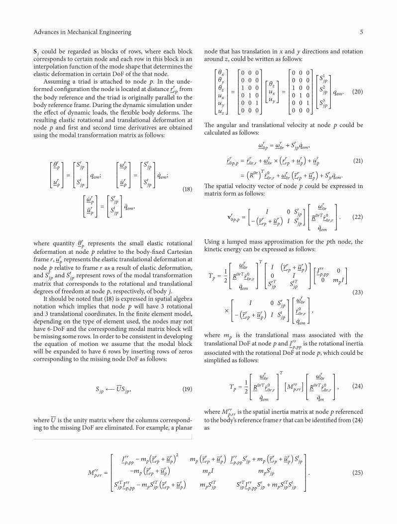
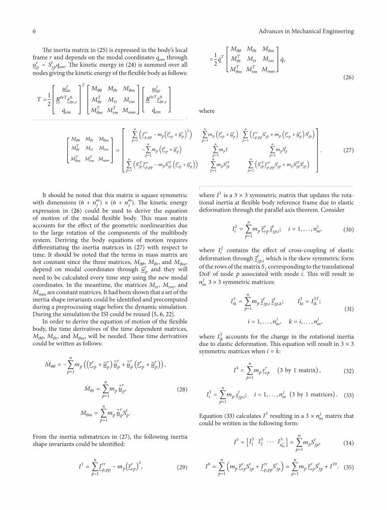
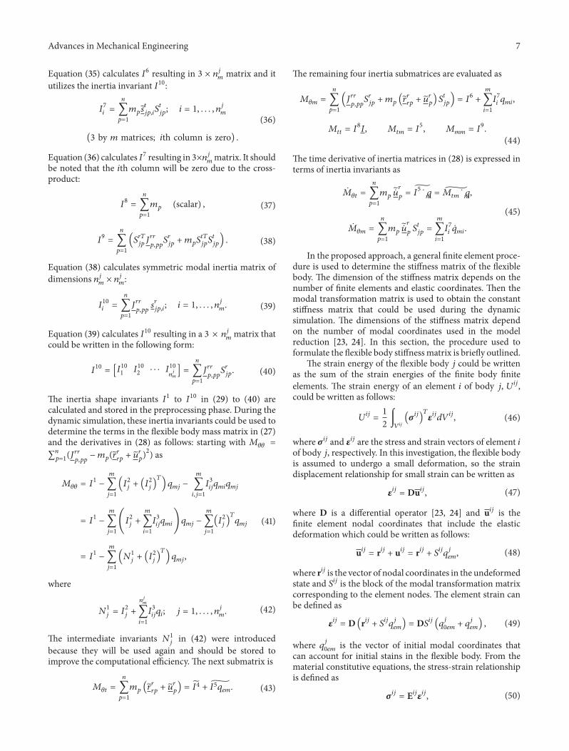
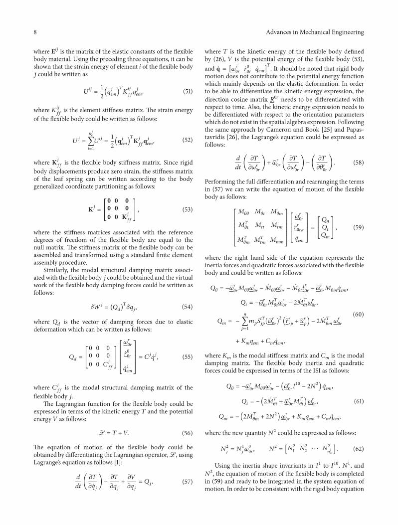
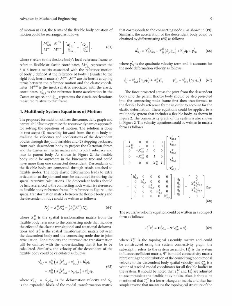
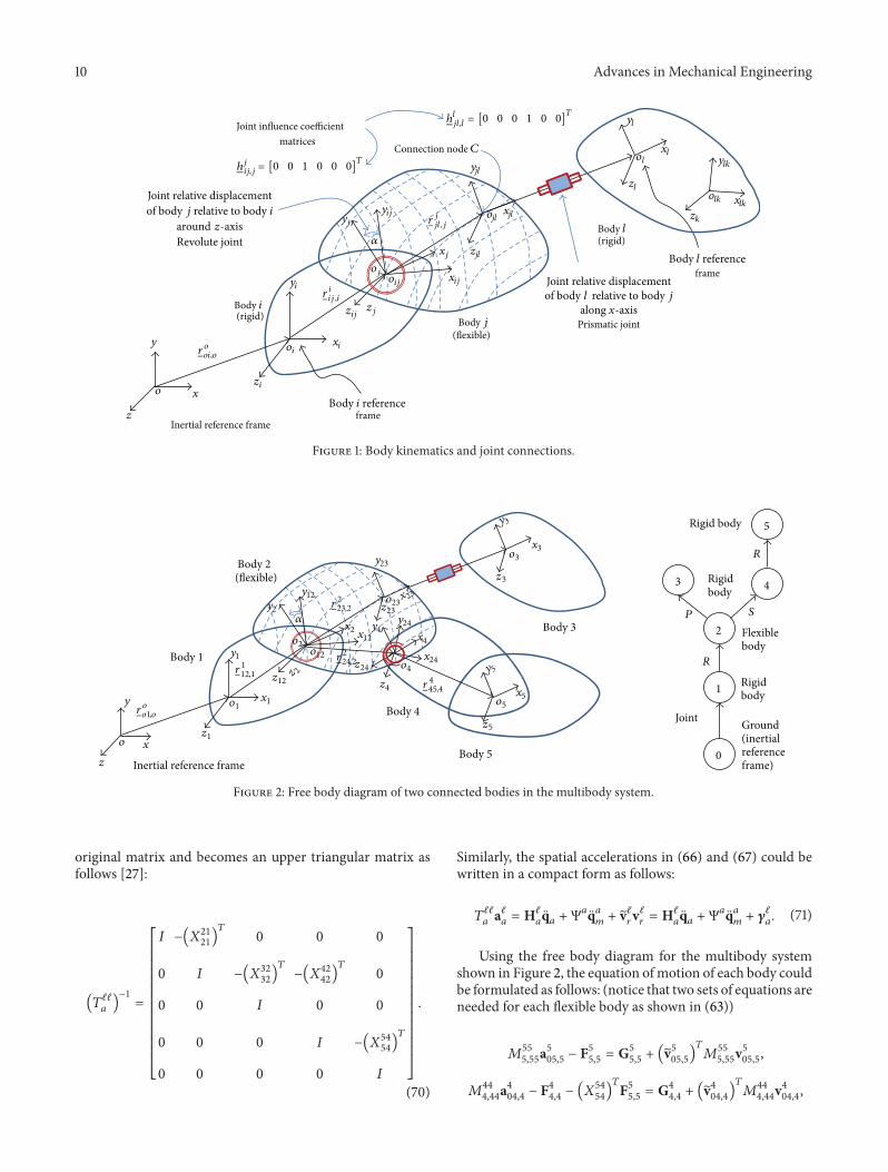
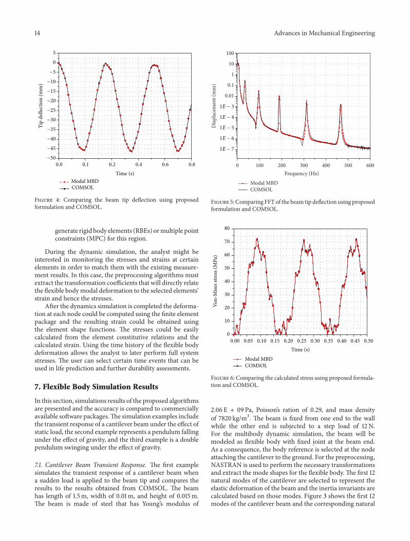
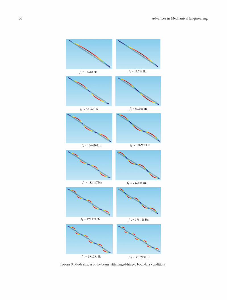
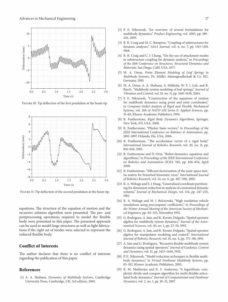
Related Documents


