HAL Id: tel-01680173 https://tel.archives-ouvertes.fr/tel-01680173 Submitted on 10 Jan 2018 HAL is a multi-disciplinary open access archive for the deposit and dissemination of sci- entific research documents, whether they are pub- lished or not. The documents may come from teaching and research institutions in France or abroad, or from public or private research centers. L’archive ouverte pluridisciplinaire HAL, est destinée au dépôt et à la diffusion de documents scientifiques de niveau recherche, publiés ou non, émanant des établissements d’enseignement et de recherche français ou étrangers, des laboratoires publics ou privés. Contribution to digital microrobotics : modeling, design and fabrication of curved beams, U-shaped actuators and multistable microrobots Hussein Hussein To cite this version: Hussein Hussein. Contribution to digital microrobotics : modeling, design and fabrication of curved beams, U-shaped actuators and multistable microrobots. Micro and nanotechnolo- gies/Microelectronics. Université de Franche-Comté, 2015. English. NNT : 2015BESA2048. tel- 01680173

Welcome message from author
This document is posted to help you gain knowledge. Please leave a comment to let me know what you think about it! Share it to your friends and learn new things together.
Transcript
HAL Id: tel-01680173https://tel.archives-ouvertes.fr/tel-01680173
Submitted on 10 Jan 2018
HAL is a multi-disciplinary open accessarchive for the deposit and dissemination of sci-entific research documents, whether they are pub-lished or not. The documents may come fromteaching and research institutions in France orabroad, or from public or private research centers.
L’archive ouverte pluridisciplinaire HAL, estdestinée au dépôt et à la diffusion de documentsscientifiques de niveau recherche, publiés ou non,émanant des établissements d’enseignement et derecherche français ou étrangers, des laboratoirespublics ou privés.
Contribution to digital microrobotics : modeling, designand fabrication of curved beams, U-shaped actuators
and multistable microrobotsHussein Hussein
To cite this version:Hussein Hussein. Contribution to digital microrobotics : modeling, design and fabricationof curved beams, U-shaped actuators and multistable microrobots. Micro and nanotechnolo-gies/Microelectronics. Université de Franche-Comté, 2015. English. �NNT : 2015BESA2048�. �tel-01680173�
Thèse de Doctorat
é c o l e d o c t o r a l e s c i e n c e s p o u r l ’ i n g é n i e u r e t m i c r o t e c h n i q u e s
U N I V E R S I T É D E F R A N C H E - C O M T É
n
Contribution to Digital Microrobotics:Modeling, Design and Fabrication ofCurved Beams, U-shaped Actuatorsand Multistable Microrobots
HUSSEIN HUSSEIN

Thèse de Doctorat
é c o l e d o c t o r a l e s c i e n c e s p o u r l ’ i n g é n i e u r e t m i c r o t e c h n i q u e s
U N I V E R S I T É D E F R A N C H E - C O M T É
THESE presentee par
HUSSEIN HUSSEIN
pour obtenir le
Grade de Docteur de
l’Universite de Franche-Comte
Specialite : Sciences pour l’ingenieur
Contribution to Digital Microrobotics: Modeling,
Design and Fabrication of Curved Beams, U-shaped
Actuators and Multistable Microrobots
Unite de Recherche :
FEMTO-ST, UMR CNRS 6174
Soutenue publiquement le 11 Decembre 2015 devant le Jury compose de :
ORPHEE CUGAT President du jury Directeur de Recherche, CNRS, G2ELAB,
Grenoble
JOEL POUGET Rapporteur Directeur de Recherche, CNRS, ∂’Alembert,
Paris
CHRISTINE PRELLE Rapporteur Professeur, UTC, Compiegne
RAFIC YOUNES Examinateur Professeur, UL, Beyrouth Liban
PHILIPPE LUTZ Directeur de these Professeur, UFC, Besancon
YASSINE HADDAB Encadrant de these Professeur,UM, Montpellier
PATRICE LE MOAL Encadrant de these Charge de recherche , CNRS, FEMTO-ST,
Besancon
GILLES BOURBON Encadrant de these Ingenieur de recherche, CNRS, FEMTO-ST,
Besancon


Acknowledgment
My thesis was realized in the AS2M department of Femto-st institute. I would like to express
my sincere gratitude to all the members of the department, starting from the director Michael
Gauthier and the colleagues for their support and the bright and stimulating environment of the
department.
I would like to express the deepest appreciation and thanks to my advisors Prof. Philippe
Lutz, Prof. Yassine Haddab, Dr. Patrice Le Moal and Dr. Gilles Bourbon, who supported me
greatly during the thesis and did every possible effort to help me in order to achieve the best
results. I am more than thankful for them for their kindness, patience, and endless encourage-
ment. I could not have imagined having a better advisor and mentor for my Ph.D study. Thanks
to you.
I would like to thank the rest of my thesis committee: Dr. Orphee Cugat, Dr. Joel Pouget,
Prof. Christine Prelle, and Prof. Rafic Younes, for serving as my committee members and for
letting my defense to be an enjoyable moment. Your insightful comments incented me to widen
my research from various perspectives. Thanks to you.
A special thanks to my family, you are everything for me. Words cannot express how grate-
ful I am to my mother and father for all of the sacrifices that you have made on my behalf. I
would also like to thank my brother and sisters for always being there beside me through thick
and thin.
I specially extend appreciation to my beloved wife, Fatima, who was always my support.
The day you stepped into my life, you changed it into something so beautiful and meaningful.
You are just so amazing to have around. I love you so much.
Finally, a new ray of sunshine will enter our lives in the next days; we are waiting the arrival
of our little princess Zahraa. Thank you my babe for the pleasure and happiness you have added
before your arrival. We are waiting impatiently ....
Hussein Hussein
v

Contents
General introduction 1
1 Digital Microrobotics 5
1.1 Introduction . . . . . . . . . . . . . . . . . . . . . . . . . . . . . . . . . . . . 6
1.2 Digital microrobot . . . . . . . . . . . . . . . . . . . . . . . . . . . . . . . . 8
1.2.1 Digital microrobotics . . . . . . . . . . . . . . . . . . . . . . . . . . . 8
1.2.2 The DiMiBot . . . . . . . . . . . . . . . . . . . . . . . . . . . . . . . 10
1.2.3 Advantages and challenges . . . . . . . . . . . . . . . . . . . . . . . . 13
1.3 Solutions for digital systems . . . . . . . . . . . . . . . . . . . . . . . . . . . 16
1.3.1 Switching function . . . . . . . . . . . . . . . . . . . . . . . . . . . . 16
1.3.2 Holding function . . . . . . . . . . . . . . . . . . . . . . . . . . . . . 18
1.3.3 Multistable mechanisms . . . . . . . . . . . . . . . . . . . . . . . . . 26
1.4 Thesis objectives and working axes . . . . . . . . . . . . . . . . . . . . . . . . 30
1.4.1 First axis: Analytical design optimization . . . . . . . . . . . . . . . . 31
1.4.2 Second axis: DiMiBot with multistable modules . . . . . . . . . . . . 32
1.5 Conclusion . . . . . . . . . . . . . . . . . . . . . . . . . . . . . . . . . . . . 33
2 Curved beam bistable mechanism 35
2.1 Introduction . . . . . . . . . . . . . . . . . . . . . . . . . . . . . . . . . . . . 37
2.2 Buckling of a beam . . . . . . . . . . . . . . . . . . . . . . . . . . . . . . . . 38
2.2.1 Buckling model . . . . . . . . . . . . . . . . . . . . . . . . . . . . . . 38
2.2.2 Buckling equation . . . . . . . . . . . . . . . . . . . . . . . . . . . . 40
2.2.3 Bifurcation of solutions . . . . . . . . . . . . . . . . . . . . . . . . . 42
2.3 Snapping force . . . . . . . . . . . . . . . . . . . . . . . . . . . . . . . . . . 45
2.3.1 Without high modes of buckling . . . . . . . . . . . . . . . . . . . . . 45
2.3.2 Considering high modes of buckling . . . . . . . . . . . . . . . . . . . 46
2.4 Bistability conditions . . . . . . . . . . . . . . . . . . . . . . . . . . . . . . . 49
2.5 Stress State . . . . . . . . . . . . . . . . . . . . . . . . . . . . . . . . . . . . 50
2.5.1 Without high modes of buckling . . . . . . . . . . . . . . . . . . . . . 51
2.5.2 Considering high modes of buckling . . . . . . . . . . . . . . . . . . . 53
vii
viii CONTENTS
2.6 FEM simulations and comparison . . . . . . . . . . . . . . . . . . . . . . . . 55
2.7 Design and optimization . . . . . . . . . . . . . . . . . . . . . . . . . . . . . 57
2.7.1 Influence of the dimensions and properties on the mechanical behavior 58
2.7.2 Curved beam design . . . . . . . . . . . . . . . . . . . . . . . . . . . 63
2.7.3 Limits of the miniaturization . . . . . . . . . . . . . . . . . . . . . . . 68
2.8 Conclusion . . . . . . . . . . . . . . . . . . . . . . . . . . . . . . . . . . . . 71
3 U-shaped electrothermal actuators 73
3.1 Introduction . . . . . . . . . . . . . . . . . . . . . . . . . . . . . . . . . . . . 75
3.2 Electrothermal model . . . . . . . . . . . . . . . . . . . . . . . . . . . . . . . 77
3.2.1 Electrothermal equation . . . . . . . . . . . . . . . . . . . . . . . . . 77
3.2.2 Lineshaped beam electrothermal response . . . . . . . . . . . . . . . . 77
3.2.3 Actuator electrothermal response . . . . . . . . . . . . . . . . . . . . 79
3.3 Thermo-mechanical model . . . . . . . . . . . . . . . . . . . . . . . . . . . . 85
3.4 Simulations, Experiments and discussion . . . . . . . . . . . . . . . . . . . . . 88
3.4.1 Electrothermal response . . . . . . . . . . . . . . . . . . . . . . . . . 89
3.4.2 Mechanical response . . . . . . . . . . . . . . . . . . . . . . . . . . . 92
3.5 Design and optimization . . . . . . . . . . . . . . . . . . . . . . . . . . . . . 95
3.5.1 Maximal voltage . . . . . . . . . . . . . . . . . . . . . . . . . . . . . 95
3.5.2 Characteristic curve of the actuator . . . . . . . . . . . . . . . . . . . 96
3.5.3 Influence of the parameters on the actuator’s performance . . . . . . . 99
3.5.4 Design methodology of the actuator . . . . . . . . . . . . . . . . . . . 106
3.6 Conclusion . . . . . . . . . . . . . . . . . . . . . . . . . . . . . . . . . . . . 112
4 Multistable module and DiMiBot 113
4.1 Introduction . . . . . . . . . . . . . . . . . . . . . . . . . . . . . . . . . . . . 115
4.2 Principle of the multistable mechanism . . . . . . . . . . . . . . . . . . . . . . 117
4.3 System 1: an accurate bistable mechanism . . . . . . . . . . . . . . . . . . . . 119
4.3.1 Microfabrication tolerances . . . . . . . . . . . . . . . . . . . . . . . 120
4.3.2 Accurate positioning mechanism . . . . . . . . . . . . . . . . . . . . . 121
4.3.3 Design of the different components in system 1 . . . . . . . . . . . . . 124
4.4 System 2 and the teeth configurations . . . . . . . . . . . . . . . . . . . . . . 127
4.4.1 Functioning . . . . . . . . . . . . . . . . . . . . . . . . . . . . . . . . 127
4.4.2 Teeth configurations . . . . . . . . . . . . . . . . . . . . . . . . . . . 128
4.5 System 3 and the moving part . . . . . . . . . . . . . . . . . . . . . . . . . . 130
4.6 Multistable module global design . . . . . . . . . . . . . . . . . . . . . . . . . 132
4.7 Multistable modules in the DiMiBot . . . . . . . . . . . . . . . . . . . . . . . 133
4.8 Conclusion . . . . . . . . . . . . . . . . . . . . . . . . . . . . . . . . . . . . 137
5 Fabrication and experiments 139
5.1 Introduction . . . . . . . . . . . . . . . . . . . . . . . . . . . . . . . . . . . . 141
5.2 Fabrication process . . . . . . . . . . . . . . . . . . . . . . . . . . . . . . . . 141
5.2.1 General process flow . . . . . . . . . . . . . . . . . . . . . . . . . . . 141
5.2.2 Layout . . . . . . . . . . . . . . . . . . . . . . . . . . . . . . . . . . 143

CONTENTS ix
5.3 Technological aspects in the fabrication process . . . . . . . . . . . . . . . . . 148
5.3.1 Hard mask (Photomask A) . . . . . . . . . . . . . . . . . . . . . . . . 148
5.3.2 Gold patterns (Photomask B) . . . . . . . . . . . . . . . . . . . . . . . 149
5.3.3 Device layer etching (Photomask C) . . . . . . . . . . . . . . . . . . . 151
5.3.4 Substrate etching . . . . . . . . . . . . . . . . . . . . . . . . . . . . . 154
5.3.5 HF release . . . . . . . . . . . . . . . . . . . . . . . . . . . . . . . . 154
5.4 Force measurement experiments . . . . . . . . . . . . . . . . . . . . . . . . . 157
5.4.1 Rectilinear beams . . . . . . . . . . . . . . . . . . . . . . . . . . . . . 159
5.4.2 Curved beams . . . . . . . . . . . . . . . . . . . . . . . . . . . . . . . 159
5.5 Experiments on the actuators . . . . . . . . . . . . . . . . . . . . . . . . . . . 161
5.5.1 Experimental setup . . . . . . . . . . . . . . . . . . . . . . . . . . . . 161
5.5.2 Remarks noticed in the experiments . . . . . . . . . . . . . . . . . . . 163
5.6 Multistable module experiment . . . . . . . . . . . . . . . . . . . . . . . . . . 165
5.6.1 Activation of the multistable modules . . . . . . . . . . . . . . . . . . 166
5.6.2 Wire bonding . . . . . . . . . . . . . . . . . . . . . . . . . . . . . . . 166
5.6.3 Electronic circuit . . . . . . . . . . . . . . . . . . . . . . . . . . . . . 166
5.6.4 Tests on the different systems of the multistable module . . . . . . . . 169
5.6.5 Sequence orders to make steps . . . . . . . . . . . . . . . . . . . . . . 169
5.6.6 Experimental functioning . . . . . . . . . . . . . . . . . . . . . . . . . 169
5.7 Conclusion . . . . . . . . . . . . . . . . . . . . . . . . . . . . . . . . . . . . 173
Conclusion and perspectives 175
Conclusion . . . . . . . . . . . . . . . . . . . . . . . . . . . . . . . . . . . . . . . 175
Perspectives . . . . . . . . . . . . . . . . . . . . . . . . . . . . . . . . . . . . . . . 177
Actuators . . . . . . . . . . . . . . . . . . . . . . . . . . . . . . . . . . . . . 177
Multistable module . . . . . . . . . . . . . . . . . . . . . . . . . . . . . . . . 178
Towards a planar multistable microrobot with holding forces . . . . . . . . . . 178
Towards a 3D multistable microrobot in three dimensions . . . . . . . . . . . . 180
Bibliography 181

List of Figures
1.1 Assembly platform for a microspectrometer (a), the assembled microspectrom-
eter (b) [28]. . . . . . . . . . . . . . . . . . . . . . . . . . . . . . . . . . . . 6
1.2 Schematic diagram for the functioning of a positioning system with feedback. . 7
1.3 Unstable, discrete, stable and maintained positions. . . . . . . . . . . . . . . . 8
1.4 Example of the ball on a surface in different positions. . . . . . . . . . . . . . 9
1.5 Schematic diagram for the functioning of a digital microrobot. . . . . . . . . . 10
1.6 Schematic of the general structural architecture of the DiMiBot. [12]. . . . . . 11
1.7 Drawing of the DiMiBot with four bistable modules with zooms on a bistable
module, a compliant hinge and the end effector.. . . . . . . . . . . . . . . . . 12
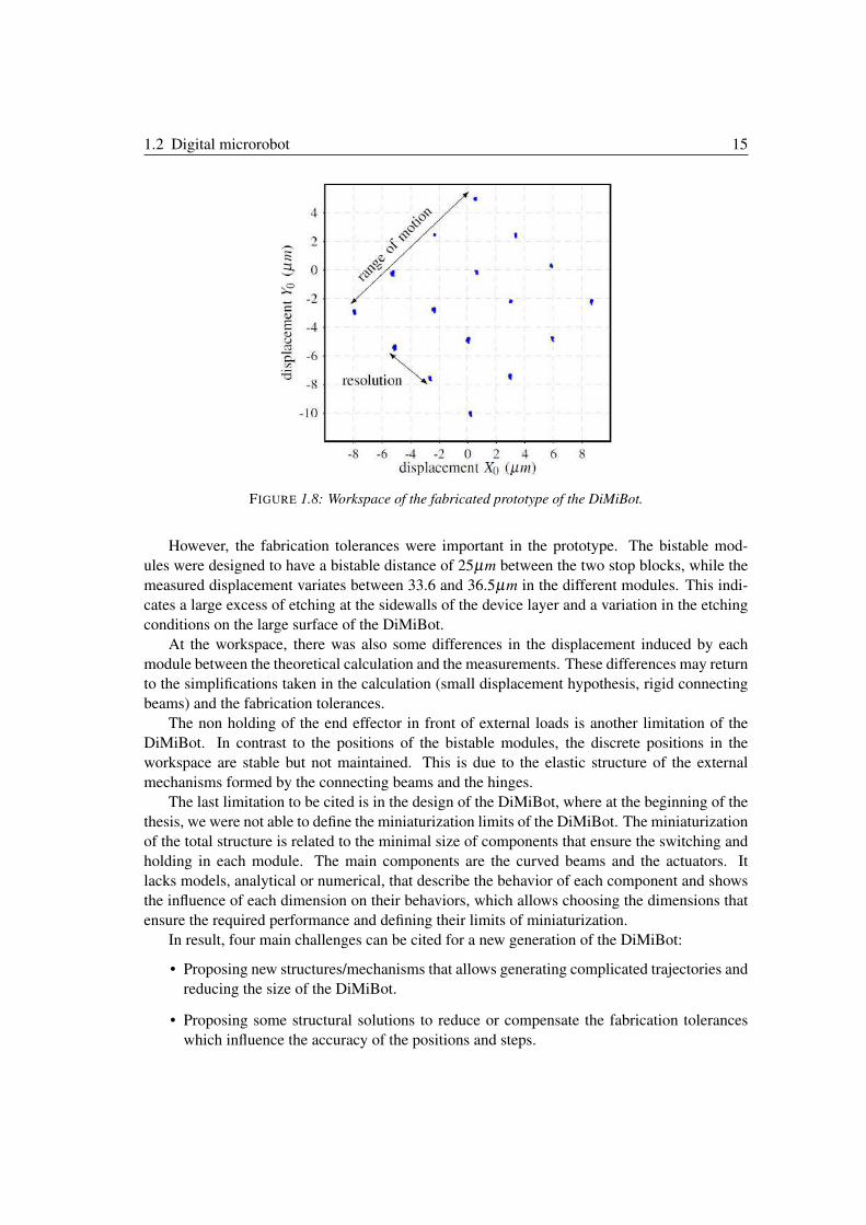
1.8 Workspace of the fabricated prototype of the DiMiBot. . . . . . . . . . . . . . 15
1.9 Holding principle via passive locking actuator(a), optical switch using passive
locking actuator [26] (b). . . . . . . . . . . . . . . . . . . . . . . . . . . . . . 20
1.10 Holding principle via permanent magnet. . . . . . . . . . . . . . . . . . . . . 20
1.11 Top (a) and front view (b) of a quadristable system [104]. . . . . . . . . . . . 21
1.12 Precompressed curved beam actuated using two SMA actuators [136] (a), pre-
stressed beam nanowire as micromechanical memory [15] (b). . . . . . . . . . 22
1.13 2x2 MEMS optical switch using preshaped curved beams [79] (a), comb drive
bistable actuator using hinged preshaped curved beams [72] (b). . . . . . . . . 22
1.14 The example of the ball on a surface in analogy with the buckled beam structure
principle. The driving force curve is shown in the bottom with respect to the
ball position. . . . . . . . . . . . . . . . . . . . . . . . . . . . . . . . . . . . 23
1.15 The example of the ball on a surface with stop blocks. . . . . . . . . . . . . . 24
1.16 Configurations of the stop blocs of the bistable module, in the DiMiBot, in three
different states: as-fabricated, at position 1 and at position 2. . . . . . . . . . . 25
1.17 Functioning principle of an electrostatic inchworm actuator [35]. LA1 and LA2
latch the two shuttles (step 0), LA1 unlatch the first shuttle (step 1), DA is
activated which moves the first shuttle ahead (step 2), LA1 latch the first shut-
tle (step3), LA2 unlatch the second shuttle (step 4), finally, DA is disactivated
which moves the second shuttle ahead. . . . . . . . . . . . . . . . . . . . . . 28
xi
xii LIST OF FIGURES
1.18 Functioning principle of stick-slip actuators (a), drawing of stick-slip device
working around and along a tube [108] (b). . . . . . . . . . . . . . . . . . . . 28
1.19 Principle of friction-inertia actuators (a), a friction-inertia microrobot [94] (b). 29
1.20 Principle of ultrasonic actuators [65] (a), XY drive which uses ultrasonic prin-
ciple [30] (b). . . . . . . . . . . . . . . . . . . . . . . . . . . . . . . . . . . . 29
1.21 Architecture of the DiMiBot with multistable modules. . . . . . . . . . . . . . 32
1.22 Woking axes and the following chapters of the thesis. . . . . . . . . . . . . . . 34
2.1 Buckling of a beam before and after a critical axial compression. . . . . . . . 38
2.2 Transition between the two stable positions of a buckled beam as a result of a
lateral force applied in the middle of the beam. . . . . . . . . . . . . . . . . . 38
2.3 Clamped-clamped curved bistable beam at the initial position and after deflec-
tion. . . . . . . . . . . . . . . . . . . . . . . . . . . . . . . . . . . . . . . . . 39
2.4 A beam in bending (a), bending stress distribution along the thickness and bend-
ing moment in a section (b) forces and moments equilibrium in a section of a
buckled beam(c). . . . . . . . . . . . . . . . . . . . . . . . . . . . . . . . . . 40
2.5 The first three buckling shape modes . . . . . . . . . . . . . . . . . . . . . . 42
2.6 Transition between the two stable positions of two curved beams connected in
the middle, mode 3 appears during transition. . . . . . . . . . . . . . . . . . . 44
2.7 Snapping force solutions without considering high modes of buckling for Q
<�(16/3), Q =
�(16/3) and Q >
�(16/3) respectively. . . . . . . . . . . 46
2.8 Evolution of the normalized axial stress N in the first kind of solution in function
of Q ratio. N is constant in the second and third kinds of solution. The shape of
the curved beam in the first, second and third case. . . . . . . . . . . . . . . . 48
2.9 Evolution of the normalized applied force F for the curved beam for different Q
values when mode 2 is constrained. . . . . . . . . . . . . . . . . . . . . . . . 48
2.10 Evolution of the maximal stress in the beam during deflection depending on Q. 52
2.11 Evolution of the maximal total stress during deflection for Q = 2, Q = 2.4 and
Q = 3. . . . . . . . . . . . . . . . . . . . . . . . . . . . . . . . . . . . . . . 55
2.12 Comparison of the snapping-force behavior during deflection between theory
and FEM simulation. . . . . . . . . . . . . . . . . . . . . . . . . . . . . . . . 55
2.13 Comparison between the maximal stress value during deflection between theory
ans FEM simulation. . . . . . . . . . . . . . . . . . . . . . . . . . . . . . . . 56
2.14 Comparison between the bending maximal stress value during deflection with
and without high modes of buckling. . . . . . . . . . . . . . . . . . . . . . . 57
2.15 Evolution of the maximal stress in function of the critical ratio Q according to
f1(Q) (blue curve left axis) and to f2(Q) (green curve right axis). . . . . . . . 59
2.16 Evolution of the condition on K1t/l with respect to Q. . . . . . . . . . . . . . 60
2.17 Evolution of the condition on K1h/l with respect to Q. . . . . . . . . . . . . . 60
2.18 Evolution of the top of the snapping forces ftop with respect to Q according to
f3(Q) (blue curve left axis) and to f4(Q) (green curve right axis). . . . . . . . 62
2.19 Evolution of the distance between the two stable positions with respect to Q. . 62
2.20 Evolution of ftop in front of the bistable distance Δstab. . . . . . . . . . . . . . 63
2.21 Block diagram representing the design method. . . . . . . . . . . . . . . . . . 64
LIST OF FIGURES xiii
2.22 Important snapping points for the design of curved beams in the bistable mod-
ule. . . . . . . . . . . . . . . . . . . . . . . . . . . . . . . . . . . . . . . . . 65
2.23 Field of possibilities for the value of the thickness and the height that is con-
cluded from the conditions extracted from the specifications and limitations.
The possible dimensions are in the white part. . . . . . . . . . . . . . . . . . . 68
3.1 U-shaped electrothermal micoractuator. . . . . . . . . . . . . . . . . . . . . . 75
3.2 Schema of lineshaped microbeam. . . . . . . . . . . . . . . . . . . . . . . . . 78
3.3 Unfolded actuator . . . . . . . . . . . . . . . . . . . . . . . . . . . . . . . . . 80
3.4 Distribution of the surface forces N and bending moments Mb in the actuator
when it is anchored at the flexure end and free in the other side after applying
virtual unit forces and moment at the free border of the hot arm, (a), (b) and (c),
and at the tip of the actuator (d). . . . . . . . . . . . . . . . . . . . . . . . . . 86
3.5 Dimensions for the U-shaped actuator in the modeling, simulations and experi-
ments. . . . . . . . . . . . . . . . . . . . . . . . . . . . . . . . . . . . . . . . 89
3.6 Evolution of the temperature distribution in the actuator obtained from the ana-
lytical solution after applying 15V voltage at the anchors. . . . . . . . . . . . . 90
3.7 Temperature profiles in the actuator obtained analytically at 0, 2, 10, 20, 40, 70,
150, 250, 500 and 1000ms after applying 15V . . . . . . . . . . . . . . . . . . . 90
3.8 Evolution of the average temperature with time in the three arms of the actuator
after applying 15V voltage. . . . . . . . . . . . . . . . . . . . . . . . . . . . 91
3.9 Comparison between the analytical model and ANSYS for the evolution of the
average temperature in the hot arm. . . . . . . . . . . . . . . . . . . . . . . . . 91
3.10 Layers of the microfabricated actuator. . . . . . . . . . . . . . . . . . . . . . . 92
3.11 Shape of the actuator at the rest position (a) and during displacement (b) in the
videos. . . . . . . . . . . . . . . . . . . . . . . . . . . . . . . . . . . . . . . 92
3.12 Comparison between the analytical model, ANSYS and experiments for the dis-
placement curves at the tip of the actuator. . . . . . . . . . . . . . . . . . . . . 93
3.13 Thermal expansion of the hot, cold and flexure arms, cold side and expansion
difference between both sides of the actuator after applying a voltage of 15V . . 94
3.14 Evolution of the characteristic curves of the actuator at several instants after
applying a constant voltage. . . . . . . . . . . . . . . . . . . . . . . . . . . . 99
3.15 The characteristic curve of the actuator at the steady state including the blocking
force and free displacement expressions. . . . . . . . . . . . . . . . . . . . . . 100
3.16 Influence of changing the general dimensions on the characteristic curve of the
actuator: including the general length l (a), the depth b (b), the general width w
(c) and l and w simultaneously with the same ratio of changing (d). . . . . . . . 101
3.17 Evolution of K�1K�
3 with respect to c and a for a constant ratio f = 1. . . . . . . 102
3.18 Evolution of K�1K�
3 with respect to c and f for a constant ratio a = 0.1. . . . . . 103
3.19 Evolution of K�1K�
3 with respect to a and f for a constant ratio c = 10. . . . . . 103
3.20 Values of the ratios f and a maximizing the free displacement d f ree for different
values of c ratio. . . . . . . . . . . . . . . . . . . . . . . . . . . . . . . . . . . 104
3.21 Evolution of K�1K�
3 at the max-free dimensions for different values of c and with
respect to a. . . . . . . . . . . . . . . . . . . . . . . . . . . . . . . . . . . . . 104
xiv LIST OF FIGURES
3.22 Evolution of K�1K�
3/K�2 with respect to c and a for a constant ratio f = 1. . . . . 105
3.23 Evolution of K�1K�
3/K�2 with respect to c and f for a constant ratio a = 0.1. . . . 105
3.24 Evolution of K�1K�
3/K�2 with respect to a and f for a constant ratio c = 10. . . . 106
3.25 Characteristic curves of the actuator before and after t = td . The loaded dis-
placement after t = td must be more important than the desired displacement
dd . . . . . . . . . . . . . . . . . . . . . . . . . . . . . . . . . . . . . . . . . . 107
3.26 The maximal performance that can be reached in terms of the displacement.
When the output is considered at the steady state, the voltage that can be applied
is lower and the performance is less important. When the output is considered
at the peak of the overshoot, the maximal allowable voltage is higher due to the
lower temperature and the performance is more important. . . . . . . . . . . . 108
3.27 Evolution of (dss −dd) with respect to the length l. . . . . . . . . . . . . . . . 109
3.28 Evolution of dssmax (left column) and lmax (right column) with respect to a.
These values are calculated for c = 20. . . . . . . . . . . . . . . . . . . . . . . 111
3.29 Evolution of the desired length ld with respect to c allowing obtaining a desired
displacement dd = 80µm. . . . . . . . . . . . . . . . . . . . . . . . . . . . . . 112
4.1 Drawing of the new generation of the DiMiBot. . . . . . . . . . . . . . . . . . 115
4.2 A drawing of the different systems and components in the multistable module.. 116
4.3 Schema of the rest configuration of the multistable mechanism including the
latches and the moving part. . . . . . . . . . . . . . . . . . . . . . . . . . . . 117
4.4 Sequence order to make an upward step. Firstly, S2 latch move upwards with
holding the moving part (a), S3 latch holds the moving part (b), S2 latch releases
the moving part (c), moves downwards (d) and holds the moving part in a bottom
position (e), finally, S3 latch releases the moving part (f). . . . . . . . . . . . . 118
4.5 Sequence order to make a downward step. Firstly, S3 latch holds the moving
part (a), S2 latch releases the moving part (b), moves upwards (c) and closes in
the upper position (d), S3 latch releases then the moving part (e), finally, S2 latch
moves downwards with holding the moving part (f). . . . . . . . . . . . . . . 118
4.6 Drawing of system 1 and its different components. . . . . . . . . . . . . . . . 119
4.7 Usual etching process steps. Photoresist deposition and UV light exposure using
a photomask (1), photoresist developing (2), DRIE of the silicon layer (3). . . 120
4.8 Distances between the sidewalls of two parallel patterns in the design (a) and
after fabrication (b). . . . . . . . . . . . . . . . . . . . . . . . . . . . . . . . 121
4.9 Drawing of the accurate positioning mechanism in the design, the important dis-
tances between the different components are shown with considering the fab-
rication tolerances (a). Drawing of the accurate positioning mechanism after
activation where the movable parts are suspended to their locks and the moving
part is in the initial position (b). . . . . . . . . . . . . . . . . . . . . . . . . . 122
4.10 Configuration of the mechanism to compensate the fabrication tolerances. The
mechanism to realize the initial activation distance d as fabricated (a) and after
the initial activation (b). The mechanism to define the step size s as fabricated
(c) and after the initial activation (d). . . . . . . . . . . . . . . . . . . . . . . 124
LIST OF FIGURES xv
4.11 Evolution of the snapping force of preshaped curved beams during deflection
for Q < 2.31 and Q > 2.31. . . . . . . . . . . . . . . . . . . . . . . . . . . . . 125
4.12 Snapping force evolution of the curved beams in system 1 during deflection. . . 126
4.13 Important distances and elastic forces in the as-fabricated configuration of sys-
tem 1 (a), after activation (b) and after switching to the second position (c). . . 126
4.14 Drawing of system 2 including S2 latch and two electrothermal actuators, and a
zoom on the teeth of the latch and the moving part before and after activation. . 127
4.15 Evolution of the retracting force after deflection of the gantry in each side of the
latch in system 2. . . . . . . . . . . . . . . . . . . . . . . . . . . . . . . . . . 128
4.16 Zoom on the contact zone between the moving part and S2 latch in the as-
fabricated configuration (a), when the latch holds the moving part (b) and when
it releases the moving part (c). . . . . . . . . . . . . . . . . . . . . . . . . . . 128
4.17 Two possible configurations of the teeth dimensions allowing engaging the teeth
at each step. Small (a) and wide (b) teeth configurations. The teeth dimensions
are shown at the left while the engagement shape of the teeth between two con-
secutive positions of the moving part is shown at the right. . . . . . . . . . . . 129
4.18 Drawing of system 3 including S3 latch, two electrothermal actuator, and a zoom
on the teeth between the latch and moving part. . . . . . . . . . . . . . . . . . 130
4.19 Evolution of the retracting force after deflection of the gantry of the latch in
system 3. . . . . . . . . . . . . . . . . . . . . . . . . . . . . . . . . . . . . . 130
4.20 Moving part of the multistable module connected to curved beams. . . . . . . 131
4.21 Evolution of the snapping forces of the curved beams connected to the moving
part after deflection and their values at each stable position. . . . . . . . . . . 131
4.22 Drawing of the multistable module including the support, conductive lines and
the different systems. . . . . . . . . . . . . . . . . . . . . . . . . . . . . . . . 133
4.23 Drawing of the multistable DiMiBot including the multistable modules, the sup-
port, the conductive lines, and the top head mechanism relating the moving parts
to the end effector. . . . . . . . . . . . . . . . . . . . . . . . . . . . . . . . . 134
4.24 Drawing of the head mechanism at the head of the DiMiBot including the end
effector, the beams and the compliant hinges. . . . . . . . . . . . . . . . . . . 134
4.25 Workspace of the DiMiBot which consists of 169 discrete positions. . . . . . . 135
4.26 Evolution of the retracting force in the bottom left hinge when the left and right
modules are in the different stable positions. . . . . . . . . . . . . . . . . . . 136
5.1 Fabrication process steps in the thesis of Vincent Chalvet [12]. Aluminum layer
deposition and patterning (1), device and handle layers etching using DRIE pro-
cess (2-3), structure releasing from the wafer using RIE of the buried oxide (4). 142
5.2 Fabrication process steps. SiO2 hard mask etching on the backside (1), gold
layer deposition (2), device and handle layers etched using DRIE process (3-4),
structure releasing from the wafer using HF wet etching (5). . . . . . . . . . . 143
5.3 Example of the layout in the cell of a multistable module. . . . . . . . . . . . . 144
xvi LIST OF FIGURES
5.4 States of a multistable prototype in the wafer during the fabrication process.
top view at the initial state (a), after deposition of the gold patterns (b), after
etching the device layer (c), after releasing the useless parts (d), after releasing
the prototype from the wafer, top view (e) bottom view (f). . . . . . . . . . . . 145
5.5 Layout of the DiMiBot with multistable modules. . . . . . . . . . . . . . . . . 146
5.6 Layout of an accurate bistable module (system 1). . . . . . . . . . . . . . . . . 146
5.7 Layout of the actuator prototypes with and without loads. . . . . . . . . . . . . 147
5.8 Layout of preshaped curved beams test. . . . . . . . . . . . . . . . . . . . . . 147
5.9 Layout of a prototype for measuring the stiffness of rectilinear beams. . . . . . 148
5.10 Process steps for patterning the hard mask in the backside. . . . . . . . . . . . 149
5.11 Process steps for sputtering and patterning the gold patterns. . . . . . . . . . . 150
5.12 Gold patterns after sputtering and patterning. . . . . . . . . . . . . . . . . . . 151
5.13 Process steps for etching the device layer. . . . . . . . . . . . . . . . . . . . . 152
5.14 SEM photos of the device layer in different places. . . . . . . . . . . . . . . . 153
5.15 Microscopic photos of the device layer after etching. Barred dimensions are the
layout dimensions, while the others are the real dimensions after fabrication . . 153
5.16 Zoom on the releasing distance in the wafer before HF releasing (a), HF com-
patible wafer holder (b). . . . . . . . . . . . . . . . . . . . . . . . . . . . . . 155
5.17 The gold patterns started to peel off from the wafer after inserting it in the HF
solution. . . . . . . . . . . . . . . . . . . . . . . . . . . . . . . . . . . . . . . 155
5.18 Wafer from the second run of fabrication where all the structures are released
without peeling off the gold patterns. . . . . . . . . . . . . . . . . . . . . . . . 156
5.19 Prototype of the DiMiBot obtained in the second run of fabrication. . . . . . . 156
5.20 Schematic diagram of the elements used in the force measurement experiments. 157
5.21 Calibration of the robotic stage signals (actuator and sensor) using an interfer-
ometer. . . . . . . . . . . . . . . . . . . . . . . . . . . . . . . . . . . . . . . 158
5.22 Photo of the experience using force sensor. . . . . . . . . . . . . . . . . . . . . 158
5.23 Curved and rectilinear beam prototypes (a), screens showing a direct image from
the side and top of the prototypes and force sensor probe (b). . . . . . . . . . . 159
5.24 force curves of a rectilinear beam obtained in the experiment and FEM sim-
ulations. The beam dimensions are as follows: t = 30µm, l = 2040µm, and
b = 100µm. . . . . . . . . . . . . . . . . . . . . . . . . . . . . . . . . . . . . 160
5.25 Snapping force curves of a hinged preshaped curved beams prototype obtained
in the experiment and FEM simulations. The beam dimensions are as follows:
t = 20µm, l = 6.8mm, b = 100µm, thinges = 15µm, lhinges = 500µm. . . . . . . 160
5.26 Micromanipulation station used in the experiments. . . . . . . . . . . . . . . . 162
5.27 An actuator in the initial position (a) and after supplying (b). . . . . . . . . . . 162
5.28 Example of the displacement curves of two actuators with the same characteris-
tics, one is free and the other acts on an elastic beam as a load. . . . . . . . . . 163
5.29 Evolution of the electrical current after applying a voltage step of 10V in one
long step (upper curve) and in successive steps with small delay between each
step (lower curve). . . . . . . . . . . . . . . . . . . . . . . . . . . . . . . . . 164
LIST OF FIGURES xvii
5.30 Failure of the actuators during the experiments at the link between the hot and
cold arms for the actuators of the first run (a), and at the flexure for those of the
second run of fabrication. . . . . . . . . . . . . . . . . . . . . . . . . . . . . . 165
5.31 Activation steps of the multistable module under a microscope using three probe
needles. . . . . . . . . . . . . . . . . . . . . . . . . . . . . . . . . . . . . . . 167
5.32 A multistable module prototype glued and wire bonded on a PCB . . . . . . . 167
5.33 The electronic circuit for supplying the multistable module prototype. . . . . . 168
5.34 Schematic of the relay circuit. . . . . . . . . . . . . . . . . . . . . . . . . . . 168
5.35 Tests on systems 1, 2 and 3 respectively. Three photos are presented for each
system, one in the off state, one in the on state and the third one is a zoom on
the part that moves. System 1 ((a), (b) & (c)), system 2 ((d), (e) & (f)), system
3 ((g), (h) & (i)). . . . . . . . . . . . . . . . . . . . . . . . . . . . . . . . . . 170
5.36 Sequence order for supplying the actuators of each system in the multistable
module in order to make upward and downward steps ((a) and (b) respectively). 171
5.37 Functioning of a multistable module during a downward step. The moving part
is initially in an upper position (a), S3 latch is firstly closed (b), S2 latch is then
opened (c), and then moved up ((d) & (e)), after that, S2 latch closes (f), S3
latch opens (g) and finally, S2 latch moves down with the moving part (h), lower
position of the moving part is shown in (i). . . . . . . . . . . . . . . . . . . . . 172
5.38 S3 latch remains closed after dis-activating system 3 in the modules with wide
teeth configuration (a), the teeth with the small configuration of S2 latch are
broken during the experiments (b). . . . . . . . . . . . . . . . . . . . . . . . . 173
1 Comparison of the size and workspace between the old and the new generation
of the DiMiBot. The two workspaces are at the same scale. . . . . . . . . . . 176
2 A proposition of a planar multistable microrobot. . . . . . . . . . . . . . . . . 179

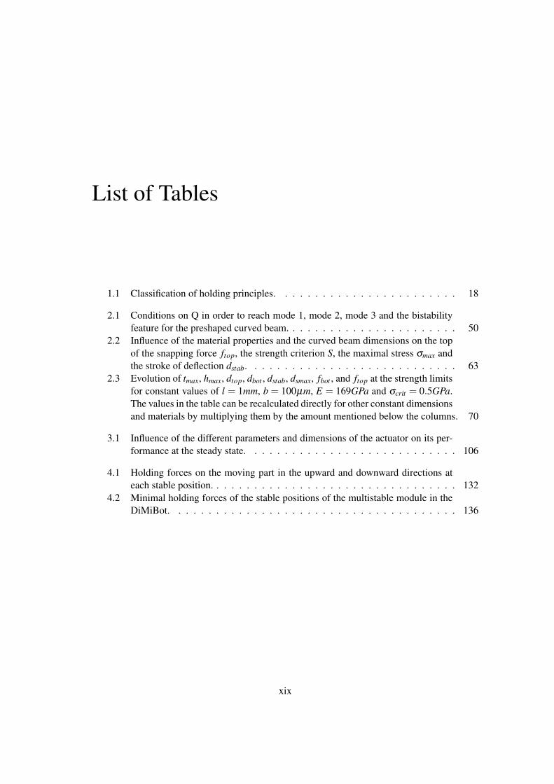
List of Tables
1.1 Classification of holding principles. . . . . . . . . . . . . . . . . . . . . . . . 18
2.1 Conditions on Q in order to reach mode 1, mode 2, mode 3 and the bistability
feature for the preshaped curved beam. . . . . . . . . . . . . . . . . . . . . . . 50
2.2 Influence of the material properties and the curved beam dimensions on the top
of the snapping force ftop, the strength criterion S, the maximal stress σmax and
the stroke of deflection dstab. . . . . . . . . . . . . . . . . . . . . . . . . . . . 63
2.3 Evolution of tmax, hmax, dtop, dbot , dstab, dsmax, fbot , and ftop at the strength limits
for constant values of l = 1mm, b = 100µm, E = 169GPa and σcrit = 0.5GPa.
The values in the table can be recalculated directly for other constant dimensions
and materials by multiplying them by the amount mentioned below the columns. 70
3.1 Influence of the different parameters and dimensions of the actuator on its per-
formance at the steady state. . . . . . . . . . . . . . . . . . . . . . . . . . . . 106
4.1 Holding forces on the moving part in the upward and downward directions at
each stable position. . . . . . . . . . . . . . . . . . . . . . . . . . . . . . . . . 132
4.2 Minimal holding forces of the stable positions of the multistable module in the
DiMiBot. . . . . . . . . . . . . . . . . . . . . . . . . . . . . . . . . . . . . . 136
xix

General introduction
Since the mid-20th century, the relationship between humans and machines are experiencing
a tremendous development. Electronic products and smart devices have become an extremely
important part of our daily life. The actual and coming tech boom makes and will make our life
so mush easier. Personal computers, smart phones, cameras, televisions and thousands of other
intelligent devices, all are operated by the silicon chips and integrated circuits inside. All the
developments nowadays in every single domain of our life including the economy, all kinds of
industries, energy production, transport, communication, medicine and many others have been
made possible mostly with the help of these powerful silicon chips. They allowed us to access
the nearby planets and explore the most distant galaxies in the large scale, and to discover the
smaller organisms ever and dive in the particles and atoms world in the downscale.
As we go down in size, there are a number of interesting opportunities coming up, plenty
of room, applications and possibilities at the bottom are not yet discovered, while the technol-
ogy of small devices is expanding fast. Micro-Electro-Mechanical Systems, or MEMS, is the
technology of miniaturized systems. It consists of micro-electro-mechanical elements that are
made using the techniques of microfabrication. An extremely large number of MEMS devices
are available in the market and many of them have demonstrated performances exceeding those
of their macroscale counterparts.
The accelerated research and development in the field of miniature systems and integrated
circuits introduced innovative products in our society and revealed the necessity to develop mi-
cromanipulators to handle microobjects, fabricate structures, assemble products, interact with a
patient, etc.. Two main elements are generally implemented in the design of a micromanipulator:
• A tool to make the final function. The tool can be a probe or a microgripper used for
handling an object, grasping, performing pick and place, pushing, pulling, positioning,
orienting, etc..
• A micropositioning system to position the tool or another substrate. This system must be
able to deliver displacement strokes with sub micrometer level accuracy, high precision
and repeatability.
Each of these elements has its own characteristics and constraints. As for the tool, scale
effect appears due to the miniaturization which is represented by the predominance of surface
2 General introduction
forces (adhesion forces ...) on the volume forces (gravity, weight ...) for small objects. Thus,
handling an object is more complicated due to the predominance of some forces (such as elec-
trostatic, Van der Waals, and capillary forces) which are negligible in traditional manipulation.
As for the micropositioning systems, several issues can be noted such as the limitation in
the fabrication process that constraints several aspects in the design (monolithic structure, multi
DoF, out of plane displacement, assembly, etc.), the need to make high precision and repeatable
systems, the need of sensors for precise positioning, the miniaturization, extending the range of
motion in the workspace, the integration in complicated environments, etc.. There are still few
work on the design of robotic carriers which are dedicated to the microworld.
Digital microrobotics is an emergent branch in micropositioning systems which avoids the
necessity of a feedback to control the position by placing the moving part in several stable posi-
tions defined in the design. This avoids the use of bulky sensors which increases the size of the
whole device, allows going further in miniaturization, simplifying the control and integrating the
device in more complicated environments. Digital microrobots consist generally of multistable
mechanisms with switching and holding functions.
For many years, the AS2M department of FEMTO-ST institute focuses in its research on the
design of robotic systems suitable for micromanipulation and micro-assembly. In this context,
digital microrobotics was recently a matter of concern in the laboratory and it was the topic
of two PhD theses made in prior years. Mr. Qiao Chen in his thesis (2010) has proposed a
bistable module that is based on the use of a buckled beam structure and U-shaped actuators.
Mr. Vincent Chalvet in a subsequent thesis (2013) has proposed a multistable microfabricated
digital microrobot DiMiBot, where a number of the bistable modules (those developed in the
thesis of Mr. Qiao Chen) are connected with an elastic structure to one end effector. The
structure of the DiMiBot allows its end effector to reach a number of discrete positions in a
square workspace distribution. The positions are non redundant with respect to the states of the
modules, and adding more positions in the workspace is made by adding extra bistable modules.
The works made in the actual thesis is a continuation of the previous works made in the
department on digital microrobotics. Based on past achievements, the thesis objectives focus
on improving the functioning of the DiMiBot, optimizing its design and improving its fabrica-
tion process, in order to make it more accurate, more controllable and smaller. To achieve these
goals, analytical studies were run for the main components in the DiMiBot (Buckled beam struc-
ture and U-shaped actuator) in order to explore their limits in terms of the miniaturization whilst
delivering the required performance. In addition, new structure of the DiMiBot was proposed
with multistable mechanisms that allow more positions in the workspace without adding more
elementary modules and increasing the size. This allows also to realize complex trajectories in
the workspace in an open loop control. These two limitations were the main drawbacks of the
previous DiMiBot. In addition, some changes were made in the fabrication process in order to
reduce the possibility of defects and getting proper structures. A new mechanism was proposed
and used in the new DiMiBot in order to compensate the fabrication tolerances and to improve
the accuracy of the discrete positions.
Challenges for a new generation of the DiMiBot are presented in Chapter 1. The differ-
ent solutions found in literature to realize a digital system in terms of the switching, holding
and multistable mechanisms are then presented. The thesis objectives and working axes are
presented and the next chapters are introduced. Two working axes were followed in the the-
General introduction 3
sis: the first one concerns the analytical modeling and design of preshaped curved beam and
U-shaped actuator, which are the main components in the DiMiBot, the second axis concerns
the development and fabrication of a new generation of the DiMiBot with multistable modules.
Chapter 2 concerns the modeling and design of a preshaped curved beam. Analytical mod-
eling of the snapping forces and internal stresses are firstly investigated. The influence of the
material and dimensions on the behavior of the curved beam and its design and optimization are
investigated subsequently.
Chapter 3 concerns the modeling and design of the actuator. The problem is treated by a
sequence of two analytical models: electro-thermal and thermo-mechanical models. The influ-
ence of the different dimensions and electro-thermo-mechanical properties on the behavior of
the actuator and its design are investigated in a second stage.
The principle and design of a new generation of the DiMiBot is investigated in Chapter 4.
Only two multistable modules are used in the new DiMiBot instead of all the bistable modules
in the old generation. The design of the different components, each internal system in the
multistable module and the global structure of the module and the DiMiBot are presented.
Finally, the fabrication and experiments are presented in Chapter 5. All the difficulties
encountered and solutions provided in the fabrication and the experiments are detailed. Oper-
ational prototypes of the multistable module are fabricated and showed a proper functioning in
the experiments.

Chapter 1Digital Microrobotics
Digital microrobotics and the digital microrobot ”DiMIBot” are presented in this
chapter including challenges for a new generation of the DiMiBot. A classification
of the solutions found in literature that allow realizing digital systems and imporov-
ing the DiMiBot is then presented. Finally, the thesis objectives and working axes
are presented and the next chapters are introduced.
Chapter contents
1.1 Introduction . . . . . . . . . . . . . . . . . . . . . . . . . . . . . . . . . . 6
1.2 Digital microrobot . . . . . . . . . . . . . . . . . . . . . . . . . . . . . . . 8
1.2.1 Digital microrobotics . . . . . . . . . . . . . . . . . . . . . . . . . . 8
1.2.2 The DiMiBot . . . . . . . . . . . . . . . . . . . . . . . . . . . . . . 10
1.2.3 Advantages and challenges . . . . . . . . . . . . . . . . . . . . . . . 13
1.3 Solutions for digital systems . . . . . . . . . . . . . . . . . . . . . . . . . . 16
1.3.1 Switching function . . . . . . . . . . . . . . . . . . . . . . . . . . . 16
1.3.2 Holding function . . . . . . . . . . . . . . . . . . . . . . . . . . . . 18
1.3.3 Multistable mechanisms . . . . . . . . . . . . . . . . . . . . . . . . 26
1.4 Thesis objectives and working axes . . . . . . . . . . . . . . . . . . . . . . 30
1.4.1 First axis: Analytical design optimization . . . . . . . . . . . . . . . 31
1.4.2 Second axis: DiMiBot with multistable modules . . . . . . . . . . . 32
1.5 Conclusion . . . . . . . . . . . . . . . . . . . . . . . . . . . . . . . . . . . 33
6 Chapter 1
1.1 Introduction
Numerous are the technological devices in the market where the miniaturization is an objective.
This applies in many application areas, from the general public to the highly specialized prod-
ucts. The miniaturization of many products becomes more and more a pressing need and the
development in this regard is on the rise. The development in microsystems is based mainly
on adding extra functionalities in smaller space and on the development of microfabrication
techniques.
Having already proven their utility at the macroscale, robots also show their usefulness
when we approach the infinitely small. The way to the microworld is not that simple, designing
microrobots is not an easy task. MEMS devices and processes are non-standard, they are gen-
erally multidisciplinary and multiphysics. The materials and fabrication process are intricately
involved. Every product requires a different design, fabrication process, expertise and specific
knowledge in various domains simultaneously. Actually, it is not sufficient to miniaturize each
part of an existing robot, then assemble them to get a robot that is less than one or few millime-
ters in size. For example, engines of the macroscale are not suited to this scale, therefore other
MEMS-compatible actuation technologies are employed.
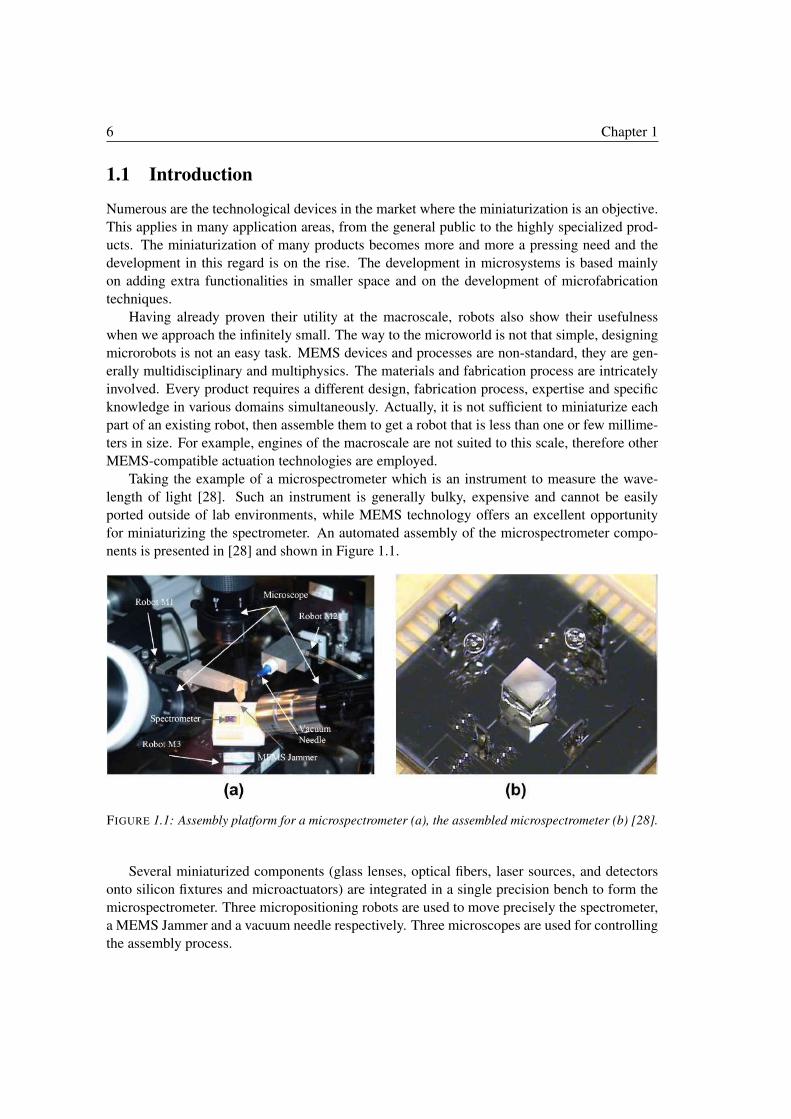
Taking the example of a microspectrometer which is an instrument to measure the wave-
length of light [28]. Such an instrument is generally bulky, expensive and cannot be easily
ported outside of lab environments, while MEMS technology offers an excellent opportunity
for miniaturizing the spectrometer. An automated assembly of the microspectrometer compo-
nents is presented in [28] and shown in Figure 1.1.
FIGURE 1.1: Assembly platform for a microspectrometer (a), the assembled microspectrometer (b) [28].
Several miniaturized components (glass lenses, optical fibers, laser sources, and detectors
onto silicon fixtures and microactuators) are integrated in a single precision bench to form the
microspectrometer. Three micropositioning robots are used to move precisely the spectrometer,
a MEMS Jammer and a vacuum needle respectively. Three microscopes are used for controlling
the assembly process.
1.1 Introduction 7
The race for miniaturization has revealed the need to handle precisely some micrometer-
sized objects. To address this need, considerable advances in the microrobotic field are made
for generating displacement and manipulating objects at the microscale. Micromanipulators
were developed and used in many fields of microrobotics in order to handle an object, fabricate
a structure, assemble a product, operate with a patient, etc.. However the necessity of vision
and measurement systems to manipulate or assemble micro components remains a challenge to
overcome.
Mechanical positioning systems are back-bone systems behind every object manipulation
task. Numerous systems for the positioning with high precision at micrometric scale have been
developed and are available in the market.
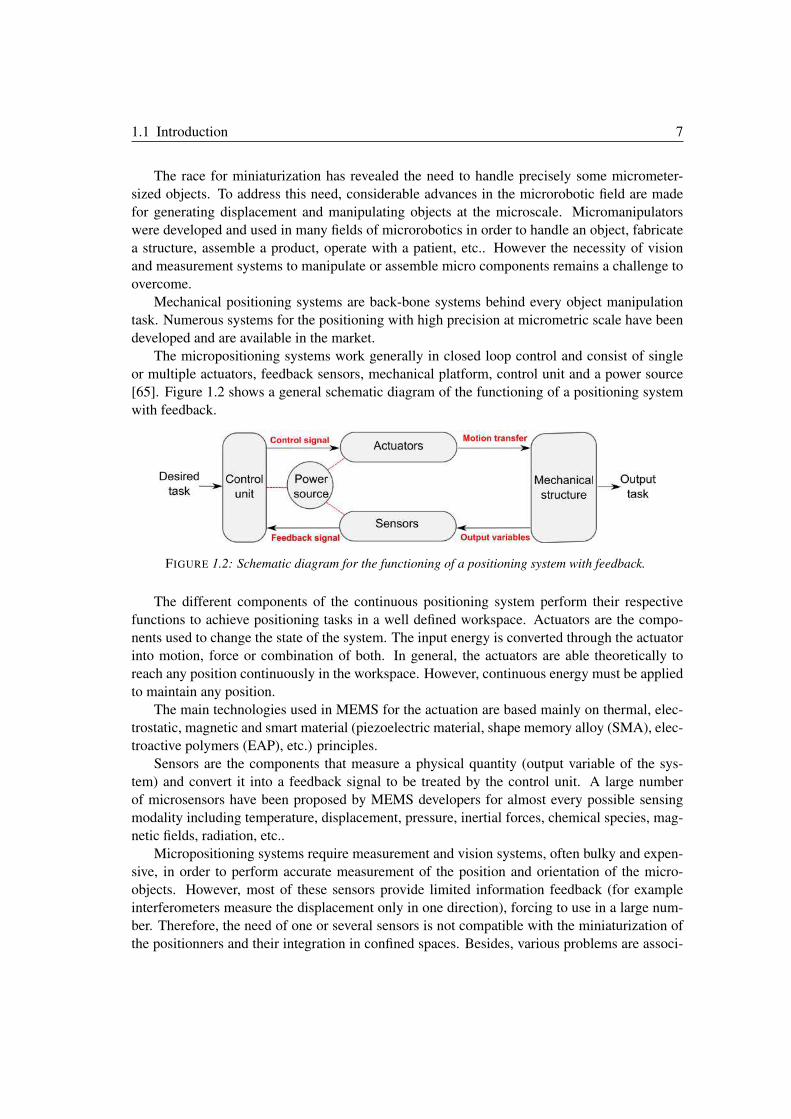
The micropositioning systems work generally in closed loop control and consist of single
or multiple actuators, feedback sensors, mechanical platform, control unit and a power source
[65]. Figure 1.2 shows a general schematic diagram of the functioning of a positioning system
with feedback.
FIGURE 1.2: Schematic diagram for the functioning of a positioning system with feedback.
The different components of the continuous positioning system perform their respective
functions to achieve positioning tasks in a well defined workspace. Actuators are the compo-
nents used to change the state of the system. The input energy is converted through the actuator
into motion, force or combination of both. In general, the actuators are able theoretically to
reach any position continuously in the workspace. However, continuous energy must be applied
to maintain any position.
The main technologies used in MEMS for the actuation are based mainly on thermal, elec-
trostatic, magnetic and smart material (piezoelectric material, shape memory alloy (SMA), elec-
troactive polymers (EAP), etc.) principles.
Sensors are the components that measure a physical quantity (output variable of the sys-
tem) and convert it into a feedback signal to be treated by the control unit. A large number
of microsensors have been proposed by MEMS developers for almost every possible sensing
modality including temperature, displacement, pressure, inertial forces, chemical species, mag-
netic fields, radiation, etc..
Micropositioning systems require measurement and vision systems, often bulky and expen-
sive, in order to perform accurate measurement of the position and orientation of the micro-
objects. However, most of these sensors provide limited information feedback (for example
interferometers measure the displacement only in one direction), forcing to use in a large num-
ber. Therefore, the need of one or several sensors is not compatible with the miniaturization of
the positionners and their integration in confined spaces. Besides, various problems are associ-
8 Chapter 1
ated with the use of sensors, such as nonlinearity, complex control law, continuous feeding and
servoing, complex connectivity, low signal to noise ratio, etc.. These problems vary with respect
to the type, technology, material and other properties of the sensor.
In addition to the high precision requirement, the integration of micromanipulation plat-
forms in reduced environments (such as scanning and transmission electron microscope) is a
recurring problem due to the complexity of the micropositioning systems.
It is often difficult to integrate the various components (sensors, power source, actuators,
etc.) into the micromanipulation platform, especially in confined spaces where the integration
of these components can be quite challenging. In the efforts to address this challenge, digital
concept in micropositioning is introduced couple of years ago [13, 21, 103, 104, 136].
1.2 Digital microrobot
In the previous theses of Vincent Chalvet [12] and Qiao Chen [20], the works have led to the
development of a digital microrobot called ”DiMiBot”. Prototypes of the DiMiBot were fab-
ricated, characterized and showed a good functioning in the experiments. However, this thesis
deals with and provides solutions for some challenging issues of concern for the DiMiBot. The
principle of digital microbotics and the DiMiBot are presented in this section. The challenges
and requirements for a new generation of the DiMiBot are then presented.
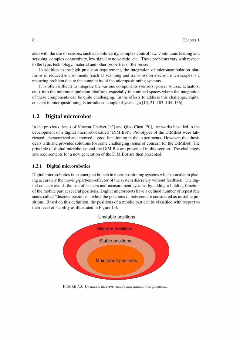
1.2.1 Digital microrobotics
Digital microrobotics is an emergent branch in micropositioning systems which consists in plac-
ing accurately the moving-part/end-effector of the system discretely without feedback. The dig-
ital concept avoids the use of sensors and measurement systems by adding a holding function
of the mobile part at several positions. Digital microrobots have a defined number of repeatable
states called ”discrete positions”, while the positions in between are considered as unstable po-
sitions. Based on this definition, the positions of a mobile part can be classified with respect to
their level of stability as illustrated in Figure 1.3.
FIGURE 1.3: Unstable, discrete, stable and maintained positions.
1.2 Digital microrobot 9
The discrete position is a position in a state of equilibrium that does not change with time.
The stable position is a discrete position which tends to return to its initial state after a small
variation. These positions have a local minimum energy. The maintained position is a stable
position that retains its state in front of external disturbance, a force barrier (holding force) must
be exceeded before changing the state of the system. In contrast, the unstable position is a
position out of static equilibrium or tends to change its state after a very small variation (local
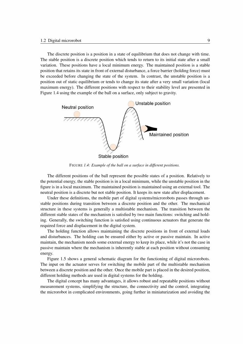
maximum energy). The different positions with respect to their stability level are presented in
Figure 1.4 using the example of the ball on a surface, only subject to gravity.
FIGURE 1.4: Example of the ball on a surface in different positions.
The different positions of the ball represent the possible states of a position. Relatively to
the potential energy, the stable position is in a local minimum, while the unstable position in the
figure is in a local maximum. The maintained position is maintained using an external tool. The
neutral position is a discrete but not stable position. It keeps its new state after displacement.
Under these definitions, the mobile part of digital systems/microrobots passes through un-
stable positions during transition between a discrete position and the other. The mechanical
structure in these systems is generally a multistable mechanism. The transition between the
different stable states of the mechanism is satisfied by two main functions: switching and hold-
ing. Generally, the switching function is satisfied using continuous actuators that generate the
required force and displacement in the digital system.
The holding function allows maintaining the discrete positions in front of external loads
and disturbances. The holding can be ensured either by active or passive maintain. In active
maintain, the mechanism needs some external energy to keep its place, while it’s not the case in
passive maintain where the mechanism is inherently stable at each position without consuming
energy.
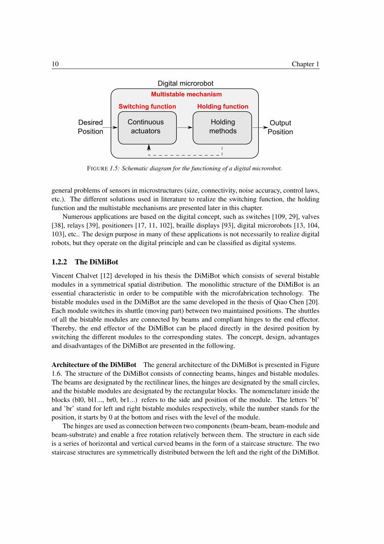
Figure 1.5 shows a general schematic diagram for the functioning of digital microrobots.
The input on the actuator serves for switching the mobile part of the multistable mechanism
between a discrete position and the other. Once the mobile part is placed in the desired position,
different holding methods are used in digital systems for the holding.
The digital concept has many advantages, it allows robust and repeatable positions without
measurement systems, simplifying the structure, the connectivity and the control, integrating
the microrobot in complicated environments, going further in miniaturization and avoiding the
10 Chapter 1
FIGURE 1.5: Schematic diagram for the functioning of a digital microrobot.
general problems of sensors in microstructures (size, connectivity, noise accuracy, control laws,
etc.). The different solutions used in literature to realize the switching function, the holding
function and the multistable mechanisms are presented later in this chapter.
Numerous applications are based on the digital concept, such as switches [109, 29], valves
[38], relays [39], positioners [17, 11, 102], braille displays [93], digital microrobots [13, 104,
103], etc.. The design purpose in many of these applications is not necessarily to realize digital
robots, but they operate on the digital principle and can be classified as digital systems.
1.2.2 The DiMiBot
Vincent Chalvet [12] developed in his thesis the DiMiBot which consists of several bistable
modules in a symmetrical spatial distribution. The monolithic structure of the DiMiBot is an
essential characteristic in order to be compatible with the microfabrication technology. The
bistable modules used in the DiMiBot are the same developed in the thesis of Qiao Chen [20].
Each module switches its shuttle (moving part) between two maintained positions. The shuttles
of all the bistable modules are connected by beams and compliant hinges to the end effector.
Thereby, the end effector of the DiMiBot can be placed directly in the desired position by
switching the different modules to the corresponding states. The concept, design, advantages
and disadvantages of the DiMiBot are presented in the following.
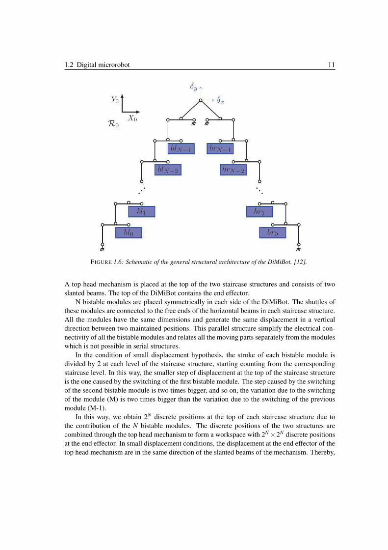
Architecture of the DiMiBot The general architecture of the DiMiBot is presented in Figure
1.6. The structure of the DiMiBot consists of connecting beams, hinges and bistable modules.
The beams are designated by the rectilinear lines, the hinges are designated by the small circles,
and the bistable modules are designated by the rectangular blocks. The nomenclature inside the
blocks (bl0, bl1..., br0, br1...) refers to the side and position of the module. The letters ’bl’
and ’br’ stand for left and right bistable modules respectively, while the number stands for the
position, it starts by 0 at the bottom and rises with the level of the module.
The hinges are used as connection between two components (beam-beam, beam-module and
beam-substrate) and enable a free rotation relatively between them. The structure in each side
is a series of horizontal and vertical curved beams in the form of a staircase structure. The two
staircase structures are symmetrically distributed between the left and the right of the DiMiBot.
1.2 Digital microrobot 11
FIGURE 1.6: Schematic of the general structural architecture of the DiMiBot. [12].
A top head mechanism is placed at the top of the two staircase structures and consists of two
slanted beams. The top of the DiMiBot contains the end effector.
N bistable modules are placed symmetrically in each side of the DiMiBot. The shuttles of
these modules are connected to the free ends of the horizontal beams in each staircase structure.
All the modules have the same dimensions and generate the same displacement in a vertical
direction between two maintained positions. This parallel structure simplify the electrical con-
nectivity of all the bistable modules and relates all the moving parts separately from the modules
which is not possible in serial structures.
In the condition of small displacement hypothesis, the stroke of each bistable module is
divided by 2 at each level of the staircase structure, starting counting from the corresponding
staircase level. In this way, the smaller step of displacement at the top of the staircase structure
is the one caused by the switching of the first bistable module. The step caused by the switching
of the second bistable module is two times bigger, and so on, the variation due to the switching
of the module (M) is two times bigger than the variation due to the switching of the previous
module (M-1).
In this way, we obtain 2N discrete positions at the top of each staircase structure due to
the contribution of the N bistable modules. The discrete positions of the two structures are
combined through the top head mechanism to form a workspace with 2N ×2N discrete positions
at the end effector. In small displacement conditions, the displacement at the end effector of the
top head mechanism are in the same direction of the slanted beams of the mechanism. Thereby,
12 Chapter 1
if the two angles of the slanted beams are equivalent to 45°, the discrete positions form a square
workspace which is rotated 45°with respect to X0 Y0 axes.
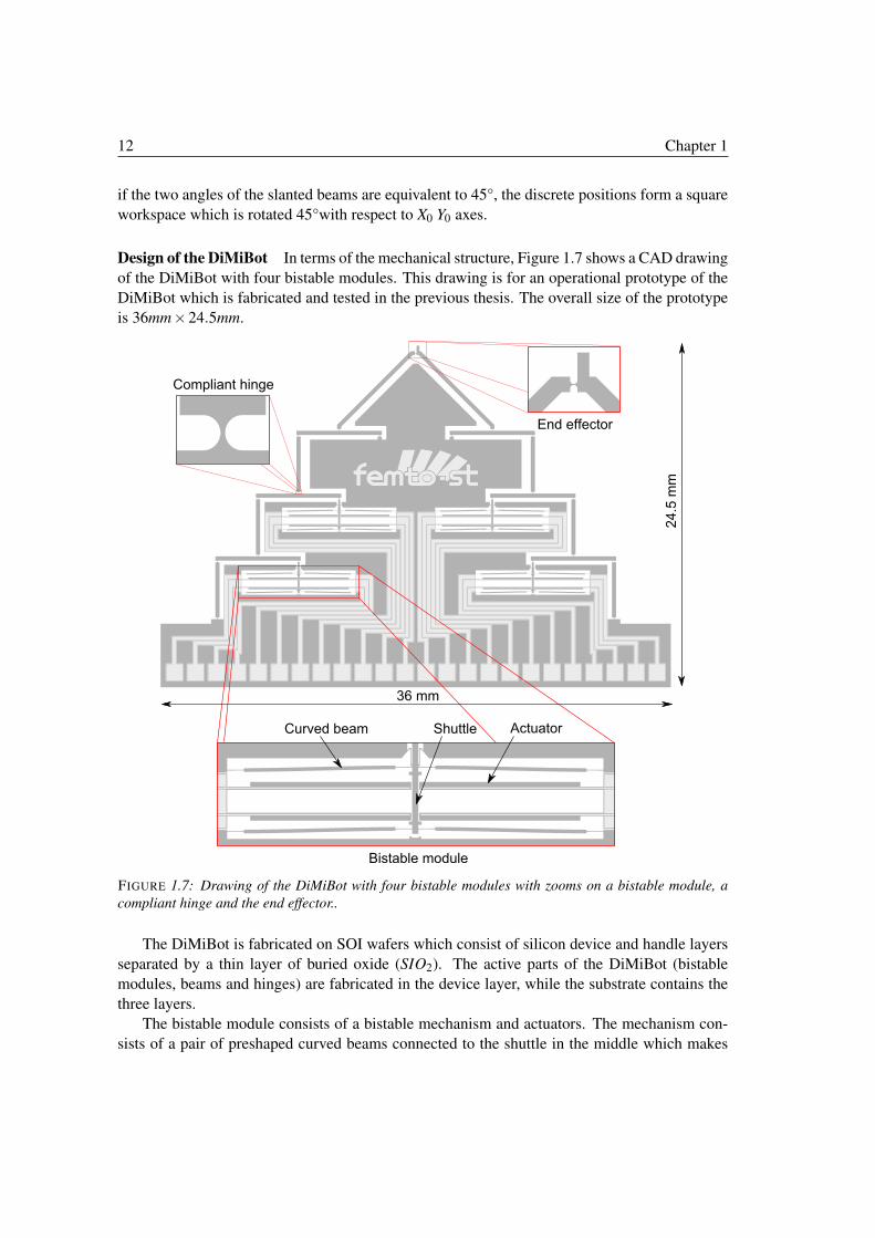
Design of the DiMiBot In terms of the mechanical structure, Figure 1.7 shows a CAD drawing
of the DiMiBot with four bistable modules. This drawing is for an operational prototype of the
DiMiBot which is fabricated and tested in the previous thesis. The overall size of the prototype
is 36mm×24.5mm.
FIGURE 1.7: Drawing of the DiMiBot with four bistable modules with zooms on a bistable module, a
compliant hinge and the end effector..
The DiMiBot is fabricated on SOI wafers which consist of silicon device and handle layers
separated by a thin layer of buried oxide (SIO2). The active parts of the DiMiBot (bistable
modules, beams and hinges) are fabricated in the device layer, while the substrate contains the
three layers.
The bistable module consists of a bistable mechanism and actuators. The mechanism con-
sists of a pair of preshaped curved beams connected to the shuttle in the middle which makes
1.2 Digital microrobot 13
a structural guidance of motion. The switching is made using four U-shaped electrothermal
actuators. Each pair of actuators is used to switch the bistable mechanism in a direction. The
shuttle can move between two stop blocks which are used to define the stroke and add holding
forces on the positions. The principle of the stop block is clarified later in the holding methods
section.
The hinge used in the structure is a compliant flexible hinge with a circular shape. In contrast
to other shapes of compliant hinges (rectangular, oval), in this shape, the rotation occurs around
a reduced area which is the closest solution which ensures similar behavior of an ideal hinge.
However, the stress is concentrated and more important in the reduced area compared to other
solutions where the stress is not concentrated and less important.
The connecting beams have a rectangular shape. The length of these beams is chosen to be
long enough to be able to consider a small displacement at the borders with respect to the length.
The width is wide enough, so that the beam is rigid and does not suffer from elastic deformation
during functioning.
A metal layer (aluminum) is deposited on the top of the device layer to supply the actuators
in the bistable modules. 24 metal lines are used to supply the bistable modules, 6 for each one.
Each actuator need to be supplied from two lines. In order to reduce the total number of metal
lines, one line is used in common between two nearby actuators in the two sides of the bistable
module. The metal lines are separated electrically from each other by etching the silicon layer
around until the buried oxide which is an electrical insulator. All the metal lines are related to
square pads at the bottom of the DiMiBot, which in turn, are connected to an external circuit
using wire bonding.
At the end effector, a rectangular shape is extruded as a probe to handle with micro-objects.
It is worth noting here that, in the previous and the actual theses on digital microrobotics, the
focus is on the realization of a digital micropositioning system, the final function of the end
effector is outside of the objectives. However, in future prospects, a specific design can be
developed for specific applications that require a digital positioning and a defined final function.
1.2.3 Advantages and challenges
1.2.3.1 Advantages
The DiMiBot has obvious and numerous advantages either in the concept or in the design. It
combines the advantages of the digital concept, passive maintain, compliant mechanism, mono-
lithic structure, and unlimited multistable mechanisms with elementary modules.
Each one of these features has its own advantages. The digital concept allows positioning in
robust and repeatable stable positions without need of measurement systems. This simplify the
structure, the connectivity and the control, avoids the general problems of sensors in microstruc-
tures (bulky size, accuracy, complicated control laws, etc.), makes the system insensitive to noise
and disturbances, and enables going further in miniaturization.
The stability of the discrete positions in the workspace of the DiMiBot returns to the stability
of the positions in each bistable module. These positions are passively maintained at rest with
the buckled beam structure of the bistable mechanism. This is an important feature since no
external energy is needed to keep the state of the system.
14 Chapter 1
The compliant structure of the DiMiBot exhibits many advantages such as increased preci-
sion and reliability, no friction, no backlash, reduced wear, and low manufacturing costs. The
use of silicon in the device layer exhibits also many advantages. The silicon has an almost
perfect elastic behavior with highly repeatable motion and without hysteresis and energy dissi-
pation, it has also a long lifetime with little fatigue. This material is widely exploited in MEMS
applications, its physical properties are well defined and the fabrication processes with silicon
are well developed.
In addition, The DiMiBot is a monolithic structure. On one hand, this feature simplify the
fabrication process and allows the fabrication in a large scale, on the other hand, it allows the
integration in complicated and compact environments.
The last feature is the unlimited principle of the used mechanism. The principle itself is an
advantage where additional positions can be added as required by simply adding more elemen-
tary modules. However, the obtained positions in the workspace are non redundant positions
where each position is equivalent to one set of states of the bistable modules. In this way, one
can switch to a desired position directly by switching the bistable modules to the corresponding
states.
1.2.3.2 Challenges for a new generation of the DiMiBot
In the other side, several limitations can be cited for the DiMiBot in the concept, design, fabri-
cation and functioning. Limitations of the DiMiBot are presented hereinafter, followed by the
challenges for a new generation.
The first limitation is that the DiMiBot is not able to reach all the positions in between in
the workspace. This is the feature that we lose when we turn to digital systems. The distance
between two adjacent positions is the resolution of the system. The resolution can be adjusted
with respect to the application.
Secondly, the transition between the discrete positions in the workspace is not always pos-
sible between the neighbor positions. This is due to the non redundant architecture of the DiMi-
Bot, where the switching of a bistable module produces 2i steps (binary jump) in the workspace
in a direction, no other module is able to produce 2i steps in the same direction (i is a positive
integer). Thereby, the transition to the adjacent positions is not possible in all the cases in one
step, and long trajectories are mandatory sometimes to reach a near position, the realization of
specific trajectories becomes also complicated.
Another limitation is that the number of stable positions in the workspace is related to the
number of bistable modules. For higher number of stable positions, higher number of bistable
modules are needed. The use of more bistable modules increases the size of the DiMiBot,
increases the failure possibilities in the fabrication, adds 6 electrical input for each module, and
the structure of the DiMiBot becomes weaker.
Further, another limitation is that the realization of the digital systems and the DiMiBot
requires a high fabrication quality in order to ensure the accuracy. This is required to avoid the
important fabrication tolerances and step/stroke differences. Several runs of microfabrication in
the previous thesis were necessary to get functional robots. One prototype with four bistable
modules was fabricated successfully and showed a proper functioning during characterization.
The measured workspace of the fabricated prototype is shown in Figure 1.8.
1.2 Digital microrobot 15
FIGURE 1.8: Workspace of the fabricated prototype of the DiMiBot.
However, the fabrication tolerances were important in the prototype. The bistable mod-
ules were designed to have a bistable distance of 25µm between the two stop blocks, while the
measured displacement variates between 33.6 and 36.5µm in the different modules. This indi-
cates a large excess of etching at the sidewalls of the device layer and a variation in the etching
conditions on the large surface of the DiMiBot.
At the workspace, there was also some differences in the displacement induced by each
module between the theoretical calculation and the measurements. These differences may return
to the simplifications taken in the calculation (small displacement hypothesis, rigid connecting
beams) and the fabrication tolerances.
The non holding of the end effector in front of external loads is another limitation of the
DiMiBot. In contrast to the positions of the bistable modules, the discrete positions in the
workspace are stable but not maintained. This is due to the elastic structure of the external
mechanisms formed by the connecting beams and the hinges.
The last limitation to be cited is in the design of the DiMiBot, where at the beginning of the
thesis, we were not able to define the miniaturization limits of the DiMiBot. The miniaturization
of the total structure is related to the minimal size of components that ensure the switching and
holding in each module. The main components are the curved beams and the actuators. It
lacks models, analytical or numerical, that describe the behavior of each component and shows
the influence of each dimension on their behaviors, which allows choosing the dimensions that
ensure the required performance and defining their limits of miniaturization.
In result, four main challenges can be cited for a new generation of the DiMiBot:
• Proposing new structures/mechanisms that allows generating complicated trajectories and
reducing the size of the DiMiBot.
• Proposing some structural solutions to reduce or compensate the fabrication tolerances
which influence the accuracy of the positions and steps.
16 Chapter 1
• Improving the fabrication process in order to avoid the difficulties encountered in the
previous thesis.
• Developing models for the curved beam and U-shaped actuator which are then used for
the dimensioning and defining miniaturization limits.
The works in the thesis have risen to and overcome these challenges and important results
were reached with respect to each challenge.
1.3 Solutions for digital systems
After presenting the digital microrobot, the purpose of this section is to present the solutions
found in literature to realize digital systems. Several classifications for the digital systems were
presented previously in [13, 21, 103, 104, 136] based on the number of discrete or stable posi-
tions, technology of the actuators, holding principles and applications.
However, a digital system is simply a multistable mechanism with switching and holding
functions. The main element in the switching is the actuator, different actuating technologies
which are compatible with MEMS and were used in digital systems are presented in the fol-
lowing. The different holding methods are presented afterwards. Finally, different approaches
to realize multistable mechanisms are introduced. Examples of digital systems which use the
different solutions for the switching, holding and mechanisms are cited in each paragraph.
1.3.1 Switching function
The first elementary function in digital systems is the switching of the mobile part between
discrete positions. To realize the switching function, a driving force is generated and exerted
on the mobile part using continuous actuators. In digital MEMS, electromagnetic, electrostatic,
electrothermal and smart materials principles are the most common physical principles used to
generate the switching. The different actuating technologies were extensively addressed in lit-
erature, a brief presentation of those used in digital systems is given hereinafter, while examples
of digital systems are only cited for each principle.
1.3.1.1 Electromagnetic principle
The electromagnetic actuation principle is characterized by the interaction between the magnetic
and the electrical phenomena, where the Lorentz force appears after charging electrically a
particle in the presence of a magnetic flux. The actuators realized with electromagnetic principle
generate the electromagnetic forces via three forms:
• Reluctance force [6, 66, 82, 83, 112, 138]: where the mobile part tend to align with the
fixed part in order to minimize the magnetic circuit reluctance.
• Laplace force [31, 102, 104, 129, 133]: which is a manifestation of the Lorentz force
acting on a current-carrying wire in a magnetic field.
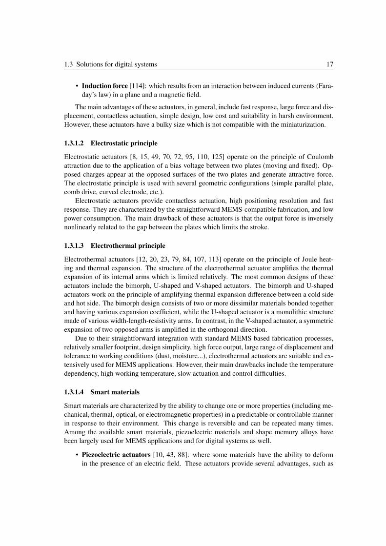
1.3 Solutions for digital systems 17
• Induction force [114]: which results from an interaction between induced currents (Fara-
day’s law) in a plane and a magnetic field.
The main advantages of these actuators, in general, include fast response, large force and dis-
placement, contactless actuation, simple design, low cost and suitability in harsh environment.
However, these actuators have a bulky size which is not compatible with the miniaturization.
1.3.1.2 Electrostatic principle
Electrostatic actuators [8, 15, 49, 70, 72, 95, 110, 125] operate on the principle of Coulomb
attraction due to the application of a bias voltage between two plates (moving and fixed). Op-
posed charges appear at the opposed surfaces of the two plates and generate attractive force.
The electrostatic principle is used with several geometric configurations (simple parallel plate,
comb drive, curved electrode, etc.).
Electrostatic actuators provide contactless actuation, high positioning resolution and fast
response. They are characterized by the straightforward MEMS-compatible fabrication, and low
power consumption. The main drawback of these actuators is that the output force is inversely
nonlinearly related to the gap between the plates which limits the stroke.
1.3.1.3 Electrothermal principle
Electrothermal actuators [12, 20, 23, 79, 84, 107, 113] operate on the principle of Joule heat-
ing and thermal expansion. The structure of the electrothermal actuator amplifies the thermal
expansion of its internal arms which is limited relatively. The most common designs of these
actuators include the bimorph, U-shaped and V-shaped actuators. The bimorph and U-shaped
actuators work on the principle of amplifying thermal expansion difference between a cold side
and hot side. The bimorph design consists of two or more dissimilar materials bonded together
and having various expansion coefficient, while the U-shaped actuator is a monolithic structure
made of various width-length-resistivity arms. In contrast, in the V-shaped actuator, a symmetric
expansion of two opposed arms is amplified in the orthogonal direction.
Due to their straightforward integration with standard MEMS based fabrication processes,
relatively smaller footprint, design simplicity, high force output, large range of displacement and
tolerance to working conditions (dust, moisture...), electrothermal actuators are suitable and ex-
tensively used for MEMS applications. However, their main drawbacks include the temperature
dependency, high working temperature, slow actuation and control difficulties.
1.3.1.4 Smart materials
Smart materials are characterized by the ability to change one or more properties (including me-
chanical, thermal, optical, or electromagnetic properties) in a predictable or controllable manner
in response to their environment. This change is reversible and can be repeated many times.
Among the available smart materials, piezoelectric materials and shape memory alloys have
been largely used for MEMS applications and for digital systems as well.
• Piezoelectric actuators [10, 43, 88]: where some materials have the ability to deform
in the presence of an electric field. These actuators provide several advantages, such as
18 Chapter 1
instant response, important output force, high energy conversion efficiency, while they
suffer from a nonlinear behavior (hysteresis, creep) and low displacement range.
• Shape Memory Alloy (SMA) [1, 5, 48, 67, 74, 81, 127, 136]:which is an alloy that
remembers its original shape due to an internal phase transformation and returns to its ini-
tial state when heated after deformation. SMA actuators have many remarkable features,
such as high power to weight ratio, sensing ability, low driving voltage, silent actuation,
lightweight, large force and displacement. In contrast, these actuators suffer from some
weak points, such as low energy efficiency, low response time, and non-linear behavior.
1.3.1.5 Synthesis
Common physical principles in literature used for the switching function including electromag-
netic, electrostatic, electrothermal, piezoelectric and SMA have been presented. For the electro-
magnetic principle, the main advantages include high speed, simple design and low cost. The
piezoelectric switching principle provides the advantages of instant response and high energy
conversion, while their main drawback is the small displacement capacity. The SMA actuators
are lightweight and provide large force and displacement. These technologies have been ignored
for the DiMiBot due to the complexity of their integration in a monolithic structure.
In the other side, the main advantage of electrostatic and electrothermal principles relatively
is their straightforward integration and compatibility with the standard MEMS based fabrica-
tion processes. The electrostatic switching principle provides contactless actuation but its main
drawbacks is the limited stroke and the need of a large footprint relatively to produce the de-
sired force. The electrothermal switching principle has the advantage to exhibit strong forces
and large displacement simultaneously with smaller footprint. Therefore, electrothermal actua-
tors were chosen in the old and the new DiMiBot. Otherwise, if faster microrobots are concerned
in the future, other technologies can be selected.
1.3.2 Holding function
The holding function is the second important function that characterizes digital systems. Thanks
to the holding method, the digital system holds the mobile part in discrete or stable positions.
Different holding principles can be found in literature, these principles are either active or pas-
sive. A classification for the most common principles, used in literature to realize the holding
function, is presented in Table 1.1.
TABLE 1.1: Classification of holding principles.
Holding principles
Active holding Passive holding
• Continuous switching function • Passive locking actuator
• Active locking actuator • Permanent magnet
• Buckled beam structure
(constrained or uncontrained)
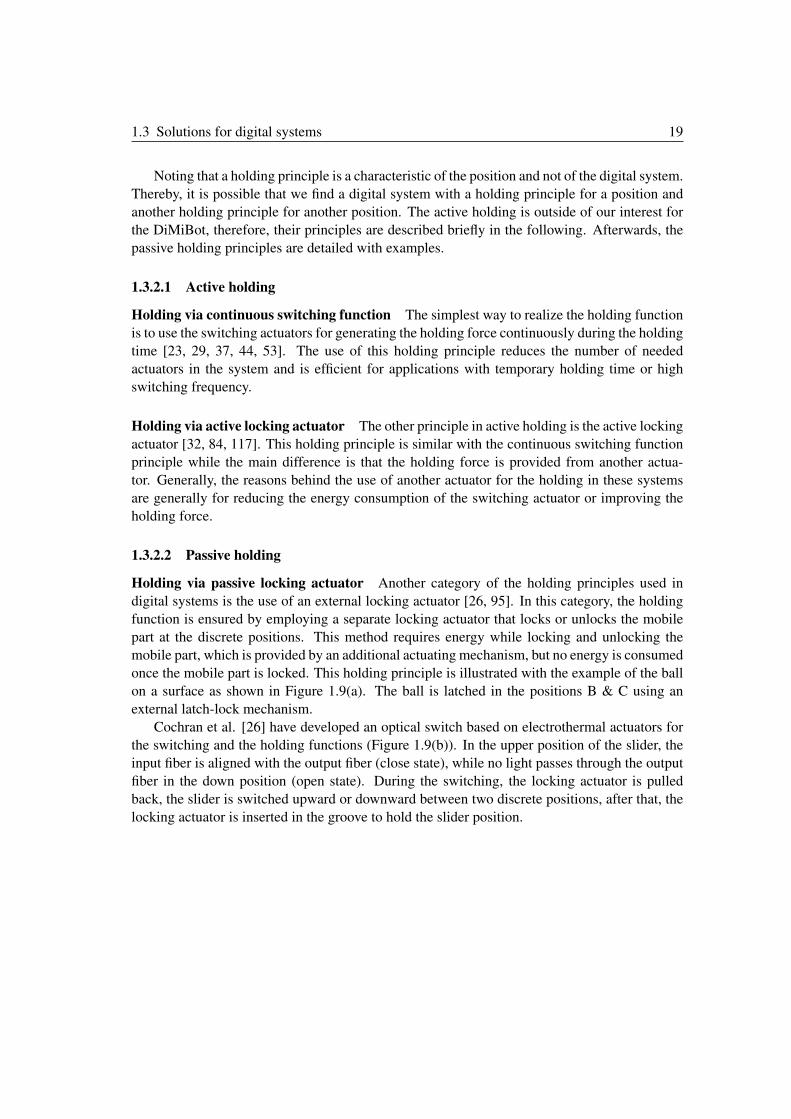
1.3 Solutions for digital systems 19
Noting that a holding principle is a characteristic of the position and not of the digital system.
Thereby, it is possible that we find a digital system with a holding principle for a position and
another holding principle for another position. The active holding is outside of our interest for
the DiMiBot, therefore, their principles are described briefly in the following. Afterwards, the
passive holding principles are detailed with examples.
1.3.2.1 Active holding
Holding via continuous switching function The simplest way to realize the holding function
is to use the switching actuators for generating the holding force continuously during the holding
time [23, 29, 37, 44, 53]. The use of this holding principle reduces the number of needed
actuators in the system and is efficient for applications with temporary holding time or high
switching frequency.
Holding via active locking actuator The other principle in active holding is the active locking
actuator [32, 84, 117]. This holding principle is similar with the continuous switching function
principle while the main difference is that the holding force is provided from another actua-
tor. Generally, the reasons behind the use of another actuator for the holding in these systems
are generally for reducing the energy consumption of the switching actuator or improving the
holding force.
1.3.2.2 Passive holding
Holding via passive locking actuator Another category of the holding principles used in
digital systems is the use of an external locking actuator [26, 95]. In this category, the holding
function is ensured by employing a separate locking actuator that locks or unlocks the mobile
part at the discrete positions. This method requires energy while locking and unlocking the
mobile part, which is provided by an additional actuating mechanism, but no energy is consumed
once the mobile part is locked. This holding principle is illustrated with the example of the ball
on a surface as shown in Figure 1.9(a). The ball is latched in the positions B & C using an
external latch-lock mechanism.
Cochran et al. [26] have developed an optical switch based on electrothermal actuators for
the switching and the holding functions (Figure 1.9(b)). In the upper position of the slider, the
input fiber is aligned with the output fiber (close state), while no light passes through the output
fiber in the down position (open state). During the switching, the locking actuator is pulled
back, the slider is switched upward or downward between two discrete positions, after that, the
locking actuator is inserted in the groove to hold the slider position.
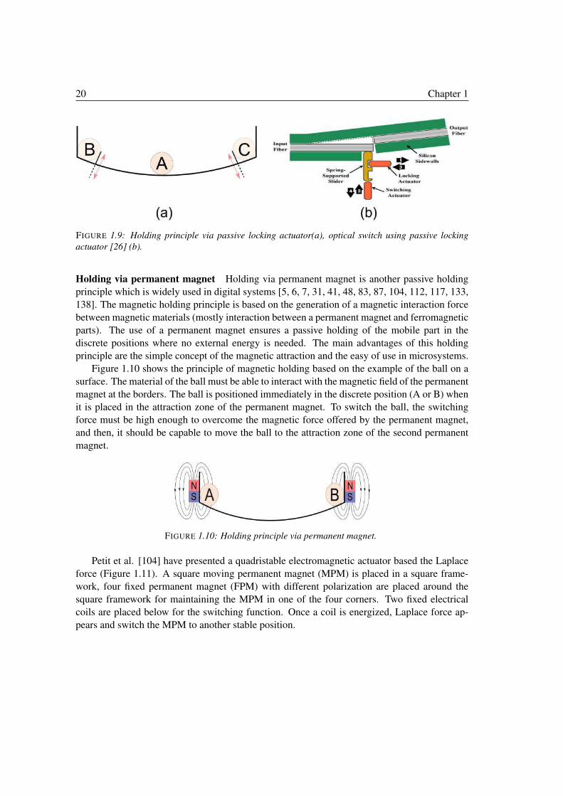
20 Chapter 1
FIGURE 1.9: Holding principle via passive locking actuator(a), optical switch using passive locking
actuator [26] (b).
Holding via permanent magnet Holding via permanent magnet is another passive holding
principle which is widely used in digital systems [5, 6, 7, 31, 41, 48, 83, 87, 104, 112, 117, 133,
138]. The magnetic holding principle is based on the generation of a magnetic interaction force
between magnetic materials (mostly interaction between a permanent magnet and ferromagnetic
parts). The use of a permanent magnet ensures a passive holding of the mobile part in the
discrete positions where no external energy is needed. The main advantages of this holding
principle are the simple concept of the magnetic attraction and the easy of use in microsystems.
Figure 1.10 shows the principle of magnetic holding based on the example of the ball on a
surface. The material of the ball must be able to interact with the magnetic field of the permanent
magnet at the borders. The ball is positioned immediately in the discrete position (A or B) when
it is placed in the attraction zone of the permanent magnet. To switch the ball, the switching
force must be high enough to overcome the magnetic force offered by the permanent magnet,
and then, it should be capable to move the ball to the attraction zone of the second permanent
magnet.
FIGURE 1.10: Holding principle via permanent magnet.
Petit et al. [104] have presented a quadristable electromagnetic actuator based the Laplace
force (Figure 1.11). A square moving permanent magnet (MPM) is placed in a square frame-
work, four fixed permanent magnet (FPM) with different polarization are placed around the
square framework for maintaining the MPM in one of the four corners. Two fixed electrical
coils are placed below for the switching function. Once a coil is energized, Laplace force ap-
pears and switch the MPM to another stable position.
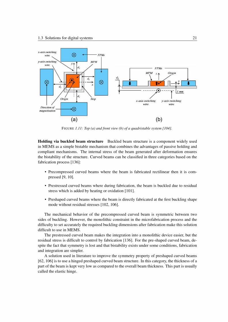
1.3 Solutions for digital systems 21
FIGURE 1.11: Top (a) and front view (b) of a quadristable system [104].
Holding via buckled beam structure Buckled beam structure is a component widely used
in MEMS as a simple bistable mechanism that combines the advantages of passive holding and
compliant mechanisms. The internal stress of the beam generated after deformation ensures
the bistability of the structure. Curved beams can be classified in three categories based on the
fabrication process [136]:
• Precompressed curved beams where the beam is fabricated rectilinear then it is com-
pressed [9, 10].
• Prestressed curved beams where during fabrication, the beam is buckled due to residual
stress which is added by heating or oxidation [101].
• Preshaped curved beams where the beam is directly fabricated at the first buckling shape
mode without residual stresses [102, 106].
The mechanical behavior of the precompressed curved beam is symmetric between two
sides of buckling. However, the monolithic constraint in the microfabrication process and the
difficulty to set accurately the required buckling dimensions after fabrication make this solution
difficult to use in MEMS.
The prestressed curved beam makes the integration into a monolithic device easier, but the
residual stress is difficult to control by fabrication [136]. For the pre-shaped curved beam, de-
spite the fact that symmetry is lost and that bistability exists under some conditions, fabrication
and integration are simpler.
A solution used in literature to improve the symmetry property of preshaped curved beams
[62, 106] is to use a hinged preshaped curved beam structure. In this category, the thickness of a
part of the beam is kept very low as compared to the overall beam thickness. This part is usually
called the elastic hinge.
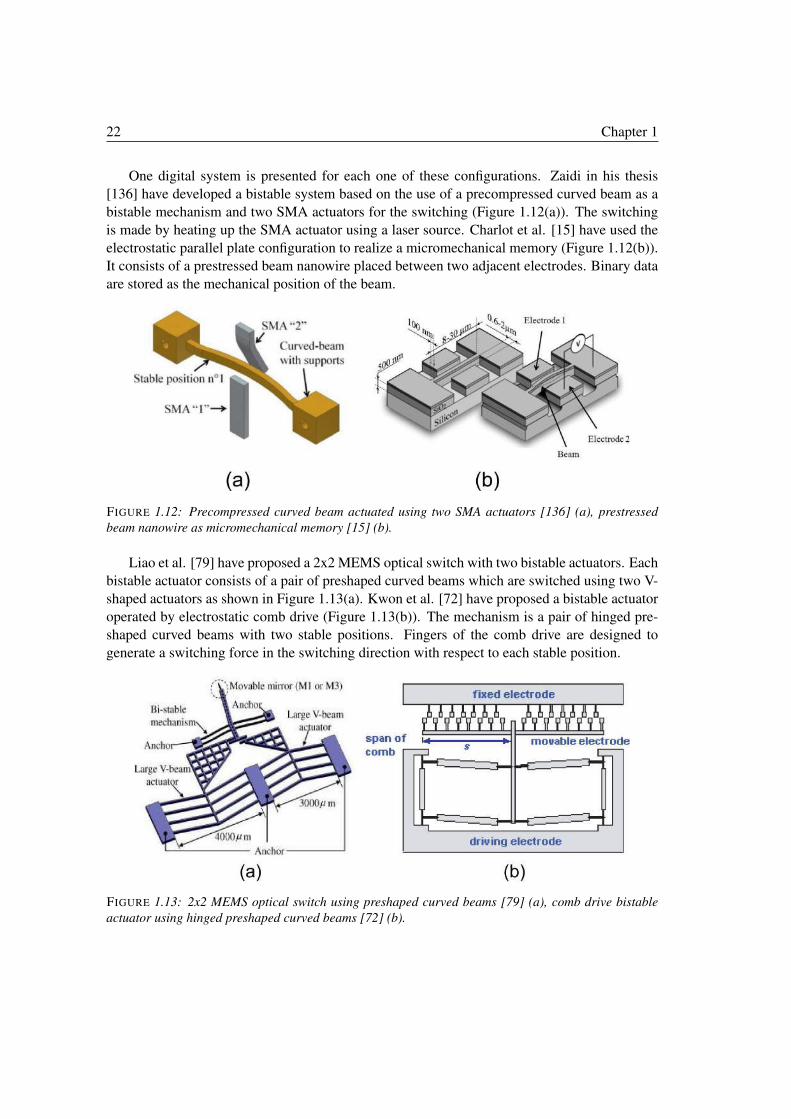
22 Chapter 1
One digital system is presented for each one of these configurations. Zaidi in his thesis
[136] have developed a bistable system based on the use of a precompressed curved beam as a
bistable mechanism and two SMA actuators for the switching (Figure 1.12(a)). The switching
is made by heating up the SMA actuator using a laser source. Charlot et al. [15] have used the
electrostatic parallel plate configuration to realize a micromechanical memory (Figure 1.12(b)).
It consists of a prestressed beam nanowire placed between two adjacent electrodes. Binary data
are stored as the mechanical position of the beam.
FIGURE 1.12: Precompressed curved beam actuated using two SMA actuators [136] (a), prestressed
beam nanowire as micromechanical memory [15] (b).
Liao et al. [79] have proposed a 2x2 MEMS optical switch with two bistable actuators. Each
bistable actuator consists of a pair of preshaped curved beams which are switched using two V-
shaped actuators as shown in Figure 1.13(a). Kwon et al. [72] have proposed a bistable actuator
operated by electrostatic comb drive (Figure 1.13(b)). The mechanism is a pair of hinged pre-
shaped curved beams with two stable positions. Fingers of the comb drive are designed to
generate a switching force in the switching direction with respect to each stable position.
FIGURE 1.13: 2x2 MEMS optical switch using preshaped curved beams [79] (a), comb drive bistable
actuator using hinged preshaped curved beams [72] (b).
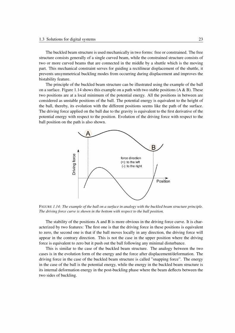
1.3 Solutions for digital systems 23
The buckled beam structure is used mechanically in two forms: free or constrained. The free
structure consists generally of a single curved beam, while the constrained structure consists of
two or more curved beams that are connected in the middle by a shuttle which is the moving
part. This mechanical constraint serves for guiding a rectilinear displacement of the shuttle, it
prevents unsymmetrical buckling modes from occurring during displacement and improves the
bistability feature.
The principle of the buckled beam structure can be illustrated using the example of the ball
on a surface. Figure 1.14 shows this example on a path with two stable positions (A & B). These
two positions are at a local minimum of the potential energy. All the positions in between are
considered as unstable positions of the ball. The potential energy is equivalent to the height of
the ball, thereby, its evolution with the different positions seems like the path of the surface.
The driving force applied on the ball due to the gravity is equivalent to the first derivative of the
potential energy with respect to the position. Evolution of the driving force with respect to the
ball position on the path is also shown.
FIGURE 1.14: The example of the ball on a surface in analogy with the buckled beam structure principle.
The driving force curve is shown in the bottom with respect to the ball position.
The stability of the positions A and B is more obvious in the driving force curve. It is char-
acterized by two features: The first one is that the driving force in these positions is equivalent
to zero, the second one is that if the ball moves locally in any direction, the driving force will
appear in the contrary direction. This is not the case in the upper position where the driving
force is equivalent to zero but it push out the ball following any minimal disturbance.
This is similar to the case of the buckled beam structure. The analogy between the two
cases is in the evolution form of the energy and the force after displacement/deformation. The
driving force in the case of the buckled beam structure is called ”snapping force”. The energy
in the case of the ball is the potential energy, while the energy in the buckled beam structure is
its internal deformation energy in the post-buckling phase where the beam deflects between the
two sides of buckling.
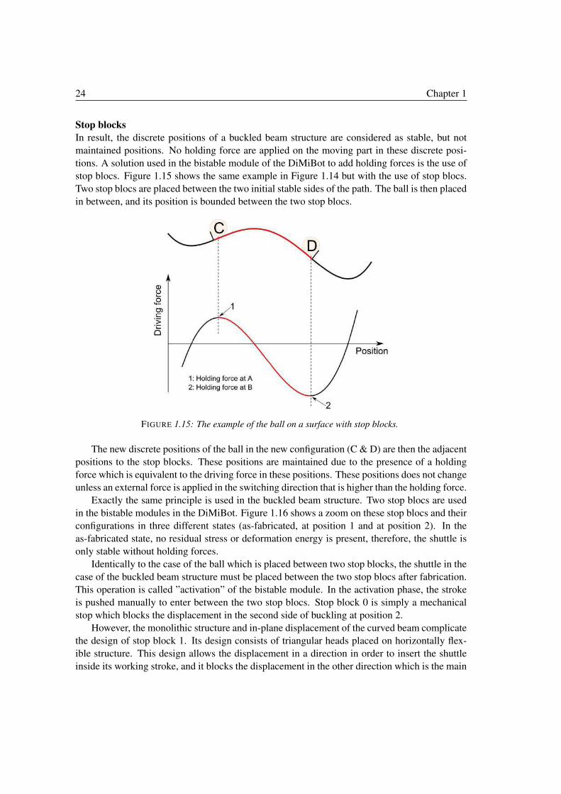
24 Chapter 1
Stop blocks
In result, the discrete positions of a buckled beam structure are considered as stable, but not
maintained positions. No holding force are applied on the moving part in these discrete posi-
tions. A solution used in the bistable module of the DiMiBot to add holding forces is the use of
stop blocs. Figure 1.15 shows the same example in Figure 1.14 but with the use of stop blocs.
Two stop blocs are placed between the two initial stable sides of the path. The ball is then placed
in between, and its position is bounded between the two stop blocs.
FIGURE 1.15: The example of the ball on a surface with stop blocks.
The new discrete positions of the ball in the new configuration (C & D) are then the adjacent
positions to the stop blocks. These positions are maintained due to the presence of a holding
force which is equivalent to the driving force in these positions. These positions does not change
unless an external force is applied in the switching direction that is higher than the holding force.
Exactly the same principle is used in the buckled beam structure. Two stop blocs are used
in the bistable modules in the DiMiBot. Figure 1.16 shows a zoom on these stop blocs and their
configurations in three different states (as-fabricated, at position 1 and at position 2). In the
as-fabricated state, no residual stress or deformation energy is present, therefore, the shuttle is
only stable without holding forces.
Identically to the case of the ball which is placed between two stop blocks, the shuttle in the
case of the buckled beam structure must be placed between the two stop blocs after fabrication.
This operation is called ”activation” of the bistable module. In the activation phase, the stroke
is pushed manually to enter between the two stop blocs. Stop block 0 is simply a mechanical
stop which blocks the displacement in the second side of buckling at position 2.
However, the monolithic structure and in-plane displacement of the curved beam complicate
the design of stop block 1. Its design consists of triangular heads placed on horizontally flex-
ible structure. This design allows the displacement in a direction in order to insert the shuttle
inside its working stroke, and it blocks the displacement in the other direction which is the main
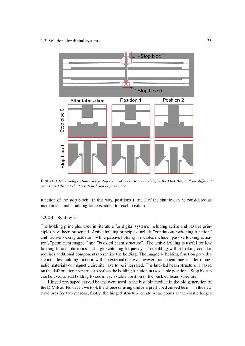
1.3 Solutions for digital systems 25
FIGURE 1.16: Configurations of the stop blocs of the bistable module, in the DiMiBot, in three different
states: as-fabricated, at position 1 and at position 2.
function of the stop block. In this way, positions 1 and 2 of the shuttle can be considered as
maintained, and a holding force is added for each position.
1.3.2.3 Synthesis
The holding principles used in literature for digital systems including active and passive prin-
ciples have been presented. Active holding principles include ”continuous switching function”
and ”active locking actuator”, while passive holding principles include ”passive locking actua-
tor”, ”permanent magnet” and ”buckled beam structure”. The active holding is useful for low
holding time applications and high switching frequency. The holding with a locking actuator
requires additional components to realize the holding. The magnetic holding function provides
a contactless holding function with no external energy, however, permanent magnets, ferromag-
netic materials or magnetic circuits have to be integrated. The buckled beam structure is based
on the deformation properties to realize the holding function in two stable positions. Stop blocks
can be used to add holding forces in each stable position of the buckled beam structure.
Hinged preshaped curved beams were used in the bistable module in the old generation of
the DiMiBot. However, we took the choice of using uniform preshaped curved beams in the new
structures for two reasons, firstly, the hinged structure create weak points at the elastic hinges
26 Chapter 1
which are susceptible to fail in the fabrication process, secondly, the symmetrical behavior can
be obtained by adjusting positions of stop blocks.
In addition, in the new generation of the DiMiBot, several internal systems are switched
temporally. The holding in these internal systems is made using continuous switching function
method in order to simplify the design and reduce the number of actuators.
1.3.3 Multistable mechanisms
A multistable mechanism has many stable force-balanced positions within its range of motion
which allows relying on the stable states to have confidence in the positions after switching
from one state to the other without need of sensors. The different solutions found in literature
to realize the multistable mechanisms can be classified in three main categories.
• Elementary multistable mechanism
• Assembly of elementary modules
• Stepping microactuators
The number of stable positions is limited in the first category (bistable, tristable quadristable,
etc.), while it is not limited (unlimited) in principle in the two other categories where more posi-
tions are added either by adding more elementary modules in the architecture of the mechanism
or by extending the range of motion of the moving part. Thereby, the number of stable positions
can be changed in each prototype with respect to the design requirements. Each category is
detailed with examples in the following.
1.3.3.1 Elementary multistable mechanism
The design of elementary multistable systems/mechanism is dedicated for switching between
limited number of stable positions. Most of the multistable digital systems found in literature
are from this category. Bistable systems are the most widespread [5, 22, 36, 56, 61, 85, 102, 107,
112, 132, 133, 135, 136, 137] (including the bistable module used in the DiMiBot). Tristable
[16, 18, 95, 128, 139], quadristable [97, 50, 96, 103, 104, 105] and pentastable designs [17,
140] are also investigated. Several examples of these mechanisms can be found in the previous
sections.
1.3.3.2 Assembly of elementary modules
Several applications can be cited that uses elementary digital systems in a large scale without
collaboration in their local specific task, including the braille display systems [86, 127], optical
switch arrays [29, 63], mechanical memories array [15, 125], etc.. However, the concerned ap-
plications in this category are the application where the elementary modules contribute together
to move one end effector.
Assembly of several digital actuators as elementary modules is a solution to add discrete
states to a digital system. In addition to the advantages of the digital concept, the advantage
of the elementary architecture is the ability to reach high number of stable positions by simply
1.3 Solutions for digital systems 27
adding digital modules. In the other side, the main drawback in these systems is that for high
number of discrete positions, a large number of digital systems is needed. This increases the
size of the device, complicates its integration and connectivity, and increases the possibility of
failure in the fabrication process.
Macroscale At the macroscale, several designs of digital positioning systems with elementary
modules were proposed previously. These designs include the VGT (variable geometry trusses)
manipulator which allows reaching positions in a tridimensional workspace [120], the BRAID
(Binary Robotic Articulated Intelligent Device) where the different modules are connected in
series [119], and the digital robotic platform developed by Wang et al. [130] which consists of
six elementary modules that are connected in parallel.
Microscale This concept is also used at the microscale where different designs with elemen-
tary modules were presented in literature. These designs include displacement tables [14, 104,
103], multistable microrobots with elementary modules distributed in series [42] and the DiMi-
Bot with elementary modules distributed in parallel [12].
1.3.3.3 Stepping microactuators
The principle of stepping microactuators is based on making consecutive steps in order to reach a
desired position. The stepping principle is very close to the digital concept. However, the focus
in these designs is generally on the step realization, not on the holding in a defined discrete
position, which implies that, in contrast to digital actuators, sensors are always required for
repeatable and accurate positioning.
Microactuators based on the stepping motion have a potential to satisfy the contradictory
requirements for micropositioning. They allows realizing high-resolution positioners that fit in
a small volume and are able to produce large stroke and large force while using little power.
Various principles for making a step are developed in literature and used widely in commercial
products. A brief description and example for each principle is given in the following
Inchworm actuators Various designs and concepts for the inchworm actuation is presented
in literature [2, 35, 73, 77, 116, 35]. The most common design comprises three independently
driven actuators, two for latching (LA1 and LA2) and one for driving (DA) with six steps of
actuation. This is the case of the inchworm developed by Erismis et al. [35] and shown in
Figure 1.17.
Stick-slip actuators The functioning of stick-slip actuator consists mainly of two steps (Fig-
ure 1.18(a)). In the first step, a slow deflection of a driving object moves the body of the device
along the actuation direction due to a static friction (stick effect). In the second step, a rapid
deflection slides the driving object towards its initial position (slip effect). The repetition of this
sequence allows unlimited strokes and submicrometric resolutions.
Based on this principle, Rakontondrabe et al. [108] have developed a 2-DoF stick-slip device
which moves around and along a tube (Figure 1.18(b)). The device consists of three microac-
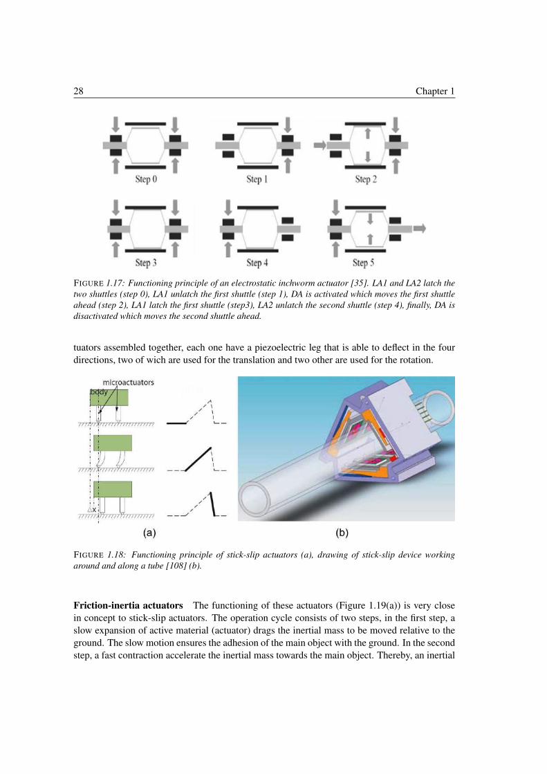
28 Chapter 1
FIGURE 1.17: Functioning principle of an electrostatic inchworm actuator [35]. LA1 and LA2 latch the
two shuttles (step 0), LA1 unlatch the first shuttle (step 1), DA is activated which moves the first shuttle
ahead (step 2), LA1 latch the first shuttle (step3), LA2 unlatch the second shuttle (step 4), finally, DA is
disactivated which moves the second shuttle ahead.
tuators assembled together, each one have a piezoelectric leg that is able to deflect in the four
directions, two of wich are used for the translation and two other are used for the rotation.
FIGURE 1.18: Functioning principle of stick-slip actuators (a), drawing of stick-slip device working
around and along a tube [108] (b).
Friction-inertia actuators The functioning of these actuators (Figure 1.19(a)) is very close
in concept to stick-slip actuators. The operation cycle consists of two steps, in the first step, a
slow expansion of active material (actuator) drags the inertial mass to be moved relative to the
ground. The slow motion ensures the adhesion of the main object with the ground. In the second
step, a fast contraction accelerate the inertial mass towards the main object. Thereby, an inertial
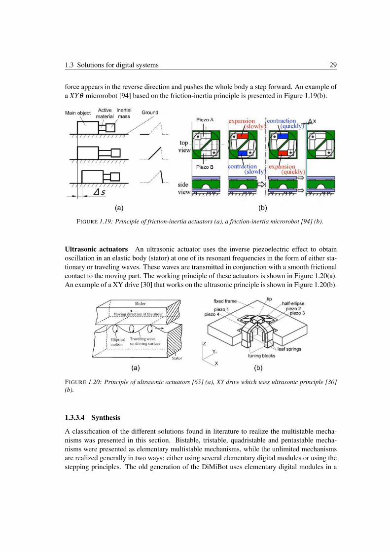
1.3 Solutions for digital systems 29
force appears in the reverse direction and pushes the whole body a step forward. An example of
a XY θ microrobot [94] based on the friction-inertia principle is presented in Figure 1.19(b).
FIGURE 1.19: Principle of friction-inertia actuators (a), a friction-inertia microrobot [94] (b).
Ultrasonic actuators An ultrasonic actuator uses the inverse piezoelectric effect to obtain
oscillation in an elastic body (stator) at one of its resonant frequencies in the form of either sta-
tionary or traveling waves. These waves are transmitted in conjunction with a smooth frictional
contact to the moving part. The working principle of these actuators is shown in Figure 1.20(a).
An example of a XY drive [30] that works on the ultrasonic principle is shown in Figure 1.20(b).
FIGURE 1.20: Principle of ultrasonic actuators [65] (a), XY drive which uses ultrasonic principle [30]
(b).
1.3.3.4 Synthesis
A classification of the different solutions found in literature to realize the multistable mecha-
nisms was presented in this section. Bistable, tristable, quadristable and pentastable mecha-
nisms were presented as elementary multistable mechanisms, while the unlimited mechanisms
are realized generally in two ways: either using several elementary digital modules or using the
stepping principles. The old generation of the DiMiBot uses elementary digital modules in a
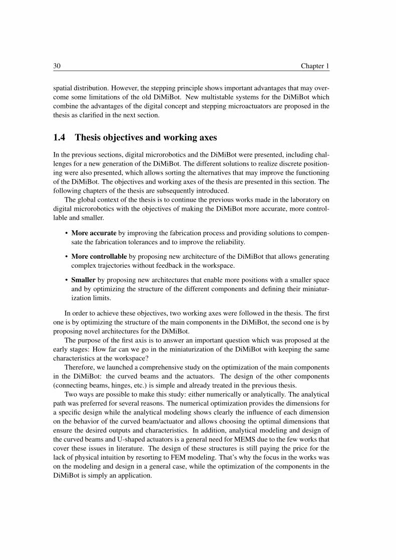
30 Chapter 1
spatial distribution. However, the stepping principle shows important advantages that may over-
come some limitations of the old DiMiBot. New multistable systems for the DiMiBot which
combine the advantages of the digital concept and stepping microactuators are proposed in the
thesis as clarified in the next section.
1.4 Thesis objectives and working axes
In the previous sections, digital microrobotics and the DiMiBot were presented, including chal-
lenges for a new generation of the DiMiBot. The different solutions to realize discrete position-
ing were also presented, which allows sorting the alternatives that may improve the functioning
of the DiMiBot. The objectives and working axes of the thesis are presented in this section. The
following chapters of the thesis are subsequently introduced.
The global context of the thesis is to continue the previous works made in the laboratory on
digital microrobotics with the objectives of making the DiMiBot more accurate, more control-
lable and smaller.
• More accurate by improving the fabrication process and providing solutions to compen-
sate the fabrication tolerances and to improve the reliability.
• More controllable by proposing new architecture of the DiMiBot that allows generating
complex trajectories without feedback in the workspace.
• Smaller by proposing new architectures that enable more positions with a smaller space
and by optimizing the structure of the different components and defining their miniatur-
ization limits.
In order to achieve these objectives, two working axes were followed in the thesis. The first
one is by optimizing the structure of the main components in the DiMiBot, the second one is by
proposing novel architectures for the DiMiBot.
The purpose of the first axis is to answer an important question which was proposed at the
early stages: How far can we go in the miniaturization of the DiMiBot with keeping the same
characteristics at the workspace?
Therefore, we launched a comprehensive study on the optimization of the main components
in the DiMiBot: the curved beams and the actuators. The design of the other components
(connecting beams, hinges, etc.) is simple and already treated in the previous thesis.
Two ways are possible to make this study: either numerically or analytically. The analytical
path was preferred for several reasons. The numerical optimization provides the dimensions for
a specific design while the analytical modeling shows clearly the influence of each dimension
on the behavior of the curved beam/actuator and allows choosing the optimal dimensions that
ensure the desired outputs and characteristics. In addition, analytical modeling and design of
the curved beams and U-shaped actuators is a general need for MEMS due to the few works that
cover these issues in literature. The design of these structures is still paying the price for the
lack of physical intuition by resorting to FEM modeling. That’s why the focus in the works was
on the modeling and design in a general case, while the optimization of the components in the
DiMiBot is simply an application.
1.4 Thesis objectives and working axes 31
The second working axis is to propose new architectures that improve the performance of
the DiMiBot. A new idea was proposed during the thesis which consists in replacing all the
bistable modules in a side of the DiMiBot by only one multistable stepper module. This does
not cancel the need for the first working axis since the curved beams and bistable modules are
also used in the multistable module.
The use of multistable modules in the DiMiBot has many advantages. Its principle is a
combination between the bistable module and the stepping microactuators. It combines the ad-
vantages of stepping actuation in the sense of generating an infinite number of positions simply
by extending the range of motion but with accuracy in the positioning and it keeps most of the
advantages of the previous DiMiBot structure. Further, it makes the system more compact, it
allows generating complex trajectories in the workspace and agrees with the objectives of the
thesis to make the DiMiBot more accurate, more controllable and smaller.
The second working axis contains several parts which have been treated in turns in the
thesis, starting with the principle, the design, the fabrication (including layouts, process and
realization), and ending with the connectivity and characterization. Loops of improvements
were made in and between these parts which allowed obtaining operational prototypes at the
end.
1.4.1 First axis: Analytical design optimization
Preshaped curved beam
In a previous analytical model presented by Qiu et al. [106], analytical solution of the
snapping force in the postbuckling phase was provided with an approximation of neglecting
high modes of buckling, this model was approved by experiments. However, no studies were
found in literature for calculating evolution of the internal stress during deflection between two
sides of buckling.
In Chapter 2, modeling of the snapping forces and internal stresses is presented with con-
sidering high modes of buckling. A comparison of the results with FEM simulations shows that
the consideration of high modes of buckling in the calculation of the snapping forces is slightly
more accurate while the calculation of stress without high modes does not correspond to FEM
results.
After that, design and optimization of the curved beam are investigated in the second part
of the chapter based on the analytical expressions obtained in the modeling. The influence
of the beam dimensions and material properties on the mechanical behavior of the beam is
clarified. A design method is provided subsequently that define the optimal dimensions of the
beam that provide the desired snapping force and stroke of deflection while respecting the design
specifications and limitations. Limits of miniaturization are investigated finally.
Electrothermal U-shaped actuator
The modeling of the electrothermal U-shaped actuator is treated by a sequence of two analytical
models: electro-thermal and thermo-mechanical. The first one concerns the computation of the
evolution of the thermal distribution in the actuator, while the second one allows computing the
displacement resulting from the thermal distribution.
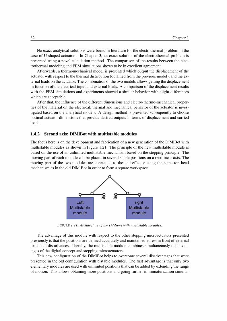
32 Chapter 1
No exact analytical solutions were found in literature for the electrothermal problem in the
case of U-shaped actuators. In Chapter 3, an exact solution of the electrothermal problem is
presented using a novel calculation method. The comparison of the results between the elec-
trothermal modeling and FEM simulations shows to be in excellent agreement.
Afterwards, a thermomechanical model is presented which output the displacement of the
actuator with respect to the thermal distribution (obtained from the previous model), and the ex-
ternal loads on the actuator. The combination of the two models allows getting the displacement
in function of the electrical input and external loads. A comparison of the displacement results
with the FEM simulations and experiments showed a similar behavior with slight differences
which are acceptable.
After that, the influence of the different dimensions and electro-thermo-mechanical proper-
ties of the material on the electrical, thermal and mechanical behavior of the actuator is inves-
tigated based on the analytical models. A design method is presented subsequently to choose
optimal actuator dimensions that provide desired outputs in terms of displacement and carried
loads.
1.4.2 Second axis: DiMiBot with multistable modules
The focus here is on the development and fabrication of a new generation of the DiMiBot with
multistable modules as shown in Figure 1.21. The principle of the new multistable module is
based on the use of an unlimited multistable mechanism based on the stepping principle. The
moving part of each module can be placed in several stable positions on a rectilinear axis. The
moving part of the two modules are connected to the end effector using the same top head
mechanism as in the old DiMiBot in order to form a square workspace.
FIGURE 1.21: Architecture of the DiMiBot with multistable modules.
The advantage of this module with respect to the other stepping microactuators presented
previously is that the positions are defined accurately and maintained at rest in front of external
loads and disturbances. Thereby, the multistable module combines simultaneously the advan-
tages of the digital concept and stepping microactuators.
This new configuration of the DiMiBot helps to overcome several disadvantages that were
presented in the old configuration with bistable modules. The first advantage is that only two
elementary modules are used with unlimited positions that can be added by extending the range
of motion. This allows obtaining more positions and going further in miniaturization simulta-
1.5 Conclusion 33
neously, and avoids the drawbacks related to the large size of the DiMiBot, such as lowering
the failure possibilities in the fabrication process, limiting the number of metal lines for the
electrical connectivity and solidifying the structure.
Further, the transition in one side of the DiMiBot with multistable modules is made incre-
mentally step by step and not by binary steps. This means that the transition in the workspace
of the DiMiBot is now between the adjacent positions. This means also that the DiMiBot is able
to realize any complex trajectory with an open loop control.
In the other side, an accurate positioning mechanism was designed and used in the multi-
stable module in order to ensure accurate maintained positions. The novel idea in this mech-
anism is the compensation of fabrication tolerances by playing on the excess/shortage in the
width of the openings and patterns of the device layer obtained in the fabrication. As the case
of stop blocks, this mechanism is used around the shuttle of a pair of preshaped curved beams
in the multistable module. It places the shuttle between two discrete positions which are ac-
curately defined by compensation of the fabrication tolerances. This adds also holding forces
on the stable positions which improves the positioning robustness in front of external loads and
disturbances.
However, The binary feature of the bistable DiMiBot is not a feature of the new structure.
The positions in the workspace are reached by incremental stepping and no absolute states of
the modules are assigned to each position. The positions in this case are determined relatively
to the first initial position by counting the steps made to reach the current state.
The principle and the design of the multistable module is presented in Chapter 4. The
stepping principle is based on a specific sequence of bistable displacement and opening normally
closed latch arms in a part and closing other normally open latch arms in the other part. The
design of the internal systems in the module, the global structure of the module and the DiMiBot
are subsequently presented.
In Chapter 5, the fabrication process, difficulties encountered and different runs are pre-
sented. The fabrication was made in the clean room MIMENTO of the institute Femto-st. Major
changes were made in the fabrication process and layouts with respect to the previous thesis in
order to obtain more proper, more accurate and more homogeneous structures and to reduce
the failure possibilities in the fabrication as possible. Finally, the experiments on some fabri-
cated tests and operational prototypes of the multistable module are presented. The experiments
showed a proper functioning of the stepping principle and accurate positioning on prototypes of
multistable modules. All the difficulties encountered and solutions provided in the fabrication
and the experiments are detailed.
1.5 Conclusion
After introducing digital microrobotics and the old generation of the DiMiBot, challenges for a
new generation were presented in the first part. These challenges include proposing new struc-
tures/mechanisms of the DiMiBot that reduce the size, allows complex trajectories and improve
the accuracy. Also, the challenges include improving the fabrication process and developing
models for designing the main components in the DiMiBot.
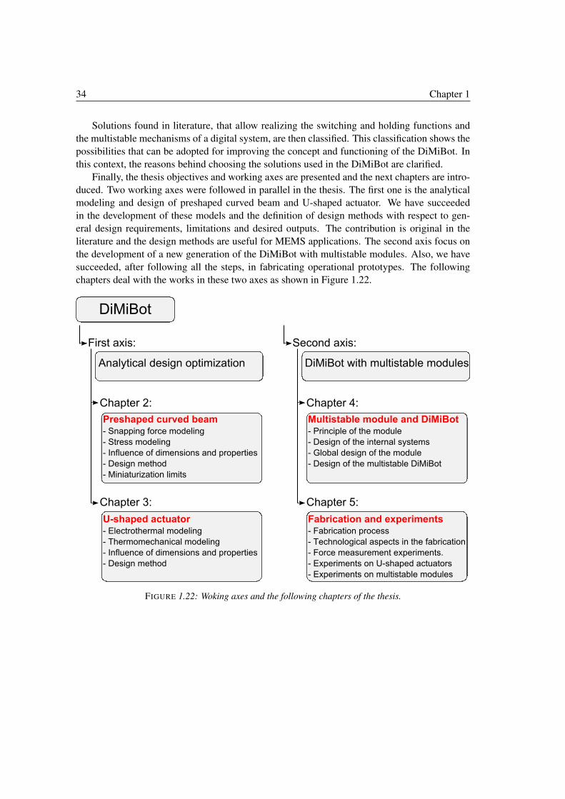
34 Chapter 1
Solutions found in literature, that allow realizing the switching and holding functions and
the multistable mechanisms of a digital system, are then classified. This classification shows the
possibilities that can be adopted for improving the concept and functioning of the DiMiBot. In
this context, the reasons behind choosing the solutions used in the DiMiBot are clarified.
Finally, the thesis objectives and working axes are presented and the next chapters are intro-
duced. Two working axes were followed in parallel in the thesis. The first one is the analytical
modeling and design of preshaped curved beam and U-shaped actuator. We have succeeded
in the development of these models and the definition of design methods with respect to gen-
eral design requirements, limitations and desired outputs. The contribution is original in the
literature and the design methods are useful for MEMS applications. The second axis focus on
the development of a new generation of the DiMiBot with multistable modules. Also, we have
succeeded, after following all the steps, in fabricating operational prototypes. The following
chapters deal with the works in these two axes as shown in Figure 1.22.
FIGURE 1.22: Woking axes and the following chapters of the thesis.
Chapter 2Curved beam bistable mechanism
This chapter deals with the modeling, stress analysis and design of a preshaped
curved beam. In a first stage, the presented modeling develops further the snapping
force solution and bistability conditions without and with including high modes of
buckling. In a second stage, we develop the analytical solution of the stresses in-
side the beam during deflection between the two sides of buckling. The analytical
expressions obtained in the modeling and stress analysis define the mechanical be-
havior of the curved beam during deflection and include the effects of high modes of
buckling. The analytical results are then compared with FEM simulations and have
shown to be in excellent agreement. The results show the importance of high modes
of buckling in the calculation of stresses and snapping force. In the final stage, de-
sign and optimization of the curved beam are investigated based on the analytical
expressions obtained in the modeling. Design elements are provided in order to
achieve the best integration of the curved beam in a complete microstructure.
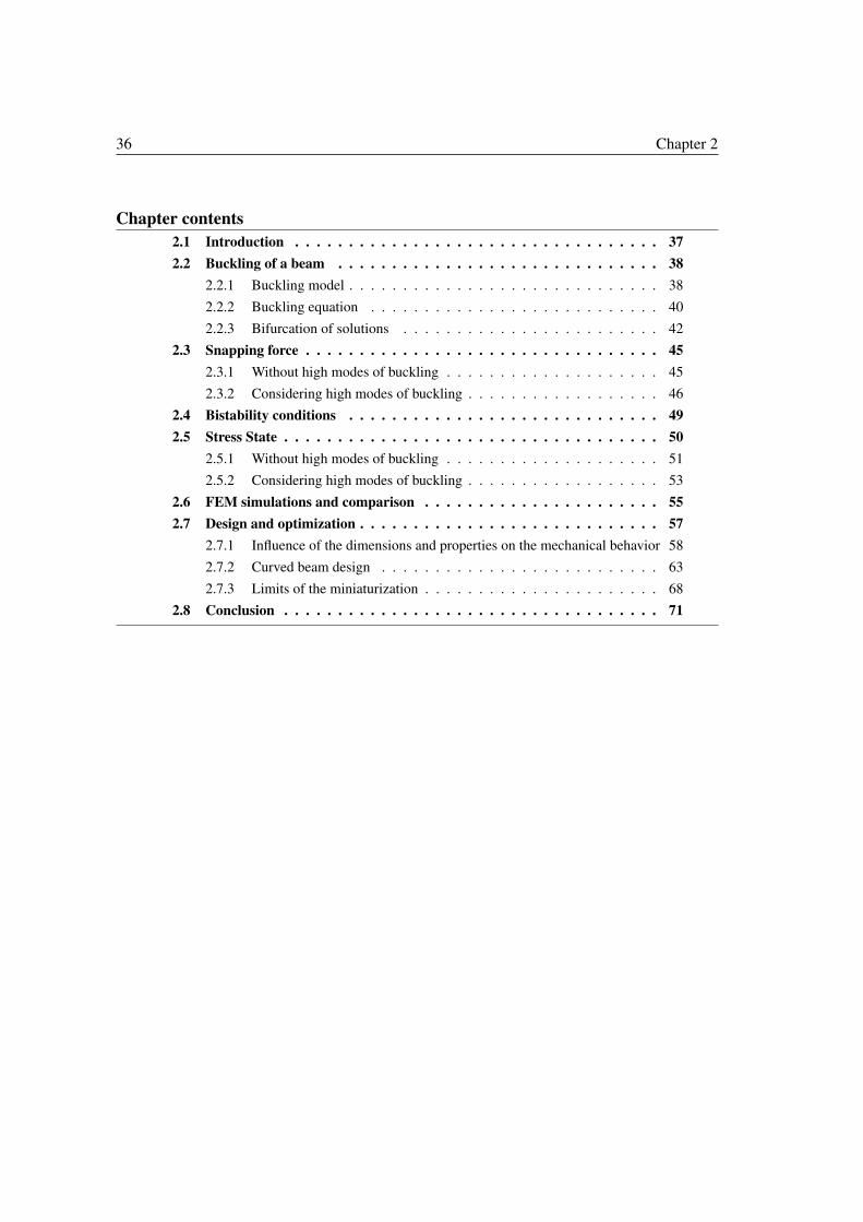
36 Chapter 2
Chapter contents
2.1 Introduction . . . . . . . . . . . . . . . . . . . . . . . . . . . . . . . . . . 37
2.2 Buckling of a beam . . . . . . . . . . . . . . . . . . . . . . . . . . . . . . 38
2.2.1 Buckling model . . . . . . . . . . . . . . . . . . . . . . . . . . . . . 38
2.2.2 Buckling equation . . . . . . . . . . . . . . . . . . . . . . . . . . . 40
2.2.3 Bifurcation of solutions . . . . . . . . . . . . . . . . . . . . . . . . 42
2.3 Snapping force . . . . . . . . . . . . . . . . . . . . . . . . . . . . . . . . . 45
2.3.1 Without high modes of buckling . . . . . . . . . . . . . . . . . . . . 45
2.3.2 Considering high modes of buckling . . . . . . . . . . . . . . . . . . 46
2.4 Bistability conditions . . . . . . . . . . . . . . . . . . . . . . . . . . . . . 49
2.5 Stress State . . . . . . . . . . . . . . . . . . . . . . . . . . . . . . . . . . . 50
2.5.1 Without high modes of buckling . . . . . . . . . . . . . . . . . . . . 51
2.5.2 Considering high modes of buckling . . . . . . . . . . . . . . . . . . 53
2.6 FEM simulations and comparison . . . . . . . . . . . . . . . . . . . . . . 55
2.7 Design and optimization . . . . . . . . . . . . . . . . . . . . . . . . . . . . 57
2.7.1 Influence of the dimensions and properties on the mechanical behavior 58
2.7.2 Curved beam design . . . . . . . . . . . . . . . . . . . . . . . . . . 63
2.7.3 Limits of the miniaturization . . . . . . . . . . . . . . . . . . . . . . 68
2.8 Conclusion . . . . . . . . . . . . . . . . . . . . . . . . . . . . . . . . . . . 71
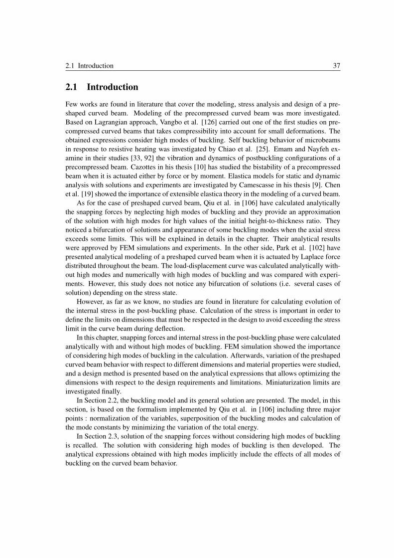
2.1 Introduction 37
2.1 Introduction
Few works are found in literature that cover the modeling, stress analysis and design of a pre-
shaped curved beam. Modeling of the precompressed curved beam was more investigated.
Based on Lagrangian approach, Vangbo et al. [126] carried out one of the first studies on pre-
compressed curved beams that takes compressibility into account for small deformations. The
obtained expressions consider high modes of buckling. Self buckling behavior of microbeams
in response to resistive heating was investigated by Chiao et al. [25]. Emam and Nayfeh ex-
amine in their studies [33, 92] the vibration and dynamics of postbuckling configurations of a
precompressed beam. Cazottes in his thesis [10] has studied the bistability of a precompressed
beam when it is actuated either by force or by moment. Elastica models for static and dynamic
analysis with solutions and experiments are investigated by Camescasse in his thesis [9]. Chen
et al. [19] showed the importance of extensible elastica theory in the modeling of a curved beam.
As for the case of preshaped curved beam, Qiu et al. in [106] have calculated analytically
the snapping forces by neglecting high modes of buckling and they provide an approximation
of the solution with high modes for high values of the initial height-to-thickness ratio. They
noticed a bifurcation of solutions and appearance of some buckling modes when the axial stress
exceeds some limits. This will be explained in details in the chapter. Their analytical results
were approved by FEM simulations and experiments. In the other side, Park et al. [102] have
presented analytical modeling of a preshaped curved beam when it is actuated by Laplace force
distributed throughout the beam. The load-displacement curve was calculated analytically with-
out high modes and numerically with high modes of buckling and was compared with experi-
ments. However, this study does not notice any bifurcation of solutions (i.e. several cases of
solution) depending on the stress state.
However, as far as we know, no studies are found in literature for calculating evolution of
the internal stress in the post-buckling phase. Calculation of the stress is important in order to
define the limits on dimensions that must be respected in the design to avoid exceeding the stress
limit in the curve beam during deflection.
In this chapter, snapping forces and internal stress in the post-buckling phase were calculated
analytically with and without high modes of buckling. FEM simulation showed the importance
of considering high modes of buckling in the calculation. Afterwards, variation of the preshaped
curved beam behavior with respect to different dimensions and material properties were studied,
and a design method is presented based on the analytical expressions that allows optimizing the
dimensions with respect to the design requirements and limitations. Miniaturization limits are
investigated finally.
In Section 2.2, the buckling model and its general solution are presented. The model, in this
section, is based on the formalism implemented by Qiu et al. in [106] including three major
points : normalization of the variables, superposition of the buckling modes and calculation of
the mode constants by minimizing the variation of the total energy.
In Section 2.3, solution of the snapping forces without considering high modes of buckling
is recalled. The solution with considering high modes of buckling is then developed. The
analytical expressions obtained with high modes implicitly include the effects of all modes of
buckling on the curved beam behavior.
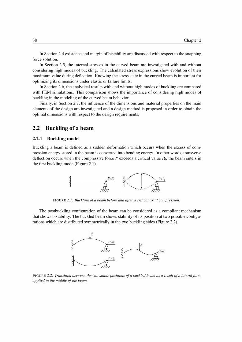
38 Chapter 2
In Section 2.4 existence and margin of bistability are discussed with respect to the snapping
force solution.
In Section 2.5, the internal stresses in the curved beam are investigated with and without
considering high modes of buckling. The calculated stress expressions show evolution of their
maximum value during deflection. Knowing the stress state in the curved beam is important for
optimizing its dimensions under elastic or failure limits.
In Section 2.6, the analytical results with and without high modes of buckling are compared
with FEM simulations. This comparison shows the importance of considering high modes of
buckling in the modeling of the curved beam behavior.
Finally, in Section 2.7, the influence of the dimensions and material properties on the main
elements of the design are investigated and a design method is proposed in order to obtain the
optimal dimensions with respect to the design requirements.
2.2 Buckling of a beam
2.2.1 Buckling model
Buckling a beam is defined as a sudden deformation which occurs when the excess of com-
pression energy stored in the beam is converted into bending energy. In other words, transverse
deflection occurs when the compressive force P exceeds a critical value P0, the beam enters in
the first buckling mode (Figure 2.1).
FIGURE 2.1: Buckling of a beam before and after a critical axial compression.
The postbuckling configuration of the beam can be considered as a compliant mechanism
that shows bistability. The buckled beam shows stability of its position at two possible configu-
rations which are distributed symmetrically in the two buckling sides (Figure 2.2).
FIGURE 2.2: Transition between the two stable positions of a buckled beam as a result of a lateral force
applied in the middle of the beam.
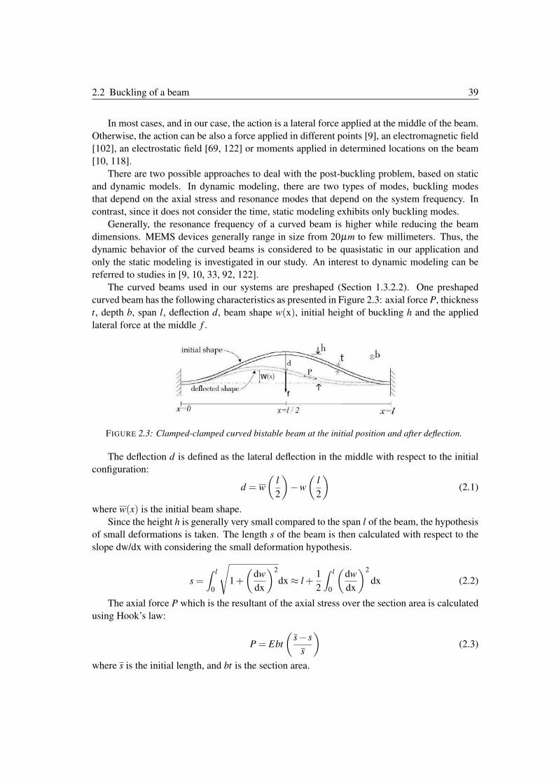
2.2 Buckling of a beam 39
In most cases, and in our case, the action is a lateral force applied at the middle of the beam.
Otherwise, the action can be also a force applied in different points [9], an electromagnetic field
[102], an electrostatic field [69, 122] or moments applied in determined locations on the beam
[10, 118].
There are two possible approaches to deal with the post-buckling problem, based on static
and dynamic models. In dynamic modeling, there are two types of modes, buckling modes
that depend on the axial stress and resonance modes that depend on the system frequency. In
contrast, since it does not consider the time, static modeling exhibits only buckling modes.
Generally, the resonance frequency of a curved beam is higher while reducing the beam
dimensions. MEMS devices generally range in size from 20µm to few millimeters. Thus, the
dynamic behavior of the curved beams is considered to be quasistatic in our application and
only the static modeling is investigated in our study. An interest to dynamic modeling can be
referred to studies in [9, 10, 33, 92, 122].
The curved beams used in our systems are preshaped (Section 1.3.2.2). One preshaped
curved beam has the following characteristics as presented in Figure 2.3: axial force P, thickness
t, depth b, span l, deflection d, beam shape w(x), initial height of buckling h and the applied
lateral force at the middle f .
FIGURE 2.3: Clamped-clamped curved bistable beam at the initial position and after deflection.
The deflection d is defined as the lateral deflection in the middle with respect to the initial
configuration:
d = w
�l
2
�−w
�l
2
�(2.1)
where w(x) is the initial beam shape.
Since the height h is generally very small compared to the span l of the beam, the hypothesis
of small deformations is taken. The length s of the beam is then calculated with respect to the
slope dw/dx with considering the small deformation hypothesis.
s =� l
0
�1+
�dw
dx
�2
dx ≈ l +1
2
� l
0
�dw
dx
�2
dx (2.2)
The axial force P which is the resultant of the axial stress over the section area is calculated
using Hook’s law:
P = Ebt
�s− s
s
�(2.3)
where s is the initial length, and bt is the section area.
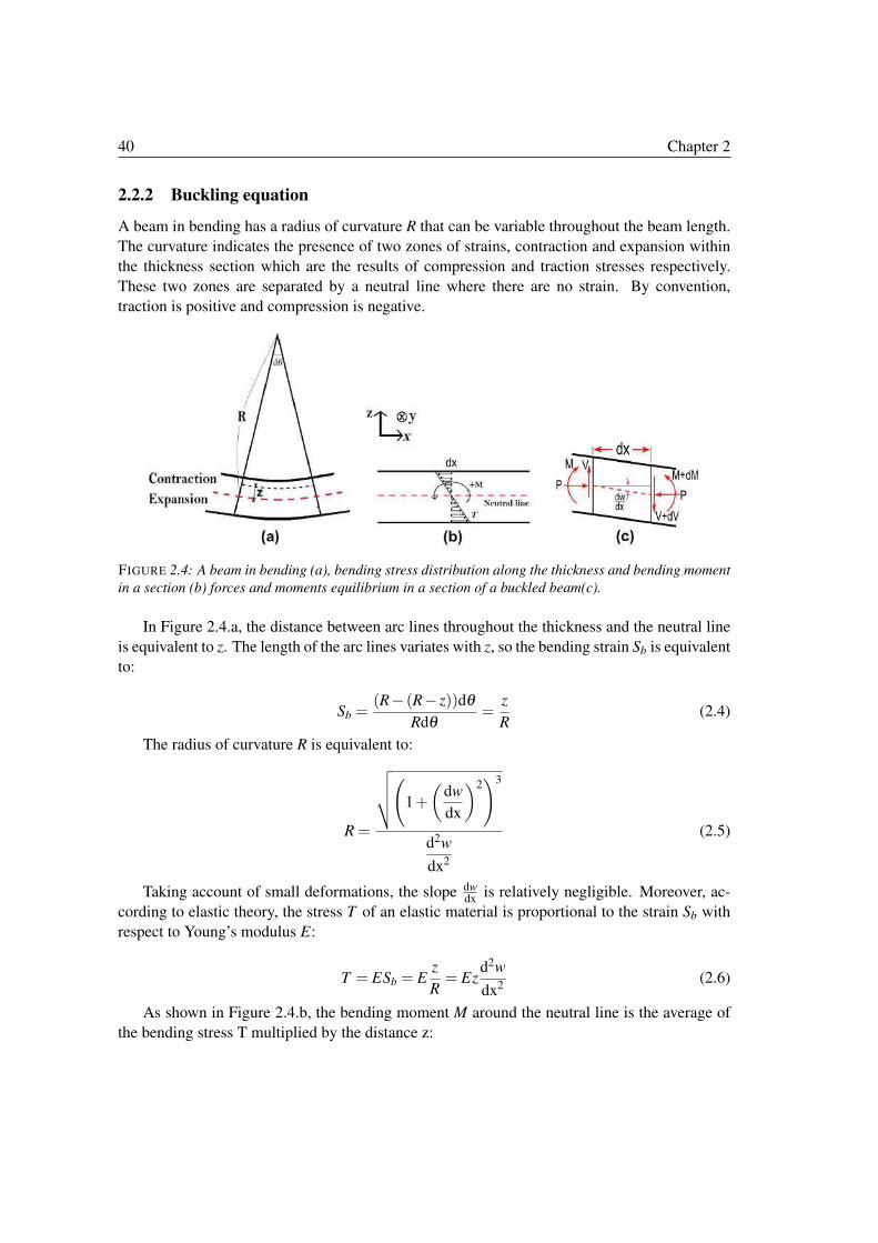
40 Chapter 2
2.2.2 Buckling equation
A beam in bending has a radius of curvature R that can be variable throughout the beam length.
The curvature indicates the presence of two zones of strains, contraction and expansion within
the thickness section which are the results of compression and traction stresses respectively.
These two zones are separated by a neutral line where there are no strain. By convention,
traction is positive and compression is negative.
FIGURE 2.4: A beam in bending (a), bending stress distribution along the thickness and bending moment
in a section (b) forces and moments equilibrium in a section of a buckled beam(c).
In Figure 2.4.a, the distance between arc lines throughout the thickness and the neutral line
is equivalent to z. The length of the arc lines variates with z, so the bending strain Sb is equivalent
to:
Sb =(R− (R− z))dθ
Rdθ=
z
R(2.4)
The radius of curvature R is equivalent to:
R =
�����
1+
�dw
dx
�2�3
d2w
dx2
(2.5)
Taking account of small deformations, the slope dwdx
is relatively negligible. Moreover, ac-
cording to elastic theory, the stress T of an elastic material is proportional to the strain Sb with
respect to Young’s modulus E:
T = ESb = Ez
R= Ez
d2w
dx2(2.6)
As shown in Figure 2.4.b, the bending moment M around the neutral line is the average of
the bending stress T multiplied by the distance z:
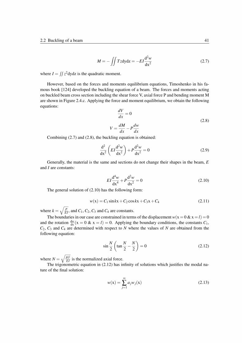
2.2 Buckling of a beam 41
M =−��
T zdydz =−EId2w
dx2(2.7)
where I =��
z2dydz is the quadratic moment.
However, based on the forces and moments equilibrium equations, Timoshenko in his fa-
mous book [124] developed the buckling equation of a beam. The forces and moments acting
on buckled beam cross section including the shear force V, axial force P and bending moment M
are shown in Figure 2.4.c. Applying the force and moment equilibrium, we obtain the following
equations:dV
dx= 0
V =dM
dx−P
dw
dx
(2.8)
Combining (2.7) and (2.8), the buckling equation is obtained:
d2
dx2
�EI
d2w
dx2
�+P
d2w
dx2= 0 (2.9)
Generally, the material is the same and sections do not change their shapes in the beam, E
and I are constants:
EId4w
dx4+P
d2w
dx2= 0 (2.10)
The general solution of (2.10) has the following form:
w(x) =C1 sinkx+C2 coskx+C3x+C4 (2.11)
where k =�
PEI
, and C1, C2, C3 and C4 are constants.
The boundaries in our case are constrained in terms of the displacement w(x= 0 & x= l)= 0
and the rotation dwdx(x = 0 & x = l) = 0. Applying the boundary conditions, the constants C1,
C2, C3 and C4 are determined with respect to N where the values of N are obtained from the
following equation:
sinN
2
�tan
N
2− N
2
�= 0 (2.12)
where N =�
Pl2
EIis the normalized axial force.
The trigonometric equation in (2.12) has infinity of solutions which justifies the modal na-
ture of the final solution:
w(x) =∞
∑j=1
a jw j(x) (2.13)
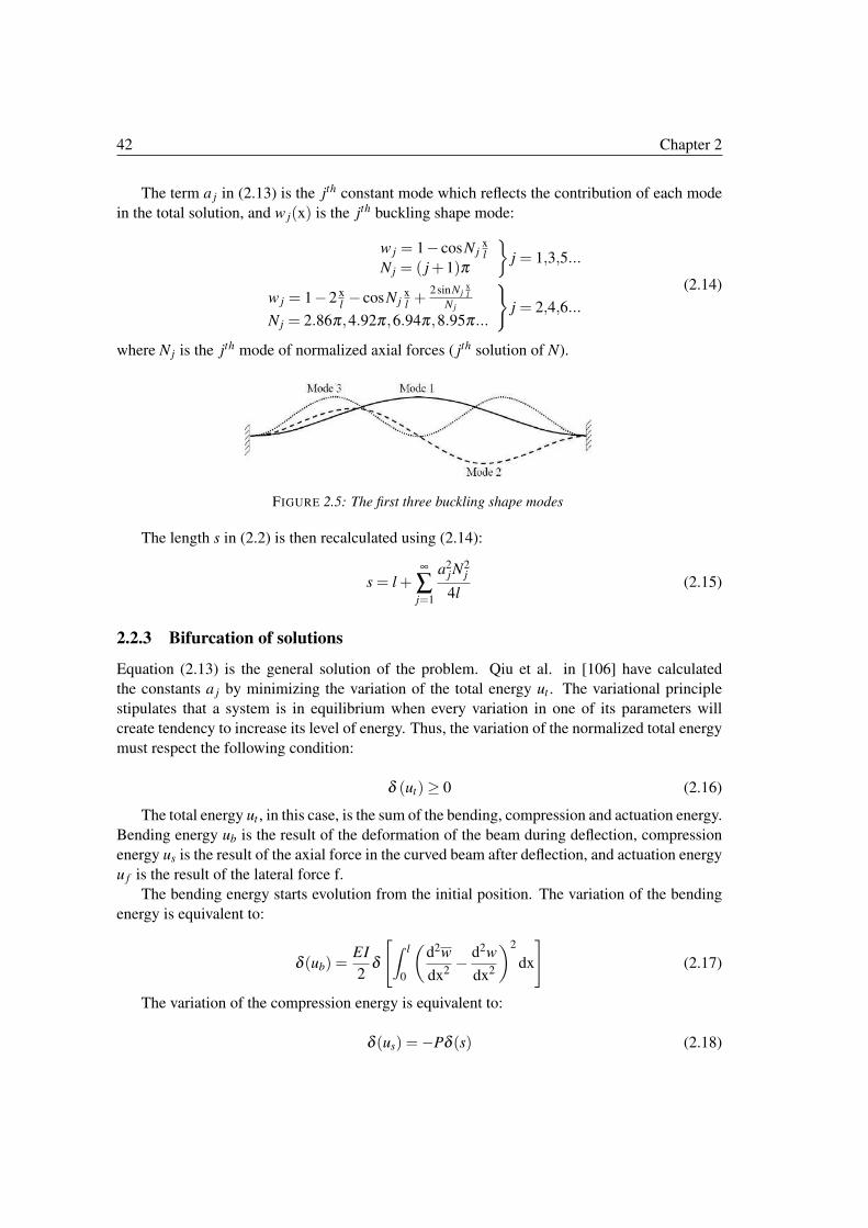
42 Chapter 2
The term a j in (2.13) is the jth constant mode which reflects the contribution of each mode
in the total solution, and w j(x) is the jth buckling shape mode:
w j = 1− cosN jxl
N j = ( j+1)π
�j = 1,3,5...
w j = 1−2 xl− cosN j
xl+
2sinN jxl
N j
N j = 2.86π,4.92π,6.94π,8.95π...
�j = 2,4,6...
(2.14)
where N j is the jth mode of normalized axial forces ( jth solution of N).
FIGURE 2.5: The first three buckling shape modes
The length s in (2.2) is then recalculated using (2.14):
s = l +∞
∑j=1
a2jN
2j
4l(2.15)
2.2.3 Bifurcation of solutions
Equation (2.13) is the general solution of the problem. Qiu et al. in [106] have calculated
the constants a j by minimizing the variation of the total energy ut . The variational principle
stipulates that a system is in equilibrium when every variation in one of its parameters will
create tendency to increase its level of energy. Thus, the variation of the normalized total energy
must respect the following condition:
δ (ut)≥ 0 (2.16)
The total energy ut , in this case, is the sum of the bending, compression and actuation energy.
Bending energy ub is the result of the deformation of the beam during deflection, compression
energy us is the result of the axial force in the curved beam after deflection, and actuation energy
u f is the result of the lateral force f.
The bending energy starts evolution from the initial position. The variation of the bending
energy is equivalent to:
δ (ub) =EI
2δ
�� l
0
�d2w
dx2− d2w
dx2
�2
dx
�(2.17)
The variation of the compression energy is equivalent to:
δ (us) =−Pδ (s) (2.18)
2.2 Buckling of a beam 43
The variation of the actuation energy is equivalent to:
δ (u f ) =− f δ (d) (2.19)
In order to simplify the solution and the presentation, the following parameters are normal-
ized as follows:
X =x
lWj(X) = w j(x) W (X) =
w(x)
h=
∞
∑j=1
A jWj(X) (2.20)
The applied force, deflection, length and energy are also normalized:
F =f l3
EIh; Δ =
d
h; S =
sl
h2; Ut =
ut l3
EIh2(2.21)
The variation of the normalized total energy has then the following form:
∂ (Ut) =
�N4
1 −N2N21
2A1 −
N41
4+2F
�∂A1 + ∑
j=5,9,13...
�N4
j −N2N2j
2A j +2F
�∂A j
+ ∑j=2,3,4,6,7...
�N4
j −N2N2j
2
�∂A2
j
(2.22)
Minimizing energy variation in (2.22) in order to satisfy (2.16) brings out bifurcation of
solutions. The bifurcation is based on the value of the axial stress inside the curved beam.
In fact, the behavior of the beam is decomposed by the compression ability. When N < N2,
the beam is in a compressible phase and N is able to be increased, the modes 2,3,4,6,7,8,10...do not appear, and the terms A j for j = 2,3,4,6,7,8,10... are equivalent to zero. At N = N2,
the system enters in the incompressible phase where no more axial stress N or extra length S
is allowed. Mode 2 is the manner used by the system to stop evolution of the axial stress and
length contraction. A2 appears with the other constants A j ( j = 1,5,9,13...) in a way that S and
N remain constants. Furthermore, N is not able to exceed N2 unless the mode 2 is constrained.
So, for j = 2,3,4,6,7,8,10... :
A j =
Mode 2 is unconstrained N ≤ N2
Mode 2 is constrained N ≤ N3
0 N < N j
A j appear N = N j
(2.23)
The other terms A j, for j = 1,5,9,13..., are calculated by setting to zero the variation of the
total energy:
A1 =−1
2
N21
N2 −N21
+4F
N21 (N
2 −N21 )
(2.24)
A j =4F
N2j (N
2−N2j )
for j = 5,9,13... (2.25)
44 Chapter 2
The normalized deflection Δ can be recalculated from (3.50) and (2.21) in function of the
mode constants as follows:
Δ = 1−2 ∑j=1,5,9...
A j (2.26)
Idem, the normalized axial stress N in function of the mode constants can be concluded from
(2.2) and (2.21) as follows:
N2
12Q2=
N21
16−
∞
∑j=1
A2jN
2j
4(2.27)
where Q is the height-to-thickness ratio Q = h/t.
Usually, in the case of a preshaped curved beam, a simple one curved beam shows bista-
bility only for high values of Q. The bistability, in this case, is highly asymmetric between the
two sides of buckling. However, it is possible to mechanically prevent asymmetrical bending
relatively to the middle of the beam and consequently preventing mode 2 from occurring.
Connecting two beams by a shuttle, as shown in Figure 2.6, can eliminate mode 2 and all
asymetrical modes. In this case, mode 2 is canceled into calculation, the force is doubled with
the same displacement and the normalized axial stress N can increase to the new critical value
N3.
FIGURE 2.6: Transition between the two stable positions of two curved beams connected in the middle,
mode 3 appears during transition.
Based on the above, we can distinguish three kinds of solutions. The first kind is when the
curved beam is in the compressible phase:
F = F1
N <
�N2 mode 2 is not constrained
N3 mode 2 is constrained
A j �= 0; j = 1,5,9,13...
(2.28)
The second kind is when N reaches N2 without mechanical constraints:
F = F2
N = N2
A j �= 0; j = 1,2,5,9,13...(2.29)
The third kind is when mode 2 is constrained and N reaches N3 :
F = F3
N = N3
A j �= 0; j = 1,3,5,9,13...(2.30)
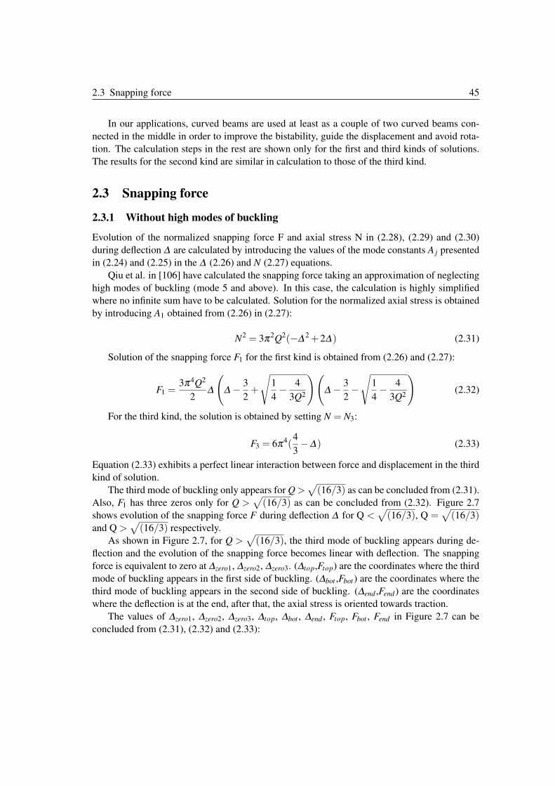
2.3 Snapping force 45
In our applications, curved beams are used at least as a couple of two curved beams con-
nected in the middle in order to improve the bistability, guide the displacement and avoid rota-
tion. The calculation steps in the rest are shown only for the first and third kinds of solutions.
The results for the second kind are similar in calculation to those of the third kind.
2.3 Snapping force
2.3.1 Without high modes of buckling
Evolution of the normalized snapping force F and axial stress N in (2.28), (2.29) and (2.30)
during deflection Δ are calculated by introducing the values of the mode constants A j presented
in (2.24) and (2.25) in the Δ (2.26) and N (2.27) equations.
Qiu et al. in [106] have calculated the snapping force taking an approximation of neglecting
high modes of buckling (mode 5 and above). In this case, the calculation is highly simplified
where no infinite sum have to be calculated. Solution for the normalized axial stress is obtained
by introducing A1 obtained from (2.26) in (2.27):
N2 = 3π2Q2(−Δ 2 +2Δ) (2.31)
Solution of the snapping force F1 for the first kind is obtained from (2.26) and (2.27):
F1 =3π4Q2
2Δ
�Δ − 3
2+
�1
4− 4
3Q2
��Δ − 3
2−�
1
4− 4
3Q2
�(2.32)
For the third kind, the solution is obtained by setting N = N3:
F3 = 6π4(4
3−Δ) (2.33)
Equation (2.33) exhibits a perfect linear interaction between force and displacement in the third
kind of solution.
The third mode of buckling only appears for Q >�(16/3) as can be concluded from (2.31).
Also, F1 has three zeros only for Q >�(16/3) as can be concluded from (2.32). Figure 2.7
shows evolution of the snapping force F during deflection Δ for Q <�(16/3), Q =
�(16/3)
and Q >�(16/3) respectively.
As shown in Figure 2.7, for Q >�
(16/3), the third mode of buckling appears during de-
flection and the evolution of the snapping force becomes linear with deflection. The snapping
force is equivalent to zero at Δzero1, Δzero2, Δzero3. (Δtop,Ftop) are the coordinates where the third
mode of buckling appears in the first side of buckling. (Δbot ,Fbot) are the coordinates where the
third mode of buckling appears in the second side of buckling. (Δend ,Fend) are the coordinates
where the deflection is at the end, after that, the axial stress is oriented towards traction.
The values of Δzero1, Δzero2, Δzero3, Δtop, Δbot , Δend , Ftop, Fbot , Fend in Figure 2.7 can be
concluded from (2.31), (2.32) and (2.33):
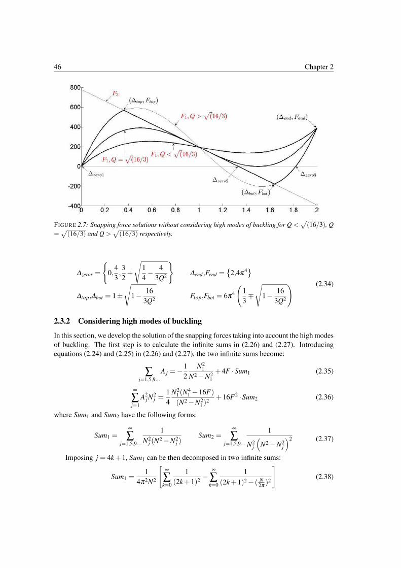
46 Chapter 2
FIGURE 2.7: Snapping force solutions without considering high modes of buckling for Q <�
(16/3), Q
=�(16/3) and Q >
�(16/3) respectively.
Δzeros =
�0,
4
3,3
2+
�1
4− 4
3Q2
�Δend ,Fend =
�2,4π4
�
Δtop,Δbot = 1±
�1− 16
3Q2Ftop,Fbot = 6π4
�1
3∓�
1− 16
3Q2
� (2.34)
2.3.2 Considering high modes of buckling
In this section, we develop the solution of the snapping forces taking into account the high modes
of buckling. The first step is to calculate the infinite sums in (2.26) and (2.27). Introducing
equations (2.24) and (2.25) in (2.26) and (2.27), the two infinite sums become:
∑j=1,5,9...
A j =−1
2
N21
N2 −N21
+4F ·Sum1 (2.35)
∞
∑j=1
A2jN
2j =
1
4
N21 (N
41 −16F)
(N2 −N21 )
2+16F2 ·Sum2 (2.36)
where Sum1 and Sum2 have the following forms:
Sum1 =∞
∑j=1,5,9...
1
N2j (N
2 −N2j )
Sum2 =∞
∑j=1,5,9...
1
N2j
�N2 −N2
j
�2 (2.37)
Imposing j = 4k+1, Sum1 can be then decomposed in two infinite sums:
Sum1 =1
4π2N2
�∞
∑k=0
1
(2k+1)2−
∞
∑k=0
1
(2k+1)2 − ( N2π )
2
�(2.38)
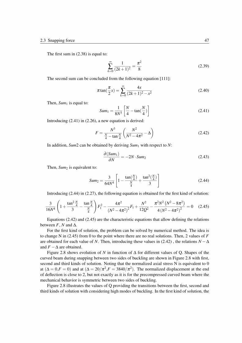
2.3 Snapping force 47
The first sum in (2.38) is equal to:
∞
∑k=0
1
(2k+1)2=
π2
8(2.39)
The second sum can be concluded from the following equation [111]:
π tan(π2
x) =∞
∑k=0
4x
(2k+1)2 − x2(2.40)
Then, Sum1 is equal to:
Sum1 =1
8N3
�N
4− tan(
N
4)
�(2.41)
Introducing (2.41) in (2.26), a new equation is derived:
F =N3
N4− tan N
4
�N2
N2 −4π2−Δ
�(2.42)
In addition, Sum2 can be obtained by deriving Sum1 with respect to N:
∂ (Sum1)
∂N=−2N ·Sum2 (2.43)
Then, Sum2 is equivalent to:
Sum2 =3
64N4
�1− tan(N
4)
N4
+tan2(N
4)
3
�(2.44)
Introducing (2.44) in (2.27), the following equation is obtained for the first kind of solution:
3
16N4
�1+
tan2 N4
3− tan N
4N4
�F2
1 − 4π2
(N2 −4π2)2F1 +
N2
12Q2− π2N2
�N2 −8π2
�
4(N2 −4π2)2= 0 (2.45)
Equations (2.42) and (2.45) are the characteristic equations that allow defining the relations
between F , N and Δ.
For the first kind of solution, the problem can be solved by numerical method. The idea is
to change N in (2.45) from 0 to the point where there are no real solutions. Then, 2 values of F
are obtained for each value of N. Then, introducing these values in (2.42) , the relations N −Δand F −Δ are obtained.
Figure 2.8 shows evolution of N in function of Δ for different values of Q. Shapes of the
curved beam during snapping between two sides of buckling are shown in Figure 2.8 with first,
second and third kinds of solution. Noting that the normalized axial stress N is equivalent to 0
at (Δ = 0,F = 0) and at (Δ = 20/π2,F = 3840/π2). The normalized displacement at the end
of deflection is close to 2, but not exactly as it is for the precompressed curved beam where the
mechanical behavior is symmetric between two sides of buckling.
Figure 2.8 illustrates the values of Q providing the transitions between the first, second and
third kinds of solution with considering high modes of buckling. In the first kind of solution, the
48 Chapter 2
FIGURE 2.8: Evolution of the normalized axial stress N in the first kind of solution in function of Q ratio.
N is constant in the second and third kinds of solution. The shape of the curved beam in the first, second
and third case.
maximum value of N that can be reached during snapping increases with increasing the value
of Q. N exceeds N1 only for:
Q ≥�
64π2
117−7π2≈ 1.16 (2.46)
Noting that at N = N1, the normalized force has a unique value F = 2π4.
On the other side, the third kind of solution is simpler. Making N constant at N3 = 4π , the
third kind simplify the previous equations. Evolution of the force can be then directly concluded
from (2.42):
F3 = 64π2
�4
3−Δ
�(2.47)
Figure 2.9 shows evolution of the snapping force F in function of Δ for different values of
Q with constraining mode 2 and considering high modes of buckling.
FIGURE 2.9: Evolution of the normalized applied force F for the curved beam for different Q values
when mode 2 is constrained.
2.4 Bistability conditions 49
The mode constant A3 which appears in the third kind of solution is obtained by recalculating
(2.45) without canceling A3, then introducing (2.42) in the new equation:
A23 =− 3
4π2Δ2 +
14
9π2Δ+
1
18− 20
27π2− 1
3Q2(2.48)
Noting that the sign of A3 changes with the direction of deflection.
In light of the equation of A3, the third mode cannot appear unless Q respects the following
condition:
Q ≥�
162π2
27π2 +32≈ 2.314 (2.49)
Further, Δtop, Δbot (Figure 2.9), which are the exact positions where the third mode appears,
and Ftop, Fbot which are the value of F at these positions can be concluded from (2.47) and
(2.48) respectively:
Δtop,Δbot =28
27±
2π3
�1
6+
16
81π2− 1
Q2
Ftop,Fbot = 64π2
�8
27∓ 2π
3
�1
6+
16
81π2− 1
Q2
� (2.50)
Equation 2.50 shows the analytical expressions of the coordinates of the main snapping
points. These expressions show clearly the influence of the different parameters on the snapping
force behavior. The influence of these parameters will be investigated in Section 2.7.
2.4 Bistability conditions
Physically, the curves in Figure 2.9 represent the amount of the lateral force produced by the
beam in the center point after deflection. In this context, the bistability that we look for is
provided by the negative portions of F produced by the beam that will push to the other buckling
side.
As we can conclude from Figure 2.9, the value of the snapping force is not symmetric
between two sides of buckling. This comes from the bending energy which starts its evolution
from the as-fabricated initial shape.
The shift-up of the curves in Figure 2.9 affects the bistability behavior. Mechanical con-
ditions must be considered in order to involve bistability, while the greater margin of stability
remains in the first side of buckling.
In the other side, canceling F in (2.45) for the first kind of solution, three values of N are
obtained. Putting these values in (2.42), three values of Δ are obtained:
Δ =
�0,
3
2±
�1
4− 4
3Q2
�(2.51)
We conclude from (2.51) and Figure 2.9 that the beam exhibits two stable positions, only
for Q >�
163≈ 2.31.
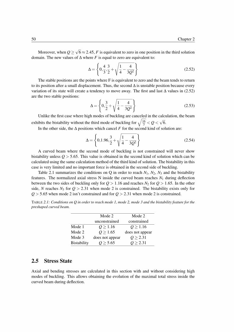
50 Chapter 2
Moreover, when Q ≥√
6 ≈ 2.45, F is equivalent to zero in one position in the third solution
domain. The new values of Δ where F is equal to zero are equivalent to:
Δ =
�0,
4
3,3
2+
�1
4− 4
3Q2
�(2.52)
The stable positions are the points where F is equivalent to zero and the beam tends to return
to its position after a small displacement. Thus, the second Δ is unstable position because every
variation of its state will create a tendency to move away. The first and last Δ values in (2.52)
are the two stable positions:
Δ =
�0,
3
2+
�1
4− 4
3Q2
�(2.53)
Unlike the first case where high modes of buckling are canceled in the calculation, the beam
exhibits the bistability without the third mode of buckling for
�163< Q <
√6.
In the other side, the Δ positions which cancel F for the second kind of solution are:
Δ =
�0,1.96,
3
2+
�1
4− 4
3Q2
�(2.54)
A curved beam where the second mode of buckling is not constrained will never show
bistability unless Q > 5.65. This value is obtained in the second kind of solution which can be
calculated using the same calculation method of the third kind of solution. The bistability in this
case is very limited and no important force is obtained in the second side of buckling.
Table 2.1 summarizes the conditions on Q in order to reach N1, N2, N3 and the bistability
features. The normalized axial stress N inside the curved beam reaches N1 during deflection
between the two sides of buckling only for Q > 1.16 and reaches N2 for Q > 1.65. In the other
side, N reaches N3 for Q > 2.31 when mode 2 is constrained. The bistability exists only for
Q > 5.65 when mode 2 isn’t constrained and for Q > 2.31 when mode 2 is constrained.
TABLE 2.1: Conditions on Q in order to reach mode 1, mode 2, mode 3 and the bistability feature for the
preshaped curved beam.
Mode 2 Mode 2
unconstrained constrained
Mode 1 Q ≥ 1.16 Q ≥ 1.16
Mode 2 Q ≥ 1.65 does not appear
Mode 3 does not appear Q ≥ 2.31
Bistability Q ≥ 5.65 Q ≥ 2.31
2.5 Stress State
Axial and bending stresses are calculated in this section with and without considering high
modes of buckling. This allows obtaining the evolution of the maximal total stress inside the
curved beam during deflection.
2.5 Stress State 51
2.5.1 Without high modes of buckling
Stresses inside the beam are decomposed into axial and bending stresses. Axial stress is constant
along the beam and has a maximum when the deflection is around the middle while bending
stress changes along the beam sections and increases as far as the deflection is closer to the
other side. Further, axial stress p is equivalent to:
p =Et2
12l2N2 (2.55)
The bending stress T given in (2.6) starts evolution from the initial shape, T becomes:
T = Ez
�d2w
dx2− d2w
dx2
�(2.56)
The approximation of neglecting high modes of buckling simplifies the calculation [106].
The following equations summarize the first and third solution kinds with eliminating high
modes. For the first kind of solution:
F1 =3π4Q2
2Δ�
Δ2 −3Δ+2+4
3Q2
�
N2 = 3π2Q2(−Δ2 +2Δ)
W (X) = A1W1(X); A1 =1−Δ
2
(2.57)
For the third kind of solution:
F3 = 6π4(4
3−Δ)
N = N3
W (X) = A1W1(X)+A3W3(X)
A1 =1−Δ
2;A2
3 =− 1
16
�Δ2 −2Δ+
16
3Q2
�(2.58)
For the first kind of solution, axial stress is simply concluded from (2.55) and (2.57):
p = π2 Eth
l2
Q
4(−Δ2 +2Δ) (2.59)
Also, bending stress is obtained using (2.56) and (2.57):
T =2π2Ezh
l2Δcos2π
x
l(2.60)
The same for the third kind of solution, axial and bending stresses are calculated from (2.55),
(2.56) and (2.58):
p = π2 Eth
l2
4
3Q(2.61)
T =2π2Ezh
l2
�Δcos2π
x
l−2
�−Δ2 +2Δ− 16
3Q2cos4π
x
l
�(2.62)
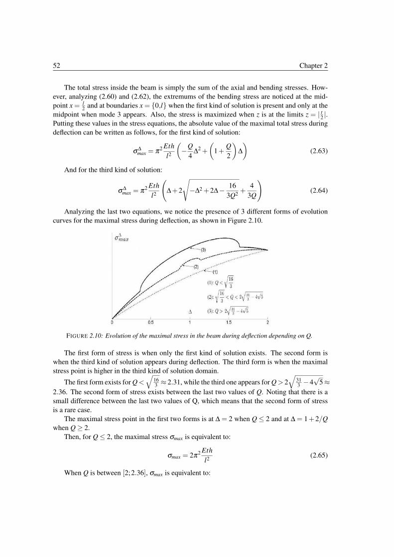
52 Chapter 2
The total stress inside the beam is simply the sum of the axial and bending stresses. How-
ever, analyzing (2.60) and (2.62), the extremums of the bending stress are noticed at the mid-
point x = l2
and at boundaries x = {0,l} when the first kind of solution is present and only at the
midpoint when mode 3 appears. Also, the stress is maximized when z is at the limits z = | t2|.
Putting these values in the stress equations, the absolute value of the maximal total stress during
deflection can be written as follows, for the first kind of solution:
σΔmax = π2 Eth
l2
�−Q
4Δ2 +
�1+
Q
2
�Δ�
(2.63)
And for the third kind of solution:
σΔmax = π2 Eth
l2
�Δ+2
�−Δ2 +2Δ− 16
3Q2+
4
3Q
�(2.64)
Analyzing the last two equations, we notice the presence of 3 different forms of evolution
curves for the maximal stress during deflection, as shown in Figure 2.10.
FIGURE 2.10: Evolution of the maximal stress in the beam during deflection depending on Q.
The first form of stress is when only the first kind of solution exists. The second form is
when the third kind of solution appears during deflection. The third form is when the maximal
stress point is higher in the third kind of solution domain.
The first form exists for Q<�
163≈ 2.31, while the third one appears for Q> 2
�313−4
√5≈
2.36. The second form of stress exists between the last two values of Q. Noting that there is a
small difference between the last two values of Q, which means that the second form of stress
is a rare case.
The maximal stress point in the first two forms is at Δ = 2 when Q ≤ 2 and at Δ = 1+2/Q
when Q ≥ 2.
Then, for Q ≤ 2, the maximal stress σmax is equivalent to:
σmax = 2π2 Eth
l2(2.65)
When Q is between [2;2.36], σmax is equivalent to:
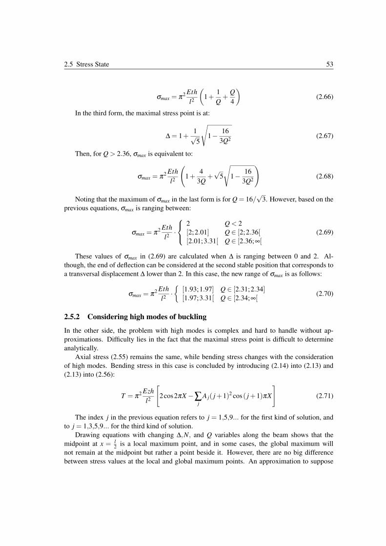
2.5 Stress State 53
σmax = π2 Eth
l2
�1+
1
Q+
Q
4
�(2.66)
In the third form, the maximal stress point is at:
Δ = 1+1√5
�1− 16
3Q2(2.67)
Then, for Q > 2.36, σmax is equivalent to:
σmax = π2 Eth
l2
�1+
4
3Q+√
5
�1− 16
3Q2
�(2.68)
Noting that the maximum of σmax in the last form is for Q = 16/√
3. However, based on the
previous equations, σmax is ranging between:
σmax = π2 Eth
l2·
2 Q < 2
[2;2.01] Q ∈ [2;2.36[[2.01;3.31[ Q ∈ [2.36;∞[
(2.69)
These values of σmax in (2.69) are calculated when Δ is ranging between 0 and 2. Al-
though, the end of deflection can be considered at the second stable position that corresponds to
a transversal displacement Δ lower than 2. In this case, the new range of σmax is as follows:
σmax = π2 Eth
l2·
�[1.93;1.97] Q ∈ [2.31;2.34][1.97;3.31[ Q ∈ [2.34;∞[
(2.70)
2.5.2 Considering high modes of buckling
In the other side, the problem with high modes is complex and hard to handle without ap-
proximations. Difficulty lies in the fact that the maximal stress point is difficult to determine
analytically.
Axial stress (2.55) remains the same, while bending stress changes with the consideration
of high modes. Bending stress in this case is concluded by introducing (2.14) into (2.13) and
(2.13) into (2.56):
T = π2 Ezh
l2
�2cos2πX −∑
j
A j( j+1)2 cos( j+1)πX
�(2.71)
The index j in the previous equation refers to j = 1,5,9... for the first kind of solution, and
to j = 1,3,5,9... for the third kind of solution.
Drawing equations with changing Δ,N, and Q variables along the beam shows that the
midpoint at x = l2
is a local maximum point, and in some cases, the global maximum will
not remain at the midpoint but rather a point beside it. However, there are no big difference
between stress values at the local and global maximum points. An approximation to suppose
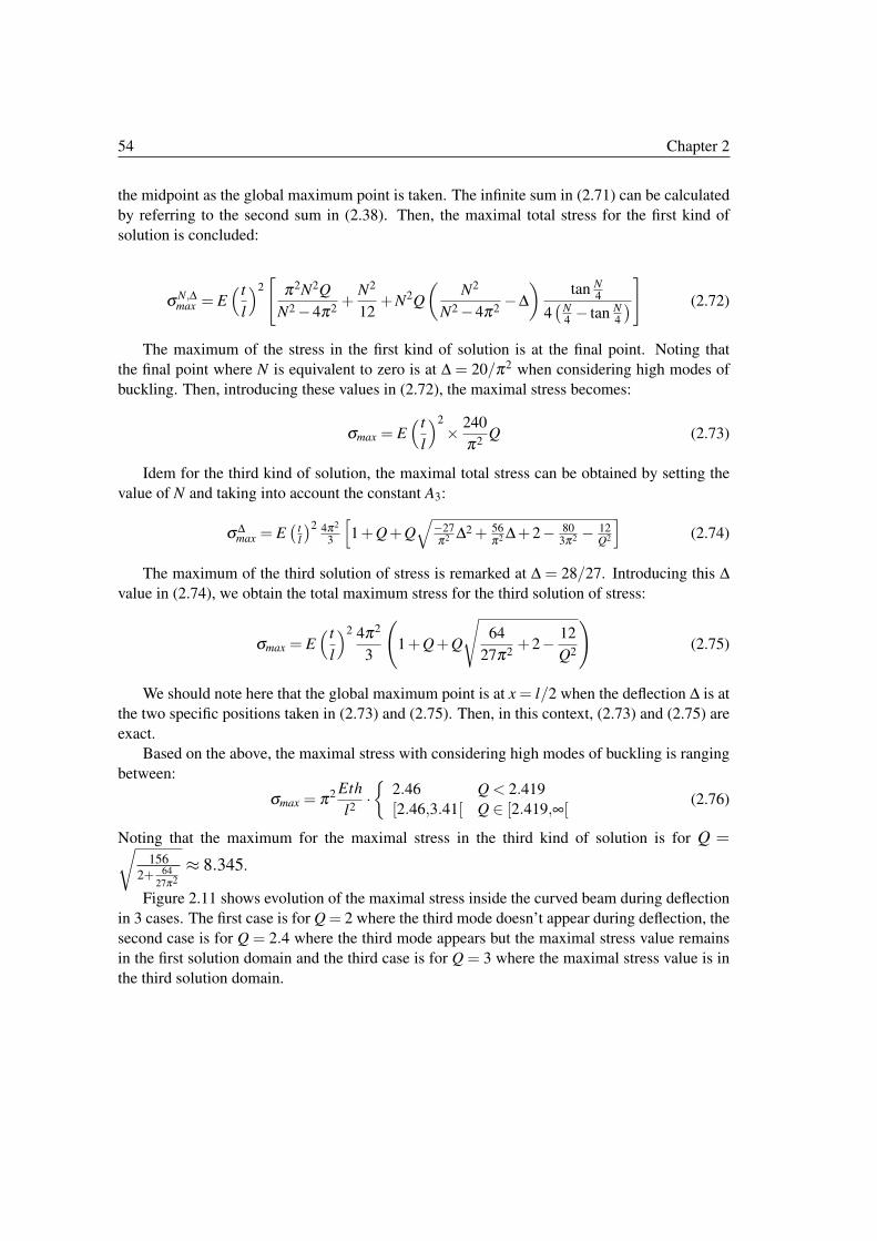
54 Chapter 2
the midpoint as the global maximum point is taken. The infinite sum in (2.71) can be calculated
by referring to the second sum in (2.38). Then, the maximal total stress for the first kind of
solution is concluded:
σN,Δmax = E
� t
l
�2�
π2N2Q
N2 −4π2+
N2
12+N2Q
�N2
N2 −4π2−Δ
�tan N
4
4�
N4− tan N
4
��
(2.72)
The maximum of the stress in the first kind of solution is at the final point. Noting that
the final point where N is equivalent to zero is at Δ = 20/π2 when considering high modes of
buckling. Then, introducing these values in (2.72), the maximal stress becomes:
σmax = E� t
l
�2
×240
π2Q (2.73)
Idem for the third kind of solution, the maximal total stress can be obtained by setting the
value of N and taking into account the constant A3:
σΔmax = E
�tl
�2 4π2
3
�1+Q+Q
�−27π2 Δ2 + 56
π2 Δ+2− 803π2 − 12
Q2
�(2.74)
The maximum of the third solution of stress is remarked at Δ = 28/27. Introducing this Δvalue in (2.74), we obtain the total maximum stress for the third solution of stress:
σmax = E� t
l
�2 4π2
3
�1+Q+Q
�64
27π2+2− 12
Q2
�(2.75)
We should note here that the global maximum point is at x = l/2 when the deflection Δ is at
the two specific positions taken in (2.73) and (2.75). Then, in this context, (2.73) and (2.75) are
exact.
Based on the above, the maximal stress with considering high modes of buckling is ranging
between:
σmax = π2 Eth
l2·
�2.46 Q < 2.419
[2.46,3.41[ Q ∈ [2.419,∞[(2.76)
Noting that the maximum for the maximal stress in the third kind of solution is for Q =�156
2+ 64
27π2
≈ 8.345.
Figure 2.11 shows evolution of the maximal stress inside the curved beam during deflection
in 3 cases. The first case is for Q = 2 where the third mode doesn’t appear during deflection, the
second case is for Q = 2.4 where the third mode appears but the maximal stress value remains
in the first solution domain and the third case is for Q = 3 where the maximal stress value is in
the third solution domain.
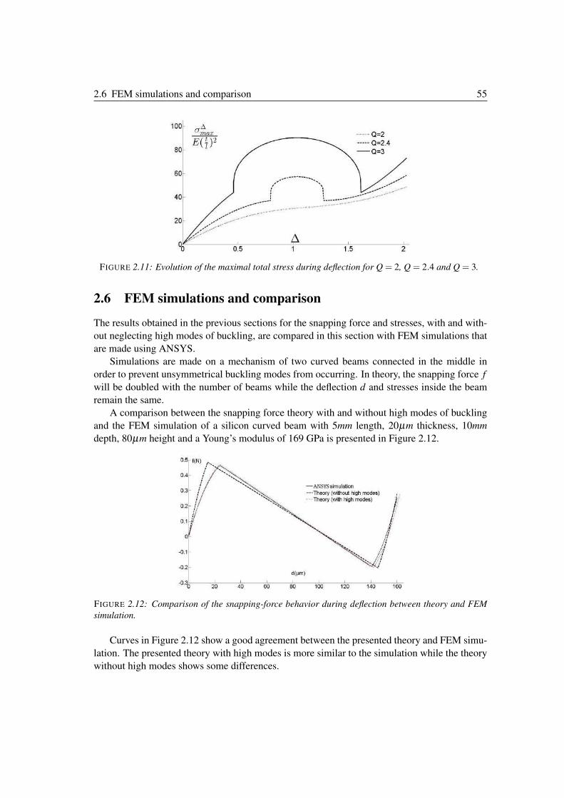
2.6 FEM simulations and comparison 55
FIGURE 2.11: Evolution of the maximal total stress during deflection for Q = 2, Q = 2.4 and Q = 3.
2.6 FEM simulations and comparison
The results obtained in the previous sections for the snapping force and stresses, with and with-
out neglecting high modes of buckling, are compared in this section with FEM simulations that
are made using ANSYS.
Simulations are made on a mechanism of two curved beams connected in the middle in
order to prevent unsymmetrical buckling modes from occurring. In theory, the snapping force f
will be doubled with the number of beams while the deflection d and stresses inside the beam
remain the same.
A comparison between the snapping force theory with and without high modes of buckling
and the FEM simulation of a silicon curved beam with 5mm length, 20µm thickness, 10mm
depth, 80µm height and a Young’s modulus of 169 GPa is presented in Figure 2.12.
FIGURE 2.12: Comparison of the snapping-force behavior during deflection between theory and FEM
simulation.
Curves in Figure 2.12 show a good agreement between the presented theory and FEM simu-
lation. The presented theory with high modes is more similar to the simulation while the theory
without high modes shows some differences.
56 Chapter 2
The presented modeling with high modes of buckling allows obtaining the expressions of the
different values of Q and the main snapping points (Δtop,Ftop,Δbot ,Fbot) that include the effects
of all modes of buckling. In the example given in Figure 2.12, the relative difference between
the negligence and the consideration of high modes of buckling for the values of the snapping
points (Δtop, Ftop, Δbot , Fbot) is equivalent to (38.53%,2.93%,2.32%,1.39%) respectively.
The quite large error on the Δtop parameter could be a problem for the design of a bistable
system. Reminding that the bistable system, as we assume , is composed of a preshaped curved
beam bistable mechanism and actuators for switching between both stable positions. The snap-
ping points in terms of displacements and forces respectively define the stroke and the force that
the actuators have to provide. Thus, the accurate knowledge of the relations between the snap-
ping points and the preshaped curved beam dimensions is very important in order to achieve the
best integration of the complete bistable system.
In the other side, Figure 2.13 shows a comparison of the evolution of the maximal stresses,
between the theory with and without high modes of buckling and FEM simulation on a curved
beam with the same dimensions and properties.
FIGURE 2.13: Comparison between the maximal stress value during deflection between theory ans FEM
simulation.
The importance of high modes of buckling is more obvious in the calculation of stresses.
As shown in Figure 2.13, neglecting high modes makes a significant difference between the
calculated stress and the simulation. Differences appear in the shape of the stress curves and in
the highest stress point position.
Figure 2.14 shows the evolution of the maximal bending stress in the two cases, with and
without high modes of buckling.
Comparing the results in Figure 2.13 and 2.14, we conclude that the bending stress has the
main contribution in the total stress value. The bending and total stress curves have almost
the same shape. Then, the contribution of high modes of buckling is more important in the
calculation of the bending stresses.
In the first kind of solution, the axial stress evolves after deflection from the two sides of
buckling to the middle (Figure 2.8), while the maximal bending stress is higher when the curved
beam is far away from its initial position (Figure 2.14, parts AB & CD).
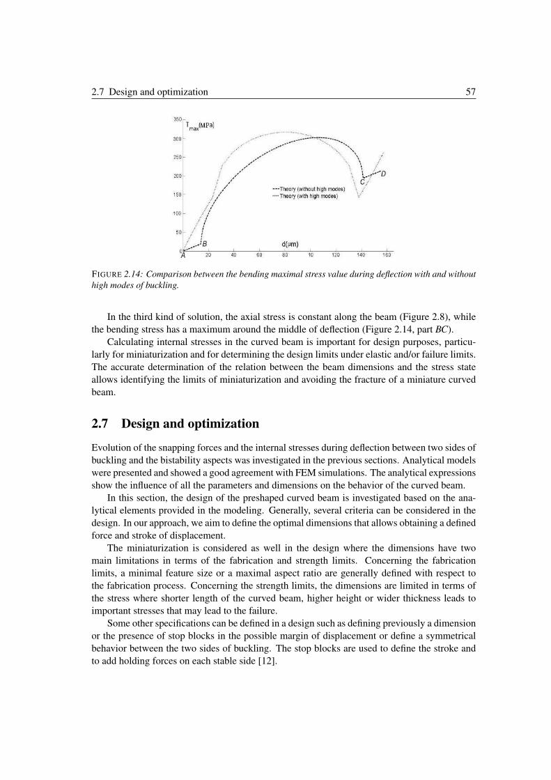
2.7 Design and optimization 57
FIGURE 2.14: Comparison between the bending maximal stress value during deflection with and without
high modes of buckling.
In the third kind of solution, the axial stress is constant along the beam (Figure 2.8), while
the bending stress has a maximum around the middle of deflection (Figure 2.14, part BC).
Calculating internal stresses in the curved beam is important for design purposes, particu-
larly for miniaturization and for determining the design limits under elastic and/or failure limits.
The accurate determination of the relation between the beam dimensions and the stress state
allows identifying the limits of miniaturization and avoiding the fracture of a miniature curved
beam.
2.7 Design and optimization
Evolution of the snapping forces and the internal stresses during deflection between two sides of
buckling and the bistability aspects was investigated in the previous sections. Analytical models
were presented and showed a good agreement with FEM simulations. The analytical expressions
show the influence of all the parameters and dimensions on the behavior of the curved beam.
In this section, the design of the preshaped curved beam is investigated based on the ana-
lytical elements provided in the modeling. Generally, several criteria can be considered in the
design. In our approach, we aim to define the optimal dimensions that allows obtaining a defined
force and stroke of displacement.
The miniaturization is considered as well in the design where the dimensions have two
main limitations in terms of the fabrication and strength limits. Concerning the fabrication
limits, a minimal feature size or a maximal aspect ratio are generally defined with respect to
the fabrication process. Concerning the strength limits, the dimensions are limited in terms of
the stress where shorter length of the curved beam, higher height or wider thickness leads to
important stresses that may lead to the failure.
Some other specifications can be defined in a design such as defining previously a dimension
or the presence of stop blocks in the possible margin of displacement or define a symmetrical
behavior between the two sides of buckling. The stop blocks are used to define the stroke and
to add holding forces on each stable side [12].
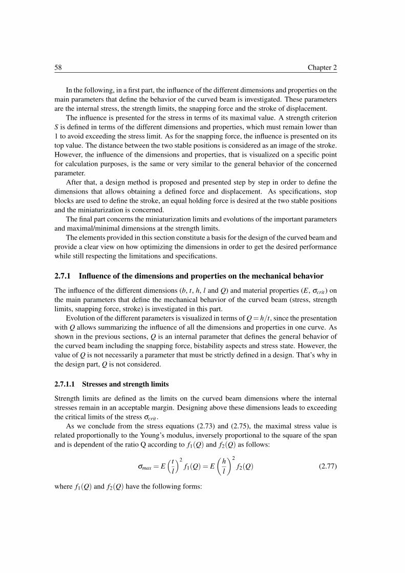
58 Chapter 2
In the following, in a first part, the influence of the different dimensions and properties on the
main parameters that define the behavior of the curved beam is investigated. These parameters
are the internal stress, the strength limits, the snapping force and the stroke of displacement.
The influence is presented for the stress in terms of its maximal value. A strength criterion
S is defined in terms of the different dimensions and properties, which must remain lower than
1 to avoid exceeding the stress limit. As for the snapping force, the influence is presented on its
top value. The distance between the two stable positions is considered as an image of the stroke.
However, the influence of the dimensions and properties, that is visualized on a specific point
for calculation purposes, is the same or very similar to the general behavior of the concerned
parameter.
After that, a design method is proposed and presented step by step in order to define the
dimensions that allows obtaining a defined force and displacement. As specifications, stop
blocks are used to define the stroke, an equal holding force is desired at the two stable positions
and the miniaturization is concerned.
The final part concerns the miniaturization limits and evolutions of the important parameters
and maximal/minimal dimensions at the strength limits.
The elements provided in this section constitute a basis for the design of the curved beam and
provide a clear view on how optimizing the dimensions in order to get the desired performance
while still respecting the limitations and specifications.
2.7.1 Influence of the dimensions and properties on the mechanical behavior
The influence of the different dimensions (b, t, h, l and Q) and material properties (E, σcrit) on
the main parameters that define the mechanical behavior of the curved beam (stress, strength
limits, snapping force, stroke) is investigated in this part.
Evolution of the different parameters is visualized in terms of Q= h/t, since the presentation
with Q allows summarizing the influence of all the dimensions and properties in one curve. As
shown in the previous sections, Q is an internal parameter that defines the general behavior of
the curved beam including the snapping force, bistability aspects and stress state. However, the
value of Q is not necessarily a parameter that must be strictly defined in a design. That’s why in
the design part, Q is not considered.
2.7.1.1 Stresses and strength limits
Strength limits are defined as the limits on the curved beam dimensions where the internal
stresses remain in an acceptable margin. Designing above these dimensions leads to exceeding
the critical limits of the stress σcrit .
As we conclude from the stress equations (2.73) and (2.75), the maximal stress value is
related proportionally to the Young’s modulus, inversely proportional to the square of the span
and is dependent of the ratio Q according to f1(Q) and f2(Q) as follows:
σmax = E� t
l
�2
f1(Q) = E
�h
l
�2
f2(Q) (2.77)
where f1(Q) and f2(Q) have the following forms:
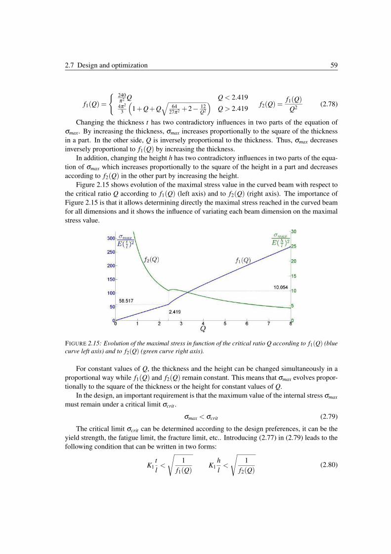
2.7 Design and optimization 59
f1(Q) =
�240π2 Q Q < 2.419
4π2
3
�1+Q+Q
�64
27π2 +2− 12Q2
�Q > 2.419
f2(Q) =f1(Q)
Q2(2.78)
Changing the thickness t has two contradictory influences in two parts of the equation of
σmax. By increasing the thickness, σmax increases proportionally to the square of the thickness
in a part. In the other side, Q is inversely proportional to the thickness. Thus, σmax decreases
inversely proportional to f1(Q) by increasing the thickness.
In addition, changing the height h has two contradictory influences in two parts of the equa-
tion of σmax which increases proportionally to the square of the height in a part and decreases
according to f2(Q) in the other part by increasing the height.
Figure 2.15 shows evolution of the maximal stress value in the curved beam with respect to
the critical ratio Q according to f1(Q) (left axis) and to f2(Q) (right axis). The importance of
Figure 2.15 is that it allows determining directly the maximal stress reached in the curved beam
for all dimensions and it shows the influence of variating each beam dimension on the maximal
stress value.
FIGURE 2.15: Evolution of the maximal stress in function of the critical ratio Q according to f1(Q) (blue
curve left axis) and to f2(Q) (green curve right axis).
For constant values of Q, the thickness and the height can be changed simultaneously in a
proportional way while f1(Q) and f2(Q) remain constant. This means that σmax evolves propor-
tionally to the square of the thickness or the height for constant values of Q.
In the design, an important requirement is that the maximum value of the internal stress σmax
must remain under a critical limit σcrit .
σmax < σcrit (2.79)
The critical limit σcrit can be determined according to the design preferences, it can be the
yield strength, the fatigue limit, the fracture limit, etc.. Introducing (2.77) in (2.79) leads to the
following condition that can be written in two forms:
K1t
l<
�1
f1(Q)K1
h
l<
�1
f2(Q)(2.80)
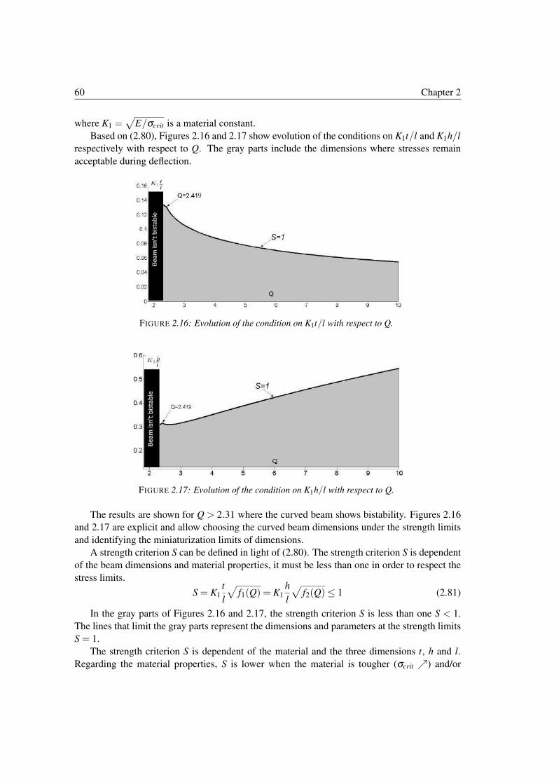
60 Chapter 2
where K1 =�
E/σcrit is a material constant.
Based on (2.80), Figures 2.16 and 2.17 show evolution of the conditions on K1t/l and K1h/l
respectively with respect to Q. The gray parts include the dimensions where stresses remain
acceptable during deflection.
FIGURE 2.16: Evolution of the condition on K1t/l with respect to Q.
FIGURE 2.17: Evolution of the condition on K1h/l with respect to Q.
The results are shown for Q > 2.31 where the curved beam shows bistability. Figures 2.16
and 2.17 are explicit and allow choosing the curved beam dimensions under the strength limits
and identifying the miniaturization limits of dimensions.
A strength criterion S can be defined in light of (2.80). The strength criterion S is dependent
of the beam dimensions and material properties, it must be less than one in order to respect the
stress limits.
S = K1t
l
�f1(Q) = K1
h
l
�f2(Q)≤ 1 (2.81)
In the gray parts of Figures 2.16 and 2.17, the strength criterion S is less than one S < 1.
The lines that limit the gray parts represent the dimensions and parameters at the strength limits
S = 1.
The strength criterion S is dependent of the material and the three dimensions t, h and l.
Regarding the material properties, S is lower when the material is tougher (σcrit �) and/or
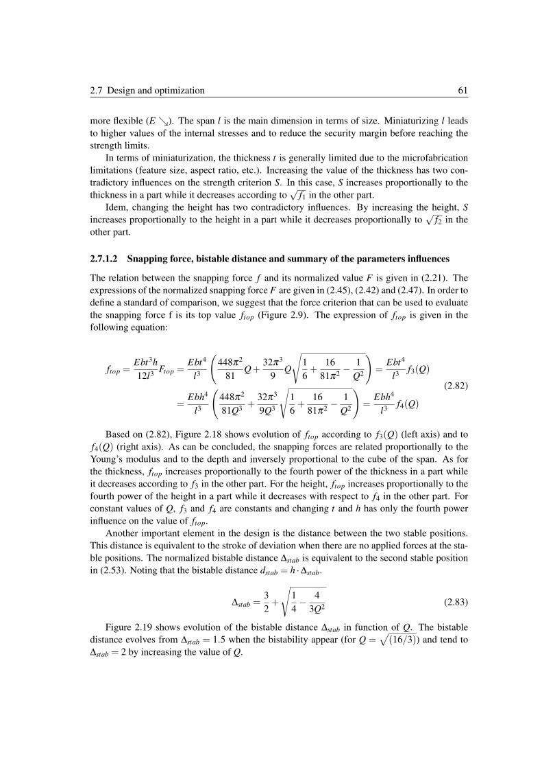
2.7 Design and optimization 61
more flexible (E �). The span l is the main dimension in terms of size. Miniaturizing l leads
to higher values of the internal stresses and to reduce the security margin before reaching the
strength limits.
In terms of miniaturization, the thickness t is generally limited due to the microfabrication
limitations (feature size, aspect ratio, etc.). Increasing the value of the thickness has two con-
tradictory influences on the strength criterion S. In this case, S increases proportionally to the
thickness in a part while it decreases according to√
f1 in the other part.
Idem, changing the height has two contradictory influences. By increasing the height, S
increases proportionally to the height in a part while it decreases proportionally to√
f2 in the
other part.
2.7.1.2 Snapping force, bistable distance and summary of the parameters influences
The relation between the snapping force f and its normalized value F is given in (2.21). The
expressions of the normalized snapping force F are given in (2.45), (2.42) and (2.47). In order to
define a standard of comparison, we suggest that the force criterion that can be used to evaluate
the snapping force f is its top value ftop (Figure 2.9). The expression of ftop is given in the
following equation:
ftop =Ebt3h
12l3Ftop =
Ebt4
l3
�448π2
81Q+
32π3
9Q
�1
6+
16
81π2− 1
Q2
�=
Ebt4
l3f3(Q)
=Ebh4
l3
�448π2
81Q3+
32π3
9Q3
�1
6+
16
81π2− 1
Q2
�=
Ebh4
l3f4(Q)
(2.82)
Based on (2.82), Figure 2.18 shows evolution of ftop according to f3(Q) (left axis) and to
f4(Q) (right axis). As can be concluded, the snapping forces are related proportionally to the
Young’s modulus and to the depth and inversely proportional to the cube of the span. As for
the thickness, ftop increases proportionally to the fourth power of the thickness in a part while
it decreases according to f3 in the other part. For the height, ftop increases proportionally to the
fourth power of the height in a part while it decreases with respect to f4 in the other part. For
constant values of Q, f3 and f4 are constants and changing t and h has only the fourth power
influence on the value of ftop.
Another important element in the design is the distance between the two stable positions.
This distance is equivalent to the stroke of deviation when there are no applied forces at the sta-
ble positions. The normalized bistable distance Δstab is equivalent to the second stable position
in (2.53). Noting that the bistable distance dstab = h ·Δstab.
Δstab =3
2+
�1
4− 4
3Q2(2.83)
Figure 2.19 shows evolution of the bistable distance Δstab in function of Q. The bistable
distance evolves from Δstab = 1.5 when the bistability appear (for Q =�(16/3)) and tend to
Δstab = 2 by increasing the value of Q.
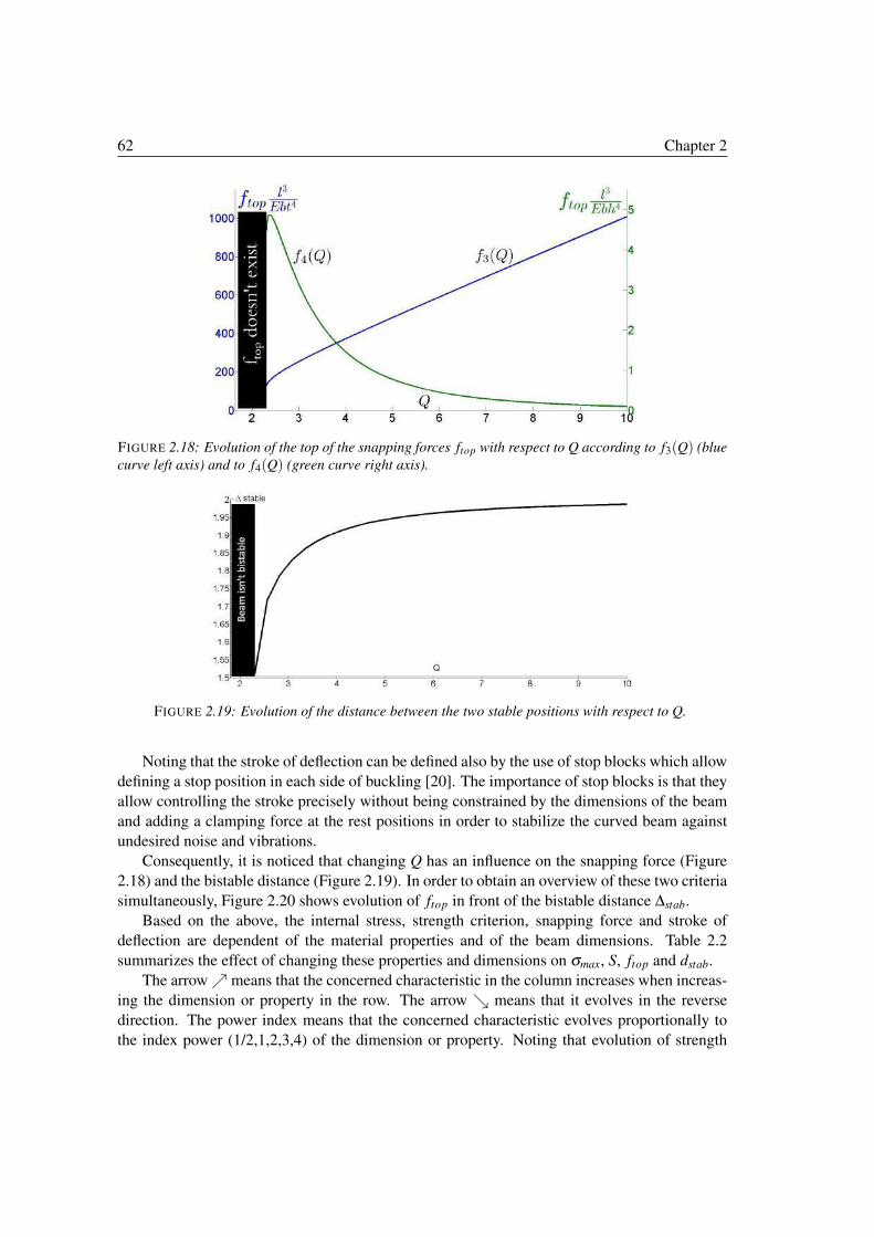
62 Chapter 2
FIGURE 2.18: Evolution of the top of the snapping forces ftop with respect to Q according to f3(Q) (blue
curve left axis) and to f4(Q) (green curve right axis).
FIGURE 2.19: Evolution of the distance between the two stable positions with respect to Q.
Noting that the stroke of deflection can be defined also by the use of stop blocks which allow
defining a stop position in each side of buckling [20]. The importance of stop blocks is that they
allow controlling the stroke precisely without being constrained by the dimensions of the beam
and adding a clamping force at the rest positions in order to stabilize the curved beam against
undesired noise and vibrations.
Consequently, it is noticed that changing Q has an influence on the snapping force (Figure
2.18) and the bistable distance (Figure 2.19). In order to obtain an overview of these two criteria
simultaneously, Figure 2.20 shows evolution of ftop in front of the bistable distance Δstab.
Based on the above, the internal stress, strength criterion, snapping force and stroke of
deflection are dependent of the material properties and of the beam dimensions. Table 2.2
summarizes the effect of changing these properties and dimensions on σmax, S, ftop and dstab.
The arrow � means that the concerned characteristic in the column increases when increas-
ing the dimension or property in the row. The arrow � means that it evolves in the reverse
direction. The power index means that the concerned characteristic evolves proportionally to
the index power (1/2,1,2,3,4) of the dimension or property. Noting that evolution of strength
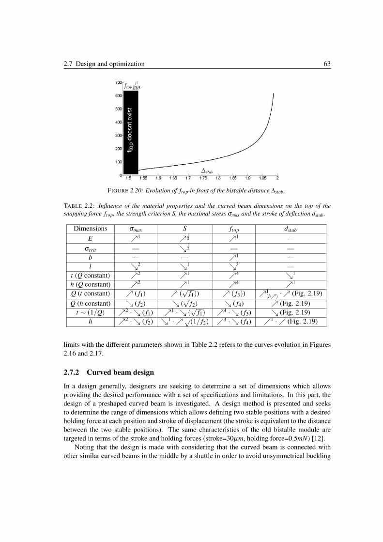
2.7 Design and optimization 63
FIGURE 2.20: Evolution of ftop in front of the bistable distance Δstab.
TABLE 2.2: Influence of the material properties and the curved beam dimensions on the top of the
snapping force ftop, the strength criterion S, the maximal stress σmax and the stroke of deflection dstab.
Dimensions σmax S ftop dstab
E �1 � 12 �1 —
σcrit — � 12 — —
b — — �1 —
l �2 �1 �3 —
t (Q constant) �2 �1 �4 �1
h (Q constant) �2 �1 �4 �1
Q (t constant) � ( f1) � (√
f1)) � ( f3)) �1(h�) ·� (Fig. 2.19)
Q (h constant) � ( f2) � (√
f2) � ( f4) � (Fig. 2.19)
t ∼ (1/Q) �2 ·� ( f1) �1 ·� (√
f1) �4 ·� ( f3) � (Fig. 2.19)
h �2 ·� ( f2) �1 ·�√(1/ f2) �4 ·� ( f4) �1 ·� (Fig. 2.19)
limits with the different parameters shown in Table 2.2 refers to the curves evolution in Figures
2.16 and 2.17.
2.7.2 Curved beam design
In a design generally, designers are seeking to determine a set of dimensions which allows
providing the desired performance with a set of specifications and limitations. In this part, the
design of a preshaped curved beam is investigated. A design method is presented and seeks
to determine the range of dimensions which allows defining two stable positions with a desired
holding force at each position and stroke of displacement (the stroke is equivalent to the distance
between the two stable positions). The same characteristics of the old bistable module are
targeted in terms of the stroke and holding forces (stroke=30µm, holding force=0.5mN) [12].
Noting that the design is made with considering that the curved beam is connected with
other similar curved beams in the middle by a shuttle in order to avoid unsymmetrical buckling
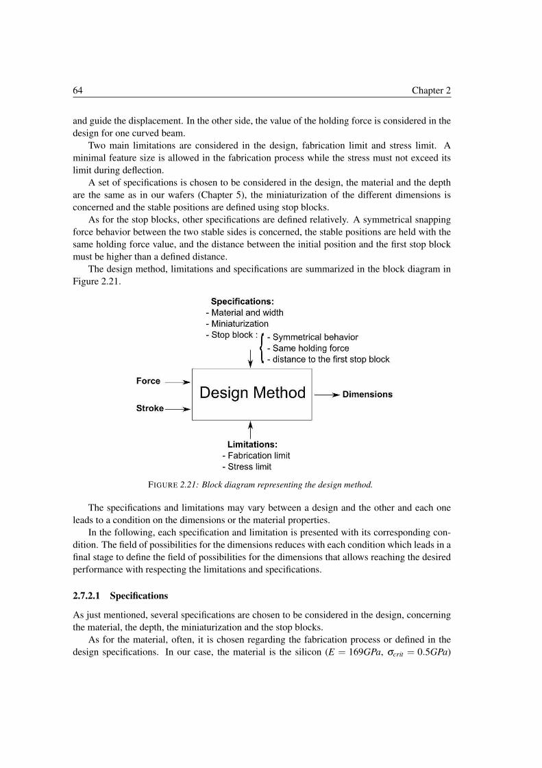
64 Chapter 2
and guide the displacement. In the other side, the value of the holding force is considered in the
design for one curved beam.
Two main limitations are considered in the design, fabrication limit and stress limit. A
minimal feature size is allowed in the fabrication process while the stress must not exceed its
limit during deflection.
A set of specifications is chosen to be considered in the design, the material and the depth
are the same as in our wafers (Chapter 5), the miniaturization of the different dimensions is
concerned and the stable positions are defined using stop blocks.
As for the stop blocks, other specifications are defined relatively. A symmetrical snapping
force behavior between the two stable sides is concerned, the stable positions are held with the
same holding force value, and the distance between the initial position and the first stop block
must be higher than a defined distance.
The design method, limitations and specifications are summarized in the block diagram in
Figure 2.21.
FIGURE 2.21: Block diagram representing the design method.
The specifications and limitations may vary between a design and the other and each one
leads to a condition on the dimensions or the material properties.
In the following, each specification and limitation is presented with its corresponding con-
dition. The field of possibilities for the dimensions reduces with each condition which leads in a
final stage to define the field of possibilities for the dimensions that allows reaching the desired
performance with respecting the limitations and specifications.
2.7.2.1 Specifications
As just mentioned, several specifications are chosen to be considered in the design, concerning
the material, the depth, the miniaturization and the stop blocks.
As for the material, often, it is chosen regarding the fabrication process or defined in the
design specifications. In our case, the material is the silicon (E = 169GPa, σcrit = 0.5GPa)
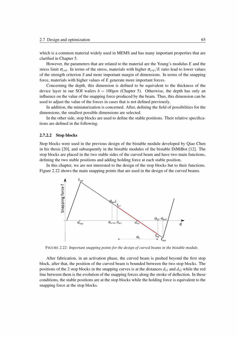
2.7 Design and optimization 65
which is a common material widely used in MEMS and has many important properties that are
clarified in Chapter 5.
However, the parameters that are related to the material are the Young’s modulus E and the
stress limit σcrit . In terms of the stress, materials with higher σcrit/E ratio lead to lower values
of the strength criterion S and more important margin of dimensions. In terms of the snapping
force, materials with higher values of E generate more important forces.
Concerning the depth, this dimension is defined to be equivalent to the thickness of the
device layer in our SOI wafers b = 100µm (Chapter 5). Otherwise, the depth has only an
influence on the value of the snapping force produced by the beam. Thus, this dimension can be
used to adjust the value of the forces in cases that is not defined previously.
In addition, the miniaturization is concerned. After, defining the field of possibilities for the
dimensions, the smallest possible dimensions are selected.
In the other side, stop blocks are used to define the stable positions. Their relative specifica-
tions are defined in the following.
2.7.2.2 Stop blocks
Stop blocks were used in the previous design of the bistable module developed by Qiao Chen
in his thesis [20], and subsequently in the bistable modules of the bistable DiMiBot [12]. The
stop blocks are placed in the two stable sides of the curved beam and have two main functions,
defining the two stable positions and adding holding force at each stable position.
In this chapter, we are not interested to the design of the stop blocks but to their functions.
Figure 2.22 shows the main snapping points that are used in the design of the curved beams.
FIGURE 2.22: Important snapping points for the design of curved beams in the bistable module.
After fabrication, in an activation phase, the curved beam is pushed beyond the first stop
block, after that, the position of the curved beam is bounded between the two stop blocks. The
positions of the 2 stop blocks in the snapping curves is at the distances ds1 and ds2 while the red
line between them is the evolution of the snapping forces along the stroke of deflection. In these
conditions, the stable positions are at the stop blocks while the holding force is equivalent to the
snapping force at the stop blocks.
66 Chapter 2
The stroke ds is the distance between the two stop blocks (ds = ds2 − ds1). The positions
of the stop blocks (at ds1 and ds2) are chosen symmetrically between the positive and negative
sides of the snapping forces (with respect to dm = 4h/3).
ds1 =4
3h− ds
2
ds2 =4
3h+
ds
2
(2.84)
In this context, the value of the holding force fh at the stop blocks can be defined using
(2.21), (2.47) and (2.84).
fh =8π2
3
Ebdst3
l3(2.85)
Considering that the snapping forces must remain linear during deflection, the maximal
stroke that can be defined is when the second stable position ds2 is at dbot , the first stable position
ds1 is at ds1m in this case (dsmax = dbot − ds1m). The maximal stroke dsmax is then expressed as
follows:
dsmax =−16
27h+
4π3
h
�1
6+
16
81π2− 1
Q2(2.86)
In light of the above, the stroke ds is limited by the value of dsmax:
ds ≤ dsmax (2.87)
The condition in the last equation leads to a condition on the height h with respect to the
thickness t and the stroke ds.
h ≥ hdsmax =2ds
π2+
��4
π4+
27
8π2
�d2
s +6t2 (2.88)
Another specification for the stop blocks is related to the position of the first stop block.
The distance ds1 must be higher than a distance ds1min = 45µm at least for feasibility reasons
(minimal distance for activating stop blocks). This leads to the following condition:
ds1 ≥ ds1min (2.89)
Introducing the expression of ds1 in the last condition leads to another condition on the
height h with respect to ds and ds1min.
h ≥ hds1min =3
4ds1min +
3
8ds (2.90)
2.7.2.3 Limitations
Two main limitations are considered in the design, the fabrication limit and the stress limit. As
for the fabrication limit, a minimal feature size of 10µm is allowed in the fabrication process.
2.7 Design and optimization 67
Besides, as the thickness is normally the smallest dimension, this leads to a condition on the
thickness that must be equivalent or higher than tmin = 10µm.
t ≥ tmin (2.91)
Concerning the stress limit, as explained previously, the strength criterion S which is defined
in function of the dimensions and material properties must be lower than 1 in order to respect
the stress limit.
S ≤ 1 (2.92)
The expression of S is dependent of t, h, l, Q and the material properties. The ratio Q can
be expressed in function of t and h while the expression of l is determined from (2.85) to adjust
the value of the holding force:
l = t3
�8π2
3
Ebds
fh
(2.93)
Replacing the expressions of Q and l in (2.92) leads to the following condition on h with
respect to thickness t and the other parameters that are already defined.
h≤ hS =t
1+ 6427π2
1− 3
4π2
�8π2
3
Ebds
K31 fh
� 23
+
����(2+64
27π2)
�1− 3
4π2
�8π2
3
Ebds
K31 fh
� 23
�2
+12
(2.94)
2.7.2.4 Defining the dimensions
The dimensions that remain to define are the thickness t, the height h and the span l. A field of
possibilities for t and h is defined with respect to the previous defined conditions:
t ≥ tmin
h ≥ hdsmax
h ≥ hds1min
h ≤ hS
(2.95)
Figure 2.23 shows the field of possibilities for the value of the thickness and the height con-
cluded from the previous conditions. These dimensions allow reaching the desired performance
and respecting limitations and specifications.
As the miniaturization is concerned, the smallest possible values of t and h are selected.
Smaller values of the thickness lead to miniaturizing the span l of the beam as can be concluded
from (2.93).
The values of t, h and l are then equivalent to t = 10µm, h = 45µm and l = 4.5mm respec-
tively. In result, the position of the first stop block is at ds1 = 45µm and of the second stop block
is at ds2 = 75µm while the holding force is equivalent to fh = 0.483mN .
In result, all the dimensions are obtained. These dimensions are defined based on the desired
stroke, holding force, the specifications and the limitations.
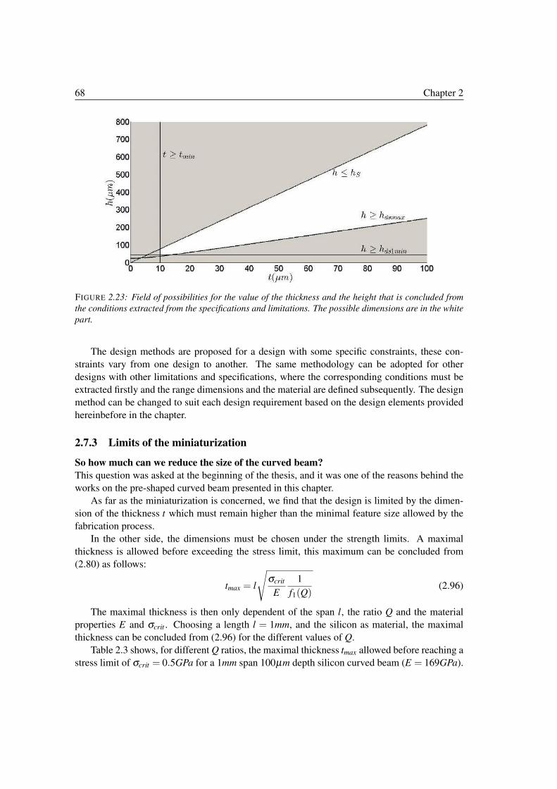
68 Chapter 2
FIGURE 2.23: Field of possibilities for the value of the thickness and the height that is concluded from
the conditions extracted from the specifications and limitations. The possible dimensions are in the white
part.
The design methods are proposed for a design with some specific constraints, these con-
straints vary from one design to another. The same methodology can be adopted for other
designs with other limitations and specifications, where the corresponding conditions must be
extracted firstly and the range dimensions and the material are defined subsequently. The design
method can be changed to suit each design requirement based on the design elements provided
hereinbefore in the chapter.
2.7.3 Limits of the miniaturization
So how much can we reduce the size of the curved beam?
This question was asked at the beginning of the thesis, and it was one of the reasons behind the
works on the pre-shaped curved beam presented in this chapter.
As far as the miniaturization is concerned, we find that the design is limited by the dimen-
sion of the thickness t which must remain higher than the minimal feature size allowed by the
fabrication process.
In the other side, the dimensions must be chosen under the strength limits. A maximal
thickness is allowed before exceeding the stress limit, this maximum can be concluded from
(2.80) as follows:
tmax = l
�σcrit
E
1
f1(Q)(2.96)
The maximal thickness is then only dependent of the span l, the ratio Q and the material
properties E and σcrit . Choosing a length l = 1mm, and the silicon as material, the maximal
thickness can be concluded from (2.96) for the different values of Q.
Table 2.3 shows, for different Q ratios, the maximal thickness tmax allowed before reaching a
stress limit of σcrit = 0.5GPa for a 1mm span 100µm depth silicon curved beam (E = 169GPa).
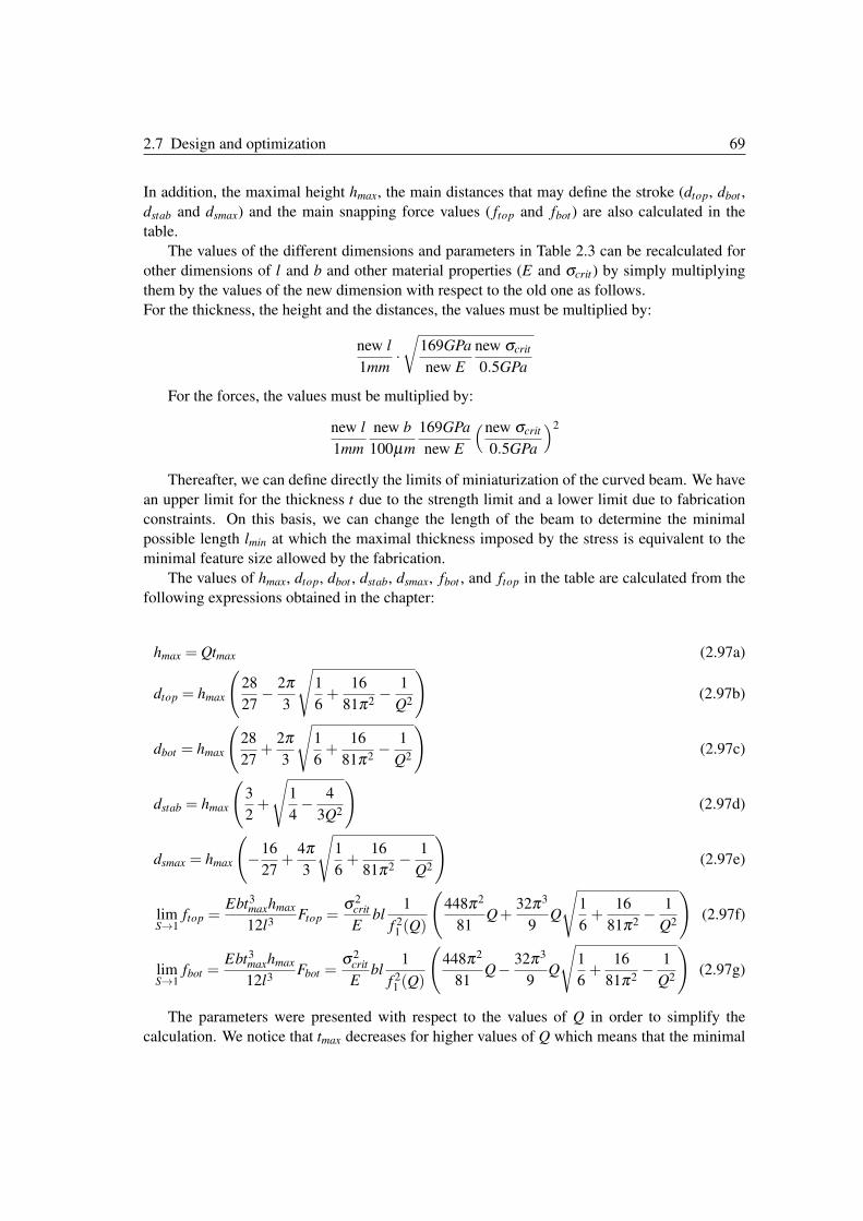
2.7 Design and optimization 69
In addition, the maximal height hmax, the main distances that may define the stroke (dtop, dbot ,
dstab and dsmax) and the main snapping force values ( ftop and fbot) are also calculated in the
table.
The values of the different dimensions and parameters in Table 2.3 can be recalculated for
other dimensions of l and b and other material properties (E and σcrit) by simply multiplying
them by the values of the new dimension with respect to the old one as follows.
For the thickness, the height and the distances, the values must be multiplied by:
new l
1mm·
�169GPa
new E
new σcrit
0.5GPa
For the forces, the values must be multiplied by:
new l
1mm
new b
100µm
169GPa
new E
�new σcrit
0.5GPa
�2
Thereafter, we can define directly the limits of miniaturization of the curved beam. We have
an upper limit for the thickness t due to the strength limit and a lower limit due to fabrication
constraints. On this basis, we can change the length of the beam to determine the minimal
possible length lmin at which the maximal thickness imposed by the stress is equivalent to the
minimal feature size allowed by the fabrication.
The values of hmax, dtop, dbot , dstab, dsmax, fbot , and ftop in the table are calculated from the
following expressions obtained in the chapter:
hmax = Qtmax (2.97a)
dtop = hmax
�28
27− 2π
3
�1
6+
16
81π2− 1
Q2
�(2.97b)
dbot = hmax
�28
27+
2π3
�1
6+
16
81π2− 1
Q2
�(2.97c)
dstab = hmax
�3
2+
�1
4− 4
3Q2
�(2.97d)
dsmax = hmax
�−16
27+
4π3
�1
6+
16
81π2− 1
Q2
�(2.97e)
limS→1
ftop =Ebt3
maxhmax
12l3Ftop =
σ2crit
Ebl
1
f 21 (Q)
�448π2
81Q+
32π3
9Q
�1
6+
16
81π2− 1
Q2
�(2.97f)
limS→1
fbot =Ebt3
maxhmax
12l3Fbot =
σ2crit
Ebl
1
f 21 (Q)
�448π2
81Q− 32π3
9Q
�1
6+
16
81π2− 1
Q2
�(2.97g)
The parameters were presented with respect to the values of Q in order to simplify the
calculation. We notice that tmax decreases for higher values of Q which means that the minimal
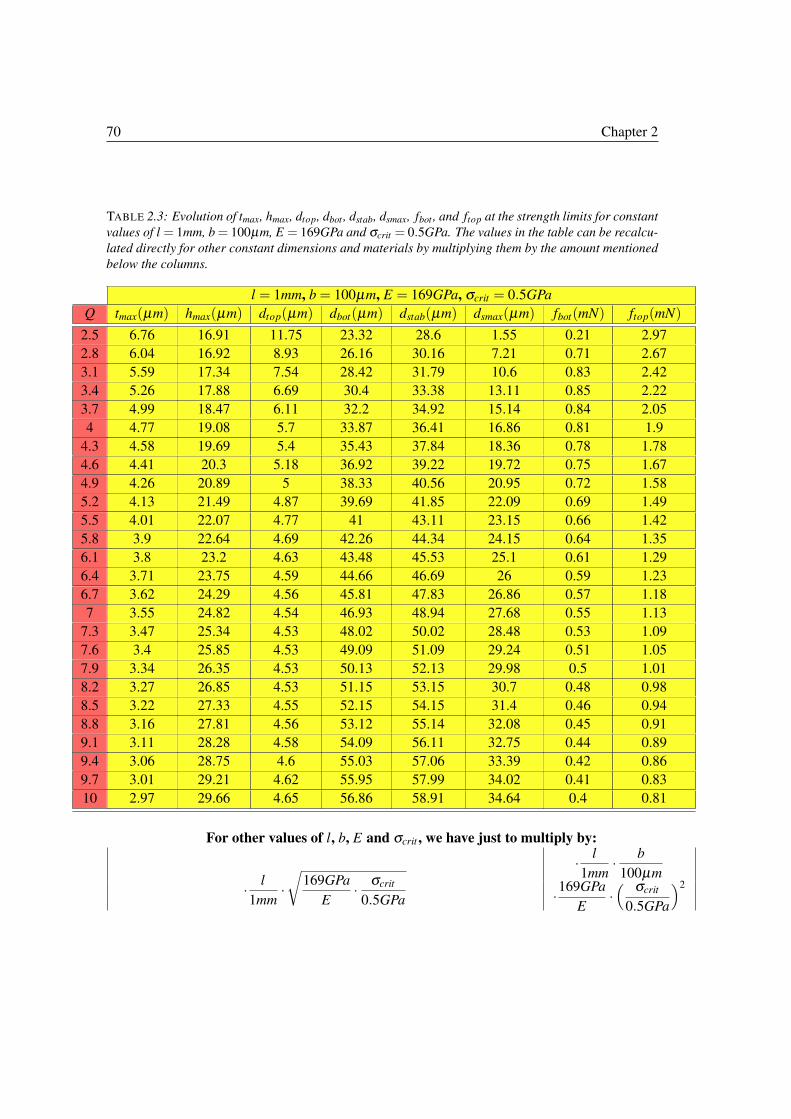
70 Chapter 2
TABLE 2.3: Evolution of tmax, hmax, dtop, dbot , dstab, dsmax, fbot , and ftop at the strength limits for constant
values of l = 1mm, b = 100µm, E = 169GPa and σcrit = 0.5GPa. The values in the table can be recalcu-
lated directly for other constant dimensions and materials by multiplying them by the amount mentioned
below the columns.
l = 1mm, b = 100µm, E = 169GPa, σcrit = 0.5GPa
Q tmax(µm) hmax(µm) dtop(µm) dbot(µm) dstab(µm) dsmax(µm) fbot(mN) ftop(mN)
2.5 6.76 16.91 11.75 23.32 28.6 1.55 0.21 2.97
2.8 6.04 16.92 8.93 26.16 30.16 7.21 0.71 2.67
3.1 5.59 17.34 7.54 28.42 31.79 10.6 0.83 2.42
3.4 5.26 17.88 6.69 30.4 33.38 13.11 0.85 2.22
3.7 4.99 18.47 6.11 32.2 34.92 15.14 0.84 2.05
4 4.77 19.08 5.7 33.87 36.41 16.86 0.81 1.9
4.3 4.58 19.69 5.4 35.43 37.84 18.36 0.78 1.78
4.6 4.41 20.3 5.18 36.92 39.22 19.72 0.75 1.67
4.9 4.26 20.89 5 38.33 40.56 20.95 0.72 1.58
5.2 4.13 21.49 4.87 39.69 41.85 22.09 0.69 1.49
5.5 4.01 22.07 4.77 41 43.11 23.15 0.66 1.42
5.8 3.9 22.64 4.69 42.26 44.34 24.15 0.64 1.35
6.1 3.8 23.2 4.63 43.48 45.53 25.1 0.61 1.29
6.4 3.71 23.75 4.59 44.66 46.69 26 0.59 1.23
6.7 3.62 24.29 4.56 45.81 47.83 26.86 0.57 1.18
7 3.55 24.82 4.54 46.93 48.94 27.68 0.55 1.13
7.3 3.47 25.34 4.53 48.02 50.02 28.48 0.53 1.09
7.6 3.4 25.85 4.53 49.09 51.09 29.24 0.51 1.05
7.9 3.34 26.35 4.53 50.13 52.13 29.98 0.5 1.01
8.2 3.27 26.85 4.53 51.15 53.15 30.7 0.48 0.98
8.5 3.22 27.33 4.55 52.15 54.15 31.4 0.46 0.94
8.8 3.16 27.81 4.56 53.12 55.14 32.08 0.45 0.91
9.1 3.11 28.28 4.58 54.09 56.11 32.75 0.44 0.89
9.4 3.06 28.75 4.6 55.03 57.06 33.39 0.42 0.86
9.7 3.01 29.21 4.62 55.95 57.99 34.02 0.41 0.83
10 2.97 29.66 4.65 56.86 58.91 34.64 0.4 0.81
For other values of l, b, E and σcrit , we have just to multiply by:
·l
1mm·
b
100µm
·l
1mm·
�169GPa
E·
σcrit
0.5GPa ·169GPa
E·� σcrit
0.5GPa
�2
2.8 Conclusion 71
length, allowed before exceeding the stress limits, is higher for high values of Q. In the other
side, the values of hmax and the different distances dtop, dbot , dstab and dsmax increase when the
value of tmax decreases. As for the snapping force, it is lower for high values of Q while fbot
tends to be equivalent to ftop/2.
2.8 Conclusion
In conclusion, analytical modeling and stress analysis of the postbuckling behavior of a pre-
shaped curved beam were presented in this chapter. The snapping force solution was inves-
tigated without and with high modes of buckling. Bistability conditions were subsequently
deduced from the snapping force solution. An analytical model was then developed (with and
without high modes of buckling), which describes the internal stress evolution during deflec-
tion. The presented modeling showed a good agreement with FEM simulations and revealed the
importance of considering high modes of buckling in the modeling in contrast to the previous
works in literature. After that, design and optimization of the curved beam was investigated
based on the analytical expressions obtained in the modeling. The influence of the different
dimensions and properties on the mechanical behavior was firstly presented, a design method
was then presented that allows choosing the dimensions and providing the desired performance,
the limit of miniaturization for the curved beam was discussed in the final part. Originality
of the works made in this chapter lies in considering high modes of buckling in the modeling,
stress analysis which is useful for the design, investigating the impact of the dimensions and
material properties on the beam behavior, proposing a design method and finally investigating
the miniaturization limits.
The other main component in the DiMiBot and in the multistable module is the U-shaped
electrothermal actuator. The modeling and design of this actuator are investigated in details in
Chapter 3.

Chapter 3U-shaped electrothermal actuators
This chapter deals with the modeling of the electro-thermo-mechanical behavior of
a U-shaped electrothermal actuator. The problem is treated by a sequence of two
analytical models: electro-thermal and thermo-mechanical. The first one concerns
the computation of the evolution of the thermal distribution in the actuator, while
the second one allows computing the displacement resulting from the thermal dis-
tribution. The electrothermal model provides an exact solution of the hybrid PDEs
that describe the electrothermal behavior in the three arms of the actuator. The
relation between the displacement and the thermal distribution is then provided in
the thermo-mechanical model. FEM simulations and experiments are run on doped
silicon actuators. The analytical models show a good agreement with the results
of the FEM simulations and experiments in terms of the thermal distribution and
the displacement. The influence of the different dimensions and electro-thermo-
mechanical properties on the electrical, thermal and mechanical behavior of the
actuator is then investigated based on the analytical models. The analytical expres-
sions provide very important key tools for the design and optimization of U-shaped
actuators.
74 Chapter 3
Chapter contents
3.1 Introduction . . . . . . . . . . . . . . . . . . . . . . . . . . . . . . . . . . 75
3.2 Electrothermal model . . . . . . . . . . . . . . . . . . . . . . . . . . . . . 77
3.2.1 Electrothermal equation . . . . . . . . . . . . . . . . . . . . . . . . 77
3.2.2 Lineshaped beam electrothermal response . . . . . . . . . . . . . . . 77
3.2.3 Actuator electrothermal response . . . . . . . . . . . . . . . . . . . 79
3.3 Thermo-mechanical model . . . . . . . . . . . . . . . . . . . . . . . . . . 85
3.4 Simulations, Experiments and discussion . . . . . . . . . . . . . . . . . . 88
3.4.1 Electrothermal response . . . . . . . . . . . . . . . . . . . . . . . . 89
3.4.2 Mechanical response . . . . . . . . . . . . . . . . . . . . . . . . . . 92
3.5 Design and optimization . . . . . . . . . . . . . . . . . . . . . . . . . . . . 95
3.5.1 Maximal voltage . . . . . . . . . . . . . . . . . . . . . . . . . . . . 95
3.5.2 Characteristic curve of the actuator . . . . . . . . . . . . . . . . . . 96
3.5.3 Influence of the parameters on the actuator’s performance . . . . . . 99
3.5.4 Design methodology of the actuator . . . . . . . . . . . . . . . . . . 106
3.6 Conclusion . . . . . . . . . . . . . . . . . . . . . . . . . . . . . . . . . . . 112
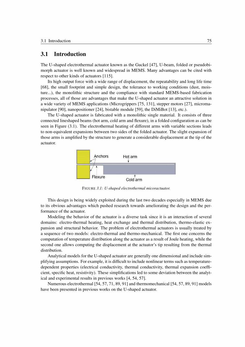
3.1 Introduction 75
3.1 Introduction
The U-shaped electrothermal actuator known as the Guckel [47], U-beam, folded or pseudobi-
morph actuator is well known and widespread in MEMS. Many advantages can be cited with
respect to other kinds of actuators [115].
Its high output force with a wide range of displacement, the repeatability and long life time
[68], the small footprint and simple design, the tolerance to working conditions (dust, mois-
ture...), the monolithic structure and the compliance with standard MEMS-based fabrication
processes, all of those are advantages that make the U-shaped actuator an attractive solution in
a wide variety of MEMS applications (Microgrippers [75, 131], stepper motors [27], microma-
nipulator [90], nanopositioner [24], bistable module [59], the DiMiBot [13], etc.).
The U-shaped actuator is fabricated with a monolithic single material. It consists of three
connected lineshaped beams (hot arm, cold arm and flexure), in a folded configuration as can be
seen in Figure (3.1). The electrothermal heating of different arms with variable sections leads
to non-equivalent expansions between two sides of the folded actuator. The slight expansion of
those arms is amplified by the structure to generate a considerable displacement at the tip of the
actuator.
FIGURE 3.1: U-shaped electrothermal micoractuator.
This design is being widely exploited during the last two decades especially in MEMS due
to its obvious advantages which pushed research towards ameliorating the design and the per-
formance of the actuator.
Modeling the behavior of the actuator is a diverse task since it is an interaction of several
domains: electro-thermal heating, heat exchange and thermal distribution, thermo-elastic ex-
pansion and structural behavior. The problem of electrothermal actuators is usually treated by
a sequence of two models: electro-thermal and thermo-mechanical. The first one concerns the
computation of temperature distribution along the actuator as a result of Joule heating, while the
second one allows computing the displacement at the actuator’s tip resulting from the thermal
distribution.
Analytical models for the U-shaped actuator are generally one dimensional and include sim-
plifying assumptions. For example, it is difficult to include nonlinear terms such as temperature-
dependent properties (electrical conductivity, thermal conductivity, thermal expansion coeffi-
cient, specific heat, resistivity). These simplifications led to some deviation between the analyt-
ical and experimental results in previous works [4, 54, 57].
Numerous electrothermal [54, 57, 71, 89, 91] and thermomechanical [54, 57, 89, 91] models
have been presented in previous works on the U-shaped actuator.
76 Chapter 3
In the other side, experiments and simulations on the actuator showed a dynamic behav-
ior/displacement which is related to the dynamic of the temperature distribution while the elas-
tic response is quasistatic relatively. Therefore, dynamic electrothermal model and static ther-
momechanical models are needed. Few studies [40, 52, 55, 75, 89, 121] are found that have
addressed the dynamic response of the U-shaped actuator.
As far as we know, no exact analytical solution of the transient electrothermal response of
the actuator was found in literature. In the case of a simple beam, solving the electrothermal
equation revolves around the recognition of a Fourier series form of the general solution after
introducing boundary and initial conditions. This is not the case for the U-shaped actuator.
The difficulty in the case of the actuator lies in the fact that the arms are differently heated,
and temperature evolution in each arm is described by an equation. This leads to a general
solution in the form of a hybrid function with three sub-functions, each one concerns one arm
of the actuator. In result, the hybrid function cannot be recognized as a Fourier series, and no
solution can be obtained with this method.
An analytical formulation of the steady state and transient solutions of the electrothermal
response of a line-shape microstructure is presented in [80]. For the U-shaped actuator case,
the steady state solution was investigated in [58]. As for the transient solution, the problem was
solved numerically in [89] using Laplace transformation. The dynamic response of the actuator
for a sine wave electrical input is investigated experimentally in [55, 121]. Lerch et al. [75],
Geisberger et al. [40] and Henneken et al. [52] have investigated the transient behavior of their
U-shaped devices with a pulse electrical input. An overshoot of displacement of the actuator is
reported in their experiments which is similar to the findings of our experiments. In their works,
a normal speed camera is used where the sampling rate is too low and the dynamic behavior is
not analyzed in details.
An exact analytical solution of the electrothermal problem of the actuator is presented in
this chapter using a novel calculation method that allows presenting an integrable function by a
hybrid function, where sub-functions consist of infinite sum of sines and cosines. Expression of
the temperature final solution is an infinite sum of periodic functions where all the parameters
are determined. This analytical expression describes evolution of the temperature distribution
inside the actuator in response to an electrical input.
As for the thermo-mechanical model, in previous works, several approaches were consid-
ered to estimate the displacement at the tip using mainly the length thermal expansion in each
arm. The difference of enthalpy approach was used in [91], Castiglianos theory approach as
in [55] and Euler-Bernoulli equation was derived to estimate the displacement in [34]. As in
the validated model [57] where the virtual works method was used, in our proposed model we
calculate the displacement using the same method but we have chosen not to make any of the
simplifications done previously (such as the same width between hot arm and flexure or the
consideration of axial stresses) in order to obtain a solution of a more general case with regard
to the actuator dimensions. In addition, the effect of the external loads on the displacement is
also considered in the calculation.
The importance of the new models (electrothermal and thermomechanical), lies not only in
the estimation of the displacement and temperature distribution; but to its capability of showing
the effects of different parameters and dimensions on the response, a key tool for the design and
optimization.
3.2 Electrothermal model 77
In Section 3.2, the electrothermal model and solutions are investigated, as we begin by
recalling the calculation method of the electrothermal response for a lineshaped structure, the
calculation method is developed and the actuator’s electrothermal new solution is obtained.
In Section 3.3, the thermomechanical model is investigated. The displacement expression is
obtained in this section as a result of the Joule heating and external loads.
In Section 3.4, the analytical solutions are discussed and compared to FEM modeling and
experimental results. The dynamic behavior is analyzed and the evolution of the physical aspects
in the actuator (temperature distribution, arms expansions, deformation, etc.) during displace-
ment is clarified.
In Section 3.4, the influence of the different dimensions and properties on the performance
the actuator is analyzed providing very important key tools for the design and optimization of
U-shaped actuators.
3.2 Electrothermal model
3.2.1 Electrothermal equation
At microscale, the heat transfer mechanisms have some differences from macroscales [64, 100].
Conduction is dominant on the free convection [100] while radiation showed a negligible in-
fluence in several studies [54, 57, 71]. Conduction should be treated as the only mode of heat
transfer in the lack of forced convection [100]. Furthermore, the temperature is considered to be
uniform in the cross section for microactuators [24, 54].
In our model, convection and radiation effects are neglected in the electrothermal part and
a one dimensional simplification is considered. The electrothermal partial differential equation
(PDE) that describes the temperature T behavior in terms of the space dimension x and the time
t is as follows:
ρdCp
∂T
∂ t= J2ρ0 +Kp
∂ 2T
∂x2(3.1)
ρd : density inkg
m3
Cp: specific heat in JK.kg
J: electrical current density in Am2
ρ0: electrical resistivity in Ω .mKp: thermal conductivity in W
K.m
The term on the left of (3.1) represents the density of heat added due to thermal variation.
The first term on the right represents the heat generation by Joule effect, the one next concerns
the conduction between sections.
3.2.2 Lineshaped beam electrothermal response
In this section, the calculation method for the electrothermal response in the case of a lineshaped
microbeam is recalled. A schema for the lineshaped beam is shown in Figure 3.2.
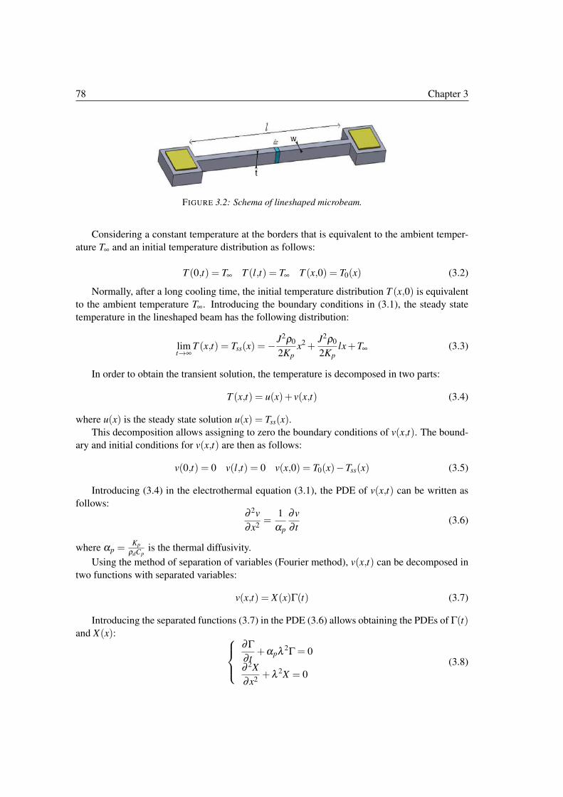
78 Chapter 3
FIGURE 3.2: Schema of lineshaped microbeam.
Considering a constant temperature at the borders that is equivalent to the ambient temper-
ature T∞ and an initial temperature distribution as follows:
T (0,t) = T∞ T (l,t) = T∞ T (x,0) = T0(x) (3.2)
Normally, after a long cooling time, the initial temperature distribution T (x,0) is equivalent
to the ambient temperature T∞. Introducing the boundary conditions in (3.1), the steady state
temperature in the lineshaped beam has the following distribution:
limt→∞
T (x,t) = Tss(x) =−J2ρ0
2Kp
x2 +J2ρ0
2Kp
lx+T∞ (3.3)
In order to obtain the transient solution, the temperature is decomposed in two parts:
T (x,t) = u(x)+ v(x,t) (3.4)
where u(x) is the steady state solution u(x) = Tss(x).This decomposition allows assigning to zero the boundary conditions of v(x,t). The bound-
ary and initial conditions for v(x,t) are then as follows:
v(0,t) = 0 v(l,t) = 0 v(x,0) = T0(x)−Tss(x) (3.5)
Introducing (3.4) in the electrothermal equation (3.1), the PDE of v(x,t) can be written as
follows:∂ 2v
∂x2=
1
αp
∂v
∂ t(3.6)
where αp =Kp
ρdCpis the thermal diffusivity.
Using the method of separation of variables (Fourier method), v(x,t) can be decomposed in
two functions with separated variables:
v(x,t) = X(x)Γ(t) (3.7)
Introducing the separated functions (3.7) in the PDE (3.6) allows obtaining the PDEs of Γ(t)and X(x):
∂Γ∂ t
+αpλ 2Γ = 0
∂ 2X
∂x2+λ 2X = 0
(3.8)
3.2 Electrothermal model 79
where λ is a positive non-zero constant assigned to X(x) and Γ(t).The general solutions of Γ(t) and X(x) have the following forms:
�Γ(t) = e−αpλ 2t
X(x) = asin(λx)+bcos(λx)(3.9)
where a, b and λ are the unknowns.
Introducing the boundary conditions, we conclude that the unknowns have infinity of solu-
tions with a periodic form: a = an, b = bn and λ = λn, where n is a positive integer. In result,
according to the superposition principle:
v(x,t) =∞
∑n=1
Xn(x)Γn(t) (3.10)
where Xn and Γn are equivalent to X and Γ respectively for a = an, b = bn and λ = λn.
For the boundary conditions in 3.2, the constants bn and λn are equivalent to: bn = 0, λn =nπ/l. Afterwards, the transient solution of the temperature has the following form:
T (x,t) = Tss(x)+∞
∑n=1
an sin�nπ
lx�
e−αpn2π2
l2t
(3.11)
Introducing the initial temperature condition, we recognize a Fourier series form, enabling
to determine the expression of an.
an =2
l
l�
0
(T0(x)−Tss(x))sin�nπ
lx�
(3.12)
Thereby, all the unknowns are determined and the solution is obtained.
3.2.3 Actuator electrothermal response
In this section, the exact solution of the electrothermal equations in the case of a U-shaped
actuator is obtained. The system is modeled using three electrothermal PDEs that are continuous
in temperature and heat flux density, one for each arm of the actuator.
The actuator is considered unfolded in order to match the one dimension 1D hypothesis.
Coordinates and dimensions of the actuator are shown in Fig. 3.3.
The temperature distribution T (x,t) in the case of the actuator is a hybrid function with three
sub-functions that represent the temperature in each of the three arms.
T (x,t) =
Th(x,t) x ∈ [0; l1]Tc(x,t) x ∈ [l1; l2]Tf (x,t) x ∈ [l2; l3]
(3.13)
where the indexes h, c and f refer to the hot arm, cold arm and flexure respectively.
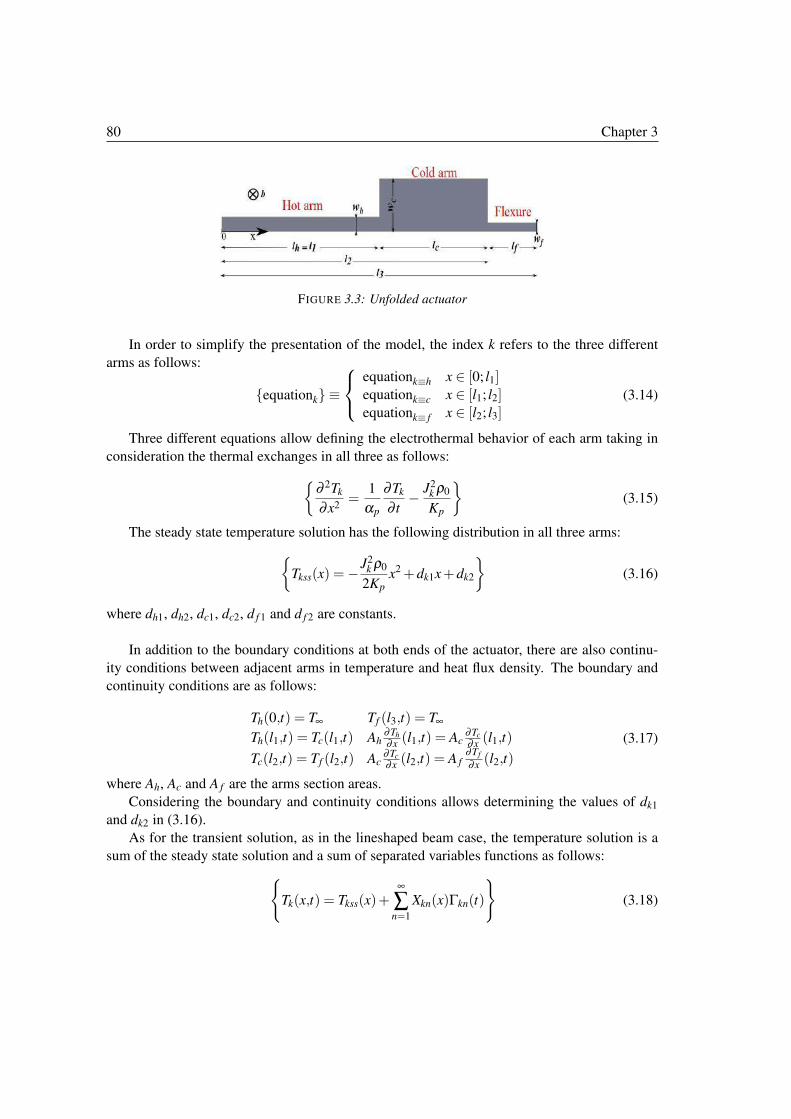
80 Chapter 3
FIGURE 3.3: Unfolded actuator
In order to simplify the presentation of the model, the index k refers to the three different
arms as follows:
{equationk}≡
equationk≡h x ∈ [0; l1]equationk≡c x ∈ [l1; l2]equationk≡ f x ∈ [l2; l3]
(3.14)
Three different equations allow defining the electrothermal behavior of each arm taking in
consideration the thermal exchanges in all three as follows:
�∂ 2Tk
∂x2=
1
αp
∂Tk
∂ t− J2
k ρ0
Kp
�(3.15)
The steady state temperature solution has the following distribution in all three arms:
�Tkss(x) =−J2
k ρ0
2Kp
x2 +dk1x+dk2
�(3.16)
where dh1, dh2, dc1, dc2, d f 1 and d f 2 are constants.
In addition to the boundary conditions at both ends of the actuator, there are also continu-
ity conditions between adjacent arms in temperature and heat flux density. The boundary and
continuity conditions are as follows:
Th(0,t) = T∞ Tf (l3,t) = T∞
Th(l1,t) = Tc(l1,t) Ah∂Th
∂x(l1,t) = Ac
∂Tc
∂x(l1,t)
Tc(l2,t) = Tf (l2,t) Ac∂Tc
∂x(l2,t) = A f
∂Tf
∂x(l2,t)
(3.17)
where Ah, Ac and A f are the arms section areas.
Considering the boundary and continuity conditions allows determining the values of dk1
and dk2 in (3.16).
As for the transient solution, as in the lineshaped beam case, the temperature solution is a
sum of the steady state solution and a sum of separated variables functions as follows:
�Tk(x,t) = Tkss(x)+
∞
∑n=1
Xkn(x)Γkn(t)
�(3.18)
3.2 Electrothermal model 81
The general solutions of Γkn(t) and Xkn(x) have the following forms:
Γkn(t) = e−αpλ 2n t
Xkn(x) = akn sin(λnx)+bkn cos(λnx)
=Ckn sin(λnx+ϕkn)
(3.19)
Introducing the boundary and continuity conditions in (3.17) allows obtaining the following
conditions on Xkn:
Xhn(0) = 0 X f n(l3) = 0
Xhn(l1) = Xcn(l1) Ah∂Xhn
∂x(l1) = Ac
∂Xcn
∂x(l1)
Xcn(l2) = X f n(l2) Ac∂Xcn
∂x(l2) = A f
∂X f n
∂x(l2)
(3.20)
Applying the conditions in (3.20) on Xkn allows obtaining the equation of λn and defining the
relation between ahn and the other constants. The relations between ahn and the other constants
are as follows:
bhn = 0bcn
ahn=
�1− Ah
Ac
�sin(λnlh)cos(λnlh)
acn
ahn= sin2(λnlh)+
Ah
Accos2(λnlh)
b f n
ahn=− a f n
ahntan(λnl3)
a f n
ahn= cos(λnlc)
�Ah
A fcos(λnl2)cos(λnl1)+ sin(λnl2)sin(λnl1)
�
+sin(λnlc)�
Ah
Acsin(λnl2)cos(λnl1)− Ac
A fcos(λnl2)sin(λnl1)
�
(3.21)
Noting that the lengths have different indexes in order to reduce the expressions inside the sine
and cosine functions as possible.
Besides, the equation of λn concluded from (3.20) is as follows:
AhAc cos(λnlh)cos(λnlc)sin(λnl f )+AhA f cos(λnlh)sin(λnlc)cos(λnl f )+AcA f sin(λnlh)cos(λnlc)cos(λnl f )−A2
c sin(λnlh)sin(λnlc)sin(λnl f ) = 0
(3.22)
Unlike the case of a lineshaped beam, the trigonometric equation (3.22) doesn’t allow ob-
taining a simple analytical form of λn. The values of λn for the actuator must be then calculated
numerically from (3.22).
Yet, a kind of periodicity for the values of λn is noticed. If the total length of the arms can
be written as a positive integer after scaling, then λKlis the Klth solution of λn:
λKl=
Klπl3
(3.23)
Kl is a least common multiple between lengths of arms:
Kl = LCM
�LCM(lh,l3)
lh,LCM(lc,l3)
lc,LCM(l f ,l3)
l f
�(3.24)
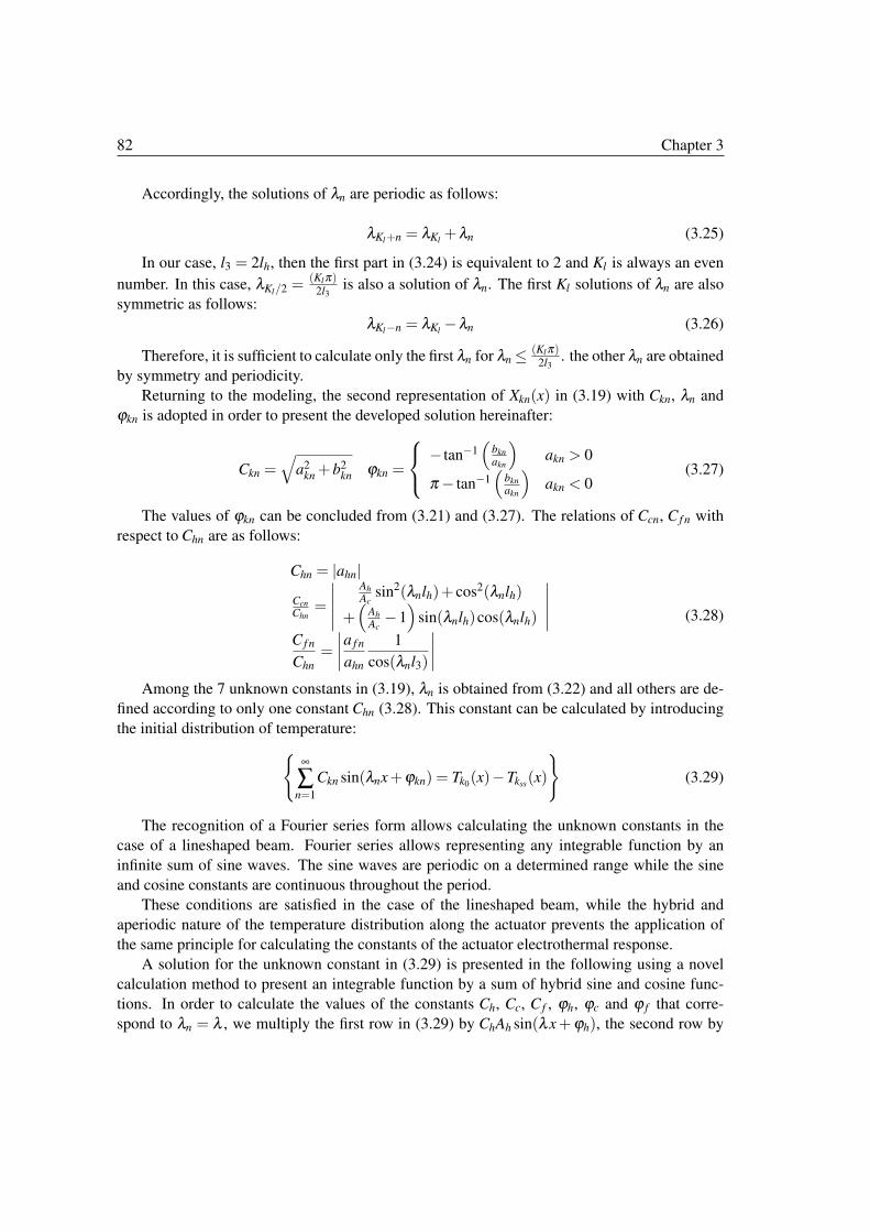
82 Chapter 3
Accordingly, the solutions of λn are periodic as follows:
λKl+n = λKl+λn (3.25)
In our case, l3 = 2lh, then the first part in (3.24) is equivalent to 2 and Kl is always an even
number. In this case, λKl/2 =(Klπ)
2l3is also a solution of λn. The first Kl solutions of λn are also
symmetric as follows:
λKl−n = λKl−λn (3.26)
Therefore, it is sufficient to calculate only the first λn for λn ≤ (Klπ)2l3
. the other λn are obtained
by symmetry and periodicity.
Returning to the modeling, the second representation of Xkn(x) in (3.19) with Ckn, λn and
ϕkn is adopted in order to present the developed solution hereinafter:
Ckn =�
a2kn +b2
kn ϕkn =
− tan−1�
bkn
akn
�akn > 0
π − tan−1�
bkn
akn
�akn < 0
(3.27)
The values of ϕkn can be concluded from (3.21) and (3.27). The relations of Ccn, C f n with
respect to Chn are as follows:
Chn = |ahn|
Ccn
Chn=
�����
Ah
Acsin2(λnlh)+ cos2(λnlh)
+�
Ah
Ac−1
�sin(λnlh)cos(λnlh)
�����C f n
Chn
=
����a f n
ahn
1
cos(λnl3)
����
(3.28)
Among the 7 unknown constants in (3.19), λn is obtained from (3.22) and all others are de-
fined according to only one constant Chn (3.28). This constant can be calculated by introducing
the initial distribution of temperature:
�∞
∑n=1
Ckn sin(λnx+ϕkn) = Tk0(x)−Tkss
(x)
�(3.29)
The recognition of a Fourier series form allows calculating the unknown constants in the
case of a lineshaped beam. Fourier series allows representing any integrable function by an
infinite sum of sine waves. The sine waves are periodic on a determined range while the sine
and cosine constants are continuous throughout the period.
These conditions are satisfied in the case of the lineshaped beam, while the hybrid and
aperiodic nature of the temperature distribution along the actuator prevents the application of
the same principle for calculating the constants of the actuator electrothermal response.
A solution for the unknown constant in (3.29) is presented in the following using a novel
calculation method to present an integrable function by a sum of hybrid sine and cosine func-
tions. In order to calculate the values of the constants Ch, Cc, C f , ϕh, ϕc and ϕ f that corre-
spond to λn = λ , we multiply the first row in (3.29) by ChAh sin(λx+ϕh), the second row by
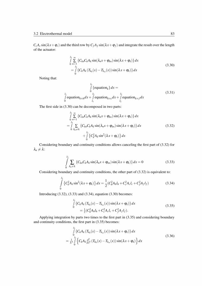
3.2 Electrothermal model 83
CcAc sin(λx+ϕc) and the third row by C f A f sin(λx+ϕ f ) and integrate the result over the length
of the actuator:
l3�0
∞∑
n=1
{CknCkAk sin(λnx+ϕkn)sin(λx+ϕk)}dx
=l3�0
{CkAk (Tk0(x)−Tkss
(x))sin(λx+ϕk)}dx
(3.30)
Noting that:
l3�0
{equationk}dx =
l1�0
equationk≡hdx+l2�l1
equationk≡cdx+l3�l2
equationk≡ f dx
(3.31)
The first side in (3.30) can be decomposed in two parts:
l3�0
∞∑
n=1
{CknCkAk sin(λnx+ϕkn)sin(λx+ϕk)}dx
=l3�0
∑λn �=λ
{CknCkAk sin(λnx+ϕkn)sin(λx+ϕk)}dx
+l3�0
�C2
k Ak sin2(λx+ϕk)�
dx
(3.32)
Considering boundary and continuity conditions allows canceling the first part of (3.32) for
λn �= λ :
l3�
0
∑λn �=λ
{CknCkAk sin(λnx+ϕkn)sin(λx+ϕk)}dx = 0 (3.33)
Considering boundary and continuity conditions, the other part of (3.32) is equivalent to:
l3�
0
�C2
k Ak sin2(λx+ϕk)�
dx =1
2(C2
hAhlh +C2c Aclc +C2
f A f l f ) (3.34)
Introducing (3.32), (3.33) and (3.34), equation (3.30) becomes:
l3�0
{CkAk (Tk0(x)−Tkss
(x))sin(λx+ϕk)}dx
= 12(C2
hAhlh +C2c Aclc +C2
f A f l f ).
(3.35)
Applying integration by parts two times to the first part in (3.35) and considering boundary
and continuity conditions, the first part in (3.35) becomes:
l3�0
{CkAk (Tk0(x)−Tkss
(x))sin(λx+ϕk)}dx
= 1λ 2
l3�0
�CkAk
d2
dx2 (Tk0(x)−Tkss
(x))sin(λx+ϕk)�
dx
(3.36)
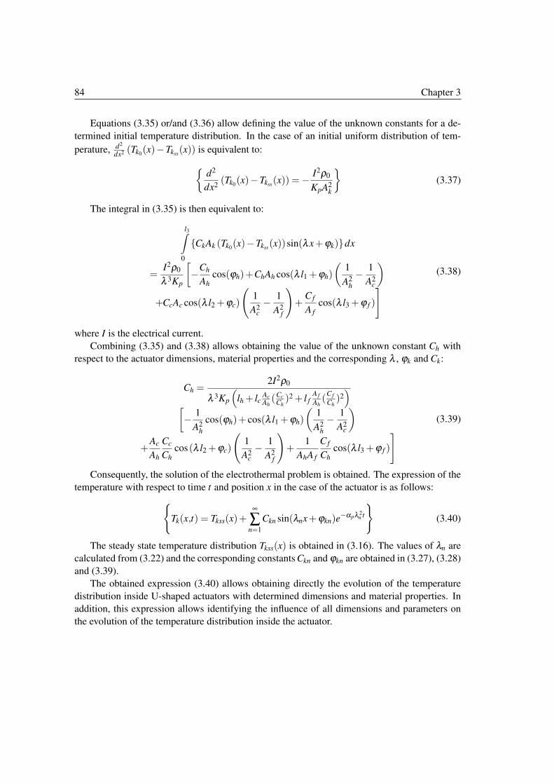
84 Chapter 3
Equations (3.35) or/and (3.36) allow defining the value of the unknown constants for a de-
termined initial temperature distribution. In the case of an initial uniform distribution of tem-
perature, d2
dx2 (Tk0(x)−Tkss
(x)) is equivalent to:
�d2
dx2(Tk0
(x)−Tkss(x)) =− I2ρ0
KpA2k
�(3.37)
The integral in (3.35) is then equivalent to:
l3�
0
{CkAk (Tk0(x)−Tkss
(x))sin(λx+ϕk)}dx
=I2ρ0
λ 3Kp
�−Ch
Ah
cos(ϕh)+ChAh cos(λ l1 +ϕh)
�1
A2h
− 1
A2c
�
+CcAc cos(λ l2 +ϕc)
�1
A2c
− 1
A2f
�+
C f
A f
cos(λ l3 +ϕ f )
�(3.38)
where I is the electrical current.
Combining (3.35) and (3.38) allows obtaining the value of the unknown constant Ch with
respect to the actuator dimensions, material properties and the corresponding λ , ϕk and Ck:
Ch =2I2ρ0
λ 3Kp
�lh + lc
Ac
Ah(Cc
Ch)2 + l f
A f
Ah(
C f
Ch)2�
�− 1
A2h
cos(ϕh)+ cos(λ l1 +ϕh)
�1
A2h
− 1
A2c
�
+Ac
Ah
Cc
Ch
cos(λ l2 +ϕc)
�1
A2c
− 1
A2f
�+
1
AhA f
C f
Ch
cos(λ l3 +ϕ f )
�(3.39)
Consequently, the solution of the electrothermal problem is obtained. The expression of the
temperature with respect to time t and position x in the case of the actuator is as follows:
�Tk(x,t) = Tkss(x)+
∞
∑n=1
Ckn sin(λnx+ϕkn)e−αpλ 2
n t
�(3.40)
The steady state temperature distribution Tkss(x) is obtained in (3.16). The values of λn are
calculated from (3.22) and the corresponding constants Ckn and ϕkn are obtained in (3.27), (3.28)
and (3.39).
The obtained expression (3.40) allows obtaining directly the evolution of the temperature
distribution inside U-shaped actuators with determined dimensions and material properties. In
addition, this expression allows identifying the influence of all dimensions and parameters on
the evolution of the temperature distribution inside the actuator.
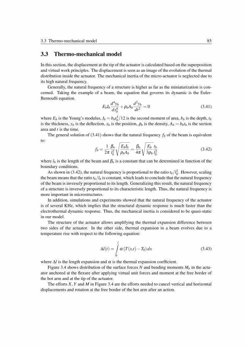
3.3 Thermo-mechanical model 85
3.3 Thermo-mechanical model
In this section, the displacement at the tip of the actuator is calculated based on the superposition
and virtual work principles. The displacement is seen as an image of the evolution of the thermal
distribution inside the actuator. The mechanical inertia of the micro-actuator is neglected due to
its high natural frequency.
Generally, the natural frequency of a structure is higher as far as the miniaturization is con-
cerned. Taking the example of a beam, the equation that governs its dynamic is the Euler-
Bernoulli equation.
EbIb
d4yb
dx4b
+ρbAb
d2yb
dt2= 0 (3.41)
where Eb is the Young’s modulus, Ib = bbt3b/12 is the second moment of area, bb is the depth, tb
is the thickness, yb is the deflection, xb is the position, ρb is the density, Ab = bbtb is the section
area and t is the time.
The general solution of (3.41) shows that the natural frequency fb of the beam is equivalent
to:
fb =1
2πβn
l2b
�EbIb
ρbAb
=βn
4π
�Eb
3ρb
tb
l2b
(3.42)
where lb is the length of the beam and βn is a constant that can be determined in function of the
boundary conditions.
As shown in (3.42), the natural frequency is proportional to the ratio tb/l2b . However, scaling
the beam means that the ratio tb/lb is constant, which leads to conclude that the natural frequency
of the beam is inversely proportional to its length. Generalizing this result, the natural frequency
of a structure is inversely proportional to its characteristic length. Thus, the natural frequency is
more important in microstructures.
In addition, simulations and experiments showed that the natural frequency of the actuator
is of several KHz, which implies that the structural dynamic response is much faster than the
electrothermal dynamic response. Thus, the mechanical inertia is considered to be quasi-static
in our model.
The structure of the actuator allows amplifying the thermal expansion difference between
two sides of the actuator. In the other side, thermal expansion in a beam evolves due to a
temperature rise with respect to the following equation:
Δl(t) =
l�
0
α (T (x,t)−T0)dx (3.43)
where Δl is the length expansion and α is the thermal expansion coefficient.
Figure 3.4 shows distribution of the surface forces N and bending moments Mb in the actu-
ator anchored at the flexure after applying virtual unit forces and moment at the free border of
the hot arm and at the tip of the actuator.
The efforts X , Y and M in Figure 3.4 are the efforts needed to cancel vertical and horizontal
displacements and rotation at the free border of the hot arm after an action.
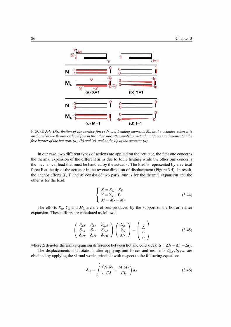
86 Chapter 3
FIGURE 3.4: Distribution of the surface forces N and bending moments Mb in the actuator when it is
anchored at the flexure end and free in the other side after applying virtual unit forces and moment at the
free border of the hot arm, (a), (b) and (c), and at the tip of the actuator (d).
In our case, two different types of actions are applied on the actuator, the first one concerns
the thermal expansion of the different arms due to Joule heating while the other one concerns
the mechanical load that must be handled by the actuator. The load is represented by a vertical
force F at the tip of the actuator in the reverse direction of displacement (Figure 3.4). In result,
the anchor efforts X , Y and M consist of two parts, one is for the thermal expansion and the
other is for the load:
X = XΔ +XF
Y = YΔ +YF
M = MΔ +MF
(3.44)
The efforts XΔ, YΔ and MΔ are the efforts produced by the support of the hot arm after
expansion. These efforts are calculated as follows:
δXX δXY δXM
δY X δYY δY M
δMX δMY δMM
XΔYΔMΔ
=
Δ0
0
(3.45)
where Δ denotes the arms expansion difference between hot and cold sides: Δ = Δlh−Δlc−Δl f .
The displacements and rotations after applying unit forces and moments δXX ,δXY ... are
obtained by applying the virtual works principle with respect to the following equation:
δ12 =
l�
0
�N1N2
EA+
M1M2
EIy
�dx (3.46)
3.3 Thermo-mechanical model 87
δ12: Displacement or rotation in the direction of the virtual unit effort 1 after applying the real
effort 2.
N1: Surface forces with the virtual effort.
N2: Surface forces with the real effort.
M1: Bending moments with the virtual effort.
M2: Bending moments with the real effort.
Iy =bw3
12: Second moment of area of section with respect to the midline.
E: Young’s modulus.
Based on (3.46), expressions of δ coefficients in (3.45) are as follows:
δXX =g�2l f
EIy f
+g��2lc
EIyc
+2g3 +3gwh(g+
wh
2)
6EIyg
+l f
ES f
+lc
ESc
+lh
ESh
(3.47a)
δYY =l3
f
3EIy f
+l3h − l3
f
3EIyc
+gl2
h
EIyg
+l3h
3EIyh
+g
ESg
(3.47b)
δMM =l f
EIy f
+lc
EIyc
+g
EIyg
+lh
EIyh
(3.47c)
δXY = δY X =g�l2
f
2EIy f
+g��(l2
h − l2f )
2EIyc
+g2lh + lhgwh
2EIyg
(3.47d)
δXM = δMX =g�l f
EIy f
+g��lcEIyc
+g(g+wh)
2EIyg
(3.47e)
δY M = δMY =l2
f
2EIy f
+l2h − l2
f
2EIyc
+glh
EIyg
+l2h
2EIyh
(3.47f)
Given that:
g: Gap width
g�: Distance between hot arm and flexure mid-lines; g� = g+wh+w f
2
g��: Distance between hot and cold arm mid-lines; g�� = g+ wh+wc
2
In the other side, U-shaped actuators work generally with loads in MEMS. The efforts XF ,
YF and MF are the anchor efforts produced to face displacements and rotation resulting from the
applied load:
δXX δXY δXM
δY X δYY δY M
δMX δMY δMM
XF
YF
MF
=−
δXF
δY F
δMF
F (3.48)
where δXF , δY F and δMF are the displacements and rotations at the free border of the hot arm
after applying a unit load F = 1.
The terms δXF , δY F and δMF are equivalent to −δX f , −δY f and −δM f respectively. In the
other side, δX f , δY f and δM f are equivalent to the vertical displacement at the tip of the actuator
after applying a unit effort on the free border X ,Y and M = 1 respectively:
88 Chapter 3
δX f =g�
EIy f
�lhl f −
l2f
2
�+
g��
EIyc
�l2h
2− lhl f +
l2f
2
�(3.49a)
δY f =1
EIy f
�lhl2
f
2−
l3f
3
�+
1
EIyc
�l3h
6−
lhl2f
2+
l3f
3
�(3.49b)
δM f =1
EIy f
�lhl f −
l2f
2
�+
1
EIyc
�l2h
2− lhl f +
l2f
2
�(3.49c)
Calculation of the anchor efforts (XΔ, YΔ and MΔ in (3.45)) and (XF , YF and MF in (3.48))
allows computing the displacement d at the tip of the actuator after applying the Joule heating
and the load F:
d = XδX f +Y δY f +MδM f +FδF f (3.50)
The term δF f corresponds to the displacement at the tip of the actuator (clamped-free) after
applying a unit force F = 1 (Figure 3.4):
δF f =1
EIy f
�−lhlcl f −
l3f
3
�+
1
EIyc
�− l3
c
3
�(3.51)
Analyzing the analytical expression of the displacement d in (3.50) shows that the displace-
ment is directly proportional to the arms expansion difference and the load:
d = K1Δ+K2F (3.52)
where K1 and K2 are calculated as follows
K1 =�
1 0 0�
δXX δY X δMX
δXY δYY δMY
δXM δY M δMM
−1
δX f
δY f
δM f
(3.53a)
K2 =�
δX f δY f δM f
�
δXX δY X δMX
δXY δYY δMY
δXM δY M δMM
−1
δX f
δY f
δM f
+δF f (3.53b)
3.4 Simulations, Experiments and discussion
The analytical models in this section are compared with FE simulations and experiments and
the evolution of the physical aspects (such as the temperature distribution and displacement) is
discussed.
Modeling, simulations and experiments are run on a doped silicon U-shaped actuator with
the dimensions in Figure 3.5. These dimensions are the same used later for the actuators in the
new digital microrobot.
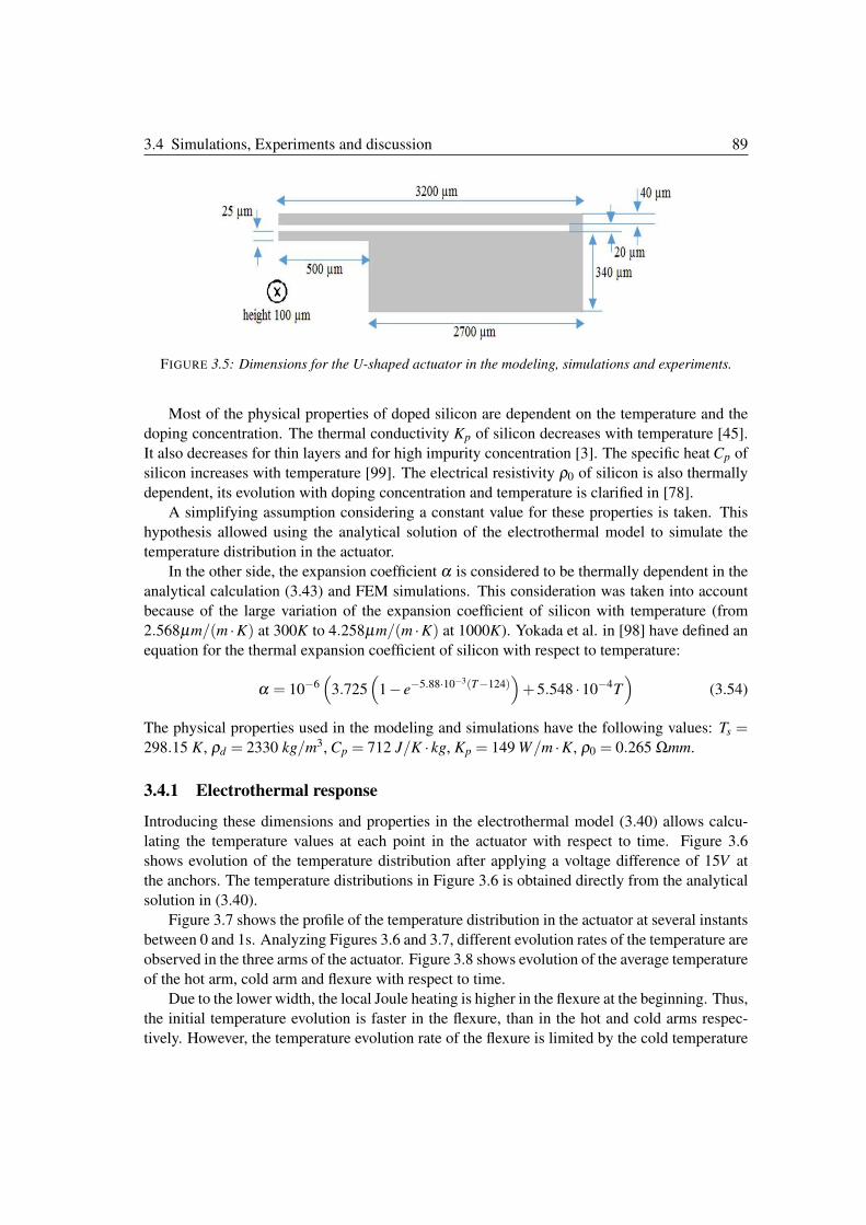
3.4 Simulations, Experiments and discussion 89
FIGURE 3.5: Dimensions for the U-shaped actuator in the modeling, simulations and experiments.
Most of the physical properties of doped silicon are dependent on the temperature and the
doping concentration. The thermal conductivity Kp of silicon decreases with temperature [45].
It also decreases for thin layers and for high impurity concentration [3]. The specific heat Cp of
silicon increases with temperature [99]. The electrical resistivity ρ0 of silicon is also thermally
dependent, its evolution with doping concentration and temperature is clarified in [78].
A simplifying assumption considering a constant value for these properties is taken. This
hypothesis allowed using the analytical solution of the electrothermal model to simulate the
temperature distribution in the actuator.
In the other side, the expansion coefficient α is considered to be thermally dependent in the
analytical calculation (3.43) and FEM simulations. This consideration was taken into account
because of the large variation of the expansion coefficient of silicon with temperature (from
2.568µm/(m ·K) at 300K to 4.258µm/(m ·K) at 1000K). Yokada et al. in [98] have defined an
equation for the thermal expansion coefficient of silicon with respect to temperature:
α = 10−6�
3.725�
1− e−5.88·10−3(T−124)�+5.548 ·10−4T
�(3.54)
The physical properties used in the modeling and simulations have the following values: Ts =298.15 K, ρd = 2330 kg/m3, Cp = 712 J/K · kg, Kp = 149 W/m ·K, ρ0 = 0.265 Ωmm.
3.4.1 Electrothermal response
Introducing these dimensions and properties in the electrothermal model (3.40) allows calcu-
lating the temperature values at each point in the actuator with respect to time. Figure 3.6
shows evolution of the temperature distribution after applying a voltage difference of 15V at
the anchors. The temperature distributions in Figure 3.6 is obtained directly from the analytical
solution in (3.40).
Figure 3.7 shows the profile of the temperature distribution in the actuator at several instants
between 0 and 1s. Analyzing Figures 3.6 and 3.7, different evolution rates of the temperature are
observed in the three arms of the actuator. Figure 3.8 shows evolution of the average temperature
of the hot arm, cold arm and flexure with respect to time.
Due to the lower width, the local Joule heating is higher in the flexure at the beginning. Thus,
the initial temperature evolution is faster in the flexure, than in the hot and cold arms respec-
tively. However, the temperature evolution rate of the flexure is limited by the cold temperature
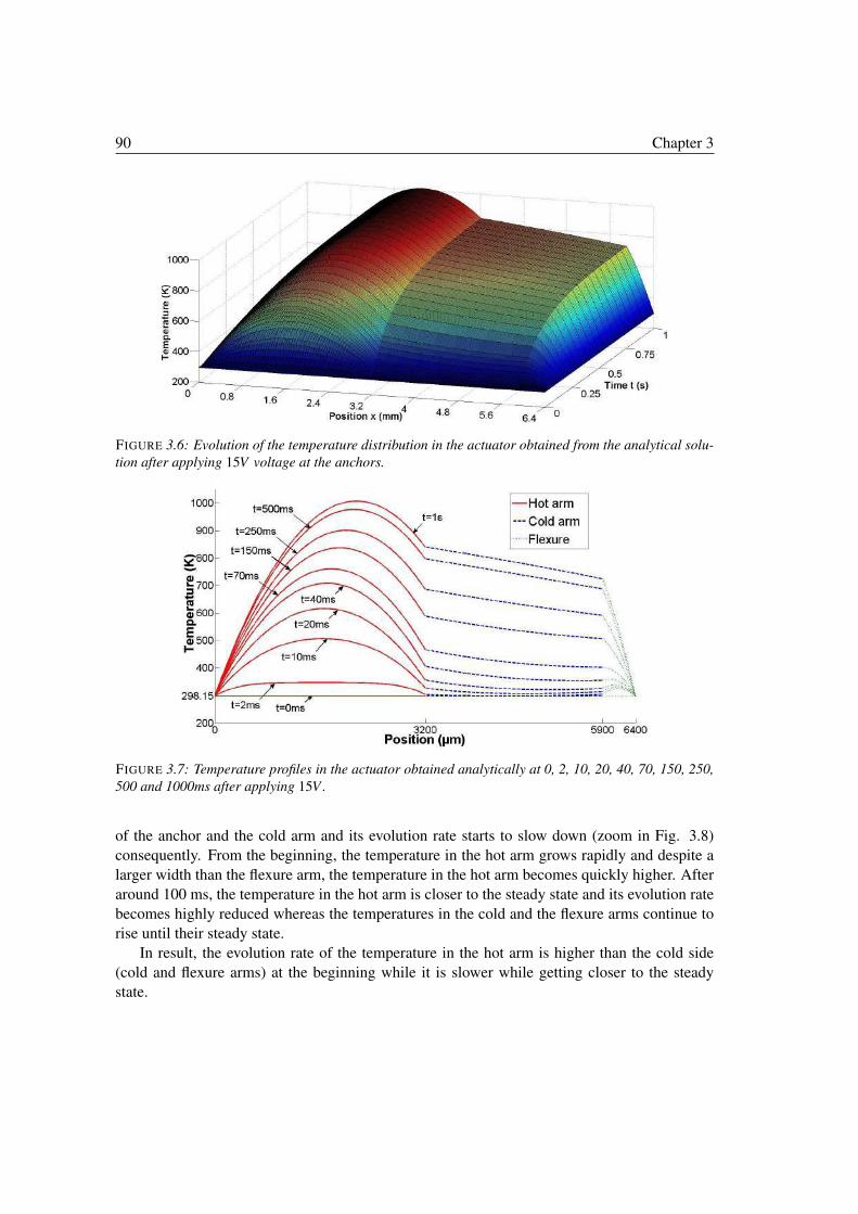
90 Chapter 3
FIGURE 3.6: Evolution of the temperature distribution in the actuator obtained from the analytical solu-
tion after applying 15V voltage at the anchors.
FIGURE 3.7: Temperature profiles in the actuator obtained analytically at 0, 2, 10, 20, 40, 70, 150, 250,
500 and 1000ms after applying 15V .
of the anchor and the cold arm and its evolution rate starts to slow down (zoom in Fig. 3.8)
consequently. From the beginning, the temperature in the hot arm grows rapidly and despite a
larger width than the flexure arm, the temperature in the hot arm becomes quickly higher. After
around 100 ms, the temperature in the hot arm is closer to the steady state and its evolution rate
becomes highly reduced whereas the temperatures in the cold and the flexure arms continue to
rise until their steady state.
In result, the evolution rate of the temperature in the hot arm is higher than the cold side
(cold and flexure arms) at the beginning while it is slower while getting closer to the steady
state.
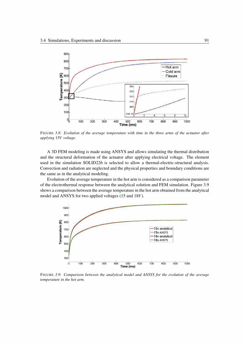
3.4 Simulations, Experiments and discussion 91
FIGURE 3.8: Evolution of the average temperature with time in the three arms of the actuator after
applying 15V voltage.
A 3D FEM modeling is made using ANSYS and allows simulating the thermal distribution
and the structural deformation of the actuator after applying electrical voltage. The element
used in the simulation SOLID226 is selected to allow a thermal-electric-structural analysis.
Convection and radiation are neglected and the physical properties and boundary conditions are
the same as in the analytical modeling.
Evolution of the average temperature in the hot arm is considered as a comparison parameter
of the electrothermal response between the analytical solution and FEM simulation. Figure 3.9
shows a comparison between the average temperature in the hot arm obtained from the analytical
model and ANSYS for two applied voltages (15 and 18V ).
FIGURE 3.9: Comparison between the analytical model and ANSYS for the evolution of the average
temperature in the hot arm.
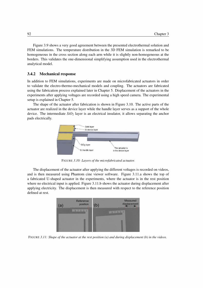
92 Chapter 3
Figure 3.9 shows a very good agreement between the presented electrothermal solution and
FEM simulations. The temperature distribution in the 3D FEM simulation is remarked to be
homogeneous in the cross section along each arm while it is slightly non-homogeneous at the
borders. This validates the one-dimensional simplifying assumption used in the electrothermal
analytical model.
3.4.2 Mechanical response
In addition to FEM simulations, experiments are made on microfabricated actuators in order
to validate the electro-thermo-mechanical models and coupling. The actuators are fabricated
using the fabrication process explained later in Chapter 5. Displacement of the actuators in the
experiments after applying voltages are recorded using a high speed camera. The experimental
setup is explained in Chapter 5.
The shape of the actuator after fabrication is shown in Figure 3.10. The active parts of the
actuator are realized in the device layer while the handle layer serves as a support of the whole
device. The intermediate SiO2 layer is an electrical insulator, it allows separating the anchor
pads electrically.
FIGURE 3.10: Layers of the microfabricated actuator.
The displacement of the actuator after applying the different voltages is recorded on videos,
and is then measured using Phantom cine viewer software. Figure 3.11.a shows the top of
a fabricated U-shaped actuator in the experiments, where the actuator is in the rest position
where no electrical input is applied. Figure 3.11.b shows the actuator during displacement after
applying electricity. The displacement is then measured with respect to the reference position
defined at rest.
FIGURE 3.11: Shape of the actuator at the rest position (a) and during displacement (b) in the videos.
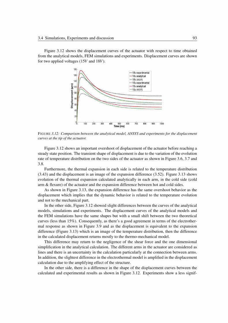
3.4 Simulations, Experiments and discussion 93
Figure 3.12 shows the displacement curves of the actuator with respect to time obtained
from the analytical models, FEM simulations and experiments. Displacement curves are shown
for two applied voltages (15V and 18V ).
FIGURE 3.12: Comparison between the analytical model, ANSYS and experiments for the displacement
curves at the tip of the actuator.
Figure 3.12 shows an important overshoot of displacement of the actuator before reaching a
steady state position. The transient shape of displacement is due to the variation of the evolution
rate of temperature distribution on the two sides of the actuator as shown in Figure 3.6, 3.7 and
3.8.
Furthermore, the thermal expansion in each side is related to the temperature distribution
(3.43) and the displacement is an image of the expansion difference (3.52). Figure 3.13 shows
evolution of the thermal expansion calculated analytically in each arm, in the cold side (cold
arm & flexure) of the actuator and the expansion difference between hot and cold sides.
As shown in Figure 3.13, the expansion difference has the same overshoot behavior as the
displacement which implies that the dynamic behavior is related to the temperature evolution
and not to the mechanical part.
In the other side, Figure 3.12 showed slight differences between the curves of the analytical
models, simulations and experiments. The displacement curves of the analytical models and
the FEM simulations have the same shapes but with a small shift between the two theoretical
curves (less than 15%). Consequently, as there’s a good agreement in terms of the electrother-
mal response as shown in Figure 3.9 and as the displacement is equivalent to the expansion
difference (Figure 3.13) which is an image of the temperature distribution, then the difference
in the calculated displacement returns mostly to the thermo-mechanical model.
This difference may return to the negligence of the shear force and the one dimensional
simplification in the analytical calculation. The different arms in the actuator are considered as
lines and there is an uncertainty in the calculation particularly at the connection between arms.
In addition, the slightest difference in the electrothermal model is amplified in the displacement
calculation due to the amplifying effect of the structure.
In the other side, there is a difference in the shape of the displacement curves between the
calculated and experimental results as shown in Figure 3.12. Experiments show a less signif-
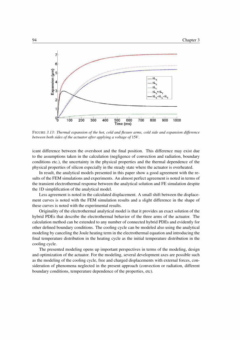
94 Chapter 3
FIGURE 3.13: Thermal expansion of the hot, cold and flexure arms, cold side and expansion difference
between both sides of the actuator after applying a voltage of 15V .
icant difference between the overshoot and the final position. This difference may exist due
to the assumptions taken in the calculation (negligence of convection and radiation, boundary
conditions etc.), the uncertainty in the physical properties and the thermal dependence of the
physical properties of silicon especially in the steady state where the actuator is overheated.
In result, the analytical models presented in this paper show a good agreement with the re-
sults of the FEM simulations and experiments. An almost perfect agreement is noted in terms of
the transient electrothermal response between the analytical solution and FE simulation despite
the 1D simplification of the analytical model.
Less agreement is noted in the calculated displacement. A small shift between the displace-
ment curves is noted with the FEM simulation results and a slight difference in the shape of
these curves is noted with the experimental results.
Originality of the electrothermal analytical model is that it provides an exact solution of the
hybrid PDEs that describe the electrothermal behavior of the three arms of the actuator. The
calculation method can be extended to any number of connected hybrid PDEs and evidently for
other defined boundary conditions. The cooling cycle can be modeled also using the analytical
modeling by canceling the Joule heating term in the electrothermal equation and introducing the
final temperature distribution in the heating cycle as the initial temperature distribution in the
cooling cycle.
The presented modeling opens up important perspectives in terms of the modeling, design
and optimization of the actuator. For the modeling, several development axes are possible such
as the modeling of the cooling cycle, free and charged displacements with external forces, con-
sideration of phenomena neglected in the present approach (convection or radiation, different
boundary conditions, temperature dependence of the properties, etc).
3.5 Design and optimization 95
3.5 Design and optimization
The dynamic behavior of the U-shaped actuator was investigated in the previous sections. An-
alytical models was presented which relate the electrical input and the applied load to the dis-
placement passing by the temperature distribution. These models was validated by comparing it
with the FEM simulations and experiments. The obtained expressions show clearly the influence
of the different dimensions and properties on the electrothermal behavior and the displacement
of the actuator. These expressions can be used for the design and the dimensioning of the U-
shaped actuator.
The purpose of this section is to provide key elements for the design of the U-shaped ac-
tuator based on the analytical models. Firstly, the maximal voltage that can be applied on the
actuator is calculated based on the maximal temperature allowed to be reached. After that, a new
formulation of the dimensions is adopted in order to present more clearly their influence and the
characteristic curve of the actuator. The influence of the different properties and dimensions
on the performance of the actuator is then clarified. Finally, a design method is proposed that
ensures obtaining the desired performance of the actuator in terms of the force and displacement.
3.5.1 Maximal voltage
As it has been recognized that the displacement of the actuator is related to the temperature
distribution, the higher is the temperature, the higher is the displacement. However, the tem-
perature in the actuator must not exceed a maximal limit that is defined with respect to the
material. Otherwise, high temperature leads to a degradation of the material properties, a plastic
deformation of the actuator, fracture at the weak points, etc..
Introducing the boundary and continuity conditions (3.17) in the steady state temperature
expressions (3.16), the different constants dh1, dh2, dc1, dc2, d f 1 and d f 2 are determined and the
steady state temperature distribution is obtained. These expressions show clearly the influence
of the different parameters on the temperature distributions (including the dimensions, voltage,
resistivity and conductivity).
Analyzing these expressions, an important conclusion is noticed. The maximal temperature
Tmax reached in the steady state for an applied voltage is independent of the actuator dimensions.
The expression of Tmax is as follows:
Tmax = T∞ +V 2
8ρ0Kp
(3.55)
In contrast, position of the maximal temperature point at the steady state xmax is dependent
only on the actuator dimensions. This point exists generally in the hot arm while it’s possible
to exist in the cold arm in some extreme cases. The expression of xmax in the two cases is as
follows:
xmax =lh
2+
Ah
2
�lc
Ac
+l f
A f
�l f
A f
+lc
Ac
<lh
Ah
xmax = lh +Ac
2
�− lh
Ah
+lc
Ac
+l f
A f
�l f
A f
+lc
Ac
>lh
Ah
(3.56)
96 Chapter 3
Based on the above, the maximal temperature expression allows defining a limitation Vmax
on the voltages, where Vmax is the maximal voltage allowed before reaching the maximal tem-
perature Tmax.
Vmax =�
8ρ0Kp(Tmax −T∞) (3.57)
The value of Vmax must be respected in the cases where the actuator is powered on for long
time and the feeding time may exceed the response time.
In the other side, the feeding time is related to the task requirement and the responsiveness
and capacity of the actuator. An optimal feeding time is when the actuator can do the task in the
time between the start of feeding and the peak of displacement. In this case, the actuator can
output a maximum of performance without overheating the different arms. During this time, the
temperature has not yet reached its maximum, thus, we can increase the voltage above the limits
imposed at the steady state. This allows reaching higher performance of the actuator.
3.5.2 Characteristic curve of the actuator
Improvement of the performance of the actuator is related to the improvement of its output,
which is expressed in terms of the displacement in the models. The expression of the displace-
ment is developed in the following in order to extract the characteristic curve of the actuator and
to show clearly the influence of the different dimensions and properties on the performance of
the actuator.
The expression of the displacement is given in (3.52). The constants K1 and K2 can be
expressed using another formulation which allows separating the general length l and width w
of the arms from the ratios of widths and length c, f , γ and a. The different lengths and widths
in this case have the following values:
lh = l lc = (1−a)l l f = a · lwh = w wc = c ·w w f = f ·w g = γ ·w (3.58)
Considering the new variables, the displacement can be expressed as follows:
d =l
wK�
1Δ− 1
E
l3
bw3K�
2F (3.59)
where K�1 and K�
2 are dependent only on a, c, γ and f . K�1 and K�
2 are obtained as follows:
K�1 =
�1 0 0
�
δ �XX δ �
Y X δ �MX
δ �XY δ �
YY δ �MY
δ �XM δ �
Y M δ �MM
−1
δ �X f
δ �Y f
δ �M f
(3.60a)
K�2 =−12
�δ �
X f δ �Y f δ �
M f
�
δ �XX δ �
Y X δ �MX
δ �XY δ �
YY δ �MY
δ �XM δ �
Y M δ �MM
−1
δ �X f
δ �Y f
δ �M f
−12δ �
F f (3.60b)
3.5 Design and optimization 97
The different terms δ � in (3.60) (δ �XX , δ �
YY , δ �MM, δ �
XY ...) are equivalent to the terms δ (δXX ,
δYY , δMM, δXY ...) in (3.47), (3.49) and (3.51). The terms δ � are related only to the ratios a, c, γand f . Some terms are neglected in the δ � expressions due to the relative difference between the
length and the width.
δ �XX =
(1+2γ + f )2a
4 f 3+
(1+2γ + c)2(1−a)
4c3+
a
12 f+
1−a
12c+
1
12(3.61a)
δ �YY =
a3
3 f 3+
1−a3
3c3+
1
3(3.61b)
δ �MM =
a
f 3+
1−a
c3+1 (3.61c)
δ �XY =
(1+2γ + f )a2
4 f 3+
(1+2γ + c)(1−a2)
4c3(3.61d)
δ �XM =
(1+2γ + f )a
2 f 3+
(1+2γ + c)(1−a)
2c3(3.61e)
δ �Y M =
a2
2 f 3+
1−a2
2c3+
1
2(3.61f)
δ �X f =
(1+2γ + f )(2a−a2)
4 f 3+
(1+2γ + c)(1−a)2
4c3(3.61g)
δ �Y f =
3a2 −2a3
6 f 3+
1−3a2 +2a3
6c3(3.61h)
δ �M f =
2a−a2
2 f 3+
(1−a)2
2c3(3.61i)
δ �F f =
−3a(1−a)−a3
3 f 3− (1−a)3
3c3(3.61j)
Equation (3.59) shows that the displacement is related linearly to the two actions: arms
expansion difference Δ and applied load F . In the other side, the different arms expansion Δlh,
Δlc and Δl f are calculated by introducing the temperature expressions (3.40) in the expansion
equation (3.43).
Δlh(t) = Δlhss −α∞
∑n=1
Chn
λn
(cos(λnl1 +ϕhn)− cos(ϕhn))e−αpλ 2n t (3.62a)
Δlc(t) = Δlcss −α∞
∑n=1
Ccn
λn
(cos(λnl2 +ϕcn)− cos(λnl1 +ϕcn))e−αpλ 2n t (3.62b)
Δl f (t) = Δl f ss −α∞
∑n=1
C f n
λn
(cos(λnl3 +ϕ f n)− cos(λnl2 +ϕ f n))e−αpλ 2n t (3.62c)
Noting that α is considered to be constant in the calculation in order to simplify the problem.
The terms Δlhss, Δlcss and Δl f ss correspond to the length expansions of the different arms
at the steady state. They are obtained by introducing the steady state temperature expressions
(3.16) in the expansion equation (3.43).
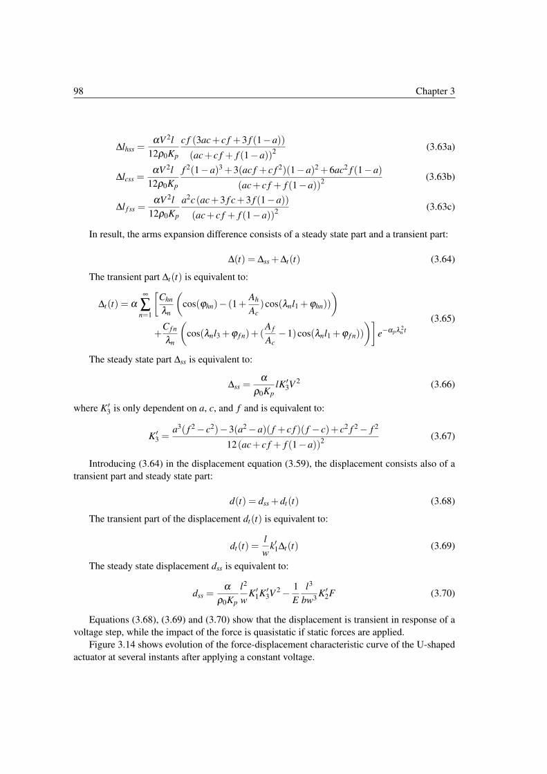
98 Chapter 3
Δlhss =αV 2l
12ρ0Kp
c f (3ac+ c f +3 f (1−a))
(ac+ c f + f (1−a))2(3.63a)
Δlcss =αV 2l
12ρ0Kp
f 2(1−a)3 +3(ac f + c f 2)(1−a)2 +6ac2 f (1−a)
(ac+ c f + f (1−a))2(3.63b)
Δl f ss =αV 2l
12ρ0Kp
a2c(ac+3 f c+3 f (1−a))
(ac+ c f + f (1−a))2(3.63c)
In result, the arms expansion difference consists of a steady state part and a transient part:
Δ(t) = Δss +Δt(t) (3.64)
The transient part Δt(t) is equivalent to:
Δt(t) = α∞
∑n=1
�Chn
λn
�cos(ϕhn)− (1+
Ah
Ac
)cos(λnl1 +ϕhn))
�
+C f n
λn
�cos(λnl3 +ϕ f n)+(
A f
Ac
−1)cos(λnl1 +ϕ f n))
��e−αpλ 2
n t
(3.65)
The steady state part Δss is equivalent to:
Δss =α
ρ0Kp
lK�3V 2 (3.66)
where K�3 is only dependent on a, c, and f and is equivalent to:
K�3 =
a3( f 2 − c2)−3(a2 −a)( f + c f )( f − c)+ c2 f 2 − f 2
12(ac+ c f + f (1−a))2(3.67)
Introducing (3.64) in the displacement equation (3.59), the displacement consists also of a
transient part and steady state part:
d(t) = dss +dt(t) (3.68)
The transient part of the displacement dt(t) is equivalent to:
dt(t) =l
wk�1Δt(t) (3.69)
The steady state displacement dss is equivalent to:
dss =α
ρ0Kp
l2
wK�
1K�3V 2 − 1
E
l3
bw3K�
2F (3.70)
Equations (3.68), (3.69) and (3.70) show that the displacement is transient in response of a
voltage step, while the impact of the force is quasistatic if static forces are applied.
Figure 3.14 shows evolution of the force-displacement characteristic curve of the U-shaped
actuator at several instants after applying a constant voltage.
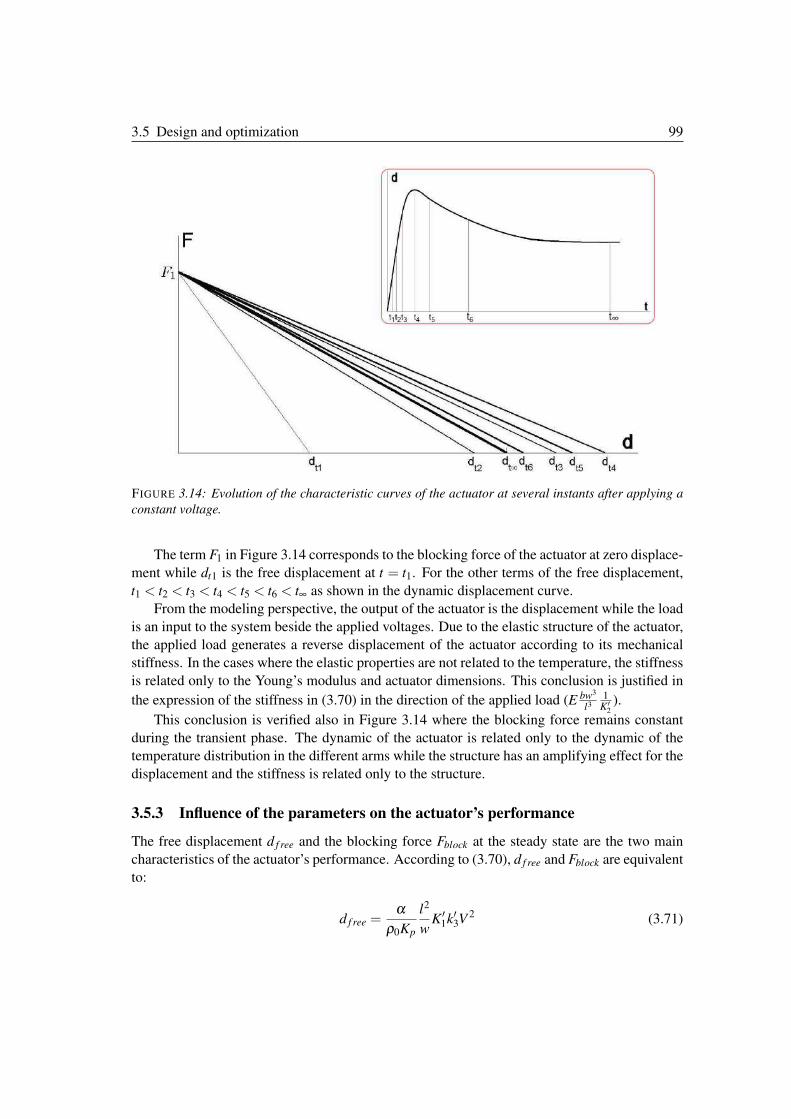
3.5 Design and optimization 99
FIGURE 3.14: Evolution of the characteristic curves of the actuator at several instants after applying a
constant voltage.
The term F1 in Figure 3.14 corresponds to the blocking force of the actuator at zero displace-
ment while dt1 is the free displacement at t = t1. For the other terms of the free displacement,
t1 < t2 < t3 < t4 < t5 < t6 < t∞ as shown in the dynamic displacement curve.
From the modeling perspective, the output of the actuator is the displacement while the load
is an input to the system beside the applied voltages. Due to the elastic structure of the actuator,
the applied load generates a reverse displacement of the actuator according to its mechanical
stiffness. In the cases where the elastic properties are not related to the temperature, the stiffness
is related only to the Young’s modulus and actuator dimensions. This conclusion is justified in
the expression of the stiffness in (3.70) in the direction of the applied load (E bw3
l31
K�2).
This conclusion is verified also in Figure 3.14 where the blocking force remains constant
during the transient phase. The dynamic of the actuator is related only to the dynamic of the
temperature distribution in the different arms while the structure has an amplifying effect for the
displacement and the stiffness is related only to the structure.
3.5.3 Influence of the parameters on the actuator’s performance
The free displacement d f ree and the blocking force Fblock at the steady state are the two main
characteristics of the actuator’s performance. According to (3.70), d f ree and Fblock are equivalent
to:
d f ree =α
ρ0Kp
l2
wK�
1k�3V 2 (3.71)
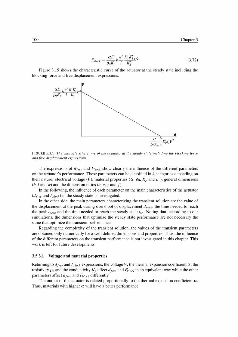
100 Chapter 3
Fblock =αE
ρ0Kp
bw2
l
K�1K�
3
K�2
V 2 (3.72)
Figure 3.15 shows the characteristic curve of the actuator at the steady state including the
blocking force and free displacement expressions.
FIGURE 3.15: The characteristic curve of the actuator at the steady state including the blocking force
and free displacement expressions.
The expressions of d f ree and Fblock show clearly the influence of the different parameters
on the actuator’s performance. These parameters can be classified in 4 categories depending on
their nature: electrical voltage (V ), material properties (α , ρ0, Kp and E ), general dimensions
(b, l and w) and the dimension ratios (a, c, γ and f ).
In the following, the influence of each parameter on the main characteristics of the actuator
(d f ree and Fblock) in the steady state is investigated.
In the other side, the main parameters characterizing the transient solution are the value of
the displacement at the peak during overshoot of displacement dpeak, the time needed to reach
the peak tpeak and the time needed to reach the steady state tss. Noting that, according to our
simulations, the dimensions that optimize the steady state performance are not necessary the
same that optimize the transient performance.
Regarding the complexity of the transient solution, the values of the transient parameters
are obtained only numerically for a well defined dimensions and properties. Thus, the influence
of the different parameters on the transient performance is not investigated in this chapter. This
work is left for future developments.
3.5.3.1 Voltage and material properties
Returning to d f ree and Fblock expressions, the voltage V , the thermal expansion coefficient α , the
resistivity ρ0 and the conductivity Kp affect d f ree and Fblock in an equivalent way while the other
parameters affect d f ree and Fblock differently.
The output of the actuator is related proportionally to the thermal expansion coefficient α .
Thus, materials with higher α will have a better performance.
3.5 Design and optimization 101
Idem, the output of the actuator is related proportionally to the square of the voltage and
inversely proportional to the resistivity and conductivity. In contrast, this doesn’t mean that the
actuator has a better performance for lower resistivity and conductivity because the maximal
allowable voltage Vmax is proportional to the root square of ρ0 and Kp as shown in (3.57). In
result, the performance is the same for variable values of ρ0 and Kp while the variation is in the
voltage margin.
The Young’s modulus E and the depth b have only an influence on the value of the blocking
force. Higher Young’s modulus for the material and depth for the actuator allow a higher pro-
portionally blocking force. Noting that for high values of the Young’s modulus E, the internal
stresses are higher and the failure limits can be early reached.
3.5.3.2 General dimensions
The general length l and width w have an inverse influence on d f ree and Fblock values. The free
displacement d f ree is proportional to the square of l and inversely proportional to w while the
blocking force Fblock is proportional to the square of w and inversely proportional to l.
Figure 3.16 shows the influence of changing the general dimensions of the actuator (l, w,
and b) on the characteristic curves. Noting that when changing l and w with the same ratio, the
characteristic curve evolves in parallel with the same ratio.
FIGURE 3.16: Influence of changing the general dimensions on the characteristic curve of the actuator:
including the general length l (a), the depth b (b), the general width w (c) and l and w simultaneously
with the same ratio of changing (d).
Furthermore, relating the influence of the general length l on the free displacement and on
the response time, we note that the two are proportional to the square of l. That means that
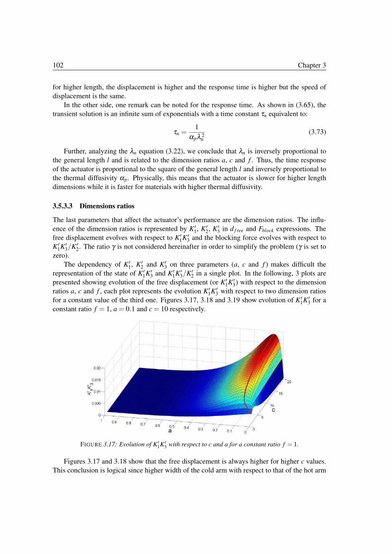
102 Chapter 3
for higher length, the displacement is higher and the response time is higher but the speed of
displacement is the same.
In the other side, one remark can be noted for the response time. As shown in (3.65), the
transient solution is an infinite sum of exponentials with a time constant τn equivalent to:
τn =1
αpλ 2n
(3.73)
Further, analyzing the λn equation (3.22), we conclude that λn is inversely proportional to
the general length l and is related to the dimension ratios a, c and f . Thus, the time response
of the actuator is proportional to the square of the general length l and inversely proportional to
the thermal diffusivity αp. Physically, this means that the actuator is slower for higher length
dimensions while it is faster for materials with higher thermal diffusivity.
3.5.3.3 Dimensions ratios
The last parameters that affect the actuator’s performance are the dimension ratios. The influ-
ence of the dimension ratios is represented by K�1, K�
2, K�3 in d f ree and Fblock expressions. The
free displacement evolves with respect to K�1K�
3 and the blocking force evolves with respect to
K�1K�
3/K�2. The ratio γ is not considered hereinafter in order to simplify the problem (γ is set to
zero).
The dependency of K�1, K�
2 and K�3 on three parameters (a, c and f ) makes difficult the
representation of the state of K�1K�
3 and K�1K�
3/K�2 in a single plot. In the following, 3 plots are
presented showing evolution of the free displacement (or K�1K�
3) with respect to the dimension
ratios a, c and f , each plot represents the evolution K�1K�
3 with respect to two dimension ratios
for a constant value of the third one. Figures 3.17, 3.18 and 3.19 show evolution of K�1K�
3 for a
constant ratio f = 1, a = 0.1 and c = 10 respectively.
FIGURE 3.17: Evolution of K�1K�
3 with respect to c and a for a constant ratio f = 1.
Figures 3.17 and 3.18 show that the free displacement is always higher for higher c values.
This conclusion is logical since higher width of the cold arm with respect to that of the hot arm
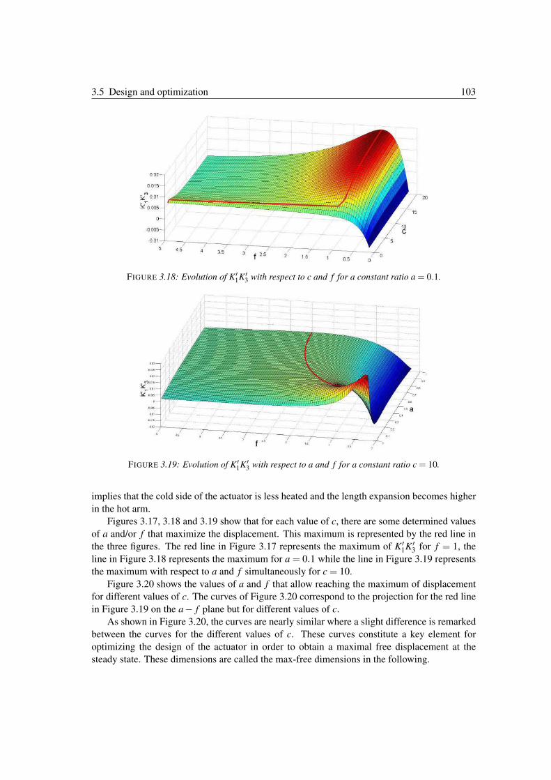
3.5 Design and optimization 103
FIGURE 3.18: Evolution of K�1K�
3 with respect to c and f for a constant ratio a = 0.1.
FIGURE 3.19: Evolution of K�1K�
3 with respect to a and f for a constant ratio c = 10.
implies that the cold side of the actuator is less heated and the length expansion becomes higher
in the hot arm.
Figures 3.17, 3.18 and 3.19 show that for each value of c, there are some determined values
of a and/or f that maximize the displacement. This maximum is represented by the red line in
the three figures. The red line in Figure 3.17 represents the maximum of K�1K�
3 for f = 1, the
line in Figure 3.18 represents the maximum for a = 0.1 while the line in Figure 3.19 represents
the maximum with respect to a and f simultaneously for c = 10.
Figure 3.20 shows the values of a and f that allow reaching the maximum of displacement
for different values of c. The curves of Figure 3.20 correspond to the projection for the red line
in Figure 3.19 on the a− f plane but for different values of c.
As shown in Figure 3.20, the curves are nearly similar where a slight difference is remarked
between the curves for the different values of c. These curves constitute a key element for
optimizing the design of the actuator in order to obtain a maximal free displacement at the
steady state. These dimensions are called the max-free dimensions in the following.
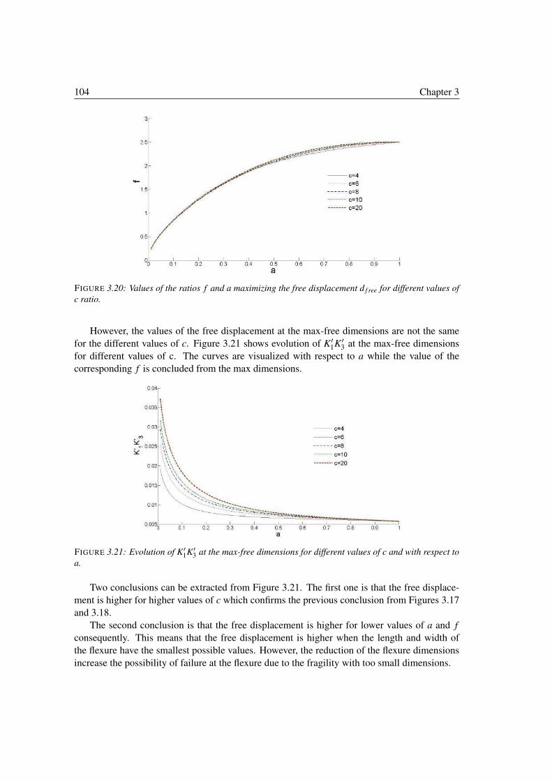
104 Chapter 3
FIGURE 3.20: Values of the ratios f and a maximizing the free displacement d f ree for different values of
c ratio.
However, the values of the free displacement at the max-free dimensions are not the same
for the different values of c. Figure 3.21 shows evolution of K�1K�
3 at the max-free dimensions
for different values of c. The curves are visualized with respect to a while the value of the
corresponding f is concluded from the max dimensions.
FIGURE 3.21: Evolution of K�1K�
3 at the max-free dimensions for different values of c and with respect to
a.
Two conclusions can be extracted from Figure 3.21. The first one is that the free displace-
ment is higher for higher values of c which confirms the previous conclusion from Figures 3.17
and 3.18.
The second conclusion is that the free displacement is higher for lower values of a and f
consequently. This means that the free displacement is higher when the length and width of
the flexure have the smallest possible values. However, the reduction of the flexure dimensions
increase the possibility of failure at the flexure due to the fragility with too small dimensions.
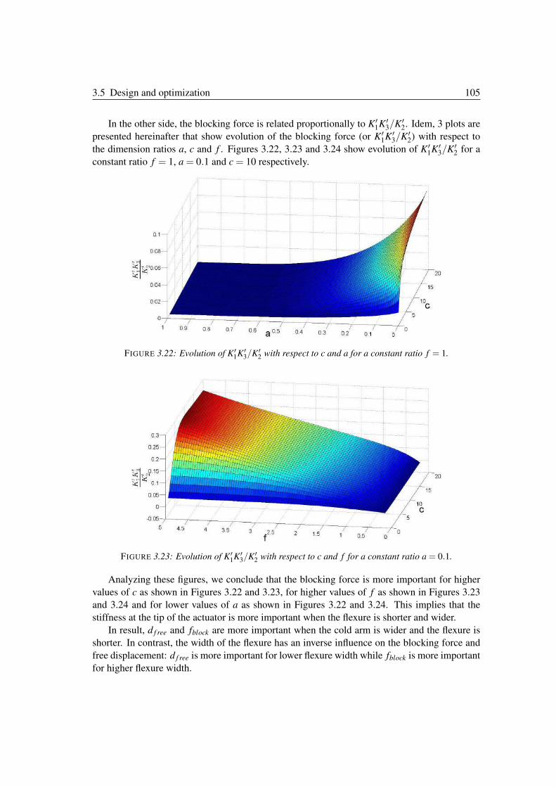
3.5 Design and optimization 105
In the other side, the blocking force is related proportionally to K�1K�
3/K�2. Idem, 3 plots are
presented hereinafter that show evolution of the blocking force (or K�1K�
3/K�2) with respect to
the dimension ratios a, c and f . Figures 3.22, 3.23 and 3.24 show evolution of K�1K�
3/K�2 for a
constant ratio f = 1, a = 0.1 and c = 10 respectively.
FIGURE 3.22: Evolution of K�1K�
3/K�2 with respect to c and a for a constant ratio f = 1.
FIGURE 3.23: Evolution of K�1K�
3/K�2 with respect to c and f for a constant ratio a = 0.1.
Analyzing these figures, we conclude that the blocking force is more important for higher
values of c as shown in Figures 3.22 and 3.23, for higher values of f as shown in Figures 3.23
and 3.24 and for lower values of a as shown in Figures 3.22 and 3.24. This implies that the
stiffness at the tip of the actuator is more important when the flexure is shorter and wider.
In result, d f ree and fblock are more important when the cold arm is wider and the flexure is
shorter. In contrast, the width of the flexure has an inverse influence on the blocking force and
free displacement: d f ree is more important for lower flexure width while fblock is more important
for higher flexure width.
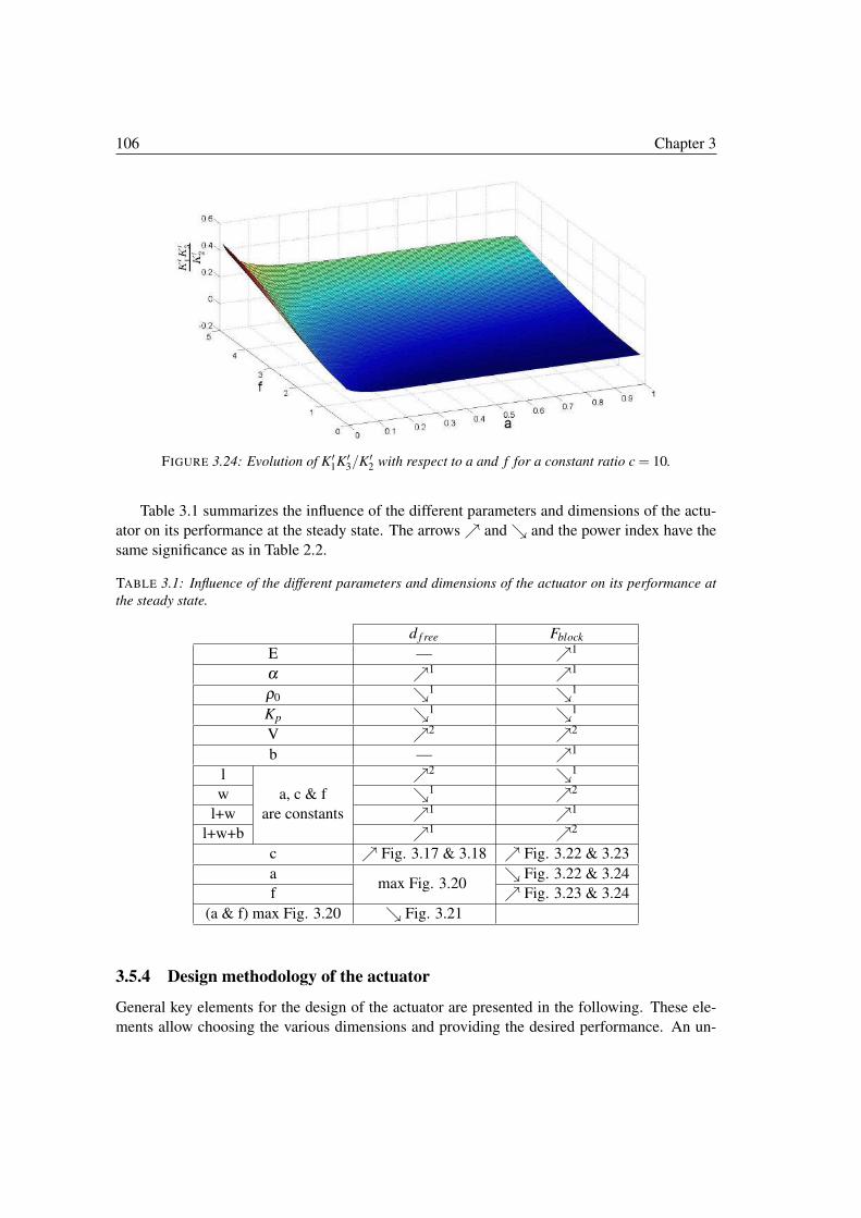
106 Chapter 3
FIGURE 3.24: Evolution of K�1K�
3/K�2 with respect to a and f for a constant ratio c = 10.
Table 3.1 summarizes the influence of the different parameters and dimensions of the actu-
ator on its performance at the steady state. The arrows � and � and the power index have the
same significance as in Table 2.2.
TABLE 3.1: Influence of the different parameters and dimensions of the actuator on its performance at
the steady state.
d f ree Fblock
E — �1
α �1 �1
ρ0 �1 �1
Kp �1 �1
V �2 �2
b — �1
l �2 �1
w a, c & f �1 �2
l+w are constants �1 �1
l+w+b �1 �2
c � Fig. 3.17 & 3.18 � Fig. 3.22 & 3.23
amax Fig. 3.20
� Fig. 3.22 & 3.24
f � Fig. 3.23 & 3.24
(a & f) max Fig. 3.20 � Fig. 3.21
3.5.4 Design methodology of the actuator
General key elements for the design of the actuator are presented in the following. These ele-
ments allow choosing the various dimensions and providing the desired performance. An un-
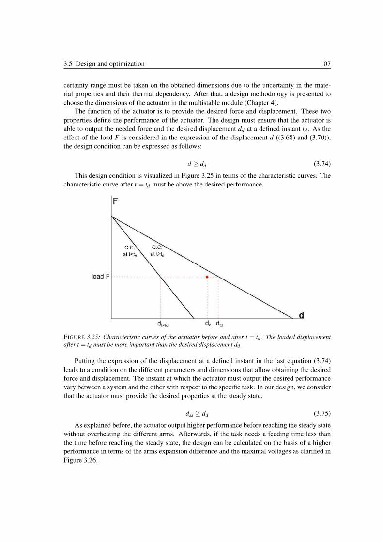
3.5 Design and optimization 107
certainty range must be taken on the obtained dimensions due to the uncertainty in the mate-
rial properties and their thermal dependency. After that, a design methodology is presented to
choose the dimensions of the actuator in the multistable module (Chapter 4).
The function of the actuator is to provide the desired force and displacement. These two
properties define the performance of the actuator. The design must ensure that the actuator is
able to output the needed force and the desired displacement dd at a defined instant td . As the
effect of the load F is considered in the expression of the displacement d ((3.68) and (3.70)),
the design condition can be expressed as follows:
d ≥ dd (3.74)
This design condition is visualized in Figure 3.25 in terms of the characteristic curves. The
characteristic curve after t = td must be above the desired performance.
FIGURE 3.25: Characteristic curves of the actuator before and after t = td . The loaded displacement
after t = td must be more important than the desired displacement dd .
Putting the expression of the displacement at a defined instant in the last equation (3.74)
leads to a condition on the different parameters and dimensions that allow obtaining the desired
force and displacement. The instant at which the actuator must output the desired performance
vary between a system and the other with respect to the specific task. In our design, we consider
that the actuator must provide the desired properties at the steady state.
dss ≥ dd (3.75)
As explained before, the actuator output higher performance before reaching the steady state
without overheating the different arms. Afterwards, if the task needs a feeding time less than
the time before reaching the steady state, the design can be calculated on the basis of a higher
performance in terms of the arms expansion difference and the maximal voltages as clarified in
Figure 3.26.
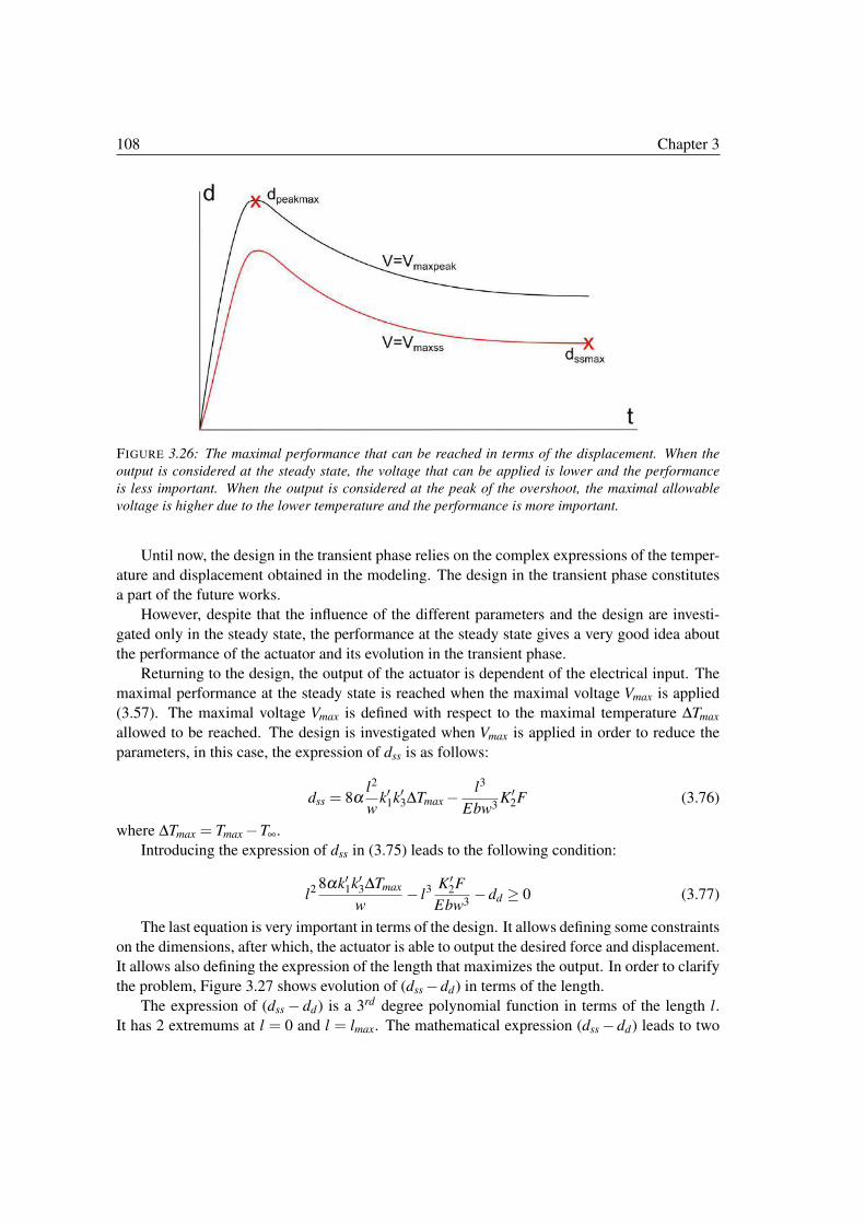
108 Chapter 3
FIGURE 3.26: The maximal performance that can be reached in terms of the displacement. When the
output is considered at the steady state, the voltage that can be applied is lower and the performance
is less important. When the output is considered at the peak of the overshoot, the maximal allowable
voltage is higher due to the lower temperature and the performance is more important.
Until now, the design in the transient phase relies on the complex expressions of the temper-
ature and displacement obtained in the modeling. The design in the transient phase constitutes
a part of the future works.
However, despite that the influence of the different parameters and the design are investi-
gated only in the steady state, the performance at the steady state gives a very good idea about
the performance of the actuator and its evolution in the transient phase.
Returning to the design, the output of the actuator is dependent of the electrical input. The
maximal performance at the steady state is reached when the maximal voltage Vmax is applied
(3.57). The maximal voltage Vmax is defined with respect to the maximal temperature ΔTmax
allowed to be reached. The design is investigated when Vmax is applied in order to reduce the
parameters, in this case, the expression of dss is as follows:
dss = 8αl2
wk�1k�3ΔTmax −
l3
Ebw3K�
2F (3.76)
where ΔTmax = Tmax −T∞.
Introducing the expression of dss in (3.75) leads to the following condition:
l2 8αk�1k�3ΔTmax
w− l3 K�
2F
Ebw3−dd ≥ 0 (3.77)
The last equation is very important in terms of the design. It allows defining some constraints
on the dimensions, after which, the actuator is able to output the desired force and displacement.
It allows also defining the expression of the length that maximizes the output. In order to clarify
the problem, Figure 3.27 shows evolution of (dss −dd) in terms of the length.
The expression of (dss − dd) is a 3rd degree polynomial function in terms of the length l.
It has 2 extremums at l = 0 and l = lmax. The mathematical expression (dss − dd) leads to two
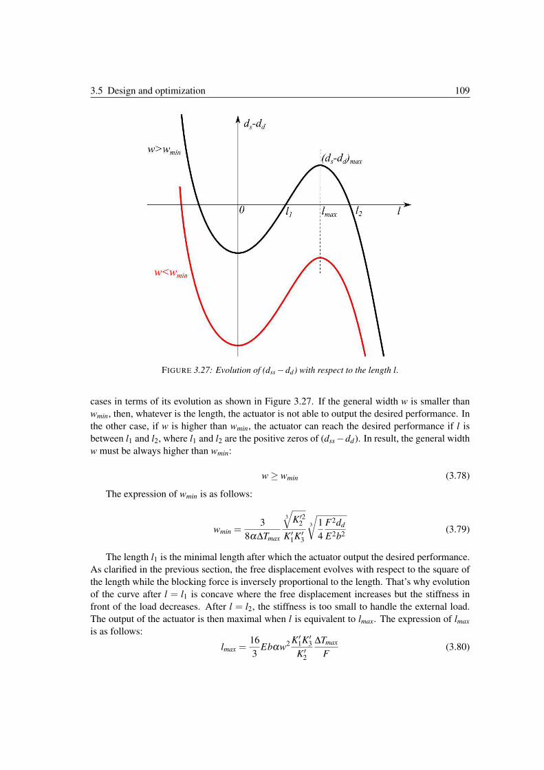
3.5 Design and optimization 109
FIGURE 3.27: Evolution of (dss −dd) with respect to the length l.
cases in terms of its evolution as shown in Figure 3.27. If the general width w is smaller than
wmin, then, whatever is the length, the actuator is not able to output the desired performance. In
the other case, if w is higher than wmin, the actuator can reach the desired performance if l is
between l1 and l2, where l1 and l2 are the positive zeros of (dss−dd). In result, the general width
w must be always higher than wmin:
w ≥ wmin (3.78)
The expression of wmin is as follows:
wmin =3
8αΔTmax
3
�K�2
2
K�1K�
3
3
�1
4
F2dd
E2b2(3.79)
The length l1 is the minimal length after which the actuator output the desired performance.
As clarified in the previous section, the free displacement evolves with respect to the square of
the length while the blocking force is inversely proportional to the length. That’s why evolution
of the curve after l = l1 is concave where the free displacement increases but the stiffness in
front of the load decreases. After l = l2, the stiffness is too small to handle the external load.
The output of the actuator is then maximal when l is equivalent to lmax. The expression of lmax
is as follows:
lmax =16
3Ebαw2 K�
1K�3
K�2
ΔTmax
F(3.80)
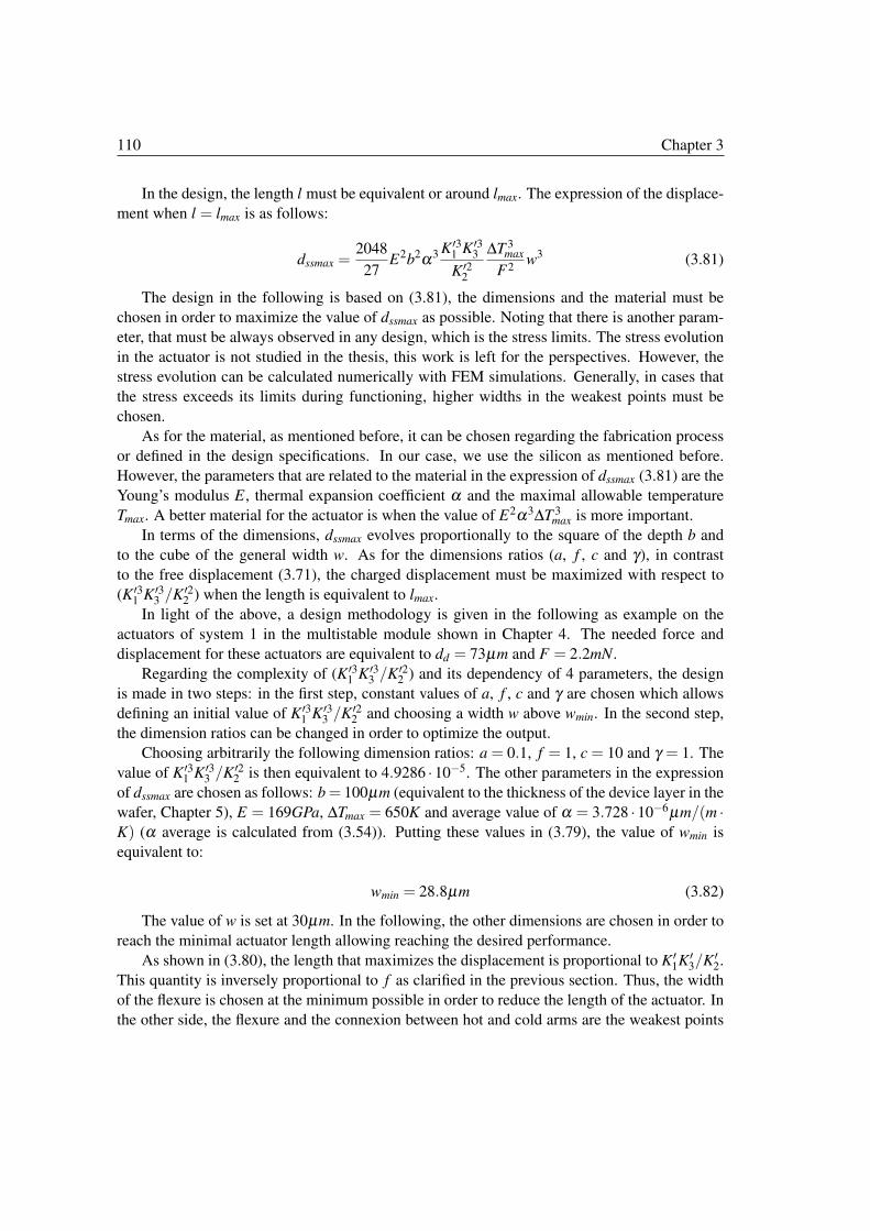
110 Chapter 3
In the design, the length l must be equivalent or around lmax. The expression of the displace-
ment when l = lmax is as follows:
dssmax =2048
27E2b2α3 K�3
1 K�33
K�22
ΔT 3max
F2w3 (3.81)
The design in the following is based on (3.81), the dimensions and the material must be
chosen in order to maximize the value of dssmax as possible. Noting that there is another param-
eter, that must be always observed in any design, which is the stress limits. The stress evolution
in the actuator is not studied in the thesis, this work is left for the perspectives. However, the
stress evolution can be calculated numerically with FEM simulations. Generally, in cases that
the stress exceeds its limits during functioning, higher widths in the weakest points must be
chosen.
As for the material, as mentioned before, it can be chosen regarding the fabrication process
or defined in the design specifications. In our case, we use the silicon as mentioned before.
However, the parameters that are related to the material in the expression of dssmax (3.81) are the
Young’s modulus E, thermal expansion coefficient α and the maximal allowable temperature
Tmax. A better material for the actuator is when the value of E2α3ΔT 3max is more important.
In terms of the dimensions, dssmax evolves proportionally to the square of the depth b and
to the cube of the general width w. As for the dimensions ratios (a, f , c and γ), in contrast
to the free displacement (3.71), the charged displacement must be maximized with respect to
(K�31 K�3
3 /K�22 ) when the length is equivalent to lmax.
In light of the above, a design methodology is given in the following as example on the
actuators of system 1 in the multistable module shown in Chapter 4. The needed force and
displacement for these actuators are equivalent to dd = 73µm and F = 2.2mN.
Regarding the complexity of (K�31 K�3
3 /K�22 ) and its dependency of 4 parameters, the design
is made in two steps: in the first step, constant values of a, f , c and γ are chosen which allows
defining an initial value of K�31 K�3
3 /K�22 and choosing a width w above wmin. In the second step,
the dimension ratios can be changed in order to optimize the output.
Choosing arbitrarily the following dimension ratios: a = 0.1, f = 1, c = 10 and γ = 1. The
value of K�31 K�3
3 /K�22 is then equivalent to 4.9286 ·10−5. The other parameters in the expression
of dssmax are chosen as follows: b= 100µm (equivalent to the thickness of the device layer in the
wafer, Chapter 5), E = 169GPa, ΔTmax = 650K and average value of α = 3.728 ·10−6µm/(m ·
K) (α average is calculated from (3.54)). Putting these values in (3.79), the value of wmin is
equivalent to:
wmin = 28.8µm (3.82)
The value of w is set at 30µm. In the following, the other dimensions are chosen in order to
reach the minimal actuator length allowing reaching the desired performance.
As shown in (3.80), the length that maximizes the displacement is proportional to K�1K�
3/K�2.
This quantity is inversely proportional to f as clarified in the previous section. Thus, the width
of the flexure is chosen at the minimum possible in order to reduce the length of the actuator. In
the other side, the flexure and the connexion between hot and cold arms are the weakest points
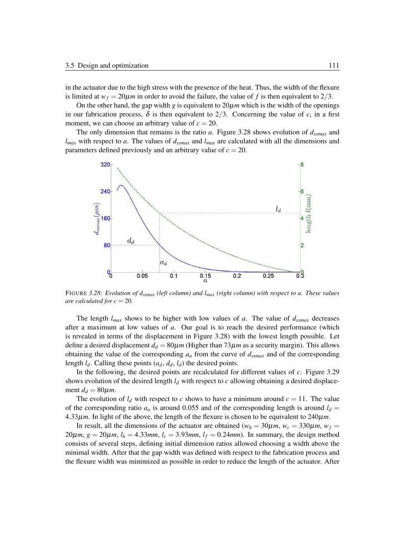
3.5 Design and optimization 111
in the actuator due to the high stress with the presence of the heat. Thus, the width of the flexure
is limited at w f = 20µm in order to avoid the failure, the value of f is then equivalent to 2/3.
On the other hand, the gap width g is equivalent to 20µm which is the width of the openings
in our fabrication process, δ is then equivalent to 2/3. Concerning the value of c, in a first
moment, we can choose an arbitrary value of c = 20.
The only dimension that remains is the ratio a. Figure 3.28 shows evolution of dssmax and
lmax with respect to a. The values of dssmax and lmax are calculated with all the dimensions and
parameters defined previously and an arbitrary value of c = 20.
FIGURE 3.28: Evolution of dssmax (left column) and lmax (right column) with respect to a. These values
are calculated for c = 20.
The length lmax shows to be higher with low values of a. The value of dssmax decreases
after a maximum at low values of a. Our goal is to reach the desired performance (which
is revealed in terms of the displacement in Figure 3.28) with the lowest length possible. Let
define a desired displacement dd = 80µm (Higher than 73µm as a security margin). This allows
obtaining the value of the corresponding aa from the curve of dssmax and of the corresponding
length ld . Calling these points (ad , dd , ld) the desired points.
In the following, the desired points are recalculated for different values of c. Figure 3.29
shows evolution of the desired length ld with respect to c allowing obtaining a desired displace-
ment dd = 80µm.
The evolution of ld with respect to c shows to have a minimum around c = 11. The value
of the corresponding ratio aa is around 0.055 and of the corresponding length is around ld =4.33µm. In light of the above, the length of the flexure is chosen to be equivalent to 240µm.
In result, all the dimensions of the actuator are obtained (wh = 30µm, wc = 330µm, w f =20µm, g = 20µm, lh = 4.33mm, lc = 3.93mm, l f = 0.24mm). In summary, the design method
consists of several steps, defining initial dimension ratios allowed choosing a width above the
minimal width. After that the gap width was defined with respect to the fabrication process and
the flexure width was minimized as possible in order to reduce the length of the actuator. After
112 Chapter 3
FIGURE 3.29: Evolution of the desired length ld with respect to c allowing obtaining a desired displace-
ment dd = 80µm.
that, scanning the values of the length with respect to a and c allowed defining the minimal value
of the length and the corresponding a and c that allows reaching the desired performance.
3.6 Conclusion
The modeling and design of the U-shaped actuator were investigated in this chapter. An exact
solution was presented for the electrothermal PDEs in the case of the actuator. The displacement
was then calculated by a thermomechanical model with respect to the temperature distribution
obtained from the electrothermal model and an external load. The two models showed a good
agreement with FEM simulations and experiments.
The design of the actuator was investigated subsequently. The impact of the different dimen-
sions and properties on the actuator behavior was studied. A design method was then proposed
that allows choosing and optimizing the dimensions that ensure reaching a required performance
at the steady state in terms of the force and displacement.
The studies in this chapter and Chapter 2 provide key elements for understanding the behav-
ior and improving the design of the main components (curved beams and U-shaped actuators)
in the DiMiBot and the multistable module which are presented in the next chapter.
Noting that the dimensions of the actuator obtained in this section are not the same in the
multistable module since this work was made at a late stage of the thesis. The length of the
actuator and its ”steady state” capacity is lower in the multistable module since the actuator
is designed to provide the desired performance near to the overshoot as clarified previously in
the chapter. The perspectives for the works on the U-shaped actuator are cited later in the final
conclusion of the thesis.
Chapter 4Multistable module and DiMiBot
In this chapter, the principle and the design of a novel multistable module are pre-
sented. The multistable module has a monolithic and compliant structure and al-
lows switching its moving part between several stable positions linearly in a one
dimensional direction back and forth. The number of stable positions can be in-
creased by increasing the range of displacement of the moving part. Transition is
made by an upward or downward step to one of the nearest two stable positions.
Upward and downward steps are made by a specific sequence of moving and open-
ing normally closed latch arms and closing other normally open latch arms. An
accurate positioning mechanism is used in order to ensure accurate steps and to
compensate the fabrication tolerances.
The design of the different components and each system in the multistable module is
presented in this chapter. The design of the global structure of a multistable module
is then presented. Finally, the design of the multistable DiMiBot, which consists of
two multistable modules, is presented.
114 Chapter 4
Chapter contents
4.1 Introduction . . . . . . . . . . . . . . . . . . . . . . . . . . . . . . . . . . 115
4.2 Principle of the multistable mechanism . . . . . . . . . . . . . . . . . . . 117
4.3 System 1: an accurate bistable mechanism . . . . . . . . . . . . . . . . . 119
4.3.1 Microfabrication tolerances . . . . . . . . . . . . . . . . . . . . . . 120
4.3.2 Accurate positioning mechanism . . . . . . . . . . . . . . . . . . . . 121
4.3.3 Design of the different components in system 1 . . . . . . . . . . . . 124
4.4 System 2 and the teeth configurations . . . . . . . . . . . . . . . . . . . . 127
4.4.1 Functioning . . . . . . . . . . . . . . . . . . . . . . . . . . . . . . . 127
4.4.2 Teeth configurations . . . . . . . . . . . . . . . . . . . . . . . . . . 128
4.5 System 3 and the moving part . . . . . . . . . . . . . . . . . . . . . . . . 130
4.6 Multistable module global design . . . . . . . . . . . . . . . . . . . . . . . 132
4.7 Multistable modules in the DiMiBot . . . . . . . . . . . . . . . . . . . . . 133
4.8 Conclusion . . . . . . . . . . . . . . . . . . . . . . . . . . . . . . . . . . . 137
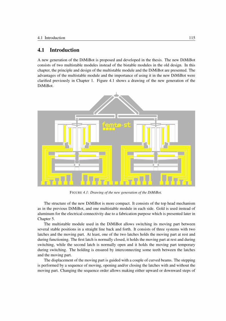
4.1 Introduction 115
4.1 Introduction
A new generation of the DiMiBot is proposed and developed in the thesis. The new DiMiBot
consists of two multistable modules instead of the bistable modules in the old design. In this
chapter, the principle and design of the multistable module and the DiMiBot are presented. The
advantages of the multistable module and the importance of using it in the new DiMiBot were
clarified previously in Chapter 1. Figure 4.1 shows a drawing of the new generation of the
DiMiBot.
FIGURE 4.1: Drawing of the new generation of the DiMiBot.
The structure of the new DiMiBot is more compact. It consists of the top head mechanism
as in the previous DiMiBot, and one multistable module in each side. Gold is used instead of
aluminum for the electrical connectivity due to a fabrication purpose which is presented later in
Chapter 5.
The multistable module used in the DiMiBot allows switching its moving part between
several stable positions in a straight line back and forth. It consists of three systems with two
latches and the moving part. At least, one of the two latches holds the moving part at rest and
during functioning. The first latch is normally closed, it holds the moving part at rest and during
switching, while the second latch is normally open and it holds the moving part temporary
during switching. The holding is ensured by interconnecting some teeth between the latches
and the moving part.
The displacement of the moving part is guided with a couple of curved beams. The stepping
is performed by a sequence of moving, opening and/or closing the latches with and without the
moving part. Changing the sequence order allows making either upward or downward steps of
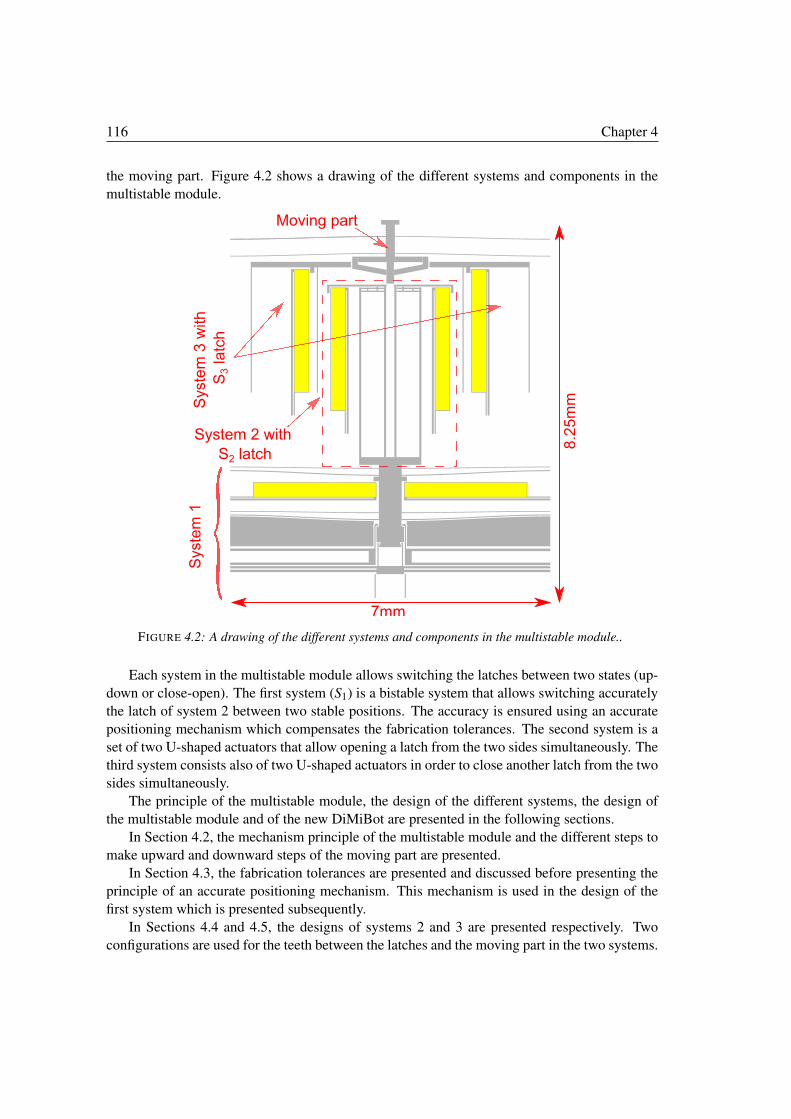
116 Chapter 4
the moving part. Figure 4.2 shows a drawing of the different systems and components in the
multistable module.
FIGURE 4.2: A drawing of the different systems and components in the multistable module..
Each system in the multistable module allows switching the latches between two states (up-
down or close-open). The first system (S1) is a bistable system that allows switching accurately
the latch of system 2 between two stable positions. The accuracy is ensured using an accurate
positioning mechanism which compensates the fabrication tolerances. The second system is a
set of two U-shaped actuators that allow opening a latch from the two sides simultaneously. The
third system consists also of two U-shaped actuators in order to close another latch from the two
sides simultaneously.
The principle of the multistable module, the design of the different systems, the design of
the multistable module and of the new DiMiBot are presented in the following sections.
In Section 4.2, the mechanism principle of the multistable module and the different steps to
make upward and downward steps of the moving part are presented.
In Section 4.3, the fabrication tolerances are presented and discussed before presenting the
principle of an accurate positioning mechanism. This mechanism is used in the design of the
first system which is presented subsequently.
In Sections 4.4 and 4.5, the designs of systems 2 and 3 are presented respectively. Two
configurations are used for the teeth between the latches and the moving part in the two systems.
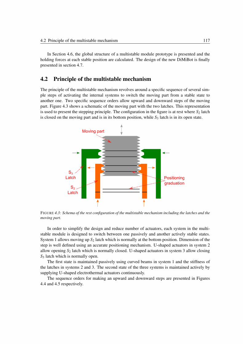
4.2 Principle of the multistable mechanism 117
In Section 4.6, the global structure of a multistable module prototype is presented and the
holding forces at each stable position are calculated. The design of the new DiMiBot is finally
presented in section 4.7.
4.2 Principle of the multistable mechanism
The principle of the multistable mechanism revolves around a specific sequence of several sim-
ple steps of activating the internal systems to switch the moving part from a stable state to
another one. Two specific sequence orders allow upward and downward steps of the moving
part. Figure 4.3 shows a schematic of the moving part with the two latches. This representation
is used to present the stepping principle. The configuration in the figure is at rest where S2 latch
is closed on the moving part and is in its bottom position, while S3 latch is in its open state.
FIGURE 4.3: Schema of the rest configuration of the multistable mechanism including the latches and the
moving part.
In order to simplify the design and reduce number of actuators, each system in the multi-
stable module is designed to switch between one passively and another actively stable states.
System 1 allows moving up S2 latch which is normally at the bottom position. Dimension of the
step is well defined using an accurate positioning mechanism. U-shaped actuators in system 2
allow opening S2 latch which is normally closed. U-shaped actuators in system 3 allow closing
S3 latch which is normally open.
The first state is maintained passively using curved beams in system 1 and the stiffness of
the latches in systems 2 and 3. The second state of the three systems is maintained actively by
supplying U-shaped electrothermal actuators continuously.
The sequence orders for making an upward and downward steps are presented in Figures
4.4 and 4.5 respectively.
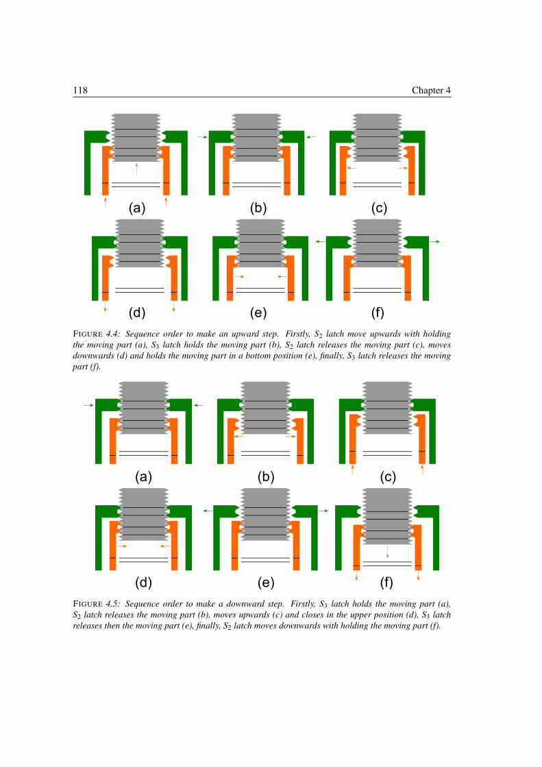
118 Chapter 4
FIGURE 4.4: Sequence order to make an upward step. Firstly, S2 latch move upwards with holding
the moving part (a), S3 latch holds the moving part (b), S2 latch releases the moving part (c), moves
downwards (d) and holds the moving part in a bottom position (e), finally, S3 latch releases the moving
part (f).
FIGURE 4.5: Sequence order to make a downward step. Firstly, S3 latch holds the moving part (a),
S2 latch releases the moving part (b), moves upwards (c) and closes in the upper position (d), S3 latch
releases then the moving part (e), finally, S2 latch moves downwards with holding the moving part (f).
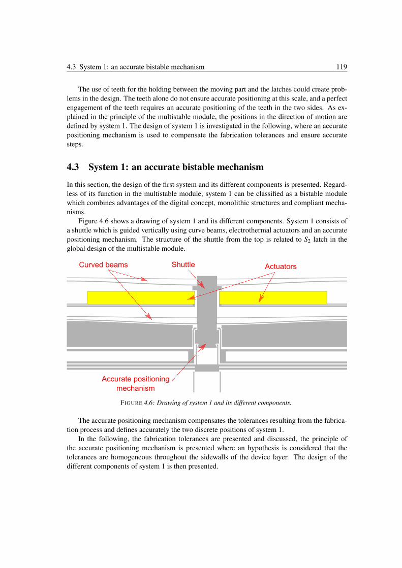
4.3 System 1: an accurate bistable mechanism 119
The use of teeth for the holding between the moving part and the latches could create prob-
lems in the design. The teeth alone do not ensure accurate positioning at this scale, and a perfect
engagement of the teeth requires an accurate positioning of the teeth in the two sides. As ex-
plained in the principle of the multistable module, the positions in the direction of motion are
defined by system 1. The design of system 1 is investigated in the following, where an accurate
positioning mechanism is used to compensate the fabrication tolerances and ensure accurate
steps.
4.3 System 1: an accurate bistable mechanism
In this section, the design of the first system and its different components is presented. Regard-
less of its function in the multistable module, system 1 can be classified as a bistable module
which combines advantages of the digital concept, monolithic structures and compliant mecha-
nisms.
Figure 4.6 shows a drawing of system 1 and its different components. System 1 consists of
a shuttle which is guided vertically using curve beams, electrothermal actuators and an accurate
positioning mechanism. The structure of the shuttle from the top is related to S2 latch in the
global design of the multistable module.
FIGURE 4.6: Drawing of system 1 and its different components.
The accurate positioning mechanism compensates the tolerances resulting from the fabrica-
tion process and defines accurately the two discrete positions of system 1.
In the following, the fabrication tolerances are presented and discussed, the principle of
the accurate positioning mechanism is presented where an hypothesis is considered that the
tolerances are homogeneous throughout the sidewalls of the device layer. The design of the
different components of system 1 is then presented.
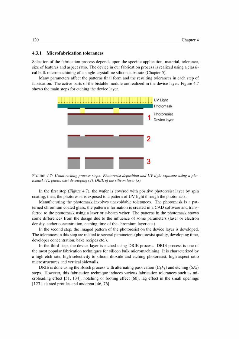
120 Chapter 4
4.3.1 Microfabrication tolerances
Selection of the fabrication process depends upon the specific application, material, tolerance,
size of features and aspect ratio. The device in our fabrication process is realized using a classi-
cal bulk micromachining of a single-crystalline silicon substrate (Chapter 5).
Many parameters affect the patterns final form and the resulting tolerances in each step of
fabrication. The active parts of the bistable module are realized in the device layer. Figure 4.7
shows the main steps for etching the device layer.
FIGURE 4.7: Usual etching process steps. Photoresist deposition and UV light exposure using a pho-
tomask (1), photoresist developing (2), DRIE of the silicon layer (3).
In the first step (Figure 4.7), the wafer is covered with positive photoresist layer by spin
coating, then, the photoresist is exposed to a pattern of UV light through the photomask.
Manufacturing the photomask involves unavoidable tolerances. The photomask is a pat-
terned chromium coated glass, the pattern information is created in a CAD software and trans-
ferred to the photomask using a laser or e-beam writer. The patterns in the photomask shows
some differences from the design due to the influence of some parameters (laser or electron
density, etcher concentration, etching time of the chromium layer etc.).
In the second step, the imaged pattern of the photoresist on the device layer is developed.
The tolerances in this step are related to several parameters (photoresist quality, developing time,
developer concentration, bake recipes etc.).
In the third step, the device layer is etched using DRIE process. DRIE process is one of
the most popular fabrication techniques for silicon bulk micromachining. It is characterized by
a high etch rate, high selectivity to silicon dioxide and etching photoresist, high aspect ratio
microstructures and vertical sidewalls.
DRIE is done using the Bosch process with alternating passivation (C4F8) and etching (SF6)steps. However, this fabrication technique induces various fabrication tolerances such as mi-
croloading effect [51, 134], notching or footing effect [60], lag effect in the small openings
[123], slanted profiles and undercut [46, 76].
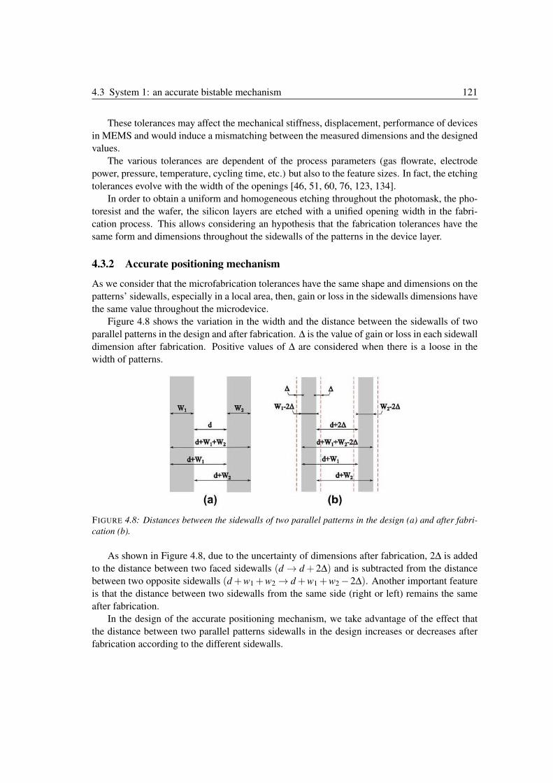
4.3 System 1: an accurate bistable mechanism 121
These tolerances may affect the mechanical stiffness, displacement, performance of devices
in MEMS and would induce a mismatching between the measured dimensions and the designed
values.
The various tolerances are dependent of the process parameters (gas flowrate, electrode
power, pressure, temperature, cycling time, etc.) but also to the feature sizes. In fact, the etching
tolerances evolve with the width of the openings [46, 51, 60, 76, 123, 134].
In order to obtain a uniform and homogeneous etching throughout the photomask, the pho-
toresist and the wafer, the silicon layers are etched with a unified opening width in the fabri-
cation process. This allows considering an hypothesis that the fabrication tolerances have the
same form and dimensions throughout the sidewalls of the patterns in the device layer.
4.3.2 Accurate positioning mechanism
As we consider that the microfabrication tolerances have the same shape and dimensions on the
patterns’ sidewalls, especially in a local area, then, gain or loss in the sidewalls dimensions have
the same value throughout the microdevice.
Figure 4.8 shows the variation in the width and the distance between the sidewalls of two
parallel patterns in the design and after fabrication. Δ is the value of gain or loss in each sidewall
dimension after fabrication. Positive values of Δ are considered when there is a loose in the
width of patterns.
FIGURE 4.8: Distances between the sidewalls of two parallel patterns in the design (a) and after fabri-
cation (b).
As shown in Figure 4.8, due to the uncertainty of dimensions after fabrication, 2Δ is added
to the distance between two faced sidewalls (d → d + 2Δ) and is subtracted from the distance
between two opposite sidewalls (d +w1 +w2 → d +w1 +w2 −2Δ). Another important feature
is that the distance between two sidewalls from the same side (right or left) remains the same
after fabrication.
In the design of the accurate positioning mechanism, we take advantage of the effect that
the distance between two parallel patterns sidewalls in the design increases or decreases after
fabrication according to the different sidewalls.
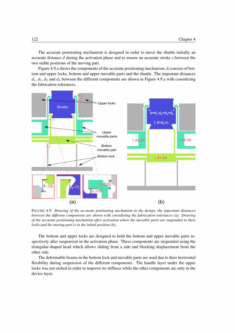
122 Chapter 4
The accurate positioning mechanism is designed in order to move the shuttle initially an
accurate distance d during the activation phase and to ensure an accurate stroke s between the
two stable positions of the moving part.
Figure 4.9.a shows the components of the accurate positioning mechanism, it consists of bot-
tom and upper locks, bottom and upper movable parts and the shuttle. The important distances
d1, d2, d3 and d4 between the different components are shown in Figure 4.9.a with considering
the fabrication tolerances.
FIGURE 4.9: Drawing of the accurate positioning mechanism in the design, the important distances
between the different components are shown with considering the fabrication tolerances (a). Drawing
of the accurate positioning mechanism after activation where the movable parts are suspended to their
locks and the moving part is in the initial position (b).
The bottom and upper locks are designed to hold the bottom and upper movable parts re-
spectively after suspension in the activation phase. These components are suspended using the
triangular-shaped head which allows sliding from a side and blocking displacement from the
other side.
The deformable beams in the bottom lock and movable parts are used due to their horizontal
flexibility during suspension of the different components. The handle layer under the upper
locks was not etched in order to improve its stiffness while the other components are only in the
device layer.
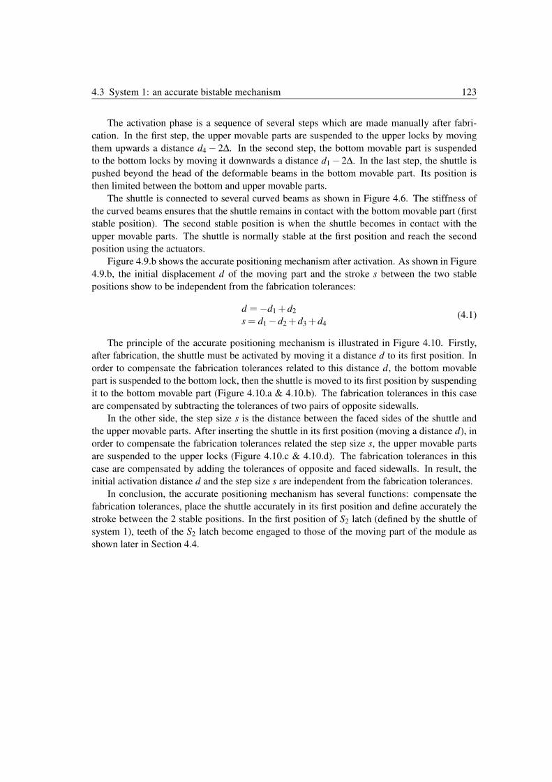
4.3 System 1: an accurate bistable mechanism 123
The activation phase is a sequence of several steps which are made manually after fabri-
cation. In the first step, the upper movable parts are suspended to the upper locks by moving
them upwards a distance d4 − 2Δ. In the second step, the bottom movable part is suspended
to the bottom locks by moving it downwards a distance d1 − 2Δ. In the last step, the shuttle is
pushed beyond the head of the deformable beams in the bottom movable part. Its position is
then limited between the bottom and upper movable parts.
The shuttle is connected to several curved beams as shown in Figure 4.6. The stiffness of
the curved beams ensures that the shuttle remains in contact with the bottom movable part (first
stable position). The second stable position is when the shuttle becomes in contact with the
upper movable parts. The shuttle is normally stable at the first position and reach the second
position using the actuators.
Figure 4.9.b shows the accurate positioning mechanism after activation. As shown in Figure
4.9.b, the initial displacement d of the moving part and the stroke s between the two stable
positions show to be independent from the fabrication tolerances:
d =−d1 +d2
s = d1 −d2 +d3 +d4(4.1)
The principle of the accurate positioning mechanism is illustrated in Figure 4.10. Firstly,
after fabrication, the shuttle must be activated by moving it a distance d to its first position. In
order to compensate the fabrication tolerances related to this distance d, the bottom movable
part is suspended to the bottom lock, then the shuttle is moved to its first position by suspending
it to the bottom movable part (Figure 4.10.a & 4.10.b). The fabrication tolerances in this case
are compensated by subtracting the tolerances of two pairs of opposite sidewalls.
In the other side, the step size s is the distance between the faced sides of the shuttle and
the upper movable parts. After inserting the shuttle in its first position (moving a distance d), in
order to compensate the fabrication tolerances related the step size s, the upper movable parts
are suspended to the upper locks (Figure 4.10.c & 4.10.d). The fabrication tolerances in this
case are compensated by adding the tolerances of opposite and faced sidewalls. In result, the
initial activation distance d and the step size s are independent from the fabrication tolerances.
In conclusion, the accurate positioning mechanism has several functions: compensate the
fabrication tolerances, place the shuttle accurately in its first position and define accurately the
stroke between the 2 stable positions. In the first position of S2 latch (defined by the shuttle of
system 1), teeth of the S2 latch become engaged to those of the moving part of the module as
shown later in Section 4.4.
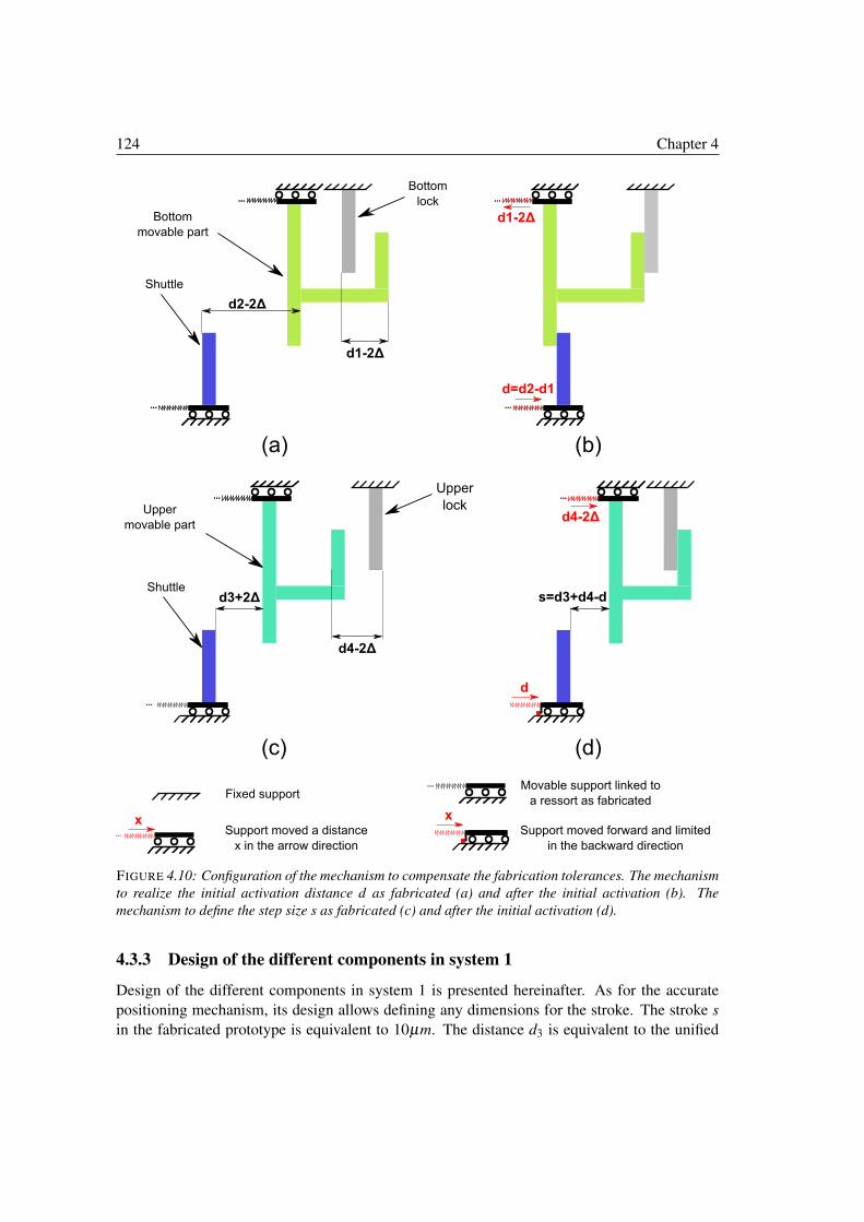
124 Chapter 4
FIGURE 4.10: Configuration of the mechanism to compensate the fabrication tolerances. The mechanism
to realize the initial activation distance d as fabricated (a) and after the initial activation (b). The
mechanism to define the step size s as fabricated (c) and after the initial activation (d).
4.3.3 Design of the different components in system 1
Design of the different components in system 1 is presented hereinafter. As for the accurate
positioning mechanism, its design allows defining any dimensions for the stroke. The stroke s
in the fabricated prototype is equivalent to 10µm. The distance d3 is equivalent to the unified
4.3 System 1: an accurate bistable mechanism 125
opening width in the device layer. The opening width is equivalent to 20µm in our fabrication
process. The distances d1 and d4 must contain 2 triangular heads which are separated by the
width of the opening between them. d1 and d4 are chosen to be equivalent to 40µm in the pro-
totype. Higher values of d1 and d4 allow higher size of the triangular heads which increases and
enhances the contact surface between them. Afterwards, the distances d and d2 are calculated
from (4.1) (d = 50µm and d2 = 90µm).
In the other side, dimensions of the different components in the accurate positioning mech-
anism are chosen in order to obtain a suspension force of 14.5mN in the bottom movable part
and 7.5mN for each one of the upper movable parts. Thus, total forces on the shuttle must not
exceed 14.5mN in the downward direction and 15mN in the upward direction.
Four curved beams were used in order to guide a vertical displacement robustly and reduce
the possibility of rotating the moving part due to external forces. The curved beams are used
instead of simple straight beams because of the exponential nature of the force evolution of
clamped-clamped straight beams after deflection in their middle. Otherwise, the actuators must
provide an important force in order to switch the shuttle between the two stable positions.
Behavior and design of preshaped curved beams was investigated in 2. Figure 4.11 shows the
snapping force-displacement curves after deflection of curved beams for Q< 2.31 and Q> 2.31.
FIGURE 4.11: Evolution of the snapping force of preshaped curved beams during deflection for Q < 2.31
and Q > 2.31.
The curved beams dimensions are chosen to ensure a significant holding force in the first
stable position and to avoid high loads on the actuators in the second stable position. Two
different dimensions are chosen for the curved beams where each set of dimensions is for two
curved beams. In the first couple, dimensions are chosen to ensure that the first position at 50µm
is after dtop (Figure 4.11). In this way, the snapping force which is a load on the actuators will
decrease during transition to the second position at 60µm. Dimensions of the first couple are as
follows (l = 6.5mm, h = 100µm, t = 20µm, b = 100µm). Dimensions of the second couple of
curved beams are chosen in order to get a nearly constant load on the actuator and to reduce the
snapping forces as possible. The dimensions are chosen under Q = 2.31 (l = 6.5mm, h = 30µm,
t = 15µm, b = 100µm).
Evolution of the snapping forces of the four curved beams together is shown in Figure 4.12.
The value of the snapping force at the first position (50µm) is equivalent to 4.4mN and at the
second position (60µm) is equivalent to 4.15mN. Noting that the values of the forces in this
paper are obtained using FEM simulations on Ansys.
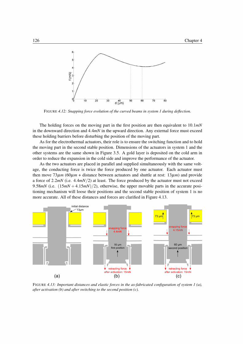
126 Chapter 4
FIGURE 4.12: Snapping force evolution of the curved beams in system 1 during deflection.
The holding forces on the moving part in the first position are then equivalent to 10.1mN
in the downward direction and 4.4mN in the upward direction. Any external force must exceed
these holding barriers before disturbing the position of the moving part.
As for the electrothermal actuators, their role is to ensure the switching function and to hold
the moving part in the second stable position. Dimensions of the actuators in system 1 and the
other systems are the same shown in Figure 3.5. A gold layer is deposited on the cold arm in
order to reduce the expansion in the cold side and improve the performance of the actuator.
As the two actuators are placed in parallel and supplied simultaneously with the same volt-
age, the conducting force is twice the force produced by one actuator. Each actuator must
then move 73µm (60µm + distance between actuators and shuttle at rest: 13µm) and provide
a force of 2.2mN (i.e. 4.4mN/2) at least. The force produced by the actuator must not exceed
9.58mN (i.e. (15mN + 4.15mN)/2), otherwise, the upper movable parts in the accurate posi-
tioning mechanism will loose their positions and the second stable position of system 1 is no
more accurate. All of these distances and forces are clarified in Figure 4.13.
FIGURE 4.13: Important distances and elastic forces in the as-fabricated configuration of system 1 (a),
after activation (b) and after switching to the second position (c).
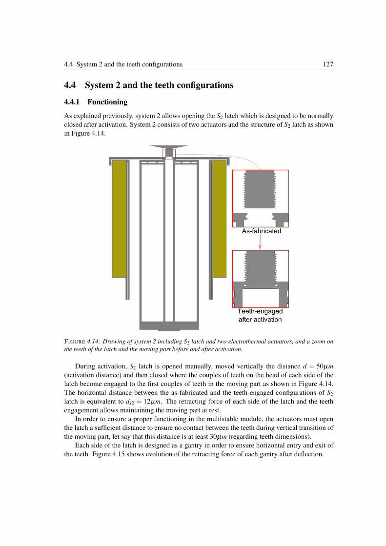
4.4 System 2 and the teeth configurations 127
4.4 System 2 and the teeth configurations
4.4.1 Functioning
As explained previously, system 2 allows opening the S2 latch which is designed to be normally
closed after activation. System 2 consists of two actuators and the structure of S2 latch as shown
in Figure 4.14.
FIGURE 4.14: Drawing of system 2 including S2 latch and two electrothermal actuators, and a zoom on
the teeth of the latch and the moving part before and after activation.
During activation, S2 latch is opened manually, moved vertically the distance d = 50µm
(activation distance) and then closed where the couples of teeth on the head of each side of the
latch become engaged to the first couples of teeth in the moving part as shown in Figure 4.14.
The horizontal distance between the as-fabricated and the teeth-engaged configurations of S2
latch is equivalent to ds2 = 12µm. The retracting force of each side of the latch and the teeth
engagement allows maintaining the moving part at rest.
In order to ensure a proper functioning in the multistable module, the actuators must open
the latch a sufficient distance to ensure no contact between the teeth during vertical transition of
the moving part, let say that this distance is at least 30µm (regarding teeth dimensions).
Each side of the latch is designed as a gantry in order to ensure horizontal entry and exit of
the teeth. Figure 4.15 shows evolution of the retracting force of each gantry after deflection.
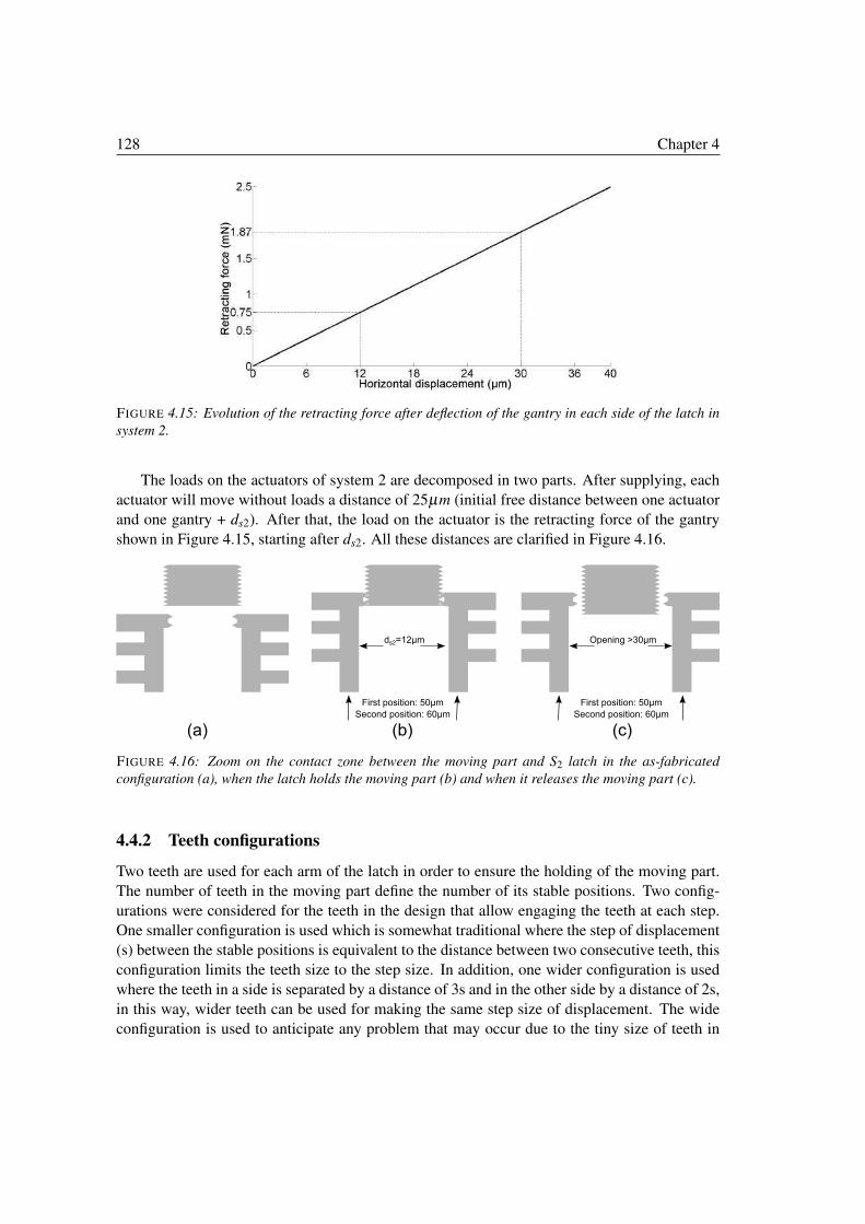
128 Chapter 4
FIGURE 4.15: Evolution of the retracting force after deflection of the gantry in each side of the latch in
system 2.
The loads on the actuators of system 2 are decomposed in two parts. After supplying, each
actuator will move without loads a distance of 25µm (initial free distance between one actuator
and one gantry + ds2). After that, the load on the actuator is the retracting force of the gantry
shown in Figure 4.15, starting after ds2. All these distances are clarified in Figure 4.16.
FIGURE 4.16: Zoom on the contact zone between the moving part and S2 latch in the as-fabricated
configuration (a), when the latch holds the moving part (b) and when it releases the moving part (c).
4.4.2 Teeth configurations
Two teeth are used for each arm of the latch in order to ensure the holding of the moving part.
The number of teeth in the moving part define the number of its stable positions. Two config-
urations were considered for the teeth in the design that allow engaging the teeth at each step.
One smaller configuration is used which is somewhat traditional where the step of displacement
(s) between the stable positions is equivalent to the distance between two consecutive teeth, this
configuration limits the teeth size to the step size. In addition, one wider configuration is used
where the teeth in a side is separated by a distance of 3s and in the other side by a distance of 2s,
in this way, wider teeth can be used for making the same step size of displacement. The wide
configuration is used to anticipate any problem that may occur due to the tiny size of teeth in
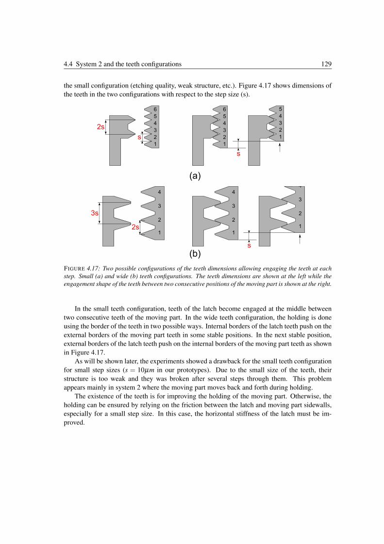
4.4 System 2 and the teeth configurations 129
the small configuration (etching quality, weak structure, etc.). Figure 4.17 shows dimensions of
the teeth in the two configurations with respect to the step size (s).
FIGURE 4.17: Two possible configurations of the teeth dimensions allowing engaging the teeth at each
step. Small (a) and wide (b) teeth configurations. The teeth dimensions are shown at the left while the
engagement shape of the teeth between two consecutive positions of the moving part is shown at the right.
In the small teeth configuration, teeth of the latch become engaged at the middle between
two consecutive teeth of the moving part. In the wide teeth configuration, the holding is done
using the border of the teeth in two possible ways. Internal borders of the latch teeth push on the
external borders of the moving part teeth in some stable positions. In the next stable position,
external borders of the latch teeth push on the internal borders of the moving part teeth as shown
in Figure 4.17.
As will be shown later, the experiments showed a drawback for the small teeth configuration
for small step sizes (s = 10µm in our prototypes). Due to the small size of the teeth, their
structure is too weak and they was broken after several steps through them. This problem
appears mainly in system 2 where the moving part moves back and forth during holding.
The existence of the teeth is for improving the holding of the moving part. Otherwise, the
holding can be ensured by relying on the friction between the latch and moving part sidewalls,
especially for a small step size. In this case, the horizontal stiffness of the latch must be im-
proved.
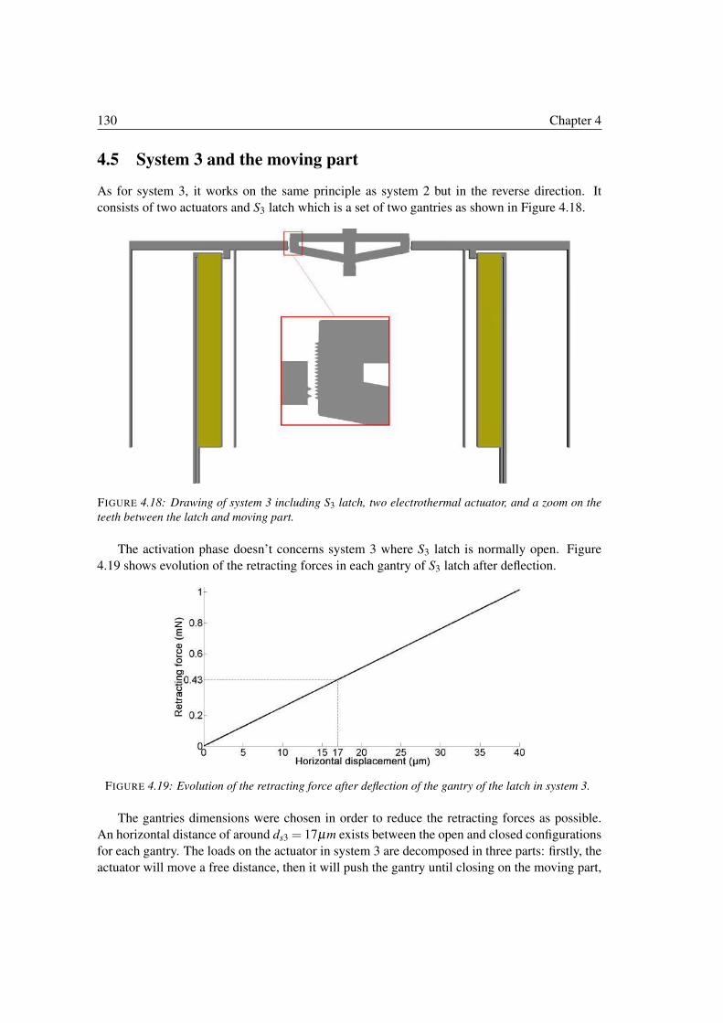
130 Chapter 4
4.5 System 3 and the moving part
As for system 3, it works on the same principle as system 2 but in the reverse direction. It
consists of two actuators and S3 latch which is a set of two gantries as shown in Figure 4.18.
FIGURE 4.18: Drawing of system 3 including S3 latch, two electrothermal actuator, and a zoom on the
teeth between the latch and moving part.
The activation phase doesn’t concerns system 3 where S3 latch is normally open. Figure
4.19 shows evolution of the retracting forces in each gantry of S3 latch after deflection.
FIGURE 4.19: Evolution of the retracting force after deflection of the gantry of the latch in system 3.
The gantries dimensions were chosen in order to reduce the retracting forces as possible.
An horizontal distance of around ds3 = 17µm exists between the open and closed configurations
for each gantry. The loads on the actuator in system 3 are decomposed in three parts: firstly, the
actuator will move a free distance, then it will push the gantry until closing on the moving part,
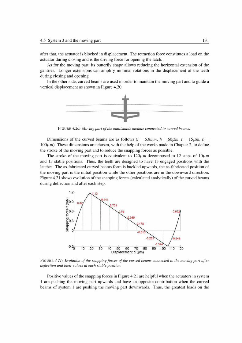
4.5 System 3 and the moving part 131
after that, the actuator is blocked in displacement. The retraction force constitutes a load on the
actuator during closing and is the driving force for opening the latch.
As for the moving part, its butterfly shape allows reducing the horizontal extension of the
gantries. Longer extensions can amplify minimal rotations in the displacement of the teeth
during closing and opening.
In the other side, curved beams are used in order to maintain the moving part and to guide a
vertical displacement as shown in Figure 4.20.
FIGURE 4.20: Moving part of the multistable module connected to curved beams.
Dimensions of the curved beams are as follows (l = 6.8mm, h = 60µm, t = 15µm, b =100µm). These dimensions are chosen, with the help of the works made in Chapter 2, to define
the stroke of the moving part and to reduce the snapping forces as possible.
The stroke of the moving part is equivalent to 120µm decomposed to 12 steps of 10µm
and 13 stable positions. Thus, the teeth are designed to have 13 engaged positions with the
latches. The as-fabricated curved beams form is buckled upwards, the as-fabricated position of
the moving part is the initial position while the other positions are in the downward direction.
Figure 4.21 shows evolution of the snapping forces (calculated analytically) of the curved beams
during deflection and after each step.
FIGURE 4.21: Evolution of the snapping forces of the curved beams connected to the moving part after
deflection and their values at each stable position.
Positive values of the snapping forces in Figure 4.21 are helpful when the actuators in system
1 are pushing the moving part upwards and have an opposite contribution when the curved
beams of system 1 are pushing the moving part downwards. Thus, the greatest loads on the
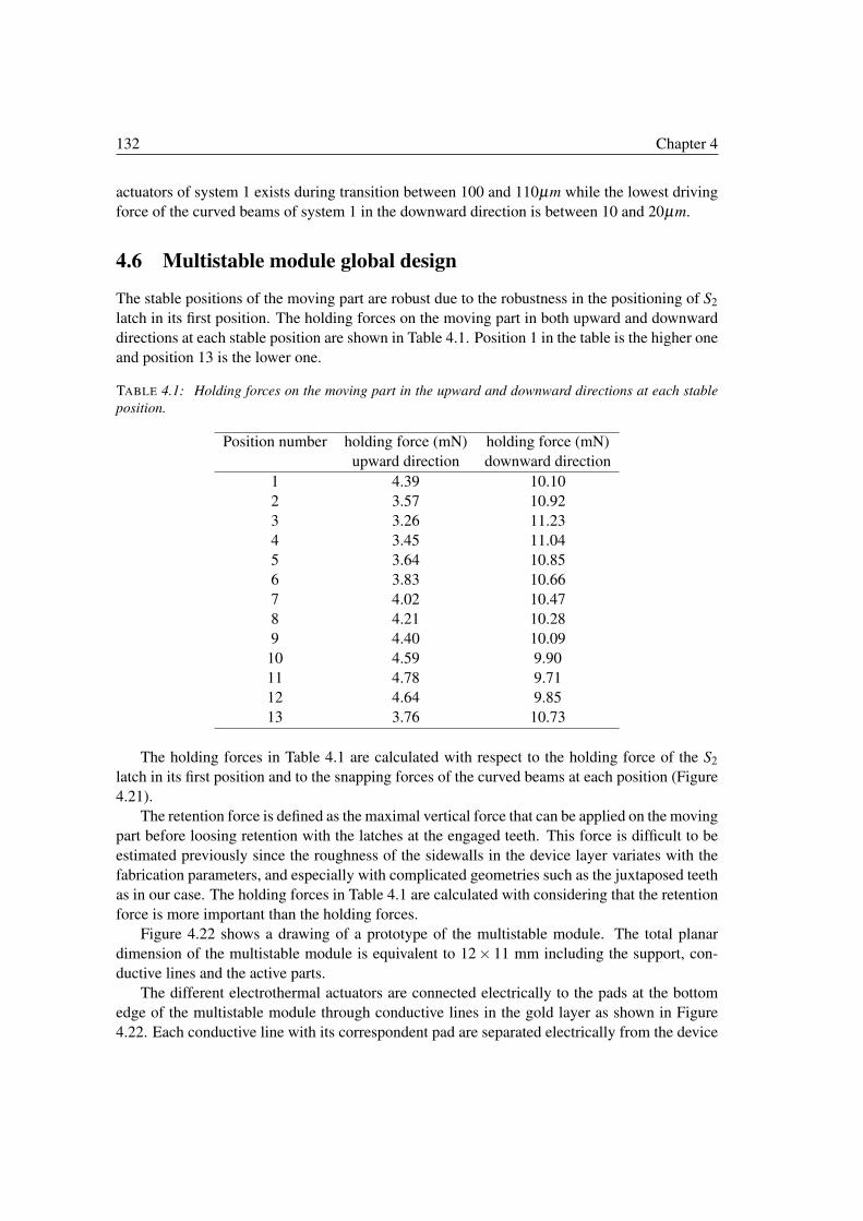
132 Chapter 4
actuators of system 1 exists during transition between 100 and 110µm while the lowest driving
force of the curved beams of system 1 in the downward direction is between 10 and 20µm.
4.6 Multistable module global design
The stable positions of the moving part are robust due to the robustness in the positioning of S2
latch in its first position. The holding forces on the moving part in both upward and downward
directions at each stable position are shown in Table 4.1. Position 1 in the table is the higher one
and position 13 is the lower one.
TABLE 4.1: Holding forces on the moving part in the upward and downward directions at each stable
position.
Position number holding force (mN) holding force (mN)
upward direction downward direction
1 4.39 10.10
2 3.57 10.92
3 3.26 11.23
4 3.45 11.04
5 3.64 10.85
6 3.83 10.66
7 4.02 10.47
8 4.21 10.28
9 4.40 10.09
10 4.59 9.90
11 4.78 9.71
12 4.64 9.85
13 3.76 10.73
The holding forces in Table 4.1 are calculated with respect to the holding force of the S2
latch in its first position and to the snapping forces of the curved beams at each position (Figure
4.21).
The retention force is defined as the maximal vertical force that can be applied on the moving
part before loosing retention with the latches at the engaged teeth. This force is difficult to be
estimated previously since the roughness of the sidewalls in the device layer variates with the
fabrication parameters, and especially with complicated geometries such as the juxtaposed teeth
as in our case. The holding forces in Table 4.1 are calculated with considering that the retention
force is more important than the holding forces.
Figure 4.22 shows a drawing of a prototype of the multistable module. The total planar
dimension of the multistable module is equivalent to 12× 11 mm including the support, con-
ductive lines and the active parts.
The different electrothermal actuators are connected electrically to the pads at the bottom
edge of the multistable module through conductive lines in the gold layer as shown in Figure
4.22. Each conductive line with its correspondent pad are separated electrically from the device
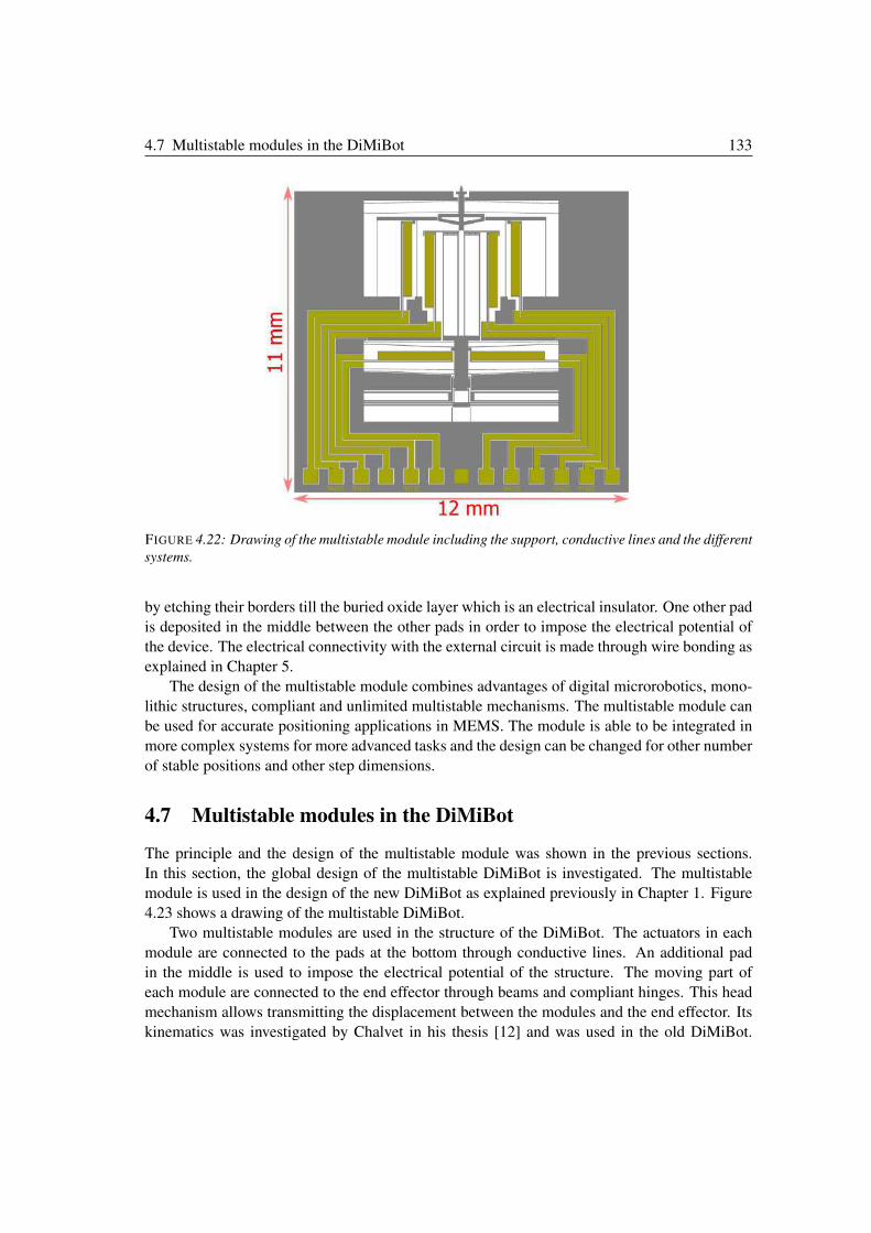
4.7 Multistable modules in the DiMiBot 133
FIGURE 4.22: Drawing of the multistable module including the support, conductive lines and the different
systems.
by etching their borders till the buried oxide layer which is an electrical insulator. One other pad
is deposited in the middle between the other pads in order to impose the electrical potential of
the device. The electrical connectivity with the external circuit is made through wire bonding as
explained in Chapter 5.
The design of the multistable module combines advantages of digital microrobotics, mono-
lithic structures, compliant and unlimited multistable mechanisms. The multistable module can
be used for accurate positioning applications in MEMS. The module is able to be integrated in
more complex systems for more advanced tasks and the design can be changed for other number
of stable positions and other step dimensions.
4.7 Multistable modules in the DiMiBot
The principle and the design of the multistable module was shown in the previous sections.
In this section, the global design of the multistable DiMiBot is investigated. The multistable
module is used in the design of the new DiMiBot as explained previously in Chapter 1. Figure
4.23 shows a drawing of the multistable DiMiBot.
Two multistable modules are used in the structure of the DiMiBot. The actuators in each
module are connected to the pads at the bottom through conductive lines. An additional pad
in the middle is used to impose the electrical potential of the structure. The moving part of
each module are connected to the end effector through beams and compliant hinges. This head
mechanism allows transmitting the displacement between the modules and the end effector. Its
kinematics was investigated by Chalvet in his thesis [12] and was used in the old DiMiBot.
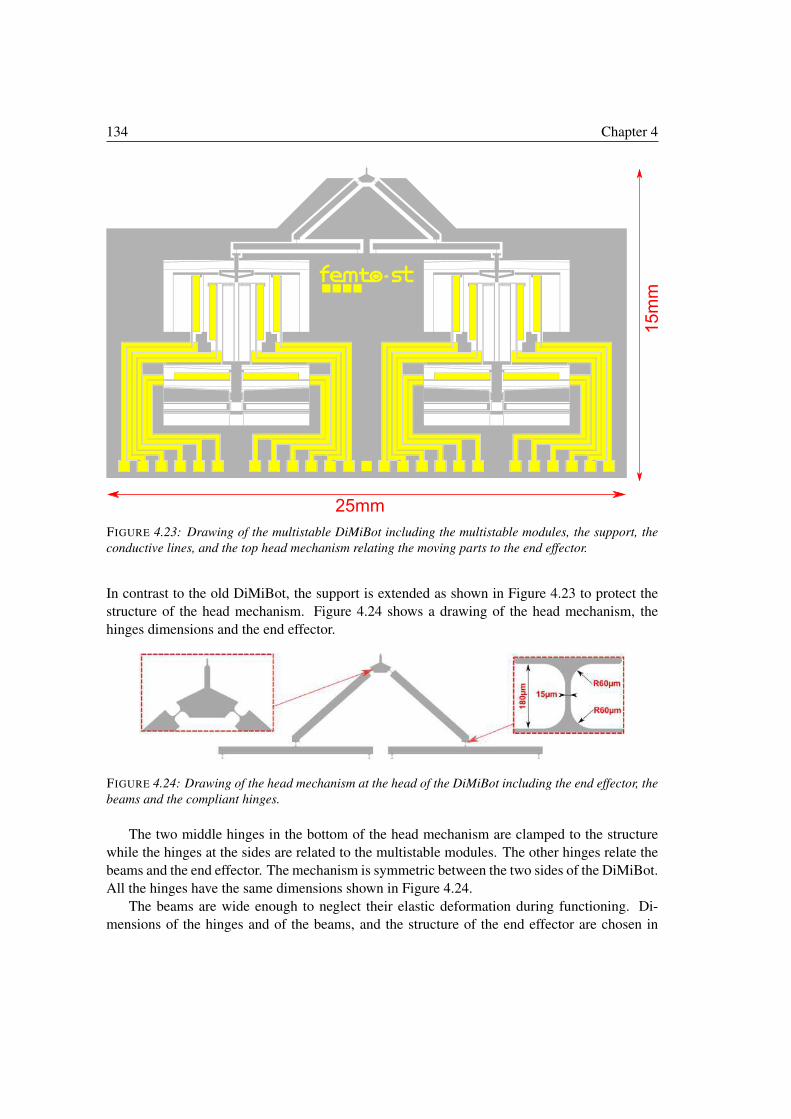
134 Chapter 4
FIGURE 4.23: Drawing of the multistable DiMiBot including the multistable modules, the support, the
conductive lines, and the top head mechanism relating the moving parts to the end effector.
In contrast to the old DiMiBot, the support is extended as shown in Figure 4.23 to protect the
structure of the head mechanism. Figure 4.24 shows a drawing of the head mechanism, the
hinges dimensions and the end effector.
FIGURE 4.24: Drawing of the head mechanism at the head of the DiMiBot including the end effector, the
beams and the compliant hinges.
The two middle hinges in the bottom of the head mechanism are clamped to the structure
while the hinges at the sides are related to the multistable modules. The other hinges relate the
beams and the end effector. The mechanism is symmetric between the two sides of the DiMiBot.
All the hinges have the same dimensions shown in Figure 4.24.
The beams are wide enough to neglect their elastic deformation during functioning. Di-
mensions of the hinges and of the beams, and the structure of the end effector are chosen in
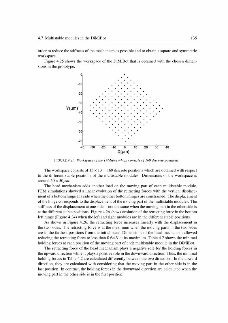
4.7 Multistable modules in the DiMiBot 135
order to reduce the stiffness of the mechanism as possible and to obtain a square and symmetric
workspace.
Figure 4.25 shows the workspace of the DiMiBot that is obtained with the chosen dimen-
sions in the prototype.
FIGURE 4.25: Workspace of the DiMiBot which consists of 169 discrete positions.
The workspace consists of 13×13 = 169 discrete positions which are obtained with respect
to the different stable positions of the multistable modules. Dimensions of the workspace is
around 50×50µm.
The head mechanism adds another load on the moving part of each multistable module.
FEM simulations showed a linear evolution of the retracting forces with the vertical displace-
ment of a bottom hinge at a side when the other bottom hinges are constrained. The displacement
of the hinge corresponds to the displacement of the moving part of the multistable modules. The
stiffness of the displacement at one side is not the same when the moving part in the other side is
at the different stable positions. Figure 4.26 shows evolution of the retracting force in the bottom
left hinge (Figure 4.24) when the left and right modules are in the different stable positions.
As shown in Figure 4.26, the retracting force increases linearly with the displacement in
the two sides. The retracting force is at the maximum when the moving parts in the two sides
are in the farthest positions from the initial state. Dimensions of the head mechanism allowed
reducing the retracting force to less than 0.6mN at its maximum. Table 4.2 shows the minimal
holding forces at each position of the moving part of each multistable module in the DiMiBot.
The retracting force of the head mechanism plays a negative role for the holding forces in
the upward direction while it plays a positive role in the downward direction. Thus, the minimal
holding forces in Table 4.2 are calculated differently between the two directions. In the upward
direction, they are calculated with considering that the moving part in the other side is in the
last position. In contrast, the holding forces in the downward direction are calculated when the
moving part in the other side is in the first position.
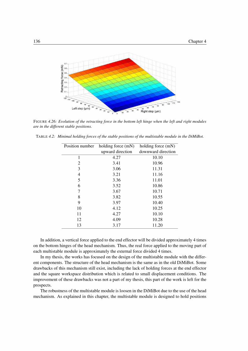
136 Chapter 4
FIGURE 4.26: Evolution of the retracting force in the bottom left hinge when the left and right modules
are in the different stable positions.
TABLE 4.2: Minimal holding forces of the stable positions of the multistable module in the DiMiBot.
Position number holding force (mN) holding force (mN)
upward direction downward direction
1 4.27 10.10
2 3.41 10.96
3 3.06 11.31
4 3.21 11.16
5 3.36 11.01
6 3.52 10.86
7 3.67 10.71
8 3.82 10.55
9 3.97 10.40
10 4.12 10.25
11 4.27 10.10
12 4.09 10.28
13 3.17 11.20
In addition, a vertical force applied to the end effector will be divided approximately 4 times
on the bottom hinges of the head mechanism. Thus, the real force applied to the moving part of
each multistable module is approximately the external force divided 4 times.
In my thesis, the works has focused on the design of the multistable module with the differ-
ent components. The structure of the head mechanism is the same as in the old DiMiBot. Some
drawbacks of this mechanism still exist, including the lack of holding forces at the end effector
and the square workspace distribution which is related to small displacement conditions. The
improvement of these drawbacks was not a part of my thesis, this part of the work is left for the
prospects.
The robustness of the multistable module is loosen in the DiMiBot due to the use of the head
mechanism. As explained in this chapter, the multistable module is designed to hold positions
4.8 Conclusion 137
of the moving part in front of external loads with some limits of robustness. The positioning
robustness is characterized by the holding forces calculated in Table 4.1. However, considering
that the bottom hinges of the head mechanism are totally constrained, the structure of the head
mechanism doesn’t allows keeping stable the discrete positions of the end effector after applying
external loads, especially in the horizontal direction.
In addition, the kinematics of the head mechanism is calculated with considering a small
deformation hypothesis [12]. For large deformation, the discrete positions in the workspace are
not distributed uniformly and the shape of workspace is not a square with rectilinear sides but
mostly a quadrilateral with arc sides. Thus, for higher workspace dimensions, the length of the
beams in the head mechanism must be increased sufficiently to consider the small deformation
hypothesis.
The dimensions of the head mechanism that allow defining a step dimension in the workspace
can be chosen using the inverse geometric model in [12]. However, the geometrical model is
not sufficiently precise due to the small deformation hypothesis, it remains difficult to ensure an
accurate and uniform step dimension in the workspace.
Further, the compliant hinges are the weakest points in the structure. Many prototypes of
the multistable DiMiBot were broken at the hinges, either in the fabrication process or during
manipulation. In the other side, the retracting force evolves rapidly with larger hinge dimen-
sions. In the design, a compromise must be made in terms of the hinge dimensions by accepting
higher in order to strengthen the structure of the hinges.
4.8 Conclusion
The principle and design of a new generation of a multistable module and the DiMiBot was
presented in this chapter. The design of the different components and each system in the mul-
tistable module, and the global structure of the module and the DiMiBot was presented. The
multistable module allows switching its moving part between several stable positions linearly
in a one dimensional direction. An accurate positioning mechanism is used in order to ensure
accurate steps and to compensate the fabrication tolerances. Only two multistable modules are
used in the new generation of the DiMiBot to realize planar positioning. The fabrication process
and the experiments made on some operational multistable module prototypes are presented in
the next chapter.

Chapter 5Fabrication and experiments
This chapter deals with the fabrication process followed in the thesis and the ex-
periments made on the fabricated prototypes. The general steps in the fabrication
process are cited, each fabrication step is detailed and the layout of the proto-
types in the wafers are presented. The experiments are then presented, they include
force measurement experiments, the experiments on U-shaped actuators and finally
experiments on some operational prototypes of the multistable module. All the dif-
ficulties encountered and solutions provided in the fabrication or the experiments
are detailed in the chapter.
140 Chapter 5
Chapter contents
5.1 Introduction . . . . . . . . . . . . . . . . . . . . . . . . . . . . . . . . . . 141
5.2 Fabrication process . . . . . . . . . . . . . . . . . . . . . . . . . . . . . . 141
5.2.1 General process flow . . . . . . . . . . . . . . . . . . . . . . . . . . 141
5.2.2 Layout . . . . . . . . . . . . . . . . . . . . . . . . . . . . . . . . . 143
5.3 Technological aspects in the fabrication process . . . . . . . . . . . . . . . 148
5.3.1 Hard mask (Photomask A) . . . . . . . . . . . . . . . . . . . . . . . 148
5.3.2 Gold patterns (Photomask B) . . . . . . . . . . . . . . . . . . . . . . 149
5.3.3 Device layer etching (Photomask C) . . . . . . . . . . . . . . . . . . 151
5.3.4 Substrate etching . . . . . . . . . . . . . . . . . . . . . . . . . . . . 154
5.3.5 HF release . . . . . . . . . . . . . . . . . . . . . . . . . . . . . . . 154
5.4 Force measurement experiments . . . . . . . . . . . . . . . . . . . . . . . 157
5.4.1 Rectilinear beams . . . . . . . . . . . . . . . . . . . . . . . . . . . . 159
5.4.2 Curved beams . . . . . . . . . . . . . . . . . . . . . . . . . . . . . . 159
5.5 Experiments on the actuators . . . . . . . . . . . . . . . . . . . . . . . . . 161
5.5.1 Experimental setup . . . . . . . . . . . . . . . . . . . . . . . . . . . 161
5.5.2 Remarks noticed in the experiments . . . . . . . . . . . . . . . . . . 163
5.6 Multistable module experiment . . . . . . . . . . . . . . . . . . . . . . . . 165
5.6.1 Activation of the multistable modules . . . . . . . . . . . . . . . . . 166
5.6.2 Wire bonding . . . . . . . . . . . . . . . . . . . . . . . . . . . . . . 166
5.6.3 Electronic circuit . . . . . . . . . . . . . . . . . . . . . . . . . . . . 166
5.6.4 Tests on the different systems of the multistable module . . . . . . . 169
5.6.5 Sequence orders to make steps . . . . . . . . . . . . . . . . . . . . . 169
5.6.6 Experimental functioning . . . . . . . . . . . . . . . . . . . . . . . . 169
5.7 Conclusion . . . . . . . . . . . . . . . . . . . . . . . . . . . . . . . . . . . 173
5.1 Introduction 141
5.1 Introduction
In the previous chapters, the theoretical works were presented including the state of the art, the
modeling and design of the preshaped curved beams and U-shaped actuators, and the design of
the new multistable module and DiMiBot. In this chapter, the fabrication and experiments are
presented.
In this thesis, two runs of fabrication were made in the clean room MIMENTO. The fabrica-
tion is made on SOI wafers using bulk micromachining fabrication techniques. Some differences
are made in the fabrication process in order to avoid the problems encountered in the previous
thesis. Fabrication tests (lithography, etching, metal deposition, etc.) were made before and
during the fabrication runs to validate the process and to define the different parameters for each
fabrication step.
The fabrication process is clarified in the first section. Layout of the prototypes fabricated
and used in the experiments are then presented. The technical aspects, difficulties and solutions
for each step in the fabrication are subsequently presented.
The experiments are presented in the second part of the chapter. Force measurement ex-
periments were made for identifying the stiffness and geometric parameters of the fabricated
structures and for measuring the snapping forces of the bistable curved beams. Experiments on
the U-shaped actuators were also made in situ in a micromanipulation station under a micro-
scope and a high speed camera.
The final section concerns the experiments made on some operational multistable modules.
The different aspects of the experiments are presented including the wire bonding, the electronic
circuit, the sequence orders, and the experimental functioning. The fabricated prototypes of the
multistable module showed a proper functioning in the experiments, this validates the principle
and design of the new multistable module.
5.2 Fabrication process
5.2.1 General process flow
Various prototypes were fabricated in the thesis either for testing the behavior of several com-
ponents or for realizing operational prototypes for the new generation of the DIMIBOT and the
multistable modules. The fabrication is realized on SOI wafers, the silicon device layer has a
single-crystalline form with (100) orientation . This material is used due to its important proper-
ties previously cited. The device layer is highly doped (p-type) in order to reduce the electrical
resistivity and to supply the actuators with low voltages.
Some improvements were made in the fabrication process with respect to the previous the-
sis to avoid previously encountered problems. The fabrication steps in the previous thesis are
recalled and the difficulties encountered are clarified in this section, followed by our fabrication
process and the improvements being made. Figure 5.1 shows the main steps in the previous
fabrication process.
The silicon etching in the previous process was made with non homogeneous openings
which have common areas between the two sides. The non homogeneous openings lead to non
homogeneous etching speed of the silicon layers and different patterns quality and tolerances
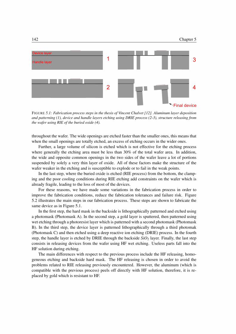
142 Chapter 5
FIGURE 5.1: Fabrication process steps in the thesis of Vincent Chalvet [12]. Aluminum layer deposition
and patterning (1), device and handle layers etching using DRIE process (2-3), structure releasing from
the wafer using RIE of the buried oxide (4).
throughout the wafer. The wide openings are etched faster than the smaller ones, this means that
when the small openings are totally etched, an excess of etching occurs in the wider ones.
Further, a large volume of silicon is etched which is not effective for the etching process
where generally the etching area must be less than 30% of the total wafer area. In addition,
the wide and opposite common openings in the two sides of the wafer leave a lot of portions
suspended by solely a very thin layer of oxide. All of these factors make the structure of the
wafer weaker in the etching and is susceptible to explode or to fail in the weak points.
In the last step, where the buried oxide is etched (RIE process) from the bottom, the clamp-
ing and the poor cooling conditions during RIE etching add constraints on the wafer which is
already fragile, leading to the loss of most of the devices.
For these reasons, we have made some variations in the fabrication process in order to
improve the fabrication conditions, reduce the fabrication tolerances and failure risk. Figure
5.2 illustrates the main steps in our fabrication process. These steps are shown to fabricate the
same device as in Figure 5.1.
In the first step, the hard mask in the backside is lithographically patterned and etched using
a photomask (Photomask A). In the second step, a gold layer is sputtered, then patterned using
wet etching through a photoresist layer which is patterned with a second photomask (Photomask
B). In the third step, the device layer is patterned lithographically through a third photomak
(Photomask C) and then etched using a deep reactive ion etching (DRIE) process. In the fourth
step, the handle layer is etched by DRIE through the backside SiO2 layer. Finally, the last step
consists in releasing devices from the wafer using HF wet etching. Useless parts fall into the
HF solution during etching.
The main differences with respect to the previous process include the HF releasing, homo-
geneous etching and backside hard mask. The HF releasing is chosen in order to avoid the
problems related to RIE releasing previously encountered. However, the aluminum (which is
compatible with the previous process) peels off directly with HF solution, therefore, it is re-
placed by gold which is resistant to HF.
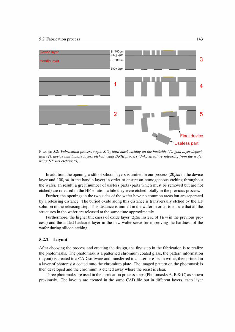
5.2 Fabrication process 143
FIGURE 5.2: Fabrication process steps. SiO2 hard mask etching on the backside (1), gold layer deposi-
tion (2), device and handle layers etched using DRIE process (3-4), structure releasing from the wafer
using HF wet etching (5).
In addition, the opening width of silicon layers is unified in our process (20µm in the device
layer and 100µm in the handle layer) in order to ensure an homogeneous etching throughout
the wafer. In result, a great number of useless parts (parts which must be removed but are not
etched) are released in the HF solution while they were etched totally in the previous process.
Further, the openings in the two sides of the wafer have no common areas but are separated
by a releasing distance. The buried oxide along this distance is transversally etched by the HF
solution in the releasing step. This distance is unified in the wafer in order to ensure that all the
structures in the wafer are released at the same time approximately.
Furthermore, the higher thickness of oxide layer (2µm instead of 1µm in the previous pro-
cess) and the added backside layer in the new wafer serve for improving the hardness of the
wafer during silicon etching.
5.2.2 Layout
After choosing the process and creating the design, the first step in the fabrication is to realize
the photomasks. The photomask is a patterned chromium coated glass, the pattern information
(layout) is created in a CAD software and transferred to a laser or e-beam writer, then printed in
a layer of photoresist coated onto the chromium plate. The imaged pattern on the photomask is
then developed and the chromium is etched away where the resist is clear.
Three photomaks are used in the fabrication process steps (Photomasks A, B & C) as shown
previously. The layouts are created in the same CAD file but in different layers, each layer
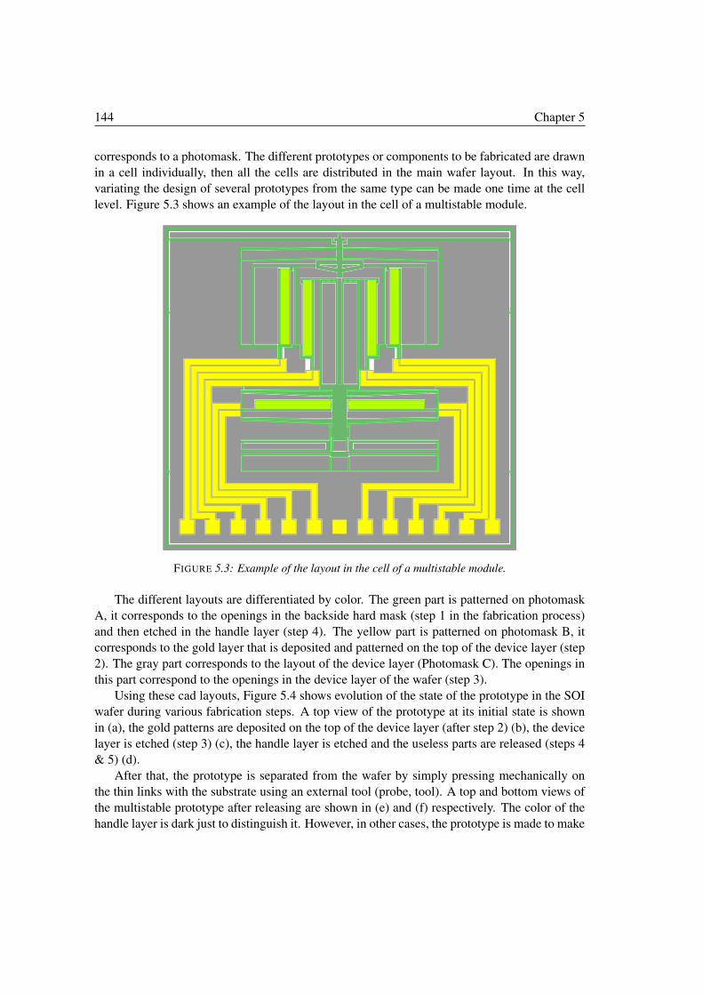
144 Chapter 5
corresponds to a photomask. The different prototypes or components to be fabricated are drawn
in a cell individually, then all the cells are distributed in the main wafer layout. In this way,
variating the design of several prototypes from the same type can be made one time at the cell
level. Figure 5.3 shows an example of the layout in the cell of a multistable module.
FIGURE 5.3: Example of the layout in the cell of a multistable module.
The different layouts are differentiated by color. The green part is patterned on photomask
A, it corresponds to the openings in the backside hard mask (step 1 in the fabrication process)
and then etched in the handle layer (step 4). The yellow part is patterned on photomask B, it
corresponds to the gold layer that is deposited and patterned on the top of the device layer (step
2). The gray part corresponds to the layout of the device layer (Photomask C). The openings in
this part correspond to the openings in the device layer of the wafer (step 3).
Using these cad layouts, Figure 5.4 shows evolution of the state of the prototype in the SOI
wafer during various fabrication steps. A top view of the prototype at its initial state is shown
in (a), the gold patterns are deposited on the top of the device layer (after step 2) (b), the device
layer is etched (step 3) (c), the handle layer is etched and the useless parts are released (steps 4
& 5) (d).
After that, the prototype is separated from the wafer by simply pressing mechanically on
the thin links with the substrate using an external tool (probe, tool). A top and bottom views of
the multistable prototype after releasing are shown in (e) and (f) respectively. The color of the
handle layer is dark just to distinguish it. However, in other cases, the prototype is made to make
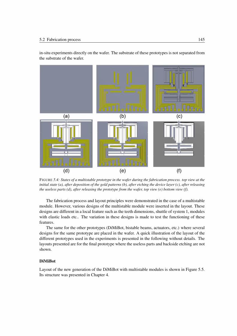
5.2 Fabrication process 145
in-situ experiments directly on the wafer. The substrate of these prototypes is not separated from
the substrate of the wafer.
FIGURE 5.4: States of a multistable prototype in the wafer during the fabrication process. top view at the
initial state (a), after deposition of the gold patterns (b), after etching the device layer (c), after releasing
the useless parts (d), after releasing the prototype from the wafer, top view (e) bottom view (f).
The fabrication process and layout principles were demonstrated in the case of a multistable
module. However, various designs of the multistable module were inserted in the layout. These
designs are different in a local feature such as the teeth dimensions, shuttle of system 1, modules
with elastic loads etc.. The variation in these designs is made to test the functioning of these
features.
The same for the other prototypes (DiMiBot, bistable beams, actuators, etc.) where several
designs for the same prototype are placed in the wafer. A quick illustration of the layout of the
different prototypes used in the experiments is presented in the following without details. The
layouts presented are for the final prototype where the useless parts and backside etching are not
shown.
DiMiBot
Layout of the new generation of the DiMiBot with multistable modules is shown in Figure 5.5.
Its structure was presented in Chapter 4.
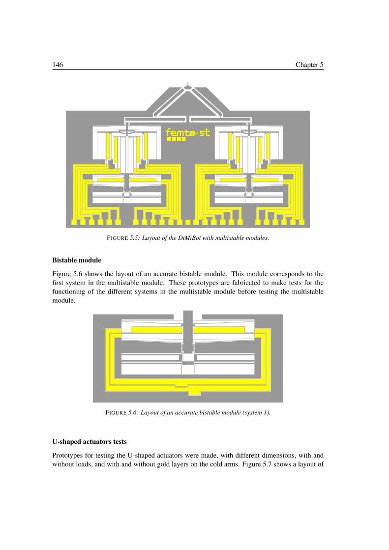
146 Chapter 5
FIGURE 5.5: Layout of the DiMiBot with multistable modules.
Bistable module
Figure 5.6 shows the layout of an accurate bistable module. This module corresponds to the
first system in the multistable module. These prototypes are fabricated to make tests for the
functioning of the different systems in the multistable module before testing the multistable
module.
FIGURE 5.6: Layout of an accurate bistable module (system 1).
U-shaped actuators tests
Prototypes for testing the U-shaped actuators were made, with different dimensions, with and
without loads, and with and without gold layers on the cold arms. Figure 5.7 shows a layout of
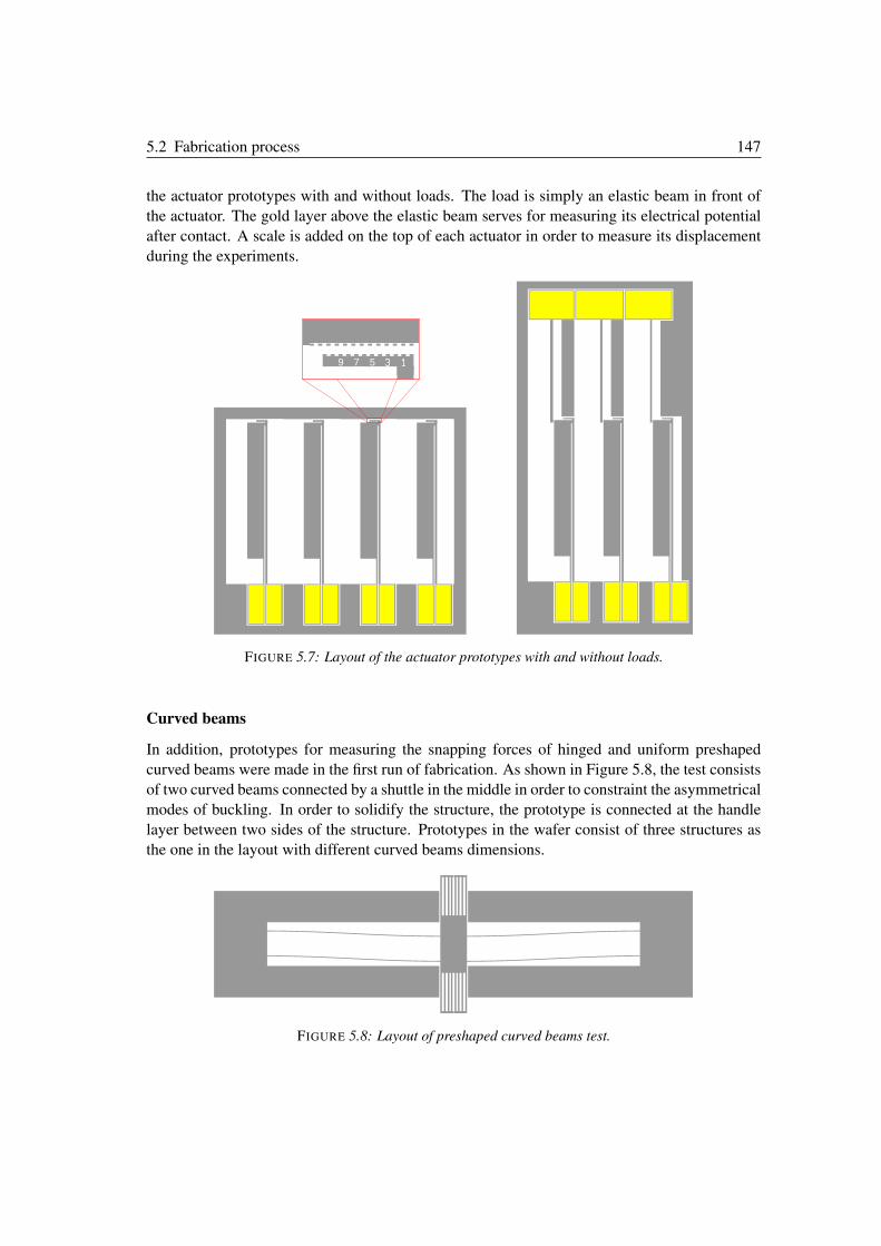
5.2 Fabrication process 147
the actuator prototypes with and without loads. The load is simply an elastic beam in front of
the actuator. The gold layer above the elastic beam serves for measuring its electrical potential
after contact. A scale is added on the top of each actuator in order to measure its displacement
during the experiments.
FIGURE 5.7: Layout of the actuator prototypes with and without loads.
Curved beams
In addition, prototypes for measuring the snapping forces of hinged and uniform preshaped
curved beams were made in the first run of fabrication. As shown in Figure 5.8, the test consists
of two curved beams connected by a shuttle in the middle in order to constraint the asymmetrical
modes of buckling. In order to solidify the structure, the prototype is connected at the handle
layer between two sides of the structure. Prototypes in the wafer consist of three structures as
the one in the layout with different curved beams dimensions.
FIGURE 5.8: Layout of preshaped curved beams test.
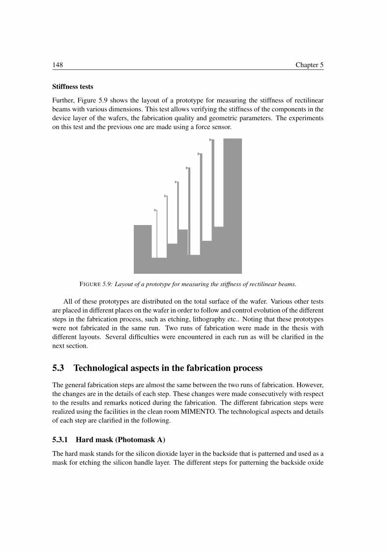
148 Chapter 5
Stiffness tests
Further, Figure 5.9 shows the layout of a prototype for measuring the stiffness of rectilinear
beams with various dimensions. This test allows verifying the stiffness of the components in the
device layer of the wafers, the fabrication quality and geometric parameters. The experiments
on this test and the previous one are made using a force sensor.
FIGURE 5.9: Layout of a prototype for measuring the stiffness of rectilinear beams.
All of these prototypes are distributed on the total surface of the wafer. Various other tests
are placed in different places on the wafer in order to follow and control evolution of the different
steps in the fabrication process, such as etching, lithography etc.. Noting that these prototypes
were not fabricated in the same run. Two runs of fabrication were made in the thesis with
different layouts. Several difficulties were encountered in each run as will be clarified in the
next section.
5.3 Technological aspects in the fabrication process
The general fabrication steps are almost the same between the two runs of fabrication. However,
the changes are in the details of each step. These changes were made consecutively with respect
to the results and remarks noticed during the fabrication. The different fabrication steps were
realized using the facilities in the clean room MIMENTO. The technological aspects and details
of each step are clarified in the following.
5.3.1 Hard mask (Photomask A)
The hard mask stands for the silicon dioxide layer in the backside that is patterned and used as a
mask for etching the silicon handle layer. The different steps for patterning the backside oxide
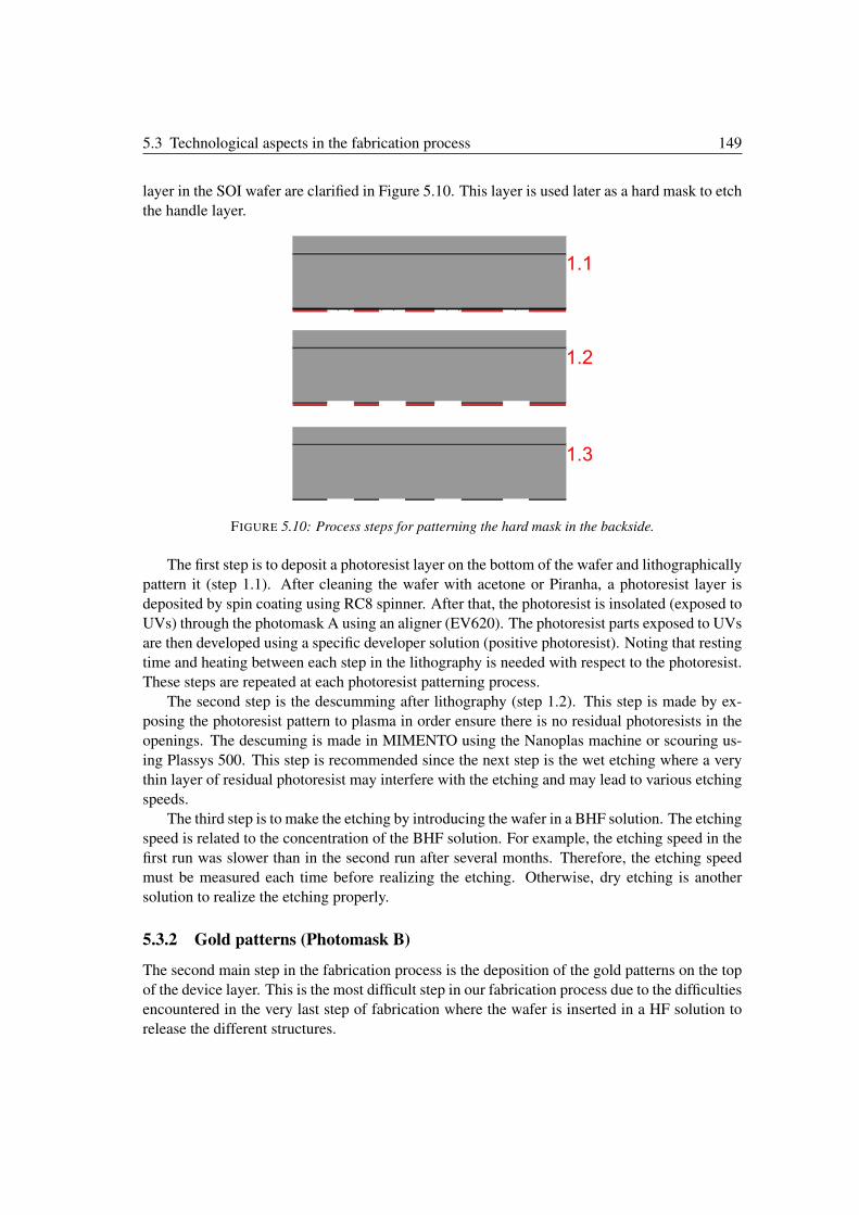
5.3 Technological aspects in the fabrication process 149
layer in the SOI wafer are clarified in Figure 5.10. This layer is used later as a hard mask to etch
the handle layer.
FIGURE 5.10: Process steps for patterning the hard mask in the backside.
The first step is to deposit a photoresist layer on the bottom of the wafer and lithographically
pattern it (step 1.1). After cleaning the wafer with acetone or Piranha, a photoresist layer is
deposited by spin coating using RC8 spinner. After that, the photoresist is insolated (exposed to
UVs) through the photomask A using an aligner (EV620). The photoresist parts exposed to UVs
are then developed using a specific developer solution (positive photoresist). Noting that resting
time and heating between each step in the lithography is needed with respect to the photoresist.
These steps are repeated at each photoresist patterning process.
The second step is the descumming after lithography (step 1.2). This step is made by ex-
posing the photoresist pattern to plasma in order ensure there is no residual photoresists in the
openings. The descuming is made in MIMENTO using the Nanoplas machine or scouring us-
ing Plassys 500. This step is recommended since the next step is the wet etching where a very
thin layer of residual photoresist may interfere with the etching and may lead to various etching
speeds.
The third step is to make the etching by introducing the wafer in a BHF solution. The etching
speed is related to the concentration of the BHF solution. For example, the etching speed in the
first run was slower than in the second run after several months. Therefore, the etching speed
must be measured each time before realizing the etching. Otherwise, dry etching is another
solution to realize the etching properly.
5.3.2 Gold patterns (Photomask B)
The second main step in the fabrication process is the deposition of the gold patterns on the top
of the device layer. This is the most difficult step in our fabrication process due to the difficulties
encountered in the very last step of fabrication where the wafer is inserted in a HF solution to
release the different structures.
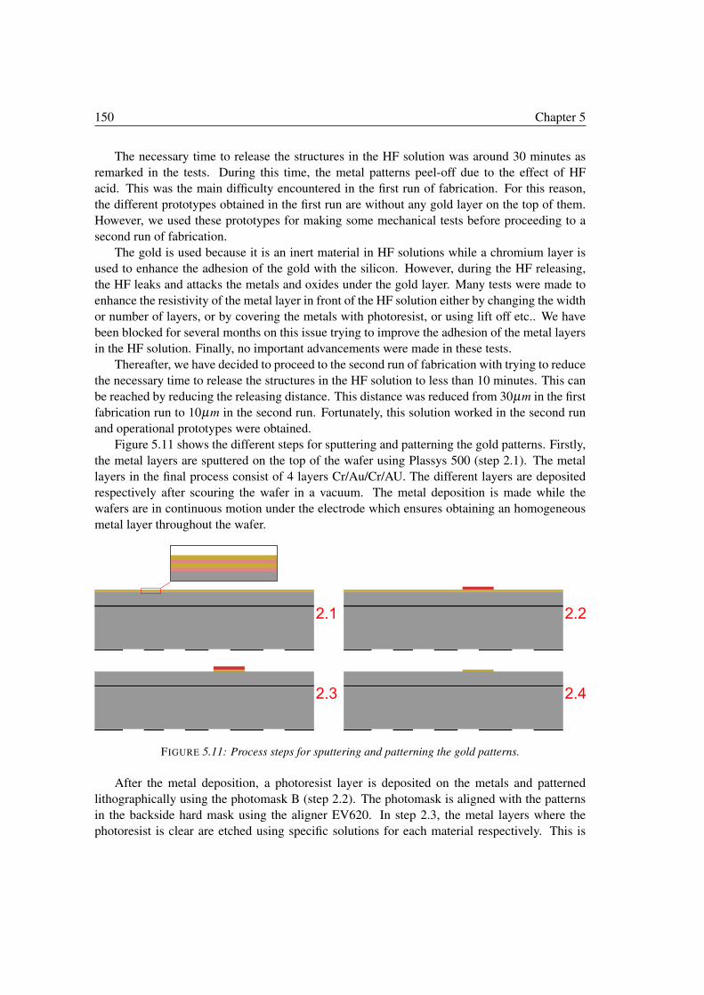
150 Chapter 5
The necessary time to release the structures in the HF solution was around 30 minutes as
remarked in the tests. During this time, the metal patterns peel-off due to the effect of HF
acid. This was the main difficulty encountered in the first run of fabrication. For this reason,
the different prototypes obtained in the first run are without any gold layer on the top of them.
However, we used these prototypes for making some mechanical tests before proceeding to a
second run of fabrication.
The gold is used because it is an inert material in HF solutions while a chromium layer is
used to enhance the adhesion of the gold with the silicon. However, during the HF releasing,
the HF leaks and attacks the metals and oxides under the gold layer. Many tests were made to
enhance the resistivity of the metal layer in front of the HF solution either by changing the width
or number of layers, or by covering the metals with photoresist, or using lift off etc.. We have
been blocked for several months on this issue trying to improve the adhesion of the metal layers
in the HF solution. Finally, no important advancements were made in these tests.
Thereafter, we have decided to proceed to the second run of fabrication with trying to reduce
the necessary time to release the structures in the HF solution to less than 10 minutes. This can
be reached by reducing the releasing distance. This distance was reduced from 30µm in the first
fabrication run to 10µm in the second run. Fortunately, this solution worked in the second run
and operational prototypes were obtained.
Figure 5.11 shows the different steps for sputtering and patterning the gold patterns. Firstly,
the metal layers are sputtered on the top of the wafer using Plassys 500 (step 2.1). The metal
layers in the final process consist of 4 layers Cr/Au/Cr/AU. The different layers are deposited
respectively after scouring the wafer in a vacuum. The metal deposition is made while the
wafers are in continuous motion under the electrode which ensures obtaining an homogeneous
metal layer throughout the wafer.
FIGURE 5.11: Process steps for sputtering and patterning the gold patterns.
After the metal deposition, a photoresist layer is deposited on the metals and patterned
lithographically using the photomask B (step 2.2). The photomask is aligned with the patterns
in the backside hard mask using the aligner EV620. In step 2.3, the metal layers where the
photoresist is clear are etched using specific solutions for each material respectively. This is
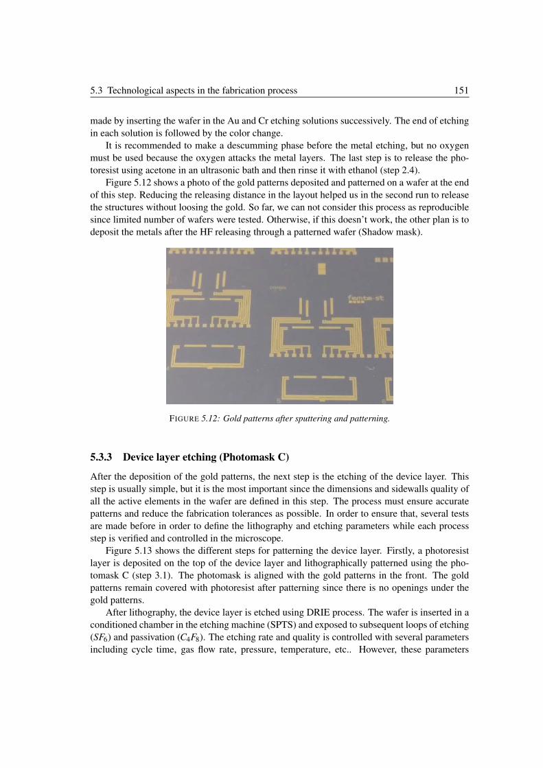
5.3 Technological aspects in the fabrication process 151
made by inserting the wafer in the Au and Cr etching solutions successively. The end of etching
in each solution is followed by the color change.
It is recommended to make a descumming phase before the metal etching, but no oxygen
must be used because the oxygen attacks the metal layers. The last step is to release the pho-
toresist using acetone in an ultrasonic bath and then rinse it with ethanol (step 2.4).
Figure 5.12 shows a photo of the gold patterns deposited and patterned on a wafer at the end
of this step. Reducing the releasing distance in the layout helped us in the second run to release
the structures without loosing the gold. So far, we can not consider this process as reproducible
since limited number of wafers were tested. Otherwise, if this doesn’t work, the other plan is to
deposit the metals after the HF releasing through a patterned wafer (Shadow mask).
FIGURE 5.12: Gold patterns after sputtering and patterning.
5.3.3 Device layer etching (Photomask C)
After the deposition of the gold patterns, the next step is the etching of the device layer. This
step is usually simple, but it is the most important since the dimensions and sidewalls quality of
all the active elements in the wafer are defined in this step. The process must ensure accurate
patterns and reduce the fabrication tolerances as possible. In order to ensure that, several tests
are made before in order to define the lithography and etching parameters while each process
step is verified and controlled in the microscope.
Figure 5.13 shows the different steps for patterning the device layer. Firstly, a photoresist
layer is deposited on the top of the device layer and lithographically patterned using the pho-
tomask C (step 3.1). The photomask is aligned with the gold patterns in the front. The gold
patterns remain covered with photoresist after patterning since there is no openings under the
gold patterns.
After lithography, the device layer is etched using DRIE process. The wafer is inserted in a
conditioned chamber in the etching machine (SPTS) and exposed to subsequent loops of etching
(SF6) and passivation (C4F8). The etching rate and quality is controlled with several parameters
including cycle time, gas flow rate, pressure, temperature, etc.. However, these parameters
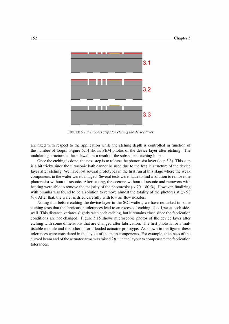
152 Chapter 5
FIGURE 5.13: Process steps for etching the device layer.
are fixed with respect to the application while the etching depth is controlled in function of
the number of loops. Figure 5.14 shows SEM photos of the device layer after etching. The
undulating structure at the sidewalls is a result of the subsequent etching loops.
Once the etching is done, the next step is to release the photoresist layer (step 3.3). This step
is a bit tricky since the ultrasonic bath cannot be used due to the fragile structure of the device
layer after etching. We have lost several prototypes in the first run at this stage where the weak
components in the wafer were damaged. Several tests were made to find a solution to remove the
photoresist without ultrasonic. After testing, the acetone without ultrasonic and removers with
heating were able to remove the majority of the photoresist (∼ 70−80 %). However, finalizing
with piranha was found to be a solution to remove almost the totality of the photoresist (> 98
%). After that, the wafer is dried carefully with low air flow nozzles.
Noting that before etching the device layer in the SOI wafers, we have remarked in some
etching tests that the fabrication tolerances lead to an excess of etching of ∼ 1µm at each side-
wall. This distance variates slightly with each etching, but it remains close since the fabrication
conditions are not changed. Figure 5.15 shows microscopic photos of the device layer after
etching with some dimensions that are changed after fabrication. The first photo is for a mul-
tistable module and the other is for a loaded actuator prototype. As shown in the figure, these
tolerances were considered in the layout of the main components. For example, thickness of the
curved beam and of the actuator arms was raised 2µm in the layout to compensate the fabrication
tolerances.
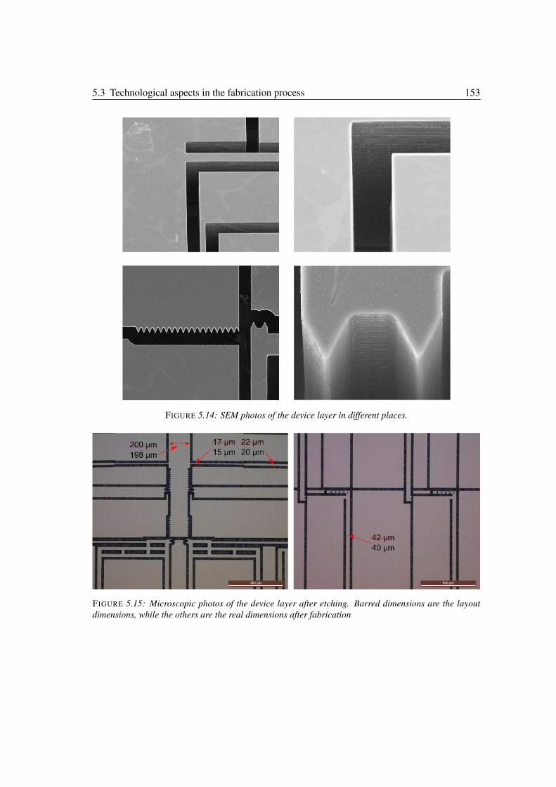
5.3 Technological aspects in the fabrication process 153
FIGURE 5.14: SEM photos of the device layer in different places.
FIGURE 5.15: Microscopic photos of the device layer after etching. Barred dimensions are the layout
dimensions, while the others are the real dimensions after fabrication
154 Chapter 5
5.3.4 Substrate etching
After the device layer, the handle layer is etched. The etching process is also the DRIE process.
The removal of the photoresist in the previous step is mandatory where no photoresist is allowed
in the backside to hold the wafer during etching in the SPTS.
The backside oxide layer is used as a hard mask which avoided the necessity of a thick
photoresist layer to make the deep etching. The accuracy is less important in this step and no
specific difficulties were expected.
This was the situation in the first run. However, in the second run after several months,
the etching quality was worst, this was the main difficulty in the second run. Excess loops
were made to finish the etching throughout the wafer where the etching was not homogeneous
throughout the wafer. This problem was worst due to an excess of wet etching in the hard mask
in the backside due to the unexpected high speed of etching of the BHF solution. In result, the
excess of silicon etching make the weak components more fragile which led to loose several
prototypes, most of them are the DiMiBot that are failed mostly at the flexible hinges.
Normally, this problem is not persistent if other fabrication runs are developed. However, we
are satisfied in the thesis by the operational prototypes of the multistable modules that showed
a proper functioning in the experiments which validate the principle and design of the module.
One of the future prospects of the thesis is to launch new runs of fabrication that take into
account the remarks and problems encountered in the first two runs of fabrication.
5.3.5 HF release
The last step in the fabrication process is to release the structure using the HF solution In this
step, the wafer is inserted in a HF solution, the HF is very selective, it starts to attack the silicon
oxide all around the wafer without etching the silicon. The first parts of SiO2 that disappear
are the oxide in the backside layer and in the openings of the middle layer. After that, the HF
attacks transversally the oxides in between the up and down silicon patterns.
The distance that must be etched transversally in order to release the structure is the releasing
distance as mentioned before and shown in Figure 5.16.a. We have used a specific wafer holder
(Figure 5.16.b) to make the releasing. This holder is made by Teflon which is a HF compatible
material. The wafer is inserted in the holder on the top of the rings inside, and then the holder is
inserted in the HF solution. In this way, the released structures fall into the bottom of the holder
due to their weight.
The end of the releasing is recognized by the fall of all the useless parts. At the end of
releasing, the wafer is inserted in three baths of ethanol successively for cleaning it and then
it is dried by the ambient air. Afterwards, the different prototypes are released manually using
an external probe. Some prototypes were released in the HF solution. These prototypes are
collected from the holder without problems.
As mentioned before, we have encountered a difficulty with the gold adhesion in the HF
solution in the first run of fabrication. Figure 5.17 shows a wafer from the first run of fabrication
where the gold patterns started to peel off from the wafer.
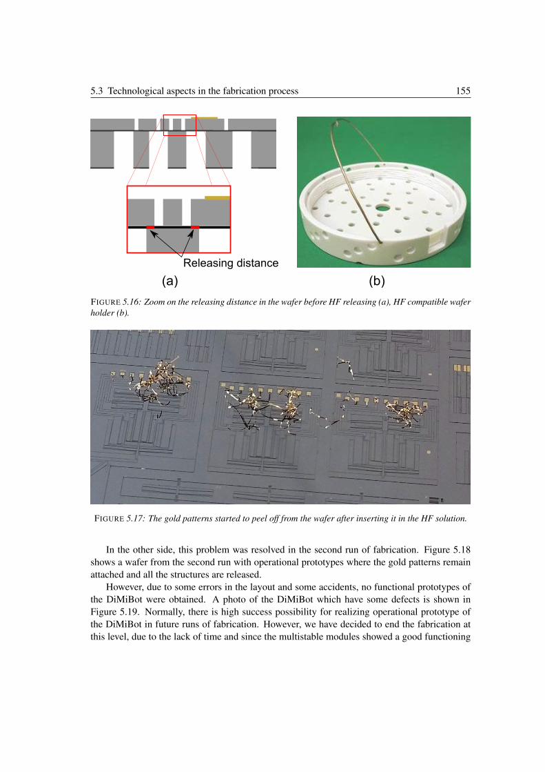
5.3 Technological aspects in the fabrication process 155
FIGURE 5.16: Zoom on the releasing distance in the wafer before HF releasing (a), HF compatible wafer
holder (b).
FIGURE 5.17: The gold patterns started to peel off from the wafer after inserting it in the HF solution.
In the other side, this problem was resolved in the second run of fabrication. Figure 5.18
shows a wafer from the second run with operational prototypes where the gold patterns remain
attached and all the structures are released.
However, due to some errors in the layout and some accidents, no functional prototypes of
the DiMiBot were obtained. A photo of the DiMiBot which have some defects is shown in
Figure 5.19. Normally, there is high success possibility for realizing operational prototype of
the DiMiBot in future runs of fabrication. However, we have decided to end the fabrication at
this level, due to the lack of time and since the multistable modules showed a good functioning
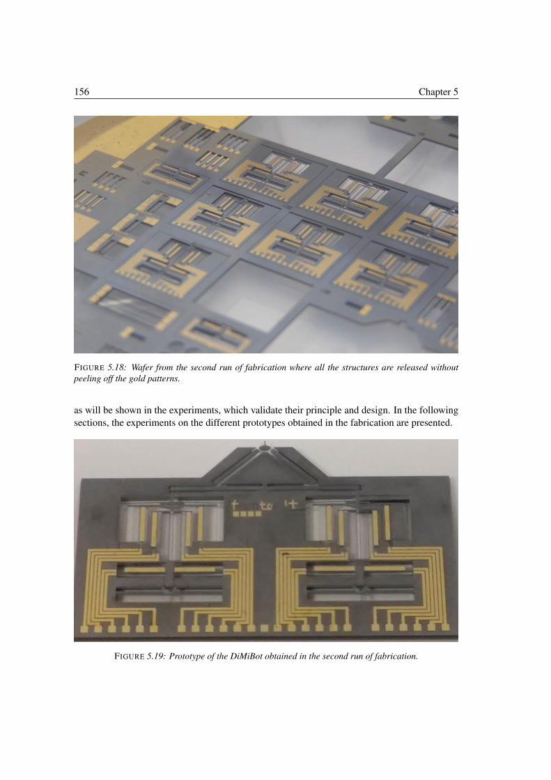
156 Chapter 5
FIGURE 5.18: Wafer from the second run of fabrication where all the structures are released without
peeling off the gold patterns.
as will be shown in the experiments, which validate their principle and design. In the following
sections, the experiments on the different prototypes obtained in the fabrication are presented.
FIGURE 5.19: Prototype of the DiMiBot obtained in the second run of fabrication.
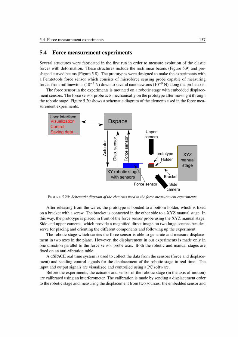
5.4 Force measurement experiments 157
5.4 Force measurement experiments
Several structures were fabricated in the first run in order to measure evolution of the elastic
forces with deformation. These structures include the rectilinear beams (Figure 5.9) and pre-
shaped curved beams (Figure 5.8). The prototypes were designed to make the experiments with
a Femtotools force sensor which consists of microforce sensing probe capable of measuring
forces from millinewtons (10−3 N) down to several nanonewtons (10−9 N) along the probe axis.
The force sensor in the experiments is mounted on a robotic stage with embedded displace-
ment sensors. The force sensor probe acts mechanically on the prototype after moving it through
the robotic stage. Figure 5.20 shows a schematic diagram of the elements used in the force mea-
surement experiments.
FIGURE 5.20: Schematic diagram of the elements used in the force measurement experiments.
After releasing from the wafer, the prototype is bonded to a bottom holder, which is fixed
on a bracket with a screw. The bracket is connected in the other side to a XYZ manual stage. In
this way, the prototype is placed in front of the force sensor probe using the XYZ manual stage.
Side and upper cameras, which provide a magnified direct image on two large screens besides,
serve for placing and orienting the different components and following up the experiment.
The robotic stage which carries the force sensor is able to generate and measure displace-
ment in two axes in the plane. However, the displacement in our experiments is made only in
one direction parallel to the force sensor probe axis. Both the robotic and manual stages are
fixed on an anti-vibration table.
A dSPACE real time system is used to collect the data from the sensors (force and displace-
ment) and sending control signals for the displacement of the robotic stage in real time. The
input and output signals are visualized and controlled using a PC software.
Before the experiments, the actuator and sensor of the robotic stage (in the axis of motion)
are calibrated using an interferometer. The calibration is made by sending a displacement order
to the robotic stage and measuring the displacement from two sources: the embedded sensor and
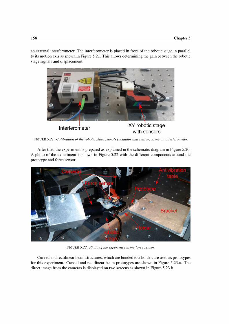
158 Chapter 5
an external interferometer. The interferometer is placed in front of the robotic stage in parallel
to its motion axis as shown in Figure 5.21. This allows determining the gain between the robotic
stage signals and displacement.
FIGURE 5.21: Calibration of the robotic stage signals (actuator and sensor) using an interferometer.
After that, the experiment is prepared as explained in the schematic diagram in Figure 5.20.
A photo of the experiment is shown in Figure 5.22 with the different components around the
prototype and force sensor.
FIGURE 5.22: Photo of the experience using force sensor.
Curved and rectilinear beam structures, which are bonded to a holder, are used as prototypes
for this experiment. Curved and rectilinear beam prototypes are shown in Figure 5.23.a. The
direct image from the cameras is displayed on two screens as shown in Figure 5.23.b.
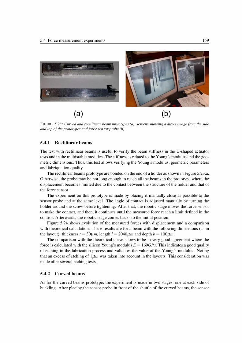
5.4 Force measurement experiments 159
FIGURE 5.23: Curved and rectilinear beam prototypes (a), screens showing a direct image from the side
and top of the prototypes and force sensor probe (b).
5.4.1 Rectilinear beams
The test with rectilinear beams is useful to verify the beam stiffness in the U-shaped actuator
tests and in the multistable modules. The stiffness is related to the Young’s modulus and the geo-
metric dimensions. Thus, this test allows verifying the Young’s modulus, geometric parameters
and fabriquation quality.
The rectilinear beams prototype are bonded on the end of a holder as shown in Figure 5.23.a.
Otherwise, the probe may be not long enough to reach all the beams in the prototype where the
displacement becomes limited due to the contact between the structure of the holder and that of
the force sensor.
The experiment on this prototype is made by placing it manually close as possible to the
sensor probe and at the same level. The angle of contact is adjusted manually by turning the
holder around the screw before tightening. After that, the robotic stage moves the force sensor
to make the contact, and then, it continues until the measured force reach a limit defined in the
control. Afterwards, the robotic stage comes backs to the initial position.
Figure 5.24 shows evolution of the measured forces with displacement and a comparison
with theoretical calculation. These results are for a beam with the following dimensions (as in
the layout): thickness t = 30µm, length l = 2040µm and depth b = 100µm.
The comparison with the theoretical curve shows to be in very good agreement where the
force is calculated with the silicon Young’s modulus E = 169GPa. This indicates a good quality
of etching in the fabrication process and validates the value of the Young’s modulus. Noting
that an excess of etching of 1µm was taken into account in the layouts. This consideration was
made after several etching tests.
5.4.2 Curved beams
As for the curved beams prototype, the experiment is made in two stages, one at each side of
buckling. After placing the sensor probe in front of the shuttle of the curved beams, the sensor
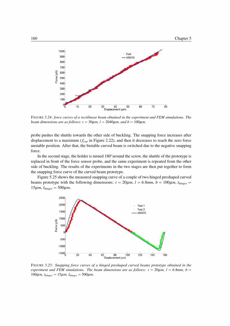
160 Chapter 5
FIGURE 5.24: force curves of a rectilinear beam obtained in the experiment and FEM simulations. The
beam dimensions are as follows: t = 30µm, l = 2040µm, and b = 100µm.
probe pushes the shuttle towards the other side of buckling. The snapping force increases after
displacement to a maximum ( ftop in Figure 2.22), and then it decreases to reach the zero force
unstable position. After that, the bistable curved beam is switched due to the negative snapping
force.
In the second stage, the holder is turned 180°around the screw, the shuttle of the prototype is
replaced in front of the force sensor probe, and the same experiment is repeated from the other
side of buckling. The results of the experiments in the two stages are then put together to form
the snapping force curve of the curved beam prototype.
Figure 5.25 shows the measured snapping curve of a couple of two hinged preshaped curved
beams prototype with the following dimensions: t = 20µm, l = 6.8mm, b = 100µm, thinges =15µm, lhinges = 500µm.
FIGURE 5.25: Snapping force curves of a hinged preshaped curved beams prototype obtained in the
experiment and FEM simulations. The beam dimensions are as follows: t = 20µm, l = 6.8mm, b =100µm, thinges = 15µm, lhinges = 500µm.
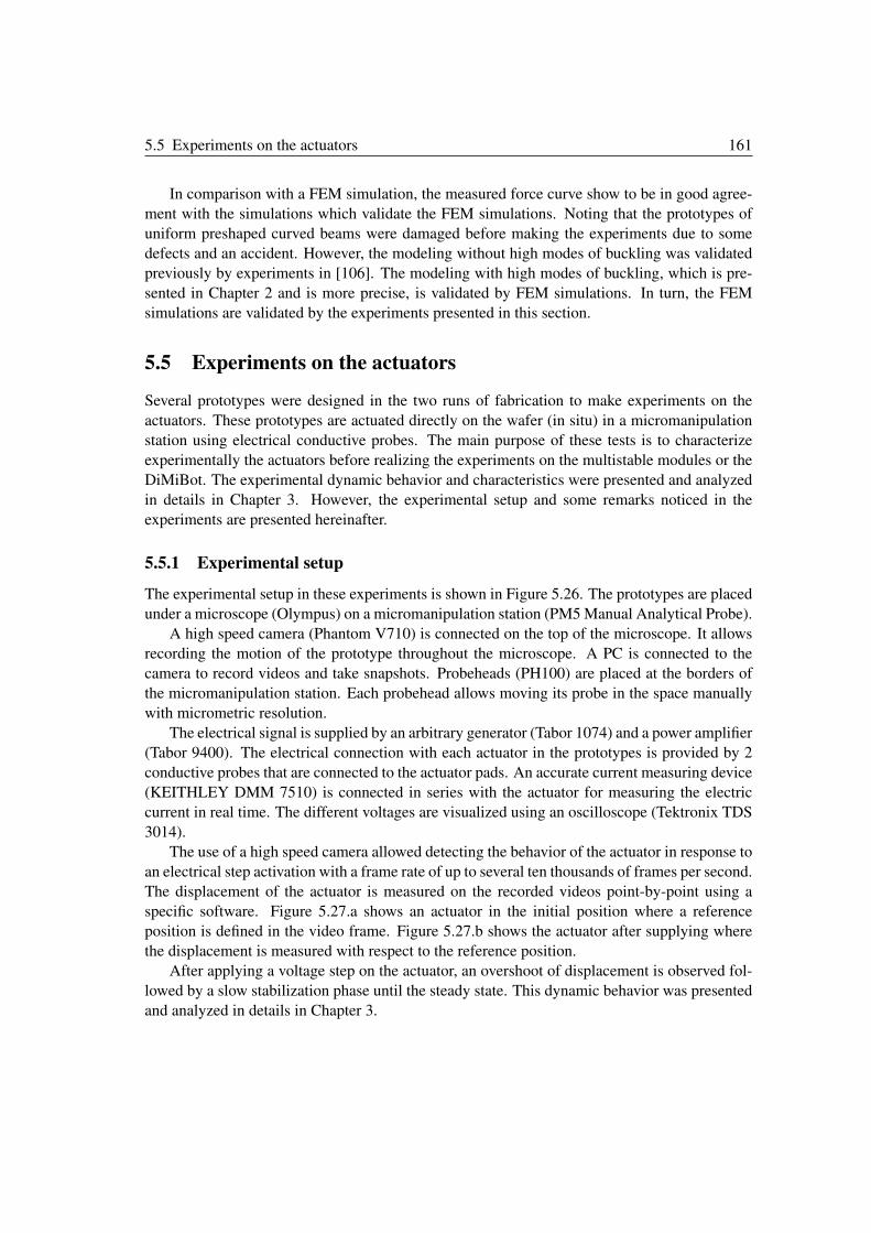
5.5 Experiments on the actuators 161
In comparison with a FEM simulation, the measured force curve show to be in good agree-
ment with the simulations which validate the FEM simulations. Noting that the prototypes of
uniform preshaped curved beams were damaged before making the experiments due to some
defects and an accident. However, the modeling without high modes of buckling was validated
previously by experiments in [106]. The modeling with high modes of buckling, which is pre-
sented in Chapter 2 and is more precise, is validated by FEM simulations. In turn, the FEM
simulations are validated by the experiments presented in this section.
5.5 Experiments on the actuators
Several prototypes were designed in the two runs of fabrication to make experiments on the
actuators. These prototypes are actuated directly on the wafer (in situ) in a micromanipulation
station using electrical conductive probes. The main purpose of these tests is to characterize
experimentally the actuators before realizing the experiments on the multistable modules or the
DiMiBot. The experimental dynamic behavior and characteristics were presented and analyzed
in details in Chapter 3. However, the experimental setup and some remarks noticed in the
experiments are presented hereinafter.
5.5.1 Experimental setup
The experimental setup in these experiments is shown in Figure 5.26. The prototypes are placed
under a microscope (Olympus) on a micromanipulation station (PM5 Manual Analytical Probe).
A high speed camera (Phantom V710) is connected on the top of the microscope. It allows
recording the motion of the prototype throughout the microscope. A PC is connected to the
camera to record videos and take snapshots. Probeheads (PH100) are placed at the borders of
the micromanipulation station. Each probehead allows moving its probe in the space manually
with micrometric resolution.
The electrical signal is supplied by an arbitrary generator (Tabor 1074) and a power amplifier
(Tabor 9400). The electrical connection with each actuator in the prototypes is provided by 2
conductive probes that are connected to the actuator pads. An accurate current measuring device
(KEITHLEY DMM 7510) is connected in series with the actuator for measuring the electric
current in real time. The different voltages are visualized using an oscilloscope (Tektronix TDS
3014).
The use of a high speed camera allowed detecting the behavior of the actuator in response to
an electrical step activation with a frame rate of up to several ten thousands of frames per second.
The displacement of the actuator is measured on the recorded videos point-by-point using a
specific software. Figure 5.27.a shows an actuator in the initial position where a reference
position is defined in the video frame. Figure 5.27.b shows the actuator after supplying where
the displacement is measured with respect to the reference position.
After applying a voltage step on the actuator, an overshoot of displacement is observed fol-
lowed by a slow stabilization phase until the steady state. This dynamic behavior was presented
and analyzed in details in Chapter 3.
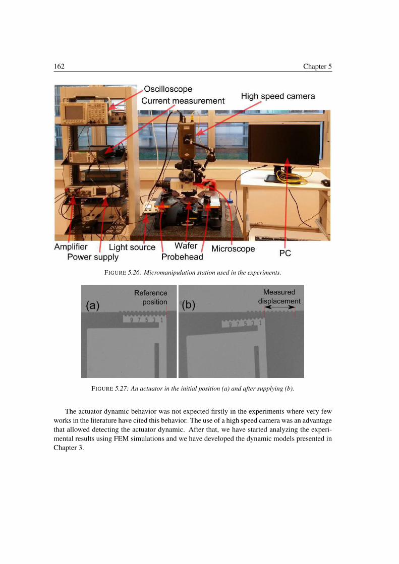
162 Chapter 5
FIGURE 5.26: Micromanipulation station used in the experiments.
FIGURE 5.27: An actuator in the initial position (a) and after supplying (b).
The actuator dynamic behavior was not expected firstly in the experiments where very few
works in the literature have cited this behavior. The use of a high speed camera was an advantage
that allowed detecting the actuator dynamic. After that, we have started analyzing the experi-
mental results using FEM simulations and we have developed the dynamic models presented in
Chapter 3.
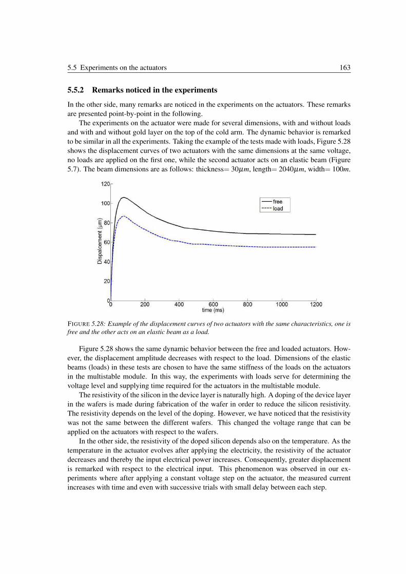
5.5 Experiments on the actuators 163
5.5.2 Remarks noticed in the experiments
In the other side, many remarks are noticed in the experiments on the actuators. These remarks
are presented point-by-point in the following.
The experiments on the actuator were made for several dimensions, with and without loads
and with and without gold layer on the top of the cold arm. The dynamic behavior is remarked
to be similar in all the experiments. Taking the example of the tests made with loads, Figure 5.28
shows the displacement curves of two actuators with the same dimensions at the same voltage,
no loads are applied on the first one, while the second actuator acts on an elastic beam (Figure
5.7). The beam dimensions are as follows: thickness= 30µm, length= 2040µm, width= 100m.
FIGURE 5.28: Example of the displacement curves of two actuators with the same characteristics, one is
free and the other acts on an elastic beam as a load.
Figure 5.28 shows the same dynamic behavior between the free and loaded actuators. How-
ever, the displacement amplitude decreases with respect to the load. Dimensions of the elastic
beams (loads) in these tests are chosen to have the same stiffness of the loads on the actuators
in the multistable module. In this way, the experiments with loads serve for determining the
voltage level and supplying time required for the actuators in the multistable module.
The resistivity of the silicon in the device layer is naturally high. A doping of the device layer
in the wafers is made during fabrication of the wafer in order to reduce the silicon resistivity.
The resistivity depends on the level of the doping. However, we have noticed that the resistivity
was not the same between the different wafers. This changed the voltage range that can be
applied on the actuators with respect to the wafers.
In the other side, the resistivity of the doped silicon depends also on the temperature. As the
temperature in the actuator evolves after applying the electricity, the resistivity of the actuator
decreases and thereby the input electrical power increases. Consequently, greater displacement
is remarked with respect to the electrical input. This phenomenon was observed in our ex-
periments where after applying a constant voltage step on the actuator, the measured current
increases with time and even with successive trials with small delay between each step.
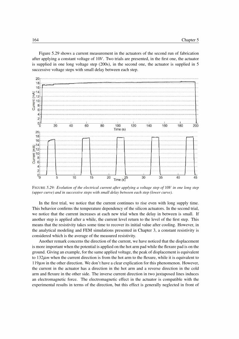
164 Chapter 5
Figure 5.29 shows a current measurement in the actuators of the second run of fabrication
after applying a constant voltage of 10V . Two trials are presented, in the first one, the actuator
is supplied in one long voltage step (200s), in the second one, the actuator is supplied in 5
successive voltage steps with small delay between each step.
FIGURE 5.29: Evolution of the electrical current after applying a voltage step of 10V in one long step
(upper curve) and in successive steps with small delay between each step (lower curve).
In the first trial, we notice that the current continues to rise even with long supply time.
This behavior confirms the temperature dependency of the silicon actuators. In the second trial,
we notice that the current increases at each new trial when the delay in between is small. If
another step is applied after a while, the current level return to the level of the first step. This
means that the resistivity takes some time to recover its initial value after cooling. However, in
the analytical modeling and FEM simulations presented in Chapter 3, a constant resistivity is
considered which is the average of the measured resistivity.
Another remark concerns the direction of the current, we have noticed that the displacement
is more important when the potential is applied on the hot arm pad while the flexure pad is on the
ground. Giving an example, for the same applied voltage, the peak of displacement is equivalent
to 132µm when the current direction is from the hot arm to the flexure, while it is equivalent to
119µm in the other direction. We don’t have a clear explication for this phenomenon. However,
the current in the actuator has a direction in the hot arm and a reverse direction in the cold
arm and flexure in the other side. The inverse current direction in two juxtaposed lines induces
an electromagnetic force. The electromagnetic effect in the actuator is compatible with the
experimental results in terms of the direction, but this effect is generally neglected in front of
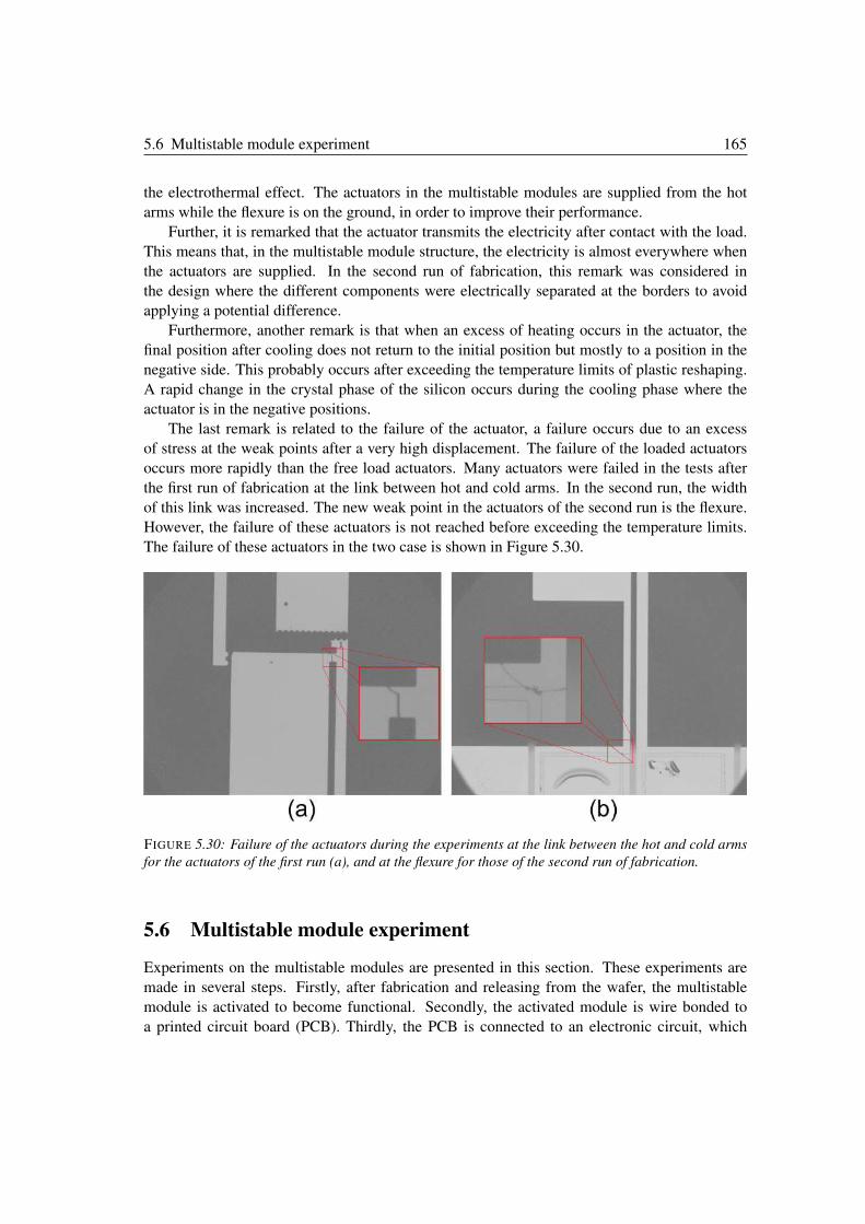
5.6 Multistable module experiment 165
the electrothermal effect. The actuators in the multistable modules are supplied from the hot
arms while the flexure is on the ground, in order to improve their performance.
Further, it is remarked that the actuator transmits the electricity after contact with the load.
This means that, in the multistable module structure, the electricity is almost everywhere when
the actuators are supplied. In the second run of fabrication, this remark was considered in
the design where the different components were electrically separated at the borders to avoid
applying a potential difference.
Furthermore, another remark is that when an excess of heating occurs in the actuator, the
final position after cooling does not return to the initial position but mostly to a position in the
negative side. This probably occurs after exceeding the temperature limits of plastic reshaping.
A rapid change in the crystal phase of the silicon occurs during the cooling phase where the
actuator is in the negative positions.
The last remark is related to the failure of the actuator, a failure occurs due to an excess
of stress at the weak points after a very high displacement. The failure of the loaded actuators
occurs more rapidly than the free load actuators. Many actuators were failed in the tests after
the first run of fabrication at the link between hot and cold arms. In the second run, the width
of this link was increased. The new weak point in the actuators of the second run is the flexure.
However, the failure of these actuators is not reached before exceeding the temperature limits.
The failure of these actuators in the two case is shown in Figure 5.30.
FIGURE 5.30: Failure of the actuators during the experiments at the link between the hot and cold arms
for the actuators of the first run (a), and at the flexure for those of the second run of fabrication.
5.6 Multistable module experiment
Experiments on the multistable modules are presented in this section. These experiments are
made in several steps. Firstly, after fabrication and releasing from the wafer, the multistable
module is activated to become functional. Secondly, the activated module is wire bonded to
a printed circuit board (PCB). Thirdly, the PCB is connected to an electronic circuit, which
166 Chapter 5
consists of microcontroller and switches, for supplying the actuators in the multistable module.
Fourthly, each system in the module is tested separately before making a complete sequence
in the fifth step. The experiments are recorded using the high speed camera shown in Figure
5.26. The multistable modules showed a proper functioning in the experiments while a defect
in the design were deduced. All of these steps are presented one by one in the following. The
sequence order, defined in the microcontroller to switch up and down, are presented before the
experiments.
5.6.1 Activation of the multistable modules
The first step after fabrication and releasing of the multistable module is to activate it. As
explained in Chapter 4, the activation phase consists in arming the different components in the
accurate positioning mechanism in system 1 and arming the teeth between S2 latch and the
moving part.
During activation, the multistable module is placed under the microscope in the microma-
nipulation station and the different components are armed using the needles of three probeheads.
Figure 5.31 shows the different steps in the activation phase. Firstly, the upper movable parts
are suspended to the upper locks ((a) & (d)), the bottom movable part is then suspended to the
bottom lock ((b) & (e)), and then the shuttle of system 1 is pushed to its first position ((c) &
(f)). Before pushing the shuttle of system 1 (connected to S2 latch) upwards, S2 latch is opened
using two needles as shown in (g) to avoid crushing the structure. Thereby, after pushing up and
releasing S2 latch, it becomes engaged to the teeth of the moving part as shown in ((h) & (f)).
5.6.2 Wire bonding
After activation, a PCB is prepared to make the electrical connectivity between the multistable
module and an external circuit. The wire bonding is made in the clean room using an ultrasonic
wire bonding machine. Figure 5.32 shows a multistable module prototype glued on the PCB
where the gold lines in the prototype are wire bonded to the copper lines in the PCB. The
prototype is glued at the top edge of the PCB as shown in the figure, while a plastic board is
glued under the PCB to protect the multistable module.
5.6.3 Electronic circuit
An electronic circuit was prepared to supply the multistable module. It consists of a micro-
controller to control the supply time and sequence order for supplying the different actuators, a
relay circuit to switch on or off the current at each actuator, control buttons to choose between
upward and downward steps and different connectors. The electronic circuit is supplied by two
external electrical sources of 5 and 20V, where 5V is the voltage needed for the microcontroller
and the relays and 20V is the voltage to be applied on the actuators. The output of the relays
are connected to a ZIF (an electrical connector with zero insertion force), so the PCB with the
multistable module can be connected directly to the electronic circuit by inserting it in the ZIF.
The electronic circuit with a connected multistable module prototype is shown in Figure 5.33.
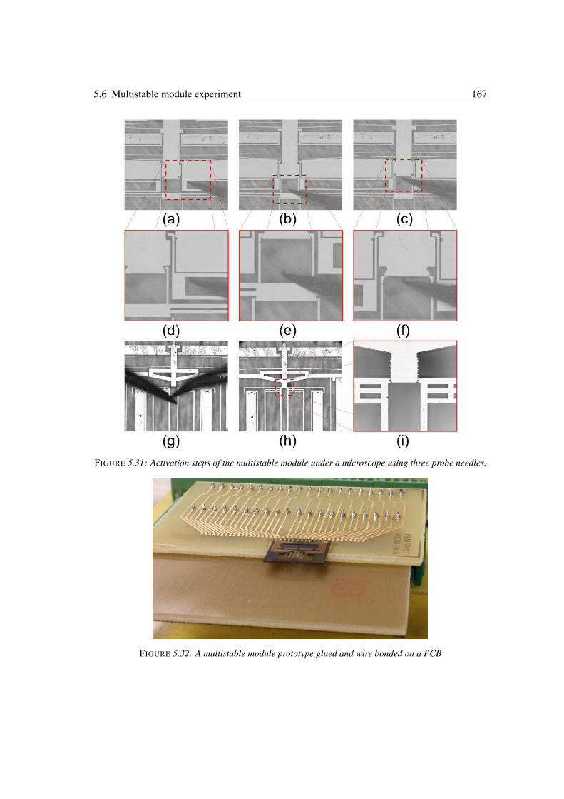
5.6 Multistable module experiment 167
FIGURE 5.31: Activation steps of the multistable module under a microscope using three probe needles.
FIGURE 5.32: A multistable module prototype glued and wire bonded on a PCB
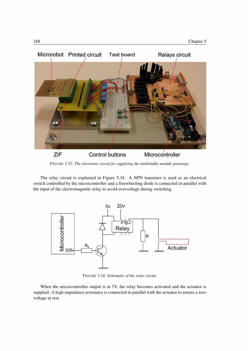
168 Chapter 5
FIGURE 5.33: The electronic circuit for supplying the multistable module prototype.
The relay circuit is explained in Figure 5.34. A NPN transistor is used as an electrical
switch controlled by the microcontroller and a freewheeling diode is connected in parallel with
the input of the electromagnetic relay to avoid overvoltage during switching.
FIGURE 5.34: Schematic of the relay circuit.
When the microcontroller output is at 5V, the relay becomes activated and the actuator is
supplied. A high impedance resistance is connected in parallel with the actuator to ensure a zero
voltage at rest.
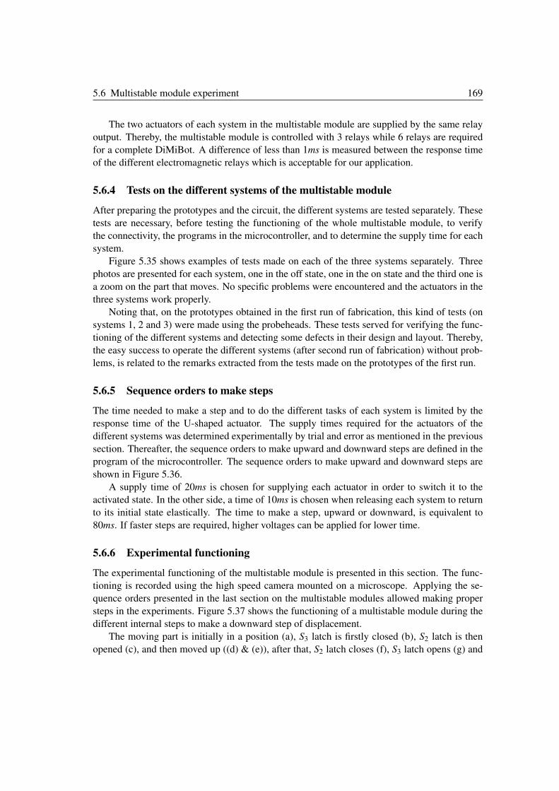
5.6 Multistable module experiment 169
The two actuators of each system in the multistable module are supplied by the same relay
output. Thereby, the multistable module is controlled with 3 relays while 6 relays are required
for a complete DiMiBot. A difference of less than 1ms is measured between the response time
of the different electromagnetic relays which is acceptable for our application.
5.6.4 Tests on the different systems of the multistable module
After preparing the prototypes and the circuit, the different systems are tested separately. These
tests are necessary, before testing the functioning of the whole multistable module, to verify
the connectivity, the programs in the microcontroller, and to determine the supply time for each
system.
Figure 5.35 shows examples of tests made on each of the three systems separately. Three
photos are presented for each system, one in the off state, one in the on state and the third one is
a zoom on the part that moves. No specific problems were encountered and the actuators in the
three systems work properly.
Noting that, on the prototypes obtained in the first run of fabrication, this kind of tests (on
systems 1, 2 and 3) were made using the probeheads. These tests served for verifying the func-
tioning of the different systems and detecting some defects in their design and layout. Thereby,
the easy success to operate the different systems (after second run of fabrication) without prob-
lems, is related to the remarks extracted from the tests made on the prototypes of the first run.
5.6.5 Sequence orders to make steps
The time needed to make a step and to do the different tasks of each system is limited by the
response time of the U-shaped actuator. The supply times required for the actuators of the
different systems was determined experimentally by trial and error as mentioned in the previous
section. Thereafter, the sequence orders to make upward and downward steps are defined in the
program of the microcontroller. The sequence orders to make upward and downward steps are
shown in Figure 5.36.
A supply time of 20ms is chosen for supplying each actuator in order to switch it to the
activated state. In the other side, a time of 10ms is chosen when releasing each system to return
to its initial state elastically. The time to make a step, upward or downward, is equivalent to
80ms. If faster steps are required, higher voltages can be applied for lower time.
5.6.6 Experimental functioning
The experimental functioning of the multistable module is presented in this section. The func-
tioning is recorded using the high speed camera mounted on a microscope. Applying the se-
quence orders presented in the last section on the multistable modules allowed making proper
steps in the experiments. Figure 5.37 shows the functioning of a multistable module during the
different internal steps to make a downward step of displacement.
The moving part is initially in a position (a), S3 latch is firstly closed (b), S2 latch is then
opened (c), and then moved up ((d) & (e)), after that, S2 latch closes (f), S3 latch opens (g) and
170 Chapter 5
FIGURE 5.35: Tests on systems 1, 2 and 3 respectively. Three photos are presented for each system, one
in the off state, one in the on state and the third one is a zoom on the part that moves. System 1 ((a), (b)
& (c)), system 2 ((d), (e) & (f)), system 3 ((g), (h) & (i)).
finally, S2 latch moves down with the moving part (h), in result, the moving part is now in a
lower position as shown in (i).
In result, the proper functioning of the multistable module in the experiments validates its
principle and design. These modules are then operational and useful for digital MEMS applica-
tions. However, despite the proper functioning, we found some defects concerning the size and
type of teeth.
As explained previously in Section 4.4, two configurations of the teeth are used in the multi-
stable modules between the latches and the moving part. In the experiments, we have remarked
two defects, one for each teeth configuration. As for the wide teeth configuration, the problem
is in the teeth of S3 latch. After activating and dis-activating system 3, the teeth of S3 latch re-
main attached with those of the moving part. In result, the latch remains closed which impedes
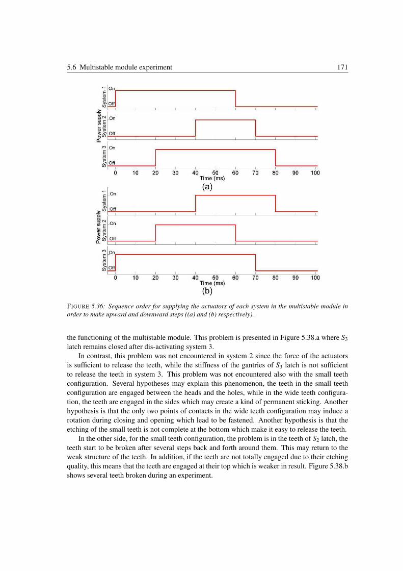
5.6 Multistable module experiment 171
FIGURE 5.36: Sequence order for supplying the actuators of each system in the multistable module in
order to make upward and downward steps ((a) and (b) respectively).
the functioning of the multistable module. This problem is presented in Figure 5.38.a where S3
latch remains closed after dis-activating system 3.
In contrast, this problem was not encountered in system 2 since the force of the actuators
is sufficient to release the teeth, while the stiffness of the gantries of S3 latch is not sufficient
to release the teeth in system 3. This problem was not encountered also with the small teeth
configuration. Several hypotheses may explain this phenomenon, the teeth in the small teeth
configuration are engaged between the heads and the holes, while in the wide teeth configura-
tion, the teeth are engaged in the sides which may create a kind of permanent sticking. Another
hypothesis is that the only two points of contacts in the wide teeth configuration may induce a
rotation during closing and opening which lead to be fastened. Another hypothesis is that the
etching of the small teeth is not complete at the bottom which make it easy to release the teeth.
In the other side, for the small teeth configuration, the problem is in the teeth of S2 latch, the
teeth start to be broken after several steps back and forth around them. This may return to the
weak structure of the teeth. In addition, if the teeth are not totally engaged due to their etching
quality, this means that the teeth are engaged at their top which is weaker in result. Figure 5.38.b
shows several teeth broken during an experiment.
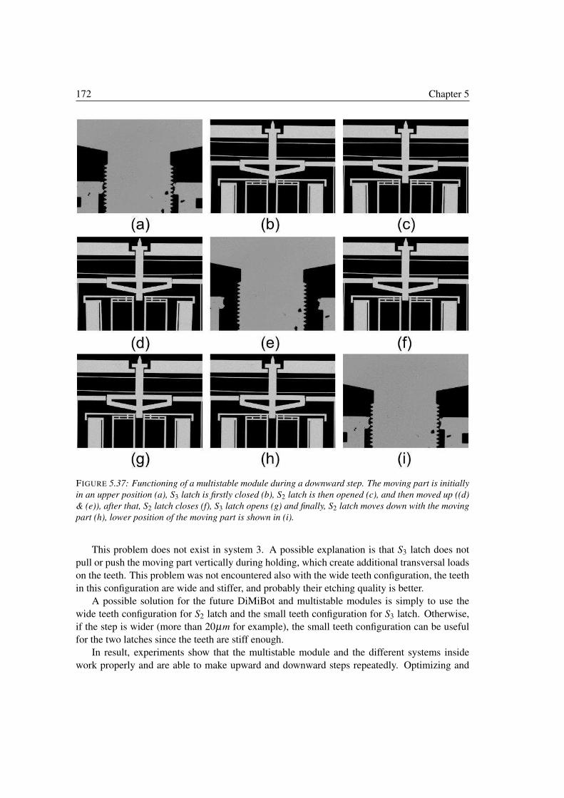
172 Chapter 5
FIGURE 5.37: Functioning of a multistable module during a downward step. The moving part is initially
in an upper position (a), S3 latch is firstly closed (b), S2 latch is then opened (c), and then moved up ((d)
& (e)), after that, S2 latch closes (f), S3 latch opens (g) and finally, S2 latch moves down with the moving
part (h), lower position of the moving part is shown in (i).
This problem does not exist in system 3. A possible explanation is that S3 latch does not
pull or push the moving part vertically during holding, which create additional transversal loads
on the teeth. This problem was not encountered also with the wide teeth configuration, the teeth
in this configuration are wide and stiffer, and probably their etching quality is better.
A possible solution for the future DiMiBot and multistable modules is simply to use the
wide teeth configuration for S2 latch and the small teeth configuration for S3 latch. Otherwise,
if the step is wider (more than 20µm for example), the small teeth configuration can be useful
for the two latches since the teeth are stiff enough.
In result, experiments show that the multistable module and the different systems inside
work properly and are able to make upward and downward steps repeatedly. Optimizing and
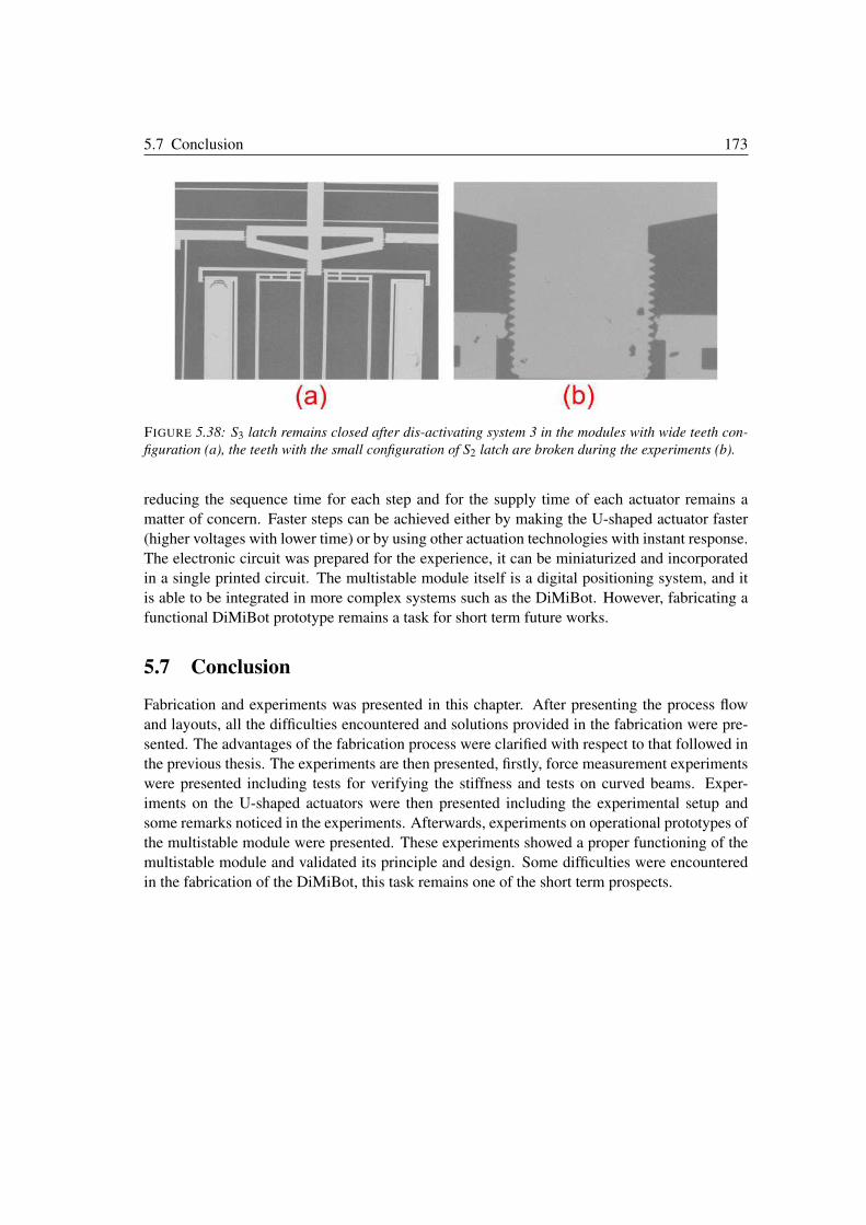
5.7 Conclusion 173
FIGURE 5.38: S3 latch remains closed after dis-activating system 3 in the modules with wide teeth con-
figuration (a), the teeth with the small configuration of S2 latch are broken during the experiments (b).
reducing the sequence time for each step and for the supply time of each actuator remains a
matter of concern. Faster steps can be achieved either by making the U-shaped actuator faster
(higher voltages with lower time) or by using other actuation technologies with instant response.
The electronic circuit was prepared for the experience, it can be miniaturized and incorporated
in a single printed circuit. The multistable module itself is a digital positioning system, and it
is able to be integrated in more complex systems such as the DiMiBot. However, fabricating a
functional DiMiBot prototype remains a task for short term future works.
5.7 Conclusion
Fabrication and experiments was presented in this chapter. After presenting the process flow
and layouts, all the difficulties encountered and solutions provided in the fabrication were pre-
sented. The advantages of the fabrication process were clarified with respect to that followed in
the previous thesis. The experiments are then presented, firstly, force measurement experiments
were presented including tests for verifying the stiffness and tests on curved beams. Exper-
iments on the U-shaped actuators were then presented including the experimental setup and
some remarks noticed in the experiments. Afterwards, experiments on operational prototypes of
the multistable module were presented. These experiments showed a proper functioning of the
multistable module and validated its principle and design. Some difficulties were encountered
in the fabrication of the DiMiBot, this task remains one of the short term prospects.

Conclusion and perspectives
Conclusion
A new version of a digital microrobot DiMiBot with multistable modules is proposed and devel-
oped in this thesis. The DiMiBot has many advantages for MEMS applications, it can perform
high accurate and repeatable positioning without the need of a feedback or measurement sys-
tems. Digital microrobotics is a topic of concern in our laboratory where a previous version of
the DiMiBot with bistable modules was proposed in a previous thesis.
Based on the past achievements, the thesis objectives at the beginning focused on improving
the functioning of the DiMiBot, optimizing its design and improving its fabrication process,
in order to make it more accurate, more controllable and smaller. Two working axes were
followed in order to achieve these goals: the first axis focus on optimizing the design of the
main components analytically, the second axis focus on proposing new architectures in order to
improve the functioning and the accuracy and going further in the miniaturization.
In the first axis, the main components in the DiMiBot (old and new versions) are the pre-
shaped curved beams and U-shaped electrothermal actuators. Analytical models for these com-
ponents were developed. As for the preshaped curved beam, in a first stage, the snapping force
solution is developed including high modes of buckling which are neglected in literature. In a
second stage, evolution of internal stresses during deflection between the two sides of buckling
were calculated. Comparison of the analytical results with FEM simulations have shown to be
in excellent agreement and showed the importance of considering high modes of buckling in the
modeling.
As for the U-shaped actuator, the modeling problem is treated by a sequence of two ana-
lytical models: electro-thermal and thermo-mechanical. The electrothermal model provides an
exact solution of the hybrid PDEs that describe the electrothermal behavior in the three arms of
the actuator. The relation between the displacement and the thermal distribution is then provided
in the thermo-mechanical model. Comparison with FEM simulations and experiments showed
a good agreement for the two models.
Based on the analytical expressions obtained in the modeling, the influence of the material
properties and the different dimensions on the behavior of the curved beam and the U-shaped
actuator were investigated. In light of that, design methods were proposed in order to choose
the optimal dimensions that ensure the desired outputs and characteristics. These components
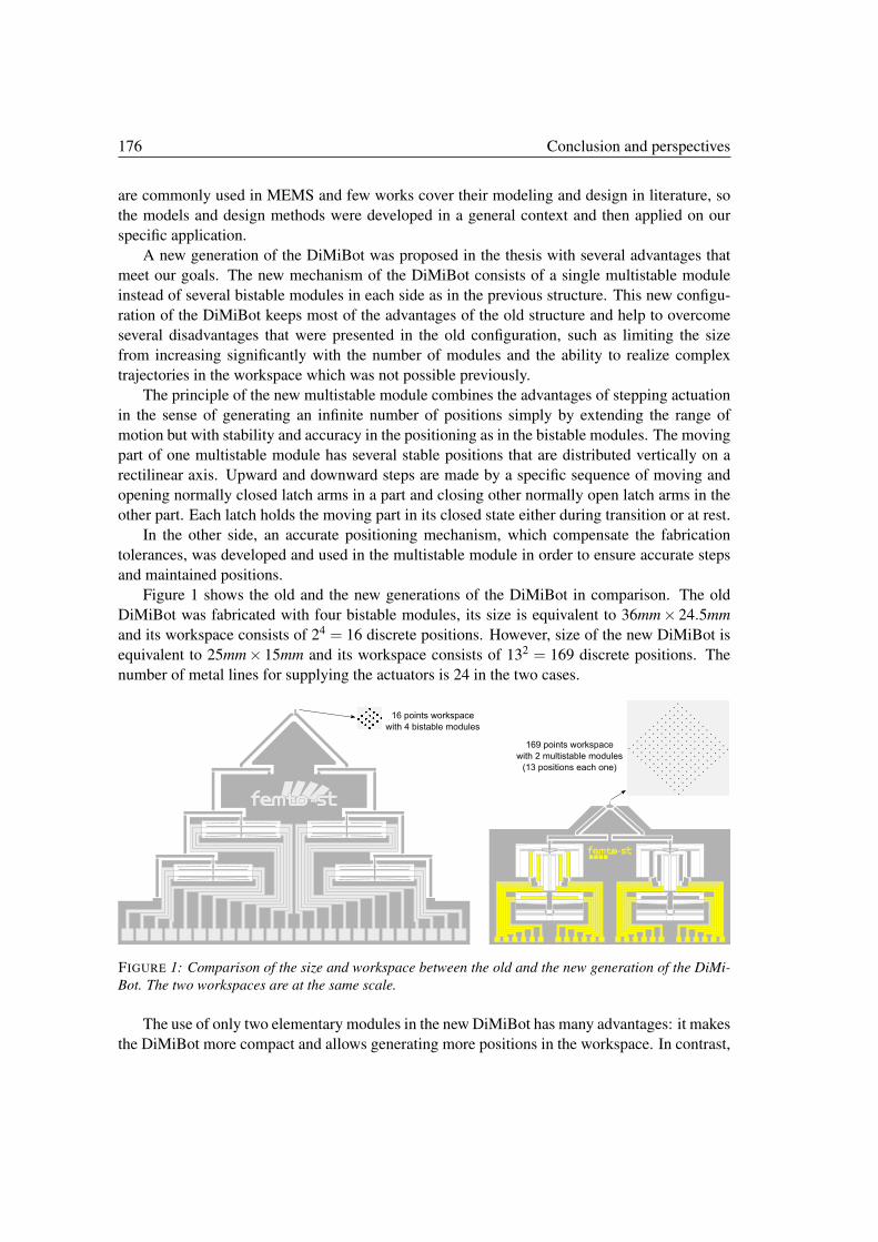
176 Conclusion and perspectives
are commonly used in MEMS and few works cover their modeling and design in literature, so
the models and design methods were developed in a general context and then applied on our
specific application.
A new generation of the DiMiBot was proposed in the thesis with several advantages that
meet our goals. The new mechanism of the DiMiBot consists of a single multistable module
instead of several bistable modules in each side as in the previous structure. This new configu-
ration of the DiMiBot keeps most of the advantages of the old structure and help to overcome
several disadvantages that were presented in the old configuration, such as limiting the size
from increasing significantly with the number of modules and the ability to realize complex
trajectories in the workspace which was not possible previously.
The principle of the new multistable module combines the advantages of stepping actuation
in the sense of generating an infinite number of positions simply by extending the range of
motion but with stability and accuracy in the positioning as in the bistable modules. The moving
part of one multistable module has several stable positions that are distributed vertically on a
rectilinear axis. Upward and downward steps are made by a specific sequence of moving and
opening normally closed latch arms in a part and closing other normally open latch arms in the
other part. Each latch holds the moving part in its closed state either during transition or at rest.
In the other side, an accurate positioning mechanism, which compensate the fabrication
tolerances, was developed and used in the multistable module in order to ensure accurate steps
and maintained positions.
Figure 1 shows the old and the new generations of the DiMiBot in comparison. The old
DiMiBot was fabricated with four bistable modules, its size is equivalent to 36mm× 24.5mm
and its workspace consists of 24 = 16 discrete positions. However, size of the new DiMiBot is
equivalent to 25mm× 15mm and its workspace consists of 132 = 169 discrete positions. The
number of metal lines for supplying the actuators is 24 in the two cases.
FIGURE 1: Comparison of the size and workspace between the old and the new generation of the DiMi-
Bot. The two workspaces are at the same scale.
The use of only two elementary modules in the new DiMiBot has many advantages: it makes
the DiMiBot more compact and allows generating more positions in the workspace. In contrast,
Conclusion and perspectives 177
adding more bistable modules in the old DiMiBot to obtain more positions in the workspace has
many drawbacks. For example, if we choose a workspace with 256 discrete positions, 8 bistable
modules are required in the old DiMiBot with a total size of 50.5mm× 33.5mm and 48 metal
lines. However, the only change to be made in the new DiMiBot is that the range of motion of
the moving part of each module must be extended to include 3 more positions.
The DiMiBot with 8 bistable modules has a big size with high number of tiny components
distributed on a large surface. This makes the structure more fragile, increases possibilities of
failure in the fabrication process and high number of metal lines are required. In addition, the
transition in the DiMiBot with multistable module is made between the adjacent positions, not
by binary jumps as with the bistable modules. This allows realizing any complex trajectory with
an open loop control.
After making the design and plotting the different layouts, two runs of fabrication were made
in the clean room MIMENTO in order to realize operational prototypes. Some differences were
made in the fabrication process in order to avoid the problems encountered in the previous
theses. All the difficulties encountered and solutions provided in the fabrication are detailed in
the thesis.
The final phase treated in the thesis is the experiments, including force measurement experi-
ments, experiments on the U-shaped actuators and experiments on some operational prototypes
of the multistable module. The experiments show that the multistable module and the differ-
ent systems inside work properly and are able to make upward and downward steps repeatedly.
Fabricating a functional DiMiBot prototype remains a task for short term future works.
Perspectives
The presented work opens up important perspectives for most of the subjects treated in the thesis.
The works presented on the modeling and design of the preshaped curved beam are satisfactory
for our needs. As for the U-shaped actuator, the consideration of some neglected effects in the
modeling, the calculation of the internal stresses and the design to have the capacity to output
a required performance at a transient instant are topics that can be addressed. The multistable
module development outlooks include the improvement of its performance, making it faster and
even more compact. The principle of the DiMiBot must be developed towards more accurate
steps with maintained positions in the planar workspace. In a long term, developing a 3D digital
microrobot is also one of the perspectives.
Actuators
The analytical models for the U-shaped actuator showed an agreement with FEM simulations
and experiments, but with slight differences. Improving the accuracy of the modeling is possi-
ble by considering some phenomena neglected in the present approach (convection or radiation,
different boundary conditions, temperature dependency of the material properties, 1D simpli-
fication, etc.). However, the consideration of some of these simplifications complicates the
solution and to date, the problem can be solved only by numerical methods. This results in
losing the benefits of the analytical solution for the design.
178 Conclusion and perspectives
Further, the calculation method used in the electrothermal model has an original contribution
mathematically. It can be developed to solve analytically other physical problems where the
problem is described by hybrid PDEs and the variables evolve between multiple connected
mediums such as the wave propagation in various environments.
In addition, providing analytical models to describe evolution of the internal stresses is
important to avoid the fracture of the weak points in the actuator at high displacement. Until
now, the stresses are calculated numerically.
As for the design, in view to the complexity of the analytical expressions, the influence of the
various variables on the transient behavior is not totally investigated. Therefore, the proposed
design method is made based on the outputs at the steady state. More works must be made
to investigate the variables influence on the transient behavior and to provide a design method
which ensures to have the capacity to output a required performance at a transient instant.
Multistable module
The multistable module showed to be operational in the experiments. It can be used for accurate
positioning applications in MEMS, integrated in more complex systems for more advanced tasks
and used in compact environments.
However, the stepping speed remains a matter of concern for the module. Faster motion can
be achieved by improving the response time of the actuator. In the case of the U-shaped actuator,
this can be achieved by increasing the input voltage with lower supply time while ensuring that
the temperature remains in the acceptable margin. Otherwise, other actuation technologies with
very low response time can be used.
In the other side, the design of the module can be changed for other number of stable posi-
tions and other step dimensions with respect to the design requirements and specific application.
However, reducing the step size and increasing the stroke as possible with faster steps pave the
way to reach a continuous micropositioning performance with all the advantages of the digital
concept previously cited.
New runs of fabrication are expected in the near future with considering the remarks noticed
in the first two runs and the experiments. The experimental electronic circuit can be miniaturized
and incorporated in a single and compact PCB.
Towards a planar multistable microrobot with holding forces
The top head flexible structure is the solution used in the DiMiBot (old and new generation) to
combine the one-axis displacement at the two sides in one planar workspace. However, positions
of the end effector in the workspace are stable but not maintained due to the use of the top head
flexible structure. The robustness and holding forces in the stable positions of the modules are
loosen in the DiMiBot due to the top head flexible structure relating the modules to the end
effector. In addition, the different positions in the workspace are not perfectly equidistant due
to the small displacement hypothesis and the imperfection of the flexible hinges.
A solution is proposed in Figure 2 for a new planar multistable microrobot architecture, with
holding forces and equidistant positions in the workspace. The end effector in this structure is
the square bloc in the middle. The displacement in the X axis is made using one multistable
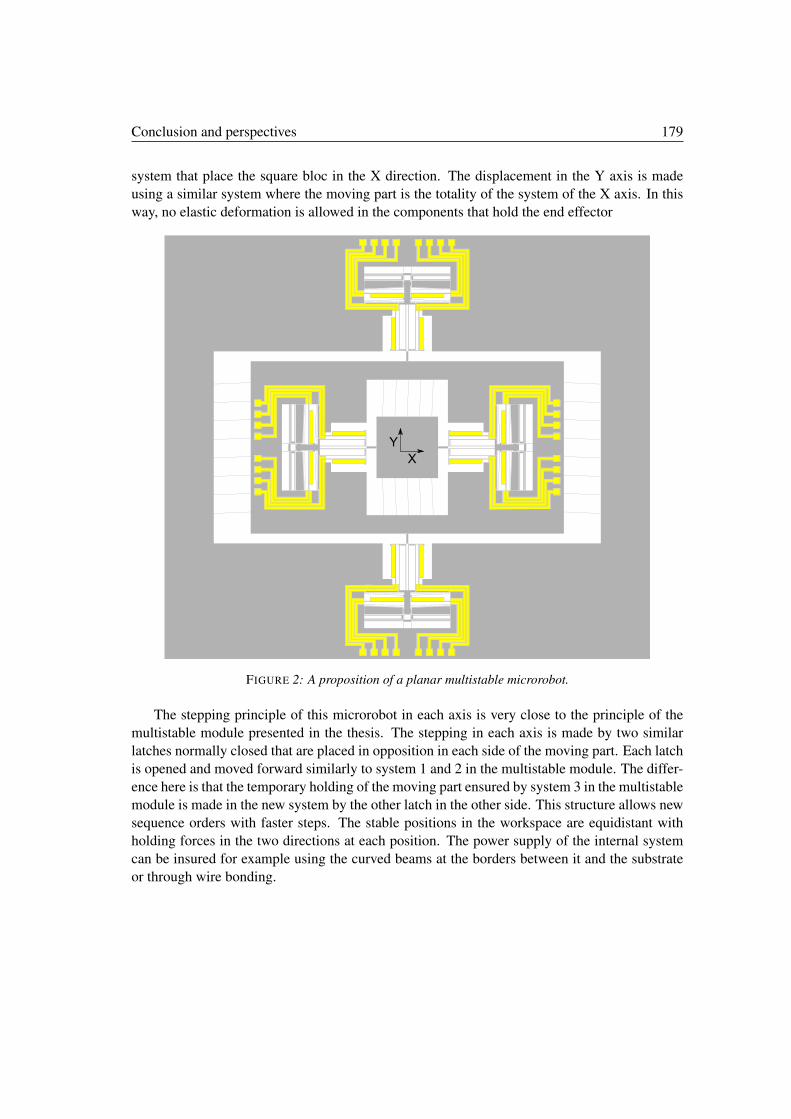
Conclusion and perspectives 179
system that place the square bloc in the X direction. The displacement in the Y axis is made
using a similar system where the moving part is the totality of the system of the X axis. In this
way, no elastic deformation is allowed in the components that hold the end effector
FIGURE 2: A proposition of a planar multistable microrobot.
The stepping principle of this microrobot in each axis is very close to the principle of the
multistable module presented in the thesis. The stepping in each axis is made by two similar
latches normally closed that are placed in opposition in each side of the moving part. Each latch
is opened and moved forward similarly to system 1 and 2 in the multistable module. The differ-
ence here is that the temporary holding of the moving part ensured by system 3 in the multistable
module is made in the new system by the other latch in the other side. This structure allows new
sequence orders with faster steps. The stable positions in the workspace are equidistant with
holding forces in the two directions at each position. The power supply of the internal system
can be insured for example using the curved beams at the borders between it and the substrate
or through wire bonding.
180 Conclusion and perspectives
Towards a 3D multistable microrobot in three dimensions
Making a 3D digital microrobot is also one of the perspectives in long term. The realization
of such a microrobot with micromachining fabrication techniques is quite difficult. Orthogonal
assembly of several digital actuators can be a solution to realize 3D digital actuators. Otherwise,
elastic mechanisms that converts in plane motion to out of plane motion can be also a solution
to fabricate these actuators.
In the other side, new fabrication techniques for microstructures are booming and under
development, including the 3D micro-printing and Smart Composite Microstructures (SCM).
In the 3D printing, successive layers of material are laid down to build a 3D structure. How-
ever, the difficulty in this technique is in adding active materials for the actuation. In the SCM
technique, flexible polymer layer is sandwiched between two patterned face sheets of rigid com-
posite materials in one monolithic flat structure. The advantage of this technology is that planar
fabrication is employed to yield 3D structure by folding. These microfabrication techniques
are promising and could lead soon to perform advanced 3D multistable mechanisms for digital
microrobotics.
Bibliography
[1] ABADIE, J., CHAILLET, N., AND LEXCELLENT, C. Modeling of a new sma micro-
actuator for active endoscopy applications. Mechatronics 19, 4 (2009), 437–442.
[2] ARTHUR, C., ELLERINGTON, N., HUBBARD, T., AND KUJATH, M. Mems earthworm:
a thermally actuated peristaltic linear micromotor. Journal of Micromechanics and Mi-
croengineering 21, 3 (2011), 035022.
[3] ASHEGHI, M., KURABAYASHI, K., KASNAVI, R., AND GOODSON, K. Thermal con-
duction in doped single-crystal silicon films. Journal of Applied Physics 91, 8 (2002),
5079–5088.
[4] ATRE, A. Effect of shape factors and material property variations on modeling the re-
sponse of thermal microactuators. Sensors and Actuators A: Physical 134, 1 (2006),
69–76.
[5] BARTH, J., AND KOHL, M. A bistable magnetically enhanced shape memory microac-
tuator with high blocking forces. Physics Procedia 10 (2010), 189–196.
[6] BINTORO, J. S., AND HESKETH, P. J. An electromagnetic actuated on/off microvalve
fabricated on top of a single wafer. Journal of Micromechanics and Microengineering
15, 6 (2005), 1157.
[7] BOHM, S., BURGER, G., KORTHORST, M., AND ROSEBOOM, F. A micromachined
silicon valve driven by a miniature bi-stable electro-magnetic actuator. Sensors and Ac-
tuators A: Physical 80, 1 (2000), 77–83.
[8] BRENNER, M. P., LANG, J. H., LI, J., QIU, J., AND SLOCUM, A. H. Optimal design
of a bistable switch. Proceedings of the National Academy of Sciences 100, 17 (2003),
9663–9667.
[9] CAMESCASSE, B. Actionnements statique et dynamique dun mecanisme bistable : as-
pects modlisation, conception et exprimental. PhD thesis, Universit Pierre et Marie Curie,
2013.
182 Conclusion and perspectives
[10] CAZOTTES, P. Actionnement des systemes bistables: modlisation et tudes exprimentales.
Thse de doctorat, Universit Pierre et Marie Curie, Paris, France, 2009.
[11] CAZOTTES, P., FERNANDES, A., POUGET, J., AND HAFEZ, M. Actuation of bistable
buckled beams with macro-fiber composites. In Intelligent Robots and Systems, 2008.
IROS 2008. IEEE/RSJ International Conference on (2008), IEEE, pp. 564–569.
[12] CHALVET, V. Conception, realisation et commande d’un microrobot numerique,
planaire, non-redondant et en technologie MEMS. PhD thesis, Universite de Franche-
Comte, 2013.
[13] CHALVET, V., HADDAB, Y., AND LUTZ, P. A microfabricated planar digital microrobot
for precise positioning based on bistable modules.
[14] CHAPUIS, Y.-A., FUKUTA, Y., MITA, Y., AND FUJITA, H. Autonomous decen-
tralized systems based on distributed controlled mems actuator for micro conveyance
application. 56, 1 (2004), 109–115.
[15] CHARLOT, B., SUN, W., YAMASHITA, K., FUJITA, H., AND TOSHIYOSHI, H. In-
plane bistable nanowire for memory devices. In Design, Test, Integration and Packaging
of MEMS/MOEMS, 2008. MEMS/MOEMS 2008. Symposium on (2008), IEEE, pp. 254–
258.
[16] CHEN, G., ATEN, Q. T., ZIRBEL, S., JENSEN, B. D., AND HOWELL, L. L. A
tristable mechanism configuration employing orthogonal compliant mechanisms. Journal
of Mechanisms and Robotics 2, 1 (2010), 014501.
[17] CHEN, G., GOU, Y., AND ZHANG, A. Synthesis of compliant multistable mechanisms
through use of a single bistable mechanism. Journal of Mechanical Design 133, 8 (2011),
081007.
[18] CHEN, G., WILCOX, D. L., AND HOWELL, L. L. Fully compliant double tensural
tristable micromechanisms (dttm). Journal of Micromechanics and Microengineering
19, 2 (2009), 025011.
[19] CHEN, J.-S., AND TSAO, H.-W. Static snapping load of a hinged extensible elastica.
Applied Mathematical Modelling (2013).
[20] CHEN, Q. Microrobotique numerique fondee sur l’utilisation de modules bistables :
conception, fabrication et commande de modules monolithiques. phdthesis, Universite
de Franche-Comte, 2010.
[21] CHEN, Q., HADDAB, Y., AND LUTZ, P. Digital microrobotics based on bistable mod-
ules: Design of compliant bistable structures. In IEEE/ASME International Confer-
ence on Mechtronic and Embedded Systems and Applications, 2008. MESA 2008 (2008),
p. 3641.
[22] CHEN, Q., HADDAB, Y., AND LUTZ, P. Microfabricated bistable module for digital
microrobotics. Journal of Micro-Nano Mechatronics 6, 1-2 (2011), 1–12.
Conclusion and perspectives 183
[23] CHEN, R., NGUYEN, H., AND WU, M. A high-speed low-voltage stress-induced mi-
cromachined 2 x 2 optical switch. IEEE Photonics Technology Letters 11, 11 (1999),
1396–1398.
[24] CHEN, S.-C., AND CULPEPPER, M. L. Design of a six-axis micro-scale
nanopositionerµhexflex. Precision engineering 30, 3 (2006), 314–324.
[25] CHIAO, M., AND LIN, L. Self-buckling of micromachined beams under resistive heat-
ing. Microelectromechanical Systems, Journal of 9, 1 (2000), 146–151.
[26] COCHRAN, K. R., FAN, L., AND DEVOE, D. L. High-power optical microswitch based
on direct fiber actuation. Sensors and Actuators A: Physical 119, 2 (2005), 512–519.
[27] COMTOIS, J. H., AND BRIGHT, V. M. Applications for surface-micromachined polysil-
icon thermal actuators and arrays. Sensors and Actuators A: Physical 58, 1 (Jan. 1997),
19–25.
[28] DAS, A. N., SIN, J., POPA, D. O., AND STEPHANOU, H. E. On the precision alignment
and hybrid assembly aspects in manufacturing of a microspectrometer. In Automation
Science and Engineering, 2008. CASE 2008. IEEE International Conference on (2008),
IEEE, pp. 959–966.
[29] DE DOBBELAERE, P., FALTA, K., GLOECKNER, S., AND PATRA, S. Digital mems for
optical switching. Communications Magazine, IEEE 40, 3 (2002), 88–95.
[30] DEVOS, S., VAN DE VIJVER, W., DECOSTER, K., REYNAERTS, D., AND VAN BRUS-
SEL, H. A planar piezoelectric drive with a stepping and a resonant operation mode. In
Proc. of 4th International Conference of the European Society for Precision Engineering
and Nanotechnology, Glasgow, May 30th–June 3rd (2004).
[31] DIEPPEDALE, C., DESLOGES, B., ROSTAING, H., DELAMARE, J., CUGAT, O., AND
MEUNIER-CARUS, J. Magnetic bistable micro-actuator with integrated permanent mag-
nets. In IEEE Sensors conference (2004).
[32] DRIESEN, M., CEYSSENS, F., DECOSTER, J., AND PUERS, R. Nickel-plated thermal
switch with electrostatic latch. Sensors and Actuators A: Physical 164, 1 (2010), 148–
153.
[33] EMAM, S. A., AND NAYFEH, A. H. On the nonlinear dynamics of a buckled beam
subjected to a primary-resonance excitation. 117.
[34] ENIKOV, E. T., KEDAR, S. S., AND LAZAROV, K. V. Analytical model for analysis and
design of v-shaped thermal microactuators. Microelectromechanical Systems, Journal of
14, 4 (2005), 788–798.
[35] ERISMIS, M. A., NEVES, H. P., DE MOOR, P., VAN HOOF, C., AND PUERS, R. Low
voltage electrostatic inchworm actuators in aqueous environments. Procedia Chemistry
1, 1 (2009), 686–689.
184 Conclusion and perspectives
[36] FREUDENREICH, M., MESCHEDER, U., AND SOMOGYI, G. Simulation and realization
of a novel micromechanical bi-stable switch. Sensors and Actuators A: Physical 114, 2
(2004), 451–459.
[37] FUKUTA, Y., CHAPUIS, Y.-A., MITA, Y., AND FUJITA, H. Design, fabrication, and
control of mems-based actuator arrays for air-flow distributed micromanipulation. Mi-
croelectromechanical Systems, Journal of 15, 4 (2006), 912–926.
[38] GALAMBOS, P., LANTZ, J., BAKER, M. S., MCCLAIN, J., BOGART, G. R., AND
SIMONSON, R. J. Active mems valves for flow control in a high-pressure micro-gas-
analyzer. Microelectromechanical Systems, Journal of 20, 5 (2011), 1150–1162.
[39] GAO, Y., YOU, Z., AND ZHAO, J. Electrostatic comb-drive actuator for mems re-
lays/switches with double-tilt comb fingers and tilted parallelogram beams. Journal of
Micromechanics and Microengineering 25, 4 (2015), 045003.
[40] GEISBERGER, A. A., SARKAR, N., ELLIS, M., AND SKIDMORE, G. D. Electrothermal
properties and modeling of polysilicon microthermal actuators. Microelectromechanical
Systems, Journal of 12, 4 (2003), 513–523.
[41] GERDES, H., DINULOVIC, D., AND GATZEN, H. Electromagnetic dual-position actua-
tor for measurement applications. In Proceedings of Actuator (2006), pp. 824–827.
[42] GERSON, Y., KRYLOV, S., ILIC, B., AND SCHREIBER, D. Design considerations of a
large-displacement multistable micro actuator with serially connected bistable elements.
Finite Elements in Analysis and Design 49, 1 (2012), 58–69.
[43] GIANNOPOULOS, G., MONREAL, J., AND VANTOMME, J. Snap-through buckling be-
havior of piezoelectric bimorph beams: I. analytical and numerical modeling. Smart
materials and structures 16, 4 (2007), 1148.
[44] GIDDINGS, P. F., KIM, H. A., SALO, A. I., AND BOWEN, C. R. Modelling of piezo-
electrically actuated bistable composites. Materials Letters 65, 9 (2011), 1261–1263.
[45] GLASSBRENNER, C., AND SLACK, G. A. Thermal conductivity of silicon and germa-
nium from 3 k to the melting point. Physical Review 134, 4A (1964), A1058.
[46] GOMEZ, S., BELEN, R. J., KIEHLBAUCH, M., AND AYDIL, E. S. Etching of high as-
pect ratio structures in si using sf 6/o 2 plasma. Journal of Vacuum Science & Technology
A: Vacuum, Surfaces, and Films 22, 3 (2004), 606–615.
[47] GUCKEL, H., KLEIN, J., CHRISTENSON, T., SKROBIS, K., LAUDON, M., AND
LOVELL, E. Thermo-magnetic metal flexure actuators. In Solid-State Sensor and Actu-
ator Workshop, 1992. 5th Technical Digest., IEEE (1992), IEEE, pp. 73–75.
[48] HAGA, Y., MAKISHI, W., IWAMI, K., TOTSU, K., NAKAMURA, K., AND ESASHI,
M. Dynamic braille display using sma coil actuator and magnetic latch. Sensors and
Actuators A: Physical 119, 2 (2005), 316–322.
Conclusion and perspectives 185
[49] HALG, B. On a micro-electro-mechanical nonvolatile memory cell. Electron Devices,
IEEE Transactions on 37, 10 (1990), 2230–2236.
[50] HAN, J. S., MAZLLER, C., WALLRABE, U., AND KORVINK, J. G. Design, simulation,
and fabrication of a quadstable monolithic mechanism with x-and y-directional bistable
curved beams. Journal of Mechanical Design 129, 11 (2007), 1198–1203.
[51] HEDLUND, C., BLOM, H.-O., AND BERG, S. Microloading effect in reactive ion etch-
ing. Journal of Vacuum Science & Technology A 12, 4 (1994), 1962–1965.
[52] HENNEKEN, V. A., TICHEM, M., AND SARRO, P. M. Improved thermal u-beam actua-
tors for micro-assembly. Sensors and Actuators A: Physical 142, 1 (2008), 298–305.
[53] HERDING, M., JOBST, G., URBAN, G., AND WOIAS, P. A polymer-based optical 1× 2
fiber switch. In Int. Conference on New Actuators (2004), pp. 246–249.
[54] HICKEY, R., KUJATH, M., AND HUBBARD, T. Heat transfer analysis and optimization
of two-beam microelectromechanical thermal actuators. Journal of Vacuum Science &
Technology A 20, 3 (2002), 971–974.
[55] HICKEY, R., SAMEOTO, D., HUBBARD, T., AND KUJATH, M. Time and frequency
response of two-arm micromachined thermal actuators. Journal of Micromechanics and
Microengineering 13, 1 (2002), 40.
[56] HUANG, H.-W., AND YANG, Y.-J. A MEMS bistable device with push-On Push-Off
capability. 79.
[57] HUANG, Q.-A., AND LEE, N. K. S. Analysis and design of polysilicon thermal flexure
actuator. J. Micromech. Microeng. 9, 1 (Mar. 1999), 64.
[58] HUANG, Q.-A., AND LEE, N. K. S. Analytical modeling and optimization for a
laterally-driven polysilicon thermal actuator. Microsystem Technologies 5, 3 (Feb. 1999),
133–137.
[59] HUSSEIN, H., CHALVET, V., LE MOAL, P., BOURBON, G., HADDAB, Y., AND LUTZ,
P. Design optimization of bistable modules electrothermally actuated for digital micro-
robotics. In Advanced Intelligent Mechatronics (AIM), 2014 IEEE/ASME International
Conference on (2014), IEEE, pp. 1273–1278.
[60] HWANG, G. S., AND GIAPIS, K. P. On the origin of the notching effect during etching in
uniform high density plasmas. Journal of Vacuum Science & Technology B 15, 1 (1997),
70–87.
[61] JENSEN, B., HOWELL, L., AND SALMON, L. Design of two-link, in-plane, bistable
compliant micro-mechanisms. Journal of Mechanical Design 121, 3 (1999), 416–423.
[62] JENSEN, B. D., PARKINSON, M. B., KURABAYASHI, K., HOWELL, L. L., AND
BAKER, M. S. Design optimization of a fully-compliant bistable micro-mechanism.
2125.
186 Conclusion and perspectives
[63] JIA, C., ZHOU, J., DONG, W., AND CHEN, W. Design and fabrication of silicon-based
8× 8 mems optical switch array. Microelectronics Journal 40, 1 (2009), 83–86.
[64] JUNGEN, A., PFENNINGER, M., TONTELING, M., STAMPFER, C., AND HIEROLD,
C. Electrothermal effects at the microscale and their consequences on system design.
Journal of Micromechanics and Microengineering 16, 8 (2006), 1633.
[65] KHAN, M. U. Contribution to the design and fabrication of an integrated micro-
positioning system. PhD thesis, Universite de Technologie de Compiegne, 2014.
[66] KO, J. S., LEE, M. G., HAN, J. S., GO, J. S., SHIN, B., AND LEE, D.-S. A laterally-
driven bistable electromagnetic microrelay. ETRI journal 28, 3 (2006), 389–392.
[67] KOHL, M., KREVET, B., AND JUST, E. Sma microgripper system. Sensors and Actua-
tors A: Physical 97 (2002), 646–652.
[68] KOLESAR, E. S., ALLEN, P. B., HOWARD, J. T., WILKEN, J. M., AND BOYDSTON, N.
Thermally-actuated cantilever beam for achieving large in-plane mechanical deflections.
Thin Solid Films 355 (1999), 295–302.
[69] KRYLOV, S., AND DICK, N. Dynamic stability of electrostatically actuated initially
curved shallow micro beams. Continuum Mechanics and Thermodynamics 22, 6-8
(2010), 445–468.
[70] KRYLOV, S., ILIC, B. R., SCHREIBER, D., SERETENSKY, S., AND CRAIGHEAD, H.
The pull-in behavior of electrostatically actuated bistable microstructures. Journal of
Micromechanics and Microengineering 18, 5 (2008), 055026.
[71] KUANG, Y., HUANG, Q.-A., AND LEE, N. K. S. Numerical simulation of a polysilicon
thermal flexure actuator. Microsystem Technologies 8, 1 (Mar. 2002), 17–21.
[72] KWON, H. N., HWANG, I.-H., AND LEE, J.-H. A pulse-operating electrostatic mi-
croactuator for bi-stable latching. Journal of Micromechanics and Microengineering 15,
8 (2005), 1511.
[73] KWON, H. N., JEONG, S. H., LEE, S. K., AND LEE, J. H. Design and characterization
of a micromachined inchworm motor with thermoelastic linkage actuators. Sensors and
Actuators A: Physical 103, 1 (2003), 143–149.
[74] LEESTER-SCHADEL, M., HOXHOLD, B., LESCHE, C., DEMMING, S., AND
BUTTGENBACH, S. Micro actuators on the basis of thin sma foils. Microsystem Tech-
nologies 14, 4-5 (2008), 697–704.
[75] LERCH, P., SLIMANE, C. K., ROMANOWICZ, B., AND RENAUD, P. Modelization and
characterization of asymmetrical thermal micro-actuators. Journal of Micromechanics
and Microengineering 6, 1 (1996), 134.
[76] LI, J., LIU, A., AND ZHANG, Q. Tolerance analysis for comb-drive actuator using drie
fabrication. Sensors and Actuators A: Physical 125, 2 (2006), 494–503.
Conclusion and perspectives 187
[77] LI, J., ZHAO, H., QU, H., CUI, T., FU, L., HUANG, H., REN, L., AND FAN, Z. A
piezoelectric-driven rotary actuator by means of inchworm motion. Sensors and Actua-
tors A: Physical 194 (2013), 269–276.
[78] LI, S. S. The dopant density and temperature dependence of hole mobility and resistivity
in boron doped silicon. Solid-State Electronics 21, 9 (1978), 1109–1117.
[79] LIAO, B.-T., SHEN, H.-H., LIAO, H.-H., AND YANG, Y.-J. A bi-stable 2x2 optical
switch monolithically integrated with variable optical attenuators. Optics express 17, 22
(2009), 19919–19925.
[80] LIN, L., AND CHIAO, M. Electrothermal responses of lineshape microstructures. Sen-
sors and Actuators A: Physical 55, 1 (1996), 35–41.
[81] LUCHETTI, T., ZANELLA, A., BIASIOTTO, M., AND SACCAGNO, A. Electrically ac-
tuated antiglare rear-view mirror based on a shape memory alloy actuator. Journal of
materials engineering and performance 18, 5-6 (2009), 717–724.
[82] LUHARUKA, R., AND HESKETH, P. J. A bistable electromagnetically actuated rotary
gate microvalve. Journal of Micromechanics and Microengineering 18, 3 (2008), 035015.
[83] MAEKOBA, H., HELIN, P., REYNE, G., BOUROUINA, T., AND FUJITA, H. Self-aligned
vertical mirror and v-grooves applied to an optical-switch: modeling and optimization of
bi-stable operation by electromagnetic actuation. Sensors and Actuators A: Physical 87,
3 (2001), 172–178.
[84] MAHMOUDI, P., AND MAHMOUDI, A. An electrothermally-driven low voltage micro
switch for high frequency applications. Journal of Electrical Engineering 14, 21 (2014).
[85] MASTERS, N. D., AND HOWELL, L. L. A self-retracting fully compliant bistable mi-
cromechanism. Microelectromechanical Systems, Journal of 12, 3 (2003), 273–280.
[86] MATSUNAGA, T., TOTSU, K., ESASHI, M., AND HAGA, Y. Tactile display using shape
memory alloy micro-coil actuator and magnetic latch mechanism. Displays 34, 2 (2013),
89–94.
[87] MATSUURA, T., FUKAMI, T., CHABLOZ, M., SAKAI, Y., IZUO, S.-I., UEMURA, A.,
KANEKO, S.-I., TSUTSUMI, K., AND HAMANAKA, K. Silicon micro optical switch-
ing device with an electromagnetically operated cantilever. Sensors and Actuators A:
Physical 83, 1 (2000), 220–224.
[88] MAURINI, C., POUGET, J., AND VIDOLI, S. Distributed piezoelectric actuation of a
bistable buckled beam. European Journal of Mechanics-A/Solids 26, 5 (2007), 837–853.
[89] MAYYAS, M., SHIAKOLAS, P. S., LEE, W. H., AND STEPHANOU, H. Thermal cycle
modeling of electrothermal microactuators. Sensors and Actuators A: Physical 152, 2
(2009), 192–202.
188 Conclusion and perspectives
[90] MOULTON, T., AND ANANTHASURESH, G. Micromechanical devices with embedded
electro-thermal-compliant actuation. Sensors and Actuators A: Physical 90, 1 (2000),
38–48.
[91] MURATET, S. Conception, caracterisation et modelisation: Fiabilite predictive de
MEMS a actionnement electrothermique. PhD thesis, INSA de Toulouse, 2005.
[92] NAYFEH, A. H., AND EMAM, S. A. Exact solution and stability of postbuckling config-
urations of beams. 395408.
[93] NIU, X., BROCHU, P., STOYANOV, H., YUN, S. R., AND PEI, Q. Bistable electroactive
polymer for refreshable braille display with improved actuation stability. In Proc. of SPIE
Vol (2012), vol. 8340, p. 83400R1.
[94] NOMURA, Y., AND AOYAMA, H. Development of inertia driven micro robot with nano
tilting stage for sem operation. Microsystem technologies 13, 8-10 (2007), 1347–1352.
[95] OBERHAMMER, J., TANG, M., LIU, A.-Q., AND STEMME, G. Mechanically tri-stable,
true single-pole-double-throw (SPDT) switches. 2251.
[96] OH, Y. Synthesis of multistable equilibrium compliant mechanisms. Ph.d theisis, Uni-
versity of Michigan, 2008.
[97] OH, Y. S., AND KOTA, S. Synthesis of multistable equilibrium compliant mechanisms
using combinations of bistable mechanisms. Journal of Mechanical Design 131, 2 (2009),
021002.
[98] OKADA, Y., AND TOKUMARU, Y. Precise determination of lattice parameter and thermal
expansion coefficient of silicon between 300 and 1500 k. Journal of applied physics 56,
2 (1984), 314–320.
[99] OKHOTIN, A. S., PUSHKARSKIJ, A. S., AND GORBACHEV, V. V. Thermophysical
properties of semiconductors.
[100] OZSUN, O., ALACA, B. E., YALCINKAYA, A. D., YILMAZ, M., ZERVAS, M., AND
LEBLEBICI, Y. On heat transfer at microscale with implications for microactuator design.
Journal of Micromechanics and Microengineering 19, 4 (2009), 045020.
[101] PANE, I. Z., AND ASANO, T. Investigation on bistability and fabrication of bistable
prestressed curved beam. 5291.
[102] PARK, S., AND HAH, D. Pre-shaped buckled-beam actuators: theory and experiments.
Sensors and Actuators A: Physical 148, 1 (2008), 186–192.
[103] PENGFEI, H. Electromagnetic digital actuators array: Characterization of a planar
conveyance application and optimized design. PhD thesis, Universite de technologie de
Compiegne, 2015.
Conclusion and perspectives 189
[104] PETIT, L. Contribution aux techniques d’actionnement numerique : cas d’un systeme
electromagntique 2D. 2009.
[105] PHAM, H.-T., AND WANG, D.-A. A quadristable compliant mechanism with a bistable
structure embedded in a surrounding beam structure. Sensors and Actuators A: Physical
167, 2 (2011), 438–448.
[106] QIU, J., LANG, J., AND SLOCUM, A. A curved-beam bistable mechanism. 137146.
[107] QIU, J., LANG, J. H., SLOCUM, A. H., AND WEBER, A. C. A bulk-micromachined
bistable relay with u-shaped thermal actuators. Microelectromechanical Systems, Journal
of 14, 5 (2005), 1099–1109.
[108] RAKOTONDRABE, M., HADDAB, Y., AND LUTZ, P. Development, modeling, and
control of a micro-/nanopositioning 2-dof stick–slip device. Mechatronics, IEEE/ASME
Transactions on 14, 6 (2009), 733–745.
[109] REBEIZ, G. M., AND MULDAVIN, J. B. Rf mems switches and switch circuits. Mi-
crowave Magazine, IEEE 2, 4 (2001), 59–71.
[110] RECEVEUR, R. A., MARXER, C. R., WOERING, R., LARIK, V. C., AND DE ROOIJ,
N.-F. Laterally moving bistable mems dc switch for biomedical applications. Microelec-
tromechanical Systems, Journal of 14, 5 (2005), 1089–1098.
[111] REMMERT, R. Modes of convergence in function theory. In Theory of Complex Func-
tions. Springer, 1991, pp. 91–107.
[112] REN, H., AND GERHARD, E. Design and fabrication of a current-pulse-excited bistable
magnetic microactuator. 259264.
[113] ROBERT, P., SAIAS, D., BILLARD, C., BORET, S., SILLON, N., MAEDER-
PACHURKA, C., CHARVET, P., BOUCHE, G., ANCEY, P., AND BERRUYER, P. Inte-
grated rf-mems switch based on a combination of thermal and electrostatic actuation. In
TRANSDUCERS, Solid-State Sensors, Actuators and Microsystems, 12th International
Conference on, 2003 (2003), vol. 2, IEEE, pp. 1714–1717.
[114] ROODENBURG, B., AND EVENBLIJ, B. H. Design of a fast linear drive for (hybrid)
circuit breakers–development and validation of a multi domain simulation environment.
Mechatronics 18, 3 (2008), 159–171.
[115] SAHU, B., TAYLOR, C. R., AND LEANG, K. K. Emerging challenges of microactuators
for nanoscale positioning, assembly, and manipulation. Journal of manufacturing science
and engineering 132, 3 (2010), 030917.
[116] SARAJLIC, E., BERENSCHOT, E., TAS, N., FUJITA, E., KRIJNEN, G., AND ELWEN-
SPOEK, M. High performance bidirectional electrostatic inchworm motor fabricated by
trench isolation technology. In Solid-State Sensors, Actuators and Microsystems, 2005.
Digest of Technical Papers. TRANSDUCERS’05. The 13th International Conference on
(2005), vol. 1, IEEE, pp. 53–56.
190 Conclusion and perspectives
[117] SHIGEMATSU, R., HIGO, A., TOSHIYOSHI, H., AND FUJITA, H. An electrostatically
latched and magnetically erased mems re-writable bitmap image display. IEICE Elec-
tronics Express 3, 5 (2006), 87–91.
[118] STOIMENOV, B. L., ROSSITER, J. M., AND MUKAI, T. Manufacturing of ionic
polymer-metal composites (IPMCs) that can actuate into complex curves. In The 14th
International Symposium on: Smart Structures and Materials & Nondestructive Eval-
uation and Health Monitoring (2007), International Society for Optics and Photonics,
pp. 65240T65240T–11.
[119] SUJAN, V., LICHTER, M. D., DUBOWSKY, S., ET AL. Lightweight hyper-redundant
binary elements for planetary exploration robots. In Advanced Intelligent Mechatronics,
2001. Proceedings. 2001 IEEE/ASME International Conference on (2001), vol. 2, IEEE,
pp. 1273–1278.
[120] SUTHAKORN, J., AND CHIRIKJIAN, G. S. A new inverse kinematics algorithm for
binary manipulators with many actuators. Advanced Robotics 15, 2 (2001), 225–244.
[121] SYMS, R. Long-travel electrothermally driven resonant cantilever microactuators. Jour-
nal of Micromechanics and Microengineering 12, 3 (2002), 211.
[122] TAJADDODIANFAR, F., YAZDI, M. H., AND PISHKENARI, H. N. Dynamics of
bistable initially curved shallow microbeams: Effects of the electrostatic fringing fields.
In IEEE/ASME International Conference on Advanced Intelligent Mechatronics AIM
(2014), p. 12791283.
[123] TAN, Y., ZHOU, R., ZHANG, H., LU, G., AND LI, Z. Modeling and simulation of
the lag effect in a deep reactive ion etching process. Journal of Micromechanics and
Microengineering 16, 12 (2006), 2570.
[124] TIMOSHENKO, S. Theory of elastic stability. McGraw-Hill, 1961.
[125] TSUCHIYA, Y., TAKAI, K., MOMO, N., NAGAMI, T., MIZUTA, H., ODA, S., YA-
MAGUCHI, S., AND SHIMADA, T. Nanoelectromechanical nonvolatile memory device
incorporating nanocrystalline si dots. Journal of applied physics 100, 9 (2006), 094306.
[126] VANGBO, M. An analytical analysis of a compressed bistable buckled beam. 212216.
[127] VITUSHINSKY, R., SCHMITZ, S., AND LUDWIG, A. Bistable thin-film shape memory
actuators for applications in tactile displays. Microelectromechanical Systems, Journal
of 18, 1 (2009), 186–194.
[128] WANG, D.-A., CHEN, J.-H., AND PHAM, H.-T. A tristable compliant micromechanism
with two serially connected bistable mechanisms. Mechanism and Machine Theory 71
(2014), 27–39.
[129] WANG, D.-A., PHAM, H.-T., AND HSIEH, Y.-H. Dynamical switching of an electro-
magnetically driven compliant bistable mechanism. Sensors and Actuators A: Physical
149, 1 (2009), 143–151.
Conclusion and perspectives 191
[130] WANG, J., GAO, F., AND ZHANG, Y. Study on binary driven pneumatic unit for hyper-
redundant robots. In Automation, Robotics and Applications (ICARA), 2011 5th Interna-
tional Conference on (2011), IEEE, pp. 329–333.
[131] WANG, Z., SHEN, X., AND CHEN, X. Design, modeling, and characterization of a
mems electrothermal microgripper. Microsystem Technologies (2015), 1–8.
[132] WILCOX, D. L., AND HOWELL, L. L. Fully compliant tensural bistable micromecha-
nisms (ftbm). Microelectromechanical Systems, Journal of 14, 6 (2005), 1223–1235.
[133] WU, Y., DING, G., ZHANG, C., WANG, J., MAO, S., AND WANG, H. Design and
implementation of a bistable microcantilever actuator for magnetostatic latching relay.
325330.
[134] YEOM, J., WU, Y., AND SHANNON, M. A. Critical aspect ratio dependence in deep
reactive ion etching of silicon. In TRANSDUCERS, Solid-State Sensors, Actuators and
Microsystems, 12th International Conference on, 2003 (2003), vol. 2, IEEE, pp. 1631–
1634.
[135] YU, Z., NIU, X., BROCHU, P., YUAN, W., LI, H., CHEN, B., AND PEI, Q. Bistable
electroactive polymers (BSEP): large-strain actuation of rigid polymers. In SPIE Smart
Structures and Materials+ Nondestructive Evaluation and Health Monitoring (2010),
International Society for Optics and Photonics, pp. 76420C76420C–9.
[136] ZAIDI, S. S. H., CHERFI-BOULANGER, Z., AND LAMARQUE, F. Contactless Energy
Transfer and Control Strategy for Bistable Micro-Actuator. Ph.d theisis, Universite de
Technologie de Compiegne, 2011.
[137] ZHANG, Y.-H., DING, G., SHUN, X., GU, D., CAI, B., AND LAI, Z. Preparing of a
high speed bistable electromagnetic RF MEMS switch. 532537.
[138] ZHANG, Y.-H., DING, G.-F., FU, S., AND CAI, B.-C. A fast switching bistable elec-
tromagnetic microactuator fabricated by uv-liga technology. Mechatronics 17, 2 (2007),
165–171.
[139] ZHAO, J., GAO, R., CHEN, G., LIU, S., CAO, Q., AND QIU, T. Nonlinear coupling
mechanical model for large stroke magnetic-based multistable mechanisms. Mechanism
and Machine Theory 83 (2015), 56–68.
[140] ZHAO, J., ZHANG, Y., HUANG, Y., LIU, S., CHEN, G., GAO, R., AND YANG, Y.
Mechanical-magnetic coupling analysis of a novel large stroke penta-stable mechanism
possessing multistability transforming capability. Journal of Mechanisms and Robotics
6, 3 (2014), 031004.

Resume :
Un nombre de sujets concernant la microrobotique numeriques ont ete abordes dans le cadre de
cette these. Une nouvelle generation du microrobot numerique ”DiMiBot” a ete propose, ce qui rend le
DiMiBot plus precis, plus controllable et plus petit. La nouvelle structure est formee de deux modules
multistables seulement, ce qui ajoute des fonctionnalites importantes comme l’augmentation du
nombre de positions avec une taille plus reduite et la capacite de realiser des trajectoires complexes
dans l’espace de travail. Le principe du nouveau module multistable combine les avantages des
microactionneurs pas a pas en termes du principe et du concept numerique en termes de la
repetabilite et la robustesse en boucle ouverte. Un mecanisme de positionnement precis, capable de
compenser les incertitudes de fabrication a ete developpe et utilise pour assurer un positionnement
precis. En parallele, des modeles analytiques ont ete developpes pour les principaux composants
dans le DiMiBot: poutres flambees preformees et actionneurs electrothermiques en U. Des methodes
de conception ont ete developpees par la suite qui permettent de choisir les dimensions optimales
garantissant les performances requises en respectant les specifications et limites de design. Des
prototypes de modules multistables, fabriques dans la salle blanche MIMENTO, ont montre un bon
fonctionnement dans les experiences.
Mots-cles : Microrobotique numerique, DiMiBot, basculement, maintien, mecanismes multistables, optimi-
sation, miniaturisation, poutre flambee preformee, actionneur electrothermique en U, module
multistable, microfabrication, micro-usinage de volume
Abstract:
A number of topics concerning digital microrobotics were addressed in this thesis. A new generation
of the digital microrobot ”DiMiBot” was proposed with several advantages making the DiMiBot more
accurate, more controllable and smaller. The new structure consists of only two multistable modules
which adds some important features such as increasing the number of positions with smaller size
and the ability to realize complex trajectories in the workspace. The principle of the new multistable
module combines the advantages of the stepping microactuators in terms of the principle and of
the digital concept in terms of the repeatability and robustness without feedback. The accuracy
is ensured with an accurate positioning mechanism that compensate the fabrication tolerances. In
parallel, analytical models was developed for the main components in the DiMiBot: preshaped curved
beams and U-shaped electrothermal actuators. Subsequently, design methods were developed that
allow choosing the optimal dimensions that ensure the desired outputs and respecting the design
specifications and limitations. Multistable module prototypes, fabricated in the clean room MIMENTO,
showed a proper functioning in the experiments.
Keywords: Digital Microrobotics, DiMiBot, switching function, holding function, multistable mechanisms, op-
timization, miniaturization, preshaped curved beam, U-shaped electrothermal actuator, multis-
table module, microfabrication, bulk micromachining
Related Documents