Modeling Contact Friction and Joint Friction in Dynamic ...

Modeling Contact Friction and Joint Friction inDynamic Robotic Simulation using the Principle ofMaximum Dissipation

Evan Drumwright and Dylan A. Shell

1 Evan Drumwright at George Washington University ([email protected])2 Dylan A. Shell at Texas A&M University ([email protected])

Summary. We present a unified treatment for modeling Coulomb and viscous friction withinmulti-rigid body simulation using the principle of maximum dissipation. This principle is usedto build two different methods—an event-driven impulse-based method and a time steppingmethod—for modeling contact. The same principle is used to effect joint friction in articu-lated mechanisms. Experiments show that the contact models are able to be solved faster andmore robustly than alternative models. Experiments on the joint friction model show that itis as accurate as a standard model while permitting much larger simulation step sizes to beemployed.

1 Introduction

Rigid body dynamics is used extensively within robotics in order to simulate robots, learn opti-mal controls, and develop inverse dynamics controllers. The forward dynamics of rigid bodiesin free space has been well understood for some time, and the recent advent of differentialalgebraic equation (DAE) based methods has made the dynamics of bodies in contact straight-forward to compute as well. However, fast and stable robotic simulation remains somewhatelusive. The numerical algorithms used to compute contact forces run (on average) in timeO(n3) in the number of contact points and are numerically brittle. In this paper, we present aclass of methods for modeling contact with friction in multi-rigid body simulation that is notonly faster empirically than existing methods, but is solvable with numerical robustness. Wealso extend our approach to modeling joint friction and show how it is at least as accurate asstandard joint friction models, while permitting much larger simulation step sizes (and thusmuch greater simulation speed).

Our approach centers around the principle of maximal dissipation. Paraphrasing Stewart(2000), the principle of maximal dissipation states that, for bodies in contact, the friction forceis the one force (of all possible friction forces) that maximizes the rate of energy dissipation. Inthis paper, we show that we can use the principle of maximal dissipation to implicitly solve forfrictional forces, in contrast to prior approaches that set the frictional force by explicitly usingthe direction of relative motion. By employing this strategy, we are able to dispense with thecomplementarity constraints that are nearly universally employed and instead formulate thecontact problem using a convex optimization model.

2 Evan Drumwright and Dylan A. Shell

2 Methods for modeling contact with friction in multi-rigid bodysimulation

2.1 Background

As stated in the previous section, modeling contact with friction in multi-rigid body simu-lation has been extensively conducted using complementarity constraints. Such constraints,which take the form a ≥ 0,b ≥ 0,aTb = 0, have been utilized in multi-rigid body simulationto ensure that forces are not applied at contact points at which bodies are separating (Anitescuand Potra, 1997), that either sticking or sliding friction is applied (Anitescu and Potra, 1997),and that forces are applied only for joints at their limits (Miller and Christensen, 2003). Anon-exhaustive survey of the literature dedicated to modeling contact with complementarityconstraints includes Lostedt (1982); Moreau (1983); Lostedt (1984); Moreau (1985, 1988);Monteiro-Marques (1993); Baraff (1994); Anitescu et al (1997); Pfeiffer and Glocker (1996);Brogliato (1996); Trinkle et al (1997); Anitescu and Potra (1997); Anitescu et al (1999); Stew-art and Trinkle (2000); Anitescu and Potra (2002); Anitescu and Hart (2004); Trinkle et al(2005); Anitescu (2006); Potra et al (2006); Erleben (2007); Anitescu and Tasora (2008);Petra et al (2009); Todorov (2010); Tassa and Todorov (2010). Initial efforts on modelingcontact with friction (Lostedt, 1982, 1984; Baraff, 1994) attempted to solve a linear com-plementarity problem (LCP) for the unknown forces and accelerations. Later work—underwhich researchers realized that solving for forces and accelerations could be subject to in-consistent configurations3 (Baraff, 1991)—solved instead for unknown impulsive forces andvelocities; this approach was able to avoid the problem of inconsistent configurations. Bothiterative sequential impulse schemes (e.g., Mirtich (1996b); Guendelman et al (2003)) andsimultaneous impulse-based methods (e.g., Anitescu and Potra (1997); Stewart and Trinkle(2000)) were employed. The former methods have been viewed as splitting methods (Cottleet al, 1992) for solving linear complementarity problems by Lacoursiere, who reported slowconvergence rates for coupled problems using such approaches (Lacoursiere, 2003). Corre-spondingly, much of the multi rigid-body simulation community currently uses explicit linearor nonlinear complementarity problem formulations (Anitescu and Potra (1997), most promi-nently) with impulses and velocities in order to model contact with friction.

Figure 1 illustrates why complementarity conditions are necessary at the accelerationlevel; further discussion of their requirement at the acceleration level is present in Baraff(1994) and Chatterjee (1999). Given that using impulsive forces is necessary to avoid theproblem of inconsistent configurations (exemplified by the problem of Painleve (1895)), itmust be discerned whether the complementarity conditions are accurate and appropriate inthat new context (i.e., at the velocity level). We stress that the context is indeed new, becauseonly “resting” (zero relative normal velocity) contacts are treated with forces at the accelera-tion level4 while both resting and impacting contact are treated with impulses at the velocitylevel.

With respect to accuracy, Chatterjee (1999) argues that the complementarity conditionsdo not necessarily reflect reality. He conducts an experiment using carbon paper, a coin, anda hammer, that serves to prove his argument: the physical accuracy of complementarity-basedmodels, at least in some scenarios, is lacking. Further physical experimentation is warranted,

3 An inconsistent configuration is a contact configuration that has no solution using non-impulsive forces.

4 Unless a penalty method is used; such methods are irrelevant to this discussion because weare assuming non-interpenetrating contact.

Modeling Friction in Dynamic Robotic Simulation via Maximum Dissipation 3

A

B

C

D

p2

p4

ˆ n 4( t0)

ˆ n 3( t

0)

ˆ n 5( t0)ˆ n 2( t0)p3

p1

1 0ˆ n (t )

p5

Figure 26: Resting contact. This configuration has five contact points; a contact force acts between

pairs of bodies at each contact point.

forces must be strong enough to prevent two bodies in contact from being pushed “towards” one

another. Second, wewant our contact forces to be repulsive; contact forces can push bodies apart, but

can never act like “glue” and hold bodies together. Last, we require that the force at a contact point

become zero if the bodies begin to separate. For example, if a block is resting on a table, some force

may act at each of the contact points to prevent the block from accelerating downwards in response

to the pull of gravity. However, if a very strong wind were to blow the brick upwards, the contact

forces on the brick would have to become zero at the instant that the wind accelerated the brick off

the table.

Let’s deal with the first condition: preventing inter-penetration. For each contact point i, we

construct an expression di(t)which describes the separation distance between the two bodies near the

contact point at time t. Positive distance indicates the bodies have broken contact, and have separated

at the ith contact point, while negative distance indicates inter-penetration. Since the bodies are in

contact at the present time t0, we will have di(t0) = 0 (within numerical tolerances) for each contact

point. Our goal is to make sure that the contact forces maintain di(t) ≥ 0 for each contact point at

future times t > t0.

For vertex/face contacts, we can immediately construct a very simple function fordi(t). If pa(t)

and pb(t) are the contact points of the ith contact, between bodies A and B, than the distance between

the vertex and the face at future times t ≥ t0 is given by

di(t) = ni(t) · (pa(t) − pb(t)). (9–1)

At time t, the function d(t) measures the separation between A and B near pa(t). If di(t) is zero,

then the bodies are in contact at the ith contact point. If di(t) > 0, then the bodies have lost contact

at the ith contact point. However, if di(t) < 0, then the bodies have inter-penetrated, which is what

we need to avoid (figure 27). The same function can also be used for edge/edge contacts; since ni(t)

SIGGRAPH ’97 COURSE NOTES D50 PHYSICALLY BASED MODELING

Fig. 1. A figure (taken from Baraff (1997)) illustrating the necessity of complementarity con-straints for contact at the acceleration level. Complementarity constraints would ensure thatbody A does not move upward unnaturally fast if a strong wind were to move between B andA, accelerating A upward. In the absence of this wind, the complementarity condition keepsblocks A and B from interpenetrating.

especially given the attention to complementarity constraints at the velocity level in the lit-erature, but if we accept that nature does not require complementarity constraints, do suchconditions lead to models that are more advantageous in some other way (e.g., computation-ally?)

Linear and nonlinear complementarity problem-based models are, in fact, inferior withrespect to computation, at least relative to the models introduced in this paper. Solutions tobisymmetric LCPs—the form that many models take—are NP-hard in the worst case in thenumber of contact points (though the expected time solution is O(n3) (Cottle et al, 1992)). Thecontact models are non-convex, so only a few algorithms are capable of solving LCP-basedcontact models; codes for solving the NCP-based models are even more rare.5 The LCP-basedmodels linearize the friction cone, and the fidelity of the friction cone approximation increasesthe size and, correspondingly, the computational cost of the model to be solved.

Given that complementarity conditions may not be physically warranted and that suchmodels can be hard to solve computationally, what is the reason behind their strong popularity?We believe this quote from Chatterjee (1999) is instructive:

It is emphasized that many authors in this area are aware of the possible physicalinaccuracies behind the complementarity assumption. For example, Moreau (1983)states that a primary benefit of such a formulation is internal mathematical consis-tency, and empirical corrections towards better accuracy can be accommodated later.Baraff (personal communication) mentions that there is no reason to think that realsystems obey the complementarity conditions. However, in Pfeiffer and Glocker’s(1996) discussion of the “corner law of contact dynamics” there is unfortunately noexplicit mention of the possible lack of physical realism behind the complementarity

5 The reader may question the desire to have multiple algorithms capable of solving a contactmodel. Optimization algorithms can be numerically brittle, so using multiple algorithmscan reduce the likelihood of a simulation crashing.


conditions in the presence of impacts. Anitescu and Potra (1997) focus on mathemat-ical aspects of their formulation, and also omit discussion of physical realism. Theauthors of the latter two authoritative works may therefore unintentionally convey aninaccurate impression to a reader who is new to the field.

2.2 Two representations for the contact models

Given that complementarity conditions are not a necessary feature of contact models, we nowproceed to present our complementarity-free contact models. We will use two representationsfor these contact models. Both representations have been employed previously in the litera-ture. We utilize the two representations here in order to make the community aware of theirexistence, to unify them, and, hopefully, to expose them to further study (for determination ofcomputational or numerical advantages, for example).

A / b representation

The first representation formulates the contact model in terms of matrices A and b (alterna-tively named K and u by Mirtich (1996b)). This representation has been employed by Baraff(1994), Mirtich (1996b), Kokkevis (2004), and Drumwright and Shell (2009). In this repre-sentation, b is a vector of relative velocities in the 3n-dimensional contact space and A isthe 3n× 3n sized contact space inertia matrix that transforms impulsive forces to relativevelocities in contact space. A is dense, symmetric, and positive-semi definite; the latter twoproperties were proven by Mirtich (1996b). The matrices A and b are related by the equation:

b+ = Ax+b− (1)

where b− is the vector of relative velocities pre-contact (external forces, such as gravity,are integrated into this vector), x is the vector of impulses applied in the contact space, and b+

is the vector of relative velocities after impulses are applied.The matrices A and b can be determined formulaically if the contacting bodies are not

articulated, and via application of test impulses otherwise (cf., Mirtich (1996b); Kokkevis(2004)). By using test impulses, the contact model can remain ignorant of whether the bodiesare articulated and, if articulated, of whether the bodies are formulated using maximal orreduced coordinates. This is an advantage of the A / b representation; this representation alsotends to produce simpler—though not necessarily computationally advantageous—objectiveand constraint function gradients and Hessians for solving the contact model.

Generalized coordinate representation

The generalized coordinate representation has been used in work by Anitescu and Potra (1997)and Stewart and Trinkle (2000), among others. This representation uses matrices M (the gen-eralized inertia matrix), N (the contact normal Jacobian), J (the joint constraint Jacobian);vectors cn (the contact normal impulse magnitudes), c j (the joint constraint impulse magni-tudes), q (the generalized coordinates), v (the generalized velocities) and k (the generalizedexternal forces), and scalar h (the step size).

For models with complementarity constraints, additional matrices are used, both to en-force the complementarity constraints and to provide a linearized friction cone; we do not listsuch matrices here. Because our model does not employ complementarity constraints, it is


able to provide a true friction cone and still remain computationally tractable. The true fric-tion cone is obtained using Jacobian matrices corresponding to the two tangential directions ateach contact normal; we denote these matrices S and T and the corresponding contact tangentimpulses as cs and ct .

All of the matrices described above are related using the following formulae:

vt+1 = M−1(NTcn +STcs +TTct +JTc j +hk)+vt (2)

qt+1 = qt +hvt+1 (3)

The second equation reflects that this representation is typically utilized in a semi-implicitintegration scheme.

Note that M is symmetric, positive-definite. M, N, S, T and J are sparse and correspond-ingly make efficient determination of the objective and constraint gradients and Hessians con-ceptually more involved than with the A / b representation. Computing M, N, S, T and J isquite simple, however, and computationally far more efficient than the test impulse method.We show below, however, that A and b can also be determined efficiently using the matricesfrom the generalized coordinate representation.

Unification of the A / b and generalized coordinate representations

The equations below show how b− and A may be obtained using the generalized coordinaterepresentation.

b− =

NST

(vt +hM−1k) (4)

A =

NST

C[

NT ST TT]

(5)

where C , M−1−M−1JT(JM−1JT)−1JM−1.These equations show that recovering N, S, T, and J from A and b− is not possible.

2.3 The contact models for event-driven and time-stepping simulation

Computer-based rigid body simulation methods have been categorized into three schemesby Brogliato et al (2002): penalty, event-driven, and time-stepping. Given that penalty meth-ods necessarily cannot enforce non-interpenetration, we focus instead on event-driven andtime-stepping methods. The former are able to utilize arbitrary integration schemes (time-stepping methods are frequently restricted to semi-implicit Euler integration) while the latteraim to be able to avoid (possibly nonexistent) accuracy problems due to continually restartingthe integration process; Brogliato et al (2002) provide greater detail of the rationale behinddevelopment of the time-stepping approaches. We note that Drumwright (2010) has shownthat one purported advantage of time-stepping approaches over event-driven simulations—avoidance of Zeno points—is nonexistent. Sections 2.4 and 2.5 present both event-driven andtime-stepping methods in order to show that our method is applicable to both. Section 2.4 usesthe A/b representation, while Section 2.5 uses the generalized coordinate representation.


2.4 Event-driven impulse-based method

Mirtich (1996b) defines the work done by collision impulses using the A/b representationas 1

2 xT(Ax + 2b−). We can use the principle of maximal dissipation to determine the set ofimpulses that maximally dissipate kinetic energy. In particular, we can formulate and solve thefollowing optimization problem.

Quadratic Program 1

Minimize12

xT(Ax+2b−)

Subject to:[AN B

]x+b−N ≥ 0 (Noninterpenetration constraint)

xN ≥ 0 (Compressive force constraint)

1TxN ≤ κ (Friction cone constraint)

µ2c x2

Ni+ µ

2v (b2

T1 i+b2

T2 i)≥ x2

T1 i+x2

T2 i∀i ∈ 1 . . .n. (Coulomb/viscous

friction constraint)

where A can be partitioned into n× n block AN , n× 2n block B, and 2n× 2n block AT

(i.e., A =[

AN BBT AT

]) and, similarly, x and b can be partitioned into x =

[xN xT1 xT2

]T and

b =[

bN bT1 bT2

]T, respectively. Scalar κ is the sum of the normal impulses that describethe minimum kinetic energy solution when the tangential impulses are zero; this scalar isdescribed further in Section 2.6.

2.5 Time stepping method

Equivalent in spirit to the event-driven method is the time-stepping method, which, like thatof Anitescu and Potra (1997), is a semi-implicit scheme and, like that of Stewart and Trinkle(2000), adds contact constraint stabilization to the dynamics equations.

Quadratic Program 2

Minimize12

vt+1TMvt+1

Subject to:

Nvt+1 ≥ 0 (Noninterpenetration constraint)

Jvt+1 = 0 (Bilateral joint constraint)

cn ≥ 0 (Compressive force constraint)

1Tcn ≤ κ (Friction cone constraint)

µ2c c2

ni+ (Coulomb/viscous

µ2v [Si(vt +hM−1k)]2+

µ2v [Ti(vt +hM−1k)]2 ≥ c2

si+ c2

ti ∀i ∈ 1 . . .n.

friction constraint)

where Si and Ti refer to the ith row of S and T, respectively. Unlike the event-drivenmethod, the time-stepping method includes a constraint for bilateral joints in case the method


is used with maximal-coordinate formulated articulated bodies; the A/b representation im-plicitly encodes such constraints into the matrix / vector formulations.

2.6 Solving the models

Both of the contact models introduced in the previous sections are convex and can be solvedin polynomial time in the number of contacts using interior-point methods. Determining thevalue κ requires solving the models in an initial, frictionless phase (phase I). Next, a frictionalphase (phase II) is solved. If normal restitution is necessary, a third phase is required as well.6

Fortunately, phase I is a quadratic programming model with box constraints, and can thus besolved extremely quickly using a gradient projection method (Nocedal and Wright, 2006). Themodel for phase I (A/b formulation) is:

Quadratic Program 3

Minimize12

xTNANxN +xT

Nb−N

Subject to:xN ≥ 0 (Compressive force constraint)

Given that AN is symmetric and positive semi-definite (follows from symmetry and pos-itive semi-definiteness of A), this model describes a convex linear complementarity problem(see Cottle et al (1992), p. 5). As a result, the constraint ANxN +b−N ≥ 0 (which is equivalentto our non-interpenetration constraint) is automatically satisfied at the optimum. This convexLCP always has a solution and we prove that this solution does not increase the energy inthe system (see Appendix). As phase II cannot increase the energy in the system our contactmodels are energetically consistent.

Phase I has two objectives: determine an energetically consistent, feasible point7 for thenonlinear Quadratic Program 1 and determine κ . The value κ is determined by calculating thesum 1TxN , using the result from phase I. Observe that the friction cone inequality constraintin Quadratic Program 1 restricts the sum of the normal impulses to that determined in phase I;thus, phase II can reorder, transfer, or remove some normal force, but the friction cone is pre-vented from becoming enlarged arbitrarily (i.e., the normal forces cannot be increased withoutbound to increase the amount of frictional force applicable) in order to decrease the kineticenergy more rapidly.

We note that, although we use a linear complementarity problem formulation to show thatour contact models are energetically consistent, our contact models do not use complementar-ity constraints: neither phase I nor phase II of the contact models explicitly include any suchconstraint.

6 We omit details of this third phase but refer the reader to Anitescu and Potra (1997), whichdescribes a Poisson-type restitution model that is applicable to our models also.

7 A feasible point is one which respects all inequality constraints. In the case of our con-tact model, a feasible point will respect non-interpenetration, compressive normal force,summed normal force, and Coulomb and viscous friction constraints.


3 Evaluating the contact models

There does not currently exist a standardized set of benchmark models for evaluating theperformance and accuracy of contact models. In order to evaluate contact models, previousapproaches have used either physical experimentation on a set of benchmark scenarios (e.g.,Stoianovici and Hurmuzlu (1996)) or pathological computer-based scenarios (e.g., Mirtich(1996b); Sauer et al (1998); Ceanga and Hurmuzlu (2001)) that are known to exhibit certainbehaviors in the real world.

Like Anitescu and Potra (1997), we do not provide exhaustive experimentation to indicatethe predictive abilities of our contact model. Instead, we note that our model possesses thefollowing properties, which are also possessed by leading alternative contact models that treatmultiple contact points simultaneously (e.g., (Anitescu and Potra, 1997; Stewart and Trinkle,2000)):

1. Energy is not added to the system.2. Interpenetration constraints are not violated.3. Only compressive normal forces are applied.4. The friction cone is not enlarged artificially.5. The principle of maximal dissipation is obeyed.

Given that these are the main characterizations of both systems, we can expect the emer-gent behavior of both the complementarity-based methods and our non-complementarity-based methods to be similar. Indeed, as Figure 2 shows, the method of Anitescu and Potra(solved using Lemke’s algorithm (Lemke, 1965; Cottle et al, 1992)) produces identical results(to numerical precision) to our non-complementarity-based model on at least one scenario.

Fig. 2. Plot illustrating accuracy of a box sliding down a ramp under both the method ofAnitescu and Potra (1997) and the convex optimization-based method introduced in this paper.Although the two models are formulated quite differently, the simulated results are identical.

We believe that our method is no more accurate than that of Anitescu and Potra or Stewartand Trinkle (notwithstanding the linearized friction cones generally employed by those twomethods). The advantage of our method lies in the computational domain. Lacking comple-mentarity constraints, our model runs faster than competing methods; additionally, the gradi-ent projection method used to solve the first phase of our algorithm—recall that the first phaseof our algorithm finds a point that respects properties (1)–(4) above—never fails to produce


a solution; failure in phase II of our method will only affect the accuracy of the solution andwill not “break” the simulation.

The experiments below showcase these advantages of our method.

4 Experiments

4.1 Event-driven example: internal combustion engine

We constructed an inline, four cylinder internal combustion engine in order to illustrate theability of our method to treat moderate numbers of contacts (between one and two hundred)far faster than complementarity-based models. All joints within the simulated engine wererealized by contact constraints only. The engine was simulated by applying a torque to thecrankshaft, which caused the cylinders to move upward and downward within the crankcase.The crankcase and crankshaft guides are stationary within the simulation—they possess infi-nite inertia, so they do not move dynamically—and the remaining parts are all of mass 1.0kg.Although the masses do not reflect reality, the moment-of-inertia matrix for each part is calcu-lated using its triangle mesh geometry via the method of Mirtich (1996a). Gravity acts alongthe vertical direction of the simulation at 9.8m/s2 and the engine surfaces are given zerocoefficients of Coulomb and viscous friction: we initially wanted to judge how rapidly thepolygonal-based geometric representation causes energy loss.

For purposes of comparison, we used the method of Anitescu and Potra (1997), modifiedto function as an event-driven method, with the simplest (i.e., pyramidal) friction model. Usingthe pyramidal friction model resulted in six LCP variables per contact; thus, LCPs of orderbetween 600 and 1200 were generated.

Fig. 3. Frames in sequence from a simulation of the rigid-body dynamics and interactionswithin an internal combustion engine


0.01

0.1

1

10

100

1000

0 0.0005 0.001 0.0015 0.002 0.0025

simulation time

com

puta

tion

time

Anitescu-Potra (Lemke)convex optimization

(a) Timings of both methods (0–0.0025s)

0.01

0.1

1

10

100

0 0.2 0.4 0.6 0.8 1 1.2 1.4

(b) Convex optimization method timing (0-1s)

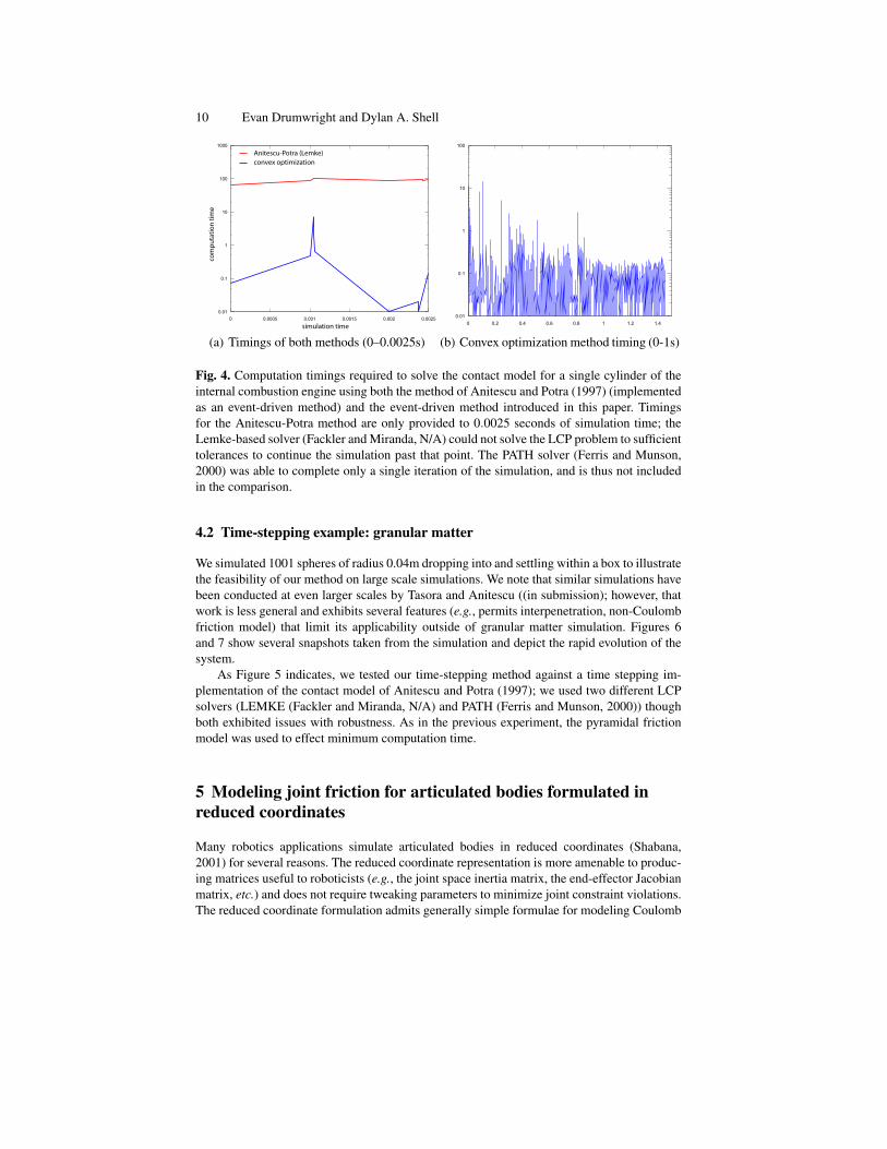
Fig. 4. Computation timings required to solve the contact model for a single cylinder of theinternal combustion engine using both the method of Anitescu and Potra (1997) (implementedas an event-driven method) and the event-driven method introduced in this paper. Timingsfor the Anitescu-Potra method are only provided to 0.0025 seconds of simulation time; theLemke-based solver (Fackler and Miranda, N/A) could not solve the LCP problem to sufficienttolerances to continue the simulation past that point. The PATH solver (Ferris and Munson,2000) was able to complete only a single iteration of the simulation, and is thus not includedin the comparison.

4.2 Time-stepping example: granular matter

We simulated 1001 spheres of radius 0.04m dropping into and settling within a box to illustratethe feasibility of our method on large scale simulations. We note that similar simulations havebeen conducted at even larger scales by Tasora and Anitescu ((in submission); however, thatwork is less general and exhibits several features (e.g., permits interpenetration, non-Coulombfriction model) that limit its applicability outside of granular matter simulation. Figures 6and 7 show several snapshots taken from the simulation and depict the rapid evolution of thesystem.

As Figure 5 indicates, we tested our time-stepping method against a time stepping im-plementation of the contact model of Anitescu and Potra (1997); we used two different LCPsolvers (LEMKE (Fackler and Miranda, N/A) and PATH (Ferris and Munson, 2000)) thoughboth exhibited issues with robustness. As in the previous experiment, the pyramidal frictionmodel was used to effect minimum computation time.

5 Modeling joint friction for articulated bodies formulated inreduced coordinates

Many robotics applications simulate articulated bodies in reduced coordinates (Shabana,2001) for several reasons. The reduced coordinate representation is more amenable to produc-ing matrices useful to roboticists (e.g., the joint space inertia matrix, the end-effector Jacobianmatrix, etc.) and does not require tweaking parameters to minimize joint constraint violations.The reduced coordinate formulation admits generally simple formulae for modeling Coulomb


Fig. 5. Kinetic energy of the granular simulation over approximately five seconds of simulationtime. The lack of robustness in the linear complementarity problem solvers is evident here, asneither solver for the Anitescu-Potra model was able to simulate to one second of simulationtime.

Fig. 6. Frames from time t = 1.95s, t = 1.96s, and t = 1.97s show the granules dropping intothe box.

Fig. 7. Frames from time t = 3.50s, and t = 3.55s depict the granules settling within the box.

and viscous friction at robot joints. From Sciavicco and Siciliano (2000), p. 141, the torquesat joints due to joint friction can be modeled as:

τµ = µv q+ µc sgn(q) (6)

where µv and µc are the coefficients for viscous and Coulomb friction, respectively.The issue with this model is that it tends to make the differential equations stiff (i.e., dif-

ficult to solve numerically) using even moderately large values of µc and µv; this statementis particularly true for µc, which uses the discontinuous signum function. The practical effectof this issue is that either extremely small integration steps must be taken or the joint fric-tion must be poorly modeled. We can, however, use the principle of maximum dissipation and


velocity-level dynamics equations to model friction properly; Section 5.3 will show that ourapproach models the viscous component of Equation 6 exactly (for sufficiently small coeffi-cients of friction or step sizes of the latter), and that the Coulomb component of Equation 6asymptotically approaches our model as the integration step tends to zero.

5.1 Maximum dissipation-based joint friction model

Under the principle of maximum dissipation, we wish to find the impulses that minimize thenew kinetic energy. The change in joint velocity is given by the formula ∆ q = H−1x, whereq is the joint-space velocity, H is the joint-space inertia matrix, and x is the vector of appliedimpulses. Thus we wish to minimize the quantity 1

2 (q+∆ q)TH(q+∆ q) subject to Coulomband viscous constraints on the applied impulses x.

Quadratic Program 4

Minimize12

xTH−1x+xTq

Subject to: −µc1−µvq≤ x≤ µc1+ µvq (Joint friction model)

5.2 Solving the joint friction model

The joint friction model provided above is a quadratic program with box constraints. Due tothe symmetry and positive semi-definiteness of H (see Featherstone (1987)), the quadraticprogram is convex, and thus a global minimum can be found in polynomial time. In fact,programs with hundreds of variables—well within the range of the joint spaces of all robotsproduced to date—can be solved within microseconds using a gradient projection methodNocedal and Wright (2006).

5.3 Empirical results

Figures 8 and 9 depict the efficacy of using the quadratic program defined above for effectingjoint friction. We simulated an anthropomorphic, eight degree-of-freedom (DOF) manipulatorarm acting only under the influence of gravity from an initial position. In Figure 8, coefficientsof joint friction of µc = 5.0 and µv = 0.0 were used, while the coefficients of joint frictionwere µc = 0.25 and µv = 0.1 in Figure 9. Two methods were used to model joint friction: theacceleration level method described in Sciavicco and Siciliano (2000) (i.e., Equation 6) andthe quadratic programming method based on the principle of maximal dissipation describedabove.

Although Figures 8 and 9 depict only a single DOF of the robot arm (the bicep), the re-sults in the plots are indicative of all the DOFs for the robot: the acceleration level methodconverges to the maximal dissipation-based method as the step size for the former becomessufficiently small. Indeed, the top plots in the two figures (i.e., the joint velocities) indicate theresult for the acceleration level method when the step size is not sufficiently small: the simu-lation becomes unstable. Our results indicate that the quadratic programming model based onthe principle of maximal dissipation is as accurate as an accepted model of joint friction butthat the former admits simulation step sizes several orders of magnitude higher (and, corre-spondingly, simulation several orders of magnitude faster).


0 2 4 6 8 10

Simulation Time (s)

-2

-1

0

1

2

q(t)(rad)

0 2 4 6 8 10

Simulation Time (s)

-4

-2

0

2

4

q(t)(rad/s)

∆t = 0.01

∆t = 0.001

∆t = 0.0001

∆t = 0.00001

Acceleration Level Method

∆t = 0.01

Maximal Dissipation Method

Manipulator Bicep Joint, µv = 0.0, µc = 5.0

0 5 10

Simulation Time (s)

-40

-20

0

20

40

Fig. 8. Plots show that joint friction is comparable between the maximal-dissipation-basedand acceleration level methods; the former method produces this behavior at a step size threeorders of magnitude larger than the latter. Note that the correct behavior is for the joint positionand velocity to remain at zero, given that the coefficient of Coulomb friction is so large (5.0).

6 Conclusions

Roboticists are very familiar with complementarity-based contact models like that of Anitescuand Potra (1997); such models have been incorporated into popular simulators like ODE(Smith, N/A). Consequently, the perception of the accuracy (and inaccuracy) of such mod-els has been informed by considerable practice. The complementarity-free models that wereintroduced in this paper do not possess such a track record, and direct, empirical comparisonbetween such models is the subject of future work. Nevertheless, the principle of maximal dis-sipation is accepted by the applied mechanics community, and we have shown evidence that—at minimum—this principle can be used to simulate plausibly mechanisms, granular matter,and joint friction. If the accuracy of the complementarity-free models proves acceptable, thecomputational advantages intrinsic to our models will yield considerable speedups in roboticsimulation. Finally, we argue that, even if the models presented in this paper are found to bepoorly predictive (compared to complementarity-based models), Chatterjee’s work makes itclear that non-complementarity-based contact models should be investigated further.

References

Anitescu M (2006) Optimization-based simulation of nonsmooth dynamics. MathematicalProgramming, Series A 105:113–143


0 2 4 6 8 10

Simulation Time (s)

-1.0

-0.5

0.0

0.5

1.0

q(t)(rad)

0 2 4 6 8 10

Simulation Time (s)

-0.4

-0.2

-0.0

0.2

0.4

q(t)(rad/s)

∆t = 0.001

∆t = 0.0001

Acceleration Level Method

∆t = 0.001

Maximal Dissipation Method

Manipulator Bicep Joint, µv = 0.1, µc = 0.25

Fig. 9. Plots show that joint friction is comparable between the maximal-dissipation-basedand acceleration level methods; the former method produces this behavior at a larger step sizethan the latter.

Anitescu M, Hart G (2004) A constraint-stabilized time-stepping approach for rigid multi-body dynamics with joints, contacts, and friction. Intl Journal for Numerical Methods inEngineering 60(14):2335–2371

Anitescu M, Potra FA (1997) Formulating dynamic multi-rigid-body contact problems withfriction as solvable linear complementarity problems. Nonlinear Dynamics 14:231–247

Anitescu M, Potra FA (2002) A time-stepping method for stiff multi-rigid-body dynamics withcontact and friction. Intl Journal for Numerical Methods in Engineering 55:753–784

Anitescu M, Tasora A (2008) An iterative approach for cone complementarity problems fornonsmooth dynamics. Computational Optimization and Applications

Anitescu M, Cremer JF, Potra FA (1997) Properties of complementarity formulations for con-tact problems with friction. In: Ferris MC, Pang JS (eds) Complementarity and VariationalProblems: State of the Art, SIAM, Philadelphia, PA, pp 12–21

Anitescu M, Potra F, Stewart D (1999) Time-stepping for three dimensional rigid body dy-namics. Computer Methods in Applied Mechanics and Engineering 177:183–197

Baraff D (1991) Coping with friction for non-penetrating rigid body simulation. ComputerGraphics 25(4):31–40

Baraff D (1994) Fast contact force computation for nonpenetrating rigid bodies. In: Proc. ofSIGGRAPH, Orlando, FL

Baraff D (1997) An introduction to physically based modeling: Rigid body simulation II –constrained rigid body dynamics. Tech. rep., Robotics Institute, Carnegie Mellon University

Brogliato B (1996) Nonsmooth Impact Mechanics: Models, Dynamics, and Control. Springer-Verlag, London


Brogliato B, ten Dam A, Paoli L, Genot F, Abadie M (2002) Numerical simulation of fi-nite dimensional multibody nonsmooth mechanical systems. ASME Appl Mech Reviews55(2):107–150

Ceanga V, Hurmuzlu Y (2001) A new look at an old problem: Newton’s cradle. ASME J ApplMech 68:575–583

Chatterjee A (1999) On the realism of complementarity conditions in rigid-body collisions.Nonlinear Dynamics 20:159–168

Cottle RW, Pang JS, Stone R (1992) The Linear Complementarity Problem. Academic Press,Boston

Drumwright E (2010) Avoiding Zeno’s paradox in impulse-based rigid body simulation. In:Proc. of IEEE Intl. Conf. on Robotics and Automation (ICRA), (to appear)

Drumwright E, Shell DA (2009) A robust and tractable contact model for dynamic roboticsimulation. In: Proc. of ACM Symp. on Applied Computing (SAC), pp 1176–1180

Erleben K (2007) Velocity-based shock propagation for multibody dynamics animation. ACMTrans on Graphics 26(12)

Fackler PL, Miranda MJ (N/A) LEMKE. http://people.sc.fsu.edu/ burkardt/m src/lemke/lemke.mFeatherstone R (1987) Robot Dynamics Algorithms. KluwerFerris MC, Munson TS (2000) Complementarity problems in GAMS and the PATH solver. J

of Economic Dynamics and Control 24(2):165–188Guendelman E, Bridson R, Fedkiw R (2003) Nonconvex rigid bodies with stacking. ACM

Trans on Graphics 22(3):871–878Kokkevis E (2004) Practical physics for articulated characters. In: Proc. of Game Developers

Conf.Lacoursiere C (2003) Splitting methods for dry frictional contact problems in rigid multibody

systems: Preliminary performance results. In: Ollila M (ed) Proc. of SIGRAD, pp 11–16Lemke CE (1965) Bimatrix equilibrium points and mathematical programming. Management

Science 11:681–689Lostedt P (1982) Mechanical systems of rigid bodies subject to unilateral constraints. SIAM

Journal on Applied Mathematics 42(2):281–296Lostedt P (1984) Numerical simulation of time-dependent contact friction problems in rigid

body mechanics. SIAM J of Scientific Statistical Computing 5(2):370–393Miller AT, Christensen HI (2003) Implementation of multi-rigid-body dynamics within a

robotic grasping simulator. In: Proc. of the IEEE Intl. Conf. on Robotics and Automation(ICRA), pp 2262–2268

Mirtich B (1996a) Fast and accurate computation of polyhedral mass properties. Journal ofGraphics Tools 1(2)

Mirtich B (1996b) Impulse-based dynamic simulation of rigid body systems. PhD thesis, Uni-versity of California, Berkeley

Monteiro-Marques MDP (1993) Differential inclusions in nonsmooth mechanical problems:Shocks and dry friction. In: Progress in Nonlinear Differential Equations and Their Appli-cations, vol 9, Birkhauser Verlag, Basel

Moreau JJ (1983) Standard inelastic shocks and the dynamics of unilateral constraints,Springer-Verlag, New York, pp 173–221

Moreau JJ (1985) Standard inelastic shocks and the dynamics of unilateral constraints. In: delPiero G, Maceri F (eds) C.I.S.M. Courses and Lectures, vol 288, Springer-Verlag, Vienna,pp 173–221

Moreau JJ (1988) Unilateral contact and dry friction in finite freedom dynamics. In: MoreauJJ, Panagiotopoulos PD (eds) Nonsmooth Mechanics and Applications, Springer-Verlag,Vienna, pp 1–82


Nocedal J, Wright SJ (2006) Numerical Optimization, 2nd ed. Springer-VerlagPainleve P (1895) Sur le lois du frottement de glissemment. C R Academie des Sciences Paris

121:112–115Petra C, Gavrea B, Anitescu M, Potra F (2009) A computational study of the use of an

optimization-based method for simulating large multibody systems. Optimization Methodsand Software

Pfeiffer F, Glocker C (1996) Dynamics of rigid body systems with unilateral constraints. JohnWiley and Sons

Potra FA, Anitescu M, Gavrea B, Trinkle J (2006) A linearly implicit trapezoidal methodfor stiff multibody dynamics with contact, joints, and friction. Intl Journal for NumericalMethods in Engineering 66(7):1079–1124

Sauer J, Schoemer E, Lennerz C (1998) Real-time rigid body simulations of some “classicalmechanics toys”. In: Proc. of European Simulation Symposium and Exhibition, Notting-ham, UK

Sciavicco L, Siciliano B (2000) Modeling and Control of Robot Manipulators, 2nd Ed.Springer-Verlag, London

Shabana AA (2001) Computational Dynamics, 2nd edn. John Wiley & SonsSmith R (N/A) ODE: Open Dynamics EngineStewart D, Trinkle J (2000) An implicit time-stepping scheme for rigid body dynamics with

coulomb friction. In: Proc. of the IEEE Intl. Conf. on Robotics and Automation (ICRA),San Francisco, CA

Stewart DE (2000) Rigid-body dynamics with friction and impact. SIAM Review 42(1):3–39Stoianovici D, Hurmuzlu Y (1996) A critical study of the applicability of rigid-body collision

theory. ASME J Appl Mech 63:307–316Tasora A, Anitescu M ((in submission)) A convex complementarity approach for simulating

large granular flow. J of Computational Nonlinear DynamicsTassa Y, Todorov E (2010) Stochastic complementarity for local control of continuous dynam-

ics. In: Proc. of Robotics: Science and SystemsTodorov E (2010) Implicit nonlinear complementarity: a new approach to contact dynamics.

In: Proc. of Intl. Conf. on Robotics and Automation ICRATrinkle J, Pang JS, Sudarsky S, Lo G (1997) On dynamic multi-rigid-body contact problems

with coulomb friction. Zeithscrift fur Angewandte Mathematik und Mechanik 77(4):267–279

Trinkle JC, Berard S, Pang J (2005) A time-stepping scheme for quasistatic multibody sys-tems. In: Proc. of IEEE Intl. Symp. on Assembly and Task Planning, pp 174–181

A Proof that feasible point determined via LCP is energeticallyconsistent

We now prove that the solution determined in phase I in Section 2.6 is energetically consistent.Working from Mirtich (1996b), the equation for work done by collision impulses is:

12

zT(Az+2b) (7)

Given that z ,

[y0

], we will prove that:


12

yT(ANy+2bN)≤ 0 (8)

The proof relies upon the linear complementarity solver finding the solution y, whichyields yT(ANy+bN) = 0.

Equation 8 simplifies to:

yT(ANy+2bN)≤ 0 (9)

or, equivalently:

yT(ANy+bN)+yTbN ≤ 0 (10)

Given the linear complementarity condition yT(ANy+bN) = 0, we are left with:

yTbN ≤ 0 (11)

The above equation must hold, because (again, due to the linear complementarity condi-tion):

yT(ANy+bN) = 0 (12)

and because AN is symmetric, positive semi-definite, which implies that yTANy≥ 0 (andtherefore, that yTbN ≤ 0).

Modeling Contact Friction and Joint Friction in Dynamic ...

Documents