Modeling Churn and Usage Behavior in Contractual Settings Eva Ascarza Bruce G. S. Hardie † March 2009 † Eva Ascarza is a doctoral candidate in Marketing at London Business School (email: [email protected]; web: www.evaascarza.com). Bruce G. S. Hardie is Professor of Mar- keting, London Business School (email: [email protected]; web: www.brucehardie.com). The authors thank Naufel Vilcassim for his helpful comments on an earlier version of this paper, and acknowledge the support of the London Business School Centre for Marketing.

Welcome message from author
This document is posted to help you gain knowledge. Please leave a comment to let me know what you think about it! Share it to your friends and learn new things together.
Transcript

Modeling Churn and Usage Behavior in
Contractual Settings
Eva AscarzaBruce G. S. Hardie†
March 2009
†Eva Ascarza is a doctoral candidate in Marketing at London Business School (email:[email protected]; web: www.evaascarza.com). Bruce G. S. Hardie is Professor of Mar-keting, London Business School (email: [email protected]; web: www.brucehardie.com). Theauthors thank Naufel Vilcassim for his helpful comments on an earlier version of this paper, andacknowledge the support of the London Business School Centre for Marketing.

Abstract
Modeling Churn and Usage Behavior in Contractual Settings
The ability to retain existing customers is a major concern for many businesses. Howeverretention is not the only dimension of interest; the revenue stream associated with eachcustomer is another key factor influencing customer profitability.
In most contractual situations the exact revenue that will be generated per customeris uncertain at the beginning of the contract period; customer revenue is determined byhow much of the service each individual consumes. While a number of researchers haveexplored the problem of modeling retention in a contractual setting, the literature has beensurprisingly silent on how to forecast customers’ usage (and therefore future revenue) incontractual situations.
We propose a dynamic latent trait model in which usage and renewal behavior are mod-eled simultaneously by assuming that both behaviors are driven by the same (individual-level) underlying process that evolves over time. We capture the dynamics in the under-lying latent variable (which we label “commitment”) using a hidden Markov model, andthen incorporate unobserved heterogeneity in the usage process.
The model parameters are estimated using hierarchical Bayesian methods. We validatethe model using data from a so-called Friends scheme run by a performing arts organiza-tion. First we show how the proposed model outperforms benchmark models on both theusage and retention dimensions. In contrast to most churn models, this dynamic model isable to identify changes in behavior before the contract is close to expiring, thus provid-ing early predictions of churn. Moreover, the model provides additional insights into thebehavior of the customer base that are of interest to managers.
Keywords: Contractual settings, hidden Markov model, RFM, Bayesian estimation, latentvariable models.
“Retention consists of two components— will the customer stay with the com-pany and how much will the customer spend. The “staying” aspect has re-ceived much more attention than the spending aspect, but they both need tobe modeled.” (Blattberg et al. 2008, p. 690)
1 Introduction
The ability to retain existing customers is a major concern for many businesses, especially
in mature industries where customer acquisition is very costly and the competitive envi-
ronment is rather severe (Blattberg et al. 2001, Rust et al. 2001). One way to increase
retention is to identify which customers are most likely to churn, and then undertake tar-
geted marketing campaigns designed to encourage them to stay. Hence, early detection
of potential churners can reduce defection, thus increasing business profitability (Bolton
et al. 2004, Reinartz et al. 2005). Moreover, in many contractual business settings, re-
tention is not the only dimension of interest in the customer relationship; there are other
behaviors that drive customer profitability. This is the case in settings where we observe
customer usage while “under contract.” Examples include mobile phone services (where
we observe the number of calls made), gym memberships (where we observe visits to the
gym, number of extra classes attended, etc.), online magazine subscriptions (where log-ins
are observed) and “friends” schemes for arts organization (where we observe the number of
exhibitions or performances attended). In such business settings, predicting future usage
is an important input into any analysis of customer profitability.1
The objective of this paper is to develop a model that can forecast both behaviors;
we are interested in predicting renewal and usage behavior in those settings where usage
is not known in advance but is of managerial interest, either because it directly affects
revenue, or because it affects service quality, which in turn affects customer retention (Nam
et al. 2007). Such a model must accommodate several aspects that are common across
1We acknowledge that in some situations customer revenue is known in advance and thus independentof usage. This is the case of flat-fee or “all inclusive” contracts, where customers’ revenue is fixed. Evenin such cases, forecasting customer usage may be of interest to the firm because it affects service quality.For example, consider a broadband provider offering flat-fee contracts: if the company does not manage topredict usage accurately, it could face capacity problems when many customers connect at the same time,thus reducing the quality of their connections.
1

contractual settings. First, one of the variables of interest is binary (renewal is always a
“yes” or “no” decision) whereas the other is not (e.g., number of transactions is a count
variable). Second, the renewal process is absorbing. That is, once a customer churns
she cannot use the service in any future period (unless she takes out a new contract).
Third, the model should allow the renewal and usage processes to occur on different time
scales. This is a very common pattern in contractual businesses. For example, let us
consider a gym offering monthly memberships and summarizing attendance on a weekly
basis, or a mobile phone operator with monthly contracts in which weekly consumption is
recorded. In these two situations, while usage is observed on a weekly basis, renewal only
happens at the end of each month. Ignoring intra-month usage would be a waste of useful
information that can enrich the model predictions. And finally, the model must require
only information that can be extracted easily from the firm’s database. The last point is
not unique to contractual settings but is a realistic requirement for the model to be used
in practice.
At first glance, a discrete/continuous model of consumer demand (e.g., Chintagunta
1993, Hanemann 1984, Krishnamurthi and Raj 1988) appears to be an obvious starting
point. This type of model was proposed in the marketing and economics literature to
model binary/continuous decisions, such as “whether to buy” and if so “how much to
buy.” More recently these models have been extended to accommodate dropout (e.g.,
Narayanan et al. 2007, Ascarza et al. 2009). However, these models do not accommodate
the two different time scales and more importantly, since they are based on a utility
maximizing framework with stable preferences over time, they are more appropriate to
explain rather than forecast customers decisions.
The problem of modeling retention has received much attention from both academics
and practitioners. Researchers working in the areas of marketing, applied statistics, and
data mining have developed a number of models that attempt to either explain or predict
churn (e.g., Bhattacharya 1998, Kim and Yoon 2004, Lariviere and Van den Poel 2005,
Lemon et al. 2002, Lu 2002, Mozer et al. 2000, Parr Rud 2001, Schweidel et al. 2008).
One stream of work has sought to model churn as a function of data readily available
in the firm’s databases, such as marketing activities, demographics, and past customer
2
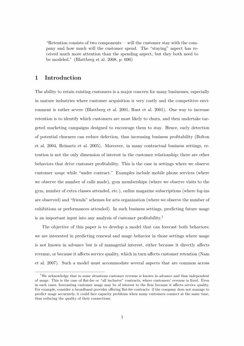
behavior. (See Blattberg et al. (2008) for a review of these various methods.) What
we observe is that past usage behavior is an important predictor variable (Figure 1a).
Another stream of work has explored the link between customers’ attitudes towards the
service and subsequent churn behavior (Figure 1b). Bolton (1998) shows that satisfaction
levels explain a substantial portion of the variance in contract durations. Athanassopoulos
(2000) and Verhoef (2003) find that affective commitment is positively related to contract
duration.
There is limited research on the modeling of service usage in contractual settings.
Nam et al. (2007) explore the effects of service quality, modeling contract duration using a
hazard rate model and usage with a Poisson regression model. Bolton and Lemon (1999)
use a Tobit model to model usage of television entertainment and cellular communications
services, finding a significant relationship between satisfaction and usage (Figure 1c).
Usage Retention Retention Usage
........
....................
...........................................
...........................................................................................................................................................................................................................
............................ ........
....................
...........................................
...........................................................................................................................................................................................................................
............................
Satisfaction/
Commitment
Satisfaction/
Commitment
.............................................................................................................................................
............................................................................................................ .............
....................
....................
....................
....................
....................
.........................................
(a) (b) (c)
Figure 1: Existing modeling approaches
Although widely used in practice, none of the above methods can be used to address
the modeling problem we are considering, either because they make use of survey data,
or because the modeling of future behavior as a direct function of past behavior limits
the forecast horizon. With regards to this later point, such a modeling exercise sees the
transaction database being split into two consecutive periods, with data from the second
period used to create the dependent variable for the model (e.g., renew (yes/no) when
modeling churn, number of transactions or total spend when modeling usage), while data
from the first period are used to create the predictor variables. In many settings, period
1 behavior is frequently summarized in terms of each customers “RFM” characteristics:
recency (time of most recent purchase), frequency (number of past purchases), and mon-
3
etary value (average purchase amount per transaction). Having calibrated the regression
model, we can predict period 3 behavior using the observed period 2 data. However, it is
difficult to use these models to forecast buyer behavior for period 4 when we are unable to
specify values for the RFM predictor variables in period 3 for each customer; rather, we
have to resort to simulated behavior. And so on. (See Fader et al. (2005) for a discussion
of this and related problems with such a modeling approach.)
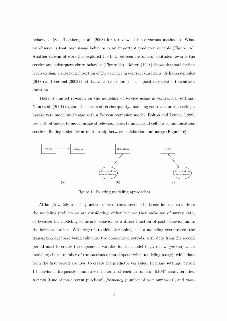
Despite the problems identified with this body of work (Figure 1), we can use the
general findings to guide us as we develop our model. We propose a joint model of
usage and retention under the assumption that both behaviors are driven by some un-
observed characteristic, something that drives both phenomena and that can be inferred
from them— Figure 2. This suggests that the observed association between usage and
retention (Figure 1a) is in fact a spurious correlation. Some researchers explore the con-
cept of “satisfaction” (Bolton et al. 2000, Bolton and Lemon 1999), while others talk of
“commitment” (Gruen et al. 2000, Verhoef 2003). In this paper we recognize the exis-
tence of such an underlying construct and seek to model it, without formally defining it.
Acknowledging the existence of this unobserved factor allows us to approach usage and
retention processes jointly, and thus make accurate predictions of customer behavior in
contractual settings. Furthermore, modeling the stochastic evolution of the underlying
construct means that we can make predictions of behavior in future periods.
Usage Retention
........
....................
...........................................
...........................................................................................................................................................................................................................
............................
Satisfaction/
Commitment
....................
....................
....................
....................
....................
.........................................
.............................................................................................................................................
............. .............
............. ............. ............. ............. ............. ...........
Figure 2: Proposed modeling approach
We propose a dynamic latent trait model in which usage and renewal behaviors are
jointly driven by the same (individual-level) underlying process (Section 2). In Section 3
we validate the proposed model using data from a performing arts organization, and show
how the proposed model can be used to provide additional insights of interest to managers.
4
We conclude with a summary of the methodological and practical contributions of this
research, as well as a discussion of directions for future research (Section 4).
2 Model Development
Our goal is to develop a joint model of contract renewal and usage while “under contract”.
We start by outlining the intuition behind our proposed model.
We assume that each customer’s usage (or consumption) and renewal (or churn) be-
havior reflects a latent trait that evolves over time. For example, let us consider a gym
membership in which a customer pays a fee every month that gives her unlimited use of
the sports facilities. In this example, the underlying trait can, for instance, be assumed to
be a measure of “commitment to the gym”. This commitment is reflected in the number of
times she goes to the gym each week (usage level). Furthermore, her monthly decision of
whether or not to continue her membership reflects the latent trait; she will stop renewing
her membership when her commitment is below a certain threshold. This is illustrated in
Figure 3.
1 2 3 4 5 6 7 8 9 10 11 12
Usage period
1 2 3
Membership period
Yes Yes No
................................................................................................................................................................................................................................................................................................................................................................................................................................................................................................................................................................................................................................................................................................................................................................................................................................................................................................................................................................................
× × × ××× ×× × × ×× ×××××××× × ×- - - - - - - - - - - - - - - - - - - - - - - - - - - - - - - - - - - - - - - - - - - - - - - - - - - - - - - - - - - - - - - - - - - - - - - -
Obse
rvable
Unobse
rvable
Renew?
Usage
- - - - - - - - - - - - - - - - - - - - - - - - - - - - - - - - - - - - - - - - - - - - - - - - - - - - - - - - - - - - - - - - - - - - - - - -
Commitment
Renewal
Threshold
..............................................................................................................................
....................................................................................
.............................................................................................................................................................
...........................................................................................................................................................................
.............................................................................................
.............................................................................................................................................................................................................................................................................................................................................................................................
..........................
.............
.............
.............
.............
.............
.............
.............
.............
.............
.............
.............
.............
.............
.............
............
.............
.............
.............
.............
.............
.............
.............
.............
.............
.............
.............
.............
.............
.............
............
.............
.............
.............
.............
.............
.............
.............
.............
.............
.............
.............
.............
.............
.............
............
.............
.............
.............
.............
.............
.............
.............
.............
.............
.............
.............
.............
.............
.............
............
Figure 3: Model Intuition
More generally, we wish to model a bivariate process measured on different time scales;
5

in Figure 3, the time scale for the renewal process is four times that of the usage pro-
cess. The model takes into account the individual dynamic latent process that drives the
observable behaviors. Modeling the evolution of the latent trait will allow us to make
simultaneous predictions about future usage and churn probabilities.
The proposed model must have three characteristics:
i. It should handle bivariate data where one variable is binary (e.g., churn) while the
other is not (e.g., usage).
ii. The usage and renewal processes do not have the same “clock” (e.g., monthly usage
vs. annual contract renewal, weekly attendance vs. monthly membership renewal).
iii. It must be able to accommodate “informative” dropout. (The binary variable of
interest (e.g., churn) is absorbing (i.e., it cannot transition from 0 to 1) and such
“dropout” is “informative” about the usage process.)
Elaborating on the notion of absorbing dropout, the fact that an individual is active
at a particular point in time implies that her underlying trait was above some renewal
threshold in all preceding renewal periods. For example, with reference to Figure 3, the
fact that this person is a member in the third month (periods 9–12) means that she
renewed in periods 4 and 8. This tells us that her underlying trait had to be above the
renewal threshold in usage periods 4 and 8. However, it does not tell us anything about
the level of the latent variable in periods 1, 2, 3, 5, . . . ; this has to be inferred from her
usage behavior.
2.1 Related Literature
A number of researchers have developed dynamic latent models. With few exceptions, they
focus on linear models (also called linear state space models, or Dynamic Linear Models
(DLM)), well suited for data generated by multivariate Gaussian processes (Gourieroux
and Jasiak 2001, West and Harrison 1997, Van Heerde et al. 2004). However, the Gaussian
assumption is not appropriate for the setting under study since the observed processes
are count and binary variables. Thus, the first challenge we face when modeling this
6

phenomenon is that the normality assumption does not hold for any of the processes
under study. While parametric models for dynamic count data have been proposed in
the econometrics literature (Hausman et al. 1984, Brannas and Johansson 1996, Congdon
2003), these methods are intended to model univariate count data and are therefore not
suitable for the bivariate process being considered here.
Other marketing researchers have proposed various models that capture consumers’
evolving behavior. Sabavala and Morrison (1981), Fader et al. (2004) and Moe and Fader
(2004a,b) present nonstationary probability models for media exposure, new product pur-
chasing, and web site usage, respectively. Netzer et al. (2008) use a hidden Markov model
to characterize the latent process that underlies individuals’ donation behaviors. Lachaab
et al. (2006) model preference evolution in a discrete choice setting using a random coeffi-
cients multinomial probit model in which the random coefficients are dynamic. A similar
approach is used by Liechty et al. (2005) in a conjoint analysis setting. However none of
these models accommodate observed dropout.
A number of biostatisticians have developed longitudinal latent models with “dropout”
(e.g. Diggle and Kenwark 1994, Henderson et al. 2000, Xu and Zeger 2001, Hashemi et
al. 2003, Liu and Huang 2009). The general approach is to assume a latent process that
is deteriorating over time, with dropout occurring when this underlying process crosses a
certain threshold. The latent process behavior is estimated by using repeated observations
of variables driven by this underlying structure. With variations particular to each prob-
lem, these models consist of a joint estimation of the measurement process and a survival
function. However, given that in our setting renewal can only occur at certain points in
time (monthly, quarterly, annually, etc.), while consumption is observed more frequently,
it is possible to have individuals whose underlying commitment has been negative for some
period/s but becomes positive before the next renewal opportunity. Thus, in contrast with
all duration/survival models, being active in a certain period does not necessarily imply
that the underlying trait was above zero for every preceding period, but only for those in
which the renewal decision was made.
In conclusion, while the established longitudinal and latent-variable models do address
each of the three required characteristics individually, none address all three simultane-
7

ously. We now turn our attention to the formal development of a model that does so.
2.2 Model Specification
Let t denote the usage time unit (periods) and i denote each customer (i = 1, ..., I). For
each customer i we have a total of Ti usage observations. Let n denote the number of usage
periods associated with each contract period (e.g., if the usage unit of time considered is
a quarter and the contract is annual, then n = 4).
The model comprises three processes, all occurring at the individual level:
i. the underlying “commitment” process that evolves over time,
ii. the renewal process that is observed only every n periods and takes the value 1 if a
person renews, 0 otherwise, and
iii. the usage process that is observed every period.
The Commitment Process
We assume that every individual has an underlying trait, which we will call “commit-
ment”.2 This underlying trait represents the predisposition of the customer to continue
the relationship and to some extent, the predisposition to use the product/service pro-
vided. We allow this individual-level trait to change over time, and also assume that it is
unobservable from the modeler’s perspective. In other words, we model “commitment” as
a latent variable that follows a dynamic stochastic process.
In Figure 3, the latent trait is presented as evolving in continuous time. However, we
model it as a discrete-time (hidden) Markov process. We assume that there exists a set of
K states 1, 2, ...,K, with 1 corresponding to the lowest level of commitment and K to
the highest. These states represent the possible commitment levels that each individual
could occupy at any point in time. We assume that Sit, the state occupied by person i in
period t, evolves over time following a Markov process with transition matrix Π = πjk,
2We acknowledge that the concept “commitment” has been defined and previously studied in themarketing literature (e.g. Garbarino and Johnson 1999, Gruen et al. 2000, Morgan and Hunt 1994). Itstheoretical definition and measurement is beyond the scope of this paper.
8

with j, k ∈ 1, ... ,K. For the sake of model parsimony, we restrict the Markov chain to
transitions between adjacent states. That is,
P (Sit = k|Sit−1 = j) =
πjk k ∈ j − 1, j, j + 1
0 otherwise .
(1)
We also need to establish the initial conditions for the commitment state in period 1.
We assume that the probability that customer i belongs to commitment state k at period
1 is determined by the vector Q = q1, ..., qK, where
P (Si1 = k) = qk , k = 1, ..., K . (2)
Hidden Markov models (HMMs) were introduced in the marketing literature by Poulsen
(1990) as a flexible framework for modeling brand choice behavior. Since then they have
been applied in the marketing literature to model a wide range of behaviors (e.g., Mont-
gomery et al. 2004; Moon et al. 2007; Smith et al. 2006; Netzer et al. 2008).
Netzer et al. (2008) use a HMM to capture customer relationship dynamics. The
approach taken in the current study is similar to theirs in the sense that we also link
transaction behavior to underlying customer relationship strength, in our case “commit-
ment” level. However, our model specification differs from their approach in two ways.
Firstly, they are working in a “noncontractual” setting (where attrition is unobserved)
and thus map the latent states with just one observable behavior (i.e., transactions). In
our setting customer attrition is observed, and therefore this information is used to define
and identify the latent states. Secondly, they model a non-homogeneous transition process
where the probability of switching among states is a function of the interactions between
the firm and the customer. As such interactions do not occur in our empirical setting, we
model the transition process in an homogeneous manner.
Having specified how the latent trait evolves over time, we now specify the mapping
between this underlying construct and the two observable behaviors of interest, usage and
renewal.
9
The Usage Process
While under contract, a customer’s usage behavior is observed every period. This behavior
reflects her underlying commitment— for any given individual, we would expect higher
commitment levels be reflected by higher usage levels. At the same time, we acknowledge
that individuals may have different intrinsic levels of usage; in other words, unobserved
cross-sectional heterogeneity in usage patters. As such, our model should allow two cus-
tomers with the same underlying pattern of commitment to have different usage patterns.
We propose two possible formulations for the usage process: Poisson and binomial. The
Poisson process is the natural specification for modeling counts. Behaviors for which this
specification is appropriate include the number of credit card transactions per month, the
number of movies purchased each month in a pay-TV setting, and the number of phone
calls made per week. However, in some settings the usage level has an upper bound,
either because of capacity constraints from the company’s side, or because the time period
in which usage is observed is short. For example, going back to the gym example, if
one wants to model the number of days a member attends in a particular week, the
Poisson may not be the most appropriate distribution since there is an upper bound of
seven days. Similarly, consider the case of an orchestra wanting to predict the number
of tickets that will be sold to their patrons. First, the number of performances attended
is bounded by the total number of performances offered by the orchestra. Second, the
number of performances offered should also be taken into consideration when predicting
customers’ future attendances; there will be periods with higher demand simply because
more performances are on offer and so the model should accommodate this information. It
therefore makes sense to model usage using the binomial distribution. (We note that the
binomial distribution can be approximated by a Poisson distribution for a high number of
“trials” with a low probability of “success.”)
We first formalize the assumptions for the Poisson specification and then outline the
changes that need to be made in order to accommodate the binomial specification. We
assume that, for an individual in state k, the usage process (number of attendances,
10

transactions, visits, etc.) in period t follows a Poisson distribution with parameter
λit | [Sit = k] = αiθk (3)
where k is the (unobserved) commitment state of individual i at time t. In other words,
the usage process is determined by a state dependent parameter θk that varies depending
on the underlying level of commitment (which varies over time) and an individual specific
parameter αi that remains constant over time.
The parameter αi captures heterogeneity in usage across the population, allowing two
customers with the same commitment level to show different patterns of transactions.
Individuals with higher values of αi are expected, on average, to have a higher transac-
tion propensity than those with lower values of αi, regardless of their commitment level.
The individual level parameter αi is assumed to follow a gamma distribution with scale
parameter r and a mean of 1.0).
The vector θ = θk, k = 1, ..., K of state-specific parameters allows the customer’s
mean usage levels to change over time, as her underlying level of commitment changes.
We impose the restriction that θk > 0 ∀ k and is increasing with the level of commitment
(i.e., 0 < θ1 < θ2 < ... < θK). Notice that for each individual i, the expected level of
usage is increasing with her commitment level, and even in the lowest commitment state,
we can still observe non-zero usage.
Let Si = [Si1, Si2, ..., Si Ti ] denote the (unobserved) sequence of states to which cus-
tomer i belongs during her entire lifetime, with realization si = [si1, si2, ..., si Ti ], where sit
takes on the value k = 1, . . . , K. The customer’s usage likelihood function is
Lusagei (θ, αi | Si = si, data) =
Ti∏
t=1
P (Yit = yit|Sit = k, θ, αi)
=Ti∏
t=1
e−αi θk (αi θk) yit
yit!. (4)
where yit is customer i’s observed usage in period t.
Turning to the binomial specification, we let mt denote the number of transaction
11

opportunities (e.g., number of performances offered, number of days in a particular pe-
riod of time) and pit the probability of a transaction occurring at any given transaction
opportunity for customer i in period t. As with the Poisson specification, the transac-
tion probability depends on the individual specific time-invariant parameter αi and the
commitment state at every period:
pit | [Sit = k] = θαik . (5)
This specification also guaranties that the transaction probability is increasing with the
level of commitment. The usage propensity parameter αi is also assumed to follow a
gamma distribution with equal scale parameter r and a mean of 1.0.
We impose the restrictions that 0 < θk < 1 for all k and that they increase with the
level of commitment (i.e., 0 < θ1 < θ2 < ... < θK < 1). The inclusion of αi as an
exponent (as opposed to a multiplier) ensures that the transaction probabilities remain
bounded between zero and one.3
It follows that the customer’s usage likelihood function is
Lusagei (θ, αi | Si = si, data) =
Ti∏
t=1
P (Yit = yit|Sit = k, θ, αi,mt)
=Ti∏
t=1
(mt
yit
) (θ αik
)yit (1− θ αik )mt−yit . (6)
The Renewal Process
At the end of each contract period (i.e., when t = n, 2n, 3n, ...), each customer decides
whether or not to renew her contract for the following n periods based on her current level
of commitment. We assume that a customer does not renew if her commitment state is 1
(the lowest commitment level); otherwise she renews. Given that in period 1 all customers
have freely decided to take out a service contract, we restrict the commitment state to
be different from 1 in the first period (i.e., q1 = 0). If a customer is active in a given
3Since this transformation is not linear in αi, the average probability of transaction across all customersbelonging to state k is not equal to θk; this quantity is found by taking the expectation of θαi
k over thedistribution of αi.
12
period t, her commitment state in all preceding renewal periods τ = n, 2n, ..., with τ ≤ t,
had to be different from 1; otherwise she would not have renewed her contract and been
active at time t. However, an active customer could have been in state 1 in any preceding
non-renewal period (i.e., t 6= n, 2n, . . .).
For example, let us consider a gym membership that is renewed monthly and where
we observe individual attendances on a weekly basis. While usage is observed at every
week, renewal/non-renewal can only happen at week 4 (end of first month), week 8 (end of
second month), etc. Therefore, the fact that an individual is active in a particular month
implies that her commitment level at the end of all preceding months (i.e., weeks 4, 8,
. . . ) was different from 1. Figure 1 shows examples of sequences of commitment states
that, based on our assumption of the renewal process, can or cannot occur in our setting:
t = 1 t = 2 t = 3 t = 4 t = 5 t = 6 t = 7 t = 8 t = 91 3 1 2 2 3 2 2 3 7
2 3 1 1 2 3 2 2 3 7
2 3 2 2 2 3 2 1 3 7
2 3 1 1 – – – – – X2 3 2 2 2 3 2 1 – X2 3 2 2 2 3 2 2 3 X2 1 1 2 2 1 2 2 1 X
Table 1: Hypothetical sequences of commitment states
The first sequence of states cannot occur since, for an individual to have become a
customer, her commitment in period 1 is by definition different from 1. The following two
sequences of states can also not occur because if a customer is active in month 3 (week
9), her commitment at the end of months 1 and 2 (weeks 4 and 8) had to be greater that
1. Notice that there is no restriction about her commitment in periods other than 4 and
8, thus the last sequence shown in the table can occur.
Bringing It All Together
Now that the renewal processes has been specified, we need to combine it with the sub-
model for usage behavior to characterize the overall model.
For each customer i, we have shown how the unobserved sequence Si determines her
13

renewal pattern over time. Moreover, conditional on her Si = si, the expression for the
usage likelihood was derived for both the Poisson and binomial specifications. To remove
the conditioning on si, we need to consider all possible paths that Si may take, weighting
each usage likelihood by the probability of that path:
Li(αi,θ,Π, Q | data) =∑
si∈Υ
Lusagei (θ, αi | Si = si, data) f(si|Π, Q), (7)
where Υ denotes all possible commitment state paths customer i might have during her
lifetime, Lusagei (θ, αi | Si = si,data) is substituted by (4) or (6) depending on whether we
estimate the Poisson or the binomial model, and f(si|Π, Q) is the probability of path si
happening.
If there were no restrictions due to the renewal process, the space Υ would include all
possible combinations of the K states across Ti periods (i.e., KTi possible paths). However,
as discussed earlier, the nature of the renewal process places constraints on the underlying
commitment process. As a consequence, Υ contains (K − 1)b(Ti−1)/ncKTi−b(Ti−1)/nc−1
possible paths.
Considering all customers in our sample, and recognizing the random nature of αi, the
overall likelihood function is:
L(θ, Π, Q, r | data) =I∏
i=1
∫ ∞
0Li(αi, θ, Π, Q |data)f(αi | r)dαi . (8)
In summary, we have proposed a hidden Markov model combined with a heteroge-
neous Poisson or binomial process to model bivariate data where the two processes occur
on different time scales. The hidden Markov process captures dynamics at the individual
level as well as renewal behavior, while the Poisson or binomial process links these un-
derlying dynamics with usage behavior allowing for unobserved individual heterogeneity.
The resulting model has (3K − 2) + (K − 1) + K + 1 population parameters, which are
the elements of Π, Q, θ and r, respectively. We estimate these model parameters using a
hierarchical Bayes framework. In particular, we use data augmentation techniques to draw
from the distribution of the latent states Sit as well as the individual-level parameter αi.
14

We control for the path restrictions (due to the nature of the contract renewal process)
when augmenting the latent states. As a consequence the evaluation of the likelihood
function becomes simpler, reduced to the expression of the conditional (usage) likelihood
function, Lusagei (θ, αi | Si = si, data). See Appendix A for details.
3 Empirical Analysis
3.1 Data
We explore the performance of the proposed model using data from a European performing
arts organization. This organization runs a so-called Friends scheme. An annual mem-
bership of this scheme provides “Friends” with several non-pecuniary benefits, including
priority ticket booking,4 newsletters, and invitations to special events.
In addition to the membership fee, Friends are an important source of income for
the organization through their buying of tickets. The company generates approximately
$5 million a year from membership fees alone and a further $40 million from members’
bookings. Each year is divided into four booking periods; all members receive a magazine
each booking period with information about the performances offered in the next period
and a booking form to purchase tickets. Given that two performances cannot be conducted
at the same time, the number of performances offered during each booking period is
limited. Furthermore, some periods see more matinee performances being offered than
others, implying that the number of available performances changes slightly from one
booking period to the other. When one’s Friends membership is close to expiring (generally
one month before the cancellation date), the company sends out a renewal letter. If
membership is not renewed, the benefits can no longer be received.
This organization offers five different types of membership that vary by price and
benefits received. In this paper we focus on those individuals who have taken out the
lowest level of membership; this accounts for over 80% of the entire membership base. We
focus on the cohort of individuals who took out their first Friends membership during the
4In contrast to the subscription schemes associated with many North American performing arts orga-nizations, tickets are not included as part of the scheme.
15
first quarter of 2002, and analyze their renewal and booking behaviors for the following
4 years (16 booking periods). Among the 1,173 members that meet these criteria, 884
renewed in year 2 (26.6% churn), 738 renewed in year 3 (16.5% churn), 634 renewed at
least three times (14.1% churn) and 575 members were still active after the four years of
observation. Expressing these data in terms of periods (as we defined t in section 2.2), we
have a total of 17 periods. We observe usage in periods 1 to 16 and renewal decisions in
periods 5, 9, 13, and 17.5
This cohort of customers made a total of 14,255 bookings across the entire observation
period. On average, a member makes 1.05 bookings per booking period. However the
transaction behavior is very heterogeneous across members, with the average number of
bookings per booking period ranging from 0 to 41.9. (Given the nature of these data,
the words booking and transaction are used interchangeably.) Figure 4 shows the total
number of transactions (in bars) and the number of active members (dotted line) for each
booking period. We observe that total number transactions decreases over time, mostly
due to membership cancellations.
1 2 3 4 5 6 7 8 9 10 11 12 13 14 15 160
200
400
600
800
1000
1200
1400
Period
# tr
ansa
ctio
ns a
nd #
mem
bers
Figure 4: Observed usage and renewal behavior
5In developing the logic of our model, we discussed a contract period of n = 4 with renewal occurringat 4, 8, 12, etc. This implicitly assumed that customers are acquired immediately at the beginning of theperiod (e.g. January 1, the first day of Q1) with the contract expiring at the end of fourth period (e.g.,December 31, the last day of Q4.), when the periods are quarters. In this empirical setting, customers areacquired throughout the first period, which means the first renewal occurs sometime in the fifth period.
16

3.2 Model Estimation and Results
We split the four years of data into a calibration period (periods 1 to 11) and a validation
period (periods 12 to 17). Note that, for this cohort, renewal decisions are made in
periods 5, 9, 13, and 17. We can therefore examine model performance in the validation
period in three ways. First, we will examine how well the model predicts usage for the
remaining periods under the current contract (i.e., forecast usage before the membership
expires). Second, we will examine the accuracy of the model’s predictions of renewal
in all future renewal periods (i.e., at the end of the current contract and at the end
of following contract). Third, we will examine the accuracy of the model’s predictions
of usage conditional on renewal (i.e., for those customers for which the model predicts
renewal, we forecast usage in future periods).
We first need to determine the most appropriate model (Poisson vs. binomial usage
process) and the optimal number of states to be considered in the (hidden) Markov chain.
Given the nature of this empirical setting, where there is a limited number of performances
on offer during each booking period and this number changes across periods, we focus on
the binomial specification for the usage process.6 We estimate the model varying the
number of (hidden) states from 2 to 5, and compute: (i) the marginal log-density,7 (ii) the
Akaike information criterion (AIC), (iii) the logarithm of the Bayes factors, and (iv) the in-
sample Mean Absolute Percentage Error (MAPE) in the predicted number of transactions.
As shown in Table 2, the specification with the highest marginal log-density and AIC
values is the model with 4 hidden states. The Bayes factor of this specification, compared
with a more parsimonious model also gives support to the 4 state model. Regarding the
in-sample predictions, we also find that the model with 4 states is marginally the most
accurate, with an MAPE of 9.63%.
6Since the number of performances offered per booking period (mt) is high, we would expect the twomodels to be quite similar in their results. Fitting the Poisson specification, we find that this is the case.
7The marginal log-density is computed using the harmonic mean on the likelihoods across iterations(Newton and Raftery 1994).
17
Marginal Log# States Log-density AIC Bayes Factor MAPE
2 −11,901.5 23,357.1 – 13.583 −11,131.5 21,781.1 770.0 9.664 −11,111.5 21,283.3 20.0 9.635 −11,262.2 22,236.8 −150.7 9.66
Table 2: Model selection criteria
Model Results
Table 3 presents the posterior means and intervals for the parameters of the usage model
under the binomial specification with 4 states.
Parameter Posterior mean 95% Intervalθ1 0.0016 [ 0.0013 0.0019 ]
Commitment θ2 0.0017 [ 0.0014 0.0020 ]parameters θ3 0.0066 [ 0.0059 0.0077 ]
θ4 0.0512 [ 0.0394 0.0694 ]Heterogeneity r 21.830 [ 19.520 24.350 ]
Table 3: Parameters of the binomial usage model with 4 states
The first set of parameters (θis) correspond to the usage parameter common to all
customers belonging to a particular commitment state. The r parameter measures the
degree of unobserved heterogeneity in usage behavior within each state. Recalling (5), the
distributions of the transaction probabilities for all individuals in each commitment state
are reported in Figure 5.8
The mean transaction probability for state 1 is 0.0035 and for state 2 is 0.0037. The
important difference between these two states is with regards to renewal behavior. The
interpretation of each state is determined by the transaction propensity and the renewal
behavior. Hence, while those individuals in state 1 will on average make ever-so-slightly
fewer transactions than those in state 2, they will churn if they remain in that state during
a renewal period. On the contrary, individuals in state 2 will renew their membership
even though they also have low transaction propensities. For individuals in state 3, the
8The exact expression for the pdf is f(pit | θk, r, Sit = k) =rr exp(−r ln(pit)/ ln(θk))
pit Γ(r)| ln(θk)|[ln(pit)
ln(θk)
]r−1
.
18
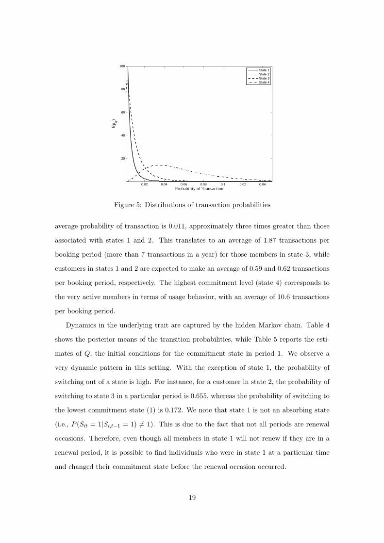
0.02 0.04 0.06 0.08 0.1 0.02 0.04
20
40
60
80
100
Probability of Transaction
f(p it)
State 1State 2State 3State 4
Figure 5: Distributions of transaction probabilities
average probability of transaction is 0.011, approximately three times greater than those
associated with states 1 and 2. This translates to an average of 1.87 transactions per
booking period (more than 7 transactions in a year) for those members in state 3, while
customers in states 1 and 2 are expected to make an average of 0.59 and 0.62 transactions
per booking period, respectively. The highest commitment level (state 4) corresponds to
the very active members in terms of usage behavior, with an average of 10.6 transactions
per booking period.
Dynamics in the underlying trait are captured by the hidden Markov chain. Table 4
shows the posterior means of the transition probabilities, while Table 5 reports the esti-
mates of Q, the initial conditions for the commitment state in period 1. We observe a
very dynamic pattern in this setting. With the exception of state 1, the probability of
switching out of a state is high. For instance, for a customer in state 2, the probability of
switching to state 3 in a particular period is 0.655, whereas the probability of switching to
the lowest commitment state (1) is 0.172. We note that state 1 is not an absorbing state
(i.e., P (Sit = 1|Si,t−1 = 1) 6= 1). This is due to the fact that not all periods are renewal
occasions. Therefore, even though all members in state 1 will not renew if they are in a
renewal period, it is possible to find individuals who were in state 1 at a particular time
and changed their commitment state before the renewal occasion occurred.
19
To stateFrom state 1 2 3 4
1 0.903 0.097 – –2 0.172 0.169 0.655 –3 – 0.427 0.567 0.0064 – – 0.434 0.566
Table 4: Estimated transition probabilities
With reference to Table 5, the qs correspond to the probabilities of being in each
state when an individual first joined the membership scheme. This is the distribution of
underlying states for a just-acquired member of this cohort. The probability of a newly
acquired member being in the highest state is very low; just over 1% of the members
acquired in 2002 were deemed to be in the top commitment state in period 1. Most
members were distributed between states 2 and 3 (41% and 58% respectively) when they
joined the Friends scheme.
Parameter Posterior mean 95% Intervalq2 0.410 [ 0.132 0.703 ]q3 0.578 [ 0.282 0.856 ]q4 0.011 [ 0.001 0.028 ]
Table 5: Estimated period 1 state probabilities
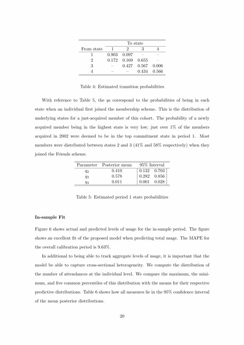
In-sample Fit
Figure 6 shows actual and predicted levels of usage for the in-sample period. The figure
shows an excellent fit of the proposed model when predicting total usage. The MAPE for
the overall calibration period is 9.63%.
In additional to being able to track aggregate levels of usage, it is important that the
model be able to capture cross-sectional heterogeneity. We compute the distribution of
the number of attendances at the individual level. We compare the maximum, the mini-
mum, and five common percentiles of this distribution with the means for their respective
predictive distributions. Table 6 shows how all measures lie in the 95% confidence interval
of the mean posterior distributions.
20
1 2 3 4 5 6 7 8 9 10 11
1000
2000
3000
4000
5000
6000
7000
8000
9000
10000
11000
12000
Period
Num
ber
of tr
ansa
ctio
ns
ActualPredicted
Figure 6: Usage (in-sample) predictions
Actual Posterior mean 95% Post. intervalMin 0.00 0.00 [ 0.00 0.00 ]5% 0.00 0.00 [ 0.00 0.00 ]
25% 2.00 1.81 [ 1.00 2.00 ]50% 4.00 4.59 [ 4.00 5.00 ]75% 11.00 11.07 [ 10.00 12.00 ]95% 32.85 32.80 [ 31.00 355.00 ]Max 457.00 444.87 [ 397.00 492.00 ]
Table 6: Distribution of in-sample predictions
3.3 Forecasting Performance
Having fitted the model to the calibration period data, we will examine the performance
of the model in the hold-out validation period. In addition to comparing its performance
relative to a set of benchmark models, we also consider two restricted versions of the
proposed model: a static latent trait model (Π = IK) in which there is heterogeneity in
transaction behavior but members cannot change their commitment state over time, and
a dynamic latent trait model with homogeneous transaction behavior (r → ∞) in which
all members in each commitment state have the same expected transaction behavior.9
We first forecast usage behavior in periods 12 and 13 for all members that were active at
the end of our calibration period. Then, conditional on each individual’s underlying state
in period 13, we predict renewal behavior at that particular moment. Finally, conditional
9The marginal log-densities of these two models are −12, 341.5 and −12, 831.5, respectively.
21
on having renewed at that time, we forecast usage behavior for all remaining periods and
renewal behavior for the last period of data. This time-split structure allows us to analyze
separately usage forecast accuracy (comparing actual vs. predicted number of transactions
in period 12), renewal forecast accuracy (comparing actual and predicted renewal rates in
periods 13 and 17) and overall forecast accuracy (comparing actual and predicted usage
levels in periods 14 onwards).
Usage Process
In order to assess the quality of the usage predictions, we compare the forecasts from
the proposed model (both the full and two restricted versions) with those generated using
two RFM-based negative binomial (NB) regression models — see Appendix B for details —
and two heuristics (drawing on the work of Wubben and Wangenheim (2008)). Heuristic
A, periodic usage, assumes that each individual repeats the same pattern every year.
Heuristic B, status quo, assumes that all customers will make as many transactions as
their current average.10
To assess the validity of the usage predictions, we compare the models’ forecasts in
period 12. (We cannot generate a forecast for period 13 (and beyond) using the RFM
models because the RFM characteristics are not available for future periods.) The predic-
tive performance is compared at the aggregate level, looking at the percentage error (PE)
in the predicted total number of transactions, as well as at disaggregate level, looking at
the histogram of the population distribution of the number of transactions. That is, we
compute, based on the model predictions, how many customers have zero transactions,
one transaction, two transactions, etc. and compare these values with the actual data. In
order to make the histograms comparable, we compute the Chi-square goodness of fit (χ2)
statistic for all models. This is a measure of how well the model recovers the distribution
of transactions across the population; the smaller the χ2 statistic, the better fit (i.e., the
more similar the distributions of actual and predicted number of transactions).
10For example, suppose a customer makes 2, 4, 2, 4 transactions over the preceding four periods. Underheuristic A, we would predict that this customer will make 2, 4, 2, 4 transactions over the next four periods.Under heuristic B, we would predict a pattern of 3, 3, 3, 3.
22
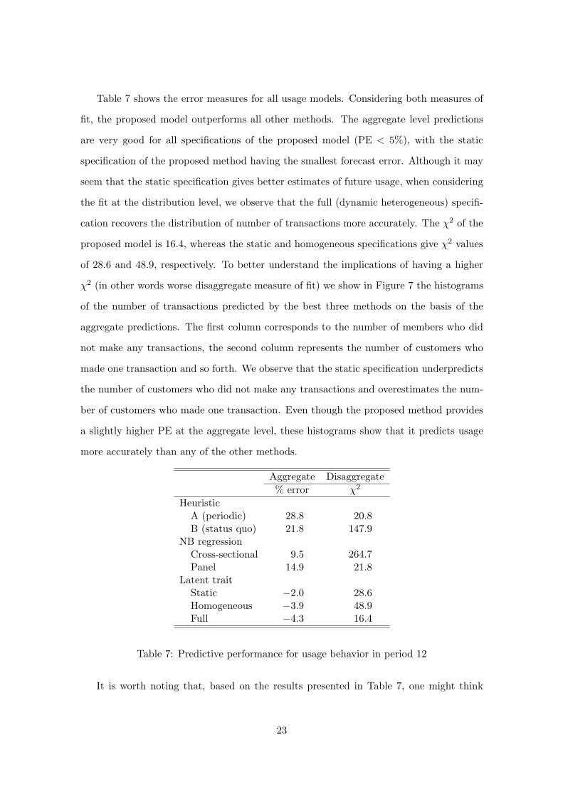
Table 7 shows the error measures for all usage models. Considering both measures of
fit, the proposed model outperforms all other methods. The aggregate level predictions
are very good for all specifications of the proposed model (PE < 5%), with the static
specification of the proposed method having the smallest forecast error. Although it may
seem that the static specification gives better estimates of future usage, when considering
the fit at the distribution level, we observe that the full (dynamic heterogeneous) specifi-
cation recovers the distribution of number of transactions more accurately. The χ2 of the
proposed model is 16.4, whereas the static and homogeneous specifications give χ2 values
of 28.6 and 48.9, respectively. To better understand the implications of having a higher
χ2 (in other words worse disaggregate measure of fit) we show in Figure 7 the histograms
of the number of transactions predicted by the best three methods on the basis of the
aggregate predictions. The first column corresponds to the number of members who did
not make any transactions, the second column represents the number of customers who
made one transaction and so forth. We observe that the static specification underpredicts
the number of customers who did not make any transactions and overestimates the num-
ber of customers who made one transaction. Even though the proposed method provides
a slightly higher PE at the aggregate level, these histograms show that it predicts usage
more accurately than any of the other methods.
Aggregate Disaggregate% error χ2
HeuristicA (periodic) 28.8 20.8B (status quo) 21.8 147.9
NB regressionCross-sectional 9.5 264.7Panel 14.9 21.8
Latent traitStatic −2.0 28.6Homogeneous −3.9 48.9Full −4.3 16.4
Table 7: Predictive performance for usage behavior in period 12
It is worth noting that, based on the results presented in Table 7, one might think
23

0 1 2 3 4 5 6 7+0
50
100
150
200
250
300
350
400
450
# of transactions
# of
cus
tom
ers
ActualHomogeneousLatentFull
Figure 7: Distribution of (predicted vs. actual) number of transactions in period 12
that heuristic A is not a bad model because its χ2 is low. However, this should not be
surprising given that heuristic A predicts that every customer will make exactly the same
number of transactions as the same period last year. In other words, by construction, this
method replicates the population distribution year after year. Nevertheless, if we look at
the error of aggregate number transactions, we see that the heuristic A method is not
accurate in its predictions, over-forecasting the total number of bookings by 28.8%.
Renewal Process
In order to assess the quality of the churn predictions, we compare the predicted renewal
rates of the proposed model (both the full and two restricted versions) with those generated
using two RFM-based logistic regression models— see Appendix B for details — and two
heuristics. The first heuristic (C) says that churn occurs if there is no usage activity during
the last two periods (Wubben and Wangenheim 2008). The second heuristic (D) says that
churn occurs if an individual’s average usage over the last two periods is lower than that of
the corresponding periods in the previous year. (This is in the spirit of Berry and Linoff’s
(2004) discussion of how changes in usage can be a leading indicator of churn.)
The predictive performance for all churn models is presented in Table 8. We compare
actual versus predicted renewal rate in periods 13 and 17. As shown in the table, the
proposed model provides the most accurate predictions of the future renewal rate. Both
heuristic methods provide very poor estimates for future churn. The two logistic regression
24
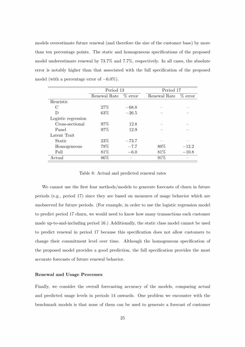
models overestimate future renewal (and therefore the size of the customer base) by more
than ten percentage points. The static and homogeneous specifications of the proposed
model underestimate renewal by 73.7% and 7.7%, respectively. In all cases, the absolute
error is notably higher than that associated with the full specification of the proposed
model (with a percentage error of −6.0%).
Period 13 Period 17Renewal Rate % error Renewal Rate % error
HeuristicC 27% −68.8 – –D 63% −26.5 – –
Logistic regressionCross-sectional 97% 12.8 – –Panel 97% 12.9 – –
Latent TraitStatic 23% −73.7 – –Homogeneous 79% −7.7 80% −12.2Full 81% −6.0 81% −10.8
Actual 86% – 91% –
Table 8: Actual and predicted renewal rates
We cannot use the first four methods/models to generate forecasts of churn in future
periods (e.g., period 17) since they are based on measures of usage behavior which are
unobserved for future periods. (For example, in order to use the logistic regression model
to predict period 17 churn, we would need to know how many transactions each customer
made up-to-and-including period 16.) Additionally, the static class model cannot be used
to predict renewal in period 17 because this specification does not allow customers to
change their commitment level over time. Although the homogeneous specification of
the proposed model provides a good prediction, the full specification provides the most
accurate forecasts of future renewal behavior.
Renewal and Usage Processes
Finally, we consider the overall forecasting accuracy of the models, comparing actual
and predicted usage levels in periods 14 onwards. One problem we encounter with the
benchmark models is that none of them can be used to generate a forecast of customer
25

behavior over the entire validation period, either because they cannot predict behavior
beyond the next period or because they do not account for the attrition process. However,
if we are interested in forecasting customer behavior in contractual settings, we need a
model that accounts for both usage and churn predictions. Aside from the full specification
of the proposed model, the two restricted versions of the proposed model (static and
homogeneous model) also account for both processes. Additionally, we use a combination
of the most accurate churn benchmark model (panel logistic regression) with the best
heuristic usage model (status quo) in the following manner.11 We first predict renewal
behavior in period 13 using the panel logistic regression. Then, for those individuals who
are predicted to renew, we use Heuristic A to forecast usage. As before, we examine the
accuracy of the predictions at the aggregate and disaggregate level.
We examine usage behavior in periods 14 to 16, which in turn depends on predicted
renewal behavior in period 13. We compare the MAPE across all forecast periods (Table
9) and find that the proposed model gives the most accurate predictions over the entire
validation period (MAPE=10.9%). The second-best method is the homogeneous speci-
fication, with an MAPE of 11.7%. (In other words, a model that does not account for
unobserved usage heterogeneity within segments increases the forecast error by 7.7%.) The
static specification provides the biggest error predictions with an MAPE of 23.7%, more
than double the error associated with the full specification. The predictions associated
with the combined benchmark models are also poor, with an MAPE of 20.9%. This result
reinforces the suggestion that the inclusion of dynamics yields more accurate predictions.
Similar results are obtained when considering the disaggregate measures of fit (average χ2
across the three forecast periods); the full specification of the proposed model is clearly
superior.
In summary, we have shown that the full specification of the proposed model predicts
retention and usage behavior accurately. Furthermore, it outperforms benchmark models
on both the usage and retention dimensions.
11We cannot use any of the usage regression models as they need as-yet unobserved RFM data in orderto make predictions for periods 14 – 16.
26
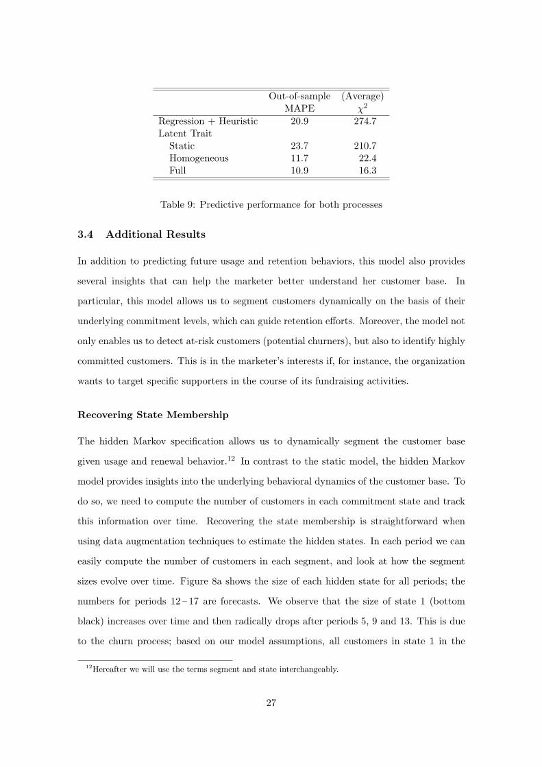
Out-of-sample (Average)MAPE χ2
Regression + Heuristic 20.9 274.7Latent Trait
Static 23.7 210.7Homogeneous 11.7 22.4Full 10.9 16.3
Table 9: Predictive performance for both processes
3.4 Additional Results
In addition to predicting future usage and retention behaviors, this model also provides
several insights that can help the marketer better understand her customer base. In
particular, this model allows us to segment customers dynamically on the basis of their
underlying commitment levels, which can guide retention efforts. Moreover, the model not
only enables us to detect at-risk customers (potential churners), but also to identify highly
committed customers. This is in the marketer’s interests if, for instance, the organization
wants to target specific supporters in the course of its fundraising activities.
Recovering State Membership
The hidden Markov specification allows us to dynamically segment the customer base
given usage and renewal behavior.12 In contrast to the static model, the hidden Markov
model provides insights into the underlying behavioral dynamics of the customer base. To
do so, we need to compute the number of customers in each commitment state and track
this information over time. Recovering the state membership is straightforward when
using data augmentation techniques to estimate the hidden states. In each period we can
easily compute the number of customers in each segment, and look at how the segment
sizes evolve over time. Figure 8a shows the size of each hidden state for all periods; the
numbers for periods 12 – 17 are forecasts. We observe that the size of state 1 (bottom
black) increases over time and then radically drops after periods 5, 9 and 13. This is due
to the churn process; based on our model assumptions, all customers in state 1 in the
12Hereafter we will use the terms segment and state interchangeably.
27
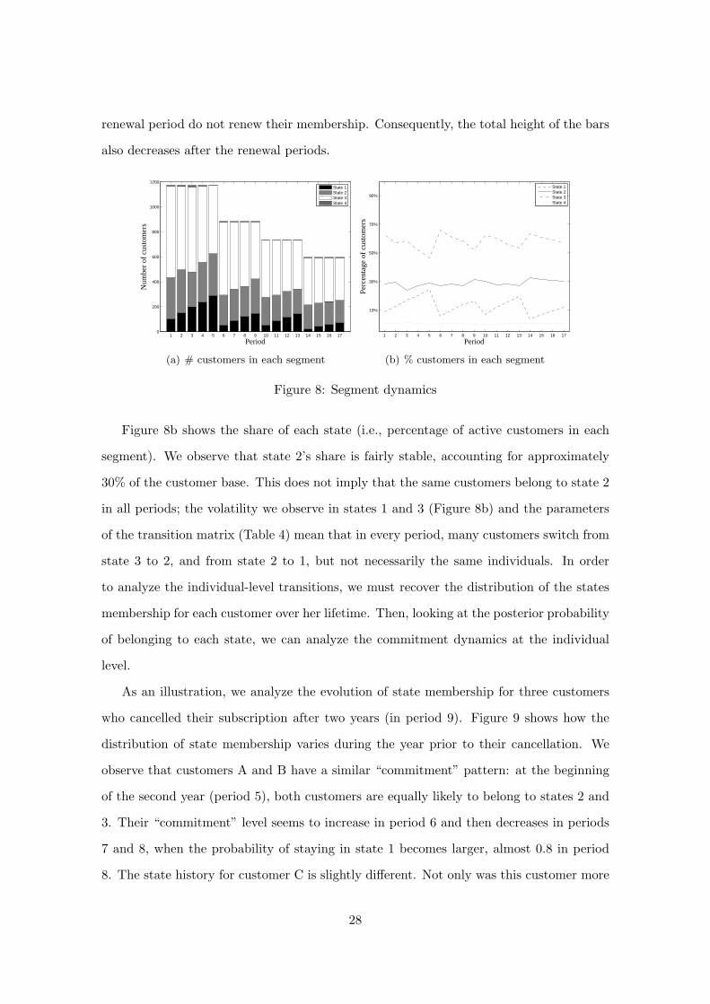
renewal period do not renew their membership. Consequently, the total height of the bars
also decreases after the renewal periods.
1 2 3 4 5 6 7 8 9 10 11 12 13 14 15 16 170
200
400
600
800
1000
1200
Num
ber
of c
usto
mer
s
Period
State 1State 2State 3State 4
(a) # customers in each segment
1 2 3 4 5 6 7 8 9 10 11 12 13 14 15 16 17
10%
30%
50%
70%
90%
Period
Perc
enta
ge o
f cu
stom
ers
State 1State 2State 3State 4
(b) % customers in each segment
Figure 8: Segment dynamics
Figure 8b shows the share of each state (i.e., percentage of active customers in each
segment). We observe that state 2’s share is fairly stable, accounting for approximately
30% of the customer base. This does not imply that the same customers belong to state 2
in all periods; the volatility we observe in states 1 and 3 (Figure 8b) and the parameters
of the transition matrix (Table 4) mean that in every period, many customers switch from
state 3 to 2, and from state 2 to 1, but not necessarily the same individuals. In order
to analyze the individual-level transitions, we must recover the distribution of the states
membership for each customer over her lifetime. Then, looking at the posterior probability
of belonging to each state, we can analyze the commitment dynamics at the individual
level.
As an illustration, we analyze the evolution of state membership for three customers
who cancelled their subscription after two years (in period 9). Figure 9 shows how the
distribution of state membership varies during the year prior to their cancellation. We
observe that customers A and B have a similar “commitment” pattern: at the beginning
of the second year (period 5), both customers are equally likely to belong to states 2 and
3. Their “commitment” level seems to increase in period 6 and then decreases in periods
7 and 8, when the probability of staying in state 1 becomes larger, almost 0.8 in period
8. The state history for customer C is slightly different. Not only was this customer more
28
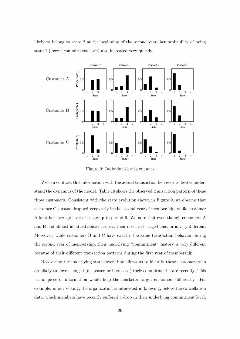
likely to belong to state 2 at the beginning of the second year, her probability of being
state 1 (lowest commitment level) also increased very quickly.
Customer A
Customer B
Customer C
1 2 3 40
0.5
1
Prob
(Sta
te)
Period 5
State1 2 3 4
0
0.5
1Period 6
State1 2 3 4
0
0.5
1Period 7
State1 2 3 4
0
0.5
1Period 8
State
1 2 3 40
0.5
1
Prob
(Sta
te)
State1 2 3 4
0
0.5
1
State1 2 3 4
0
0.5
1
State1 2 3 4
0
0.5
1
State
1 2 3 40
0.5
1
Prob
(Sta
te)
State1 2 3 4
0
0.5
1
State1 2 3 4
0
0.5
1
State1 2 3 4
0
0.5
1
State
Figure 9: Individual-level dynamics
We can contrast this information with the actual transaction behavior to better under-
stand the dynamics of the model. Table 10 shows the observed transaction pattern of these
three customers. Consistent with the state evolution shown in Figure 9, we observe that
customer C’s usage dropped very early in the second year of membership, while customer
A kept her average level of usage up to period 6. We note that even though customers A
and B had almost identical state histories, their observed usage behavior is very different.
Moreover, while customers B and C have exactly the same transaction behavior during
the second year of membership, their underlying “commitment” history is very different
because of their different transaction patterns during the first year of membership.
Recovering the underlying states over time allows us to identify those customers who
are likely to have changed (decreased or increased) their commitment state recently. This
useful piece of information would help the marketer target customers differently. For
example, in our setting, the organization is interested in knowing, before the cancellation
date, which members have recently suffered a drop in their underlying commitment level,
29

Year 1 Year 21 2 3 4 5 6 7 8
Customer A 2 1 0 1 1 2 0 1Customer B 0 0 0 0 0 1 0 0Customer C 2 1 4 3 0 1 0 0
Table 10: Customer-level usage behavior (actual)
so that pre-emptive retention activities can be undertaken. (As illustrated by the poor
performance of Heuristics C and D in predicting churn, such at-risk customers cannot be
identified without the use of a formal model.)
Incorporating New Information
In dynamic environments, updating the list of at-risk customers is central to any efforts
designed to increase the success of retention campaigns. Apart from using past behavior
to identify changes in commitment level (as illustrated in Figure 9), another way to detect
changes in commitment levels is to use the most recent piece of information, when available,
to update the model estimates. For example, having estimated the model using data from
periods 1 – 11, suppose we now observe usage behavior for period 12. What can we learn
from this additional information? In other words, how can this new data be used to
update what we knew already about the customer base? Once the model is calibrated, it
is easy to incorporate new information as more behavior is observed. We can simply use
the model estimates at period 11 and use Bayes’ rule to update the parameter estimates
given the individuals’ period 12 transaction data. More specifically, using the posterior
distribution of state membership at period 11 (Si,11) and the estimated transition matrix
(Π), we compute the prior distribution of state membership in the following period (i.e.,
P (Si,12 = k|Si,11, Π) for k = 1, ..., K). Then, we calculate the likelihood of observing
period 12 usage behavior conditional on the individual-level parameters αi. Finally, we
compute the posterior distribution of state membership in period 12 using Bayes’ rule:
P (Si,12 = k|Yi,12 = yi,12,Ω) =P (Yi,12 = yi,12|Si,12 = k, αi, θ)P (Si,12 = k|Si,11, Π)K∑
l=1
P (Yi,12 = yi,12|Si,12 = l, αi,θ)P (Si,12 = l|Si,11, Π)(9)
30
where Ω denotes all the model parameters.
We can now compare the distribution of state membership in periods 11 and 12 and
identify those customers who have changed their commitment state in the current period.
Following this procedure, we identify 45 customers who have shifted in their commitment
level to the lowest state from period 11 to period 12.13 Similarly, we identify 2 members
who moved to state 4 (highly committed level) in period 12. The main advantage of the
updating process is that it requires simple computations and can serve as the basis for a
dynamic resource allocation tool.
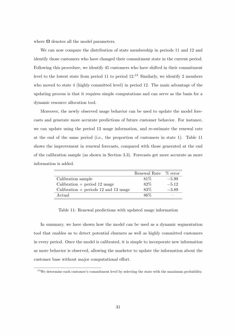
Moreover, the newly observed usage behavior can be used to update the model fore-
casts and generate more accurate predictions of future customer behavior. For instance,
we can update using the period 13 usage information, and re-estimate the renewal rate
at the end of the same period (i.e., the proportion of customers in state 1). Table 11
shows the improvement in renewal forecasts, compared with those generated at the end
of the calibration sample (as shown in Section 3.3). Forecasts get more accurate as more
information is added.
Renewal Rate % errorCalibration sample 81% −5.99Calibration + period 12 usage 82% −5.12Calibration + periods 12 and 13 usage 83% −3.89Actual 86% –
Table 11: Renewal predictions with updated usage information
In summary, we have shown how the model can be used as a dynamic segmentation
tool that enables us to detect potential churners as well as highly committed customers
in every period. Once the model is calibrated, it is simple to incorporate new information
as more behavior is observed, allowing the marketer to update the information about the
customer base without major computational effort.
13We determine each customer’s commitment level by selecting the state with the maximum probability.
31

External Validity
We have developed a joint model for usage and renewal behavior in contractual settings.
The model incorporates both behaviors for two reasons: first, these are the two key drivers
of customer profitability and, second, this information is generally available in a company’s
database. At the heart of the model is a dynamic latent trait that can be interpreted
as commitment, engagement, satisfaction, etc. So far we have examined the predictive
validity of the model. However little has been said about the underlying process that
drives both behaviors. While a comprehensive discussion of what the latent variable (as
captured in a discretized form by the states of the HMM) actually represents, we can
provide some evidence that is consistent with our contention that it capture the notion of
commitment, etc.
In addition to priority booking privileges, membership of the organization’s Friends
scheme gives the option to attend special events such as workshops, rehearsals, and educa-
tional events. Collecting information on the attendance of these events is not straightfor-
ward as they are organized by the Friends office and the data are not generally linked to
the box-office data. We obtained information on event attendance for 2004 and extracted
the records for those members belonging to the cohort analyzed in this paper. The rate
of attendance of these events is very low compared to that of the general performances;
on average, a member attends to 0.41 special events a year (0.10 per booking period),
whereas the average attendance rate for general performances is 3.8.
On average, we would expect the attendance of such events to reflect a member’s
“commitment”. Given that period 12 corresponds to the end of year 2004, we select
the model predictions about state membership in period 12 (as shown in section 3.4)
and compute the average attendance rate to special events by the members of each group.
With reference to Table 12, we observe that the average number of special events attended
is higher for higher commitment states.14 This average can be decomposed into i) the
percentage of members attending at least one event, and ii) the average number of events
attended given attendance of at least one event. We note that both of these quantities
14We do not consider the attendance rate for state 4 because the small size of the group.
32

increase with higher commitment states.
Average Attending Average givenState # customers # events any event attendance
1 54 0.13 9% 1.42 135 0.44 23% 1.93 547 0.77 24% 3.24 2 – – –
Table 12: Attendance of other events
We recognize that this analysis has several limitations. First, we only consider one
year and one booking period rather than performing a longitudinal analysis. If possible,
one should get periodic information about attendance to special events, and match this
information with the state membership estimates provided by the model. Second, the
attendance of these events may not perfectly reflect commitment (or any other label we
could assign to the latent trait that drives behavior in a particular setting). Nevertheless,
we have shown that those customers identified by the model as more committed members
attend special events more often than those who are assigned to lower states.
3.5 Generalizing the Model
There are certain aspects of this model that may appear to have been dictated by the
specific empirical setting under study. We now briefly discuss the generalizability of the
model.
First, there are situations where usage or consumption is not discrete. These are
cases in which usage refers to time (e.g., minutes used in wireless contracts), expenditure
(e.g., total amount spent), or other quantities (e.g., MB downloaded in an Internet data
plan). The proposed model is easily applied in such settings, provided the distributional
assumption of the usage process (derived in section 2.2) is modified. We would simply
replace the Poisson or binomial with, say, a gamma or log-normal distribution.
Second, we may wish to incorporate time-invariant covariates (e.g., customer demo-
graphics) and/or time-varying covariates (e.g., marketing activities, competitors actions).
In order to do so, we could simply make (3) or (5) a function of the covariates using,
33

say, an exponential link function. We could also use this information to explain observed
heterogeneity in the transition behavior, as in Netzer et al. (2008).
4 Discussion
We have proposed a dynamic latent trait model in which usage and renewal behavior
are modeled simultaneously by assuming that both behaviors are driven by the same
(individual-level) underlying process that evolves over time. Dynamics in the underlying
latent variable (which we label “commitment”) are captured using a hidden Markov model.
With regards to predicting churn behavior, the proposed model outperforms a set of
benchmark models. It not only gives more accurate predictions in the short-term, but
also forecasts churn further into the future. Given the usage component of the model,
it is especially valuable in those contractual settings where future usage is not known in
advance but is of importance, either because it directly affects revenue (e.g., credit cards,
wireless contracts, arts organizations memberships), or because it affects service quality,
which in turn affects customer retention and usage (e.g., gym memberships, DVD rental
services).
We have quantified the importance of including dynamics in the latent variable and
unobserved heterogeneity in usage behavior. We found that a model not considering
heterogeneity in usage behavior increases the forecast error. Furthermore, we found that
using a model that does not allow for dynamics in the latent variable yields a forecast
error that is more than twice that associated with the proposed model.
Besides its methodological contribution, the model also provides important manage-
rial insights. First, the retention and usage forecasts are vital inputs to any analysis of
customer profitability. Second, the proposed model provides information that can be used
by the marketer to target retention efforts individually and dynamically. Third, the model
not only detects at-risk customers (potential churners) but also identifies highly committed
customers. Fourth, because heterogeneity in usage behavior is allowed within each state,
the model allows us to detect heavy users who might be at risk, and also light-users whose
underlying level of commitment may be high. This information would be impossible to
34

extract from a segmentation scheme based entirely on observed transactional behavior.
Moreover, model-derived insights can be updated easily as more behavior is observed,
allowing the marketer to detect customers who recently changed their commitment to
the organization. Finally, the model has been estimated using a freely available software,
which facilitates its use by practitioners.
We recognize that this analysis is not free of limitations. First, we have not formally
defined or measured the underlying construct that drives churn and usage and which
makes it possible to model both processes simultaneously (even though we have called it
commitment). Although the attempt of this work is to provide a methodological tool to
predict churn and usage rather than identify such a construct, it would be very useful for
the marketer to identify this underlying trait and also investigate what makes it change
over time. To address this issue, customers’ attitudes could be measured periodically and
linked to the latent variable (using a factor-analytic measurement model). Incorporating
this information might be costly. However, we hope that this research opens new venues to
understand the dynamics between all customer’s behaviors. Second, for the sake of model
parsimony, we have proposed a homogeneous transition matrix. As such predictions about
future commitment states might be misleading if the model is applied in a setting where
there is a mix of “stable” and “volatile” customers. Nevertheless, the accuracy of the model
forecasts provides support for our belief that the homogeneous HMM is appropriate for the
empirical setting considered in this paper. A natural extension for the proposed method
would be to incorporate unobserved individual heterogeneity in the (hidden) transition
matrix. Moreover, one could even incorporate (when available) marketing actions carried
out by the company that may affect the latent variable. The model could also be extended
to accommodate seasonality in settings where such effects are present. Finally, another
extension of our model is to include revenue as variable of interest. This could be done
in two ways, either modeling revenue directly, as we have modeled usage (e.g., using a
lognormal or gamma distribution) or modeling the link between usage and revenue.
35

Appendix A
The model is estimated in a Bayesian framework. We obtain estimates of all model param-
eters by drawing from the marginal posterior distributions, and use a data augmentation
approach to deal with the latent states Sit.
Let Ω denote all the model parameters, including the population parameters (Q,Π, θ, r),
the individual-level parameters α = αii=1,...,I , and the set of augmented paths of com-
mitment states s = sii=1,...,I . The full joint posterior distribution can be written as:
f(Ω|data) ∝ I∏
i=1
Lusagei (θ, αi |Si, data)
f(θ)f(α|r)f(s|Q,Π)f(r)f(Q)f(Π)
where f(θ) is the prior distribution of the commitment-state-specific usage parameters,
f(α|r) is the prior (or mixing) distribution for the αi, which is assumed to follow a
gamma distribution with shape and scale parameter r. The term f(s|Q,Π) refers to the
distribution of the latent states, assumed to follow a hidden Markov process with renewal
restrictions in periods t = 1, n + 1, 2n + 1, ...
The terms f(Q), f(Π), and f(r) are the (hyper)priors for the population parameters.
Noninformative (vague) priors are used for all parameters. For the vector Q and all
rows of the matrix Π we use Dirichlet prior with equal probabilities. We use a diffuse
gamma distribution as a prior for the parameter r (shape and scale parameters being
0.01). In the Poisson specification we need to restrict the prior for θ to ensure that
0 < θ1 < θ2 < ... < θK . Therefore, we use a uniform prior over the interval (0,10) for
θ1 and reparameterize θτ = θτ−1 + eγτ ∀ τ > 1. Diffuse normal priors (with mean 0 and
variance 10000) are used for the γτ s. When estimating the binomial model, we also need
to guaranty that all θ’s are lower than 1. To do so, we use a uniform (0,1) as prior for θ1,
a uniform (θ1, 1) for θ2, a uniform (θ2, 1) for θ3 and so on.
This is implemented using the freely available software WinBUGS (Lunn et al. 2000).
We use the categorical distribution in WinBUGS to draw the augmented states, and
control for the path restrictions (due to the contractual specification) by truncating the
categorical distribution function in the renewal periods (t = 1, n + 1, 2n + 1, ..). (Further
36

details of the estimation procedure and the associated WinBUGS code used to estimate
both Poisson and binomial specifications are available from the authors on request.)
We burn-in the first 95,000 iterations and use the following 5,000 iterations to draw
from the posterior marginal distributions. Convergence of the parameters was diagnosed
visually, looking at the historical draws of all parameters, and also using the Gelman-
Rubin statistic R, which compares the ratio of the pooled chain variance with the within
chain variance, for a model estimated using multiple and disperse starting values.
37

Appendix B
Within both academic and practitioner circles, there is a tradition of building regression-
type models for predicting churn and, to a lesser extent, usage (or related quantities). In
this appendix, we describe the specification of the benchmark regression models used in
our analyses.
As previously noted, the regressions model the behavior of interest as a function of the
customer’s past behavior, frequently summarized in terms of their RFM characteristics.
We operationalize these RFM characteristics in the following manner. Recency is defined
as the number of periods since the last usage transaction (i.e., ticket purchase). Frequency
is defined as the total number of usage transactions in the previous four periods. We also
compute another measure of frequency, Fsum, which is the total number of transactions
per customer over the entire period of interest. Monetary value is the average expenditure
per transaction, where the average is computed over the previous four periods. We also
compute Msum, the customer’s total spend over the entire period of interest. (In explor-
ing possible model specifications, we also consider logarithmic transformations of these
variables, as well as interactions between the RFM measures.)
Perhaps the most common approach to developing a churn model is to use a “cross-
sectional” logistic regression with the last renewal observation as the dependent variable
and RFM measures as covariates. In developing such a benchmark model, we selected
the specification that provided the most accurate predictions. The associated parameter
estimates are given in Table B1. We note that the recency variable is not a significant
predictor by itself, although its interaction with frequency is a significant predictor of
renewal behavior.
Given the nature of the usage data, we used a count model to develop our regression-
based benchmark model. Given that we observe over-dispersion in our data, we used a
negative binomial (NB) regression model, which can be viewed as a Poisson regression
with a random effect that is distributed gamma with parameters (r, α). We selected those
individuals that were still members at the end of our calibration period. We used the
number of transactions in the last period (11) as the dependent variable and the RFM
38
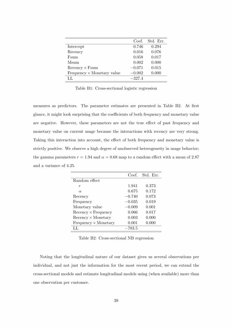
Coef. Std. Err.Intercept 0.746 0.294Recency 0.016 0.076Fsum 0.058 0.017Msum 0.002 0.000Recency×Fsum −0.071 0.015Frequency×Monetary value −0.002 0.000LL −327.4
Table B1: Cross-sectional logistic regression
measures as predictors. The parameter estimates are presented in Table B2. At first
glance, it might look surprising that the coefficients of both frequency and monetary value
are negative. However, these parameters are not the true effect of past frequency and
monetary value on current usage because the interactions with recency are very strong.
Taking this interaction into account, the effect of both frequency and monetary value is
strictly positive. We observe a high degree of unobserved heterogeneity in usage behavior;
the gamma parameters r = 1.94 and α = 0.68 map to a random effect with a mean of 2.87
and a variance of 4.25.
Coef. Std. Err.Random effect
r 1.941 0.373α 0.675 0.172
Recency −0.740 0.073Frequency −0.035 0.019Monetary value −0.009 0.001Recency×Frequency 0.066 0.017Recency×Monetary 0.003 0.000Frequency×Monetary 0.001 0.000LL −783.5
Table B2: Cross-sectional NB regression
Noting that the longitudinal nature of our dataset gives us several observations per
individual, and not just the information for the most recent period, we can extend the
cross-sectional models and estimate longitudinal models using (when available) more than
one observation per customer.
39
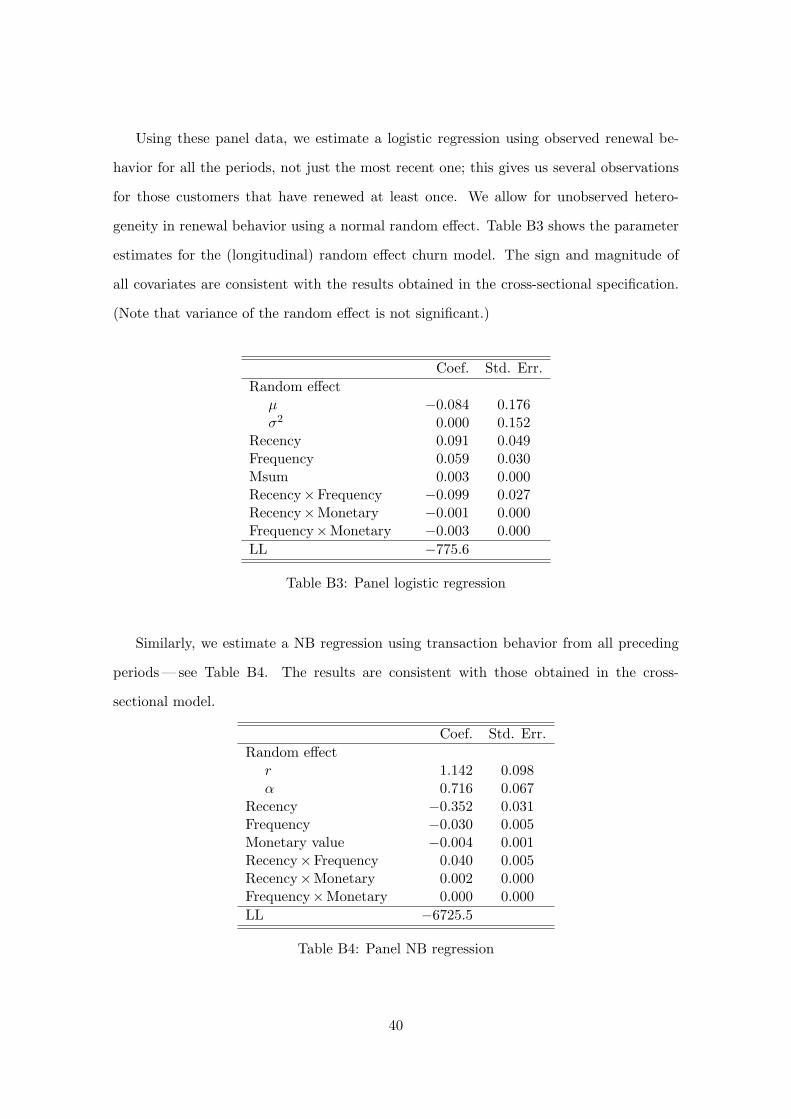
Using these panel data, we estimate a logistic regression using observed renewal be-
havior for all the periods, not just the most recent one; this gives us several observations
for those customers that have renewed at least once. We allow for unobserved hetero-
geneity in renewal behavior using a normal random effect. Table B3 shows the parameter
estimates for the (longitudinal) random effect churn model. The sign and magnitude of
all covariates are consistent with the results obtained in the cross-sectional specification.
(Note that variance of the random effect is not significant.)
Coef. Std. Err.Random effect
µ −0.084 0.176σ2 0.000 0.152
Recency 0.091 0.049Frequency 0.059 0.030Msum 0.003 0.000Recency×Frequency −0.099 0.027Recency×Monetary −0.001 0.000Frequency×Monetary −0.003 0.000LL −775.6
Table B3: Panel logistic regression
Similarly, we estimate a NB regression using transaction behavior from all preceding
periods— see Table B4. The results are consistent with those obtained in the cross-
sectional model.
Coef. Std. Err.Random effect
r 1.142 0.098α 0.716 0.067
Recency −0.352 0.031Frequency −0.030 0.005Monetary value −0.004 0.001Recency×Frequency 0.040 0.005Recency×Monetary 0.002 0.000Frequency×Monetary 0.000 0.000LL −6725.5
Table B4: Panel NB regression
40
References
Ascarza, E., A. Lambrecht, N. Vilcassim. 2009. When talk is “free”: An analysisof subscriber behavior under two- and three-part tariffs. Working Paper, LondonBusiness School.
Athanassopoulos, A.D. 2000. Customer satisfaction cues to support market segmentationand explain switching behavior. J. Business Res. 47(3) 191–207.
Berry, M.J.A., G.S. Linoff. 2004. Data Mining Techniques: For Marketing, Sales, andCustomer Relationship Management. John Wiley & Sons, Indianapolis, IN.
Bhattacharya, C.B. 1998. When customers are members: Customer retention in paidmembership context. J. Marketing 26(Winter) 31–44.
Blattberg, R.C., G. Getz, J.S. Thomas. 2001. Customer Equity: Building and ManagingRelationships as Valuable Assets. Harvard Business School Press, Boston, MA.
Blattberg, R.C., B-D. Kim, S.A. Neslin. 2008. Database Marketing. Analyzing andManaging Customers. Springer, New York, NY.
Bolton, R.N. 1998. A dynamic model of duration of the customer’s relationship with acontinuous service provider: The role of satisfaction. Marketing Sci. 17(1) 45–65.
Bolton, R.N., P.K. Kannan, M.D. Bramlett. 2000. Implications of loyalty programmembership and service experiences for customer retention and value. J. AcademyMarketing Sci. 28(Winter) 95–108.
Bolton, R.N., K.N. Lemon. 1999. A dynamic model of customers’ usage of services:Usage as a n antecedent and consequence of satisfaction. J. Marketing Res. 36(2)171–186.
Bolton, R.N., K.N. Lemon, P.C. Verhoef. 2004. The theoretical underpinnings of cus-tomer asset management: A framework and propositions for future research. J.Academy Marketing Sci. 32(3) 271–292.
Brannas, K., P. Johansson. 1996. Panel data regression for counts. Statistical Papers 37191–213.
Chintagunta, P.K. 1993. Investigating purchase incidence, brand choice and purchasequantity decisions of households. Marketing Sci. 12(Spring) 184–204.
Congdon, P. 2003. Bayesian Statistical Modelling. John Wiley & Sons, Chichester,England.
Diggle, P., M.G. Kenward. 1994. Informative drop-out in longitudinal data analysis.App. Stat. 43(1) 49–93.
Fader, P.S., B.G.S. Hardie, C-Y. Huang. 2004, A dynamic changepoint model for newproduct sales forecasting. Marketing Sci. 23(Winter) 50–65.
Fader, P.S., B.G.S. Hardie, K.L. Lee. 2005. RFM and CLV: Using iso-value curves forcustomer base analysis. J. Marketing Res. 42(November) 415–430.
41
Garbarino, E., M.S. Johnson. 1999. The different roles of satisfaction, trust, and com-mitment in customer relationships. J. Marketing 63(April) 70–87.
Gourieroux, C., J. Jasiak. 2001. Dynamic factor models. Econometric Reviews 20(4)385–424.
Gruen, T.W., J.O. Summers, F. Acito. 2000. Relationship marketing activities, commit-ment, and membership behaviors in professional associations. J. Marketing 64(July)34–49.
Hanemann, W.M. 1984. Discrete/continuous models of consumer demand. Econometrica52(3) 541–561.
Hashemi, R., H. Janqmin-Dagga, D. Commenges. 2003. A latent process model for jointmodeling of events and marker. Lifetime Data Analysis 9(December) 331–343.
Hausman, J., B.H. Hall, Z. Griliches. 1984. Econometric models for count data with anapplication to the patents-R&D relationship. Econometrica 52(4) 909–938.
Henderson, R., P. Diggle, A. Dobson. 2000. Joint modelling of longitudinal measurementsand event time data. Biostatistics 1(4) 465–480.
Kim, H.S., C.H. Yoon. 2004. Determinants of subscriber churn and customer loyalty inthe Korean mobile telephony market. Telecommunications Policy 28(40095) 751–765.
Krishnamurthi, L., S.P. Raj. 1988. A model of brand choice and purchase quantity pricesensitivities. Marketing Sci. 7(Winter) 1–20.
Lachaab, M., A. Ansari, K. Jedidi, A. Trabelsi. 2006. Modeling preference evolution indiscrete choice models: A Bayesian state-space approach. Quant. Marketing andEcon. 4 57–81.
Lariviere, B., D. Van den Poel. 2005. Predicting customer retention and profitabilityby using random forests and regression forests techniques. Expert Systems withApplications 29(2) 472–484.
Lemon, K.N., T.B. White, R.S. Winer. 2002. Dynamic customer relationship manage-ment: Incorporating future considerations into the service retention decision. J.Marketing 66(January) 1–14.
Liechty, J.C., D.K.H. Fong, W.S. DeSarbo. 2005. Dynamic models incorporating individ-ual heterogeneity: Utility evolution in conjoint analysis. Marketing Sci. 24(Spring)285–293.
Liu, L., X. Huang. 2009. Joint analysis of correlated repeated measures and recurrentevents processes in the presence of death, with application to a study on acquiredimmune deficiency syndrome. App. Stat. 58(1) 65–81.
Lu, J. 2002. Predicting customer churn in the telecommunications industry— An ap-plication of survival analysis modeling using SAS R©. SAS User Group Internat.(SUGI27) Online Proceedings 114–27.
42
Lunn, D.J., A. Thomas, N. Best, D. Spiegelhalter. 2000. WinBUGS — A Bayesianmodelling framework: Concepts, structure, and extensibility. Stat. and Computing10(4) 325–337.
Moe, W.W., P.S. Fader. 2004a. Capturing evolving visit behavior in clickstream data.J. Interactive Marketing 18(Winter) 5–19.
Moe, W.W., P.S. Fader. 2004b. Dynamic conversion behavior at e-commerce sites.Management Sci. 50(March) 326–335.
Montgomery, A.L., S. Li, K. Srinivasan, J.C. Liechty. 2004. Predicting online purchaseconversion using web path analysis. Marketing Sci. 23(4) 579–595.
Moon, S., W.A. Kamakura, J. Ledolter. 2007. Estimating promotion response whencompetitive promotions are unobservable. J. Marketing Res. 44(3) 503–515.
Morgan, R.Y.H., S. Hunt. 1994. The commitment-trust theory of relationship marketing.J. Marketing 58(July) 20–38.
Mozer, M.C., R. Wolniewicz, D.B. Grimes, E. Johnson, H. Kaushansky. 2000. Predictingsubscriber dissatisfaction and improving retention in the wireless telecommunicationsindustry. IEEE Trans. Neural Networks 11(3) 690–696.
Nam, S., P. Manchanda, P.K. Chintagunta. 2007. The effects of service quality andword of mouth on customer acquisition, retention and usage. (http://ssrn.com/abstract=969770).
Narayanan, S., P.K. Chintagunta, E.J. Miravete. 2007. The role of self selection andusage uncertainty in the demand for local telephone service. Quantitative Marketingand Econom. 5(1) 1–34.
Netzer, O., J.M. Lattin, V. Srinivasan. 2008. A hidden Markov model of customerrelationship dynamics. Marketing Sci. 27(March-April) 185–204.
Newton, M.A., A.E. Raftery. 1994. Approximate Bayesian inference with the weightedlikelihood bootstrap. J. Roy. Stat. Soc. B 56(1) 3–48.
Parr Rud, O. 2001. Data Mining Cookbook. John Wiley & Sons, New York, NY.
Poulsen, C.S. 1990. Mixed Markov and latent Markov modelling applied to brand choicebehaviour. Internat. J. Res. in Marketing 7 5–19.
Reinartz, W., J.S. Thomas, V. Kumar. 2005. Balancing acquisition and retention re-sources to maximize customer profitability. J. Marketing 69(January) 63–79.
Rust, R.T., V.A. Zeithaml, K.N. Lemon. 2001. Driving Customer Equity: How CustomerLifetime Value Is Reshaping Corporate Strategy. The Free Press, New York, NY.
Sabavala, D.J., D.G. Morrison. 1981. A nonstationary model of binary choice applied tomedia exposure. Management Sci. 27(June) 637–657.
Schweidel, D.A., P.S. Fader, E.T. Bradlow. 2008. Understanding service retention withinand across cohorts using limited information. J. Marketing 72(1) 82–94.
43
Smith, A., P.A. Naik, C.L. Tsai. 2006. Markov-switching model selection using Kullback–Leibler divergence. J. Econometrics 134(2) 553–577.
Van Heerde, H.J., C.F. Mela, P. Manchanda. 2004. The dynamic effect of innovation onmarket structure. J. Marketing Res. 41(May) 166–183.
Verhoef, P.C. 2003. Understanding the effect of customer relationship management effortson customer retention and customer share development. J. Marketing 67(October)30–45.
West, M., J. Harrison. 1997. Bayesian Forecasting and Dynamic Models, 2nd ed.Springer, New York, NY.
Wubben, M., F. Wangenheim. 2008. Instant customer base analysis: Managerial heuris-tics often get it right. J. Marketing 72(3) 82–93.
Xu, J., S.L. Zeger. 2001. Joint analysis of longitudinal data comprising repeated measuresand times to events. App. Stat. 50(3) 375–387.
44
Related Documents