Modeling Cascading Network Disruptions under Uncertainty

Modeling Cascading Network Disruptions under Uncertainty

For Managing Hurricane Evacuation

by

Ketut Gita

A Dissertation Presented in Partial Fulfillment

of the Requirements for the Degree

Doctor of Philosophy

Approved June 2020 by the

Graduate Supervisory Committee:

Pitu Mirchandani, Chair

Ross Maciejewski

Jorge Sefair

Xuesong Zhou

ARIZONA STATE UNIVERSITY

August 2020

i

ABSTRACT

Short-notice disasters such as hurricanes involve uncertainties in many facets, from the

time of its occurrence to its impacts’ magnitude. Failure to incorporate these uncertainties

can affect the effectiveness of the emergency responses. In the case of a hurricane event,

uncertainties and corresponding impacts during a storm event can quickly cascade. Over

the past decades, various storm forecast models have been developed to predict the storm

uncertainties; however, access to the usage of these models is limited. Hence, as the first

part of this research, a data-driven simulation model is developed with aim to generate

spatial-temporal storm predicted hazards for each possible hurricane track modeled. The

simulation model identifies a means to represent uncertainty in storm’s movement and its

associated potential hazards in the form of probabilistic scenarios tree where each branch

is associated with scenario-level storm track and weather profile. Storm hazards, such as

strong winds, torrential rain, and storm surges, can inflict significant damage on the road

network and affect the population’s ability to move during the storm event. A cascading

network failure algorithm is introduced in the second part of the research. The algorithm

takes the scenario-level storm hazards to predict uncertainties in mobility states over the

storm event. In the third part of the research, a methodology is proposed to generate a

sequence of actions that simultaneously solve the evacuation flow scheduling and

suggested routes which minimize the total flow time, or the makespan, for the evacuation

process from origins to destinations in the resulting stochastic time-dependent network.

The methodology is implemented for the 2017 Hurricane Irma case study to recommend

an evacuation policy for Manatee County, FL. The results are compared with evacuation

ii

plans for assumed scenarios; the research suggests that evacuation recommendations that

are based on single scenarios reduce the effectiveness of the evacuation procedure. The

overall contributions of the research presented here are new methodologies to: (1) predict

and visualize the spatial-temporal impacts of an oncoming storm event, (2) predict

uncertainties in the impacts to transportation infrastructure and mobility, and (3) determine

the quickest evacuation schedule and routes under the uncertainties within the resulting

stochastic transportation networks.

iii

This dissertation is dedicated to

my father

and those whom I love

iv

ACKNOWLEDGMENTS

I would like to express my deepest appreciation to my advisor, Professor Pitu

Mirchandani, for the opportunity to work with him for the last five years. Without his

constant guidance, challenges, and had-my-back support from the research funding to well-

being throughout the program, this dissertation would not have been possible.

I am tremendously fortunate to have committee members Dr. Ross Maciejewski,

Dr. Jorge Sefair, and Dr. Xuesong Zhou who brought a depth of knowledge that few could

match and complete the dissertation in various angles. I thank them for their support and

feedback which have been valuable and always pushing me forward.

I would also like to thank Prof. Harjanto Prabowo, the Rector of BINUS University,

Indonesia, for his moral support as well as for allowing me to take sabbatical leave to

pursue doctoral degree overseas. My gratitude to Dr. Iman H. Kartowisastro, the Provost

of BINUS Higher Education, for his strong encouragement during the difficult times I

encountered especially towards the end of my study.

My appreciation also extends to Dr. Larry Mays, who recently retired; informally

advised me on his expertise in the area of surface water hydrology, an invaluable topic in

this dissertation. Thanks to Dr. Linda Chattin for her encouragement and support in many

aspects, who has become a great friend. I am grateful to have Christina Sebring as my

academic advisor. Her quick response and accommodating guidance allowed me to

proceed seamlessly throughout the program. She is the best academic advisor I’ve ever

had throughout my education path. Lots of thanks go to my friends, especially, Gina

Dumkrieger, Kerem Demirtas, Elizabeth Danielson, Nathan Gaw, Kwabena Bosompem,

v

Faisal Alfaisal, and Daniel Tran for their tremendous technical and moral assistance and

faith in my success to this day. I would also like to mention Brint MacMillan and Monica

Dugan for their continuous support related to computing and administrative work. Also,

thanks to all Brickyard’s staff, security guards, and janitors for providing conducive

environment throughout my study (August 2015 – June 2020).

Finally, I would like to express my gratitude for the financial support from the Data

Storm project supported by the National Science Foundation (NSF) and the Proactive

project supported by Center for Accelerating Operational Efficiency (CAOE), a

Department of Homeland Security Centers of Excellence. This material is based upon work

supported by the U.S. Department of Homeland Security under Cooperative Agreement

No. 2014-ST-061-ML0001. The views and conclusions contained in this document are

those of the authors and should not be interpreted as necessarily representing the official

policies, either expressed or implied, of the U.S. Department of Homeland Security. I also

thank the Graduate Professional and Student Association (GPSA) for the travel support

and the Industrial Engineering Program for providing me the financial support in the early

years of my doctoral program, as well as for the summer 2020 fellowship.

vi

TABLE OF CONTENTS

Page

LIST OF TABLES .............................................................................................................. x

LIST OF FIGURES .......................................................................................................... xii

CHAPTER

1. INTRODUCTION ....................................................................................................... 1

1.1. Motivation ............................................................................................................ 1

1.2. Statements of Research Problems ........................................................................ 7

1.3. Dissertation Contributions.................................................................................... 8

1.4. Organization of the Dissertation .......................................................................... 9

2. LITERATURE REVIEW .......................................................................................... 11

2.1. Past Evacuation Studies ..................................................................................... 11

2.2. Hurricane and Storm Hazards ............................................................................ 15

2.3. Simulation Model Validation and Verification .................................................. 18

2.4. Road Transportation ........................................................................................... 19

2.5. Evacuation Models and Methods ....................................................................... 21

2.5.1. Network Flow Models ............................................................................. 21

2.5.2. Concept of Residual Network .................................................................. 24

2.5.3. Time-Dependent Shortest Path (TDSP) ................................................... 24

2.5.4. Column Generation Approaches in Optimization.................................... 26

2.5.5. Makespan Minimization .......................................................................... 27

2.5.6. Binary Search Approach .......................................................................... 27

2.5.7.Decision Tree Analysis ............................................................................. 28

vii

CHAPTER Page

3. OVERVIEW OF RESEARCH SCOPE AND METHODOLOGIES ....................... 30

4. DATA-DRIVEN SIMULATION MODEL .............................................................. 35

4.1. Problem Description ........................................................................................... 35

4.2. Simulation Model Objective .............................................................................. 35

4.3. Solution Approach.............................................................................................. 36

4.4. Mathematical Formulations................................................................................ 38

4.4.1. Scenario and Wind Speed Probability Models ........................................ 38

4.4.2. Precipitation Quantity and Probability Models ........................................ 41

4.4.3. Storm Surge Probability Models .............................................................. 60

4.5. Hurricane Irma Empirical Results ...................................................................... 64

4.5.1. Hurricane Irma Overview ........................................................................ 64

4.5.2. Scenario Probabilities .............................................................................. 68

4.5.3. Scenario-level Storm Impacts .................................................................. 68

4.5.4. Visualization ............................................................................................ 69

4.6. Conclusions on the Probabilistic Simulation Model .......................................... 76

5. CASCADING NETWORK FAILURE ALGORITHMS .......................................... 77

5.1. Problem Description ........................................................................................... 77

5.2. Overview of Approach to Model Cascading Network Failures ......................... 78

5.3. Storm Impact Algorithms ................................................................................... 79

5.3.1. Wind Impact............................................................................................. 79

5.3.2. Rain Impact .............................................................................................. 83

5.3.3. Storm Surge Impact ................................................................................. 88

viii

CHAPTER Page

5.3.4. Overall Storm Impacts ............................................................................. 90

5.4. Hurricane Irma Empirical Results ...................................................................... 92

5.4.1. Tampa Bay Transportation Network ....................................................... 92

5.4.2. Tampa Bay’s Mobility States................................................................... 98

5.5. Conclusions on Modeling Cascading Impacts on Transportation Network ..... 105

6. HURRICANE EVACUATION IN A STOCHASTIC DYNAMIC NETWORK ... 106

6.1. Problem Description ......................................................................................... 106

6.2. Objective for the Evacuation Problem ............................................................. 108

6.3. Inner Loop – Minimum Makespan Search ....................................................... 108

6.3.1. Restricted Master Problem (RMP)......................................................... 112

6.3.2. Sub Problem (SP) ................................................................................... 114

6.4. Outer Loop – Evacuation Decision Tree Analysis (EDTA) ............................ 116

6.4.1. Single Storm-track Scenario .................................................................. 116

6.4.2. Multiple Storm-track Scenario ............................................................... 123

6.5. Small Hypothetical Network Example ............................................................. 133

6.6. Hurricane Irma Empirical Results .................................................................... 139

6.6.1. Manatee County ..................................................................................... 139

6.6.2. One Storm-track Scenario ...................................................................... 142

6.6.3. Multiple Storm-track Scenario ............................................................... 147

7. CONCLUSION AND FUTURE RESEARCH DIRECTIONS .............................. 157

7.1. Summary of Research Findings ....................................................................... 157

7.2. Future Research Directions .............................................................................. 159

ix

CHAPTER Page

REFERENCES ............................................................................................................... 163

APPENDIX

A SCENARIO-LEVEL STORM HAZARDS ....................................................... 183

B PSEUDOCODE OF STORM IMPACTS ON TRANSPORT NETWORK ...... 190

C HURRICANE EVACUATION DECISIONS ................................................... 199

x

LIST OF TABLES

Table Page

1. Review of Literature on Disaster Management .............................................................. 3

2. Grid Possible Position and Its Maximum Duration in Each Quadrant ......................... 48

3. Rainfall Climatology for Tropical Storms, Category 1-2, and Category 3-5 ............... 49

4. The SSE and Runtime of the Component Models ........................................................ 69

5. Wind Impacts on the Transport Network...................................................................... 82

6. Rain Impacts on Roads ................................................................................................. 86

7. Piecewise Function of Rainfall Intensity and Reduction in Arc Capacity.................... 86

8. Rain Impacts on the Transport Network ....................................................................... 88

9. Storm Surge Impacts on the Transport Network .......................................................... 90

10. Individual Storm Impacts on Arcs in the “Probabilistic” Case................................... 90

11. Overall Storm Impacts on the Transport Network ...................................................... 91

12. Risk Category of Buildings and Structures According to FBC 2010 ......................... 94

13. Arc’s Maximum Capacity ........................................................................................... 97

14. The Wind Speed Probability Thresholds .................................................................... 98

15. The Runtime of Cascading Network Failure Algorithm............................................. 99

16. Evacuating Nodes for Each Scenario along with its Required Vacant Time ........... 100

17. Solution for 1-OD Pair at Time t = 0 in a 4n5a Network ......................................... 116

18. The Cost of Each Evacuation Plan for Each Assumed Scenario (Dataset 1) ........... 136

19. The Cost of Each Evacuation Plan for Each Assumed Scenario (Dataset 2) ........... 138

20. Vacated Time of Evacuated Nodes in Manatee County in All Scenarios ................ 140

21. Best Makespan and Runtime on Manatee’s Network ............................................... 143

xi

Table Page

22. Evacuation Schedule in Scenario 1 ........................................................................... 144

23. EDTA Runtime on Manatee’s Network for Scenario 1 (Origin Nodes) .................. 145

24. EDTA Runtime on Manatee’s Network per Scenario 1 (Origin Sets) ...................... 146

25. Advantages from Clustering Origins to Sets ............................................................ 147

26. Probability of Occurrence of Sets in Chance Events Tree (MS-Data1) ................... 148

27. The Cost of Each Evacuation Plan in Assumed Scenario (2-OD Pair) .................... 150

28. The Cost of Each Evacuation Plan in Assumed Scenario (3-OD Pair) .................... 151

29. The Cost of Each Evacuation Plan in an Assumed Scenario (3-OD/4O) ................. 153

30. The Cost of Each Evacuation Plan in an Assumed Scenario (3OD/5O) .................. 155

31. Total Runtime and Tree Size .................................................................................... 156

xii

LIST OF FIGURES

Figure Page

1. Phenomena-Impacts-Consequences (PIC) Diagram ..................................................... 20

2. Overview of Research Scope and Methodologies ........................................................ 30

3. Data-Driven Probabilistic Scenarios Simulation Algorithm......................................... 37

4. The Scenario and Wind Speed Probability Algorithm ................................................. 38

5. Relationship Between Distance and Wind Speed Probability ...................................... 40

6. The Precipitation Quantity and Precipitation Probability (PoP) Algorithms................ 42

7. Position of Area i with Respect to(a) Storm Track and (b) Approach Angle ............... 47

8. Illustration of a Rainfall Intensity (RFI) Graph ............................................................ 49

9. Simplified Illustration of Duration and RFI Computation Concepts ............................ 52

10. Relationship Between Relative Distance and Precipitation Quantity ......................... 53

11. (a) Grid's Position with Respect to Storm Path and (b) The Possible Cases .............. 56

12. Areal Coverage for Case II ......................................................................................... 57

13. Areal Coverage for Case I........................................................................................... 57

14. Case I with (a) 1, (b) 2, or (c) 3 Corner Points Located Within dmax ....................... 58

15. Relationship Between PoP and QPF ........................................................................... 59

16. The Storm Surge Probability Algorithm ..................................................................... 61

17. Illustration of Grid’s Possible Positions with Respect to Storm Trajectory ............... 63

18. Relationship Between Relative Distance and Surge Probability ................................ 64

19. 34-kt, 50-kt, and 64-kt Wind Speed Probabilities in Scenario 3 ................................ 71

20. 1-ft, (b) 2-ft, (c) 3-ft, (d) 4-ft and (e) 5-ft Surge Probability in Scenario 3 ................ 71

21. 34-kt Wind Probability in Scenario (a) 1, (b) 2, (c) 3, and (d) 4 ................................ 71

xiii

Figure Page

22. QPF in Scenario (a) 1, (b) 2, (c) 3, and (d) 4 .............................................................. 72

23. PoP at 36-42 h in Scenario (a) 1, (b) 2, (c) 3, and (d) 4 .............................................. 72

24. 1-ft Surge Probability in Scenario (a) 1, (2) 2, (c) 3, and (d) 4................................... 72

25. (a) Spatial Residual and (b) Fitted-Actual Plots of 34-kt Wind Probability ............... 73

26. (a) Spatial Residual and (b) Fitted-Actual Plots of QPF at 60-66 h ........................... 74

27. (a) Spatial Residuals and (b) Fitted-Actual Plots of PoP at 60-66 h ........................... 74

28. (a) Spatial Residuals and (b) Fitted-Actual Plots of Storm Surge at 36-42 h ............. 75

29. The Cascading Network Failure Modeling Approach ................................................ 79

30. The Algorithm of Wind Speed Impacts on the Transport Network............................ 82

31. The Algorithm of Rain Impacts on the Transport Network ........................................ 87

32. The Algorithm of Storm Surge Impacts on the Transport Network ........................... 89

33. Possible Arc States: Untraversable (0), Reduced (cij), Normal (1) ............................ 91

34. Florida’s 10 Regional Planning Councils ................................................................... 92

35. Transport Network of Tampa Bay Region.................................................................. 93

36. Ultimate Design Wind Speed for Buildings and Structures in Risk Category II ........ 95

37. 100-Year Hourly Rainfall in Inches (Figure 1106.1 in 2010 FBCP) .......................... 96

38. NOAA Atlas 14 Volume 9 Rainfall Distribution for Florida ..................................... 97

39. Individual and Overall Storm Impacts in scenario 1 at 36 h..................................... 101

40. Individual and Overall Storm Impacts in Scenario 2 at 36 h .................................... 102



43. Inner Loop Algorithmic Procedure ........................................................................... 109

xiv

Figure Page

44. BMS Algorithm Pseudocode .................................................................................... 111

45. A Set of Possible Cases for a Given Makespan t0 ................................................... 112

46. Steps of Least Time Paths Algorithm ....................................................................... 114

47. Hypothetical 4n5a Network and the Attributes (Travel time and Capacity) ............ 115

48. Decision Tree for One Scenario with One OD Pair .................................................. 117

49. Decision Tree for One Scenario with Multiple OD Pairs ......................................... 118

50. Choice Subset Elimination Approach ....................................................................... 119

51. Evacuation Decision Tree Generation in a Single Scenario ..................................... 120

52. Tree Generation Algorithm for One Scenario Case .................................................. 121

53. Evacuation Decision Tree Analysis in a Single Scenario ......................................... 122

54. Decision Tree Analysis Algorithms in a Single Scenario ......................................... 123

55. Chance Event Sets Tree (𝑠1, 𝑠2, 𝑠3, 𝑠4 are four storm-track scenarios) ................... 125

56. Pseudocode of Chance Event Sets Generation Algorithm ........................................ 126

57. Pseudocode of Chance Event Sets Probability Computation Algorithm .................. 126

58. Network at Each Decision Epoch ............................................................................. 128

59. Pseudocode of Tree Generation Algorithm in a Multiple Scenarios Case ............... 130

60. Evacuation Decision Tree Generation in a Multiple Scenarios Case ....................... 131

61. Pseudocode of Tree Analysis Algorithm in a Multiple Scenarios Case ................... 131

62. Pseudocode of Decision Sequence Algorithm in a Multiple Scenarios Case ........... 132

63. Evacuation Decision Tree Analysis in a Multiple Scenarios Case ........................... 133

64. Evacuation Decision Sequence in a Multiple Scenarios Case .................................. 133

65. Hypothetical 8n11a Network .................................................................................... 134

xv

Figure Page

66. Chance Events Tree of 8-nodes11-arcs Network (Dataset 1) ................................... 134

67. Chance Events Tree of 8-nodes11-arcs Network (Dataset 2) ................................... 135

68. Suggested Routes for All Four Scenarios ................................................................. 135

69. Time-Space Diagram for the Suggested Routes of Figure 67 for Scenario 𝑠1 ......... 136

70. Evacuation Cost for EDTA Strategy and 𝐸𝑃𝑖, 𝑖 = 1,2,3,4 (Dataset 1) .................... 137

71. Performance of Evacuation Costs for EDTA Strategy and 𝐸𝑃𝑖, 𝑖 = 1,2,3,4 Plans

(Dataset 2) ....................................................................................................................... 138

72. Manatee County's Transport Network ...................................................................... 139

73. Traffic Counts Data Plots.......................................................................................... 141

74. Evacuation Routes (Colored Arcs) for All Scenarios ............................................... 143

75. Evacuation Routes (Colored Arcs) of Scenario 1 with One OD Pair ....................... 145

76. Chance Events Tree of the Four Scenarios (MS-Data1) ........................................... 147

77. Evacuation Decision Tree of 1-OD Pair (MS-Data1) ............................................... 149

78. Evacuation Costs for EDTA Strategy and Plan Assumed Scenario (2-OD Pair) ..... 150

79. Performance of Evacuation Plan in Each Assumed Scenario (3-OD Pair) .............. 152

80. Evacuation Costs for EDTA Strategy and Plan Assumed Scenario (3-OD/4O) ...... 154

81. Evacuation Costs for EDTA Strategy and Plan Assumed Scenario (3OD/5O) ........ 155

1

1. INTRODUCTION

1.1. Motivation

Disasters triggered by natural hazards can occur suddenly (e.g., earthquakes) or with some

warning (e.g., hurricanes, wildfire, landslide, and volcanic eruptions) and are sometimes

categorized as no-notice and short-notice disasters, respectively. In a sudden-onset no-

notice disaster, its time of occurrence cannot be predicted in advance, while in a short-

notice disaster, some advance predictions are available with varying degrees of

uncertainties (Çelik et al., 2012). In a short-notice disaster that may require evacuation,

advance warning allows people to depart at different times, giving them enough time to

prepare for evacuation (Mirchandani, Chiu, Hickman, Noh, & Zheng, 2009).

Disaster impacts on the society could be horrendous. According to Dr. James

Daniell from Karlsruhe Institute of Technology, since the start of the 20th century until

2015, there were over 35,000 natural disasters worldwide that caused more than $7 trillion

(US$) in economic damage and resulted in 8 million deaths (James, 2016). In 2016 alone,

the total damage caused by natural catastrophes reached $175 billion (US$) as reported by

German reinsurance firm Munich RE (Riley, 2017). Hurricanes are an example of sudden-

onset short-notice disasters. The 2017 Hurricane Harvey, Irma, and Maria resulted in $125

billion, $50 billion, and $90 billion, respectively, in damage and lost productivity (CNN,

2018; Dillow, 2017). These 2017 hurricanes are listed in the top five costliest hurricanes

in the United States since 1900 (J. Cangialosi, Latto, & Berg, 2018).

The case of Hurricane Irma reminds us how uncertainty is pervasive and plays

important roles particularly on the time of occurrence and on the potential paths, which

2

thus makes disaster response decisions complex and complicated. Hurricane Irma is

considered as the largest storm in the history of the Atlantic Basin with a rapidly changing

forecast track (Palin et al., 2018). It was initially predicted that Irma would go along the

east coast of Florida; however, as the storm hit Cuba, the forecast predictions shifted

towards the west. The Global Forecast System (GFS) model used by National Weather

Service (NWS) did not catch on the storm’s unusual track until about five days in advance,

as compared to the European Centre for Medium-Range Weather (ECMWF) (Freedman,

2017) which predicted it earlier. In the blizzard of January 2015, the GFS provided better

predictions than the ECMWF model on the storm impact on New York City (Durbin, 2018).

The take away message in here is that despite the fact that there are various advanced storm

forecast models available, the essence of uncertainty in disaster should not be overlooked,

emphasizing the need to think probabilistically about the catastrophic event – in terms of

its likely time of occurrence, possible storm tracks, and potential magnitude of impacts.

Disaster management aims to lessen the impacts of disaster in terms of fatalities

and the potential losses experienced by the society. Acknowledging that occurrences of

disasters with extreme damages have increased in recent years and the magnitude of its

impacts can be devastating, disaster management issues have received increasing interest

reflected by the rapid growth in research and publications on this topic (see Table 1).

This rapid growth in disaster management research has led to more disaster

management surveys with varying emphases. Altay and Green (2006) are among the first

to review scientific papers from operations research and management science perspective

in disaster management. There are also general reviews on existing analytical models and

their limitations – e.g., Apte (2009), Caunhye (2012), Leiras et al. (2014), Overstreet et al.

3

(2011), surveys towards specific activities such as transportation and logistics for relief

distribution – e.g., Anaya-Arenas et al. (2014), De la Torre et al. (2012), Ozdamar and

Ertem (2014), Safeer et al. (2014), evacuation modeling – e.g., Murray-Tuite and Wolshon

(2013), behavioral assumptions in evacuation modeling – e.g., Pel et al. (2012), and multi-

criteria optimization – e.g., Gutjahr and Nolz (2016).

Table 1. Review of Literature on Disaster Management

Disaster related topic Literature

Network design Hadas and Laor (2013)

Resilience Czajkowski and Tonn (2016), IRGC (2016)

Flood risk projection Grover and Freitag (2017), Salathé (2016)

Shelter, facility, and

depot location

Doerner et al. (2009), Li et al. (2012), Vargas Florez et al. (2015),

Yazici and Ozbay (2007)

Supplies prepositioning Pacheco and Batta (2016)

Supplies distribution Bozorgi-Amiri and Khorsi (2016), Li et al. (2017), Rivera-

Royero et al. (2016), Vitoriano et al. (2011), Zahiri et al. (2017),

Zhang et al. (2012)

Joint prepositioning

and distribution of

supplies

Abounacer et al. (2014), Afshar and Haghani (2012), Alem et al.

(2016), Chang et al. (2007), Davis et al. (2013), Ergun et al.

(2010), Garrido et al. (2015), Nolz et al. (2011), Rawls and

Turnquist (2010, 2012), Rezaei-Malek et al. (2016)

Location and

distribution

Döyen et al. (2012), Gutjahr and Dzubur (2016), Hasanzadeh and

Bashiri (2016), Rath et al. (2016), Widener and Horner (2011)

Distribution and road

repair operations

Liberatore et al. (2014), Yan and Shih (2009)

Evacuation Ben-Tal et al. (2011), Bretschneider and Kimms (2011), Campos

et al. (2012), Chiu and Mirchandani (2008), Coutinho-Rodrigues

et al. (2012), Cova and Johnson (2003), Lim et al. (2012), Liu et

al. (2007), Mirchandani et al. (2009), Noh et al. (2009), Sadri et

al. (2014), Sayyady and Eksioglu (2010), Stepanov and Smith

(2009), Wolshon (2002), Wolshon et al. (2006), Yao et al.

(2009), Yazici and Ozbay (2010), Zheng et al. (2010)

Joint evacuation and

shelter location

Bayram and Yaman (2015, 2017)

Evacuation and road

repair

Wang et al. (2010)

4

Disaster management includes the cyclic processes that society must conduct

before (e.g., mitigate), during (e.g., prepare, respond) and after (e.g., recover) a disaster has

occurred. In brief, the mitigation phase focuses on prevention or lessening the potential

damages; the preparedness and response phases are strategic and operational procedures

to facilitate appropriate actions before and as disaster progresses; and the recovery phase

focuses on returning the society and environment back to their normal state (Çelik et al.,

2012; National Governors’ Association, 1979).

Actions during both mitigation and response phases have the common goal of

reducing the impacts of a disaster. Mitigation focuses on prevention whereas response

operations focus on adaptation during disaster. Since uncertainty is pervasive in all types

of disasters, mitigation can be done only to some extent, leaving response operations to fill

in the gap during the event to continue minimizing the disaster impacts. As a result,

response operations are essential, regardless of the level of mitigation.

Two types of activities, inbound and outbound, are performed in the response stage.

The outbound operations consider situations where people and emergency resources need

to be sent out from the (potentially) affected locations within a given time interval, while

the inbound operations consider people/emergency resources to be sent to the affected

locations. Both outbound and inbound operations can occur simultaneously to be more

effective. Evacuation is an example of outbound operations whereas resource

prepositioning and distribution are examples of inbound operations. Appropriate actions

taken at any phase in the disaster management cycle will lead to lesser vulnerability and

improved benefits of the current and subsequent phases.

5

Evacuation management plays a significant role in ensuring (potentially) affected

population arrive to safety in a timely manner. It guides the activities, operations and

directions for avoiding disaster impacts and minimizing casualties, particularly in the case

where a large area is affected, and many people need to travel over more route-miles

(Wolshon, Urbina Hamilton, Levitan, & Wilmot, 2005). Owing to the fact that population

at risk need to reach safe destinations as quickly as possible, evacuation management

influence decision in shelters opening and resource prepositioning. As an example, learning

from Hurricane Rita’s impacts, Houston’s local officials decided not to order an evacuation

in response to Hurricane Harvey claiming it will only create major calamity considering

the very short evacuation time window and uncertainties on the road conditions at that time

(Andone, 2017). As a result, after the landfall, overwhelming number of calls requesting

for rescue jammed the emergency line and affected population had to wait hours and even

days to receive emergency supports because priority was given to life-threatening calls

only (Levenson, 2017). As another example, pertaining to Hurricane Irma, approximately

three days prior the landfall, Miami-Dade and Monroe County (including Florida Keys)

announced mandatory evacuation. Within a day later, an evacuation order was issued in

Collier County as Irma changed its direction towards the west of Florida. Massive flow of

evacuees from both east and west of Florida resulted in severe congestion on I-95 and I-75

as these highways are the only two main Interstates going north to escape from Hurricane

Irma’s powers (Palin et al., 2018). According to the Florida Department of Transportation

(FDOT), the hourly traffic volume during September 6-9, 2017, on the I-75 northbound, in

the Ocala area, increased by 1236% over the same days the previous year (FDOT, 2018).

With such high demand and congestion, gasoline shortages were observed along the

6

evacuation routes going north. In fact, such shortages have become the second most

reoccurring incident during hurricane evacuations (Bomey, 2018).

The above examples provide evidence that the currently available evacuation

models seem inadequate in responding to regional disaster scenarios. To argue, let’s

consider the event of Hurricane Rita, which made landfall in the southern Texas on

September 24, 2005 as a Category 3 hurricane. Evacuation orders were given for residents

from Brownsville to Corpus Christi to Houston that led to unbearable traffic jams as 3

million people hit the road concurrently (Gomez, 2015). To eliminate the congestion, local

officials implemented contra-flow to control evacuation traffic. However, its initiation was

far too late as evident by the massive gridlock for over 20 hours, which resulted in stranded

cars along the evacuation routes and some en-route evacuees’ deaths from heat stroke.

Upon analysis, it was found that the average occupancy per vehicle was 1.2 occupants

instead of the 2.1 occupants assumed in the evacuation planning (US Climate Change

Science Program, 2008). In the hurricane Irma event, the local government of Florida

initially gave out evacuation order to the state’s east coast. As Irma was expected to make

landfall in Florida Keys and move along the west instead, the local government enacted

mandatory evacuation orders to both east and west coast residents. With only two primary

highways available going north, a mass of exodus from the east coast caused severe

gridlocks along the state’s main highways (Aaron Mak, 2017) and gas shortages occurred

throughout the state as well as in its neighboring states (Business Wire, 2017), which

hindered the evacuations.

Considering that research and literature focusing on modeling evacuations have

rapidly appeared for the past decades, we question, where did these evacuation models fall

7

short? Recall that the short notice disasters typically impact large areas and these impacts

cascade in time and space. When impact predictions can be made with no uncertainty,

“what-if” scenario predictions (often through simulations) can be made and good

evacuation plans can be developed for each “what-if” scenario, which is the current state

of practice. However, when the predictions are highly uncertain, then an evacuation

strategy is needed where evacuation decisions are made as the impacts and its cascading

effects become clearer over time and our predictions improve.

1.2. Statements of Research Problems

Disaster such as hurricanes, by nature, involves uncertainties in many facets, from the time

of its occurrence to magnitude of its impacts. These uncertainties can substantially

influence the effectiveness and efficiency of any actions taken prior and/or during the

course of the storm event. In other words, these uncertainties need to be explicitly

considered when formulating evacuation recommended actions. Hence, this dissertation

will focus on developing models and algorithms for hurricane evacuation in a scenario

where the transportation network is explicitly described as a stochastic dynamic network.

Specifically, the dissertation will address the following problems:

1. Predict and visualize the spatial-temporal impacts of an oncoming storm event.

2. Predict uncertainties in the impacts to transportation infrastructure and mobility.

3. Determine the quickest evacuation schedule and the corresponding evacuees’

routes under the uncertainties of underlying stochastic dynamic transportation

networks.

8

1.3. Dissertation Contributions

The expected contributions of this research is mostly to the body of knowledge of disaster

management, particularly on evacuation strategies in the stochastic dynamic network

resulting in the disaster. These are discussed below.

First, emergency officials can utilize the outcomes of this research to have a better

understanding about disaster uncertainty and its impact on the underlying transportation

infrastructure, as well as the response operations to consider.

Second, the hurricane evacuation models and algorithms proposed in this research

provides an alternative to emergency official to explicitly consider and model uncertainty,

which has not been addressed in the evacuation models in reported research. The

considered uncertainty reflects the storm evolution and the impact of the storm hazards on

the underlying transport network where most evacuation action takes place. A sequence of

evacuation decisions is developed, where each decision is better defined and clearer as

more the information about the network is revealed over time. The novel methodology

developed integrates cascading impacts and associated uncertainties of the storm event to

develop an adaptive evacuation strategy on the resulting stochastic dynamic transportation

network.

Third, since the problems inherent in developing response operations decision for

other large-scale short-notice disastrous events, for examples, landslides, volcanic

eruptions, and wildfires, are similar in terms of (a) availability of some predictions, (b)

severity of the damages on the infrastructure, and (c) necessity of sequential decision-

making, the proposed approach will be, in most cases, applicable, with some adjustments,

for other applications besides hurricanes.

9

1.4. Organization of the Dissertation

The dissertation is organized as follows.

The first part of Chapter 2 provides review on the evacuation related studies over

the past few decades. It reveals that majority of these literatures rely on deterministic

models that adopt a single hazard scenario. The review then extends to the types of

assumption used when developing the evacuation models in the subset of the literature that

do consider uncertainty. The second part of Chapter 2 gives an overview of hurricane and

its associated hazards, which become the parameters and variables in the modeling of the

underlying uncertainties, and their impacts on the transport network. The review then

covers algorithms and methods for network flows, column generation, and decision tree

analysis. A framework to scope this research concludes the literature review chapter.

A methodology that explicitly incorporates the storm uncertainty in evacuation

decisions is presented in Chapter 3. It begins with an introduction on how the uncertainty

of an oncoming hurricane that is approaching a geographical area of interest can be

modeled in a form of a probabilistic scenarios tree. The discussion continues with the

development of an algorithm that predicts the cascading failures in the transportation

network states due to the storm hazards. Then a methodology is developed that generates

a sequence of evacuation decisions in the resulting transportation network, which is

modeled as a stochastic dynamic network.

Chapters 4, 5, and 6 present an implementation of the developed models and

algorithms on case study with the 2017 Hurricane Irma, from representing storm track

uncertainties (Chapter 4) to probabilistic predictions of impacts on the transportation

10

network (Chapter 5), to generating the evacuation decisions for the Manatee county in

Florida (Chapter 6).

Finally, Chapter 7 concludes with a summary and discussions of potential future

research directions.

11

2. LITERATURE REVIEW

2.1. Past Evacuation Studies

Evacuation involves moving residents from danger zone to safety as quickly as possible

and with utmost reliability (Hamacher & Tjandra, 2002). When the estimation of the

potential risk and evacuation time can be done a priori, evacuation acts as a precautionary

action. However, when insufficient warning has prevented the possibility to act a priori,

evacuation becomes a life-saving operation rescuing injured evacuees in and around the

damaged area. Evacuation should ideally be ordered only for areas where foreseeable

hazards represent a significant risk to human life. However, it is not possible to determine

the hazardous conditions precisely because uncertainty prevails in disaster. One possible

solution is to evacuate all locations having any potential risk. Yet, doing so will

simultaneously overstress the transport system and possibly reducing access of those who

are most at risk and in need of evacuation. A stage evacuation is an orderly withdrawal of

people and is commonly used to minimize the possibility of overstressing the system while

simultaneously ensure evacuees reach safety in a timely manner. An example of stage

evacuation can be found in Mirchandani et al.(2009).

Evacuation operates on a transport network which may be characterized by supply

and demand attributes. Transport supply is defined by the capacity of the transport

infrastructure, which can be affected by various factors ranging from physical

characteristics (e.g., road conditions, number of lanes) to the management of the network

(e.g., control measures). The need to travel, on the other hand, defines the transport

demand, or sometimes referred to as travel demand. Interaction between the supply and

12

demand results in variations of travel times. During normal conditions, travel demand tends

to be variable in time and space, whereas transport supply is commonly fixed (Rodrigue &

Notteboom, 2013). During disaster event; however, both demand and supply vary in time

and space. As a matter of fact, depending on the severity of the weather impacts, transport

infrastructure can often be temporarily inaccessible due to damages or destruction of roads,

leading to reduction in transport supply (e.g., unsafe for travel due to weather condition or

road damage). The corresponding locations and severity of the road impacts are only

revealed over time as the disaster unfolds.

Studies in evacuation range from social science to engineering. According to

Thompson, Garfin, & Silver (2017), social science literature focuses on examining factors

such as social ties, demographic factors, and perceived risks, whereas the engineering

studies tend to focus more on physical and mobility related issues.

Significant amount of evacuation research that is engineering related has appeared

in the past few decades, most of which simply assume static networks, whereas cascading

impacts on the networks makes them dynamic as this dissertation assumes. Nevertheless,

reviewing some of the recent static network research; (a) Cova and Johnson (2003) and

Bretschneider and Kimms (2011), propose evacuation models with aim to prohibit conflicts

within intersections; (b) Campos et al. (2012) and Coutinho et al. (2012) develop model to

identify two disjoint evacuation paths from origin to destination; (c) Lim et al. (2012)

propose decision making tool for assigning evacuation routes and schedules to evacuees in

different evacuation areas; (d) Üster et al. (2018) propose and analyze a strategic planning

tool to facilitate preparedness for large scale evacuations; (e) Hadas and Laor (2013)

13

proposes an optimal network design that minimizes evacuation time and network

construction costs. this research assumes static road capacity and travel time.

Arguably, one of the most salient characteristics which ought to be considered when

developing effective evacuation model is the uncertainties in the disaster event with respect

to its time of occurrence, magnitude, and impacts on the transport infrastructure. Also

important characteristic is population’s evacuation behaviors. Surveys conducted by

Galindo and Batta (2013b), Hoyos et al. (2015), Kovács and Spens (2007), and Liberatore

et al. (2012), agree on the importance of incorporating uncertainty into the evacuation

models. Yet, majority of the literature in evacuation rely on deterministic models that adopt

a single hazard scenario, for examples the most probable scenario and the worst case

scenario (Bayram, 2016). In a recent survey conducted by Kunz et al. (2017) the actual

impact of research on the practice of national emergency management claimed to fall short

because the scenarios considered are not grounded with empirical evidence. Hoss and

Fischbeck (2016) claims the lack of inclusion of probabilistic nature of the event in the

currently available models makes them less useful. .

Uncertainty exists in the travel demand, road capacity, and travel time – resulting

from the unpredictability of time of occurrence, coverage areas of the event, and magnitude

of the expected damages and human travel response. Among the subset of the literature

that does consider uncertainty, the overwhelming majority focus on inclusion of

uncertainty in the travel demand resulting from evacuees’ behavior. Other focus, to a lesser

extent, is on uncertainty in infrastructure availability or road capacity. Ben-Tal et al. (2011)

and Yao et al. (2009) address the uncertainty travel demand. Their models assume

evacuation demand in each origin is a random variable and its uncertainty belong to a

14

prescribed uncertainty set. In the same spirit, travel demand distribution is assumed to

follow S-curves in Ozbay & Yazici (2006), follow Rayleigh distribution in Noh et al.

(2009), or a Markovian process in Stepanov & Smith (2009). Analogously, as probabilistic

route choice behavior is considered as a major contributor in travel demand uncertainty,

some literatures assume logit model to represent the evacuees’ behavior. For example,

Sadri et al. (2014) proposed a mixed random parameter logit model, which captures the

type of routes evacuees choose during a hurricane, among “a familiar route”, “the advised

route”, or a route detouring to obtain a better travel time. With a similar goal, but different

approach, Wolshon et al. (2015) propose an agent-based traffic simulation to analyze

evacuation traffic in megaregion road networks, where the behavior of individuals is

explicitly described through a time-dependent sequential logit model. In contrast, Chiu and

Mirchandani (2008) claim that route choice behavior of evacuees cannot precisely be

modeled or predicted. Hence, they propose an online behavior-robust feedback information

routing model that captures the uncertain nature of evacuees’ behavior through information

feedback that update advised optimal routes for evacuees. In a similar spirit, Liu et al.

(2007) propose a model reference adaptive control for real-time traffic management for

emergency evacuation. Chiu and Mirchandani (2008) and Liu et al. (2007) are among the

very few papers in the literature that propose a real-time dynamic evacuation model to

capture uncertainty and regularly update the strategy over time. However, uncertainty in

the road capacity was not considered in their models.

Although uncertainties in the road capacity and travel time can affect the efficacy

of an evacuation plan, limited number of evacuation studies incorporate uncertainties in

these aspects. Among the literature that encompass at least one of these uncertainties, most

15

assume without much justification that these uncertainties: (a) follow some given

probability distributions (A. C. Y. Li et al., 2012; Sadri et al., 2014; Stepanov & Smith,

2009; Wolshon et al., 2015; A. Yazici & Ozbay, 2010) ; (b) are modeled by time-dependent

travel times (Sayyady & Eksioglu, 2010; Zheng et al., 2010) ; (c) define congestion factors

(Ozbay, Yazici, & Chien, 2006) ; (d) have a constant variation (Huibregtse, Hegyi, &

Hoogendoorn, 2011) , (e) have time-dependent parameters (Bayram & Yaman, 2015, 2017;

M. Yazici & Ozbay, 2007); or (f) modeled scenario-dependent parameters (Chang et al.,

2007; Garrido et al., 2015; Liu et al., 2007; Noh et al., 2009; Zheng et al., 2010).

Few of recent papers explicitly incorporate hurricane weather conditions in their

evacuation modeling (Blanton et al., 2018; Davidson et al., 2018; Nozick et al., 2019). A

set of scenarios is utilized to describe a range of ways the hurricane might evolve. Storm

surge, wind wave, and hydrological models are used to compute the coastal inundation

levels. Evacuating zones are defined that meet predetermined thresholds, for example, the

percentage of zone’s area that is inundated. Multistage stochastic programming model is

then used to determine when and where to issue the evacuation orders. The framework is

later extended by including inland flooding (Nozick et al., 2019). These papers incorporate

disaster uncertainty but do not consider the cascading supplies/demands of transport

network on which the evacuation occurs. Moreover, reductions in the road capacities and

the resultant increases in travel times are not considered.

2.2. Hurricane and Storm Hazards

Hurricanes are tropical cyclones that form over warm ocean waters and dissipates when

they move over land or reach locations where the environment counteracts the movement.

16

Potential threats from hurricanes are strong winds, rainfall, storm surges, and tornadoes. In

the northern hemisphere, the right side of hurricane relative to its direction of travel is

found to be the most dangerous part of the storm due to the additive effect from the storm

movement (NOAA, 2014). The rainbands, eye, and eyewall are the main parts of a

hurricane. The eye is a relatively clear and calm area while the eyewall has the strongest

winds within the storm. Heavy convective showers are commonly expected around the

rainbands. It is important to note that hurricane size determines the coverage of impacted

areas while its category rating and forward speed determine its intensity, level, and duration

of the impacts (Irish, Resio, & Ratcliff, 2008; UCAR Community Program, 2019).

The Atlantic hurricane season starts in the beginning of June and ends in late

November with climatological peak of activity occurring around October (NOAA, 2017b).

These hurricanes have commonly made landfall in multiple states with 40% of them hitting

Florida (NOAA, 2017c). The National Hurricane Center (NHC) is a component of National

Oceanic and Atmospheric Administration (NOAA) whose role is to track and provide

analyses on hurricanes within the North Atlantic and eastern North Pacific basins. The

NHC issues forecast advisories, which include watches and warnings for all storms in the

North Atlantic and North Pacific area expected to occur within 120 hours. This forecast

advisory includes the latitude and longitude of the center of a single storm path, its forward

speed and direction, and the maximum sustained winds and gusts at 12-, 24-, 36-, 48-, and

72-hour intervals of prediction. The advisories also provide the wind forecasts up to 72

hours in advance based on the radial extent of winds in compass directions radiating from

the estimated center of the storm along the direction and distance in nautical miles (NHC,

2016a). The direction is represented as quadrant radii (e.g., northeast, southeast, southwest,

17

and northwest). The 64-kt wind radii information are available for up to 48-hour forecast

horizon, while the 34-kt and 50-kt wind radii are available for up to 72 hours. These radii

imply that winds of within a given threshold are possible anywhere in the respective

quadrant. Other NHC products are wind speed probability information, public advisories,

and discussions. Forecast advisories and wind speed probability products are updated every

6 hours while public advisories are updated in a more frequent basis as it gets closer to

landfall.

The primary hurricane phenomena of concerns are storm surges, heavy rain, and

strong winds (Wolshon et al., 2005). The sheer force of hurricane strength winds as well

as wind-borne debris may not only lead to fatalities but also infrastructures damages;

however, the worst hurricane impacts are usually caused by flooding, precipitation, and

storm surges. Moreover, NOAA Tropical Prediction Center statistics indicate that the

leading cause of death during storm events is inland flooding, followed by winds and storm

surge.

Because of the level of devastation that a hurricane commonly causes, it is desirable

for proactive disaster response that forecast models are capable to generate prediction of

tracks with good accuracy within a reasonable amount of runtime. However, due to many

factors affecting the formation of hurricanes, its path and landfall can only be predicted,

with probabilities, within several days prior to making landfall (NOAA, 2017a). The

ECMWF and the GFS are the two most reliable hurricane forecast models used worldwide.

NHC utilizes GFS model run by the National Weather Service (NWS) as their main source

in preparing official intensity and hurricane tracks forecasts. Unfortunately, access to these

proprietary models is limited or come at substantial costs (ECMWF, 2019). As a result,

18

NHC products become the primary source of information used by the local response and

other agencies to provide weather forecasts and emergency warnings and as a basis for

emergency responders in forming preparedness and response decisions (DeMaria et al.,

2009; Demuth, Morss, Morrow, & Lazo, 2012; NHC, 2018c; Wolshon et al., 2005). It is

also a common practice that emergency managers retrieve and repeat these official

published forecast information to their citizens as they do not have the confidence to

consider uncertainty in their response decisions (Hoss & Fischbeck, 2016; Rappaport et al.,

2008). It is also worth mentioning that the preparedness and response operations models in

literatures are commonly tested against either hypothetical scenarios (see e.g., Afshar and

Haghani (2012), Bayram and Yaman (2015, 2017), Beheshtian et al. (2017), Chiu et al.

(2007), Döyen et al. (2012), Mitchell et al. (2018), Ozbay et al. (2006), and Rath et al.

(2016)) or historical-based scenarios (see e.g., Kim et al. (2018), Rawls and Turnquist

(2012), and Vargas Florez et al. (2015) to represent disaster uncertainties.

2.3. Simulation Model Validation and Verification

Naylor and Finger’s 3-step approach (Naylor & Finger, 1967) provides a mean to validate

and verify model’s performance with respect to its objective. The approach comprises of

assumption, face (or logical) and input-output validations. Examples of assumption

validation are data source reliability and statistical distributions of the dataset. Face

validation is a form of validity where subjective assessment is performed as covering the

concepts it purports to measure. Visualization comparison for reasonableness of the outputs

and residual analysis between actual and fitted values (Hayter, 2007) are examples of face

and input-output validation.

19

Sequential and divergence color schemes are commonly used in visualization. Dark

colors are used in the sequential color scheme to represent the higher ranges of the attribute

value (e.g., normal capacity, slightly reduced capacity) and light colors are used to

represent the lower ranges (e.g., low capacity, zero capacity). The drawback of this color

scheme, as noted in Maciejewski (2011), is the limited number of distinguishable values

that can be represented. Since choosing effective color scheme itself is a complex process

as we must consider the end-use environment system, we utilize an online tool

ColorBrewer (www.colorbrewer2.org) to help us in determining the appropriate colors for

our visualization. The tool selects the appropriate color scheme for a given nature of the

data (e.g., sequential, diverging, or qualitative) and number of data classes (Brewer,

Harrower, Sheesley, Woodruff, & Heyman, 2013). Divergence color scheme is for

categorical data and is useful when the goal of the visualization is to represent data where

there are equal emphasis on midpoint (zero error and commonly visualized with white) and

the extremes at both ends residual ranges with darker colors and shades associated to larger

values (Brewer et al., 2013; Maciejewski, 2011).

2.4. Road Transportation

As the road transport is the backbone of moving people and goods particularly in the United

States (Pisano, Goodwin, & Stern, 2001), its operational activities are greatly affected by

the environment. Since weather is complex and dynamic, it is impractical to examine the

impacts of every weather phenomenon. Thus, only selected phenomena with significant

immediate effects on the transport network should be considered when determining the

changes in the transport system. In the context of a storm event, these phenomena are winds,

20

precipitation, and storm surge (US Climate Change Science Program, 2008). Storm surge

and intense rainfall affect roads through freshwater inundation and inland flooding whereas

wind and rainfall affect vehicle maneuverability and driver capabilities. All of these affect

the performance of the transport system in forms of reduction in traffic speed and roadway

capacity, and increase in travel time (Pisano et al., 2001). Figure 1 illustrates the causal

relationship between weather phenomena in a storm event and transport system

performance, referred as Phenomena-Impacts-Consequences diagram (VIT, 2011).

Figure 1. Phenomena-Impacts-Consequences (PIC) Diagram

In the event of evacuation, the importance of road transport amplifies, and the

performance measures are largely dependent on the network structure and travel demand

(Hobeika & Kim, 1998). During a storm event, the structure and demand are dependent on

the severity of the storm impacts. Hence, it is necessary to take justifiable predictions on

both the changes in the mobility and travel demand over the course of a storm event into

consideration when developing any response operations models.

21

2.5. Evacuation Models and Methods

2.5.1. Network Flow Models

Network flow problems are ubiquitous as they arise in numerous applications for problems

that are linked to either a physical entity or an abstract representation. Transport network

is the most visible and readily identifiable class of flow networks (Ahuja, Magnanti, &

Orlin, 1989). As evacuation typically involves utilization of a capacitated transport network,

significant amount of literatures makes use of network flow models to tackle evacuation

related problems.

In summary, the problems can be modeled using either microscopic or macroscopic

approaches to estimate the egress time – the time needed by the evacuees to move to safety.

Microscopic models focus on modeling and simulating the evacuee individual behavior,

movement, and interactions during the movement. Examples of microscopic-based

evacuation model can be found in Chen et al. (2006), Dixit et al. (2011), Lämmel et al.

(2010), Wolshon et al. (2015), and Yin et al. (2014). The microscopic approach; however,

requires integration of human behavioral models in the evacuation process, which are

profoundly difficult to model precisely (Chiu & Mirchandani, 2008). Recent studies show

that social ties and the increasing reliance on social media as a data source influence the

decision to evacuate during disasters (Y. Jiang, Li, & Cutter, 2019; Kryvasheyeu, Chen,

Moro, Van Hentenryck, & Cebrian, 2015; Metaxa-Kakavouli, Maas, & Aldrich, 2018)

which can further complicate the modeling with a microscopic scope. Macroscopic models,

on the other hand, aggregates evacuees and model their movements as a flow of

homogenous group with common characteristics. Its main objective is to determine

evacuation routes and schedules so that a safe and timely evacuation process can be

22

seamlessly executed. Macroscopic approach is normally utilized to model room evacuation

(Twarogowska, Goatin, & Duvigneau, 2014), earthquake evacuation (Ndiaye, Neron, &

Jouglet, 2017), and pedestrian evacuation (Appert-Rolland, Degond, & Motsch, 2014).

A transport network consists of nodes, say 𝑛 nodes and arcs, say 𝑚 arcs. The node,

shown as a circle, represents some a physical location, while arc is a directed line segment

representing directed road connecting two nodes. During a hurricane event, the connection

between two nodes in a network may temporarily unavailable or operates at reduced

mobility performance, due to, for instance, flooding or strong winds, which can interrupt

the evacuation process. In this case, time attributes may not be properly modeled using

static flow network. Hence, with time as a critical attribute in evacuation, most

macroscopic approaches are better to represent a dynamic flow network.

In dynamic models, time can be represented as either discrete or continuous. A

discrete-time dynamic network flows is a discrete time expansion of a static network in

which flows can be distributed over a set of predetermined time periods (Hamacher &

Tjandra, 2002). This is not a loss of generality, as time “discretization” is generally

performed in transportation (Pallottino & Scutellà, 1998). Considering time is a continuous

entity by nature, continuous-time dynamic network flows can provide better representation,

but its problem solvability becomes an issue in the large-scale problems. Thus, discrete-

time dynamic network flows are frequently used. One can argue by setting the basic time

unit small enough, accuracy can be improved while maintaining problem tractability.

Maximum flows, minimum cost flows, earliest arrival flows, and quickest flows

are the commonly used network flow models in macroscopic models. The maximum flow

problem aims to find a flow from sources (e.g. danger zones) to sinks (e.g. safe zones)

23

within a given time horizon such that its amount of flow is maximized. It is a suitable

approach to model evacuation processes where minimum information on the number of

evacuees is available. Dunn and Newton (1992), Lim et al. (2012), and Lim et al. (2012),

for instance, employed the maximum flows approach to move the most number of evacuees

to safety in a capacitated network. The minimum cost flows aim to generate flows that

minimizes the total evacuation cost. For example, Yamada (1996) modeled city evacuation

as a minimum cost flow problem to obtain an evacuation plan that minimizes the total

travel distance of all evacuees. Cova and Johnson (2003) proposed an extension of

minimum cost flow model that route vehicles to the nearest safe points while minimizing

the traffic crossing-conflicts at intersections. In addition, to minimizing the total evacuation

time, the earliest arrival flows aim to simultaneously maximize the number of individuals

that reach safe nodes at each time step regardless the available time for evacuation. The

“earliest arrival flow solutions” were used by Baumann and Köhler (2004), Baumann and

Skutella (2006), Schmidt and Skutella (2010), Zheng et al. (2015), and Pyakurel and

Dhamala (2017). Lastly, the “quickest flow solutions” capture the idea of finding a flow

over time such that the network clearance time is minimized. It assigns flows of evacuees

to multiple paths to totally clear the network in the minimum possible time. The solution

is obtained by iterating over two steps: first, estimate time bound 𝑇 using binary search or

interpolation techniques, then solve as minimum cost flow problem with parameter 𝑇

(Fleischer & Tardos, 1998; Hamacher & Tjandra, 2002). Quickest flows approach is used

to model evacuation in a large building (Chalmet, Francis, & Saunders, 1982), in a

hypothetical bomb threat during a football game scenario (Zheng et al., 2010), and in a

tsunami (Takizawa, Inoue, & Katoh, 2012).

24

2.5.2. Concept of Residual Network

The “remaining flow network” for carrying additional flow is referred to as residual

network with positive residual capacities (Ahuja et al., 1989). Given a flow, 𝑥𝑖𝑗 from node

𝑖 to node 𝑗 using arcs (𝑖, 𝑗) the residual network has residual capacities of 𝑟𝑖𝑗 and is the

maximum additional flow that can be sent on (𝑖, 𝑗) .This network concept provides

flexibility to develop algorithms to send incremental flow instead of total arc flows. It plays

a central role in the development of many maximum flow and minimum cost flow

algorithms (Ahuja et al., 1989) such as flow decomposition, augmenting path, and

successive shortest path algorithms.

2.5.3. Time-Dependent Shortest Path (TDSP)

A network or graph consists of 𝑛 nodes and 𝑚 arcs with capacities and lengths as their

associated attributes. In the case of evacuation, node capacity is the upper bound on the

possible number of residents allowed to stay at a node, whereas arc capacity is the upper

bound of the number of people that can traverse the arc per unit time. Node with zero

capacity at some time implies that the node is unsafe at that time; thus, all residents must

be evacuated by that time. Arc with zero capacity implies that the arc is untraversable at

that time step. Various shortest paths algorithms have been developed for the case of static

networks. The Dijkstra’s algorithm, for instance, solves the single-source shortest path (i.e.

one-to-all) in 𝑂(𝑛2) time. The algorithm is suitable only to solve a network with

nonnegative arc length. The Bellman-Ford algorithm also solves one-to-all shortest paths

in 𝑂(𝑛𝑚) time and is capable of handling network with negative arc lengths. The Floyd-

Warshall algorithm solve all pairs shortest paths in 𝑂(𝑛3) time (Ahuja et al., 1989). These

algorithms are among the best to solve shortest path problems on static networks.

25

During disaster event, the attributes of both nodes and arcs can vary over time.

Classical shortest path algorithms like the ones mentioned in the above paragraph, cannot

be utilized to determine the optimal route in a dynamic time-dependent network. The first

paper dealing with time-dependent shortest path (TDSP) algorithm is by Cooke and Halsey

(1966). They developed iterative function–extension of Bellman’s principle of optimality,

that gives the all-to-one shortest paths in a set of discrete departure time steps. Based on

Bellman-Ford algorithm, Orda and Rom (1990) introduced TDSP algorithm to find

optimum delay on the visited nodes when waiting at a node is allowed or on the optimum

delay on the source node if waiting at a node is not allowed. Unlike the algorithm proposed

by Cooke and Halsey, their approach does not require the First in First Out (FIFO) property

to hold on the network arcs. Also, their approach does not apply when the arc travel cost

does not denote the travel time. Mahmassani et al. (1994) proposed time-dependent least-

time path (LTP) and time-dependent least-cost path (LCP) algorithms. The LTP computes

the least time paths, while the LCP computes the optimum paths where the arc travel cost

is not its travel time. Both algorithms use discretized arc attributes over time horizon and

do not require the assumption that the FIFO property holds on the network arcs.

The changes in the arc attributes can be probabilistic. Network with arc attributes

that are random variables that may probabilistically change over time, as in the storm

hazard situation, can be generally called stochastic dynamics networks. When network

characteristics can be modeled with time-dependent distributions, it is sometimes referred

to a stochastic time-dependent (STD) network. Gao and Chabini (2002, 2006) proposed

optimal routing policy in an STD network. The optimal routing policy specifies which node

to take next at each decision node defined based on current time and realized network arc

26

attributes such that traveler is moved with the least expected travel times. They claimed

that their DOT-SPI algorithm is not intended to be deployed in practice because it is

difficult to obtain the a priori joint realization as well as it has a high runtime.

Dong et al. (2013) introduced robust framework to find all-to-all stochastic TDSP

with the least expected travel time. The model considered spatial and temporal arc travel

time correlation in the process of selecting the optimal route. The spatial correlation is

represented by a Markovian property of the arc states while the temporal correlation is

manifested through the time-dependent expected arc travel time given the condition of the

arc traversed. In Sun et al. (2014), under stochastic consistent condition, the robust optimal

path in STD network can be simplified into a TDSP in a FIFO network and is solvable in

polynomial time. The optimal path minimizes the worst-case travel time and does not

require probability distribution of arc travel times.

2.5.4. Column Generation Approaches in Optimization

Ford and Fulkerson proposed the column generation algorithm to solve a linear program

where there are a large number of variables compared to the number of constraints (Ford,

Fulkerson, & Kennington, 2004). The step of determining whether the current solution is

optimal or finding a variable to enter the basis is done by solving an optimization problem

instead of enumerating all possible variables that can enter, which can be time consuming

even with efficient algorithms. This algorithm limits what is enumerated and bringing new

column only when needed. The key idea is to work with only a subset of variables and

generate “attractive” variables on demand.

The column generation algorithm is based on Dantzig-Wolfe decomposition where

the algorithm partitions the constraints into a set of master constraints and a set of

27

subproblem constraints (Nemhauser, 2012). More precisely, at each iteration, the column

generation algorithm works with a subset of the variables and solves a “restricted master

problem” (RMP). The RMP’s optimal dual solutions provide prices to the subproblem (SP).

The SP finds new “attractive” extreme point variables for the RMP. The process iterates

until no new variable can be found. Upon completion, the optimal solution to the RMP

becomes the upper bound to the optimal solution of the original problem. Column

generation has been widely used to solve various types of large-scale MIP such as crew

scheduling and vehicle routing problems (Desaulniers, Desrosiers, & Solomon, 2005;

Elhallaoui, Villeneuve, Soumis, & Desaulniers, 2005; Feillet, Dejax, Gendreau, &

Gueguen, 2004; Irnich & Desaulniers, 2005; Leventhal, Nemhauser, & Trotter, 1973;

Lozano & Medaglia, 2013; Pillac, Cebrian, & Van Hentenryck, 2015; Pillac, Van

Henetenryck, & Even, 2013; Pillac, Van Hentenryck, & Even, 2014).

2.5.5. Makespan Minimization

In operations research, project makespan is defined as the amount of elapsed time from the

start of the first activity of the end of project. That is, the total completion time (Rardin,

1998) for getting all jobs done (e.g., sending evacuees to safety) as soon as possible. The

objective of minimizing makespan is appropriate when there are a fixed number of tasks

(e.g., evacuation of population before the storm arrives) to be completed.

2.5.6. Binary Search Approach

Binary search is a popular search technique to find a solution satisfying desired properties

from among a sorted set of feasible solutions (Ahuja et al., 1989). In general, the binary

search technique is used to identify an optimal or close to optimal value of a parameter

within a continuous interval of possible values. It eliminates a fixed percentage of the

28

interval until the interval becomes so small that it contains only points that are optimal or

very close to optimal solutions. It begins by comparing an element with a current target

value and moves the search to the “left” (or “right”) side of the interval to get closer to the

target value.

2.5.7. Decision Tree Analysis

In many situations, we are faced with several sequential decisions where current decision

depends on the future one. Under uncertainty, these future decisions will be influenced by

what we have learned in the meanwhile (Magee, 1964). In these dynamic decision

situations, it is important to know not only the specific decisions to be made but also the

sequence in which they will arise (Clemen & Reilly, 2002). Decision trees are used

extensively in decision analysis. A decision tree is a model representation of various

alternative solutions that are available to solve a decision problem. It is claimed to be a

much more lucid mean of representing relevant information in a complex decision-making

problem since the interactions between present decision choices, their uncertain but

probabilistic outcomes, and subsequent future choices, can be represented by decision

trees; the final result of the sequential decisions can be computed through “folding-back”

of the partial results from the branching (this described further in below paragraphs).

Decision tree has a tree-like structure where squares (i.e. decision nodes) represent

decisions to be made, circles represent chance events (i.e. scenarios), and triangles

represent the consequence of any decisions that could be made and are specified at the end

of the branches. Each branch emanating from a decision node correspond to available

choices (e.g., evacuate or not evacuate) whereas the branches from a circle represent

possible outcomes of a chance event. In a hurricane event, the chance event nodes represent

29

possible storm evolution over time. Decision time provides a realization of the uncertain

variables up to that time and each path through the tree represents a scenario describing

how the uncertainty is revealed over the time horizon. Yang et al. (2017) adapted this idea

and solved it as an integer linear program (ILP) with objective to minimize the number of

clusters with maximum allowable of dissimilarity of distances between scenarios and

differences in intensity within the cluster.

Decision tree analysis assumes (a) only one option can be selected at each decision

node, (b) branches emanated from a chance node correspond to a set of mutually exclusive

and collectively exhaustive outcomes, and (c) the decision nodes and chance events occur

in chronological order (Clemen & Reilly, 2002; Raiffa, 1970).

For the hurricane evacuation case, where imperfect future information is ubiquitous,

potential decisions can be represented with decision trees. This can be modified further to

reflect a sequential decision with recourse, where the first choice is whether to wait for the

next forecast with better accuracy or evacuate now. Observe that decision trees can display

all of the minute details and as the number of available options and chance events increase,

the number of branches can increase dramatically in the full-blown decision tree.

To determine the best decisions (e.g., option chosen at any particular decision node)

given the information and choices pertinent to that decision, a method known as folding

back technique is commonly used in the decision tree analysis. The folding back algorithm

proceeds from the last decision in the sequence and works back to the initial decision node,

determining the certain equivalent fold back values for each node. The optimal strategy

and decisions can then be identified by working forward through the tree. We note that this

procedure is similar to backward and forward passes in dynamic programming.

30

3. OVERVIEW OF RESEARCH SCOPE AND METHODOLOGIES

Figure 2. Overview of Research Scope and Methodologies

Figure 2 above shows a map of the research scope and methodologies that are developed

in this dissertation. The numbers in the boxes relate to chapters and sections where the

corresponding models and methods are developed. Since addressing the evacuation

problem on stochastic dynamic networks, described previously in this document, is the

central theme of the dissertation, this research first models how hurricane forecasts provide

predictions of weather elements that may impact the transportation network (in Chapter 4).

In Chapter 5 the research develops procedures to estimate the cascading impacts on the

transportation network based on local geo-physical characteristics, building codes, and

roadway design. The strategies for evacuation of residents from the potentially affected

locations to safe zones are developed in Chapter 6.

31

In Chapter 4, we begin with developing a means to represent uncertainty of a

hurricane which is approaching the geographical area of interest. A probabilistic scenarios

tree is chosen to depict cascading impacts and their uncertainties in a hurricane evolution.

The first node and associated branches of the tree represent possible storm tracks, which

will be referred to as the “scenarios” and the associated predicted storm impacts for each

scenario. The predicted storm impacts can drive models for disruption in infrastructures

and evaluate performance of response operation models in an uncertain disrupted

environment. Since primary hurricane phenomena of concerns are strong winds,

precipitation, and storm surges, we limit the scope of the probabilistic scenarios tree to

these three hazards.

During a storm event, uncertainty is largest with respect to the consequences for

wind strengths, precipitation patterns, and surge heights. Disclosing changes in the

transport network and its uncertainties due to these storm impacts could avoid a later loss

of credibility if actual result proved to be significantly different from the predicted results.

Hence, a procedure to predict network failures is proposed to address this concern. The

procedure takes the storm impacts predictions from the above hurricane scenarios model

to predict changes in the transport infrastructure while simultaneously determining the

demand for population movement and potentially safe destinations. Chapter 5 develops

these procedures, mostly through applications for hurricanes for Florida locations.

The hurricane evacuation strategy on a stochastic dynamic network can then be

formulated as follows. There are two loops utilized to solve this multistage decision

problem. The first loop, referred to as the “inner loop”, involves scheduling flows on routes

that minimizes the makespan for a given action; here, we have a set of evacuating nodes,

32

and is formulated as a minimum cost network flow problem (MCNFP). To overcome the

complexity of generating routes, assigning flows, and determining the minimum makespan

concurrently, we first fix the makespan 𝑡0 and then assign flows to feasible routes with

length less than or equal to the makespan. We employ column generation approach, to

solve the flow assignment as it allows us to partition the problem into restricted master

problem (RMP) and subproblem (SP) and then solved iteratively. For a given time horizon

[0, 𝑇] and makespan 𝑡0, the goal of the RMP is to assign flows to each assumed possible

route that minimizes the travel cost. Hence, the RMP contains routes considered up to the

current iteration. The goal of the SP is to generate and add new routes with positive residual

capacity having travel time less than the makespan 𝑡0 to the set of routes for the next

iteration of the RMP. The pricing problem SP in this case is solved using time-dependent

shortest path (TDSP) algorithm. The iteration between RMP and SP stops when feasible

schedule is obtained, or infeasibility is pronounced. The column generation approach is

explained in Section 6.3.

The above was with candidate makespan which can be considered as an upper

bound for the minimum makespan. Now, a binary search gives us the minimum makespan.

More information on this makespan search algorithm, from hereon will be referred to as

BMS algorithm, is given in Section 6.3. In brief, this “inner” loop takes the predicted future

network states as input to generate flow schedule (i.e. flows, routes and departure times)

that minimizes the makespan for a given action.

The “outer loop” involves forming a sequence of actions, defined at each decision

time 𝒟𝑡, over the time horizon. Decision tree analysis is used to determine this sequence

with objective to find optimal sequence of actions that minimizes the overall decision cost.

33

As we are formulating decisions for a stochastic dynamic network, we first discretize the

uncertainty through the use of chance events or scenarios tree. This tree represents how the

network states evolve over the time horizon. The steps in the generation of this scenarios

tree is basically the partition of the scenarios 𝑆 into disjoint event sets at each decision

epoch.

The decision tree is created through iterating over the branches in the tree with the

branching determined upon comparing the current and next decision epochs in the tree;

that is, we add decision branches only if foreseeable probability exists in the next decision

epoch. The iteration stops when all potential branches have been enumerated.

As a preview, we discuss now the procedure for evaluating the decisions through

the decision tree; this procedure will be clearer when we implement it in Section 6.4. When

evaluating the decisions, if the current branch is being evaluated is a decision branch, we

solve the MCNFP by calling the “inner loop”. If solution is found, the solution is stored

(i.e. flow schedule and routes) and check whether flows from all origins (or sources) have

been assigned. If some flows are unassigned, we again compare the current and next

decision epochs in the tree. The probability branches are added only if a foreseeable

probability exists at the next decision epoch, and then corresponding emanating branches

and subtrees are added. Once the decision tree is completed, fold-back procedure, or the

backward pass, is used to compute the decisions. It begins by computing the optimal value

function at the last decision time and folding back one decision time step at a time. For a

probability branch, we first compute the expected cost of each chance event. Then, for each

decision branch, we select the decision that has the minimum expected cost. The optimal

value function 𝑣𝒟𝑡(𝒷𝒟𝑡) and action 𝑥𝒟𝑡 can then be written in a recursive form as:

34

𝑣𝒟𝑡(𝒷𝒟𝑡) = min𝐸 [𝑓𝒟𝑡(𝒟𝑡, 𝑐𝒟𝑡 , 𝑒𝒟𝑡)+ 𝑣𝒟𝑡+1(�̅�𝒟𝑡+1)]

𝑥𝒟𝑡 = 𝑎𝑟𝑔𝑚𝑖𝑛 𝐸 [𝑓𝒟𝑡(𝒟𝑡, 𝑐𝒟𝑡 , 𝑒𝒟𝑡)+ 𝑣𝒟𝑡+1(�̅�𝒟𝑡+1)]

where 𝑓𝒟𝑡(𝒟𝑡, 𝑐𝒟𝑡 , 𝑒𝒟𝑡) is the cost of implement action 𝑐 at decision epoch 𝒟𝑡 which is

equivalent to the optimal value obtained from solving the associated MCNFP. The optimal

sequence of actions is then identified by the forward pass, that is, working forward through

the tree. More explanation on the outer loop algorithm can be found in Section 6.4. in this

dissertation. The block diagram summarizing the proposed methodology to solve the

evacuation problem on a stochastic dynamic network is shown in Figure 2.

35

4. DATA-DRIVEN SIMULATION MODEL

4.1. Problem Description

Realizing that hurricane movement is highly erratic and constantly changes in speed or

direction, it is essential that decision makers have access to, as much as possible, all

available storm information including all possible trajectories and the associated potential

impacts. This would allow the recommended actions confluence uncertainties inherent in

predictions, leading to more effective and efficient decisions. Unfortunately, access to

these proprietary models is limited or come at substantial costs (ECMWF, 2019). As a

result, National Hurricane Center (NHC) products become the primary source of

information used by the local response and other agencies to provide weather forecasts and

emergency warnings, which becomes the basis for emergency responders in forming

preparedness and response decisions.

4.2. Simulation Model Objective

The proposed model generates spatial-temporal storm probabilistic scenarios in terms of

hurricane tracks and intensities and the corresponding impacts. It takes publicly available

external static and dynamic data to create a predicted storm impacts for each potential

scenario. It also estimates the scenario probabilities which are not directly provided in the

public forecast. The hurricane uncertainty can then be illustrated in a form of probabilistic

scenario tree where each node represents a scenario and their associated conditional

probabilities with corresponding storm impact predictions.

36

4.3. Solution Approach

The model takes publicly available data as inputs, including the rolling horizon of weather

forecast data available from official governmental sites, to create a predicted storm impacts

for each potential scenario. If these tracks are not available, we can create 𝑠 hypothetical

hurricane tracks (i.e. scenarios) using the cone of uncertainty information provided in the

NHC forecast advisory. Since the occurrence probability of these hypothetical scenarios

are not available, the model initially estimates these probabilities iteratively by assuming

the sum of all scenario-level storm impacts constitute the weather forecast given in the

official sources.

The primary hurricane phenomena of concerns are storm surges, heavy rain, and

strong winds. The sheer force of hurricane strength winds as well as wind-borne debris can

not only lead to fatalities but also damage infrastructures and the worst hurricane impacts

are usually caused by flooding, precipitation, and storm surge. Moreover, NOAA Tropical

Prediction Center statistics indicate that the leading cause of death during storm events is

inland flooding, followed by winds and storm surge. Hence, the model developed limits

the scope of hurricane hazards to precipitation, winds, and storm surge. Associated

component models are then introduced to compute the predicted storm impacts in terms of

wind speed probability, precipitation quantity, precipitation probability, and storm surge

probability. The probabilistic scenarios tree generated by the simulation model portrays

cascading impacts and their uncertainties in a hurricane evolution where the first node and

associated branches represent possible storm tracks and branches further down the tree

represent the associated storm impact predictions. Figure 3 provides a schematic

illustration of the algorithm.

37

Figure 3. Data-Driven Probabilistic Scenarios Simulation Algorithm

Least square data fitting that minimizes the sum of squared residuals is the key

concept in this simulation model. As can be seen in Figure 3, the model consists of four

component models to generate the scenario-level storm impacts. Forecast weather data

retrieved from official sites provide the following in our new defined notation: 𝑊𝑆𝑖,𝑗,𝑡 the

predicted storm impact of type 𝑗 at location 𝑖 at time step 𝑡 . Now, since scenario

probabilities are typically unavailable in most cases, let �̂�𝑠 be the probability of occurrence

of scenario 𝑠, and then let the contribution of that scenario to the prediction 𝑊𝑆𝑖,𝑗,𝑡 be

𝑊�̂�𝑖,𝑗,𝑡|𝑠. �̂�𝑠 . Hence for least-square fitting, each component model has the following

objective, min ∑ ∑ ∑ [∑ 𝑊�̂�𝑖,𝑗,𝑡|𝑠𝑠 . �̂�𝑠 −𝑊𝑆𝑖,𝑗,𝑡]2

𝑗𝑖𝑡 , which is minimizing the differences

between the overall scenario-level storm impacts and predicted storm impacts. The

constraints of each component optimization, yet, varies according to the impact type being

considered as described below. The mathematical formulations of all of the component

models were coded in Python 3.5 and solved using CPLEX IDE 12.7.1.

38

4.4. Mathematical Formulations

4.4.1. Scenario and Wind Speed Probability Models

As the component models require scenario probabilities to determine the scenario-level

storm impacts, we initially compute these probabilities through iterating over two least-

squares fitting models. These models solve for one variable type at a time while keeping

the other variable type fixed, allowing them to be solved using a commercial software as

linear program. One model (i.e. Model 2), computes the probability of each scenario (�̂�𝑠)

with fixed scenario-level wind speed probabilities (𝑊�̂�𝑖,𝑗,𝑡|𝑠). The other model (i.e. Model

1) computes the scenario-level wind speed probabilities (𝑊�̂�𝑖,𝑗,𝑡|𝑠), with fixed scenario

probabilities (�̂�𝑠) estimated by Model 2. The two model iterates until the objective function

values converge, that is, the differences are less than the preset improvement threshold

of 𝜀 ≤ 10−4. See Figure 4 for the solution algorithm.

Figure 4. The Scenario and Wind Speed Probability Algorithm

39

Sets

𝐼 = a set of locations (grids)

𝐽 = a set of wind speed levels

𝑆 = a set of scenarios

𝑇 = a set of time periods

Parameters and Variables

�̂�𝑠 probability of occurrence of scenario 𝑠

𝑊𝑆𝑖,𝑗,𝑡 probability of location 𝑖 experience wind speed ≥ 𝑗 during time 𝑡

𝑊�̂�𝑖,𝑗,𝑡|𝑠 probability of location 𝑖 experiences wind speed ≥ 𝑗 during time 𝑡 in

scenario 𝑠

𝑈�̂�𝑖,𝑗,𝑡|𝑠 equals to 1 if location 𝑖 is within the hull of wind speed level 𝑗 during time 𝑡

and 0 otherwise

𝜉(𝑘),(𝑘+1) weight factor between scenario (𝑘) and scenario (𝑘 + 1)

𝑑𝑖,𝑡,𝑠 distance of location 𝑖 during time 𝑡 in scenario 𝑠

Model 1 (estimating wind speed probability)

min ∑ ∑ ∑ [∑ 𝑊�̂�𝑖,𝑗,𝑡|𝑠𝑠 . �̂�𝑠 −𝑊𝑆𝑖,𝑗,𝑡]2

𝑗𝑖𝑡 (1.1)

subject to 𝑊�̂�𝑖,𝑗,𝑡|𝑠(𝑘) − 𝜉(𝑘),(𝑘+1) 𝑊�̂�𝑖,𝑗,𝑡|𝑠(𝑘+1) ≥ 0, ∀𝑖, 𝑗, 𝑡

where 𝑑𝑖,𝑡|𝑠(1) ≤ ⋯ ≤ 𝑑𝑖,𝑡|𝑠(𝑘) ≤ 𝑑𝑖,𝑡|𝑠(𝑘+1) ≤ ⋯ ≤ 𝑑𝑖,𝑡|𝑠(4)

(1.2)

𝑊�̂�𝑖,𝑗,𝑡|𝑠 −𝑊�̂�𝑖,𝑗+1,𝑡|𝑠 ≥ 0, ∀𝑖, 𝑡, 𝑠 (1.3)

0 ≤ 𝑊�̂�𝑖,𝑗,𝑡|𝑠 ≤ 𝑈�̂�𝑖,𝑗,𝑡|𝑠, ∀𝑖, 𝑗, 𝑡, 𝑠 (1.4)

Model 2 (estimating scenario probabilities)

min ∑ ∑ ∑ [∑ 𝑊�̂�𝑖,𝑗,𝑡|𝑠𝑠 . �̂�𝑠 −𝑊𝑆𝑖,𝑗,𝑡]2

𝑗𝑖𝑡 (2.1)

subject to ∑ �̂�𝑠𝑠 = 1 (2.2)

0 ≤ �̂�𝑠 ≤ 1, ∀𝑠 (2.3)

The objectives in (1.1) and (2.1) are to minimize the sum of square errors (SSE) of

the prediction. We introduce a proportionality factor in constraints (1.2) to ensure wind

speed probability reduces as distance to the storm center increases (Murnane et al., 2000).

That is, if a location is located closer to the storm center in scenario 𝑠(𝑘) than in

40

scenario 𝑠(𝑘+1), then its wind speed probability should be no less than the wind speed

probability in 𝑠(𝑘+1). The proportionality factor, 𝜉(𝑘),(𝑘+1) is determined upon observing

nonlinearity relation between distance 𝑥 and the wind speed probability 𝑦 over the 72-hour

time horizon at 6-hour interval (see Figure 5) and is modeled as a logistic power regression,

𝑦 = 𝑎/(1 + (𝑥/𝑏)𝑐) where 𝑎, 𝑏, and 𝑐 correspond to 84.88, 239.47, and 3.89, respectively,

obtained using CurveExpert 2.1.0. (Hyams, 2019). Constraints (1.3) assures that the

scenario-level wind speed probability decreases as the intensity level increases, that is 34-

kt wind speed probability should be no less than the 50-kt wind speed probability which in

turn should be no less than the 64-kt wind speed probability.

Figure 5. Relationship Between Distance and Wind Speed Probability

Finally, the NHC forecast advisories provide the wind forecasts up to 72 hours in

advance based on the radial extent of winds in compass directions radiating from the

41

estimated center of the storm along the direction and distance in nautical miles (NHC,

2016a). The direction is represented as quadrant radii (e.g., northeast, southeast, southwest,

and northwest). The 64-kt wind radii information are available for up to 48-hour while the

34-kt and 50-kt wind radii are available for up to 72 hours. These radii imply that winds of

within a given threshold are possible anywhere in the respective quadrant. Constraints (1.4)

in Model 1 utilizes the radii information to define the upper bounds of the wind speed

probability. In other words, it enforces that only locations inside the hull generated from

the quadrant radii can have wind speed probability for that particular threshold. Model 2

employs a simple constraint structure. Constraints (2.2) ensures that the total probability

law is satisfied (i.e. the scenario probabilities sum to one) while constraints (2.3) limit

probability values to be in the [0,1] range. As a remark, the objective functions of the two

models are the same. Hence, it is possible also to combine these two models and solve it

simultaneously as one nonlinear program.

4.4.2. Precipitation Quantity and Probability Models

Hurricanes often produce widespread, excessive torrential rains which commonly result in

destructive floods and becomes the major threat for people living inland. The amount of

precipitation and its probability of occurrence are two vital pieces of information related to

precipitation. By definition, the quantitative precipitation forecast (QPF) or precipitation

quantity is the expected amount of rainfall (in hundredths of inches) accumulated over a

six-hour period. The probability of precipitation (PoP), on the contrary, is defined as the

chance (in percent) of measurable precipitation (at least 0.01 inch) occurs at any given

point in the forecast area during the specified 12-hour period (Joslyn, Berg, & Nichols,

2010; NOAA, 2016a, 2018). Both QPF and PoP are critical for decision makers and

42

emergency responders because QPF identifies the potential for heavy precipitation and

possible associated flash flooding whereas PoP provides information on the occurrence of

precipitation (Hall, Brooks, & Doswell, 1999). We introduce two component models

related to precipitation to determine the scenario-level QPF and PoP. See Figure 6 for

solution algorithm of the two precipitation models.

Figure 6. The Precipitation Quantity and Precipitation Probability (PoP) Algorithms

Sets


Ψ = a set of regions (RB, LB, RM, LM, RT, LT)

Ω = a set of quadrants

Χ = a set of hurricane positions (start, mid, end)



43

Parameters

𝑄𝑃𝐹𝑖,𝑡 precipitation quantity at location 𝑖 during time 𝑡

𝑝𝑠 probability of occurrence of scenario 𝑠

(Δ𝑡)𝜔,𝑖,𝑡|𝑠 amount of time location 𝑖 is in quadrant 𝜔 during time 𝑡 in scenario 𝑠 (h)

𝐿𝐵̅̅̅̅ 𝜔,𝑖,𝑡|𝑠 min rain rate at location 𝑖 when in quadrant 𝜔 during time 𝑡 in scenario 𝑠

(in/h)

𝑈𝐵̅̅ ̅̅ 𝜔,𝑖,𝑡|𝑠 max rain rate at location 𝑖 when in quadrant 𝜔 during time 𝑡 in scenario 𝑠

(in/h)

𝑊𝜒,𝑖,𝑡|𝑠(𝜃) asymmetric factor for rainfall intensity at location 𝑖 as hurricane is in 𝜒

during time 𝑡 in scenario 𝑠

𝐷𝑠𝑚 Euclidean distance from 𝜒 = 1 (start position) to 𝜒 = 2 (mid position)

�̂�𝑠,𝑡 average hurricane forward speed during time 𝑡 in scenario 𝑠

𝜉𝑖,𝑡|𝑠 weight factor for location 𝑖 during time 𝑡 in scenario 𝑠

(to represents relationship between precipitation quantity and distance

with parameters vary according to storm intensity, e.g., rational model)

𝜁𝑖,𝑡 penalty factor for the performance of prediction at location 𝑖 at time 𝑡

Decision Variables

�̂�𝜔,𝑖,𝑡|𝑠 estimated average rainfall intensity at location 𝑖 when in quadrant 𝜔 during

time 𝑡 in scenario 𝑠 (in/h)

Other Variables

𝑄𝑃�̂�𝑖,𝑡|𝑠 estimated total precipitation in location 𝑖 during time 𝑡 in scenario 𝑠 (in)

𝐿�̃�𝜒,𝑖,𝑡|𝑠 adjusted lower bound of rainfall intensity in location 𝑖 when hurricane is in 𝜒

during time 𝑡 in scenario 𝑠 (upon considering 𝑊𝜒,𝑖,𝑡|𝑠(𝜃))

𝑈�̃�𝜒,𝑖,𝑡|𝑠 adjusted upper bound of rainfall intensity in location 𝑖 when hurricane is in 𝜒

during time 𝑡 in scenario 𝑠 (upon considering 𝑊𝜒,𝑖,𝑡|𝑠(𝜃))

Model 3 (estimating precipitation quantity)

min ∑ ∑ 𝜁𝑖,𝑡[∑ 𝑝𝑠𝑠∈𝑆 𝑄𝑃�̂�𝑖,𝑡|𝑠 − 𝑄𝑃𝐹𝑖,𝑡]2

𝑖∈𝐼𝑡∈𝑇 (3.1)

subject to ∑ (𝛥𝑡)𝜔,𝑖,𝑡|𝑠�̂�𝜔,𝑖,𝑡|𝑠𝜔∈Ω − 𝑄𝑃�̂�𝑖,𝑡|𝑠 = 0, ∀𝑖 ∈ 𝐼, 𝑡 ∈ 𝑇, 𝑠 ∈ 𝑆 (3.2)

𝑅𝜔,𝑖,𝑡|𝑠 ≥ 𝐿𝐵̅̅̅̅ 𝜔,𝑖,𝑡|𝑠, ∀𝜔 ∈ Ω, 𝑖 ∈ 𝐼, 𝑡 ∈ 𝑇, 𝑠 ∈ 𝑆 (3.3)

𝑅𝜔,𝑖,𝑡|𝑠 ≤ 𝑈𝐵̅̅ ̅̅ 𝜔,𝑖,𝑡|𝑠, ∀𝜔 ∈ Ω, 𝑖 ∈ 𝐼, 𝑡 ∈ 𝑇, 𝑠 ∈ 𝑆 (3.4)

𝑄𝑃�̂�𝑖,𝑡|𝑠(𝑘) −𝜉𝑖,𝑡|𝑠(𝑘)

𝜉𝑖,𝑡|𝑠(𝑘+1)

𝑄𝑃�̂�𝑖,𝑡|𝑠(𝑘+1) ≥ 0, ∀𝑖, 𝑗, 𝑡


(3.5)

44

𝑊𝜒,𝑖,𝑡|𝑠(𝜃) = 𝑎0 |cos𝜃𝜒,𝑖,𝑡|𝑠

2| + 1, ∀𝜒 ∈ Χ, 𝑖 ∈ 𝐼, 𝑡 ∈ 𝑇, 𝑠 ∈ 𝑆 (3.6)

𝐿�̃�𝜒,𝑖,𝑡|𝑠 = 𝑊𝜒,𝑖,𝑡|𝑠(𝜃)𝐿𝐵𝜒,𝑖,𝑡|𝑠, ∀𝜒 ∈ Χ, 𝑖 ∈ 𝐼, 𝑡 ∈ 𝑇, 𝑠 ∈ 𝑆 (3.7)

𝑈�̃�𝜒,𝑖,𝑡|𝑠 = 𝑊𝜒,𝑖,𝑡|𝑠(𝜃)𝑈𝐵𝜒,𝑖,𝑡|𝑠, ∀𝜒 ∈ Χ, 𝑖 ∈ 𝐼, 𝑡 ∈ 𝑇, 𝑠 ∈ 𝑆 (3.8)

𝐿𝐵̅̅̅̅ 𝐼,𝑖,𝑡|𝑠 = min {(𝐿�̃�𝑠𝑡𝑎𝑟𝑡,𝑖,𝑡|𝑠, 𝐿�̃�𝑚𝑖𝑑,𝑖,𝑡|𝑠), ∀𝑖 ∈ 𝜓𝑅𝑀

(𝐿�̃�𝑠𝑡𝑎𝑟𝑡,𝑖,𝑡|𝑠, 𝐿�̃�𝑒𝑛𝑑,𝑖,𝑡|𝑠), ∀𝑖 ∈ 𝜓𝑅𝑇, 𝑡 ∈ 𝑇, 𝑠 ∈ 𝑆

(3.9)

𝐿𝐵̅̅̅̅ 𝐼𝐼,𝑖,𝑡|𝑠 = min {(𝐿�̃�𝑚𝑖𝑑,𝑖,𝑡|𝑠, 𝐿�̃�𝑚𝑖𝑑,𝑖,𝑡|𝑠), ∀𝑖 ∈ 𝜓𝐿𝑀

(𝐿�̃�𝑠𝑡𝑎𝑟𝑡,𝑖,𝑡|𝑠, 𝐿�̃�𝑒𝑛𝑑,𝑖,𝑡|𝑠), ∀𝑖 ∈ 𝜓𝐿𝑇, 𝑡 ∈ 𝑇, 𝑠 ∈ 𝑆

(3.10)

𝐿𝐵̅̅̅̅ 𝐼𝐼𝐼,𝑖,𝑡|𝑠 = min {(𝐿�̃�𝑠𝑡𝑎𝑟𝑡,𝑖,𝑡|𝑠, 𝐿�̃�𝑚𝑖𝑑,𝑖,𝑡|𝑠), ∀𝑖 ∈ 𝜓𝐿𝑀

(𝐿�̃�𝑠𝑡𝑎𝑟𝑡,𝑖,𝑡|𝑠, 𝐿�̃�𝑒𝑛𝑑,𝑖,𝑡|𝑠), ∀𝑖 ∈ 𝜓𝐿𝐵, 𝑡 ∈ 𝑇, 𝑠 ∈ 𝑆

(3.11)

𝐿𝐵̅̅̅̅ 𝐼𝑉,𝑖,𝑡|𝑠 = min {(𝐿�̃�𝑚𝑖𝑑,𝑖,𝑡|𝑠, 𝐿�̃�𝑚𝑖𝑑,𝑖,𝑡|𝑠), ∀𝑖 ∈ 𝜓𝑅𝑀

(𝐿�̃�𝑠𝑡𝑎𝑟𝑡,𝑖,𝑡|𝑠, 𝐿�̃�𝑒𝑛𝑑,𝑖,𝑡|𝑠), ∀𝑖 ∈ 𝜓𝑅𝐵, 𝑡 ∈ 𝑇, 𝑠 ∈ 𝑆

(3.12)

𝑈𝐵̅̅ ̅̅ 𝐼,𝑖,𝑡|𝑠 = max {(𝑈�̃�𝑠𝑡𝑎𝑟𝑡,𝑖,𝑡|𝑠, 𝑈�̃�𝑚𝑖𝑑,𝑖,𝑡|𝑠), ∀𝑖 ∈ 𝜓𝑅𝑀

(𝑈�̃�𝑠𝑡𝑎𝑟𝑡,𝑖,𝑡|𝑠, 𝑈�̃�𝑒𝑛𝑑,𝑖,𝑡|𝑠), ∀𝑖 ∈ 𝜓𝑅𝑇, 𝑡 ∈ 𝑇, 𝑠 ∈ 𝑆

(3.13)

𝑈𝐵̅̅ ̅̅ 𝐼𝐼,𝑖,𝑡|𝑠 = max {(𝑈�̃�𝑚𝑖𝑑,𝑖,𝑡|𝑠, 𝑈�̃�𝑚𝑖𝑑,𝑖,𝑡|𝑠), ∀𝑖 ∈ 𝜓𝐿𝑀

(𝑈�̃�𝑠𝑡𝑎𝑟𝑡,𝑖,𝑡|𝑠, 𝑈�̃�𝑒𝑛𝑑,𝑖,𝑡|𝑠), ∀𝑖 ∈ 𝜓𝐿𝑇, 𝑡 ∈ 𝑇, 𝑠 ∈ 𝑆

(3.14)

𝑈𝐵̅̅ ̅̅ 𝐼𝐼𝐼,𝑖,𝑡|𝑠 = max {(𝑈�̃�𝑠𝑡𝑎𝑟𝑡,𝑖,𝑡|𝑠, 𝑈�̃�𝑚𝑖𝑑,𝑖,𝑡|𝑠), ∀𝑖 ∈ 𝜓𝐿𝑀

(𝑈�̃�𝑠𝑡𝑎𝑟𝑡,𝑖,𝑡|𝑠, 𝑈�̃�𝑒𝑛𝑑,𝑖,𝑡|𝑠), ∀𝑖 ∈ 𝜓𝐿𝐵, 𝑡 ∈ 𝑇, 𝑠 ∈ 𝑆

(3.15)

𝑈𝐵̅̅ ̅̅ 𝐼𝑉,𝑖,𝑡|𝑠 = max {(𝑈�̃�𝑚𝑖𝑑,𝑖,𝑡|𝑠, 𝑈�̃�𝑚𝑖𝑑,𝑖,𝑡|𝑠), ∀𝑖 ∈ 𝜓𝑅𝑀

(𝑈�̃�𝑠𝑡𝑎𝑟𝑡,𝑖,𝑡|𝑠, 𝑈�̃�𝑒𝑛𝑑,𝑖,𝑡|𝑠), ∀𝑖 ∈ 𝜓𝑅𝐵, 𝑡 ∈ 𝑇, 𝑠 ∈ 𝑆

(3.16)

(Δ𝑡)𝐼,𝑖,𝑡|𝑠 = 6, ∀𝑖 ∈ 𝜓𝑅𝑇 , 𝑡 ∈ 𝑇, 𝑠 ∈ 𝑆 (3.17)

(Δ𝑡)𝐼𝐼,𝑖,𝑡|𝑠 = 6, ∀𝑖 ∈ 𝜓𝐿𝑇 , 𝑡 ∈ 𝑇, 𝑠 ∈ 𝑆 (3.18)

(Δ𝑡)𝐼𝐼𝐼,𝑖,𝑡|𝑠 = 6, ∀𝑖 ∈ 𝜓𝑅𝐵, 𝑡 ∈ 𝑇, 𝑠 ∈ 𝑆 (3.19)

(Δ𝑡)𝐼𝑉,𝑖,𝑡|𝑠 = 6, ∀𝑖 ∈ 𝜓𝐿𝐵, 𝑡 ∈ 𝑇, 𝑠 ∈ 𝑆 (3.20)

(Δ𝑡)𝐼,𝑖,𝑡|𝑠 = 𝐷𝑠𝑚�̂�𝑠,𝑡

×6, ∀𝑖 ∈ 𝜓𝑅𝑀, 𝑡 ∈ 𝑇, 𝑠 ∈ 𝑆 (3.21)

(Δ𝑡)𝐼𝑉,𝑖,𝑡|𝑠 + (Δ𝑡)𝐼,𝑖,𝑡|𝑠 = 6, ∀𝑖 ∈ 𝜓𝑅𝑀, 𝑡 ∈ 𝑇, 𝑠 ∈ 𝑆 (3.22)

(Δ𝑡)𝐼𝐼,𝑖,𝑡|𝑠 = 𝐷𝑠𝑚�̂�𝑠,𝑡

×6, ∀𝑖 ∈ 𝜓𝐿𝑀, 𝑡 ∈ 𝑇, 𝑠 ∈ 𝑆 (3.23)

(Δ𝑡)𝐼𝐼𝐼,𝑖,𝑡|𝑠 + (Δ𝑡)𝐼𝐼,𝑖,𝑡|𝑠 = 6, ∀𝑖 ∈ 𝜓𝐿𝑀, 𝑡 ∈ 𝑇, 𝑠 ∈ 𝑆 (3.24)

(Δ𝑡)𝐼,𝑖,𝑡|𝑠 + (Δ𝑡)𝐼𝐼,𝑖,𝑡|𝑠 + (Δ𝑡)𝐼𝐼𝐼,𝑖,𝑡|𝑠 + (Δ𝑡)𝐼𝑉,𝑖,𝑡|𝑠 = 6, ∀𝑖 ∉ 𝜓𝑅𝑀 , 𝜓𝐿𝑀, 𝑡 ∈ 𝑇, 𝑠 ∈ 𝑆 (3.25)

Predicting storm rain is very complex process as it highly affected by the storm

structure. Firstly, storm rainfall intensity depends on various storm’s attributes such as its

intensity level, size, maximum sustained wind speed, and forward speed (Grieser & Jewson,

45

2012; H. Jiang, Halverson, & Simpson, 2006; H. Jiang, Halverson, Simpson, & Zipser,

2008; Langousis & Veneziano, 2009; F. Marks, Kappler, & DeMaria, 2000; Roth, 2017).

Moreover, rainfall intensity also varies in accordance with radial distance from the storm

center (H. Jiang et al., 2008; Lonfat, Marks, & Chen, 2004). Jiang et al. (2006, 2008)

demonstrated that rainfall distributions in Atlantic tropical storms are significantly

different from the ones overland due to the strong relationship with the storm’s maximum

wind. Lonfat et al. (2004) categorized rainfall distribution according to a storm’s intensity

level which is classified into three classes– tropical storm (TS), hurricane category 1-2

(CAT12) and hurricane category 3-5 (CAT35). They claimed that in addition to storm

intensity, the storm’s geographic location also contributes to the variability and

asymmetricity in the rainfall distribution. This asymmetricity factor is also mentioned in

Grieser and Jewson (2012) who claimed that the highest rain rate commonly occurred to

the right of the forward direction of the storm, conforming to Isaac Clines’ tropical storm’s

rule of thumb. Similar argument can be found in NOAA (2014, 2015, 2016b) and Shephard

(2017). In a nutshell, the developed QPF model needs to incorporate storm’s attributes (e.g.,

intensity level, size, origin, forward speed, and maximum sustained wind speed) in addition

to the geographic position of the location of interest with respect to the storm center.

Note that the amount of rain a location is expected to receive in a given time step 𝑡

can be described as the product of the rainfall rate and duration of exposure. Both rainfall

rate and duration depend on where it is located with respect to the storm path and direction.

To do so, we first delineate the geographic area of location 𝑖 in time step 𝑡 with respect to

the storm center using the following approach (illustrated in Figure 7). Define three

clusters representing possible positions a location 𝑖 could be with respect to the storm’s

46

track in a given time step: before the storm’s start location (B), after the end location (T),

and somewhere between the start and end locations (M). Since locations on the right side

of hurricane relative to its direction of travel is profound to have to highest rainfall intensity,

we further divide each cluster based on its physical relative directions to the storm track,

whether it is at the right (R) or left (L) side. Hence, as illustrated in Figure 7(a), right

bottom (RB), left bottom (LB), right middle (RM), left middle (LM), right top (RT), and

left top (LT) are the six possible positions location 𝑖 could be with respect to the storm’s

track. As the approach angle of the storm also contributes to the variation in the storm’s

rainfall intensity, we define four quadrants with respect to the storm center as the epicenter,

as illustrated in Figure 7(b). These quadrants are top right (quadrant I), top left (quadrant

II), bottom left (quadrant III), and bottom right (quadrant IV). Given the storm movement,

location 𝑖 can be in at least one and at most two quadrants. For instance, if it is located at

the “bottom” (e.g., before the storm’s starting position) or “top” (e.g., after the storm’s

ending position) of the storm trajectory, then it can only be in one quadrant throughout the

storm movement. However, if it is located anywhere between the storm’s start and end

locations, then it can be in a total of two quadrants. The decision on which quadrant(s) it

can lay on depends on whether it is located on the right or left side of the storm track. For

example, if it is located on the right side of the track, then it can only be in quadrant I and/or

IV. Conversely, if it is located on the left side, then it can only be in quadrant II and/or III.

Put simply, location 𝑖 can be denoted by which quadrant(s) it is in, whether it is located on

the right or left side of the storm track and whether it is ahead or behind the epicenter. This

configuration allows the rain rate at 𝑖 to vary according to the storm’s location attributes

(with respect to north/south hemisphere and bodies of water) as it progresses on its track.

47

Figure 7. Position of Area 𝑖 with Respect to(a) Storm Track and (b) Approach Angle

The objective in (3.1) aims to minimize the sum of square errors of precipitation

prediction by regulating the value of rainfall rate, �̂�𝜔,𝑖,𝑡|𝑠. Because the precipitation amount

has no absolute value scale, i.e. it can range from zero to a very large number, we introduce

a penalty factor, 𝜁𝑖,𝑡 in the objective function, so that the significance of estimation errors

is according to its relative amount. Total amount of rain (i.e. QPF) in a 6-hour interval is

computed in constraints (3.2) by summing up the rain quantity over all quadrants. The

amount of rain location 𝑖 is expected to receive when it is in quadrant 𝜔 is a product of rain

rate (�̂�𝜔,𝑖,𝑡|𝑠) and its duration (Δ𝑡𝜔,𝑖) in that quadrant. Concisely, the QPF at location 𝑖 is

𝑄𝑃𝐹𝑖,𝑡|𝑠 = 𝑄𝑃𝐹𝐼,𝑖,𝑡|𝑠 + 𝑄𝑃𝐹𝐼𝐼,𝑖,𝑡|𝑠 + 𝑄𝑃𝐹𝐼𝐼𝐼,𝑖,𝑡|𝑠 + 𝑄𝑃𝐹𝐼𝑉,𝑖,𝑡|𝑠 = ∑ 𝑄𝑃𝐹𝜔,𝑖,𝑡|𝑠𝐼𝑉𝜔=𝐼 .

In order to minimize confusion, we refer location as grid in the following discussion.

Recall that precipitation quantity of grid 𝑖 in a given quadrant, 𝑄𝑃𝐹𝜔,𝑖,𝑡|𝑠, is a product of

rain rate in that quadrant �̂�𝜔,𝑖,𝑡|𝑠 – our decision variable, and duration of exposure in that

quadrant Δ𝑡𝜔,𝑖,𝑡|𝑠 – our parameter. To determine Δ𝑡𝜔,𝑖,𝑡|𝑠 we first need to define in which

48

quadrant grid 𝑖 is located using the clustering scheme, i.e. six regions (e.g., RB, LB, RM,

LM, RT, LT) and four quadrants (e.g., quadrant I, II, III, IV), explained previously. The

duration Δ𝑡𝜔,𝑖,𝑡|𝑠 can then be computed using the following approach. The storm’s

predicted locations at 6-hour intervals and its initial forward speed are known. By

approximating that the storm moves linearly at a constant average forward speed during

that short period of 6 hours, both the average forward speed for each time step (e.g., 0-6-

hour interval, 6-12-hour interval, and so on) as well as the amount of time grid 𝑖 is in

quadrant 𝜔 during each interval, (𝛥𝑡)𝜔,𝑖,𝑡|𝑠, can be estimated using a simple velocity-time-

distance equation. For example, a storm is predicted to move from location 𝑚 to location

𝑛. If grid 𝑖 is located before the storm start location 𝑚, depending on whether it is located

on the left or right of the storm center, it will always be in the same quadrant as the storm

moves from 𝑚 to 𝑛 – e.g., six hours in quadrant III (or IV) if it is located on the left (or

right) side of the storm center. When it is located somewhere between 𝑚 and 𝑛, then it will

be in one quadrant for 𝑝 hours and in another quadrant for the remaining time, 6 − 𝑝 hours

where 𝑝 can be estimated using velocity-time-distance equation. Table 2 summarizes the

duration grid 𝑖 can spend in each quadrant and are reflected in constraints (3.17) to (3.25).

Table 2. Grid Possible Position and Its Maximum Duration in Each Quadrant

Grid Location 𝚫𝐭𝐈 (hr) 𝚫𝐭𝐈𝐈 (hr) 𝚫𝐭𝐈𝐈𝐈 (hr) 𝚫𝐭𝐈𝑽 (hr)

Right Top (RT) 6 0 0 0

Left Top (LT) 0 6 0 0

Right Middle (RM) 𝑝 0 0 6 − 𝑝

Left Middle (LM) 0 𝑝 6 − 𝑝 0

Right Bottom (RB) 0 0 0 6

Left Bottom (LB) 0 0 6 0

49

Table 3. Rainfall Climatology for Tropical Storms, Category 1-2, and Category 3-5

(dist., 𝑹𝒒) in (km, mm/h)

Intensity class A B (max) C D E

TS (tropical storm) (0, 3.0) (70, 3.2) (100, 2.5) (400, 0.5) (1000, 0.25)

CAT12 (hurricane cat 1,2) (0, 6.35) (35, 7.0) (50, 6.35) (400, 0.5) (1000, 0.25)

CAT35 (hurricane cat 3,4,5) (0, 8.0) (15, 13) (50, 11.5) (350, 0.5) (1000, 0.25)

Figure 8. Illustration of a Rainfall Intensity (RFI) Graph

The variation in rain rate is depicted by limiting its value to be no less than a preset

minimum (i.e. lower bound) and no more than a preset maximum (i.e. upper bound) rates

as denoted in constraints (3.3) and (3.4). The preset values of these bounds should be

analogous with the rainfall distribution characteristics discussed earlier and are computed

as follow. Initially, we create storm rainfall intensity (RFI) graph that is classified

according to storm’s intensity level, e.g., tropical storm, category 1-2, and category 3-5, as

defined in the literatures (Grieser & Jewson, 2012; H. Jiang et al., 2008; Lonfat et al., 2004;

F. D. Marks & Demaria, 2003; NOAA, 2015; Quiring, Schumacher, Labosier, & Zhu,

2011; The University of Rhode Island, 2015). Figure 8 and Table 3 illustrate the estimated

rain rate as a function of radial distance to the storm center of a typical RFI graph.

50

As the storm progresses, the shape of the RFI graph changes. Research shows that

the location of heaviest rainfall relative to the storm is strongly related to the storm’s

structure (NOAA, 2015). Very heavy rainfall and strong winds typically occur around the

hurricane eyewall (Lonfat et al., 2004; The University of Rhode Island, 2015) which

implies that the highest rainfall rate occurs near the radius of the maximum wind speed of

the storm. Hence, the radius of maximum rainfall rate can be assumed to be equivalent to

the radius of maximum wind, which from hereon will be referred as 𝑅𝑚𝑎𝑥. As storm’s size

has been shown to vary by sub-basin, Quiring et al. (2011) present three sub-basin based

regressions to calculate radius of maximum wind for storm originating from North Atlantic,

Caribbean, and Gulf of Mexico. All these regressions assume linear relationship between

radius (in nautical miles) and its maximum wind speed or MWS (in knots). For the North

Atlantic sub-basin, the regression model is 𝑅max = 52.27 − 0.26MWS. Observe that the

maximum wind speed varies in each time interval results in variation in the radius of the

maximum rainfall. To equipoise this fact, we use 𝑅𝑚𝑎𝑥 from the Quiring’s regression

model to compute the radius of maximum rain rate (𝑅𝑚𝑎𝑥) according to its maximum wind

speed and adjust the RFI graph to the extent that an RFI graph can be constructed for any

particular storm location along its trajectory at any given time step. This allows us to

emulate rainfall rate hinges on storm’s intensity, forward speed, size, and maximum wind

speed. The upper and lower bounds of rain rate of location 𝑖 are then set according to its

radial distance to the storm center based on this RFI graph. For example, if the radial

distance of location 𝑖 is less than 𝑅𝑚𝑎𝑥, then its lower and upper bounds are the rain rate

of points A and B in Figure 8, respectively.

51

Notice that setting the bounds using this approach alone will result in symmetric

bounds in all quadrants. Yet, research finds that the highest rain rate is commonly found to

be in the front right quadrant (Grieser & Jewson, 2012; Lonfat et al., 2004; NOAA, 2014,

2015, 2016b; Shephard, 2017) in North America hurricanes. Thus, we introduce a cosine-

function-based factor to accommodate the asymmetry a storm’s rainfall distribution. This

weight factor is estimated based on storm’s approach angle in constraints (3.6). Constraints

(3.7) and (3.8) then utilize the weight factors to adjust both the lower and upper bounds.

These bounds assure that the resulting rain rate in each quadrant is analogous with the

storm rainfall distribution characteristics, e.g., asymmetricity and geographic position of

area of interest with respect to storm center, storm’s intensity, forward speed, size, and

maximum wind speed, presented in past studies (Grieser & Jewson, 2012; H. Jiang et al.,

2006, 2008; Langousis & Veneziano, 2009; Lonfat et al., 2004; F. D. Marks & Demaria,

2003; F. Marks et al., 2000; NOAA, 2014, 2015, 2016b; Quiring et al., 2011; Roth, 2017;

Shephard, 2017; The University of Rhode Island, 2015).

Constraints (3.9) to (3.12) set the minimum of the adjusted lower bounds as the

lower bound of the rain rate, �̂�𝑞,𝑖,𝑡|𝑠. Constraints (3.13) to (3.16) set the maximum of the

adjusted upper bounds as the upper bounds of the rain rate, �̂�𝑞,𝑖,𝑡|𝑠. To demonstrate the

computation concepts of these bounds, assume a category 3 hurricane moves from location

A to C in a given time interval (see Figure 9). Storm’s maximum sustained wind speed at

location these two locations are specified. From Table 3, we can define the initial RFI

graph for a category 3 hurricane. As the maximum wind at location A and C are known,

we can use the 𝑅𝑚𝑎𝑥 at these two locations, computed using Quiring’s equation, to adjust

the initial RFI graphs, creating a tailored RFI graph when the storm is at location A and C.

52

The initial bounds of the rain rate can then be set according to grid 𝑅𝑀’s radial distance to

the storm center. It is worth mentioning that location B is the turning point for a grid from

being in one quadrant to another. Its maximum wind speed (MWS) can be estimated using

linear interpolation as MWS at location A and C are known and its associated RFI graph

can be determined using similar approach. Notice that grid 𝑅𝑀 is in quadrant I when the

storm is moving from location A to location B, and in quadrant IV when it is moving from

location B to location C. We can define the lower and upper bounds of the rain rate at

quadrant I by simply set the minimum (or maximum) values of the bounds when the storm

is at location A and B as the lower (or upper) bound. By the same token, lower (or upper)

bounds of the rain rate in quadrant IV is equivalent to setting the minimum (or maximum)

of the bounds when the storm is at location B and C.

Figure 9. Simplified Illustration of Duration and RFI Computation Concepts

Returning to explain constraints (3.5), they ensure that precipitation for scenario s

at grid 𝑖 at time step t reflects its relative distance to the storm center which is represented

by 𝜉𝑖,𝑡|𝑠 . That is, if location i is closer to the storm center in scenario 𝑠(𝑘) than in

53

scenario 𝑠(𝑘+1), then it expects to receive no less amount of rain than the amount expected

in scenario 𝑠(𝑘+1) . The rational regression model obtained through CurveExpert 2.1.0

(Hyams, 2019) is utilized to estimate 𝜉𝑖,𝑡|𝑠. The regression model takes the following form

𝑦 = (𝑎 + 𝑏𝑥)/(1 + 𝑐𝑥 + 𝑑𝑥2), where 𝑦 is the precipitation quantity, 𝑥 is distance to the

storm center, 𝑎 is the maximum rain rate and its value depends on the storm intensity, and

𝑏, 𝑐, and 𝑑 correspond to constants with values −5.11 × 10−5 , −5.54 × 10−3 , and

7.06 × 10−5, respectively (see Figure 10). As a remark, constraints (3.6) through (3.25)

are merely determining input parameters and can be preprocessed prior running the

optimization model.

Figure 10. Relationship Between Relative Distance and Precipitation Quantity

Sets


Ψ = a set of regions (B, M, T)

Χ = a set of hurricane positions (start, end)



54

Parameters

𝑃𝑜𝑃𝑖,𝑡 probability of precipitation at location 𝑖 during time 𝑡


𝑄𝑃𝐹𝑖,𝑡|𝑠 precipitation quantity at location 𝑖 during time 𝑡

�̃�𝑖,𝑡|𝑠 estimated percent of area of location 𝑖 is expected to receive rain during time

𝑡 in scenario 𝑠

𝑑𝑖,𝑡|𝑠 distance from location 𝑖 centroid to storm path during time 𝑡 in scenario 𝑠

𝑑(𝑞) Euclidean distance from location’s corner point 𝑞 to storm path

𝑑𝑚𝑎𝑥 maximum distance to storm path in which precipitation is expected to occur

𝑑(𝑎, 𝑏) Euclidean distance between point 𝑎 and point 𝑏

𝑞𝑛 location’s corner point with shortest distance to the storm path

Decision Variables

�̂�𝑖,𝑡|𝑠 confidence that rain will occur at location 𝑖 during time 𝑡 in scenario 𝑠

Other Variables

𝑃𝑜�̂�𝑖,𝑡|𝑠 estimated probability of rain at location 𝑖 during time 𝑡 in scenario 𝑠

Model 4 (estimating precipitation probability)

min ∑ ∑ [∑ 𝑝𝑠𝑠∈𝑆 𝑃𝑜�̂�𝑖,𝑡|𝑠 − 𝑃𝑜𝑃𝑖,𝑡]2

𝑖∈𝐼𝑡∈𝑇 (4.1)

subject to �̂�𝑖,𝑡|𝑠 × �̃�𝑖,𝑡|𝑠 − 𝑃𝑜�̂�𝑖,𝑡|𝑠 = 0, ∀𝑖 ∈ 𝐼, 𝑡 ∈ 𝑇, 𝑠 ∈ 𝑆 (4.2)

�̂�𝑖,𝑡|𝑠(𝑘) − �̂�𝑖,𝑡|𝑠(𝑘+1) ≥ 0, ∀𝑖 ∈ 𝐼, 𝑡 ∈ 𝑇,


(4.3)

𝑄𝑃𝐹𝑖,𝑡|𝑠(2.76 + 6.41𝑄𝑃𝐹𝑖,𝑡|𝑠3.21)

−1

3.21 ≤ 𝑃𝑜�̂�𝑖,𝑡|𝑠 , ∀𝑖 ∈ 𝐼, 𝑡 ∈

𝑇, 𝑠 ∈ 𝑆

(4.4)

0 ≤ �̂�𝑖,𝑡|𝑠 ≤ 1, ∀𝑖 ∈ 𝐼, 𝑡 ∈ 𝑇, 𝑠 ∈ 𝑆 (4.5)

�̃�𝑖,𝑡|𝑠 = {�̃�𝐼 , ∀𝑖 ∈ 𝜓𝑇 , 𝜓𝐵, 𝑡 ∈ 𝑇, 𝑠 ∈ 𝑆

�̃�𝐼𝐼 , ∀𝑖 ∈ 𝜓𝑀, 𝑡 ∈ 𝑇, 𝑠 ∈ 𝑆

(4.6)

�̃�𝐼𝐼 =

{

1, if |𝑑(𝑞) ≤ 𝑑𝑚𝑎𝑥| = 4

1 − (1

2[𝑑(𝑞𝑘)−1000]

2

[𝑑(𝑞𝑘)−𝑑(𝑞𝑘+1)][𝑑(𝑞𝑘)−𝑑(𝑞𝑘−1)]) , if |𝑑(𝑞) ≤ 𝑑𝑚𝑎𝑥| = 3

1

2(

[1000−𝑑(𝑞𝑘)]

[𝑑(𝑞𝑘+1)−𝑑(𝑞𝑘)]+

[1000−𝑑(𝑞𝑙)]

[𝑑(𝑞𝑙+1)−𝑑(𝑞𝑙)]) , if |𝑑(𝑞) ≤ 𝑑𝑚𝑎𝑥| = 2

1

2(

[1000−𝑑(𝑞𝑘)]2

[𝑑(𝑞𝑘+1)−𝑑(𝑞𝑘)][𝑑(𝑞𝑘−1)−𝑑(𝑞𝑘)]) , if |𝑑(𝑞) ≤ 𝑑𝑚𝑎𝑥| = 1

0, if |𝑑(𝑞) ≤ 𝑑𝑚𝑎𝑥| = 0

(4.7)

55

�̃�𝐼1 =

{

1 −

1

2[√10002−𝑑(𝑠,𝑝𝑡1)2−𝑑(𝑝𝑡1,𝑞𝑘)][𝑑(𝑝𝑡2,𝑞𝑘)+√1000

2−𝑑(𝑠,𝑝𝑡2)2]

[𝑑(𝑞1, 𝑞2)𝑑(𝑞1,𝑞4)],

if (𝑥𝑞𝑘 < 𝑥𝑠 < 𝑥𝑞𝑘+1) or (𝑦𝑞𝑘 < 𝑦𝑠 < 𝑦𝑞𝑘+1)

1 −1

2[√10002−𝑑(𝑠,𝑝𝑡1)2−𝑑(𝑝𝑡1,𝑞𝑘)][√1000

2−𝑑(𝑠,𝑝𝑡2)2−𝑑(𝑝𝑡2,𝑞𝑘)]

[𝑑(𝑞1, 𝑞2)𝑑(𝑞1,𝑞4)],

otherwise

(4.8)

�̃�𝐼2 = 1 −

1

2[√10002−𝑑(𝑠,𝑝𝑡1)2−𝑑(𝑝𝑡1,𝑞𝑘)+√1000

2−𝑑(𝑠,𝑝𝑡2)2−𝑑(𝑝𝑡2,𝑞𝑙)]

[𝑑(𝑞𝑘, 𝑞𝑘+1)]

(4.9)

�̃�𝐼3 = 1 −

1

2[𝑑(𝑝𝑡1,𝑞𝑘)−√1000

2−𝑑(𝑠,𝑝𝑡1)2][𝑑(𝑝𝑡2,𝑞𝑘)−√10002−𝑑(𝑠,𝑝𝑡2)2]

[𝑑(𝑞1, 𝑞2)𝑑(𝑞1,𝑞4)]

(4.10)

Analogous to the other models, the objective (4.1) aims to minimize the total

estimation error. Constraints (4.2) compute the precipitation probability (PoP) by

multiplying the forecaster’s confidence level �̂�𝑖,𝑡|𝑠 (decision variables) and percent of area

that will receive measurable precipitation if it occurs �̃�𝑖,𝑡|𝑠 (NOAA, 2016a). As storm paths

are assumed known, areal coverage �̃�𝑖,𝑡|𝑠 can be estimated using basic geometry with the

approximation that the surface of the earth is flat in these small neighborhoods. To do so,

we first define the grid as a 0.250 by 0.250 rectangle that is equivalent to approximately 27

km by 28 km. We also define above (T), below (B), and along the path (M) as the three

positions location 𝑖 could be with respect to the storm’s track. The areal coverage is then

equivalent to the portion of the grid that is expected to receive precipitation during the

storm movement. We identify the maximum distance (𝑑𝑚𝑎𝑥) in which measurable amount

of rain is expected to be observed from the RFI graphs introduced in the QPF model (see

Figure 8). The shape of the areal coverage varies depending on grid’s position with respect

to the storm path. Hence, we cluster these possibilities into three cases – I) grid is located

either below or above the storm path, II) grid is located somewhere within the range of

perpendicular distance of storm’s start and end positions, or III) part of the grid is located

56

below or above the storm path (see Figure 11(a)). Each of these three cases can be further

divided into five possible subcases considering the number of grid’s corner points are

located within 𝑑𝑚𝑎𝑥 as illustrated in Figure 11(b). For simplicity purpose, we adapt case I

approach to approximate areal coverage for location that falls into case III as the error rate

for computing the area in case III using case I approach is less than 5%. Hence, we cluster

grids according to whether it is located anywhere along the path (i.e. case II) or at the end

points (i.e. case I) as summarized in constraints (4.6).

Figure 11. (a) Grid's Position with Respect to Storm Path and (b) The Possible Cases

In case II, if the shortest distances to the storm center of all grid’s corner points are

located beyond (or within) the maximum distance, 𝑑𝑚𝑎𝑥 , then its areal coverage, 𝐴 is

simply 0 (or 1). If the grid is located partially within the maximum distance (e.g., distances

to the storm center of 1, 2, or 3 of its corner points are less than or equal to 𝑑𝑚𝑎𝑥), we can

compute 𝐴 using basic geometry (see Figure 12). Constraints (4.7) summarizes the

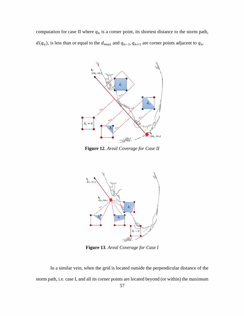
57

computation for case II where 𝑞𝑛 is a corner point, its shortest distance to the storm path,

𝑑(𝑞𝑛), is less than or equal to the 𝑑𝑚𝑎𝑥 and 𝑞𝑛−1, 𝑞𝑛+1 are corner points adjacent to 𝑞𝑛.

Figure 12. Areal Coverage for Case II

Figure 13. Areal Coverage for Case I

In a similar vein, when the grid is located outside the perpendicular distance of the

storm path, i.e. case I, and all its corner points are located beyond (or within) the maximum

58

distance, 𝑑𝑚𝑎𝑥, then the grid’s areal coverage, 𝐴, is merely 0 (or 1). However, if the grid

is partially within the maximum distance (e.g., 1, 2, or 3 of its corner points are less than

or equal to 𝑑𝑚𝑎𝑥), we can again compute 𝐴 using basic geometry. Figure 13 illustrates

these subcases.

Figure 14. Case I with (a) 1, (b) 2, or (c) 3 Corner Points Located Within 𝑑𝑚𝑎𝑥

Constraints (4.8) through (4.10) show the computation for areal coverage in case I

where �̃�𝑖1, �̃�𝑖

2, and �̃�𝑖3 are area in which 1, 2, or 3 corner point(s) are within 𝑑𝑚𝑎𝑥 from the

storm start/end location (see Figure 14). Akin to case II, 𝑞𝑛 is a corner point in which its

shortest distance to storm trajectory, 𝑑(𝑞𝑛), is less than or equal to the preset 𝑑𝑚𝑎𝑥 and

𝑞𝑛−1, 𝑞𝑛+1 are corner points adjacent to 𝑞𝑛. Additionally, we define 𝑑(𝑎, 𝑏) as distance

between point 𝑎 and 𝑏 , and introduce two dummy points, namely 𝑝𝑡1 and 𝑝𝑡2 . In

constraints (4.8), we set 𝑝𝑡1 = (𝑥𝑞𝑘 , 𝑦𝑠) and 𝑝𝑡2 = (𝑥𝑠, 𝑦𝑞𝑘). In constraints (4.9), these

dummy points are set as 𝑝𝑡1 = (𝑥𝑠, 𝑦𝑞1) and 𝑝𝑡2 = (𝑥𝑠, 𝑦𝑞2) if 𝑑(𝑞1) and 𝑑(𝑞2) are within

𝑑𝑚𝑎𝑥 , 𝑝𝑡1 = (𝑥𝑞2 , 𝑦𝑠) and 𝑝𝑡2 = (𝑥𝑞3 , 𝑦𝑠) if 𝑑(𝑞2) and 𝑑(𝑞3) are within 𝑑𝑚𝑎𝑥 , 𝑝𝑡1 =

59

(𝑥𝑠, 𝑦𝑞3) and 𝑝𝑡2 = (𝑥𝑠, 𝑦𝑞4) if 𝑑(𝑞3) and 𝑑(𝑞4) are within 𝑑𝑚𝑎𝑥, and 𝑝𝑡1 = (𝑥𝑞4 , 𝑦𝑠) and

𝑝𝑡2 = (𝑥𝑞1 , 𝑦𝑠) if 𝑑(𝑞4) and 𝑑(𝑞1) are within 𝑑𝑚𝑎𝑥. Lastly, in constraints (4.10), we set

𝑝𝑡1 = (𝑥𝑞𝑘′ , 𝑦𝑠) and 𝑝𝑡2 = (𝑥𝑠, 𝑦𝑞𝑘

′ ) where 𝑞𝑘′ is a corner point in which its shortest

distance to storm trajectory, 𝑑(𝑞𝑛), is greater than the preset 𝑑𝑚𝑎𝑥.

Constraints (4.3) ensure that the forecaster’s confidence decreases when a location

is further away from the storm center in one scenario than another. As can be seen in Figure

15, it is unrealistic for location 𝑖 to have any precipitation (e.g., 𝑄𝑃𝐹𝑖,𝑡|𝑠 > 0 ) when

precipitation is not expected to occur (e.g. 𝑃𝑜�̂�𝑖,𝑡|𝑠 = 0). Thus, constraints (4.4) introduce

a QPF-based lower bound to assure PoP can be nonnegative only when QPF is nonnegative.

The QPF-PoP relation is modeled as Bleasdale-YD regression using CurveExpert 2.1.0.

which takes the following form: 𝑦 = 𝑥(𝑎 + 𝑏𝑥𝜃) exp(−1/𝜃) where 𝑦 is the PoP, 𝑥 is the

QPF, and 𝑎, 𝑏, and 𝜃 are constants with values of 2.7612, 6.4134, and 0.2127, respectively.

Finally, constraints (4.5) bound the forecasters confidence to be between 0 and 1.

Figure 15. Relationship Between PoP and QPF

60

4.4.3. Storm Surge Probability Models

Storm surge is primarily caused by the relationship between a storm’s winds and the

ocean’s surface. The force of the winds pushes the water in the ocean toward the shore.

This rise of water can reach heights over 20 feet, span hundreds of miles of coastline, and

travel several miles inland (NWS, 2015). Storm surge is affected by the storm’s intensity,

its angle of approach, width and slope of the continental shelf, and local features (NOAA,

2008; NWS, 2015). Larger and faster storms produce higher surge. Lower pressure also

produces higher surge, but its contribution is minimal. The angle at which the storm

approaches a coastline determines the amount of surge generated and its height. Storms

that move onshore perpendicular to the coast produce higher surge than the ones that move

parallel or landfall at small oblique angles. Moreover, landfall on a concave coastline with

a gulf like feature results in higher surge as opposed to landfall on a convex coastline.

Hurricane-induced storm surge is the severe threat to life and property especially of the

coastal communities.

Over the past years, large amount of deaths and transportation infrastructure

damages in the coastal area are resulted from storm surge. As storm surge can cause severe

flooding and damages particularly in the coastal areas and areas surrounding rivers and

streams (NOAA, 2008), information to predict the likelihood of water above any selected

height is vital. What could happen (e.g., surge height) and how likely it is to occur are of

interest to emergency officials since these can enhance the guidance for evacuation and

other response operations. We introduce the component model to estimate the scenario-

level probability of storm surge exceeding a given height. Figure 16 illustrates the storm

surge probability algorithm.

61

Figure 16. The Storm Surge Probability Algorithm

Sets


Ψ = a set of regions (B, M, T)

𝐾 = a set of surge heights (ft)

Χ = a set of hurricane positions (start, end)



Parameters

𝑃𝑆𝑆𝑘,𝑖,𝑡 probability of location 𝑖 is expected to have surge height of at least 𝑘 during

time 𝑡


𝜃𝑖,𝑡|𝑠 angle between location 𝑖 and storm direction during time 𝑡 in scenario 𝑠

𝜉𝑖,𝑡|𝑠 weight factor location 𝑖 during time 𝑡 in scenario 𝑠

(to represents probability-distance relationship, e.g., polynomial regression)

Decision Variables

�̂�𝑘,𝑖,𝑡|𝑠 probability of location 𝑖 is expected to have surge height of at least 𝑘 during

time 𝑡 in scenario 𝑠

Other Variables

𝑃𝑆�̂�𝑘,𝑖,𝑡|𝑠 estimated probability of surge height of at least 𝑘 at location 𝑖 during time 𝑡

in scenario 𝑠

62

Model 5 (estimating storm surge probability)

min ∑ ∑ ∑ [∑ 𝑝𝑠𝑠∈𝑆 𝑃𝑆�̂�𝑘,𝑖,𝑡|𝑠 − 𝑃𝑆𝑆𝑘,𝑖,𝑡]2

𝑘∈𝐾𝑖∈𝐼𝑡∈𝑇 (5.1)

subject to

(1 + |𝑐𝑜𝑠(𝜃𝑖,𝑡,𝑠)|)�̂�𝑘,𝑖,𝑡|𝑠 − 𝑃𝑆�̂�𝑘,𝑖,𝑡|𝑠 = 0, ∀𝑘 ∈ 𝐾, 𝑖 ∈ 𝜓𝑇 , 𝑡 ∈ 𝑇, 𝑠 ∈ 𝑆

(5.2)

�̂�𝑘,𝑖,𝑡|𝑠 − 𝑃𝑆�̂�𝑘,𝑖,𝑡|𝑠 = 0, ∀𝑘 ∈ 𝐾, 𝑖 ∉ 𝜓𝑇 , 𝑡 ∈ 𝑇, 𝑠 ∈ 𝑆 (5.3)

𝜉𝑖,𝑡|𝑠�̂�𝑘,𝑖,𝑡|𝑠(𝑛) − 𝜉𝑖,𝑡|𝑠�̂�𝑘,𝑖,𝑡|𝑠(𝑛+1) ≥ 0, ∀𝑘 ∈ 𝐾, 𝑖 ∈ 𝐼, 𝑡 ∈ 𝑇, 𝑠 ∈ 𝑆

where 𝑑𝑖,𝑡|𝑠(1) ≤ ⋯ ≤ 𝑑𝑖,𝑡|𝑠(𝑛) ≤ 𝑑𝑖,𝑡|𝑠(𝑛+1) ≤ ⋯ ≤ 𝑑𝑖,𝑡|𝑠(4)

(5.4)

𝑃𝑆�̂�𝑘,𝑖,𝑡|𝑠 − 𝑃𝑆�̂�𝑘+1,𝑖,𝑡|𝑠 ≥ 0, ∀𝑘 ∈ 𝐾, 𝑖 ∈ 𝐼, 𝑡 ∈ 𝑇, 𝑠 ∈ 𝑆 (5.5)

0 ≤ �̂�𝑘,𝑖,𝑡|𝑠 ≤ 1, ∀𝑘 ∈ 𝐾, 𝑖 ∈ 𝐼, 𝑡 ∈ 𝑇, 𝑠 ∈ 𝑆 (5.6)

0 ≤ 𝑃𝑆�̂�𝑘,𝑖,𝑡|𝑠 ≤ 1, ∀𝑘 ∈ 𝐾, 𝑖 ∈ 𝐼, 𝑡 ∈ 𝑇, 𝑠 ∈ 𝑆 (5.7)

The objective (5.1) minimizes the prediction errors of the model by regulating value

that decision variable, �̂�𝑘,𝑖,𝑡|𝑠, can take. As storm’s approach angle affects storm surge, we

first outline the geographic position of location 𝑖 in period 𝑡 with respect to the storm

center using a simplified version of the configuration used in the precipitation models.

Define, above (T), below (B), and along the path (M) as the three positions location 𝑖 could

be with respect to the storm’s track (see Figure 17). Location that is positioned below (B)

or along the storm’s path (M) suggests that it is at an oblique angle or parallel to the storm

direction, respectively. Location that is positioned in front of the storm (T) is, however, at

an acute angle and more likely to receive higher surge. Again, a cosine-based-function 1 +

|𝑐𝑜𝑠(𝜃𝑖,𝑡,𝑠)| is introduced to determine weight factor so that locations positioned at acute

angles have higher chance of receiving storm surge than the ones at obtuse angles. The

computations are represented by constraints (5.2) and (5.3). Other factors such as width

and slope of the continental shelf and local features affect the storm surge. As we were

evaluating predictions for Hurricane Irma over the State of Florida which has significantly

flat topography and the scenarios occur over nearly identical surfaces, at this point in our

63

modeling efforts we ignored physical features in surge prediction model. Thus, the storm’s

approach angle becomes the main factor considered in estimating the scenario-level storm

surge probability.

Figure 17. Illustration of Grid’s Possible Positions with Respect to Storm Trajectory

Constraints (5.4) ensure that scenario-level storm surge probability of location 𝑖

reflects its relative distance to the storm center and is represented as 𝜉𝑖,𝑡|𝑠 . That is, if

location 𝑖 is closer to the storm center in scenario 𝑠(𝑘) than in scenario 𝑠(𝑘+1), then its surge

probability cannot be less than the surge probability in scenario 𝑠(𝑘+1). The 𝜉𝑖,𝑡|𝑠 can be

estimated using polynomial regression, 𝑦 = 𝑎 + 𝑏𝑥 + 𝑐𝑥2 + 𝑑𝑥3 + 𝑒𝑥4 where 𝑦 is the

storm surge probability, 𝑥 is the relation distance, and 𝑎, 𝑏, 𝑐, 𝑑, and 𝑒 are 0.38 ,

−2.84 × 10−3 , 9.61 × 10−6 , −1.24 × 10−8 , and 5.29 × 10−12 , respectively. This

regression model is obtained from CurveExpert 2.1.0. Note that the relationship between

surge probability and distance to the storm path is not apparent (see Figure 18) which

implies that other contributing factor(s) may exist and ought to be considered when

64

determining the storm surge probability. Constraints (5.5) guarantee that scenario-level

surge probability always decreases as its height increases. Finally, constraints (5.6) and

(5.7) limit the probability values to be in the [0,1] range.

Figure 18. Relationship Between Relative Distance and Surge Probability

4.5. Hurricane Irma Empirical Results

4.5.1. Hurricane Irma Overview

The National Hurricane Center (NHC) products contain significant information on winds,

hurricane watches and warnings but not on precipitation and storm surge. The NHC

forecast advisory provides impacts of precipitation and storm surge only in terms of

locations and expected flood heights for selected coastal and inland cities. The NHC wind

speed probability product contains both cumulative (overall chances of occurrence during

the specified cumulative forecast period) and onset (chances of occurrence during the

specified forecast period) wind speed probabilities (in percentage) of at least 34-kt (tropical

storm force winds), 50-kt (storm force winds), or 64-kt (hurricane force winds) (NHC,

65

2014). In the case of Hurricane Irma, only major cities in Florida are listed in the NHC

products which results in spatially sparse information on storm hazards over Florida. Thus,

we use the NHC products only to determine the scenario probabilities. The wind speed,

precipitation, and storm surge models were then fitted using higher resolution datasets from

National Weather Service (NWS) corresponding to the NHC advisories.

NWS gives weather, water, and climate forecasts and warnings for the United

States, its territories, adjacent waters, and ocean areas; these are used by governmental

agencies such as the NHC, private sector, and the public (NWS, 2019b). Its National

Digital Forecast Database or NDFD provides more comprehensive weather data. The

NDFD is a publicly available suite of gridded forecasts of weather elements in much finer

spatial-temporal resolution of 2.5 km by 2.5 km grid for the contiguous United States at 3-

hour or 6-hour intervals depending on the weather attributes of interest (NWS, 2003). Its

service quality is controlled by NOAA and its database is regularly validated by the NWS

verification team (S. H. Kim & Augenbroe, 2012). The NDFD weather data corresponding

to Hurricane Irma advisories is used to test the wind speed and precipitation models.

Sea, Lake, and Overland Surges from Hurricanes (SLOSH) model is another

product from NWS that estimates storm surge heights resulting from predicted hurricanes’

track, size, forward speed, and intensity data (NHC, 2016b). The NHC uses the SLOSH to

forecast storm surge and to estimate storm surge vulnerability in advisories approximately

48 hours before potential surge occurrence for areas along the Gulf and Atlantic coasts. P-

Surge is a publicly available graphical product developed by the Meteorological

Development Laboratory (MDL) of the NWS, in cooperation with the NHC, that gives

probabilistic forecasts of hurricane storm surge. It is an ensemble model that uses storm

66

surge values produced by SLOSH to provide the emergency managers, government

agencies, and general public with probabilistic storm surge information, which could

enhance their ability to make emergency preparedness decisions due to storm surge (NHC,

2016c; NWS, 2016). The P-Surge model generates two products, exceedance (maximum

height (in feet) that will be exceeded by a given percentage) and probability (likelihood of

water above any selected height at any selected location, in terms of incremental water

level increase for every time step, e.g., 6-hour intervals) (Taylor & Glahn, 2008). What

could happen (e.g., surge height) and how likely it is to occur are in the best interest of

emergency officials since these can enhance the guidance for evacuation. The developed

storm surge model was fitted using P-Surge dataset, particularly with respect to surge

height probability, corresponding to the NHC advisories for Hurricane Irma.

The simulation model aims to generate scenario-level prediction of storm impacts

over the State of Florida for Hurricane Irma. A total of 52 NHC forecast advisories were

issued for Hurricane Irma. The NHC forecast advisory number 30 was the first advisory

where cities in Florida were predicted to experience wind speed with probability of at least

0.10 at 72-hour. The NHC advisory number 50 was the last advisory where cities in Florida

were predicted to experience high wind speed at time 6-hour. Hence, NDFD dataset

corresponding to the NHC advisory number 30 to 50 were used to test wind speed and

precipitation models. Since the storm surge information is only available approximately 48

hours prior to the storm’s arrival, no P-Surge dataset corresponding to NHC advisory

number 30 to 33 were available. Thus, the storm surge model was fitted to P-Surge dataset

corresponding to NHC advisory number 34 to 50.

67

Throughout testing the simulation model, we assumed four potential storm tracks

(i.e., scenarios) to represent the full range of potential hurricane paths in each advisory that

make up the cone of uncertainty shown by NHC. The cone of uncertainty represents the

probable tracks of the center of a cyclone and is formed by enclosing the area swept out by

a set of circles along the forecast track which provides a reasonable approximation for

determining the area likely to be affected by the storm (NHC, 2018a). These tracks were

used as a design alternative in our simulation model and could easily be, but time tediously,

extended to higher numbers to simulate with greater fidelity. if deemed necessary. The four

tracks consist of one track from NHC forecast advisory, with a slight modification to meet

uniformity on the time interval among all weather forecast data, and three hypothetical

tracks constructed based on the cone of uncertainty provided in the NHC graphic products.

All other storm information such as storm size, intensity, forward speed, and maximum

sustained wind speed were retrieved directly from the NHC forecast advisory.

According to Cangialosi (2017), the NHC probabilistic forecasts for the 2017

Atlantic hurricanes, for up to 48 hours are quite reliable and well calibrated but slight bias

on the low side for 120-h probabilities forecasts. For Hurricane Irma, the model’s errors

for 96-h and 120-h forecasts were larger than its 5-year averages (J. Cangialosi et al., 2018).

Thus, we limited the time horizon to three days (72 hours) at 6-hour intervals. The spatial

resolution for a location was chosen to be 0.250 by 0.250 grid which is equivalent to

approximately 27-28 km grid in contrast to the finer 2.5 km by 2.5 km NDFD grid. This

reduced the number of grids in our forecasting from 7463 to 511 for the State of Florida,

which lessens the model’s runtime. It is possible to directly use the NDFD grids if finer

resolution is preferable, but it will require more computing resources and longer runtimes.

68

4.5.2. Scenario Probabilities

These probabilities were computed by running Model 1 and Model 2 on NHC wind speed

dataset retrieved from the NHC wind speed probability product for advisory number 30 to

50. Twenty-six cities in Florida were considered as those are listed in the NHC products.

The time intervals were set to be 0-12, 12-24, 24-36, 36-48, and 48-72 hour to comply with

the NHC wind speed probability data. The average runtime was 70 seconds for the two

models to converge to the optimal solution. More iterations and longer runtimes as the size

of dataset increases as can be seen for advisories 40 to 46 (see Table A.1 in Appendix A).

4.5.3. Scenario-level Storm Impacts

The wind speed and precipitation models were fitted to NDFD dataset corresponding to

NHC advisories 30 to 50 (see Table A.2). The average runtime for the wind speed (WS)

model was 16.5 seconds with error rate of 1.486 x 10-5.

The NDFD dataset for precipitation quantity (QPF) is truncated for some advisories,

e.g., QPF data are available only for up to 54-hour for advisory number 39. Upon

observation, weather forecast data between advisories for the same time interval do not

differ much. Hence, we use weather data from the subsequent advisories to replace these

missing data. For instance, we use 60-66 h QPF data in advisory 40 to fill in the 54-60 h

missing data in advisory 39, and so on. The average runtime of the QPF model was 463

seconds with mostly (77%) is contributed to the preprocessing activity of creating rainfall

intensity graphs for each possible storm center location. The average SSE of the QPF model

was 10.31 as we set the penalty factor, 𝜁𝑖,𝑡, in the objective function of QPF model to be

1/𝑄𝑃𝐹𝑖,𝑡 . This average may seem large; however, this is due to the setting of 𝜁𝑖,𝑡 that

allows value of the squared error to be up to its actual QPF which ranges from 0 to 7 inches.

69

No missing data was encountered in the NDFD dataset for precipitation probability (PoP);

however, it is at 12-hour interval. Thus, we assumed the precipitation probability at 0-6 h

and precipitation probability at 6-12 h are same as the precipitation probability at 0-12 h.

The model’s average runtime was 15 seconds with fitting SSE error on the average of 0.97.

The storm surge model was fitted using a 17-instance P-Surge dataset

corresponding to NHC advisories 34 to 50 under similar settings. Considering storm surge

occurs only on coastal areas and areas surrounding rivers and streams, we removed

locations that do not fall into any of these two regions and resulted in a total of 186 grids

instead of 511 grids to be evaluated. The maximum height was preset to 10 feet as the

probability of surge height greater than 11 feet were all zeroes for Hurricane Irma. Table

A.2 includes the fitting errors and runtimes for the storm surge probability model. The

average runtime was 34.4 seconds with fitting error of 0.1392. See Table 4 for the summary

of the average error rates and runtimes for each component model.

Table 4. The SSE and Runtime of the Component Models

Average

WS

(wind

speed)

QPF

(precipitation

quantity)

PoP

(precipitation

probability)

SS

(storm surge)

SSE 16.5 463 15 34.4

Runtime 1.486 x 10-5 10.31 0.97 0.1392

4.5.4. Visualization

Three types of visualization comparisons were considered: visualization with respect to (a)

spatial coverage between scenarios, (b) spatial coverage of impact levels within scenario –

applicable only for wind speed and storm surge, and (c) spatial residual plots. The

70

visualization on spatial coverage between scenarios aims to assure that coverage area

between scenarios are not identical. Visualization of impacts within scenario aims to ensure

that coverage area shown decreases as the storm impact level increase. That is, spatial

coverage of the 34-kt wind speed should include and no less than the coverage of the 50-

kt wind speed. Rainbow color scheme was used in these visualizations where shades of

green represent low values and shades of red represent high values. As residual can be

positive or negative, the spatial residual plot allows us to pinpoint locations with positive

or negative residuals, that cannot be discovered through SSE alone. Note that, positive

residuals over land in Florida are much of our interest as opposed to residuals over the sea

where infrastructure damages are low. Divergence color scheme was used to allow quick

identification on locations with positive residual (i.e. colored with blue shades), negative

residuals (i.e. colored with red shades), or close to no errors (i.e. white).

We performed visualization comparison of all storm impacts for NHC advisory 40.

The visualization with respect to spatial coverage of impacts levels within scenario showed

no anomality. That is, the probability values decrease as its impact level increases. See

Figure 19 and Figure 20 for examples of spatial coverage of impact levels within scenario

3 at 36-42-hour of wind speed probability (e.g., 34-kt, 50-kt, and 64-kt wind speed) and

storm surge probability (e.g., 1-ft, 2-ft, 3-ft, 4-ft, and 5-ft), respectively.

71

Figure 19. 34-kt, 50-kt, and 64-kt Wind Speed Probabilities in Scenario 3

Figure 20. 1-ft, (b) 2-ft, (c) 3-ft, (d) 4-ft and (e) 5-ft Surge Probability in Scenario 3

The visualization of spatial coverage between scenarios also shows that the

coverages were not identical. For the same time step, i.e. 36-42-hour, in advisory 40,

Figure 21, Figure 22, Figure 23, and Figure 24 are examples of spatial coverage between

scenarios visualization for 34-kt wind speed probability, precipitation quantity (QPF),

precipitation probability (PoP), and 1-ft storm surge probability, respectively.

Figure 21. 34-kt Wind Probability in Scenario (a) 1, (b) 2, (c) 3, and (d) 4

72

Figure 22. QPF in Scenario (a) 1, (b) 2, (c) 3, and (d) 4

Figure 23. PoP at 36-42 h in Scenario (a) 1, (b) 2, (c) 3, and (d) 4

Figure 24. 1-ft Surge Probability in Scenario (a) 1, (2) 2, (c) 3, and (d) 4

The spatial residual plot of the wind speed model shows no location with positive

nor negative residuals over the time horizon. These results had very low SSE values (see

Table A.2) and the fact that no distortion was observed with respect to associated residual

analysis plots. Figure 25 gives example of residual plots of 34-kt wind speed probability

73

at 36-42-hour. Figure A.1 and Figure A.5 in the Appendix A give all spatial residual plots

and residual analysis plots of 34-kt wind speed.

(a)

(b)

Figure 25. (a) Spatial Residual and (b) Fitted-Actual Plots of 34-kt Wind Probability

In the spatial residual plot for the QPF model fitting, some locations with positive

residuals, shown with shaded grids in blue were observed during 6-hour intervals 30-36,

36-42, 54-60, and 60-66-hour and were mostly located above the sea. In the 60-66-hour

interval in Figure 26(a), few locations have positive residual values up to 0.10 to 0.25 inch.

This may seem like a large difference, but the values correspond to at most 5% error in the

actual data (e.g., 0.23-inch when its actual data is 5 inches corresponds to less than 5%

error). In compliance with these results, only little distortion was observed in the residual

analysis plots of QPF. Figure 26(a) and Figure 26(b) show examples of the spatial residual

plot and fitted-actual forecast data plot at 60-66-hour interval, respectively. Figure A.2 and

Figure A.6 give the spatial residual plot and residual analysis plot for QPF forecasts.

74

(a)

(b)

Figure 26. (a) Spatial Residual and (b) Fitted-Actual Plots of QPF at 60-66 h

Some locations with negative residuals (shown shaded grid in red) were observed

in the spatial residual plots of the PoP, but then again, these locations were over the sea,

and therefore these errors were not crucial. Figure 27 shows the spatial residual plot and

fitted-actual plot of PoP for the same time step, 60-66-hour. Figure A.3 and Figure A.7 in

the Appendix A give all spatial residual plot and fitted-actual plot, respectively.

(a)

(b)

Figure 27. (a) Spatial Residuals and (b) Fitted-Actual Plots of PoP at 60-66 h

75

With respect to surge probability, some locations with positive residuals were

observed during 6-hr intervals 24-30, 30-36, 36-42, 42-48, and 48-54 h, with majority of

them are also being over the sea. Figure 28 shows the spatial residual plot and residual

analysis plot of 1-ft storm surge probability at time step 36-42-hour. We suspect the

presence of these residuals is due to the independence assumption on the relationship

between (i) distance to the storm center and angular position of the location of a grid square,

and (ii) surge probability. Alike, Figure A.4 and Figure A.8 in the Appendix give all spatial

residual and fitted-actual plots, respectively. The complete visualization of the spatial

residual plots and fitted-actual plots of wind speed probability, QPF, PoP, and storm surge

probability are given in Appendix A.

(a)

(b)

Figure 28. (a) Spatial Residuals and (b) Fitted-Actual Plots of Storm Surge at 36-42 h

76

4.6. Conclusions on the Probabilistic Simulation Model

Short-notice sudden onset natural disaster such as hurricane are laden with uncertainties.

Discounting these uncertainties when forming response strategies and operations can

substantially deteriorate their overall effectiveness because such disasters commonly can

cause substantial level of devastation and damages over space and time.

A data-driven probabilistic simulation model proposed in this dissertation aims to

generate spatial-temporal storm predicted impacts, e.g., wind speed probability,

precipitation quantity and probability, and storm surge height probability, for each assumed

storm trajectory. This simulation model also estimates the probabilities of occurrence of

each scenario which are not directly provided in the available public forecasts. The model

was verified and validated by testing it on dataset of for our Hurricane Irma case study.

The results demonstrate that the storm impacts are generated accurately with short runtimes.

Local officials and other emergency decision makers can utilize such simulation models to

generate weather forecast profiles for all potential trajectories (scenarios) for improving

decisions for response operations.

77

5. CASCADING NETWORK FAILURE ALGORITHMS


The network consists of 𝑛 nodes and 𝑚 arcs. Nodes represent incorporated places, for

example, cities, towns, municipalities, and census-designated places. The attributes of a

node include geographic (e.g., latitude, longitude, and elevation) and demographics (e.g.,

population count, household, number of vehicles per households, and housing year built).

Google Maps application is utilized to determine the location and the demographics data

is retrieved from the 2017 American Community Survey (US Census Bureau, 2019).

Arcs represent major, arterial, and connector roads which include interstate

highways, turnpikes and most other toll roads, U.S. Routes, and State Roads (FDOT, 2013).

The arc’s elevation is assumed to be within the range of the elevations of its two end nodes,

that is, no “valley” arc. The attributes of an arc include its two end nodes, maximum

capacity, length, and average travel speed without traffic. The maximum capacity is

estimated based on the number of lanes and road type (e.g., interstate, US routes, state

roads, county roads). Google Maps application can again be used to determine these arc

attributes. As the predicted storm hazards are at the grid level, their effect on nodes (and

arcs) are determined based on the grid(s) in which these nodes (and arcs) reside. An

algorithm, not discussed in here, is introduced to determine the grid where the node (and

arc) is located.

During a storm event, uncertainty is largest with respect to the consequences for

wind strengths, precipitation patterns, and surge heights. Disclosing changes in the

transport network and its uncertainty due to these storm impacts could avoid a later loss of

78

credibility if actual result proved to be significantly different from the estimated results.

Hence, in this part of the dissertation, we propose a cascading network failure model that

takes the storm impacts predictions from the simulation model to predict changes in the

transport network while simultaneously determines the demand for population movement

and potential destinations.

5.2. Overview of Approach to Model Cascading Network Failures

The approach begins with predicting the change in the transport network upon considering

individual storm impact and then assimilate them to generate the predicted overall impacts

over the time horizon. In here, we assume the coming hurricane is a 24-hour 100-year storm

event and its attributes and associated hazards over the study area at every time step are

available. We also assume that the predicted storm hazards are independent of each other.

There are two possible cases: threshold case and probabilistic case, are considered. In the

threshold case, the algorithm takes a preset threshold value for an impact to be considered

significant. Its output is a deterministic spatial-temporal mobility states, for example, a

node is safe or unsafe and an arc is traversable at normal, reduced, or zero capacity. In the

probabilistic case, the mobility states are expressed in a form of piecewise function with

probability of occurrences (e.g. probability of a node being safe, probability of an arc being

traversable at normal, reduced, or zero capacity). Outputs from the network failure model

is the probabilistic predicted changes in the transport network states over time. Emergency

responders can use the resulting network as basis in developing or evaluating their response

operation models. See Figure 29 for the schematic illustration of the cascading network

failure approach.

79

Figure 29. The Cascading Network Failure Modeling Approach

5.3. Storm Impact Algorithms

The algorithm is comprised of three sub-algorithms, each generates the individual spatial-

temporal predicted impact (i.e. wind, precipitation, storm surge), and one sub-algorithm

that assimilates the individual impacts to generate the overall storm impacts unto the

network. These sub-algorithms will be discussed separately in the following sequence: the

algorithm for 1) wind speed impact, 2) rain impact, 3) storm surge impact, and 4) overall

storm impacts. We utilize Naylor and Finger’s 3-step approach to validate the algorithm.

In the face validation, we use visualization comparison and reasonableness of the outputs,

data source reliability and statistical distribution for assumption validation, and the

visualization comparison for spatial aspect for the input-output validation.

5.3.1. Wind Impact

High winds commonly occur during strong weathers, such as hurricanes. When the 1-

minute average surface winds are sustained at least 40 mph or 34.8 knots for one hour or

longer, the National Weather Service (NWS) issues high wind warnings and watches as

any unsecured outdoor objects could easily blow away and cause damage or injury (NHC,

80

2018b). Damages caused by the high winds include downed trees and power lines, building

or structure collapses, and flying debris. These wind damages lead to transportation

disruptions, power outage, uninhabitable places, and injury or death – altering the state of

both nodes (i.e. safe or unsafe) and arcs (i.e. traversable or not) in the transport network.

Recall that a node represents a city, town, village, or census-designated place. A node is

unsafe when buildings and structures in the node are expected to be damaged by the high

wind. That is, the predicted maximum sustained wind speed (MWS) exceeds the wind

design speed of the buildings and structures, commonly referred to as the ultimate design

wind speed, 𝑉𝑢𝑙𝑡 , which its value can be obtained from the state’s building code. This

building code regulates all buildings or structure, or any appurtenances connected or

attached to such buildings or structures and is based on the national model building codes

and national consensus standards. For example, Florida Building Code provides discussion

in detail about the design wind speed for buildings and structures that fall in each risk

category. By assuming that all buildings and structures in the nodes comply with the code,

we can determine the respective 𝑉𝑢𝑙𝑡 accordingly.

To determine the maximum wind speed (MWS) in a node, we first define the

hurricane winds’ radial structure which can be represented using piecewise continuous

wind profiles (Kossin et al., 2007; Willoughby, Darling, & Rahn, 2006). That is, inside the

eyewall, wind increases in proportion to a power of radius while outside the eyewall, the

wind decays exponentially. As the strongest wind within the storm occurs at the eyewall,

a node that is located inside the eyewall, at any moment as the storm moves, is expected to

experience the maximum wind speed. A node that is located outside the eyewall, the MWS

can be estimated using exponential decay function. Let 𝑥 be the distance to the storm center

81

and 𝑦 be the wind speed. Note that, the radius of 64-kt or 𝑅64 and MWS can be retrieved

from the National Hurricane Center (NHC) forecast advisory (NHC, 2016a) whereas the

radius of the maximum wind, 𝑅𝑚𝑎𝑥 , can be computed using equation in Quiring et al.

(2011). Using these two (𝑥, 𝑦) points (𝑅𝑚𝑎𝑥, 𝑀𝑊𝑆) and (𝑅64, 64), we can generate the

decay function by substituting the 𝑥 and 𝑦 of the two points into the equation 𝑦 = 𝑎𝑥𝑏 and

solving for the parameters 𝑎 and 𝑏. The maximum wind speed that a node is expected to

experience can be computed based on its radial distance to the storm center.

We define, in the “threshold” case, a node is unsafe only if the following two

conditions are met: (1) the maximum wind speed exceeds the design speed, i.e. 𝑀𝑊𝑆 ≥

𝑉𝑢𝑙𝑡, and (2) the probability of wind speed exceeds 64 knots exceeds the threshold value 𝛼,

i.e. 𝑃(wind speed ≥ 64𝑘𝑡) > 𝛼 . Otherwise, we claim that the node is safe. In the

“probabilistic” case, we define the probability of a node being unsafe as the probability of

wind speed exceeds 64 knots when the predicted maximum wind speed value exceeds its

design speed, 𝑃(node is unsafe) = 𝑃(wind speed ≥ 64𝑘𝑡,𝑀𝑊𝑆 ≥ 𝑉𝑢𝑙𝑡). In summary,

when 𝑀𝑊𝑆 ≥ 𝑉𝑢𝑙𝑡 , the probability of a node is safe, 𝑃(node is safe) = 1 −

𝑃(wind speed ≥ 64𝑘𝑡,𝑀𝑊𝑆 ≥ 𝑉𝑢𝑙𝑡) and when the 𝑀𝑊𝑆 < 𝑉𝑢𝑙𝑡, then the node is safe,

i.e. 𝑃(node is safe) = 1, regardless of the value of the 64-kt wind speed probability.

High winds can play a major role in vehicle operations as it can decrease their

stability and control. As tropical storm-force winds (34-kt) are strong enough to be

dangerous, evacuation process are commonly terminated before the onset of the tropical

storm-force winds (NHC, 2015; Wolshon et al., 2005). The federal highway regulation

regulates bridge closure when the sustained wind speed blowing across reaches 39 mph or

34 knots (I-95 Corridor Coalition, 2013). Based on these facts, an arc can be either

82

traversable or untraversable. In the “threshold” case, if the probability of wind speed of at

least 34 knots blowing across the arc exceeds the threshold value 𝛼 (i.e. 𝑃(wind speed ≥

34𝑘𝑡) > 𝛼 ), then the arc is untraversable. Whereas in the “probabilistic case”, the

probability of an arc being untraversable is the 34-kt wind speed probability itself. See

Figure 30 for the illustration and Table 5 for the summary of the wind impact algorithm.

Figure 30. The Algorithm of Wind Speed Impacts on the Transport Network

Table 5. Wind Impacts on the Transport Network

“Threshold” case:

Node state (𝑖) = {1, otherwise 0, if 𝑃(wind ≥ 64 kt) ≥ α and MWS ≥ V𝑢𝑙𝑡

Arc cap (𝐿𝑖𝑗) = {1, if 𝑃(wind ≥ 34 kt) < α0, otherwise

“Probabilistic” case:

Node 𝑃(state (𝑖) = 1) = 1 − 𝑃(wind ≥ 64 kt,MWS ≥ Vult)

𝑃(state (𝑖) = 0) = 𝑃(wind ≥ 64 kt,MWS ≥ Vult)

Arc 𝑃(cap (Lij) = 1) = 1 − 𝑃(wind ≥ 34 kt)

𝑃(cap (Lij) = 0) = 𝑃(wind ≥ 34 kt)

83

As an arc can reside across several grids, in the “threshold” case, we define an arc

is untraversable if it is untraversable in at least one of its segments. For example, if arc 𝐿𝑖𝑗

is in grid {𝐺1, 𝐺2}, then arc 𝐿𝑖𝑗 is traversable only if it is traversable in both grids. In the

“probabilistic” case, we use pessimistic approach and set the probability of arc 𝐿𝑖𝑗 being

untraversable as the maximum of its probability being untraversable over all segments.

𝑃(𝐿𝑖𝑗 untraversable) = max{𝑃(𝐿𝑖𝑗 untraversable|𝐺1), 𝑃(𝐿𝑖𝑗 untraversable|𝐺2)}.

5.3.2. Rain Impact

Potential roadway flooding comes from storm surge for coastal areas and torrential

rain for inland areas. Rain of any intensity decreases traffic speed and roadway capacity

which result in higher crash risk and increase in travel time. Heavy rain in particular can

produce very low visibility, lane submersion, flooded underpasses, and damage to roadbeds

(Pisano et al., 2001) altering the state of both nodes (i.e. safe or unsafe) and arcs (i.e.

traversable at normal attribute value, traversable at reduced attribute value, or

untraversable) of the transport network.

A node is considered unsafe if flooding due to torrential rain is expected to occur.

That is, the predicted rainfall intensity 𝑟 exceeds the design storm drains 𝜔 of the node.

The storm drain is designed to drain excess rain and ground water from impervious surfaces

(Chow, Maidment, & Mays, 2003). Plumbing section in the state’s building code provides

discussion on storm drainage that is based on 100-year hourly rainfall rate (in inches/hour).

Hence, assuming the drainage system of the nodes comply with the plumbing regulation

listed in the building code, we can specify the storm drains of the nodes in the network

according to their whereabouts.

84

The available spatial-temporal rainfall data is in the form of precipitation amount

(QPF) expected to fall in a 6-hour interval (inches/6-hour), while the storm drains discharge

rate is at hourly interval (inches/hour). To match the units, we need to convert the 6-hour

QPF to hourly rain rate. One option is by assuming that the QPF value is uniformly

distributed within the 6-hour interval, but this approach underestimates the maximum

rainfall rate which is critical in determining potential flooding of an area. The other possible

approach is to utilize design storm to create distribution of rainfall intensity over the time

horizon. Design storm represents storm precipitation pattern where its amount corresponds

to rare frequencies (i.e. “worst case scenario”). It is constructed based upon historical

precipitation data or general characteristics of precipitation in the surrounding regions

(USDA-NRCS, 2015). The design storm is used in the design of hydrologic systems in

most jurisdictions in the United States. It can be defined by a design hyetograph, an

isohyetal map, or a value for precipitation depth at a point (Chow et al., 2003). Design

hyetograph specifies the time distribution of rainfall during a storm while isohyetal map

specifies the spatial pattern of the precipitation. As our interest is the temporal distribution

of rainfall intensity, we utilize design hyetograph to generate the distribution.

The hyetograph is developed by the Natural Resource Conservation Service

(NRCS) or previously Soil Conservation Service (SCS) based on the analysis of observed

storm events (USDA, 1986). As the patterns in precipitation of event storms have been

changing over the past decades, NOAA Atlas 14 is introduced to replace the SCS design

hyetograph developed in 1961 (Merkel & Moody, 2015). NOAA Atlas 14 incorporates

precipitation data through 2011 and utilizes data from more weather stations. It is the

official U.S. Government source of precipitation frequency estimates on temporal

85

distribution of heavy precipitation (HRWC’s Climate Resilient Communities Project,

2016; Perica et al., 2018; USDA-NRCS, 2017). Volume 9 of NOAA Atlas 14, for example,

was released in 2013 for Midwest and Southeast (MSE) regions. A rainfall distribution

map with six rainfall distribution patterns are generated to cover the Midwest and Southeast

regions. These distributions are named MSE-1 through MSE-6 (Merkel & Moody, 2015).

These MSEs provide ratio of accumulated rainfall distribution at 1-hour interval of a 24-

hour 100-year storm event. The temporal rainfall distribution is then estimated by

multiplying the ratio with the predicted accumulated rain over the 24-hour interval.

In the “threshold” case, a node as unsafe (or flooded) when the rain rate exceeds

node’s storm drains discharge rate and the probability of precipitation (PoP) exceeds the

threshold value 𝛼. The duration of flooding depends on the node’s previous state, i.e.

flooded or not. When the previous state is flooded, we need to consider the accumulated

rain to be discharged by the storm drains. For example, if the rain rate on a node with storm

drain rate 𝜔, 4 in/h at time (𝑡) and (𝑡 + 1) are 6 and 3 in/h, respectively, then the status of

the node at time [𝑡, (𝑡 + 1)] is [unsafe, unsafe] instead [unsafe, safe] due to the rain

accumulated by time (𝑡 + 1). In the “probabilistic” case, the probability of a node being

unsafe is the rain probability when the rain rate exceeds the storm drains discharge rate,

that is 𝑃(node is unsafe) = 𝑃(rain, 𝑟𝑡 > ω) where 𝑟𝑡 is the rainfall intensity at time 𝑡.

The Federal Highway Administration (FHWA) provides documented operational

practices under various weather threats such as rain, snow, and fog (FHWA, 2017; Hranac,

Sterzin, Krechmer, Rakha, & Farzaneh, 2006). The FHWA define rain impacts on roads in

terms of reduction in speed, volume, and road capacity (see Table 6).

86

Table 6. Rain Impacts on Roads

Element (reduction) Light rain Heavy rain

Average speed 3-13% 3-16%

Free flow speed 2-13% 6-17%

Volume 5-10% 14%

Capacity 4-11% 10-30%

The rainfall is classified as light rain when the rate is 0.01 to 0.25 in/h and heavy

rain when the rate is greater than 0.25 in/h. Hranac et al. (2006) claimed that capacity

reduction remains constant and not affected by the rain intensity when it is in range of 0 to

0.67 in/h. Moreover, a 2 to 3 in/h rain is claimed to typically create minor street flooding

and cumulative of 8-10 inches within an hour or two usually severely flooded roads and

overflowed canals (Kaye, 2013). Based on these facts, we define three arc states:

untraversable, traversable at reduced value, or traversable at normal value. For simplicity

purpose, throughout the discussion, let’s assume that the arc attribute we are interested in

is its capacity. The reduced value can be computed using the piecewise function according

to the findings from the literature. This piecewise function represents the relationship

between rainfall intensity and reduction in arc’s attribute and is summarized in Table 7.

Table 7. Piecewise Function of Rainfall Intensity and Reduction in Arc Capacity

Rain type Rain rate (in/h) % reduction Relationship

Very light rain 𝑟 < 0.01 0 Constant

Light to heavy rain 0.01 ≤ 𝑟 < 0.67 4 – 11 Linear

Very heavy rain 0.67 ≤ 𝑟 < 2.00 11 – 30 Exponential

Torrential rain (minor flooding) 2.00 ≤ 𝑟 < 𝜔 30 – 100 Exponential

Torrential rain (major flooding) 𝜔 ≤ 𝑟 100 Constant

87

The piecewise function provides information only on the amount of capacity

changes. By incorporating the precipitation probability information, we can define the state

of an arc in both cases as follow. In the “threshold” case, when the rain probability exceeds

the threshold value 𝛼 (i.e. 𝑃𝑜𝑃 > 𝛼), depending on the rainfall intensity at that particular

time step, the arc can be traversable at its maximum capacity (rain rate 𝑟 < 0.01 in/h), at

reduced capacity (0.01 in/h ≤ 𝑟 < 𝜔 in/h) , or untraversable (𝑟 ≥ 𝜔 in/h). Otherwise, the

arc is traversable at its maximum capacity. In the “probabilistic case”, the PoP value

represents the probability of the arc having such capacity. As an arc can be across several

grids, the arc capacity is determined as the minimum capacity over all its segments and its

associated occurrence probability. The illustration and summary of the algorithm can be

seen in Figure 31 and Table 8, respectively.

Figure 31. The Algorithm of Rain Impacts on the Transport Network

88

Table 8. Rain Impacts on the Transport Network


Node state (𝑖) = {1, otherwise 0, if 𝑃(rain) ≥ α and r ≥ ω

Arc cap (𝐿𝑖𝑗) = {

1, otherwise 𝑐𝑖𝑗 , if 𝑃(rain) ≥ 𝛼 and 0.01 ≤ 𝑟 < 𝜔

0, if 𝑃(rain) ≥ 𝛼 and 𝑟 > 𝜔

“Probabilistic”

case:

Node 𝑃(state (𝑖) = 1) = 1 − 𝑃(rain, 𝑟𝑡 > 𝜔)

𝑃(state (𝑖) = 0) = 𝑃(rain, 𝑟𝑡 > 𝜔)

Arc 𝑃(cap (𝐿𝑖𝑗) = 𝑐𝑖𝑗

′ ) = 𝑃(rain) where 𝑐𝑖𝑗′ = {

1, otherwise 𝑐𝑖𝑗 , if 0.01 ≤ 𝑟 < 𝜔

0, if 𝑟 > 𝜔

𝑃(cap (𝐿𝑖𝑗) = 1) = 1 − 𝑃(rain)

5.3.3. Storm Surge Impact

Storm surge poses significant risk to transport network due to the immediate flooding on

the infrastructure and damage caused by water force. The amount of inundation inland

caused by the surge is controlled by the elevation of the land (US Climate Change Science

Program, 2008). For example, in a 5 feet surge, a land at elevation of 3 feet will receive as

much as 2 feet of inundation but a land at elevation above 5 feet will expect no inundation.

During each period of inundation, roads are impassable affecting the state of both nodes

(i.e. safe or unsafe) and arcs (i.e. traversable at normal attribute value or untraversable) of

the transport network.

As we assume population is concentrated in a node, it is important to know whether

or not the node is inundated due to the storm surge. We define a node is unsafe (i.e.

inundated) if the predicted surge height exceeds the node’s elevation and safe otherwise.

As an arc represents a road connecting two nodes, it is unreasonable to traverse along the

arc if any of its end nodes is inundated. Based on these assumptions, we define the states

of nodes and arcs as follow. In the “threshold” case, a node is unsafe (or inundated) if the

89

occurrence probability of surge height surpasses the node’s elevation exceeds the threshold

value 𝛼. In other words, 𝑃(surge height ≥ elevation) > 𝛼. An arc is traversable at its

normal attribute value (e.g., maximum capacity) only if both of its end nodes are safe. In

the “probabilistic” case, the probability of a node being unsafe is defined as the probability

of surge height surpasses the node’s elevation, that is 𝑃(node is unsafe) =

𝑃(surge height ≥ elevation), whereas the probability of an arc being untraversable is

equivalent to the maximum of the probabilities of its end nodes being unsafe, i.e. 𝑃(arc

𝐿𝑖𝑗 is untraversable) = max{𝑃(node 𝑖 is unsafe), 𝑃(node 𝑗 is unsafe)}. Considering an

arc can be across several grids, in the “threshold” case, an arc is untraversable if it is

untraversable in at least one of its segments whilst in the “probabilistic” case, the

probability of arc 𝐿𝑖𝑗 being untraversable is the maximum of its probability being

untraversable over all segments. See Figure 32 and Table 9 for the illustration and

summary of the algorithm.

Figure 32. The Algorithm of Storm Surge Impacts on the Transport Network

90

Table 9. Storm Surge Impacts on the Transport Network


Node state (𝑖) = {1, otherwise 0, if 𝑃(surge height ≥ elevation) ≥ α

Arc cap (𝐿𝑖𝑗) = {1, if state(𝑖) = state(𝑗) = 1 0, otherwise


Node 𝑃(state (𝑖) = 1) = 1 − 𝑃(surge height ≥ elevation)

𝑃(state (𝑖) = 0) = 𝑃(surge height ≥ elevation)

Arc 𝑃(cap (𝐿𝑖𝑗) = 1) = min{𝑃(state (𝑖) = 1), 𝑃(state (𝑗) = 1)}

𝑃(cap (𝐿𝑖𝑗) = 0) = max{𝑃(state (𝑖) = 0), 𝑃(state (𝑗) = 0)}

5.3.4. Overall Storm Impacts

To this end, we define the individual storm impacts on nodes and arcs of the transport

network. As we assume these storm impacts are independent of each other, we can define

the impacts of wind, rain, and surge altogether on the transport network using basic

probability theory. For the “threshold” case, a node is safe only if it is safe in all impacts

and unsafe otherwise, whereas the arc’s attribute value (e.g. capacity, travel speed) is

equivalent to the minimum value across all impacts.

Table 10. Individual Storm Impacts on Arcs in the “Probabilistic” Case

Storm Impact Untraversable

(value = 0)

Traversable at reduced

(value = 𝑐𝑖𝑗)

Traversable at normal

(value = 1)

Wind 𝑃(𝑤𝑠 ≥ 34𝑘𝑡) - 1 − 𝑃(𝑤𝑠 ≥ 34𝑘𝑡)

Rain - 𝑃𝑜𝑃 1 − 𝑃𝑜𝑃

Storm surge 𝑃(height ≥ elev. ) - 1 − 𝑃(height ≥ elev. )

For the “probabilistic” case, a node is safe only if it is safe in all impacts. Recall

that the wind impact as well as the storm surge impact results in an arc be either traversable

at its normal attribute value or untraversable. The impact of rain, on the other hand, can

result in variation in the arc’s attribute value ranging from untraversable to traversable at

91

its normal value. Fortunately, this variation is binary, aka traversable at a “reduced” value

when precipitation occurs or traversable at its normal value when no rain is expected to

occur. See Table 10 for the summary of these individual storm impacts on arcs.

Define three possible arc state: (a) traversable at its normal value, (b) traversable at

a reduced value, and (c) untraversable. As the storm impacts are assumed independent,

eight possible events constitute the sample space of the possible combinations along with

their occurrence probabilities can be seen in Figure 33. The overall storm impacts in both

“threshold” case and “probabilistic” case are then summarized in Table 11.

Figure 33. Possible Arc States: Untraversable (0), Reduced (𝑐𝑖𝑗), Normal (1)

Table 11. Overall Storm Impacts on the Transport Network


Node state (𝑖) = {1, if [state(i) = 1|wind] and [state(i) = 1|rain] and [state(i) = 1|surge]

0, otherwise

Arc cap (𝐿𝑖𝑗) = min{[cap(𝐿𝑖𝑗)|wind], [cap(𝐿𝑖𝑗)|rain], [cap(𝐿𝑖𝑗)|surge]}


Node 𝑃(state (𝑖) = 1) = min{𝑃(state(𝑖) = 1|wind), 𝑃(state(𝑖) = 1|rain), 𝑃(state(𝑖) = 1|surge)}

𝑃(state (𝑖) = 0) = 1 − 𝑃(state(𝑖) = 1)

Arc

𝑃(cap (𝐿𝑖𝑗) = 1) = 𝑃(cap(𝐿𝑖𝑗) = 1|wind). 𝑃(cap(𝐿𝑖𝑗) = 1|rain). 𝑃(cap(𝐿𝑖𝑗) = 1|surge)

𝑃(cap (𝐿𝑖𝑗) = 𝑐𝑖𝑗) = 𝑃(cap(𝐿𝑖𝑗) = 1|wind). 𝑃(cap(𝐿𝑖𝑗) = 𝑐𝑖𝑗|rain). 𝑃(cap(𝐿𝑖𝑗) = 1|surge)

𝑃(cap (𝐿𝑖𝑗) = 0) = 1 − 𝑃(cap (𝐿𝑖𝑗) = 1) − 𝑃(cap (𝐿𝑖𝑗) = 𝑐𝑖𝑗)

92


5.4.1. Tampa Bay Transportation Network

Figure 34. Florida’s 10 Regional Planning Councils

The Florida Regional Planning Councils (RPCs) are quasi-governmental organizations

comprised of local governments to address problems and plan solutions that are greater

than local scope (FRCA, 2019). The RPCs are required to exercise regional cooperation in

growth management programs and in emergency preparedness program planning and

hurricane evacuation and recovery planning (Tampa Bay RPC, 2018).

In this research, we limit the scope of the transport network being evaluated to the

Tampa Bay RPC (see Figure 34) which covers six counties, Citrus, Hernando,

Hillsborough, Manatee, Pasco, and Pinellas. The Tampa Bay network has 152 nodes and

271 arcs with line thickness represents the arc capacity (see Figure 35). The nodes represent

incorporated places such as cities, towns, villages, and census-designated places while the

arcs represent major, arterial, and collector roads connecting the nodes. Dummy nodes are

93

added around the border of the Tampa Bay region as exit/entry nodes between Tampa Bay

and its surrounding RPCs. Dummy nodes are also added in selected intersections where

there is more than one main road that connects the same two end nodes. Each node has

location information (e.g., latitude, longitude, elevation, grid number where it resides) and

demographic data (e.g., population, housing, number of vehicles), except the dummy nodes

which only have the location information. The location and demographic data are retrieved

from Google Maps and 2017 American Community Survey, respectively.

Figure 35. Transport Network of Tampa Bay Region

All buildings and structures in the network are assumed comply with the 2010

Florida Building Code (FBC). The FBC regulates all buildings or structure or any

appurtenances connected or attached to such buildings or structures in the State of Florida

(FBC, 2010). The 2010 edition of the FBC introduced significant changes to wind load

design, particularly in the presentation of the wind speed maps. No changes to the wind

94

speed maps were observed from the 2010 edition to the latest one, 2017 FBC. Moreover,

the 2017 edition was issued in December 2017, few months after Hurricane Irma. Hence,

we refer to the 2010 FBC to define the wind design speed of a node. Chapter 16 in the 2010

FBC discusses in detail about the wind speed requirement, the ultimate design wind speed,

𝑉𝑢𝑙𝑡, for buildings and structures that fall in each category.

Table 12. Risk Category of Buildings and Structures According to FBC 2010

Risk Nature of Occupancy Examples

I Buildings and other structures that

represent a low hazard to human life in the

event of failure.

Agricultural, temporary, and minor

storage facilities.

II Buildings and other structures except those

listed in Risk Categories I, III and IV.

Residential, commercial, and industrial

buildings.

III Buildings and other structures that houses a

large number of people in one place or

persons with limited mobility and represent

a substantial hazard to human life in the

event of failure.

Resident care, schools, municipal

buildings, prisons, and public utility

facilities not included in Risk Category

IV.

IV Buildings and other structures designated as

essential facilities.

Emergency shelters, police stations, fire

stations, public utility facilities as backup

in emergency, and hospitals.

Four risk categories are assigned to reflect current understanding of the nature of

occupancy and risk to human life in the event of damaged or failure. Buildings and

structures with a low hazard to human life are assigned to Risk Category I while the ones

with substantial hazard are assigned to Risk Category III. Essential facilities where their

availabilities are necessary to cope with an emergency are assigned to Risk Category IV.

All other buildings and other structures do not fall into any of the aforementioned three

categories are assigned to Risk Category II. Examples of Risk Category II buildings are

residential, commercial, and industrial buildings. Table 12 provides a summary of the four

95

categories defined in 2010 FBC. The wind design speed, 𝑉𝑢𝑙𝑡, for buildings and structures

over Florida that fall in Risk Category II is depicted in Figure 36 which is equivalent to

Figure 1609.3(1) in the 2010 FBC. By assuming that all buildings and structures comply

with the 2010 FBC, we can determine the 𝑉𝑢𝑙𝑡 of a node based on Figure 36.

Figure 36. Ultimate Design Wind Speed for Buildings and Structures in Risk Category II

Chapter 11 in the building code of the 2010 Florida Building Code: Plumbing

(FBCP) also provides discussion on storm drainage that is based on 100-year hourly rainfall

rate (inches/hour) as indicated in Figure 37 (or Figure 1106.1 in the 2010 FBCP). By

assuming that the storm event being studied is a 24-hour 100-year storm and the drainage

system in Tampa Bay area complies with the 2010 FBCP, we can specify the storm drains

of the nodes in the network according to their whereabouts in Figure 37. For example, the

storm drains discharge rate 𝜔 in Lee county is 4.5 in/h whereas in Levy county is 4.25 in/h.

96

Figure 37. 100-Year Hourly Rainfall in Inches (Figure 1106.1 in 2010 FBCP)

Volume 9 of NOAA Atlas 14 was released in 2013 for Midwest and Southeast

(MSE) regions. A rainfall distribution map with six rainfall distribution patterns are

generated to cover the Midwest and Southeast regions. These distributions are named

MSE-1 through MSE-6 (Merkel & Moody, 2015). As can be seen in Figure 38, MSE-4,

MSE-5, and MSE-6 are the rainfall distribution patterns for locations in Florida. The MSEs

provide ratio of accumulated rainfall distribution at 1-hour interval of a 24-hour 100-year

storm event. Hence, the temporal rainfall distribution can be computed by multiplying the

ratio with the predicted accumulated rain over the 24-hour interval.

The arcs connecting the nodes are mostly major, arterial, and collector roads. Some

local roads are included if it is the only road that connects the nodes. Each arc has its normal

capacity, distance, average travel speed, and the grid(s) where it lays on. Google Maps is

again used to determine the arc attributes except the capacity. As capacity varies according

to the travel speed and road size, we define the maximum arc capacity according its road

type (e.g., interstate, US route, state road, county road, or local) and the number of lanes

97

which is summarized in Table 13. This maximum capacity is estimated using FDOT real-

time traffic counts during Hurricane Irma. For simplicity purpose, the storm impacts are

represented as weight factor. The arc capacity can then be estimated by multiplying the

weight factor with its maximum capacity during normal condition.

Figure 38. NOAA Atlas 14 Volume 9 Rainfall Distribution for Florida

Table 13. Arc’s Maximum Capacity

Road type

Speed

limit

Number of lanes

2 4 6 8

Interstate 70 - 4727 6642 8882

US route 60 1701 3254 4807 6360

State/county road 55 1278 2517 3835 5153

Local road 45 1139 2271 3492 -

98

5.4.2. Tampa Bay’s Mobility States

We define 15 instances generated by the simulation model correspond to NHC advisory

number 34 to 48 as our test cases1 because no storm surge data of Hurricane Irma is

available for the other advisories. For the threshold case, the algorithm first convert the

probabilities to binary state based the preset value 𝛼 of an impact to be considered as

significant, i.e. if 𝑃(occurrence) > α , then 𝑃(occurrence) = 1 . For the wind speed

probabilities, 𝛼 varies according to the forecast periods and wind types (Brown, 2013;

NWS, 2019a) and these values are listed in Table 14.

Table 14. The Wind Speed Probability Thresholds

Period number Thresholds for

Tropical Storm

Thresholds for

Hurricane

1 (12 h) 45 25

2 (24 h) 35 20

3 (36 h) 30 15

4 (48 h) 25 12.5

5 (60 h) 22.5 10

6 (72 h) 20 8

In this case study, we set 𝛼 = 0.35 and 𝛼 = 0.20 for the wind speed probabilities

of a tropical storm and hurricane, respectively, 𝛼 = 0.60 for the precipitation (NWS, 2018;

WPC, 2016), and 𝛼 = 0.10 for the storm surge because the NHC uses a 10% probability

of occurrence as a first-cut threshold for the surge watch/warnings (J. Cangialosi et al.,

2018). No preset value is defined in the probabilistic case. The overall runtime of the

algorithm is approximately 8 minutes on average (see Table 15).

1 Courtesy of Shaurya Jaisinghani for compiling the dataset

99

Table 15. The Runtime of Cascading Network Failure Algorithm

Adv.

no.

Computation time (in seconds)

wind rain surge overall Total

34 148 208 91 40 487

35 149 210 92 40 491

36 149 209 92 40 490

37 150 210 94 39 493

38 149 205 91 40 485

39 148 204 91 39 482

40 151 206 91 39 487

41 147 205 92 38 482

42 147 206 90 38 481

43 147 205 96 39 487

44 135 190 92 33 450

45 136 190 91 35 452

46 129 183 92 32 436

47 131 183 96 31 441

48 131 185 93 30 439

Average 143 200 92 38 472

The wind and rain impact algorithms have larger runtime because these two

algorithms have to generate the associated wind graph and rainfall distribution,

respectively, for each grid prior determining the status of the network. Note that, the

algorithm generates not only the state of the transport network over the time horizon, but

also provides information on the origins and potential destinations for evacuation. Zooming

into advisory 40, according to the predicted state of the network over time, population in

Bradenton Beach must be evacuated by 49 h in all scenarios except in scenario 2. We also

observe variations on the evacuation time and origins among scenarios (see Table 16)

which underlines the importance of incorporating uncertainty when determining response

actions particularly in evacuation.

100

Table 16. Evacuating Nodes for Each Scenario along with its Required Vacant Time

Scenario Evacuated by Origin(s)

1 49 h Bradenton Beach

2 43 h Bradenton Beach

49 h Cortez, Holmes Beach, Longboat Key

55 h Anna Maria, Aripeka, Hernando Beach, Jasmine Estates, South

Pasadena, St. Pete beach, Tierra Verde

3 49 h Anna Maria, Bradenton Beach, Cortez, Holmes Beach, Longboat

Key, Spring Hill, St. Pete Beach, Tierra Verde

55 h Aripeka, Hernando Beach, Jasmine Estates

4 49 h Anna Maria, Bradenton Beach, Cortez, Holmes Beach, Longboat

Key, South Pasadena, St. Pete Beach, Tierra Verde

55 h Aripeka, Hernando Beach, Jasmine Estates

Sequential color scheme is used in the visualization to analyze the underlying arc’s

attribute value, i.e. normal capacity, reduced capacity, and zero capacity. We set five

classes to represent the changes in the arc’s attribute over time where the lighter the color

implies the attribute value decreases and dashed line implies that the arc is impassable.

Figure 39 to Figure 42 provide examples of the individual and overall storm impacts on

the Tampa Bay region network in all scenarios at time 36 h for advisory number 40.

101

(a)

(b)

(c)

(d)

Figure 39. Individual and Overall Storm Impacts in scenario 1 at 36 h

102

(a)

(b)

(c)

(d)

Figure 40. Individual and Overall Storm Impacts in Scenario 2 at 36 h

103

(a)

(b)

(c)

(d)


104

(a)

(b)

(c)

(d)


105

5.5. Conclusions on Modeling Cascading Impacts on Transportation Network

Road transport network is the backbone of moving people and goods in the United States

and its operational activities are greatly affected by the weather conditions. During a storm

event, the importance of road transport amplifies as it becomes primary means for

evacuation and other response operations. Being able to predict the potential changes in

the transport network due to the storm impact is of interest to decision makers to arrive at

founded response operations. Hence, providing prediction on the future mobility states of

the transport network resulting from the storm impacts becomes the goal of the cascading

network failure model.

The model takes these scenario-level storm impacts as inputs to determine the

changes in the mobility state of the transport network over the time horizon. Two cases –

threshold-based case and probabilistic case. We use the model to determine the mobility

states of the Tampa Bay network over the time horizon during Hurricane Irma. The results

demonstrate that predictions are accurate and within reasonably short runtime. The

cascading network failure model serves as a mean to predict uncertainty in the mobility

states over the course of a storm event – a critical factor in forming effective and efficient

response operation models.

106

6. HURRICANE EVACUATION IN A STOCHASTIC DYNAMIC NETWORK


Over the course of a storm event, the incoming disaster may create significant damage to

the transport network in the effected region. The transport network cannot be repaired

within the short time period of the storm event. As the available response actions in the

aftermath becomes limited, it is in the best interest of the emergency managers to evacuate

the potentially affected population before the disaster strikes. It is also important for the

officials to provide route guidance in order to avoid potential congestion along the

evacuation routes as it can lead to a gridlock and increase the risk to the evacuating people.

This type of problem structure is commonly encountered in emergency response

particularly during large-scale disastrous events, such as hurricanes, earthquake, landslide,

and volcanic eruption, where predictions are available to some extent, and the resulting

damages to the transport network may severely disrupt network usage while instantaneous

repair on the network is not feasible. Hence, the response operations, for example,

population evacuation and resource prepositioning, must be planned immediately before

the disaster strike.

The evacuation problem may be defined as follows. The road network is

represented as a directed stochastic time-dependent network 𝒢 = {𝒩,𝒜, 𝑇, 𝑆} which is

defined by a set 𝒩 of 𝑛 nodes, a set 𝒜 of 𝑚 directed arcs, a set 𝑇 of 𝑡 discretized time

periods with time step ℓ, and a set 𝑆 of 𝑠 scenarios with the associated probability of

occurrence 𝑝𝑠 and the total probabilities of their occurrences is sum to one, ∑ 𝑝𝑠𝑠∈𝑆 = 1.

Each node 𝑖 ∈ 𝒩 has an integer number 𝑏(𝑖) representing its supply/demand. The 𝑏(𝑖) >

107

0 if node 𝑖 is an origin (or supply) node, 𝑏(𝑖) < 0 if node 𝑖 is a destination (or demand)

node, and 𝑏(𝑖) = 0 if node 𝑖 is neither an origin nor destination node. Each arc (𝑖, 𝑗) ∈ 𝒜

has a nondecreasing nonnegative travel time 𝑑𝑖𝑗𝑡|𝑠 from node 𝑖 to node 𝑗 when departing

at time 𝑡 in scenario 𝑠. We also associate with each arc (𝑖, 𝑗) ∈ 𝒜, a cost 𝑐𝑖𝑗𝑡|𝑠 as the cost

per unit travel and a nonincreasing nonnegative flow bound 𝑢𝑖𝑗𝑡|𝑠 that denotes the

maximum amount that can flow on that arc at time 𝑡 in scenario 𝑠. The 𝑑𝑖𝑗𝑡|𝑠, 𝑐𝑖𝑗𝑡|𝑠, and

𝑢𝑖𝑗𝑡|𝑠 are defined ∀𝑡 ∈ [0, ℓ, 2ℓ, … , 𝑇] where ℓ is the time step and 𝑇 is the time horizon.

Decisions have to be performed at fixed time intervals, as more predictive

information becomes available of the storm event. Let decision time 𝒟𝑡 ∈ [0, 𝑑𝑡, 2𝑑𝑡, … , 𝑇]

where 𝑑𝑡 is each decision time interval and the number of decision stages over the time

horizon equals to 𝑇/𝑑𝑡.

A decision tree provides a simple yet detailed illustration for a sequential decision

problem. The tree consists of nodes and branches. If it is a decision node then the node will

be drawn as a square, if it is a probability node then it can be denoted with a circle. Branches

emanating from a square represent choices and branches emanating from a circle represent

chance events. At the end of the branches, consequences are specified. Define a chance

event 𝑒 as the set of possible scenarios after collecting information up to time 𝑡. As 𝑡

increases and more information is gathered, the number of chance events can either

decrease or remain the same. When 𝑒 = {𝑠𝑘}, the chance event becomes a singleton and a

deterministic network is obtained. We associate with each chance event 𝑒, a probability

𝑝𝑒,𝒟𝑡 that denotes its occurrence probability at decision time 𝒟𝑡 and is computed using the

scenario probability 𝑝𝑠. Hence, 𝑝𝑒,𝒟𝑡 is not necessarily identical with 𝑝𝑠 at a decision time

108

𝒟𝑡. Let 𝓉 be a discrete available action at decision time 𝒟𝑡, thus, 𝒯(𝒟𝑡) is a set of actions

available at 𝒟𝑡. Note that, 𝓉 also depends on the current event set. Thus, we can simplify

the notation by defining a node as a state with attributes (𝒟𝑡, 𝓉, 𝑒).

6.2. Objective for the Evacuation Problem

The aim of the hurricane evacuation methodology is to propose a sequence of

recommending pre-emergency actions to move evacuees to safety. The evacuation has two

sets of major decisions: (1) for a given predicted future network states, decision on when

an evacuation order must be issued to which population (e.g., nodes) and (2) decisions on

when these population should depart and which route they should take to reach safety so

the makespan of the evacuation process is minimal. Makespan in here is defined as the

duration that elapsed from the start of the evacuation process (e.g., issuance of evacuation

order) to the when all evacuees reach safety.

6.3. Inner Loop – Minimum Makespan Search

The inner loop focuses on determining the feasible evacuation schedule. It employs column

generation (CG) approach to overcome the complexity of generating and assigning

evacuees on routes concurrently. The CG approach allows us to partition the primal

problem into restricted master problem (RMP) and subproblem (SP). For a given time

horizon [0, 𝑇] and makespan 𝑡0, the goal of the RMP is to assign evacuees to each assumed

possible route that minimizes the total evacuation cost. Thus, the RMP contains routes

considered up to the current iteration. The goal of the SP is to generate possible new routes

with positive residual capacity having travel time less than the makespan 𝑡0 which are then

109

added into the set of routes for the next iteration of the RMP. The pricing problem SP is

essentially a time-dependent shortest path problem in a time-dependent network. It

considers multiple evacuation routes for each origin-destination (OD) pair. The iteration

between RMP and SP stops when feasible schedule is obtained, or it is pronounced the

current makespan is infeasible.

Binary search algorithm is then employed in the loop to determine the best

makespan 𝑡0 for the evacuation schedule. Figure 43 depicts the algorithm of the inner loop

in as a flow chart.

Figure 43. Inner Loop Algorithmic Procedure

For a given set of OD pairs, the algorithm begins with initializing the left pointer 𝐿

and right pointer 𝑅 (used for binary search), optimal flow 𝑓𝑜𝑝𝑡, and best makespan, denoted

by 𝑚𝑠. It also sets the initial makespan 𝑡0 as the midpoint time step of the time horizon.

For the given makespan 𝑡0, the algorithm calls the least-time paths (LTP) algorithm to

110

generate the time-dependent shortest path matrix 𝑇𝐷𝑚𝑎𝑡 for all OD pairs which are then

taken as input of the subproblem SP to construct a list of possible routes with length less

than the makespan 𝑡0. If no route is present (i.e., case a), the current makespan is infeasible

and all other makespan values less than 𝑡0 will also be infeasible. Hence, we update the left

pointer 𝐿 to 𝑡0 and begin searching to the right side of 𝑡0 up to the time horizon 𝑇. If a set

of routes is available, then the restricted master problem RMP assigns flows to these routes

and determine the number of unassigned evacuees Δ, if any. If all evacuees are assigned,

then the current flow schedule is feasible (i.e., case b), that is, the current flow and

makespan 𝑡0 are set as the candidate optimal flow 𝑓𝑜𝑝𝑡 and the candidate best makespan

𝑚𝑠, respectively. In the next iteration with the right pointer set to 𝑡0, the algorithm begins

searching from 𝐿 to the left side of 𝑡0.

If there are some unassigned evacuees (i.e., Δ > 0), the algorithm initializes the

status of the routes set as false and begins performing column generation until either all

evacuees are assigned, or no further new routes can be added. In here, for a given flow

schedule generated by the RMP, we first generate its associated residual network and based

on this network, the SP determines a set of additional routes with length less than the

makespan 𝑡0 from origin nodes of the unassigned evacuees. This set is then compared with

the current set to see whether there is at least one new route that can be added into the

current route set. If there is no new route, the status of the routes set is set to true and we

exit the while loop (i.e., case c – no feasible solution is found). If at least one new route is

available, the algorithm calls the RMP to assign flows to the updated routes set and

determine the number of unassigned evacuees, if any.

111

If all evacuees are assigned upon exiting the while loop, a feasible schedule is found

(i.e., case d), the optimal flow 𝑓𝑜𝑝𝑡, best makespan 𝑚𝑠, and the right pointer 𝑅 are updated.

Otherwise, the current makespan is infeasible and we update left pointer 𝐿 to 𝑡0. Either

way, 𝑡0 is set as the midpoint between the new left and right pointers and the binary search

continues. The algorithm terminates when the minimum makespan 𝑚𝑠 is found, i.e. 𝑡0 is

less than or equal to the left pointer. Upon termination, it returns the optimal 𝑚𝑠, flow

schedule, and number of unassigned evacuees, if any. Figure 44 summarizes these steps

and Figure 45 illustrates the four cases the algorithm can encounter during the execution.

Best Makespan Search Algorithm

1 initialize 𝐿 = −1,𝑅 = 𝑇, 𝑓𝑜𝑝𝑡 = −1,𝑚𝑠 = −1

2 set initial makespan 𝑡0 = ⌊(𝐿 + 𝑅)/2⌋ 3 while 𝑡0 > 𝐿:

4 𝑇𝐷𝑚𝑎𝑡 ← call LTR algorithm to get time-dependent matrix of all origin nodes

5 𝑅𝑜𝑢𝑡𝑒𝑠 ← call [SP] to get a list of routes with length ≤ 𝑡0

6 if 𝑅𝑜𝑢𝑡𝑒𝑠 = ∅: 𝐿 ← 𝑡0

7 else:

8 𝑓𝑙𝑜𝑤, Δ ← call [RMP] to get flow schedule and number of unassigned units

9 if Δ = 0: 10 𝑅,𝑚𝑠 ← 𝑡0

11 𝑓𝑜𝑝𝑡 ← 𝑓𝑙𝑜𝑤

12 else:

13 𝑠𝑎𝑚𝑒 = 𝐹𝑎𝑙𝑠𝑒

14 while Δ ≠ 0 and 𝑛𝑜𝑡 𝑠𝑎𝑚𝑒:

15 𝑅𝑒𝑠𝑁𝑒𝑡 ← generate residual network of a given flow schedule

16 𝑇𝐷𝑚𝑎𝑡 ← call LTR to get time-dependent matrix of origins with Δ > 0

17 𝑎𝑑𝑑𝑅𝑜𝑢𝑡𝑒 ← call [SP] to get routes with length ≤ 𝑡0

18 𝑅𝑜𝑢𝑡𝑒𝑠, 𝑠𝑎𝑚𝑒 ← update the route set and check whether the updated

set is identical with the old set.

19 𝑓𝑙𝑜𝑤, Δ ← call [RMP] to get flow schedule and number of unassigned

20 if Δ = 0: 21 𝑅,𝑚𝑠 ← 𝑡0

22 𝑓𝑜𝑝𝑡 ← 𝑓𝑙𝑜𝑤

23 else: 𝐿 ← 𝑡0

24 update makespan 𝑡0 ← ⌊(𝐿 + 𝑅)/2⌋ 25 return 𝑓𝑜𝑝𝑡, Δ,𝑚𝑠

Figure 44. BMS Algorithm Pseudocode

112

Figure 45. A Set of Possible Cases for a Given Makespan 𝑡0

6.3.1. Restricted Master Problem (RMP)

For a given network states over the time horizon, the RMP schedules flow of evacuees for

each OD pair using the subset of feasible routes generated by SP. Each RMP’s column

represents a route-variable 𝑝 = ⟨𝑘, 𝑑, 𝑡⟩, an evacuation path for an OD pair ⟨𝑘, 𝑑⟩ ∈ 𝔎

where 𝑘 is the origin node and 𝑑 is the destination node for departure time 𝑡. Let 𝑇 be the

time horizon, ℙ be the set of routes with length no more than a given makespan 𝑡0, 𝑐𝑝 be

the cost of using route 𝑝, 𝛾𝑒,𝑝,𝑡 be a binary variable which takes the value of 1 if arc 𝑒 is in

route 𝑝 at time 𝑡, ℙ𝑘 be the subset of routes in ℙ corresponding to origin node 𝑘, and 𝑏𝑘

be the total population to be evacuated from node 𝑘. Also let 𝑢𝑒,𝑡 and 𝑐𝑒,𝑡 be the capacity

and cost to travel on arc 𝑒 at time 𝑡, respectively. Hence, cost of using route 𝑝 is can be

calculated by summing up all arc costs used in route 𝑝, that is 𝑐𝑝 = ∑ ∑ 𝛾𝑒,𝑝,𝑡𝑐𝑒,𝑡𝑡∈𝑇𝑒∈𝒜 .

The decision variables for RMP are 𝑥𝑝, the number of evacuees assigned to use route 𝑝

and Δ𝑘, the number of unassigned evacuees from origin node 𝑘. Since all evacuees must

evacuate, we introduce 𝒞𝑘 as the penalty cost for any unassigned evacuatees from origin

node 𝑘 to a safe destination. In summary, the evacuation cost 𝐶 = ∑ 𝑐𝑝𝑥𝑝p∈ℙ + ∑ 𝒞𝑘Δ𝑘𝑘∈𝔎 .

113

Parameters and variables

𝒢 = (𝒱,𝒜) network with a set of nodes 𝒱 and a set of arcs 𝒜

𝑡0 (given) makespan

𝔎 a set of origin nodes

𝑏𝑘 demand to evacuate from origin node 𝑘

𝑢𝑒,𝑡 capacity of arc 𝑒 at time 𝑡 𝑐𝑒,𝑡 cost to travel on arc 𝑒 at time 𝑡 ℙ a set of routes with length ≤ 𝑡0

ℙ𝑘 a subset ℙ departing from origin node 𝑘

𝑝 = ⟨𝑘, 𝑑, 𝑡⟩ a route departing from origin node 𝑘 to node 𝑑 at time 𝑡 𝑐𝑝 cost of using route 𝑝

𝛾𝑒,𝑝,𝑡 {1, if arc 𝑒 is in route 𝑝 at time 𝑡0, otherwise

𝑥𝑝 number of evacuees assigned to use route 𝑝

Δ𝑘 number of unassigned evacuees from origin node 𝑘

𝒞𝑘 penalty cost for each unassigned evacuee from origin node 𝑘

[RMP]

min∑ 𝑐𝑝𝑥𝑝p∈ℙ + ∑ 𝒞𝑘Δ𝑘𝑘∈𝔎 (6.1)

subject to ∑ 𝑥𝑝𝑝∈ℙ𝑘 + Δ𝑘 = 𝑏𝑘, ∀k ∈ 𝔎 (6.2)

∑ 𝛾𝑒,𝑝,𝑡𝑥𝑝𝑝∈ℙ ≤ 𝑢𝑒,𝑡, ∀𝑒 ∈ 𝒜, 𝑡 ∈ 𝑇 (6.3)

𝑥𝑝 ≥ 0, ∀𝑝 ∈ ℙ (6.4)

Δ𝑘 ≥ 0, ∀𝑘 ∈ 𝔎 (6.5)

In the above RMP formulation, we first assume multiple origins with one

destination, though this can be easily extended. The evacuation process starts at time 𝑡 =

0 . Equation (6.1) represents the model’s objective to minimize the evacuation cost.

Constraints (6.2) ensure that evacuees’ demands at all origin nodes are fulfilled. As arc’s

maximum capacity varies over time, constraints (6.3) enforces the total flow on arc at each

time step does not exceed its maximum capacity at any given time t and constraints (6.4)

and (6.5) ensures nonnegative flows and number of unassigned evacuees.

114

6.3.2. Sub Problem (SP)

The subproblem SP aims to generate routes in time-dependent network with positive

residual capacity having length not exceeding the makespan 𝑡0 . The SP begins with

generating the time-dependent shortest routes for all OD pairs with arrival time no later

than the makespan 𝑡0. These routes are added into the subset only if they are unique. The

updated subset becomes input to the RMP for flow scheduling.

[1] create 𝑆𝐸𝑙𝑖𝑠𝑡 = {𝐷} [“scan eligible” list]

set Λ𝐷 = [0,… , 0] and Λ𝑖 = [∞,… , ∞], ∀𝑖 ∈ 𝒱\𝐷

Μ𝐷 = [𝐷,… , 𝐷] and Μ𝑖 = [−1,… ,−1], ∀𝑖 ∈𝒱\𝐷

[initialize total travel time

and next node matrices]

[2] 𝐶𝑢𝑟𝑟𝑁𝑜𝑑𝑒 = the first node 𝑖 from the 𝑆𝐸𝑙𝑖𝑠𝑡 [scan current node]

𝑆𝐸𝑙𝑖𝑠𝑡 ← 𝑆𝐸𝑙𝑖𝑠𝑡 − 𝐶𝑢𝑟𝑟𝑁𝑜𝑑𝑒

if 𝑆𝐸𝑙𝑖𝑠𝑡 = ∅: go to step [4]

else:

for 𝑗 ∈ Γ−1{𝑖} and for every time step 𝑡 ∈ [0,… , 𝑇] update = 0

if 𝜆𝑗(𝑡) ← 𝑑𝑗𝑖(𝑡) + 𝜆𝑖(𝑡 + 𝑑𝑗𝑖(𝑡)):

𝜆𝑗(𝑡) ← 𝑑𝑗𝑖(𝑡) + 𝜆𝑖(𝑡 + 𝑑𝑗𝑖(𝑡))

𝜇𝑗(𝑡) ← 𝑗

update = 1

[update travel time, next

node, and status if

necessary]

if update = 1: 𝑆𝐸𝑙𝑖𝑠𝑡 ← 𝑆𝐸𝑙𝑖𝑠𝑡 ∪ {𝑗} [add node 𝑗 into 𝑆𝐸𝑙𝑖𝑠𝑡]

[3] go to step [2] [iterate until 𝑆𝐸𝑙𝑖𝑠𝑡 = ∅]

[4] Stop [algorithm terminates]

Figure 46. Steps of Least Time Paths Algorithm

Several algorithms have been developed to compute time-dependent shortest routes.

In this research, the arc travel cost is assumed to be equivalent with the arc’s travel time

and adapt the one presented by Mahmassani (1994) to generate the routes. The least time

routing (LTR) algorithm begins with creating the scan eligible (SE) list and initialize all

total travel time Λ and next node Μ matrices. The iteration begins by scanning the first

115

node 𝑖 in the SE list and stop when the SE list is empty. For each node 𝑖, iterate all nodes

in 𝛤−1{𝑖}, a set of nodes that can directly reach node 𝑖, of all time steps, and update the

travel time, total cost, and next node information only if the travel time of using node 𝑗 to

reach node 𝑖 is less than the current travel time. See Figure 46 for the algorithm.

We use a small deterministic time-dependent network with four nodes to illustrate

how the inner loop algorithm works. The network has five arcs, and the values of the travel

time and arc capacity realizations at each time step is presented in Figure 47. The cost to

traverse a route is assumed to follow a utility function, 𝑢(𝑡𝑡, 𝑎) = ln(𝑡𝑡) + ln (𝑎) where

𝑡𝑡 and 𝑎 correspond to travel time and arrival time at destination, respectively. The penalty

cost for each unassigned evacuee is assumed to be a constant large number. We set the time

horizon 𝑇 = 10 and assume ten vehicles will depart from origin node 𝑠 to destination node

4 at time 𝑡 = 0. For this network, the inner loop algorithm suggests that the best makespan

of 5 time-units can be obtained by sending one vehicle departing at time 0 as well as at

time 1 along route 1-3-4 and 5 vehicles, 1 vehicle, and 1 vehicle at time 0, 1, and 2,

respectively on route 1-2-4. The flow schedule can be seen in Table 17.

Travel time at 𝑡 Arc capacity at 𝑡 Arc 0 1 2 3 4 5 0 1 2 3 4 5

(1,2) 1 1 1 1 2 2 5 5 5 5 3 3

(1,3) 1 1 2 2 2 2 1 1 0 0 0 0

(2,3) 2 2 2 2 3 3 5 5 5 4 4 4

(2,4) 2 2 2 2 2 2 6 6 6 6 6 6

(3,4) 1 1 1 1 2 2 4 4 4 4 3 3

Figure 47. Hypothetical 4n5a Network and the Attributes (Travel time and Capacity)

116

Table 17. Solution for 1-OD Pair at Time t = 0 in a 4n5a Network

Route No. vehicles Departure time Arrival time

1-3-4 1 0 2

1-3-4 1 1 3

1-2-4 5 0 3

1-2-4 1 1 4

1-2-4 2 2 5

6.4. Outer Loop – Evacuation Decision Tree Analysis (EDTA)

Recall that the minimum makespan search or BMS algorithm determines the schedule (e.g.,

routes, departure time, and flow assignment) assuming the evacuation from origin(s) to

destination begins at time 𝑡 and over the time horizon [𝑡, 𝑇] . The decision on which

origin(s) and when the evacuation begins is defined in this outer loop which utilizes

decision tree analysis approach. This outer loop decides the sequence of evacuation order

for a given set of predicted mobility network states over the time horizon.

6.4.1. Single Storm-track Scenario

Consider the simplest case with one OD pair and one storm-track scenario. The

associated decision-tree can be described as follows. Let 𝐶(𝒟𝑡) be the decision cost at time

𝒟𝑡. Observe that, we are faced with only two choices at each decision epoch (or decision

node), that is, “evacuate” or “not evacuate” (e.g., wait until the next decision node). Let the

decision node at time 𝒟𝑡′ be the last time best makespan first becomes unavailable. At 𝑡 =

𝑡′, we have only one choice, to stay with penalty cost 𝐶̅(𝒟𝑡′). Looking backwards, the

optimal decision at time 𝑡′ − 𝑑𝑡 where 𝑑𝑡 is the decision time interval, is to evacuate only

if the cost to evacuate 𝐶(𝒟𝑡′−𝑑𝑡) is less than the penalty cost 𝐶̅(𝒟𝑡′−𝑑𝑡) , and not to

evacuate otherwise. Similarly, the optimal decision at time 𝑡′ − 2𝑑𝑡 is to evacuate only if

its cost at time 𝑡′ − 2𝑑𝑡 is less than the optimal decision at time 𝑡′ − 𝑑𝑡, and so on.

117

The decision at time 𝑡 = 0 is equivalent to argmin {𝐶(0), 𝐶(𝑑𝑡),… , 𝐶(𝑡′ −

𝑑𝑡), 𝐶̅(𝑡′)} with its associate cost of min{𝐶(0), 𝐶(𝑑𝑡),… , 𝐶(𝑡

′ − 𝑑𝑡), 𝐶̅(𝑡′)} . Figure 48

illustrates the decision tree of one OD pair in one scenario case.

Figure 48. Decision Tree for One Scenario with One OD Pair

In a multiple OD pairs case, the decision branch is not only whether or not we

evacuate, but also which node should be evacuated. Let 𝐶({𝑘}, 𝒟𝑡) be the decision cost for

evacuating origin set {𝑘} at time 𝑡 and 𝐶̅({𝑘}, 𝒟𝑡) be the penalty cost for not evacuating

origin set {𝑘} at decision time 𝒟𝑡. In a two OD pairs case where origins are node 1 and

node 2, for instance, there are at most four possible choices we can select at each decision

node. That is, evacuating both, one, and wait until the next decision time. Figure 49

provides an illustration of this two OD pairs decision tree where each branch represents

decision (e.g., evacuate {1,2}, {1}, {2}, or wait/stay) along with the associated costs.

The size of the decision tree is governed by the number of available choices at each

decision point which in turns depends on the number of origins. As the number of origin

nodes increases, the number of possible choices at each decision node increases

exponentially at a rate of at most 2|𝑘| where |𝑘| is the number of un-evacuated nodes

118

leading to significant increase in the runtime. We introduce some approaches to work

around this issue. First, recall that the network failure algorithm provides information on

not only the changes in the network states over the time horizon, but also the time when a

node or location has to be vacated due to potential hazards. Assuming that all nodes with

the same departure time are equally important, setting the “origin” nodes as a set of

evacuating nodes with identical departure time can be seen as a mean to decrease the

number of choices.

Figure 49. Decision Tree for One Scenario with Multiple OD Pairs

Cities are commonly clustered into zones to ease the issuance of evacuation order

during a hurricane event. Hence, it is justifiable to cluster origins into zone-sets for

evacuation purposes. Alternatively, the number of branches emanating from each decision

node can be reduced using choice subset elimination. As shown in Figure 50(a), a branch

with set of successor nodes can be removed if its successors have no feasible solution. Also,

due to problem structure, we can set a penalty at the consequence node if none of its

outgoing evacuation branches has a feasible solution, that is, it is unnecessary to wait since

119

no better choices are foreseen to be available in the future (see Figure 50(b)). Finally, since

the prediction accuracy decreases when the forecast duration increases, setting the

appropriate time horizon and increasing the decision time interval can be seen as means to

reduce the number of decision tree nodes.

Figure 50. Choice Subset Elimination Approach

The decision tree analysis computes the sequence of evacuation order given the

predictions of the mobility network states over time. It generates the tree and traces back

the sequence of solutions in terms of recommended routes and flow schedule. Tree arrays

are used to store branch data (e.g., evacuation start time, set of evacuating nodes, set of

remaining origins, solution pointer, evacuation cost, future cost, previous branch pointer,

and next branch pointer), and solution array to store the corresponding makespans, flow

routes and schedules, and residual network. Both the tree and solution arrays are updated

at each iteration.

To generate the decision tree, we create branches emanating from the first decision

node at time epoch 𝑡 = 0. These choice branches represent all possible evacuation choices

120

ranging from evacuating all origins at once to none. The iteration begins with evaluating

the first branch and stops when all branches in the tree array have been evaluated. If the

current branch being evaluated has at least one evacuating node, that is, {𝑘} ≠ ∅, then the

algorithm calls the BMS to determine whether or not a better makespan for evacuating

origin set {𝑘} starting at time 𝑡 exists. If infeasibility is pronounced, we delete this current

branch and proceed to the next one in the tree. On the other hand, if the best makespan

solution exists, we store the solution, update its information, that is, solution pointer and

evacuation cost, and check the set of remaining nodes ℛ. When all origins have been

already evacuated (e.g., ℛ = ∅), we set the future cost of this current branch to zero and

move to evaluate the next branch in the tree. However, if there is at least one remaining

node, then we create new branches representing all possible evacuation choices for a given

set of un-evacuated nodes ℛ, add them to the tree, and continue to evaluate the next branch

in the tree.

Figure 51. Evacuation Decision Tree Generation in a Single Scenario

121

Tree Generation Algorithm

[1] initialize 𝑖𝑑𝑥 = 0, 𝑑𝑡𝑟𝑒𝑒 and solution arrays

[2] if set of origin nodes 𝒦 = ∅: STOP and return the tree

[3] else:

[4] for a given set of origin nodes 𝒦, create and add a set of choice branches 𝔼 and

its remaining node(s) ℛ to the tree

[5] 𝑝𝑟𝑒𝑣 ← −1, 𝑡 ← 0, and 𝑓𝑒𝑎𝑠𝑏 ← 0

[6] while 𝑖𝑑𝑥 < size of the tree:

[7] if the set of evacuating nodes in the current branch is empty:

[8] evacuation cost = 0

[9] if the previous branch in the current branch = 𝑝𝑟𝑒𝑣 && 𝑓𝑒𝑎𝑠𝑏 = 0:

[10] future cost ← penalty cost

[11] else:

[12] 𝑓𝑒𝑎𝑠𝑏 ← 0

[13] if ℛ = ∅: future cost ← 0

[14] else:

[15] 𝒦 ← ℛ, 𝑡 ← 𝑡𝑖𝑑𝑥 + 6

[16] for a given set of origin nodes 𝒦, create and add a set of choice

branches 𝔼 and its remaining node(s) ℛ to the tree

[17] 𝑖𝑑𝑥 ← 𝑖𝑑𝑥 + 1

[18] else:

[19] 𝑚𝑠, 𝑥, 𝑟𝑜𝑢𝑡𝑒𝑠, 𝑟𝑒𝑠𝑛𝑒𝑡 ← run the BMS to get makespan, flows, routes,

and residual network

[20] 𝑝𝑟𝑒𝑣 ← previous branch in the current branch

[21] if 𝑚𝑠 = −1: delete the current branch

[22] else:

[23] 𝑓𝑒𝑎𝑠𝑏 ← 1

[24] if ℛ = ∅: future cost ← 0

[25] else:

[26] 𝒦 ← ℛ, 𝑡 ← 𝑡𝑖𝑑𝑥 + 6

[27] for a given set of origin nodes 𝒦, create and add a set of choice

branches 𝔼 and its remaining node(s) ℛ to the tree

[28] 𝑖𝑑𝑥 ← 𝑖𝑑𝑥 + 1

Figure 52. Tree Generation Algorithm for One Scenario Case

Note that, the “wait/stay” choice can significantly lengthen and expand the tree

because its total number of outgoing branches can be up to 2|𝑘|. We utilize the choice

subset elimination approach explained in the above paragraph to truncate outgoing

branches resulting from the “wait/stay” decision. That is, if all of the evacuating branches

emanating from the same decision node are infeasible, we set future cost as the penalty

cost of an un-evacuated origin. Otherwise, we check the set of remaining nodes using

122

similar steps explained in the last paragraph. In both cases, the evacuation cost is set to

zero. This concludes the decision tree generation algorithm. Figure 51 shows the flow

chart and Figure 52 summarizes these steps in pseudocode.

Once the tree is generated, the foldback algorithm computes the future cost of each

branch and finding the sequence of evacuation order. The future cost is determined by

folding back the tree from the last decision time in the sequence to the initial decision node

at time 𝑡 = 0; the sequence of evacuation decisions is then identified by working forward

through the tree. The flow charts for foldback algorithm and evacuation decision sequence

are depicted in Figure 53 and Figure 54 summarizes the steps in pseudocode.

Figure 53. Evacuation Decision Tree Analysis in a Single Scenario

123

Tree Analysis Algorithm

[1] 𝒫 ← a set of all previous branches in the tree (in descending order)

[2] while 𝒫 ≠ ∅:

[3] select the first element in 𝒫 and set it to 𝒷

[4] update 𝒫 ← 𝒫 − {𝒷} [5] ℬ ← a set of branches in the tree with previous branch = 𝒷

[6] update 𝒷(future cost) = min𝑖∈ℬ

{evaccost𝑖 + futurecost𝑖}

𝒷(next pointer) = argmin𝑖∈ℬ


[7] return the tree

Decision Sequence Algorithm

[1] 𝔇 ← a set of all branches in the tree with previous = −1 (the first decision point)

[2] initialize decision sequence array

[3] determine optimal decision at 𝑡 = 0

total cost 𝓂 ← min𝔡∈𝔇

(evaccost𝔡 + futurecost𝔡)

choice branch 𝒷 ← argmin 𝔡∈𝔇


𝑛𝑒𝑥𝑡 ← next pointer of branch 𝒷

[4] append branch 𝒷 to the sequence array

[5] while 𝑛𝑒𝑥𝑡 ≠ −1:

[6] append branch pointed by 𝑛𝑒𝑥𝑡 to the sequence array

[7] update 𝑛𝑒𝑥𝑡 ← next of the recently added branch

[8] return decision sequence array

Figure 54. Decision Tree Analysis Algorithms in a Single Scenario

6.4.2. Multiple Storm-track Scenario

Decision situations, especially during emergency operations, involve some chance events

in addition to the sequence of decisions. Each chance event and the corresponding

decisions taken can result in different outcomes and affect the future decisions. The chance

events are determined mostly by the uncertainty on how the disaster evolves (that is, a set

of possible storm tracks in a hurricane event). Recall in the single scenario case, the

available choices at each decision node are the sole factor affecting the size of the decision

tree. In the multiple scenarios case, however, the number of possible events that could

occur at each chance node also affects the tree size. Put simply, as both the number of

choices and scenarios being considered increase, the number of branches at each decision

124

node also increases, resulting in a larger tree. We can use similar pruning approaches

introduced previously to reduce the size of the tree. Also, as a singleton scenario will

remain singleton throughout the time horizon allows us to prune some inessential branches

at the chance node.

We propose an algorithm to generate the chance events tree (CETree) which will

be an input for the decision tree for the multiple scenarios to be presented shortly. The

fundamental procedure in creating the CETree is to cluster the scenarios such that each

chance node provides a realization of the uncertain variable (e.g. arc travel times) up to

that time and each path through the tree represents how the uncertainty is revealed over the

time horizon.

We define the chance event to describe how the network states changes over time

as a result from storm uncertainty, instead of storm characteristics as in Yang et al. (2017),

since evacuation orders are commonly enacted based on the predicted future network

conditions. Such representation allows us to have better uniformity within the set at each

chance node. The algorithm generates the chance events tree and computes the respective

probabilities at each chance node. The steps in the event sets generation is basically

division of scenarios 𝑆 into disjoint sets at each chance node (i.e. each decision time).

We adapt the event collection generation presented in Gao and Chabini (2002) to

perform this task. The probabilities of the event sets are then computed iteratively by

comparing each set in the current event sets (i.e. sub-current) with each set in the previous

event sets (i.e. sub-previous). Let 𝑗 ∈ 𝐽 be the sub-current set from sub-previous set 𝑖, 𝑝𝑗|𝑖

be the probability of sub-current set 𝑗 occurs in the next chance node given sub-previous

set 𝑖 occurs at the present chance node, and 𝑝𝑖|ℎ be the probability of sub-previous set 𝑖

125

occurs given its sub-previous set ℎ occurs at the past chance node. If the sub-current and

sub-previous sets are identical, we set probability 𝑝𝑗|𝑖 = 𝑝𝑖|ℎ, its predecessor probability.

If the sub-current is the remaining set of the sub-previous, then we set 𝑝𝑗|𝑖 = (1 −

∑ 𝑝𝑗|𝑖𝑗∈𝐽 )𝑝𝑖|ℎ, otherwise, the probability 𝑝𝑗|𝑖 remains as a decision variable multiplied 𝑝𝑖|ℎ.

The iteration stops when each set becomes a singleton, e.g., {𝑠1}, … , {𝑠𝑛}. As the scenario

probability 𝑝𝑠 is known, we set the last set of equations equal to 𝑝𝑠 and solve the resulting

nonlinear system of equations with |𝑆| − 1 decision variables. Figure 55 is an illustration

of generating chance events tree for a 4-scenario case whereas the pseudocode of the event

sets generation and probability computation algorithms are presented in Figure 56 and

Figure 57, respectively.

Figure 55. Chance Event Sets Tree (𝑠1, 𝑠2, 𝑠3, 𝑠4 are four storm-track scenarios)

126

Event Sets Tree Generation Algorithm (Gao & Chabini, 2002)

[1] 𝐷 = {{𝑣1, … , 𝑣𝑆}} [2] for 𝑡 ∈ (0, 𝑇, +1) [3] for each link (𝑗, 𝑘) ∈ 𝐸

[4] for each disjoint set 𝑆 ∈ 𝐷

[5] 𝑤 = number of distinct values among 𝒯(𝑗,𝑘),𝑡𝑠 , ∀𝑠|𝑣𝑠 ∈ 𝑆

[6] divide 𝑆 into disjoint sets 𝑆1′ , 𝑆2

′ , … , 𝑆𝑤′ such that 𝒯(𝑗,𝑘),𝑡

𝑠 is constant

∀𝑠|𝑣𝑠 ∈ 𝑆𝑙′, 𝑖 = 1,… ,𝑤 and ∪𝑙 𝑆𝑙

′ = 𝑆

[7] 𝐷′ ← 𝐷′\{𝑆} ∪ {𝑆1′ , 𝑆2

′ , … , 𝑆𝑤′ }

[8] next 𝑆

[9] 𝐷 ← 𝐷′ [10] next (𝑗, 𝑘) [11] 𝐸𝑉(𝑡) ← 𝐷

[12] next 𝑡

Figure 56. Pseudocode of Chance Event Sets Generation Algorithm

Events Set Probability Algorithm

[1] 𝑙𝑎𝑠𝑡𝑖𝑑𝑥 ← the first index in the events set tree where each scenario is an individual

set

[2] initialize 𝑝𝑡𝑟𝑒𝑒 array and 𝑣𝑐𝑡𝑟 ← 0 (variable 𝑝 counter)

[3] for 𝑖𝑑𝑥 ∈ [0, 𝑙𝑎𝑠𝑡𝑖𝑑𝑥]: [4] if 𝑖𝑑𝑥 = 0: 𝑝𝑟𝑒𝑣, 𝑝𝑟𝑜𝑏 ← {𝑠𝑖∀𝑖 ∈ 𝑆}, 1

[5] else: 𝑝𝑟𝑒𝑣, 𝑝𝑟𝑜𝑏 ← previous row’s sets and the associated probabilities

[6] 𝑐𝑢𝑟𝑟 ← current row’s sets and initialize 𝑡𝑒𝑚𝑝 to store current row’s probability

[7] 𝑡𝑒𝑚𝑝 ← initialize array to store current row’s probabilities

[8] for 𝑖 ∈ [0, |𝑝𝑟𝑒𝑣|]: [9] 𝑠𝑢𝑏𝑝𝑟𝑒𝑣 ← 𝑝𝑟𝑒𝑣[𝑖], 𝑠𝑢𝑏𝑝𝑟𝑜𝑏 ← 𝑝𝑟𝑜𝑏[𝑖] [10] 𝑖𝑛𝑖𝑡𝑙𝑒𝑛 ← |𝑠𝑢𝑏𝑝𝑟𝑒𝑣| [11] 𝑣𝑠𝑒𝑡 array to store the variable ‘p’ names for the 𝑠𝑢𝑏𝑝𝑟𝑒𝑣

[12] for 𝑗 ∈ [0, |𝑐𝑢𝑟𝑟|]: [13] 𝑠𝑢𝑏𝑐𝑢𝑟𝑟 ← 𝑐𝑢𝑟𝑟[𝑗] [14] if 𝑠𝑢𝑏𝑐𝑢𝑟𝑟 = 𝑠𝑢𝑏𝑝𝑟𝑒𝑣:

[15] if 𝑖𝑛𝑖𝑡𝑙𝑒𝑛 = length of the 𝑠𝑢𝑏𝑐𝑢𝑟𝑟: [16] 𝑡𝑒𝑚𝑝 ← 𝑡𝑒𝑚𝑝 ∪ {𝑠𝑢𝑏𝑝𝑟𝑜𝑏} [17] Break

[18] else:

[19] 𝑡𝑒𝑚𝑝 ← 𝑡𝑒𝑚𝑝 ∪ {(1 − ∑ 𝑝𝑖𝑖∈𝑣𝑠𝑒𝑡 )(𝑠𝑢𝑏𝑝𝑟𝑜𝑏)} [20] else if 𝑠𝑢𝑏𝑐𝑢𝑟𝑟 < 𝑠𝑢𝑏𝑝𝑟𝑒𝑣: [21] 𝑡𝑒𝑚𝑝 ← 𝑡𝑒𝑚𝑝 ∪ {𝑝𝑣𝑐𝑡𝑟) [22] 𝑣𝑐𝑡𝑟 ← 𝑣𝑐𝑡𝑟 + 1

[23] 𝑠𝑢𝑏𝑝𝑟𝑒𝑣 ← 𝑠𝑢𝑏𝑝𝑟𝑒𝑣 − 𝑠𝑢𝑏𝑐𝑢𝑟𝑟

[24] 𝑝𝑡𝑟𝑒𝑒 ← 𝑝𝑡𝑟𝑒𝑒 ∪ 𝑡𝑒𝑚𝑝

[25] 𝑝𝑠 ← rearranged 𝑝𝑠 with identical sequence as in the chance events tree at 𝑙𝑎𝑠𝑡𝑖𝑑𝑥

Figure 57. Pseudocode of Chance Event Sets Probability Computation Algorithm

127

Recapping, decision situations, especially during emergency operations, involve

some chance events in addition to the sequence of decisions. Each chance event and the

corresponding decision can result in different outcomes and affect the future decisions. The

chance events are determined mostly by the uncertainty on how the disaster evolves (e.g.,

a set of possible storm tracks in a hurricane event). Recall in the single scenario case, the

available choices at each decision node are the sole factor affecting the size of the decision

tree. In the multiple scenarios case; however, the number of possible events that could

occur at each chance node also affects the tree size. Put simply, as both the number of

choices and scenarios being considered increase, the number of branches at each decision

node also increases, resulting in a larger tree. Similar pruning approach can be used to

reduce the tree size. Also, as a singleton scenario will remain singleton throughout the time

horizon, so it is unnecessary to consider all scenarios at each chance node, allowing us to

prune some inessential branches at the chance node.

Both decision epochs and changes in the network states are defined in intervals.

That is, for a given chance event tree as illustrated in Figure 58, the network states in

scenario 𝑠1 and 𝑠2 are presumably similar at time interval [0,6), but not afterwards. Of

course in practice, slight variations in capacities and travel times between scenarios 𝑠1 and

𝑠2 in interval [0,6), may occur but we assume these are negligible. If the variations are

significant, we could keep them disaggregated or simply reduce the time interval to create

the chance event tree with more frequent updates along the time horizon. Hence, we can

safely assume that decision at [0,6) can be determined based on “one” time-dependent

network, allowing us to use the BMS we have developed above.

128

In that vein, the “one” network represents the changes in the network states (if any)

of all scenarios within the same event set, for instance, scenario 𝑠1 and 𝑠2 at time [0,6) in

Figure 58. That is, the variations in both capacity and travel time among scenarios within

the set in the 6-hour interval are assumed negligible. Since it is not possible to have the

capacity and travel time exactly the same at each time instant during [t, t+6], we use the

worst attributes for that time period: the maximum value for the travel time and the

minimum value for the capacity for that period. Then the problem structure defines the arc

capacity as a nonincreasing function and the travel time a nondecreasing function over time.

Figure 58. Network at Each Decision Epoch

Moving into a discussion on the generation of the decision tree, note that the

decision tree algorithms for a multiple scenario requires additional branching criteria

resulting from uncertainty in the state of the transport networks due to the disaster evolution

over the time horizon, which represent chance events trees. To generate the decision tree,

we create branches emanating from the first decision node at time 𝒟𝑡 = 0. These branches

represent all possible evacuation choices ranging from evacuating all origins at once to no

129

origins at time 𝑡 . Similar with the tree generation algorithm in a single scenario, the

iteration begins with evaluating the first branch and stopping when all branches in the

decision tree array have been evaluated. If the probability of event set 𝑝 in the current

branch is less than 1, this implies that the current branch is a chance event branch, thus, we

create chance branches for the current decision time 𝑡 and append it to the tree. Otherwise,

the current branch is a choice branch and we evaluate it by retrieving the event set at the

next decision time 𝒟𝑡 = 𝑑𝑡. We compare these two event sets to determine whether we

should add choice or chance branches into the tree for the subsequent decision times when

some non-evacuated nodes are included in the current choice branch.

If the current choice branch being evaluated has at least one evacuating node, that

is {𝑘} ≠ ∅, then the algorithm calls the BMS to determine whether or not a best makespan

for evacuating origin set {𝑘} starting at time 𝑡 exists. If infeasibility is pronounced, we

delete the current branch and proceed to the next one in the tree. On the other hand, if the

best makespan exists, we store the solution, update its information, (i.e., solution pointer

and evacuation cost), and check the set of remaining nodes ℛ. When all origins have been

already evacuated (i.e., ℛ = ∅), the future cost of this current choice branch is zero and we

move to evaluate the next branch in the tree. Otherwise, we create new branches

representing all possible evacuation choices for a given set of non-evacuated nodes ℛ, add

them to the tree, and continue to evaluate the next branch in the tree. We also adapt the

choice subset elimination approach to truncate unnecessary outgoing branches resulting

from the “wait/stay” decision. This concludes the decision tree generation algorithm in a

multiple scenario. Figure 59 summarizes these steps in pseudocode and Figure 60 shows

the associated flow chart.

130

Tree Generation Algorithm

[1] initialize 𝑖𝑑𝑥 = 0, 𝑑𝑡𝑟𝑒𝑒, 𝑠𝑜𝑙𝑛, and 𝑟𝑒𝑠𝑛𝑒𝑡 arrays

[2] 𝑟𝑒𝑠𝑛𝑒𝑡 ← network data (travel times, capacities) of all scenarios

[3] 𝑐𝑒𝑡𝑟𝑒𝑒 ← generate chance events tree per changes in the travel times in all scenarios

[4] if set of origin nodes 𝒦 = ∅: STOP and return the tree

[5] else:

[6] 𝑒𝑣𝑠𝑒𝑡 ← events set at time 𝑡 = 0

[7] for a given set of origin nodes 𝒦, create and add a set of choice branches 𝔼 and its

remaining node(s) ℛ to 𝑑𝑡𝑟𝑒𝑒

[8] 𝑝𝑟𝑒𝑣 ← −1, 𝑡 ← 0, and 𝑓𝑒𝑎𝑠𝑏 ← 0

[9] while 𝑖𝑑𝑥 < size of the 𝑑𝑡𝑟𝑒𝑒:

[10] 𝑡𝑖𝑑𝑥, 𝑒𝑣𝑎𝑐, 𝑟𝑒𝑚, 𝑒𝑣𝑠𝑒𝑡, 𝑝, 𝑐𝑢𝑟𝑟 ← current branch’s data (time, evacuating nodes,

remaining nodes, event set, probability of event set, and previous branch pointer)

[11] if 𝑝 < 1: [12] 𝑑𝑏𝑟𝑎𝑛𝑐ℎ𝑒𝑠 ← generate choice branches for the current decision time

[13] 𝑑𝑡𝑟𝑒𝑒𝑠 ← 𝑑𝑡𝑟𝑒𝑒 ∪ 𝑑𝑏𝑟𝑎𝑛𝑐ℎ𝑒𝑠 [14] else:

[15] 𝑒𝑣𝑠𝑒𝑡𝑝𝑟𝑖𝑚𝑒 ← events set at next decision time

[16] 𝑠𝑎𝑚𝑒 ← compare 𝑒𝑣𝑠𝑒𝑡 and 𝑒𝑣𝑠𝑒𝑡𝑝𝑟𝑖𝑚𝑒

[17] if 𝑒𝑣𝑎𝑐 = ∅ & 𝑓𝑒𝑎𝑠𝑏 = 0:

[18] update current branch’s evacuation cost ← 0 and future cost ← penalty

cost

[19] else if 𝑒𝑣𝑎𝑐 = ∅ & 𝑓𝑒𝑎𝑠𝑏 = 1 & 𝑐𝑢𝑟𝑟 = 𝑝𝑟𝑒𝑣:

[20] update current branch’s evacuation cost ← 0

[21] update the residual network

[22] if 𝑠𝑎𝑚𝑒: 𝑏𝑟𝑎𝑛𝑐ℎ𝑒𝑠 ← choice branches for the next decision time

[23] else: 𝑏𝑟𝑎𝑛𝑐ℎ𝑒𝑠 ← chance branches for the next decision time

[24] 𝑑𝑡𝑟𝑒𝑒 ← 𝑑𝑡𝑟𝑒𝑒 ∪ 𝑏𝑟𝑎𝑛𝑐ℎ𝑒𝑠 [25] 𝑓𝑒𝑎𝑠𝑏 ← 0

[26] else:

[27] 𝑡𝑡, 𝑐𝑎𝑝 ← residual network data from 𝑟𝑒𝑠𝑛𝑒𝑡 array for the current branch

[28] 𝑂𝐷 ← generate OD pairs for the given 𝑒𝑣𝑎𝑐 nodes

[29] 𝑚𝑠, 𝑐𝑜𝑠𝑡, 𝑥, 𝑟𝑜𝑢𝑡𝑒𝑠, 𝑐𝑎𝑝, 𝑡𝑡 ← run BMS to obtain best makespan,

evacuation cost, flows, routes, residual capacity and travel time

[30] 𝑝𝑟𝑒𝑣 ← 𝑐𝑢𝑟𝑟

[31] if 𝑚𝑠 = −1: delete the current branch and set 𝑖𝑑𝑥 ← 𝑖𝑑𝑥 − 1

[32] else:

[33] update current branch and set 𝑓𝑒𝑎𝑠𝑏 ← 1

[34] if 𝑟𝑒𝑚 = ∅: update current branch’s future cost ← 0

[35] else:

[36] update the residual network

[37] if 𝑠𝑎𝑚𝑒: 𝑏𝑟𝑎𝑛𝑐ℎ𝑒𝑠 ← choice branches for next decision time

[38] else: 𝑏𝑟𝑎𝑛𝑐ℎ𝑒𝑠 ← chance branches for next decision time

[39] 𝑑𝑡𝑟𝑒𝑒 ← 𝑑𝑡𝑟𝑒𝑒 ∪ 𝑏𝑟𝑎𝑛𝑐ℎ𝑒𝑠 [40] 𝑖𝑑𝑥 ← 𝑖𝑑𝑥 + 1

Figure 59. Pseudocode of Tree Generation Algorithm in a Multiple Scenarios Case

131

Figure 60. Evacuation Decision Tree Generation in a Multiple Scenarios Case

Once the tree is generated, we employed the foldback algorithm to compute the

future cost of each branch and finding the sequence of evacuation order. See Figure 61

and Figure 62 for the pseudocodes and Figure 63 and Figure 64 for the flow chart of the

foldback and decision sequence algorithms.

Tree Analysis Algorithm

[1] 𝒫 ← a set of all previous branches in the tree (in descending order)

[2] while 𝒫 ≠ ∅:

[3] select the first element in 𝒫 and set it to 𝒷

[4] update 𝒫 ← 𝒫 − {𝒷} [5] ℬ ← a set of branches in the tree with previous branch = 𝒷

[6] if 𝑝𝑖 = 1, ∀𝑖 ∈ ℬ:

[7] update choice branch 𝒷(future cost) = min𝑖∈ℬ


𝒷(next pointer) = argmin𝑖∈ℬ


[8] else:

[9] update chance event branch 𝒷

(future cost) = ∑ (𝑝𝑖)(𝑖∈ℬ evaccost𝑖 + futurecost𝑖) 𝒷(next branch) ← ℬ

[10] return the tree

Figure 61. Pseudocode of Tree Analysis Algorithm in a Multiple Scenarios Case

132

Decision Sequence Algorithm

[1] initialize 𝑠𝑒𝑞 ←decision sequence array

[2] 𝔇 ← a set of all branches in the tree with previous pointer = -1 (1st decision point)

[3] 𝑡𝑜𝑡𝑐𝑜𝑠𝑡 ← compute the total cost of all branches in 𝔇

[4] if 𝑝𝑖 < 1, ∀𝑖 ∈ 𝔇:

[5] append all branch 𝑖 ∈ 𝔇 to 𝑠𝑒𝑞

[6] for 𝑖 ∈ 𝔇:

[7] 𝑠𝑒𝑞 ←recursive algorithm (𝑡𝑟𝑒𝑒, 𝑠𝑒𝑞, 𝑖) [8] else:

[9] determine optimal decision at 𝑡 = 0

total cost 𝓂 ← min𝔡∈𝔇

(evaccost𝔡 + futurecost𝔡),

branch 𝒷 ← argmin 𝔡∈𝔇


𝑛𝑒𝑥𝑡 ← next pointer of branch 𝒷

[10] append branch 𝒷 to the sequence array

[11] 𝑠𝑒𝑞 ←recursive algorithm (𝑡𝑟𝑒𝑒, 𝑠𝑒𝑞, 𝑛𝑒𝑥𝑡) [12] return decision sequence array

Recursive Algorithm

[1] 𝑠𝑒𝑞 ← current decisions sequence, 𝑛𝑒𝑥𝑡 ← next pointer

[2] while 𝑛𝑒𝑥𝑡 ≠ −1:

[3] append branch pointed by 𝑛𝑒𝑥𝑡 to 𝑠𝑒𝑞 array

[4] update 𝑛𝑒𝑥𝑡 ← next of the recently added branch

[5] if |𝑛𝑒𝑥𝑡| > 1: [6] for 𝑖 ∈ 𝑛𝑒𝑥𝑡: [7] 𝑠𝑒𝑞 ← recursive algorithm (𝑑𝑡𝑟𝑒𝑒, 𝑠𝑒𝑞, 𝑖) [8] update 𝑛𝑒𝑥𝑡 ← next of the recently added branch

[9] return 𝑠𝑒𝑞

Figure 62. Pseudocode of Decision Sequence Algorithm in a Multiple Scenarios Case

The process is straightforward with some steps added to consider branching due to

a chance event. The future cost is determined by folding back the tree from the last decision

time in the sequence to the initial decision node at time 𝑡 = 0. The future cost of a choice

branch/node is the minimum total cost among all possible choices while of a chance branch

is the sum of the total cost of all possible events. The sequence of evacuation decisions is

then identified by a forward pass through the tree.

133

Figure 63. Evacuation Decision Tree Analysis in a Multiple Scenarios Case

Figure 64. Evacuation Decision Sequence in a Multiple Scenarios Case

6.5. Small Hypothetical Network Example

To illustrate how the outer loop algorithm works, we use a hypothetical network with eight

nodes, eleven arcs, and with 48time periods. We assume 500 vehicles have to be evacuated

from node 8 and 4000 vehicles from node 22 will evacuate with node 11 as their destination

node (see Figure 65). The travel time and arc capacity at each time step vary according to

the realized scenario from a total of four scenarios.

134

Figure 65. Hypothetical 8n11a Network

The network and the associated dataset were designed so that a distinct evacuation

plan can be recommended for each assumed scenario. Two datasets, “Dataset 1” and

“Dataset 2”, are generated for this example. The EDTA algorithm starts with creating the

chance events or probability tree of the network states upon considering all scenarios. The

resulting probability tree of Dataset 1 has the first branching occurs at 𝑡 = 0 (Figure 66),

while the first branching occurs at 𝑡 = 6 in the probability tree of Dataset 2 (Figure 67).

Figure 66. Chance Events Tree of 8-nodes11-arcs Network (Dataset 1)

135

Figure 67. Chance Events Tree of 8-nodes11-arcs Network (Dataset 2)

Using Dataset 1, the evacuation strategy is obtained within 1445 seconds (24

minutes) with the following sequence. At time 𝑡 = 0, if 𝑠1 is foreseeable to be the realized

scenario, then evacuate node 8 at time 0-h and node 22 at time 24-h. For all other scenarios,

evacuate node 8 at 0-h and node 22 at 6-h. The suggested routes are depicted in Figure 68

and the associated time-space diagram for scenario 𝑠1 are illustrated in Figure 69. The

performance of the proposed strategy given the uncertainties associated with all four

scenarios (obtained from EDTA) is then compared with the performance of evacuations

plans generated from “what-if” scenario in for each of assumed scenario (see Figure 71

and Table 18), denoted by EP1, EP2, EP3, and EP4.

Figure 68. Suggested Routes for All Four Scenarios

136

Figure 69. Time-Space Diagram for the Suggested Routes of Figure 67 for Scenario 𝑠1

Table 18. The Cost of Each Evacuation Plan for Each Assumed Scenario (Dataset 1)

Plan

no.

Evacuation

Decision

Assumed Scenario Expected

Cost 𝑠1 𝑠2 𝑠3 𝑠4

EP1 8@6-h, 22@24-h 32304 4003564 34314 35020 232318

EP2 22@6-h, 8@12-h 32308 32638 33068 33826 33016

EP3 8@0-h, 22@6-h 32370 32758 32983 33630 32957

EP4 22@0-h, 8@12-h 32308 32638 33068 32819 32724

EDTA at 0-h, if s1, 8@6-h, 22@24-h

else, 8@0-h, 22@6-h 32304 32638 32983 32734 32669

137

Figure 70. Evacuation Cost for EDTA Strategy and 𝐸𝑃𝑖 , 𝑖 = 1,2,3,4 (Dataset 1)

For dataset 2, the chance events tree is illustrated in Figure 67 and the proposed

EDTA strategy can be described as follows. At time 𝑡 = 0, if the 𝑠1 is foreseeable to be

realized, then evacuate node 8 at time 6-h and node 22 at time 24-h. For all other scenarios,

evacuate node 8 at 0-h and wait until the next decision time. At 𝑡 = 6, if 𝑠3 is expected to

realize, then evacuate node 22, otherwise, wait until the next decision time. At 𝑡 = 12, if

𝑠2 is the foreseeable scenario, then evacuate node 22. Otherwise, evacuate node 22 at 18-

h. The total makespan of this strategy is 34 time-units. As can be seen in Figure 71 (and

Table 19), the performance of the proposed strategy is among the best in each assumed

scenario.

138

Table 19. The Cost of Each Evacuation Plan for Each Assumed Scenario (Dataset 2)

Plan

no.

Evacuation

Decision


Cost

𝑠1 𝑠2 𝑠3 𝑠4

EP1 8@6-h, 22@24-h 32304 4003065 34314 32623 231598

EP2 22@6-h, 8@12-h 32878 32638 33629 32939 33131

EP3 8@0-h, 22@6-h 32370 32758 32983 32480 32624

EP4 22@0-h, 8@12-h 32308 32638 33068 32439 32614

EDTA 0-h: if 𝑠1, 8@6-h, 22@24-h

0-h: else, 8@0-h

6-h: if 𝑠3, 22@6-h

6-h: else, wait

12-h: if 𝑠4, 22@18-h

12-h: else if 𝑠2, 22@12-h 32304 32441 32983 32476 32585

Figure 71. Performance of Evacuation Costs for EDTA Strategy and 𝐸𝑃𝑖 , 𝑖 = 1,2,3,4

Plans (Dataset 2)

139


6.6.1. Manatee County

Figure 72. Manatee County's Transport Network

The transport network in Manatee County consists of 26 nodes and 40 arcs. Assuming

people evacuate North and towards the inland area as the storm moves upwards, we

simplify the network into a directed network with at most one arc connecting two nodes

(see Figure 72). We introduce node 30 as a (safe) terminal node. Node 21, 24, and 25 are

far inland and can be assumed as safe nodes. Dummy arcs connecting these nodes to the

terminal node 30 are introduced for network modeling purposes, where these arcs have

zero travel time and unlimited capacity. ode 17, 19, and 20 are close to coastal area, thus,

unsafe. Dummy arcs connecting these nodes to node 30 is added with travel time and

capacity according to the values defined by the network failure model of the scenarios

correspond to NHC advisory number 40 which was issued on Saturday September 9, 2017

at 3:00 UTC (Friday September 8, 2017 at 11:00 p.m. EST).

140

The time step ℓ is dependent on the time unit in which travel times are measured.

The number of time steps equals to 𝑇/ℓ, the time horizon divided by the length of the time

unit. The smaller the time unit, the more accurate the model; but, will increase the network

size. Hence, the choice of time unit is a compromise between model realism and

complexity. For the Manatee network, we set the time step ℓ as a 5-minute increment and

convert the number of vehicles per hour (vph) to number of vehicles per time unit. This is

due to the travel time’s median and mode are 9 and 8 minutes, respectively.

Table 20. Vacated Time of Evacuated Nodes in Manatee County in All Scenarios

Scenario Bradenton

Beach (𝑛1)

Anna

Maria (𝑛2)

Cortez

(𝑛3)

Holmes

Beach (𝑛4)

Longboat

Key (𝑛5)

1 49-h - - - -

2 43-h 55-h 49-h 49-h 49-h

3 49-h 49-h 49-h 49-h 49-h

4 49-h 49-h 49-h 49-h 49-h

No. of evacuating vehicles 613 664 2686 2845 4928

Recall that the network failure model generates not only the network states over the

time horizon, but also the time when an impacted node must be vacated. This time, from

hereon, will be referred to as begone time. Thus, the origin nodes of Manatee’s county are

the evacuating nodes determined by the network failure model. These nodes are Bradenton

(𝑛1), Anna Maria (𝑛2), Cortez (𝑛3), Holmes Beach (𝑛4), and Longboat Key (𝑛5) and their

vacated times are scenario-dependent, ranging from 43-h to 55-h (see Table 20).

Background traffic reduces the available capacity for evacuation, and it varies

according to the day and time of the week. It is defined as trips of commuters going about

their day-to-day travels that are relatively insensitive to an evacuation order. Although the

141

background traffic is not the primary focus in evacuation, its existence consumes some of

the available roadway capacity, which can affect the performance measures of the

evacuation. The available traffic count data on Florida Department of Transportation

(FDOT) website is for the year 2018 and we use the late August to early October 2018

traffic data to estimate the hourly travels. We collected the data on the observed number of

vehicles per hour (vph), according to the day of the week and the time of the day.

Figure 73. Traffic Counts Data Plots

As can be seen in Figure 73, weekdays traffic patterns are different from weekend

traffic pattern (Saturday-red, Sunday-purple). Hence, instead of assuming identical percent

of reduction in the available capacity, we represent background traffic during this time

142

interval as percent capacity reduced in each arc estimated by multiplying the percent of

population who decided to not to evacuate from the Statewide Regional Evacuation Study

Program (2017) with the average hourly travels. Some interpolation was performed to

estimate the hourly travels in some arcs where historical traffic count data were not

available. The available capacity during this time interval is then computed by subtracting

the background traffic from the available capacity considering the storm impacts . That is,

available capacity = capacity after storm impacts – (% stays) x (hourly travels).

The evacuee’s full compliance assumption allows us to assign all evacuating traffic

to the destination node, 𝑡, as well as to omit the existence of shadow evacuees. Of course,

we can easily incorporate the shadow evacuation by combining their OD pairs to the

evacuees’ OD pair when run the algorithms; however, longer computational times will be

expected as more origins have to be considered when determining the possible routes. We

assume the cost to traverse a route follows a utility function, 𝑢(𝑡𝑡, 𝑎) = ln(𝑡𝑡) + ln (𝑎)

where 𝑡𝑡 and 𝑎 correspond to travel time and arrival time at destination, respectively. The

penalty cost for each unassigned evacuee is assumed to be a large constant. The last row in

Table 20 provides a summary of the number of evacuating vehicles from each origin.

6.6.2. One Storm-track Scenario

We initially tested the inner loop. Assuming that evacuation begins at 20-h, we run the

algorithm to determine the best makespan plan in each scenario (“what-if” scenario) where

the RMP model is solved as a relaxed integer program. The best makespan in scenario 1 is

very small considering we only need to evacuate one node (e.g., Bradenton Beach). In

scenarios 3 and 4, the makespan is 7.9 hours if we begin evacuating at 20-h. No makespan

is available in scenario 2 as it is impossible to evacuate all five cities at once. We reran the

143

model as a pure integer program (IP) to understand the impacts of integrality and found

that such restriction leads to an increase up to 5% in runtime, for this small network. See

Table 21 for the best makespan and runtimes in each scenario and Appendix C for the

routes, the number of distinct departure times, and the flow assignment.

Table 21. Best Makespan and Runtime on Manatee’s Network

Scenario Evacuating

node(s)

Best makespan

(in hours)

Runtime of relaxed IP

(in seconds)

Runtime of IP

(in seconds)

1 {𝑛1} 1.50 14 13

2 {𝑛1, 𝑛2, 𝑛3, 𝑛4, 𝑛5} n/a 231 -

3 {𝑛1, 𝑛2, 𝑛3, 𝑛4, 𝑛5} 7.92 101 100

4 {𝑛1, 𝑛2, 𝑛3, 𝑛4, 𝑛5} 7.92 109 114

Figure 74. Evacuation Routes (Colored Arcs) for All Scenarios

We observed that in most scenarios, similar routes are used to evacuate but varying

numbers of assigned vehicles into each route. Some arcs are heavily utilized (see Figure

74), such as the road connecting Samoset (node 11) to Cypress (node 16) which highlights

144

the necessity to apply appropriate traffic management strategies, to manage the evacuation

traffic in these arcs. Moreover, the evacuating nodes and best makespan are scenario

dependent due to the variation in network states among scenarios.

The outer loop, EDTA algorithm, generates the optimal sequence of evacuation

decisions. Recall that in scenario 1, we have only one evacuating node, Bradenton Beach

(𝑛1), whereas in the remaining three scenarios we have five evacuating nodes with varying

required begone times. Using the predicted network states in scenario 1, we test both the

EDTA algorithm for single OD pair and multiple OD pairs. The time interval between

decision node is set to be 6 hours as the NHC advisory is updated at 6-hour intervals. In

the single OD pair case, the recommendation is to evacuate Bradenton Beach at 24-h with

makespan of 1.5 hours, total evacuation cost of 3298 (in terms of travel time and arrival

time at safety). The recommended routes (see Figure 75), number of distinct departure

times, and flow assignment are summarized in Table 22 .

Table 22. Evacuation Schedule in Scenario 1

Evacuation

start time Origin

Route No. of

departure times

Total

assigned flows

24 𝑛1 1-3-7-11-18-17-30 2 192

1-3-7-11-18-19-30 1 103

1-4-6-11-18-17-30 2 52

1-4-6-11-18-19-30 5 266

145

Figure 75. Evacuation Routes (Colored Arcs) of Scenario 1 with One OD Pair

For the multiple OD pairs case, we first randomly select Bradenton Beach and Anna

Maria (𝑛2) as the origin nodes and node 30 as the terminal node. Under the same predicted

network states, the model recommends evacuating Anna Maria at 6-h and Bradenton Beach

at 24-h with makespan of 19.5 hours and evacuation cost of 7030. The solution is generated

in less than ten minutes (537 seconds). As we increase the number of origins, the model’s

runtime increases exponentially as shown in Table 23.

Table 23. EDTA Runtime on Manatee’s Network for Scenario 1 (Origin Nodes)

Origin

node(s)

Total

vehicles

Evacuation

order

Total

branches

Makespan

(in hours) Cost

Runtime

(in sec)

𝑛1 613 [𝑛1]

[24-h]

13 1.5 3,298 90

𝑛1, 𝑛2 1,277 [𝑛2, 𝑛1]

[6-h, 24-h]

97 19.5 7,030 537

𝑛1, 𝑛2, 𝑛3 3,963 [𝑛3, 𝑛1, 𝑛2]

[6-h, 24-h, 30-h]

685 26.3 23,042 4,326

𝑛1, 𝑛2, 𝑛3, 𝑛4 6,808 [𝑛1, 𝑛3, 𝑛4, 𝑛2]

[0-h, 6-h, 24-h, 30-h]

4206 32.3 40,200 35,700

146

Early truncation of the unnecessary branches becomes necessary to reduce the

model’s runtime. Since affected population in locations (nodes) with identical required

begone time are equally important, we can redefine the “origins” as “origin sets” where

nodes with identical begone time are clustered into a set. This reasoning is justifiable

considering the fact that cities are commonly clustered into evacuation zones during a

hurricane event. To see the amount of improvement in the runtime from employing this

approach, we rerun the model by clustering the origin nodes into sets. For example, in the

three origins {𝑛1, 𝑛2, 𝑛3} case, assuming 𝑛1 has to be vacated at different time than the

other nodes, we can redefine the problem as a two OD set pairs, that is, (𝑛1) and (𝑛2, 𝑛3).

The resulting runtimes are shown in Table 24. The reduction in the number of branches,

makespan, total cost, and runtime when OD pairs are defined as OD sets is summarized in

Table 25. As a caveat, adding more nodes into the origin set increases the runtime; but, at

a much lower rate than when each node is treated as an origin.

Table 24. EDTA Runtime on Manatee’s Network per Scenario 1 (Origin Sets)

Origin

set(s)

Total

vehicles

Evacuation

order

Total

branches

Makespan

(in hours) Cost

Runtime

(in sec)

(𝑛1),

(𝑛2, 𝑛3)

3,963 [(𝑛2, 𝑛3), (𝑛1)]

[6-h, 24-h]

96 19.5 23,138 860

(𝑛1), (𝑛2),

(𝑛3, 𝑛4)

6,808 [(𝑛1), (𝑛2), (𝑛3, 𝑛4)]

[0-h, 6-h, 24-h]

598 29.4 40,457 7,111

(𝑛1), (𝑛2),

(𝑛3, 𝑛4, 𝑛5)

11,736 [(𝑛3, 𝑛4, 𝑛5), (𝑛1), (𝑛2)]

[0-h, 6-h, 24-h]

598 32.3 75,440 13,127

147

Table 25. Advantages from Clustering Origins to Sets

Origins Reduction

As node As set Tree size Best makespan Cost Runtime

𝑛1, 𝑛2, 𝑛3 (𝑛1), (𝑛2, 𝑛3) 1% 23% -0.4% 80%

𝑛1, 𝑛2, 𝑛3, 𝑛4 (𝑛1), (𝑛2), (𝑛3, 𝑛4) 13% 9% -0.6% 80%

𝑛1, 𝑛2, 𝑛3, 𝑛4, 𝑛5 (𝑛1), (𝑛2), (𝑛3, 𝑛4, 𝑛5) 86%

6.6.3. Multiple Storm-track Scenario

The chance events tree is first generated as a representation on how the storm is predicted

to evolve over the time horizon. The tree is developed by examining the changes in the arc

travel times of the four scenarios. The occurrence probability of scenario 𝑠1, 𝑠2, 𝑠3, and 𝑠4

are the ones computed in the simulation model with the following values: 0.33, .05, 0.33,

and 0.29, respectively. Similarly, as the advisory is updated every six hours, we assume

both the chance nodes and decision nodes are coincided at 6-hour interval over the 48-h

time horizon. The resulting tree has its first branch at 𝑡 = 0 . Figure 76 provides an

illustration of this tree while the event sets along with the associate probability of

occurrences are shown in Table 26.

Figure 76. Chance Events Tree of the Four Scenarios (MS-Data1)

148

Table 26. Probability of Occurrence of Sets in Chance Events Tree (MS-Data1)

𝑡 Set Probability

0 {𝑠1}, {𝑠2, 𝑠3, 𝑠4} [0.33, 0.67]

6 {𝑠1}, {𝑠2, 𝑠3, 𝑠4} [1, 1]

12 {𝑠1}, {𝑠3, 𝑠4}, {𝑠2} [1, 0.93, 0.07]

18 {𝑠1}, {𝑠3, 𝑠4}, {𝑠2} [1, 1, 1]

24 {𝑠1}, {𝑠4}, {𝑠3}, {𝑠2} [1, 0.47, 0.53, 1]

30-48 {𝑠1}, {𝑠4}, {𝑠3}, {𝑠2} [1, 1, 1]

We modified travel time data and retested the algorithm to generate a chance events

tree where the branching does not start until later. This dataset will be referred to as “MS-

Data2” while the previous one will be referred to as “MS-Data1” from hereon. The chance

events tree and recommended evacuation decisions generated by the proposed evacuation

decision tree analysis (EDTA) model on MS-Data2 can be found in Appendix C.

When we implement the EDTA algorithm on MS-Data1 where the chance events

tree is depicted in Figure 76, the recommended strategy adapts this uncertainty. For the 1-

OD pair case, if at 𝑡 = 0 we foresee that scenario 𝑠1 will be realized, then evacuate

Bradenton Beach (node 1) at 24-h. Otherwise, wait until 12-h. If at this time we foresee 𝑠2

will be the one realized, then evacuation will take place at 18-h. However, if we foresee 𝑠3

or 𝑠4 then evacuation will take place at 24-h. The solution has a total cost of 3298 and is

generated within 224 seconds. See Figure 77 for the evacuation decision tree and the

branch information is available in Appendix C.

It is critical to incorporate uncertainty when generating any evacuation decisions.

Of course, this can be done by employing “what-if” approach by running the algorithm

independently for each scenario being considered to come up with evacuation plans. When

a large number of scenarios are to be considered, the “what-if” approach can be problematic.

149

Arguably, albeit it can be done through parallel computing, integrating the results to come

up with a comprehensive evacuation decision results another conundrum. Hence, to

understand the impact of explicitly incorporating uncertainty into evacuation decision

making, we compare the performance by implementing the evacuation plans generated

from each scenario with the evacuation strategy generated by our EDTA algorithm in each

assumed scenario. Four cases, i.e. 2-OD pair, 3-OD pair, 3-OD sets with four origins, and

3-OD sets with five origins, will be discussed in the subsequent paragraphs.

Figure 77. Evacuation Decision Tree of 1-OD Pair (MS-Data1)

In the 2-OD pair case, running the scenarios independently, resulted in two distinct

evacuation plans. First plan is to evacuate node 2 at 6-h and node 1 at 24-h. Second plan is

to evacuate node 1 at 0-h and node 2 at 6-h. The first plan is associated to scenario 𝑠1, 𝑠3,

and 𝑠4, while the second plan is associated to scenario 𝑠2. Recall the proposed evacuation

strategy is to evacuate node 2 at 6-h and node 1 at 24-h if we foresee 𝑠1 as the coming

scenario at time 𝑡 = 0. Otherwise, wait until the next decision time. At 𝑡 = 6, we evacuate

node 2 and if at time 𝑡 = 12, we foresee scenario 𝑠2 as the soon-to-be-realized scenario,

we evacuate node 1 at 18-h and at 24-h, otherwise. The proposed strategy outperformed

150

these plans in all scenarios except in scenario 𝑠2 with difference of 0.016% (see Figure

78). Table 27 for the summary of the total cost and associated evacuation plans.

Table 27. The Cost of Each Evacuation Plan in Assumed Scenario (2-OD Pair)

Plan

no.

Evacuation

Decision



EP1 𝑛2@6-h, 𝑛1@24-h 7030.4 616732.6 7030.4 7030.4 37515.5

EP2 𝑛1@0-h, 𝑛2@6-h 7030.7 7030.7 7030.7 7030.7 7030.7

EP3 𝑛2@6-h, 𝑛1@24-h 7030.4 616732.6 7030.4 7030.4 37515.5

EP4 𝑛2@6-h, 𝑛1@24-h 7030.4 616732.6 7030.4 7030.4 37515.5

EDTA 0-h: if 𝑠1, 𝑛2@6-h, 𝑛1@24-h,

else, wait.

6-h: 𝑛2

12-h: if 𝑠2, 𝑛1@18-h

else 𝑛1@24-h 7030.4 7031.8 7030.4 7030.4 7030.4

Figure 78. Evacuation Costs for EDTA Strategy and Plan Assumed Scenario (2OD Pair)

151

In the 3-OD pair, running the scenarios independently results in three evacuation

plans. The first plan is generated from running scenario 𝑠2 suggests to evacuate 𝑛3 at 6-h,

𝑛1 at 24-h, and 𝑛2 at 30-h. The second plan which is based on scenario 𝑠2 suggests to

evacuate 𝑛1 at 0-h, 𝑛3 at 6-h, and 𝑛2 at 12-h. The plans obtained from running scenario 𝑠3

and 𝑠4 are identical which recommends to evacuate 𝑛3 at 6-h, 𝑛2 at 12-h, and 𝑛1 at 24-h.

Our proposed strategy is to observe if 𝑠1 is foreseeable scenario, then evacuate 𝑛3 at 6-h,

𝑛1 at 24-h, and 𝑛2 at 30-h. Otherwise, wait until the next decision time. At 𝑡 = 6, evacuate

𝑛3 and, wait until the next decision time. At 𝑡 = 12 , evacuate 𝑛2 and if 𝑠2 is the

foreseeable scenario, then evacuate 𝑛1 at 18-h. Otherwise, evacuate 𝑛1 at 24-h. The

performances of the proposed EDTA strategy is found to be among the best in each

assumed scenario except in scenario 𝑠2 in which ep2 is better by 0.005% (see Figure 79).

Table 28 provides the summary of the evacuation plan cost in each assumed scenario.

Table 28. The Cost of Each Evacuation Plan in Assumed Scenario (3-OD Pair)

Plan

no.

Evacuation

Decision



EP1 𝑛3@6-h, 𝑛1@24-h, 𝑛2@30-h 23042.7 1293011.4 23256.8 23259.1 86674

EP2 𝑛1@0-h, 𝑛3@6-h, 𝑛2@12-h 23043.9 23043.9 23043.9 23043.9 23044

EP3 𝑛3@6-h, 𝑛2@12-h, 𝑛1@24-h 23043.6 632745.8 23043.6 23043.6 53529

EP4 𝑛3@6-h, 𝑛2@12-h, 𝑛1@24-h 23043.6 632745.8 23043.6 23043.6 53529

EDTA 0-h: if 𝑠1, 𝑛3@6-h, 𝑛1@24-

h, 𝑛2@30-h, else, wait.

6-h: 𝑛3

12-h: 𝑛2, if 𝑠2, then 𝑛1@18-

h, else 𝑛1@24-h 23041.7 23045.0 23043.6 23043.6 23043

152

Figure 79. Performance of Evacuation Plan in Each Assumed Scenario (3-OD Pair)

In the 3-OD pair sets with four origins, a total of three distinct plans are generated

from running four scenarios independently. The first plan is to evacuate node 𝑛1 at 0-h, 𝑛2

at 6-h, and (𝑛3, 𝑛4) at 24-h. This plan is based on scenario 𝑠1 and 𝑠4. The second plan is

based on scenario 𝑠2, that is to evacuate 𝑛1 at 0-h, (𝑛3, 𝑛4) at 6-h, and 𝑛2 at 24-h. The last

plan is to evacuate (𝑛3, 𝑛4) at 0-h, 𝑛2 at 6-h, and 𝑛1 at 24-h, obtained by implementing the

algorithm in a single case scenario. The EDTA algorithm suggests the following strategy.

At time 𝑡 = 0, if 𝑠1 is the foreseeable scenario, then evacuate 𝑛1 at 0-h, 𝑛2 at 6-h, and

(𝑛3, 𝑛4) at 24-h, which is identical with the result generated by running the algorithm on

network data of scenario 𝑠1. Otherwise, evacuate (𝑛3, 𝑛4). At the next decision time, 𝑡 =

153

6, evacuate 𝑛2. If at the next decision time, 𝑡 = 12, scenario 𝑠2 is seemed to be realized,

then evacuate 𝑛1 at 18-h and at 24-h, otherwise.

Table 29. The Cost of Each Evacuation Plan in an Assumed Scenario (3-OD/4O)

Plan

no.

Evacuation

Decision



EP1 𝑛1@0-h, 𝑛2@6-h, (𝑛3, 𝑛4)@24-h 40457 5538031 40781 40457 315443

EP2 𝑛1@0-h, (𝑛3, 𝑛4)@6-h, 𝑛2@12-h 40466 40466 40466 40466 40466

EP3 (𝑛3, 𝑛4)@0-h, 𝑛2@6-h, 𝑛1@24-h 40465 650167 40465 40465 70950

EP4 𝑛1@0-h, 𝑛2@6-h, (𝑛3, 𝑛4)@24-h 40457 5538031 40781 40457 315443

EDTA 0-h: if 𝑠1, 𝑛1@0-h, 𝑛2@6-h,

(𝑛3, 𝑛4)@24-h, else, (𝑛3, 𝑛4)

6-h: 𝑛2

12-h: if 𝑠2, then 𝑛1@18-h, else

𝑛1@24-h

40457 40466 40465 40457 40460

Similarly, the proposed strategy outperformed the three plans in almost all

scenarios except in 𝑠2 with difference of 0.0015%. Although it seems that ep2 has equal

performance with our proposed strategy, upon observing further, we found that the strategy

outperformed ep2 in scenario 𝑠3 by 0.0020%. Hence, we can conclude that the proposed

strategy is better than ep2. Table 29 and Figure 80 summarize the total cost of the plans in

each assumed scenario in a table format and figure, respectively.

154

Figure 80. Evacuation Costs for EDTA Strategy and Plan Assumed Scenario (3-OD/4O)

In the 3-OD pair sets with five origins, three distinct plans are generated from

running four scenarios independently. The first plan, based on scenario 𝑠1, is to evacuate

(𝑛3, 𝑛4, 𝑛5) at 6-h, 𝑛1 at 24-h, and 𝑛2 at 30-h. The second plan that is based on scenario 𝑠2

is to evacuate 𝑛1 at 0-h, (𝑛3, 𝑛4, 𝑛5) at 6-h, and 𝑛2 at 18-h. The third plan is to evacuate 𝑛2

at 0-h, (𝑛3, 𝑛4, 𝑛5) at 6-h, and 𝑛2 at 24-h and it is applicable for scenario 𝑠3 and 𝑠4. The

EDTA algorithm suggests the following strategy. If we foresee scenario 𝑠1 at 𝑡 = 0, then

evacuate (𝑛3, 𝑛4, 𝑛5) at 6-h, 𝑛1 at 24-h, and 𝑛2 at 30-h. Otherwise, evacuate 𝑛2 . At the

next decision time, 𝑡 = 6, evacuate (𝑛3, 𝑛4, 𝑛5). At 𝑡 = 12, if we see 𝑠2 as the foreseeable

scenario, then evacuate 𝑛1 at 18-h and for all remaining scenarios, evacuate 𝑛1 at 24-h.

155

Figure 81. Evacuation Costs for EDTA Strategy and Plan Assumed Scenario (3OD/5O)

Table 30. The Cost of Each Evacuation Plan in an Assumed Scenario (3OD/5O)

Plan

no.

Evacuation

Decision



EP1 (𝑛3, 𝑛4, 𝑛5)@6-h, 𝑛1@24-h,

𝑛2@30-h 74551 1344514 747656 74768 138183

EP2 𝑛1@0-h, (𝑛3, 𝑛4, 𝑛5)@6-h,

𝑛2@18-h 74555 74549 74555 74555 74554

EP3 𝑛2@0-h, (𝑛3, 𝑛4, 𝑛5)@6-h,

𝑛1@24-h 74553 684250 74553 74553 105038

EP4 𝑛2@0-h, (𝑛3, 𝑛4, 𝑛5)@6-h,

𝑛1@24-h 74553 684250 74553 74553 105038

EDTA 0-h: if 𝑠1, (𝑛3, 𝑛4, 𝑛5)@6-h,

𝑛1@24-h, 𝑛2@30-h, else, 𝑛2

6-h: (𝑛3, 𝑛4, 𝑛5)

12-h: if 𝑠2, then 𝑛1@18-h,

else 𝑛1@24-h 74553 74549 74553 74553 74553

156

When comparing the performances, we found that our proposed strategy performs

better than the three plans in almost all scenarios except in 𝑠2 with difference of 0.0002%.

Table 30 and Figure 81 summarize the total cost of the plans in each assumed scenario in

a table format and figure, respectively.

Lastly, in terms of the runtime, we found that the solutions generated by our EDTA

algorithm resulted in reduced runtime and number of branches to be evaluated by, on

average, 30.1% and 10.7%, respectively (Table 31). The total cost, best makespan,

computational time, number of tree branches, and recommended actions along with the

suggested flow schedules of the solutions are listed in Appendix C.

Table 31. Total Runtime and Tree Size

Reduction (in percentage)

OD Pair(s) Runtime Tree size

1 42.5 21.0

2 29.5 6.3

3 18.2 4.8

157

7. CONCLUSIONS AND FUTURE RESEARCH DIRECTIONS

7.1. Summary of Research Findings

Short-notice sudden onset natural disasters, such as hurricanes, are laden with uncertainties

– in locations of occurrences, in extent of intensities, in nature of impacts, and in extent of

disruptions. Commonly, such disasters can cause substantial levels of devastation and

damages over space and time. Not accounting for the inherent uncertainties when forming

response operations can substantially deteriorate their overall effectiveness. Various

forecast models have been developed by organizations and researchers over the last 50

years they provide some predictions of forthcoming disasters. Unfortunately, access to

these forecast models is limited or access comes at substantial costs even for local agencies

and emergency responders, as well as requiring in-house specialized expertise often not

easily available for small organizations. From the ones that are publicly accessible, the

inherent uncertainties are not explicitly given albeit such information could influence

recommended actions to consider these uncertainties and lead to more efficient and cost-

effective response decisions.

In this dissertation several areas related to the evacuation in a transportation

network with cascading stochastic impacts were formulated, solved, and analyzed. It

begins with generating a probabilistic scenarios tree as a means to represent disaster

inherent uncertainties where each branch represents a possible scenario along with its

associated impact predictions. A simulation model is developed to generate the scenarios

tree using the publicly available data. The model is verified and validated by testing it on

dataset of the Hurricane Irma case study to determine the spatial-temporal storm predicted

158

impacts (wind speed probability, precipitation quantity, precipitation probability, and

storm surge probability) as well as the probability of occurrence of each assumed storm

path. The results demonstrate that the storm impacts are generated accurately with short

runtimes. Local officials and other emergency decision makers can utilize such simulation

model to generate weather forecast profiles for all potential trajectories (scenarios) for

improving decision-making for response operations.

Since a large part of disaster response operations use transportation networks,

which are greatly impacted by the weather conditions, a network failure model is

introduced in the second part of the dissertation, with aim to predict the network states for

a given set of weather forecasts over the course of a disaster event. The model takes the

spatial-temporal weather profiles from the simulation model to determine the mobility

states of the Tampa Bay area network during Hurricane Irma. The results were found to be

accurate and generated within reasonably short runtimes. The underlying stochastic

dynamic network model explicitly represents uncertainties in the predictions of the network

states during a storm event.

Finally, as the last part of the dissertation, a methodology is developed to determine

the quickest evacuation schedule and the corresponding evacuees’ routes under the

uncertainties modeled via the underlying stochastic dynamic transportation network

representation. The methodology begins with discretizing the time steps and decision time

epochs to model the uncertainties of the network states using probabilistic trees. It then

evaluates each possible decision at each decision time to generate an evacuation strategy.

Its performance is then compared with the evacuation plans that assume a single scenario

with its attendent uncertainties. It should be noted that the developed strategy suggests

159

evacuation decisions as the impacts unfold over time and are dependent on real-time

observations, whereas the evacuation plan provides a time-staged set of decisions for a

single assumed scenario. The results show that the evacuation strategies perform best or

near best, with respect to several metrics, in comparison to the evacuation plans. We notice

that when there is a large number of potential scenarios at each decision time, the model’s

runtime increases significantly. An approach with early decision tree truncation through

subset elimination and clustering at the evacuation origin nodes was developed to decrease

runtimes; the computational results on test cases show positive impact in reducing the

runtime (by up to 42%). It should be noted that the concepts of (a) cascading stochastic

dynamic networks, (b) evacuation strategies from origins to destinations on such networks

and (c) dynamic decision making via decision tree analyses of scenario trees are all novel

and they form the fundamental contributions of this dissertation.

7.2. Future Research Directions

This research opens path to new alternatives to solve for evacuation decisions in a

stochastic dynamic network, but the research is far from being mature. Yet, it provides

encouragement for further research on evacuation response.

Weather Impacts Simulation. With respect to the simulation model developed in

this research, having domain-specific knowledge is critical to be able to properly develop

each of the models for weather impact components. Multivariate functions can be used to

better model the relationship between surge probability, distance to storm center, and

angular position with respect to storm trajectory. Also, since the storm behavior over the

sea are typically different than over the land, incorporating these differences into the model

160

constraints can improve the prediction errors. Lastly, the precipitation quantity and

probability were tested separately although the results of one becomes input to the other.

Thus, running these two component models altogether could provide more representative

predictions.

Modeling Mobility Needs. When predicting the mobility states, the model

compares the node’s elevation with the storm surge height to determine whether evacuation

should be issued for population residing in that node. Since choosing the appropriate

elevation is important, it is possible to define the elevation of a node using the center of

population distribution approach as opposed to using directly the one available in Google

Maps (as done in the models in this dissertation).

Impacts on Buildings. Current impacts model assumes that buildings, structures,

and storm drainage comply with the current building code. Yet, per demographic data, vast

majority of the buildings and structures are built in much earlier years. Upon comparing

the building codes which are generated every four years, it was found that the wind load

requirement can vary significantly during these years. Hence, it may be better to utilize the

year structure built in order to better represent the impacts on building structures.

Evacuees’ Compliance. The dissertation assumed full compliance in the

evacuation response modeling which allows us to define evacuees’ origins and destinations.

However, due to uncertainty in human behavior, each evacuee’s destination and choice of

departures times can vary. Some evacuees may decide to stay while the others who decide

to evacuate may have their own preference on perceived safe destinations. The dissertation

also assumed no shadow evacuation. Yet, shadow evacuation can create additional travel

161

demand to be loaded unto the network which can result in longer travel times and hence

longer makespan. This may suggest the need to issue an earlier evacuation order.

Pre-evacuation Activities. The nature of short-notice disaster allows some time

for potential evacuees to prepare for evacuation. Such pre-evacuation activities, for

example, purchasing food and supplies and filling in gas tanks, can increase the demand

on the transport network that is not directly related to evacuation to safe destinations. It is

possible to assume these activities can be completed within origin nodes. Due to the sudden

spike in demand, resources scarcities commonly occur much sooner which may require the

evacuees to travel further, possibly to nearby nodes, to complete these pre-evacuation

activities. Moreover, households in coastal areas commonly load boats onto trailers to take

with them when they evacuate, which in turn may require more space on the roads (Lindell

& Prater, 2007; Wolshon, 2002).

Incorporation of Evacuee Behaviors. Some of the above considerations lead to

possibility to integrate the human behavioral model into the evacuation response problem.

A valid approach may be to relax the full compliance assumption and obtain better

estimation on the number of evacuees, and their origins/destinations. How to address these

behavioral factors in the evacuation response problem could be an interesting future

research direction.

Computational Time Considerations. Another future research direction is to

design time-efficient algorithms for determining optimal evacuation flow scheduling. In

the current algorithm of the dissertation, the iteration in the inner loop, (that is, between

subproblem and restricted master problem to determine the best makespan at each decision

branch), is a major factor in the runtime. Shortening the time to obtain a feasible solution

162

at each decision branch through approximations can possibly reduce the runtime and points

to useful future research direction. Such an approximation can be done using a lookup table

where the potential routes are stored and pre-checked for their feasibility; this reduces the

need to generate the routes at each iteration in the inner loop. The caveat, however, is this

approach may not be much beneficial if the potential routes are very diverse between

decision times.

Fidelity in Modeling Uncertainties. While considerable stochasticity is modeled

in the evacuation response problem, it was assumed the arc attributes are deterministic per

weather impact. For instance, if the rain probability exceeds 0.40 then the arc becomes

traversable at reduced capacity. Although the threshold of 0.40 is based on government

guidelines, there is a downside of such an approach of using fixed threshold values. In fact,

the network failure model in this dissertation uses arc information with discrete probability

distributions. For example, for the predicted hazards in one assumed scenario, an arc is

predicted to have normal, reduced, and zero capacity with probability 0.6, 0.35, and 0.05,

respectively. It would be beneficial to compare the two approaches to understand the

impacts on the solution generated with more fidelity in modeling uncertainties.

Evacuation Impacts from Neighboring Locations. Finally, as disasters

commonly affect large areas, it is important to consider the impact of evacuation orders

issued in neighboring locations as resulting traffic can affect the available roadway

capacities. A useful, but difficult, direction for future research would be develop evacuation

strategies to jointly consider neighboring zones, where roadway connectivity, network

topologies, and traffic management coupling mechanisms need to be considered to

recommend routes and departure times for minimum makespan evacuation.

163

REFERENCES

Aaron Mak, S. (2017, September 9). Florida highways are gridlocked because of

Hurricane Irma evacuees. Retrieved September 9, 2017, from

http://www.businessinsider.com/florida-highways-gridlocked-hurricane-irma-

evacuees-2017-9

Abounacer, R., Rekik, M., & Renaud, J. (2014). An exact solution approach for multi-

objective location-transportation problem for disaster response. Computers and

Operations Research, 41(1), 83–93. https://doi.org/10.1016/j.cor.2013.08.001

Afshar, A., & Haghani, A. (2012). Modeling integrated supply chain logistics in real-time

large-scale disaster relief operations. Socio-Economic Planning Sciences, 46(4),

327–338. https://doi.org/10.1016/j.seps.2011.12.003

Ahuja, R. K., Magnanti, T. L., & Orlin, J. B. (1989). Network flows. Handbooks in

Operations Research and Management Science (Vol. 1). New Jersey: Prentice-Hall,

Inc. https://doi.org/10.1016/S0927-0507(89)01005-4

Alem, D., Clark, A., & Moreno, A. (2016). Stochastic network models for logistics

planning in disaster relief. European Journal of Operational Research, 255(1), 187–

206. https://doi.org/10.1016/j.ejor.2016.04.041

Altay, N., & Green, W. G. (2006). OR/MS research in disaster operations management.

European Journal of Operational Research, 175(1), 475–493.

https://doi.org/10.1016/j.ejor.2005.05.016

Anaya-Arenas, A. M., Renaud, J., & Ruiz, A. (2014). Relief distribution networks: a

systematic review. Annals of Operations Research, 223(1), 53–79.

https://doi.org/10.1007/s10479-014-1581-y

Andone, D. (2017). Houston knew it was at risk of flooding, so why didn’t the city

evacuate? Retrieved August 29, 2017, from

http://www.cnn.com/2017/08/27/us/houston-evacuation-hurricane-

harvey/?iid=ob_lockedrail_topeditorial

Appert-Rolland, C., Degond, P., & Motsch, S. (2014). A Macroscopic Model for

Bidirectional Pedestrian Flow. Pedestrian and Evacuation Dynamics 2012, 575–

583. https://doi.org/10.1007/978-3-319-02447-9_48

Apte, A. (2009). Humanitarian logistics: A new field of research and action. Foundations

and Trends® in Technology, Information and Operations Management, 3(1), 1–100.

https://doi.org/10.1561/0200000014

Baumann, N., & Köhler, E. (2004). Approximating earliest arrival flows with flow-

dependent transit times. Lecture Notes in Computer Science (Including Subseries

164

Lecture Notes in Artificial Intelligence and Lecture Notes in Bioinformatics), 3153,

599–610. https://doi.org/10.1007/978-3-540-28629-5_46

Baumann, N., & Skutella, M. (2006). Solving evacuation problems efficiently Earliest

arrival flows with multiple sources. Proceedings - Annual IEEE Symposium on

Foundations of Computer Science, FOCS, 399–408.

https://doi.org/10.1109/FOCS.2006.70

Bayram, V. (2016). Optimization models for large scale network evacuation planning and

management: A literature review. Surveys in Operations Research and Management

Science, 21(2), 63–84. https://doi.org/10.1016/j.sorms.2016.11.001

Bayram, V., & Yaman, H. (2015). A stochastic programming approach for shelter

location and evacuation planning. Optimization Online, Preprint ID, 9–5088.

Bayram, V., & Yaman, H. (2017). Shelter location and evacuation route assignment

under uncertainty: A Benders decomposition approach. Transportation Science,

1655(2006), 1–21. Retrieved from http://www.optimization-

online.org/DB_HTML/2015/12/5253.html

Beheshtian, A., Donaghy, K. P., Geddes, R. R., & Rouhani, O. M. (2017). Planning

resilient motor-fuel supply chain. International Journal of Disaster Risk Reduction,

24(October 2016), 312–325. https://doi.org/10.1016/j.ijdrr.2017.06.021

Ben-Tal, A., Chung, B. Do, Mandala, S. R., & Yao, T. (2011). Robust optimization for

emergency logistics planning: Risk mitigation in humanitarian relief supply chains.

Transportation Research Part B: Methodological, 45(8), 1177–1189.

https://doi.org/10.1016/j.trb.2010.09.002

Blanton, B., Dresback, K., Colle, B., Kolar, R., Vergara, H., Hong, Y., … Wachtendorf,

T. (2018). An Integrated Scenario Ensemble-Based Framework for Hurricane

Evacuation Modeling: Part 2-Hazard Modeling. Risk Analysis, 00(00).

https://doi.org/10.1111/risa.13004

Bomey, N. (2018). Gas shortages, long lines worsen in North, South Carolina as

Hurricane Florence nears. Retrieved December 11, 2018, from

https://www.usatoday.com/story/money/2018/09/12/hurricane-florence-gasoline-

gas/1277357002/

Bozorgi-Amiri, A., & Khorsi, M. (2016). A dynamic multi-objective location–routing

model for relief logistic planning under uncertainty on demand, travel time, and cost

parameters. International Journal of Advanced Manufacturing Technology, 85(5–8),

1633–1648. https://doi.org/10.1007/s00170-015-7923-3

Bretschneider, S., & Kimms, A. (2011). A basic mathematical model for evacuation

problems in urban areas. Transportation Research Part A: Policy and Practice,

45(6), 523–539. https://doi.org/10.1016/j.tra.2011.03.008

165

Brewer, C., Harrower, M., Sheesley, B., Woodruff, A., & Heyman, D. (2013). Color

Brewer 2. Retrieved August 4, 2018, from http://colorbrewer2.org/#

Brown, D. P. (2013). Wind Speed and Intensity Probabilities. Retrieved October 7, 2018,

from

https://www.nhc.noaa.gov/outreach/presentations/2013_06nhcL311_windSpeedProb

abilities.pdf

Business Wire. (2017). Hurricane irma: Gas Stations Across Florida, Georgia, North

Carolina and South Carolina Currently Without Fuel Due to Hurricane, According to

GasBuddy. Retrieved December 10, 2018, from

https://www.businesswire.com/news/home/20170906006757/en/HURRICANE-

IRMA-Gas-Stations-Florida-Georgia-North

Campos, V., Bandeira, R., & Bandeira, A. (2012). A method for evacuation route

planning in disaster situations. Procedia - Social and Behavioral Sciences, 54, 503–

512. https://doi.org/10.1016/j.sbspro.2012.09.768

Cangialosi, J., Latto, A., & Berg, R. (2018). National Hurricane Center Tropical Cyclone

Report Hurricane Irma (AL112017).

Cangialosi, J. P. (2017). National Hurricane Center Forecast Verification Report 2017

Hurricane Season. Hurricane Season, 3, 1–73.

https://doi.org/10.1110/ps.0207702.proaches

Caunhye, A. M., Nie, X., & Pokharel, S. (2012). Optimization models in emergency

logistics: A literature review. Socio-Economic Planning Sciences, 46(1), 4–13.

https://doi.org/10.1016/j.seps.2011.04.004

Çelik, M., Ergun, Ö., Johnson, B., Keskinocak, P., Lorca, Á., Pekgün, P., & Swann, J.

(2012). Humanitarian logistics. INFORMS Tutorials in Operations Research, 9, 18–

49.

Chalmet, L. G., Francis, R. L., & Saunders, P. B. (1982). Network Models for Building

Evacuation. Management Science, 28(1), 86–105.

https://doi.org/10.1287/mnsc.28.1.86

Chang, M. S., Tseng, Y. L., & Chen, J. W. (2007). A scenario planning approach for the

flood emergency logistics preparation problem under uncertainty. Transportation

Research Part E: Logistics and Transportation Review, 43(6), 737–754.

https://doi.org/10.1016/j.tre.2006.10.013

Chen, X., Meaker, J. W., & Zhan, F. B. (2006). Agent-based modeling and analysis of

hurricane evacuation procedures for the Florida Keys. Natural Hazards, 38(3), 321–

338. https://doi.org/10.1007/s11069-005-0263-0

166

Chiu, Y. C., & Mirchandani, P. B. (2008). Online behavior-robust feedback information

routing strategy for mass evacuation. IEEE Transactions on Intelligent

Transportation Systems, 9(2), 264–274. https://doi.org/10.1109/TITS.2008.922878

Chiu, Y. C., Zheng, H., Villalobos, J., & Gautam, B. (2007). Modeling no-notice mass

evacuation using a dynamic traffic flow optimization model. IIE Transactions

(Institute of Industrial Engineers), 39(1), 83–94.

https://doi.org/10.1080/07408170600946473

Chow, V. Te, Maidment, D. R., & Mays, L. W. (2003). Applied hydrology. Journal of

Hydrology (Vol. 6). Singapore. https://doi.org/10.1016/0022-1694(68)90169-8

Clemen, R., & Reilly, T. (2002). Making Hard Decisions. Technometrics (Vol. 44).

https://doi.org/10.1198/tech.2002.s729

CNN. (2018). Hurricane Statistics Fast Facts. Retrieved December 10, 2018, from

https://www.cnn.com/2013/05/31/world/americas/hurricane-statistics-fast-

facts/index.html

Cooke, K. L., & Halsey, E. (1966). The shortest route through a network with time-

dependent internodal transit times. Journal of Mathematical Analysis and

Applications, 14(3), 493–498. https://doi.org/10.1016/0022-247X(66)90009-6

Coutinho-Rodrigues, J., Tralhão, L., & Alçada-Almeida, L. (2012). Solving a location-

routing problem with a multiobjective approach: The design of urban evacuation

plans. Journal of Transport Geography, 22, 206–218.

https://doi.org/10.1016/j.jtrangeo.2012.01.006

Cova, T. J., & Johnson, J. P. (2003). A network flow model for lane-based evacuation

routing. Transportation Research Part A: Policy and Practice, 37(7), 579–604.

https://doi.org/10.1016/S0965-8564(03)00007-7

Czajkowski, J., & Tonn, G. (2016). Improving U.S. Transportation Infrastructure

Resilience through Insurance and Incentives. Retrieved January 18, 2018, from

http://ciri.illinois.edu/content/improving-us-transportation-infrastructure-resilience-

through-insurance-and-incentives

Davidson, R. A., Nozick, L. K., Wachtendorf, T., Blanton, B., Colle, B., Kolar, R. L., …

Leonardo, N. (2018). An Integrated Scenario Ensemble-Based Framework for

Hurricane Evacuation Modeling: Part 1-Decision Support System. Risk Analysis.


Davis, L. B., Samanlioglu, F., Qu, X., & Root, S. (2013). Inventory planning and

coordination in disaster relief efforts. International Journal of Production

Economics, 141(2), 561–573. https://doi.org/10.1016/j.ijpe.2012.09.012

167

De-la Torre, L. E., Dolinskaya, I. S., & Smilowitz, K. R. (2012). Disaster relief routing:

Integrating research and practice. Socio-Economic Planning Sciences, 46(1), 88–97.

https://doi.org/10.1016/j.seps.2011.06.001

DeMaria, M., Knaff, J. A., Knabb, R., Lauer, C., Sampson, C. R., & DeMaria, R. T.

(2009). A New Method for Estimating Tropical Cyclone Wind Speed Probabilities.

Weather and Forecasting, 24(6), 1573–1591.

https://doi.org/10.1175/2009waf2222286.1

Demuth, J. L., Morss, R. E., Morrow, B. H., & Lazo, J. K. (2012). Creation and

communication of hurricane risk information. Bulletin of the American

Meteorological Society, 93(8), 1133–1145. https://doi.org/10.1175/BAMS-D-11-

00150.1

Desaulniers, G., Desrosiers, J., & Solomon, M. M. (2005). Column generation. Column

Generation. https://doi.org/10.1007/b135457

Dillow, C. (2017). The Hidden Costs of Hurricanes. Retrieved from

http://fortune.com/2017/09/22/hurricane-maria-irma-harvey-damage-cost/

Dixit, V., Montz, T., & Wolshon, B. (2011). Validation techniques for region-level

microscopic mass evacuation traffic simulations. Transportation Research Record,

(2229), 66–74. https://doi.org/10.3141/2229-08

Doerner, K. F., Gutjahr, W. J., & Nolz, P. C. (2009). Multi-criteria location planning for

public facilities in tsunami-prone coastal areas. OR Spectrum, 31(3), 651–678.

https://doi.org/10.1007/s00291-008-0126-7

Dong, W., Vu, H. L., Nazarathy, Y., Vo, B. Q., Li, M., & Hoogendoorn, S. P. (2013).

Shortest paths in Stochastic time-dependent networks with link travel time

correlation. Transportation Research Record, (2338), 58–64.

https://doi.org/10.3141/2338-07

Döyen, A., Aras, N., & Barbarosoǧlu, G. (2012). A two-echelon stochastic facility

location model for humanitarian relief logistics. Optimization Letters, 6(6), 1123–

1145. https://doi.org/10.1007/s11590-011-0421-0

Dunn, C. E., & Newton, D. (1992). Optimal routes in GIS and emergency planning

applications. Area, 24(3), 259–267. https://doi.org/10.2307/20003145

Durbin, S. (2018). What are weather models, exactly, and how do they work? Retrieved

December 10, 2018, from https://www.washingtonpost.com/news/capital-weather-

gang/wp/2018/05/18/what-exactly-are-weather-models-and-how-do-they-

work/?utm_term=.69e204880121

168

ECMWF. (2019). Direct access to the ECMWF Meteorological archive (MARS).

Retrieved February 1, 2019, from https://www.ecmwf.int/en/forecasts/accessing-

forecasts/order-historical-datasets

Elhallaoui, I., Villeneuve, D., Soumis, F., & Desaulniers, G. (2005). Dynamic

aggregation of set-partitioning constraints in column generation. Operations

Research, 53(4), 632–645. https://doi.org/10.1287/opre.1050.0222

Ergun, Ö., Heier Stamm, J. L., Keskinocak, P., & Swann, J. L. (2010). Waffle House

Restaurants hurricane response: A case study. International Journal of Production

Economics, 126(1), 111–120. https://doi.org/10.1016/j.ijpe.2009.08.018

FBC. (2010). Florida Building Code 2010: Building.

FDOT. (2013). Florida Transportation Trends & Conditions 2013. Retrieved from

www.dot.state.fl.us/plannings/trends

FDOT. (2018). Hurricane Irma’s Effect on Florida’s Fuel Distribution System and

Recommended Improvements, (January), 15. Retrieved from

http://www.fdot.gov/info/CO/news/newsreleases/020118_FDOT-Fuel-Report.pdf

Feillet, D., Dejax, P., Gendreau, M., & Gueguen, C. (2004). An exact algorithm for the

elementary shortest path problem with resource constraints: Application to some

vehicle routing problems. Networks, 44(3), 216–229.

https://doi.org/10.1002/net.20033

FHWA. (2017). How Do Weather Events Impact Roads? Retrieved January 10, 2019,

from https://ops.fhwa.dot.gov/weather/q1_roadimpact.htm

Fleischer, L., & Tardos, É. (1998). Efficient continuous-time dynamic network flow

algorithms. Operations Research Letters, 23(3–5), 71–80.

https://doi.org/10.1016/s0167-6377(98)00037-6

Ford, L. R., Fulkerson, D. R., & Kennington, J. (2004). A suggested computation for

maximal multi-commodity network flows. Management Science, 50(12 SUPPL.),

1778–1781. https://doi.org/10.1287/mnsc.1040.0269

FRCA. (2019). Florida Regional Councils Association. Retrieved July 26, 2019, from

http://www.flregionalcouncils.org/

Freedman, A. (2017). Hurricane Irma again demonstrated the inferiority of the top U.S.

weather model. Retrieved December 10, 2018, from

https://mashable.com/2017/09/14/hurricane-irma-weather-forecast-models-gfs-vs-

european/#R9R6xw3zAOqT

169

Galindo, G., & Batta, R. (2013). Review of recent developments in OR/MS research in

disaster operations management. European Journal of Operational Research,

230(2), 201–211. https://doi.org/10.1016/j.ejor.2013.01.039

Gao, S., & Chabini, I. (2002). Best Routing Policy Problem in Stochastic Time-

Dependent Networks. Transportation Research Record: Journal of the

Transportation Research Board, 1783, 188–196. https://doi.org/10.3141/1783-23

Gao, S., & Chabini, I. (2006). Optimal routing policy problems in stochastic time-

dependent networks. Transportation Res. Part B, 40(2), 93–122.

https://doi.org/10.1016/j.trb.2005.02.001

Garrido, R. A., Lamas, P., & Pino, F. J. (2015). A stochastic programming approach for

floods emergency logistics. Transportation Research Part E: Logistics and

Transportation Review, 75, 18–31. https://doi.org/10.1016/j.tre.2014.12.002

Gomez, A. (2015). 10 years later, officials still learning from Hurricane Rita. USA Today.

Retrieved from https://www.usatoday.com/story/news/nation/2015/09/22/hurricane-

rita-10-year-anniversary/72577748/

Grieser, J., & Jewson, S. (2012). The RMS TC-rain model. Meteorologische Zeitschrift,

21(1), 79–88. https://doi.org/10.1127/0941-2948/2012/0265

Grover, H., & Freitag, B. (2017). Scenario-based flood risk mapping. Retrieved January

18, 2018, from http://ciri.illinois.edu/research/scenario-based-flood-risk-mapping

Gutjahr, W. J., & Dzubur, N. (2016). Bi-objective bilevel optimization of distribution

center locations considering user equilibria. Transportation Research Part E:

Logistics and Transportation Review, 85, 1–22.


Gutjahr, W. J., & Nolz, P. C. (2016). Multicriteria optimization in humanitarian aid.

European Journal of Operational Research, 252(2), 351–366.


Hadas, Y., & Laor, A. (2013). Network design model with evacuation constraints.

Transportation Research Part A: Policy and Practice, 47, 1–9.

https://doi.org/10.1016/j.tra.2012.10.027

Hall, T., Brooks, H. E., & Doswell, C. A. (1999). Precipitation Forecasting Using a

Neural Network. Weather and Forecasting, 14(3), 338–345.

https://doi.org/http://dx.doi.org/10.1175/1520-

0434(1999)014<0338:PFUANN>2.0.CO;2

Hamacher, H. W., & Tjandra, S. A. (2002). Mathematical modelling of evacuation

problems: a state of the art. Pedestrian and Evacuation Dynamics, 24(24), 227–266.

https://doi.org/citeulike-article-id:6650160

170

Hasanzadeh, H., & Bashiri, M. (2016). An efficient network for disaster management:

Model and solution. Applied Mathematical Modelling, 40(5–6), 3688–3702.

https://doi.org/10.1016/j.apm.2015.09.113

Hayter, A. (2007). Probability and Statistics for Engineers and Scientists (3rd editio).

Thomson Brooks/Cole.

Hobeika, A. G., & Kim, C. (1998). Comparison of traffic assignments in evacuation

modeling. IEEE Transactions on Engineering Management, 45(2), 192–198.

https://doi.org/10.1109/17.669768

Hoss, F., & Fischbeck, P. (2016). Increasing the value of uncertain weather and river

forecasts for emergency managers. Bulletin of the American Meteorological Society,

97(1), 85–97. https://doi.org/10.1175/BAMS-D-13-00275.1

Hoyos, M. C., Morales, R. S., & Akhavan-Tabatabaei, R. (2015). OR models with

stochastic components in disaster operations management: A literature survey.

Computers & Industrial Engineering, 82, 183–197.

https://doi.org/10.1016/j.cie.2014.11.025

Hranac, R., Sterzin, E., Krechmer, D., Rakha, H., & Farzaneh, M. (2006). Empirical

Studies on Traffic Flow in Inclement Weather.

HRWC’s Climate Resilient Communities Project. (2016). Implications of NOAA Atlas

14: Precipitation-Frequency Atlas of the United States for Stormwater Management.

Retrieved December 19, 2018, from https://www.hrwc.org/wp-

content/uploads/2016/02/1_Description-of-NOAA-Atlas-14_in-Stormwater-and-

Climate-Guide.pdf

Huibregtse, O., Hegyi, A., & Hoogendoorn, S. (2011). Robust optimization of evacuation

instructions, applied to capacity, hazard pattern, demand, and compliance

uncertainty. 2011 International Conference on Networking, Sensing and Control,

ICNSC 2011, (April), 335–340. https://doi.org/10.1109/ICNSC.2011.5874936

Hyams, D. (2019). CurveExpert. Retrieved November 4, 2018, from

https://www.curveexpert.net/

I-95 Corridor Coalition. (2013). I-95 Corridor Coalition Significant Weather-Related

Events Bridge-Highway Closure Policies Survey Summary of Results Bridge-

Highway Closure Policies Summary Report.

IRGC. (2016). Measuring Economic Resilience to Disasters: An Overview. In Resource

Guide on Resilience (9th-07–2016th ed., p. 7). Lausanne: EPFL International Risk

Governance Center.

171

Irish, J. L., Resio, D. T., & Ratcliff, J. J. (2008). The Influence of Storm Size on

Hurricane Surge. Journal of Physical Oceanography, 38(9), 2003–2013.

https://doi.org/10.1175/2008JPO3727.1

Irnich, S., & Desaulniers, G. (2005). Shortest path problems with resource constraints.

Column Generation, 33–65. https://doi.org/10.1007/0-387-25486-2_2

James, D. (2016). Natural disasters since 1900: over 8 million deaths, 7 trillion US

dollars. Retrieved August 8, 2017, from

https://www.sciencedaily.com/releases/2016/04/160418092043.htm

Jiang, H., Halverson, J. B., & Simpson, J. (2006). Difference of Rainfall Distribution for

Tropical Cyclones Over Land and Ocean and Rainfall Potential Derived From

Satellite Observations and Its Implication on Hurricane.

Jiang, H., Halverson, J. B., Simpson, J., & Zipser, E. J. (2008). Hurricane “rainfall

potential” derived from satellite observations aids overland rainfall prediction.

Journal of Applied Meteorology and Climatology, 47(4), 944–959.

https://doi.org/10.1175/2007JAMC1619.1

Jiang, Y., Li, Z., & Cutter, S. L. (2019). Social Network, Activity Space, Sentiment, and

Evacuation: What Can Social Media Tell Us? Annals of the American Association of

Geographers, 109(6), 1795–1810. https://doi.org/10.1080/24694452.2019.1592660

Joslyn, S., Berg, L. N., & Nichols, R. M. (2010). Probability of Precipitation, (April),

2010. https://doi.org/10.1175/2008BAMS2509.1

Kaye, K. (2013). How much rain before South Florida floods? Retrieved November 3,

2018, from https://www.sun-sentinel.com/local/broward/fl-flooding-rain-20130920-

story.html

Kim, K., Pant, P., & Yamashita, E. (2018). Integrating travel demand modeling and flood

hazard risk analysis for evacuation and sheltering. International Journal of Disaster

Risk Reduction, 31, 1177–1186. https://doi.org/10.1016/j.ijdrr.2017.10.025

Kim, S. H., & Augenbroe, G. (2012). Using the National Digital Forecast Database for

model-based building controls. Automation in Construction, 27, 170–182.

https://doi.org/10.1016/j.autcon.2012.05.012

Kossin, J. P., Knaff, J. A., Berger, H. I., Herndon, D. C., Cram, T. A., Velden, C. S., …

Hawkins, J. D. (2007). Estimating Hurricane Wind Structure in the Absence of

Aircraft Reconnaissance. Weather and Forecasting, 22(1), 89–101.

https://doi.org/10.1175/WAF985.1

Kovács, G., & Spens, K. M. (2007). Humanitarian logistics in disaster relief operations.

International Journal of Physical Distribution & Logistics Management, 37(2), 99–

114. https://doi.org/10.1108/09600030710734820

172

Kryvasheyeu, Y., Chen, H., Moro, E., Van Hentenryck, P., & Cebrian, M. (2015).

Performance of social network sensors during Hurricane Sandy. PLoS ONE, 10(2).

https://doi.org/10.1371/journal.pone.0117288

Kunz, N., Van Wassenhove, L. N., Besiou, M., Hambye, C., & Kovács, G. (2017).

Relevance of humanitarian logistics research: best practices and way forward.

International Journal of Operations & Production Management, 37(11), 1585–

1599. https://doi.org/10.1108/IJOPM-04-2016-0202

Lämmel, G., Grether, D., & Nagel, K. (2010). The representation and implementation of

time-dependent inundation in large-scale microscopic evacuation simulations.

Transportation Research Part C: Emerging Technologies, 18(1), 84–98.

https://doi.org/10.1016/j.trc.2009.04.020

Langousis, A., & Veneziano, D. (2009). Theoretical model of rainfall in tropical cyclones

for the assessment of long-term risk. Journal of Geophysical Research Atmospheres,

114(2), 1–11. https://doi.org/10.1029/2008JD010080

Leiras, A., de Brito Jr, I., Queiroz Peres, E., Rejane Bertazzo, T., & Tsugunobu Yoshida

Yoshizaki, H. (2014). Literature review of humanitarian logistics research: trends

and challenges. Journal of Humanitarian Logistics and Supply Chain Management,

4(1), 95–130. https://doi.org/10.1108/JHLSCM-04-2012-0008

Levenson, E. (2017). Trapped Texas residents face desperate waiting game. Retrieved

December 11, 2018, from https://www.cnn.com/2017/08/28/us/hurricane-harvey-

flooding-rescues-trnd/index.html

Leventhal, T., Nemhauser, G., & Trotter, L. (1973). Column Generation Algorithm for

Optimal Traffic Assignment. Transportation Science, 7(2), 168–176.

https://doi.org/10.1287/trsc.7.2.168

Li, A. C. Y., Nozick, L., Xu, N., & Davidson, R. (2012). Shelter location and

transportation planning under hurricane conditions. Transportation Research Part

E: Logistics and Transportation Review, 48(4), 715–729.


Li, X., Batta, R., & Kwon, C. (2017). Effective and equitable supply of gasoline to

impacted areas in the aftermath of a natural disaster. Socio-Economic Planning

Sciences, 57, 25–34. https://doi.org/10.1016/j.seps.2016.08.001

Liberatore, F., Ortuño, M. T., Tirado, G., Vitoriano, B., & Scaparra, M. P. (2014). A

hierarchical compromise model for the joint optimization of recovery operations and

distribution of emergency goods in Humanitarian Logistics. Computers and

Operations Research, 42, 3–13. https://doi.org/10.1016/j.cor.2012.03.019

Liberatore, F., Pizarro, C., Simon de Blas, C., Orutuño, M. T., & Vitoriano, B. (2012).

Uncertainty in humanitarian logistics for disaster management. A review. Decision

173

Aid Models for Disaster Management and Emergencies.

https://doi.org/10.2991/978-94-91216-74-9_3

Lim, G. J., Zangeneh, S., Reza Baharnemati, M., & Assavapokee, T. (2012). A

capacitated network flow optimization approach for short notice evacuation

planning. European Journal of Operational Research, 223(1), 234–245.


Lindell, M. K., & Prater, C. S. (2007). Critical Behavioral Assumptions in Evacuation

Time Estimate Analysis for Private Vehicles: Examples from Hurricane Research

and Planning. Journal of Urban Planning and Development, 133(1), 18–29.

https://doi.org/10.1061/(ASCE)0733-9488(2007)133:1(18)

Liu, H. X., Ban, J. X., Ma, W., & Mirchandani, P. B. (2007). Model reference adaptive

control framework for real-time traffic management under emergency evacuation.

Journal of Urban Planning and Development, 133(1), 43–50.


Lonfat, M., Marks, F. D., & Chen, S. (2004). Precipitation distribution in tropical

cyclones using the Tropical Rainfall Measuring Mission (TRMM) microwave

imager: A global perspective. Monthly Weather Review, (132.7), 1645–1660.

Lozano, L., & Medaglia, A. L. (2013). On an exact method for the constrained shortest

path problem. Computers and Operations Research, 40(1), 378–384.

https://doi.org/10.1016/j.cor.2012.07.008

Maciejewski, R. (2011). Data Representations, Transformations, and Statistics for Visual

Reasoning. Synthesis Lectures on Visualization (Vol. 2).

https://doi.org/10.2200/s00357ed1v01y201105vis002

Magee, J. F. (1964). Decision Trees for Decision Making. Harvard Buisness Review.

Mahmassani, H. S., Hu, T.-Y., Peeta, S., & Ziliaskopoulos, A. K. (1994). Development

and Testing of Dynamic Traffic Assignment and Simulation Procedures for ATIS /

ATMS Applications. The University of Texas at Austin, (June 1993).

Marks, F. D., & Demaria, M. (2003). Development of a Tropical Cyclone Rainfall

Climatology and Persistence (R-CLIPER) Model. Miami.

Marks, F., Kappler, G., & DeMaria, M. (2000). Development of a Tropical Cyclone

Rainfall Climatology, (December 1997), 2000–2001. Retrieved from

https://ams.confex.com/ams/pdfpapers/35695.pdf

Merkel, W., & Moody, H. F. (2015). NOAA Atlas 14 rainfall for Midwest and Southeast

states. Retrieved from

https://www.wcc.nrcs.usda.gov/ftpref/wntsc/H&H/rainDist/NOAA_Atlas_14_MW_

SE_rainfall_ state_county_documentation_2015.pdf

174

Metaxa-Kakavouli, D., Maas, P., & Aldrich, D. P. (2018). How social ties influence

hurricane evacuation behavior. Proceedings of the ACM on Human-Computer

Interaction, 2(CSCW). https://doi.org/10.1145/3274391

Mirchandani, P., Chiu, Y.-C., Hickman, M., Noh, H., & Zheng, H. (2009). A Platform for

Evaluating Emergency Evacuation Strategies.

Mitchell, B., Purdum, J. C., Iles, R. L., Meyer, M. A., & Breen, K. (2018). Previous

hurricane evacuation decisions and future evacuation intentions among residents of

southeast Louisiana. International Journal of Disaster Risk Reduction, 31, 1231–

1244. https://doi.org/10.1016/j.ijdrr.2018.01.003

Murnane, R. J., Barton, C., Collins, E., Donnelly, J., Elsner, J., Emanuel, K., … Webb

III, T. (2000). Model Estimates Hurricane Wind Speed Probabilities, 81(38).

Murray-Tuite, P., & Wolshon, B. (2013). Evacuation transportation modeling: An

overview of research, development, and practice. Transportation Research Part C:

Emerging Technologies, 27, 25–45. https://doi.org/10.1016/j.trc.2012.11.005

National Governors’ Association. (1979). Comprehensive emergency management: a

Governor’s guide. Washington: Department of Defense, Defense Civil Preparedness

Agency.

Naylor, T. H., & Finger, J. M. (1967). Verification of Computer Simulation Models.

Management Science, 14(2), B-92-B-101. https://doi.org/10.1287/mnsc.14.2.B92

Ndiaye, I. A., Neron, E., & Jouglet, A. (2017). Macroscopic evacuation plans for natural

disasters. OR Spectrum, 39(1), 231–272. https://doi.org/10.1007/s00291-016-0451-1

Nemhauser, G. (2012). Column Generation for Linear and Integer Programming.

Optimization Stories, I, 65–73. Retrieved from

http://www.emis.ams.org/journals/DMJDMV/vol-ismp/21_nemhauser-george-

colgen.pdf

NHC. (2014). Tropical Cyclone Wind Speed Probabilities Products, (July). Retrieved

from https://www.nhc.noaa.gov/about/pdf/About_Windspeed_Probabilities.pdf

NHC. (2015). Hurricane Preparedness - Hazards. Retrieved March 17, 2019, from

http://www.nhc.noaa.gov/prepare/hazards.php

NHC. (2016a). How To Read The Forecast/Advisory. Retrieved January 25, 2019, from

https://www.nhc.noaa.gov/help/tcm.shtml?text+ALL

NHC. (2016b). Sea, Lake, and Overland Surges from Hurricanes. Retrieved November 7,

2018, from http://www.nhc.noaa.gov/surge/slosh.php#COVERAGE

175

NHC. (2016c). Tropical Cyclone Storm Surge Probabilities. Retrieved November 18,

2018, from https://www.nhc.noaa.gov/surge/psurge.php

NHC. (2018a). Definition of the NHC Track Forecast Cone. Retrieved January 21, 2019,

from https://www.nhc.noaa.gov/aboutcone.shtml

NHC. (2018b). Glossary of NHC Terms. Retrieved July 19, 2019, from

https://www.nhc.noaa.gov/aboutgloss.shtml

NHC. (2018c). Storm Surge Product Decision Support Wedge. Retrieved February 27,

2018, from https://www.nhc.noaa.gov/surge/products.php?text

NOAA. (2008). Introduction to Storm Surge. Coastal Engineering, 57(9), 850–863.

https://doi.org/10.1103/PhysRevD.94.124042

NOAA. (2014). Why are the strongest winds in a hurricane typically on the right side of

the storm? Retrieved from http://www.aoml.noaa.gov/hrd/tcfaq/D6.html

NOAA. (2015). Hurricane and Extreme Rainfall. Retrieved October 8, 2018, from

https://www.wpc.ncep.noaa.gov/research/mcs_web_test_test_files/Page1637.htm

NOAA. (2016a). Explaining “Probability of Precipitation.” Retrieved November 5, 2018,

from https://www.weather.gov/ffc/pop

NOAA. (2016b). Hurricane Facts. Retrieved November 3, 2018, from

https://www.weather.gov/source/zhu/ZHU_Training_Page/tropical_stuff/hurricane_

anatomy/hurricane_anatomy.html

NOAA. (2017a). NOAA 2017 Atlantic Hurricane Season Outlook. Retrieved January 21,

2019, from http://www.cpc.ncep.noaa.gov/products/outlooks/hurricane.shtml

NOAA. (2017b). Tropical Cyclone Climatology. Retrieved October 20, 2017, from

http://www.nhc.noaa.gov/climo/

NOAA. (2017c). Tropical Cyclone Records. Retrieved May 10, 2018, from

http://www.aoml.noaa.gov/hrd/tcfaq/tcfaqE.html

NOAA. (2018). Weather Prediction Center. Retrieved January 5, 2019, from

http://www.wpc.ncep.noaa.gov

Noh, H., Chiu, Y.-C., Zheng, H., Hickman, M., & Mirchandani, P. (2009). Approach to

modeling demand and supply for a short-notice evacuation. Transportation

Research Record: Journal of the Transportation Research Board, 2091(1), 91–99.

https://doi.org/10.3141/2091-10

176

Nolz, P. C., Semet, F., & Doerner, K. F. (2011). Risk approaches for delivering disaster

relief supplies. OR Spectrum, 33(3), 543–569. https://doi.org/10.1007/s00291-011-

0258-z

Nozick, L. K., Vergara, H., Davidson, R. A., Dresback, K. M., Trivedi, J., Kolar, R. L.,

… Wachtendorf, T. (2019). Incorporating inland flooding into hurricane evacuation

decision support modeling. Natural Hazards, (Rappaport 2014).

https://doi.org/10.1007/s11069-019-03573-9

NWS. (2003). NDFD Overview. Retrieved January 29, 2019, from

https://www.weather.gov/mdl/ndfd_home

NWS. (2015). Storm Surge FAQ. Retrieved November 11, 2018, from

https://www.weather.gov/mdl/stormsurge_faq

NWS. (2016). About P-Surge. Retrieved from

https://slosh.nws.noaa.gov/psurge2.0/about.php?S=Bill2015&Adv=1&Ty=e30&Z=

y9&D=agl&Ti=inc&Msg=1&Help=about

NWS. (2018). Forecast Terms. Retrieved October 24, 2018, from

https://www.weather.gov/bgm/forecast_terms

NWS. (2019a). TC Wind Speed Probability Loops. Retrieved August 8, 2019, from

https://www.weather.gov/mfl/tcwsploop

NWS. (2019b). The National Weather Service (NWS). Retrieved January 10, 2019, from

https://www.weather.gov/about/

Orda, A., & Rom, R. (1990). Shortest-Path and Minimum-Delay Algorithms in Networks

with Time-Dependent Edge-Length. Journal of the ACM (JACM), 37(3), 607–625.

https://doi.org/10.1145/79147.214078

Overstreet, R. E., Hall, D., Hanna, J. B., & Kelly Rainer, R. (2011). Research in

humanitarian logistics. Journal of Humanitarian Logistics and Supply Chain

Management, 1(2), 114–131. https://doi.org/10.1108/20426741111158421

Ozbay, K., Yazici, M. ., & Chien, S. . (2006). Study of the Network-Wide Impacts of

Various Demand Generation Methods under Hurricane Evacuation Conditions.

Transportation Research Board’s 85th Annual Meeting, Washington, D.C., 1–18.

Ozbay, K., & Yazici, M. A. (2006). Analysis of network-wide impacts of behavioral

response curves for evacuation conditions. 2006 IEEE Intelligent Transportation

Systems Conference, 157–162. https://doi.org/1-4244-0094-5/06

Ozdamar, L., & Ertem, M. A. (2014). Models, solutions and enabling technologies in

humanitarian logistics. European Journal of Operational Research, 244, 55–65.


177

Pacheco, G. G., & Batta, R. (2016). Forecast-driven model for prepositioning supplies in

preparation for a foreseen hurricane. Journal of the Operational Research Society,

67(1), 98–113. https://doi.org/10.1057/jors.2015.54

Palin, A. P. J., Hanson, L. S., Barton, D., Frohwein, A., Biglow, C. J., Casey, A., …

Nieves, B. (2018). Supply Chain Resilience and the 2017 Hurricane Season,

(October).

Pallottino, S., & Scutellà, M. G. (1998). Shortest Path Algorithms In Transportation

Models: Classical and Innovative Aspects. Equilibrium and Advanced

Transportation Modelling, 10(1), 245–281. https://doi.org/10.1007/978-1-4615-

5757-9_11

Pel, A. J., Bliemer, M. C. J., & Hoogendoorn, S. P. (2012). A review on travel behaviour

modelling in dynamic traffic simulation models for evacuations. Transportation,

39(1), 97–123. https://doi.org/10.1007/s11116-011-9320-6

Perica, S., Pavlovic, S., Laurent, M. St., Trypaluk, C., Unruh, D., & Wilhite, O. (2018).

NOAA Atlas 14: Precipitation-Frequency Atlas of the United States. NOAA atlas

(Vol. 11). Silver Spring, Marlyland. Retrieved from

https://www.nws.noaa.gov/oh/hdsc/PF_documents/Atlas14_Volume11.pdf

Pillac, V., Cebrian, M., & Van Hentenryck, P. (2015). A column-generation approach for

joint mobilization and evacuation planning. Constraints, 20(3), 285–303.

https://doi.org/10.1007/s10601-015-9189-7

Pillac, V., Van Henetenryck, P., & Even, C. (2013). A Conflict-Based Path-Generation

Heuristic for Evacuation Planning, 1–21. Retrieved from

http://arxiv.org/abs/1309.2693

Pillac, V., Van Hentenryck, P., & Even, C. (2014). A path-generation matheuristic for

large scale evacuation planning. Lecture Notes in Computer Science (Including

Subseries Lecture Notes in Artificial Intelligence and Lecture Notes in

Bioinformatics), 8457 LNCS, 71–84. https://doi.org/10.1007/978-3-319-07644-7_6

Pisano, B. P., Goodwin, L., & Stern, A. (2001). Surface Transportation Safety and

Operations : The Impacts of Weather within the Context of Climate Change.

Weather, 1–20. Retrieved from

http://climate.dot.gov/documents/workshop1002/pisano.pdf%5Cn

Pyakurel, U., & Nath Dhamala, T. (2017). Evacuation planning by earliest arrival

contraflow. Journal of Industrial & Management Optimization, 13(1), 489–503.

https://doi.org/10.3934/jimo.2016028

Quiring, S., Schumacher, A., Labosier, C., & Zhu, L. (2011). Variations in mean annual

tropical cyclone size in the Atlantic. Journal of Geophysical Research Atmospheres,

116(9), 1–10. https://doi.org/10.1029/2010JD015011

178

Raiffa, H. (1970). Decision Analysis: Introductory Lectures on Choices under

Uncertainty. Menlo Park, CA: Addison-Wesley.

https://doi.org/10.4324/9780203476123_chapter_7

Rappaport, E. N., Franklin, J. L., Avila, L. A., Baig, S. R., Beven, J. L., Blake, E. S., …

Tribble, A. N. (2008). Advances and Challenges at the National Hurricane Center.

Weather and Forecasting, 24(2), 395–419.

https://doi.org/10.1175/2008waf2222128.1

Rardin, R. L. (1998). Optimization in operations research. Retrieved from

http://books.google.co.za/books?id=9WVRAAAAMAAJ

Rath, S., Gendreau, M., & Gutjahr, W. J. (2016). Bi-objective stochastic programming

models for determining depot locations in disaster relief operations. International

Transactions in Operational Research, 23(6), 997–1023.

https://doi.org/10.1111/itor.12163

Rawls, C. G., & Turnquist, M. A. (2010). Pre-positioning of emergency supplies for

disaster response. Transportation Research Part B: Methodological, 44(4), 521–

534. https://doi.org/10.1016/j.trb.2009.08.003

Rawls, C. G., & Turnquist, M. A. (2012). Pre-positioning and dynamic delivery planning

for short-term response following a natural disaster. Socio-Economic Planning

Sciences, 46(1), 46–54. https://doi.org/10.1016/j.seps.2011.10.002

Rezaei-Malek, M., Tavakkoli-Moghaddam, R., Zahiri, B., & Bozorgi-Amiri, A. (2016).

An interactive approach for designing a robust disaster relief logistics network with

perishable commodities. Computers and Industrial Engineering, 94, 201–215.

https://doi.org/10.1016/j.cie.2016.01.014

Riley, C. (2017, January 4). Natural disasters caused $175 billion in damage in 2016.

Retrieved August 8, 2017, from http://money.cnn.com/2017/01/04/news/natural-

disaster-cost-insurance-2016/

Rivera-Royero, D., Galindo, G., & Yie-Pinedo, R. (2016). A dynamic model for disaster

response considering prioritized demand points. Socio-Economic Planning Sciences,

55, 59–75. https://doi.org/10.1016/j.seps.2016.07.001

Rodrigue, J.-P., & Notteboom, T. (2013). Transport Supply and Demand. In The

Geography of Transport Systems (pp. 226–249).

Roth, D. (2017). Tropical Cyclone Rainfall. College Park.

Sadri, A. M., Ukkusuri, S. V., Murray-Tuite, P., & Gladwin, H. (2014). How to evacuate:

Model for understanding the routing strategies during hurricane evacuation. Journal

of Transportation Engineering, 140(1), 61–69.

https://doi.org/10.1061/(ASCE)TE.1943-5436.0000613

179

Safeer, M., Anbuudayasankar, S. P., Balkumar, K., & Ganesh, K. (2014). Analyzing

transportation and distribution in emergency humanitarian logistics. Procedia

Engineering, 97, 2248–2258. https://doi.org/10.1016/j.proeng.2014.12.469

Salathé, E. P. (2016). Changing Flood Risk: Extreme Precipitation, Sea Level Rise, and

Inundation. Retrieved January 18, 2018, from

http://ciri.illinois.edu/research/changing-flood-risk-extreme-precipitation-sea-level-

rise-and-inundation

Sayyady, F., & Eksioglu, S. D. (2010). Optimizing the use of public transit system during

no-notice evacuation of urban areas. Computers and Industrial Engineering, 59(4),

488–495. https://doi.org/10.1016/j.cie.2010.06.001

Schmidt, M., & Skutella, M. (2010). Earliest arrival flows in networks with multiple

sinks. Electronic Notes in Discrete Mathematics, 36(C), 607–614.

https://doi.org/10.1016/j.endm.2010.05.077

Shephard, M. (2017). Why The Right Side Of A Hurricane Is Particularly Dangerous.

Retrieved October 8, 2018, from

https://www.forbes.com/sites/marshallshepherd/2017/09/13/why-the-right-side-of-a-

hurricane-is-particularly-dangerous/#588d1fce6e16%0A

Stepanov, A., & Smith, J. M. (2009). Multi-objective evacuation routing in transportation

networks. European Journal of Operational Research, 198(2), 435–446.


Sun, S., Duan, Z., Sun, S., & Yang, D. (2014). How to find the optimal paths in

stochastic time-dependent transportation networks? 2014 17th IEEE International

Conference on Intelligent Transportation Systems, ITSC 2014, 2348–2353.

https://doi.org/10.1109/ITSC.2014.6958066

Takizawa, A., Inoue, M., & Katoh, N. (2012). An Emergency Evacuation Planning

Model Using the Universally Quickest Flow. The Review of Socionetwork

Strategies, 6(1), 15–28. https://doi.org/10.1007/s12626-012-0024-y

Tampa Bay RPC. (2017). Florida Statewide Regional Evacuation Study Program

Regional: Behavioral Survey Report (Vol. 3).

Tampa Bay RPC. (2018). About Tampa Bay Regional Planning Council. Retrieved July

26, 2019, from http://www.tampabaydisaster.org/

Taylor, A., & Glahn, B. (2008). Probabilistic guidance for hurricane storm surge.

Proceedings of the 88th Annual Meeting of the American Meteorological Society, 1–

8.

The University of Rhode Island. (2015). Hurricane Structure. Retrieved October 2, 2018,

from http://hurricanescience.org/science/science/hurricanestructure/

180

Thompson, R. R., Garfin, D. R., & Silver, R. C. (2017). Evacuation from Natural

Disasters: A Systematic Review of the Literature. Risk Analysis, 37(4), 812–839.


Twarogowska, M., Goatin, P., & Duvigneau, R. (2014). Macroscopic modeling and

simulations of room evacuation. Applied Mathematical Modelling, 38(24), 5781–

5795. https://doi.org/10.1016/j.apm.2014.03.027

UCAR Community Program. (2019). Community Hurricane Preparedness. Retrieved

from http://www.unidata.ucar.edu/data/NGCS/lobjects/chp/structure/

US Census Bureau. (2019). American Community Survey (ACS). Retrieved July 18,

2019, from https://www.census.gov/programs-surveys/acs

US Climate Change Science Program. (2008). Impacts of climate change and variability

on transportation systems and infrastructure: Gulf coast study, phase 1. Task 1:

Assessing Infrastructure for Criticality in Mobile, AL.

USDA-NRCS. (2015). Storm Rainfall Depth and Distribution.

USDA-NRCS. (2017). Information on Rainfall, Frequency, and Distribution. Retrieved

December 5, 2018, from

https://www.nrcs.usda.gov/wps/portal/nrcs/detailfull/national/water/?cid=stelprdb10

44959

USDA. (1986). Urban Hydrology for Small Watersheds TR-55. Tr-55, (Technical

Release 55 (TR-55)), 164. https://doi.org/Technical Release 55

Üster, H., Wang, X., & Yates, J. T. (2018). Strategic Evacuation Network Design

(SEND) under cost and time considerations. Transportation Research Part B:

Methodological, 107, 124–145. https://doi.org/10.1016/j.trb.2017.11.010

Vargas Florez, J., Lauras, M., Okongwu, U., & Dupont, L. (2015). A decision support

system for robust humanitarian facility location. Engineering Applications of

Artificial Intelligence, 46, 326–335. https://doi.org/10.1016/j.engappai.2015.06.020

VIT. (2011). Extreme weather impacts on transport systems. English.

Vitoriano, B., Ortuño, M. T., Tirado, G., & Montero, J. (2011). A multi-criteria

optimization model for humanitarian aid distribution. Journal of Global

Optimization, 51(2), 189–208. https://doi.org/10.1007/s10898-010-9603-z

Wang, J. W., Ip, W. H., & Zhang, W. J. (2010). An integrated road construction and

resource planning approach to the evacuation of victims from single source to

multiple destinations. IEEE Transactions on Intelligent Transportation Systems,

11(2), 277–289. https://doi.org/10.1109/TITS.2010.2040276

181

Widener, M. J., & Horner, M. W. (2011). A hierarchical approach to modeling hurricane

disaster relief goods distribution. Journal of Transport Geography, 19(4), 821–828.

https://doi.org/10.1016/j.jtrangeo.2010.10.006

Willoughby, H., Darling, R. W. R., & Rahn, M. E. (2006). Parametric Representation of

the Primary Hurricane Vortex . Part II : A New Family of Sectionally Continuous

Profiles. Monthly Weather Review, 134, 1102–1120.

Wolshon, B. (2002). Planning for the evacuation of New Orleans. ITE Journal (Institute

of Transportation Engineers), 72(2), 44–49.

Wolshon, B., Catarella-Michel, A., & Lambert, L. (2006). Louisiana highway evacuation

plan for hurricane Katrina: Proactive management of a regional evacuation. Journal

of Transportation Engineering, 132(1), 1–10. https://doi.org/10.1061/(ASCE)0733-

947X(2006)132:1(1)

Wolshon, B., Urbina Hamilton, E., Levitan, M., & Wilmot, C. (2005). Review of Policies

and Practices for Hurricane Evacuation. II: Traffic Operations, Management, and

Control. Natural Hazards Review, 6(3), 143–161.


Wolshon, B., Zhang, Z., Parr, S., Mitchell, B., & Pardue, J. (2015). Agent-based

modeling for evacuation traffic analysis in megaregion road networks. Procedia

Computer Science, 52(1), 908–913. https://doi.org/10.1016/j.procs.2015.05.164

WPC. (2016). WPC Quantitative Precipitation Forecasting (QPF) Program Overview.

Retrieved November 10, 2018, from

https://www.wpc.ncep.noaa.gov/html/webinar/presentation_html5.html

Yamada, T. (1996). A network flow approach to a city emergency evacuation planning.

International Journal of Systems Science, 27(10), 931–936.

https://doi.org/10.1080/00207729608929296

Yan, S., & Shih, Y. L. (2009). Optimal scheduling of emergency roadway repair and

subsequent relief distribution. Computers and Operations Research, 36(6), 2049–

2065. https://doi.org/10.1016/j.cor.2008.07.002

Yang, K., Davidson, R. A., Nozick, L. K., Blanton, B., & Colle, B. (2017). Scenario-

Based Hazard Trees for Depicting Resolution of Hurricane Uncertainty over Time.

Natural Hazards Review, 18(3), 1–10. https://doi.org/10.1061/(ASCE)NH.1527-

6996.0000236

Yao, T., Mandala, S. R., & Chung, B. Do. (2009). Evacuation transportation planning

under uncertainty: A robust optimization approach. Networks and Spatial

Economics, 9(2), 171–189. https://doi.org/10.1007/s11067-009-9103-1

182

Yazici, A., & Ozbay, K. (2010). Evacuation network modeling via dynamic traffic

assignment with probabilistic demand and capacity constraints. Transportation

Research Record: Journal of the Transportation Research Board, 2196, 11–20.

https://doi.org/10.3141/2196-02

Yazici, M., & Ozbay, K. (2007). Impact of probabilistic road capacity constraints on the

spatial distribution of hurricane evacuation shelter capacities. Transportation

Research Record: Journal of the Transportation Research Board, 2022, 55–62.

Yin, W., Murray-Tuite, P., Ukkusuri, S. V., & Gladwin, H. (2014). An agent-based

modeling system for travel demand simulation for hurricane evacuation.

Transportation Research Part C: Emerging Technologies, 42, 44–59.

https://doi.org/10.1016/j.trc.2014.02.015

Zahiri, B., Torabi, S. A., & Tavakkoli-Moghaddam, R. (2017). A novel multi-stage

possibilistic stochastic programming approach (with an application in relief

distribution planning). Information Sciences, 385–386, 225–249.

https://doi.org/10.1016/j.ins.2017.01.018

Zhang, J. H., Li, J., & Liu, Z. P. (2012). Multiple-resource and multiple-depot emergency

response problem considering secondary disasters. Expert Systems with

Applications, 39(12), 11066–11071. https://doi.org/10.1016/j.eswa.2012.03.016

Zheng, H., Chiu, Y.-C., & Mirchandani, P. B. (2015). On the System Optimum Dynamic

Traffic Assignment and Earliest Arrival Flow Problems. Transportation Science,

49(1), 13–27. https://doi.org/10.1287/trsc.2013.0485

Zheng, H., Chiu, Y.-C., Mirchandani, P. B., & Hickman, M. (2010). Modeling of

evacuation and background traffic for optimal zone-based vehicle evacuation

strategy. Transportation Research Record: Journal of the Transportation Research

Board, 2196, 65–74. https://doi.org/10.3141/2196-07

183

APPENDIX A

SCENARIO-LEVEL STORM HAZARDS

184

Table A.1. Total Iterations, SSE, and Runtimes of Model 1 and Model 2

Adv.

no.

No. of

iterations SSE

Runtime (s) p(s1) p(s2) p(s3) p(s4)

30 2 0.090 11.50 0.00 1.00 0.00 0.00

31 2 0.231 11.66 0.00 0.64 0.00 0.36

32 3 0.286 22.64 0.16 0.40 0.00 0.44

33 2 0.346 11.57 0.30 0.33 0.24 0.13

34 9 0.215 93.99 0.23 0.33 0.00 0.44

35 4 0.939 35.58 0.41 0.41 0.00 0.18

36 5 1.334 46.54 0.42 0.21 0.16 0.21

37 7 1.587 72.97 0.43 0.22 0.26 0.09

38 7 1.828 70.19 0.38 0.25 0.00 0.37

39 9 1.323 95.99 0.41 0.39 0.00 0.20

40 10 1.890 104.00 0.33 0.05 0.33 0.29

41 13 2.041 139.80 0.02 0.39 0.34 0.25

42 12 2.408 131.01 0.29 0.35 0.00 0.36

43 13 2.132 114.93 0.24 0.26 0.40 0.10

44 15 1.851 132.25 0.03 0.39 0.17 0.41

45 21 1.307 187.55 0.04 0.32 0.38 0.26

46 16 1.346 107.22 0.53 0.24 0.23 0.00

47 7 3.431 41.40 0.39 0.00 0.24 0.37

48 4 4.200 21.06 0.62 0.00 0.00 0.38

49 3 4.269 10.05 0.00 0.49 0.00 0.51

50 2 2.509 4.75 0.00 0.99 0.00 0.01

185

Table A.2. Error Rates and Runtimes for NHC Advisories 30-50 for Hurricane Irma

Adv.

no.

Sum of Squared Error Runtime (in seconds)

WS QPF PoP SS WS QPF PoP SS

30 0.00 6.19 0.00 - 18.80 478.06 17.75 -

31 0.00 6.32 0.03 - 19.12 466.56 18.94 -

32 0.00 2.16 0.04 - 18.94 459.07 18.13 -

33 0.00 1.94 0.04 - 18.84 476.35 17.67 -

34 0.00 2.00 0.26 0.02 19.26 487.51 17.44 41.18

35 0.00 4.14 0.63 0.02 19.57 481.08 17.43 41.77

36 0.00 0.14 0.79 0.10 18.94 475.63 17.42 41.46

37 0.00 1.41 2.46 0.10 18.94 480.25 17.57 42.14

38 0.00 9.51 2.31 0.33 18.89 478.80 16.70 41.29

39 0.00 11.37 2.03 0.08 20.96 514.00 17.08 41.41

40 0.00 1.03 1.24 0.10 18.71 523.21 18.21 41.53

41 0.00 6.15 1.56 0.11 18.77 511.89 17.26 43.70

42 0.00 18.08 2.10 0.04 18.70 481.07 17.31 41.49

43 0.00 4.60 1.90 0.10 18.73 485.16 17.05 41.34

44 0.00 18.65 1.54 0.55 13.65 451.37 11.98 30.95

45 0.00 11.16 1.55 0.11 14.00 444.69 12.74 28.83

46 0.00 4.94 1.35 0.13 11.39 410.86 9.80 24.35

47 0.00 25.47 0.60 0.16 11.41 410.31 10.73 23.84

48 0.00 12.57 0.00 0.37 11.44 406.53 10.60 23.40

49 0.00 43.16 0.01 0.04 9.22 397.64 7.81 18.33

50 0.00 25.47 0.00 0.02 8.65 398.36 7.49 17.53

Average 0.00 10.31 0.97 0.14 16.52 462.78 15.10 34.38

186

Figure A.1. Spatial Residual Plots of 34-kt Wind Speed Probability

Figure A.2. Spatial Residual Plots of QPF

187

Figure A.3. Spatial Residual Plots of PoP

Figure A.4. Spatial Residual Plots of 1-ft Storm Surge Probability

188

Figure A.5. Fitted-Actual Plots for Wind Speed Probability of at Least 34-kt

Figure A.6. Fitted-Actual Plots for QPF

189

Figure A.7. Fitted- Actual Plots for PoP

Figure A.8. Fitted- Actual Plots for 1-ft Storm Surge Probability

190

APPENDIX B

PSEUDOCODE OF STORM IMPACTS ON TRANSPORT NETWORK

191

Wind Impact Algorithm

192

193

194

Rain Impact Algorithm

1

2 let α be the threshold value

3 for i in nodes: # iterate over nodes then over time

4 get the status of the grid where node i resides

5 get the rain probability in the grid where node i resides

6 if stat = 0: then status = 1 - rain_prob # P (node is safe)

7 else, status = 1 # P (node is safe) = 1

8 append status to nstat

9 return (nstat)

let nstat be an empty array to store the status of all nodes at all time steps

# takes list of nodes, grids' status, and grids' rain probability

# returns the statuses of all nodes (e.g., P(node is safe) = [0 (implies that the node is unsafe), 1 (safe)]

Algorithm det_node_stat (nodes, gstat, gpop)

195

1

2 for i,val in enumerate (gdist): # iterate over grids

3 get storm drains discharge rate

4 accum_rain = 0

5 for rate in val: # iterate over time steps

6 accum_rain += rate # update the total rain amount

7 if accum_rain < storm drains discharge rate:

8 status = 1 and accum_rain = 0 # no flood and reset the total rain amount

9 else:

10 status = 0 # flood

11 accum_rain -= storm drains discharge rate # update the total rain amount

12 append status to gstat

13 return (gstat)

# returns the status of all grids over all time steps

Algorithm det_gstat4node (grdist, gdrains)

let gstat be an empty array to store the status of all grids at all time steps

# takes grids' rainfall distribution and storm drains discharge rate

1 let grdist be an empty array to store the rainfall distribution of all grids

2 for i,val in enumerate (zip (gqpf, gdstorm)): # iterate over grids

3 let ri be the hourly ratio of the design storm

4 let rdist be an empty array to store the rainfall distribution over the time horizon

5 range, total = get_24storm_data (val[0]) # get the data to create the 24-h rainfall distribution

6 rdist = add_uniform_rate (range, val[0], rdist) # add the uniform rate

7 rdist = add_24h_rate (range, total, ri, rdist) # add the 24-h storm rain distribution

8 append rdist to grdist

9 return (grdist)

# takes precipitation quantity of all grids over all time steps and grids' design storms

# returns the hourly rainfall distribution over the time horizon

Algorithm create_rain_dist (gqpf, gdstorm)

Function det_reduction (grdist) returns the attribute value (e.g., capacity) upon considering rain impacts

Function add_uniform_rate (range, gqpf, rdist) adds the uniform rate for periods outside the 24-h into the distribution

Function add_24hour_rate (range, total, ri, rdist) adds the 24-h storm rainfall into the distribution

Function get_24storm_data (gqpf) return the start period, end period, and total rain of the 24-h storm rainfall

196

Storm Surge Impact

1 # grids information

2 let gss be the probability of surge height exceed 1ft, 2ft, …, 10 ft

3 # transport network data

4 let nodes be all nodes being considered in the transport network

5 let links be all arcs being considered in the transport network

6 nstat = det_node_stat (nodes, gss) # get the status of all nodes at all time steps

7 lstat = det_link_stat (links, nstat) # get the status of all arcs at all time steps

Algorithm surge_impacts ()

# Main algorithm

1

2 for i in nodes: # iterate over nodes then over time

3

4 if surge height ≥ elevation of i : then status = 1 - ss # P (node is safe)

5 else, status = 1 # P (node is safe) = 1

6 append status to nstat

7 return (nstat)

let ss be the probability where surge height in the grid where the node resides exceeds elevation

let nstat be an empty array to store the status of all nodes at all time steps

# takes list of nodes, grids' storm surge probabilities

# returns the statuses of all nodes (e.g., P(node is safe) = [0 (implies that the node is unsafe), 1 (safe)]

Algorithm det_node_stat (nodes, gmws, gvult, gwsp64)

197

Overall Storm Impacts

1 # individual storm impacts on nodes

2 let ws_ndata be the wind impact on nodes over the time horizon

3 let rain_ndata be the rain impact on nodes over the time horizon

4 let ss_ndata be the surge impact on nodes over the time horizon

5 # individual storm impacts on arcs

6 let ws_ldata be the wind impact on arcs over the time horizon

7 let rain_ldata be the rain impact on arcs over the time horizon

8 let ss_ldata be the surge impact on arcs over the time horizon

9 # overall impacts in "threshold" case

10 nstat = get_min (ws_ndata, rain_ndata, ss_ndata) # overall storm impacts on nodes

11 lstat = get_min (ws_ldata, rain_ldata, ss_ldata) # overall storm impacts on arcs

12 # overall impacts in "probabilistic" case

13 nstat = get_min (ws_ndata, rain_ndata, ss_ndata) # overall storm impacts on nodes

14 lstat = get_lcap_impact (ws_ldata, rain_ldata, ss_ldata) # overall storm impacts on arcs [capacities, probabilities]

# Main algorithm

Algorithm overall_impacts ()

1 p1 = pss * pws * (1-prain) # probability of arc with normal attribute value

2 pred = pss * pws * prain # probability of arc with reduced attribute value

3 p0 = 1 - (p1 + pred) # total probability = 1

4 # adjust the values

5 if rcap = 0: # reduced = 0, hence there are only two possible values {0,1}

6 p0 += pred

7 lstat = [[0, 1], [p0, p1]]

8 elif rcap = 1: # reduced = 1, hence there are only two possible values {0,1}

9 p1 += pred

10 lstat = [[0, 1], [p0, p1]]

11 else:

12 lstat = [[0, rcap, 1], [p0, pred, p1]]

13 return (lstat)

# takes P(value = 1|wind), P(value = reduced|rain), reduced value, and P(value = 1|surge)

# returns the possible attribute values of an arc and its associated probabilities

Algorithm get_pair (pws, prain, rcap, pss)

198

1 let lstat be an empty array to store the possible arc's attribute values and its associated probabilities

2 for i in links: # iterate over arcs

3 for t in i: # iterate over time

4 let pws be the probability that the arc is at its normal value given wind

5 let prain be the probability that the arc is at reduced value given rain

6 let rcap be the reduced value due to rain

7 let pss be the probability that the arc is at its normal value given storm surge

8 status = get_pair (pws, prain, rcap, pss) # get the [[possible capacities], [associated probabilities]]

9 append status to lstat

10 return (lstat)

# returns the statuses of all arcs along with its occurrence probability

Algorithm get_lcap_impact (ws_data, rain_data, ss_data)

# arc capacity [0, reduced, 1] and its associated probability [P(cap =0), P(cap = reduced), P(cap = 1)]

# takes the individual storm impacts (wind, rain, and surge)

Function get_min (ws_data, rain_data, ss_data) return the minimum of surge, wind, and rain data at all time steps

199

APPENDIX C

HURRICANE EVACUATION DECISIONS

200

Scheduled Flows and Routes of Best Makespan Search Model

Table C.1. Evacuation Schedule Starts at 20-h in Scenario 1

(O, D) Route Number of

departure times

Total

assigned flows

(1, 30) 1-3-7-11-18-17-30 2 193

1-3-7-11-18-19-30 1 102

1-4-6-11-18-17-30 2 55

1-4-6-11-18-19-30 4 263

Table C.2. Evacuation Schedule Starts at 20-h in Scenario 3 and 4

(O, D) Route No. of departure times Total assigned flows

scenario 3 scenario 4 scenario 3 scenario 4

(1, 30) 1-3-7-11-16-25-30 4 12 269 508

1-3-7-11-18-17-30 8 1 344 105

(2, 30) 2-4-6-11-16-25-30 - 2 - 79

2-4-6-11-18-17-30 10 23 515 585

2-4-6-11-18-19-30 3 - 149 -

(3, 30) 3-7-11-16-25-30 4 14 173 887

3-7-11-18-17-30 35 18 1159 1238

3-7-11-18-19-30 34 16 1354 561

(4, 30) 4-6-11-16-25-30 - 1 - 2

4-6-11-18-17-30 17 2 515 14

4-6-11-18-19-30 54 59 2330 2829

(5, 30) 5-1-3-7-11-16-17-30 1 - 12 -

5-1-3-7-11-16-25-30 6 13 384 789

5-1-3-7-11-18-17-30 22 26 1217 1313

5-1-3-7-11-18-19-30 16 11 744 256

5-1-4-6-11-16-25-30 - 1 - 60

5-1-4-6-11-18-17-30 18 14 1014 423

5-1-4-6-11-18-19-30 - 17 - 438

5-22-12-14-15-24-30 20 29 1547 1649

5-22-12-14-16-17-30 7 - 8 -

5-22-12-14-16-25-30 2 - 2 -

201

Evacuation Recommending Actions for Manatee County

Table C.3. Evacuation Decisions for 1-OD Pair (MS-Data1)

(O, D) Decision

time

Route Number of

departure times

Total

assigned flows

(1, 30) t = 18,

{s1} 1-3-7-11-18-17-30 2 193

1-3-7-11-18-19-30 1 102

1-4-6-11-18-17-30 2 56

1-4-6-11-18-19-30 5 262

t = 24,

{s2, s3, s4} 1-3-7-11-18-17-30 2 193

1-3-7-11-18-19-30 1 102

1-4-6-11-18-17-30 2 56

1-4-6-11-18-19-30 5 262

Table C.4. EDTA for 1-OD Pair (MS-Data1)

No. t

Evac

node(s)

Rem

node(s)

Event

set Prob.

Evac.

cost

Future

cost

Prev.

branch

Next

branch

0 0 0 {1} {0} 0.33 0.00 3297.78 -1 3

1 0 0 {1} {1, 2, 3} 0.67 0.00 3297.88 -1 5

2 0 {1} - {0} 1 3298.08 0.00 0 -1

3 0 - {1} {0} 1 0.00 3297.78 0 7

4 0 {1} - {1, 2, 3} 1 3298.08 0.00 1 -1

5 0 - {1} {1, 2, 3} 1 0.00 3297.88 1 9

6 6 {1} - {0} 1 3299.15 0.00 3 -1

7 6 - {1} {0} 1 0.00 3297.78 3 11

8 6 {1} - {1, 2, 3} 1 3299.15 0.00 5 -1

9 6 - {1} {1, 2, 3} 1 0.00 3297.88 5 [12, 13]

10 12 {1} - {0} 1 3308.10 0.00 7 -1

11 12 - {1} {0} 1 0.00 3297.78 7 15

12 12 0 {1} {2, 3} 0.93 0.00 3297.78 9 17

13 12 0 {1} {1} 0.07 0.00 3299.20 9 19

14 18 {1} - {0} 1 3299.20 0.00 11 -1

15 18 - {1} {0} 1 0.00 3297.78 11 20

16 12 {1} - {2, 3} 1 3308.10 0.00 12 -1

17 12 - {1} {2, 3} 1 0.00 3297.78 12 23

18 12 {1} - {1} 1 3308.10 0.00 13 -1

19 12 - {1} {1} 1 0.00 3299.20 13 24

20 24 {1} - {0} 1 3297.78 0.00 15 -1

21 24 - {1} {0} 1 0.00 3299.15 15 26

22 18 {1} - {2, 3} 1 3299.20 0.00 17 -1

23 18 - {1} {2, 3} 1 0.00 3297.78 17 [28, 29]

24 18 {1} - {1} 1 3299.20 0.00 19 -1

25 18 - {1} {1} 1 0.00 613000.00 19 30

26 30 {1} - {0} 1 3299.15 0.00 21 -1

27 30 - {1} {0} 1 0.00 613000.00 21 31

28 24 0 {1} {3} 0.47 0.00 3297.78 23 32

29 24 0 {1} {2} 0.53 0.00 3297.78 23 34

30 24 - {1} {1} 1 0.00 613000.00 25 -1

31 36 - {1} {0} 1 0.00 613000.00 27 -1

32 24 {1} - {3} 1 3297.78 0.00 28 -1

202

Table C.14. Continued

No. t

Evac

node(s)

Rem

node(s)

Event

set Prob.

Evac.

cost

Future

cost

Prev.

branch

Next

branch

33 24 - {1} {3} 1 0.00 3412.45 28 36

34 24 {1} - {2} 1 3297.78 0.00 29 -1

35 24 - {1} {2} 1 0.00 3411.75 29 38

36 30 {1} - {3} 1 3412.45 0.00 33 -1

37 30 - {1} {3} 1 0.00 613000.00 33 40

38 30 {1} - {2} 1 3411.75 0.00 35 -1

39 30 - {1} {2} 1 0.00 3413.64 35 41

40 36 - {1} {3} 1 0.00 613000.00 37 -1

41 36 {1} - {2} 1 3413.64 0.00 39 -1

42 36 - {1} {2} 1 0.00 613000.00 39 43

43 42 - {1} {2} 1 0.00 613000.00 42 -1


(O, D) Decision

time

Route Number of

departure times

Total

assigned flows

(2, 30) t = 6, {s1} 2-4-6-11-18-19-30 13 664

(1, 30) t = 24, {s1} 1-3-7-11-18-17-30 2 192

1-3-7-11-18-19-30 1 103

1-4-6-11-18-17-30 2 52

1-4-6-11-18-19-30 5 266

(2, 30) t = 6, {s2, s3, s4} 2-4-6-11-18-19-30 13 664

(1, 30) t = 24, {s3, s4} 1-3-7-11-18-17-30 2 192

1-3-7-11-18-19-30 1 103

1-4-6-11-18-17-30 2 52

1-4-6-11-18-19-30 5 266

(1, 30) t = 18, {s2} 1-3-7-11-18-17-30 2 193

1-3-7-11-18-19-30 1 102

1-4-6-11-18-17-30 2 56

1-4-6-11-18-19-30 5 262

203

Table C.6. Summary of Evacuation Decision with Origin Nodes (MS-Data1)

Case Total

cost

BMS

(in hours)

Runtime

(in seconds)

Tree

size

No.

vehicle

Evacuation decision

[node] at [hour]

s1 3297.78 1.5 87 13 613 [n1] at [24]

s2 3298.08 1.5 70 9 [n1] at [0]

s3 3297.78 1.5 85 15 [n1] at [24]

s4 3297.78 1.5 82 13 [n1] at [24]

All 3297.85 1.5 224 44 0-h: if s1 → evac n1 at 24-h,

else, wait.

12-h: if s2 → evac n1 at 18-h,

else, n1 at 24-h.

s1 7030.36 19.5 508 97 1,227 [n2, n1] at [6, 24]

s2 7030.66 8.3 380 60 [n1, n2] at [0, 6]

s3 7030.36 19.5 552 97 [n2, n1] at [6, 24]

s4 7030.36 19.5 488 97 [n2, n1] at [6, 24]

All 7030.43 19.5 1504 359 0-h: if s1 → evac [n2, n1] at [6, 24],

else, wait.

6-h: evac n2.


else, evac n1 at 24-h.

s1 23041.79 32.3 4189 685 3,963 [n3, n1, n2] at [6-h, 24-h, 30-h]

s2 23043.90 14.3 2817 368 [n1, n3, n2] at [0-h, 6-h, 12-h]

s3 23043.60 19.5 5144 1023 [n3, n2, n1] at [6-h, 12-h, 24-h]

s4 23043.60 19.5 4039 685 [n3, n2, n1] at [6-h, 12-h, 24-h]

All 23043.07 26.3 14281 2701 0-h: if s1 → evac [n3, n1, n2] at [6-h, 24-h, 30-h],

else, wait.

6-h: evac n3.

12-h: if s2 → evac n2

evac n1 at 18-h.

else, evac n2

evac n1 at 24-h.

204

Table C.7. Summary of Evacuation Decision with Origin Sets (MS-Data1)

Case Total

cost

BMS

(in hours)

Runtime

(in seconds)

Tree

size

No.

vehicle

Evacuation decision

[node] at [hour]

s1 23138.72 19.5 861 97 3,963 [(n2, n3), (n1)] at [6, 24]

s2 23139.02 10.1 641 60 [(n1), (n2, n3)] at [0, 6]

s3 23138.72 19.5 982 127 [(n2, n3), (n1)] at [6, 24]

s4 23138.72 19.5 838 97 [(n2, n3), (n1)] at [6, 24]

All 23139.02 10.1 2761 359 6-h: evac (n2, n3), if s1 → evac n1 at 24-h,

else, wait.



s1 40457.40 29.4 6985 598 6,808 [(n1), (n2), (n3, n4)] at [0, 6, 24]

s2 40465.51 14.3 4698 308 [(n1), (n3, n4), (n2)] at [0, 6, 12]

s3 40464.70 25.5 7508 908 [(n3, n4), (n2), (n1)] at [0, 6, 24]

s4 40457.40 29.4 6950 598 [(n1), (n2), (n3, n4)] at [0, 6, 24]

All 40465.51 14.3 24002 2223 0-h: if s1 → evac [n1, n2, (n3, n4)] at [0-h, 6-h, 24-h],

else, evac (n3, n4). 6-h: evac n2.


else, evac n1 at 24-h

s1 74550.70 26.3 12971 598 11,736 [(n3, n4, n5), (n1), (n2)] at [6, 24, 30]

s2 74548.84 20.3 7958 308 [(n1), (n3, n4, n5), (n2)] at [0, 6, 18]

s3 74553.39 25.5 15714 908 [(n2), (n3, n4, n5), (n1)] at [0, 6, 24]

s4 74553.39 25.5 14416 598 [(n2), (n3, n4, n5), (n1)] at [0, 6, 24]

All 74548.69 32.3 45258 2352 0-h: if s1 → evac (n3, n4, n5) at 6-h

evac (n1) at 24-h.

evac (n2) at 30-h

else, evac n2.

6-h: evac (n3, n4, n5). 12-h: if s2 → evac n1 at 18-h,


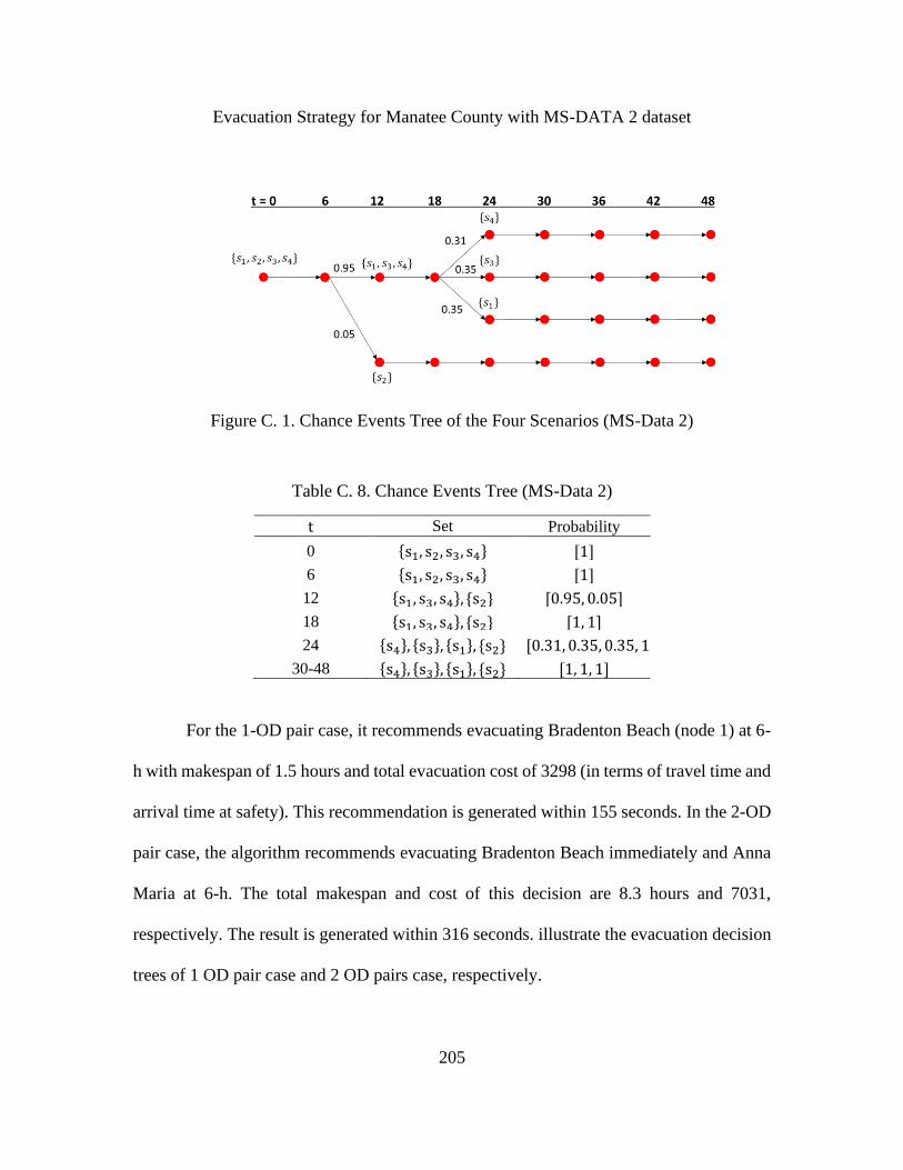
205

Evacuation Strategy for Manatee County with MS-DATA 2 dataset

Figure C. 1. Chance Events Tree of the Four Scenarios (MS-Data 2)

Table C. 8. Chance Events Tree (MS-Data 2)

t Set Probability

0 {s1, s2, s3, s4} [1]

6 {s1, s2, s3, s4} [1]

12 {s1, s3, s4}, {s2} [0.95, 0.05]

18 {s1, s3, s4}, {s2} [1, 1]

24 {s4}, {s3}, {s1}, {s2} [0.31, 0.35, 0.35, 1]

30-48 {s4}, {s3}, {s1}, {s2} [1, 1, 1]

For the 1-OD pair case, it recommends evacuating Bradenton Beach (node 1) at 6-

h with makespan of 1.5 hours and total evacuation cost of 3298 (in terms of travel time and

arrival time at safety). This recommendation is generated within 155 seconds. In the 2-OD

pair case, the algorithm recommends evacuating Bradenton Beach immediately and Anna

Maria at 6-h. The total makespan and cost of this decision are 8.3 hours and 7031,

respectively. The result is generated within 316 seconds. illustrate the evacuation decision

trees of 1 OD pair case and 2 OD pairs case, respectively.

206

Figure C. 2. Evacuation Decision Tree of 1-OD Pair (MS-Data2)

Figure C. 3. Evacuation Decision Tree of 1-OD Pair (MS-Data2)

207


(O, D) Decision

time

Route Number of

departure times

Total

assigned flows

(1, 30) t = 0 1-3-7-11-18-17-30 2 192

1-3-7-11-18-19-30 1 103

1-4-6-11-18-17-30 2 52

1-4-6-11-18-19-30 5 266

Table C.10. EDTA for 1-OD Pair (MS-Data2)

No. t

Evac

node(s)

Rem

node(s)

Event

set Prob.

Evac.

cost

Future

cost

Prev.

branch

Next

branch

0 0 {1} - {0, 1, 2, 3} 1 3298.08 0.00 -1 -1

1 0 - {1} {0, 1, 2, 3} 1 0.00 3299.15 -1 2

2 6 {1} - {0, 1, 2, 3} 1 3299.15 0.00 1 -1

3 6 - {1} {0, 1, 2, 3} 1 0.00 3299.20 1 [4, 5]

4 12 - {1} {0, 2, 3} 0.95 0.00 3299.20 3 7

5 12 - {1} {1} 0.05 0.00 3299.20 3 9

6 12 {1} - {0, 2, 3} 1 3308.10 0.00 4 -1

7 12 - {1} {0, 2, 3} 1 0.00 3299.20 4 10

8 12 {1} - {1} 1 3308.10 0.00 5 -1

9 12 - {1} {1} 1 0.00 3299.20 5 12

10 18 {1} - {0, 2, 3} 1 3299.20 0.00 7 -1

11 18 - {1} {0, 2, 3} 1 0.00 3330.76 7 [14, 15, 16]

12 18 {1} - {1} 1 3299.20 0.00 9 -1

13 18 - {1} {1} 1 0.00 613000.00 9 17

14 24 - {1} {3} 0.31 0.00 3297.78 11 18

15 24 - {1} {2} 0.35 0.00 3297.78 11 20

16 24 - {1} {0} 0.35 0.00 3297.78 11 22

17 24 - {1} {1} 1 0.00 613000.00 13 -1

18 24 {1} - {3} 1 3297.78 0.00 14 -1

19 24 - {1} {3} 1 0.00 3412.45 14 24

20 24 {1} - {2} 1 3297.78 0.00 15 -1

21 24 - {1} {2} 1 0.00 3411.75 15 26

22 24 {1} - {0} 1 3297.78 0.00 16 -1

23 24 - {1} {0} 1 0.00 3299.15 16 28

24 30 {1} - {3} 1 3412.45 0.00 19 -1

25 30 - {1} {3} 1 0.00 613000.00 19 30

26 30 {1} - {2} 1 3411.75 0.00 21 -1

27 30 - {1} {2} 1 0.00 3413.64 21 31

28 30 {1} - {0} 1 3299.15 0.00 23 -1

29 30 - {1} {0} 1 0.00 613000.00 23 33

30 36 - {1} {3} 1 0.00 613000.00 25 -1

31 36 {1} - {2} 1 3413.64 0.00 27 -1

32 36 - {1} {2} 1 0.00 613000.00 27 34

33 36 - {1} {0} 1 0.00 613000.00 29 -1

34 42 - {1} {2} 1 0.00 613000.00 32 -1

208


(O, D) Decision

time

Route Number of

departure times

Total

assigned flows

(1, 30) t = 0 1-3-7-11-18-17-30 2 192

1-3-7-11-18-19-30 1 103

1-4-6-11-18-17-30 2 52

1-4-6-11-18-19-30 5 266

(2, 30) t = 6 2-4-6-11-18-19-30 13 664

Table C.12. EDTA for 2-OD Pair (Dataset 2)

No. t

Evac

node(s)

Rem

node(s)

Event

set Prob.

Evac.

cost

Future

cost

Prev.

branch

Next

branch

0 0 {1, 2} - {0, 1, 2, 3} 1 7193.09 0.00 -1 -1

1 0 {1} {2} {0, 1, 2, 3} 1 3298.08 3732.58 -1 4

2 0 {2} {1} {0, 1, 2, 3} 1 3735.27 3299.15 -1 6

3 0 - {1, 2} {0, 1, 2, 3} 1 0.00 7031.78 -1 10

4 6 {2} - {0, 1, 2, 3} 1 3732.58 0.00 1 -1

5 6 - {2} {0, 1, 2, 3} 1 0.00 3734.39 1 [12, 13]

6 6 {1} - {0, 1, 2, 3} 1 3299.15 0.00 2 -1

7 6 - {1} {0, 1, 2, 3} 1 0.00 3299.20 2 [14, 15]

8 6 {1, 2} - {0, 1, 2, 3} 1 7185.54 0.00 3 -1

9 6 {1} {2} {0, 1, 2, 3} 1 3299.15 3734.39 3 [16, 17]

10 6 {2} {1} {0, 1, 2, 3} 1 3732.58 3299.20 3 [18, 19]

11 6 - {1, 2} {0, 1, 2, 3} 1 0.00 7033.59 3 [20, 21]

12 12 - {2} {0, 2, 3} 0.95 0.00 3734.39 5 22

13 12 - {2} {1} 0.05 0.00 3734.39 5 24

14 12 - {1} {0, 2, 3} 0.95 0.00 3299.20 7 27

15 12 - {1} {1} 0.05 0.00 3299.20 7 29

16 12 - {2} {0, 2, 3} 0.95 0.00 3734.39 9 30

17 12 - {2} {1} 0.05 0.00 3734.39 9 32

18 12 - {1} {0, 2, 3} 0.95 0.00 3299.20 10 35

19 12 - {1} {1} 0.05 0.00 3299.20 10 37

20 12 - {1, 2} {0, 2, 3} 0.95 0.00 7033.59 11 40

21 12 - {1, 2} {1} 0.05 0.00 7033.59 11 44

22 12 {2} - {0, 2, 3} 1 3734.39 0.00 12 -1

23 12 - {2} {0, 2, 3} 1 0.00 3736.21 12 46

24 12 {2} - {1} 1 3734.39 0.00 13 -1

25 12 - {2} {1} 1 0.00 3736.21 13 48

26 12 {1} - {0, 2, 3} 1 3308.10 0.00 14 -1

27 12 - {1} {0, 2, 3} 1 0.00 3299.20 14 50

28 12 {1} - {1} 1 3308.10 0.00 15 -1

29 12 - {1} {1} 1 0.00 3299.20 15 52

30 12 {2} - {0, 2, 3} 1 3734.39 0.00 16 -1

31 12 - {2} {0, 2, 3} 1 0.00 3736.21 16 54

32 12 {2} - {1} 1 3734.39 0.00 17 -1

33 12 - {2} {1} 1 0.00 3736.21 17 56

34 12 {1} - {0, 2, 3} 1 3308.10 0.00 18 -1

35 12 - {1} {0, 2, 3} 1 0.00 3299.20 18 58

36 12 {1} - {1} 1 3308.10 0.00 19 -1

37 12 - {1} {1} 1 0.00 3299.20 19 60

38 12 {1, 2} - {0, 2, 3} 1 7187.02 0.00 20 -1

209


No. t

Evac

node(s)

Rem

node(s)

Event

set

Prob

.

Evac.

cost

Future

cost

Prev.

branch

Next

branch

39 12 {1} {2} {0, 2, 3} 1 3308.10 3736.21 20 62

40 12 {2} {1} {0, 2, 3} 1 3734.39 3299.20 20 64

41 12 - {1, 2} {0, 2, 3} 1 0.00 7066.97 20 68

42 12 {1, 2} - {1} 1 7187.02 0.00 21 -1

43 12 {1} {2} {1} 1 3308.10 3736.21 21 70

44 12 {2} {1} {1} 1 3734.39 3299.20 21 72

45 12 - {1, 2} {1} 1 0.00 7190.70 21 74

46 18 {2} - {0, 2, 3} 1 3736.21 0.00 23 -1

47 18 - {2} {0, 2, 3} 1 0.00 3771.68 23 [78, 79, 80]

48 18 {2} - {1} 1 3736.21 0.00 25 -1

49 18 - {2} {1} 1 0.00 3951.50 25 81

50 18 {1} - {0, 2, 3} 1 3299.20 0.00 27 -1

51 18 - {1} {0, 2, 3} 1 0.00 3330.76 27 [83, 84, 85]

52 18 {1} - {1} 1 3299.20 0.00 29 -1

53 18 - {1} {1} 1 0.00 613000.00 29 86

54 18 {2} - {0, 2, 3} 1 3736.21 0.00 31 -1

55 18 - {2} {0, 2, 3} 1 0.00 3771.68 31 [87, 88, 89]

56 18 {2} - {1} 1 3736.21 0.00 33 -1

57 18 - {2} {1} 1 0.00 3951.50 33 90

58 18 {1} - {0, 2, 3} 1 3299.20 0.00 35 -1

59 18 - {1} {0, 2, 3} 1 0.00 3330.76 35 [92, 93, 94]

60 18 {1} - {1} 1 3299.20 0.00 37 -1

61 18 - {1} {1} 1 0.00 613000.00 37 95

62 18 {2} - {0, 2, 3} 1 3736.21 0.00 39 -1

63 18 - {2} {0, 2, 3} 1 0.00 3771.68 39 [96, 97, 98]

64 18 {1} - {0, 2, 3} 1 3299.20 0.00 40 -1

65 18 - {1} {0, 2, 3} 1 0.00 3330.76 40 [99, 100, 101]

66 18 {1, 2} - {0, 2, 3} 1 7190.70 0.00 41 -1

67 18 {1} {2} {0, 2, 3} 1 3299.20 3771.68 41 [102, 103,

104]

68 18 {2} {1} {0, 2, 3} 1 3736.21 3330.76 41 [105, 106,

107]

69 18 - {1, 2} {0, 2, 3} 1 0.00 7177.88 41 [108, 109,

110]

70 18 {2} - {1} 1 3736.21 0.00 43 -1

71 18 - {2} {1} 1 0.00 3951.50 43 111

72 18 {1} - {1} 1 3299.20 0.00 44 -1

73 18 - {1} {1} 1 0.00 613000.00 44 113

74 18 {1, 2} - {1} 1 7190.70 0.00 45 -1

75 18 {1} {2} {1} 1 3299.20 3951.50 45 114

76 18 {2} {1} {1} 1 3736.21 613000.00 45 116

77 18 - {1, 2} {1} 1 0.00 616951.50 45 117

78 24 - {2} {3} 0.31 0.00 3735.27 47 119

79 24 - {2} {2} 0.35 0.00 3735.27 47 121

80 24 - {2} {0} 0.35 0.00 3732.58 47 124

81 24 {2} - {1} 1 3951.50 0.00 49 -1

82 24 - {2} {1} 1 0.00 664000.00 49 125

83 24 - {1} {3} 0.31 0.00 3297.78 51 126

84 24 - {1} {2} 0.35 0.00 3297.78 51 128

85 24 - {1} {0} 0.35 0.00 3297.78 51 130

86 24 - {1} {1} 1 0.00 613000.00 53 -1

87 24 - {2} {3} 0.31 0.00 3735.27 55 132

88 24 - {2} {2} 0.35 0.00 3735.27 55 134

210


No. t

Evac

node(s)

Rem

node(s)

Event

set Prob.

Evac.

cost

Future

cost

Prev.

branch

Next

branch

89 24 - {2} {0} 0.35 0.00 3732.58 55 137

90 24 {2} - {1} 1 3951.50 0.00 57 -1

91 24 - {2} {1} 1 0.00 664000.00 57 138

92 24 - {1} {3} 0.31 0.00 3297.78 59 139

93 24 - {1} {2} 0.35 0.00 3297.78 59 141

94 24 - {1} {0} 0.35 0.00 3297.78 59 143

95 24 - {1} {1} 1 0.00 613000.00 61 -1

96 24 - {2} {3} 0.31 0.00 3735.27 63 145

97 24 - {2} {2} 0.35 0.00 3735.27 63 147

98 24 - {2} {0} 0.35 0.00 3732.58 63 150

99 24 - {1} {3} 0.31 0.00 3297.78 65 151

100 24 - {1} {2} 0.35 0.00 3297.78 65 153

101 24 - {1} {0} 0.35 0.00 3297.78 65 155

102 24 - {2} {3} 0.31 0.00 3735.27 67 157

103 24 - {2} {2} 0.35 0.00 3735.27 67 159

104 24 - {2} {0} 0.35 0.00 3732.58 67 162

105 24 - {1} {3} 0.31 0.00 3297.78 68 163

106 24 - {1} {2} 0.35 0.00 3297.78 68 165

107 24 - {1} {0} 0.35 0.00 3297.78 68 167

108 24 - {1, 2} {3} 0.31 0.00 7147.72 69 171

109 24 - {1, 2} {2} 0.35 0.00 7147.02 69 175

110 24 - {1, 2} {0} 0.35 0.00 7030.36 69 178

111 24 {2} - {1} 1 3951.50 0.00 71 -1

112 24 - {2} {1} 1 0.00 664000.00 71 181

113 24 - {1} {1} 1 0.00 613000.00 73 -1

114 24 {2} - {1} 1 3951.50 0.00 75 -1

115 24 - {2} {1} 1 0.00 664000.00 75 182

116 24 - {1} {1} 1 0.00 613000.00 76 -1

117 24 {2} {1} {1} 1 3951.50 613000.00 77 183

118 24 - {1, 2} {1} 1 0.00 1277000.00 77 184

119 24 {2} - {3} 1 3735.27 0.00 78 -1

120 24 - {2} {3} 1 0.00 3949.85 78 185

121 24 {2} - {2} 1 3735.27 0.00 79 -1

122 24 - {2} {2} 1 0.00 3947.64 79 187

123 24 {2} - {0} 1 3735.27 0.00 80 -1

124 24 - {2} {0} 1 0.00 3732.58 80 189

125 30 - {2} {1} 1 0.00 664000.00 82 -1

126 24 {1} - {3} 1 3297.78 0.00 83 -1

127 24 - {1} {3} 1 0.00 3412.45 83 191

128 24 {1} - {2} 1 3297.78 0.00 84 -1

129 24 - {1} {2} 1 0.00 3411.75 84 193

130 24 {1} - {0} 1 3297.78 0.00 85 -1

131 24 - {1} {0} 1 0.00 3299.15 85 195

132 24 {2} - {3} 1 3735.27 0.00 87 -1

133 24 - {2} {3} 1 0.00 3949.85 87 197

134 24 {2} - {2} 1 3735.27 0.00 88 -1

135 24 - {2} {2} 1 0.00 3947.64 88 199

136 24 {2} - {0} 1 3735.27 0.00 89 -1

137 24 - {2} {0} 1 0.00 3732.58 89 201

138 30 - {2} {1} 1 0.00 664000.00 91 -1

139 24 {1} - {3} 1 3297.78 0.00 92 -1

140 24 - {1} {3} 1 0.00 3412.45 92 203

141 24 {1} - {2} 1 3297.78 0.00 93 -1

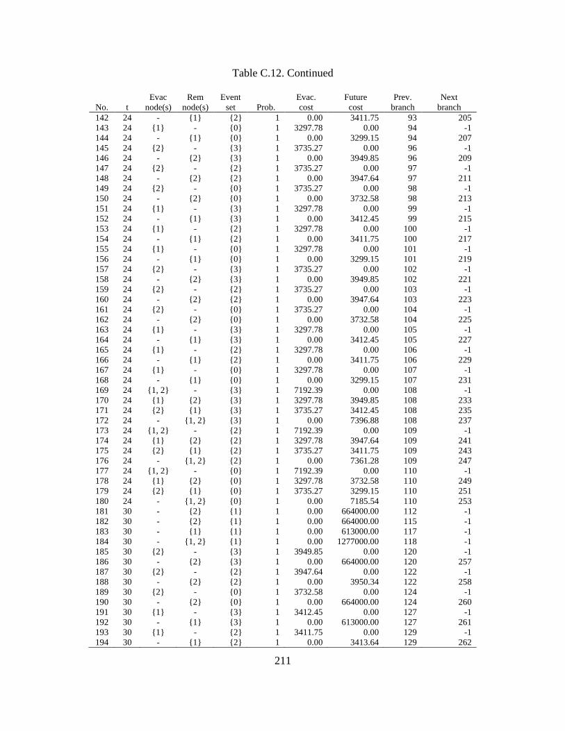
211


No. t

Evac

node(s)

Rem

node(s)

Event

set Prob.

Evac.

cost

Future

cost

Prev.

branch

Next

branch

142 24 - {1} {2} 1 0.00 3411.75 93 205

143 24 {1} - {0} 1 3297.78 0.00 94 -1

144 24 - {1} {0} 1 0.00 3299.15 94 207

145 24 {2} - {3} 1 3735.27 0.00 96 -1

146 24 - {2} {3} 1 0.00 3949.85 96 209

147 24 {2} - {2} 1 3735.27 0.00 97 -1

148 24 - {2} {2} 1 0.00 3947.64 97 211

149 24 {2} - {0} 1 3735.27 0.00 98 -1

150 24 - {2} {0} 1 0.00 3732.58 98 213

151 24 {1} - {3} 1 3297.78 0.00 99 -1

152 24 - {1} {3} 1 0.00 3412.45 99 215

153 24 {1} - {2} 1 3297.78 0.00 100 -1

154 24 - {1} {2} 1 0.00 3411.75 100 217

155 24 {1} - {0} 1 3297.78 0.00 101 -1

156 24 - {1} {0} 1 0.00 3299.15 101 219

157 24 {2} - {3} 1 3735.27 0.00 102 -1

158 24 - {2} {3} 1 0.00 3949.85 102 221

159 24 {2} - {2} 1 3735.27 0.00 103 -1

160 24 - {2} {2} 1 0.00 3947.64 103 223

161 24 {2} - {0} 1 3735.27 0.00 104 -1

162 24 - {2} {0} 1 0.00 3732.58 104 225

163 24 {1} - {3} 1 3297.78 0.00 105 -1

164 24 - {1} {3} 1 0.00 3412.45 105 227

165 24 {1} - {2} 1 3297.78 0.00 106 -1

166 24 - {1} {2} 1 0.00 3411.75 106 229

167 24 {1} - {0} 1 3297.78 0.00 107 -1

168 24 - {1} {0} 1 0.00 3299.15 107 231

169 24 {1, 2} - {3} 1 7192.39 0.00 108 -1

170 24 {1} {2} {3} 1 3297.78 3949.85 108 233

171 24 {2} {1} {3} 1 3735.27 3412.45 108 235

172 24 - {1, 2} {3} 1 0.00 7396.88 108 237

173 24 {1, 2} - {2} 1 7192.39 0.00 109 -1

174 24 {1} {2} {2} 1 3297.78 3947.64 109 241

175 24 {2} {1} {2} 1 3735.27 3411.75 109 243

176 24 - {1, 2} {2} 1 0.00 7361.28 109 247

177 24 {1, 2} - {0} 1 7192.39 0.00 110 -1

178 24 {1} {2} {0} 1 3297.78 3732.58 110 249

179 24 {2} {1} {0} 1 3735.27 3299.15 110 251

180 24 - {1, 2} {0} 1 0.00 7185.54 110 253

181 30 - {2} {1} 1 0.00 664000.00 112 -1

182 30 - {2} {1} 1 0.00 664000.00 115 -1

183 30 - {1} {1} 1 0.00 613000.00 117 -1

184 30 - {1, 2} {1} 1 0.00 1277000.00 118 -1

185 30 {2} - {3} 1 3949.85 0.00 120 -1

186 30 - {2} {3} 1 0.00 664000.00 120 257

187 30 {2} - {2} 1 3947.64 0.00 122 -1

188 30 - {2} {2} 1 0.00 3950.34 122 258

189 30 {2} - {0} 1 3732.58 0.00 124 -1

190 30 - {2} {0} 1 0.00 664000.00 124 260

191 30 {1} - {3} 1 3412.45 0.00 127 -1

192 30 - {1} {3} 1 0.00 613000.00 127 261

193 30 {1} - {2} 1 3411.75 0.00 129 -1

194 30 - {1} {2} 1 0.00 3413.64 129 262

212


No. t

Evac

node(s)

Rem

node(s)

Event

set Prob.

Evac.

cost

Future

cost

Prev.

branch

Next

branch

195 30 {1} - {0} 1 3299.15 0.00 131 -1

196 30 - {1} {0} 1 0.00 613000.00 131 264

197 30 {2} - {3} 1 3949.85 0.00 133 -1

198 30 - {2} {3} 1 0.00 664000.00 133 265

199 30 {2} - {2} 1 3947.64 0.00 135 -1

200 30 - {2} {2} 1 0.00 3950.34 135 266

201 30 {2} - {0} 1 3732.58 0.00 137 -1

202 30 - {2} {0} 1 0.00 664000.00 137 268

203 30 {1} - {3} 1 3412.45 0.00 140 -1

204 30 - {1} {3} 1 0.00 613000.00 140 269

205 30 {1} - {2} 1 3411.75 0.00 142 -1

206 30 - {1} {2} 1 0.00 3413.64 142 270

207 30 {1} - {0} 1 3299.15 0.00 144 -1

208 30 - {1} {0} 1 0.00 613000.00 144 272

209 30 {2} - {3} 1 3949.85 0.00 146 -1

210 30 - {2} {3} 1 0.00 664000.00 146 273

211 30 {2} - {2} 1 3947.64 0.00 148 -1

212 30 - {2} {2} 1 0.00 3950.34 148 274

213 30 {2} - {0} 1 3732.58 0.00 150 -1

214 30 - {2} {0} 1 0.00 664000.00 150 276

215 30 {1} - {3} 1 3412.45 0.00 152 -1

216 30 - {1} {3} 1 0.00 613000.00 152 277

217 30 {1} - {2} 1 3411.75 0.00 154 -1

218 30 - {1} {2} 1 0.00 3413.64 154 278

219 30 {1} - {0} 1 3299.15 0.00 156 -1

220 30 - {1} {0} 1 0.00 613000.00 156 280

221 30 {2} - {3} 1 3949.85 0.00 158 -1

222 30 - {2} {3} 1 0.00 664000.00 158 281

223 30 {2} - {2} 1 3947.64 0.00 160 -1

224 30 - {2} {2} 1 0.00 3950.34 160 282

225 30 {2} - {0} 1 3732.58 0.00 162 -1

226 30 - {2} {0} 1 0.00 664000.00 162 284

227 30 {1} - {3} 1 3412.45 0.00 164 -1

228 30 - {1} {3} 1 0.00 613000.00 164 285

229 30 {1} - {2} 1 3411.75 0.00 166 -1

230 30 - {1} {2} 1 0.00 3413.64 166 286

231 30 {1} - {0} 1 3299.15 0.00 168 -1

232 30 - {1} {0} 1 0.00 613000.00 168 288

233 30 {2} - {3} 1 3949.85 0.00 170 -1

234 30 - {2} {3} 1 0.00 664000.00 170 289

235 30 {1} - {3} 1 3412.45 0.00 171 -1

236 30 - {1} {3} 1 0.00 613000.00 171 290

237 30 {1, 2} - {3} 1 7396.88 0.00 172 -1

238 30 {1} {2} {3} 1 3412.45 664000.00 172 291

239 30 {2} {1} {3} 1 3949.85 613000.00 172 292

240 30 - {1, 2} {3} 1 0.00 1277000.00 172 293

241 30 {2} - {2} 1 3947.64 0.00 174 -1

242 30 - {2} {2} 1 0.00 3950.34 174 294

243 30 {1} - {2} 1 3411.75 0.00 175 -1

244 30 - {1} {2} 1 0.00 3413.64 175 296

245 30 {1, 2} - {2} 1 7395.64 0.00 176 -1

246 30 {1} {2} {2} 1 3411.75 3950.34 176 298

247 30 {2} {1} {2} 1 3947.64 3413.64 176 300

213


No. t

Evac

node(s)

Rem

node(s)

Event

set Prob.

Evac.

cost

Future

cost

Prev.

branch

Next

branch

248 30 - {1, 2} {2} 1 0.00 7398.90 176 302

249 30 {2} - {0} 1 3732.58 0.00 178 -1

250 30 - {2} {0} 1 0.00 664000.00 178 306

251 30 {1} - {0} 1 3299.15 0.00 179 -1

252 30 - {1} {0} 1 0.00 613000.00 179 307

253 30 {1, 2} - {0} 1 7185.54 0.00 180 -1

254 30 {1} {2} {0} 1 3299.15 664000.00 180 308

255 30 {2} {1} {0} 1 3732.58 613000.00 180 309

256 30 - {1, 2} {0} 1 0.00 1277000.00 180 310

257 36 - {2} {3} 1 0.00 664000.00 186 -1

258 36 {2} - {2} 1 3950.34 0.00 188 -1

259 36 - {2} {2} 1 0.00 664000.00 188 311

260 36 - {2} {0} 1 0.00 664000.00 190 -1

261 36 - {1} {3} 1 0.00 613000.00 192 -1

262 36 {1} - {2} 1 3413.64 0.00 194 -1

263 36 - {1} {2} 1 0.00 613000.00 194 312

264 36 - {1} {0} 1 0.00 613000.00 196 -1

265 36 - {2} {3} 1 0.00 664000.00 198 -1

266 36 {2} - {2} 1 3950.34 0.00 200 -1

267 36 - {2} {2} 1 0.00 664000.00 200 313

268 36 - {2} {0} 1 0.00 664000.00 202 -1

269 36 - {1} {3} 1 0.00 613000.00 204 -1

270 36 {1} - {2} 1 3413.64 0.00 206 -1

271 36 - {1} {2} 1 0.00 613000.00 206 314

272 36 - {1} {0} 1 0.00 613000.00 208 -1

273 36 - {2} {3} 1 0.00 664000.00 210 -1

274 36 {2} - {2} 1 3950.34 0.00 212 -1

275 36 - {2} {2} 1 0.00 664000.00 212 315

276 36 - {2} {0} 1 0.00 664000.00 214 -1

277 36 - {1} {3} 1 0.00 613000.00 216 -1

278 36 {1} - {2} 1 3413.64 0.00 218 -1

279 36 - {1} {2} 1 0.00 613000.00 218 316

280 36 - {1} {0} 1 0.00 613000.00 220 -1

281 36 - {2} {3} 1 0.00 664000.00 222 -1

282 36 {2} - {2} 1 3950.34 0.00 224 -1

283 36 - {2} {2} 1 0.00 664000.00 224 317

284 36 - {2} {0} 1 0.00 664000.00 226 -1

285 36 - {1} {3} 1 0.00 613000.00 228 -1

286 36 {1} - {2} 1 3413.64 0.00 230 -1

287 36 - {1} {2} 1 0.00 613000.00 230 318

288 36 - {1} {0} 1 0.00 613000.00 232 -1

289 36 - {2} {3} 1 0.00 664000.00 234 -1

290 36 - {1} {3} 1 0.00 613000.00 236 -1

291 36 - {2} {3} 1 0.00 664000.00 238 -1

292 36 - {1} {3} 1 0.00 613000.00 239 -1

293 36 - {1, 2} {3} 1 0.00 1277000.00 240 -1

294 36 {2} - {2} 1 3950.34 0.00 242 -1

295 36 - {2} {2} 1 0.00 664000.00 242 319

296 36 {1} - {2} 1 3413.64 0.00 244 -1

297 36 - {1} {2} 1 0.00 613000.00 244 320

298 36 {2} - {2} 1 3950.34 0.00 246 -1

299 36 - {2} {2} 1 0.00 664000.00 246 321

300 36 {1} - {2} 1 3413.64 0.00 247 -1

214


No. t

Evac

node(s)

Rem

node(s)

Event

set Prob.

Evac.

cost

Future

cost

Prev.

branch

Next

branch

301 36 - {1} {2} 1 0.00 613000.00 247 322

302 36 {1, 2} - {2} 1 7398.90 0.00 248 -1

303 36 {1} {2} {2} 1 3413.64 664000.00 248 323

304 36 {2} {1} {2} 1 3950.34 613000.00 248 324

305 36 - {1, 2} {2} 1 0.00 1277000.00 248 325

306 36 - {2} {0} 1 0.00 664000.00 250 -1

307 36 - {1} {0} 1 0.00 613000.00 252 -1

308 36 - {2} {0} 1 0.00 664000.00 254 -1

309 36 - {1} {0} 1 0.00 613000.00 255 -1

310 36 - {1, 2} {0} 1 0.00 1277000.00 256 -1

311 42 - {2} {2} 1 0.00 664000.00 259 -1

312 42 - {1} {2} 1 0.00 613000.00 263 -1

313 42 - {2} {2} 1 0.00 664000.00 267 -1

314 42 - {1} {2} 1 0.00 613000.00 271 -1

315 42 - {2} {2} 1 0.00 664000.00 275 -1

316 42 - {1} {2} 1 0.00 613000.00 279 -1

317 42 - {2} {2} 1 0.00 664000.00 283 -1

318 42 - {1} {2} 1 0.00 613000.00 287 -1

319 42 - {2} {2} 1 0.00 664000.00 295 -1

320 42 - {1} {2} 1 0.00 613000.00 297 -1

321 42 - {2} {2} 1 0.00 664000.00 299 -1

322 42 - {1} {2} 1 0.00 613000.00 301 -1

323 42 - {2} {2} 1 0.00 664000.00 303 -1

324 42 - {1} {2} 1 0.00 613000.00 304 -1

325 42 - {1, 2} {2} 1 0.00 1277000.00 305 -1


(O, D) Decision

time

Route Number of

departure times

Total

assigned flows

(1, 30) 0 1-3-7-11-18-17-30 2 193

1-3-7-11-18-19-30 1 102

1-4-6-11-18-17-30 2 56

1-4-6-11-18-19-30 5 262

(3, 30) 6 3-7-11-18-17-30 14 846

3-7-11-18-19-30 24 1840

(2, 30) 12: {s2} 2-4-6-11-18-19-30 13 664

12: {s1, s3, s4} 2-4-6-11-18-19-30 13 664

215

Table C. 14. Evacuation Decisions for 2 OD Sets (MS-Data2)

(O, D) Decision

time

Route Number of

departure times

Total

assigned flows

(1, 30) t = 0 1-3-7-11-18-17-30 2 192

1-3-7-11-18-19-30 1 103

1-4-6-11-18-17-30 2 52

1-4-6-11-18-19-30 5 266

({2,3}, 30) t = 6 2-4-6-11-16-25-30 2 53

2-4-6-11-18-17-30 11 471

2-4-6-11-18-19-30 4 140

3-7-11-18-17-30 14 1055

3-7-11-18-19-30 27 1631

Table C.15. EDTA for 2 OD Sets (MS-Data2)

No. t

Evac

node(s)

Rem

node(s)

Event

set Prob.

Evac.

cost

Future

cost

Prev.

branch

Next

branch

0 0 {1, 2, 3} - {0, 1, 2, 3} 1 23528.44 0.00 -1 -1

1 0 {1} [2, 3] {0, 1, 2, 3} 1 3298.08 19840.94 -1 4

2 0 {2, 3} [1] {0, 1, 2, 3} 1 19864.70 3299.15 -1 6

3 0 - [1], [2, 3] {0, 1, 2, 3} 1 0.00 23140.14 -1 10

4 6 {2, 3} - {0, 1, 2, 3} 1 19840.94 0.00 1 -1

5 6 - [2, 3] {0, 1, 2, 3} 1 0.00 19886.59 1 [12, 13]

6 6 {1} - {0, 1, 2, 3} 1 3299.15 0.00 2 -1

7 6 - [1] {0, 1, 2, 3} 1 0.00 3299.20 2 [14, 15]

8 6 {1, 2, 3} - {0, 1, 2, 3} 1 23553.11 0.00 3 -1

9 6 {1} [2, 3] {0, 1, 2, 3} 1 3299.15 19886.59 3 [16, 17]

10 6 {2, 3} [1] {0, 1, 2, 3} 1 19840.94 3299.20 3 [18, 19]

11 6 - [1], [2, 3] {0, 1, 2, 3} 1 0.00 23194.69 3 [20, 21]

12 12 - [2, 3] {0, 2, 3} 0.95 0.00 19886.35 5 23

13 12 - [2, 3] {1} 0.05 0.00 19891.12 5 25

14 12 - [1] {0, 2, 3} 0.95 0.00 3299.20 7 27

15 12 - [1] {1} 0.05 0.00 3299.20 7 29

16 12 - [2, 3] {0, 2, 3} 0.95 0.00 19886.35 9 31

17 12 - [2, 3] {1} 0.05 0.00 19891.12 9 33

18 12 - [1] {0, 2, 3} 0.95 0.00 3299.20 10 35

19 12 - [1] {1} 0.05 0.00 3299.20 10 37

20 12 - [1], [2, 3] {0, 2, 3} 0.95 0.00 23194.45 11 39

21 12 - [1], [2, 3] {1} 0.05 0.00 23199.22 11 43

22 12 {2, 3} - {0, 2, 3} 1 19989.52 0.00 12 -1

23 12 - [2, 3] {0, 2, 3} 1 0.00 19886.35 12 46

24 12 {2, 3} - {1} 1 19989.52 0.00 13 -1

25 12 - [2, 3] {1} 1 0.00 19891.12 13 48

26 12 {1} - {0, 2, 3} 1 3308.10 0.00 14 -1

27 12 - [1] {0, 2, 3} 1 0.00 3299.20 14 50

28 12 {1} - {1} 1 3308.10 0.00 15 -1

29 12 - [1] {1} 1 0.00 3299.20 15 52

30 12 {2, 3} - {0, 2, 3} 1 19989.52 0.00 16 -1

31 12 - [2, 3] {0, 2, 3} 1 0.00 19886.35 16 54

32 12 {2, 3} - {1} 1 19989.52 0.00 17 -1

33 12 - [2, 3] {1} 1 0.00 19891.12 17 56

34 12 {1} - {0, 2, 3} 1 3308.10 0.00 18 -1

216


No. t

Evac

node(s)

Rem

node(s)

Event

set Prob.

Evac.

cost

Future

cost

Prev.

branch

Next

branch

35 12 - [1] {0, 2, 3} 1 0.00 3299.20 18 58

36 12 {1} - {1} 1 3308.10 0.00 19 -1

37 12 - [1] {1} 1 0.00 3299.20 19 60

38 12 {1, 2, 3} - {0, 2, 3} 1 23760.95 0.00 20 -1

39 12 {1} [2, 3] {0, 2, 3} 1 3308.10 19886.35 20 62

40 12 {2, 3} [1] {0, 2, 3} 1 19989.52 3299.20 20 64

41 12 - [1], [2, 3] {0, 2, 3} 1 0.00 23217.11 20 68

42 12 {1, 2, 3} - {1} 1 23769.13 0.00 21 -1

43 12 {1} [2, 3] {1} 1 3308.10 19891.12 21 70

44 12 {2, 3} [1] {1} 1 19989.52 3299.20 21 72

45 12 - [1], [2, 3] {1} 1 0.00 23557.17 21 74

46 18 {2, 3} - {0, 2, 3} 1 19886.35 0.00 23 -1

47 18 - [2, 3] {0, 2, 3} 1 0.00 20082.47 23 [78, 79,

80]

48 18 {2, 3} - {1} 1 19891.12 0.00 25 -1

49 18 - [2, 3] {1} 1 0.00 20267.89 25 81

50 18 {1} - {0, 2, 3} 1 3299.20 0.00 27 -1

51 18 - [1] {0, 2, 3} 1 0.00 3330.76 27 [83, 84,

85]

52 18 {1} - {1} 1 3299.20 0.00 29 -1

53 18 - [1] {1} 1 0.00 613000.00 29 86

54 18 {2, 3} - {0, 2, 3} 1 19886.35 0.00 31 -1

55 18 - [2, 3] {0, 2, 3} 1 0.00 20082.47 31 [87, 88,

89]

56 18 {2, 3} - {1} 1 19891.12 0.00 33 -1

57 18 - [2, 3] {1} 1 0.00 20267.89 33 90

58 18 {1} - {0, 2, 3} 1 3299.20 0.00 35 -1

59 18 - [1] {0, 2, 3} 1 0.00 3330.76 35 [92, 93,

94]

60 18 {1} - {1} 1 3299.20 0.00 37 -1

61 18 - [1] {1} 1 0.00 613000.00 37 95

62 18 {2, 3} - {0, 2, 3} 1 19886.35 0.00 39 -1

63 18 - [2, 3] {0, 2, 3} 1 0.00 20082.47 39 [96, 97,

98]

64 18 {1} - {0, 2, 3} 1 3299.20 0.00 40 -1

65 18 - [1] {0, 2, 3} 1 0.00 3330.76 40 [99, 100,

101]

66 18 {1, 2, 3} - {0, 2, 3} 1 23550.21 0.00 41 -1

67 18 {1} [2, 3] {0, 2, 3} 1 3299.20 20082.47 41 [102,

103, 104]

68 18 {2, 3} [1] {0, 2, 3} 1 19886.35 3330.76 41 [105,

106, 107]

69 18 - [1], [2, 3] {0, 2, 3} 1 0.00 23489.14 41 [108,

109, 110]

70 18 {2, 3} - {1} 1 19891.12 0.00 43 -1

71 18 - [2, 3] {1} 1 0.00 20267.89 43 111

72 18 {1} - {1} 1 3299.20 0.00 44 -1

73 18 - [1] {1} 1 0.00 613000.00 44 113

74 18 {1, 2, 3} - {1} 1 23557.17 0.00 45 -1

75 18 {1} [2, 3] {1} 1 3299.20 20267.89 45 114

76 18 {2, 3} [1] {1} 1 19891.12 613000.00 45 116

77 18 - [1], [2, 3] {1} 1 0.00 633267.89 45 117

217


No. t

Evac

node(s)

Rem

node(s)

Event

set Prob.

Evac.

cost

Future

cost

Prev.

branch

Next

branch

78 24 - [2, 3] {3} 0.31 0.00 19854.52 47 119

79 24 - [2, 3] {2} 0.35 0.00 19933.87 47 121

80 24 - [2, 3] {0} 0.35 0.00 19859.17 47 123

81 24 {2, 3} - {1} 1 20267.89 0.00 49 -1

82 24 - [2, 3] {1} 1 0.00 3350000.00 49 125

83 24 - [1] {3} 0.31 0.00 3297.78 51 126

84 24 - [1] {2} 0.35 0.00 3297.78 51 128

85 24 - [1] {0} 0.35 0.00 3297.78 51 130

86 24 - [1] {1} 1 0.00 613000.00 53 -1

87 24 - [2, 3] {3} 0.31 0.00 19854.52 55 132

88 24 - [2, 3] {2} 0.35 0.00 19933.87 55 134

89 24 - [2, 3] {0} 0.35 0.00 19859.17 55 136

90 24 {2, 3} - {1} 1 20267.89 0.00 57 -1

91 24 - [2, 3] {1} 1 0.00 3350000.00 57 138

92 24 - [1] {3} 0.31 0.00 3297.78 59 139

93 24 - [1] {2} 0.35 0.00 3297.78 59 141

94 24 - [1] {0} 0.35 0.00 3297.78 59 143

95 24 - [1] {1} 1 0.00 613000.00 61 -1

96 24 - [2, 3] {3} 0.31 0.00 19854.52 63 145

97 24 - [2, 3] {2} 0.35 0.00 19933.87 63 147

98 24 - [2, 3] {0} 0.35 0.00 19859.17 63 149

99 24 - [1] {3} 0.31 0.00 3297.78 65 151

100 24 - [1] {2} 0.35 0.00 3297.78 65 153

101 24 - [1] {0} 0.35 0.00 3297.78 65 155

102 24 - [2, 3] {3} 0.31 0.00 19854.52 67 157

103 24 - [2, 3] {2} 0.35 0.00 19933.87 67 159

104 24 - [2, 3] {0} 0.35 0.00 19859.17 67 161

105 24 - [1] {3} 0.31 0.00 3297.78 68 163

106 24 - [1] {2} 0.35 0.00 3297.78 68 165

107 24 - [1] {0} 0.35 0.00 3297.78 68 167

108 24 - [1], [2, 3] {3} 0.31 0.00 23266.97 69 171

109 24 - [1], [2, 3] {2} 0.35 0.00 23345.62 69 175

110 24 - [1], [2, 3] {0} 0.35 0.00 23158.32 69 179

111 24 {2, 3} - {1} 1 20267.89 0.00 71 -1

112 24 - [2, 3] {1} 1 0.00 3350000.00 71 181

113 24 - [1] {1} 1 0.00 613000.00 73 -1

114 24 {2, 3} - {1} 1 20267.89 0.00 75 -1

115 24 - [2, 3] {1} 1 0.00 3350000.00 75 182

116 24 - [1] {1} 1 0.00 613000.00 76 -1

117 24 {2, 3} [1] {1} 1 20267.89 613000.00 77 183

118 24 - [1], [2, 3] {1} 1 0.00 3963000.00 77 184

119 24 {2, 3} - {3} 1 19854.52 0.00 78 -1

120 24 - [2, 3] {3} 1 0.00 20241.47 78 185

121 24 {2, 3} - {2} 1 19933.87 0.00 79 -1

122 24 - [2, 3] {2} 1 0.00 20241.32 79 187

123 24 {2, 3} - {0} 1 19859.17 0.00 80 -1

124 24 - [2, 3] {0} 1 0.00 19870.01 80 189

125 30 - [2, 3] {1} 1 0.00 3350000.00 82 -1

126 24 {1} - {3} 1 3297.78 0.00 83 -1

127 24 - [1] {3} 1 0.00 3412.45 83 191

128 24 {1} - {2} 1 3297.78 0.00 84 -1

129 24 - [1] {2} 1 0.00 3411.75 84 193

130 24 {1} - {0} 1 3297.78 0.00 85 -1

218


No. t

Evac

node(s)

Rem

node(s)

Event

set Prob.

Evac.

cost

Future

cost

Prev.

branch

Next

branch

131 24 - [1] {0} 1 0.00 3299.15 85 195

132 24 {2, 3} - {3} 1 19854.52 0.00 87 -1

133 24 - [2, 3] {3} 1 0.00 20241.47 87 197

134 24 {2, 3} - {2} 1 19933.87 0.00 88 -1

135 24 - [2, 3] {2} 1 0.00 20241.32 88 199

136 24 {2, 3} - {0} 1 19859.17 0.00 89 -1

137 24 - [2, 3] {0} 1 0.00 19870.01 89 201

138 30 - [2, 3] {1} 1 0.00 3350000.00 91 -1

139 24 {1} - {3} 1 3297.78 0.00 92 -1

140 24 - [1] {3} 1 0.00 3412.45 92 203

141 24 {1} - {2} 1 3297.78 0.00 93 -1

142 24 - [1] {2} 1 0.00 3411.75 93 205

143 24 {1} - {0} 1 3297.78 0.00 94 -1

144 24 - [1] {0} 1 0.00 3299.15 94 207

145 24 {2, 3} - {3} 1 19854.52 0.00 96 -1

146 24 - [2, 3] {3} 1 0.00 20241.47 96 209

147 24 {2, 3} - {2} 1 19933.87 0.00 97 -1

148 24 - [2, 3] {2} 1 0.00 20241.32 97 211

149 24 {2, 3} - {0} 1 19859.17 0.00 98 -1

150 24 - [2, 3] {0} 1 0.00 19870.01 98 213

151 24 {1} - {3} 1 3297.78 0.00 99 -1

152 24 - [1] {3} 1 0.00 3412.45 99 215

153 24 {1} - {2} 1 3297.78 0.00 100 -1

154 24 - [1] {2} 1 0.00 3411.75 100 217

155 24 {1} - {0} 1 3297.78 0.00 101 -1

156 24 - [1] {0} 1 0.00 3299.15 101 219

157 24 {2, 3} - {3} 1 19854.52 0.00 102 -1

158 24 - [2, 3] {3} 1 0.00 20241.47 102 221

159 24 {2, 3} - {2} 1 19933.87 0.00 103 -1

160 24 - [2, 3] {2} 1 0.00 20241.32 103 223

161 24 {2, 3} - {0} 1 19859.17 0.00 104 -1

162 24 - [2, 3] {0} 1 0.00 19870.01 104 225

163 24 {1} - {3} 1 3297.78 0.00 105 -1

164 24 - [1] {3} 1 0.00 3412.45 105 227

165 24 {1} - {2} 1 3297.78 0.00 106 -1

166 24 - [1] {2} 1 0.00 3411.75 106 229

167 24 {1} - {0} 1 3297.78 0.00 107 -1

168 24 - [1] {0} 1 0.00 3299.15 107 231

169 24 {1, 2, 3} - {3} 1 23521.54 0.00 108 -1

170 24 {1} [2, 3] {3} 1 3297.78 20241.47 108 233

171 24 {2, 3} [1] {3} 1 19854.52 3412.45 108 235

172 24 - [1], [2, 3] {3} 1 0.00 24194.26 108 237

173 24 {1, 2, 3} - {2} 1 23630.74 0.00 109 -1

174 24 {1} [2, 3] {2} 1 3297.78 20241.32 109 241

175 24 {2, 3} [1] {2} 1 19933.87 3411.75 109 243

176 24 - [1], [2, 3] {2} 1 0.00 23654.96 109 247

177 24 {1, 2, 3} - {0} 1 23543.60 0.00 110 -1

178 24 {1} [2, 3] {0} 1 3297.78 19870.01 110 249

179 24 {2, 3} [1] {0} 1 19859.17 3299.15 110 251

180 24 - [1], [2, 3] {0} 1 0.00 23563.88 110 253

181 30 - [2, 3] {1} 1 0.00 3350000.00 112 -1

182 30 - [2, 3] {1} 1 0.00 3350000.00 115 -1

219


No. t

Evac

node(s)

Rem

node(s)

Event

set Prob.

Evac.

cost

Future

cost

Prev.

branch

Next

branch

183 30 - [1] {1} 1 0.00 613000.00 117 -1

184 30 - [1], [2, 3] {1} 1 0.00 3963000.00 118 -1

185 30 {2, 3} - {3} 1 20241.47 0.00 120 -1

186 30 - [2, 3] {3} 1 0.00 3350000.00 120 257

187 30 {2, 3} - {2} 1 20241.32 0.00 122 -1

188 30 - [2, 3] {2} 1 0.00 20253.45 122 258

189 30 {2, 3} - {0} 1 19870.01 0.00 124 -1

190 30 - [2, 3] {0} 1 0.00 3350000.00 124 260

191 30 {1} - {3} 1 3412.45 0.00 127 -1

192 30 - [1] {3} 1 0.00 613000.00 127 261

193 30 {1} - {2} 1 3411.75 0.00 129 -1

194 30 - [1] {2} 1 0.00 3413.64 129 262

195 30 {1} - {0} 1 3299.15 0.00 131 -1

196 30 - [1] {0} 1 0.00 613000.00 131 264

197 30 {2, 3} - {3} 1 20241.47 0.00 133 -1

198 30 - [2, 3] {3} 1 0.00 3350000.00 133 265

199 30 {2, 3} - {2} 1 20241.32 0.00 135 -1

200 30 - [2, 3] {2} 1 0.00 20253.45 135 266

201 30 {2, 3} - {0} 1 19870.01 0.00 137 -1

202 30 - [2, 3] {0} 1 0.00 3350000.00 137 268

203 30 {1} - {3} 1 3412.45 0.00 140 -1

204 30 - [1] {3} 1 0.00 613000.00 140 269

205 30 {1} - {2} 1 3411.75 0.00 142 -1

206 30 - [1] {2} 1 0.00 3413.64 142 270

207 30 {1} - {0} 1 3299.15 0.00 144 -1

208 30 - [1] {0} 1 0.00 613000.00 144 272

209 30 {2, 3} - {3} 1 20241.47 0.00 146 -1

210 30 - [2, 3] {3} 1 0.00 3350000.00 146 273

211 30 {2, 3} - {2} 1 20241.32 0.00 148 -1

212 30 - [2, 3] {2} 1 0.00 20253.45 148 274

213 30 {2, 3} - {0} 1 19870.01 0.00 150 -1

214 30 - [2, 3] {0} 1 0.00 3350000.00 150 276

215 30 {1} - {3} 1 3412.45 0.00 152 -1

216 30 - [1] {3} 1 0.00 613000.00 152 277

217 30 {1} - {2} 1 3411.75 0.00 154 -1

218 30 - [1] {2} 1 0.00 3413.64 154 278

219 30 {1} - {0} 1 3299.15 0.00 156 -1

220 30 - [1] {0} 1 0.00 613000.00 156 280

221 30 {2, 3} - {3} 1 20241.47 0.00 158 -1

222 30 - [2, 3] {3} 1 0.00 3350000.00 158 281

223 30 {2, 3} - {2} 1 20241.32 0.00 160 -1

224 30 - [2, 3] {2} 1 0.00 20253.45 160 282

225 30 {2, 3} - {0} 1 19870.01 0.00 162 -1

226 30 - [2, 3] {0} 1 0.00 3350000.00 162 284

227 30 {1} - {3} 1 3412.45 0.00 164 -1

228 30 - [1] {3} 1 0.00 613000.00 164 285

229 30 {1} - {2} 1 3411.75 0.00 166 -1

230 30 - [1] {2} 1 0.00 3413.64 166 286

231 30 {1} - {0} 1 3299.15 0.00 168 -1

232 30 - [1] {0} 1 0.00 613000.00 168 288

233 30 {2, 3} - {3} 1 20241.47 0.00 170 -1

234 30 - [2, 3] {3} 1 0.00 3350000.00 170 289

235 30 {1} - {3} 1 3412.45 0.00 171 -1

220


No. t

Evac

node(s)

Rem

node(s)

Event

set Prob.

Evac.

cost

Future

cost

Prev.

branch

Next

branch

236 30 - [1] {3} 1 0.00 613000.00 171 290

237 30 {1, 2, 3} - {3} 1 24194.26 0.00 172 -1

238 30 {1} [2, 3] {3} 1 3412.45 3350000.00 172 291

239 30 {2, 3} [1] {3} 1 20241.47 613000.00 172 292

240 30 - [1], [2, 3] {3} 1 0.00 3963000.00 172 293

241 30 {2, 3} - {2} 1 20241.32 0.00 174 -1

242 30 - [2, 3] {2} 1 0.00 20253.45 174 294

243 30 {1} - {2} 1 3411.75 0.00 175 -1

244 30 - [1] {2} 1 0.00 3413.64 175 296

245 30 {1, 2, 3} - {2} 1 24194.30 0.00 176 -1

246 30 {1} [2, 3] {2} 1 3411.75 20253.45 176 298

247 30 {2, 3} [1] {2} 1 20241.32 3413.64 176 300

248 30 - [1], [2, 3] {2} 1 0.00 24218.55 176 302

249 30 {2, 3} - {0} 1 19870.01 0.00 178 -1

250 30 - [2, 3] {0} 1 0.00 3350000.00 178 306

251 30 {1} - {0} 1 3299.15 0.00 179 -1

252 30 - [1] {0} 1 0.00 613000.00 179 307

253 30 {1, 2, 3} - {0} 1 23563.88 0.00 180 -1

254 30 {1} [2, 3] {0} 1 3299.15 3350000.00 180 308

255 30 {2, 3} [1] {0} 1 19870.01 613000.00 180 309

256 30 - [1], [2, 3] {0} 1 0.00 3963000.00 180 310

257 36 - [2, 3] {3} 1 0.00 3350000.00 186 -1

258 36 {2, 3} - {2} 1 20253.45 0.00 188 -1

259 36 - [2, 3] {2} 1 0.00 3350000.00 188 311

260 36 - [2, 3] {0} 1 0.00 3350000.00 190 -1

261 36 - [1] {3} 1 0.00 613000.00 192 -1

262 36 {1} - {2} 1 3413.64 0.00 194 -1

263 36 - [1] {2} 1 0.00 613000.00 194 312

264 36 - [1] {0} 1 0.00 613000.00 196 -1

265 36 - [2, 3] {3} 1 0.00 3350000.00 198 -1

266 36 {2, 3} - {2} 1 20253.45 0.00 200 -1

267 36 - [2, 3] {2} 1 0.00 3350000.00 200 313

268 36 - [2, 3] {0} 1 0.00 3350000.00 202 -1

269 36 - [1] {3} 1 0.00 613000.00 204 -1

270 36 {1} - {2} 1 3413.64 0.00 206 -1

271 36 - [1] {2} 1 0.00 613000.00 206 314

272 36 - [1] {0} 1 0.00 613000.00 208 -1

273 36 - [2, 3] {3} 1 0.00 3350000.00 210 -1

274 36 {2, 3} - {2} 1 20253.45 0.00 212 -1

275 36 - [2, 3] {2} 1 0.00 3350000.00 212 315

276 36 - [2, 3] {0} 1 0.00 3350000.00 214 -1

277 36 - [1] {3} 1 0.00 613000.00 216 -1

278 36 {1} - {2} 1 3413.64 0.00 218 -1

279 36 - [1] {2} 1 0.00 613000.00 218 316

281 36 - [2, 3] {3} 1 0.00 3350000.00 222 -1

282 36 {2, 3} - {2} 1 20253.45 0.00 224 -1

283 36 - [2, 3] {2} 1 0.00 3350000.00 224 317

284 36 - [2, 3] {0} 1 0.00 3350000.00 226 -1

285 36 - [1] {3} 1 0.00 613000.00 228 -1

286 36 {1} - {2} 1 3413.64 0.00 230 -1

287 36 - [1] {2} 1 0.00 613000.00 230 318

288 36 - [1] {0} 1 0.00 613000.00 232 -1

289 36 - [2, 3] {3} 1 0.00 3350000.00 234 -1

221


No. t

Evac

node(s)

Rem

node(s)

Event

set Prob.

Evac.

cost

Future

cost

Prev.

branch

Next

branch

290 36 - [1] {3} 1 0.00 613000.00 236 -1

291 36 - [2, 3] {3} 1 0.00 3350000.00 238 -1

292 36 - [1] {3} 1 0.00 613000.00 239 -1

293 36 - [1], [2, 3] {3} 1 0.00 3963000.00 240 -1

294 36 {2, 3} - {2} 1 20253.45 0.00 242 -1

295 36 - [2, 3] {2} 1 0.00 3350000.00 242 319

296 36 {1} - {2} 1 3413.64 0.00 244 -1

297 36 - [1] {2} 1 0.00 613000.00 244 320

298 36 {2, 3} - {2} 1 20253.45 0.00 246 -1

299 36 - [2, 3] {2} 1 0.00 3350000.00 246 321

300 36 {1} - {2} 1 3413.64 0.00 247 -1

301 36 - [1] {2} 1 0.00 613000.00 247 322

302 36 {1, 2, 3} - {2} 1 24218.55 0.00 248 -1

303 36 {1} [2, 3] {2} 1 3413.64 3350000.00 248 323

304 36 {2, 3} [1] {2} 1 20253.45 613000.00 248 324

305 36 - [1], [2, 3] {2} 1 0.00 3963000.00 248 325

306 36 - [2, 3] {0} 1 0.00 3350000.00 250 -1

307 36 - [1] {0} 1 0.00 613000.00 252 -1

308 36 - [2, 3] {0} 1 0.00 3350000.00 254 -1

309 36 - [1] {0} 1 0.00 613000.00 255 -1

310 36 - [1], [2, 3] {0} 1 0.00 3963000.00 256 -1

311 42 - [2, 3] {2} 1 0.00 3350000.00 259 -1

312 42 - [1] {2} 1 0.00 613000.00 263 -1

313 42 - [2, 3] {2} 1 0.00 3350000.00 267 -1

314 42 - [1] {2} 1 0.00 613000.00 271 -1

315 42 - [2, 3] {2} 1 0.00 3350000.00 275 -1

316 42 - [1] {2} 1 0.00 613000.00 279 -1

317 42 - [2, 3] {2} 1 0.00 3350000.00 283 -1

318 42 - [1] {2} 1 0.00 613000.00 287 -1

319 42 - [2, 3] {2} 1 0.00 3350000.00 295 -1

320 42 - [1] {2} 1 0.00 613000.00 297 -1

321 42 - [2, 3] {2} 1 0.00 3350000.00 299 -1

322 42 - [1] {2} 1 0.00 613000.00 301 -1

323 42 - [2, 3] {2} 1 0.00 3350000.00 303 -1

324 42 - [1] {2} 1 0.00 613000.00 304 -1

325 42 - [1], [2, 3] {2} 1 0.00 3963000.00 305 -1

222


(O, D) Decision

time

Route Number of

departure times

Total

assigned flows

(1, 30) 𝑡 = 0 1-3-7-11-18-17-30 2 192

1-3-7-11-18-19-30 1 103

1-4-6-11-18-17-30 2 52

1-4-6-11-18-19-30 5 266

({3,4}, 30) 𝑡 = 6 3-7-11-18-17-30 37 2382

3-7-11-18-19-30 19 304

4-6-11-18-17-30 6 268

4-6-11-18-19-30 46 2577

(2, 30) 𝑡 = 12 2-4-6-11-18-19-30 13 664


(O, D) Decision

time

Route Number of

departure times

Total

assigned flows

(1, 30) 𝑡 = 0 1-3-7-11-18-17-30 2 192

1-3-7-11-18-19-30 1 103

1-4-6-11-18-17-30 2 52

1-4-6-11-18-19-30 5 266

({3,4,5}, 30) 𝑡 = 6 3-7-11-16-25-30 5 302

3-7-11-18-17-30 38 1760

3-7-11-18-19-30 17 624

4-6-11-18-17-30 24 1196

4-6-11-18-19-30 41 1649

5-1-3-7-11-16-25-30 3 303

5-1-3-7-11-18-17-30 17 1075

5-1-3-7-11-18-19-30 21 990

5-1-4-6-11-16-25-30 1 88

5-1-4-6-11-18-17-30 12 341

5-1-4-6-11-18-19-30 17 648

5-22-12-14-15-24-30 16 1479

5-22-12-14-16-17-30 1 1

5-22-12-14-16-25-30 3 3

(2, 30) 𝑡 = 18 2-4-6-11-18-19-30 13 664

223

Table C.18. Summary of Evacuation Decision (MS-Data2)

Case Total

cost

BMS

(in hours)

Runtime

(in seconds)

Tree

size

No.

vehicle

Evacuation decision

[node] at [hour]

𝑠1 3297.78 1.5 89 12 613 [𝑛1] at [24]

𝑠2 3298.08 1.5 74 9 [𝑛1] at [0]

𝑠3 3297.78 1.5 87 15 [𝑛1] at [24]

𝑠4 3297.78 1.5 87 13 [𝑛1] at [24]

All 3298.08 1.5 155 35 [𝑛1] at [0]

𝑠1 7030.36 19.5 531 97 1,227 [𝑛2, 𝑛1] at [6, 24]

𝑠2 7030.66 8.3 407 60 [𝑛1, 𝑛2] at [0, 6]

𝑠3 7030.36 19.5 515 97 [𝑛2, 𝑛1] at [6, 24]

𝑠4 7030.36 19.5 515 97 [𝑛2, 𝑛1] at [6, 24]

All 7030.66 8.3 1151 326 [𝑛1, 𝑛2] at [0, 6]

𝑠1 23041.79 32.3 4299 685 3,963 [𝑛3, 𝑛1, 𝑛2] at [6, 24, 30]

𝑠2 23043.90 14.3 2910 368 [𝑛1, 𝑛3, 𝑛2] at [0, 6, 12]

𝑠3 23043.60 19.5 5199 1023 [𝑛3, 𝑛2, 𝑛1] at [6, 12, 24]

𝑠4 23043.60 19.5 4270 685 [𝑛3, 𝑛2, 𝑛1] at [6, 12, 24]

All 23043.90 14.3 11992 2572 [𝑛1, 𝑛3, 𝑛2] at [0, 6, 12]

𝑠1 23138.72 19.5 887 97 3,963 [(𝑛2, 𝑛3), (𝑛1)] at [6, 24]

𝑠2 23139.02 10.1 681 60 [(𝑛1), (𝑛2, 𝑛3)] at [0, 6]

𝑠3 23138.72 19.5 1011 127 [(𝑛2, 𝑛3), (𝑛1)] at [6, 24]

𝑠4 23138.72 19.5 871 97 [(𝑛2, 𝑛3), (𝑛1)] at [6, 24]

All 23139.02 10.1 2175 326 [(n1), (n2, n3)] at [0, 6]

s1 40457.40 29.4 6918 598 6,808 [(n1), (n2), (n3, n4)] at [0, 6, 24]

s2 40465.51 14.3 4607 308 [(n1), (n3, n4), (n2)] at [0, 6, 12]

s3 40464.70 25.5 7356 908 [(n3, n4), (n2), (n1)] at [0, 6, 24]

s4 40457.40 29.4 6953 598 [(n1), (n2), (n3, n4)] at [0, 6, 24]

All 40465.51 14.3 19936 2223 [(n1), (n3, n4), (n2)] at [0, 6, 12]

s1 74550.70 26.3 12971 598 11,736 [(n3, n4, n5), (n1), (n2)] at

[6, 24, 30]

s2 74548.84 20.3 7958 308 [(n1), (n3, n4, n5), (n2)] at

[0, 6, 18]

s3 74553.39 25.5 15714 908 [(n2), (n3, n4, n5), (n1)] at

[0, 6, 24]

s4 74553.39 25.5 14416 598 [(n2), (n3, n4, n5), (n1)] at

[0, 6, 24]

All 74548.84 20.3 37129 2223 [(n1), (n3, n4, n5), (n2)] at

[0, 6, 18]

Modeling Cascading Network Disruptions under Uncertainty

Documents