Modeling Bank Loan LGD of Corporate and SME Segments: …journal.fsv.cuni.cz/storage/1165_360-382---chal.-kop.pdf · Modeling Bank Loan LGD of Corporate and SME Segments: A Case Study*

360 Finance a úv r – Czech Journal of Economics and Finance, 59, 2009, no. 4

JEL Classification: G21, G28 Keywords: credit risk, loss given default, fractional responses, ordinal regression, quasi-maximum likelihood

estimator

Modeling Bank Loan LGD of Corporate and SME Segments: A Case Study* Radovan CHALUPKA Juraj KOPECSNI both: Institute of Economic Studies at the Faculty of Social Sciences,

Charles University in Prague(corresponding author:[email protected])

Abstract Loss given default (LGD) is one of key parameters to estimate credit risk in an internal rating based approach considered in The New Basel Capital Accord. The aim of this paper is to find determinants of LGD using a set of firm loan micro-data of an anonymous Czech commercial bank. We find that LGD is driven primarily by the period of loan origination, relative value of collateral, loan size and length of business relationship. Different models employed in our analysis provide similar results; in more complex models, log-log models appear to perform better, implying an asymmetric response of the dependent variable.

1. Introduction The New Basel Capital Accord (Basel Committee on Banking Supervision,

2006) has been created with an objective to better align regulatory capital with the un-derlying risk in the bank’s credit portfolio. The New Accord motivates international banks to develop and use internal risk models for calculating credit risk capital re-quirement. It allows banks to compute their regulatory capital in two ways: (1) using a revised standardised approach based on the 1998 Capital Accord which applies regulatory ratings for risk weighting assets or (2) using an internal rating based (IRB) approach where banks are permitted to develop and employ their own internal risk ratings.

The IRB approach is based on three key parameters used to estimate credit risk: PD – a probability of default of a borrower over a one-year horizon, LGD – loss given default, a credit loss incurred if a counterparty of a bank defaults, and EAD – an exposure at default. These parameters are used to estimate an expected loss, which is a product of PD, LGD and EAD. There are two possible variants of IRB, the foun-dation and the advanced approach. The difference between them lies in the way of estimating parameters. In the foundation approach only PD is estimated internally, LGD and EAD are based on supervisory values. On the other hand, in the advanced approach, all parameters are determined by a bank.

Most banks are prepared to use the foundation approach, since they have al-ready built internal models to estimate PD. However, many banks are not ready to fully implement the advanced IRB approach, because the advanced approach also re-quires to model and determine LGD.

* This research was supported by the Grant Agency of Charles University Grant No. 131707/2007 A-EK, by the Grant Agency of the Czech Republic Grant No. 402/08/0501, and by the IES Institutional ResearchFramework 2005-2010, MSM0021620841.

Finance a úv r – Czech Journal of Economics and Finance, 59, 2009, no. 4 361

This research contributes to propose a methodology to estimate the loss given default and then apply it to a set of loan micro-data to small and medium sized enter-prises (SMEs) and corporations. The data was provided by an anonymous Czech com-mercial bank (the “Bank”). The access to a unique database of loans enables us to show empirically economic determinants of LGD. The focus of our paper is on iden-tification of LGD drivers using various statistical approaches.

Based on the literature, we propose and apply three different statistical model-ing techniques in order to estimate determinants of LGD — (1) generalised linear models using symmetric logit and asymmetric log-log link functions for ordinal re-sponses, as well as (2) for fractional responses using beta inflated distribution and (3) quasi-maximum likelihood estimator. Moreover, several ways how to measure pre-dictive performance are suggested.

Our paper is organised as follows: the second section is a brief literature re-view, the third section discusses the key regulatory issues regarding LGD, such as definition of default and measurement of LGD, the fourth section focuses on charac-teristics of LGD from a modeling perspective and on description of data, the fifth section analyses and discusses typical risk drivers, the next section depicts the re-gression methodology used, whereas the last three sections provide results, goodness- -of-fit performance measures and conclusions, respectively.

2. Literature Review The banks which are using the advanced IRB approach need to consider com-

mon characteristics of losses and recoveries. These basic characteristics are bimodali-ty, seniority and type of collateral, business cycles, industry and the size of loan.

Loss given default,1 defined as 100% minus a percentage of recovered expo-sure during a workout process, tends to have a bimodal distribution. Bimodality im-plies that most loans have LGD close to 0% (full recovery), or there is 100% LGD (no recovery at all). Bimodality makes parametric modeling of recovery difficult and requires a non-parametric approach (Renault and Scaillet, 2004).

The second important issue is collateral of defaulted claims and a place in the debt structure. Bank loans are typically at the top of the debt structure, generally implying higher recovery rates than bonds. LGD tends to be lower (i.e. recovery rate tends to be higher) when a claim is secured by collateral of high quality. Asarnov and Edwards (1995), Carey (1998) and Gupton et al. (2000) confirm that seniority and collateral do matter. They primarily use the data from Citibank and Moody’s.

There is strong evidence that LGD in recessions is higher than during expan-sions, for instance according to Carey (1998) and Frye (2000). Employing Moody’s data they show that during recessions recoveries are lower by one third.

Other studies by Grossman et al. (2001) and Acharya et al. (2003) argue that in-dustry type is another important determinant of LGD. Results of Altman and Kishore (1996) provide evidence that some industries such as utilities (30% average LGD) do better than others (e.g. manufacturing 58%).

The most ambiguous key characteristic is the size of loan. Asarnov and Ed-wards (1995) and Carty and Lieberman (1996) find no relationship between LGD 1 The same applies to recovery rate defined as 100% minus a LGD percentage. To retain consistency among results, we have recalculated recovery rates of some studies to LGD.


and the size of loan in the U.S. market. Thornburn (2000) obtains similar negative result for Swedish business bankruptcies. However, Hurt and Felsovalyi (1998) show that large loan defaults exhibit lower recovery rates. They attribute it to the fact that large loans are often unsecured, and they are provided to economic groups that are family owned.

Currently, bank loan LGD is not explored well by theoretical and empirical literature. Although several empirical academic studies have analyzed credit risk on corporate bonds, only a few studies have been applied to bank loans. The reason for this is that since bank loans are private instruments, little data is publicly available.

Asarnow and Edwards (1995) analyzed 831 defaulted loans at Citibank over the period 1970–1993 and they show that the distribution of LGD is bimodal, with concentration of LGD on either the low or high end of the distribution. Their average LGD is 35%. Carty and Lieberman (1996) measured the recovery rate on a sample of 58 bank loans for the period 1989–1996 and reported skewness toward the high end of price scale with an average LGD of 29%. Gupton et al. (2000) reported lower LGD of 30% for senior secured loans as compared to unsecured loans (48%), based on 1989–2000 data sample consisting of 181 observations. The above studies focused on the U.S. market. Hurt and Felsovalyi (1998) who analyze 1,149 bank loan losses in Latin America over 1970–1996 found an average LGD of 32%. Another study by Franks et al. (2004) calculated recovery rates of 2,280 defaulted companies whose data was taken from 10 banks in three countries over the period 1984–2003. They found a country-specific bankruptcy regime, which indicates significantly different recovery rates. Average LGD is 25% for the UK, 39% for Germany and 47% for France. The results of these studies are sensitive to the analyzed data sample, regu-latory framework of workout process and modeling techniques used and therefore it is hard to compare them directly.

The paper by Dermine and Neto de Carvalho (2006) is the first study to apply the workout LGD methodology on a micro-data set from Europe. They estimate LGD for a sample of 374 corporate loans over the period 1995–2000. The estimates are based on the discounted value of cash flows recovered after the default event and the estimated LGD is 29%. They find that beta distribution does not capture the bi-modality of data and using multivariate analysis they identify several significant explanatory variables.

3. Key Regulatory LGD Issues The following are the key LGD issues (Schuermann, 2004): (1) definition and

measurement, (2) key drivers and (3) modeling and estimation approaches. In this section we describe some of these characteristics of LGD which are important for the empirical part of our paper. LGD is typically defined as a ratio of losses to an exposure at default. There are three classes of LGD for an instrument. These are market, workout and implied market LGD. Market LGD is observed from market prices of defaulted bonds or mar-ketable loans soon after an actual default event. Workout LGD is derived from the set of estimated cash flows resulting from a workout and collection process, properly discounted to the date of default. Thirdly, implied market LGD is derived from the risky but not defaulted bond prices, using a theoretical asset pricing model. In this


paper only workout LGD is considered. A recent study by Seidler and Jakubík (2009) deals with implied market LGD in the Czech economic context.

3.1 Definition of Default There is no standard definition of default. Different definitions are used for

different purposes. Even the international rating agencies, like S&P, Moody’s and Fitch, use different default definitions. However, a measured loss at default depends on the definition, so it is important to make the definition that is used clear.

According to the Bank for International Settlements (BIS), default is a situ-ation when an obligor is unlikely to pay credit obligations or the obligor is past due more than 90 days on any material credit obligation. We follow this definition.

3.2 Measurement of LGD There are four ways of measuring long-term average LGD at the portfolio level,

using default weighted averaging vs. time weighted averaging and default count averaging vs. exposure weighted averaging. Table 1 shows these four options.

The time weighted averaging is less desirable as it smoothes out high LGD years with low ones; therefore, it can underestimate the LGD. Thus, the default weight-ed averaging is used in practice. The default count averaging is recommended for the non-retail segment and it is employed in our analysis along with the default weighted averaging. On the other hand, the exposure weighted averaging is frequent-ly used for retail portfolios.

3.3 Economic Loss The loss used in LGD estimation for regulatory purposes is the economic loss.

When measuring the economic loss, all relevant factors should be taken into account, such as material discount effects and material direct and indirect costs associated with collection of the exposure.2 Direct (external) costs include the fees paid to an in-solvency practitioner, costs of selling assets, costs of running a business and other

Table 1 – Different Measurement of LGD on the Portfolio Leveli is a default observation, y is the year of default, there are ny defaults in each year and a total of m years of observations, LR is the loss rate or LGD for each observation

Default count averaging Exposure weighted averaging

Default weighted averaging

,1 1

1

ynm

i yy i

m

yy

LRLGD

n

, ,1 1

,1 1

y

y

nm

i y i yy i

nm

i yy i

EAD LRLGD

EAD

Time weighted averaging

,1

1

yn

i ymi

y y

LR

n

LGDm

, ,1

1,

1

y

y

n

i y i ymi

ny

i yi

EAD LR

EADLGD

m


professional fees. Indirect (internal) costs are the costs incurred by a bank for re-covery in the form of intensive care and workout department costs. Economic loss should also consider costs of holding non-performing assets (funding costs) over a work-out period. The funding costs should be reflected in an appropriate discount rate, which includes a risk premium of the underlying assets.3 Moreover, it is also impor-tant to understand effectiveness of the workout process in time, particularly to make appropriate assumptions for modeling LGD.4

To estimate internal costs, several methods are possible. Aggregate workout costs or costs of intensive care of the workout department could be related to the (1) ag-gregated amount of exposure, (2) aggregate recovery amount or (3) to the number of defaults in a given period. The reasoning for the first alternative is that more costs are allocated to events with larger exposure. However, the amount recovered is even more important, so the option where higher costs are related to higher recoveries could be more appropriate.5 The third case suggests that workout costs are more or less constant, regardless of the size of an exposure or recovery of a particular file. In this study internal costs of the workout process are estimated as 1.8%6 relative to the re-covered amount based on past experience. Actual external costs were available for each default case, so they are used in our analysis.

3.4 Downturn LGD The last important regulatory issue we would like to discuss is downturn LGD.

Basel II requires reflecting economic downturn conditions when estimating LGD. Downturn LGD cannot be less than a long-run default-weighted average. To estimate downturn LGD based on own historical data, banks need to have at least seven years long period of high quality dataset. In most Central European commercial banks this condition is currently not met. For this reason, several options are available to achieve an indication of downturn LGD: – use a different discount factor; – work with default weighted LGD instead of exposure weighted or time weighted

LGD; – take into consideration non-closed files, where a recovery is lower; – use macroeconomic factors within several stress scenarios; or – choose 5 worst years out of last 7 years.

To estimate downturn LGD, non-closed files are recommended to be included in the model, until there are enough of long periods available. In this study, non- -closed files are included also, hence the estimated LGD can be considered as an in-dication of downturn LGD.

2 Taking into account these factors distinguish an economic loss from an accounting loss. 3 The issue of an appropriate discount rate is discussed in the following section. 4 The analysis of workout period length and time distribution of recoveries is presented later in the next section. 5 For these two alternatives it is preferable to set a floor and a ceiling for minimum and maximum internal costs. 6 Dermine and Neto de Carvalho (2006) receive similar 1.2% internal costs.


4. Data Sample and Selected Modeling Issues In this section we describe a portfolio that is analyzed in the paper and we dis-

cuss associated issues of effective workout period and discount rate.

4.1 Data sample The original data sample is based on all available historical closed files for

1989–20077 and all open defaulted issues. In the first step we picked all closed files. Then we decided to enhance the dataset and so we also included those non-closed files whose recovery period was longer than the effective recovery period. As shown in the analysis presented later in this section, after twelve quarters of a workout pro-cess, a recovery increases only slightly. Hence, such files might be considered as closed. We are aware of the fact that our estimation of LGD could be overestimated.8

Additionally, we decided to split the sample into two parts; the first subsample includes the cases closed within a year, whereas the second part contains defaults with a longer recovery period. Observations with a very short workout period likely re-present special cases that are different from a normal workout process. These might be either “technical defaults” when a client falls in the definition of default for hav-ing temporary past due obligations (LGD close to 0%) or cases of frauds with LGD close to 100%. Possibly different determinants of LGD might be important for each subsample, so we analyze the whole sample and each of the subsamples separately. The overall LGD is 52%, for files closed within a year the figure is 16%, while for the second subsample LGD amounts to 60%.9

Due to a relatively low number of observations closed within a year, in this study we only focus on LGD determinants of cases resolved outside a year. It might be important to determine ex ante which cases are likely to fall in each subsample. We performed a logistic regression analysis in order to find factors which govern whether a defaulted case is likely to be settled within a year, or its workout period is expected to be longer. The same explanatory variables as to explain determinants of LGD were experimented with, however, no conclusive factors were found. We be-lieve that technical defaults or frauds can be more easily detected by an expert judg-ment.

Altogether there are several hundred data points.10 For each default case an amount of cash flows received from the workout process11 and their timing is available together with other data collected by the workout department, such as exposure at default, type and amount of collateral, type of loan, a year of loan origi-nation, etc.

The observations are aggregated at the level of counterparty. Date of default is determined on counterparty level and is the same for all contracts related to that

7 In early years of this period, however, not all defaults were recorded and some information was missing.Moreover, recent defaults are not closed and workout periods are short, so this data is not included in our dataset. The majority of quality data is for the period 1995–2004. 8 On the other hand, as we have noted, employing this approach is an indication of downturn LGD. 9 For comparison with studies which include only closed files, the entire sample can be divided into closed files (LGD of 34%) and open files (LGD of 67%). The LGD of closed files outside a year is 45%. 10 A more exact number is not presented to preserve confidentiality of the Bank. 11 The cash flows from the workout process equal recovered amount minus direct costs of recoveries.


client. Contract drivers are assigned to a client level in different ways. Exposures on all contracts of a certain client are summed up and create a total exposure at the client. Similarly, for each default case the amounts of cash flow received from the workout process on all contracts are aggregated and create a total cash flow received during the workout process. In the case of loan origination, the oldest loan was taken into consideration.

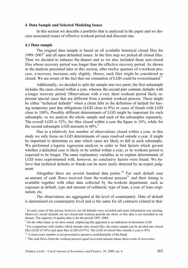
To account for bimodality we used an option to map continuous LGD to a num-ber of LGD grades. In each of these classes, data is more normally distributed than overall LGD. We use LGD grades based on Moody’s.:12 LGD1 is 0–10%, LGD2 is 10–30%, LGD3 is 30–50%, LGD4 is 50–70%, LGD5 is 70–90% and LGD6 is 90– –100%. The frequency counts based on these grades as already depicted in Figure 1, which reveals a binomial pattern of the LGD distribution.

LGD can be less than 0%, implying that a bank ultimately recovers more than 100% or more than 100%, e.g. as a result of high workout costs which exceed re-coveries. LGD needs to be cut off to avoid distortions. In this paper LGD is censored between 0 and 1, similarly to many other publications.

4.2 Effective Length of Workout Period The estimation of a workout period length and analysis of recoveries in time is

important from both regulatory and modeling perspective. The recovery period starts when client defaults or when workout department undertakes a file. The recovery pe-riod ends when the file is officially written-off or when the counterparty recovers and gets back to the portfolio of performing loans. Nowadays, most issues in Central Euro-pean commercial banks are non-closed because of a relatively short period since transition to market economy and emergence of first defaults. Some of the non-clos-ed files can be included in a sample of closed files if the estimated amount to be re-covered is not significant. For these cases the length of the workout period can be considered: – until non-recovered value is less than 5% of EAD; – one year after default (mainly used in retail); – +25% upper percentile from the distribution of length of workout period; – until effective recovery period (useful for non-retail).

Figure 1 The Effect of a Discount Factor on LGDa

0%

10%

20%

30%

40%

LGD 1 LGD 2 LGD 3 LGD 4 LGD 5 LGD 6Without a discount factor With asset class discount factors

Note: a LGD grades 1 to 6 are based on Moody’s grades and are described in the next section.

12 Alternatives are the other major rating agencies such as S&P and Fitch with similar LGD grades.


In this research, the last option is used; the effective workout period is esti-mated on the basis of cumulative recovery rate analysis. A cumulative recovery rate was calculated in order to show dynamic evolution of recovery rates over time,13 i.e. the time distribution of recovery rates. This enables us to analyze the evolution of recovered amount and to identify reasons of a non-efficient workout process. Count weighted and exposure weighted average cumulative and marginal recovery rates are calculated quarterly after the default date (see Appendix).

Based on this analysis we can conclude that the workout process is effective until the end of the third year. After the third year of recovery process there are only minor recovered amounts, mainly due to earlier defaulted counterparties with a long recovery period. Therefore, in our paper we considered a file with a workout period longer than three years to be a closed file.

4.3 Discount Rate In order to calculate LGD for a particular client, ex-post realized cash-flows

have to be discounted back to the date of default. Although there is no agreement about which discount rate to choose,14 we consider systematic asset risk class ap-proach proposed by Maclachlan (2005) as a preferred option to derive a risk premium of the discount rate.15 Risk premium for a particular client is determined by the class of collateral used to secure its claim. This approach enables to distinguish between various risks based on different sources of net cash flows.

We assigned different risk premiums as follows: – 0 basis points – cash collateral; – 240 basis points – residential real estate and land; – 420 basis points – movables and receivables; – 600 basis points – commercial real estate, stocks and unsecured loans; – 990 basis points – guarantees and promissory notes.16

The effect of application of discount rate based on the systematic asset risk class approach is shown in Figure 1.

As a benchmark option we consider a flat risk premium of 940 bps derived from ex post defaulted traded loans from a study by Brady et al. (2007). This study calculates a flat 940 bps premium for bank debt, which seems much more con-servative to the systematic asset risk class approach in which only the last category has a higher risk premium.

In our calculations we also tested flat LGD premiums in the range of 0–9%, increasing the premium by 1% resulted in an increase of LGD by approximately the same percentage point. This relatively small effect is due to a relatively short average workout period and significant portion of payments received in early years.

13 The methodology is based on a univariate mortality-based approach applied in Dermine and Neto de Car-valho (2006); the calculation does not include internal and external costs. 14 A summary of LGD discount rate issues can be found e.g. in Chalupka and Kopecsni (2008). 15 A discount rate can be simply defined as a sum of a risk-free rate and a risk premium. 16 As a client generally has more than one type of collateral, we weight the risk-premiums based on the per-centage of particular collateral out of an exposition at default (EAD) to arrive at a composite discount rate for the client.


The resulting average LGD from applying the systematic asset risk class approach is similar to the flat premium of 5%.

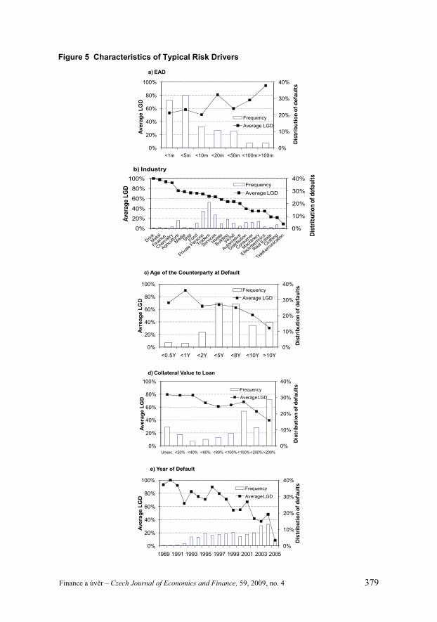
5. Analysis of Typical Risk Drivers Figure 5 in Appendix shows17 the distribution of the portfolio and average

LGD according to factors typically discussed in the literature – EAD, industry, age of the counterparty at the moment of default, collateral value to a loan and year of default. Columns marked in the right axis indicate frequencies and the lines are the average LGDs with values shown in the left axis. In general, the features of our data sample are consistent with the characteristics described in the literature.18

5.1 Year of Default and Loan Origination We hypothesize that year of default and loan origination are important deter-

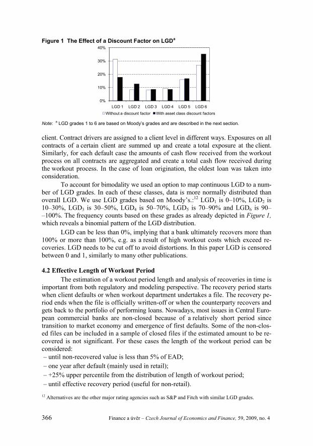
minants of LGD. Because of small number of observations in individual years we grouped cases in consecutive years into three periods. The first period contains cases which originated or defaulted in 1994 and earlier. The remaining cases are divided in another two groups, the first one containing observations which originated or de-faulted in 1995–2000, the other covering the period 2000–2005. All three subsamples are aimed to cover different stages in development of the Czech banking sector or different cycles of the Czech economy.

The first period can be characterized by transformation phase in the Czech economy with low prudence in loan origination process and subsequent problems with high proportion of non-performing loans. In 1990–1994 the government took steps to solve the problem in large banks by the Consolidation program, in which apart from other measures the non-performing loans of some banks were taken over by the government consolidation agency (Jaroš, 2000). As depicted in Figure 2b, the loans originated in this period have the highest (worst) LGD compared to the other periods. Because some cases defaulted in the second or third period, the pattern is not so clear when LGD is analyzed according to year of default (Figure 2a). Nevertheless, the over-all pattern is as expected.

The second and third period represent different macroeconomic cycles of the Czech economy. While the period 1995–2000 recorded a modest growth in the level

Figure 2 LGD in Different Periods According to the Year of Default and the Year of the Loan

0

10

20

30

40

50

60

1 2 3 4 5 6

Freq

uenc

y

LGD grades

a) LGD vs. Year of default

Year of default < 1995

Year of default 1995–2000

Year of default 2000–2005

0

10

20

30

40

50

60

1 2 3 4 5 6

Freq

uenc

y

LGD grades

b) LGD vs. Year of loan

Year of loan < 1995

Year of loan 1995–2000

Year of loan 2000–2005

17 A more detailed discussion is presented in the paper by Chalupka and Kopecsni (2008). 18 The sample also consists of non-closed files whose recovery period is currently longer than effective re-covery period. For this reason graphs do not show the definite figures.


of real HDP with two negative rates in 1997 and 1998, in 2000–2005 the Czech econ-omy experienced stable growth ranging from 1.9 to 6.3% ( SÚ 2009). The positive economic conditions appear to translate into relatively low LGD in 2000–2005 (Fig-ure 2a and Figure 2b).

In line with the results of this analysis we decided to use three periods (two dummy variables19) based on the year of default as another explanatory variable. Ad-ditionally, we also used a dummy variable for the year of default with the cases which defaulted before 1995.

6. Regression Methodology This section describes how the regression models employed in our analysis

are carried out. Before performing calculations the data is processed in several steps. Firstly, missing data is handled in the following ways: – Observations with missing data are excluded from the dataset. This option was

used in the cases when data necessary for modeling was missing, such as a col-lateral value.

– Missing data are added, replaced by an average or median value of the portfolio, replaced by a lower or higher cut-off. The age of counterparty is an example.

– Missing data are not replaced, neither those observations are excluded. This data is not essential for modeling; an illustrative factor is an industry where the miss-ing industry was coded as one level along with the data where information on the industry was available.

Outliers are detected on the basis of factor distribution and an expert judg-ment. An appropriate conservative cut-off value is applied, which is determined on the basis of the median, quantiles and power statistics20 of the factor.

In order to receive a more powerful model, different types of data need differ-ent transformation and adjustment. For continuous factors normalizing is applied after elimination of outliers. This is useful when the variables such as EAD (with a wide range of 0 to hundreds of millions in currency units) or factors such as age of counterparty (with a narrow range of 0–30 in years) are included in the model.

For some categorical factors a transformation into dummy variables is carried out. For collateral type and industry, grouping similar categories into one class is em-ployed. We have used four collateral type classes based on the risk aspect of the col-lateral, similar to the classes used in the calculation of the discount rate: – Class A: low risk – cash, land and residential real estate – Class B: lower average risk – movables and receivables – Class C: upper average risk – commercial real estate – Class D: high risk – securities and guarantees

There are 30 industry groups in the datasets, we grouped them into fewer cate-gories based on two classifications. Additionally, we “compressed” the alternative industry classification even further by having only two groups, the first one con-taining the “new industries” (Financial Services, Life Sciences and Healthcare, Tech-

19 The first dummy for loans originating in 1995–2000 and the other for loans started after 2000. 20 The power statistic is measured as an accuracy ratio defined in Sobehart and Keenan (2007).


nology, Media and Telecommunications and Business and Consumer Services) and the rest being the “traditional industries”.

6.1 Explanatory Variables Used From a statistical modeling point of view, factors are divided into continuous

factors (can be of any value), categorical factors (can be only of certain number of values) and dummy factors (can be of two values – zero and one). However, from a practical point of view, factors are divided into four main categories. We list the var-iables that are available for our analysis and in Table 2 we show those determinants of recovery which are actually used in the models.

Counterparty related factors:21 industry classification, the company’s age at the time of default, year of default, year of company origination, year of loan origi-nation and length of business connection at the time of default.

Contract related factors:22 type of the contract, exposure at the time of default, interest rate on the loan, tenure and number of different type of contracts.

Collateral related factors: collateral type, collateral value by type, aggregate collateral value, collateral value relative to the EAD, collateral value as a percentage

Table 2 Recovery Rate Determinants Used in the Models (type of variable and expected correlation with recovery rate)

Recovery rate determinants Type Correlation

Counterparty related factors Age of a counterparty Continuous Positive Length of business relationship Continuous ?Year of default before 1995 Dummy Negative Year of loan origination 1995–2000 Dummy Positive Year of loan origination after 2000 Dummy Positive New industries Dummy ?Industry not specified Dummy ?

Contract related factors Exposure at default Continuous ?Number of loans Categorical ?Investment type of loan Dummy ?Overdraft type of loan Dummy ?Revolving type of loan Dummy ?Purpose type of loan Dummy ?

Collateral related factors Collateral value of A relative to EAD Continuous Positive Collateral value of B relative to EAD Continuous Positive Collateral value of C relative to EAD Continuous Positive Collateral value of D relative to EAD Continuous Positive Number of different collaterals Categorical Positive

21 Other possible counterparty related factors are a reason of default; a legal form of the company, a count-erparty segment (SME, corporation, small tickets, etc.) size of the company, probability of default one year before default, length of time spent in default, intensity of business connection as distance from the domi-cile, financial indicators such as profitability, liquidity, solvency, capital market ratio, structure of the bal-ance sheet, stock return volatility. 22 Other possible contract related factors are seniority of the loan, size of the loan, type of approval and type of monitoring process.


of aggregate collateral value, a number of collaterals and diversification as a number of different collaterals.

Macroeconomic factors23 are not analyzed, because the dataset is relatively short.

6.2 Multivariate Analysis Three different generalized linear models are applied in order to estimate de-

terminants of the LGD – the first two models employ fractional responses either assuming beta inflated distribution or a more general model estimated by the quasi- -maximum likelihood estimator, the last one uses ordinal responses of dependent variable. In all three cases logit and log-log link functions are applied to capture both, a symmetric (logit) and an asymmetric case (log-log). As a benchmark, we firstly used a classical linear regression model to fit the data.

6.3 Models with Fractional Responses Using Quasi-Maximum Likelihood Estimator

Since LGD is a continuous variable typically bound within the interval [0,1], we need to map the limited interval of LGD on the potentially unlimited interval of LGD scores ( ’x). Generalized Linear Models (GLM) with an appropriate link function can be used for this procedure (McCullagh and Nelder, 1989). The quasi- -maximum likelihood estimator (QML) described below does not assume a particular distribution and it is hence more flexible to fit the data than a model using a par-ticular distribution.

If we denote the transformation function as G (.), the logit link using the lo-gistic function is

exp( ' )( ' )1 exp( ' )

G xxx

the log-log link using the extreme value distribution for dependent variable (the stand-ard Gumbel’s case) is

'( ' ) eG e

xx

and the complementary log-log link is '

( ' ) 1 eG ex

x

To estimate this GLM we use the non-linear estimation procedure which maximizes a Bernoulli log-likelihood function24

( , ) log ( ' ) (1 ) log 1 ( ' )i i i i iL a y G a y G ab b x b x

where a and b are estimated values of and .

6.4 Models with Fractional Responses Using a Beta Distribution Beta distribution has been also used to model LGD, for example in the com-

mercially available application LossCalc by Moody’s (Gupton and Stein, 2002). This

23 Possible macroeconomic factors are default rates, interest rate, GDP growth, inflation rate, industry con-centration. 24 For further technical details and practical applications see Papke and Wooldridge (1996).


approach assumes that LGD has a beta distribution. As the values of the distribution itself are bound within the range [0,1] a link function has to be used to map LGD scores onto this interval. As LGD of 0% or 100% are the values which are normally observable and hence have non-zero probabilities p0 and p1, we have used the inflated beta distribution25 with the location, scale and two shape parameters, , , and respectively, that allows for 0 and 1 defined by

0

110 1

1

01| , , , 1 1 0 1,

1Y

pif y

f y p p y y f yB

f yp

for 0 y 1, where = (1 – 2)/ 2, = (1 – )(1 – 2)/ 2, p0 = (1 + + )–1, p1 = (1 + + )–1 so > 0, > 0, 0 < p0 < 1, 0 < p1 < 1 – p0.

The parameter estimates of this GLM model were produced using a maximum likelihood.

6.5 Models with Ordinal Responses As an alternative technique, we have modeled 6 discrete LGD grades defin-

ed earlier using ordinal regression instead of continuous dependent variable used in the previous models.26 These models might be more appropriate if we expect default cases to be homogenous within the LGD grade but to be different between grades, either by having a different response to factors (different ) or a different likelihood that a default case will fall into a particular grade (a different intercept). The ordinary regression model using cumulative logit link function is defined as:

1

1

|| log

1 |

log 1, , 1j

j J

P Y jlogit P Y j

P Y j

j J

xx

x

x xx x

Each cumulative logit uses all J response categories. A model for logit[P(Y j)] alone is an ordinary logit model for a binary response in which categories 1 to j form one outcome and categories j + 1 to J form the other. A model that simultaneously uses all cumulative logits is

| 1, , 1jlogit P Y j j Jx x

Each cumulative logit has its own intercept. The j are increasing in j, since P(Y j|x) increases in j for fixed x, and the logit is an increasing function of this probability. This model has the same effects for each logit and since we consider the same effects in each grade as appropriate, we have used it; we allow for different intercepts.

25 This definition of beta inflated distribution is based on (Rigby and Stasinopulos, 2005). 26 Since LGD grades are a dependent variable in ordinal regressions, we have used recovery rates (not LGD)as a fractional response to have the same sign of estimated coefficients in both cases.


To fit this special case of the GLM, we let (yi1, …, yiJ) to be the binary indi-cators of the response for the subject i. The likelihood function (e.g. Agresti (2002)) is

1 1 1 1

1

1 1 1

| 1 |

exp exp

1 exp 1 exp

ijij

ij

n J n J yyj i i i

i j i j

yn J j i j i

i j j i j i

P Y j P Y j

' '

x x x

x x

'x 'x

It is minimized as a function of different intercepts j and common slope coefficients for each LGD grade.

The complementary log-log link for ordinal regression model is defined as

log log 1 | , 1, , 1jP Y j j Jx x

With this link, P(Y j) approaches 1 at a faster rate than it approaches 0. The log-log link

log log | , 1, , 1jP Y j j Jx x

is appropriate when the complementary log-log link holds for the categories listed in reverse order.

7. Results of Models In order to select the most appropriate model, some commonly used proce-

dures are followed. Continuous variables are plotted against LGD (and against LGD grades for ordinal responses) to get “a feel” of the underlying relationship.27 Simi-larly, categorical variables are tabulated to form an expectation of a potential rela-tionship. Moreover, a frequency table provides information whether there are enough counts for each cell to estimate the effect reliably.28 Thirdly, correlation29 and power statistics (Table 5 in Appendix) using each explanatory variable separately is per-formed to see the effect of each variable independent of the other effects. All poten-tially plausible variables are then put together in a regression model. Afterwards, the variables not contributing significantly to the explanatory power of a model are gradually eliminated from the model (backward elimination) based on Akaike (AIC) and Schwarz information criteria (SIC). For models where continuous dependent

27 If a relationship was not monotonous because of a few extreme observations, an appropriate cut-off was ap-plied. Provided that the relationship was unclear and no transformation of a variable was suitable, the var-iable was not used in the analysis. 28 This is important for ordinal regression as we have six grades and we must have enough observations foreach explanatory variable in each grade. If necessary, categorical drivers with numerous levels were grouped. 29 Kendall’s tau rank correlation coefficient (Kendall, 1990) is utilised as it does not require normallydistributed variables to calculate p-values like parametric Pearson’s correlation and it is also preferredto more popular Spearman’s rank correlation when a data set is small with large number of tied ranks(Field, 2005).


variable is estimated and a specific distribution is assumed, worm plots for residuals (van Buuren and Fredriks, 2001), and QQ-plots30 were utilized to have a visual in-dication of normality of residuals.

8. Summary of Findings The results in Table 3 reveal interesting findings.31 As expected, collaterals of

class A and C have a positive and strong effect on recovery rates. These collaterals represent land, residential real estate, cash and commercial real estate. Hence there is no surprise if we find a strong positive relationship, higher proportion of collateral as a percent of EAD increases recovery or likelihood of recovery. Similarly, the year of loan origination has a significant impact on LGD. Both periods (loans originating in 1995–2000 and after 2000) have a negative influence on LGD when compared to loans extended before 1995. As we have already outlined, the period before 1995 was characterized by several problems in the Czech banking sector with a high level of non-performing loans. Weak efficiency of workout process was thus very likely, trans-lating into high average LGD. The situation improved in the period 1995–2000; the low LGD after 2000 is further fuelled by a positive macroeconomic climate. EAD is the next variable significant in almost all the models. The correlation with re-coveries is negative and recoveries tend to be lower with the higher loans. The first explanation from the literature could be a weaker link between the management and company results in the case of big companies having high bank loans. This contra-dicts the assumption that a bank intensifies the enquiry of the creditworthiness and the monitoring of the borrower with high loans. The second explanation could be high leverage of big companies and violation of the absolute priority rule. If a big company defaults, there are many creditors competing for the company’s assets, so the recovery for a bank can be small. Length of business relationship appears in half of the models and it has a strong negative effect on the recovery rate. For clients with long relationship, lower recoveries can be explained by the less prudent attitude to-wards the “familiar” clients. The effect of other variables is not so unambiguous and the results are different for different models, the specifics are discussed for each class of models.

8.1 Classical Linear Regression Model The linear regression model as the benchmark is the simplest case in which

a continuous recovery rate variable is regressed on a linear combination of explana-tory variables. The major drawback of this method is that the predicted values can be outside the range [0,1]. Rather surprisingly, the simple linear model is able “to remove” bimodality of the whole sample as shown by residuals which are inside the bounds of confidence intervals of the worm plot, close to normal quantile in the QQ-plot (as depicted in Figure W1 – see the web-page of this journal).

Apart from the common factors discussed in the previous subsection, there are no other significant variables.

30 In the QQ-plots sample values are plotted against theoretical values predicted by a distribution. 31 We report only results based on SIC; AIC yields similar results, but allows more variables to be includedin the models.

Tabl

e 3

Sum

mar

y of

Sig

nific

ant D

eter

min

ants

for A

ll M

odel

s (p

-val

ues

are

in th

e br

acke

ts)

Mod

el

Exposure at default – EAD

Collateral class A as % of EAD

Collateral class B as % of EAD

Collateral class C as % of EAD

Collateral class D as % of EAD

Age of a counterparty

Length of business relationship

No of different collateral classes

Year of default before 1995

New industries

Industry not specified

Number of loans

Investment type of loan

Overdraft type of loan

Revolving type of loan

Purpose type of loan

Loan origination 1995–2000

Loan origination after 2000

Line

ar m

odel

0.46

9(0

.000

)0.

491

(0.0

00)

-0.2

14(0

.001

)

0.23

6(0

.000

)0.

389

(0.0

00)

Frac

tiona

l res

pons

e (lo

git l

ink)

2.

518

(0.0

01)

2.67

7(0

.001

)-1

.235

(0.0

13)

1.

288

(0.0

00)

1.96

8(0

.000

)

Frac

tiona

l res

pons

e (lo

g-lo

g lin

k)

1.78

4(0

.002

)1.

688

(0.0

05)

0.79

7(0

.000

)1.

290

(0.0

00)

Frac

tiona

l res

pons

e (c

ompl

emen

tary

lo

g-lo

g lin

k)

1.53

8(0

.000

)1.

640

(0.0

00)

-0.9

51(0

.012

)

1.03

5(0

.000

)1.

458

(0.0

00)

Frac

tiona

l res

pons

e be

ta (l

ogit

link)

-1

.228

(0.0

01)

0.97

4(0

.018

)

-0

.766

(0.0

00)

1.

107

(0.0

00)

1.69

6(0

.000

)

Frac

tiona

l res

pons

e be

ta (l

og-lo

g lin

k)

-0.6

28(0

.000

)0.

723

(0.0

14)

-0.4

42(0

.000

)

0.61

9(0

.000

)1.

048

(0.0

00)

Frac

tiona

l res

pons

e be

ta

(com

plem

enta

ry

log-

log

link)

-1.0

86(0

.000

)

-0.6

37(0

.000

)

0.93

6(0

.000

)1.

350

(0.0

00)

Ord

inal

resp

onse

(lo

git l

ink)

-2

.228

(0.0

03)

2.78

7(0

.000

)2.

673

(0.0

00)

-1.1

17(0

.006

)-0

.909

(0.0

01)

1.

676

(0.0

00)

2.64

3(0

.000

)


Ord

inal

resp

onse

(c

ompl

emen

tary

lo

g-lo

g lin

k)

-1.4

88(0

.008

)1.

321

(0.0

00)

1.48

1(0

.000

)-0

.746

(0.0

06)

-0.5

40(0

.004

)

1.03

4(0

.000

)1.

478

(0.0

00)


8.2 Models with Fractional Responses Using Quasi-Maximum Likelihood Estimator

Applying the asymmetric log-log link function32 to regress continuous recov-ery rates estimated by quasi-maximum likelihood yields slightly better results than the logit link function. A period of loan origination, along with collateral of class A and C are the major determinants of LGD. EAD which is strongly negatively cor-related to the collateral classes appears not to be a significant factor.33 Length of busi-ness relationship is also significant in two of the three models.

8.3 Models with Fractional Responses Using a Beta Distribution The fit employing the inflated beta distribution and the logit link is very simi-

lar to the log-log link.34 Logit fits the data reasonably (Figure W2 – see the web-page of this journal), although the fit is worse for higher recovery rates.

Compared to the other models, collateral of class A (residential real estate) is not significant. The model identifies a non-specified industry as an additional im-portant factor. These singularities can be explained by the assumption of beta dis-tributed errors. The other factors are in line with the previous results.

8.4 Models with Ordinal Responses As for ordinal response models, increasing the length of business relationship

measured as a period between the date of bank account opening and the date of de-fault decreases the likelihood of low LGD, similarly to the classical linear model. Also consistent to previous results, a loan originated after 1995 has lower probability of high LGD. Correspondingly to the beta distribution model, a non-specified in-dustry is a statistically significant determinant of LGD also.

9. Comparing Goodness-of-Fit of the Models Goodness-of-fit summary measures offer an overall indication of the model

fit. Out of parametric performance measures, mean square error (MSE), mean ab-solute deviation (MAD) and correlation between observed and modeled LGD have been evaluated to compare predictive power of suggested models. The outcomes from correlation are listed in Table 4.

MSE, MAD and correlation coefficient measure model performance para-metrically and are sensitive to model calibration. In contrast, a power statistic is a non-parametric measure that focuses on the ability to discriminate “good” out-comes from “bad” outcomes without being sensitive to the calibration. It indicates a model’s power and ranges from zero to one. It provides information about different aspects of model performance not registered by the above mentioned measures.

The power statistic35 is commonly used for PD models where there are only two possibilities – a default or a non-default. However, in LGD models the depend- 32 Determinants of recovery rates for the logit and complementary log-log function are shown in the sum-mary table in Appendix. 33 However, a larger sample would enable to distinguish the effects of highly correlated factors better and we expect EAD to have an impact. 34 The log-log and complementary log-log links are again shown in the summary table in Appendix. 35 The Power statistic is described for instance in Gupton and Stein (2002).


ent variable is continuous. In order to apply the power statistic, it is necessary to de-fine what is considered as “good” and what is considered as “bad”. In the paper by Chalupka and Kopecsni (2008) three different alternatives are proposed.

Alternatively, ordinal power statistic can be applied to LGD models. This sta-tistic (Table 4) measures the ability of a certain model to differentiate between any numbers of rating categories in the correct order; hence it is used particularly for the ordinal response models. The results are similar to the previous case.

The linear model, fractional models using quasi- maximum likelihood and or-dinal response models perform similarly and relatively well in absolute terms.

9.1 Robustness Tests The studied sample was divided into two halves based on three different cri-

teria to test robustness of our results. Firstly, the sample was ordered according to the date of default and each second observation was put into one subsample and the rest of observations into the other subsample. Secondly, observations were ar-ranged according to LGD grades, and again every second observation was put into one sample and the rest into the other. Thirdly, observations were randomly assigned into two subsamples. For each division we re-performed calculations of the models and checked whether subsamples had the same significant drivers as the whole sam-ple. We can conclude that results of subsamples are consistent with the whole sample; the major drivers, as well as the signs of coefficients remained the same. Only mag-nitudes changed somewhat; especially in the case of the random division.36

Additionally, we have verified the models’ out-of-sample predictive power. Employing the results of the subsamples in each of the three divisions, the estimated coefficients were applied to predict LGD in the other half of each subsample. The re-sulting power statistics yield satisfactory results ranging from 54 to 60%.

Table 4 Performance Measures – Kendall’s Tau Rank Correlation and Power Statistic

Model Correlation P-value Power Statistic SE

Linear model 0.423 0.000 63.6% 4.2%Fractional response (logit link) 0.382 0.000 60.9% 4.7%Fractional response (log-log link) 0.388 0.000 61.3% 4.5%Fractional response (complementary log-log link) 0.362 0.000 58.3% 4.3%

Fractional response beta (logit link) 0.423 0.000 63.6% 4.1%Fractional response beta (log-log link) 0.416 0.000 62.9% 4.5%Fractional response beta (complementary log-log link) 0.416 0.000 61.4% 4.1%

Ordinal response (logit link) 0.429 0.000 65.6% 4.5%Ordinal response (complementary log-log link) 0.425 0.000 65.3% 3.8%

36 The estimated coefficients of the subsamples are available from the authors upon request.


10. Conclusions In this paper, various statistical models were applied to test empirically the de-

terminants of LGD. We have found that the main drivers are the period of loan origination, relative value of collateral, loan size and length of business relationship. Different models provided similar results. As for the different links in more complex models, log-log models in some cases performed better, implying an asymmetric re-sponse of the dependent variable. All models performed relatively well when the over-all fit of the different models was assessed. However, the models with the commonly assumed beta distribution achieved slightly worse results and hence are not deemed optimal for our data.

From a policy perspective, the paper provides evidence that workout LGD is a viable option in the credit risk estimation, despite various methodological diffi-culties. In this study, we try to provide a reasonable detail of various issues to be tackled and propose methodological alternatives to cope with these issues.

There are several ways in which our research can be improved. Firstly, a simi-lar study can be done on a larger sample of data and hence some of the effects could be estimated more precisely. Secondly, correlation of recovery rate and probability of default, effects of macroeconomic factors and downturn LGD should be thoroughly analyzed for a complete LGD model.

APPENDIX

FIGURESFigure 3 Average Cumulative Recovery Rate

0%

20%

40%

60%

80%

Q1 Q5 Q9 Q13 Q17 Q21 Q25 Q29 Q33

Count Weighted Exposure Weighted

Figure 4 Average Marginal Recovery Rate

0%

4%

8%

12%

16%

20%

Q1 Q5 Q9 Q13 Q17 Q21 Q25 Q29 Q33

Count Weighted Exposure Weighted


Figure 5 Characteristics of Typical Risk Drivers

0%

10%

20%

30%

40%

0%

20%

40%

60%

80%

100%

<1m <5m <10m <20m <50m <100m>100m

Dis

trib

utio

n of

def

aults

Aver

age

LGD

a) EAD

FrequencyAverage LGD

0%

10%

20%

30%

40%

0%

20%

40%

60%

80%

100%

Dist

ribut

ion

of d

efau

lts

Aver

age

LGD

b) Industry

Frequency

Average LGD

0%

10%

20%

30%

40%

0%

20%

40%

60%

80%

100%

<0.5Y <1Y <2Y <5Y <8Y <10Y >10Y

Dist

ribut

ion

of d

efau

lts

Avre

age

LGD

c) Age of the Counterparty at Default

FrequencyAverage LGD

0%

10%

20%

30%

40%

0%

20%

40%

60%

80%

100%

Unsec. <20% <40% <60% <80% <100%<150%<200%>200%

Dis

trib

utio

n of

def

aults

Aver

age

LGD

d) Collateral Value to Loan

Frequency

Average LGD

0%

10%

20%

30%

40%

0%

20%

40%

60%

80%

100%

1989 1991 1993 1995 1997 1999 2001 2003 2005

Dis

trib

utio

n of

def

aults

Aver

age

LGD

e) Year of Default

Frequency

Average LGD


0%

10%

20%

30%

40%

0

3

6

9

12

15

18

1989 1991 1993 1995 1997 1999 2001 2003 2005

Dist

ribut

ion

of d

efau

lts

Reco

very

per

iod

f) Year of default vs. Recovery period

Frequency

Recovery Period

TABLES Table 5 Power Statistic of Individual Factors

Factor Power statistic SE Exposure at default – EAD 17% 6% Collateral class A as % of EAD -18% 6% Collateral class B as % of EAD -5% 4% Collateral class C as % of EAD -18% 6% Collateral class D as % of EAD -2% 6% Age of a counterparty -30% 6% Length of business relationship 20% 6% Number of different collateral classes -29% 5% Year of default before 1995 14% 3% New industries 0% 3% Industry not specified 5% 5% Number of loans -3% 5% Investment type of loan -2% 5% Overdraft type of loan -9% 4% Revolving type of loan -11% 4% Purpose type of loan 5% 6% Loan origination 1995–2000 -7% 6% Loan origination after 2000 -33% 5%


REFERENCES

Acharya VV et al. (2003): Understanding the Recovery Rate of Defaulted Securities. Center for Economic Policy Research Discussion Papers, no. 4098. Agresti A (2002): Categorical Data Analysis. 2nd Edition. Wiley Series in Probability and Statistics, John Wiley & Sons, Inc., Hoboken, New Jersey. Altman E, Kishore V (1996): Almost everything you want to know about Recoveries on Defaulted Bonds. Financial Analyst Journal, 52(6):57–64. Asarnov E, Edwards D (1995): Measuring Loss on Defaulted Bank Loans: A 24 year study. Journal of Commercial Lending, 77(7):11–23. Basel Committee on Banking Supervision (2006): International Convergence of Capital Measure-ment and Capital Standards. Bank for International Settlements, Basel. Brady B et al. (2007): Discount Rate for Workout Recovery: An Empirical Study. Available at SSRN: http://ssrn.com/abstract=907073. Buuren S van, Fredriks M (2001): Worm plot: a simple diagnostic device for modeling growth reference curves. Statistics in Medicine, 20(8):1259–1277. Carey M (1998): Credit Risk in Private Debt Portfolios, Journal of Finance, 53(4):1363–1387. Carty L, Lieberman D (1996): Defaulted Bank Loan Recoveries, Global Credit Research, Moody's. Chalupka R, Kopecsni J (2008): Modelling Bank Loan LGD of Corporate and SME Segment: A Case Study. Charles University in Prague, Faculty of Social Sciences, IES Working Paper, no. 27. Dermine J, Neto de Carvalho C (2006): Bank Loan Losses-Given-Default, A case study. Journal of Banking and Finance, 30(4):1219–1243. Field A (2005): Discovering Statistics Using SPSS. 2nd Edition. Sage Publications Ltd, London, UK. Franks J et al. (2004): A comparative analysis of the recovery process and recovery rates for private companies in the UK, France and Germany. Risk Solutions, Standard & Poor’s. Frye J (2000): Depressing recoveries. Risk, 13(11):108–111. Grossman R et al. (1997): Syndicated Bank Loan Recovery Study, Fitch Research. Grossman R et al. (2001): Bank Loan and Bond Recovery Study: 1997–2000. Fitch Loan products special report. Grunert J, Weber M (2005): Recovery Rates of Bank Loans: Empirical Evidence for Germany. University of Mannheim - Working Paper. Gupton GM et al. (2000): Bank Loan Loss Given Default. Global Credit Research, Moody's. Gupton GM, Stein RM (2002): LossCalc: Model for predicting loss given default (LGD). Global Credit Research, Moody’s. Hurt L, Felsovalyi A (1998): Measuring loss on Latin American defaulted bank loans, a 27-year study of 27 countries. The Journal of Lending and Credit Risk Management, 81(2):41–46. Jaroš T (2000): Credit Crunch (teorie a eská praxe). Diploma thesis, Charles University in Prague. Kendall MG (1990): Rank Correlation Methods. 4th Edition. A Charles Griffin Book, London. Maclachlan I (2005): Choosing the Discount Factor for Estimating Economic LGD. In: Altman E, Resti A, Sironi A (Eds.): Recovery Risk, The Next Challenge in Credit Risk Management. Risk Books, London, 285–305. McCullagh P, Nelder JA (1989): Generalized Linear Models. 2nd edition. Chapman and Hall, London. Papke LE, Wooldrigdge JM (1996): Econometric Method for Fractional Response Variables with an Application to 401 (K) Plan Participation Rates. Journal of Applied Econometrics, 11(6):619–632. Renault O, Scaillet O (2004): On the Way to Recovery: A Non-parametric bias free estimation of recovery rate intensities. Journal of Banking and Finance, 28(12):2915–31.


Rigby RA, Stasinopoulos DM (2005): Generalized additive models for location, scale and shape, (with discussion). Applied Statistics, 54(3):507–554. Schuermann T (2004): What do we know about Loss Given Default? In: Shimko D: Credit Risk Models and Managament. Risk Books, London. Seidler J, Jakubík P (2009): Implied Market Loss Given Default in the Czech Republic: Structural- -Model Approach. Finance a úv r-Czech Journal of Economics and Finance, 59(1):20–40. Thornburn K (2000): Bankruptcy auctions: costs, debt recovery and firm survival, Journal of Financial Economics, 58(3):337–368.

Modeling Bank Loan LGD of Corporate and SME Segments: …journal.fsv.cuni.cz/storage/1165_360-382---chal.-kop.pdf · Modeling Bank Loan LGD of Corporate and SME Segments: A Case Study*

Documents