JOURNAL OF COMPUTATIONAL PHYSICS 147, 402–440 (1998) ARTICLE NO. CP986097 Modeling Arteriolar Flow and Mass Transport Using the Immersed Boundary Method Kayne M. Arthurs, * Leon C. Moore,† Charles S. Peskin,‡ E. Bruce Pitman,§ and H. E. Layton * * Department of Mathematics, Duke University, Durham, North Carolina 27708-0320; †Department of Physiology and Biophysics, State University of New York, Stony Brook, New York 11794-8661; ‡Courant Institute of Mathematical Sciences, New York University, New York, New York 10012; §Department of Mathematics, State University of New York, Buffalo, New York 14214-3093 E-mail: [email protected], [email protected], [email protected], [email protected], [email protected] Received April 28, 1998; revised August 14, 1998 Flow in arterioles is determined by a number of interacting factors, including per- fusion pressure, neural stimulation, vasoactive substances, the intrinsic contractility of arteriolar walls, and wall shear stress. We have developed a two-dimensional model of arteriolar fluid flow and mass transport. The model includes a phenomenological representation of the myogenic response of the arteriolar wall, in which an increase in perfusion pressure stimulates vasoconstriction. The model also includes the release, advection, diffusion, degradation, and dilatory action of nitric oxide (NO), a potent, but short-lived, vasodilatory agent. Parameters for the model were taken primarily from the experimental literature of the rat renal afferent arteriole. Solutions to the incompressible Navier-Stokes equations were approximated by means of a splitting that used upwind differencing for the inertial term and a spectral method for the viscous term and incompressibility condition. The immersed boundary method was used to include the forces arising from the arteriolar walls. The advection of NO was computed by means of a high-order flux-corrected transport scheme; the diffusion of NO was computed by a spectral solver. Simulations demonstrated the efficacy of the numerical methods employed, and grid refinement studies confirmed anticipated first-order temporal convergence and demonstrated second-order spatial convergence in key quantities. By providing information about the effective width of the immersed boundary and sheer stress magnitude near that boundary, the grid refinement studies indicate the degree of spatial refinement required for quantitatively reliable simula- tions. Owing to the dominating effect of NO advection, relative to degradation and diffusion, simulations indicate that NO has the capacity to produce dilation along the entire length of the arteriole. c 1998 Academic Press 402 0021-9991/98 $25.00 Copyright c 1998 by Academic Press All rights of reproduction in any form reserved.

Welcome message from author
This document is posted to help you gain knowledge. Please leave a comment to let me know what you think about it! Share it to your friends and learn new things together.
Transcript
JOURNAL OF COMPUTATIONAL PHYSICS147,402–440 (1998)ARTICLE NO. CP986097
Modeling Arteriolar Flow and Mass TransportUsing the Immersed Boundary Method
Kayne M. Arthurs,∗ Leon C. Moore,† Charles S. Peskin,‡E. Bruce Pitman,§ and H. E. Layton∗
∗Department of Mathematics, Duke University, Durham, North Carolina 27708-0320;†Departmentof Physiology and Biophysics, State University of New York, Stony Brook, New York
11794-8661;‡Courant Institute of Mathematical Sciences, New York University,New York, New York 10012;§Department of Mathematics, State University
of New York, Buffalo, New York 14214-3093E-mail: [email protected], [email protected], [email protected],
[email protected], [email protected]
Received April 28, 1998; revised August 14, 1998
Flow in arterioles is determined by a number of interacting factors, including per-fusion pressure, neural stimulation, vasoactive substances, the intrinsic contractilityof arteriolar walls, and wall shear stress. We have developed a two-dimensional modelof arteriolar fluid flow and mass transport. The model includes a phenomenologicalrepresentation of the myogenic response of the arteriolar wall, in which an increase inperfusion pressure stimulates vasoconstriction. The model also includes the release,advection, diffusion, degradation, and dilatory action of nitric oxide (NO), a potent,but short-lived, vasodilatory agent. Parameters for the model were taken primarilyfrom the experimental literature of the rat renal afferent arteriole. Solutions to theincompressible Navier-Stokes equations were approximated by means of a splittingthat used upwind differencing for the inertial term and a spectral method for theviscous term and incompressibility condition. The immersed boundary method wasused to include the forces arising from the arteriolar walls. The advection of NO wascomputed by means of a high-order flux-corrected transport scheme; the diffusionof NO was computed by a spectral solver. Simulations demonstrated the efficacy ofthe numerical methods employed, and grid refinement studies confirmed anticipatedfirst-order temporal convergence and demonstrated second-order spatial convergencein key quantities. By providing information about the effective width of the immersedboundary and sheer stress magnitude near that boundary, the grid refinement studiesindicate the degree of spatial refinement required for quantitatively reliable simula-tions. Owing to the dominating effect of NO advection, relative to degradation anddiffusion, simulations indicate that NO has the capacity to produce dilation along theentire length of the arteriole. c© 1998 Academic Press
402
0021-9991/98 $25.00Copyright c© 1998 by Academic PressAll rights of reproduction in any form reserved.
MODELING ARTERIOLAR FLOW 403
Key Words:computational biofluiddynamics; blood vessel; renal microvasculature;myogenic autoregulation; nitric oxide.
1. INTRODUCTION
The goals of this study are to formulate a detailed model for blood flow and mass transportin an arteriole and to develop and evaluate a numerical algorithm for the solution of themodel. The model and numerical algorithm rely heavily on the immersed boundary method(IMBM), which was originally developed to study fluid motion in the heart [27].
Arterioles have diameters ranging from about 10 to 200µm and lengths ranging from100 to 1000µm. Average flow velocities are∼1 cm/s, and pressure gradients along thedirection of flow are∼1000 mm Hg/cm. The Reynolds number of arteriolar flow is typicallyabout 0.1 (based on an arteriolar diameter of 20µm and a kinematic blood viscosity of1.66× 10−2 cm2/s [1, 23]).
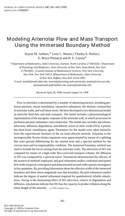
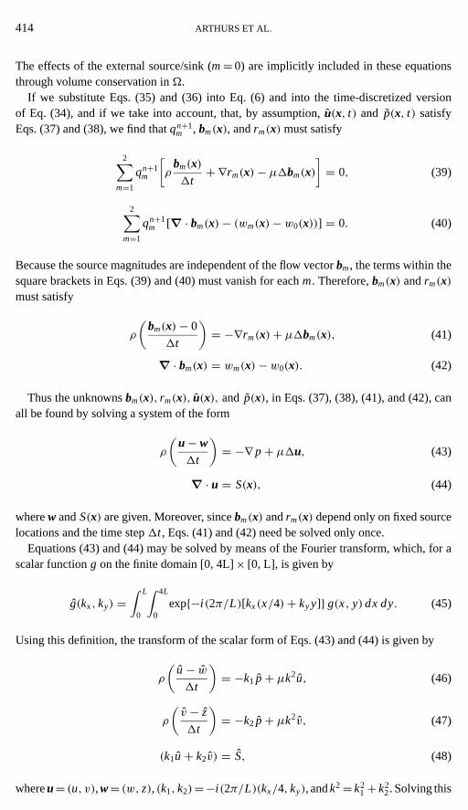
Arteriolar walls consist of several outer layers of smooth muscle cells and an innerlayer of endothelial cells. These endothelial cells can release vasoactive substances intothe blood stream and into the arteriolar wall, where they can influence the adjacent smoothmuscle cells. In this study, the arteriolar wall is modeled as a massless, elastic–contractileclosed boundary immersed in a viscous, incompressible fluid. The boundary is initiallyconfigured as parallel line segments with semi-circular closures at the ends (see Fig. 1).The fluid region inside the boundary represents blood; the exterior fluid region representsthe local surroundings of the arteriole. Flow through the model arteriole is induced by ahigh-pressure fluid source at one end and by a low-pressure fluid sink at the opposite end.
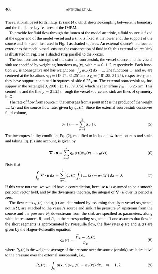
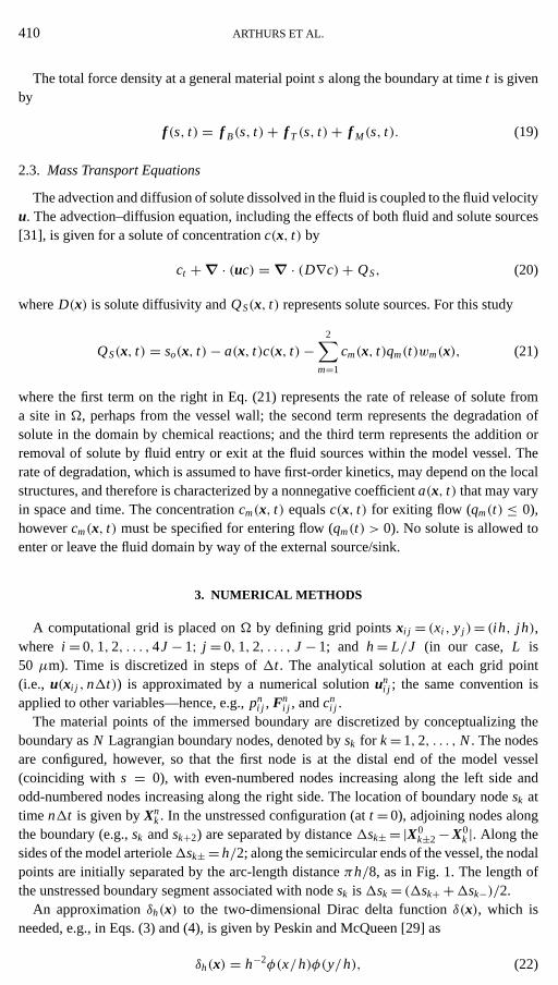
FIG. 1. The domainÄ, with model configuration, is shown at left. The initial position of the model arteriolarwall (dark heavy line) encloses the fluid source (upper shaded square) and sink (lower shaded square), which havefixed positions. The shaded vertical strip is the support of the external source/sink. An enlarged portion ofÄ, atright, shows the support of the source, relative to the Eulerian grid, and the individual nodes used in the numericaldiscretization of the arteriolar wall (see Section 3). Length scales are in micrometers.
404 ARTHURS ET AL.
Fluid velocities and pressures are determined by solving the incompressible Navier–Stokesequations, modified in accordance with the IMBM (see below). After pressurization, themodel arteriole is approximately 20µm in diameter and 150µm in length.
The description of the boundary includes a phenomenological model of the myogenicresponse, in which an increase in intravascular pressure causes a contraction of vascularsmooth muscle. This contraction reduces average arteriolar diameter, which increases totalsegmental resistance and thereby acts to stabilize downstream pressure [5]. In vivo, thiscontractile response is modulated by the local concentration of vasoactive agents, e.g., nitricoxide (NO), a potent vasodilator. The release of NO from the arteriolar wall is stimulatedby shear stress [4] and by the binding of a number of other vasoactive substances [24].Alternatively, NO may be released as a consequence of vascular injury [18]. The arteriolarmodel includes provisions for the mass transport of NO, specifically, the release, advection,diffusion, degradation, and vasodilatory action of NO. Mathematical models have beendeveloped by other investigators to examine the temporal evolution of NO in tissue [8, 22].Our model is distinguished by its emphasis on the detailed description of fluid motion andcoupled NO transport.
The IMBM was used to model the interaction between the fluid and the arteriolar wallby means of an immersed elastic–contractile boundary. The action of the boundary on thefluid arises from a body force included in the Navier–Stokes equations. The boundary, asa consequence of the no-slip condition, is required to move at the local fluid velocity. TheIMBM has been used to simulate fluid dynamics of the inner ear [2], bacterial swimming[9], biofilm processes [10], peristaltic pumping of solid particles [11], sperm motility in thepresence of boundaries [12], aquatic animal locomotion [13], platelet aggregation duringblood clotting [14], suspended particles in three-dimensional Stokes flow [15], and three-dimensional heart motion [29].
The Navier–Stokes equations were solved by a tripartite splitting that is first-order in time.The body force arising from the boundary was evaluated by an explicit differencing. Theinertial term, which makes only a small contribution to the solution for low Reynolds numberflow, was evaluated by upwind differencing. The viscous term and the incompressibilitycondition were considered together in a backward Euler discretization of the time-dependentStokes equations. These equations were then evaluated by a spectral method.
The advection–diffusion equation for mass transport was also solved by a tripartite split-ting. Solute sources were evaluated by an explicit differencing. The advection term, whichrequires special care to avoid artifactual diffusion and dispersion, was evaluated by a flux-corrected transport scheme that employs upwind-differencing for the low-order componentand an eighth-order Richtmyer two-step Lax–Wendroff scheme for the high-order compo-nent. The diffusion term, represented by a backward Euler discretization, was evaluated bya spectral method.
Simulation parameters are based on experimental measurements from the renal afferentarteriole of the rat. The afferent arteriole has been heavily studied because of its role inhemodynamic control, which is critical to the homeostatic function of the kidney and whichprotects delicate down-stream structures (e.g., the glomerulus) [32].
Extensive tests were conducted to confirm the accuracy and adequacy of the numeri-cal methods and to determine the degree of numerical resolution required for quantita-tively reliable simulations. In particular, tests were conducted to determine the effectiveimmersed boundary width and the shear stress magnitude near the boundary. Simulationsindicate that the model exhibits first-order convergence in time and that key quantities exhibit
MODELING ARTERIOLAR FLOW 405
second-order convergence in space. Simulations also indicate that a spatial grid resolutionof <1µm is required to adequately represent mass transport of NO.
2. MODEL FORMULATION
2.1. Fluid Equations and Immersed Boundary Method
In this two-dimensional model, the arteriolar wall is modeled as an immersed boundaryin a rectangular Eulerian fluid domainÄ with periodic boundary conditions. The domainÄ, expressed in units ofµm, is the set [0, 200]× [0, 50]; position inÄ will be denotedby x= (x, y), with the positivex-direction usually pointing downward in our figures (seeFig. 1). The fluid is assumed to be incompressible with uniform densityρ and uniform dy-namic viscosityµ. The immersed boundary is initially situated withinÄ as shown in Fig. 1.The boundary configuration at timet is given parametrically byX(s, t),−l/2≤ s≤ l/2,whereX is a point inÄ, the parameters marks a fixed material point of the bound-ary, and l is the length of the unstressed boundary. Because the boundary is closed,X(−l/2, t)=X(l/2, t). The values= 0 corresponds to the point on the boundary havingthe largestx-coordinate. The parameters increases with counterclockwise orientation.
The Navier–Stokes equations, modified for our application, are given by
ρ(∂tu+ (u · ∇)u) = −∇ p+ µ1u+ F − σκu, (1)
∇ · u = 0, (2)
whereu(x, t) is the fluid velocity andp(x, t) is the fluid pressure. The body forces that theimmersed boundary imparts to the fluid are included as an external force densityF(x, t).To simulate the anatomical structures and interstitial matrix external to the arteriole, adamping term,σκu, proportional to the fluid velocity and with constant damping coefficientκ has been added to the Navier–Stokes equations. The dimensionless functionσ(x, t) isconstructed so that damping acts externally to the vessel;σ is approximately one outsidethe model vessel and zero inside the vessel (see Eq. (31) below). The damping term, byreducing the velocity of flow that is induced exterior to the model vessel (by expansionof the vessel), allows more rapid attainment of a near steady state. The divergence-freecondition given by Eq. (2) applies overÄ except at fluid sources or sinks (see below).
The force densityF(x, t), a Dirac delta-function layer along the immersed boundary, isgiven by
F(x, t) =∫ l/2
−l/2f (s, t)δ(x− X(s, t)) ds, (3)
whereδ is the two-dimensional Dirac delta function andf (s, t) is the density of the bound-ary force with respect to the measureds. The boundary force densityf (s, t) arises fromthe properties of the boundary and, therefore, is specific to the particular application of themethod. To represent arteriolar walls,f (s, t) should include the elastic–contractile proper-ties of the smooth muscle sheath and its modulation by vasoactive agents.
Because the immersed boundary moves with the fluid, the equation of motion for theboundary, equivalent to the no-slip condition, is given by
∂X(s, t)∂t
= u(X(s, t), t) =∫Ä
u(x, t)δ(x− X(s, t)) dx. (4)
406 ARTHURS ET AL.
The relationships set forth in Eqs. (3) and (4), which describe coupling between the boundaryand the fluid, are key features of the IMBM.
To provide for fluid flow through the lumen of the model arteriole, a fluid source is fixedat the upper end of the model vessel and a sink is fixed at the lower end; the support of thesource and sink are illustrated in Fig. 1 as shaded squares. An external source/sink, locatedexterior to the model vessel, ensures the conservation of fluid inÄ; this external source/sinkis illustrated in Fig. 1 as a shaded strip parallel to thex-axis.
The locations and strengths of the external source/sink, the vessel source, and the vesselsink are specified by weighting functionswm(x), with m= 0, 1, 2, respectively. Each func-tionwm is nonnegative and has weight one:
∫Äwm(x) dx= 1. The functionsw1 andw2 are
centered at the locationsxS1= (18.75, 31.25) andxS2= (181.25, 31.25), respectively, andthey have support contained in squares of side 6.25µm. The external source/sinkw0 hassupport in the rectangle [0, 200]×[3.125, 9.375], which has centerlineyS0 = 6.25µm. Thiscenterline and the liney = 31.25 through the vessel source and sink are lines of symmetryin Ä.
The rate of flow from sourcem that emerges from a point inÄ is the product of the weightwm(x) and the source flow rate, given byqm(t). Since the external source/sink conservesfluid volume,
q0(t) = −2∑
m=1
qm(t). (5)
The incompressibility condition, Eq. (2), modified to include flow from sources and sinksand taking Eq. (5) into account, is given by
∇ · u =2∑
m=1
qm(t)(wm(x)− w0(x)). (6)
Note that ∫Ä
∇ · u dx =2∑
m=1
qm(t)∫Ä
(wm(x)− w0(x)) dx = 0. (7)
If this were not true, we would have a contradiction, becauseu is assumed to be a smoothperiodic vector field, and by the divergence theorem, the integral of∇ · u over its period iszero.
The flow ratesq1(t) andq2(t) are determined by assuming that short vessel segments,not inÄ, are attached to the vessel’s source and sink. The pressureP1 upstream from thesource and the pressureP2 downstream from the sink are specified as parameters, alongwith the resistancesR1 andR2 in the corresponding segments. If one assumes that flow inthe short segments is approximated by Poiseuille flow, the flow ratesq1(t) andq2(t) aregiven by the Hagen–Poiseuille equation,
qm(t) = Pm − Pm(t)
Rm, (8)
wherePm(t) is the weighted average of the pressure over the source (or sink), scaled relativeto the pressure over the external source/sink, i.e.,
Pm(t) =∫Ä
p(x, t)(wm(x)− w0(x)) dx, m= 1, 2. (9)
MODELING ARTERIOLAR FLOW 407
Onceq1 andq2 are computed,q0 follows from Eq. (5). Although in this study the externalpressuresPm and resistancesRm are defined to be constant, one may allow them to vary intime.
2.2. Force Density Equations
The force density exerted by the immersed boundary arises from the properties of theboundary. For the model arteriole, the boundary force densityf (s, t) has three components:
(i) an elastic componentf B(s, t) generated by tension in the boundary;(ii) a tether componentf T (s, t) that arises from elastic connections between the boundary
and specific points inÄ; and(iii) an elastic–contractile componentf M(s, t), which is typically nearly perpendicu-
lar to the boundary and which depends on the local intravascular pressure and the localconcentrations of vasoactive substances.
The component of force density generated by tension in the boundary is given by
f B =∂(Bτ B)
∂s, (10)
where the tensionB, which arises from boundary strain at all points along the boundary, isgiven by a continuous version of Hooke’s law with spring constantKB:
B(s, t) = KB
(∣∣∣∣∂X(s, t)∂s
∣∣∣∣− 1
). (11)
The direction ofB is given by the unit tangent vector
τ B(s, t) =(∂X(s, t)∂s
)/∣∣∣∣∂X(s, t)∂s
∣∣∣∣ . (12)
Tethers are used to stabilize the model arteriole inÄ, much as surrounding structuresand connective tissue stabilize arterioles in vivo. In the absence of tethers, the expansion ofthe model vessel, upon pressurization, excites currents that cause the vessel to translate inthe fluid domain. Since the formulation and solution of the model is simpler with sourcesthat remain fixed inÄ, tethers serve the practical purpose of keeping the vessel nearlytranslation-free.
A tether is constructed as an elastic component connecting a material points′ on theboundary to a fixed anchor pointxT inÄ; the elastic component may be allowed to expandto a given lengthLT before a restoring force is activated. The force density arising from asingle tether is given by
f T (s, t) = KT max{0, (|xT − X(s, t)| − LT )} δ(s− s′) τ T (s, t), (13)
where the unit vectorτ T is given by
τ T (s, t) =
xT−X(s, t)|xT−X(s, t)| , xT 6= X(s, t),
0, xT = X(s, t).(14)
408 ARTHURS ET AL.
TABLE I
Initial Coordinates of Tether Attachments to Nodes (µm)
Tether x y s
T1 10.937500000000 31.250000000000 ±l/2T2 10.977602212310 30.638158473969 −l/2+ l1/12T3 10.977602212310 31.861841526031 +l/2− l1/12T4 11.097222689270 30.036785726082 −l/2+ l1/6T5 11.097222689270 32.463214273918 +l/2− l1/6T6 15.625000000000 26.562500000000 −l2 − l1
T7 15.625000000000 35.937500000000 +l2 + l1
T8 184.37500000000 26.562500000000 −l1
T9 184.37500000000 35.937500000000 +l1
T10 189.06250000000 31.250000000000 0
Note.Here,l = 4l1+ 2l2, with l1= (600/64)(π/4) and l2= 108(100/64)= 168.75. Thetotal length of the unstressed boundary is given byl ; 2l1 is the length of the upper or lowerunstressed semi-circle;l2 is the unstressed length of the straight portion of a side. EachLagrangian attachment points remains fixed in time, but its Eulerian coordinate will evolvewith the motion of the boundary.
The Dirac delta function in Eq. (13), with support ats′, specifies that the tether force actsats′.
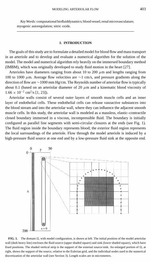
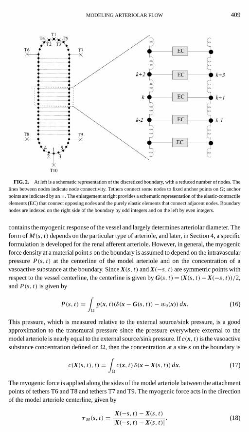
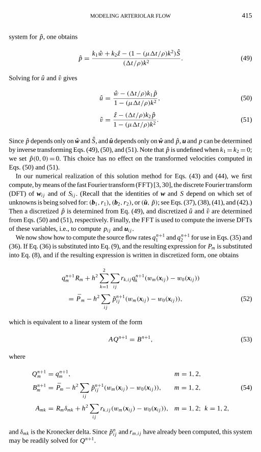
Ten tethers of the type that have just been described are connected to the immersedboundary that forms the model arteriole wall; their points of attachment to the boundary aregiven in Table I, and their anchor points are given in Table II. Tether placement is shown inFig. 2. Five tethers with zero rest length (LT = 0), labeled T1–T5, anchor the model arterioleabove the fluid source. Four additional tethers, labeled T6–T9, are attached to the ends ofthe initially straight sections of the boundary, and a tenth, T10, is attached to the base of theboundary. For these tethers,LT = 200/256µm, which allows the model arteriole to expandand lengthen before a stabilizing force is applied.
The elastic–contractile component of force density, given by
f M(s, t) = M(s, t) τ M(s, t), (15)
TABLE II
Tether Anchor Locations (µm)
Tether x y
T1 10.937500000000 31.250000000000T2 10.977602212310 30.638158473969T3 10.977602212310 31.861841526031T4 11.097222689270 30.036785726082T5 11.097222689270 32.463214273918T6 15.625000000000 25.781250000000T7 15.625000000000 36.718750000000T8 184.37500000000 25.781250000000T9 184.37500000000 36.718750000000
T10 189.84375000000 31.250000000000
MODELING ARTERIOLAR FLOW 409
FIG. 2. At left is a schematic representation of the discretized boundary, with a reduced number of nodes. Thelines between nodes indicate node connectivity. Tethers connect some nodes to fixed anchor points onÄ; anchorpoints are indicated by an×. The enlargement at right provides a schematic representation of the elastic-contractileelements (EC) that connect opposing nodes and the purely elastic elements that connect adjacent nodes. Boundarynodes are indexed on the right side of the boundary by odd integers and on the left by even integers.
contains the myogenic response of the vessel and largely determines arteriolar diameter. Theform of M(s, t) depends on the particular type of arteriole, and later, in Section 4, a specificformulation is developed for the renal afferent arteriole. However, in general, the myogenicforce density at a material pointson the boundary is assumed to depend on the intravascularpressureP(s, t) at the centerline of the model arteriole and on the concentration of avasoactive substance at the boundary. SinceX(s, t) andX(−s, t) are symmetric points withrespect to the vessel centerline, the centerline is given byG(s, t)= (X(s, t)+X(−s, t))/2,andP(s, t) is given by
P(s, t) =∫Ä
p(x, t)(δ(x−G(s, t))− w0(x)) dx. (16)
This pressure, which is measured relative to the external source/sink pressure, is a goodapproximation to the transmural pressure since the pressure everywhere external to themodel arteriole is nearly equal to the external source/sink pressure. Ifc(x, t) is the vasoactivesubstance concentration defined onÄ, then the concentration at a sites on the boundary is
c(X(s, t), t) =∫Ä
c(x, t) δ(x− X(s, t)) dx. (17)
The myogenic force is applied along the sides of the model arteriole between the attachmentpoints of tethers T6 and T8 and tethers T7 and T9. The myogenic force acts in the directionof the model arteriole centerline, given by
τ M(s, t) = X(−s, t)− X(s, t)|X(−s, t)− X(s, t)| . (18)
410 ARTHURS ET AL.
The total force density at a general material points along the boundary at timet is givenby
f (s, t) = f B(s, t)+ f T (s, t)+ f M(s, t). (19)
2.3. Mass Transport Equations
The advection and diffusion of solute dissolved in the fluid is coupled to the fluid velocityu. The advection–diffusion equation, including the effects of both fluid and solute sources[31], is given for a solute of concentrationc(x, t) by
ct +∇ · (uc) =∇ · (D∇c)+ QS, (20)
whereD(x) is solute diffusivity andQS(x, t) represents solute sources. For this study
QS(x, t) = so(x, t)− a(x, t)c(x, t)−2∑
m=1
cm(x, t)qm(t)wm(x), (21)
where the first term on the right in Eq. (21) represents the rate of release of solute froma site inÄ, perhaps from the vessel wall; the second term represents the degradation ofsolute in the domain by chemical reactions; and the third term represents the addition orremoval of solute by fluid entry or exit at the fluid sources within the model vessel. Therate of degradation, which is assumed to have first-order kinetics, may depend on the localstructures, and therefore is characterized by a nonnegative coefficienta(x, t) that may varyin space and time. The concentrationcm(x, t) equalsc(x, t) for exiting flow (qm(t) ≤ 0),howevercm(x, t) must be specified for entering flow (qm(t) > 0). No solute is allowed toenter or leave the fluid domain by way of the external source/sink.
3. NUMERICAL METHODS
A computational grid is placed onÄ by defining grid pointsxi j = (xi , yj )= (ih, jh),where i = 0, 1, 2, . . . ,4J− 1; j = 0, 1, 2, . . . , J− 1; and h= L/J (in our case,L is50 µm). Time is discretized in steps of1t . The analytical solution at each grid point(i.e., u(xi j , n1t)) is approximated by a numerical solutionun
i j ; the same convention isapplied to other variables—hence, e.g.,pn
i j , Fni j , andcn
i j .The material points of the immersed boundary are discretized by conceptualizing the
boundary asN Lagrangian boundary nodes, denoted bysk for k= 1, 2, . . . , N. The nodesare configured, however, so that the first node is at the distal end of the model vessel(coinciding with s = 0), with even-numbered nodes increasing along the left side andodd-numbered nodes increasing along the right side. The location of boundary nodesk attime n1t is given byXn
k. In the unstressed configuration (att = 0), adjoining nodes alongthe boundary (e.g.,sk andsk+2) are separated by distance1sk± = |X0
k±2−X0k |. Along the
sides of the model arteriole1sk± = h/2; along the semicircular ends of the vessel, the nodalpoints are initially separated by the arc-length distanceπh/8, as in Fig. 1. The length ofthe unstressed boundary segment associated with nodesk is1sk= (1sk+ +1sk−)/2.
An approximationδh(x) to the two-dimensional Dirac delta functionδ(x), which isneeded, e.g., in Eqs. (3) and (4), is given by Peskin and McQueen [29] as
δh(x) = h−2φ(x/h)φ(y/h), (22)
MODELING ARTERIOLAR FLOW 411
where the one-dimensional approximate Dirac delta functionφ(r ) is given by
φ(r ) =
18(3− 2|r | +
√1+ 4|r | − 4r 2), |r | ≤ 1,
12 − φ(2− |r |), 1≤ |r | ≤ 2,
0, |r | ≥ 2.
(23)
This formulation of an approximate delta function has properties that are particularly ap-propriate for use in the IMBM [29].
The approximate delta function is also used to describe the source weighting functions.The discretization ofwm(x) is given bywm(xi j )= δho(xi j − xSm), wherexSm is the centerof the source or sink form= 1, 2 andho is the coarsest grid spacing, which is (50/32)µm.(Note that the parameterho is fixed so that the physical sizes of the source, sink, and externalsource/sink are maintained when the space discretization is varied.) The weighting functionover the external source/sink,w0(x), is discretized as the one-dimensional approximation tothe Dirac delta function, normalized to have weight one; it is given byφ((yi − yS0)/ho)/200.
At time n1t , the node locationsXnk, fluid velocity un
i j , and solute concentrationcni j
are assumed known. The updated dependent variables (un+1i j , pn+1
i j , cn+1i j , andXn+1
k ) arecomputed by a first-order splitting in time, which may be summarized in four steps:
1. Compute the boundary force densityf nk at each nodesk and spread this force density
to the grid via the approximate delta functionδh(xi j ) to obtain the corresponding grid forcedensityFn
i j .2. Using the grid force densityFn
i j , solve the discretized Navier–Stokes equations to
obtain the updated fluid velocityun+1i j and pressurepn+1
i j .3. Use interpolation via the approximate delta functionδh(xi j ) to determine the bound-
ary node fluid velocityUn+1k from the nearby grid velocitiesun+1
i j ; move each node at thevelocityUn+1
k to obtain the updated boundary node configurationXn+1k .
4. Compute the updated solute concentrationcn+1i j by advection with the fluid velocity
un+1i j ; include solute diffusion and solute sources.
Each step will now be described in detail.
3.1. Force Determination
The boundary force component is given by a centered-difference discretization ofEqs. (10)–(12),
( f B)nk =
KB
1sk
[(∣∣∣∣1Xnk+
1sk+
∣∣∣∣− 1
)(τ B)
nk+ −
(∣∣∣∣1Xnk−
1sk−
∣∣∣∣− 1
)(τ B)
nk−
], (24)
where1Xnk+ = Xn
k+2− Xnk,1Xn
k− = Xnk − Xn
k−2, and(τ B)nk± = 1Xn
k±/|1Xnk±|.
For simplicity, each tether will be constructed to always act at a particular node. Ifa tether (fixed to a pointxT ) is attached to a nodeXn
k (corresponding to the parametriclocations′ = sk), then the tether force density (c.f. Eqs. (13)–(14)) is given by
( f T )nk =
KT
1skmax
{0,(∣∣xT − Xn
k
∣∣)− (LT )k}(τ T )
nk, (25)
where the unit vector(τ T )nk for xT 6= Xn
k is given by
(τ T )nk =
xT − Xnk∣∣xT − Xnk
∣∣ . (26)
412 ARTHURS ET AL.
The myogenic component of the force density( f M)nk on nodesk depends on the ap-
proximate pressurePnk and approximate concentrationcn
k (corresponding toP(sk, n1t)andc(X(sk, t), n1t), respectively). The expression approximating the transmural pressure(Eq. (16)) is discretized as
Pnk = h2
∑i j
pni j
(δh(xi j −Gn
k
)− w0(xi j )). (27)
The concentration at the boundary is computed by
cnk = h2
∑i j
cni j δh(xi j − Xn
k
). (28)
Because of the symmetry of our labeling convention, the nodes labeledk andk+ 1, forevenk, are located at the samex-location on opposite sides of the model arteriole; thus,Pn
k = Pnk+1, Gn
k =Gnk+1= (Xn
k +Xnk+1)/2, and( f M)
nk+1=−( f M)
nk.
Once the force density component at each node has been computed, the total force densityat time indexn and nodesk is given byf n
k = ( f B)nk + ( f T )
nk + ( f M)
nk. This force density is
transferred to the nearby grid points by the discretized version of Eq. (3):
Fni j =
∑k
f nkδh(xi j − Xn
k
)1sk. (29)
3.2. Fluid Equations
The updated fluid velocity is computed in a tripartite splitting that is similar to thatdescribed in Ref. [29]. However, here we use a spectral method to evaluate the contributionsof the viscous and incompressibility terms, i.e., we apply the continuous Fourier transform,evaluate unknown quantities algebraically in transform space, and then use the discreteFourier transform (DFT) to return to physical space. In Ref. [29], the same terms are firstdiscretized in physical space, and the DFT is then used to solve the discretized equations.The sources and sinks are handled much as in Ref. [27].
In the tripartite splitting, two provisional values,un+1,1i j andun+1,2
i j , are calculated beforeun+1
i j is finally determined. The first provisional value includes contributions from the forcedensityF, computed by an explicit forward Euler step, and from the damping term−σκu,computed by an implicit backward Euler step, yielding
un+1,1i j = un
i j + (1t/ρ)Fni j
1+ (1t/ρ)κσ ni j
. (30)
The values ofσ ni j are obtained fromσ , a linear superposition of hyperbolic tangent functions
constructed to give a value of approximately one outside the vessel and zero inside. Alongthe gridlinesxi that intersect the boundary,σ n
i j is given by
σ ni j = σ(xi , yj , n1t)
= 1− 1
2
[tanh
(0.8(yj −
(yn
ibl − 2ho)))+ tanh
(0.8(yj −
(yn
ibr + 2ho)))]
, (31)
whereynibl and yn
ibr are the left and righty-coordinates of the intersection ofx= xi withthe immersed boundary, respectively, at timen1t . For gridlinesxi that do not intersect the
MODELING ARTERIOLAR FLOW 413
immersed boundary,σ = 1. With this specification ofσ ,σ ni j ≈ 0.001 at a distanceho/2 inside
the boundary, andσ ni j is orders of magnitude smaller for points further inside the boundary.
At a distance 4ho outside the boundary,σ ni j exceeds 0.99, andσ n
i j rapidly approaches 1 asthe distance from the boundary increases.
The second provisional valueun+1,2i j = (un+1,2
i j , vn+1,2i j ), which includes the contribution
of the advection term(u · ∇)u, is obtained fromun+1i j by an upwind differencing,
un+1,2i j = un+1,1
i j − 1t
h
[(u+(un+1,1
i j − un+1,1i−1, j
)+ u−(un+1,1
i+1, j − un+1,1i j
))+ (v+(un+1,1
i j − un+1,1i, j−1
)+ v−(un+1,1i, j+1 − un+1,1
i j
))], (32)
vn+1,2i j = vn+1,1
i j − 1t
h
[(u+(v
n+1,1i j − vn+1,1
i−1, j
)+ u−(v
n+1,1i+1, j − vn+1,1
i j
))+ (v+(vn+1,1
i j − vn+1,1i, j−1
)+ v−(vn+1,1i, j+1 − vn+1,1
i j
))], (33)
whereu± =±max{0,±uni j } andv± =±max{0,±vn
i j }.In the third and final step of the splitting, discretized forms of the equations
ρ∂tu = −∇ p+ µ1u, (34)
∇ · u =2∑
m=1
qm(t)(wm(x)− w0(x)) (6)
are solved simultaneously for the updated fluid velocityun+1i j and pressurepn+1
i j . To in-corporate the fluid sources, the fluid velocity and pressure are written as a superpositionof a solution without fluid sources plus terms that include each source independently. Forsimplicity in the derivation of the appropriate equations, we will use equations that arecontinuous in space but discretized in time. Thus we will write the second provisional valueun+1,2
i j asun+1,2(x), and we will write the time-advanced fluid velocityun+1i j and pressure
pn+1i j asu(x) and p(x), respectively.Now using superposition, we assume that
u(x) = u(x)+2∑
m=1
bm(x)qn+1m (35)
and
p(x) = p(x)+2∑
m=1
rm(x)qn+1m , (36)
where the terms arising in the absence of sources,u(x) and p(x), satisfy
ρ
(u(x)− un+1,2(x)
1t
)= −∇ p(x)+ µ1u(x), (37)
∇ · u(x) = 0, (38)
and the terms on the far right in Eqs. (35) and (36) represent contributions from the sources.
414 ARTHURS ET AL.
The effects of the external source/sink (m= 0) are implicitly included in these equationsthrough volume conservation inÄ.
If we substitute Eqs. (35) and (36) into Eq. (6) and into the time-discretized versionof Eq. (34), and if we take into account, that, by assumption,u(x, t) and p(x, t) satisfyEqs. (37) and (38), we find thatqn+1
m , bm(x), andrm(x) must satisfy
2∑m=1
qn+1m
[ρ
bm(x)1t+∇rm(x)− µ1bm(x)
]= 0, (39)
2∑m=1
qn+1m [∇ · bm(x)− (wm(x)− w0(x))] = 0. (40)
Because the source magnitudes are independent of the flow vectorbm, the terms within thesquare brackets in Eqs. (39) and (40) must vanish for eachm. Therefore,bm(x) andrm(x)must satisfy
ρ
(bm(x)− 0
1t
)= −∇rm(x)+ µ1bm(x), (41)
∇ · bm(x) = wm(x)− w0(x). (42)
Thus the unknownsbm(x), rm(x), u(x), and p(x), in Eqs. (37), (38), (41), and (42), canall be found by solving a system of the form
ρ
(u− w1t
)= −∇ p+ µ1u, (43)
∇ · u = S(x), (44)
wherew andS(x) are given. Moreover, sincebm(x) andrm(x) depend only on fixed sourcelocations and the time step1t , Eqs. (41) and (42) need be solved only once.
Equations (43) and (44) may be solved by means of the Fourier transform, which, for ascalar functiong on the finite domain [0, 4L]× [0, L], is given by
g(kx, ky) =∫ L
0
∫ 4L
0exp{−i (2π/L)[kx(x/4)+ kyy]} g(x, y) dx dy. (45)
Using this definition, the transform of the scalar form of Eqs. (43) and (44) is given by
ρ
(u− w1t
)= −k1 p+ µk2u, (46)
ρ
(v − z
1t
)= −k2 p+ µk2v, (47)
(k1u+ k2v) = S, (48)
whereu= (u, v),w= (w, z), (k1, k2)=−i (2π/L)(kx/4, ky), andk2= k21+ k2
2. Solving this
MODELING ARTERIOLAR FLOW 415
system forp, one obtains
p = k1w + k2z− (1− (µ1t/ρ)k2)S
(1t/ρ)k2. (49)
Solving foru andv gives
u = w − (1t/ρ)k1 p
1− (µ1t/ρ)k2, (50)
v = z− (1t/ρ)k2 p
1− (µ1t/ρ)k2. (51)
Sincep depends only onwandS, andu depends only onwandp, u andp can be determinedby inverse transforming Eqs. (49), (50), and (51). Note thatp is undefined whenk1= k2= 0;we set p(0, 0)= 0. This choice has no effect on the transformed velocities computed inEqs. (50) and (51).
In our numerical realization of this solution method for Eqs. (43) and (44), we firstcompute, by means of the fast Fourier transform (FFT) [3, 30], the discrete Fourier transform(DFT) of wi j and of Si j . (Recall that the identities ofw and S depend on which set ofunknowns is being solved for:(b1, r1), (b2, r2), or(u, p); see Eqs. (37), (38), (41), and (42).)Then a discretizedp is determined from Eq. (49), and discretizedu andv are determinedfrom Eqs. (50) and (51), respectively. Finally, the FFT is used to compute the inverse DFTsof these variables, i.e., to computepi j andui j .
We now show how to compute the source flow ratesqn+11 andqn+1
2 for use in Eqs. (35) and(36). If Eq. (36) is substituted into Eq. (9), and the resulting expression forPm is substitutedinto Eq. (8), and if the resulting expression is written in discretized form, one obtains
qn+1m Rm + h2
2∑k=1
∑i j
rk,i j qn+1k (wm(xi j )− w0(xi j ))
= Pm − h2∑
i j
pn+1i j (wm(xi j )− w0(xi j )), (52)
which is equivalent to a linear system of the form
AQn+1 = Bn+1, (53)
where
Qn+1m = qn+1
m , m= 1, 2,
Bn+1m = Pm − h2
∑i j
pn+1i j (wm(xi j )− w0(xi j )), m= 1, 2, (54)
Amk = Rmδmk+ h2∑
i j
rk,i j (wm(xi j )− w0(xi j )), m= 1, 2; k = 1, 2,
andδmk is the Kronecker delta. Sincepni j andrm,i j have already been computed, this system
may be readily solved forQn+1.
416 ARTHURS ET AL.
Now, sinceuni j , pn+1
i j , bm,i j , rm,i j , andqn+1m are known, the updated velocityun+1
i j and pres-
surepn+1i j may be computed from the discretized versions of Eqs. (35) and (36), given by
un+1i j = un
i j +2∑
m=1
bm,i j qn+1m (55)
and
pn+1i j = pn+1
i j +2∑
m=1
rm,i j qn+1m . (56)
So that the pressure displayed in the figures would be compatible with experimental usage,the pressure computed through Eq. (56) was translated so that the average exterior pressureis near zero and the interior pressure approximates the transmural pressure. The translationwas effected by averaging the pressure over the generalized source/sink and subtractingthat average from the pressure computed in Eq. (56). The resulting pressure exterior to thevessel falls between−1 and 1 mm Hg. The translated pressures are used in the figures.
3.3. Boundary Nodes
The local fluid velocity at nodeXnk is computed by interpolation from the velocity at
nearby grid points; thus
Un+1k = h2
∑i j
uni j δh(xi j − Xn
k
). (57)
The boundary node location is then updated by a forward difference, given by
Xn+1k = Xn
k +1tUn+1k , (58)
the discretized version of Eq. (4).
3.4. Solute
The solute equation, Eq. (20), is solved by a tripartite splitting. The advection step,ct +∇·(uc)= 0, is solved using a multidimensional flux-corrected transport (FCT) method,with an eighth-order Richtmyer two-step Lax–Wendroff scheme as the high-order schemeand upwind differencing as the low-order scheme [37]. Zalesak has shown that this methodprovides good shape preservation when applied to the linear advection problem [38].
The diffusion step,ct =∇ · (D(x)∇c), may be solved using backward-time, centered-in-space differencing, and an iterative scheme, e.g., Richardson iteration [20]. However, inthe computational examples presented below,D is assumed to be constant, so the system iseasily solved by means of the Fourier transform. Thus, ifcn+1,1 is the concentration com-puted by the advection step, the second provisional concentration,cn+1,2, may be computedby the backward difference
cn+1,2(x)− cn+1,1(x)1t
= D1cn+1,2(x). (59)
This equation may be Fourier transformed in space (using Eq. (45)), solved forcn+1,2, andinverse transformed to obtaincn+1,2. In practice, the discrete transforms are computed bymeans of the FFT.
Finally, the solute source step, expressed asct = QS, is solved by the forward Eulermethod to obtaincn+1
i j .
MODELING ARTERIOLAR FLOW 417
4. AFFERENT ARTERIOLE
Thus far, the model has been described in general terms for application to a genericarteriole. However, in numerical simulations, we will represent an afferent arteriole in thekidney of a rat. A typical rat afferent arteriole is approximately 20µm in diameter and is100–300µm in length. Flow in the afferent arteriole is regulated in large measure by themyogenic response of the walls and by vasoactive substances that modulate the contrac-tility of vascular smooth muscle. The model afferent arteriole developed here includes themyogenic response and the action of the vasodilator nitric oxide (NO), which is released bythe endothelial and smooth muscle cells that make up the vessel wall and which undergoesadvection, diffusion, and degradation in the fluid flow.
Two aspects of the myogenic response will be included in the myogenic force densitycomponentf M(s, t): a steady-state response that reduces vessel diameter as steady-stateperfusion pressure increases (see Fig. 3), and a transient response to an increase in perfusionpressure that initially allows the vessel diameter to increase elastically, but subsequentlyinitiates a muscular contraction, leading to a decrease in vessel diameter (see Fig. 4).
The myogenic response was computed from a phenomenological model in which themagnitude of the myogenic force component is given by
M(s, t) = KM(s, t)D(s, t)
D0+ γ ∂t D(s, t)
D0, (60)
whereD(s, t)= |X(s, t)−X(−s, t)| is vessel diameter,KM(s, t) is a myogenic force coeffi-cient,γ is a constant coefficient of viscosity, andD0 is a reference diameter. Equation (60) isbased on the Voigt model for a viscoelastic material; the first term is suggested by Laplace’slaw and the second term represents the viscous response of the tissue [16].
The coefficientKM(s, t) is constructed as a linear combination of a coefficientKa(s, t)for fully active myogenic response and a coefficientK p(s, t) for a fully passive (i.e., elastic)vessel,
KM = (Ka − K p)(1− r )+ K p, (61)
wherer depends on the concentration of NO along the vessel wall,c(X(s, t), t). The fullyactive myogenic coefficient is the solution of a second-order differential equation thatpermits a transient response,
b3∂2t Ka + b2∂t Ka + b1(s, t)Ka = P(s, t), (62)
whereP(s, t) is the transmural pressure.The coefficientb1, which models the steady-state response, is given by
b1(P(s, t)) = 22− d(s)(P(s, t)− 50)
D0, (63)
whered(s) increases along the active portion of the model arteriole. Specifically, assvaries from the attachment point of tether T6 to the attachment point of T8,d(s) increaseslinearly from a value of 0.1 to a value of 0.3. Because intravascular pressure decreasesalong the flow direction, the scaling provided byd(s) is necessary for the model arteriole tomaintain a nearly constant diameter along its length, as do afferent arterioles in vivo. Fromthis result one may reasonably hypothesize that the myogenic response in vivo is spatiallyinhomogeneous.
418 ARTHURS ET AL.
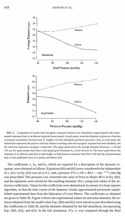
FIG. 3. Comparison of steady-state myogenic responses based on our simulations (upper panel) with experi-mental responses from a rat afferent arteriole (lower panel). In each panel, arteriolar diameter is given as a functionof pressure (simulation feed pressureP1 slightly exceeds simulation perfusion pressure). Also, in each panel, thedashed line represents the passive arteriolar dilation resulting when the myogenic response has been disabled, andthe solid line represents myogenic contraction. The upper panel shows the average diameter betweenx= 50 and150µm for quasi-steady-state flows with spatial grid refinementho/2 (see Section 5). The lower panel shows theresponse of rat afferent arterioles at mid-length, as feed pressure increases from 60 to 140 mm Hg. (Experimentaldata is from published work of Casellas and Moore [6]).
The coefficientsγ , b2, andb3, which are required for a description of the dynamic re-sponse, were obtained as follows. Equations (60) and (62) were considered to be independentof s, d(s) in Eq. (63) was set to 0.1, and a pressureP(t)= 60+ 40(1− exp−1.12t ) mm Hgwas prescribed. This pressure was converted into units of force to obtainM(t) in Eq. (60),and the equations were solved for the resulting diameterD(t), using trial values of the un-known coefficients. Values for the coefficients were determined, by means of a least-squaresalgorithm, so that the time course of the diameter closely approximated previously unpub-lished experimental data from the laboratory of Leon Moore. The coefficients so obtainedare given in Table III. Figure 4 shows the experimental values for arteriolar diameter, the so-lution obtained from the model when Eqs. (60) and (62) were solved as just described usingthe coefficients in Table III, and the diameter obtained for the full simulation, incorporatingEqs. (60), (62), and (63). In the full simulation,P(s, t) was computed through the fluid
MODELING ARTERIOLAR FLOW 419
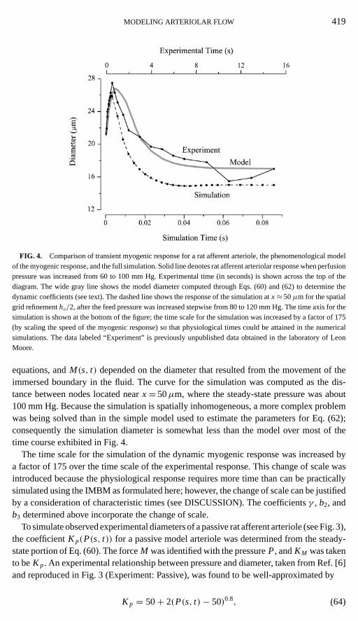
FIG. 4. Comparison of transient myogenic response for a rat afferent arteriole, the phenomenological modelof the myogenic response, and the full simulation. Solid line denotes rat afferent arteriolar response when perfusionpressure was increased from 60 to 100 mm Hg. Experimental time (in seconds) is shown across the top of thediagram. The wide gray line shows the model diameter computed through Eqs. (60) and (62) to determine thedynamic coefficients (see text). The dashed line shows the response of the simulation atx≈ 50µm for the spatialgrid refinementho/2, after the feed pressure was increased stepwise from 80 to 120 mm Hg. The time axis for thesimulation is shown at the bottom of the figure; the time scale for the simulation was increased by a factor of 175(by scaling the speed of the myogenic response) so that physiological times could be attained in the numericalsimulations. The data labeled “Experiment” is previously unpublished data obtained in the laboratory of LeonMoore.
equations, andM(s, t) depended on the diameter that resulted from the movement of theimmersed boundary in the fluid. The curve for the simulation was computed as the dis-tance between nodes located nearx= 50µm, where the steady-state pressure was about100 mm Hg. Because the simulation is spatially inhomogeneous, a more complex problemwas being solved than in the simple model used to estimate the parameters for Eq. (62);consequently the simulation diameter is somewhat less than the model over most of thetime course exhibited in Fig. 4.
The time scale for the simulation of the dynamic myogenic response was increased bya factor of 175 over the time scale of the experimental response. This change of scale wasintroduced because the physiological response requires more time than can be practicallysimulated using the IMBM as formulated here; however, the change of scale can be justifiedby a consideration of characteristic times (see DISCUSSION). The coefficientsγ , b2, andb3 determined above incorporate the change of scale.
To simulate observed experimental diameters of a passive rat afferent arteriole (see Fig. 3),the coefficientK p(P(s, t)) for a passive model arteriole was determined from the steady-state portion of Eq. (60). The forceM was identified with the pressureP, andKM was takento beK p. An experimental relationship between pressure and diameter, taken from Ref. [6]and reproduced in Fig. 3 (Experiment: Passive), was found to be well-approximated by
K p = 50+ 2(P(s, t)− 50)0.8, (64)
420 ARTHURS ET AL.
whereP(s, t) is in millimeters of mercury. Figure 3 shows the passive response, for the fullsimulation, with this specification ofK p.
The percentage of relaxation at a particular vasodilator concentration, which can bedetermined from a dose–response curve, gives the fractional relaxation,r , as a function oflocal solute concentration. For NO, this relationship was approximated by
r (c(X(s, t), t)) = 1
2[1+ tanh(π [log10(c(X(s, t), t)/0.0004)− 1])] (65)
which gives practically no relaxation at a concentration of 0.0004µM (r ≈ 0.00186) andnearly complete relaxation at a concentration of 0.04µM (r ≈ 0.998). This relationshipwas based on data from Ref. [21].
In the numerical implementation of the myogenic force component, Eq. (62) is recastas two first-order differential equations and solved at each nodesk by the forward Eulermethod for(Ka)
nk. The NO concentration at each nodecn
k is computed via Eq. (28), and theaverage ofcn
k andcnk+1 is used in Eq. (65) to determine the fractional relaxation.
The myogenic component of the force density at nodesk is then calculated as
( f M)nk =
((KM)
nk
Dnk
D0+ γ
(Dn
k − Dn−1k
)D01t
)Xn
k+1− Xnk∣∣Xn
k+1− Xnk
∣∣ (66)
for k even. Because nodessk andsk+1 are opposing,( f M)nk+1=−( f M)
nk for k even.
5. NUMERICAL SIMULATIONS
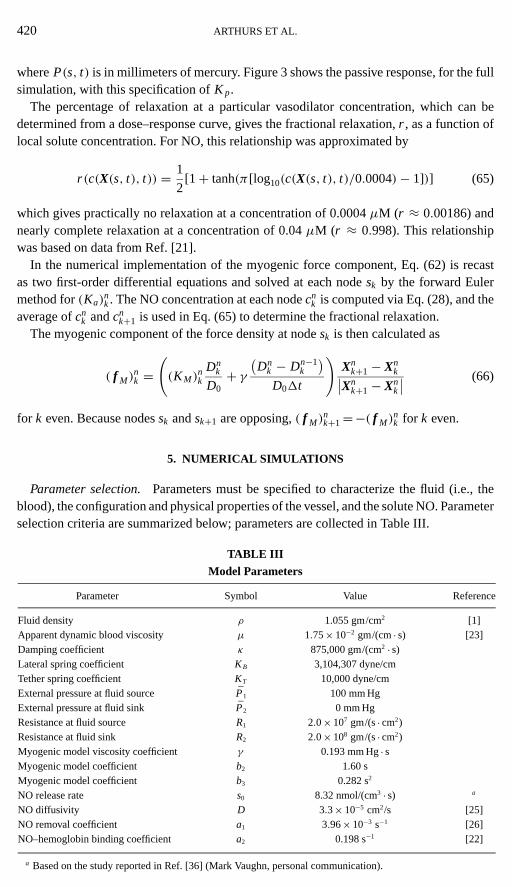
Parameter selection.Parameters must be specified to characterize the fluid (i.e., theblood), the configuration and physical properties of the vessel, and the solute NO. Parameterselection criteria are summarized below; parameters are collected in Table III.
TABLE III
Model Parameters
Parameter Symbol Value Reference
Fluid density ρ 1.055 gm/cm2 [1]Apparent dynamic blood viscosity µ 1.75× 10⁻² gm/(cm· s) [23]Damping coefficient κ 875,000 gm/(cm2 · s)Lateral spring coefficient KB 3,104,307 dyne/cmTether spring coefficient KT 10,000 dyne/cmExternal pressure at fluid source P1 100 mm HgExternal pressure at fluid sink P2 0 mm HgResistance at fluid source R1 2.0× 10⁷ gm/(s· cm2)Resistance at fluid sink R2 2.0× 10⁸ gm/(s· cm2)Myogenic model viscosity coefficient γ 0.193 mm Hg· sMyogenic model coefficient b2 1.60 sMyogenic model coefficient b3 0.282 s2
NO release rate s0 8.32 nmol/(cm3 · s) a
NO diffusivity D 3.3× 10⁻⁵ cm2/s [25]NO removal coefficient a1 3.96× 10⁻³ s−1 [26]NO–hemoglobin binding coefficient a2 0.198 s−1 [22]
a Based on the study reported in Ref. [36] (Mark Vaughn, personal communication).
MODELING ARTERIOLAR FLOW 421
Blood is a complex non-Newtonian fluid composed of plasma, red blood cells, whiteblood cells, and platelets. To obtain a tractable model, however, blood was simulated as aNewtonian fluid with an apparent dynamic viscosity. Experimental measurements in anarteriole of diameter 23µm in cat mesentery indicate an apparent viscosity of 1.75×10⁻² gm/(cm· s) [23]. (The viscosity of water at body temperature is≈0.725× 10⁻² gm/(cm· s)).
The damping coefficientκ was chosen empirically to damp fluid motion exterior to themodel vessel. The spring coefficientsKB andKT were chosen empirically to contain thepressures in the physiological range and to anchor the model vessel over the vessel sourceand sink.
The external pressure at the fluid source,P1= 100 mm Hg, and the external resistanceat the fluid source,R1= 2× 10⁷ gm/(s· cm2), were chosen so that the pressure at the fluidsource would be approximately 95 mm Hg. The external pressure at the fluid sink,P2=0 mm Hg, and the external resistance at the fluid sink,R2= 2×10⁸ gm/(s· cm2), were chosenso that the pressure at the fluid sink would be approximately 50 mm Hg. These values areconsistent with pressures found in mid-juxtamedullary afferent arterioles in rat [6]. Themyogenic model coefficientsγ , b2, andb3 were determined as described in Section 4.
The NO release rate, per unit area, from the wall of rabbit aorta, has been estimated[36; Mark Vaughn, personal communication] from experimental data [25] to be 5.2×10⁻¹⁴µmol/(µm2 · s). In the simulation, NO was released from an approximate delta func-tion with side 4ho centered on the vessel wall. For a fluid domain of any given thicknessH , the rate of release of NO from the wall segment covered by the delta function (s0 inEq. (21)), equals the area of the vessel wall of heightH enclosed by the delta function, timesthe release rate per unit area, divided by the volume enclosed by the box of heightH ; that is,
s0 = 4hoH × release rate/(unit area)
(4ho)2H= 8.32 nmol/(cm3 · s). (67)
NO diffusivity has been measured to be 3.3× 10⁻⁵ cm2/s at 37◦C in rabbit aorta, andevidence indicates that NO diffuses freely in aqueous solutions and across biological mem-branes [25]. The rate of NO degradation, through reaction with oxygen and water to producenitrites and nitrates, was based on a half-life of 3 s [26]. Based on a calculation that indicatedthat the rate of NO reaction with hemoglobin is more than 100 times more rapid than the rateof reaction with O2 [22], the rate of NO-hemoglobin binding was assumed to be 50 timesfaster than the reaction of NO with water and dissolved oxygen.
Discretization in space and time.Simulations were conducted withJ= 32, 64, and128 points along they-axis; thush= 50/32, 50/64, or 50/128µm. As already specified inSection 3,ho= 50/32, and the two grid refinements will be referred to asho/2 andho/4.Empirical studies indicate that a time step of1t = (5/175) × 10−5 s or smaller is neces-sary to maintain numerical stability, and except where stated otherwise, this time step wasused. Simulations were conducted in double precision on Sun® Workstations or in singleprecision, using one processor on the Cray® T-90 supercomputer at the North Carolina Su-percomputing Center. (Single precision on the Cray® is essentially equivalent to double pre-cision on the Sun® Workstation.) A single numerical iteration that includes the full function-ality of the simulation required approximately 0.025 CPU s on the Cray® supercomputer.
Machine error. Although the model prescribes a line of symmetry running through thecenter of the model arteriole (y= 31.25µm) and although the myogenic forces acting on
422 ARTHURS ET AL.
corresponding nodes (sk andsk−1) are equal and opposite, we observed a loss of symmetryin boundary node locations. Investigation showed that the loss of symmetry arises fromreductions in the number of significant digits in the subtractions that compute the boundaryforce component (i.e., in the evaluation of Eq. (24)), coupled with asymmetric machineroundoff. The loss of symmetry in boundary node locations results in a loss of symmetryin the force density applied to the vessel wall by the myogenic components. Eventually aregion of reduced force density along one side of the model vessel results in an outwardcurvature of the wall; this curvature is accompanied by an inward curvature on the otherside of the model vessel. When the curvature becomes sufficiently large, increased nodalseparation results in a loss of fluid containment.
The accumulation of asymmetry was controlled by adjusting the computation of theforce density pairs( f M)
nk+1, ( f M)
nk: in response to any deviation from symmetry, a weight-
ing of force components was applied to these force densities in the direction needed torestore symmetry. The weighting was constructed to correct both translational and rota-tional asymmetries.
The adjustment in weighting for the myogenic force density pairs was determined inthe following way. Assume that nodesk has Eulerian positionXk= (Xk,Yk) and nodesk+1 has positionXk+1= (Xk+1,Yk+1). The line segment connecting these nodes crossesthe line of symmetry at the point, say(px, py), wherepy= 31.25µm. Let ( fM)
nk,y be the
y-component of the myogenic force density at nodesk, computed via Eq. (66). Then theadjusted component was computed as
2|Yk − py||Yk+1− Yk| ( fM)
nk,y, (68)
and the adjustment for( fM)nk+1,y was computed analogously. Thus the node more distant
from the centerline received more force than the other node, resulting in a correction towardthe line of symmetry.
Similarly, if ( fM)nk,x was the computedx-component of the myogenic force density at
nodesk, the adjusted component was computed as
2|Xk − px||Xk+1− Xk| ( fM)
nk,x, (69)
and the adjustment for( fM)nk+1,x was computed analogously. Since the signs of( fM)
nk,x and
( fM)nk+1,x differ if there is any rotation relative to they-axis, the adjustedx-components
applied a corrective torque. The magnitude of these corrections was small relative to themyogenic force density; at quasi-steady-state (see below) the ratio of the myogenic forcedensity to the adjustment force was more than 1010.
Overview of simulation results.The following subsections describe an extensive seriesof tests that were performed to evaluate the properties, accuracy, and convergence of thenumerical methods. For quasi-steady-state (see below), the flow profile in the model vesselhas the expected parabolic shape for planar Poiseuille flow; the effective width of themodel vessel wall is about 2h. Shear stress magnitude at the model wall is consistent withvalues expected for planar Poiseuille flow. For a sufficiently refined spatial grid (e.g.,ho/4),the method exhibits robust first-order temporal convergence as the time step is refined.However, while vessel pressure and diameter profiles support convergence in space as thespatial grid is refined, the attainment of good convergence throughout the fluid domain
MODELING ARTERIOLAR FLOW 423
appears to be limited by the relatively coarse grids that are currently practicable. For goodspatial resolution in the representation of the flow velocity profile, shear stress, and soluteadvection and diffusion, a grid refinement withh < 1µm is needed.
5.1. The Pressurized Vessel
The first test of the method was to compute a quasi-steady-state configuration for the walland fluid flow and to compare the velocity in thex-direction with the parabolic velocityprofile for planar Poiseuille flow. We say quasi-steady-state to indicate that the input andoutput flows are very nearly constant and equal; a pure steady state is not attainable becausethe walls continue to undergo small motions for long times. Beginning from a completelyquiescent state, approximately 0.06 s are required to reach a quasi-steady-state.
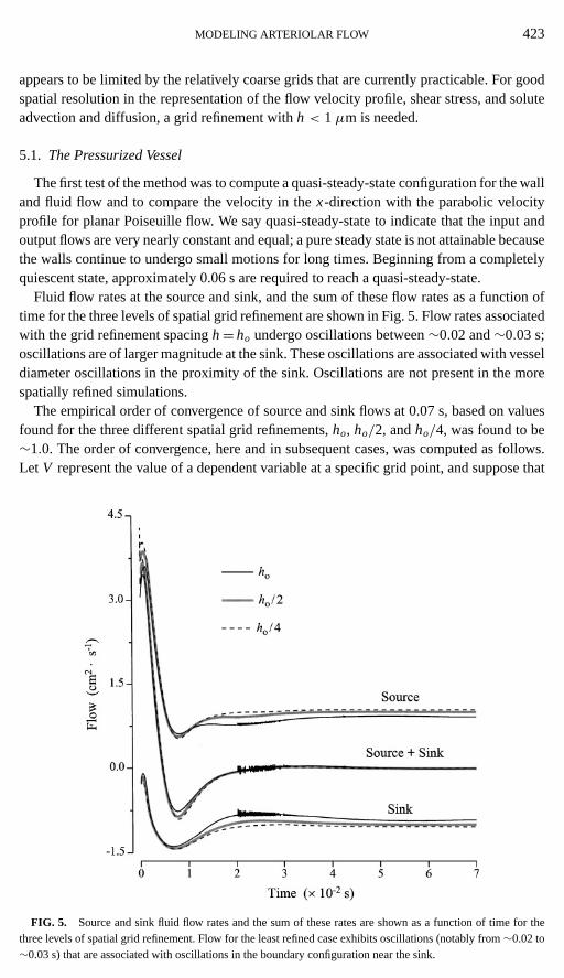
Fluid flow rates at the source and sink, and the sum of these flow rates as a function oftime for the three levels of spatial grid refinement are shown in Fig. 5. Flow rates associatedwith the grid refinement spacingh= ho undergo oscillations between∼0.02 and∼0.03 s;oscillations are of larger magnitude at the sink. These oscillations are associated with vesseldiameter oscillations in the proximity of the sink. Oscillations are not present in the morespatially refined simulations.
The empirical order of convergence of source and sink flows at 0.07 s, based on valuesfound for the three different spatial grid refinements,ho, ho/2, andho/4, was found to be∼1.0. The order of convergence, here and in subsequent cases, was computed as follows.Let V represent the value of a dependent variable at a specific grid point, and suppose that
FIG. 5. Source and sink fluid flow rates and the sum of these rates are shown as a function of time for thethree levels of spatial grid refinement. Flow for the least refined case exhibits oscillations (notably from∼0.02 to∼0.03 s) that are associated with oscillations in the boundary configuration near the sink.
424 ARTHURS ET AL.
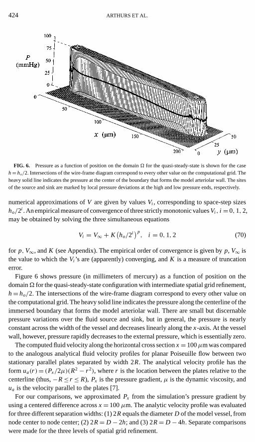
FIG. 6. Pressure as a function of position on the domainÄ for the quasi-steady-state is shown for the caseh= ho/2. Intersections of the wire-frame diagram correspond to every other value on the computational grid. Theheavy solid line indicates the pressure at the center of the boundary that forms the model arteriolar wall. The sitesof the source and sink are marked by local pressure deviations at the high and low pressure ends, respectively.
numerical approximations ofV are given by valuesVi , corresponding to space-step sizesho/2i . An empirical measure of convergence of three strictly monotonic valuesVi , i = 0, 1, 2,may be obtained by solving the three simultaneous equations
Vi = V∞ + K(ho/2
i)p, i = 0, 1, 2 (70)
for p,V∞, andK (see Appendix). The empirical order of convergence is given byp, V∞ isthe value to which theVi ’s are (apparently) converging, andK is a measure of truncationerror.
Figure 6 shows pressure (in millimeters of mercury) as a function of position on thedomainÄ for the quasi-steady-state configuration with intermediate spatial grid refinement,h= ho/2. The intersections of the wire-frame diagram correspond to every other value onthe computational grid. The heavy solid line indicates the pressure along the centerline of theimmersed boundary that forms the model arteriolar wall. There are small but discernablepressure variations over the fluid source and sink, but in general, the pressure is nearlyconstant across the width of the vessel and decreases linearly along thex-axis. At the vesselwall, however, pressure rapidly decreases to the external pressure, which is essentially zero.
The computed fluid velocity along the horizontal cross sectionx= 100µm was comparedto the analogous analytical fluid velocity profiles for planar Poiseuille flow between twostationary parallel plates separated by width 2R. The analytical velocity profile has theform ua(r )= (Px/2µ)(R2 − r 2), wherer is the location between the plates relative to thecenterline (thus,−R≤ r ≤ R), Px is the pressure gradient,µ is the dynamic viscosity, andua is the velocity parallel to the plates [7].
For our comparisons, we approximatedPx from the simulation’s pressure gradient byusing a centered difference acrossx= 100µm. The analytic velocity profile was evaluatedfor three different separation widths: (1) 2Requals the diameterD of the model vessel, fromnode center to node center; (2) 2R= D− 2h; and (3) 2R= D− 4h. Separate comparisonswere made for the three levels of spatial grid refinement.
MODELING ARTERIOLAR FLOW 425
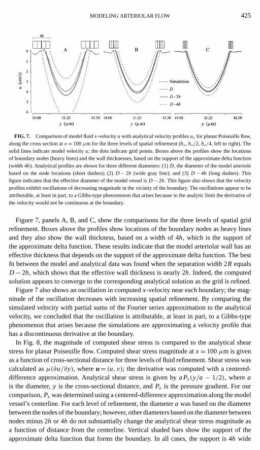
FIG. 7. Comparison of model fluidx-velocityu with analytical velocity profilesua for planar Poiseuille flow,along the cross section atx= 100µm for the three levels of spatial refinement (ho, ho/2, ho/4, left to right). Thesolid lines indicate model velocityu; the dots indicate grid points. Boxes above the profiles show the locationsof boundary nodes (heavy lines) and the wall thicknesses, based on the support of the approximate delta function(width 4h). Analytical profiles are shown for three different diameters: (1)D, the diameter of the model arteriolebased on the node locations (short dashes); (2)D− 2h (wide gray line); and (3)D− 4h (long dashes). Thisfigure indicates that the effective diameter of the model vessel isD− 2h. This figure also shows that the velocityprofiles exhibit oscillations of decreasing magnitude in the vicinity of the boundary. The oscillations appear to beattributable, at least in part, to a Gibbs-type phenomenon that arises because in the analytic limit the derivative ofthe velocity would not be continuous at the boundary.
Figure 7, panels A, B, and C, show the comparisons for the three levels of spatial gridrefinement. Boxes above the profiles show locations of the boundary nodes as heavy linesand they also show the wall thickness, based on a width of 4h, which is the support ofthe approximate delta function. These results indicate that the model arteriolar wall has aneffective thickness that depends on the support of the approximate delta function. The bestfit between the model and analytical data was found when the separation width 2R equalsD− 2h, which shows that the effective wall thickness is nearly 2h. Indeed, the computedsolution appears to converge to the corresponding analytical solution as the grid is refined.
Figure 7 also shows an oscillation in computedx-velocity near each boundary; the mag-nitude of the oscillation decreases with increasing spatial refinement. By comparing thesimulated velocity with partial sums of the Fourier series approximation to the analyticalvelocity, we concluded that the oscillation is attributable, at least in part, to a Gibbs-typephenomenon that arises because the simulations are approximating a velocity profile thathas a discontinuous derivative at the boundary.
In Fig. 8, the magnitude of computed shear stress is compared to the analytical shearstress for planar Poiseuille flow. Computed shear stress magnitude atx= 100µm is givenas a function of cross-sectional distance for three levels of fluid refinement. Shear stress wascalculated asµ(∂u/∂y), whereu= (u, v); the derivative was computed with a centered-difference approximation. Analytical shear stress is given byaPx(y/a − 1/2), whereais the diameter,y is the cross-sectional distance, andPx is the pressure gradient. For ourcomparison,Px was determined using a centered-difference approximation along the modelvessel’s centerline. For each level of refinement, the diametera was based on the diameterbetween the nodes of the boundary; however, other diameters based on the diameter betweennodes minus 2h or 4h do not substantially change the analytical shear stress magnitude asa function of distance from the centerline. Vertical shaded bars show the support of theapproximate delta function that forms the boundary. In all cases, the support is 4h wide
426 ARTHURS ET AL.
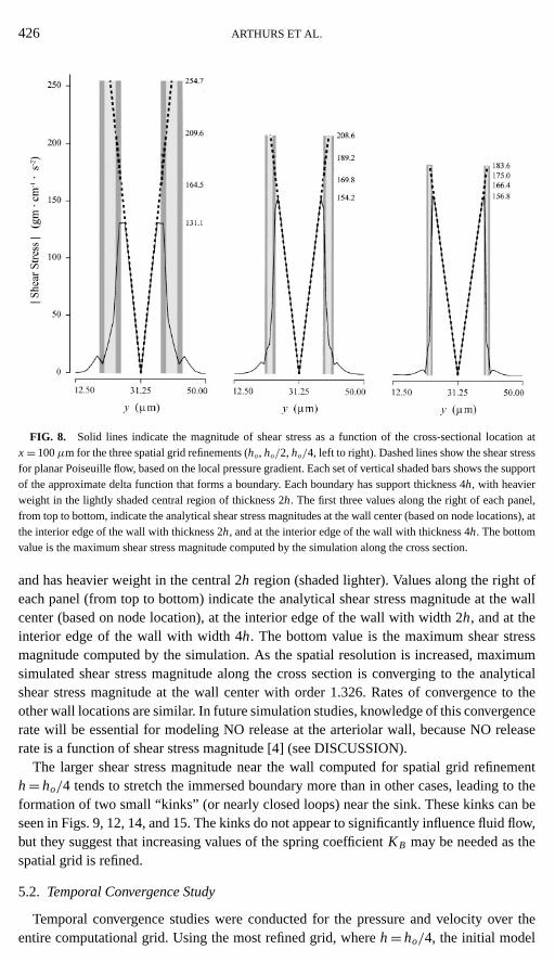
FIG. 8. Solid lines indicate the magnitude of shear stress as a function of the cross-sectional location atx= 100µm for the three spatial grid refinements (ho, ho/2, ho/4, left to right). Dashed lines show the shear stressfor planar Poiseuille flow, based on the local pressure gradient. Each set of vertical shaded bars shows the supportof the approximate delta function that forms a boundary. Each boundary has support thickness 4h, with heavierweight in the lightly shaded central region of thickness 2h. The first three values along the right of each panel,from top to bottom, indicate the analytical shear stress magnitudes at the wall center (based on node locations), atthe interior edge of the wall with thickness 2h, and at the interior edge of the wall with thickness 4h. The bottomvalue is the maximum shear stress magnitude computed by the simulation along the cross section.
and has heavier weight in the central 2h region (shaded lighter). Values along the right ofeach panel (from top to bottom) indicate the analytical shear stress magnitude at the wallcenter (based on node location), at the interior edge of the wall with width 2h, and at theinterior edge of the wall with width 4h. The bottom value is the maximum shear stressmagnitude computed by the simulation. As the spatial resolution is increased, maximumsimulated shear stress magnitude along the cross section is converging to the analyticalshear stress magnitude at the wall center with order 1.326. Rates of convergence to theother wall locations are similar. In future simulation studies, knowledge of this convergencerate will be essential for modeling NO release at the arteriolar wall, because NO releaserate is a function of shear stress magnitude [4] (see DISCUSSION).
The larger shear stress magnitude near the wall computed for spatial grid refinementh= ho/4 tends to stretch the immersed boundary more than in other cases, leading to theformation of two small “kinks” (or nearly closed loops) near the sink. These kinks can beseen in Figs. 9, 12, 14, and 15. The kinks do not appear to significantly influence fluid flow,but they suggest that increasing values of the spring coefficientKB may be needed as thespatial grid is refined.
5.2. Temporal Convergence Study
Temporal convergence studies were conducted for the pressure and velocity over theentire computational grid. Using the most refined grid, whereh= ho/4, the initial model
MODELING ARTERIOLAR FLOW 427
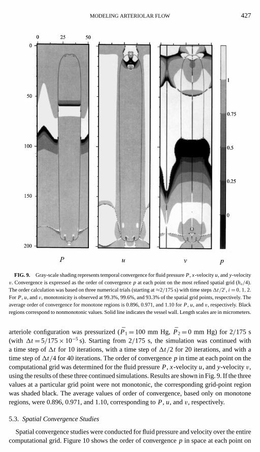
FIG. 9. Gray-scale shading represents temporal convergence for fluid pressureP, x-velocityu, andy-velocityv. Convergence is expressed as the order of convergencep at each point on the most refined spatial grid (ho/4).The order calculation was based on three numerical trials (starting at≈2/175 s) with time steps1t/2i , i = 0, 1, 2.For P, u, andv, monotonicity is observed at 99.3%, 99.6%, and 93.3% of the spatial grid points, respectively. Theaverage order of convergence for monotone regions is 0.896, 0.971, and 1.10 forP, u, andv, respectively. Blackregions correspond to nonmonotonic values. Solid line indicates the vessel wall. Length scales are in micrometers.
arteriole configuration was pressurized (P1= 100 mm Hg,P2= 0 mm Hg) for 2/175 s(with 1t = 5/175× 10−5 s). Starting from 2/175 s, the simulation was continued witha time step of1t for 10 iterations, with a time step of1t/2 for 20 iterations, and with atime step of1t/4 for 40 iterations. The order of convergencep in time at each point on thecomputational grid was determined for the fluid pressureP, x-velocityu, andy-velocityv,using the results of these three continued simulations. Results are shown in Fig. 9. If the threevalues at a particular grid point were not monotonic, the corresponding grid-point regionwas shaded black. The average values of order of convergence, based only on monotoneregions, were 0.896, 0.971, and 1.10, corresponding toP, u, andv, respectively.
5.3. Spatial Convergence Studies
Spatial convergence studies were conducted for fluid pressure and velocity over the entirecomputational grid. Figure 10 shows the order of convergencep in space at each point on
428 ARTHURS ET AL.
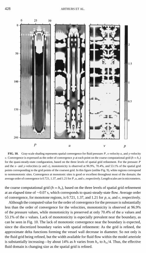
FIG. 10. Gray-scale shading represents spatial convergence for fluid pressureP, x-velocityu, andy-velocityv. Convergence is expressed as the order of convergencep at each point on the coarse computational grid (h= ho)for the quasi-steady-state configuration, based on the three levels of spatial grid refinement. For the pressurePand thex- andy-velocities (u andv), monotonicity is observed at 96.9%, 70.4%, and 53.1% of the spatial gridpoints corresponding to the grid points of the coarsest grid. In this figure (unlike Fig. 9), white regions correspondto nonmonotonic sites. Convergence at monotonic sites is good or excellent throughout most of the domain; theaverage order of convergence is 0.721, 1.37, and 1.21 forP,u, andv, respectively. Length scales are in micrometers.
the coarse computational grid (h= ho), based on the three levels of spatial grid refinementat an elapsed time of∼0.07 s, which corresponds to quasi-steady-state flow. Average orderof convergence, for monotone regions, is 0.721, 1.37, and 1.21 forp, u, andv, respectively.
Although the computed value for the order of convergence for the pressure is substantiallyless than the order of convergence for the velocities, monotonicity is observed at 96.9%of the pressure values, while monotonicity is preserved at only 70.4% of theu values and53.1% of thev values. Lack of monotonicity is especially prevalent near the boundary, ascan be seen in Fig. 10. The lack of monotonic convergence near the boundary is expected,since the discretized boundary varies with spatial refinement: As the grid is refined, theapproximate delta functions forming the vessel wall decrease in diameter. So not only isthe fluid grid being refined, but the width available for fluid flow within the model arterioleis substantially increasing—by about 14% ash varies fromho to ho/4. Thus, the effectivefluid domain is changing size as the spatial grid is refined.
MODELING ARTERIOLAR FLOW 429
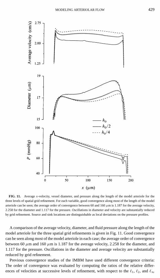
FIG. 11. Averagex-velocity, vessel diameter, and pressure along the length of the model arteriole for thethree levels of spatial grid refinement. For each variable, good convergence along most of the length of the modelarteriole can be seen; the average order of convergence between 60 and 160µm is 1.187 for the average velocity,2.258 for the diameter and 1.117 for the pressure. Oscillations in diameter and velocity are substantially reducedby grid refinement. Source and sink locations are distinguishable as local deviations on the pressure profiles.
A comparison of the average velocity, diameter, and fluid pressure along the length of themodel arteriole for the three spatial grid refinements is given in Fig. 11. Good convergencecan be seen along most of the model arteriole in each case; the average order of convergencebetween 60µm and 160µm is 1.187 for the average velocity, 2.258 for the diameter, and1.117 for the pressure. Oscillations in the diameter and average velocity are substantiallyreduced by grid refinement.
Previous convergence studies of the IMBM have used different convergence criteria:The order of convergence was evaluated by computing the ratios of the relative differ-ences of velocities at successive levels of refinement, with respect to the`1, `2, and`∞
430 ARTHURS ET AL.
TABLE IV
Convergence Study of Fluid Velocity and Pressure
Norm
Convergence measure `1 `2 `∞
A = ‖uho/4−uho/2‖‖uho/4‖
0.07372 0.05697 0.07018
B = ‖uho/4−uho ‖‖uho/4‖
0.20901 0.15651 0.22732
Convergence ratio (A/B) 0.35271 0.36400 0.30873
Order of convergencep for u 0.87593 0.80509 1.16290
C= ‖Pho/4−Pho/2‖‖Pho/4‖
0.04754 0.10992 0.68464
D = ‖Pho/4−Pho ‖‖Pho/4‖
0.12943 0.24217 1.04328
Convergence ratio (C/D) 0.36730 0.45390 0.65624
Order of convergencep for P 0.78456 0.26679 −0.93282a
Note.The convergence ratios reported here were determined using the specified norm overall computational points for the spatial grid refinementh= ho. The order of convergence wasdetermined using Eq. (A2), whereq is the convergence ratio.
a The negative value indicates that pressure does not converge in the`∞ norm.
norms, evaluated over theentire fluid domain [10, 28]. These studies demonstrated first-order spatial convergence. We have used these criteria to evaluate our simulation results, forquasi-steady-state, using the velocity on the most refined grid (ho/4) as the reference, i.e.,(‖uho/4− uh‖p)/‖uho/4‖p, whereh= ho, ho/2, andp= 1, 2,∞. Table IV shows that theconvergence results from our simulations, using these criteria, are consistent with first-orderconvergence. Because fluid pressure is used in the determination of model arteriole diame-ter, Table IV also includes results for pressure convergence; previous convergence studiesdid not include fluid pressure, since it was considered an intermediate step in calculatingvelocity.
Thus far, measures of spatial convergence have been applied to fluid variables in thedomain. Since we are also seeking to simulate the motion of vasoactive substances in thearteriolar flow, it is also important to measure the spatial convergence of solute that isadvected with the local fluid velocity. To test the spatial convergence of solute distribution,a solute bolus was introduced into quasi-steady-state flow, and the resulting solute advectionwas observed. Initially, the solute concentration, measured in units of micromolar(µM),was a Gaussian centered at the coordinates (39.0625µm, 31.2500µm) and given by
c(x, y, 0)= exp
(−(x − 39.0625)2
2(2.01875)2
)exp
(−(y− 31.2500)2
2(2.01875)2
). (71)
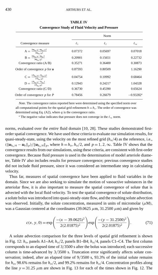
A solute advection comparison for the three levels of spatial grid refinement is shownin Fig. 12:ho, panels A1–A4;ho/2, panels B1–B4;ho/4, panels C1–C4. The first columncorresponds to an elapsed time of 3/3500 s after the bolus was introduced; each successivecolumn is time-advanced by 3/3500 s. Truncation error significantly affects solute con-servation; indeed, after an elapsed time of 9/3500 s, 93.3% of the initial solute remainsfor ho, 98.6% remains forho/2, and 99.2% remains forho/4. Concentration profiles alongthe line y= 31.25µm are shown in Fig. 13 for each of the times shown in Fig. 12. The
MODELING ARTERIOLAR FLOW 431
FIG. 12. Advection of solute bolus in quasi-steady-state flow for the three levels of spatial grid refinement:ho, panels A1–A4;ho/2, panels B1–B4;ho/4, panels C1–C4. The first column corresponds to dimensional timet = 3/3500 s; each successive column is time-advanced by 3/3500 s. The bar at the right indicates the concentrationscale in micromolar. Initially the bolus has a Gaussian distribution. The figure shows that the eighth-order methodemployed controls artifactual diffusion, but that substantial grid refinement is needed for accurate representationof solute distribution in time. For the simulations shown in column 4, solute has begun to leave the domain throughthe fluid sink. The solid line indicates the vessel wall. Length scales are in micrometers.
432 ARTHURS ET AL.
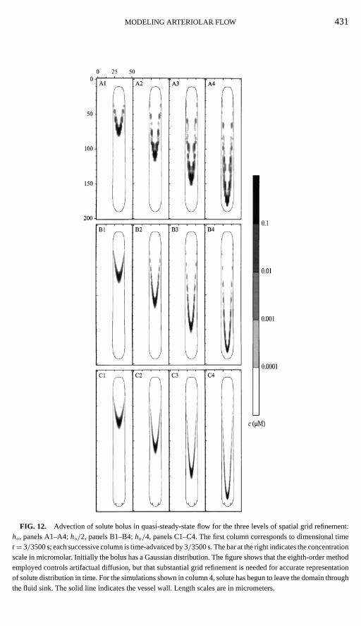
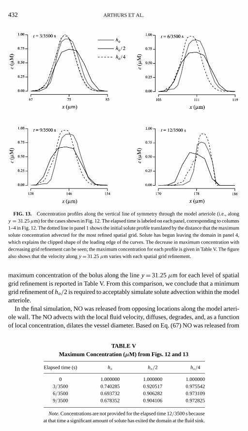
FIG. 13. Concentration profiles along the vertical line of symmetry through the model arteriole (i.e., alongy = 31.25µm) for the cases shown in Fig. 12. The elapsed time is labeled on each panel, corresponding to columns1–4 in Fig. 12. The dotted line in panel 1 shows the initial solute profile translated by the distance that the maximumsolute concentration advected for the most refined spatial grid. Solute has begun leaving the domain in panel 4,which explains the clipped shape of the leading edge of the curves. The decrease in maximum concentration withdecreasing grid refinement can be seen; the maximum concentration for each profile is given in Table V. The figurealso shows that the velocity alongy= 31.25µm varies with each spatial grid refinement.
maximum concentration of the bolus along the liney= 31.25µm for each level of spatialgrid refinement is reported in Table V. From this comparison, we conclude that a minimumgrid refinement ofho/2 is required to acceptably simulate solute advection within the modelarteriole.
In the final simulation, NO was released from opposing locations along the model arteri-ole wall. The NO advects with the local fluid velocity, diffuses, degrades, and, as a functionof local concentration, dilates the vessel diameter. Based on Eq. (67) NO was released from
TABLE V
Maximum Concentration (µM) from Figs. 12 and 13
Elapsed time (s) ho ho/2 ho/4
0 1.000000 1.000000 1.0000003/3500 0.740285 0.920517 0.9755426/3500 0.693732 0.906282 0.9731099/3500 0.678352 0.904106 0.972825
Note.Concentrations are not provided for the elapsed time 12/3500 s becauseat that time a significant amount of solute has exited the domain at the fluid sink.
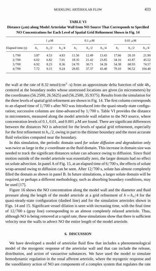
MODELING ARTERIOLAR FLOW 433
TABLE VI
Distance (µm) along Model Arteriolar Wall from NO Source That Corresponds to Specified
NO Concentrations for Each Level of Spatial Grid Refinement Shown in Fig. 14
1µM 0.1µM 0.01µM
Elapsed time (s) ho ho/2 ho/4 ho ho/2 ho/4 ho ho/2 ho/4
1/700 3.87 4.53 4.83 11.56 12.49 13.43 17.66 20.10 21.902/700 6.02 6.82 7.01 18.35 21.42 23.85 34.16 41.87 45.523/700 6.92 8.23 8.36 24.70 30.71 34.26 54.38 68.93 74.574/700 7.72 9.15 9.24 28.85 37.37 43.40 79.10 96.52 104.40
the wall at the rate of 8.32 nmol/(cm3 · s) from an approximate delta function of side 4ho
centered at the boundary nodes whose unstressed locations are given (in micrometers) bythe coordinates (56.2500, 26.5625) and (56.2500, 35.9375). Results from the simulation forthe three levels of spatial grid refinement are shown in Fig. 14. The first column correspondsto an elapsed time of 1/700 s after NO was introduced into the quasi-steady-state configu-ration; successive columns are time-advanced by 1/700 s. Table VI provides the distancein micrometers, measured along the model arteriole wall relative to the NO source, whereconcentration levels of 0.1, 0.01, and 0.001µM are found. There are significant differencesbetween the distances NO is advected for the levels of spatial grid refinement, especiallyfor the first refinement toho/2, owing in part to the thinner boundary and the more accuratefluid velocities computed near the boundary.
In this simulation, the periodic domain usedfor solute diffusion and degradation onlywas twice as large in they-coordinate as the fluid domain. This increase in domain size wasneeded to track the significant distances solute can advance owing to diffusion. Since fluidmotion outside of the model arteriole was essentially zero, the larger domain had no effecton solute advection. In panel A of Fig. 15, at an elapsed time of 6/700 s, the effects of solutewrap-around owing to diffusion can be seen. After 12/700 s, solute has almost completelyfilled the domain as shown in panel B. In future simulations, a larger solute domain will berequired, or perhaps a different methodology, such as absorbing boundary conditions, maybe used [17].
Figure 16 shows the NO concentration along the model wall and the diameter and fluidpressure along the length of the model arteriole at a grid refinement ofh= ho/4 for thequasi-steady-state configuration (dashed line) and for the simulation arterioles shown inFigs. 14 and 15. Significant vessel dilation is seen with increasing time, with the final timeof 12/700 s (gray line) corresponding to an almost completely relaxed arteriole. Thus,although NO is being removed at a rapid rate, these simulations show that there is sufficientvelocity near the walls to advect NO the entire length of the model arteriole.
6. DISCUSSION
We have developed a model of arteriolar fluid flow that includes a phenomenologicalmodel of the myogenic response of the arteriolar wall and that can include the release,distribution, and action of vasoactive substances. We have used the model to simulatehemodynamic regulation in the renal afferent arteriole, where the myogenic response andthe vasodilatory action of NO are components of a complex system that regulates the rate
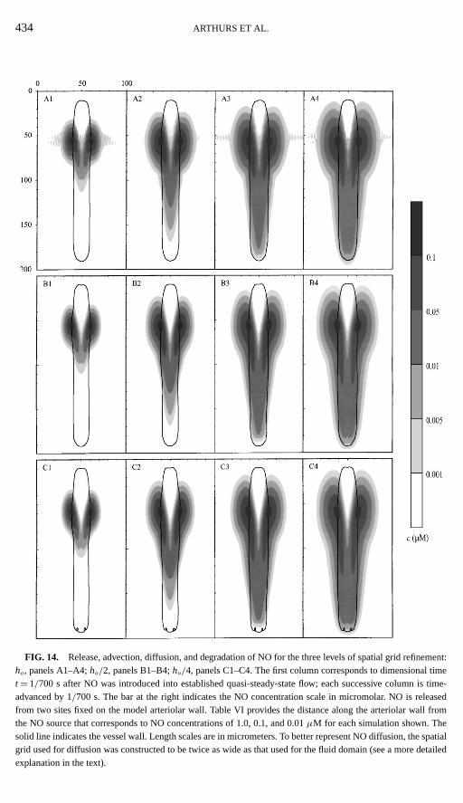
434 ARTHURS ET AL.
FIG. 14. Release, advection, diffusion, and degradation of NO for the three levels of spatial grid refinement:ho, panels A1–A4;ho/2, panels B1–B4;ho/4, panels C1–C4. The first column corresponds to dimensional timet = 1/700 s after NO was introduced into established quasi-steady-state flow; each successive column is time-advanced by 1/700 s. The bar at the right indicates the NO concentration scale in micromolar. NO is releasedfrom two sites fixed on the model arteriolar wall. Table VI provides the distance along the arteriolar wall fromthe NO source that corresponds to NO concentrations of 1.0, 0.1, and 0.01µM for each simulation shown. Thesolid line indicates the vessel wall. Length scales are in micrometers. To better represent NO diffusion, the spatialgrid used for diffusion was constructed to be twice as wide as that used for the fluid domain (see a more detailedexplanation in the text).
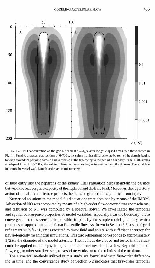
MODELING ARTERIOLAR FLOW 435
FIG. 15. NO concentration on the grid refinementh= ho/4 after longer elapsed times than those shown inFig. 14. Panel A shows an elapsed time of 6/700 s; the solute that has diffused to the bottom of the domain beginsto wrap around the periodic domain and to overlap at the top, owing to the periodic boundary. Panel B illustratesan elapsed time of 12/700 s; the solute diffused at the sides begins to wrap around the domain. The solid lineindicates the vessel wall. Length scales are in micrometers.
of fluid entry into the nephrons of the kidney. This regulation helps maintain the balancebetween the reabsorptive capacity of the nephron and the fluid load. Moreover, the regulatoryaction of the afferent arteriole protects the delicate glomerular capillaries from injury.
Numerical solutions to the model fluid equations were obtained by means of the IMBM.Advection of NO was computed by means of a high-order flux-corrected transport scheme,and diffusion of NO was computed by a spectral solver. We investigated the temporaland spatial convergence properties of model variables, especially near the boundary; theseconvergence studies were made possible, in part, by the simple model geometry, whichproduces an approximation to planar Poiseuille flow. As shown in Section 5.3, a spatial gridrefinement withh< 1 µm is required to track fluid and solute with sufficient accuracy forphysiologically meaningful simulations. This grid refinement corresponds to approximately1/25th the diameter of the model arteriole. The methods developed and tested in this studycould be applied to other physiological tubular structures that have low Reynolds numberflow, e.g., to other small vessels, to vessel networks, or to the tubules of the nephron.
The numerical methods utilized in this study are formulated with first-order differenc-ing in time, and the convergence study of Section 5.2 indicates that first-order temporal
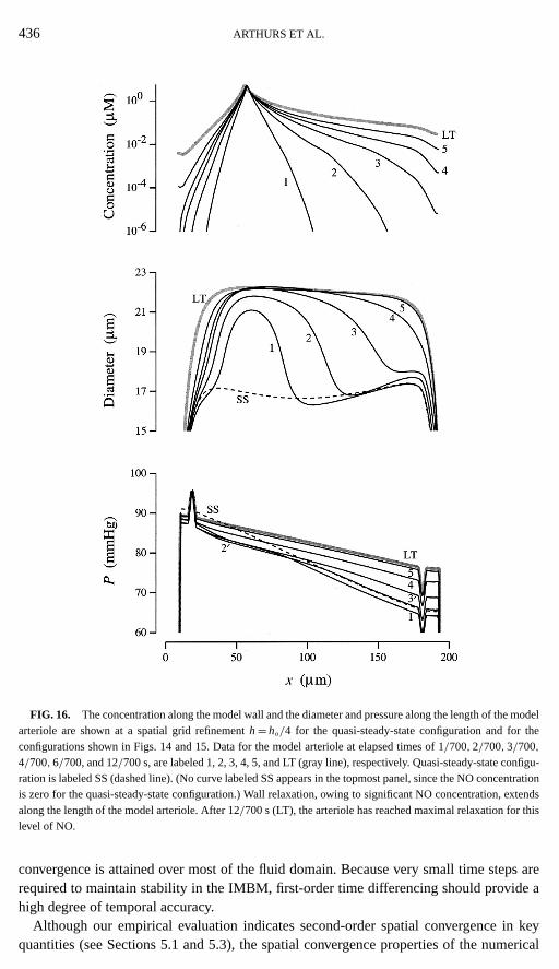
436 ARTHURS ET AL.
FIG. 16. The concentration along the model wall and the diameter and pressure along the length of the modelarteriole are shown at a spatial grid refinementh= ho/4 for the quasi-steady-state configuration and for theconfigurations shown in Figs. 14 and 15. Data for the model arteriole at elapsed times of 1/700, 2/700, 3/700,4/700, 6/700, and 12/700 s, are labeled 1, 2, 3, 4, 5, and LT (gray line), respectively. Quasi-steady-state configu-ration is labeled SS (dashed line). (No curve labeled SS appears in the topmost panel, since the NO concentrationis zero for the quasi-steady-state configuration.) Wall relaxation, owing to significant NO concentration, extendsalong the length of the model arteriole. After 12/700 s (LT), the arteriole has reached maximal relaxation for thislevel of NO.
convergence is attained over most of the fluid domain. Because very small time steps arerequired to maintain stability in the IMBM, first-order time differencing should provide ahigh degree of temporal accuracy.
Although our empirical evaluation indicates second-order spatial convergence in keyquantities (see Sections 5.1 and 5.3), the spatial convergence properties of the numerical
MODELING ARTERIOLAR FLOW 437
methods differ. The tripartite splitting in the fluid solver uses first-order upwind differencingfor the inertial (hyperbolic) term, a spectral method—which is high-order—for the viscous(parabolic) term, and a method of unknown spatial convergence for the force arising fromthe boundary nodes. The hyperbolic term, because its relative contribution to the solution issmall, probably has little influence on the spatial convergence of the fluid solver. Indeed, inthe calculation of thex-velocity u at the location (100µm, 31.25µm), the center of fullydeveloped simulated arteriolar flow, the ratio of the viscous term magnitude to the inertialterm magnitude is∼105.
An important scientific conclusion of this study is that NO transported in the intravascularflow can stimulate significant downstream vasodilation, because NO advection, relative todiffusion and degradation, is the dominating effect. This conclusion is consistent with theresults of Lancaster whose one-dimensional model included NO diffusion, degradation, andbinding with luminal hemoglobin [22]. Also, since experimental observations show that themyogenic response maintains a nearly constant vessel diameter as length along the vesselincreases (and thus intravascular pressure decreases), this study suggests that there is anintrinsic mechanism that modulates the myogenic response so that it acts more strongly inthe proximal arteriole, where the pressure is higher, than in the distal arteriole, where thepressure is lower.
Several computational issues merit more attention. As noted in Section 4, the time scaleof the dynamic myogenic response was increased by more than two orders of magnitudeso that the myogenic response could be simulated with currently available supercomputingresources. Depending on the phenomenon under investigation, this may not be a seriousshortfall of the simulation. For example, in the current application, the distribution of NOis advection dominated, and the fluid transit time of the afferent arteriole is much fasterthan the characteristic time of the myogenic response. Indeed, the physiological myogenicresponse requires∼10 s, the accelerated myogenic response requires∼0.06 s, and the fluidtransit time is∼0.006 s. To perform simulations on a true time scale, longer time stepswould need to be taken, perhaps by using a more stable numerical method for incorporatingthe boundary force density.
In long-time simulations, the accumulation of machine error causes a loss of symmetryin the configuration of the model vessel wall, which may eventually lead to a loss of fluidcontainment. In Section 5 we described a numerical adjustment that acts to reduce theaccumulation of machine roundoff error by adjusting the forces arising from the modelof the myogenic response. However, a better method for controlling this error is neededfor reliable long-time solutions. For more quantitatively accurate simulations, the modelshould be formulated in three-dimensional space, perhaps by using a fluid solver formulatedin cylindrical coordinates, which would enforce radial symmetry.
Several physiological issues also merit attention. The diameter of red blood cells is about0.4 of the diameter of the arteriole; blood cells are known to be concentrated near thecenter of the arteriolar flow and to therefore exert a spatially inhomogeneous effect onthe flow characteristics [34]. Also, the NO carried by the plasma undergoes complicatedchemical interactions with the hemoglobin in the red blood cells, including binding of NOto hemoglobin, saturation of binding sites, and downstream release of NO, where plasma O2
concentration is reduced [35]. We have not modeled red blood cells (although this is possibleby means of the IMBM), and we have not modeled the chemical interactions in this study.Moreover, several other important vasoactive substances (e.g., endothelin, a vasoconstrictorreleased by endothelial cells [26]) have been identified which could be included in a more
438 ARTHURS ET AL.
realistic model. An additional factor that influences afferent arteriolar muscle tension is thetubuloglomerular feedback (TGF) mechanism. Many aspects of TGF are well understood[33], and its effects could be integrated into the model.
Because our model for the myogenic response was based on experiments in which shear-stress-induced release of NO from endothelial cells was active, the model implicitly includesthe response of the arteriolar wall to baseline levels of NO. In subsequent simulations,however, the myogenic response and arteriolar wall response to shear-stress-induced NOmight be profitably decoupled. Such a decoupling could be important in the simulation ofa focal constriction arising from injury [18].
In this study, we have not modeled the physical structure of the arteriolar wall, nor themechanism of myogenic response; the IMBM is formulated as a boundary with singularsupport and our model for the myogenic response is phenomenological, i.e., it depends onthe response to tubular pressure but does not incorporate the biochemical mediation andcellular generation of the contractile response. However, we have modeled the effect ofthe wall and the action of the myogenic mechanism in regulating arteriolar flow. The fluidinteraction with the wall is of critical importance in determining the flow characteristics, andtherefore, in this study, we conducted extensive tests to ascertain the degree of numericalrefinement required for an accurate representation of that interaction. Because we intendto apply this model to realistic physiological contexts, this investigation, which serves tovalidate our methodology, is an essential first step.
APPENDIX
Here we provide explicit formulas for computingp, V∞, andK from Eq. (70). Let
q= V2− V1
V2− V0. (A1)
Then, after straightforward calculations, one finds
p = ln(1/q − 1)
ln(2), (A2)
K = V0− V1
(ho)p(1− 2−p), (A3)
and
V∞=V0− K (ho)p. (A4)
ACKNOWLEDGMENTS
This study is largely based on material that appeared in the first author’s doctoral dissertation,Flow Regulation inthe Afferent Arteriole: An Application of the Immersed Boundary Method(University Microfilms, Ann Arbor, MI,1996). This research was supported in part by the National Institute of Diabetes and Digestive and Kidney Diseasesthrough Grant DK42091 to H. E. Layton and the National Science Foundation through Group Infrastructure GrantDMS-9709608 to M. C. Reed, H. E. Layton, and J. J. Blum. Supercomputer time was provided by the NorthCarolina Supercomputing Center in the form of several allocations to H. E. Layton. We thank John M. Davies forassistance in figure preparation.
MODELING ARTERIOLAR FLOW 439
REFERENCES
1. P. L. Altman and D. S. Dittmer,Respiration and Circulation(Federation of American Societies for Experi-mental Biology, Bethesda, MD, 1971).
2. R. P. Beyer Jr., A computational model of the cochlea using the immersed boundary method,J. Comput. Phys.98, 145 (1992).
3. W. L. Briggs and V. E. Henson,The DFT: An Owner’s Manual for the Discrete Fourier Transform(Soc. Indus.Appl. Math., Philadelphia, 1995).
4. R. Busse, I. Fleming, and V. B. Schini, Nitric oxide formation in the vascular wall: Regulation and functionalimplications,Curr. Top. Microbiol. Immunol.196, 7 (1995).
5. D. Casellas and L. C. Moore, Autoregulation of intravascular pressure in preglomerular juxtamedullary vessels,Am. J. Physiol.264[Renal Fluid Electrolyte Physiol. 33], F315 (1993).
6. D. Casellas and L. C. Moore, Autoregulation and tubuloglomerular feedback in juxtamedullary glomerulararterioles,Am. J. Physiol.258[Renal Fluid Electrolyte Physiol. 27], F660 (1990).
7. A. J. Chorin and J. E. Marsden,A Mathematical Introduction to Fluid Mechanics(Springer-Verlag, New York,1993).
8. G. J. Christ, P. R. Brink, and S. V. Ramanan, Dynamic gap junctional communication: A delimiting modelfor tissue response,Biophys. J.67, 1335 (1994).
9. R. Dillon, L. Fauci, and D. Gaver III, A microscale model of bacterial swimming, chemotaxis, and substratetransport,J. Theor. Biol.177, 325 (1995).
10. R. Dillon, L. Fauci, A. Fogelson, and D. Gaver III, Modeling biofilm processes using the immersed boundarymethod,J. Comput. Phys.129, 57 (1996).
11. L. J. Fauci, Peristaltic pumping of solid particles,Comp. Fluids21, 583 (1992).
12. L. J. Fauci and A. McDonald, Sperm motility in the presence of boundaries,Bull. Math. Biol. 57, 679(1995).
13. L. J. Fauci and C. S. Peskin, A computational model of aquatic animal locomotion,J. Comput. Phys.77, 85(1988).
14. A. L. Fogelson, A mathematical model and numerical method for studying platelet adhesion and aggregationduring blood clotting,J. Comput. Phys.56, 111 (1984).
15. A. L. Fogelson and C. S. Peskin, A fast numerical method for solving the three-dimensional Stokes’ equationsin the presence of suspended particles,J. Comput. Phys.79, 50 (1988).
16. Y. C. Fung,Biomechanics: Mechanical Properties of Living Tissues, 2nd ed. (Springer-Verlag, New York,1993).
17. L. Halpern and J. Rauch, Absorbing boundary conditions for diffusion equations,Numer. Math.71, 185(1995).
18. G. Hansson, Y. Geng, J. Holm, P. H˚ardhammar,A. Wennmalm, and E. Jennische, Arterial smooth musclecells express nitric oxide synthase in response to endothelial injury,J. Exp. Med.180, 733 (1994).
19. L. Jia, C. Bonaventura, J. Bonaventura, and J. S. Stamler, S-nitrosohaemoglobin: A dynamic activity of bloodinvolved in vascular control,Nature380, 221 (1996).
20. C. T. Kelly, Iterative Methods for Linear and Nonlinear Equations, Frontiers in Applied Math., Vol. 16(Soc. Indus. Appl. Math., Philadelphia, 1995).
21. M. Kelm, M. Feelisch, R. Spahr, H. Piper, E. Noack, and J. Schrader, Quantitative and kinetic characterizationof nitric oxide and ERDF released from cultured endothelial cells,Biochem. Biophys. Res. Commun.154(1),236 (1988).
22. J. R. Lancaster Jr., Simulation of the diffusion and reaction of endogenously produced nitric oxide,Proc. Nat.Acad. Sci. USA91, 8137 (1994).
23. H. H. Lipowsky and B. W. Zweifach, Methods for the simultaneous measurement of pressure differentialsand flow in single unbranched vessels of the microcirculation for rheological studies,Microvasc. Res.14, 345(1977).
24. T. F. Luescher, Imbalance of endothelium-dervied relaxing and contracting factors: A new concept in hyper-tension,Am. J. Hypertension3, 317 (1990).
440 ARTHURS ET AL.
25. T. Malinski, Z. Taha, S. Grunfeld, S. Patton, M. Kapturczak, and P. Tomboulian, Diffusion of nitric oxide inthe aorta wall monitored in situ by porphyrinic microsensors,Biochem. Biophys. Res. Commun.193, 1076(1993).
26. B. O. Oluwole, M. McMillen, and B. E. Sumpio, Endothelial cell control of vasomotor tone,Ann. Vasc. Surg.9, 293 (1995).
27. C. S. Peskin, Numerical analysis of blood flow in the heart,J. Comput. Phys.25, 220 (1977).
28. C. S. Peskin and D. M. McQueen, A three-dimensional computational method for blood flow in the heart.I. Immersed elastic fibers in a viscous incompressible fluid,J. Comput. Phys.81, 372 (1989).
29. C. S. Peskin and D. M. McQueen, A general method for the computer simulation of biological systemsinteracting with fluids, inBiological Fluid Dynamics, edited by C. P. Ellington and T. J. Pedley, Symposiaof the Society for Experimental Biology, No. 49 (Soc. Exp. Biol. Company of Biologists Ltd., Cambridge,1995), p. 265.
30. W. H. Press, S. A. Teukolsky, W. T. Vetterling, and B. P. Flannery,Numerical Recipes in Fortran: The Art ofScientific Computing, 2d ed. (Cambridge Univ. Press, New York, 1992).
31. N. Rashevsky,Mathematical Biophysics: Physico-Mathematical Foundations of Biology, Vol. 1 (Dover, NewYork, 1960).
32. B. D. Rose and H. G. Rennke,Renal Pathophysiology—The essentials(Williams & Wilkins, Baltimore, 1994).
33. J. Schnermann and J. Briggs, Function of the juxtaglomerular apparatus: Control of glomerular hemodynamicsand renin secretion, inThe Kidney: Physiology and Pathophysiology(2d ed.), edited by D. W. Seldin andG. Giebisch (Raven, New York, 1992), p. 1249.
34. T. W. Secomb, Mechanics of blood flow in the microcirculation, inBiological Fluid Dynamics, edited byC. P. Ellington and T. J. Pedley, Symposia of the Society for Experimental Biology, No. 49 (Soc. Exp. Biol.Company of Biologists Ltd., Cambridge, 1995), p. 305.
35. J. S. Stamler, L. Jia, J. P. Eu, T. J. McMahon, I. T. Demchenko, J. Bonaventura, K. Gernert, and C. A.Piantadosi, Blood flow regulation by S-nitrosohemoglobin in the physiological oxygen gradient,Science276,2034 (1997).
36. M. W. Vaughn, L. Kuo, and J. C. Liao, Modeling of endothelial nitric oxide production and diffusion,FASEBJ. 11(3), A288, Abstract No. 1673 (1997).
37. S. T. Zalesak, Fully multidimensional flux-corrected transport algorithms for fluidsJ. Comput. Phys.31, 335(1979).
38. S. T. Zalesak, A preliminary comparison of modern shock-capturing schemes: Linear advection, inAdvancesin Computer Methods for Partial Differential Equations VI: Proceedings of the 1987 IMACS Conference,edited by R. Vichnevetsky and R. S. Stepleman (Internat. Assoc. Math. Comput. Simulation, New Brunswick,NJ, 1987), p. 15.
Related Documents


![IMMERSED BOUNDARY METHOD FOR VARIABLE ...ymori/docs/publications/fai1.pdfTryggvason [17], has been used together with the immersed boundary method to simulate multiphase uids with](https://static.cupdf.com/doc/110x72/5b0317847f8b9a4e538bd090/immersed-boundary-method-for-variable-ymoridocspublicationsfai1pdftryggvason.jpg)


