Modeling and simulation of the fluid–solid interaction in wetting

This content has been downloaded from IOPscience. Please scroll down to see the full text.

Download details:

IP Address: 109.175.6.198

This content was downloaded on 19/10/2013 at 23:19

Please note that terms and conditions apply.

Modeling and simulation of the fluid–solid interaction in wetting

View the table of contents for this issue, or go to the journal homepage for more

J. Stat. Mech. (2009) P06008

(http://iopscience.iop.org/1742-5468/2009/06/P06008)

Home Search Collections Journals About Contact us My IOPscience

J.Stat.M

ech.(2009)

P06008

ournal of Statistical Mechanics:An IOP and SISSA journalJ Theory and Experiment

Modeling and simulation of thefluid–solid interaction in wetting

Fabiano G Wolf, Luis O E dos Santos and Paulo C Philippi

Department of Mechanical Engineering, Porous Media and ThermophysicalProperties Laboratory, Federal University of Santa Catarina, Trindade,Florianopolis/SC, 88040-900, BrazilE-mail: [email protected], [email protected] and [email protected]

Received 3 November 2008Accepted 5 March 2009Published 15 June 2009

Online at stacks.iop.org/JSTAT/2009/P06008doi:10.1088/1742-5468/2009/06/P06008

Abstract. In this work, a lattice-Boltzmann method based on field mediatorsis proposed for the simulation of wetting in a liquid–vapor system. The methodincludes the effect of long-range interactions between the particles and solid walls,and is implemented together with a liquid–vapor model which is known fromthe literature. The results that were obtained in the simulations show that thecontact angle is strongly dependent on the long-range interactions. The initialformation of a film ahead of the macroscopic bulk liquid is observed below aspecific contact angle. When rough solid surfaces were used, the simulationsexhibit the contact angle hysteresis. The spreading dynamics on solid surfaceswas studied and showed a considerable discrepancy from the expected value,which was attributed to the high resolution of the numerical simulations. It isshown that the initial conditions have a strong influence on the first steps of thedroplet spreading, but they become negligible at long times.

Keywords: wetting (theory), microfluidics (theory), discrete fluid models, latticeBoltzmann methods

c©2009 IOP Publishing Ltd and SISSA 1742-5468/09/P06008+21$30.00

J.Stat.M

ech.(2009)

P06008

Modeling and simulation of the fluid–solid interaction in wetting

Contents

1. Introduction 2

2. The lattice-Boltzmann method 32.1. Interaction forces between the fluid particles . . . . . . . . . . . . . . . . . 42.2. Long-range attractive forces between fluid and solid particles . . . . . . . . 5

3. Results and discussion 83.1. Measuring the static contact angle . . . . . . . . . . . . . . . . . . . . . . . 83.2. Relationship between the contact angle and microscopic parameters . . . . 93.3. Rough surfaces and hysteresis . . . . . . . . . . . . . . . . . . . . . . . . . 103.4. Spreading dynamics . . . . . . . . . . . . . . . . . . . . . . . . . . . . . . . 133.5. Influence of the initial conditions . . . . . . . . . . . . . . . . . . . . . . . 16

4. Conclusions 19

Acknowledgments 20

References 20

1. Introduction

The study of problems involving wettability has been a subject of great scientific andeconomic interest. The importance of this study is manifested by the many technologicalprocesses that include the direct application of fluids on surfaces of all kinds. Someexamples are found in industries related to coating, lubrication, fabrics, advanced oilrecovery, agriculture and ink-jet printers. Wettability is an important property whenthree phases coexist at the same place, like liquid–vapor–solid and liquid–liquid–solidsystems, because it represents the macroscopic result of microscopic interactions betweenthe fluid and solid molecules [1]. In a general sense, such a property measures the affinityof one particular liquid for the solid. Frequently, the wettability is quantified by usingthe definition of the contact angle, which is the angle formed between the tangent line tothe solid and that tangent line to the liquid–vapor interface; a smaller contact angle for agiven surface means a better wettability.

In the context of modeling of wetting on solid surfaces, a lattice-Boltzmann methodis proposed for modeling the physical phenomena related to the fluid–solid interaction.It uses the concept of field mediators [2]–[5] to take the effect of attractive long-rangeinteractions between the particles and solid walls into account. The role of field mediatorsis to mediate the long-range interactions among the particles located on a discrete lattice insuch a way that the information on the field from the neighborhood sites is found locallyat each site on the lattice. The purpose is to avoid the computing awkward searchingprocedure around a given site. To achieve this, liquid–vapor coexistence is required as astarting point and was done by modeling the fluid–fluid interaction using the Shan andChen model [6, 7]. That model enables the simulation of phase equilibrium retrieving anequation of state similar to the van der Waals equation.

doi:10.1088/1742-5468/2009/06/P06008 2

J.Stat.M

ech.(2009)

P06008

Modeling and simulation of the fluid–solid interaction in wetting

For simplicity and computational convenience, only two-dimensional situations wereconsidered, allowing us to explore different aspects of wetting under dynamic and staticconditions. In such a way, the model was used to study the relationship between thecontact angle and microscopic parameters, the influence of roughness on the measuredcontact angle, the droplet spreading dynamics and its dependence on the initial conditions.

2. The lattice-Boltzmann method

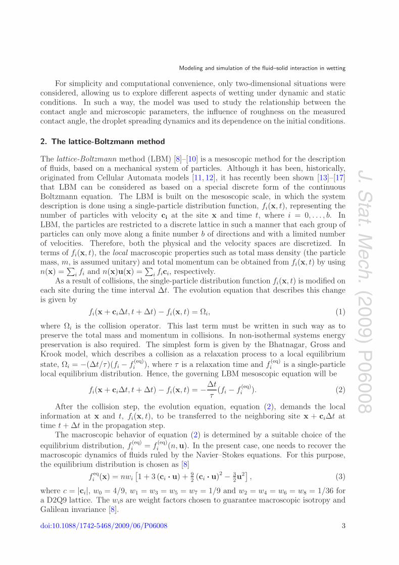
The lattice-Boltzmann method (LBM) [8]–[10] is a mesoscopic method for the descriptionof fluids, based on a mechanical system of particles. Although it has been, historically,originated from Cellular Automata models [11, 12], it has recently been shown [13]–[17]that LBM can be considered as based on a special discrete form of the continuousBoltzmann equation. The LBM is built on the mesoscopic scale, in which the systemdescription is done using a single-particle distribution function, fi(x, t), representing thenumber of particles with velocity ci at the site x and time t, where i = 0, . . . , b. InLBM, the particles are restricted to a discrete lattice in such a manner that each group ofparticles can only move along a finite number b of directions and with a limited numberof velocities. Therefore, both the physical and the velocity spaces are discretized. Interms of fi(x, t), the local macroscopic properties such as total mass density (the particlemass, m, is assumed unitary) and total momentum can be obtained from fi(x, t) by usingn(x) =

∑i fi and n(x)u(x) =

∑i fici, respectively.

As a result of collisions, the single-particle distribution function fi(x, t) is modified oneach site during the time interval Δt. The evolution equation that describes this changeis given by

fi(x + ciΔt, t + Δt) − fi(x, t) = Ωi, (1)

where Ωi is the collision operator. This last term must be written in such way as topreserve the total mass and momentum in collisions. In non-isothermal systems energypreservation is also required. The simplest form is given by the Bhatnagar, Gross andKrook model, which describes a collision as a relaxation process to a local equilibrium

state, Ωi = −(Δt/τ)(fi − f(eq)i ), where τ is a relaxation time and f

(eq)i is a single-particle

local equilibrium distribution. Hence, the governing LBM mesoscopic equation will be

fi(x + ciΔt, t + Δt) − fi(x, t) = −Δt

τ(fi − f

(eq)i ). (2)

After the collision step, the evolution equation, equation (2), demands the localinformation at x and t, fi(x, t), to be transferred to the neighboring site x + ciΔt attime t + Δt in the propagation step.

The macroscopic behavior of equation (2) is determined by a suitable choice of the

equilibrium distribution, f(eq)i = f

(eq)i (n,u). In the present case, one needs to recover the

macroscopic dynamics of fluids ruled by the Navier–Stokes equations. For this purpose,the equilibrium distribution is chosen as [8]

f eqi (x) = nwi

[1 + 3 (ci · u) + 9

2(ci · u)2 − 3

2u2

], (3)

where c = |ci|, w0 = 4/9, w1 = w3 = w5 = w7 = 1/9 and w2 = w4 = w6 = w8 = 1/36 fora D2Q9 lattice. The wis are weight factors chosen to guarantee macroscopic isotropy andGalilean invariance [8].

doi:10.1088/1742-5468/2009/06/P06008 3

J.Stat.M

ech.(2009)

P06008

Modeling and simulation of the fluid–solid interaction in wetting

Using a multiscale method such as Chapman–Enskog [18], it is possible to showthat the system described above recovers the Navier–Stokes equations in the limit ofnear incompressible flows [8, 9, 19, 10]. Next to the solid surfaces, a halfway bounce-backboundary condition [10] is imposed for the particles leaving the fluid domain.

2.1. Interaction forces between the fluid particles

In order to take into account the physical ingredients found in the microscopic interactionsamong the molecules of a fluid, Shan and Chen [6, 7] inserted an interaction potentialamong the particles in the LBM. In this way, the model is able to reproduce the liquid–vapor phase transition and coexistence of two distinct phases of a single component inequilibrium, in which the density distribution allows us to identify both phases. Theauthors used the following nearest-neighbor interaction potential between a pair of particlegroups localized at the sites x and y:

V (x,y) = ϕ(x)Gi(x,y)ϕ(y), (4)

where, for a D2Q9 lattice [20], Gi(x,y) = G for |ci| =√

2, Gi(x,y) = 4G for |ci| = 1and Gi(x,y) = 0 for two sites which are not nearest-neighboring sites. The functionϕ(x) ≡ ϕ[n(x)] will be chosen in a way to establish a correspondence between the LBMand an isotherm in a PV T system. The strength of the interaction potential among theparticles is given by G, while its sign defines if the potential is attractive or repulsive. Theresulting interaction force due to this potential acting on the particles located at the sitex at time t is then

Fσ(x, t) = −ϕ(x)∑

i

Giϕ(x + ciΔt)ci. (5)

In the LBM, the local velocity, u(x), in the equilibrium distribution, equation (3), ismodified due to the force Fσ in the following way:

ueq = u +τ

nFσ. (6)

This type of interaction among the particles does not preserve the local momentum duringthe collisional process because the force Fσ behaves as an external force acting on thesite. Nevertheless, Shan and Chen [6, 7] showed that the total momentum of the systemis preserved and no net momentum is inserted in the system by the above interaction.Redefining the fluid momentum, nv, as an arithmetic average for the states before andafter the collision step, nv = nu + 1

2Fσ, the method of Chapman–Enskog [18] allows us

to determine the macroscopic behavior of the referred microscopic system. The resultingmacroscopic equation describes a non-ideal fluid whose equation of state is written for aD2Q9 lattice as

P =n

3+ 6Gϕ2(n). (7)

The correct choice of the function ϕ(n) enables the modeling of a wide variety of fluids,including the liquid–vapor phase transition. Supposing the equation of state, equation (7),to correspond to an isotherm in the PV T system, Shan and Chen [7] determined a specific

doi:10.1088/1742-5468/2009/06/P06008 4

J.Stat.M

ech.(2009)

P06008

Modeling and simulation of the fluid–solid interaction in wetting

coexistence curve, concluding that if ϕ(n) is chosen to be

ϕ(n) = ϕ0 exp(−n0/n), (8)

where n0 and ϕ0 are arbitrary constants, the LBM will be consistent with that of anisothermal process [7]. Further on the functional, equation (8), the authors showed thatthe model ϕ(n) = ϕ0[1− exp(−n/n0)] can also be used, because the resulting coexistencecurve exhibits notable discrepancies with respect to the functional, equation (8), onlywhen the temperature parameter goes far below the critical value [7].

2.2. Long-range attractive forces between fluid and solid particles

When there are n(x) molecules located at point x of the fluid and ns(y) sources ofattraction located at y, if the shape and size of molecules are not considered, anapproximated form for the potential energy will be

Φ = n(x)ns(y)φ(|x− y|), (9)

where φ(|x − y|) is a function dependent on the distance separating x and y. Therefore,the potential energy related to the intermolecular interaction between the fluid moleculesat a position x and the solid attractive sources at a point y in the solid phase can bewritten as

Φ(fs)(|x − y|) = n(x)ns(y)ωα(|x− y|), (10)

where ω is a parameter related to the potential strength at the surface and α is a decayingfunction, which will be written as

α(|x − y|) = exp (−|x − y|/κ) , (11)

where κ is a constant related to the potential interaction length.From a physical point of view, the electrostatic field generated by the atoms on

the surface of a solid is affected by the electrical properties of the fluid molecules in itsneighborhood. Indeed, an electrical field can induce or modify the dipolar moments ofthese molecules, in accordance with their polarizability. The interaction between a fluidand a solid surface will, thus, simultaneously depend on the surface itself and on theelectrical polarizability of the fluid molecules. In the present paper, the parameter ω isused to describe the surface, giving the potential strength, i.e. the potential very close tothis surface. In addition to being dependent on the solid itself, the potential strength ωis dependent on the electrical properties of the fluid molecules, since the electrical fieldaround these molecules affects the potential at the solid sites. On the other hand, theparameter κ in the decaying law, equation (11), is directly related to the way the fluid feelsthe solid wall, i.e. to its polarizability: when the fluid molecules have a low polarizability,the surface potential have a strong decay and the fluid behaves as if it was free.

Since only attractive fields were considered for simulating the potential energybetween any two particles, when the above expression, equation (11), is used to calculatethe potential energy between two sites in the fluid phase, it produces a mass collapse inthe sites, since LBM particles are supposed without volume and each site becomes anincreasingly attractive sink of particles as the number density of particles increases in thissite. This is the main tactical reason that prevented the use of this potential form for

doi:10.1088/1742-5468/2009/06/P06008 5

J.Stat.M

ech.(2009)

P06008

Modeling and simulation of the fluid–solid interaction in wetting

calculating the potential energy among fluid particles in the last section. In the presentcase, although the sites in the solid phase act as attractive sinks of fluid particles, thebounce-back boundary condition used for the particles that reach the solid surface preventsthe accumulation of these particles on the boundary. In physical terms, a density increaseof the liquid in the immediate neighborhood of the solid is to be expected, but the correctprediction of this mass accumulation is a difficult and open question and would require amore detailed analysis, taking the correct fluid–solid interaction laws into account. Thedetailed description of this solid–fluid transition layer is beyond the purposes of this work.

In a discrete space, the potential energy at x due to the interaction with the solidwall S will be

Φ(fs)(x) =∑

y∈S

n(x)ns(y)ωα(|x− y|). (12)

From a numerical point of view, the above calculation is extremely cumbersome becauseit requires, for each time step and for each point x, a searching step along all theneighborhood sites of x that belong to the solid phase.

In this work, a lattice-Boltzmann method is proposed for modeling the physicalphenomena related to the fluid–solid interaction. It uses the concept of field mediators [2]–[5] to take the effect of attractive long-range interactions between the particles and solidwalls into account. The role of the field mediators is to mediate the long-range interactionsamong the particles located on a discrete lattice in such a way that the information onthe field from the neighborhood sites is found locally at each site on the lattice. Thepurpose is to avoid the computing awkward searching procedure around a given site. Toget such an effect, some particles with null mass, called mediators, are emitted from thesolid sites at each time step. Each mediator is able to carry with it, the information onthe number density of attractive sources on the solid site from where it was emitted. Asa consequence, each fluid site next to the wall gets this information after a few time stepsand this information is used to modify the local momentum of the fluid particles. Sincea field travels at the speed of light, this delay in field information was investigated bySantos, Facin and Philippi [3] in the study of capillary waves and no meaningful effectwas observed. For the simulation of the fluid–solid interaction using field mediators, thefollowing procedure has been adopted. At each time step, field mediators are emittedfrom the solid sites with the information on the number density of the attractive sourcesns and on the potential strength ωi:

M(s)i = nsωi, (13)

where, for a D2Q9 lattice [20], ωi = ω for |ci| =√

2, ωi = 4ω for |ci| = 1 and ωi = 0 fortwo sites which are not nearest-neighboring sites.

In the propagation step, the mediators are moved from y to the nearest-neighbor sitesy + ciΔt, suffering an attenuation, in accordance with the following relation:

M(s)i (y + ciΔt, t + Δt) = α(r)M(s)

i (y, t), (14)

where r is unity, because the mediators are only moved to the nearest-neighboring sites.

After this step the new variable M(s)i contains the information: (i) on the number density

of attractive sources at the point y of the solid surface; (ii) on the potential strength and(iii) on the distance traveled by the mediator. Figure 1 illustrates this numerical scheme.

doi:10.1088/1742-5468/2009/06/P06008 6

J.Stat.M

ech.(2009)

P06008

Modeling and simulation of the fluid–solid interaction in wetting

Figure 1. Schematic illustration of the emission and propagation steps for themediators as a function of time on a discrete lattice. The open circles abovethe wall represent the information transported by the mediators in different timesteps.

The fluid–solid interaction force, Fs(x, t), on the particles located at the site x attime t, due to the field mediators coming from the solid wall, can thus be written as

Fs(x, t) = −n(x)∑

i

M(s)i (x, t)ci. (15)

The fluid–solid force, equation (15), is imposed on the particles through a change in theirmomentum, in the same way as explained in section 2.1.

In comparison with other models, the present model includes explicitly the effectof long-range forces among the particles, allowing the interaction length to be easilycontrolled by only changing a single parameter. Such an attribute had not been consideredin previous models, such as the ones by Martin and Chen [21] and Raiskinmaki et al[22], based on nearest-neighbor interactions. In the work by Zhang and Kwok [23] adistance-dependent fluid–solid potential was considered explicitly in describing the fluid–wall interaction. However, the methodology adopted by Zhang and Kwok assumes theuse of a simple wall geometry—a flat plate—for which the net force on the fluid particlesat a given site is previously known and only depends on the height z. The interactionfield in the neighborhood of more complex solid surfaces, such as rough surfaces, dependson the coordinates x and y, in addition to z, requiring previous knowledge of the specificfluid–wall potential. In the present model, it is only necessary to know the inter-particlepotential itself, the field information being carried out from the solid sites to the fluid sitesand among fluid sites by mediators, avoiding the use of simplified z-dependent decayinglaws. In contrast, more complex solid surfaces demand lattices with higher numbers oflattice directions, since the emission and propagation steps are carried out according tothe nearest-neighbor sites. Higher-order lattices would thus imply a better representationof the net force on a given site. Benzi et al [24] discussed a generalization of the Shanand Chen model [6, 7] which includes the fluid–wall interaction. They also showed anextension of the model with long-range forces by using a distance-dependent potentialsimilar to the one used by Zhang and Kwok [23].

doi:10.1088/1742-5468/2009/06/P06008 7

J.Stat.M

ech.(2009)

P06008

Modeling and simulation of the fluid–solid interaction in wetting

Figure 2. Measurement of the static contact angle by extrapolating thecylindrical shape from the height y to the solid surface, y = 0.

3. Results and discussion

3.1. Measuring the static contact angle

In this work, the measurement of the static contact angle was carried out by consideringtwo different techniques, both of them putting in evidence the contact angle as amacroscopic property in essence. The first method is based on geometrical relationswhich are grounded on a cylindrical bidimensional droplet shape when gravity is missing.Due to the field mediators, the long-range force length, �FS, is larger than one latticespacing, which induces the deformation of the liquid–vapor interface curvature near thetriphasic contact line, the use of cylindrical-shape-based relations becoming imprecise inthe measurement of the contact angle. The mentioned inaccuracy can be avoided if theangle, θ(y), is measured far away from the contact line, at a specific height y from the solidsurface, and after that the static contact angle is obtained by extrapolating the cylindricalshape up to the solid surface, y = 0. This is illustrated in figure 2. Therefore, the staticcontact angle is a function of geometrical parameters such as the droplet base radius atheight y, r(y), the droplet height, H , and θ(y), and can be calculated by

θs = arccos

[

1 − H

r(y)sen θ(y)

]

, (16)

where θ(y) = 2 arctan[(H − y)/r(y)]. In all the cases considered here, y = 4.5 latticespacings is chosen. The determination of droplet dimensions, as r(y) and H , was donethrough the density field by considering the abrupt variation of local densities, whichoccurs near the interface region. From the calculation of the density gradient in a specificdirection, for instance y, dn/dy ≈ [n(y + Δy) − n(y − Δy)]/2Δy, the interface positioncan be determined by noticing that |dn/dy| is a maximum at the liquid–vapor interface.Considering a specific coordinate system, as shown in figure 3, all droplet dimensions areavailable.

In these simulations there was observed the detachment of a precursor film ahead ofthe macroscopic bulk liquid, when the contact angle is smaller than around 34◦ (ω = 0.3and κ = 0.5) (see figure 4). When the film movement ceases, it has something similar to a

doi:10.1088/1742-5468/2009/06/P06008 8

J.Stat.M

ech.(2009)

P06008

Modeling and simulation of the fluid–solid interaction in wetting

Figure 3. Schematic illustration of the static contact angle, θs, the apparentdroplet base radius, R, defined from the inflection point and the actual dropletbase radius, Ra.

‘tongue’ ahead of the droplet as cited by Kavehpour et al [25]. The presence of a precursorfilm in physical systems, whose thickness is normally below the micron range [26], has beenreported by several authors in the literature (see, e.g., [27]–[29], [26, 30, 25]). That filmexhibits a peculiar dynamics and it will be not explored here, because the main objectiveof this work is to study the wettability from a macroscopic point of view by comparingsimulation results with experiments available in the literature.

A second technique for measuring the contact angle was used due to the presenceof the mentioned precursor film, which breaks down the supposition of a cylindricaldroplet shape, particularly for small contact angles. An alternative way to measure thecontact angle is given in terms of the inflection point. The existence of an inflectionpoint is a requirement for droplets with small apparent contact angles and provides aconnection between the inner region near the ‘tongue’ and the outer macroscopic bulkliquid region [25], as is illustrated in figure 3. The determination of the inflectionpoint is based on the knowledge of the droplet profile, h(x), and can be obtained usingthe numerical procedures which incorporate the maximum density gradient method asdescribed above. The droplet profile is built from the set of all interface positions ona given coordinate system. From the droplet profile, the macroscopic contact angle isconventionally defined as θs = max[arctan(dh/dx)] [31, 25], which is the slope of theliquid–vapor interface at the inflection point.

3.2. Relationship between the contact angle and microscopic parameters

The method proposed in this work allows the interactions occurring between the latticesites separated by greater distances than one lattice spacing. Thus, it is possible toinvestigate the static contact angle, θs, as a function of the microscopic parameters relatedto the long-range fluid–solid potential, given by the strength and length of the fluid–solid

doi:10.1088/1742-5468/2009/06/P06008 9

J.Stat.M

ech.(2009)

P06008

Modeling and simulation of the fluid–solid interaction in wetting

Figure 4. Equilibrium configurations for κ = 0.5 and different values of ω. Fromtop to bottom, the strength parameter ω was adjusted to 0.08, 0.15, 0.20, 0.30and 0.325, respectively.

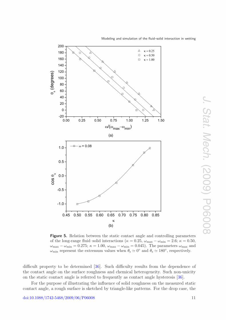
interaction, ω and κ, respectively. For this purpose, a lattice D2Q9 with 500 × 78 siteswas initialized with the parameters τ = 1.0 and G = −0.15, resulting in a liquid–vapordensity ratio, nL/nV � 20. For simplicity and computational convenience, only two-dimensional simulations were considered. The initial condition was based on a liquiddroplet (nL = 2.261) with an initial diameter, R0, equal to 35 lattice spacings in contactwith a solid surface (nS = 1.0). In all domain boundaries periodic boundary conditionswere imposed. The dependence between θs and the parameters ω and κ is shown infigures 4 and 5.

In figure 5, the obtained results show that the static contact angle is stronglydependent on the interaction potential defined by the microscopic parameters ω and κ.By varying the strength of the fluid–solid interaction, it was verified that any contactangle between 0◦ and 180◦ can be simulated and that an increase in the adhesion forcesleads to a decrease in the contact angle. This is in agreement with simulation resultsbased on molecular dynamics methods [32, 33]. The dependence between θs and ω seemsto be approximately linear, similar to the results related by Zhang and Kwok [23] whoused the mean-field free-energy lattice-Boltzmann approach. The parameter κ controlsthe fluid–solid interaction length of the field mediators and allows us to modulate theinfluence on the triphasic contact line from the particles that are located at sites far fromthe solid surface, 5(b).

3.3. Rough surfaces and hysteresis

Most of the experimental results available in the literature [34]–[36] are based on theapparent contact angle, θap, and not on the actual contact angle [35], θs, which is a very

doi:10.1088/1742-5468/2009/06/P06008 10

J.Stat.M

ech.(2009)

P06008

Modeling and simulation of the fluid–solid interaction in wetting

(a)

(b)

Figure 5. Relation between the static contact angle and controlling parametersof the long-range fluid–solid interactions (κ = 0.25, ωmax − ωmin = 2.6; κ = 0.50,ωmax − ωmin = 0.275; κ = 1.00, ωmax − ωmin = 0.045). The parameters ωmax andωmin represent the extremum values when θs � 0◦ and θs � 180◦, respectively.

difficult property to be determined [36]. Such difficulty results from the dependence ofthe contact angle on the surface roughness and chemical heterogeneity. Such non-unicityon the static contact angle is referred to frequently as contact angle hysteresis [36].

For the purpose of illustrating the influence of solid roughness on the measured staticcontact angle, a rough surface is sketched by triangle-like patterns. For the drop case, the

doi:10.1088/1742-5468/2009/06/P06008 11

J.Stat.M

ech.(2009)

P06008

Modeling and simulation of the fluid–solid interaction in wetting

vapor

L1

L2 L3

Figure 6. Idealized rough surface and initial conditions for three liquid drops.

(a)

(b)

Figure 7. Equilibrium configuration for liquid drops in contact with a rough solidsurface obtained from the LBM simulations. Three drops are put artificiallyin contact with a rough surface for a domain size of (a) 800 × 200 sites and(b) 1600 × 377 sites. Notice that the size of the drops is doubled, while the sizeof the rough pattern is kept constant. In this case, κ = 0.5 and ω = 0.25.

contact angle hysteresis can be easily observed when very different initial conditions areimposed. The simulation is initiated by considering three different liquid drops in contactwith a rough surface, as shown in figure 6.

In the simulation, the mechanical equilibrium condition was supposed to be reachedafter around 3 × 104 time steps. In figure 7(a) is shown the final configuration of threeliquid drops arranged according to the initial conditions in figure 6. As can be seen, froma macroscopic point of view, the static contact angles seem to be very distinct from eachother, even though the entire solid surface exhibits the same fluid–solid interaction, witha corresponding static contact angle of around 69◦. By tracing a straight line parallel tothe solid surface, one can determine the following apparent contact angles (from left to

right): θ(1)ap � 66◦, θ

(2)ap � 105◦ and θ

(3)ap � 119◦. It is important to notice that, if the surface

were ideally smooth, the three drops would show exactly the same static contact angle,

that is, θ(1)ap = θ

(2)ap = θ

(3)ap = θs � 69◦, without any influence of the initial conditions. These

obtained results show that the measured static contact angle is strongly influenced by theroughness of the surface as a result of the changes in the curvature of the liquid–vaporinterface. Though those dissimilar initial conditions were generated artificially, they mightoccur in laboratory conditions. Thus, a given measured contact angle is dependent on itsown history.

doi:10.1088/1742-5468/2009/06/P06008 12

J.Stat.M

ech.(2009)

P06008

Modeling and simulation of the fluid–solid interaction in wetting

A sinusoidal-shaped solid surface was studied theoretically by Johnson and Dettre [37].Focusing the analysis on the drop size scale, those authors were able to show that morethan one static contact angle can be obtained and that all observable contact angles are ina bounded range, similar to the results shown in this work. Notice that in the simulationshown in figure 7(a) the effect of roughness is overestimated, since that roughness patternhas the order of magnitude of the drop size. Nevertheless, when the characteristic dropsize is increased, the same effect is observed. Figure 7(b) illustrates such a result, in whichthe doubled size drops were simulated on the same rough surface of figure 7(a). Evidently,the effect of roughness on the apparent contact angle decreases when this roughness isreduced.

Such interesting results demonstrate an intrinsic property of the liquid–vapor–solidsystem: the locality of the contact angle. As was mentioned above, the measured staticcontact angle is modified by the roughness, requiring the definition of an apparent contactangle.

3.4. Spreading dynamics

The relaxation of a liquid drop to the equilibrium state is analyzed by considering thetime evolution of its apparent base radius, R(t), outlined in figure 3. It is well known(see, e.g., [38, 28, 29]) that, under complete wetting conditions (θs → 0◦), a liquid dropletspreads on a solid surface exhibiting a universal behavior, independent of the materialproperties of the involved substrate. Such behavior is commonly referred to as Tanner’slaw [38] and is represented by a power law for droplet base radius, R(t), given by

R(t) ∝ tN , (17)

where N is the spreading exponent, being N = 1/7 for two-dimensional drops andN = 1/10 for three-dimensional ones. In most of the experimental results reportedin the literature in three-dimensional systems, the exponent N was found in the rangebetween 0.1 and 0.145, although values of 0.033 and 0.3135 have already been reported [28].Tanner’s law is only valid in the macroscopic scale, since microscopic droplets follow adifferent spreading dynamics dominated by van der Waals forces [39].

For studying the spreading dynamics resulting from the model described above, a two-dimensional system of L×H sites was used with ‘mirror’ and periodic boundary conditionsimposed on the top and left/right, respectively. The bottom line in the domain is filledwith solid sites, representing a solid surface with a thickness of one lattice spacing andcorresponding physical dimension, δx. In the considered cases, the interaction length ofthe long-range fluid–solid forces, �FS, is not negligible with respect to the system size(�FS ≈ 6δx for κ = 0.5). It is thus necessary to determine if the characteristic scalein the simulations is comparable to the laboratory conditions, for which Tanner’s law isrecovered. For that, a liquid drop with radius R0 was initialized in contact with the solidsurface. The drop radius was varied from 30 to 150 lattice spacings, but keeping the valuesof the ratios L/2R0 = C1 and L/H = C2 constant, where C1 � 6.4 and C2 � 3.6. In thismanner, an increase in the droplet size led to a proportional increase in the domain size.The model parameters G and ω were adjusted to −0.15 and 0.06, respectively, resultingin a liquid drop with density nL = 2.261 immersed in vapor with density nV = 0.116, asurface tension γ = 0.086 and a static contact angle θs � 180◦, where all parameters arein lattice units. That configuration was kept constant for 3 × 104 time steps, for which

doi:10.1088/1742-5468/2009/06/P06008 13

J.Stat.M

ech.(2009)

P06008

Modeling and simulation of the fluid–solid interaction in wetting

Figure 8. Spreading dynamics of a liquid droplet with an initial radius R0 = 60lattice spacings. The process goes from left to right and from top to bottom.

the system came into the mechanical equilibrium state. After that, the strength of thefluid–solid interaction, ω, was set to 0.335, for which θs → 0◦, simulating a liquid–vapor–solid system in which the liquid wets the solid surface completely. The obtained resultsare shown in figures 8 and 9.

In figure 8, the time evolution of the droplet at the first steps of spreading is seen,when the droplet assumes different shapes before attaining an almost circular shape inthe liquid bulk. There is observed an initial formation of a film ahead of the droplet,which is faster than the main part. Figure 9 shows the apparent droplet base radius,R∗ = R/R0, as a function of the reduced time, t∗ = tγ/(νLnLR0) [40], where νL is thekinematic viscosity given by 1/6 in the D2Q9 lattice [8]. For analyzing the spreadingbehavior at long times, the obtained curves were fitted in the ranges 100 ≤ t∗ ≤ 520 and150 ≤ t∗ ≤ 520 by supposing a power law like

R∗ = C (t∗ − t∗0)N

, (18)

where N , C and t∗0 are constants calculated by the fitting process.Figure 9(a) presents the results for the dimensionless apparent droplet base radius

versus reduced time for different droplet sizes. It is noticed that there is a superpositionof curves for R0 greater than about 100 lattice spacings, which means that larger dropletsspread in a similar way, leading to a single ‘master’ curve. The analysis of the resultspresented in figure 9(b) indicates that the effect of the droplet size on the spreadingdynamics is almost irrelevant in practical terms, when the analysis was performed bytaking into account later periods of time, as was made for the reduced time in the range

doi:10.1088/1742-5468/2009/06/P06008 14

J.Stat.M

ech.(2009)

P06008

Modeling and simulation of the fluid–solid interaction in wetting

(a)

(b)

Figure 9. In (a) One has the dimensionless droplet base radius, R∗ = R/R0,as a function of the reduced time, t∗, and in (b) the droplet size dependence indifferent reduced time ranges.

150 ≤ t∗ ≤ 520. As is observed in the range 100 ≤ t∗ ≤ 520, there is a size dependence onthe spreading, related to the influence of the initial conditions on the spreading dynamics.

However, it is noticed that the mean spreading exponent simulated by the LB model,N � 0.2423± 0.0005 (with a mean coefficient of determination R2 = 0.999 97), exhibits aconsiderable deviation from the expected value of 1/7, predicted by equation (18). Some

doi:10.1088/1742-5468/2009/06/P06008 15

J.Stat.M

ech.(2009)

P06008

Modeling and simulation of the fluid–solid interaction in wetting

LBM results under two-dimensional and complete wetting conditions were also providedby Iwahara et al [41], obtaining N equal to 0.43 and attributing such a discrepancy to theimposed initial conditions. They also stated that the droplet size did not influence thespreading exponent, according to the results obtained here in the range 150 ≤ t∗ ≤ 520.A possible explanation for the discrepancy in these results can be related to the highresolution of these numerical experiments.

To clarify the reason for that difference between numerical and experimental results,the power law, equation (18), was determined for distinct liquid layers next to the solidwall, represented by the liquid layer–solid distance, y − ys, where ys is the solid plateposition on the y axis. The results shown in figure 9 were obtained by measuring theexponent N on the first liquid layer above the solid wall, i.e. where y − ys = 1 latticespacing.

For the determination of the spreading exponent as a function of the distance betweeneach layer and the solid surface, two methods were used: (i) the apparent droplet baseradius was measured in the same way as was done above by using the inflection point onthe droplet profile, h(x), and (ii) the actual droplet base radius was measured directlyfrom the density field, n(x, y), with the maximum gradient method. The obtained resultsare shown in figure 10.

It is noticed that the spreading exponent is dependent on the distance from the solidwall; the liquid layers spread following different power laws and those nearest the solidmove faster than others. The measuring process based on the actual droplet base radiusshows that the liquid layers relative to the precursor film spread at higher rates than thebulk liquid, which is not seen when the method based on the profile slope at inflection isapplied.

Both methods provide the same dependence between N and y−ys for distances greaterthan or equal to 8 lattice spacings, where the liquid layer spreads with the exponent ina power law similar to that observed experimentally. Such a distance between the liquidlayer and the solid, or at least the region between 6 and 8 lattice spacings far from thesolid wall, seems to represent very well the transition between macroscopic and microscopicregions. It should be noticed that most of the experimental results for droplet base radiusare based on low-resolution optical measurements, so that only the macroscopic portion ofthe droplet is monitored, i.e. the inner region composed by the precursor film is invisibleand does not influence the measurement of the power law exponent. In terms of theinteraction length, �FS, that liquid layer where the simulated power law agrees with theexperimental results is found at (y − ys)/�FS ≈ 1.33 and is represented by the dashedline in figure 10(b). As can be seen, the droplet profile above that delimiting transitionregion is weakly affected by the presence of the precursor film. Therefore, when thetangent line is extrapolated from the inflection point to the solid wall, one gets a spreadingdynamics which appears to be non-representative of the experimental visualizations. Thiscould explain the differences that were found between the numerical and experimentallydetermined exponents in Tanner’s law, equation (18).

3.5. Influence of the initial conditions

Tanner’s law [38] has been considered a universal law, under complete wetting conditions,since most of the experimental results has pointed out an exponent N in the range between

doi:10.1088/1742-5468/2009/06/P06008 16

J.Stat.M

ech.(2009)

P06008

Modeling and simulation of the fluid–solid interaction in wetting

(a)

(b)

Figure 10. (a) Spreading exponent as a function of the distance from the solidwall calculated by two methods mentioned in the text for R0 = 50 lattice spacings.In (b) one has droplet profiles, h(x), at different reduced times. Notice the dashedline at (y − ys)/�FS ≈ 1.33, where the simulated N is closer than that predictedby Tanner’s law.

doi:10.1088/1742-5468/2009/06/P06008 17

J.Stat.M

ech.(2009)

P06008

Modeling and simulation of the fluid–solid interaction in wetting

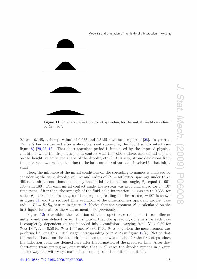
Figure 11. First stages in the droplet spreading for the initial condition definedby θ0 = 90◦.

0.1 and 0.145, although values of 0.033 and 0.3135 have been reported [28]. In general,Tanner’s law is observed after a short transient succeeding the liquid–solid contact (seefigure 8) [29, 26, 42]. That short transient period is influenced by the imposed physicalconditions when the droplet is put in contact with the solid surface, and should dependon the height, velocity and shape of the droplet, etc. In this way, strong deviations fromthe universal law are expected due to the large number of variables involved in that initialstage.

Here, the influence of the initial conditions on the spreading dynamics is analyzed byconsidering the same droplet volume and radius of R0 = 50 lattice spacings under threedifferent initial conditions defined by the initial static contact angle, θ0, equal to 90◦,135◦ and 180◦. For each initial contact angle, the system was kept unchanged for 6× 104

time steps. After that, the strength of the fluid–solid interaction, ω, was set to 0.335, forwhich θs → 0◦. The first stages of the droplet spreading for the cases θ0 = 90◦ is shownin figure 11 and the reduced time evolution of the dimensionless apparent droplet baseradius, R∗ = R/R0, is seen in figure 12. Notice that the exponent N is calculated on thefirst liquid layer above the wall, as mentioned previously.

Figure 12(a) exhibits the evolution of the droplet base radius for three differentinitial conditions defined by θ0. It is noticed that the spreading dynamics for each caseis completely dependent on the imposed initial conditions, varying from N ≈ 0.60 forθ0 � 180◦, N ≈ 0.50 for θ0 � 135◦ and N ≈ 0.37 for θ0 � 90◦, when the measurement wasperformed during this initial stage, corresponding to t∗ < 25 in figure 12(a). Notice thatthe method based on the actualdroplet base radius was applied for the first steps, sincethe inflection point was defined here after the formation of the precursor film. After thatshort-time transient regime, one verifies that in all cases the droplet spreads in a quitesimilar way and with very small effects coming from the initial conditions.

doi:10.1088/1742-5468/2009/06/P06008 18

J.Stat.M

ech.(2009)

P06008

Modeling and simulation of the fluid–solid interaction in wetting

Figure 12. Log–log plot of the dimensionless actual (for t∗ < 25) and apparent(for t∗ > 25) droplet base radius, R∗ = R/R0, as a function of the reduced time,t∗, for three different initial conditions. The continuous line represents the fittingcurve in the range 100 ≤ t∗ ≤ 520.

Tanner’s law [38] is well established in the complete wetting regime and anycomparison between numerical and experimental results must be done in this regime, afterthe short initial period. Three-dimensional results reported by Raiskinmaki et al [22] andDupuis and Yeomans [43] were carried out under partial wetting conditions. Although thepower law, equation (17), was observed, it is related to the transitional regime succeedingthe contact between the droplet and surface. Thus, the values of N found by the authorswere higher than expected, and about N ≈ 0.33 by Raiskinmaki et al [22] and N = 0.28by Dupuis and Yeomans [43] for the case of θ0 � 180◦. Furthermore, Raiskinmaki et al[22] reported a strong influence of the initial conditions, showing that, if θ0 → 90◦, thesimulated exponents tend towards the experimental results, for which N = 1/10. Despitethe results presented in the present work being two-dimensional, it can be seen in figure 12that, when θ0 → 90◦, the slope of the curve R∗ versus t∗ at short times in the log–log plottends to be similar to that slope at long times, and this was possibly the reason for thatconclusion. Iwahara et al [41] provided two-dimensional results for θ0 � 180◦ under thecomplete wetting regime and obtained N ≈ 0.43 and attributed such a discrepancy to theinitial boundary conditions.

The results obtained in this section show that the initial conditions have a stronginfluence on the first steps of the droplet spreading, but such influence disappears afterlong times. This is consistent with the experimentally available results.

4. Conclusions

A lattice-Boltzmann method based on field mediators is proposed for modeling the fluid–solid interaction. The obtained results were shown to be consistent with results found

doi:10.1088/1742-5468/2009/06/P06008 19

J.Stat.M

ech.(2009)P

06008

Modeling and simulation of the fluid–solid interaction in wetting

in the literature and provided additional information about the macroscopic behaviorresulting from microscopic interactions around the contact line. It was observed thatthe static contact angle is strongly dependent on the interaction potential defined by thefield strength and interaction length, and that a precursor film can appear under certainconditions. The contact angle hysteresis and its dependence on the initial conditions wassimulated for simple rough surfaces. That pointed out the locality of the contact angle,which is an intrinsic property of the liquid–vapor–solid system. The spreading dynamicson solid surfaces was studied, showing a power law time behavior but with a remarkabledifference in the exponent given by Tanner’s law. Finally, the influence of the initialconditions was shown to be important only in the first steps of the droplet spreading,becoming negligible after long times according to the experimental results.

Acknowledgments

Financial support was given by the National Petroleum Agency—PRH09-ANP/MME/MCT, CENPES/PETROBRAS, Financial Supporter of Studies and Projects—FINEPand the National Council for Scientific and Technological Development—CNPq—Brazil.

References

[1] Lyklema J, 2000 Fundamentals of Interface and Colloid Science: Liquid–Fluid Interfaces vol III (New York:Academic)

[2] dos Santos L O E and Philippi P C, Lattice-gas model based on field mediators for immiscible fluids, 2002Phys. Rev. E 65 046305

[3] Santos L O E, Facin P C and Philippi P C, Lattice-Boltzmann model based on field mediators for immisciblefluids, 2003 Phys. Rev. E 68 056302

[4] dos Santos L O E, Wolf F G and Philippi P C, Dynamics of interface displacement in capillary flow , 2005J. Stat. Phys. 121 197

[5] Wolf F G, dos Santos L O E and Philippi P C, Micro-hydrodynamics of immiscible displacement insidetwo-dimensional porous media, 2008 Microfluid. Nanofluid. 4 307

[6] Shan X and Chen H, Lattice-Boltzmann model for simulating flows with multiple phases and components,1993 Phys. Rev. E 47 1815

[7] Shan X and Chen H, Simulation of nonideal gases and liquid–gas phase transitions by the lattice-Boltzmannequation, 1994 Phys. Rev. E 49 2941

[8] Qian Y H, d’Humieres D and Lallemand P, Lattice BGK models for Navier–Stokes equations, 1992Europhys. Lett. 17 479

[9] Chen H, Chen S and Matthaeus W H, Recovery of the Navier–Stokes equations using a lattice-gasBoltzmann method , 1992 Phys. Rev. A 45 R5339

[10] Wolf-Gladrow D A, 2000 Lattice Gas Cellular Automata and Lattice-Boltzmann Models: An Introduction(Berlin: Springer)

[11] Frisch U, Hasslacher B and Pomeau Y, Lattice-gas automata for the Navier–Stokes equations, 1986 Phys.Rev. Lett. 56 1505

[12] Wolfram S, Cellular automaton fluids 1: basic theory , 1986 J. Stat. Phys. 45 471[13] He X and Luo L S, Theory of lattice-Boltzmann method: from the Boltzmann equation to the lattice

Boltzmann equation, 1997 Phys. Rev. E 56 6811[14] Abe T, Derivation of the lattice Boltzmann method by means of the discrete ordinate method for the

Boltzmann equation, 1997 J. Comput. Phys. 131 241[15] Shan X and He X, Discretization of the velocity space in the solution of the Boltzmann equation, 1998 Phys.

Rev. Lett. 80 65[16] Shan X, Yuan X F and Chen H, Kinetic theory representation of hydrodynamics: a way beyond the

Navier–Stokes equation, 2006 J. Fluid Mech. 550 413[17] Philippi P C, Hegele L A Jr, dos Santos L O E and Surmas R, From the continuous to the lattice

Boltzmann equation: the discretization problem and thermal models, 2006 Phys. Rev. E 73 056702[18] Chapman S and Cowling T G, 1970 The Mathematical Theory of Non-Uniform Gases 3rd edn

(Cambridge: Cambridge University Press)

doi:10.1088/1742-5468/2009/06/P06008 20

J.Stat.M

ech.(2009)

P06008

Modeling and simulation of the fluid–solid interaction in wetting

[19] Chen S and Doolen G D, Lattice Boltzmann methods for fluid flow , 1998 Annu. Rev. Fluid Mech. 30 329[20] Shan X, Analysis and reduction of the spurious current in a class of multiphase lattice Boltzmann models,

2006 Phys. Rev. E 73 047701[21] Martys N S and Chen H, Simulation of multicomponent fluids in complex three-dimensional geometries by

the lattice Boltzmann method , 1996 Phys. Rev. E 53 743[22] Raiskinmaki P, Koponen A, Merikoski J and Timonen J, Spreading dynamics of three-dimensional droplets

by the lattice-Boltzmann method , 2000 J. Comput. Mater. Sci. 18 7[23] Zhang J and Kwok D Y, Apparent slip over a solid–liquid interface with a no-slip boundary condition, 2004

Phys. Rev. E 70 056701[24] Benzi R, Biferale L, Sbragaglia M, Succi S and Toschi F, Mesoscopic modeling of a two-phase flow in the

presence of boundaries: the contact angle, 2006 Phys. Rev. E 74 021509[25] Kavehpour H P, Ovryn B and Mckinley G, Microscopic and macroscopic structure of the precursor layer in

spreading viscous drops, 2003 Phys. Rev. Lett. 91 196104[26] Cazabat A M, How does a droplet spread? , 1987 Contemp. Phys. 28 347[27] Hardy W, The spreading of fluids on glass, 1919 Phil. Mag. 38 49[28] Marmur A, Equilibrium and spreading of liquids on solids surfaces, 1983 Adv. Colloid Interface Sci. 19 75[29] de Gennes P G, Wetting: Statics and dynamics, 1985 Rev. Mod. Phys. 57 827[30] Beaglehole D, Profiles of the precursor drops of siloxane oil on glass, fused silica, and mica, 1989 J. Phys.

Chem. 93 893[31] Middleman S, 1995 Modeling Axisymmetric Flows (San Diego, CA: Academic)[32] Sikkenk J H, Indekeu J O and van Leeuwen J M J, Molecular-dynamics simulation of wetting and drying at

solid–fluid interfaces, 1987 Phys. Rev. Lett. 59 98[33] Nijmeijer M J P, Bruin C and Bakker A F, Wetting and drying of an inert wall by a fluid in a

molecular-dynamics simulation, 1990 Phys. Rev. A 42 6052[34] Johnson R E and Dettre R H, 1993 Wettability—Wetting of Low-Energy Surfaces (New York: Dekker)

chapter 1 pp 1–73[35] Marmur A, Wetting on real surfaces, 2000 J. Imaging Sci. Technol. 44 406[36] Dussan E B V, On the spreading of liquids on solid surfaces: static and dynamic contact lines, 1979 Annu.

Rev. Fluid Mech. 11 371[37] Johnson R E and Dettre R H, Contact angle hysteresis. I. study of an idealized rough surface, 1964 Adv.

Chem. Ser. 43 112[38] Tanner L H, The spreading of silicone oil drops on horizontal surfaces, 1979 J. Phys. D: Appl. Phys.

12 1473[39] Perez E, Schaffer E and Steiner U, Spreading dynamics of polydimethylsiloxane drops: crossover from

laplace to van der waals spreading , 2001 J. Colloid Interface Sci. 234 178[40] Zosel A, Studies of the wetting kinetics of liquid drops on solid surfaces, 1993 Colloid Polym. Sci. 271 680[41] Iwahara D, Shinto H, Miyahara M and Higashitani K, Liquid drops on homogeneous and chemically

heterogeneous surfaces: a two-dimensional lattice Boltzmann study , 2003 Langmuir 19 9086[42] Biance A, Clanet C and Quere D, First steps in the spreading of a liquid droplet, 2004 Phys. Rev. E

69 016301[43] Dupuis A and Yeomans J M, Lattice Boltzmann modelling of droplets on chemically heterogeneous surfaces,

2004 Future Generation Computer Systems 20 993

doi:10.1088/1742-5468/2009/06/P06008 21