Modeling and Simulation of Dispersed Two-Phase Flow Transport Phenomena in Electrochemical Processes Von der Fakult¨ at f¨ ur Maschinenwesen der Rheinisch-Westf¨ alischen Technischen Hochschule Aachen zur Erlangung des akademischen Grades eines Doktors der Ingenieurwissenschaften genehmigte Dissertation vorgelegt von: Dipl.-Ing. Thomas Nierhaus Berichter: Univ.-Prof. Dr.-Ing. Wolfgang Schr¨ oder Prof. Dr. Ir. Johan Deconinck Tag der m¨ undlichen Pr¨ ufung: 15. Oktober 2009 Diese Dissertation ist auf den Internetseiten der Hochschulbibliothek online verf¨ ugbar.

Welcome message from author
This document is posted to help you gain knowledge. Please leave a comment to let me know what you think about it! Share it to your friends and learn new things together.
Transcript

Modeling and Simulation of DispersedTwo-Phase Flow Transport Phenomena
in Electrochemical Processes
Von der Fakultat fur Maschinenwesen derRheinisch-Westfalischen Technischen Hochschule Aachen zur
Erlangung des akademischen Grades eines Doktors derIngenieurwissenschaften genehmigte Dissertation
vorgelegt von:
Dipl.-Ing. Thomas Nierhaus
Berichter:
Univ.-Prof. Dr.-Ing. Wolfgang SchroderProf. Dr. Ir. Johan Deconinck
Tag der mundlichen Prufung: 15. Oktober 2009
Diese Dissertation ist auf den Internetseitender Hochschulbibliothek online verfugbar.

This doctoral thesis is published in the context of a partnershipagreement governing the joint supervision and awarding of a
doctorate diploma between
Rheinisch-Westfalische Technische Hochschule Aachen
and
Vrije Universiteit Brussel
The according contract is dated January 19, 2009.

Abstract
Modeling the physics of two-phase flows and the development of numerical tools fortheir simulation are important challenges in modern CFD. Contrary to single-phaseflows, where the underlying physics is quite well understood and relatively generalnumerical methods can be employed in flow simulations, the physical phenomenaoccurring in two-phase flows are far more versatile and still not fundamentally un-derstood in all details. The difficulties in multiphase flow modeling arise from largedissimilarities between different types of flow configurations and the complex flowconditions associated. Various modeling approaches and numerical methods havebeen derived and applied in this scope during the last decades. This process leadto the conclusion that the applicability of a particular modeling approach stronglydepends on the type of two-phase flow configuration involved. In other words, topick an adequate numerical approach to simulate a particular two-phase flow prob-lem on a computer, it is required to carefully identify the underlying physics beforeselecting a solution method.
This Ph.D. thesis deals with modeling and simulation of dispersed two phaseflows. Such flows involve a continuous carrier medium that contains small dispersedparticles or bubbles. In terms of material properties and states of matter involved,gaseous flows involving solid particles differ significantly from liquid flows involvinggas bubbles. However, if we regard the physical topologies of these two types oftwo-phase flow, we see that there are also very high similarities. In dispersed flows,the secondary phase is scattered into small entities in a continuous primary phaseflow. The phase interfaces in dispersed two-phase flows are very small compared tothe the global scale of the flow problem of interest. These circumstances lead to theconclusion that dispersed two-phase flows, regardless of their physical parameters,can generally be treated by a unified modeling approach, where only the modelingparameters distinguish the sub-type of the flow, may it be of particle-laden or bub-bly nature.
A promising model to provide a numerical solution to incorporate different typesof dispersed two-phase flows is the Eulerian-Lagrangian approach. In the presentwork, the development of an integrated numerical tool for the simulation of particle-laden and bubbly two-phase flows based on this approach is documented. The largesimilarities but also the differences between particle-laden and bubbly flows are iden-tified and taken into account in the simulations carried out in the scope of this work.
i

Abstract
Various simulation examples to validate the simulation software are given for bothflow sub-types.
A further challenge in nowadays CFD is the integration of combined simulationapproaches that allow to track different physical and even chemical mechanisms. Afrequently referred key word concerning such ambitious intentions is multi-physics.A topical numerical application of a multi-physical problem is the combination ofdispersed two-phase flow with electrochemical phenomena such as ion transport andreaction kinetics. In nowadays literature, broad spectra of models exist to simu-late two-phase flow and electrochemistry separately, while an integrated approachtaking into account the coupling and interaction of both phenomena has not beenaddressed in great detail so far.
In the present Ph.D. thesis, an approach for the numerical modeling of bub-bly two-phase flow combined with ion transport and gas-producing electrochemicalreactions is carried out. The fluid flow part of the problem is addressed by theEulerian-Lagrangian approach while the electrochemistry is taken into account bythe Multi Ion Transport and Reaction Model (MITReM). An integrated numericalmethod combining those two building blocks allows to take into account couplingeffects, such as the influence of the gas phase on the conductivity of a liquid elec-trolyte and the current density field as well as the conversion of a gas flux into aset of bubbles on a gas-producing electrode. This approach is found promising andcomprises a set of novelties regarding multi-physics simulations.
ii

Zusammenfassung
Die Modellierung sowie die Entwicklung numerischer Methoden zur computerge-stutzten Simulation von Zweiphasenstromungen sind von großer Bedeutung in derheutigen CFD. Im Gegensatz zu Einphasenstromungen, bei denen die physikalis-chen Grundlagen weitestgehend erforscht sind und zu deren Simulation eine Vielzahlnumerischer Methoden existiert, liegen Zweiphasenstromungen weitaus komplexerephysikalische Zusammenhange zugrunde, welche noch nicht vollends erforscht sind.Die Schwierigkeit in der Modellierung von Zweiphasenstromungen liegt in der Viel-zahl von auftretenden Stromungskonfigurationen, zu deren Simulation in den letztenJahrzehnten ein großer Fundus an numerischen Methoden entwickelt wurde. Aus derAnalyse dieser Entwicklung laßt sich schlussfolgern, dass die Anwendbarkeit einerbestimmten numerischen Methode stark von der Stromungskonfiguration abhangigist. Grundsatzlich gilt, dass eine umfassende Analyse des zugerundeliegenden Stro-mungsproblems unabdingbar fur die Wahl der Simulationsmethode ist.
Die vorliegende Arbeit behandelt die Modellierung und Simulation disperser Zwei-phasenstromungen. Diese Art von Stromung zeichnet sich durch eine kontinuierlicheTragerphase aus, die disperse Partikel oder Blaschen beinhaltet. In der Anwendungunterscheiden sich Partikelstromungen zwar grundlegend von Blaschenstromungen,jedoch lassen sich bezuglich der Stromungskonfiguration viele Ahnlichkeiten fest-stellen. Bei beiden Stromungstypen ist die Sekundarphase auf kleine Entitaten inder Primarphase verteilt. Die Phasengrenzen sind klein und kommen nur lokal vor.Der einzige Unterschied besteht folglich in den unterschiedlichen Aggregatzustandenund Materialeigenschaften der Phasen. Dieser Umstand laßt die Schlussfolgerungzu, dass sich beide Stromungstypen grundsatzlich mit derselben numerischen Meth-ode simulieren lassen. Die Modellierungsparameter bestimmen dabei den Typ derZweiphasenstromung.
Der in dieser Arbeit verwendete Ansatz zur Simulation verschiedener Typen dis-perser Zweiphasenstromungen ist die Euler-Lagrange-Methode. Die Arbeit doku-mentiert die Entwicklung eines numerischen Werkzeugs zur Simulation von Partikel-und Blaschenstromungen und zeigt die Gemeinsamkeiten sowie die Unterschiededieser beiden Stromungstypen auf. Die grundlegenden physikalischen Zusammenhangewerden durch zahlreiche Simulationsbeispiele veranschaulicht, welche daruberhinauszur Validierung der im Rahmen der Arbeit entwickelten Modellierungssoftware di-enen.
iii

Zusammenfassung
Eine weitere große Herausforderung in der heutigen CFD ist die Integration ver-schiedener Simulationstechniken, um komplexe Probleme, welche verschiedene phy-sikalische und chemische Aspekte beinhalten, numerisch zu losen. Ein heutzutage oftreferenziertes Schlusselwort in diesem Zusammenhang istMulti-physics. Ein Beispielfur eine solche komplexe Problemstellung ist die Kombination einer Zweiphasen-stromung mit einem elektrochemischen Prozess, in dem Ionentransport und Reak-tionskinetik eine Rolle spielen. In der heutigen wissenschaftichen Literatur findetsich eine Vielzahl von Modellen zur Simulation von Zweiphasenstromungen und elek-trochemischen Prozessen, doch nur wenige pramature Ansatze, welche diese beidenPhanomene in einem integrierten Rechenverfahren miteinander koppeln.
Die vorliegende Arbeit beschreibt einen Ansatz zur Modellierung und integriertenSimulation von Blaschenstromungen, Ionentransport und gaserzeugunden elektro-chemischen Reaktionen. Dabei wird die Zweiphasenstromung wie beschrieben mitder Euler-Lagrange-Methode simuliert, wahrend die elektrochemischen Parametermit dem Multi Ion Transport and Reaction Model (MITReM) berechnet werden.Dies resultiert in einem integrierten numerischen Ansatz, der es erlaubt, auftretendeKopplungen zwischen Zweiphasenstromung und elektrochemischen Phanomenen zusimulieren. Beispiele fur solche Kopplungen sind der Einfluss der Gasphase auf dieelektrische Leitfahigkeit eines Elektolyts sowie das Stromdichtefeld, oder der Um-satz eines an einer Elektrode auftretenden Gasmassenstroms in Gasblaschen. Derin dieser Arbeit gezeigte Ansatz beinhaltet einige wissenschaftliche Neuheiten imHinblick auf die Kopplung multiphysikalischer Phanomene.
iv

Acknowledgements
Sincere thanks to my promoter Wolfgang Schroder for giving me the opportunity tocarry out this Ph.D. thesis at the Faculty of Mechanical Engineering of the RWTHAachen and for support and valuable advice in technical and administrative issues.He always had the willingness to help me during my work and gave me the optionto pursue own ideas.
Concerning the promotion of the present Ph.D. work at the Faculteit Ingenieur-wetenschappen of the Vrije Universiteit Brussel, I would like to give sincere thanksto my promoter Johan Deconinck for his huge support throughout my studies, espe-cially regarding the numerical simulation of electrochemical processes. Furthermore,I give many thanks to Inge Aerts for supporting me in administrative issues.
I have to thank Herman Deconinck of the Aeronautics and Aerospace Departmentat the Von Karman Institute for Fluid Dynamics, who introduced me to the worldof CFD and without whom I’d never have chosen this Ph.D. subject. Furthermore,I have to thank to the Directors of the Von Karman Institute for Fluid Dynamics,Mario Carbonaro and Jean-Marie Muylaert for making it possible for me to jointhe pleasant environment of the institute and for all the support given throughoutmy stay. Special thanks to Stella Sauvan for giving me much help in administrativeissues.
I would like to thank David Vanden Abeele for scientific guidance throughoutthe first two years of my Ph.D., for his valuable advice and the huge motivationhe gave me for my Ph.D. work. Through him I could improve my skill in writingarticles. Furthermore, I have to thank Patrick Rambaud, Jean-Marie Buchlin andJeroen Van Beeck for sharing their great research experience with me in scientificdiscussions.
Sincere thanks to my colleagues Tamas Banyai and Pawel Skuza for the greattime we had together in our work group and for sharing their great programmingknowledge with me. I experienced that code-development is team-work and team-work includes going out for a beer from time to time.
Thanks to Pedro Maciel, Steven Van Damme, Heidi Van Parys and Annick Hu-bin for helping me to improve my knowledge of electrochemistry. Furthermore, big
v

Acknowledgements
thanks to Flora Tomasoni and Sam Dehaeck for their advice about experiments ontwo-phase flow. I enjoyed very much the inter-disciplinary collaboration and thediscussions we had.
For the positive work atmosphere at the VKI and for valuable discussions aboutCFD and fluid dynamics in general, I would like to thank my fellow Ph.D. stu-dents and co-workers Tiago Quintino, Andrea Lani, Nadege Villedieu, Mehmet SarpYalim, Thomas Wuilbaut, Mario Ricchiuto, Jirka Dobes, Telis Athanasiadis, CarloBagnera, Bart de Maerschalck, Janos Molnar, Jan Thomel, Marco Panesi, JasonMeyers, Anne Gosset, Marcos Lema, Cem Ozan Asma, Tomas Hofer, Kostas Myril-las, Calin Dan, Tom Verstraete, Raf Theunissen and Vincent Van der Haegen.
A big thank you goes out to my students Jean-Francois Thomas and Mark CostaSitja for being a great help in the improvement and validation of the PLaS code.
I give thanks and kisses to my girlfriend Ariane for all her support and her lovethroughout the last years. Thank you!
I’d like to thank the Instituut voor de Aanmoediging van Innovatie door Weten-schap en Technologie in Vlaanderen (IWT) for the financial support of my Ph.D. inthe frame of the SBO-project MuTEch.
vi

Contents
Abstract i
Zusammenfassung iii
Acknowledgements v
List of Symbols xix
1 Introduction 1
1.1 Categories of two-phase flows . . . . . . . . . . . . . . . . . . . . . . 21.2 Industrial applications of dispersed flows . . . . . . . . . . . . . . . . 41.3 Modeling approaches for dispersed flows . . . . . . . . . . . . . . . . 51.4 Motivation for the present work . . . . . . . . . . . . . . . . . . . . . 61.5 Overview of the thesis . . . . . . . . . . . . . . . . . . . . . . . . . . 7
2 Eulerian-Lagrangian modeling of dispersed flows 9
2.1 Properties of the Eulerian-Lagrangiam model . . . . . . . . . . . . . . 92.2 Characteristics of dispersed two-phase flows . . . . . . . . . . . . . . 112.3 Governing equations . . . . . . . . . . . . . . . . . . . . . . . . . . . 13
2.3.1 Continuous phase equations . . . . . . . . . . . . . . . . . . . 132.3.2 Dispersed phase equations . . . . . . . . . . . . . . . . . . . . 15
2.4 Particle-laden flow . . . . . . . . . . . . . . . . . . . . . . . . . . . . 162.4.1 Drag force . . . . . . . . . . . . . . . . . . . . . . . . . . . . . 162.4.2 Lift force . . . . . . . . . . . . . . . . . . . . . . . . . . . . . . 172.4.3 Equation of motion for a particle . . . . . . . . . . . . . . . . 18
2.5 Bubbly flow . . . . . . . . . . . . . . . . . . . . . . . . . . . . . . . . 192.5.1 Drag force . . . . . . . . . . . . . . . . . . . . . . . . . . . . . 192.5.2 Lift force . . . . . . . . . . . . . . . . . . . . . . . . . . . . . . 212.5.3 Pressure gradient and buoyancy force . . . . . . . . . . . . . . 222.5.4 Virtual mass force . . . . . . . . . . . . . . . . . . . . . . . . 222.5.5 Basset history force . . . . . . . . . . . . . . . . . . . . . . . . 222.5.6 Equation of motion for a bubble . . . . . . . . . . . . . . . . . 23
2.6 Coupling between dispersed and continuous phase . . . . . . . . . . . 242.6.1 Momentum coupling regimes . . . . . . . . . . . . . . . . . . . 252.6.2 One-way coupling . . . . . . . . . . . . . . . . . . . . . . . . . 26
vii

Contents
2.6.3 Two-way coupling . . . . . . . . . . . . . . . . . . . . . . . . . 272.6.4 Four-way coupling . . . . . . . . . . . . . . . . . . . . . . . . 27
2.7 Turbulent dispersed two-phase flows . . . . . . . . . . . . . . . . . . . 292.7.1 Dispersed entities and carrier phase turbulence . . . . . . . . . 292.7.2 Turbulence models for dispersed flows . . . . . . . . . . . . . . 31
2.8 Simulation approach . . . . . . . . . . . . . . . . . . . . . . . . . . . 332.9 The Lagrangian solver module PLaS . . . . . . . . . . . . . . . . . . 35
2.9.1 Structure of the code . . . . . . . . . . . . . . . . . . . . . . . 352.9.2 Procedural description . . . . . . . . . . . . . . . . . . . . . . 362.9.3 Input parameters . . . . . . . . . . . . . . . . . . . . . . . . . 372.9.4 Parallelization . . . . . . . . . . . . . . . . . . . . . . . . . . . 382.9.5 Trajectory integration . . . . . . . . . . . . . . . . . . . . . . 392.9.6 Neighbour search method . . . . . . . . . . . . . . . . . . . . 412.9.7 Velocity interpolation . . . . . . . . . . . . . . . . . . . . . . . 432.9.8 Computation of the volume fraction field . . . . . . . . . . . . 442.9.9 Computation of the back-coupling terms . . . . . . . . . . . . 45
3 Simulation of turbulent particle-laden two-phase flow 47
3.1 Turbulent carrier flow simulation . . . . . . . . . . . . . . . . . . . . 483.2 Particle dispersion in a turbulent channel . . . . . . . . . . . . . . . . 49
3.2.1 Turbulent single-phase channel flow . . . . . . . . . . . . . . . 503.2.2 Physical mechanisms in wall-bounded turbulence . . . . . . . 533.2.3 Particle-laden channel flow . . . . . . . . . . . . . . . . . . . . 55
3.3 Particle interaction with decaying isotropic turbulence . . . . . . . . 603.3.1 Single-phase isotropic turbulence . . . . . . . . . . . . . . . . 613.3.2 Particle-turbulence interaction . . . . . . . . . . . . . . . . . . 64
3.4 Conclusion . . . . . . . . . . . . . . . . . . . . . . . . . . . . . . . . . 71
4 Simulation of bubbly two-phase flow 73
4.1 Properties of bubbles . . . . . . . . . . . . . . . . . . . . . . . . . . . 744.2 Carrier flow simulation . . . . . . . . . . . . . . . . . . . . . . . . . . 764.3 Study of the hydrodynamics in a bubble column . . . . . . . . . . . . 78
4.3.1 Physical mechanisms in a bubble column . . . . . . . . . . . . 804.3.2 Two-phase hydrodynamics . . . . . . . . . . . . . . . . . . . . 80
4.4 Bubbly flow in an IRDE reactor . . . . . . . . . . . . . . . . . . . . . 864.4.1 Carrier flow characterization . . . . . . . . . . . . . . . . . . . 884.4.2 Experiments on bubble size distribution . . . . . . . . . . . . 984.4.3 Comments on the measurement uncertainty . . . . . . . . . . 1034.4.4 Bubble dispersion and size distribution in rotating flow . . . . 1044.4.5 Two-way coupling effects between bubbles and electrolyte . . . 110
4.5 Conclusion . . . . . . . . . . . . . . . . . . . . . . . . . . . . . . . . . 113
viii

Contents
5 Coupling of two-phase flow and electrochemistry 115
5.1 Introduction to electrochemistry . . . . . . . . . . . . . . . . . . . . . 1155.1.1 The electrochemical cell . . . . . . . . . . . . . . . . . . . . . 1155.1.2 Reactions on electrodes . . . . . . . . . . . . . . . . . . . . . . 1175.1.3 Faraday’s laws of electrolysis . . . . . . . . . . . . . . . . . . . 1185.1.4 Modeling requirements . . . . . . . . . . . . . . . . . . . . . . 118
5.2 The MITReM model . . . . . . . . . . . . . . . . . . . . . . . . . . . 1195.2.1 Transport equations . . . . . . . . . . . . . . . . . . . . . . . 1205.2.2 Boundary conditions . . . . . . . . . . . . . . . . . . . . . . . 122
5.3 Gas evolution in electrochemical reactions . . . . . . . . . . . . . . . 1245.3.1 Gas-evolving electrodes . . . . . . . . . . . . . . . . . . . . . . 1245.3.2 Effect of gas bubbles on electrochemical parameters . . . . . . 125
5.4 Multi-physical simulation approach . . . . . . . . . . . . . . . . . . . 1275.4.1 Realization . . . . . . . . . . . . . . . . . . . . . . . . . . . . 1275.4.2 The MITReM module . . . . . . . . . . . . . . . . . . . . . . 1295.4.3 The bubble evolution module . . . . . . . . . . . . . . . . . . 131
5.5 Bubble evolution in a parallel flow reactor . . . . . . . . . . . . . . . 1335.5.1 Reaction kinetics and species concentrations . . . . . . . . . . 1365.5.2 Dispersion of electrochemically generated bubbles . . . . . . . 142
5.6 Conclusion . . . . . . . . . . . . . . . . . . . . . . . . . . . . . . . . . 146
6 General conclusion 149
Curriculum vitae 169
List of publications 171
ix


List of Figures
1.1 Two-phase flow categorization according to Ishii [1] and Sommerfeld[2]: (a) transient flow patterns, (b) separated flow in film and slugpatterns, (c) dispersed flow with solid particles, droplets and bubbles. 3
2.1 Characteristic measures of dense and dilute flows according to Crowe[3]: (a) Control volume Vc including dispersed entities, (b) Conceptof the entity spacing L/d. . . . . . . . . . . . . . . . . . . . . . . . . 11
2.2 Effect of the Stokes number on the motion of a dispersed entity. . . . 122.3 Drag coefficient variation with Reynolds number for a rigid sphere [3]. 172.4 Drag coefficient variation with Reynolds number for an air bubble in
a purified liquid [19]. . . . . . . . . . . . . . . . . . . . . . . . . . . . 202.5 Drag coefficient variation with Reynolds number for an air bubble in
a contaminated liquid [19]. . . . . . . . . . . . . . . . . . . . . . . . . 212.6 Schematic diagram of (a) one-way (b) two-way and (c) four-way cou-
pling between carrier flow and dispersed entities. . . . . . . . . . . . . 262.7 Quantification of momentum coupling approaches in terms of entity
spacing L/d and volume fraction �d, according to [2]. . . . . . . . . . 262.8 Effect of the particle size on the turbulent intensity [50]. The hori-
zontal axis shows the ratio of the entity diameter d to a characteristicturbulence length scale. . . . . . . . . . . . . . . . . . . . . . . . . . . 29
2.9 Particle-turbulence modulation effects in terms of the Stokes numberas a function of dispersed phase volume fraction �d [40]. . . . . . . . 30
2.10 Algorithm flowchart of the Eulerian-Lagrangian two-phase flow sim-ulations performed by coupling PLaS to a fluid flow solver. . . . . . . 34
2.11 Algorithm flowchart of the PLaS main routine. . . . . . . . . . . . . . 362.12 Example for the geometric division of a three-dimensional mesh into
sub-regions for parallelization. . . . . . . . . . . . . . . . . . . . . . . 392.13 Two example search paths through an unstructures grid [75]. The
gray circle marks the last known entity position, while the arrowsshow the sequence of elements searched. . . . . . . . . . . . . . . . . 42
2.14 Median dual cell of triangles meeting in node j. The cell volume isindicated by Vj. . . . . . . . . . . . . . . . . . . . . . . . . . . . . . . 44
3.1 Geometry for the turbulent channel flow test case. . . . . . . . . . . . 51
xi

List of Figures
3.2 Averaged streamwise velocity profile u+ and diagonal Reynolds stresses⟨urms⟩, ⟨vrms⟩ and ⟨wrms⟩ compared to DNS results of Kim et al. [99]. 52
3.3 Fluctuating velocity quadrant analysis for fluid motion in a turbulentboundary layer. . . . . . . . . . . . . . . . . . . . . . . . . . . . . . . 54
3.4 Turbulence regeneration cycle [104]. . . . . . . . . . . . . . . . . . . . 543.5 Schematic view of particle accumulation in a low-speed streak due to
the motion of a counter-rotating vortex pair. . . . . . . . . . . . . . . 553.6 Instantaneous particle distribution in a streamwise plane for �+p = 25
at t∗ = 10 compared to reference results. . . . . . . . . . . . . . . . . 563.7 Top view of the instantaneous particle distribution in the turbulent
boundary layer for �+p = 25 at y+ < 3 and t∗ = 10 compared toreference results. . . . . . . . . . . . . . . . . . . . . . . . . . . . . . 57
3.8 Iso-surfaces of streamwise vorticity !z,1 = −0.1 and !z,2 = 0.1 alongwith particle locations in the viscous sub-layer. . . . . . . . . . . . . . 58
3.9 Normalized particle volume fraction �d/�d,0 as a function of y+ fordifferent Stokes numbers. . . . . . . . . . . . . . . . . . . . . . . . . . 59
3.10 Normalized particle volume fraction �d/�d,0 as a function of y+ for�+p = 0.2 and �+p = 1 compared to the results of [88]. . . . . . . . . . 59
3.11 Normalized particle volume fraction �d/�d,0 as a function of y+ for�+p = 5 and �+p = 25 compared to the results of [88]. . . . . . . . . . . 60
3.12 Characteristic initial velocity vector and pressure field for the isotropicturbulence decay test case [123]. . . . . . . . . . . . . . . . . . . . . . 63
3.13 Kinetic energy decay for isotropic turbulence with Re�,0 = 32, �c =0.02m2/s and q20 = 0.32m2/s2 compared to spectral DNS data [123]. . 64
3.14 Effect of increasing mass loading �d on the temporal evolution of theturbulent kinetic energy q2. . . . . . . . . . . . . . . . . . . . . . . . 67
3.15 Effect of increasing mass loading �d on the temporal evolution of thedissipation rate " of the turbulent kinetic energy. . . . . . . . . . . . 68
3.16 Effect of increasing mass loading �d on the temporal evolution of theparticle Reynolds number Red. . . . . . . . . . . . . . . . . . . . . . . 69
3.17 Effect of increasing mass loading �d on the temporal evolution of theKolmogorov length scale �. . . . . . . . . . . . . . . . . . . . . . . . . 70
3.18 Effect of mass loading �d on the kinetic energy q2 and the dissipationrate " normalized by their values at �d = 0, compared to [77]. . . . . 70
4.1 Bubble shapes in unhindered gravitational rise through liquids de-pending on Eotvos, Reynolds and Morton numbers [15]. . . . . . . . . 74
4.2 Terminal rise velocity of air bubbles in water at 20∘C [15]. . . . . . . 754.3 Sketches of the bubble column geometry and computational grid used
for the present simulations. . . . . . . . . . . . . . . . . . . . . . . . . 794.4 Instantaneous bubble positions and the corresponding carrier velocity
field in the y = 0.075m plane for mGas = 0.0482g/s (Case 3). . . . . . 82
xii

List of Figures
4.5 Instantaneous bubble positions and the corresponding carrier velocityfield in the y = 0.075m plane for mGas = 0.0723g/s (Case 5). . . . . . 83
4.6 Time variation of the induced vertical velocity uz at x = y = 0.075mand z = 0.252m for minimum and maximum mass flow rate values. . 84
4.7 Time variation of the horizontal velocity ux at x = y = 0.075m andz = 0.252m for minimum and maximum mass flow rate values. . . . . 84
4.8 Fluctuating velocity components u′x and u′z as a function of the gasmass flow mGas. . . . . . . . . . . . . . . . . . . . . . . . . . . . . . . 85
4.9 Comparison of numerical results for the liquid average vertical veloc-ity uz(x) at y = 0.075m and z = 0.252m with PIV measurements[135]. . . . . . . . . . . . . . . . . . . . . . . . . . . . . . . . . . . . . 85
4.10 Comparison of numerical results for the liquid vertical and horizontalvelocity fluctuations u′z(x) and u
′
x(x) at y = 0.075m and z = 0.252mwith PIV measurements [135]. . . . . . . . . . . . . . . . . . . . . . . 86
4.11 Geometry of the IRDE reactor [136]. . . . . . . . . . . . . . . . . . . 874.12 Computational grid used for the IRDE reactor simulations. . . . . . . 894.13 Schematic sketch of the velocity flow field in the vicinity of a rotating
disk [147]. . . . . . . . . . . . . . . . . . . . . . . . . . . . . . . . . . 914.14 Mean radial velocity component profiles u∗r( ) and comparison to the
analytical solution proposed in [150]. . . . . . . . . . . . . . . . . . . 934.15 Mean swirl velocity component profiles u∗�( ) and comparison to the
analytical solution proposed in [150]. . . . . . . . . . . . . . . . . . . 934.16 Mean axial velocity component profiles u∗z( ) and comparison to the
analytical solution proposed in [150]. . . . . . . . . . . . . . . . . . . 944.17 Mean axial (uz), radial (ur) and swirl (u�) velocity contour plots for
the IRDE reactor at 100rpm . . . . . . . . . . . . . . . . . . . . . . . 954.18 Mean axial (uz), radial (ur) and swirl (u�) velocity contour plots for
the IRDE reactor at 250rpm. . . . . . . . . . . . . . . . . . . . . . . 964.19 Mean axial (uz), radial (ur) and swirl (u�) velocity contour plots for
the IRDE reactor at 500rpm. . . . . . . . . . . . . . . . . . . . . . . 974.20 Mean axial (uz), radial (ur) and swirl (u�) velocity contour plots for
the IRDE reactor at 1000rpm. . . . . . . . . . . . . . . . . . . . . . . 984.21 Principles of LMS and ILIDS [143]. . . . . . . . . . . . . . . . . . . . 1004.22 GPVS images of hydrogen bubbles released from the rotating elec-
trode for the 100rpm case. . . . . . . . . . . . . . . . . . . . . . . . . 1014.23 Backlighting images of hydrogen bubbles released from the rotating
electrode at t = 9s after bubble injection. . . . . . . . . . . . . . . . . 1014.24 Positions of the optical windows W1 and W2 for bubble size mea-
surements in the IRDE reactor. . . . . . . . . . . . . . . . . . . . . . 1024.25 Bubble diameter distribution in windowW1 for the 0rpm case. Light
bars: Experimentally obtained values. Dark bars: Input diameterspectrum for the simulations. . . . . . . . . . . . . . . . . . . . . . . 104
xiii

List of Figures
4.26 Instantaneous bubble distribution obtained from the IRDE reactorsimulations at t = 9s for the two lower rotational speeds tested. . . . 106
4.27 Instantaneous bubble distribution obtained from the IRDE reactorsimulations at t = 9s for the two higher rotational speeds tested. . . . 106
4.28 Comparison of experimental and simulation data for the bubble di-ameter distribution in window W1 in the 100rpm case. . . . . . . . . 108
4.29 Comparison of experimental and simulation data for the bubble di-ameter distribution in window W1 in the 250rpm case. . . . . . . . . 108
4.30 Comparison of experimental and simulation data for the bubble di-ameter distribution in window W2. . . . . . . . . . . . . . . . . . . . 109
4.31 Axial electrolyte velocity uz near the rotating electrode before andt = 9s after bubble injection. . . . . . . . . . . . . . . . . . . . . . . . 111
4.32 Radial electrolyte velocity ur near the rotating electrode before andt = 9s after bubble injection. . . . . . . . . . . . . . . . . . . . . . . . 112
5.1 Example for a simple electrolytic cell. . . . . . . . . . . . . . . . . . . 116
5.2 Algorithm flowchart of multi-physical simulations including electrolyteflow, multi-ion transport, gas evolution and bubble dispersion. . . . . 128
5.3 Algorithm flowchart of the MITReM module. . . . . . . . . . . . . . 130
5.4 Algorithm flowchart of the bubble evolution module. . . . . . . . . . 132
5.5 Geometric specifications of the parallel channel flow reactor. . . . . . 133
5.6 Qualitative flowchart for hydrogen produced in the electrochemicalprocess. . . . . . . . . . . . . . . . . . . . . . . . . . . . . . . . . . . 136
5.7 Potential curves U(x) in the centerline of the channel for varyingelectrode potential difference ΔV . . . . . . . . . . . . . . . . . . . . . 137
5.8 Concentration profiles ck(z) of sodium and sulfate ions normal to thecathode for varying electrode potential difference ΔV . . . . . . . . . . 138
5.9 Concentration profiles ck(z) of NaSO−4 and bisulfate normal to thecathode for varying electrode potential difference ΔV . . . . . . . . . . 138
5.10 Concentration profiles ck(z) of hydroxide and hydrogen ions normalto the cathode for varying electrode potential difference ΔV . . . . . . 139
5.11 Concentration profiles cH2(z) of dissolved hydrogen normal to the
cathode for varying electrode potential difference ΔV . . . . . . . . . . 139
5.12 Concentration profiles ck(x) of sodium and sulfate ions along the cath-ode for varying electrode potential difference ΔV . . . . . . . . . . . . 140
5.13 Concentration profiles ck(x) of NaSO−
4 and bisulfate along the cath-ode for varying electrode potential difference ΔV . . . . . . . . . . . . 140
5.14 Concentration profiles ck(x) of hydroxide and hydrogen ions along thecathode for varying electrode potential difference ΔV . . . . . . . . . . 141
5.15 Concentration profiles cH2(x) of dissolved hydrogen along the cathode
for varying electrode potential difference ΔV . . . . . . . . . . . . . . 141
xiv

List of Figures
5.16 Quantification of hydrogen gas evolution with increasing electrode po-tential difference in terms of (a) gas mass fluxes and (b) peak volumefractions. . . . . . . . . . . . . . . . . . . . . . . . . . . . . . . . . . . 143
5.17 Side-view of gas bubbles emerging from the cathode at the three lowerlevels of ΔV at t = 2s. . . . . . . . . . . . . . . . . . . . . . . . . . . 144
5.18 Side-view of gas bubbles emerging from the cathode at the threehigher levels of ΔV at t = 2s. . . . . . . . . . . . . . . . . . . . . . . 145
xv


List of Tables
2.1 Material properties for particle-laden flows with gaseous carrier me-dia. Values for gases are given at a temperature of 20∘C. . . . . . . . 18
2.2 Material properties for bubbly flows. All values are given for a tem-perature of 20∘C. Values for acids are at 100% concentration. . . . . . 23
3.1 Reynolds numbers, grid and domain sizes for the turbulent channelflow test case compared to the reference. . . . . . . . . . . . . . . . . 52
3.2 Flow parameters, length and time scales of the initial field. All lengthscales are normalized by 1m. . . . . . . . . . . . . . . . . . . . . . . . 65
3.3 Particle properties for the varying particle density case (ConfigurationI). . . . . . . . . . . . . . . . . . . . . . . . . . . . . . . . . . . . . . 66
3.4 Particle properties for the varying particle response time case (Con-figuration II). . . . . . . . . . . . . . . . . . . . . . . . . . . . . . . . 66
3.5 Comparison of characteristic turbulence length and time scales to thevalues used in the reference calculations. . . . . . . . . . . . . . . . . 68
4.1 Characteristics of the bubble column test case configurations. . . . . . 814.2 Reynolds number analysis for the numerical IRDE reactor tests at
various rotational speeds !z. . . . . . . . . . . . . . . . . . . . . . . . 904.3 Analytical values of the rotation-induced downflow velocity for an
infinitely large rotating disk compared to the present, wall-boundedcase. . . . . . . . . . . . . . . . . . . . . . . . . . . . . . . . . . . . . 94
4.4 Comparison between numerical and experimental data in terms ofmeasured mean bubble diameters d and standard deviations �d. . . . 107
4.5 Electrolyte downflow velocities ∥uz,max∥ before bubble injection andtheoretical values of dtℎ for the present test cases. . . . . . . . . . . . 110
5.1 Parallel channel flow reactor dimensions. . . . . . . . . . . . . . . . . 1345.2 Bulk concentrations and diffusion coefficients of the ionic species in-
volved in the electrochemical system. . . . . . . . . . . . . . . . . . . 1355.3 Gas-evolving cathode parameters for different electrode potential dif-
ferences: Peak hydrogen volume fractions �H2,max, mass fluxes mH2
and average bubble number density fluxes Navg. . . . . . . . . . . . . 143
xvii


List of Symbols
Alphanumeric symbols
A [m2] AreaA [−] Jacobianc [mol/m3] Species concentrationc0 [mol/m2] Surface concentrationCn [−] Time integration coefficientsCa,Cb [−] Power series coefficientsCA,CB [−] Turbulence spectrum coefficientsCD [−] Drag coefficientCL [−] Lift coefficientd [m] DiameterD [m2/s] Diffusion coefficientE(k) [m2/s2] Energy spectrumEo [−] Eotvos numberf [1/s] Frequency
f [kg/m2s2] Volume specific force
F ,G,H [−] Dimensionless distance function
F [kg m/s2] Force
g [m/s2] Gravityℎ [m] Heighti,j [−] IndicesI [A] Electric currentI [−] Unity matrix
J [A/m2] Current density
k [−] Fourier modekr [−] Reaction rate constantL [m] Lengthm [kg] Massm [kg/s] Mass fluxM [kg/mol] Molar mass
xix

List of Symbols
Mo [−] Morton numbern [−] NumberN [−] Number density
N [1/s] Production rateNi,Nj [−] Finite Element basis functions
N [mol/m2s] Ion flux
P [m] Node distancep [kg/ms2] Pressureq2 [m2/s2] Turbulent kinetic energyQ [As] Charger [m] RadiusR [−] ResidualRe [−] Reynolds numberRe� [−] Shear Reynolds numbers [−] Stoichiometric coefficientS [m] Signed distanceSt [−] Stokes numbert [s] Time
T [kg m2/s2] Torque
u,v,w [m/s] Cartesian velocity componentsur,u�,uz [m/s] Cylindrical velocity componentsus [m/s] Slip velocityu� [m/s] Shear velocityu+ [−] Wall velocityu [m/s] Continuous fluid flow velocityvr [mol/m2s] Reaction ratevT [m/s] Terminal rise velocityv [m/s] Dispersed entity velocityU [V ] Potential
U [−] Vector of unknowns
V [m3] VolumeΔV [V ] Electrode potential differenceW [−] Weighted inverse distancex [m] Positionz [−] Charge number
xx

Greek symbols
� [−] Volume fraction� [−] Mass loading� [m2mol/Js] Ion mobility [−] Dimensionless distance� [m] Displacement thickness�ℎ [m] Boundary layer thickness�ij [−] Kronecker delta�(x) [−] Dirac delta function" [m2/s3] Dissipation rate� [−] Charge transfer coefficient
Φ [kg/m2s2] Momentum source term
� [m] Kolmogorov length scale� [m] Taylor micro scaleΛ [m] Integral turbulent length scale� [kg/ms] Dynamic viscosity� [m2/s] Kinematic viscosity� [−] Surface blockage fractionΘ [kg m2] Moment of inertia� [kg/m3] Density� [kg/s2] Surface tension� [s] Response time�e [s] Eulerian time scale�k [s] Kolmogorov time scale�� [s] Taylor micro time scale�Λ [s] Large eddy turnover time
�PS,�SU [s] Petrov-Galerkin time scales�w [kg/ms2] Wall shear stress� [kg/ms2] Viscous stress tensor!i [−] Finite Element weighting function! [rad/s] Angular velocity, VorticityΩ [−] Spatial domain
�D, D [−] Stokes drag parameters
Coordinate Systems
r,�,z Cylindrical coordinate systemx,y,z Cartesian coordinate system
xxi

List of Symbols
Subscripts
b Bubblec Continuous phased Dispersed phasek SpeciesOx Oxidationp ParticleRed Reduction
Superscripts
Diss DissolvedGas GaseousLiq LiquidSol Solid
xxii

Chapter 1
Introduction
Two-phase flows occur in a wide variety of applications in diverse industrial branches.They are present e.g. in boilers, condensers, cooling systems, fluidized beds and cy-clones. Numerical strategies for effective computational simulations of two-phaseflows contribute to the solution of industrial problems in nowadays engineering togreat extent. Moreover, numerical modeling and computer simulation provide apromising way to gain fundamental understanding of process parameters involvedin two-phase flows at a wide range of scales, from the process control macro-scaleto nano-scale material specifications at molecular level.
An industrial field where two-phase flows play an important role are electrochem-ical systems and reactors. To successfully simulate an electrochemical process thatinvolves two-phase flow, it is inevitable to first have working tools for the separatedsimulation of two-phase flow, ion transport and reaction kinetics available. Onlyif all those phenomena can be reliably simulated independent from each other, itis possible to go a step further and aim at an integrated numerical approach thatallows to simulate these phenomena in a coupled manner. Such a combined ap-proach results in a complex multi-physical simulation, where interactions betweentwo-phase flow and electrochemistry can be taken into account.
The present Ph.D. thesis aims to derive an integrated simulation approach whichallows to model electrochemical systems involving bubbly flow. The first step to-wards this goal is the development of an adequate numerical tool that allows tosimulate dispersed two-phase flow, i.e. gas bubbles in a liquid carrier flow. Oncethis building block software tool is provided, it becomes possible to use it for thesimulation of a multi-physical problem involving electrochemistry and two-phaseflow. Therefore, the first chapters of the present thesis deal solely with two-phaseflow, while the electrochemical aspects and the coupling between two-phase flow andelectrochemistry are addressed afterwards. Since the simulation approach chosen forthis work allows to describe the physics of all sub-types of dispersed two-phase flows,also particle-laden flows will be addressed for validation purposes.
1

Chapter 1 Introduction
1.1 Categories of two-phase flows
The classification of two-phase flows can be based on the structure of the inter-faces separating the phases. Ishii [1] distinguishes two-phase flows according to thefollowing three categories:
∙ Separated flows.
∙ Dispersed flows.
∙ Transient flows.
In separated flows, the phases are spatially disassociated from each other (i.e.film flows, annular flows or jet flows), while in dispersed flows, a continuous primaryphase encounters a secondary phase which is scattered into small volumes (i.e. bub-bles, droplets or solid particles). In between those two main categories lie numeroustypes of transient flows, which can be exemplified e.g. by a flow configuration wherea pure liquid evaporates to steam. Ishii’s categorization of two-phase flow configura-tions can be illustrated by Figure 1.1, which was taken from the work of Sommerfeld[2]. Here, one can clearly identify the large differences in terms of flow patterns be-tween the three flow categories, underlining the fact that the possible topologies oftwo-phase flows cover a wide spectrum.
The concerns of the present work are the modeling and the numerical simulationof dispersed two-phase flows. This generally includes all types of two-phase flowwhere one phase is not materially connected, but scattered into small regions en-countered by the other phase. The primary phase can thus be referred to as thecarrier phase for the dispersed entities forming the secondary phase. As mentionedabove, dispersed flows can be subdivided into flows with solid particles, dropletsand bubbles, according to the material specification of the carrier phase and thedispersed entities involved. The properties of these flow patterns can be summedup as follows:
∙ Solid particles in gas or liquid: Flows involving solid particles are generallyreferred to as particle-laden flows in the scope of this work. Gas-solid flowshave a gaseous carrier medium, while the carrier phase in liquid-solid flows isof liquid type. There are large differences regarding the material propertiesof the carrier phase (i.e. density and viscosity) between those two sub-types.Moreover, a gaseous carrier medium may be of compressible nature, whilea liquid carrier medium can be ideally regarded as incompressible. In thepresent work, only gas-solid flows involving an incompressible carrier phasewill be addressed. They are mainly characterized by a large density ratiobetween the carrier and the dispersed phase, where the carrier phase is thelighter one.
2

1.1 Categories of two-phase flows
(c) Transient flow
(d) Separated flow
(e) Dispersed flow
Figure 1.1: Two-phase flow categorization according to Ishii [1] and Sommerfeld [2]:(a) transient flow patterns, (b) separated flow in film and slug patterns,(c) dispersed flow with solid particles, droplets and bubbles.
∙ Gas bubbles in liquid: Dispersed two-phase flows including gas bubbles arereferred to as bubbly flows throughout this work. Alternatively, this type offlow is often called liquid-gas flows in literature. Contrary to particle-ladenflows, the dispersed entities in bubbly flows consist of a fluid material, leadingto the fact that there is fluid flow inside a bubble. Due to this circumstance,the interface between the two phases is of deformable nature in bubbly flows.Compared to gas-particle flows, the density ratio between the phases is inversedand the dispersed phase is much lighter than the carrier phase.
∙ Liquid droplets in gas: In droplet-laden flows, both phases are of a fluidmedium, but with an inverse density ratio between the phases compared tobubbly flows. The carrier medium in this type of flow is a gas, therefore flows
3

Chapter 1 Introduction
with droplets are also referred to as gas-liquid flows. Like in bubbly flows,deformable interfaces between the two phases are involved in droplet-ladenflows. However, dispersed flows with droplets are not considered in the scopeof this work.
1.2 Industrial applications of dispersed flows
Dispersed two-phase flows involving small solid particles occur in many industrialapplications, ranging from processes for flow separation (e.g. settling chambers orcyclone separators) over particle transport applications (e.g. pneumatic conveyingsystems) and fluidized beds to high-enthalpy flow applications like plasma spraycoating [3]. Further possible applications are re-entry problems in dusty atmo-spheres, which are characterized by supersonic conditions at very high velocitiesand temperatures [4] as well as the generation of nano-powders, where particle sizesand volume-to-surface ratios are orders of magnitudes smaller than in common in-dustrial particle processes [5].
Bubbly flows appear as well in a variety of industrially relevant processes in en-vironmental, chemical, electrochemical and nuclear engineering. There is a widerange of applications where bubbly flow phenomena like boiling (heat-exchangers,steam generators, cooling systems), cavitation (ultrasonic cleaning, degassing andhomogenization of liquids) and bubble formation due to chemical and electrochem-ical reactions play an important role. The latter of those phenomena is subject andmotivation of the present work.
In electrochemical applications, small gas bubbles may appear due to gas-producingreactions at the electrodes of an electrolytic process, where the reactions are drivenby an externally applied current [6]. In most cases, the gas bubble formation is nota principal goal but rather a side-effect of the process. Industrial applications ofinterest in this scope are:
∙ Surface treatment of metallic substrates like e.g. etching, graining or electro-chemical machining.
∙ Electrolytic production of alkali metal chlorate.
∙ Electrodeposition of metals (e.g. chromium plating).
The above mentioned types of applications are governed by mass and chargetransport in a fluid medium, where the carrier flow regime ranges from laminar toturbulent nature, resulting in multi-physical problems of high complexity [7, 8].
4

1.3 Modeling approaches for dispersed flows
1.3 Modeling approaches for dispersed flows
Various modeling approaches and numerical methods for dispersed two-phase flowshave been developed in the past and are well known in nowadays CFD. The moststraightforward way for a numerical simulation is to solve the conservation equa-tions of mass, momentum and energy together with the constitutive equations ofthe phases and the interface conditions between the continuous and the dispersedphase. This approach offers a fully resolved simulation to any dispersed two-phaseflow problem. The main concern in such a direct method is the resolution of thephase interfaces. The numerical techniques associated to this problem are com-putationally extremely costly, thus they can only be applied to problems where arelatively small number of dispersed entities is involved. Up to now, direct methodsare for this reason only used in fundamental studies. In industrially relevant, com-plex simulations, mostly a very large number of particles or bubbles is involved andthese methods are not applicable. The most widely used techniques in this field areVolume-of-Fluid methods [9], level-set methods [10] and front-tracking methods [11].
Apart from direct methods, which are by nature the most accurate techniques,more simple and therefore better applicable models exist. Two distinct approachescan be considered to be the most well known ones in multiphase CFD, namely:
∙ The Eulerian-Eulerian model.
∙ The Eulerian-Lagrangian model.
A widely used technique is to set up transport laws based on the volume fractionsof the two phases in every computational control volume, which leads to a contin-uous representation of both phases. This approach is referred to as the Two-fluidmodel or also called Eulerian-Eulerian model and is based on the work of Ishii [1],which was later followed by Carver [12] and Drew [13]. Its basic feature is thatthe two phases are treated as inter-penetrating, non-mixing continua. Each of thetwo phases occupies a certain space volume in the computational domain. Since thecontinuous flow fields of both phases have to fulfill the conservation laws for mass,momentum and energy, they are weighted by the fraction of volume they occupy inevery control volume. As a closure relation, the sum of the volume fractions equalsone in every control volume.
Another approach is to treat only the carrier phase in a continuous manner, whilethe dispersed entities are approximated as mass-points and tracked individually,each one represented by Newton’s equation of motion. This approach is referred toas Eulerian-Lagrangian model. This modeling approach is the one chosen for thenumerical simulations discussed in this work and will be discussed in detail through-
5

Chapter 1 Introduction
out this thesis.
Eulerian-Eulerian and Eulerian-Lagrangian methods are both applicable to meso-scale modeling of dispersed two-phase flows and provide reliable, often identicalresults [14]. The choice which method to apply strongly depends on the specificphysical problem one wishes to solve. For dilute dispersed two-phase flows withsmall entities, the Eulerian-Lagrangian method is preferred, while for denser mix-tures, an Eulerian-Eulerian representation is regarded to be more useful.
1.4 Motivation for the present work
As pointed out in Section 1.1, two-phase flows cover a large range of flow patterns.For this reason, it is important to identify the flow regime of the application ofinterest before considering a suitable modeling approach and an adequate numer-ical solution technique. The present work is dedicated to the physical phenomenainvolved in dispersed two-phase flows, i.e. flows with small particles and bubbles.A high amount of fundamental research in this field has already been performedand is substantially documented in verious textbooks [3, 15, 16]. However, there isstill room for numerical investigations concerning dispersed two-phase flows. Thefollowing points stress the main motivation of the present work:
∙ The numerical simulation of particle-laden and bubbly two-phase flows is atopical task in nowadays CFD. With growing computational power, the fun-damental understanding of the dynamics of the dispersed phase as well as theinteraction of particles and bubbles with the carrier fluid surrounding themcan be improved, a fact that especially concerns carrier flows of turbulent na-ture. The CFD community has put great effort to these kinds of problems inthe recent years and there is still a large resort of fundamental questions notbeing answered in all details.
∙ For effective numerical simulation of industrially relevant dispersed flow prob-lems, there is strong need for simulation software that is applicable to bothparticle-laden and bubbly two-phase flows and which can be used as an add-onto existing single-phase flow solvers. A further requirement of such a softwaresolution is that it can be used on parallel computers in order to allow thesimulation of complex problems involving large computational meshes.
∙ Bubbly two-phase flows in electrochemical processes have not been investi-gated in great detail by previous numerical studies, although they appear inmany applications. In industrial processes, two-phase phenomena may arisewhen gas-evolving reactions take place at the electrodes of an electrochemical
6

1.5 Overview of the thesis
reactor and gas bubbles are produced. These bubbles are known to affect theion transport properties of the electrochemical system, leading to a stronglycoupled multi-physical problem of high complexity.
1.5 Overview of the thesis
The present Ph.D. thesis describes the process of developing a CFD solver modulefor the numerical simulation of particle-laden and bubbly two-phase flows. Fur-thermore, this solver module is coupled to an electrochemistry solver in order toperform an integrated simulation approach for bubbly flows in electrochemical sys-tems. Computations for different flow patterns in various numerical test cases havebeen carried out. The thesis is decomposed into the following chapters:
∙ Chapter 2 gives an introduction to the modeling principles of dispersed two-phase flows, describing the general characteristics of flows involving particlesand bubbles along with the governing equations of the Eulerian-Lagrangiantwo-phase flow model. The differences between modeling particle-laden flowsand bubbly flows are pointed out and phase-coupling as well as turbulenceeffects are discussed. Furthermore, the numerical techniques used in the La-grangian simulation software PLaS, which has been developed in the scope ofthe present work, are pointed out.
∙ Chapter 3 includes a discussion of results obtained by numerical simulations ofturbulent particle-laden flows, which have been performed in order to validatethe PLaS software. Numerical test cases to simulate particle dispersion ina fully turbulent channel flow as well as particle interaction with isotropicturbulence are discussed and both one-way and two-way momentum couplingeffects between the phases are addressed.
∙ Chapter 4 is dedicated to the numerical simulations of bubbly flows. It ad-dresses investigations on the hydrodynamics and dispersive phenomena of bub-ble plumes in column reactors, including bubble injection and plume formationin an initially quiescent fluid as well as bubble generation and dispersion in arotating electrochemical reactor. The modeling of the electrochemical param-eters is omitted in this section and the focus lies purely on the two-phase flowphenomena.
∙ Chapter 5 describes an approach to perform numerical simulations of bubblytwo-phase flow coupled to electrochemical phenomena, which are modeled bythe MITReM model. This integrated approach allows to perform a full simula-tion cycle including electrolyte flow, ion transport, gas evolution on electrodes
7

Chapter 1 Introduction
and bubble dispersion. Results of this complex multi-physical simulation ap-proach are presented for the case of a parallel channel flow reactor with agas-producing electrode configuration.
∙ Chapter 6 summarizes the investigations carried out in the present Ph.D. workand points out conclusions. Furthermore, suggestions for further numericalwork in related research projects are given.
8

Chapter 2
Eulerian-Lagrangian modeling of
dispersed flows
The Eulerian-Lagrangian method has been chosen as modeling approach for thenumerical simulations presented in this work. This technique represents the carrierphase in a continuous manner, while the dispersed phase entities are tracked indi-vidually by their equations of motion. The interfaces between the phases are notresolved, since the dispersed entities are modeled as mass-points, i.e. they have nospatial extent and are represented solely by their velocity and position. Size, shape,mass and volume of a dispersed entity are taken into account in terms of simulationparameters. The continuous carrier phase is not affected by the presence of the par-ticles or bubbles in the sense of material boundaries. For this reason, simple modelsincluding adequate closure relations for mass, momentum and energy transfer can beintroduced in the governing equations of the continuous phase in order to introducethe presence of the secondary phase and to couple the dynamics of both phases ina straightforward way.
2.1 Properties of the Eulerian-Lagrangiam model
The Eulerian-Lagrangian approach suffers from limitations regarding the size andvolume loading of the dispersed entities and can only be applied if both the sizeand the number of the dispersed entities present in the two-phase mixture are ofmoderate extent. If the entities are too large in size, the scale of the fluid flowaround the entity is becoming significant and the mass-point approximation doesnot hold any more [17]. On the other hand, in case of a heavy volume loading ofdispersed entities, the two-phase mixture becomes dense and the spacing betweenthe entities is so small that their motion becomes driven by collisions, such thataccurate numerical predictions of the entity trajectories are not feasible any morewithout further modeling effort [18]. The introduction of appropriate collision and(in case of bubbly flow) coalescence models is a way to overcome this [2, 19].
9

Chapter 2 Eulerian-Lagrangian modeling of dispersed flows
In the applications of interest for the present work, relatively small dispersed en-tities with sizes in the micrometer regime are present at volume loadings below onepercent. If such small sizes and volume loadings of dispersed entities are involved,the Eulerian-Lagrangian method is a well suited modeling approach.
The size of the dispersed entities compared to the spacing of the computationalgrid used for the primary phase simulations is another crucial factor for the applica-bility of the Eulerian-Lagrangian method. Since the entities have no spatial extentdue to the mass-point approximation, a characteristic parameter representing theirdiameter is assigned to each of them. If the diameter of a particle or bubble is ofthe same length scale as the grid cells representing the continuous domain of theprimary phase, the flow around the entity cannot be simulated accurately any more.In an ideal case, the entities are an order of magnitude smaller than the cells ofthe computational grid in order to assure accurate numerical predictability of thetwo-phase mixture [20].
Another important point in Eulerian-Lagrangian modeling is related to the factthat the mass-point approximation prevents the dispersed entities from having adefinite shape. The most straightforward approach to model the dynamics of anentity is to regard it as spherical, since in this way its size can be represented bythe diameter of a sphere and well-known and relatively simple formulas to modelthe carrier flow around an entity can be applied. The dynamics of spherical entitieshas been analyzed in great detail in the past, e.g. the patterns of flow around andpast spheres has been subject to many investigations for both laminar and turbulentflows, whereas the flow around non-spherical, randomly shaped objects is a difficultproblem due to the lack of a single unambiguous dimension. For such cases, rathercomplex non-sphericity correlations have to be applied [15]. Throughout the presentwork, a sphericity assumption for the dispersed entities is made even if in the realflow particles and bubbles might be non-spherical.
The Eulerian-Lagrangian method has been widely used in numerical investigationsof dispersed two-phase flows including particles and bubbles over the last years. Aca-demic test cases with rather simple set-ups like homogeneous and isotropic turbu-lence, mixing-layers as well as turbulent wall-bounded flows were applied to study thedispersion of particles and bubbles and the mass, momentum and energy exchangebetween the dispersed entities and the carrier flow. However, this method has notbeen used excessively for industrial simulation purposes until the recent years, whenthe Eulerian-Lagrangian model was implemented to commercially available CFDcodes like Fluent, CFX or StarCD.
10

2.2 Characteristics of dispersed two-phase flows
2.2 Characteristics of dispersed two-phase flows
An important issue in the scope of modeling continuous carrier media containingsmall particles, droplets or bubbles is to find measures to characterize and quantifythe dispersed two-phase mixture in terms of volume loading, entity spacing, andsizing as well as interaction between the dispersed entities and the carrier fluid flow.The dispersed entities are modeled as mass-points characterized by a parameterrepresenting their szie. Because of the sphericity assumption made for the dispersedentities throughout the present work, as mentioned in Section 2.1, they are modeledby a sphere diameter d, while their volume is given by
Vd =�d3
6(2.1)
(a) Volume fraction (b) Entity spacing
Figure 2.1: Characteristic measures of dense and dilute flows according to Crowe [3]:(a) Control volume Vc including dispersed entities, (b) Concept of theentity spacing L/d.
An important aspect in the frame of dispersed two-phase flows is the classificationof the flow as dense or dilute. In a dilute flow, the motion of dispersed entities ismainly driven by the fluid forces acting on them, while in a dense flow, collisionsbetween entities play a major role. Two quantities that classify the flow patternare the dispersed phase volume fraction �d and the entity spacing L/d. The volumefraction of a number of n spherical dispersed entities with diameter d in a controlvolume Vc is defined by
�d =nVdVc
=n�d3
6Vc, (2.2)
as illustrated in Figure 2.1a. The characteristic entity spacing L/d of a dispersedtwo-phase flow is defined as the distance L between the middle-points of two adjacent
11

Chapter 2 Eulerian-Lagrangian modeling of dispersed flows
dispersed entities divided by the entity diameter d and can be can be stated by
L
d=
(
�
6�d
)1
3
, (2.3)
as illustrated in Figure 2.1b. In this way, the maximum volume fraction forL/d = 1 and spherical entities in a simple cubic lattice arrangement is �d,max = �/6.
Another important parameter is the response time scale of a dispersed entity tomomentum fluctuations of the carrier flow. The definition of the response time �dof a spherical body in a flow derives from the expression of the drag force over thebody [3] and can be formulated as
�d =4
3�c
�dd2
RedCD
, (2.4)
where �c is the continuous phase viscosity, �d is the density of the dispersed entity,CD is the drag coefficient and Red is the Reynolds number with respect to the entity:
Red =�c∣u− v∣d
�c
. (2.5)
The velocity scale used in the above expression is the relative velocity betweenthe entity velocity v and the flow velocity u at the position of the entity. It tendsto zero if the entity is moving with the flow.
Figure 2.2: Effect of the Stokes number on the motion of a dispersed entity.
The response time of a particle or bubble can be normalized by a characteristictime scale �c of the carrier flow. The resulting non-dimensional parameter is referredto as Stokes number:
St =�d�c
. (2.6)
12

2.3 Governing equations
The motion of a dispersed entity in a carrier flow field generally depends on theStokes number of the entity. Dispersed entities with a low Stokes number tend tofollow a flow with less inertia than entities with a high Stokes number. As the re-sponse time is proportional to the square of the entity diameter, small entities tendto follow the flow closer than large ones, as schematically shown in Figure 2.2.
2.3 Governing equations
In the Eulerian-Lagrangian modeling approach, the physical representations of thecarrier and the dispersed phase, respectively, are entirely different in nature. Thecarrier phase is described as a continuum and can thus be described by single-phaseflow equations, which can be discretized in space on a computational mesh by well-known techniques like Finite Differences [21], Finite Volumes [22], Finite Elements[23] or Residual Distribution Schemes [24]. On the other hand, the mass-point ap-proximation assumed for the dispersed entities makes it necessary to formulate anequation of motion for every entity involved in the two-phase mixture. According tothis principle, the governing equations of the two phases are initially fully decoupledfrom each other, so that a suitable coupling approach to model mass, momentumand energy exchange between the phases has to be formulated.
2.3.1 Continuous phase equations
Continuous fluid media can be described by the Navier-Stokes equations, whichare expressing the conservation of mass, momentum and energy. Throughout thepresent work, the carrier phase flow is assumed to be incompressible and isothermal.Under these circumstances, the density �c is constant and the conservation of energyis not taken into account. The governing equations for the continuous phase thusreduce to the incompressible Navier-Stokes equations, which govern the pressure pand velocity u of the carrier fluid.
Regarding the two-phase flow formulation, a significant amount of dispersed phasevolume fraction �d may be present in the two-phase mixture. As the mass andmomentum conservation of the continuous phase are based on balances in elementaryvolumes of the fluid, the presence of the dispersed phase causes an imbalance andviolates the conservation laws. To overcome this deviation, we introduce volume-weighted Navier-Stokes equations for the continuous carrier phase, i.e. we weight theNavier-Stokes equations by the carrier phase volume fraction �c, which is expressed
13

Chapter 2 Eulerian-Lagrangian modeling of dispersed flows
by the following constitutive law:
�c = 1− �d . (2.7)
In this way, the incompressible conservation equations of the carrier phase in caseof non-negligible dispersed volume fractions �d can be written as follows:
∂�c
∂t+∇ ⋅ �cu = 0 , (2.8)
∂ (�cu)
∂t+∇ ⋅ �cuu+
1
�c�c∇p+
1
�c∇ ⋅ �c�c =
1
�cΦ . (2.9)
This formulation is consistent with the average phase equations for a two-phasemixture derived in [1, 13] and has been widely used for Eulerian-Lagrangian simu-lations of dispersed two-phase flows with considerably large dispersed phase volumefractions over the last years [25, 26].
In case of low dispersed phase volume fractions present in the two-phase mixture(�d → 0), one can neglect the effect of the secondary phase. In this case, equations(2.8) and (2.9) reduce to the incompressible Navier-Stokes equations for single-phaseflow:
∇ ⋅ u = 0 , (2.10)
∂u
∂t+∇ ⋅ uu+ 1
�c∇p+ 1
�c∇ ⋅ �c =
1
�cΦ . (2.11)
The right hand side term Φ in the momentum equations (2.9) and (2.11) representsthe transfer of momentum between the phases. In case of momentum back-couplingfrom the dispersed entities to the flow, Φ contains reaction contributions from allentities of the secondary phase in order to balance the phases. The reader is referredto Section 2.6 for a detailed description of this term.
The viscous stress tensor �c of the continuous phase is modeled assuming Newto-nian behavior of the fluid, where �c is the viscosity:
�c = −�c
(
∇u+∇uT)
. (2.12)
Throughout this work, we assume that no mass transfer occurs between the contin-uous and the dispersed phase. Thus, the right hand side of the continuity equations(2.8) and (2.10) is always zero.
14

2.3 Governing equations
2.3.2 Dispersed phase equations
In the Eulerian-Lagrangian method, each dispersed entity is modeled individuallyby an equation of motion. An ordinary differential equation for the velocity v of adispersed entity, may it be a particle, a droplet or a bubble, can be derived fromNewtons second law:
�dVddv
dt= F , (2.13)
where �dVd represents the mass of the entity and the temporal derivative of v isits acceleration. The momentum balance for a dispersed entity states that the masstimes the acceleration of the entity equals the sum of all volume and surface forcesF acting on the entity. In Section 2.4 and Section 2.5, all relevant forces acting onparticles and bubbles are identified and explained in detail.
In addition to equation (2.13), a second ordinary differential equation can bestated to link the entity velocity v to its position x:
v =dx
dt. (2.14)
Equations (2.13) and (2.14) form the Lagrangian equations of motion for a dis-persed entity. Thus it requires the solution of two ordinary differential equations totrack the trajectory of a dispersed entity inside a continuous carrier flow.
In order to take into account the rotation of a dispersed entity, an additionalequation for its angular velocity ! has to be solved:
Θd!
dt= T , (2.15)
where Θ is the moment of inertia of the entity and T the torque acting on it. Inthe present work, effects of particle, bubble or droplet rotation are neglected andonly equations (2.13) and (2.14) are solved to determine the trajectory of a dispersedentity.
In case of mass transfer between the continuous and the dispersed phase, the massand thus the diameter of a dispersed entity changes with time, so that an appro-priate model has to be formulated. This results in a differential equation for theentity diameter d. On top of this, the volume Vd of the entity is not constant anymore, so that equation (2.13) will be modified as well, resulting in a coupled systemof differential equations. This is documented for the case of droplet evaporation in[27]. In the present work, phase mass transfer will not be taken into account.
15

Chapter 2 Eulerian-Lagrangian modeling of dispersed flows
In the present modeling framework, the dispersed entities are assumed to be small,so that the mass-point approximation can be applied. The physical representationof the fluid flow in the vicinity of a dispersed entity, however, has to assume a cer-tain spatial extent of the entity. For this reason, the fluid flow over the entity isrepresented as flow over a rigid spherical body with an ideally smooth surface.
2.4 Particle-laden flow
Small particles at low particle Reynolds numbers Red are mainly driven by thesteady-state drag force, the lift force and the gravity [17, 28]. The force vector F inequation (2.13) thus can thus be written as:
F = FD + FL +mdg , (2.16)
where FD is the drag force, FL the lift force and mdg is the force due to gravity.
2.4.1 Drag force
The drag force reduces the difference in velocity due to the different densities of thephases. Acting on a spherical rigid body, it can be denoted by
FD =3
4
�c�d
CD
dmd ∣u− v∣ (u− v) , (2.17)
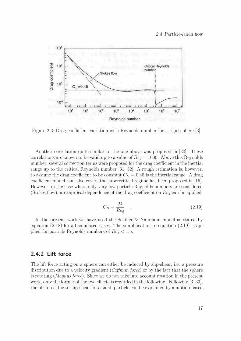
where CD is the drag coefficient and md = �dVd is the mass of the dispersed en-tity, while the volume Vd of a sphere of diameter d is given by equation (2.1). Inthe Stokes flow regime, which is characterized by entity Reynolds numbers belowRed = 1, the drag coefficient for a spherical solid particle is proportional to theinverse of the Reynolds number. With increasing Reynolds number, the drag co-efficient decreases before approaching a nearly constant value in the inertial rangeabove Red = 1000. A significant drop of the drag coefficient occurs at the criticalReynolds number of Red = 300000, where the boundary layer around the spherebecomes turbulent. A sketch of this standard drag curve for a rigid particle takenfrom [3] is shown in Figure 2.3.
Various approaches exist to model the drag coefficient analytically. A first em-pirical particle drag model and an expression for CD as a function of the dispersedphase Reynolds number Red was proposed by Schiller & Naumann [29]:
CD =24
Red
(
1 + 0.15Re0.687d
)
. (2.18)
16
2.4 Particle-laden flow
Figure 2.3: Drag coefficient variation with Reynolds number for a rigid sphere [3].
Another correlation quite similar to the one above was proposed in [30]. Thesecorrelations are known to be valid up to a value of Red = 1000. Above this Reynoldsnumber, several correction terms were proposed for the drag coefficient in the inertialrange up to the critical Reynolds number [31, 32]. A rough estimation is, however,to assume the drag coefficient to be constant CD = 0.45 is the inertial range. A dragcoefficient model that also covers the supercritical regime has been proposed in [15].However, in the case where only very low particle Reynolds numbers are considered(Stokes flow), a reciprocal dependence of the drag coefficient on Red can be applied:
CD =24
Red. (2.19)
In the present work we have used the Schiller & Naumann model as stated byequation (2.18) for all simulated cases. The simplification to equation (2.19) is ap-plied for particle Reynolds numbers of Red < 1.5.
2.4.2 Lift force
The lift force acting on a sphere can either be induced by slip-shear, i.e. a pressuredistribution due to a velocity gradient (Saffman force) or by the fact that the sphereis rotating (Magnus force). Since we do not take into account rotation in the presentwork, only the former of the two effects is regarded in the following. Following [3, 33],the lift force due to slip-shear for a small particle can be explained by a motion based
17

Chapter 2 Eulerian-Lagrangian modeling of dispersed flows
on the velocity difference between the bottom and top of the particle in a shear flow:
FL = 1.61d2√
�c�c∣∇ × u∣ ((u− v)× (∇× u)) . (2.20)
The cross product ∇× u evaluated at the particle middle-point represents an an-gular velocity. The lift force thus acts in the direction perpendicular to this angularvelocity and the relative velocity u − v of the particle. If the relative velocity ispositive, there is a lift force towards the higher velocity and if the relative velocityis negative, the lift force acts towards the lower velocity.
For particles of small diameter and low Reynolds number, the response time �p tobalance the velocity difference u− v is very small. Thus, in the simulations carriedout in the present work, the Saffman lift force on particles is found to be negligiblysmall and has therefore been omitted.
2.4.3 Equation of motion for a particle
In the particle-laden flows regarded in the present work, the continuous carriermedium is assumed to be gaseous. In most cases, solid particles are of materialsthat are much heavier than gases. Some examples for material combinations inparticle-laden flows are given in Table 2.1. The density ratio �c/�d in those cases isof the order of 10−3 or even 10−4.
Phase Material Density � [kg/m3]Hydrogen 0.084
Continuous Nitrogen 1.17Air 1.2Oxygen 1.33Cork 500Polystyrene 1050
Dispersed Quartz 2200Iron oxide 5100Copper 8950
Table 2.1: Material properties for particle-laden flows with gaseous carrier media.Values for gases are given at a temperature of 20∘C.
If we assume flow in the Stokes regime, i.e. at very low particle Reynolds numbers,and make use of relations (2.5) and (2.19), the response time (2.4) for a particle
18
2.5 Bubbly flow
simplifies to the following:
�p =�dd
2
18�c
. (2.21)
Using the above expression for the response time in the drag force term (2.17) andneglecting the lift force, the equation of motion for a particle can finally be writtenas follows:
dv
dt=
1
�p(u− v) + g . (2.22)
2.5 Bubbly flow
Regarding the flow around a rigid spherical bubble, one can identify a number offorces constituting the vector F on the right hand side of equation (2.13). Thefollowing formulation has been stated by Maxey & Riley [34]:
F = FD + FL + FP + FV + FB +mdg . (2.23)
Here, FD represents the steady-state drag force and FL the lift force on the entity.FP includes the force due to the local pressure gradient and the shear-stress of thecarrier phase. The unsteady forces can be divided into the virtual mass force FV dueto the acceleration of the dispersed entity and the Basset history force FB. Finally,mdg is the force due to gravity.
From the above stated formulation, one can see that the physical phenomenainvolved in bubbly flow are more complex than in the particle-laden flow case (dis-cussed in Section 2.4). This is mainly due to the inverse density ratio between thosetwo types of flow, which allows to neglect certain forces in particle-laden flow thathave to be considered in the case of bubbly flow.
2.5.1 Drag force
Since we limit ourselves to spherical entities in the present work, the drag forceformulation for a bubble is the same than for a particle, given by equation (2.17):
FD =3
4
�c�d
CD
dmd ∣u− v∣ (u− v) . (2.24)
Gas bubbles are characterized by internal fluid flow circulation and do not behavelike rigid particles in all Reynolds number regimes. In the Stokes regime, the dragcoefficient for a bubble depends reciprocally on Red and thus fairly behaves like for a
19

Chapter 2 Eulerian-Lagrangian modeling of dispersed flows
solid particle. It has been mentioned in [25, 35] that the values of CD with increasingRed are lower for a bubble in a purified liquid than in a liquid contaminated bysurfactants. If a contaminated carrier flow medium like e.g. tap water is used, thesurfactants tend to collect at the rear of the bubble. In this way, the slip along thesurface of the bubble is restrained and the bubble behaves almost exactly like a solidparticle:
CD =�DRed
, where
{
�D = 16 for a purified liquid
�D = 24 for a contaminated liquid. (2.25)
For higher Reynolds numbers than Red = 100, an increase of CD with Red occurs,before a constant value of about CD = 2.61 is reached around Red = 1500. Figure2.4 and Figure 2.5 show this behavior for both purified and contaminated liquidcarrier media, as proposed by [19], based on analytical models [36, 37] as well asexperimental studies [38, 39].
Figure 2.4: Drag coefficient variation with Reynolds number for an air bubble in apurified liquid [19].
In case of Stokes flow at low entity Reynolds numbers and under the assumptionthat in most industrial applications involving bubbly flow a contaminated carrierliquid is used rather than a purified one, the Schiller & Naumann drag coefficientmodel given by equation (2.18) is thus applicable for both spherical bubbles andparticles and has been used throughout the present work.
20

2.5 Bubbly flow
Figure 2.5: Drag coefficient variation with Reynolds number for an air bubble in acontaminated liquid [19].
2.5.2 Lift force
As discussed for solid particles in Section 2.4.2, we do not take into account theMagnus lift force due to slip-rotation in the present work, because rotational motionof the dispersed entities is neglected. A proposition for the Saffman lift force actingon a spherical bubble has been made by Auton [35]:
FL = CLmd�c�d
((u− v)× (∇× u)) , (2.26)
where CL is the lift coefficient, which can be estimated using a constant value ofCL = 0.53. Equation (2.26) is valid under the following assumption:
Red∇uu
→ 0 , (2.27)
which is satisfied in cases when the bubbles are of small diameter and the liquidvelocity gradients are small, i.e. in a homogeneous flow regime. Throughout thepresent work, Auton’s lift coefficient estimation is used .
21

Chapter 2 Eulerian-Lagrangian modeling of dispersed flows
2.5.3 Pressure gradient and buoyancy force
The pressure force FP can be divided into a contribution due to the hydrostaticpressure and another one due to shear stress in the carrier fluid:
FP = FH + F� . (2.28)
The force due to the hydrostatic pressure gradient is denoted by:
FH = −∇pVd = −�cVdg , (2.29)
and represents the buoyancy. It is equal to the weight of the fluid displaced bythe volume of the bubble. The force due to the shear stress in the carrier fluid canbe expressed as follows:
F� = ∇ ⋅ �Vd = md�c�d
Du
Dt, (2.30)
underlying the estimate that the magnitude of the pressure gradient in the carrierphase is the order of the flow acceleration [3, 15].
2.5.4 Virtual mass force
When a sphere is accelerated by the carrier fluid, it experiences a virtual mass force,meaning that the fluid around the sphere is accelerated as well and additional workis done. This results is an additional unsteady drag due to the fluid acceleration.The virtual mass force can be stated as follows:
FV =1
2md
�c�d
(
Du
Dt− dv
dt
)
. (2.31)
In the above equation, the derivative d/dt is following the moving sphere with re-spect to time, while D/Dt is the total acceleration of the fluid as seen by the sphere,evaluated at the position of the sphere [3, 15]. The virtual mass force is equivalentto adding mass to the sphere and is often referred to as added or apparent mass force.
2.5.5 Basset history force
The Basset history force accounts for the unsteady viscous effects of the fluid andrepresents the temporal delay of the boundary layer development as the relativevelocity between the sphere and the fluid is changing with time, resulting in an
22

2.5 Bubbly flow
additional unsteady drag on the sphere. The analytical expression for the Bassethistory force is
FB =3
2d2√��c�c
t∫
0
(
Du
D�− dv
d�
)
d�√t− �
, (2.32)
implying that the temporal history of the entity’s acceleration plays a role inpredicting the dynamics and the trajectory of the entity [3, 15]. For numericalcomputations, this means that when applying the Basset history force, derivativesof both the fluid and the entity velocity have to be stored for various time steps,leading to significant storage requirements. Note that the Basset history force willnot be used throughout the present work
2.5.6 Equation of motion for a bubble
Contrary to particle-laden flows, where the ratio of the densities �c/�d between thephases is small, it becomes very large in the case of bubbly flows and takes valuesof the orders of 103 or 104, because the primary phase is a liquid and the dispersedbubbles are gaseous. Table 2.2 gives examples for common material combinationsoccurring in bubbly flows.
Phase Material Symbol Density Viscosity� [kg/m3] � [kg/ms]
Water H2O 1000 1.02⋅10−3Continuous Nitric acid HNO3 1512 8.8⋅10−4
Sulfuric acid H2SO4 1834 2.46⋅10−2Hydrogen H2 0.09 8.4⋅10−6
Dispersed Air - 1.2 1.74⋅10−5Oxygen O2 1.43 1.92⋅10−5Chlorine Cl2 3.21 1.35⋅10−5
Table 2.2: Material properties for bubbly flows. All values are given for a tempera-ture of 20∘C. Values for acids are at 100% concentration.
The response time of a bubble in the Stokes flow regime can be stated by usingequations (2.4) and (2.25):
�b =�dd
2
D�c
, where
{
D = 12 for a purified liquid
D = 18 for a contaminated liquid. (2.33)
23

Chapter 2 Eulerian-Lagrangian modeling of dispersed flows
The Lagrangian equation of motion (2.13) with all relevant forces included canbe re-written as follows:
dv
dt=
3
4
�c�d
CD
d∣u− v∣ (u− v) +
1
2
�c�d
(
Du
Dt− dv
dt
)
+�c�d
Du
Dt+
CL�c�d
((u− v)× (∇× u)) +
(
1− �c�d
)
g . (2.34)
The Basset history force has been neglected in the above equation, since it willnot be used in the following. By multiplying equation (2.34) by �d/�c and somealgebraic transformations we get:
(
�d�c
+1
2
)
dv
dt=
3
4
CD
d∣u− v∣ (u− v) +
3
2
Du
Dt+
CL ((u− v)× (∇× u)) +
(
�d�c− 1
)
g . (2.35)
If we finally neglect the density ratio �d/�c in equation (2.35), we end up with thefollowing equation of motion for a bubble:
dv
dt=
2
�b(u− v) + 3
Du
Dt+ 2CL ((u− v)× (∇× u))− 2g (2.36)
2.6 Coupling between dispersed and continuous phase
In dispersed two-phase flow, the particles, bubbles or droplets interact with thecontinuous carrier phase in various ways. The coupling comes to pass through mass,momentum and energy exchange between the phases:
∙ Mass exchange takes place e.g. during evaporation, condensation or sublima-tion of droplets or particles. Chemical reactions can as well lead to an exchangeof mass between the two phases.
∙ Momentum exchange describes the effect of the carrier fluid on the dynamicbehavior (i.e. the trajectory) of a dispersed entity and the counter-effect of theentity on the fluid velocity field surrounding it. These effects strongly dependon the carrier flow pattern around the entity as well as on the inertia of theentity and therefore on its Stokes number.
∙ An example for energy exchange is e.g. the heat from a hot particle augmentingthe thermal energy of the carrier phase.
24

2.6 Coupling between dispersed and continuous phase
All investigations in the present work are assuming isothermal conditions. More-over, we do not take into account phase changes. Therefore, mass and energy cou-pling are neglected and the further emphasis of this section lies on momentumcoupling effects.
2.6.1 Momentum coupling regimes
Concerning the momentum coupling between the dispersed entities and the carrierflow, different modeling approaches are applicable, depending on how the dynamicbehavior of both phases is expected to be influenced by the presence of the otherphase. Suitable criteria to distinguish these effects are the volume fraction of thedispersed phase in the two-phase mixture and the entity spacing as introduced inSection 2.2 and denoted by equations (2.2) and (2.3).
∙ For dilute flows with a low dispersed phase volume fraction and a large entityspacing L/d → ∞, the influence of the dispersed entities on the continuousphase can be neglected, which results in a one-way coupling, where the dis-persed phase motion is entirely driven by the continuous carrier flow.
∙ With growing volume fraction, the modification of the carrier flow by thedispersed entities has to be taken into account by means of two-way coupling.
∙ For dense flows with L/d→ 1, collisions between dispersed entities need to beconsidered in addition, leading to a so called four-way coupling approach. Incase of a bubbly flow, the latter can eventually lead to effects like coalescenceand break-up of bubbles.
A schematic diagram of the fluid-entity-interaction pointed out above is providedin Figure 2.6, while Figure 2.7 quantifies the introduced coupling regions by meansof the entity spacing and the volume fraction. According to Sommerfeld [2], one-waycoupling is applicable up to volume fractions of �d = 10−6, while the upper limitof two-way coupling lies at �d = 10−3, corresponding to entity spacing values ofL/d = 100 and L/d = 10 respectively. These values are based on particle-ladenflows and agree well with those published by Elghobashi [40]. Sommerfeld indicatesa two phase mixture as dilute if four-way coupling can be neglected, while the mix-ture is dense in case of higher dispersed phase volume fraction.
For bubbly flow, however, general quantitative studies about the effect of the vol-ume fraction and the entity spacing on the momentum coupling mechanisms havenot been carried out so far. However, from a qualitative point of view, the physicalbehavior is found to be the same as for particles, namely that two- and four-waycoupling become more important with increasing gas volume fraction [41].
25

Chapter 2 Eulerian-Lagrangian modeling of dispersed flows
(a) One-way (b) Two-way (c) Four-way
Figure 2.6: Schematic diagram of (a) one-way (b) two-way and (c) four-way couplingbetween carrier flow and dispersed entities.
Figure 2.7: Quantification of momentum coupling approaches in terms of entityspacing L/d and volume fraction �d, according to [2].
2.6.2 One-way coupling
For very dilute flows with a dispersed phase volume fraction of �d < 10−6, a one-waymomentum coupled approach leads to sufficiently accurate results since the effectof the dispersed entities on the fluid flow is negligibly small in this case. The mo-mentum transfer from the dispersed entities to the carrier fluid is neglected and nosource term Φ is put into the Navier-Stokes momentum equation (2.9) of the fluidphase. The motion of a dispersed entity is driven entirely by the fluid flow throughthe force F described in equation (2.13). This force vector is depending on the
26

2.6 Coupling between dispersed and continuous phase
material properties of the two phases as well as on the continuous phase velocityat the position of the entity, as discussed in Section 2.4 and Section 2.5, respectively.
2.6.3 Two-way coupling
If the volume fraction of the dispersed phase reaches values of �d > 10−6, momentumback-coupling from the dispersed entities to the carrier fluid can not be neglected anymore and a two-way coupling approach has to be applied. According to Newton’sfirst law, the impact of the surface forces imposed from the fluid phase to eachparticle or bubble causes a negative reaction force of the same amount on the fluidphase at the position of the dispersed entity. This back-coupling force is modeledby a local source term Φ in the Navier-Stokes momentum equation. In order tocompute this term, we define a negative volume weighted momentum transfer forcefd,i acting from a dispersed entity i on the flow, which is a reaction force due to thesurface forces acting on the entity [25]:
fd,i = −(
FD,i + FL,i + FV,i
Vd,i
)
. (2.37)
To assemble the momentum transfer term Φ in the Navier-Stokes equation for acontrol volume j, the following general formulation can be applied:
Φj =1
Vj
Nj∑
i=0
Vd,ifd,i (xi) � (x− xi) . (2.38)
The reaction forces of all entities i contained in the control volume Vj of thefluid flow are summed up, weighted by the volumes Vd,i of the entities. The term� (x− xi) indicates that the entities are modeled as Dirac forces at the positions xi,resulting from the mass-point approximation.
2.6.4 Four-way coupling
For dense two-phase flows of a dispersed volume fraction of �d > 10−3, the impactof collisions between the dispersed entities can not be neglected any more. Crowe[42] proposes the averaged time �Coll between two successive collisions relative tothe response time �d of an entity as a criterion to classify the two-phase mixture asdense:
�d�Coll
> 1 . (2.39)
27

Chapter 2 Eulerian-Lagrangian modeling of dispersed flows
In this case, the time between collisions is smaller than the response time andthe dispersed entities are not able to completely respond to fluctuations of the pri-mary phase fluid between two collisions. The collisions thus dominate the dynamicbehavior of the dispersed entities. In dilute flows, characterized by
�d�Coll
< 1 . (2.40)
collisions may also occur, but in this case it is the fluid dynamic transport whichis dominating the behavior of the entities and the impact of the collisions can beneglected.
When using the Eulerian-Lagrangian approach for dispersed two-phase flow sim-ulations, a severe problem arises when it comes to the modeling of inter-particle andinter-bubble collisions, because the momentum equations of the dispersed entitiesare fully decoupled from each other. Thus, no direct information about the momen-tum interaction of a dispersed entity with its neighbouring entities is available. Thisleads to the fact that the numerical consideration of collisions requires the use of anappropriate collision model.
Various numerical techniques to model collisions have been invented over the pastyears for both particle-laden and bubbly flows. The most straightforward way toprecisely model the collisions between the entities is to correlate the trajectories ofeach entity in the simulation process in order to check for an intersection [43]. Theimpact between two entities can then be determined by means of their position andrelative motion. However, such a direct approach is computationally very expensivefor flows involving a large number of dispersed entities and therefore not applicableto complex problems. A more suitable method is to model the collisions by meansof a stochastic approach, where the interactions between dispersed entities are mod-eled by means of collision probabilities. Such methods are of course microscopicallyinvalid, but for high number densities they become reliable in a macroscopic sense.Stochastic collision models were originally developed for particles [2, 44, 45, 46] andlater adopted for bubbles. In the latter case, one can also include bubbly flow phe-nomena like bubble coalescence and break-up in a stochastic manner [19].
Collision-driven two-phase flows involving particles and bubbles are not consideredin the present work. An implementation of a stochastic collision model according to[2, 46] is documented in [47].
28

2.7 Turbulent dispersed two-phase flows
2.7 Turbulent dispersed two-phase flows
An important aspect regarding dispersed two-phase flow mixtures is the interactionof dispersed entities with a turbulent carrier medium. In the past, several investiga-tions on this subject have been carried out. A major part of these studies has beenaccomplished in the scope of understanding the role of the particle or bubble sizeand the volumetric loading of the dispersed phase when interacting with turbulentstructures in the carrier flow.
2.7.1 Dispersed entities and carrier phase turbulence
A comparative analysis of experimental data on turbulent particle-laden flow hasbeen carried out by Hetsroni [48]. In this study, it has been concluded that particleswith a low particle Reynolds number tend to suppress the turbulence of the carrierfluid, while particles of Reynolds numbers above Red = 400 tend to enhance turbu-lence, most likely due to vortex shedding.
Figure 2.8: Effect of the particle size on the turbulent intensity [50]. The horizontalaxis shows the ratio of the entity diameter d to a characteristic turbulencelength scale.
Further comparative studies have been published by Gore & Crowe [49, 50], whorelated this behavior to the ratio of the particle diameter to the turbulence length
29

Chapter 2 Eulerian-Lagrangian modeling of dispersed flows
scales. From the collected data, shown in Figure 2.8, it has been concluded that thetransition from an attenuating to an amplifying behavior occurs when the particlesize is about 1/10 of the integral length scale of turbulence.
Elghobashi [40, 51] proposed the map depicted in Figure 2.9 to classify the effectof particles on carrier-phase turbulence. For the one-way coupling region character-ized by volume fractions less than 10−6, the presence of the particles is assumed tohave no effect on the turbulent flow structures. For volume fractions between 10−6
and 10−3, in the region where two-way coupling is applied, the particles can eitheraugment the turbulence - if the Stokes number based on the characteristic turnovertime of a large eddy is greater than unity - or attenuate turbulence in the other case.For volume fractions greater than 10−3, inter-particle collisions become significantand the turbulence of the carrier phase is found to be affected by the oscillatorymotion due to those collisions.
Figure 2.9: Particle-turbulence modulation effects in terms of the Stokes number asa function of dispersed phase volume fraction �d [40].
While the momentum interaction between solid particles and turbulent carrierflow media has been investigated in great detail over the last decades both experi-mentally and numerically, comparable quantitative results for bubbly flows are quiterare up to now. It has been reported that the presence and accumulation of verysmall bubbles in vortical structures of the carrier flow enhances the decay rate ofvorticity and enstrophy [52, 53, 54, 55] and thus reduces the turbulent kinetic energyin decaying turbulence [56, 57, 58]. For larger bubbles and significant amounts of gas
30

2.7 Turbulent dispersed two-phase flows
volume loadings, like e.g. in bubble columns, the phenomena of bubble-induced fluidflow [59, 60] and bubble-generated turbulence [37] have been reported along with theconclusion that a reliable and global model of bubble-fluid-interaction is still lacking.
2.7.2 Turbulence models for dispersed flows
Since there is only one continuous flow field in the Eulerian-Lagrangian method, thechoice to apply a single-phase turbulence model for the simulation of the carrier fluidis reasonable. However, the source terms and transport coefficients of the chosenturbulence model have to be modified in order to take into account the presence ofthe dispersed phase. On the other hand, the fluid velocity in the momentum equa-tion of a dispersed entity has to represent the turbulent fluctuations of the carrierflow. In the following, a few comments on the applicability of some of the mostfrequently used turbulence modeling approaches to Eulerian-Lagrangian two-phaseflow simulations are given.
Two-equation RANS models
Reynolds-averaged Navier-Stokes (RANS) models can be regarded as the basis ofconsiderable research on turbulent flow CFD. Many two-equation closure models forthe RANS equations have been derived in the last decades and are frequently usedto simulate complex industrial problems. The most widely used type along themare turbulence energy-dissipation models like the k − � or the k − ! model, whereconservation equations for the turbulent kinetic energy and its dissipation are solvedamong with the Navier-Stokes equations of the mean flow. These models are knownto be robust, well resolved and have been implemented to all relevant, commerciallyavailable CFD solvers.
One of the problems in coupling Lagrangian particle tracking to a carrier flowsolved by a RANS approach is that the local instantaneous fluid velocity at the po-sition of a dispersed entity is not directly available from the solution of the carrierflow field, since only a mean flow velocity is calculated in the fluid momentum equa-tion and the velocity fluctuations are expressed by the turbulent kinetic energy andits dissipation. Various stochastic approaches to model these velocity fluctuationsexist. Yuu et al. [61] proposed to sample it from a Gaussian distribution aroundthe mean velocity with a variance related to k, Dukowicz [62] chose to calculate arandom particle displacement based on the Gaussian distribution corresponding toa dispersion coefficient, while Lockwood et al. [63] introduced a diffusional velocityrelated to k and the carrier flow velocity gradient ∇u. All these approaches arefound to be robust and relatively simple to implement. However, they are only valid
31

Chapter 2 Eulerian-Lagrangian modeling of dispersed flows
in a stochastic manner and do not allow to accurately predict the trajectories ofdispersed entities on a microscopic scale.
When taking into account momentum back-coupling from the dispersed entitiesto the carrier flow, a further problem arises, because introducing local perturbationsrepresenting the motion of dispersed entities to the fluid momentum equation willnot lead to accurate results in terms of flow modulation. A suitable solution is tomodify the equation of the turbulent kinetic energy in order to model the small-scalefluctuations resulting from the two-way momentum coupling, as proposed in variousmodes, such as of Shuen et al. [64] and Yuan & Michaelides [65].
Large Eddy Simulation
Large Eddy Simulation (LES) involves features of both Reynolds-averaging and di-rect simulation of turbulence. The large-scale effects of the flow are solved directly,while the small-scale eddies below a certain cut-off length are modeled by an appro-priate sub-grid scale (SGS) model. In a turbulent flow, the large eddies are mostimportant in terms of momentum and energy transport. LES brings the advantage ofbeing able to accurately predict these large scale turbulent structures. Since the fil-tered small-scale eddies can in most cases be regarded as homogeneous and isotropicover a space and time average, as well as independent of the overall flow geometry, itis obvious that LES offers reasonably accurate results on all turbulence length scales.
The coupling of LES with Lagrangian tracking of dispersed particles is a rathernew topic in the CFD community. Elghobashi [40] pointed out that a crucial pointin employing this technique is the prediction of two-way momentum coupled flows,since this implies a modification of the sub-grid scale turbulence model, because theparticles mostly affect the smallest scales of turbulent structures. Recent studies byArmenio et al. [66], Yamamoto et al. [67] and Fede & Simonin [68] tracked thisproblem for simple particle-turbulence test cases, showing that particle concentra-tion, dispersion and collisions are strongly affected by the sub-grid scale turbulence.
Direct Numerical Simulation
The most straightforward, but also the computationally most costly method tomodel turbulence is its Direct Numerical Simulation (DNS). In this approach, allturbulent length scales are resolved and the computational mesh is refined up to theKolmogorov scale, on which the smallest turbulent structures are dissipated intoheat. In this way, the direct simulation of the Navier-Stokes equations leads to anaccurate prediction of turbulence.
32

2.8 Simulation approach
Since all scales of the fluid flow are solved directly, Lagrangian particle trackingcan be applied to DNS without any restrictions on one-way, two-way and four-waymomentum coupling. However, the dispersed entities should not be larger in sizethan the Kolmogorov length scale of the turbulence spectrum in order to ensure thatfluid-particle interaction is computed accurately. Many numerical studies of turbu-lent dispersed two-phase flow using DNS have been carried out over the last decades.
In the scope of the present work, we will focus on particle-turbulence interactionwhere the carrier flow is simulated by means of a DNS approach. In Chapter 3 ofthis thesis, two numerical studies related to this topic are documented.
2.8 Simulation approach
The Eulerian-Lagrangian two-phase flow simulations carried out in the scope of thepresent work were achieved by using two software modules:
∙ A fluid flow solver to simulate the primary phase flow by solving the incom-pressible Navier-Stokes equations.
∙ The Lagrangian solver module PLaS to simulate the dispersed phase, i.e. smallsolid particles or gas bubbles. PLaS stands for Parallel Lagrangian Solver andis a solver module developed exclusively for the simulation of dispersed two-phase flows. It has been designed and implemented in the scope of the presentPh.D. work. Based on the Eulerian-Lagrangian modeling strategy, it tracks thetrajectories of a set of dispersed entities inside a three-dimensional continuouscarrier flow, including phase coupling.
PLaS is not a standalone computer program, since it has to be linked to an ex-ternal Navier-Stokes solver, which performs the computation the carrier phase flow.A standardized data interface to couple these two modules has been designed andimplemented.
Figure 2.10 shows the operational principle of a simulation performed by couplingPLaS to a Navier-Stokes solver. The flow solver serves as driving program of aniterative simulation cycle. It hosts the computational geometry and mesh and com-putes the flow field of the carrier phase. PLaS updates the velocities and positionsof a set of dispersed entities by solving its Lagrangian equations of motion. Thetwo software modules are synchronized by a discrete time-stepping procedure. Ineach time step Δt, the primary phase flow field is solved before the dispersed enti-ties are tracked. This succession is applied in order to provide an updated carrier
33

Chapter 2 Eulerian-Lagrangian modeling of dispersed flows
Figure 2.10: Algorithm flowchart of the Eulerian-Lagrangian two-phase flow simu-lations performed by coupling PLaS to a fluid flow solver.
phase velocity field as an input to PLaS, since the fluid velocity is the main drivingmechanism for the motion of the dispersed entities. According to this principle, theback-coupling forces of the dispersed entities on the continuous phase flow field arecomputed after solving the trajectories of the dispersed entities and plugged intothe Navier-Stokes equations in the following time step.
In the scope of the present work, the PLaS module has been successfully interfacedto the following Navier-Stokes solvers:
∙ The 2D/3D incompressible Finite Element solver Morpheus [69].
∙ The 3D pseudo-spectral DNS solver SFELES [70].
∙ The 2D/3D incompressible Finite Volume and Residual Distribution basedsolver included in the software framework COOLFluiD [71].
The data interface between the flow solver and PLaS is bilateral. To compute thetrajectories of the dispersed entities, PLaS needs the following information from thecarrier flow solver:
∙ Information about the grid topology (nodes, elements and connectivity).
∙ Information about the boundaries of the computational domain.
∙ The velocity field of the carrier phase.
To take into account the back-coupling of the particles on the carrier flow, theNavier-Stokes solver needs the following information from PLaS:
34

2.9 The Lagrangian solver module PLaS
∙ The volume fraction field of the secondary phase.
∙ Mass, momentum and energy transfer terms computed on the nodes of thecomputational grid. In the present work, this is limited to momentum transfer.
2.9 The Lagrangian solver module PLaS
As mentioned in Section 2.8, the Lagrangian solver PLaS provides functionality totrack the trajectories of a set of entities involved in a dispersed two-phase mixture. Itis designed for the simulation of particle-laden, droplet-laden and bubbly two-phaseflow. The PLaS module is written in standard C language, following a proceduralprogramming strategy. Its structure, functionality and the main numerical tech-niques involved are documented in the following.
2.9.1 Structure of the code
PLaS is structured in a modular way. It is decomposed into several files and sub-routines, which are grouped under functional aspects. The code module is designedas an add-on to a single-phase Navier-Stokes flow solver. Its data interface to theflow solver consists of only three functions:
∙ An initialization function initPLaS(*PLAS DATA) to allocate the memory neededby PLaS. This function is called once before starting the iterative simulationcycle.
∙ A main function runPLaS(*PLAS DATA), which is the core of the module andsolves the trajectories of the dispersed entities. It is called by the flow solverat every time step Δt after updating the carrier velocity field. Its functionalitywill be discussed in detail in Section 2.9.2.
∙ A termination function terminatePLaS(*PLAS DATA) to de-allocates memoryand finalizes PLaS. It is called once after the iterative simulation cycle isfinished.
To instantiate the PLaS data, a single instance of the data type PLAS DATA hasto be created in the flow solver. This data type consists of various custom sub-structures, in which all PLaS data is grouped and encapsulated. The instance ofPLAS DATA is passed to the PLaS interface functions by reference. In this way itis assured that all PLaS data is provided with the program lifetime of the drivingprimary phase flow solver.
35

Chapter 2 Eulerian-Lagrangian modeling of dispersed flows
2.9.2 Procedural description
As mentioned in Section 2.9.1, the PLaS main function runPLaS(PLAS DATA*) iscalled by the flow solver at every time step Δt of the iterative simulation cycle.Since PLaS is a procedural code, this function is run through from top to bottomat every call.
Figure 2.11: Algorithm flowchart of the PLaS main routine.
Figure 2.11 shows a flowchart of the PLaS main function. In the following, itsfunctionality regarding the computation of the dispersed phase trajectory incrementsand the back-coupling terms is described step by step:
∙ The PLaS input parameters are read from a data file.
∙ Initial and boundary conditions for the dispersed phase are imposed. Newentities are created in defined local production domains at given mass flowrates. This is explained in detail in Section 2.9.3.
∙ A loop over all dispersed entities is performed to sequentially update theirtrajectories by solving the entity’s equations of motion.
∙ In case of a parallel computation (see Section 2.9.4), entity information ispassed between processes. This is necessary when entities leave the computa-tional domain of one process to another one.
36

2.9 The Lagrangian solver module PLaS
∙ Dispersed phase data for post-processing is computed on all nodal volumes ofthe computational grid given by the flow solver (see Section 2.9.8).
∙ Back-coupling terms for the fluid flow solver equations are computed.
All dispersed entities are tracked sequentially. A trajectory increment of a singleentity follows the procedure described in the following. According to a stabilitycriterion, i.e. that an entity should not cross more than one computational cell persub-step, a Lagrangian time step ΔtL ≤ Δt is computed and the trajectory updateis performed in sub-steps. The following procedure is undergone for every sub-stepof every trajectory calculation:
∙ The element of the computational grid that hosts the entity position is deter-mined by a successive neighbour search method as described in Section 2.9.6.
∙ The fluid velocity u at the entity position, its derivatives in space and timeand the fluid vorticity are computed by means of interpolation from the nodesof the computational grid. The interpolation method is described in Section2.9.7.
∙ The relative velocity between the phases, the flow coefficients, the dispersedReynolds number and the response time are computed.
∙ The entity trajectory (velocity v and position x) is updated by solving theLagrangian equations of motion. The numerical procedure is described inSection 2.9.5.
∙ Wall bounces are performed and entities leaving the domain through periodicboundaries, flow outlets and process boundaries are identified.
∙ Entity collisions and, in case of bubbly flow, coalescence are included by meansof according stochastic models.
2.9.3 Input parameters
A set of input parameters has to be specified in order to determine the performanceof PLaS. According to the type and the topology of the dispersed two-phase flow tosimulate, different configurations can be chosen. The following parameters have tobe specified and are read from an input file during the simulation cycle:
∙ Number of initially distributed entities: Determines the number of enti-ties present at the first iteration. This option offers the choice to either restartPLaS from a previous solution or impose entities at random positions.
37
Chapter 2 Eulerian-Lagrangian modeling of dispersed flows
∙ Production domains and dispersed phase mass fluxes: Determines ge-ometric domains in which dispersed entities are produced. These domainsrepresent dispersed phase inlets. Various geometric types of domains are fea-tured: Lines, rectangles, boxes, circles, spheres or ellipsoids. The dispersedphase mass flux specifies how many entities per second are generated in a pro-duction domain. In this way, mass flow boundary conditions for the dispersedphase can be specified.
∙ Diameter: Determines the diameter distribution of the entities. Differenttypes of diameter spectra can be applied: Constant diameter, Gaussian di-ameter distribution and log-normal diameter distribution. In case of a non-constant diameter distribution, a mean diameter and a standard deviationhave to be specified.
∙ Initial relative velocity: Determines the initial velocity of an entity relativeto the carrier flow.
∙ Temperature: This parameter specifies the value for the dispersed phaseinitial temperature. Note that the inclusion of heat and mass transfer effectsgoes beyond the contents of the present Ph.D. thesis, thus a constant dispersedphase temperature of 293K is applied in all discussed two-phase flow cases.However, a study on mass and energy transfer in droplet-laden flow with PLaShas been carried out in [27].
∙ Entity material: Parameter to choose the material of the dispersed enti-ties and thus the flow type (particle-laden or bubbly flow). PLaS features amaterial database supporting many common materials occurring in two-phaseflows.
∙ Momentum back-coupling: Determines whether one-way or two-way cou-pling is used. In the latter case, the dispersed entities have a counter-effect onthe fluid flow.
∙ Collision model: Determines whether a collision model for the simulationof four-way coupled flows is used or not. The collision model functionality ofPLaS is not applied in the present Ph.D. work, but is described in a separatestudy [47].
2.9.4 Parallelization
The simulation cycle presented in Section 2.8 has been conceptually designed tooperate as well in serial as in parallel (multi-processor) computing environments. Inorder to perform parallel computations, PLaS needs to be linked to a flow solverthat features a parallel programming architecture by means of mesh partitioning.
38

2.9 The Lagrangian solver module PLaS
Inter-process communication is hereby realized through MPI [72, 73].
In the parallel computation case, PLaS adapts the geometric partitioning topol-ogy defined by the Navier-Stokes solver, where the computational mesh is dividedinto sub-regions in which the flow equations are solved on different processors (seeFigure 2.12). In this way, PLaS distributes the particle or bubble tracking on aparallel computer architecture according to the partitioning of the spatial computa-tional domain. Trajectories of dispersed entities located in a sub-region of the meshare computed on the same processor as the according fluid flow. Once an entityleaves the sub-region via an inter-process boundary, its data is passed to anotherprocessor and the computation for this entity is continued there.
Figure 2.12: Example for the geometric division of a three-dimensional mesh intosub-regions for parallelization.
2.9.5 Trajectory integration
For each dispersed entity, its Lagrangian equations of motion (2.13) and (2.14) inthree space dimensions form a system of six ordinary differential equations with thevector of unknowns being:
U = (u, v, w, x, y, z)T . (2.41)
39

Chapter 2 Eulerian-Lagrangian modeling of dispersed flows
Since the position can be determined by integrating the velocity, the Lagrangianequations of motion can be decoupled and solved one after another, leading to thefollowing vectors of unknowns:
U1 = v = (u, v, w)T , (2.42)
U2 = x = (x, y, z)T . (2.43)
To compute the updated entity velocity vn+1, the entity momentum equation(2.13) is integrated in time by using the trapezoidal Crank-Nicholson scheme, whichprovides second order accuracy:
vn+1 − vn
Δt=
1
2R(vn+1) +
1
2R(vn) . (2.44)
In the above equation, the residual R(v) corresponds to the right hand side of theentity momentum equation. A first order Taylor series expansion of R(vn+1) leadsto
R(vn+1) = R(vn) +AΔv + . . . , (2.45)
where the cut-off term is of second order. The matrix A is the Jacobian of theresidual
A =∂R(vn)
∂v, (2.46)
and the velocity increment Δv is defined as:
Δv = vn+1 − vn . (2.47)
To obtain the velocity increment for the time step Δt, the following linear systemis solved for each dispersed entity:
(
I
Δt− A
2
)
Δv = R(vn) , (2.48)
where I is the unity matrix.
Once the velocity increment is computed, equation (2.47) is used to obtain theupdated velocity vn+1, since the velocity vn is known from the previous time step.
To compute the updated entity position xn+1, the entity position equation (2.14)gives the following expression after discretization by means of the trapezoidal Crank-Nicholson scheme:
xn+1 =1
2
(
vn+1 + vn)
Δt+ xn . (2.49)
40

2.9 The Lagrangian solver module PLaS
Since the updated velocity vn+1 is already known, the position can be computeddirectly.
2.9.6 Neighbour search method
In order to map a dispersed entity to the computational grid of the flow solver, wehave to determine the grid element in which the entity is located. For this pur-pose, PLaS makes use of an effective neighbour search algorithm that is similar toparticle tracer methods as introduced by Brackbill & Ruppel [74] and Lohner & Am-brosiano [75]. This mapping is needed to track the entity trajectory with respect toan unstructured computational mesh, allowing the interpolation of the carrier fluidvelocity u from the nodes of the computational grid to the entity position (see Sec-tion 2.9.7). Furthermore, the mapping allows the computation of cell-wise dispersedphase data like the volume fraction and back-coupling terms.
The neighbour search method makes use of a geometric criterion to map entitiesto the elements of the mesh, using the element last occupied as an initial guess andsearching the adjacent neighbouring element in the direction of the entity position.The basic problem concerning the search for a neighbouring element is to find theelement face through which the entity has left its host element after a trajectoryincrement. One possible approach to determine this face is to use the propertiesof linear basis functions, which are used in the Finite Element Method [76]. Thisis a trivial task for linear Simplex elements like triangles and tetrahedra [75], butleads to a higher complexity for arbitrary element shapes and higher-order elements.Therefore, a more general geometric criterion is introduced in the following.
For each element face i, the geometric face center xf,i and the unit inward normalvector ni can be computed. On this basis, the signed face distance Si of an entitylocated at position xd to the element face i is computed according to the followingscalar product:
Si = (xd − xf,i) ⋅ ni . (2.50)
The scalar product is nothing else than the entity position relative to the facecenter projected to the unit inward normal vector of the face. The entity at xd lieswithin the element only if its signed distances to all element faces are positive, i.e.the following relation is fulfilled:
Smin = min(S1, S2 . . . Sn) ≥ 0 . (2.51)
If one or several signed face distances Si are less than zero, the entity at xd isnot located inside the element, but beyond the element faces i for which the signed
41

Chapter 2 Eulerian-Lagrangian modeling of dispersed flows
distances are not positive. Thus, the neighbouring element adjacent to the face withthe smallest signed distance Smin is searched in the next step. This procedure isrepeated until the target element is found, leading to a directive neighbour searchmethod as illustrated in Figure 2.13. This algorithm provides a simple geometric cri-terion to decide whether an entity position lies within an element represented by itsface centers and normals. It works for arbitrary types of two- and three-dimensionalelements, of which the most common are triangles, tetrahedra, quadrilaterals, hex-ahedra, prisms and pyramids.
Figure 2.13: Two example search paths through an unstructures grid [75]. The graycircle marks the last known entity position, while the arrows show thesequence of elements searched.
A drawback of successive neighbour search methods is that they fail to find an ele-ment when reaching a domain boundary, meaning an element face with no neighbourelement on the other side. This causes a problem in case of geometric domains thatare not convex or domains with interior boundaries. For these cases, PLaS featuresan additional brute force search algorithm which consecutively applies the signedface distance criterion to all elements in order to make sure that no dispersed entityis lost due to a failing neighbour search. This direct method is computationally verycostly. However, since the successive method always starts with the element thatcontained the entity in the last time step, such cases are minimized in the presentimplementation.
42

2.9 The Lagrangian solver module PLaS
2.9.7 Velocity interpolation
As stated in Section 2.9.5, it is necessary to interpolate the fluid velocity and itsderivatives in time and space from the computational grid of the fluid flow solver tothe position of the entity in order to assemble the Lagrangian equation of motion.Once the link between a dispersed entity at position xd and its hosting grid elementhas been established by means of the neighbour search algorithm presented in Sec-tion 2.9.6, an interpolation method to obtain the local instantaneous carrier fluidvelocity at the entity position is applied. This local velocity is interpolated from thenodes of the element that hosts the entity, meaning that the interpolation methodin PLaS is restricted to element topologies where the flow variables are stored node-wise. However, if the flow variables are stored cell-wise, no interpolation is necessarybecause the fluid velocity of the cell is directly available.
The nodal interpolation method used in PLaS is based on weighted inverse dis-tances Wi of the entity position xd to the nodes of the element:
Wi =1
Pi ⋅Nnod∑
j=0
1Pj
, (2.52)
where Pi is the distance of the entity position to node i of the element:
Pi = ∥xd − xn,i∥ . (2.53)
The sum of all weighted inverse distances in an element is equal to one in everycase:
Nnod∑
i=0
Wi = 1 . (2.54)
In this way, each element node is assigned an impact factor on the dispersed entityat xd, which is reciprocal to the distance between the node and the entity. For anode i that is located n times further away from the entity position as another nodej, this means:
Pi = nPj → Wi =1
nWj . (2.55)
The element node that is located the closest to the entity position thus has thehighest impact on the local instantaneous fluid velocity at the entity position. Thefollowing formula is applied to interpolate the carrier fluid velocity from the element
43

Chapter 2 Eulerian-Lagrangian modeling of dispersed flows
nodes to an entity position:
u =
Nnod∑
i=0
Wiui . (2.56)
The velocity interpolation method based on inverse distances is very fast and ap-plicable to elements of arbitrary shape, since it takes into account the element nodesas a set of points without regard to their connectivity.
2.9.8 Computation of the volume fraction field
As stated in Section 2.3.1, the fluid flow equations (2.8) and (2.9) are weighted by thecontinuous phase volume fraction �c in order to balance the mass and momentumconservation. To estimate the dispersed phase volume fraction on a node of thecomputational mesh used by the flow solver, the volumes of all dispersed entities ilocated in the median dual cell of a node j are summed up and divided by the nodalcell volume Vj:
�d =
Nj∑
i=0
Vd,i
Vj. (2.57)
Figure 2.14: Median dual cell of triangles meeting in node j. The cell volume isindicated by Vj.
The principle to compute a median dual cell around a node j is shown in Figure2.14 for triangles in two space dimensions. The extension to three space dimensionsand arbitrary element types is straightforward. The middle points of all grid ele-ments adjacent to node j are connected to form the median dual cell with volume Vj.
44

2.9 The Lagrangian solver module PLaS
The volume fraction weighting of the Navier-Stokes equations is realized throughadditional source terms. By applying some algebraic manipulation to the volumefraction weighted continuity equation (2.8) and introducing equation (2.7) as closurerelation, we get
∇ ⋅ u =1
1− �d
⋅(
∂�d
∂t+ u ⋅ ∇�d
)
. (2.58)
which is nothing else than the single-phase continuity equation with a right handside term that can be calculated explicitly from the volume fraction, its temporaland spatial derivatives and the interpolated local instantaneous fluid velocity ascomputed by equation (2.56). The right hand side expression in equation (2.58)gets singular in case of a dispersed phase volume fraction of �d = 1, which is thephysical limit of the two-phase mixture.
A similar algebraic manipulation can be applied to the fluid momentum equation(2.9), which leads to the following:
∂u
∂t+∇⋅uu+ 1
�c∇p+ 1
�c∇⋅ �c =
1
(1− �d)
1
�cΦ+
u
1− �d
⋅(
∂�d
∂t+ u ⋅ ∇�d
)
. (2.59)
Here, the right hand side term can as well be calculated explicitly, following theapproach introduced for the continuity equation above.
2.9.9 Computation of the back-coupling terms
In case of two-way momentum coupling between the continuous fluid phase andthe dispersed phase, back-coupling contributions from the dispersed entities to thecarrier flow are assembled, as pointed out in Section 2.6. The momentum transferresulting from the surface forces acting from a dispersed entity to the flow, as givenby equation (2.38), acts at the position of the dispersed entity according to the masspoint approximation. Various methods to interpolate this force to the grid nodes ofthe computational flow domain exist.
The most straightforward approach is to transfer the entity force fd,i to the nearestgrid node j. This method is referred to as Particle-In-Cell (PIC) or Particle-Source-In-Cell (PSIC) method [2, 77], since it sums up the force contributions of all dispersedentities located in a nodal cell:
Φj =1
Vj
Nj∑
i=0
Vd,ifd,i . (2.60)
45

Chapter 2 Eulerian-Lagrangian modeling of dispersed flows
Here, Vd,i is the volume of a dispersed entity i and Vj is the nodal cell volume ofnode j.
A more accurate approach is to distribute the back-coupling force of an entity ito all grid nodes of the element that contains the entity. This can be achieved bymaking use of the weighted inverse distances introduced in equation (2.52):
Φj =1
Vj
Nj∑
i=0
WijVd,ifd,i . (2.61)
Here, Wij is the weighted inverse distance of an entity i to each node j of its hostelement.
46

Chapter 3
Simulation of turbulent particle-laden
two-phase flow
Particle-laden two-phase flows involving turbulent carrier fluids are of interest fora large field of industrial applications. The numerical modeling of small particlesinteracting with turbulent flows is an important issue to understand the physicalphenomena involved in such type of flows. Recent work in this field focused oncollective effects, such as dispersion and evolution of local particle concentrationsusing different kinds of approaches to model turbulence, ranging from two-equationRANS models up to LES and DNS techniques [78].
In the following, dispersed turbulent two-phase flows involving small solid particlesare discussed on the basis of two academic DNS test cases. Particle segregation in aone-way coupled dilute two-phase flow has been analyzed for the case of a turbulentchannel flow (see Section 3.2), while the two-way coupled interaction of particlesand turbulence has been studied for the case of decaying isotropic turbulence (seeSection 3.3).
The particle-laden two-phase flow simulations have been performed by couplingthe Lagrangian solver PLaS to the pseudo-spectral flow solver SFELES, which isbriefly described in Section 3.1. PLaS computes the trajectories of the dispersedparticles by solving their equations of motion (see Section 2.9), while the turbulentcarrier flow is computed by solving the Navier-Stokes equations in the computationaldomain with SFELES.
It is known from turbulent flow theory that the energy transfer in a turbulent flowcovers the range between the macroscopic system length scale and the Kolmogorovlength scale, where the smallest turbulent structures are dissipated into heat. Theparticles involved in the present simulations are smaller in size than the Kolmogorovlength scale. If such small particles interact with a turbulent flow, the kinematicphenomena involved lie below the smallest turbulence length scales, which allows usto use the Eulerian-Lagrangian two-phase model without restrictions.
47

Chapter 3 Simulation of turbulent particle-laden two-phase flow
The transport of particles in turbulent flow depends highly on the dynamics of theturbulent structures in the flow. Due to their inertia, the response of solid particlesto turbulent carrier flow fluctuations is selective, depending on the particle massand size as well as on the intensity of the carrier flow velocity fluctuations. Thisbehavior may lead to collective effects like particle accumulation and segregation.
The presence of particles in turbulent flows can significantly influence the struc-tures of turbulence. While the turbulent dispersion of particles is controlled by localfluctuations of the carrier flow, the particles have a counter-effect on the turbulenceintensity by modulating the turbulent kinetic energy and its dissipation rate. Thisbehavior depends on the particle volume fraction and the characteristic turbulentlength scales, as pointed out in Section 2.7.
3.1 Turbulent carrier flow simulation
The numerical framework used for the turbulent carrier flow simulations is the Spec-tral/Finite Element code SFELES, as described by Snyder & Degrez [79]. It dis-cretizes the incompressible Navier-Stokes in x-y-planes using P1 linear Finite Ele-ments, while the transverse z-direction of the flow field is represented by means ofa truncated Fourier series, assuming periodicity in this direction. For the temporaldiscretization, the second order accurate Crank-Nicholson scheme is used to inte-grate the pressure and viscous terms in time while the Adams-Bashforth method isused for the convective terms:
Rn+1C = ∇ ⋅ un+1 = 0 , (3.1)
Rn+1M =
1
Δt
(
un+1 − un)
+3
2(u ⋅ ∇u)n − 1
2(u ⋅ ∇u)n−1 + 1
�c∇pn+ 1
2
−1
2�c∇2
(
un+1 + un)
− 1
�cfn+ 1
2 = 0 , (3.2)
where the continuity and momentum residuals, Rn+1C and Rn+1
M respectively, mustequal zero.
In the Finite Element discretization of the continuity equation, spurious pressureoscillations are encountered when using equal order elements for pressure and ve-locity [80, 81, 82]. For this reason, the Pressure-Stabilized Petrov-Galerkin (PSPG)dissipation is used in SFELES. The idea behind this approach is to add an extra
48

3.2 Particle dispersion in a turbulent channel
term to the mass conservation law, based on the divergence of the momentum equa-tion. The pressure Laplacian in this term keeps the pressure field smooth. Thisapproach is known to retain second order accuracy [83]. To eliminate convectiveinstabilities, a fourth order Laplacian dissipation term similar to the one used byJameson et al. [84] is used to stabilize the momentum equation. In this way thespatial discretization is ensured to be of second order.
To eliminate the remaining z-derivatives occurring after the Finite Element dis-cretization, a truncated Fourier series is used. The 3D problem in physical spaceis transformed into a series of loosely coupled 2D problems in Fourier space bymeans of an FFT. For reasons of computational efficiency, the convective terms arecomputed in physical space and then transformed to Fourier space, which makes ita pseudo-spectral approach. The 2D linear problems are solved sequentially on adistributed memory parallel computer [70]. Inter-process communication is realizedthrough standard MPI operations.
3.2 Particle dispersion in a turbulent channel
Turbulent particle-laden channel flow has been widely investigated in the past.McLaughlin [28], Young & Hanratty [85] as well as Brooke et al. [86] analyzedthe dispersion of one-way coupled particles in a turbulent channel and found thatthe particles tend to accumulate in the viscous sublayer, leading to irreversible parti-cle clustering at the wall. Recent work carried out by Soldati et al. [87, 88] analyzedthis behavior in greater detail for different particle sizes and pointed out preferen-tial accumulation in the low-speed streaks of the turbulent boundary layer, linkingit to the sweep and ejection phenomena occurring in near-wall turbulence. Pan &Banerjee [89, 90] used near-neutral density particles to investigate two-way couplingbetween particles and the carrier flow and showed that particles smaller than theKolmogorov length scale reduce the turbulence intensity while larger particles tendto amplify it. While all the studies cited above focused on DNS of the turbulentcarrier fluid, Wang & Squires [91] as well as Portela & Oliemans [92] investigated theperformance of LES modes in this scope, pointing out that an appropriate sub-gridscale model for particle-turbulence momentum interaction is needed.
Experimental investigations of particle-laden flow in turbulent boundary layerswere performed by Fessler et al. [93], Kulick et al. [94], Kaftori et al. [95] as wellas Taniere et al. [96]. Since it has been shown that in experiments it is generallydifficult to analyze the effects of different, superimposed physical phenomena, DNSand LES are found to be suitable methods of investigation for turbulent two-phaseflows. In a numerical simulation, one can control all flow parameters separate from
49

Chapter 3 Simulation of turbulent particle-laden two-phase flow
each other, the turbulence properties of every single particle are directly availableand a detailed investigation of the flow in the micro-scale range is feasible.
Particle motion, dispersion and segregation in a turbulent channel flow have beeninvestigated numerically in the scope of the present work. We assume the parti-cles to be small enough so that their back-coupling effect on the primary phasecan be neglected [40]. For this reason, the particles are not affecting the turbulentstructures of the flow. We first compare the flow field statistics obtained from DNSsimulations of the single-phase Navier-Stokes equations to reference results, beforeanalyzing and discussing the particle phenomena in the channel.
3.2.1 Turbulent single-phase channel flow
Turbulent flow in a fully developed channel is a classical test case for single-phaseDNS. It contains a wealth of information that has lead to a great understandingof the nature of wall-bounded turbulence in the past. Near the channel walls, inthe turbulent boundary layer, high momentum fluid is swept from the center ofthe channel towards the wall by coherent vortical structures. In the same way, lowmomentum fluid near the wall is ejected to the center of the channel. This motionincreases the mixing of momentum and gives rise to strong velocity fluctuations.The coherent vortical structures present in the turbulent boundary layer provide anexcellent test for DNS investigations.
Due to its geometric simplicity but rich turbulent nature, the turbulent channelflow test case has been subject to many studies in the past. Eckelmann [97] andNiederschulte et al. [98] performed fundamental experimental investigations, whileKim et al. [99], Jimenez & Moin [100] as well as Moser et al. [101] published seminalnumerical benchmark results in this field.
In the present work, turbulent single-phase channel flow DNS simulations havebeen performed by the Spectral/Finite Element code SFELES, as described in Sec-tion 3.1. The channel is bounded by no-slip walls on its top and bottom, wherethe half-height of the channel is denoted by ℎ. Periodic boundary conditions areapplied in the streamwise and spanwise directions, respectively. The domain size ofthe channel was chosen such that all spatial correlations vanish at the half of thetotal channel length in order to avoid auto-excitation phenomena due to the periodicboundary conditions. The periodic length of the channel in the streamwise directionis 4�ℎ and the periodic width in the spanwise direction is 2�ℎ, which correspondsto the dimensions used in [99]. Due to the periodicity in two space dimensions, thistest case can be physically regarded as a fully developed turbulent flow between twoinfinitely long plates. The geometry of this test case is shown in Figure 3.1. The
50

3.2 Particle dispersion in a turbulent channel
flow is orineted in the spectral direction, thus flow phenomena in the wall-normaland transverse directions are computed on a stretched Finite Element mesh.
Figure 3.1: Geometry for the turbulent channel flow test case.
We use the shear velocity u� and the length scale y+ = yu�/�c as characteristicscales to describe the turbulent flow of the continuous phase. The shear velocity isdefined by
u� =
√
�w�c
, (3.3)
where �w is the average wall shear stress. The shear Reynolds number is definedas
Re� =u�ℎ
�c, (3.4)
and has been set to Re� = 154 in the present calculations. This corresponds toa bulk Reynolds number Rebulk = ubulkℎ/�c = 2450, where ubulk is the streamwisevelocity averaged over the height ℎ of the channel. The flow medium is consideredto be air of density �c = 1.3kg/m3 and viscosity �c = 15.7 ⋅ 10−6m2/s. The com-putational grid used in the present case consisted of 128×160×129 points in thestreamwise, spanwise and wall-normal directions, respectively. The grid is stretchedin the wall-normal direction such that the size of the first cell at the wall is y+ = 0.05and 12 grid points are located within y+ < 8. This provides a good resolution ofthe viscous sub-layer. Turbulence statistics were taken by averaging the flow vari-ables in time and the streamwise and spanwise directions over a dimensionless timet∗ = tu�/ℎ = 10 with a time step of Δt∗ = 4.8 ⋅ 10−4. This time step is smaller thanthe time step required for a temporally resolved simulation, as stated in [102].
51

Chapter 3 Simulation of turbulent particle-laden two-phase flow
Case Rebulk Re� Grid size Domain sizeSFELES 2450 154 128×160×129 4�h×2�h×2h
Kim et al. [99] 2792 178 192×160×129 4�h×2�h×2h
Table 3.1: Reynolds numbers, grid and domain sizes for the turbulent channel flowtest case compared to the reference.
Table 3.1 shows a comparison of the test case configuration used in the presentwork to the configuration used in the validation reference [99]. The grid in thepresent case is slightly coarser in the streamwise direction, while the resolution ofthe turbulent boundary layer is of the same order. The slight difference in Reynoldsnumber is the result of an inaccuracy introduced by the forcing function to sustainthe turbulence in the SFELES code.
(a) Streamwise velocity profile (b) Diagonal Reynolds stresses
Figure 3.2: Averaged streamwise velocity profile u+ and diagonal Reynolds stresses⟨urms⟩, ⟨vrms⟩ and ⟨wrms⟩ compared to DNS results of Kim et al. [99].
Comparisons of turbulence statistics were accomplished in terms of mean flowprofiles (Figure 3.2a) and root-mean-square velocity fluctuations (Figure 3.2b) ac-cording to the following relations:
u+ =u
u�, (3.5)
52

3.2 Particle dispersion in a turbulent channel
⟨urms⟩ =√
⟨
(u− u)2
u2�
⟩
. (3.6)
The results performed with SFELES show very good agreement with the referenceresults. The small differences in the velocity fluctuation plots can be explained bythe slightly different Reynolds number. As a conclusion of the turbulent single-phasesimulations, we can state that the turbulent carrier phase flow field is sufficientlyresolved to provide accurate simulations for the case of a particle-laden channel.
3.2.2 Physical mechanisms in wall-bounded turbulence
To investigate particle dynamics in wall-bounded turbulence, the physics of turbu-lent structures at the wall has to be understood [103]. In a turbulent boundary layer,momentum transfer is controlled by the instantaneous realizations of the Reynoldsstresses, which may be conveniently examined by employing the quadrant analysisfor the wall-normal and the streamwise components of the fluctuating velocity field.Considering the events in the v′-w′ plane shown in Figure 3.3, Reynolds stresses areproduced by four types of events:
∙ First quadrant events (Q1): Outward motion of high-speed (w′ > 0) fluidaway from the wall (v′ > 0).
∙ Second quadrant events (Q2): Outward motion of low-speed (w′ < 0) fluidaway from the wall (v′ > 0), usually referred to as ejection.
∙ Third quadrant events (Q3): Inward motion of low-speed (w′ < 0) fluidtowards the wall (v′ < 0).
∙ Fourth quadrant events (Q4): Inward motion of high-speed (w′ > 0) fluidtowards the wall (v′ < 0), usually referred to as sweep.
Drag-generating events fall in the second and fourth quadrant, since both sweepsand ejections contribute to negative Reynolds stress, i.e. to the increase of turbu-lence production and thus to an increase in drag. Contrary to this, first and thirdquadrant events contribute to positive Reynolds stress and lead to a decrease in drag.Sweeps and ejections are separated by the level of wall shear stress they generate.While sweeps correspond to high shear stress regions, ejections correspond to regionsof low shear stress. Sweep and ejection events are part of the turbulence regener-ation cycle shown in Figure 3.4. There is still some uncertainty about the natureof these mechanisms, but according to Waleffe & Kim [104] they are generated bythe quasi-streamwise vortices in the turbulent boundary layer, which redistribute
53

Chapter 3 Simulation of turbulent particle-laden two-phase flow
Figure 3.3: Fluctuating velocity quadrant analysis for fluid motion in a turbulentboundary layer.
the mean shear, resulting in patterns of low-speed streaks near the wall. Manyquasi-streamwise vortices are usually associated with one single low-speed streak.The streaks are unstable and the nonlinear self-interaction of the perturbation thatresults from this instability directly feeds back onto the streamwise vortex rolls.
(a) Self-sustained process. (b) Quasi-streamwise vortices
Figure 3.4: Turbulence regeneration cycle [104].
According to Soldati [88], Willmarth & Lu [105] and Cleaver & Yates [106], par-ticle transport towards the wall is driven by Q4-events (sweeps), while Q2-events(ejections) force the transport of the particles away from the wall. Due to their
54

3.2 Particle dispersion in a turbulent channel
high density, particles cluster around the large quasi-streamwise vortical flow struc-tures. This behavior is driven by the centripetal forces of these vortices. From theso formed clusters, the particles are transported to the wall by sweeps and accumu-late in specific reservoirs, classified by a streamwise velocity lower than the mean.Even though these low-speed regions are characterized by ejection environments,the particles remain trapped in the viscous sub-layer, leading to an irreversible ac-cumulation of particles at the wall. Figure 3.5 presents a schematic view of theaccumulation process.
Figure 3.5: Schematic view of particle accumulation in a low-speed streak due to themotion of a counter-rotating vortex pair.
3.2.3 Particle-laden channel flow
Once a statistically validated turbulent single-phase channel flow is obtained by SFE-LES, small solid particles are immersed into the flow at random locations within thecomputational domain at time step t = 0. The paerticle trajectories are tracked bythe Lagrangian solver PLaS. The initial velocity of each particle is set to the localinstantaneous fluid velocity at the position of the particle. Gravitational settlinghas been set aside for the time being, allowing the particles to cluster at the sameaccumulation rates both on the top as on the bottom wall of the channel. Theparticles are supposed to be non-interacting and do not have an effect on the carrierflow, meaning that one-way momentum coupling is applied. The particle size hasbeen computed from a given Stokes number, defined as the dimensionless responsetime of the particle in wall units:
St = �+p =�pu��c
. (3.7)
All particle parameters have been chosen such that they match the configurationused in [88] in order to be able to compare the results with this reference. The
55

Chapter 3 Simulation of turbulent particle-laden two-phase flow
number of initially released particles is 105 and the density ratio �c/�d has beenset to a value of 0.001. To investigate segregation effect of particles at the walls,instantaneous particle distributions were taken at t∗ = 10 for different values of �+p .
Figure 3.6 shows the instantaneous particle distribution in a streamwise cross-section of the channel for �+p = 25. It is clearly visible that the particles are nothomogeneously distributed along the channel, but tend to cluster at the top andbottom walls. This qualitatively agrees to the reference results.
(a) SFELES/PLaS results
(b) Reference results of Soldati et al. [88]
Figure 3.6: Instantaneous particle distribution in a streamwise plane for �+p = 25 at
t∗ = 10 compared to reference results.
To closer identify the particle clustering effect near the wall, Figure 3.7 showsthe instantaneous distribution of particles in the low-speed streaks of the viscoussub-layer for y+ < 3. The clustering in the streaks, driven by the sweeps and ejec-tions in the turbulent boundary layer, is well visible. Again, very good qualitativeagreement to the reference results is achieved.
The clustering effect of the particles in between two pairwise counter-rotating
56

3.2 Particle dispersion in a turbulent channel
(a) SFELES/PLaS results (b) Reference results [88]
Figure 3.7: Top view of the instantaneous particle distribution in the turbulentboundary layer for �+p = 25 at y+ < 3 and t∗ = 10 compared to ref-
erence results.
vortex tubes is illustrated by the snapshot shown in Figure 3.8, where iso-surfaces ofnegative and positive streamwise vorticity are presented together with instantaneousparticle locations in the viscous sub-layer. The skin friction is represented by iso-contours at the wall. The streamwise vorticity is computed as follows:
!z =∂v
∂x− ∂u
∂y. (3.8)
To quantify the effect of the Stokes number on the particle accumulation, suc-cessive simulations were performed with a varying Stokes number, taking values of�+p = 0.2, �+p = 1, �+p = 5 and �+p = 25. Figure 3.9 shows the particle volume fractionplotted as a function of the non-dimensional wall distance y+ for all four indicatedcases. A logarithmic scale is used to capture the detail of particle distribution inthe near-wall region. The particle volume fraction �d has been normalized by theinitially uniform volume fraction �d,0 after randomly distributing the particles overthe channel volume. It is clearly visible that the tendency of wall accumulation ismore pronounced for large particles than for small ones. The particle concentration
57

Chapter 3 Simulation of turbulent particle-laden two-phase flow
near the wall rises with increasing Stokes number. This behavior can be explainedby the fact that particles with a low Stokes number follow small scale flow varia-tions more closely and can thus be easily ejected from the low speed streaks of theturbulent boundary layer.
Figure 3.8: Iso-surfaces of streamwise vorticity !z,1 = −0.1 and !z,2 = 0.1 alongwith particle locations in the viscous sub-layer.
Comparisons of particle concentration profiles for the different Stokes numbersto the reference results presented in [88] are shown in Figure 3.10 and Figure 3.11.The profiles have good quantitative agreement to the reference, but do not matchexactly. In all four cases, the deviation is most significant in the region close to thewall. The particle accumulation at the wall is known to be increasing with time andreaches statistically steady concentration profiles after 20000 wall time units (t∗),as reported in [92, 107]. Thus, the present profiles taken after t∗ = 10 have to beregarded as not being fully developed. Moreover, in the present case we start thesimulation from an initially random particle distribution with the starting velocityfixed to the flow velocity at the particle center, instead of averaging from an alreadydeveloped particle field.
58

3.2 Particle dispersion in a turbulent channel
Figure 3.9: Normalized particle volume fraction �d/�d,0 as a function of y+ for dif-ferent Stokes numbers.
(a) �+p = 0.2 (b) �+p = 1
Figure 3.10: Normalized particle volume fraction �d/�d,0 as a function of y+ for�+p = 0.2 and �+p = 1 compared to the results of [88].
59

Chapter 3 Simulation of turbulent particle-laden two-phase flow
(a) �+p = 5 (b) �+p = 25
Figure 3.11: Normalized particle volume fraction �d/�d,0 as a function of y+ for�+p = 5 and �+p = 25 compared to the results of [88].
3.3 Particle interaction with decaying isotropic
turbulence
The decay of isotropic turbulence has been studied extensively in the past, startingwith the experiments of Taylor [108]. Since then, various fundamental analyticalstudies have been carried out e.g. by Kolmogorov [109], Reeks [110] and George[111], leading to circumstantial understanding of the physics behind this type offlow. Since isotropic turbulence features no wall-boundedness and no turbulenceproduction mechanism, it turns out to be a suitable test case to quantitatively an-alyze the interaction of dispersed particles with turbulent flow.
Concerning the two-way momentum interaction between small solid particles andturbulent flow structures, many experimental investigations have been performedin the past. Rogers & Eaton [112] as well as Taniere et al. [96] carried out ex-perimental studies about particle effects on turbulent boundary layers, Kulick etal. [94] investigated turbulence modulation by particles in fully developed turbulentchannel flow, while Fessler & Eaton [113] investigated the effect of small particleson turbulent flow in a backward-facing step. All these experimental studies haveshown independently of the test case geometry that turbulence velocity fluctuationsmay either be amplified or damped out due to the modulation of the flow by thepresence of the particles, basically depending on the particle size and mass loading.
60

3.3 Particle interaction with decaying isotropic turbulence
Regarding the coupling of particles and turbulent flow structures in grid-generatedisotropic turbulence, experimental investigations have been performed by Comte-Bellot & Corrsin [114]. Since in experiments it is generally very difficult to analyzethe effects of different flow parameters, the use of computational models for turbu-lent flows provides a suitable approach of investigation for particle-laden turbulentflows. In this way, detailed investigations in the micro-scale range are feasible. Inthe past, DNS investigations of heavy particle transport in isotropic turbulence havebeen carried out for one-way momentum coupled flows by Squires & Eaton [115, 116]and Wang & Maxey [117], who reported strong preferential concentrations of parti-cles in regions of low vorticity and high strain rate. Concerning two-way momentumcoupling, Squires & Eaton [17] found that turbulence modulation depends stronglyon the particle response time. Further investigations by Boivin et al. [77], El-ghobashi & Truesdell [118, 119], Druzhinin & Elghobashi [120] as well as Ferrante& Elghobashi [121] have shown that particles of sizes below the Kolmogorov lengthscale increase the decay of turbulent kinetic energy.
In the present work, the behavior of a large number of randomly distributedparticles in decaying isotropic turbulence in a cubic domain with periodic bound-ary conditions has been analyzed by means of DNS of the turbulent flow field andLagrangian tracking of the particles. Two-way momentum coupling between theparticles and the carrier flow is taken into account. A comparison to reference re-sults is applied in order to validate the two-way momentum coupling performanceof the Lagrangian solver PLaS. The dispersed phase volume fractions occurring inthe present numerical simulations do not significantly exceed �d = 10−3, so that ac-cording to [40], the two-phase mixture is dilute enough to neglect four-way couplingeffects like inter-particle collisions (see Section 2.6). A previous study of this workhas been carried out in [122].
In the following, we first compare the isotropic turbulence flow field statisticsobtained from DNS simulations of the single-phase Navier-Stokes equations to ref-erence results, before analyzing and discussing particle-turbulence interaction.
3.3.1 Single-phase isotropic turbulence
Isotropic turbulence is characterized by a Reynolds number based on the Taylormicro scale � as follows:
Re� =�utot�c
, (3.9)
� =
√
15�cu2tot"
, (3.10)
61

Chapter 3 Simulation of turbulent particle-laden two-phase flow
where utot is a measure of the total velocity in the domain and can be computedfrom the total kinetic energy q2 as follows:
utot =
√
2
3q2 . (3.11)
The kinetic energy q2 and the dissipation rate " are obtained from the energyspectrum E(k):
q2 =
∞∫
0
E(k)dk , (3.12)
" = 2�c
∞∫
0
k2E(k)dk . (3.13)
The integral length scale Λ of turbulence and the Kolmogorov length scale � aregiven by the following relations:
Λ =�
2u2tot
∞∫
0
E(k)
kdk , (3.14)
� =
(
�3c"
)1/4
, (3.15)
while the relevant time scales based on the Kolmogorov length �, the Taylor microlength-scale � and the integral length scale Λ are denoted as follows:
�k =(�c"
)1/2
, (3.16)
�� =
(
�2
"
)1/3
, (3.17)
�Λ =Λ
utot. (3.18)
The above time scales are referred to as Kolmogorov time scale �k, Taylor timescale �� and large eddy turnover time �Λ. Furthermore, we define an Eulerian timescale of turbulence �e as:
�e =q2
". (3.19)
The pseudo-spectral Navier-Stokes solver SFELES, which has been described inSection 3.1, was used to obtain DNS simulations of decaying isotropic turbulence in a
62

3.3 Particle interaction with decaying isotropic turbulence
cubic domain with with a side length of L = 2� and periodic boundary conditions inall three space dimensions. All length scales used in this test case are dimensionlessand were normalized by 1m. The initial velocity and pressure fields for the presentsimulations were generated by using a specified energy spectrum, which satisfiesthe incompressible Navier-Stokes equations. The input energy spectrum has beendefined by a function of the form:
E(k) = CAk4e−2
(
kCB
)2
. (3.20)
Here, the constants CA and CB were used to characterize the spectrum. Theamplitude is controlled by CA, while CB determines the upper extent of the rangewhere the −5/3 law is enforced. For the computations carried out in the following,the constants were set to CA = 1.0 and CB = 1.0. Figure 3.12 shows a typical initialvelocity vector and pressure field as well as pressure iso-contours for this test case,giving an idea about the characteristic length scales involved. The simulations wereperformed on a grid consisting of 643 points equally distributed along the x-, y- andz-axis, respectively.
(a) Velocity vector and pressure field (b) Pressure iso-contours
Figure 3.12: Characteristic initial velocity vector and pressure field for the isotropicturbulence decay test case [123].
Starting from the flow field generated according to the initial energy spectrum, theflow solver was run to let the turbulence decay, while statistics of the flow variableswere taken. Since there is no turbulence production mechanism in isotropic turbu-lence, the kinetic energy and dissipation rate decrease and the turbulent time andlength scales increase with time. The flow was decaying until it became independent
63

Chapter 3 Simulation of turbulent particle-laden two-phase flow
of its initial conditions. The velocity field was amplified after every few iterations inorder to maintain a constant Reynolds number Re�. The moment when a suitable,divergence-free flow field has established defines the particle release time t = 0, fromwhere on the velocity field was not amplified any longer.
Figure 3.13 shows a comparison of single-phase results obtained from a SFELESsimulation to results of a spectral DNS code in terms of the decay of turbulent ki-netic energy over time [123]. In both cases, the initial kinetic energy at t = 0 wasq20 = 0.32m2/s2. The results show an almost perfect agreement, which means thatthe decay of isotropic turbulence is accurately simulated.
Figure 3.13: Kinetic energy decay for isotropic turbulence with Re�,0 = 32, �c =0.02m2/s and q20 = 0.32m2/s2 compared to spectral DNS data [123].
3.3.2 Particle-turbulence interaction
The particle-turbulence simulations were started from the initial fluid flow conditionsstated in Section 3.3.1. The initial parameters of the carrier fluid flow, includingall relevant length and time scales, are summarized in Table 3.2. At the initialtime t = 0, a number of 105 randomly placed particles were released into the flowat random positions in the cubic domain. Their trajectories were tracked by theLagrangian solver PLaS. The mass loading �d of the particles can be defined as afunction of the dispersed phase volume fraction �d and the density ratio between
64

3.3 Particle interaction with decaying isotropic turbulence
the phases:
�d = �d�d�c
. (3.21)
In the present study, the mass loading has been varied between �d = 0 (whichcorresponds to fluid flow without particles) and �d = 1. Turbulence modulation dueto two-way interaction between the particles and the flow has been studied. Thedensity �d and the response time �d of the particles were varied in order to adjustthe mass loading. This study was preliminary carried out in [122] and compares tosimilar investigations published in [17, 77, 119].
Quantity Symbol Unit ValueFluid density �c [kg/m3] 1.0Fluid viscosity �c [m2/s] 0.003Turbulent kinetic energy q2 [m2/s2] 0.33Dissipation rate " [m2/s3] 0.064Reynolds number Re� [−] 62.0Integral length scale Λ [−] 2.29Taylor micro-scale � [−] 0.39Kolmogorov length scale � [−] 0.025Eulerian time scale �e [s] 5.17Large eddy turnover time �Λ [s] 4.86Taylor time scale �� [s] 1.34Kolmogorov time scale �k [s] 0.22
Table 3.2: Flow parameters, length and time scales of the initial field. All lengthscales are normalized by 1m.
Due to computational limitations, a larger number of simulated particles than 105
could not be used in the present simulations. In order to compare the obtained re-sults to other studies published in nowadays literature, particles of larger sizes thanin the reference studies were used to obtain comparable volume fractions and massloadings. In the investigations of Boivin et al. [77], 9⋅105 particles have been used.Recent studies like the one published by Ferrante & Elghobashi [121] use up to 8⋅107particles. In these cases, much smaller particle sizes have been imposed to obtainthe same volume fractions and mass loadings as in the present work. However, allparticles in the present simulations were smaller than the Kolmogorov length scale(d < �) in order to ensure that two-way momentum coupling can be accuratelypredicted on the small scales of the flow.
65

Chapter 3 Simulation of turbulent particle-laden two-phase flow
Turbulence statistics for all test runs were taken for a period of t = 20s, which isapproximately equal to four large eddy turnover times �Λ. Two different configura-tions have been defined to analyze the effect of the particle mass loading �d on thedecaying turbulent flow field. In the first configuration (cases 1 to 4), the particledensity �d has been varied, while in the second configuration (cases 5 to 8), theparticle response time �d has been varied. Case 0 denotes isotropic turbulent decaywithout the influence of particles (i.e. �d = 0), as described in Section 3.3.1.
Quantity Unit Case 1 Case 2 Case 3 Case 4�d [kg/m3] 5475 1370 610 345�d [s] 3.65 3.65 3.65 3.65d [−] 0.006 0.012 0.018 0.024�d [−] 4.57⋅10−5 3.65⋅10−4 1.23⋅10−3 2.92⋅10−3�d [−] 0.25 0.5 0.75 1.0d/�0 [−] 0.24 0.48 0.72 0.96d/Λ0 [−] 2.62⋅10−3 5.24⋅10−3 7.86⋅10−3 1.05⋅10−2�d/�k,0 [−] 16.59 16.59 16.59 16.59�d/�Λ,0 [−] 0.75 0.75 0.75 0.75
Table 3.3: Particle properties for the varying particle density case (Configuration I).
Quantity Unit Case 5 Case 6 Case 7 Case 8�d [kg/m3] 1000 1000 1000 1000�d [s] 2.08 3.33 4.34 5.23d [−] 0.0106 0.0134 0.0153 0.0168�d [−] 2.52⋅10−4 5.09⋅10−4 7.57⋅10−4 1.01⋅10−3�d [−] 0.25 0.5 0.75 1.0d/�0 [−] 0.424 0.536 0.612 0.672d/Λ0 [−] 4.63⋅10−3 5.85⋅10−3 6.68⋅10−3 7.34⋅10−3�d/�k,0 [−] 9.45 15.14 19.73 23.77�d/�Λ,0 [−] 0.43 0.69 0.89 1.08
Table 3.4: Particle properties for the varying particle response time case (Configu-ration II).
Table 3.3 and Table 3.4 show the particle properties for all test runs in both con-figurations. In order to compare the particle length and time scales d and �d withthe according scales of both ends of the turbulence spectrum, the particle diameteris non-dimensionalized by both the Kolmogorov length scale � as well as the integral
66

3.3 Particle interaction with decaying isotropic turbulence
length scale of turbulence Λ. The particle response time �d has accordingly beennon-dimensionalized by the Kolmogorov time scale �k and the large eddy turnovertime �Λ. We can see that the particle response time is in the order of magnitude ofthe large scale fluctuations of the turbulent flow, but an order of magnitude largerthan the small scale fluctuations at the level of the Kolmogorov scale.
(a) Configuration I (b) Configuration II
Figure 3.14: Effect of increasing mass loading �d on the temporal evolution of theturbulent kinetic energy q2.
In Figure 3.14, the turbulent kinetic energy q2 is plotted as a function of time forall computed test cases. Its decaying character is pointed out as a function of theparticle mass loading �d. The particles increase the decay rate of turbulent kineticenergy with increasing mass loading for both configurations, a fact that qualitativelycorresponds with the predictions made by Boivin et al. [77], who analyzed particlemass loadings between 0 and 1 for isotropic turbulence at the same Reynolds num-ber and comparable turbulence length scales as in the present simulations (see Table3.5). However, the integral length scale of turbulence in the reference calculation isabout two times smaller, indicating a difference in the energy spectrum. In addi-tion, all relevant time scales are about four times smaller than in the present study.This is related to the above mentioned fact that we use less but larger particles.According to the correlations of Gore & Crowe [50], which are pointed out in Sec-tion 2.7.1, the particles in the present case are sufficiently small to have a dampingeffect on the turbulent flow structures, since the ratio d/Λ is far below 0.1 in all cases.
Figure 3.15 shows the temporal development of the dissipation rate " of the tur-
67

Chapter 3 Simulation of turbulent particle-laden two-phase flow
q2 " Λ � �d �e �kCase [m2/s2] [m2/s3] [−] [−] [s] [s] [s]
SFELES/PLaS 0.33 0.064 2.29 0.025 2.08 - 5.23 5.17 0.22Boivin et al. [77] 7.0 5.7 0.92 0.028 0.006 - 0.58 1.23 0.051
Table 3.5: Comparison of characteristic turbulence length and time scales to thevalues used in the reference calculations.
(a) Configuration I (b) Configuration II
Figure 3.15: Effect of increasing mass loading �d on the temporal evolution of thedissipation rate " of the turbulent kinetic energy.
bulent kinetic energy. It indicates that the presence of the particles increases thedecay of " with increasing mass loading. Thus, an increase of �d amplifies the decayof both q2 and " for the given turbulence length and time scale configuration atRe� = 62, a result that as well agrees with what has been found in [77].
Figure 3.16 shows the temporal development of the particle Reynolds number Red,which has been ensemble averaged at every time step over all particles present in thesimulation. Since the particle Reynolds number is a measure for the relative veloc-ity between the particles and the flow, this shows how fast the particles align withthe flow over time. By nature, smaller particles (case 1 and 5, respectively) have alower relative velocity compared to larger ones. The curves in Figure 3.16 show anincrease in particle Reynolds number in the beginning, when the particles are notaligned with the flow velocity. After approximately half a large eddy turnover time
68

3.3 Particle interaction with decaying isotropic turbulence
(a) Configuration I (b) Configuration II
Figure 3.16: Effect of increasing mass loading �d on the temporal evolution of theparticle Reynolds number Red.
�Λ, the particle Reynolds number reaches a peak value before it decays due to thedecreasing turbulence intensity. From this point on, the particles start to align withthe large fluid flow structures. This behavior agrees well with what has been foundout in similar investigations published by Elghobashi & Truesdell [119].
Figure 3.17 shows the temporal evolution of the Kolmogorov length scale � withincreased mass loading for both tested configurations. The value of � increases withtime as it is expected in isotropic turbulence due to the absence of a turbulenceproduction mechanism [124]. The Kolmogorov length scale grows faster when themass loading is increased, which goes along with the increase in dissipation observed.
Figure 3.18 compares the normalized values of kinetic energy q2 and dissipationrate " at time t = 10 as a function of the mass loading �d to the reference resultspresented in [77]. The present results were obtained after 3�Λ, when the particleswere already aligned with the large turbulent flow structures, and are found to be invery good qualitative agreement to the reference. For the case of the kinetic energy,it is observed that the curves follow a relatively steep decay in the low mass loadingregion while they flatten out for higher values of �d. According to [40], particlestend to enhance production of turbulence at very high mass loadings, meaning thatwe expect the q2-curves to have a minimum at a critical value of �d above whichturbulent kinetic energy is increased. From a quantitative point of view, the q2-and "-profiles obtained in the present simulations have lower values compared to
69

Chapter 3 Simulation of turbulent particle-laden two-phase flow
(a) Configuration I (b) Configuration II
Figure 3.17: Effect of increasing mass loading �d on the temporal evolution of theKolmogorov length scale �.
(a) Configuration I (b) Configuration II
Figure 3.18: Effect of mass loading �d on the kinetic energy q2 and the dissipationrate " normalized by their values at �d = 0, compared to [77].
the results of [77], which results from two facts:
∙ Different values for particle number density and particle size have been appliedcompared to the reference study, a circumstance that is due to computational
70

3.4 Conclusion
limitations.
∙ A different initial energy spectrum compared to the reference computation hasbeen used, expressed by a different initial kinetic energy q20 and dissipation rate"0 as well as different turbulence length and time scales.
The obtained simulation results agree quantitatively well with similar investiga-tions available in literature. Even though the particle properties and the turbulentenergy spectrum differed from the chosen reference computation, the good quanti-tative agreement is regarded to be reasonable for the validation of the accuracy ofthe Lagrangian solver PLaS in terms of predicting two-way momentum interactionbetween solid particles and the carrier flow.
3.4 Conclusion
Two numerical studies about the interaction of small particles with turbulent car-rier flow media have been carried out by means of the Eulerian-Lagrangian modelingapproach. These studies serve to validate the robustness, accuracy and overall per-formance of the Lagrangian solver PLaS, which has been developed and implementedin the scope of the present Ph.D. work. All simulations have been carried out bycoupling PLaS to the Navier-Stokes solver SFELES.
For the case of a dilute particle-laden flow in a fully turbulent channel of Re� =154, the phenomenon of particle segregation in the low-speed streaks in the sub-region of the turbulent boundary layer of the channel has been investigated. Con-centration profiles of particles near the wall were found to match well with referenceresults published in [88] for various particle sizes. All particle parameters have beenchosen such that they match the configuration used in the cited reference. One-waymomentum coupling between the particles and the carrier flow has been taken intoaccount.
From the instantaneous particle distribution in a streamwise cross-section of thechannel, it is observed that the particles tend to cluster at the top and bottom walls.The instantaneous distribution of particles in the y+ = 3 plane of the channel showspreferential particle accumulation in the low-speed streaks of the viscous sub-layer.This behavior qualitatively agrees well with what has been found in various exper-imental and numerical studies. To quantify the effect of the Stokes number on theparticle accumulation, successive simulations were performed with a varying Stokesnumber. The tendency of wall accumulation is more pronounced for large particlesthan for small ones. The particle concentration near the wall rises with increasing
71

Chapter 3 Simulation of turbulent particle-laden two-phase flow
Stokes number. The obtained particle concentration profiles have good quantitativeagreement with the cited reference.
For the case of two-way momentum interaction between small particles and tur-bulent flow, the behavior of a large number of randomly distributed particles indecaying isotropic turbulence of Re� = 62 in a cubic domain with periodic bound-ary conditions has been analyzed by means of DNS of the turbulent flow field andLagrangian tracking of the particles. The impact of the particles on the decay of theturbulent kinetic energy and its dissipation rate for varying particle mass loading(ranging from �d = 0 to �d = 1) has been found to be in good agreement withreference results published in [77]. Two-way momentum coupling between the par-ticles and the carrier flow is taken into account. All particles were smaller than theKolmogorov length scale of the turbulent flow.
From turbulence statistics taken over a period of four large eddy turnover times,it is observed that an increase of the particle mass loading amplifies the decay ofboth the turbulent kinetic energy and its dissipation rate for the given turbulencelength and time scale configuration. The obtained results agree quantitatively wellwith the cited reference. After approximately half a large eddy turnover time, theparticles start to align with the large fluid flow structures.
The results obtained for particle-laden two-phase flow simulations with the La-grangian solver PLaS can be regarded as a reasonable basis to validate the perfor-mance of the Lagrangian solver PLaS in terms of predicting one-way and two-waymomentum interaction between solid particles and a turbulent carrier flow.
72

Chapter 4
Simulation of bubbly two-phase flow
Bubbly flows occur in a variety of processes in the chemical, electrochemical andnuclear industry. The bubbles involved in these processes can be generated by injec-tion into the flow, by cavitation as well as by chemical or electrochemical reactions.Chemical reactions cause bubbles to grow and detach from surfaces, i.e. in etch-ing processes. In electrochemical processes, bubbles emerge from electrode surfaces,e.g. in hydrolysis of water, the production of chloride or as a side-reaction in metalplating. In many of these processes, bubble columns play an important role. Suchcolumns occur due to a large number of bubbles generated in the same location overa certain time and their buoyant rise induced by the density difference between thetwo phases. Understanding the fundamental physical principles of such a processbenefits from advances in experimental bubble measurement devices as well as in-creasingly adequate numerical simulations.
In the following, the hydrodynamics of air-liquid two-phase flows in bubble columnsis simulated. Two numerical test cases were chosen in the scope of modeling gas-liquid bubble columns. In order to study the unsteady flow phenomena inside abubble column, a numerical study of gas injection into an initially quiescent fluidin a rectangular tank has been performed (see Section 4.3), while the bubble plumeformation in the flow field of a rotating electrochemical reactor has been simulatedin order to gain fundamental understanding about two-phase flow in a complex elec-trochemical application (see Section 4.4).
To simulate the bubbly two-phase flow, the Lagrangian solver PLaS has beencoupled to the Finite Element Navier-Stokes solver Morpheus, which is describedin Section 4.2. The equations of motion for a set of bubbles are computed byPLaS (see Section 2.9), while Morpheus solves the Navier-Stokes equations in thecomputational domain.
73

Chapter 4 Simulation of bubbly two-phase flow
4.1 Properties of bubbles
A bubble is a closed gas-liquid phase interface, where the gaseous phase is locatedin the interior and surrounded by the liquid phase. The pressure inside the bubbleis a function of the surface tension � and the bubble diameter d:
p = p0 +4�
d, (4.1)
where p0 is the pressure in the liquid surrounding the bubble.
Figure 4.1: Bubble shapes in unhindered gravitational rise through liquids depend-ing on Eotvos, Reynolds and Morton numbers [15].
74

4.1 Properties of bubbles
In the scope of this thesis, we generally assume all bubbles to be of sphericalshape as well as non-deformable. A bubble can be approximated by a sphere ifits interfacial tension or viscous forces are large compared to its inertia forces. Forbubbles rising due to buoyancy, the Eotvos and Morton numbers can be determinedas criteria of the bubble shape:
Eo =Δ�d2g
�, (4.2)
Mo =g�4
c
�c�3, (4.3)
where g = 9.81m/s2 the gravitational acceleration. Figure 4.1 shows a classifica-tion of bubble shapes in function of the Eotvos number Eo, the Morton numberMoand the bubble Reynolds number Red according to [15]. The sphericity assumptionof bubbles is thus valid if both Eo and Red are of the order of 10 or lower.
Figure 4.2: Terminal rise velocity of air bubbles in water at 20∘C [15].
When a bubble is rising in a surrounding liquid due to buoyancy, it will be ac-celerated until it reaches its terminal rise velocity vT . Figure 4.2 shows a collectionof experimental results for terminal velocities in air-water systems. For low bubble
75

Chapter 4 Simulation of bubbly two-phase flow
diameters and Eotvos numbers, a linear relation between d and vT can be derivedby balancing buoyancy and drag effects on the bubble:
vT =gd2
12�c. (4.4)
This relation is valid for bubble diameters up to a critical value of approximatelyd = 1mm (spherical regime). Above this limit, the terminal velocity of the bubble isno longer proportional to the bubble size, since its drag coefficient CD is increasingdramatically (ellipsoidal regime). Thus, the terminal velocity reaches an upperlimit. The following relation for vT can be applied in the ellipsoidal regime abovethe critical size for air bubbles rising in purified water:
vT =
√
2.14�
�cd+ 0.505gd . (4.5)
For contaminated liquids, the terminal velocity curve is flatter in the ellipsoidalregime, because the drag coefficient curve has a different profile than for the purifiedliquid case (see Figure 2.5). However, for small bubbles of diameters below 1mmthe linear relation (4.4) holds for both pure and contaminated carrier liquid.
4.2 Carrier flow simulation
For the carrier phase flow simulations, the incompressible Navier-Stokes solver Mor-pheus has been used. It discretizes the incompressible Navier-Stokes equations in asecond order accurate manner in space by means of a 3D Petrov-Galerkin stabilizedFinite Element method using linear tetrahedral (T1) elements, in which the discretesolution of the governing equations is represented as:
U(t, x) =∑
j
Uj(t)Nj(x) , (4.6)
where U = (p, u)T is the vector consisting the set of dependent variables and Nj
is the linear T1 basis function, which is equal to 1 in any node j in the element and0 in the neighbouring nodes:
Nj(xi) = �ij . (4.7)
The discretized equations are multiplied by a set of test functions !i and inte-grated over the computational domain. The result is set to zero to minimize the
76

4.2 Carrier flow simulation
residual R of the equation system. This leads to the weighted residual Finite Ele-ment formulation of the discretized governing equations:
∫
Ω
!i(x)R(t, x)dΩ = 0 . (4.8)
The Galerkin approach sets the basis functions equal to the test functions:
!i(x) = Ni(x) . (4.9)
It is well known that for linear Finite Elements, the Galerkin approach suffersfrom oscillative behavior when applied to the Navier-Stokes equations, unless ap-propriate stabilization terms are introduced. For this reason, the PSPG dissipationis used to avoid spurious pressure oscillations that are encountered when using equalorder pressure and velocity discretization, while the SUPG dissipation is applied toeliminate convective instabilities [69, 82]. The discretized and stabilized governingequations thus can be written as follows:
∫
Ω
NiRcdΩ +
∫
Ω
�PS∇Ni ⋅ RmdΩ = 0 , (4.10)
∫
Ω
NiRmdΩ +
∫
Ω
�SU u ⋅ ∇NiRmdΩ = 0 , (4.11)
where Rc and Rm are the residuals of the continuity and momentum equations,respectively, and �PS and �SU are the PSPG and SUPG time scales.
The time integration scheme of Morpheus follows the fully coupled approach doc-umented in [69]. The convective velocity is extrapolated from the values of pasttime steps to a value at time step n+ 1/2 before spatial discretization is applied:
un+1/2 = C0un + C1u
n−1 + C2un−2 + C3u
n−3 . (4.12)
This procedure offers an elegant way to treat the non-linear convection term andallows to perform time-accurate simulations with no linear time step restrictionand without Newton-like inner iterations. This time integration scheme can beformulated for any order of accuracy by choosing appropriate coefficients Ci. Secondorder accuracy is given for the following configuration:
C0 = 1.5 , C1 = −0.5 , C2 = 0 , C3 = 0 . (4.13)
77

Chapter 4 Simulation of bubbly two-phase flow
4.3 Study of the hydrodynamics in a bubble column
A bubble column is a tank which is used for a process wherein gas and liquid aremixed and which is supplied with a gas rising from its bottom at a certain mass flowrate m. The gas is agitating in the fluid in the form of dispersed bubbles. A bubbleplume is generated and rises towards the top of the column due to buoyancy.
Gas-liquid bubble columns occur in a wide range of processes in the biologicaland chemical industry. However, full physical understanding of time-dependentphenomena concerning the hydrodynamics of bubble columns is not accomplishedyet in nowadays fluid dynamics research [60].
Various numerical studies on bubble columns have been performed over the pastdecades. Torvik & Svendsen [125], Sokolichin & Eigenberger [126] as well as Pan &Dudukovic [127] used the two-fluid approach to validate experimental bubble col-umn measurements on a numerical basis. The two-fluid model is known to sufferfrom various disadvantages, the most crucial of them being that the assumption of aconstant bubble size does not allow to take into account size distributions. Further-more, bubble-liquid and bubble-bubble interaction as well as mass transfer effectsor bubble coalescence cannot be modeled on small scales. To overcome these dis-advantages, the Eulerian-Lagrangian method is known to be a suitable and widelyused technique to simulate bubble columns, as reported by Lapin & Lubbert [128].In the recent years, this method has been applied in various numerical studies aboutbubble columns. Delnoij et al. [60] investigated the influence of the aspect ratioof a bubble column on the overall fluid motion in the column. Lain et al. [36, 37]investigated turbulence effects generated by the bubble source and Darmana et al.[26] combined a hydrodynamic study including mass transfer and chemical reactions,leading to a complex multi-physical approach.
In the present study, we model the gas-liquid flow in a square bubble columnincluding two-way momentum interaction between the carrier fluid flow and the gasbubbles. The column has a square geometry of side length Lx = Ly = 0.15m and aheight of Lz = 0.45m, thus the aspect ration of the column is Lz/Lx = 3. A simplesketch of the column rector and the computational grid used for the simulations areshown in Figure 4.3. The geometry and all flow conditions are in agreement with areference study performed by Darmana et al. [26]. The computational grid used forthe present bubble column simulations consists of 73.000 unstructured tetrahedrawith an average cell size of Δx = 0.01m.
The carrier flow medium in the column is water with a density of �c = 1000kg/m3
and a viscosity of �c = 1.025 ⋅ 10−6kg/ms. Air bubbles of diameter d = 0.004m anddensity �d = 1.2kg/m3 are injected into the column from a square bottom plate,
78

4.3 Study of the hydrodynamics in a bubble column
which is located in the center of the square base area and has a side length of0.0375m. The injection velocity of the bubbles is 0.0049m/s.
Figure 4.3: Sketches of the bubble column geometry and computational grid usedfor the present simulations.
Since all bubbles in this test case are of the same diameter, a global Eotvosnumber Eo = 2.18 can be calculated. The bubbles present in the simulation wereassumed to be spherical, an assumption which is on the brink of being valid for thebubble size chosen, but can still considered to be acceptable in our case for bubbleReynolds numbers up to the order of magnitude of 1000. We neglect the fact thatthe bubbles might be slightly wobbling under the present conditions. From Figure4.2 and equation (4.5), we can furthermore estimate the terminal rise velocity of thebubbles a priori to be approximately vT,est = 0.17m/s, which means that a bubblewill leave the column about 2.25s after it is released at the bottom.
79

Chapter 4 Simulation of bubbly two-phase flow
4.3.1 Physical mechanisms in a bubble column
The hydrodynamic phenomena in a bubble column are dominated by the motion ofthe bubble plume, which is rising from the bottom of the column to the top surfaceunder the influence of buoyancy [129, 130, 131]. The bubbles drag carrier fluid withthem and thus set the entire fluid in the column in motion. Vortical flow structuresthat continuously change sizes and positions occur in the liquid phase and have acounter-effect on the bubble plume [126]. It is generally accepted that only threedimensional simulations can track the essential features of bubble columns in anaccurate manner [60, 132].
On a large scale, the bubble-induced upward flow in the center of the columncauses a downward oriented flow on the sides of the tank, leading to large recir-culation zone patterns. Whereas the time-averaged gas and liquid flow structuresare regular and symmetric, the instantaneous flow behavior is found to be highlyunstructured and asymmetric, because it is driven at small scales by the motion ofthe bubbles. For certain configurations, the bubble plume moves periodically in thelateral direction [133, 134].
Bubble columns with a rectangular cross-section have been of great interest fornumerical simulations in the past years and various studies have been carried out todescribe their physical mechanisms. It has been found that the characteristic flowstructures of both phases, liquid and gas, depend on operating parameters such asthe gas flow rate, the height and length of the column as well as the location of thegas-producing inlet on the bottom of the column.
When the bubbles are released into an initially quiescent fluid and the bubbleplume evolves, it is characterized by a mushroom-like shape, which is referred toas the starting plume. It is characterized by a pressure peak induced by the liquidpushed away by the rising bubbles. From the sides, liquid is drawn towards theplume, hence a small recirculation zone develops. A rotating vortex ring is inducedwhich captures bubbles and generates the mushroom shape of the plume. Its motionand development depend strongly on the size spectrum of the bubbles involved aswell as on the gas flow rate and the local gas volume fraction.
4.3.2 Two-phase hydrodynamics
The hydrodynamics of the air-water-system described above has been studied overa time period of t = 120s. The bubbles were released into the column at mass flowrates ranging from 0.0241g/s to 0.0844g/s. Table 4.1 gives an overview of the config-urations of the simulated test cases. Here, N is the production rate of bubbles and
80

4.3 Study of the hydrodynamics in a bubble column
mGas is the gas mass flow per second. The values given for the gas volume fraction�tot provide an estimate of the total fraction of gas in the column without respectto local concentrations. The a posteriori computed values of �max correspond to thehighest occurring volume fraction in the core of the bubble plume averaged over thesampling time. Ensemble averaged values for the bubble rise velocity ⟨ub⟩ and timeaverages of the induced flow velocity uz have been taken.
Case N [1/s] mGas[g/s] �tot �max ⟨ub⟩[m/s] uz[m/s] ⟨us⟩[m/s]1 600 0.0241 0.0045 0.2581 0.3230 0.1695 0.15352 900 0.0362 0.0067 0.2840 0.3186 0.1328 0.18583 1200 0.0482 0.0089 0.3742 0.3312 0.1606 0.17064 1500 0.0603 0.0112 0.4257 0.3320 0.1829 0.14915 1800 0.0723 0.0134 0.4600 0.3254 0.1950 0.13046 2100 0.0844 0.0156 0.4877 0.3302 0.1874 0.1428
Table 4.1: Characteristics of the bubble column test case configurations.
Figure 4.4 and Figure 4.5 show instantaneous snapshots of the gas bubble fieldviewed from the side of the reactor and corresponding induced carrier flow velocityvectors in the y = 0.075m plane for test cases 3 and 5 at time steps t = 72s andt = 120s. The first bubbles leave the reactor at t = 1.82s after gas injection in case1 and at t = 1.62 after gas injection in case 6, so that the presented instantaneousflow fields can be considered as independent of the starting plume.
When comparing the flow fields at the two different time steps, we clearly see thechaotic motion of the bubble plume and the induced fluid velocity field. The flowfields can not be correlated to each other. The effect of the increased number den-sity of bubbles at the higher mass loading (case 5) is clearly visible. The gas massflow rate is found to have a strong effect on the induced fluid velocity fluctuations.With increased gas mass flow, the gas volume fraction in the column increases bothglobally and locally. Thus the mass and momentum back-coupling from the bubblesto the flow become stronger and higher flow velocities are induced.
To compare the results in a quantitative manner, we define a temporal velocitymean u and a velocity fluctuation u′ from N samples in time as follows:
u =1
N
N∑
i=0
ui (4.14)
81

Chapter 4 Simulation of bubbly two-phase flow
(a) t = 72s (b) t = 120s
Figure 4.4: Instantaneous bubble positions and the corresponding carrier velocityfield in the y = 0.075m plane for mGas = 0.0482g/s (Case 3).
u′ =1
N
√
√
√
⎷
N∑
i=0
(ui − u)2 . (4.15)
Figure 4.6 shows the time variation of the induced upward velocity uz at x =y = 0.075m and z = 0.252m for two different mass flow rates (test cases 1 and 6).For both cases, we can clearly see the unsteady behavior of the fluid flow due tothe bubble plume. In case of increasing mass loading, the peak fluctuations u′z arehigher, while the mean fluid flow uz does not change significantly (see Table 4.1).The average slip velocity ⟨us⟩ between the phases is defined as
⟨us⟩ = ⟨ub⟩ − uz , (4.16)
and is found to be matching well with the a priori estimated value of vT,est =0.17m/s.
Figure 4.7 shows the fluctuating behavior of the horizontal velocity component uxat the same sample coordinates as for uz. The mean lateral flow is zero as expected,
82

4.3 Study of the hydrodynamics in a bubble column
(a) t = 72s (b) t = 120s
Figure 4.5: Instantaneous bubble positions and the corresponding carrier velocityfield in the y = 0.075m plane for mGas = 0.0723g/s (Case 5).
since the unsteady bubble plume is randomly changing direction.
From Figure 4.6 and Figure 4.7 we see that the velocity fluctuations are strongerin the case of higher gas mas flow. To illustrate this observation quantitatively,Figure 4.8 shows the increase of u′x and u′z with respect to the gas mass flow mGas.Both curves have an almost linear behavior, so that it seems possible to predict themagnitude of both vertical and horizontal velocity fluctuations for given gas flowrates. Further studies with varying bubble diameter and injection velocity will givea more global understanding of this phenomenon.
It is observed that a stable mean flow profile establishes, where the carrier flowis dragged upwards by the bubbles in the center of the column, while it flows backdownwards at the sides. In the following, we compare results for the mean andfluctuating components of the bubble-induced carrier flow velocity to reference datacoming from PIV measurements of Deen et al. [26, 135].
Statistics according to equations (4.14) and (4.15) were taken between t = 20sand t = 120s in order to start the sampling from a fully established two-phase flow
83

Chapter 4 Simulation of bubbly two-phase flow
(a) m = 0.0241g/s (Case 1) (b) m = 0.0844g/s (Case 6)
Figure 4.6: Time variation of the induced vertical velocity uz at x = y = 0.075mand z = 0.252m for minimum and maximum mass flow rate values.
(a) m = 0.0241g/s (Case 1) (b) m = 0.0844g/s (Case 6)
Figure 4.7: Time variation of the horizontal velocity ux at x = y = 0.075m andz = 0.252m for minimum and maximum mass flow rate values.
field and to drop out the effect of the starting plume. Horizontal velocity profileswere taken along the x-axis of the column at y = 0.075m and z = 0.252m, which isin agreement with the reference.
84

4.3 Study of the hydrodynamics in a bubble column
Figure 4.8: Fluctuating velocity components u′x and u′z as a function of the gas massflow mGas.
Figure 4.9: Comparison of numerical results for the liquid average vertical velocityuz(x) at y = 0.075m and z = 0.252m with PIV measurements [135].
Figure 4.9 shows a comparison between the obtained numerical results and thePIV measurements published in [135] in terms of the averaged vertical velocity uz(x)of the carrier phase, which is induced by the bubble plume rising in the column. Thecomputed profiles for different gas flow rates (cases 2, 4 and 6) stress that the aver-age velocity profile is independent of m. The present results are found to match very
85

Chapter 4 Simulation of bubbly two-phase flow
(a) Vertical fluctuation (b) Horizontal fluctuation
Figure 4.10: Comparison of numerical results for the liquid vertical and horizontalvelocity fluctuations u′z(x) and u′x(x) at y = 0.075m and z = 0.252mwith PIV measurements [135].
well with the experimental reference results. Figure 4.10 shows profiles of the liquidvertical and horizontal velocity fluctuations u′z(x) and u
′
x(x) in comparison with thePIV results for case 6. The gas mass flow rate applied in the reference matches thisconfiguration best and the numerical and experimental results are found to be ingood agreement.
4.4 Bubbly flow in an IRDE reactor
In the framework of electrochemically generated bubbles, an inverted rotating diskelectrode (IRDE) reactor geometry as proposed by Van Parys et al. [136, 137] hasbeen studied in terms of hydrodynamic effects of bubbly two-phase flow at differentrotational speeds of the rotating electrode, following a previous study which hasbeen documented in [138]. The present results have also been documented in [139].
The IRDE reactor configuration develops from the rotating disk electrode (RDE)reactor, which is known to be an important tool for the elucidation of reactionmechanisms and the study of the kinetics of electrochemical reactions. Due to thecontrolled convection obtained by the rotating electrode, it is possible to distinguishbetween mass and charge transport control in surface reactions. The drawback of
86

4.4 Bubbly flow in an IRDE reactor
the RDE configuration is that its working electrode is located at the top of the reac-tor and faces downwards. In case of gas-evolving reactions, the formed gas bubblestend to stick to the electrode and shield the active surface in this way. To over-come this problem, the inverted rotating disk electrode (IRDE) has been proposed[140, 141, 142]. The main difference between the RDE and the IRDE configurationis that in the IRDE case, the rotating electrode is placed at the bottom of the cell,with the electrode surface facing upwards. In this way, the produced gas can freelyrise due to buoyancy and does no longer shield the electrode surface. It has beenshown in [137], that if no bubbles are disturbing the flow, the same analytical equa-tions of mass and charge transfer as in the classical RDE can be used in the IRDEconfiguration.
Figure 4.11: Geometry of the IRDE reactor [136].
Figure 4.11 shows a simple sketch of the IRDE reactor geometry used in thepresent study. The reactor consists of a cylindrical vessel of 74mm diameter and
87

Chapter 4 Simulation of bubbly two-phase flow
200mm height with a square water jacket around it to control the temperature ofthe electrolyte. The rotating disk electrode is of 4mm diameter and thus it has asurface of 12.56mm2. It consists of a platinum rod embedded in an insulating PVDFcylinder of 18mm diameter and 30mm height. This cylinder is put into rotation at acontrolled angular velocity !z. A platinum grid counter-electrode and an Ag/AgClreference-electrode are located in the liquid electrolyte just below the surface of theelectrolyte at the top in order to close the electric circuit. The presence of bothcounter and reference electrode is assumed to have no influence on the flow in thereactor, therefore they were not included in the test case geometry for the for fluidflow calculations.
When a potential difference is externally applied between the two electrodes ofthe reactor, electrochemical reactions take place on the electrodes, leading to thegeneration of small hydrogen bubbles on the surface of the rotating electrode, whichis cathodically polarized. The bubbles grow and detach into the flow. Experimentsperformed by Dehaeck [143] indicate that typical bubble sizes lie in the micrometerregime (d < 300�m). Due to this observation, we assume all bubbles to be of lowEotvos number, thus they can be regarded to be non-deformable and of sphericalshape (see Figure 4.1).
The electrolyte used in the experimental reactor consists of 0.1M sodium sulfate(Na2SO4). Once-distilled and de-mineralized water is used. Sulfuric acid is addedto the solution to adjust the pH. In the present case, a value of pH = 2.5 is imposed.From correlations pointed out in [144], we can estimate the density and kinematicviscosity of our solution at 20∘C to be �c = 1015kg/m3 and �c = 1.05 ⋅ 10−6m2/s.These values are slightly higher compared to pure water.
We set aside the electrochemical part of the problem for the time being and focuson the hydrodynamics of the bubbly flow in the IRDE reactor, which results in abubble plume emerging from a rotating disk in a cylindrical tank. The dynamics ofthe liquid phase as well as the bubble behavior near the rotating cylinder is studiednumerically for different rotational speeds and validated against experimental dataobtained from optical measurements.
4.4.1 Carrier flow characterization
The carrier flow simulations have been performed by the Navier-Stokes solver Mor-pheus, which is described in Section 4.2. According to the reactor geometry shownin Figure 4.11, a three-dimensional grid of 145.000 tetrahedral cells has been usedfor the simulations. The grid is shown in Figure 4.12. The flow patterns of maininterest are present in the regions around the rotating cylinder, especially in the
88

4.4 Bubbly flow in an IRDE reactor
vicinity above the rotating disk electrode. At the side of the cylinder, a boundarylayer with the smallest element being of the size Δx = 10−4m was used, while on topof the cylinder, in the region of the gas-producing electrode, a boundary layer witha refinement of Δx = 5 ⋅ 10−6m was used in order to re-use the grid for future elec-trochemistry simulations, which require such a high resolution on electrode surfaces.
(a) Full view (b) Cross-cut
Figure 4.12: Computational grid used for the IRDE reactor simulations.
In order to delimit laminar from turbulent flow patterns, a Reynolds numberanalysis is performed. The geometry and flow topology of the present case are ofrather complex nature, so that we first decompose the geometry into a combinationof sub-geometries for which a definition of the Reynolds number exists.
Near the outer wall of the reactor, the flow pattern can be ideally regarded asflow in a rotating cylinder. The Reynolds number for this case is
89

Chapter 4 Simulation of bubbly two-phase flow
ReCyl =!zr
2Cyl
�c, (4.17)
where rCyl is the radius of the outer cylinder of the reactor and !z is the angularvelocity of the fluid rotating around the z-axis. The critical Reynolds number wheretransition from laminar to turbulent flow occurs is Re = 105 [145].
The flow field in the region above the rotating cylinder can be ideally regardedas flow over an infinitely large rotating disk. The Reynolds number for this type offlow can be stated as follows:
ReRD =1.217r!z�
�c, (4.18)
where r is the radius from the axis of rotation and � is the displacement thicknessof the fluid boundary layer, which is defined by
� =
√
�c!z
. (4.19)
To assure unperturbed laminar flow behavior in the vicinity of the electrode sur-face, the Reynolds number must be below a critical value of ReRD = 332, which hasbeen proposed by Kobayashi et al. [146].
In the present study, the IRDE reactor operates at rotational speeds which arelow enough to ensure laminar flow both in the outer part of the cylinder reactoras well as over the whole surface of the rotating disk. Thus, we do not take intoaccount transition and turbulence phenomena in the present study. Table 4.2 givesan overview of all relevant variables used the Reynolds number analysis for variousrotational speeds.
Case !z [rad/s] � [�m] �ℎ [�m] ReCyl ReRD
0rpm 0.0 - - - -100rpm 10.5 314 1129 2215 32.4250rpm 26.2 198 714 5540 51.3500rpm 52.4 140 505 11080 72.51000rpm 104.7 99 357 22150 102.5
Table 4.2: Reynolds number analysis for the numerical IRDE reactor tests at variousrotational speeds !z.
90

4.4 Bubbly flow in an IRDE reactor
Figure 4.13: Schematic sketch of the velocity flow field in the vicinity of a rotatingdisk [147].
Figure 4.13 shows a schematic sketch of the velocity flow field near the rotatingdisk electrode, indicating the flow patterns and the velocity components in radial,swirl and axial direction, ur, u� and uz, respectively [147]. The hydrodynamicboundary layer thickness �ℎ for a rotating disk is defined as [148]:
�ℎ = 3.6� = 3.6
√
�c!z
. (4.20)
The flow profile in the laminar boundary layer (z < �ℎ) over a rotating disk canbe compared to an analytical solution for an infinitely large rotating disk. The flowabove a rotating disk with infinite radial and axial dimensions was first describedanalytically by Von Karman [149], who stated that the radial, swirl and axial flowvelocity components can be described in function of a dimensionless distance variable as follows:
ur = −r!z ⋅ F ( ) , (4.21)
u� = r!z ⋅G( ) , (4.22)
uz = −√!z�c ⋅H( ) , (4.23)
91

Chapter 4 Simulation of bubbly two-phase flow
where
=z
�. (4.24)
Later, Cochran [150] proposed power series solutions for F ( ), G( ) and H( ) inthe vicinity close to the rotating disk ( → 0) as follows:
F ( ) = Ca +1
2 2 +
Cb
3 3 + ⋅ ⋅ ⋅ , (4.25)
G( ) = 1 + Cb −Ca
3 3 + ⋅ ⋅ ⋅ , (4.26)
H( ) = Ca 2 +
1
3 3 +
Cb
6 4 + ⋅ ⋅ ⋅ , (4.27)
where
Ca = −0.51 and Cb = −0.616 . (4.28)
In the following, we analyze the flow close to the rotating disk. Therefore wecompare time averaged flow profiles u∗r( ), u
∗
�( ) and u∗
z( ) obtained from the sim-ulations to the values predicted by the analytical solution according to equations(4.25), (4.26) and (4.27) above. The velocity components have been normalized by
u∗r =urr!z
, u∗� =u�r!z
, u∗z =uz√!z�c
. (4.29)
Figure 4.14 shows profiles for the radial velocity u∗r in function of the dimensionlessheight . Up to a value of = 0.6, the agreement of the profiles with the analyticalsolution is almost perfect for the 100rpm case, while there is a slight divergence forthe 1000rpm case. At = 1, which represents the displacement thickness � of theboundary layer, the curves are within 5% error (100rpm) and 12% error (1000rpm),respectively. Above = 1, the three-term power series equation (4.25) is found tobecome invalid, a fact that has also been documented in [151]. However, the ana-lytical solution is strictly valid only for an infinitely large rotating disk, while in thepresent case the disk is of finite lateral extent.
Swirl velocity profiles u∗�( ) are shown in Figure 4.15. Again, the power seriesanalytical solution (4.26) is only valid below = 1. In the range close to the disk,within the displacement thickness � of the fluid boundary layer, the velocity profilesare in very good agreement and within 4% error (100rpm) and 10% error (1000rpm),respectively. The calculated profiles are slightly under-preducted with respect to theanalytical solution. The slope ∂u∗�/∂ is predicted accurately.
92

4.4 Bubbly flow in an IRDE reactor
(a) 0 < < 4 (b) 0 < < 0.8
Figure 4.14: Mean radial velocity component profiles u∗r( ) and comparison to theanalytical solution proposed in [150].
(a) 0 < < 4 (b) 0 < < 0.8
Figure 4.15: Mean swirl velocity component profiles u∗�( ) and comparison to theanalytical solution proposed in [150].
Figure 4.16 compares the computed axial velocity component profiles u∗z( ). Thisvelocity component shows the best agreement between computed and analytical so-lution (4.27). The computed profiles match the analytical solution almost exactly
93

Chapter 4 Simulation of bubbly two-phase flow
(a) 0 < < 4 (b) 0 < < 0.8
Figure 4.16: Mean axial velocity component profiles u∗z( ) and comparison to theanalytical solution proposed in [150].
in the region close to the electrode up to = 1, the error is below 1.5% in this casefor both rotational speeds, thus the perfect agreement in terms of axial velocity isfound to be independent of !z.
As a conclusion on the characterization of the electrolyte flow in the vicinity ofthe rotating electrode, we can say that up to = 1, an almost perfect agreementbetween the obtained velocity profiles and the analytical solution is reached. Thisagrees well with the results of Mandin [151], who carried out a similar hydrodynamicstudy in an RDE reactor. The inversion of the geometry in the IRDE case has thusno influence on the fluid flow patterns in the vicinity of the gas-producing electrode.
Case uz,∞ [m/s] uz,max [m/s] uz,max/uz,∞ uz,max/!z [m/rad]100rpm -0.0029 -0.0085 2.93 -8.11⋅10−4250rpm -0.0046 -0.0207 4.50 -7.91⋅10−4500rpm -0.0065 -0.0422 6.49 -8.06⋅10−41000rpm -0.0092 -0.0765 8.31 -7.31⋅10−4
Table 4.3: Analytical values of the rotation-induced downflow velocity for an in-finitely large rotating disk compared to the present, wall-bounded case.
In Figure 4.17, Figure 4.18, Figure 4.19 and Figure 4.20, instantaneous contour
94

4.4 Bubbly flow in an IRDE reactor
(a) ur (b) u� (c) uz
Figure 4.17: Mean axial (uz), radial (ur) and swirl (u�) velocity contour plots forthe IRDE reactor at 100rpm .
plots of the radial, swirl and axial velocity components of the flow in the IRDEreactor are presented for all rotational speeds investigated. The laminar flow in thereactor is found to develop to a quasi-steady state, thus marginal derivations froma perfectly symmetric profile are present in the contour plots.
The flow patterns in the IRDE reactor can be divided into two characteristicregions, namely the lower part of the reactor adjacent to the rotating cylinder(z < 0.03m) and the upper part of the reactor (z > 0.03m). While the flow inthe lower part is mainly consisting of circulation patterns due to the rotation of theinner cylinder, the downflow motion of the fluid due to the rotation-induced suctionis dominant in the upper part.
The axial flow velocity component uz shows high gradients in the radial direction(∂uz/∂r), while the gradients along the axis (∂uz/∂z) are very small, except near
95

Chapter 4 Simulation of bubbly two-phase flow
(a) ur (b) u� (c) uz
Figure 4.18: Mean axial (uz), radial (ur) and swirl (u�) velocity contour plots forthe IRDE reactor at 250rpm.
the top and bottom wall. This indicates the large recirculation patterns inducedby the rotation of the cylinder. A downflow motion is induced in the center of thereactor while fluid is flowing upwards at the sides. For the lowest rotational speed,the recirculation does not propagate to the top of the reactor due to diffusive effects.With increasing !z, the advective behavior becomes dominant and the recirculationzone covers the whole tank.
The axial downflow velocity in the reactor reaches maximum values uz,max at acertain height ℎz in the centerline above the rotating cylinder. The value of ℎzshifts upwards for increasing rotational speed. For the case of an infinitively largerotating disk (see Figure 4.13), the downflow velocity tends asymptotically to aconstant value uz,∞ far away from the disk [149, 150]:
uz,∞ = −0.866√!z�c . (4.30)
96

4.4 Bubbly flow in an IRDE reactor
(a) ur (b) u� (c) uz
Figure 4.19: Mean axial (uz), radial (ur) and swirl (u�) velocity contour plots forthe IRDE reactor at 500rpm.
In the present case, the peak downflow velocity uz,max is larger than the valuepredicted by (4.30), as denoted in Table 4.3. This deviation from the analyticallycomputed value can be explained by the wall-boundedness of the flow domain andthe according recirculation patterns in the reactor, which amplify the flow in thecenter of the reactor with respect to the infinite disk case. The maximum downflowvelocity uz,max is found to be proportional to the rotational speed !z.
The radial velocity ur reaches its peak value close to the rotating cylinder, whilefar from walls, the values of ur are very low. Large gradients in axial direction(∂ur/∂z) appear near the rotating disk and close to the top of the reactor. Thesegradients are more distinct for higher rotation speeds and indicate the intensity ofthe large recirculation patterns.
The swirl velocity u� reaches maximum values halfway between the axial center-
97
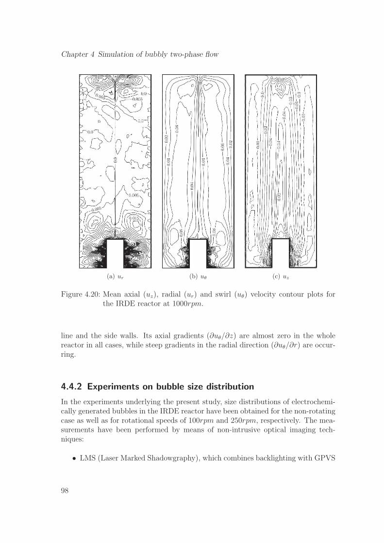
Chapter 4 Simulation of bubbly two-phase flow
(a) ur (b) u� (c) uz
Figure 4.20: Mean axial (uz), radial (ur) and swirl (u�) velocity contour plots forthe IRDE reactor at 1000rpm.
line and the side walls. Its axial gradients (∂u�/∂z) are almost zero in the wholereactor in all cases, while steep gradients in the radial direction (∂u�/∂r) are occur-ring.
4.4.2 Experiments on bubble size distribution
In the experiments underlying the present study, size distributions of electrochemi-cally generated bubbles in the IRDE reactor have been obtained for the non-rotatingcase as well as for rotational speeds of 100rpm and 250rpm, respectively. The mea-surements have been performed by means of non-intrusive optical imaging tech-niques:
∙ LMS (Laser Marked Shadowgraphy), which combines backlighting with GPVS
98

4.4 Bubbly flow in an IRDE reactor
(Glare Point Velocimetry and Sizing). Backlighting is a technique in whichthe bubbles are illuminated by a diffuse light source from the back of the fieldof view. The bubbles cast shadows, which are imaged. The size of the shadowimage is representative for the bubble size. Since the distance of the bubbleto the camera is not exactly known, considerable sizing errors may arise. Toovercome these deviations, GPVS is applied, meaning that the bubbles areadditionally illuminated from two sides by a laser sheet that is perpendicularlypositioned to the lens and camera. When the camera is positioned in the focalplane of the lens, two glare points are visible on the image. They originatefrom the reflected and refracted light of the laser sheet on the bubble surface.Due to the presence of these glare points, the distance between lens and bubbleis exactly known and the bubble size can be accurately determined [143, 152].
∙ ILIDS (Interferometric Laser Imaging for Droplet Sizing), which uses the sameset up as GPVS with the camera being placed out-of-focus. In this case, theglare points morph into circular shapes determined by the aperture of the lens.If the camera is place sufficiently out-of-focus the two circles overlap and createan interference pattern. The frequency of this interference pattern can berecorded by a camera and is proportional to the bubble size [143, 153, 154, 155].
Figure 4.21 shows the principles of the measurement techniques described above.Both techniques are complimentary. ILIDS is best suited to scan a large field of viewcontaining only some microscopic bubbles, whereas LMS gives better results withhigher gas volume fractions but only over a relatively small field of view. Thereforeboth techniques were used to obtain bubble size distributions.
In the experimental investigations carried out, H2 gas production in a Na2SO4
electrolyte with pH = 2.5 is studied. Hydrogen bubbles were generated electro-chemically by applying a potential difference of −1.8V versus NHE between the twoelectrodes of the IRDE reactor. The following hydrogen-producing reaction takesplace on the cathodically polarized cylinder electrode, where hydrogen protons (H+)are reduced:
2H+ + 2e− → H2 . (4.31)
The hydrogen protons are produced in an oxygen-producing reaction on the anod-ically polarized electrode on top of the reactor, where water molecules are oxidized:
2H2O → O2 + 4H+ + 4e− . (4.32)
In the present work, the focus is put on the study of the gas bubbles formed bythe hydrogen reduction reaction, so we set aside the effect of oxygen production
99

Chapter 4 Simulation of bubbly two-phase flow
Figure 4.21: Principles of LMS and ILIDS [143].
at the anode. The H2 produced at the cathode dissolves into the electrolyte ona molecular level and saturates the region adjacent to the electrode. When theconcentration of gas reaches a certain critical level, the electrode gets supersatu-rated. Supersaturation enables the formation of gas bubbles at nucleation sites onthe electrode surface. The bubbles grow in size until they reach a critical break-offdiameter. Afterwards, they are released and disperse into the electrolyte. Sources ofnucleation are irregularities of the electrode surfaces, which may contain entrappedgas. Section 5.3 gives a more detailed description of the underlying phenomena ofsurface gas evolution in electrochemical processes.
The experimental investigations show that when hydrogen bubbles are injectedfrom the rotating electrode into the swirling electrolyte flow, the bubble motion inthe region above the inner cylinder is mainly determined by the ability of the bubblesto overcome the rotation-induced downflow velocity uz of the electrolyte near thedisk surface. If a bubble is large enough to overcome the drag of the counter flow bybuoyancy, it rises upwards towards the top of the reactor. Smaller bubbles withouta sufficiently large buoyancy are dragged away from the electrode in radial directionand transported into the circulation zone in the bottom region of the reactor [138].
To illustrate the bubble behavior macroscopically, Figure 4.22 shows instantaneousGPVS snapshots of the bubbly flow field in the IRDE reactor near the rotating elec-trode at a rotational speed of 100rpm. It can be seen that the larger bubbles moveupwards, while the smaller bubbles are dragged to the side. The larger bubbles are
100

4.4 Bubbly flow in an IRDE reactor
able to overcome the rotation-induced downflow velocity towards the electrode andform a rising bubble plume. The shape of the plume does not significantly changebetween the two instantaneous snapshots taken at times t = 4s and t = 8s. Thisindicates a stable, non-oscillating behavior of the plume at 100rpm.
(a) t = 4s (b) t = 8s
Figure 4.22: GPVS images of hydrogen bubbles released from the rotating electrodefor the 100rpm case.
(a) 100rpm (b) 250rpm
Figure 4.23: Backlighting images of hydrogen bubbles released from the rotatingelectrode at t = 9s after bubble injection.
101

Chapter 4 Simulation of bubbly two-phase flow
Figure 4.24: Positions of the optical windows W1 and W2 for bubble size measure-ments in the IRDE reactor.
The backlighting images in Figure 4.23 give a more detailed view on the regionclose to the electrode surface, clearly pointing out the size difference between thebubbles that move to the sides and those which move upwards. The bubbles thatremain in the plume for 250rpm are apparently larger than for 100rpm, indicatingthat the threshold in bubble size to overcome the increasing downflow velocity riseswith the rotational speed.
The mass flux of hydrogen emerging from the rotating electrode surface has beencalculated from the electric current I at the electrode by Faraday’s law of electrolysis:
mH2=MH2
I
nF= 1.5 ⋅ 10−10kg/s , (4.33)
where MH2= 2.016g/mol is the molar mass of H2, n = 2 is the number of hy-
drogen valence ions and F = 9.649 ⋅ 104C/mol is Faraday’s constant. A constantelectric current has been applied in the experiments, thus the value of the hydrogenmass flux is fixed for all investigated cases.
Bubble size distributions were measured in two optical windows. Window W1 islocated in the region above the electrode and is used to track bubbles in the risingplume, while window W2 is placed at the side of the rotating cylinder and serves totrack the bubbles going to the side by centripetal forces. The window configurationis illustrated in Figure 4.24. Both optical windows are of width lW = 18mm andheight ℎW = 12mm and focus in the plane of symmetry of the IRDE reactor. Thefocal thickness of the windows is �W = 1mm.
To obtain a bubble diameter spectrum for the non-rotating reactor case (0rpm),rising bubbles have been tracked for a time of 29s through the optical window W1.
102

4.4 Bubbly flow in an IRDE reactor
In absence of rotational movement, all generated bubbles move upwards throughthis window and no bubbles move sidewards, thus the size distribution obtained bythe optical measurements corresponds to the distribution of bubbles generated atthe electrode.
4.4.3 Comments on the measurement uncertainty
Regarding the measurement uncertainty of the optical techniques used in the exper-iments to obtain the bubble diameter distributions (LMS and ILIDS), we first haveto identify the measurement parameters on which the measured diameter depends.
For the case of LMS, Dehaeck states in [143] that the measured bubble diameterfor a spherical bubble with both glare points present can be inferred from the sepa-rating distance of these glare points at 90∘ as follows:
d =
√2�pixn
. (4.34)
Here, �pix is the separating distance in pixels between the two glare points and n isis the amount of pixels per millimetre. The measurement uncertainty of LMS is thus
Δd
d=
√
(
Δ�pix�pix
)2
+
(
Δn
n
)2
, (4.35)
and is estimated to be 0.3%, as stated in [143].
Concernig the ILIDS technique, the following relation is given in [153] for a mea-sured bubble diameter:
d = ��airf . (4.36)
Here, � is the laser wavelength, �air is the conversion factor to calculate the parti-cle diameter from the observed glare point separation in air as used in GPVS [152],while f is thr frequency of the fringes, i.e. the amount of fringes per radian. Sincethe uncertainty related to the laser wavelength is negligible compared to the othersources, only the uncertainties related to the three remaining parameters are takeninto account in defining the measurement uncertainty of ILIDS:
103

Chapter 4 Simulation of bubbly two-phase flow
Δd
d=
√
(
Δ�air
�air
)2
+
(
Δf
f
)2
. (4.37)
Each of these uncertainty sources is discussed in detail in [153] along with an in-tegrated view of how these error sources can be minimized by choosing appropriateset-up parameters. This shows that combined uncertainties below 2% are realisticfor bubble diameter measurements.
4.4.4 Bubble dispersion and size distribution in rotating flow
In the numerical test cases for bubbly two-phase flow in the IRDE reactor, a sizedistribution obtained experimentally by the techniques described in Section 4.4.2for the zero rotation case has been used as input spectrum. The mean diameter forbubbles generated at 0rpm was measured to d = 145�m with a standard deviationof �d = 76�m.
Figure 4.25: Bubble diameter distribution in window W1 for the 0rpm case. Lightbars: Experimentally obtained values. Dark bars: Input diameter spec-trum for the simulations.
The experimentally measured bubble size spectrum is shown by the light bars inFigure 4.25. It is found to be best described by a log-normal distribution. There-fore, a random sampled log-normal size distribution following the experimentally
104

4.4 Bubbly flow in an IRDE reactor
measured values for the arithmetic mean d and the standard deviation �d has beenused as input spectrum for the numerical test cases. In this way, the gas mass fluxmH2
measured in the experiments and described by equation (4.33) is conserved.Random sample diameters were obtained by means of a Box-Muller transformationalgorithm [156]. This technique generates random values of Gaussian distributionaccording to an expected value E and a variance V . To obtain log-normal distributedrandom values from the Gaussian distribution, the following transformations haveto be performed:
�2 = ln
(
V
E2+ 1
)
, (4.38)
� = ln(E)− �2
2. (4.39)
Here, � and � are the arithmetic mean and variance of the natural logarithm ofa Gaussian distributed variable X, so that random values exp(X) obtained by aBox-Muller transformation obey a log-normal distribution with arithmetic mean Eand variance V , as defined above.
Figure 4.25 compares the numerical input diameter spectrum obtained by therandomly generated bubbles (dark bars) to the experimental results for 0rpm (lightbars). The slight differences between the two spectra are due to the fact that theexperimentally measured results are not exactly fitting a log-normal distribution. Atthe left end of the spectrum, the deviation can be explained by the fact that smallerbubbles rise slower than larger ones. Since the experimentally achieved data consistsof a series of images obtained at a frequency of f = 11.4/s, the small bubbles mightbe detected in more than one image and thus distort the spectrum, leading to ameasurement uncertainty. This is compensated in the numerical input spectrum.
Figure 4.26 and Figure 4.27 show snapshots of instantaneous bubble distributionsin the IRDE reactor at different rotational speeds obtained at t = 9s after the firstbubbles emerge from the rotating electrode. These snapshots allow to qualitativelycharacterize the bubble dispersion in the reactor. At 100rpm, the bubble plume isnot significantly affected by the rotation and only a few small bubbles are draggedto the side of the rotating cylinder. For 250rpm and 500rpm, we see already alarge distortion of the plume and many small bubbles going to the side due to therotation. At 1000rpm, the bubble plume brakes up almost completely. The bubblesmove through the reactor in a chaotic motion and even larger bubbles are draggedto the side due to the rotation.
105

Chapter 4 Simulation of bubbly two-phase flow
(a) 100rpm (b) 250rpm
Figure 4.26: Instantaneous bubble distribution obtained from the IRDE reactor sim-ulations at t = 9s for the two lower rotational speeds tested.
(a) 500rpm (b) 1000rpm
Figure 4.27: Instantaneous bubble distribution obtained from the IRDE reactor sim-ulations at t = 9s for the two higher rotational speeds tested.
Table 4.4 gives an overview of mean values and standard deviations of the di-ameter spectra for all measured cases in both experiments and simulations. Figure4.28 and Figure 4.29 show the according diameter distributions for the rising bubbleplumes at rotational speeds of 100rpm and 250rpm, respectively. In the numericalcases, the spectra were obtained by detecting the bubbles in the region correspond-
106

4.4 Bubbly flow in an IRDE reactor
0rpm 100rpm 250rpm
d [�m] �d [�m] d [�m] �d [�m] d [�m] �d [�m]Optical window W1 (top)
Experiment 145 76 145 85 153 80Simulation 145 74 147 71 171 59
Optical window W2 (side)Experiment - - 44 13 64 29Simulation - - 44 9 88 20
Table 4.4: Comparison between numerical and experimental data in terms of mea-sured mean bubble diameters d and standard deviations �d.
ing to the optical windows W1 and W2 used in the measurements.
Experimentally we were not able to measure the correct bubble size distributionsfor 500rpm and 1000rpm. Due to the chaotic motion of the bubbles, too few bubblesare passing through the measuring windowW1. This makes it difficult to determinethe size distribution in a statistically accurate way, so the present analysis of bubbledispersion and size distribution is limited to the rotational speeds of 100rpm and250rpm.
In the 100rpm case (see Figure 4.28), the agreement of the diameter spectrabetween experiment and simulation is very good except for a few outliers in theexperimental data. The calculated mean diameters d agree, though the standarddeviation �d is slightly higher for the experimental case. This is judged to be anoutcome of the measurement uncertainty regarding the image processing for smallbubble sizes, as mentioned above.
The agreement between experimental data and simulation results in the 250rpmcase (see Figure 4.29) is less good than in the 100rpm case, but still acceptable.The simulation results show a log-normal diameter distribution, but in comparisonto the experimental data, the spectrum is shifted to the right. The obtained meandiameter in the simulation results is significantly higher than in the experiment,while the standard deviation is lower.
The discrepancies between numerical and experimental results in terms of bub-ble size distribution is related to the fact that with growing rotational speed of theRDE, the size of detaching bubbles decreases due to the higher amount of rotation-induced shear on the electrode surface. This causes the bubbles to detach earlierfrom the electrode and as a consequence, the detaching bubbles are smaller. Since
107

Chapter 4 Simulation of bubbly two-phase flow
Figure 4.28: Comparison of experimental and simulation data for the bubble diam-eter distribution in window W1 in the 100rpm case.
Figure 4.29: Comparison of experimental and simulation data for the bubble diam-eter distribution in window W1 in the 250rpm case.
the diameter spectrum of the bubble plume obtained in non-rotating flow is takenas numerical input even for the cases including rotation, the computation of thetwo-phase flow field suffers from slightly wrong initial conditions.
108

4.4 Bubbly flow in an IRDE reactor
(a) 100rpm (b) 250rpm
Figure 4.30: Comparison of experimental and simulation data for the bubble diam-eter distribution in window W2.
Figure 4.30 shows the bubble diameter distributions for the optical window W2for the rotational speeds of 100rpm and 250rpm, respectively. The size distributionof the bubbles that are dragged to the side after emerging from the rotating electrodeis presented. As for the W1 results, the experimental and simulation data matchvery well in case of 100rpm, while for 250rpm the numerically obtained bubble sizesare much higher than in the experiments. Again, we see that for increased rotationalspeed of the RDE, the size spectrum of bubbles emerging from the electrode shiftsto smaller diameters.
To estimate the bubble size threshold to overcome the rotation-induced downflow,we set the peak fluid downflow velocity ∥uz,max∥ in the region above the rotatingelectrode before bubble injection equal to the terminal rise velocity vT of a genericbubble of diameter d, as stated by equation (4.4). If the rise velocity is larger thanthe downflow velocity of the electrolyte, the bubble is considered to overcome thefluid flow and becomes able to rise to the top of the reactor. In this way, the followingexpression for a threshold diameter is obtained:
dtℎ =
√
12�c∥uz,max∥g
with g = 9.81m/s2 . (4.40)
Table 4.5 summarizes theoretical values of dtℎ for the different rotational speeds
109

Chapter 4 Simulation of bubbly two-phase flow
applied in the present test cases based on equation (4.40). With increasing rotationalspeed, the threshold diameter rises. The computed values of dtℎ for the 100rpm andthe 250rpm case correspond well with the observed numerical and experimental be-havior. Form Figure 4.30 we see that the bubbles that are dragged to the side obeythe predicted values for the threshold diameter.
Case ∥uz,max∥ [m/s] dtℎ [�m]100rpm 0.0062 88.4250rpm 0.0140 132.8500rpm 0.0175 148.51000rpm 0.0298 193.8
Table 4.5: Electrolyte downflow velocities ∥uz,max∥ before bubble injection and the-oretical values of dtℎ for the present test cases.
As a conclusion about bubble dispersion and size distribution in the rotating flowof an IRDE reactor, we can state that the numerical investigations carried out agreewell with the data obtained from the experiments. However, we do not take intoaccount the fact that for increasing rotational movement of the gas-producing elec-trode, the detaching bubbles are of smaller sizes. This results in a deviation ofnumerical and experimental results in terms of size distributions for higher rota-tional speeds. Thus, in more advanced modeling the effect of the shear velocity atthe rotating electrode on the bubble size distribution should be taken into account.Since the size distribution of bubbles detaching from the electrode in case of rotationcannot be measured directly by the experimental techniques proposed in this work,a suitable future point of research would be to perform an extensive experimentalcorrelation study of bubble size spectra and rotational speeds.
4.4.5 Two-way coupling effects between bubbles and electrolyte
When bubbles are injected from the rotating electrode into the electrolyte, theyinduce an upward flow velocity in the reactor due to two-way momentum couplingwith the fluid, as described in Section 2.6.3. The induced velocity acts in oppositedirection to the downward flow velocity induced by the rotation, leading to an in-teraction of physical phenomena that causes a complex flow problem. It has beenfound that the upward flow induced by the bubbles is logarithmically increasingwith the gas mass flow rate [138].
If we consider a cylindrical fluid control volume Vc of radius rc = 2mm just above
110

4.4 Bubbly flow in an IRDE reactor
the gas-producing electrode, bubbles of a mean diameter following the experimen-tally obtained value of d = 145�m and a gas mass flux of 1.5 ⋅10−10kg/s, as given byequation (4.33), we end up with a hydrogen volume fraction in the control volume of
�H2=
mH2
�r2cvT�H2
= 0.88 ⋅ 10−3 . (4.41)
This value of �H2is found to have a strong two-way coupling impact after [40, 41],
thus the rising bubble plume is expected to significantly influence the fluid flow, in-ducing an upward motion.
The influence of the bubble motion on the fluid flow and thus the two-way cou-pling effect is shown in Figure 4.31 and Figure 4.32. The axial (uz) and radial (ur)fluid velocity components in the vicinity of the rotating electrode for two differentrotation speeds, namely 100rpm and 1000rpm, are plotted as a function of the lat-eral distance x from the vertical centerline of the reactor in the plane of symmetry,where x = 0.002m corresponds to the outer electrode edge and x = 0 is the centerof the electrode. The velocities are calculated at a height of = 3.6, which repre-sents the edge of the hydrodynamic layer, and at = 1, below which the analyticalsolution of the flow field without bubbles holds for all three components of the flowvelocity, as described in section Section 4.4.1.
(a) 100rpm (b) 1000rpm
Figure 4.31: Axial electrolyte velocity uz near the rotating electrode before and t =9s after bubble injection.
111

Chapter 4 Simulation of bubbly two-phase flow
(a) 100rpm (b) 1000rpm
Figure 4.32: Radial electrolyte velocity ur near the rotating electrode before andt = 9s after bubble injection.
The axial fluid flow velocity (see Figure 4.31) calculated before bubble injectionshows almost unperturbed downward flow towards the electrode for both rotationalspeeds. At t = 9s after bubble injection, we clearly see a two-way coupling effectin the case of 100rpm, resulting in a reduced flow velocity above the electrode. At = 1 the axial velocity with and without bubble induced flow deviates up to 75%.At = 3.6 the two-way coupling even results in an upward fluid flow above theelectrode surface. At 1000rpm, the bubbles do not have a significant effect on thedownward flow velocity. This indicates that the axial velocity profiles predicted bythe Cochran solution are no longer valid in case of gas bubbles created at the ro-tating electrode at low rotational speeds, while for higher speeds, the bubbles donot seem to affect the axial flow component. This can be related to the increasedamount of dispersion at high rotational speeds.
The radial flow velocity profiles (see Figure 4.32) on injection time clearly showthe centripetal effect of the rotation, which accelerates the flow with increasing dis-tance to the axis of symmetry. The gas bubbles are found to have a reducing effecton the radial velocity. For both rotational speeds, there is a strong reduction ofthe radial fluid velocity due to the bubble-induced upward flow. For 100rpm and = 3.6, the centripetal fluid motion is even inverted by the presence of the bubbleplume. This is due to the bubble-induced upward motion in the reactor which re-sults in an inversion of the vortical flow pattern near the electrode.
112

4.5 Conclusion
4.5 Conclusion
Two studies on bubbly two-phase flows, involving hydrodynamics and dispersivephenomena of bubble plumes, have been performed by means of the Eulerian-Lagrangian modeling approach in order to validate the robustness, accuracy andoverall performance of the Lagrangian solver PLaS, which has been developed andimplemented in the scope of the present Ph.D. work. All simulations have beencarried out by coupling PLaS to the Navier-Stokes solver Morpheus.
The simulation of the unsteady motion of the air-lift flow in a square bubble col-umn at different gas mass flow rates lead to very good agreement to experimentalresults published in [135] in terms of mean and fluctuating liquid velocity. Thecolumn dimensions and bubble size have been chosen such that they match the con-figuration used in the cited reference. Two-way momentum coupling between thebubbles and the carrier liquid has been taken into account.
Regarding the two-phase flow field over a smapling time of t = 120s, chaoticmotion of the bubble plume and the according induced fluid velocity field is found.Instantaneous flow fields at different time steps can not be correlated to each other.With increased gas mass flow, the mass and momentum back-coupling from thebubbles to the flow become stronger and higher flow velocities are induced. Com-parisons to the cited reference in terms of averaged vertical liquid velocity as wellas vertical and horizontal liquid velocity fluctuations show very good agreement.
The motion of a bubble plume in the rotating flow field of an inverted rotatingdisk electrode (IRDE) reactor has been analyzed for varying rotational speed of thedisk electrode. Bubble dispersion effects and size distributions have been comparedto data obtained by the optical measurement techniques LMS and ILIDS, leadingto a good agreement between experiment and simulation.
Two-way momentum coupling effects between bubbles and carrier flow have beeninvestigated near the rotating disk of the IRDE reactor, showing that the analyticalfluid flow solution for single phase flow documented in [150] is violated by the pres-ence of the gas phase for moderate rotational speeds. For high rotational speeds,however, this violation is found to be less significant, because the momentum inducedby the rotating electrode becomes dominant over the phase momentum transfer.
The results obtained for bubbly two-phase flow simulations with the Lagrangiansolver PLaS prove that the developed solver is well suited for the simulation ofcomplex two-phase flow problems in the frame of air-lift flows and electrochemicallygenerated bubbles, including two-way mass and momentum coupling.
113


Chapter 5
Coupling of two-phase flow and
electrochemistry
In many industrially relevant electrochemical reactors, bubbly flows occur as a side-effect of the electrochemical process, when gas-producing electrode reactions areinvolved. The produced gas bubbles are known to affect the ion transport proper-ties of the system, thus influencing the overall performance of the reactor. This leadsto a multi-physical problem of high complexity involving fluid flow, electrochemicalreactions and gas bubble evolution. In the following, an integrated modeling ap-proach to such a complex mechanism is presented and applied to simulate a simpleelectrochemical channel flow reactor.
5.1 Introduction to electrochemistry
Electrochemistry deals with the mutual conversion of chemical and electrical energyin electrochemical reactions. Contrary to a normal, homogeneous chemical reactionbetween ionic species, which occurs in any location where the involved species col-lide, an electrochemical reaction is governed by heterogeneous transfer of electrons,taking place only at the interface between an electrode and an electrolyte solution.As a result of the charge exchange at the electrode/electrolyte interface, electricalenergy is converted into chemical energy and vice versa. In this process, substancesare consumed and generated at the electrodes. For a detailed description of thesubject, the reader is referred to textbooks on electrochemistry, as published byNewman [157], Bockris & Reddy [158] and Walsh [159].
5.1.1 The electrochemical cell
A simple electrochemical cell consists of two electrodes immersed in an electrolytesolution. The electrodes are connected by a conducting material through an exter-nal circuit, in which electron flow occurs. The liquid electrolyte is governed by ion
115

Chapter 5 Coupling of two-phase flow and electrochemistry
flow, while an exchange of electrons takes place at the electrode surfaces. An elec-trode on which an oxidation reaction takes place is called anode, while the electrodehosting a reduction reaction is called cathode. Electrochemical reactions either useor generate an electric current in the external circuit. Electrochemical cells whichgenerate an electric current by spontaneously occurring reactions are called galvaniccells, while cells that use an externally supplied electric current to drive an otherwisenon-spontaneous chemical reaction are called electrolytic cells. In the frame of thepresent work we will deal with the latter type of cell, thus galvanic cells will not bediscussed further.
Figure 5.1: Example for a simple electrolytic cell.
A common example for an electrolytic cell is the electrolysis of molten sodiumchloride (NaCl). Electrolysis literally uses an electric current to split a compoundinto its elements. Its idealized concept is shown in Figure 5.1. The NaCl salt hasbeen heated until it melts. An anode and a cathode are immersed into the solutionof molten NaCl. If an external voltage is applied, this results in an electrostaticpotential difference between the two electrodes. As a result, a current I is flowingand electrochemical reactions occur on both electrode surfaces. In the solution,NaCl is split up into Na+ and Cl−. The Na+ ions flow toward the cathode andthe Cl− ions flow toward the anode, where they donate electrons and gaseous Cl2 isformed. The electrons flow through the external circuit to the cathode, where theycombine with Na+ ions to form sodium (Na). The dotted vertical line in the centerof the above figure represents a diaphragm that keeps the Cl2 gas produced at theanode from coming into contact with the sodium metal generated at the cathode.The reactions occurring at the electrodes and in the bulk of the two electrolyte
116

5.1 Introduction to electrochemistry
solutions of the electrolytic cell described above are formally written as follows:
Anode: 2Cl− → Cl2 + 2e− , (5.1)
Electrolyte: 2NaClLiq → 2NaLiq + ClGas2 , (5.2)
Cathode: Na+ + e− → Na . (5.3)
5.1.2 Reactions on electrodes
Electrochemical reactions like (5.3) and (5.1) take place at the interface between anelectrode and the electrolyte solution. In this region, several layers can be distin-guished. Close to the electrode surface, a double layer is formed, which consists oftwo characteristic adjacent regions [8]:
∙ The compact layer, which develops directly next to the electrode surface dueto the hydratation shells around the reacting ions as well as the non-reactingmolecules that restrict the access of reacting ions to the electrode. The thick-ness of this layer is of the size of these molecules. Ions must reach a certainpotential to surpass this molecular barrier.
∙ The diffuse layer develops in the bulk next to the compact double layer becauseof the imbalance between the number of anions and cations present in thislayer.
Outside of the double layer, the so called diffusive layer is located. In this layer,concentration gradients of ionic species are present and ion diffusion dominates overadvective ion transport. Outside of this layer, in the bulk of the electrolyte, thespecies concentrations are homogeneous. The double layer is usually several magni-tudes smaller than the hydrodynamic boundary layer over the electrode, while thediffusive layer has a magnitude of 1/10 of the hydrodynamic boundary layer.
The rate of an electrochemical reaction at an electrode and thus the value ofthe electrical current through the circuit are determined by the slowest step in thereaction mechanism. The steps of the reaction mechanism are:
∙ Electron transfer at the electrode.
∙ Transport of electrochemically active species towards the electrode.
∙ Chemical reactions that produce one of the electrochemically active species.
117

Chapter 5 Coupling of two-phase flow and electrochemistry
Just like homogeneous reactions, electrochemical reactions are characterized by ki-netic parameters and depend on the local temperature, pressure and concentrations.In addition, the potential difference over the compact layer close to the electrodeplays a role on electrochemical reactions.
5.1.3 Faraday’s laws of electrolysis
The most fundamental principles concerning electrolytic cells are Faraday’s first andsecond law of electroylsis, which are stated as follows:
∙ Faraday’s first law: The mass m of a substance generated by an electrolyticreaction is proportional to the amount of electric current I passed through thecell.
∙ Faraday’s second law: One equivalent weight of a substance is generated atan electrode during the passage of 96485C of charge Q through an electrolyticcell. Here, F = 96485C/mol is known as Faraday’s constant.
The two laws combined can be written as
m =Q
nF, (5.4)
where n is the number of electrons consumed in the reduction reaction to formone molecule of the reduced substance. Since current is defined as
Q = It , (5.5)
we end up with a mass flux m of the reduced substance:
m =I
nF. (5.6)
Equation (5.6) gives the mass flux in the unit mol/s. To calculate the mass fluxin kg/s, one has to multiply by the molar mass M of the substance.
5.1.4 Modeling requirements
In order to describe all physical phenomena present in electrochemical systems, oneneeds an adequate modeling strategy, taking into account the following phenomena:
∙ The transport of all involved ionic species through the electrolyte due to con-vection, diffusion and migration.
118

5.2 The MITReM model
∙ The electrochemical reactions at the electrode surfaces, involving electron andion transfer between electrode and electrolyte.
∙ The electrical properties of the electrode.
∙ The electron flow in the external circuit that connects the electrodes.
On top of modeling the electrochemical parameters, the electrolyte itself has tobe considered as a fluid medium and therefore it has to be modeled by fluid flowequations. In case of electrode reactions that produce a gaseous species, two-phasephenomena arise due to the formation of gas bubbles that detach from the electrodesurface into the electrolyte. In this way, a complex multi-physical problem involvingelectrochemistry and two-phase flow, i.e. ion and gas transport in electrochemicalreactors, is formulated.
In the present work, we simulate the bubbly electrolyte flow by means of theEulerian-Lagrangian method, as pointed out in Chapter 2, while the ion transportin the electrolyte and the electrode reactions will be tracked by the MITReM model,which is presented in Section 5.2. The description of the external circuit and themodeling of the electrodes itself is omitted. Thus, uniform distributions of electrodepotential on the electrode surfaces are considered. Although numerous materials indifferent states of matter for both electrodes and electrolyte are conceivable, onlymetal electrodes and liquid electrolytes will be considered.
5.2 The MITReM model
In the recent years, a variety of models have been proposed in order to describeelectron transfer and ion transport in electrochemical processes. A review of exist-ing models can be found in [160, 161, 162]. For the electrochemistry simulations inthe present work, the multi-ion transport and reaction model (MITReM), which isbased on the dilute solution model proposed in [157], has been chosen. This modelhas recently been implemented and validated by Bortels [160, 163] and Van denBossche [161, 164] for one-dimensional, planar and axi-symmetrical configurationsand a wide variety of electrochemical systems. Furthermore, Nelissen [162, 165] ex-tended the model to turbulent flows and mass transfer and Dan [8] considered theeffects of gas produced at an electrode coupled with electrochemical reactions usingthe MITReM model.
The MITReM model is based on mass conservation and potential field equations,which completely describe the transport of ionic species in an infinitely diluted elec-trolyte. The electron transfer by electrochemical reactions is taken into account in
119

Chapter 5 Coupling of two-phase flow and electrochemistry
terms of non-linear boundary conditions at the electrode surface.
5.2.1 Transport equations
Considering an electrochemical system with N ionic species in a non-ionized solventat constant pressure and temperature, one can write down an equation system con-sisting of N + 1 equations, namely N conservation equations for each ionic speciesin the electrolyte and an additional equation to calculate the electric potential field.This equation system has to be solved for N ion concentrations ck and the electro-static potential U . Based on the ion concentrations and potential values one maycalculate the physical properties relevant for the simulation, such as the currentdensity J or deposition thickness �dep after a given time.
Mass conservation
For each ion species k, the change of its concentration in a control volume must beequal to the flux over the control volume boundaries plus the local production rateRk due to homogeneous chemical reactions in the solution:
∂ck∂t
= −∇ ⋅ Nk +Rk . (5.7)
The flux density Nk is a vector quantity indicating the mean direction in whichions of the species k are moving and the number of molecules going through a planeoriented perpendicular to the mean flow of these ions. In dilute solutions, the fluxof an ion species k with a local concentration ck due to the convection, diffusion andmigration is given by [157]:
Nk = cku−Dk∇ck − zkck�kF∇U . (5.8)
The first term on the right hand side of the above equation expresses convection,which is caused by the motion of the ions driven by the fluid electrolyte velocityfield u. The second term reflects the effects of ionic diffusion due to concentrationgradients in the solution, leading to a movement of ions towards regions of low con-centrations. The diffusion coefficient Dk is independent of the ionic concentrationsck in dilute solutions, but depends on pressure, temperature and the composition ofthe electrolyte. The third term expresses migration of ions due to external electricalforces. The migration contribution in dilute solution depends on the gradient ofelectric potential ∇U , the charge zk and the mobility �k of the ions:
�k =Dk
RT, (5.9)
120

5.2 The MITReM model
where R = 8.314J/molK is the universal gas constant and T is the temperature.Relation (5.9) is known as the Nernst-Einstein equation [157].
From (5.7) and (5.8), one obtains the following differential equation for the ionconcentration of species k:
∂ck∂t
= −∇ ⋅ (cku) +∇ ⋅ (Dk∇ck) + zkF∇ ⋅ (�kck∇U) +Rk . (5.10)
Potential field
The charge density at each point of the solution is the sum of the charges of allions per unit volume zkck. The electric potential U in a medium with a dielectricconstant " is given by the Poisson equation:
∇2U = −F"
∑
k
zkck . (5.11)
The constant given by the ratio F/" is usually very large compared to the Lapla-cian of the potential ∇2U , so that (5.11) can be approximated by the so calledelectroneutrality condition:
∑
k
zkck = 0 . (5.12)
The electroneutrality condition, implying that considerable changes of the elec-tric potential are necessary to create a charge separation, is valid in the whole bulkelectrolyte, while it is violated in the double layer near an electrode.
Current density field
The current density due to the movement of an ionic species k in the electrolyte isobtained by multiplying the ion flux by the corresponding charge per mole:
Jk = zkFNk . (5.13)
The total current density is obtained by summing up the current densities of allionic species k present in the solution:
J =∑
k
Jk . (5.14)
121

Chapter 5 Coupling of two-phase flow and electrochemistry
Since in the bulk electrolyte, the electroneutrality condition stated by (5.12) holds,the convection term cancels out after plugging (5.8) and (5.13) into (5.14) and thecurrent density reduces to the following equation:
J = −�∇U − F∑
k
zkDk∇ck , (5.15)
where � is the electric conductivity of the solution
� = F 2∑
k
z2k�kck . (5.16)
From the above equations we see that the current density is proportional to theelectrical field and the sum of the species concentration gradients. Thus if there areconcentration gradients present in the solution, there is also a diffusion current andOhm’s law does no longer hold.
5.2.2 Boundary conditions
As stated above, the MITReM model composed by the mass conservation and po-tential field equations bears N +1 unknowns, namely the ion concentrations ck andthe electrical potential U . The underlying system of equations has to be completedby appropriate boundary conditions for electrodes, insulators as well as electrolyteinlets and outlets.
Electrodes
An electrode is regarded as a wall from the fluid flow point of view. The ion fluxnormal to the electrode is zero for non-reacting ions, but non-zero for reacting ions,which leave the computational domain via the electrode/electrolyte interface wherethe electrochemical reactions take place.
For non-reacting ions, the flux of an ionic species k in the direction n normal tothe electrode is zero, therefore the concentration gradient will always compensatethe local potential gradient. This can be derived from (5.8), as stated in [8]:
zk�kFck∂U
∂n= −Dk
∂ck∂n
. (5.17)
For reacting ions, the flux of a reacting ionic species normal to the electrode iscalculated from the current density going through the electrode. In the most generalcase, several ionic species k react simultaneously on an electrode in several differentreactions r. According to equation (5.14), the total current density J normal to the
122

5.2 The MITReM model
electrode can be considered as the sum of the current densities originating from thereacting ions Jk, which can be calculated based on the reaction current densities Jr:
Jk =∑
r
skrJr , (5.18)
where skr is the stoichiometric coefficient of ion k in the reaction r. The fluxNk of a reacting ionic species k normal to an electrode can then be computed byre-writing equation (5.13) and inserting equation (5.18):
Nk = Nk ⋅ 1n =
∑
r skrJrzkF
. (5.19)
The remaining unknowns in (5.19) are the reaction current densities Jr, whichare modeled by the Butler-Volmer equation. This equation describes how the elec-trical current on an electrode depends on the potential difference across the elec-trode/electrolyte interface and the local concentration of the reacting ions:
Jr = kOxc0,Oxe�OxnF
RT(V−U0) − kRedc0,Rede
�RednF
RT(V−U0) , (5.20)
where the former part of the right hand side describes the oxidation reaction,while the latter part stands for the reduction reaction. In equation (5.20), c0,Ox andc0,Red are the surface concentrations of the reacting ions involved in the reaction r,�Ox and �Red are the charge transfer coefficients, while kOx and kRed are reactionrate constants. The term V − U0 represents the potential difference over the com-pact layer, where V is the potential of the electrode and U0 is the potential of theelectrolyte solution on the other side of the compact layer. For a closer descriptionon the Butler-Volmer equation, the reader is referred to [8, 157, 162].
Insulators, inlets and outlets
On insulators, which are solid walls from the fluid flow point of view, the electrolytevelocity must be equal to the velocity of the wall, i.e. zero in case of a stationarywall. Because there is no flux of ions through the insulator, one must impose that theflux of each ionic species in direction n normal to the wall is zero, as demonstratedin [160]:
∂ck∂n
=∂U
∂n= 0 . (5.21)
Bulk values of the concentrations for all ionic species are imposed as Dirichletboundary conditions for electrolyte inlets, such that the values obey the electroneu-trality and the homogeneous reaction equilibrium conditions:
ck = ck,Bulk . (5.22)
123

Chapter 5 Coupling of two-phase flow and electrochemistry
As no current may enter or leave the system through an electrolyte inlet or out-let, the normal gradients of both ion concentration and potential need to be zeroin order to assure that no current leaves the system. Thus, the insulator boundaryconditions (5.21) hold as well for inlets and outlets.
5.3 Gas evolution in electrochemical reactions
In electrochemical reactions, some products are released in the form of a gaseousphase (e.g. oxygen, hydrogen, chloride). The gas is generated at the electrode sur-face on a molecular level. When the saturation concentration cSat is reached, gasbubbles may be formed. These bubbles grow on the electrode surface and detachinto the electrolyte. Gas-evolving electrodes are frequent in industrial applications.In many cases, the formation of gas bubbles is an unwanted side-effect of the electro-chemical system. It affects the motion of the electrolyte flow and as a consequenceit has an effect on the mass transport of the electrochemically active species in theprocess [166]. Furthermore, the conductivity of the electrolyte is affected by thepresence of the bubbles [167, 168].
5.3.1 Gas-evolving electrodes
At low current densities, the gas produced on the electrode surface diffuses on amolecular level and is transported away from the electrode by liquid convectionwithout forming a gas phase. This phenomenon occurs even at high current densityif the dissolved gas immediately reacts with other species in homogeneous reactions.For the electrochemical systems considered in the present work, we assume that thosekinds of homogeneous reactions do not appear. Thus, the released gas ions saturatethe electrolyte near the electrode at high current densities. When the concentrationof gas reaches a certain critical level, supersaturation occurs and gas bubbles areformed out of the gas ions. For hydrogen and oxygen evolving electrodes in acidicsolutions, Shibata [169, 170] found that supersaturation occurs at current densitiesof about J = 1000Am−2. The amount of supersaturation depends on the currentdensity, the electrolyte material properties and the flow field near the electrode.
Gas bubbles develop at nucleation sites on the electrode surface, grow in size untilthey reach a critical break-off diameter and detach into the electrolyte afterwards.The gas evolution mechanisms in electrochemical reactions are in many aspects anal-ogous to boiling. When a bubble detaches from the electrode surface, some residualgas remains at the nucleation site and another bubble will form at the same place.Sources of nucleation are usually irregularities of the electrode surfaces, e.g. pits
124

5.3 Gas evolution in electrochemical reactions
and scratches, that are capable of containing entrapped gas. Once a nucleus exists,the formed bubble grows in size once a certain level of supersaturation of the gasspecies around the nucleus is reached. If the current density is low, no bubbles willform even if suitable nucleation sites are present. Besides the supersaturation level,the growth of bubbles depends also on the hydrodynamic properties of the liquidelectrolyte, i.e. on inertial, viscous and interfacial forces. The bubbles detach fromthe electrode when they reach a critical diameter. This diameter depends on variousfactors, such as buoyancy, pressure and adhesion forces as well as on the electrolytecomposition. A detailed description of models to calculate the rate of bubble growthand the critical lift-off size is discussed by Vogt [6]. Typical lift-off diameters rangefrom 50�m for aqueous solutions to 1mm for salt melts. According to Figure 4.2 andequation (4.4), gas bubbles in this size range can be regarded as spherical entitieswith their terminal rise velocity depending linearly on their diameter.
At very high current densities, the level of supersaturation increases and morenucleation sites are activated. Coalescence, i.e. the interaction of a forming bubblewith other bubbles, also plays a role in this context. Bubbles collide and merge onthe electrode, so that a gas film covers the whole electrode surface. Contrary toboiling, where the heat flux is able to pass through the gas film by conduction andradiation, the charge transfer of the electrochemical reaction is interrupted by thegas film and the electrode is blocked.
Once the bubbles have detached from the electrode, they can still grow in size ifthe electrolyte is saturated with dissolved gas. As mentioned in [171], for oxygenand hydrogen evolution in the electrolysis of aqueous H2SO4 solutions, only 20%to 60% of the gas generated at the electrode is immediately absorbed into growingbubbles. The remaining gas is transported into the electrolyte on a molecular leveland gives rise to supersaturation that causes an increase of the growth of bubblesthat move through electrolyte.
5.3.2 Effect of gas bubbles on electrochemical parameters
The presence of a gas phase in a continuous electrolyte changes its conductivity �,which is a consequence of the global decrease of the diffusion coefficient Dk. Therelation between the local conductivity and the gas volume fraction �d has beenintensively studied in the past. Empirical relations proposed by different authorsare discussed e.g. by Vogt [6] and Kreysa & Kuhn [172]. Considering the gas bubblesas non-conducting spheres surrounded by a continuum liquid with conductivity �0,several expressions have been proposed for the conductivity of an electrolyte withgas fraction, where the best fit with available experimental data was found to be
125

Chapter 5 Coupling of two-phase flow and electrochemistry
the Bruggemann formulation [173], which has been used in the present work:
� = �0
√
(1− �d)3 . (5.23)
According to equations (5.9) and (5.16), the conductivity � varies linearly with theion mobility �k and the diffusion coefficient Dk for very dilute solutions. Accordingto the Bruggemann formulation, we can state the following:
�k = �k,0
√
(1− �d)3 . (5.24)
Dk = Dk,0
√
(1− �d)3 . (5.25)
In the above equations, �k,0 and Dk,0 are the properties of ion k when there is nogas in the electrolyte.
Regarding the continuous electrolyte flow, the presence of gas changes the velocityprofiles of the liquid at the electrode and in the bulk due to two-way momentumcoupling between the two phases, as described in Section 2.6.3. Consequently, thetransport of ions in the electrolyte is modified due to the convection contribution inthe MITReM model. According to [174], there are three main effects related to thepresence of gas in the electrolyte:
∙ The penetration effect is caused by bubbles detaching from the electrode, bring-ing the surrounding liquid towards the electrode. As a result, the electrolyteadjacent to the electrode is periodically refreshed with ions by the centripetalflow of the liquid around the detached bubble.
∙ The microconvection effect is due to microflows that are generated by bub-bles detaching from the electrode, pushing the liquid past the electrode incentrifugal directions.
∙ The macroconvection effect is a global convective effect caused by the move-ment of the bubble swarm through the bulk electrolyte.
The first two effects mentioned above are related to single bubble movement,whereas the last effect is a consequence of bubble swarm movement, i.e. the motionof numerous bubbles [8].
126

5.4 Multi-physical simulation approach
5.4 Multi-physical simulation approach
An integrated, fully coupled multi-physical simulation approach that combines nu-merical models for electrolyte flow, ion transport, gas evolution and bubble disper-sion has been designed and implemented in the frame of the present Ph.D. thesis.For this purpose, different software modules were coupled, resulting in a processconsisting of the following components:
∙ The fluid flow solver Morpheus (see Section 4.2) to compute the flow of theelectrolyte.
∙ The Lagrangian tracking solver module PLaS (see Section 2.9) to compute thetrajectories of the gas bubbles created in the electrochemical process.
∙ The ion-transport and reaction kinetics simulation module MITReM, whichuses the model described in Section 5.2 to compute the electrostatic potentialfield and the concentrations of the ionic species involved in the electrochemicalsystem. Furthermore, the MITReM module computes fluxes of gaseous speciesproduced on electrodes. A detailed description of this module is given inSection 5.4.2.
∙ A bubble evolution module, which transforms the gas fluxes produced on theelectrodes, as computed by MITReM, into input data for PLaS, i.e. positions,velocities and diameters of gas bubbles. A detailed description of this moduleis given in Section 5.4.3.
The above mentioned software modules were developed independent of each otherand were linked via data interfaces in order to form an integrated, fully coupledmulti-physics software approach, which has also been documented in [175, 176].
5.4.1 Realization
Figure 5.2 shows the operational principle of the multi-physical simulation approach.The software modules are synchronized by a discrete time-stepping procedure, drivenby the fluid flow solver, from where the PLaS, MITReM and the bubble evolutionmodule are interfaced. This approach is similar to the one presented in Section 2.8,including two additional modules in the simulation cycle.
In each time step Δt imposed by the fluid flow solver, the electrolyte flow field issolved before the electrochemistry calculations are performed and the gas bubblesare tracked. All data flow in this process cycle is managed by the fluid flow solver,while the three additional modules are interfaced to the flow solver as plug-ins. Theprocess for a time step of the multi-physics simulation cycle is as follows:
127

Chapter 5 Coupling of two-phase flow and electrochemistry
Figure 5.2: Algorithm flowchart of multi-physical simulations including electrolyteflow, multi-ion transport, gas evolution and bubble dispersion.
∙ The fluid flow solver Morpheus updates the electrolyte velocity field u andpressure field p by solving the incompressible Navier-Stokes equations on thecomputational mesh. Source terms resulting from two-way coupling with thegas bubbles are taken into account.
∙ The MITReM module updates the ion concentrations ck and the potentialfield U by solving the MITReM equations on the computational mesh, whileelectrode reactions are determined by the Butler-Volmer model. The fluidflow velocity u and the gas volume fraction �d serve as input parameters.The Bruggemann relations are used to take into account the presence of gasbubbles in the electrolyte. In case of gas-evolving reactions taking place atelectrodes, the MITReM module provides a gas flux per boundary element oneach gas-producing electrode.
∙ The bubble evolution module transforms the element-wise gas flux, as com-puted by the MITReM module, into a set of bubbles for PLaS, represented bytheir positions, lift-off velocities and diameters. The size distribution of thebubbles is hereby defined inside PLaS. The electrode surface blocking effectinduced by the presence of a gas phase on the electrode is taken into account.
∙ PLaS updates the trajectories of the bubbles created on the electrodes by thebubble evolution module. The gas volume fraction field is updated and thetwo-way coupling source terms acting on the fluid flow are computed.
128

5.4 Multi-physical simulation approach
Equivalent to the approach pointed out in Section 2.8, the data interface betweenthe flow solver and its plug-ins in the present case is bilateral. The flow solverprovides information about the computational mesh (nodes, elements and connec-tivity), the boundaries of the computational domain and the velocity field of thefluid electrolyte to the plug-in modules, while output data from the plug-ins is givento the flow solver.
The software process described above is designed to operate on a multi-processorparallel computer architecture, where inter-process communication is realized bymeans of MPI [72, 73]. All plug-ins adapt the mesh partitioning defined by theNavier-Stokes solver in the parallel case. This concept has been pointed out for thecase of PLaS coupled to a flow solver in Section 2.9.4 and is extended in a straight-forward manner in case of the present, multi-physical approach.
5.4.2 The MITReM module
The MITReMmodule computes the electrochemical parameters of the multi-physicalprocess. The ion concentrations ck of a set of k ionic species and the electrostaticpotential U are updated by solving k mass conservation equations (5.10) and thePoisson equation (5.11). Alternatively to the Poisson equation, the electrostaticpotential can be computed by the electroneutrality condition (5.12). Boundary con-ditions on inlets, outlets, walls and electrodes are applied according to Section 5.2.2.The electrode reactions of the electrochemical process are computed by the Butler-Volmer reaction kinetics as stated by equation (5.20). For each simulation case, onehas to define the following parameters for the MITReM module:
∙ The composition of the electrolyte, i.e. the involved ionic species together withtheir initial (bulk) values, diffusion coefficients and inlet boundary conditions.
∙ The position of the electrodes, which have to be defined as wall segments ofthe computational domain defined in the flow solver.
∙ The electrochemical reactions taking place at the electrodes and the homo-geneous reactions taking place in the bulk electrolyte, as well as kinematicparameters for every reaction.
Figure 5.3 shows the operational principle of the MITReM solver module, whichdiscretizes the governing equations, i.e. the balance equations for each species ktogether with the Poisson (or electroneutrality) equation, on the computational gridin three space dimensions by means of a Galerkin Finite Element approach usingT1 linear elements. This method has been pointed out in Section 4.2 for the Navier-Stokes equations. To avoid convective instabilities, the convection term of the species
129

Chapter 5 Coupling of two-phase flow and electrochemistry
Figure 5.3: Algorithm flowchart of the MITReM module.
balance equations (5.10) is discretized by means of a Residual Distribution (RDS)method, using the N-scheme [24]. Partial integration is applied to the diffusion andmigration terms, resulting in fluxes perpendicular to the domain boundary.
The MITReM module needs the following data as input for every element of thecomputational grid:
∙ The coordinates of the element nodes, defining the spatial extent of the ele-ment.
∙ The fluid electrolyte velocity u in the element nodes in order to compute theconvective contributions to the concentration equations.
∙ The ion concentrations ck and the electrostatic potential U in the elementnodes of the previous time step.
∙ The values of fluid temperature Tc and density �c on the element nodes. Sincein this work we limit the physical complexity of the multi-physical problemto incompressible, iso-thermal flows, the fluid temperature and density areconstant for the time being.
∙ The gas volume fraction �d on the element nodes in order to take into accountthe presence of a gas phase through the Bruggemann relations.
To impose boundary conditions, MITReM needs the following information forevery electrode boundary element of the computational mesh:
∙ The surface coverage � of the boundary element in order to take into accountthe blockage effect of the electrode.
130

5.4 Multi-physical simulation approach
∙ The electrode reactions taking place at the electrode to which the presentboundary element belongs. This includes gas-producing reactions.
∙ The electrode potential V to be imposed.
On inlet, outlet and wall boundary elements of the computational domain, thegradients of ion concentration and potential normal to the boundary are imposed tobe zero in order to prevent the passage of current. On inlet boundary elements, thebulk concentrations ck,bulk of the ionic species are imposed in addition. At electrode
boundary elements, the flux Nk is replaced by the flux calculated by the Butler-Volmer relation. The boundary conditions are described in detail in Section 5.2.2.
According to the gas-producing reactions specified on the electrodes of the electro-chemical system, the MITReM module computes a gas mass flux mk of the gaseousreaction products for every electrode boundary element where a gas-producing reac-tion takes place. This gas-producing reaction transfers the molar flux of a gaseousspecies k into a gas phase at a given reaction rate.
The surface coverage � of a boundary element is calculated as follows:
� =�4
(
6VGas
�
)2/3
A, (5.26)
where A is the surface of the boundary element and VGas the residual volume ofgas produced in the boundary element which has not been transformed into bub-bles yet (see Section 5.4.3). The above formula assumes that VGas corresponds to aspherical bubble attached to the boundary element.
5.4.3 The bubble evolution module
The bubble evolution module converts the gas mass flux mk, as computed by theMITReM module, into a set of bubbles, which are tracked by PLaS afterwards. Toconvert the gas mass flux into a set of bubbles, the following procedure is undergonefor every electrode boundary element of the grid:
∙ A bubble diameter d is picked randomly from a pre-defined bubble size spec-trum and the position of the bubble nucleation site is randomly computedwithin the boundary element.
∙ The mass flux of gas mk in the present time step Δt, as computed by theMITReM module, is transformed into a gas volume and cumulated, i.e. addedto the remaining amount of gas from the previous time step.
131

Chapter 5 Coupling of two-phase flow and electrochemistry
∙ If the amount of the cumulated gas volume is larger than the volume of aspherical bubble with diameter d, this bubble is produced and its volume issubtracted from the cumulated gas volume. A new diameter and a new nucle-ation position are computed. This procedure is repeated until the cumulatedgas volume is not sufficient to produce another bubble in the present time step.
∙ The bubbles produced in the present time step are given to PLaS. Their lift-off velocity is set to zero for the time being, i.e. the bubbles do not have asuperficial velocity on injection time.
Figure 5.4: Algorithm flowchart of the bubble evolution module.
The above described procedure is depicted in Figure 5.4. The present modelingapproach to transform a gas flux coming from the computation of the gas-producingelectrode reaction kinetics is a very simple approach, which is based on a series ofassumptions. It does not take into account the distribution of nucleation sites onthe electrode material, i.e. the influence of the roughness of the electrode surfaceis neglected. Instead, bubbles are created in random positions. However, the de-scribed approach is regarded to give a sufficiently accurate bubble distribution on amacroscopic process level in the applications of interest.
132

5.5 Bubble evolution in a parallel flow reactor
5.5 Bubble evolution in a parallel flow reactor
In nowadays literature on electrochemical reactors, several attempts to take intoaccount the arising two-phase flow phenomena in case of gas-evolving reactions atelectrodes are proposed. Ibl & Venczel [177] linked the bubble evolution rate on anelectrode to the local mass transport and the mass diffusion toward the electrodesurface by a deterministic approach without solving a two-phase flow field. Byrne etal. [178] used this formulation to calculate the current distribution in a chlor-alkalimembrane cell. Wedin & Dahlkild [179, 180] performed two-phase simulations in avertical channel flow for a single vertical electrode, where the gas bubbles rise due tobuoyancy. Their model solves the coupled hydrodynamic and electrical properties inthe case of a mono-disperse gas using the two fluid formulation proposed by Ishii [1].Mandin et al. [151, 181] pointed out that the momentum exchange between liquidand bubbles is an important factor to calculate the electrochemical cell performance.He proposed to model the secondary phase flow by means of a Lagrangian modeland emphasizes the need for experimental and numerical data obtained in the sameconfiguration. In previous studies, we performed DNS of a fully turbulent channelto analyze the transport of small gas bubbles rising from a bottom electrode intothe turbulent boundary layer of the lower channel wall [182, 183]. It has been foundthat the motion of the bubbles is influenced by the coherent turbulent structures ofa turbulent boundary layer, but this influence is partially overcome by the effect ofbuoyancy.
In the present study we simulate a parallel flow channel reactor with a hydrogen-producing electrode on the bottom. The flow in the channel is assumed to follow alaminar Poiseuille profile that is constant in the spanwise direction of the channeland does not change with time. The flow is driven by a pressure gradient in thestreamwise direction and is retarded by viscous drag along the top and bottom wallsof the channel, such that pressure and viscosity forces are in balance. For the sidewalls, slip conditions are applied.
Figure 5.5: Geometric specifications of the parallel channel flow reactor.
133

Chapter 5 Coupling of two-phase flow and electrochemistry
Figure 5.5 shows a simple sketch of the parallel channel flow reactor. Its heightis ℎ = 0.01m while its width is w = 0.1m. The total length of the channel isl = 0.864m. Two electrodes are located at the channel walls, a cathode at thebottom and an anode at the top. Both electrodes have a streamwise length oflE = 0.06m and cover the whole span of the channel. The anode at the top wall ofthe reactor is located downstream of the cathode at the bottom wall. All channel di-mensions are outlined in Table 5.1. The average streamwise velocity of the Poiseuilleflow profile is uz = 0.2m/s, leading to a Reynolds number of Re = 970 based on thehalf-height of the channel. As electrolyte, a 1M sodium sulfate (Na2SO4) solutionis used, having a density of �c = 1030kg/m3 and a viscosity of �c = 1.35 ⋅ 10−6m2/s,as calculated after [144]. The computational mesh used in the present simulationsconsists of 72.000 tetrahedral cells. On both electrodes a boundary layer with thesmallest cell size in wall-normal direction being Δz = 2 ⋅ 10−5m is applied in orderto accurately capture the concentration boundary layers of the species involved inthe electrode reactions.
Length Symbol Value [m]Channel height ℎ 0.01Channel width w 0.1Bottom wall upstream segment LW1 0.402Bottom wall downstream segment LW2 0.402Top wall upstream segment LW3 0.467Top wall downstream segment LW4 0.337Electrode length LE 0.06
Table 5.1: Parallel channel flow reactor dimensions.
The electrochemical system used in the parallel channel flow reactor test caseconsists of eight species, which are sodium ions (Na+), sulfate (SO2−
4 ), NaSO−4 ,bisulfate (HSO−4 ), hydroxide (OH−), water (H2O), hydrogen ions (H+) and dis-solved hydrogen (HDiss
2 ). Table 5.2 shows the bulk concentrations cBulk,k and thediffusion coefficients Dk of the involved species.
On the cathode, the following hydrogen production reactions take place:
2H+ + 2e− → HDiss2 at pH < 7 , (5.27)
2H2O + 2e− → HDiss2 + 2OH− at pH ≥ 7 . (5.28)
These reactions are only acting in one direction, i.e. hydrogen ions or watermolecules are reduced to form dissolved hydrogen. The pH of the solution deter-
134

5.5 Bubble evolution in a parallel flow reactor
Species k cBulk,k [mol/m3] Dk [m2/s]Na+ 1285.97 9.30⋅10−10SO2−
4 283.01 7.19⋅10−10NaSO−4 714.02 6.75⋅10−10HSO−4 9.23 9.35⋅10−10OH− 3.05⋅10−9 5.22⋅10−9H2O 5.55⋅104 1.55⋅10−9H+ 3.29 9.30⋅10−9HDiss
2 0.0 4.87⋅10−9
Table 5.2: Bulk concentrations and diffusion coefficients of the ionic species involvedin the electrochemical system.
mines which of the two reactions takes place. Analogous to the hydrogen productionon the cathode, an oxygen production reaction takes place on the anode:
2H2O → O2 + 4H+ + 4e− . (5.29)
Here, water molecules are oxidized to form oxygen and H+. In the electrolyte,a set of homogeneous reactions take place. Those reactions are the dissociation ofwater, bisulfate and NaSO−4 :
H2O ⇀↽ H+ +OH− , (5.30)
HSO−4 ⇀↽ H+ + SO2−4 , (5.31)
NaSO−4 ⇀↽ Na+ + SO2−4 . (5.32)
These homogeneous reactions are equilibrium reactions, i.e. they are reversibleand act in forward and backward direction in order to balance the solution. Com-plete dissociation of sodium sulfate and sulphuric acid has been assumed:
Na2SO4 → Na+ +NaSO−4 , (5.33)
H2SO4 → H+ +HSO−4 . (5.34)
The reaction rates vr of the electrode reactions (5.27), (5.28) and (5.29) are relatedto the reaction current densities Jr as computed by the Butler-Volmer relation (5.20)as follows:
vr =JrnF
. (5.35)
135

Chapter 5 Coupling of two-phase flow and electrochemistry
The dissolved hydrogen produced at the cathode by reactions (5.27) and (5.28) istransferred into a gas phase:
HDiss2 → HGas
2 . (5.36)
This phase transfer takes place at a reaction rate vGas with a given rate constantkGas, when a specific saturation concentration cH2,Sat is reached:
vGas = kGasmax (0, cH2 − cH2,Sat) . (5.37)
Figure 5.6 shows a qualitative flowchart for the hydrogen generated in the electro-chemical process. Dissolved hydrogen HDiss
2 is generated by the cathode reactionsand forms gaseous hydrogen HGas
2 according to the local supersaturation level ofHDiss
2 . The remaining hydrogen diffuses away from the cathode in dissolved form.
Figure 5.6: Qualitative flowchart for hydrogen produced in the electrochemicalprocess.
In the following, we focus only on the hydrogen-producing cathode. Thus, theproduction of O2 as stated by reaction (5.29) and the formation of an accordingoxygen gas phase are not studied for the time being.
5.5.1 Reaction kinetics and species concentrations
The fully coupled multi-physical simulations of the parallel channel flow reactorwere performed for a varying electrode potential difference, which ranged betweenΔV = 1.0V and ΔV = 2.0V and has been incremented in steps of 0.2V . Thecathode potential has been set to zero in all presented cases. To obtain an electrodepotential difference, the anode potential has been varied. The saturation concen-tration of hydrogen in the present case is cH2,Sat = 0.00075mol/m3, which fits thesolubility of H2 in water at a temperature of 25 ∘ C, as presented in [184].
136

5.5 Bubble evolution in a parallel flow reactor
Figure 5.7 shows curves of the potential U as a function of the channel lengthx. The profiles were taken in the lateral and vertical centerline of the channel ata spanwise width of y = 0.05m and a height of z = 0.005m. We can see a steepincrease of U in the streamwise direction in the region below the anode. The po-tential jumps from a low level upstream of the anode to a higher level downstream.This jump is more distinct for increasing anode potential. While at low electrodepotential differences ΔV = 1.0 and ΔV = 1.2 it is almost negligibly small, thepotential increases by 80% at ΔV = 1.8 and by 155% at ΔV = 2.0.
Figure 5.7: Potential curves U(x) in the centerline of the channel for varying elec-trode potential difference ΔV .
Figure 5.8 and Figure 5.9 show concentration profiles ck(z) of the ionic species ofthe supporting electrolyte, namely Na+, SO2−
4 , NaSO−4 and HSO−4 . The profileswere taken normal to the lower channel wall in the streamwise and spanwise center ofthe cathode at x = 0.432m and y = 0.05m. The height z is plotted in a logarithmicscale. At ΔV = 1.0, we see almost no variance from the bulk concentrations near thecathode. With increasing electrode potential difference, the electrochemical reactionmechanisms accelerate and the species concentrations near the cathode rise. How-ever, compared to their bulk concentrations, the supporting electrolyte componentconcentration gradients are rather small, as one would expect. For the ΔV = 2.0Vcase, the increase of cNa+ is 0.004%, while for cSO2−
4and cNaSO−
4it is 0.05%, which
is almost negligibe. The decrease of 10% for cHSO−4
is more significant. This is
due to the fact that H+ ions are consumed to form HDiss2 and thus the chemical
reaction (5.31) will restore the balance by dissociating HSO−4 . The same concen-tration characteristics as for the supporting electrolyte components is observed for
137

Chapter 5 Coupling of two-phase flow and electrochemistry
(a) Na+ (b) SO2−
4
Figure 5.8: Concentration profiles ck(z) of sodium and sulfate ions normal to thecathode for varying electrode potential difference ΔV .
(a) NaSO−4 (b) HSO−4
Figure 5.9: Concentration profiles ck(z) of NaSO−
4 and bisulfate normal to the cath-ode for varying electrode potential difference ΔV .
the species involved in the cathode reactions (H+, OH− and HDiss2 ), as plotted in
Figure 5.10 and Figure 5.11. The increase in concentration for the ΔV = 2.0V casetakes significant values of 1840% for cOH− and 10% for cH+ . For cH2
, a concentration
138

5.5 Bubble evolution in a parallel flow reactor
(a) H+ (b) OH−
Figure 5.10: Concentration profiles ck(z) of hydroxide and hydrogen ions normal tothe cathode for varying electrode potential difference ΔV .
Figure 5.11: Concentration profiles cH2(z) of dissolved hydrogen normal to the cath-
ode for varying electrode potential difference ΔV .
increase can not be quantified, because the bulk concentratin of HDiss2 is zero. The
dissolved hydrogen concentration at the cathode for the ΔV = 1.0 case lies onlyslightly above the saturation concentration cH2,Sat, so that we expect a very low gasphase evolution. For increasing potential, the concentration of HDiss
2 at the cathoderises, thus a growing amount of produced hydrogen gas is expected. Figure 5.12
139

Chapter 5 Coupling of two-phase flow and electrochemistry
(a) Na+ (b) SO2−
4
Figure 5.12: Concentration profiles ck(x) of sodium and sulfate ions along the cath-ode for varying electrode potential difference ΔV .
(a) NaSO−4 (b) HSO−4
Figure 5.13: Concentration profiles ck(x) of NaSO−
4 and bisulfate along the cathodefor varying electrode potential difference ΔV .
and Figure 5.13 show the concentration variance over the cathode length for thesupporting electrolyte species Na+, SO2−
4 , NaSO−4 and HSO−4 , while Figure 5.14and Figure 5.15 show the same for the ions involved in the cathode reactions. The
140

5.5 Bubble evolution in a parallel flow reactor
(a) H+ (b) OH−
Figure 5.14: Concentration profiles ck(x) of hydroxide and hydrogen ions along thecathode for varying electrode potential difference ΔV .
Figure 5.15: Concentration profiles cH2(x) of dissolved hydrogen along the cathode
for varying electrode potential difference ΔV .
concentrations were measured in the first grid cell at z = 2 ⋅ 10−5m for all cases.The streamwise concentration profiles clearly show the effect of advection due tothe electrolyte velocity. All species have a significant increase in concentration to-wards the downstream edge of the cathode, whereafter the concentration drops tothe bulk value. The concentration is more distinct with increasing electrode po-
141

Chapter 5 Coupling of two-phase flow and electrochemistry
tential difference. Concerning the production of hydrogen gas, the largest amountof hydrogen bubbles is expected to be formed at the downstream edge of the cathode.
5.5.2 Dispersion of electrochemically generated bubbles
Hydrogen ions are produced on the cathode by reactions (5.27) and (5.28). Thereaction rate vGas, as stated by equation (5.37), determines the speed of the gas-evolution due to supersaturation of HDiss
2 in the electrolyte near the cathode. Itdepends on the reaction rate constant kGas. In the present case, we imposed a reac-tion rate constant of kGas = 0.01m/s. This value is large enough to ensure that allproduced hydrogen is consumed to form gas bubbles and the amount of dissolvedhydrogen is minimized.
The diameter spectrum of the produced bubbles has been imposed to be of log-normal type with a mean diameter of 100�m and a standard deviation of 30�m.Two-way coupling between the bubbles and the fluid flow has been neglected forthe time being, so the laminar Poiseuille flow profile at the lower channel wall is notdisturbed.
As discussed in Section 5.5.1, the electron and ion transfer rates in the electro-chemical system are augmented for increasing electrode potential difference ΔV andthe concentration of hydrogen cH2
at the cathode rises. Table 5.3 shows quantitativeparameters for the hydrogen gas evolution on the cathode of the parallel channel flowreactor. The peak hydrogen gas volume fractions �H2,max measured were occurringright above the downstream edge of the cathode, where the hydrogen gas evolutionis most pronounced. The average bubble number density flux Navg indicates howmany hydrogen bubbles are produced on the whole cathode in a certain time, whilethe indicated mass flux mH2
gives the total mass of hydrogen gas produced.
From Table 5.3 we see that for an increasing electrode potential difference ΔV ,the number of produced bubbles increases along with the mass flux of HGas
2 . Thus,the volume fraction of the hydrogen gas phase rises accordingly. The bubble num-ber density and mass fluxes at ΔV = 2.0V are more than two orders of magnitudehigher than at ΔV = 1.0V .
Figure 5.16 shows plots of the peak volume fraction and the HGas2 mass flux as
functions of the electrode potential difference. The figures indicate that the gasproduction grows exponentially with ΔV . We can see that ΔV = 1.0V marks athreshold below which the electrochemical reaction rates are too slow to inducesignificant ion transfer on the electrodes. This observation agrees with the speciesconcentration profiles at the cathode, which have been discussed in Section 5.5.1.
142

5.5 Bubble evolution in a parallel flow reactor
ΔV [V ] �H2,max [−] mH2[kg/s] Navg [1/s]
1.0 0.0029 3.52 ⋅ 10−11 7471.2 0.0062 1.37 ⋅ 10−10 29061.4 0.0124 4.48 ⋅ 10−10 95101.6 0.0169 1.29 ⋅ 10−9 273431.8 0.0248 3.02 ⋅ 10−9 641522.0 0.0421 5.76 ⋅ 10−9 122135
Table 5.3: Gas-evolving cathode parameters for different electrode potential differ-ences: Peak hydrogen volume fractions �H2,max, mass fluxes mH2
andaverage bubble number density fluxes Navg.
Regarding the values of the dispersed phase volume fraction, which in the peakregions above the downstream edge of the cathode reach values around 4% for theΔV = 2.0V case, it is obvious that two-way coupling effects of the gas phase onthe carrier phase have to be taken into account in a further study to investigate themomentum transfer effect of the bubbles on the electrolyte flow.
(a) mH2(ΔV ) (b) �H2,max(ΔV )
Figure 5.16: Quantification of hydrogen gas evolution with increasing electrode po-tential difference in terms of (a) gas mass fluxes and (b) peak volumefractions.
143

Chapter 5 Coupling of two-phase flow and electrochemistry
(a) ΔV = 1.0V
(b) ΔV = 1.2V
(c) ΔV = 1.4V
Figure 5.17: Side-view of gas bubbles emerging from the cathode at the three lowerlevels of ΔV at t = 2s.
In Figure 5.17 and Figure 5.18, instantaneous side views of the parallel flow re-actor in the region of the downstream edge of the cathode are shown for differentvalues of the electrode potential difference ΔV at t = 2s after the gas production
144

5.5 Bubble evolution in a parallel flow reactor
(a) ΔV = 1.6V
(b) ΔV = 1.8V
(c) ΔV = 2.0V
Figure 5.18: Side-view of gas bubbles emerging from the cathode at the three higherlevels of ΔV at t = 2s.
started. From these figures, we obtain a qualitative idea about the bubble disper-sion downstream of the cathode. The bubbles rise due to buoyancy, while they areadvected by the electrolyte due to drag force. Since non-uniform bubble sizes are
145

Chapter 5 Coupling of two-phase flow and electrochemistry
present, the effect of buoyancy is clearly visible, i.e. large bubbles rise faster thansmaller ones. The gas production is most pronounced at the downstream edge of thecathode, as expected from the concentration profiles documented in Section 5.5.1.
Downstream of the gas-producing bottom electrode, a bubble-free zone occurs.This happens since in the flow conditions applied, the trajectories of the detachingbubbles are inclined under a certain angle that is determined by the bubble diam-eter and the Reynolds number of the channel flow [182, 183]. Moreover, two-waymomentum coupling effects between the bubbles and the carrier electrolyte have notbeen taken into account, so that the laminar flow profile applied in the present testcase remains unperturbed by the presence of the bubbles and thus the trajectoriesare not affected by fluctuating motion of the carrier fluid. Two-way momentumcoupling effects between the dispersed and the continuous phase in the region abovethe gas-producing cathode of the parallel channel flow reactor should be subject toa further numerical study.
5.6 Conclusion
Based on the Eulerian-Lagrangian two-phase flow approach using the PLaS solver,which has been developed and implemented in the scope of the present Ph.D. work,a simulation approach that combines numerical models for bubbly two-phase flow,ion transport and gas evolution has been proposed. This approach is suited to sim-ulate electrochemical processed where gas bubbles are produced due to electrodereactions. It is found to be promising with regard to industrially relevant multi-physical problems.
The mass and momentum conservation of the liquid electrolyte flow is modeledby the incompressible Navier-Stokes equations, using the Moprheus solver. Basedon the MITReM model, a concentration balance equation for each ionic species inthe system is stated together with a closure relation for the electric potential. Thisset of equations has been implemented in terms of a MITReM module, which hasbeen coupled to the Navier-Stokes solver and the Lagrangian module PLaS. For theelectrochemical reactions on the electrodes, the Butler-Volmer kinetics is used. Gasbubbles are formed by consuming dissolved gas based on a supersaturation mod-elm, which has been implemented in terms of a bubble evolution module. The gasbubbles produced in this process are tracked by the PLaS solver. The presence ofthe gas bubbles in the electrolyte solution is taken into account by the Bruggemannrelations. All developed code modules have been coupled together and operate in amulti-physical simulation cycle.
146

5.6 Conclusion
Two-phase flow and electrochemical effects in a parallel flow channel reactor witha sodium sulfate electrolyte solution have been simulated. An anode is located atthe top of the channel, while a hydrogen producing electrode is located on the bot-tom. The flow in the channel follows a laminar, steady-state Poiseuille profile that isconstant in the spanwise direction of the channel. The electrochemical system usedin the parallel channel flow reactor test case consists of eight species. On the cath-ode, hydrogen production reactions take place, in which hydrogen ions and watermolecules are reduced to form dissolved hydrogen. This dissplved hydrogen is trans-formed into a gaseous species when supersaturation is reached. In the electrolyte, aset of homogeneous reactions take place in terms of the dissociation of water, bisul-fate and NaSO−4 . Complete dissociation of sodium sulfate and sulphuric acid hasbeen assumed.
Results show that for an increasing electrode potential difference, the concentra-tion of dissolved hydrogen increases in the vicinity of the cathode. Above ΔV = 1.0,supersaturation occurs and gas bubbles are produced. The amount of bubbles evolv-ing from the gas-producing electrode rises exponentially with increasing electrodepotential difference. Streamwise concentration profiles near the electrode surfaceshow the effect of advection due to the electrolyte velocity. All species have a signif-icant increase in concentration towards the downstream edge of the cathode, wherethe largest amount of gas bubbles is produced. The bubbles which are emergingfrom the electrode surface rise due to buoyancy, while they are advected by theelectrolyte due to drag force.
The simulations carried out in the present work serve as an initial test case for in-tegrated numerical research on complex multi-physical problems involving two-phaseflow, ion transport, reaction kinetics and gas production. The novel, fully-coupledsimulation approach pointed out in the frame of the present Ph.D. thesis proved towork well. Promising results for the parallel channel flow reactor test case have beenobtained.
147


Chapter 6
General conclusion
In the present Ph.D. thesis, the development of a CFD software tool for the simula-tion of particle-laden and bubbly two-phase flows based on the Eulerian-Lagrangianmodeling approach has been documented. Furthermore, bubbly flow simulationshave been coupled with simulations for ion-transport, reaction kinetics and gas evo-lution occurring in an electrochemical system, leading to a promising multi-physicalsimulation approach with regard to complex, industrially relevant problems.
Dispersed two-phase flows involve a continuous carrier medium that contains dis-persed entities. Regarding the physical topologies of particle-laden and bubbly flow,very high similarities can be observed between these two sub-types of dispersed flow.This leads to the conclusion that regardless of their physical parameters, these sub-types of flow can be tracked by a unified modeling approach, namely the Eulerian-Lagrangian two-phase flow model used in the scope of the present Ph.D. work. Thelarge similarities but also the differences between particle-laden and bubbly flowshave been identified and taken into account in the simulations carried out in thescope of this work, as documented in Chapter 2. Various simulation examples tovalidate the developed simulation software have been given for both flow sub-types.
Concerning particle-laden two-phase flows, two studies have been carried out andare documented in Chapter 3. They are subject to the interaction of small particleswith turbulent carrier flow media. The obtained results have been compared toreference results published in nowadays fluid dynamics literature. For the case of aone-way coupled dilute two-phase flow in a fully turbulent channel, the phenomenonof particle segregation in the low-speed streaks in the sub-region of the turbulentboundary layer has been investigated. The obtained results are found to match wellwith reference results published in [88] for various particle sizes. For the case oftwo-way momentum interaction between small particles and homogeneous isotropicturbulence, the impact of the particles on the decay of turbulent kinetic energyand its dissipation rate for varying particle mass loading was found to be in goodagreement with reference results published in [77]. The particle-laden two-phaseflow results clearly state the accuracy and reliability of the Eulerian-Lagrangian
149

Chapter 6 General conclusion
two-phase flow solver PLaS developed in the scope of this work.
Concerning bubbly two-phase flows, two studies involving hydrodynamics and dis-persive phenomena of bubble plumes have been performed and are documented inChapter 4. The simulation of the unsteady motion of an air-lift flow in a squarebubble column at different gas mass flow rates lead to very good agreement to ex-perimental results published in [135]. Furthermore, the motion of a bubble plumein the rotating flow field of an inverted rotating disk electrode (IRDE) reactor hasbeen analyzed. Bubble dispersion effects and size distributions have been comparedto experimentally obtained data, leading to a good agreement. These results provethat the developed Eulerian-Lagrangian solver PLaS is suited for the simulation ofcomplex bubbly two-phase flow problems.
The integration of simulation approaches to track multi-physical mechanisms isa challenge in nowadays CFD. A topical numerical application of a multi-physicalproblem is the combination of dispersed two-phase flow and electrochemical phe-nomena such as ion transport and reaction kinetics. In the present Ph.D. thesis,an approach for the numerical modeling of bubbly two-phase flow combined withion transport and gas-producing electrochemical reactions has been carried out.The fluid flow part of the problem has been addressed by the Eulerian-Lagrangianapproach while the ion transport in the electrolyte has been taken into accountby the MITReM model. The electrode reaction kinetics has been modeled by theButler-Volmer kinetics. An approach to convert a gas mass flux evolving from a gas-producing electrode into a set of bubbles according to a pre-defined size spectrumhas been introduced. The procedure is documented in Chapter 5 and is found to bea promising simulation approach for industrially relevant multi-physical problemsinvolving two-phase flow and electrochemistry.
Two-phase flow and electrochemical effects in a parallel flow channel reactor havebeen simulated. The obtained results show that for an increasing electrode potentialdifference, supersaturation of gaseous species increases and the amount of bubblesevolving from the gas-producing electrode rises. The novel simulation approachpointed out in the present work proved to work well and promising initial results forthe parallel channel flow reactor test case have been obtained.
With the multi-physical simulation tool developed in the frame of the presentPh.D. work, a large amount of possible future applications concerning is conceivable:
∙ The effect of two-way and four-way momentum coupling between gas bubblesand carrier electrolyte should be studied for the test case of the parallel channelflow reactor. The present one-way coupled simulations have shown that highvolume fractions of gas are reached even for moderate electrostatic potentials.
150

The application of suitable collision and coalescence models for dispersed two-phase flow would be of interest in this frame.
∙ In the frame of the IWT-SBO project MuTEch, in which the present workhas been accomplished, a parallel channel flow reactor and an IRDE reactormatching the geometrical specifications of the present simulation cases havebeen built. This generally allows to aim for more detailed experimental corre-lations serving as input parameters for future simulations. In this framework,an experimental fitting of the gas production reaction rate coefficient coulde.g. lead to a more reliable modeling of electrochemical cells.
∙ The application of the present multi-physical modeling approach to turbulentelectrolyte flow would give more insight in industrially relevant reactor model-ing test cases. The two-phase flow solver developed in the present work provedto give accurate results for turbulent dispersed flow.
∙ A more reliable nucleation site modeling strategy for gas evolution on elec-trodes could lead to microscopically more accurate gas bubble distributionsand bubble size spectra, modeling electrode surface structures as well as bub-ble growth and detachment. In the present approach, a random distributionof nucleation sites in the boundary elements of the computational grid is used,leading to macroscopically valid bubble distributions. A bubble size spectrumis imposed, because bubble growth and detachment are not modeled.
151


Bibliography
[1] M. Ishii : Thermo-fluid dynamic theory of two phase flow, Eyrolles, Paris,France (1975). xi, 2, 3, 5, 14, 133
[2] M. Sommerfeld : Modellierung und numerische Berechnung von partikelbelade-nen turbulenten Stromungen mit Hilfe des Euler/Lagrange-Verfahrens, ShakerVerlag, Aachen, Germany (1996). xi, 2, 3, 9, 25, 26, 28, 45
[3] C. Crowe, M. Sommerfeld, Y. Tsuji : Multiphase flows with droplets and parti-cles, CRC Press, New York, United States (1998). xi, 4, 6, 11, 12, 16, 17, 22,23
[4] O. Chazot, E. Boschek : Plasmatron facility for combined particle-impact andaero-heating tests, In: Proc. of the 36th AIAA Thermophysics Conf., Orlando(2003). 4
[5] R.M. Laine, J.C. Marchal, H.P. Sun, X.Q. Pan : Nano-�-Al2O3 by liquid-feedflame spray pyrolysis of nano-transition aluminas, Nature Materials, Vol. 5,pp.710-712 (2006). 4
[6] H. Vogt : Gas evolving electrodes, Comprehensive treatise of electrochemistry,Vol. 6, pp. 445-489 (1983). 4, 125
[7] R. Wetind : Two-phase flows in gas-evolving electrochemical applications, Ph.D.Thesis, Royal Institute of Technology, Stockholm, Sweden (2001). 4
[8] C. Dan : Contribution to the modeling of electrochemical systems: Multi-ionmodel in presence of gas evolution, Ph.D. Thesis, Vrije Universiteit Brussel,Belgium (2006). 4, 117, 119, 122, 123, 126
[9] C.W. Hirt, B.D. Nichols : Volume of Fluid (VoF) method for the dynamics offree boundaries, J. Comp. Phys., Vol. 39, pp. 201-225 (1981). 5
[10] J.A. Sethian : Level-set methods and fast marching methods. Evolving interfacesin computational geometry, fluid mechanics, computer vision and materials sci-ence, Cambridge University Press, Cambridge (1999). 5
[11] G. Tryggvason, B. Brunner, A. Esmaeli, D. Juric, N. Al-Rawahi, W. Tauber,J. Han, S. Nas, Y.J. Jan : A front-tracking method for the computations ofmultiphase flow, J. Comp. Phys., Vol. 169, pp. 708-759 (2001). 5
153

Bibliography
[12] M. Carver : A Method of Limiting Intermediate Values of Volume Fractionin Iterative Two-Fluid Computations, J. Mech. Eng. Sci., Vol. 24, pp.221-224(1982). 5
[13] D. Drew : Mathematical Modelling of Two Phase Flows, Annual Review inFluid Mechanics, Vol. 15, pp.261-291 (1983). 5, 14
[14] R.S. Oey : Gas-liquid flows in a two-fluid formulation, Ph.D. Thesis, Universityof Delft, the Netherlands (2005). 6
[15] R. Clift, J.R. Grace, M.E. Weber : Bubbles, drops and particles, AcademicPress, New York, United States (1978). xii, 6, 10, 17, 22, 23, 74, 75
[16] C.E. Brennen : Fundamentals of multiphase flow, Cambridge University Press,Cambridge, United Kingdom (2005). 6
[17] K.D. Squires, J.K. Eaton : Particle response and turbulence modification inisotropic turbulence, Phys. Fluids A, Vol. 2, pp. 1191-1203 (1990). 9, 16, 61, 65
[18] T. Nierhaus, J.F. Thomas, Y. Detandt, D. Vanden Abeele : Direct numericalsimulation of bubbly Taylor-Couette flow, In: Proc. of the 4th Int. Conf. onComputational Fluid Dynamics (ICCFD), Gent, Belgium, (2006). 9
[19] M. Sommerfeld, E. Bourloutski, D. Broder : Euler/Lagrange calculations ofbubbly flows with consideration of bubble coalescence, Can. J. Chem. Eng., Vol.81, pp. 508-518 (2003). xi, 9, 20, 21, 28
[20] ,J.A.M. Kuipers : Multilevel modelling of dispersed multiphase flows, Oil & GasSci. Tech., Vol. 55, pp. 427-435 (2000). 10
[21] G.R. Forsythe, W. Wasow : Finite Difference Methods for partial differentialequations, Wiley, New York, United States (1960). 13
[22] R.J. LeVeque : Finite Volume Methods for hyperbolic problems, CambridgeUniversity Press, Cambridge, United Kingdom (2002). 13
[23] O.C. Zienkiewicz, R.L. Taylor, P. Nithiarasu : The Finite Element Method forfluid dynamics, 6th Edition, Elsevier, Amsterdam, the Netherlands (2005). 13
[24] H. Paillere : Multidimensional upwind residual distribution schemes for theEuler and Navier-Stokes equations on unstructured grids, Ph.D. Thesis, VonKarman Institute for Fluid Dynamics, St-Genesius-Rode, Belgium (1995). 13,130
[25] E. Delnoij : Fluid dynamics of gas-liquid bubble columns, Ph.D. Thesis, Uni-versity of Twente, the Netherlands (1999). 14, 20, 27
154

Bibliography
[26] D. Darmana, N. Deen, J.A.M. Kuipers : Modelling of mass transfer an chemicalreactions in a bubble column reactor using a discrete bubble model, In: Proc. ofthe 5th Int. Conf. on Multiphase Flow (ICMF), Yokohama, Japan (2004). 14,78, 83
[27] M. Costa Sitja : Simulation of multi-phase flow via Eulerian-Lagrangian model,Stagiaire Report 2008-24, Von Karman Institute for Fluid Dynamics, St-Genesius-Rode, Belgium (2008). 15, 38
[28] J.B. McLaughlin : Aerosol particle deposition in numerically simulated channelflow, Phys. Fluids A, Vol. 1, pp. 1211-1224 (1989). 16, 49
[29] L. Schiller, A. Naumann : A drag coefficient correlation, VDI Zeitschrift, Vol.77, pp. 318-320 (1933). 16
[30] S. Morsi, A. Alexander : An Investigation of Particle Trajectories in Two-PhaseFlow Systems, J. Fluid Mech., Vol. 55, pp.193-208 (1972). 17
[31] A. Putnam : Integratable form of droplet drag coefficient, ARS J., Vol. 31, pp.1467-1468 (1961). 17
[32] R. Clift, W.H. Gauvin : Motion of entrained particles in gas streams, Can. J.Chem. Eng., Vol. 49, pp. 439-448 (1971). 17
[33] P.G. Saffman : The lift on a small sphere in a slow shear flow, J. Fluid Mech.,Vol. 22, pp. 385-400 (1965). 17
[34] M.R. Maxey, J.J. Riley : Equation of motion for a small rigid sphere in anonuniform flow, Phys. Fluids, Vol. 26, pp. 883-889 (1983). 19
[35] T.R. Auton : The dynamics of bubbles, drops and particles in motion in liquids,Pd.D. Thesis, University of Cambridge, United Kingdom (1983). 20, 21
[36] S. Lain, D. Broder, M. Sommerfeld : Experimental and numerical studies ofthe hydrodynamics in a bubble column, Chem. Eng. Sci., Vol. 54, pp. 4913-4920(1999). 20, 78
[37] S. Lain, D. Broder, M. Sommerfeld, M.F. Goz : Modelling hydrodynamics andturbulence in a bubble column using the Euler-Lagrange procedure, Int. J. Mul-tiphase Flows, Vol. 28, pp.1381-1407 (2002). 20, 31, 78
[38] W.L. Haberman, R.K. Morton : An experimental investigation of the drag andshape of air bubble rising in various liquids, DTMB Report 802, Navy Dept.,Washington, United States of America (1953). 20
155

Bibliography
[39] M. Kubota, T. Akehata and T. Shirai : The behavior of single air bubbles inliquids of small viscosity, Kagaku Kogaku, Vol. 31, pp. 1074-1080 (1967). 20
[40] S. Elghobashi : On predicting particle-laden turbulent flows, Appl. Sci. Res.,Vol. 52, pp. 309-329 (1994). xi, 25, 30, 32, 50, 61, 69, 111
[41] I. Mazzitelli : Turbulent bubbly flow, Ph.D. Thesis, University of Twente, theNetherlands (2003). 25, 111
[42] C.T. Crowe : On the relative importance of particle-particle collisions in gas-particle flows, In: Proc. of the Conf. on Gas Borne Particles, Oxford, UnitedKingdom (1981). 27
[43] T. Tanaka, Y. Tsuji : Numerical simulation of gas-solid two-phase flow in avertical pipe: On the effect of inter-particle collision, In: D.E. Stock et al.(Eds.), Gas-solid flows, ASME FED, Vol. 121, pp. 123-128 (1991). 28
[44] C.K.K. Lun, S.B. Savage : A simple kinetic theory for the granular flow ofrough, inelastic, spherical particles, J. App. Mech., Vol. 54, pp. 47-53 (1987).28
[45] M. Sommerfeld, G. Zivkovic : Recent advances in the numerical simulation ofpneumatic conveying through pipe systems, In: C. Hirsch et al. (Eds.), Compu-tational Methods in Applied Science, pp.201-212 (1992). 28
[46] B. Oesterle, A. Petitjean : Simulation of particle-to-particle interactions in agas-solid flows, Int. J. Multiphase Flow, Vol. 19, pp. 199-211 (1993). 28
[47] B. Chassaigne : Modelling collision and coalescence for particulate and bubblyflows, Project Report 2007-06, Von Karman Institute for Fluid Dynamics, St-Genesius-Rode, Belgium (2007). 28, 38
[48] G. Hetsroni : Particles-turbulence interaction, Int. J. Multiphase Flow, Vol. 15pp. 735-746 (1989). 29
[49] R.A. Gore, C.T. Crowe : Effect of particle size on turbulence intensity, Int. J.Multiphase Flow, Vol. 15 pp. 279-285 (1989). 29
[50] R.A. Gore, C.T. Crowe : Modulation of turbulence by a dispersed phase, J.Fluids Eng., Vol. 113 pp. 304-307 (1991). xi, 29, 67
[51] S. Elghobashi : Particle-laden turbulent flows: Direct simulation and closuremodels, Appl. Sci. Res., Vol. 48, pp. 301-314 (1991). 30
[52] G. Ruetsch, E. Meiburg : On the motion of small spherical bubble in two-dimensional vortical flows, Phys. Fluids A, Vol. 5, pp. 2326-2341 (1993). 30
156

Bibliography
[53] O.A. Druzhinin, S. Elghobashi : Direct numerical simulations of bubble-ladenturbulent flows using the two-fluid formulation, Phys. Fluids, Vol. 10, pp. 685-697 (1998). 30
[54] O.A. Druzhinin, S. Elghobashi : Direct numerical simulation of a three-dimensional spatially developing bubble-laden mixing layer with two-way cou-pling, J. Fluid Mech., Vol. 429, pp. 23-61 (2001). 30
[55] A. Ferrante, S. Elghobashi : On the effects of microbubbles on Taylor-Greenvortex flow, J. Fluid Mech., Vol. 572, pp. 145-177 (2007). 30
[56] E. Climent, J. Magnaudet : Large-scale simulations of bubble-induced convec-tion in a liquid layer, Phys. Rev. Lett., Vol. 82, pp. 4827-4830 (1999). 30
[57] I.M. Mazzitelli, D. Lohse, F. Toschi : On the relevance of the lift force in bubblyturbulence, J. Fluid Mech., Vol. 488, pp. 283-313 (2003). 30
[58] I.M. Mazzitelli, D. Lohse, F. Toschi : The effect of microbubbles on developedturbulence, Phys. Fluids, Vol. 15, pp. L5-L8 (2003). 30
[59] B. Brunner, G. Tryggvason : Direct numerical simulations of three-dimensionalbubbly flows, Phys. Fluids, Vol. 11, pp. 1967-1969 (1999). 31
[60] E. Delnoij, J.A.M. Kuipers, W.P.M. Van Swaaij : A three dimensional CFDmodel for liquid-gas bubble columns, Chem. Eng. Sci., Vol. 54, pp.2217-2226(1999). 31, 78, 80
[61] S. Yuu, N. Yasukouchi, Y. Hirosawa, T. Jotaki : Particle turbulent diffusion ina duct laden jet, AIChE J., Vol. 24, pp. 509-519 (1978). 31
[62] J.K. Dukowicz : A particle-fluid numerical model for liquid sprays J. Comp.Phys., Vol. 33, pp. 229-253 (1980). 31
[63] F.C. Lockwood, A.P. Salooja, S.A. Syed : A prediction method for coal-firedfurnaces, Combust. Flame, Vol. 38, pp. 1-15 (1980). 31
[64] J.S. Shuen, A.S.P. Solomon, Q.F. Zhang, G.M. Faeth : Structure of particle-laden jets: Measurements and predictions, AIAA J., Vol. 23, pp. 396-404 (1985).32
[65] Z. Yuan, E.E. Michaelides : Turbulence modulation in particulate flows - Atheoretical approach, Int. J. Multiphase Flow, Vol. 18, pp. 779-785 (1992). 32
[66] V. Armenio, U. Piomelli, V. Fiorotto : Effect of the subgrid scales on particlemotion, Phys. Fluids, Vol. 11, pp. 3030-3042 (1999). 32
157

Bibliography
[67] Y. Yamamoto, M. Potthoff, T. Tanaka, T. Kajishima, Y. Tsuji : Large-eddysimulation of turbulent gas-particle flow in a vertical channel: Effect of con-sidering inter-particle collisions, J. Fluid Mech., Vol. 442, pp. 303-334 (2001).32
[68] P. Fede, O. Simonin : Numerical study of the subgrid fluid turbulence effects onthe statistics of heavy colliding particles, Phys. Fluids, Vol. 18, 045103 (2006).32
[69] T. Banyai, D. Vanden Abeele, H. Deconinck : A fast fully-coupled solutionalgorithm for the unsteady incompressible Navier-Stokes equations, In: Proc. ofthe Conf. on Modelling Fluid Flow (CMFF), Budapest, Hungary (2006). 34,77
[70] D. Vanden Abeele, G. Degrez, D.O. Snyder : Parallel turbulent flow com-putations using a hybrid spectral/finite element method on Beowulf clusters,In: Proc. of the 3rd Int. Conf. on Computational Fluid Dynamics (ICCFD),Toronto, Canada (2004). 34, 49
[71] A. Lani, T. Quintino, D. Kimpe, H. Deconinck, S. Vandewalle, S. Poedts :Reusable object-oriented solutions for numerical simulation of PDEs in a highperformance environment, Scientific Programming, Vol. 14, pp. 111-139 (2006).34
[72] W. Gropp, E. Lusk, A. Skjellum : Using MPI: Portable parallel program-ming with the message-passing interface, MIT Press, Cambridge, United States(1994). 39, 129
[73] M. Snir, S. Otto, S. Huss-Lederman, D. Walker, J. Dongarra : MPI: The Com-plete Reference, MIT Press, Cambridge, United States (1995). 39, 129
[74] J.U. Brackbill, H.M. Ruppel : FLIP: A method for adaptively zoned, particle-in-cell calculations of fluid flows in two dimensions, J. Comp. Phys., Vol. 65,pp. 314-343 (1986). 41
[75] R. Lohner, J. Ambrosiano : A vectorized particle tracer for unstructured grids,J. Comp. Phys., Vol. 91, pp. 22-31 (1990). xi, 41, 42
[76] O.C. Zienkiewicz, K. Morgan : Finite Elements and approximation, Wiley, NewYork (1983). 41
[77] M. Boivin, O. Simonin, K.D. Squires : Direct numerical simulation of turbulencemodulation by particles in isotropic turbulence, J. Fluid. Mech., Vol. 375, pp.235-263 (1998). xii, 45, 61, 65, 67, 68, 69, 70, 72, 149
158

Bibliography
[78] C.T. Crowe, T. Troutt, J.N. Chung : Numerical models for two-phase turbulentflows, Ann. Rev. Fluid. Mech., Vol. 28, pp. 11-43 (1996). 47
[79] D.O. Snyder, G. Degrez : Large eddy simulation with complex 2D geometriesunder a parallel finite-element/spectral algorithm, Int. J. Numer. Meth. Fluids,Vol. 41, pp. 1119-1135 (2003). 48
[80] I. Babuska : Error bounds for finite element methods, Numerische Mathematik,Vol. 20, pp.322-333 (1971). 48
[81] I. Babuska : The finite element method with Lagrangian multipliers, NumerischeMathematik, Vol. 20, pp.179-192 (1974). 48
[82] T. Tezduyar, S. Mittal, S. Ray, R. Shih : Incompressible Flow Computationswith Stabilized Bilinear and Linear Equal-order Interpolation Velocity-PressureElements, Comp. Meth. Mech. Eng., Vol. 95, pp.221-242 (1992). 48, 77
[83] J.R. Hughes, L.P. Franca, M. Balestra : A stable Petrov-Galerkin formulationof the Stokes problem accomodating equal-order interpolations, Comp. Meth.App. Mech. Eng., Vol. 59, pp. 85-99 (1986). 49
[84] A. Jameson, W. Schmidt, E. Turkel : Numerical solutions of the Euler equationsby finite volume methods using Runge-Kutta time stepping schemes, In: Proc.of the AIAA 14th Fluid and Plasma Dynamic Conf., Palo Alto, United Statesof America (1981). 49
[85] B. Young, T.J. Hanratty : Trapping of solid particles at a wall in a turbulentflow, Am. Inst. Chem. Eng. J., Vol. 37, pp. 1529-1536 (1991). 49
[86] J.W. Brooke, T.J. Hanratty, J.B. McLaughlin : Free-flight mixing and deposi-tion of aerosols, Phys. Fluids, Vol. 6, pp. 3404-3415 (1994). 49
[87] C. Marchioli, A. Soldati : Mechanisms for particle transfer and segregation ina turbulent boundary layer, J. Fluid Mech., Vol. 468, pp. 283-315 (2002). 49
[88] A. Soldati : Particles turbulence interactions in boundary layers, J. Appl. Math.and Mech., Vol. 85, pp. 683-699 (2005). xii, 49, 54, 55, 56, 57, 58, 59, 60, 71,149
[89] Y. Pan, S. Banerjee : Numerical simulation of particle interactions with turbu-lence, Phys. Fluids, Vol. 8, pp. 2733-2755 (1996). 49
[90] Y. Pan, S. Banerjee : Numerical investigation of the effects of large particleson wall-turbulence, Phys. Fluids, Vol. 9, pp. 3786-3807 (1997). 49
159

Bibliography
[91] Q. Wang, K.D. Squires : Large eddy simulation of particle-laden turbulent chan-nel flow, Phys. Fluids, Vol. 8, pp. 1207-1223 (1996). 49
[92] L.M. Portela, R.V.A. Oliemans : Eulerian-Lagrangian DNS/LES of particle-turbulence interactions in wall-bounded flows, Int. J. Numer. Meth. Fluids.,Vol. 43, pp. 1045-1065 (2003). 49, 58
[93] J.R. Fessler, J.D. Kulick, J.K. Eaton : Preferential concentration of heavy par-ticles in a turbulent channel flow, Phys. Fluids, Vol. 6, pp. 3742-3749 (1994).49
[94] J.D. Kulick, J.R. Fessler, J.K. Eaton : Particle response and turbulence mod-ification in fully developed channel flow, J. Fluid Mech., Vol. 277, pp. 109-134(1994). 49, 60
[95] D. Kaftori, G. Hetsroni, S. Banerjee : Particle behavior in the turbulent bound-ary layer, Phys. Fluids, Vol. 7, pp.1095-1121 (1995). 49
[96] A. Taniere, B. Oesterle, J.C. Monnier : On the behavior of solid particles ina horizontal boundary layer with turbulence and saltation effects, Exp. Fluids,Vol. 23, pp. 463-471 (1997). 49, 60
[97] H. Eckelmann : The structure of viscous sublayer and the adjacent wall regionin a turbulent channel flow, J. Fluid Mech., Vol. 65, pp. 439-459 (1974). 50
[98] M. Niederschulte, R. Adrian, T.J. Hanratty : Measurements of turbulent flowin a channel at low Reynolds numbers, Exp. Fluids, Vol. 9, pp. 222-230 (1990).50
[99] J. Kim, P. Moin, R. Moser : Turbulence statistics in fully developed channelflow at low Reynolds number, J. Fluid Mech., Vol. 177, pp. 133-166 (1987). xii,50, 52
[100] J. Jimenez, P. Moin : The minimal flow unit in near-wall turbulence, J. FluidMech., Vol. 225, pp. 213-240 (1991). 50
[101] R. Moser, J. Kim, N. Mansour : Direct numerical simulation of turbulentchannel flow up to Re� = 590, Phys. Fluids, Vol. 11, pp. 943-945 (1999). 50
[102] H. Choi, P. Moin : Effects of the computational time step on numerical solu-tions of turbulent flow, J. Comp. Phys., Vol. 113, pp. 1-4 (1994). 51
[103] J.F. Thomas : Direct Numerical Simulation of two-phase turbulent flows,Project Report 2006-30, Von Karman Institute for Fluid Dynamics, St-Genesius-Rode, Belgium (2006). 53
160

Bibliography
[104] F. Waleffe, J. Kim : How streamwise rolls and streaks self-sustain in a shearflow, In: Self-sustaining mechanisms of wall turbulence, Computational Me-chanics Publication, pp. 309-332, Southampton/Boston (1997). xii, 53, 54
[105] W.W. Willmarth, S.S. Lu : Structure of the Reynolds stress near the wall, J.Fluid Mech., Vol. 55, pp. 65-92 (1972). 54
[106] J.W. Cleaver, B. Yates : A sublayer model for the deposition of particles froma turbulent flow, Chem. Eng. Sci., Vol. 30, pp. 983-992 (1975). 54
[107] C. Marchioli, A. Soldati, J.G.M. Kuerten, B. Arcen, A. Taniere, G. Gold-ensoph, K.D. Squires, M.F. Cargnelutti, L.M. Portela : Statistics of particledispersion in Direct Numerical Simulation of wall-bounded turbulence: Resultsof an international collaborative benchmark test, In: Proc. of the 6th Int. Conf.on Multiphase Flow (ICMF), Leipzig, Germany (2007). 58
[108] G.I. Taylor : Statistical theory of turbulence, Proc. Roy. Soc. A, Vol. 151, pp.421-478 (1935). 60
[109] A.N. Kolmogorov : On degeneration of isotropic turbulence in an incompress-ible viscous liquid, Dokl. Akad. Nauk. SSSR, Vol. 31, pp. 538-541 (1941). 60
[110] M.W. Reeks : On the dispersion of small particles suspended in an isotropicturbulent field, J. Fluid Mech., Vol. 83, pp. 529-546 (1977). 60
[111] W.K. George : The decay of homogeneous isotropic turbulence, Phys. FluidsA, Vol. 4, pp. 1492-1509 (1992). 60
[112] C.B. Rogers, J.K. Eaton : The effect of small particles on fluid turbulence in aflat-plate turbulent boundary layer, Phys. Fluids A, Vol. 3, pp. 928-937 (1991).60
[113] J.R. Fessler, J.K. Eaton : Turbulence modification by particles in a backward-facing step flow, J. Fluid Mech., Vol. 394, pp. 97-117 (1999). 60
[114] G. Comte-Bellot, S. Corrsin : Simple Eulerian time correlation of full andnarrow-band velocity signals in grid-generated isotropic turbulence, J. FluidMech., Vol. 48, pp. 273-337 (1971). 61
[115] K.D. Squires, J.K. Eaton : Preferential concentration of particles by turbu-lence, Phys. Fluids A, Vol. 3, pp. 1169-1178 (1991). 61
[116] K.D. Squires, J.K. Eaton : Measurements of particle dispersion obtained fromDirect Numerical Simulation of isotropic turbulence, J. Fluid Mech., Vol. 226,pp. 1-35 (1991). 61
161

Bibliography
[117] L. P. Wang and M. R. Maxey : Settling velocity and concentration distributionof heavy particles in homogeneous isotropic turbulence, J. Fluid Mech., Vol. 256,pp. 27-68 (1993). 61
[118] S. Elghobashi, G.C. Truesdell : Direct simulation of particle dispersion in adecaying isotropic turbulence, J. Fluid Mech., Vol. 242, pp. 655-700 (1992). 61
[119] S. Elghobashi, G.C. Truesdell : On the two-way interaction between homo-geneous turbulence and dispersed solid particles, Phys. Fluids A, Vol. 5, pp.1790-1801 (1993). 61, 65, 69
[120] O.A. Druzhinin, S. Elghobashi : On the decay rate of isotropic turbulenceladen with microparticles, Phys. Fluids, Vol. 11, pp. 602-610 (1999). 61
[121] A. Ferrante, S. Elghobashi : On the physical mechanisms of two-way couplingin particle-laden isotropic turbulence, Phys. Fluids, Vol. 15, pp. 315-329 (2003).61, 65
[122] T. Nierhaus, D. Vanden Abeele, H. Deconinck, J. Deconinck : Spectral/FiniteElement modeling of turbulence modulation by solid particles in decayingisotropic turbulence, 7th National Congress on Theoretical and Applied Me-chanics (NCTAM), Mons, Belgium (2006). 61, 65
[123] S.R. Fugal : Application of a stabilized Spectral/Finite Element solver to DNStest cases, Project Report 2005-13, Von Karman Institute for Fluid Dynamics,St-Genesius-Rode, Belgium (2006). xii, 63, 64
[124] G.K. Batchelor : The theory of homogeneous turbulence, Cambridge UniversityPress, Cambridge (1960). 69
[125] R. Torvik, H.F. Svendsen : Modeling of slurry reactors - A fundamental ap-proach, Chem. Eng. Sci., Vol. 45, pp. 2325-2332 (1990). 78
[126] A. Sokolichin, G. Eigenberger : Gas-liquid flows in bubble columns and loopreactors, Chem. Eng. Sci., Vol. 49, pp. 5735-5746 (1994). 78, 80
[127] Y. Pan, M.P. Dudukovic : Numerical investigation of gas-driven flow in 2Dbubble columns, AIChE Journal, Vol. 46, pp. 434-449 (2000). 78
[128] A. Lapin, A. Lubbert : Numerical simulation of the dynamics of two phasegas-liquid flows in bubble columns, Chem. Eng. Sci., Vol. 49, pp. 3661- 3674(1994). 78
[129] J.H. Milgram : Mean flow in round bubble plumes, J. Fluid Mech., Vol. 133,pp. 345-376 (1983). 80
162
Bibliography
[130] A.M. Leitch, W.D. Baines : Liquid volume flux in a weak bubble plume, J.Fluid Mech., Vol. 205, pp. 77-98 (1989). 80
[131] M. Alam, V.H. Arakeri : Observations on transition in plane bubble plumes,J. Fluid Mech., Vol. 254, pp. 363-374 (1993). 80
[132] D. Pfleger, S. Becker : Modelling and simulation of the dynamics flow behaviorin a bubble column, Chem. Eng. Sci., Vol. 56, pp. 1737-1747 (2001). 80
[133] N. Devanathan, M.P. Dudukovic, A. Lapin, A. Lubbert : Chaotic flow inbubble column reactors, Chem. Eng. Sci., Vol. 50, pp. 2661-2667 (1995). 80
[134] S. Becker, H. De Bie, J. Sweeney : Dynamic flow behavior in bubble columns,Chem. Eng. Sci., Vol. 54, pp. 4929-4935 (1999). 80
[135] N.G. Deen, T. Solberg, B.H. Hjertager : Large eddy simulation of the gas-liquid flow in a square cross-sectioned bubble column, Chem. Eng. Sci., Vol. 56,pp. 6341-6349 (2001). xiii, 83, 85, 86, 113, 150
[136] H. Van Parys, E. Tourwe, M. Depauw, T. Breugelmans, J. Deconinck, A. Hu-bin : IRDE and RDE electrochemical cells evaluation: Comparison of electronand mass transfer, In: Proc. of the 2nd Int. Conf. on Simulation of Electro-chemical Processes (ELECTROCOR), Myrtle Beach, USA (2007). xiii, 86, 87
[137] H. Van Parys, E. Tourwe, T. Breugelmans, M. Depauw, J. Deconinck, A.Hubin : Modeling of mass and charge transfer in an inverted rotating diskelectrode (IRDE) reactor, J. Electroanal. Chem., Vol. 622, pp. 44-50 (2008).86, 87
[138] T. Nierhaus, S. Dehaeck, T. Banyai, H. Van Parys, D. Vanden Abeele, A.Hubin : Numerical simulation and experimental validation of bubbly flow inan electrochemical reactor, In: Proc. of the 6th Int. Conf. on Multiphase Flow(ICMF), Leipzig, Germany (2007). 86, 100, 110
[139] T. Nierhaus, H. Van Parys, S. Dehaeck, J. Van Beeck, H. Deconinck, J. Decon-inck, A. Hubin : Simulation of the two-phase flow hydrodynamics in an invertedrotating disk electrode (IRDE) reactor, J. Elchem. Soc., Vol. 156, pp. 139-148(2009). 86
[140] A.D. Zdunek, J.R. Selman : A novel rotating disk electrode cell design: Theinverted rotating disk electrode, J. Electrochem. Soc., Vol. 139, pp. 2549-2551(1992). 87
[141] P.M.M.C. Bressers, J.J. Kelly : A new dell design for the inverted rotatingdisk electrode, J. Electrochem. Soc., Vol. 142, pp. L114-L115 (1995). 87
163

Bibliography
[142] P.E. Bradley, D. Landholt : New cell design for inverted rotating disk electrode,J. Electrochem. Soc., Vol. 144, pp. L145-L148 (1997). 87
[143] S. Dehaeck : Development of glare point, shadow and interferometric pla-nar techniques for gas bubble sizing, Ph.D. Thesis, Ghent University, Belgium(2007). xiii, 88, 99, 100, 103
[144] V.M.M. Lobo, J.L. Quaresma : Handbook of electrolyte solutions, Elsevier,Amsterdam, the Netherlands (1990). 88, 134
[145] V.G. Levich : Physiochemical hydrodynamics, Prentice-Hall, Inglewood Cliffs,United States (1962). 90
[146] R. Kobayashi, Y. Kohama, C. Takamadate : Spiral vortices in boundary layertransition regime on a rotating disk, Act. Mech., Vol. 35, pp. 71-82 (1980). 90
[147] H. Schlichting : Boundary-Layer Theory, 7th Edition, McGraw-Hill, NewYork, United States (1979). xiii, 91
[148] A. Bard, L.R. Faulkner : Electrochemical methods. Fundamentals and appli-cations, Wiley, New York, United States (1991). 91
[149] T. Von Karman : Uber laminare und turbulente Reibung, Z. angew. Math.Mech., Vol. 1, pp. 233-252 (1921). 91, 96
[150] W.G. Cochran : The flow due to a rotating disc, Proc. Camb. Phil. Soc., Vol.30, pp. 365-375 (1934). xiii, 92, 93, 94, 96, 113
[151] P. Mandin, T. Pauporte, P. Franouillere, D. Lincot : Modelling and numericalsimulation of hydrodynamical processes in a confined rotating electrode config-uration, J. Electroanal. Chem, Vol. 565, pp. 159-173 (2004). 92, 94, 133
[152] S. Dehaeck, J.P.A.J. Van Beeck, M.L. Riethmuller : Extended glare pointvelocimetry and sizing for bubbly flows, Exp. Fluids, Vol. 39, pp. 407-419 (2005).99, 103
[153] S. Dehaeck, J.P.A.J. Van Beeck : Designing a maximum precision interfero-metric particle imaging set-up, Exp. Fluids, Vol. 42, pp. 767-781 (2007). 99,103, 104
[154] S. Dehaeck, J.P.A.J. Van Beeck : Multifrequency interferometric particle imag-ing for gas bubble sizing, Exp. Fluids, Vol. 45, pp. 823-831 (2008). 99
[155] G. Konig, K. Anders, A. Frohn : A new light scattering technique to measurethe size of periodically generated moving particles, J. Aerosol Sci., Vol. 17, pp.157- (1986). 99
164

Bibliography
[156] G.E.P. Box, M.E. Muller : A note on the generation of random normal devi-ates, Ann. Math. Stat., Vol. 29. pp. 610-611 (1958). 105
[157] J. S. Newman : Electrochemical Systems, Prentice-Hall, Inglewood Cliffs,United States (1973). 115, 119, 120, 121, 123
[158] J.O.M. Bockris, A.K.N. Reddy : Modern electrochemistry, Plenum, New York,United States (1977). 115
[159] F. Walsh : A first course in electrochemical engineering, Electrochemical Con-sultancy, Hants, United Kingdom (1993). 115
[160] L. Bortels : The multi-dimensional upwinding method as a simulation toolfor the analysis of multi-ion electrolytes controlled by diffusion, convection andmigration, Ph.D. thesis, Vrije Universiteit Brussel, Belgium (1996). 119, 123
[161] B. Van Den Bossche : Numerical modelling and validation of electrochemicalcopper deposition processes for the production of printed circuits, Ph.D. thesis,Vrije Universiteit Brussel, Belgium (1998). 119
[162] G. Nelissen : Simulation of multi-ion transport in turbulent flow, Ph.D. thesis,Vrije Universiteit Brussel, Belgium (2003). 119, 123
[163] L. Bortels, J. Deconinck, B. van den Bossche : The multi-dimensional up-winding method (MDUM) as a new simulation tool for the analysis of multi-ionelectrolytes controlled by diffusion, convection and migration, J. Electroanal.Chem., Vol. 404, pp. 15-26 (1996). 119
[164] B. Van Den Bossche, L. Bortels, J. Deconinck, S. Vandeputte, A. Hubin :Quasi-onedimensional steady-state analysis of multi-ion electrochemical systemsat a rotating disc electrode controlled by diffusion, migration, convection andhomogeneous reactions, J. Electroanal. Chem., Vol. 397, pp. 35-44 (1995). 119
[165] G. Nelissen, A. Van Theemsche, C. Dan, B. Van Den Bossche, J. Deconinck :Multi-ion transport and reaction simulations in turbulent parallel plate flow, J.Electroanal. Chem., Vol. 563, pp. 213-220 (2004). 119
[166] J.E. Funk, J.F. Thorpe : Void fraction and current density distributions in awater electrolysis cell, J. Electrochem. Soc., Vol. 116, pp. 48-54 (1969). 124
[167] F. Hine, M. Yasuda, Y. Ogata, K. Hara : Hydrodynamic studies on a verticalelectrolyzer with gas evolution under forced circulation, J. Electrochem. Soc.,Vol. 131, pp 83-89 (1984). 124
[168] H. Vogt, R.J. Balzer : The bubble coverage of gas-evolving electrodes in stag-nant electrolytes, Electrochimica Acta, Vol. 50, pp 2073-2079 (2005). 124
165

Bibliography
[169] S. Shibata : Supersolubility of hydrogen in acidic solution in the vicinity of anhydrogenevolving platinum cathodes in different surface states, Denki Kagaku,Vol. 44, pp. 709-712 (1976). 124
[170] S. Shibata : Supersaturation of oxygen in acidic solution in the vicinity ofan oxygen-evolving platinum anode, Electrochemical Acta, Vol. 23, pp. 619-623(1978). 124
[171] L.I. Kheifets, A.B. Goldberg : Mathematical modeling of electrochemical reac-tors, Elektrokhimiya, Vol. 25, pp. 3-33 (1989). 125
[172] G. Kreysa, M. Kuhn : Modelling of a gas evolving electrolysis cell - The gasvoidage problem, J. App. Elchem., Vol. 15, pp. 517-526 (1985). 125
[173] D.A.G. Bruggemann : Berechnung verschiedener physikalischer Konstantenvon heterogenen Substanzen, Ann. Phys., Vol. 24, pp. 636-664 (1935). 126
[174] H. Vogt : The role of single-phase free convection in mass transfer at the gasevolving electrodes, Electrochemical Acta, Vol. 38, pp. 1421-1426 (1993). 126
[175] P. Maciel, T. Nierhaus, S. Van Damme, H. Van Parys, J. Deconinck, A. Hubin: New model for gas evolving electrodes based on supersaturation, Electrochem-istry Communications, Vol. 11, pp. 875-877 (2009). 127
[176] H. Van Parys, S. Van Damme, P. Maciel, T. Nierhaus, F. Tomasoni, A. Hu-bin, H. Deconinck, J. Deconinck: Eulerian-Lagrangian model for gas-evolvingprocesses based on supersaturation, In: Simulation of Electrochemical ProcessesIII, Vol. 65, pp. 109-118, (2009). 127
[177] N. Ibl, J. Venczel : Untersuchung des Stofftransportes an gasentwickelndenElektroden, Metalloberflache, Vol. 24, pp. 365-374 (1970). 133
[178] P. Byrne, P. Bosander, O. Parhammar, E. Fontes : A primary, secondary andpseudo-tertiary mathematical model of a chlor-alkali membrane cell, J. Appl.Electrochem., Vol. 30, pp. 1361-1367 (2000). 133
[179] R. Wedin, A.A. Dahlkild : On the transport of small bubbles under developingchannel flow in a buoyant gas-evolving electrochemical cell, Ind. Eng. Chem.Res., Vol. 40, pp. 5228-5233 (2001). 133
[180] A.A. Dahlkild : Modelling the two-phase flow and current distribution alonga vertical gas-evolving electrode, J. Fluid Mech., Vol. 428, pp. 249-272 (2001).133
166

Bibliography
[181] P. Mandin, J. Hamburger, S. Bessou, G. Picard : Modelling and calculationof the current density distribution evolution at vertical gas-evolving electrodes,Electrochimica Acta, Vol. 51, pp. 1140-1156 (2005). 133
[182] T. Nierhaus, D. Vanden Abeele, H. Deconinck, P. Planquart : Modelling ofturbulent bubble-laden flow in a parallel plate electrochemical reactor, In: Proc.of the Conf. on Modelling Fluid Flow (CMFF), Budapest, Hungary (2006). 133,146
[183] T. Nierhaus, D. Vanden Abeele, H. Deconinck : Direct Numerical Simulationof bubbly flow in the turbulent boundary layer of a horizontal parallel plateelectrochemical reactor, Int. J. Heat Fluid Flow, Vol. 28, pp. 542-551 (2007).133, 146
[184] H.L. Strauss, Z. Chen, C.K. Loong : The diffusion of H2 in hexagonal ice atlow temperatures, J. Chem. Phys., Vol. 101, pp. 7177-7180 (1994). 136
167


Curriculum vitae
Name Thomas Nierhaus
Date of birth October 18, 1977
Place of birth Oberhausen
08/1984 - 06/1988 Elementary school,Grundschule am Blotter Weg, Mulheim an der Ruhr
08/1988 - 06/1997 Secondary school,Gymnasium Broich, Mulheim an der Ruhr
08/1997 - 08/1998 Civilian service,Theodor-Fliedner-Werk, Mulheim an der Ruhr
10/1998 - 07/2003 Mechanical engineering studiesUniversitat Duisburg-Essen
09/2003 - 06/2004 Post-graduate diploma course in fluid dynamicsVon Karman Institute for Fluid Dynamics, St-Genesius-Rode
09/2004 - 01/2009 Research assistantVon Karman Institute for Fluid Dynamics, St-Genesius-Rode
Ph.D. studentRheinisch-Westfalische Technische Hochschule Aachenand Vrije Universiteit Brussel
since 02/2009 Project engineerEvonik Energy Services GmbH, Essen
169


List of publications
Journal papers
T. Nierhaus, D. Vanden Abeele, H. Deconinck : Direct Numerical Simulation of bub-bly flow in the turbulent boundary layer of a horizontal parallel plate electrochemicalreactor, Int. J. Heat and Fluid Flow, Vol.28, pp. 542-551 (2007).
T. Nierhaus, H. Van Parys, S. Dehaeck, J. Van Beeck, H. Deconinck, J. Deconinck,A. Hubin : Simulation of the two-phase flow hydrodynamics in an inverted rotatingdisk electrode (IRDE) reactor, J. Elchem. Soc., Vol. 156, pp. 139-148 (2009).
P. Maciel, T. Nierhaus, S. Van Damme, H. Van Parys, J. Deconinck, A. Hubin :New model for gas evolving electrodes based on supersaturation, ElectrochemistryCommunications, Vol. 11, pp. 875-877 (2009).
H. Van Parys, S. Van Damme, P. Maciel, T. Nierhaus, F. Tomasoni, A. Hubin,H. Deconinck, J. Deconinck : Eulerian-Lagrangian model for gas-evolving processesbased on supersaturation, In: Simulation of Electrochemical Processes III, Vol. 65,pp. 109-118, (2009).
Conference proceedings
T. Nierhaus, D. Vanden Abeele, H. Deconinck, J. Deconinck : Spectral/Finite El-ement modelling of turbulence modulation by solid particles in decaying isotropicturbulence, In: Proceedings of the 7th National Congress on Theoretical and Ap-plied Mechanics (NCTAM), Mons, Belgium, (2006).
T. Nierhaus, J.F. Thomas, Y. Detandt, D. Vanden Abeele : Direct numerical simu-lation of bubbly Taylor-Couette flow, In: Proceedings of the 4th International Con-ference on Computational Fluid Dynamics (ICCFD), Gent, Belgium, (2006).
T. Nierhaus, D. Vanden Abeele, H. Deconinck, P. Planquart : Modelling of turbulentbubble-laden flow in a parallel plate electrochemical reactor, In: Proceedings of the
171

List of publications
Conference on Modelling Fluid Flow (CMFF), Budapest, Hungary, (2006).
T. Nierhaus, S. Dehaeck, T. Bnyai, H. van Parys, D. Vanden Abeele, A. Hubin :Numerical simulation and experimental validation of bubbly flow in an electrochemi-cal reactor, In: Proceedings of the 6th International Conference on Multiphase Flow(ICMF), Leipzig, Germany (2007).
Oral presentations at conferences
T. Nierhaus, J.F. Thomas, D. Vanden Abeele, H. Deconinck : Numerical modellingof particle and bubble dispersion in wall-bounded turbulent flows, Annual Seminar ofthe ERCOFTAC Belgian Pilot Centre, Louvain-la-Neuve, Belgium (2006).
H. Van Parys, T. Nierhaus, S. Dehaeck, J. Van Beeck, J. Deconinck, A. Hubin : Nu-merical simulation of an electrodeposition reaction under two-phase flow conditions,213th Electrochemical Society (ECS) Meeting, Phoenix, USA (2008).
H. Van Parys, F. Tomasoni, T. Nierhaus, P. Planquart, J. Deconinck, A. Hubin: Contribution to the two-phase modeling of gas evolution reactions, 59th AnnualMeeting of the International Society of Electrochemistry (ISE), Sevilla, Spain (2008).
H. Van Parys , A. Hubin, J. Deconinck, F. Tomasoni, T. Nierhaus, P. Maciel, S. VanDamme : New model for gas-evolving processes based on supersaturation, 60th An-nual Meeting of the International Society of Electrochemistry (ISE), Beijing, China(2009).
Posters
T. Nierhaus, H. Deconinck : Eulerian/Lagrangian simulations of particle-laden andbubbly two-phase flows, GraSMech Poster Day, Brussels, Belgium (2008).
172
Related Documents