1 MASTER THESIS IN MICRODATA ANALYSIS Modeling and forecasting regional GDP in Sweden using autoregressive models Author: Haonan Zhang Supervisor: Niklas Rudholm 2013 Business Intelligence Program School for Technology and Business Studies Dalarna University

Welcome message from author
This document is posted to help you gain knowledge. Please leave a comment to let me know what you think about it! Share it to your friends and learn new things together.
Transcript
1
MASTER THESIS IN MICRODATA ANALYSIS
Modeling and forecasting regional GDP in Sweden
using autoregressive models
Author:
Haonan Zhang
Supervisor:
Niklas Rudholm
2013
Business Intelligence Program
School for Technology and Business Studies
Dalarna University

2
Abstract
Regional Gross Domestic Product (GDP) per capita is an important indicator of
regional economic activity, and is often used by decision makers to plan economic
policy. In this thesis, based on time series data of regional GDP per capita in Sweden
from 1993 to 2009, three autoregressive models are used to model and forecast
regional GDP per capita. The included models are the Autoregressive Integrated
Moving Average (ARIMA) model, the Vector Autoregression (VAR) model and the
First-order Autoregression (AR(1)) model. Data from five counties were chosen for
the analysis, Stockholm, Västra Götaland, Skåne, Östergötland and Jönköping, which
are the top 5 ranked counties in Sweden with regard to regional GDP per capita. Data
from 1993 to 2004 are used to fit the model, and then data for the last 5 years are used
to evaluate the performance of the prediction. The results show that all the three
models are valid in forecasting the GDP per capita in short-term. However, generally,
the performance of the AR(1) model is better than that of the ARIMA model. And the
predictive performance of the VAR model was shown to be the worst.
KEY WORDS: Autoregressive model, GDP per capita, ARIMA model, VAR model,
AR(1) model

3
This thesis is dedicated to my parents
for their love and support
throughout my life.

I
Table of Contents
1. Introduction ................................................................................................................ 1
2. Literature review ........................................................................................................ 4
3. Methodology .............................................................................................................. 6
3.1 ARIMA Time Series Analysis ......................................................................... 6
3.1.1 Testing the stationarity of the time series ............................................. 6
3.1.2 Model identification .............................................................................. 7
3.1.3 The estimation of parameters ................................................................ 8
3.1.4 Model diagnostics ................................................................................. 9
3.2 VAR time series analysis ................................................................................. 9
3.2.1 The choice of variables ....................................................................... 10
3.2.2 Testing the stationarity of time series ................................................. 10
3.2.3 Model identification ............................................................................ 11
3.2.4 The estimation of parameters and the model diagnostics ................... 11
4. Empirical analysis .................................................................................................... 12
4.1 Data description ............................................................................................. 12
4.2 ARIMA modeling .......................................................................................... 12
4.2.1 Testing the stationarity ........................................................................ 12
4.2.2 Model identification and parameters estimation ................................. 15
4.2.3 Model diagnostics ............................................................................... 16
4.2.4 Prediction results ................................................................................. 17
4.3 VAR modeling-1 ............................................................................................ 17
4.3.1 Testing the stationarity ........................................................................ 17
4.3.2 Model identification and parameter estimation .................................. 20
4.3.3 Model diagnostics ............................................................................... 22
4.3.4 Prediction results ................................................................................. 22
4.3 VAR modeling-2 ............................................................................................ 23
4.3.1 Testing the stationarity ........................................................................ 23

II
4.3.2 Model identification and parameters estimation ................................. 24
4.3.3 Model diagnostics ............................................................................... 26
4.3.4 Prediction results ................................................................................. 27
4.4 AR(1) modeling ............................................................................................. 27
4.4.1 Model specification ............................................................................. 27
4.4.2 Prediction results ................................................................................. 28
4.5 Performance comparison, Stockholm ............................................................ 28
4.6 Predictive performance, four other regions ................................................... 30
5. Discussion and Conclusions .................................................................................... 34
References .................................................................................................................... 36

1
1. Introduction
Gross domestic product (GDP) refers to the value of all final goods and services
produced within a country or an area in a period of time (a quarter or a year), and is
often considered the best standard of measuring national economic conditions
(Mankiw & Taylor 2007). According to the data of GDP all over the world (the latest
update is 24th
March 2013), the United States was ranked at the top of the list, while
Sweden was ranked 21st. The GDP of Sweden in 2012 was 524 billion US dollars,
and the growth rate of the GDP was 1.5%.1
Regional gross domestic product (GDPR) refers to the final results of all resident
units’ production activities in a certain region in a period of time (Pavía & Cabrer
2007). GDPR estimated from the production side is the aggregate of value added in a
region. The sum of all regions' GDPR is equal to the GDP of the country.
Gross Domestic Product per capita (GDP per capita) is often used as a measure of
economic development, and is one of the most important measures in
macroeconomics. GDP per capita is a useful tool to study the macroeconomic
situation of a country or a region. We use a real GDP in a national accounting period
(usually a year) divided by the resident population (registered population) to get GDP
per capita. GDP per capita is often combined with measures of the purchasing power
parity (PPP) to measure people’s living standard more objectively (Larsson & Harrtell
2007). The GDP per capita in Sweden in 2012 was 56,956 US dollars, which was
ranked 8th
in the world.2 Although the GDP of Sweden was ranked 21
th in the world,
the GDP per capita of Sweden was ranked a lot higher.
1 Source: World Economic Outlook Database, April 2012.Official website of IMF.
2 Source: World Economic Outlook Database, April 2012.Official website of IMF.

2
The significance of GDP per capita as a measure of economic development can be
seen in three aspects. Firstly, GDP per capita reflects the level and degree of
economic development in industrialized countries. For instance, the GDP per capita of
Luxembourg was ranked 1st in the world in 2012. Although the international status
and influence of Luxembourg is inferior to India’s, which was ranked 140th
in the
world, in terms of education, health, social security etc., the Luxembourg social
development level and the balanced development between urban and rural areas
would by most be considered better than India (Yan 2011).
Secondly, if individual income levels in a country do not vary much between residents,
the data collected to measure GDP per capita can also be used to measure social
justice and equality. In fact, the countries which emphasize GDP-growth per capita
usually also pay attention to improve the level of income per capita and social equity.
Thirdly, GDP per capita has also been shown to be related to the level of social
stability in a country. At a certain stage, the growth of GDP per capita is often related
to social stability. Research indicates that 1000-3000 US dollars per capita is
considered as the initial stage of industrialization, 4000-6000 US dollars per capita is
considered as the medium stage of industrialization. After the initial stage of
industrialization, and compared with a traditional society, the social instability factor
can increase. Some countries in the process of modernization will often get into the
high-risk stage of decreased social stability when the GDP per capita reaches
4000-6000 US dollars. Nevertheless, once the GDP per capita reached 6000-8000 US
dollars, especially exceeding 8000 US dollars, the nation basically will enter into a
new social stable state (Chen 2011).
The GDP measure has also been criticized. First, GDP does not measure important

3
non-market economic activities. In developed countries, the degree of domestic labor
market is relatively high (Yan & Zhu 2003). For example, most families raise their
children to go to kindergarten; many families often go to restaurants, etc. The degree
of domestic labor market use in developing countries is relatively low, as family
members always do the housework by themselves. Thus, the contribution to GDP in
developed countries is higher than in developing countries. Due to this, the GDP of
developed countries and developing countries are not entirely comparable.
Secondly, GDP does not reflect possible negative impact of economic development
on natural resources and the environment. For instance, cutting trees will increase
GDP, but also result in a reduction of forest resources. Obviously, in this case, GDP
reflects only the positive side of economic development, but does not reflect the
environment damage.
Since the GDP and GDP per capita are such important indicators, forecasting GDP
can be useful for decision makers not only in drawing up economic development
plans but also to be able to counter potential recessions in advance. A lot of models
could be used to do forecasting, each of which has its own characteristics, advantages
and disadvantages. In this paper, three time series models are applied to forecast
regional GDP per capita, the Autoregressive Integrated Moving Average (ARIMA)
model, the Vector Autoregression (VAR) model and the First-order Autoregression
(AR(1)) model.
The purpose of this thesis is to test and distinguish which of the three different
autoregressive models performs best in forecasting regional GDP per capita. The
results show that, to some degree, all the three models are valid in forecasting GDP
per capita in a short-term. However, as the sample size is very small, the simpler
AR(1) model performs better than the other two models.
4
2. Literature review
Wang and Wang (2011) forecast the GDP of China based on the time series methods
developed by Box and Jenkins (1976). They set up an ARIMA model of the GDP of
China from 1978 to 2006. They then choose the best ARIMA model based on
statistical tests and forecast the GDP from 2007 to 2011. The result shows that the
error between the actual value and the predicted value is small which indicates that
the ARIMA model is a high precision and effective method to forecast the GDP time
series.
Sheng (2006) analyze and forecast the GDP per capita development in the Zhejiang
province in China based on the back propagation (BP) neural network and an ARIMA
model. The result indicates that, from 2006 to 2010, the average GDP per capita of
Zhejiang province during these five years will be 40624.53 Yuan, and the average
growth rate of GDP per capita is 10.01% per year.
Wei, Bian and Yuan (2010) forecast the GDP of the Shanxi province in China based
on the ARIMA model. Using GDP data from 1952 to 2007, they set up an ARIMA (1,
2, 1) time series model, and compare the actual and predicted values from 2002 to
2007. The result indicates that the error between the real GDP value and the predicted
value is within 5%.
Mei, Liu and Jing (2011) constructed a multi-factor dynamic system VAR forecast
model of GDP by selecting six important economic indicators, which include the
social retail goods, fiscal revenue, investment in fixed assets, secondary industry
output, tertiary industry output, and employment rate, based on data from the
Shanghai region in China. The analysis show that the significance of model is high
5
and the results show that the relative forecast error is quite small, leading the authors
to conclude that the VAR model has a considerable practical value.
Hui and Jia (2003) investigate the forecasting performance of the non-linear series
self-exciting threshold auto regressive (SETAR) model using Canadian GDP data
from 1965 to 2000. Besides the within-sample fit, a standard linear ARIMA model for
the same sample has also been generated to compare with the SETAR model. Two
forecasting methods, one-step ahead and multi-step ahead forecasting, are compared
for each type of model. In one-step-ahead forecasting, actual data is used to predict
for every forecasting period. While in the multi-step ahead forecasting, previous
periods’ predictions are used as part of the forecasting equation. Their results show
that the two forecasting methods can both offer good forecasting results. But in real
life, the multi-step-ahead forecasting tends to be more practical.
Clarida and Friedman (1984) use a VAR model and forecast the United States
short-term interest rates during April 1979 to February 1983. A constant-coefficient,
linear VAR model is generated to estimate the pre-October 1979 probability structure
of the quarterly data , which takes six important United States macroeconomic factors
into consideration. The result shows that short-term interest rates in the United States
have been "too high" since October 1979. Because, based on their VAR model, the
prediction results of conditional and unconditional forecast are both lower than the
actual United States short-term interest rates during this period.

6
3. Methodology
3.1 ARIMA Time Series Analysis
Autoregressive integrated moving average (ARIMA) model was first popularized by Box and
Jenkins (1970). It forecasts future values of a time series as a linear combination of its own
past values and a series of errors (also called random shocks or innovations). ARIMA models
are always applied in some cases where time series show evidence of non-stationarity by
using an initial differencing step to remove the non-stationarity (Hamilton 1994).
3.1.1 Testing the stationarity of the time series
First, we have to test the stationarity of the time series. We can use scatter plots or line plots
to get an initial idea of the problem. Then, an Augmented Dickey-Fuller (ADF) unit root test
is used to determine the stationarity of the data. If the data is non-stationary, we do a
logarithm transformation or take the first (or higher) order difference of the data series which
may lead to a stationary time series. This process will be repeated until the data exhibit no
apparent deviations from stationarity. The times of differencing of the data is indicated by the
parameter d in the ARIMA(p,d,q) model. Theoretically, differencing the time series
repeatedly will eliminate the non-stationarity of the time series. However, it does not mean
that the more differencing, the better. Since differencing is a procedure of extracting
information and processing the data, each time the procedure is performed it will lead to a
loss of information (Harvey 1989).
After transforming the data into a stationary time series by differencing, the ARIMA(p,d,q)
model can be taken as ARMA(p,q), which is the combination of autoregression and moving
average. Generally, the ARMA(p,q) model can be expressed as follows:
(3.1)

7
where the are the parameters of the autoregressive part of the model, and are the
parameters of the moving average part.
It is convenient to use the more concise form of (3.1)
( ) ( ) (3.2)
where ( ) and ( ) are the pth amd qth-degree polynomials
( )
and
( )
And where L is the lag operator ( ). The time series
{ } is said to be an autoregressive process of order p (or AR(p)) if ( ) , and a
moving-average process of order q (or MA(q)) if ( ) .
3.1.2 Model identification
The Autocorrelation Function (ACF) plots and the Partial Autocorrelation Function (PACF)
plots can help us to determine the properties and number of lags in the models. If the ACF
plot displays an exponentially declining trend and the PACF plot spikes in the first one or
more lags, it suggests that the process best fits the AR models. The number of spikes in the
PACF plot indicates the order of the AR terms. If the ACF plot spikes in the first one or more
lags and the PACF plot displays an exponentially declining trend, it suggests that the process
best fits the MA models. The number of spikes in the ACF plots indicates the order of MA
terms. If both ACF and PACF plots display exponentially declining trend, it suggests that the
process best fits the mixed model, i.e. the ARMA model. (Robert, 2005).
After the tentative identification of the orders p and q in the ARMA(p,q) model, the model
that best describes the dataset at hand can be constructed using the Akaike Information
Criterion (AIC) and Schwarz Criterion (SC) (Harvey, Leybourne & Newhold 1998).
8
The Akaike Information Criterion (AIC) was developed by Hirotugu Akaike, under the name
of "an information criterion" (Akaike, 1974). The AIC rule provides the best number of lags
and parameters to be estimated in the ARMA(p,q) models. In the ARMA model, the AIC
function can be defined as follows
( ) ( ) ( )
where L indicates the likelihood of the data with a certain model, p and q indicate the lag
orders of AR term and MA term.
The AIC rule used to determine the lags can be expressed as follows:
( )
( ) ( )
where k and l indicates the different choices of lag orders.
The Schwarz Criterion (SC, also called Schwarz information criterion (SIC) or Bayesian
information criterion (BIC)) was popularized by Schwarz (1978), who gave a Bayesian
argument for adopting it. The SC is a criterion used for selecting the best fitted model among
different ones. Partly related to AIC, the SC is based on the likelihood function. In the
ARMA model, the SC function can be expressed as follows:
( ) ( ) ( )
where T indicates the number of observations in the stationary time series, L indicates the
likelihood of the data from a certain model, p and q indicate the lag orders of AR term and
MA term.
A lower value of SC means either better fit, fewer independent variables, or both. So when
we compare two models, the model with the lower SC is better than the other one.
3.1.3 The estimation of parameters
After determining the number of lags in the model, we have to estimate the parameters of the
9
ARMA model. In this paper, the OLS method is used to estimate the parameters.
3.1.4 Model diagnostics
While we estimate the model parameters, it is also necessary to do model diagnostics, in
order to check whether the fitted model is appropriate. If not, we have to know how to adjust
it. So in this step, the main objective is to examine the validity of the fitted model. Firstly, we
have to check whether the estimated parameters of the model are significant; secondly, we
have to test whether the residuals are white noise. As to check the significance of the
parameters, we use the t test. And the Ljung and Box (1978) Q test (also called portmanteau
test) is applied to do the white noise test. The Q-statistic is defined as:
( ) ∑
( )
where T is the sample size, is the sample autocorrelation at lag k and m is the lag
order that needs to be specified. Under the null hypothesis that the ARMA model is adequate,
the Q-statistic is Chi-squared distributed, ( ), where p and q are the lag orders of
AR term and MA term. The judge criteria can be written as:
if ( ),then 0H is not rejected;
if ( ), then 0H is rejected,
where is the significance level.
3.2 VAR time series analysis
The Vector Autoregression (VAR) model, proposed by Sims (1980), is one of the most
successful, flexible, and easy to use models for analysis of multivariate time series. It is
applied to grasp the mutual influence among multiple time series. VAR models extend the
univariate autoregressive (AR) model to dynamic multivariate time series by allowing for
more than one evolving variable. All variables in a VAR model are treated symmetrically in a
structural sense; each variable has an equation explaining its evolution based on its own lags
10
and the lags of the other model variables (Walter 2003).
Let ( ) denote an ( ) vector of time series variables. A VAR
model with p lags can then be expressed as follows:
( )
where is a ( ) coefficient matrix, is an ( ) unobservable zero mean white
noise vector process, and c is an ( ) vector of constants (intercepts).
3.2.1 The choice of variables
We have to determine a list of variables which can be assumed to affect each other
intertemporally. When we choose the variables, it is necessary to take three aspects into
consideration: 1) The chosen variables should be related to the research problem; 2) The
choice of the variables should be in accordance with the theoretical hypothesis; 3) Data used
for fitting the model must be available and of good quality.
In this study, two kinds of VAR models were set up. First, we take the GDP per capita of the
target county and its adjacent counties as inter-affect variables to set up the structural models.
Second, we take the GPD per capita of the target county and the national average GDP per
capita (except the target county) as inter-affect variables to generate the VAR model.
3.2.2 Testing the stationarity of time series
Sim, Stock and Watson (1990) suggest that non-stationary time series are still feasible in
VAR modeling. But in practice, using the non-stationary time series in VAR modeling is
problematic with regards to statistical inference since the standard statistical tests used for
inference are based on the condition that all of the series used must be stationary. In the VAR

11
modeling, we continue to use the ADF unit-root test to check the stationarity of the time
series.
3.2.3 Model identification
It is known that the more the lags there are, the less the degrees of freedom are. When we
determine the number of lags, we choose the one with the minimum AIC and SC value. If the
AIC and SC value are not minimized using the same model, we instead apply a
likelihood-ratio (LR) test (Johansen 1995). The LR-statistic can be expressed as follows:
( ( ) ( )) ( ) ( )
where k is the lag order, L is the maximized likelihood of the model and n is the number of
variables.
If , we do not reject the null hypothesis that all the elements in the coefficient
matrix are zero. Then we can reduce the lag order until the null hypothesis is rejected.
3.2.4 The estimation of parameters and the model diagnostics
Although the structure of the VAR model looks very complex, the estimation of the
parameters is not difficult. The most common methods are the Maximum Likelihood
Estimator (MLE) and the Ordinary Least Square Estimator (OLS) (Yang & Yuan 1991). Is
this study, we use the OLS method to estimate the parameters.
Similar as ARIMA modeling, a Q test is applied to test whether the residuals of the VAR
models are white noise.

12
4. Empirical analysis
4.1 Data description
The data include the regional GDP and regional GPD per capita of 25 counties in
Sweden during 1993 to 2009. We use the regional GDP per capita to fit the model.
Among the 25 counties, we choose to study the five of them with the highest regional
GDP per capita. The regional GDP is calculated as the sum of value added (roughly
the sum of firm profits and salaries to employees) of firms and residents in the region.
The sum of all regional GDP is then equal to the total value added of Sweden, i.e. the
GDP of Sweden.
We use data from 1993 to 2004 to fit the model, and then the last 5 years’ data
(2005-2009) are used to assess the forecasting ability of the models. In order to
eliminate the influence of inflation from the analysis, we calculate the real GDP using
the consumer price index (CPI) of 1990 as the baseline.
In the modeling section of this thesis, we only take the Stockholm region as an
example to explain in detail since the modeling procedure and forecasting method for
the other counties is similar. And the forecasts of other counties are presented in the
last part.
4.2 ARIMA modeling
4.2.1 Testing the stationarity
We denote the GDP per capita of Stockholm as Y1. The line plot of the Y1 is presented
in Figure 1. Obviously, the GDP per capita in Stockholm has an increasing trend

13
showing that it is a non-stationary process. Furthermore, we can also use the ADF test
to test the stationary of the time series. As shown in Table 4.1, the same conclusion is
obtained. In order to reduce problems with heteroscedasticity, we take the logarithm
transformation of GDP per capita in Stockholm, Ln(Y1). What is more, first order
differencing is needed to ensure that the stationarity assumption of the ARIMA model
is satisfied.
Figure 4.1 The line plot of GDP per capita in Stockholm
Table 4.1 The ADF test result of Y1
t-Statistic Prob.*
ADF test statistic -0.862534 0.9356
Test critical values: 1% level
5% level
10% level
-4.667883
-3.7333200
-3.310349
1993 1995 1997 1999 2001 2003
220
240
260
280
300
Stockholm
year
GD
P p
er
ca
pita
(tk
r)

14
The line plot of ( ) is presented in Figure 4.2. The ADF test results presented
in Table 4.2 indicates that we can reject the null hypothesis that the first difference of
GDP has a unit root (non-stationary) at the 5% significance level. It means that the
first order difference of the Y1 time series turns out to be stationary.
Figure 4.2 The line plot of differenced of ln(Y1)
Table 4.2 The ADF test result of first order difference of Ln(Y1)
t-Statistic Prob.*
ADF test statistic -5.646789 0.0042
Test critical values: 1% level
5% level
10% level
-4.992279
-3.875302
-3.388330
1994 1996 1998 2000 2002 2004
-0.0
05
0.0
05
0.0
15
0.0
25
Stockholm
year
DL
n(Y
1)
15
4.2.2 Model identification and parameters estimation
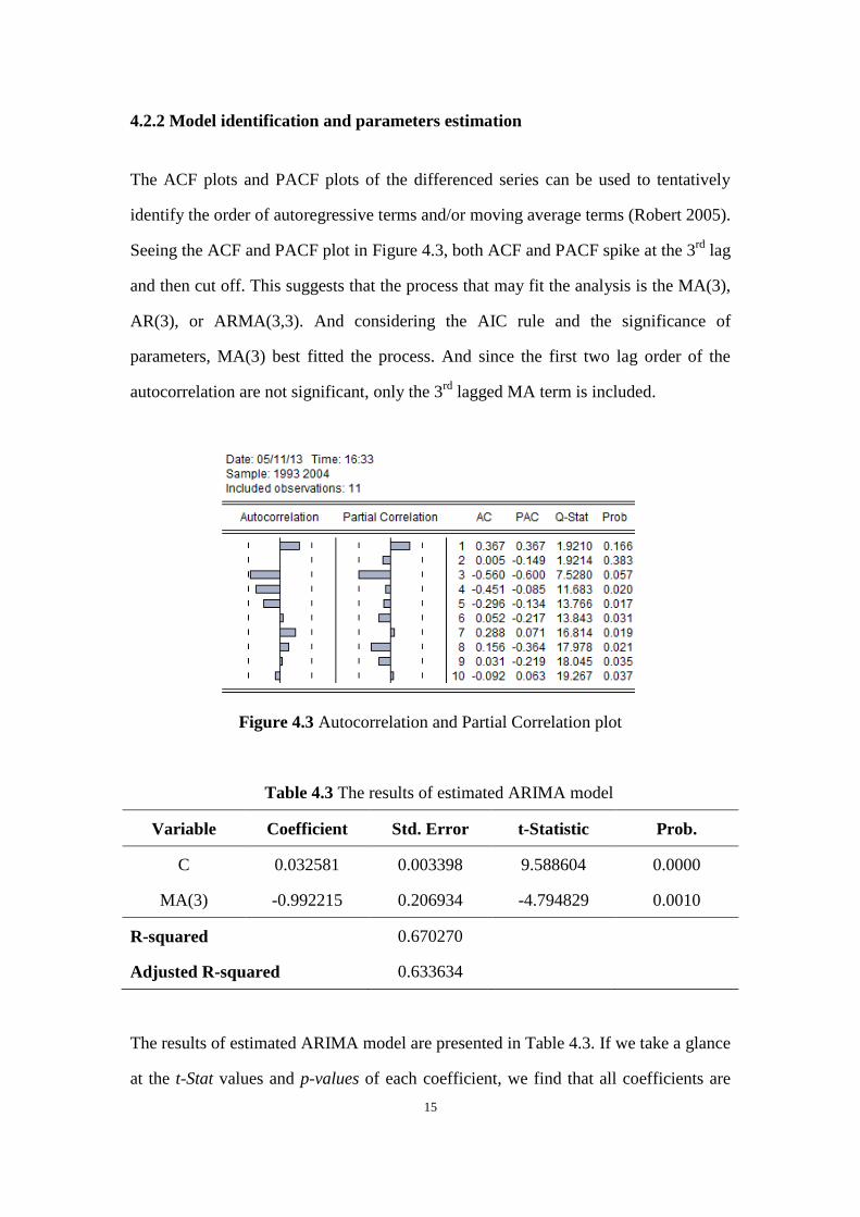
The ACF plots and PACF plots of the differenced series can be used to tentatively
identify the order of autoregressive terms and/or moving average terms (Robert 2005).
Seeing the ACF and PACF plot in Figure 4.3, both ACF and PACF spike at the 3rd
lag
and then cut off. This suggests that the process that may fit the analysis is the MA(3),
AR(3), or ARMA(3,3). And considering the AIC rule and the significance of
parameters, MA(3) best fitted the process. And since the first two lag order of the
autocorrelation are not significant, only the 3rd
lagged MA term is included.
Figure 4.3 Autocorrelation and Partial Correlation plot
Table 4.3 The results of estimated ARIMA model
Variable Coefficient Std. Error t-Statistic Prob.
C 0.032581 0.003398 9.588604 0.0000
MA(3) -0.992215 0.206934 -4.794829 0.0010
R-squared 0.670270
Adjusted R-squared 0.633634
The results of estimated ARIMA model are presented in Table 4.3. If we take a glance
at the t-Stat values and p-values of each coefficient, we find that all coefficients are
16
significantly different from zero for a confidence level of 95%.
As a result the fitted model is:
( )
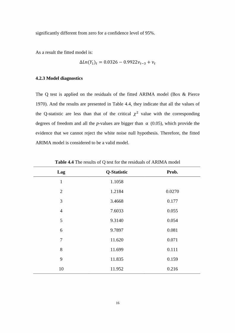
4.2.3 Model diagnostics
The Q test is applied on the residuals of the fitted ARIMA model (Box & Pierce
1970). And the results are presented in Table 4.4, they indicate that all the values of
the Q-statistic are less than that of the critical value with the corresponding
degrees of freedom and all the p-values are bigger than (0.05), which provide the
evidence that we cannot reject the white noise null hypothesis. Therefore, the fitted
ARIMA model is considered to be a valid model.
Table 4.4 The results of Q test for the residuals of ARIMA model
Lag Q-Statistic Prob.
1 1.1058
2 1.2184 0.0270
3 3.4668 0.177
4 7.6033 0.055
5 9.3140 0.054
6 9.7897 0.081
7 11.620 0.071
8 11.699 0.111
9 11.835 0.159
10 11.952 0.216
17
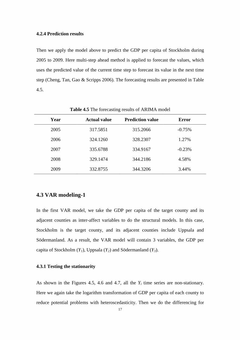
4.2.4 Prediction results
Then we apply the model above to predict the GDP per capita of Stockholm during
2005 to 2009. Here multi-step ahead method is applied to forecast the values, which
uses the predicted value of the current time step to forecast its value in the next time
step (Cheng, Tan, Gao & Scripps 2006). The forecasting results are presented in Table
4.5.
Table 4.5 The forecasting results of ARIMA model
Year Actual value Prediction value Error
2005 317.5851 315.2066 -0.75%
2006 324.1260 328.2307 1.27%
2007 335.6788 334.9167 -0.23%
2008 329.1474 344.2186 4.58%
2009 332.8755 344.3206 3.44%
4.3 VAR modeling-1
In the first VAR model, we take the GDP per capita of the target county and its
adjacent counties as inter-affect variables to do the structural models. In this case,
Stockholm is the target county, and its adjacent counties include Uppsala and
Södermanland. As a result, the VAR model will contain 3 variables, the GDP per
capita of Stockholm (Y1), Uppsala (Y2) and Södermanland (Y3).
4.3.1 Testing the stationarity
As shown in the Figures 4.5, 4.6 and 4.7, all the Yi time series are non-stationary.
Here we again take the logarithm transformation of GDP per capita of each county to
reduce potential problems with heteroscedasticity. Then we do the differencing for

18
each series, denoting the differenced time series as ( ).
Figure 4.5 The line plot of GDP per capita in Stockholm
Figure 4.6 The line plot of GDP per capita in Uppsala
1993 1995 1997 1999 2001 2003
220
240
260
280
300
Stockholm
year
GD
P p
er
ca
pita
(tk
r)
1993 1995 1997 1999 2001 2003
130
140
150
160
170
180
190
Uppsala
year
GD
P p
er
ca
pita
(tk
r)
19
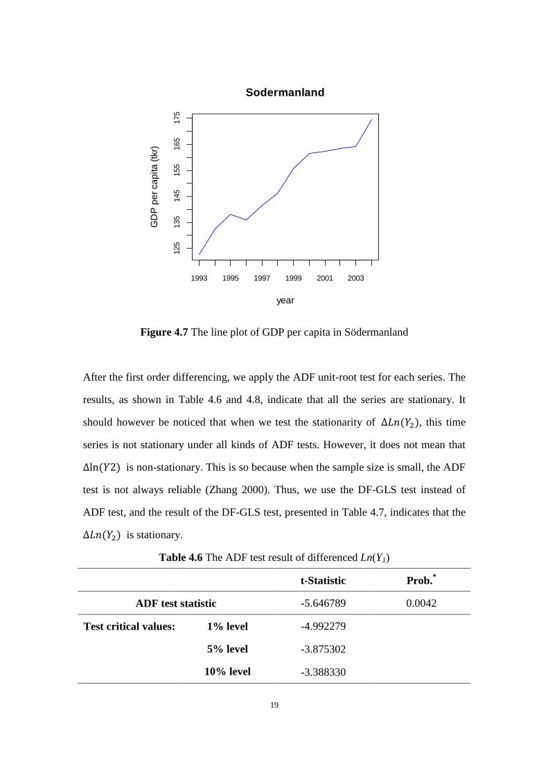
Figure 4.7 The line plot of GDP per capita in Södermanland
After the first order differencing, we apply the ADF unit-root test for each series. The
results, as shown in Table 4.6 and 4.8, indicate that all the series are stationary. It
should however be noticed that when we test the stationarity of ( ), this time
series is not stationary under all kinds of ADF tests. However, it does not mean that
( ) is non-stationary. This is so because when the sample size is small, the ADF
test is not always reliable (Zhang 2000). Thus, we use the DF-GLS test instead of
ADF test, and the result of the DF-GLS test, presented in Table 4.7, indicates that the
( ) is stationary.
Table 4.6 The ADF test result of differenced Ln(Y1)
t-Statistic Prob.*
ADF test statistic -5.646789 0.0042
Test critical values: 1% level
5% level
10% level
-4.992279
-3.875302
-3.388330
1993 1995 1997 1999 2001 2003
125
135
145
155
165
175
Sodermanland
year
GD
P p
er
ca
pita
(tk
r)

20
Table 4.7 The DF-GLS test result of differenced Ln(Y2)
t-Statistic Prob.*
DF-GLS test statistic -2.233120 0.0401
Test critical values: 1% level
5% level
10% level
-2.886101
-2.995865
-1.599088
Table 4.8 The ADF test result of differenced Ln(Y3)
t-Statistic Prob.*
ADF test statistic -3.617635 0.0382
Test critical values: 1% level
5% level
10% level
-4.803491
-3.403313
-2.841819
4.3.2 Model identification and parameter estimation
Since we only have 12 annual observations in the sample, when constructing the VAR
model, the number of lags could not be large. Given the minimum AIC and SC rules,
as shown in Table 4.9, and in order to avoid the loss of information, we determine that
the optimal number of lags is 2. Then there are 21 parameters to be estimated. The
result of the estimated model is presented in Table 4.10.
Table 4.9 VAR model-1 lag order selection criteria
Lag AIC SC
1 -4.20105 -4.25173
2 -4.40488* -4.39175*

21
Table 4.10 The result of estimated VAR model-1
( ) ( ) ( )
( )(-1) 0.339193
(0.53509)
[0.63390]
0.499960
(0.75704)
[0.66042]
0.157901
(0.29556)
[0.53424]
( )(-2) -0.213079
(0.58906)
[-0.36861]
0.294562
(0.81784)
[0.36017]
0.691388
(0.31930)
[2.16532]
( )(-1) 0.026123
(0.41503)
[0.06294]
-0.266387
(0.58718)
[-0.45367]
-0.157239
(0.22925)
[-0.68589]
( )(-2) -0.553319
(0.29470)
[-1.87758]
0.153307
(0.41694)
[0.36770]
-0.481125
(0.16278)
[-2.95567]
( )(-1) -0.211743
(0.45125)
[-0.4692]
0.740328
(0.63842)
[0.75118]
-0.641854
(0.24925)
[-2.57510]
( )(-2) -0.119832
(0.35107)
[-0.34133]
0.740328
(0.49669)
[1.49501]
-0.144210
(0.19392)
[-0.74366]
0.062069
(0.02646)
[2.34562]
-0.019556
(0.03744)
[-0.52237]
0.044531
(0.01462)
[3.04663]
Therefore, the estimated VAR model-1 can be expressed as following:
( ) ( ) ( ) ( )
( ) ( )
( )
( ) ( ) ( ) ( )
( ) ( )
( )
( ) ( ) ( ) ( )
( ) ( )
( )
22
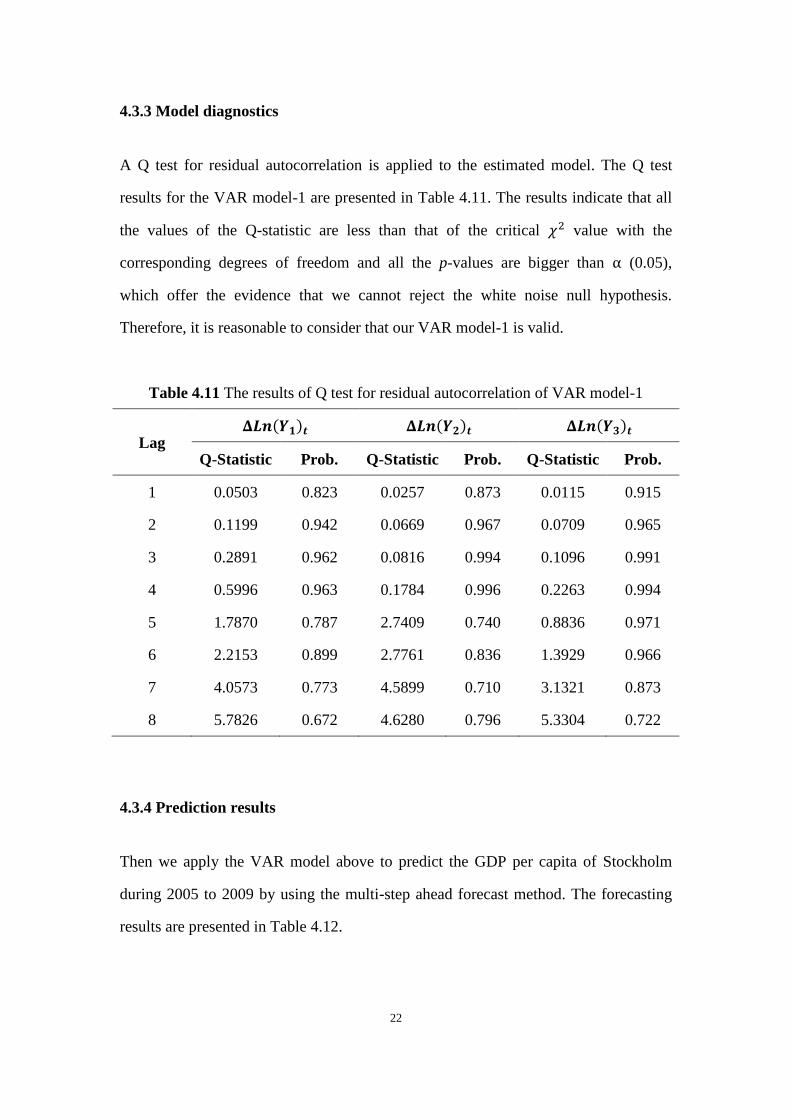
4.3.3 Model diagnostics
A Q test for residual autocorrelation is applied to the estimated model. The Q test
results for the VAR model-1 are presented in Table 4.11. The results indicate that all
the values of the Q-statistic are less than that of the critical value with the
corresponding degrees of freedom and all the p-values are bigger than (0.05),
which offer the evidence that we cannot reject the white noise null hypothesis.
Therefore, it is reasonable to consider that our VAR model-1 is valid.
Table 4.11 The results of Q test for residual autocorrelation of VAR model-1
Lag ( ) ( ) ( )
Q-Statistic Prob. Q-Statistic Prob. Q-Statistic Prob.
1 0.0503 0.823 0.0257 0.873 0.0115 0.915
2 0.1199 0.942 0.0669 0.967 0.0709 0.965
3 0.2891 0.962 0.0816 0.994 0.1096 0.991
4 0.5996 0.963 0.1784 0.996 0.2263 0.994
5 1.7870 0.787 2.7409 0.740 0.8836 0.971
6 2.2153 0.899 2.7761 0.836 1.3929 0.966
7 4.0573 0.773 4.5899 0.710 3.1321 0.873
8 5.7826 0.672 4.6280 0.796 5.3304 0.722
4.3.4 Prediction results
Then we apply the VAR model above to predict the GDP per capita of Stockholm
during 2005 to 2009 by using the multi-step ahead forecast method. The forecasting
results are presented in Table 4.12.
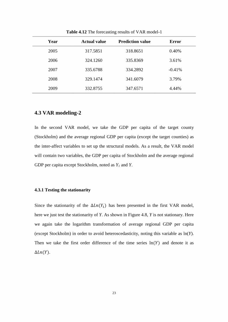
23
Table 4.12 The forecasting results of VAR model-1
Year Actual value Prediction value Error
2005 317.5851 318.8651 0.40%
2006 324.1260 335.8369 3.61%
2007 335.6788 334.2892 -0.41%
2008 329.1474 341.6079 3.79%
2009 332.8755 347.6571 4.44%
4.3 VAR modeling-2
In the second VAR model, we take the GDP per capita of the target county
(Stockholm) and the average regional GDP per capita (except the target counties) as
the inter-affect variables to set up the structural models. As a result, the VAR model
will contain two variables, the GDP per capita of Stockholm and the average regional
GDP per capita except Stockholm, noted as Y1 and Y.
4.3.1 Testing the stationarity
Since the stationarity of the ( ) has been presented in the first VAR model,
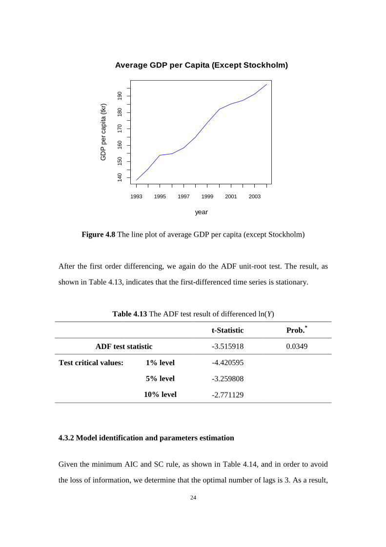
here we just test the stationarity of Y. As shown in Figure 4.8, Y is not stationary. Here
we again take the logarithm transformation of average regional GDP per capita
(except Stockholm) in order to avoid heteroscedasticity, noting this variable as ln(Y).
Then we take the first order difference of the time series ( ) and denote it as
( ).
24
Figure 4.8 The line plot of average GDP per capita (except Stockholm)
After the first order differencing, we again do the ADF unit-root test. The result, as
shown in Table 4.13, indicates that the first-differenced time series is stationary.
Table 4.13 The ADF test result of differenced ln(Y)
t-Statistic Prob.*
ADF test statistic -3.515918 0.0349
Test critical values: 1% level
5% level
10% level
-4.420595
-3.259808
-2.771129
4.3.2 Model identification and parameters estimation
Given the minimum AIC and SC rule, as shown in Table 4.14, and in order to avoid
the loss of information, we determine that the optimal number of lags is 3. As a result,
1993 1995 1997 1999 2001 2003
140
150
160
170
180
190
Average GDP per Capita (Except Stockholm)
year
GD
P p
er
ca
pita
(tk
r)

25
there are then 14 parameters to be estimated. The result of the estimated model is
presented in Table 4.15.
Table 4.14 VAR model-2 lag order selection criteria
Lag AIC SC
1 -4.41011 -4.31933
2 -3.82217 -3.71260
3 -4.71215 -4.64264
Table 4.15 The result of estimated VAR model-2
( ) ( )
( )( ) 0.386627
(0.48760)
[0.79292]
0.263411
(0.24788)
[1.06267]
( )( ) 0.624794
(0.067029)
[0.93212]
0.247666
(0.34075)
[0.72682]
( )( ) -0.524337
(0.68265)
[-0.76809]
0.057537
(0.34703)
[0.016580]
( )( ) -1.020122
(1.55965)
[-0.65407]
-0.270666
(0.79287)
[-0.80467]
( )( ) -0.019949
(0.60197)
[-0.03314]
-0.246245
(0.30602)
[-0.80467]
( )( ) -0.247727
(0.75328)
[-0.32887]
-0.352661
(0.38294)
[-0.92094]
C 0.054577
(0.04404)
[1.23923]
0.038507
(0.02239)
[1.71989]
Therefore, the estimated VAR model-2 can be expressed as follows:

26
( ) ( ) ( ) ( )
( ) ( ) ( )
( ) ( ) ( ) ( )
( ) ( ) ( )
4.3.3 Model diagnostics
VAR model-2 is also tested for the serial correlation. Q test for residual
autocorrelation is applied. The Q test results for the VAR model-2 are presented in the
Table 4.16. The results indicate that all the values of the Q-statistic are less than that
of the critical value with the corresponding degrees of freedom and all the
p-values are bigger than (0.05), which shows that we cannot reject the white noise
null hypothesis. Therefore, it is reasonable to consider that the VAR model-2 is valid.
Table 4.16 The results of Q test for residual autocorrelation of VAR model-2
Lag ( ) ( )
Q-Statistic Prob. Q-Statistic Prob.
1 4.0885 0.054 4.0736 0.053
2 4.0889 0.129 4.149 0.133
3 4.8787 0.181 4.7950 0.190
4 5.1220 0.276 5.0240 0.292
5 5.1163 0.402 5.0108 0.411
6 5.1222 0.528 5.1365 0.517
7 5.1224 0.645 5.1396 0.663

27
4.3.4 Prediction results
Then we again apply the VAR model above to predict the GDP per capita of
Stockholm during 2005 to 2009 by using the multi-step ahead forecast method. The
forecasting results are shown in Table 4.17.
Table 4.17 The forecasting results of VAR model-2
Year Actual value Prediction value Error
2005 317.5851 316.5259 -0.33%
2006 324.1260 338.1571 4.33%
2007 335.6788 324.9721 -3.19%
2008 329.1474 336.9865 2.38%
2009 332.8755 351.1386 5.49%
4.4 AR(1) modeling
In practice, a simple time series model could offer good forecasts of regional GDP. So
here we use an AR(1) model, that is an autoregression with one lag, to do the
forecasting. In order to keep the modeling as simple as possible, we ignore testing for
stationarity, white noise, etc.
4.4.1 Model specification
We use the time series data of Stockholm GDP per capita to fit the AR(1) model. The
model was estimated as presented in Table 4.18.

28
Table 4.18 The result of estimated AR(1) model
Variable Coefficient Std. Error t-Statistic Prob.
C 2125.875 31196.42 0.068145 0.9472
AR(1) 0.995690 0.072329 13.76606 0.0000
R-squared 0. 954661
Adjusted R-squared 0.949623
As a result, the AR(1) model can be expressed as following:
Therefore,
4.4.2 Prediction results
Then we apply the AR(1) model above to predict the GDP per capita of Stockholm
during 2005 to 2009. The forecasting results are presented in Table 4.19.
Table 4.19 The forecasting results of AR(1)
Year Actual value Prediction value Error
2005 317.5851 312.9179 -1.47%
2006 324.1260 325.3788 0.39%
2007 335.6788 331.8961 -1.13%
2008 329.1474 343.3946 4.33%
2009 332.8755 336.8913 1.21%
4.5 Performance comparison, Stockholm

29
We test and distinguish the performance of the different models for the purpose of
finding a better forecasting model. Figure 4.9 gives us a very clear picture of the
forecasting results from different models. And the percentage errors and mean
absolute percentage errors (MAPE) are used to evaluate the performance of different
autoregressive models (Diebold 1995). The results are presented in Table 4.20. The
measure of MAPE can be expressed as follows:
[ ⁄ ∑ (( ̂ ) ⁄ )
] ( )
where ̂ is the predicted value, is the actual value, and n indicates the number of
fitted points.
Figure 4.9 Actual value of GDP per capita and predicted values from ARIMA model,
VAR model-1, VAR model-2, AR(1) model for Stockholm
We find that, for 2008 when the economic crisis took place, each model offers a
prediction with a big percentage error. Therefore, when we assess the performance of
2005 2006 2007 2008 2009
32
03
30
34
03
50
Year
GD
P p
er
ca
pita
(tkr)
Actual valueARIMAVAR-1VAR-2AR(1)

30
the different models, we offer two kinds of MAPE, one is with 2008, and the other
without 2008. If we are just focusing on the prediction accuracy of the models,
obviously, the AR(1) model is the best one in forecasting the GPD per capita in the 5
years with less than 2% mean absolute percentage error. Then the next is the ARIMA
model, the VAR model-1 and the VAR model-2.
Table 4.20 The percentage error of different models for Stockholm
Stockholm Year ARIMA VAR-1 VAR-2 AR(1)
Percentage
error
2005 -0.75% 0.40% -0.33% -1.47%
2006 1.27% 3.61% 4.33% 0.39%
2007 -0.23% -0.41% -3.19% -1.13%
2008 4.58% 3.79% 2.38% 4.33%
2009 3.44% 4.44% 5.49% 1.21%
MAPE 2.05% 2.53% 3.14% 1.71%
MAPE except 2008 1.42% 2.22% 3.34% 1.05%
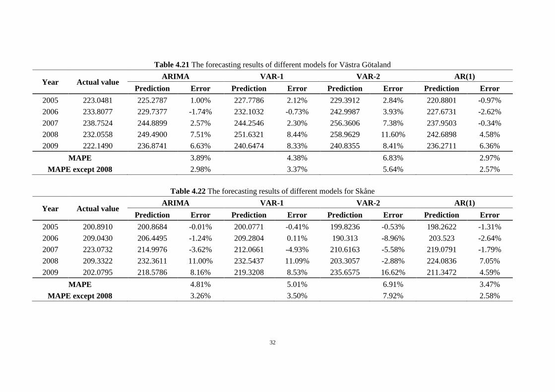
4.6 Predictive performance, four other regions
In this thesis, we used the same method to do the forecasts for four other counties
with top GDP per capita in Sweden. These counties include Västra Götaland, Skåne,
Östergötland, and Jönköping. Similarly, three kinds of models, ARIMA model, VAR
model and AR(1) model, were applied to predict GDP per capita for these four
counties and the performance of the different models was compared as shown in the
following tables.
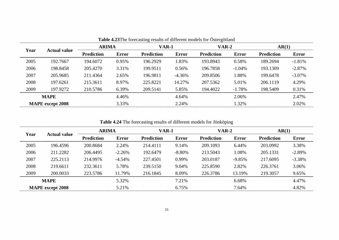
As seen in the Table 4.21, 4.22, 4.23 and 4.24, generally, the performance of the
AR(1) model is impressive. For Västra Götaland, Skåne and Jönköping, the forecast
accuracy of the AR(1) model is better than the other three kinds of models with less

31
than 5% mean absolute percentage error, and the performance of the ARIMA model is
better than that of the VAR models. However, for Östergötland, there is an exception
in that the VAR-2 model is the best one when forecasting the GDP per capita.
Similarly, when the different models are applied to forecast the GDP per capita in
2008, the results are less encouraging due to the impact of the financial crisis on the
forecasts.
32
Table 4.21 The forecasting results of different models for Västra Götaland
Year Actual value ARIMA VAR-1 VAR-2 AR(1)
Prediction Error Prediction Error Prediction Error Prediction Error
2005 223.0481 225.2787 1.00% 227.7786 2.12% 229.3912 2.84% 220.8801 -0.97%
2006 233.8077 229.7377 -1.74% 232.1032 -0.73% 242.9987 3.93% 227.6731 -2.62%
2007 238.7524 244.8899 2.57% 244.2546 2.30% 256.3606 7.38% 237.9503 -0.34%
2008 232.0558 249.4900 7.51% 251.6321 8.44% 258.9629 11.60% 242.6898 4.58%
2009 222.1490 236.8741 6.63% 240.6474 8.33% 240.8355 8.41% 236.2711 6.36%
MAPE 3.89%
4.38% 6.83%
2.97%
MAPE except 2008 2.98%
3.37%
5.64%
2.57%
Table 4.22 The forecasting results of different models for Skåne
Year Actual value ARIMA VAR-1 VAR-2 AR(1)
Prediction Error Prediction Error Prediction Error Prediction Error
2005 200.8910 200.8684 -0.01% 200.0771 -0.41% 199.8236 -0.53% 198.2622 -1.31%
2006 209.0430 206.4495 -1.24% 209.2804 0.11% 190.313 -8.96% 203.523 -2.64%
2007 223.0732 214.9976 -3.62% 212.0661 -4.93% 210.6163 -5.58% 219.0791 -1.79%
2008 209.3322 232.3611 11.00% 232.5437 11.09% 203.3057 -2.88% 224.0836 7.05%
2009 202.0795 218.5786 8.16% 219.3208 8.53% 235.6575 16.62% 211.3472 4.59%
MAPE
4.81%
5.01%
6.91%
3.47%
MAPE except 2008
3.26%
3.50%
7.92%
2.58%
33
Table 4.23The forecasting results of different models for Östergötland
Year Actual value ARIMA VAR-1 VAR-2 AR(1)
Prediction Error Prediction Error Prediction Error Prediction Error
2005 192.7667 194.6072 0.95% 196.2929 1.83% 193.8943 0.58% 189.2694 -1.81%
2006 198.8458 205.4270 3.31% 199.9511 0.56% 196.7858 -1.04% 193.1309 -2.87%
2007 205.9685 211.4364 2.65% 196.9811 -4.36% 209.8506 1.88% 199.6478 -3.07%
2008 197.6261 215.3611 8.97% 225.8221 14.27% 207.5362 5.01% 206.1119 4.29%
2009 197.9272 210.5786 6.39% 209.5141 5.85% 194.4022 -1.78% 198.5409 0.31%
MAPE
4.46%
4.64%
2.06% 2.47%
MAPE except 2008 3.33%
2.24%
1.32%
2.02%
Table 4.24 The forecasting results of different models for Jönköping
Year Actual value ARIMA VAR-1 VAR-2 AR(1)
Prediction Error Prediction Error Prediction Error Prediction Error
2005 196.4596 200.8684 2.24% 214.4111 9.14% 209.1093 6.44% 203.0992 3.38%
2006 211.2282 206.4495 -2.26% 192.6479 -8.80% 213.5043 1.08% 205.1331 -2.89%
2007 225.2113 214.9976 -4.54% 227.4501 0.99% 203.0187 -9.85% 217.6095 -3.38%
2008 219.6611 232.3611 5.78% 239.5150 9.04% 225.8590 2.82% 226.3761 3.06%
2009 200.0033 223.5786 11.79% 216.1845 8.09% 226.3786 13.19% 219.3057 9.65%
MAPE
5.32%
7.21%
6.68%
4.47%
MAPE except 2008 5.21%
6.75%
7.64%
4.82%

34
5. Discussion and Conclusions
The purpose of this thesis is to test and distinguish which of the three time series
models performs best in forecasting regional GDP per capita. Here, three kinds of
models were taken into consideration, the ARIMA, VAR and AR(1) models. In the
empirical analysis, 17 annual observations from 1993 to 2009 are available. The
original data are separated into 12 in-sample years (1993-2004), thus using
approximately 70% of the original data for fitting the model, and 5 out-of-sample
years (2005-2009) for prediction. Since there are so few observations in total
available, increasing the size of the out-of-sample data is difficult and would probably
decrease the accuracy of the forecasts.
As the sample size is very small, with only 12 annual observations available for each
region, the performance of complex models is very limited. Taking Stockholm as an
example, the mean absolute percentage error of two kinds of VAR models are 2.53%
and 3.14%, respectively. The performance of the ARIMA model is better than the
VAR models with a 2.05% mean absolute percentage error. However, the
performance of the simplest time series model, the AR(1) model, is impressive by
offering a 5 year prediction with only 1.71% mean absolute percentage error. The
results are similar for the three of the other four regions, Västra Götaland, Skåne, and
Jönköping. However, for Östergötland, there is an exception in that the performance
of the VAR model-2 is the best.
In practice, we often face the situation that the number of observations we can get is
few. However, the decision makers still need to forecast the economic development
and decide the government policy. Based on the analysis above, under such conditions,
the simple AR(1) model is still quite useful. Sometimes, as shown in this empirical

35
study, the performance of the AR(1) model is even better than other complex ones.
Obviously, the prediction of GDP per capita is very complicated, since the value is
affected by a great deal of factors, such as prices, disasters, and the economic crisis
and so on. Therefore, the simple time series models are not always enough to offer an
accurate prediction of GDP per capita. However, for short-term forecasting, the
results of time series models could be used as preliminary predictions, which can be
used for the regional government to draw up economics plans and policies.

36
References
Akaike, H. (1974). A New Look at the Statistical Model Identification. IEEE
Transactions on Automatic Control, 19 (6), 716–723.
Box, G. E. P. & Jenkins, G. M. (1976). Time Series Analysis: Forecasting and
Control. University of Michigan: Holden-Day.
Box, G. E. P. & Ljung, G. M. (1978). On a Measure of Lack of Fit in Time Series
Models. Biometrika, 65(2), 297–303.
Box, G. E. P. & Pierce. D. A. (1970). Distribution of Residual Autocorrelations in
Autoregressive-Integrated Moving Average Time Series Models. Journal of the
American Statistical Association, 65(332), 1509–1526.
Chen, X. (2011). We cannot negate the significance of GDP. Global Times, 8(1),
23-25.
Cheng, H., Tan, P. -N., Gao, J., & Scripps, J. (2006). Multi-step ahead time series
prediction. In W. K. Ng, M. Kitsuregawa, J. Li, & K. Chang (Eds.) PAKDD. Lecture
notes in computer science, 3918(2006), 765-774.
Clarida, R. H. & Friedman, B. M. (1984). The Behavior of U.S. Short-term Interest
Rates since October 1979. The Journal of Finance, 39(3), 671-682.
Diebold, F. X. & Mariano, R. S. (1995). Comparing predictive accuracy. Journal of
Business and Statistics, 13 (3), 253–263.
37
Enders, W. (2003). Applied Econometric Time Series, 2nd Edition, John Wiley &
Sons.
Feng, H., & Liu, J. (2003). A SETAR model for Canadian GDP: Non-linearities and
Forecast Comparisons. Applied Economics, 35(18), 1957-1964.
Hamilton, J. D. (1994). Time Series Analysis. Princeton University Press: Princeton,
NJ.
Harvey, A. C. (1989). Forecasting, Structural Time Series Models and the Kalman
Filter. UK: Cambridge University Press, Cambridge.
Harvey, D. I., Leybourne, S. J. & Newbold, P. (1998). Tests for forecast
encompassing. Journal of Business and Economic Statistics, 16(2), 254–259.
Johansen, S. (1995). Likelihood-Based Inference in Cointegrated Vector
Autoregressive Models. Oxford: Oxford University Press.
Larsson, H. & Harrtell, E. (2007). Does choice of transition model affect GDP per
capita growth? Jönköping University: JIBS, Economics.
Mankiw, N. G. & Taylor, M. P. (2007). Macroeconomics. New York: Worth.
Mei, Q., Liu, Y. & Jing, X. (2011). Forecast the GDP of Shanghai Based on the
Multi-factors VAR Model. Journal of Hubei University of Technology, 26(3).
Robert, F. N. (2005). Identifying the numbers of AR or MA terms. Available from:
http://people.duke.edu/~rnau/411arim3.htm[Accessed 20 February 2013]
38
Sheng, Y. (2006). Forecast the GDP per Capita of Zhejiang Province Based on the BP
Neural Network and ARIMA Model. Journal of Modern Shopping Malls, 23(1).
Sims, C. A. (1980). Macroeconomics and Reality. Economatrica, 48(1), 1-48.
Sims, C. A., Stock, J. H. & Watson, M. W. (1990). Inference in Linear Time Series
Models With Some Unit Roots. Econometrica, 58(1), 113-144.
Wang, Z. & Wang, H. (2011). GDP Prediction of China Based on ARIMA Model.
Journal of Foreign Economic and Trade, 210(12).
Wei, N., Bian, K. J. & Yuan, Z. F. (2010). Analyze and Forecast the GDP of Shaanxi
Province Based on the ARIMA Model. Journal of Asian Agricultural Research, 2(1),
34-41.
Yan, X. (2011). Be vigilant about the misleading of GDP per capita. Global Times.
8(1), 30-33.
Yan, R. & Zhu, X. (2003). The analysis of significance and critique of GDP. Journal
of economic study of quantity economic and technical. 1(3).
Yang, S., Wu, Y. & Wang, Z. (1991). Engineering Apply of Time Series Analysis.
Wuhan Province: Huazhong University of Science and Engineering.
Zhang, X. (2000). The analysis of econometrics. Beijing: Economics and Science.
Related Documents