Modeling and Design of Integrated Optical Microresonator with Rectangular Cavity Shapes Didit Yudistira June, 2003

Welcome message from author
This document is posted to help you gain knowledge. Please leave a comment to let me know what you think about it! Share it to your friends and learn new things together.
Transcript

Modeling and Design of Integrated OpticalMicroresonator with Rectangular Cavity
Shapes
Didit Yudistira
June, 2003
Contents
1 Introduction 3
1.1 Background . . . . . . . . . . . . . . . . . . . . . . . . . . . . . 3
1.2 Objective . . . . . . . . . . . . . . . . . . . . . . . . . . . . . . . 4
1.3 Notation and Assumptions . . . . . . . . . . . . . . . . . . . . . 5
1.4 Organisation of the thesis . . . . . . . . . . . . . . . . . . . . . 5
2 Coupled-mode theory modeling 7
2.1 Codirectional Propagation along Parallel Multimode Waveg-uides . . . . . . . . . . . . . . . . . . . . . . . . . . . . . . . . . 8
2.2 Reflector-Bragg Waveguide . . . . . . . . . . . . . . . . . . . . . 14
2.3 CMT Microresonator Model . . . . . . . . . . . . . . . . . . . . 22
2.3.1 Resonant State . . . . . . . . . . . . . . . . . . . . . . . 24
3 Applications of the Formulation 28
3.1 Structural parameters . . . . . . . . . . . . . . . . . . . . . . . 29
3.1.1 Port waveguides . . . . . . . . . . . . . . . . . . . . . . . 29
3.1.2 Bragg-grating . . . . . . . . . . . . . . . . . . . . . . . . 30
3.1.3 Cavity waveguide . . . . . . . . . . . . . . . . . . . . . . 31
3.2 Simulation results . . . . . . . . . . . . . . . . . . . . . . . . . . 34
3.2.1 Symmetric Bragg-reflectors . . . . . . . . . . . . . . . . 34
3.2.2 Nonsymmetric Bragg-reflectors . . . . . . . . . . . . . . 40
3.2.3 Filter simulations . . . . . . . . . . . . . . . . . . . . . . 41
1

CONTENTS 2
4 Conclusions and remarks 49
A Cholesky Decomposition 51
B Matlab Code 53
Bibliography 61
Acknowledgment 64

Chapter 1
Introduction
1.1 Background
In the past years, the technological progress in the field of integrated op-tics has opened up possibilities for the realisation of optical devices withhigher complexity and integration density. In applications especially in op-tical communications, optical wavelength division multiplexing (WDM) is amajor objective of the current research efforts. Some promising device con-cepts have been investigated and developed using micoresonator elementsas basic building blocks [11]. The typical microresonator device consists oftwo parallel straight waveguides and a small optical cavity placed betweenthese two in which the waveguides function as input and output ports. Thecharacteristic spectral response enables the design of microresonator de-vices with a variety of functionalities, e.g. filtering, switching, routing, ormodulation.
In the past few years, in particular microresonator with cylindrical [10]cavity shapes have been investigated. Rectangular cavity shapes have alsoattracted some interests [14, 15, 12], but only quite recently. However inapplications the conventional form of rectangular cavity shapes requires anextremely high refractive index contrast for the total reflection at facets ofthe cavity segment [7]. In order to deal with this problem, a way out isfound by replacing the waveguide facets by Bragg reflectors [8]. This leadsto device similiar to the well known Fabry-Perot resonator concept. The
3

CHAPTER 1. INTRODUCTION 4
devices itself is then called a grating assisted rectangular optical microres-onator.
At least in a two dimensional setting the structures can be analysed quiterigorously by means of finite differences, bidirectional eigenmode propa-gation (BEP), and mode expansions. Because of rigorousness, these ap-proaches give only little insight into the design principles of the structure.For this purpose in this thesis we will analyse the structure by means ofcoupled-mode theory (CMT)[5].
In this analytical approximate approach, the total field of the coupled waveg-uides is expressed as a linear combination of the modal fields supported bythe individual waveguides. The power transfer between the propagatingmodes is described by the coupled-mode equations for the modal ampli-tudes. Coupling effects are characterised only by the coupling coefficientsand therefore it is easily applied when the number of waveguides increases.In particular the coupled-mode theory allows to consider the cavity sep-arated from the port waveguide and grating segment. The formulationresembles that given in Ref. [13] for the unidirectional light propagationalong a three waveguide coupler where forward and backward travelingfield are considered simultanously.
1.2 Objective
As stated generally in the previous section the purpose of this thesis is toinvestigate the grating assisted rectangular microresonators using coupled-mode theory as a basic simulation tool [5]. The coupled-mode technique hasoccupied an important place in applied mathematics and physics becausethe perturbational expansions are useful for a qualitative as well as quan-titative approximation representation of the solution. The investigationis limited to the 2D problem and the resonant wavelength interests else-where around λ0 = 1.55µm. The wavelength range is of interest to be inbetween 1.5µm and 1.6µm. The present thesis uses a coupled-mode formu-lation based on perturbation techniques and a assumption that the individ-ual waveguide modes are nonorthogonal. The basic idea of the formulationwas originally presented by Hammer [6] for rectangular microresonatorswithout Bragg-reflectors. Here, we will do calculations for devices with

CHAPTER 1. INTRODUCTION 5
Bragg-reflectors. We will apply this formulation to several specified con-figurations of the microresonators. The validity of the formulation will beconfirmed by comparing with more accurate numerical simulations with acommercial tool Olympios [3] based on bidirectional eigenmode propagation(BEP).
1.3 Notation and Assumptions
The optical electromagnetic field consists of electric part E(x, z, t) and mag-netic part H(x, z, t). Note that these are vector fields, which means that atany point in space (x, z) and at any time t, both E and H are (where weadopt common complex notation) vectors that can differ at every position,and can point in any direction. In this thesis, time harmonic electromag-netic waves are investigated. A time dependence of a monochromatic waveejωt is always assumed with j =
√−1. The expression is usually omitted.The constant angular frequency a ω = kc = 2πc/λ is related to the vacuumwavenumber k, to the vacuum speed of light c ,and to the vacuum wave-length λ. All dielectrics under consideration are linear, isotropic, losslessmedia, and the permeability µ of free space is assumed. When applyingCMT, we shall deal with only guided mode waves propagating along thewaveguide structures, and in that case the radiative parts of the field areignored. It is customary to normalise the mode profiles such that the arbi-trary normalisation constant is equal to 1, and can therefore be omitted; sothat any modal field Ei and Hi will always be normalised as
∫
A∞[Ei ×Hi] · zdA = 1
In all simulations we assume that the fields TE polarised.
1.4 Organisation of the thesis
This thesis is organised as follows. This Chapter 1 gives an introduction. Itshows the backgrounds and objective of our study. The notation rules andassumptions are also presented in this chapter.
CHAPTER 1. INTRODUCTION 6
In Chapter 2, the coupled-mode theory modeling for a grating assisted rect-angular microresonator problem is explained in detail. We will start withthe analysis of codirectional propagation in parallel multimode waveguidesand it is followed by the analysis of Bragg-reflectors with so-called contradi-rectional coupled-mode theory. In Section 2.3 these analyses are combinedand yield a single coupled-mode formulation for the corresponding problem.In a subsection of Section 2.3, we also explain in detail about the character-istics of resonance in the cavity.
The application of the coupled-mode formulation will be presented in Chap-ter 3. The first application considered in Section 3.1 is an analysis of thestructural parameters of the device and the procedure to select them. Next,the implementation of CMT to three different configuration settings of theresonator is presented. We verify the CMT results by comparison with rig-orous numerical computations (BEP) with Olympios.
In Chapter 4, the results obtained throughout this study are briefly sum-marised, and also some remarks regarding the performance of CMT com-pared to Olympios in terms of computation times and computer efficiencyare given.

Chapter 2
Coupled-mode theorymodeling
The geometry of the grating assisted rectangular microresonator is shownin Fig. 2.1. The device consists of two parallel waveguide cores of width
D
C
B
A
L
p
0
x
z
s
w
p
ng
ng
1 ... N
d
W
nb
!!!!!!
""""""
####$$$$
Figure 2.1: Schematic of a grating assisted rectangular microresonator
w, the port waveguides which are coupled by a cavity waveguide of widthW and length L, separated by gaps d. In addition gratings with Np peri-ods of length p with a spacing s enclose the cavity. The refractive index of
7

CHAPTER 2. COUPLED-MODE THEORY MODELING 8
guiding regions is denoted by ng and nb denotes the refractive index of thebackground medium. Capital letters A to B denote the input and outputports.
From this figure we see that the problem for the entire resonator indeedbecomes complicated. Rather than doing the calculation in one time for thewhole structure, in this thesis we propose to investigate the structure partlyby splitting the problem in two separated problems, namely the cavity seg-ment and the grating problem (left and right grating). Thus we will get twosets of coupled-mode equations, one for the cavity segment and another onefor the grating part, which can be solved independently. After that we com-bine the two solutions to a complete solution of the resonator problem. Forsimplification, when deriving the coupled-mode theory for the grating part,we neglect the presence of the port waveguides. This simplification leads toa model of ordinary contradirectional coupling for the grating problem. Anillustration of the splitted structure is given in Fig. (2.2).
The problems are treated as follows. We start with a CMT model for thecavity segment, continue with a model for the grating structure, and finallywe combine them.
2.1 Codirectional Propagation along ParallelMultimode Waveguides
The region 0 < z < L of the microresonator can be regarded as a symmet-rical directional coupler which consists of three parallel waveguides, whereWG I and WG II are called the port waveguides, and WG III is called thecavity waveguide, as illustrated by Fig. (2.3). In an isolated condition, theport waveguides with thickness w are supposed to support only one mode,whereas the cavity with thicknessW may support more than one mode. Thebasis fields are given by the electric part Ek = (0, Ek,y, 0) and magnetic partHk = (Hk,x, 0, jHk,z) of the mode profile, with real components Ek,x, ..., Hk,z
depending on the transverse coordinates only. By solving Maxwell equa-tions, the modal fields of the isolated waveguides are given by:
E+k (x, z) = E+
k (x) exp[−jβkz],

CHAPTER 2. COUPLED-MODE THEORY MODELING 9
0
x
z
+
+
~=
Figure 2.2: The illustration of the approximated model of the grating as-sisted rectangular microresontor
CHAPTER 2. COUPLED-MODE THEORY MODELING 10
H+k (x, z) = H+
k (x) exp[−jβkz] (2.1)
for the forward propagating fields with k = I, II, III indicating the waveg-uide. Based on inversion symmetry in the−z direction, the following set offields will also be solutions to the Maxwell equations [4]
E−k (x, z) = E−k (x) exp[jβkz]
H−k (x, z) = H−k (x) exp[jβkz], (2.2)
where the basis fields for forward propagating modes are given by the elec-tric part E+
k = (0, Ek,y, 0), and the magnetic part H+k = (Hk,x, 0, jHk,z),
while the basis fields for backward propagating fields are given by E−k =(0, Ek,y, 0) and H−
k = (−Hk,x, 0, jHk,z). With the convention E+k = E−k = Ek
and H+k = Hk. In the two sets of solutions above, βk is a positive number
which denotes the propagation constant of mode k at frequency ω corre-sponding to wavelength λ in vacuum.
In this section, we derive a CMT of the problem by considering the forward
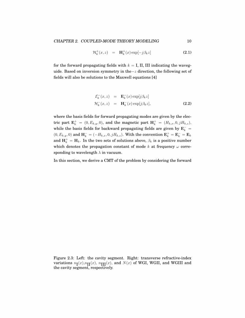
Figure 2.3: Left: the cavity segment. Right: transverse refractive-indexvariations nI(x),nII(x), nIII(x), and N(x) of WGI, WGII, and WGIII andthe cavity segment, respectively.

CHAPTER 2. COUPLED-MODE THEORY MODELING 11
and the backward propagating fields separately. The forward and back-ward propagating optical electromagnetic fields in the cavity segment areassumed to be superpositions:
(EH
)+
(x, z) =∑
i
Fi(z)
(E
H
)+
i
, (2.3)
(EH
)−
(x, z) =∑
i
Bi(z)
(E
H
)−
i
(2.4)
of the single modes. Here Fi(z) and Bi(z) denote the modal amplitudes ofthe fields propagating in the +z and −z direction, respectively. The fol-lowing derivation is based on the forward propagating fields. The sameprocedure will be used for the backward propagating field.
From Maxwell equations, the following reciprocity identity can be derivedstraight forward [16].
div((E+k )∗ ×H+ − (H+
k )∗ × E+) = −jωε(N − nk)(E+
k )∗E+ (2.5)
Substituting Eq. (2.3) into the reciprocity relation Eq. (2.5). That yields
∑
i
M+ki(∂zFi(z) + jβkFi(z)) = −j
∑
i
(K+ki)
IFi(z) (2.6)
with M+ki is given by
M+ki =
14
∫ ∞
−∞((E+
k )∗ ×H+i + E+
i × (H+k )∗) · zdx, (2.7)
and (K+ki)
I is given by
(K+ki)
I =14ωεo
∫ ∞
−∞(N2 − n2
k)(E+k )∗ ·E+
i dx. (2.8)
Due to the fact that E+k = Ek and H+
k = Hk, furthermore the superscriptsymbol + can be omitted.

CHAPTER 2. COUPLED-MODE THEORY MODELING 12
We can invoke the reciprocity theorem a second time, now in the form
div(E∗k ×Hi −H∗k × Ei) = −jωε0(n2i − n2
k)(Ek)∗ · Ei. (2.9)
Substituting Eq. (2.1) into Eq. (2.9), and inserting KIIki yields
Mki(βi − βk) = KIki −KII
ki , (2.10)
where KIIki is given by
KIIki =
14ωεo
∫ ∞
−∞(n2
i − n2k)(Ek)∗ ·Eidx (2.11)
If βk and KIki in Eq. (2.6) are replaced by Eq. (2.10), that leads to the
following equation
∑
i
Mki(∂zFi(z) + jβiFi(z)) = −j∑
i
KIIki Fi(z). (2.12)
Combination of Eq. (2.6) and Eq. (2.12) yields the coupled-mode equation
∑
i
Mki∂zFi = − j2
∑
i
Mki(βk + βi)Fi − j∑
i
KkiFi (2.13)
where the coupling coefficients Kki are defined by
Kki =18ωεo
∫ ∞
−∞(2N2 − (n2
k + n2i ))E
∗k ·Eidx (2.14)
In matrix form, Eq. (2.13) can be written as
S∂zF = −j(Q + K)F (2.15)
with real symmetric matrices S = (Mki), Q = (Mki(βi + βk)/2), and Hermi-tian K = (Kki) due to the lossless materials.
The solution of Eq. (2.15) can be found by taking the particular ansatz [6]:

CHAPTER 2. COUPLED-MODE THEORY MODELING 13
F(z) =∑
s
fsas exp(−jβsz) (2.16)
where in this equation βs are the the so-called supermode propagation con-stants and as are the corresponding amplitude vectors . If we substitutethis ansatz into Eq. (2.15), it leads to the generalised eigenvalue problem(EVP)
(Q + K)as = βsSas (2.17)
with vectors as satisfying the orthogonality properties (ar)TSas = δrs, whereδrs is the Kronecker delta, δrr = 1 and 0 otherwise . Eq. (2.17) can be solvedwith Cholesky decomposition by splitting the matrix as S = CTC to findthe supermode propagating coefficients βs and the vectors as (see AppendixA). The coefficients fs are defined as fs = (as)TSF(0) such that the gen-eral solution of Eq. (2.15) for the forward propagating along the segment0 < z < L can be written as
F(L) = T(L)F(0) (2.18)
with
T(L) =
(∑s
exp(−jβsL)as(as)T)
S (2.19)
The same procedure is carried out for the backward propagating fields,yielding the general solution :
B(0) = T(L)B(L). (2.20)
This equation describes the fields which propagate along the cavity segmentfrom z = L to z = 0.

CHAPTER 2. COUPLED-MODE THEORY MODELING 14
2.2 Reflector-Bragg Waveguide
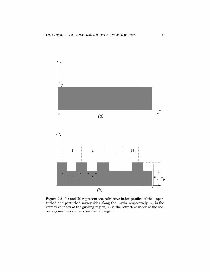
Fig. (2.4) sketches the geometry of the Bragg-reflector structure which isto be investigated. The refractive index profile of the structure is shownin Fig. (2.5b). The grating can be seen as a perturbed structure of theunperturbed one that is shown Fig. (2.5). When the medium is lossless andtranslational invariant in the z−direction, we know that the field solutionsdefined by the width W of unperturbed structure of the form given by Eq.(2.1) exist that correspond to fields propagating in the +z direction and Eq.(2.2) for the fields propagating in the −z direction.
In this section we formulate Coupled-Mode Equations (CME) of the problemby considering the forward and backward propagating fields simultanously.Therefore, it is assumed that the mode fields of the perturbed structure areapproximated by a weighted sum of the forward and backward propagatingfields of the unperturbed one, with z- dependent modal amplitudes:
(EH
)(x, z) =
∑
i
Fi(z)
(E
H
)+
i
(x) +∑
i
Bi(z)
(E
H
)−
i
(x)(2.21)
Substituting this trial field into the reciprocity relation
x
z0
n
W
g
Figure 2.4: Top view of the Bragg grating structure
CHAPTER 2. COUPLED-MODE THEORY MODELING 15
1
g
z
bn
z
0
n
n
s ng
N
(a)
(b)
...p
N2
p
Figure 2.5: (a) and (b) represent the refractive index profiles of the unper-turbed and perturbed waveguides along the z-axis, respectively. ng is therefractive index of the guiding region, nb is the refractive index of the sec-ondary medium and p is one period length.

CHAPTER 2. COUPLED-MODE THEORY MODELING 16
div((E(+,−)k )∗ ×H− (H(+,−)
k )∗ × E) = −jωε(N − nk)(E(+,−)
k )∗E , (2.22)
and integration along the x−axis, after substituting first Eq. (2.1) and sec-ondly Eq. (2.2) into Eq. (2.22), yields to the following set of equations:
∑
i
M+ki(∂zFi + jβkFi) = −j
∑
i
Kki(Fi +Bi) (2.23)
and
∑
i
M−ki(∂zBi − jβkBi) = −j
∑
i
Kki(Fi +Bi). (2.24)
In Eq. (2.22) N and nk associate with the refractive index of perturbed andunperturbed structure, respectively (see Fig. (2.5)). The parameters M (+,−)
ki
are the power coupling coefficients, where M+ki is given by Eq. (2.7) and M−
ki
is expressed by
M ,−ki =
14
∫ ∞
−∞((E−k )∗ ×H−
i + E−i × (H−k )∗) · zdx. (2.25)
The parameters Kki are the so-called coupling coefficients:
Kki =14ωεo
∫ ∞
−∞(N2 − n2
i )(Ek)∗ ·Eidx (2.26)
Eqs (2.23) and (2.24) describe the most general case of mode coupling due to(not necessarily) a periodic dielectric perturbation. In practice, often onlythe coupling between two modes is relevant. Since we are investigating thecontra-directional grating-assisted reflector problem, the coupling interestsbetween one mode traveling in positive z−direction and the correspondingmode traveling in the opposite direction. Neglecting the interaction withany of the other modes, the sum in Eqs. (2.23) and (2.24) can be omittedand the equations turn out to be in the form :
(∂zF + jβF ) = −jK(F +B)M+
, (2.27)
and

CHAPTER 2. COUPLED-MODE THEORY MODELING 17
(∂zB − jβB) = −jK(F +B)M− . (2.28)
Since E+ = E− = E, the power coupling coefficients then become.
M− = −M+ = − β
2ωµ0
∫ ∞
−∞|Ey|2 dx, (2.29)
Let us introduce a new parameter κ associated with the coupling coefficient,defined by
κ(z) =12ωε0
∫∞−∞(N2 − n2) |Ey|2 dx
βωµ0
∫∞−∞ |Ey|2 dx
. (2.30)
Substitution of Eqs. (2.29) and Eq. (2.30) into Eq. (2.27) and Eq.(2.28) leadsto CME, which read in matrix form
∂
∂z
[F
B
]= −j
[β + κ κ
−κ −(β + κ)
][F
B
](2.31)
The difficulty of Eq. (2.31) is that the coupling coefficient is still z-dependentin a complicated way, because N is z-dependent. This dependence can betaken out of the coupling coefficient if it is assumed that the perturbationis small and separable into a x- and z-component [2]. For this case, we canwrite N(x, z) = n(x) + ∆ng(x)f(z) and
n(x) =
ng for −W/2 ≤ x ≤W/2nb for otherwise
(2.32)
where ∆ng(x)f(z) is very small due to the refractive index contrast ∆n =nb − ng assumed to be small. Therefore, the following approximation cannow be made:
N2 − n2 ≈ 2ng∆nf(z)g(x) (2.33)
where ng and nb are the refractive index of the guiding layer and the back-ground, respectively. The function g(x) describes how the refractive indexvaries along the x-axis and f(z) describes the variation of the perturbation∆n along the z-axis. The variation of the perturbation f(z) is defined by

CHAPTER 2. COUPLED-MODE THEORY MODELING 18
f(z) =
0, for 0 ≤ z < (Λ− s)/21, for (Λ− s)/2 ≤ z < (Λ + s)/20 for (Λ + s)/2 ≤ z < Λ
(2.34)
with periodic extension, and g(x) is given by
g(x) =
1, for −W/2 ≤ x ≤W/20, for otherwise
. (2.35)
We substitute Eq. (2.33) into Eq. (2.30) for the coupling coefficient. Theresult is
κ(z) =1
Neffkng∆nf(z)
∫ W/2
−W/2|Ey|2 dx∫∞
−∞ |Ey|2 dx(2.36)
where Neff = β/k is the effective refractive index. Since the perturbationis periodic with period p, the function f(z) can be expanded into a Fourierseries as:
f(z) =∑
Fm exp[jmKz], K =2πp
(2.37)
The Fourier representation of f(z) described by Eq. (2.34) of the gratingstructure , 0 ≤ z ≤ L and L = Npp, is given by
f(z) =∑
m 6=0
−j 12πm
(−e−j(p+s)πm/p + ej(−p+s)πm/p)ejmKz +s
p(2.38)
From Eq. (2.38), we obtain −j 12πm (−e−j(p+s)πm/p + ej(−p+s)πm/p) and F0 =
s/p. By separating the mode amplitudes of the trial functions, F (z) andB(z), into a slowly-varying envelope and a fast-oscillating carrier
F (z) = A1(z)e−jβz
B(z) = A2(z)ejβz (2.39)
and substituting this equation and Eq. (2.37) into (2.31), Eq. (2.31) reduces
CHAPTER 2. COUPLED-MODE THEORY MODELING 19
to
∂
∂z
[A1
A2
]= −j
[ ∑m Cme
jmKz∑
m Cmej(2β+mK)z
−∑m Cme
−j(2β−mK)z −∑m Cme
jmKz
][A1
A2
]
(2.40)These equations describe the coupling between two modes of the unper-turbed waveguide, propagating both in +z and −z directions. Most of theterms on the right-hand side oscillate rapidly with z, making a significantpower exchange of A1 and A2 impossible. There will be a significant powerexchange between the two modes, if the exponent terms are close to zero.This condition is known as the phase-matching condition. As a simplifica-tion, the sum is restricted to a single term, selected such that the exponentterm 2β −mK is closest to zero. After applying the phase matching condi-tion, the Eq. (2.40) reduces to
∂
∂z
[A1
A2
]= −j
[C0 C−me
j∆βz
−Cme−j∆βz −C0
][A1
A2
](2.41)
where ∆β = 2β −mK . In Eq. (2.41), Cm, C−m , and C0 are
C−m =kng∆nNeff
F−m
∫ W/2
−W/2|Ey|2 dx∫∞
−∞ |Ey|2 dx,
Cm =kng∆nNeff
Fm
∫ W/2
−W/2|Ey|2 dx∫∞
−∞ |Ey|2 dx,
C0 =kng∆nNeff
F0
∫ W/2
−W/2|Ey|2 dx∫∞
−∞ |Ey|2 dx. (2.42)
Since the matrix in Eq. (2.41) still has a dependence on z, we should trans-form these equations into a linear set of differential equations with con-stant coefficients by introducing:
A1(z) ≡ A1(z) exp[−12j∆βz],
A2(z) ≡ A2(z) exp[+12j∆βz]. (2.43)

CHAPTER 2. COUPLED-MODE THEORY MODELING 20
Upon substituting these expressions into Eq. (2.41), the coupled-mode equa-tions become:
∂
∂z
[A1
A2
]= −j
[12∆β + C0 C−m
−Cm − 12∆β − C0
][A1
A2
](2.44)
One can rewrite this equation as:
∂zA = −jHA (2.45)
with A = [A1, A2]T . Since the matrix H in the equation above is Hermitianbecause of the lossless system, it can be diagonalised as
P−1HP = O, (2.46)
where O is a diagonal matrix
O =
[λ1 00 λ2
].
Inserting this in the Eq. (2.45) and pre-multiplying both sides by P−1 weobtain
P−1∂zA = −jOP−1A (2.47)
If we define a new vector a(z)≡P−1A(z) then the following equation can bederived
∂za = −jOa (2.48)
the solution to this equation is
a(z) = e−jOza(0) (2.49)
the matrix eOz simply contains the exponentials of the eigenvalues of thematrix H multiplied by z on its main diagonal. Using the definition of thevectors a and A the solution can now be written in terms of the vector a(z) :

CHAPTER 2. COUPLED-MODE THEORY MODELING 21
a(L) = S(0, L)a(0) (2.50)
with vector a(z) = [F (z), B(z)]T . A matrix S(0, L) appearing in Eq. (2.50)detones a scattering matrix of p grating periods given by Pe−jOLP−1. Thecomponents of the scattering matrix S(0, L):
S11 =1s[s cosh sL− j(
∆β2
+ C0) sinh sL] exp[+j(12∆β + C0)L] exp[−jβL],
S12 = −1sC−m sinh sL exp[+j(
12∆β + C0)L] exp[−jβL],
S21 = −1sCm sinh sL exp[−j(1
2∆β + C0)L] exp[+jβL],
S22 =1s[s cosh sL+ j(
∆β2
+ C0) sinh sL] exp[−j 12(∆β + C0)L] exp[+jβL]
(2.51)
with:
s =
√CmC−m − (
∆β2
)2 (2.52)
In a contra-directional Bragg grating, a certain amplitude F is prescribedand only the amplitude B(0) of the reflected wave at z = 0 is of interest. Atthe other end of the grating, at z = L, the amplitude of the wave travelingin the negative z-direction is zero. Therefore from Eqs. (2.50) and (2.51),we can find the reflection and transmission coefficients:
r = −(S21/S22)
t = (S11 − S12S21/S22)e−jβLej∆βL/2 (2.53)
and then from the expressions for the the reflectance and transmittance:R = |r|2and T = |t|2 of the grating. Notice that this “reflectance” is actuallythe power transfer between mode 1 (running in the positive z-direction) tomode 2 (running the negative z-direction) due to coupling between mode1 and mode 2, where “transmittance” is the power left in mode 1 at the

CHAPTER 2. COUPLED-MODE THEORY MODELING 22
end of the grating. This reflectance is the important quantity when we arehandling the the cavity facet problem in the next section.
2.3 CMT Microresonator Model
Note that the coupled-mode theory is based on basis fields in which themodal fields of the three parallel waveguides in isolated condition are notorthogonal. Theoretical speaking the solution will be perfectly adequateif we remain in this framework that implies the non-unitary matrix T (L).However, if we still keep this viewpoint then we get into difficulties whenhandling the problem at the facets of the cavity, where the field propagatingin the cavity segment is to be connected to the facet model. The facet modelis nothing else than the CMT description of the reflector-bragg waveguidethat has been derived in previous section.
In order to deal with this problem we have to assume that the problem is de-fined as two independent problems, where the mode amplitudes that belongto them are orthogonal. That implies that the total power is to be evaluatedas the absolute square (F†F) of the mode amplitude vectors. Therefore, thissetting requires T (L) to be unitary; otherwise the optical power will not beconserved. But T (L) as defined in Eq. (2.19) is not a unitary matrix. There-fore, we should transform the matrix T (L) by splitting the matrix S withthe Cholesky factors C. This yields
T (L) = CT (L)C−1 (2.54)
as a replacement for the transmission matrix T (L). In the following we dropthe symbol˜that is a direct consequence of the approximation inherent incoupled-mode ansatz Eq. (2.16). This inconsistency leads to reasonablepower transmission curves; the optical power is conserved.
The next step is that we split the expression for the propagation matrixEq.(2.54) and the amplitude vectors F and B as
F =
(FpFc
), B =
(BpBc
)

CHAPTER 2. COUPLED-MODE THEORY MODELING 23
T =
(Tpp TpcTpc Tcc
)(2.55)
where the indices p and c denote the quantities related to the port and thecavity, respectively. In this expression we can regard Fp(0) and Bp(L) asthe amplitudes of the input fields and Fp(L) and Bp(L) as the amplitudesof the output fields. The cavity amplitudes Fc andBc are to be related at thepositions z = 0 and z = L of the facets of the cavity waveguide. Neglectingcompletely the presence of the port cores as a rough approximation whenhandling the cavity facet problem [6], we apply the coupled-mode theory forthe reflector-bragg waveguide mentioned in previous section. Restricted tothe guided incident and reflected mode in the core layer, the results estab-lish linear relations
Bc(L) = rFc(L)
Fc(0) = rBc(0) (2.56)
between the mode amplitudes involved in the two independent facet prob-lems at z = 0 and z = L, where r is a complex number given by Eq. (2.53).
Now we combine the independent expressions Eqs (2.18), (2.20) and (2.55)for the propagation along the cavity segment and Eq. (2.56) for the reflec-tion at the facet. Due to the symmetry of the linear device it is sufficientto consider an input from one side only. If it is supposed that the incomingfield is launched from the left Fp(0) and, there is no incoming field from theright Bp(L) = 0, we obtain
Fp(L) = (Tpp + TpcrΩ−1TccrTcc)Fp(0)
Bp(0) = TpprΩ−1TcpFp(0) (2.57)
describing the transmission through the device and the reflection causedby the resonator. The amplitudes of the fields inside the cavity are given by
Fc(L) = Ω−1TcpFp(0),

CHAPTER 2. COUPLED-MODE THEORY MODELING 24
Bc(0) = Ω−1TccrTcpFp(0), (2.58)
and Ω is defined as
Ω = 1− TccrTccr (2.59)
Let the upper and the lower port waveguides be identified by indices 1 and2 respectively, with the input field in port A represented by Fp(0) = (1, 0)T.Then Eq. (2.57) yields :
PA =∣∣∣Bp,1(0)
∣∣∣2
,
PB =∣∣∣Fp,1(L)
∣∣∣2
,
PC =∣∣∣Fp,2(L)
∣∣∣2
,
PD =∣∣∣Bp,2(0)
∣∣∣2
(2.60)
for the relative amounts of reflected, directly transmitted, and forwards andbackwards dropped optical power.
2.3.1 Resonant State
As being stated before in the isolated condition the cavity waveguide sup-ports more than one mode. It means that in principle all cavity modes haveto be taken into account in the calculation in oder to get the complete solu-tion. However, in practice the phase matching condition, and the resonantstates inside the cavity lead to conditions where only one mode in the cavitywill play a dominant role.
In a phase-matching state, the maximum fraction of power exchange be-tween port waveguide WGI and the cavity is proportional to |K13| /(|K13|2 +(∆β/2)2) which becomes small if ∆β À |K13|, where|K13| are the couplingcoefficients between port waveguide WGI and the cavity waveguide and∆β = βp − β
(m)c . A complete exchange of power is only possible when
∆β ≈ 0, that is, when phase matching is established [1].

CHAPTER 2. COUPLED-MODE THEORY MODELING 25
The quantity Ω−1 defined by Eq. (2.59) plays a crucial role for the resonantphenomena in the cavity. According to Eq. (2.58), the amplitude of the fieldat the end of the cavity Fc(L) are excited by mapping the input Fp(0) withTcp and being amplified by the term Ω−1. The amplification factor Ω−1 isdefined by
Ω−1 =1
1 + r4 − 2r2 cos(2φ)(2.61)
with r and φ are the absolute value and the phase of Tccr, respectively withφis given by φ = ϕ− β(m)L and ϕ is given by the complex valued amplitudereflection coefficient r of the grating. In a resonant state, the field will bereflected by the right cavity facet and then propagate backward throughthe cavity. It will be reflected a second time and then be transferred to itsoriginal position.
If for instance we take the gap width d between the cavity and the portsthat is very large (an isolated cavity), then the cavity entry of the prop-agation matrix Tcc is exp(−jβ(m)L), β(m) is the propagation constant ofthe relevant mode m of the cavity. Therefore, in a configuration where theport waveguides are not present, the evaluation of the amplification factorsyields a quantitative characterisation of the resonance in the 2D dielectricresonator. This condition shows that the length of cavity L determines thecharacteristic of the resonance. However, as a matter of fact the presence ofthe port waveguides also contributes to this characteristic. Simultaneously,the port waveguide configuration determines the strength of the excitation,or whether a resonance appears at all [6].
In isolation condition, the cavity waveguide can viewed as a slab waveguidewith its basis modes being the solution of a problem for an ordinary sym-metric slab structure. Reflection at the cavity facets preserves that symme-try. Referring to [6] this approximation is adequate for the field inside thecavity.
From the analysis above we find that if a single mode resonance is excitedinside the cavity, the resonant and phase matching condition of the cavityare satisfied simultaneously. A single mode then plays a dominant rolefor the power transfer within the cavity whereas the contributions of theother modes are small compared to this mode, they can be neglected in the
CHAPTER 2. COUPLED-MODE THEORY MODELING 26
calculation. Hence in the simulation especially when calculating the powertransfer from the port waveguide to the the other port through the cavityonly one mode of the cavity waveguide with propagation constant β willbe employed. Therefore in total there are three modal fields involved: twomodes are from the two port waveguides and another one is from the cavity.
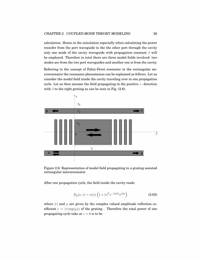
Referring to the concept of Fabry-Perot resonator in the rectangular mi-croresonator the resonance phenomenon can be explained as follows. Let usconsider the modal field inside the cavity traveling over in one propagationcycle. Let us then assume the field propagating in the positive z−directionwith β to the right grating as can be seen in Fig. (2.6).
0
A B
CD
z
x
L
g
ng
n
nb
!!!!!!
""""""
######
$$$$$$
%%%%%%%%%%%%%%%
&&&&&&&&&&&&&&&
''''''''''''''''
((((((((((((
))))))))
********
Figure 2.6: Representation of modal field propagating in a grating assistedrectangular microresonator
After one propagation cycle, the field inside the cavity reads
Ey(x, z) = ψ(x)(1 + |r|2 e−j2βLej2ϕ
)(2.62)
where |r| and ϕ are given by the complex valued amplitude reflection co-efficient r = |r| exp(jϕ) of the grating . Therefore the total power of onepropagating cycle take at z = 0 is to be

CHAPTER 2. COUPLED-MODE THEORY MODELING 27
|Ey(x, 0)|2 = |ψ(x)|2 (1 + 2 |r|2 cos(2(βL− ϕ)) + |r|4), (2.63)
where it will be maximum if 2(βL− ϕ) = l2πor
2βL = l2π + 2ϕ, (2.64)
is satisfied with l = 0, 1, 2, .... The maximum power inside the cavity yieldsthe maximum power coupled to the upper port. Hence Eq. (2.64) is theresonance condition for the rectangular microcavity that has to be fulfilledfor the maximum transmission.
Using the relation Eq. (2.64), this is analogous to the common theory of FPresonators. The cavity length have to be chosen according to the followingrelation:
L = (lπ + ϕ)λ0
2πNeff, (2.65)
if a resonance is to be established at wavelength λ0, with Neff = βλ0/2π.
If it is supposed that Neff is wavelength independent and assuming a longcavity mφÀ ϕ, we obtain the so-called Free Spectral Range (FSR) ∆λ givenby
∆λ ≈ λ0
l≈ λ2
0
2LNeff. (2.66)
The equation above shows that L or l is to be selected such that there is achance for pronounced resonances in the window of high Bragg reflectivityaround the design wavelength, λ0.

Chapter 3
Applications of theFormulation
In the previous chapter the basic simulation tool (CMT) was discussed andthe solution of the CME for the present problem was obtained. In the firstsection of this chapter the geometrical and material parameters of the de-vice will be presented. In determining suitable parameters the formulationgiven in the previous chapter will be applied. Simulation results for severalinteresting configurations will be given in the following section. Note thatfor the geometrical device parameters, we select them such that our deviceis as small as possible.
x0
t
wW d
y
Figure 3.1: Cross section of the realistic device (3D model)
28

CHAPTER 3. APPLICATIONS OF THE FORMULATION 29
3.1 Structural parameters
As a starting point for the choice of resonator parameters let us considerthe medium of the guiding cores and the background medium. Assumingthat the hypothetical device will be realised on the the basis of rectangularSi3N4 channels with refractive index 1.98 surrounded by a SiO2 backgroundmedium, we fix a common channel thickness of 0.223 µm referring to [8].The illustration of the device can be seen in Fig. (3.1).
Since we are considering a 2D problem, the model has to be transformed to2D in order apply the presented formulation. After the transformation, therefractive index of the medium is now replaced by an effective index projec-tion of the realistic 3D structure which is determined by solving the eigenmode problem of the ordinary symmetric slab waveguide with the thick-ness t at the design wavelength λ0 = 1.55µm. It leads to the effective indexprojection of the realistic 3D structure ng = 1.6 at λ0. The refractive indexof the background medium remains nb = 1.45. In the 2D investigation, nb,
ng can be viewed as effective index projection of a 3D device witha crosssection shown in Fig. (3.1).
The next step is that we will select suitable geometrical device parameters:the width of the port waveguides w, the width W and the length L of thecavity, and also the grating parameters s and p in such a way that the devicewill work as required. After all the parameters are fixed, the gap width d
should be determined such that on the one hand there is enough powertransfer between the port waveguide and the cavity and on the other handthe direct coupling in nonresonant states remains negligible. In this thesisfor d we employ a value as proposed by Hammer et al [8], where d = 1.6µm.
3.1.1 Port waveguides
Let us consider the port waveguide as a starting point to select the geomet-rical parameters. The port waveguides have to be designed such that theywill support a single mode.
This condition is fulfilled if the width w of the port waveguides is chosen inthe range w∈ (0, 1.1458]µm calculated at λ0. Let us then w = 1µm. Withthis width we obtain the effective mode index of the port, Neff = 1.5404 µm

CHAPTER 3. APPLICATIONS OF THE FORMULATION 30
at λ0. Thus this width number is to be a reference point for the design ofthe grating and of the cavity waveguide.
3.1.2 Bragg-grating
θ z0
n ng b
p s ...x
Figure 3.2: A finite periodic multilayer stack
The pronounced resonances require a reflectivity close to unity at the endsof the cavity for the relevant mode that corresponds to the effective modeindex of the port waveguides. It is known from previous study [6] that thiscondition can be satisfied with Bragg-gratings as reflectors put at the cavityfacets with suitably selected grating parameters.
The corresponding Bragg-reflector can be constructed on the basis of titledplane wave incidence on a multilayer stack with equivalent refractive indexcomposition (see Fig. (3.2)). We consider an incidence angle θ that corre-sponds to the angle of the relevant mode in the cavity, where we know thatthis mode corresponds to the one of the port waveguides with an effectiveindex given by Neff. Using relation cos θ = Neff/ng, we obtain θ = 15.690.
Optimisation of the layer stack for the present mode angle of 15.690 at λ0
with the aid of a Transfer Matrix Method (TMM) [19] leads to the grating

CHAPTER 3. APPLICATIONS OF THE FORMULATION 31
parameters p = 1.538µm and s = 0.281µm, respectively. The reflection willbe close to unity if the number of grating periods is selected e.g to be 40(see. Fig. (3.3) ). Although Np ≥ 40 will give the same condition, that willincrease the size of our device.
1.5 1.51 1.52 1.53 1.54 1.55 1.56 1.57 1.58 1.59 1.60
0.1
0.2
0.3
0.4
0.5
0.6
0.7
0.8
0.9
1
λ[µm]
Np = 5
Np = 10
Np = 20 N
p = 40
R
Figure 3.3: Reflectivity R of a multilayer stack for different numbers ofgrating periods Np at λ0 = 1.55 µm
3.1.3 Cavity waveguide
According to the coupled-mode model provided in previous section for thecavity segment, only one guided mode of the cavity segment is likely to berelevant for a specific standing wave resonance. Due to the phase matchingcondition that has to be satisfied in the coupling of the fields of the cavityand the port waveguides, the width W of the cavity waveguide has to beadjusted such that the cavity waveguide supports a guided mode that isdegenerate with the port fields.

CHAPTER 3. APPLICATIONS OF THE FORMULATION 32
We are then searching W such that one of the effective index mode indicesof the cavity is close to Neff = 1.5404. Therefore W will be determined withthe aid of the dispersion relation of the symmetric slab waveguide problem(transverse resonance) given by bW − 2χ = lπ with b = k
√n2
g −N2
eff, χ =
tan−1(√
(N2
eff − n2b)/b); ng, nb and Neff are already known. Substituting
these parameters into the transverse resonance condition yields
W = (1.0 + l1.791)µm. (3.1)
Thus the width W has to be selected among the discrete values given bythe relation above.
W
Figure 3.4: The reflection of the mode field by a Bragg-reflector at the endof the cavity waveguide
l 0 1 2 3 4 5R 0.838 0.898 0.912 0.918 0.922 0.924
Table 3.1: The level of reflectance R in different mode order l
Concerning the reflectivity at the end of the cavity by the grating structure,let us consider Eq. (2.53). In this case, let us then take Np = 20 with areason that the variation of reflectance R in different cavity width W can bedistinguished clearly. By combining Eqs. (2.53) and (3.1) with the aid of thegrating parameters s and p and β = kNeff at λ0, by CMT computations for aBragg-reflector as shown in Fig. (3.4) we observed the reflectivity levels ascan be seen in Table. (3.1) with the last value already closes to the limitinglevel of 0.952 of the reflectivity of a plane wave, incident under an angle of15.690 on laterally unbound multilayer stack. Obviously, the reflectivity is

CHAPTER 3. APPLICATIONS OF THE FORMULATION 33
higher if the fraction of the mode profile that encounters to the corrugationof the Bragg-reflector is larger. Consequently, most of the power can bekept inside the cavity when that condition fulfilled. Therefore a width W
corresponding to a higher order mode is preferred. We select W = 9.955µmwhich corresponds to the 5th order mode (l = 5) for the present simulations.Fig. (3.5) shows that the reflectance spectrum computed by CMT resemblesthe curve expected from the plane wave model. Actually CMT shows thatfor l > 5 higher reflectivity will be obtained and it is closer to the limitinglevel. However, it will imply to the size of our device.
Hence a suitable Bragg-reflector indeed can be designed on the basis of theplane wave approach.
1.5 1.51 1.52 1.53 1.54 1.55 1.56 1.57 1.58 1.59 1.60
0.1
0.2
0.3
0.4
0.5
0.6
0.7
0.8
0.9
1
λ[µm]
Np = 5
Np = 10
Np = 20
Np = 40
R
Figure 3.5: Reflectivity R of Bragg-reflectors for the 5th order mode withthe selected grating parameters s and p, for different numbers of gratingperiods Np . Results calculated using CMT are plotted with dashed lines.The reflectivities of an equivalent multilayer stack for plane wave incidenceunder the respective mode angle 15.690 are plotted with solid lines.

CHAPTER 3. APPLICATIONS OF THE FORMULATION 34
In determining the cavity length L, we apply the resonance condition givenby Eq. (2.65). For the present simulations we refer to [8] with l = 159 whichcorresponds to a cavity length L of about 79.985µm.
The design procedure leads to the selected parameters as summarised inTable (3.2). Note that in the following simulation we always keep the pa-
ng nb w/µm W /µm L/µm p/µm s/µm Np1.6 1.45 1 9.955 79.985 1.538 0.281 40
Table 3.2: Material and geometrical parameters
rameters of the cavity and the port waveguides constant, while the gratingparameters will be varied for the numerical experiments.
3.2 Simulation results
We have chosen device parameters. In this section we apply the presentedcoupled-mode formulation. For implementation we use the computing envi-ronment Matlab [17]. First we consider a resonator with symmetric Bragg-reflectors latter with nonsymmetric reflectors. Finally, we will investigatea filter device.
Alternatively, the devices are simulated with Olympios [3]. Here we takethe computational windows to be x ∈ [−10, 10]µm with Perfectly MatchedLayers (PML) as boundary conditions (BC) are chosen with a PML thick-ness of 1µm and a strength of 0.5. The number. BEP modes is set to 128mode. In the simulations (CMT and Olympios) mainly the vacuum wave-length will be varied between 1.5µm to 1.6µm with a stepsize of 0.2 nm andof 0.04 nm for λ ∈ [1.548, 1.552]µm.
3.2.1 Symmetric Bragg-reflectors
The input power is launched into the device via the guided mode of portA. As we can see from Fig. (3.6) for most wavelengths the major part ofinput power is directly transmitted to port B, while at resonance there aresome fractions of power transferred into ports A, C, and D as shown by the

CHAPTER 3. APPLICATIONS OF THE FORMULATION 35
Figure 3.6: Spectral response of resonators with symmetric reflector grat-ings. PA to PD are the relative power fractions that are reflected and trans-mitted into ports A to D. Red lines shows the simulation results from CMT;Olympios results are shown by blue lines.
CHAPTER 3. APPLICATIONS OF THE FORMULATION 36
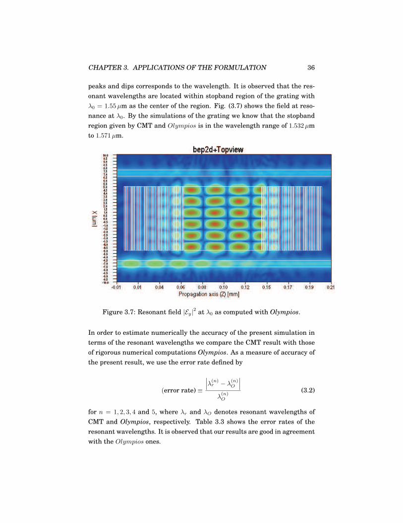
peaks and dips corresponds to the wavelength. It is observed that the res-onant wavelengths are located within stopband region of the grating withλ0 = 1.55µm as the center of the region. Fig. (3.7) shows the field at reso-nance at λ0. By the simulations of the grating we know that the stopbandregion given by CMT and Olympios is in the wavelength range of 1.532µmto 1.571µm.
Figure 3.7: Resonant field |Ey|2 at λ0 as computed with Olympios.
In order to estimate numerically the accuracy of the present simulation interms of the resonant wavelengths we compare the CMT result with thoseof rigorous numerical computations Olympios. As a measure of accuracy ofthe present result, we use the error rate defined by
(error rate) ≡
∣∣∣λ(n)r − λ
(n)O
∣∣∣λ
(n)O
(3.2)
for n = 1, 2, 3, 4 and 5, where λr and λO denotes resonant wavelengths ofCMT and Olympios, respectively. Table 3.3 shows the error rates of theresonant wavelengths. It is observed that our results are good in agreementwith the Olympios ones.
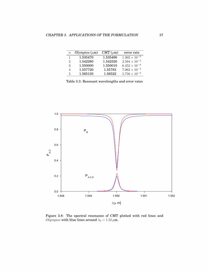
CHAPTER 3. APPLICATIONS OF THE FORMULATION 37
n Olympios (µm) CMT (µm) error rate1 1.535470 1.535490 1.302× 10⁻⁵
2 1.542280 1.542320 2.594× 10⁻⁵
3 1.550000 1.550010 6.452× 10⁻⁶
4 1.557720 1.55783 7.062× 10⁻⁵
5 1.565130 1.56522 5.750× 10⁻⁵
Table 3.3: Resonant wavelengths and error rates
Figure 3.8: The spectral resonance of CMT plotted with red lines andOlympios with blue lines around λ0 = 1.55µm.

CHAPTER 3. APPLICATIONS OF THE FORMULATION 38
In Fig. (3.6) up to λ ≈ 1.58µm we can see that the trend of the shapeof the CMT simulation coincides well with Olympios. However, as we cansee in Fig. (3.11) in the wavelength range 1.58 < λ < 1.6µm,other minorsresonances appear,which are not shown by the CMT results.
Furthermore the CMT shows spectral distance between two neighboringresonance ∆λ of about 7.6 nm. The same value of ∆λ is also more less givenby Olympios. Nevertheless, from Table 3.6 and by considering the spectrumaround one of the resonance wavelengths (i.e λ3
r = 1.55µm) we can see thatapparently the spectral resonance curve of CMT is little bit shifted to theright with the spectral curve of Olympios as a reference. By calculating theFSR ∆λ, where it is defined by
∆λk =∣∣∣λ(k+1) − λ(k)
∣∣∣ , for k = 1, .., 4 (3.3)
we know that all points of the curve are shifted to the right. Table 3.4 showsthe FSR of CMT and BEP simulations.
Apart from that if we look to the relative power calculated at the portsin Fig. (3.6), apparently the power at port B PB predicted by CMT is ingeneral higher than PB predicted by Olympios. It is remarkable becausethe CMT is constructed under the assumption that no radiation mode isincluded and the interaction between the port waveguides and the gratingis neglected. Consequently, the power indeed can be transfered withoutlosses that usually comes from the radiation.
∆λ1 ∆λ2 ∆λ3 ∆λ4
Olympios 6.80 7.72 7.72 7.41CMT 6.83 7.69 7.82 7.39
Table 3.4: Free Spectral Range ∆λ of CMT and BEP simulation
In order to explain the deviation of the resonance position of CMT simula-tion from the Olympios results, let us consider Eq.(2.65). This equation canbe rewritten to be
λ0 =L(2πNeff)(lπ + ϕ)
(3.4)

CHAPTER 3. APPLICATIONS OF THE FORMULATION 39
According to Eq. (3.4) λ0 is determined by four parameters: Neff, ϕ, L, andl. Since l and L are known beforehand, and Neff is the effective index of 5thorder mode of the cavity waveguide and it is known accurately, thereforethe precise λ0 is determined only by ϕ given by the complex valued ampli-tude reflection coefficient r. Substituting l, L, Neff into Eq. (3.4) and theCMT results for λ3
r = 1.550010µm, corresponds to ϕ = −0.0720771 and theOlympios result λ3
O = 1.55µm to ϕ = −0.065288. Taken Olympios as a ref-erence, the spectral resonance is shifted because of a error in ϕ of r of theCMT simulation for the grating. Note that for the reflectance R, the CMTgives accurate results when compared to Olympios (see Fig. 3.9).
Figure 3.9: Reflectance curve of the Bragg-gratings. The red curve corre-sponds to CMT simulations, the blue curve to Olympios.

CHAPTER 3. APPLICATIONS OF THE FORMULATION 40
3.2.2 Nonsymmetric Bragg-reflectors
As we can see from previous results the resonances are present within thestopband region and we know that the region (i.e bandwidth) is only de-termined by the grating of the Bragg-reflectors. It means the peaks arerestricted to the wavelength interval that is defined by the high reflectiv-ity region of the Bragg reflectors. Thus this property enables us to modifythe spectral characteristic of the resonances, for instance the number ofresonant wavelengths, by only changing the grating parameters.
0
L
A B
CD
z
x
sp
ng
ng
nbNp
s rl rpl
1 ...
w
d
W
!!!!!!
""""""####$$$$ %%
%%%%
&&&&&&
''''''
((((((
Figure 3.10: Nonsymmetric grating assisted rectangular microresonator.
Theoretically the left and right grating can be designed such that it givescharacteristics such as a broad or narrow stopband (bandwidth) or suchthat it shows other properties, for instance a shift in the curve of reflectanceR. However the bandwidth of the Bragg-reflectors is determined by thefractional difference of the index of refraction of the neighboring layers [18]and the index is kept fix in this simulation. Thus instead of changing theindex of refraction of the grating we can tune the geometrical parameters sand p .
What we would like to aim at in this section is a device that shows a sin-gle resonant wavelength which is realised with nonsymmetrical detunedBragg-reflectors. In the previous simulation we put identical Bragg-reflectorsat the left and the right cavity facets. For the sake of a single resonance inthis simulation we let them be different. Let us then introduce two pairs of

CHAPTER 3. APPLICATIONS OF THE FORMULATION 41
the grating parameters: (pr, sr) denotes the grating parameters of the rightgrating and (pl, sl) for the left grating (see Fig. 3.10). What we are going todo is that first we keep sr = sr = s constant and tune pl and pr, second itis the other way around, keep pl = pr = p and vary s. The values of p ands are given in Table (3.2). The simulation results are shown in Fig. (3.11)and Fig. (3.12).
For the first simulation, Fig. (3.11), we select pr = 1.549µm and pl =1.523µm for the grating parameters which refers to the values given in[8]. Along with the period length the complex reflection coefficients of thegratings at the target wavelength λ0 change. Therefore, the cavity lengthshould be slightly adjusted to a new values L = 80.006µm in order toreestablish the resonance at λ0. [9]
Fig. (3.11a) shows the spectral reflectance of the left and right Bragg-reflectors of the solution of CMT for the structure shown in Fig. (3.4). Inthis figure it can be seen that the reflectance R of the left and right gratingsoverlaps with λ0 = 1.55µm as a center, where the width of the overlap isabout 0.015µm. This width covers the wavelength range from 1.543µm to1.558µm. The overlap becomes the actual spectral reflectance due to non-symmetric reflectors. As expected, it implies the spectral resonance shownin Fig. (3.11) in which there is only one pronounced resonant wavelength.From this figure, it can be seen that CMT is in a good agreement withOlympios.
In the second simulation we select sr = 0.181µm and sl = 0.381µm and wekeep p constant. These parameters are obtained by numerical experimentsof the grating using the CME given in Eq. (2.53). In this simulation wetake L of 79.985µm. As we can see in Fig. (3.12), with this setting CMTgives more less the same result as before in which p is adjusted. This isverified by Olympios which shows more less the same resonance curve.
With respect to the present problems, apparently CMT simulation resultsare quite adequate when compared to Olympios ones.
3.2.3 Filter simulations
While at resonance the present device distributes the input among all fourports, a filter that properly drops the power into a single port can be realised

CHAPTER 3. APPLICATIONS OF THE FORMULATION 42
(a)
(b)
Figure 3.11: (a) Spectral reflectance of Bragg-reflectors, red curve fromCMT while blue curve from Olympios. (b) Spectral resonance of Nonsym-metrical grating assisted resonators with pl = 1.538µm and pr = 1.549µm,red lines correspond to CMT simulation, blue lines to Olympios.

CHAPTER 3. APPLICATIONS OF THE FORMULATION 43
(a)
(b)
Figure 3.12: (a) Spectral reflectance of Bragg-reflectors. The red curve rep-resents the results from the approximative CMT, while the blue curve corre-sponds to the Olympios. (b) Spectral resonance of Nonsymmetrical gratingassisted resonators with sl = 3.81µm and sr = 1.81µm, red lines correspondto CMT simulation, blue lines to Olympios.

CHAPTER 3. APPLICATIONS OF THE FORMULATION 44
with two cascaded single cavity resonators. The idea is firstly introduced inpapers for the case without the gratings [14, 12]. The configuration of thedevice can be seen in Fig. (3.13). The simulation in this section employs thenumber of periods Nm of the middle grating provided in [8] with Nm = 33;the others parameters remain. Compared to the single cavity configurationone new parameter introduced in this configuration is the distance betweenthe individual cavities. Thus two cavities are spaced by a distance g givenby Nmp+ s = 51.035µm. Due to the presence of this shorter grating, we canexpect that there is a direct interaction between the separated cavities toestablish the desired type of resonance.
z
D
A
L
0
B
C
p
s
x
... Nm nb
ng
ng
1
W
d
w
...1 Np
!!!!!!!!
""""""""
######$$$$$$
Figure 3.13: Schematic of an add-drop filter based on two cascaded iden-tical rectangular microresonators. Compared to Fig. (2.1), in between thecavities a grating is present with the number of periods Nm introduced asan additional parameter.
For this device, we use the same treatment a when deriving CMT for asingle cavity in which the coupling between the ports and the grating is ne-glected. Consequently, the mode amplitude of forward and backward prop-agating fields of the ports at z = L+ g can be defined by
Fp(L+ g) = Fp(L) exp(−jβg),Bp(L) = Bp(L+ g) exp(jβg), (3.5)
respectively. Let us consider again the solution of CME given in section 1

CHAPTER 3. APPLICATIONS OF THE FORMULATION 45
of the previous chapter, Eq. (2.18) and Eq. (2.20). Using this solution, theamplitude of the forward propagating fields at z = 2L+ g is given by
F(2L+ g) = T(L)F(L+ g), (3.6)
and the backward ones at z = L+ g
B(L+ g) = T(L)B(2L+ g), (3.7)
respectively; notice that no incoming field is launched at the right Bp(2L+g) ≡ 0. Due to the presence of the grating Fc(L + g) and Bc(L) are definedas follows:
Fc(L+ g) = tmFc(L) + rmBc(L+ g) (3.8)
and
Bc(L) = tmBc(L+ g) + rmFc(L). (3.9)
Parameters rm and tm appearing in Eqs. (3.8) and (3.9) are reflection andtransmission coefficients of the middle grating given by Eq. (2.53).
Combining Eqs. (2.18), (2.20), (3.5) to (3.9), we obtain
Fp(2L+ g) = Tpp exp(−jβg)Fp(L) + TpcrmTccrFc(2L+ g)
Bp(0) = (TppTpcr exp(jβg) + TpctmTccr)Fc(2L+ g) + TpcrmFc(L)
(3.10)
for the transmission through the device and for the reflection caused by theresonator, while the field inside the cavity given by
Fc(2L+ g) = Ω−1[(Tcp exp(−jβg)Fp(L) + TcctmFc(L)] (3.11)

CHAPTER 3. APPLICATIONS OF THE FORMULATION 46
with Ω = 1 − T 2ccrmr. The forward propagating fields at z = L F(L) are
given by Eq. (2.57) with Bc(0) defined as follows:
Bc(0) = 1− [Ω−1(TcpTpcr exp(jβg) + T 2cctmr)(T 2
cctmr +
TcpTpcr exp(−jβg) + Tccrm]−1[Ω−1(TcpTpcr exp(jβg) + T 2cctmr)
T 2cctmr)(TcctmTcp + TcpTpcr exp(−jβg)Tpp) + TccrFp(0) (3.12)
The simulation results of CMT and Olympios for this configuration areshown in Fig. (3.14). From this result we can see that the trend of spec-tral response obtained CMT simulation is in good agreement to the Olym-pios results. CMT predicts that the extremal transfer is reached at λr =1.55003µm in which a major part of the power is dropped in the forwarddirection into port C, while about 1% of the input power is reflected to portsA and C or transmitted to B. Olympios locates the resonance precisely atλO = 1.55µm.
Using Eq. (3.2), we can calculate that the error of the CMT calculationcompared to Olympios is about 1.953 × 10⁻⁵ when looking at the highestpeak in port C. Compared to the previous calculation for single cavity, theerror obtained in this calculation is quite similar.
The corresponding field pattern in Fig. (3.15) shows simultaneously ap-pearing high intensities in both cavities.

CHAPTER 3. APPLICATIONS OF THE FORMULATION 47
(a)
(b)
Figure 3.14: Spectral resonance of a filter device according to CMT (solidred line) and Olympios plotted (solid blue line). (b) Extremal relativelevels of power transmission are predicted at the resonance wavelengthλr = 1.55003µm (CMT) and at λO = 1.55000µm (Olympios).

CHAPTER 3. APPLICATIONS OF THE FORMULATION 48
Figure 3.15: Field pattern at resonance |E|2, for a grating assisted rectan-gular microresonator with two cavities for λ0 = 1.55µm.

Chapter 4
Conclusions and remarks
In conclusion, coupled mode theory can be successfully applied to the anal-ysis of the grating assisted rectangular microresonator structure. We havepresented the derivation of a coupled-mode formulation and given its gen-eral solution for the resonator device. The general solution is obtained bysplitting the problem into two: the cavity segment and the Bragg-reflectors.Furthermore the parts are investigated separately under the asumptionthat the coupling between the port waveguides and the grating can be ne-glected and that the interaction between the confined modes of the portwaveguides and one specific guided mode of the cavity is relevant. Forthe simulations of the Bragg-reflectors we have employed contradirectionalcoupled-mode theory, based on the forward and backward traveling versionsof a corresponding guided mode supported by the cavity core.
We have analysed the process of determining suitable parameters for thedevice with the aid of the CMT formulation. Based on the solution of CMEand the parameters, we have presented some simulation results of CMTsimulations for several configurations: symmetrical and non symmetricalresonators and a filter device. For the sake of comparison we also presentedresults of rigorous numerical computations (BEP, Olympios).
From the results, we have found good agreement between the approxima-tive CMT model and Olympios. Concerning the position of resonancs theerror of the CMT results compared to the more accurate BEP is in the or-der of 10−5. Since no radiation is included and some (crude) approximations
49

CHAPTER 4. CONCLUSIONS AND REMARKS 50
are made (e.g. the interaction between the port waveguides and the Bragggrating neglected) in the CME derivation, it leads no perfect coincidencecan be expected. Nevertheless, the numerical simulations have verified ourtheoretical predictions, hence we can conclude that our CMT model is quiteadequate to describe the presented problems.
The calculations with CMT are much efficient. For illustration, the lengthof time required by CMT to perform the computations to get the resultsshown in Fig. (3.11) is only a few minutes, while Olympios takes aboutalmost a day. Apart from that, the Olympios computations require muchmore computer memory and hard disk space to store the simulation results.

Appendix A
Cholesky Decomposition
A symmetric and positive definite matrix can be efficiently decomposed intoa lower and upper triangular matrix. Using LU decomposition we can fac-torise A = LU . If A satisfies the above criteria, we can decompose moreefficiently into A = CCT, where C is a lower triangular matrix with posi-tive diagonal elements. To solve Ax = b, we solve firstly Cy = b for y, andthen CTx = y for x.
To derive A = CCT, we simply equate coefficients on both sides of theequation:
a11 a12 . . . a1n
a21 a22 . . . a2n
......
. . ....
an1 an2 . . . ann
=
c11 0 . . . 0c21 c22 . . . 0...
.... . . 0
cn1 cn2 . . . cnn
c11 c21 . . . cn1
0 c22 . . . cn2
......
. . ....
0 0 . . . cnn
to obtain in general for i = 1, ..., n and j = i+ 1, ..., n:
cii =
√√√√(aii −
i−1∑
k=1
c2ik
),
cji =
(aji −
i−1∑
k=1
cjkcik
)/cii
51

APPENDIX A. CHOLESKY DECOMPOSITION 52
Since A is symmetric and positive definite, the expression under the squareroot is always positive, and all cij are real.

Appendix B
Matlab Code
MATLAB programs implementing of the CMT have been written to simu-late the grating assisted rectangular microresonator devices. A listing ofthe code is the following.
Main program
clear
nl = 1.6; %refractive index of guided system
nr = 1.45; %refractive index of background
PA = []; PB = []; PC = []; PD = []; l=[];
for lmd = 1.5:0.00001:1.6; %vacuum wavelength
l = [l,lmd];
k = 2*pi/lmd; %wave number
m0 = 4*pi*10ˆ-13; %permeability in vacuum
e0 = 8.854*10ˆ-18; %permittivity in vacuum
omg =k*3*10ˆ14; %harmonic frequency
Fp0 = [1 0]’; % Incoming field
M = zeros(3,3); K = zeros(3,3);
%information about rectangular part
53

APPENDIX B. MATLAB CODE 54
W = 9.955; %the width of cavity
S = W/2; % half of cavity’s width
w = 1; % the width of port
d = 1.6; % length of gap between cavity and port waveguide
Z = 79.985; % Length of cavity
%Z = 79.985; %information about assited Bragg grating
Pr = 1.538; %Length of periode of grating
Pl = 1.538; N = 40; %Number of periode
L = N*Pr; %Length of the grating
sr = 0.281; %the distance between two high refractive index right grating sl
= 0.281; %the distance between two high refractive index left grating
dn = nr-nl; %index contrast
ndelta = nlˆ2-nrˆ2;
MM = 1; %mode number which is being taken inside the port
NN = 6; %mode number for cavity
NeffP = modesolv(nl,nr,lmd,w,MM); %effective index of port
NeffC = modesolv(nl,nr,lmd,W,NN); %effective index of cavity
betaP = k*NeffP;
betaC = k*NeffC;
kx1P = k*sqrt(NeffPˆ2-nrˆ2); % propagation in x in background of port
kx1C = k*sqrt(NeffCˆ2-nrˆ2); % propagation in x in background of cavity
kx2P = k*sqrt(nlˆ2-NeffPˆ2); % propagation in x in ports
kx2C = k*sqrt(nlˆ2-NeffCˆ2); % propagation in x in cavity
%Normalised Amplitude
A2=sqrt((2*omg*m0/betaP)*(exp(kx1P*d)/(2*kx1P)*((cos(kx2P*w/2)+kx2P*sin(kx2P*w/2))/((1+kx1P)*exp(kx1P*d/2)))ˆ2+(sin(kx2P*w)+
kx2P*w)/(2*kx2P)+(2*kx1P)ˆ-1*((cos(kx2P*w/2)-kx2P*sin(kx2P*w/2))/(1-kx1P))ˆ2)ˆ-1);

APPENDIX B. MATLAB CODE 55
A8=sqrt((2*omg*m0/betaC)*(exp(kx1C*d)/(2*kx1C)*((-sin(kx2C*S)+kx2C*cos(kx2C*S))/((1+kx1C)*exp(kx1C*d/2)))ˆ2+(-
sin(2*kx2C*S)+2*kx2C*S)/(2*kx2C)+(exp(kx1C*d)/(2*kx1C))*((sin(kx2C*S)+kx2C*cos(kx2C*S))/((1-
kx1C)*exp(kx1C*d/2)))ˆ2)ˆ-1);
A11=sqrt((2*omg*m0/betaP)*(1/(2*kx1P)*((cos(kx2P*w/2)+kx2P*sin(kx2P*w/2))/(1+kx1P))ˆ2+
(sin(kx2P*w)+kx2P*w)/(2*kx2P)+(exp(kx1P*d)/(2*kx1P))*((cos(kx2P*w/2)-
kx2P*sin(kx2P*w/2))/((1-kx1P)*exp(kx1P*d/2)))ˆ2)ˆ-1);
A1=((cos(kx2P*w/2)-kx2P*sin(kx2P*w/2))/(1-kx1P))*A2;
A5=((cos(kx2P*w/2)+kx2P*sin(kx2P*w/2))/((1+kx1P)*exp(kx1P*d/2)))*A2;
A4 = ((sin(kx2C*S)+kx2C*cos(kx2C*S))/((1-kx1C)*exp(kx1C*d/2)))*A8;
A9 = ((-sin(kx2C*S)+kx2C*cos(kx2C*S))/((1+kx1C)*exp(kx1C*d/2)))*A8;
A10 = ((cos(kx2P*w/2)-kx2P*sin(kx2P*w/2))/((1-kx1P)*exp(kx1P*d/2)))*A11;
A13 = ((cos(kx2P*w/2)+kx2P*sin(kx2P*w/2))/(1+kx1P))*A11;
%A = [A1 A2 A4 A5 A8 A9 A10 A11 A13]; %the mode amplitude of sparated parts
%Element of matrix M (power coefficient)
M(2,2)=(betaP/(2*omg*m0))*(exp(kx1P*d)*A5ˆ2/(2*kx1P)+(sin(kx2P*w)+kx2P*w)*
A2ˆ2/(2*kx2P)+A1ˆ2/(2*kx1P));
M(3,3)=(betaC/(2*omg*m0))*(exp(kx1C*d)*A9ˆ2/(2*kx1C)+(-sin(2*kx2C*S)+
2*kx2C*S)*A8ˆ2/(2*kx2C)+exp(kx1C*d)*A4ˆ2/(2*kx1C));
M(1,1)=(betaP/(2*omg*m0))*(A13ˆ2/(2*kx1P)+(sin(kx2P*w)+kx2P*w)*A11ˆ2/(2*kx2P)+exp(kx1P*d)*A10ˆ2/(2*kx1P));
M(1,2)=(betaP/(2*omg*m0))*(A13*A5*exp(-0.5*kx1P*(4*S+3*d+2*w))/(2*kx1P)+A11*A5*(kx1P*cos(0.5*kx2P*w)+
kx2P*sin(0.5*kx2P*w))*exp(-0.5*kx1P*(4*S+3*d))/(kx1Pˆ2+kx2Pˆ2)+A11*A5*(-kx1P*cos(0.5*kx2P*w)+kx2P*
sin(0.5*kx2P*w))*exp(-0.5*kx1P*(4*S+3*d+2*w))/(kx1Pˆ2+kx2Pˆ2)+2*A10*A5*(S+d)*exp(-kx1P*(2*S+d))+
A10*A2*(-kx1P*cos(0.5*kx2P*w)+kx2P*sin(0.5*kx2P*w))*exp(-0.5*kx1P*(4*S+3*d+2*w))/(kx1Pˆ2+kx2Pˆ2)+
A10*A2*(kx1P*cos(0.5*kx2P*w)+kx2P*sin(0.5*kx2P*w))*exp(-0.5*kx1P*(4*S+3*d))/(kx1Pˆ2+kx2Pˆ2)+A10*
A1*exp(-0.5*kx1P*(4*S+3*d+2*w))/(2*kx1P);
M(2,1)=M(1,2);
if

APPENDIX B. MATLAB CODE 56
kx1P==kx1C M(1,3)=(1/(4*omg*m0))*(betaP+betaC)*(A13*A9*exp(-0.5*kx1C*(d+2*w))/(kx1P+kx1C)+A11*A9*(-
exp(-1/2*kx1C*
d-kx1C*w)*kx1C*cos(1/2*kx2P*w)+exp(-1/2*kx1C*d-kx1C*w)*kx2P*sin(1/2*kx2P*w)+exp(-1/2*kx1C*d)*kx1C*
cos(1/2*kx2P*w)+exp(-1/2*kx1C*d)*kx2P*sin(1/2*kx2P*w))/(kx1Cˆ2+kx2Pˆ2)+A10*A9*d+(-kx2C*cos(kx2C*S)-
kx1P*sin(kx2C*S))*exp(-0.5*kx1P*(4*S+d))*A8*A10/(kx1Pˆ2+kx2Cˆ2)+(kx2C*cos(kx2C*S)-kx1P*sin(kx2C*S))*
exp(-0.5*kx1P*d)*A8*A10/(kx1Pˆ2+kx2Cˆ2)+A10*A4*exp(-2*kx1P*S-1/2*kx1P*d+1/2*kx1C*d)/(kx1P+kx1C));
M(3,2)=-M(1,3);
else
M(1,3)=(1/(4*omg*m0))*(betaP+betaC)*(A13*A9*exp(-0.5*kx1C*(d+2*w))/(kx1P+kx1C)+A11*A9*(-
exp(-1/2*kx1C*
d-kx1C*w)*kx1C*cos(1/2*kx2P*w)+exp(-1/2*kx1C*d-kx1C*w)*kx2P*sin(1/2*kx2P*w)+exp(-1/2*kx1C*d)*
kx1C*cos(1/2*kx2P*w)+exp(-1/2*kx1C*d)*kx2P*sin(1/2*kx2P*w))/(kx1Cˆ2+kx2Pˆ2)+A10*A9*(exp(-
1/2*kx1P*
d+1/2*kx1C*d)-exp(1/2*kx1P*d-1/2*kx1C*d))/(-kx1P+kx1C)+(-kx2C*cos(kx2C*S)-kx1P*sin(kx2C*S))*exp(-
0.5*
kx1P*(4*S+d))*A8*A10/(kx1Pˆ2+kx2Cˆ2)+(kx2C*cos(kx2C*S)-kx1P*sin(kx2C*S))*exp(-0.5*kx1P*d)*A8*
A10/(kx1Pˆ2+kx2Cˆ2)+A10*A4*exp(-2*kx1P*S-1/2*kx1P*d+1/2*kx1C*d)/(kx1P+kx1C));
M(3,2) = -M(1,3);
end
M(3,1)=M(1,3); M(2,3)=M(3,2);
%Element of matrix K (coupling coefficient)
K(1,3)=ndelta*(e0*omg/8)*(A11*A9*(-exp(-1/2*kx1C*d-kx1C*w)*kx1C*cos(1/2*kx2P*w)+exp(-1/2*kx1C*d-
kx1C*w)*kx2P*sin(1/2*kx2P*w)+exp(-1/2*kx1C*d)*kx1C*cos(1/2*kx2P*w)+exp(-1/2*kx1C*d)*kx2P*sin(1/2*
kx2P*w))/(kx1Cˆ2+kx2Pˆ2)+-A8*A10*(exp(-2*kx1P*S-1/2*kx1P*d)*kx2C*cos(kx2C*S)+exp(-2*kx1P*S-
1/2*
kx1P*d)*kx1P*sin(kx2C*S)-exp(-1/2*kx1P*d)*kx2C*cos(kx2C*S)+exp(-1/2*kx1P*d)*kx1P*sin(kx2C*S))/

APPENDIX B. MATLAB CODE 57
(kx1Pˆ2+kx2Cˆ2)+2*A10*A4*(-exp(-2*kx1P*S-3/2*kx1P*d-kx1P*w-1/2*kx1C*d-kx1C*w)+exp(-
2*kx1P*S-3/2*
kx1P*d-1/2*kx1C*d))/(kx1P+kx1C));
K(3,1)=K(1,3);
K(3,2)=ndelta*(e0*omg/8)*(2*A5*A9*(-exp(-2*kx1P*S-3/2*kx1P*d-kx1P*w-1/2*kx1C*d-kx1C*w)+exp(-
2*kx1P*
S-3/2*kx1P*d-1/2*kx1C*d))/(kx1P+kx1C)+A8*A5*(exp(-2*kx1P*S-1/2*kx1P*d)*kx2C*cos(kx2C*S)+exp(-
2*
kx1P*S-1/2*kx1P*d)*kx1P*sin(kx2C*S)-exp(-1/2*kx1P*d)*kx2C*cos(kx2C*S)+exp(-1/2*kx1P*d)*kx1P*s
in(kx2C*S))/(kx1Pˆ2+kx2Cˆ2)+A2*A4*(-kx1C*cos(0.5*kx2P*w)+kx2P*sin(0.5*kx2P*w))/(kx1Cˆ2+kx2Pˆ2)*
exp(-0.5*kx1C*(d+2*w))+A2*A4*(kx1C*cos(0.5*kx2P*w)+kx2P*sin(0.5*kx2P*w))/(kx1Cˆ2+kx2Pˆ2)*exp(-
0.5*d*kx1C));
K(2,3)=K(3,2);
K(1,2)=ndelta*(e0*omg/8)*(A11*A5*(exp(-2*kx1P*S-3/2*kx1P*d)*kx1P*cos(1/2*kx2P*w)+exp(-
2*kx1P*S-3/2*
kx1P*d)*kx2P*sin(1/2*kx2P*w)-exp(-2*kx1P*S-3/2*kx1P*d-kx1P*w)*kx1P*cos(1/2*kx2P*w)+exp(-
2*kx1P*S-
3/2*kx1P*d-kx1P*w)*kx2P*sin(1/2*kx2P*w))/(kx1Pˆ2+kx2Pˆ2)+4*S*A5*A10*exp(-kx1P*(2*S+d))+A2*A10*
(exp(-2*kx1P*S-3/2*kx1P*d)*kx1P*cos(1/2*kx2P*w)+exp(-2*kx1P*S-3/2*kx1P*d)*kx2P*sin(1/2*kx2P*w)-
exp(-2*kx1P*S-3/2*kx1P*d-kx1P*w)*kx1P*cos(1/2*kx2P*w)+exp(-2*kx1P*S-3/2*kx1P*d-kx1P*w)*kx2P*
sin(1/2*kx2P*w))/(kx1Pˆ2+kx2Pˆ2));
K(2,1) = K(1,2);
K(2,2)=ndelta*(e0*omg/8)*A5ˆ2*(exp(-kx1P*(4*S+3*d))+exp(-d*kx1P)-exp(-kx1P*(4*S+3*d+2*w))-
exp(-kx1P*(4*S+d)))/kx1P;K(3,3)=ndelta*(e0*omg/8)*(A4ˆ2*(-exp(-1/2*kx1C*(d+2*w))ˆ2+exp(-
1/2*kx1C*
d)ˆ2)/kx1C+A9ˆ2*(-exp(-1/2*kx1C*(d+2*w))ˆ2+exp(-1/2*kx1C*d)ˆ2)/kx1C);
K(1,1)=ndelta*(e0*omg/8)*(-A10ˆ2*(exp(-1/2*kx1P*(4*S+d))ˆ2-exp(-1/2*kx1P*d)ˆ2)/kx1P+-A10ˆ2*
APPENDIX B. MATLAB CODE 58
(exp(-1/2*kx1P*(4*S+3*d+2*w))ˆ2-exp(-1/2*kx1P*(4*S+3*d))ˆ2)/kx1P);
beta = (betaP+betaC)*0.5;
H = beta*M+K; O = chol(M); % cholesky decomposition
HH = inv(O)’*H*inv(O);
[WW,bsuper] = eig(HH);
bsuper = diag(bsuper); % supermode
for j = 1 : length(bsuper)
a(:,j) = inv(O)*WW(:,j);
end
dumm = 0;
for ii =1:length(bsuper)
dumm = dumm + (exp(-i*bsuper(ii)*Z)*a(:,ii)*(a(:,ii))’);
end
T = O*dumm*O’; %Propagation matrix
% Split matrix
Tcc = T(3,3);
Tpp = [ T(1,1) T(1,2) T(2,1) T(2,2)];
Tpc = [ T(1,3) T(2,3)];
Tcp = [ T(3,1) T(3,2)];
Rr = gratpartm(nl,nr,W,Pr,N,sr,lmd,NeffC,NN,1); % coefficient of reflectivity of rigth grating
Rl = gratpartm(nl,nr,W,Pl,N,sl,lmd,NeffC,NN,1); % coefficient of reflectivity of left grating %R =
1; Omega = 1 - Tcc*Rr*Tcc*Rl;
FpL = (Tpp + Tpc*Rl*inv(Omega)*Tcc*Rr*Tcp)*Fp0;
FcL = (Tcp+Tcc*Rl*inv(Omega)*Tcc*Rr*Tcp)*Fp0;
Bp0 = Tpc*Rr*FcL; Bc0 = inv(Omega)*Tcc*Rr*Tcp*Fp0;
PA = [PA, abs(Bp0(1,:))ˆ2];
PB = [PB, abs(FpL(1,:))ˆ2];

APPENDIX B. MATLAB CODE 59
PC = [PC, abs(FpL(2,:))ˆ2];
PD = [PD, abs(Bp0(2,:))ˆ2];
end
Grating part
function y = gratpart(n1,n2,Width,Periode, NPeriode, space, lambda,neff,MNum,Pil)
R =[]; RR=[]; T = []; Pz = [];
L = NPeriode*Periode;
dn = n2-n1;
k = 2*pi/lambda; %wavenumber
if mod(MNum-1,2)==0
kxr = k*sqrt(neffˆ2-n2ˆ2);
kxm = k*sqrt(n1ˆ2-neffˆ2);
C=0.5*n1*dn*k*(neffˆ-1)*(((kxm*Width+sin(kxm*Width))/(kxm))*((kxm*Width+sin(kxm*Width))/(2*kxm)+(cos(kxm*0.5*Width)-
kxm*
sin(kxm*0.5*Width))ˆ2/(kxr*(1-kxr)ˆ2))ˆ-1);
else
kxr = k*sqrt(neffˆ2-n2ˆ2);
kxm = k*sqrt(n1ˆ2-neffˆ2);
C=0.5*n1*dn*k*(neffˆ-1)*(((kxm*Width-sin(kxm*Width))/(kxm))*((kxm*Width-sin(kxm*Width))/(2*kxm)+(kxm*
cos(kxm*0.5*Width)+sin(kxm*0.5*Width))ˆ2/(kxr*(1-kxr)ˆ2))ˆ-1);
end
beta = k*neff; dum2 = beta*Periode/pi;
if (dum2-floor(dum2))¿0.5
NN = floor(dum2)+1;
else NN = floor(dum2);
end
F1=-1/2*i*(-exp(-i*(Periode+space)*pi*-NN/Periode)+exp(i*(-Periode+space)*pi*-NN/Periode))/(pi*-
NN);
APPENDIX B. MATLAB CODE 60
F2=-1/2*i*(-exp(-i*(Periode+space)*pi*NN/Periode)+exp(i*(-Periode+space)*pi*NN/Periode))/(pi*NN);
F0 = space/(Periode);
C1 = C*F1;
C2 = C*F2;
dbeta = 2*beta-NN*2*pi/Periode;
Q = [(-i*0.5*dbeta-i*C*F0) -i*C1 i*C2 (i*0.5*dbeta+i*C*F0)];
[PP,eg]=eig(Q);
eg1 = eg(1,1);
eg2 = eg(2,2);
M = matE(L,eg1,eg2);
TT = (PP)*M*inv(PP);
r = -(TT(2,1)/TT(2,2));
t = TT(1,1)-TT(1,2)*TT(2,1)/TT(2,2);
if Pil==1 y = r; else y = t; end
Mode solver
function y=modesolv(nleft,nright,lambda,Width,M)
m = smodes(nleft,nright,lambda,Width); %the number of modes nl¿nr
sol = [];
k=2*pi/lambda;
for p = 1:m
if mod(p-1,2)==0
xl = 0; xu = ((p-1)*0.5*pi+pi/2)-10ˆ-20;
dum = bisection1(nleft,nright,lambda,Width,xu,xl);
sol =[sol, sqrt((k*nleft)ˆ2-(2*dum/Width)ˆ2)/k];
else xl = pi/2; xu = ((p-1)*0.5*pi+pi/2)-10ˆ-20;
dum = bisection2(nleft,nright,lambda,Width,xu,xl);
sol=[sol,sqrt((k*nleft)ˆ2-(2*dum/Width)ˆ2)/k];

APPENDIX B. MATLAB CODE 61
end
end
y = sol(M);
Bibliography
[1] Yariv Amnon and Pochi Yeh. Optical waves in crystal:Propagation andcontrol of laser radiation. Wiley, Canada, 1994.
[2] Han Berends. Integrated Optical Bragg Reflectors as NarrowbandWavelength Filters. PhD thesis, the University of Twente, P.O. Box217, 7500 AE Enschede, The Netherlands, 1997.
[3] OlympIOs Integrated Optics Software C2V. P.O. Box 318, 7500 AHEnschede, The Netherlands. http://www.c2v.nl/software.
[4] Shun-Lien Chuang. A coupled-mode theory for multiwaveguide sys-tems satisfying the reciprocity theorem and power conservation. J.Lightwave Technol., LT-5(1):174–183, 1987.
[5] D.G. Hall and B.J. Thompson. Selected papers on coupled-mode theoryin guided-wave optics. volume MS 84 of SPIE Milestone Series. SPIEOptical Engineering Press, Bellingham, Washington USA, 1993.
[6] M. Hammer. Resonant coupling of dielectric optical waveguides viarectangular microcavities: The coupled guided mode perspective. Opt.Quantum Electron., 214(1), 2002.
[7] M. Hammer and E.van Groesen. Total multimode reflection at facetsof planar high contrast optical waveguides. J. Lightwave Technol.,20(8):1549–1555, 2002.
[8] M. Hammer and D. Yudistira. Grating assited rectangular integratedoptical microresonator. Proceedings of ECIO, 2003.
62
BIBLIOGRAPHY 63
[9] M. Hammer, D. Yudistira, and R. Stoffer. Modeling of grating assistedstanding wave microresonators for filter applications in integrated op-tics. to be pubslished, 2003.
[10] B.E. Little, S.T. Chu, H.A. Haus, J. Foresi, and J.-P. Laine. Microringresonator channel dropping filters. J. Lightwave Technol., 15(6):998–1005, 1997.
[11] B.E. Little, S.T. Chu, Y. Pan, and W.nad Kokubun. Microring resonatorarrays for vlsi photonics. IEEE Photonics Technol. Lett., 12(3):323–325, 2000.
[12] M Lohmeyer. Mode expansion modeling of rectangular integrated op-tical microresonators. Opt. Quantum Electron., 34(5):541–557, 2002.
[13] M. Lohmeyer, N. Bahlmann, O. Zhuromskyy, and P. Hertel. Ra-diatively coupled waveguide polarization splitter simulated by wave-matching-based coupled mode theory. Opt. Quantum Electron.,31:877–891, 1999.
[14] C. Manolatou, M.J. Khan, S. Fan, H.A. Haus, and J.D. Joannopoulos.Coupling of modes analysis of resonant channel add-drop filters. IEEEJ. Quantum Electron., 35(9):1322–1331, 1999.
[15] A.I. Nosich and S.V. Boriskina. Fast solution to the scattering by ar-bitrary smooth dielectric cylinders based on the method of regularisa-tion. Proceedings of ICTON, pages 27–30, 2000.
[16] C. Vassallo. Optical Waveguide Concepts. Elsevier, Amsterdam, 1991.
[17] The Math Works. The student edition of MATLAB the ultimate comput-ing environment for technical education. Prentice Hall, 1995. User’sGuide.
[18] Pochi Yeh. Optical Waves in Layered Media. Wiley, 1988.
[19] D. Yudistira. Reflection of Plane Electromagnetic Waves from a Dielec-tric Multilayer Stack. University of Twente, Dept. of Applied Mathe-matics, 2002. Modeling project.

Acknowledgment
While the actual writing of a graduation thesis usually is the results ofdays, and sometimes nights, of writing, reading, and rewriting by the au-thor, the content of the thesis is the results of contributions of many. Real-ising that it may be an impossible task acknowledging each and every oneI will make an attempt to do so anyway.
First, many suggestions have been useful to complete this thesis. In partic-ular, I would like to express my deepest appreciation to my daily supervisorDr. Manfred Hammer for his proper guidance and support. I would like tothank Dr. Hugo Hoekstra and Prof. Brenny van Groesen and Prof. Tjia MayOn of Institute Teknologi Bandung (ITB) Indonesia for their support. LightDevices Group (LDG) of department of Electrical Engineering at Universityof Twente that provided me a nice place to work with nice colleagues (Wico,Edwin and Ronald) and the important thing is that they provided computersimulation Olympios for my thesis.
Also, I would like to thank to my friends in Master of Science program ofApplied Mathematics 2001 in particular to Hala for her advice in..., to myfriends in faith Indonesian Moslems community in Enschede, The Nether-lands (IMEA), to my beloved friends in PPI Enschede, to my lunch friendsPak Freddy, Pak Henri, David, and Jahja (Yukem), for a warm friendship.Fruthermore, I want to thank to my friends in Calslaan 1 (Calslaan ers)Rayi, Adi, Esther, Iren that provided me a special dinner with the Calslaanfamily during the past months. It was really unforgetable moments. Also, Iwould like to address my grateful thank to my best friend Lukmanul Hakimfor his support.
Last but not least I want to thank to my family, my mother, my brothersand sister for their support throughout the years.
64
Related Documents


![arXiv:0708.0611v1 [physics.optics] 4 Aug 2007 · 2008. 2. 1. · arXiv:0708.0611v1 [physics.optics] 4 Aug 2007 Optical frequency comb generation from a monolithic microresonator P.](https://static.cupdf.com/doc/110x72/60a83917d68594239d325006/arxiv07080611v1-4-aug-2007-2008-2-1-arxiv07080611v1-4-aug-2007.jpg)