Modeling and Control of Three-Phase Self-Excited Induction ...

265 http://www.transeem.org

Regular Paper OAK Central: http://central.oak.go.kr DOI: https://doi.org/10.4313/TEEM.2017.18.5.265

pISSN: 1229-7607 eISSN: 2092-7592

† Author to whom all correspondence should be addressed:E-mail: [email protected]

Copyright ©2017 KIEEME. All rights reserved.This is an open-access article distributed under the terms of the Creative Commons Attribution Non-Commercial License (http://creativecommons.org/licenses/by-nc/3.0) which permits unrestricted noncommercial use, distribution, and reproduction in any medium, provided the original work is properly cited.

TRANSACTIONS ON ELECTRICAL AND ELECTRONIC MATERIALSVol. 18, No. 5, pp. 265-272, October 25, 2017

Modeling and Control of Three-Phase Self-Excited Induction Generator Connected to Grid

Chandrasekaran Natarajan† and Karthikeyan ADepartment of Electrical and Electronics Engineering, PSNA College of Engineering and Technology, Tamilnadu 624622, India

Received November 3, 2016; Revised June 5, 2017; Accepted June 6, 2017

This paper presents the dynamic modeling, analysis, and control of an AC/DC/AC-assisted, self-excited induction generator connected to the grid. The dynamic model includes wind turbine models with pitch control, gear boxes, self-excited induction generators, excitation capacitance, inductive load models, controlled six-pulse rectifiers, and novel state-space models of a grid-connected inverter. The system has been simulated to verify its capabilities of buildup voltage, stator flux response, stator phase current, electromagnetic torque, and magnetizing inductance variation during both the dynamic and steady states with a variable-speed prime mover. The complete setup of the above dynamic models was simulated using MATLAB/SIMULINK.

Keywords : Dynamic models, Self-excited induction generator, State-space model, Grid-connected inverter, Magnetizing inductance

1. INTRODUCTION

Because of the increasing concerns about CO2 emissions and the finite supply of fossil fuels, renewable energy has become a major topic across the globe. Wind energy generation has attracted much interest in the last few years and large wind farms have been planned and installed in various locations around the world. Many of these wind farms are based on the induction generator (IG) technology with converter ratings around 30 percent of the generator ratings [1]. Induction machines (usually squirrel cage rotor-type) are often used for wind power generation because of their ruggedness and low cost [2]. However, they are used mostly in grid-connected operation because of their excitation requirement. Induction machines can be used in stand-alone applications provided enough reactive excitation is provided for self-excitation [3,4]. IGs can cope with a small increase in speed from the rated value because, due to saturation, the rate of increase of the generated voltage is nonlinear with speed.

Furthermore, a self-excited induction generator (SEIG) has a self-protection mechanism because its output voltage collapses when overloaded [5–7]. In this paper, the modeling of variable-speed wind energy conversion systems is discussed.

A description of the proposed wind energy conversion system (WECS) is presented, and dynamic models for both the SEIG and wind turbine are developed. In addition, the effects of saturation characteristics on the SEIG are presented. The developed models are simulated in MATLAB/Simulink [8]. Different wind and load conditions are applied to the WECS model for validation purposes.

2. SYSTEM CONFIGURATION

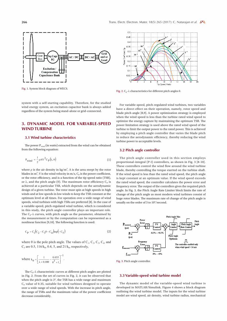
The configuration of the studied WECS is illustrated in Fig. 1. A SEIG, driven by a pitch-controlled, variable-speed wind turbine acting as the prime mover, is used to generate electricity. The output AC voltage (with variable frequency) of the SEIG is rectified into DC and then a DC/AC inverter is used to convert the DC into 50-Hz AC. For stand-alone operation, an excitation-compensating capacitor bank is necessary to start the IG. For grid-connected applications, the compensating capacitor bank can be eliminated from the system. However, for a weak grid, the reactive power consumed by the IG will deteriorate the situation. It is more beneficial to have a generation

266 Trans. Electr. Electron. Mater. 18(5) 265 (2017): C. Natarajan et al.

system with a self-starting capability. Therefore, for the studied wind energy system, an excitation capacitor bank is always added regardless of the system being stand-alone or grid-connected.

3. DYNAMIC MODEL fOR VARIAbLE-SPEED WIND TURbINE

3.1 Wind turbine characteristics

The power Pwind (in watts) extracted from the wind can be obtained from the following equation:

(1)

where ρ is the air density in kg/m3, A is the area swept by the rotor blades in m2, V is the wind velocity in m/s, CP is the power coefficient, or the rotor efficiency, and is a function of the tip speed ratio (TSR), or λ, and the pitch angle (θ). The maximum rotor efficiency CP is achieved at a particular TSR, which depends on the aerodynamic design of a given turbine. The rotor must spin at high speeds in high winds and at low speeds in low winds to keep the TSR constant at the optimum level at all times. For operation over a wide range of wind speeds, wind turbines with high TSRs are preferred [8]. In the case of a variable-speed, pitch-regulated wind turbine, which is considered in this study, the pitch angle controller plays an important role. The CP–λ curves, with pitch angle as the parameter, obtained by the measurement or by the computation can be represented as a nonlinear function [9,10]. The following function is used:

(2)

where θ is the pole pitch angle. The values of C1, C2, C3, C4, and C5 are 0.5, 116/kθ, 0.4, 5, and 21/kθ, respectively,

where .

The CP–λ characteristic curves at different pitch angles are plotted in Fig. 2. From the set of curves in Fig. 2, it can be observed that when the pitch angle is 2°, the TSR has a wide range and maximum CP value of 0.35, suitable for wind turbines designed to operate over a wide range of wind speeds. With the increase in pitch angle, the range of TSRs and the maximum value of the power coefficient decrease considerably.

For variable-speed, pitch-regulated wind turbines, two variables have a direct effect on their operation, namely, rotor speed and blade pitch angle [8,9]. A power optimization strategy is employed when the wind speed is less than the turbine rated wind speed to optimize the energy capture by maintaining the optimum TSR. The power limitation strategy is used above the rated wind speed of the turbine to limit the output power to the rated power. This is achieved by employing a pitch angle controller that varies the blade pitch to reduce the aerodynamic efficiency, thereby reducing the wind turbine power to acceptable levels.

3.2 Pitch angle controller

The pitch angle controller used in this section employs proportional-integral (P-I) controllers, as shown in Fig. 3 [8-10]. These controllers control the wind flow around the wind turbine blade, thereby controlling the torque exerted on the turbine shaft. If the wind speed is less than the rated wind speed, the pitch angle is kept constant at an optimum value. If the wind speed exceeds the rated wind speed, the controller calculates the power error and frequency error. The output of the controllers gives the required pitch angle. In Fig. 3, the Pitch Angle Rate Limiter block limits the rate of change of the pitch angle as most modern wind turbines consist of huge rotor blades. The maximum rate of change of the pitch angle is usually on the order of 3 to 10°/second.

3.3 Variable-speed wind turbine model

The dynamic model of the variable-speed wind turbine is developed in MATLAB/Simulink. Figure 4 shows a block diagram outlining the wind turbine model. The inputs for the wind turbine model are wind speed, air density, wind turbine radius, mechanical

Fig. 2. Cp–λ characteristics for different pitch angles θ.

Fig. 3. Pitch angle controller.

Fig. 1. System block diagram of WECS.

267Trans. Electr. Electron. Mater. 18(5) 265 (2017): C. Natarajan et al.

speed of rotor on wind turbine side, and power reference for the pitch angle controller.

The output is the drive torque Tdrive, which drives the electrical generator. The wind turbine calculates the TSR from the input values and estimates the value of the power coefficient from the performance curves. The pitch angle controller maintains the value of the blade pitch at the optimum value until the power output of the wind turbine exceeds the reference power input. The model of a 50 kW, variable-speed wind energy conversion system consisting of a pitch-regulated wind turbine and SEIG is developed in a MATLAB/Simulink environment using the Sim Power systems blockset.

4. MODELLING Of SEIG

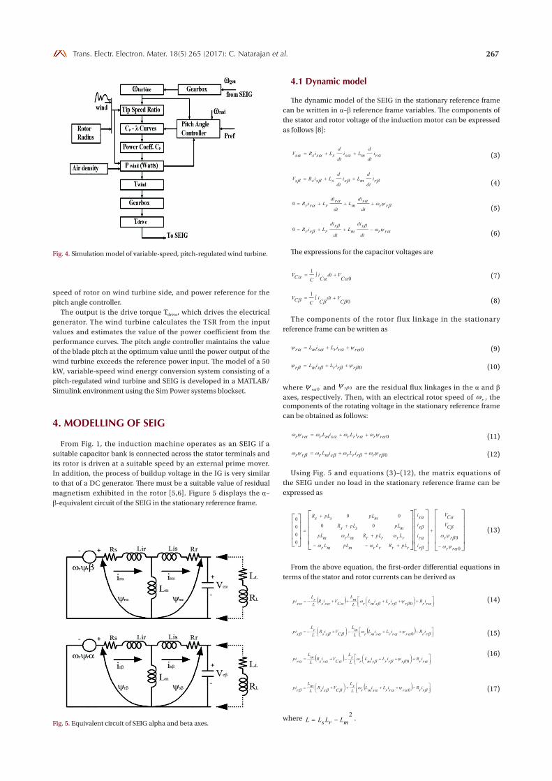
From Fig. 1, the induction machine operates as an SEIG if a suitable capacitor bank is connected across the stator terminals and its rotor is driven at a suitable speed by an external prime mover. In addition, the process of buildup voltage in the IG is very similar to that of a DC generator. There must be a suitable value of residual magnetism exhibited in the rotor [5,6]. Figure 5 displays the α–β-equivalent circuit of the SEIG in the stationary reference frame.

4.1 Dynamic model

The dynamic model of the SEIG in the stationary reference frame can be written in α–β reference frame variables. The components of the stator and rotor voltage of the induction motor can be expressed as follows [8]:

(3)

(4)

(5)

(6)

The expressions for the capacitor voltages are

(7)

(8)

The components of the rotor flux linkage in the stationary reference frame can be written as

(9)

(10)

where 0αψ r and 0βψ r are the residual flux linkages in the α and β axes, respectively. Then, with an electrical rotor speed of rω , the components of the rotating voltage in the stationary reference frame can be obtained as follows:

(11)

(12)

Using Fig. 5 and equations (3)–(12), the matrix equations of the SEIG under no load in the stationary reference frame can be expressed as

(13)

From the above equation, the first-order differential equations in terms of the stator and rotor currents can be derived as

(14)

(15)

(16)

(17)

where 2

mLrLsLL −= .

Fig. 4. Simulation model of variable-speed, pitch-regulated wind turbine.

Fig. 5. Equivalent circuit of SEIG alpha and beta axes.


The components of the differential load voltage equations can be written as

(18)

(19)

where βββααα LisiciLisici −=−= , .

The components of the differential load current equations can be written as

(20)

(21)

4.2 Magnetizing inductance and capacitance on self-excitation

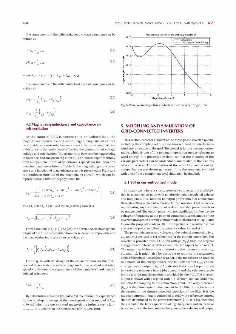
As the stator of SEIG is connected to an isolated load, the magnetizing inductance and stator magnetizing current cannot be considered constants, because the variation in magnetizing inductance is the main factor affecting the generation of voltage buildup and stabilization. The relationship between the magnetizing inductance and magnetizing current is obtained experimentally from an open circuit test at synchronous speeds for the induction machine parameters listed in Table 1. The magnetizing inductance curve as a function of magnetizing current is presented in Fig. 6 and is a nonlinear function of the magnetizing current, which can be represented as a fifth-order polynomial fit:

(22)

where Im is 0 < Im ≤ 6.0 A and the magnetizing current is

(23)

From equations (14)–(17) and (22), the developed electromagnetic torque of the SEIG is computed from these current components and the magnetizing inductance can be written as

(24)

From Fig. 6, with the design of the capacitor bank for the SEIG, needed to generate the rated voltage under the no-load and rated speed conditions, the capacitance of the capacitor bank can be defined as follows:

(25)

By substituting equation (22) into (25), the minimum capacitance for the buildup of voltage at the rated speed under no load is Cmin = 50 mF when the unsaturated magnetizing inductance is Lm = Lunsaturated = 141.56 mH at the rated speed of Nr = 1,400 rpm.

5. MODELING AND SIMULATION Of GRID-CONNECTED INVERTERS

This section presents a model of the three-phase inverter system, including the complete set of subsystems required for interfacing a wind energy source to the grid. The model is for the current-control mode, which is one of the two main operation modes relevant to wind energy. It is presented in detail so that the meaning of the various parameters can be understood and related to the features of real inverters. The validation of the model is carried out by comparing the waveforms generated from the state-space model with those from a component-level simulation in Simulink.

5.1 VSI in current-control mode

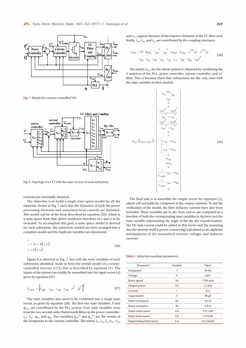
In situations where a strong network connection is available, that is, a connection point with an already tightly regulated voltage and frequency, it is common to output power into that connection through setting a current reference for the inverter. That reference representing any combination of real and reactive power needs to be understood. The output power will not significantly influence the voltage or frequency at the point of connection. A schematic of the inverter arranged in current-control mode is illustrated in Fig. 7 and follows the proposal made in [10]. The objective is to regulate the real and reactive power to follow the reference values (P* and Q*).

The power references and voltages at the point of connection (vOa, vOb, and vOc) are used to set references for the current controllers. The inverter is provided with a DC link voltage (VDC) from the original energy source. These variables constitute the inputs to the model. The output variables of direct interest are the output currents (iOa, iOb, and iOc). It might also be desirable to monitor the alignment angle of the phase-locked loop (PLL) or, if the model is to be coupled to a model of the energy source, the DC link current (iDC) can be arranged as an output. Figure 7 indicates that control is performed in a rotating reference frame (dq domain) and the reference angle for the abc–dq transformation is provided by the PLL. The inverter output is shown with a second-order LC element and an additional inductor for coupling to the connection point. The output current (iOdq) is therefore equal to the current in the filter inductor minus the current in the shunt-connected capacitor of the filter. It is the inductor current iL that is controlled to follow the reference current (in turn determined by the power references) [10]. It is assumed that the current in the filter capacitor is of high frequency and, in terms of power output at the fundamental frequency, the inductor and output

Fig. 6. Variation in magnetizing inductance with magnetizing current.


currents are essentially identical. The objective is to build a single state-space model for all the

elements shown in Fig. 7 such that the dynamics of both the power processing elements and associated local controls are included. This model will be of the form described by equation (26), which is a state-space form that allows nonlinear functions of x and u to be included. To accomplish this goal, a state-space model is derived for each subsystem. The subsystem models are then arranged into a complete model and the duplicate variables are eliminated.

(26)

Figure 8 is identical to Fig. 7, but with the state variables of each subsystem identified, ready to form the overall model of a current-controlled inverter (CCI) that is described by equation (1). The inputs of the system can readily be assembled into the input vector (u) given by equation (27).

(27)

The state variables also need to be combined into a single state vector, as given by equation (28). The first two state variables, θ and фPLL, are contributed by the PLL system. Four state variables arise from the two second-order Butterworth filters in the power controller: iLd

*, iLq*, q3d, and q3q. The variables qLd

err and qLqerr are the results of

the integrators in the current controller. The states, iLd, iLq, iLo, vCd, vCq,

and vCo, appear because of the reactive elements of the LC filter and, finally, iOd, iOq, and iOo are contributed by the coupling reactance.

(28)

The matrix ACCI for the whole system is obtained by combining the A matrices of the PLL, power controller, current controller, and LC filter. This is because these four subsystems are the only ones with the state variables in their models.

(29)

The final task is to assemble the output vector for equation (1), which will normally be composed of the output currents. To aid the verification of the model, the filter inductor currents have also been included. These variables are in abc form and so are computed as a function of both the corresponding state variables in dq form and the state variable representing the angle of the dq–abc transformation. The DC link current could be added to this vector and (by assuming that the inverter itself is power-conserving) calculated as an algebraic manipulation of the normalized inverter voltages and inductor currents.

Fig. 7. Model of a current-controlled VSI.

Fig. 8. Topology of a CCI with the state vectors of each subsystem.

Table 1. Induction machine parameters.

Parameter Symbol Value

Frequency f 50 Hz

Voltage V 220 v

Rotor speed Nr 1760 rpm

Output power Po 2.2 kW

Current I 8 A

Capacitance C 90 µF

Stator resistance Rs 0.9 Ω

Rotor resistance Rr 0.9 Ω

Stator inductance Lls 3.57 mH

Rotor Inductance Llr 3.57mH

Magnetising Inductance Lm 141.56mH


(30)

(31)

6. VALIDATION EXAMPLES

The state-space model relies on the development of many

supporting equations and several modeling assumptions. To verify the state-space model, its generated solutions were compared to the solutions from a component and block level simulation in Simulink.

6.1 Model responses under wind speed changes

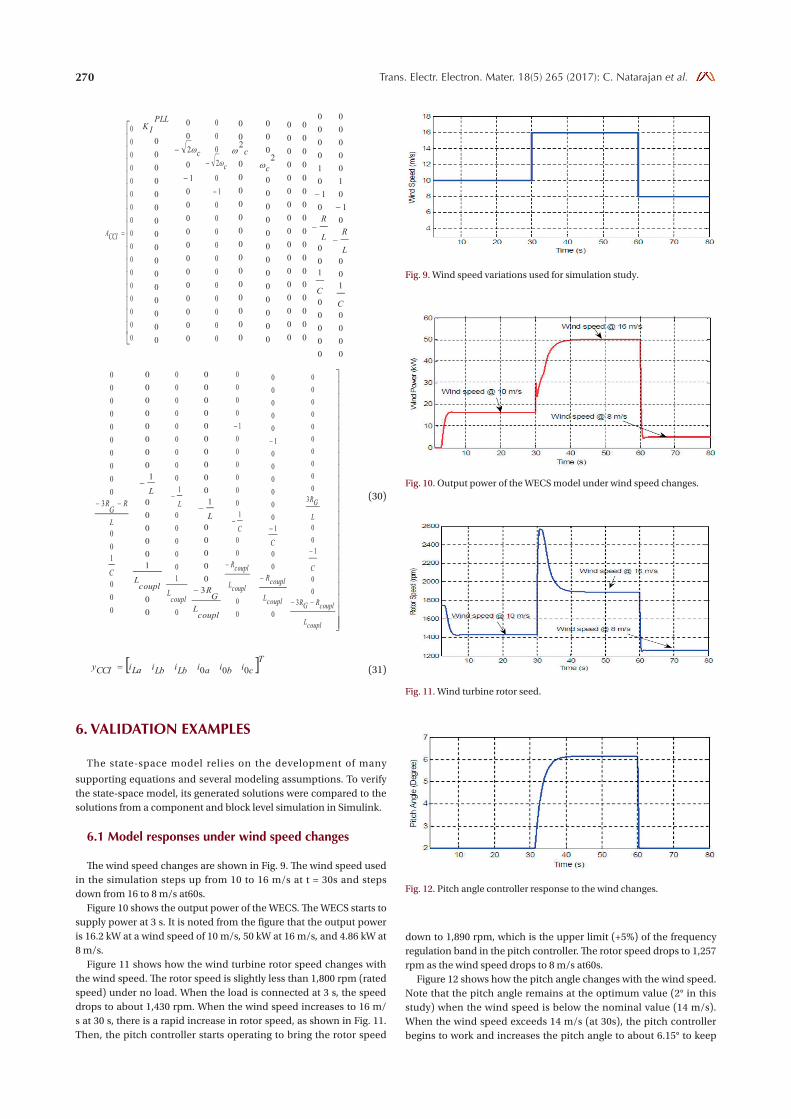
The wind speed changes are shown in Fig. 9. The wind speed used in the simulation steps up from 10 to 16 m/s at t = 30s and steps down from 16 to 8 m/s at60s.

Figure 10 shows the output power of the WECS. The WECS starts to supply power at 3 s. It is noted from the figure that the output power is 16.2 kW at a wind speed of 10 m/s, 50 kW at 16 m/s, and 4.86 kW at 8 m/s.

Figure 11 shows how the wind turbine rotor speed changes with the wind speed. The rotor speed is slightly less than 1,800 rpm (rated speed) under no load. When the load is connected at 3 s, the speed drops to about 1,430 rpm. When the wind speed increases to 16 m/s at 30 s, there is a rapid increase in rotor speed, as shown in Fig. 11. Then, the pitch controller starts operating to bring the rotor speed

down to 1,890 rpm, which is the upper limit (+5%) of the frequency regulation band in the pitch controller. The rotor speed drops to 1,257 rpm as the wind speed drops to 8 m/s at60s.

Figure 12 shows how the pitch angle changes with the wind speed. Note that the pitch angle remains at the optimum value (2° in this study) when the wind speed is below the nominal value (14 m/s). When the wind speed exceeds 14 m/s (at 30s), the pitch controller begins to work and increases the pitch angle to about 6.15° to keep

Fig. 9. Wind speed variations used for simulation study.

Fig. 10. Output power of the WECS model under wind speed changes.

Fig. 11. Wind turbine rotor seed.

Fig. 12. Pitch angle controller response to the wind changes.


the output power constant (at 50 kW). The corresponding CP is shown in Fig. 13.

6.2 SEIG responses

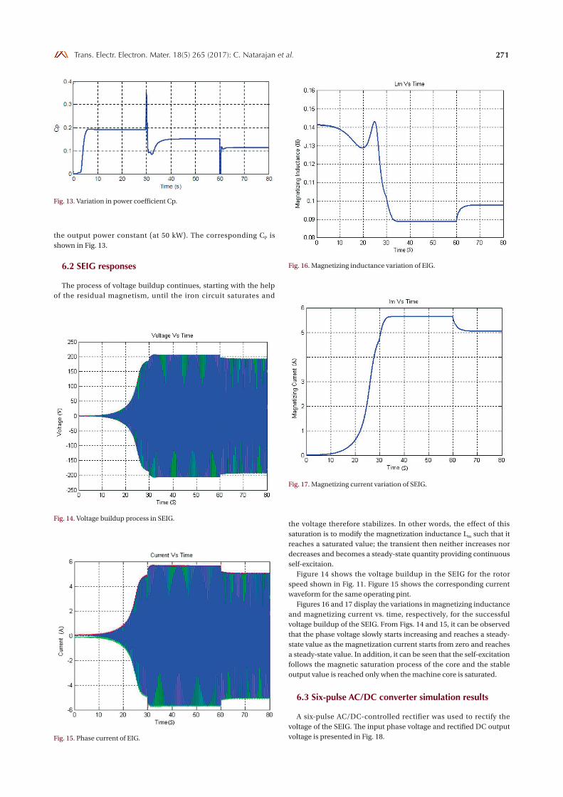
The process of voltage buildup continues, starting with the help of the residual magnetism, until the iron circuit saturates and

the voltage therefore stabilizes. In other words, the effect of this saturation is to modify the magnetization inductance Lm such that it reaches a saturated value; the transient then neither increases nor decreases and becomes a steady-state quantity providing continuous self-excitaion.

Figure 14 shows the voltage buildup in the SEIG for the rotor speed shown in Fig. 11. Figure 15 shows the corresponding current waveform for the same operating pint.

Figures 16 and 17 display the variations in magnetizing inductance and magnetizing current vs. time, respectively, for the successful voltage buildup of the SEIG. From Figs. 14 and 15, it can be observed that the phase voltage slowly starts increasing and reaches a steady-state value as the magnetization current starts from zero and reaches a steady-state value. In addition, it can be seen that the self-excitation follows the magnetic saturation process of the core and the stable output value is reached only when the machine core is saturated.

6.3 Six-pulse AC/DC converter simulation results

A six-pulse AC/DC-controlled rectifier was used to rectify the voltage of the SEIG. The input phase voltage and rectified DC output voltage is presented in Fig. 18.

Fig. 13. Variation in power coefficient Cp.

Fig. 14. Voltage buildup process in SEIG.

Fig. 15. Phase current of EIG.

Fig. 16. Magnetizing inductance variation of EIG.

Fig. 17. Magnetizing current variation of SEIG.


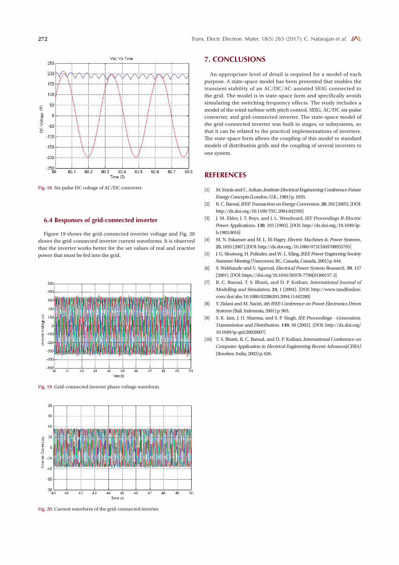
6.4 Responses of grid-connected inverter

Figure 19 shows the grid-connected inverter voltage and Fig. 20 shows the grid-connected inverter current waveforms. It is observed that the inverter works better for the set values of real and reactive power that must be fed into the grid.

7. CONCLUSIONS

An appropriate level of detail is required for a model of each purpose. A state-space model has been presented that enables the transient stability of an AC/DC/AC-assisted SEIG connected to the grid. The model is in state-space form and specifically avoids simulating the switching frequency effects. The study includes a model of the wind turbine with pitch control, SEIG, AC/DC six-pulse converter, and grid-connected inverter. The state-space model of the grid-connected inverter was built in stages, or subsystems, so that it can be related to the practical implementations of inverters. The state-space form allows the coupling of this model to standard models of distribution grids and the coupling of several inverters to

one system.

REfERENCES

[1] M. Ermis and C. Arikan, Institute Electrical Engineering Conference Future Energy Concepts (London, U.K., 1981) p. 1035.

[2] R. C. Bansal, IEEE Transaction on Energy Conversion, 20, 292 (2005). [DOI:

http://dx.doi.org./10.1109/TEC.2004.842395]

[3] J. M. Elder, J. T. Boys, and J. L. Woodward, IEE Proceedings B-Electric Power Applications, 130, 103 (1983). [DOI: http://dx.doi.org./10.1049/ip-

b.1983.0016]

[4] M. N. Eskanser and M. L. El-Hagry, Electric Machines &. Power Systems,

25, 1035 (2007).[DOI: http://dx.doi.org./10.1080/07313569708955795]

[5] J. G. Slootweg, H. Polinder, and W. L. Kling, IEEE Power Engieering Society Summer Meeting (Vancouver, BC, Canada, Canada, 2001) p. 644.

[6] S. Wekhande and V. Agarwal, Electrical Power System Research, 59, 157

(2001). [DOI: https://doi.org/10.1016/S0378-7796(01)00157-2]

[7] R. C. Bansal, T. S. Bhatti, and D. P. Kothari, International Journal of Modelling and Simulation, 24, 1 (2004). [DOI: http://www.tandfonline.

com/doi/abs/10.1080/02286203.2004.11442280]

[8] Y. Zidani and M. Naciri, 4th IEEE Conference on Power Electronics Drives Systems (Bali, Indonesia, 2001) p. 903.

[9] S. K. Jain, J. D. Sharma, and S. P. Singh, IEE Proceedings - Generation, Transmission and Distribution, 149, 50 (2002). [DOI: http://dx.doi.org/

10.1049/ip-gtd:20020007]

[10] T. S. Bhatti, R. C. Bansal, and D. P. Kothari, International Conference on Computer Application in Electrical Engineering Recent Advances(CERA)

(Roorkee, India, 2002) p. 626.

Fig. 18. Six-pulse DC voltage of AC/DC converter.

Fig. 19. Grid-connected inverter phase voltage waveform.

Fig. 20. Current waveform of the grid-connected inverter.

Modeling and Control of Three-Phase Self-Excited Induction ...

Documents