Modeling, Analysis, and Design of Responsive Manufacturing Systems Using Classical Control Theory by Nga Hin Benjamin Fong Dissertation submitted to the Faculty of the Virginia Polytechnic Institute and State University In partial fulfillment of the requirements leading to the degree of Doctor of Philosophy (Ph.D.) in Industrial and Systems Engineering (Manufacturing Systems Option) _____________________________ ____________________________ Co- Chair: Dr. John P. Shewchuk Co-Chair: Dr. Robert H. Sturges _____________________ _____________________ Dr. F. Frank Chen Dr. Ting-Chung Poon ______________________ Dr. Harry H. Robertshaw April 15, 2005 Blacksburg, Virginia Keywords: Classical Control Theory, System Responsiveness, Responsive Manufacturing Systems

Welcome message from author
This document is posted to help you gain knowledge. Please leave a comment to let me know what you think about it! Share it to your friends and learn new things together.
Transcript

Modeling, Analysis, and Design of Responsive Manufacturing
Systems Using Classical Control Theory
by
Nga Hin Benjamin Fong
Dissertation submitted to the Faculty of the
Virginia Polytechnic Institute and State University
In partial fulfillment of the requirements leading to the degree of
Doctor of Philosophy (Ph.D.)
in
Industrial and Systems Engineering (Manufacturing Systems Option)
_____________________________ ____________________________ Co- Chair: Dr. John P. Shewchuk Co-Chair: Dr. Robert H. Sturges
_____________________ _____________________ Dr. F. Frank Chen Dr. Ting-Chung Poon
______________________ Dr. Harry H. Robertshaw
April 15, 2005
Blacksburg, Virginia
Keywords: Classical Control Theory, System Responsiveness, Responsive Manufacturing Systems

Modeling, Analysis, and Design of Responsive Manufacturing Systems
Using Classical Control Theory
by
Nga Hin Benjamin Fong
(ABSTRACT)
The manufacturing systems operating within today’s global enterprises are invariably dynamic and complicated. Lean manufacturing works well where demand is relatively stable and predictable where product diversity is low. However, we need a much higher agility where customer demand is volatile with high product variety. Frequent changes of product designs need quicker response times in ramp-up to volume. To stay competitive in this 21st century global industrialization, companies must posses a new operation design strategy for responsive manufacturing systems that react to unpredictable market changes as well as to launch new products in a cost-effective and efficient way. The objective of this research is to develop an alternative method to model, analyze, and design responsive manufacturing systems using classical control theory. This new approach permits industrial engineers to study and better predict the transient behavior of responsive manufacturing systems in terms of production lead time, WIP overshoot, system responsiveness, and lean finished inventory. We provide a one-to-one correspondence to translate manufacturing terminologies from the System Dynamics (SD) models into the block diagram representation and transfer functions. We can analytically determine the transient characteristics of responsive manufacturing systems. This analytical formulation is not offered in discrete event simulation or system dynamics approach. We further introduce the Root Locus design technique that investigates the sensitivity of the closed-loop poles location as they relate to the manufacturing world on a complex s-plane. This subsequent complex plane analysis offers new management strategies to better predict and control the dynamic responses of responsive manufacturing systems in terms of inventory build-up (i.e., leanness) and lead time. We define classical control theory terms and interpret their meanings according to the closed-loop poles locations to assist production management in utilizing the Root Locus design tool. Again, by applying this completely graphic view approach, we give a new design approach that determine the responsive manufacturing parametric set of values without iterative trial-and-error simulation replications as found in discrete event simulation or system dynamics approach.

Acknowledgements
It has been a challenging and fruitful journey to return to Virginia Tech to study my Ph.D. program in Industrial and Systems Engineering. I am very thankful to have such a unique and multi-disciplinary research committee which they have taught me how to think, learn, and communicate. I would like to take this opportunity to thank them for their guidance and support which greatly enhanced the value of my eight year journey. Dr. John P. Shewchuk, my Co-Chairman of the Committee, has spent tremendous amount of time and effort to guide me through this research journey. From initial research ideas to models implementation, from model validation to dissertation writing, he has provided a lot of good advice and help to make my Ph.D. commencement happening. In particular, his input and concern on validating CCT models to discrete manufacturing world is a crucial part to implement our new methodology from the industrial engineering point of view. Lastly, his high standard writing style has made my dissertation so completed. My heartfelt thanks to him! Dr. Robert H. Sturges, my Co-Chairman of the Committee, is truly a role model in both teaching and research excellence. His innovative ideas, kindness, courage and motivation have made me to realize how fortunate I am to have him to be my co-advisor. From academic research to industrial projects, from departmental politics to my personal issues, we can spend numerous hours to chat and discuss without feeling the time has gone so fast. He has transformed me from a below average graduate student to become awards winning research scholar. In Chinese term, he is my “Inspirational Master”!! Truly, I may never be able to complete translating CCT terminologies to manufacturing world without him. That “special Friday talk” outside Durham in September 2003 has significantly changed my career life. Thanks Dr. Bob! ☺ Dr. Harry H. Robertshaw, my former advisor for my MS in Mechanical Engineering, has guided me through many challenges throughout the past 13 years. From my MS research work to Labor Certification supporting letter, from preliminary research to latest Intel Case Study, it is unquestionable that his willingness to support is vital. I especially appreciate his extra time and effort to assist me to formulate the block diagrams and algebraic expressions for my dissertation work. Definitely, he has spent at least three times amount of time to assist my Ph.D. work than my MS program. Big thanks to him! Dr. F. Frank Chen, my most respectful industrial-managerial, research professor, has taught me one should have long term visions and plans to be success in both academia and industrial world. As the founder of the Center for High Performance Manufacturing (CHPM), Dr. Chen has provided me the complete financial support through my three years of full-time studies. Besides, he gave tremendous advice and help to make my dissertation completed. I look forward to follow his successful foot steps to work for Caterpillar at Peoria, IL. Many thanks to him!! Dr. T.C. Poon, my most admirable professor and long-time friend, has been advising me since I came to Virginia Tech in Fall 1992. Throughout these 13 years in Blacksburg, there are uncountable incidents that required his help and advice to get over the challenges. I really
iii

appreciated to have him to serve in my dissertation committee. Although the work of modeling manufacturing systems via electrical circuit network has not completed, it is noteworthy to continue these ideas for future work. Hopefully, my upcoming design engineering position will enhance my skills to work with network modeling and frequency response analysis. Thanks very much Dr. Poon! Special thanks to my former boss, Graham Swinfen, an engineering manager at BBA Friction, Inc. in Dublin, VA. Without his persistent help, I would never work at BBA Friction to get my green card and have the opportunity to begin my PhD study at Virginia Tech. From Fall 1997 to Spring 2000, I was able to drive back-and-forth for two hours to go to work-school-work-home regularly. I still remembered how much heat Graham had to take to support of the justification of my continuous education at Virginia Tech giving the time and the financial support from BBA Friction, Inc. Big thanks to Graham! Throughout my eight years of study (3.5 years part-time, 1 year off, 3.5 years full-time), I met so many helpful and interesting colleagues among the student group. Special thanks go to Nathan Ivey and Hitesh Attri in assisting me for the ARENA programming. I wish the best luck to Nate, Hitesh and Radu Babiceanu for their job hunting. It is very thankful to have known Dr. Y.A. Liu and Dr. Hing-Har Lo (Mrs. Liu) through the VT Chinese Bible Study since Fall 1992. They have been acting like my guardian throughout the years – give me the spiritual support and advice while keeping “little Ben” behaves well. ☺ Again, many thanks to Dr. T.C. Poon and Eliza Poon (Mrs. Poon), they are like my older brother and sister via Hong Kong Club and VT Chinese Bible Study. They gave me so many advices and ideas for my daily life, such as school work, buying house, raising kids, career development, retirement plan, etc. Give thanks to the Lord, I have learned so much from these two lovely families! It has been a blessing to get the role to lead and care many young Hong Kong students through the VT Chinese Bible Study and HK Club. Best wishes to my spiritual brothers, Carlos Siu, Henry Yuen, and Winston Ma for their first career challenge as engineers and/or statistical analyst. I enjoyed those uncountable hours to share our joy and sadness while we were in Blacksburg. I especially missed our weekly soccer games at Tech! No doubt in my mind, my life will ever reach to this stage without the support from my family. Thanks be to my Lord to provide me such a lovely and heart-bonded family. I would like to express my heartfelt appreciation to my parents, Hoo-Shin Fong and Shau-Shan Lai, for their unyielding love and support since I was born. My bond with my parents grew even stronger when I left home to England since 1985. They provided me with tremendous mental and financial support through these years. Particularly in the past three years, after their retirement from Hong Kong, they even came to stay with my family to help baby-sit their lovely grandchildren. For sure, their physical support has allowed me to concentrate on my research while my daughters are often crying for milk. I also give thanks to the Lord to giving me such a wonderful and supportive elder brothers, Ricky and Joe. We have grown up together back in Hong Kong, then we all went to Rishworth for high
iv

school in England, and we all came to States for gaining our higher education. Throughout these years, we have shared and supported each other via visit, phone calls, and prayers. It is so important to maintain this high degree of brother-hood to be able to face all those up-and-down in life. As Ricky said, I shall be thankful to have completed my Ph.D. as a by-product due to my long-waiting green card application process. While Joe always reminds me that getting a Ph.D. is just a beginning for the next chapter of life. Thank you my dearest brothers!! I also give thanks to my two lovely sisters-in-law, Susanna and Florence, for their prayers, supports, and sharing in all these years. Lastly, I would dedicate this dissertation to my beloved wife, Iris (Ching) for her unyielding love, support and care to make me become Dr. Fong! I give thanks to my Lord to give me such an understandable and dedicated wife and mother. Iris and I had gone through so many challenges since we were together in Spring 1995. Our life faced a lot of challenge in the early stage, such as, I worked over 70+ hours weekly in Hazard, KY, then she worked over 70+ hours in Hotel Roanoke, VA. Sure, we were just a cheap-labor whom decided to live in US. By summer 1998, we got married and began our next challenge for the school work at Tech. I began my part-time PhD study while I was working full-time at BBA Friction and she returned to Virginia Tech to study her MS in Accounting and Information Systems in Spring 1998. The most difficult challenge was to study together almost every night at Durham Hall until 4 am while I still had to return to work by 8 am. It is so thankful to have her support and patience to host numerous Friday night gathering with those HK students right after the bible study. We both learned so much and became more mature to take care this young students group. Without a doubt, Iris has sacrificed her career twice to choose a less competitive and lower-paid job to stay in Blacksburg to give me time to finish my PhD program. Her unique encouraging style by keep reminding me “not to waste time and move on” has made me even stronger and more self-confidence to continue to pursue my PhD program. ☺ I give thanks to her to be such a caring mother and daughter-in-law to help taking care our two lovely daughters, Vera and Audrey, and my parents while I was busy preparing my dissertation work. Iris will probably give up her career for the third time when we move to Peoria, IL. But I am sure that the kids must love to see Mommy spend more time at home. ☺ Thank you Lord for giving me such a loving family, I would never complete my PhD study without their support. My final sharing for those whom love to get a PhD degree, you should equip the following elements to be succeeded, such as willingness, hard-work, discipline, persistence, research topic, supportive professor committee and most importantly, communication skills. God Bless America!! ☺
v

Table of Contents
Chapter 1 Introduction............................................................................................................1
1.1 Background....................................................................................................................1
1.2 Problem Statement .........................................................................................................5
1.3 Research Objectives.......................................................................................................6
1.4 Contents of Dissertation.................................................................................................7
Chapter 2 Literature Review ..................................................................................................9
2.1 Agile and Responsive Manufacturing............................................................................9
2.2 Early Development in System Dynamics ..........................................................................13
2.3 Recent Applications of System Dynamics...................................................................14
2.4 Input-Output Analysis in modeling production-inventory systems.............................16
2.5 Other approaches to model dynamic manufacturing systems ..................................................20
2.6 Missing link of the existing modeling approaches ......................................................20
Chapter 3 Modeling and Analysis of Responsive Manufacturing Systems......................23
3.1 Modeling and Analysis via System Dynamics……………………………………. ................24
3.1.1 System Dynamics Approach ………………………………………………......24
3.1.2 A Single-Stage Production Control System ……………….. ………………....26
3.1.3 A Basic Kanban System Model ……………….. …………………………… ..28
3.1.4 A Two-Stage Production Control System ……………………………………..31
3.1.5 A Two-Stage Production Control System with Time Delay ………………… .33
vi

3.2 Modeling and Analysis via Classical Control Theory ………………………….…................36
3.2.1 Fundamentals of Classical Control Theory …………………….. ………….................36
3.2.2 Transfer Function of a Single-Stage Production Control System ………….. ................37
3.2.3 Transfer Function of a Basic Kanban System Model ……………………… ....40
3.2.4 Transfer Function of a Two-Stage Production Control System …………….....48
3.2.5 Transfer Function of a Two-Stage Production Control System w/ Time Delay 54
3.3 Guidelines to Translate Responsive Manufacturing Systems via CCT ………….…..............58
Chapter 4 Model Validation ………………………………………………. .. 61
4.1 Discrete Event Modeling of a Single-Stage Production Control System ....................63
4.2 Comparison between Discrete Event Model and Classical Control Model.................67
Chapter 5 Design of Responsive Manufacturing Systems ………………. .. 72
5.1 Root Locus Analysis and Design of a Two-Stage Production System ….………......73
5.2 Interpretation of CCT Terms to the Manufacturing World ………………………. ...81
5.3 Root Locus Design of a Two-Stage Production System with Time Delay ….……....87
5.4 Guidelines to perform Root Locus Design in Responsive Manufacturing System … 96
Chapter 6 Industrial Case Study ………………………….………………. . 98
Chapter 7 Conclusions and Research Contributions ...................................116
vii
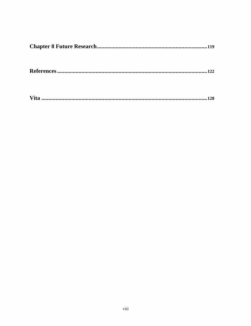
Chapter 8 Future Research.............................................................................119
References .........................................................................................................122
Vita ....................................................................................................................128
viii
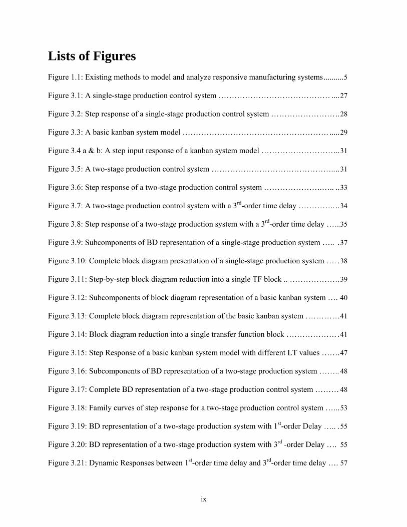
Lists of Figures Figure 1.1: Existing methods to model and analyze responsive manufacturing systems..........5
Figure 3.1: A single-stage production control system …………………………………… ....27
Figure 3.2: Step response of a single-stage production control system ……………………..28
Figure 3.3: A basic kanban system model ………………………………………………. .....29
Figure 3.4 a & b: A step input response of a kanban system model ………………………...31
Figure 3.5: A two-stage production control system ………………………………………....31
Figure 3.6: Step response of a two-stage production control system ………………….….. ..33
Figure 3.7: A two-stage production control system with a 3rd-order time delay ………….. ..34
Figure 3.8: Step response of a two-stage production system with a 3rd-order time delay …...35
Figure 3.9: Subcomponents of BD representation of a single-stage production system ….. .37
Figure 3.10: Complete block diagram presentation of a single-stage production system …. .38
Figure 3.11: Step-by-step block diagram reduction into a single TF block .. ……………….39
Figure 3.12: Subcomponents of block diagram representation of a basic kanban system …. 40
Figure 3.13: Complete block diagram representation of the basic kanban system ………….41
Figure 3.14: Block diagram reduction into a single transfer function block ………………. .41
Figure 3.15: Step Response of a basic kanban system model with different LT values …….47
Figure 3.16: Subcomponents of BD representation of a two-stage production system …….. 48
Figure 3.17: Complete BD representation of a two-stage production control system ……… 48
Figure 3.18: Family curves of step response for a two-stage production control system …...53
Figure 3.19: BD representation of a two-stage production system with 1st-order Delay ….. .55
Figure 3.20: BD representation of a two-stage production system with 3rd -order Delay …. 55
Figure 3.21: Dynamic Responses between 1st-order time delay and 3rd-order time delay …. 57
ix

Figure 4.1: A Single-Stage Production Control System …………………………………… .64
Figure 4.2: Step Response of a Single-Stage Production Control System ………………… .64
Figure 4.3: ARENA discrete-event model of a single-stage production control system …....65
Figure 4.4: A single-stage production system (Ship every 2 hr; Production update 4 hr) …..67
Figure 4.5: A single-stage production system (Ship every 4 hr; Production update 4 hr).......68
Figure 4.6: A single-stage production system (Ship every 8 hr; Production update 4 hr)…...68
Figure 4.7: A single-stage production system (Ship every 24 hr; Production update 4 hr) ....69
Figure 4.8: Discrete vs. Continuous in modeling single-stage production system …………. 70
Figure 5.1: A system for Root Locus ……………………………………………………….. 74 Figure 5.2: Root-Locus Plot of a Two-Stage Production Control System …………………. 75
Figure 5.3: Contour Plot of ζ values as a function of LT and WAT ………………………. .78
Figure 5.4: Contour Plot of Breakaway Points as a function of LT and WAT ……………...79
Figure 5.5: Step Response Comparison of a Two-Stage Production Control System……… ..............80
Figure 5.6: Complex s-plane interpretation of varying location of closed-loop poles ……. ..83
Figure 5.7: Transient mode shapes associated with locations of roots in complex s-plane.....86
Figure 5.8: Root-Locus Plot of a two-stage production system with 3rd-order time delay ….89
Figure 5.9: Step Responses of a two-stage system with 3rd-order time delay under
various K values ……………………………………………………………………………. 91
Figure 5.10: Root-Locus Plot of a two-stage production system w/ 3rd-order time delay…... 93
Figure 5.11: Various Step Response of a two-stage production control system
with 3rd-order time delay …………………………………………………………………….94
Figure 6.1: Hybrid Push-Pull Intel Semiconductor Production System …………………… 99
Figure 6.2: System Equations for 1st Stage Process – Fabrication WIP…… ....................... 102
x
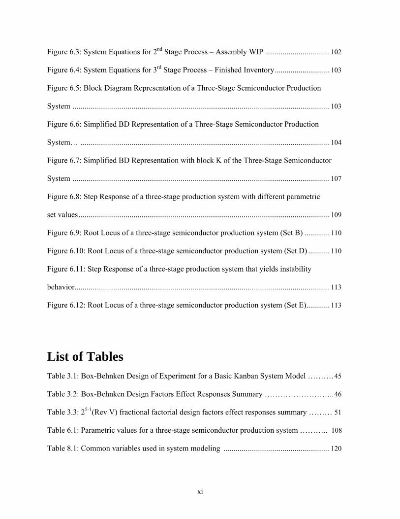
Figure 6.3: System Equations for 2nd Stage Process – Assembly WIP ................................. 102
Figure 6.4: System Equations for 3rd Stage Process – Finished Inventory............................ 103
Figure 6.5: Block Diagram Representation of a Three-Stage Semiconductor Production
System ................................................................................................................................... 103
Figure 6.6: Simplified BD Representation of a Three-Stage Semiconductor Production
System… ............................................................................................................................... 104
Figure 6.7: Simplified BD Representation with block K of the Three-Stage Semiconductor
System ................................................................................................................................... 107
Figure 6.8: Step Response of a three-stage production system with different parametric
set values................................................................................................................................ 109
Figure 6.9: Root Locus of a three-stage semiconductor production system (Set B) ............. 110
Figure 6.10: Root Locus of a three-stage semiconductor production system (Set D) ........... 110
Figure 6.11: Step Response of a three-stage production system that yields instability
behavior.................................................................................................................................. 113
Figure 6.12: Root Locus of a three-stage semiconductor production system (Set E)............ 113
List of Tables Table 3.1: Box-Behnken Design of Experiment for a Basic Kanban System Model ………. 45
Table 3.2: Box-Behnken Design Factors Effect Responses Summary ……………………...46
Table 3.3: 25-1(Rev V) fractional factorial design factors effect responses summary ……… 51
Table 6.1: Parametric values for a three-stage semiconductor production system ……….. 108
Table 8.1: Common variables used in system modeling ...................................................... 120
xi

Chapter 1 Introduction N.H. Ben Fong
Chapter 1 Introduction
1.1 Background
Many enterprises have practiced the lean thinking paradigm to enhance the efficiency of their
business processes. In recent years, an agile manufacturing paradigm has been underlined as an
alternative to, and possibly an improvement on, leanness. Christopher and Towill [1] have
described that lean concepts work well where demand is relatively stable and predictable where
product diversity is low. In contrast, when customer requirement for variety is high and volatile,
a much higher level of agility is required. Helo [2] defined agile manufacturing as the capability
of reacting to unpredictable market changes in a cost-effective way, simultaneously prospering
from the uncertainty. In many manufacturing companies, dynamically changing markets are
demanding more differentiated products in lower volumes and within less production lead time.
Any uncertain conditions challenge the dynamic response of manufacturing systems. Enterprises
have to deal with high seasonal rise and fall in demand. Frequent changes of product designs and
complex products need quicker response times in ramp-up to volume. To stay competitive in this
21st century global industrialization, companies require responsive manufacturing systems that
can react to unpredictable market changes as well as launch new products economically and
efficiently. Responsive manufacturing systems yield shorter production lead time, minimal
inventory build-up and related cost, better overall dynamic system behavior and thus lead to
excellent customer satisfaction.
1

Chapter 1 Introduction N.H. Ben Fong
In order to have responsive manufacturing systems, we must develop a methodology or an
approach which permits engineers to mathematically model, analyze, and design to such systems.
In most manufacturing systems, engineers often categorize models by their computational form,
either analytical or experimental. Analytical models represent a mathematical abstraction of the
real manufacturing systems. A set of equations is formulated that summarizes the aggregate
performance of the system models. Simulation models are experimental and mimic the events
that occur in the real system.
Queuing network analysis is the most common analytical method to find rough-cut or quickly
evaluate average steady-state performance of manufacturing systems [3]. A network of queues is
a system in which materials arrive at a queue, wait until they are processed, and then move to the
next processing stage of a system. Queuing network models are built upon steady-state
probability distributions, often having Poisson arrivals and exponentially distributed processing
time. Gershwin [4] stated that there are limitations in applying queuing network. Blocking would
not occur due to the assumption of infinite buffer size. In addition, queuing models only work for
a limited set of queue disciplines. Furthermore, they do not generally allow a system controller to
observe the queue length or service duration at one station, and change the control policy of the
whole system or of another station. Hence, when a particular processing stage takes an unusual
long operation, the overall system is not permitted to take any kind of action in response.
Moreover, most real manufacturing systems are complex with multiple system feedback loops
under transient conditions, such systems are too complicated to analytically derive mathematical
formulation by queuing network analysis.
2
Chapter 1 Introduction N.H. Ben Fong
Discrete event simulation (DES) is the most popular tool for modeling and analyzing dynamic
manufacturing systems at a very detailed level. DES is typically characterized by queues, servers,
and probabilistic distributions of parameters such as arrival and service times. Unfortunately, the
DES method often requires too much time to construct models, perform simulation experiments,
and analyze results. In addition, DES is an event-based simulation and modeling tool, it does not
depend on the causality relationships among system variables. There is no analytical solution or
feedback nature for design and analysis purposes. It often requires the use of design of
experiments or trial-and-error iterative simulation replications to generate output performance for
decision-making. Moreover, the transient responses generated by DES generally consider as the
warm-up period behavior and its output performance measures are statistically evaluated at the
steady-state condition. DES does not predict apriori the dynamic characteristics of system
models under transient conditions, such as production settling time, WIP overshoot and lean
finished inventory level. Engineers have to rely on numerous simulation replications and large
numbers of data points to generate solutions for decision-making.
System Dynamics (SD) is an alternative technique developed by Jay W. Forrester [5] to build
dynamic system models. The term SD refers to a business system modeling technique that
employs causal loop diagrams (CLD) and stock-and-flow diagrams (SFD) to describe
information and materials flow. SD is based upon the concept of feedback thinking and control
engineering to the study of economic, business, and organizational systems. It builds on how
information flow, feedback-loops, and time delays within the structure of a system create
dynamic behavior. SD is a simulation-based modeling technique that requires numerous trial-
and-error iterations to study the dynamic behavior of responsive manufacturing systems. It does
3

Chapter 1 Introduction N.H. Ben Fong
not provide any analytical solution to determine key transient system parameters and their
corresponding output measures. For most control engineers, a mathematical model of a dynamic
system is usually described in terms of differential equations based upon physical laws or
idealized constitutive relationships among system variables. For the latest literature review, there
is no one-to-one correspondence to model dynamic manufacturing systems between the
differential equation formulation and the CLD and SFD structures applied in the SD approach.
There is an alternative method called Input-Output Analysis developed by Dennis R. Towill [6,7]
to model dynamic manufacturing systems in block diagram representation. The input-output
analysis mimics the differential equation formulation. As stated in the literature review section,
the block diagram representation of the input-output analysis system models can convert into
transfer functions for control analysis under Laplace Transform domain. Those first-order lag
transfer functions are applied to model and describe supply chain dynamics and inventory-
production control systems. Lately, researchers apply the analogies of electrical circuit and fluid
system to model and study dynamic manufacturing systems behavior. The inter-relationship
among these modeling techniques is illustrated as shown in Figure 1.1
4

Chapter 1 Introduction N.H. Ben Fong
Responsive Manufacturing Systems
DES (steady-state, simulation based, no analytical, no feedback, design via iterations)
System Dynamics (dynamics, simulation based, with feedback, no analytical solutions, design via iterations)
Block Diagram Representation
Transfer Function (dynamics, analytical solutions, analytical system design, stability analysis, structure improvement)
Electrical Circuit Model
Fluid Model
Figure 1.1: Existing methods to model and analyze responsive manufacturing systems
1.2 Problem Statement
The manufacturing systems operating within today’s global enterprises are invariably dynamic
and complicated. As manufacturing business leans towards globalization, market demand
appears to be highly fluctuated; lean manufacturing philosophies may no longer work well under
these frequently change and unpredictable conditions. It is an awesome challenge for practicing
managers and engineers in attempting to design and improve the overall responsiveness of those
dynamic manufacturing systems. The big picture question here is whether we can develop an
engineering methodology to assist production management to model, analyze, and design
responsive manufacturing systems in this 21st century global industrial market. Can we
5

Chapter 1 Introduction N.H. Ben Fong
analytically determine key transient manufacturing system parameters, such as production
settling time, WIP overshoot, system responsiveness, and lean finished inventory level? In
addition, without doing any iterative trial-and-error simulation replications, can we assist
management to design, improve, and control the overall dynamic behavior of such
manufacturing systems? The author truly believes that one can find these answers in this
dissertation work. Lastly, this alternative modeling, analysis, and design methodology can be
applied to any manufacturing system in general.
1.3 Research Objectives
The objectives of this dissertation research are as follows:
1) Develop a one-to-one correspondence to model manufacturing systems between the
differential dynamic models (Classical Control Theory) and the CLD and SFD structures
employed in the SD approach;
(2) Derive resulting transfer functions from the particular system block diagram representation to
analytically determine the transient characteristics of the manufacturing systems;
(3) Sensitivity analysis of key manufacturing system parameters that influence the overall
manufacturing system responsiveness and leanness;
(4) Apply the Root Locus technique from Classical Control Theory as a new production
management strategy to better predict and design key manufacturing terms on a complex s-plane
environment;
(5) Define and interpret classical control theory terms as they relate to the manufacturing world;
6

Chapter 1 Introduction N.H. Ben Fong
(6) Reveal the potential for system instability due to management policies in higher-order system
with time delays dynamics;
(7) Validate the continuous differential equation model as a good approximation of real
discretized manufacturing systems.
1.4 Contents of Dissertation
The rest of the dissertation is outlined as follows. Chapter 2 presents the literature review. We
begin the review by examining agile and responsive manufacturing systems, followed by the
early development of System Dynamics (SD) and its recent applications. We further describe
other modeling approaches, like, input-output analysis, fluid model, and electric circuit modeling.
Chapter 3 describes the modeling and analysis of responsive manufacturing systems. The
fundamental mechanism of SD developed by Jay Forrester is discussed in detail. Four particular
production control system models are presented to translate the SD terminologies into classical
control theory (CCT) approach. The resulting differential equation models permit production
management and industrial engineers to analytically determine the transient characteristics of the
responsive manufacturing systems. The objective of Chapter 4 is to validate the CCT approach
by comparing with discrete event simulation. In Chapter 5, we investigate design issues and
show how we can employ the Root Locus technique and incorporate third-order time delays. To
enhance the validation of this new CCT design and modeling approach, we include an industrial
case study in Chapter 6. In that chapter, we apply the CCT approach developed in this
dissertation to model and design an Intel hybrid push-pull production system for semiconductors
7

Chapter 1 Introduction N.H. Ben Fong
manufacturing. Chapter 7 highlights the concluding remarks and research contribution from this
dissertation work. Finally, we provide some future research directions in Chapter 8.
8
Chapter 2 Literature Review N.H. Ben Fong
Chapter 2 Literature Review
This chapter presents the literature review of the rise of responsive manufacturing systems
modeling and analysis, the development and recent applications of system dynamics (SD), the
input-output analysis in modeling production-inventory systems, and other analogous approaches
to model dynamic manufacturing systems. Finally, we state the missing links of these existing
modeling approaches that lead to our new alternative modeling and design approach.
2.1 Agile and Responsive Manufacturing
In the early 20th century, Henry Ford introduces the well-known mass production system. Ford’s
philosophy is to build a simple, low cost, and fully utilized assembly line system. Such a mass
production system is very inflexible and is not responsive to changing customer demands. It
relies on forecasting future customer demand and scheduling the release of orders. This system
often results in high work-in-process levels and excess finished inventories. In the 1980s, the
Toyota production system or just-in-time (JIT) system is developed to provide better flexibility
through the concept of pull within the factory. JIT production depends on actual customer
demand activating the release of orders into the system to fill the demand. The JIT philosophy
emphasizes making the right products in the right amount at the right time. JIT eliminates excess
inventory, shortens production lead-time, and increases quality in both products and customer
service. In the 1990s, companies begin to implement the concept of lean manufacturing that
9

Chapter 2 Literature Review N.H. Ben Fong
evolved from the Toyota production system. Lean manufacturing is a comprehensive philosophy
where employees continue to strive for improvement to eliminate all non-value added activities.
Although JIT or lean manufacturing has a significant culture impact to improve production
efficiency, its system performance measures are restricted under steady-state conditions.
In the 21st century, due to the highly fluctuating market demand and the frequent change of
product designs, to stay competitive in this global market, manufacturing companies must
possess a new kind of manufacturing system that can be very responsive to volatile global
markets. Helo [2] defines agile manufacturing as the capability of reacting to unpredictable
market changes in a cost-effective way, simultaneously prospering from the uncertainty. In his
paper, three system dynamic simulation models are analyzed to the agility of supply chains. The
analysis recommends smaller order sizes, echelon synchronization and capacity analysis as
methods of improving the responsiveness of the supply chain. Sanchez and Nagi [8] have
reviewed a wide range of recent literature on agile manufacturing. Their paper concludes agile
manufacturing as the solution to a society with an unpredictable and dynamic demand.
Christopher and Towill [1] show the various ways to combine the paradigms of leanness and
agility to enable highly competitive supply chains in a volatile and cost-conscious environment.
The paper emphasizes the important differences between the two paradigms and how one may
benefit from the implementation of the other. In the literature, Naylor et al. [9] define agility as
the use of market knowledge and a virtual corporation to exploit profitable opportunities in a
volatile market place. Whereas leanness is constructing a value stream to eliminate all waste
including time and to enable a level schedule.
10

Chapter 2 Literature Review N.H. Ben Fong
Asi et al. [10,11] define a new manufacturing paradigm called reconfigurable manufacturing
systems (RMS). RMS is designed at the outset for rapid change in the system configuration, their
machines, and controls in order to quickly adjust production capacity and functionality in
response to market changes. This type of system will provide customized flexibility for a
particular part family, and will be open-ended, such that it can be improved and reconfigured,
rather than scrapped and replaced. Mehrabi et al. [12] describe agile manufacturing to focus on
the manufacturing enterprise and the business practices needed to adapt to a changing global
market characterized by uncertainty. It does not provide any operational techniques or any
engineering solutions. In contrast, RMS does not deal with the entire enterprise but only with the
responsiveness of the production system to new market opportunities in an environment of
global competition with suitable market production. The RMS methodologies of rapid system
design and ramp-up, as well as the capability to add incremental capacity and functionality in
response to market demands, is one aspect of agility. Hence, agile manufacturing shares with
reconfigurable manufacturing the ability to improve the overall manufacturing responsiveness.
Consequently, agile manufacturing is complementary to reconfigurable manufacturing.
Asi et al. [10] introduce a control-theory based fluid dynamic model to assist in implementing
the optimum reconfiguration policy and production scheduling of an RMS. They develop and
analyze a simplified dynamic production model whose capacity and/or functionality can change
over time. Asi and Ulsoy [11] further formulate and provide a sub-optimal solution for a general
capacity management using feedback control theory approach under both deterministic and
stochastic market demand.
11

Chapter 2 Literature Review N.H. Ben Fong
Suri [13,14] defined a new company wide-strategy called Quick Response Manufacturing (QRM)
to pursue the reduction of lead time in all aspects of a company’s operations, both internally and
externally. Internally, QRM focuses on reducing the lead times for all tasks across the whole
enterprise, resulting in improved quality, lower cost, and quick response. From a customer’s
view point, QRM responds to their needs by rapidly designing and manufacturing products
customized to those needs. In addition, Suri has developed a new material control method, called
Paired-Cell Overlapping Loops of Cards with Authorization (POLCA) to provide companies
with significant competitive advantage over the traditional MRP and Kanban systems.
Whether it is agile manufacturing, reconfigurable manufacturing systems, or quick response
manufacturing, companies must be able to react and respond quickly to predict and improve their
overall manufacturing system performance in fast-changing and uncertain global markets. In
other words, the manufacturing system must be responsive in such environments and be able to
operate effectively in transient mode (as well as steady-state). This in turn necessitates news
methods for modeling, analyzing, and designing responsive manufacturing systems. In particular,
it is important to be able to establish the fundamental cause-and-effect relationships among key
manufacturing variables, such as production start rate, production completion rate, WIP level,
Finished Inventory level, desired production rate, production lead time, etc. Unfortunately,
idealized constitutive laws like Newton’s laws in mechanical systems and Kirchhoff’s laws for
electrical systems do not apply in the manufacturing systems world. System Dynamics
developed by Jay W. Forrester [5,15,16] is the most popular modeling technique available to
model and analyze dynamic manufacturing systems, but still leave room for improvement.
12
Chapter 2 Literature Review N.H. Ben Fong
2.2 Early Development in System Dynamics
The discipline of system dynamics (SD) has been studied over forty years. Dr. Jay W. Forrester
originally developed the framework of SD at the Massachusetts Institute of Technology (MIT) in
the late 1950s [5]. SD builds on how information flow, feedback-loops, and time delays within
the structure of a system create dynamic behavior. SD applies the feedback system thinking and
control engineering concepts to the study of economics, business, and organizational systems
[5,15,16]. Forrester defines SD as the study of the information-feedback characteristic of
industrial activity to show how organization structure, amplification and time delays interact to
influence the success of the enterprises. Forrester argues that mathematical analysis is not
powerful enough to solve the problems of the complex system and we need a simulation
approach. The first major piece of Forrester work published in 1958 gives a succinct explanation
of dynamic behavior in a production-distribution chain. In 1961, this work forms the core of the
book Industrial Dynamics [5]. There are other major publication come in the following years,
include, Urban Dynamics (1969), World Dynamics (1973), and the Collected Papers published
in 1975 [17]. Forrester applies the concepts of feedback loops in the understanding of system
behavior. He discusses the use of mathematical representations coupled with simulation.
Simulation takes the emphasis off mathematics for the sake of analytical solutions. Analytical
solutions are no longer as important as to provide an additional perspective and insight into the
nature that underline system dynamics. To facilitate model simulation, Forrester develops a
dynamic modeling language and simulation tool called DYNAMO [17]. This modeling tool
identifies flows within the system and forms the model about the structure derived from the
interactions of their paths.
13

Chapter 2 Literature Review N.H. Ben Fong
Although the use of Forrester’s concepts has significant impact to the field of system modeling,
it also produces controversy. Ansoff and Slevin [17] give some criticism on the validity of the
SD technique published by Forrester. Their paper has questioned whether Forrester’s ideas are a
proven theory, plus the span of his potential application that he claimed. Ansoff and Slevin
suggest that SD can give the promise of advantages that may grow from a better understanding
of systems, but it does not adequately convey the essential mathematics in modeling dynamic
systems. In 1980, Anderson and Richardson [17] further state that analytical representation can
be very useful to simulation in system dynamics modeling. The analytical formats will not only
be useful in relating behavior to system structure but their applications can encourage wider
interest in SD from the control theory discipline. Forrester describes that the future SD work
could include the basic structures recurrent in system models to be converted into a generic
library in explicit dynamic form. Edghill and Towill [17] express that explicit dynamic form can
be interpreted as the block diagram representation and Laplace transforms from the control
theory. Computer-based methods are found to be more successful in modeling and simulating
live-system dynamic behavior but they do not provide an analytical approach to analyze the
relationship of cause and effect of the systems. Beginning late 80s, there has been a drift in
emphasis away from the original SD applications that focuses on the design of production-
inventory systems to the latest business consulting process modeling [16,18,19].
2.3 Recent Applications of System Dynamics
O’Callaghan [20] applies system dynamics to model and simulate a kanban-based JIT production
system. The multi-stage manufacturing system model is simulated to show the dynamic behavior
14

Chapter 2 Literature Review N.H. Ben Fong
subjected to different management policies. Gupta and Gupta [21] further employ SD approach
to model a multi-stage, multi-line, dual-card, JIT-kanban production system. This paper focuses
on the inherent characteristics of the kanban system and investigates the system behavior under
various management policies. Ravishankar [22] at Intel Corporation develops several SD models
to understand the effect of management policies on the performance of a semiconductor
fabrication line. He constructs a resource allocation model within an organization to illustrate
how explicit and implicit policy decisions can have an impact on factory output and equipment
performance. Bianchi and Virdone [23] use a SD approach to re-engineer the manufacturing
processes in a European telecommunication firm. The model is set to estimate potential benefits
of a shift from a push system to a pull system.
Lin et al. [24] give a brief review of the role of SD in manufacturing system modeling. The
limitations of available SD software are identified and the SD generic modeling approach is
stated. Baines and Harrison [18] describe an opportunity for SD in manufacturing system
modeling. They address that it appears to be a lack of applications of continuous simulation
methods for industrial modeling. The reasons may lead to a decline in the general popularity of
SD or whether there is a missed opportunity for SD in manufacturing system modeling. Their
paper reviews problems with SD in the early years. The mathematical equations are too
approximate to be credible to control engineers but too complex to be understood by managers.
A structured classification approach is used to make a survey of the published applications of SD
in the 1990s. Baines and Harrison describe observations and opportunities about the SD
applications for future research. Oyarbide et al. [25] further discusses the difference between SD
principles and discrete event simulation. He develops a SD based computer tool to model an
15

Chapter 2 Literature Review N.H. Ben Fong
engine production assembly line. The modeling tool has a user interface based on multi
document interface (MDI) approach that is programmed in visual basic (VB). Lai et al. [26]
build an integrated framework of JIT system model in an electronic commerce environment
using SD for modeling and simulation. The model integrates the information flow from the
customer to the supplier and formed a single supply chain. This paper claims that SD approach
can help manager to make policy and decision, and improve the communication in customer,
supplier, and the company. Wikner [27] describes three different approaches to continuous-time
dynamic modeling of variable lead times based on control theory. The three approaches include
first-order delay, third-order delay, and pure delay. He establishes a generic lead-time model
with two parameters, order and average lead-time. The delay model is interpreted as generating
the expected dynamic behavior of a system containing Erlang-k distributed lead times.
2.4 Input-Output Analysis in modeling production-inventory systems
In 1982, Axsäter [28] provides an overview of earlier research using control theory applications
in production and inventory control. In his paper, three areas of control theory applications are
considered: linear deterministic systems, linear stochastic systems, and non-linear deterministic
systems. Axsäter addresses that despite the difficulty to directly apply control theory methods to
production systems, the fundamentals of control theory help on designing and utilizing
production-inventory systems. However, control theory techniques cannot in general contribute
to the problems of lot sizing and machines sequencing. It offers an attractive methodology for
analyzing deterministic dynamic systems at the aggregate level. Towill has been a supporter of
Forrester’s work and most of his work has been involved with developing the Forrester supply
16

Chapter 2 Literature Review N.H. Ben Fong
chain models [1,7,19,29,30,31]. Towill [29] describes that the big drawback of the SD simulation
is essentially preceded on a trial-and-error basis. He believes that there is a need to examine the
middle ground between the analysis and simulation approaches. He introduces the block diagram
representation to describe an inventory and order based production control system (IOBPCS). He
applies transfer functions from control laws and feedback paths to tune local system parameters
in an industrial dynamic simulation application. Towill defines the demand averaging process
and the production delay as two first-order lag transfer functions. The terms damping ratio and
the undamped natural frequency are briefly introduced in relating to the IOBPCS. Towill [32]
further applies an Input-Output Analysis to identify the man-machine interface prior to computer
simulation for robust system design. The fundamental responses of the SD approach are stated in
the paper. The use of Input-Output Analysis results in a block diagram representation of a
planning department’s decision-making progress.
Edghill and Towill [17] takes a critical review of Forrester’s work that it requires a middle
ground of dynamic system behavior between continuous computer simulated approach and
mathematical approach. Three fundamental flows of dynamic manufacturing characteristics,
include orders, materials and information, are investigated. This paper concludes that the
mathematical models of limited complexity provide the necessary insight to guide the design and
appraisal of live system models built with a continuous computer package. Towill [6,7] has
published two parts detail review on SD in term of its background, methodology, and
applications. Part I shows how servo control theory and cybernetics have influenced SD and
examine the linguistic and numerical information that applies for constructing models. The use
of input-output analysis is an essential SD modeling tool and it mimics the use of differential
17
Chapter 2 Literature Review N.H. Ben Fong
equations by attempting to balance activities at key points. He comments the role of SD as a
user-friendly software in the business game environment and the relevance of the method as
perceived by an experienced management consultant. In Part II, Towill considers to better
exploit SD in the area of improving business competitiveness by integrating the servo control
theory within the SD framework. The example illustrated requires the smoothing of material
flow within a supply chain through the use of all available marketplace information in contrast to
acting only on distorted orders passed on by the adjacent echelon.
Towill and Del Vecchio [31] further propose the use of filter theory to minimize the total system
stocks in the presence of demand fluctuations as orders proceed along a three-echelons dynamic
supply chain. The simulation results explain the reason behind the selection of a particular sub-
optimal supply chain design as identified via an expert system based on the multi-attribute utility
technique. The overview of the supply chain dynamic model is described in block diagram
representation. Based on the linear control law, each echelon of the supply chain dynamics is
formulated into a single transfer function that consists of first-order time lag or exponential
smoothing of time constant [31]. The complete supply chain can be regarded as the sequence of
amplifiers as shown by the coupling of the each individual transfer functions from different
stages of the production-inventory system. Towill [19] shows various ways to build industrial
dynamics models and exploit in supply chain re-engineering. His paper concludes the improved,
enhanced supply chain dynamics are obtained by adopting a holistic approach in which the basic
disciplines of industrial engineering and business process re-engineering are integrated into a
comprehensive methodology. Disney et al. [33] establish a decision support production system
model coupled with a simulation facility and genetic algorithm based controller to give an
18

Chapter 2 Literature Review N.H. Ben Fong
enhanced performance with an acceptable trade-off between production smoothing and a high
level of stock turnover. Their paper emphasizes the concept of lean logistics via smart modeling.
By an intelligent design, the chain amplification reduces to a 20-fold improvement. Furthermore,
Disney et al. [34] describe a procedure for optimizing the performance of an industrial designed
inventory control system with three classic control policies. By utilizing sales, inventory, and
pipeline information of the order rate, it gives a desired balance between capacity, demand and
minimum associated stock level. Five selected benchmark performance measures use that
includes inventory recovery to shock demands, in-built filtering capability, robustness to
production lead-time variations, robustness to pipeline level information fidelity, and systems
selectivity. They use these five factors and genetic algorithm to optimize system performance.
Although the focuses on a single supply chain interface, the methodology is applicable to
complete supply chains. Disney et al. [35] further investigate the use of continuous and discrete
time analytical results for studying production and inventory control system design problem
using block diagram representations and transfer functions. A generalized Order-Up-To policy is
chosen to show the equivalence of both continuous and discrete control theory approaches yield
similar qualitative interpretations of the system stability analysis. Finally, Fowler [36] suggests
that concepts such as JIT/Kanban and supply chains are special cases of generic feedback control
principles, while pure MRP is a classic example of feedforward. A hybrid combination of
feedback loop and feedforward control is used to model and analyze a multistage supply chain
model. The resulting system improves the system response rates, eliminates stock fluctuations,
and minimizes total finished inventory.
19

Chapter 2 Literature Review N.H. Ben Fong
2.5 Other approaches to model dynamic manufacturing systems
Chryssolouris et al [37] describe an analogy between a dynamic manufacturing system and a
mechanical system. The paper attempts to resemble the behavior of a mechanical system under
the excitation of a force that changes over time in the study of an industrial system. The
processing time and the flow times are collected to apply Fourier transform to create a transfer
function to represent the dynamic manufacturing system model. This approach can lead to make
an optimum control policy for the manufacturing system and predict its system performance.
Sader and Sorensen [38] construct a continuous manufacturing dynamic system model using
analogies to electrical systems. They describe the model through the application to a
representative continuous manufacturing line for both deterministic and stochastic cases. The
simulated results are compared to the discrete event simulation approach. As mentioned in the
earlier section, Asi and Ulsoy [10] develop a fluid dynamic analogy to model reconfigurable
manufacturing systems. This analogous dynamic model characterizes the reconfiguration policy
and the production scheduling of an RMS.
2.6 Missing link of the existing modeling approaches
As mentioned in the previous sections, although system dynamics (SD) is built upon the
feedback concepts of control theory, it does not provide any analytical formulation to determine
key transient system parameters and their corresponding output measures due to its simulation-
based modeling nature. Furthermore, SD relies on iterative simulation trials with different
parametric set values to yield specific system dynamic behavior. SD is not capable to predict or
improve system structure for design purposes and system stability analysis. The input-output
20
Chapter 2 Literature Review N.H. Ben Fong
analysis as described by Towill [6,7] is an alternative method to model dynamic production-
inventory control systems or supply chain systems. By introducing first-order lag functions into
the supply chain system, it mimics the use of differential equations to describe the idealized
constitutive relationships among production system variables. This resulting overall system
transfer function is a powerful tool to analyze and improve supply chain dynamic system
performance. However, for most control engineers, a mathematical model of a dynamic system is
usually described in terms of differential equations based upon physical laws or idealized
constitutive relationships among system variables. It will be a great interest for researchers to
describe the structure of dynamic manufacturing systems via the physical relationships among
system variables instead of using multiple first-order time-delay transfer functions. The fluid
dynamic system analogy for RMS as proposed by Asl et al. [10] is an interest piece of research
work, however, the dynamic structure of the model is based on the first-order lag that is very
similar to the work described by Towill. In addition, backward flow could occur at the fluid
model if control valve is not included to prevent negative production rate. Asl et al. [10] briefly
mentioned the stability boundary issue due to the complex roots of its characteristic equation,
however there is no solid mathematical formulation available to reveal the potential of
manufacturing system instability due to the poor management strategies. Finally, the electrical
dynamic system analogy to a continuous manufacturing systems as described by Sader and
Sorensen [38] is based on the cascaded, three first-order dynamic systems. Hence, the output
response of their three-stations manufacturing system behaves similar to a first-order, goal-
seeking structure, with no oscillation occurs. In a real life manufacturing application, a small
amount of inventory overshoot always occurs during the transient period to give faster
responsive time to meet the specific customer demand.
21

Chapter 2 Literature Review N.H. Ben Fong
Given these reasons, it is necessary to develop an alternative methodology for modeling,
analyzing, and designing responsive manufacturing systems. In the next section, we tackle
modeling and analysis by translating the terminology from system dynamics to block diagrams
and transfer functions. This allows us to analytically establish key transient system parameters.
Additionally, the resulting differential transfer functions are critical elements for performing
design strategies as discussed in later chapters.
22

Chapter 3 Modeling and Analysis of Responsive Manufacturing Systems N.H. Ben Fong
Chapter 3 Modeling and Analysis of Responsive
Manufacturing Systems
In this chapter, we present two alternative approaches for modeling and analyzing responsive
manufacturing systems. Section 3.1 introduces the basic structures and fundamental modes of
System Dynamics (SD) developed by Jay W. Forrester. We apply SD approach to model and
analyze the dynamic behavior of four specific manufacturing models: a Single-Stage Production
Control System, a Basic Kanban System Model, a Two-Stage Production Control System, and a
Two-Stage Production Control System with 3rd Order Time Delay. The models and their
corresponding dynamic analysis have been performed using VENSIM software [39]. Vensim is a
visual modeling tool that allows one to conceptualize, document, simulate, and analyze models
of dynamic systems made from causal loop diagrams and/or stock and flow diagrams. Section
3.2 describes the proposed approach of using Classical Control Theory (CCT) for modeling and
analysis of responsive manufacturing systems. We apply the Block Diagram (BD) and Transfer
Function (TF) techniques to define a one-to-one correspondence in modeling dynamic
manufacturing systems from CLD and SFD structures to differential equations formulation. This
mathematical translation is applied to the previous four production control systems, resulting in a
1st order differential equation model, two 2nd order differential system models, and a 4th order
differential control model, respectively.
23

Chapter 3 Modeling and Analysis of Responsive Manufacturing Systems N.H. Ben Fong
3.1 Modeling and Analysis via System Dynamics
In this section, we study the basic mechanism and fundamental modes of System Dynamics
originally developed by Dr. Jay W. Forrester at MIT. We have chosen four specific production
control systems to analyze for their dynamic behavior using causal loop diagrams (CLD) and
stock-and-flow diagrams (SFD). We have extracted both a single-stage and a two-stage stock
management structures from Sterman [16]. Their model terminologies have been modified to
become two different production control models. In addition, a SD kanban-based dynamic model
is extracted and modified from O’Callaghan’s paper [20]. Finally, we include a third-order time
delay in the two-stage production control system model. We construct the models using Vensim
software as shown in Figures 3.1, 3.3, 3.5, and 3.7.
3.1.1 System Dynamics Approach
In John D. Sterman’s award winning textbook [16], he introduced several diagramming tools
used in SD to capture the structure of systems, including causal loop diagrams (CLD) and stock-
and-flow diagrams (SFD). CLD represents a closed loop of cause-effect linkages that intends to
capture how system variables interrelate. CLD represents a closed-loop of cause-effect linkages
(causal link) that intend to capture how the manufacturing variables interrelate. SFD provides the
storage element of the manufacturing systems that is accumulating or draining over certain
amount of time. The storage element, like stock or level, is the memory of a system and is only
affected by flows. The stock is an accumulation of any particular manufacturing stage. It
represents the accumulated difference between inflow and outflow rates, illustrating the results
of dynamics within the system over time. Stocks are conserved quantities that can be changed
24
Chapter 3 Modeling and Analysis of Responsive Manufacturing Systems N.H. Ben Fong
only moving contents in and out. Variables are related by causal links, shown by arrows. Each
causal link is assigned a polarity, either positive (+) or negative (-) to indicate how the dependent
variable changes when the independent variable changes. A positive link indicates that if the
cause increases, the effect increases; whereas a negative link refers to the effect decreases as the
cause increases. However, link polarities only describe the structure of the system but not the
behavior of the variables. They do not describe what happens in terms of the actual changing
value of the variables. For example, the polarity of every link in a diagram, the feedback-loop
identifier uses “+” or “R” to indicate that it is a positive (reinforcing) feedback loop; and use “-
“ or “B” to show it is a negative (balancing) feedback loop.
The most fundamental modes of system dynamic behavior [16] are defined as exponential
growth, goal seeking, and oscillation. Each of these modes is caused by a simple feedback
structure: positive feedback loop yields exponential growth, goal seeking arises from negative
feedback, and negative feedback loops with time delays give system oscillation. More complex
modes such as S-shaped growth and overshoot and collapse arise from the nonlinear interaction
of these fundamental feedback structures. Exponential growth arises from positive feedback. The
larger the quantity, the greater its net increases, further boosting the quantity and guiding even
faster growth. Whereas, negative loops seek balance and equilibrium. Negative feedback loops
act to bring the state of the system in line with a goal or desired state. Like goal-seeking behavior,
oscillations are also caused by negative feedback loops. The state of the system is compared to
its goal, and corrective actions are taken to eliminate any discrepancies. In an oscillatory system,
the state of the system constantly overshoots its goal or equilibrium state, reverses, then
undershoots, and so on. The overshooting proceeds from the presence of significant time delays
25
Chapter 3 Modeling and Analysis of Responsive Manufacturing Systems N.H. Ben Fong
in the negative loop. The time delays make corrective actions to continue even after the state of
the system reaches its goal, forcing the system to adjust too much, and triggering a new
correction in the opposite direction. In contrast, S-shaped growth begins with an exponential
growth at first, and then it gradually slows until the state of the system reaches an equilibrium
level.
3.1.2 A Single-Stage Production Control System
As shown in Fig. 3.1, our objective is to reach a particular inventory value (i.e., desired inventory,
INV*) of a single-stage production system subjected to a particular customer demand. Given a
new program launch of product, the management policy is to determine a set of system
parameters such that the production will meet the target inventory level within a reasonable
settling time. The production inventory is the accumulation of a difference between the
production rate (PR) and the shipment rate (SR) during a certain shipment time (ST). The
shipment rate is calculated from dividing the total inventory level by the average shipment time.
The production rate (PR) is given by the desired production rate (DPR). Sterman [9] applies a
Max function inside the production rate formulation to prevent any negative production even if
there is a large surplus of inventory presented. The desired production rate (DPR) represents the
rate at which the units of product are to be made to the inventory.
26

Chapter 3 Modeling and Analysis of Responsive Manufacturing Systems N.H. Ben Fong
InventoryINV Shipment Rate
SR
Adjustment forInventory AINV
ExpectedShipment Rate
ESR
+
-
+
ProductionRate PR
DesiredProduction Rate
DPR+
+
+
InventoryAdjustment Time
IAT
-
ShipmentTime ST
-
DesiredInventory INV*
<Initial DesiredInventory>
<Input>+
B
InventoryControl
Figure 3.1: A single-stage production control system
There are two fundamental decision rules to determine the desired production quantity. First,
production should replace the expected shipment rate (ESR) from the inventory. Second, if there
is any discrepancy between the desired inventory INV* and the actual inventory INV, the
production rate should be controlled by either making more than ESR or making less than ESR
while the inventory level is below or above the target value respectively (i.e., AINV). Hence,
DPR is the sum of ESR and AINV. The adjustment for the inventory AINV generates the
negative (balancing) “inventory control” feedback loop as shown in Fig.3.1. AINV is a linear
adjustment in the discrepancy between INV* and INV over the inventory adjustment time (IAT).
Sterman [16] describes this adjustment time as the time constant for the particular feedback loop.
The IAT represents how fast the production system reacts to correct the discrepancy of inventory
level. In the later section, we show that IAT of this single-stage system model only represents a
portion of the entire system time constant of the actual transfer function. This time delay is
sometimes so short relative to the dynamics of interest, we can assume that there is no delay so
that it is acceptable to let ESR = SR.
27
Chapter 3 Modeling and Analysis of Responsive Manufacturing Systems N.H. Ben Fong
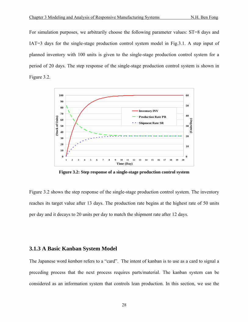
For simulation purposes, we arbitrarily choose the following parameter values: ST=8 days and
IAT=3 days for the single-stage production control system model in Fig.3.1. A step input of
planned inventory with 100 units is given to the single-stage production control system for a
period of 20 days. The step response of the single-stage production control system is shown in
Figure 3.2.
0
10
20
30
40
50
60
70
80
90
100
1 2 3 4 5 6 7 8 9 10 11 12 13 14 15 16 17 18 19 20
Time (Day)
(Sto
ck o
f Uni
ts)
0
10
20
30
40
50
60
(Uni
ts/D
ay)
Inventory INV
Production Rate PR
Shipment Rate SR
Figure 3.2: Step response of a single-stage production control system
Figure 3.2 shows the step response of the single-stage production control system. The inventory
reaches its target value after 13 days. The production rate begins at the highest rate of 50 units
per day and it decays to 20 units per day to match the shipment rate after 12 days.
3.1.3 A Basic Kanban System Model
The Japanese word kanban refers to a “card”. The intent of kanban is to use as a card to signal a
preceding process that the next process requires parts/material. The kanban system can be
considered as an information system that controls lean production. In this section, we use the
28

Chapter 3 Modeling and Analysis of Responsive Manufacturing Systems N.H. Ben Fong
basic structure of a kanban system model extracted from O’Callaghan’s paper [20]. This kanban
system model has been modified to a two-stage kanban system and constructed using Vensim
software as shown in Fig.3.3. Vensim provides a simple and flexible way of building simulation
models from causal loop diagrams and/or stock and flow diagrams.
Work-In-Process WIP
FinishedInventory FIProduction Start Rate
PSRProduction
Completion RatePCR
Shipment RateSR
Desired ProductionRate DPR
ProductionOrders PO
Lead TimeLT
++ +
-
- -
Kanban CycleKC
-
Shipment TimeST
-
Total Number ofKanban TNK
<ContainerSize>
<Input>
+
Figure 3.3: A basic kanban system model
Referring to Fig. 3.3, the work-in-process (WIP) level is the accumulation of a difference
between the production start rate (PSR) and the production completion rate (PCR) during a
certain production lead- time (LT). The finished inventory (FI) determines the stock level
between the production completion rate less the shipment rate (SR) over an average shipment
time (ST). The total number of kanbans defines the inventory allowed in the entire system. Any
kanban has to be either attached to the stock container (WIP or FI) or the dispatching post (i.e.,
kanban receiving box). Each time a unit is withdrawn from the finished inventory, its kanban is
detached and put in the collection box. Based on a certain time interval, the detached kanbans
found in the collection box will be taken to the dispatching post, where they become production
orders (PO). O’Callaghan states this time interval as the kanban cycle (KC), and it determines
29

Chapter 3 Modeling and Analysis of Responsive Manufacturing Systems N.H. Ben Fong
how fast the system reacts to changes in production rate. He further asserts that the kanban cycle
is a “time constant”. However, we show in the later section that the kanban cycle of this
particular system model only represents portion of the entire system time constant from the
actual transfer function. Finally, the backlog of PO determines the desired production rate (DPR).
The total number of kanbans (TNK) is defined as the number of kanban multiplied by each
container size. In this kanban system, TNK has to be equal to the sum of the number of WIP
kanbans, the number of FI kanbans and the number of PO kanbans at all times.
We arbitrarily choose the following system parameter values for the kanban system model from
Fig.3.3: number of kanbans=10, container size=10 units, LT=0.5 day, KC=0.5 day, ST=5 days
(assume that production works 20 hours/day). By giving a step input of 100 units’ inventory, the
FI system output response behaves similar to a goal seeking feedback loop structure as shown in
Fig.3.4a [20,21]. The goal is to reach the planned inventory of 100 units. For the given set of
parameters, the steady-state finished inventory reaches 83.33 units instead. The reasons for this
effect are not immediately clear from Fig. 3.3 alone, but will be seen from the corresponding
transfer functions. The WIP level has reached 37 units at its early stage and reduces down to 8.33
units after 3 days. Fig. 3.4b shows the production rates response subjected to the given step input.
The Production Start Rate (PSR) starts producing at a rate of 200 units/day and drops down to
16.67 units/day, whereas the Production Completion Rate (PCR) takes 0.5 day to reach its peak
at 74 units/day and reduces down to 16.67 units/day after 4 days.
30

Chapter 3 Modeling and Analysis of Responsive Manufacturing Systems N.H. Ben Fong
0
10
20
30
40
50
60
70
80
90
100
0 1 2 3 4 5 6 7 8 9 10Time (Day)
(Sto
ck o
f Uni
ts)
Work-In-Process WIPFinished Inventory FI
0
20
40
60
80
100
120
140
160
180
200
0 1 2 3 4 5 6 7 8 9 10Time (Day)
(Uni
ts/D
ay)
Production Start Rate PSR
Production Completion Rate PCR
Figures 3.4a and 3.4b: A step input response of a kanban system model
3.1.4 A Two-Stage Production Control System
We further modify the single-stage model to become a two-stage production control system by
adding to the preceding stage of production a “work-in-process control” feedback loop and
Figure 3.5: A two-stage pr
related causal loop variables as shown in Fig.3.5.
oduction control system
Work-In-Process WIP
FinishedInventory FIProduction Start
Rate PSRProduction
Completion RatePCR
ShipmentRate SR
DesiredProduction Rate
DPR
Adjustment forWork-In-Process
AWIP
DesiredWork-In-Process
WIP*
Adjustment forFinished Inventory
AFI
ExpectedShipment Rate
ESR
Lead TimeLT
++
+
+
+
-
-
-
+Finished InventoryAdjustment Time
FATWork-In-ProcessAdjustment Time
WAT
-
-Expected Lead
Time ELT
+
+
Desired ProductionCompletion Rate
DPCR +
+
ShipmentTime ST
-
DesiredInventory DI*
<Initial DesiredInventory>
<Input>+
+
+
B
WIP Control B
FI Control
31

Chapter 3 Modeling and Analysis of Responsive Manufacturing Systems N.H. Ben Fong
There are two stock elem ork-in-process (WIP)
roduction units and its finished inventory (FI) units. WIP accumulates the difference between
production start rate (PSR) and production completion rate (PCR) during a certain production
lead-time (LT). The finished inventory (FI) determines the stock level between production
completion rate (PCR) less shipment rate (SR) over an average shipment time (ST). There are
two balancing feedback loops found to adjust the work-in-process (WIP) and the finished
inventory (FI). Similar to the single-stage model, there is a linear adjustment between desired
work-in-process (WIP*) and WIP over a specified work-in-process adjustment time (WAT) as
the adjustment for work-in-process (AWIP). Likewise, there is an adjustment for finished
inventory (AFI) between desired inventory (DI*) and FI over a specified finished inventory
adjustment time (FAT). In addition, the desired production completion rate (DPCR) is the sum of
AFI and expected shipment rate (ESR). Similarly, the desired production rate (DPR) is
calculated by adding AWIP and desired production completion rate (DPCR). In this model, the
desired work-in-process (WIP*) is the product of DPCR and the expected lead time (ELT). It is
assumed that expected lead time is equal to lead time (ELT=LT), and that there is no time delay
between shipments such that ESR = SR.
For the two-stage production control system from Fig. 3.5, we arbitrarily set the following
system parameter values: LT=3 days, ST=5 days, WAT=1 day, and FAT=1 day. A step input of
desired inventory (DI*) with 100 units is given to this two-stage model for a period of 20 days.
Figure 3.6 shows the step response of the two-stage production control system. The finished
inventory FI rises rapidly to give an inventory of 120.25 units before it gets to the desired
inventory of 100 units after 10 days. The work-in-process WIP also reaches its peak at 195.13
ents found in this model that accumulates the w
p
32
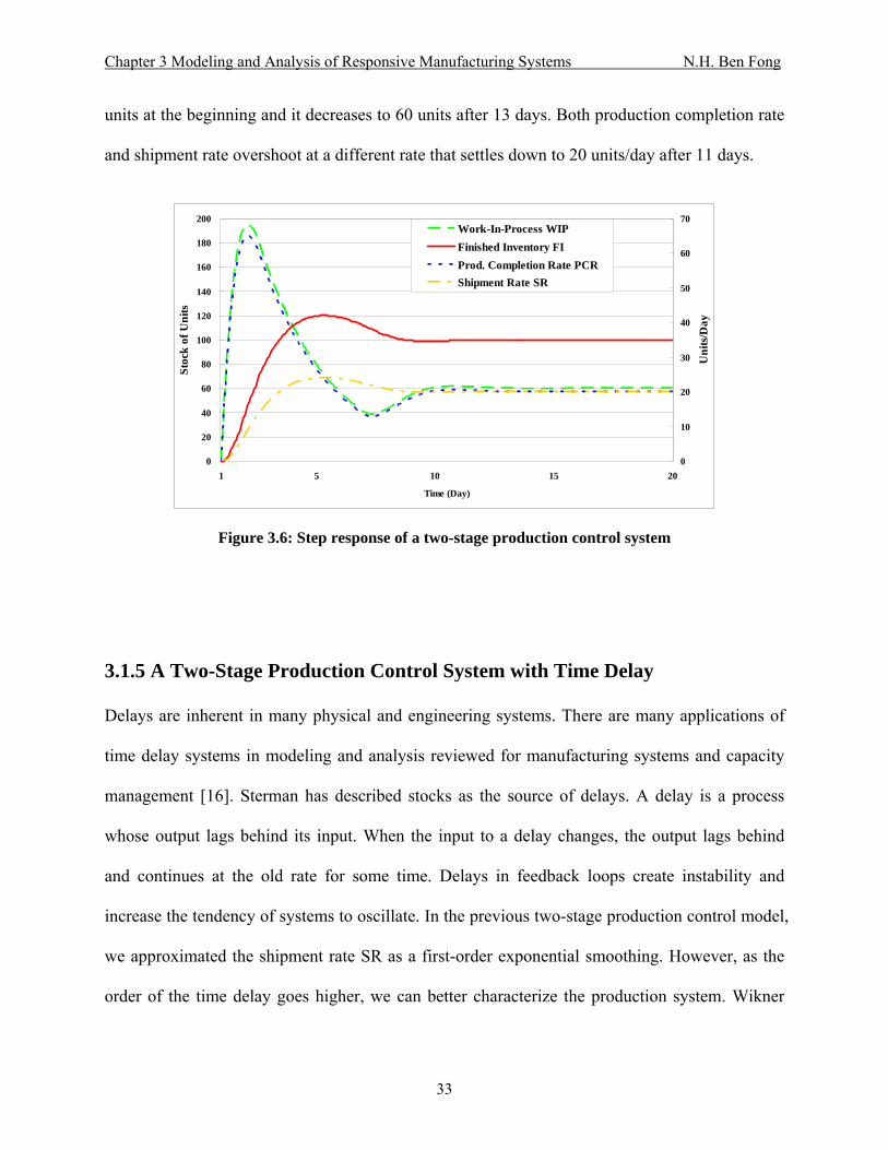
Chapter 3 Modeling and Analysis of Responsive Manufacturing Systems N.H. Ben Fong
units at the beginning and it decreases to 60 units after 13 days. Both production completion rate
and shipment rate overshoot at a different rate that settles down to 20 units/day after 11 days.
0
20
40
60
80
100
120
140
160
180
200
1 5 10 15 20
Time (Day)
Stoc
k of
Uni
ts
0
10
20
30
40
50
60
70
Uni
ts/D
ay
Work-In-Process WIPFinished Inventory FIProd. Completion Rate PCRShipment Rate SR
Figure 3.6: Step response of a two-stage production control system
.1.5 A Two-Stage Production Control System with Time Delay
y applications of
3
Delays are inherent in many physical and engineering systems. There are man
time delay systems in modeling and analysis reviewed for manufacturing systems and capacity
management [16]. Sterman has described stocks as the source of delays. A delay is a process
whose output lags behind its input. When the input to a delay changes, the output lags behind
and continues at the old rate for some time. Delays in feedback loops create instability and
increase the tendency of systems to oscillate. In the previous two-stage production control model,
we approximated the shipment rate SR as a first-order exponential smoothing. However, as the
order of the time delay goes higher, we can better characterize the production system. Wikner
33

Chapter 3 Modeling and Analysis of Responsive Manufacturing Systems N.H. Ben Fong
[27] stated that a third-order delay has proved to be an appropriate compromise between model
complexity and model accuracy for most dynamic modeling of production-inventory systems. In
this section, we modify the previous two-stage production control system by formulating the
Production Completion Rate as a third-order delay function of PSR and LT as shown in Fig. 3.7.
Work-In-Process WIP
FinishedInventory FI
Production StartRate PSR
ProductionCompletion Rate
PCR
ShipmentRate SR
Desired ProductionRate DPR
Adjustment forWork-In-Process
AWIP DesiredWork-In-Process
WIP*
Adjustment forFinished Inventory
AFI
ExpectedShipment Rate
ESR
Lead Time LT
+
+
+
-
--
+
B B
WIP Control FI Control
Finished InventoryAdjustment Time
FATWork-In-ProcessAdjustment Time
WAT
-
-
Expected LeadTime ELT
+
+
Desired ProductionCompletion Rate
DPCR +
+
ShipmentTime ST
-
DesiredInventory DI*
<Initial DesiredInventory>
<Input>+
+
+
Figure 3.7: A two-stage production control system with a 3rd-order time delay
xcept for the addition of the third-order time delay to compute the PCR, the rest of the model E
structure and system flow remains the same as the two-stage production control system shown in
Figure 3.5. Again, we arbitrarily set the system parameter as follows: LT=3 days, ST=5 days,
WAT=1 day, and FAT=1 day. A step input of desired inventory (DI*) with 100 units is given to
this third-order time delay model for a period of 40 days. Figure 3.8 shows the step response of
the two-stage production system with a third-order time delay. The finished inventory FI yields a
much higher initial overshoot of 174.17 units and it gives three more oscillations of overshoot
before it reaches to the desired inventory of 100 units after 35 days. The work-in-process WIP
34

Chapter 3 Modeling and Analysis of Responsive Manufacturing Systems N.H. Ben Fong
initially peaks with 279 units and oscillates four more times until it decreases to 60 units after 37
days. Both production completion rate and shipment rate overshoot and oscillate at a different
rate that reduces down to 20 units/day after 35 days.
0
50
100
150
200
250
300
1 5 10 15 20 25 30 35 40
Time (Day)
Stoc
k of
Uni
ts
0
10
20
30
40
50
60
70
80
90
Uni
ts/D
ay
Work-In-Process WIP
Finished Inventory FI
Prod. Completion Rate PCR
Shipment Rate SR
Figure 3.8: Step response of a two-stage production system with a 3rd-order time delay
he result indicates that the higher the order of the time delay, more dynamics and oscillations T
add to the production system structure. Hence, it takes longer lead time to bring the finished
inventory to the desired steady-state final target. For the next section, we will develop a
mathematical equivalence of translating the CLD and SFD terminologies in modeling those four
production control systems using Block Diagram (BD) representation and Transfer Function (TF)
from classical control theory (CCT). This one-to-one correspondence to translate System
Dynamics terminologies into CCT yields a new way to determine an analytical formulation to
design and predict dynamic manufacturing systems in terms of inventory overshoot, lead time,
responsiveness, and production leanness.
35

Chapter 3 Modeling and Analysis of Responsive Manufacturing Systems N.H. Ben Fong
3.2 Modeling and Analysis via Classical Control Theory
he block diagram (BD)
.2.1 Fundamentals of Classical Control Theory
f a system is defined as a set of
In this section, we begin by reviewing some fundamentals of t
representation and transfer function (TF) from classical control theory (CCT). Our objective is to
develop a one-to-one correspondence to model dynamic manufacturing systems between the
differential equation formulation and the CLD and SFD applied in the System Dynamics (SD)
approach. The resulting mathematical equivalence will offer a new way to determine some key
system parameters and their corresponding performance measures for dynamic manufacturing
systems measures which are not provided by SD and are not possible or difficult to obtain via
other approaches such as discrete event simulation. We apply the CCT approach to model and
formulate the same four production control systems as described from last section. Based on the
result, we can analytically determine some key manufacturing dynamic characteristics without
iterative simulation like inventory overshoot, settling time, responsiveness, and production
leanness.
3
In the control engineering field, the mathematical model o
differential equations. As stated in Ogata [40], the transfer function (TF) of a linear, time-
invariant, differential equation system is defined as the ratio of the Laplace transform of the
output (response function) to the Laplace transform of the input (driving function) under all zero
initial conditions. Like the SD representation of Sterman [16], a block diagram (BD) of a system
is a graphical representation of the cause-and-effect relations operating in a particular system
[40,41]. In a BD, all system variables are linked to each other through functional blocks. The
36

Chapter 3 Modeling and Analysis of Responsive Manufacturing Systems N.H. Ben Fong
functional block is a symbol for the mathematical operation on the input signal to the block that
produces the output. This links express the information flow from block to block. We typically
enter the transfer functions of the components in the corresponding blocks that are connected by
arrows to indicate the direction of the flow of signals. One of the major advantages of using BD
representation is to form the overall BD for the entire system by connecting the blocks of the
components according to the signal flow in evaluating the overall performance and the
interaction of each system components. In addition, the algebraic representation of the system’s
equations in terms of transfer functions allows easy manipulation for design and analysis
purposes.
3.2.2 Transfer Function of a Single-Stage Production Control System
deling the
Referring to Figure 3.1, we can translate those CLD and SFD terminologies in mo
single-stage production system using BD representations from CCT as shown in Fig. 3.9 and Fig.
3.10.
Figure 3.9: Subcomponents of BD representation of a single-stage production system
PRPRProduction Rate:
Desired Production Rate:
DPRDPR+
+
INVINV1/sInventory:
PR
_
+ESRShipment
Rate:
Expected
AINVAdjustment for Inventory:
IAT1+
_
Desired Inventory: INV*Input
SRShipment Rate: ST
1
SR
INV
DPR
AINV
ESR
SR
INV*
INV
INV*0
37

Chapter 3 Modeling and Analysis of Responsive Manufacturing Systems N.H. Ben Fong
INVINVInput
PRPRDPRDPR1/s
_
ESR
+ AINV
IAT1 +
_INV*0INV*0
SR
+
+
1ST1
2ST1
Figure 3.10: Complete BD representation of a single-stage production system
As illustrate lation for
variable. By linking all these individual subsets together, we will generate the
nt called the
d in Fig. 3.9, each individual subset of block diagrams represents the formu
each system
complete block diagram as shown in Fig. 3.10. This complete block diagram is mathematically
equivalent to the single-stage model as shown in Fig.3.1. There are a total of two feedback loops
and a feedforward gain found in Fig. 3.10 with the corresponding loop gains, 1/ST1, 1/ST2, and
1/IAT, respectively. The 1/s block represents an integrator. We can simplify this multiple
feedback loops BD into a single transfer function by a step-by-step rearrangeme
block diagram reduction technique. Details of the technique are found in references
[40,41,42,43]. After the BD reduction is applied, Fig. 3.10 representation reduces to a single TF
block as shown in Fig. 3.11. The resulting single TF block can be expressed in the Laplace
transform domain and it yields a first-order closed-loop transfer function of eq. (3.1). Equation
(3.2) gives the time constant of the first-order dynamic system model.
38

Chapter 3 Modeling and Analysis of Responsive Manufacturing Systems N.H. Ben Fong
+
_ IAT1
⎟⎟⎠
⎞⎜⎜⎝
⎛−⎟⎟
⎠
⎞⎜⎜⎝
⎛+
21 ST1s)/1(
ST1(1/s)1
1/sINV* INVINV
⎟⎟⎠
⎞⎜⎜⎝
⎛+−+
⎟⎠⎞
⎜⎝⎛
IAT1
ST1
ST1s
IAT1
21
INV* INVINV
Figure 3.11: Step-by-step block diagram reduction into a single TF block
( )( )
⎟⎟⎠
⎞⎜⎜⎝
⎛+−+
⎟⎠⎞
⎜⎝⎛
=
IAT1
ST1
ST1 s
IAT1
sINVsINV
21
*
(3.1)
where 1
21 IAT1
ST1
ST1
−
⎥⎦
⎤⎢⎣
⎡+−=τ (3.2)
1s
K X(s)Y(s)
+=
τ (3.3)
The time constant term, τ is a function of ST1, ST2, and IAT, not only IAT. It determines how
quickly the production reacts to changes in the inventory level. In a first-order linear system, it
takes 4τ settling time to reach 98.2% of its steady-state value. Equation (3.3) gives a specific
form of a first-order linear differential equation with nonunity gain, where K is the proportional
gain factor. By comparing eq. (3.1) to eq. (3.3), it yields,
IAT
K τ= (3.4)
The inverse Laplace transform of equation (3.3) with a unit step input is obtained as:
⎟⎠⎞⎜
⎝⎛= τ
-te - 1K y(t) ; with K y(t) lim
t=
∞→ (3.5)
The single-stage production control system subjected to a unit step input yields the following
responses: time constant, τ=3 days, steady-state value, K=1 (i.e., 100% of the desired inventory),
39

Chapter 3 Modeling and Analysis of Responsive Manufacturing Systems N.H. Ben Fong
and 98% settling time=12 days. Remember, we assume that there is no delay and ESR = SR, thus
the loop gain ST1=ST2. The time constant tells how fast the production system could respond to
any given input. It takes about 12 days for production to reach 98% of its target value as shown
in Fig.3.2. Referring to eq. (3.2), the time constant is a function of IAT, ST1, and ST2. If the Max
function is taken off and we allow ST2<ST1, and if IAT>>ST2, the time constant could go
negative, and the system model could grow exponentially without bound (unstable). In practice,
we would not consider an expected shipment rate higher than an actual shipment rate.
3.2.3 Transfer Function of a Basic Kanban System Model
We make a mathematical equivalence of translating the basic kanban system from Fig. 3.3 into
BD representation as shown in Figs. 3.12 and 3.13. Figure 3.12 shows all the subcomponents of
block diagram representation and each system variable relationship of the kanban system. Figure
3.13 indicates the complete block diagram representation of the kanban system.
PCRPCRProductionCompletion Rate (PCR):
ProductionOrders (PO):
POPO+
WIPWIP1/sWork-In-Process (WIP): _
+
DPRDesiredProductionRate (DPR): KC
1Total Number of Kanban(TNK):
TNKInput
SRShipment Rate (SR): ST
1
PSR
PCR
FI
WIP
TNK
FI
POContainer Size
FIFI1/sFinishedInventory (FI): _
+PCR
SR
LT1
WIP__
Figure 3.12: Subcomponents of block diagram representation of a basic kanban system
40

Chapter 3 Modeling and Analysis of Responsive Manufacturing Systems N.H. Ben Fong
TNK 1/s FILT1
LT1
1/sKC
1+ + +
__
__
ST1
r
Figure 3.13: Complete block diagram representation of the basic kanban system
⎥⎦⎤
⎢⎣⎡ +++⎥⎦
⎤⎢⎣⎡ +++
⎟⎠⎞
⎜⎝⎛
⎟⎠⎞
⎜⎝⎛
LT1
KC1
ST1
KC1
ST1
LT1 s
ST1
KC1
LT1 s
LT1
KC1TNK
2
r FI
Figure 3.14: Block diagram reduction into a single transfer function block
As illustrated in Fig.3.13, there are a total of four feedback loops found. The first two feedback
loops contain the loop gain value of unity, whereas the third and the fourth loop have a loop gain
of 1/LT and 1/ST, respectively. The 1/s term is simply an integrator. The complete block
diagram representation as shown in Fig. 3.13 is mathematically equivalent to the kanban system
model built by Vensim as shown in Fig. 3.3. For this multiple feedback loop block diagram as
shown in Fig. 3.13, we can simplify it into a single transfer function by the block diagram
reduction technique. Details of the technique are found in references [40,41,42]. After the block
diagram reduction is applied, Fig. 3.13 representation reduces to a single TF block as shown in
Fig. 3.14.
⎥⎦⎤
⎢⎣⎡ +++⎥⎦
⎤⎢⎣⎡ +++
⎟⎠⎞
⎜⎝⎛
⎟⎠⎞
⎜⎝⎛
=
LT1
KC1
ST1
KC1
ST1
LT1 s
ST1
KC1
LT1 s
LT1
KC1TNK
r(s)FI(s)
2
(3.6)
( )
( ) 2nn
2
2n
s 2sK
X(s)Y(s)
ωζωω
++= (3.7)
41

Chapter 3 Modeling and Analysis of Responsive Manufacturing Systems N.H. Ben Fong
The resulting single TF block can be expressed in the Laplace transform domain, and it yields a
second-order closed-loop transfer function as stated in eq. (3.6). The denominator of eq. (3.6) is
the characteristic equation of the closed-loop kanban system model. Equation (3.7) gives a
specific form of a second-order system differential equation with nonunity gain, where K is the
proportional gain factor, ωn is the undamped natural frequency, and ζ is the damping ratio of the
system. Equation (3.7) can be put into standard form for a second-order system equation by
taking off the K term. The dynamic behavior of a second-order system can be described in terms
of two parameters ωn and ζ. If 0<ζ<1, the closed-loop poles are complex conjugates and its
transient response is oscillatory. This system is called “underdamped”. If ζ=0, the transient
response does not die out, it will oscillate forever. If ζ=1, the system is called “critically
damped”; exponential behavior occurs if ζ>1, the system is called “overdamped”. Overshoot or
oscillation will not occur unless ζ<= 0.707. To better understand the concept of the classical
control theory, please see references [40,41,42,43]. For any linear second-order system, the time
constant is computed as : τ = (1/ζωn). By comparing eq. (3.6) to eq. (3.7), it yields,
Undamped natural frequency: LT1
KC1
ST1
KC1
ST1
LT1 n ++=ω (3.8)
Damping ratio: ⎥⎦⎤
⎢⎣⎡ ++
++=
ST1
KC1
LT1
LT1
KC1
ST1
KC1
ST1
LT1
121 ζ
(3.9)
Damped natural frequency: 2nd 1 ζωω −= (3.10)
Roots of characteristic equation: -1 - s 2
nn1,2 ζωζω j±= (3.11)
42
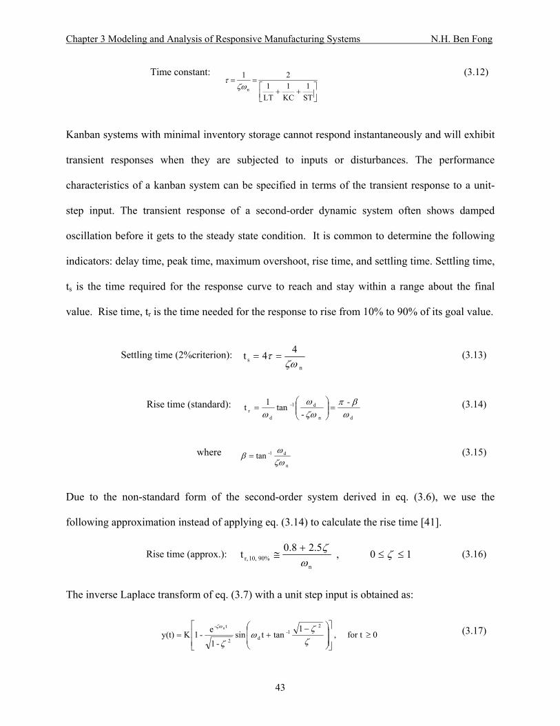
Chapter 3 Modeling and Analysis of Responsive Manufacturing Systems N.H. Ben Fong
Time constant:
⎥⎦⎤
⎢⎣⎡ ++
==
ST1
KC1
LT1
2 1 nζω
τ (3.12)
Kanban systems with minimal inventory storage cannot respond instantaneously and will exhibit
transient responses when they are subjected to inputs or disturbances. The performance
characteristics of a kanban system can be specified in terms of the transient response to a unit-
step input. The transient response of a second-order dynamic system often shows damped
oscillation before it gets to the steady state condition. It is common to determine the following
indicators: delay time, peak time, maximum overshoot, rise time, and settling time. Settling time,
ts is the time required for the response curve to reach and stay within a range about the final
value. Rise time, tr is the time needed for the response to rise from 10% to 90% of its goal value.
Settling time (2%criterion):
ns
4 4 tζω
τ == (3.13)
Rise time (standard): dn
d1-
dr
- -
tan1 tω
βπζωω
ω=⎟⎟
⎠
⎞⎜⎜⎝
⎛= (3.14)
where
n
d1- tan ζωω
β = (3.15)
Due to the non-standard form of the second-order system derived in eq. (3.6), we use the
following approximation instead of applying eq. (3.14) to calculate the rise time [41].
Rise time (approx.): 10 , 2.5 0.8 tn
90% 10, r, ≤≤+
≅ ζω
ζ (3.16)
The inverse Laplace transform of eq. (3.7) with a unit step input is obtained as:
0 for t , 1
tant sin -1
e -1K y(t)2
1-d2
t- n
≥⎥⎥⎦
⎤
⎢⎢⎣
⎡
⎟⎟
⎠
⎞
⎜⎜
⎝
⎛ −+=
ζζ
ωζ
ζω (3.17)
43
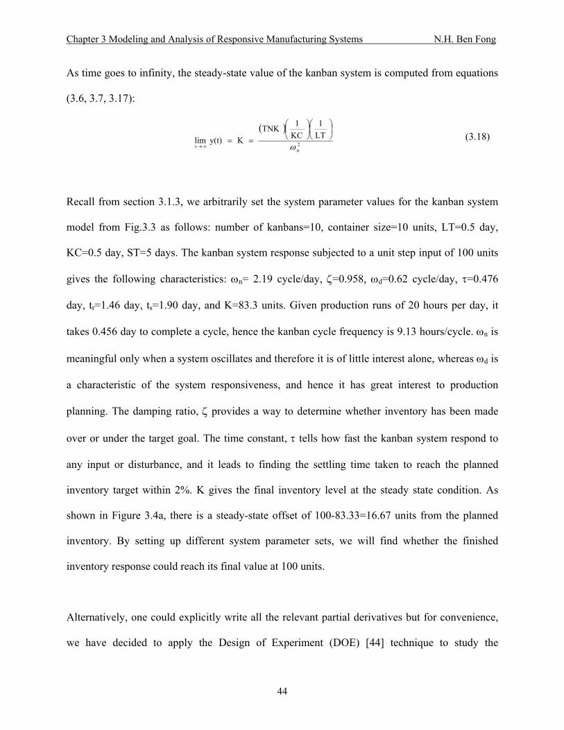
Chapter 3 Modeling and Analysis of Responsive Manufacturing Systems N.H. Ben Fong
As time goes to infinity, the steady-state value of the kanban system is computed from equations
(3.6, 3.7, 3.17):
( )
2n
t
LT1
KC1TNK
K y(t) limω
⎟⎠⎞
⎜⎝⎛
⎟⎠⎞
⎜⎝⎛
==∞→
(3.18)
Recall from section 3.1.3, we arbitrarily set the system parameter values for the kanban system
model from Fig.3.3 as follows: number of kanbans=10, container size=10 units, LT=0.5 day,
KC=0.5 day, ST=5 days. The kanban system response subjected to a unit step input of 100 units
gives the following characteristics: ωn= 2.19 cycle/day, ζ=0.958, ωd=0.62 cycle/day, τ=0.476
day, tr=1.46 day, ts=1.90 day, and K=83.3 units. Given production runs of 20 hours per day, it
takes 0.456 day to complete a cycle, hence the kanban cycle frequency is 9.13 hours/cycle. ωn is
meaningful only when a system oscillates and therefore it is of little interest alone, whereas ωd is
a characteristic of the system responsiveness, and hence it has great interest to production
planning. The damping ratio, ζ provides a way to determine whether inventory has been made
over or under the target goal. The time constant, τ tells how fast the kanban system respond to
any input or disturbance, and it leads to finding the settling time taken to reach the planned
inventory target within 2%. K gives the final inventory level at the steady state condition. As
shown in Figure 3.4a, there is a steady-state offset of 100-83.33=16.67 units from the planned
inventory. By setting up different system parameter sets, we will find whether the finished
inventory response could reach its final value at 100 units.
Alternatively, one could explicitly write all the relevant partial derivatives but for convenience,
we have decided to apply the Design of Experiment (DOE) [44] technique to study the
44
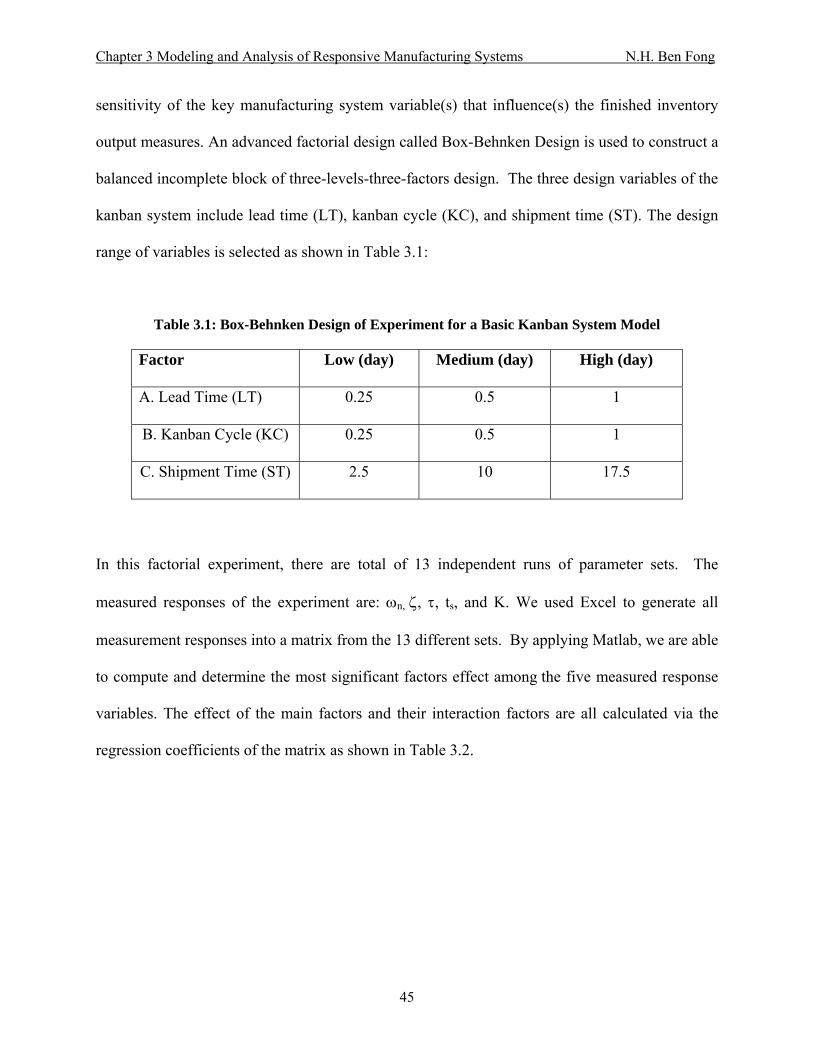
Chapter 3 Modeling and Analysis of Responsive Manufacturing Systems N.H. Ben Fong
sensitivity of the key manufacturing system variable(s) that influence(s) the finished inventory
output measures. An advanced factorial design called Box-Behnken Design is used to construct a
balanced incomplete block of three-levels-three-factors design. The three design variables of the
kanban system include lead time (LT), kanban cycle (KC), and shipment time (ST). The design
range of variables is selected as shown in Table 3.1:
Table 3.1: Box-Behnken Design of Experiment for a Basic Kanban System Model
Factor Low (day) Medium (day) High (day)
A. Lead Time (LT) 0.25 0.5 1
B. Kanban Cycle (KC) 0.25 0.5 1
C. Shipment Time (ST) 2.5 10 17.5
In this factorial experiment, there are total of 13 independent runs of parameter sets. The
measured responses of the experiment are: ωn, ζ, τ, ts, and K. We used Excel to generate all
measurement responses into a matrix from the 13 different sets. By applying Matlab, we are able
to compute and determine the most significant factors effect among the five measured response
variables. The effect of the main factors and their interaction factors are all calculated via the
regression coefficients of the matrix as shown in Table 3.2.
45
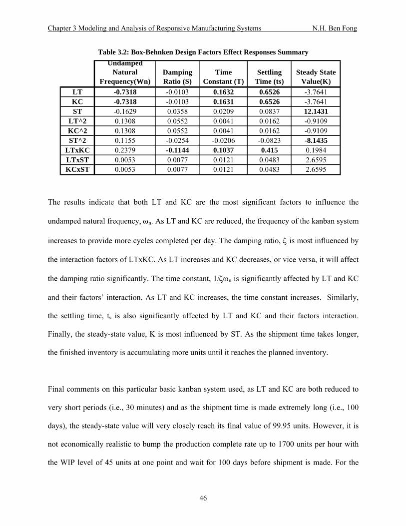
Chapter 3 Modeling and Analysis of Responsive Manufacturing Systems N.H. Ben Fong
Table 3.2: Box-Behnken Design Factors Effect Responses Summary
Undamped Natural
Frequency(Wn)Damping Ratio (S)
Time Constant (T)
Settling Time (ts)
Steady State Value(K)
LT -0.7318 -0.0103 0.1632 0.6526 -3.7641KC -0.7318 -0.0103 0.1631 0.6526 -3.7641ST -0.1629 0.0358 0.0209 0.0837 12.1431
LT^2 0.1308 0.0552 0.0041 0.0162 -0.9109KC^2 0.1308 0.0552 0.0041 0.0162 -0.9109ST^2 0.1155 -0.0254 -0.0206 -0.0823 -8.1435
LTxKC 0.2379 -0.1144 0.1037 0.415 0.1984LTxST 0.0053 0.0077 0.0121 0.0483 2.6595KCxST 0.0053 0.0077 0.0121 0.0483 2.6595
The results indicate that both LT and KC are the most significant factors to influence the
undamped natural frequency, ωn. As LT and KC are reduced, the frequency of the kanban system
increases to provide more cycles completed per day. The damping ratio, ζ is most influenced by
the interaction factors of LTxKC. As LT increases and KC decreases, or vice versa, it will affect
the damping ratio significantly. The time constant, 1/ζωn is significantly affected by LT and KC
and their factors’ interaction. As LT and KC increases, the time constant increases. Similarly,
the settling time, ts is also significantly affected by LT and KC and their factors interaction.
Finally, the steady-state value, K is most influenced by ST. As the shipment time takes longer,
the finished inventory is accumulating more units until it reaches the planned inventory.
Final comments on this particular basic kanban system used, as LT and KC are both reduced to
very short periods (i.e., 30 minutes) and as the shipment time is made extremely long (i.e., 100
days), the steady-state value will very closely reach its final value of 99.95 units. However, it is
not economically realistic to bump the production complete rate up to 1700 units per hour with
the WIP level of 45 units at one point and wait for 100 days before shipment is made. For the
46
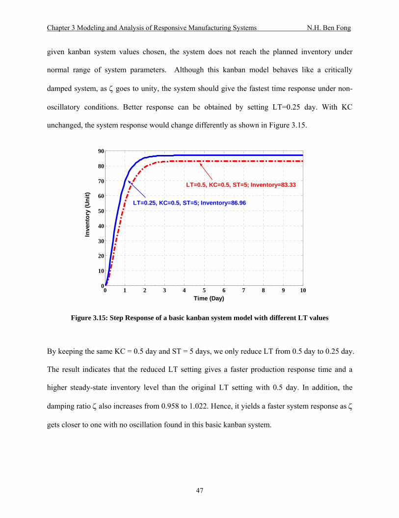
Chapter 3 Modeling and Analysis of Responsive Manufacturing Systems N.H. Ben Fong
given kanban system values chosen, the system does not reach the planned inventory under
normal range of system parameters. Although this kanban model behaves like a critically
damped system, as ζ goes to unity, the system should give the fastest time response under non-
oscillatory conditions. Better response can be obtained by setting LT=0.25 day. With KC
unchanged, the system response would change differently as shown in Figure 3.15.
0 1 2 3 4 5 6 7 8 9 100
10
20
30
40
50
60
70
80
90
Time (Day)
Inve
ntor
y (U
nit)
LT=0.5, KC=0.5, ST=5; Inventory=83.33
LT=0.25, KC=0.5, ST=5; Inventory=86.96
Figure 3.15: Step Response of a basic kanban system model with different LT values
By keeping the same KC = 0.5 day and ST = 5 days, we only reduce LT from 0.5 day to 0.25 day.
The result indicates that the reduced LT setting gives a faster production response time and a
higher steady-state inventory level than the original LT setting with 0.5 day. In addition, the
damping ratio ζ also increases from 0.958 to 1.022. Hence, it yields a faster system response as ζ
gets closer to one with no oscillation found in this basic kanban system.
47

Chapter 3 Modeling and Analysis of Responsive Manufacturing Systems N.H. Ben Fong
3.2.4 Transfer Function of a Two-Stage Production Control System
Similar to section 3.3.1, the two-stage production control system from Fig 3.5 can translate into a
set of subcomponents of block diagrams as shown in Fig.3.16. It can combine to give a complete
block diagram as shown in Fig. 3.17 that is mathematically equivalent to the two-stage
production control model from Fig. 3.5.
PSRPSRProduction Start Rate, PSR:
Desired Production Rate, DPR:
DPRDPR+
+
FIFI1/sFinished InventoryFI:
_
+ESR
Expected Shipment Rate:
AFIAdjustment for FI:
FAT1+
_
Desired Inventory: DI*Input
SRShipment Rate, SR: ST
1
PCR
SR
FI
DPR
AWIP
DPCR
SR
DI*
DI
DI*0
WIPWIP1/sWork-In-ProcessWIP:
_
+PSR
PCR
AWIPAdjustment for WIP:
WAT1+
_
WIP*
WIP
Desired Production Completion Rate:
DPCRDPCR+
+
ESR
AFI
PCRProduction Completion Rate: LT
1WIP
Figure 3.16: Subcomponents of BD representation of a two-stage production control system
ELT 1/sFI
LT1
WAT1
1/sFAT
1+ + +
__ _+LT1DI + +
+
+
_
1ST1
2ST1
AFI
ESR
DPCRWIP* AWIP
DPR
PSR WIP PCR
SR
Figure 3.17: Complete BD representation of a two-stage production control system
48

Chapter 3 Modeling and Analysis of Responsive Manufacturing Systems N.H. Ben Fong
There are a total of five feedback loops and one feedforward loop found in Fig. 3.16 with the
corresponding loop gains of unity, 1/ST2, unity, 1/LT, 1/ST1 and unity, respectively. Again, the
1/s block is an integrator. By applying the block diagram reduction technique, Fig. 3.16 reduces
to a single TF block and yields a second-order closed-loop transfer function under the Laplace
domain as stated in equation (3.19). Equation (3.20) is a non-standard form of a second-order DE
with nonunity gain, where K is the proportional gain factor, ωn is the undamped natural
frequency and ζ is the damping ratio of the dynamic system. Equations (3.21)-(3.29) provides
the complete formulation of the dynamic characteristics of the two-stage production system as
shown in Fig. 3.5 [40,41,42,43]. These characteristics will next be evaluated for sample cases.
⎥⎦
⎤⎢⎣
⎡⎟⎟⎠
⎞⎜⎜⎝
⎛+−⎟
⎠⎞
⎜⎝⎛ ++⎥
⎦
⎤⎢⎣
⎡+++
⎟⎠⎞
⎜⎝⎛ +⎟
⎠⎞
⎜⎝⎛
⎟⎠⎞
⎜⎝⎛
=
FAT1
ST1
ST1
WAT1
LT1
ST1
WAT1
LT1ss
WATLT1
LT1
FAT1
DI(s)FI(s)
211
2
(3.19)
2nd order linear DE (non-standard form): ( )( ) 2
nn2
2n
s 2sK
X(s)Y(s)
ωζωω
++= (3.20)
Undamped natural frequency:
⎥⎦
⎤⎢⎣
⎡⎟⎟⎠
⎞⎜⎜⎝
⎛+−⎟
⎠⎞
⎜⎝⎛ +=
FAT1
ST1
ST1
WAT1
LT1
21nω (3.21)
Damping ratio: ⎥⎦
⎤⎢⎣
⎡++=
1n ST1
WAT1
LT1
21 ω
ζ (3.22)
Time constant:
⎥⎦
⎤⎢⎣
⎡++
==
1
n
ST1
WAT1
LT1
2 1 ζω
τ (3.23)
Closed-Loop Poles: -1 - s 2
nn1,2 ζωζω j±= (3.24)
Rise time (approx.): 10 , 2.5 0.8 tn
90% 10, r, ≤≤+
≅ ζω
ζ (3.25)
49

Chapter 3 Modeling and Analysis of Responsive Manufacturing Systems N.H. Ben Fong
Maximum overshoot % : ( ) 100*e M )/-(
pdn πωζω≈ (3.26)
Settling time (2% criterion):
ns
4 4 tζω
τ == (3.27)
The inverse Laplace transform of equation (3.20) with a unit step input is obtained as:
0 for t , 1
tant sin -1
e -1K y(t)2
1-d2
t- n
≥⎥⎥⎦
⎤
⎢⎢⎣
⎡
⎟⎟
⎠
⎞
⎜⎜
⎝
⎛ −+=
ζζ
ωζ
ζω (3.28)
As time goes to infinity, the steady-state FI of the two-stage production system is computed from
eqs. (3.19, 3.20, 3.27):
2n
t
WATLT1
LT1
FAT1
K y(t) limω
⎟⎠⎞
⎜⎝⎛ +⎟
⎠⎞
⎜⎝⎛
⎟⎠⎞
⎜⎝⎛
==∞→
(3.29)
According to the section 3.1.4, the two-stage production control system subjected to a unit step
input gives the following responses as shown in Fig.3.6: ωn= 1.155 cycle/day, ζ=0.664, τ=1.30
day, tr=2.13 days, ts=5.22 days, K=100 units and Mp=108.4 units. Assuming production runs 20
hours per day and no time delay between shipment rates (i.e., ST1=ST2), it takes about 0.866 day
to complete a cycle, and hence one production cycle frequency is 17.32 hours/cycle. The
damping ratio, ζ provides a way to determine whether the inventory has been made over or under
the desired production goal during the transient period. In this example, the inventory overshoots
before it reaches the goal value of 100 units. The time constant, τ tells how quickly production
can respond to the given input. We find the settling time of 5.22 days to reach the target value
within 2%. The rise time, tr is the time it takes for the system response to rise from 10% to 90%
of its goal value. It only takes 2.13 days for production to make 90 units of stock.
We again apply a Design of Experiment (DOE) technique [44] to identify some key system
variables that influence some of the output measures of the two-stage production model. For this
50

Chapter 3 Modeling and Analysis of Responsive Manufacturing Systems N.H. Ben Fong
two-stage system model, we have a total of five system variables, LT, ST1, ST2, WAT, and FAT,
to adjust for six corresponding dynamic output responses, ωn, ζ,τ, tr, ts, and K. A 25-1 (Rev V)
design is used to construct a two-levels-five-factors fractional factorial design matrix. The design
system variables are set as follows: A=Lead Time (1 day or 4 days), B=Shipment Time1 (4 days
or 8 days), C=Shipment Time2 (4 days or 8 days), D=WIP adjustment time (1 day or 4 days), and
E=FI adjustment time (1 day or 4 days). In this experiment, there are total of 16 independent
parameter sets. Excel is used to generate all measurement responses into a matrix from the 16
different sets. By applying Matlab, we can compute and determine the most significant factors’
effect among the six response variables. The main factors’ effect and their interaction factors’
effect are all calculated via the regression coefficients of the matrix as shown in Table 3.3.
Table 3.3: 25-1(Rev V) fractional factorial design factors effect responses summary
Undamped Natural
Frequency(Wn)Damping Ratio (S)
Time Constant (T)
Rise Time (tr)
Settling Time (ts)
Steady State Value(K)
A -0.1324 -0.1081 0.5046 0.4311 2.0183 0B -0.0528 0.0585 0.1035 0.9062 0.414 19.8413C 0.0528 -0.1057 0 -1.1328 0 -19.8413D -0.1324 -0.1081 0.5046 0.4311 2.0183 0E -0.2766 0.3507 0 3.1009 0 7.9365
AB 0.0055 -0.0106 0.0601 -0.0634 0.2405 0AC -0.0055 -0.0005 0 -0.0538 0 0AD -0.0173 -0.0423 0.2652 -0.2429 1.0605 -7.9365AE 0.044 -0.0355 0 0.2033 0 0BC 0.0124 -0.0366 0 -0.3707 0 -8.7302BD 0.0055 -0.0106 0.0601 -0.0634 0.2405 0BE -0.0196 0.0693 0 0.8623 0 13.4921CD -0.0055 -0.0005 0 -0.0538 0 0CE 0.0196 -0.0885 0.0429 -1.0264 0.1716 -13.4921DE 0.044 -0.0355 0 0.2033 0 0
In marked contrast to the previous system, the result indicates that FAT is the most significant
factor to influence the undamped natural frequency, ωn. As FAT decreases, ωn increases, thus
one production cycle gets completed more frequently. Variables LT and WAT have a similar
51

Chapter 3 Modeling and Analysis of Responsive Manufacturing Systems N.H. Ben Fong
effect on ωn with less magnitude. The damping ratio, ζ is most influenced by FAT. As FAT
increases, ζ increases. The time constant, 1/ζωn is significantly affected by LT and WAT and
their factors’ interaction. The time constant increases as LT and WAT increase. Similarly, the
settling time, ts is also significantly influenced by LT and WAT and their factors’ interaction. It
appears that the regression coefficients are zero for both ST2 and FAT for time constant and
settling time because they are not included in the formulation as stated in eq. (3.23). The FAT
has the most significant impact on rise time, tr. Both ST1 and ST2 have a similar effect on tr and
their own interaction with FAT also influences the rise time. Finally, the steady-state value K is
most affected by ST1 and ST2 and their individual interaction with FAT.
We can study the responsiveness, the inventory overshoot, the rise time, and the steady-state
value by plotting a family of step response curves under different damping ratio values as shown
in Fig. 3.18. It shows that all response curves eventually reach the desired 100 units. As damping
ratio, ζ decreases from 1.43 to 0.35, the gradient of the response curve increases. As ζ drops
below 0.7, overshoot occurs. The magnitude of the excess inventory increases as ζ continues to
drop. At lower damping ratios, the system response curve oscillates at a higher frequency that
leads to multiple excess inventories taken within the same production cycle. The rise time also
gets improved as ζ goes lower, thus it increases the responsiveness of the system. As ζ increases
over 1.0 or more, it takes a much longer time for the system to reach the desired inventory level.
52

Chapter 3 Modeling and Analysis of Responsive Manufacturing Systems N.H. Ben Fong
0 5 10 15 20 25 300
20
40
60
80
100
120
140
Time in days
Fini
shed
Inve
ntor
y Le
vel (
Uni
t)
ζ=1.43 ζ=1.0
ζ=0.7
ζ=0.61
ζ=0.35
ζ=0.49
Figure 3.18: Family curves of step response for a two-stage production control system
There are some other observations we can make from this two-stage production system response
analysis. The overshoot of the early stage of the transient response can be interpreted as the
excess inventory built up. The reciprocal of rise time, 1/tr can be treated as the responsiveness or
the “agility” of the production system. The shorter tr, the greater the slope of the system curves
response. The greater the slope of curve, the higher excess inventory may occur. The production
management team can use the steady-state value, K to determine whether the finished inventory
level is over or below the desired planned inventory. We can predict this offset inventory and
keep the excess cost low to make our production system more “lean”.
It is not feasible to realize from the SD model the fact that FAT does not play any role in
determining the entire system time constant. However, for the system responsiveness or agility
53
Chapter 3 Modeling and Analysis of Responsive Manufacturing Systems N.H. Ben Fong
of the system, FAT has the biggest impact on the rising slope of the system response curve. We
can decide the amount of inventory cost and the finished inventory response time by trading off
responsiveness and maximum overshoot. The shipment rate and its interaction with FAT have a
significant affect the final outcome of the finished inventory level. The location of the closed-
loop poles defined in eq.(3.24) is a key element for system stability design and analysis purposes.
3.2.5 Transfer Function of a Two-Stage Production System with Time Delay
We have learned from section 3.1.5 that the higher the order of the time delay added to the
manufacturing system, the higher number of oscillations occurred for its dynamic system
behavior. In this section, we study the difference of the block diagram representation and its
corresponding transfer function formulation among three kinds of time delay included in the
two-stage production control system. The original two-stage production control system is
modeled via a first-order exponential smoothing to formulate the shipment rate. We will show
that this is mathematically equivalent to a two-stage system with first-order time delay as a
second-order differential equation. Lastly, we show to include the third-order time delay to the
two-stage production system will increase the order of the dynamics to a fourth-order differential
equation, better representing the sudden change that actually occur in a real industrial system.
The original two-stage production control system with first-order exponential smoothing is
shown again in Fig. 3.17. Figure 3.19 shows the same production system with a modification of a
first-order time delay inclusion. We again apply the block diagram reduction technique to reduce
the BD representations from Figs. 3.16 and 3.18 into transfer functions as shown in eq. (3.30)
and eq. (3.31). The result indicates that the two different BD representations yield the same
54

Chapter 3 Modeling and Analysis of Responsive Manufacturing Systems N.H. Ben Fong
mathematical formulation of transfer functions. Thus, for this particular two-stage production
control system, a first-order exponential smoothing gives equivalent system characteristics with a
first-order time delay. The mathematical equivalence check is found in eq. (3.32).
Figure 3.17: Complete BD representation of a two-stage production control system
ELT 1/sFI
LT1
WAT1
1/sFAT
1+ + +
__ _+LT1DI + +
+
+
_
1ST1
2ST1
AFI
ESR
DPCRWIP* AWIP
DPR
PSR WIP PCR
SR
Figure 3.19: BD representation of a two-stage production control system with 1st-order Delay
ELT
1/sFI
WAT1
WAT1
WAT1 1/s
FAT1
FAT1
FAT1+ + +
__ _+
1+(LT)s1
1+(LT)s1
1+(LT)s1
DI + +
+
+
_
1ST1
1ST1
1ST1
2ST1
2ST1
2ST1
AFI
ESR
DPCR
WIP* AWIP
DPR
PSR
WIP
PCR
SR
PCR
ELT
1/sFI
WAT1
WAT1
WAT1 1/s
FAT1
FAT1
FAT1+ + +
__ _+
DI + +
+
+
_
1ST1
1ST1
1ST1
2ST1
2ST1
2ST1
AFI
ESR
DPCR
WIP* AWIP
DPR
PSR
WIP
PCR
SR
PCR
3
3(LT)s1
1
⎥⎦⎤
⎢⎣⎡ +
Figure 3.20: BD representation of a two-stage production control system with 3rd -order Delay
55
Chapter 3 Modeling and Analysis of Responsive Manufacturing Systems N.H. Ben Fong
(3.30)
(3.31)
(3.32)
or the third-order tim find more dynamics and
(3.33)
where,
iven the same yields a higher
⎥⎦
⎤⎢⎣
⎡⎟⎟⎠
⎞⎜⎜⎝
⎛+−⎟
⎠⎞
⎜⎝⎛ ++⎥
⎦
⎤⎢⎣
⎡+++
⎟⎞
⎜⎛ +⎟
⎞⎜⎛
⎟⎞
⎜⎛ LT111
⎠⎝⎠⎝⎠⎝=
FAT1
ST1
ST1
WAT1
LT1
ST1
WAT1
LT1ss
WATLTFAT DI(s)FI(s)
211
2
⎥⎦
⎤⎢⎣
⎡⎟⎟⎠
⎞⎜⎜⎝
⎛+−⎟
⎠⎞
⎜⎝⎛ ++⎥
⎦
⎤⎢⎣
⎡+++
=
FAT1
ST1
ST1
WAT1
LT1
ST1
WAT1
LT1ss
DI(s)
211
2
⎟⎠⎞
⎜⎝⎛ +⎟
⎠⎞
⎜⎝⎛
WAT1
LT1
FAT1
FI(s)
( ) ( ) ⎥⎦⎤
⎢⎣⎡
⎥⎦
⎤⎢⎣
⎡+
=⎞
⎝⎛ LT
11sLT
LT
LT11
s1
⎟
⎠⎜+ s1
F e delay system, as mentioned in section 3.2.4, we
oscillations in the production control system. Its corresponding BD presentation is shown in Fig.
3.19. By reducing the block diagrams step-by-step into a single transfer function, it gives a 4th-
order differential equation as stated in eq. (3.33)
( )( )[ ] [ ] [ ] [ ]D s C s B s A s
WATLTLTFAT
DI(s)FI(s)
234
23
++++⎠⎝⎠⎝=
1127⎟⎟⎞
⎜⎜⎛
+⎟⎞
⎜⎛
( )( ) ( )( ) ( )( )
( )( ) ( )( ) ( )( )( )
⎟⎟⎠
⎞⎜⎜⎝
⎛−+⎟
⎠⎞
⎜⎝⎛ +=
+++=
+++=
212
12
123
112
1
ST1
ST1
FAT1
WAT1
LT1
LT27 D
WATSTLT9
WATLT27
STLT27
LT27 C
WATST1
WATLT9
STLT9
LT27 B
WATSTLT++=
119 A G initial system parameters, the third-order time delay system
inventory overshoot peak of 174 units instead of 120 units. In addition, the peak of the WIP
overshoot rises from 195 units to 279 units. The higher order system also takes a longer settling
56

Chapter 3 Modeling and Analysis of Responsive Manufacturing Systems N.H. Ben Fong
time to reach its desired finished inventory of 100 units (i.e., about 23 days instead of 8 days).
Finally, there are more number of inventory overshoot oscillations found at the higher order
system. Perhaps we change the system parameters as: LT=4; ST=8; WAT=1; FAT=1, we could
observe a significant dynamic oscillation difference between a third-order delay model and a
first-order exponential smoothing model as shown in Fig. 3.20.
0 5 10 15 20 25 300
20
40
60
80
100
120
140
160
180
Time in days
Fini
shed
Inve
ntor
y Le
vel (
Uni
t)
1st-Order Delay
3rd-Order Delay
Figure 3.21: Dynamic Responses between 1st-order time delay and 3rd-order time delay
is vital to notice here that the representation of a real system by linear feedback models has a It
very significant affect on the predicted result. It is therefore necessary to explore the boundaries
of such errors, and make a careful comparison between models and real systems. This will be
described in chapter 5. In addition, we will also introduce the Root Locus design technique from
classical control theory as our new management strategies to design and improve transient
characteristics of agile manufacturing systems.
57

Chapter 3 Modeling and Analysis of Responsive Manufacturing Systems N.H. Ben Fong
3.3 Guidelines to Translate Responsive Manufacturing Systems via CCT
study
o the best of the author’s knowledge, there are no idealized constitutive laws available in
In this chapter, we have demonstrated two alternative modeling and analysis approaches to
the dynamic behavior of four production control systems. As stated, the proposed Classical
Control Theory (CCT) approach provides a new way to study and analytically formulate
transient manufacturing system variables, such as production settling and lead time, WIP
overshoot, system responsiveness (shape of dynamics in terms of damping ratio) and lean
finished inventory level. In this section, we summarize and provide some basic guidelines using
CCT approach to model and analyze generalized responsive manufacturing systems.
T
describing the causality among dynamic manufacturing system variables in classical control
theory textbooks. In order to mathematically model the responsive manufacturing systems at the
transient condition, we apply System Dynamics (SD) approach to describe the dynamic
relationships among manufacturing variables through the causal-loop diagrams (CLD) and stock-
and-flow diagrams (SFD). The cause-and-effect expressions from the CLDs can convert into
different sets of system equations that represent the physical relationship among different
manufacturing variables, like work-in-process, production start rate, and production completion
rate, etc. The storage characteristic of the SFD in manufacturing systems can describe as an
integrator of products in buffer (i.e., 1/s in Laplace domain) in the differential equation format.
All those different sets of system equations further link to each other through functional blocks.
As mentioned, the functional block is a symbol for the mathematical operation on the input
signal to the block that produces the output. By integrating all those functional blocks of the
corresponding differential system equations, we can graphically represent the dynamic cause-
58

Chapter 3 Modeling and Analysis of Responsive Manufacturing Systems N.H. Ben Fong
and-effect relationships in block diagram representation. By describing the manufacturing
systems dynamic in this mathematical and graphical expression, we can further apply the block
diagram reduction technique to make the block diagram representation to become a single
function block with specific input and output. The resulting single function block is the transfer
function of the particular responsive manufacturing system model. Once the particular
responsive manufacturing system is described in a differential equation format as a transfer
function, we can analytically determine the key transient characteristics of the particular
manufacturing system. Again, we highlight this classical control theory approach for responsive
manufacturing systems step-by-step as follows:
(1) Apply SD approach to describe the manufacturing system variables through CLD and SFD.
) Convert the cause-and-effect expressions from CLDs and SFDs into different sets of system
) Construct different sets of functional blocks (i.e., subcomponents of block diagram
(Use causality expression to describe relationships among variables. Stocks are used to
define the accumulation elements, like WIP, Finished Inventory, whereas flows are described
as production rates and shipment rate.)
(2
equations. (The resulting causality expression among variables is algebraically translated into
multiple linear system equations.)
(3
representation) from those system equations. (Each function block represents each of those
original linear system equations.)
59

Chapter 3 Modeling and Analysis of Responsive Manufacturing Systems N.H. Ben Fong
(4) By integrating and linking each of those functional blocks, we graphically represent the
particular responsive manufacturing system dynamics into block diagram representation.
(5) Apply block diagram reduction technique to transform the block diagram into a single
functional block called transfer function in differential equation format. (A step-by-step
algebraic technique to reduce multiple functional blocks diagram into a single block transfer
function.)
(6) Once the transfer function is obtained, we can analytically determine the key transient
characteristics of the particular responsive manufacturing system model.
60
Chapter 4 Model Validation N.H. Ben Fong
Chapter 4 Model Validation
In the 21st century there are more frequent changes of product designs and fluctuating market
demand, so manufacturing companies must seize a new manufacturing system that is responsive
to volatile global business. Discrete event simulation (DES) is still the most popular tool used to
model and analyze performance of any given manufacturing facilities. Through statistical
analysis, DES aids management to make important strategic decisions. However, DES is a very
detailed and precise technique that requires extensive time and effort for development. Hence,
researchers like Forrester, Sterman, Baines, and Harrison [5,15,16,18] promoted another other
kind of simulation and modeling tool, System Dynamics (SD), to take decisions in a more
aggregate way. SD is based upon the concepts of causal loop diagrams and stock-and-flow
diagrams with feedback analysis. The SD approach underlines system structure rather than
collecting statistical data for modeling and analysis purposes. Unfortunately, both DES and SD
rely on trial-and-error or numerical iteration to determine the dynamic characteristics of rapidly
changing manufacturing systems. Fong et al. [45,46] (Appendices I, II) have illustrated the
approach of translating system dynamics manufacturing structure into classical control theory
and differential equation formulation. The resulting transfer function determines key transient
system variables that enable management to more readily predict and analyze important dynamic
characteristics of responsive manufacturing systems.
61

Chapter 4 Model Validation N.H. Ben Fong
During the process of model building, design engineers and modeling analysts must be
constantly concerned with how closely the model reflects the real system. The process of
determining the degree to which the model corresponds to the real system, or at least accurately
represents the system, is referred to as model validation. Law and Kelton [47] hold that a
simulation model of any complex system can only be an approximation to the actual system
regardless of the amount of effort is spent on the model building. The more time it takes to build
the model, in general the more valid the model should be but there is no such thing as absolute
model validity. Nevertheless, the most valid model is not necessarily the most cost-effective.
Furthermore, a simulation model should always be developed for a particular set of purposes.
Certainly, a model valid for one purpose may not be for another. There is no simple test to
establish the validity of a model. Validation is an inductive process through which the engineers
draw conclusions about the accuracy of the model based on the available information. We can
examine the model structure (i.e., causality relationships among system variables) to see how
closely it corresponds to the actual system definition. Finally, we can analyze the output
performance of the model to see whether the results appear reasonable. Nevertheless, for discrete
manufacturing, like engine blocks, washers, TVs, and computers, simulation is considered the
best approach for obtaining valid models and results.
The main objective of this chapter is to validate the continuous differential modeling approach
developed by classical control theory (CCT) by comparing it with discrete event simulation.
Although differential CCT approach can save time and money to build dynamic models, it is a
continuous and aggregate approximation of any particular real-life discrete manufacturing
systems. To make this validation simple and understandable, we again apply a single-stage
62

Chapter 4 Model Validation N.H. Ben Fong
production control system to compare the difference in dynamic characteristics between CCT
and DES approaches. We have employed ARENA [48] simulation software to model and
simulate the dynamic behavior of the particular production control system under real-life
discrete-time domain.
4.1 Discrete Event Modeling of a Single-Stage Production Control System
Discrete event simulation (DES) involves the modeling of a system in which the state variables
of the system change instantaneously at only a countable number of points in time. These points
in time are the ones at which an event occurs, where an event is defined as an instantaneous
occurrence that may change the state of the system [47]. In this section, we apply the ARENA
software to model and simulate the single-stage production control system.
From section 3.1.2, the main objective of the single-stage production control system model is to
obtain a particular inventory value (i.e., desired inventory, INV*) subjected to a particular
customer demand. From the aggregate point of view for the new program launch of product, the
management policy is to determine a set of responsive manufacturing system parameters such
that the production will meet the target finished inventory level within a decent amount of
settling time. The single-stage production control system is again showed in Figure 4.1. The
single-stage production control system shown in Figure 4.1 is constructed using System
Dynamics (SD) approach. By applying the block diagram representation and the block diagram
reduction technique, we translate the single-stage production control system into a transfer
function formulation as shown in Eq. (3.1). A step input of finished inventory with 100 units is
63

Chapter 4 Model Validation N.H. Ben Fong
given to the single-stage production control system for a period of 20 days. The step response of
the single-stage production control system is shown in Figure 4.2.
InventoryINV Shipment Rate
SR
Adjustment forInventory AINV
ExpectedShipment Rate
ESR
+
-
+
ProductionRate PR
DesiredProduction Rate
DPR+
+
+
InventoryAdjustment Time
IAT
-
ShipmentTime ST
-
DesiredInventory INV*
<Initial DesiredInventory>
<Input>+
B
InventoryControl
Figure 4.1: A Single-Stage Production Control System
0
10
20
30
40
50
60
70
80
90
100
1 2 3 4 5 6 7 8 9 10 11 12 13 14 15 16 17 18 19 20
Time (Day)
(Sto
ck o
f Uni
ts)
0
10
20
30
40
50
60
(Uni
ts/D
ay)
Inventory INV
Production Rate PR
Shipment Rate SR
Figure 4.2: Step Response of a Single-Stage Production Control System
The result shows that it takes about 12 days to make the Inventory level steady to meet the target
value of 100 production units. At time = 12 days, both production rate and shipment rate obtain
64

Chapter 4 Model Validation N.H. Ben Fong
equilibrium at a rate of 20 units/day. This continuous single-stage production system model
allows production rate, shipment rate, and inventory level to be updated simultaneously.
Perhaps in the real manufacturing system, the production rate is determined by the amount of
workers scheduled at the particular shift. While the workers are producing the products, the
finished units will probably be kept in a temporary container until the total quantity has met the
preset batch size for shipment. Moreover, in a real manufacturing system, no one could expect
continuous shipment, i.e., shipping units every single minute while production workers are
making the units. Production management has to decide the desired feasible shipment rate, like
ship all finished units at the end of each shift (i.e., 8 hours long), or ship at the end of the day (i.e.,
24 hours). In order to model such a detailed real-life manufacturing scenario, we apply discrete
event simulation. We use ARENA simulation software to describe the same single-stage
production control system as shown in Figure 4.3.
Shipping
Create 1 Entity Values
Assign Inital
Parts in Inventory
Update Prod_Rate
Production
Update Inventory
Duplicate
Production
Plot Graph1
Shift TeamTrue
False
0
0
(Ship every X hours)
(Team shift every Y hours)
Ship Every X hours Update and Ship Parts are ShippedPlot Graph20 0
Ship Every X hours Update and Ship Parts are ShippedPlot Graph20 0
0
Figure 4.3: ARENA discrete-event model of a single-stage production control system
65

Chapter 4 Model Validation N.H. Ben Fong
Figure 4.3 displays a discrete-event simulation model created in ARENA for the single-stage
production control system. The cause-and-effect interrelationships among the manufacturing
system variables are based upon the original system dynamics model as described in Fig. 4.1.
However, in order to better mimic the real manufacturing shop-floor behavior, we have to
simulate the system model as an event-based system changing at countable points in time instead
of continuous changing time. Firstly, the production lead time is now discretized into increments
of time steps (i.e., minute). Secondly, we define every Y amount of hours to permit updating the
total production work force. For instance, if Y = 4 hours, the management will evaluate the
current level of the finished inventory whether the production workers have overproduced or
under-performed to meet the target level. Hence the management will adjust the production rate
accordingly by adding or taking off workers at each Y hours. Thirdly, the management will
check the current stock level of the finished inventory every X hours to prevent excess inventory
cost occurred at the shipping area. The production manager evaluates every X hours to decide the
shipment rate of the finished product units.
Again, the main objective of this single-stage production control system is to manufacture 100
new products while keeping the appropriate work force according to the particular shipment rate
determined by the production management. In the next section, we demonstrate the differences
among different sets of X shipment hours and Y production hours in comparing the continuous
CCT single-stage production system model.
66

Chapter 4 Model Validation N.H. Ben Fong
4.2 Comparison between Discrete Event Model and Classical Control Model
To better validate the dynamic behavior of the discrete-event, single-stage production model, as
a production manager, we decide to evaluate our production workers performance at a rate of Y
= 4 hours. At the middle and end of each 8-hr shift, we will allocate workers to either increase or
decrease our production rate according to the finished inventory stock. In addition, we want to
investigate the effect of the shipment update to the finished inventory level as X varies at 2 hours,
4 hours, 8 hours, and 24 hours. We show four plots of the discrete-event simulation result given
the shipment update varying at X= 2 hr, 4 hr, 8 hr, and 24 hr, while the total production work
force evaluated at every 4 hours. For each plot, we display the inventory level, the production
rate, and the shipment rate as shown in Figures 4.4, 4.5, 4.6, 4.7, 4.8. The results indicate that as
the shipment update rate increases (i.e., X hours increases), the higher variation of rate (i.e., zip-
sack effects) occurs. Vice versa, the quicker the shipment update, the closer the dynamic
characteristics behaves like the continuous differential equation model.
0
20
40
60
80
100
120
1 20 39 58 77 96 115 134 153 172 191 210 229 248 267 286 305 324 343 362 381 400 419 438 457
Time Step
Stoc
k (U
nit)
0
10
20
30
40
50
60R
ate
(Uni
t/Day
)
INV-2PR-2SR-2
Figure 4.4: A single-stage production system (Ship every 2 hr; Production update 4 hr)
67
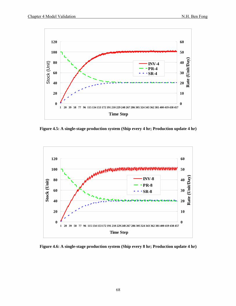
Chapter 4 Model Validation N.H. Ben Fong
0
20
40
60
80
100
120
1 20 39 58 77 96 115 134 153 172 191 210 229 248 267 286 305 324 343 362 381 400 419 438 457
Time Step
Sto
ck (U
nit)
0
10
20
30
40
50
60
Rat
e (U
nit/D
ay)
INV-4PR-4SR-4
Figure 4.5: A single-stage production system (Ship every 4 hr; Production update 4 hr)
0
20
40
60
80
100
120
1 20 39 58 77 96 115 134 153 172 191 210 229 248 267 286 305 324 343 362 381 400 419 438 457
Time Step
Stoc
k (U
nit)
0
10
20
30
40
50
60
Rat
e (U
nit/D
ay)
INV-8PR-8SR-8
Figure 4.6: A single-stage production system (Ship every 8 hr; Production update 4 hr)
68

Chapter 4 Model Validation N.H. Ben Fong
0
20
40
60
80
100
120
1 20 39 58 77 96 115 134 153 172 191 210 229 248 267 286 305 324 343 362 381 400 419 438
Time Step
Stoc
k (U
nit)
0
10
20
30
40
50
60
Rat
e (U
nit/D
ay)
INV-24PR-24SR-24
Figure 4.7: A single-stage production system (Ship every 24 hr; Production update 4 hr)
In Figure 4.4, the production rate updates every 4 hours with a shipment rate of every 2 hours.
The steady-state value for production rate and shipment rate is in the range of 20-20.7 units/day
and 20-20.2 units/day, respectively. The finished inventory level is within 100-101 units. As we
increases X hour from 2 to 4 hours, the increase in variation raises very little. As we update the
shipment rate from 4 to 8 hours, we have seen the increase in the range for production rate and
shipment rate as 19.4-20.6 unit/day and 19.6-20.8 unit/day, respectively. The steady-state range
of the final inventory is 98-104 units. If we assume the production take shipment every 24 hours,
it yields the production rate with a range of 17.6-22.7 units/day and 18.2-22 units/day for the
shipment rate. The variation of the final inventory is between 91-110 units. We compare the
discrete event model at a shipment update of X= 4 hr and production update at Y= 4hr with the
continuous classical control model as shown in Figure 4.8.
69

Chapter 4 Model Validation N.H. Ben Fong
0
10
20
30
40
50
1 17 33 49 65 81 97 113 129 145 161 177 193 209 225 241 257 273 289 305 321 337 353 369 385 401 417 433
Time Step
Stoc
k (U
nit)
0
20
40
60
80
100
Rat
e (U
nit/D
ay)PR(Cont) SR(Cont)
PR(Dis) SR(Dis)INV(Cont) INV(Dis)
Figure 4.8: Discrete vs. Continuous in modeling single-stage production system
Figure 4.8 shows that the state variables of the continuous model like production rate, shipment
rate, and inventory change continuously with respect to time, it yields a greater rate of change of
the state variables. For the discrete model, we have selected to update the production work force
and the shipment every 4 hours, the rate of change of the curves is much slower than the
continuous case. However, as the system reaches to its steady-state, about 12-14 days, the final
steady-state values of inventory, production rate, and shipment rate are insignificantly different
from the CCT continuous system model.
If the shipment rate and the production work force adjust at a shorter interval, say 30 minutes,
the slope of the finished inventory should increase. As the production work force and the
shipment continue to adjust at smaller time intervals, the rising slope of the finished inventory
behaves more like the continuous differential model. In other words, the CCT approach is
optimistic with respect to real discrete manufacturing systems and it always provides a lower
bound on the rise time of the system response. Additionally, the less rapid the management
70

Chapter 4 Model Validation N.H. Ben Fong
changes the schedule of production work force and shipment, the more of an optimistic CCT
approximation yields (i.e., gives more error to real industrial scenario).
In real life, customer demands often come randomly and unexpected. The CCT approach is
mathematically limited in that it cannot include any stochastic elements. In addition, production
management schedule their amount of work force according to the maximum capacity of the
overall machine throughput rate. The CCT approach cannot model any non-linear elements that
contain saturation due to maximum capacity. For unreliable manufacturing processes and
machine breakdowns, we can still apply CCT approach to model the machine failure as a system
disturbance input. In order to overcome these limitations of the CCT approach, we can apply
Non-Linear Control Theory and Stochastic Linear Control Theory to further enhance model
validity.
In this chapter, we have demonstrated that the classical control theory (CCT) modeling approach
appears to provide valid approximations of real discrete manufacturing systems. To further
validate the CCT approach, we will use it to model, analyze, and design a real three-stage
semiconductor manufacturing system in Chapter 6.
71

Chapter 5 Design of Responsive Manufacturing Systems N.H. Ben Fong
Chapter 5 Design of Responsive Manufacturing
Systems
In this chapter, we introduce a new design methodology to assist management in identifying
operation strategies to better predict the dynamic responses of responsive manufacturing systems
subjected to rapidly changing market demands. Section 5.1 introduces the Root Locus design
technique, originating from classical control theory. In that section, we apply the Root Locus
design tool to improve the overall system responsiveness of a two-stage production control
system. By varying the system loop gain K, the location of the closed-loop poles moves
predictably on the complex s-plane. Hence, management can predict and design the particular
responsive manufacturing systems in terms of production lead time, degree of WIP overshoot
(i.e., damping ratio) and lean finished inventory. In Section 5.2, we further define and interpret
the meanings of those classical control terms, such as damping ratio, closed-loop poles location,
and settling time as they relate to the manufacturing world on a complex s-plane representation.
We give examples of various step response dynamic behaviors according to the different
locations of the closed-loop poles. This complex plane analysis offers a graphical view to
evaluate and understand the overall dynamics and the corresponding parametric sensitivity of
any responsive manufacturing systems. Finally, section 5.3 applies the Root Locus to design a
two-stage production control system with 3rd-order time delay. From section 3.2, we extended
the two-stage production control system with a 3rd-order time delay inclusion and it turned into a
fourth-order differential equation model. The corresponding root locus and dynamic behavior of
this higher-order system behaves very differently. We introduce the Dominant Roots or
72

Chapter 5 Design of Responsive Manufacturing Systems N.H. Ben Fong
dominant closed-loop poles concept to design higher-order differential system models. The
resulting root locus reveals the potential for system instability due to poor management policies
through the location of the closed-loop poles.
5.1 Root Locus Analysis and Design of a Two-Stage Production System
In this section, we introduce the Root-Locus technique from classical control theory [40,41,42]
to improve the overall system responsiveness and lead time for the two-stage production control
model. Phillips and Harbor [42] defined: “A Root Locus of a system is a plot of the roots of the
system characteristic equation (the poles of the closed-loop transfer function) as some parameter
of the system is varied”. The location of the system closed-loop poles, as given by Eq. (5.1),
determines the transient characteristics of the two-stage production system.
Closed-Loop Poles: -1 - s 2nn1,2 ζωζω j±= (5.1)
As mentioned, the closed-loop poles of a system are the roots of the characteristic equation. It is
instructive to see how the closed-loop poles move in the complex s-plane as the loop gain of the
system is varied. From a design point of view, an adjustment of the gain value(s) may bring the
closed-loop poles to certain desired locations. We apply the Root-Locus technique to plot the
roots of the characteristic equation for different values of gain K. The root locus is the locus of
roots of the characteristic equation of the closed-loop system as the gain K is varied from zero to
infinity. Such a plot clearly indicates how to modify the open-loop poles such that the response
of the manufacturing system can meet the specific customer requirements. We generally consider
the system of Fig. 5.1 in describing the concept of root locus as stated in Phillips and Harbor [42],
73

Chapter 5 Design of Responsive Manufacturing Systems N.H. Ben Fong
with 0 K< ∞. In Figure 5.1, we assume that G(s) comprises both the compensator transfer
function and the plant transfer function. The characteristic equation for this system is given in Eq.
(5.2). A value s
≤
1 is a point on the root locus if and only if s1 satisfies Eq.(5.2) for a real value of
K, with 0 ≤ K< ∞.
1 + KG(s) H(s) = 0 (5.2)
K G(s)
H(s)
+_
Figure 5.1: A system for Root Locus
For more detail on Root-Locus methodology, see Ogata [40] and Phillips and Harbor [42].
According to the closed-loop transfer function of the two-stage production system as derived in
Eq.(3.19), the system equation KG(s) for the root locus analysis as shown in Fig. 5.1 will
become:
⎥⎦
⎤⎢⎣
⎡⎟⎠⎞
⎜⎝⎛ +⎟⎟
⎠
⎞⎜⎜⎝
⎛−+⎥
⎦
⎤⎢⎣
⎡+++
⎟⎠⎞
⎜⎝⎛ +⎟
⎠⎞
⎜⎝⎛
⎟⎠⎞
⎜⎝⎛
=
WAT1
LT1
ST1
ST1
ST1
WAT1
LT1 ss
WATLT1
LT1
FAT1
KG(s)
211
2
(5.3)
Given that the loop gain, ST1=ST2, Eq.(5.3) reduces to:
ST
1WAT
1LT1 ss
WATLT1
LT1
FAT1
KG(s)
1
2⎥⎦
⎤⎢⎣
⎡+++
⎟⎠⎞
⎜⎝⎛ +⎟
⎠⎞
⎜⎝⎛
⎟⎠⎞
⎜⎝⎛
= (5.4)
74
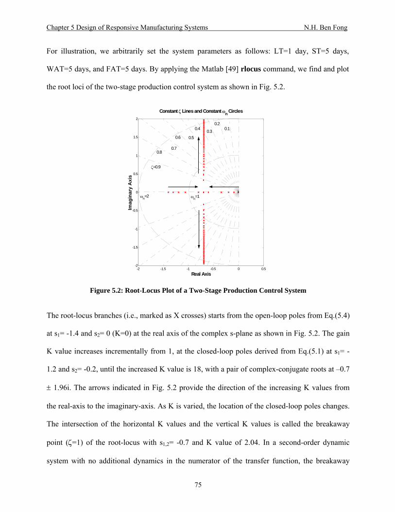
Chapter 5 Design of Responsive Manufacturing Systems N.H. Ben Fong
For illustration, we arbitrarily set the system parameters as follows: LT=1 day, ST=5 days,
WAT=5 days, and FAT=5 days. By applying the Matlab [49] rlocus command, we find and plot
the root loci of the two-stage production control system as shown in Fig. 5.2.
-2 -1.5 -1 -0.5 0 0.5-2
-1.5
-1
-0.5
0
0.5
1
1.5
2
Real Axis
Imag
inar
y A
xis
Constant ζ Lines and Constant ωn Circles
ζ=0.9
0.80.7
0.6 0.5
0.4 0.3
0.20.1
ωn=1ωn=2
Figure 5.2: Root-Locus Plot of a Two-Stage Production Control System
The root-locus branches (i.e., marked as X crosses) starts from the open-loop poles from Eq.(5.4)
at s1= -1.4 and s2= 0 (K=0) at the real axis of the complex s-plane as shown in Fig. 5.2. The gain
K value increases incrementally from 1, at the closed-loop poles derived from Eq.(5.1) at s1= -
1.2 and s2= -0.2, until the increased K value is 18, with a pair of complex-conjugate roots at –0.7
± 1.96i. The arrows indicated in Fig. 5.2 provide the direction of the increasing K values from
the real-axis to the imaginary-axis. As K is varied, the location of the closed-loop poles changes.
The intersection of the horizontal K values and the vertical K values is called the breakaway
point (ζ=1) of the root-locus with s1,2= -0.7 and K value of 2.04. In a second-order dynamic
system with no additional dynamics in the numerator of the transfer function, the breakaway
75

Chapter 5 Design of Responsive Manufacturing Systems N.H. Ben Fong
point is simply (s1+s2)/2. The damping ratio ζ of the system is always equal or greater than one
as the closed-loop poles are found along the real-axis on the s-plane. Once the closed-loop poles
have passed the breakaway point, ζ begins to reduce further with pairs of complex-conjugate
roots. Figure 5.2 also plots the grid of constant damping ratio ζ lines and constant undamped
natural frequency ωn lines. The constant ζ lines are radial lines passing through the origin with a
decrement of 0.1 from ζ=1 to 0.1, whereas the constant ωn loci are circles.
In the complex s-plane, we can express the damping ratio ζ of a pair of complex-conjugate poles
in terms of the angle φ which is measured from the negative real-axis with ζ= cosφ, and
determine the distance of the pole from the origin by the undamped natural frequency ωn. As
discussed in the previous section, we quantify the transient dynamic responses of the two-stage
production system by the key parameters ζ and ωn. The importance of introducing Root-Locus
method here is to provide a predictive design technique to improve the overall dynamic behavior
of this manufacturing system. As per classical control theory, we can design a desirable transient
response of a second-order system with a damping ratio around 0.707. It is justified with results
in the next phase. Small values of ζ<0.4 yield excessive overshoot where a system with ζ>0.8
responds sluggishly as shown in Fig. 3.17 previously. The further the closed-loop pole is away
from the origin of the s-plane, the faster the response of the system behaves. However, the
system will become unstable if there is any closed-loop pole found on the right-hand side of the
s-plane.
For our example, in order to bring the system model to ζ=0.707, the K value from the root-locus
analysis is increased to 4.08 with ωn=0.99 at s1,2= -0.7 ± 0.70i as shown in Figure 5.2. Given this
76

Chapter 5 Design of Responsive Manufacturing Systems N.H. Ben Fong
particular parametric set of values, the system equation has an initial non-unity loop gain K of
0.24 as computed from Eq.(5.3). As a result, we have to multiply every root-locus gain K from
Matlab by a factor of 0.24. Although K is a function of Finished Inventory Adjustment Time
(FAT), Lead Time (LT), and WIP Adjustment Time (WAT) as given by Eq.(3.29), in order to
keep the same breakaway point while changing the K value, we can only vary K as a function of
FAT.
2n
t
WATLT1
LT1
FAT1
K y(t) limω
⎟⎠⎞
⎜⎝⎛ +⎟
⎠⎞
⎜⎝⎛
⎟⎠⎞
⎜⎝⎛
==∞→
(3.29)
By setting FAT=1.224, we make the system respond with ζ=0.707 at K=4.08*0.24=0.98. In
designing a fast-response manufacturing system, setting ζ to 0.707 is crucial; however, moving
the breakaway point further away from the origin is another vital step. According to Eq.(3.23),
the time response of the system is a function of LT, WAT and ST.
Time constant:
⎥⎦
⎤⎢⎣
⎡++
==
1
n
ST1
WAT1
LT1
2 1 ζω
τ (3.23)
Since we have assumed the shipment time to be 5 days for a transportation schedule, we will
further study the dynamic characteristics of this system model as a function of LT and WAT.
Figures 5.3 and 5.4 show, respectively, contour plots of ζ values and breakaway points against
WAT and LT while keeping FAT=1 day.
77

Chapter 5 Design of Responsive Manufacturing Systems N.H. Ben Fong
0.5 1 1.5 2 2.5
0.5
1
1.5
2
2.5
Le ad Tim e (LT) in day s
WIP
Adj
ustm
ent T
ime
(WA
T) in
day
s
Constant ST=5 day s and Constant FAT=1 day
0.57
0.585
0.6
0.625
0.650.675
0.707
0.750.8
0.850.90.951
Figure 5.3: Contour Plot of ζ values as a function of LT and WAT
Figure 5.3 shows the contour of ζ values as a function of WAT and LT with a constant FAT=1.
A combination choice of LT and WAT along a particular contour line gives the desired damping
ratio. For example, if we pick WAT=1.5, by taking LT=1.1, it results in ζ≈ 0.707 and a
breakaway point of –0.89 (i.e., an improvement from –0.7). Figure 5.3 shows that ζ values
decrease from 1 to 0.57 with increasing values of both LT and WAT. As stated earlier, FAT is
the most significant factor that affects ζ values. With a FAT value higher than 2.0 (not shown
here), changing any value in LT and WAT will not make any impact to reduce ζ to less than
unity (i.e., the system is always overdamped or critically damped). For the contour of breakaway
points as shown in Figure 5.4, the breakaway point moves towards more negative from –0.53
to –4.0 as LT and WAT are reduced, hence it improves the system response as the breakaway
point moves further away from the origin at the complex plane. FAT does not play a role in the
location of the breakaway point. If we arbitrarily pick LT=1 and WAT=1 from Figure 5.4, it
78
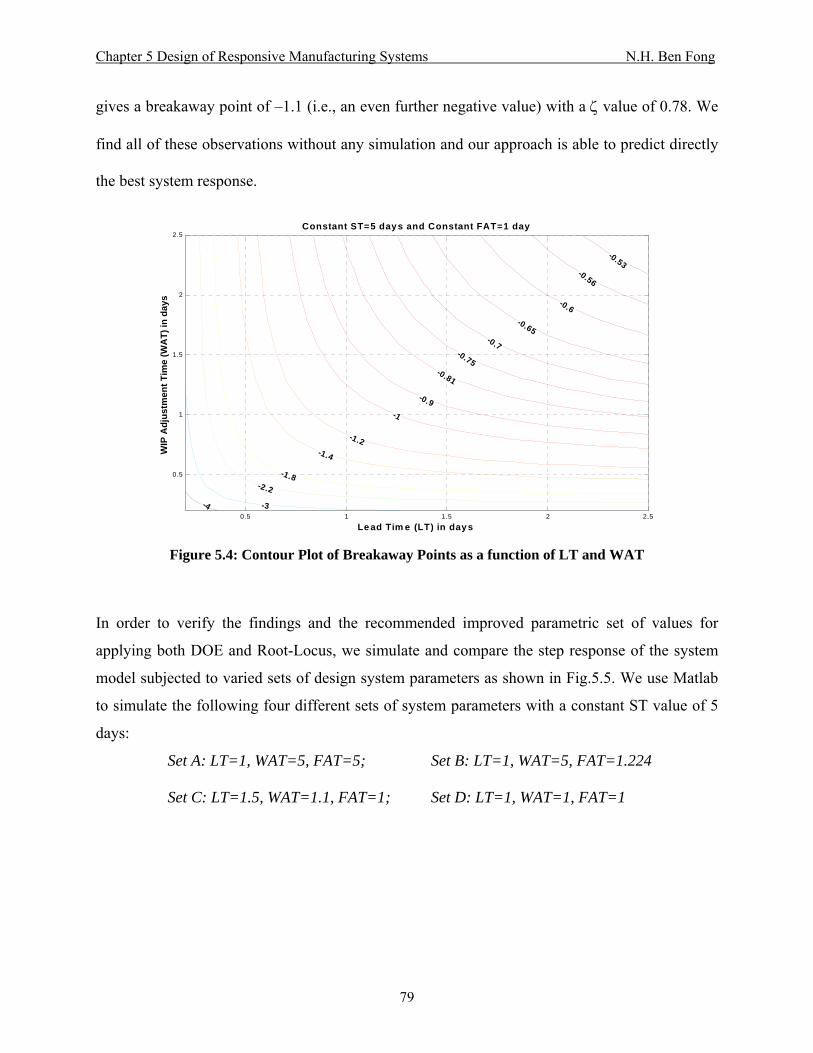
Chapter 5 Design of Responsive Manufacturing Systems N.H. Ben Fong
gives a breakaway point of –1.1 (i.e., an even further negative value) with a ζ value of 0.78. We
find all of these observations without any simulation and our approach is able to predict directly
the best system response.
Figure 5.4: Contour Plot of Breakaway Points as a function of LT and WAT
0.5 1 1.5 2 2.5
0.5
1
1.5
2
2.5
Le ad Tim e (LT) in days
WIP
Adj
ustm
ent T
ime
(WA
T) in
day
s
Constant ST=5 days and Constant FAT=1 day
-0.53-0.56
-0.6-0.65
-0.7-0.75
-0.81
-0.9-1
-1.2-1.4
-1.8-2.2
-3-4
In order to verify the findings and the recommended improved parametric set of values for
applying both DOE and Root-Locus, we simulate and compare the step response of the system
model subjected to varied sets of design system parameters as shown in Fig.5.5. We use Matlab
to simulate the following four different sets of system parameters with a constant ST value of 5
days:
Set A: LT=1, WAT=5, FAT=5; Set B: LT=1, WAT=5, FAT=1.224
Set C: LT=1.5, WAT=1.1, FAT=1; Set D: LT=1, WAT=1, FAT=1
79

Chapter 5 Design of Responsive Manufacturing Systems N.H. Ben Fong
0 5 10 150
20
40
60
80
100
120
Time in days
Fini
shed
Inve
ntor
y Le
vel i
n st
ocks
Set A: ζ=1, Brkaway Pt=-0.7
Set B: ζ=0.707, Brkaway Pt=-0.7
Set C: ζ=0.7073, Brkaway Pt=-0.8879
Set D: ζ=0.7778, Brkaway Pt=-1.1
Figure 5.5: Step Response Comparison of a Two-Stage Production Control System
The results show that the original parametric set A responds sluggishly due to its ζ value of 1
(i.e., critically damped) with a breakaway point of –0.7. The root-locus analysis suggests to
increase the gain K value to 4.08 and with FAT=1.224. The set B curve has shown a significant
improvement in term of the overall system response. Curve B has a ζ value of 0.707 with the
same breakaway point of –0.7. We further improve the system response by changing the values
of LT, WAT and FAT according to the contour plots. The set C curve gives an even quicker rise
time as compared to curve B due to the improvement of the breakaway point (i.e., increases
from –0.7 to –0.89). Curve D appears to be the best suggested system response. Again, by
studying the dynamic characteristics at the contour plots, we further improve the breakaway
point from –0.89 to –1.1 with even smaller inventory overshoot.
80

Chapter 5 Design of Responsive Manufacturing Systems N.H. Ben Fong
5.2 Interpretation of CCT Terms to the Manufacturing World
As stated previously, the root locus is the locus of roots of the characteristic equation of the
closed-loop system as a specific parameter (usually, gain K) varies from zero to infinity. This
technique is very useful since it provides guidelines in which the open-loop poles and/or zeros
(definition of these CCT terms will be described later) should be modified such that the system
responses meet the desired performance specifications. By using the root-locus method, we can
determine the value of the loop gain K that makes the damping ratio, ζ of the dominant closed-
loop poles as prescribed. In the manufacturing world, industrial engineers and managers prefer to
predict and control the critical system variables, like lead time, inventory level, settling time for
production control planning purposes. In this section, we define and interpret some key
manufacturing system variables as they relate to the classical control theory terms described in
the complex s-plane. The aim of this interpretation is to offer a new operation planning strategy
for manufacturing managers to better predict and study the transient behavior of responsive
manufacturing systems. This approach offers a systematic and graphical view to evaluate and
understand the overall dynamics and its corresponding parametric sensitivity of any responsive
manufacturing system model.
Responsiveness is an overall strategy focused on thriving in an unpredictable and dynamic
environment. Lean is a philosophy that seeks to minimize all waste that includes long lead time,
excess WIP inventory, non-value added activities. Responsiveness refers to the dynamics of
manufacturing system behavior in term of damping ratio ζ value. Fowler [31] described an MRP
system as a feedforward system where the production is pulled through the system by a
feedforward scheduling system, referenced to the particular customer demand. He further stated
81

Chapter 5 Design of Responsive Manufacturing Systems N.H. Ben Fong
that the Kanban control system may be seen as the production pulled through the system by a
sequence of cascaded feedback control loops. However, there has never been an example to
describe whether these loops are stable or tuned properly. We will now do this with a new
systematic method to study and predict production operation strategies based upon the key
manufacturing variables as they relate to the closed-loop poles location in the complex s-plane.
Again, we pick the Root Locus plot of the two-stage production control system as shown in
Figure 5.2 to perform the investigation. As stated previously, the root-locus branches of this
model (marked as X crosses) starts from the open-loop poles at s1= -1.4 and s2=0 (K=0) at the
real axis of the complex s-plane as shown in Figure 5.6. The gain K value increases
incrementally from 1, at the closed-loop poles at s1= -1.2 and s2= -0.2, until the increased K
value is 18, with a pair of complex-conjugate roots at -0.7 ± 1.96i. We added nine “+ crosses” on
the s-plane to examine different dynamic characteristics according to the location of the closed-
loop poles as shown in Figure 5.6 (next page).
In this section, by varying the location of different closed-loop poles or roots on the complex s-
plane as shown in Figure 5.6, we specifically define and interpret the significance of each
location as it relates to the dynamic behavior found in the manufacturing environment. The x-
axis and the y-axis on Figure 5.6 represent the real axis and the imaginary axis, respectively. The
closed-loop poles can be interpreted as the production buffers (i.e., accumulates products). The
pole located at point A indicates a negative real root of the characteristic equation, Eq. (5.3). This
pole location gives the production inventory level to decay exponentially until it reaches steady
stable condition. Any manufacturing system that contains only real roots, closed-loop poles on
the x-axis will not obtain any inventory overshoot and dynamic oscillation (i.e., ζ ≥1.0).
82

Chapter 5 Design of Responsive Manufacturing Systems N.H. Ben Fong
-2 -1.5 -1 -0.5 0 0.5-2
-1.5
-1
-0.5
0
0.5
1
1.5
2
Real Axis
Imag
inar
y A
xis
X X
+
+
+
+
+
+
+
A B
C
D
E
F
G
H
J
+
+
K
L
Figure 5.6: Complex s-plane interpretation of varying location of closed-loop poles The pole located at point B is special case when production maintains at a certain inventory level
steadily (i.e., no rise or fall), thus it is considered as a limited stable condition due to the potential
of inventory growing exponentially. The pair of complex-conjugate roots with negative real parts
located at points C and D give dynamics that makes production inventory oscillate and dies
down to stable condition within its envelope. The points C and D are found at the contour line of
damping ratio, ζ = 0.8. In terms of the speed of the production lead time, points A, C, and D shall
behave similarly except there is no oscillation at point A. As the closed-loop poles get closer to
the right, the speed of the system responsiveness shall decrease. The pair of complex-conjugate
roots with negative real parts located at points E and F is expected to respond slower than the
pair located at points C and D. In addition, the degree of oscillation shall magnify as the damping
83

Chapter 5 Design of Responsive Manufacturing Systems N.H. Ben Fong
ratio decreases from ζ =0.8 to 0.5. Their rate of exponential decay will be less than the pair from
C and D but it still leads to a steady stable condition. The pair of complex-conjugate roots on the
imaginary axis located at points G and H yields a limit cycle for the manufacturing system.
Given ζ =0, the production inventory will behave periodically within a particular set range of
inventory level. The production attempts to respond due to the seasonal customer demand,
however given the fixed maximum customer demand, the corresponding production inventory
oscillate within the same envelope. Obviously, operation management does not want to keep a
fixed amount of annual inventory costs to forecast seasonal customer requirements. Rather,
management shall determine a strategy to make shipments as needed. In CCT terms, this type of
manufacturing system is considered to be marginally stable due to the potential to grow
exponentially positive. In practice, of course, saturation of some limited resource will eventually
occur to keep the results finite.
Once the closed-loop poles go beyond the imaginary axis to the right-hand-side of the s-plane,
the manufacturing system will behave unstable without bound or until the plant capacity
saturates. For instance, the pole located at point L has a positive real root. Thus, the production
inventory will grow positively without bound. This is the typical scenario when the management
decided to build as much inventory as production can provide to prevent the unexpected sudden
request by their customers. Truly, this kind of operation policy should not continue to run, given
the concept of Kanban from the Lean manufacturing system. Lastly, the pair of complex-
conjugate roots with positive real parts located at points J and K indicates that production
inventory continues to increase with dynamics and oscillation. This system grows positive and
84

Chapter 5 Design of Responsive Manufacturing Systems N.H. Ben Fong
sinusoidal with an increasing size of envelope with no bound. Obviously, it turns into a poor
management policy to let inventory costs add accumulatively in seasons without bound.
We graphically display the dynamic behavior of those six special cases as discussed as shown in
Figure 5.7. Again, the two stable cases, include, a single negative real root (A) and a pair of
complex conjugate roots with negative real parts (C and D). The two marginally stable cases,
contain, a single root at the origin (B), and a single pair of complex conjugate roots on imaginary
axis (G and H). Finally, the two unstable cases comprise, a positive real root (L) and a complex
conjugate roots with positive real parts (J and K).
85
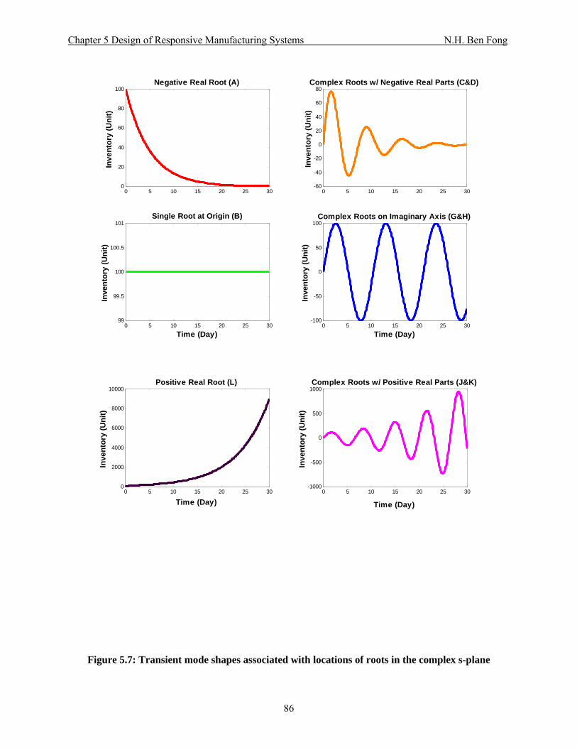
Chapter 5 Design of Responsive Manufacturing Systems N.H. Ben Fong
0 5 10 15 20 25 300
20
40
60
80
100Negative Real Root (A)
Inve
ntor
y (U
nit)
0 5 10 15 20 25 30-60
-40
-20
0
20
40
60
80Complex Roots w/ Negative Real Parts (C&D)
Inve
ntor
y (U
nit)
0 5 10 15 20 25 3099
99.5
100
100.5
101Single Root at Origin (B)
Inve
ntor
y (U
nit)
Time (Day)0 5 10 15 20 25 30
-100
-50
0
50
100Complex Roots on Imaginary Axis (G&H)
Inve
ntor
y (U
nit)
Time (Day)
0 5 10 15 20 25 300
2000
4000
6000
8000
10000Positive Real Root (L)
Inve
ntor
y (U
nit)
Time (Day)0 5 10 15 20 25 30
-1000
-500
0
500
1000Complex Roots w/ Positive Real Parts (J&K)
Inve
ntor
y (U
nit)
Time (Day)
Figure 5.7: Transient mode shapes associated with locations of roots in the complex s-plane
86

Chapter 5 Design of Responsive Manufacturing Systems N.H. Ben Fong
5.3 Root Locus Design of a Two-Stage Production System with Time Delay
Delays are inherent in many physical and engineering systems. There are different kinds of
delays found as described by Forrester and Sterman [5,16]. They are such as material delays,
pipeline delay or transportation lag, and information delays. For the manufacturing sector,
material delay is a kind that captures the physical flow of material through a delay process. For
example, this delay often happens in a supply chain, distribution business, and construction
management. For multi-stage manufacturing processes, between each station, there is a delay
caused by transportation and order handling. Each station operates individually based on demand
information provided from upstream. As the number of stations increase, the demand signal
amplifies from station to station as orders go through the chain of supply. Forrester described
those oscillations in demand along the chain as the bullwhip effect [2]. In the previous sections,
we stated that the higher the order of the time delay goes, the better the production system can be
characterized. Wikner [27] has described that a third-order delay has proved to be an appropriate
compromise between model complexity and model accuracy for most dynamic modeling of
production-inventory systems. In this section, we investigate the dynamic behavior of the two-
stage production control system with a 3rd-order time delay from Figure 3.7 on the complex s-
plane environment. As recall from Eq.(3.33), the 4th-order differential equation formulated for
the two-stage with a 3rd-order time delay model is as:
( )( )
[ ] [ ] [ ] [ ]D s C s B s A sWATLT
1LT
1FAT
27
DI(s)FI(s)
234
23
++++
⎟⎟⎠
⎞⎜⎜⎝
⎛+⎟
⎠⎞
⎜⎝⎛
= (5.5)
87

Chapter 5 Design of Responsive Manufacturing Systems N.H. Ben Fong
where,
( )( ) ( )( ) ( )( )
( )( ) ( )( ) ( )( )( )
⎟⎟⎠
⎞⎜⎜⎝
⎛−+⎟
⎠⎞
⎜⎝⎛ +=
+++=
+++=
++=
212
12
123
112
1
ST1
ST1
FAT1
WAT1
LT1
LT27 D
WATSTLT9
WATLT27
STLT27
LT27 C
WATST1
WATLT9
STLT9
LT27 B
WAT1
ST1
LT9 A
Given the set of selected system parameters: LT=4; ST=8; WAT=1; FAT=1, we observe a
significant dynamic oscillation difference between the third-order delay model and the first-order
exponential smoothing model for the two-stage production system from Figure 3.20.
0 5 10 15 20 25 300
20
40
60
80
100
120
140
160
180
Time in days
Fini
shed
Inve
ntor
y Le
vel (
Uni
t)
1st-Order Delay
3rd-Order Delay
Figure 3.21: Dynamic Responses between 1st-order time delay and 3rd-order time delay
Again, we apply the Root Locus technique to investigate the effect of the closed-loop poles
location for the dynamic production control system. Since it is a fourth-order differential
88

Chapter 5 Design of Responsive Manufacturing Systems N.H. Ben Fong
equation model, there are four closed-loop poles found on the complex s-plane as shown in
Figure 5.8
-2.5 -2 -1.5 -1 -0.5 0 0.5 1-1.5
-1
-0.5
0
0.5
1
1.5Im
ag A
xes
Real Axis
LT=4, ST=8, WAT=1, FAT=1
ζ=0.9 ζ=0.8
ζ=0.7ζ=0.6
X X
X
X
+
+
+
+
Figure 5.8: Root-Locus Plot of a two-stage production control system with 3rd-order time delay
The root-locus branches starts from the open-loop poles location where s1= 0, s2= -1.74, and s3,s4
= -0.819±0.909i, (K=0) on the complex s-plane as shown in Fig. 5.8. The gain K value increases
in the direction of the arrows from the starting poles location (K=0) to the stopping poles
location (K=8). As observed in Figure 5.8, the complex conjugate pair of poles enters the right-
hand side of the s-plane as K increases over 1.305 (not explicitly shown here). As the gain K
continues to increase to infinity (K→∞), the production system grows oscillatory with no bound
(i.e., unstable). Whereas, the two real roots (poles) continue to go towards to the further left of
the s-plane (i.e., stable) as the gain K value increases to infinity. The major challenge here is to
89

Chapter 5 Design of Responsive Manufacturing Systems N.H. Ben Fong
design and improve this 3rd-order time delay, two-stage production control system to give quick-
responsive production lead time, less oscillation, and lean final inventory level. Although we
have derived the fourth-order differential equation for this particular production system, there is
no standard formulation that describes damping ratio, time constant, rise time and settling time
for higher-order control systems. In MATLAB programming software [49], we can apply a
function command, rltool, from the Control System Toolbox, to determine the corresponding
gain K value of the corresponding higher-order manufacturing system that yields fast production
lead time and less inventory overshoot on the rlocus plot as shown in Figure 5.8. For higher-
order dynamic systems, it is a good rule of thumb to set the damping ratio between 0.7 and 0.9 to
obtain a fast responsive system behavior [40,41,42,43]. As the gain K value is varied, the
location of the closed-loop poles changes. However, there are altogether four closed-loop poles
or roots to be adjusted in this fourth-order system model. The challenge is to select the particular
K gain value such that the overall production control system yields the best system performance.
Fortunately, there is a concept called Dominant Roots or dominant closed-loop poles from
classical control theory [40,41,42] to help in determining the most influential pole(s) for the
system. We have seen that a time constant τ is a measure of the decay rate of an exponential e-at,
where τ=1/a. The time constant corresponds to the characteristic roots, s= -a, or a complex pair,
s= -a ± ib. If a stable dynamic system model has several roots with different real parts, the root
having the largest time constant (i.e., the one lying the farthest to the right on the complex s-
plane) is the root whose exponential term dominates the overall system response. This particular
root is called the dominant root. There can be two dominant roots (complex pair) existing in a
system because they both have the same real part and same time constant. We illustrate different
90
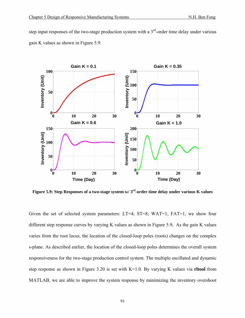
Chapter 5 Design of Responsive Manufacturing Systems N.H. Ben Fong
step input responses of the two-stage production system with a 3rd-order time delay under various
gain K values as shown in Figure 5.9.
0 10 20 300
50
100Gain K = 0.1
Inve
ntor
y (U
nit)
0 10 20 300
50
100
150Gain K = 0.35
Inve
ntor
y (U
nit)
0 10 20 300
50
100
150Gain K = 0.6
Time (Day)
Inve
ntor
y (U
nit)
0 10 20 300
50
100
150
200Gain K = 1.0
Time (Day)
Inve
ntor
y (U
nit)
Figure 5.9: Step Responses of a two-stage system w/ 3rd-order time delay under various K values
Given the set of selected system parameters: LT=4; ST=8; WAT=1; FAT=1, we show four
different step response curves by varying K values as shown in Figure 5.9, As the gain K values
varies from the root locus, the location of the closed-loop poles (roots) changes on the complex
s-plane. As described earlier, the location of the closed-loop poles determines the overall system
responsiveness for the two-stage production control system. The multiple oscillated and dynamic
step response as shown in Figure 3.20 is set with K=1.0. By varying K values via rltool from
MATLAB, we are able to improve the system response by minimizing the inventory overshoot
91

Chapter 5 Design of Responsive Manufacturing Systems N.H. Ben Fong
and reducing the production lead time as shown in Figure 5.9. In this particular case, by reducing
the K value, we decrease the amount of oscillation and improve the system settling time.
However, if we reduce K value too low, like K=0.1, the higher-order system behaves sluggishly
like a first-order dynamic system as shown on the top left hand corner of Figure 5.9. Obviously,
we would like the system respond similar to the case when K=0.35. As recall from the previous
section, the gain K is a function of Finished Inventory Adjustment Time (FAT), Lead Time (LT),
and WIP Adjustment Time (WAT). Plus, this fourth-order system equation has an initial non-
unity loop gain K of 2.109. Hence, in order to set K=0.35 from the rltool in MATLAB, we have
to multiply 0.35 by a factor of 2.109 to give 0.7383. The dynamic structure of this fourth-order
differential model is very similar to its previous 2nd-order system except for the third-order delay
term of 1/LT3. Again, in order to keep the same breakaway point while changing the K value, we
only vary K as a function of FAT. By setting FAT=2.8571, we make the system respond with a
settling time of 12 days at ζ = 0.67 and Kactual = 0.7383. Its resulting closed-loop poles are s1,2 =
-0.4521±0.4884i, s3,4= -1.2354±0.3747i. Given the same breakaway point, we can improve the
system response by changing the K value from 0.35 to 0.300676, thus FAT becomes 3.3258. The
production lead time reduces to 10 days with no oscillation with ζ = 0.83 and Kactual=0.6342. Its
corresponding closed-loop poles are s1,2= -0.6203±0.4148i, s3,4= -1.067.
The lead time has been reduced from 12 days to 10 days because the dominant pair of roots go
further left from the imaginary axis (i.e., from -0.45 to -0.62). In addition, the damping ratio
increases from 0.67 to 0.83, especially the improved roots, s3 and s4, are located on the real axis
with real parts to give fast response time. Finally, we can further reduce the production lead time
and system settling time by changing the parametric set of system variables to LT=1, ST=5,
92

Chapter 5 Design of Responsive Manufacturing Systems N.H. Ben Fong
WAT=1, and FAT=1.4. For this particular parametric set of values, we find a different initial
non-unity loop gain K of 54. The root-locus branches start from the open-loop poles with arrows
at s1=0, s2= -5.1042, s3,4= -2.5479±2.345i (K=0) and go towards the poles ending at K=13 as
shown in Figure 5.10.
-8 -7 -6 -5 -4 -3 -2 -1 0 1 2-4
-3
-2
-1
0
1
2
3
4
Real Axis
Imag
Axe
s
LT=1, ST=5, WAT=1, FAT=1.4
ζ=0.9
+
+
+
+
X
X X
X ζ=0.8
ζ=0.7
Figure 5.10: Root-Locus Plot of a two-stage production control system with 3rd-order time delay
It is shown that the root-locus plot in Figure 5.10 is very different from the Figure 5.8. All the
closed-loop poles can be found on the real axis depending on their selected K values. Whereas,
the pair of dominant poles in the previous case could never reach ζ>0.9 nor the real axis as gain
K varies. As mentioned, the starting open-loop poles location and its breakaway points are
determined by the given set of design system variables in terms of LT, ST, WAT, and FAT. By
changing the K value to 0.7143 with FAT=1.4, we make the system respond with ζ=0.89 and
93

Chapter 5 Design of Responsive Manufacturing Systems N.H. Ben Fong
Kactual =0.7143*54=38.57. Its corresponding closed-loop poles are located at s1,2= -1.5087
±0.7675i and s3,4= -3.5913±0.7513i. The resulting production lead time has significantly
improved and reduced from 10 days to 4.3 days. In order to verify the findings and the
recommended improved parametric set of system variables applying Root Locus technique, we
simulate and compare those four particular step responses of the two-stage production control
model with a 3rd-order time delay subjected to varied sets of design system parameters as shown
in Figure 5.11.
Set A: LT=4, ST=8, WAT=1, FAT=1; (Multiple oscillations with very long settling time)
Set B: LT=4, ST=8, WAT=1, FAT=2.8571; (Single Overshoot with reduced lead time, 12 days)
Set C: LT=4, ST=8, WAT=1, FAT=3.326; (No Overshoot with improved lead time, 10 days)
Set D: LT=1, ST=5, WAT=1, FAT=1.4; (No Overshoot, quick-response lead time, 4.3 days)
0 2 4 6 8 10 12 14 16 18 200
20
40
60
80
100
120
140
160
180
Time (Day)
Fini
shed
Inve
ntor
y (U
nit)
Set A
Set B
Set C
Set D
Figure 5.11: Various Step Response of a two-stage production system with 3rd-order time delay
94
Chapter 5 Design of Responsive Manufacturing Systems N.H. Ben Fong
We have demonstrated a new operation design method that permits production management to
better predict and design manufacturing system variables that yield responsive production lead
time and minimal inventory build-up (i.e., leanness) under transient manufacturing conditions.
This Root Locus design approach gives a completely graphic view to understand the sensitivity
on the location of the closed-loop poles by varying the loop gain K values to the dynamic system
models in the complex s-plane. We are able to determine responsive production parametric
values without iterative trial-and-error simulation as found in discrete event simulation or the
system dynamics approach.
The Root Locus design method we demonstrated here is based on varying the loop gain K values,
plus changing the manufacturing system parameters to reduce the time constant of the dominant
poles. In many industrial cases, however, the adjustment of the gain K values alone may not
provide sufficient alternation of the manufacturing system structure to meet the specific customer
requirement. As we learned from this section, as gain K values increases, it improves the steady-
state behavior but it could make the system in a poor stability region (even unstable) as K goes to
infinity. If it is the case, it may be necessary to redesign the dynamic manufacturing system
structure to alter the overall transient behavior to meet the management specification. Such a
redesign approach is called System Compensation technique found in classical control theory
[40,41,42]. We can easily perform this redesign approach using rltool from MATLAB by adding
selective poles and zeros into the original differential equation system model. In general, by
adding poles (more feedback loops) to the system, we destabilize the dynamic behavior with the
addition of production buffers. Whereas, adding zeros is similar to anticipating the customer
demand (i.e., forecasting with feedforward loops) to the system, in result, it has a stabilizing
95

Chapter 5 Design of Responsive Manufacturing Systems N.H. Ben Fong
influence. In root locus plotting, the gain K always begins at its open-loop location as K
increases until it reaches either to a zero location or infinity. System compensation is definitely
something we shall consider for responsive manufacturing systems applications in the near future.
5.4 Guidelines to perform Root Locus Design in Responsive Manufacturing Systems In this chapter, we have demonstrated how to apply Root Locus design technique from classical
control theory to improve the overall dynamic responsiveness of responsive manufacturing
systems according to the closed-loop poles locations on the complex s-plane. We here
summarize and give some basic guidelines for those whom may interest to apply Root Locus to
design and improve their particular manufacturing system dynamic behavior.
(1) Model the responsive manufacturing system into transfer function (i.e., differential equation
format).
(2) Apply Root Locus design technique to identify the root locus of the particular dynamic
manufacturing system behavior by varying the loop gain K values on a complex s-plane (you
can use MATLAB Control Toolbox to perform this function task).
(3) Select your desired closed-loop poles location (i.e., damping ratio in the range of 0.7-0.9)
and record your corresponding system loop gain K value.
(4) Adjust your key manufacturing system variables to match the same loop gain K value.
(5) Plot your resulting dynamic step response according to your selected parametric set values.
96

Chapter 5 Design of Responsive Manufacturing Systems N.H. Ben Fong
(6) Shorten your production lead time by moving your dominant closed-loop poles location
further to the left-hand side of the complex s-plane and adjust your key manufacturing
system variables to match the new loop gain K value.
(7) Verify your dynamic step response behavior according to your selected parametric set values.
97

Chapter 6 Industrial Case Study N.H. Ben Fong
Chapter 6 Industrial Case Study
The purpose of this chapter is to enhance the validation of applying classical control theory
(CCT) methodology to responsive manufacturing systems. By using a real industrial case study,
we aim to further validate the potential of using CCT approach to model, design, and improve
the overall responsiveness of manufacturing systems. We have chosen a hybrid push-pull
production system for semiconductor manufacturing to represent a particular Intel Corporation
plant facility as extracted from the proceedings of the 22nd International Conference of the
System Dynamics Society (July 2004) written by Goncalves et.al. [50]. In their industrial case
study, Goncalves, Hines, Sterman, and Lertpattarapong undertook a year-long, in-depth research
project to develop and analyze a manufacturing model of producing semiconductors via the
System Dynamics (SD) approach. Their case study addressed the causes of oscillatory behavior
in capacity utilization at a semiconductor manufacturer and the role of endogenous customer
demand in influencing the company’s production and service level. For more a detailed
understanding of this 41-pages case study, please read Goncalves et al. [50].
We intend to make use of this particular Intel hybrid push-pull semiconductor production system
in the following way:
(1) Demonstrate the use of classical control theory approach to convert this real industrial SD-
based semiconductor manufacturing system into block diagram representation and transfer
function.
98

Chapter 6 Industrial Case Study N.H. Ben Fong
(2) Apply the Root Locus design technique to study the sensitivity of the closed-loop pole
locations and the dynamic behavior of this higher-order differential equation system model.
(3) Investigate any new findings and difficulties to design this industrial higher-order
responsive manufacturing system.
We will find that the CCT approach suggests new ways to control the studied production system
and to represent its improvement potential. This hybrid push-pull semiconductor production
consists of three stages (i.e., Fabrication WIP for Wafers, Assembly WIP for dies, and Finished
Inventory for chips) as shown in Figure 6.1. The push system is found at the upstream stages and
a pull system is at the downstream stages.
FabricationWIP (FWIP)
FinishedInventory
(FI)Wafer Start(WS) Net Wafers
Outflow (NWO)
Shipment Rate(SR)
Desired FinishedInventory (FI*)
Desired FabWIP (FWIP*)
Adjustment forFGI (AFGI)
Adjustment forFab WIP (AFWIP)
Desired WaferStart (WS*)
ManufacturingCycle Time (MCT)
FabWIPAdjustment Time
(FWAT)
+
-
FI AdjustmentTime (FIAT)
+
-
+
- +
-
+
AssemblyWIP (AWIP)
Net AssemblyOutflow (NAO)
Desired NetAssembly Outflow
(NAO*)
DesiredAssembly WIP
(AWIP*)
Adjustment forAWIP (AAWIP)
CompleteAssembly Time
(CAT)
AWIP AdjustmentTime (AWAT)
+
+
-
-
Die Inflow (DI)+
Desired Net WaferStart (NWS*)
Minimum OrderProcessing Time
(MOPT)
ExpectedShimpent
Rate (ESR)
UpdateShipments Time
(UST)
-
+
+
+
<Total Demand(TD)>
+-
++
+
-+
+
+
+-
+
Safety StockPercentage (SSP)
+
Figure 6.1: Hybrid Push-Pull Intel Semiconductor Production System
The push system characterizes the front-end: weekly updates from the total demand and the
adjustment from Fabrication and Assembly WIP serve as the basis for the desired wafer
production rate (i.e., Wafer Start). In contrast, the back-end operates as a pull system, with
assembly/testing, packing, and distribution based on current customer demand. Production
99

Chapter 6 Industrial Case Study N.H. Ben Fong
decisions often rely on customer demand. The current customer demand drives the particular
shipment and its assembly completion, whereas the demand forecasts influence production start
rate. All the incoming orders are logged by the Intel’s information system and tracked until they
are shipped to customers or cancelled. If the finished products (i.e., microprocessors) are
available in Finished Inventory (FI), orders can be filled immediately. Hence, incoming customer
orders “pull” the available microprocessors from FI. Consequently, the replenishment of FI
shipped to customers “pull” microprocessors from the Assembly WIP (AWIP).
The current customer demand drives the pull characteristic of assembly WIP and finished
inventory. The actual shipment operates in a pull mode, with shipment being determined by the
desired rate. However, if there is not enough finished inventory, the system will ship out only
what it is available. The Finished Inventory (FI, units) is the accumulation of difference between
Net Assembly Outflow and Shipment Rate. The shipment rate (SR, units/month) depends on the
stock of FI and the minimum order processing time (MOPT, month) via a simple first-order
delay process. The expected shipment rate (ESR, units/month) is computed under the feedback
of the current shipment rate with a first-order delay of Update Shipment Time (UST, month).
The desired net chips (Adjustment finished inventory, AFI (units/month)) is adjusted above or
below recent shipment to close any gap between the desired finished inventory FI* (units) and
the actual FI proportional to the Finished Inventory Adjustment Time (FIAT, month). The
desired finished inventory is calculated by the product of ESR and MOPT with a safety stock
percentage (SSP) factor. The Desired Net Assembly Outflow (NAO*, units/month) is the
summation of AFI and ESR.
100

Chapter 6 Industrial Case Study N.H. Ben Fong
At the Assembly WIP process stage, the Adjustment Assembly WIP (AAWIP, units/month) is
adjusted between the desired Assembly WIP (units) and the current Assembly WIP (units)
proportional to an Assembly WIP Adjustment Time (AWAT, month). The desired Assembly
WIP (AWIP*, units) is the product of desired Net Assembly Outflow (NAO*, units/month) and
Complete Assembly Time (CAT, month). The desired Net Wafer Start (NWS*, units/month) is
the summation of AAWIP (units/month) and the total demand by the customer (TD, units/month).
The stock level of Assembly WIP (AWIP, units) is the accumulation of difference between Die
Inflow (DI, unit/month) and Net Assembly Outflow (NAO, units/month). NAO is computed as a
first-order delay between Assembly WIP proportional to Complete Assembly Time.
The wafers produced in the fabrication process stage are pushed into the Assembly WIP where
they are stored until orders for specific products pull them from AWIP into Finished Inventory
for shipment. While the Net Wafer Outflow (NOW, units/month) depletes fabrication WIP
(FWIP, units), wafer start (WS, unit/month) replenishes it. The Net Wafer Outflow is a first-
order time delay of Manufacturing Completion Time (MCT, month) from the Fab WIP (FWIP,
units). The decision on actual production rate, WS, is based directly on the desired Wafer Start
(WS*, units/month). The Fab planners determine the desired wafer start considering the desired
Net Wafer Start (NWS*, units/month) requested by the Assembly Stage and an adjustment for
fabrication WIP (AFWIP, units/month). The AFWIP is calculated as the difference between the
current Fab WIP and the desired Fab WIP (FWIP*) proportional to a FWIP Adjustment Time
(FWAT, month). The FWIP* is the product of the desired Net Wafer Start (NWS*, units/month)
and the Manufacturing Completion Time (MCT).
101

Chapter 6 Industrial Case Study N.H. Ben Fong
To simplify the non-linear mathematical expression for the non-negativity constraints to prevent
negative production at Wafer Start, Desired Net Wafer Start, and Desired Net Assembly Outflow,
we assume that there is no backlog in this industrial case study. The system variables, WS,
NWS*, and NAO* always have positive productive rates. For the detail descriptions of this case
study, please refer to Goncalves et al. [50].
Following the guidelines stated in Section 3.3, we now convert the cause-and-effect expressions
from CLDs and SFDs into different sets of system equations as shown in Figures 6.2, 6.3, 6.4.
Fabrication WIP Stage:
FWIP = WS - NWO∫
FWIPNWO = MCT
WS = Max (0, WS*) WS* = AFWIP + NWS*
FWIP* - FWIPAFWIP = FWAT
⎛ ⎞⎜ ⎟⎝ ⎠
FWIP* = (NWS*) (MCT)
Figure 6.2: System Equations for 1st Stage Process – Fabrication WIP
Assembly WIP Stage:
AWIP = DI - NAO∫
AWIPNAO = CAT
NWS* = Max (0, AAWIP +TD)
AWIP* - AWIPAAWIP = AWAT
⎛ ⎞⎜ ⎟⎝ ⎠
AWIP* = (NAO*) (CAT)
Figure 6.3: System Equations for 2nd Stage Process – Assembly WIP
102

Chapter 6 Industrial Case Study N.H. Ben Fong
:
Finished Inventory Stage
FI = NAO - SR∫
FISR = M OPT
NAO* = Max (0, AFI + ESR)
FI* - FIAFI = FIAT
⎛ ⎞⎜ ⎟⎝ ⎠
FI* = (ESR) (MOPT) (SSP)
ESR = Delay1(SR, UST)
Figure 6.4: System Equations for 3rd Stage Process – Finished Inventory
By constructing sets of functional blocks according to the above system equations, we integrate
and link each of those functional blocks to generate our complete block diagram representation
of a three-stage semiconductor production system as shown in Figure 6.5
1MCT
1FWAT
1MCT
1/s 1/s
1CAT
1MOPT
1AWAT
1MOPT
1FIAT
11+(UST) s
11+(UST) s
MCT
SSP
CAT
TD NWS*FWIP* FWIP NWO
WS
FWIP
AWIP
NAOAWIP*
AAWIP NAO
FISR
ESR
FI
FI*
NAO*
+
+ +
++ +
− − −
−
NWO
+
+
+
+
+
−
− AWIP
1CAT
1/s
SR+
AFI
Figure 6.5: Block Diagram Representation of a Three-Stage Semiconductor Production System
103

Chapter 6 Industrial Case Study N.H. Ben Fong
To simplify the algebraic expression from Figure 6.5, we use basic capital letters (A,B,C, etc.) to
represent individual key production system variables. In addition, we apply the block diagram
reduction technique to make the mathematical relationship between Net Wafer Outflow (NOW)
and Desired Net Wafer Start (NWS*) to the following:
( )
( )A + ENWO
NWS* AEs + A + E=
where A = MCT
B = CAT
C = MOPT
D = UST
E = FWAT
F = AWAT
G = FIAT
V = A E+
H = SSP
1C
1F
1G
1Ds + 1
H
B
TD AWIP
AWIP*
AAWIP
FI
ESR
FI
FI*
NAO*
+
−
+
+
+
+
− AWIP
SR+
AFI
VAEs + V
BBs + 1
CCs + 1
1B
1Ds + 1
Figure 6.6: Simplified BD Representation of a Three-Stage Semiconductor Production System
104

Chapter 6 Industrial Case Study N.H. Ben Fong
After algebraic simplification, the block diagram representation of a three-stage semiconductor
production system is shown in Fig. 6.6. We again apply the block diagram reduction technique to
reduce the algebraic expression into a single, 4th-order differential equation, transfer function as
stated as below:
( )4 3 2
V Ds + 1FI ABDETD s [I] s [II] s [III] s + [IV]
⎛ ⎞⎜ ⎟⎝ ⎠=
+ + + (6.1)
where
[ ]1[I] = ADE(B+C) + BC(AE+DV)ABCDE
( )1 V[II] = AE B+C+D DV(B+C) BCV + ABCDE F
⎡ ⎤+ +⎢ ⎥⎣ ⎦
BCD
1 VBC[III] = V(B+C+D) + AE + 1ABCDE F C G
⎡ ⎤⎛ ⎞+ +⎜ ⎟⎢ ⎥⎝ ⎠⎣ ⎦
D D
( )1 VBC[IV] = V + 1 HABCDE FG
⎡ ⎤−⎢ ⎥⎣ ⎦
We observe a new finding from equation (6.1) that there is a Laplace s term found in the
numerator of the transfer function. From the classical control theory [40,41,42], we know that a
zero exists whenever the differential equation contains numerator dynamics. This particular
numerator dynamic is caused by the first-order delay from the expected shipment rate while the
finished inventory (FI) is sending back as a velocity feedback (or tachometer feedback) through
its derivative action. In manufacturing terms, a zero is acting like a forecast for product demand.
105

Chapter 6 Industrial Case Study N.H. Ben Fong
It usually improves the stability of the manufacturing system as the varying loop gain K
increases until it reaches the location of a zero.
Next, we apply the Root Locus design technique per Section 5.4 guidelines, to study the
sensitivity of the closed-loop poles location of this three-stage production control system. Given
the complexity of this, multiple feedback and forward loops, system transfer function as stated in
eq. (6.1), it is not an easy task to derive its corresponding open-loop system transfer function for
Root Locus analysis. Instead, we can add a gain block K in the simplified block diagram from
Fig. 6.6, such that we can adjust the gain K value to bring the closed-loop poles to certain desired
locations. The simplified system block diagram with an additional block K is displayed in Figure
6.7. Referring to eq. (5.2) from Section 5.1, we assume that G(s) comprises both the compensator
transfer function and the plant transfer function. The characteristic equation for the system is
computed as follows, where H(S) =1:
1+KG(s) H(s) = 0 (6.2)
We can algebraically derive the new system transfer function from the block diagram in Figure
6.7. Its corresponding characteristic equation, G(s) for this new system is computed as in eq.
(6.3).
106

Chapter 6 Industrial Case Study N.H. Ben Fong
1C
1F
1G
1Ds + 1
H
B
TD AWIP
AWIP*
AAWIP
FI
ESR
FI
FI*
NAO*
+
−
+
+
+
+
− AWIP
SR+
AFI
VAEs + V
BBs + 1
CCs + 1
1B
1Ds + 1
K
Figure 6.7: Simplified BD Representation with block K of the Three-Stage Semiconductor System
( )
[ ] [ ] [ ] [ ]
2
4 3 2
1- HV 1 1 1s + s AEF C D G DG
G(s) = s + s + s + s +δ ε λ σ
⎡ ⎤⎛ ⎞+ + +⎢ ⎥⎜ ⎟⎝ ⎠⎣ ⎦
(6.3)
where
( ) (1 = ADE B+C + BC AE+DVABCDE
δ ⎡ ⎤⎣ ⎦) ;
( ) ( )1 = AE B+C+D DV B+C BCVABCDE
ε ⎡ ⎤+ +⎣ ⎦ ;
( )1 = V B+C+D AEABCDE
λ ⎡ ⎤+⎣ ⎦ ;
V = ABCDE
σ
107

Chapter 6 Industrial Case Study N.H. Ben Fong
There are total of four closed-loop poles (roots) found in this particular system. In addition, there
are two numerator dynamics (i.e., zeros) found according to where we added the gain block K.
Assume that production management wants to investigate the overall production lead time and
its dynamic behavior to manufacture a target of 5000 chips. Given the four different sets of
system parameters shown in Table 6.1, we use MATLAB [49] to investigate each individual step
response dynamic behavior and its corresponding root loci. These system parameters are
disguised to maintain confidentiality for Intel Corporation. Figure 6.8 shows the step response of
the three-stage semiconductor production system with four different sets of system parameters,
labeled as Set A, Set B, Set C, and Set D.
Table 6.1: Parametric Values for a three-stage semiconductor production system
SET A SET B SET C SET DA = MCT (month) 1 1 1 1B = CAT (month) 0.1 0.4 0.1 0.1C = MOPT (month) 7 0.7 1.3 0.94D = UST (month) 0.2 0.5 0.2 0.1E = FWAT (month) 1 0.2 1 1F = AWAT (month) 0.1 0.2 1 0.4G = FIAT (month) 0.3 0.3 0.3 0.4H = SSP 1.1 1.1 1.1 1.1TD = 5000 Chips
108

Chapter 6 Industrial Case Study N.H. Ben Fong
0 5 10 15 20 25 30 35 40 45 500
1000
2000
3000
4000
5000
6000
7000N
umbe
r of C
hips
Time (month)
SET A
SET B
SET C SET D
Figure 6.8: Step Response of a three-stage production system with different parametric set values
As shown in Figure 6.8, Set A curve yields a sluggish dynamic response (i.e., overdamped with
ζ>1) with an offset of 400 chips less than the target 5000 units as it reaches the steady-state at
time 20 months. Set B curve responds with a less rising slope but gives a surplus of 1400 chips at
time 50 months. Set C curve gives a much steeper rising slope and it reaches its steady-state at
time 10 months. Unfortunately, the system passes the target value with a surplus of 1800 chips.
Set D curve yields the fastest rising slope with no surplus made. It reaches the target value of
5000 chips at time 8 months. Among all four different parametric sets values, Set D gives the
best overall dynamic response that leads to shorter production lead time, minimal WIP overshoot,
fastest rising slope at the transient period. Figures 6.9-6.10 show the corresponding root loci
from the parametric set values of Set B and Set D.
109

Chapter 6 Industrial Case Study N.H. Ben Fong
-8 -7 -6 -5 -4 -3 -2 -1 0 1 2-8
-6
-4
-2
0
2
4
6
8
Real Axis
Imag
Axe
s
ζ=0.9
X X X X
ζ=0.8 ζ=0.7
Figure 6.9: Root Locus of a three-stage semiconductor production system (Set B)
-15 -10 -5 0 5-15
-10
-5
0
5
10
15
Real Axis
Imag
Axe
s
ζ=0.9
X X X
ζ=0.8
ζ=0.7
Figure 6.10: Root Locus of a three-stage semiconductor production system (Set D)
110

Chapter 6 Industrial Case Study N.H. Ben Fong
Figure 6.9 shows that there are two zeros found on the root locus plot, located at -6.7 and +0.15
respectively. The location of the four closed-loop poles with K=0 begins at s1 = -6.0, s2 = -2.5, s3
= -2.0, s4 = -1.4286 (i.e., all real roots on the real-axis). The arrows indicate the direction of the
four closed-loop poles movement as the gain K values varies from 0 to infinity. The breakaway
points of the pair of complex conjugate roots are located at -2.273. The major difference between
this three-stage semiconductor production system from the previous two-stage production system
with a 3rd-order delay is that the two dominant closed-loops (i.e., closest to the imaginary axis)
will terminate their movement once they reach the zeros at -6.86 and +0.097 respectively. By
applying rltool from Matlab, we determine that as K>2.142, the dominant closed-loop pole will
reach a positive value on the real axis. Hence, the manufacturing system could lead unstable or
marginally stable response.
We can improve the overall dynamic response by moving the breakaway point and the dominant
poles further away from the imaginary axis as shown in Figure 6.10. The location of the four
closed-loop poles are found at s1 = -11, s2,s3 = -10, and s4 = -1.0638 when K=0. As gain K
increases, the repeated roots, s2 and s3 breakaway from each other and stay with the same real
value of -9.1345 with increasing complex conjugate values as K continues to increase. The two
zeros are located at -13.7 and +0.182. By comparing Figure 6.9 to Figure 6.10, the breakaway
point of the complex conjugate pair has moved from -2.273 to -10. Hence, Set D responds much
faster than Set B with a shorter production lead time. Again, the arrows indicate the direction of
the four closed-loop poles movement as the gain K values varies from 0 to infinity Although all
the closed-loop poles are located at the right-half plane, if gain K goes beyond 17, the
manufacturing system will behave unstable or marginally stable. Obviously, it takes much higher
111

Chapter 6 Industrial Case Study N.H. Ben Fong
gain K value to bring the manufacturing system to be unstable, hence Set D is the best parametric
set values among the four choices.
We address that the root locus of any dynamic system could behave differently according to the
system parametric set values chosen. For instance, if we chose the following parametric set
values (i.e., Set E): MCT=1 month, CAT = 5 months, MOPT= 0.6 month, UST=8 months,
FWAT=1 month, AWAT=0.2 month, FIAT=0.2 month, and SSP=1.1. The three-stage
semiconductor manufacturing system behaves very different as shown in Figure 6.11 and its
corresponding root locus plot is displayed in Figure 6.12.
Figure 6.11 indicates that the three-stage production system gives unstable and oscillatory
behavior after 20 months. The envelope of the oscillations gets larger as time continues to
increase. In Figure 6.12, it shows that the four closed-loop poles are located at s1 = -2, s2 = -1,667,
s3 = -0.2, and s4 = -0.125 with K=0. As gain K increases, the dominant closed-loop poles will
move towards the right-half plane. As a result, it makes the system become unstable and
oscillatory.
112

Chapter 6 Industrial Case Study N.H. Ben Fong
0 5 10 15 20 25 30 35 40 45 50-8
-6
-4
-2
0
2
4
6
8 x 10⁴
Num
ber o
f Chi
ps
Time (month)
Figure 6.11: Step Response of a three-stage production system that yields instability behavior
-8 -7 -6 -5 -4 -3 -2 -1 0 1 2-20
-15
-10
-5
0
5
10
15
20
Real Axis
Imag
Axe
s
ζ=0.9
X X X X
ζ=0.8
ζ=0.7
Figure 6.12: Root Locus of a three-stage semiconductor production system (Set E)
113

Chapter 6 Industrial Case Study N.H. Ben Fong
In this particular industrial case study, due to the complexity of the differential transfer function
as shown in Eq. (6.1), it may not be so clear to identify which particular production system
variables influence the most as the loop gain K is varying on the Root Locus plot. By applying
the Final Value Theorem from classical control theory [40,41], we can analytically determine the
steady-state function as:
( ) ( )t s 0lim t = lim sF sf→∞ →
that yields the steady-state value from eq. (6.1) as follows:
( )s 0
FI Clim BCTD 1 1-FG
→
⎛ ⎞ =⎜ ⎟⎝ ⎠ + H
)
(6.4)
Equation (6.4) shows that the steady-state final value is not influenced by variables A, D, and E.
This result allows us to determine the final finished inventory without adjusting the
manufacturing system values of (A)MCT, (D)UST, and (E)FWAT.
To fully utilize the results of Chapter 6, consider the dominant closed-loop poles of Fig. 6.9 with
location of a ± bi on the complex plane. We can solve for b in terms of the characteristic
equation of G(s), so that, (b = , , ,f δ ε λ σ . By adjusting the original manufacturing variables, we
can position b to give our desired dynamic behavior. We can either apply the Design of
Experiments or analytically determine the partial derivative of b with respect to ( ), , ,δ ε λ σ to
find the most significant system variables that most influence b. This approach is in fact the Pole
Placement technique from Control Theory.
114
Chapter 6 Industrial Case Study N.H. Ben Fong
Moreover, since we have inserted a gain block K into the original System Dynamics model from
Fig. 6.1, we have merely asked the production management to compute K(TD+AAWIP) instead
of the original case when K=1. This single step has created a new state variable (i.e., control
handle) that could not be seen otherwise. Given K≠1, we can now adjust the overall dynamic
characteristics without changing any original manufacturing variables and can make the system
model to behave to our desired specifications. These tasks are left for future work.
In conclusion, poles tend to destabilize a system and that the closer they are to the imaginary axis,
the more destabilizing they are. Adding zeros makes the production system more stable, however,
a too stabilized system could give a very sluggish and slow response. A zero in the right-half
plane on the other hand leads to unstable operation which could not be predicted by typical
System Dynamics (SD) approach by Goncalves et. al.[50].
In this chapter, we have applied the guidelines from Section 3.3 and 5.4 to model, analyze, and
design a real manufacturing system. This provides evidence that our classical control theory
(CCT) approach can apply to higher-order responsive manufacturing systems. However, as the
order of the manufacturing system goes higher with more processing variables, it becomes a
greater challenge for engineers to model and translate the system model into differential
equations. Nevertheless, the ideas and the concepts of applying CCT approach hold as the real
life manufacturing system gets more complicated, and even more control opportunities are
developed.
115

Chapter 7 Conclusions and Research Contributions N.H. Ben Fong
Chapter 7 Conclusions and Research
Contributions In this research, we have demonstrated a new alternative method to model, analyze, and design
responsive manufacturing systems using classical control theory (CCT). This new approach
permits manufacturing engineers and production managers to translate System Dynamics (SD)
models into differential equation system models. The resulting transfer functions provide
engineers a new way to analytically determine production lead time, settling time, WIP
overshoot, system responsiveness, and lean finished inventory. Moreover, we have introduced
the Root Locus design technique to offer a new production operation strategy that engineers and
management can predict and improve the overall system responsiveness without running
numerous simulation replications as found in discrete event simulation and system dynamics
approach. The Root Locus technique provides a complete graphical overview to identify the
critical desired dynamic responses according to the location of the closed-loop poles. In addition,
we have revealed the potential for manufacturing system instability due to poor management
policies through the movement of the closed-loop poles.
It is known that continuous differential system modeling is only an approximation of discrete
manufacturing systems. We have shown a comparison in modeling and analyzing a single-stage
production control system between discrete event simulation (i.e., ARENA) and CCT approach.
Depending on the discrete time step to update particular production work force and shipment rate,
CCT appears to give valid approximations of real manufacturing systems. To further enhance the
116

Chapter 7 Conclusions and Research Contributions N.H. Ben Fong
validation of using CCT approach, we include a real industrial case study in the semiconductor
manufacturing industry. We have applied CCT to model a three-stage push-pull semiconductor
production system with a first-order time delay expected shipment rate. As the order of the
differential system model increases, the analytical formulation becomes less observable to
compute those key manufacturing system variables, such as WIP overshoot, production settling
time, and lean finished inventory. Nevertheless, we are still able to model and formulate the
multi-stage production system into a higher-order differential equation model. By deriving the
resulting transfer function, we can apply the Root Locus technique to adjust and design the
dynamic characteristics of the system model to the desired specifications.
The major contributions of this dissertation research are as follows:
(1) An alternative way to model dynamic manufacturing systems in terms of block diagram
representations and transfer functions using classical control theory approach;
(2) Analytical formulation of key responsive manufacturing system variables, such as production
lead time, inventory overshoot, rise time, system responsiveness in terms of damping ratio, and
lean finished inventory level;
(3) A new operation design method that permits production management to better predict and
design responsive manufacturing system variables that yield shorter settling time and minimal
inventory build-up (i.e., leanness) under transient conditions;
(4) An interpretation of classical control theory terms as responsive manufacturing system
variables in the complex s-plane environment;
117

Chapter 7 Conclusions and Research Contributions N.H. Ben Fong
(5) Mathematical formulation and graphical evaluation of the difference in dynamic system
behavior between a 1st-order delay and a 3rd-order delay for the same two-stage production
control system;
(6) A method for establishing the likelihood of manufacturing system instability due to poor
management policies via location of the closed-loop poles;
We have addressed the limitation of applying CCT to approximate the real discrete
manufacturing systems. The CCT approach can only apply for time-invariant, linear systems. To
include maximum capacity (i.e., system saturation) and account for randomness, we have to
apply Non-Linear Control Theory and Stochastic Control Theory or other methods such as
simulation.
We conclude that we can apply Classical Control Theory as a good approximation to model,
analyze, and design responsive manufacturing systems to obtain shorter production lead time,
minimal inventory build-up and related cost, and better overall dynamic system behavior. Again,
this alternative modeling, analysis, and design methodology can be applied to any manufacturing
system in general.
118

Chapter 8 Future Research N.H. Ben Fong
Chapter 8 Future Research
In studying classical control theory, a mathematical model of a dynamic system is defined as a
set of equations that adequately predicts the behavior of a system to a set of known inputs
[40,51,52,53,54]. A system may be represented in many different ways of mathematical models,
depending on one’s perspective. Whether the systems are mechanical, electrical, fluid, thermal,
economic, or even biological, may be described in terms of differential equations. These
differential equations are derived by using physical laws or idealized constitutive relationship
among particular system variables. It is important to realize that deriving the reasonable
mathematical models plays a vital role for analyzing control systems.
Idealized constitutive laws are essential to describe the causality among dynamic system
variables. They are such as Newton’s laws found in the mechanical systems and Kirchhoff’s
laws for the electrical systems. A complicated physical dynamic system can be approximately
modeled by a network of simply physical elements (or lumps) in term of differential equations.
These equations are obtained by formulating a set of mathematical equations by summation of
through-variables at any junction, summation of across-variables within any closed loop, and a
mathematical representation of each element of the system. The dynamical order (i.e., 1st or 2nd
order, etc) of the system is governed by the number of independent energy storing elements. The
major components of lumped-element models are energy sources, passive energy storage
119

Chapter 8 Future Research N.H. Ben Fong
elements, and passive dissipative elements. Variables required to formulate various lumped
element models and symbols commonly used to denote them are listed in Table 8.1.
Table 8.1: Common variables used in system modeling
System Through-Variable Across-Variable Accumulated-Variable
______________________________________________________________________________
Electrical Current (I) Voltage (V) Capacitor (C)
Hydraulic Fluid flow rate (q) Pressure (P) Volume (Vol)
Rotational Torque (T) Angular Velocity (ω) Torsional Spring (kt)
Translational Force (F) Velocity (v) Spring (k)
Thermal Heat flow rate (q) Temperature (T) Thermal Capacity (C)
Little’s Law (named for John D. C. Little at MIT, 1961) is perhaps the most widely recognized
principle of manufacturing systems [44,45]. At every work-in-process (WIP) level, WIP is equal
to the product of throughput (TH) and cycle time (CT). However, the WIP levels and cycle time
referred to are average values that assume the system is under steady-state conditions. Due to the
dynamic nature of fast-changing market demand, there is a strong desire to draw an analogy
between responsive manufacturing systems and electrical circuit systems to analyze transient
system behavior. In the near future, we should consider modeling responsive manufacturing
systems directly from electrical circuit theory. The advantage of modeling manufacturing
systems in electrical circuit theory is due to well-established techniques and tools that permit
production management to improve their operation strategies in terms of supply chain filtering,
120

Chapter 8 Future Research N.H. Ben Fong
frequency responsive analysis for seasonal demand, and integrated hybrid circuits with the use of
operational amplifiers.
Furthermore, we can consider an in-depth study of applying System Compensation techniques to
further improve the overall dynamic behavior of responsive manufacturing systems. Tools like
Feedback compensation, Cascade control, Velocity feedback control, State-variable feedback,
and Disturbance Rejection (i.e., machine breakdowns) could be implicitly included in those
production systems that are constructed by the System Dynamics approach.
As stated previously, to better enhance model validity, we can consider the advanced control
theory such as Non-Linear Control Theory and Stochastic Control Theory to include maximum
machine capacity (i.e., system saturation) and stochastic random processes found in typical
manufacturing plants.
Lastly, real industrial management often works with multiple customer demands and different
product varieties while trying to improve their own manufacturing system performance, such as
reduce scrap rate, shorten lead time, and minimize inventory costs. In that scenario, we can
consider implementing the multiple-input-multiple-output (MIMO) principles from the State
Space Method of Modern Control Theory.
121

References N.H. Ben Fong
REFERENCES
[1] Christopher, M. and Towill, D. (2001), “An integrated model for the design of agile supply
chains”, International Journal of Physical Distribution & Logistics Management, vol. 31, no.4,
pp.235-246.
[2] Helo, P.T. (2000), “Dynamic modeling of surge effect and capacity limitation in supply
chains”, International Journal of Production Research, vol. 38, no. 17, pp. 4521-4533.
[3] Askin, R.G. and Standridge, C.R. (1993), Modeling and Analysis of Manufacturing Systems,
John Wiley & Sons, Inc.
[4] Gershwin Stanley B. (1994), Manufacturing Systems Engineering, PTR Prentice Hall.
[5] Forrester, J.W. (1961), Industrial Dynamics, MIT Press and John Wiley & Sons, Inc.
[6] Towill, D.R. (1993), “System dynamics-background, methodology, and applications – Part 1:
Background and methodology”, Computing & Control Engineering Journal, Oct, pp.201-208
[7] Towill, D.R. (1993), “System dynamics-background, methodology, and applications – Part 2:
Applications”, Computing & Control Engineering Journal, Dec, pp.261-268.
[8] Sanchez, L.M. and Nagi, R. (2001), “A review of agile manufacturing systems”, International
Journal of Production Research, vol. 39, no.16, pp. 3561-3600.
[9] Naylor, J.B., Naim, M.M. and Berry, D. (1999), “Leagility: interfacing the lean and agile
manufacturing paradigm in the total supply chain”, International Journal of Production
Economics, vol. 62, pp.107-118.
[10] Asl, F.M., Ulsoy, A.G., and Koren, Y. (2000), “Dynamic Modeling and Stability of the
Reconfiguration of Manufacturing Systems”, Proc. of Japan-USA Symposium on Flexible
Automation, Ann Arbor, MI.
122

References N.H. Ben Fong
[11] Asl, F.M. and Ulsoy, A.G. (2002), “Capacity Management via Feedback Control in
Reconfigurable Manufacturing Systems”, Proc. of Japan-USA Symposium on Flexible
Automation, Hiroshima, Japan, July 14-19.
[12] Mehrabi, M.G., Ulsoy, A.G., and Koren, Y. (2000), “Reconfigurable manufacturing systems:
Key to future manufacturing”, Journal of Intelligent Manufacturing, 11, p.403-419.
[13] Suri Rajan, (2003),”QRM and POLCA: A Winning Combination for Manufacturing
Enterprises in the 21st Century”, Technical Report, Center for Quick Response Manufacturing.
[14] Suri R. and Krishnamurthy A. (2003), “How to Plan and Implement POLCA: A Material
Control System for High-Variety or Custom-Engineered Products”, Technical Report, Center for
Quick Response Manufacturing, May, 2003.
[15] Legasto, Jr., A.A., Forrester, J.W., and Lyneis, J.M. (1980), System Dynamics, North-
Holland publishing company.
[16] Sterman, J.D. (2000), Business Dynamics: Systems Thinking and Modeling for a Complex
World, The McGraw-Hill Companies, Inc.
[17] Edghill, J. and Towill, D. (1989), “The use of system dynamics in manufacturing systems
engineering”, Transactions of the Institute of Measurement & Control, vol.11, no.4, pp.208-216.
[18] Baines, TS and Harrison, DK (1999), “An opportunity for system dynamics in
manufacturing system modeling”, Production Planning & Control, vol.10, no.6, pp.542-552.
[19] Towill, DR(1996), “Industrial dynamics modeling of supply chains”, IJPDLM, vol.26, no.2,
p23-42.
[20] O’Callaghan, R. (1986), “A System Dynamic Perspective on JIT-Kanban”, International
Conference of the System Dynamics Society, Sevilla, Oct. 1986, pp. 960-1004.
123
References N.H. Ben Fong
[21] Gupta, Y.P. and Gupta M.C.(1989), “A system dynamics model for a multi-stage multi-line
dual-card JIT-kanban system”, International Journal of Production Research, vol.27, no.2, pp.
309-352.
[22] Ravishankar, G.(1993), “Role of System Dynamics in Semiconductor Fabrication”,
IEEE/SEMI Advanced Semiconductor Manufacturing Conference, pp.40-44.
[23] Bianchi, C and Virdone, F (1997), “Re-engineering manufacturing processes in a
telecommunication company: A system dynamic approach”, 15th International SD Conf., Turkey,
p.19-22.
[24] Lin, C, Baines, TS, O’Kane, J. and Link, D. (1998), “A Generic Methodology that aids the
application of system dynamics to manufacturing system modeling”, Proceedings of the 1998
International Conference on Simulation, IIE Conf. Publication, n.457, pp. 344-349.
[25] Oyarbide, A, Baines, TS, and Kay, JM (2003), “Manufacturing Systems Modelling using
System Dynamics: Forming a dedicated modeling tool”, 2nd International Conference On
Systems Thinking in Management, pp.26-32.
[26] Lai, CL, Lee, WB, and Ip, WH (2003), “A study of system dynamics in just-in-time
logistics”, Journal of Materials Processing Technology, vol.138, pp. 265-269.
[27] Wikner, J. (2003), “Continuous-time dynamic modeling of variable lead times”,
International Journal of Production Research, vol.41, no.12, pp. 2787-2798.
[28] Axsäter, S. (1985), “Control theory concepts in production and inventory control”,
International Journal of Systems Science, vol.16, no.2, pp.161-169.
[29] Towill, D.R. (1982), “Dynamic analysis of an inventory and order based production control
system”, International Journal of Production Research, vol.20, no.6, pp.671-687.
124

References N.H. Ben Fong
[30] Del Vecchio, AL and Towill, DR (1990), “Conceptual modelling of industrial production-
distribution systems via standard forms”, Math. Comput. Modelling, vol.14, pp.1029-1034.
[31] Towill, DR and Del Vecchio, A. (1994), “The application of filter theory to the study of
supply chain dynamics”, Production Planning & Control, vol.5, no.1, pp.82-96.
[32] Towill, DR (1989), “The Dynamic Analysis Approach to Manufacturing Systems Design”,
Advanced Manufacturing Engineering, vol.1, no.3, April, pp.131-140.
[33] Disney, SM, Naim, MM, and Towill, DR (1997), “Dynamic simulation modeling for lean
logistics”, IJPDLM, vol.27, no.3/4, pp.174-196.
[34] Disney, SM, Naim, MM, and Towill, DR (2000), “Genetic algorithm optimization of a class
of inventory control systems”, Int. J. Production Economics, vol.68, pp.259-278.
[35] Disney, SM, Towill, DR, and Warburton, R. (2003), “On the equivalence of the control
theoretic, differential and difference equation approaches to solving the production and inventory
control system design problem”, ICPR-17, August, pp.1-11.
[36] Fowler A. (1999), “Feedback and feedforward as systemic frameworks for operations
control”, IJOPM, vol.19, no.2, pp. 182-204.
[37] Chryssolouris, G., Anifantis, N. and Karagiannis, S. (1998), “An approach to the dynamic
modeling of manufacturing systems”, Int. J. Prod. Research, vol. 36, no.2, pp. 475-483.
[38] Sader, BH and Sorensen CD (2003), “Deterministic and Stochastic Dynamic Modeling of
continuous manufacturing systems using analogies to Electrical Systems”, Proc. of the 2003
Winter Simulation Conference, pp. 1134-1142.
[39] Vensim’s user guide and reference manual, Ventana Systems, Inc., October 7, 2003.
[40] Ogata, K. (2002), Modern Control Engineering, 4th edition, Prentice-Hall, Inc.
125

References N.H. Ben Fong
[41] Palm III, W.J. (1998), Modeling, Analysis, and Control of Dynamic Systems, 2nd edition,
John Wiley & Sons, Inc.
[42] Phillips, CL and Harbor, RD (1991), Feedback Control Systems, 2nd edition, Prentice-Hall,
Inc.
[43] Van De Vegte, J. (1986), Feedback Control Systems, Prentice-Hall, Inc.
[44] Montgomery, D.C. (1991), Design and Analysis of Experiments, 3rd edition, John Wiley &
Sons, Inc.
[45] Fong, N.H., Sturges, R.H., and Shewchuk, J.P.(2004), “Classical Control Theory Analysis
of a Lean Manufacturing System”, IIE 13th Industrial Engineering Research Conference,
Houston, Texas, May 15-19, 2004, IIE Press.
[46] Fong, N.H., Sturges, R.H., and Shewchuk, J.P.(2004), “Understanding System Dynamics
via Transfer Function in Modeling Production Control Systems”, Proceedings of the 14th
International Conference on Flexible Automation and Intelligent Manufacturing, p.1033-1041,
Toronto, Ontario, Canada, July 12-14, 2004, NRC Research Press, National Research Council of
Canada.
[47] Law, A.M. and Kelton W.D. (2000), Simulation Modeling and Analysis, 3rd Edition,
McGraw-Hill Companies, Inc.
[48] Kelton, W.D., Sadowski, R.P., and Sadowski, D.A. (2001), Simulation with ARENA, 2nd
edition, The McGraw-Hill Companies, Inc.
[49] MATLAB 5.3 version (1999), The MathWorks, Inc.
[50] P. Goncalves, J.Hines, J.Sterman, and C. Lertpattarapong, “The Impact of Endogenous
Demand on Push-Pull Production Systems”, Proceedings of the 22nd International Conference of
the System Dynamics Society, Oxford, England, July 25-29, 2004, MIT Press.
126

References N.H. Ben Fong
[51] Samad, T. (2001), Perspectives in Control Engineering: Technologies, Applications, and
New Directions, Institute of Electrical and Electronics Engineers, Inc.
[52] Cha, P.D., Rosenberg, J.J., and Dym, C.L. (2000), Fundamentals of Modeling and
Analyzing Engineering Systems, Cambridge University Press.
[53] Dorny, C.N. (1993), Understanding Dynamic Systems: Approaches to Modeling, Analysis,
and Design, Prentice-Hall, Inc.
[54] Ogata, K. (1992), System Dynamics, 2nd Edition, Prentice-Hall, Inc.
127

Vita N.H. Ben Fong
Vita Nga Hin Benjamin Fong (Square Head) was born in Hong Kong on July 25, 1970. He grew up
in Hong Kong where he completed his 9th grade in St. Joseph’s College. He left home in
September 1985 to follow his two elder brothers’ foot steps to study high school at Rishworth
School, West Yorkshire, England. In Fall 1988, Ben came to US to study his Bachelor of Science
in Mechanical Engineering at the University of Texas at Arlington and completed his program in
May 1992. In August 1992, he began his new journey at Blacksburg, Virginia. He completed his
Master of Science in Mechanical Engineering (Vibration and Control Theory) at Virginia Tech
(VPI&SU) in December 1994.
Ben began his career as a Process Engineer at Trus Joist MacMillan in Hazard, Kentucky. After
working regularly for 70+ hours at that (painful) engineered-lumber start-up plant, he left and
began his second career as a Manufacturing Engineer at BBA Friction, Inc. in Dublin, Virginia.
While working at BBA Friction, he was given the opportunity to start his part-time PhD program
in Industrial and Systems Engineering at Virginia Tech in Fall 1997. He held various positions as
Manufacturing Engineer, Operations Engineer, and Process Engineering Specialist at BBA
Friction and later became the expert in applying Six Sigma Tools to improve overall process
variation and product development. Ben got married with his lovely wife, Iris in August 1998. In
Fall 2000, due to the company reconstructed, Ben decided to leave and began his third career as
a Process Development Engineer at Haleos, Inc. in Blacksburg, VA (manufacturer of wafer
microphotonic components and optical interconnect).
After the September 11 attack, the entire US economy hit bad especially in the field of fiber
optical and telecommunication industries. Ben got laid off and returned to Virginia Tech as a
full-time student in Spring 2002. After working with Dr. Bob as a GTA in Spring 2002, Ben
began to work as a GRA and was financially supported by the Center for High Performance
Manufacturing (CHPM) until January 2005. Ben and Iris have two lovely daughters, Vera and
Audrey, born in October 2002 and December 2004, respectively. Thankfully, Ben has
128

Vita N.H. Ben Fong
successfully defended his dissertation in April 15, 2005 and has already accepted an offer from
Caterpillar, Inc in January 2005. Ben will begin his new career as a Senior Engineer at the
Advanced Technology Analysis & Support Division of the CAT Electronics Division in
Mossville, Illinois.
Ben’s next five year career goal is to pursue an engineering management position, possibly
explore to the International business in China or Europe. Nevertheless, Ben will love to teach as
an Adjunct Professor to share his experiences with the students while working full-time at
Caterpillar, Inc. Lastly, Ben has great desire to continue doing research and submitting journal
publications regularly with his respectful committee professors.
129
Related Documents