Model to estimate the sampling density for establishment of yield mapping

449Model to estimate the sampling density for establishment of yield mapping

R. Bras. Eng. Agríc. Ambiental, v.16, n.4, p.449–457, 2012.

1 Programa de Pós-Graduação em Eng. Agrícola, CCET - UNIOESTE/Cascavel, PR. CEP 85819-110, Cascavel, PR. Fone: (45) 3220-3175. E-mail:[email protected]

2 Programa de Pós-Graduação em Eng. Agrícola, CCET - UNIOESTE, Grupos de Pesquisa GROSAP e GGEA, Pesquisador de Produtividade do CNPq.CEP 85819-110 Cascavel, PR. Fone: (45) 3220-3175. E-mail: [email protected]; [email protected]; [email protected]

3 Departamento de Engenharia de Biossistemas, ESALQ/USP, CP 09, CEP 13418-900 Piracicaba, SP. Fone: (19) 3429-4165. E-mail: [email protected] UTFPR, CEP 85884-000 Medianeira, PR. Fone: (45) 3240-8000. E-mail: [email protected]

Model to estimate the sampling densityfor establishment of yield mapping

Graciele R. Spezia1, Eduardo G. de Souza2, Lúcia H. P. Nóbrega2,Miguel A. Uribe-Opazo2, Marcos Milan3 & Claudio L. Bazzi4

ABSTRACTYield mapping represents the spatial variability concerning the features of a productive area and allowsintervening on the next year production, for example, on a site-specific input application. The trial aimedat verifying the influence of a sampling density and the type of interpolator on yield mapping precision tobe produced by a manual sampling of grains. This solution is usually adopted when a combine withyield monitor can not be used. An yield map was developed using data obtained from a combineequipped with yield monitor during corn harvesting. From this map, 84 sample grids were establishedand through three interpolators: inverse of square distance, inverse of distance and ordinary kriging, 252yield maps were created. Then they were compared with the original one using the coefficient of relativedeviation (CRD) and the kappa index. The loss regarding yield mapping information increased as thesampling density decreased. Besides, it was also dependent on the interpolation method used. A multipleregression model was adjusted to the variable CRD, according to the following variables: spatial variabilityindex and sampling density. This model aimed at aiding the farmer to define the sampling density, thus,allowing to obtain the manual yield mapping, during eventual problems in the yield monitor.

Key words: precision agriculture, thematic map, spatial variability

Estimativa de densidade amostral para elaboraçãode mapas de produtividade

RESUMOO mapa de produtividade representa a variabilidade espacial das características de uma área cultivadae permite intervir na produção dos anos posteriores, na aplicação diferenciada de insumos. Este trabalhoteve por objetivo verificar a influência da densidade amostral e do tipo de interpolação na exatidão dosmapas de produtividade, gerados a partir da amostragem manual de grãos, solução que pode seradotada quando um monitor não pode ser utilizado. Um mapa de produtividade foi obtido com monitorde colheita comercial em lavoura de milho, a partir do qual foram estabelecidas 84 grades e, por meiode três interpoladores, o inverso da distância ao quadrado, inverso da distância e krigagem geraram-se,assim, 252 mapas de produtividade, que foram então comparados com o original, utilizando-se ocoeficiente de desvio relativo (CDR) e o índice kappa. A perda de informação do mapa de produtividadeaumentou à medida em que se diminuiu a densidade amostral e foi dependente do método de interpolaçãoutilizado. Um modelo de regressão múltipla foi ajustado à variável CDR, em função das variáveis: índicede variabilidade espacial e densidade amostral. Este modelo teve a finalidade de auxiliar o agricultor nadefinição da densidade amostral e permitir obter-se, manualmente, o mapa de produtividade, casoocorram problemas eventuais no monitor de colheita.

Palavras-chave: agricultura de precisão, mapas temáticos, variabilidade espacial

Revista Brasileira deEngenharia Agrícola e Ambientalv.16, n.4, p.449–457, 2012Campina Grande, PB, UAEA/UFCG – http://www.agriambi.com.brProtocolo 138.11 – 24/06/2011 • Aprovado em 30/01/2012

mailto:[email protected]



http://www.agriambi.com.br

450 Graciele R. Spezia et al.


INTRODUCTION

The spatial variability of soil properties in an agriculturalarea is something already known by producers. With the adventof precision agriculture (PA), spatial and temporal variabilitycan be considered at large scale aiming to improve theimplementation and use of inputs, increase productivity, reduceproduction costs and environmental impact (Farias et al., 2003).PA provides necessary accuracy and precision in its tools andtechnologies, making it possible to increase productivity andprofitability of crop production while lowering environmentalimpacts (Corwin & Plant, 2005; Koch et al., 2004). This variabilityis observed through yield maps that provide parameters todiagnose and correct the causes of lower yields in some areasand study why yield is high in other areas.

However, when a combine is operating in a given area andmonitoring yield, problems may occur with the monitor, whichprevent the monitoring of the remaining area. In this case, onesolution would be to obtain the yield map from a manualsampling. However, there are doubts concerning the samplingdensity to be used and what would be the loss of informationregarding the map that hypothetically would be produced bythe monitor. This loss of information, however, can be measuredfrom the comparison of maps produced by both methodologies.From a georeferenced database of yield and using a GeographicInformation System (GIS) it is possible to generate yield mapsthrough interpolation. However, one aspect still to be exploredis the influence of different types of interpolators in thepreparation of thematic maps. Jones et al. (2003) cites that manyarticles have been published comparing different interpolationmethods in a variety of data types. Most of these studiesinvolved comparisons of two-dimensional interpolationmethods. The most studied methods were kriging and inversedistance weighting (IDW). Eight studies showed kriging asthe best; even when kriging was better “on average”, IDWwas higher under certain circumstances. Two of the studiesshowed IDW superior to kriging, and six studies showed littledifference between kriging and IDW.

There are algorithms available to construct maps but notfor comparison among maps (Lourenço & Landim, 2004). Oneway is to compare maps by multiple linear regression analysisas Brower & Merriam (2001) when comparing structural contourmaps in order to understand the geological history of a region.According to EMBRAPA (2007), another way of comparingmaps is by using the kappa index of agreement, which tests theassociation among maps. The analysis of accuracy is achievedby confusion matrix or error matrix, and subsequently calculatedthe kappa index of agreement (Congalton & Green, 1993).According to Coelho et al. (2009), another parameter forcomparing two thematic maps is the coefficient of relativedeviation (CRD), which expresses the average difference, inmodule, of interpolated values in each map considering oneof them as standard map. The lower the percentage found, thehigher the similarity between them.

In this context, the objective was to determine the influenceof sample density and the type of interpolator on the accuracyof yield maps to be produced from manual sampling of grains.

MATERIAL AND METHODS

Yield data used in this study were collected from a farmlocated in Cascavel, Paraná, with geographic center under thecoordinates 24º 58' 44.4'’ S and 53º 31' 26.4'’ W, 650 m averagealtitude. The maize crop with physiological cycle of about 120days was planted between 25 to 30 January 2004 under no-tillage system and 0.20 m plant spacing and 0.70 m row spacing.The crop was harvested from June 30 to July 2, 2004, separatingfrom a 13.2 ha sub-area to be analyzed in this study. The wholearea was harvested with combine and harvest monitor anddata used to simulate a manual harvest. The yield monitor usedwas AgLeader® PF 3000®, installed in a combine harvesterNew Holland TC 57®, corn platform with six row. 14,760 pointswere collected, which passed through filtration and removal ofinconsistent data following the methodology used by Bazzi etal. (2008). In this analysis, spots with times of filling andemptying the harvester less than six seconds and delay time ofless than twelve seconds were eliminated. It was also eliminatedpoints with incorrect platform width, failure to GPS differentialsignal, outliers or zero water content of grains (below 12% andabove 40%), positioning error, and discrepant yield values(through the box-plot graphs). When concluded the eliminationof data considered inconsistent, remained 13,473 points, whichoriginated the map (Figure 1A) of observed yield. From this,maps were constructed performing the points interpolation,resulting in contour maps which allowed a better analysis(Figure 1B).

For convenience, the map was rotated 53° (Figure 2A) anddivided into three smaller and regular areas (Figure 2B), calledArea 1 (4.38 ha, 2,728 points), Area 2 (4.86 ha, 2,860 points) andArea 3 (4.99 ha, 2,921 points) in order to obtain better localcontrol.

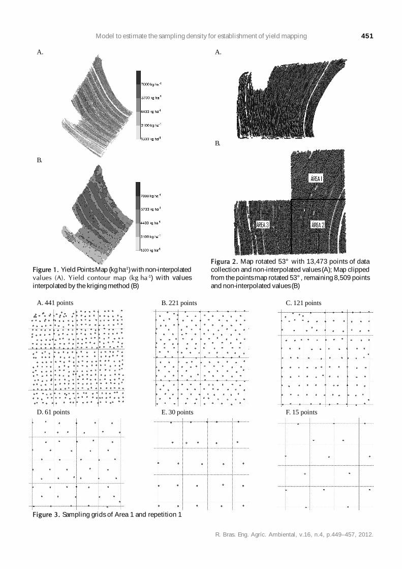
Maize yield maps using manual sampling are performed byharvesting 1 to 2 linear meters of two adjacent rows. However,in this work, no manual samplings were performed, which weresimulated using six grids (Figure 3) from the elimination ofpoints of maps corresponding to areas 1, 2 and 3. This estimateconsiders that the manual sample (usually between 0.7 and 1.4m2) has average productivity similar to the sample taken withthe yield monitor (15 to 20 m2). For more information sources,four replications were performed in each area, taking care notto repeat the same points in each repetition and that they stayas far away as possible. Once four replications were performedin each one of the seven grids and at three areas, it reached atotal of 84 data sets. The objective of this simulation was tostudy the sampling density needed to produce maps ofproductivity from manual sampling, when sampling for somereason cannot be carried out with a harvest monitor.

Data normality was verified by tests of Anderson-Darlingand Kolmogorov-Smirnovs at 5% significance level. Datashowing normality in at least one of the tests were consideredas having normal probability. The outliers were checkedthrough the box-plot graphs. The coefficient of variation (CV)was considered low when 10% (homoscedasticity), mediumwhen 10% < CV 20%, high when 20% < CV 30%, and veryhigh when > 30% (heteroscedasticity) according to Gomes &Garcia (2002).



A.

B.

Figura 2. Map rotated 53° with 13,473 points of datacollection and non-interpolated values (A); Map clippedfrom the points map rotated 53°, remaining 8,509 pointsand non-interpolated values (B)

Figure 3. Sampling grids of Area 1 and repetition 1

D. 61 points

A. 441 points

E. 30 points F. 15 points

B. 221 points C. 121 points

Figure 1. Yield Points Map (kg ha-1) with non-interpolatedvalues (A). Yield contour map (kg ha-1) with valuesinterpolated by the kriging method (B)

B.

A.



In geostatistics analysis semivariograms were constructedto verify the spatial dependence on the data. To estimate theexperimental semivariance function, the estimator proposedby Cressie & Hawkins (1980) was used. Experimentalsemivariograms were obtained by applying methods of ordinaryleast squares adjustment (OLS), adopting the isotropic model(unidirectional semivariogram) with 50% cut-off the maximumdistance. In this analysis, the computer program VESPER ® 1.6Demo was used. Similarly to the spatial dependence index (SDI),proposed by Cambardella et al. (1994), spatial variability index(SVI) Eq. 1, was defined in order to define a proportional indexto the spatial variability and not inversely proportional as theSDI. The SVI classification adopted was: very low for SVI <20%; low for 20 SVI < 40%; medium for 40 SVI < 60%; highfor 60 SVI < 80%; and very high for SVI > 80%.

.100CC

CSDI0

0

.100CC

CSDI1SVI10

1

where:Co - nugget effect of the adjusted semivariogramC1 - scale, C0 + C1: sill (variance estimate)

In generating thematic maps three types of interpolatorswere used: inverse of distance (ID), inverse of squaredistance (ISD), and ordinary kriging and, using the computerprogram SURFER® 8.0 were prepared the yield maps. Incomparing the maps generated from each grid with theoriginal map were used the coefficient of relative deviation(CRD) (Coelho et al., 2009) Eq. 3, which expresses the averagedifference in module of interpolated values in each map,considering one of them as a standard map and the kappaindex (Cohen, 1960) Eq. 4, which uses a confusion matrix forfurther index calculation. The aim was to evaluate the qualityloss of yield maps when reducing the number of samplingpoints.

n

100P

PPCRD

n

1i ist

istij

where:n - number of pointsPij - productivity at point i to the map jPist - productivity at point i for the standard map (kriging

with original data)

r

1iii

2

r

1i

r

1iiiii

x*xn

x*xxn

K

where:r - number of rows in a cross-classification tablexii - number of combinations on the diagonalxi+ - total observations in row ix+i - total number of observations in column in - total number of observations

Landis & Koch (1977) suggested the followinginterpretation for kappa index values (K): no agreement < 0,poor agreement for 0 K 0.19, partial agreement for 0.20 K 0.39, moderate agreement for 0.40 K 0.59, excellentagreement for 0.60 K 0.79, perfect agreement for 0.80 d” Kd” 1.00. In practice, the kappa index represents the proportionof pixels that were coincident beyond those that would be bypure chance. To evaluate the behavior of similarity betweenmaps, as measured by the coefficient of deviation (CRD),depending on the density and spatial variability, it was fittedthe multiple regression model to the CRD variable, dependingon the variables SDI (spatial dependence index) and SD(sampling density). The variable selection method used wasthe best subset. 0.05 significance for F distribution was usedto control entry and exit effects. The adjusted coefficient ofmultiple determination (adjusted R2) was used as criterion forselection of the best models.

RESULTS AND DISCUSSION

For space reasons, only data for Area 1 (chosen by lottery)and those for the three areas together will be shown. Themaize’s average yield (second season) from Area 1 ranged from5,795 to 6,082 kg ha-1, with a mean value of 5,919 kg ha-1, 38.7%above the average for Paraná state (4,266 kg ha-1) and 94.6%above the average for Brazil (3,041 kg ha-1) (SEAB, 2007). Thecoefficients of variation (CV) ranged from 13.8% (medium) to25.2% (high), with 16.7% average (medium), thus characterizingrelative data homogeneity (Pimentel-Gomes & Garcia, 2002).Through the normality tests performed was found that 50%yield data sets showed normal distribution at 5% significancelevel (Table 1).

Regarding the three areas studied, the average yield rangedfrom 4,491 to 6,082 kg ha-1 (Table 2), averaging 5,440 kg ha-1,78.9% above the national average and 27.5% above the Paranáaverage. CVs ranged from 11.8% (average) to 26.1% (high),with 18.5% average (medium), thus characterizing relative datahomogeneity. Through the normality tests performed was foundthat 64% yield data sets showed normal distribution at 5%significance level.

Models and parameters adjusted to the semivariograms forArea 1 are shown in Table 3.

The nugget effect (C0) for data set of the sampling scheme61_A1_R1 (61-point grid of Area 1 and repetition 1) was 454,602,which compared to other nugget effects for different purposessampling schemes showed the lowest value. However, thesampling scheme with data set 15_A1_R3 had showed highestC0, (1,969,444). The range was the greatest for 121_A1_R3,(361.6 m) while the least range was 25.9 m for 61_A1_R1. Thesill ranged between 663,333 for the data set 30_A1_R2 and

(1)

(2)

(3)

(4)



Table 1. Descriptive analysis of yield for data sets used in Area 1Mean SD Minimum Median Maximum

Data sets Number of samples kg ha-1

CV (%) kg ha-1

Normality

Minimum 5795 0815 13.8 1827 5778 7082 Total Area 1 Maxiumum 6082 1494 25.2 4112 6315 8527

Medium 5919 0985 16.7 2615 6068 7835 Original_A1_R1 2728 5974 0956 16.0 1827 6116 8527 No

441_A1_R1 0441 5926 0988 16.7 1827 6100 8129 No 221_A1_R1 0221 5902 0953 16.1 2630 6069 8055 No 121_A1_R1 0121 5890 0956 16.2 2630 6021 8055 No 61_A1_R1 0061 6014 0897 14.9 3851 6049 8055 Yes 30_A1_R1 0030 5963 0851 14.3 3851 6004 7501 Yes 15_A1_R1 0015 5844 0984 16.8 3851 5988 7501 Yes

Original_A1_R2 2728 5974 0956 16.0 1827 6116 8527 No 441_A1_R2 0441 5935 0995 16.8 1827 6091 8129 No 221_A1_R2 0221 5941 0932 15.7 3093 6108 7859 No 121_A1_R2 0121 5947 0949 16.0 3348 6132 7859 Yes 61_A1_R2 0061 5902 0951 16.1 3507 6044 7607 Yes 30_A1_R2 0030 5906 0815 13.8 4112 6039 7501 Yes 15_A1_R2 0015 5970 0893 15.0 4112 6044 7501 Yes

Original_A1_R3 2728 5974 0956 16.0 1827 6116 8527 No 441_A1_R3 0441 5892 0991 16.8 1827 5999 8129 No 221_A1_R3 0221 5887 1009 17.2 1827 5974 8129 No 121_A1_R3 0121 5935 1009 17.0 1827 6019 8129 Yes 61_A1_R3 0061 5808 1025 17.6 1827 5834 7607 Yes 30_A1_R3 0030 5795 1129 19.5 1827 5778 7333 Yes 15_A1_R3 0015 5935 1494 25.2 1827 6315 7333 Yes

Original_A1_R4 2728 5974 0956 16.0 1827 6116 8527 No 441_A1_R4 0441 5903 0982 16.6 1827 6107 7894 No 221_A1_R4 0221 5890 1017 17.3 1827 6114 7894 No 121_A1_R4 0121 5887 1070 18.2 1827 6195 7677 No 61_A1_R4 0061 5870 0888 15.1 3613 6043 7214 Yes 30_A1_R4 0030 5820 0969 16.7 3613 6082 7082 Yes 15_A1_R4 0015 6082 1024 16.8 3613 6280 7082 Yes

* Normality according to the test of Anderson-Darling and Kolmogorov-Smirnovs at 5% significance level.Meaning of acronyms: XXX_YY_ZZ. Where: XX - Number of points per grid; YY - area to which the grid belongs to; ZZ - repetition to which the grid belongs to. Ex.441_A1_R1: 441-point grid from Area1 of repetition 1, SD - standard deviation

Table 2. Global overview of the data descriptive analysisused in the three areas studied

2,223,757 for 15_A1_R3. The spatial variability was betweenvery low (10.6%) and medium (45.0%) according to theclassification adopted for the spatial dependence index.

Regarding the three areas studied, 77% cases used thespherical model while 23% used that exponential. The nuggeteffect (C0) ranged between 434,977 and 1,969,444. The majorand minor ranges were 361.6 m and 17.0 m respectively. The sillvaried between 488,275 and 2,223,757. Spatial dependenceshowed between very low (5.4%) and high (61.7%).

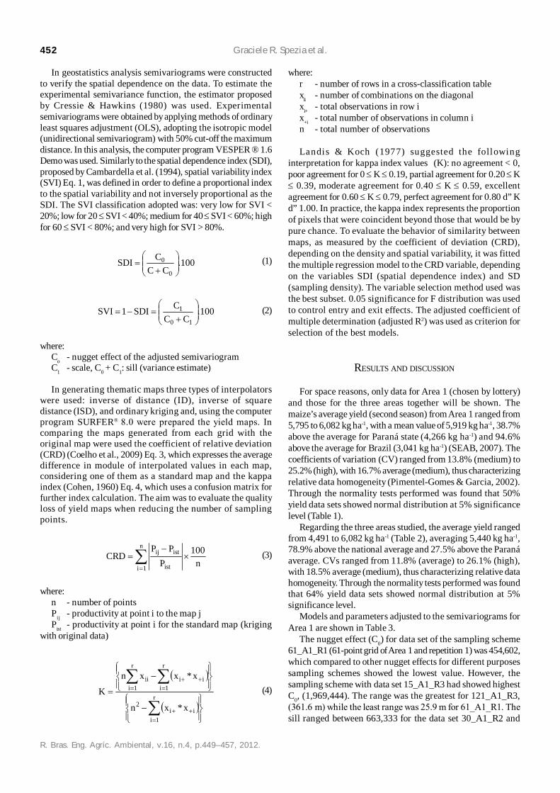
Based on the fitting parameters and models fitted toindividual semivariograms (Figure 4, Area 1 and repetition 1)thematic maps were constructed by applying the interpolationinverse of square distance, inverse of distance and kriging forthe study variable (maize yield in kg ha 1). With seven gridsmade in each area (1, 2 and 3), four replicates per area, and

three interpolators, 252 maps were obtained. For similarityanalysis of thematic maps was calculated the average differencein module, ie the coefficient of relative deviation (CRD). Asexamples, Figure 5 shows yield maps generated by krigingmethod corresponding to the semivariograms in Figure 4, whereone can observe the loss of information with decreased numberof points used.

Coefficients of relative deviations (CRD) derived from thecomparison between simulated and original grids show gradualincrease of deviation as the amount of points decreases in thethree interpolation methods, ie, CRD decreased with increasingsampling density (division of the number of sampling data andsampling area) (Figure 6). For the same sampling density, CRD,deviation from the original map, was smaller for the interpolationinverse of square distance (ISD), followed by the inverse ofdistance (ID) and lastly by kriging (KRIG) (except for higherdensity of points). This result is in agreement with Coelho etal. (2009) and Bazzi et al. (2008), who found better performancefor interpolation using inverse distance weighting whencompared to kriging. Comparing the explanation of thedependent variable CRD, R2 assumed values of 0.32 (Kriging),0.61 (ID), and 0.79 (ISD), ie, explanations ranged from 32 to79%.

Mean SD Minimum Median Maximum Data sets Values kg ha-1

CV (%) kg ha-1

Minimum 4491 0696 11.8 1767 4340 6278 All Maximum 6082 1494 26.1 4559 6315 8527

Medium 5440 0984 18.5 2641 5584 7499

SD - standard deviation



Table 3. Models and parameters adjusted to the semivariogram for yield data sets for Area 1Nugget Effect Scale Range Sill Spatial variability index (%)

Data sets Model C0 C1 a (m) (C0 + C1) SVI = (C1/C0 + C1) . 100

Total Área 1 Maximum 1969444 562092 361.6 2223757 45.0 Medium 0782942 268717 156.0 1051659 25.6 Original_A1_R1 Spherical 0606881 328514 036.9 0935395 35.1

441_A1_R1 Spherical 0790750 214461 105.2 1005211 21.3 221_A1_R1 Spherical 0767237 144835 045.6 0912072 15.9 121_A1_R1 Spherical 0720145 194634 036.9 0914779 21.9 61_A1_R1 Exponential 0454602 371811 025.9 0826413 45.0 30_A1_R1 Spherical 0602933 079727 089.2 0682660 11.7 15_A1_R1 Spherical 0760684 154662 045.3 0915346 16.9

Original_A1_R2 Spherical 0606881 328514 036.9 0935395 35.1 441_A1_R2 Exponential 0726741 407337 084.3 1134078 35.9 221_A1_R2 Spherical 0700387 285943 253.4 0986330 29.0 121_A1_R2 Exponential 0756371 290705 109.8 1047076 27.8 61_A1_R2 Spherical 0769462 220665 242.5 0990127 22.3 30_A1_R2 Spherical 0555844 107489 252.5 0663333 16.2 15_A1_R2 Spherical 0622591 079653 082.4 0702244 11.3

Original_A1_R3 Spherical 0606881 328514 036.9 0935395 35.1 441_A1_R3 Spherical 0786200 439273 337.7 1225473 35.8 221_A1_R3 Spherical 0852952 279297 260.5 1132249 24.7 121_A1_R3 Spherical 0987020 117083 361.6 1104103 10.6 61_A1_R3 Spherical 0947470 163414 234.9 1110884 14.7 30_A1_R3 Exponential 1075067 158389 078.6 1233456 12.8 15_A1_R3 Spherical 1969444 254313 100.0 2223757 11.4

Original_A1_R4 Spherical 0606881 328514 036.9 0935395 35.1 441_A1_R4 Spherical 0783758 384415 306.8 1168173 32.9 221_A1_R4 Spherical 0780668 511420 287.2 1292088 40.0 121_A1_R4 Spherical 0908281 562092 339.7 1470373 38.2 61_A1_R4 Exponential 0559228 413513 113.4 0972741 42.5 30_A1_R4 Spherical 0811941 146416 218.3 0958357 15.3 15_A1_R4 Spherical 0805082 228469 209.9 1033551 22.1

Figura 4. Experimental semivariograms for yield (kg ha 1) of Area 1 and repetition 1

A. Original

D. 121 points

G. 15 points

C. 221 points


B. 441 points960000

720000

480000

240000

0

1280000

960000

640000

320000

00 5 0 10 0 15 0 20 0 25 0

0 4 0 8 0 12 0 16 0 20 0

0 5 0 10 0 15 0 20 0 25 0

1200000

960000

720000

480000

240000

0

1280000

960000

640000

320000

0

320000

240000

160000

80000

0

1000000

800000

600000

400000

200000

0

1000000

800000

600000

400000

200000

0



A. 441 points

D. 61 points

C. 121 points


B. 221 points

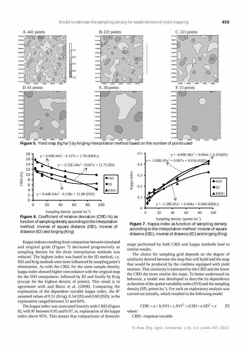
Figure 5. Yield map (kg ha-1) by kriging interpolation method based on the number of points used

y = 8.44E-04x2 - 0.138x + 11.88 (ISD)

y = -2.52E-04x2 - 0.047x + 11.75 (ID)

y = 6.94E-04x2 - 0.127x + 1.78 (KRIG)

02468

1012141618

0 20 40 60 80 100

CR

D (%

)

Sampling density (points ha-1)

ISD

ID

KRIG

Figure 6. Coefficient of relative deviation (CRD,%) asfunction of sampling density according to the interpolationmethod: inverse of square distance (ISD), inverse ofdistance (ID) and kriging (Krig)

Kappa indexes resulting from comparison between simulatedand original grids (Figure 7) decreased progressively assampling density for the three interpolation methods wasreduced. The highest index was found in the ID method, i.e.ISD and Krig methods were more influenced by sampling point’selimination. As with the CRD, for the same sample density,kappa index showed higher concordance with the original mapfor the ISD interpolator; followed by ID and finally by Krig(except for the highest density of points). This result is inagreement with and Bazzi et al. (2008). Comparing theexplanation of the dependent variable kappa index, the R2

assumed values of 0.51 (Krig), 0.54 (ID) and 0.60 (ISD), ie theexplanation ranged between 51 and 60%.

The kappa index was associated linearly with CRD (Figure8), with R2 between 0.95 and 0.97, ie, explanation of the kappaindex above 95%. This means that comparisons of thematic

y = -3.08E-05x2 + 0.007x + 0.034 (IQD)y = -4.89E-06x2 + 0.004x + 0.103(ID)

y = -1.58E-05x2 + 0.004x + 0.068 (KRIG)0

0.1

0.2

0.3

0.4

0.5

0 20 40 60 80 100

Kap

pa in

dex

Sampling density (points ha-1)

ISDIDKRIG

Figure 7. Kappa index as function of sampling densityaccording to the interpolation method: inverse of squaredistance (ISD), inverse of distance (ID) and kriging (Krig)

maps performed by both CRD and kappa methods lead tosimilar results.

The choice for sampling grid depends on the degree ofsimilarity desired between the map that will build and the mapthat would be produced by the combine equipped with yieldmonitor. This similarity is estimated by the CRD and the lowerthe CRD the more similar the maps. To better understand itsbehavior, a model was developed to describe its dependenceas function of the spatial variability index (SVI) and the samplingdensity (SD, points ha-1). For such an exploratory analysis wascarried out initially, which resulted in the following model

εe.SDd.SDc.SVIb.SVIaCDR 22 where:

CRD - response variable

(5)



from the monitor is estimated the spatial variability index (SVI)through statistical and geostatistical analysis of these data; ifthis is not possible, the SVI from previous years can be used oreven take the 100% maximum value; 2) Adopting the desireddegree of similarity map (CRD); 3) Choosing the method ofinterpolation using the corresponding model in Table 4 (orother developed for the property) and 4) Finding the samplingdensity suggested.

CONCLUSIONS

1. The loss of information in yield map due to the decreasedsampling density depends on the interpolation method, beingless significant for the method of inverse of square distanceand more significant for ordinary kriging, among the threemethods evaluated;

2. The regression model developed to describe thedependence of the coefficient of relative deviation on the spatialvariability index and sampling density, allowed explainingbetween 87% (inverse of distance) and 93% (kriging);

3. This model serves to enable the farmer obtaining a yieldmap, even when problems occur on the harvest monitorpreventing data storage; sampling density to be collecteddepend on the accuracy desired by the farmer.

ACKNOWLEDGEMENTS

The authors thank the Coordenação de Aperfeiçoamentode Pessoal de Nível (CAPES) and the Conselho Nacional deDesenvolvimento Científico e Tecnológico (CNPq) for thesupport provided.

LITERATURE CITED

Bazzi, C. L.; Souza, E. G.; Uribe-Opazo, M. A.; Nóbrega, L. H. P.;Pinheiro Neto, R. Influência da distância entre passadas decolhedora equipada com monitor de colheita na precisãodos mapas de produtividade na cultura do milho. EngenhariaAgrícola, v.28, p.355-363, 2008.

Brower, J. C.; Merriam, D. F. Thematic map analysis using multipleregression. Mathematical Geology, v.33, p.353-368, 2001.

Cambardella, C. A.; Moorman, T. B.; Novak, J. M.; Parkin, T. B.;Karlen, D. L.; Turco, R. F.; Konopka, A. E. Field-scalevariability or soil properties in Central lowa Soils. Soil ScienceSociety America Journal, v.58, p.1501-1511, 1994.

Coelho, E. C.; Souza, E. G.; Uribe-Opazo, M. A.; Pinheiro Neto,R. Influência da densidade amostral e do tipo de interpoladorna elaboração de mapas temáticos. Acta Scientiarum, v.31,p.165-174, 2009.

Cohen, J. A coefficient of agreement for nominal scales. Educationaland Psychological Measurement, v.20, p.37-46, 1960.

Congalton, R.G.; Green, K. A practical look at sources ofconfusion in error matrix generation. PhotogrammetricEngineering and Remote Sensing, v.59, p.641-644, 1993.

A.

y = -6.409x + 0.778R² = 0.95

0

0,2

0,4

0,6

3% 6% 9% 12% 15% 18%B.

y = -4.213x + 0.620R² = 0.97

0

0,2

0,4

0,6

C.

y = -4.350x + 0.742R² = 0.97

0

0,2

0,4

0,6

3% 6% 9% 12% 15% 18%D.y = -3.207x + 0.534

R² = 0.66

0

0,2

0,4

0,6

3% 6% 9% 12% 15% 18%

Kap

pa

CDRFigure 8. Kappa coefficient as function of the coefficientof relative deviation (CRD) interpolated by (A) inverse ofsquare distance, (B) inverse of distance, (C) kriging and(D) three interpolation methods

Table 4 Estimated coefficients of multiple regression forthe coefficient of relative deviation (CRD) according tothe spatial variability index (SVI) and the sampling density(SD, points ha-1)

Note: All estimators were significant by t test at 5% probability

Interpolator Constant SVI SVI2 SD SD2 R2 ISD 16.09 -0.3885 0.0064 -0.1461 -0.0010 0.91

ID 16.45 -0.3970 0.0064 -0.0640 -0.0002 0.87 KRIG 20.59 -0.5027 0.0087 -0.1304 -0.0007 0.93

SVI and SD - independent variables a, b,...,a, b, c, d, and e - model parameters to be estimated by the

method of least squarese - random error, which is assumed with normal

distribution, zero mean and constant variance 2

Applying the aforementioned model to the data collected,an explanation between 87% (ID) and 93% (KRIG) was obtained(Table 4).

In practice, these models serve to enable the farmer to obtainthe yield map, even when problems occur on the harvestmonitor preventing data storage. For such, the followingprocedure is suggested: 1) With the data already collected



Corwin, D. L.; Plant, R. E. Applications of apparent soil electricalconductivity in precision agriculture. Computers andElectronics in Agriculture, v.46, p.1-10, 2005.

Cressie, N.; Hawkins, M. Robust estimation of the variogram:I. Mathematical geology, v.12, p.115-125, 1980.

EMBRAPA – Empresa Brasileira de Pesquisa Agropecuária.Fertilidade de solos. http://www.cnpms.embrapa.br/publicacoes/sorgo/solamostra.htm. 10 de Abr. 2007.

Farias, P. R. S.; Nociti, L. A. S.; Barbosa, J. C.; Perecin, D.Agricultura de precisão: mapeamento da produtividade empomares cítricos usando geoestatística. Revista Brasileirade Fruticultura, v.25, p.235-241, 2003.

Gomes, F. P.; Garcia, C. H. Estatística aplicada a experimentosagronômicos e florestais. Piracicaba: Biblioteca de CiênciasAgrárias Luiz de Queiroz/FEALQ. 2002. 307p.

Jones, N. L.; Davis, R. J.; Sabbah, W. A comparison of three-dimensional interpolation techniques for plumecharacterization. Ground Water, v.41, p.411-419, 2003.

Koch, B.; Khosla, R.; Westfall, D. G.; Frasier, M.; Inman, D.Economic feasibility of variable rate N application in irrigatedcorn. Agronomy Journal, v.96, p.1572-1580, 2004.

Landis, J. R.; Koch, G. G. The measurement of observeragreement for categorical data. Biometrics, v.33, p.159-174,1977.

Lourenço, R. W.; Landim, P. M. B. Análise de regressão múltiplaespacial. UNESP/Rio Claro, IGCE, DGA, Lab. Geomatemática.Texto didático 13, 34p. 2004. http://www.rc.unesp.br/igce/aplicada/DIDATICOS/LANDIM/Texto13.pdf. 14 Jan. 2010.

SEAB – Secretaria da Agricultura e do Abastecimento do Paraná2007. http://www.pr.gov.br/seab. 8 Jan. 2008.

http://www.cnpms.embrapa.br/

http://www.rc.unesp.br/igce/

http://www.pr.gov.br/seab.

Model to estimate the sampling density for establishment of yield mapping

Documents