Model Specification Tests in Nonparametric Stochastic Regression Models

324

⁄0047-259X/02 $35.00© 2002 Elsevier Science (USA)All rights reserved.

Journal of Multivariate Analysis 83, 324–359 (2002)doi:10.1006/jmva.2001.2058

Model Specification Tests in Nonparametric StochasticRegression Models

Jiti Gao1

1 To whom correspondence should be addressed at Department of Mathematics andStatistics, The University of Western Australia, Crawley WA 6009, Australia; E-mail:[email protected].

The University of Western Australia, Nedlands, Australia

Howell Tong

The University of Hong Kong, Hong Kong, China;and The London School of Economics, London, United Kingdom

and

Rodney Wolff

The University of Queensland, Queensland, Australia

Received March 18, 1999; published online February 12, 2002

In this paper, we consider testing for additivity in a class of nonparametricstochastic regression models. Two test statistics are constructed and their asympto-tic distributions are established. We also conduct a small sample study for one ofthe test statistics through a simulated example. © 2002 Elsevier Science (USA)

AMS 1991 subject classifications: 62E20; 62E25; 62G10; 62G20.Key words and phrases: additivity; dependent process; model determination;

nonlinear time series; nonparametric regression; semiparametric autoregression.

1. INTRODUCTION

Recent studies indicate that due to the so-called curse of dimensionality,multivariate surface smoothing techniques are in practice not very usefulwhen there are more than two or three predictor variables [see Fan andGijbels (1996), for example.] Recently, several approaches have beenproposed to deal with the curse of dimensionality. These include additivemodelling [see, for example, Hastie and Tibshirani (1990)] and partially

linear modelling [see, for example, Fan and Gijbels (1996); Härdle, Liang,and Gao (2000)]. For additive modelling, iterative estimation procedureshave already been proposed to estimate additive regression models. SeeStone (1985), Hastie and Tibshirani (1990), Chen and Tsay (1993),Tjøstheim and Auestad (1994a, 1994b), and Masry and Tjøstheim (1997).More recently, Gao, Tong, and Wolff (2001) propose a direct estimationprocedure for an additive nonparametric time series regression model. Seealso Fan, Härdle, and Mammen (1998), who construct a kernel basedestimation procedure for a class of additive models with independentobservations.

In this paper, we consider a general model of the form

Yt=Cp

i=1gi(Uti)+g(Vt)+et, t=1, 2, ..., T, (1.1)

where Ut=(Ut1, ..., Utp)y and Vt=(Vt1, ..., Vtq)y are two vectors with p,q \ 1, each gi( · ) is a smooth function over R1, g( · ) is a smooth functionover Rq, et=Yt − E[Yt | Ut, Vt] is a sequence of error processes withE[et]=0, and (Ut, Vt, et) is assumed to be a strictly stationary anda-mixing stochastic process.

Model (1.1) covers many cases. For Yt=yt+r, Uti=Vti=yt+r−i and gi(Uti)=biUti, model (1.1) is a partially linear autoregressive model of the form

yt+p=Cp

i=1bi yt+p−i+g(yt+p−1, ..., yt)+et. (1.2)

See Robinson (1988), Gao (1998), Gao and Liang (1995), and Gao and Yee(2000). For gi(Uti)=biUti, model (1.1) is a general semiparametric regres-sion model. See, for example, Robinson (1988), Speckman (1988), Fan andLi (1996), Gao and Liang (1997), Gao and Shi (1997), Gao and Anh(1999), Härdle, Liang, and Gao (2000), and Gao, Wolff, and Anh (2001).For Yt=yt+r, Uti=yt+r−i, gi(Uti)=biUti and Vt is a vector of exogenousvariables, model (1.1) is an ARX model of the form

yt+p=Cp

i=1bi yt+p−i+g(Vt)+et. (1.3)

See Teräsvirta, Tjøstheim, and Granger (1994). For the case where both Utand Vt are time series, model (1.1) is an additive state-space model.

Due to the fact that g of (1.1) is still a q-dimensional function, it wouldbe better to test whether the null hypothesis H0: g=0 holds before apply-ing model (1.1) to fit the data (Ut, Vt, Yt). A number of authors havealready considered testing for additivity in nonparametric regression withindependent observations and nonparametric autoregression. Hastie and

NONPARAMETRIC REGRESSION MODELS 325

Tibshirani (1990) suggest using a backfitting algorithm for testing foradditivity for the i.i.d. case with p=q=2 in (1.1). Eubank et al. (1995)construct an explicit test statistic for the i.i.d. case with p=q=2,

Yt=g1(Ut1)+g2(Ut2)+g(Ut1, Ut2)+et.

For the i.i.d. case, see also Barry (1993), Hart (1997), and Härdle andKneip (1999). Gozalo and Linton (1999) recently develop several kernel-based consistent tests of an hypothesis of additivity in generalized non-parametric regression models for the i.i.d. case. Chen, Liu, and Tsay (1995)consider testing for additivity for the case where model (1.1) is a second-order autoregressive model

yt+2=g1(yt+1)+g2(yt)+g(yt+1, yt)+et.

See also Hjellvik and Tjøstheim (1995), who consider the case where p=1in (1.2) and construct a test statistic for testing whether the null hypothesisH0: g=0 holds. Recently, Hjellvik, Yao, and Tjøstheim (1998) extend thediscussion of Hjellvik and Tjøstheim (1995). More recently, Fan andHuang (2001) propose several new tests for examining the adequacy of afamily of parametric models against large nonparametric alternatives. Fan,Zhang, and Zhang (2001) consider using generalized likelihood ratiostatistics for nonparametric testing problems. Other related papers includeFan and Li (1996), Kreiss, Neumann, and Yao (1999), Li (1999), andLavergne and Vuong (2000).

In this paper, we consider model (1.1). For the sake of identifiability, weneed only to consider the following transformed model

Yt=a+Cp

i=1gi(Uti)+g(Vt)+et,

where a=;pi=1 E[gi(Uti)]+E[g(Vt)] is an unknown parameter, gi(Uti)=

gi(Uti) − E[gi(Uti)] and g(Vt)=g(Vt) − E[g(Vt)]. It is obvious from theproofs of Theorems 2.1–2.3 below that the conclusions of Theorems2.1–2.3 remain unchanged when Yt is replaced by Yt=Yt − a, wherea=1

T;Tt=1 Yt is defined as the estimator of a.

This paper mainly focuses on testing the nonparametric null hypothesisH0: g=0, which is equivalent to testing whether the true model is

Yt=Cp

i=1gi(Uti)+et.

In our discussion, Ut and Vt are allowed to be two different processes. Forexample, Ut is a sequence of endogenous processes while Vt is a sequence ofexogenous processes.

326 GAO, TONG, AND WOLFF

By approximating g( · ) and {gi( · ): 1 [ i [ p} by orthogonal series;ki=1 zi( · ) ci and ;hi

j=1 fij( · ) hij, respectively, test statistics are constructedand their asymptotic distributions are established. In the meantime, selec-tion criteria for k and {hi: 1 [ i [ p} are proposed. Additionally, a smallsample study for one of the test statistics is conducted through a simulatedexample.

The organisation of this paper is as follows. Section 2 develops two teststatistics and their asymptotic distributions. Section 3 proposes a selectioncriterion for k and {hi: 1 [ i [ p}. A small sample study is given inSection 4. Mathematical details are relegated to Appendixes A and B.

2. TESTS FOR ADDITIVITY

By approximating g( · ) and {gi( · ): 1 [ i [ p} by the orthogonal series;ki=1 zi( · ) ci and ;hi

j=1 fij( · ) hij, respectively, we define the least squaresestimator of (h, c) of (h, c) as the solution of

CT

t=1

5Yt − Cp

i=1Fi(Uti)y hi − Z(Vt)y c6

2

=min!, (2.1)

where

h=h(h, k)=(h1, ..., hp)y, h=(h1, ..., hp)y,

hi=(hi1, ..., hihi )y,

c=c(k, h)=(c1, ..., ck)y, c=(c1, ..., ck)y,

Fi(Uti)=(fi1(Uti), ..., fihi (Uti))y,

and Z( · )=(z1( · ), ..., zk( · ))y.It follows from (2.1) that

h=h(h, k)=(FyF)+ FyY,

c=c(k, h)=(ZyZ)+Zy(I − F(FyF)+ Fy) Y,

provided the right-hand sides are well defined, where Y=(Y1, ..., YT)y,F=(F1, ..., Fp), Fi=(Fi(U1i), ..., Fi(UTi))y, F=(I−P) F, P=Z(ZyZ)+Zy,Z=(Z(V1), ..., Z(VT))y, h=(h1, ..., hp), and ( · )+ denotes the Moore–Penroseinverse.

Given the truncation parameters k and {hi: 1 [ i [ p}, we propose thefollowing prediction equation

P(Xt; h, k)=Cp

i=1Fi(Uti)y hi(h, k)+Z(Vt)y c(k, h). (2.2)


Obviously, Eq. (2.2) depends on not only the functions {fij: 1 [ j [ hi,1 [ i [ p} and {zi( · ) : 1 [ i [ k} but also h and k. The functions arerequired to satisfy Assumptions A.2 and A.3 below, which hold in manycases. See Example 4.1 below for more details. Therefore, a crucial problemis how to select h and k practically. This problem is discussed in some detailin Section 3 below.

As the construction of test statistics depends on the structure of the errorprocess et of (1.1), we consider the homoskedastic case and the hetero-skedastic case separately.

2.1. The Homoskedastic Case

In this section, we focus on testing H0: g=0 under homoskedasticity(i.e., E[e2t |Wt−1]=E[e2t ] a.s., with Wt−1 defined in Assumption A.1(ii)below).

It is obvious that in order to test the nonparametric hypothesis H0: g=0,it suffices to test the parametric hypothesis H −

0 : c=0. In this section, weconsider using the following normalized statistic

LT=c(k, h)y ZyZc(k, h) − ks20

`2k s20, (2.3)

where 0 < s20=E[e2t ] <..Before stating a main result of this paper, we give some important

remarks about the orthogonal series approach and the use of (2.3).

Remark 2.1. The form (2.3) can be understood heuristically byconsidering that c(k, h)y ZyZc(k, h)/s20 behaves asymptotically like a q2kstatistic. Standardization toward normality involves subtracting the mean kand dividing by the standard deviation `2k . As k Q., the standardizedquantity becomes more nearly normal (our proofs, however, do not dependon this heuristic idea, as it is bit too simplistic). Recently, Hong and White(1995) use a similar form to test nonparametric series regression for thei.i.d. case.

Remark 2.2. Apart from the local polynomial regression method [Fan(1992); Fan and Gijbels (1996); Hjellvik, Yao, and Tjøstheim (1998)],which has been proved to be an alternative to the kernel method, theorthogonal series estimation method is another alternative to the kernelestimation. As suggested in the recent econometric literature [see Eastwoodand Gallant (1991)], the orthogonal series estimation method has thefollowing advantages. First of all, the main advantages of the seriesapproach are its simplicity, ease of implementation, and ease of extensionto nonlinear, multivariate, and time series applications. Second, theorthogonal series strategies are natural extensions of ordinary parametric


inference. Third, the orthogonal series estimation method can provide anexplicit estimation procedure for each nonparametric component (seeEq. (2.1) above). Thus, both the local polynomial regression and theorthogonal series estimation methods can complement the kernel method-ology for modelling nonparametric and semiparametric regression, ratherthan replace it.

Remark 2.3. The construction of the test statistic (2.3) is based on thefact that g is approximated by the orthogonal series. We can estimate g bya kernel estimator and construct a kernel-based test statistic for testingH0g: g=0. The proof of the asymptotic normality of the kernel-basedstatistic is much more complicated than that of Theorem 2.1 below due tothe fact that a T × T random matrix is involved in the kernel-based statistic.Recently, Kreiss, Neumann, and Yao (1999) avoid using this kind of teststatistic by adopting an alternative version.

Now, we have the following main result of this paper.

Theorem 2.1. Assume that Assumptions A.1(i) (ii)–A.4 listed in Appen-dix A hold. If g(Vt)=(k1/4/`T) g0(Vt) with g0(Vt) satisfying 0 < E[g0(Vt)2]<., then as T Q.

LT QD N(L0, 1), (2.4)

where L0=(1/`2 s20) E[g0(Vt)2]. Furthermore, under H1: g ] 0, we havelimTQ. P(LT \ CT)=1, where CT is any positive, nonstochastic sequencewith CT=o(Tk−1/2).

It follows from (2.4) that LT has an asymptotic normality distributionunder the null hypothesis H0. In general, H0 should be rejected if LTexceeds a critical value, Lg

0 , of normal distribution. If s20 is unknown in(2.3) and (2.4), it can be replaced by a consistent estimator withoutaffecting the conclusion of Theorem 2.1. Theorem 2.2 below provides aconsistent estimator of s20. Since s2(h, k) depends on (h, k), we suggestconstructing a data based only consistent estimator of s20. The constructionis similar to Eubank et al. (1998). See also Hall, Kay, and Titterington(1990).

Remark 2.4. Theorem 2.1 states the asymptotic normality for the casewhere both gi( · ) and g( · ) of (1.1) are unknown and smooth functions.When gi(Uti) is already a known linear function of Uti, the proposed seriesapproximation to gi( · ) is not needed. For this case, one can replace theseries based least squares estimator of gi( · ) by the usual least squaresestimator. The test statistic LT now does not depend on the smoothingparameter h. The proof of Theorem 2.1 can now be simplified. Some test


procedures for this case have already been proposed. See, for example, Fanand Li (1996), Li (1999), and Fan and Huang (2001).

We now have the following consistency result.

Theorem 2.2. Under the conditions of Theorem 2.1, we obtain that asT Q.

s2(h, k)=1T

CT

t=1[Yt − P(Xt; h, k)]2Q s20

holds in probability.

The proofs of Theorems 2.1 and 2.2 are relegated to Appendix A.

2.2. The Heteroskedastic Case

Recently, regression estimation of conditional heteroscedasticity hasgained much attention due to the fact that conditional heteroscedasticityhas often been used in modelling and understanding the variability ofstatistical data. It is of common interest to estimate conditional variancefunctions in a variety of statistical models. See, for example, Masry andTjøstheim (1995, 1997), and Fan and Yao (1998).

This section considers the case where the error process et of (1.1) isheteroscedastic. For this case, in order to construct an asymptoticallynormal test statistic, Eq. (2.3) needs to be modified.

As given in the proof of Theorem 2.1, one can obtain that as T Q.

c(k, h)y ZyZc(h, h)=eyPe+op(eyPe)

= CT

s, t=1psteset+op(eyPe)

= CT

s ] t=1psteset+C

T

t=1ptte

2t+op(eyPe), (2.5)

where e=(e1, ..., eT)y and pst denotes the (s, t) element of P=Z(ZyZ)+Zy.In view of (2.5), we consider using a statistic of the form

MT=c(k, h)y ZyZc(k, h) − mT

ST, (2.6)

where

mT=CT

t=1ptt e

2t and S2T=2 C

T

t=1CT

s=1p2st e

2s e2t ,

in which et=Yt − P(Xt; h, k) with P(Xt; h, k) given in (2.2).


The following result establishes the asymptotic distribution of MT.

Theorem 2.3. Assume that the conditions of Theorem 2.1 hold. Inaddition, Assumption A.1(iii) is satisfied. Then as T Q.

MT QD N(M0, 1),

whereM0=L0 is as defined in (2.4).

As the proof of Theorem 2.3 is extremely technical, we provide only anoutline of the proof in Appendix B.

Remark 2.5. As Theorem 2.3 considers both the heteroskedastic caseand the a-mixing case, the conclusion of Theorem 2.3 obviously extendsand complements some existing results for both the i.i.d. case and the timeseries case with the b-mixing. See, for example, Eubank et al. (1995), Hongand White (1995), Hjellvik and Tjøstheim (1995), Hjellvik, Yao, andTjøstheim (1998), and Li (1999).

3. SELECTION OF THE TRUNCATION PARAMETERS

As we mentioned before, the selection of k and h is critical in practice. Intheory, however, the selection has not been solved thoroughly for the timeseries case. For the i.i.d. case, Eubank and Hart (1992) propose a data-driven selection for the choice of k when h is fixed. See also Eubank, et al.(1995) and Hart (1997). For the time series case, similar to Eubank andHart (1992) we can assume that the following orthogonality conditionshold with probability one or in probability,

CT

t=1zj(Vt) zl(Vt)=Tdjl and C

T

t=1Fi(Uti)y Z(Vt)=0, (3.1)

where j, l=1, 2, ..., k and i=1, 2, ..., p, and

djl=31 if j=l0 otherwise.

Under (3.1), we have that

h=(FyF)+FyY and ci=1T

CT

t=1zi(Vt) Yt (3.2)


hold with probability one or in probability. Thus, with probability one orin probability, we obtain

1T

CT

t=1[Yt − F(Ut)y h− Z(Vt)y c]2+

2s20(h+k)T

=1T

CT

t=1[Yt − F(Ut)y h]2− C

k

j=1c 2j+

2s20(h+k)T

,

where F(Ut)=(F1(Ut1), ..., Fp(Utp))y.Thus, maximising

r(k)=Ck

j=1c 2j −

2s20kT

over k can provide an optimum choice for k.As it is not easy to justify (3.1) in both theory and practice, one needs to

avoid using the orthogonality conditions directly for the time series case.As an alternative, by considering the fact that under (3.1)–(3.2) maximisingr(k) is equivalent to minimising

R(k)=1T

CT

t=1E[Z(Vt)y c− g(Vt)]2,

we suggest using the quantities D(h, k) and D(h, k) in the discussion ofselecting optimum values for both k and h, where

D(h, k)=1T

CT

t=1

3 Cp

i=1[Fi(Uti)y hi − gi(Uti)]+Z(Vt)y c(k, h) − g(Vt)4

2

and

D(h, k)=E[D(h, k)]

=1T

CT

t=1E 3 C

p

i=1[Fi(Uti)y hi − gi(Uti)]+Z(Vt)y c(k, h) − g(Vt)4

2

.

In this section, we introduce an extended version of the generalizedcross-validation (GCV) criterion, which was originally proposed for non-parametric regression smoothing. We apply the extended version to selectoptimum values for both k and h. Before discussing the selection criterion,we need to introduce the following notation and definition.

Let

KT={[a0Tq

2(m+1)+q−c0], ..., [b0T

q2(m+1)+q

+c0]}


and

HiT={[aiT1

2(mi+1)+1−ci], ..., [biT

12(mi+1)+1

+ci]},

where 0 < a0 < b0 <., 0 < c0 < q/2(m+1)(2(m+1)+q), 0 < ai < bi <.and 0 < ci < 1/2(mi+1)(2(mi+1)+1) are absolute constants, in which mand mi denote the smoothness orders of g and gi, respectively.

Definition 3.1. Select (h, k), denoted by (hG, kG), that achieves

GCV(hG, kG)= inf{h ¥HT, k ¥KT}

GCV(h, k)= inf{h ¥HT, k ¥KT}

s2(h, k)

51 −1T1 Cp

i=1hi+k26

2,

(3.3)

where HT={h=(h1, ..., hp) : hi ¥ HiT} and s2(h, k) is as defined inTheorem 2.2.

Similar to the discussion of Gao, Tong, and Wolff (2001), we can estab-lish the following results

D(h, k)=s20T5Cp

i=1hi+k6+C

p

i=1Cih

−2(mi+1)i +C0k

−2(m+1)q +op(D(h, k)),

and

D(h, k)=E[D(h, k)] %s20T5Cp

i=1hi+k6+C

p

i=1Cih

−2(mi+1)i +C0k

−2(m+1)q ,

(3.4)

where the symbol % indicates that the ratio tends to one as T Q., and Ciand C0 are as defined in Assumption A.2.

Thus, it follows from (3.4) that if Ci > 0 and C0 > 0, then the followingvalues

k=1C0s202

q2(m+1)+q

· [Tq

2(m+1)+q] and hi=1Cis202

12(mi+1)+1 · [T

12(mi+1)+1]

(3.5)

minimize D(h, k), where [x] [ x denotes the largest integer part of x.


Analogous to Gao, Tong, and Wolff (2001), it can be shown that for kand hi given in (3.5)

hGh

− 1 Qp 0 andkGk

− 1 Qp 0 as T Q., (3.6)

where h=(h1, ..., hp). The proof of (3.6) is very lengthy and we shall notdetail it here. However, it is available upon request.Remark 3.1. This section considers the selection of the truncation

parameters h and k based on (3.3). Equation (3.5) not only provides thetheoretically optimum values but also suggests the choice of h and k inAssumption A.2. Moreover, for the case where the error process ishomoskedastic and Gaussian, it can be shown that the conclusion ofTheorems 2.1 and 2.2 remains unchanged when (h, k) is replaced by(hG, kG). For the case where the error process is non-Gaussian, we have notbeen able to show that the conclusion of Theorems 2.1–2.3 remainsunchanged when (h, k) is replaced by (hG, kG). In conclusion, the problemof selecting an optimum truncation parameter or an optimum bandwidthfor testing procedures for the time series case has not been completelysolved.

Remark 3.2. As can be seen, a bothersome aspect of the proposedtest procedures given in Theorems 2.1 and 2.3 is that one must fix thesmoothing parameters h and k in order to carry out the test procedures inpractice. More recently, Fan and Huang (2001) consider the case where thedistribution of residuals is normal and propose new test procedures fortesting linearity, additivity and parametric models versus nonparametricalternatives. One of the novel features of their test procedures is that theyavoid using any smoothing parameter in their test procedures. It is hopedthat one can extend their results to the case where the observationsare dependent time series and the error process is non-Gaussian andheteroscedastic.

4. A SMALL SAMPLE STUDY

In this section, we illustrate the above estimation and testing procedureby a simulated example. Rejection rates of the test statistic LT are detailedin Example 4.1. For convenience and simplicity, in this section we consideronly the case where p=2, and denote Ut=Ut1, Wt=Ut2 and Vt=(Ut, Wt)in model (1.1). Let X ’ U(a, b) denote that X is uniformly distributed over[a, b], and e ’ N(m, s2) denote that e is normally distributed with mean mand variance s2. This example considers using the theoretical values of kand hi given in (3.5) for the discussion of rejection rates. In addition,similar small sample results are given for the case where both k and h arereplaced by kG and hG, respectively.


Example 4.1. Consider a state-space model of the form

Yt=g1(Ut)+g2(Wt)+g(Vt)+et, t=1, 2, ..., T,

Ut=−0.5Ut−1+et, Wt=0.5Wt−1+gt,(4.1)

where the forms of g1, g2 and g are to be specified, both {et : t \ 1} and{gt : t \ 1} are mutually independent and identically distributed, the{et : t \ 1} are independent of U0, the {gt : t \ 1} are independent of W0,et ’ U(−0.5, 0.5), U0 ’ U(−1, 1), gt ’ U(−0.5, 0.5), W0 ’ U(−1, 1), Ut andWt are mutually independent, et is i.i.d. random error and independent of{(Ut, Wt): t \ 1}, and et ’ N(0, s20) with s20 to be given.

In this example, we consider the following two cases,

g1(Ut)=0.3 cos(pUt), g2(Wt)=0.6 sin(pWt),

g(Vt)=f cos(pUt) sin(pWt)(4.2)

and

g1(Ut)=exp(−U2t ), g2(Wt)=

Wt1+W2

t

, g(Vt)=k exp(−U2t )

Wt1+W2

t

,

(4.3)

where 0 [ f [ 1 and 0 [ k [ 1 are parameters to be chosen. The choice of(4.2) is due to the fact that trigonometric functions can be used to describeperiodic series. Model (4.3) considers both the exponential component anda special type of the Mackey–Glass system [see Section 4 of Nychka et al.(1992)].

First, it is clear from (4.1)–(4.3) that Assumptions A.1 and A.4 hold. See,for example, Chapter 4 of Tong (1990), Tjøstheim (1994, Sect. 2.4) and Lu(1998).

Second, applying the orthogonality property of trigonometric functions,functions, one can verify that

E[cos(ipXt) sin(jpXt)]=0, E[zi(Xs) zi(Xt)]=0, and

E[zi(Xt) zj(Xt)]=0

for all i ] j \ 1 and s ] t, where Xt=Ut or Wt, and zi(Xt)=cos(ipXt) orsin(ipXt). Therefore Assumption A.3 holds.

Third, due to the even property of g1 and the odd property of g2it is obvious to see that for model (4.2), g1(u), g2(w) and g(v) can beapproximated by


gg1 (u)=C

h1

i=1cos(p(i − 1) u) h1i, gg

2 (w)=Ch2

i=1sin(piw) h2i, (4.4)

g*(u, w)=5Ck1

i=1cos(p(i − 1) u) h1i6 5C

k2

i=1sin(piw) h2i6

— Ck

j=1zj(u, w) cj, (4.5)

where (u, w) ¥ [ − 1, 1] × [ − 1, 1], h1=[T1/5], h2=2[T1/5], and k1 and k2are positive integers such that k1k2=k. For this case, due to (4.1)–(4.3) wecan choose m1=m2=1, m=2 and q=2 in Assumption A.2. Thus,Eq. (3.5) suggests k=2[T1/4]. Obviously, Assumption A.2 holds.

Similarly, as pointed out by Hong and White (1995), Eumunds andMoscatelli’s results (1977) can be applied to show that gg

1 (u), gg2 (w) and

g*(v) of (4.4) and (4.5) can be used to approximate g1, g2 and g of (4.3)respectively, although g1, g2 and g of (4.3) are not periodic functions.Moreover, the optimum convergence rates given in Assumption A.2(i) andA.2(ii) are obtained as in the periodic case. Unlike the one-dimensionalcase, there are several choices of trigonometric functions for the two-dimensional case. As pointed out by Chen and Hsieh (1993), form (4.5) isan obvious one. Another obvious choice suggested by Gallant (1981) is

g(u, w)=Ck1

i=1Ck2

j=1{aij cos(j(li1u+li2w))+bij sin(j(li1u+li2w))}, (4.6)

where aij and bij are coefficients, and li1 and li2 are elementary multi-indices. See Gallant (1981) for details of the construction of li1 and li2.Moreover, it can be shown that the approximation (4.6) is equivalent to(4.5). We refer some detailed properties of nonparametric trigonometricseries regression to Gallant (1981), Andrews (1991), and Hong and White(1995).

In order to construct LT of (2.3) for this example, we introduce thefollowing notation.

Z(U, W)=(z1(U, W), ..., zk(U, W))y,

ZUW=(Z(U1, W1), ..., Z(UT, WT))y,

Xt=(Ut, Wt)y, X=(X1, ..., XT)y, Y=(Y1, ..., YT)y,

PUW=ZUW(ZyUWZUW)+Zy

UW, X=(I − PUW) X,

F1(Ut)=(1, cos(pUt), ..., cos(p(h1 − 1) Ut))y,

F2(Wt)=(sin(pWt), ..., sin(ph2Wt))y,


F1=(F1(U1), ..., F1(UT))y, F2=(F2(W1), ..., F2(WT))y,

F=(F1, F2), FUW=(I − PUW) F, hUW=(FyUWFUW)+ FyUWY,

and

cUW=(ZyUWZUW)+ZyUW(I − X(XyX)+ Xy) Y.

Now we define the required test statistic

LT=c yUWZy

UWZUW cUW − ks20`2k s20

,

where s20=1T (Y − FhUW − ZUW cUW)y (Y − FhUW − ZUW cUW).

For Example 4.1, we need to find Lg0 , an approximation to the 95th per-

centile of LT. As suggested by Härdle and Mammen (1993), a modificationof the bootstrap can be used to determine critical values. In the example,we use a modification of the approximation proposed by Buckley andEagleson (1988) due to the asymptotic normality given in Theorem 2.1.Using the same argument as in the discussion of Buckley and Eagleson(1988), one can show that the distribution of eyPe/s20 can be approximatedby that of ;k

t=1 N2t , where {Nt: t \ 1} are independent N(0, 1) random

variables and k=2[T1/4]. This implies that a reasonable approximation tothe 95th percentile is [see p. 153 of Buckley and Eagleson (1988)]

q2k, 0.05 − k

`2k,

where q2k, 0.05 is the 95th percentile of the chi-squared distribution with kdegrees of freedom.

For (4.2) and (4.4)–(4.5), we consider the cases where T=100, 150 and300. The approximate critical values Lg

0 at a=0.05 were equal to 1.91,1.91, and 1.88 for T equal to 100, 150, and 300, respectively.

As the approximation of (4.3) by (4.4)–(4.5) requires large number ofobservations, for model (4.3) we consider the cases where T=250, 500,750, and 1000. The approximate critical values Lg

0 at a=0.05 were equal to1.91, 1.88, 1.86, and 1.86 for T equal to 250, 500, 750, and 1000,respectively.

Moreover, we compute the rejection rates for both models (4.2) and (4.3)for the case where (k, h) is replaced by (kG, hG), which minimizesGCV(h, k) over

h ¥ HT={h=(h1, h2) : hi ¥ HiT} and k ¥ KT={k=k1k2 : ki ¥ KiT},

where

H1T=H2T={[T1/6], ..., [2.5T7/30]}


TABLE I

Rejection Rates For Model (4.2)

Sample andvariance Rejection rate based on k Rejection rate based on kG

T s20 k f=0 f=1.00 k1G k2G kG f=0 f=1.00

100 0.01 6 0.066 1.000 2 2 4 0.069 1.000150 0.01 6 0.059 1.000 2 2 4 0.051 1.000300 0.01 8 0.038 1.000 3 3 9 0.043 1.000100 0.04 6 0.076 0.712 2 2 4 0.081 0.747150 0.04 6 0.069 0.831 2 2 4 0.062 0.829300 0.04 8 0.048 1.000 3 3 9 0.041 0.995

and

K1T=K2T={[T11/48], ..., [2.5T13/48]}.

The choice of HT and KT has been mentioned in Section 3. For thisexample, we choose m1=m2=1, m=2, q=2, a0=a1=a2=1, b0=b1=b2=2.5, c0=

148 and ci=

130 .

The simulation results were performed 1500 times and the rejection ratesare tabulated in Tables I and II.

Remark 4.1. Tables I and II both show that the rejection rates seemrelatively sensitive to the choice of T, f, k, and s0. The power increased asf or k increased while the power decreased as s0 increased for the case off=1 or k=1. In addition, Tables I and II show that the simulationstudies for models (4.1) and (4.3) require larger number of observationsthan those for models (4.1)–(4.2). For example, the rejection rate for

TABLE II

Rejection Rates For Model (4.3)

Sample andvariance Rejection rate based on k Rejection rate based on kG

T s20 k k=0 k=1.0 k1G k2G kG k=0 k=1.00

250 0.04 6 0.164 0.619 3 2 6 0.186 0.762500 0.04 8 0.152 0.765 4 2 8 0.147 0.854750 0.04 10 0.098 0.872 3 3 9 0.102 0.951

1000 0.04 10 0.084 0.951 3 3 9 0.081 0.959250 0.09 6 0.279 0.581 3 2 6 0.264 0.633500 0.09 8 0.217 0.674 4 2 8 0.225 0.647750 0.09 10 0.166 0.768 3 3 9 0.156 0.771

1000 0.09 10 0.114 0.834 3 3 9 0.128 0.779


models (4.1), (4.3), and (4.4)–(4.5) with k=1.0, s20=0.04, k=10, andT=1000 is only 95.1% even when T is as large as 1000. By contrast, therejection rate for models (4.1), (4.2), and (4.4)–(4.5) with f=1.0, s20=0.04,k=8, and T=300 is 100% when T is just 300. This is mainly because theapproximation of g in (4.3) by g* of (4.5) requires more terms than those inthe approximation of g in (4.2) by g* of (4.5).

Tables I and II also show that the rejection rates based on kG are com-parable to those based on k. For example, for the case where s20=0.04,f=1 and T=300, Table I shows that the rejection rate based on kG is99.5%, which is comparable to 100%, the corresponding rejection ratebased on k. For the case where s20=0.04, k=1 and T=1000, Table IIshows that the rejection rate based on kG is 95.9%, which is actually higherthan 95.1%, the corresponding rejection rate based on k.

Finally, we want to point out that Tables I and II both show that thesimulation results for kG support the second part of (3.6).

APPENDIX A

A.1. Assumptions

Assumption A.1. (i) Assume that the process (Ut, Vt, et) is strictlystationary and is a-mixing with the mixing coefficient a(t)=Cag t defined by

a(t)=sup{|P(A 5 B) − P(A) P(B)|: A ¥ W s1, B ¥ W.s+t}

for all s, t \ 1, where 0 < Ca <. and 0 < g < 1 are constants, and W jidenotes the s-field generated by {(Ut, Vt, Yt): i [ t [ j}.

(ii) Assume that the et=Yt − E[Yt | (Ut, Vt)] satisfies for all t \ 1

E[et |Wt−1]=0, E[e4t |Wt−1] <., and P(E[e2t |Wt−1]=s20)=1,

where Wt=s{(Us+1, Vs+1, Ys): 1 [ s [ t} is a sequence of s-fields generatedby {(Us+1, Vs+1, Ys): 1 [ s [ t}.

(iii) In the case where s2t=E[e2t |Wt−1] is a process, suppose that theprocess s2t=E[e2t |Wt−1] satisfies

P(0 < mint \ 1s2t [ max

t \ 1s2t <.)=1.

Let g (m) and g (mi)i be the m and mi-order derivatives of the functions gand gi, respectively, and M0 and M0i be constants,

Gm(S)={g: |g(m)(s) − g (m)(sŒ)| [ M0 ||s − sŒ||, s, sŒ ¥ S … Rq},

Gmi (Si)={gi: |g (mi)i (s) − g (mi)i (sŒ)| [ M0i |s − sŒ|, s, sŒ ¥ Si … R1},


where m and mi \ 1 are integers, 0 < M, M0i <., S and Si are compactsubsets of Rq and R1, respectively, and || · || denotes the Euclidean norm.

Assumption A.2. (i) For gi ¥ Gm(Si) and {fij( · ): 1 [ j [ hi, 1 [ i [ p}given above, there exists a vector of unknown parameters hi=(hi1, ..., hihi )

y

such that for a sequence of constants {Ci: 1 [ i [ p} (0 [ Ci <.) inde-pendent of T

h2(mi+1)i E 5Chi

j=1fij(Uti) hij − gi(Uti)6

2

% Ci,

where hi=(Ci/s20)1/(2(mi+1)+1) · [T1/(2(mi+1)+1)].

(ii) For g ¥ Gm(S) and {zj( · ) : j=1, 2, ...} given above, there exists avector of unknown parameters c=(c1, ..., ck)y such that for a constant C0(0 [ C0 <.) independent of T

k2(m+1)q E 5C

k

j=1zj(Vt) cj − g(Vt)6

2

% C0,

where k=(C0/s20)q/(2(m+1)+q) · [Tq/(2(m+1)+q)], m+1 > q and min1 [ i [ p mi \

m+1−qq .

Assumption A.3. (i) Fi is of full column rank hi, {fij : 1 [ j [ hi,1 [ i [ p} are continuous functions with supv supi, j \ 1 |fij(v)| <..

(ii) Assume that c2in=E[fin(Uti)2] exists and that

E[fin(Usi) fjl(Utj)]=0 and E[fin(Usi) fjl(Utj) zk(Vs) zk(Vt)]=0

for all (i, j, n, l) ¥ IJNL={(i, j, n, l): 1 [ i, j [ p, 1 [ n [ hi, 1 [ l [ hj} −{(i, j, n, l): 1 [ i=j [ p, 1 [ n=l [ hi}, k \ 1 and s, t \ 1.

(iii) Z is of full column rank k, {zi( · ): 1 [ i [ k} are continuousfunctions with sup(v, i) |zi(v)| <..

(iv) Assume that d2i=E[zi(Vt)2] exists and that

E[zi(Vs) zi(Vt)]=0 and E[zi(Vt) zj(Vt)]=0

for all i \ 1, i ] j and s ] t.

Assumption A.4. There exists an absolute constant K \ 2 such that forall t \ 1

supu, v

E(|Yt − E(Yt | (Ut, Vt))|2K | Ut=u, Vt=v) <..


Remark A.1. (i) Assumption A.1(i) is quite common in suchproblems. See Härdle and Vieu (1992) for the advantages of the geometricmixing. However, it would be possible, but with more tedious proofs, toobtain the above Theorems under less restrictive assumptions that includesome algebraically decaying rates. See for example, Yoshihara (1976), Yaoand Tong (1994), Cox and Kim (1995), and Doukhan (1995).

(ii) Assumption A.1(iii) holds in many cases including the time seriescase. For example, when either the process (Ut, Vt, Yt) is independent withet=Yt − E[Yt | (Ut, Vt)] independent of (Us, Vs) for all t > s or Yt=yt+p,Uti=yt+r−i and et=yt+p − E[yt+p | (yt+p−1, ..., yt)] is a sequence of i.i.d.random errors, Assumption A.1(iii) holds. In addition, Assumption A.1(iii)allows that model (1.1) covers the ARCH-related model withet=h(Ut, Vt) et, where the et is an i.i.d. random process with E[et]=0 andE[e2t ] <..

(iii) The purpose of introducing Assumption A.2 is to replace theunknown functions by finite series sums together with vectors of unknownparameters. Recently, Hong and White (1995) consider a nonparametricregression model and estimate the nonparametric model by series regres-sion directly without requiring any rate of approximation. In this case,Assumption A.2 holds automatically with Ci — 0 and C0 — 0. Due to thestationarity assumption in Assumption A.1(i), Assumptions A.2(i), andA.2(ii) are equivalent to

h2(mi+1)i F [Fi(ui)y hi − gi(ui)]2 pi(ui) dui % Ci (A.1)

and

k2(m+1)q F [Z(v)y c− g(v)]2 p(v) dv % C0, (A.2)

respectively, where pi(ui) and p(v) denote the density functions of Uti andVt respectively. (A.2) is a standard smoothness condition in approximationtheory. See Theorems 3.1 and 4.1 of Agarwal and Studden (1980) for theB-spline approximation, model (3.1) of Hong and White (1995) for thetrigonometric series case, Kashin and Saakyan (1989), and DeVore andLorentz (1993) for the general orthogonal series approximation. Bymodifying the proof of Theorem 2.1, the mean squared rate of convergencegiven in Assumption A.2 can be replaced by the uniform rate of conver-gence. In addition, the conditions of m+1 > q and min1 [ i [ p mi \

m+1−qq in

Assumption A.2(ii) restrict the smoothness of g. This condition is reason-able and provides a criterion for the choice of smoothness orders. Due tothe orthogonality conditions assumed in Assumption A.3, we don’t need toassume k4(m+1)+q/T2qQ. as used in Theorem 3.1 of Hong and White(1995).


(iv) As discussed in Example 4.1, Assumptions A.2 and A.3 holdwhen Assumption A.1(i) holds and the series functions are in the family oftrigonometric series. See recent developments in nonparametric seriesregression for the i.i.d. case by Andrews (1991), Eastwood and Gallant(1991), and Hong and White (1995). See also Gao (1998) for the semi-parametric autoregression case. Assumption A.4 is required to deal withthe strict stationarity and a-mixing case. Many authors have used muchstronger conditions. See, for example, (C.7) of Härdle and Vieu (1992).

A.2. Technical Lemmas

For simplicity, let C (C <.) denote a positive constant which may havedifferent values at each appearance throughout this section. Without lossof generality, we assume that 0 < c211 [ · · · [ c21h1 [ c221 [ · · · [ c22h2 [ · · · [c2p1 [ · · · [ c2php <. and 0 < d21 [ d22 [ · · · [ d2k <..

Lemma A.1 (Bernstein Inequality for a-Mixing). Let {Di} be a sequenceof geometrically a-mixing random variables satisfying E[Di]=0, |Di | [ 1.Denote by c= 2

(1−h) for some 0 < h < 1 and by s=sup{E(|Di |c)1/c: i ¥ N}.Then there exist constants C1 and C2 which depend only on the mixingcoefficients, such that for 0 < h < 1

P 1 : Cn

i=1Di : > e2 [ C1h−1 exp(−C2, ne1/2/(n1/4s1/2)),

where C2, n=C2 if n1/2s [ 1 and C2, n=C2n1/4s1/2 if n1/2s > 1.

Proof. See Lemma 3.1 of Boente and Fraiman (1988).

Lemma A.2. Assume that the conditions of Theorem 2.1 hold. Then

c211+op(d1(h)) [ lmin 11T

FyF2 [ lmax 11T

FyF2 [ c2php+op(d1(h))

d21+op(l2(k)) [ lmin 11T

, ZyZ2 [ lmax 11T

ZyZ2 [ d2k+op(l2(k))

(A.3)

and for all i=1, 2, ..., M(h)=;pi=1 hi and j=1, 2, ..., k

li 11T

FyF − I1(h)2=op(d1(h)) and lj 11T

ZyZ − I2(k)2=op(l2(k)),

(A.4)


whereM(h)=;pi=1 hi,

I1(h)=diag(c211, ..., c21h1 ; c221, ..., c22h2 , ..., c2p1, ..., c2php )

and I2(k)=diag(d21, ..., d2k) are M(h) × M(h) and k × k diagonal matricesrespectively, lmin(B) and lmax(B) denote the smallest and largest eigenvaluesof matrix B respectively, {li(D)} denotes the ith eigenvalue of matrix D, andd1(h) > 0 and l2(k) > 0 satisfy max{d1(h), l2(k)} · max{M(h), k} Q 0 asT Q..

Proof. Here we only prove the second inequalities of (A.3) and (A.4).The proofs of the first ones of (A.3) and (A.4) follow similarly. LetB=(bnl)1 [ n, l [ k denote the matrix 1

T ZyZ − I2(k). From a basic result ofmatrix theory, we obtain for all l=1, 2, ..., k

|ll(B)| [ max1 [ i [ k

|bii |+k · max1 [ i ] j [ k

|bij |.

For 1 [ i ] j [ k, define

ci=1T

CT

t=1{zi(Vt)2− d2i } and cij=

1T

CT

t=1zi(Vt) zj(Vt).

Using Assumptions A.1 and A.3, and applying Lemma A.1, for anygiven e > 0

P(l2(k)−1 max1 [ i [ k

|ci | > e) [ Ck

i=1P(|ci | > el2(k))

[ Ck · exp(−C ·l2(k)1/2 T1/4) Q 0

as T Q., where C and C are constants.Thus

max1 [ i [ k

|ci |=op(l2(k)).

Similarly, using Assumptions A.1 and A.3, and applying Lemma A.1again, we have

max1 [ i ] j [ k

|cij |=op(l2(k) k−1).

Therefore, the proof of the second inequality of (A.4) follows from theabove equations. The proof of the second inequality of (A.3) follows easilyfrom the second inequality of (A.4) and

lmin(B)+lmin(I2(k)) [ lmin 11T

ZyZ2 [ lmax 11T

ZyZ2

[ lmax(B)+lmax(I2(k)).


Lemma A.3. Suppose that Mnm are the s-fields generated by a stationary

a-mixing process ti with the mixing coefficient a(i). For some positiveintegers m let gi ¥ M ti

si where s1 < t1 < s2 < t2 < · · · < tm and suppose ti − si> y for all i. Assume further that

||gi ||pipi=E |gi |pi <.,

for some pi > 1 for which

Q=Cm

i=1

1pi

< 1.

Then

:E 5 Dm

i=1gi6− D

m

i=1E[gi] : [ 10(m − 1) a(y) (1−Q) D

m

i=1||gi ||pi .

Proof. See Roussas and Ionnides (1987). L

A.3. Proof of Theorem 2.1

Without loss of generality, we assume that the inverse matrices (ZyZ)−1,(FyF)−1 and (FyF)−1 exist and that d21=d22= · · · =d2q=1. Let s20=1.

By Assumption A.2, we have

(ZyZ)1/2 (c− c)=(ZyZ)−1/2 Zy(I − F(FyF)−1 Fy)(e+R)

=(ZyZ)−1/2 Zye+(ZyZ)−1/2 ZyR

− (ZyZ)−1/2 ZyF(FyF)−1 Fye

− (ZyZ)−1/2 ZyF(FyF)−1 FyR

— I1T+I2T+I3T+I4T, (A.5)

where e=(e1, ..., eT)y, R=R1+R2, R1=(r11, ..., r1T)y, R2=(r21, ..., r2T)y,r1t=;p

i=1 [gi(Uti) − Fi(Uti)y hi], and r2t=g(Vt) − Z(Vt)y c.In view of (A.5), in order to prove Theorem 2.1, it suffices to show that

as T Q.

eyPe − k

`2kQD N(0, 1) (A.6)

and for i=2, 3, 4

Iy1TIiT=op(k1/2) and IyiTIiT=op(k1/2). (A.7)


Before proving (A.6), we need to show that

eyPe= C1 [ s, t [ T

asteset+op(k1/2) (A.8)

holds in probability, where ast=1T;k

i=1 zi(Vs) zi(Vt).In order to prove (A.8), it suffices to show that

k−1/2 |ey(P − Q) e|=op(1), (A.9)

where Q={ast}1 [ s, t [ T is a matrix of order T × T.Note that Lemma A.2 holds and

:eyZ((ZyZ)−1 (I2(k) −1T

ZyZ) I2(k)−1) Zye :2

[ eyZ(ZyZ)−1 Zye · eyZ 1I2(k) −1T

ZyZ2 (ZyZ)−1 1I2(k) −1T

ZyZ2 Zye

[CT2lmax 15I2(k) −

1T

ZyZ622 (eyZZye)2. (A.10)

In order to prove (A.9), it suffices to show that

l2(k) T−1k−1/2(Zye)y (Zye)=op(1), (A.11)

which follows from the Markov inequality and

P(l2(k) T−1k−1/2(Zye)y (Zye) > e)

[ e−1l2(k) T−1k−1/2E 3 Ck

i=1

5CT

t=1zi(Vt) et6

24

[ Cl2(k) T−1k−1/2kT=Cl2(k) k1/2=o(1) (A.12)

using Assumptions A.1 and A.3.Thus, the proof of (A.8) is finished. Noting (A.8), in order to prove

(A.6), it suffices to show that as T Q.

;Tt=1 atte

2t − k

`kQp 0 (A.13)

and

CT

t=2WTt QD N(0, 1), (A.14)


where WTt=`2/k ; t−1s=1 asteset forms a zero mean martingale difference

with respect to Wt−1 defined in Assumption A.1.Before proving (A.14), we present the following remark.

Remark A.2. Equation (A.14) is equivalent to a central limit theoremfor a degenerate U-statistic of a strictly stationary process. Hall (1984), DeJong (1987), and Fan and Li (1996) have established similar results for thei.i.d. case. Hjellvik, Yao, and Tjøstheim (1998) have established a similarresult for a degenerate U-statistic of an absolutely regular process.However, their results cannot be applied directly to prove (A.14). In thissection, we apply Lemma A.3 to prove (A.14) directly. Lemma A.3 hasbeen used extensively by Cox and Kim (1995) for estimating nonparametricregression with dependent observations.

Now applying a central limit theorem for martingale sequences[see Theorem 1 of Chapter VIII of Pollard (1984)], we can deduce

CT

t=2WTt QD N(0, 1) (A.15)

if

CT

t=2E[W2

Tt |Wt−1] Qp 1 (A.16)

and

CT

t=2E[W2

TtI[|WTt | > d] |Wt−1] Qp 0 (A.17)

for all d > 0.It is obvious that in order to prove (A.16) and (A.17), it suffices to show

that as T Q.

2k

CT

t=2Ct−1

s=1a2ste

2s − 1 Qp 0, (A.18)

2k

CT

t=1Cr ] s

astarteser Qp 0, (A.19)

and

4k2

CT

t=2E 5C

t−1

s=1astes6

4

Q 0. (A.20)


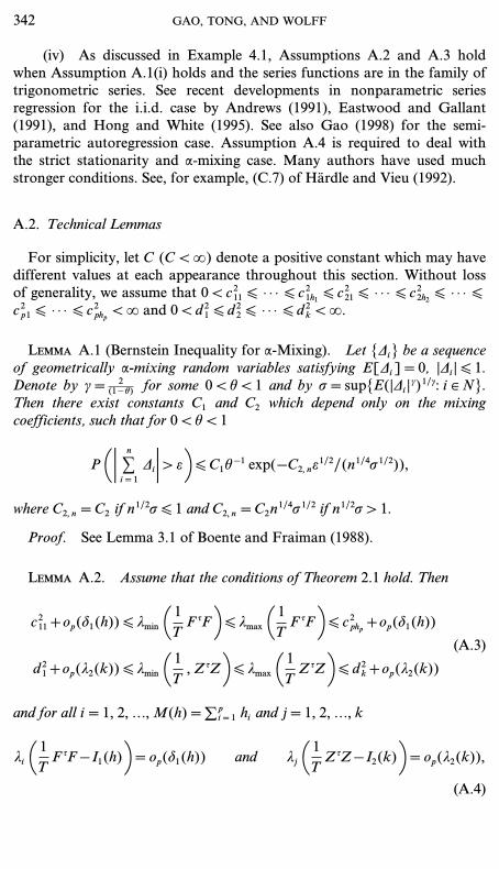
The left-hand side of (A.18) is

2k

CT

t=2

3 Ct−1

s=1a2st[e2s − 1]4+32

kCT

t=2Ct−1

s=1a2st − 14 . (A.21)

Also, the first term in (A.21) is

2k

Ck

i=1

3 1T

CT

t=2zi(Vt)2 ·5

1T

Ct−1

s=1zi(Vs)2 (e2s − 1)64

+2k

Ck

i=1Ck

j=1, ] i

3 1T2

CT

t=2Ct−1

s=1zi(Vs) zj(Vs) zi(Vt) zj(Vt)[e2s − 1]4

—2k

Ck

i=1M1i+

2k

Ck

i=1Ck

j=1, ] iM1ij.

The second term in (A.21) is

1k

Ck

i=1

35 1T

CT

t=1zi(Vt)2− 16

2

+2 5 1T

CT

t=1zi(Vt)2− 164

+1k

Ck

i=1Ck

j=1, ] i

3 1T2

CT

t=1CT

s=1zi(Vs) zj(Vs) zi(Vt) zj(Vt)4

—1k

Ck

i=1M2i+

1k

Ck

i=1Ck

j=1, ] iM2ij.

Analogously, the left-hand side of (A.19) is

4k

Ck

i=1

3 1T

CT

t=2zi(Vt)2 ·5

1T

Ct−1

r=2Cr−1

s=1zi(Vs) zi(Vr) eser64

+4k

Ck

i=1Ck

j=1, ] i

3 1T2

CT

t=2Ct−1

r=2Cr−1

s=1zi(Vs) eszj(Vr) erzi(Vt) zj(Vt)4

—4k

Ck

i=1M3i+

4kCk

i=1Ck

j=1, ] iM3ij.

In order to prove (A.18) and (A.19), its suffices to show that for s=1, 2, 3and all i, j \ 1

Msi=op(1) and Msij=op(k−1). (A.22)

We first prove (A.22) for M1ij. For any given e > 0, we have


P 3 1T2

max1 [ i ] j [ k

: CT

t=2Ct−1

s=1zi(Vs) zj(Vs) zi(Vt) zj(Vt)[e2s − 1] : > e

k4

[ Ck

i=1Ck

j=1, ] iP 3 1

T2: CT

t=2Ct−1

s=1zi(Vs) zj(Vs) zi(Vt) zj(Vt)[e2s − 1] : > e

k4

[k2

e2T4Ck

i=1Ck

j=1, ] iE 5C

T

t=2Ct−1

s=1zi(Vs) zj(Vs) zi(Vt) zj(Vt)[e2s − 1]6

2

=k2

e2T4Ck

i=1Ck

j=1, ] iCT

t=2E 51 C

t−1

s=1zi(Vs) zj(Vs)(e2s − 1)2

2

zi(Vt)2 zj(Vt)26

+k2

e2T4Ck

i=1Ck

j=1, ] iCT

t1=3Ct1 −1

t2=2Ct2 −1

s1=1

× E[zi(Vs1 )2 zj(Vs1 )

2 (e2s1 − 1)2 zi(Vt1 ) zj(Vt1 ) zi(Vt2 ) zj(Vt2 )]

+k2

e2T4Ck

i=1Ck

j=1, ] iCT

t1=4Ct1 −1

t2=3Ct2 −1

s1=2Cs1 −1

s2=1

× E 3 D2

l=1[zi(Vsl ) zj(Vsl )(e2sl − 1) zi(Vtl ) zj(Vtl )]4

+k2

e2T4Ck

i=1Ck

j=1, ] iCT

t1=2Ct1 −1

t2=1Ct1 −1

s1=t2

Ct2 −1

s2=1

× E 3 D2

l=1[zi(Vsl ) zj(Vsl )(e2sl − 1) zi(Vtl ) zj(Vtl )]4

— A1T+A2T+A3T+A4T. (A.23)

We first apply Lemma A.3 to show that

A2T=O 1 k4

T22=o(1).

Let

g1=zi(Vs1 )2 zj(Vs1 )

2 (e2s1 − 1)2 zi(Vt2 ) zj(Vt2 ), g2=zi(Vt1 ) zj(Vt1 )

and d(s1, t2, t1)=min(t2 − s1, t1 − t2). Using the fact that E[g2]=0 andapplying Assumptions A.1, A.3(iii)–(iv) and Lemma A.3, we have

|E[g1g2]| [ 10a(d(s1, t2, t1))C1=10 exp(−C2 d(s1, t2, t1))

for some positive constants C1 and C2.


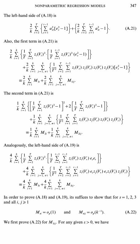
By a simple calculation we can obtain

A2T=k2

e2T4Ck

i=1Ck

j=1, ] iCT

t1=3Ct1 −1

t2=2Ct2 −1

s1=1E[g1g2] [ O 1 k

4

T22=o(1).

Similarly, we can show that

A1T=O 1 k4

T22=o(1) and AiT=O 1k

4

T2=o(1)

for i=3, 4.Analogously, we can prove (A.22) for M3i and M3ij. The proof of (A.22)

for M2i and M2ij can be obtained directly by applying Assumption A.3(iv).Now, we begin to prove (A.20). Obviously,

3 Ct−1

s=1astes 4

4

=1

T43 Ck

i=1

5Ct−1

s=1zi(Vs) es6 zi(Vt)4

4

[Ck3

T4Ck

i=1

5Ct−1

s=1zi(Vs) es6

4

,

using Assumption A.3(iii).First, for any fixed i \ 1

CT

t=2E 5C

t−1

s=1zi(Vs) es6

4

=CT

t=2E 5 C

t−1

s1=1Ct−1

s2=1Ct−1

s3=1Ct−1

s4=1zi(Vs1 ) es1zi(Vs2 ) es2zi(Vs3 ) es3zi(Vs4 ) es4 6

=C1 CT

t=2Ct−1

s=1E[zi(Vs) es]4

+C2 CT

t=2Ct−1

s1=1Ct−1

s2=1, ] s1

E[zi(Vs1 )2 e2s1zi(Vs2 )

2 e2s2]

+C3 CT

t=2Ct−1

s1=1Ct−1

s2=1, ] s1

E[zi(Vs1 )3 e3s1zi(Vs2 ) es2]

+C4 CT

t=2Ct−1

s1=1Ct−1

s3 ] s2 ] s1

E[zi(Vs1 )2 e2s1zi(Vs2 ) es2zi(Vs3 ) es3]

+C5 CT

t=2Ct−1

s1=1Ct−1

s4 ] s3 ] s2 ] s1

E[zi(Vs1 ) es1zi(Vs2 ) es2zi(Vs3 ) es3zi(Vs4 ) es4]

— J1T+J2T+J3T+J4T+J5T. (A.24)

Applying Assumptions A.1(ii) and A.3(iii) again, we have for i=1, 2, 3

JiT [ C6T3. (A.25)


Second, the above J4T is

J4T=C4 CT

t=2Ct−1

s1=1Ct−1

s3 ] s2 ] s1

E[zi(Vs1 )2 e2s1zi(Vs2 ) es2zi(Vs3 ) es3]

=2C4 CT

t=2Ct−1

s1=2Cs1 −1

s2=2Cs2 −1

s3=1E[zi(Vs1 )

2 e2s1zi(Vs2 ) es2es3zi(Vs3 )]

+2C4 CT

t=2Ct−1

s1=2Ct−1

s2=s1+1Cs2 −1

s3=1E[zi(Vs1 )

2 e2s1zi(Vs3 ) es3zi(Vs2 ) es2]

=2C4 CT

t=2Ct−1

s1=2Cs1 −1

s2=2Cs2 −1

s3=1E[zi(Vs1 )

2 e2s1zi(Vs2 ) es2es3zi(Vs3 )]

+2C4 CT

t=2Ct−1

s1=2Ct−1

s2=s1+1Cs2 −1

s3=1

× E[zi(Vs1 )2 e2s1zi(Vs3 ) es3zi(Vs2 ) E[es2 |Ws2 −1]]

— B1T+B2T. (A.26)

By using the fact that E[es2es3]=0 for 1 [ s3 [ s2 − 1 and applyingLemma A.3 again, we can show that B1T=O(T3). The second term B2T iszero because Assumption A.1(ii) holds, s2 \ s3+1 > s3 and s2 > s2 − 1 \ s1.

Third, for any fixed i

J5T=C5 CT

t=2Ct−1

s4 ] s3 ] s2 ] s1

E[zi(Vs1 ) es1zi(Vs2 ) es2zi(Vs3 ) es3zi(Vs4 ) es4]

=64C5 CT

t=2Ct−1

s1=2Cs1 −1

s2=2Cs2 −1

s3=2Cs3 −1

s4=1

× E 3D4

i=2[zi(Vsi ) esi] zi(Vs1 ) E[es1 |Ws1 −1]4=0 (A.27)

using Assumption A.1(ii) again.Thus, (A.24)–(A.27) imply (A.20). Until now, (A.18)–(A.20) are proved

and therefore (A.14) holds. In the following we finish the proof of (A.13).For any 1 [ i [ k, define

fii=1T

CT

t=1[zi(Vt)2− 1].

Using Assumptions A.1 and A.3, and applying Lemma A.1 again, we havefor any given e > 0

P[ max1 [ i [ k

|fii | > ek−1/2] [ Ck

i=1P[|fii | > ek−1/2] [ C1k exp(−C2T1/2k−1/2) Q 0

as T Q., where {Ci : i=1, 2} are constants.


Thus

max1 [ i [ k

|fii |=op(k−1/2).

Therefore, using Assumptions A.1 and A.3, and applying theCauchy–Schwarz inequality, we obtain

CT

t=1atte

2t − k=C

T

t=1att(e2t − 1)+tr(Z(T−1I2(k)−1) Zy) − k

=CT

t=1att[e2t − 1]+tr(I2(k)−1 (T−1ZyZ − I2(k)))

=CT

t=1att[e2t − 1]+C

k

i=1fii=op(k1/2),

where tr(B) denotes the trace of matrix B. Until now, we complete theproof of (A.6).

Next, we begin to prove (A.7). In order to prove (A.7), it suffices toshow that for i=2, 3, 4

IyiTIiT=op(k1/2) and Iy1TIiT=op(k1/2). (A.28)

Before proving (A.28), we need to prove for T large enough

lmax 11T

ZZy2=op 11

`k k log(k)2 ,

which follows from for any given e > 0

P 5: CT

t=1CT

s=1Ck

i=1zi(Vs) zi(Vt) lslt : >

eT

`k k log(k)6

[`k k log(k)

TeE : C

T

t=1CT

s=1Ck

i=1zi(Vs) zi(Vt) lslt :

[ C`k k log(k)

TCk

i=1E : C

T

t=1CT

s=1zi(Vs) zi(Vt) lslt :

=c`k k log(k)

TCk

i=1E 5C

T

t=1zi(Vt) lt6

2

[ Ck5/2 log(k)

T[ C

k3

TQ 0


using Assumption A.2(ii) and A.3(iv), and the fact that l=(l1, ..., lT)y isany identical vector satisfying ;T

t=1 l2t=1.Thus

RyPR [ lmax((ZyZ)−1) RyZZyR

[CTlmax(ZZy) RyR=op(k1/2)

which follows from for any given d > 0

P[RyR > d log(k) k] [1

dk log(k)E[RyR] [

Clog(k)

Q 0

using Assumption A.2 and the fact that E[RyR]=O(k)+O(M(h))=O(k).We now begin to prove

Iy3TI3T=op(k1/2).

It is obvious that

Iy3TI3T=eyF(FyF)−1 FyPF(FyF)−1 Fye

[ lmax(FyPF) ·lmax((FyF)−1) · eyF(FyF)−1 Fye

[CTlmax((ZyZ)+) lmax(FyZZyF) eyF(FyF)−1 Fye. (A.29)

Similar to the proof of (A.8), we can prove

eyF(FyF)−1 Fye=M(h)+op(M(h)1/2)

by applying Assumptions A.3(i)–(ii).In order to estimate the order of (A.29), it suffices to estimate

lmax 11T

(ZyF)y (ZyF)2 .

Analogous to the proof of Lemma A.2, we have for 1 [ i [ M(h)

li 11T

(ZyF)y (ZyF)2 [ 2M(h) max1 [ i, j [ p; 1 [ u [ hi, 1 [ v [ hj

|dijuv |=op(e(h) Tk),

(A.30)

using Assumption A.3(ii), where

dijuv=1T

Ck

l=1

5CT

s=1fiu(Usi) zl(Vs)6 5C

T

t=1fjv(Utj) zl(Vt)6


and {dijuv} denote the elements of the matrix 1T (ZyF)y (ZyF), and e(h)

satisfies e(h) Q 0 as T Q..Therefore, Eqs. (A.29) and (A.30) imply

Iy3TI3T [ op(e(h) M(h) k)=op(k1/2)

when e(h)=(M(h)`k)−1.Finally, we can prove the rest of (A.28) similarly and therefore we finish

the proof of Theorem 2.1.

A.4. Proof of Theorem 2.2

Here we only provide an outline. It follows from (2.1) and (2.2) that

s2(h, k)=1T

(Y − Fh(h, k) − Zc(k, h))y (Y − Fh(h, k) − Zc(k, h))

=1T

ey 1I −1T

PZ − PF 2 e −2T

ey(I − PZ − PF) R

+1T

Ry(I − PZ − PF) R,

where PZ=Z(ZyZ)+Zy, PF=F(FyF)− Fy, and R is as defined in (A.5).Therefore, the proof of Theorem 2.2 follows from Assumptions A.2

and A.3.

APPENDIX B

B.1 Proof of Theorem 2.3. Without loss of generality, we assume thatthe inverse matrices (ZyZ)−1, (FyF)−1 and (FyF)−1 exist and thatd21=d22= · · · =d2q=1. Let s2t=E[e2t |Wt−1] as defined in AssumptionA.1(iii).

First, one needs to show that as T Q.

1k

CT

s=1CT

t=1{a2sts

2ss2t − E[a2sts

2ss2t ]} Qp 0, (B.1)

where ast=1T;k

i=1 zi(Vs) zi(Vt).Note that

a2st=1

T2Ck

i=1z2i (Vs) z2i (Vt)+

1T2

Ck

i ] jzi(Vs) zj(Vs) zi(Vt) zj(Vt). (B.2)


In order to prove (B.1), in view of (B.2), it suffices to show that

max1 [ i, j [ k

1T

CT

s=1(zi(Vs) zj(Vs) − E[zi(Vs) zj(Vs)]) Qp 0, (B.3)

1T

CT

s=1(s2s − E[s2s ]) Qp 0, (B.4)

max1 [ i, j [ k

1T

CT

s=1(zi(Vs) zj(Vs) s

2s − E[zi(Vs) zj(Vs) s

2s ]) Qp 0. (B.5)

The proof of (B.3)–(B.5) follows similarly from (A.18)– (A.19).Let

y=yT=CT

s=1CT

t=1E[a2sts

2ss2t ] and WTt==

2y

Ct−1

s=1asteset. (B.6)

Similar to (A.15)–(A.17), we now can deduce

CT

t=2WTt QD N(0, 1) (B.7)

if

CT

t=2E[W2

Tt |Wt−1] Qp 1 (B.8)

and

CT

t=2E[W2

TtI[|WTt | > d] |Wt−1] Qp 0 (B.9)

for all d > 0.It is obvious that in order to prove (B.8) and (B.9), its suffices to show

that as T Q.

2y

CT

t=2Ct−1

s=1a2sts

2t [e2s −s2s ] Qp 0, (B.10)

2y

CT

t=1

1 Ct−1

r ] sastarteser 2 s2t Qp 0, (B.11)

and

4y2

CT

t=2E 35C

t−1

s=1astes6

4

s4t 4Q 0. (B.12)


Analogous to (A.18)–(A.20), and using Assumption A.1(iii), (B.10)–(B.12)can be proved and therefore (B.7) is proved.

Recall the notation introduced in (2.6),

mT=CT

t=1ptt e

2t and S2T=2 C

T

t=1CT

s=1p2st e

2s e2t ,

and let

mT=CT

t=1ptte

2t , mT=C

T

t=1ptts

2t ,

S2T=2 CT

t=1CT

s=1p2ste

2s e2t , and S2T=2 C

T

t=1CT

s=1p2sts

2ss2t .

(B.13)

In view of (2.5), (2.6), (B.7), and (B.13), in order to prove Theorem 2.3, itsuffices to show that as T Q.

mT − mT`k

Qp 0, (B.14)

mT −mT`k

Qp 0, (B.15)

S2T − S2Tk

Qp 0, andS2T − S2T

kQp 0. (B.16)

Note that

et=Yt − F(Ut)y h− Z(Vt)y c

=et+F(Ut)y [h− h]+Z(Vt)y [c− c]+Rt — et+D1t+D2t+Rt, (B.17)

where

Rt=Cp

i=1[gi(Uti) − Fi(Uti)y hi]+g(Vt) − Z(Vt)y c.

Similar to the proof of (A.10)–(A.12), one can show that as T Q.

CT

t=1[ptt − att] e2t=op(`k) and C

T

t=1[ptt − att] e2t=op(`k).

(B.18)

In view of (B.17) and (B.18), in order to prove (B.14), it suffices to showthat as T Q.

CT

t=1att[e2t − e2t ]=op(`k), (B.19)


which follows from

: CT

t=1att[e2t − e2t ]: [ C C

T

t=1att[D

21t+D

22t+R2t ]=op(`k)

by using Assumption A.2 and (A.5)–(A.7).Analogously, in order to prove (B.15), it suffices to show that as T Q.

E 5CT

t=1att(e2t −s2t )6

2

=o(k), (B.20)

which follows from

E 3 CT

t=1att[e2t −s2t ]4

2

=CT

t=1E[att(e2t −s2t )]2

+CT

s ] tE{assatt[e2s −s2s ][e2t −s2t ]}=o(k),

where the first term is o(k) by the definition of {att}, the second termfollows from

E{ass[e2s −s2s ]}=E{E[ass(e2s −s2s ) |Ws−1]}=0

and an application of Lemma A.3.Similar to (B.18)–(B.20), one can prove (B.16) by using Lemma A.3.

Therefore, an outline of the proof of Theorem 2.3 is completed.

ACKNOWLEDGMENTS

The authors thank the Editor and the two referees for their constructive comments anddetailed suggestions which have improved the original manuscript. The first and the thirdauthors thank the Australian Research Council for its financial support. The second authoracknowledges financial support from the EU under the Human Capital Programme (CHRX-CT 94-0693), the Engineering and Physical Science Research Council of UK, and the HongKong University CRCG award.

REFERENCES

G. G. Agarwal and W. J. Studden, Asymptotic integrated mean square error using leastsquares and bias minimizing splines, Ann. Statist. 8 (1980), 1307–1325.

D. W. K. Andrews, Asymptotic normality of series estimators for nonparametric andsemiparametric regression models, Econometrica 59 (1991), 307–345.

D. Barry, Testing for additivity of a regression function, Ann. Statist. 21 (1993), 235–254.G. Boente and R. Fraiman, Consistency of a nonparametric estimate of a density function for

dependent variables, J. Multivariate Anal. 25 (1988), 90–99.


M. J. Buckley and G. K. Eagleson, An approximation to the distribution of quadratic formsin normal random variables, Austral. J. Static. A 30 (1988), 150–159.

C. P. Chen and P. H. Hsieh, Pointwise convergence of double trigonometric series,J. Math. Anal. Appl. 172 (1993), 582–599.

R. Chen and R. Tsay, Nonlinear additive ARX models, J. Amer. Statist. Assoc. 88 (1993),955–967.

R. Chen, J. Liu, and R. Tsay, Additivity tests for nonlinear autoregression, Biometrika 82(1995), 369–383.

D. D. Cox and T. Y. Kim, Moment bounds for mixing random variables useful innonparametric function estimation, Stochastic Process. Appl. 56 (1995), 151–158.

P. De Jong, A central limit theorem for generalized quadratic forms, Probab. Theory RelatedFields 75 (1987), 261–277.

R. A. DeVore and G. G. Lorentz, ‘‘Constructive Approximation,’’ Springer-Verlag,New York, 1993.

P. Doukhan, ‘‘Mixing: Properties and Examples,’’ Lecture Notes in Statistics, Vol. 85,Springer-Verlag, New York, 1995.

B. J. Eastwood and A. R. Gallant, Adaptive rules for seminonparametric estimators thatachieve asymptotic normality, Econometric Theory 7 (1991), 307–340.

R. L. Eubank and J. D. Hart, Testing goodness-of-fit in regression via order selectioncriteria, Ann. Statist. 20 (1992), 1412–1425.

R. L. Eubank, J. D. Hart, D. G. Simpson, and L. A. Stefanski, Testing for additivity innonparametric regression, Ann. Statist. 23 (1995), 1896–1920.

R. L. Eubank, E. L. Kambour, J. T. Kim, K. Klipple, C. S. Reese, and M. Schimek,Estimation in partially linear models, Comput. Statist. Data Anal. 29 (1998), 27–34.

D. E. Eumunds and V. B. Moscatelli, Fourier approximation and embeddings of Sobolevspace, Dissertationes Math., 1977.

J. Fan, Design-adaptive nonparametric regression, J. Amer. Statist. Assoc. 87 (1992),998–1004.

J. Fan and I. Gijbels, ‘‘Local Polynomial Modelling and Its Applications,’’ Chapman& Hall, London, 1996.

J. Fan, W. Härdle, and E. Mammen, Direct estimation of low dimensional components inadditive models, Ann. Statist. 26 (1998), 943–971.

J. Fan and L. S. Huang, Goodness-of-fit tests for parametric regression models, J. Amer.Statist. Assoc. 96 (2001), 640–652.

J. Fan and Q. W. Yao, Efficient estimation of conditional variance functions in stochasticregression, Biometrika 85 (1998), 645–660.

J. Fan, C. M. Zhang, and J. Zhang, Generalized likelihood ratio statistics and Wilksphenomenon, Ann. Statist. 29 (2001), 153–193.

Y. Fan and Q. Li, Consistent model specification tests: omitted variables and semiparametricfunctional forms, Econometrica 64 1996, 865–890.

A. R. Gallant, On the bias in flexible functional forms and an essentially unbiased form: TheFourier flexible form, J. Econometrics 15 (1981), 211–245.

J. Gao, Semiparametric regression smoothing of nonlinear time series, Scand. J. Statist. 251998, 521–539.

J. Gao and V. Anh, Semiparametric regression under long-range dependent errors,J. Statist. Plann. Inference 80 (1999), 37–57.

J. Gao and H. Liang, Asymptotic normality of pseudo-LS estimator for partially linearautoregressive models, Statist. Probab. Lett. 23 (1995), 27–34.

J. Gao and H. Liang, Statistical inference in single-index and partially nonlinearregression models, Ann. Inst. Statist. Math. 49 (1997), 493–517.

J. Gao and P. Shi, M-type smoothing splines in nonparametric and semiparametric regressionmodels, Statist. Sinica 7 (1997), 1155–1169.


J. Gao, H. Tong, and R. Wolff, Adaptive orthogonal series estimation in additive stochasticregression models, Statist. Sinica 11 (2001), 1007–1027.

J. Gao, R. Wolff, and V. Anh, Semiparametric approximation methods in multivariate modelselection, J. Complexity 17 (2001), 446–461.

J. Gao and T. Yee, Adaptive estimation in partially linear autoregressive models, Canad. J.Statist. 28 (2000), 571–586.

P. L. Gozalo and O. B. Linton, Testing additivity in generalized nonparametric regressionmodels with estimated parameters, Private communication, 1999.

P. Hall, Central limit theorem for integrated square error of multivariate nonparametricdensity estimators, J. Multivariate Anal. 14 (1984), 1–16.

P. Hall, J. Kay, and D. M. Titterington, Asymptotically optimal difference basedestimation of variance in nonparametric regression, Biometrika 77 (1990), 521–528.

W. Härdle and A. Kneip, Testing a regression model when we have smooth alternatives inmind, Scand. J. Statist. 26 (1999), 221–238.

W. Härdle, H. Liang, and J. Gao, ‘‘Partially Linear Models,’’ Springer Series inContributions to Statistics, Physica-Verlag, New York, 2000.

W. Härdle and E. Mannen, Comparing nonparametric versus parametric regression fits, Ann.Statist. 21 (1993), 1926–1947.

W. Härdle and P. Vieu, Kernel regression smoothing of time series, J. Time Ser. Anal. 13(1992), 209–232.

J. Hart, ‘‘Nonparametric Smoothing and Lack-of-Fit Tests,’’ Springer-Verlag, New York,1997.

T. J. Hastie and R. J. Tibshirani, ‘‘Generalized Additive Models,’’ Chapman & Hall, London,1990.

V. Hjellvik and D. Tjøstheim, Nonparametric tests of linearity for time series, Biometrika 82(1995), 351–368.

V. Hjellvik, Q. W. Yao, and D. Tjøstheim, Linearity testing using local polynomialapproximation, J. Statist. Plann. Inference 68 (1998), 295–321.

Y. Hong and H. White, Consistent specification testing via nonparametric seriesregression, Econometrica 63 (1995), 1133–1159.

B. S. Kashin and A. A. Saakyan, ‘‘Orthogonal Series,’’ Translations of MathematicalMonographs, Vol. 75, Amer. Math. Soc., Providence, 1989.

J. P. Kreiss, M. H. Neumann, and Q. W. Yao, Bootstrap tests for simple structures innonparametric time series regression, private communication, 1999.

P. Lavergne and Q. H. Vuong, Nonparametric significance testing, Econometric Theory 16(2000), 576–601.

Q. Li, Consistent model specification tests for time series econometric models,J. Econometrics 92 (1999), 101–147.

Z. D. Lu, On the geometric ergodicity of a nonlinear autoregressive model with anautoregressive conditional heteroscedastic term, Statist. Sinica 8 (1998), 1205–1217.

E. Masry and D. Tjøstheim, Nonparametric estimation and identification of ARCHnonlinear time series: Strong convergence and asymptotic normality, Econometric Theory11 (1995), 258–289.

E. Masry and D. Tjøstheim, Additive nonlinear ARX time series and projection estimates,Econometric Theory 13 (1997), 214–252.

D. Nychka, S. Elliner, A. Gallant, and D. McCaffery, Finding chaos in noisy systems,J. Roy. Statist. Soc. Ser. B 54 (1992), 399–426.

D. Pollard, ‘‘Convergence of Stochastic Processes,’’ Springer-Verlag, New York, 1984.P. Robinson, Root-N-consistent semiparametric regression, Econometrica 56 (1988),

931–964.G. Roussas and D. Ioannides, Moment inequalities for mixing sequences of random variables,Stochastic Anal. Appl. 5 (1987), 61–120.


P. Speckman, Kernel smoothing in partial linear models, J. Roy. Statist. Soc. Ser. B 50 (1988),413–436.

C. J. Stone, Additive regression and other nonparametric models, Ann. Statist. 13 (1985),689–705.

T. Teräsvirta, D. Tjøstheim, and C. W. J. Granger, Aspects of modelling nonlinear time series,in ‘‘Handbook of Econometrics’’ (R. F. Engle and D. L. McFadden, Eds.), Vol. 4,pp. 2919–2957, 1994.

D. Tjøstheim, Nonlinear time series: A selective review, Scand. J. Statist. 21 (1994), 97–130.D. Tjøstheim and B. Auestad, Nonparametric identification of nonlinear time series:

Projections, J. Amer. Statist. Assoc. 89 (1994a), 1398–1409.D. Tjøstheim and B. Auestad, Nonparametric identification of nonlinear time series: Selecting

significant lags, J. Amer. Statist. Assoc. 89 (1994b), 1410–1419.H. Tong, ‘‘Nonlinear Time Series,’’ Oxford Univ. Press, London, 1990.C. M. Wong and R. Kohn, A Bayesian approach to estimating and forecasting additive

nonparametric autoregressive models, J. Time Ser. Anal. 17 (1996), 203–220.Q. W. Yao and H. Tong, On subset selection in nonparametric stochastic regression, Statist.Sinica 4 (1994), 51–70.

K. Yoshihara, Limiting behaviour of U-statistics for stationary absolutely regular process,Z. Wahrsch. Verw. Gebiete 35 (1976), 237–252.


Model Specification Tests in Nonparametric Stochastic Regression Models

Documents