Model simulations of agri-food trade liberalisation - World …siteresources.worldbank.org/.../ModelSims_vanTongeren.pdf · Model simulations of agri-food trade liberalisation Paper

Model simulations of agri-food trade liberalisation

Paper prepared for

Wageningen University PHLO course

Agricultural Trade, the World Trade Organization and the Doha Round

May 2005

Frank van Tongeren

[email protected]

Outline

Introduction

Modelling approaches

Review of recent modelling result

Why the results differ: a primer

Features of individual modelling studies

Key lessons from the ex ante assessments

Who gains from agricultural reform?

What is the contribution of agriculture?

The three pillars in the agricultural negotiations

Miscellaneous issues

Trade effects

Concluding remarks

References

Introduction

Assessing the impact of changes in agricultural and trade policies poses

methodological challenges inherent in all policy assessment exercises. Since we are

interested in the counterfactual situation with the policy change compared to a

situation without the policy change, we cannot simply rely on observations that

compare a pre-change state to the post-change state. Too many factors interfere to be

able to isolate the effects of the policy change in question. Fortunately, the arsenal of

economic research provides for a rich set of tools that facilitates policy assessment,

both ex ante and ex post. As far as ex post assessment is concerned, there exist

sophisticated econometric methods to disentangle the various intervening effects.1

This paper is particularly concerned with ex ante assessment of agricultural policy

changes, against the background of the ongoing Doha round of multilateral trade

policy negotiations. Ex ante assessments help to identify potential winners and losers

of such agreements and aim to inform the policy debate. Numerous studies have

recently been published on the broad, macro-economic, assessment of further changes

on agricultural (trade) policies, and this paper is an attempt to summarize the method

of those studies as well as to provide a summary of results.

Modelling approaches

Since policy assessment is concerned with evaluating a situation with a

proposed policy change against a situation without the policy change, economists

favour structural economic models for this task. Economic models start from a

portrait of an existing situation, using many assumptions on economic behaviour, and

then proceed to paint a counterfactual world that includes the proposed policy

changes. The most commonly used models are so-called market equilibrium models.2

These contain the response (behaviour) of economic agents to changes in prices

(costs), and prices adjust so as to clear markets. The objective of these models is the

determination of equilibrium prices and quantities on (interrelated) sets of markets.

This class of models is firmly established within mainstream economics where the

1 For an excellent overview of recent advances see Smith and Todd (2005). 2 ‘Gravity models’ are another important class of model in international trade analysis. These are

less explicit about their theoretical underpinning and focus on econometric estimates. They are

sometimes used in ex-ante analysis of trade policy changes.

1

behavioural response of suppliers and buyers is typically derived from optimising

assumptions: given a description of the production technology, the supplier chooses a

combination of inputs such that costs are minimised for a given level of output. Given

a description of consumer preferences, the buyer determines his preferred

consumption bundle such that his/her utility is maximized for a given level of his/her

budget. Standard assumptions include constant returns technology, homothetic

preferences, and markets characterised by perfect competition. While these basic

theoretical assumptions underlie equilibrium modelling, the optimization process is

usually not modelled explicitly. Rather, a reduced form approach is common, where

demand and supply are specified as functions of income, prices and elasticities.

Depending on assumptions made about the flexibility of production factors,

equilibrium models can be classified as short term, medium term or long term. Short

term (in the Marshallian sense) means that some production factors are fixed, and are

not allowed to reallocate between alternative uses. The fixed factors in the short run

will typically be capital, agricultural land, and perhaps agricultural labour. If the

model is applied to actual data, as opposed to theoretical models, the modeller also

needs to use data to estimate parameters and relationships included in the model.

Although this paper is concerned with macro-economic effects of agricultural

policy changes, and hence concentrates on economy-wide models, it is worthwhile to

briefly distinguish this type of analysis from partial models of agriculture. For a fuller

discussion of alternative modelling approaches see Van Tongeren et al. (2001).

Partial models treat international markets for a selected set of traded goods, e.g.

agricultural goods. They consider the agricultural system as a closed system without

linkages with the rest of the economy. Partial models of international trade in

agriculture generally focus on trade in primary commodities. They capture

agricultural supply, demand and trade for unprocessed or first-stage processed

agricultural products without taking into account trade in processed food products,

despite the fact that the latter commodities represent an increasing share of world

trade. The main area of application of partial equilibrium models is detailed trade

policy analysis to specific products, which represent only a small portion of the

activities of the economy in question. This (small sector) condition implies that

policy-induced changes on the rest of the economy are so small that they can be

ignored. While agriculture typically represents only a small portion of GDP in

industrialised countries, this is certainly not true in the developing world, where

2

agriculture is the dominant source of income and employment. A more complete

representation of these economies is required to fathom the likely impacts of trade

reforms.

Economy-wide models provide such a complete representation of national

economies. This is obtained when the model is closed with respect to the generation

of factor income and expenditures, which requires the explicit specification of factor

markets for land, labour and capital. In other words, the essential general equilibrium

features are captured by including factor movements between sectors, next to

allowing for demand interactions. Economy-wide models capture implications of

international trade for the economy as a whole, covering the circular flow of income

and expenditure and taking care of inter-industry relations.

All the estimates of potential economic gains from policy reforms considered

below are obtained using a class of economy-wide models known as CGE

(computable general equilibrium) or AGE (applied general equilibrium) models. This

has become the dominant tool in global trade policy analysis. CGE models provide a

complete representation of national economies, and a specification of trade relations

between economies. CGE models are specifically concerned with resource allocation

issues, that is, where the allocation of production factors over alternative uses is

affected by certain policies or exogenous developments. International trade is

typically an area where such induced effects are important consequences of policy

choices. In the face of changing international prices, resources will move between

alternative uses within the domestic economy, or even between economies if

production factors are internationally mobile. The main features of CGE models can

be summarized as follows, see also Kehoe and Kehoe (1994):

Within each regional economy a standard CGE model covers inter-industry

linkages through an input–output structure. Demand for factors of production is

derived from cost minimisation, given a sectoral production function (nested CES)

that allows for substitution between inputs. Typically, substitution is allowed only

between primary factors — land, labour, capital — while intermediate inputs are used

in fixed proportion with output (Leontief technology). The production structure is

typically constant returns to scale and perfect competition is assumed to prevail on all

markets. Each sector produces one homogeneous good that is perfectly substitutable

domestically but substitutes imperfectly with foreign goods (Armington assumption).

3

Next to the binary distinction ‘domestic versus foreign’, the multi-region nature of the

model enables a distinction of traded commodities according to their region of origin.

That is, bilateral trade flows are captured. Factor markets for land, labour and

capital are included, endowments for these primary factors are given and the factors

are fully employed. Labour and capital are assumed to be fully mobile across

domestic sectors, while land is imperfectly mobile and tied to agricultural production.

Consumer demand is derived from utility maximization under a budget constraint, and

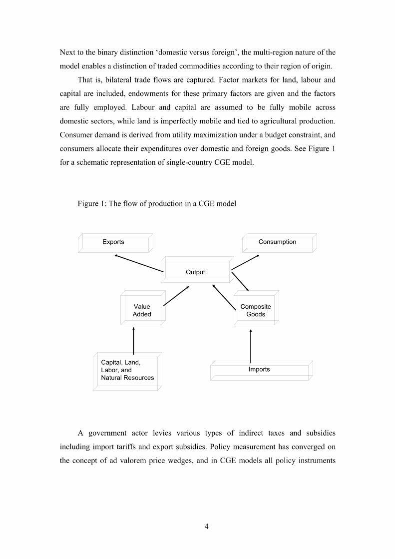
consumers allocate their expenditures over domestic and foreign goods. See Figure 1

for a schematic representation of single-country CGE model.

Figure 1: The flow of production in a CGE model

Output

ValueAdded

CompositeGoods

ImportsCapital, Land, Labor, and Natural Resources

Exports Consumption

A government actor levies various types of indirect taxes and subsidies

including import tariffs and export subsidies. Policy measurement has converged on

the concept of ad valorem price wedges, and in CGE models all policy instruments

4

are typically specified in this way.3 All factor markets and commodity markets are

assumed to clear, which yields equilibrium solutions to factor- and commodity prices

as well as the corresponding equilibrium quantities.

All regional economies are linked through bilateral commodity trade and

through interregional investment flows. If one is willing to assume a constant current

account balance in all regions, then the difference between regional savings and

investments is essentially predetermined, and as a consequence the aggregate level of

the savings — investment balance is also predetermined. If one wants to allow for

endogenous determination of the current account balance, the model must include a

mechanism to redistribute aggregate savings over regions.

Some models include a recursive sequence of temporary equilibria. Recursive

models do generate time paths for endogenous variables, but there is in fact no

behavioural linkage between periods. As a result, the equilibrium solution in each

period can essentially be calculated without reference to earlier or later periods.

Market imperfections are typically ignored in standard CGE models.

Information problems, lack of infrastructure, monopolistic market structures and

similar frictions abound in agricultural markets, especially in developing countries.

However, CGE models rarely include those in the analysis. Only so-called ‘second

generation’ models add increasing returns and imperfect competition in some of the

sectors, allowing for estimates of scale and variety effects.

The comparative static analysis performed with CGE models does not reveal

adjustments processes and possible adjustment costs involved when far reaching

policy changes are implemented. Policy-induced resource shifts will always entail

income losses and adjustment processes for some people. The comparative static CGE

analysis typically sidesteps these issues and concentrates on the features of the new

equilibrium in which the system settles after the policy change has been implemented.

Relatively recent methodological developments on have resulted in so-called ‘Third

generation’ models that include time consistent forward looking behaviour and

3 Instead of including the wedges that policies create between buyer’s and sellers’ prices one

might attempt to explicitly model policy instruments. For example quantitative instruments such as

production quota and import quota, nut also price based instruments such as intervention prices could

be modelled explicitly in CGE models. For an application on the European Union’s CAP along these

lines see Van Meijl and Van Tongeren (2002).

5

endogenous savings rates, hence allowing for the modelling of short run dynamics.

While these models focus on savings-investment issues, including international

capital flows, they could in principle be adapted to capture short- to medium-term real

adjustment processes.

Finally a word on interpreting the oft-reported income effects from CGE model

is in order. The macro economic effects of changes in policies are typically assessed

by the well-established welfare economic compensation measure. The so-called

equivalent variation (EV) measures what change in income would be equivalent to the

proposed policy change. In other words, instead of effectuating a certain policy

change how much income should be given to (or taken away from) households to

achieve the same welfare. This measure always informs us about the potential welfare

change and it does not inform us about distributive effects. In fact, if the EV is

positive, we know that enough resources are mobilized such that the winners from the

policy move can potentially compensate the losers. The EV is firmly grounded in the

welfare economic literature, and provides the ultimate measure of how well an

economy is doing when implementing a policy change.4 When CGE models report

national income changes these are typically EV measures and not Gross Domestic

Product (GDP) or similar national accounting indicators.

Review of recent modelling results

All the models discussed here are built around the GTAP (Global Trade

Analysis Project) database.5 Some follow, in addition, the GTAP modelling approach,

while others develop their own CGE model with special features. The GTAP database

is maintained by the GTAP consortium which is based at Purdue University with

funding from an international consortium of national and international agencies,

universities and research centres. Development of the GTAP databases was started in

the early 1990s and has since then become the prime dataset for global economic

analysis.

4 While the EV takes the new situation as a reference, the alternative measure known as

Compensating Variation (CV) takes the old situation as the reference. It asks the hypothetical question:

‘what is the minimum amount of compensation after the price change in order to be as well off as

before the change? 5 See www.gtap.org for more information.

6

Most of the studies reported here rely on version 5 of the GTAP database, which

was benchmarked to the tear 1997. The two most recent studies included in this

review use the most recent version 6, which is still in the pre-release phase as of early

2005, i.e. not yet publicly available. Version 6 differs in some important respects: it

has more countries and regions included, it is benchmarks to the year 2001 (instead of

1997) and it has more sophisticated measurement of levels of protection. Specifically,

it includes existing preferential trade agreements and the conversion of specific to ad

valorem tariff equivalents. Therefore the new database captures the liberalisation

efforts that have been ongoing in the wake of the Uruguay Round as well as

autonomous liberalisation done by many countries, especially in Asia after the Asian

financial crisis of the late 1990s

Talking about gains from reform, one typically wants to know not only the size

of the gains, but also their distribution. In addition, the sources of gains from

liberalisation are important to inform the policy debate: which of the negotiation

issues is most important and to whom? Tables 1 and 2 and Figure 2 attempt to

summarize exactly this type of information arising from recent CGE modelling

studies.

Figure 2 shows estimates of annual welfare gains from full agricultural

liberalisation, i.e. a complete and multilateral removal of all border protection and

domestic support. The estimates span a rather wide range, from roughly 30 billion

USD (USDA, 2001; OECD, 2003) to 193 billion USD (World Bank, 2004). Table 1

and Table 2 provide further decomposition of results into the effects of broad sectors

and country groupings. Since all the studies discussed use the same database, the

reason for this variance of results must be found in either the modelling assumptions

or the scenario design. We summarize key factors that influence the results from

GTAP-based CGE models, before proceeding to discuss in the specific modelling

assumptions behind these results.

7

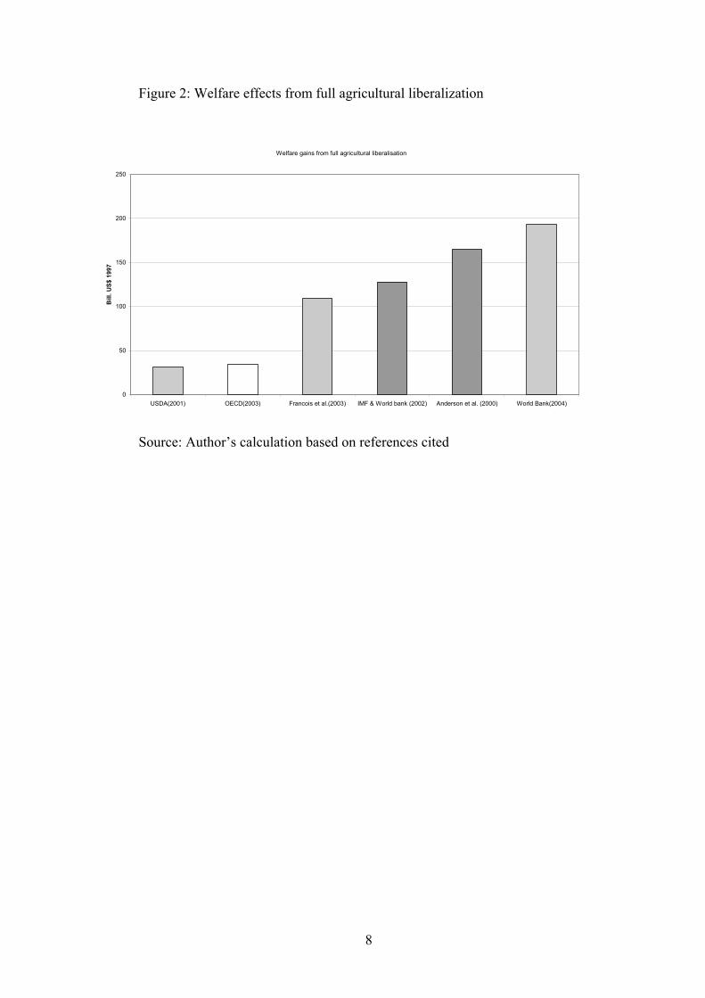
Figure 2: Welfare effects from full agricultural liberalization

Welfare gains from full agricultural liberalisation

0

50

100

150

200

250

USDA(2001) OECD(2003) Francois et al.(2003) IMF & World bank (2002) Anderson et al. (2000) World Bank(2004)

Bill

. US$

199

7

Source: Author’s calculation based on references cited

8

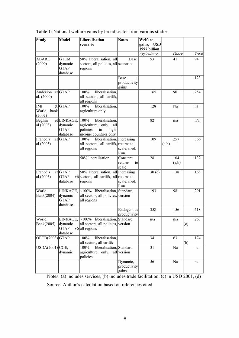
Table 1: National welfare gains by broad sector from various studies

Study Model Liberalisation scenario

Notes Welfare gains, USD 1997 billion

Agriculture Other TotalABARE (2000)

GTEM, dynamic GTAP database

50% liberalisation, all sectors, all policies, all regions

Base scenario

53 41 94

Base + productivity gains

123

Anderson et al. (2000)

GTAP 100% liberalisation, all sectors, all tariffs, all regions

165 90 254

IMF & World bank (2002)

GTAP 100% liberalisation, agriculture only

128 Na na

Beghin et al.(2003)

LINKAGE, dynamic GTAP database

100% liberalisation, agriculture only, all policies in high-income countries only

82 n/a n/a

Francois et al.(2003)

GTAP 100% liberalisation, all sectors, all tariffs, all regions

Increasing returns to scale, med. Run

109 257 (a,b)

366

50% liberalisation Constant returns to scale

28 104 (a,b)

132

Francois et al.(2005)

GTAP GTAP v6 database

50% liberalisation, all sectors, all tariffs, all regions

Increasing returns to scale, med. Run

30 (c) 138 168

World Bank(2004)

LINKAGE, dynamic GTAP database

~100% liberalisation, all sectors, all policies, all regions

Standard version

193 98 291

Endogenous productivity

358 156 518

World Bank(2005)

LINKAGE, dynamic GTAP v6 database

~100% liberalisation, all sectors, all policies, all regions

Standard version

n/a n/a 263 (c)

OECD(2003) GTAP 100% liberalisation, all sectors, all tariffs

34 63 174 (b)

USDA(2001) CGE, dynamic

100% liberalisation, agriculture only, all policies

Standard version

31 Na na

Dynamic, productivity gains

56 Na na

Notes: (a) includes services, (b) includes trade facilitation, (c) in USD 2001, (d)

Source: Author’s calculation based on references cited

9

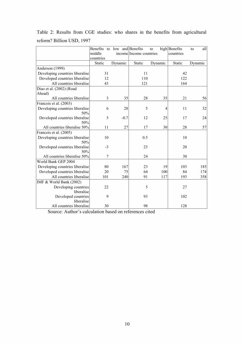
Table 2: Results from CGE studies: who shares in the benefits from agricultural

reform? Billion USD, 1997 Benefits to low and

middle income countries

Benefits to high Income countries

Benefits to all countries

Static Dynamic Static Dynamic Static Dynamic Anderson (1999) Developing countries liberalise 31 11 42 Developed countries liberalise 12 110 122

All countries liberalise 43 121 164 Diao et al. (2002) (Road Ahead)

All countries liberalise 3 35 28 35 21 56Francois et al. (2003) Developing countries liberalise

50% 6 28 5 4 11 32

Developed countries liberalise 50%

5 -0.7 12 25 17 24

All countries liberalise 50% 11 27 17 30 28 57Francois et al. (2005) Developing countries liberalise

50% 10 0.5 10

Developed countries liberalise 50%

-3 23 20

All countries liberalise 50% 7 24 30 World Bank GEP 2004 Developing countries liberalise 80 167 23 19 103 185Developed countries liberalise 20 75 64 100 84 174

All countries liberalise 101 240 91 117 193 358IMF & World Bank (2002)

Developing countries liberalise

22 5 27

Developed countries liberalise

9 93 102

All countries liberalise 30 98 128 Source: Author’s calculation based on references cited

10

Why the results differ: a primer

There are three main sources for differing outcomes in terms of national and

global welfare:

- The scenario design: the representation of existing policies I the base

situation and the subsequent reform scenario makes a difference. In

relation to border protection, the binding overhang (difference between

bound and applied rates) makes a difference, as seen in OECD (2003)

and UNECA (2004). When the scenarios reduce applied levels of

tariffs, they may therefore overstate the true effect on market access.

Likewise, the representation of existing trade preferences has an impact

on the results, as seen in Francois et al (2005). With regard to domestic

agricultural policies, the treatment of ‘decoupled’ payments appears to

be important (USDA, 2001). In addition the AMS-ceilings agreed in the

Uruguay Round have never been binding due to a variety of reasons.

Again, the effects of reducing ceilings on domestic support may be

overstated by this approach.

- Dynamic versus static effects: The World Bank linkage model is

recursive dynamic model that moves the database forward to the year

2015. The projected composition of the economy in the future

determines to a large part where the reform gains are occurring. If

agriculture occupies a large share of GDP in the future projected

economy, then also will the gains from liberalisation come mainly from

agriculture.

- Inclusion of non-standard features, such as increasing returns to scale,

imperfect competition and trade-productivity linkages. All these tend to

boost the estimates of welfare gains from reform.

Features of individual modelling studies

The Australian Bureau of Agriculture and Resource Economics (ABARE

2000) used their dynamic CGE, called GTEM, to assess the impact of trade

liberalisation in all sectors. This model is designed specifically to assess economic

policy issues with long term, global dimensions.

11

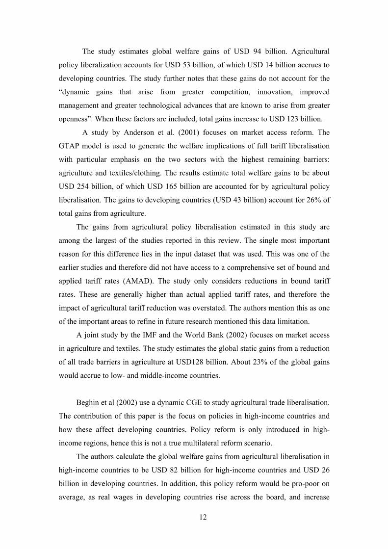
The study estimates global welfare gains of USD 94 billion. Agricultural

policy liberalization accounts for USD 53 billion, of which USD 14 billion accrues to

developing countries. The study further notes that these gains do not account for the

“dynamic gains that arise from greater competition, innovation, improved

management and greater technological advances that are known to arise from greater

openness”. When these factors are included, total gains increase to USD 123 billion.

A study by Anderson et al. (2001) focuses on market access reform. The

GTAP model is used to generate the welfare implications of full tariff liberalisation

with particular emphasis on the two sectors with the highest remaining barriers:

agriculture and textiles/clothing. The results estimate total welfare gains to be about

USD 254 billion, of which USD 165 billion are accounted for by agricultural policy

liberalisation. The gains to developing countries (USD 43 billion) account for 26% of

total gains from agriculture.

The gains from agricultural policy liberalisation estimated in this study are

among the largest of the studies reported in this review. The single most important

reason for this difference lies in the input dataset that was used. This was one of the

earlier studies and therefore did not have access to a comprehensive set of bound and

applied tariff rates (AMAD). The study only considers reductions in bound tariff

rates. These are generally higher than actual applied tariff rates, and therefore the

impact of agricultural tariff reduction was overstated. The authors mention this as one

of the important areas to refine in future research mentioned this data limitation.

A joint study by the IMF and the World Bank (2002) focuses on market access

in agriculture and textiles. The study estimates the global static gains from a reduction

of all trade barriers in agriculture at USD128 billion. About 23% of the global gains

would accrue to low- and middle-income countries.

Beghin et al (2002) use a dynamic CGE to study agricultural trade liberalisation.

The contribution of this paper is the focus on policies in high-income countries and

how these affect developing countries. Policy reform is only introduced in high-

income regions, hence this is not a true multilateral reform scenario.

The authors calculate the global welfare gains from agricultural liberalisation in

high-income countries to be USD 82 billion for high-income countries and USD 26

billion in developing countries. In addition, this policy reform would be pro-poor on

average, as real wages in developing countries rise across the board, and increase

12

more than capital returns. The authors also find that world food prices would rise

significantly, leading to an important re-orientation of agricultural trade.

In a study by OECD (2003), gains from further reduction of bound tariff rates

were analyzed. In particular, the study takes into account the difference between

bound tariff rates and applied tariff rates (those actually used in trade). The authors

note that this difference is significant. Particularly in the agriculture sector they

estimate the binding overhang to amount to 33%. The GTAP model is used to

consider three sets of scenarios for tariff reduction. Taking into account the binding

overhang appears to explain the relatively small welfare gains from reductions of

(bound) tariffs.

In the full liberalization scenario, the global welfare gains were found to be over

USD 173 billion. About 52% of total gains accrue to developing countries. This is

largely due to the fact that tariffs are relatively high in developing countries. If

agricultural tariff liberalization is excluded, the gains amount to USD 139 billion –

that is, the potential gains from further liberalization with respect to industrial goods

may be even larger than gains from agriculture.

Overall, this study underscores the importance to developing countries of both

greater access to developed countries’ markets as well as their own engagement in

trade liberalization.

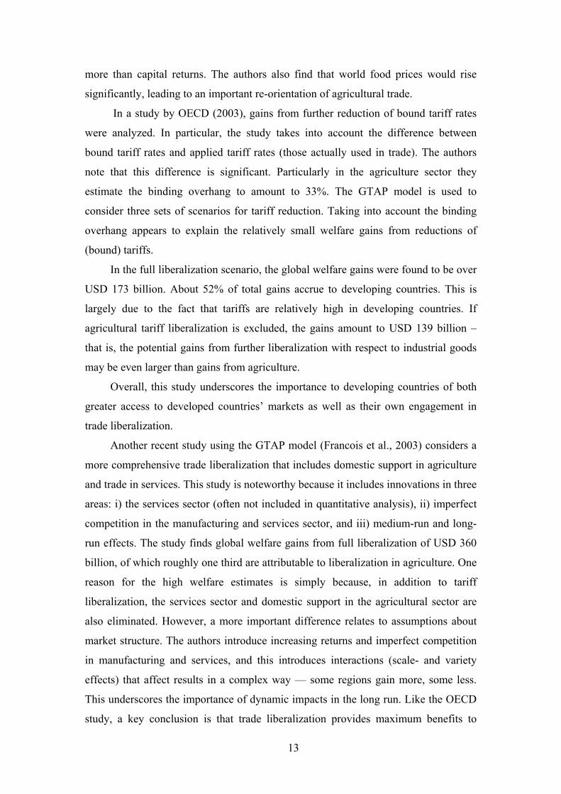
Another recent study using the GTAP model (Francois et al., 2003) considers a

more comprehensive trade liberalization that includes domestic support in agriculture

and trade in services. This study is noteworthy because it includes innovations in three

areas: i) the services sector (often not included in quantitative analysis), ii) imperfect

competition in the manufacturing and services sector, and iii) medium-run and long-

run effects. The study finds global welfare gains from full liberalization of USD 360

billion, of which roughly one third are attributable to liberalization in agriculture. One

reason for the high welfare estimates is simply because, in addition to tariff

liberalization, the services sector and domestic support in the agricultural sector are

also eliminated. However, a more important difference relates to assumptions about

market structure. The authors introduce increasing returns and imperfect competition

in manufacturing and services, and this introduces interactions (scale- and variety

effects) that affect results in a complex way — some regions gain more, some less.

This underscores the importance of dynamic impacts in the long run. Like the OECD

study, a key conclusion is that trade liberalization provides maximum benefits to

13

developing countries when they reform their own policies. The policy reform scenario

is conducted relative to a ‘baseline’ that includes China’s WTO accession,

implementation of Agenda 2000 of the European Union, enlargement of the EU by 10

new members and full implementation the Uruguay Round commitments.

In a follow-up study, Francois et al (2005) use the more recent GTAP version 6

database (see discussion above). This reduces the estimated gains from reform, as this

database has an improved representation of trade preferences, improved

representation of domestic agricultural policies and it is benchmarked to a more

recent year. The authors do not report long run dynamic results, but provide a detailed

decomposition into the effects of reform by the different WTO pillars and by broad

country group implementing the policy change (OECD versus non-OECD).

The World Bank (2004) uses their dynamic LINKAGE model to assess trade

liberalization under two formulations. In the first version, it is assumed that trade

reform has no impact on productivity —these are the static gains. The second version

models dynamic gains. It is assumed that productivity is a function of the degree of

openness of the economy. Measured in static terms, world income would increase by

USD 291 billion in 2015. The gains resulting from liberalization of agricultural

policies are USD 193 billion. In dynamic terms, these gains reach USD 358 billion,

the largest estimate contained in this review (even after adjusting for time frame, as

the study reports gains in 2015). In both static and dynamic simulations, agricultural

reform accounts for70% of the global gains. The study reports that for developing

countries, the gains are likely to decrease poverty. Rising unskilled wages, in

combination with decreasing prices for the consumption basket of poor people “could

be quite substantial”.

In a recent update for the Global Economic Prospects 2005 (World bank 2005),

the authors reach slightly lower estimates liberalization gains. The more recent

estimate comes to USD 263 billion (instead of 291 billion) for the ‘static’ model

without the openness-productivity linkage. The authors attribute the difference largely

to the new GTAP version 6 database. See the discussion above.

A USDA study (USDA, 2001) uses a dynamic CGE model to look at

liberalization in the agriculture sector for WTO member countries (at the time China

was therefore excluded). This study is somewhat different from the others in that it

seeks to go more deeply into sector detail. In particular, it focuses on decomposing the

global effects of full agricultural reform by type of policy. Accordingly, separate

14

scenarios are run that eliminate i) import barriers, ii) export subsidies, iii) domestic

support, and iv) combination of all three policies.

The study finds that using a dynamic model that assumes gains in total factor

productivity (a long run formulation), the removal of agricultural policy distortions

implies an annual world welfare gain of USD 56 billion. This pay-off to the

liberalization process takes time. In comparison, the static welfare gains were found to

be USD 31 billion, or only slightly more than half of the gains using the dynamic

model. This static estimate may be lower than most of the others in this review in part

because of one key assumption, that direct payments to owners of farmland (with no

crop targeting, or decoupled) have little effect on production. The most striking result

from this analysis arises from the distribution of gains. The static welfare gains accrue

almost exclusively to developed countries, while in the long run, both developed and

developing countries benefit from investment and increased productivity that is linked

to more open economies. The study finds that investment growth and productivity

gains due to agricultural policy reform account for 45% of total benefits from trade

liberalization.

Key lessons from the ex ante assessments

Who gains from agricultural reform?

The largest part of the world welfare benefits of agricultural liberalization accrues to

industrial countries. Only in the World Bank studies benefits for developing countries

are higher.6 The higher simulated benefits for industrialized countries are a

consequence of the fact that these countries tend to have higher degrees of protection

6 In my view this can be explained by the dynamic updating procedure used in LINKAGE. The

model projects the economy into the year 2015, keeping all the ad valorem price wedges of policies

constant, but taking exogenous GDP growth rates from other sources. As this rate of growth is higher

for developing countries than for industrialised countries, and agriculture will grow approximately

proportional to GDP the incidence of taxes and subsidies now falls on a much bigger agriculture in

developing countries (an indeed a much bigger economy) than in the base year of the projection. As a

result the absolute welfare gains in monetary units from removing these distortions will also be higher

when calculated relative to 20015 than the same removal calculated relative to the base year. Also,

since agriculture in developing countries is growing faster than agriculture in industrialised countries,

the relative distribution of welfare gains from agricultural policy reform will be skewed towards

developing countries.

15

and of subsidization. Reduction, or even removal, of these policy interventions leads

to elimination of deadweight losses and to more economically efficient resource

allocation, which is fully counted as a welfare gain. Developing countries, in contrast,

do not typically subsidize their domestic agriculture.

Although the largest absolute gains (in dollar terms) accrue to industrialized

countries, the largest relative gains in terms of GDP are obtained for developing

countries. Welfare benefits for developing countries vary between $11 billion and $43

billion in the non-World Bank studies. This is equal to 0.2% and 0.7% of GDP of

developing countries. In the World Bank study welfare effects vary between $101

billion (static) and $120 billion (dynamic). The most optimistic World Bank scenario

adds 1.7% to the GDP of developing countries. While these estimated gains indeed

raise GDP, they are nowhere sufficient to ease poverty in developing countries.

Welfare gains for developing countries from liberalizing agricultural policies in

Industrial (OECD) countries vary between $5 billion and $20 billion. This is equal to

0.1% and 0.3% of GDP in developing countries. The gains from liberalization are

therefore limited.

At the broad level of country grouping into low-income and high-income

countries, all the studies find that the benefits from own liberalization are larger than

the benefit derived from other countries liberalizing. This hides important cross-

country differences. The important agricultural exporters in Latin America, Australia

and New Zealand will tend to benefit most from improved market access in OECD

countries.

While the empirical studies generally estimate positive welfare gains for most

participating countries, there are important exceptions. For net food importing

countries the negative terms of trade effects, which occur through raised world food

prices in the wake of the policy changes, is not outweighed by efficiency gains from

reallocating resources. Another exception is the loss of rents from preferential market

access or loss of quota rents which may lead to reductions in welfare estimates for

individual countries and sectors. Findings from a recent study by the United Nations

Economic Commission for Africa (2004) highlights the importance of accounting for

existing preferential trade arrangements. See also World Bank (2005) and Bouet et al.

(2004) on this issue.

What is the contribution of agriculture?

16

There is a considerable variation in the contribution of agricultural liberalization

to the global welfare gains. One third of the total gains represents a low-range

estimate (where manufacturing and services are included), while a share of more than

two thirds is estimated in other studies.

Between 70 and 85 per cent of the benefits for developing countries is the result

of their own reform policies in agriculture. Because estimated own trade barriers in

developing countries are higher than those in developed countries, the removal of

those barriers will lead to relatively larger impact in developing countries. This sheds

some doubts on the assertion that developing countries would experience high gains

from removal of trade barriers by industrialized countries. A related issue is the

prevalence of preferential trade agreements. Once those are taken into account, the

gains for preference-receiving countries may even be smaller.

The three pillars in the agricultural negotiations

Effects of removing agricultural subsidies alone is likely to be negative for

many individual developing countries, specifically those depending on imports of

agricultural products that are currently subsidized in industrialized countries. The

main positive welfare effects are found in OECD countries themselves, which are the

countries where agriculture tends to be subsidized. However, as for example the

USDA (2001) study highlights, once the decoupling of subsidies from production is

taken into account, the welfare- and trade effects from lowering the subsidies also

become smaller. Subsidies that are directly targeted at farmer’s income tend to have

less side effects and the transfer efficiency of subsidization is improved.

Export subsidies have become relatively less important in recent years.

Consequently the reduction of these payments alone does not yield grand effects. Of

course, export subsidization cannot be viewed in isolation from domestic policies.

The single most consistent positive contribution to global welfare is derived

from improved market access. This issue, therefore, should remain high on the

negotiation agenda. However, an important warning must be issued here. Given high

tariff barriers and other measurable import restrictions, some technical barriers may

not be binding now, but may become binding if the more traditional import

impediments are reduced. Indeed, recent years have seen a proliferation of import

restrictions related to quality standards and to sanitary- and phytosanitary standards.

None of the existing studies reviewed here has been able to consider those. The issue

17

is furthermore complicated by the fact that many of the quality-related trade

restrictions are not the result of government intervention, but arise from private

standard setting by internationally operating supply chains.

Miscellaneous issues

In many developing countries tariff revenues represent an important source for

government revenue (see WDI). Revenue replacement through alternative domestic

taxes seems not to be considered in any of the studies reviewed here, and

consequently the gains from trade liberalization maybe overstated.

Some studies yield high estimates of effects of services liberalization, but the

variance is extremely high. This area is plagued with measurement difficulties.

Some studies emphasize dynamic gains, such as gains through the enlargement

of the resources base through capital accumulation, gains from improved productivity

through more openness and gains from exhausting economies of scale. As a rule these

dynamic gains tend to be orders of magnitude more important than the static gains

from trade liberalization. While nobody will deny the importance of supplementary

investments to reap the potential benefits of increased trade opportunities for

developing countries, the empirical results obtained from the modeling studies should

be taken with a grain of salt. The level of aggregation in these models does simply not

permit an in-depth analysis on a country-by-country and sector-by-sector analysis of

bottlenecks hampering agricultural development. As a consequence, the analysis of

dynamic effects in the studies considered here has to rely on rather general estimates

of the relationships between trade and growth.

Trade effects7

So far, we have concentrated on nation income effects from policy reform.

Another important dimension of the CGE modelling approach is the pattern of

international trade. Indeed, some of the studies stress the importance of tapping the

potential for increased south-south trade. Although trade volumes between developing

countries have displayed a remarkable rising trend in recent years, especially African-

Asian trade, it is still the case that developing country exports are biased towards

trade with the EU and the USA. Lowering trade barriers amongst developing

7 This section leans heavily on Francois et al. (2005)

18

countries would open increased opportunities for exports from low-income countries

to middle-income countries.

As a typical example, we discuss here the finding reported in Francois et al.

(2005). Table XXX presents the estimated changes bilateral trade flows for three

regional groupings. Two scenarios are considered: a Global Trade Round scenario,

wherein all countries actually engage in liberalization, and a OECD-based scenario,

where only OECD countries engage in reforms, and non-OECD countries do not.

Under the global trade round scenario, global trade expands by 11%. Trade growth

far exceeds the income effects discussed above because increased exports also imply

increased opportunity costs.

While intra-EU25 trade declines with –2 percent as a consequence of

diminishing intra-EU trade preferences, suppliers from developing countries expand

their exports to the EU by 16%, and realize the most impressive growth in market

share on European markets. Developing countries obtain the highest overall growth in

exports (21%). They are simulated to expand exports to all destinations, but the

greatest surge is observed in trade amongst developing countries themselves. The

lower-left part of the Table breaks out agricultural trade from the aggregate. By

comparing these numbers with those for all commodities we see that developing

country exports are mainly driven by agricultural exports, with the exception of

exports to ‘Other OECD countries’, which sees smaller expansion in agricultural

exports than in overall exports from developing countries. This is to a large extent

due to the fact that the ‘Other OECD’ grouping comprises Australia and New

Zealand, who are themselves important agricultural exporters.

Turning to the right panel of Table XXX we see that an OECD-based round,

with developing countries not participating in reform, reduces trade growth for this

group of countries substantially. First, intra-developing country South-South trade

shrinks relative to the base. This points to yet more trade diversion effects in the face

of OECD countries lowering their trade barriers while non-OECD barriers remain in

place. Second, developing country exports to developed economies expand at a

slower pace, including agricultural exports. This is because failure to engage in own

reforms precludes specialization gains and insufficient resources are freed to allow

19

expansion in export-oriented industries. The slower export growth implies that

insufficient foreign exchange is earned to finance an expansion in imports.8

8 A technical term in trade theory, Lerner symmetry, is relevant here. Import barriers also end up,

in the end, suppressing exports. This is very evident in the pattern of developing country exports.

20

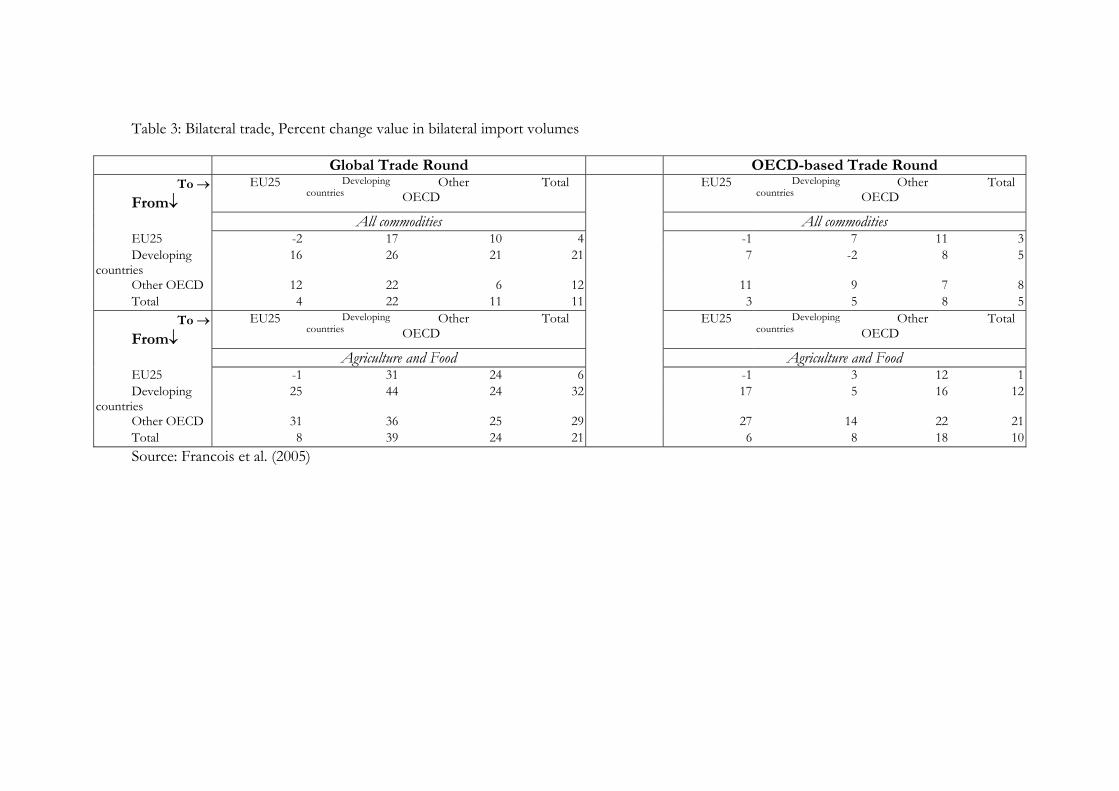
Table 3: Bilateral trade, Percent change value in bilateral import volumes Global Trade Round OECD-based Trade Round

To →From↓

EU25 Developing countries

Other OECD

Total EU25 Developing countries

Other OECD

Total

All commodities All commodities EU25 -2 17 10 4 -1 7 11 3 Developing

countries 16 26 21 21 7 -2 8 5

Other OECD 12 22 6 12 11 9 7 8 Total 4 22 11 11 3 5 8 5

To →From↓

EU25 Developing countries

Other OECD

Total EU25 Developing countries

Other OECD

Total

Agriculture and Food Agriculture and Food EU25 -1 31 24 6 -1 3 12 1 Developing

countries 25 44 24 32 17 5 16 12

Other OECD 31 36 25 29 27 14 22 21 Total 8 39 24 21 6 8 18 10 Source: Francois et al. (2005)

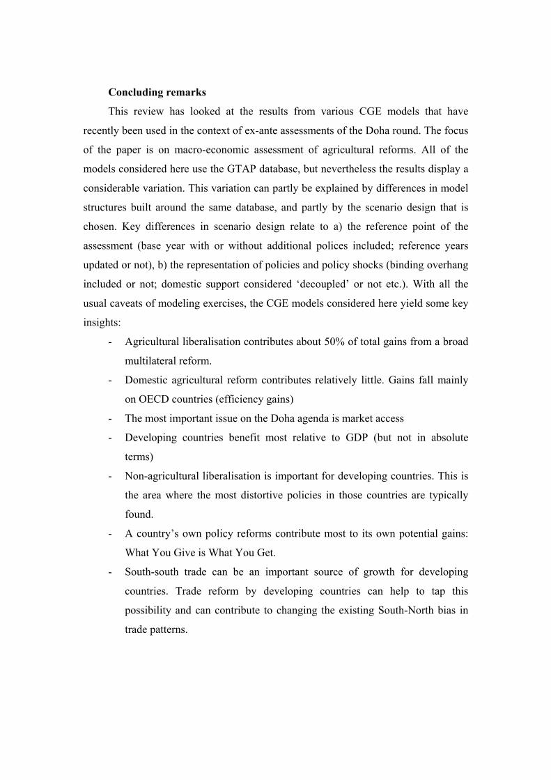
Concluding remarks

This review has looked at the results from various CGE models that have

recently been used in the context of ex-ante assessments of the Doha round. The focus

of the paper is on macro-economic assessment of agricultural reforms. All of the

models considered here use the GTAP database, but nevertheless the results display a

considerable variation. This variation can partly be explained by differences in model

structures built around the same database, and partly by the scenario design that is

chosen. Key differences in scenario design relate to a) the reference point of the

assessment (base year with or without additional polices included; reference years

updated or not), b) the representation of policies and policy shocks (binding overhang

included or not; domestic support considered ‘decoupled’ or not etc.). With all the

usual caveats of modeling exercises, the CGE models considered here yield some key

insights:

- Agricultural liberalisation contributes about 50% of total gains from a broad

multilateral reform.

- Domestic agricultural reform contributes relatively little. Gains fall mainly

on OECD countries (efficiency gains)

- The most important issue on the Doha agenda is market access

- Developing countries benefit most relative to GDP (but not in absolute

terms)

- Non-agricultural liberalisation is important for developing countries. This is

the area where the most distortive policies in those countries are typically

found.

- A country’s own policy reforms contribute most to its own potential gains:

What You Give is What You Get.

- South-south trade can be an important source of growth for developing

countries. Trade reform by developing countries can help to tap this

possibility and can contribute to changing the existing South-North bias in

trade patterns.

References

Anderson, K., B. Dimaranan, J. Francois, T. Hertel, B. Hoekman and W. Martin

(2001), “The Cost of Rich (and Poor) Country Protection to Developing

Countries”, Journal of African Economies 10(3): 227-57

Australian Bureau of Agricultural and Resource Economics, “Developing Countries:

Impact of Agricultural Trade Liberalization.” ABARE Current Issues, July 2000

Beghin, John C., D. Roland-Holst and D. van der Mensbrugghe (2002)“Global

Agricultural Trade and the Doha Round: What are the Implications for North

and South?”, CCNM/GF/AGR(2002)5

Bouët, Antoine, Lionel Fontagné and Sébastien Jean (2004), Is erosion of preferences

a serious concern? Paper presented at the World Bank conference, Agricultural

Trade Reform and the Doha Development Agenda, 1-2 December 2004, LEI

The Hague.

Francois, J.F., H. van Meijl and F.W. van Tongeren (2003), Economic Benefits of the

Doha Round for the Netherlands, report submitted to the Ministry of Economic

Affairs, Directorate-General for Foreign Economic Relations, Netherlands.

Francois, Joseph, Hans van Meijl and Frank van Tongeren (2005), Trade

liberalization in the Doha development Round, Economic Policy, vol 42 (April):

pp. 349 – 391.

International Monetary Fund and The World bank (2002), Market access for

developing countries exports – Selected issues. Mimeo, September 2002.

Kehoe Patrick J., Timothy J. Kehoe, A Primer on Static Applied General Equilibrium

Models, Federal Reserve Bank of Minneapolis Quarterly Review, Spring 1994,

Volume 18, No. 1

OECD (2003), “Doha Development Agenda: Welfare Gains from Further Multilateral

Trade Liberalisation with Respect to Tariffs”, TD/TC/WP(2003)10/Final, Paris.

2

OECD (2000), “The impact of further trade liberalization on the food security

situation in developing countries”, COM/AGR/TR/WP(2000)93, Paris.

Smith, Jeffrey A. , Petra E. Todd (2005), Does matching overcome LaLonde’s

critique of nonexperimental estimators?, Journal of Econometrics 125 (2005)

305–353

United Nations Economic Commission for Africa (2004), Trade Liberalization under

the Doha Development Agenda: Options and Consequences for Africa, draft.

U.S. Department of Agriculture (USDA), "The Road Ahead: Agricultural Policy

Reform in the WTO, Summary Report." Agriculture Economic Report No.

797, Washington, DC: Economic Research Service, U.S. Department of

Agriculture, January 2001

Van Meijl, J.C.M., and F.W. van Tongeren, “Multilateral trade liberalisation and

developing countries: A North-South perspective on agriculture and processing

sectors.” Agricultural Economics Research Institute (LEI), The Hague. Report

6.01.07, July 2001

Van Meijl Hans, and Frank van Tongeren (2002), The Agenda 2000 CAP reform, world

prices and URAA GATT-WTO export constraints, European Review of

Agricultural Economics, Vol. 29 (4) (2002) pp. 445-470.

Van Tongeren, Frank, Hans van Meijl, Yves Surry, (2001), Global models of trade in

agriculture: a review and assessment, Agricultural Economics. Vol 26:2, pp. 149-

172.

World Bank (2001) “Global Economic Prospects and the Developing Countries

2003.” The World Bank: Washington, DC, October 2001.

World Bank (2005) “Global Economic Prospects and the Developing Countries

2005.” The World Bank: Washington, DC.

3