Model Selection, Estimation, and Bootstrap Smoothingstatweb.stanford.edu/~ckirby/brad/talks/2012ModelSelection.pdf · Model Selection, Estimation, and Bootstrap Smoothing Bradley

Model Selection, Estimation,and Bootstrap Smoothing

Bradley Efron

Stanford University

Estimation After Model Selection

• Usually:

(a) look at data

(b) choose model (linear, quad, cubic . . . ?)

(c) fit estimates using chosen model

(d) analyze as if pre-chosen

• Today: include model selection process in the analysis

• Question:

Effects on standard errors, confidence intervals, etc.?

• Two Examples: nonparametric, parametric

Model Selection · Estimation · Bootstrap Smoothing 1

Cholesterol Data

• n = 164 men took Cholestyramine for ∼ 7 years

• x = compliance measure (adjusted: x ∼ N(0, 1))

• y = cholesterol decrease

• Regression y on x?

[wish to estimate: µ j = E{y|x j}, j = 1, 2, . . . ,n]


●

●●●

●

●

●●

●

●

● ●

●

●

●

● ●

●

●

●

●

●

●

●●●

●

●

●

●

●

●

●

●

●

●

●

●

●

●

●

●

●

●

●

●

●

●

●

●

●

●

●

●

●●

●

●

●

●

●

●

●

●

●

●

●

●

●

●

●●

●

●

●

●

●

●

●

●

●

●

●

●

●

●

●●

●

●

●

●

●●

●

●

●

●

●

●

●

●

●

●

●

●

●

●

●

●

●

●

●

●

●

●

●

●

●

●●

●

●

●

●

●

●

●

●●●

●

●

●

●

●

●

●

●

●

●

●

●

●●●

●

●

●

●

●

●

●

●

●●

●

●

●●

●

●

●

●

−2 −1 0 1 2

050

100

Cholesterol data, n=164 subjects: cholesterol decrease plottedversus adjusted compliance; Green curve is OLS cubic regression;

Red points indicate 5 featured subjects

compliance

chol

este

rol d

ecre

ase

●

●

●

●

●

1

2

3

4

5


Cp Selection Criterion

• Regression Model yn×1= X

n×mβ

m×1+ e

n×1

[ei ∼ (0, σ2)

]• Cp Criterion

∥∥∥y − Xβ∥∥∥2+ 2mσ2

β = OLS estimate, m = “degrees of freedom”

• Model Selection: From possible models X1,X2,X3, . . .

choose the one minimizing Cp.

• Then use OLS estimate from chosen model.


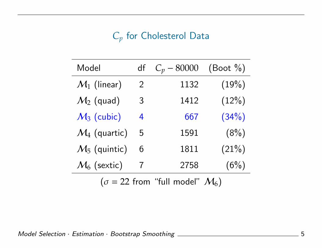
Cp for Cholesterol Data

Model df Cp − 80000 (Boot %)

M1 (linear) 2 1132 (19%)

M2 (quad) 3 1412 (12%)

M3 (cubic) 4 667 (34%)

M4 (quartic) 5 1591 (8%)

M5 (quintic) 6 1811 (21%)

M6 (sextic) 7 2758 (6%)

(σ = 22 from “full model” M6)


Nonparametric Bootstrap Analysis

• data = {(xi, yi), i = 1, 2, . . . ,n = 164} gave original estimate

µ = X3β3

• Bootstrap data set data∗ ={(x j, y j)∗, j = 1, 2, . . . ,n

}where

(x j, y j)∗ drawn randomly and with replacement from data:

data∗ −→Cp

m∗ −→OLS

β∗m∗ −→ µ∗ = Xm∗ β∗

m∗

• I did this all B = 4000 times.


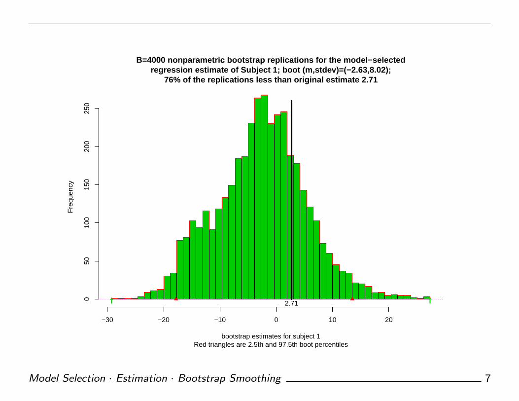
B=4000 nonparametric bootstrap replications for the model−selectedregression estimate of Subject 1; boot (m,stdev)=(−2.63,8.02);

76% of the replications less than original estimate 2.71

Red triangles are 2.5th and 97.5th boot percentilesbootstrap estimates for subject 1

Fre

quen

cy

−30 −20 −10 0 10 20

050

100

150

200

250

^ ^2.71


−3 −2 −1 0 1 2 3

−3

−2

−1

01

23

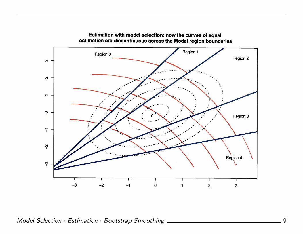
Smooth Estimation Model: ' y ' is observed data; Ellipses indicate bootstrap distribution for ' y* ';

Red curves level surfaces of equal estimation for thetahat=t(y)

thetahat=t(y)

●

y



●●

●

●

●

●

●●●●

●

●

●

●

●●●

●

●●●●●

●

●

●

●

●●

●

●

●●

●

●●

●●

●

●

●

●

●●

●

●

●

●

●

● ●

●

●

●

●

●

●

●

●

●

●

●

●

●

●

●

●

●

●●

●

●

●

●

●●

●

●

●

●

●

●

●

●

1 2 3 4 5 6

−40

−30

−20

−10

010

2030

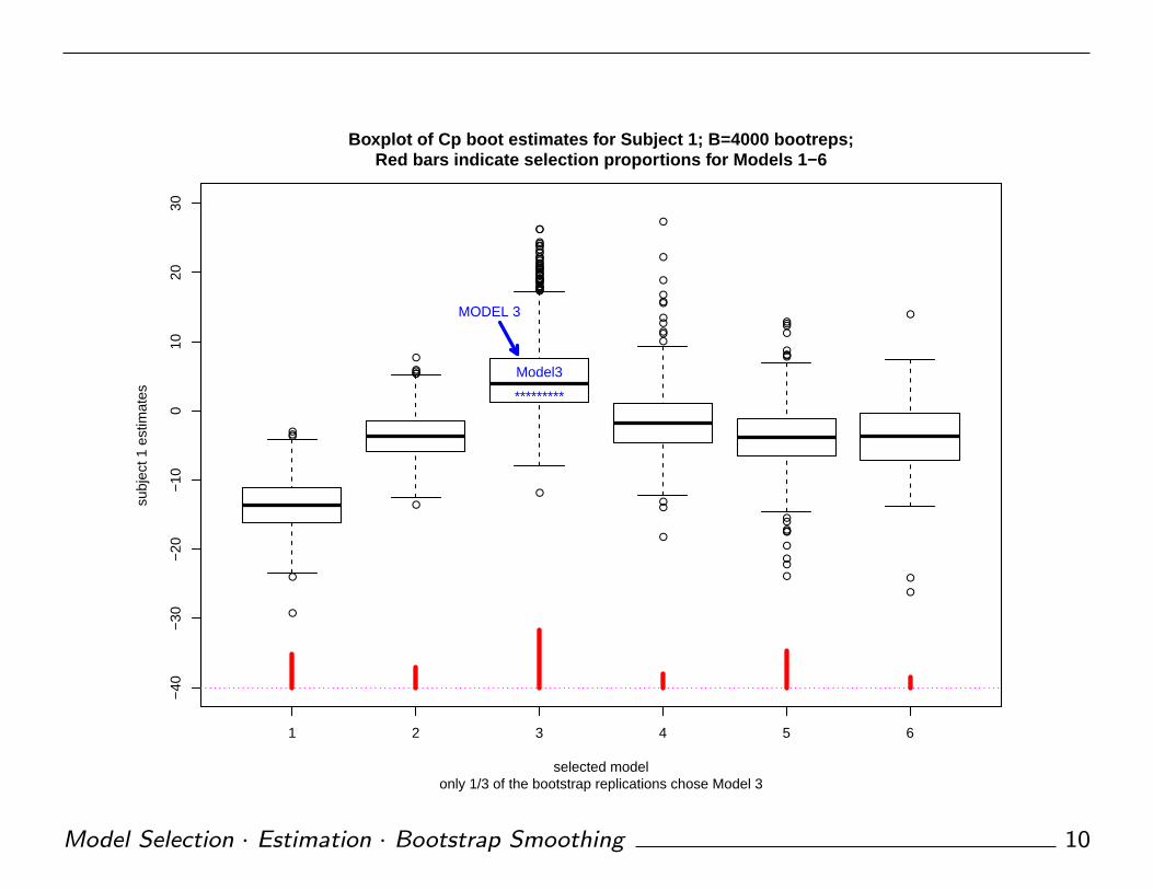
Boxplot of Cp boot estimates for Subject 1; B=4000 bootreps;Red bars indicate selection proportions for Models 1−6

only 1/3 of the bootstrap replications chose Model 3selected model

subj

ect 1

est

imat

es

Model3

*********

MODEL 3


Bootstrap Confidence Intervals

• Standard: µ ± 1.96 se

• Percentile:[µ∗(.025), µ∗(.975)

]• Smoothed Standard: µ ± 1.96 se

• BCa/ABC: corrects percentiles for bias and changing se


0.5 1.0 1.5 2.0 2.5 3.0 3.5

−20

−10

010

20

95% Bootstrap Confidence Intervals for Subject 1C

onfid

ence

Inte

rval

●

●

●

●

●

●

Standard(−13.0,18.4)

Percentile(−17.8,13.5)

Smoothed(−13.3,8.0)


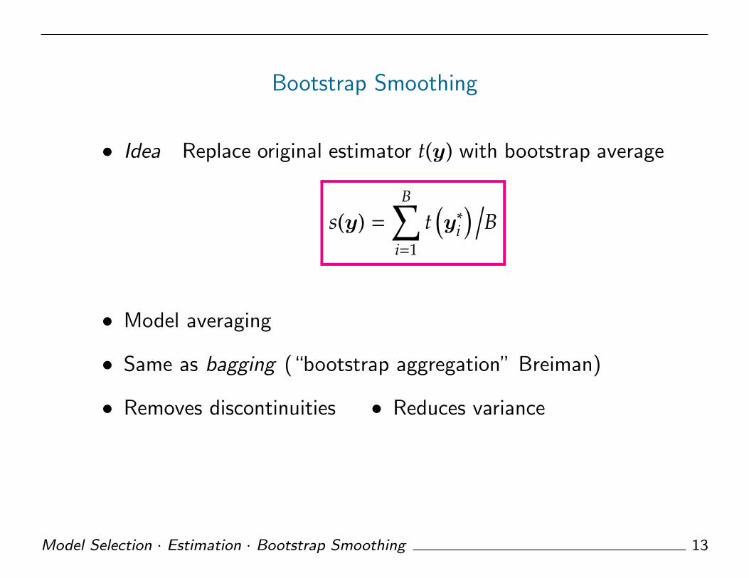
Bootstrap Smoothing

• Idea Replace original estimator t(y) with bootstrap average

s(y) =B∑

i=1

t(y∗i

) /B

• Model averaging

• Same as bagging (“bootstrap aggregation” Breiman)

• Removes discontinuities • Reduces variance


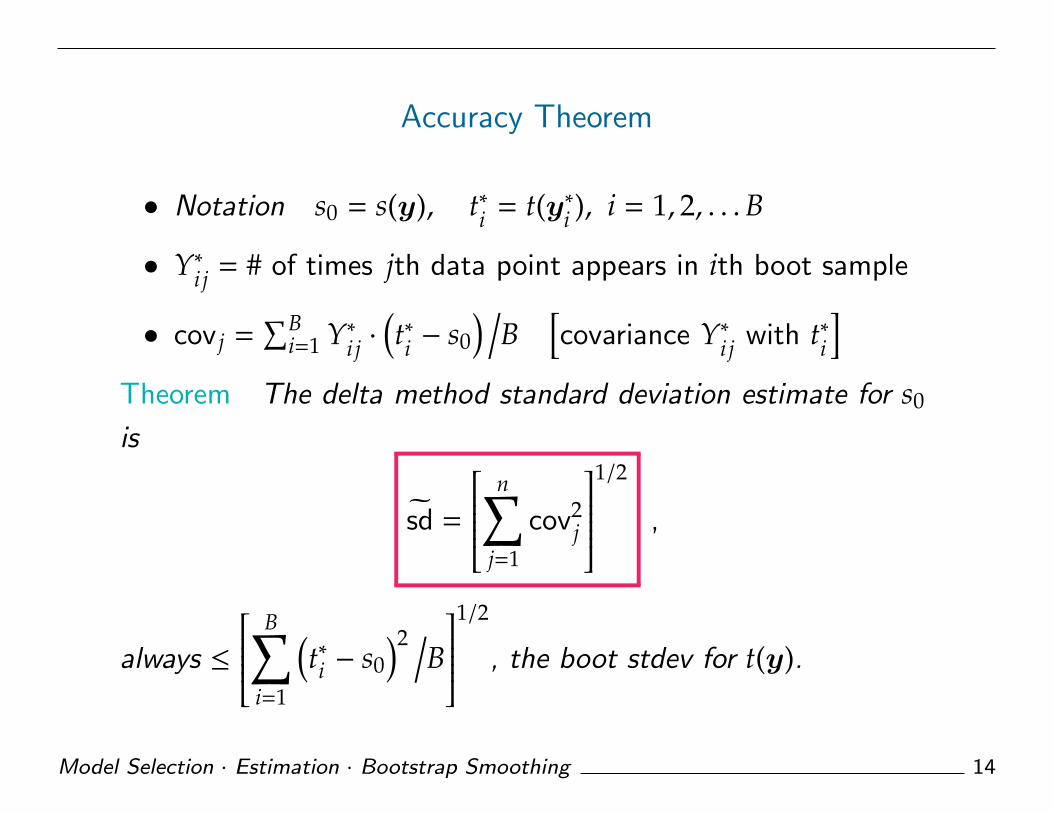
Accuracy Theorem

• Notation s0 = s(y), t∗i = t(y∗i ), i = 1, 2, . . .B

• Y∗i j = # of times jth data point appears in ith boot sample

• cov j =∑B

i=1 Y∗i j ·(t∗i − s0

) /B

[covariance Y∗i j with t∗i

]Theorem The delta method standard deviation estimate for s0

is

sd =

n∑j=1

cov2j

1/2

,

always ≤

B∑i=1

(t∗i − s0

)2 /B

1/2

, the boot stdev for t(y).


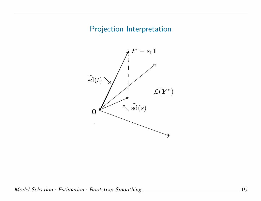
Projection Interpretation

0


1 2 3 4 5

0.0

0.2

0.4

0.6

0.8

1.0

1.2

Standard Deviation of smoothed estimate relative to original (Red)for five subjects; green line is stdev Naive Cubic Model

bottom numbers show original standard deviationsSubject number

Rel

ativ

e st

dev

● ● ● ● ●

7.9 3.9 4.1 4.7 6.8

●

●

●

●

●

*

* *

*

*


How Many Bootstrap Replications Are Enough?

• How accurate is sd? Jackknife

• Divide the 4000 bootreps t∗i into 20 groups of 200 each

• Recompute sd with each group removed in turn

• Jackknife gave coef variation(sd

)� 0.02 for all 164 subjects

(could have stopped at B = 500)


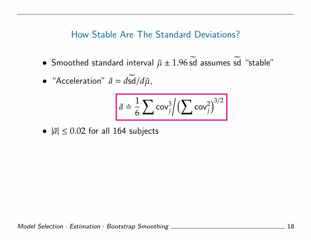
How Stable Are The Standard Deviations?

• Smoothed standard interval µ ± 1.96 sd assumes sd “stable”

• “Acceleration” a = dsd/dµ,

a �16

∑cov3

j

/ (∑cov2

j

)3/2

• |a| ≤ 0.02 for all 164 subjects


Model Probability Estimates

• 34% of the 4000 bootreps chose the cubic model

• Poor man’s Bayes posterior prob for “cubic”

• How accurate is that 34%?

• Apply accuracy theorem to indicator function for choosing

“cubic”


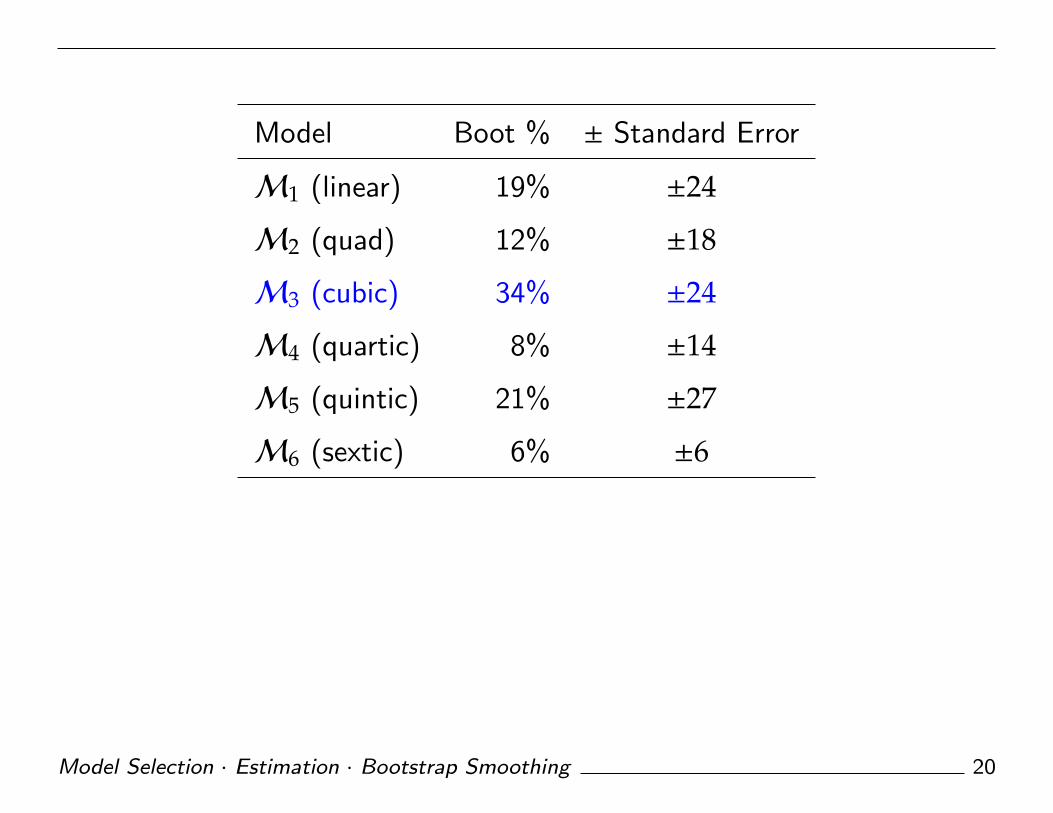
Model Boot % ± Standard Error

M1 (linear) 19% ±24

M2 (quad) 12% ±18

M3 (cubic) 34% ±24

M4 (quartic) 8% ±14

M5 (quintic) 21% ±27

M6 (sextic) 6% ±6


The Supernova Data

• data ={(x j, y j), j = 1, 2, . . . ,n = 39

}• y j = absolute magnitude of Type Ia supernova

• x j = vector of 10 spectral energies (350–850nm)

• Full Model y = X39×10

β + e[ei

ind∼ N(0, 1)

]


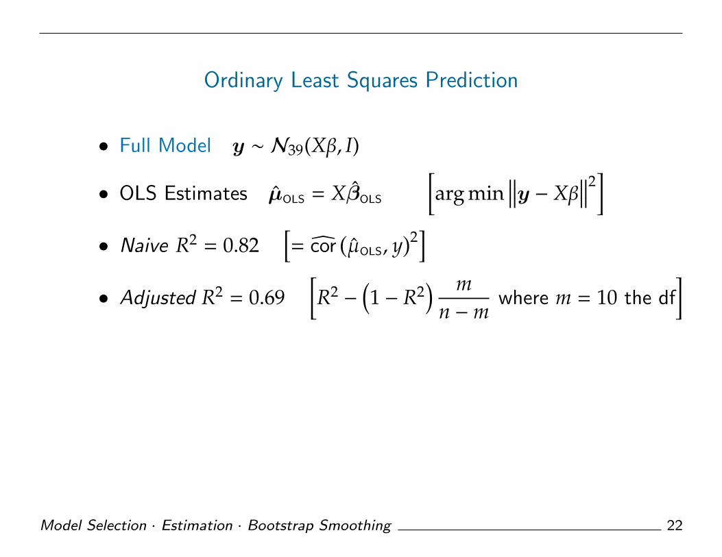
Ordinary Least Squares Prediction

• Full Model y ∼ N39(Xβ, I)

• OLS Estimates µOLS = XβOLS

[arg min

∥∥∥y − Xβ∥∥∥2

]• Naive R2 = 0.82

[= cor

(µOLS, y

)2]

• Adjusted R2 = 0.69[R2−

(1 − R2

) mn −m

where m = 10 the df]


●

●

●

●

●

●

●

●

●

●

●

●

●

●

●

●

●●●

●

●

●●

●

●

●

●

●

●

●

●

●●

●

●

●

●

●

●

−4 −2 0 2 4 6

−4

−2

02

46

Adjusted absolute magnitudes for 39 Type1A supernovas plotted versus OLS predictions from 10 spectral measurments;

Naive R2 (squared correlation)=.82; Adjusted R2=.62

Red points are 5 featured casesFull Model OLS Prediction−−>

Abs

olut

e M

agni

tude

−−

>

●

●

●

●

●

1

2

3

4

5


Lasso Model Selection

• Lasso estimate is β minimizing∥∥∥y − Xβ

∥∥∥2+ λ

p∑1

∣∣∣βk

∣∣∣• Shrinks OLS estimates toward zero (all the way for some)

• Degrees of freedom “m” = number of nonzero βk’s

• Model Selection: Choose λ (or m) to maximize adjusted R2.

• Then µ = Xβm.


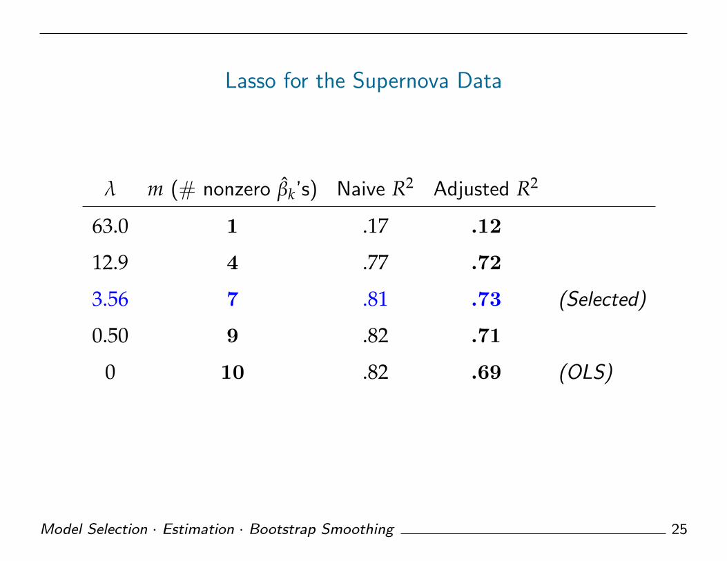
Lasso for the Supernova Data

λ m (# nonzero βk’s) Naive R2 Adjusted R2

63.0 1 .17 .12

12.9 4 .77 .72

3.56 7 .81 .73 (Selected)

0.50 9 .82 .71

0 10 .82 .69 (OLS)


Parametric Bootstrap Smoothing

• Original Estimates

yLasso−→ m, βm −→ µ = Xβm

• Full Model Bootstrap y∗ ∼ N39 (µOLS, I)

y∗ −→ m∗, β∗m∗ −→ µ∗ = Xβ∗m∗

• I did this all B = 4000 times. • t∗ik = µ∗

ik

• Smoothed Estimates sk =

4000∑i=1

t∗ik/4000 [k = 1, 2, . . . , 39]


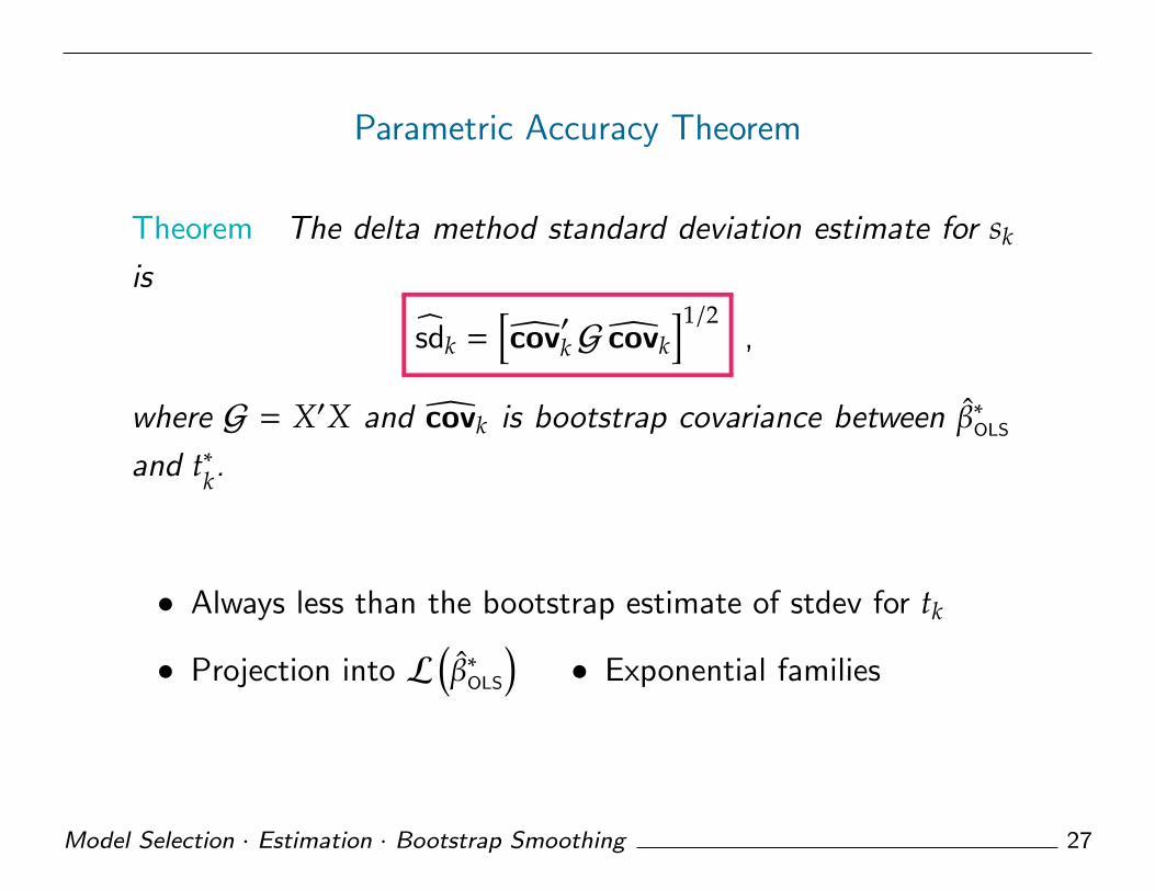
Parametric Accuracy Theorem

Theorem The delta method standard deviation estimate for sk

is

sdk =[cov

′

kG covk

]1/2,

where G = X′X and covk is bootstrap covariance between β∗OLS

and t∗k.

• Always less than the bootstrap estimate of stdev for tk

• Projection into L(β∗OLS

)• Exponential families


1 2 3 4 5

0.0

0.2

0.4

0.6

0.8

1.0

1.2

Standard Deviation of smoothed estimate relative to original (Red)for five Supernova; green line using Bootstrap reweighting

bottom numbers show original standard deviationsSupernova number

Rel

ativ

e st

dev

● ● ● ● ●

0.37 0.36 0.53 0.24 0.6

●

● ●

●

●*

**

*

*


Better Confidence Intervals

• Smoothed standard intervals and percentile intervals have

coverage errors of order O(1/√

n).

• “ABC” intervals have errors O(1/n): corrects for bias and

“acceleration” (change in stdev as estimate varies).

• Uses local reweighting for 2nd order correction


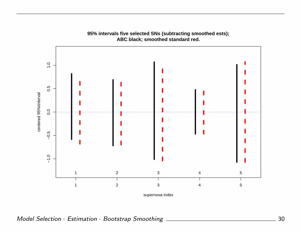
1 2 3 4 5

−1.

0−

0.5

0.0

0.5

1.0

95% intervals five selected SNs (subtracting smoothed ests);ABC black; smoothed standard red.

supernova index

cent

ered

95%

iInte

rval

1 2 3 4 5


Brute Force Simulation

• Sample 500 times: y∗ ∼ N(µOLS, I

); gives µ∗OLS

• Resample B = 1000 times: y∗∗ ∼ N(µ∗OLS, I

)• Use ABC to get sd, bias, ˜acceleration

• Calculate ABC coverage of one-sided interval (−∞, sk)

[sk the original smoothed estimate]

• Should be uniform [0, 1]


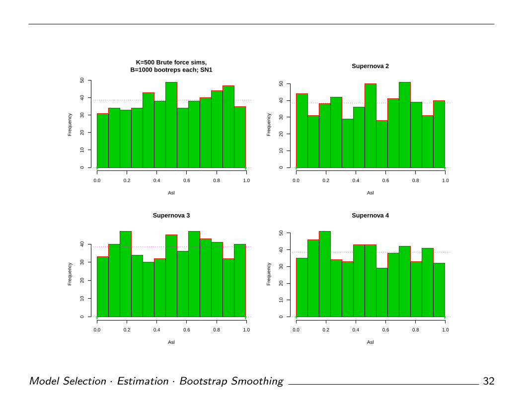
K=500 Brute force sims,B=1000 bootreps each; SN1

Asl

Fre

quen

cy

0.0 0.2 0.4 0.6 0.8 1.0

010

2030

4050

^ ^

Supernova 2

Asl

Fre

quen

cy

0.0 0.2 0.4 0.6 0.8 1.0

010

2030

4050

^ ^

Supernova 3

Asl

Fre

quen

cy

0.0 0.2 0.4 0.6 0.8 1.0

010

2030

40

^ ^

Supernova 4

Asl

Fre

quen

cy

0.0 0.2 0.4 0.6 0.8 1.0

010

2030

4050

^ ^


References

Berk, R., Brown, L., Buja, A., Zhang, K. and Zhao, L. (2012).

Valid post-selection inference. Submitted Ann. Statist. http:

//stat.wharton.upenn.edu/˜zhangk/PoSI-submit.pdf;

conservative frequentist intervals a la Tukey, Scheffe.

Buja, A. and Stuetzle, W. (2006). Observations on bagging.

Statist. Sinica 16: 323–351, more on bagging.

DiCiccio, T. J. and Efron, B. (1992). More accurate confidence

intervals in exponential families. Biometrika 79: 231–245,

ABC confidence intervals.

DiCiccio, T. J. and Efron, B. (1996). Bootstrap confidence


http://stat.wharton.upenn.edu/~zhangk/PoSI-submit.pdf

http://stat.wharton.upenn.edu/~zhangk/PoSI-submit.pdf

intervals. Statist. Sci. 11: 189–228, with comments and a

rejoinder by the authors.

Hastie, T., Tibshirani, R. and Friedman, J. (2009). The Elements

of Statistical Learning . Springer Series in Statistics. New York:

Springer, 2nd ed., Section 8.7, bagging.

Hjort, N. L. and Claeskens, G. (2003). Frequentist model average

estimators. J. Amer. Statist. Assoc. 98: 879–899, model

selection asymptotics.


Model Selection, Estimation, and Bootstrap Smoothingstatweb.stanford.edu/~ckirby/brad/talks/2012ModelSelection.pdf · Model Selection, Estimation, and Bootstrap Smoothing Bradley

Documents