J¨ornZimmerling (TU Delft) Model reduction of wave propagation November 8, 2017 1 / 37 Model reduction of wave propagation via phase-preconditioned rational Krylov subspaces Delft University of Technology † and Schlumberger * V. Druskin * , R. Remis † , M. Zaslavsky * , J¨ orn Zimmerling † November 8, 2017

Welcome message from author
This document is posted to help you gain knowledge. Please leave a comment to let me know what you think about it! Share it to your friends and learn new things together.
Transcript

Jorn Zimmerling (TU Delft) Model reduction of wave propagation November 8, 2017 1 / 37
Model reduction of wave propagationvia phase-preconditioned rational Krylov subspacesDelft University of Technology† and Schlumberger∗
V. Druskin∗, R. Remis†, M. Zaslavsky∗, Jorn Zimmerling†
November 8, 2017

Motivation
• Second order wave equation withwave operator A
Au− s2u = −δ(x− xS)
• Assume N grid steps in everyspatial direction
• Scaling of surface seismic in 3D:
• # Grid points O(N3)
• # Sources O(N2)
• # Frequencies O(N)
• Overall O(N6)ψ(N3)
500 1000 1500
y-direction [m]
500
1000
1500
2000
2500
3000
x-d
irection [m
]
Receiver
Source
PML
1500
2000
2500
3000
3500
4000
4500
5000
5500
Wavespeed [m
/s]
(a) Section of wave speed profileof the Marmousi model.
Jorn Zimmerling (TU Delft) Model reduction of wave propagation November 8, 2017 2 / 37

Goal of this work
• Simulate and compress large scale wave fields in modern highperformance computing environment(parallel CPU and GPU environment)
• Use projection based model order reduction to• Approximate transfer function• reduce # of frequencies needed to solve• reduce # of sources to be considered• reduce # number of grid points needed
Jorn Zimmerling (TU Delft) Model reduction of wave propagation November 8, 2017 3 / 37
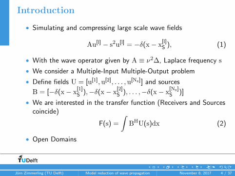
Introduction
• Simulating and compressing large scale wave fields
Au[l] − s2u[l] = −δ(x− x[l]S ), (1)
• With the wave operator given by A ≡ ν2∆, Laplace frequency s
• We consider a Multiple-Input Multiple-Output problem
• Define fields U = [u[1],u[2], . . . ,u[Ns]] and sources
B = [−δ(x− x[1]S ),−δ(x− x
[2]S ), . . . ,−δ(x− x
[Ns]S )]
• We are interested in the transfer function (Receivers and Sourcescoincide)
F(s) =
∫BHU(s)dx (2)
• Open Domains
Jorn Zimmerling (TU Delft) Model reduction of wave propagation November 8, 2017 4 / 37

Problem Formulation
• After finite difference discretization with PML
(A(s)− s2I)U = B
• Step sizes inside the PML hi = αi + βis
• Frequency dependent A(s) caused by absorbing boundary
Q(s)U = B with Q(s) ∈ CN×N
• Q(s) propterties• sparse• complex symmetric (reciprocity)• Schwarz reflection principle Q(s) = Q(s)• passive (nonlinear NR1 Re < 0)
1NR:W {A(s)} ={s ∈ C : xHA(s)x = 0 ∀x ∈ Ck\0
}
Jorn Zimmerling (TU Delft) Model reduction of wave propagation November 8, 2017 5 / 37
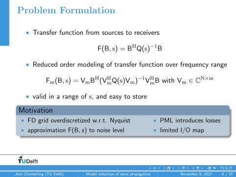
Problem Formulation
• Transfer function from sources to receivers
F(B, s) = BHQ(s)−1B
• Reduced order modeling of transfer function over frequency range
Fm(B, s) = VmBH(VHmQ(s)Vm)−1VH
mB with Vm ∈ CN×m
• valid in a range of s, and easy to store
Motivation• FD grid overdiscretized w.r.t. Nyquist
• approximation F(B, s) to noise level
• PML introduces losses
• limited I/O map
Jorn Zimmerling (TU Delft) Model reduction of wave propagation November 8, 2017 6 / 37
Outline
1 Problem formulation
2 Model order reduction – Rational Krylov subspaces
3 Phase-Preconditioning
4 Numerical Experiments
5 Conclusions
Jorn Zimmerling (TU Delft) Model reduction of wave propagation November 8, 2017 7 / 37

Structure preserving rational Krylov subspaces
• Preserve: symmetry (w.r.t. matrix, frequency), passivity
• Block rational Krylov subspace approach κ = s1, . . . , sm
Km(κ) = span{
Q(s1)−1B, . . . ,Q(sm)−1B}
K2mRe = span {Km(κ),Km(κ)}
• Let Vm be a (real) basis for KmRe then with reduced order model
(via Galerkin condition)
Rm(s) = VHmQ(s)Vm
we approximate
Fm(s) = (VHmB)HRm(s)−1VH
mB,
Jorn Zimmerling (TU Delft) Model reduction of wave propagation November 8, 2017 8 / 37

Structure preserving rational Krylov subspaces
• Numerical Range: W {Rm(s)} ⊆ W {Q(s)}Proof: xHmRm(s)xm = (Vmxm)HQ(s)(Vmxm)⇒ Rm(s) is passive
• Fm(s) is Hermite interpolant of F(s) on κ ∪ κQ(κ)−1B ∈ K2m
Re + uniqueness of Galerkin
• Schwarz reflection and symmetry hold aswell
Jorn Zimmerling (TU Delft) Model reduction of wave propagation November 8, 2017 9 / 37

RKS for a Resonant cavity
0 0.1 0.2 0.3 0.4 0.5
Normalized Frequency
0
1
2
3
4
5
6R
espo
nse
[a.u
]FDFD ResponseRKS Response m=60RKS Response m=20
20 40 60 80 100 120
y-direction
20
40
60
80
100
120
x-d
ire
ctio
n
Receiver
Source
PML
0
0.2
0.4
0.6
0.8
1
• RKS has excellent convergence if singular Hankel values ofsystem decay fast (few contributing eigenvectors)
• Fm(s) is a [2m − 1/2m] rational function
Jorn Zimmerling (TU Delft) Model reduction of wave propagation November 8, 2017 10 / 37
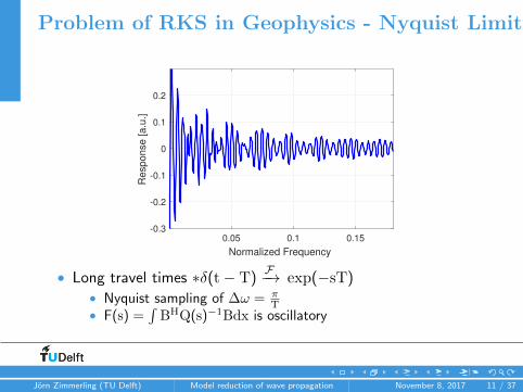
Problem of RKS in Geophysics - Nyquist Limit
0.05 0.1 0.15
Normalized Frequency
-0.3
-0.2
-0.1
0
0.1
0.2
Re
sp
on
se
[a
.u.]
• Long travel times ∗δ(t− T)F−→ exp(−sT)
• Nyquist sampling of ∆ω = πT
• F(s) =∫
BHQ(s)−1Bdx is oscillatory
Jorn Zimmerling (TU Delft) Model reduction of wave propagation November 8, 2017 11 / 37

Filion Quadrature
• Filion quadrature deals with oscillatory integral
F(s) =
∫exp(st) f(t)dt
quadrature requires s∆t � 1
F(s) ≈ ∆t∑n
an exp(s n∆t) f(n∆t)
• Filion quadrature makes an function of s∆t
F(s) ≈ ∆t∑n
an(s∆t) exp(s n∆t) f(n∆t)
• ⇒ Make projection basis s dependent
• ⇒ Frequency dependence from asymptotic s→ i∞ (WKB)
Jorn Zimmerling (TU Delft) Model reduction of wave propagation November 8, 2017 12 / 37
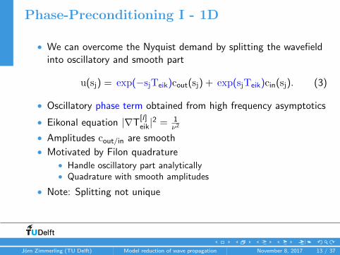
Phase-Preconditioning I - 1D
• We can overcome the Nyquist demand by splitting the wavefieldinto oscillatory and smooth part
u(sj) = exp(−sjTeik)cout(sj) + exp(sjTeik)cin(sj). (3)
• Oscillatory phase term obtained from high frequency asymptotics
• Eikonal equation |∇T[l ]eik|
2 = 1ν2
• Amplitudes cout/in are smooth
• Motivated by Filon quadrature• Handle oscillatory part analytically• Quadrature with smooth amplitudes
• Note: Splitting not unique
Jorn Zimmerling (TU Delft) Model reduction of wave propagation November 8, 2017 13 / 37

Phase-Preconditioning II
• Projection on frequency dependent Reduced Order Basis
K2mEIK(κ, s) = span{ exp(−sTeik) cout(s1), . . . , exp(−sTeik) cout(sm),
exp( sTeik) cin (ss), . . . , exp( sTeik) cin (sm)}
• Preserve Schwartz reflection principle
K4mEIK;R(κ, s) = span
{K2m
EIK(κ, s),K2mEIK(κ, s)
}(4)
• equivalent to changing Operator
• Coefficients from Galerkin condition
um(s) =m∑i=1
αi (s) exp(−sTeik) cout(si )+m∑i=1
βi (s) exp(sTeik) cin(si )+. . .
Jorn Zimmerling (TU Delft) Model reduction of wave propagation November 8, 2017 14 / 37

Phase-Preconditioning III
• Non-uniqueness of splitting resolved by one-way WEQ
cout(sj) =ν
2sjexp( sjTeik)
(sjνu(sj)−
∂
∂|x − xS|u(sj)
), (5)
cin (sj) =ν
2sjexp(−sjTeik)
(sjνu(sj) +
∂
∂|x − xS|u(sj)
). (6)
Effects of Phase preconditioning on
• Number of Interpolation points
• Size of the computational Grid
• MIMO problems
• Computational Scheme
Jorn Zimmerling (TU Delft) Model reduction of wave propagation November 8, 2017 15 / 37

Projection on frequency dependent space
• Let Vm;EIK(s) be a real basis of K4mEIK;R(κ, s)
• The reduced order model is given by
Rm;EIK(s) = VHm;EIK(s)Q(s)Vm;EIK(s).
• large inner products on GPU
• This preserves• symmetry• Schwarz reflection principle• passivity• Interpolation
Jorn Zimmerling (TU Delft) Model reduction of wave propagation November 8, 2017 16 / 37

Number of interpolation points needed
• Double interpolation of transfer function still holds
Fm(s) = Fm(s) andd
dsFm(s) =
d
dsF(s) with s ∈ κ ∪ κ. (7)
• Number of interpolation point needed dependent on complexitymedium, not latest arrival
• Proposition: Let a 1D problem have ` homogenous layers .Then there exist m ≤ `+ 1 non-coinciding interpolation points,such that the solution um;EIK(s) = u.
Jorn Zimmerling (TU Delft) Model reduction of wave propagation November 8, 2017 17 / 37

Illustration of Proposition
Source L1 L2 L3 L4 L5 L6 L70
0.5
1
Wavespeed
Source L1 L2 L3 L4 L5 L6 L7-10
0
10Real part field
Source L1 L2 L3 L4 L5 L6 L70
5
10Imag(C) outgooing
Source L1 L2 L3 L4 L5 L6 L70
2
4Imag(C) incoming
• Amplitudes are constants in layers + left and right of source
• Basis is complete after `+ 1 iterations
Jorn Zimmerling (TU Delft) Model reduction of wave propagation November 8, 2017 18 / 37

Phase-Preconditioning higherdimensions/MIMO
• Split with dimension specific function
u(sj)[l] = g(sjT
[l]eik)cout(sj)
[l] + g(−sjT[l]eik)cin(sj)
[l], (8)
• g(x) obtained from WKB approximation
• One way wave equations along ∇Teik used for decomposition
• In 2D is we use g(x) = K0 (x) for outgoing
• Multiple T[l]eik for multiple sources [l] account for multiple
direction
cin(sj) =sjT
sign(Im (sj))iπ
[K1 (sjT) u(sj) +K0 (sjT)
ν2
sj∇T · ∇u(sj)
]
Jorn Zimmerling (TU Delft) Model reduction of wave propagation November 8, 2017 19 / 37

Size of the computational Grid
500 1000 1500
y-direction [m]
500
1000
1500
2000
2500
3000
x-d
irection [m
]
Receiver
Source
PML
1500
2000
2500
3000
3500
4000
4500
5000
wa
ve
sp
ee
d [
m/s
]
(b) Section of the wave speed profile ofthe smoothed Marmousi model.
(c) Real part of thewavefield u[4].
(d) Real part of the
amplitude c[4]out.
Jorn Zimmerling (TU Delft) Model reduction of wave propagation November 8, 2017 20 / 37

Numerical Experiments - I
• Configurations (Neumann boundarycondition on top)
• Layered medium
• Travel time dominated
• 5 Sources and 5 Receivers∆x 4mComp. Size 829x480 pointsSize 3160 m x 1920mrange c 1500 - 5500 m/sRange Quadrature 0-40 Hz
500 1000 1500
y-direction [m]
500
1000
1500
2000
2500
3000
x-d
ire
ctio
n [
m]
Receiver
Source
PML
1500
2000
2500
3000
3500
4000
4500
5000
wavespeed [m
/s]
(e) Section of the wave speedprofile of the smoothed Marmousimodel.
Jorn Zimmerling (TU Delft) Model reduction of wave propagation November 8, 2017 21 / 37

Numerical Experiments
0 0.05 0.1 0.15
normalized frequency
-0.6
-0.4
-0.2
0
0.2
0.4
response [a.u
.]
Full Response
RKS m=20
PPRKS m=20
Interpolation points
(f) Real part of the frequency-domain transfer function
• Source 1 toReceiver 5
• PPRKS clearlyoutperformsRKS
Jorn Zimmerling (TU Delft) Model reduction of wave propagation November 8, 2017 22 / 37
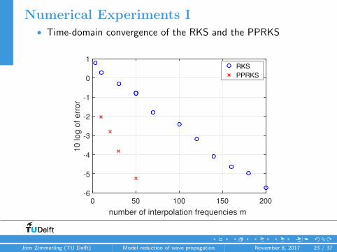
Numerical Experiments I• Time-domain convergence of the RKS and the PPRKS
0 50 100 150 200
number of interpolation frequencies m
-6
-5
-4
-3
-2
-1
0
1
10 log o
f err
or
RKS
PPRKS
(g)
Jorn Zimmerling (TU Delft) Model reduction of wave propagation November 8, 2017 23 / 37
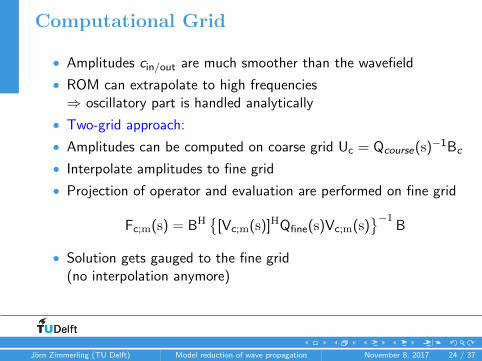
Computational Grid
• Amplitudes cin/out are much smoother than the wavefield
• ROM can extrapolate to high frequencies⇒ oscillatory part is handled analytically
• Two-grid approach:
• Amplitudes can be computed on coarse grid Uc = Qcourse(s)−1Bc
• Interpolate amplitudes to fine grid
• Projection of operator and evaluation are performed on fine grid
Fc;m(s) = BH{
[Vc;m(s)]HQfine(s)Vc;m(s)}−1
B
• Solution gets gauged to the fine grid(no interpolation anymore)
Jorn Zimmerling (TU Delft) Model reduction of wave propagation November 8, 2017 24 / 37

Phase-Preconditioning SVD• Amplitudes are smooth in space and can become redundant• Reduce amplitudes via SVD of [cout cin]⇒ c jSVD• Amplitudes have no source information
0 100 200 300 400 500index singular value
-4
-3.5
-3
-2.5
-2
-1.5
-1
-0.5
0
10
log
no
rma
lize
d s
ing
ula
r va
lue
s
RKSContracted amplitude basis
(h) Singular values of normalized (cout cin)
# singular values larger than 0.01
versus # sources with m = 40
Nsrc 12 24 48 96
[cout, cin] 69 72 73 73u 457 833 1369 1741m · Nsrc 480 960 1920 3840
⇒ Reduction of sources
Jorn Zimmerling (TU Delft) Model reduction of wave propagation November 8, 2017 25 / 37

Phase-Preconditioning SVD
• Assume s ∈ iR then we obtain
u[l ]m (s) =
Nsrc∑r=1
MSVD∑j=1
[a
[l ]rj
α[l ]rj
]T [g(sT
[r ]eik)c jSVD
g(−sT [r ]eik)c jSVD
](9)
where MSVD � 2mNsrc.
• Coefficients from Galerkin condition
• c jSVD is no longer source dependent
Jorn Zimmerling (TU Delft) Model reduction of wave propagation November 8, 2017 26 / 37

Computational Scheme - Coarse Grid - CPU
ROM Construction phase
EmbarrassinglyParallel
ROM Evaluation Phase
Initialize Simulation
Compute T[l ]eik
Solve coarse problemsingle shot/frequency
Qcoarse(κi )u[l ](κi ) = b[l ]
Compute SVD of
c[l ]out and c
[l ]in
Evaluate ROM single Frequency se
Hm;EIK = Vm;EIK(se)HQfineVm;EIK(se)
Fc,m = BHs Vm;EIK(se)H−1
m;EIKVm;EIK(se)HBs
Compute inverseFourier Transform
Fm;c(t) = F−1Fm;c(iω)
Jorn Zimmerling (TU Delft) Model reduction of wave propagation November 8, 2017 27 / 37

Computational Scheme - Fine Grid - GPU
ROM Evaluation Phase
Compute SVD of
c[l ]out and c
[l ]in
Evaluate ROM single Frequency se
Rm;EIK = Vm;EIK(se)HQfineVm;EIK(se)
Fc,m = BHs Vm;EIK(se)R−1
m;EIKVm;EIK(se)HBs
Compute inverseFourier Transform
Fm;c(t) = F−1Fm;c(iω)
Jorn Zimmerling (TU Delft) Model reduction of wave propagation November 8, 2017 28 / 37
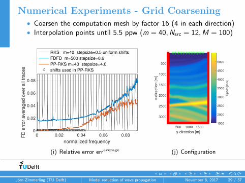
Numerical Experiments - Grid Coarsening• Coarsen the computation mesh by factor 16 (4 in each direction)• Interpolation points until 5.5 ppw (m = 40,Nsrc = 12,M = 100)
0 0.02 0.04 0.06 0.08
normalized frequency
0
0.02
0.04
0.06
0.08
FD
err
or
ave
rag
ed
ove
r a
ll tr
ace
s
RKS m=40 stepsize=0.5 uniform shifts
FDFD m=500 stepsize=0.6
PP-RKS m=40 stepsize=4.0
shifts used in PP-RKS
(i) Relative error erraverage
500 1000 1500
y-direction [m]
500
1000
1500
2000
2500
3000
x-d
irection [m
]
1500
2000
2500
3000
3500
4000
4500
5000
Speed [m
/s]
(j) Configuration
Figure: Smooth Marmousi test configuration with grid coarsening.
Jorn Zimmerling (TU Delft) Model reduction of wave propagation November 8, 2017 29 / 37

Numerical Experiments - Grid Coarsening• Projection of fine operator gauges the ROM• Direct evaluation of coarse operator not accurate
10 20 30 40 50points per wavelength
10-3
10-2
10-1
100
FD
err
or
avera
ged
ove
r all
trace
s
Direct evaluation of 500 frequency points
PPRKS with m=40 shifts
(k) erraverageROM;coarse versus erraverageFD;coarse
Figure: Smooth Marmousi test configuration with grid coarsening.
Jorn Zimmerling (TU Delft) Model reduction of wave propagation November 8, 2017 30 / 37

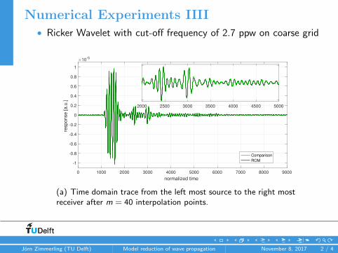
Numerical Experiments - Grid Coarsening• Ricker Wavelet with cut-off frequency of 2.7 ppw on coarse grid
0 1000 2000 3000 4000 5000 6000 7000
normalized time
-8
-6
-4
-2
0
2
4
6
response [a.u
.]
×10-6
Comparison
ROM
2000 2500 3000 3500 4000 4500 5000
(l) Time domain trace from the left most source to the right mostreceiver after m = 40 interpolation points.
Jorn Zimmerling (TU Delft) Model reduction of wave propagation November 8, 2017 31 / 37

Numerical Experiment III
• Resonant Borehole in smoothGeology
• Resonant behavior causeslong runtimes
• 6 Surface- and 8 BHsource-receiver pairs
200 600 1000
y-direction [m]
500
1000
1500
2000
2500
x-d
ire
ctio
n [
m]
Reiceiver
Source
PML
1500
2000
2500
3000
3500
4000
4500
5000
wavespeed [m
/s]
1
2
3
4
5
6
7
8
9 14
(m) Simulated configuration.
Jorn Zimmerling (TU Delft) Model reduction of wave propagation November 8, 2017 32 / 37

Numerical Experiments III
200 600 1000
y-direction [m]
500
1000
1500
2000
2500
x-di
rect
ion
[m]
ReiceiverSourcePML
1000
2000
3000
4000
5000
Spe
ed [m
/s]
(n) Isosurfaces Teik.
200 600 1000
y-direction [m]
500
1000
1500
2000
2500
x-di
rect
ion
[m]
ReiceiverSourcePML
1000
2000
3000
4000
5000
Spe
ed [m
/s]
(o) Isosurf. Teik;CM.
u[l ](sj) = g(sjT[l ]eik)c
[l ]out;eik(sj)
+ g(−sjT[l ]eik)c
[l ]in;eik(sj),
u[l ](sj) = g(sjT[l ]eik;CM)c
[l ]out;CM(sj)
+ g(−sjT[l ]eik;CM)c
[l ]in;CM(sj).
• m = 40, Nsrc = 14,MSVD = 30
• cin/out;eik/CM
Jorn Zimmerling (TU Delft) Model reduction of wave propagation November 8, 2017 33 / 37

Numerical Experiments III• Ricker Wavelet with cut-off frequency of 2.7 ppw on coarse grid
0 1000 2000 3000 4000 5000 6000 7000 8000 9000 10000
normalized time
-1
-0.75
-0.5
-0.25
0
0.25
0.5
0.75
1re
sponse [a.u
.]×10
-4
Comparison
ROM
8000 8500 9000 9500
(p) Time-domain trace of the coinciding source receiver pair number 1 afterm = 40 interpolation points, together with the comparison solution.
Jorn Zimmerling (TU Delft) Model reduction of wave propagation November 8, 2017 34 / 37

Numerical Experiments III• Ricker Wavelet with cut-off frequency of 2.7 ppw on coarse grid
1000 2000 3000 4000 5000 6000 7000 8000 9000 10000
normalized time
-1
-0.5
0
0.5
1
response [a.u
.]
×10-6
3500 4000 4500 5000 5500 6000
(q) Time-domain trace from source number 7 inside the borehole to therightmost surface receiver number 14 after m = 40 interpolation points.
Jorn Zimmerling (TU Delft) Model reduction of wave propagation November 8, 2017 35 / 37

Conclusions
• All three challenges (Grid size, Nr of Sources, Nr of interpolationpoints) can be reduced with phase preconditioning
• Projection on frequency dependent basis allows ROM beyond theNyquist limit
• Can be used for other oscillatory PDEs that have asymptoticsolutions
• Work shifted from solvers to inner products
• Significantly compressed the ROM into coarse amplitudes
Jorn Zimmerling (TU Delft) Model reduction of wave propagation November 8, 2017 36 / 37
Paper
V. Druskin, R. Remis, M. Zaslavsky and J. Zimmerling,Compressing Large-Scale Wave Propagation Models viaPhase-Preconditioned Rational Krylov Subspaces, arXiv:1711.00942
Thanks2
2STW (project 14222, Good Vibrations) and Schlumberger Doll-Research
Jorn Zimmerling (TU Delft) Model reduction of wave propagation November 8, 2017 37 / 37

Numerical Experiments IIII• Coarsen the computation mesh by factor 16 (4 in each direction)• Interpolation points until 5.5 ppw (m = 40,Nsrc = 12,M = 150)
0 0.05 0.1 0.15
normalized frequency
0
0.2
0.4
0.6
0.8
1
FD
err
or
avera
ged o
ver
all
traces
RKS m=40 step size=1.0
FDFD m=500 step size=4.0
FDFD m=500 step size=1.2
PP-RKS m=40 step size=4.0
(g) Relative error erraverage
500 1000 1500
y-direction [m]
500
1000
1500
2000
2500
3000
x-d
ire
ctio
n [
m]
Receiver
Source
PML
1500
2000
2500
3000
3500
4000
4500
5000
5500
Wa
ve
sp
ee
d [
m/s
]
(h) Configuration
Figure: Marmousi test configuration with grid coarsening.
Jorn Zimmerling (TU Delft) Model reduction of wave propagation November 8, 2017 1 / 4
Numerical Experiments IIII• Ricker Wavelet with cut-off frequency of 2.7 ppw on coarse grid
0 1000 2000 3000 4000 5000 6000 7000 8000 9000
normalized time
-1
-0.8
-0.6
-0.4
-0.2
0
0.2
0.4
0.6
0.8
1re
sp
on
se
[a
.u.]
×10-5
Comparison
ROM
2000 2500 3000 3500 4000 4500 5000
(a) Time domain trace from the left most source to the right mostreceiver after m = 40 interpolation points.
Jorn Zimmerling (TU Delft) Model reduction of wave propagation November 8, 2017 2 / 4

Computational Complexity
• Cost of the basis computation and evaluation of the ROM
• Basis Computation on CPU3, Evaluation GPU4
Basis Computation comparison Computation Time
Block solve fine grid Qfine(si )−1B 10.3s
Single solve fine grid Qfine(si )−1b 4.1s
Block solve coarse grid Qcoarse(si )−1B 0.6s
Single solve coarse grid Qcoarse(si )−1b 0.2s
Evaluation Step Computation Time Scaling
Computing phase functions exp(iωTeik) 0.00546s NsrcNf
Hadamard Products exp(iωTeik) cSVD 0.01496s MSVDNsrcNf
Galerkin inner product Vm;EIK(se)H · QfineVm;EIK(se) 1.752s NfM2SVDN
2src
3Solved using UMFPACK v 5.4.0 on a 4-Core Intel i5-4670 [email protected] GHzwith parallel BLAS level-3 routines
4Double precision python implementation on an Nvidia GTX 1080 Ti
Jorn Zimmerling (TU Delft) Model reduction of wave propagation November 8, 2017 3 / 4

Dispersion Correction
• At 5.5 ppw with a second order scheme we dispersion
• analytical travel time does not correspond to numerical
• use ν ′[l ] in decomposition to cancel highest s2 term
exp(
2sT[l ]eik
) k∑i=1
|Dxi exp(−sT
[l ]eik
)|2 =
s2
ν ′[l ]2
(10)
Jorn Zimmerling (TU Delft) Model reduction of wave propagation November 8, 2017 4 / 4
Related Documents