MODEL REDUCTION FOR FLUIDS, USING BALANCED …cwrowley.princeton.edu/papers/bt_ijbc3.pdf · MODEL REDUCTION FOR FLUIDS, USING BALANCED PROPER ORTHOGONAL DECOMPOSITION ... that are

MODEL REDUCTION FOR FLUIDS, USINGBALANCED PROPER ORTHOGONAL

DECOMPOSITION

C.W. Rowley

Department of Mechanical and Aerospace EngineeringPrinceton University

Princeton, NJ 08544 USA

31 January, 2005

To appear in Int. J. on Bifurcation and Chaos.

Keywords: model reduction, proper orthogonal decomposition, balanced truncation,snapshots

Abstract

Many of the tools of dynamical systems and control theory have gone largely un-used for fluids, because the governing equations are so dynamically complex, bothhigh-dimensional and nonlinear. Model reduction involves finding low-dimensionalmodels that approximate the full high-dimensional dynamics. This paper comparesthree different methods of model reduction: proper orthogonal decomposition (POD),balanced truncation, and a method called balanced POD. Balanced truncation pro-duces better reduced-order models than POD, but is not computationally tractable forvery large systems. Balanced POD is a tractable method for computing approximatebalanced truncations, that has computational cost similar to POD. The method pre-sented here is a variation of existing methods using empirical Gramians, and the maincontributions of the present paper are a version of the method of snapshots that allowsone to compute balancing transformations directly, without separate reduction of theGramians; and an output projection method, which allows tractable computation evenwhen the number of outputs is large. The output projection method requires minimaladditional computation, and has a priori error bounds that can guide the choice ofrank of the projection. Connections between POD and balanced truncation are alsoilluminated: in particular, balanced truncation may be viewed as POD of a particulardataset, using the observability Gramian as an inner product. The three methods areillustrated on a numerical example, the linearized flow in a plane channel.

1

1 Introduction

The past several decades have produced major advances in techniques for analyzing dynam-ical systems, both analytically and numerically. However, despite continuing improvementsin computing power, many systems of interest remain out of reach of these tools, because oftheir high dimension. For instance, the mechanisms by which a fluid flow transitions fromlaminar to turbulent are still not fully understood: at this point, it is not even clear whetherthe mechanisms are fundamentally nonlinear [Holmes et al., 1996] or linear [Farrell & Ioan-nou, 1993; Bamieh & Daleh, 2001]. The full nonlinear partial differential equations thatdescribe a fluid flow are too complex to be analyzed directly, so in order to answer questionssuch as these, lower-dimensional models that approximate the full system are desirable.

The problem of obtaining a lower-dimensional approximation to a high-dimensional dy-namical system is known as model reduction. This paper reviews two well-known approachesto model reduction, and presents a method which compares favorably with both of these.The method of proper orthogonal decomposition (POD) and Galerkin projection is popular inthe fluids community, and in this method, one obtains a lower-dimensional approximation byprojecting the full nonlinear system onto a set of basis functions determined from empiricaldata. However, the POD/Galerkin method can yield unpredictable results, and is sensitiveto details such as the empirical data used [Rathinam & Petzold, 2003], and the choice ofinner product [Colonius & Freund, 2002]. POD/Galerkin models near stable equilibriumpoints can even be unstable [Smith, 2003].

A related method known as balanced truncation was developed in the control theorycommunity for stable, linear, input-output systems [Moore, 1981], and does not suffer thesame limitations as the POD method. Most notably, balanced truncation has error boundsthat are close to the lowest error possible from any reduced-order model. In addition, thismethod has recently been extended to nonlinear systems using two distinct approaches [Lallet al., 1999, 2002; Scherpen, 1993]. Balanced truncation has been used on some fluidsproblems [Cortelezzi & Speyer, 1998], but becomes computationally intractable for systemsof very large dimension (e.g., 10,000 states or more), and so is not practical for many fluidssystems.

This paper presents a method we refer to as balanced proper orthogonal decomposition,which combines ideas from POD and balanced truncation. The goal is to compute balancedtruncations, or approximations to these, with computational cost similar to POD. Severalprevious methods have combined ideas from POD and balanced truncation, including theoriginal work of Moore [1981]. The method presented here relies heavily on the work of Lallet al. [1999, 2002], who used empirical Gramians to generalize balanced truncation to non-linear systems. Our goal is to use empirical Gramians to compute balancing transformationsfor very large systems. Previous works have addressed this problem as well, notably the workof Willcox & Peraire [2002], which used POD to compute low-rank approximations to theGramians, from which the balancing transformation was computed using an efficient solverto find the eigenvectors of their product. However, this method has several drawbacks. Inparticular, it becomes intractable when the number of outputs is large, as a separate adjointsimulation is required for each output. Furthermore, in reducing the rank of the controlla-bility and observability Gramians before the balancing is performed, one risks prematurelytruncating states that are poorly observable yet very strongly controllable, which can lead

2

to less accurate models, as we shall see in the numerical example shown in Figs. 7 and 8.The present method overcomes this latter drawback using a different method of snapshots,

described in Sec. 3.1, in which one computes the balancing transformation directly from thesnapshots, without individual reduction of the Gramians, and without a separate eigenvectorsolve. Furthermore, we describe an output projection method in Sec. 3.2, which allows theempirical observability Gramian to be computed even when the number of outputs is large,using many fewer adjoint simulations. This output projection is optimal in an L2 sense,involves very little extra computation, and comes with an a priori error bounds which canguide the rank of the output projection used (Eq. (27)). Like balanced truncation, thepresent method is limited to stable, linear systems. However, because our method usesmany of the same ideas as Lall et al. [1999] (in particular, empirical Gramians constructedfrom impulse responses), it is likely that similar computational techniques may be appliedto nonlinear systems as well.

The paper is outlined as follows: in Sec. 2, we review the methods of POD/Galerkinprojection and balanced truncation; we present our method in Sec. 3; and in Sec. 4, wecompare the three methods on a example, the linearized flow in a plane channel.

2 Background on Model Reduction

The model reduction methods discussed in this paper fall in the category of projectionmethods, in that they involve projecting the equations of motion onto a subspace of theoriginal phase space. The methods of POD/Galerkin and balanced truncation are brieflyreviewed here, both for comparison with balanced POD, and also because our method usesideas from both POD and balanced truncation. There are many other methods available forreducing both linear and nonlinear systems, and several of these are reviewed in Antoulaset al. [2001].

2.1 Proper orthogonal decomposition

Proper orthogonal decomposition, also known as principal component analysis, or the Karhunen-Loeve expansion, has been used for some time in developing low-dimensional models of flu-ids [Lumley, 1970; Sirovich, 1987; Holmes et al., 1996]. The idea is, given a set of data thatlies in a vector space V , to find a subspace Vr of fixed dimension r such that the error inthe projection onto the subspace is minimized. Here, for simplicity, we will consider the casewhere V = Rn. For a fluid, V will be infinite-dimensional, consisting of functions on somespatial domain (for instance, velocity and pressure everywhere), but we will assume thatthe equations have already been discretized in space, for instance by a finite-difference orspectral method, so that V has finite dimension n (e.g., for a finite-difference simulation, nis the number of gridpoints times the number of flow variables). For the infinite-dimensionalcase, see Holmes et al. [1996]; Rowley et al. [2004].

Suppose we have a set of data given by x(t) ∈ Rn, with 0 ≤ t ≤ T . We seek a projectionPr : Rn → Rn of fixed rank r, that minimizes the total error∫ T

0

‖x(t)− Prx(t)‖2 dt. (1)

3

To solve this problem, introduce the n× n matrix

R =

∫ T

0

x(t)x(t)∗ dt, (2)

where ∗ denotes the transpose, and find the eigenvalues and eigenvectors of R, given by

Rϕk = λkϕk, λ1 ≥ · · · ≥ λn ≥ 0. (3)

Since R is symmetric, positive-semidefinite, all the eigenvalues λk are real and nonnegative,and the eigenvectors ϕk may be chosen to be orthonormal. The main result of POD is thatthe optimal subspace of dimension r is spanned by {ϕ1, . . . , ϕr}, and the optimal projectionPr is then given by

Pr =r∑

k=1

ϕkϕ∗k.

The vectors ϕk are called POD modes.

Galerkin projection. One can then form reduced order models using Galerkin projectiononto this subspace. Suppose the dynamics of a system are described by

x(t) = f(x(t)). (4)

Galerkin projection specifies dynamics of a variable xr(t) ∈ span{ϕ1, . . . , ϕr} by xr(t) =Prf(xr(t)), that is, simply projecting the original vector field f onto the r-dimensionalsubspace. Writing

xr(t) =r∑

j=1

aj(t)ϕj, (5)

substituting into the equations, and multiplying by ϕ∗k, one obtains

ak(t) = ϕ∗kf(xr), k = 1, . . . , r, (6)

a set of r ODEs that describe the evolution of xr(t).

Method of snapshots. To compute the POD modes, one must solve an n×n eigenvalueproblem (3). For a discretization of a fluid problem, the dimension n often exceeds 106,so direct solution of this eigenvalue problem is often not feasible. If the data is given as“snapshots” x(tj) at discrete times t1, . . . , tm, then one can transform the n × n eigenvalueproblem (3) into an m × m eigenvalue problem [Sirovich, 1987]. In this case, the integralin (3) becomes a sum

R =m∑

j=1

x(tj)x(tj)∗δj (7)

4

where δj are quadrature coefficients. Assembling the data into an n×m matrix

X =[x(t1)

√δ1 · · · x(tm)

√δm

](8)

the sum (7) may be written R = XX∗. In the method of snapshots, one then solves them×m eigenvalue problem

X∗Xuk = λkuk, uk ∈ Rm, (9)

where the eigenvalues λk are the same as in (3). The eigenvectors uk may be chosen to beorthonormal, and the POD modes are then given by ϕk = Xuk/

√λk. In matrix form, with

Φ =[ϕ1 · · · ϕm

], and U =

[u1 · · · um

], this becomes

Φ = XUΛ−1/2. (10)

The m ×m eigenvalue problem (9) is more efficient than the n × n eigenvalue problem (3)when the number of snapshots m is smaller than the number of states n.

Remarks and limitations. A physical explanation of POD modes is that they maximizethe average energy in the projection of the data onto the subspace spanned by the modes.This is equivalent to minimizing the error (1), since

arg min{ϕk}

⟨‖x− Prx‖2

⟩= arg max

{ϕk}

⟨‖Prx‖2

⟩where 〈·〉 is the average over the data ensemble (this follows from the Pythagorean theorem,since Pr is an orthogonal projection). In particular, the energy in the projection is given by∫ T

0

‖Prx(t)‖2 dt =r∑

k=1

λk. (11)

Though POD modes are very effective (indeed optimal) at approximating a given dataset,they are not necessarily the best modes for describing the dynamics that generate a particulardataset, since low-energy features may be critically important to the dynamics. For instance,in a fluid flow where acoustic resonances occur, acoustic waves play a crucial role, eventhough they have much smaller energy than hydrodynamic pressure fluctuations. In practice,one sometimes neglects some of the higher-energy POD modes in forming reduced-ordermodels [Smith, 2003], in favor of lower-energy modes that are more dynamically important.In fact, adding more POD modes can even make dynamical models worse [Rowley et al.,2004]. These are undesirable characteristics of a model reduction procedure, and part of themotivation behind balanced POD is to improve on these limitations.

2.2 Balanced truncation

Balanced truncation is a method of model reduction for stable, linear input-output systems,introduced by Moore [1981]. Consider a stable linear input-output system

x = Ax+Bu

y = Cx(12)

5

where u(t) ∈ Rp is a vector of inputs, y(t) ∈ Rq is a vector of outputs, and x(t) ∈ Rn is thestate vector.

One begins by defining controllability and observability Gramians, which are symmetric,positive-semidefinite matrices defined by

Wc =

∫ ∞

0

eAtBB∗eA∗t dt Wo =

∫ ∞

0

eA∗tC∗CeAt dt, (13)

usually computed by solving the Lyapunov equations

AWc +WcA∗ +BB∗ = 0 A∗Wo +WoA+ C∗C = 0. (14)

The controllability Gramian Wc measures to what degree each state is excited by an input.For two states x1 and x2 with ‖x1‖ = ‖x2‖, if x∗1Wcx1 > x∗2Wcx2, then state x1 is “morecontrollable” than x2 (that is, it takes a smaller input to drive the system from rest to x1

than to x2). The Gramian Wc is positive-definite if and only if all states are reachable withsome input u(t).

Conversely, the observability Gramian Wo measures to what degree each state excitesfuture outputs. For an initial state x0, and with zero input, one has ‖y‖2

2 = x∗0Wox0, where‖ · ‖2 denotes the L2[0,∞) norm. States which excite larger output signals are called “moreobservable,” and in this sense are more dynamically important than states that are lessobservable.

The Gramians depend on the coordinates, and under a change of coordinates x = Tz,they transform as

Wc 7→ T−1Wc(T−1)∗, Wo 7→ T ∗WoT.

Balancing refers to changing to coordinates in which the controllability and observabilityproperties are balanced—more precisely, the transformed Gramians are equal and diagonal:

T−1Wc(T−1)∗ = T ∗WoT = Σ = diag(σ1, . . . , σn). (15)

The diagonal elements σ1 ≥ . . . ≥ σn ≥ 0 are called the Hankel singular values of thesystem, and are independent of the coordinate system. A basic result is that a balancingtransformation T exists as long as the system is both controllable and observable (i.e.,Wc,Wo > 0). The transformation is found by computing appropriately scaled eigenvectorsof the product WcWo (in particular, WcWoT = TΣ2). In the balanced coordinates, thestates that are least influenced by the input also have the least influence on the output.Balanced truncation involves first changing to these coordinates, and then truncating theleast controllable/observable states, which have little effect on the input-output behavior.

Error bounds A useful property of balanced truncation is that one has a priori errorbounds that are close to the lower bound achievable by any reduced-order model. To under-stand these error bounds, consider the transfer function

G(s) = C(sI − A)−1B,

6

which relates the Laplace transform of the input to the Laplace transform of the output(y(s) = G(s)u(s)). The L2-induced operator norm of G is defined by

maxu

‖Gu‖2

‖u‖2

= ‖G‖∞ ≡ maxω

σ1(G(iω)), (16)

where σ1(M) denotes the maximum singular value of the matrix M . The following errorbounds are standard results [Dullerud & Paganini, 1999]: first, any reduced order model Gr

with r states must satisfy

‖G−Gr‖∞ > σr+1, (17)

where σr+1 is the first neglected Hankel singular value of G. This is a fundamental limitationfor any reduced order model. Balanced truncation also guarantees an upper bound of theerror:

‖G−Gr‖∞ < 2n∑

j=r+1

σj, (18)

which is usually close to the lower bound (17), if the Hankel singular values drop off quickly.Balanced truncation is not optimal, in the sense that there may be other reduced-ordermodels with smaller error norms, but the a priori guarantees and strong heuristic justificationmake it a popular and effective technique.

Empirical Gramians Instead of computing the Gramians by solving Lyapunov equa-tions (14), one may compute them from data from numerical simulations. This was theoriginal approach used by Moore [1981], and was used in Lall et al. [1999, 2002] to extendbalanced truncation to nonlinear systems.

Controllability Gramian. To compute the controllability Gramian for a system with pinputs, writing B = [b1, . . . , bp], one forms the state responses to unit impulses

x1(t) = eAtb1 = response to impulsive input u1(t) = δ(t)

...

xp(t) = eAtbp = response to impulsive input up(t) = δ(t)

Then the controllability Gramian is given by

Wc =

∫ ∞

0

(x1(t)x1(t)

∗ + · · ·+ xp(t)xp(t)∗) dt. (19)

Note the similarity between the expression above and the operator in (2) that arises inPOD of the dataset {x1(t), . . . , xp(t)}. In fact, the POD modes for this dataset of impulseresponses are just the largest eigenvectors of Wc, or, in other words, the most controllablemodes of the realization. Note that since the Gramian matrices depend on the coordinatesystem, so do the POD modes of this dataset.

7

If data from simulations is used to find the impulse responses, then it is usually given atdiscrete times t1, . . . , tm, and the integral above becomes a quadrature sum, as in (7), andwe may stack the snapshots as columns of a matrix

X =[x1(t1)

√δ1 · · · x1(tm)

√δm · · · xp(t1)

√δ1 · · · xp(tm)

√δm

], (20)

where again δj are quadrature coefficients. The quadrature approximation to (19) is then

Wc = XX∗. (21)

Observability Gramian. The procedure for computing the empirical observability Gramianproceeds analogously: we compute impulse responses of the adjoint system

z = A∗z + C∗v.

If q is the number of outputs and C∗ = (c1, . . . , cq), then let

z1(t) = eA∗tc1 = response to impulsive input v1(t) = δ(t)

...

zq(t) = eA∗tcq = response to impulsive input vq(t) = δ(t),

from which the observability Gramian is given by

Wo =

∫ ∞

0

(z1(t)z1(t)

∗ + · · ·+ zq(t)zq(t)∗) dt.

One then forms the data matrix Y , as in (20), and writes the Gramian as

Wo = Y Y ∗.

Note that this method requires q integrations of the adjoint system, where q is the numberof outputs. Thus, this method is not feasible when the number of outputs is large, forinstance if the output is the full state. The empirical Gramian may also be computed from nsimulations of the primal system x = Ax, where n is the number of states (as is done in Lallet al. [2002]), but clearly this is also not feasible when the number of states is large. Thisdifficulty is the motivation behind the output projection method to be discussed in Sec. 3.2.

3 Balanced POD

The main idea of balanced POD is to obtain an approximation to balanced truncation that iscomputationally tractable for large systems. The present method involves two components:computing the balancing transformation directly from snapshots of empirical Gramians,without needing to compute the Gramians themselves; and an output projection method toenable tractable computation even when the number of outputs is large. The method hasdeep connections with POD: it may be viewed as POD with respect to a particular innerproduct, or as a biorthogonal decomposition, as discussed in Sec. 3.4.

8

3.1 Balanced truncation using the method of snapshots

Suppose the controllability and observability Gramians may be factored as

Wc = XX∗ Wo = Y Y ∗, (22)

where Wc and Wo are n×n square matrices, but X and Y may be rectangular, with differingdimensions. For instance, X and Y may be data matrices used to form empirical Gramians,as described in the previous section. In the method of snapshots used here, the balancingmodes are computed by forming the singular value decomposition (SVD) of the matrix Y ∗X:

Y ∗X = UΣV ∗ =[U1 U2

] [Σ1 00 0

] [V ∗

1

V ∗2

]= U1Σ1V

∗1 (23)

where Σ1 ∈ Rr×r is invertible, r is the rank of Y ∗X, and and U∗1U1 = V ∗

1 V1 = Ir. Define thematrices T1 ∈ Rn×r and S1 ∈ Rr×n by

T1 = XV1Σ−1/21 , S1 = Σ

−1/21 U∗

1Y∗. (24)

A proposition proved in the appendix establishes that if r = n (that is, the Gramians are fullrank), then the matrix Σ1 contains the Hankel singular values, T1 determines the balancingtransformation, and S1 is its inverse. Furthermore, if r < n, then the columns of T1 formthe first r columns of the balancing transformation, and the rows of S1 form the first r rowsof the inverse transformation.

Remarks. The major advantage of the above method for computing the balancing trans-formation is that the Gramians themselves never need to be computed. Only one SVD isneeded, of a matrix with dimension Np × Nd, where Np is the number of primal snapshots(columns of X), and Nd is the number of dual snapshots (columns of Y ). If the number ofsnapshots is much smaller than the number of states n, as is typical for a problem in fluids,then this represents considerable savings. In particular, the size of the SVD is independentof n, and once the snapshots are computed, the entire method scales linearly with n. Thus,the overall computation time is similar to POD (compare (23–24) with (9–10)), except thathere one also needs to compute adjoint snapshots, which do not arise in POD.

The method above is also similar to a well-known method for computing balancing trans-formations from the Cholesky factorization of the Gramians [Laub et al., 1987]. The presentmethod differs in that the factorization (22) need not be the Cholesky factorization, andneither of the Gramians needs to be full-rank. (In particular, the system does not need tobe controllable or observable.) The present method does share the same desirable numericalcharacteristics as the method in [Laub et al., 1987], in particular that the Gramians neverneed to be “squared up,” and thus the method is less sensitive to numerical round-off thanmethods that involve computing the full Gramians Wc and Wo, rather than a factorization.1

1As one reviewer remarked, POD modes may also be computed by a SVD of the snapshot matrix Xfrom (8). This approach also has better roundoff properties than computing the eigenvalue decompositionof X∗X as in (9), although it requires more computation.

9

3.2 Output projection

Recall from Sec. 2.2 that in order to compute data for the observability Gramian, one requiresq simulations of the adjoint system, where q is the number of outputs. This procedure isclearly not feasible if the number of outputs is large. The idea of this section is to alleviatethis problem by projecting the output onto an appropriate subspace, in such a way that theinput-output behavior is almost unchanged. Instead of the system (12), consider the relatedsystem

x = Ax+Bu

y = PrCx(25)

where Pr is an orthogonal projection with rank r. Such a projection allows us to computethe empirical observability Gramian using only r simulations of the adjoint system, ratherthan q simulations. To see this, write the projection Pr as the product Pr = ΦrΦ

∗r, where Φr

is a q × r matrix, with Φ∗rΦr = Ir (this can always be done for any orthogonal projection).

The observability Gramian (13) then becomes

Wo =

∫ ∞

0

eA∗tC∗ΦrΦ∗rCe

At dt

and so may be computed from r simulations of the adjoint system

z(t) = A∗z + C∗Φrv

where v ∈ Rr. When the number of outputs q is large, the reduction in computational costis substantial.

We would like to choose Pr such that the input-output behavior of (25) is as close aspossible to the input-output behavior of (12). We can measure this input-output behavior byconsidering the impulse response matrix G(t), whose element Gij(t) is the output componentyi(t) corresponding to an impulsive input uj(t) = δ(t). The impulse response completelydetermines the input-output behavior of a linear system. If G(t) is the impulse responseof (12), then the impulse response of (25) is PrG(t), and we seek a projection Pr thatminimizes the error∫ ∞

0

‖G(t)− PrG(t)‖2 dt (26)

with respect to some norm on matrices. If we use a norm induced by an inner product,for instance the Frobenius norm ‖A‖2

F = Tr(A∗A), which is induced by the inner product〈A,B〉 = Tr(A∗B), then the projection Pr that minimizes the error (26) is the projectiononto the first r POD modes of the dataset G(t). For instance, if Φr =

[ϕ1 . . . ϕr

]is a

matrix containing the first r POD modes of G(t), then Pr = ΦrΦ∗r is the projection that

minimizes (26).A convenient numerical feature of this method for computing Pr is that the necessary

snapshots for computing the POD modes of G(t) have already been computed, for theempirical controllability Gramian. To compute the snapshots for Wc, as in Sec. 2.2, wecompute impulse responses x1(t), . . . , xp(t), for each of the p inputs. The dataset requiredfor computing Pr is simply Cx1(t), . . . , Cxp(t), so we need only to multiply each of oursnapshots by the output matrix C.

10

Error bounds One can also quantify the error for the projected system. In particular, ifλ1, . . . , λm denote the POD eigenvalues of the dataset {Cx1(t), . . . , Cxp(t)}, then

‖G− PrG‖22 =

m∑j=r+1

λj, (27)

where m is the number of outputs, and the 2-norm is given by

‖G‖22 =

∫ ∞

0

Tr(G(t)∗G(t)) dt. (28)

The proof follows immediately from a variant of (11). This result gives us guidance inchoosing the number of modes to keep in the projection, based on the desired accuracy ofthe reduced-order model, and the POD eigenvalues computed from the impulse responsedata.

3.3 Summary

To summarize, the steps in the balanced POD method are as follows:

1. Integrate solutions x1(t), . . . , xp(t) of the system x = Ax, with initial conditionsxk(0) = bk, where bk denotes the k-th column of the B matrix in (12).

2. Compute POD modes ϕk of the dataset {Cx1(t), . . . , Cxp(t)}, and choose a projectionrank r such that the error (27) is acceptable.

3. Integrate solutions z1(t), . . . , zr(t) of the adjoint system z = A∗z, with initial conditionszk(0) = C∗ϕk.

4. Form the data matrices X and Y for the primal and dual solutions, as in (20).

5. Compute the SVD of Y ∗X, and the balanced POD modes are given by (24).

If the number of outputs is small, then one may skip step 2 and in step 3 use initial conditionszk(0) = c∗k, where ck is the k-th row of C.

Reduced-order models may then be formed by transforming to balanced coordinates andprojecting. Note that there is no need to transform all of the states: if we write

x(t) = Tz(t) =[T1 T2

] [z1(t)z2(t)

]= T1z1(t) + T2z2(t),

where z1(t) are states to be retained and z2(t) are states to be truncated, then the transformedequations are

z1 = S1AT1z1 + S1AT2z2 + S1Bu

z2 = S2AT1z1 + S2AT2z2 + S2Bu

y = CT1z1 + CT2z2,

11

where S = T−1. Setting z2 = 0 gives the truncated model

z1 = S1AT1z1 + S1Bu

y = CT1z1

Thus, to compute a reduced-order model of order r, all we need is the first r columns of T andthe first r rows of S, given by (24). Note, however, that this is not the same as orthogonalprojection onto the subspace spanned by the first r columns of T , since the columns of Tare not orthogonal.

3.4 Relation to POD

There are deep connections between the POD/Galerkin method and balanced truncation,which are elucidated by the balanced POD procedure. For instance, balanced truncationmay be viewed as a bi-orthogonal decomposition, instead of the orthogonal decompositiongiven by POD. Alternatively, balanced truncation may be viewed as a special case of POD,using a particular dataset (impulse responses), and using the observability Gramian as aninner product. The former point of view is useful for numerics, and the latter is useful foranalysis, as it yields a guarantee that if balanced POD is used, then Galerkin projections ofstable nonlinear systems are guaranteed to be stable as well.

3.4.1 Biorthogonal decomposition

In the POD/Galerkin procedure, one finds a sequence of orthogonal basis functions {ϕj},for projection of the dynamics. Balanced truncation can be viewed in the same way, butusing a sequence of biorthogonal functions {ϕj}, {ψj}. Let the matrices T1 and S1 from (24)be written

T1 =[ϕ1 · · · ϕr

], S1 =

ψ∗1...ψ∗r

,with ϕj, ψj ∈ Rn. Then since S1T1 = Ir, we have ψ∗iϕj = δij, so the sequences are biorthog-onal. Now, approximate x(t) as in (5), as

xr(t) =r∑

j=1

aj(t)ϕj, aj(t) = ψ∗jx(t).

Substituting into the equation x = f(x), multiplying by ψ∗k and using biorthogonality nowgives

ak = ψ∗kf(x),

which is identical to (6), but using the adjoint modes ψk for the projection. Of course, oneneeds a linear system to define Gramians or adjoint equations, but the idea is that even fora nonlinear system, one may compute balancing modes {ϕj}, {ψj} using a linearization, or amethod similar to that in Lall et al. [2002], and then project the nonlinear system x = f(x)without having to transform the entire state before truncating.

12

3.4.2 Observability Gramian as an inner product

One of the difficulties with the POD/Galerkin method is that the inner product used forcomputing POD modes and projecting the dynamics is arbitrary. Sometimes, an appropriateinner product is obvious, as for incompressible flow [Holmes et al., 1996], but other times,as for compressible flow, a suitable inner product is not obvious [Rowley et al., 2004], anddifferent choices can give dramatically different results [Colonius & Freund, 2002]. Perhapsthe deepest connection between POD/Galerkin and balanced truncation is that for a stablelinear system, balanced truncation may be viewed as a special case of POD, using impulseresponses for a dataset (i.e., the matrix X in (20)), and using the observability Gramian asan inner product.

To see this, first define an inner product on Rn by

〈a, b〉Wo= a∗Wob (29)

where Wo is the observability Gramian (which is positive definite as long as the system isobservable). As mentioned in Sec. 2.2, Wo measures states of large “dynamical importance,”so this inner product weights dynamically important states more heavily. The POD modes ofthe dataset X with respect to this inner product are eigenvectors of R = XX∗Wo (see [Row-ley et al., 2004] for an explanation of POD with respect to an arbitrary inner product).These eigenvectors will be orthogonal with respect to the inner product (29), though notwith respect to the standard inner product.

POD modes are normalized balancing modes. Since the dataset X was producedsuch that XX∗ = Wc, the POD modes are just the eigenvectors of R = WcWo: in otherwords, they are the balancing modes, normalized differently. Furthermore, the eigenvaluesof R are the squares of the Hankel singular values. If we compute the POD modes using themethod of snapshots as in (9), we form the SVD X∗WoX = V1Σ

21V

∗1 , and the POD modes

are columns of

Φ =[ϕ1 · · · ϕr

]= XV1Σ

−1.

Note that these modes are the same as columns of T1 in (24), with a different scaling. If wedefine “adjoint modes” ψj = Woϕj, then

〈ϕi, ϕj〉Wo= ϕ∗iWoϕj = ψ∗i ϕj = δij

so these adjoint modes may be viewed as a biorthogonal decomposition with respect to thestandard inner product 〈ψ, ϕ〉 = ψ∗ϕ, as in the previous section. These adjoint modes arealso rescaled versions of the rows of S1 in (24), since one easily checks that, with Wo = Y Y ∗,and X∗Y = U1Σ1V

∗1 ,

S1 :=

ψ∗1...

ψ∗r

= Φ∗Wo = Σ−11 V ∗

1 X∗Y Y ∗ = U∗

1Y∗,

a rescaling of S1 in (24).

13

x

y

zU(y)

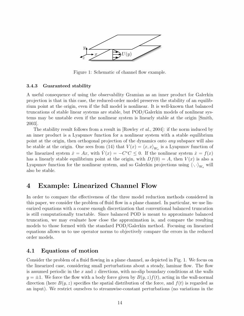
Figure 1: Schematic of channel flow example.

3.4.3 Guaranteed stability

A useful consequence of using the observability Gramian as an inner product for Galerkinprojection is that in this case, the reduced-order model preserves the stability of an equilib-rium point at the origin, even if the full model is nonlinear. It is well-known that balancedtruncations of stable linear systems are stable, but POD/Galerkin models of nonlinear sys-tems may be unstable even if the nonlinear system is linearly stable at the origin [Smith,2003].

The stability result follows from a result in [Rowley et al., 2004]: if the norm induced byan inner product is a Lyapunov function for a nonlinear system with a stable equilibriumpoint at the origin, then orthogonal projection of the dynamics onto any subspace will alsobe stable at the origin. One sees from (14) that V (x) = 〈x, x〉Wo

is a Lyapunov function of

the linearized system x = Ax, with V (x) = −C∗C ≤ 0. If the nonlinear system x = f(x)has a linearly stable equilibrium point at the origin, with Df(0) = A, then V (x) is also aLyapunov function for the nonlinear system, and so Galerkin projections using 〈·, ·〉Wo

willalso be stable.

4 Example: Linearized Channel Flow

In order to compare the effectiveness of the three model reduction methods considered inthis paper, we consider the problem of fluid flow in a plane channel. In particular, we use lin-earized equations with a coarse enough discretization that conventional balanced truncationis still computationally tractable. Since balanced POD is meant to approximate balancedtruncation, we may evaluate how close the approximation is, and compare the resultingmodels to those formed with the standard POD/Galerkin method. Focusing on linearizedequations allows us to use operator norms to objectively compare the errors in the reducedorder models.

4.1 Equations of motion

Consider the problem of a fluid flowing in a plane channel, as depicted in Fig. 1. We focus onthe linearized case, considering small perturbations about a steady, laminar flow. The flowis assumed periodic in the x and z directions, with no-slip boundary conditions at the wallsy = ±1. We force the flow with a body force given by B(y, z)f(t), acting in the wall-normaldirection (here B(y, z) specifies the spatial distribution of the force, and f(t) is regarded asan input). We restrict ourselves to streamwise-constant perturbations (no variations in the

14

0 5 10 15 2010−8

10−6

10−4

10−2

100

102

Index j

σj , λj

Figure 2: Hankel singular values σj for linearized channel flow: balanced truncation (×),balanced POD with 5-mode output projection (◦), 10-mode output projection (�); and PODeigenvalues λj (4).

x-direction), and for this case the equations are given by

∂v

∂t=

1

R∇2v +Bf

∂η

∂t=

1

R∇2η − U ′∂v

∂z

where v is the wall-normal velocity and η = uz − wx is the perturbation in wall-normalvorticity. Numerical investigations indicate that the laminar velocity profile u = (U(y), 0, 0),with U(y) = 1−y2, is linearly stable for Reynolds numbers R < 5772 [Drazin & Reid, 1981],so the infinite-time Gramians will be well defined.

For the numerical examples considered here, we consider R = 100, on the domain z ∈[0, 2π], and discretize the problem using 16 Chebyshev modes in the y-direction, and 16Fourier modes in the z-direction. The forcing B(y, z) is zero everywhere except in a smallregion at the center of the domain (y = 0, z = π). We take the output to be the entire state,that is, the values of (v, η) everywhere in space. The total number of states is 2 ·16 ·15 = 480,which is small enough that we may compute the full Gramians exactly, for comparison withour approximate methods.

4.2 Results

Hankel singular values. We begin by comparing the Hankel singular values σj, shownin Fig. 2. Here, the exact values for balanced truncation are compared to the approximatevalues for balanced POD, for both 5-mode and 10-mode output projections Pr. Also shownare the POD eigenvalues λj, computed from (9), and observe that the eigenvalues fall offquite rapidly. The first 5 POD modes capture 95.6% of the energy, while the first 10 modes

15

Normal vorticity ηNormal velocity v

z

y

z

z z

z

z

y

y

0 2 4 6−1

0

1

0 2 4 6−1

0

1

0 2 4 6−1

0

1

0 2 4 6−1

0

1

0 2 4 6−1

0

1

0 2 4 6−1

0

1

Balanced

truncation

Balanced

POD

POD

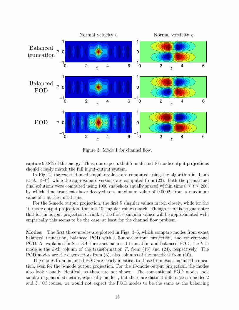
Figure 3: Mode 1 for channel flow.

capture 99.8% of the energy. Thus, one expects that 5-mode and 10-mode output projectionsshould closely match the full input-output system.

In Fig. 2, the exact Hankel singular values are computed using the algorithm in [Laubet al., 1987], while the approximate versions are computed from (23). Both the primal anddual solutions were computed using 1000 snapshots equally spaced within time 0 ≤ t ≤ 200,by which time transients have decayed to a maximum value of 0.0002, from a maximumvalue of 1 at the initial time.

For the 5-mode output projection, the first 5 singular values match closely, while for the10-mode output projection, the first 10 singular values match. Though there is no guaranteethat for an output projection of rank r, the first r singular values will be approximated well,empirically this seems to be the case, at least for the channel flow problem.

Modes. The first three modes are plotted in Figs. 3–5, which compare modes from exactbalanced truncation, balanced POD with a 5-mode output projection, and conventionalPOD. As explained in Sec. 3.4, for exact balanced truncation and balanced POD, the k-thmode is the k-th column of the transformation T , from (15) and (24), respectively. ThePOD modes are the eigenvectors from (3), also columns of the matrix Φ from (10).

The modes from balanced POD are nearly identical to those from exact balanced trunca-tion, even for the 5-mode output projection. For the 10-mode output projection, the modesalso look visually identical, so these are not shown. The conventional POD modes looksimilar in general structure, especially mode 1, but there are distinct differences in modes 2and 3. Of course, we would not expect the POD modes to be the same as the balancing

16

Normal vorticity ηNormal velocity v

z

y

z

z z

z

z

y

y

Balanced

truncation

Balanced

POD

POD

0 2 4 6−1

0

1

0 2 4 6−1

0

1

0 2 4 6−1

0

1

0 2 4 6−1

0

1

0 2 4 6−1

0

1

0 2 4 6−1

0

1

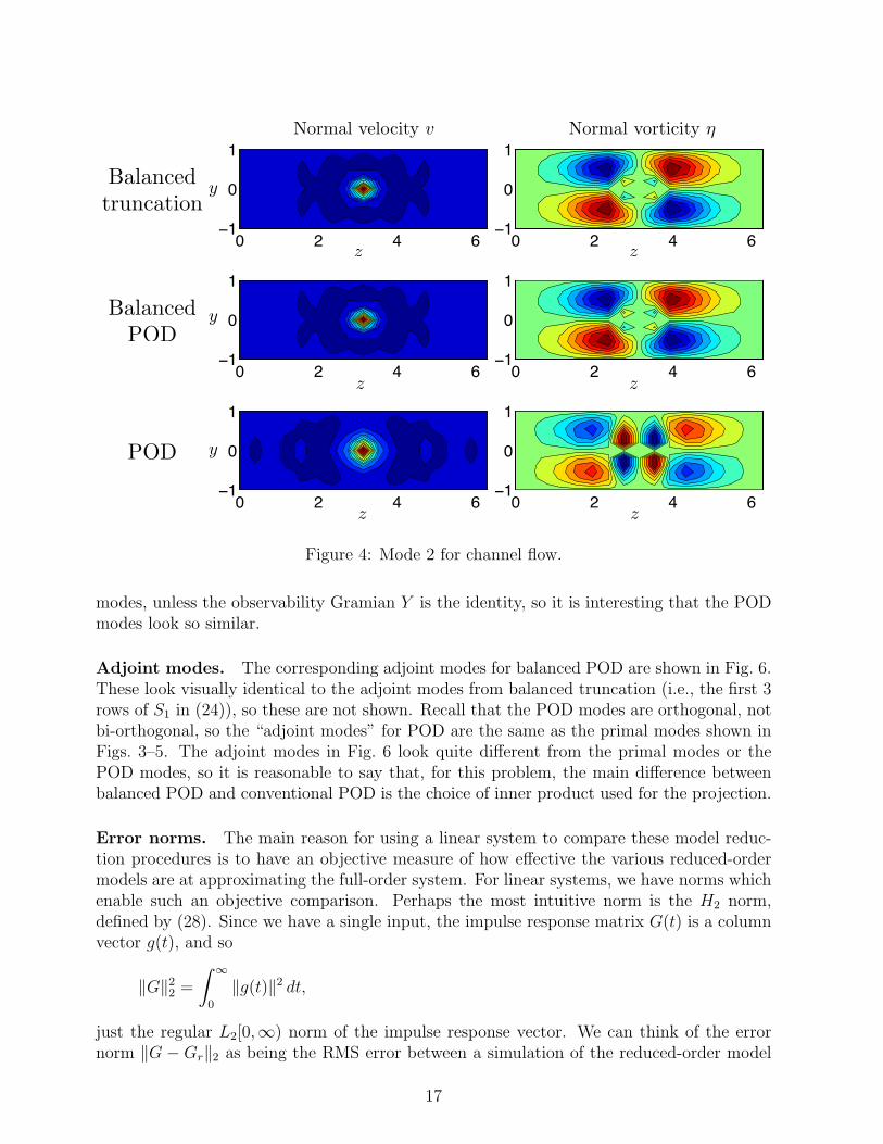
Figure 4: Mode 2 for channel flow.

modes, unless the observability Gramian Y is the identity, so it is interesting that the PODmodes look so similar.

Adjoint modes. The corresponding adjoint modes for balanced POD are shown in Fig. 6.These look visually identical to the adjoint modes from balanced truncation (i.e., the first 3rows of S1 in (24)), so these are not shown. Recall that the POD modes are orthogonal, notbi-orthogonal, so the “adjoint modes” for POD are the same as the primal modes shown inFigs. 3–5. The adjoint modes in Fig. 6 look quite different from the primal modes or thePOD modes, so it is reasonable to say that, for this problem, the main difference betweenbalanced POD and conventional POD is the choice of inner product used for the projection.

Error norms. The main reason for using a linear system to compare these model reduc-tion procedures is to have an objective measure of how effective the various reduced-ordermodels are at approximating the full-order system. For linear systems, we have norms whichenable such an objective comparison. Perhaps the most intuitive norm is the H2 norm,defined by (28). Since we have a single input, the impulse response matrix G(t) is a columnvector g(t), and so

‖G‖22 =

∫ ∞

0

‖g(t)‖2 dt,

just the regular L2[0,∞) norm of the impulse response vector. We can think of the errornorm ‖G − Gr‖2 as being the RMS error between a simulation of the reduced-order model

17

Normal vorticity ηNormal velocity v

z

y

z

z z

z

z

y

y

Balanced

truncation

Balanced

POD

POD

0 2 4 6−1

0

1

0 2 4 6−1

0

1

0 2 4 6−1

0

1

0 2 4 6−1

0

1

0 2 4 6−1

0

1

0 2 4 6−1

0

1

Figure 5: Mode 3 for channel flow.

0 2 4 6−1

0

1

0 2 4 6−1

0

1

0 2 4 6−1

0

1

0 2 4 6−1

0

1

0 2 4 6−1

0

1

0 2 4 6−1

0

1

Mode 1

Mode 2

Mode 3

Normal vorticity ηNormal velocity v

z

y

z

z z

z

z

y

y

Figure 6: Adjoint modes 1–3 for balanced POD. The adjoint modes for balanced truncationare nearly identical, and the adjoint modes for POD are the same as the primal modes.

18

0 2 4 6 8 1010−3

10−2

10−1

100

101

r (order of reduced model)

‖G − Gr‖2

‖G‖2

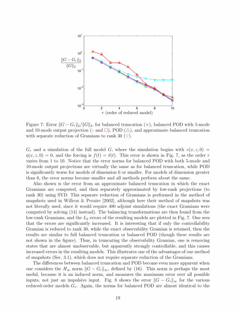
Figure 7: Error ‖G−Gr‖2/‖G‖2, for balanced truncation (×), balanced POD with 5-modeand 10-mode output projection (◦ and �), POD (4), and approximate balanced truncationwith separate reduction of Gramians to rank 30 (O).

Gr and a simulation of the full model G, where the simulation begins with v(x, z, 0) =η(x, z, 0) = 0, and the forcing is f(t) = δ(t). This error is shown in Fig. 7, as the order rvaries from 1 to 10. Notice that the error norms for balanced POD with both 5-mode and10-mode output projections are virtually the same as for balanced truncation, while PODis significantly worse for models of dimension 6 or smaller. For models of dimension greaterthan 6, the error norms become smaller and all methods perform about the same.

Also shown is the error from an approximate balanced truncation in which the exactGramians are computed, and then separately approximated by low-rank projections (torank 30) using SVD. This separate reduction of Gramians is performed in the method ofsnapshots used in Willcox & Peraire [2002], although here their method of snapshots wasnot literally used, since it would require 480 adjoint simulations (the exact Gramians werecomputed by solving (14) instead). The balancing transformations are then found from thelow-rank Gramians, and the L2 errors of the resulting models are plotted in Fig. 7. One seesthat the errors are significantly increased. It is interesting that if only the controllabilityGramian is reduced to rank 30, while the exact observability Gramian is retained, then theresults are similar to full balanced truncation or balanced POD (though these results arenot shown in the figure). Thus, in truncating the observability Gramian, one is removingstates that are almost unobservable, but apparently strongly controllable, and this causesincreased errors in the resulting models. This illustrates one of the advantages of our methodof snapshots (Sec. 3.1), which does not require separate reduction of the Gramians.

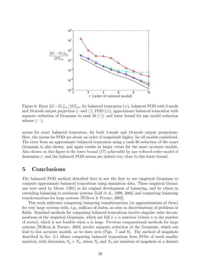
The differences between balanced truncation and POD become even more apparent whenone considers the H∞ norm ‖G − Gr‖∞, defined by (16). This norm is perhaps the mostuseful, because it is an induced norm, and measures the maximum error over all possibleinputs, not just an impulsive input. Fig. 8 shows the error ‖G − Gr‖∞ for the variousreduced-order models Gr. Again, the norms for balanced POD are almost identical to the

19

r (order of reduced model)

‖G − Gr‖∞‖G‖∞

0 2 4 6 8 1010−4

10−3

10−2

10−1

100

101

102

Figure 8: Error ‖G−Gr‖∞/‖G‖∞, for balanced truncation (×), balanced POD with 5-modeand 10-mode output projection (◦ and �), POD (4), approximate balanced truncation withseparate reduction of Gramians to rank 30 (O), and lower bound for any model reductionscheme (—).

norms for exact balanced truncation, for both 5-mode and 10-mode output projections.Here, the norms for POD are about an order of magnitude higher, for all models considered.The error from an approximate balanced truncation using a rank-30 reduction of the exactGramians is also shown, and again results in larger errors for the more accurate models.Also shown on this figure is the lower bound (17) achievable by any reduced-order model ofdimension r, and the balanced POD norms are indeed very close to this lower bound.

5 Conclusions

The balanced POD method described here is not the first to use empirical Gramians tocompute approximate balanced truncations using simulation data. These empirical Grami-ans were used by Moore [1981] in his original development of balancing, and by others inextending balancing to nonlinear systems [Lall et al., 1999, 2002] and computing balancingtransformations for large systems [Willcox & Peraire, 2002].

This work addresses computing balancing transformations (or approximations of them)for very large systems with, e.g., millions of states, as arise in discretizations of problems influids. Standard methods for computing balanced truncations involve singular value decom-positions of the empirical Gramians, which are full n × n matrices (where n is the numberof states), which is not feasible when n is large. Previous computational methods for largesystems [Willcox & Peraire, 2002] involve separate reduction of the Gramians, which canlead to less accurate models, as we have seen (Figs. 7 and 8). The method of snapshotsdescribed in Sec. 3.1 allows computing balanced truncations from SVDs of much smallermatrices, with dimension Np ×Nd, where Np and Nd are numbers of snapshots in a dataset

20

of primal and dual solutions, respectively, without separate reduction of the Gramians.Furthermore, previous methods as in Lall et al. [1999] and Willcox & Peraire [2002] are

not tractable for systems with large numbers of outputs, as one must integrate an adjointsolution for each output. Sec. 3.2 describes an output projection method that approximatesfull balanced truncation with guaranteed error bounds, and dramatically reduces the numberof adjoint solutions necessary. In the example shown, integration of 5 adjoint solutionsproduced models that were virtually indistinguishable in the H∞ norm from full balancedtruncations, which would have required 480 adjoint simulations using previous methods.

The formulation of balanced POD also clarifies some connections between balanced trun-cation and POD, most importantly that for a linear system, balanced truncation is a specialcase of POD. In particular, one uses a dataset consisting of responses to unit impulses (onefor each input), and uses the observability Gramian for the inner product. This inner prod-uct weights states of large “dynamical importance,” as opposed to POD, which retains onlythe most energetic modes. This suggests that even for a nonlinear system, the observabilityGramian from a linearization might be a good choice of inner product for POD, if reduced-order models are desired. The balanced POD procedure not only removes subjectivity in thechoice of inner product for POD, but also guarantees that a Galerkin projection of a nonlin-ear system with a stable equilibrium point at the origin will also have a stable equilibriumpoint at the origin.

Although many of the developments in this paper are restricted to stable, linear systems,Sec. 3.4 suggests how many of these ideas might be extended to large-scale nonlinear systemsas well, following the approaches in Lall et al. [2002].

Acknowledgements

This work was partially supported by the NSF, grant CMS-0347239, under program managerM. Tomizuka; and by AFOSR, grant F49620-03-1-0081, under program managers B. King,S. Heise, and J. Schmisseur.

A Theorems on computing balancing transformations

Here, we consider empirical Gramians defined by (22), with balancing transformations T1

and S1 defined by (23–24). The following theorem establishes that if one takes enoughsnapshots that the empirical Gramians Wc and Wo have full rank n (clearly, at least nsnapshots are required, and the system must be both controllable and observable), then Σ1

contains the Hankel singular values (square roots of the eigenvalues of the product WcWo),and T1 is the balancing transformation that simultaneously diagonalizes Wc and Wo.

Proposition 1. Let Wc and Wo be empirical Gramians defined by (22), and suppose Y ∗Xhas rank r = n. Then the matrix T1 is square and invertible, with inverse S1, and

S1WcS∗1 = T ∗

1WoT1 = Σ1.

21

Proof. To show S1 = T−11 , we have

S1T1 = Σ−1/21 U∗

1Y∗XV1Σ

−1/21 = Σ

−1/21 Σ1Σ

−1/21 = In.

Also,

S1WcS∗1 = Σ

−1/21 U∗

1Y∗XX∗Y U1Σ

−1/2

= Σ−1/21 (Σ1V

∗1 )(V1Σ1)Σ

−1/21 = Σ1,

and a similar calculation shows T ∗1WoT1 = Σ1.

Of course, our main interest is in large systems for which the number of snapshots, andhence the rank of Wc, Wo is much smaller than n. The following theorem establishes thatin this case, Σ1 also contains all nonzero Hankel singular values, and T1 contains the first rcolumns of the balancing transformation.

Proposition 2. Suppose Y ∗X has rank r < n. Then there exist matrices S2, T2 ∈ Rn×(n−r)

such that for

T =[T1 T2

], S =

[S1

S2

],

T is invertible with T−1 = S, and

SWcWoT =

[Σ2

1 00 0

], (30)

and furthermore,

SWcS∗ =

[Σ1 00 M1

], T ∗WoT =

[Σ1 00 M2

], (31)

where M1 and M2 are matrices in R(n−r)×(n−r).

Proof. As in the proof of Theorem 1, S1T1 = Ir. Choose T2 such that its columns form abasis for the nullspace of S1 (an (n − r)-dimensional subspace of Rn). Then S1T2 = 0, andT is invertible, since its columns are linearly independent. Define S2 as the last n− r rowsof T−1, and it follows that S2T1 = 0.

First, we show

T ∗WoT =

[T ∗

1WoT1 T ∗1WoT2

T ∗2WoT1 T ∗

2WoT2

]=

[Σ1 00 M2

].

As in the proof of Theorem 1, T ∗1WoT1 = Σ1. Next,

T ∗1WoT2 = Σ

−1/21 V ∗

1 X∗Y Y ∗T2

= Σ−1/21 (Σ1U

∗1 )Y ∗T2 = Σ1S1T2 = 0r×(n−r),

and thus T ∗2WoT1 = (T ∗

1WoT2)∗ = 0(n−r)×r. The results for SWcS

∗ and SWcWoT followsimilarly, using that S2T1 = 0.

22

References

Antoulas, A. C., Sorensen, D. C., & Gugercin, S. [2001] A survey of model reduction methodsfor large-scale systems. Contemp. Math. 280, 193–219.

Bamieh, B. & Daleh, M. [2001] Energy amplification in channel flows with stochastic exci-tation. Phys. Fluids 13 (11), 3258–3269.

Colonius, T. & Freund, J. B. [2002] POD analysis of sound generation by a turbulent jet.AIAA Paper 2002-0072.

Cortelezzi, L. & Speyer, J. L. [1998] Robust reduced-order controller of laminar boundarylayer transitions. Phys. Rev. E 58 (2), 1906–1910.

Drazin, P. G. & Reid, W. H. [1981] Hydrodynamic Stability . Cambridge University Press.

Dullerud, G. E. & Paganini, F. [1999] A Course in Robust Control Theory: A ConvexApproach, vol. 36 of Texts in Applied Mathematics . Springer-Verlag.

Farrell, B. F. & Ioannou, P. J. [1993] Stochastic forcing of the linearized Navier-Stokesequations. Phys. Fluids A 5 (11), 2600–2609.

Holmes, P., Lumley, J. L., & Berkooz, G. [1996] Turbulence, Coherent Structures, DynamicalSystems and Symmetry . Cambridge University Press.

Lall, S., Marsden, J. E., & Glavaski, S. [1999] Empirical model reduction of controllednonlinear systems. In Proceedings of the IFAC World Congress , vol. F, pp. 473–478.

Lall, S., Marsden, J. E., & Glavaski, S. [2002] A subspace approach to balanced truncationfor model reduction of nonlinear control systems. Int. J. Robust Nonlinear Control 12,519–535.

Laub, A. J., Heath, M. T., Page, C. C., & Ward, R. C. [1987] Computation of balancingtransformations and other applications of simultaneous diagonalization algorithms. IEEETrans. Automat. Contr. 32, 115–122.

Lumley, J. L. [1970] Stochastic Tools in Turbulence. Academic Press.

Moore, B. C. [1981] Principal component analysis in linear systems: Controllability, observ-ability, and model reduction. IEEE Trans. Automat. Contr. 26 (1).

Rathinam, M. & Petzold, L. R. [2003] A new look at proper orthogonal decomposition.SIAM J. Numer. Anal. 41 (5), 1893–1925.

Rowley, C. W., Colonius, T., & Murray, R. M. [2004] Model reduction for compressible flowusing POD and Galerkin projection. Phys. D 189 (1–2), 115–129.

Scherpen, J. M. A. [1993] Balancing for nonlinear systems. Sys. Control Lett. 21 (2), 143–153.

Sirovich, L. [1987] Turbulence and the dynamics of coherent structures, parts I–III. Q. Appl.Math. XLV (3), 561–590.

23

Smith, T. R. [2003] Low-dimensional models of plane Couette flow using the proper orthog-onal decomposition. Ph.D. thesis, Princeton University.

Willcox, K. & Peraire, J. [2002] Balanced model reduction via the proper orthogonal decom-position. AIAA J. 40 (11).

24