Model Predictive Controller Emad Ali Chemical Engineering Department King Saud University.

Model Predictive Model Predictive ControllerController

Emad AliEmad Ali

Chemical Engineering Chemical Engineering DepartmentDepartment

King Saud UniversityKing Saud University

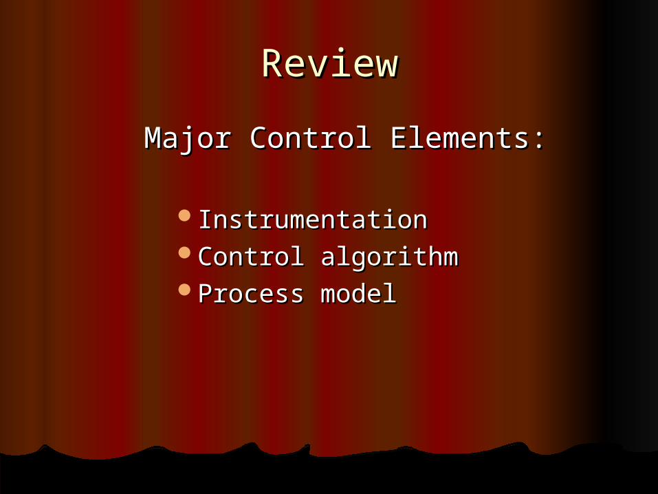
ReviewReview

Major Control Elements:Major Control Elements:

InstrumentationInstrumentationControl algorithmControl algorithmProcess modelProcess model

ReviewReview

Control AlgorithmsControl Algorithms:: Classical:Classical:

PID, cascade, override, ratio, split range, inferentialPID, cascade, override, ratio, split range, inferential

Advanced:Advanced:Adaptive controlAdaptive controlFuzzy logic controlFuzzy logic control Internal model controlInternal model controlOptimal controlOptimal controlNeural network controlNeural network controlGlobally linearizing controlGlobally linearizing controlModel predictive controlModel predictive control

Benefits of MPCBenefits of MPC

1. Optimization: consistent product quality, reduced off-specs products, minimizing the operating cost.

2. Multivariable: Superior for processes with large

number of manipulated and controlled variables with strong coupling.

3. Constraints: Allows constraints to be imposed on

both MV and CV. 4. Prediction: good for time delays, inverse response,

inherent nonlinearities, changing control objectives and sensor failure.

Industrial MPC TechnologyIndustrial MPC Technology IDCOM (Identification and Command)IDCOM (Identification and Command)

Model type: Impulse response Model type: Impulse response Optimization is solved by QP approachOptimization is solved by QP approach

DMC (Dynamic Matrix Control)DMC (Dynamic Matrix Control) Model type: Step responseModel type: Step response Optimization is solved by LP approach Optimization is solved by LP approach

OPC (Optimum Predictive Control)OPC (Optimum Predictive Control) Use step response, solves LP problemUse step response, solves LP problem Model building, controller design and simulation Model building, controller design and simulation tasks are carried out on PCstasks are carried out on PCs

PCT (Predictive Control Technology)PCT (Predictive Control Technology) Combines the aspects of IDCOM and DMCCombines the aspects of IDCOM and DMC

HMPC (Horizon Multivariable Predictive Control)HMPC (Horizon Multivariable Predictive Control) For proprietary reasons, information is unavailable For proprietary reasons, information is unavailable

Multivariable vs. Multi-loopsMultivariable vs. Multi-loops

Process

Controller

Process

Controller

Controller

Outputs

Outputs

Inputs

Inputs

Mulit-loops Scheme

Mulit-variables Scheme

General Application ConceptGeneral Application Concept

PlantMPC

Model+

-

+

_

yp

ym

u

x

er

Receding Horizon ConceptReceding Horizon Concept(Prediction)(Prediction)

k k+1 k +M -1 k + P

FuturePast

Reference, r (k+1)

Predicted output, y (k+1/k)

Control action, u (k/k)

Control horizon

Prediction horizon

Process ModelProcess Model

Model:

Y(k/k) = [y(k/k) y(k+1/k) … y(k+n-1/k)]

Y(k-1/k) = [y(k-1/k) y(k/k) … y(k+n-2/k)]

Prediction:

Y(k+1/k) = [y(k/k) y(k+1/k) … y(k+P-1/k)]

U(k/k) = [u(k/k) u(k+1/k) … u(k+M-1/k)]

Y(k/k) = M Y(k-1/k) + S u(k-1/k)

Y(k+1/k) = MP Y(k/k) + SP U(k/k)

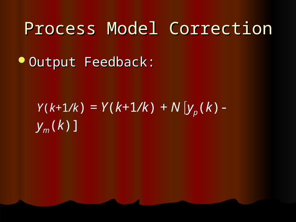
Process Model CorrectionProcess Model Correction

Output Feedback:Output Feedback:

Y(k+1/k) = Y(k+1/k) + N yp(k)-ym(k)]

Methods of SolutionMethods of Solution

1. Algebraic Equation:

2. Linear Programming (LP)

R(k+1)=Y(k+1) = MP Y(k) + SP U(k)

|R(k+1)-Y(k+1)| =

|R(k+1)-[MP Y(k) + SP U(k)]| = 0

3. Quadratic Programming

Methods of solutionMethods of solution

4. Constrained QP

min [R(k+1)-Y(k+1)]T [R(k+1)-Y(k+1)] + UT(k) U(k)U(k)

min [R(k+1)-Y(k+1)]T [R(k+1)-Y(k+1)] + UT(k) U(k)U(k)

Ul ≤ U ≤ Uu

Ul ≤ U ≤ Uu

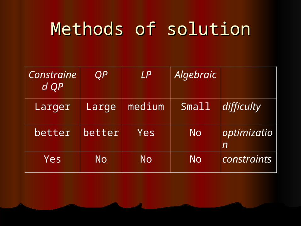
Methods of solutionMethods of solution

AlgebraicLPQPConstrained QP

difficultySmallmediumLargeLarger

optimizationNoYesbetterbetter

constraintsNoNoNoYes

Tuning ParametersTuning Parameters

Output weights:

3

2

1

0 0

0 0

0 0

Input weights:

3

2

1

0 0

0 0

0 0

Prediction horizon: Y(k+1/k) = [y(k+1/k) y(k+2/k) … y(k+P/k)]

Control horizon: U(k/k) = [u(k/k) u(k+1/k) … u(k+M-1/k)]

Tuning GuidelinesTuning Guidelines

Tuning Tuning parameteparameterr

functionfunction

Gives more weight to a Gives more weight to a specific outputspecific output

Slower response, stabilizing Slower response, stabilizing effecteffect

PPMore stable and robust More stable and robust responseresponse

MMFaster (even unstable) Faster (even unstable) responseresponse

Generating Step Response Generating Step Response ModelModel

1 .Step testing

DynamicProcess

Input 1 Output 1

s1,1

s2,1

s3,1

sn,1

Unit Step Response

Output nyInput nu

Input 2

Unit Step Change

Constant

Constants1,ny

s2,ny

s3,nysn,ny

h1,1

h2,1

h3,1

h1,ny

h2,ny

h3,ny

Generating Step Response Generating Step Response ModelModel

2 .PBRS Testing

DynamicProcess

Input 1 Output 1

Unit Step Response

Output nyInput nu

Input 2

PBRS

PBRS

PBRS

Step Vs. PBRSStep Vs. PBRS

Step Step Simple and Simple and straightforwardstraightforward

Requires long Requires long testing timetesting time

PBRSPBRSRequires Requires knowledge knowledge about about identification identification theory theory

Requires less Requires less testing timetesting time

Implementation requirementImplementation requirement

DCS systemDCS systemPersonal ComputerPersonal ComputerStep response modelStep response modelTuningTuning

Special Features of MPCSpecial Features of MPC

Feed-forward capabilityFeed-forward capability

Inferential controlInferential control

Output ConstraintsOutput Constraints

Y(k+1/k) = M Y(k/k) + S U(k/k) + W d(k/k)

Y(k+1/k) = M Y(k/k) + S U(k/k)

Z(k+1/k) = CY(k+1/k)

Yl (k+1) ≤ Y (k+1) ≤ Yu(k+1)

Special Features of MPCSpecial Features of MPC

Variable set point Variable set point

or constraintsor constraints

Simulation ExampleSimulation Example

Pump-1

F200T200

F5

F4

L2

F2C2T2

F1C1T1

F3

P2

P100F100T100

Steam

Separator

Coolingwater

ProductFeed

F200/C2, P100/P2F200/C2, P100/P2

P100/C2, F200/P2P100/C2, F200/P2

0.14

0.16

0.18

0.20

C2

set po in t

P = 2

P = 50

0 35 70

T im e (m in)

3 2

3 2 . 4

3 2 . 8

3 3 . 2

3 3 . 6

P2

(kP

a)

0.14

0.16

0.18

0.20

C2

set po in t

P = 2 , G = 1 /1 , L = 0 /0

P = 2, G = 1 /1, L = 0 .001/0.001

P = 2, G = 10/1 , L = 0 .001/0 .001

0 35 70

T im e (m in)

32.0

32.4

32.8

33.2

33.6

P2

(kP

a)

Thank YouThank You

Questions ?Questions ?