Fakultt für Maschinenwesen Lehrstuhl für Angewandte Mechanik Model Order Reduction for Nonlinear Structural Dynamics Simulation-free Approaches Johannes Baptist Rutzmoser Vollstndiger Abdruck der von der Fakultt für Maschinenwesen der Technischen Universitt München zur Erlangung des akademischen Grades eines Doktor-Ingenieurs (Dr.-Ing.) genehmigten Dissertation. Vorsitzender: Prof. Dr.-Ing. Michael W. Gee Prüfer der Dissertation: 1. Prof. dr. ir. Daniel Rixen 2. Ass. Prof. Dr. Joaqun Alberto HernÆndez Ortega Die Dissertation wurde am 19.09.2017 bei der Technischen Universitt München eingereicht und durch die Fakultt für Maschinenwesen am 12.02.2018 angenommen.

Welcome message from author
This document is posted to help you gain knowledge. Please leave a comment to let me know what you think about it! Share it to your friends and learn new things together.
Transcript
Fakultät für MaschinenwesenLehrstuhl für Angewandte Mechanik
Model Order Reduction for
Nonlinear Structural Dynamics
Simulation-free Approaches
Johannes Baptist Rutzmoser
Vollständiger Abdruck der von der Fakultät für Maschinenwesen der Technischen UniversitätMünchen zur Erlangung des akademischen Grades eines
Doktor-Ingenieurs (Dr.-Ing.)
genehmigten Dissertation.
Vorsitzender: Prof. Dr.-Ing. Michael W. Gee
Prüfer der Dissertation:
1. Prof. dr. ir. Daniel Rixen
2. Ass. Prof. Dr. Joaquín Alberto Hernández Ortega
Die Dissertation wurde am 19.09.2017 bei der Technischen Universität München eingereicht unddurch die Fakultät für Maschinenwesen am 12.02.2018 angenommen.

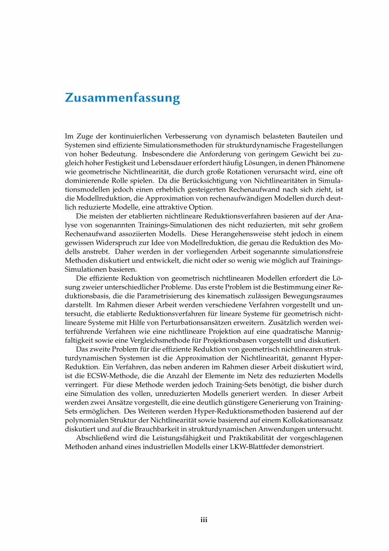
Zusammenfassung
Im Zuge der kontinuierlichen Verbesserung von dynamisch belasteten Bauteilen undSystemen sind effiziente Simulationsmethoden für strukturdynamische Fragestellungenvon hoher Bedeutung. Insbesondere die Anforderung von geringem Gewicht bei zu-gleich hoher Festigkeit und Lebensdauer erfordert häufig Lösungen, in denen Phänomenewie geometrische Nichtlinearität, die durch große Rotationen verursacht wird, eine oftdominierende Rolle spielen. Da die Berücksichtigung von Nichtlinearitäten in Simula-tionsmodellen jedoch einen erheblich gesteigerten Rechenaufwand nach sich zieht, istdie Modellreduktion, die Approximation von rechenaufwändigen Modellen durch deut-lich reduzierte Modelle, eine attraktive Option.
Die meisten der etablierten nichtlineare Reduktionsverfahren basieren auf der Ana-lyse von sogenannten Trainings-Simulationen des nicht reduzierten, mit sehr großemRechenaufwand assoziierten Modells. Diese Herangehensweise steht jedoch in einemgewissen Widerspruch zur Idee von Modellreduktion, die genau die Reduktion des Mo-dells anstrebt. Daher werden in der vorliegenden Arbeit sogenannte simulationsfreieMethoden diskutiert und entwickelt, die nicht oder so wenig wie möglich auf Trainings-Simulationen basieren.
Die effiziente Reduktion von geometrisch nichtlinearen Modellen erfordert die Lö-sung zweier unterschiedlicher Probleme. Das erste Problem ist die Bestimmung einer Re-duktionsbasis, die die Parametrisierung des kinematisch zulässigen Bewegungsraumesdarstellt. Im Rahmen dieser Arbeit werden verschiedene Verfahren vorgestellt und un-tersucht, die etablierte Reduktionsverfahren für lineare Systeme für geometrisch nicht-lineare Systeme mit Hilfe von Perturbationsansätzen erweitern. Zusätzlich werden wei-terführende Verfahren wie eine nichtlineare Projektion auf eine quadratische Mannig-faltigkeit sowie eine Vergleichsmethode für Projektionsbasen vorgestellt und diskutiert.
Das zweite Problem für die effiziente Reduktion von geometrisch nichtlinearen struk-turdynamischen Systemen ist die Approximation der Nichtlinearität, genannt Hyper-Reduktion. Ein Verfahren, das neben anderen im Rahmen dieser Arbeit diskutiert wird,ist die ECSW-Methode, die die Anzahl der Elemente im Netz des reduzierten Modellsverringert. Für diese Methode werden jedoch Training-Sets benötigt, die bisher durcheine Simulation des vollen, unreduzierten Modells generiert werden. In dieser Arbeitwerden zwei Ansätze vorgestellt, die eine deutlich günstigere Generierung von Training-Sets ermöglichen. Des Weiteren werden Hyper-Reduktionsmethoden basierend auf derpolynomialen Struktur der Nichtlinearität sowie basierend auf einem Kollokationsansatzdiskutiert und auf die Brauchbarkeit in strukturdynamischen Anwendungen untersucht.
Abschließend wird die Leistungsfähigkeit und Praktikabilität der vorgeschlagenenMethoden anhand eines industriellen Modells einer LKW-Blattfeder demonstriert.
iii
tum
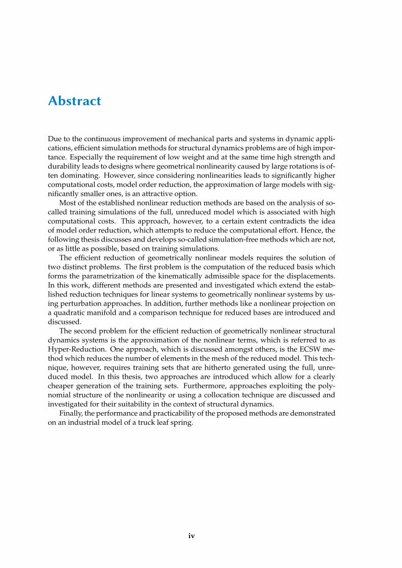
Abstract
Due to the continuous improvement of mechanical parts and systems in dynamic appli-cations, efficient simulation methods for structural dynamics problems are of high impor-tance. Especially the requirement of low weight and at the same time high strength anddurability leads to designs where geometrical nonlinearity caused by large rotations is of-ten dominating. However, since considering nonlinearities leads to significantly highercomputational costs, model order reduction, the approximation of large models with sig-nificantly smaller ones, is an attractive option.
Most of the established nonlinear reduction methods are based on the analysis of so-called training simulations of the full, unreduced model which is associated with highcomputational costs. This approach, however, to a certain extent contradicts the ideaof model order reduction, which attempts to reduce the computational effort. Hence, thefollowing thesis discusses and develops so-called simulation-free methods which are not,or as little as possible, based on training simulations.
The efficient reduction of geometrically nonlinear models requires the solution oftwo distinct problems. The first problem is the computation of the reduced basis whichforms the parametrization of the kinematically admissible space for the displacements.In this work, different methods are presented and investigated which extend the estab-lished reduction techniques for linear systems to geometrically nonlinear systems by us-ing perturbation approaches. In addition, further methods like a nonlinear projection ona quadratic manifold and a comparison technique for reduced bases are introduced anddiscussed.
The second problem for the efficient reduction of geometrically nonlinear structuraldynamics systems is the approximation of the nonlinear terms, which is referred to asHyper-Reduction. One approach, which is discussed amongst others, is the ECSW me-thod which reduces the number of elements in the mesh of the reduced model. This tech-nique, however, requires training sets that are hitherto generated using the full, unre-duced model. In this thesis, two approaches are introduced which allow for a clearlycheaper generation of the training sets. Furthermore, approaches exploiting the poly-nomial structure of the nonlinearity or using a collocation technique are discussed andinvestigated for their suitability in the context of structural dynamics.
Finally, the performance and practicability of the proposed methods are demonstratedon an industrial model of a truck leaf spring.
iv
Danksagung
Die vorliegende Arbeit entstand während meiner Zeit von 2011 bis 2017 als wissenschaft-licher Mitarbeiter am Lehrstuhl für Angewandte Mechanik der Technischen UniversitätMünchen. Den vielen Personen, die mich während dieser Zeit unterstützt und geförderthaben, möchte ich meinen ganz herzlichen Dank aussprechen.
Mein erster Dank gilt meinem Doktorvater Prof. dr. ir. Daniel Rixen für das in michgesetzte Vertrauen, die wohlwollende Begleitung und Unterstützung. Er gab mir dieMöglichkeit, an einem spannenden und vielseitigen Thema zu arbeiten und stand mitRat und Tat zur Seite. Sowohl die intensive Betreuung und die fachliche Unterstützung,als auch die großen Freiräume waren und sind für mich von unschätzbarem Wert.
Des Weiteren möchte ich mich bei Prof. Dr.-Ing. Michael W. Gee für die Übernahmedes Vorsitzes der Prüfungskommission sowie bei Prof. Dr. Joaquín Alberto HernándezOrtega für das Interesse an meiner Arbeit und die Übernahme des Zweitgutachtens be-danken.
Die Zeit am Lehrstuhl wird mir vor allem auch wegen der Kollegen in bester Erin-nerung bleiben. Ihnen danke ich für die offene und hilfsbereite Atmosphäre, den span-nenden Austausch und die zahlreichen und regen fachlichen und nicht-fachlichen Diskus-sionen. Insbesondere möchte ich mich bei Andreas Bartl, Bastian Eselfeld, AlexanderEwald, Fabian Gruber und Christian Meyer für die kollegiale und intensive Zusamme-narbeit in Lehre und Forschung herzlich bedanken.
Auch bei den Studenten möchte ich mich bedanken, die in Form von Studienarbeiteneinen wertvollen Beitrag zum Gelingen dieser Arbeit beigetragen haben. Nicht nur durchdie fleißige Arbeit, sondern auch durch die Diskussionen bei der Betreuung gab es stetsneue Denkanstöße. Besonders danken möchte ich dabei Amandine Desjardins, GabrielGruber, Anton Mayr, Sebastian Otten, Mikhail Pak, Daniel Scheffold und Xuwei Wu. Be-danken möchte ich mich auch bei Pascal Reuß, der mich dazu ermutigte, die entwickeltenMethoden auf ein industrielles Beispiel anzuwenden. Christian Meyer und Daniel Schef-fold gilt mein Dank für die wertvollen Hinweise bei der Durchsicht des Manuskripts.
Ganz herzlich möchte ich meiner Familie danken, die mich an so vielen Stellen ge-fördert und unterstützt hat, insbesondere meinen Eltern. Schade, dass mein Vater denAbschluss dieser Arbeit nicht mehr erleben durfte.
Nicht zuletzt gilt meine aufrichtigste Dankbarkeit meiner Frau Nathalie, die michin allen Belangen in ihrer unnachahmlichen Art unterstützt und mir den Rücken freigehalten hat. Ohne ihre Ausdauer, ihre Geduld und ihr Verständnis wäre diese Arbeitundenkbar.
Garching, im März 2018
v

Table of Contents
Table of Contents vii
1 Introduction 11.1 Objective . . . . . . . . . . . . . . . . . . . . . . . . . . . . . . . . . . . . . . 31.2 Scientific Contributions . . . . . . . . . . . . . . . . . . . . . . . . . . . . . . 31.3 Outline . . . . . . . . . . . . . . . . . . . . . . . . . . . . . . . . . . . . . . . 41.4 Remarks on Notation . . . . . . . . . . . . . . . . . . . . . . . . . . . . . . . 5
2 Nonlinear Finite Elements 72.1 Continuum Mechanics . . . . . . . . . . . . . . . . . . . . . . . . . . . . . . 72.2 Nonlinear Material . . . . . . . . . . . . . . . . . . . . . . . . . . . . . . . . 102.3 Finite Element Discretization . . . . . . . . . . . . . . . . . . . . . . . . . . 10
2.3.1 Approximation with Shape Functions . . . . . . . . . . . . . . . . . 112.3.2 Assembly . . . . . . . . . . . . . . . . . . . . . . . . . . . . . . . . . 132.3.3 Equations of Motion . . . . . . . . . . . . . . . . . . . . . . . . . . . 13
2.4 Time Integration . . . . . . . . . . . . . . . . . . . . . . . . . . . . . . . . . . 152.5 Applications: Large Deformations and Geometric Nonlinearity . . . . . . 18
I Reduced Basis 21
3 Model Order Reduction using Subspace Projection 233.1 Fundamentals of Projective Model Order Reduction . . . . . . . . . . . . . 233.2 Problem Statement . . . . . . . . . . . . . . . . . . . . . . . . . . . . . . . . 253.3 Measurement of Reduction Error . . . . . . . . . . . . . . . . . . . . . . . . 25
4 Model Order Reduction in Linear Structural Dynamics 274.1 Key Idea: Subspace Projection of Linear Operators . . . . . . . . . . . . . . 274.2 Modal Truncation . . . . . . . . . . . . . . . . . . . . . . . . . . . . . . . . . 284.3 Perturbation of Eigenmodes . . . . . . . . . . . . . . . . . . . . . . . . . . . 304.4 Krylov Subspace Reduction . . . . . . . . . . . . . . . . . . . . . . . . . . . 324.5 Component Mode Synthesis and Substructuring . . . . . . . . . . . . . . . 33
4.5.1 Guyan Reduction . . . . . . . . . . . . . . . . . . . . . . . . . . . . . 344.5.2 Craig-Bampton Reduction . . . . . . . . . . . . . . . . . . . . . . . . 35
4.6 System Theoretic Approaches . . . . . . . . . . . . . . . . . . . . . . . . . . 354.6.1 Conceptual Differences . . . . . . . . . . . . . . . . . . . . . . . . . 364.6.2 Moment Matching and Krylov Subspaces . . . . . . . . . . . . . . . 374.6.3 Further Approaches . . . . . . . . . . . . . . . . . . . . . . . . . . . 38
vii
viii TABLE OF CONTENTS
5 Proper Orthogonal Decomposition (POD) 415.1 Key Idea: Principal Component Analysis . . . . . . . . . . . . . . . . . . . 415.2 Variants and Improvements . . . . . . . . . . . . . . . . . . . . . . . . . . . 44
5.2.1 Smooth Orthogonal Decomposition . . . . . . . . . . . . . . . . . . 455.2.2 Weighted POD . . . . . . . . . . . . . . . . . . . . . . . . . . . . . . 45
5.3 Advantages and Drawbacks . . . . . . . . . . . . . . . . . . . . . . . . . . . 46
6 Simulation-Free Approaches 496.1 Motivating Example . . . . . . . . . . . . . . . . . . . . . . . . . . . . . . . 506.2 Key Idea: Augmentation of Reduction Basis . . . . . . . . . . . . . . . . . . 51
6.2.1 Modal Derivatives . . . . . . . . . . . . . . . . . . . . . . . . . . . . 516.2.2 Static Derivatives . . . . . . . . . . . . . . . . . . . . . . . . . . . . . 526.2.3 Deflation and Orthogonalization . . . . . . . . . . . . . . . . . . . . 546.2.4 Selection Criteria for Modal Derivatives . . . . . . . . . . . . . . . . 55
6.3 Numerical Differentiation . . . . . . . . . . . . . . . . . . . . . . . . . . . . 566.4 Applications . . . . . . . . . . . . . . . . . . . . . . . . . . . . . . . . . . . . 59
7 Quadratic Manifold 697.1 Key Idea: Nonlinear Projection . . . . . . . . . . . . . . . . . . . . . . . . . 707.2 Mapping on Quadratic Manifold . . . . . . . . . . . . . . . . . . . . . . . . 71
7.2.1 Modal Derivatives . . . . . . . . . . . . . . . . . . . . . . . . . . . . 717.2.2 Static Modal Derivatives . . . . . . . . . . . . . . . . . . . . . . . . . 727.2.3 Force Compensation Method . . . . . . . . . . . . . . . . . . . . . . 727.2.4 Stabilization Through Orthogonalization . . . . . . . . . . . . . . . 757.2.5 Time Integration . . . . . . . . . . . . . . . . . . . . . . . . . . . . . 75
7.3 Quadratic Manifold for von Karman Structures . . . . . . . . . . . . . . . . 787.3.1 Kinematic Formulation and Polynomial Structure . . . . . . . . . . 787.3.2 Nonlinear Static Condensation . . . . . . . . . . . . . . . . . . . . . 797.3.3 Application to the von Karman Beam . . . . . . . . . . . . . . . . . 807.3.4 Force Compensation Approach . . . . . . . . . . . . . . . . . . . . . 817.3.5 Relation between QM Approach and Static Condensation . . . . . 82
7.4 Applications . . . . . . . . . . . . . . . . . . . . . . . . . . . . . . . . . . . . 827.4.1 Approach to Investigation of the Proposed Methods . . . . . . . . . 837.4.2 Clamped-Clamped Beam . . . . . . . . . . . . . . . . . . . . . . . . 847.4.3 Arch . . . . . . . . . . . . . . . . . . . . . . . . . . . . . . . . . . . . 897.4.4 3D Membrane Structure . . . . . . . . . . . . . . . . . . . . . . . . . 897.4.5 Cantilever . . . . . . . . . . . . . . . . . . . . . . . . . . . . . . . . . 91
7.5 Discussion . . . . . . . . . . . . . . . . . . . . . . . . . . . . . . . . . . . . . 92
8 Comparison of Bases: Subspace Angles 998.1 The Basis Problem in Nonlinear Reduction . . . . . . . . . . . . . . . . . . 998.2 Principal Angles of Subspaces: Measurements of Bases . . . . . . . . . . . 1008.3 Applications . . . . . . . . . . . . . . . . . . . . . . . . . . . . . . . . . . . . 102
9 Summary of Part I 107
II Hyper-Reduction 111
10 The Need for Hyper-Reduction in Nonlinear Model Order Reduction 11310.1 Problem Statement . . . . . . . . . . . . . . . . . . . . . . . . . . . . . . . . 11310.2 Measurement of Hyper-Reduction Error . . . . . . . . . . . . . . . . . . . . 115
TABLE OF CONTENTS ix
11 Polynomial Tensors 11711.1 Key Idea: Taylor Expansion . . . . . . . . . . . . . . . . . . . . . . . . . . . 11811.2 Polynomial Structure for St. Venant-Kirchhoff materials . . . . . . . . . . . 11811.3 Computation of Coefficients . . . . . . . . . . . . . . . . . . . . . . . . . . . 120
11.3.1 Direct Computation . . . . . . . . . . . . . . . . . . . . . . . . . . . 12011.3.2 Determining the Tensor Expansion by Numerical Differentiation . 12011.3.3 Determining the Tensor Expansion by Identification . . . . . . . . . 12111.3.4 Other Approaches . . . . . . . . . . . . . . . . . . . . . . . . . . . . 123
11.4 Efficient Treatment of Symmetric Arrays . . . . . . . . . . . . . . . . . . . . 12411.4.1 Efficient Storage . . . . . . . . . . . . . . . . . . . . . . . . . . . . . . 12411.4.2 Efficient Multiplication . . . . . . . . . . . . . . . . . . . . . . . . . . 125
11.5 Applications . . . . . . . . . . . . . . . . . . . . . . . . . . . . . . . . . . . . 12811.5.1 Comparison of Identification Techniques . . . . . . . . . . . . . . . 12811.5.2 Accelerated Multiplication . . . . . . . . . . . . . . . . . . . . . . . 131
12 Discrete Empirical Interpolation Method (DEIM) 13512.1 Key Idea: Interpolation and Collocation . . . . . . . . . . . . . . . . . . . . 135
12.1.1 Oblique Projection . . . . . . . . . . . . . . . . . . . . . . . . . . . . 13712.1.2 Loss of Stability and Stabilization . . . . . . . . . . . . . . . . . . . . 139
12.2 Variants and Improvements . . . . . . . . . . . . . . . . . . . . . . . . . . . 14012.2.1 Unassembled DEIM (UDEIM) . . . . . . . . . . . . . . . . . . . . . . 14112.2.2 Collocation Techniques . . . . . . . . . . . . . . . . . . . . . . . . . . 14212.2.3 A Failed Attempt to Symmetrize UDEIM . . . . . . . . . . . . . . . 143
12.3 Applications . . . . . . . . . . . . . . . . . . . . . . . . . . . . . . . . . . . . 146
13 Energy Conserving Mesh Sampling and Weighting (ECSW) 15113.1 Key Idea: Reduced Quadrature . . . . . . . . . . . . . . . . . . . . . . . . . 15213.2 Simulation-Based Training Sets . . . . . . . . . . . . . . . . . . . . . . . . . 15513.3 Simulation-Free Training Sets . . . . . . . . . . . . . . . . . . . . . . . . . . 155
13.3.1 Preliminaries and Previous Approaches . . . . . . . . . . . . . . . . 15513.3.2 Nonlinear Stochastic Krylov Training Sets (NSKTS) . . . . . . . . . 15713.3.3 Nonlinear Stochastic Modal Training Sets (NSMTS) . . . . . . . . . 162
13.4 Applications . . . . . . . . . . . . . . . . . . . . . . . . . . . . . . . . . . . . 16613.4.1 Cantilever with Nonlinear Material . . . . . . . . . . . . . . . . . . 16713.4.2 Rubber Boot . . . . . . . . . . . . . . . . . . . . . . . . . . . . . . . . 16813.4.3 Robustness of the Method . . . . . . . . . . . . . . . . . . . . . . . . 17313.4.4 Offline Costs . . . . . . . . . . . . . . . . . . . . . . . . . . . . . . . . 177
14 Summary of Part II 179
III Closure 181
15 Real-Life Application 18315.1 Introduction to the Leaf Spring Model . . . . . . . . . . . . . . . . . . . . . 18315.2 Simulation-Free Basis . . . . . . . . . . . . . . . . . . . . . . . . . . . . . . . 18515.3 Hyper-Reduction . . . . . . . . . . . . . . . . . . . . . . . . . . . . . . . . . 190
15.3.1 Nonlinear Stochastic Krylov Training Sets (NSKTS) . . . . . . . . . 19015.3.2 Nonlinear Stochastic Modal Training Sets (NSMTS) . . . . . . . . . 19015.3.3 Polynomial Tensors . . . . . . . . . . . . . . . . . . . . . . . . . . . . 192
15.4 Discussion . . . . . . . . . . . . . . . . . . . . . . . . . . . . . . . . . . . . . 193
x TABLE OF CONTENTS
16 Closure 19516.1 Conclusions and Discussion . . . . . . . . . . . . . . . . . . . . . . . . . . . 19516.2 Future Directions of Research . . . . . . . . . . . . . . . . . . . . . . . . . . 198
Bibliography 201
List of Figures 221
List of Tables 225
Nomenclature 227
Appendices 231
A AMFE: The Finite Element Toolbox for Python with Simplicity in Mind 233A.1 Design of the Code . . . . . . . . . . . . . . . . . . . . . . . . . . . . . . . . 233A.2 Nonlinear Finite Element Formulation . . . . . . . . . . . . . . . . . . . . . 240
B Parameters of Numerical Experiments 247
Chapter 1
Introduction
The development process in structural dynamics engineering has dramatically changedin the past decades. With the numerical analysis tools available, the behavior of complexstructures and systems can be predicted as efficiently and effectively as never before.However, despite the exponential growth of the hardware performance for over half acentury, which has already been predicted by Gordon Moore [Moo65] back in 1965, thedemand for faster and more accurate simulation tools is still unbroken.
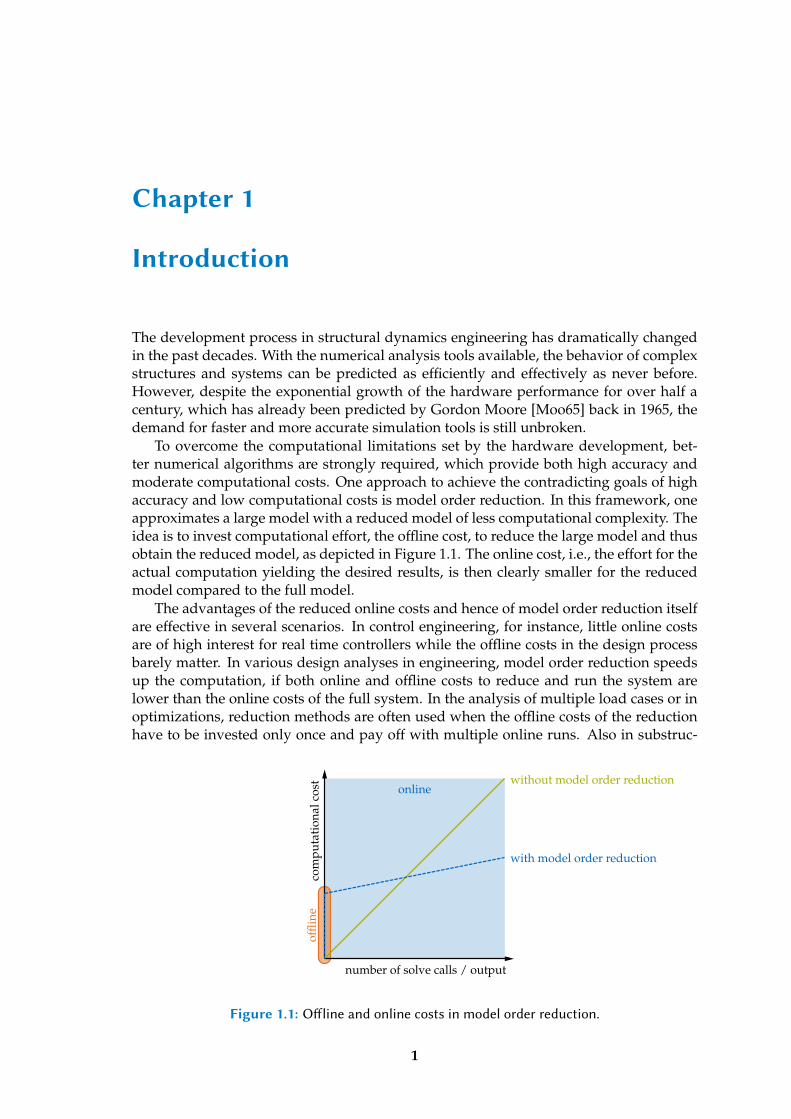
To overcome the computational limitations set by the hardware development, bet-ter numerical algorithms are strongly required, which provide both high accuracy andmoderate computational costs. One approach to achieve the contradicting goals of highaccuracy and low computational costs is model order reduction. In this framework, oneapproximates a large model with a reduced model of less computational complexity. Theidea is to invest computational effort, the offline cost, to reduce the large model and thusobtain the reduced model, as depicted in Figure 1.1. The online cost, i.e., the effort for theactual computation yielding the desired results, is then clearly smaller for the reducedmodel compared to the full model.
The advantages of the reduced online costs and hence of model order reduction itselfare effective in several scenarios. In control engineering, for instance, little online costsare of high interest for real time controllers while the offline costs in the design processbarely matter. In various design analyses in engineering, model order reduction speedsup the computation, if both online and offline costs to reduce and run the system arelower than the online costs of the full system. In the analysis of multiple load cases or inoptimizations, reduction methods are often used when the offline costs of the reductionhave to be invested only once and pay off with multiple online runs. Also in substruc-
onlinewithout model order reduction
with model order reduction
offli
ne
number of solve calls / output
com
puta
tion
alco
st
Figure 1.1: Oline and online costs in model order reduction.
1
2 Introduction
COPYRIGHT © 2010 THE BOEING COMPANY Smith, 7-April-2011, ESASI-Lisbon | 5
787 Wing Flex - On-Ground
On-Ground 0 ft
COPYRIGHT © 2010 THE BOEING COMPANY Smith, 7-April-2011, ESASI-Lisbon | 6
787 Wing Flex - 1G Flight
1G Flight
1G Flight ~12 ft
On-Ground 0 ft
COPYRIGHT © 2010 THE BOEING COMPANY Smith, 7-April-2011, ESASI-Lisbon | 7
787 Wing Flex
Max-Load
Ultimate-Load ~26 ft
1G Flight ~12 ft
On-Ground 0 ft
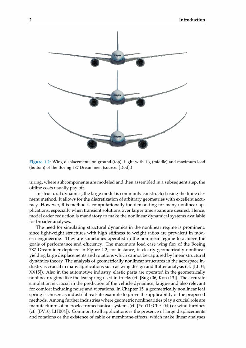
Figure 1.2: Wing displacements on ground (top), flight with 1 g (middle) and maximum load(boom) of the Boeing 787 Dreamliner. (source: [Dod].)
turing, where subcomponents are modeled and then assembled in a subsequent step, theoffline costs usually pay off.
In structural dynamics, the large model is commonly constructed using the finite ele-ment method. It allows for the discretization of arbitrary geometries with excellent accu-racy. However, this method is computationally too demanding for many nonlinear ap-plications, especially when transient solutions over larger time spans are desired. Hence,model order reduction is mandatory to make the nonlinear dynamical systems availablefor broader analyses.
The need for simulating structural dynamics in the nonlinear regime is prominent,since lightweight structures with high stiffness to weight ratios are prevalent in mod-ern engineering. They are sometimes operated in the nonlinear regime to achieve thegoals of performance and efficiency. The maximum load case wing flex of the Boeing787 Dreamliner depicted in Figure 1.2, for instance, is clearly geometrically nonlinearyielding large displacements and rotations which cannot be captured by linear structuraldynamics theory. The analysis of geometrically nonlinear structures in the aerospace in-dustry is crucial in many applications such as wing design and flutter analysis (cf. [LL04;XX15]). Also in the automotive industry, elastic parts are operated in the geometricallynonlinear regime like the leaf spring used in trucks (cf. [Sug+06; Kon+13]). The accuratesimulation is crucial in the prediction of the vehicle dynamics, fatigue and also relevantfor comfort including noise and vibrations. In Chapter 15, a geometrically nonlinear leafspring is chosen as industrial real-life example to prove the applicability of the proposedmethods. Among further industries where geometric nonlinearities play a crucial role aremanufacturers of microelectromechanical systems (cf. [You11; Che+04]) or wind turbines(cf. [BV10; LHB04]). Common to all applications is the presence of large displacementsand rotations or the existence of cable or membrane-effects, which make linear analyses
1.1 Objective 3
insufficient and require geometrically nonlinear investigations.
1.1 Objective
Model order reduction is well established in linear structural dynamics. Various meth-ods exist, which rely on intrinsic properties such as eigenmodes and hence are backedup by system theoretic properties. For nonlinear systems, however, these properties doeither not exist or are very hard to compute, so that the linear methods are in generalnot successfully applicable to nonlinear systems. Thus, the state-of-the-art approach innonlinear model order reduction is a detour over statistical methods, where so-calledtraining snapshots computed using the full, unreduced system are used to build the re-duced models. This approach, however, is to a certain extent contradictory to the conceptof model order reduction, since the large, unreduced system needs to be solved first inorder to reduce exactly this system. Depending on the system and the computationalhardware available, these offline costs associated with the solution of the full, unreducedsystem are inconvenient in the best case. In the worst case, model order reduction withsimulation-based methods requiring the large training snapshots is infeasible when thecomputational hardware for the full system is not available.
Simulation-free methods solve this issue by circumventing the necessity of full sys-tems’s training sets for generating nonlinear reduced models. They identify the nonlineareffects by other means like Taylor expansions or cheaper static training sets with pseudo-dynamic forces. Thereby, the task of model order reduction for nonlinear systems canbe subdivided into the reduced basis problem and the hyper-reduction problem. In theformer, the kinematic space of motion is reduced yielding a reduced set of generalizedcoordinates. The latter deals with the accelerated evaluation of the nonlinearities in thereduced equations of motion. Hence, the objective of this thesis is to discuss already knownand introduce new simulation-free methods for both reduced basis methods and hyper-reductionmethods in the context of nonlinear structural dynamics.
Not discussed are methods based on the proper generalized decomposition (PGD),which take a completely different approach. While the reduced basis methods haveproven to be excellent procedures for the reduction of linear and nonlinear structural dy-namical systems, it is still unclear if the PGD is applicable in this regime, see for instanceBoucinha et al. [BGA13; Bou+14].
1.2 Scientific Contributions
This thesis gives an overview of simulation-free reduced basis and hyper-reduction meth-ods. Some approaches presented are novel scientific contributions of the author:
• A nonlinear projection technique named quadratic manifold approach introducedin Chapter 7, of which parts are published in [RR14b; RRT14; Jai+17; Rut+17],
• a clarification and generalization of the static derivatives and how they fit into theframework of simulation-free nonlinear reduction, which is published in [Rut+17],
• a comparison technique of reduction bases using subspace angles discussed in Chap-ter 8, which is published in [RGR15],
• the alternative computation of the polynomial tensors used for polynomial tensorshyper-reduction based on numerical differentiation as well as the speedup tech-nique to exploit the symmetry of the polynomial tensors both addressed in Chap-ter 11, and
4 Introduction
• the generation of almost simulation-free training snapshots named NSKTS andNSMTS for the ECSW hyper-reduction proposed in Chapter 13, published in [RR17].
Furthermore, numerical experiments for the relevant methods are reported. Some ofthem reveal novel results, which are discussed in the respective chapter. To enable theapplication of the advanced reduction techniques to academic and industrial examples,a non-linear structural dynamics research code named AMFE, based on finite elementsand written in Python and Fortran, was entirely developed by the author in the contextof this thesis.
1.3 Outline
After this introductory chapter, the fundamentals of the finite element method are in-troduced in Chapter 2 with special focus on geometrical nonlinearity. Closely related isChapter A in the Appendix, where the nonlinear finite element formulation is covered indetail together with the structure of the code AMFE.
Then, the thesis is subdivided in three parts. Part I is devoted to the reduced basisapproach which is introduced in Chapter 3. In the following four chapters, differentapproaches to the construction of the reduced basis are discussed. Chapter 4 deals withthe reduction of linear structural dynamics systems. The two main methods proposedare embedded in the substructuring context, which is very common in linear model orderreduction, as well as in the system theoretics context, which provides more underlyingtheory.
The reduction of nonlinear systems is addressed by the three subsequent chapters.Chapter 5 introduces the Proper Orthogonal Decomposition (POD), the state-of-the-artmethod for the reduction of nonlinear systems, which is simulation-based, though. Thus,Chapter 6 investigates the simulation-free reduced basis methods. These methods extendthe linear reduction methods introduced in Chapter 4 with static and modal derivatives,making them suitable for geometrically nonlinear systems. Several variants of the staticand modal derivative approach are discussed as well as techniques for selecting specificbasis vectors. In numerical experiments, these procedures are applied to academic exam-ples revealing certain novel patterns of the methods.
A fundamentally different approach for projective model order reduction is taken inChapter 7, where a nonlinear mapping technique is introduced. In this simulation-freemethod, the projectional subspace is constantly altered based on a quadratic manifoldwhich is constructed using basis vectors and quadratic expansion vectors. These are ei-ther chosen as modal derivatives or static derivatives which result from the so-calledforce compensation approach. This technique provides a minimal number of degrees offreedom (dofs), however it is limited to special cases. For deeper insights, the methodis discussed in the context of von Karman kinematics, where it evolves in a nonlinearGuyan reduction scheme. A broad numerical investigation is conducted in the applica-tions section. It unveils the pattern, that the quadratic manifold approach is successfullyapplicable to structures where the nonlinearity is associated with small rotations, as it isthe case for membrane-like structures.
Chapter 8 addresses the comparison of bases using subspace angles and principalvectors. They form a powerful and insightful tool for comparing reduced bases, which isexemplarily applied to one of the examples used throughout this thesis. In this numericalexperiment it is shown that the linearization of rotations is the main reason for the fail-ure of linear reduction methods in the context of geometrically nonlinear finite elementsystems. Part I is concluded with a brief summary given in Chapter 9.
Part II is devoted to the hyper-reduction problem emerging from the reduced basisreduction of nonlinear systems. In Chapter 10, the hyper-reduction problem is explained,
1.4 Remarks on Notation 5
which is then addressed in the following three chapters. Chapter 11 deals with the poly-nomial tensors hyper-reduction. This method is based on the fact that the internal non-linear forces are third order polynomials for systems modeled with St. Venant-Kirchhoffmaterial. To obtain the polynomial coefficients, different non-intrusive methods are in-vestigated. Furthermore, an approach for exploiting the symmetry of the polynomialcoefficient arrays is proposed for both efficient storing and efficient multiplication.
A different hyper-reduction approach named Discrete Empirical Interpolation Method(DEIM) is discussed in Chapter 12. It approximates the nonlinear internal forces in theunreduced domain using an empirically computed force basis and a collocation scheme,which however breaks the symmetry and with it the stability of the reduced system.Various improvements of the method are discussed, which however cannot alleviate thefundamental flaw of lost symmetry cast into the method. A brief empirical study inves-tigates why the DEIM fails for what concerns both accuracy and stability when appliedin the geometrically nonlinear finite element context.
Chapter 13 is committed to the Energy Conserving Mesh Sampling and Weighting(ECSW) hyper-reduction method. It is similar to the DEIM, as it also relies on a reducedevaluation of the internal forces, but resolves the fundamental flaws of the DEIM allow-ing for the construction of accurate and stable hyper-reduced models. The main issue ofthe method in the context of simulation-free reduced bases is the need for training snap-shots, which are commonly obtained from a training simulation of the full, unreducedsystem. In order to make the ECSW applicable in a simulation-free context and fill thegap between simulation-free reduced bases and the ECSW hyper-reduction, the novelNonlinear Stochastic Krylov Training Sets (NSKTS) and the Nonlinear Stochastic ModalTraining Sets (NSMTS) are proposed. In a detailed study, the applicability and robustnessof these lean training sets is demonstrated. In Chapter 14, a concise summary of Part IIist given.
Part III of this thesis concludes the two previous parts. In Chapter 15, the simulation-free framework of building a reduced basis and applying a hyper-reduction is demon-strated on a real-life example of a leaf spring of a truck. The applicability, accuracy andgreat speedup factors are confirmed in a thorough investigation. Chapter 16 summa-rizes the thesis with a conclusion of the main results and with topics suitable for futureresearch.
1.4 Remarks on Notation
Throughout this thesis, the symbols are mostly used in a consistent manner. If not explic-itly denoted otherwise, non-boldface symbols refer to scalar values, lowercase boldfacesymbols are column vectors and uppercase boldface symbols are matrices. Calligraphicletters, e.g., E , refer to sets.
All numerical experiments are conducted with AMFE, the Python module written inthe context of this thesis. Hence, the indexing and slicing convention follows the zero-based style of Python, i.e., a[0] selects the first element of vector a, a[: 5] the first fiveelements of a and A[:, : 3] the first three columns of the matrix A. Furthermore, in theranges used in for-loops of algorithms, the upper value is not included in the range, i.e.,for i := 0 : 10 yields ten ascending values for i in every iteration with the first beingzero and the last being nine.

Chapter 2
Nonlinear Finite Elements
The key technology in structural dynamics is the finite element method, which allowsfor the discretization of the continuous elasto-dynamic problem. Since the method is sowidespread and successful, it has an enormous body of literature. In this section, onlythe basic concepts are briefly introduced, which are necessary for the understanding ofthe reduction methods in the following chapters. For introductory textbooks on the topic,the reader is referred to, e.g., Bonet and Wood [BW97], Belytschko et al. [BLM00], Reddy[Red04], Simo and Hughes [SH06] or Crisfield et al. [C+12].
Different textbooks come with different notations. Throughout this thesis, the nota-tion is kept close to Belytschko et al. [BLM00] using the Total Lagrangian framework.Several modifications are done in order to keep the notation consistent with the softwareAMFE, which is discussed in Chapter A in the Appendix.
2.1 Continuum Mechanics
P
Ω0
Ωt
P
XPxP(t)
reference configuration
e1
e2
e3
deformed configuration
u(XP, t)
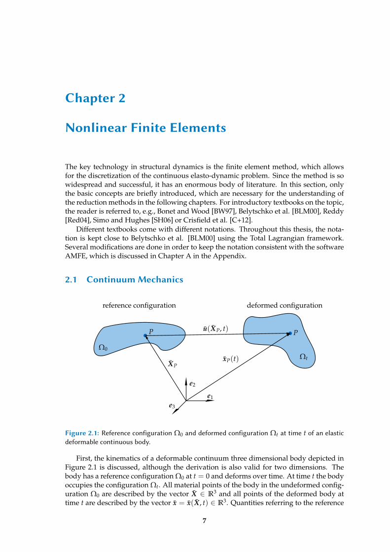
Figure 2.1: Reference configuration Ω0 and deformed configuration Ωt at time t of an elasticdeformable continuous body.
First, the kinematics of a deformable continuum three dimensional body depicted inFigure 2.1 is discussed, although the derivation is also valid for two dimensions. Thebody has a reference configuration Ω0 at t = 0 and deforms over time. At time t the bodyoccupies the configuration Ωt. All material points of the body in the undeformed config-uration Ω0 are described by the vector X ∈ R3 and all points of the deformed body attime t are described by the vector x = x(X, t) ∈ R3. Quantities referring to the reference
7
8 Nonlinear Finite Elements
domain are expressed with uppercase letters, whereas quantities in the deformed domainare expressed with lowercase letters. The bar over the letters X and x denotes that thesevariables are continuous in space in contrary to the nodal quantities of discretized finiteelements, see Section 2.3. The displacement of a particle is then expressed by the dis-placement vector u describing the position of the deformed configuration relative to theinitial configuration:
u(X, t) = x(X, t)− X. (2.1)
The deformation is measured with the deformation gradient F ∈ R3×3. It is the partialderivative of the deformed configuration with respect to the initial configuration and canalso be expressed in terms of the displacement vector u using the identity matrix I ∈ R3:
F =∂x∂X
=∂u∂X
+ I. (2.2)
The deformation gradient describes the mapping of an infinitesimal vector dX fromthe reference domain to the current domain dx = FdX, which is also denoted the pushforward operation. Since the mapping is bijective, dx can also be uniquely mapped todX with dX = F−1dx in the pull back operation. The deformation gradient F, which isnot symmetric in general, accounts for both stretching and rotation.
For describing strains in a large deformation context, a strain measure should notfeature strains for pure rigid body rotations, but should be rotation-invariant or objective.Before introducing an objective strain measure, the deformation gradient F is investi-gated further. The mapping of F can be decomposed mathematically with the singularvalue decomposition (SVD) to
F = UsvdΣsvdV Tsvd, (2.3)
where Usvd ∈ R3×3 and V svd ∈ R3×3 are orthogonal matrices and Σsvd ∈ R3×3 is a di-agonal matrix formed by the singular values. In the geometric interpretation of the SVD,the orthogonal matrices represent rotation operators in the 3D space, while the diagonalmatrix represents a stretching along the main axes. Hence, the mapping F from the refer-ence configuration to the deformed configuration can be split into a rotation performedby V T
svd followed by a stretch along the main axes performed by Σsvd followed by an-other rotation performed by Usvd. Since Σsvd is a diagonal matrix, the stretch operationis performed along the main axes of the intermediate coordinate system, into which therotation V T
svd was transforming. The stretch operation performed by Σsvd can also be ex-pressed as a stretch operation not along the principal axes but along axes different fromthem, leading to the symmetric material stretch tensor U:
U = V svdΣsvdV Tsvd. (2.4)
If F is to be expressed as a stretch operation with the material stretch operator U, therotation
R = UsvdV Tsvd (2.5)
completes the mapping of F since V TsvdV svd = I, leading to the polar decomposition of
the deformation gradient F:
F = RU. (2.6)
The orthogonal matrix R represents the rotation, which is performed after the mate-rial stretching performed by the symmetric tensor U.
2.1 Continuum Mechanics 9
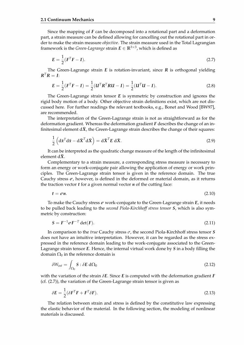
Since the mapping of F can be decomposed into a rotational part and a deformationpart, a strain measure can be defined allowing for cancelling out the rotational part in or-der to make the strain measure objective. The strain measure used in the Total Lagrangianframework is the Green-Lagrange strain E ∈ R3×3, which is defined as
E =12(FT F − I). (2.7)
The Green-Lagrange strain E is rotation-invariant, since R is orthogonal yieldingRTR = I:
E =12(FT F − I) =
12(UTRTRU − I) =
12(UTU − I). (2.8)
The Green-Lagrange strain tensor E is symmetric by construction and ignores therigid body motion of a body. Other objective strain definitions exist, which are not dis-cussed here. For further readings the relevant textbooks, e.g., Bonet and Wood [BW97],are recommended.
The interpretation of the Green-Lagrange strain is not as straightforward as for thedeformation gradient. Whereas the deformation gradient F describes the change of an in-finitesimal element dX, the Green-Lagrange strain describes the change of their squares:
12
(dxTdx− dXTdX
)= dXTE dX. (2.9)
It can be interpreted as the quadratic change measure of the length of the infinitesimalelement dX.
Complementary to a strain measure, a corresponding stress measure is necessary toform an energy or work-conjugate pair allowing the application of energy or work prin-ciples. The Green-Lagrange strain tensor is given in the reference domain. The trueCauchy stress σ, however, is defined in the deformed or material domain, as it returnsthe traction vector t for a given normal vector n of the cutting face:
t = σn. (2.10)
To make the Cauchy stress σ work-conjugate to the Green-Lagrange strain E, it needsto be pulled back leading to the second Piola-Kirchhoff stress tensor S, which is also sym-metric by construction:
S = F−1σF−T det(F). (2.11)
In comparison to the true Cauchy stress σ, the second Piola-Kirchhoff stress tensor Sdoes not have an intuitive interpretation. However, it can be regarded as the stress ex-pressed in the reference domain leading to the work-conjugate associated to the Green-Lagrange strain tensor E. Hence, the internal virtual work done by S in a body filling thedomain Ω0 in the reference domain is
δWint =∫
Ω0
S : δE dΩ0 (2.12)
with the variation of the strain δE. Since E is computed with the deformation gradient F(cf. (2.7)), the variation of the Green-Lagrange strain tensor is given as
δE =12(δFT F + FTδF). (2.13)
The relation between strain and stress is defined by the constitutive law expressingthe elastic behavior of the material. In the following section, the modeling of nonlinearmaterials is discussed.
10 Nonlinear Finite Elements
2.2 Nonlinear Material
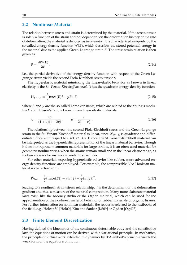
The relation between stress and strain is determined by the material. If the stress tensoris solely a function of the strain and not dependent on the deformation history or the rateof deformation, the material is denoted as hyperelastic. It is characterized uniquely by theso-called energy density function W(E), which describes the stored potential energy inthe material due to the applied Green-Lagrange strain E. The stress strain relation is thengiven as
S =∂W(E)
∂E, (2.14)
i.e., the partial derivative of the energy density function with respect to the Green-La-grange strain yields the second Piola-Kirchhoff stress tensor S.
The hyperelastic material mimicking the linear-elastic behavior as known in linearelasticity is the St. Venant-Kirchhoff material. It has the quadratic energy density function
WSV−K =λ
2trace(E)2 + µE : E, (2.15)
where λ and µ are the so-called Lamé constants, which are related to the Young’s modu-lus E and Poisson’s ratio ν known from linear elastic materials:
λ =νE
(1 + ν)(1− 2ν), µ =
E2(1 + ν)
. (2.16)
The relationship between the second Piola-Kirchhoff stress and the Green-Lagrangestrain in the St. Venant-Kirchhoff material is linear, since WSV−K is quadratic and differ-entiated once with respect to E (cf. (2.14)). Hence, the St. Venant-Kirchhoff material canbe interpreted as the hyperelastic representation of the linear material behavior. Thoughit does not represent common materials for large strains, it is an often used material forgeometric nonlinearities, when the strains remain small and in the linear-elastic range, asit often appears for instance in metallic structures.
For other materials exposing hyperelastic behavior like rubber, more advanced en-ergy density functions are employed. For example, the compressible Neo-Hookean ma-terial is characterized by
WNH =µ
2(trace(E))− µ ln(J) +
λ
2(ln(J))2, (2.17)
leading to a nonlinear strain-stress relationship. J is the determinant of the deformationgradient and thus a measure of the material compression. Many more elaborate materiallaws exist, like the Mooney-Rivlin or the Ogden material, which can be used for theapproximation of the nonlinear material behavior of rubber materials or organic tissues.For further information on nonlinear materials, the reader is referred to the textbooks ofthe field, e.g., Holzapfel [Hol00], Kim and Sankar [KS09] or Ogden [Ogd97].
2.3 Finite Element Discretization
Having defined the kinematics of the continuous deformable body and the constitutivelaw, the equations of motion can be derived with a variational principle. In mechanics,the principle of virtual work extended to dynamics by d’Alembert’s principle yields theweak form of the equations of motion:
2.3 Finite Element Discretization 11
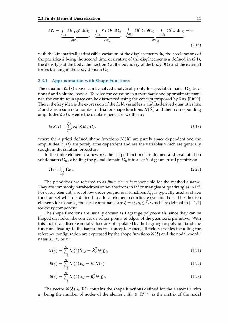
δW =∫
Ω0
δuTρ0 ¨u dΩ0
︸ ︷︷ ︸δWkin
+∫
Ω0
S : δE dΩ0
︸ ︷︷ ︸δWint
−∫
∂Ω0
δuTt d∂Ω0 −∫
Ω0
δuTb dΩ0
︸ ︷︷ ︸δWext
= 0
(2.18)
with the kinematically admissible variation of the displacements δu, the accelerations ofthe particles ¨u being the second time derivative of the displacements u defined in (2.1),the density ρ of the body, the traction t at the boundary of the body ∂Ω0 and the externalforces b acting in the body domain Ω0.
2.3.1 Approximation with Shape Functions
The equation (2.18) above can be solved analytically only for special domains Ω0, trac-tions t and volume loads b. To solve the equation in a systematic and approximate man-ner, the continuous space can be discretized using the concept proposed by Ritz [Rit09].There, the key idea is the expression of the field variables u and its derived quantities likeE and S as a sum of a number of trial or shape functions N(X) and their correspondingamplitudes ue(t). Hence the displacements are written as
u(X, t) =nn
∑i=1
Ni(X)ue,i(t), (2.19)
where the a priori defined shape functions Ni(X) are purely space dependent and theamplitudes ue,i(t) are purely time dependent and are the variables which are generallysought in the solution procedure.
In the finite element framework, the shape functions are defined and evaluated onsubdomains Ω0,e dividing the global domain Ω0 into a set E of geometrical primitives:
Ω0 ≈⋃
e∈EΩ0,e. (2.20)
The primitives are referred to as finite elements responsible for the method’s name.They are commonly tetrahedrons or hexahedrons in R3 or triangles or quadrangles in R2.For every element, a set of low order polynomial functions Ne,i is typically used as shapefunction set which is defined in a local element coordinate system. For a Hexahedronelement, for instance, the local coordinates are ξ = (ξ, η, ζ)T, which are defined in [−1, 1]for every component.
The shape functions are usually chosen as Lagrange polynomials, since they can behinged on nodes like corners or center points of edges of the geometric primitive. Withthis choice, all discrete nodal values are interpolated by the Lagrangian polynomial shapefunctions leading to the isoparametric concept. Hence, all field variables including thereference configuration are expressed by the shape functions N(ξ) and the nodal coordi-nates Xe, xe or ue:
X(ξ) =nn
∑i=1
Ni(ξ)Xe,i = XTe N(ξ), (2.21)
x(ξ) =nn
∑i=1
Ni(ξ)xe,i = xTe N(ξ), (2.22)
u(ξ) =nn
∑i=1
Ni(ξ)ue,i = uTe N(ξ). (2.23)
The vector N(ξ) ∈ Rnn contains the shape functions defined for the element e withnn being the number of nodes of the element, Xe ∈ Rnn×3 is the matrix of the nodal
12 Nonlinear Finite Elements
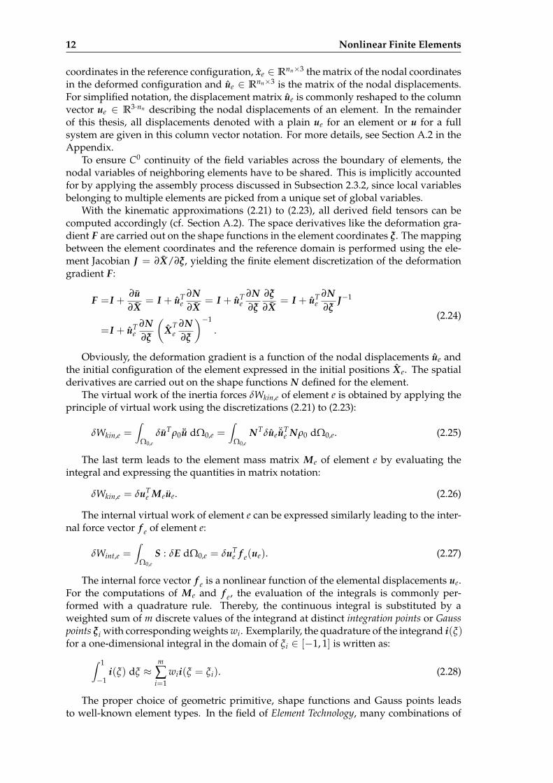
coordinates in the reference configuration, xe ∈ Rnn×3 the matrix of the nodal coordinatesin the deformed configuration and ue ∈ Rnn×3 is the matrix of the nodal displacements.For simplified notation, the displacement matrix ue is commonly reshaped to the columnvector ue ∈ R3·nn describing the nodal displacements of an element. In the remainderof this thesis, all displacements denoted with a plain ue for an element or u for a fullsystem are given in this column vector notation. For more details, see Section A.2 in theAppendix.
To ensure C0 continuity of the field variables across the boundary of elements, thenodal variables of neighboring elements have to be shared. This is implicitly accountedfor by applying the assembly process discussed in Subsection 2.3.2, since local variablesbelonging to multiple elements are picked from a unique set of global variables.
With the kinematic approximations (2.21) to (2.23), all derived field tensors can becomputed accordingly (cf. Section A.2). The space derivatives like the deformation gra-dient F are carried out on the shape functions in the element coordinates ξ. The mappingbetween the element coordinates and the reference domain is performed using the ele-ment Jacobian J = ∂X/∂ξ, yielding the finite element discretization of the deformationgradient F:
F =I +∂u∂X
= I + uTe
∂N∂X
= I + uTe
∂N∂ξ
∂ξ
∂X= I + uT
e∂N∂ξ
J−1
=I + uTe
∂N∂ξ
(XT
e∂N∂ξ
)−1
.(2.24)
Obviously, the deformation gradient is a function of the nodal displacements ue andthe initial configuration of the element expressed in the initial positions Xe. The spatialderivatives are carried out on the shape functions N defined for the element.
The virtual work of the inertia forces δWkin,e of element e is obtained by applying theprinciple of virtual work using the discretizations (2.21) to (2.23):
δWkin,e =∫
Ω0,e
δuTρ0 ¨u dΩ0,e =∫
Ω0,e
NTδue ¨uTe Nρ0 dΩ0,e. (2.25)
The last term leads to the element mass matrix Me of element e by evaluating theintegral and expressing the quantities in matrix notation:
δWkin,e = δuTe Meue. (2.26)
The internal virtual work of element e can be expressed similarly leading to the inter-nal force vector f e of element e:
δWint,e =∫
Ω0,e
S : δE dΩ0,e = δuTe f e(ue). (2.27)
The internal force vector f e is a nonlinear function of the elemental displacements ue.For the computations of Me and f e, the evaluation of the integrals is commonly per-formed with a quadrature rule. Thereby, the continuous integral is substituted by aweighted sum of m discrete values of the integrand at distinct integration points or Gausspoints ξi with corresponding weights wi. Exemplarily, the quadrature of the integrand i(ξ)for a one-dimensional integral in the domain of ξi ∈ [−1, 1] is written as:
∫ 1
−1i(ξ) dξ ≈
m
∑i=1
wii(ξ = ξi). (2.28)
The proper choice of geometric primitive, shape functions and Gauss points leadsto well-known element types. In the field of Element Technology, many combinations of
2.3 Finite Element Discretization 13
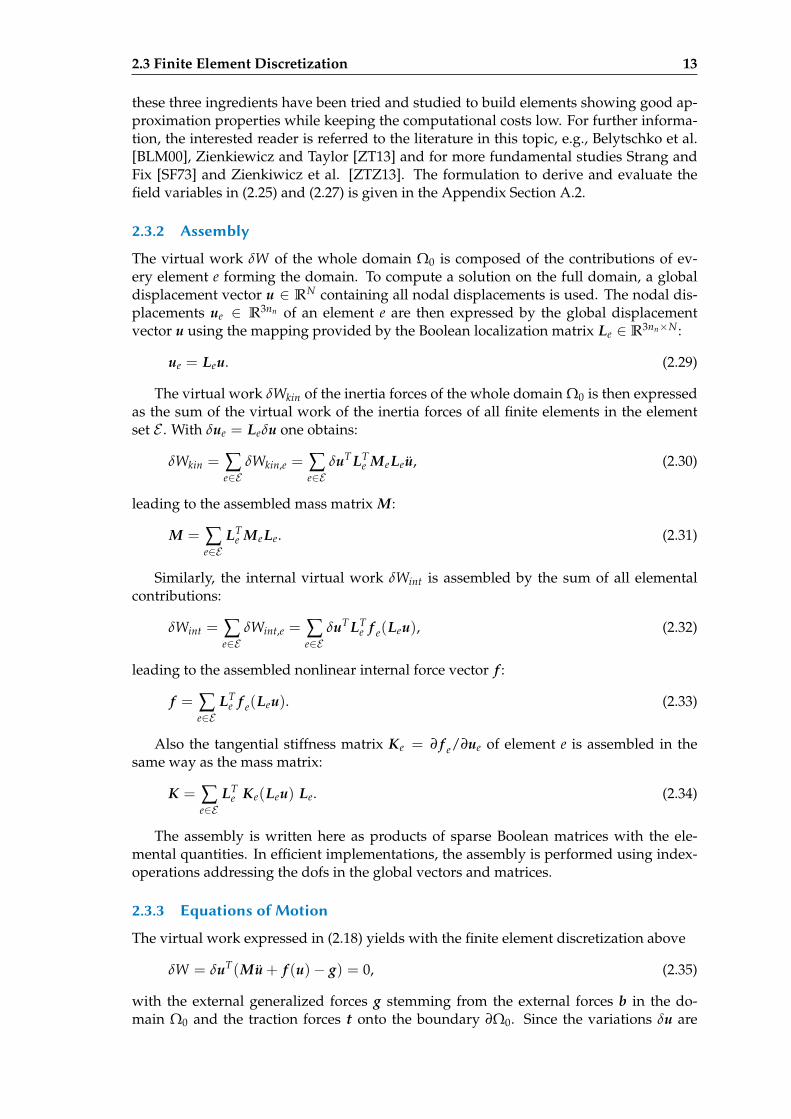
these three ingredients have been tried and studied to build elements showing good ap-proximation properties while keeping the computational costs low. For further informa-tion, the interested reader is referred to the literature in this topic, e.g., Belytschko et al.[BLM00], Zienkiewicz and Taylor [ZT13] and for more fundamental studies Strang andFix [SF73] and Zienkiwicz et al. [ZTZ13]. The formulation to derive and evaluate thefield variables in (2.25) and (2.27) is given in the Appendix Section A.2.
2.3.2 Assembly
The virtual work δW of the whole domain Ω0 is composed of the contributions of ev-ery element e forming the domain. To compute a solution on the full domain, a globaldisplacement vector u ∈ RN containing all nodal displacements is used. The nodal dis-placements ue ∈ R3nn of an element e are then expressed by the global displacementvector u using the mapping provided by the Boolean localization matrix Le ∈ R3nn×N :
ue = Leu. (2.29)
The virtual work δWkin of the inertia forces of the whole domain Ω0 is then expressedas the sum of the virtual work of the inertia forces of all finite elements in the elementset E . With δue = Leδu one obtains:
δWkin = ∑e∈E
δWkin,e = ∑e∈E
δuT LTe MeLeu, (2.30)
leading to the assembled mass matrix M:
M = ∑e∈E
LTe MeLe. (2.31)
Similarly, the internal virtual work δWint is assembled by the sum of all elementalcontributions:
δWint = ∑e∈E
δWint,e = ∑e∈E
δuT LTe f e(Leu), (2.32)
leading to the assembled nonlinear internal force vector f :
f = ∑e∈E
LTe f e(Leu). (2.33)
Also the tangential stiffness matrix Ke = ∂ f e/∂ue of element e is assembled in thesame way as the mass matrix:
K = ∑e∈E
LTe Ke(Leu) Le. (2.34)
The assembly is written here as products of sparse Boolean matrices with the ele-mental quantities. In efficient implementations, the assembly is performed using index-operations addressing the dofs in the global vectors and matrices.
2.3.3 Equations of Motion
The virtual work expressed in (2.18) yields with the finite element discretization above
δW = δuT(Mu + f (u)− g) = 0, (2.35)
with the external generalized forces g stemming from the external forces b in the do-main Ω0 and the traction forces t onto the boundary ∂Ω0. Since the variations δu are
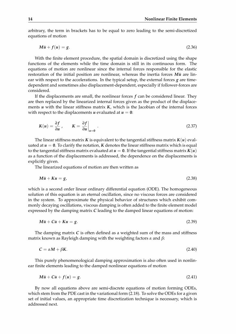
14 Nonlinear Finite Elements
arbitrary, the term in brackets has to be equal to zero leading to the semi-discretizedequations of motion
Mu + f (u) = g. (2.36)
With the finite element procedure, the spatial domain is discretized using the shapefunctions of the elements while the time domain is still in its continuous form. Theequations of motion are nonlinear since the internal forces responsible for the elasticrestoration of the initial position are nonlinear, whereas the inertia forces Mu are lin-ear with respect to the accelerations. In the typical setup, the external forces g are time-dependent and sometimes also displacement-dependent, especially if follower-forces areconsidered.
If the displacements are small, the nonlinear forces f can be considered linear. Theyare then replaced by the linearized internal forces given as the product of the displace-ments u with the linear stiffness matrix K, which is the Jacobian of the internal forceswith respect to the displacements u evaluated at u = 0:
K(u) =∂ f∂u
, K =∂ f∂u
∣∣∣∣u=0
. (2.37)
The linear stiffness matrix K is equivalent to the tangential stiffness matrix K(u) eval-uated at u = 0. To clarify the notation, K denotes the linear stiffness matrix which is equalto the tangential stiffness matrix evaluated at u = 0. If the tangential stiffness matrix K(u)as a function of the displacements is addressed, the dependence on the displacements isexplicitly given.
The linearized equations of motion are then written as
Mu + Ku = g, (2.38)
which is a second order linear ordinary differential equation (ODE). The homogeneoussolution of this equation is an eternal oscillation, since no viscous forces are consideredin the system. To approximate the physical behavior of structures which exhibit com-monly decaying oscillations, viscous damping is often added to the finite element modelexpressed by the damping matrix C leading to the damped linear equations of motion:
Mu + Cu + Ku = g. (2.39)
The damping matrix C is often defined as a weighted sum of the mass and stiffnessmatrix known as Rayleigh damping with the weighting factors α and β:
C = αM + βK. (2.40)
This purely phenomenological damping approximation is also often used in nonlin-ear finite elements leading to the damped nonlinear equations of motion
Mu + Cu + f (u) = g. (2.41)
By now all equations above are semi-discrete equations of motion forming ODEs,which stem from the PDE cast in the variational form (2.18). To solve the ODEs for a givenset of initial values, an appropriate time discretization technique is necessary, which isaddressed next.
2.4 Time Integration 15
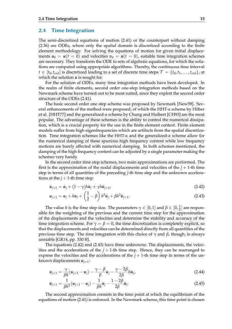
2.4 Time Integration
The semi-discretized equations of motion (2.41) or the counterpart without damping(2.36) are ODEs, where only the spatial domain is discretized according to the finiteelement methodology. For solving the equations of motion for given initial displace-ments u0 = u(t = 0) and velocities v0 = u(t = 0), suitable time integration schemesare necessary. They transform the ODE to sets of algebraic equations, for which the solu-tions are computed using appropriate algorithms. Thereby, the continuous time intervalt ∈ [t0, tend] is discretized leading to a set of discrete time steps T = t0, t1, . . . , tend, atwhich the solution u is sought for.
For the solution of ODEs, many time integration methods have been developed. Inthe realm of finite elements, second order one-step integration methods based on theNewmark scheme have turned out to be most suited, since they exploit the second orderstructure of the ODEs (2.41).
The basic second order one step scheme was proposed by Newmark [New59]. Sev-eral enhancements of the method were proposed, of which the HHT-α scheme by Hilberet al. [HHT77] and the generalized-α scheme by Chung and Hulbert [CH93] are the mostpopular. The advantage of these schemes is the ability to control the numerical dissipa-tion, which is a crucial property for the use in the finite element context. Finite elementmodels suffer from high eigenfrequencies which are artifacts from the spatial discretiza-tion. Time integration schemes like the HHT-α and the generalized-α scheme allow forthe numerical damping of these spurious high frequency content while low frequencymotions are barely affected with numerical damping. In both schemes mentioned, thedamping of the high frequency content can be adjusted by a single parameter making theschemes very handy.
In the second order time step schemes, two main approximations are performed. Thefirst is the approximation of the nodal displacements and velocities of the j + 1-th timestep in terms of all quantities of the preceding j-th time step and the unknown accelera-tions at the j + 1-th time step:
uj+1 = uj + (1− γ)huj + γhuj+1, (2.42)
uj+1 = uj + huj +
(12− β
)h2uj + βh2uj+1. (2.43)
The value h is the time step size. The parameters γ ∈ [0, 1] and β ∈ [0, 12 ] are respon-
sible for the weighting of the previous and the current time step for the approximationof the displacements and the velocities and determine the stability and accuracy of thetime integration scheme. For γ = β = 0, the time discretization is completely explicit, sothat the displacements and velocities can be determined directly from all quantities of theprevious time step. The time integration with this choice of γ and β, though, is alwaysunstable [GR14, pp. 530 ff].
The equations (2.42) and (2.43) have three unknowns: The displacements, the veloc-ities and the accelerations of the j + 1-th time step. Hence, they can be rearranged toexpress the velocities and the accelerations of the j + 1-th time step in terms of the un-known displacements uj+1:
uj+1 =γ
βh(uj+1 − uj)−
γ− β
βuj −
γ− 2β
2βhuj, (2.44)
uj+1 =1
βh2 (uj+1 − uj)−1
βhuj −
1− 2β
2βuj. (2.45)
The second approximation consists in the time point at which the equilibrium of theequations of motion (2.41) is enforced. In the Newmark scheme, this time point is chosen
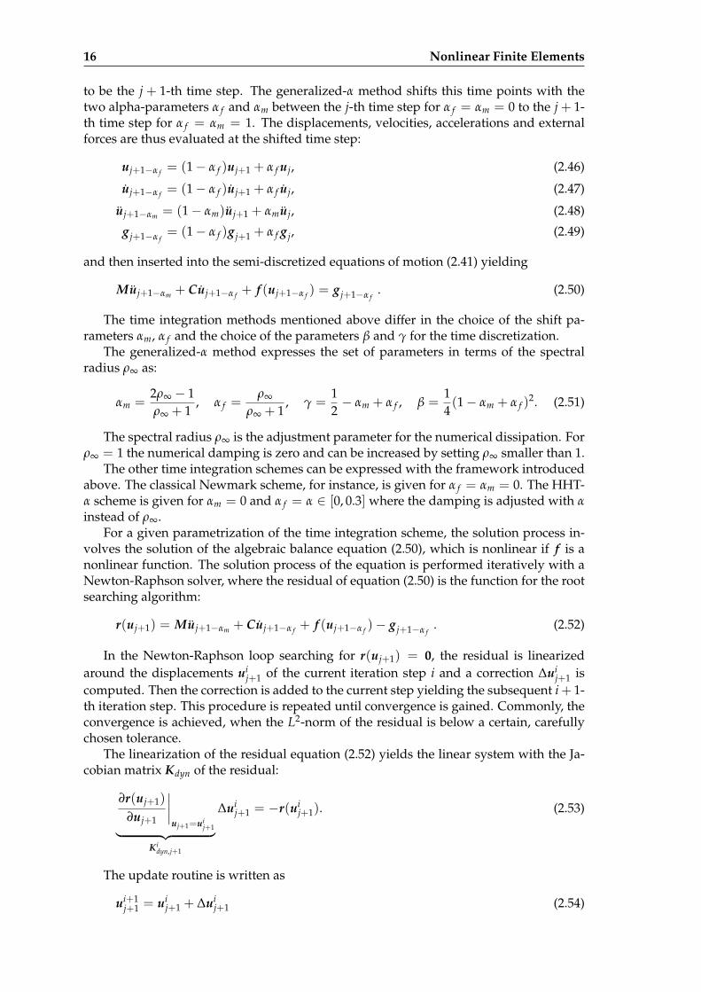
16 Nonlinear Finite Elements
to be the j + 1-th time step. The generalized-α method shifts this time points with thetwo alpha-parameters α f and αm between the j-th time step for α f = αm = 0 to the j + 1-th time step for α f = αm = 1. The displacements, velocities, accelerations and externalforces are thus evaluated at the shifted time step:
uj+1−α f = (1− α f )uj+1 + α f uj, (2.46)
uj+1−α f = (1− α f )uj+1 + α f uj, (2.47)
uj+1−αm = (1− αm)uj+1 + αmuj, (2.48)
g j+1−α f= (1− α f )g j+1 + α f g j, (2.49)
and then inserted into the semi-discretized equations of motion (2.41) yielding
Muj+1−αm + Cuj+1−α f + f (uj+1−α f ) = g j+1−α f. (2.50)
The time integration methods mentioned above differ in the choice of the shift pa-rameters αm, α f and the choice of the parameters β and γ for the time discretization.
The generalized-α method expresses the set of parameters in terms of the spectralradius ρ∞ as:
αm =2ρ∞ − 1ρ∞ + 1
, α f =ρ∞
ρ∞ + 1, γ =
12− αm + α f , β =
14(1− αm + α f )
2. (2.51)
The spectral radius ρ∞ is the adjustment parameter for the numerical dissipation. Forρ∞ = 1 the numerical damping is zero and can be increased by setting ρ∞ smaller than 1.
The other time integration schemes can be expressed with the framework introducedabove. The classical Newmark scheme, for instance, is given for α f = αm = 0. The HHT-α scheme is given for αm = 0 and α f = α ∈ [0, 0.3] where the damping is adjusted with αinstead of ρ∞.
For a given parametrization of the time integration scheme, the solution process in-volves the solution of the algebraic balance equation (2.50), which is nonlinear if f is anonlinear function. The solution process of the equation is performed iteratively with aNewton-Raphson solver, where the residual of equation (2.50) is the function for the rootsearching algorithm:
r(uj+1) = Muj+1−αm + Cuj+1−α f + f (uj+1−α f )− g j+1−α f. (2.52)
In the Newton-Raphson loop searching for r(uj+1) = 0, the residual is linearizedaround the displacements ui
j+1 of the current iteration step i and a correction ∆uij+1 is
computed. Then the correction is added to the current step yielding the subsequent i + 1-th iteration step. This procedure is repeated until convergence is gained. Commonly, theconvergence is achieved, when the L2-norm of the residual is below a certain, carefullychosen tolerance.
The linearization of the residual equation (2.52) yields the linear system with the Ja-cobian matrix Kdyn of the residual:
∂r(uj+1)
∂uj+1
∣∣∣∣uj+1=ui
j+1︸ ︷︷ ︸Ki
dyn,j+1
∆uij+1 = −r(ui
j+1). (2.53)
The update routine is written as
ui+1j+1 = ui
j+1 + ∆uij+1 (2.54)
2.4 Time Integration 17
yielding the displacements for the subsequent iteration step. If the underlying equationsof motion are nonlinear, the iteration matrix Kdyn changes with every iteration step. Thisis due to the fact, that Kdyn involves the Jacobian of the nonlinear forces which is alsoknown as the tangential stiffness matrix K(u) (cf. (2.37)):
Kidyn,j+1 =
∂r(uj+1)
∂uj+1
∣∣∣∣ui
j+1
=
(1− αm
βh2 M +(1− α f )γ
βhC + (1− α f )K(ui
j+1−α f)
).
(2.55)
In the Newton-Raphson procedure above, the linear system of equations has to besolved in every iteration step. Since the dimension of the system is associated with thedofs of the finite element discretization, fine and accurate meshes involve computer in-tensive solutions. One approach to circumvent the expensive solution is the use of ex-plicit integration schemes. However, since the finite element system has very high fre-quencies due to the spatial discretization, explicit integration schemes require extremelysmall time steps, which are only efficient for scenarios, where shock wave propagationsare the relevant dynamics in the system (cf. [GR14]).
In other applications, where the overall global motion of the system is dominat-ing, implicit time integration methods are indispensable. Thereby, the Newton-Raphsonmethod can be substituted by secant methods, quasi-Newton methods or other variantsof it. However, the appeal of the Newton method is the quadratic convergence in thevicinity of the solution, which is not gained with other methods.
When static systems instead of dynamical systems are addressed, the same proce-dure as described above is applied. In the nonlinear balance equation defining the resid-ual (2.52), the inertia and damping terms drop out and the residual is composed of thebalance of internal forces f and external forces g. For the solution of these type of sys-tems, the external force is usually stepwise increased using pseudo time steps or moreadvanced techniques like arc-length continuation methods are used. Since the thesis ismainly about the reduction of dynamical systems and the specific solution technique issecondary, the interested reader is referred to literature on this topic, e.g., Bathe [Bat06],Wriggers [Wri08] and Kim and Sankar [KS09].
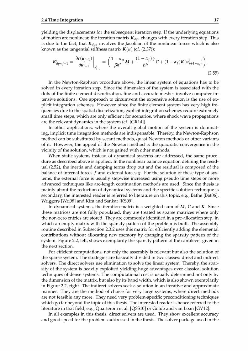
In dynamical systems, the iteration matrix is a weighted sum of M, C and K. Sincethese matrices are not fully populated, they are treated as sparse matrices where onlythe non-zero entries are stored. They are commonly identified in a pre-allocation step, inwhich an empty matrix with the sparsity pattern of the problem is built. The assemblyroutine described in Subsection 2.3.2 uses this matrix for efficiently adding the elementalcontributions without allocating new memory by changing the sparsity pattern of thesystem. Figure 2.2, left, shows exemplarily the sparsity pattern of the cantilever given inthe next section.
For efficient computations, not only the assembly is relevant but also the solution ofthe sparse system. The strategies are basically divided in two classes: direct and indirectsolvers. The direct solvers use elimination to solve the linear system. Thereby, the spar-sity of the system is heavily exploited yielding huge advantages over classical solutiontechniques of dense systems. The computational cost is usually determined not only bythe dimension of the matrix, but also by its band width, which is also shown exemplarilyin Figure 2.2, right. The indirect solvers seek a solution in an iterative and approximatemanner. They are the method of choice for very large systems, where direct methodsare not feasible any more. They need very problem-specific preconditioning techniqueswhich go far beyond the topic of this thesis. The interested reader is hence referred to theliterature in that field, e.g., Quarteroni et al. [QSS10] or Golub and van Loan [GV12].
In all examples in this thesis, direct solvers are used. They show excellent accuracyand good speed for the problems addressed in the thesis. The solver package used in the
18 Nonlinear Finite Elements
Figure 2.2: Sparsity paern of the iteration matrix Kdyn of the cantilever depicted in Figure 2.4.Every dot represents a non-zero entry in the matrix. Le the original matrix, right the reorderedmatrix (reordered using the reverse Cuthill-McKee algorithm [CM69]) revealing the bandwidthof the problem.
AMFE code is the PARDISO package [Sch+10] which has excellent execution speeds andproved to be very efficient for PDE based nonlinear solutions (cf. eg. [Sch+01]).
2.5 Applications: Large Deformations and Geometric Nonlinear-ity
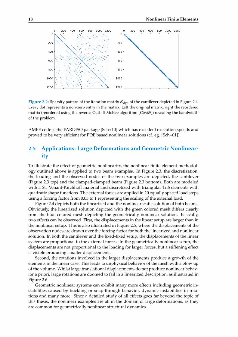
To illustrate the effect of geometric nonlinearity, the nonlinear finite element methodol-ogy outlined above is applied to two beam examples. In Figure 2.3, the discretization,the loading and the observed nodes of the two examples are depicted, the cantilever(Figure 2.3 top) and the clamped-clamped beam (Figure 2.3 bottom). Both are modeledwith a St. Venant-Kirchhoff material and discretized with triangular Tri6 elements withquadratic shape functions. The external forces are applied in 20 equally spaced load stepsusing a forcing factor from 0.05 to 1 representing the scaling of the external load.
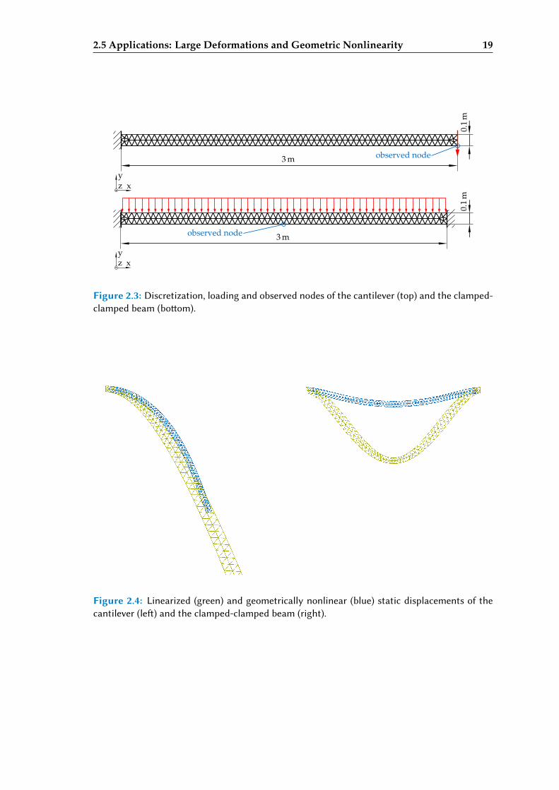
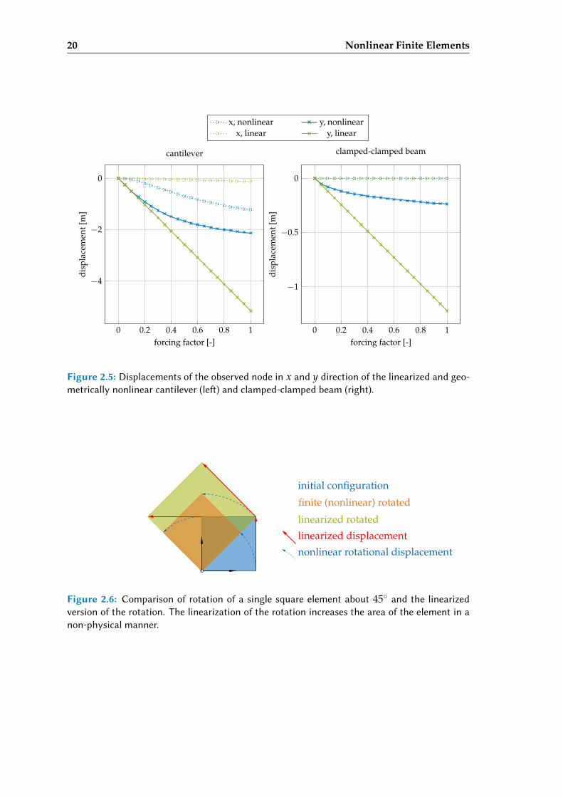
Figure 2.4 depicts both the linearized and the nonlinear static solution of both beams.Obviously, the linearized solution depicted with the green colored mesh differs clearlyfrom the blue colored mesh depicting the geometrically nonlinear solution. Basically,two effects can be observed. First, the displacements in the linear setup are larger than inthe nonlinear setup. This is also illustrated in Figure 2.5, where the displacements of theobservation nodes are drawn over the forcing factor for both the linearized and nonlinearsolution. In both the cantilever and the fixed-fixed setup, the displacements of the linearsystem are proportional to the external forces. In the geometrically nonlinear setup, thedisplacements are not proportional to the loading for larger forces, but a stiffening effectis visible producing smaller displacements.
Second, the rotations involved in the larger displacements produce a growth of theelements in the linear case. This leads to unphysical behavior of the mesh with a blow upof the volume. Whilst large translational displacements do not produce nonlinear behav-ior a priori, large rotations are doomed to fail in a linearized description, as illustrated inFigure 2.6.
Geometric nonlinear systems can exhibit many more effects including geometric in-stabilities caused by buckling or snap-through behavior, dynamic instabilities in rota-tions and many more. Since a detailed study of all effects goes far beyond the topic ofthis thesis, the nonlinear examples are all in the domain of large deformations, as theyare common for geometrically nonlinear structural dynamics.
2.5 Applications: Large Deformations and Geometric Nonlinearity 19
xyz
3 m
0.1
m
observed node
xyz
3 m
0.1
m
observed node
Figure 2.3: Discretization, loading and observed nodes of the cantilever (top) and the clamped-clamped beam (boom).
Figure 2.4: Linearized (green) and geometrically nonlinear (blue) static displacements of thecantilever (le) and the clamped-clamped beam (right).
20 Nonlinear Finite Elements
0 0.2 0.4 0.6 0.8 1
−4
−2
0
forcing factor [-]
disp
lace
men
t[m
]
cantilever
x, nonlinear y, nonlinearx, linear y, linear
0 0.2 0.4 0.6 0.8 1
−1
−0.5
0
forcing factor [-]
disp
lace
men
t[m
]
clamped-clamped beam
Figure 2.5: Displacements of the observed node in x and y direction of the linearized and geo-metrically nonlinear cantilever (le) and clamped-clamped beam (right).
finite (nonlinear) rotated
linearized rotated
initial configuration
linearized displacement
nonlinear rotational displacement
Figure 2.6: Comparison of rotation of a single square element about 45 and the linearizedversion of the rotation. The linearization of the rotation increases the area of the element in anon-physical manner.

Part I
Reduced Basis
21

Chapter 3
Model Order Reduction using Subspace Pro-jection
Projective model order reduction is the key concept in reducing the number of dofs ofa dynamical system from a large number N to a small number n. Since the projectioncan be interpreted as a Ritz or Galerkin method, it shares the same underlying theoryas the discretization of the finite element method, which has been discussed in the pre-vious chapter. In contrary to the finite element method, where a continuous problem ofdimension infinity is reduced to a discrete problem of dimension N, the projective modelorder reduction repeats the procedure to reduce N further to the reduced dimension n. Itis, however, not limited to finite element systems but can be applied to various systems.In this context, though, it is derived and discussed for nonlinear finite element systemswhich have been introduced in Chapter 2.
3.1 Fundamentals of Projective Model Order Reduction
The point of departure are the semi-discretized equations of motion, which might stemfrom a finite element system (cf. (2.41)):
Mu + Cu + f (u) = g. (3.1)
The matrix M ∈ RN×N is the constant mass matrix, C ∈ RN×N is the damping matrixand f ∈ RN denotes the nonlinear restoring forces. The vector g ∈ RN represents theexternal forces and u ∈ RN is the vector of generalized displacements. If the equationabove stems from the finite element discretization, the generalized displacement vector urepresents the nodal displacements. The dimension N of the equations of motion rep-resents directly the resolution of the finite element mesh, i.e., a coarse mesh results in asmaller dimension of (3.1) compared to a finer mesh and vice versa.
The number of unknowns N is typically very high for industrial finite element mod-els, since complicated geometries require fine meshes. The dimension of the dynamicproblem, though, is often much smaller than N, i.e., the resulting displacements u of themechanical problem are bound to a small subspace forming the set of all possible config-urations. This fact is exploited by projective model order reduction.
If the subspace is known, in which the solution u of (3.1) is assumed to live, it canbe spanned by a set of n basis vectors. These basis vectors can be arranged in a ma-trix V ∈ RN×n and the physical displacement vector u can then be approximated by alinear combination of these basis vectors. When the amplitudes of the basis vectors arestored in q ∈ Rn, the physical displacements u can be expressed in terms of the basis Vand the new generalized coordinates gathered in q as:
u = Vq. (3.2)
23
24 Model Order Reduction using Subspace Projection
This approximation is the key concept in projective model order reduction. The matrixV is referred to as reduced basis spanning the subspace onto which the problem is pro-jected. If (3.2) is inserted in the equations of motion, a residual r ∈ RN occurs, since theN equations cannot be satisfied in general by the n unknowns in q:
MVq + CVq + f (Vq) = g + r. (3.3)
This residual has to be treated in order to make the equation above uniquely deter-mined. The common concept to handle the residual r is to keep it orthogonal to thecolumn space of V , which describes the space of all possible motions of u in (3.2). Hence,with the condition
V Tr = 0, (3.4)
the residual can be projected out of (3.3) by premultiplying with V T, leading to the re-duced equations of motion of dimension n instead of N in (3.1):
V T MV︸ ︷︷ ︸Mr
q + V TCV︸ ︷︷ ︸Cr
q + V T f (Vq)︸ ︷︷ ︸f r(q)
= V Tg︸︷︷︸gr
. (3.5)
The matrix Mr ∈ Rn×n is the reduced mass matrix, Cr ∈ Rn×n the reduced dampingmatrix, f r ∈ Rn the reduced internal force vector and gr ∈ Rn the reduced external forcevector.
Similarly, the reduced equations of motion can also be retrieved by the principle ofvirtual work, since the kinematically admissible displacements δu are defined with (3.2)to
δu = Vδq. (3.6)
The reduced equations of motion are then equivalent to the derivation above
δW = δqTV T(MVq + CVq + f (Vq)− g) = 0, (3.7)
V T MVq + V TCVq + V T f (Vq) = V Tg. (3.8)
The condition (3.4) for the residual is hence equivalent to the application of the princi-ple of virtual work. This principle, which holds for all mechanical systems, results in theorthogonal projection of the residual onto the column space of V (cf. (3.4)). For ODEs ina domain, where the principle of virtual work does not hold like, e.g., heat transfer prob-lems, the space for the left sided projection can be chosen differently to the approximationspace of the primal variable u. Then, (3.3) is premultiplied by a matrix W different fromV leading to the Petrov-Galerkin approach. The symmetric projection of the matrices Mand C is referred to as Galerkin or Bubnov-Galerkin approach, which is in accordancewith the principle of virtual work.
The reduction of the semi-discretized equations of motion with the reduced basis Vis conceptually the same step as the finite element discretization in Subsection 2.3.1. Inthe latter, the continuous problem (2.18) living in the infinite function space is projectedonto the function space spanned by the shape functions (2.19). This projection is inher-ently performed by the principle of virtual work, which leads to the symmetric Bubnov-Galerkin projection of the linear and nonlinear operators in (2.18). Due to this symmetricprojection, in which function space and trial space are equal, the resulting matrices Mand K are symmetric. They can be interpreted as the discrete representation of linearoperators defined in the function space spanned by the shape functions. The same holds
3.2 Problem Statement 25
also for the reduced matrices Mr and Kr, where the function space is not spanned by lo-cal shape functions defined on the element level but global function spaces of piecewisepolynomials.
When the reduction of the semi-discrete equations of motion is performed accordingto (3.5) or (3.7), the number of dofs is reduced from N to n. If n is much smaller thanN, the computational costs for the time integration as explained in Section 2.4 or otheranalysis processes reduce drastically. This is usually the case, since the factorization ofa matrix of dimension n is much cheaper if n N, even though the high dimensionalmatrices are sparse. Since the reduced matrices are generally very small, they do notneed to be sparse, though they could be made sparse by a special choice of V .
Besides the reduced order, the reduced system does not represent the original systemaccurately. Since the displacements, the velocities and the accelerations are forced to livein the space spanned by V , the reduced system contains additional constraints. Theylimit the motion of the system, as they reduce the number of dofs. Consequently thereduced system is equivalent to the original system of dimension N with the constraints(3.4) enforced.
3.2 Problem Statement
The key question in projective model order reduction is to find a set of basis vectors form-ing the reduced basis V . Thereby, the reduced basis V should span the subspace, in whichthe high dimensional displacements u evolve. Since the reduced system is constrainedto the subspace spanned by the reduced basis, the proper choice of V is elementary toobtain a reduced system, which is a good approximation of the full, unreduced system.
In the construction of the reduced basis, the specific parametrization of V is arbitrary.It can be built by combining various displacement vectors into the matrix V . Solely fornumerical reasons, it is beneficial for V having a low condition number. A poorly con-ditioned V can be orthogonalized with orthogonalization schemes like Gram-Schmidt orHouseholder procedures, so that the numerical procedures are stable. The results of thereconstructed u = Vq, however, only depend on the spanned subspace and not on thecolumn vectors in V .
3.3 Measurement of Reduction Error
The ability of a reduced system to represent the full system is a key requirement in modelorder reduction. Hence, the accuracy of a reduction method is measured by comparingthe displacement field obtained from the reduced system with the displacement field ofthe full, unreduced model, which serves as a reference. To quantify this approximationaccuracy, the relative error measure RE is used:
RE =
√∑t∈T ∆u(t)T∆u(t)√∑t∈T uref(t)Turef(t)
· 100% with ∆u(t) = u(t)− uref(t). (3.9)
The vector uref represents the displacement field of the full, unreduced system andu = Vq the restored displacements of the reduced system. The time step set T =t0, t1, . . . , tend contains the time steps of the time integration.
The RE as a global error measure considers the error in the full time interval of thetime steps in T . Since errors in a time integration are cumulated, the error measuresof different time spans are different even when the systems are equal but are run fordifferent time frames. Consequently, the RE error is only a valid comparative measurefor different reduction methods, when the time frame is kept equal.

Chapter 4
Model Order Reduction in Linear StructuralDynamics
The finite element method was developed for linear elastic systems first and was sub-sequently extended to nonlinear continuum mechanics. As the computational resourceswere more limited in the early days of the development of the finite element method, re-duction and substructuring methods were simultaneously invented in the field of struc-tural dynamics. In the 1960s and 1970s, the most prominent linear substructuring tech-niques were developed which are still state of the art like the Guyan Reduction method[Guy65], the Craig-Bampton method [CB68], or later on the methods by MacNeal [Mac71]or Rubin [Rub75].
Model order reduction did not only grow popular in structural dynamics. Also inthe field of systems theory and control, the demand for fast and compact linear mod-els drove the development of linear reduction techniques. Since the linear equations ofmotion can be investigated with the methods known from both structural dynamics andsystems theory, many methods were developed independently. Furthermore, these twobranches still face independent developments and improvements, and were linked, if so,not from the early days on. Since the task of discussing linear reduction methods eitherin linear structural dynamics or systems theory goes far beyond the scope of the thesis,only a short introduction to the common concepts is given. Exhaustive overviews forthe system theoretics based methods can be found in the textbook of Antoulas [Ant09]and the references therein. Model order reduction in the realm of structural dynamicsis discussed broadly in the textbook of Craig and Kurdilla [Cra81] and of Géradin andRixen [GR14].
4.1 Key Idea: Subspace Projection of Linear Operators
In linear structural dynamics systems, the internal forces are linearized around a point ofequilibrium. If the zero-displacements are chosen such, that the selected point of equilib-rium is at u = 0, the governing equation is given as
Mu + Cu + Ku = g (4.1)
with the mass matrix M, the damping matrix C, the stiffness matrix K being the Jacobianof the internal forces ∂ f /∂u|u=0 and the external force vector g. Since all operators arelinear, the reduced system is obtained as
V T MV︸ ︷︷ ︸Mr
q + V TCV︸ ︷︷ ︸Cr
q + V TKV︸ ︷︷ ︸Kr
q = V Tg︸︷︷︸gr
(4.2)
27
28 Model Order Reduction in Linear Structural Dynamics
with the reduced mass, damping and stiffness matrices Mr, Cr and Kr, which can beprecomputed. These reduced matrices characterize the reduced system and can be inter-preted as the projection of the linear operators onto the subspace spanned by V .
Since the linear mechanical system is entirely characterized by the mass, damping andstiffness matrix, system theoretic properties and also rather intuitive physical insightsform the basis for the reduction methods. They are discussed in the following.
4.2 Modal Truncation
The oldest model order reduction technique is the modal truncation. It relies on theprinciple, that the dynamical system is approximated by a superposition of modal dis-placements. This idea goes back at least to Lord Rayleigh [Lor94], where the vibrationmodes were computed in an analytical fashion for simple structures like bars, beams andplates even before the finite element method was developed.
The basic idea is the analysis of the free motion of the undamped homogeneous sys-tem:
Mu + Ku = 0 (4.3)
which can be analytically solved with the ansatz
u(t) = φi cos(ωit + α). (4.4)
Inserting this ansatz into (4.3) and cancelling out the time dependent part cos(ωit +α), one obtains the generalized eigenvalue problem
ω2i Mφi = Kφi (4.5)
where the solutions ωi are the undamped eigenfrequencies and φi are the correspondingeigenvectors of the system characterized in (4.3).
The eigenvectors φi, which are also denoted as vibration modes, eigenmodes or modeshapes, are the spatial solutions of the homogeneous undamped system (4.3), which os-cillate with the associated frequency ωi according to the ansatz (4.4).
The solutions of the eigenvalue problem (4.5) are not unique, since the norm of theeigenvector φi is not determined. Consequently, an additional condition can be appliedto define the norm of φi. Most commonly, a mass normalization is employed which fixesthe length of the eigenvector φi to one in the M-norm:
φTi Mφi = 1. (4.6)
The vibration modes φi share a further property. They are mass and stiffness orthog-onal, i.e., in both the M and K-norm, the modes are orthogonal to each other. For aderivation of this property, the interested reader is referred to Ewins [Ewi84]. If all eigen-modes are gathered in the matrix Φ = [φ1, . . . , φN ], the mass and stiffness matrix are di-agonalized by the transformation given by Φ. While the transformed mass matrix yieldsidentity, the stiffness matrix results in the squared diagonal matrix Ω = diag(ω1, . . . , ωN)which contains the undamped eigenfrequencies ωi of the system:
ΦT MΦ = I, ΦTKΦ = Ω2 =
ω21 0
. . .0 ω2
N
. (4.7)
Model order reduction using modal truncation is realized by composing the basis Vof a selected set of vibration modes φi. When the damped system (4.1) is considered, the
4.2 Modal Truncation 29
system can only be decoupled if the damping matrix C is diagonalized by the projectiononto the modal coordinates. When Rayleigh damping is applied (cf. Subsection 2.3.3), Cis diagonalized since M and K are diagonalized as above. Using the full modal basis Φ
as reduction basis V , the system (4.1) decouples into
q1...
qN
+ 2
ζ1ω1. . .
ζNωN
q1...
qN
+
ω21
. . .ω2
N
q1...
qN
=
φT1...
φTN
g,
(4.8)
leading to a system of N decoupled equations with the modal amplitudes qi gatheredin q =
(q1, . . . , qN
)and the damping ratio ζi. The excitation of mode i is given by the
projection of the external forces g onto the mode yielding φTi g.
As (4.8) illustrates, the modal basis Φ decouples the equations of motion (4.1) intoN independent ODEs. In modal truncation, the full basis Φ is truncated, so that V isonly composed of a selection of vibration modes φi. Since the equations of motion aredecoupled in the modal space, the truncation of a mode does not influence the result ofanother mode, which is left in the basis V .
Basically two criteria exist for the selection of the modes φi as members for the ba-sis V . The first criterion is based on the eigenfrequency ωi associated with the eigen-mode φi. According to Géradin and Rixen [GR14], as a rule of thumb, the modes witheigenfrequencies up to twice as high as the frequency range of interest are recommendedto be taken into the basis. Hence, when the n-th eigenfrequency ωn is about two timesthe maximum frequency of interest, the reduced basis of size n is constructed as:
V =(φ1, . . . , φn
). (4.9)
The second criterion is based on the excitation of one modal dof. Since the excitationof the i-th mode is given by φT
i g, different variants of the so-called modal dominancecriterion can be applied. In this criterion, the modes where the term φT
i g is high andwhich are thus strongly excited are chosen for the basis V , whereas the modes with smallexcitation are left out. In practical applications, usually both concepts are combined toobtain a good approximation while keeping the size n of the reduced basis small.
The modal truncation approach has multiple advantages. Since the vibration modesare associated with an eigenfrequency, they are a good choice for harmonic excitations.Furthermore, modal reduction is commonly used when experimental data of the struc-ture area available. Then, the modal decoupling allows for assigning modal dampingratios obtained from the measurements to every mode. One further advantage of modalreduction is, that the system is decoupled when transformed into modal space, as illus-trated in (4.8). Due to the decoupling, the truncation of modes as performed in the modalreduction does not affect the motion of the retained modes. That means, that the reduc-tion error is limited to the space of the truncated modes in the metric of the M-norm. Asa consequence, the displacements of a modal reduced system are equal to the displace-ments of a full, unreduced system, when observed in the modal space spanned by V inthe M-norm.
The drawbacks are the computational costs associated with the computation of theeigenmodes. For large systems, this is a computer intensive task, for which several meth-ods have been developed for the efficient computation of eigenmodes in a certain fre-quency range. Most prominently, power iteration methods are used in combination withLanczos iterations. However, other methods have been developed like the Jacobsen orthe FEAST algorithm proposed by Bai et al. [Bai+00] and Polizzi [Pol09], which has not
30 Model Order Reduction in Linear Structural Dynamics
been used in the realm of structural dynamics yet. For established strategies for the com-putation of large eigenvalue problems, the reader is referred to the textbooks of Craig[CK06], Géradin and Rixen [GR14] and Golub and van Loan [GV12].
4.3 Perturbation of Eigenmodes
When the linearized system (4.1) is a parametric system and the system matrices M andK depend on a parameter p, the change of the vibration modes φi in dependence of p areoften of interest. This sensitivity is expressed by the so-called modal derivative ∂φi/∂pyielding the perturbation of mode φi with respect to the parameter p. In the follow-ing, the modal derivatives are derived based on the concept of Nelson [Nel76], which istransformed to second order systems here. For the sake of completeness it is mentionedthat further techniques exist like , e.g., Seyranian [Sey93], Akgun [Akg94] and Zhangpingand JinWu [ZJ07]. The interested reader is referred to the extensive overview papers ofTortorelli and Michaleris [TM94] and Van Keulen et al. [VHK05] in that field.
With M = M(p) and K = K(p), the eigenvalue problem (4.5) becomes dependent onthe parameter p. The derivation of the eigenvalue problem with respect to this parameterleads to
∂
∂p(−ω2
i M(p) + K(p))
φi = 0 (4.10)(−∂ω2
i∂p
M −ω2i
∂M∂p
+∂K∂p
)φi +
(−ω2
i M + K) ∂φi
∂p= 0 (4.11)
with the modal derivative ∂φi/∂p of mode φi with respect to the parameter p. To keep thenotation uncluttered, the dependence of M and K on p is not given explicitly. The deriva-tives ∂M/∂p and ∂K/∂p are determined by the parametric mechanical system. They canbe computed via an analytic scheme, where the dependence of p is explicitly accountedfor or an implicit finite difference scheme. However, the derivative of the squared i-theigenfrequency cannot be obtained directly. To obtain ∂ω2
i /∂p from the equation above,(4.11) is premultiplied by φT
i . With the definition of the eigenvalue problem in its trans-posed form φT
i (ω2i M + K) = 0T and φT
i Mφi = 1, one obtains the desired
∂ω2i
∂p= φT
i
(−ω2
i∂M∂p
+∂K∂p
)φi. (4.12)
With ∂ω2i /∂p given in the equation above, the modal derivative can be determined
by solving the rearranged (4.11) with the right hand side rhs:
(−ω2
i M + K) ∂φi
∂p=
(∂ω2
i∂p
M + ω2i
∂M∂p− ∂K
∂p
)φi
︸ ︷︷ ︸rhs
. (4.13)
The right hand side rhs is known, since ∂M/∂p and ∂K/∂p are given by the me-chanical system and ∂ω2
i /∂p is computed according to (4.12). The coefficient matrix(−ω2
i M + K) is singular, though. This means, that the solution of the equation aboveis not determined in the direction of the null space, which is formed by the vibrationmode φi. Consequently, an additional constraint is necessary for determining the com-ponent of the modal derivative in the null space of the coefficient matrix. Requiring, thatthe norm of the vibration mode (4.6) remains unchanged is one of the manners to imposesuch a condition. With differentiating (4.6) with respect to p, one obtains:
∂
∂p
(φT
i Mφi
)= 0, (4.14)
4.3 Perturbation of Eigenmodes 31
(∂φi∂p
)T
Mφi + φTi
∂M∂p
φi + φTi M
∂φi∂p
= 0, (4.15)
and with the symmetry of M, the condition for the modal derivative ∂φi/∂p is:
(∂φi∂p
)T
Mφi = −12
φTi
∂M∂p
φi. (4.16)
The condition above gives an additional constraint to the modal derivative. To solvethe singular system (4.13), one dof affecting the null space of the coefficient matrix is fixedin order to make the coefficient matrix invertible. The system is partitioned such, that theindex 2 denotes the index of the fixed dof:
−ω2
i M11 + K11 0 −ω2i M13 + K13
0 1 0−ω2
i M31 + K31 0 −ω2i M33 + K33
v1v2v3
=
rhs10
rhs3
. (4.17)
The system is non-singular, if the pivot index v2 is chosen well. Since the null space ofthe coefficient matrix is φi, a good choice to affect the subspace is to pick the maximumabsolute value of the eigenvector φi. The solution of (4.13) is given with the particularsolution v =
(vT
1 , 0, vT3)T of (4.17) and the null space solution which is φi:
∂φi∂p
= v + cφi. (4.18)
The amplitude of the null space solution is then determined with (4.16) yielding thecomponent c for the null space solution in the equation above:
(v + cφi)T Mφi = −
12
φTi
∂M∂p
φi, (4.19)
c = −12
φTi
∂M∂p
φ− vT Mφi. (4.20)
With the procedure described above, the derivatives of vibration modes can be de-termined analytically. Other methods exist to incorporate the constraint (4.16) to the sin-gular system (4.13). However, with the proposed approach, neither the sparsity nor thesymmetry of the coefficient matrix is spoiled, whereas several other approaches sufferfrom these drawbacks. Note, that the procedure is only valid for two distinct eigenfre-quencies ωi. If multiple eigenfrequencies exist, they have to be accounted for as dis-cussed, e.g., in Slaats et al. [SdS95].
The derivatives of the mass and stiffness matrices have to be computed within thefinite element program. This can either be done directly, so that the derivatives ∂K/∂pand ∂M/∂p are computed on the element level and then assembled as described in Sub-section 2.3.2 and discussed in Idelsohn and Cardona [IC85b]. Other approaches are thecomputation via finite differences of the full assembled matrices. However, these pro-cedures can lead to numerical errors, if one-sided difference schemes are used insteadof central differences with tuned step width. For speeding up finite difference schemes,hybrid approaches as proposed by [VD98] or the refined version [DV00] can be used,as they allow to obtain good accuracy with one-sided difference schemes by a specialtreatment of the rigid body modes of every element. They require a modification of theelement routines, though.
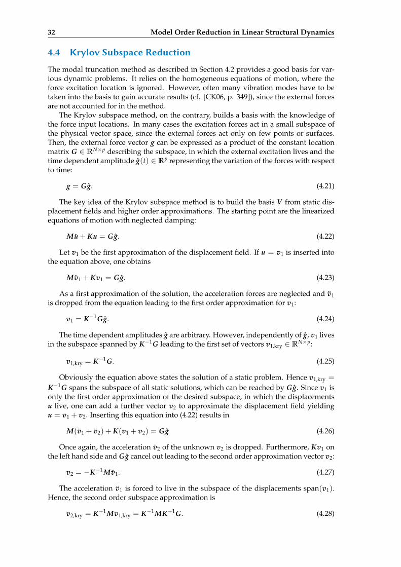
32 Model Order Reduction in Linear Structural Dynamics
4.4 Krylov Subspace Reduction
The modal truncation method as described in Section 4.2 provides a good basis for var-ious dynamic problems. It relies on the homogeneous equations of motion, where theforce excitation location is ignored. However, often many vibration modes have to betaken into the basis to gain accurate results (cf. [CK06, p. 349]), since the external forcesare not accounted for in the method.
The Krylov subspace method, on the contrary, builds a basis with the knowledge ofthe force input locations. In many cases the excitation forces act in a small subspace ofthe physical vector space, since the external forces act only on few points or surfaces.Then, the external force vector g can be expressed as a product of the constant locationmatrix G ∈ RN×p describing the subspace, in which the external excitation lives and thetime dependent amplitude g(t) ∈ Rp representing the variation of the forces with respectto time:
g = Gg. (4.21)
The key idea of the Krylov subspace method is to build the basis V from static dis-placement fields and higher order approximations. The starting point are the linearizedequations of motion with neglected damping:
Mu + Ku = Gg. (4.22)
Let v1 be the first approximation of the displacement field. If u = v1 is inserted intothe equation above, one obtains
Mv1 + Kv1 = Gg. (4.23)
As a first approximation of the solution, the acceleration forces are neglected and v1is dropped from the equation leading to the first order approximation for v1:
v1 = K−1Gg. (4.24)
The time dependent amplitudes g are arbitrary. However, independently of g, v1 livesin the subspace spanned by K−1G leading to the first set of vectors v1,kry ∈ RN×p:
v1,kry = K−1G. (4.25)
Obviously the equation above states the solution of a static problem. Hence v1,kry =
K−1G spans the subspace of all static solutions, which can be reached by Gg. Since v1 isonly the first order approximation of the desired subspace, in which the displacementsu live, one can add a further vector v2 to approximate the displacement field yieldingu = v1 + v2. Inserting this equation into (4.22) results in
M(v1 + v2) + K(v1 + v2) = Gg (4.26)
Once again, the acceleration v2 of the unknown v2 is dropped. Furthermore, Kv1 onthe left hand side and Gg cancel out leading to the second order approximation vector v2:
v2 = −K−1Mv1. (4.27)
The acceleration v1 is forced to live in the subspace of the displacements span(v1).Hence, the second order subspace approximation is
v2,kry = K−1Mv1,kry = K−1MK−1G. (4.28)
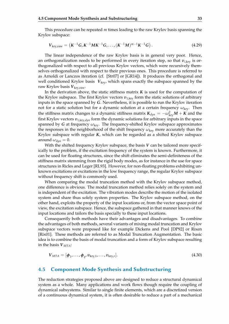
4.5 Component Mode Synthesis and Substructuring 33
This procedure can be repeated m times leading to the raw Krylov basis spanning theKrylov subspace:
Vkry,raw =(K−1G, K−1MK−1G, . . . , (K−1M)m−1K−1G
). (4.29)
The linear independence of the raw Krylov basis is in general very poor. Hence,an orthogonalization needs to be performed in every iteration step, so that vi,kry is or-thogonalized with respect to all previous Krylov vectors, which were recursively them-selves orthogonalized with respect to their previous ones. This procedure is referred toas Arnoldi or Lanczos iteration (cf. [Str07] or [GR14]). It produces the orthogonal andwell conditioned Krylov basis Vkry, which spans exactly the subspace spanned by theraw Krylov basis Vkry,raw.
In the derivation above, the static stiffness matrix K is used for the computation ofthe Krylov subspace. The first Krylov vectors v1,kry form the static solutions of arbitraryinputs in the space spanned by G. Nevertheless, it is possible to run the Krylov iterationnot for a static solution but for a dynamic solution at a certain frequency ωkry. Thenthe stiffness matrix changes to a dynamic stiffness matrix Kdyn = −ω2
kryM + K and thefirst Krylov vectors v1,kry,dyn form the dynamic solutions for arbitrary inputs in the spacespanned by G at frequency ωkry. The frequency-shifted Krylov subspace approximatesthe responses in the neighborhood of the shift frequency ωkry more accurately than theKrylov subspace with regular K, which can be regarded as a shifted Krylov subspacearound ωdyn = 0.
With the shifted frequency Krylov subspace, the basis V can be tailored more specif-ically to the problem, if the excitation frequency of the system is known. Furthermore, itcan be used for floating structures, since the shift eliminates the semi-definiteness of thestiffness matrix stemming from the rigid body modes, as for instance in the use for spacestructures in Ricles and Leger [RL93]. However, for non-floating problems exhibiting un-known excitations or excitations in the low frequency range, the regular Krylov subspacewithout frequency shift is commonly used.
When comparing the modal truncation method with the Krylov subspace method,one difference is obvious. The modal truncation method relies solely on the system andis independent of the excitation. The vibration modes describe the motion of the isolatedsystem and share thus solely system properties. The Krylov subspace method, on theother hand, exploits the property of the input locations or, from the vector space point ofview, the excitation subspace. Hence, the subspace gathered in that manner knows of theinput locations and tailors the basis specially to these input locations.
Consequently both methods have their advantages and disadvantages. To combinethe advantages of both methods, several variants of mixing modal truncation and Krylovsubspace vectors were proposed like for example Dickens and Pool [DP92] or Rixen[Rix01]. These methods are referred to as Modal Truncation Augmentation. The basicidea is to combine the basis of modal truncation and a form of Krylov subspace resultingin the basis V MTA:
V MTA = [φ1, . . . , φq, vkry,1, . . . , vkry,r]. (4.30)
4.5 Component Mode Synthesis and Substructuring
The reduction strategies proposed above are designed to reduce a structural dynamicalsystem as a whole. Many applications and work flows though require the coupling ofdynamical subsystems. Similar to single finite elements, which are a discretized versionof a continuous dynamical system, it is often desirable to reduce a part of a mechanical
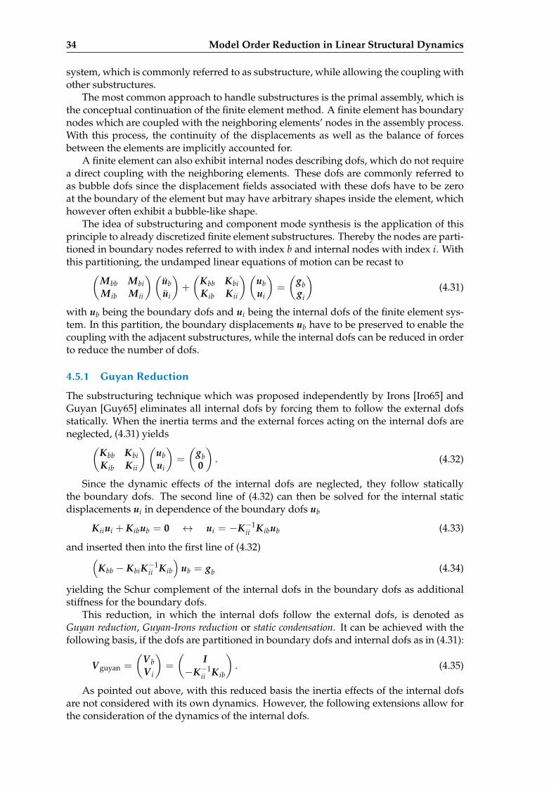
34 Model Order Reduction in Linear Structural Dynamics
system, which is commonly referred to as substructure, while allowing the coupling withother substructures.
The most common approach to handle substructures is the primal assembly, which isthe conceptual continuation of the finite element method. A finite element has boundarynodes which are coupled with the neighboring elements’ nodes in the assembly process.With this process, the continuity of the displacements as well as the balance of forcesbetween the elements are implicitly accounted for.
A finite element can also exhibit internal nodes describing dofs, which do not requirea direct coupling with the neighboring elements. These dofs are commonly referred toas bubble dofs since the displacement fields associated with these dofs have to be zeroat the boundary of the element but may have arbitrary shapes inside the element, whichhowever often exhibit a bubble-like shape.
The idea of substructuring and component mode synthesis is the application of thisprinciple to already discretized finite element substructures. Thereby the nodes are parti-tioned in boundary nodes referred to with index b and internal nodes with index i. Withthis partitioning, the undamped linear equations of motion can be recast to
(Mbb MbiM ib M ii
)(ubui
)+
(Kbb KbiKib Kii
)(ubui
)=
(gbgi
)(4.31)
with ub being the boundary dofs and ui being the internal dofs of the finite element sys-tem. In this partition, the boundary displacements ub have to be preserved to enable thecoupling with the adjacent substructures, while the internal dofs can be reduced in orderto reduce the number of dofs.
4.5.1 Guyan Reduction
The substructuring technique which was proposed independently by Irons [Iro65] andGuyan [Guy65] eliminates all internal dofs by forcing them to follow the external dofsstatically. When the inertia terms and the external forces acting on the internal dofs areneglected, (4.31) yields
(Kbb KbiKib Kii
)(ubui
)=
(gb0
). (4.32)
Since the dynamic effects of the internal dofs are neglected, they follow staticallythe boundary dofs. The second line of (4.32) can then be solved for the internal staticdisplacements ui in dependence of the boundary dofs ub
Kiiui + Kibub = 0 ↔ ui = −K−1ii Kibub (4.33)
and inserted then into the first line of (4.32)(
Kbb − KbiK−1ii Kib
)ub = gb (4.34)
yielding the Schur complement of the internal dofs in the boundary dofs as additionalstiffness for the boundary dofs.
This reduction, in which the internal dofs follow the external dofs, is denoted asGuyan reduction, Guyan-Irons reduction or static condensation. It can be achieved with thefollowing basis, if the dofs are partitioned in boundary dofs and internal dofs as in (4.31):
Vguyan =
(V bV i
)=
(I
−K−1ii Kib
). (4.35)
As pointed out above, with this reduced basis the inertia effects of the internal dofsare not considered with its own dynamics. However, the following extensions allow forthe consideration of the dynamics of the internal dofs.
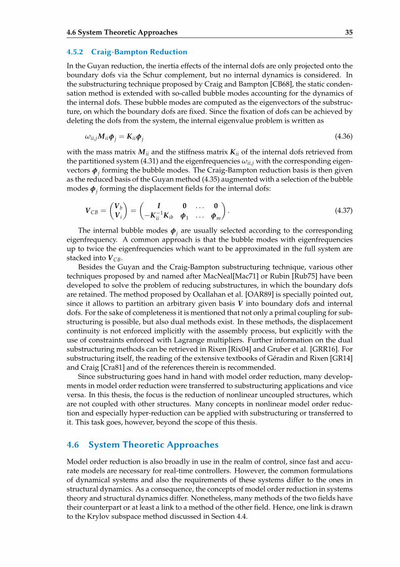
4.6 System Theoretic Approaches 35
4.5.2 Craig-Bampton Reduction
In the Guyan reduction, the inertia effects of the internal dofs are only projected onto theboundary dofs via the Schur complement, but no internal dynamics is considered. Inthe substructuring technique proposed by Craig and Bampton [CB68], the static conden-sation method is extended with so-called bubble modes accounting for the dynamics ofthe internal dofs. These bubble modes are computed as the eigenvectors of the substruc-ture, on which the boundary dofs are fixed. Since the fixation of dofs can be achieved bydeleting the dofs from the system, the internal eigenvalue problem is written as
ωii,j M iiφj = Kiiφj (4.36)
with the mass matrix M ii and the stiffness matrix Kii of the internal dofs retrieved fromthe partitioned system (4.31) and the eigenfrequencies ωii,j with the corresponding eigen-vectors φj forming the bubble modes. The Craig-Bampton reduction basis is then givenas the reduced basis of the Guyan method (4.35) augmented with a selection of the bubblemodes φj forming the displacement fields for the internal dofs:
VCB =
(V bV i
)=
(I 0 . . . 0
−K−1ii Kib φ1 . . . φm
). (4.37)
The internal bubble modes φj are usually selected according to the correspondingeigenfrequency. A common approach is that the bubble modes with eigenfrequenciesup to twice the eigenfrequencies which want to be approximated in the full system arestacked into VCB.
Besides the Guyan and the Craig-Bampton substructuring technique, various othertechniques proposed by and named after MacNeal[Mac71] or Rubin [Rub75] have beendeveloped to solve the problem of reducing substructures, in which the boundary dofsare retained. The method proposed by Ocallahan et al. [OAR89] is specially pointed out,since it allows to partition an arbitrary given basis V into boundary dofs and internaldofs. For the sake of completeness it is mentioned that not only a primal coupling for sub-structuring is possible, but also dual methods exist. In these methods, the displacementcontinuity is not enforced implicitly with the assembly process, but explicitly with theuse of constraints enforced with Lagrange multipliers. Further information on the dualsubstructuring methods can be retrieved in Rixen [Rix04] and Gruber et al. [GRR16]. Forsubstructuring itself, the reading of the extensive textbooks of Géradin and Rixen [GR14]and Craig [Cra81] and of the references therein is recommended.
Since substructuring goes hand in hand with model order reduction, many develop-ments in model order reduction were transferred to substructuring applications and viceversa. In this thesis, the focus is the reduction of nonlinear uncoupled structures, whichare not coupled with other structures. Many concepts in nonlinear model order reduc-tion and especially hyper-reduction can be applied with substructuring or transferred toit. This task goes, however, beyond the scope of this thesis.
4.6 System Theoretic Approaches
Model order reduction is also broadly in use in the realm of control, since fast and accu-rate models are necessary for real-time controllers. However, the common formulationsof dynamical systems and also the requirements of these systems differ to the ones instructural dynamics. As a consequence, the concepts of model order reduction in systemstheory and structural dynamics differ. Nonetheless, many methods of the two fields havetheir counterpart or at least a link to a method of the other field. Hence, one link is drawnto the Krylov subspace method discussed in Section 4.4.
36 Model Order Reduction in Linear Structural Dynamics
4.6.1 Conceptual Dierences
In control theory, dynamical systems are typically described and analyzed differentlythan in structural dynamics. In the latter, the dynamics of the system is described using asecond order ordinary differential equation with symmetric and positive (semi) definitemass, damping and stiffness matrices and the displacements as the primal variable (cf.(4.1)). In control theory, the dynamical system is commonly described as a state-spacesystem, where both displacements and velocities form the unknown variables of the statevector x:
x = Assx + Bssuss, (4.38)yss = Cssx, (4.39)
which can be realized as
x =
(uu
)∈ R2N , Ass =
(0 I
−M−1K −M−1C
)∈ R2N×2N ,
Bss =
(0
M−1G
)∈ R2N×p, uss = g ∈ Rp.
(4.40)
The subscript ss denotes state-space matrices and vectors. The system matrix Assdescribes the dynamics and can be constructed using the mass, damping and stiffnessmatrix of the second order mechanical system. It is not symmetric and non positivedefinite. The input locations are expressed with the input location matrix Bss and theexternal excitation uss is equal to the external forcing g.
The state-space description in the use of structural dynamics has the drawback thatthe physical interpretation of a state-space vector is lost to a certain extent. While thedisplacements u are associated to a displacement field, the state-space vector x describesboth a displacement field with a velocity field, which makes general interpretations dif-ficult.
The reduction of a state-space system is performed with the expression of the state-space vector x by a combination of basis vectors gathered in V ss ∈ R2N×2n and the re-duced state-space coordinates xr ∈ R2n with n N:
x = V ssxr. (4.41)
Similar to (3.3), the application of the transformation to the dynamics equations leadsto a residual rss:
V ss xr = AssV ssxr + Bssuss + rss. (4.42)
Again, as in (3.4), a constraint for the residual has to be found in order to make theequations above determined. However, the physical units of the equations above arenot of one type like in second order systems, where the equations of motion are forceequations. With the realization (4.40), for instance, the units in (4.38) are both velocitiesand accelerations. Since the constraints have to be applied to both units, the handlingof constraints is more complicated for first order state-space systems than for secondorder systems. In the latter, the principle of virtual work requires the residual forces tobe orthogonal to the kinematically admissible displacements resulting in the symmetricprojection discussed in Section 3.2. In the former, the orthogonality is enforced with asecond matrix W ss, which is defined by the chosen first order reduction method:
W Tssrss = 0. (4.43)
4.6 System Theoretic Approaches 37
With applying (4.43) to (4.42), the following reduced state-space system is obtained:
xr = Ass,rxr + Bss,ru (4.44)yss = Css,rxr (4.45)
with
Ass,r = (W TssV ss)
−1W Tss AssV ss ∈ R2n×2n, (4.46)
Bss,r = (W TssV ss)
−1W TssBss ∈ R2n×p, (4.47)
Css,r = CssV ss ∈ Rm×2n. (4.48)
Note, that in general V ss and W ss are not equal. In the projective model order reduc-tion for second order mechanical systems, the principle of virtual work requires the leftand right sided projection to be equal. When the principle of virtual work is not violated,the mechanical system properties like stability, passivity and symmetry are preserved.This makes second order reduction an easy task, since any non-singular basis V pre-serves all properties associated with mechanical systems. In a reduction scheme for firstorder systems, however, the preservation of the mechanical properties like stability orpassivity is not genuinely given and has to be investigated and proved for every method.
In control theory, commonly the input-output behavior of a system is of interest whilethe approximation of the internal state variable x is not important. In structural dynam-ics, on the contrary, the full displacement field is usually of interest, since very oftenstress distributions are sought, e.g., for fatigue analyses where the critical location is notknown beforehand. Consequently, it is not the approximation of the input-output behav-ior which matters most in structural dynamics, but the accurate reconstruction of the fulldisplacement field of the system.
Due to these differences, most projective reduction techniques from system theorycannot be directly transferred to the realm of structural dynamics. However, severallinks exist, for which the link between the moment matching technique and the Krylovsubspace technique introduced in Section 4.4 is drawn in the next subsection.
4.6.2 Moment Matching and Krylov Subspaces
As discussed above, the input-output behavior is the key property in the system theoryreduction methods. The transfer function H(s) describes the input-output behavior inthe Laplace domain. For the state-space system (4.38) it is defined as
H(s) =Y ss(s)Uss(s)
= Css(sI − Ass)−1Bss (4.49)
with the Laplace transform Uss(s) of the input vector uss(t) and the Laplace transformY ss(s) of the output vector yss(t).
The transfer function can be expanded as a power series around the point s0 in theLaplace domain (cf. [Ant09, p. 345]) yielding the so-called moments of the transfer func-tion:
H(s) = H(s0) + H(1)(s0)(s− s0)
1!+ · · ·+ H(k)(s0)
(s− s0)k
k!+ . . . (4.50)
= T0 + T1(s− s0) + · · ·+ Tk(s− s0)k + . . . (4.51)
The polynomial coefficients H(s0) = T0(s0), H(1)(s0) = T1(s0), . . . , H(k)/k! = Tk(s0)are called zeroth, first or k-th Moment of the transfer function about the point s0. Theycan be derived as [Ant09, p. 345]:
38 Model Order Reduction in Linear Structural Dynamics
Tk = Css(s0I − Ass)−(k+1)Bss. (4.52)
The goal of model order reduction using moment matching is that the first k momentsof the reduced system about s0 are equal to the first k moments about s0 of the full, unre-duced system. Grimme [Gri97] showed that the first k moment are matched when theleft and right sided projection matrices W ss and V ss span the subspace of the followingKrylov subspace:
V ss,raw =((s0I − Ass)−1Bss, . . . , (s0I − Ass)−(k+1)Bss
)(4.53)
W ss,raw =((s0I − AT
ss)−1CT
ss, . . . , (s0I − ATss)−(k+1)CT
ss)
(4.54)
The subspace spanned by V ss is the so-called input Krylov subspace and the subspacespanned by W ss is the so-called output Krylov subspace.
The concept of moment matching can also be applied to second order systems withoutdamping. When the full displacements u of the second order system are of interest, thetransfer function of the input vector g to the displacement field u is given as
H(s) =(s2M + K
)−1G (4.55)
=∞
∑i=0
[(K + s2
0M)−1M]i(K + s2
0M)−1G︸ ︷︷ ︸
T i(s0)
(s2 − s20)
i (4.56)
with the force input location matrix G. The power series above yield the moments of thesecond order system, which are matched (cf. [Bes+13]) when the second order projectionis performed with the following Krylov subspace:
V =((K + s2
0M)−1G, . . . ,[(K + s2
0M)−1M]k(K + s2
0M)−1G)
. (4.57)
Note, that this subspace is equal to the Krylov subspace stemming from the consid-eration in Section 4.4, when s0 = iω0. Hence, the Krylov subspace technique discussedin Section 4.4 matches the first 2k moments of the transfer function of the undampedmechanical system. In the presence of damping, second order methods to build an ap-propriate Krylov subspace exist, e.g., Salimbahrami and Lohmann [SL06], Bai and Su[BS05] or Lehner and Eberhard [LE06].
For building the Krylov subspace, the expansion point s0 can be chosen. In structuraldynamics, it is common to choose s0 = 0 (cf. [Rix01], [GR14]), since the static approxi-mation and the low frequency range is of great interest. When the input-output behavioris addressed, however, the accuracy of the Krylov reduction basis can be increased bya better choice of the expansion points s0. One popular strategy is the so-called IRKAmethod proposed by Gugercin et al. [GAB08], which has been modified and improvedin various ways. The interested reader is referred to the work of Panzer [Pan14], Wolf[Wol14], Beattie and Gugercin [BG16] and the references therein.
4.6.3 Further Approaches
Besides the Krylov subspace method, further system theory inspired methods have beendeveloped. The most prominent method is probably the Balanced Truncation methodfirst proposed by Mullis and Roberts [MR76] and then generalized by Moore [Moo81]for general linear, time invariant systems, where the concept of controllability and ob-servability is exploited to rank the state variables. The reduction basis is then built withthe states which are both well controllable and observable, and the remaining states aretruncated.
4.6 System Theoretic Approaches 39
This concept has been successfully applied to systems in control, elastic multibodysystems and other domains like electrical engineering, e.g., [FE10], [Now+13], [GA04].With the high computational costs associated with the solution of a Lyapunov equation,this method is limited to small size systems, where computations of systems with morethan 2,500 displacement dofs and hence 5,000 states become tough [Wol14, pp. 7f.].
Even though the method was extended to second order systems by Chahlaoui et al.[Cha+06] and Reis and Stykel [RS08], it is merely used in structural dynamics. This mightalso be due to the fact, that the modal basis yields systems, which are called almost bal-anced, see Jonckheere [Jon84], Davis and Skelton [DS84], Gawronski and Lim [GL96] orGawronski [Gaw97; Gaw04; Gaw06]. The Balanced Truncation method converges to theModal reduction method when the system is very lightly damped, the eigenfrequenciesare separated enough and the input and output locations are collocated, which is the casefor many metallic structures.
As mentioned above, many other model order reduction methods like the Hankel-Norm approximation or Krylov-SVD methods were developed in the realm of systemstheory. The interested reader is referred to the textbook of Antoulas [Ant05] and thereferences therein.

Chapter 5
Proper Orthogonal Decomposition (POD)
In the previous chapter, a few reduction methods for linear structural dynamical systemsare discussed. Since these systems are linear, they are characterized by a mass, stiffnessand damping matrix and sometimes by input and output locations. The reduction meth-ods are hence explicitly or implicitly based on system theoretic concepts. For instance, thedecoupling of states results in modal truncation, the approximation of the transfer func-tion results in the Krylov subspace methods with moment matching, or the concept ofcontrollability and observability results in Balanced Truncation or – for slightly dampedsystems – in modal truncation with modal dominance ranking.
Nonlinear systems lack these systems theoretic concepts in most cases. They are usu-ally not defined for nonlinear systems or, if they are defined, they are extremely expensiveto compute. Hence, the concept of finding a reduced basis V for a nonlinear system isusually conceptually different to the strategies of finding a reduced basis for a linear sys-tem. Since nonlinear systems cannot be fully described by system matrices, a detour overdata-driven methods is a common approach. This means that training simulations of thefull, high dimensional system are run in a first step, of which the results are analyzed ina second step to build the projection matrix V . The most prominent method is the ProperOrthogonal Decomposition (POD), which is discussed in this chapter.
According to Berkooz et al. [BHL93], the POD was developed independently bya number of scientists, e.g., by Karhunen [Kar46] and Loève [Loè48], after whom theprocedure is given the name Karhunen-Loève decomposition, but also Kosambi [Kos43],Pougachev [Pug53] and Obukhov [Obu54]. It was first used widely in fluid dynamics toidentify coherent structures [Sir87] and is now widely used in the field of model orderreduction for turbulent flows, see, e.g., [HTD00; WP02; Epu03; Lum07; Hol12]. Further-more, it is used in the control of dynamical systems [Rav00; AM02; BCB05], damagedetection [DG03; LD06; Muj+11], finite element model updating [HD01; LKG03; KAS07]and of course in model order reduction of structural dynamics, e.g., [AV99; KF99; AV01;KLM01; ST01; Lia+02b; AP03; TWS05; GSD08], besides many other domains. For a moredetailed overview of the POD and its history, the publications of Kerschen et al. [Ker+05],Liang et al. [Lia+02a] and Berkooz [Ber92] are recommended.
5.1 Key Idea: Principal Component Analysis
The POD is a data driven method, which identifies the optimal subspace from a set of dis-placement snapshots us. This task is related to the principal component analysis (PCA)used in statistics, where the so-called principal components are sought, which minimizethe Euclidean distance to a set of data points. In the POD, the displacement snapshots usare the data points, for which the subspace V is sought to fulfill the following minimiza-tion problem:
41
42 Proper Orthogonal Decomposition (POD)
minm
∑i=1||us(ti)− Vq(ti)||2. (5.1)
In this minimization problem, the subspace V ∈ RN×n of predefined dimension nis searched for, while the vector of amplitudes q(ti) ∈ Rn is adapted to minimize theexpression above. The solution of this minimization problem can be obtained with thesingular value decomposition (SVD), the underlying mathematical operation of the PCAand the POD. It identifies the subspace V fulfilling (5.1) when applied to the snapshotmatrix Sd ∈ RN×m, in which the displacements of all m sampled time steps us are gath-ered:
Sd =(us(t1), . . . , us(tm)
)= UsvdΣV T
svd. (5.2)
The SVD of the snapshot matrix Sd yields the orthogonal matrix Usvd ∈ RN×m con-taining the left singular vectors, the diagonal matrix Σ = diag(σ1, . . . , σm) containing thesingular values σi, which are ordered decreasingly with σi ≥ σi+1 and the orthogonalmatrix V svd ∈ Rm×m containing the right singular vectors. The declared dimensions areonly valid for the case, in which the number of snapshots m is smaller than the numberof dofs N. This is the case in most reduction settings, when large models are considered.In the other case for m > N, the dimensions of the matrices are Usvd ∈ RN×N , Σ ∈ RN×N
and V svd ∈ RN×m.The left singular vectors usvd,i form the principal components of the displacement
field set gathered in Sd. For a given dimension n, the first n principal components ful-fill the optimality condition (5.1) and minimize the Euclidean error. Consequently, thePOD builds the basis V using the first n left sided singular vectors usvd,i. Since both theleft and the right singular vectors are normalized, the amplitude for reconstructing thedisplacement snapshots is stored in the singular values σi. Thus, the importance of thei-th principal component usvd,i is associated with the value of the corresponding singularvalue σi.
While the left singular vectors usvd,i carry the information of the dominating spatialdisplacement fields, the right singular vectors vsvd,i composing V svd describe the tempo-ral evolution of them. Consequently, the SVD of the snapshots does not only provide thedominant subspace of the motion but also the temporal information, which can be usedin applications such as model updating as reported by Hemez and Deobling [HD01] orLenaerts et al. [LKG03].
The minimization (5.1) can also be expressed in matrix notation, where the SVD iden-tifies an optimal low rank approximation Sd,approx with rank n of the snapshot matrix Sd.This optimal approximation is obtained when the L2 norm or the Frobenius norm of thedifference between Sd and Sd,approx is minimal. The L2 error ε2 and the Frobenius error ε fare given as:
ε2 = ||Sd,approx − Sd||2, ε f = ||Sd,approx − Sd|| f . (5.3)
According to the Eckart-Young-Mirsky theorem (cf. [GV12]), both errors ε2 and ε fare minimized at the same time, when the approximation matrix Sd,approx is built from asum of n rank one matrices. Each of them is defined as the outer product of the normalvectors usvd,i and vsvd,i and a weighting factor σi being exactly the left and right singularvectors and the corresponding singular value stemming from the SVD:
Sd,approx =n
∑i=1
σiusvd,ivTsvd,i. (5.4)
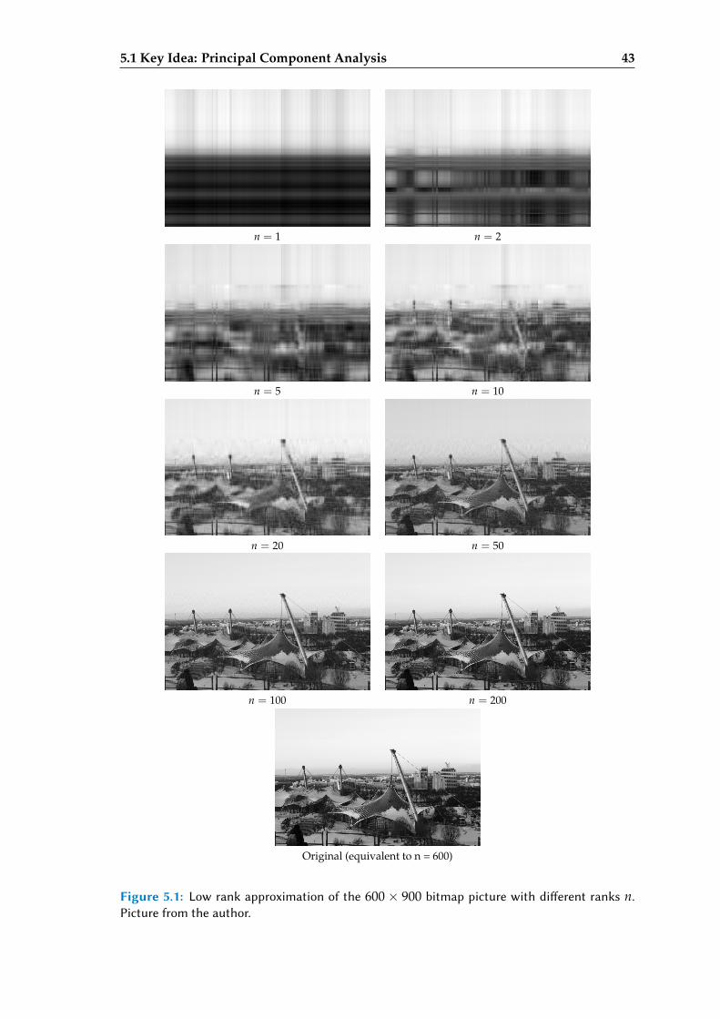
5.1 Key Idea: Principal Component Analysis 43
n = 1 n = 2
n = 5 n = 10
n = 20 n = 50
n = 100 n = 200
Original (equivalent to n = 600)
Figure 5.1: Low rank approximation of the 600× 900 bitmap picture with dierent ranks n.Picture from the author.
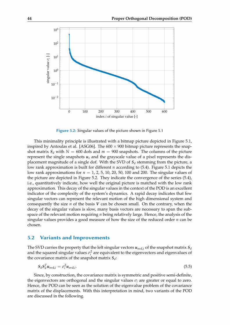
44 Proper Orthogonal Decomposition (POD)
0 100 200 300 400 500 600
10−2
10−1
100
101
102
103
index i of singular value [-]
sing
ular
valu
eσ i
[-]
Figure 5.2: Singular values of the picture shown in Figure 5.1
This minimality principle is illustrated with a bitmap picture depicted in Figure 5.1,inspired by Antoulas et al. [ASG06]. The 600× 900 bitmap picture represents the snap-shot matrix Sd with N = 600 dofs and m = 900 snapshots. The columns of the picturerepresent the single snapshots us and the grayscale value of a pixel represents the dis-placement magnitude of a single dof. With the SVD of Sd stemming from the picture, alow rank approximation is built for different n according to (5.4). Figure 5.1 depicts thelow rank approximations for n = 1, 2, 5, 10, 20, 50, 100 and 200. The singular values ofthe picture are depicted in Figure 5.2. They indicate the convergence of the series (5.4),i.e., quantitatively indicate, how well the original picture is matched with the low rankapproximation. This decay of the singular values in the context of the POD is an excellentindicator of the complexity of the system’s dynamics. A rapid decay indicates that fewsingular vectors can represent the relevant motion of the high dimensional system andconsequently the size n of the basis V can be chosen small. On the contrary, when thedecay of the singular values is slow, many basis vectors are necessary to span the sub-space of the relevant motion requiring n being relatively large. Hence, the analysis of thesingular values provides a good measure of how the size of the reduced order n can bechosen.
5.2 Variants and Improvements
The SVD carries the property that the left singular vectors usvd,i of the snapshot matrix Sdand the squared singular values σ2
i are equivalent to the eigenvectors and eigenvalues ofthe covariance matrix of the snapshot matrix Sd:
SdSTd usvd,i = σ2
i usvd,i. (5.5)
Since, by construction, the covariance matrix is symmetric and positive semi-definite,the eigenvectors are orthogonal and the singular values σi are greater or equal to zero.Hence, the POD can be seen as the solution of the eigenvalue problem of the covariancematrix of the displacements. With this interpretation in mind, two variants of the PODare discussed in the following.
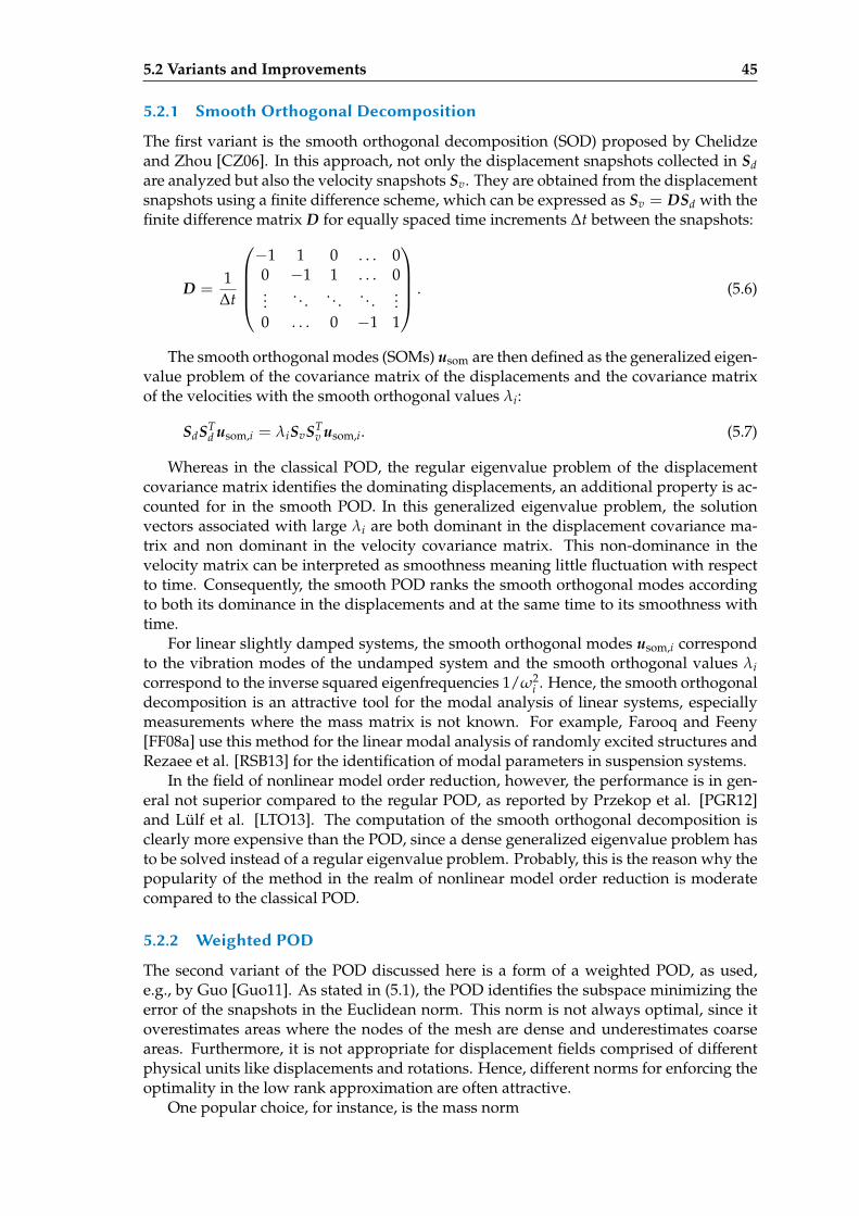
5.2 Variants and Improvements 45
5.2.1 Smooth Orthogonal Decomposition
The first variant is the smooth orthogonal decomposition (SOD) proposed by Chelidzeand Zhou [CZ06]. In this approach, not only the displacement snapshots collected in Sdare analyzed but also the velocity snapshots Sv. They are obtained from the displacementsnapshots using a finite difference scheme, which can be expressed as Sv = DSd with thefinite difference matrix D for equally spaced time increments ∆t between the snapshots:
D =1
∆t
−1 1 0 . . . 00 −1 1 . . . 0...
. . . . . . . . ....
0 . . . 0 −1 1
. (5.6)
The smooth orthogonal modes (SOMs) usom are then defined as the generalized eigen-value problem of the covariance matrix of the displacements and the covariance matrixof the velocities with the smooth orthogonal values λi:
SdSTd usom,i = λiSvST
v usom,i. (5.7)
Whereas in the classical POD, the regular eigenvalue problem of the displacementcovariance matrix identifies the dominating displacements, an additional property is ac-counted for in the smooth POD. In this generalized eigenvalue problem, the solutionvectors associated with large λi are both dominant in the displacement covariance ma-trix and non dominant in the velocity covariance matrix. This non-dominance in thevelocity matrix can be interpreted as smoothness meaning little fluctuation with respectto time. Consequently, the smooth POD ranks the smooth orthogonal modes accordingto both its dominance in the displacements and at the same time to its smoothness withtime.
For linear slightly damped systems, the smooth orthogonal modes usom,i correspondto the vibration modes of the undamped system and the smooth orthogonal values λicorrespond to the inverse squared eigenfrequencies 1/ω2
i . Hence, the smooth orthogonaldecomposition is an attractive tool for the modal analysis of linear systems, especiallymeasurements where the mass matrix is not known. For example, Farooq and Feeny[FF08a] use this method for the linear modal analysis of randomly excited structures andRezaee et al. [RSB13] for the identification of modal parameters in suspension systems.
In the field of nonlinear model order reduction, however, the performance is in gen-eral not superior compared to the regular POD, as reported by Przekop et al. [PGR12]and Lülf et al. [LTO13]. The computation of the smooth orthogonal decomposition isclearly more expensive than the POD, since a dense generalized eigenvalue problem hasto be solved instead of a regular eigenvalue problem. Probably, this is the reason why thepopularity of the method in the realm of nonlinear model order reduction is moderatecompared to the classical POD.
5.2.2 Weighted POD
The second variant of the POD discussed here is a form of a weighted POD, as used,e.g., by Guo [Guo11]. As stated in (5.1), the POD identifies the subspace minimizing theerror of the snapshots in the Euclidean norm. This norm is not always optimal, since itoverestimates areas where the nodes of the mesh are dense and underestimates coarseareas. Furthermore, it is not appropriate for displacement fields comprised of differentphysical units like displacements and rotations. Hence, different norms for enforcing theoptimality in the low rank approximation are often attractive.
One popular choice, for instance, is the mass norm
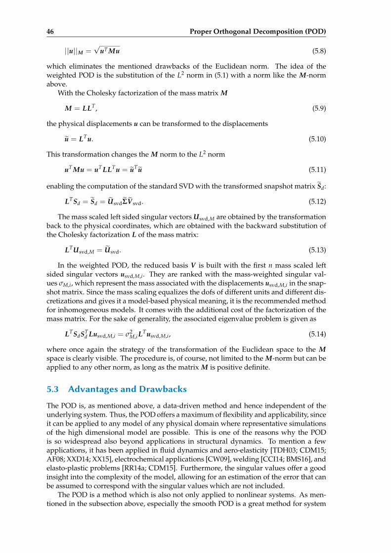
46 Proper Orthogonal Decomposition (POD)
||u||M =√
uT Mu (5.8)
which eliminates the mentioned drawbacks of the Euclidean norm. The idea of theweighted POD is the substitution of the L2 norm in (5.1) with a norm like the M-normabove.
With the Cholesky factorization of the mass matrix M
M = LLT, (5.9)
the physical displacements u can be transformed to the displacements
u = LTu. (5.10)
This transformation changes the M norm to the L2 norm
uT Mu = uT LLTu = uT u (5.11)
enabling the computation of the standard SVD with the transformed snapshot matrix Sd:
LTSd = Sd = UsvdΣV svd. (5.12)
The mass scaled left sided singular vectors Usvd,M are obtained by the transformationback to the physical coordinates, which are obtained with the backward substitution ofthe Cholesky factorization L of the mass matrix:
LTUsvd,M = Usvd. (5.13)
In the weighted POD, the reduced basis V is built with the first n mass scaled leftsided singular vectors usvd,M,i. They are ranked with the mass-weighted singular val-ues σM,i, which represent the mass associated with the displacements usvd,M,i in the snap-shot matrix. Since the mass scaling equalizes the dofs of different units and different dis-cretizations and gives it a model-based physical meaning, it is the recommended methodfor inhomogeneous models. It comes with the additional cost of the factorization of themass matrix. For the sake of generality, the associated eigenvalue problem is given as
LTSdSTd Lusvd,M,i = σ2
M,iLTusvd,M,i, (5.14)
where once again the strategy of the transformation of the Euclidean space to the Mspace is clearly visible. The procedure is, of course, not limited to the M-norm but can beapplied to any other norm, as long as the matrix M is positive definite.
5.3 Advantages and Drawbacks
The POD is, as mentioned above, a data-driven method and hence independent of theunderlying system. Thus, the POD offers a maximum of flexibility and applicability, sinceit can be applied to any model of any physical domain where representative simulationsof the high dimensional model are possible. This is one of the reasons why the PODis so widespread also beyond applications in structural dynamics. To mention a fewapplications, it has been applied in fluid dynamics and aero-elasticity [TDH03; CDM15;AF08; XXD14; XX15], electrochemical applications [CW09], welding [CCI14; BMS16], andelasto-plastic problems [RR14a; CDM15]. Furthermore, the singular values offer a goodinsight into the complexity of the model, allowing for an estimation of the error that canbe assumed to correspond with the singular values which are not included.
The POD is a method which is also not only applied to nonlinear systems. As men-tioned in the subsection above, especially the smooth POD is a great method for system
5.3 Advantages and Drawbacks 47
identification of linear systems in both experimental and simulation setups. Intrinsicproperties of linear systems like vibration modes can be identified under certain circum-stances. Literature discussing the relation of linear system properties and the POD arefor instance the publications of Feeny and Kappaguntu [FK98], Kim [Kim98], Kerschenand Golinval [KG02], Feeny and Liang [FL03] or Feeny and Farooq [FF08b].
The necessity to require a high dimensional training simulation is one of the majordrawbacks though. In many applications, these immense offline costs are not affordableor even not feasible if the computational resources are not available. Especially in sin-gle query scenarios, where the number of reduced runs is limited, the POD is often notattractive. However, in cases, where the offline costs do not matter like applications incontrol or scenarios with many reduced runs, the POD is a very competitive choice.
Another drawback is associated with the inherent nature of the method as a statisti-cal method. Since only the output data of the high dimensional model are analyzed, onlythe states which are triggered in the training simulation are incorporated into the reducedbasis. If model parameters, boundary conditions or excitations change, the snapshots ob-tained by the changed model can be different. Hence, the POD is very sensitive to theparameters and especially the excitations of the training simulation. As often differentload cases compared to the trained ones should be simulated with the reduced model,it is necessary to design training simulations capturing the full dynamics, which shouldbe represented by the reduced model. Hence, the generation of good snapshots remainsan open topic. The drawbacks of the POD mentioned above are motivation for so-calledsimulation-free reduction methods, which are not based on training sets requiring full sim-ulation runs. They are discussed in the following chapter.

Chapter 6
Simulation-Free Approaches
The previous two chapters discuss the construction of reduced bases for linear and non-linear systems. The methods for generating a reduced basis for linear systems use invari-ant physical properties characterizing the system like the mass and the stiffness matrix.On the contrary, the state-of-the-art POD method uses the data generated by trainingsimulations, since invariant and meaningful physical properties are generally hard toretrieve for arbitrary nonlinear systems.
For nonlinear structural systems, especially for geometric nonlinearity, the generationof reduced bases in a non-POD fashion is possible, though. The key idea is the exploita-tion of the physical structure of the system similar to the linear reduction methods, how-ever with capturing the information about the nonlinearity. Hence, these methods rely onthe linearized system and extend the operation to the nonlinear regime via informationfrom perturbation techniques.
The construction of reduced bases for nonlinear structural dynamics goes back toNoor and Peters [NP80] and Noor [Noo82], where so-called path derivatives are pro-posed and applied to static problems. The subspace obtained by triggering the nonlin-earity using displacement fields as perturbation parameters is successfully used for theaugmentation of the basis obtained from linear methods. Since then, several approacheshave been proposed which differ often only in details. Idelsohn and Cardona [IC85b]propose the so-called modal derivatives, where the eigenvalue problem is perturbed toobtain the derivatives of vibration modes of a nonlinear system, which are applied suc-cessfully for the reduction of nonlinear dynamical problems. In [IC85a] they extend themethod to other types of vectors. Perturbation techniques for reduction in the realmof structural dynamics are further used by, e.g., Chang and Engblom [CE91], Jacob andEbecken [JE92], Noor et al. [NAP93], Bauchau and Guernsey [BG93], Slaats et al. [SdS95],Tiso and Rixen [TR11], Tiso et al. [TJA11] and Weeger et al. [WWS14; WWS16]. Recently,methods based on this principle were extended to substructuring applications by Wen-necker and Tiso [WT14], to localized nonlinearities by Witteveen and Pichler [WP14] andto elastic multibody dynamics by Tiso and Wu [WT16b]. Selection strategies are proposedby Tiso in [Tis11]. The concept of derivatives is further successfully used in computergraphics, e.g., by Barbic and James [BJ05] or Hildebrand et al. [Hil+11]. In the former, theconcept of modal derivatives is combined with a polynomial hyper-reduction techniqueto obtain further speedups. Tycowicz et al. [Tyc+13] propose an alternative method toobtain spatial augmentation modes based on rotational properties, which are similar inperformance to modal derivatives.
In the following, the necessity for augmentation of linear bases in the use for struc-tural dynamics is illustrated and the concept of static and modal derivatives is discussed.Furthermore, strategies to handle the rank deficiency, the quadratically increasing num-ber of derivatives and the computation of the derivatives are given before the methods
49
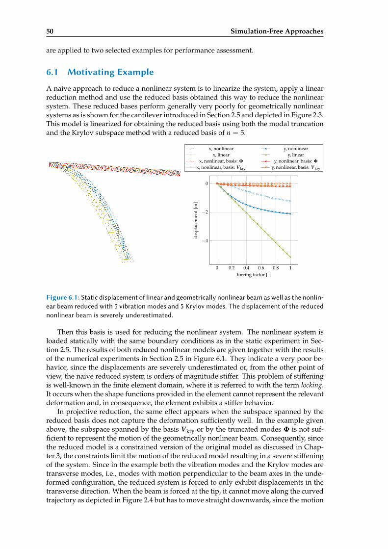
50 Simulation-Free Approaches
are applied to two selected examples for performance assessment.
6.1 Motivating Example
A naive approach to reduce a nonlinear system is to linearize the system, apply a linearreduction method and use the reduced basis obtained this way to reduce the nonlinearsystem. These reduced bases perform generally very poorly for geometrically nonlinearsystems as is shown for the cantilever introduced in Section 2.5 and depicted in Figure 2.3.This model is linearized for obtaining the reduced basis using both the modal truncationand the Krylov subspace method with a reduced basis of n = 5.
0 0.2 0.4 0.6 0.8 1
−4
−2
0
forcing factor [-]
disp
lace
men
t[m
]
x, nonlinear y, nonlinearx, linear y, linear
x, nonlinear, basis: Φ y, nonlinear, basis: Φ
x, nonlinear, basis: Vkry y, nonlinear, basis: Vkry
Figure 6.1: Static displacement of linear and geometrically nonlinear beam as well as the nonlin-ear beam reduced with 5 vibration modes and 5 Krylov modes. The displacement of the reducednonlinear beam is severely underestimated.
Then this basis is used for reducing the nonlinear system. The nonlinear system isloaded statically with the same boundary conditions as in the static experiment in Sec-tion 2.5. The results of both reduced nonlinear models are given together with the resultsof the numerical experiments in Section 2.5 in Figure 6.1. They indicate a very poor be-havior, since the displacements are severely underestimated or, from the other point ofview, the naive reduced system is orders of magnitude stiffer. This problem of stiffeningis well-known in the finite element domain, where it is referred to with the term locking.It occurs when the shape functions provided in the element cannot represent the relevantdeformation and, in consequence, the element exhibits a stiffer behavior.
In projective reduction, the same effect appears when the subspace spanned by thereduced basis does not capture the deformation sufficiently well. In the example givenabove, the subspace spanned by the basis Vkry or by the truncated modes Φ is not suf-ficient to represent the motion of the geometrically nonlinear beam. Consequently, sincethe reduced model is a constrained version of the original model as discussed in Chap-ter 3, the constraints limit the motion of the reduced model resulting in a severe stiffeningof the system. Since in the example both the vibration modes and the Krylov modes aretransverse modes, i.e., modes with motion perpendicular to the beam axes in the unde-formed configuration, the reduced system is forced to only exhibit displacements in thetransverse direction. When the beam is forced at the tip, it cannot move along the curvedtrajectory as depicted in Figure 2.4 but has to move straight downwards, since the motion
6.2 Key Idea: Augmentation of Reduction Basis 51
is constrained to the reduced basis. This, however, causes unphysical in-plane strains,which cause the stiffening of the structure.
This academic example shows that the basis has to capture the full motion of thenonlinear system. Otherwise, unphysical stiffening effects may occur making the ap-proximation of the reduced model extremely poor. Thereby, the subspace identified witha linear reduction method of the linearized system is generally too small and does notcapture directions in the displacement vector space, which are necessary to represent thefull nonlinear motion. So even adding more basis vectors from the linear reduction tech-nique does not solve the problem, since they are based on the linearized system and donot consider the nonlinearity triggered.
However, there exist techniques to identify possible directions, which are discussedin the following. They investigate the nonlinearity and identify directions, which arenecessary to represent the nonlinear motion.
6.2 Key Idea: Augmentation of Reduction Basis
A way to account for the nonlinearities ignored by the linear reduction techniques is theaugmentation of the reduced basis V lin stemming from the linearized system with basisvectors θ ’knowing’ the nonlinearity. Hence the linear basis composed of m modes isaugmented with o basis vectors θ1, . . . , θo to receive the augmented basis V as:
V =(φ1, . . . , φm, θ1, . . . , θo
). (6.1)
In the following, the basis stemming from the linear system is called lin basis V linand the augmentation vectors capturing the nonlinearity are given with the symbol Θ =(θ1, . . . , θo
), independent of the technique applied to generate them. The basis for the
reduction of the nonlinear problem is referred to as V .
6.2.1 Modal Derivatives
When a modal basis is used for the reduction of the geometrically nonlinear system, themodes are based on the linearized system. Thereby the point of linearization is com-monly the equilibrium position, for which both the internal and the external forces arezero.
The idea of modal derivatives (MDs) for use in nonlinear reduction is to introducethe point of linearization as a parameter p for the perturbation of the eigenvalue problem(4.11) in Section 4.3. If the nonlinear system (2.41) is linearized about a point in the dis-placement space, the resulting system can be considered as both linear and parametric,allowing for the modal derivative computation as outlined in Section 4.3. The displace-ments form an N dimensional parameter space, though. To obtain a single parameter pto compute the perturbation of mode φi, p is chosen as the amplitude of a given displace-ment field, namely the j-th vibration mode φj. Hence, the stiffness matrix is treated asa parametric stiffness matrix K(p), where the parameter p = ηj is the amplitude of thedisplacement field formed by φj, which is the point of linearization:
K(p) = K(u = φjηj) =∂ f (u)
∂u
∣∣∣∣u=φjηj
(6.2)
Since the mass matrix M of the nonlinear equations of motion (2.36) is constant, theparameter dependency of the linearized system is only in the stiffness matrix K. Themodal derivative θij = ∂φi/∂ηj is then the derivative of mode φi with respect to theamplitude ηj of mode φj, see (4.13):
52 Simulation-Free Approaches
(−ω2
i M + K) ∂φi
∂ηj=
φT
i
∂K(u = φjηj)
∂ηj
∣∣∣∣∣ηj=0
φi M −∂K(u = φjηj)
∂ηj
∣∣∣∣∣ηj=0
φi (6.3)
As in (4.13), the coefficient matrix (−ω2i M +K) of the linear problem above is singular
and is solved with the additional constraint (4.16) as given in Section 4.3. Since the massmatrix is constant, the constraint is
∂φi∂ηj
Mφi = 0. (6.4)
Hence, any MD θij = ∂φi/∂ηj is M-orthogonal with respect to the vibration mode φi.The augmentation of the lin basis (6.1) is then performed with the o = n2 modal
derivatives θij = ∂φi/∂ηj corresponding to the n vibration modes of the lin basis. Sincethe raw reduced basis, where both the vibration modes and the modal derivatives aregathered, is not guaranteed to be well conditioned, a deflation as given in Subsection 6.2.3is necessary to obtain a reduced basis with a low condition number.
6.2.2 Static Derivatives
The computation of the modal derivatives introduced in the previous section involve thesolution of a singular system, which is not desirable. Hence, in many applications, themass terms in (6.3) are neglected leading to the linear system of equations
K∂φi∂ηj
∣∣∣∣s
= −∂K(u = φjηj)
∂ηj
∣∣∣∣∣ηj=0
φi (6.5)
which defines the so-called static Modal Derivative (SMD) θs,ij = ∂φi/∂ηj|s with the su-per or subscript s indicating the static version. The computation of the SMDs is related tosmaller computational costs, since the coefficient matrix of (6.5) is the stiffness matrix K,which is nonsingular when the system is not floating. Furthermore, the coefficient ma-trix is constant, so that only one factorization of the matrix K is necessary to compute allSMDs of a number of modes.
These benefits make the SMDs very popular in the literature for the reduction of geo-metrically nonlinear systems. However, they are seldom distinguished from the classicalMDs as defined in (6.3). Consequently, the modal perturbations computed according to(6.3) are referred to as modal derivatives (MDs) with the symbol θij, whereas the perturba-tions with neglected mass effects as given in (6.5) are called static modal derivatives (SMDs)(cf. [SdS95]) and referred to with the symbol θs,ij.
The MDs θij = ∂φi/∂ηj as well as the SMDs capture the change of the modes withrespect to a changed configuration. Hence, they capture the displacement fields, whichare necessary to complement the basis vectors from the linearized system to account forthe nonlinearity. This property is illustrated in Figure 6.2, where the SMDs of the firstthree modes of a cantilevered plate are given.
The first three vibration modes of the plate are transverse modes: φ1 is the first bend-ing mode, φ2 is the second bending mode and φ3 is the first torsion mode. These modescan represent the transverse motion of a linearized system but not the in-plane motionwhich is triggered by the geometric nonlinearity as illustrated in the motivating examplein the section before. The (static) modal derivatives account exactly for these in-plane mo-tions. When the vibration modes are transverse modes, the corresponding (S)MDs turnout to be in-plane modes representing the in-plane stretching which is triggered when thetransverse modes are applied to the nonlinear system. Consequently, the (S)MDs are the
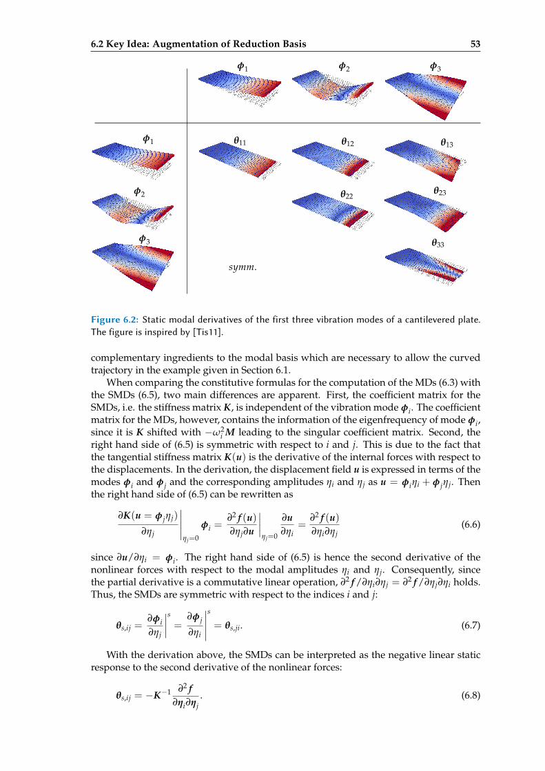
6.2 Key Idea: Augmentation of Reduction Basis 53
symm.
φ2 φ3
φ1
φ2
φ3
φ1
θ11 θ12
θ22
θ13
θ23
θ33
Figure 6.2: Static modal derivatives of the first three vibration modes of a cantilevered plate.The figure is inspired by [Tis11].
complementary ingredients to the modal basis which are necessary to allow the curvedtrajectory in the example given in Section 6.1.
When comparing the constitutive formulas for the computation of the MDs (6.3) withthe SMDs (6.5), two main differences are apparent. First, the coefficient matrix for theSMDs, i.e. the stiffness matrix K, is independent of the vibration mode φi. The coefficientmatrix for the MDs, however, contains the information of the eigenfrequency of mode φi,since it is K shifted with −ω2
i M leading to the singular coefficient matrix. Second, theright hand side of (6.5) is symmetric with respect to i and j. This is due to the fact thatthe tangential stiffness matrix K(u) is the derivative of the internal forces with respect tothe displacements. In the derivation, the displacement field u is expressed in terms of themodes φi and φj and the corresponding amplitudes ηi and ηj as u = φiηi + φjηj. Thenthe right hand side of (6.5) can be rewritten as
∂K(u = φjηj)
∂ηj
∣∣∣∣∣ηj=0
φi =∂2 f (u)∂ηj∂u
∣∣∣∣ηj=0
∂u∂ηi
=∂2 f (u)∂ηi∂ηj
(6.6)
since ∂u/∂ηi = φi. The right hand side of (6.5) is hence the second derivative of thenonlinear forces with respect to the modal amplitudes ηi and ηj. Consequently, sincethe partial derivative is a commutative linear operation, ∂2 f /∂ηi∂ηj = ∂2 f /∂ηj∂ηi holds.Thus, the SMDs are symmetric with respect to the indices i and j:
θs,ij =∂φi∂ηj
∣∣∣∣s
=∂φj
∂ηi
∣∣∣∣∣
s
= θs,ji. (6.7)
With the derivation above, the SMDs can be interpreted as the negative linear staticresponse to the second derivative of the nonlinear forces:
θs,ij = −K−1 ∂2 f∂ηi∂ηj
. (6.8)
54 Simulation-Free Approaches
With this in mind, it becomes clear that the SMDs ‘know’ the nonlinearity of the sys-tem. They capture the quadratic nonlinearities triggered and extend the basis with com-ponents, the linear reduction techniques are not aware of.
With the interpretation of the SMDs as the displacement fields triggered by the secondorder derivatives of the nonlinear forces, the concept of SMDs is not limited to vibrationmodes. This concept can be applied to all types of displacement fields used for linear re-duction. These modes are referred to as static derivatives (SDs), since they do not involveany dynamical effects but are based on the static higher order analysis of the nonlinearinternal forces. This generalization was first proposed in Idelsohn and Cardona [IC85a]for Krylov subspace vectors, though lacking a sound theory. A deeper physical interpre-tation can be achieved with the concept of Quadratic Manifold, which is introduced inthe following chapter.
Similar to the MDs, the SMDs or SDs form the augmentation vectors in (6.1). Sincethe SMDs and SDs are symmetric with θs,ij = θs,ji, o = n(n + 1)/2 distinct S(M)Ds for nvibration modes exist. Like the MDs, the SMDs do not form a linearly independent basiswhen combined with the vibration modes. Hence, the raw basis of the concatenatedmodes and (S)MDs has to be processed further to build a basis which is numericallystable.
6.2.3 Deflation and Orthogonalization
When the basis V =(V lin, Θ
)is built according to (6.1), the condition number of V
becomes in general very high, when the size of V lin and Θ increases. This can causenumerical errors, since the reduced system is projected onto this basis resulting in poorlyconditioned reduced mass, damping and tangential stiffness matrices. Since the matricesMr = V T MV , Cr = V TCV and Kr(q) = V TK(Vq)V are multiplied by V twice, thecondition number of V gets generally squared leading to very ill-conditioned systems inthe time integration causing poor convergence and even instability.
The potentially high condition number of the raw basis constructed in (6.1) stemsfrom the fact, that the (S)MDs or the SDs are based on perturbations of vibration modes orthe nonlinear forces and are not necessarily linear independent with respect to the otherbasis vectors. In the reduced basis technique, though, only the subspace spanned by thebasis V is of interest, while the parametrization of the basis is arbitrary. Consequently,a Gram-Schmidt like orthogonalization technique can be used to obtain a low conditionnumber for the basis. However, for the sake of efficiency, it is better to deflate the rawbasis, i.e., to remove the linear dependent vectors from the basis and capture the subspacespanned by the raw basis. Then, the reduced dimension of the model is equivalent to therank of V .
To obtain the subspace spanned by V lin and Θ, an SVD can reveal the continuousrank decay associated with the (S)MDs. Therefore, the basis vectors are normed and thengathered in the raw matrix Rraw:
Rraw =(
v1|v1| . . . vm
|vm|θ11|θ11| . . . θ1m
|θ1m|θ21|θ21| . . . θmm
|θmm|)
. (6.9)
Note, that for the non-symmetric case of the MDs, all MDs are gathered in Rraw ∈Rm(m+1). For the symmetric S(M)Ds, only the unique basis vectors are collected in Rraw ∈R
m(m+3)2 . The SVD of Rraw results in
Rraw = UsvdΣsvdV svd (6.10)
with the orthogonal matrices Usvd and V svd and the diagonal matrix Σsvd composed ofthe singular values arranged in decreasing order σ1 ≥ σ2 ≥ . . . . These singular values
6.2 Key Idea: Augmentation of Reduction Basis 55
indicate the continuous rank decay of the raw basis Rraw. An orthogonal basis spanningthe relevant subspace of Rraw can be built with the n left singular vectors, which areassociated with the n largest singular values. One possible way to identify the numericalrank of Rraw is the introduction of the tolerance ε, so that only singular vectors associatedwith singular values smaller than ε σ1 are dismissed:
V =(usvd,1, . . . , usvd,n
), with ε σ1 > σn+1. (6.11)
The tolerance ε gives the accuracy, up to which threshold the subspace spanned byRraw is kept. In the applications in this work, ε is chosen to be 10−8 and thus smallenough to capture the full rank of Rraw in a numerically stable way.
In the literature, refinements for the identification of the subspace are presented inBarbic and James [BJ05], where the procedure above is altered in two places. First, adifferent norming of the raw matrix Rraw in (6.9) is possible. The norming might bebased on the eigenfrequencies of the modes, the un-normed length of the (S)MDs or otherproperties. The second place is the computation of the SVD in (6.10), where a weightedSVD as explained in Subsection 5.2.2 can be used. Especially the mass-weighted SVDis a proper choice, since it alleviates the issues of different mesh densities and differentphysical coordinates.
6.2.4 Selection Criteria for Modal Derivatives
The augmentation approach presented in the previous subsections has one fundamen-tal drawback: the quadratic growth of the basis with respect to the size of the lin basis.This flaw is due to the fact, that the (S)MDs are quantities based on the interaction ofmodes and hence the number of interaction possibilities rises quadratically. Though de-flation strategies as proposed in the previous subsection are able to extract the relevantsubspace of all modes and the corresponding (S)MDs and thus may reduce the size ofthe quadratically growing basis, this course of dimensionality is prohibitive for modelsexhibiting complex motions, for which many linear modes are necessary.
To alleviate this issue, selection techniques have been developed in order to retainonly a few (S)MDs necessary to represent the motion properly. These techniques relyon heuristic rankings of the (S)MDs, where either a cheap linear test run is performedwith the given external excitation or where system-specific properties of the linearizedsystem are exploited like the eigenfrequencies of the system. All these methods can begeneralized to a method, where a weighting matrix W ∈ Rn×n is built. This matrix,where the row and column indices stand for the indices of the (S)MD, is filled by themethods with importance factors so that the entry Wij represents the importance of MDθij or SMD θs,ij. The value of these factors give then the ranking of the (S)MDs to beselected for the basis V .
The first proposed method is inspired by Barbic and James [BJ05], where the reducedbasis is used for real-time computer graphics. It is named here frequency weighting(FW) as it selects the SMDs based on the eigenfrequency of the two modes involved inthe SMDs. Since in the weighting matrix W higher values are ranked higher, the inverseof the product of both eigenfrequencies is used as weighting factor:
W f w,ij =1
ωiωj. (6.12)
This method selects the SMDs independently of the excitation, since the eigenfre-quencies are properties obtained from the homogeneous linearized system. One methodconsidering the excitation is the Maximum Modal Interaction (MMI) scheme proposedby Tiso [Tis11]. It relies on a training simulation of the linearized system reduced with
56 Simulation-Free Approaches
modal truncation. The amplitudes ηi of the modal coordinates are evaluated to identifythe modes which are triggered simultaneously in the linearized system:
Wmmi,ij =∫ T
0|ηi(t)ηj(t)|dt. (6.13)
When the training simulation is run with a time integration scheme with evenlyspaced time steps, the weighting matrix is obtained as
Wmmi,ij = ∑t∈T|ηi(t)ηj(t)| (6.14)
with the set T of all time steps. The correction with ∆t to fulfill the approximation of theintegral in (6.13) is not necessary, since the weights are ranked and constant factors donot change this ranking.
Another technique named Modal Virtual Work (MVW) proposed by Jain et al. [Jai+17]assesses the virtual work of mode i done on mode j based on the linear training set as inthe method before:
tmax,i = arg max |ηi(t)| (6.15)
Wmvw,ij = |φTj f (φiηi(tmax))|. (6.16)
Since the MVW method is not symmetric, it is specially suited for the MDs, whichare also not symmetric. However, if the symmetric SMDs are used, the symmetric ModalVirtual Work (SMVW) is proposed with the weighting coefficients given as:
tmax,ij = arg max(ηi(t)ηj(t))2 (6.17)
Wsmvw,ij =
√(φT
j f(φiηi
(tmax,ij
)))2+(
φTi f(
φjηj(tmax,ij
)))2. (6.18)
This method captures the approximated virtual work of a mode pair φi and φj in asymmetric fashion.
All selection methods are purely heuristic methods which are based on the linearizedsystem. They rank the (S)MDs by importance according to the heuristic scheme and donot suggest a selection of vibration modes. As they do not consider the nonlinearity,their performance is very problem-dependent. Hence, a non-exhaustive investigationof the performance of these methods is given in the application part of this chapter inSection 6.4.
6.3 Numerical Dierentiation
The computation of the (S)MDs and the SDs involves the derivative of the tangent stiff-ness matrix with respect to a displacement direction. This derivative has to be carriedout either intrusively within the finite element framework or non-intrusively via finitedifferences or an identification technique.
In the intrusive computation, the derivative with respect to the displacement field iscomputed analytically on the level of the finite element, as for instance given in the ap-pendix of Barbic and James [BJ05]. This requires special implementation for all elementtypes and is often not available in general finite element codes. However, it enjoys thebenefit of accuracy up to machine precision. The non-intrusive methods, on the otherhand, do not require the access to special implementations within the finite element rou-tines but allow the determination of the derivatives with multiple evaluations of tangen-tial stiffness matrices or nonlinear forces. However, when these methods are used, specialcare has to be taken in order to obtain accurate results.
6.3 Numerical Differentiation 57
The most prominent method to obtain the derivatives is the finite difference method,where the derivative is computed as a discrete difference of two evaluations. The dif-ference can either be computed with forward, backward or central differences. For theevaluation of the right hand side of the SMDs, the derivative of the tangential stiffnessmatrix K(u) with respect to the amplitude ηj of mode φj is approximated with forwarddifferences as
∂K(u = φjηj)
∂ηj
∣∣∣∣∣
f d
ηj=0
=K(u = φj · h)− K(u = 0)
h, (6.19)
with backward differences as
∂K(u = φjηj)
∂ηj
∣∣∣∣∣
bd
ηj=0
=K(u = 0)− K(u = −φj · h)
h(6.20)
and with central differences as
∂K(u = φjηj)
∂ηj
∣∣∣∣∣
cd
ηj=0
=K(u = φj · h)− K(u = −φj · h)
2h. (6.21)
The forward and backward differences share the benefit, that the linear stiffness ma-trix K = K(u = 0) can be reused and hence only one evaluation of the tangential stiffnessmatrix is necessary for the computation of one directional derivative.
The finite difference scheme is an approximation, which should come as close to theoriginal derivative as possible. To achieve good accuracy, both the choice of the schemeand the step width h have to be chosen correctly. As measure for the accuracy of the finitedifference scheme, the symmetry of the SMDs can be used. Since for the computation ofθij the derivative of Kr(q) with respect to ηj is evaluated and for θji the derivative is takenwith respect to ηi, numerical errors in the finite difference scheme result in deviationsbetween θij and θji. Hence, the error measure εsymm is a good indicator for the quality ofthe numerical differentiation scheme:
εsymm =
√∑n
i=1 ∑nj=1(θij − θji)T(θij − θji)√
∑ni=1 ∑n
j=1 θTjiθij
(6.22)
In Figure 6.3, the relative symmetry error εsymm for the cantilevered beam examplefrom Section 6.1 is depicted. The forward and backward finite difference schemes showalmost the same symmetry error for the given step width. They perform poorly, sincetheir minimal symmetry error is in the range of εsymm = 10−5, while the central finitedifference scheme achieves a minimal error in the range below εsymm = 10−11. The lowestsymmetry error and hence the highest accuracy of the one-sided schemes is in the rangeof the step width h = 10−6. This is in accordance with the common step width for floatingpoint computations as recommended for instance in Gill et al. [GMW81], which is givenin the range
√ε, where ε is the machine precision which is approximately 2.2 · 10−16 for
a 64 bit double precision floating point number. The central difference scheme, however,has its minimum in the range of h = 100 − 101. In the author’s experience, the optimalstep width with the lowest symmetry error is always in this range. However, a detailedinvestigation revealing a reason or a pattern for the optimal step width is a topic forfuture research.
The first reason for the poor performance of the one-sided finite difference schemeslies in the rotational rigid body modes of the elements. They can spoil the accuracy of
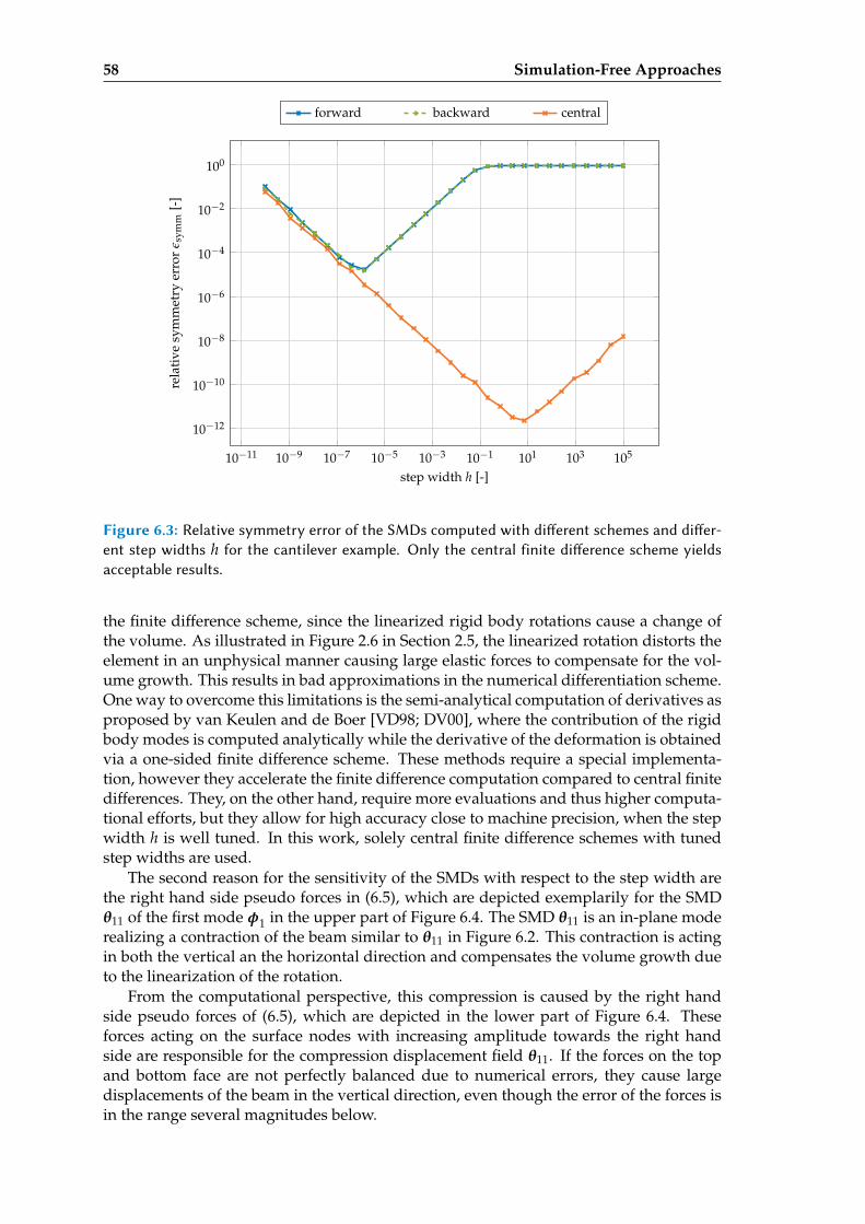
58 Simulation-Free Approaches
10−11 10−9 10−7 10−5 10−3 10−1 101 103 105
10−12
10−10
10−8
10−6
10−4
10−2
100
step width h [-]
rela
tive
sym
met
ryer
ror
ε sym
m[-
]
forward backward central
Figure 6.3: Relative symmetry error of the SMDs computed with dierent schemes and dier-ent step widths h for the cantilever example. Only the central finite dierence scheme yieldsacceptable results.
the finite difference scheme, since the linearized rigid body rotations cause a change ofthe volume. As illustrated in Figure 2.6 in Section 2.5, the linearized rotation distorts theelement in an unphysical manner causing large elastic forces to compensate for the vol-ume growth. This results in bad approximations in the numerical differentiation scheme.One way to overcome this limitations is the semi-analytical computation of derivatives asproposed by van Keulen and de Boer [VD98; DV00], where the contribution of the rigidbody modes is computed analytically while the derivative of the deformation is obtainedvia a one-sided finite difference scheme. These methods require a special implementa-tion, however they accelerate the finite difference computation compared to central finitedifferences. They, on the other hand, require more evaluations and thus higher computa-tional efforts, but they allow for high accuracy close to machine precision, when the stepwidth h is well tuned. In this work, solely central finite difference schemes with tunedstep widths are used.
The second reason for the sensitivity of the SMDs with respect to the step width arethe right hand side pseudo forces in (6.5), which are depicted exemplarily for the SMDθ11 of the first mode φ1 in the upper part of Figure 6.4. The SMD θ11 is an in-plane moderealizing a contraction of the beam similar to θ11 in Figure 6.2. This contraction is actingin both the vertical an the horizontal direction and compensates the volume growth dueto the linearization of the rotation.
From the computational perspective, this compression is caused by the right handside pseudo forces of (6.5), which are depicted in the lower part of Figure 6.4. Theseforces acting on the surface nodes with increasing amplitude towards the right handside are responsible for the compression displacement field θ11. If the forces on the topand bottom face are not perfectly balanced due to numerical errors, they cause largedisplacements of the beam in the vertical direction, even though the error of the forces isin the range several magnitudes below.
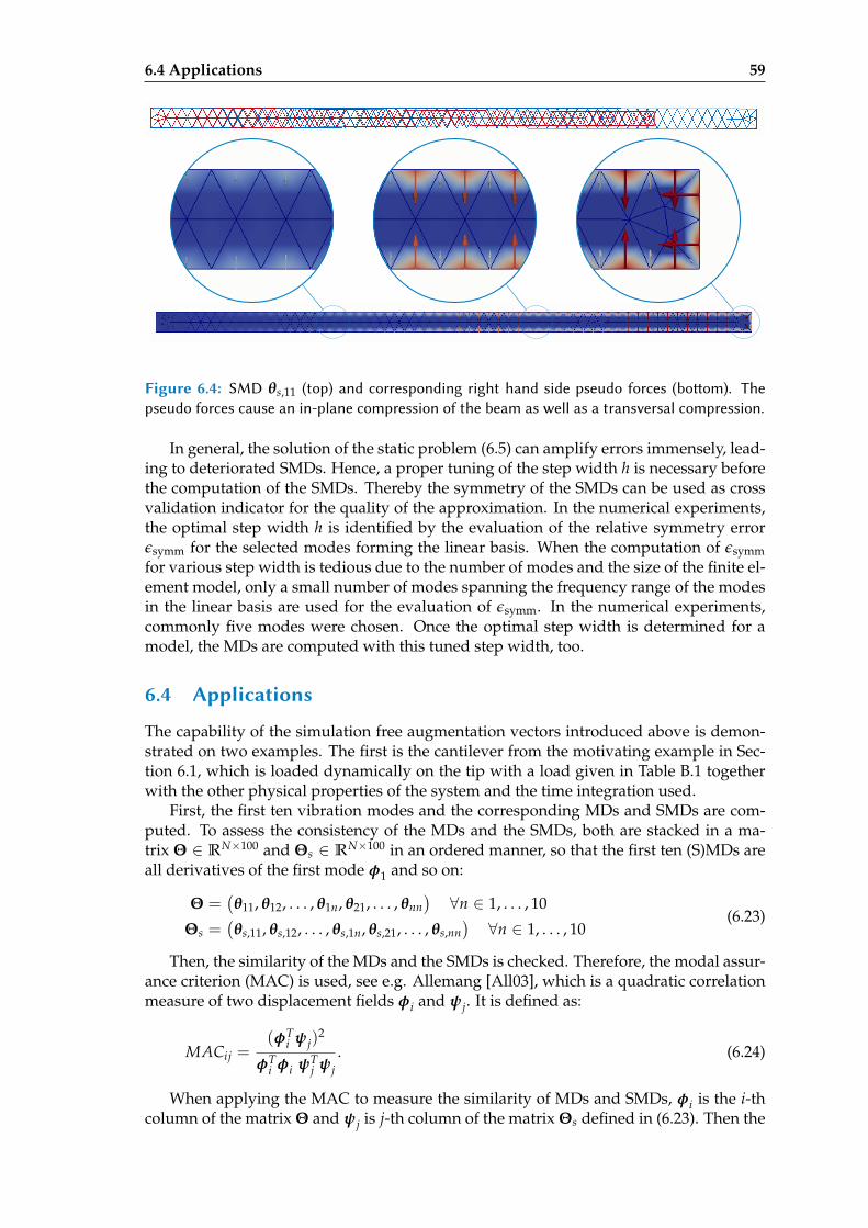
6.4 Applications 59
Figure 6.4: SMD θs,11 (top) and corresponding right hand side pseudo forces (boom). Thepseudo forces cause an in-plane compression of the beam as well as a transversal compression.
In general, the solution of the static problem (6.5) can amplify errors immensely, lead-ing to deteriorated SMDs. Hence, a proper tuning of the step width h is necessary beforethe computation of the SMDs. Thereby the symmetry of the SMDs can be used as crossvalidation indicator for the quality of the approximation. In the numerical experiments,the optimal step width h is identified by the evaluation of the relative symmetry errorεsymm for the selected modes forming the linear basis. When the computation of εsymmfor various step width is tedious due to the number of modes and the size of the finite el-ement model, only a small number of modes spanning the frequency range of the modesin the linear basis are used for the evaluation of εsymm. In the numerical experiments,commonly five modes were chosen. Once the optimal step width is determined for amodel, the MDs are computed with this tuned step width, too.
6.4 Applications
The capability of the simulation free augmentation vectors introduced above is demon-strated on two examples. The first is the cantilever from the motivating example in Sec-tion 6.1, which is loaded dynamically on the tip with a load given in Table B.1 togetherwith the other physical properties of the system and the time integration used.
First, the first ten vibration modes and the corresponding MDs and SMDs are com-puted. To assess the consistency of the MDs and the SMDs, both are stacked in a ma-trix Θ ∈ RN×100 and Θs ∈ RN×100 in an ordered manner, so that the first ten (S)MDs areall derivatives of the first mode φ1 and so on:
Θ =(θ11, θ12, . . . , θ1n, θ21, . . . , θnn
)∀n ∈ 1, . . . , 10
Θs =(θs,11, θs,12, . . . , θs,1n, θs,21, . . . , θs,nn
)∀n ∈ 1, . . . , 10
(6.23)
Then, the similarity of the MDs and the SMDs is checked. Therefore, the modal assur-ance criterion (MAC) is used, see e.g. Allemang [All03], which is a quadratic correlationmeasure of two displacement fields φi and ψj. It is defined as:
MACij =(φT
i ψj)2
φTi φi ψT
j ψj. (6.24)
When applying the MAC to measure the similarity of MDs and SMDs, φi is the i-thcolumn of the matrix Θ and ψj is j-th column of the matrix Θs defined in (6.23). Then the
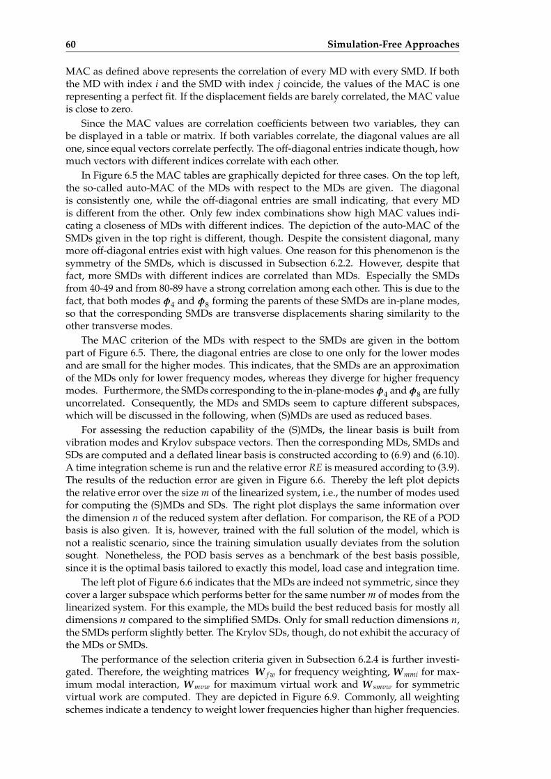
60 Simulation-Free Approaches
MAC as defined above represents the correlation of every MD with every SMD. If boththe MD with index i and the SMD with index j coincide, the values of the MAC is onerepresenting a perfect fit. If the displacement fields are barely correlated, the MAC valueis close to zero.
Since the MAC values are correlation coefficients between two variables, they canbe displayed in a table or matrix. If both variables correlate, the diagonal values are allone, since equal vectors correlate perfectly. The off-diagonal entries indicate though, howmuch vectors with different indices correlate with each other.
In Figure 6.5 the MAC tables are graphically depicted for three cases. On the top left,the so-called auto-MAC of the MDs with respect to the MDs are given. The diagonalis consistently one, while the off-diagonal entries are small indicating, that every MDis different from the other. Only few index combinations show high MAC values indi-cating a closeness of MDs with different indices. The depiction of the auto-MAC of theSMDs given in the top right is different, though. Despite the consistent diagonal, manymore off-diagonal entries exist with high values. One reason for this phenomenon is thesymmetry of the SMDs, which is discussed in Subsection 6.2.2. However, despite thatfact, more SMDs with different indices are correlated than MDs. Especially the SMDsfrom 40-49 and from 80-89 have a strong correlation among each other. This is due to thefact, that both modes φ4 and φ8 forming the parents of these SMDs are in-plane modes,so that the corresponding SMDs are transverse displacements sharing similarity to theother transverse modes.
The MAC criterion of the MDs with respect to the SMDs are given in the bottompart of Figure 6.5. There, the diagonal entries are close to one only for the lower modesand are small for the higher modes. This indicates, that the SMDs are an approximationof the MDs only for lower frequency modes, whereas they diverge for higher frequencymodes. Furthermore, the SMDs corresponding to the in-plane-modes φ4 and φ8 are fullyuncorrelated. Consequently, the MDs and SMDs seem to capture different subspaces,which will be discussed in the following, when (S)MDs are used as reduced bases.
For assessing the reduction capability of the (S)MDs, the linear basis is built fromvibration modes and Krylov subspace vectors. Then the corresponding MDs, SMDs andSDs are computed and a deflated linear basis is constructed according to (6.9) and (6.10).A time integration scheme is run and the relative error RE is measured according to (3.9).The results of the reduction error are given in Figure 6.6. Thereby the left plot depictsthe relative error over the size m of the linearized system, i.e., the number of modes usedfor computing the (S)MDs and SDs. The right plot displays the same information overthe dimension n of the reduced system after deflation. For comparison, the RE of a PODbasis is also given. It is, however, trained with the full solution of the model, which isnot a realistic scenario, since the training simulation usually deviates from the solutionsought. Nonetheless, the POD basis serves as a benchmark of the best basis possible,since it is the optimal basis tailored to exactly this model, load case and integration time.
The left plot of Figure 6.6 indicates that the MDs are indeed not symmetric, since theycover a larger subspace which performs better for the same number m of modes from thelinearized system. For this example, the MDs build the best reduced basis for mostly alldimensions n compared to the simplified SMDs. Only for small reduction dimensions n,the SMDs perform slightly better. The Krylov SDs, though, do not exhibit the accuracy ofthe MDs or SMDs.
The performance of the selection criteria given in Subsection 6.2.4 is further investi-gated. Therefore, the weighting matrices W f w for frequency weighting, Wmmi for max-imum modal interaction, Wmvw for maximum virtual work and W smvw for symmetricvirtual work are computed. They are depicted in Figure 6.9. Commonly, all weightingschemes indicate a tendency to weight lower frequencies higher than higher frequencies.
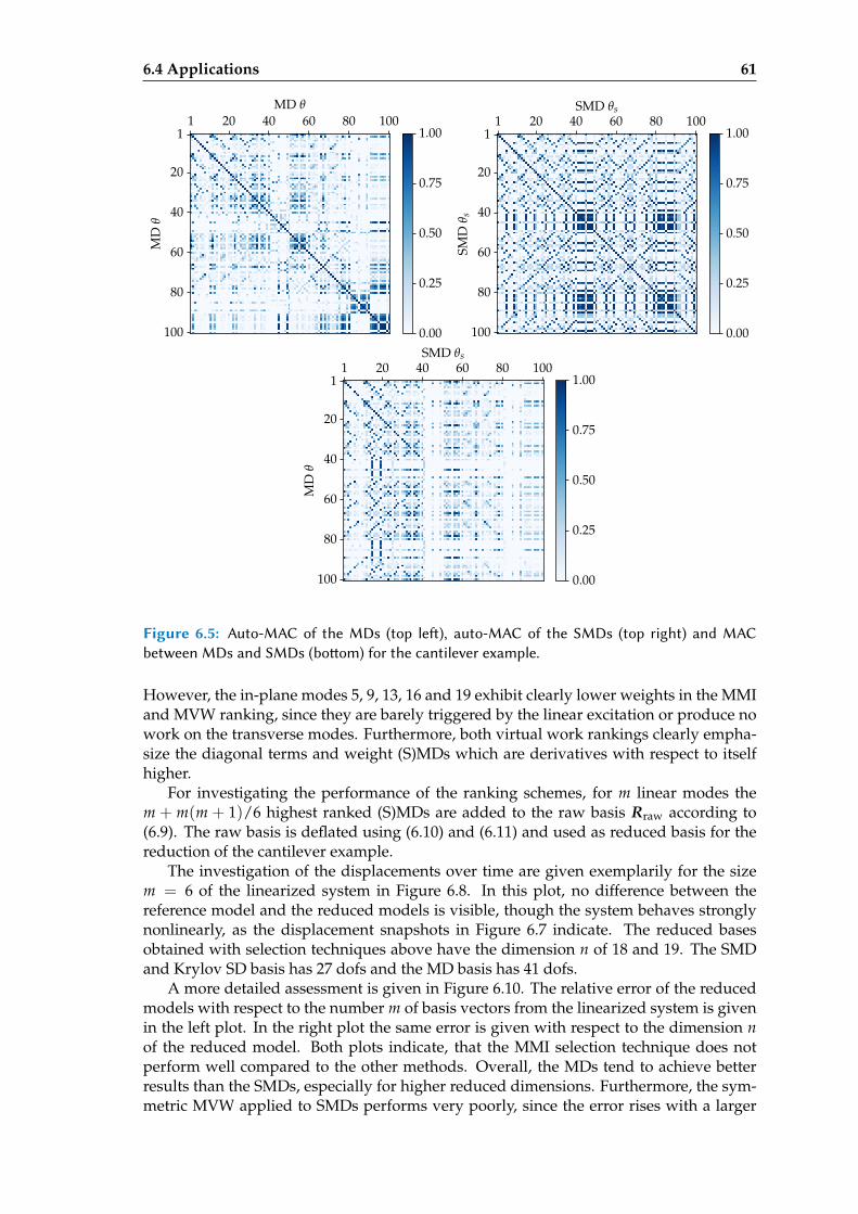
6.4 Applications 61
1
20
40
60
80
100
MD
θ
1 20 40 60 80 100MD θ
0.00
0.25
0.50
0.75
1.001 20 40 60 80 100
SMD θs
1
20
40
60
80
100
SMD
θ s
0.00
0.25
0.50
0.75
1.00
1 20 40 60 80 100SMD θs
1
20
40
60
80
100
MD
θ
0.00
0.25
0.50
0.75
1.00
Figure 6.5: Auto-MAC of the MDs (top le), auto-MAC of the SMDs (top right) and MACbetween MDs and SMDs (boom) for the cantilever example.
However, the in-plane modes 5, 9, 13, 16 and 19 exhibit clearly lower weights in the MMIand MVW ranking, since they are barely triggered by the linear excitation or produce nowork on the transverse modes. Furthermore, both virtual work rankings clearly empha-size the diagonal terms and weight (S)MDs which are derivatives with respect to itselfhigher.
For investigating the performance of the ranking schemes, for m linear modes them + m(m + 1)/6 highest ranked (S)MDs are added to the raw basis Rraw according to(6.9). The raw basis is deflated using (6.10) and (6.11) and used as reduced basis for thereduction of the cantilever example.
The investigation of the displacements over time are given exemplarily for the sizem = 6 of the linearized system in Figure 6.8. In this plot, no difference between thereference model and the reduced models is visible, though the system behaves stronglynonlinearly, as the displacement snapshots in Figure 6.7 indicate. The reduced basesobtained with selection techniques above have the dimension n of 18 and 19. The SMDand Krylov SD basis has 27 dofs and the MD basis has 41 dofs.
A more detailed assessment is given in Figure 6.10. The relative error of the reducedmodels with respect to the number m of basis vectors from the linearized system is givenin the left plot. In the right plot the same error is given with respect to the dimension nof the reduced model. Both plots indicate, that the MMI selection technique does notperform well compared to the other methods. Overall, the MDs tend to achieve betterresults than the SMDs, especially for higher reduced dimensions. Furthermore, the sym-metric MVW applied to SMDs performs very poorly, since the error rises with a larger
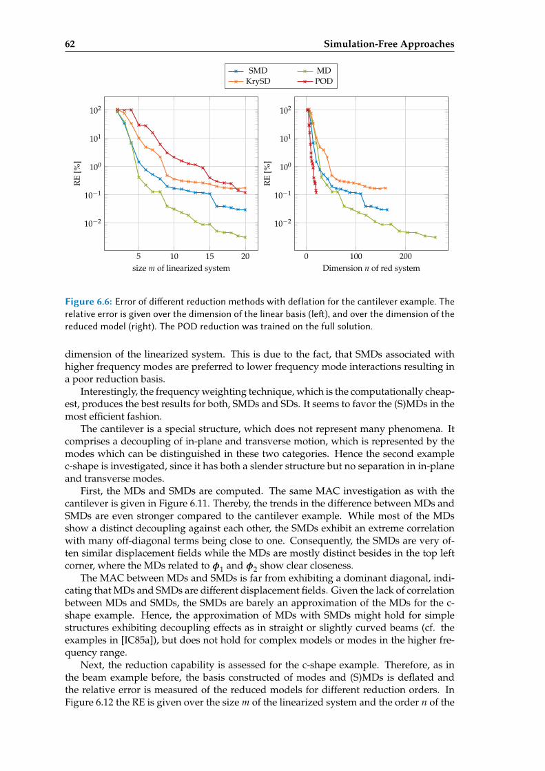
62 Simulation-Free Approaches
5 10 15 20
10−2
10−1
100
101
102
size m of linearized system
RE
[%]
SMD MDKrySD POD
0 100 200
10−2
10−1
100
101
102
Dimension n of red systemR
E[%
]
Figure 6.6: Error of dierent reduction methods with deflation for the cantilever example. Therelative error is given over the dimension of the linear basis (le), and over the dimension of thereduced model (right). The POD reduction was trained on the full solution.
dimension of the linearized system. This is due to the fact, that SMDs associated withhigher frequency modes are preferred to lower frequency mode interactions resulting ina poor reduction basis.
Interestingly, the frequency weighting technique, which is the computationally cheap-est, produces the best results for both, SMDs and SDs. It seems to favor the (S)MDs in themost efficient fashion.
The cantilever is a special structure, which does not represent many phenomena. Itcomprises a decoupling of in-plane and transverse motion, which is represented by themodes which can be distinguished in these two categories. Hence the second examplec-shape is investigated, since it has both a slender structure but no separation in in-planeand transverse modes.
First, the MDs and SMDs are computed. The same MAC investigation as with thecantilever is given in Figure 6.11. Thereby, the trends in the difference between MDs andSMDs are even stronger compared to the cantilever example. While most of the MDsshow a distinct decoupling against each other, the SMDs exhibit an extreme correlationwith many off-diagonal terms being close to one. Consequently, the SMDs are very of-ten similar displacement fields while the MDs are mostly distinct besides in the top leftcorner, where the MDs related to φ1 and φ2 show clear closeness.
The MAC between MDs and SMDs is far from exhibiting a dominant diagonal, indi-cating that MDs and SMDs are different displacement fields. Given the lack of correlationbetween MDs and SMDs, the SMDs are barely an approximation of the MDs for the c-shape example. Hence, the approximation of MDs with SMDs might hold for simplestructures exhibiting decoupling effects as in straight or slightly curved beams (cf. theexamples in [IC85a]), but does not hold for complex models or modes in the higher fre-quency range.
Next, the reduction capability is assessed for the c-shape example. Therefore, as inthe beam example before, the basis constructed of modes and (S)MDs is deflated andthe relative error is measured of the reduced models for different reduction orders. InFigure 6.12 the RE is given over the size m of the linearized system and the order n of the
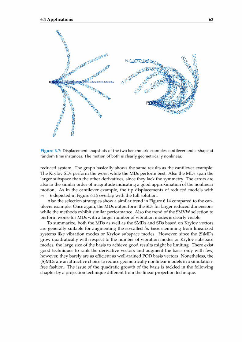
6.4 Applications 63
Figure 6.7: Displacement snapshots of the two benchmark examples cantilever and c-shape atrandom time instances. The motion of both is clearly geometrically nonlinear.
reduced system. The graph basically shows the same results as the cantilever example:The Krylov SDs perform the worst while the MDs perform best. Also the MDs span thelarger subspace than the other derivatives, since they lack the symmetry. The errors arealso in the similar order of magnitude indicating a good approximation of the nonlinearmotion. As in the cantilever example, the tip displacements of reduced models withm = 6 depicted in Figure 6.15 overlap with the full solution.
Also the selection strategies show a similar trend in Figure 6.14 compared to the can-tilever example. Once again, the MDs outperform the SDs for larger reduced dimensionswhile the methods exhibit similar performance. Also the trend of the SMVW selection toperform worse for MDs with a larger number of vibration modes is clearly visible.
To summarize, both the MDs as well as the SMDs and SDs based on Krylov vectorsare generally suitable for augmenting the so-called lin basis stemming from linearizedsystems like vibration modes or Krylov subspace modes. However, since the (S)MDsgrow quadratically with respect to the number of vibration modes or Krylov subspacemodes, the large size of the basis to achieve good results might be limiting. There existgood techniques to rank the derivative vectors and augment the basis only with few,however, they barely are as efficient as well-trained POD basis vectors. Nonetheless, the(S)MDs are an attractive choice to reduce geometrically nonlinear models in a simulation-free fashion. The issue of the quadratic growth of the basis is tackled in the followingchapter by a projection technique different from the linear projection technique.
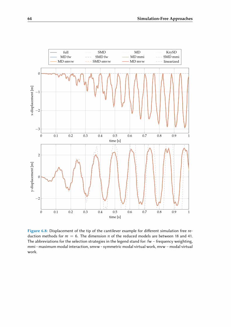
64 Simulation-Free Approaches
0 0.1 0.2 0.3 0.4 0.5 0.6 0.7 0.8 0.9 1
−3
−2
−1
0
time [s]
x-di
spla
cem
ent[
m]
full SMD MD KrySDMD fw SMD fw MD mmi SMD mmi
MD smvw SMD smvw MD mvw linearized
0 0.1 0.2 0.3 0.4 0.5 0.6 0.7 0.8 0.9 1
−2
0
2
time [s]
y-di
spla
cem
ent[
m]
Figure 6.8: Displacement of the tip of the cantilever example for dierent simulation free re-duction methods for m = 6. The dimension n of the reduced models are between 18 and 41.The abbreviations for the selection strategies in the legend stand for: fw – frequency weighting,mmi - maximum modal interaction, smvw - symmetric modal virtual work, mvw – modal virtualwork.

6.4 Applications 65
1 5 10 15 20φj
1
5
10
15
20
φi
10−8
10−7
10−6
10−5
10−4
1 5 10 15 20φj
1
5
10
15
20
φi
10−11
10−8
10−5
10−2
101
104
107
Frequency Weighting W f w Maximum Modal Interaction Wmmi
1 5 10 15 20φj
1
5
10
15
20
φi
10−12
10−9
10−6
10−3
100
103
106
109
1 5 10 15 20φj
1
5
10
15
20
φi
10−13
10−10
10−7
10−4
10−1
102
105
108
Maximum Virtual Work Wmvw Symmetric Maximum Virtual Work W smvw
Figure 6.9: Weighting matrices for dierent weighting schemes applied to the cantilever exam-ple.
5 10 15 20
10−1
100
101
102
size m of linearized system
RE
[%]
MD fw SMD fwMD mmi SMD mmi
MD smvw SMD smvwMD mvw
0 20 40 60 80 100
10−1
100
101
102
Dimension n of red system
RE
[%]
Figure 6.10: Comparison of dierent selection methods with deflation for the cantilever exam-ple. The relative error is given over the dimension of the linear basis (le), and over the dimensionof the reduced model (right).
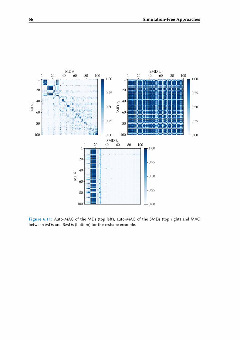
66 Simulation-Free Approaches
1 20 40 60 80 100MD θ
1
20
40
60
80
100
MD
θ
0.00
0.25
0.50
0.75
1.001 20 40 60 80 100
SMD θs
1
20
40
60
80
100
SMD
θ s
0.00
0.25
0.50
0.75
1.00
1 20 40 60 80 100SMD θs
1
20
40
60
80
100
MD
θ
0.00
0.25
0.50
0.75
1.00
Figure 6.11: Auto-MAC of the MDs (top le), auto-MAC of the SMDs (top right) and MACbetween MDs and SMDs (boom) for the c-shape example.
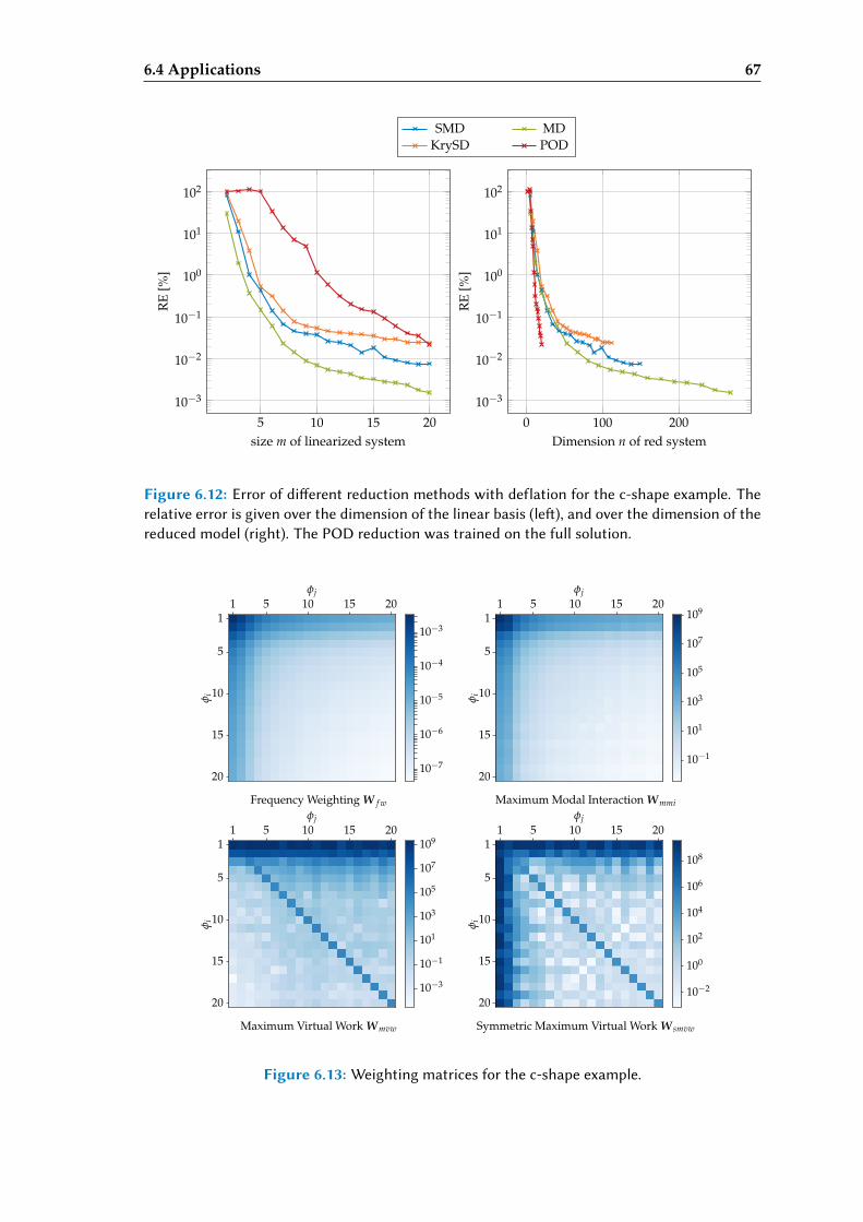
6.4 Applications 67
5 10 15 20
10−3
10−2
10−1
100
101
102
size m of linearized system
RE
[%]
SMD MDKrySD POD
0 100 200
10−3
10−2
10−1
100
101
102
Dimension n of red system
RE
[%]
Figure 6.12: Error of dierent reduction methods with deflation for the c-shape example. Therelative error is given over the dimension of the linear basis (le), and over the dimension of thereduced model (right). The POD reduction was trained on the full solution.
1 5 10 15 20φj
1
5
10
15
20
φi
10−7
10−6
10−5
10−4
10−3
1 5 10 15 20φj
1
5
10
15
20
φi
10−1
101
103
105
107
109
Frequency Weighting W f w Maximum Modal Interaction Wmmi
1 5 10 15 20φj
1
5
10
15
20
φi
10−3
10−1
101
103
105
107
1091 5 10 15 20
φj
1
5
10
15
20
φi
10−2
100
102
104
106
108
Maximum Virtual Work Wmvw Symmetric Maximum Virtual Work W smvw
Figure 6.13: Weighting matrices for the c-shape example.
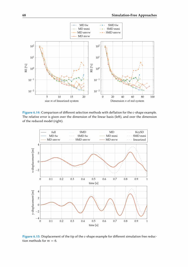
68 Simulation-Free Approaches
5 10 15 20
10−2
10−1
100
101
102
size m of linearized system
RE
[%]
MD fw SMD fwMD mmi SMD mmi
MD smvw SMD smvwMD mvw
0 20 40 60 80 100
10−2
10−1
100
101
102
Dimension n of red system
RE
[%]
Figure 6.14: Comparison of dierent selection methods with deflation for the c-shape example.The relative error is given over the dimension of the linear basis (le), and over the dimensionof the reduced model (right).
0 0.1 0.2 0.3 0.4 0.5 0.6 0.7 0.8 0.9 1
−2
0
2
4
time [s]
x-di
spla
cem
ent[
m]
full SMD MD KrySDMD fw SMD fw MD mmi SMD mmi
MD smvw SMD smvw MD mvw linearized
0 0.1 0.2 0.3 0.4 0.5 0.6 0.7 0.8 0.9 1−4
−2
0
2
4
time [s]
y-di
spla
cem
ent[
m]
Figure 6.15: Displacement of the tip of the c-shape example for dierent simulation free reduc-tion methods for m = 6.
Chapter 7
adratic Manifold
In the previous chapter, simulation-free reduction techniques were addressed. In thesetechniques the basis is formed of two ingredients: the so-called lin basis stemming froma linearized system and the augmentation vectors like (S)MDs, which account for thenonlinearity. One issue of these techniques is, that the number of (S)MDs grows quadrat-ically with the size of the lin basis. This leads to very large bases when the lin basis islarge, which limit the gain in computational time of the reduced basis projection.
One approach to tackle the problem is the use of selection criteria as discussed in Sub-section 6.2.4 and Section 6.4. Another approach to alleviate the issue of the quadraticallygrowing basis is the concept of quadratic manifolds, where the (S)MDs are not treatedas independent dofs but are quadratically coupled with the modes of the lin basis. Thenumber of unknowns is then reduced to a minimum. Then, the mapping from the gener-alized coordinates to the physical coordinates is nonlinear, leading to a different structurein the equations of motion.
However, the reduction technique proposed in this chapter is not suitable for allgeometrically nonlinear problems. It is an attractive option for beam and shell struc-tures, where the von Karman kinematic assumption is used for approximating the Green-Lagrange strain. Hence, in Section 7.3 the von Karman beam theory is introduced andthe relation to the static condensation method discussed in Subsection 4.5.1 is studied inSubsection 7.3.2.
Nonlinear projection with the aim of model order reduction is already used in theGlobal Modal Parametrization technique introduced by Aarts and Jonker [AJ02] and ex-tended by Brüls et al. [BDG07] and Naets et al. [Nae+11; Nae+12], where elastic multi-body systems are reduced to a set of minimal coordinates using a database of configu-ration-specific mappings. A similar approach is also used by Tamarozzi et al. [THD14]and Blockmans et al. [Blo+15] to update the basis for contact problems, where the contactlocation is changing. A further approach to reduce mechanical systems using nonlinearprojections is proposed by Millan and Arroyo [MA13], where the nonlinear projection istrained in a machine-learning style from a set of training snapshots. With the methodproposed in this work, however, the manifold is defined to be quadratic leading to asimple mathematical structure not requiring database operations.
In this chapter first the nonlinear projection framework is introduced and then spec-ified further to the quadratic manifold approach. After the discussion of a stabilizationtechnique and the application of time integration schemes, the application to models us-ing von Karman beams is discussed. The chapter ends with applications to various struc-tures using von Karman beam elements and solid elements to illustrate the potential andthe limits of this method. The quadratic manifold approach is published in [RR14b],[Jai+17] and [Rut+17], on which this chapter bases. Furthermore it is mentioned, that Wuand Tiso [WT16a] propose an approach of the quadratic manifold approach in the context
69
70 Quadratic Manifold
of nonlinear substructuring.
7.1 Key Idea: Nonlinear Projection
The key in the projectional reduction is the linear mapping (3.2) expressing the physi-cal displacements u in terms of the reduced generalized coordinates q as u = Vq. Inthe framework of nonlinear projection, the physical displacements u are expressed as anonlinear function
u = Γ(z) (7.1)
with the reduced generalized coordinates z ∈ Rn. Γ : Rn → RN is a nonlinear mappingfrom the reduced generalized coordinates to the physical coordinates, which is to be de-fined later. Since Γ is not an explicit function of time, the velocities and accelerations arethen given as
u =∂Γ
∂zz, u =
∂Γ
∂zz +
∂2Γ
∂z2 zz (7.2)
with the Jacobian ∂Γ/∂z ∈ RN×n and the second derivative tensor ∂2Γ/∂z2 ∈ RN×n×n.When the nonlinear transformation (7.1) and its derivatives (7.2) are inserted into thenonlinear equations of motion (2.41), one obtains the residual r similar to (3.3). As inChapter 3, the principle of virtual work leads to the equations of motion for a reduced setof generalized coordinates, since the residual is forced to be orthogonal to the kinemati-cally admissible displacements and is thus projected out. The variation of the displace-ment field u with the nonlinear mapping is given as
δu =∂Γ
∂zδz = PΓδz (7.3)
with the tangent projector PΓ = ∂Γ/∂z being the Jacobian of the nonlinear mapping,which spans the tangent subspace of the kinematically admissible displacements δu. Ap-plying the principle of virtual work results in the nonlinear projected reduced equationsof motion
PTΓ MPΓz + PT
Γ M∂2Γ
∂z2 zz + PTΓ CPΓz + PT
Γ f (Γ(z)) = PTΓ g, (7.4)
which can be rearranged to
Mrz + p + Crz + f r(z) = gr(z, t). (7.5)
The reduced mass matrix Mr = PTΓ MPΓ ∈ Rn×n is state dependent, Cr = PT
Γ CPΓ ∈Rn×n is the reduced damping matrix, f r(z) = PT
Γ f (Γ(z)) ∈ Rn the reduced internalforce vector and gr = PT
Γ g the reduced external force vector. The term p = PTΓ M ∂2Γ
∂z2 zzcan be interpreted as a convective term which is state dependent, proportional to thesquared velocities and proportional to the curvature of the nonlinear mapping Γ(z). Thestructure of equation (7.5) is well-known from multibody dynamics and finite elements,where frames are rotating and thus the mapping of the derivative of the generalizedcoordinates to the velocities involves a state depending mapping similar to (7.2).
The equations of motion (7.5) describe the dynamics of a reduced system for an ar-bitrary nonlinear mapping Γ(z). If the mapping is linear, as in the common projectivemodel order reduction, the question of reduction boils down to the question of the sub-space spanned by the basis V . However, for a nonlinear mapping, first the structure ofthe nonlinearity is to be chosen before the parameters of the mapping are determined.
7.2 Mapping on Quadratic Manifold 71
7.2 Mapping on adratic Manifold
In the Quadratic Manifold (QM) approach, the mapping Γ(z) is chosen to be a quadraticfunction of z. This allows to keep the dimension of the reduced generalized coordinates zsmall while still incorporating the information of MDs or SMDs. However, first the gen-eral framework of quadratic projection is addressed before the incorporation of MDs,SMDs and SDs is discussed. The quadratic mapping can be expressed as
Γ = Vz +12(Θz)z (7.6)
with the linear part of the transformation V ∈ RN×n and the quadratic part Θ ∈ RN×n×n.In index notation, the quadratic mapping (7.6) is written as
ui = Vijzj +12
Θijkzjzk. (7.7)
To make the mapping unique, Θ has to be symmetric with respect to the last twoindices, since the anti symmetric part is eliminated by the quadratic form of z. To il-lustrate this, an anti-symmetric three dimensional tensor Λ ∈ RN×n×n is added to thesymmetric Θ. If Λijk = −Λikj, then the mapping (7.6) yields
Γi = Vijzj +12(Θijk + Λijk)zjzk
= Vijzj +12
Θijkzjzk +12
Λijkzjzk
= Vijzj +14
Θijkzjzk +14
Λijkzjzk +14
Λijkzjzk
= Vijzj +14
Θijkzjzk +14
Λijkzjzk −14
Λikjzjzk
= Vijzj +14
Θijkzjzk +14
Λijkzjzk −14
Λijkzkzj
= Vijzj +14
Θijkzjzk
(7.8)
eliminating the anti-symmetric part of the quadratic mapping (7.6). Consequently, Θ hasonly N · n · (n + 1)/2 independent entries, while the remaining entries are defined withthe symmetry constraint.
The velocities and the accelerations of the physical dofs are then expressed as
u = Γ = PΓz, u = Γ = PΓz + Θzz, PΓ = V + Θz. (7.9)
with the tangent projector PΓ ∈ RN×n being a function depending linearly on the gen-eralized quadratic coordinates z. If the mapping is chosen to be quadratic, not only thelinear part V but also the nonlinear part Θ of the mapping need to be defined. In thefollowing, two options are presented to form the quadratic part, if the basis is filled withvibration modes. Furthermore, the force compensation method is presented to build Θ
for an arbitrary linear basis V .
7.2.1 Modal Derivatives
If the linear part of the quadratic mapping (7.6) is composed of vibration modes, thequadratic part Θ should capture the change of the vibration modes with respect to achange of the geometrical configuration. This change is expressed by MDs, which are
72 Quadratic Manifold
constructed by the perturbation of the eigenvalue problem and hence capture the changeof one mode with respect to a geometry change in the direction of another mode shape.
Consequently, the quadratic part Θ can be composed of MDs when the linear part Vis built using vibration modes. However, since the MDs are not symmetric with respectto the last two indices θij 6= θji, the quadratic tensor Θ is to be composed of the symmetricpart of the tensor Ω ∈ RN×n×n which is filled with the MDs θij = ∂φi/∂ηj:
Ω[:, i, j] = θij (7.10)
The quadratic tensor Θ of the mapping is then given as the symmetric part of Ω
yielding
Θijk =12(Ωijk + Ωikj
). (7.11)
The approach using MDs as the quadratic extension for a linear part V composedof vibration modes is motivated by the conceptual idea of MDs. Since they representthe perturbation of modes, it seems to be a reasonable quadratic extension to the linearmapping of modes. The concept of using MDs as quadratic extension is purely heuristic.The suitability of this approach is illustrated in the Applications in Section 7.4.
The SMDs also capture the change of modes in a different fashion than the MDs.Hence, they can also be regarded as reasonable extensions for the quadratic mapping Θ.
7.2.2 Static Modal Derivatives
As a second approach, the quadratic part Θ can be composed of SMDs if the linear part Vis built using vibration modes. Since the SMDs are symmetric with respect to the last twoindices, they form directly the second order tensor Θ:
Θ[:, i, j] = θs,ij (7.12)
with θs,ij = ∂φi/∂ηj|s. It should be pointed out, that the MDs and the SMDs are builtusing different assumptions. While the MDs stem from the perturbation of an eigenvalueproblem, where the nonlinear system is made both linear and parametric, the concept ofthe SMDs is different. They are solely based on the quadratic part of the nonlinearity ofthe forces which can be given a different interpretation in the context of a QM mapping.This other route to define SDs named force compensation method or force compensationapproach is given next.
7.2.3 Force Compensation Method
In the previous two sections, the quadratic part Θ of the nonlinear mapping was builteither from MDs or SMDs in the case, that V is built from vibration modes. When usingSMDs in the quadratic part, however, a condition is satisfied which can be generalizedto the force compensation method. The motivation of this approach is that the quadraticnonlinearity of the internal forces is swapped to the quadratic manifold, so that the inter-nal forces have not quadratic terms on the manifold.
When only the linear part V is given as vibration modes or any other type of modes,the quadratic part can be uniquely determined, when the second derivative of the non-linear forces with respect to the generalized quadratic coordinate z is forced to be zero:
∂2 f (Γ(z))∂z2
∣∣∣∣z=0
= 0. (7.13)
7.2 Mapping on Quadratic Manifold 73
This condition defines the quadratic manifold such that it compensates the quadraticpart of the nonlinear forces with respect to the generalized coordinates z. Then, thequadratic tensor Θ can be derived from (7.13) in the following manner:
After applying the chain rule yielding[(
∂2 f∂u2 ·
∂u∂z
)∂u∂z
+∂ f∂u
∂2u∂z2
]
z=0= 0, (7.14)
with the first and second derivative of the quadratic mapping given as
∂u∂z
∣∣∣∣z=0
= V ,∂2u∂z2
∣∣∣∣z=0
= Θ, (7.15)
and the definition of the stiffness matrix K = ∂ f (u)u
∣∣∣u=0
, one obtains the equation for thethird order tensor Θ as
(∂2 f∂u2
∣∣∣∣u=0· V)
V + K ·Θ = 0. (7.16)
From (7.16), the tensor Θ is uniquely defined if K is not rank deficient. In other words,there exists a unique quadratic tensor Θ compensating the nonlinear forces to meet con-dition (7.13) for any linear basis V . Thereby, V does not have to be composed of vibrationmodes, but can be composed of any suitably chosen set of linearly independent vectors.Furthermore, Θ is symmetric with respect to the last two indices, i.e., Θijk = Θikj.
For further analysis (7.16) is recast to index notation yielding(
∂2 fk
∂ul∂um
∣∣∣∣u=0
)VliVmj + Kklθlij = 0, (7.17)
where k, l, m ∈ 1, . . . , N are the indices of the physical domain, and i, j ∈ 1, . . . , n areof the reduced domain. Since (7.16) is evaluated at u = 0, the matrix V can be interpretedas the linear mapping of the reduced, linear generalized coordinates q to the full displace-ments u = Vq as in the linear basis projection discussed in Chapter 3. Then the partialderivative ∂um/∂qj|u=0 yields Vmj and one can rewrite (7.17) using ∂ fk/∂ul |u=0 = Kkl to
∂
∂um
(∂ fk
∂ul
)∂um
∂qj
∣∣∣∣∣u=0
Vli + Kklθlij = 0 (7.18)
=⇒ ∂
∂um(Kkl)
∂um
∂qj
∣∣∣∣∣u=0
Vli + Kklθlij = 0. (7.19)
With the chain rule, (7.19) can be simplified to
∂Kkl
∂qjVli + Kklθlij = 0. (7.20)
The expression above can be rewritten in matrix-vector notation with l being the indexof column vectors and k being the row-index of matrices as
∂K∂qj
vi + Kθij = 0 ⇔ Kθij = −∂K∂qj
vi. (7.21)
The solution of (7.21) which yields the Static Derivatives (SDs) θs,ij is equivalent to thedefinition of the SMDs (7.21), if the linear part V of the quadratic mapping is chosen to
74 Quadratic Manifold
consist of vibration modes: V = [φ1, φ2, . . . , φn]. Hence, SMDs are obtained as a specialcase of the general framework described by the force compensation approach using (7.13).
The approach presented above yields the same static derivatives as presented in Sub-section 6.2.2. In the force compensation approach, the nonlinearity is mapped from theinternal forces to the quadratic part of the basis, leading to exactly the static derivativesin the quadratic part. The fact that the two interpretations are equivalent for vibrationmodes enables one to extend the concept of quadratic manifolds to bases different fromvibration modes, such as Krylov subspace vectors or other linear reduction techniques.Since both concepts are interrelated, a physical interpretation of the SDs obtained withinthe QM framework should be given, which is also illustrated in Figure 7.1.
For two given linear displacement fields v1 and v2, where for instance v1 is a staticdisplacement mode of a unit force at the tip of the beam and v2 is the second vibra-tion mode, there exists a unique corresponding force distribution f 1 and f 2 such thatf i = Kvi : i ∈ 1, 2. If both force distributions are combined and applied to the nonlinearsystem, the resulting displacements can be split in two contributions: the linear displace-ments v1 + v2, and a nonlinear correction resulting from the combination of both forcesand the nonlinearity. As is shown below, the quadratic part of this nonlinear contributioncontains exactly all SDs associated to the displacement fields v1 and v2.
The nonlinear forces can be expanded using a Taylor expansion up to the quadraticpart as
f =∂ f∂u
u +12
∂2 f∂u2 uu +O(u3) = Ku + K(2)uu +O(||u||3) (7.22)
with the linear stiffness matrix K ∈ RN×N and the second order stiffness tensor K(2) ∈RN×N×N . The external forces g in Figure 7.1 are the response of the linearized systemwhich is perturbed with the displacements v1 and v2, i.e.,
g = εK(v1 + v2), (7.23)
where ε > 0 is a load scaling factor. Setting the static equilibrium of the external forces gwith the Taylor expanded internal forces (7.22), one obtains
g = f (7.24)
=⇒ εK(v1 + v2) = Ku +12
K(2)uu +O(||u||3) , (7.25)
with the unknown displacement field u. When ε is assumed to be small, the solution canbe expanded with the bookkeeping notation as
u = εu(1) + ε2u(2) + . . . . (7.26)
Substituting (7.26) into (7.25) and comparing coefficients of different powers of ε, oneobtains the leading order coefficient to the solution u as
u(1) = v1 + v2, (7.27)
and the second order approximation as
u(2) =−12
K−1K(2)(v1 + v2)(v1 + v2) . (7.28)
Now, the SD θij is defined according to (7.17) as
θij = −K−1K(2)vivj. (7.29)
7.2 Mapping on Quadratic Manifold 75
Thus, by using the fact that the SDs are symmetric, i.e., θs,12 = θs,21, u(2) from (7.28)can be expressed in terms of SDs as
u(2) =12(θs,11 + θs,12 + θs,21 + θs,22) = θs,12 +
12(θs,11 + θs,22). (7.30)
Consequently, the displacement field is composed of all three static derivatives, θs,11,θs,22 and θs,12.
7.2.4 Stabilization Through Orthogonalization
In some cases, the tangent projector PΓ = V + Θz is not well conditioned. As discussedin Subsection 6.2.3, the subspace spanned by the linear part V formed by vibration modesor other basis modes and the quadratic part Θ formed by MDs or SDs is not necessarilydistinct. Then, for certain generalized coordinates z, the tangent projector PΓ might bepoorly conditioned leading to poor or even no convergence in the Newton-Raphson loopof the time integration scheme. To solve this issue, a Gram-Schmidt like orthogonaliza-tion of the quadratic part with respect to the linear part can be applied, which alleviatesthe convergence issue. The orthogonalization can be written as
Θ⊥V = (I −n
∑i=1
vivTi )Θ, with vT
i vi = 1 (7.31)
so that the orthogonality condition of Θ⊥V and V is fulfilled:
V TΘ⊥V = 0. (7.32)
This orthogonalization, however, breaks the quadratic manifold. If Θ is built usingSDs for instance, the condition (7.13) is violated. In the other case, when the QM is con-structed with MDs, the MDs are deteriorated so that the projection is performed on adifferent manifold which is stabilized but not the original one.
The effect of the orthogonalization is commonly dependent on the size of the linearpart V of the mapping. In the extreme case of V being square and having full rank,the orthogonalization (7.31) leads to Θ⊥V = 0. However, if V is only composed of fewmodes, the deterioration effect on the quadratic mapping due to the orthogonalization isgenerally mild.
7.2.5 Time Integration
For solving the equations of motion (7.4) for a given set of initial reduced displace-ments z0 = z(t = 0) and velocities z0 = z(t = 0), a time stepping integration schemelike the generalized-α method as outlined in Section 2.4 is necessary.
The generalized-α integration scheme has two different balancing time shifts αm forthe acceleration forces and α f for the internal, external and damping forces. However,since in the QM approach the basis is changed with the current displacement state, theidea of balancing, which leads to an optimized numerical damping behavior, is hardlyphysically reasonable for state dependent bases. In order to keep the time integra-tion variationally consistent, so that both the acceleration forces as well as the internal,external and damping forces are acting in the same tangential subspace PΓ, the time in-tegration recommended and used in the examples is the Newmark scheme, where thebalancing time shifts are set to zero, i.e. α f = αm = 0. As a consequence, the tangentialsubspace is consistent with the reconstructed displacement field uj+1 = Γ(qj+1). The nu-merical damping can be adjusted by the damping constant α ≥ 0, which determines theparameters β and γ as
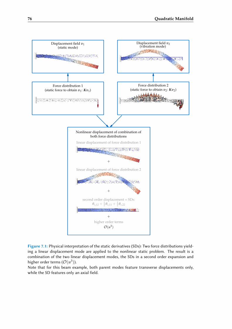
76 Quadratic Manifold
Displacement field v1(static mode)
Displacement field v2(vibration mode)
Force distribution 2(static force to obtain v2: Kv2)
O(u3)
linear displacement of force distribution 1
linear displacement of force distribution 2
second order displacement = SDs:
higher order terms
Nonlinear displacement of combination ofboth force distributions
+
+
+
θs,12 +12 θs,11 +
12 θs,22
Force distribution 1(static force to obtain v1: Kv1)
Figure 7.1: Physical interpretation of the static derivatives (SDs): Two force distributions yield-ing a linear displacement mode are applied to the nonlinear static problem. The result is acombination of the two linear displacement modes, the SDs in a second order expansion andhigher order terms (O(u3)).Note that for this beam example, both parent modes feature transverse displacements only,while the SD features only an axial field.
7.2 Mapping on Quadratic Manifold 77
γ =12+ α, β =
14(1 + α)2, 0 ≤ α ≤ 0.3. (7.33)
Numerical damping is introduced by choosing α > 0. However, this choice destroysthe second order accuracy of the integration scheme, since the Newmark scheme is onlysecond order accurate for α = 0. In the author’s experience, the QM approach yields bestresults with the Newmark integration scheme. Hence, this scheme using α f = αm = 0 isderived in the following.
Similar to the balance equation (2.50), the balance equation for the j + 1-th time stepof the QM projected system is written as
Mr,j+1zj+1 + pj+1 + Cr,j+1zj+1 + f r,j+1(zj+1) = gr,j+1(zj+1, tj+1). (7.34)
The reduced quantities are obtained with the tangent projector PΓ given with thereduced generalized displacements zj+1 at the j + 1-th time step:
PΓ = V + Θzj+1. (7.35)
Consequently, the residual of the force balance equation (7.34) yields
r(zj+1) =PTΓ
(MPΓzj+1 + MΘzj+1zj+1 + CPΓzj+1 + f (Γ(zj+1))− g j+1
)(7.36)
=PTΓ rfull(zj+1), (7.37)
which is solved for in every iteration step with a Newton-Raphson iteration. The JacobianKi
dyn,j+1 = ∂r(zj+1)/∂zj+1 necessary for the iteration is given exactly as
Kdyn,j+1 =1
βh2 PTΓ MPΓ +
γ
βh
(PT
Γ CPΓ + 2PTΓ MΘzj+1
)+ PT
Γ K(Γ(zj+1)
)PΓ
+PTΓ(
MΘzj+1 + CΘzj+1)+ ΘTrfull(zj+1)
(7.38)
with the residual of the full system rfull(zj+1) from (7.37). The transposed third ordertensor multiplication ΘT in the last term is expressed in index notation as
ΘTrfull = Θkilrfull,k (7.39)
with i and l being the row and column index of the resulting matrix.The Jacobian given in (7.38) is the exact Jacobian leading to optimal quadratic conver-
gence in the Newton-Raphson iteration. However, it involves several terms arising dueto the change of the tangential projector PΓ, which can be neglected. The approximateJacobian Kdyn,j+1 ≈ Kdyn,approx,j+1 then yields
Kdyn,approx,j+1 =1
βh2 PΓ MPΓ +γ
βhPΓCPΓ + PT
Γ K(Γ(zj+1))PΓ. (7.40)
which can also be used in the Newton-Raphson iteration instead of Kdyn,j+1 from (7.38).The convergence rate is not as good as with the exact Jacobian, though. In the author’sexperience it is problem dependent, if the approximate or the full Jacobian yields to fastercomputations. In the given examples, the time integration is performed with full Jaco-bians to benefit of the optimal convergence behavior.
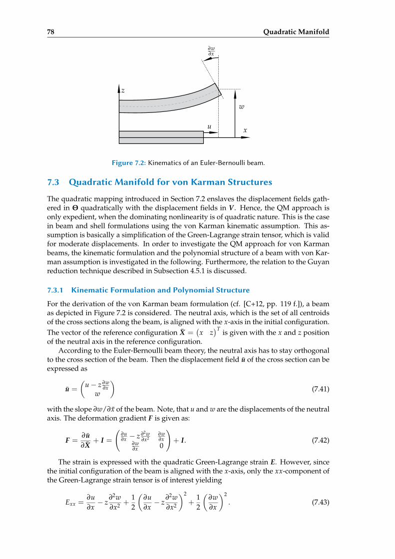
78 Quadratic Manifold
x
z
∂w∂x
w
u
Figure 7.2: Kinematics of an Euler-Bernoulli beam.
7.3 adratic Manifold for von Karman Structures
The quadratic mapping introduced in Section 7.2 enslaves the displacement fields gath-ered in Θ quadratically with the displacement fields in V . Hence, the QM approach isonly expedient, when the dominating nonlinearity is of quadratic nature. This is the casein beam and shell formulations using the von Karman kinematic assumption. This as-sumption is basically a simplification of the Green-Lagrange strain tensor, which is validfor moderate displacements. In order to investigate the QM approach for von Karmanbeams, the kinematic formulation and the polynomial structure of a beam with von Kar-man assumption is investigated in the following. Furthermore, the relation to the Guyanreduction technique described in Subsection 4.5.1 is discussed.
7.3.1 Kinematic Formulation and Polynomial Structure
For the derivation of the von Karman beam formulation (cf. [C+12, pp. 119 f.]), a beamas depicted in Figure 7.2 is considered. The neutral axis, which is the set of all centroidsof the cross sections along the beam, is aligned with the x-axis in the initial configuration.The vector of the reference configuration X =
(x z
)T is given with the x and z positionof the neutral axis in the reference configuration.
According to the Euler-Bernoulli beam theory, the neutral axis has to stay orthogonalto the cross section of the beam. Then the displacement field u of the cross section can beexpressed as
u =
(u− z ∂w
∂xw
)(7.41)
with the slope ∂w/∂x of the beam. Note, that u and w are the displacements of the neutralaxis. The deformation gradient F is given as:
F =∂u∂X
+ I =
(∂u∂x − z ∂2w
∂x2∂w∂x
∂w∂x 0
)+ I. (7.42)
The strain is expressed with the quadratic Green-Lagrange strain E. However, sincethe initial configuration of the beam is aligned with the x-axis, only the xx-component ofthe Green-Lagrange strain tensor is of interest yielding
Exx =∂u∂x− z
∂2w∂x2 +
12
(∂u∂x− z
∂2w∂x2
)2
+12
(∂w∂x
)2
. (7.43)
7.3 Quadratic Manifold for von Karman Structures 79
The von Karman assumption (cf. [FT01; C+12]) claims that the axial strains and thecurvature are small compared to the bending rotation. This condition is stated as
12
(∂u∂x− z
∂2w∂x2
)2
= 0 (7.44)
resulting in the quadratic von Karman strain expression
Ex,Karman =∂u∂x− z
∂2w∂x2 +
12
(∂w∂x
)2
. (7.45)
When this strain is used with a linear constitutive law and the finite element proce-dure is applied, one obtains a polynomial system of equations for the Euler-BernoulliBeam theory applied with von Karman strain assumption. The dofs can be partitionedin membrane dofs u acting in x-direction and bending dofs w acting in z-direction re-sulting in two coupled equations, which are given in index notation following Einstein’ssummation convention over repeated indices:
Mm,ijuj + K(1)m,ijuj + K(2)
mb,ijkwjwk = gm,i (7.46)
Mb,ijwj + K(1)b,ijwj + K(2)
bm,ijkwjuk + K(3)b,ijklwjwkwl = gb,i (7.47)
The subscripts b and m stand for bending and membrane respectively. The equa-tions (7.46) and (7.47) are the coupled equations of motion for a von Karman beam forthe membrane and bending dofs, respectively. The first equation shows, that the mem-brane dynamics is linear but coupled nonlinearly with the bending displacements, whichtrigger the membrane forces quadratically. The bending restoring forces are linear andcubic with respect to the bending displacements and coupled with the membrane dis-placements in a bilinear fashion. The equations (7.46) and (7.47) can be rearranged tohighlight the structure of the coupling as
(Mm
Mb
)(uw
)+
(K(1)
m
K(1)b
)(uw
)+
(K(2)
mb wwK(2)
bm wu + K(3)b www
)=
(gmgb
).
(7.48)
7.3.2 Nonlinear Static Condensation
Consider a more general nonlinear system with separated nonlinear terms and neglecteddamping for the sake of simplicity
Mu + Ku + f (u) = g(t) (7.49)
and assume that the nonlinearity is such, that the equations can be written in partitionedform as
(M11 M12M21 M22
)(u1u2
)+
(K11 K12K21 K22
)(u1u2
)+
(f 1(u1, u2)
f 2(u1)
)=
(g1(t)g2(t)
). (7.50)
Note, that in (7.49) and (7.50) a more general case is investigated which translates to(7.48) with u1 = w and u2 = u. In the partitioned equation (7.50), the nonlinearity iscoupled only in one way, so that the nonlinear forces f 2 are only dependent on u1 andnot u2. If the inertia forces acting on u2 are set to zero:
M21u1 + M22u2 = 0, (7.51)
80 Quadratic Manifold
the second line of (7.50) is an algebraic equation. It yields for the excitation forces g2(t)set to zero:
K21u1 + K22u2 + f 2(u1) = 0. (7.52)
This algebraic equation can be solved for u2 resulting in
u2 = −K−122 (K21u1 + f 2(u1)). (7.53)
If this equation (7.53) is inserted into the first line of (7.50), one obtains the staticcondensed equations of motion, where u2 is eliminated under the condition (7.51).
Exactly the same result is obtained, if the nonlinear transformation(
u1u2
)=
(u1
−K−122 (K21u1 + f 2(u1))
)= Γ(u1), (7.54)
in which u1 is enslaved in terms of u1, is applied to the linear and nonlinear restoringforces in (7.50).
However, the mapping (7.54) can be applied not only to the restoring forces, as in thenonlinear static condensation approach above, but also to the full system as in Section 7.1.Then, the acceleration forces in the u2 direction as stated in (7.51) are not forced to bezero, since this is only the constraint for the kinematic mapping but not for the resultingdynamic equation.
The procedure of nonlinear static condensation and full nonlinear mapping is sub-sequently applied to the von Karman beam, which exhibits the decoupling structure asgiven in (7.50).
7.3.3 Application to the von Karman Beam
Now, the theory developed in the previous section is applied to the von Karman beamcharacterized by the partitioned system (7.48) with u1 = w and u2 = u. The assumptionof the static condensation approach is, that the acceleration forces in the in-plane directionare zero:
Mm,ijuj = 0. (7.55)
Then the second line in (7.48) becomes an algebraic equation, which can be solved forthe membrane displacements u with the external forcing gm,i set to zero:
uj = −(
K(1)m,ij
)−1K(2)
mb,iklwkwl (7.56)
This equation can be inserted into (7.47), yielding the equations of motion for themembrane dofs with the bending dofs condensed out:
Mb,ijwj + K(1)b,ijwj − K(2)
bm,ijkwj
(K(1)
m,lk
)−1K(2)
mb,lnownwo + K(3)b,ijklwjwkwl = gb,i. (7.57)
It can be recast to the condensed equation with all cubic terms gathered in K(3)b,ijkl :
Mb,ijwj + K(1)b,ijwj + K(3)
b,ijklwjwkwl = gb,i (7.58)
In this equation, the nonlinear beam is modeled solely with bending displacements w,whereas the membrane displacements u are forced to follow the bending displacementsin a static fashion. This equation is based, however, on the negligence of the membranedynamics by setting the inertia forces in x-direction to zero (7.55).
7.3 Quadratic Manifold for von Karman Structures 81
As in the previous section, the static condensation approach can also be expressed interms of a nonlinear basis. The membrane dofs are then enslaved in terms of the bendingdofs by the following nonlinear mapping applied to (7.48):
(uw
)= Γ(w) =
(−(
K(1)m
)−1K(2)
mb www
)=
(Θmbww
w
)(7.59)
with the bending dofs w being the generalized quadratic coordinates z. If the mapping(7.59) is applied only on the internal forces in (7.48) and the acceleration forces in mem-brane direction are set to zero, i.e. Mmu = 0, the resulting equations are exactly thecondensed equations of motion (7.57). The quadratic manifold is formed by the sym-metric second oder tensor Θmb = −(K(1)
m )−1K(2)mb . Note that in the static condensation
approach, the quadratic mapping is only applied on the internal restoring forces and noton the acceleration terms. Next, the force compensation approach is applied to the vonKarman beam and the similarities are pointed out.
7.3.4 Force Compensation Approach
Up to now, only the dofs of the beam are partitioned in bending and membrane dofs. If aQM reduction is applied using the force compensation approach, first the linear basis isdefined. Assuming that the linear basis V is built using modes which are solely bendingmodes, like the first vibration modes or Krylov subspace modes due to pure bendingforces, the linear basis V can be partitioned into
V =
(V mV b
)(7.60)
with V m describing the membrane components and V b the bending components of thelinear basis V . Since the basis consists only of bending modes, the membrane componentsare zero, leading to
V =
(0
V b
). (7.61)
When the force compensation approach (cf. Subsection 7.2.3 is applied, the third ordertensor Θ is defined in accordance with (7.16) and with u = (wT, uT)T as
θij = K−1 ∂2 f∂u2
∣∣∣∣u=0
vivj. (7.62)
With the partitioning in (7.48), one finds
Θ =
(K(1)
m
)−10
0(
K(1)b
)−1
K(2)mbV bV b
K(2)bmV bV m
(7.63)
with the second order derivative ∂2 f /∂u2 of the internal forces forming the quadraticstiffness terms K(2)
mb and K(2)bm . Since V m = 0, (7.63) simplifies to
Θ =
((K(1)
m
)−1K(2)
mbV bV b
0
)(7.64)
and the full quadratic mapping Γ is then given as
82 Quadratic Manifold
Γ =
(uw
)=
[(
K(1)m
)−1K(2)
mbV bV b
]zz
V bz
(7.65)
=
(0
V b
)
︸ ︷︷ ︸V
z +
((K(1)
m
)−1K(2)
mbV bV b
0
)
︸ ︷︷ ︸Θ
zz. (7.66)
This quadratic mapping is the result of the force compensation approach applied to avon Karman beam. This mapping shows clearly, that the membrane displacements u areenslaved quadratically to the bending displacements w. Note that the mapping (7.65) isequivalent to (7.59) with w = Vz substituted. This means that the force compensationapproach yields exactly the same basis as the static condensation approach for the vonKarman beam, given that the linear basis V is composed of bending displacements only.
7.3.5 Relation between QM Approach and Static Condensation
Using the mapping (7.59) solely on the internal forces and not the acceleration termsresults in the static condensation (7.57). However, when using the quadratic mapping(7.59) in the nonlinear projection framework (7.4), the resulting equations of motion arewritten as:
[(Θmbw)T MmΘmbw + Mb]w + (Θmbw)T MmΘmbww
+ K(1)b w + K(2)
bm w(
K(1)m
)−1K(2)
mb ww + K(3)b www = gb + (Θmbw)Tgm
(7.67)
Or recast and written in index notation:[
M(3)m,ijklwkwl + Mb,ij
]wj + M(3)
m,ijklwjwkwl
+ K(1)b,ijwj + K(3)
b,ijklwjwkwl = gb,i + Θjikwkgm,j
(7.68)
with the membrane mass tensor M(3)m,ijkl = Mm,noΘnijΘokl and Θijk = (K(1)
m,li)−1K(2)
mb,l jk.When comparing the nonlinear projected equations of motion (7.68) with the equa-
tions of motion with static condensation (7.57), the difference between the nonlinear pro-jection and the static condensation lies in the additional acceleration terms associatedwith Mm, which are only in place in the nonlinear projection. They represent the inertiaeffect in the membrane direction. They are only nonzero if the bending displacement wis nonzero leading to a tangential motion of the nonlinear beam which carries a compo-nent in membrane direction. This additional inertia is often negligible making the staticcondensation a good choice in general. However, in special cases, they can play a non-negligible role as illustrated in [RR14b].
Compared to static condensation, the QM approach carries the advantage that it isapplicable to systems where the decomposition in master and slave dofs is not possibleor convenient. Hence, the nonlinear mapping using a quadratic manifold opens the fieldto other systems not comprising these properties.
7.4 Applications
To show the feasibility of the QM approach as well as its limits, it is applied to severalexamples. The QM approach is an extension of the reduced basis approach introducedin Chapter 3, the goal is the reduction of the number of dofs. Since, as will be discussedin Part II of this thesis, the bottleneck of reduced models is very often the evaluation of
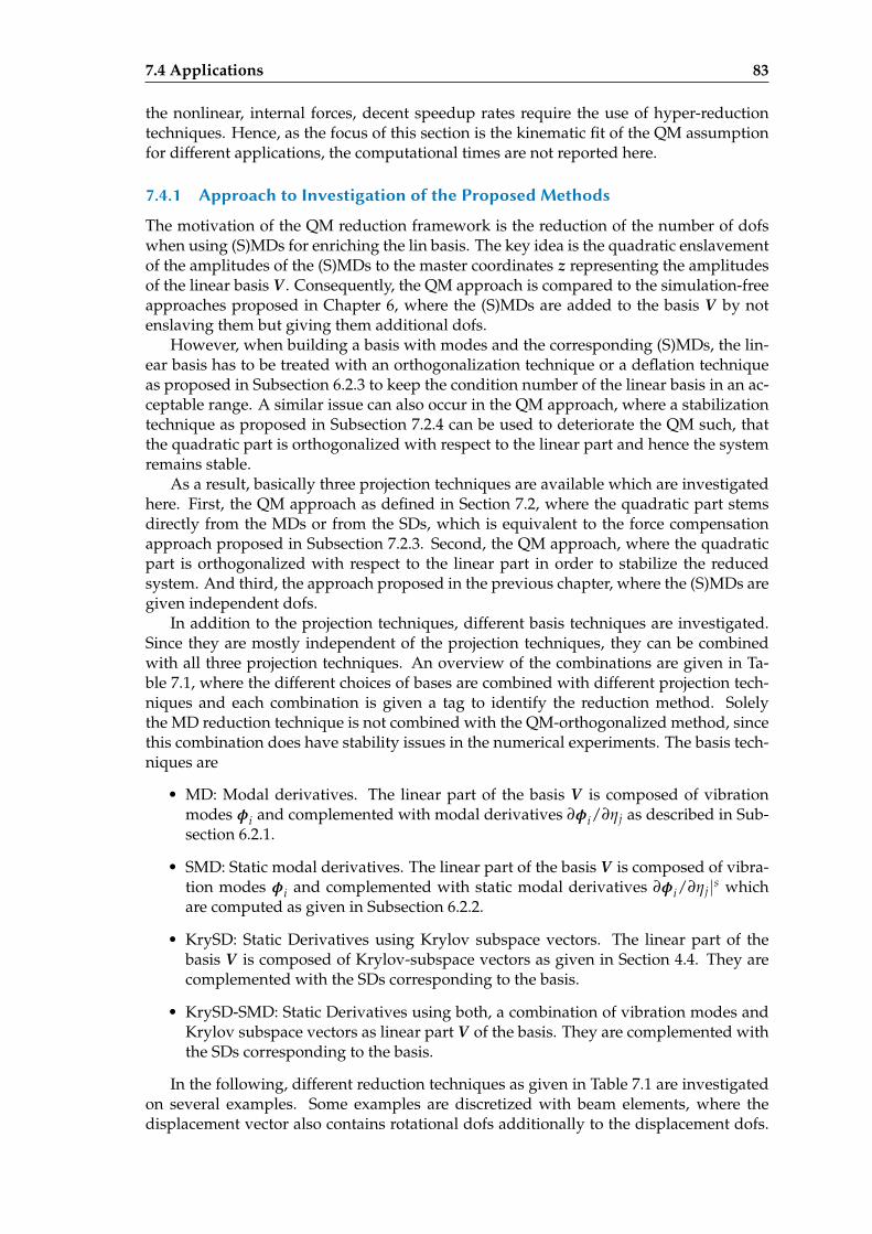
7.4 Applications 83
the nonlinear, internal forces, decent speedup rates require the use of hyper-reductiontechniques. Hence, as the focus of this section is the kinematic fit of the QM assumptionfor different applications, the computational times are not reported here.
7.4.1 Approach to Investigation of the Proposed Methods
The motivation of the QM reduction framework is the reduction of the number of dofswhen using (S)MDs for enriching the lin basis. The key idea is the quadratic enslavementof the amplitudes of the (S)MDs to the master coordinates z representing the amplitudesof the linear basis V . Consequently, the QM approach is compared to the simulation-freeapproaches proposed in Chapter 6, where the (S)MDs are added to the basis V by notenslaving them but giving them additional dofs.
However, when building a basis with modes and the corresponding (S)MDs, the lin-ear basis has to be treated with an orthogonalization technique or a deflation techniqueas proposed in Subsection 6.2.3 to keep the condition number of the linear basis in an ac-ceptable range. A similar issue can also occur in the QM approach, where a stabilizationtechnique as proposed in Subsection 7.2.4 can be used to deteriorate the QM such, thatthe quadratic part is orthogonalized with respect to the linear part and hence the systemremains stable.
As a result, basically three projection techniques are available which are investigatedhere. First, the QM approach as defined in Section 7.2, where the quadratic part stemsdirectly from the MDs or from the SDs, which is equivalent to the force compensationapproach proposed in Subsection 7.2.3. Second, the QM approach, where the quadraticpart is orthogonalized with respect to the linear part in order to stabilize the reducedsystem. And third, the approach proposed in the previous chapter, where the (S)MDs aregiven independent dofs.
In addition to the projection techniques, different basis techniques are investigated.Since they are mostly independent of the projection techniques, they can be combinedwith all three projection techniques. An overview of the combinations are given in Ta-ble 7.1, where the different choices of bases are combined with different projection tech-niques and each combination is given a tag to identify the reduction method. Solelythe MD reduction technique is not combined with the QM-orthogonalized method, sincethis combination does have stability issues in the numerical experiments. The basis tech-niques are
• MD: Modal derivatives. The linear part of the basis V is composed of vibrationmodes φi and complemented with modal derivatives ∂φi/∂ηj as described in Sub-section 6.2.1.
• SMD: Static modal derivatives. The linear part of the basis V is composed of vibra-tion modes φi and complemented with static modal derivatives ∂φi/∂ηj|s whichare computed as given in Subsection 6.2.2.
• KrySD: Static Derivatives using Krylov subspace vectors. The linear part of thebasis V is composed of Krylov-subspace vectors as given in Section 4.4. They arecomplemented with the SDs corresponding to the basis.
• KrySD-SMD: Static Derivatives using both, a combination of vibration modes andKrylov subspace vectors as linear part V of the basis. They are complemented withthe SDs corresponding to the basis.
In the following, different reduction techniques as given in Table 7.1 are investigatedon several examples. Some examples are discretized with beam elements, where thedisplacement vector also contains rotational dofs additionally to the displacement dofs.
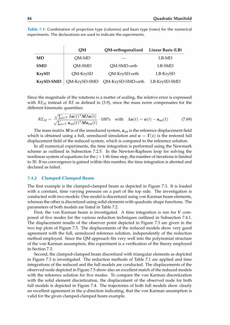
84 Quadratic Manifold
Table 7.1: Combination of projection type (columns) and basis type (rows) for the numericalexperiments. The declarations are used to indicate the experiments.
QM QM-orthogonalized Linear Basis (LB)
MD QM-MD — LB-MD
SMD QM-SMD QM-SMD-orth LB-SMD
KrySD QM-KrySD QM-KrySD-orth LB-KrySD
KrySD-SMD QM-KrySD-SMD QM-KrySD-SMD-orth LB-KrySD-SMD
Since the magnitude of the rotations is a matter of scaling, the relative error is expressedwith REM instead of RE as defined in (3.9), since the mass norm compensates for thedifferent kinematic quantities:
REM =
√∑t∈T ∆u(t)T M∆u(t)√∑t∈T uref(t)T Muref(t)
· 100% with ∆u(t) = u(t)− uref(t) (7.69)
The mass matrix M is of the unreduced system, uref is the reference displacement fieldwhich is obtained using a full, unreduced simulation and u = Γ(z) is the restored fulldisplacement field of the reduced system, which is compared to the reference solution.
In all numerical experiments, the time integration is performed using the Newmarkscheme as outlined in Subsection 7.2.5. In the Newton-Raphson loop for solving thenonlinear system of equations for the j+ 1-th time step, the number of iterations is limitedto 30. If no convergence is gained within this number, the time integration is aborted anddeclared as failed.
7.4.2 Clamped-Clamped Beam
The first example is the clamped-clamped beam as depicted in Figure 7.3. It is loadedwith a constant, time varying pressure on a part of the top side. The investigation isconducted with two models: One model is discretized using von Karman beam elements,whereas the other is discretized using solid elements with quadratic shape functions. Theparameters of both models are listed in Table 7.2.
First, the von Karman beam is investigated. A time integration is run for V com-posed of five modes for the various reduction techniques outlined in Subsection 7.4.1.The displacement results of the observer point depicted in Figure 7.3 are given in thetwo top plots of Figure 7.5. The displacements of the reduced models show very goodagreement with the full, unreduced reference solution, independently of the reductionmethod employed. Since the QM approach fits very well into the polynomial structureof the von Karman assumption, this experiment is a verification of the theory employedin Section 7.3.
Second, the clamped-clamped beam discretized with triangular elements as depictedin Figure 7.3 is investigated. The reduction methods of Table 7.1 are applied and timeintegrations of the reduced and the full models are conducted. The displacements of theobserved node depicted in Figure 7.5 show also an excellent match of the reduced modelswith the reference solution for five modes. To compare the von Karman discretizationwith the solid element discretization, the displacement of the observed node for bothfull models is depicted in Figure 7.4. The trajectories of both full models show clearlyan excellent agreement in the y-direction indicating, that the von Karman assumption isvalid for the given clamped-clamped beam example.
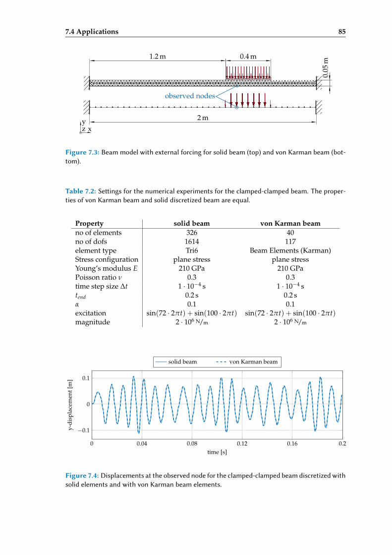
7.4 Applications 85
2 m
0.05
m
0.4 m1.2 m
observed nodes
xyz
Figure 7.3: Beam model with external forcing for solid beam (top) and von Karman beam (bot-tom).
Table 7.2: Seings for the numerical experiments for the clamped-clamped beam. The proper-ties of von Karman beam and solid discretized beam are equal.
Property solid beam von Karman beamno of elements 326 40no of dofs 1614 117element type Tri6 Beam Elements (Karman)Stress configuration plane stress plane stressYoung’s modulus E 210 GPa 210 GPaPoisson ratio ν 0.3 0.3time step size ∆t 1 · 10−4 s 1 · 10−4 stend 0.2 s 0.2 sα 0.1 0.1excitation sin(72 · 2πt) + sin(100 · 2πt) sin(72 · 2πt) + sin(100 · 2πt)magnitude 2 · 106 N/m 2 · 106 N/m
0 0.04 0.08 0.12 0.16 0.2
−0.1
0
0.1
time [s]
y-di
spla
cem
ent[
m]
solid beam von Karman beam
Figure 7.4: Displacements at the observed node for the clamped-clamped beam discretized withsolid elements and with von Karman beam elements.
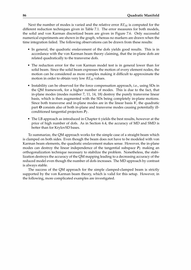
86 Quadratic Manifold
Next the number of modes is varied and the relative error REM is computed for thedifferent reduction techniques given in Table 7.1. The error measures for both models,the solid and von Karman discretized beam are given in Figure 7.6. Only successfulnumerical experiments are shown in the graph, whereas no markers are drawn when thetime integration failed. The following observations can be drawn from these results:
• In general, the quadratic enslavement of the dofs yields good results. This is inaccordance with the von Karman beam theory claiming, that the in-plane dofs arerelated quadratically to the transverse dofs.
• The reduction error for the von Karman model test is in general lower than forsolid beam. Since the solid beam expresses the motion of every element nodes, themotion can be considered as more complex making it difficult to approximate themotion in order to obtain very low REM values.
• Instability can be observed for the force compensation approach, i.e., using SDs inthe QM framework, for a higher number of modes. This is due to the fact, thatin-plane modes (modes number 7, 11, 14, 18) destroy the purely transverse linearbasis, which is then augmented with the SDs being completely in-plane motions.Since both transverse and in-plane modes are in the linear basis V , the quadraticpart Θ consists also of both in-plane and transverse modes causing potentially ill-conditioned tangential projectors PΓ.
• The LB approach as introduced in Chapter 6 yields the best results, however at theprice of high number of dofs. As in Section 6.4, the accuracy of MD and SMD isbetter than for KrylovSD bases.
To summarize, the QM approach works for the simple case of a straight beam whichis clamped on both sides. Even though the beam does not have to be modeled with vonKarman beam elements, the quadratic enslavement makes sense. However, the in-planemodes can destroy the linear independence of the tangential subspace PΓ making anorthogonalization technique necessary to stabilize the problem. Nonetheless, the stabi-lization destroys the accuracy of the QM mapping leading to a decreasing accuracy of thereduced model even though the number of dofs increases. The MD approach by contrastis always stable.
The success of the QM approach for the simple clamped-clamped beam is strictlysupported by the von Karman beam theory, which is valid for this setup. However, inthe following, more complicated examples are investigated.
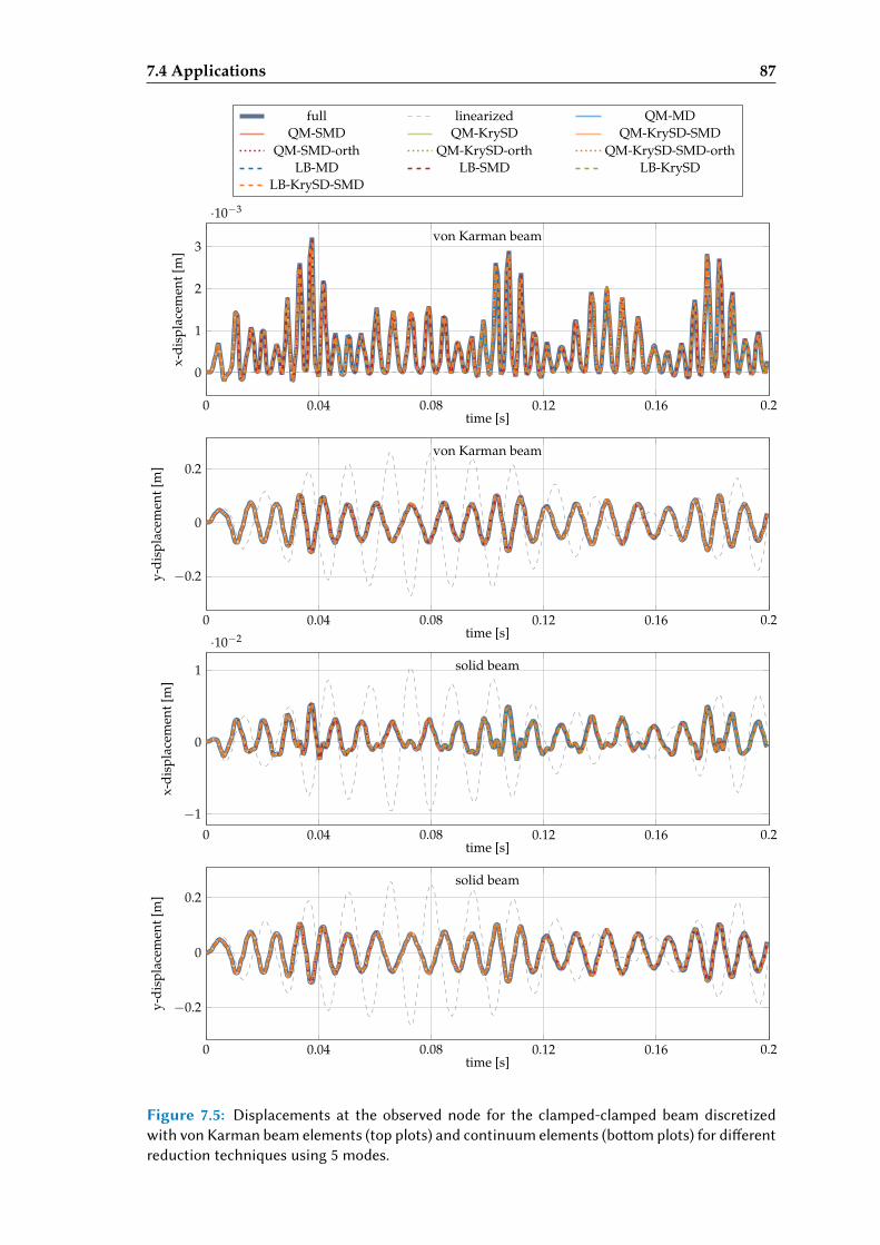
7.4 Applications 87
0 0.04 0.08 0.12 0.16 0.2
0
1
2
3
·10−3
time [s]
x-di
spla
cem
ent[
m]
von Karman beam
full linearized QM-MDQM-SMD QM-KrySD QM-KrySD-SMD
QM-SMD-orth QM-KrySD-orth QM-KrySD-SMD-orthLB-MD LB-SMD LB-KrySD
LB-KrySD-SMD
0 0.04 0.08 0.12 0.16 0.2
−0.2
0
0.2
time [s]
y-di
spla
cem
ent[
m]
von Karman beam
0 0.04 0.08 0.12 0.16 0.2
−1
0
1
·10−2
time [s]
x-di
spla
cem
ent[
m]
solid beam
0 0.04 0.08 0.12 0.16 0.2
−0.2
0
0.2
time [s]
y-di
spla
cem
ent[
m]
solid beam
Figure 7.5: Displacements at the observed node for the clamped-clamped beam discretizedwith von Karman beam elements (top plots) and continuum elements (boom plots) for dierentreduction techniques using 5 modes.
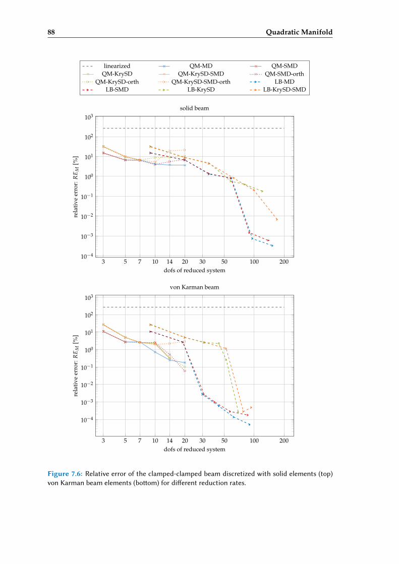
88 Quadratic Manifold
3 5 7 10 14 20 30 50 100 20010−4
10−3
10−2
10−1
100
101
102
103
dofs of reduced system
rela
tive
erro
r:R
EM
[%]
solid beam
linearized QM-MD QM-SMDQM-KrySD QM-KrySD-SMD QM-SMD-orth
QM-KrySD-orth QM-KrySD-SMD-orth LB-MDLB-SMD LB-KrySD LB-KrySD-SMD
3 5 7 10 14 20 30 50 100 200
10−4
10−3
10−2
10−1
100
101
102
103
dofs of reduced system
rela
tive
erro
r:R
EM
[%]
von Karman beam
Figure 7.6: Relative error of the clamped-clamped beam discretized with solid elements (top)von Karman beam elements (boom) for dierent reduction rates.
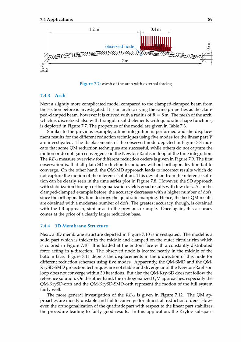
7.4 Applications 89
2 m
0.05
mobserved node
1.2 m 0.4 m
xyz
Figure 7.7: Mesh of the arch with external forcing.
7.4.3 Arch
Next a slightly more complicated model compared to the clamped-clamped beam fromthe section before is investigated. It is an arch carrying the same properties as the clam-ped-clamped beam, however it is curved with a radius of R = 8 m. The mesh of the arch,which is discretized also with triangular solid elements with quadratic shape functions,is depicted in Figure 7.7. The properties of the model are given in Table 7.3.
Similar to the previous example, a time integration is performed and the displace-ment results for the different reduction techniques using five modes for the linear part Vare investigated. The displacements of the observed node depicted in Figure 7.8 indi-cate that some QM reduction techniques are successful, while others do not capture themotion or do not gain convergence in the Newton-Raphson loop of the time integration.The REM measure overview for different reduction orders is given in Figure 7.9. The firstobservation is, that all plain SD reduction techniques without orthogonalization fail toconverge. On the other hand, the QM-MD approach leads to incorrect results which donot capture the motion of the reference solution. This deviation from the reference solu-tion can be clearly seen in the time series plot in Figure 7.8. However, the SD approachwith stabilization through orthogonalization yields good results with few dofs. As in theclamped-clamped example before, the accuracy decreases with a higher number of dofs,since the orthogonalization destroys the quadratic mapping. Hence, the best QM resultsare obtained with a moderate number of dofs. The greatest accuracy, though, is obtainedwith the LB approach, similar as in the previous example. Once again, this accuracycomes at the price of a clearly larger reduction base.
7.4.4 3D Membrane Structure
Next, a 3D membrane structure depicted in Figure 7.10 is investigated. The model is asolid part which is thicker in the middle and clamped on the outer circular rim whichis colored in Figure 7.10. It is loaded at the bottom face with a constantly distributedforce acting in y-direction. The observed node is located nearly in the middle of thebottom face. Figure 7.11 depicts the displacements in the y direction of this node fordifferent reduction schemes using five modes. Apparently, the QM-SMD and the QM-KrySD-SMD projection techniques are not stable and diverge until the Newton-Raphsonloop does not converge within 30 iterations. But also the QM-Kry-SD does not follow thereference solution. On the other hand, the orthogonalized QM approaches, especially theQM-KrySD-orth and the QM-KrySD-SMD-orth represent the motion of the full systemfairly well.
The more general investigation of the REM is given in Figure 7.12. The QM ap-proaches are mostly unstable and fail to converge for almost all reduction orders. How-ever, the orthogonalization of the quadratic part with respect to the linear part stabilizesthe procedure leading to fairly good results. In this application, the Krylov subspace
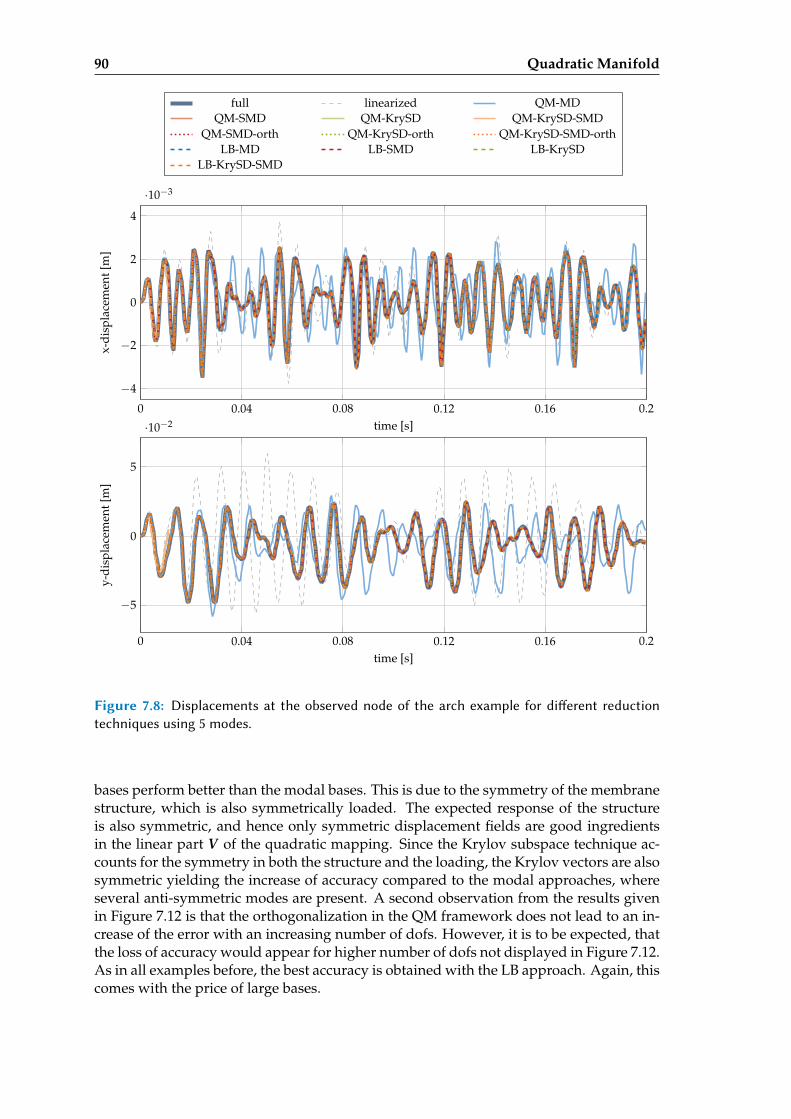
90 Quadratic Manifold
0 0.04 0.08 0.12 0.16 0.2
−4
−2
0
2
4
·10−3
time [s]
x-di
spla
cem
ent[
m]
full linearized QM-MDQM-SMD QM-KrySD QM-KrySD-SMD
QM-SMD-orth QM-KrySD-orth QM-KrySD-SMD-orthLB-MD LB-SMD LB-KrySD
LB-KrySD-SMD
0 0.04 0.08 0.12 0.16 0.2
−5
0
5
·10−2
time [s]
y-di
spla
cem
ent[
m]
Figure 7.8: Displacements at the observed node of the arch example for dierent reductiontechniques using 5 modes.
bases perform better than the modal bases. This is due to the symmetry of the membranestructure, which is also symmetrically loaded. The expected response of the structureis also symmetric, and hence only symmetric displacement fields are good ingredientsin the linear part V of the quadratic mapping. Since the Krylov subspace technique ac-counts for the symmetry in both the structure and the loading, the Krylov vectors are alsosymmetric yielding the increase of accuracy compared to the modal approaches, whereseveral anti-symmetric modes are present. A second observation from the results givenin Figure 7.12 is that the orthogonalization in the QM framework does not lead to an in-crease of the error with an increasing number of dofs. However, it is to be expected, thatthe loss of accuracy would appear for higher number of dofs not displayed in Figure 7.12.As in all examples before, the best accuracy is obtained with the LB approach. Again, thiscomes with the price of large bases.
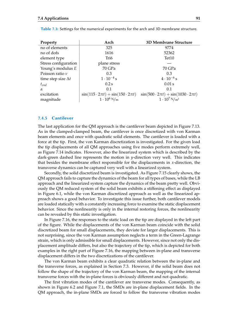
7.4 Applications 91
Table 7.3: Seings for the numerical experiments for the arch and 3D membrane structure.
Property Arch 3D Membrane Structureno of elements 325 9774no of dofs 1616 52362element type Tri6 Tet10Stress configuration plane stress —Young’s modulus E 70 GPa 70 GPaPoisson ratio ν 0.3 0.3time step size ∆t 1 · 10−4 s 4 · 10−6 stend 0.2 s 0.01 sα 0.1 0.1excitation sin(115 · 2πt) + sin(150 · 2πt) sin(500 · 2πt) + sin(1030 · 2πt)magnitude 1 · 106 N/m 1 · 107 N/m2
7.4.5 Cantilever
The last application for the QM approach is the cantilever beam depicted in Figure 7.13.As in the clamped-clamped beam, the cantilever is once discretized with von Karmanbeam elements and once with quadratic solid elements. The cantilever is loaded with aforce at the tip. First, the von Karman discretization is investigated. For the given loadthe tip displacements of all QM approaches using five modes perform extremely well,as Figure 7.14 indicates. However, also the linearized system which is described by thedark-green dashed line represents the motion in y-direction very well. This indicatesthat besides the membrane effect responsible for the displacements in x-direction, thetransverse dynamics can be captured very well with a linearized system.
Secondly, the solid discretized beam is investigated. As Figure 7.15 clearly shows, theQM approach fails to capture the dynamics of the beam for all types of bases, while the LBapproach and the linearized system capture the dynamics of the beam pretty well. Obvi-ously the QM reduced system of the solid beam exhibits a stiffening effect as displayedin Figure 6.1, while the von Karman discretized approach as well as the linearized ap-proach shows a good behavior. To investigate this issue further, both cantilever modelsare loaded statically with a constantly increasing force to examine the static displacementbehavior. Since the nonlinearity is only in the internal restoring forces, the nonlinearitycan be revealed by this static investigation.
In Figure 7.16, the responses to the static load on the tip are displayed in the left partof the figure. While the displacements of the von Karman beam coincide with the soliddiscretized beam for small displacements, they deviate for larger displacements. This isnot surprising, since the von Karman assumption neglects a term in the Green-Lagrangestrain, which is only admissible for small displacements. However, since not only the dis-placement amplitude differs, but also the trajectory of the tip, which is depicted for bothexamples in the right part of Figure 7.16, the mapping between in-plane and transversedisplacement differs in the two discretizations of the cantilever.
The von Karman beam exhibits a clear quadratic relation between the in-plane andthe transverse forces, as explained in Section 7.3. However, if the solid beam does notfollow the shape of the trajectory of the von Karman beam, the mapping of the internaltransverse forces with the in-plane forces is obviously different and not quadratic.
The first vibration modes of the cantilever are transverse modes. Consequently, asshown in Figure 6.2 and Figure 7.1, the SMDs are in-plane displacement fields. In theQM approach, the in-plane SMDs are forced to follow the transverse vibration modes
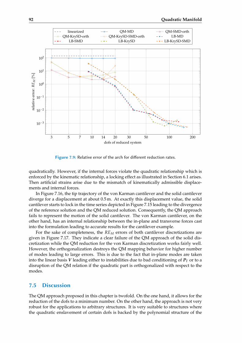
92 Quadratic Manifold
3 5 7 10 14 20 30 50 100 200
10−3
10−2
10−1
100
101
102
dofs of reduced system
rela
tive
erro
r:R
EM
[%]
linearized QM-MD QM-SMD-orthQM-KrySD-orth QM-KrySD-SMD-orth LB-MD
LB-SMD LB-KrySD LB-KrySD-SMD
Figure 7.9: Relative error of the arch for dierent reduction rates.
quadratically. However, if the internal forces violate the quadratic relationship which isenforced by the kinematic relationship, a locking effect as illustrated in Section 6.1 arises.Then artificial strains arise due to the mismatch of kinematically admissible displace-ments and internal forces.
In Figure 7.16, the tip trajectory of the von Karman cantilever and the solid cantileverdiverge for a displacement at about 0.5 m. At exactly this displacement value, the solidcantilever starts to lock in the time series depicted in Figure 7.15 leading to the divergenceof the reference solution and the QM reduced solution. Consequently, the QM approachfails to represent the motion of the solid cantilever. The von Karman cantilever, on theother hand, has an internal relationship between the in-plane and transverse forces castinto the formulation leading to accurate results for the cantilever example.
For the sake of completeness, the REM errors of both cantilever discretizations aregiven in Figure 7.17. They indicate a clear failure of the QM approach of the solid dis-cretization while the QM reduction for the von Karman discretization works fairly well.However, the orthogonalization destroys the QM mapping behavior for higher numberof modes leading to large errors. This is due to the fact that in-plane modes are takeninto the linear basis V leading either to instabilities due to bad conditioning of PΓ or to adisruption of the QM relation if the quadratic part is orthogonalized with respect to themodes.
7.5 Discussion
The QM approach proposed in this chapter is twofold. On the one hand, it allows for thereduction of the dofs to a minimum number. On the other hand, the approach is not veryrobust for the applications to arbitrary structures. It is very suitable to structures wherethe quadratic enslavement of certain dofs is backed by the polynomial structure of the
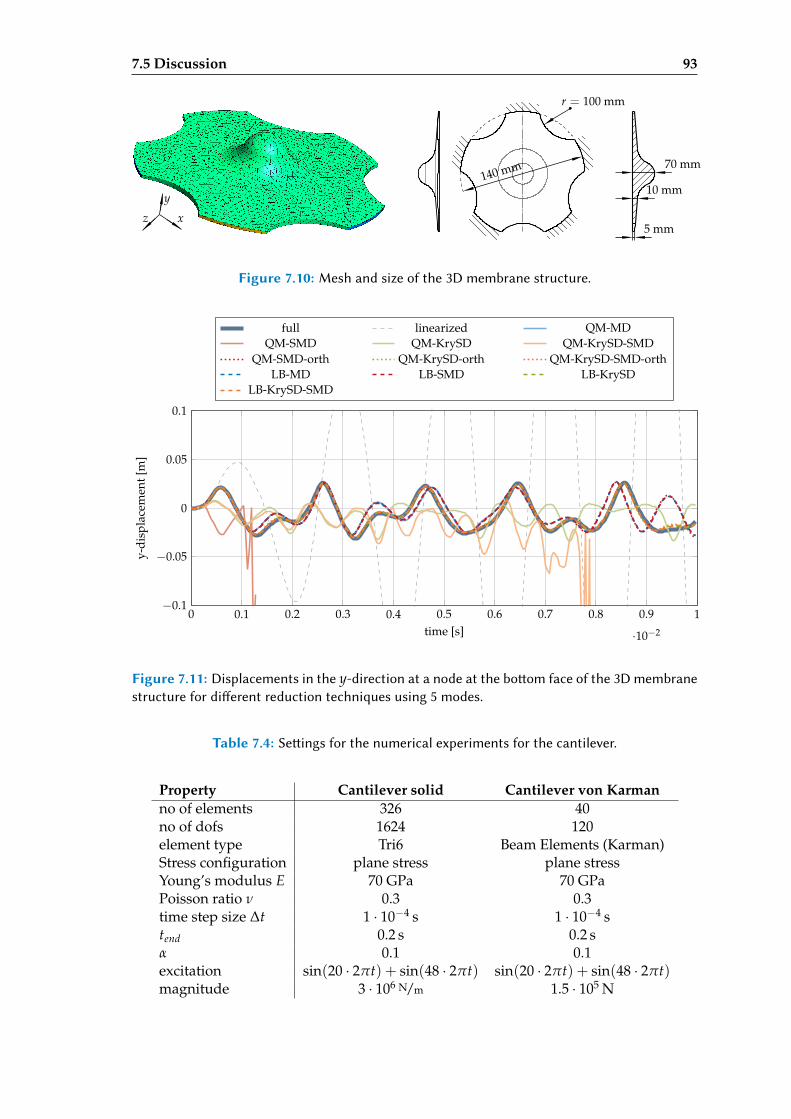
7.5 Discussion 93
140 mm
r = 100 mm
5 mm
70 mm
10 mm
x
y
z
Figure 7.10: Mesh and size of the 3D membrane structure.
0 0.1 0.2 0.3 0.4 0.5 0.6 0.7 0.8 0.9 1
·10−2
−0.1
−0.05
0
0.05
0.1
time [s]
y-di
spla
cem
ent[
m]
full linearized QM-MDQM-SMD QM-KrySD QM-KrySD-SMD
QM-SMD-orth QM-KrySD-orth QM-KrySD-SMD-orthLB-MD LB-SMD LB-KrySD
LB-KrySD-SMD
Figure 7.11: Displacements in the y-direction at a node at the boom face of the 3D membranestructure for dierent reduction techniques using 5 modes.
Table 7.4: Seings for the numerical experiments for the cantilever.
Property Cantilever solid Cantilever von Karmanno of elements 326 40no of dofs 1624 120element type Tri6 Beam Elements (Karman)Stress configuration plane stress plane stressYoung’s modulus E 70 GPa 70 GPaPoisson ratio ν 0.3 0.3time step size ∆t 1 · 10−4 s 1 · 10−4 stend 0.2 s 0.2 sα 0.1 0.1excitation sin(20 · 2πt) + sin(48 · 2πt) sin(20 · 2πt) + sin(48 · 2πt)magnitude 3 · 106 N/m 1.5 · 105 N
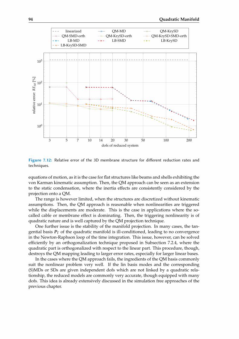
94 Quadratic Manifold
3 5 7 10 14 20 30 50 100 200
100
101
102
103
dofs of reduced system
rela
tive
erro
r:R
EM
[%]
linearized QM-MD QM-KrySDQM-SMD-orth QM-KrySD-orth QM-KrySD-SMD-orth
LB-MD LB-SMD LB-KrySDLB-KrySD-SMD
Figure 7.12: Relative error of the 3D membrane structure for dierent reduction rates andtechniques.
equations of motion, as it is the case for flat structures like beams and shells exhibiting thevon Karman kinematic assumption. Then, the QM approach can be seen as an extensionto the static condensation, where the inertia effects are consistently considered by theprojection onto a QM.
The range is however limited, when the structures are discretized without kinematicassumptions. Then, the QM approach is reasonable when nonlinearities are triggeredwhile the displacements are moderate. This is the case in applications where the so-called cable or membrane effect is dominating. Then, the triggering nonlinearity is ofquadratic nature and is well captured by the QM projection technique.
One further issue is the stability of the manifold projection. In many cases, the tan-gential basis PΓ of the quadratic manifold is ill-conditioned, leading to no convergencein the Newton-Raphson loop of the time integration. This issue, however, can be solvedefficiently by an orthogonalization technique proposed in Subsection 7.2.4, where thequadratic part is orthogonalized with respect to the linear part. This procedure, though,destroys the QM mapping leading to larger error rates, especially for larger linear bases.
In the cases where the QM approach fails, the ingredients of the QM basis commonlysuit the nonlinear problem very well. If the lin basis modes and the corresponding(S)MDs or SDs are given independent dofs which are not linked by a quadratic rela-tionship, the reduced models are commonly very accurate, though equipped with manydofs. This idea is already extensively discussed in the simulation free approaches of theprevious chapter.
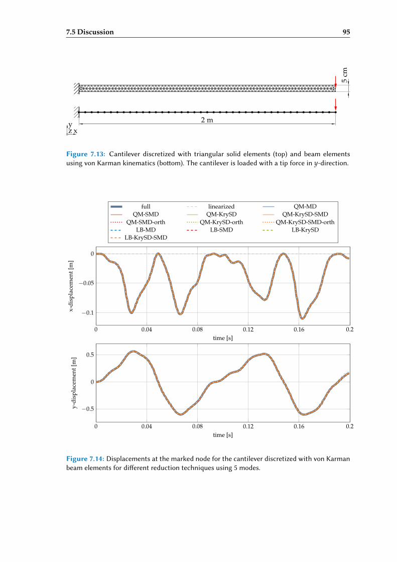
7.5 Discussion 95
2 m
5cm
xyz
Figure 7.13: Cantilever discretized with triangular solid elements (top) and beam elementsusing von Karman kinematics (boom). The cantilever is loaded with a tip force in y-direction.
0 0.04 0.08 0.12 0.16 0.2
−0.1
−0.05
0
time [s]
x-di
spla
cem
ent[
m]
full linearized QM-MDQM-SMD QM-KrySD QM-KrySD-SMD
QM-SMD-orth QM-KrySD-orth QM-KrySD-SMD-orthLB-MD LB-SMD LB-KrySD
LB-KrySD-SMD
0 0.04 0.08 0.12 0.16 0.2
−0.5
0
0.5
time [s]
y-di
spla
cem
ent[
m]
Figure 7.14: Displacements at the marked node for the cantilever discretized with von Karmanbeam elements for dierent reduction techniques using 5 modes.
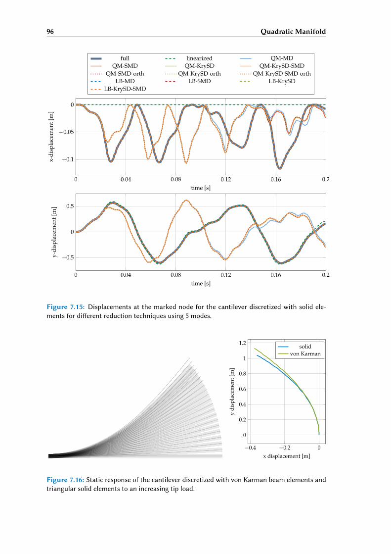
96 Quadratic Manifold
0 0.04 0.08 0.12 0.16 0.2
−0.1
−0.05
0
time [s]
x-di
spla
cem
ent[
m]
full linearized QM-MDQM-SMD QM-KrySD QM-KrySD-SMD
QM-SMD-orth QM-KrySD-orth QM-KrySD-SMD-orthLB-MD LB-SMD LB-KrySD
LB-KrySD-SMD
0 0.04 0.08 0.12 0.16 0.2
−0.5
0
0.5
time [s]
y-di
spla
cem
ent[
m]
Figure 7.15: Displacements at the marked node for the cantilever discretized with solid ele-ments for dierent reduction techniques using 5 modes.
−0.4 −0.2 0
0
0.2
0.4
0.6
0.8
1
1.2
x displacement [m]
ydi
spla
cem
ent[
m]
solidvon Karman
Figure 7.16: Static response of the cantilever discretized with von Karman beam elements andtriangular solid elements to an increasing tip load.
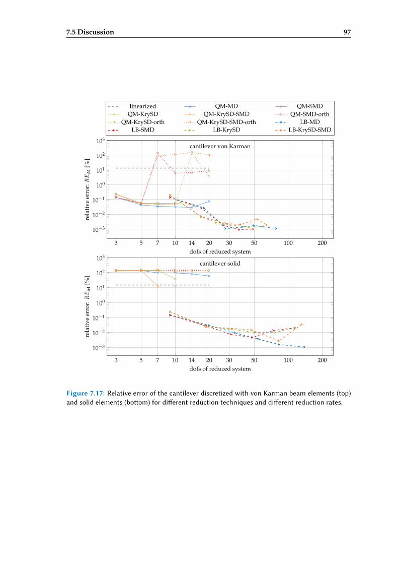
7.5 Discussion 97
3 5 7 10 14 20 30 50 100 200
10−3
10−2
10−1
100
101
102
103
dofs of reduced system
rela
tive
erro
r:R
EM
[%]
cantilever von Karman
linearized QM-MD QM-SMDQM-KrySD QM-KrySD-SMD QM-SMD-orth
QM-KrySD-orth QM-KrySD-SMD-orth LB-MDLB-SMD LB-KrySD LB-KrySD-SMD
3 5 7 10 14 20 30 50 100 200
10−3
10−2
10−1
100
101
102
103
dofs of reduced system
rela
tive
erro
r:R
EM
[%]
cantilever solid
Figure 7.17: Relative error of the cantilever discretized with von Karman beam elements (top)and solid elements (boom) for dierent reduction techniques and dierent reduction rates.

Chapter 8
Comparison of Bases: Subspace Angles
When a system is reduced using a reduced basis as described in Chapter 3, the subspacespanned by the reduction basis V is the essential contribution to the characteristics of thereduced order model. This subspace can be parametrized in arbitrary variants, since aninfinite number of bases V cover exactly the same subspace. ROMs reduced with differ-ent bases however covering the same subspace exhibit the same dynamics and lead toexactly the same results, when the physical state is reconstructed. Hence, these equiva-lent models can be seen as different realizations of the same physical model.
In this chapter, a method to compare different subspaces by the concept of subspaceangles is presented. It allows comparing different subspaces in a way that is not de-pending on the specific vectors used to represent them. This chapter is based on thepublication [RGR15].
8.1 The Basis Problem in Nonlinear Reduction
The issue that an infinite number of systems have the same dynamics, is well-knownin systems theory as the realization problem [Ant09; Bro15]. To make the comparison ofsystems independent of the realization, which is in its parts arbitrary, invariant systemtheoretic properties can be used to describe the characteristics of the reduced system.For linear systems, the most popular tool for investigation is the analysis of the transferfunction. This concept works, when only a few inputs and outputs are of interest as itis most often the case in control theory. Hence, many reduction techniques rely on thisconcept and minimize different error measures on the transfer function, mostly in theH2- or theH∞-norm, (cf. [Ant09]).
In nonlinear systems, however, these system theoretic concepts are either not existentor hard to compute. Hence, most error analyses rely on the comparison of the systemresponse to certain inputs requiring great computational effort. In nonlinear structuraldynamics, Nonlinear Normal Modes (NNMs) have been used for the characterization ofthe reduction quality [KBA14; KA16]. They require the computation of the NNMs, whichis commonly performed with a shooting method, where a time integration is necessary.Hence, these methods are also associated with high computational costs.
As a consequence, it is desirable to have a tool to compare the reduction bases fornonlinear systems which do not require a full simulation of the system. In the followinga concept is proposed, where the reduction bases are compared in a mathematical rig-orous way. It allows only to compare reduction bases and not measuring errors. As aconsequence, it cannot be directly applied to assess the quality of reduced bases. How-ever, it can be used to assess the difference between one basis and another basis whichis known to be optimal, like the POD basis obtained for a given excitation. Then, forinstance simulation-free bases can assessed by the comparison against the optimal basis
99
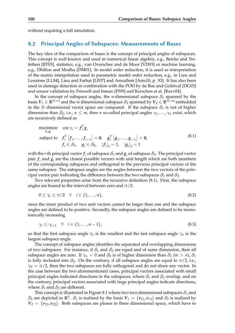
100 Comparison of Bases: Subspace Angles
without requiring a full simulation.
8.2 Principal Angles of Subspaces: Measurements of Bases
The key idea of the comparison of bases is the concept of principal angles of subspaces.This concept is well-known and used in numerical linear algebra, e.g., Betcke and Tre-fethen [BT05], statistics, e.g., van Overschee and de Moor [VD93] or machine learning,e.g., Dhillon and Modha [DM01]. In model order reduction, it is used as interpretationof the matrix interpolation used in parametric model order reduction, e.g., in Lieu andLesoinne [LL04], Lieu and Farhat [LF07] and Amsallem [Ams10, p. 93]. It has also beenused in damage detection in combination with the POD by de Boe and Golinval [DG03]and sensor validation by Friswell and Inman [FI99] and Kerschen et al. [Ker+04].
In the concept of subspace angles, the n-dimensional subspace S1 spanned by thebasis V1 ∈ RN×n and the m dimensional subspace S2 spanned by V2 ∈ RN×m embeddedin the N dimensional vector space are compared. If the subspace S1 is not of higherdimension than S2, i.e., n ≤ m, then n so-called principal angles γ1, . . . , γn exist, whichare recursively defined as
maximizef i ,gi
cos γi = f Ti gi
subject to f Ti[
f 1, . . . , f i−1]= 0, gT
i[g1, . . . , gi−1
]= 0,
f i ∈ S1, gi ∈ S2, | f i|2 = 1, |gi|2 = 1
(8.1)
with the i-th principal vector f i of subspace S1 and gi of subspace S2. The principal vectorpair f i and gi are the closest possible vectors with unit length which are both membersof the corresponding subspaces and orthogonal to the previous principal vectors of thesame subspace. The subspace angles are the angles between the two vectors of the prin-cipal vector pair indicating the difference between the two subspaces S1 and S2.
Two relevant properties arise from the recursive definition (8.1). First, the subspaceangles are bound to the interval between zero and π/2:
0 ≤ γi ≤ π/2 ∀ i ∈ 1, . . . , n, (8.2)
since the inner product of two unit vectors cannot be larger than one and the subspaceangles are defined to be positive. Secondly, the subspace angles are defined to be mono-tonically increasing
γi ≤ γi+1 ∀ i ∈ 1, . . . , n− 1, (8.3)
so that the first subspace angle γ1 is the smallest and the last subspace angle γn is thelargest subspace angle.
The concept of subspace angles identifies the separated and overlapping dimensionsof two subspaces. For instance, if S1 and S2 are equal and of same dimension, then allsubspace angles are zero. If γn = 0 and S2 is of higher dimension than S1 (m > n), S1is fully included into S2. On the contrary, if all subspace angles are equal to π/2, i.e.,γ0 = π/2, then the two subspaces are fully orthogonal and do not share any vector. Inthe case between the two aforementioned cases, principal vectors associated with smallprincipal angles indicated directions in the subspaces, where S1 and S2 overlap, and onthe contrary, principal vectors associated with large principal angles indicate directions,where S1 and S2 are different.
This concept is illustrated in Figure 8.1 where two two-dimensional subspaces S1 andS2 are depicted in R3. S1 is realized by the basis V1 =
(v11, v12
)and S2 is realized by
V2 =(v21, v22
). Both subspaces are planes in three dimensional space, which have to
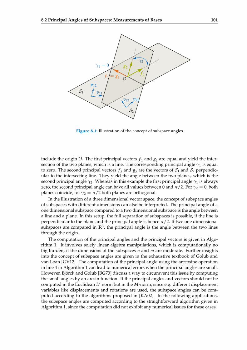
8.2 Principal Angles of Subspaces: Measurements of Bases 101
S1 v11
v12
S2
v21v22
Of 1 = g1
γ2g2
f 2
γ1 = 0
Figure 8.1: Illustration of the concept of subspace angles
include the origin O. The first principal vectors f 1 and g1 are equal and yield the inter-section of the two planes, which is a line. The corresponding principal angle γ1 is equalto zero. The second principal vectors f 2 and g2 are the vectors of S1 and S2 perpendic-ular to the intersecting line. They yield the angle between the two planes, which is thesecond principal angle γ2. Whereas in this example the first principal angle γ1 is alwayszero, the second principal angle can have all values between 0 and π/2. For γ2 = 0, bothplanes coincide, for γ2 = π/2 both planes are orthogonal.
In the illustration of a three dimensional vector space, the concept of subspace anglesof subspaces with different dimensions can also be interpreted. The principal angle of aone dimensional subspace compared to a two dimensional subspace is the angle betweena line and a plane. In this setup, the full separation of subspaces is possible, if the line isperpendicular to the plane and the principal angle is hence π/2. If two one dimensionalsubspaces are compared in R3, the principal angle is the angle between the two linesthrough the origin.
The computation of the principal angles and the principal vectors is given in Algo-rithm 1. It involves solely linear algebra manipulations, which is computationally nobig burden, if the dimensions of the subspaces n and m are moderate. Further insightsinto the concept of subspace angles are given in the exhaustive textbook of Golub andvan Loan [GV12]. The computation of the principal angle using the arccosine operationin line 4 in Algorithm 1 can lead to numerical errors when the principal angles are small.However, Björck and Golub [BG73] discuss a way to circumvent this issue by computingthe small angles by an arcsin function. If the principal angles and vectors should not becomputed in the Euclidean L2 norm but in the M-norm, since e.g. different displacementvariables like displacements and rotations are used, the subspace angles can be com-puted according to the algorithms proposed in [KA02]. In the following applications,the subspace angles are computed according to the straightforward algorithm given inAlgorithm 1, since the computation did not exhibit any numerical issues for these cases.
102 Comparison of Bases: Subspace Angles
Algorithm 1: Algorithm for computing the principal vectors and subspace anglesof two bases V1 and V2, based on [GV12]
Input : Reduced bases V1 ∈ RN×n and V2 ∈ RN×m spanning S1 and S2Output : Vector of subspace angles γ =
(γ1, . . . , γn
),
principal vectors F =(
f 1, . . . , f n), G =
(g1, . . . , gn
)
1 V1 = Q1R1, V2 = Q2R2 // Orthogonalize reduced bases V1 and V2 via QR decomposition
2 C = QT1 Q2 // Compute the correlation matrix of the two orthogonalized subspaces
3 UΣV T = C with Σ = diag(σ) // Compute the SVD of the correlation matrix4 γ = arccos(σ) // Compute the subspace angles from the singular values
5 F =(
f 1, . . . , f n)= Q1U // Compute the principal vectors, if necessary
6 G =(
g1, . . . , gn)= Q2V
8.3 Applications
To show the usefulness of the subspace angles and the corresponding principal vectors,the POD reduction basis and the simulation free reduction basis are investigated withthis tool on the c-shape example of Section 6.4. The model is run with exactly the samemodel parameters as there, however the simulation time is taken longer from 2 s to 3 s.
First, a POD is run. In the case when no parameters in the model are changed, thePOD basis is the optimal basis as discussed in Chapter 5. The first 100 singular values ofthe POD are depicted in Figure 8.2. They indicate that the model is of limited complexity,since the decay in the first 10 to 20 POD modes is over 3 to 4 orders of magnitude. Tocheck the results, one simulation is run with 10 POD vectors yielding a relative error ofRE = 8.7 % and with 20 POD vectors yielding RE = 0.12 %. The first 10 POD modescan be considered as necessary to obtain good results while the first 20 POD modes arenecessary for very good results. For the sake of better presentability, the first 10 PODmodes are used as benchmark modes to be captured by a simulation free basis.
The naive basis composed solely of vibration modes has been shown to fail in captur-ing the nonlinear effects, as illustrated with the static example in Section 6.1. A similarinvestigation is performed by comparing purely modal bases of different sizes againstthe ten dimensional POD basis using subspace angles. The results of this investigationare depicted in Figure 8.3. As expected, a basis of 10 vibration modes is not equal tothe POD basis and consequently many subspace angles are fairly large. However, if thenumber of vibration modes in the basis is increased, the subspace angles with greaterindices decrease only slowly, seemingly converging to a fairly large value.
To investigate this issue further, the principal vectors for the subspaces spanned by40 vibration modes versus ten POD modes are computed and depicted as displacementfields of the mesh in Figure 8.4. They confirm the observations already made. In ac-cordance with Figure 8.3, the first four subspace angles are comparably low, and nodifference can be seen in the principal vectors, which are plotted as displacement field.However, the principal vectors with larger indices show some deviation, so that the blueprincipal vectors of the modal subspace do not cover fully the green principal vectors ofthe POD subspace. A closer look at the difference reveals that the main difference be-tween the modal subspace and the POD subspace is the contraction and the expansion ofthe mesh.
As discussed in Chapter 6, the linear basis fails to capture the nonlinear effects of thelarge rotation. These large rotations cause an enlargement of the mesh when they are lin-earized. Consequently, the linear bases fail to capture the displacement fields necessaryfor displaying nonlinear large rotations. However, the (static) modal derivatives are ableto capture them.
8.3 Applications 103
0 20 40 60 80 10010−6
10−3
100
103
index i of singular value
sing
ular
valu
eσ i
[-]
Figure 8.2: Singular values of the snapshot matrix built by a full training simulation. The lesingular vectors associated with the first ten singular values were used as POD-basis.
Hence, the subspace angles between the first ten POD modes and a simulation-freebasis composed of the first 6 vibration modes and 14 SMDs are computed. The SMDsare selected based on the frequency weighting algorithm introduced in Subsection 6.2.4.The principal angles of this computation are also given in Figure 8.3 together with theprincipal angles of the purely modal bases. The subspace angles of the simulation-freebasis composed of SMDs are all fairly small indicating a good match with the POD basis.Also the principal vectors of the two subspaces, which are depicted in Figure 8.5, showan extremely good overlap of the simulation-free basis and the POD basis. The principalvectors of the simulation-free basis (blue) practically cover the principal vectors of thePOD basis.
The similarity of the simulation-free subspace and the POD subspace is also validatedwith a time integration of the simulation-free reduced system. It exhibits a relative errorof RE = 2.0 % indicating that the subspace is chosen well with the simulation free tech-nique. To recall, the relative errors of the POD reduced system were 8.7 % for 10 PODvectors and 0.12 % for 20 POD vectors. Given that the simulation free technique does notknow the excitation, which the POD method does, the simulation-free basis turns out tobe very effective for these types of geometrically nonlinear problems.
The concept of subspace angles thereby turns out to be a valuable tool to comparethe subspaces spanned by the bases. Furthermore, the principal vectors can be used toidentify the similarities and differences of subspaces. Hence, they are an ideal tool forpost-processing, debugging, subspace identification of certain nonlinear methods andthe design of new methods.
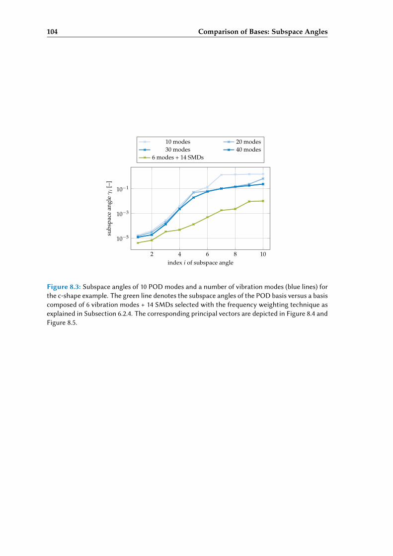
104 Comparison of Bases: Subspace Angles
2 4 6 8 10
10−5
10−3
10−1
index i of subspace angle
subs
pace
angl
eγ
i[–
]
10 modes 20 modes30 modes 40 modes
6 modes + 14 SMDs
Figure 8.3: Subspace angles of 10 POD modes and a number of vibration modes (blue lines) forthe c-shape example. The green line denotes the subspace angles of the POD basis versus a basiscomposed of 6 vibration modes + 14 SMDs selected with the frequency weighting technique asexplained in Subsection 6.2.4. The corresponding principal vectors are depicted in Figure 8.4 andFigure 8.5.
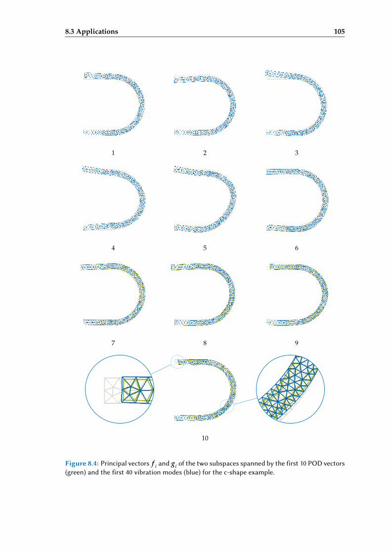
8.3 Applications 105
1 2 3
4 5 6
7 8 9
10
1 2 3
4 5 6
7 8 9
10
1 2 3
4 5 6
7 8 9
10
Figure 8.4: Principal vectors f i and gi of the two subspaces spanned by the first 10 POD vectors(green) and the first 40 vibration modes (blue) for the c-shape example.
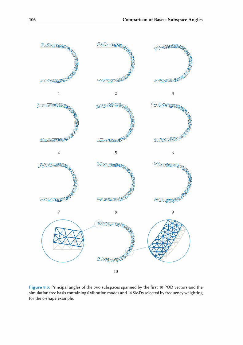
106 Comparison of Bases: Subspace Angles
1 2 3
4 5 6
7 8 9
10
1 2 3
4 5 6
7 8 9
10
1 2 3
4 5 6
7 8 9
10
Figure 8.5: Principal angles of the two subspaces spanned by the first 10 POD vectors and thesimulation free basis containing 6 vibration modes and 14 SMDs selected by frequency weightingfor the c-shape example.

Chapter 9
Summary of Part I
In the previous six chapters, various aspects of the reduced basis method have been dis-cussed, which are summarized in this chapter. The main question in projective model or-der reduction is the determination of a reduced basis V ∈ RN×n spanning the subspace,in which the relevant dynamics of the system of dimension N happens. The projection ofthe system onto the subspace spanned by V is equivalent to a coordinate transform witha subsequent truncation, resulting into a system on n reduced equations.
In linear structural dynamics, the established reduction methods for determining Vrely on system intrinsic properties, which are often supported by system-theoretic con-cepts. This is due to the fact, that the linear system is fully characterized by its mass,stiffness and damping matrix, which can be analyzed by system theoretic procedures re-lying on linear algebra operations. The two methods covered in Chapter 4 are modaltruncation, which relies on the decoupling of states, and the Krylov subspace method,where the higher order displacement fields of the force inputs are regarded. It is furthershown, that the Krylov subspace method exists also in systems theory, where the methodmatches the moments of the transfer function.
In nonlinear systems, the characterization of the system solely with matrices is notpossible, though, since the nonlinear operators cannot be cast into matrix-vector opera-tions. As a consequence, the state-of-the–art reduction method for nonlinear systems, theProper Orthogonal Decomposition (POD) discussed in Chapter 5, takes a detour over astatistical evaluation of training sets obtained with expensive training simulations of thefull, unreduced system. While this method builds an optimal basis for the given trainingsets and is not limited to structural dynamics systems, the requirement of the full trainingsimulation is very prohibitive in many contexts, where the costs of the full simulation arenot affordable or even infeasible. Furthermore, the method is very sensitive with respectto the training sets requiring them to be representative and not too different for the casesfor the reduced system.
The disadvantages of training simulations associated with the construction of a re-duced basis are the motivation for the so-called simulation-free reduced basis methodsaddressed in Chapter 6. There, extensions to the so-called lin basis obtained from a lin-ear reduction method applied to the linearized system are addressed. As exemplarilyshown, these lin bases exhibit severe locking when applied to geometrically nonlinearsystems making them useless for the reduction of these systems. However, they form thestarting point for the established modal derivatives (MDs) and static derivatives (SDs),which capture the nonlinear effects of the system. The concatenated lin basis and thecorresponding MDs or SDs form an excellent simulation-free basis suited for geometri-cally nonlinear problems. The MDs are based on the perturbation of vibration modes andrequire the solution of multiple singular systems in order to obtain the augmentation vec-tors for the lin basis. Hence, this technique is limited to a lin basis composed of vibration
107
108 Summary of Part I
modes. The SDs, on the contrary, base on the perturbation of the nonlinear internal forcesand are hence applicable to every lin basis. Furthermore, they are less computational ex-pensive, since only one non-singular system needs to be solved for multiple right handsides.
The computation of both the MDs and the SDs requires derivatives of the nonlinearinternal forces. For this computation, a numerical differentiation approach is suggested,which requires solely the computation of tangential stiffness matrices. The differentiationscheme, however, is sensitive with respect to the step width requiring a tuning of thisparameter. This is achieved by exploiting the fact, that the SDs are symmetric allowingfor tracking the accuracy of the differentiation by evaluating the symmetry error. Thequadratic growth of the number of the augmentation vectors with respect to the lin basisis a further issue of the simulation-free reduction schemes covered. Hence, selectionstrategies which heuristically rank the importance of the SDs or MDs are discussed. In thenumerical experiments, reduced bases built with the different simulation-free methodsare investigated. Thereby, the MDs turn out to be excellent ingredients for the reducedbasis. The SDs perform also well, especially when combined with a selection strategy. Forthe examples which are investigated, the frequency weighting strategy in combinationwith static modal derivatives turns out to be the best, since it provides good performancewith computational ease.
A second attempt to address the quadratic growth of the number of SDs and SMDswith respect to the size of the lin basis is given in Chapter 7. In this novel approachnamed Quadratic Manifold (QM), the basis projection is not linear but nonlinear, project-ing the equations of motion onto the tangent space of the nonlinear transformation. Thenonlinear function is chosen to be quadratic, enslaving the modal derivatives with thevibration modes which form the linear part of the transformation. Alternatively, whenthe linear part is built from basis vectors different from vibration modes, the so-calledforce compensation approach allows to transfer the quadratic part of the nonlinear forces tothe quadratic transformation. Interestingly, it turns out that the resulting quadratic partis composed of the SDs. Hence, the QM approach provides a further theoretic foundationto the SDs.
The QM approach allows to keep the number of unknowns minimal, since the MDsor SDs are not treated as independent dofs. Especially when dealing with flat structuresusing von Karman kinematic assumptions within beam or shell elements, a sound theoryis derived supporting the good performance for applications with these structures. TheQM approach, however, turns out to be fairly unstable for discretizations using solidelements. This can be solved by an orthogonalization procedure, which destroys theoriginal form of the quadratic mapping, though. Since sufficient accuracy is gained onlyfor membrane-dominated motions, as shown in the extensive numerical investigation,the applicability of this method is fairly limited.
The key in projective model order reduction is the subspace spanned by the reducedbasis V . However, since the subspace is always realized by a parametrization leading tothe projection basis V , the comparison of subspaces is a non-trivial task. In Chapter 8,subspace angles and principal vectors are suggested as main tools for the comparisonof reduced bases. Thereby, the angles give an insight to the proximity of the two inves-tigated subspaces and detect intersections and differences. But not only the principalangles, but especially the principal vectors can be used to identify the differences of thesubspaces making physically-based insights possible. In the context of geometricallynonlinear reduction it is shown, that even a large reduction basis composed of vibrationmodes does not capture the displacement fields necessary to describe rigid body rota-tions of elements. It is further shown that the augmentation vectors in the simulationfree approaches like static derivatives capture these displacement fields.

109
Part I of this thesis discusses extensively the reduced basis approach which reducesthe dimension of the system from a large number N to the small number n. As a conse-quence, the solution of the system of linear equations necessary in the Newton-Raphsonloop is accelerated. However, since the reduced nonlinear internal forces cannot be pre-computed a priory, the computational bottleneck of the reduced basis system is the con-struction of the internal forces and, in implicit time integrations, the tangential stiffnessmatrix. This issue, which is addressed with hyper-reduction, is the topic of the secondpart of this thesis to follow.


Part II
Hyper-Reduction
111

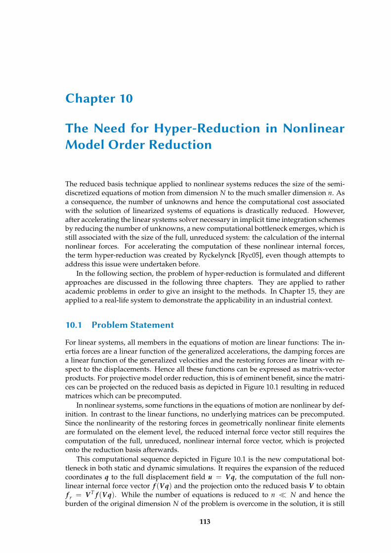
Chapter 10
The Need for Hyper-Reduction in NonlinearModel Order Reduction
The reduced basis technique applied to nonlinear systems reduces the size of the semi-discretized equations of motion from dimension N to the much smaller dimension n. Asa consequence, the number of unknowns and hence the computational cost associatedwith the solution of linearized systems of equations is drastically reduced. However,after accelerating the linear systems solver necessary in implicit time integration schemesby reducing the number of unknowns, a new computational bottleneck emerges, which isstill associated with the size of the full, unreduced system: the calculation of the internalnonlinear forces. For accelerating the computation of these nonlinear internal forces,the term hyper-reduction was created by Ryckelynck [Ryc05], even though attempts toaddress this issue were undertaken before.
In the following section, the problem of hyper-reduction is formulated and differentapproaches are discussed in the following three chapters. They are applied to ratheracademic problems in order to give an insight to the methods. In Chapter 15, they areapplied to a real-life system to demonstrate the applicability in an industrial context.
10.1 Problem Statement
For linear systems, all members in the equations of motion are linear functions: The in-ertia forces are a linear function of the generalized accelerations, the damping forces area linear function of the generalized velocities and the restoring forces are linear with re-spect to the displacements. Hence all these functions can be expressed as matrix-vectorproducts. For projective model order reduction, this is of eminent benefit, since the matri-ces can be projected on the reduced basis as depicted in Figure 10.1 resulting in reducedmatrices which can be precomputed.
In nonlinear systems, some functions in the equations of motion are nonlinear by def-inition. In contrast to the linear functions, no underlying matrices can be precomputed.Since the nonlinearity of the restoring forces in geometrically nonlinear finite elementsare formulated on the element level, the reduced internal force vector still requires thecomputation of the full, unreduced, nonlinear internal force vector, which is projectedonto the reduction basis afterwards.
This computational sequence depicted in Figure 10.1 is the new computational bot-tleneck in both static and dynamic simulations. It requires the expansion of the reducedcoordinates q to the full displacement field u = Vq, the computation of the full non-linear internal force vector f (Vq) and the projection onto the reduced basis V to obtainf r = V T f (Vq). While the number of equations is reduced to n N and hence theburden of the original dimension N of the problem is overcome in the solution, it is still
113
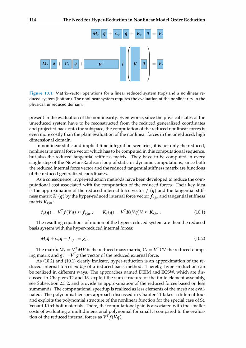
114 The Need for Hyper-Reduction in Nonlinear Model Order Reduction
Mr q + Cr q + Kr q = Fr
Mr q + Cr q + V T f
V q
= Fr
Figure 10.1: Matrix-vector operations for a linear reduced system (top) and a nonlinear re-duced system (boom). The nonlinear system requires the evaluation of the nonlinearity in thephysical, unreduced domain.
present in the evaluation of the nonlinearity. Even worse, since the physical states of theunreduced system have to be reconstructed from the reduced generalized coordinatesand projected back onto the subspace, the computation of the reduced nonlinear forces iseven more costly than the plain evaluation of the nonlinear forces in the unreduced, highdimensional domain.
In nonlinear static and implicit time integration scenarios, it is not only the reduced,nonlinear internal force vector which has to be computed in this computational sequence,but also the reduced tangential stiffness matrix. They have to be computed in everysingle step of the Newton-Raphson loop of static or dynamic computations, since boththe reduced internal force vector and the reduced tangential stiffness matrix are functionsof the reduced generalized coordinates.
As a consequence, hyper-reduction methods have been developed to reduce the com-putational cost associated with the computation of the reduced forces. Their key ideais the approximation of the reduced internal force vector f r(q) and the tangential stiff-ness matrix Kr(q) by the hyper-reduced internal force vector f r,hr and tangential stiffnessmatrix Kr,hr:
f r(q) = V T f (Vq) ≈ f r,hr , Kr(q) = V TK(Vq)V ≈ Kr,hr . (10.1)
The resulting equations of motion of the hyper-reduced system are then the reducedbasis system with the hyper-reduced internal forces:
Mrq + Crq + f r,hr = gr. (10.2)
The matrix Mr = V T MV is the reduced mass matrix, Cr = V TCV the reduced damp-ing matrix and gr = V Tg the vector of the reduced external force.
As (10.2) and (10.1) clearly indicate, hyper-reduction is an approximation of the re-duced internal forces on top of a reduced basis method. Thereby, hyper-reduction canbe realized in different ways. The approaches named DEIM and ECSW, which are dis-cussed in Chapters 12 and 13, exploit the sum-structure of the finite element assembly,see Subsection 2.3.2, and provide an approximation of the reduced forces based on lesssummands. The computational speedup is realized as less elements of the mesh are eval-uated. The polynomial tensors approach discussed in Chapter 11 takes a different tourand exploits the polynomial structure of the nonlinear function for the special case of St.Venant-Kirchhoff materials. There, the computational gain is associated with the smallercosts of evaluating a multidimensional polynomial for small n compared to the evalua-tion of the reduced internal forces as V T f (Vq).
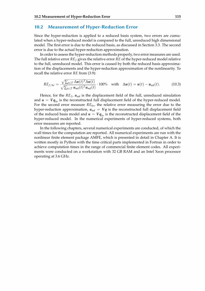
10.2 Measurement of Hyper-Reduction Error 115
10.2 Measurement of Hyper-Reduction Error
Since the hyper-reduction is applied to a reduced basis system, two errors are cumu-lated when a hyper-reduced model is compared to the full, unreduced high dimensionalmodel. The first error is due to the reduced basis, as discussed in Section 3.3. The seconderror is due to the actual hyper-reduction approximation.
In order to assess the hyper-reduction methods properly, two error measures are used.The full relative error RE f gives the relative error RE of the hyper-reduced model relativeto the full, unreduced model. This error is caused by both the reduced basis approxima-tion of the displacements and the hyper-reduction approximation of the nonlinearity. Torecall the relative error RE from (3.9):
RE f /hr =
√∑t∈T ∆u(t)T∆u(t)√∑t∈T uref(t)Turef(t)
· 100% with ∆u(t) = u(t)− uref(t). (10.3)
Hence, for the RE f , uref is the displacement field of the full, unreduced simulationand u = Vqhr is the reconstructed full displacement field of the hyper-reduced model.For the second error measure REhr, the relative error measuring the error due to thehyper-reduction approximation, uref = Vq is the reconstructed full displacement fieldof the reduced basis model and u = Vqhr is the reconstructed displacement field of thehyper-reduced model. In the numerical experiments of hyper-reduced systems, botherror measures are reported.
In the following chapters, several numerical experiments are conducted, of which thewall times for the computation are reported. All numerical experiments are run with thenonlinear finite element package AMFE, which is presented in detail in Chapter A. It iswritten mostly in Python with the time critical parts implemented in Fortran in order toachieve computation times in the range of commercial finite element codes. All experi-ments were conducted on a workstation with 32 GB RAM and an Intel Xeon processoroperating at 3.6 GHz.

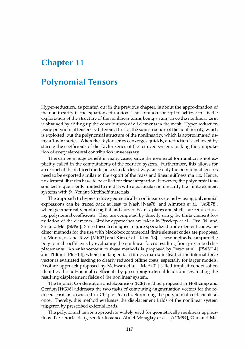
Chapter 11
Polynomial Tensors
Hyper-reduction, as pointed out in the previous chapter, is about the approximation ofthe nonlinearity in the equations of motion. The common concept to achieve this is theexploitation of the structure of the nonlinear terms being a sum, since the nonlinear termis obtained by adding up the contributions of all elements in the mesh. Hyper-reductionusing polynomial tensors is different. It is not the sum structure of the nonlinearity, whichis exploited, but the polynomial structure of the nonlinearity, which is approximated us-ing a Taylor series. When the Taylor series converges quickly, a reduction is achieved bystoring the coefficients of the Taylor series of the reduced system, making the computa-tion of every elemental contribution unnecessary.
This can be a huge benefit in many cases, since the elemental formulation is not ex-plicitly called in the computations of the reduced system. Furthermore, this allows foran export of the reduced model in a standardized way, since only the polynomial tensorsneed to be exported similar to the export of the mass and linear stiffness matrix. Hence,no element libraries have to be called for time integration. However, the polynomial ten-sors technique is only limited to models with a particular nonlinearity like finite elementsystems with St. Venant-Kirchhoff materials.
The approach to hyper-reduce geometrically nonlinear systems by using polynomialexpressions can be traced back at least to Nash [Nas78] and Almroth et al. [ASB78],where geometrically nonlinear, flat and curved beams, plates and shells are reduced us-ing polynomial coefficients. They are computed by directly using the finite element for-mulation of the elements. Similar approaches are taken in Przekop et al. [Prz+04] andShi and Mei [SM96]. Since these techniques require specialized finite element codes, in-direct methods for the use with black-box commercial finite element codes are proposedby Muravyov and Rizzi [MR03] and Kim et al. [Kim+13]. These methods compute thepolynomial coefficients by evaluating the nonlinear forces resulting from prescribed dis-placements. An enhancement to these methods is proposed by Perez et al. [PWM14]and Phlipot [Phl+14], where the tangential stiffness matrix instead of the internal forcevector is evaluated leading to clearly reduced offline costs, especially for larger models.Another approach proposed by McEwan et al. [McE+01] called implicit condensationidentifies the polynomial coefficients by prescribing external loads and evaluating theresulting displacement fields of the nonlinear system.
The Implicit Condensation and Expansion (ICE) method proposed in Hollkamp andGordon [HG08] addresses the two tasks of computing augmentation vectors for the re-duced basis as discussed in Chapter 6 and determining the polynomial coefficients atonce. Thereby, this method evaluates the displacement fields of the nonlinear systemtriggered by prescribed external loads.
The polynomial tensor approach is widely used for geometrically nonlinear applica-tions like aeroelasticity, see for instance Abdel-Motaglay et al. [ACM99], Guo and Mei
117
118 Polynomial Tensors
[GM03] and Ghoman and Azzouz [GAM09] or computer graphics, e.g., Capell et al.[Cap+02] or Barbic and James [BJ05]. In the latter, the polynomial tensor approach isused in combination with the static modal derivatives discussed in Subsection 6.2.2. Fur-thermore, substructuring techniques have been developed using polynomial expansion,e.g., Kuether and Allen [KA14] and Kuether et al. [KAH15], as well as methods for usewith uncertainty, e.g., Capiez-Lernout et al. [CSM14]. For an overview of the differ-ent methodologies and applications, the interested reader is referred to Mignolet et al.[Mig+13].
11.1 Key Idea: Taylor Expansion
The key idea in polynomial tensor hyper-reduction is the approximation of the nonlinearrestoring forces f r(q) ∈ Rn as a Taylor expansion around the point of equilibrium. As inlinear systems, the displacements q ∈ Rn are zero at the point of equilibrium, so that theconstant part is zero. The Taylor expansion up to the k-th order is then:
f r(q) =∂ f r∂q
q +12
∂2 f r∂q∂q
qq +16
∂3 f r∂q3 qqq + · · ·+ 1
k!∂k f r∂qk qk + O(qk+1) (11.1)
= K(1)q +12
K(2)qq +16
K(3)qqq + · · ·+ 1k!
K(k)qk + O(qk+1). (11.2)
Since the internal force vector is a multidimensional function, the Taylor coefficientsare symmetric arrays of dimension k+ 1. They can be interpreted as higher order stiffnessarrays K(1), . . . , K(k), of which the first array K(1) = ∂ f r/∂q yields the reduced stiffnessmatrix Kr ∈ Rn×n. The second term is the reduced quadratic stiffness tensor K(2) =
∂2 f r/∂q2 ∈ Rn×n×n and so on. Throughout this thesis, the polynomial tensors K(k) aredefined as the k-th derivative of the reduced internal force vector ∂k f r/∂qk without thecoefficient 1/k! of the Taylor series. It is pointed out, that in several publications thecoefficients 1/k! are added to the tensors.
The size of the coefficient arrays grows exponentially with the number of membersin the Taylor series. As the higher order polynomial terms are very inefficient for bothstoring in memory and evaluating through multiplication, a polynomial tensors hyper-reduction is only efficient when only few members of the Taylor series (11.1) are necessaryto approximate the nonlinear forces accurately. Hence, the convergence of the series isof extreme importance. To assess this, the mathematical structure of the internal forcesof a St. Venant-Kirchhoff material, which mimics the linear-elastic behavior for largedeformations, is investigated next.
11.2 Polynomial Structure for St. Venant-Kirchho materials
For analyzing the polynomial structure of the restoring forces of a hyperelastic St. Venant-Kirchhoff material, the Total Lagrangian formulation discussed in Section 2.1 is used.The deformation is characterized by the deformation gradient F which is the spatialderivative of the continuous displacement field u with respect to the undeformed con-figuration X. In the finite element approximation, the continuous displacement field isexpressed by the nodal displacements u, which are the amplitudes of the spatial shapefunctions N. As a consequence, u is a linear function of u. As the spatial derivative ofthe deformation gradient acts only on the shape functions (cf. (2.24)), F is a function ofpolynomial order one with respect to the nodal displacements u:
F =∂u∂X
+ I ⇒ F = O(u1). (11.3)
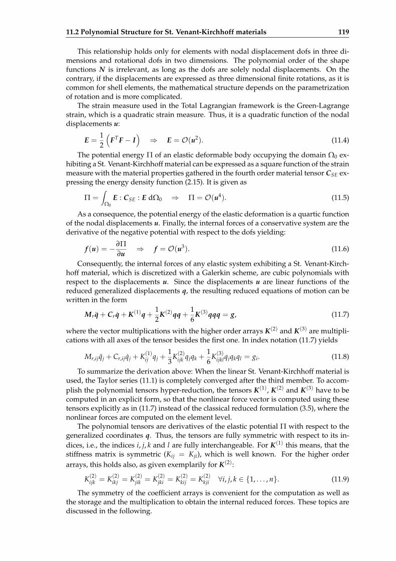
11.2 Polynomial Structure for St. Venant-Kirchhoff materials 119
This relationship holds only for elements with nodal displacement dofs in three di-mensions and rotational dofs in two dimensions. The polynomial order of the shapefunctions N is irrelevant, as long as the dofs are solely nodal displacements. On thecontrary, if the displacements are expressed as three dimensional finite rotations, as it iscommon for shell elements, the mathematical structure depends on the parametrizationof rotation and is more complicated.
The strain measure used in the Total Lagrangian framework is the Green-Lagrangestrain, which is a quadratic strain measure. Thus, it is a quadratic function of the nodaldisplacements u:
E =12
(FT F − I
)⇒ E = O(u2). (11.4)
The potential energy Π of an elastic deformable body occupying the domain Ω0 ex-hibiting a St. Venant-Kirchhoff material can be expressed as a square function of the strainmeasure with the material properties gathered in the fourth order material tensor CSE ex-pressing the energy density function (2.15). It is given as
Π =∫
Ω0
E : CSE : E dΩ0 ⇒ Π = O(u4). (11.5)
As a consequence, the potential energy of the elastic deformation is a quartic functionof the nodal displacements u. Finally, the internal forces of a conservative system are thederivative of the negative potential with respect to the dofs yielding:
f (u) = −∂Π∂u
⇒ f = O(u3). (11.6)
Consequently, the internal forces of any elastic system exhibiting a St. Venant-Kirch-hoff material, which is discretized with a Galerkin scheme, are cubic polynomials withrespect to the displacements u. Since the displacements u are linear functions of thereduced generalized displacements q, the resulting reduced equations of motion can bewritten in the form
Mrq + Crq + K(1)q +12
K(2)qq +16
K(3)qqq = g, (11.7)
where the vector multiplications with the higher order arrays K(2) and K(3) are multipli-cations with all axes of the tensor besides the first one. In index notation (11.7) yields
Mr,ijqj + Cr,ijqj + K(1)ij qj +
13
K(2)ijk qjqk +
16
K(3)ijklqjqkql = gi. (11.8)
To summarize the derivation above: When the linear St. Venant-Kirchhoff material isused, the Taylor series (11.1) is completely converged after the third member. To accom-plish the polynomial tensors hyper-reduction, the tensors K(1), K(2) and K(3) have to becomputed in an explicit form, so that the nonlinear force vector is computed using thesetensors explicitly as in (11.7) instead of the classical reduced formulation (3.5), where thenonlinear forces are computed on the element level.
The polynomial tensors are derivatives of the elastic potential Π with respect to thegeneralized coordinates q. Thus, the tensors are fully symmetric with respect to its in-dices, i.e., the indices i, j, k and l are fully interchangeable. For K(1) this means, that thestiffness matrix is symmetric (Kij = Kji), which is well known. For the higher orderarrays, this holds also, as given exemplarily for K(2):
K(2)ijk = K(2)
ikj = K(2)jik = K(2)
jki = K(2)kij = K(2)
kji ∀i, j, k ∈ 1, . . . , n. (11.9)
The symmetry of the coefficient arrays is convenient for the computation as well asthe storage and the multiplication to obtain the internal reduced forces. These topics arediscussed in the following.
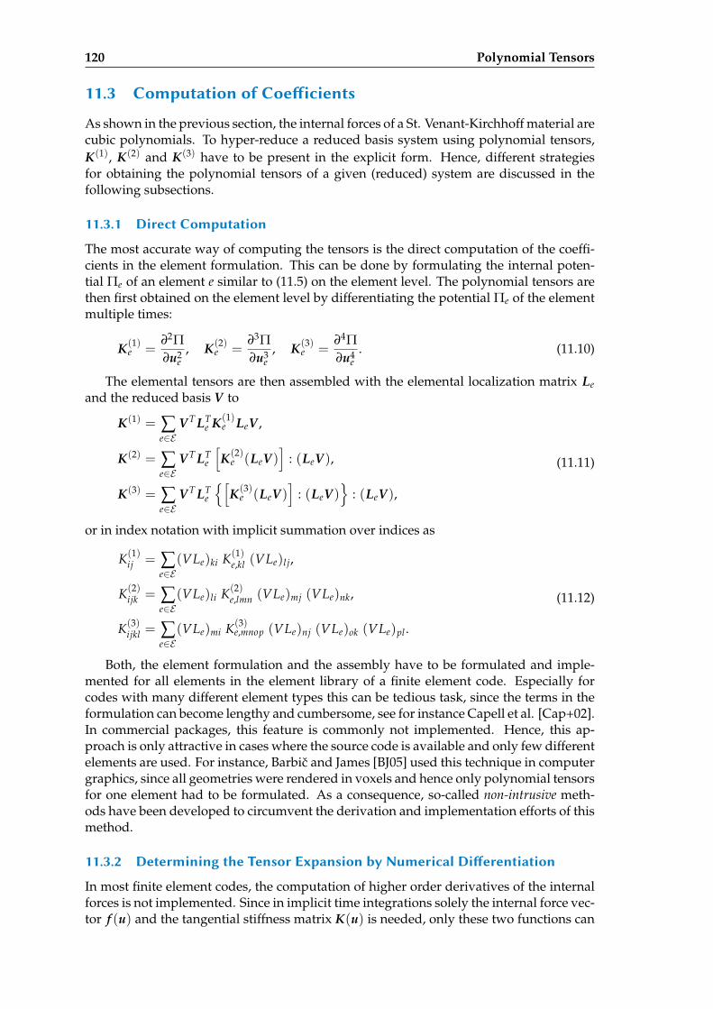
120 Polynomial Tensors
11.3 Computation of Coeicients
As shown in the previous section, the internal forces of a St. Venant-Kirchhoff material arecubic polynomials. To hyper-reduce a reduced basis system using polynomial tensors,K(1), K(2) and K(3) have to be present in the explicit form. Hence, different strategiesfor obtaining the polynomial tensors of a given (reduced) system are discussed in thefollowing subsections.
11.3.1 Direct Computation
The most accurate way of computing the tensors is the direct computation of the coeffi-cients in the element formulation. This can be done by formulating the internal poten-tial Πe of an element e similar to (11.5) on the element level. The polynomial tensors arethen first obtained on the element level by differentiating the potential Πe of the elementmultiple times:
K(1)e =
∂2Π∂u2
e, K(2)
e =∂3Π∂u3
e, K(3)
e =∂4Π∂u4
e. (11.10)
The elemental tensors are then assembled with the elemental localization matrix Leand the reduced basis V to
K(1) = ∑e∈E
V T LTe K(1)
e LeV ,
K(2) = ∑e∈E
V T LTe
[K(2)
e (LeV)]
: (LeV),
K(3) = ∑e∈E
V T LTe
[K(3)
e (LeV)]
: (LeV)
: (LeV),
(11.11)
or in index notation with implicit summation over indices as
K(1)ij = ∑
e∈E(VLe)ki K(1)
e,kl (VLe)l j,
K(2)ijk = ∑
e∈E(VLe)li K(2)
e,lmn (VLe)mj (VLe)nk,
K(3)ijkl = ∑
e∈E(VLe)mi K(3)
e,mnop (VLe)nj (VLe)ok (VLe)pl .
(11.12)
Both, the element formulation and the assembly have to be formulated and imple-mented for all elements in the element library of a finite element code. Especially forcodes with many different element types this can be tedious task, since the terms in theformulation can become lengthy and cumbersome, see for instance Capell et al. [Cap+02].In commercial packages, this feature is commonly not implemented. Hence, this ap-proach is only attractive in cases where the source code is available and only few differentelements are used. For instance, Barbic and James [BJ05] used this technique in computergraphics, since all geometries were rendered in voxels and hence only polynomial tensorsfor one element had to be formulated. As a consequence, so-called non-intrusive meth-ods have been developed to circumvent the derivation and implementation efforts of thismethod.
11.3.2 Determining the Tensor Expansion by Numerical Dierentiation
In most finite element codes, the computation of higher order derivatives of the internalforces is not implemented. Since in implicit time integrations solely the internal force vec-tor f (u) and the tangential stiffness matrix K(u) is needed, only these two functions can
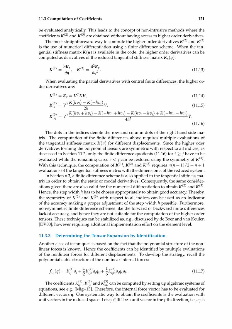
11.3 Computation of Coefficients 121
be evaluated analytically. This leads to the concept of non-intrusive methods where thecoefficients K(2) and K(3) are obtained without having access to higher order derivatives.
The most straightforward way to compute the higher order derivatives K(2) and K(3)
is the use of numerical differentiation using a finite difference scheme. When the tan-gential stiffness matrix K(u) is available in the code, the higher order derivatives can becomputed as derivatives of the reduced tangential stiffness matrix Kr(q):
K(2) =∂Kr
∂q, K(3) =
∂2Kr
∂q2 . (11.13)
When evaluating the partial derivatives with central finite differences, the higher or-der derivatives are:
K(1) = Kr = V TKV , (11.14)
K(2)..i = V T K(hvi)− K(−hvi)
2hV , (11.15)
K(3)..ij = V T K(hvi + hvj)− K(−hvi + hvj)− K(hvi − hvj) + K(−hvi − hvj)
4h2 V .
(11.16)
The dots in the indices denote the row and column dofs of the right hand side ma-trix. The computation of the finite differences above requires multiple evaluations ofthe tangential stiffness matrix K(u) for different displacements. Since the higher oderderivatives forming the polynomial tensors are symmetric with respect to all indices, asdiscussed in Section 11.2, only the finite difference quotients (11.16) for i ≥ j have to beevaluated while the remaining cases i < j can be restored using the symmetry of K(3).With this technique, the computation of K(1), K(2) and K(3) requires n(n + 1)/2 + n + 1evaluations of the tangential stiffness matrix with the dimension n of the reduced system.
In Section 6.3, a finite difference scheme is also applied to the tangential stiffness ma-trix in order to obtain the static or modal derivatives. Consequently, the same consider-ations given there are also valid for the numerical differentiation to obtain K(2) and K(3).Hence, the step width h has to be chosen appropriately to obtain good accuracy. Thereby,the symmetry of K(2) and K(3) with respect to all indices can be used as an indicatorof the accuracy making a proper adjustment of the step width h possible. Furthermore,non-symmetric finite difference schemes like the forward or backward finite differenceslack of accuracy, and hence they are not suitable for the computation of the higher ordertensors. These techniques can be stabilized as, e.g., discussed by de Boer and van Keulen[DV00], however requiring additional implementation effort on the element level.
11.3.3 Determining the Tensor Expansion by Identification
Another class of techniques is based on the fact that the polynomial structure of the non-linear forces is known. Hence the coefficients can be identified by multiple evaluationsof the nonlinear forces for different displacements. To develop the strategy, recall thepolynomial cubic structure of the nonlinear internal forces:
fr,i(q) = K(1)ij qj +
12
K(2)ijk qjqk +
16
K(3)ijklqjqkql . (11.17)
The coefficients K(1)ij , K(2)
ijk and K(3)ijkl can be computed by setting up algebraic systems of
equations, see e.g. [Mig+13]. Therefore, the internal force vector has to be evaluated fordifferent vectors q. One systematic way to obtain the coefficients is the evaluation withunit vectors in the reduced space. Let ej ∈ Rn be a unit vector in the j-th direction, i.e., ej is
122 Polynomial Tensors
the j-th column vector of the identity matrix I ∈ Rn×n. Then, for three randomly chosendifferent displacement amplitudes a1, a2 and a3, the internal force vector is evaluatedfor the displacement fields a1ej, a2ej and a3ej. In this case, no summation over repeatedindices is assumed:
fr,i(q = a1ej) = a1K(1)ij + a2
112
K(2)ijj + a3
116
K(3)ijjj ,
fr,i(q = a2ej) = a2K(1)ij + a2
212
K(2)ijj + a3
216
K(3)ijjj ,
fr,i(q = a3ej) = a3K(1)ij + a2
312
K(2)ijj + a3
316
K(3)ijjj .
(11.18)
The resulting system of equations allows determining the unknown coefficients K(1)ij ,
K(2)ijj and K(3)
ijjj , which are obtained in a subsequent step by solving the linear system ofequations:
a1a2
12
a31
6
a2a2
22
a32
6
a3a2
32
a33
6
K(1)ij
K(2)ijj
K(3)ijjj
=
fr,i(q = a1ej)fr,i(q = a2ej)fr,i(q = a3ej)
. (11.19)
This procedure is performed n times for j = 1 . . . n to obtain all coefficients for allcombinations for i and j. In the next step, displacement fields composed from two unitdisplacement vectors ej and ek are addressed. They have to be evaluated for three differ-ent amplitudes a1, a2 and a3 and are exemplarily given for a1:
fr,i(q = a1(ej + ek)) =a1
(K(1)
ij + K(1)ik
)+ a2
112
(K(2)
ijj + K(2)ikk + 2K(2)
ijk
)
+ a31
16
(K(3)
ijjj + 3K(3)ijjk + 3K(3)
ijkk
).
(11.20)
The equation above has three new unknowns K(2)ijk and K(3)
ijjk and K(3)ijkk which can be
determined with three different amplitudes a1, a2 and a3 and the coefficients obtainedfrom the previous step (11.18). Note that in this step the symmetry is exploited, sinceKijjk = Kijkj = Kikjj is summarized by Kijjk. Consequently, only 3n(n− 1)/2 evaluationsof (11.20) have to be performed, as only combinations with k < j have to be evaluated andthe other ones with k > j are obtained using symmetry. In the last step, the displacementfield with three different unit displacements ej, ek, el are evaluated yielding:
fr,i(q = a1(ej + ek + el)) =a1(K(1)ij + K(1)
ik + K(1)il )
+ a21
12(K(2)
ijj + K(2)ikk + K(2)
ill + 2K(2)ijk + 2K(2)
ijl + 2K(2)ikl )
+ a31
16(K(3)
ijjj + 3K(3)ijjk + 3K(3)
ijkk + 3K(3)ijll
+ 3K(3)il jj + 3K(3)
ikll + 3K(3)ilkk + 6K(3)
ijkl),(11.21)
which can be directly solved for Kijkl . The symmetry is also exploited here so that onlyn(n− 1)(n− 2)/6 cases for j < k < l have to be evaluated. The other terms are obtainedusing the symmetry, as above.
The method described above evaluates the nonlinear internal forces. However, thesame information can be obtained by evaluating the reduced tangential stiffness ma-trix Kr(q) for different displacement fields, see Perez et.al. [PWM14]. The reduced tan-gential stiffness matrix is a quadratic function:
11.3 Computation of Coefficients 123
Kr,ij(q) = K(1)ij + K(2)
ijk qk +12
K(3)ijklqkql . (11.22)
Similarly, the coefficients can be obtained by evaluating the tangential stiffness matrixfor the unit displacement with two amplitudes a1 and a2. As in (11.18), no summationover repeated indices is assumed:
Kr,ij(q = a1ek) = K(1)ij + a1K(2)
ijk + a21
12
K(3)ijkk,
Kr,ij(q = a2ek) = K(1)ij + a2K(2)
ijk + a22
12
K(3)ijkk.
(11.23)
With the equations above, the unknown coefficients K(2)ijk and K(3)
ijkk can be identified inthe same fashion as in (11.19). Then, in a subsequent step, the coefficients with differentindices can be obtained by solving
Kr,ij(q = a1(ek + el)) = K(1)ij + a1
(K(2)
ijk + K(2)ijl
)+ a2
112
(K(3)
ijkk + K(3)ijll + 2K(3)
ijkl
)
(11.24)
for the unknown coefficient K(3)ijkl . The identification technique using the stiffness matrix
needs only 2n computations of the tangential stiffness matrix in order to determine termswith similar indices and n(n− 1)/2 evaluations for the terms with different indices, sincethe symmetry can be exploited. As a consequence, the number of operations is clearlysmaller compared to the force identification technique.
In both techniques described above, the choice of the amplitudes a1, a2 and a3 forthe unit displacements is to be specified. When the material of the underlying modelis a St. Venant-Kirchhoff material which exhibits a third order polynomial structure forthe internal forces, the choice of the parameters is arbitrary as long as they are sufficientlydifferent from each other leading to invertible matrices in (11.19). However, the inversionof the matrix can be simplified, if the coefficients are chosen in a certain pattern likea1 = 1, a2 = −1 and a3 = 2. Then, the solution of the system like (11.19) can be obtaineddirectly by algebraic operations.
11.3.4 Other Approaches
All approaches presented above are approaches where the polynomial coefficients of areduced system are computed and hence a hyper-reduction is performed. Thereby thereduction basis is chosen a priori and the coefficients are independent of the method used.However, for the sake of completeness it is mentioned, that a whole group of so-calledforce-based methods exist. In these methods, instead of prescribing the displacements asin the methods above for obtaining the nonlinear forces or tangential stiffness matrices,the external force vector is prescribed on the full model and the nonlinear problem issolved iteratively.
From the resulting displacement fields of the high dimensional, unreduced model,different approximations can be taken. In the so-called Implicit Condensation (IC) methodproposed by Hollkamp et al. [HGS05], the nonlinear effects, which are not considered inthe reduction basis, are accounted for in the polynomial tensors. In the extension of theIC method named Implicit Condensation and Expansion (ICE), see Kim et al. [Kim+13]and Mignolet et al. [Mig+13], the so-called dual modes similar to the SMDs introducedin Subsection 6.2.2 are identified empirically.
These methods require multiple nonlinear static solutions of the full model. Further-more, they require a careful selection of the forcing amplitudes, which have to be man-ually controlled on certain points on the mesh requiring elaborate preprocessing, see
124 Polynomial Tensors
Guerin et al. [GKA16]. These methods are attractive in scenarios where the solutionsof the nonlinear problem are used for both, the basis construction and the identifica-tion of the polynomial coefficients. These methods have mainly been applied to flat orslightly curved shell and beam problems [GKA16; KA16; Wan+09; Mig+13] as well asmore elaborate airplane structures [Phl+14] with moderate rotations. How they performfor arbitrary geometries exhibiting large rotations is still an open question.
11.4 Eicient Treatment of Symmetric Arrays
The multidimensional arrays K(2) and K(3) are highly symmetric. Hence, if they arestored and treated naively as regular dense high dimensional arrays, a remarkable amountof storage is used redundantly. Especially for K(3), the amount of RAM can increasequickly when the basis becomes larger. As an example, for a basis of n = 20, K(3) re-quires 1.28 MB of storage, if 64 bit float numbers with double precision are used. How-ever, when only the unique values are stored, this number reduces to 0.071 MB. This ratiobecomes even more dramatic, if n becomes larger. For instance for n = 50, the naive stor-age of K(3) requires 50 MB vs. 2.34 MB in efficient storage or 800 MB vs. 35.4 MB forn = 100. Thus, efficient storage of the higher order tensors is necessary, if the memory islimited.
However, not only for storage reasons, a special treatment of the high dimensionalarrays is necessary. The computation of the internal forces f r and the tangential stiff-ness matrix Kr(q) become extremely costly for growing reduction dimension n, since thenumber of multiplications and hence for floating point operations grows with order n4.This makes the polynomial multiplication unattractive for larger n, if it is performed di-rectly as given in (11.8). So not only an efficient storage strategy, but also an efficientmultiplication strategy is necessary to achieve good speedup factors for polynomial ten-sor hyper-reduced models.
11.4.1 Eicient Storage
First, the efficient storage of K(2) and K(3) is addressed. Since both multidimensionalarrays are symmetric with respect to all axes, it is sufficient to store entries with one indexcombination only once. Hence, for efficient storage, only the unique, non-redundantentries of K(2) and K(3) are stored in the vectors k(2) and k(3) in a prescribed sequence:
k(2) =
((k(2)
iii
)T,(
k(2)iij
)T,(
k(2)ijj
)T,(
k(2)ijk
)T)T
∀ i, j, k ∈ 1, . . . , n | i > j > k,(11.25)
k(3) =
((k(3)
iiii
)T,(
k(2)iiij
)T,(
k(3)iijj
)T,(
k(3)ijjj
)T,(
k(3)iijk
)T,(
k(3)ijjk
)T,(
k(3)ijkk
)T,(
k(3)ijkl
)T)T
∀ i, j, k, l ∈ 1, . . . , n | i > j > k > l).(11.26)
The vectors k(2) ∈ Rn(n+1)(n+2)/6 and k(3) ∈ Rn(n+1)(n+2)(n+3)/24 are column vectorscontaining all entries corresponding to the index combination of the higher dimensionalarrays. For instance, k(2)
iii contains all diagonal entries of K(2), i.e., k(2)iii =
(K(2)
111, . . . , K(2)nnn
).
Similarly, the vectors containing combinations of different indices are constructed withthe first index i changing slowest and l changing fastest like in nested loops. For a deeperexplanation, the construction of the vector k(2) is exemplarily given in Algorithm 2. Theconstruction of k(3), which is more lengthy, follows the same principle.
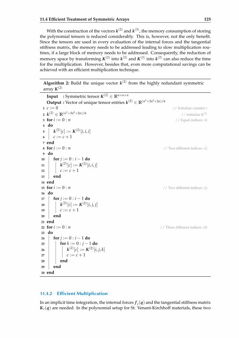
11.4 Efficient Treatment of Symmetric Arrays 125
With the construction of the vectors k(2) and k(3), the memory consumption of storingthe polynomial tensors is reduced considerably. This is, however, not the only benefit.Since the tensors are used in every evaluation of the internal forces and the tangentialstiffness matrix, the memory needs to be addressed leading to slow multiplication rou-tines, if a large block of memory needs to be addressed. Consequently, the reduction ofmemory space by transforming K(2) into k(2) and K(3) into k(2) can also reduce the timefor the multiplication. However, besides that, even more computational savings can beachieved with an efficient multiplication technique.
Algorithm 2: Build the unique vector k(2) from the highly redundant symmetricarray K(2)
Input : Symmetric tensor K(2) ∈ Rn×n×n
Output : Vector of unique tensor entries k(2) ∈ R(n3+3n2+2n)/6
1 c := 0 // Initialize counter c
2 k(2) ∈ R(n3+3n2+2n)/6 // initialize k(2)
3 for i := 0 : n // Equal indices: iii4 do5 k(2)[c] := K(2)[i, i, i]6 c := c + 17 end8 for i := 0 : n // Two different indices: iij9 do
10 for j := 0 : i− 1 do11 k(2)[c] := K(2)[i, i, j]12 c := c + 113 end14 end15 for i := 0 : n // Two different indices: ijj16 do17 for j := 0 : i− 1 do18 k(2)[c] := K(2)[i, j, j]19 c := c + 120 end21 end22 for i := 0 : n // Three different indices: ijk23 do24 for j := 0 : i− 1 do25 for k := 0 : j− 1 do26 k(2)[c] := K(2)[i, j, k]27 c := c + 128 end29 end30 end
11.4.2 Eicient Multiplication
In an implicit time integration, the internal forces f r(q) and the tangential stiffness matrixKr(q) are needed. In the polynomial setup for St. Venant-Kirchhoff materials, these two
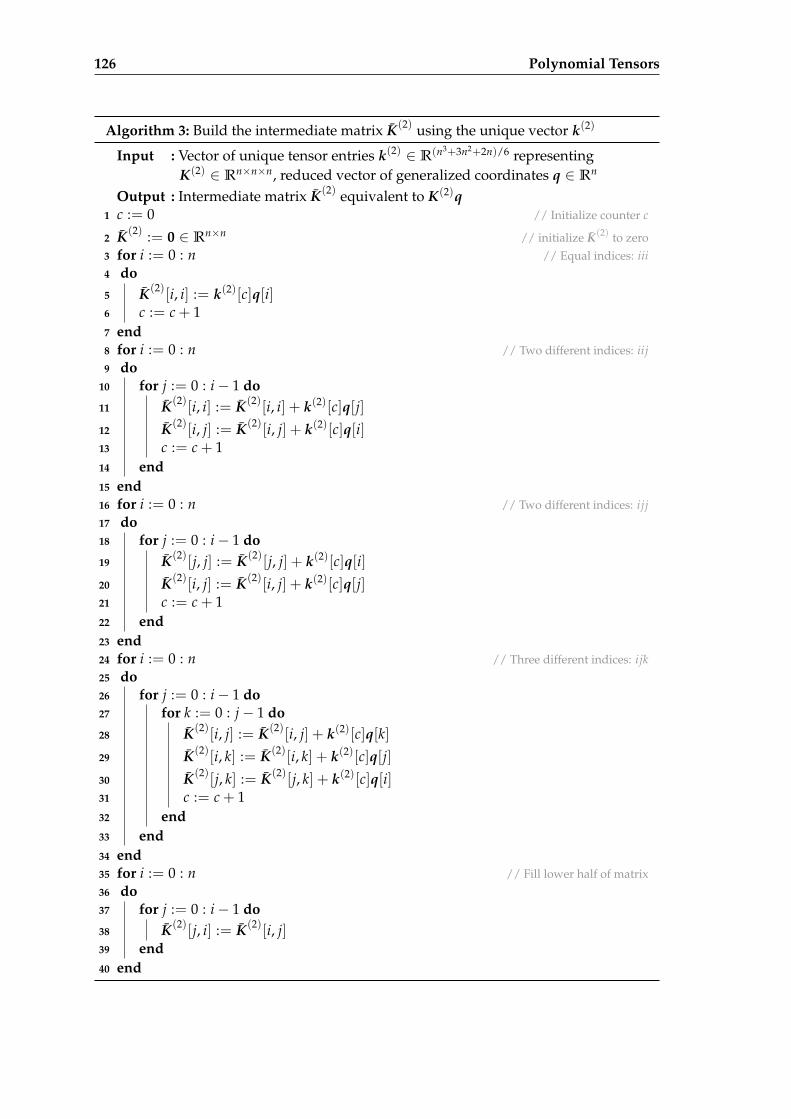
126 Polynomial Tensors
Algorithm 3: Build the intermediate matrix K(2) using the unique vector k(2)
Input : Vector of unique tensor entries k(2) ∈ R(n3+3n2+2n)/6 representingK(2) ∈ Rn×n×n, reduced vector of generalized coordinates q ∈ Rn
Output : Intermediate matrix K(2) equivalent to K(2)q1 c := 0 // Initialize counter c
2 K(2) := 0 ∈ Rn×n // initialize K(2) to zero3 for i := 0 : n // Equal indices: iii4 do5 K(2)[i, i] := k(2)[c]q[i]6 c := c + 17 end8 for i := 0 : n // Two different indices: iij9 do
10 for j := 0 : i− 1 do11 K(2)[i, i] := K(2)[i, i] + k(2)[c]q[j]12 K(2)[i, j] := K(2)[i, j] + k(2)[c]q[i]13 c := c + 114 end15 end16 for i := 0 : n // Two different indices: ijj17 do18 for j := 0 : i− 1 do19 K(2)[j, j] := K(2)[j, j] + k(2)[c]q[i]20 K(2)[i, j] := K(2)[i, j] + k(2)[c]q[j]21 c := c + 122 end23 end24 for i := 0 : n // Three different indices: ijk25 do26 for j := 0 : i− 1 do27 for k := 0 : j− 1 do28 K(2)[i, j] := K(2)[i, j] + k(2)[c]q[k]29 K(2)[i, k] := K(2)[i, k] + k(2)[c]q[j]30 K(2)[j, k] := K(2)[j, k] + k(2)[c]q[i]31 c := c + 132 end33 end34 end35 for i := 0 : n // Fill lower half of matrix36 do37 for j := 0 : i− 1 do38 K(2)[j, i] := K(2)[i, j]39 end40 end
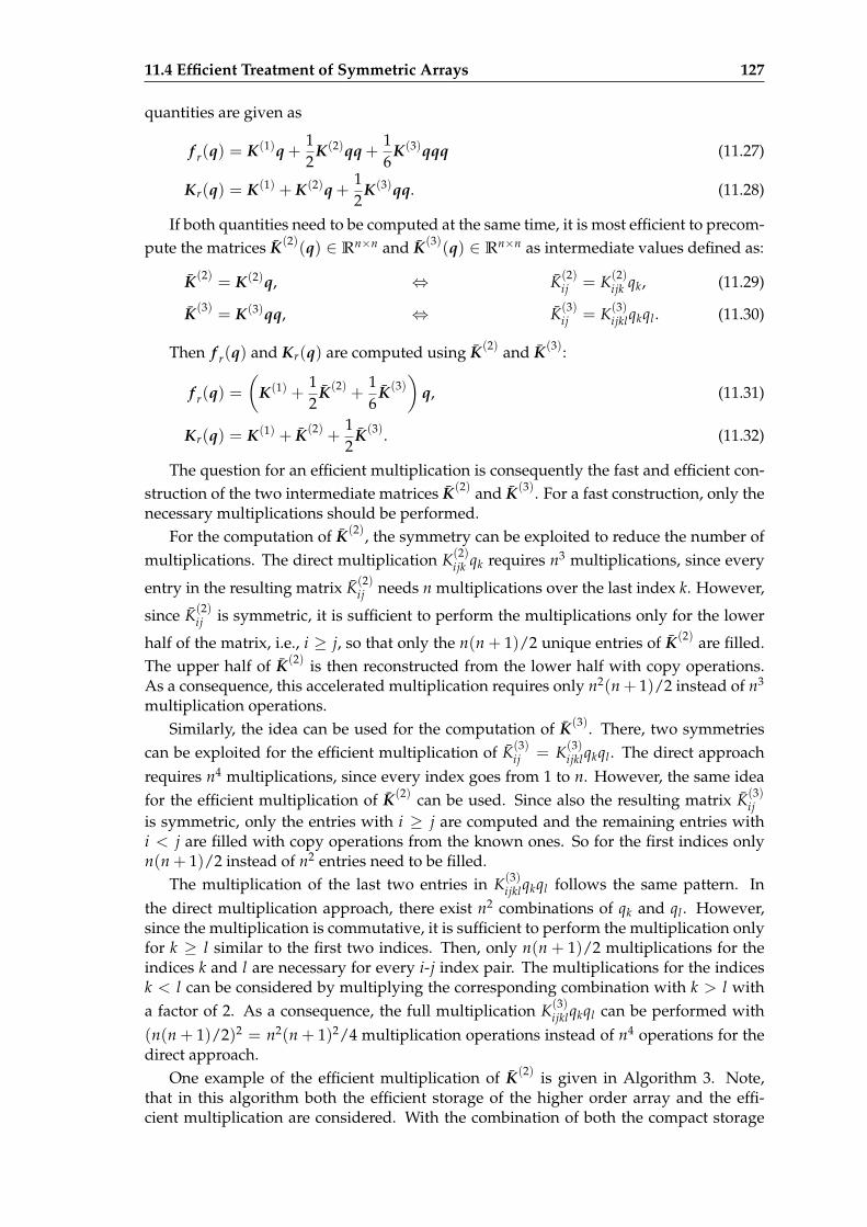
11.4 Efficient Treatment of Symmetric Arrays 127
quantities are given as
f r(q) = K(1)q +12
K(2)qq +16
K(3)qqq (11.27)
Kr(q) = K(1) + K(2)q +12
K(3)qq. (11.28)
If both quantities need to be computed at the same time, it is most efficient to precom-pute the matrices K(2)(q) ∈ Rn×n and K(3)(q) ∈ Rn×n as intermediate values defined as:
K(2) = K(2)q, ⇔ K(2)ij = K(2)
ijk qk, (11.29)
K(3) = K(3)qq, ⇔ K(3)ij = K(3)
ijklqkql . (11.30)
Then f r(q) and Kr(q) are computed using K(2) and K(3):
f r(q) =(
K(1) +12
K(2) +16
K(3))
q, (11.31)
Kr(q) = K(1) + K(2) +12
K(3). (11.32)
The question for an efficient multiplication is consequently the fast and efficient con-struction of the two intermediate matrices K(2) and K(3). For a fast construction, only thenecessary multiplications should be performed.
For the computation of K(2), the symmetry can be exploited to reduce the number ofmultiplications. The direct multiplication K(2)
ijk qk requires n3 multiplications, since every
entry in the resulting matrix K(2)ij needs n multiplications over the last index k. However,
since K(2)ij is symmetric, it is sufficient to perform the multiplications only for the lower
half of the matrix, i.e., i ≥ j, so that only the n(n + 1)/2 unique entries of K(2) are filled.The upper half of K(2) is then reconstructed from the lower half with copy operations.As a consequence, this accelerated multiplication requires only n2(n + 1)/2 instead of n3
multiplication operations.Similarly, the idea can be used for the computation of K(3). There, two symmetries
can be exploited for the efficient multiplication of K(3)ij = K(3)
ijklqkql . The direct approachrequires n4 multiplications, since every index goes from 1 to n. However, the same ideafor the efficient multiplication of K(2) can be used. Since also the resulting matrix K(3)
ijis symmetric, only the entries with i ≥ j are computed and the remaining entries withi < j are filled with copy operations from the known ones. So for the first indices onlyn(n + 1)/2 instead of n2 entries need to be filled.
The multiplication of the last two entries in K(3)ijklqkql follows the same pattern. In
the direct multiplication approach, there exist n2 combinations of qk and ql . However,since the multiplication is commutative, it is sufficient to perform the multiplication onlyfor k ≥ l similar to the first two indices. Then, only n(n + 1)/2 multiplications for theindices k and l are necessary for every i-j index pair. The multiplications for the indicesk < l can be considered by multiplying the corresponding combination with k > l witha factor of 2. As a consequence, the full multiplication K(3)
ijklqkql can be performed with(n(n + 1)/2)2 = n2(n + 1)2/4 multiplication operations instead of n4 operations for thedirect approach.
One example of the efficient multiplication of K(2) is given in Algorithm 3. Note,that in this algorithm both the efficient storage of the higher order array and the effi-cient multiplication are considered. With the combination of both the compact storage
128 Polynomial Tensors
and the accelerated multiplication the computational effort can be clearly reduced. Onthe one hand, the efficient multiplication requires less floating point operations to obtainthe results, as discussed above. On the other hand, the efficient storage of the higherorder tensors minimizes the memory reading effort, since the values are called subse-quently and are not scattered in the memory. Since both effects promise to clearly reducethe computational effort, this technique is applied to an academic but insightful exam-ple in the subsequent section. An overview of the polynomial tensors hyper-reductiontechnique using the accelerated multiplication is given in Figure 11.1. Note, that in theoverview and in the numerical experiments, first the symmetric higher order tensors K(2)
and K(3) are computed before they are transformed to the lean vectorial representationk(2) and k(3). It is, however, possible to store the results of the coefficient computationlike the finite difference scheme or the identification directly into k(2) and k(3) without thedetour over K(2) and K(3). This enhancement which requires more sophisticated index-ing is specially important for larger reduced models, since the size of K(2) and especiallyK(3) becomes quickly prohibitive for larger n.
11.5 Applications
The following applications are run on the cantilever example introduced in Section 6.4.The reduced basis model of the cantilever is constructed with a simulation-free basisbuilt with five vibration modes and all corresponding SMDs yielding a reduced model ofdimension n = 20. The parameters of the model and for the time integration are equal tothe experiments in Section 6.4.
11.5.1 Comparison of Identification Techniques
First, the different methods for computing the polynomial tensors are compared. There-fore, a relative error measure similar to the relative error given in (3.9) is used. With the
error measure εrel , the multidimensional arrays K(2) and K(2)
, or K(3) and K(3)
respec-
tively, are compared. The tensors K(2) and K(3) are the reference tensors and K(2)
and
K(3)
are the tensors to be measured against the reference:
εrel =
√∑n
i=1 ∑nj=1 ∑n
k=1
(K(2)
ijk − K(2)ijk
)2
√∑n
i=1 ∑nj=1 ∑n
k=1
(K(2)
ijk
)2,
εrel =
√∑n
i=1 ∑nj=1 ∑n
k=1 ∑nl=1
(K(3)
ijkl − K(3)ijkl
)2
√∑n
i=1 ∑nj=1 ∑n
k=1 ∑nl=1
(K(3)
ijkl
)2.
(11.33)
The computation of K(2) and K(3) via finite differences, as shown in Subsection 11.3.2,requires the choice of a proper step width h. Similar to the computation of the quadratictensor Θ in Section 6.3, the symmetry can be used to control the error, as the higher odertensors should remain the same when the indices are swapped. The symmetry of thehigher order tensors is assessed with the relative error εrel given above. Thereby, the
tensors K(2)
and K(3)
are equal to K(2) and K(3), however with swapped indices:
K(2)ijk = K(2)
ikj , K(3)ijkl = K(3)
ikjl . (11.34)
11.5 Applications 129
Input:
• Finite element system using St. Venant-Kirchoff material
• Reduction basis V
Define reduced system:
Mr = V T MV Cr = V TCV
f r(q) = V T f (Vq) Kr(q) = V TK(Vu)V
Compute polynomial tensors with method of choice:
• Direct computation (higher order derivatives have to beimplemented in codebase)
• Finite differences (step width h has to be chosen carefully)
• Identification using f r or Kr
• Other identification method (e.g. force based methods likeIC or ICE)
Result: K(1), K(2), K(3)
Compute vectorial representation k(2) and k(3) of K(2) and K(3):
k(2) = vectorize(
K(2))
k(3) = vectorize(
K(3))
Define polynomially reduced system with efficientmultiplication:
K(2)(q) = accelerated multiply(
k(2), q)
K(3)(q) = accelerated multiply(
k(3), q)
f r(q) =(
K(1) +12
K(2)(q) +16
K(3)(q))
q
Kr(q) = K(1) + K(2)(q) +12
K(3)(q)
Figure 11.1: Overview of the reduction process using polynomial tensors and accelerated mul-tiplication.
The relative error εrel for assessing the symmetry is evaluated with K(2)
and K(3)
givenin (11.34) for the cantilever example for different step width h, see Figure 11.2. The rel-ative symmetry error has its minimum at the step width h ≈ 1 similar to the finite dif-ference scheme used for Θ. The error is in the range of machine epsilon indicating, thatthe finite difference scheme is very exact for the correct step width. The error for the ten-sor K(2) responsible for the quadratic contributions in the forces rises after this optimalstep width. The error for K(3) responsible for the cubic forces, however, remains in theorder of machine epsilon. This is due to the fact, that for larger step width, the secant er-ror rises, whereas for small step width the round-off errors dominate, see Griewank andWalter [GW08]. Since the tangential stiffness matrix is a purely quadratic function, thesecant error is zero for the second order derivative, since the central difference scheme isof second order accuracy (cf. [Str07, pp. 15]). Consequently, a larger step width h ≥ 1 is
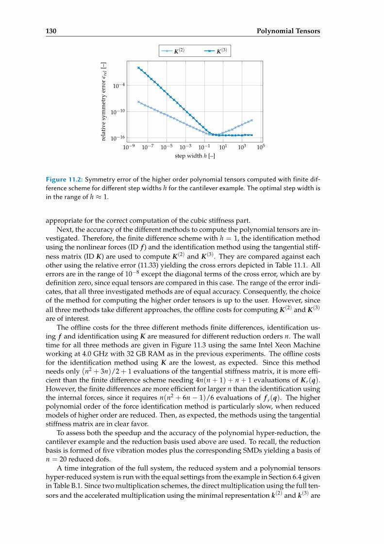
130 Polynomial Tensors
10−9 10−7 10−5 10−3 10−1 101 103 10510−16
10−10
10−4
step width h [–]
rela
tive
sym
met
ryer
ror
ε rel
[–]
K(2) K(3)
Figure 11.2: Symmetry error of the higher order polynomial tensors computed with finite dif-ference scheme for dierent step widths h for the cantilever example. The optimal step width isin the range of h ≈ 1.
appropriate for the correct computation of the cubic stiffness part.Next, the accuracy of the different methods to compute the polynomial tensors are in-
vestigated. Therefore, the finite difference scheme with h = 1, the identification methodusing the nonlinear forces (ID f ) and the identification method using the tangential stiff-ness matrix (ID K) are used to compute K(2) and K(3). They are compared against eachother using the relative error (11.33) yielding the cross errors depicted in Table 11.1. Allerrors are in the range of 10−8 except the diagonal terms of the cross error, which are bydefinition zero, since equal tensors are compared in this case. The range of the error indi-cates, that all three investigated methods are of equal accuracy. Consequently, the choiceof the method for computing the higher order tensors is up to the user. However, sinceall three methods take different approaches, the offline costs for computing K(2) and K(3)
are of interest.The offline costs for the three different methods finite differences, identification us-
ing f and identification using K are measured for different reduction orders n. The walltime for all three methods are given in Figure 11.3 using the same Intel Xeon Machineworking at 4.0 GHz with 32 GB RAM as in the previous experiments. The offline costsfor the identification method using K are the lowest, as expected. Since this methodneeds only (n2 + 3n)/2 + 1 evaluations of the tangential stiffness matrix, it is more effi-cient than the finite difference scheme needing 4n(n + 1) + n + 1 evaluations of Kr(q).However, the finite differences are more efficient for larger n than the identification usingthe internal forces, since it requires n(n2 + 6n − 1)/6 evaluations of f r(q). The higherpolynomial order of the force identification method is particularly slow, when reducedmodels of higher order are reduced. Then, as expected, the methods using the tangentialstiffness matrix are in clear favor.
To assess both the speedup and the accuracy of the polynomial hyper-reduction, thecantilever example and the reduction basis used above are used. To recall, the reductionbasis is formed of five vibration modes plus the corresponding SMDs yielding a basis ofn = 20 reduced dofs.
A time integration of the full system, the reduced system and a polynomial tensorshyper-reduced system is run with the equal settings from the example in Section 6.4 givenin Table B.1. Since two multiplication schemes, the direct multiplication using the full ten-sors and the accelerated multiplication using the minimal representation k(2) and k(3) are
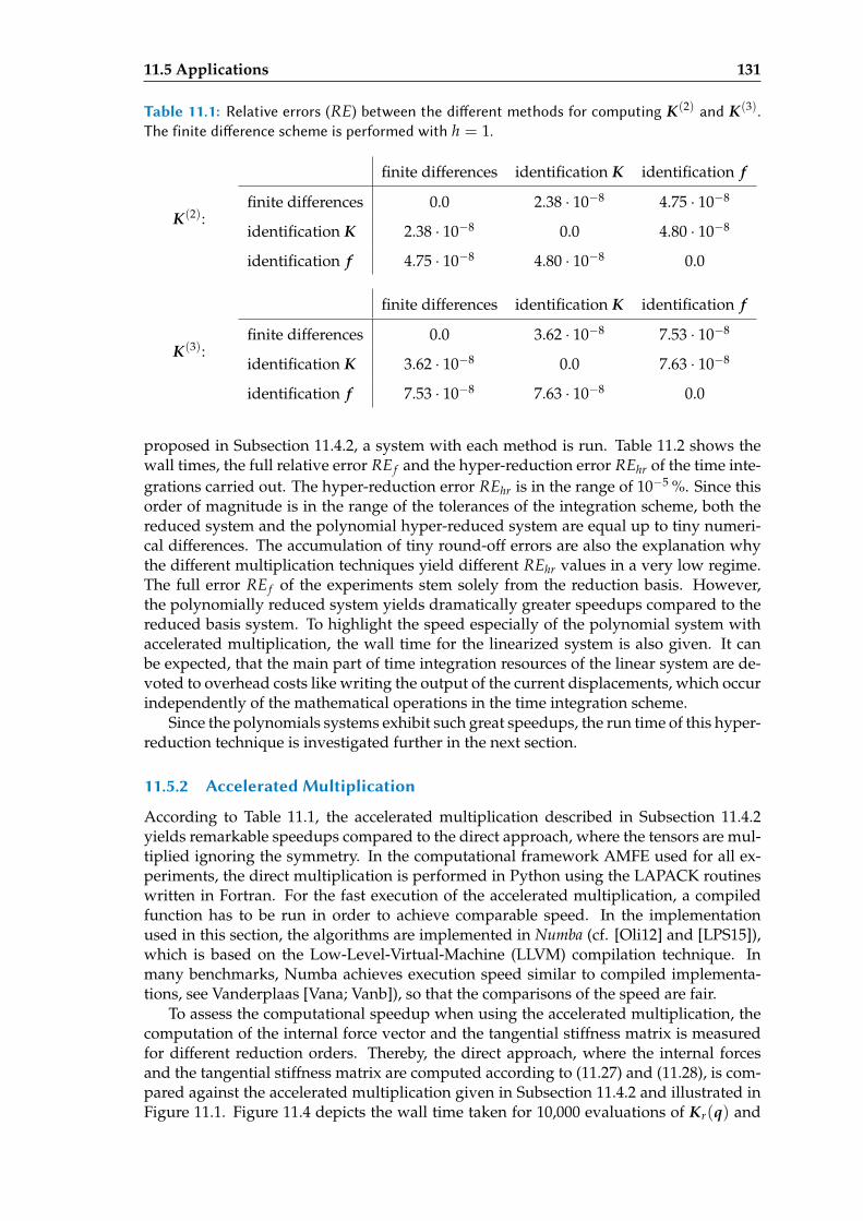
11.5 Applications 131
Table 11.1: Relative errors (RE) between the dierent methods for computing K(2) and K(3).The finite dierence scheme is performed with h = 1.
K(2):
finite differences identification K identification f
finite differences 0.0 2.38 · 10−8 4.75 · 10−8
identification K 2.38 · 10−8 0.0 4.80 · 10−8
identification f 4.75 · 10−8 4.80 · 10−8 0.0
K(3):
finite differences identification K identification f
finite differences 0.0 3.62 · 10−8 7.53 · 10−8
identification K 3.62 · 10−8 0.0 7.63 · 10−8
identification f 7.53 · 10−8 7.63 · 10−8 0.0
proposed in Subsection 11.4.2, a system with each method is run. Table 11.2 shows thewall times, the full relative error RE f and the hyper-reduction error REhr of the time inte-grations carried out. The hyper-reduction error REhr is in the range of 10−5 %. Since thisorder of magnitude is in the range of the tolerances of the integration scheme, both thereduced system and the polynomial hyper-reduced system are equal up to tiny numeri-cal differences. The accumulation of tiny round-off errors are also the explanation whythe different multiplication techniques yield different REhr values in a very low regime.The full error RE f of the experiments stem solely from the reduction basis. However,the polynomially reduced system yields dramatically greater speedups compared to thereduced basis system. To highlight the speed especially of the polynomial system withaccelerated multiplication, the wall time for the linearized system is also given. It canbe expected, that the main part of time integration resources of the linear system are de-voted to overhead costs like writing the output of the current displacements, which occurindependently of the mathematical operations in the time integration scheme.
Since the polynomials systems exhibit such great speedups, the run time of this hyper-reduction technique is investigated further in the next section.
11.5.2 Accelerated Multiplication
According to Table 11.1, the accelerated multiplication described in Subsection 11.4.2yields remarkable speedups compared to the direct approach, where the tensors are mul-tiplied ignoring the symmetry. In the computational framework AMFE used for all ex-periments, the direct multiplication is performed in Python using the LAPACK routineswritten in Fortran. For the fast execution of the accelerated multiplication, a compiledfunction has to be run in order to achieve comparable speed. In the implementationused in this section, the algorithms are implemented in Numba (cf. [Oli12] and [LPS15]),which is based on the Low-Level-Virtual-Machine (LLVM) compilation technique. Inmany benchmarks, Numba achieves execution speed similar to compiled implementa-tions, see Vanderplaas [Vana; Vanb]), so that the comparisons of the speed are fair.
To assess the computational speedup when using the accelerated multiplication, thecomputation of the internal force vector and the tangential stiffness matrix is measuredfor different reduction orders. Thereby, the direct approach, where the internal forcesand the tangential stiffness matrix are computed according to (11.27) and (11.28), is com-pared against the accelerated multiplication given in Subsection 11.4.2 and illustrated inFigure 11.1. Figure 11.4 depicts the wall time taken for 10,000 evaluations of Kr(q) and
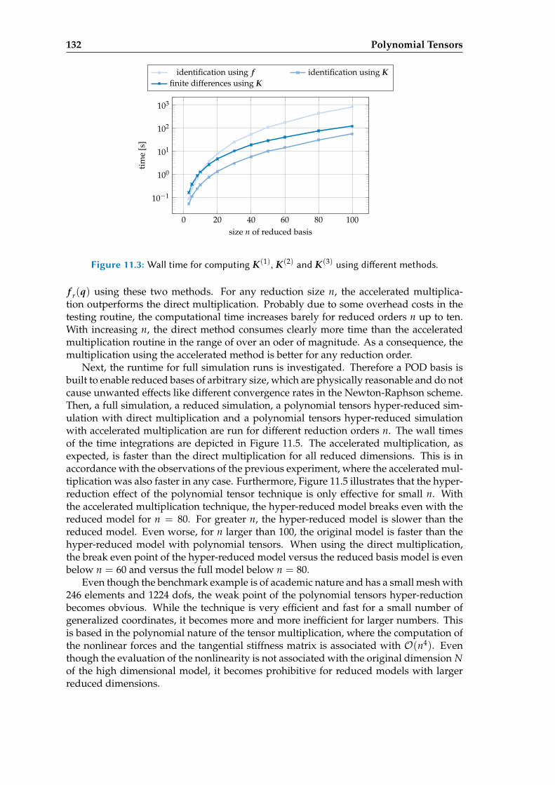
132 Polynomial Tensors
0 20 40 60 80 100
10−1
100
101
102
103
size n of reduced basis
tim
e[s
]
identification using f identification using Kfinite differences using K
Figure 11.3: Wall time for computing K(1), K(2) and K(3) using dierent methods.
f r(q) using these two methods. For any reduction size n, the accelerated multiplica-tion outperforms the direct multiplication. Probably due to some overhead costs in thetesting routine, the computational time increases barely for reduced orders n up to ten.With increasing n, the direct method consumes clearly more time than the acceleratedmultiplication routine in the range of over an oder of magnitude. As a consequence, themultiplication using the accelerated method is better for any reduction order.
Next, the runtime for full simulation runs is investigated. Therefore a POD basis isbuilt to enable reduced bases of arbitrary size, which are physically reasonable and do notcause unwanted effects like different convergence rates in the Newton-Raphson scheme.Then, a full simulation, a reduced simulation, a polynomial tensors hyper-reduced sim-ulation with direct multiplication and a polynomial tensors hyper-reduced simulationwith accelerated multiplication are run for different reduction orders n. The wall timesof the time integrations are depicted in Figure 11.5. The accelerated multiplication, asexpected, is faster than the direct multiplication for all reduced dimensions. This is inaccordance with the observations of the previous experiment, where the accelerated mul-tiplication was also faster in any case. Furthermore, Figure 11.5 illustrates that the hyper-reduction effect of the polynomial tensor technique is only effective for small n. Withthe accelerated multiplication technique, the hyper-reduced model breaks even with thereduced model for n = 80. For greater n, the hyper-reduced model is slower than thereduced model. Even worse, for n larger than 100, the original model is faster than thehyper-reduced model with polynomial tensors. When using the direct multiplication,the break even point of the hyper-reduced model versus the reduced basis model is evenbelow n = 60 and versus the full model below n = 80.
Even though the benchmark example is of academic nature and has a small mesh with246 elements and 1224 dofs, the weak point of the polynomial tensors hyper-reductionbecomes obvious. While the technique is very efficient and fast for a small number ofgeneralized coordinates, it becomes more and more inefficient for larger numbers. Thisis based in the polynomial nature of the tensor multiplication, where the computation ofthe nonlinear forces and the tangential stiffness matrix is associated with O(n4). Eventhough the evaluation of the nonlinearity is not associated with the original dimension Nof the high dimensional model, it becomes prohibitive for reduced models with largerreduced dimensions.
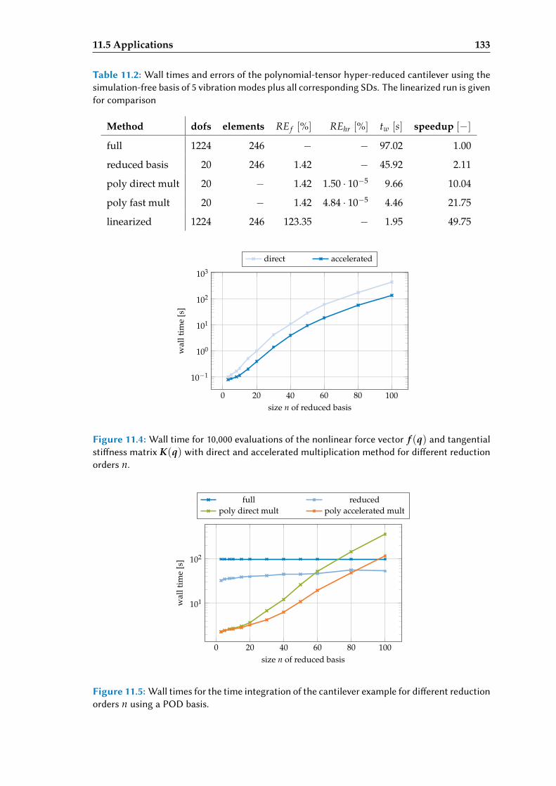
11.5 Applications 133
Table 11.2: Wall times and errors of the polynomial-tensor hyper-reduced cantilever using thesimulation-free basis of 5 vibration modes plus all corresponding SDs. The linearized run is givenfor comparison
Method dofs elements RE f [%] REhr [%] tw [s] speedup [−]full 1224 246 − − 97.02 1.00
reduced basis 20 246 1.42 − 45.92 2.11
poly direct mult 20 − 1.42 1.50 · 10−5 9.66 10.04
poly fast mult 20 − 1.42 4.84 · 10−5 4.46 21.75
linearized 1224 246 123.35 − 1.95 49.75
0 20 40 60 80 100
10−1
100
101
102
103
size n of reduced basis
wal
ltim
e[s
]
direct accelerated
Figure 11.4: Wall time for 10,000 evaluations of the nonlinear force vector f (q) and tangentialstiness matrix K(q) with direct and accelerated multiplication method for dierent reductionorders n.
0 20 40 60 80 100
101
102
size n of reduced basis
wal
ltim
e[s
]
full reducedpoly direct mult poly accelerated mult
Figure 11.5: Wall times for the time integration of the cantilever example for dierent reductionorders n using a POD basis.

Chapter 12
Discrete Empirical Interpolation Method (DEIM)
This chapter discusses the Discrete Empirical Interpolation Method (DEIM), a hyper-reduction method to approximate the high dimensional nonlinear force vector using anempirical force basis. In contrary to the polynomial tensors hyper-reduction discussed inthe previous section, the reduction is achieved by an evaluation of the nonlinear forcesonly at selected points of the mesh.
The key idea of the DEIM goes back at least to the gappy POD method proposedin Everson and Sirovich [ES95], where facial images are reconstructed using "gappy",partial data. This idea is used in several approaches to hyper-reduce nonlinear dynamicalsystems such as fluid dynamics, e.g., in Bui et al. [BDW03], Willcox [Wil06] and Astridet al. [Ast+08], or process simulations in Astrid [Ast04].
The Empirical Interpolation Method (EIM) proposed by Barrault et al. [Bar+04] andin a slightly different version by Ryckelynck [Ryc05] uses the same idea, however at thecontinuous level. It can be seen as the underlying theoretical framework of the DiscreteEmpirical Interpolation Method (DEIM) proposed by Chaturantabut et al. [CS10]. Thismethod distinguishes itself from the others by the ease of computation, since a greedyalgorithm is used for the selection of the gappy data points, the collocation points. Ap-proaches similar to the DEIM are the best point interpolation method of Nguyen et al.[NPP08] and the method proposed by Nguyen and Peraire [NP08].
Further improvements for the DEIM were proposed, as to mention a few, the adap-tation to finite element systems by Tiso and Rixen [TR13] called unassembled DEIM(UDEIM), a localized DEIM approach proposed by Peherstorfer et al. [Peh+14], strategiesto handle parametric systems as proposed in Antil et al. [AHS14] as well as improvedselection strategies in Drmac and Gugercin [DG16]. Adaptations to parametric systemsare discussed in the overview paper on parametric model order reduction of Benner et al[BGW15]. Radermacher and Reese [RR16] applied the DEIM to geometrically and mate-rial nonlinear static systems.
12.1 Key Idea: Interpolation and Collocation
The idea of the DEIM is to approximate the high dimensional nonlinear force f (Vq)with a force basis U f , similar to approximation of the full displacement field u usingthe reduced basis V (cf. Chapter 3). Hence, f is approximated as linear combination ofthe column vectors of the force basis U f ∈ RN×m with the time dependent amplitudescollected in c(Vq) ∈ Rm:
f (Vq) = U f c(Vq) + r. (12.1)
Equation (12.1) has more equations than unknowns. Hence, the residual r occurs,as the basis U f can only represent forces in the subspace spanned by U f . To solve the
135
136 Discrete Empirical Interpolation Method (DEIM)
equation above for the unknown reduced force vector c(Vq), a constraint for the residualis necessary for projecting the residual out.
In the derivation of the basis projection in Chapter 3, the residual was made orthogo-nal to the subspace spanned by the basis leading to the symmetric Galerkin projection. Inthe DEIM, the residual is treated in a different way. It is made zero only for certain dofs,which are the non-zero entries in the columns of the Boolean matrix P ∈ RN×m. Everycolumn of P is a column of the identity matrix I ∈ RN×N . With enforcing
PTr = 0, (12.2)
the residual is hence set to zero only for the dofs corresponding to the non-zero coeffi-cients in P. When the residual is zero at certain dofs, (12.1) is collocated at exactly thesedofs. Thus, the collocation of (12.1) is achieved by the premultiplication with the trans-posed collocation matrix PT. This leads to a determined system of equations, which canbe solved for the unknown force amplitudes gathered in c:
PT f (Vq) = PTU f c(Vq) (12.3)
c(Vq) =(
PTU f
)−1PT f (Vq). (12.4)
It can be inserted in the approximation (12.1), and with accepting the residual being theerror of the approximation, one gains the collocated reduced force vector
f (Vq) ≈ f DEIM(Vq) = U f
(PTU f
)−1PT f (Vq). (12.5)
The collocated internal force vector approximating the internal forces is the DEIMreduced internal force vector f DEIM(Vq). It can be computed cheaper than the full forcevector f (Vq), since the collocation matrix P is a sparse matrix with many zero entries.To evaluated the product PT f in (12.5), only the entries corresponding to a non-zero rowin P have to be evaluated. The computation of all other entries in f corresponding tozero-rows in P can be omitted leading to a reduction of the computational costs.
For the design of the DEIM approximation of the nonlinear forces (12.5), two ingre-dients have to be determined: The force basis U f and the Boolean collocation matrix P.For the force basis, the issues discussed for kinematic bases in Chapter 5 hold also forfinding an appropriate force basis: The lack of system theoretic properties allowing forproper nonlinear force estimations. Hence, the force basis U f is computed with a PODof the force snapshots of a full, unreduced simulation similar to the POD reduced basismethod discussed in Chapter 5.
To compute the Boolean matrix P containing the collocation dofs, a greedy methodlisted in Algorithm 4 is used, see also Chaturantabut and Sorensen [CS10]. This methoditerates over the column vectors of the force basis U f . For every column, a residual ris computed representing the gap in the forces, which cannot be represented using boththe force basis U f and the collocation matrix P of the previous iteration step. Then themaximum value of the residual is picked as new collocation dof and added to the collo-cation dof set ℘tmp. As the dof is associated with a node of the finite element mesh, it isan option to manipulate the selected collocation dof. For instance, it is reasonable to pickall dofs corresponding to the node of the selected dof. With the collocation point set ℘tmpand the collocation points of the former iteration step, the Boolean collocation matrix Pis built for the next iteration step.
When the collocation point set ℘tmp is manipulated, as for instance all dofs of theselected node are collocated and not only the dof with the maximum residual, the num-ber c of collocation points is larger than the number m of force basis vectors. Since thenP ∈ RN×c and U f ∈ RN×m are of different dimensions with c > m, the collocation (12.3)
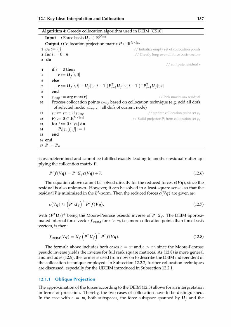
12.1 Key Idea: Interpolation and Collocation 137
Algorithm 4: Greedy collocation algorithm used in DEIM [CS10]
Input : Force basis U f ∈ RN×n
Output : Collocation projection matrix P ∈ RN×|℘n|
1 ℘0 := // Initialize empty set of collocation points2 for i := 0 : n // Greedy loop over all force basis vectors3 do
// compute residual r4 if i = 0 then5 r := U f [:, 0]6 else7 r := U f [:, i]−U f [:, : i− 1](PT
i−1U f [:, : i− 1])+PTi−1U f [:, i]
8 end9 ℘tmp := arg max(r) // Pick maximum residual
10 Process collocation points ℘tmp based on collocation technique (e.g. add all dofsof selected node: ℘tmp := all dofs of current node)
11 ℘i := ℘i−1 ∪ ℘tmp // update collocation point set ℘i
12 Pi := 0 ∈ RN×|℘i | // Build projector Pi from collocation set ℘i
13 for j := 0 : |℘i| do14 Pi[℘i[j], j] := 115 end16 end17 P := Pn
is overdetermined and cannot be fulfilled exactly leading to another residual r after ap-plying the collocation matrix P:
PT f (Vq) = PTU f c(Vq) + r. (12.6)
The equation above cannot be solved directly for the reduced forces c(Vq), since theresidual is also unknown. However, it can be solved in a least-square sense, so that theresidual r is minimized in the L2-norm. Then the reduced forces c(Vq) are given as:
c(Vq) ≈(
PTU f
)+PT f (Vq), (12.7)
with (PTU f )+ being the Moore-Penrose pseudo inverse of PTU f . The DEIM approxi-
mated internal force vector f DEIM for c > m, i.e., more collocation points than force basisvectors, is then:
f DEIM(Vq) = U f
(PTU f
)+PT f (Vq). (12.8)
The formula above includes both cases c = m and c > m, since the Moore-Penrosepseudo inverse yields the inverse for full rank square matrices. As (12.8) is more generaland includes (12.5), the former is used from now on to describe the DEIM independent ofthe collocation technique employed. In Subsection 12.2.2, further collocation techniquesare discussed, especially for the UDEIM introduced in Subsection 12.2.1.
12.1.1 Oblique Projection
The approximation of the forces according to the DEIM (12.5) allows for an interpretationin terms of projection. Thereby, the two cases of collocation have to be distinguished.In the case with c = m, both subspaces, the force subspace spanned by U f and the
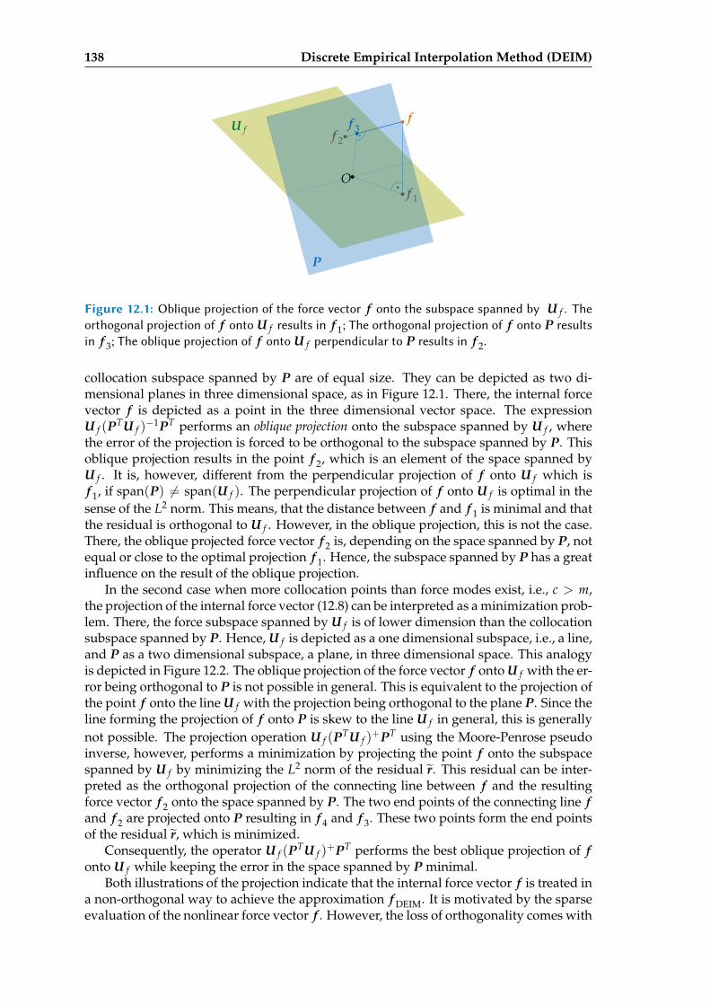
138 Discrete Empirical Interpolation Method (DEIM)
O
f
f 1
P
U f f 2
f 3
Figure 12.1: Oblique projection of the force vector f onto the subspace spanned by U f . Theorthogonal projection of f onto U f results in f 1; The orthogonal projection of f onto P resultsin f 3; The oblique projection of f onto U f perpendicular to P results in f 2.
collocation subspace spanned by P are of equal size. They can be depicted as two di-mensional planes in three dimensional space, as in Figure 12.1. There, the internal forcevector f is depicted as a point in the three dimensional vector space. The expressionU f (PTU f )
−1PT performs an oblique projection onto the subspace spanned by U f , wherethe error of the projection is forced to be orthogonal to the subspace spanned by P. Thisoblique projection results in the point f 2, which is an element of the space spanned byU f . It is, however, different from the perpendicular projection of f onto U f which isf 1, if span(P) 6= span(U f ). The perpendicular projection of f onto U f is optimal in thesense of the L2 norm. This means, that the distance between f and f 1 is minimal and thatthe residual is orthogonal to U f . However, in the oblique projection, this is not the case.There, the oblique projected force vector f 2 is, depending on the space spanned by P, notequal or close to the optimal projection f 1. Hence, the subspace spanned by P has a greatinfluence on the result of the oblique projection.
In the second case when more collocation points than force modes exist, i.e., c > m,the projection of the internal force vector (12.8) can be interpreted as a minimization prob-lem. There, the force subspace spanned by U f is of lower dimension than the collocationsubspace spanned by P. Hence, U f is depicted as a one dimensional subspace, i.e., a line,and P as a two dimensional subspace, a plane, in three dimensional space. This analogyis depicted in Figure 12.2. The oblique projection of the force vector f onto U f with the er-ror being orthogonal to P is not possible in general. This is equivalent to the projection ofthe point f onto the line U f with the projection being orthogonal to the plane P. Since theline forming the projection of f onto P is skew to the line U f in general, this is generallynot possible. The projection operation U f (PTU f )
+PT using the Moore-Penrose pseudoinverse, however, performs a minimization by projecting the point f onto the subspacespanned by U f by minimizing the L2 norm of the residual r. This residual can be inter-preted as the orthogonal projection of the connecting line between f and the resultingforce vector f 2 onto the space spanned by P. The two end points of the connecting line fand f 2 are projected onto P resulting in f 4 and f 3. These two points form the end pointsof the residual r, which is minimized.
Consequently, the operator U f (PTU f )+PT performs the best oblique projection of f
onto U f while keeping the error in the space spanned by P minimal.Both illustrations of the projection indicate that the internal force vector f is treated in
a non-orthogonal way to achieve the approximation f DEIM. It is motivated by the sparseevaluation of the nonlinear force vector f . However, the loss of orthogonality comes with
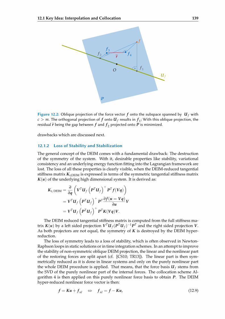
12.1 Key Idea: Interpolation and Collocation 139
O
f
P
U f
f 2
f 3
rf 4
f 1
Figure 12.2: Oblique projection of the force vector f onto the subspace spanned by U f withc > m. The orthogonal projection of f onto U f results in f 1; With this oblique projection, theresidual r being the gap between f and f 2 projected onto P is minimized.
drawbacks which are discussed next.
12.1.2 Loss of Stability and Stabilization
The general concept of the DEIM comes with a fundamental drawback: The destructionof the symmetry of the system. With it, desirable properties like stability, variationalconsistency and an underlying energy function fitting into the Lagrangian framework arelost. The loss of all these properties is clearly visible, when the DEIM-reduced tangentialstiffness matrix Kr,DEIM is expressed in terms of the symmetric tangential stiffness matrixK(u) of the underlying high dimensional system. It is derived as:
Kr, DEIM =∂
∂q
(V TU f
(PTU f
)+PT f (Vq)
)
= V TU f
(PTU f
)+PT ∂ f (u = Vq)
∂uV
= V TU f
(PTU f
)+PTK(Vq)V .
The DEIM reduced tangential stiffness matrix is computed from the full stiffness ma-trix K(u) by a left sided projection V TU f (PTU f )
−1PT and the right sided projection V .As both projectors are not equal, the symmetry of K is destroyed by the DEIM hyper-reduction.
The loss of symmetry leads to a loss of stability, which is often observed in Newton-Raphson loops in static solutions or in time integration schemes. In an attempt to improvethe stability of non-symmetric oblique DEIM projection, the linear and the nonlinear partof the restoring forces are split apart (cf. [CS10; TR13]). The linear part is then sym-metrically reduced as it is done in linear systems and only on the purely nonlinear partthe whole DEIM procedure is applied. That means, that the force basis U f stems fromthe SVD of the purely nonlinear part of the internal forces. The collocation scheme Al-gorithm 4 is then applied on this purely nonlinear force basis to obtain P. The DEIMhyper-reduced nonlinear force vector is then:
f = Ku + f nl ⇔ f nl = f − Ku, (12.9)
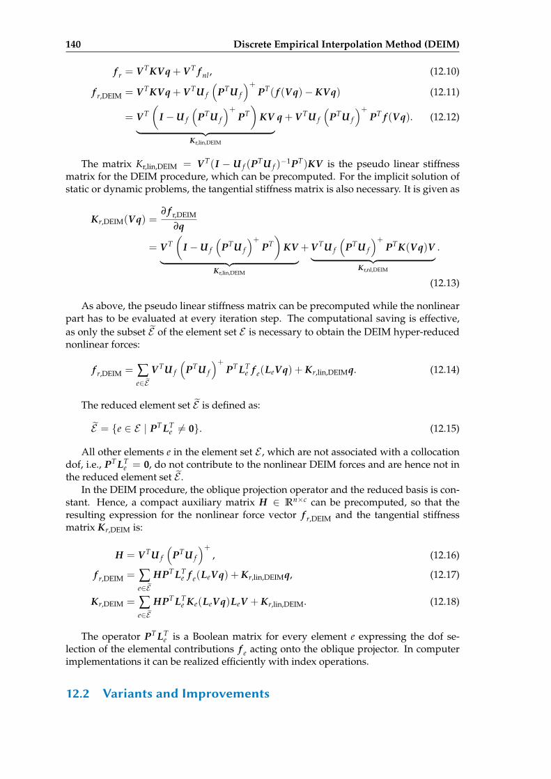
140 Discrete Empirical Interpolation Method (DEIM)
f r = V TKVq + V T f nl , (12.10)
f r,DEIM = V TKVq + V TU f
(PTU f
)+PT( f (Vq)− KVq) (12.11)
= V T(
I −U f
(PTU f
)+PT)
KV︸ ︷︷ ︸
Kr,lin,DEIM
q + V TU f
(PTU f
)+PT f (Vq). (12.12)
The matrix Kr,lin,DEIM = V T(I − U f (PTU f )−1PT)KV is the pseudo linear stiffness
matrix for the DEIM procedure, which can be precomputed. For the implicit solution ofstatic or dynamic problems, the tangential stiffness matrix is also necessary. It is given as
Kr,DEIM(Vq) =∂ f r,DEIM
∂q
= V T(
I −U f
(PTU f
)+PT)
KV︸ ︷︷ ︸
Kr,lin,DEIM
+V TU f
(PTU f
)+PTK(Vq)V
︸ ︷︷ ︸Kr,nl,DEIM
.
(12.13)
As above, the pseudo linear stiffness matrix can be precomputed while the nonlinearpart has to be evaluated at every iteration step. The computational saving is effective,as only the subset E of the element set E is necessary to obtain the DEIM hyper-reducednonlinear forces:
f r,DEIM = ∑e∈E
V TU f
(PTU f
)+PT LT
e f e(LeVq) + Kr,lin,DEIMq. (12.14)
The reduced element set E is defined as:
E = e ∈ E | PT LTe 6= 0. (12.15)
All other elements e in the element set E , which are not associated with a collocationdof, i.e., PT LT
e = 0, do not contribute to the nonlinear DEIM forces and are hence not inthe reduced element set E .
In the DEIM procedure, the oblique projection operator and the reduced basis is con-stant. Hence, a compact auxiliary matrix H ∈ Rn×c can be precomputed, so that theresulting expression for the nonlinear force vector f r,DEIM and the tangential stiffnessmatrix Kr,DEIM is:
H = V TU f
(PTU f
)+, (12.16)
f r,DEIM = ∑e∈E
HPT LTe f e(LeVq) + Kr,lin,DEIMq, (12.17)
Kr,DEIM = ∑e∈E
HPT LTe Ke(LeVq)LeV + Kr,lin,DEIM. (12.18)
The operator PT LTe is a Boolean matrix for every element e expressing the dof se-
lection of the elemental contributions f e acting onto the oblique projector. In computerimplementations it can be realized efficiently with index operations.
12.2 Variants and Improvements
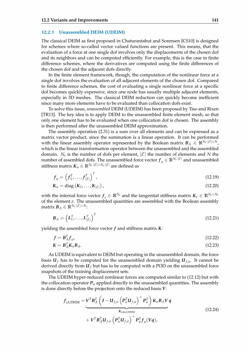
12.2 Variants and Improvements 141
12.2.1 Unassembled DEIM (UDEIM)
The classical DEIM as first proposed in Chaturantabut and Sorensen [CS10] is designedfor schemes where so-called vector valued functions are present. This means, that theevaluation of a force at one single dof involves only the displacements of the chosen dofand its neighbors and can be computed efficiently. For example, this is the case in finitedifference schemes, where the derivatives are computed using the finite differences ofthe chosen dof and the adjacent dofs directly.
In the finite element framework, though, the computation of the nonlinear force at asingle dof involves the evaluation of all adjacent elements of the chosen dof. Comparedto finite difference schemes, the cost of evaluating a single nonlinear force at a specificdof becomes quickly expensive, since one node has usually multiple adjacent elements,especially in 3D meshes. The classical DEIM reduction can quickly become inefficientsince many more elements have to be evaluated than collocation dofs exist.
To solve this issue, unassembled DEIM (UDEIM) has been proposed by Tiso and Rixen[TR13]. The key idea is to apply DEIM to the unassembled finite element mesh, so thatonly one element has to be evaluated when one collocation dof is chosen. The assemblyis then performed after the unassembled DEIM approximation.
The assembly operation (2.31) is a sum over all elements and can be expressed as amatrix vector product, since the summation is a linear operation. It can be performedwith the linear assembly operator represented by the Boolean matrix BA ∈ RNe·|E |×N ,which is the linear transformation operator between the unassembled and the assembleddomain. Ne is the number of dofs per element, |E | the number of elements and N thenumber of assembled dofs. The unassembled force vector f u ∈ RNe·|E | and unassembledstiffness matrix Ku ∈ RNe·|E |×Ne·|E | are defined as
f u =(
f T1 , . . . , f T
|E |)T
, (12.19)
Ku = diag(K1, . . . , K|E |
), (12.20)
with the internal force vector f e ∈ RNe and the tangential stiffness matrix Ke ∈ RNe×Ne
of the element e. The unassembled quantities are assembled with the Boolean assemblymatrix BA ∈ RNe·|E |×N :
BA =(
LT1 , . . . , LT
|E |)T
(12.21)
yielding the assembled force vector f and stiffness matrix K:
f = BTA f u, (12.22)
K = BTAKuBA. (12.23)
As UDEIM is equivalent to DEIM but operating in the unassembled domain, the forcebasis U f has to be computed for the unassembled domain yielding U f ,u. It cannot bederived directly from U f but has to be computed with a POD on the unassembled forcesnapshots of the training displacement sets.
The UDEIM hyper-reduced nonlinear forces are computed similar to (12.12) but withthe collocation operator Pu applied directly to the unassembled quantities. The assemblyis done directly before the projection onto the reduced basis V :
f r,UDEIM =V TBTA
(I −U f ,u
(PT
u U f ,u
)+PT
u
)KuBAV
︸ ︷︷ ︸Kr,lin,UDEIM
q
+ V TBTAU f ,u
(PT
u U f ,u
)+PT
u f u(Vq),
(12.24)
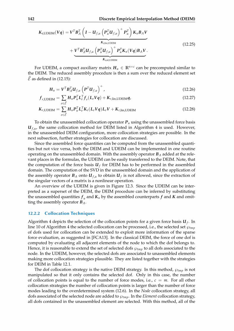
142 Discrete Empirical Interpolation Method (DEIM)
Kr,UDEIM(Vq) =V TBTA
(I −U f ,u
(PT
u U f ,u
)+PT
u
)KuBAV
︸ ︷︷ ︸Kr,lin,UDEIM
+ V TBTAU f ,u
(PT
u U f ,u
)+PT
u Ku(Vq)BAV︸ ︷︷ ︸
Kr,nl,UDEIM
.(12.25)
For UDEIM, a compact auxiliary matrix Hu ∈ Rn×c can be precomputed similar tothe DEIM. The reduced assembly procedure is then a sum over the reduced element setE as defined in (12.15):
Hu = V TBTAU f ,u
(PTU f ,u
)+, (12.26)
f r,UDEIM = ∑e∈E
HuPTu LT
e f e(LeVq) + Kr,lin,UDEIMq, (12.27)
Kr,UDEIM = ∑e∈E
HuPTu LT
e Ke(LeVq)LeV + Kr,lin,UDEIM (12.28)
To obtain the unassembled collocation operator Pu using the unassembled force basisU f ,u, the same collocation method for DEIM listed in Algorithm 4 is used. However,in the unassembled DEIM configuration, more collocation strategies are possible. In thenext subsection, further strategies for collocation are discussed.
Since the assembled force quantities can be computed from the unassembled quanti-ties but not vice versa, both the DEIM and UDEIM can be implemented in one routineoperating on the unassembled domain. With the assembly operator BA added at the rele-vant places in the formulas, the UDEIM can be easily transferred to the DEIM. Note, thatthe computation of the force basis U f for DEIM has to be performed in the assembleddomain. The computation of the SVD in the unassembled domain and the application ofthe assembly operator BA onto U f ,u to obtain U f is not allowed, since the extraction ofthe singular vectors of a matrix is a nonlinear operation.
An overview of the UDEIM is given in Figure 12.3. Since the UDEIM can be inter-preted as a superset of the DEIM, the DEIM procedure can be inferred by substitutingthe unassembled quantities f u and Ku by the assembled counterparts f and K and omit-ting the assembly operator BA.
12.2.2 Collocation Techniques
Algorithm 4 depicts the selection of the collocation points for a given force basis U f . Inline 10 of Algorithm 4 the selected collocation can be processed, i.e., the selected set ℘tmpof dofs used for collocation can be extended to exploit more information of the sparseforce evaluation, as suggested in [FCA13]. In the classical DEIM, the force of one dof iscomputed by evaluating all adjacent elements of the node to which the dof belongs to.Hence, it is reasonable to extend the set of selected dofs ℘tmp to all dofs associated to thenode. In the UDEIM, however, the selected dofs are associated to unassembled elementsmaking more collocation strategies plausible. They are listed together with the strategiesfor DEIM in Table 12.1.
The dof collocation strategy is the native DEIM strategy. In this method, ℘tmp is notmanipulated so that it only contains the selected dof. Only in this case, the numberof collocation points is equal to the number of force modes, i.e., c = m. For all othercollocation strategies the number of collocation points is larger than the number of forcemodes leading to the overdetermined system (12.6). In the Node collocation strategy, alldofs associated of the selected node are added to ℘tmp. In the Element collocation strategy,all dofs contained in the unassembled element are selected. With this method, all of the
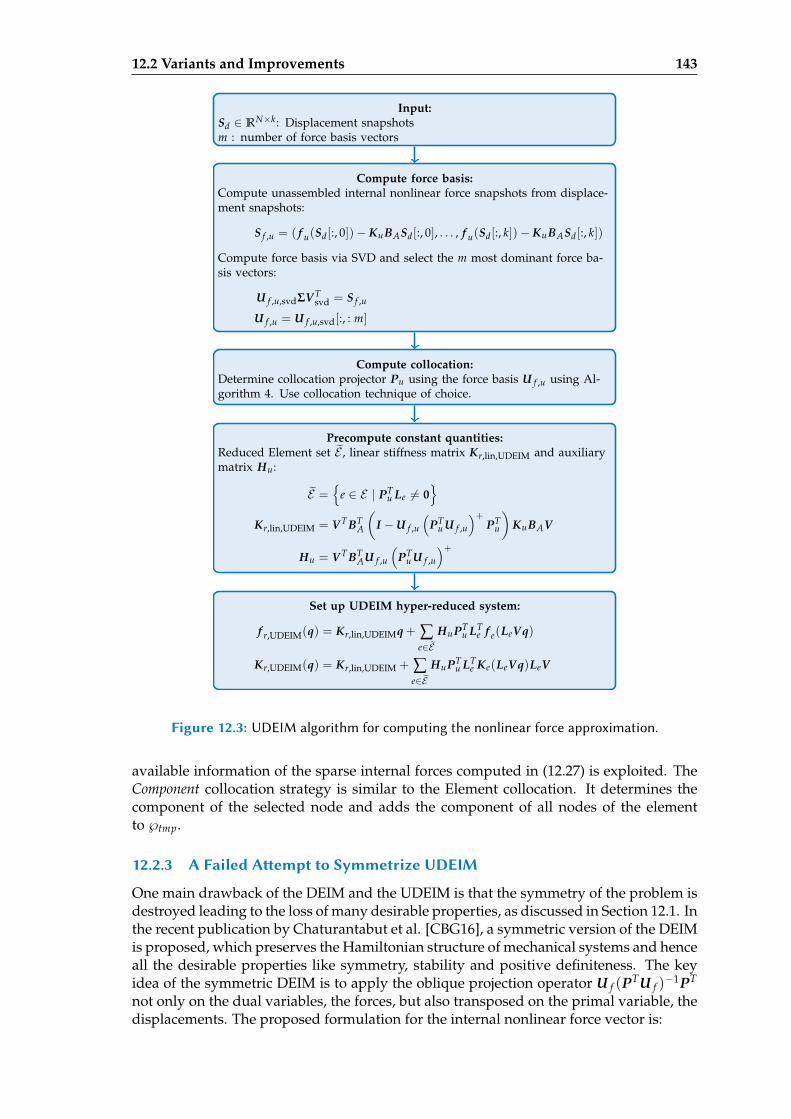
12.2 Variants and Improvements 143
Input:Sd ∈ RN×k: Displacement snapshotsm : number of force basis vectors
Compute force basis:Compute unassembled internal nonlinear force snapshots from displace-ment snapshots:
S f ,u = ( f u(Sd[:, 0])− KuBASd[:, 0], . . . , f u(Sd[:, k])− KuBASd[:, k])
Compute force basis via SVD and select the m most dominant force ba-sis vectors:
U f ,u,svdΣV Tsvd = S f ,u
U f ,u = U f ,u,svd[:, : m]
Compute collocation:Determine collocation projector Pu using the force basis U f ,u using Al-gorithm 4. Use collocation technique of choice.
Precompute constant quantities:Reduced Element set E , linear stiffness matrix Kr,lin,UDEIM and auxiliarymatrix Hu:
E =
e ∈ E | PTu Le 6= 0
Kr,lin,UDEIM = V T BTA
(I −U f ,u
(PT
u U f ,u
)+PT
u
)KuBAV
Hu = V T BTAU f ,u
(PT
u U f ,u
)+
Set up UDEIM hyper-reduced system:
f r,UDEIM(q) = Kr,lin,UDEIMq + ∑e∈E
HuPTu LT
e f e(LeVq)
Kr,UDEIM(q) = Kr,lin,UDEIM + ∑e∈E
HuPTu LT
e Ke(LeVq)LeV
Figure 12.3: UDEIM algorithm for computing the nonlinear force approximation.
available information of the sparse internal forces computed in (12.27) is exploited. TheComponent collocation strategy is similar to the Element collocation. It determines thecomponent of the selected node and adds the component of all nodes of the elementto ℘tmp.
12.2.3 A Failed Aempt to Symmetrize UDEIM
One main drawback of the DEIM and the UDEIM is that the symmetry of the problem isdestroyed leading to the loss of many desirable properties, as discussed in Section 12.1. Inthe recent publication by Chaturantabut et al. [CBG16], a symmetric version of the DEIMis proposed, which preserves the Hamiltonian structure of mechanical systems and henceall the desirable properties like symmetry, stability and positive definiteness. The keyidea of the symmetric DEIM is to apply the oblique projection operator U f (PTU f )
−1PT
not only on the dual variables, the forces, but also transposed on the primal variable, thedisplacements. The proposed formulation for the internal nonlinear force vector is:
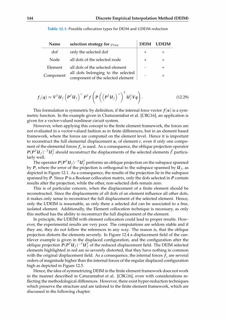
144 Discrete Empirical Interpolation Method (DEIM)
Table 12.1: Possible collocation types for DEIM and UDEIM reduction
Name selection strategy for ℘tmp DEIM UDEIM
dof only the selected dof + +
Node all dofs of the selected node + +
Element all dofs of the selected element - +
Componentall dofs belonging to the selectedcomponent of the selected element - +
f r(q) ≈ V TU f
(PTU f
)+PT f
(P((
PTU f
)+)T
UTf Vq
). (12.29)
This formulation is symmetric by definition, if the internal force vector f (u) is a sym-metric function. In the example given in Chaturantabut et al. [CBG16], an application isgiven for a vector-valued nonlinear circuit system.
However, when applying this concept to the finite element framework, the forces arenot evaluated in a vector-valued fashion as in finite differences, but in an element basedframework, where the forces are computed on the element level. Hence it is importantto reconstruct the full elemental displacement ue of element e, even if only one compo-nent of the elemental forces f e is used. As a consequence, the oblique projection operatorP(PTU f )
−TUTf should reconstruct the displacements of the selected elements E particu-
larly well.The operator P(PTU f )
−TUTf performs an oblique projection on the subspace spanned
by P, where the error of the projection is orthogonal to the subspace spanned by U f , asdepicted in Figure 12.1. As a consequence, the results of the projection lie in the subspacespanned by P. Since P is a Boolean collocation matrix, only the dofs selected in P containresults after the projection, while the other, non-selected dofs remain zero.
This is of particular concern, when the displacement of a finite element should bereconstructed. Since the displacements of all dofs of an element influence all other dofs,it makes only sense to reconstruct the full displacement of the selected element. Hence,only the UDEIM is reasonable, as only there a selected dof can be associated to a free,isolated element. Additionally, the Element collocation technique is necessary, as onlythis method has the ability to reconstruct the full displacement of the element.
In principle, the UDEIM with element collocation could lead to proper results. How-ever, the experimental results are very poor. The computations are seldom stable and ifthey are, they do not follow the references in any way. The reason is, that the obliqueprojection distorts the elements severely. In Figure 12.4 a displacement field of the can-tilever example is given in the displaced configuration, and the configuration after theoblique projection P(PTU f )
−TUTf of the reduced displacement field. The DEIM selected
elements highlighted in red are so severely distorted, that they have nothing in commonwith the original displacement field. As a consequence, the internal forces f r are severalorders of magnitude higher than the internal forces of the regular displaced configurationhigh as depicted in Figure 12.5.
Hence, the idea of symmetrizing DEIM in the finite element framework does not workin the manner described in Caturantabut et al. [CBG16], even with considerations re-flecting the methodological differences. However, there exist hyper-reduction techniqueswhich preserve the structure and are tailored to the finite element framework, which arediscussed in the following chapter.
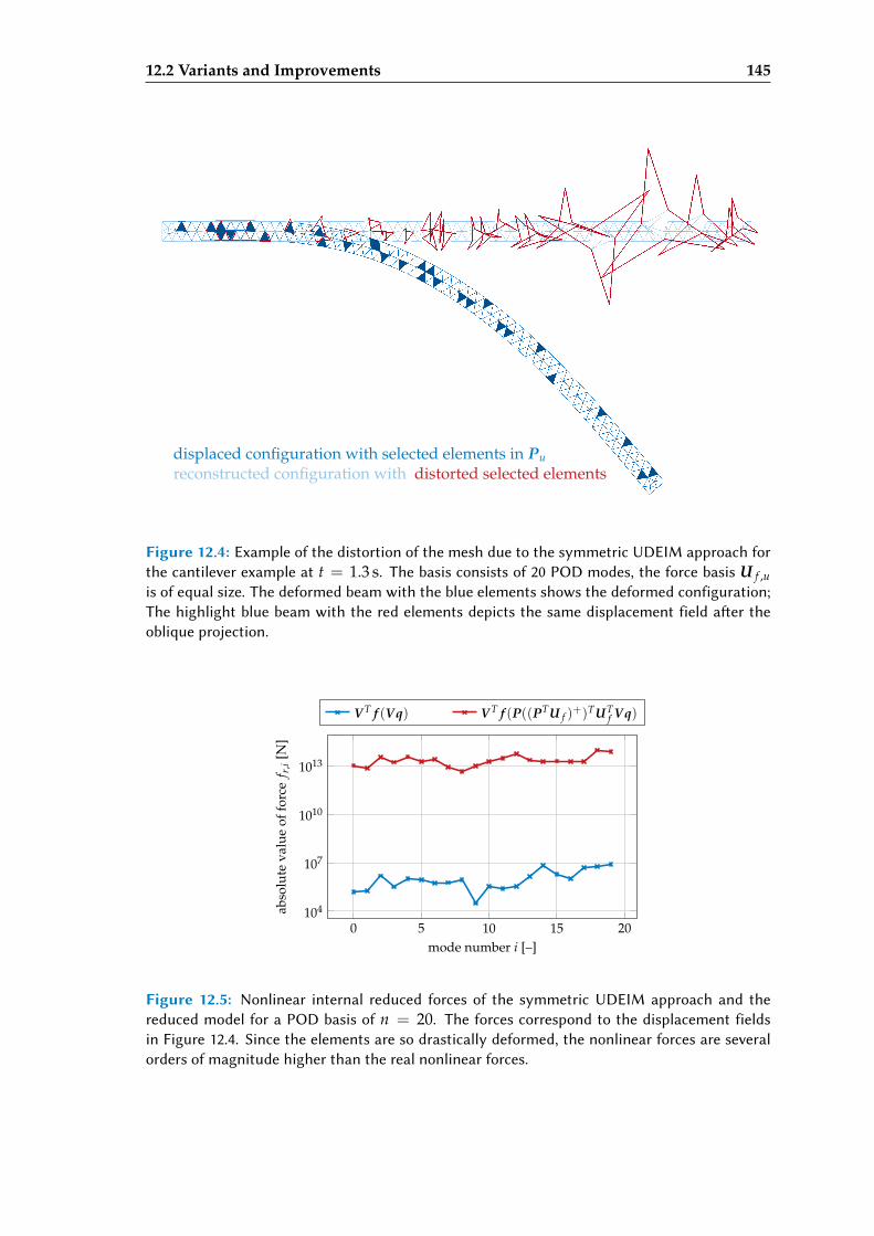
12.2 Variants and Improvements 145
displaced configuration with selected elements in Pureconstructed configuration with distorted selected elements
Figure 12.4: Example of the distortion of the mesh due to the symmetric UDEIM approach forthe cantilever example at t = 1.3 s. The basis consists of 20 POD modes, the force basis U f ,uis of equal size. The deformed beam with the blue elements shows the deformed configuration;The highlight blue beam with the red elements depicts the same displacement field aer theoblique projection.
0 5 10 15 20104
107
1010
1013
mode number i [–]
abso
lute
valu
eof
forc
ef r
,i[N
]
V T f (Vq) V T f (P((PTU f )+)TUT
f Vq)
Figure 12.5: Nonlinear internal reduced forces of the symmetric UDEIM approach and thereduced model for a POD basis of n = 20. The forces correspond to the displacement fieldsin Figure 12.4. Since the elements are so drastically deformed, the nonlinear forces are severalorders of magnitude higher than the real nonlinear forces.
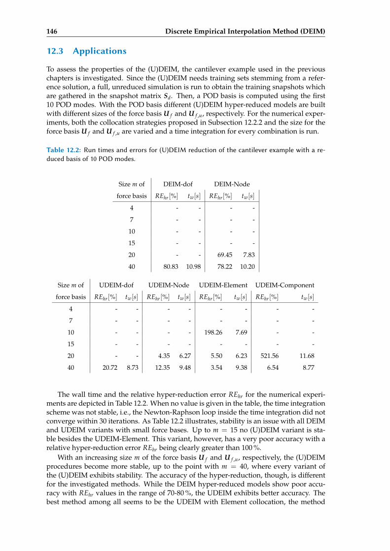
146 Discrete Empirical Interpolation Method (DEIM)
12.3 Applications
To assess the properties of the (U)DEIM, the cantilever example used in the previouschapters is investigated. Since the (U)DEIM needs training sets stemming from a refer-ence solution, a full, unreduced simulation is run to obtain the training snapshots whichare gathered in the snapshot matrix Sd. Then, a POD basis is computed using the first10 POD modes. With the POD basis different (U)DEIM hyper-reduced models are builtwith different sizes of the force basis U f and U f ,u, respectively. For the numerical exper-iments, both the collocation strategies proposed in Subsection 12.2.2 and the size for theforce basis U f and U f ,u are varied and a time integration for every combination is run.
Table 12.2: Run times and errors for (U)DEIM reduction of the cantilever example with a re-duced basis of 10 POD modes.
Size m of DEIM-dof DEIM-Node
force basis REhr[%] tw[s] REhr[%] tw[s]
4 - - - -
7 - - - -
10 - - - -
15 - - - -
20 - - 69.45 7.83
40 80.83 10.98 78.22 10.20
Size m of UDEIM-dof UDEIM-Node UDEIM-Element UDEIM-Component
force basis REhr[%] tw[s] REhr[%] tw[s] REhr[%] tw[s] REhr[%] tw[s]
4 - - - - - - - -
7 - - - - - - - -
10 - - - - 198.26 7.69 - -
15 - - - - - - - -
20 - - 4.35 6.27 5.50 6.23 521.56 11.68
40 20.72 8.73 12.35 9.48 3.54 9.38 6.54 8.77
The wall time and the relative hyper-reduction error REhr for the numerical experi-ments are depicted in Table 12.2. When no value is given in the table, the time integrationscheme was not stable, i.e., the Newton-Raphson loop inside the time integration did notconverge within 30 iterations. As Table 12.2 illustrates, stability is an issue with all DEIMand UDEIM variants with small force bases. Up to m = 15 no (U)DEIM variant is sta-ble besides the UDEIM-Element. This variant, however, has a very poor accuracy with arelative hyper-reduction error REhr being clearly greater than 100 %.
With an increasing size m of the force basis U f and U f ,u, respectively, the (U)DEIMprocedures become more stable, up to the point with m = 40, where every variant ofthe (U)DEIM exhibits stability. The accuracy of the hyper-reduction, though, is differentfor the investigated methods. While the DEIM hyper-reduced models show poor accu-racy with REhr values in the range of 70-80 %, the UDEIM exhibits better accuracy. Thebest method among all seems to be the UDEIM with Element collocation, the method
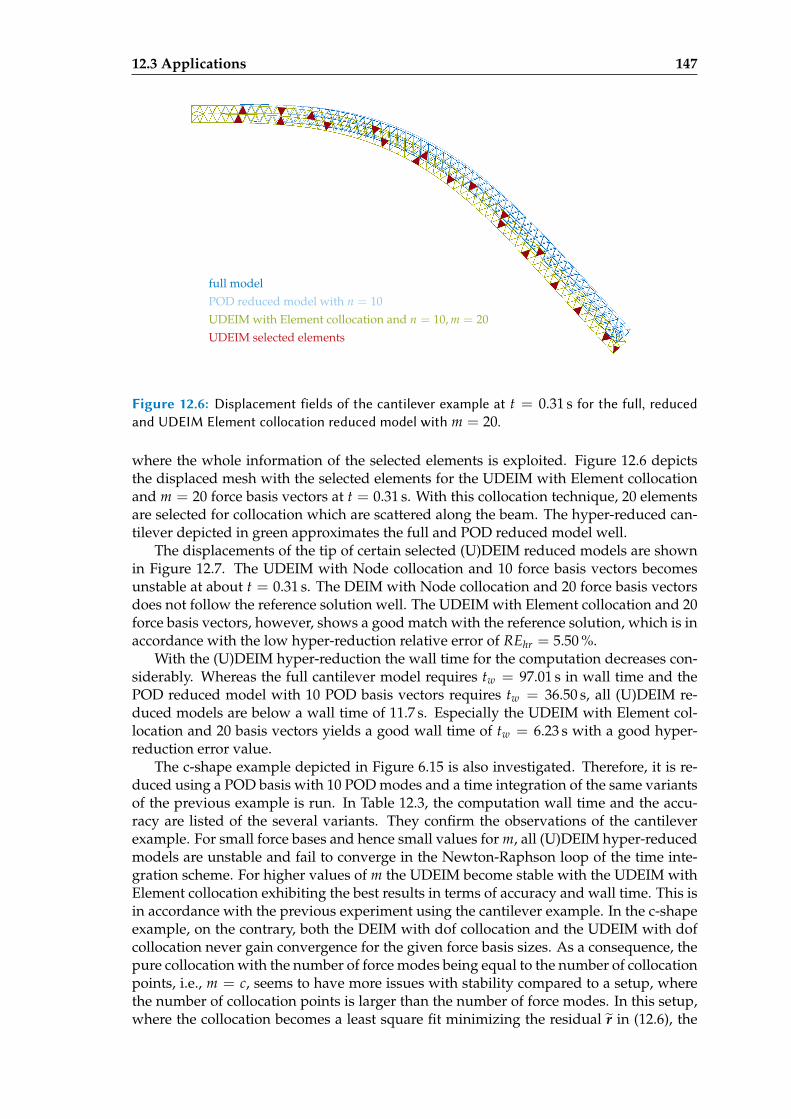
12.3 Applications 147
full modelPOD reduced model with n = 10UDEIM with Element collocation and n = 10, m = 20UDEIM selected elements
Figure 12.6: Displacement fields of the cantilever example at t = 0.31 s for the full, reducedand UDEIM Element collocation reduced model with m = 20.
where the whole information of the selected elements is exploited. Figure 12.6 depictsthe displaced mesh with the selected elements for the UDEIM with Element collocationand m = 20 force basis vectors at t = 0.31 s. With this collocation technique, 20 elementsare selected for collocation which are scattered along the beam. The hyper-reduced can-tilever depicted in green approximates the full and POD reduced model well.
The displacements of the tip of certain selected (U)DEIM reduced models are shownin Figure 12.7. The UDEIM with Node collocation and 10 force basis vectors becomesunstable at about t = 0.31 s. The DEIM with Node collocation and 20 force basis vectorsdoes not follow the reference solution well. The UDEIM with Element collocation and 20force basis vectors, however, shows a good match with the reference solution, which is inaccordance with the low hyper-reduction relative error of REhr = 5.50 %.
With the (U)DEIM hyper-reduction the wall time for the computation decreases con-siderably. Whereas the full cantilever model requires tw = 97.01 s in wall time and thePOD reduced model with 10 POD basis vectors requires tw = 36.50 s, all (U)DEIM re-duced models are below a wall time of 11.7 s. Especially the UDEIM with Element col-location and 20 basis vectors yields a good wall time of tw = 6.23 s with a good hyper-reduction error value.
The c-shape example depicted in Figure 6.15 is also investigated. Therefore, it is re-duced using a POD basis with 10 POD modes and a time integration of the same variantsof the previous example is run. In Table 12.3, the computation wall time and the accu-racy are listed of the several variants. They confirm the observations of the cantileverexample. For small force bases and hence small values for m, all (U)DEIM hyper-reducedmodels are unstable and fail to converge in the Newton-Raphson loop of the time inte-gration scheme. For higher values of m the UDEIM become stable with the UDEIM withElement collocation exhibiting the best results in terms of accuracy and wall time. This isin accordance with the previous experiment using the cantilever example. In the c-shapeexample, on the contrary, both the DEIM with dof collocation and the UDEIM with dofcollocation never gain convergence for the given force basis sizes. As a consequence, thepure collocation with the number of force modes being equal to the number of collocationpoints, i.e., m = c, seems to have more issues with stability compared to a setup, wherethe number of collocation points is larger than the number of force modes. In this setup,where the collocation becomes a least square fit minimizing the residual r in (12.6), the
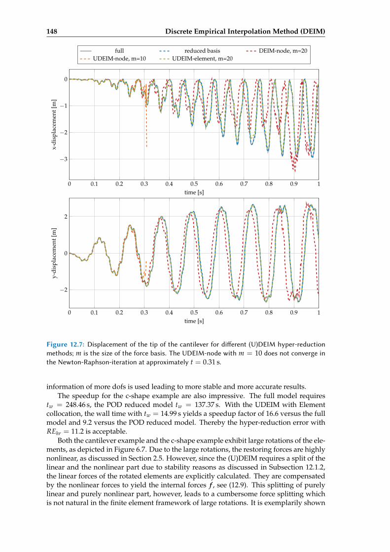
148 Discrete Empirical Interpolation Method (DEIM)
0 0.1 0.2 0.3 0.4 0.5 0.6 0.7 0.8 0.9 1
−3
−2
−1
0
time [s]
x-di
spla
cem
ent[
m]
full reduced basis DEIM-node, m=20UDEIM-node, m=10 UDEIM-element, m=20
0 0.1 0.2 0.3 0.4 0.5 0.6 0.7 0.8 0.9 1
−2
0
2
time [s]
y-di
spla
cem
ent[
m]
Figure 12.7: Displacement of the tip of the cantilever for dierent (U)DEIM hyper-reductionmethods; m is the size of the force basis. The UDEIM-node with m = 10 does not converge inthe Newton-Raphson-iteration at approximately t = 0.31 s.
information of more dofs is used leading to more stable and more accurate results.The speedup for the c-shape example are also impressive. The full model requires
tw = 248.46 s, the POD reduced model tw = 137.37 s. With the UDEIM with Elementcollocation, the wall time with tw = 14.99 s yields a speedup factor of 16.6 versus the fullmodel and 9.2 versus the POD reduced model. Thereby the hyper-reduction error withREhr = 11.2 is acceptable.
Both the cantilever example and the c-shape example exhibit large rotations of the ele-ments, as depicted in Figure 6.7. Due to the large rotations, the restoring forces are highlynonlinear, as discussed in Section 2.5. However, since the (U)DEIM requires a split of thelinear and the nonlinear part due to stability reasons as discussed in Subsection 12.1.2,the linear forces of the rotated elements are explicitly calculated. They are compensatedby the nonlinear forces to yield the internal forces f , see (12.9). This splitting of purelylinear and purely nonlinear part, however, leads to a cumbersome force splitting whichis not natural in the finite element framework of large rotations. It is exemplarily shown
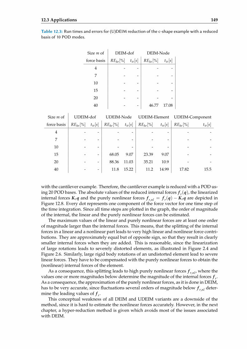
12.3 Applications 149
Table 12.3: Run times and errors for (U)DEIM reduction of the c-shape example with a reducedbasis of 10 POD modes.
Size m of DEIM-dof DEIM-Node
force basis REhr[%] tw[s] REhr[%] tw[s]
4 - - - -
7 - - - -
10 - - - -
15 - - - -
20 - - - -
40 - - 46.77 17.08
Size m of UDEIM-dof UDEIM-Node UDEIM-Element UDEIM-Component
force basis REhr[%] tw[s] REhr[%] tw[s] REhr[%] tw[s] REhr[%] tw[s]
4 - - - - - - - -
7 - - - - - - - -
10 - - - - - - - -
15 - - 68.05 9.07 23.39 9.07 - -
20 - - 88.36 11.03 35.21 10.9 - -
40 - - 11.8 15.22 11.2 14.99 17.82 15.5
with the cantilever example. Therefore, the cantilever example is reduced with a POD us-ing 20 POD bases. The absolute values of the reduced internal forces f r(q), the linearizedinternal forces Krq and the purely nonlinear forces f r,nl = f r(q) − Krq are depicted inFigure 12.8. Every dot represents one component of the force vector for one time step ofthe time integration. Since all time steps are plotted in the graph, the order of magnitudeof the internal, the linear and the purely nonlinear forces can be estimated.
The maximum values of the linear and purely nonlinear forces are at least one orderof magnitude larger than the internal forces. This means, that the splitting of the internalforces in a linear and a nonlinear part leads to very high linear and nonlinear force contri-butions. They are approximately equal but of opposite sign, so that they result in clearlysmaller internal forces when they are added. This is reasonable, since the linearizationof large rotations leads to severely distorted elements, as illustrated in Figure 2.4 andFigure 2.6. Similarly, large rigid body rotations of an undistorted element lead to severelinear forces. They have to be compensated with the purely nonlinear forces to obtain the(nonlinear) internal forces of the element.
As a consequence, this splitting leads to high purely nonlinear forces f r,nl , where thevalues one or more magnitudes below determine the magnitude of the internal forces f r.As a consequence, the approximation of the purely nonlinear forces, as it is done in DEIM,has to be very accurate, since fluctuations several orders of magnitude below f r,nl deter-mine the leading values of f r.
This conceptual weakness of all DEIM and UDEIM variants are a downside of themethod, since it is hard to estimate the nonlinear forces accurately. However, in the nextchapter, a hyper-reduction method is given which avoids most of the issues associatedwith DEIM.
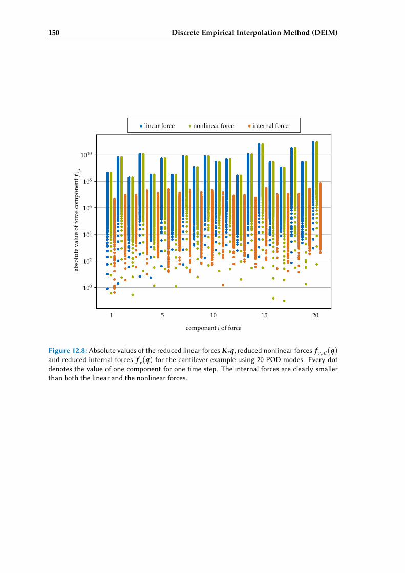
150 Discrete Empirical Interpolation Method (DEIM)
1010
100
102
104
106
108
• linear force • nonlinear force • internal force
abso
lute
valu
eof
forc
eco
mpo
nent
f r,i
component i of force
1 5 10 15 20
Figure 12.8: Absolute values of the reduced linear forces Krq, reduced nonlinear forces f r,nl(q)and reduced internal forces f r(q) for the cantilever example using 20 POD modes. Every dotdenotes the value of one component for one time step. The internal forces are clearly smallerthan both the linear and the nonlinear forces.
Chapter 13
Energy Conserving Mesh Sampling and Weight-ing (ECSW)
The hyper-reduction methods considered in the previous two chapters have two differentstrategies. The polynomial hyper-reduction in Chapter 11 exploits the polynomial struc-ture of the nonlinear finite element system and expands it using tensors. The computa-tional speedup comes from the fact, that the internal forces can be computed faster usingpolynomial arrays than evaluating every element in the mesh, when the reduced basisis small enough. The DEIM hyper-reduction introduced in Chapter 12 approximates theinternal forces of the high dimensional model by reducing the number of elements in theassembly routine. The computational speedup is due to the reduced mesh, i.e., the non-linear internal forces are computed by evaluating only a few elements and not the fullmesh of the high dimensional model. However, this method does not guarantee stabil-ity, since the symmetry is broken due to the approximation strategy based on collocationusing an empirical force basis.
In this chapter, the ECSW hyper-reduction method is discussed. The speedup is alsorealized by reducing the mesh and hence reducing the number of elements to be called.However, this method does not approximate the internal forces in the high dimensionalphysical space and project them onto the reduced basis afterwards as the DEIM does, butcomputes the approximation of the reduced forces directly. Within this strategy, the de-sired properties like symmetry, stability and the existence of an underlying Lagrangianenergy function are preserved. As a consequence, this method is among the most promis-ing hyper-reduction methods in the finite element framework.
The ECSW method was first proposed by An et al. [AKJ08] in the context of com-puter graphics. It has been adapted to engineering applications by Farhat et al. [Far+14;FCA15], where the method is applied to structural dynamics problems using POD bases.Chapman et al. [Cha+17] investigate techniques to speed up the offline costs associatedwith the solution of the non-negative least square problem, which is the core operation ofthe ECSW method. Hernandez et al. [HCF17] propose a variation of the ECSW method,in which the nonlinearity is not selectively evaluated on the element level but on theGauss point level.
Besides the ECSW, a structure preserving hyper-reduction method has been proposedby Carlberg [CTB15]. This method is based on the Gauss-Newton with ApproximatedTensors (GNAT) method, see Carlberg et al. [CBF11], however with an adaptation to theGalerkin projection allowing for the preservation of the structure. Since it does not enjoythe simplicity of the ECSW in the finite element context, it is not further discussed in thisthesis.
The ECSW needs training sets for the computation of the reduced mesh similar tothe DEIM. When the reduced basis is computed using simulation-based methods like thePOD, these training sets are commonly the snapshots of the high dimensional model.
151
152 Energy Conserving Mesh Sampling and Weighting (ECSW)
However, when a simulation-free reduced basis is used, the training snapshots of the fullmodel are not available. Alternative computations of training sets are proposed in thischapter, after the ECSW is outlined. Parts of this chapter are based on the publication[RR17].
13.1 Key Idea: Reduced adrature
The ECSW can be seen as a reduced cubature method which preserves the virtual work ofthe reduced forces for a set of training snapshots. The virtual work done by the reducedinternal forces is given as
δW f ,r = ∑e∈E
δqTV T LTe f e(LeVq). (13.1)
The ECSW is seeking to find an approximation δW f ,r for δW f ,r with a sum over asmaller number of elements. In order to match the energy of the full system and to ensurepositiveness, the virtual work of every element is weighted by a weighting factor ξe ≥ 0,similar to a weighting factor of a quadrature method (cf. (2.28)). The approximatedvirtual work is then written as
δW f ,r = ∑e∈E
ξeδqTV T LTe f e(LeVq), (13.2)
with the reduced set of elements E containing all elements with a nonzero positive weight-ing factor ξe. The balance of virtual work δW f ,r and approximated virtual work δW f ,r isenforced for a set of m reduced training displacements qt,i. To cast the balance in a matrix-vector problem, one can collect the summands of (13.2) in the matrix Υ ∈ Rn·m×|E| andthe weights ξe in ξ ∈ R|E | with |E | being the number of elements in the element set E . Asthe virtual displacements δq are arbitrary, the balance of approximated virtual work andthe virtual work of the full system is written as:
Υξ = b, (13.3)
Υ =
V T LT1 f 1(L1Vqt,1) . . . V T LT
|E | f |E |(L|E |Vqt,1)...
. . ....
V T LT1 f 1(L1Vqt,m) . . . V T LT
|E | f |E |(L|E |Vqt,m)
, (13.4)
b =
∑e∈E
V T LTe f e(LeVqt,1)
...∑
e∈EV T LT
e f e(LeVqt,m)
. (13.5)
The equation above is fulfilled exactly for ξ = (1, . . . , 1)T; this translates (13.2) to (13.1)with E = E and means that every element is contained in the reduced set and weightedwith one. In order to achieve a reduction, one tries to find a sparse weighting vector ξ?
with as many zero entries as possible fulfilling (13.3) up to a tolerance τ. Furthermore,all entries of ξ? have to be positive in order to guarantee the positive definiteness of thevirtual work of the nonlinear forces. The problem to solve is stated as
arg min #(i | ξ?i 6= 0) subject to ||Υξ? − b||2 ≤ τ||b||2 and ξ? ≥ 0. (13.6)
This optimization problem is NP-hard to solve, meaning that a solution cannot besought in polynomial time. However, an approximate solution for ξ? can be computed
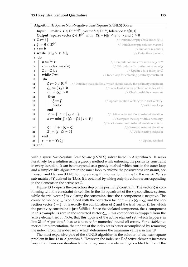
13.1 Key Idea: Reduced Quadrature 153
Algorithm 5: Sparse Non-Negative Least Square (sNNLS) Solver
Input : matrix Υ ∈ Rn·m×|E|, vector b ∈ Rn·m, tolerance τ ∈]0, 1[Output : sparse vector ξ ∈ R|E | with ||Υξ − b||2 ≤ τ||b||2 and ξ ≥ 0
1 I := // Initialize empty active index set I2 ξ := 0 ∈ R|E | // Initialize empty solution vector ξ
3 r := b // Initialize residual r4 while ||r||2 > τ||b||2 // Outer iteration loop5 do6 µ := ΥTr // Compute column error measure µ of Υ
7 i := index max(µ) // Pick index with maximum value of µ
8 I := I ∪ i // Update active index set I9 while True // Inner loop for enforcing positivity constraint
10 do11 ζ := 0 ∈ R|E | // Initialize trial solution ζ which should satisfy the positivity constraint12 ζI := (ΥI )+b // Solve least squares problem on index set I13 if min(ζ) > 0 // Check positivity constraint14 then15 ξ := ζ // Update solution vector ξ with trial vector ζ
16 break // exit inner loop
17 end18 V := i ∈ I | ζi < 0 // Define index set V of constraint violation
19 α := minξi/(ξi − ζi) | i ∈ V // Compute the step width α necessary// to set maximum constraint violation to zero.
20 ξ := ξ + α(ζ − ξ) // Correct constraint violation21 I := i | ξi 6= 0 // Update active index set
22 end23 r := b− ΥIξI // Update residual
24 end
with a sparse Non-Negative Least Square (sNNLS) solver listed in Algorithm 5. It seeksiteratively for a solution using a greedy method while enforcing the positivity constraintin every iteration. It can be interpreted as a greedy method which runs in the outer loopand a simplex-like algorithm in the inner loop to enforce the positiveness constraint, seeLawson and Hanson [LH95] for more in-depth information. In line 19, the matrix ΥI is asub-matrix of Υ defined in (13.4). It is obtained by taking only the columns correspondingto the elements in the active set I .
Figure 13.1 depicts the correction step of the positivity constraint. The vector ξ is con-forming with the constraint since it lies in the first quadrant of the x-y coordinate system,while the trial vector ζ is violating the constraint, since the x-component is negative. Thecorrected vector ξcorr is obtained with the correction factor α = ξi/(ξi − ζi) and the cor-rection vector ζ − ξ. It is exactly the combination of ξ and the trial vector ζ, for whichthe positivity constraint is just fulfilled. Since the violated component, the x-componentin this example, is zero in the corrected vector ξcorr, this component is dropped from theactive element set I . Note, that this update of the active element set, which happens inline 21 of Algorithm 5, has to take care for numerical round off errors. For a stable nu-merical implementation, the update of the index set is better accomplished by removingthe index i from the index set I which determines the minimum value α in line 19.
The most expensive part of the sNNLS algorithm is the solution of the least-squareproblem in line 12 in Algorithm 5. However, the index set I of active elements increasesvery often from one iteration to the other, since one element gets added to it and the
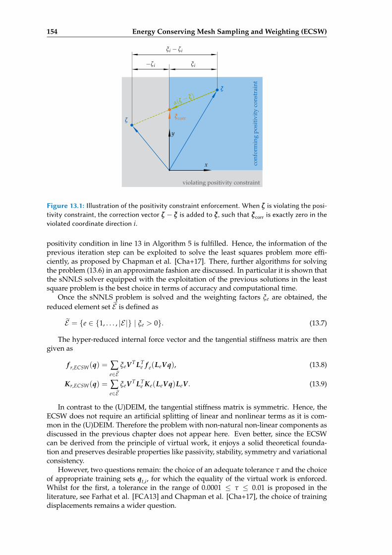
154 Energy Conserving Mesh Sampling and Weighting (ECSW)
conf
orm
ing
posi
tivi
tyco
nstr
aint
violating positivity constraint
ξ
ζξcorr
ξi−ζi
ξi − ζi
α(ζ− ξ)
x
y
Figure 13.1: Illustration of the positivity constraint enforcement. When ζ is violating the posi-tivity constraint, the correction vector ζ − ξ is added to ξ, such that ξcorr is exactly zero in theviolated coordinate direction i.
positivity condition in line 13 in Algorithm 5 is fulfilled. Hence, the information of theprevious iteration step can be exploited to solve the least squares problem more effi-ciently, as proposed by Chapman et al. [Cha+17]. There, further algorithms for solvingthe problem (13.6) in an approximate fashion are discussed. In particular it is shown thatthe sNNLS solver equipped with the exploitation of the previous solutions in the leastsquare problem is the best choice in terms of accuracy and computational time.
Once the sNNLS problem is solved and the weighting factors ξe are obtained, thereduced element set E is defined as
E = e ∈ 1, . . . , |E | | ξe > 0. (13.7)
The hyper-reduced internal force vector and the tangential stiffness matrix are thengiven as
f r,ECSW(q) = ∑e∈E
ξeV T LTe f e(LeVq), (13.8)
Kr,ECSW(q) = ∑e∈E
ξeV T LTe Ke(LeVq)LeV . (13.9)
In contrast to the (U)DEIM, the tangential stiffness matrix is symmetric. Hence, theECSW does not require an artificial splitting of linear and nonlinear terms as it is com-mon in the (U)DEIM. Therefore the problem with non-natural non-linear components asdiscussed in the previous chapter does not appear here. Even better, since the ECSWcan be derived from the principle of virtual work, it enjoys a solid theoretical founda-tion and preserves desirable properties like passivity, stability, symmetry and variationalconsistency.
However, two questions remain: the choice of an adequate tolerance τ and the choiceof appropriate training sets qt,i, for which the equality of the virtual work is enforced.Whilst for the first, a tolerance in the range of 0.0001 ≤ τ ≤ 0.01 is proposed in theliterature, see Farhat et al. [FCA13] and Chapman et al. [Cha+17], the choice of trainingdisplacements remains a wider question.
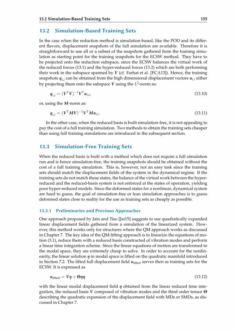
13.2 Simulation-Based Training Sets 155
13.2 Simulation-Based Training Sets
In the case when the reduction method is simulation-based, like the POD and its differ-ent flavors, displacement snapshots of the full simulation are available. Therefore it isstraightforward to use all or a subset of the snapshots gathered from the training simu-lation as starting point for the training snapshots for the ECSW method. They have tobe projected onto the reduction subspace, since the ECSW balances the virtual work ofthe reduced forces (13.1) and the hyper-reduced forces (13.2) which are both performingtheir work in the subspace spanned by V (cf. Farhat et al. [FCA13]). Hence, the trainingsnapshots qt,i can be obtained from the high dimensional displacement vectors ut,i eitherby projecting them onto the subspace V using the L2-norm as:
qt,i = (V TV)−1V Tut,i, (13.10)
or, using the M-norm as:
qt,i = (V T MV)−1V T Mut,i. (13.11)
In the other case, when the reduced basis is built simulation-free, it is not appealing topay the cost of a full training simulation. Two methods to obtain the training sets cheaperthan using full training simulations are introduced in the subsequent section.
13.3 Simulation-Free Training Sets
When the reduced basis is built with a method which does not require a full simulationrun and is hence simulation-free, the training snapshots should be obtained without thecost of a full training simulation. This is, however, not an easy task since the trainingsets should match the displacement fields of the system in the dynamical regime. If thetraining sets do not match these states, the balance of the virtual work between the hyper-reduced and the reduced-basis system is not enforced at the states of operation, yieldingpoor hyper-reduced models. Since the deformed states for a nonlinear, dynamical systemare hard to guess, the goal of simulation-free or lean simulation approaches is to guessdeformed states close to reality for the use as training sets as cheaply as possible.
13.3.1 Preliminaries and Previous Approaches
One approach proposed by Jain and Tiso [Jai15] suggests to use quadratically expandedlinear displacement fields gathered from a simulation of the linearized system. How-ever, this method works only for structures where the QM approach works as discussedin Chapter 7. The key idea of the QM-lifting approach is to linearize the equations of mo-tion (3.1), reduce them with a reduced basis constructed of vibration modes and performa linear time integration scheme. Since the linear equations of motion are transformed tothe modal space, they are extremely cheap to solve. In order to account for the nonlin-earity, the linear solution η in modal space is lifted on the quadratic manifold introducedin Section 7.2. The lifted full displacement field ulifted serves then as training sets for theECSW. It is expressed as
ulifted = Vη+ Θηη (13.12)
with the linear modal displacement field η obtained from the linear reduced time inte-gration, the reduced basis V composed of vibration modes and the third order tensor Θ
describing the quadratic expansion of the displacement field with MDs or SMDs, as dis-cussed in Chapter 7.
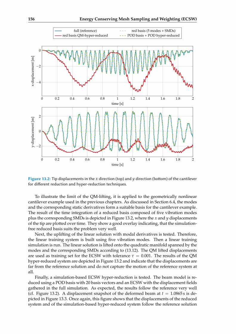
156 Energy Conserving Mesh Sampling and Weighting (ECSW)
0 0.2 0.4 0.6 0.8 1 1.2 1.4 1.6 1.8 2
−4
−2
0
time [s]
x-di
spla
cem
ent[
m]
full (reference) red basis (5 modes + SMDs)red basis QM-hyper-reduced POD basis + POD hyper-reduced
0 0.2 0.4 0.6 0.8 1 1.2 1.4 1.6 1.8 2
−2
0
2
time [s]
y-di
spla
cem
ent[
m]
Figure 13.2: Tip displacements in the x direction (top) and y direction (boom) of the cantileverfor dierent reduction and hyper-reduction techniques.
To illustrate the limit of the QM-lifting, it is applied to the geometrically nonlinearcantilever example used in the previous chapters. As discussed in Section 6.4, the modesand the corresponding static derivatives form a suitable basis for the cantilever example.The result of the time integration of a reduced basis composed of five vibration modesplus the corresponding SMDs is depicted in Figure 13.2, where the x and y displacementsof the tip are plotted over time. They show a good overlay indicating, that the simulation-free reduced basis suits the problem very well.
Next, the uplifting of the linear solution with modal derivatives is tested. Therefore,the linear training system is built using five vibration modes. Then a linear trainingsimulation is run. The linear solution is lifted onto the quadratic manifold spanned by themodes and the corresponding SMDs according to (13.12). The QM lifted displacementsare used as training set for the ECSW with tolerance τ = 0.001. The results of the QMhyper-reduced system are depicted in Figure 13.2 and indicate that the displacements arefar from the reference solution and do not capture the motion of the reference system atall.
Finally, a simulation-based ECSW hyper-reduction is tested. The beam model is re-duced using a POD basis with 20 basis vectors and an ECSW with the displacement fieldsgathered in the full simulation. As expected, the results follow the reference very well(cf. Figure 13.2). A displacement snapshot of the deformed beam at t = 1.0865 s is de-picted in Figure 13.3. Once again, this figure shows that the displacements of the reducedsystem and of the simulation-based hyper-reduced system follow the reference solution
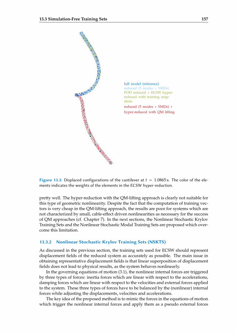
13.3 Simulation-Free Training Sets 157
full model (reference)reduced (5 modes + SMDs)POD reduced + ECSW hyper-reduced with training snap-shotsreduced (5 modes + SMDs) +hyper-reduced with QM lifting
Figure 13.3: Displaced configurations of the cantilever at t = 1.0865 s. The color of the ele-ments indicates the weights of the elements in the ECSW hyper-reduction.
pretty well. The hyper-reduction with the QM-lifting approach is clearly not suitable forthis type of geometric nonlinearity. Despite the fact that the computation of training vec-tors is very cheap in the QM-lifting approach, the results are poor for systems which arenot characterized by small, cable-effect driven nonlinearities as necessary for the successof QM approaches (cf. Chapter 7). In the next sections, the Nonlinear Stochastic KrylovTraining Sets and the Nonlinear Stochastic Modal Training Sets are proposed which over-come this limitation.
13.3.2 Nonlinear Stochastic Krylov Training Sets (NSKTS)
As discussed in the previous section, the training sets used for ECSW should representdisplacement fields of the reduced system as accurately as possible. The main issue inobtaining representative displacement fields is that linear superposition of displacementfields does not lead to physical results, as the system behaves nonlinearly.
In the governing equations of motion (3.1), the nonlinear internal forces are triggeredby three types of forces: inertia forces which are linear with respect to the accelerations,damping forces which are linear with respect to the velocities and external forces appliedto the system. These three types of forces have to be balanced by the (nonlinear) internalforces while adjusting the displacements, velocities and accelerations.
The key idea of the proposed method is to mimic the forces in the equations of motionwhich trigger the nonlinear internal forces and apply them as a pseudo external forces
158 Energy Conserving Mesh Sampling and Weighting (ECSW)
to the nonlinear static system. The triggering forces are linear with respect to the dis-placements and their time derivatives, and can thus be superposed. They are assumed tolive in a Krylov-subspace, which is built to represent the external forces g together withapproximations of the inertia forces Mu. They are mixed using stochastic distributionsin order to obtain multiple training sets of possible pseudo-dynamic force vectors. Thedamping forces are neglected in this method.
In the following, the construction of the Krylov force subspace is spelled out similar tothe Krylov subspace for displacements in Section 4.4. It is based on the linearized systemwithout damping, where K = ∂ f /∂u|u=0 is the linear stiffness matrix for a reference staticequilibrium chosen here as u = 0. The external forces g(t) are assumed to have a time-invariant input location expressed by g ∈ RN and the time dependent amplitude g(t) ∈R, so that g can be represented by g g(t). The linearized equations of motion are
Mu + Ku = g g. (13.13)
The inertia forces Mu are unknown and thus represented by a first order force correc-tion h1. The equation is then written as
h1 + Ku = g g (13.14)
and can be solved for the displacements u:
u = K−1(g g− h1). (13.15)
If the displacements and the second time derivatives are inserted in (13.13), one ob-tains
MK−1(g g− h1) + KK−1(g g− h1) = g g. (13.16)
The second derivative h1 of the correction is unknown and thus dropped from theequation in a first order approximation yielding
h1 = MK−1 g g. (13.17)
As the acceleration of the external forces g g lives in the subspace spanned by g, h1lives in the subspace
h1 ∈ span(MK−1 g). (13.18)
This means that the direction of the unknown inertia forces Mu is approximated inthe first order by h1. The second order approximation can be obtained similarly, if theacceleration term Mu in (13.13) is substituted by the sum of the already known h1 andthe unknown second correction term h2:
h2 + h1 + Ku = g g ↔ u = K−1(g g− h1 − h2) (13.19)
and inserted into the linearized equations of motion (13.13) yielding:
MK−1(g g− h1 − h2) + KK−1(g g− h1 − h2) = g g. (13.20)
Once again, h2 is dropped as it is unknown, MK−1 g g and −h1 cancel out leading tothe second order force expansion
h2 = MK−1(−h1). (13.21)
13.3 Simulation-Free Training Sets 159
As above, h1 lies in the subspace spanned by h1 and thus h2 lies in the subspacespanned by MK−1h1. The Krylov procedure explained above can be conducted p − 1times leading to the Krylov force sequence
Fkry,raw =(
g, h1, h2, . . . , hp−1)=(
g, MK−1 g, (MK−1)2 g, . . . , (MK−1)p−1 g)
,(13.22)
where p moments of the force subspace around frequency zero are matched. The vectorg is the low dimensional subspace in which the external forces g act. In the derivationabove it was chosen to be a one dimensional subspace. However, it could have beenequally derived for higher dimensional subspaces.
The Krylov force subspace is constructed similarly to a Krylov displacement sub-space sequence for linear systems, which matches p moments around frequency zero,as discussed in Section 4.4. However, in this case, the Krylov subspace is not a displace-ment subspace, but a force subspace representing the expansion of the acceleration forces.Likewise, it could have been obtained by multiplying the typical Krylov sequence fordisplacements Vkry =
(K−1 g, . . . , (K−1M)p−1K−1 g
)with K to obtain the corresponding
linear forces of the Krylov displacements.Krylov sequences are usually poorly conditioned, as the vectors tend to become less
linearly independent for higher order corrections (cf. [Str07] and [GR14]). In order toobtain a good basis, an orthogonalization is necessary, as classically performed in anArnoldi procedure or a Lanczos procedure for symmetric systems respectively. Whenperforming these orthogonalization iterations, a suitable norm has to be defined, forwhich the Krylov vectors are made orthogonal.
In the case of the Krylov force subspace, a norm allowing for physical interpretationis desirable. Forces applied to linear systems can be measured according to the work theydo when applied. The work Wg of the forces g applied statically is defined as
Wg =∫
gTdu =∫
gTK−1dg =12
gTK−1 g, (13.23)
as the linear displacements are u = K−1 g. The metric expressed in the static energy offorce vector g is the so-called impedance norm:
|x|K−1 =√
xTK−1x. (13.24)
This norm is chosen for the orthogonalization of the Krylov force sequence (13.22),such that the Krylov force basis is orthogonalized and normalized:
FTkryK−1Fkry = I. (13.25)
With this orthogonalization, every column vector in Fkry ∈ RN×p represents a forcevector that does the same work when applied to the static linear system. Or, from theother perspective, the elastic potential energy stored in the mechanical system is equalfor every force vector applied.
In order to obtain force vectors mimicking the external and dynamic forces of thesystem, all column vectors of Fkry representing the subspace of these forces are amplifiedrandomly. The amplification is cast in the i-th random vector ni ∈ Rp which carriesGaussian distributed random values:
ni(µ, σ) =(N1(µ, σ), . . . ,Np(µ, σ)
)T , (13.26)
with a Gaussian distributed random number N (µ, σ) for a given mean µ and standarddeviation σ. A random force sample f rand,i ∈ RN is then expressed as
160 Energy Conserving Mesh Sampling and Weighting (ECSW)
f rand,i = Fkryni. (13.27)
The training displacements are computed by solving the nonlinear static problem forthe displacements ui caused by the given random force vector. The force is applied in ksteps, for which the load is increased with 1
k -th of f rand,i:
f (ui,l) =lk
f rand,i, with l ∈ [1, . . . , k]. (13.28)
The solution of the nonlinear displacements using a force increment technique leadsto k displacement training snapshots for one stochastic force vector f rand,i. For d randomforce vectors, d · k displacement training snapshots are generated. These training snap-shots are then used as training sets to hyper-reduce a reduced-basis model by setting up(13.4) and solving (13.6) with an appropriate solution strategy.
As hyper-reduction works upon a reduced basis model for a given V (cf. (13.8)), twooptions exist for the computation of NSKTS:
1. compute the NSKTS in the physical, unreduced domain by solving full static prob-lems and project the training snapshots ut afterwards onto the reduced basis using(13.10), and
2. compute the NSKTS in the reduced basis domain of the desired hyper-reducedmodel and obtain the training snapshots qt directly (cf. second block of Figure 13.4).
The first option involves the solution of the nonlinear static problem (13.28) in thehigh dimensional physical domain. As this is a costly procedure, it is desirable to cir-cumvent this costs with the second option where the nonlinear static problem is solvedin the domain of the reduced basis and the matrices to be factorized are of size n insteadof N. Furthermore, it has some additional advantages. First, in the author’s experience,the number of iterations inside the Newton-Raphson loop of the nonlinear static solveris smaller than for option one. Second, the training snapshots are directly computed inthe desired reduced form. Third, the reduced elemental forces are computed and can bestored for setting up the sNNLS problem (13.4). Hence, the second option is favored andthe NSKTS are proposed to be computed in the reduced domain.
An overview of the NSKTS computation procedure is given in Figure 13.4. The am-plitude of the input vector g for the Krylov force subspace has no effect on the NSKTS,as g is scaled to one in the impedance norm. Hence g is evaluated at a random amplitudeto only obtain the direction of g in the physical domain. Furthermore, the coefficientsfor the Gaussian distribution have to be specified. For the examples investigated by theauthor, a Gaussian distribution with mean µ = 0 and with standard deviation σ in therange of the impedance norm of the external forces is used. For practical use, the maxi-mum absolute value of the impedance norm of the external force vector is computed andamplified with a correction factor a:
σ = a|gmax|K−1 . (13.29)
As the external forces are time dependent, gmax is the external force vector for a time,where g has its maximal L2-norm. The correction factor a is to be chosen such that theresulting static displacements ui obtained by (13.28) are in the range of the expected mo-tion of the system. In the author’s practical experience, a should be in the range [0.1, 5],and toward the lower end, if the forces are applied for a short time or at a high frequencyand rather high if they are applied at a low frequency or close to an eigenfrequency ofthe linearized system.
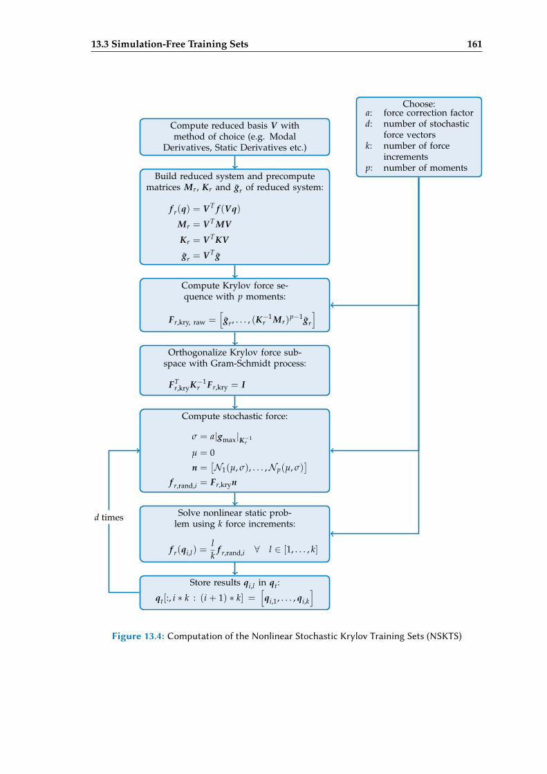
13.3 Simulation-Free Training Sets 161
Compute reduced basis V withmethod of choice (e.g. Modal
Derivatives, Static Derivatives etc.)
Build reduced system and precomputematrices Mr, Kr and gr of reduced system:
f r(q) = V T f (Vq)
Mr = V T MV
Kr = V TKV
gr = V T g
Compute Krylov force se-quence with p moments:
Fr,kry, raw =[
gr, . . . , (K−1r Mr)
p−1 gr
]
Orthogonalize Krylov force sub-space with Gram-Schmidt process:
FTr,kryK−1
r Fr,kry = I
Compute stochastic force:
σ = a|gmax|K−1r
µ = 0
n =[N1(µ, σ), . . . ,Np(µ, σ)
]
f r,rand,i = Fr,kryn
Solve nonlinear static prob-lem using k force increments:
f r(qi,l) =lk
f r,rand,i ∀ l ∈ [1, . . . , k]
Store results qi,l in qt:
qt[:, i ∗ k : (i + 1) ∗ k] =[qi,1, . . . , qi,k
]
Choose:a: force correction factord: number of stochastic
force vectorsk: number of force
incrementsp: number of moments
d times
Figure 13.4: Computation of the Nonlinear Stochastic Krylov Training Sets (NSKTS)
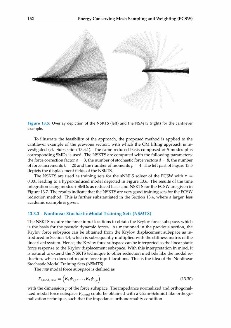
162 Energy Conserving Mesh Sampling and Weighting (ECSW)
Figure 13.5: Overlay depiction of the NSKTS (le) and the NSMTS (right) for the cantileverexample.
To illustrate the feasibility of the approach, the proposed method is applied to thecantilever example of the previous section, with which the QM lifting approach is in-vestigated (cf. Subsection 13.3.1). The same reduced basis composed of 5 modes pluscorresponding SMDs is used. The NSKTS are computed with the following parameters:the force correction factor a = 3, the number of stochastic force vectors d = 8, the numberof force increments k = 20 and the number of moments p = 4. The left part of Figure 13.5depicts the displacement fields of the NSKTS.
The NSKTS are used as training sets for the sNNLS solver of the ECSW with τ =0.001 leading to a hyper-reduced model depicted in Figure 13.6. The results of the timeintegration using modes + SMDs as reduced basis and NSKTS for the ECSW are given inFigure 13.7. The results indicate that the NSKTS are very good training sets for the ECSWreduction method. This is further substantiated in the Section 13.4, where a larger, lessacademic example is given.
13.3.3 Nonlinear Stochastic Modal Training Sets (NSMTS)
The NSKTS require the force input locations to obtain the Krylov force subspace, whichis the basis for the pseudo dynamic forces. As mentioned in the previous section, theKrylov force subspace can be obtained from the Krylov displacement subspace as in-troduced in Section 4.4, which is subsequently multiplied with the stiffness matrix of thelinearized system. Hence, the Krylov force subspace can be interpreted as the linear staticforce response to the Krylov displacement subspace. With this interpretation in mind, itis natural to extend the NSKTS technique to other reduction methods like the modal re-duction, which does not require force input locations. This is the idea of the NonlinearStochastic Modal Training Sets (NSMTS).
The raw modal force subspace is defined as
Fr,mod, raw =(
Krφr,1, . . . , Krφr,p
)(13.30)
with the dimension p of the force subspace. The impedance normalized and orthogonal-ized modal force subspace Fr,mod could be obtained with a Gram-Schmidt like orthogo-nalization technique, such that the impedance orthonormality condition
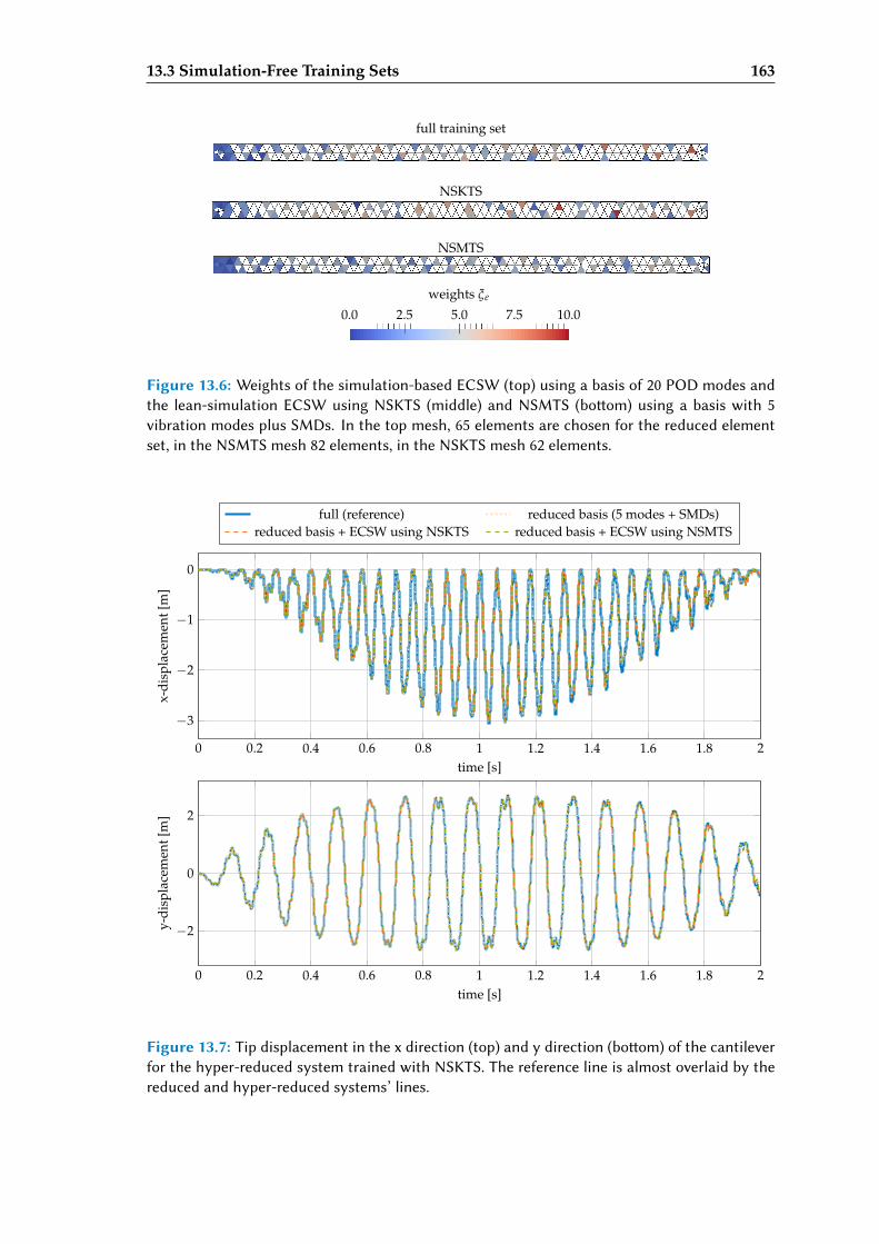
13.3 Simulation-Free Training Sets 163
full training set
NSKTS
NSMTS
weights ξe
0.0 2.5 5.0 7.5 10.0
Figure 13.6: Weights of the simulation-based ECSW (top) using a basis of 20 POD modes andthe lean-simulation ECSW using NSKTS (middle) and NSMTS (boom) using a basis with 5vibration modes plus SMDs. In the top mesh, 65 elements are chosen for the reduced elementset, in the NSMTS mesh 82 elements, in the NSKTS mesh 62 elements.
0 0.2 0.4 0.6 0.8 1 1.2 1.4 1.6 1.8 2
−3
−2
−1
0
time [s]
x-di
spla
cem
ent[
m]
full (reference) reduced basis (5 modes + SMDs)reduced basis + ECSW using NSKTS reduced basis + ECSW using NSMTS
0 0.2 0.4 0.6 0.8 1 1.2 1.4 1.6 1.8 2
−2
0
2
time [s]
y-di
spla
cem
ent[
m]
Figure 13.7: Tip displacement in the x direction (top) and y direction (boom) of the cantileverfor the hyper-reduced system trained with NSKTS. The reference line is almost overlaid by thereduced and hyper-reduced systems’ lines.
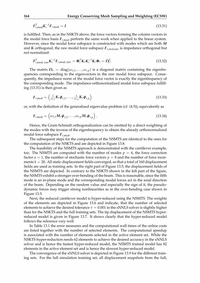
164 Energy Conserving Mesh Sampling and Weighting (ECSW)
FTr,modK−1
r Fr,mod = I (13.31)
is fulfilled. Then, as in the NSKTS above, the force vectors forming the column vectors inthe modal force basis Fr,mod perform the same work when applied to the linear system.However, since the modal force subspace is constructed with modes which are both Mand K orthogonal, the raw modal force subspace Fr,mod,raw is impedance orthogonal butnot normalized:
FTr,mod, rawK−1
r Fr,mod, raw = ΦTr KrK−1
r KrΦr = Ω2r . (13.32)
The matrix Ωr = diag(ωr,1, . . . , ωr,p) is a diagonal matrix containing the eigenfre-quencies corresponding to the eigenvectors in the raw modal force subspace. Conse-quently, the impedance norm of the modal force vector is exactly the eigenfrequency ofthe corresponding mode. The impedance-orthonormalized modal force subspace fulfill-ing (13.31) is then given as
Fr,mod =(
1ωr,1
Krφr,1, . . . , 1ωr,p
Krφr,p
)(13.33)
or, with the definition of the generalized eigenvalue problem (cf. (4.5)), equivalently as
Fr,mod =(
ωr,1Mrφr,1, . . . , ωr,p Mrφr,p
). (13.34)
Hence, the Gram-Schmidt orthogonalization can be omitted by a direct weighting ofthe modes with the inverse of the eigenfrequency to obtain the already orthonormalizedmodal force subspace Fr,mod.
The subsequent steps for the computation of the NSMTS are identical to the ones forthe computation of the NSKTS and are depicted in Figure 13.8.
The feasibility of the NSMTS approach is demonstrated with the cantilever example,too. The NSMTS are computed with the number of modes p = 6, the force correctionfactor a = 1, the number of stochastic force vectors p = 8 and the number of force incre-ments k = 20. All static displacement fields converged, so that a total of 160 displacementfields are used as training sets. In the right part of Figure 13.5, the displacement fields ofthe NSMTS are depicted. In contrary to the NSKTS shown in the left part of the figure,the NSMTS exhibit a stronger over-bending of the beam. This is reasonable, since the fifthmode is an in-plane mode and the corresponding modal forces act in the axial directionof the beam. Depending on the random value and especially the sign of it, the pseudo-dynamic forces may trigger strong nonlinearities as in the over-bending case shown inFigure 13.5.
Next, the reduced cantilever model is hyper-reduced using the NSMTS. The weightsof the elements are depicted in Figure 13.6 and indicate, that the number of selectedelements to achieve the desired tolerance τ = 0.001 in the sNNLS solver is slightly higherthan for the NSKTS and the full training sets. The tip displacement of the NSMTS hyper-reduced model is given in Figure 13.7. It shows clearly that the hyper-reduced modelfollows the reference very well.
In Table 13.1 the error measures and the computational wall times of the online costsare listed together with the number of selected elements. The computational speedupis associated with the number of elements selected in the active element set. While theNSKTS hyper-reduction needs 62 elements to achieve the desired accuracy in the sNNLSsolver and is hence the fastest hyper-reduced model, the NSMTS trained model has 82elements in the active element set and is hence the slowest hyper-reduced model.
The convergence of the sNNLS solver is depicted in Figure 13.9 for the different train-ing sets. For the full simulation training set, all displacement snapshots from the full,
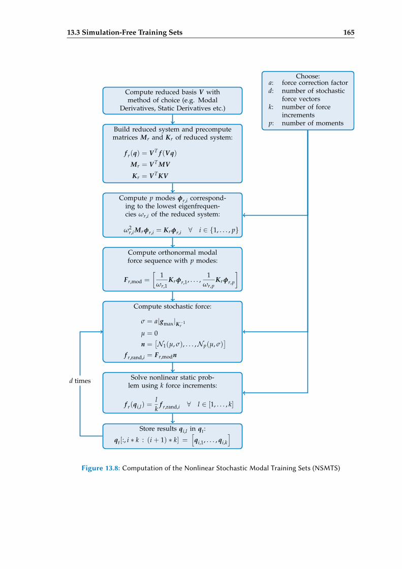
13.3 Simulation-Free Training Sets 165
Compute reduced basis V withmethod of choice (e.g. Modal
Derivatives, Static Derivatives etc.)
Build reduced system and precomputematrices Mr and Kr of reduced system:
f r(q) = V T f (Vq)
Mr = V T MV
Kr = V TKV
Compute p modes φr,i correspond-ing to the lowest eigenfrequen-cies ωr,i of the reduced system:
ω2r,i Mrφr,i = Krφr,i ∀ i ∈ 1, . . . , p
Compute orthonormal modalforce sequence with p modes:
Fr,mod =
[1
ωr,1Krφr,1, . . . ,
1ωr,p
Krφr,p
]
Compute stochastic force:
σ = a|gmax|K−1r
µ = 0
n =[N1(µ, σ), . . . ,Np(µ, σ)
]
f r,rand,i = Fr,modn
Solve nonlinear static prob-lem using k force increments:
f r(qi,l) =lk
f r,rand,i ∀ l ∈ [1, . . . , k]
Store results qi,l in qt:
qt[:, i ∗ k : (i + 1) ∗ k] =[qi,1, . . . , qi,k
]
Choose:a: force correction factord: number of stochastic
force vectorsk: number of force
incrementsp: number of moments
d times
Figure 13.8: Computation of the Nonlinear Stochastic Modal Training Sets (NSMTS)
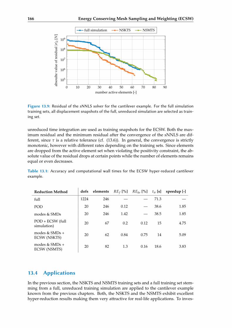
166 Energy Conserving Mesh Sampling and Weighting (ECSW)
0 10 20 30 40 50 60 70 80 90
105
106
107
108
109
number active elements [-]
abso
ulte
valu
eof
resi
dual
|r|2
[N]
full simulation NSKTS NSMTS
Figure 13.9: Residual of the sNNLS solver for the cantilever example. For the full simulationtraining sets, all displacement snapshots of the full, unreduced simulation are selected as train-ing set.
unreduced time integration are used as training snapshots for the ECSW. Both the max-imum residual and the minimum residual after the convergence of the sNNLS are dif-ferent, since τ is a relative tolerance (cf. (13.6)). In general, the convergence is strictlymonotonic, however with different rates depending on the training sets. Since elementsare dropped from the active element set when violating the positivity constraint, the ab-solute value of the residual drops at certain points while the number of elements remainsequal or even decreases.
Table 13.1: Accuracy and computational wall times for the ECSW hyper-reduced cantileverexample.
Reduction Method dofs elements RE f [%] REhr [%] tw [s] speedup [-]
full 1224 246 — — 71.3 —
POD 20 246 0.12 — 38.6 1.85
modes & SMDs 20 246 1.42 — 38.5 1.85
POD + ECSW (fullsimulation)
20 67 0.2 0.12 15 4.75
modes & SMDs +ECSW (NSKTS)
20 62 0.84 0.75 14 5.09
modes & SMDs +ECSW (NSMTS)
20 82 1.3 0.16 18.6 3.83
13.4 Applications
In the previous section, the NSKTS and NSMTS training sets and a full training set stem-ming from a full, unreduced training simulation are applied to the cantilever exampleknown from the previous chapters. Both, the NSKTS and the NSMTS exhibit excellenthyper-reduction results making them very attractive for real-life applications. To inves-
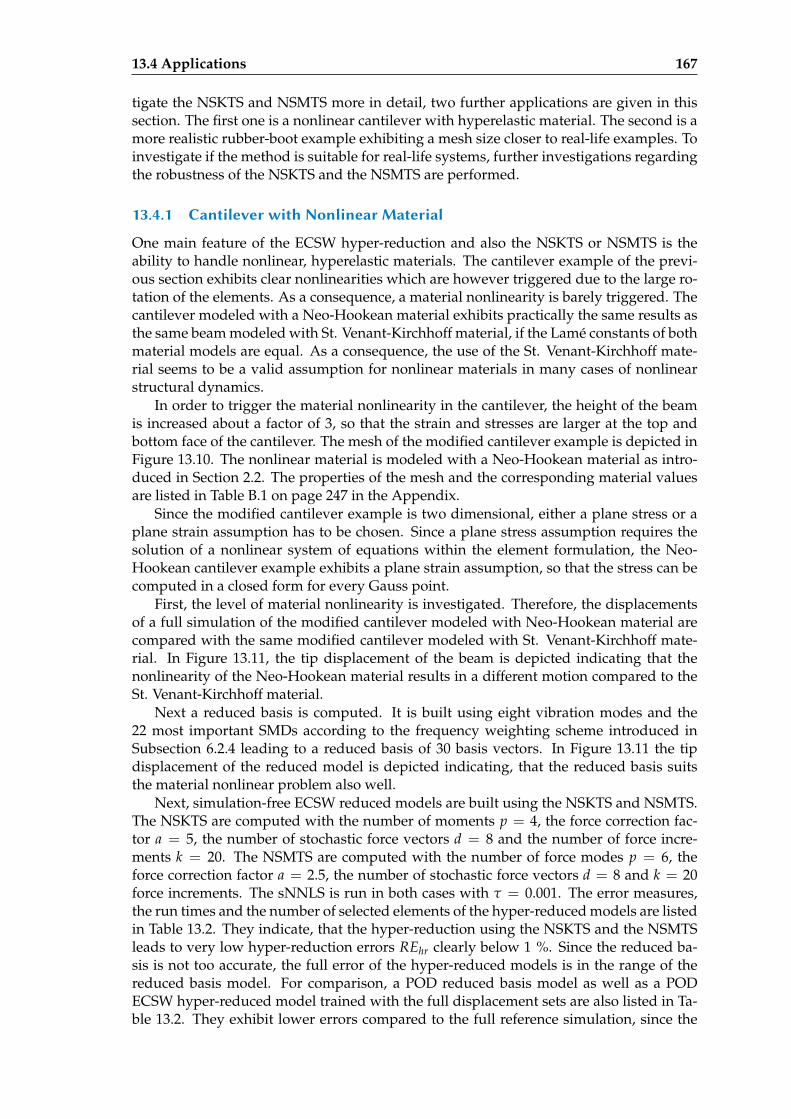
13.4 Applications 167
tigate the NSKTS and NSMTS more in detail, two further applications are given in thissection. The first one is a nonlinear cantilever with hyperelastic material. The second is amore realistic rubber-boot example exhibiting a mesh size closer to real-life examples. Toinvestigate if the method is suitable for real-life systems, further investigations regardingthe robustness of the NSKTS and the NSMTS are performed.
13.4.1 Cantilever with Nonlinear Material
One main feature of the ECSW hyper-reduction and also the NSKTS or NSMTS is theability to handle nonlinear, hyperelastic materials. The cantilever example of the previ-ous section exhibits clear nonlinearities which are however triggered due to the large ro-tation of the elements. As a consequence, a material nonlinearity is barely triggered. Thecantilever modeled with a Neo-Hookean material exhibits practically the same results asthe same beam modeled with St. Venant-Kirchhoff material, if the Lamé constants of bothmaterial models are equal. As a consequence, the use of the St. Venant-Kirchhoff mate-rial seems to be a valid assumption for nonlinear materials in many cases of nonlinearstructural dynamics.
In order to trigger the material nonlinearity in the cantilever, the height of the beamis increased about a factor of 3, so that the strain and stresses are larger at the top andbottom face of the cantilever. The mesh of the modified cantilever example is depicted inFigure 13.10. The nonlinear material is modeled with a Neo-Hookean material as intro-duced in Section 2.2. The properties of the mesh and the corresponding material valuesare listed in Table B.1 on page 247 in the Appendix.
Since the modified cantilever example is two dimensional, either a plane stress or aplane strain assumption has to be chosen. Since a plane stress assumption requires thesolution of a nonlinear system of equations within the element formulation, the Neo-Hookean cantilever example exhibits a plane strain assumption, so that the stress can becomputed in a closed form for every Gauss point.
First, the level of material nonlinearity is investigated. Therefore, the displacementsof a full simulation of the modified cantilever modeled with Neo-Hookean material arecompared with the same modified cantilever modeled with St. Venant-Kirchhoff mate-rial. In Figure 13.11, the tip displacement of the beam is depicted indicating that thenonlinearity of the Neo-Hookean material results in a different motion compared to theSt. Venant-Kirchhoff material.
Next a reduced basis is computed. It is built using eight vibration modes and the22 most important SMDs according to the frequency weighting scheme introduced inSubsection 6.2.4 leading to a reduced basis of 30 basis vectors. In Figure 13.11 the tipdisplacement of the reduced model is depicted indicating, that the reduced basis suitsthe material nonlinear problem also well.
Next, simulation-free ECSW reduced models are built using the NSKTS and NSMTS.The NSKTS are computed with the number of moments p = 4, the force correction fac-tor a = 5, the number of stochastic force vectors d = 8 and the number of force incre-ments k = 20. The NSMTS are computed with the number of force modes p = 6, theforce correction factor a = 2.5, the number of stochastic force vectors d = 8 and k = 20force increments. The sNNLS is run in both cases with τ = 0.001. The error measures,the run times and the number of selected elements of the hyper-reduced models are listedin Table 13.2. They indicate, that the hyper-reduction using the NSKTS and the NSMTSleads to very low hyper-reduction errors REhr clearly below 1 %. Since the reduced ba-sis is not too accurate, the full error of the hyper-reduced models is in the range of thereduced basis model. For comparison, a POD reduced basis model as well as a PODECSW hyper-reduced model trained with the full displacement sets are also listed in Ta-ble 13.2. They exhibit lower errors compared to the full reference simulation, since the
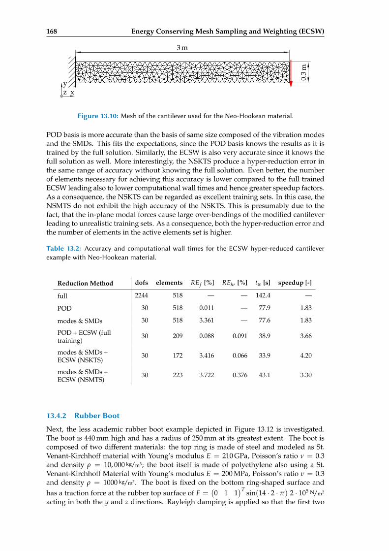
168 Energy Conserving Mesh Sampling and Weighting (ECSW)
3 m
0.3
m
xyz
Figure 13.10: Mesh of the cantilever used for the Neo-Hookean material.
POD basis is more accurate than the basis of same size composed of the vibration modesand the SMDs. This fits the expectations, since the POD basis knows the results as it istrained by the full solution. Similarly, the ECSW is also very accurate since it knows thefull solution as well. More interestingly, the NSKTS produce a hyper-reduction error inthe same range of accuracy without knowing the full solution. Even better, the numberof elements necessary for achieving this accuracy is lower compared to the full trainedECSW leading also to lower computational wall times and hence greater speedup factors.As a consequence, the NSKTS can be regarded as excellent training sets. In this case, theNSMTS do not exhibit the high accuracy of the NSKTS. This is presumably due to thefact, that the in-plane modal forces cause large over-bendings of the modified cantileverleading to unrealistic training sets. As a consequence, both the hyper-reduction error andthe number of elements in the active elements set is higher.
Table 13.2: Accuracy and computational wall times for the ECSW hyper-reduced cantileverexample with Neo-Hookean material.
Reduction Method dofs elements RE f [%] REhr [%] tw [s] speedup [-]
full 2244 518 — — 142.4 —
POD 30 518 0.011 — 77.9 1.83
modes & SMDs 30 518 3.361 — 77.6 1.83
POD + ECSW (fulltraining)
30 209 0.088 0.091 38.9 3.66
modes & SMDs +ECSW (NSKTS)
30 172 3.416 0.066 33.9 4.20
modes & SMDs +ECSW (NSMTS)
30 223 3.722 0.376 43.1 3.30
13.4.2 Rubber Boot
Next, the less academic rubber boot example depicted in Figure 13.12 is investigated.The boot is 440 mm high and has a radius of 250 mm at its greatest extent. The boot iscomposed of two different materials: the top ring is made of steel and modeled as St.Venant-Kirchhoff material with Young’s modulus E = 210 GPa, Poisson’s ratio ν = 0.3and density ρ = 10, 000 kg/m3; the boot itself is made of polyethylene also using a St.Venant-Kirchhoff Material with Young’s modulus E = 200 MPa, Poisson’s ratio ν = 0.3and density ρ = 1000 kg/m3. The boot is fixed on the bottom ring-shaped surface andhas a traction force at the rubber top surface of F =
(0 1 1
)T sin(14 · 2 · π) 2 · 105 N/m2
acting in both the y and z directions. Rayleigh damping is applied so that the first two
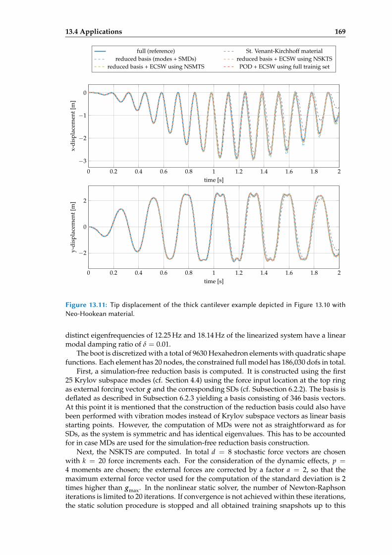
13.4 Applications 169
0 0.2 0.4 0.6 0.8 1 1.2 1.4 1.6 1.8 2
−3
−2
−1
0
time [s]
x-di
spla
cem
ent[
m]
full (reference) St. Venant-Kirchhoff materialreduced basis (modes + SMDs) reduced basis + ECSW using NSKTS
reduced basis + ECSW using NSMTS POD + ECSW using full trainig set
0 0.2 0.4 0.6 0.8 1 1.2 1.4 1.6 1.8 2
−2
0
2
time [s]
y-di
spla
cem
ent[
m]
Figure 13.11: Tip displacement of the thick cantilever example depicted in Figure 13.10 withNeo-Hookean material.
distinct eigenfrequencies of 12.25 Hz and 18.14 Hz of the linearized system have a linearmodal damping ratio of δ = 0.01.
The boot is discretized with a total of 9630 Hexahedron elements with quadratic shapefunctions. Each element has 20 nodes, the constrained full model has 186,030 dofs in total.
First, a simulation-free reduction basis is computed. It is constructed using the first25 Krylov subspace modes (cf. Section 4.4) using the force input location at the top ringas external forcing vector g and the corresponding SDs (cf. Subsection 6.2.2). The basis isdeflated as described in Subsection 6.2.3 yielding a basis consisting of 346 basis vectors.At this point it is mentioned that the construction of the reduction basis could also havebeen performed with vibration modes instead of Krylov subspace vectors as linear basisstarting points. However, the computation of MDs were not as straightforward as forSDs, as the system is symmetric and has identical eigenvalues. This has to be accountedfor in case MDs are used for the simulation-free reduction basis construction.
Next, the NSKTS are computed. In total d = 8 stochastic force vectors are chosenwith k = 20 force increments each. For the consideration of the dynamic effects, p =4 moments are chosen; the external forces are corrected by a factor a = 2, so that themaximum external force vector used for the computation of the standard deviation is 2times higher than gmax. In the nonlinear static solver, the number of Newton-Raphsoniterations is limited to 20 iterations. If convergence is not achieved within these iterations,the static solution procedure is stopped and all obtained training snapshots up to this
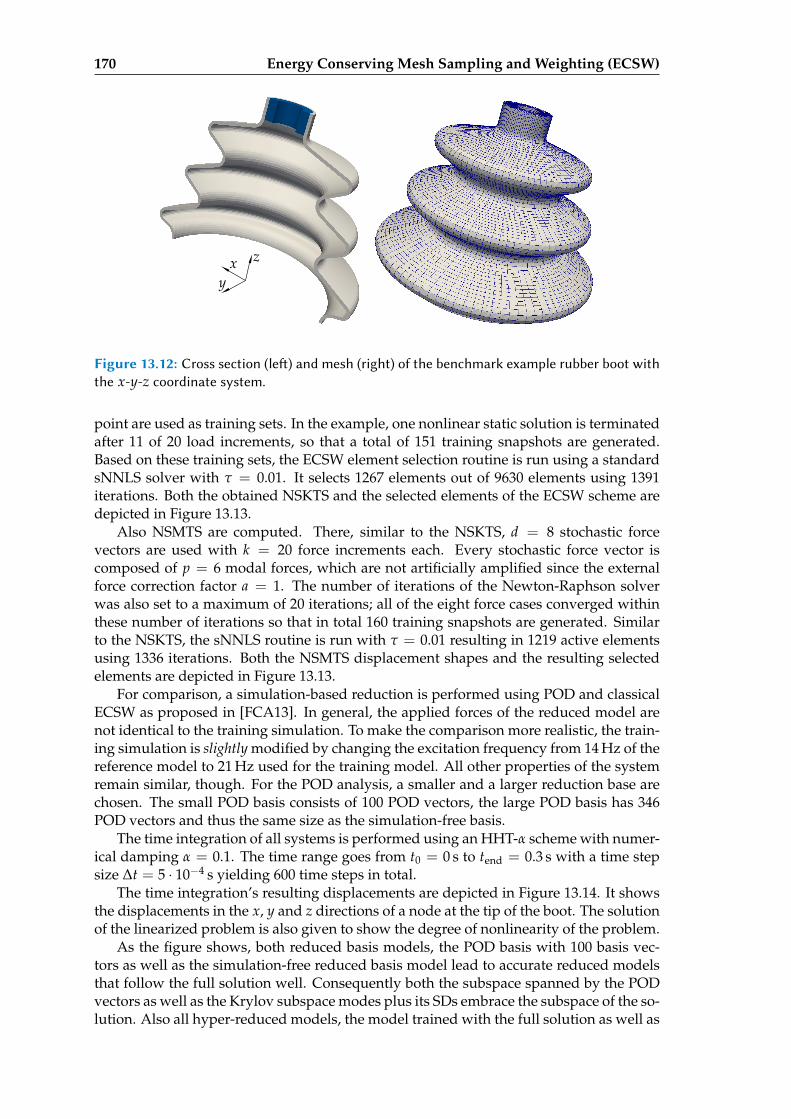
170 Energy Conserving Mesh Sampling and Weighting (ECSW)
zxy
Figure 13.12: Cross section (le) and mesh (right) of the benchmark example rubber boot withthe x-y-z coordinate system.
point are used as training sets. In the example, one nonlinear static solution is terminatedafter 11 of 20 load increments, so that a total of 151 training snapshots are generated.Based on these training sets, the ECSW element selection routine is run using a standardsNNLS solver with τ = 0.01. It selects 1267 elements out of 9630 elements using 1391iterations. Both the obtained NSKTS and the selected elements of the ECSW scheme aredepicted in Figure 13.13.
Also NSMTS are computed. There, similar to the NSKTS, d = 8 stochastic forcevectors are used with k = 20 force increments each. Every stochastic force vector iscomposed of p = 6 modal forces, which are not artificially amplified since the externalforce correction factor a = 1. The number of iterations of the Newton-Raphson solverwas also set to a maximum of 20 iterations; all of the eight force cases converged withinthese number of iterations so that in total 160 training snapshots are generated. Similarto the NSKTS, the sNNLS routine is run with τ = 0.01 resulting in 1219 active elementsusing 1336 iterations. Both the NSMTS displacement shapes and the resulting selectedelements are depicted in Figure 13.13.
For comparison, a simulation-based reduction is performed using POD and classicalECSW as proposed in [FCA13]. In general, the applied forces of the reduced model arenot identical to the training simulation. To make the comparison more realistic, the train-ing simulation is slightly modified by changing the excitation frequency from 14 Hz of thereference model to 21 Hz used for the training model. All other properties of the systemremain similar, though. For the POD analysis, a smaller and a larger reduction base arechosen. The small POD basis consists of 100 POD vectors, the large POD basis has 346POD vectors and thus the same size as the simulation-free basis.
The time integration of all systems is performed using an HHT-α scheme with numer-ical damping α = 0.1. The time range goes from t0 = 0 s to tend = 0.3 s with a time stepsize ∆t = 5 · 10−4 s yielding 600 time steps in total.
The time integration’s resulting displacements are depicted in Figure 13.14. It showsthe displacements in the x, y and z directions of a node at the tip of the boot. The solutionof the linearized problem is also given to show the degree of nonlinearity of the problem.
As the figure shows, both reduced basis models, the POD basis with 100 basis vec-tors as well as the simulation-free reduced basis model lead to accurate reduced modelsthat follow the full solution well. Consequently both the subspace spanned by the PODvectors as well as the Krylov subspace modes plus its SDs embrace the subspace of the so-lution. Also all hyper-reduced models, the model trained with the full solution as well as
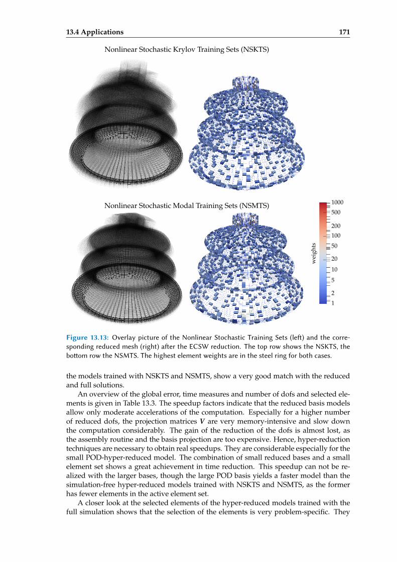
13.4 Applications 171
Nonlinear Stochastic Krylov Training Sets (NSKTS)
Nonlinear Stochastic Modal Training Sets (NSMTS)
1
200
100
wei
ghts
2
5
10
20
50
500
1000
Figure 13.13: Overlay picture of the Nonlinear Stochastic Training Sets (le) and the corre-sponding reduced mesh (right) aer the ECSW reduction. The top row shows the NSKTS, theboom row the NSMTS. The highest element weights are in the steel ring for both cases.
the models trained with NSKTS and NSMTS, show a very good match with the reducedand full solutions.
An overview of the global error, time measures and number of dofs and selected ele-ments is given in Table 13.3. The speedup factors indicate that the reduced basis modelsallow only moderate accelerations of the computation. Especially for a higher numberof reduced dofs, the projection matrices V are very memory-intensive and slow downthe computation considerably. The gain of the reduction of the dofs is almost lost, asthe assembly routine and the basis projection are too expensive. Hence, hyper-reductiontechniques are necessary to obtain real speedups. They are considerable especially for thesmall POD-hyper-reduced model. The combination of small reduced bases and a smallelement set shows a great achievement in time reduction. This speedup can not be re-alized with the larger bases, though the large POD basis yields a faster model than thesimulation-free hyper-reduced models trained with NSKTS and NSMTS, as the formerhas fewer elements in the active element set.
A closer look at the selected elements of the hyper-reduced models trained with thefull simulation shows that the selection of the elements is very problem-specific. They
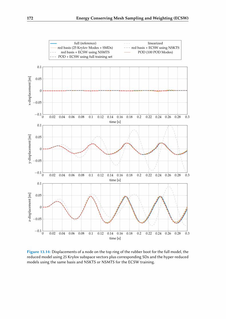
172 Energy Conserving Mesh Sampling and Weighting (ECSW)
0 0.02 0.04 0.06 0.08 0.1 0.12 0.14 0.16 0.18 0.2 0.22 0.24 0.26 0.28 0.3−0.1
−0.05
0
0.05
0.1
time [s]
x-di
spla
cem
ent[
m]
full (reference) linearizedred basis (25 Krylov Modes + SMDs) red basis + ECSW using NSKTS
red basis + ECSW using NSMTS POD (100 POD Modes)POD + ECSW using full training set
0 0.02 0.04 0.06 0.08 0.1 0.12 0.14 0.16 0.18 0.2 0.22 0.24 0.26 0.28 0.3−0.1
−0.05
0
0.05
0.1
time [s]
y-di
spla
cem
ent[
m]
0 0.02 0.04 0.06 0.08 0.1 0.12 0.14 0.16 0.18 0.2 0.22 0.24 0.26 0.28 0.3−0.1
−0.05
0
0.05
0.1
time [s]
z-di
spla
cem
ent[
m]
Figure 13.14: Displacements of a node on the top ring of the rubber boot for the full model, thereduced model using 25 Krylov subspace vectors plus corresponding SDs and the hyper-reducedmodels using the same basis and NSKTS or NSMTS for the ECSW training.
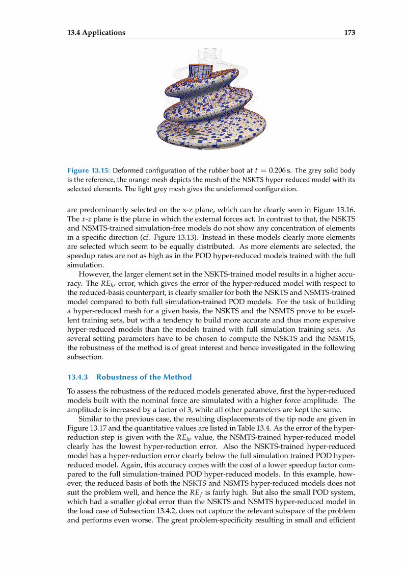
13.4 Applications 173
Figure 13.15: Deformed configuration of the rubber boot at t = 0.206 s. The grey solid bodyis the reference, the orange mesh depicts the mesh of the NSKTS hyper-reduced model with itsselected elements. The light grey mesh gives the undeformed configuration.
are predominantly selected on the x-z plane, which can be clearly seen in Figure 13.16.The x-z plane is the plane in which the external forces act. In contrast to that, the NSKTSand NSMTS-trained simulation-free models do not show any concentration of elementsin a specific direction (cf. Figure 13.13). Instead in these models clearly more elementsare selected which seem to be equally distributed. As more elements are selected, thespeedup rates are not as high as in the POD hyper-reduced models trained with the fullsimulation.
However, the larger element set in the NSKTS-trained model results in a higher accu-racy. The REhr error, which gives the error of the hyper-reduced model with respect tothe reduced-basis counterpart, is clearly smaller for both the NSKTS and NSMTS-trainedmodel compared to both full simulation-trained POD models. For the task of buildinga hyper-reduced mesh for a given basis, the NSKTS and the NSMTS prove to be excel-lent training sets, but with a tendency to build more accurate and thus more expensivehyper-reduced models than the models trained with full simulation training sets. Asseveral setting parameters have to be chosen to compute the NSKTS and the NSMTS,the robustness of the method is of great interest and hence investigated in the followingsubsection.
13.4.3 Robustness of the Method
To assess the robustness of the reduced models generated above, first the hyper-reducedmodels built with the nominal force are simulated with a higher force amplitude. Theamplitude is increased by a factor of 3, while all other parameters are kept the same.
Similar to the previous case, the resulting displacements of the tip node are given inFigure 13.17 and the quantitative values are listed in Table 13.4. As the error of the hyper-reduction step is given with the REhr value, the NSMTS-trained hyper-reduced modelclearly has the lowest hyper-reduction error. Also the NSKTS-trained hyper-reducedmodel has a hyper-reduction error clearly below the full simulation trained POD hyper-reduced model. Again, this accuracy comes with the cost of a lower speedup factor com-pared to the full simulation-trained POD hyper-reduced models. In this example, how-ever, the reduced basis of both the NSKTS and NSMTS hyper-reduced models does notsuit the problem well, and hence the RE f is fairly high. But also the small POD system,which had a smaller global error than the NSKTS and NSMTS hyper-reduced model inthe load case of Subsection 13.4.2, does not capture the relevant subspace of the problemand performs even worse. The great problem-specificity resulting in small and efficient
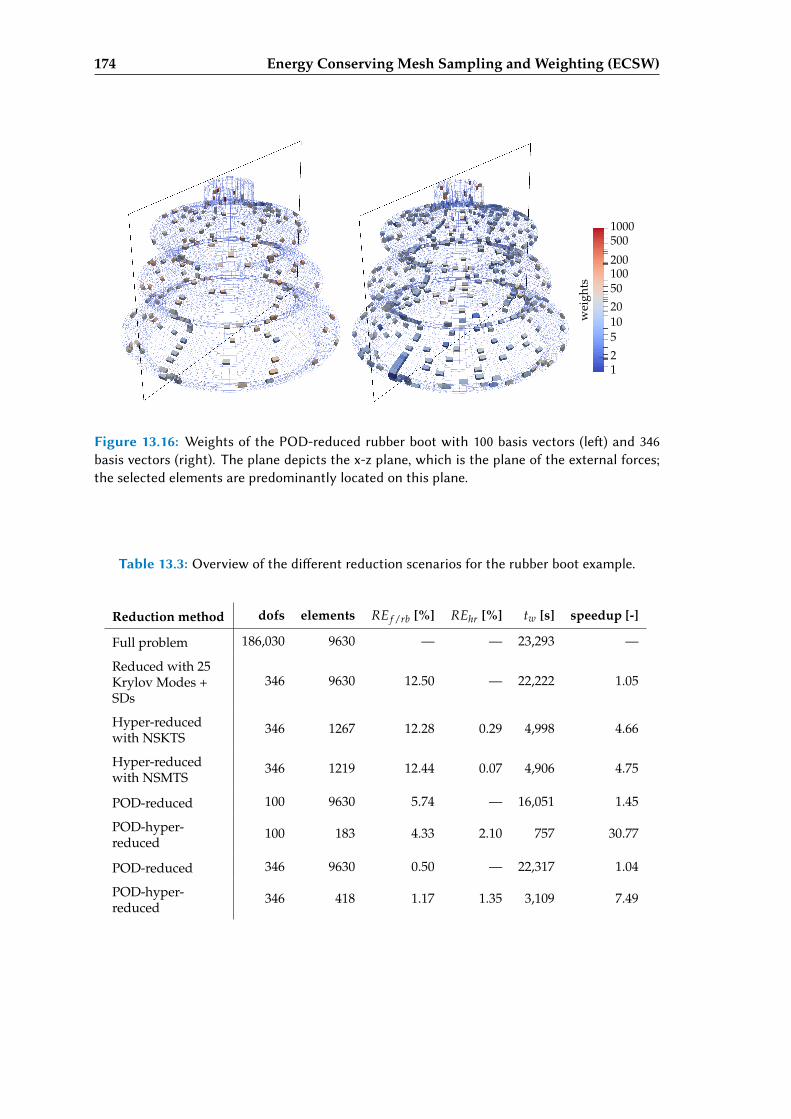
174 Energy Conserving Mesh Sampling and Weighting (ECSW)
1
200100
wei
ghts
2
51020
50
5001000
Figure 13.16: Weights of the POD-reduced rubber boot with 100 basis vectors (le) and 346basis vectors (right). The plane depicts the x-z plane, which is the plane of the external forces;the selected elements are predominantly located on this plane.
Table 13.3: Overview of the dierent reduction scenarios for the rubber boot example.
Reduction method dofs elements RE f /rb [%] REhr [%] tw [s] speedup [-]
Full problem 186,030 9630 — — 23,293 —
Reduced with 25Krylov Modes +SDs
346 9630 12.50 — 22,222 1.05
Hyper-reducedwith NSKTS
346 1267 12.28 0.29 4,998 4.66
Hyper-reducedwith NSMTS
346 1219 12.44 0.07 4,906 4.75
POD-reduced 100 9630 5.74 — 16,051 1.45
POD-hyper-reduced
100 183 4.33 2.10 757 30.77
POD-reduced 346 9630 0.50 — 22,317 1.04
POD-hyper-reduced
346 418 1.17 1.35 3,109 7.49
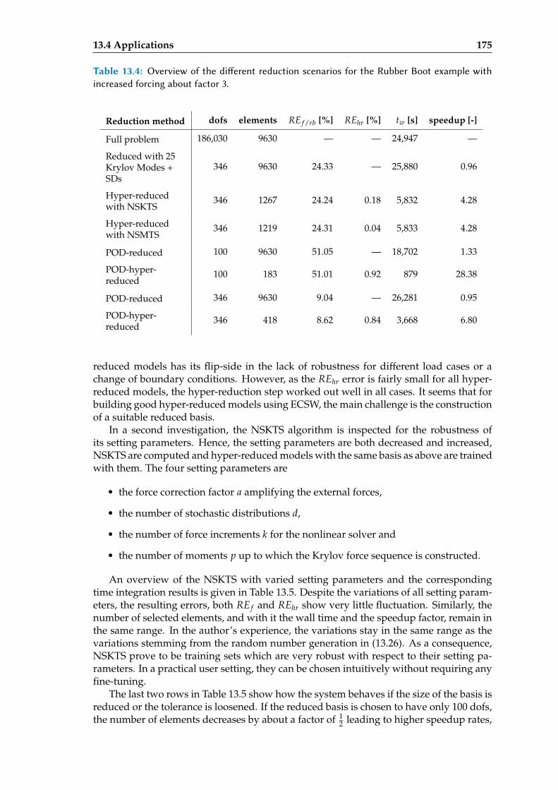
13.4 Applications 175
Table 13.4: Overview of the dierent reduction scenarios for the Rubber Boot example withincreased forcing about factor 3.
Reduction method dofs elements RE f /rb [%] REhr [%] tw [s] speedup [-]
Full problem 186,030 9630 — — 24,947 —
Reduced with 25Krylov Modes +SDs
346 9630 24.33 — 25,880 0.96
Hyper-reducedwith NSKTS
346 1267 24.24 0.18 5,832 4.28
Hyper-reducedwith NSMTS
346 1219 24.31 0.04 5,833 4.28
POD-reduced 100 9630 51.05 — 18,702 1.33
POD-hyper-reduced
100 183 51.01 0.92 879 28.38
POD-reduced 346 9630 9.04 — 26,281 0.95
POD-hyper-reduced
346 418 8.62 0.84 3,668 6.80
reduced models has its flip-side in the lack of robustness for different load cases or achange of boundary conditions. However, as the REhr error is fairly small for all hyper-reduced models, the hyper-reduction step worked out well in all cases. It seems that forbuilding good hyper-reduced models using ECSW, the main challenge is the constructionof a suitable reduced basis.
In a second investigation, the NSKTS algorithm is inspected for the robustness ofits setting parameters. Hence, the setting parameters are both decreased and increased,NSKTS are computed and hyper-reduced models with the same basis as above are trainedwith them. The four setting parameters are
• the force correction factor a amplifying the external forces,
• the number of stochastic distributions d,
• the number of force increments k for the nonlinear solver and
• the number of moments p up to which the Krylov force sequence is constructed.
An overview of the NSKTS with varied setting parameters and the correspondingtime integration results is given in Table 13.5. Despite the variations of all setting param-eters, the resulting errors, both RE f and REhr show very little fluctuation. Similarly, thenumber of selected elements, and with it the wall time and the speedup factor, remain inthe same range. In the author’s experience, the variations stay in the same range as thevariations stemming from the random number generation in (13.26). As a consequence,NSKTS prove to be training sets which are very robust with respect to their setting pa-rameters. In a practical user setting, they can be chosen intuitively without requiring anyfine-tuning.
The last two rows in Table 13.5 show how the system behaves if the size of the basis isreduced or the tolerance is loosened. If the reduced basis is chosen to have only 100 dofs,the number of elements decreases by about a factor of 1
2 leading to higher speedup rates,
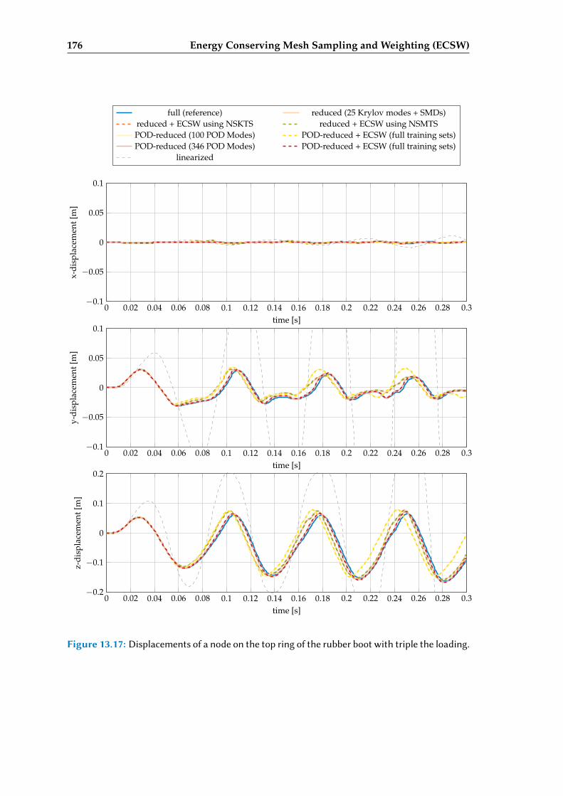
176 Energy Conserving Mesh Sampling and Weighting (ECSW)
0 0.02 0.04 0.06 0.08 0.1 0.12 0.14 0.16 0.18 0.2 0.22 0.24 0.26 0.28 0.3−0.1
−0.05
0
0.05
0.1
time [s]
x-di
spla
cem
ent[
m]
full (reference) reduced (25 Krylov modes + SMDs)reduced + ECSW using NSKTS reduced + ECSW using NSMTSPOD-reduced (100 POD Modes) POD-reduced + ECSW (full training sets)POD-reduced (346 POD Modes) POD-reduced + ECSW (full training sets)
linearized
0 0.02 0.04 0.06 0.08 0.1 0.12 0.14 0.16 0.18 0.2 0.22 0.24 0.26 0.28 0.3−0.1
−0.05
0
0.05
0.1
time [s]
y-di
spla
cem
ent[
m]
0 0.02 0.04 0.06 0.08 0.1 0.12 0.14 0.16 0.18 0.2 0.22 0.24 0.26 0.28 0.3−0.2
−0.1
0
0.1
0.2
time [s]
z-di
spla
cem
ent[
m]
Figure 13.17: Displacements of a node on the top ring of the rubber boot with triple the loading.
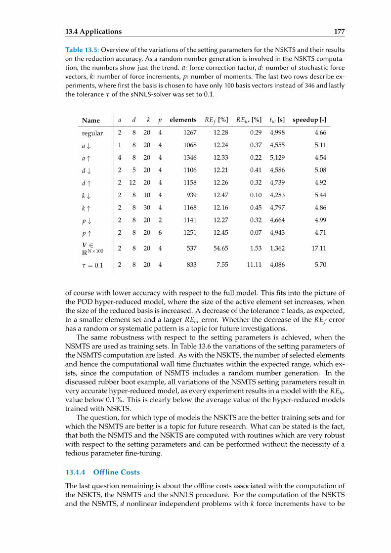
13.4 Applications 177
Table 13.5: Overview of the variations of the seing parameters for the NSKTS and their resultson the reduction accuracy. As a random number generation is involved in the NSKTS computa-tion, the numbers show just the trend. a: force correction factor, d: number of stochastic forcevectors, k: number of force increments, p: number of moments. The last two rows describe ex-periments, where first the basis is chosen to have only 100 basis vectors instead of 346 and lastlythe tolerance τ of the sNNLS-solver was set to 0.1.
Name a d k p elements RE f [%] REhr [%] tw [s] speedup [-]
regular 2 8 20 4 1267 12.28 0.29 4,998 4.66
a ↓ 1 8 20 4 1068 12.24 0.37 4,555 5.11
a ↑ 4 8 20 4 1346 12.33 0.22 5,129 4.54
d ↓ 2 5 20 4 1106 12.21 0.41 4,586 5.08
d ↑ 2 12 20 4 1158 12.26 0.32 4,739 4.92
k ↓ 2 8 10 4 939 12.47 0.10 4,283 5.44
k ↑ 2 8 30 4 1168 12.16 0.45 4,797 4.86
p ↓ 2 8 20 2 1141 12.27 0.32 4,664 4.99
p ↑ 2 8 20 6 1251 12.45 0.07 4,943 4.71
V ∈RN×100 2 8 20 4 537 54.65 1.53 1,362 17.11
τ = 0.1 2 8 20 4 833 7.55 11.11 4,086 5.70
of course with lower accuracy with respect to the full model. This fits into the picture ofthe POD hyper-reduced model, where the size of the active element set increases, whenthe size of the reduced basis is increased. A decrease of the tolerance τ leads, as expected,to a smaller element set and a larger REhr error. Whether the decrease of the RE f errorhas a random or systematic pattern is a topic for future investigations.
The same robustness with respect to the setting parameters is achieved, when theNSMTS are used as training sets. In Table 13.6 the variations of the setting parameters ofthe NSMTS computation are listed. As with the NSKTS, the number of selected elementsand hence the computational wall time fluctuates within the expected range, which ex-ists, since the computation of NSMTS includes a random number generation. In thediscussed rubber boot example, all variations of the NSMTS setting parameters result invery accurate hyper-reduced model, as every experiment results in a model with the REhrvalue below 0.1 %. This is clearly below the average value of the hyper-reduced modelstrained with NSKTS.
The question, for which type of models the NSKTS are the better training sets and forwhich the NSMTS are better is a topic for future research. What can be stated is the fact,that both the NSMTS and the NSKTS are computed with routines which are very robustwith respect to the setting parameters and can be performed without the necessity of atedious parameter fine-tuning.
13.4.4 Oline Costs
The last question remaining is about the offline costs associated with the computation ofthe NSKTS, the NSMTS and the sNNLS procedure. For the computation of the NSKTSand the NSMTS, d nonlinear independent problems with k force increments have to be

178 Energy Conserving Mesh Sampling and Weighting (ECSW)
Table 13.6: Overview of the variations of the seing parameters for the NSMTS and their resultson the reduction accuracy. As a random number generation is involved in the NSMTS computa-tion, the numbers show just the trend. a: force correction factor, d: number of stochastic forcevectors, k: number of force increments, p: number of force modes.
Name a d k p elements RE f [%] REhr [%] tw [s] speedup [-]
regular 1 8 20 6 1219 12.44 0.072 4906 4.75
a ↓ 0.5 8 20 6 1106 12.43 0.087 4611 5.05
a ↑ 2 8 20 6 1308 12.47 0.032 5057 4.61
d ↓ 1 5 20 6 1146 12.45 0.092 4676 4.98
d ↑ 1 12 20 6 1229 12.46 0.057 4859 4.79
k ↓ 1 8 10 6 1070 12.47 0.072 4497 5.18
k ↑ 1 8 30 6 1240 12.45 0.093 4878 4.78
p ↓ 1 8 20 3 1026 12.52 0.079 4422 5.27
p ↑ 1 8 20 9 1253 12.43 0.089 4920 4.73
solved. As they can be parallelized with no effort, all NSKTS and NSMTS were computedin a parallel manner on all four cores available on the workstation. The computation ofthe NSKTS for d = 8 took 2811 s, and the solution of the sNNLS problem took 3218 s. Forthe NSMTS with d = 8, 3880 s were needed and the solution of the sNNLS problem took3288 s. With the construction of the reduced basis requiring 554 s, the total computationeffort of both offline and online is still considerably smaller than one single full trainingsimulation required for the POD and the ECSW with full training set.
Hence, both the NSKTS and the NSMTS are very attractive not only if hyper-reducedmodels are to be obtained with little offline costs, but also for scenarios where the fullsimulation is too expensive, and an approximation of the full solution is to be obtainedwith less effort.
Chapter 14
Summary of Part II
The previous four chapters cover the hyper-reduction of geometrically nonlinear struc-tural dynamics systems, which are summarized in the following. The starting point ofhyper-reduction is the reduced basis method, which projects the equations of motion ofthe full, unreduced system onto a low-dimensional subspace, resulting in a reduced setof equations. The evaluation of the nonlinearities, however, is still associated with the di-mension of the full, unreduced system leading to moderate speedup rates for nonlinearreduced systems. Hyper-reduction accelerates the computation of the nonlinear terms,which are the nonlinear internal forces and, as they are necessary for implicit time inte-gration schemes, the derivatives forming the tangential stiffness matrix.
The first hyper-reduction method addressed in Chapter 11 speeds up the evaluationof the internal forces by treating it as a Taylor series. Thereby it is convenient, that theinternal forces of a continuum modeled with the linear St. Venant-Kirchhoff materialand discretized with geometrically nonlinear finite elements are third order polynomi-als. Consequently, the Taylor series converges with the cubic term resulting in an exactrepresentation of the internal forces. The computational effort is reduced, since evaluat-ing the polynomials is less computationally expensive for highly reduced systems thanthe standard finite element procedure involving an element-wise evaluation and a sub-sequent assembly. In the offline stage, the polynomial coefficients have to be determined,which can be arranged as multidimensional symmetric arrays of dimension two, threeand four. A numerical differentiation scheme operating on tangential stiffness matricesis proposed for computing the polynomial coefficients. It turns out to be more efficientthan established displacement-based identification methods using the internal forces, butless efficient than methods using the tangential stiffness matrix. The investigated meth-ods are intrinsically simulation-free, since no training sets of the full, unreduced systemare required.
One issue of the polynomial tensors hyper-reduction is theO(n4) dependence of boththe model size and the number of multiplications with respect to the dimension n of thereduced system. While for small systems the method is unbeatably fast, the requirementof memory and computational time for large systems becomes quickly prohibitive. Toaddress this issue, an efficient storage and multiplication scheme is proposed, which ex-ploits the symmetry of the polynomial coefficient arrays. With this technique, remarkablespeedups and perfect accuracies are reported for the examples investigated.
The Discrete Empirical Interpolation Method (DEIM) discussed in Chapter 12 takesa different approach and reduces the computational costs by evaluating only a subsetof nodal forces. The omitted forces are accounted for with an empirically determinedforce basis and a collocation strategy. This approach can be interpreted as an obliqueprojection of the nodal forces onto the force basis which, however, destroys desirableproperties like symmetry and stability. The strategy to alleviate this issue proposed in
179
180 Summary of Part II
the literature is a splitting of the internal forces into linear and nonlinear part. This is,however, cumbersome in the framework of geometrically nonlinear finite elements andleads to a very disadvantageous approximation of the internal forces.
A further issue of the DEIM is the operation on single nodal forces which are, how-ever, computed on the element level in the finite element framework. The unassembledDEIM called UDEIM adapts the DEIM to the finite element framework allowing for re-duced computational costs and more flexibility and modifications in the choice of colloca-tion points. This approach is used to adapt an approach reported in the literature to sym-metrize DEIM and transfer it to finite elements, however without success. The numericalexperiments show that the symmetric application of the oblique projection distorts theelements so severely, that no reasonable force evaluation is possible in general. Further-more, the numerical experiments reveal that both the DEIM and the UDEIM performextremely poorly in geometrically nonlinear structural dynamics, especially when largerotations are present. The instability issues are accompanied by high hyper-reductionerrors, even though training snapshots of the full solution are used in the experiments.Since the methods perform so poorly even when they ’know’ the solution a priori, furtherpossible modifications of the (U)DEIM to simulation-free techniques are not consideredin this work.
The Energy Conserving Mesh Sampling and Weighting (ECSW) method discussedin Chapter 13 is based on the evaluation of a subset of elements, too. It does, however,not suffer from instability and does not require an artificial splitting of linear and non-linear part making it a stable and accurate hyper-reduction technique suited for geomet-rically nonlinear structural dynamics systems. It carries the drawback, that it requirestraining sets which are commonly obtained from full, unreduced training simulations.To apply the method in a simulation-free context, lean, almost simulation-free trainingsets named Nonlinear Stochastic Krylov Training Sets (NSKTS) and Nonlinear StochasticModal Training Sets (NSMTS) are proposed. These training sets are obtained by solvinga set of nonlinear, reduced, static problems, where the right hand side consists of stochas-tically weighted pseudo-dynamic forces. To compute these forces, a Krylov force basisor a modal force basis is built for the NSKTS or the NSMTS, respectively. It is orthonor-malized using the impedance norm of the linearized system and then multiplied with aGaussian distributed random vector resulting in one pseudo-dynamic force vector.
As reported by the extensive numerical experiments conducted, both the NSKTS andNSMTS yield very accurate hyper-reduced models with convenient speedup rates. Thehyper-reduced models are very robust with respect to both parameter changes and differ-ent load cases. In contrast to simulation-based ECSW hyper-reduced models, the NSKTSand NSMTS ECSW hyper-reduced models tend to have more elements in the reducedelement set. They are also more robust with respect to a change of the excitation forces,so that they are different from the ones used for generating the training set. Due to theirsuccess in both accuracy and speedup rates, the NSKTS and NSMTS open the ECSW toalmost simulation-free scenarios.

Part III
Closure
181

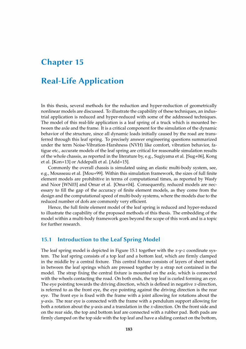
Chapter 15
Real-Life Application
In this thesis, several methods for the reduction and hyper-reduction of geometricallynonlinear models are discussed. To illustrate the capability of these techniques, an indus-trial application is reduced and hyper-reduced with some of the addressed techniques.The model of this real-life application is a leaf spring of a truck which is mounted be-tween the axle and the frame. It is a critical component for the simulation of the dynamicbehavior of the structure, since all dynamic loads initially caused by the road are trans-ferred through this leaf spring. To precisely answer engineering questions summarizedunder the term Noise-Vibration-Harshness (NVH) like comfort, vibration behavior, fa-tigue etc., accurate models of the leaf spring are critical for reasonable simulation resultsof the whole chassis, as reported in the literature by, e.g., Sugiyama et al. [Sug+06], Konget al. [Kon+13] or Addepalli et al. [Add+15].
Commonly the overall chassis is simulated using an elastic multi-body system, see,e.g., Mousseau et al. [Mou+99]. Within this simulation framework, the sizes of full finiteelement models are prohibitive in terms of computational times, as reported by Wasfyand Noor [WN03] and Omar et al. [Oma+04]. Consequently, reduced models are nec-essary to fill the gap of the accuracy of finite element models, as they come from thedesign and the computational speed of multi-body systems, where the models due to thereduced number of dofs are commonly very efficient.
Hence, the full finite element model of the leaf spring is reduced and hyper-reducedto illustrate the capability of the proposed methods of this thesis. The embedding of themodel within a multi-body framework goes beyond the scope of this work and is a topicfor further research.
15.1 Introduction to the Leaf Spring Model
The leaf spring model is depicted in Figure 15.1 together with the x-y-z coordinate sys-tem. The leaf spring consists of a top leaf and a bottom leaf, which are firmly clampedin the middle by a central fixture. This central fixture consists of layers of sheet metalin between the leaf springs which are pressed together by a strap not contained in themodel. The strap fixing the central fixture is mounted on the axle, which is connectedwith the wheels contacting the road. On both ends, the top leaf is curled forming an eye.The eye pointing towards the driving direction, which is defined in negative x-direction,is referred to as the front eye, the eye pointing against the driving direction is the reareye. The front eye is fixed with the frame with a joint allowing for rotations about they-axis. The rear eye is connected with the frame with a pendulum support allowing forboth a rotation about the y-axis and a translation in the x-direction. On the front side andon the rear side, the top and bottom leaf are connected with a rubber pad. Both pads arefirmly clamped on the top side with the top leaf and have a sliding contact on the bottom,
183
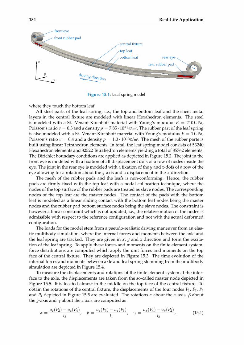
184 Real-Life Application
x
y
z
central fixture
front eye
rear eye
rear rubber pad
front rubber pad
driving direction
top leaf
bottom leaf
Figure 15.1: Leaf spring model
where they touch the bottom leaf.All steel parts of the leaf spring, i.e., the top and bottom leaf and the sheet metal
layers in the central fixture are modeled with linear Hexahedron elements. The steelis modeled with a St. Venant-Kirchhoff material with Young’s modulus E = 210 GPa,Poisson’s ratio ν = 0.3 and a density ρ = 7.85 · 103 kg/m3. The rubber part of the leaf springis also modeled with a St. Venant-Kirchhoff material with Young’s modulus E = 1 GPa,Poisson’s ratio ν = 0.4 and a density ρ = 1.0 · 103 kg/m3. The mesh of the rubber parts isbuilt using linear Tetrahedron elements. In total, the leaf spring model consists of 53240Hexahedron elements and 32522 Tetrahedron elements yielding a total of 85762 elements.The Dirichlet boundary conditions are applied as depicted in Figure 15.2. The joint in thefront eye is modeled with a fixation of all displacement dofs of a row of nodes inside theeye. The joint in the rear eye is modeled with a fixation of the y and z-dofs of a row of theeye allowing for a rotation about the y-axis and a displacement in the x-direction.
The mesh of the rubber pads and the leafs is non-conforming. Hence, the rubberpads are firmly fixed with the top leaf with a nodal collocation technique, where thenodes of the top surface of the rubber pads are treated as slave nodes. The correspondingnodes of the top leaf are the master nodes. The contact of the pads with the bottomleaf is modeled as a linear sliding contact with the bottom leaf nodes being the masternodes and the rubber pad bottom surface nodes being the slave nodes. The constraint ishowever a linear constraint which is not updated, i.e., the relative motion of the nodes isadmissible with respect to the reference configuration and not with the actual deformedconfiguration.
The loads for the model stem from a pseudo-realistic driving maneuver from an elas-tic multibody simulation, where the internal forces and moments between the axle andthe leaf spring are tracked. They are given in x, y and z direction and form the excita-tion of the leaf spring. To apply these forces and moments on the finite element system,force distributions are computed which apply the unit forces and moments on the topface of the central fixture. They are depicted in Figure 15.3. The time evolution of theinternal forces and moments between axle and leaf spring stemming from the multibodysimulation are depicted in Figure 15.4.
To measure the displacements and rotations of the finite element system at the inter-face to the axle, the displacements are taken from the so-called master node depicted inFigure 15.5. It is located almost in the middle on the top face of the central fixture. Toobtain the rotations of the central fixture, the displacements of the four nodes P1, P2, P3and P4 depicted in Figure 15.5 are evaluated. The rotations α about the x-axis, β aboutthe y-axis and γ about the z axis are computed as
α =uz(P2)− uz(P4)
l2, β =
uz(P3)− uz(P1)
l1, γ =
ux(P4)− ux(P2)
l2, (15.1)
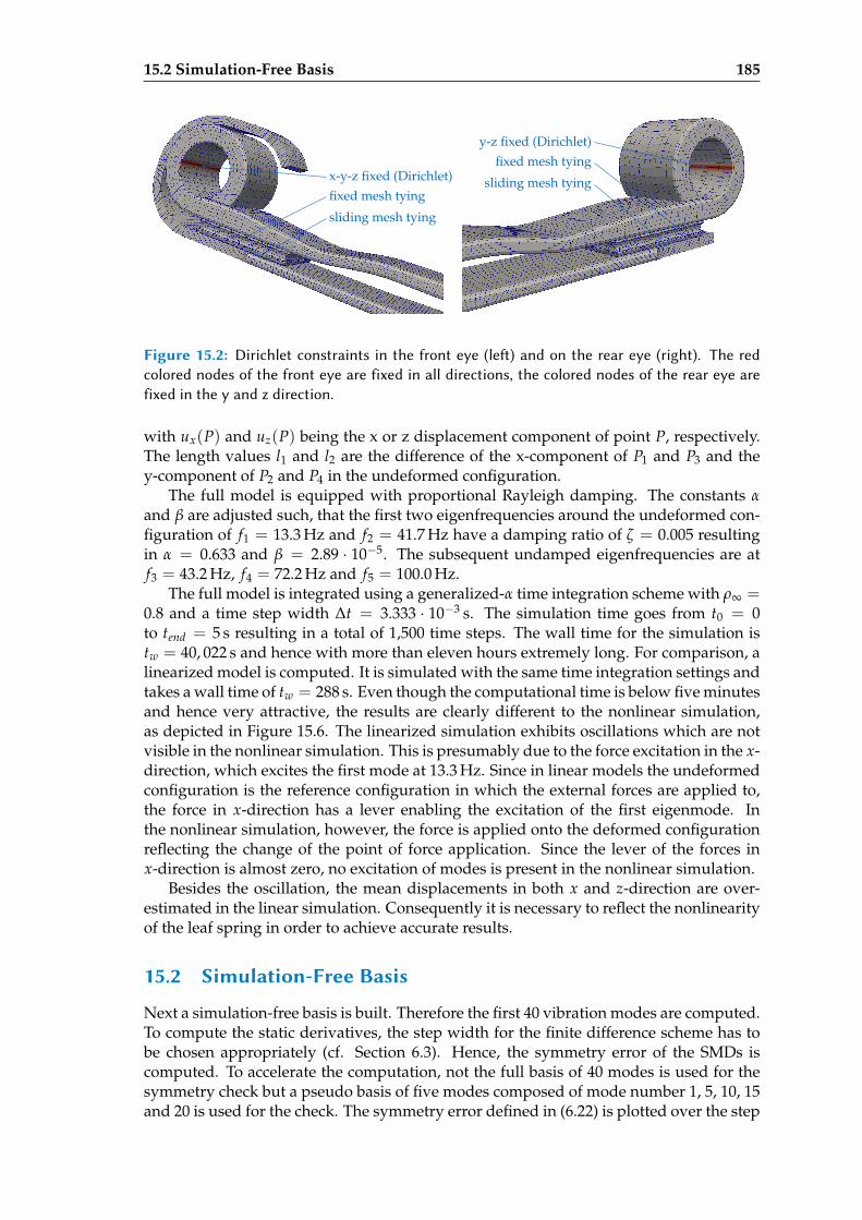
15.2 Simulation-Free Basis 185
fixed mesh tying
sliding mesh tying
x-y-z fixed (Dirichlet)fixed mesh tying
sliding mesh tying
y-z fixed (Dirichlet)
Figure 15.2: Dirichlet constraints in the front eye (le) and on the rear eye (right). The redcolored nodes of the front eye are fixed in all directions, the colored nodes of the rear eye arefixed in the y and z direction.
with ux(P) and uz(P) being the x or z displacement component of point P, respectively.The length values l1 and l2 are the difference of the x-component of P1 and P3 and they-component of P2 and P4 in the undeformed configuration.
The full model is equipped with proportional Rayleigh damping. The constants αand β are adjusted such, that the first two eigenfrequencies around the undeformed con-figuration of f1 = 13.3 Hz and f2 = 41.7 Hz have a damping ratio of ζ = 0.005 resultingin α = 0.633 and β = 2.89 · 10−5. The subsequent undamped eigenfrequencies are atf3 = 43.2 Hz, f4 = 72.2 Hz and f5 = 100.0 Hz.
The full model is integrated using a generalized-α time integration scheme with ρ∞ =0.8 and a time step width ∆t = 3.333 · 10−3 s. The simulation time goes from t0 = 0to tend = 5 s resulting in a total of 1,500 time steps. The wall time for the simulation istw = 40, 022 s and hence with more than eleven hours extremely long. For comparison, alinearized model is computed. It is simulated with the same time integration settings andtakes a wall time of tw = 288 s. Even though the computational time is below five minutesand hence very attractive, the results are clearly different to the nonlinear simulation,as depicted in Figure 15.6. The linearized simulation exhibits oscillations which are notvisible in the nonlinear simulation. This is presumably due to the force excitation in the x-direction, which excites the first mode at 13.3 Hz. Since in linear models the undeformedconfiguration is the reference configuration in which the external forces are applied to,the force in x-direction has a lever enabling the excitation of the first eigenmode. Inthe nonlinear simulation, however, the force is applied onto the deformed configurationreflecting the change of the point of force application. Since the lever of the forces inx-direction is almost zero, no excitation of modes is present in the nonlinear simulation.
Besides the oscillation, the mean displacements in both x and z-direction are over-estimated in the linear simulation. Consequently it is necessary to reflect the nonlinearityof the leaf spring in order to achieve accurate results.
15.2 Simulation-Free Basis
Next a simulation-free basis is built. Therefore the first 40 vibration modes are computed.To compute the static derivatives, the step width for the finite difference scheme has tobe chosen appropriately (cf. Section 6.3). Hence, the symmetry error of the SMDs iscomputed. To accelerate the computation, not the full basis of 40 modes is used for thesymmetry check but a pseudo basis of five modes composed of mode number 1, 5, 10, 15and 20 is used for the check. The symmetry error defined in (6.22) is plotted over the step
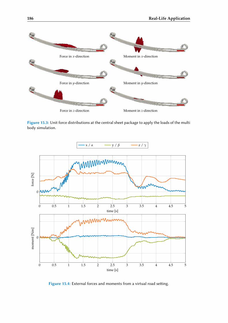
186 Real-Life Application
Force in x-direction Moment in x-direction
Force in y-direction Moment in y-direction
Force in z-direction Moment in z-direction
Figure 15.3: Unit force distributions at the central sheet package to apply the loads of the multibody simulation.
0 0.5 1 1.5 2 2.5 3 3.5 4 4.5 5
0
time [s]
forc
e[N
]
x / α y / β z / γ
0 0.5 1 1.5 2 2.5 3 3.5 4 4.5 5
0
time [s]
mom
ent[
Nm
]
Figure 15.4: External forces and moments from a virtual road seing.
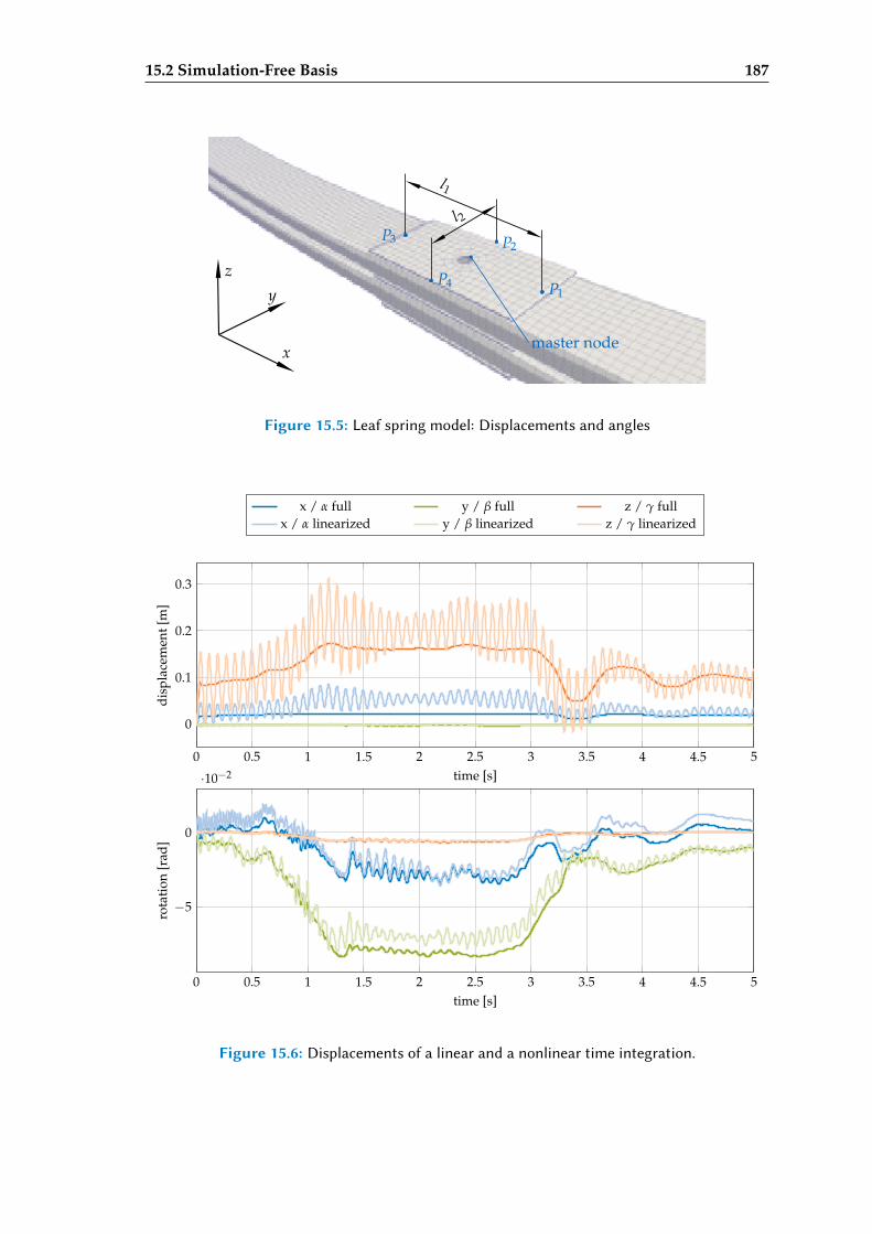
15.2 Simulation-Free Basis 187
x
yz
l1
l2
master node
P1
P2P3
P4
Figure 15.5: Leaf spring model: Displacements and angles
0 0.5 1 1.5 2 2.5 3 3.5 4 4.5 5
0
0.1
0.2
0.3
time [s]
disp
lace
men
t[m
]
x / α full y / β full z / γ fullx / α linearized y / β linearized z / γ linearized
0 0.5 1 1.5 2 2.5 3 3.5 4 4.5 5
−5
0
·10−2
time [s]
rota
tion
[rad
]
Figure 15.6: Displacements of a linear and a nonlinear time integration.
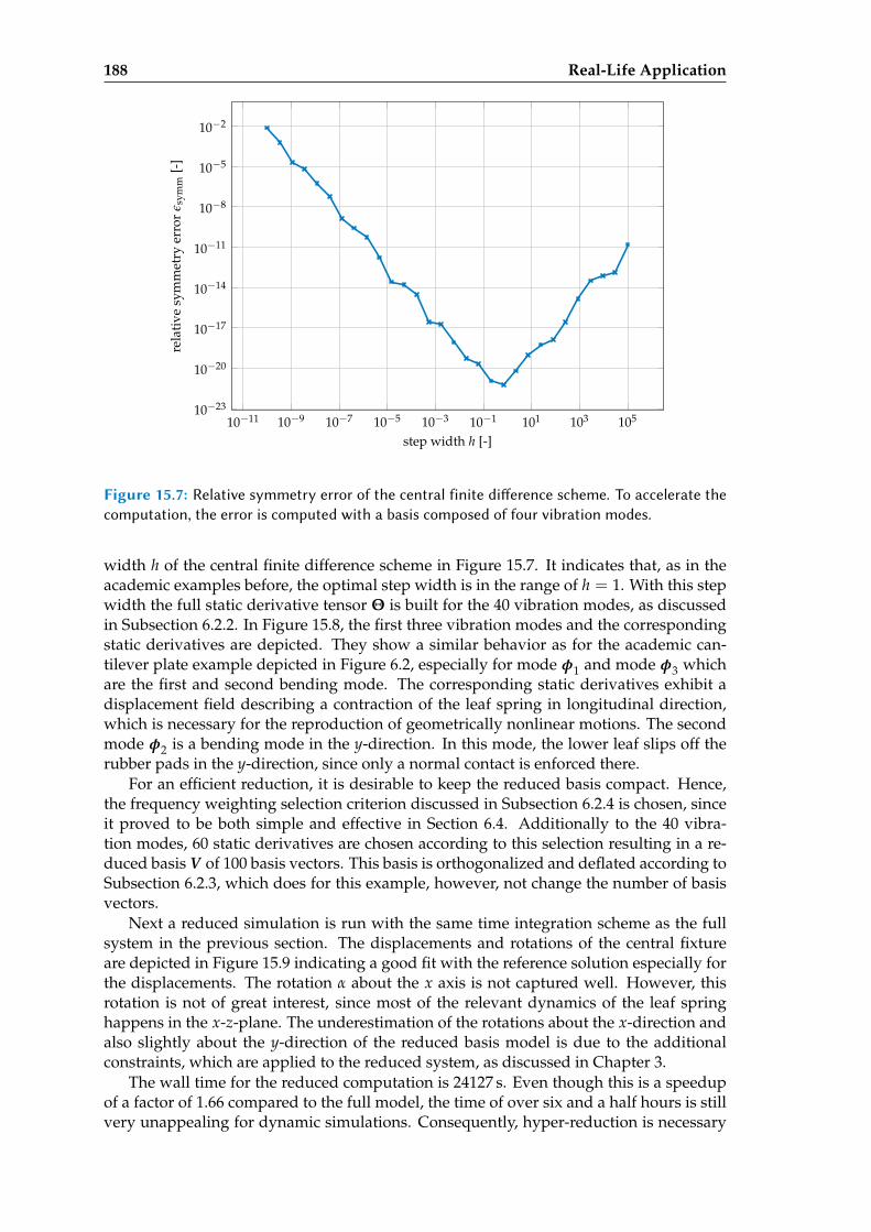
188 Real-Life Application
10−11 10−9 10−7 10−5 10−3 10−1 101 103 10510−23
10−20
10−17
10−14
10−11
10−8
10−5
10−2
step width h [-]
rela
tive
sym
met
ryer
ror
ε sym
m[-
]
Figure 15.7: Relative symmetry error of the central finite dierence scheme. To accelerate thecomputation, the error is computed with a basis composed of four vibration modes.
width h of the central finite difference scheme in Figure 15.7. It indicates that, as in theacademic examples before, the optimal step width is in the range of h = 1. With this stepwidth the full static derivative tensor Θ is built for the 40 vibration modes, as discussedin Subsection 6.2.2. In Figure 15.8, the first three vibration modes and the correspondingstatic derivatives are depicted. They show a similar behavior as for the academic can-tilever plate example depicted in Figure 6.2, especially for mode φ1 and mode φ3 whichare the first and second bending mode. The corresponding static derivatives exhibit adisplacement field describing a contraction of the leaf spring in longitudinal direction,which is necessary for the reproduction of geometrically nonlinear motions. The secondmode φ2 is a bending mode in the y-direction. In this mode, the lower leaf slips off therubber pads in the y-direction, since only a normal contact is enforced there.
For an efficient reduction, it is desirable to keep the reduced basis compact. Hence,the frequency weighting selection criterion discussed in Subsection 6.2.4 is chosen, sinceit proved to be both simple and effective in Section 6.4. Additionally to the 40 vibra-tion modes, 60 static derivatives are chosen according to this selection resulting in a re-duced basis V of 100 basis vectors. This basis is orthogonalized and deflated according toSubsection 6.2.3, which does for this example, however, not change the number of basisvectors.
Next a reduced simulation is run with the same time integration scheme as the fullsystem in the previous section. The displacements and rotations of the central fixtureare depicted in Figure 15.9 indicating a good fit with the reference solution especially forthe displacements. The rotation α about the x axis is not captured well. However, thisrotation is not of great interest, since most of the relevant dynamics of the leaf springhappens in the x-z-plane. The underestimation of the rotations about the x-direction andalso slightly about the y-direction of the reduced basis model is due to the additionalconstraints, which are applied to the reduced system, as discussed in Chapter 3.
The wall time for the reduced computation is 24127 s. Even though this is a speedupof a factor of 1.66 compared to the full model, the time of over six and a half hours is stillvery unappealing for dynamic simulations. Consequently, hyper-reduction is necessary
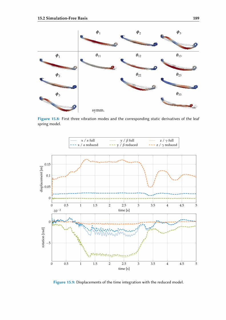
15.2 Simulation-Free Basis 189
φ1 φ2 φ3
φ1 θ11 θ12 θ13
φ2 θ22 θ23
φ3 θ33
symm.
Figure 15.8: First three vibration modes and the corresponding static derivatives of the leafspring model.
0 0.5 1 1.5 2 2.5 3 3.5 4 4.5 5
0
0.05
0.1
0.15
time [s]
disp
lace
men
t[m
]
x / α full y / β full z / γ fullx / α reduced y / β reduced z / γ reduced
0 0.5 1 1.5 2 2.5 3 3.5 4 4.5 5
−5
0
·10−2
time [s]
rota
tion
[rad
]
Figure 15.9: Displacements of the time integration with the reduced model.
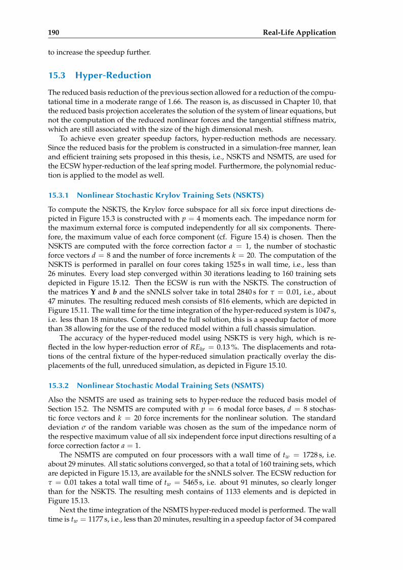
190 Real-Life Application
to increase the speedup further.
15.3 Hyper-Reduction
The reduced basis reduction of the previous section allowed for a reduction of the compu-tational time in a moderate range of 1.66. The reason is, as discussed in Chapter 10, thatthe reduced basis projection accelerates the solution of the system of linear equations, butnot the computation of the reduced nonlinear forces and the tangential stiffness matrix,which are still associated with the size of the high dimensional mesh.
To achieve even greater speedup factors, hyper-reduction methods are necessary.Since the reduced basis for the problem is constructed in a simulation-free manner, leanand efficient training sets proposed in this thesis, i.e., NSKTS and NSMTS, are used forthe ECSW hyper-reduction of the leaf spring model. Furthermore, the polynomial reduc-tion is applied to the model as well.
15.3.1 Nonlinear Stochastic Krylov Training Sets (NSKTS)
To compute the NSKTS, the Krylov force subspace for all six force input directions de-picted in Figure 15.3 is constructed with p = 4 moments each. The impedance norm forthe maximum external force is computed independently for all six components. There-fore, the maximum value of each force component (cf. Figure 15.4) is chosen. Then theNSKTS are computed with the force correction factor a = 1, the number of stochasticforce vectors d = 8 and the number of force increments k = 20. The computation of theNSKTS is performed in parallel on four cores taking 1525 s in wall time, i.e., less than26 minutes. Every load step converged within 30 iterations leading to 160 training setsdepicted in Figure 15.12. Then the ECSW is run with the NSKTS. The construction ofthe matrices Υ and b and the sNNLS solver take in total 2840 s for τ = 0.01, i.e., about47 minutes. The resulting reduced mesh consists of 816 elements, which are depicted inFigure 15.11. The wall time for the time integration of the hyper-reduced system is 1047 s,i.e. less than 18 minutes. Compared to the full solution, this is a speedup factor of morethan 38 allowing for the use of the reduced model within a full chassis simulation.
The accuracy of the hyper-reduced model using NSKTS is very high, which is re-flected in the low hyper-reduction error of REhr = 0.13 %. The displacements and rota-tions of the central fixture of the hyper-reduced simulation practically overlay the dis-placements of the full, unreduced simulation, as depicted in Figure 15.10.
15.3.2 Nonlinear Stochastic Modal Training Sets (NSMTS)
Also the NSMTS are used as training sets to hyper-reduce the reduced basis model ofSection 15.2. The NSMTS are computed with p = 6 modal force bases, d = 8 stochas-tic force vectors and k = 20 force increments for the nonlinear solution. The standarddeviation σ of the random variable was chosen as the sum of the impedance norm ofthe respective maximum value of all six independent force input directions resulting of aforce correction factor a = 1.
The NSMTS are computed on four processors with a wall time of tw = 1728 s, i.e.about 29 minutes. All static solutions converged, so that a total of 160 training sets, whichare depicted in Figure 15.13, are available for the sNNLS solver. The ECSW reduction forτ = 0.01 takes a total wall time of tw = 5465 s, i.e. about 91 minutes, so clearly longerthan for the NSKTS. The resulting mesh contains of 1133 elements and is depicted inFigure 15.13.
Next the time integration of the NSMTS hyper-reduced model is performed. The walltime is tw = 1177 s, i.e., less than 20 minutes, resulting in a speedup factor of 34 compared
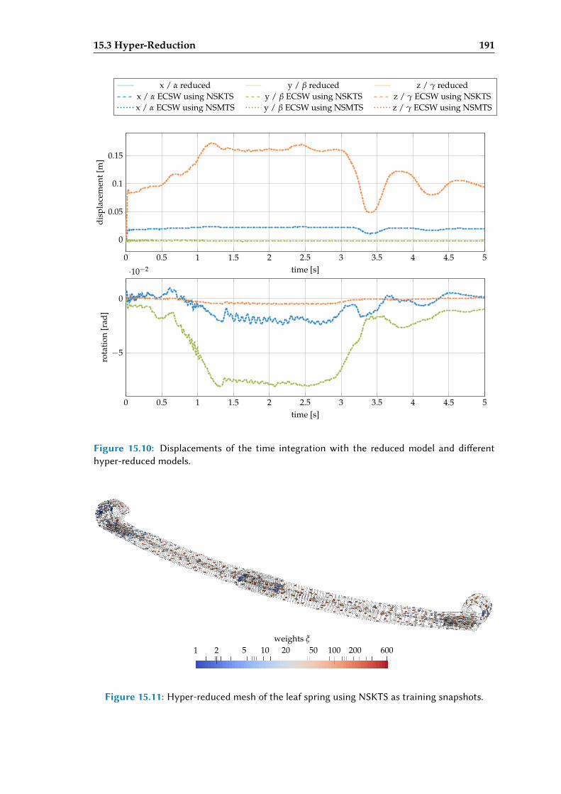
15.3 Hyper-Reduction 191
0 0.5 1 1.5 2 2.5 3 3.5 4 4.5 5
0
0.05
0.1
0.15
time [s]
disp
lace
men
t[m
]
x / α reduced y / β reduced z / γ reducedx / α ECSW using NSKTS y / β ECSW using NSKTS z / γ ECSW using NSKTSx / α ECSW using NSMTS y / β ECSW using NSMTS z / γ ECSW using NSMTS
0 0.5 1 1.5 2 2.5 3 3.5 4 4.5 5
−5
0
·10−2
time [s]
rota
tion
[rad
]
Figure 15.10: Displacements of the time integration with the reduced model and dierenthyper-reduced models.
1 2 5 10 20 50 100 200 600weights ξ
Figure 15.11: Hyper-reduced mesh of the leaf spring using NSKTS as training snapshots.
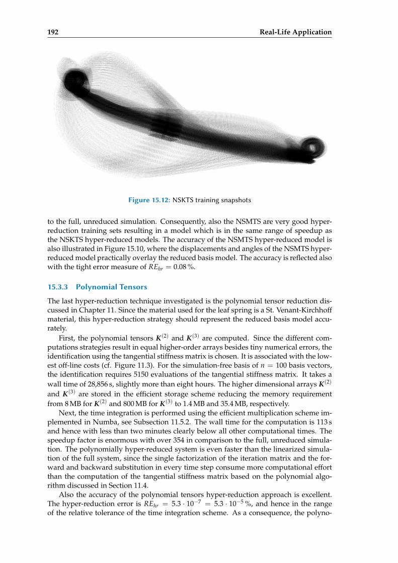
192 Real-Life Application
Figure 15.12: NSKTS training snapshots
to the full, unreduced simulation. Consequently, also the NSMTS are very good hyper-reduction training sets resulting in a model which is in the same range of speedup asthe NSKTS hyper-reduced models. The accuracy of the NSMTS hyper-reduced model isalso illustrated in Figure 15.10, where the displacements and angles of the NSMTS hyper-reduced model practically overlay the reduced basis model. The accuracy is reflected alsowith the tight error measure of REhr = 0.08 %.
15.3.3 Polynomial Tensors
The last hyper-reduction technique investigated is the polynomial tensor reduction dis-cussed in Chapter 11. Since the material used for the leaf spring is a St. Venant-Kirchhoffmaterial, this hyper-reduction strategy should represent the reduced basis model accu-rately.
First, the polynomial tensors K(2) and K(3) are computed. Since the different com-putations strategies result in equal higher-order arrays besides tiny numerical errors, theidentification using the tangential stiffness matrix is chosen. It is associated with the low-est off-line costs (cf. Figure 11.3). For the simulation-free basis of n = 100 basis vectors,the identification requires 5150 evaluations of the tangential stiffness matrix. It takes awall time of 28,856 s, slightly more than eight hours. The higher dimensional arrays K(2)
and K(3) are stored in the efficient storage scheme reducing the memory requirementfrom 8 MB for K(2) and 800 MB for K(3) to 1.4 MB and 35.4 MB, respectively.
Next, the time integration is performed using the efficient multiplication scheme im-plemented in Numba, see Subsection 11.5.2. The wall time for the computation is 113 sand hence with less than two minutes clearly below all other computational times. Thespeedup factor is enormous with over 354 in comparison to the full, unreduced simula-tion. The polynomially hyper-reduced system is even faster than the linearized simula-tion of the full system, since the single factorization of the iteration matrix and the for-ward and backward substitution in every time step consume more computational effortthan the computation of the tangential stiffness matrix based on the polynomial algo-rithm discussed in Section 11.4.
Also the accuracy of the polynomial tensors hyper-reduction approach is excellent.The hyper-reduction error is REhr = 5.3 · 10−7 = 5.3 · 10−5 %, and hence in the rangeof the relative tolerance of the time integration scheme. As a consequence, the polyno-
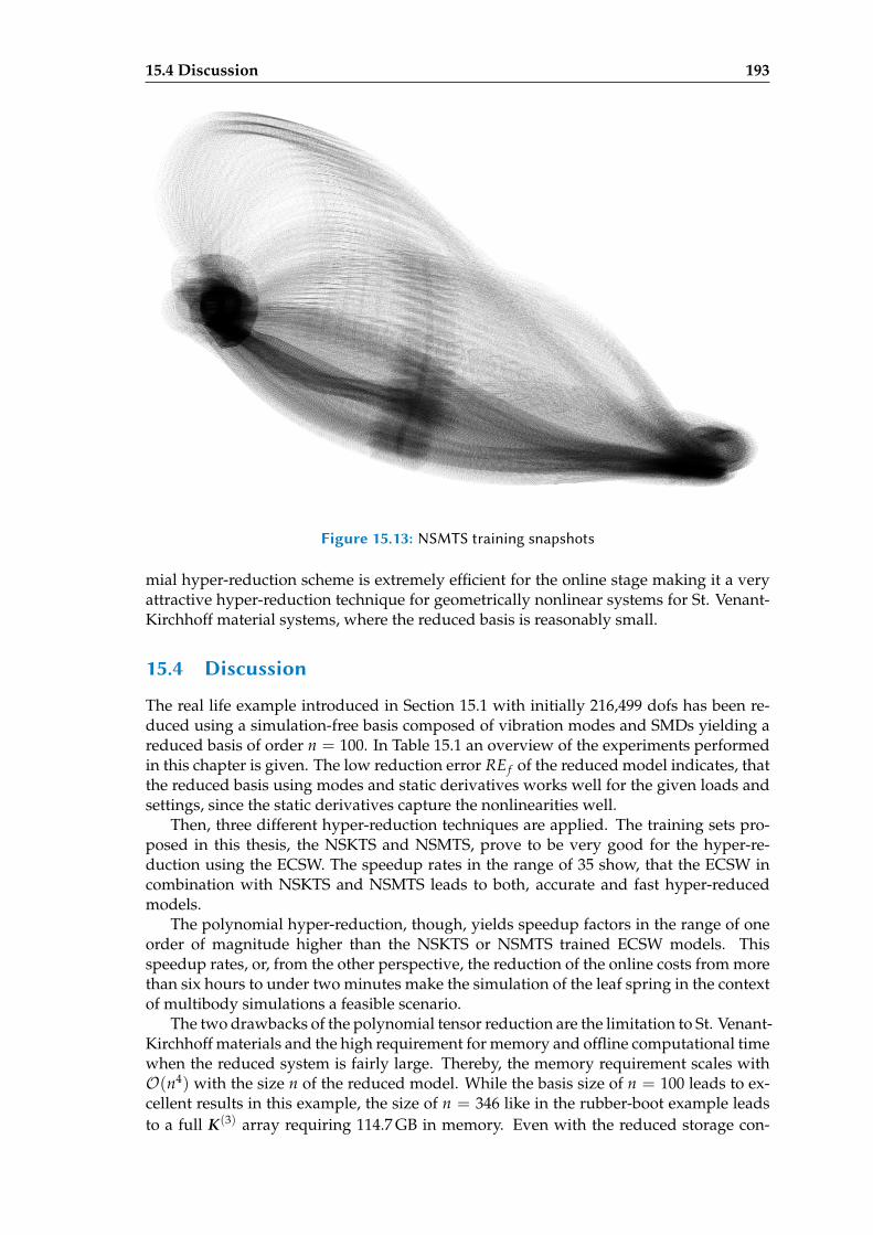
15.4 Discussion 193
Figure 15.13: NSMTS training snapshots
mial hyper-reduction scheme is extremely efficient for the online stage making it a veryattractive hyper-reduction technique for geometrically nonlinear systems for St. Venant-Kirchhoff material systems, where the reduced basis is reasonably small.
15.4 Discussion
The real life example introduced in Section 15.1 with initially 216,499 dofs has been re-duced using a simulation-free basis composed of vibration modes and SMDs yielding areduced basis of order n = 100. In Table 15.1 an overview of the experiments performedin this chapter is given. The low reduction error RE f of the reduced model indicates, thatthe reduced basis using modes and static derivatives works well for the given loads andsettings, since the static derivatives capture the nonlinearities well.
Then, three different hyper-reduction techniques are applied. The training sets pro-posed in this thesis, the NSKTS and NSMTS, prove to be very good for the hyper-re-duction using the ECSW. The speedup rates in the range of 35 show, that the ECSW incombination with NSKTS and NSMTS leads to both, accurate and fast hyper-reducedmodels.
The polynomial hyper-reduction, though, yields speedup factors in the range of oneorder of magnitude higher than the NSKTS or NSMTS trained ECSW models. Thisspeedup rates, or, from the other perspective, the reduction of the online costs from morethan six hours to under two minutes make the simulation of the leaf spring in the contextof multibody simulations a feasible scenario.
The two drawbacks of the polynomial tensor reduction are the limitation to St. Venant-Kirchhoff materials and the high requirement for memory and offline computational timewhen the reduced system is fairly large. Thereby, the memory requirement scales withO(n4) with the size n of the reduced model. While the basis size of n = 100 leads to ex-cellent results in this example, the size of n = 346 like in the rubber-boot example leadsto a full K(3) array requiring 114.7 GB in memory. Even with the reduced storage con-
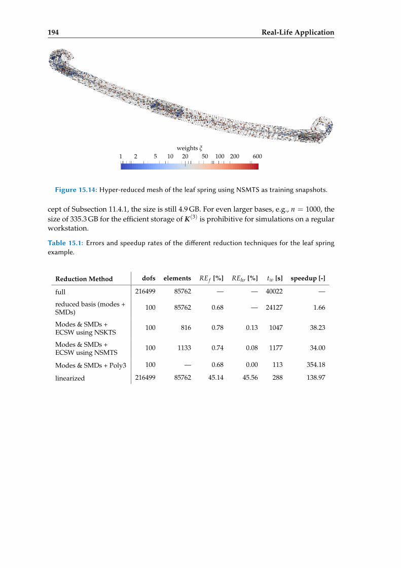
194 Real-Life Application
1 2 5 10 20 50 100 200 600weights ξ
Figure 15.14: Hyper-reduced mesh of the leaf spring using NSMTS as training snapshots.
cept of Subsection 11.4.1, the size is still 4.9 GB. For even larger bases, e.g., n = 1000, thesize of 335.3 GB for the efficient storage of K(3) is prohibitive for simulations on a regularworkstation.
Table 15.1: Errors and speedup rates of the dierent reduction techniques for the leaf springexample.
Reduction Method dofs elements RE f [%] REhr [%] tw [s] speedup [-]
full 216499 85762 — — 40022 —
reduced basis (modes +SMDs)
100 85762 0.68 — 24127 1.66
Modes & SMDs +ECSW using NSKTS
100 816 0.78 0.13 1047 38.23
Modes & SMDs +ECSW using NSMTS
100 1133 0.74 0.08 1177 34.00
Modes & SMDs + Poly3 100 — 0.68 0.00 113 354.18
linearized 216499 85762 45.14 45.56 288 138.97
Chapter 16
Closure
In this thesis, simulation-free model order reduction methods are investigated in the con-text of geometrically nonlinear structural dynamics. This chapter discusses the mainresults of the thesis and emerging research topics for future work. Since the thesis isdivided in three parts, the rather detailed summary of the first two parts is given at itsrespective last chapter: Part I is summarized in Chapter 9 on page 107, Part II in Chap-ter 14 on page 179. The summary and a discussion of the real-life example addressed inPart III of the thesis is given at the end of the previous chapter in Section 15.4. The mainconclusions resulting from the work described in this thesis are given in the following.
16.1 Conclusions and Discussion
Linear reduction methods cannot be naively applied to nonlinear systems. When ge-ometrically nonlinear systems are considered, the computation of a reduced basis is nota trivial task. For linear systems various methods exist which rely on system intrinsicproperties like decoupling of states, approximation of the transfer function or balancingof observability and controllability. In nonlinear systems, however, these properties donot exist or are extremely expensive to compute. Hence, the linear reduction methods,which are addressed in Chapter 4, cannot be applied to nonlinear systems. When theyare applied to the linearized version of the nonlinear system, the resulting reduced basisis not suited for the nonlinear system, since it does not capture the nonlinear behaviorand leads to severe locking, as illustrated in Section 6.1. As a consequence, the commonapproach to reduce nonlinear systems is a detour over a statistical investigation of train-ing sets obtained in training simulations of the full, unreduced system, as discussed inChapter 5. A further class of approaches used in nonlinear structural dynamics is basedon perturbations of reduced bases, which are addressed in Chapter 6.
Modal derivatives and static derivatives are excellent simulation-free augmentationvectors for linear reduction techniques to reduce geometrically nonlinear structuraldynamics systems. The reduced bases obtained with linear reduction methods appliedto a linearized system are not suited to the original nonlinear system. However, thelinear basis can be extended by modal derivatives (MDs) and static derivatives (SDs)which both capture the nonlinear behavior and make the augmented basis applicableto the nonlinear system. While the modal derivatives are based on the perturbation ofvibration modes and are hence limited to bases composed of those, the static derivativesare applicable to all types of linear bases. In the literature, MDs and SDs are sometimesused synonymously, but they are different vectors as shown in the numerical experimentsconducted in Chapter 6. The experiments also reveal that both MDs and SDs are wellsuited to reduce geometrically nonlinear systems. One drawback is, though, that their
195
196 Closure
number grows quadratically with respect to the number of modes gathered in the initiallinear basis. To address this issue, heuristic selection strategies are available to select asmall number of MDs or SDs forming smaller bases.
adratic manifold approach allows to reduce a system to a minimum set of gener-alized coordinates, however it is limited in its applicability. A conceptually differentmethod for reduction is the quadratic manifold approach, where the transformation be-tween physical coordinates and reduced generalized coordinates is a quadratic functionand hence nonlinear. The full system is projected onto the tangent subspace of the non-linear transformation resulting in more complicated reduced equations of motion. Thequadratic manifold approach allows to reduce a geometrically nonlinear system to a min-imum set of generalized coordinates. In the method proposed, the quadratic transforma-tion is composed of a linear part, which is formed by a linear basis, and a quadratic part,which is chosen to be either MDs or SDs. The quadratic manifold approach is closelyrelated to nonlinear static condensation when applied to beams and shells with von Kar-man kinematics. While the quadratic manifold approach leads to accurate results in thesecases, it suffers from locking when applied to general structures discretized with solidelements. As revealed by the numerical experiments, they are then only applicable tostructures with a membrane-dominated nonlinearity exhibiting small rotations.
Subspace angles allow for comparison of reduced bases. Principal vectors can show thedierences of reduction bases making them a useful tool for analyses. With subspaceangles and the corresponding principal vectors, the overlapping and distant spaces oftwo reduced bases can be identified independently of the realization. The principal vec-tors correspond to displacement fields which can be visualized for an intuitive investi-gation of the differences. In Section 8.3, this technique is used to descriptively show thatthe linear bases do not capture the contraction of a mesh necessary to represent large ro-tational deformations. To assess the suitability of a reduced basis to a certain problem, acomparison to a POD basis is often expedient, since this basis can be considered optimalfor a certain system under given excitation. When multiple bases need to be assessed, it isin general cheaper to compute the POD basis and compare the basis against this optimalbasis using subspace angles instead of running full simulations of the reduced systemwith a subsequent investigation of the reduction error.
Hyper-reduction is necessary to exploit the full potential of projective model order re-duction for nonlinear systems. While the reduced basis method decreases the numberof dofs of a finite element system, it does not reduce the cost for the computation of thenonlinear terms, which are evaluated on the finite element level. As a consequence, thecomputation of the nonlinear internal force and the tangential stiffness matrix is the com-putational bottleneck of a nonlinear reduced basis system limiting clearly the speeduprate of the reduced basis system. To alleviate the computational burden associated withthe evaluation of the nonlinearity, hyper-reduction is necessary. It approximates the non-linear internal force leading to clearly reduced computational costs allowing for clearlylarger speedup rates, as illustrated in the numerical examples given in Part II.
Polynomial tensors hyper-reduction is the method to go for reduced systems with smallnumber of dofs and St. Venant-Kirchho material. Among the hyper-reduction meth-ods investigated within this thesis, the polynomial tensors hyper-reduction has clearlythe lowest online costs for systems with a low reduced order n. This is due to the factthat the computational cost of the evaluation of the polynomial tensors scales withO(n4),
16.1 Conclusions and Discussion 197
which makes this method the clear winner for small n. This hyper-reduction method ex-presses the nonlinear internal forces as third order polynomials, which is an exact repre-sentation for St. Venant-Kirchhoff materials. Hence, the hyper-reduction error is in therange of the tolerances used for the computation, e.g., the numerical tolerances set inthe time integration scheme. A further advantage of the method is that the reduced sys-tem is independent of the finite element formulation, since the three symmetric arraysK(1) ∈ Rn×n, K(2) ∈ Rn×n×n and K(3) ∈ Rn×n×n×n completely describe the nonlinearinternal forces of the reduced system. This makes the method very attractive for scenar-ios like model predictive control, in which a nonlinear system needs to be exported toa controller software framework, for instance. The drawbacks of this method, however,are the limited applicability to only St. Venant-Kirchhoff materials and the fourth ordergrowth of the memory requirement and the computational effort with respect to the or-der n of the reduced system. The efficient storage and multiplication scheme proposedin Section 11.4 allows to keep both memory and computational effort to a minimum butdoes not revoke this general issue.
Discrete Empirical Interpolation Method (DEIM) has many drawbacks in the context ofgeometrically nonlinear structural dynamics. The DEIM turns out to be a second-classhyper-reduction method for geometrically nonlinear structural dynamics when comparedto the other investigated methods. This is mostly due to the fact that the approximationof the internal nonlinear force using a force basis and a collocation strategy destroys thesymmetry of the system and with it desirable properties like stability. Furthermore, theDEIM requires a cumbersome splitting of the internal force in a linear and a nonlinearpart, which is very unfavorable in the context of large rotations of elements present ingeometrically nonlinear systems. While the unassembled DEIM (UDEIM) as a specialadaptation to the finite element framework allows for more flexibility in the applicationof collocation strategies, it does not repeal the main issues. As shown in the numeri-cal experiments, both the DEIM and the UDEIM suffer of instability and poor accuracymaking them an inferior choice as hyper-reduction method for geometrically nonlinearstructural dynamics.
Energy Conserving Mesh Sampling and Weighting (ECSW) is a very promising method.The use of NSKTS and NSMTS allows to use this method in a simulation-free context.The ECSW is a hyper-reduction method similar to the DEIM which, however, does notcarry the drawbacks of it. It allows for the hyper-reduction of geometrically nonlinearstructural dynamics systems with different hyperelastic materials and leads to accurateand stable hyper-reduced systems. However, training snapshots are required for thecomputation of the active element set, which is the reduced set of elements responsiblefor the reduced computational costs. To use the ECSW in a simulation-free setup, theso-called Nonlinear Stochastic Krylov Training Sets (NSKTS) and Nonlinear StochasticModal Training Sets (NSMTS) are proposed in this thesis. They allow for an accuratehyper-reduction in an almost simulation-free way, since the training snapshots are ob-tained by solving a set of nonlinear problems with pseudo-dynamic right hand sides. Asdemonstrated in Section 13.3, both the NSKTS and NSMTS are very robust in terms ofchanges of the parameters which are needed for the computation as well as changes of theexcitation forces of the reduced system. While the polynomial tensors hyper-reductiondistinguishes itself with the extremely low online costs for small reduced systems, theECSW using NSKTS and NSMTS shows clearly lower offline costs especially for largerreduced systems making them an attractive hyper-reduction method.
198 Closure
The proposed simulation-free reduced basis and hyper-reduction methods are applica-ble in an industrial context. As proved by the industrial example of a leaf spring of atruck discussed in Chapter 15, both simulation-free reduced basis methods and (almost)simulation-free hyper-reduction methods are applicable to drastically reduce the compu-tational times in geometrically nonlinear structural dynamics. Thereby, speedup rates ofover two orders of magnitude for the online computation are possible. The polynomialtensors hyper-reduction achieves the best online speedups while the ECSW using NSKTSand NSMTS are clearly slower. However, this trend is flipped in the offline costs, wherethe computation of the polynomial tensors is clearly more computationally demandingthan the computation of the NSKTS or the NSMTS and the ECSW hyper-reduction. Themethods proposed and discussed form a foundation for future applications in geometri-cally nonlinear structural dynamics and further research in this field.
16.2 Future Directions of Research
This thesis shows that geometrically nonlinear dynamical systems can successfully be re-duced by the appropriate methods in a simulation-free fashion. However, the successfulsimulation of a system is usually not the end point of a development cycle but the start-ing point. In many cases, parameter studies, optimizations, what if?-scenarios and morein-depth investigations are executed, in which numerical simulations should be quickand affordable making model order reduction an attractive option. However, many as-pects which are required in these studies are not addressed within this thesis. They formexciting questions and possible directions of future research:
• For optimization and parameter studies, the systems are treated as parametric re-quiring parametric model order reduction techniques. Parametric reduced basissystems have been studied in the literature in the field of simulation-based reducedbasis methods, see e.g., Amsallem et. al. [Ams+09; Ams10; AF11], where reducedbases are computed for certain points in the parameter space. However, it is yet un-clear, if parametric, geometrically nonlinear structural dynamics systems can be re-duced more efficiently by exploiting intrinsic physical properties. Furthermore, thehyper-reduction of parametric systems is an open topic in both simulation-basedand simulation-free setups.
• Within this thesis, solely systems with linear Dirichlet boundary conditions areaddressed. Many real-life applications, however, are characterized by nonlinearconstraints such as joints, rigid body elements or contacts. One way to expressthese nonlinear constraints systematically is the use of Lagrange multipliers, wherethe nonlinear constraint equations are considered explicitly. It has not been clari-fied yet, to what extent the concepts of simulation-free reduced bases and hyper-reduction are applicable to systems with nonlinear constraints. For possible adap-tations, novel methods are required to handle these systems.
• The systems covered in this thesis are only characterized by viscous damping. Itdoes, however, not recognize the geometric nonlinearity since it is not objectiveand results in damping forces for pure rigid body motions (cf. Section 2.1). A moreaccurate damping approximation can be expected from viscoelastic material mod-els like the Kelvin-Voigt model, where the stress originated from viscous dampingis proportional to the rate of deformation of the nonlinear strain measure. Thesemodels, however, result in equations of motion with a different mathematical struc-ture compared to the ones discussed here, which stem from hyperelastic materials.Hence, further research is necessary to adapt the simulation-free methods discussedand developed here to the field of geometric nonlinearity with viscoelasticity.
16.2 Future Directions of Research 199
• In several industrial applications, nonlinear structural dynamics problems are cou-pled with other physical areas such as thermal effects, plasticity, fatigue or fluidstructure interaction. Fundamental research is necessary to answer the questions,how these coupled systems can be reduced in a simulation-free manner.
• Untapped potential lies in the transformation and adaptation of the discussed simu-lation-free reduced basis methods and the hyper-reduction methods to substructureframeworks. This would allow to assemble large nonlinear systems using small,reduced substructures with the potential to higher speedup rates, particularly forlarge systems with complex dynamics requiring a high number of basis vectors.Notably the polynomial tensors hyper-reduction technique could unfold its poten-tial, when the system to be reduced is divided in small parts of which each partrequires only a small number of basis vectors. Since the computational costs of thismethod are associated with O(n4) with respect to the dimension n of the reducedsystem, or in this context with the substructure, impressive online cost reductionseven for large systems are feasible in principle.
• The polynomial tensors hyper-reduction suffers of the curse of dimensionality mak-ing it not attractive for reduced systems with large n. In principle, a low rank ap-proximation of the higher order tensors could allow for further speedup factorsmaking the polynomial tensors hyper-reduction accessible for higher reduction or-ders n. However, approaches for low rank approximations for higher order sym-metric arrays as well as identification techniques still need to be developed.

Bibliography
[AP03] P. G. A. Cizmas and A. Palacios. “Proper orthogonal decomposition of tur-bine rotor-stator interaction”. In: Journal of propulsion and power 19.2 (2003),pp. 268–281.
[AJ02] R. G. Aarts and J. B. Jonker. “Dynamic simulation of planar flexible link ma-nipulators using adaptive modal integration”. In: Multibody System Dynamics7.1 (2002), pp. 31–50.
[ACM99] K. Abdel-Motaglay, R. Chen, and C. Mei. “Nonlinear flutter of compositepanels under yawed supersonic flow using finite elements”. In: AIAA journal37.9 (1999), pp. 1025–1032.
[Add+15] K. C. Addepalli, N. Remisoski, A. Sleath, and S. Liu. “A Multibody DynamicsApproach to Leaf Spring Simulation for Upfront Analyses”. In: SAE TechnicalPaper. SAE International, June 2015.
[Akg94] M. A. Akgun. “New family of modal methods for calculating eigenvectorderivatives”. In: AIAA Journal 32.2 (1994), pp. 379–386.
[All03] R. J. Allemang. “The modal assurance criterion–twenty years of use andabuse”. In: Sound and vibration 37.8 (2003), pp. 14–23.
[ASB78] B. Almroth, P. Stern, and F. Brogan. “Automatic choice of global shape func-tions in structural analysis”. In: Aiaa Journal 16.5 (1978), pp. 525–528.
[Ams10] D. Amsallem. “Interpolation on manifolds of CFD-based fluid and finiteelement-based structural reduced-order models for on-line aeroelastic pre-dictions”. PhD thesis. Stanford University, 2010.
[Ams+09] D. Amsallem, J. Cortial, K. Carlberg, and C. Farhat. “A method for interpo-lating on manifolds structural dynamics reduced-order models”. In: Interna-tional journal for numerical methods in engineering 80.9 (2009), pp. 1241–1258.
[AF11] D. Amsallem and C. Farhat. “An online method for interpolating linear para-metric reduced-order models”. In: SIAM Journal on Scientific Computing 33.5(2011), pp. 2169–2198.
[AF08] D. Amsallem and C. Farhat. “Interpolation method for adapting reduced-order models and application to aeroelasticity”. In: AIAA Journal 46.7 (2008),pp. 1803–1813.
[AKJ08] S. S. An, T. Kim, and D. L. James. “Optimizing cubature for efficient integra-tion of subspace deformations”. In: ACM Transactions on Graphics (TOG) 27.5(2008), No. 165.
201
202 BIBLIOGRAPHY
[AHS14] H. Antil, M. Heinkenschloss, and D. C. Sorensen. “Application of the discreteempirical interpolation method to reduced order modeling of nonlinear andparametric systems”. In: Reduced order methods for modeling and computationalreduction. Springer, 2014, pp. 101–136.
[ASG06] A. Antoulas, D. Sorensen, and S. Gugercin. “A survey of model reductionmethods for large-scale systems”. In: Contemporary mathematics 280 (2006),pp. 193–220.
[Ant09] A. C. Antoulas. Approximation of large-scale dynamical systems. Vol. 6. Societyfor Industrial and Applied Mathematics, 2009.
[Ant05] A. C. Antoulas. Approximation of large-scale dynamical systems. Vol. 6. Siam,2005.
[Ast04] P. Astrid. Reduction of process simulation models: a proper orthogonal decomposi-tion approach. Technische Universiteit Eindhoven PhD-thesis, 2004.
[Ast+08] P. Astrid, S. Weiland, K. Willcox, and T. Backx. “Missing point estimation inmodels described by proper orthogonal decomposition”. In: IEEE Transac-tions on Automatic Control 53.10 (2008), pp. 2237–2251.
[AV01] M. Azeez and A. Vakakis. “Proper orthogonal decomposition (POD) of aclass of vibroimpact oscillations”. In: Journal of Sound and Vibration 240.5(2001), pp. 859–889.
[AV99] M. F. A. Azeez and A. F. Vakakis. “Numerical and experimental analysisof a continuous overhung rotor undergoing vibro-impacts”. In: Internationaljournal of non-linear mechanics 34.3 (1999), pp. 415–435.
[Bai+00] Z. Bai, J. Demmel, J. Dongarra, A. Ruhe, and H. van der Vorst. Templates forthe solution of algebraic eigenvalue problems: a practical guide. SIAM, 2000.
[BS05] Z. Bai and Y. Su. “Dimension reduction of large-scale second-order dynami-cal systems via a second-order Arnoldi method”. In: SIAM Journal on Scien-tific Computing 26.5 (2005), pp. 1692–1709.
[BJ05] J. Barbic and D. L. James. “Real-Time subspace integration for St.Venant-Kirchhoff deformable models”. In: ACM Transactions on Graphics(TOG). Vol. 24. 3. ACM. 2005, pp. 982–990.
[BV10] T. K. Barlas and G. Van Kuik. “Review of state of the art in smart rotor con-trol research for wind turbines”. In: Progress in Aerospace Sciences 46.1 (2010),pp. 1–27.
[Bar+04] M. Barrault, Y. Maday, N. C. Nguyen, and A. T. Patera. “An ’empirical in-terpolation’ method: application to efficient reduced-basis discretization ofpartial differential equations”. In: Comptes Rendus Mathematique 339.9 (2004),pp. 667–672.
[Bat06] K.-J. Bathe. Finite element procedures. Klaus-Jurgen Bathe, 2006.
BIBLIOGRAPHY 203
[BG93] O. Bauchau and D. Guernsey. “On the choice of appropriate bases for non-linear dynamic modal analysis”. In: Journal of the American Helicopter Society38.4 (1993), pp. 28–36.
[BG16] C. Beattie and S. Gugercin. “Model Reduction by Rational Interpolation”. In:Model Reduction and Approximation: Theory and Algorithms (2016).
[BLM00] T. Belytschko, W. K. Liu, and B. Moran. Nonlinear Finite Elements for Continuaand Structures. John Wiley & Sons, 2000.
[BGW15] P. Benner, S. Gugercin, and K. Willcox. “A Survey of Projection-based ModelReduction Methods for Parametric Dynamical Systems”. In: SIAM Review57.4 (2015), pp. 483–531.
[BCB05] M. Bergmann, L. Cordier, and J.-P. Brancher. “Optimal rotary control ofthe cylinder wake using proper orthogonal decomposition reduced-ordermodel”. In: Physics of fluids 17.9 (2005), pp. 97–101.
[Ber92] G. Berkooz. “Observations on the proper orthogonal decomposition”. In:Studies in Turbulence. Springer, 1992, pp. 229–247.
[BHL93] G. Berkooz, P. Holmes, and J. L. Lumley. “The proper orthogonal decompo-sition in the analysis of turbulent flows”. In: Annual review of fluid mechanics25.1 (1993), pp. 539–575.
[Bes+13] B. Besselink, U. Tabak, A. Lutowska, N. van de Wouw, H. Nijmeijer, D. J.Rixen, M. Hochstenbach, and W. Schilders. “A comparison of model reduc-tion techniques from structural dynamics, numerical mathematics and sys-tems and control”. In: Journal of Sound and Vibration 332.19 (2013), pp. 4403–4422.
[BT05] T. Betcke and L. N. Trefethen. “Reviving the method of particular solutions”.In: SIAM review 47.3 (2005), pp. 469–491.
[BG73] Å. Björck and G. H. Golub. “Numerical methods for computing anglesbetween linear subspaces”. In: Mathematics of computation 27.123 (1973),pp. 579–594.
[Blo+15] B. Blockmans, T. Tamarozzi, F. Naets, and W. Desmet. “A nonlinear paramet-ric model reduction method for efficient gear contact simulations”. In: Inter-national Journal for Numerical Methods in Engineering 102.5 (2015), pp. 1162–1191.
[BW97] J. Bonet and R. D. Wood. Nonlinear continuum mechanics for finite element anal-ysis. Cambridge university press, 1997.
[Bou+14] L. Boucinha, A. Ammar, A. Gravouil, and A. Nouy. “Ideal minimalresidual-based proper generalized decomposition for non-symmetricmulti-field models – Application to transient elastodynamics in space-timedomain”. In: Computer Methods in Applied Mechanics and Engineering 273(2014), pp. 56–76.
204 BIBLIOGRAPHY
[BGA13] L. Boucinha, A. Gravouil, and A. Ammar. “Space–time proper generalizeddecompositions for the resolution of transient elastodynamic models”. In:Computer Methods in Applied Mechanics and Engineering 255 (2013), pp. 67–88.
[BMS16] B. Brands, J. Mergheim, and P. Steinmann. “Reduced-order modelling forlinear heat conduction with parametrised moving heat sources”. In: GAMM-Mitteilungen 39.2 (2016), pp. 170–188.
[Bro15] R. W. Brockett. Finite dimensional linear systems. SIAM, 2015.
[BDG07] O. Brüls, P. Duysinx, and J.-C. Golinval. “The global modal parameterizationfor non-linear model-order reduction in flexible multibody dynamics”. In:International journal for numerical methods in engineering 69.5 (2007), pp. 948–977.
[BDW03] T. Bui-Thanh, M. Damodaran, and K. Willcox. “Proper orthogonal decom-position extensions for parametric applications in compressible aerodynam-ics”. In: AIAA paper 4213 (2003).
[CW09] L. Cai and R. E. White. “Reduction of model order based on proper orthog-onal decomposition for lithium-ion battery simulations”. In: Journal of TheElectrochemical Society 156.3 (2009), A154–A161.
[Cap+02] S. Capell, S. Green, B. Curless, T. Duchamp, and Z. Popovic. “Interactiveskeleton-driven dynamic deformations”. In: ACM Transactions on Graphics(TOG). Vol. 21. 3. ACM. 2002, pp. 586–593.
[CSM14] E. Capiez-Lernout, C. Soize, and M.-P. Mignolet. “Post-buckling nonlinearstatic and dynamical analyses of uncertain cylindrical shells and experimen-tal validation”. In: Computer Methods in Applied Mechanics and Engineering 271(2014), pp. 210–230.
[CBF11] K. Carlberg, C. Bou-Mosleh, and C. Farhat. “Efficient non-linear model re-duction via a least-squares Petrov–Galerkin projection and compressive ten-sor approximations”. In: International Journal for Numerical Methods in Engi-neering 86.2 (2011), pp. 155–181.
[CTB15] K. Carlberg, R. Tuminaro, and P. Boggs. “Preserving Lagrangian structurein nonlinear model reduction with application to structural dynamics”. In:SIAM Journal on Scientific Computing 37.2 (2015), B153–B184.
[Cha+06] Y. Chahlaoui, D. Lemonnier, A. Vandendorpe, and P. V. Dooren. “Second-order balanced truncation”. In: Linear Algebra and its Applications 415.2 (2006).Special Issue on Order Reduction of Large-Scale Systems, pp. 373–384.
[CE91] C. Chang and J. J. Engblom. “Nonlinear dynamical response of impulsivelyloaded structures-A reduced basis approach”. In: AIAA Journal 29.4 (1991),pp. 613–618.
[Cha+17] T. Chapman, P. Avery, P. Collins, and C. Farhat. “Accelerated mesh samplingfor the hyper reduction of nonlinear computational models”. In: InternationalJournal for Numerical Methods in Engineering 109.12 (2017), pp. 1623–1654.
BIBLIOGRAPHY 205
[CBG16] S. Chaturantabut, C. Beattie, and S. Gugercin. “Structure-preserving modelreduction for nonlinear port-Hamiltonian systems”. In: SIAM Journal on Sci-entific Computing 38.5 (2016), B837–B865.
[CS10] S. Chaturantabut and D. C. Sorensen. “Nonlinear model reduction via dis-crete empirical interpolation”. In: SIAM Journal on Scientific Computing 32.5(2010), pp. 2737–2764.
[CZ06] D. Chelidze and W. Zhou. “Smooth orthogonal decomposition-basedvibration mode identification”. In: Journal of Sound and Vibration 292.3(2006), pp. 461–473.
[Che+04] J. Chen, S.-M. Kang, J. Zou, C. Liu, and J. E. Schutt-Ainé. “Reduced-ordermodeling of weakly nonlinear MEMS devices with Taylor-series expansionand Arnoldi approach”. In: Journal of Microelectromechanical systems 13.3(2004), pp. 441–451.
[CH93] J. Chung and G. Hulbert. “A time integration algorithm for structural dy-namics with improved numerical dissipation: the generalized-α method”.In: Journal of applied mechanics 60.2 (1993), pp. 371–375.
[CN01] J. A. Clarke and R. Namburu. The eXtensible Data Model and Format: A HighPerformance Data Hub for Connecting Parallel Codes and Tools. Tech. rep. DTICDocument, 2001.
[CDM15] A. Corigliano, M. Dossi, and S. Mariani. “Model Order Reduction and do-main decomposition strategies for the solution of the dynamic elastic–plasticstructural problem”. In: Computer Methods in Applied Mechanics and Engineer-ing 290 (2015), pp. 127–155.
[CCI14] A. Cosimo, A. Cardona, and S. Idelsohn. “Improving the k-compressibility ofhyper reduced order models with moving sources: applications to weldingand phase change problems”. In: Computer Methods in Applied Mechanics andEngineering 274 (2014), pp. 237–263.
[Cra81] R. R. Craig. Structural dynamics: an introduction to computer methods. John Wi-ley & Sons Inc, 1981.
[CB68] R. R. Craig Jr and M. C. Bampton. “Coupling of substructures for dynamicanalyses.” In: AIAA Journal 6.7 (1968), pp. 1313–1319.
[CK06] R. R. Craig and A. J. Kurdila. Fundamentals of structural dynamics. John Wiley& Sons, 2006.
[C+12] M. A. Crisfield, J. J. Remmers, C. V. Verhoosel, et al. Nonlinear finite elementanalysis of solids and structures. John Wiley & Sons, 2012.
[CM69] E. Cuthill and J. McKee. “Reducing the bandwidth of sparse symmetric ma-trices”. In: Proceedings of the 1969 24th national conference. ACM. 1969, pp. 157–172.
[DS84] J. Davis and R. Skelton. “Another balanced controller reduction algorithm”.In: Systems & Control Letters 4.2 (1984), pp. 79–83.
206 BIBLIOGRAPHY
[DG03] P. De Boe and J.-C. Golinval. “Principal component analysis of a piezosen-sor array for damage localization”. In: Structural health monitoring 2.2 (2003),pp. 137–144.
[DV00] H. De Boer and F. Van Keulen. “Refined semi-analytical design sensitivities”.In: International journal of solids and structures 37.46 (2000), pp. 6961–6980.
[DM01] I. S. Dhillon and D. S. Modha. “Concept decompositions for large sparse textdata using clustering”. In: Machine learning 42.1 (2001), pp. 143–175.
[DP92] J. Dickens and K. Pool. “Modal truncation vectors and periodic time domainanalysis applied to a cyclic symmetry structure”. In: Computers & structures45.4 (1992), pp. 685–696.
[AM02] A. Al-Dmour and K. Mohammad. “Active control of flexible structures usingprincipal component analysis in the time domain”. In: Journal of sound andvibration 253.3 (2002), pp. 545–569.
[Dod] T. Dodt. Introducing the 787. Presentation at the International Society of AirSafety Investigators. URL: http://www.isasi.org/Documents/library/technical- papers/2011/Introducing- 787.pdf,visited on 04/28/2017.
[DG16] Z. Drmac and S. Gugercin. “A new selection operator for the discrete empir-ical interpolation method—Improved a priori error bound and extensions”.In: SIAM Journal on Scientific Computing 38.2 (2016), A631–A648.
[Epu03] B. Epureanu. “A parametric analysis of reduced order models of viscousflows in turbomachinery”. In: Journal of fluids and structures 17.7 (2003),pp. 971–982.
[ES95] R. Everson and L. Sirovich. “Karhunen–Loeve procedure for gappy data”.In: Journal of the Optical Society of America A 12.8 (1995), pp. 1657–1664.
[Ewi84] D. J. Ewins. Modal testing: theory and practice. Vol. 15. Chichester: Researchstudies press, 1984.
[Far+14] C. Farhat, P. Avery, T. Chapman, and J. Cortial. “Dimensional reduction ofnonlinear finite element dynamic models with finite rotations and energy-based mesh sampling and weighting for computational efficiency”. In: Inter-national Journal for Numerical Methods in Engineering 98 (2014), pp. 625–662.
[FCA13] C. Farhat, T. Chapman, and P. Avery. “ECSW: An energy-basedstructure-preserving method for the hyper reduction of nonlinear finiteelement reduced-order models”. In: International Journal for NumericalMethods in Engineering 00 (2013), pp. 1–33.
[FCA15] C. Farhat, T. Chapman, and P. Avery. “Structure-preserving, stability, and ac-curacy properties of the energy-conserving sampling and weighting methodfor the hyper reduction of nonlinear finite element dynamic models”. In: In-ternational Journal for Numerical Methods in Engineering 102.5 (2015), pp. 1077–1110.
BIBLIOGRAPHY 207
[FF08a] U. Farooq and B. Feeny. “Smooth orthogonal decomposition for modal anal-ysis of randomly excited systems”. In: Journal of Sound and Vibration 316.1(2008), pp. 137–146.
[FF08b] B. Feeny and U. Farooq. “A nonsymmetric state-variable decomposition formodal analysis”. In: Journal of Sound and Vibration 310.4 (2008), pp. 792–800.
[FK98] B. Feeny and R. Kappagantu. “On the physical interpretation of proper or-thogonal modes in vibrations”. In: Journal of Sound and Vibration 211.4 (1998),pp. 607–616.
[FL03] B. Feeny and Y. Liang. “Interpreting proper orthogonal modes of randomlyexcited vibration systems”. In: Journal of Sound and Vibration 265.5 (2003),pp. 953–966.
[FE10] J. Fehr and P. Eberhard. “Error-controlled model reduction in flexiblemultibody dynamics”. In: Journal of Computational and Nonlinear Dynamics5.3 (2010), pp. 031005–031005-8.
[Fol+11] M. Folk, G. Heber, Q. Koziol, E. Pourmal, and D. Robinson. “An overviewof the HDF5 technology suite and its applications”. In: Proceedings of theEDBT/ICDT 2011 Workshop on Array Databases. ACM. 2011, pp. 36–47.
[FI99] M. I. Friswell and D. J. Inman. “Sensor validation for smart structures”. In:Journal of intelligent material systems and structures 10.12 (1999), pp. 973–982.
[FT01] Y. C. Fung and P. Tong. Classical and computational solid mechanics. Vol. 1.World Scientific Publishing Co Inc, 2001.
[Gaw97] W. Gawronski. “Actuator and sensor placement for structural testing andcontrol”. In: Journal of Sound and Vibration 208.1 (1997), pp. 101–109.
[Gaw06] W. Gawronski. Balanced control of flexible structures. Vol. 211. Lecture Notes inControl and Information Sciences. Springer, 2006.
[Gaw04] W. K. Gawronski. Dynamics and control of structures: A modal approach.Springer Science & Business Media, 2004.
[GL96] W. Gawronski and K. Lim. “Balanced actuator and sensor placement for flex-ible structures”. In: International Journal of Control 65.1 (1996), pp. 131–145.
[GR14] M. Géradin and D. J. Rixen. Mechanical vibrations: theory and application tostructural dynamics. John Wiley & Sons, 2014.
[GR09] C. Geuzaine and J.-F. Remacle. “Gmsh: A 3-D finite element mesh generatorwith built-in pre-and post-processing facilities”. In: International journal fornumerical methods in engineering 79.11 (2009), pp. 1309–1331.
[GAM09] S. Ghoman, M. S. Azzouz, and C. Mei. “Time domain method for nonlinearflutter of curved panels under yawed supersonic flow at elevated tempera-ture”. In: Proceedings of the 50th Structures, Structural Dynamics and MaterialsConference. Palm Springs, California, April 2009, pp. 2009–2598.
208 BIBLIOGRAPHY
[GMW81] P. E. Gill, W. Murray, and M. H. Wright. Practical optimization. Academicpress, 1981.
[GV12] G. H. Golub and C. F. Van Loan. Matrix computations. Vol. 3. JHU Press, 2012.
[GSD08] P. Gonçalves, F. Silva, and Z. Del Prado. “Low-dimensional models for thenonlinear vibration analysis of cylindrical shells based on a perturbation pro-cedure and proper orthogonal decomposition”. In: Journal of Sound and Vibra-tion 315.3 (2008), pp. 641–663.
[GW08] A. Griewank and A. Walther. Evaluating derivatives: principles and techniquesof algorithmic differentiation. SIAM, 2008.
[Gri97] E. J. Grimme. “Krylov projection methods for model reduction”. PhD thesis.University of Illinois at Urbana-Champaign Urbana-Champaign, IL, 1997.
[GRR16] F. M. Gruber, J. B. Rutzmoser, and D. J. Rixen. “Generalized Craig-BamptonMethod Using Robin Boundary Conditions”. In: Topics in Modal Analysis &Testing, Volume 10. Springer, 2016, pp. 111–115.
[GKA16] L. C. Guerin, R. J. Kuether, and M. S. Allen. “Considerations for IndirectParameter Estimation in Nonlinear Reduced Order Models”. In: NonlinearDynamics, Volume 1. Springer, 2016, pp. 327–342.
[GA04] S. Gugercin and A. C. Antoulas. “A survey of model reduction by balancedtruncation and some new results”. In: International Journal of Control 77.8(2004), pp. 748–766.
[GAB08] S. Gugercin, A. C. Antoulas, and C. Beattie. “H2 model reduction for large-scale linear dynamical systems”. In: SIAM journal on matrix analysis and ap-plications 30.2 (2008), pp. 609–638.
[Guo11] X. Guo. “Energy-Weighted Modes Selection in Reduced-Order NonlinearSimulations”. In: 52nd AIAA/ASME/ASCE/AHS/ASC Structures, StructuralDynamics and Materials Conference. Ed. by AIAA. AIAA 2011-2063. AIAA.April 2011.
[GM03] X. Guo and C. Mei. “Using aeroelastic modes for nonlinear panel flutter atarbitrary supersonic yawed angle”. In: AIAA journal 41.2 (2003), pp. 272–279.
[Guy65] R. J. Guyan. “Reduction of stiffness and mass matrices”. In: AIAA Journal 3.2(1965), pp. 380–380.
[HTD00] K. C. Hall, J. P. Thomas, and E. H. Dowell. “Proper orthogonal decomposi-tion technique for transonic unsteady aerodynamic flows”. In: AIAA Journal38.10 (2000), pp. 1853–1862.
[HD01] F. M. Hemez and S. W. Doebling. “Review and assessment of model up-dating for non-linear, transient dynamics”. In: Mechanical Systems and SignalProcessing 15.1 (2001), pp. 45–74.
[HCF17] J. A. Hernandez, M. A. Caicedo, and A. Ferrer. “Dimensionalhyper-reduction of nonlinear finite element models via empirical cubature”.
BIBLIOGRAPHY 209
In: Computer methods in applied mechanics and engineering 313 (2017),pp. 687–722.
[HKS01] Hibbitt, Karlsson, and Sorensen. ABAQUS/standard User’s Manual. Vol. 1.2001.
[HHT77] H. M. Hilber, T. J. Hughes, and R. L. Taylor. “Improved numerical dissipa-tion for time integration algorithms in structural dynamics”. In: EarthquakeEngineering & Structural Dynamics 5.3 (1977), pp. 283–292.
[Hil+11] K. Hildebrandt, C. Schulz, C. V. Tycowicz, and K. Polthier. “Interactivesurface modeling using modal analysis”. In: ACM Transactions on Graphics(TOG) 30.5 (2011), p. 119.
[HG08] J. J. Hollkamp and R. W. Gordon. “Reduced-order models for nonlinear re-sponse prediction: Implicit condensation and expansion”. In: Journal of Soundand Vibration 318.4 (2008), pp. 1139–1153.
[HGS05] J. J. Hollkamp, R. W. Gordon, and S. M. Spottswood. “Nonlinear modal mod-els for sonic fatigue response prediction: a comparison of methods”. In: Jour-nal of Sound and Vibration 284.3 (2005), pp. 1145–1163.
[Hol12] P. Holmes. Turbulence, coherent structures, dynamical systems and symmetry.Cambridge university press, 2012.
[Hol00] G. A. Holzapfel. Nonlinear solid mechanics: A continuum approach for engineer-ing. Vol. 24. Wiley Chichester, 2000.
[IC85a] S. R. Idelsohn and A. Cardona. “A load-dependent basis for reduced non-linear structural dynamics”. In: Computers & Structures 20.1 (1985), pp. 203–210.
[IC85b] S. R. Idelsohn and A. Cardona. “A reduction method for nonlinear structuraldynamic analysis”. In: Computer Methods in Applied Mechanics and Engineering49.3 (1985), pp. 253–279.
[Iro65] B. Irons. “Structural eigenvalue problems - elimination of unwanted vari-ables”. In: AIAA Journal 3.5 (1965), pp. 961–962.
[JE92] B. Jacob and N. Ebecken. “Adaptive reduced integration method for non-linear structural dynamic analysis”. In: Computers & structures 45.2 (1992),pp. 333–347.
[Jai15] S. Jain. “Model Order Reduction for Non-Linear Structural Dynamics”. MAthesis. Delft University of Technology, 2015.
[Jai+17] S. Jain, P. Tiso, J. B. Rutzmoser, and D. J. Rixen. “A quadratic manifold formodel order reduction of nonlinear structural dynamics”. In: Computers &Structures 188 (2017), pp. 80–94.
[Jon84] E. A. Jonckheere. “Principal component analysis of flexible systems—Open-loop case”. In: Mathematical Theory of Networks and Systems. Springer. 1984,pp. 494–512.
210 BIBLIOGRAPHY
[KF99] R. Kappagantu and B. Feeny. “An "optimal" modal reduction of a systemwith frictional excitation”. In: Journal of Sound and vibration 224.5 (1999),pp. 863–877.
[Kar46] K. Karhunen. “Über lineare Methoden in der Wahrscheinlichkeitsrechnung”.In: Annals of Academic Science Fennicae, Series A1 Mathematics and Physics 37(1946), pp. 3–79.
[Ker+04] G. Kerschen, P. De Boe, J.-C. Golinval, and K. Worden. “Sensor validationusing principal component analysis”. In: Smart Materials and Structures 14.1(2004), pp. 36–42.
[KG02] G. Kerschen and J.-C. Golinval. “Physical interpretation of the properorthogonal modes using the singular value decomposition”. In: Journal ofSound and Vibration 249.5 (2002), pp. 849–865.
[Ker+05] G. Kerschen, J.-C. Golinval, A. F. Vakakis, and L. A. Bergman. “The methodof proper orthogonal decomposition for dynamical characterization and or-der reduction of mechanical systems: an overview”. In: Nonlinear Dynamics41.1-3 (2005), pp. 147–169.
[KAS07] M. Khalil, S. Adhikari, and A. Sarkar. “Linear system identification usingproper orthogonal decomposition”. In: Mechanical Systems and Signal Process-ing 21.8 (2007), pp. 3123–3145.
[Kim+13] K. Kim, A. G. Radu, X. Wang, and M. P. Mignolet. “Nonlinear reduced or-der modeling of isotropic and functionally graded plates”. In: InternationalJournal of Non-Linear Mechanics 49 (2013), pp. 100–110.
[KS09] N.-H. Kim and B. V. Sankar. Introduction to finite element analysis and design.Wiley, 2009.
[Kim98] T. Kim. “Frequency-domain Karhunen-Loeve method and its application tolinear dynamic systems”. In: AIAA Journal 36.11 (1998), pp. 2117–2123.
[KA02] A. V. Knyazev and M. E. Argentati. “Principal angles between subspaces inan A-based scalar product: algorithms and perturbation estimates”. In: SIAMJournal on Scientific Computing 23.6 (2002), pp. 2008–2040.
[Kon+13] Y. Kong, M. Z. Omar, L. Chua, and S. Abdullah. “Explicit nonlinear finiteelement geometric analysis of parabolic leaf springs under various loads”.In: The Scientific World Journal 2013 (2013).
[Kos43] D. D. Kosambi. “Statistics in function space”. In: Journal of Indian Mathemati-cal Society 7 (1943), pp. 76–88.
[KLM01] P. Krysl, S. Lall, and J. Marsden. “Dimensional model reduction in non-linearfinite element dynamics of solids and structures”. In: International Journal fornumerical methods in engineering 51.4 (2001), pp. 479–504.
[KA16] R. J. Kuether and M. S. Allen. “Validation of nonlinear reduced order mod-els with time integration targeted at nonlinear normal modes”. In: NonlinearDynamics, Volume 1. Springer, 2016, pp. 363–375.
BIBLIOGRAPHY 211
[KA14] R. J. Kuether and M. S. Allen. “Craig-Bampton substructuring for geometri-cally nonlinear subcomponents”. In: Dynamics of Coupled Structures, Volume1. Springer, 2014, pp. 167–178.
[KAH15] R. J. Kuether, M. S. Allen, and J. J. Hollkamp. “Modal substructuring of ge-ometrically nonlinear finite element models with interface reduction”. In:AIAA Journal 54.2 (2015), pp. 1–12.
[KBA14] R. J. Kuether, M. R. Brake, and M. S. Allen. “Evaluating convergence of re-duced order models using nonlinear normal modes”. In: Model Validation andUncertainty Quantification, Volume 3. Springer, 2014, pp. 287–300.
[LPS15] S. K. Lam, A. Pitrou, and S. Seibert. “Numba: A llvm-based python jit com-piler”. In: Proceedings of the Second Workshop on the LLVM Compiler Infrastruc-ture in HPC. ACM. 2015, pp. 1–6.
[LD06] F. Lanata and A. Del Grosso. “Damage detection and localization for continu-ous static monitoring of structures using a proper orthogonal decompositionof signals”. In: Smart Materials and Structures 15.6 (2006), pp. 1811–1829.
[LHB04] T. J. Larsen, A. M. Hansen, and T. Buhl. “Aeroelastic effects of large bladedeflections for wind turbines”. In: Special topic conference: The science of makingtorque from wind. 2004, pp. 238–246.
[LH95] C. L. Lawson and R. J. Hanson. Solving least squares problems. Vol. 15. SIAM,1995.
[LE06] M. Lehner and P. Eberhard. “On the use of moment-matching to build re-duced order models in flexible multibody dynamics”. In: Multibody SystemDynamics 16.2 (2006), pp. 191–211.
[LKG03] V. Lenaerts, G. Kerschen, and J.-C. Golinval. “Identification of a continuousstructure with a geometrical non-linearity. Part II: Proper orthogonal decom-position”. In: Journal of Sound and vibration 262.4 (2003), pp. 907–919.
[Lia+02a] Y. Liang, H. Lee, S. Lim, W. Lin, K. Lee, and C. Wu. “Proper orthogonal de-composition and its applications—Part I: Theory”. In: Journal of Sound andvibration 252.3 (2002), pp. 527–544.
[Lia+02b] Y. Liang, W. Lin, H. Lee, S. Lim, K. Lee, and H. Sun. “Proper orthogonaldecomposition and its applications–part II: Model reduction for MEMS dy-namical analysis”. In: Journal of Sound and Vibration 256.3 (2002), pp. 515–532.
[LF07] T. Lieu and C. Farhat. “Adaptation of aeroelastic reduced-order models andapplication to an F-16 configuration”. In: AIAA journal 45.6 (2007), pp. 1244–1257.
[LL04] T. Lieu and M. Lesoinne. “Parameter adaptation of reduced order models forthree-dimensional flutter analysis”. In: 42nd AIAA Aerospace Sciences Meetingand Exhibit. 2004, p. 888.
[Loè48] M. Loève. “Fonctions Aléatoires du Second Ordre”. In: Processus stochastiqueset mouvement Brownien (1948).
212 BIBLIOGRAPHY
[Lor94] B. J. W. S. Lord Rayleigh. Theory of Sound, Vol. 1. 2nd. London and New York(first edition in 1877): Macmillan and Co., 1894.
[LTO13] F. A. Lülf, D.-M. Tran, and R. Ohayon. “Reduced bases for nonlinear struc-tural dynamic systems: A comparative study”. In: Journal of Sound and Vibra-tion 332.15 (2013), pp. 3897–3921.
[Lum07] J. L. Lumley. Stochastic tools in turbulence. Courier Corporation, 2007.
[Lut10] M. Lutz. Programming Python: Powerful Object-Oriented Programming.O’Reilly, 2010.
[Mac71] R. H. MacNeal. “A hybrid method of component mode synthesis”. In: Com-puters & Structures 1.4 (1971), pp. 581–601.
[McC72] C. W. McCormick. The NASTRAN User’s Manual (Level 15). 1972.
[McE+01] M. McEwan, J. Wright, J. Cooper, and A. Leung. “A finite element/modaltechnique for nonlinear plate and stiffened panel response prediction”. In:Proceedings of the 42nd AIAA/ASME/ASCE/AHS/ASC Structures, StructuralDynamics, and Materials Conference and Exhibit Technical Papers. 2001,pp. 3061–3070.
[McK12] W. McKinney. Python for data analysis: Data wrangling with Pandas, NumPy,and IPython. O’Reilly, 2012.
[Mig+13] M. P. Mignolet, A. Przekop, S. A. Rizzi, and S. M. Spottswood. “A reviewof indirect/non-intrusive reduced order modeling of nonlinear geometricstructures”. In: Journal of Sound and Vibration 332.10 (2013), pp. 2437–2460.
[MA13] D. Millán and M. Arroyo. “Nonlinear manifold learning for model reduc-tion in finite elastodynamics”. In: Computer Methods in Applied Mechanics andEngineering 261 (2013), pp. 118–131.
[Moo81] B. Moore. “Principal component analysis in linear systems: Controllability,observability, and model reduction”. In: IEEE transactions on automatic control26.1 (1981), pp. 17–32.
[Moo65] G. E. Moore. “Cramming more components onto integrated circuits”. In:Electronics 38.8 (1965).
[Mou+99] C. Mousseau, T. Laursen, M. Lidberg, and R. Taylor. “Vehicle dynamics sim-ulations with coupled multibody and finite element models”. In: Finite Ele-ments in Analysis and Design 31.4 (1999), pp. 295–315.
[Muj+11] L. Mujica, J. Rodellar, A. Fernandez, and A. Güemes. “Q-statistic andT2-statistic PCA-based measures for damage assessment in structures”. In:Structural Health Monitoring 10.5 (2011), pp. 539–553.
[MR76] C. Mullis and R. Roberts. “Synthesis of minimum roundoff noise fixed pointdigital filters”. In: IEEE Transactions on Circuits and Systems 23.9 (1976),pp. 551–562.
BIBLIOGRAPHY 213
[MR03] A. A. Muravyov and S. A. Rizzi. “Determination of nonlinear stiffness withapplication to random vibration of geometrically nonlinear structures”. In:Computers & Structures 81.15 (2003), pp. 1513–1523.
[Nae+11] F. Naets, G. Heirman, D. Vandepitte, and W. Desmet. “Inertial force termapproximations for the use of global modal parameterization for planarmechanisms”. In: International journal for numerical methods in engineering85.4 (2011), pp. 518–536.
[Nae+12] F. Naets, T. Tamarozzi, G. H. Heirman, and W. Desmet. “Real-time flexiblemultibody simulation with Global Modal Parameterization”. In: MultibodySystem Dynamics 27.3 (2012), pp. 267–284.
[Nas78] M. Nash. “Nonlinear structural dynamics by finite element model synthe-sis”. PhD thesis. Imperial College London (University of London), 1978.
[Nel76] R. B. Nelson. “Simplified calculation of eigenvector derivatives”. In: AIAAJournal 14.9 (1976), pp. 1201–1205.
[New59] N. M. Newmark. “A method of computation for structural dynamics”. In:Journal of the engineering mechanics division 85.3 (1959), pp. 67–94.
[NPP08] N. Nguyen, A. Patera, and J. Peraire. “A ‘best points’ interpolation methodfor efficient approximation of parametrized functions”. In: International jour-nal for numerical methods in engineering 73.4 (2008), pp. 521–543.
[NP08] N. Nguyen and J. Peraire. “An efficient reduced-order modeling approachfor non-linear parametrized partial differential equations”. In: InternationalJournal for Numerical Methods in Engineering 76.1 (2008), pp. 27–55.
[Noo82] A. K. Noor. “On making large nonlinear problems small”. In: Computer meth-ods in applied mechanics and engineering 34.1 (1982), pp. 955–985.
[NAP93] A. K. Noor, C. Andersen, and J. M. Peters. “Reduced basis technique fornonlinear vibration analysis of composite panels”. In: Computer methods inapplied mechanics and engineering 103.1-2 (1993), pp. 175–186.
[NP80] A. K. Noor and J. M. Peters. “Reduced basis technique for nonlinear analysisof structures”. In: AIAA Journal 18.4 (1980), pp. 455–462.
[Now+13] C. Nowakowski, P. Kürschner, P. Eberhard, and P. Benner. “Model reduc-tion of an elastic crankshaft for elastic multibody simulations”. In: ZAMM -Journal of Applied Mathematics and Mechanics / Zeitschrift für Angewandte Math-ematik und Mechanik 93.4 (2013), pp. 198–216.
[Obu54] A. Obukhov. “Statistical description of continuous fields”. In: Transactions ofthe Geophysical International Academy Nauk USSR 24.24 (1954), pp. 3–42.
[OAR89] J. O’Callahan, P. Avitabile, and R. Riemer. “System equivalent reduction ex-pansion process (SEREP)”. In: Proceedings of the 7th international modal analysisconference. Vol. 1. Union College Schnectady, NY. 1989, pp. 29–37.
[Ogd97] R. W. Ogden. Non-linear elastic deformations. Courier Corporation, 1997.
214 BIBLIOGRAPHY
[Oli12] T. Oliphant. “Numba python bytecode to LLVM translator”. In: Proceedingsof the Python for Scientific Computing Conference (SciPy). 2012.
[Oma+04] M. A. Omar, A. A. Shabana, A. Mikkola, W.-Y. Loh, and R. Basch. “Multibodysystem modeling of leaf springs”. In: Modal Analysis 10.11 (2004), pp. 1601–1638.
[Pan14] H. K. Panzer. “Model order reduction by krylov subspace methods withglobal error bounds and automatic choice of parameters”. PhD thesis. Tech-nische Universität München, 2014.
[Peh+14] B. Peherstorfer, D. Butnaru, K. Willcox, and H.-J. Bungartz. “Localized dis-crete empirical interpolation method”. In: SIAM Journal on Scientific Comput-ing 36.1 (2014), A168–A192.
[PWM14] R. Perez, X. Wang, and M. P. Mignolet. “Nonintrusive Structural DynamicReduced Order Modeling for Large Deformations: Enhancements forComplex Structures”. In: Journal of Computational and Nonlinear Dynamics 9.3(2014), pp. 031008-1–12.
[Phl+14] G. Phlipot, X. Wang, M. P. Mignolet, L. Demasi, and R. Cavallaro. “Nonintru-sive reduced order modeling for the nonlinear geometric response of somejoined wings”. In: Proceedings of the AIAA Science and Technology Forum andExposition (SciTech2014), National Harbor, MD. 2014.
[Pol09] E. Polizzi. “Density-matrix-based algorithm for solving eigenvalueproblems”. In: Physical Review B 79.11 (2009), p. 115112.
[Prz+04] A. Przekop, M. S. Azzouz, X. Guo, C. Mei, and L. Azrar. “Finite elementmultiple-mode approach to nonlinear free vibrations of shallow shells”. In:AIAA Journal 42.11 (2004), pp. 2373–2381.
[PGR12] A. Przekop, X. Guo, and S. A. Rizzi. “Alternative modal basis selection proce-dures for reduced-order nonlinear random response simulation”. In: Journalof sound and vibration 331.17 (2012), pp. 4005–4024.
[Pug53] V. S. Pugachev. “The general theory of correlation of random functions”.In: Izvestiya Rossiiskoi Akademii Nauk. Seriya Matematicheskaya 17.5 (1953),pp. 401–420.
[QSS10] A. Quarteroni, R. Sacco, and F. Saleri. Numerical mathematics. Vol. 37. SpringerScience & Business Media, 2010.
[RR14a] A. Radermacher and S. Reese. “Model reduction in elastoplasticity: properorthogonal decomposition combined with adaptive sub-structuring”. In:Computational Mechanics 54.3 (2014), pp. 677–687.
[RR16] A. Radermacher and S. Reese. “POD-based model reduction with empiri-cal interpolation applied to nonlinear elasticity”. In: International Journal forNumerical Methods in Engineering 107.6 (2016), pp. 477–495.
[Rav00] S. S. Ravindran. “A reduced-order approach for optimal control of fluids us-ing proper orthogonal decomposition”. In: International journal for numericalmethods in fluids 34.5 (2000), pp. 425–448.
BIBLIOGRAPHY 215
[Red04] J. N. Reddy. Nonlinear finite element analysis. New York: Oxford UniversityPress, 2004.
[RS08] T. Reis and T. Stykel. “Balanced truncation model reduction of second-ordersystems”. In: Mathematical and Computer Modelling of Dynamical Systems 14.5(2008), pp. 391–406.
[RSB13] M. Rezaee, V. Shaterian-Alghalandis, and A. Banan-Nojavani.“Development of the smooth orthogonal decomposition method to derivethe modal parameters of vehicle suspension system”. In: Journal of Soundand Vibration 332.7 (2013), pp. 1829–1842.
[RL93] J. Ricles and P. Leger. “Use of load-dependent vectors for dynamic analysisof large space structures”. In: International Journal for Numerical Methods inBiomedical Engineering 9.11 (1993), pp. 897–908.
[Rit09] W. Ritz. “Über eine neue Methode zur Lösung gewisser Variationsproblemeder mathematischen Physik”. In: Journal für die reine und angewandte Mathe-matik 135 (1909), pp. 1–61.
[Rix04] D. Rixen. “A Dual Craig-Bampton method for dynamic substructuring”. In:Journal of Computational and Applied Mathematics 168.1-2 (2004), pp. 383–391.
[Rix01] D. Rixen. “Generalized mode acceleration methods and modal truncationaugmentation”. In: Structures, Structural Dynamics and Material Conference andExhibit, 42st AIAA/ASME/ASCE/AHS/ASC. AIAA. Vol. 1300. 2001.
[Rub75] S. Rubin. “Improved component-mode representation for structuraldynamic analysis”. In: AIAA Journal 13.8 (1975), pp. 995–1006.
[RGR15] J. B. Rutzmoser, F. M. Gruber, and D. J. Rixen. “A Comparison on Model Or-der Reduction Techniques for Geometrically Nonlinear Systems Based ona Modal Derivative Approach Using Subspace Angles”. In: Proceedings ofthe 11th International Conference on Engineering Vibration. Ljubljana, Slovenia,September 2015.
[RR17] J. B. Rutzmoser and D. J. Rixen. “A lean and efficient snapshot generationtechnique for the Hyper-Reduction of nonlinear structural dynamics”. In:Computer Methods in Applied Mechanics and Engineering 325 (2017), pp. 330–349.
[RR14b] J. B. Rutzmoser and D. J. Rixen. “Model Order Reduction for Geometric Non-linear Structures with Variable State-Dependent Basis”. In: Dynamics of Cou-pled Stuctures. Ed. by M. Allen, R. Mayes, and D. Rixen. Vol. 1. ConferenceProceedings of the Society for Experimental Mechanics Series. Proceedingsof the 32nd IMAC, A Conference and Exposition on Structural Dynamics.2014, pp. 455–462.
[RRT14] J. B. Rutzmoser, D. J. Rixen, and P. Tiso. “Model Order Reduction Using anAdaptive Basis for Geometrically Nonlinear Structural Dynamics”. In: Pro-ceedings of the Conference on noise and vibration engineering (ISMA). Leuven,2014.
216 BIBLIOGRAPHY
[Rut+17] J. B. Rutzmoser, D. J. Rixen, P. Tiso, and S. Jain. “Generalization of quadraticmanifolds for reduced order modeling of nonlinear structural dynamics”. In:Computers & Structures 192 (2017), pp. 196–209.
[Ryc05] D. Ryckelynck. “A priori hyperreduction method: an adaptive approach”.In: Journal of Computational Physics 202.1 (2005), pp. 346–366.
[SL06] B. Salimbahrami and B. Lohmann. “Order reduction of large scale second-order systems using Krylov subspace methods”. In: Linear Algebra and itsApplications 415.2-3 (2006), pp. 385–405.
[Sch+10] O. Schenk, K. Gärtner, G. Karypis, S. Röllin, and M. Hagemann. “PARDISOsolver project”. In: URL: http://www. pardiso-project. org (2010).
[Sch+01] O. Schenk, K. Gärtner, W. Fichtner, and A. Stricker. “PARDISO: a high-per-formance serial and parallel sparse linear solver in semiconductor devicesimulation”. In: Future Generation Computer Systems 18.1 (2001), pp. 69–78.
[Sey93] A. P. Seyranian. “Sensitivity analysis of multiple eigenvalues”. In: Journal ofStructural Mechanics 21.2 (1993), pp. 261–284.
[SM96] Y. Shi and C. Mei. “A finite element time domain modal formulation forlarge amplitude free vibrations of beams and plates”. In: Journal of Sound andVibration 193.2 (1996), pp. 453–464.
[SH06] J. C. Simo and T. J. Hughes. Computational inelasticity. Vol. 7. Springer Science& Business Media, 2006.
[Sir87] L. Sirovich. “Turbulence and the dynamics of coherent structures. I. Coherentstructures”. In: Quarterly of applied mathematics 45.3 (1987), pp. 561–571.
[SdS95] P. Slaats, J. de Jongh, and A. Sauren. “Model reduction tools for nonlinearstructural dynamics”. In: Computers & structures 54.6 (1995), pp. 1155–1171.
[ST01] A. Steindl and H. Troger. “Methods for dimension reduction and their appli-cation in nonlinear dynamics”. In: International Journal of Solids and Structures38.10 (2001), pp. 2131–2147.
[Str07] G. Strang. Computational science and engineering. Wellesley-Cambridge PressWellesley, 2007.
[SF73] G. Strang and G. J. Fix. An analysis of the finite element method. Vol. 212.Prentice-Hall Englewood Cliffs, NJ, 1973.
[Sug+06] H. Sugiyama, A. A. Shabana, M. A. Omar, and W.-Y. Loh. “Developmentof nonlinear elastic leaf spring model for multibody vehicle systems”. In:Computer methods in applied mechanics and engineering 195.50 (2006), pp. 6925–6941.
[THD14] T. Tamarozzi, G. H. Heirman, and W. Desmet. “An on-line time dependentparametric model order reduction scheme with focus on dynamic stressrecovery”. In: Computer Methods in Applied Mechanics and Engineering 268(2014), pp. 336–358.
BIBLIOGRAPHY 217
[TDH03] J. P. Thomas, E. H. Dowell, and K. C. Hall. “Three-dimensional transonicaeroelasticity using proper orthogonal decomposition-based reduced-ordermodels”. In: Journal of Aircraft 40.3 (2003), pp. 544–551.
[Tis11] P. Tiso. “Optimal second order reduction basis selection for nonlinear tran-sient analysis”. In: Modal Analysis Topics, Volume 3. Springer, 2011, pp. 27–39.
[TJA11] P. Tiso, E. Jansen, and M. Abdalla. “Reduction method for finite element non-linear dynamic analysis of shells”. In: AIAA Journal 49.10 (2011), pp. 2295–2304.
[TR13] P. Tiso and D. J. Rixen. “Discrete empirical interpolation method for finiteelement structural dynamics”. In: Topics in Nonlinear Dynamics, Volume 1.Springer, 2013, pp. 203–212.
[TR11] P. Tiso and D. J. Rixen. “Reduction methods for MEMS nonlinear dynamicanalysis”. In: Nonlinear Modeling and Applications, Volume 2. Springer, 2011,pp. 53–65.
[TM94] D. A. Tortorelli and P. Michaleris. “Design sensitivity analysis: overview andreview”. In: Inverse problems in Engineering 1.1 (1994), pp. 71–105.
[TWS05] M. A. Trindade, C. Wolter, and R. Sampaio. “Karhunen–Loeve decomposi-tion of coupled axial/bending vibrations of beams subject to impacts”. In:Journal of sound and vibration 279.3 (2005), pp. 1015–1036.
[Tyc+13] C. von Tycowicz, C. Schulz, H.-P. Seidel, and K. Hildebrandt. “An efficientconstruction of reduced deformable objects”. In: ACM Transactions on Graph-ics (TOG) 32.6 (2013), p. 213.
[VD98] F. Van Keulen and H. De Boer. “Rigorous improvement of semi-analyticaldesign sensitivities by exact differentiation of rigid body motions”. In: Inter-national journal for numerical methods in engineering 42.1 (1998), pp. 71–91.
[VHK05] F. Van Keulen, R. Haftka, and N. Kim. “Review of options for structural de-sign sensitivity analysis. Part 1: Linear systems”. In: Computer methods in ap-plied mechanics and engineering 194.30 (2005), pp. 3213–3243.
[VD93] P. Van Overschee and B. De Moor. “Subspace algorithms for the stochasticidentification problem”. In: Automatica 29.3 (1993), pp. 649–660.
[Vana] J. Vanderplaas. Numba vs. Cython: Take 2. URL: https ://jakevdp.github.io/blog/2013/06/15/numba-vs-cython-take-2, visited on 04/21/2017.
[Vanb] J. Vanderplaas. Optimizing Python in the Real World: NumPy, Numba, and theNUFFT. URL: https://jakevdp.github.io/blog/2015/02/24/optimizing- python- with- numpy- and- numba, visited on04/21/2017.
[Wan+09] X. Wang, M. Mignolet, T. Eason, and S. Spottswood. “Nonlinear reduced or-der modeling of curved beams: a comparison of methods”. In: 50th AIAA/AS-ME/ASCE/AHS/ASC Structures, Structural Dynamics, and Materials Conference
218 BIBLIOGRAPHY
17th AIAA/ASME/AHS Adaptive Structures Conference 11th AIAA. 2009-2433.2009.
[WN03] T. M. Wasfy and A. K. Noor. “Computational strategies for flexible multi-body systems”. In: Applied Mechanics Reviews 56.6 (2003), pp. 553–614.
[WWS14] O. Weeger, U. Wever, and B. Simeon. “Nonlinear frequency response analy-sis of structural vibrations”. In: Computational Mechanics 54 (2014), pp. 1477–1495.
[WWS16] O. Weeger, U. Wever, and B. Simeon. “On the use of modal derivatives fornonlinear model order reduction”. In: International Journal for NumericalMethods in Engineering 108.13 (2016), pp. 1579–1602.
[WT14] F. Wenneker and P. Tiso. “A substructuring method for geometrically nonlin-ear structures”. In: Dynamics of Coupled Structures, Volume 1. Springer, 2014,pp. 157–165.
[Wil06] K. Willcox. “Unsteady flow sensing and estimation via the gappy properorthogonal decomposition”. In: Computers & fluids 35.2 (2006), pp. 208–226.
[WP02] K. Willcox and J. Peraire. “Balanced model reduction via the proper orthog-onal decomposition”. In: AIAA Journal 40.11 (2002), pp. 2323–2330.
[WP14] W. Witteveen and F. Pichler. “Efficient Model Order Reduction for the Dy-namics of Nonlinear Multilayer Sheet Structures with Trial Vector Deriva-tives”. In: Shock and Vibration 2014 (2014).
[Wol14] T. Wolf. “H2 pseudo-optimal model order reduction”. PhD thesis. TechnischeUniversität München, 2014.
[Wri08] P. Wriggers. Nonlinear finite element methods. Springer Science & Business Me-dia, 2008.
[WT16a] L. Wu and P. Tiso. “A Geometrically Nonlinear Craig-Bampton MethodUsing Quadratic Projection”. In: IMAC-XXXIV: International Modal AnalysisConference, Orlando, FL. Society for Experimental Mechanics. Bethel, CT,January 2016.
[WT16b] L. Wu and P. Tiso. “Nonlinear model order reduction for flexible multibodydynamics: a modal derivatives approach”. In: Multibody System Dynamics36.4 (2016), pp. 405–425.
[XX15] D. Xie and M. Xu. “A comparison of numerical and semi-analytical properorthogonal decomposition methods for a fluttering plate”. In: Nonlinear Dy-namics 79.3 (2015), pp. 1971–1989.
[XXD14] D. Xie, M. Xu, and E. H. Dowell. “Proper orthogonal decompositionreduced-order model for nonlinear aeroelastic oscillations”. In: AIAAJournal 52.2 (2014), pp. 229–241.
[You11] M. I. Younis. MEMS linear and nonlinear statics and dynamics. Vol. 20. SpringerScience & Business Media, 2011.

BIBLIOGRAPHY 219
[ZJ07] L. ZhangPing and X. JinWu. “Novel modal method for efficient calculationof complex eigenvector derivatives”. In: AIAA Journal 45.6 (2007), pp. 1406–1414.
[ZT13] O. C. Zienkiewicz and R. L. Taylor. The finite element method for solid and struc-tural mechanics. Vol. 7. Elsevier Butterworth-Heinemann, 2013.
[ZTZ13] O. C. Zienkiewicz, R. L. Taylor, and J. Z. Zhu. The finite element method: Itsbasis & fundamentals. Vol. 7. Elsevier Butterworth-Heinemann, 2013.

List of Figures
1.1 Offline and online costs in model order reduction. . . . . . . . . . . . . . . . . 11.2 Boeing 787 Dreamliner wing displacements . . . . . . . . . . . . . . . . . . . 2
2.1 Reference configuration and deformed configuration of elastic deformablecontinuous body . . . . . . . . . . . . . . . . . . . . . . . . . . . . . . . . . . . 7
2.2 Sparsity pattern of iteration matrix Kdyn . . . . . . . . . . . . . . . . . . . . . 182.3 Discretization, loading and observed nodes of the cantilever (top) and the
clamped-clamped beam (bottom). . . . . . . . . . . . . . . . . . . . . . . . . . 192.4 Linearized (green) and geometrically nonlinear (blue) static displacements of
the cantilever (left) and the clamped-clamped beam (right). . . . . . . . . . . 192.5 Displacements of the observed node in x and y direction of the linearized and
geometrically nonlinear cantilever (left) and clamped-clamped beam (right). 202.6 Linearization of rotation of a square element . . . . . . . . . . . . . . . . . . . 20
5.1 Low rank approximation of a bitmap picture . . . . . . . . . . . . . . . . . . . 435.2 Singular values of the picture shown in Figure 5.1 . . . . . . . . . . . . . . . . 44
6.1 Cantilever beam exhibiting locking . . . . . . . . . . . . . . . . . . . . . . . . 506.2 Static modal derivatives of the first three vibration modes of a cantilevered
plate . . . . . . . . . . . . . . . . . . . . . . . . . . . . . . . . . . . . . . . . . . 536.3 Relative symmetry error of the SMDs computed with different schemes and
different step widths . . . . . . . . . . . . . . . . . . . . . . . . . . . . . . . . . 586.4 SMD θs,11 and corresponding compression force . . . . . . . . . . . . . . . . . 596.5 Auto-MAC of MDs and SMDs, MAC between MDs and SMDs . . . . . . . . 616.6 Error of different reduction methods with deflation for the cantilever example 626.7 Displacement snapshots of the two benchmark examples cantilever and c-
shape at random time instances . . . . . . . . . . . . . . . . . . . . . . . . . . 636.8 Displacement of the tip of the cantilever example for different simulation free
reduction methods . . . . . . . . . . . . . . . . . . . . . . . . . . . . . . . . . . 646.9 Weighting matrices for different weighting schemes applied to the cantilever
example. . . . . . . . . . . . . . . . . . . . . . . . . . . . . . . . . . . . . . . . . 656.10 Comparison of different selection methods with deflation for the cantilever
example . . . . . . . . . . . . . . . . . . . . . . . . . . . . . . . . . . . . . . . . 656.11 Auto-MAC of the MDs (top left), auto-MAC of the SMDs (top right) and
MAC between MDs and SMDs (bottom) for the c-shape example. . . . . . . . 666.12 Error of different reduction methods with deflation for the c-shape example 676.13 Weighting matrices for the c-shape example. . . . . . . . . . . . . . . . . . . . 676.14 Comparison of different selection methods with deflation for the c-shape ex-
ample . . . . . . . . . . . . . . . . . . . . . . . . . . . . . . . . . . . . . . . . . 686.15 Displacement of the tip of the c-shape example for different simulation free
reduction methods . . . . . . . . . . . . . . . . . . . . . . . . . . . . . . . . . . 68
221
222 LIST OF FIGURES
7.1 Physical interpretation of the static derivatives . . . . . . . . . . . . . . . . . . 767.2 Kinematics of an Euler-Bernoulli beam. . . . . . . . . . . . . . . . . . . . . . . 787.3 Beam model with external forcing for solid beam (top) and von Karman beam
(bottom). . . . . . . . . . . . . . . . . . . . . . . . . . . . . . . . . . . . . . . . 857.4 Displacements at the observed node for the clamped-clamped beam discretized
with solid elements and with von Karman beam elements. . . . . . . . . . . . 857.5 Displacements at the observed node for the clamped-clamped beam discretized
with von Karman beam elements (top plots) and continuum elements (bot-tom plots) for different reduction techniques using 5 modes. . . . . . . . . . . 87
7.6 Relative error of the clamped-clamped beam discretized with solid elements(top) von Karman beam elements (bottom) for different reduction rates. . . . 88
7.7 Mesh of the arch with external forcing. . . . . . . . . . . . . . . . . . . . . . . 897.8 Displacements at the observed node of the arch example for different reduc-
tion techniques using 5 modes. . . . . . . . . . . . . . . . . . . . . . . . . . . . 907.9 Relative error of the arch for different reduction rates. . . . . . . . . . . . . . 927.10 Mesh and size of the 3D membrane structure. . . . . . . . . . . . . . . . . . . 937.11 Displacements in the y-direction at a node at the bottom face of the 3D mem-
brane structure for different reduction techniques using 5 modes. . . . . . . . 937.12 Relative error of the 3D membrane structure for different reduction rates and
techniques. . . . . . . . . . . . . . . . . . . . . . . . . . . . . . . . . . . . . . . 947.13 Cantilever discretized with triangular solid elements (top) and beam ele-
ments using von Karman kinematics (bottom) . . . . . . . . . . . . . . . . . . 957.14 Displacements at the marked node for the cantilever discretized with von
Karman beam elements for different reduction techniques using 5 modes. . . 957.15 Displacements at the marked node for the cantilever discretized with solid
elements for different reduction techniques using 5 modes. . . . . . . . . . . 967.16 Static response of the cantilever discretized with von Karman beam elements
and triangular solid elements to an increasing tip load. . . . . . . . . . . . . . 967.17 Relative error of the cantilever discretized with von Karman beam elements
(top) and solid elements (bottom) for different reduction techniques and dif-ferent reduction rates. . . . . . . . . . . . . . . . . . . . . . . . . . . . . . . . . 97
8.1 Illustration of the concept of subspace angles . . . . . . . . . . . . . . . . . . 1018.2 Singular values of the snapshot matrix built by a full training simulation . . 1038.3 Subspace angles of 10 POD modes and a number of vibration modes for the
c-shape example . . . . . . . . . . . . . . . . . . . . . . . . . . . . . . . . . . . 1048.4 Principal vectors f i and gi of the two subspaces spanned by the first 10 POD
vectors and the first 40 vibration modes for the c-shape example. . . . . . . . 1058.5 Principal angles of the two subspaces spanned by the first 10 POD vectors
and the simulation free basis containing 6 vibration modes and 14 SMDs se-lected by frequency weighting for the c-shape example. . . . . . . . . . . . . 106
10.1 Matrix-vector operations for a linear reduced system and a nonlinear reducedsystem . . . . . . . . . . . . . . . . . . . . . . . . . . . . . . . . . . . . . . . . . 114
11.1 Overview of the reduction process using polynomial tensors and acceleratedmultiplication. . . . . . . . . . . . . . . . . . . . . . . . . . . . . . . . . . . . . 129
11.2 Symmetry error of the higher order polynomial tensors computed with finitedifference scheme for different step widths h for the cantilever example . . . 130
11.3 Wall time for computing K(1), K(2) and K(3) using different methods. . . . . . 132
LIST OF FIGURES 223
11.4 Wall time for 10,000 evaluations of the nonlinear force vector f (q) and tan-gential stiffness matrix K(q) with direct and accelerated multiplication methodfor different reduction orders n. . . . . . . . . . . . . . . . . . . . . . . . . . . 133
11.5 Wall times for the time integration of the cantilever example for differentreduction orders n using a POD basis. . . . . . . . . . . . . . . . . . . . . . . . 133
12.1 Oblique projection of nonlinear forces . . . . . . . . . . . . . . . . . . . . . . . 13812.2 Oblique projection of nonlinear force vector with c > m . . . . . . . . . . . . 13912.3 Algorithm UDEIM . . . . . . . . . . . . . . . . . . . . . . . . . . . . . . . . . . 14312.4 Example of the distortion of the mesh due to the symmetric UDEIM approach
for the cantilever example . . . . . . . . . . . . . . . . . . . . . . . . . . . . . . 14512.5 Nonlinear internal reduced forces of the symmetric UDEIM approach and
the reduced model for a POD basis of n = 20 . . . . . . . . . . . . . . . . . . . 14512.6 Displacement fields of the cantilever example at t = 0.31 s for the full, re-
duced and UDEIM Element collocation reduced model with m = 20. . . . . . 14712.7 Displacement of the tip of the cantilever for different (U)DEIM hyper-reduction
methods . . . . . . . . . . . . . . . . . . . . . . . . . . . . . . . . . . . . . . . . 14812.8 Absolute values of the reduced linear forces Krq, reduced nonlinear forces
f r,nl(q) and reduced internal forces f r(q) for the cantilever example using 20POD modes . . . . . . . . . . . . . . . . . . . . . . . . . . . . . . . . . . . . . . 150
13.1 Illustration of the positivity constraint enforcement . . . . . . . . . . . . . . . 15413.2 Tip displacements in the x direction (top) and y direction (bottom) of the
cantilever for different reduction and hyper-reduction techniques. . . . . . . 15613.3 Displaced configurations of the cantilever at t = 1.0865 s. The color of the
elements indicates the weights of the elements in the ECSW hyper-reduction. 15713.4 Computation of the Nonlinear Stochastic Krylov Training Sets (NSKTS) . . . 16113.5 Overlay depiction of the NSKTS (left) and the NSMTS (right) for the can-
tilever example. . . . . . . . . . . . . . . . . . . . . . . . . . . . . . . . . . . . 16213.6 Weights of the simulation-based ECSW (top) using a basis of 20 POD modes
and the lean-simulation ECSW using NSKTS (middle) and NSMTS (bottom)using a basis with 5 vibration modes plus SMDs. . . . . . . . . . . . . . . . . 163
13.7 Tip displacement in the x direction (top) and y direction (bottom) of the can-tilever for the hyper-reduced system trained with NSKTS . . . . . . . . . . . 163
13.8 Computation of the Nonlinear Stochastic Modal Training Sets (NSMTS) . . . 16513.9 Residual of the sNNLS solver for the cantilever example . . . . . . . . . . . . 16613.10 Mesh of the cantilever used for the Neo-Hookean material. . . . . . . . . . . 16813.11 Tip displacement of the thick cantilever example depicted in Figure 13.10
with Neo-Hookean material. . . . . . . . . . . . . . . . . . . . . . . . . . . . . 16913.12 Cross section (left) and mesh (right) of the benchmark example rubber boot
with the x-y-z coordinate system. . . . . . . . . . . . . . . . . . . . . . . . . . 17013.13 Overlay picture of the Nonlinear Stochastic Training Sets and the correspond-
ing reduced mesh after the ECSW reduction . . . . . . . . . . . . . . . . . . . 17113.14 Displacements of a node on the top ring of the rubber boot for the full model,
the reduced model using 25 Krylov subspace vectors plus corresponding SDsand the hyper-reduced models using the same basis and NSKTS or NSMTSfor the ECSW training. . . . . . . . . . . . . . . . . . . . . . . . . . . . . . . . . 172
13.15 Deformed configuration of the rubber boot . . . . . . . . . . . . . . . . . . . . 17313.16 Weights of the POD-reduced rubber boot with 100 basis vectors (left) and 346
basis vectors (right) . . . . . . . . . . . . . . . . . . . . . . . . . . . . . . . . . 17413.17 Displacements of a node on the top ring of the rubber boot with triple the
loading. . . . . . . . . . . . . . . . . . . . . . . . . . . . . . . . . . . . . . . . . 176
224 LIST OF FIGURES
15.1 Leaf spring model . . . . . . . . . . . . . . . . . . . . . . . . . . . . . . . . . . 18415.2 Dirichlet constraints in the front eye (left) and on the rear eye (right) . . . . . 18515.3 Unit force distributions at the central sheet package to apply the loads of the
multi body simulation. . . . . . . . . . . . . . . . . . . . . . . . . . . . . . . . 18615.4 External forces and moments from a virtual road setting. . . . . . . . . . . . . 18615.5 Leaf spring model: Displacements and angles . . . . . . . . . . . . . . . . . . 18715.6 Displacements of a linear and a nonlinear time integration. . . . . . . . . . . 18715.7 Relative symmetry error of the central finite difference scheme . . . . . . . . 18815.8 First three vibration modes and the corresponding static derivatives of the
leaf spring model. . . . . . . . . . . . . . . . . . . . . . . . . . . . . . . . . . . 18915.9 Displacements of the time integration with the reduced model. . . . . . . . . 18915.10 Displacements of the time integration with the reduced model and different
hyper-reduced models. . . . . . . . . . . . . . . . . . . . . . . . . . . . . . . . 19115.11 Hyper-reduced mesh of the leaf spring using NSKTS as training snapshots. . 19115.12 NSKTS training snapshots . . . . . . . . . . . . . . . . . . . . . . . . . . . . . 19215.13 NSMTS training snapshots . . . . . . . . . . . . . . . . . . . . . . . . . . . . . 19315.14 Hyper-reduced mesh of the leaf spring using NSMTS as training snapshots. 194
A.1 Structure of the general workflow with AMFE. . . . . . . . . . . . . . . . . . 235A.2 Structure of the AMFE toolbox. . . . . . . . . . . . . . . . . . . . . . . . . . . . 236
List of Tables
7.1 Combination of projection type (columns) and basis type (rows) for the nu-merical experiments. The declarations are used to indicate the experiments. 84
7.2 Settings for the numerical experiments for the clamped-clamped beam.The properties of von Karman beam and solid discretized beam are equal. 85
7.3 Settings for the numerical experiments for the arch and 3D membranestructure. . . . . . . . . . . . . . . . . . . . . . . . . . . . . . . . . . . . . . . 91
7.4 Settings for the numerical experiments for the cantilever. . . . . . . . . . . 93
11.1 Relative errors (RE) between the different methods for computing K(2) andK(3). The finite difference scheme is performed with h = 1. . . . . . . . . . 131
11.2 Wall times and errors of the polynomial-tensor hyper-reduced cantileverusing the simulation-free basis of 5 vibration modes plus all correspondingSDs. The linearized run is given for comparison . . . . . . . . . . . . . . . 133
12.1 Possible collocation types for DEIM and UDEIM reduction . . . . . . . . . 14412.2 Run times and errors for (U)DEIM reduction of the cantilever example
with a reduced basis of 10 POD modes. . . . . . . . . . . . . . . . . . . . . 14612.3 Run times and errors for (U)DEIM reduction of the c-shape example with
a reduced basis of 10 POD modes. . . . . . . . . . . . . . . . . . . . . . . . 149
13.1 Accuracy and computational wall times for the ECSW hyper-reduced can-tilever example. . . . . . . . . . . . . . . . . . . . . . . . . . . . . . . . . . . 166
13.2 Accuracy and computational wall times for the ECSW hyper-reduced can-tilever example with Neo-Hookean material. . . . . . . . . . . . . . . . . . 168
13.3 Overview of the different reduction scenarios for the rubber boot example. 17413.4 Overview of the different reduction scenarios for the Rubber Boot example
with increased forcing about factor 3. . . . . . . . . . . . . . . . . . . . . . . 17513.5 Overview of the variations of the setting parameters for the NSKTS and
their results on the reduction accuracy . . . . . . . . . . . . . . . . . . . . . 17713.6 Overview of the variations of the setting parameters for the NSMTS and
their results on the reduction accuracy . . . . . . . . . . . . . . . . . . . . . 178
15.1 Errors and speedup rates of the different reduction techniques for the leafspring example. . . . . . . . . . . . . . . . . . . . . . . . . . . . . . . . . . . 194
B.1 Parameters of the examples cantilever, c-shape and cantilever with Neo-Hookean material used in several chapters. . . . . . . . . . . . . . . . . . . 247
225

Nomenclature
Operators
˙(·) . . . . Time derivative¨(·) . . . . Second time derivative(·)T . . Transpose
(·)−1 . Inverse(·)+ . . Moore-Penrose pseudo inverse|(·)| . . Absolute value of vector /
cardinality of a set
Subscripts
(·)approx . . . approximated(·)b . . . . . . . bending(·)e . . . . . . . element(·)hr . . . . . . .hyper-reduced(·)int . . . . . . internal(·)kin . . . . . . kinetic(·)kry . . . . . .krylov(·)lin . . . . . . linear
(·)m . . . . . . . membrane(·)nl . . . . . . .nonlinear(·)r . . . . . . . reduced(·)raw . . . . . raw(·)re f . . . . . . reference(·)ss . . . . . . . state-space(·)svd . . . . . singular value decomposition
Greek Symbols
α . . . . . Time integration constantβ . . . . . Time integration constantγ . . . . . Time integration constantγi . . . . Subspace angleη . . . . . Modal amplitudeλ . . . . . Lamé constantλi . . . . i-th eigenvalueµ . . . . . Lamé constantν . . . . . Poisson ratio
ρ∞ . . . .Spectral radiusΠ . . . . Potential of elastic systemσ . . . . . Singular valueτ . . . . . Tolerance of sNNLSξe . . . . Weight of element eω . . . . .Eigenfrequencyω0 . . . . Shift frequencyΩ0 . . . Reference configuration domainΩt . . . . Deformed configuration domain
227

228 Nomenclature
Boldface Greek Symbols
Γ . . . . . Nonlinear displacement functionθ . . . . . Modal derivativeθs . . . . Static derivativeΘ . . . . Second order tensor of quadratic
mappingφ . . . . .Vibration modeΦ . . . . Matrix of vibration modes
σ . . . . . Cauchy stress tensorΣ . . . . . Singular value matrixξ . . . . . Vector of element weightsΥ . . . . . Matrix of elemental force
contributionsζ . . . . . Trial vector for element weights
Latin Symbols
E . . . . . Young’s modulusg . . . . . External force amplitudeh . . . . . Step widthJ . . . . . Determinant of deformation
gradientm . . . . Number of force modes in force
basisn . . . . . Number of dofs of the reduced
systemN . . . . Number of dofs of the unreduced
systemNe . . . . Number of dofs of element e
p . . . . . Parameterrhs . . . Right hand sideRE . . . Relative errorRE f . . Relative full errorREhr . .Relative hyper-reduction errorREM . Relative error in M-normRErb . . Relative reduced basis errors . . . . . Laplace transform of time tt . . . . . .Timetw . . . . Wall timeW . . . . Energy density function
229
Boldface Latin Symbols
Ass . . . State-space system matrixb . . . . . Vector of reduced forces of
training snapshotsBss . . . State-space input matrixBA . . . Assembly matrixc . . . . . Force amplitudesC . . . . . Damping matrixCSE . . .Tangent modulusCss . . . State-space output matrixD . . . . Finite difference matrixe . . . . . Unit vectorE . . . . . Green-Lagrange strain tensorf . . . . . Internal force vectorf u . . . . Unassembled internal force vectorF . . . . . Deformation gradientg . . . . . External force vectorg . . . . . External force shape vectorg . . . . . External force amplitude vectorG . . . . Matrix of force input locationsH . . . . Transfer functionI . . . . . Identity matrixK . . . . .Stiffness matrixk(2) . . . Vector of quadratic stiffness
coefficientsk(3) . . . Vector of cubic stiffness
coefficientsK(1) . . Reduced linear stiffness tensorK(2) . . Reduced quadratic stiffness tensorK(3) . . Reduced cubic stiffness tensorKu . . . Unassembled stiffness matrixL . . . . . Cholesky factorization matrixLe . . . . Boolean localization matrix for
element eM . . . . Mass matrixn . . . . . Normal vectorN . . . . Vector of shape functionsP . . . . . Boolean collocation matrix
PΓ . . . . Tangent projector oftransformation Γ
q . . . . . Reduced generalized coordinatesr . . . . . ResidualR . . . . .Rotation tensorS . . . . . Second Piola-Kirchhoff stress
tensorSd . . . . Displacement snapshot matrixSv . . . . Velocity snapshot matrixt . . . . . Traction vectorT i . . . . i-th momentu . . . . . Nodal displacement vectorue . . . . Nodal displacement vector of
element eu . . . . . Continuous displacement fieldue . . . . Nodal displacement matrix of
element eusvd . . Left singular vectorU . . . . Stretch tensorU f . . . Force basisUsvd . . Matrix of left singular vectorsv . . . . . Vector of reduced basis VV . . . . .Reduced basisV ss . . . Right state-space projection matrixV svd . . Matrix of right singular vectorsw . . . . Transversal displacementsW . . . . Weighting matrixW ss . . Left state-space projection matrixx . . . . . State-space vectorx . . . . . Continuous coordinates in
deformed configurationX . . . . Continuous coordinates in
reference configurationyss . . . .State-space outputz . . . . . Nonlinear reduced generalized
coordinates
Calligraphic Symbols
T . . . . Set of time stepsE . . . . . Element setE . . . . . Reduced element set
I . . . . . Set of indicesN . . . . Gaussian distributed random
number℘ . . . . . Set of collocation dofs
230 Nomenclature
Abbreviations
DEIM . . . . Discrete EmpiricalInterpolation Method
dof . . . . . . degree of freedomECSW . . . Energy Conserving Mesh
Sampling and WeightingEIM . . . . . Empirical Interpolation
MethodFW . . . . . . Frequency WeightingGB. . . . . . .Giga ByteGNAT . . . Gauss-Newton with
Approximated TensorsHHT-α . . . Hilber Hughes Taylor-αIC . . . . . . . Implicit CondensationICE . . . . . . Implicit Condensation and
ExpansionIRKA . . . . Iterative Rational Krylov
AlgorithmKrySD . . . Krylov Static DerivativeLB . . . . . . . Linear BasisLLVM . . . Low-Level Virtual MachineMAC . . . . Modal Assurance CriterionMB . . . . . . Mega ByteMD . . . . . . Modal DerivativeMKL. . . . .Math Kernel LibraryMMI . . . . . Maximum Modal InteractionMTA. . . . .Modal Truncation
AugmentationMVW . . . . Modal Virtual Work
NP . . . . . . Non-PolynomialNSKTS . . Nonlinear Stochastic Krylov
Training SetsNSMTS . . Nonlinear Stochastic Modal
Training SetsNVH . . . . Noise Vibration HarshnessODE . . . . . Ordinary Differential EquationPCA . . . . . Principal Component AnalysisPDE . . . . . Partial Differential EquationPGD . . . . . Proper Generalized
DecompositionPOD . . . . . Proper Orthogonal
DecompositionQM . . . . . . Quadratic ManifoldRAM . . . . Random Access MemoryRE . . . . . . . Relative ErrorSD . . . . . . . Static DerivativesNNLS . . sparse Non-Negative Least
SquareSMD. . . . . Static Modal DerivativeSMVW . . Symmetric Modal Virtual
WorkSOD . . . . . Smooth Orthogonal
DecompositionSOM. . . . .Smooth Orthogonal ModeSVD . . . . . Singular Value DecompositionUDEIM . . Unassembled Discrete
Empirical InterpolationMethod

Appendices
231


Appendix A
AMFE: The Finite Element Toolbox for Pythonwith Simplicity in Mind
All numerical experiments in this thesis are performed with the finite element frameworkAMFE, which has been developed in the context of this thesis. In comparison to manyother finite element frameworks, the goal of AMFE is to provide a tool for the rapidprototyping of algorithms in an interpreted environment. The goals determining thedesign are given in the following list:
• Comprehensiveness: The code should be able to handle regular finite element prob-lems as they are common in industry with a large element library.
• Access to all internal routines: In nonlinear model order reduction, especially inhyper-reduction, internal routines of the computational process have to be accessedand modified.
• Interactivity: The data types appearing in a simulation should be available in aninteractive interface allowing for quick investigations, analyses and debugging.
• Modularity and Extensibility: The code should be organized such, that the depen-dency of different routines is set to a minimum. The interactions of the routinesshould be clearly specified.
• Speed: The code should have execution times similar to commercial packages inorder to make runtime comparisons reasonable.
• Simplicity: The code should exhibit a clear structure and be simple to read andunderstand.
The AMFE toolbox is developed in a way to achieve the best possible balance of theoften contradictory requirements. It is mostly written in Python with some of the time-critical parts implemented in Fortran in order to achieve comparable speeds to commer-cial software packages.
A.1 Design of the Code
A finite element simulation is typically split in three parts: pre-processing, solving andpost-processing. The AMFE code is a pure solver only capable of the intermediate so-lution step. Hence, it relies on preprocessing tools for the mesh generation and post-processing tools for the analysis of the results.
In Figure A.1, the general workflow of a simulation using AMFE is depicted. In thepreprocessing step, the mesh of the spatial domain is generated. A mesh is defined by
233
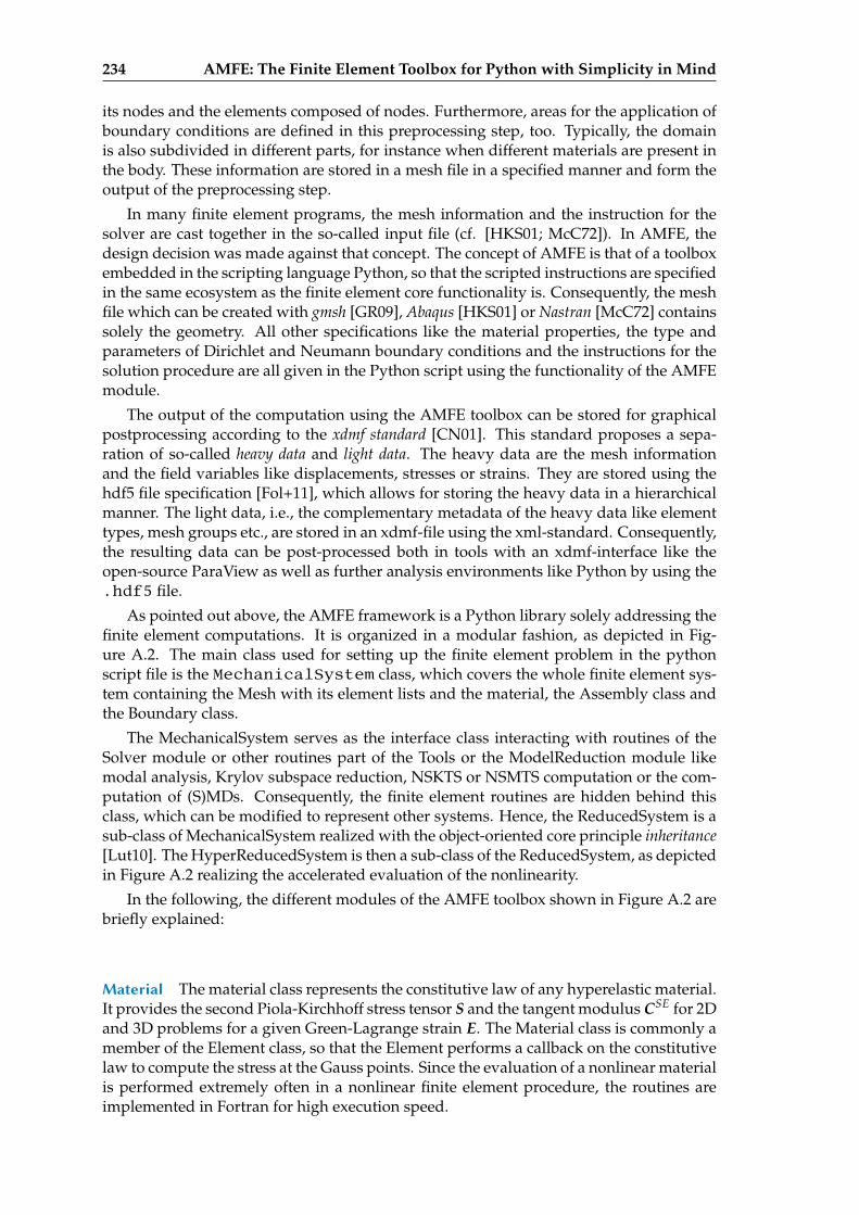
234 AMFE: The Finite Element Toolbox for Python with Simplicity in Mind
its nodes and the elements composed of nodes. Furthermore, areas for the application ofboundary conditions are defined in this preprocessing step, too. Typically, the domainis also subdivided in different parts, for instance when different materials are present inthe body. These information are stored in a mesh file in a specified manner and form theoutput of the preprocessing step.
In many finite element programs, the mesh information and the instruction for thesolver are cast together in the so-called input file (cf. [HKS01; McC72]). In AMFE, thedesign decision was made against that concept. The concept of AMFE is that of a toolboxembedded in the scripting language Python, so that the scripted instructions are specifiedin the same ecosystem as the finite element core functionality is. Consequently, the meshfile which can be created with gmsh [GR09], Abaqus [HKS01] or Nastran [McC72] containssolely the geometry. All other specifications like the material properties, the type andparameters of Dirichlet and Neumann boundary conditions and the instructions for thesolution procedure are all given in the Python script using the functionality of the AMFEmodule.
The output of the computation using the AMFE toolbox can be stored for graphicalpostprocessing according to the xdmf standard [CN01]. This standard proposes a sepa-ration of so-called heavy data and light data. The heavy data are the mesh informationand the field variables like displacements, stresses or strains. They are stored using thehdf5 file specification [Fol+11], which allows for storing the heavy data in a hierarchicalmanner. The light data, i.e., the complementary metadata of the heavy data like elementtypes, mesh groups etc., are stored in an xdmf-file using the xml-standard. Consequently,the resulting data can be post-processed both in tools with an xdmf-interface like theopen-source ParaView as well as further analysis environments like Python by using the.hdf5 file.
As pointed out above, the AMFE framework is a Python library solely addressing thefinite element computations. It is organized in a modular fashion, as depicted in Fig-ure A.2. The main class used for setting up the finite element problem in the pythonscript file is the MechanicalSystem class, which covers the whole finite element sys-tem containing the Mesh with its element lists and the material, the Assembly class andthe Boundary class.
The MechanicalSystem serves as the interface class interacting with routines of theSolver module or other routines part of the Tools or the ModelReduction module likemodal analysis, Krylov subspace reduction, NSKTS or NSMTS computation or the com-putation of (S)MDs. Consequently, the finite element routines are hidden behind thisclass, which can be modified to represent other systems. Hence, the ReducedSystem is asub-class of MechanicalSystem realized with the object-oriented core principle inheritance[Lut10]. The HyperReducedSystem is then a sub-class of the ReducedSystem, as depictedin Figure A.2 realizing the accelerated evaluation of the nonlinearity.
In the following, the different modules of the AMFE toolbox shown in Figure A.2 arebriefly explained:
Material The material class represents the constitutive law of any hyperelastic material.It provides the second Piola-Kirchhoff stress tensor S and the tangent modulus CSE for 2Dand 3D problems for a given Green-Lagrange strain E. The Material class is commonly amember of the Element class, so that the Element performs a callback on the constitutivelaw to compute the stress at the Gauss points. Since the evaluation of a nonlinear materialis performed extremely often in a nonlinear finite element procedure, the routines areimplemented in Fortran for high execution speed.
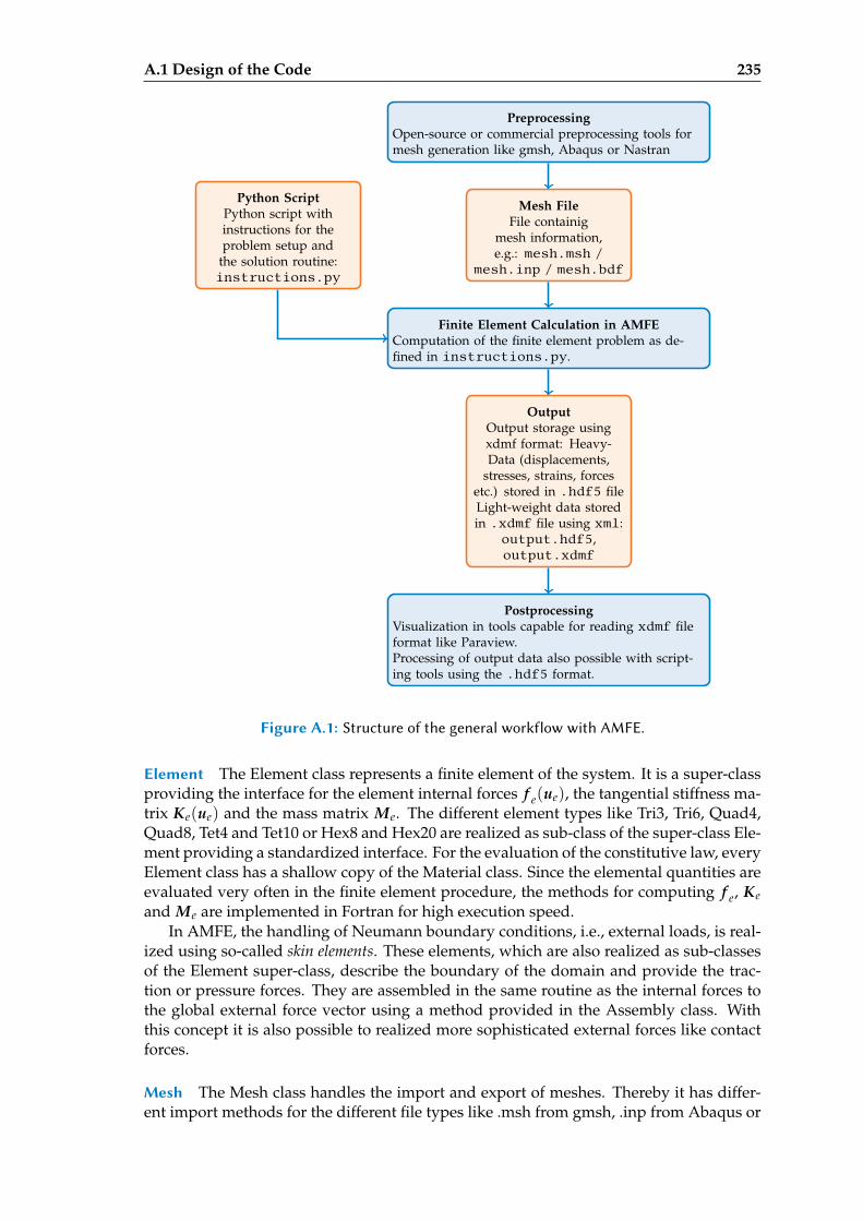
A.1 Design of the Code 235
PreprocessingOpen-source or commercial preprocessing tools formesh generation like gmsh, Abaqus or Nastran
Mesh FileFile containig
mesh information,e.g.: mesh.msh /
mesh.inp / mesh.bdf
Finite Element Calculation in AMFEComputation of the finite element problem as de-fined in instructions.py.
OutputOutput storage usingxdmf format: Heavy-Data (displacements,
stresses, strains, forcesetc.) stored in .hdf5 fileLight-weight data storedin .xdmf file using xml:
output.hdf5,output.xdmf
PostprocessingVisualization in tools capable for reading xdmf fileformat like Paraview.Processing of output data also possible with script-ing tools using the .hdf5 format.
Python ScriptPython script withinstructions for theproblem setup and
the solution routine:instructions.py
Figure A.1: Structure of the general workflow with AMFE.
Element The Element class represents a finite element of the system. It is a super-classproviding the interface for the element internal forces f e(ue), the tangential stiffness ma-trix Ke(ue) and the mass matrix Me. The different element types like Tri3, Tri6, Quad4,Quad8, Tet4 and Tet10 or Hex8 and Hex20 are realized as sub-class of the super-class Ele-ment providing a standardized interface. For the evaluation of the constitutive law, everyElement class has a shallow copy of the Material class. Since the elemental quantities areevaluated very often in the finite element procedure, the methods for computing f e, Keand Me are implemented in Fortran for high execution speed.
In AMFE, the handling of Neumann boundary conditions, i.e., external loads, is real-ized using so-called skin elements. These elements, which are also realized as sub-classesof the Element super-class, describe the boundary of the domain and provide the trac-tion or pressure forces. They are assembled in the same routine as the internal forces tothe global external force vector using a method provided in the Assembly class. Withthis concept it is also possible to realized more sophisticated external forces like contactforces.
Mesh The Mesh class handles the import and export of meshes. Thereby it has differ-ent import methods for the different file types like .msh from gmsh, .inp from Abaqus or
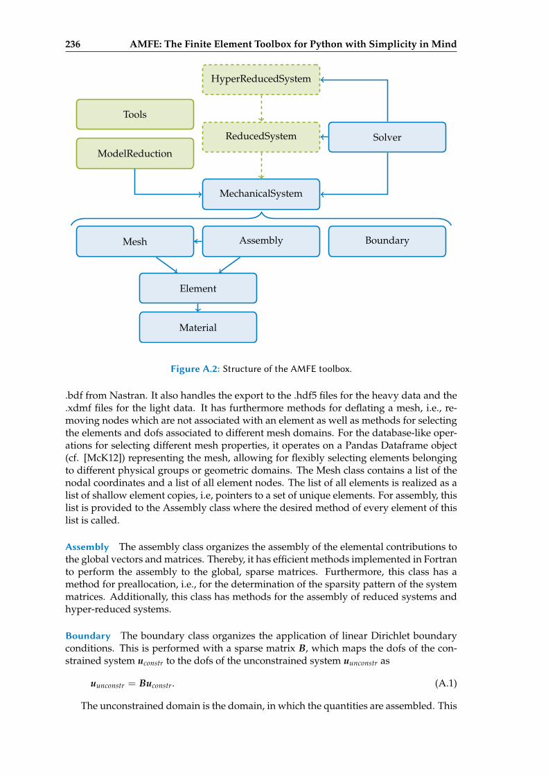
236 AMFE: The Finite Element Toolbox for Python with Simplicity in Mind
Mesh Assembly
Element
Material
Boundary
MechanicalSystem
ReducedSystem
HyperReducedSystem
ModelReduction
Tools
Solver
Figure A.2: Structure of the AMFE toolbox.
.bdf from Nastran. It also handles the export to the .hdf5 files for the heavy data and the
.xdmf files for the light data. It has furthermore methods for deflating a mesh, i.e., re-moving nodes which are not associated with an element as well as methods for selectingthe elements and dofs associated to different mesh domains. For the database-like oper-ations for selecting different mesh properties, it operates on a Pandas Dataframe object(cf. [McK12]) representing the mesh, allowing for flexibly selecting elements belongingto different physical groups or geometric domains. The Mesh class contains a list of thenodal coordinates and a list of all element nodes. The list of all elements is realized as alist of shallow element copies, i.e, pointers to a set of unique elements. For assembly, thislist is provided to the Assembly class where the desired method of every element of thislist is called.
Assembly The assembly class organizes the assembly of the elemental contributions tothe global vectors and matrices. Thereby, it has efficient methods implemented in Fortranto perform the assembly to the global, sparse matrices. Furthermore, this class has amethod for preallocation, i.e., for the determination of the sparsity pattern of the systemmatrices. Additionally, this class has methods for the assembly of reduced systems andhyper-reduced systems.
Boundary The boundary class organizes the application of linear Dirichlet boundaryconditions. This is performed with a sparse matrix B, which maps the dofs of the con-strained system uconstr to the dofs of the unconstrained system uunconstr as
uunconstr = Buconstr. (A.1)
The unconstrained domain is the domain, in which the quantities are assembled. This
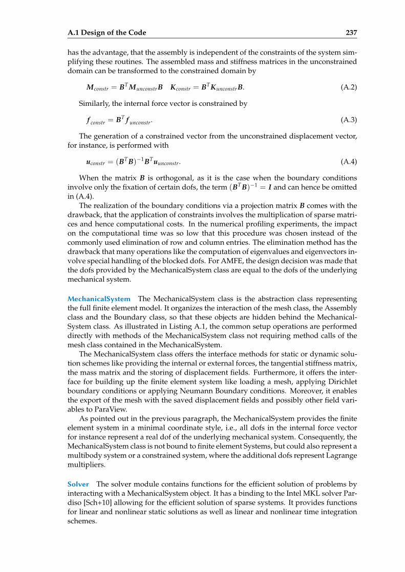
A.1 Design of the Code 237
has the advantage, that the assembly is independent of the constraints of the system sim-plifying these routines. The assembled mass and stiffness matrices in the unconstraineddomain can be transformed to the constrained domain by
Mconstr = BT MunconstrB Kconstr = BTKunconstrB. (A.2)
Similarly, the internal force vector is constrained by
f constr = BT f unconstr. (A.3)
The generation of a constrained vector from the unconstrained displacement vector,for instance, is performed with
uconstr = (BTB)−1BTuunconstr. (A.4)
When the matrix B is orthogonal, as it is the case when the boundary conditionsinvolve only the fixation of certain dofs, the term (BTB)−1 = I and can hence be omittedin (A.4).
The realization of the boundary conditions via a projection matrix B comes with thedrawback, that the application of constraints involves the multiplication of sparse matri-ces and hence computational costs. In the numerical profiling experiments, the impacton the computational time was so low that this procedure was chosen instead of thecommonly used elimination of row and column entries. The elimination method has thedrawback that many operations like the computation of eigenvalues and eigenvectors in-volve special handling of the blocked dofs. For AMFE, the design decision was made thatthe dofs provided by the MechanicalSystem class are equal to the dofs of the underlyingmechanical system.
MechanicalSystem The MechanicalSystem class is the abstraction class representingthe full finite element model. It organizes the interaction of the mesh class, the Assemblyclass and the Boundary class, so that these objects are hidden behind the Mechanical-System class. As illustrated in Listing A.1, the common setup operations are performeddirectly with methods of the MechanicalSystem class not requiring method calls of themesh class contained in the MechanicalSystem.
The MechanicalSystem class offers the interface methods for static or dynamic solu-tion schemes like providing the internal or external forces, the tangential stiffness matrix,the mass matrix and the storing of displacement fields. Furthermore, it offers the inter-face for building up the finite element system like loading a mesh, applying Dirichletboundary conditions or applying Neumann Boundary conditions. Moreover, it enablesthe export of the mesh with the saved displacement fields and possibly other field vari-ables to ParaView.
As pointed out in the previous paragraph, the MechanicalSystem provides the finiteelement system in a minimal coordinate style, i.e., all dofs in the internal force vectorfor instance represent a real dof of the underlying mechanical system. Consequently, theMechanicalSystem class is not bound to finite element Systems, but could also represent amultibody system or a constrained system, where the additional dofs represent Lagrangemultipliers.
Solver The solver module contains functions for the efficient solution of problems byinteracting with a MechanicalSystem object. It has a binding to the Intel MKL solver Par-diso [Sch+10] allowing for the efficient solution of sparse systems. It provides functionsfor linear and nonlinear static solutions as well as linear and nonlinear time integrationschemes.
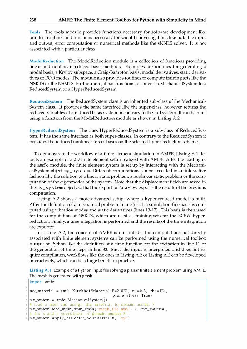
238 AMFE: The Finite Element Toolbox for Python with Simplicity in Mind
Tools The tools module provides functions necessary for software development likeunit test routines and functions necessary for scientific investigations like hdf5 file inputand output, error computation or numerical methods like the sNNLS solver. It is notassociated with a particular class.
ModelReduction The ModelReduction module is a collection of functions providinglinear and nonlinear reduced basis methods. Examples are routines for generating amodal basis, a Krylov subspace, a Craig-Bampton basis, modal derivatives, static deriva-tives or POD modes. The module also provides routines to compute training sets like theNSKTS or the NSMTS. Furthermore, it has functions to convert a MechanicalSystem to aReducedSystem or a HyperReducedSystem.
ReducedSystem The ReducedSystem class is an inherited sub-class of the Mechanical-System class. It provides the same interface like the super-class, however returns thereduced variables of a reduced basis system in contrary to the full system. It can be builtusing a function from the ModelReduction module as shown in Listing A.2.
HyperReducedSystem The class HyperReducedSystem is a sub-class of ReducedSys-tem. It has the same interface as both super-classes. In contrary to the ReducedSystem itprovides the reduced nonlinear forces bases on the selected hyper-reduction scheme.
To demonstrate the workflow of a finite element simulation in AMFE, Listing A.1 de-picts an example of a 2D finite element setup realized with AMFE. After the loading ofthe amfe module, the finite element system is set up by interacting with the Mechani-calSystem object my_system. Different computations can be executed in an interactivefashion like the solution of a linear static problem, a nonlinear static problem or the com-putation of the eigenmodes of the system. Note that the displacement fields are saved inthe my_system object, so that the export to ParaView exports the results of the previouscomputation.
Listing A.2 shows a more advanced setup, where a hyper-reduced model is built.After the definition of a mechanical problem in line 5 - 11, a simulation-free basis is com-puted using vibration modes and static derivatives (lines 13-17). This basis is then usedfor the computation of NSKTS, which are used as training sets for the ECSW hyper-reduction. Finally, a time integration is performed and the results of the time integrationare exported.
In Listing A.2, the concept of AMFE is illustrated. The computations not directlyassociated with finite element systems can be performed using the numerical toolboxnumpy of Python like the definition of a time function for the excitation in line 11 orthe generation of time steps in line 33. Since the input is interpreted and does not re-quire compilation, workflows like the ones in Listing A.2 or Listing A.2 can be developedinteractively, which can be a huge benefit in practice.
Listing A.1: Example of a Python input file solving a planar finite element problem using AMFE.The mesh is generated with gmsh.
1 import amfe2
3 my_material = amfe . Ki rchhof fMater ia l ( E=210E9 , nu = 0 . 3 , rho=1E4 ,4 p l a n e _ s t r e s s =True )5 my_system = amfe . MechanicalSystem ( )6 # load a mesh and ass ign the m a t e r i a l to domain number 77 my_system . load_mesh_from_gmsh ( ’ mesh_f i le . msh ’ , 7 , my_material )8 # f i x x and y coordinate of domain number 89 my_system . apply_di r i ch le t_boundar ies ( 8 , ’ xy ’ )
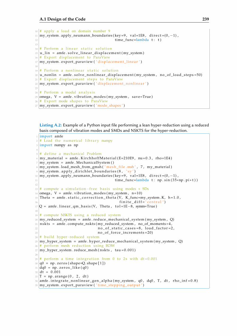
A.1 Design of the Code 239
10 # apply a load on domain number 911 my_system . apply_neumann_boundaries ( key =9 , val =1E8 , d i r e c t =(0 ,−1) ,12 t ime_func=lambda t : t )13
14 # Perform a l i n e a r s t a t i c s o l u t i o n15 u_l in = amfe . so lve_ l inear_d isp lacement ( my_system )16 # Export displacement to ParaView17 my_system . export_paraview ( ’ d i sp lacement_ l inear ’ )18
19 # Perform a nonl inear s t a t i c s o l u t i o n20 u_nonlin = amfe . so lve_nonl inear_displacement ( my_system , no_of_load_steps =50)21 # Export displacement s teps to ParaView22 my_system . export_paraview ( ’ displacement_nonl inear ’ )23
24 # Perform a modal a n a l y s i s25 omega , V = amfe . vibration_modes ( my_system , save=True )26 # Export mode shapes to ParaView27 my_system . export_paraview ( ’ mode_shapes ’ )
Listing A.2: Example of a Python input file performing a lean hyper-reduction using a reducedbasis composed of vibration modes and SMDs and NSKTS for the hyper-reduction.
1 import amfe2 # Load the numerical l i b r a r y numpy3 import numpy as np4
5 # def ine a mechanical Problem6 my_material = amfe . Ki rchhof fMater ia l ( E=210E9 , nu = 0 . 3 , rho=1E4 )7 my_system = amfe . MechanicalSystem ( )8 my_system . load_mesh_from_gmsh ( ’ mesh_f i le . msh ’ , 7 , my_material )9 my_system . apply_di r i ch le t_boundar ies ( 8 , ’ xy ’ )
10 my_system . apply_neumann_boundaries ( key =9 , val =1E8 , d i r e c t =(0 ,−1) ,11 t ime_func=lambda t : np . s i n ( 3 5 * np . pi * t ) )12
13 # compute a simulat ion−f r e e b a s i s using modes + SDs14 omega , V = amfe . vibration_modes ( my_system , n=10)15 Theta = amfe . s t a t i c _ c o r r e c t i o n _ t h e t a (V, K_func=my_system . K, h = 1 . 0 ,16 f i n i t e _ d i f f = ’ c e n t r a l ’ )17 Q = amfe . l inear_qm_basis (V, Theta , t o l =1E−8, symm=True )18
19 # compute NSKTS using a reduced system20 my_reduced_system = amfe . reduce_mechanical_system ( my_system , Q)21 nskts = amfe . compute_nskts ( my_reduced_system , no_of_moments =4 ,22 n o _ o f _ s t a t i c _ c a s e s =8 , l o a d _ f a c t o r =2 ,23 no_of_force_increments =20)24 # bui ld hyper−reduced system25 my_hyper_system = amfe . hyper_reduce_mechanical_system ( my_system , Q)26 # perform mesh reduct ion using ECSW27 my_hyper_system . reduce_mesh ( nskts , tau = 0 . 0 0 1 )28
29 # perform a time i n t e g r a t i o n from 0 to 2 s with dt =0.00130 q0 = np . zeros ( shape=Q. shape [ 1 ] )31 dq0 = np . z e r o s _ l i k e ( q0 )32 dt = 0 .00133 T = np . arange ( 0 , 2 , dt )34 amfe . in tegra te_nonl inear_gen_a lpha ( my_system , q0 , dq0 , T , dt , rho_ inf = 0 . 8 )35 my_system . export_paraview ( ’ t ime_stepping_output ’ )
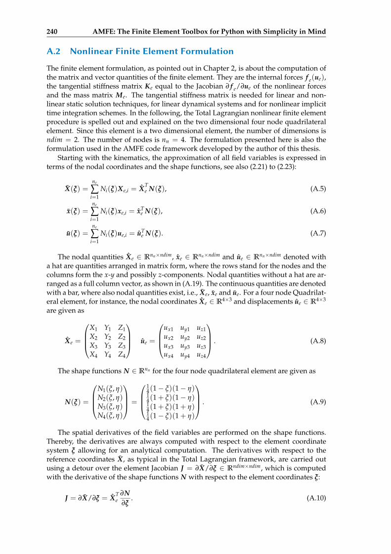
240 AMFE: The Finite Element Toolbox for Python with Simplicity in Mind
A.2 Nonlinear Finite Element Formulation
The finite element formulation, as pointed out in Chapter 2, is about the computation ofthe matrix and vector quantities of the finite element. They are the internal forces f e(ue),the tangential stiffness matrix Ke equal to the Jacobian ∂ f e/∂ue of the nonlinear forcesand the mass matrix Me. The tangential stiffness matrix is needed for linear and non-linear static solution techniques, for linear dynamical systems and for nonlinear implicittime integration schemes. In the following, the Total Lagrangian nonlinear finite elementprocedure is spelled out and explained on the two dimensional four node quadrilateralelement. Since this element is a two dimensional element, the number of dimensions isndim = 2. The number of nodes is nn = 4. The formulation presented here is also theformulation used in the AMFE code framework developed by the author of this thesis.
Starting with the kinematics, the approximation of all field variables is expressed interms of the nodal coordinates and the shape functions, see also (2.21) to (2.23):
X(ξ) =ne
∑i=1
Ni(ξ)Xe,i = XTe N(ξ), (A.5)
x(ξ) =ne
∑i=1
Ni(ξ)xe,i = xTe N(ξ), (A.6)
u(ξ) =ne
∑i=1
Ni(ξ)ue,i = uTe N(ξ). (A.7)
The nodal quantities Xe ∈ Rnn×ndim, xe ∈ Rnn×ndim and ue ∈ Rnn×ndim denoted witha hat are quantities arranged in matrix form, where the rows stand for the nodes and thecolumns form the x-y and possibly z-components. Nodal quantities without a hat are ar-ranged as a full column vector, as shown in (A.19). The continuous quantities are denotedwith a bar, where also nodal quantities exist, i.e., Xe, xe and ue. For a four node Quadrilat-eral element, for instance, the nodal coordinates Xe ∈ R4×3 and displacements ue ∈ R4×3
are given as
Xe =
X1 Y1 Z1X2 Y2 Z2X3 Y3 Z3X4 Y4 Z4
ue =
ux1 uy1 uz1ux2 uy2 uz2ux3 uy3 uz3ux4 uy4 uz4
. (A.8)
The shape functions N ∈ Rnn for the four node quadrilateral element are given as
N(ξ) =
N1(ξ, η)N2(ξ, η)N3(ξ, η)N4(ξ, η)
=
14 (1− ξ)(1− η)14 (1 + ξ)(1− η)14 (1 + ξ)(1 + η)14 (1− ξ)(1 + η)
. (A.9)
The spatial derivatives of the field variables are performed on the shape functions.Thereby, the derivatives are always computed with respect to the element coordinatesystem ξ allowing for an analytical computation. The derivatives with respect to thereference coordinates X, as typical in the Total Lagrangian framework, are carried outusing a detour over the element Jacobian J = ∂X/∂ξ ∈ Rndim×ndim, which is computedwith the derivative of the shape functions N with respect to the element coordinates ξ:
J = ∂X/∂ξ = XTe
∂N∂ξ
. (A.10)
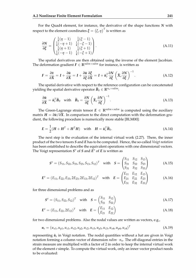
A.2 Nonlinear Finite Element Formulation 241
For the Quad4 element, for instance, the derivative of the shape functions N withrespect to the element coordinates ξ =
(ξ, η)T is written as
∂N∂ξ
=
14 (η − 1) 1
4 (ξ − 1)14 (−η + 1) 1
4 (−ξ − 1)14 (η + 1) 1
4 (ξ + 1)14 (−η − 1) 1
4 (−ξ + 1)
. (A.11)
The spatial derivatives are then obtained using the inverse of the element Jacobian.The deformation gradient F ∈ Rndim×ndim for instance, is written as
F =∂x∂X
= I +∂u∂X
= I +∂u∂ξ
∂ξ
∂X= I + uT
e∂N∂ξ
(Xe
∂N∂ξ
)−1
. (A.12)
The spatial derivative with respect to the reference configuration can be concatenatedyielding the spatial derivative operator B0 ∈ Rnn×ndim:
∂u∂X
= uTe B0 with B0 =
∂N∂ξ
(Xe
∂N∂ξ
)−1
. (A.13)
The Green-Lagrange strain tensor E ∈ Rndim×ndim is computed using the auxiliarymatrix H = ∂u/∂X. In comparison to the direct computation with the deformation gra-dient, the following procedure is numerically more stable [BLM00]:
E =12(H + HT + HT H) with H = uT
e B0. (A.14)
The next step is the evaluation of the internal virtual work (2.27). There, the innerproduct of the two tensors S and E has to be computed. Hence, the so-called Voigt notationhas been established to describe the equivalent operations with one dimensional vectors.The Voigt representation Sv of S and Ev of E is written as
Sv = (S11, S22, S33, S23, S13, S12)T with S =
S11 S12 S13S21 S22 S23S31 S32 S33
(A.15)
Ev = (E11, E22, E33, 2E23, 2E13, 2E12)T with E =
E11 E12 E13E21 E22 E23E31 E32 E33
(A.16)
for three dimensional problems and as
Sv = (S11, S22, S12)T with S =
(S11 S12S21 S22
)(A.17)
Ev = (E11, E22, 2E12)T with E =
(E11 E12E21 E22
)(A.18)
for two dimensional problems. Also the nodal values are written as vectors, e.g.,
ue = (ux1, uy1, uz1, ux2, uy2, uz2, ux3, uy3, uz3, ux4, uy4, uz4)T (A.19)
representing ue in Voigt notation. The nodal quantities without a hat are given in Voigtnotation forming a column vector of dimension ndim · nn. The off-diagonal entries in thestrain measure are multiplied with a factor of 2 in order to keep the internal virtual workof the element e simple. To compute the virtual work, only an inner vector product needsto be evaluated:
242 AMFE: The Finite Element Toolbox for Python with Simplicity in Mind
δWint,e =∫
Ω0,e
S : δE dΩ0,e =∫
Ω0,e
(δEv)TSv dΩ0,e. (A.20)
For the application of the principle of virtual work, the variation of the Green-Lagran-ge tensor δE is necessary. According to the definition (2.13), recalled here for clarity:
δE =12(δFT F + FTδF), (A.21)
the variation of the Voigt representation δEv can be expressed in terms of the variationsof the displacement vector δu:
δEv = B0δue. (A.22)
The tangent matrix B0 ∈ Rndim(ndim+1)/2×ndim·nn is dependent on the deformation andhence a linear function of the nodal displacements. It is composed of both entries of thedeformation gradient and of the spatial derivative matrix B0. The first three columns aregiven as
B0[:, : 3] =
F11B11 F21B11 F31B11F12B12 F22B12 F32B12F13B13 F23B13 F33B13
F12B13 + F13B12 F22B13 + F23B12 F32B13 + F33B12F11B13 + F13B11 F21B13 + F23B11 F31B13 + F33B11F11B12 + F12B11 F21B12 + F22B11 F31B12 + F32B11
(A.23)
with
F =
F11 F21 F31F12 F22 F32F13 F23 F33
and B0 =
B11 B12 B13B21 B22 B23
......
...
. (A.24)
Having defined the tangent operator δEv, the virtual work δWint,e yields the nonlinearinternal forces f e(ue):
δWe =∫
Ω0,e
(δEv)TSv dΩ0,e = δuTe
∫
Ω0,e
BT0 Sv dΩ0,e = δuT
e f e(ue) (A.25)
as
f e(ue) =∫
Ω0,e
BT0 Sv dΩ0,e, (A.26)
since the variations of the nodal displacements δue are arbitrary. The evaluation of theintegral in the equation above is performed using Gauss integration (cf. (2.28)).
Next the virtual work of the inertia forces is evaluated. Recalling (2.25), δWkin,e iswritten as
δWkin,e =∫
Ω0,e
δuTρ ¨u dΩ0,e. (A.27)
To receive the mass matrix in terms of the displacements ue in Voigt notation, thematrix of shape functions N need to be given in Voigt notation as well, so that the contin-uous displacement field is a function of the nodal displacements given in Voigt notationu = Nvue:
Nv =
N1(ξ) 0 0 N2(ξ) 0 0 . . .0 N1(ξ) 0 0 N2(ξ) 0 . . .0 0 N1(ξ) 0 0 N2(ξ) . . .
(A.28)
A.2 Nonlinear Finite Element Formulation 243
Then the virtual work of the inertia forces δWkin,e is rewritten as
δWkin,e =∫
Ω0,e
δuTe (Nv)TρNvue dΩ0,e = δuT
e
∫
Ω0,e
ρ(Nv)T Nv dΩ0,e ue = δuTe Meue
(A.29)
yielding the mass matrix Me of element e as
Me =∫
Ω0,e
ρ(Nv)T Nv dΩ0,e. (A.30)
Similar to the internal nonlinear forces, the integrals are evaluated with a Gaussquadrature scheme.
Finally the tangential stiffness matrix Ke is derived. It is the Jacobian of the internalforces (A.26) with respect to the nodal displacements. Since in the expression (A.26) bothmembers in the integrand are dependent on the nodal displacements, the stiffness ma-trix is split into two parts, the geometric stiffness matrix Kgeo,e and the material stiffnessmatrix Kmat,e:
∂ f e∂ue
= Ke =∫
Ω0,e
∂BT0
∂ueSv dΩ0,e
︸ ︷︷ ︸Kgeo,e
+∫
Ω0,e
BT0
∂Sv
∂uedΩ0,e
︸ ︷︷ ︸Kmat,e
. (A.31)
The geometric stiffness matrix Kgeo,e is different from zero only for deformed statesand is thus omitted in linear finite elements. The material stiffness matrix Kmat,e is equalto the linear stiffness matrix for a zero displacement. It is simple to derive using the chainrule:
Kmat,e =∫
Ω0,e
BT0
∂Sv
∂uedΩ0,e =
∫
Ω0,e
BT0
∂Sv
∂Ev∂Ev
∂uedΩ0,e =
∫
Ω0,e
BT0 CSEB0 dΩ0,e. (A.32)
The matrix CSE = ∂Sv/∂Ev is the so-called tangent modulus describing the tangentialmap between the second Piola-Kirchhoff stress tensor S and the Green-Lagrange straintensor E. This tangent modulus is provided by the constitutive law as discussed in Sec-tion 2.2.
The geometric stiffness matrix is more complicated to derive. The internal virtualwork can be expressed by another work-conjugate pair, the deformation gradient F andthe first Piola–Kirchhoff stress tensor P = FS yielding
δWint,e = δue : f e =∫
Ω0,e
δF : P dΩ0,e =∫
Ω0,e
δFijPij dΩ0,e. (A.33)
Since the variation of the deformation gradient is δF = δuTe B0, in index notation
δFij = δue,ki B0,kj, the internal forces f e given in matrix notation are
δWint,e = δue : f e = δue,ki fe,ki (A.34)
=∫
Ω0,e
δFijPij dΩ0,e = δue,ki
∫B0,kjPij dΩ0,e (A.35)
= δue :∫
Ω0,e
B0PT dΩ0,e. (A.36)
Hence the nonlinear forces f e in matrix notation are given as
f e =∫
Ω0,e
B0PT dΩ0,e =∫
Ω0,e
B0SFT dΩ0,e. (A.37)
244 AMFE: The Finite Element Toolbox for Python with Simplicity in Mind
The tangential stiffness matrix can be obtained by taking the time derivative of theinternal forces, since Jacobians of matrices are difficult to book-keep:
˙f e =∫
Ω0,e
B0SFT dΩ0,e
︸ ︷︷ ︸˙f mat,e
+∫
Ω0,e
B0SFT dΩ0,e
︸ ︷︷ ︸˙f geo,e
. (A.38)
The first summand represents the change of the forces due to the material change in-duced by S. The second summand represents the change of the forces due to the changeof the geometry, represented by the change rate of the deformation gradient F. The sec-ond change rate leads to the geometric stiffness matrix Kgeo,e, since the rate of the defor-mation gradient F can be expressed in terms of the nodal velocities to F = ˙uT
e B0:
˙f geo,e =∫
Ω0,e
B0SFT dΩ0,e =∫
Ω0,e
B0SBT0 dΩ0,e ˙ue = Kgeo,e ˙ue, (A.39)
leading to the geometric stiffness matrix Kgeo for one coordinate direction:
Kgeo,e =∫
B0SBT0 dΩ0,e. (A.40)
The matrix Kgeo,e can be expanded to the geometric stiffness matrix Kgeo,e for Voigtnotation by applying the Kronecker product with the identity matrix I ∈ Rndim×ndim:
Kgeo,e = Kgeo,e ⊗ I. (A.41)
The tangential stiffness Ke of element e is then given as the sum of both, the materialand the geometric stiffness:
Ke = Kmat,e + Kgeo,e. (A.42)
The procedure of the finite element method to compute the elemental matrices Ke, Meand the internal force vector f e is given in Algorithm 6. For more in-depth informationthe reader is referred to [BLM00].
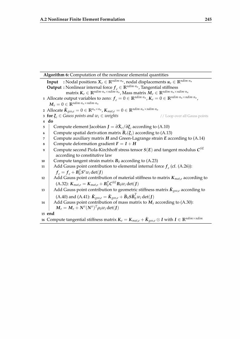
A.2 Nonlinear Finite Element Formulation 245
Algorithm 6: Computation of the nonlinear elemental quantities
Input : Nodal positions Xe ∈ Rndim·nn , nodal displacements ue ∈ Rndim·nn
Output : Nonlinear internal force f e ∈ Rndim·nn , Tangential stiffnessmatrix Ke ∈ Rndim·nn×ndim·nn , Mass matrix Me ∈ Rndim·nn×ndim·nn
1 Allocate output variables to zero: f e = 0 ∈ Rndim·nn , Ke = 0 ∈ Rndim·nn×ndim·nn ,Me = 0 ∈ Rndim·nn×ndim·nn
2 Allocate Kgeo,e = 0 ∈ Rnn×nn , Kmat,e = 0 ∈ Rndim·nn×ndim·nn
3 for ξi ∈ Gauss points and wi ∈ weights // Loop over all Gauss points4 do5 Compute element Jacobian J = ∂Xe/∂ξi according to (A.10)6 Compute spatial derivation matrix Be(ξi) according to (A.13)7 Compute auxiliary matrix H and Green-Lagrange strain E according to (A.14)8 Compute deformation gradient F = I + H9 Compute second Piola-Kirchhoff stress tensor S(E) and tangent modulus CSE
according to constitutive law10 Compute tangent strain matrix B0 according to (A.23)11 Add Gauss point contribution to elemental internal force f e (cf. (A.26)):
f e = f e + BT0 Svwi det(J)
12 Add Gauss point contribution of material stiffness to matrix Kmat,e according to(A.32): Kmat,e = Kmat,e + BT
0 CSEB0wi det(J)13 Add Gauss point contribution to geometric stiffness matrix Kgeo,e according to
(A.40) and (A.41): Kgeo,e = Kgeo,e + B0SBT0 wi det(J)
14 Add Gauss point contribution of mass matrix to Me according to (A.30):Me = Me + Nv(Nv)Tρ0wi det(J)
15 end16 Compute tangential stiffness matrix Ke = Kmat,e + Kgeo,e ⊗ I with I ∈ Rndim×ndim

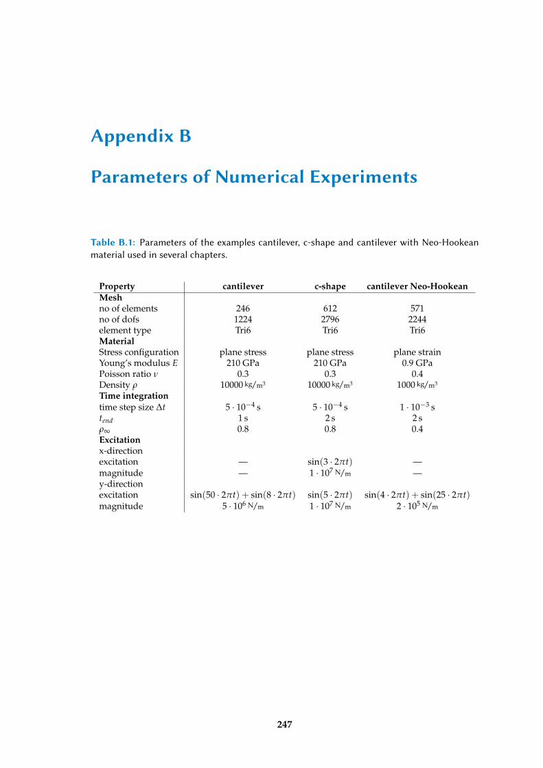
Appendix B
Parameters of Numerical Experiments
Table B.1: Parameters of the examples cantilever, c-shape and cantilever with Neo-Hookeanmaterial used in several chapters.
Property cantilever c-shape cantilever Neo-HookeanMeshno of elements 246 612 571no of dofs 1224 2796 2244element type Tri6 Tri6 Tri6MaterialStress configuration plane stress plane stress plane strainYoung’s modulus E 210 GPa 210 GPa 0.9 GPaPoisson ratio ν 0.3 0.3 0.4Density ρ 10000 kg/m3 10000 kg/m3 1000 kg/m3
Time integrationtime step size ∆t 5 · 10−4 s 5 · 10−4 s 1 · 10−3 stend 1 s 2 s 2 sρ∞ 0.8 0.8 0.4Excitationx-directionexcitation — sin(3 · 2πt) —magnitude — 1 · 107 N/m —y-directionexcitation sin(50 · 2πt) + sin(8 · 2πt) sin(5 · 2πt) sin(4 · 2πt) + sin(25 · 2πt)magnitude 5 · 106 N/m 1 · 107 N/m 2 · 105 N/m
247
Related Documents