Model-Free in situ Optimisation of Data-Ferried Sensor ... - CU Scholar

Model-Free in situ Optimisation of Data-Ferried Sensor

Networks

by

Ben Pearre

B.S.E. in Computer Science, Princeton University, 1996

A thesis submitted to the

Faculty of the Graduate School of the

University of Colorado in partial fulfillment

of the requirements for the degree of

Doctor of Philosophy

Department of Computer Science

2013

This thesis entitled:Model-Free in situ Optimisation of Data-Ferried Sensor Networks

written by Ben Pearrehas been approved for the Department of Computer Science

Timothy X Brown

Prof. Eric W. Frew

Date

The final copy of this thesis has been examined by the signatories, and we find that both the content andthe form meet acceptable presentation standards of scholarly work in the above mentioned discipline.

Pearre, Ben (Ph.D., Computer Science)

Model-Free in situ Optimisation of Data-Ferried Sensor Networks

Thesis directed by Prof. Timothy X Brown

Given multiple widespread stationary data sources (nodes), an unmanned aircraft (UA) can fly over

the sensors and gather the data via a wireless link. This is known as data ferrying or data muling, and finds

application in surveillance and scientific monitoring of remote and inaccessible regions. Desiderata for such a

network include competing objectives related to latency, bandwidth, power consumption by the nodes, and

tolerance for imperfect environmental information. For any design objective, network performance depends

upon the control policies of UA and nodes.

A model of such a system permits optimal planning, but is difficult to acquire and maintain. Node

locations may not be precisely known. Radio fields are directional and irregular, affected by antenna shape,

occlusions, reflections, diffraction, and fading. Complex aircraft dynamics further hamper planning. The

conventional approach is to plan trajectories using approximate models, but inaccuracies in the models

degrades the quality of the solution.

In order to provide an alternative to the process of building and maintaining detailed environmental

and system models, we present a model-free learning framework for trajectory optimisation and control of

node radio transmission power in UA-ferried sensor networks. We introduce policy representations that are

easy both for learning algorithms to manipulate and for off-the-shelf autopilots and radios to work with.

We show that the policies can be optimised through direct experience with the environment. To speed and

stabilise the policy learning process, we introduce a metapolicy that learns through experience with past

scenarios, transferring knowledge to new problems.

Algorithms are tested using two radio propagation simulators, both of which produce irregular radio

fields not commonly studied in the data-ferrying literature. The first introduces directional antennas and

point noise sources. The second additionally includes interaction with terrain.

Under the simpler radio simulator, the proposed algorithms generally perform within ∼15% of optimal

performance after a few dozen trials. Environments produced by the terrain-based simulator are more

iv

challenging, with learners generally approaching to within ∼40% of optimal performance in similar time. We

show that under either simulator even small modelling errors can reduce the optimal planner’s performance

below that of the proposed learning approach.

v

Acknowledgements

It’s been an adventure, and credit should be spread far and wide. I have neither the space nor the

words to thank everyone who deserves thanks, but I can thank a few of those who had the greatest effect.

My advisor, Prof. Tim Brown, managed to strike a brilliant balance between support, criticism,

creativity, enthusiasm, perspective, curiosity, patience, and novel ideas anent bike-commuting weather. My

committee, Profs. Mike Mozer, Eric Frew, Nikolaus Correll, and Lijun Chen, offered a stream of sharp

constructive criticism, astonishing support, advice, and guidance.

My parents pushed, consoled, supported, reminded me that it was fine if I quit and fine if I didn’t.

They taught me to find everything fascinating, which is probably what got me into this. For amazing

adventures, holidays, roadtrips, planetrips, intellectual snacks, dancing, patience, food, and love, thank you

Anne Harrington, Alia Zelinskaya, Xu Simon, Erica Schmitt! You especially have my undying gratitude.

Deanna Fierman, Steve Bentley, Justin Werfel, Jen Wang, Yang He, Erik Angerhofer, Cathy Bell, and Melissa

Warden: you inspired me more than I’ve ever expressed. Dave Peascoe: thank you especially for the bike

named Trebuchet—it transformed commuting and errands from annoying chores into exercise, relaxation,

health, and occasional brushes with sanity. The CU Tango Club, the Boulder tango community, Nick Jones,

and many others introduced me to what was often my only social activity, sometimes my only exercise, and

frequently the best reason to finish a chunk of work before evening.

Finally, the Free / Open Source software community helped me enormously. The list of contributors

to such projects as Linux, Emacs, gcc, LATEX, SPLAT!, etc., would fill another book.

Thank you all!

Contents

Chapter

1 Introduction 1

1.1 Problem . . . . . . . . . . . . . . . . . . . . . . . . . . . . . . . . . . . . . . . . . . . . . . . . . . . 1

1.2 Thesis . . . . . . . . . . . . . . . . . . . . . . . . . . . . . . . . . . . . . . . . . . . . . . . . . . . . 5

1.3 Evaluation . . . . . . . . . . . . . . . . . . . . . . . . . . . . . . . . . . . . . . . . . . . . . . . . . . 8

1.4 Contributions . . . . . . . . . . . . . . . . . . . . . . . . . . . . . . . . . . . . . . . . . . . . . . . . 11

2 Related Work 14

2.1 Data Ferrying . . . . . . . . . . . . . . . . . . . . . . . . . . . . . . . . . . . . . . . . . . . . . . . . 14

2.1.1 Objectives . . . . . . . . . . . . . . . . . . . . . . . . . . . . . . . . . . . . . . . . . . . . . 15

2.1.2 Radio . . . . . . . . . . . . . . . . . . . . . . . . . . . . . . . . . . . . . . . . . . . . . . . . 18

2.1.3 Ferries . . . . . . . . . . . . . . . . . . . . . . . . . . . . . . . . . . . . . . . . . . . . . . . . 20

2.1.4 Sensors . . . . . . . . . . . . . . . . . . . . . . . . . . . . . . . . . . . . . . . . . . . . . . . 21

2.1.5 Knowledge models . . . . . . . . . . . . . . . . . . . . . . . . . . . . . . . . . . . . . . . . . 21

2.1.6 Sensor networks that learn . . . . . . . . . . . . . . . . . . . . . . . . . . . . . . . . . . . . 22

2.1.7 Problem “size” . . . . . . . . . . . . . . . . . . . . . . . . . . . . . . . . . . . . . . . . . . . 24

2.2 Reinforcement Learning . . . . . . . . . . . . . . . . . . . . . . . . . . . . . . . . . . . . . . . . . . 24

2.2.1 Reinforcement Metalearning . . . . . . . . . . . . . . . . . . . . . . . . . . . . . . . . . . . 26

2.2.2 Policy initialisation from past experience . . . . . . . . . . . . . . . . . . . . . . . . . . . 27

vii

3 The Simulator 30

3.1 Radio Environment Model . . . . . . . . . . . . . . . . . . . . . . . . . . . . . . . . . . . . . . . . 30

3.2 Policy, Autopilot, Trajectory . . . . . . . . . . . . . . . . . . . . . . . . . . . . . . . . . . . . . . . 32

3.2.1 The Reference trajectory . . . . . . . . . . . . . . . . . . . . . . . . . . . . . . . . . . . . 32

3.2.2 The Data-loops trajectory representation . . . . . . . . . . . . . . . . . . . . . . . . . . 34

3.2.3 The Waypoints trajectory representation . . . . . . . . . . . . . . . . . . . . . . . . . . 34

4 Data-loops Trajectories 35

4.1 Waypoint placement . . . . . . . . . . . . . . . . . . . . . . . . . . . . . . . . . . . . . . . . . . . . 35

4.2 The Data-loops trajectory representation . . . . . . . . . . . . . . . . . . . . . . . . . . . . . . 36

4.3 Gradient estimation . . . . . . . . . . . . . . . . . . . . . . . . . . . . . . . . . . . . . . . . . . . . 36

4.4 Learning waypoint placement . . . . . . . . . . . . . . . . . . . . . . . . . . . . . . . . . . . . . . 38

4.4.1 Policy . . . . . . . . . . . . . . . . . . . . . . . . . . . . . . . . . . . . . . . . . . . . . . . . 38

4.4.2 Reward . . . . . . . . . . . . . . . . . . . . . . . . . . . . . . . . . . . . . . . . . . . . . . . 39

4.5 Scalability . . . . . . . . . . . . . . . . . . . . . . . . . . . . . . . . . . . . . . . . . . . . . . . . . . 39

4.6 Optimal trajectory planning . . . . . . . . . . . . . . . . . . . . . . . . . . . . . . . . . . . . . . . 40

4.7 Experiments . . . . . . . . . . . . . . . . . . . . . . . . . . . . . . . . . . . . . . . . . . . . . . . . . 42

4.7.1 Data-loops vs. optimal trajectories . . . . . . . . . . . . . . . . . . . . . . . . . . . . . . . 43

4.7.2 Accurate network layout information . . . . . . . . . . . . . . . . . . . . . . . . . . . . . 49

4.7.3 Position error . . . . . . . . . . . . . . . . . . . . . . . . . . . . . . . . . . . . . . . . . . . 54

4.7.4 Antenna patterns . . . . . . . . . . . . . . . . . . . . . . . . . . . . . . . . . . . . . . . . . 56

4.8 Summary . . . . . . . . . . . . . . . . . . . . . . . . . . . . . . . . . . . . . . . . . . . . . . . . . . 58

5 Waypoints Trajectories 60

5.1 The Waypoints trajectory representation . . . . . . . . . . . . . . . . . . . . . . . . . . . . . . . 60

5.2 The learner . . . . . . . . . . . . . . . . . . . . . . . . . . . . . . . . . . . . . . . . . . . . . . . . . 61

5.3 Reward . . . . . . . . . . . . . . . . . . . . . . . . . . . . . . . . . . . . . . . . . . . . . . . . . . . . 61

5.4 Experiments . . . . . . . . . . . . . . . . . . . . . . . . . . . . . . . . . . . . . . . . . . . . . . . . . 62

viii

5.4.1 Waypoints vs. Data-loops . . . . . . . . . . . . . . . . . . . . . . . . . . . . . . . . . . . . 62

5.4.2 Position error . . . . . . . . . . . . . . . . . . . . . . . . . . . . . . . . . . . . . . . . . . . 66

5.5 Summary . . . . . . . . . . . . . . . . . . . . . . . . . . . . . . . . . . . . . . . . . . . . . . . . . . 68

6 Local Credit Assignment 71

6.1 Components of the reward . . . . . . . . . . . . . . . . . . . . . . . . . . . . . . . . . . . . . . . . 72

6.2 Credit Assignment . . . . . . . . . . . . . . . . . . . . . . . . . . . . . . . . . . . . . . . . . . . . . 73

6.2.1 Waypoints ↔ Timesteps . . . . . . . . . . . . . . . . . . . . . . . . . . . . . . . . . . . . . 74

6.2.2 Timesteps ↔ Reward summands . . . . . . . . . . . . . . . . . . . . . . . . . . . . . . . . 75

6.2.3 LCA-Length . . . . . . . . . . . . . . . . . . . . . . . . . . . . . . . . . . . . . . . . . . . . 77

6.3 Combining the gradient estimates . . . . . . . . . . . . . . . . . . . . . . . . . . . . . . . . . . . . 77

6.4 Experiments . . . . . . . . . . . . . . . . . . . . . . . . . . . . . . . . . . . . . . . . . . . . . . . . . 78

6.4.1 Scalability . . . . . . . . . . . . . . . . . . . . . . . . . . . . . . . . . . . . . . . . . . . . . 78

6.4.2 LCA-length for Data-loops trajectories . . . . . . . . . . . . . . . . . . . . . . . . . . . . 80

6.5 Summary . . . . . . . . . . . . . . . . . . . . . . . . . . . . . . . . . . . . . . . . . . . . . . . . . . 83

7 Node Energy Management 84

7.1 Radio transmission power . . . . . . . . . . . . . . . . . . . . . . . . . . . . . . . . . . . . . . . . . 85

7.2 The optimal power policy . . . . . . . . . . . . . . . . . . . . . . . . . . . . . . . . . . . . . . . . . 86

7.3 Learning . . . . . . . . . . . . . . . . . . . . . . . . . . . . . . . . . . . . . . . . . . . . . . . . . . . 87

7.3.1 Power Policies . . . . . . . . . . . . . . . . . . . . . . . . . . . . . . . . . . . . . . . . . . . 87

7.3.2 Baselines . . . . . . . . . . . . . . . . . . . . . . . . . . . . . . . . . . . . . . . . . . . . . . 94

7.3.3 Reward . . . . . . . . . . . . . . . . . . . . . . . . . . . . . . . . . . . . . . . . . . . . . . . 95

7.3.4 Policy Updates . . . . . . . . . . . . . . . . . . . . . . . . . . . . . . . . . . . . . . . . . . . 96

7.3.5 An example failsafe mechanism . . . . . . . . . . . . . . . . . . . . . . . . . . . . . . . . . 97

7.4 Experiments . . . . . . . . . . . . . . . . . . . . . . . . . . . . . . . . . . . . . . . . . . . . . . . . . 98

7.4.1 Comparison to the optimal policy . . . . . . . . . . . . . . . . . . . . . . . . . . . . . . . 98

7.4.2 Single node, no position error . . . . . . . . . . . . . . . . . . . . . . . . . . . . . . . . . . 105

ix

7.4.3 Position error . . . . . . . . . . . . . . . . . . . . . . . . . . . . . . . . . . . . . . . . . . . 108

7.4.4 Scalability . . . . . . . . . . . . . . . . . . . . . . . . . . . . . . . . . . . . . . . . . . . . . 108

7.5 Summary . . . . . . . . . . . . . . . . . . . . . . . . . . . . . . . . . . . . . . . . . . . . . . . . . . 111

8 Learning to Learn Energy Policies 113

8.1 Motivation . . . . . . . . . . . . . . . . . . . . . . . . . . . . . . . . . . . . . . . . . . . . . . . . . . 114

8.2 Metapolicies . . . . . . . . . . . . . . . . . . . . . . . . . . . . . . . . . . . . . . . . . . . . . . . . . 116

8.2.1 Metapolicy . . . . . . . . . . . . . . . . . . . . . . . . . . . . . . . . . . . . . . . . . . . . . 119

8.2.2 Metareward . . . . . . . . . . . . . . . . . . . . . . . . . . . . . . . . . . . . . . . . . . . . . 121

8.2.3 Time-discounted credit . . . . . . . . . . . . . . . . . . . . . . . . . . . . . . . . . . . . . . 121

8.2.4 Training . . . . . . . . . . . . . . . . . . . . . . . . . . . . . . . . . . . . . . . . . . . . . . . 123

8.3 Three Learners . . . . . . . . . . . . . . . . . . . . . . . . . . . . . . . . . . . . . . . . . . . . . . . 123

8.3.1 PGRL . . . . . . . . . . . . . . . . . . . . . . . . . . . . . . . . . . . . . . . . . . . . . . . . 123

8.3.2 Pure µ . . . . . . . . . . . . . . . . . . . . . . . . . . . . . . . . . . . . . . . . . . . . . . . . 123

8.3.3 Gradient-guided meta-exploration with hybrids . . . . . . . . . . . . . . . . . . . . . . . 124

8.4 Combining ∇∆ and ∇µ . . . . . . . . . . . . . . . . . . . . . . . . . . . . . . . . . . . . . . . . . . 124

8.4.1 Mean Squared Error of the gradient updates . . . . . . . . . . . . . . . . . . . . . . . . . 124

8.4.2 Combining the gradient estimates . . . . . . . . . . . . . . . . . . . . . . . . . . . . . . . 125

8.4.3 Is the true gradient the best update? . . . . . . . . . . . . . . . . . . . . . . . . . . . . . 126

8.5 Experiments . . . . . . . . . . . . . . . . . . . . . . . . . . . . . . . . . . . . . . . . . . . . . . . . . 126

8.5.1 Learning from base gradient, learning from a Metapolicy . . . . . . . . . . . . . . . . . 128

8.5.2 PGRL vs. Pure µ vs. hybrids . . . . . . . . . . . . . . . . . . . . . . . . . . . . . . . . . . 132

8.5.3 Sensitivity to learning rates . . . . . . . . . . . . . . . . . . . . . . . . . . . . . . . . . . . 132

8.5.4 Mitigating flaws in the policy update step . . . . . . . . . . . . . . . . . . . . . . . . . . 135

8.5.5 Larger problems . . . . . . . . . . . . . . . . . . . . . . . . . . . . . . . . . . . . . . . . . . 138

8.5.6 Knowledge transfer . . . . . . . . . . . . . . . . . . . . . . . . . . . . . . . . . . . . . . . . 140

8.5.7 Impact on the comparison to the optimal policy . . . . . . . . . . . . . . . . . . . . . . . 142

x

8.6 Summary . . . . . . . . . . . . . . . . . . . . . . . . . . . . . . . . . . . . . . . . . . . . . . . . . . 144

9 Assessment under a complex, noisy, terrain-based radio model 145

9.1 Terrain interactions and SPLAT! . . . . . . . . . . . . . . . . . . . . . . . . . . . . . . . . . . . . 146

9.1.1 Modifications to the scenario assumptions . . . . . . . . . . . . . . . . . . . . . . . . . . 146

9.1.2 Changes to SPLAT! . . . . . . . . . . . . . . . . . . . . . . . . . . . . . . . . . . . . . . . . 150

9.2 Model-based Optimal Planning . . . . . . . . . . . . . . . . . . . . . . . . . . . . . . . . . . . . . 151

9.2.1 Stochastic autopilot tracking error . . . . . . . . . . . . . . . . . . . . . . . . . . . . . . . 153

9.2.2 Model errors . . . . . . . . . . . . . . . . . . . . . . . . . . . . . . . . . . . . . . . . . . . . 153

9.3 Experiments . . . . . . . . . . . . . . . . . . . . . . . . . . . . . . . . . . . . . . . . . . . . . . . . . 154

9.3.1 Perfect information . . . . . . . . . . . . . . . . . . . . . . . . . . . . . . . . . . . . . . . . 155

9.3.2 Trajectory tracking error . . . . . . . . . . . . . . . . . . . . . . . . . . . . . . . . . . . . . 159

9.3.3 Node location error . . . . . . . . . . . . . . . . . . . . . . . . . . . . . . . . . . . . . . . . 162

9.3.4 Terrain model error . . . . . . . . . . . . . . . . . . . . . . . . . . . . . . . . . . . . . . . . 164

9.4 Summary . . . . . . . . . . . . . . . . . . . . . . . . . . . . . . . . . . . . . . . . . . . . . . . . . . 166

10 Conclusion 169

10.1 Summary . . . . . . . . . . . . . . . . . . . . . . . . . . . . . . . . . . . . . . . . . . . . . . . . . . 171

10.1.1 Trajectory optimisation . . . . . . . . . . . . . . . . . . . . . . . . . . . . . . . . . . . . . 171

10.1.2 Energy optimisation . . . . . . . . . . . . . . . . . . . . . . . . . . . . . . . . . . . . . . . . 173

10.1.3 Learning to learn energy policies . . . . . . . . . . . . . . . . . . . . . . . . . . . . . . . . 174

10.1.4 Evaluation under a terrain-based radio simulator . . . . . . . . . . . . . . . . . . . . . . 176

10.2 Open issues and future work . . . . . . . . . . . . . . . . . . . . . . . . . . . . . . . . . . . . . . . 177

10.2.1 Time-varying effects . . . . . . . . . . . . . . . . . . . . . . . . . . . . . . . . . . . . . . . . 177

10.2.2 Metapolicy training . . . . . . . . . . . . . . . . . . . . . . . . . . . . . . . . . . . . . . . . 178

10.2.3 Real-world tests . . . . . . . . . . . . . . . . . . . . . . . . . . . . . . . . . . . . . . . . . . 178

10.2.4 Wind . . . . . . . . . . . . . . . . . . . . . . . . . . . . . . . . . . . . . . . . . . . . . . . . 180

10.2.5 Intra-trajectory learning . . . . . . . . . . . . . . . . . . . . . . . . . . . . . . . . . . . . . 180

xi

10.2.6 Dynamic network requirements . . . . . . . . . . . . . . . . . . . . . . . . . . . . . . . . . 180

10.3 Conclusion . . . . . . . . . . . . . . . . . . . . . . . . . . . . . . . . . . . . . . . . . . . . . . . . . . 181

Bibliography 183

Appendix

A Convergence of the gradient estimate 190

B Creating new policies by combining old ones 194

B.1 Preface . . . . . . . . . . . . . . . . . . . . . . . . . . . . . . . . . . . . . . . . . . . . . . . . . . . . 194

B.2 Introduction . . . . . . . . . . . . . . . . . . . . . . . . . . . . . . . . . . . . . . . . . . . . . . . . . 194

B.3 Reward functions and resource allocation . . . . . . . . . . . . . . . . . . . . . . . . . . . . . . . 196

B.4 Policy regression . . . . . . . . . . . . . . . . . . . . . . . . . . . . . . . . . . . . . . . . . . . . . . 197

B.5 Experiments . . . . . . . . . . . . . . . . . . . . . . . . . . . . . . . . . . . . . . . . . . . . . . . . . 198

B.5.1 Single nodes . . . . . . . . . . . . . . . . . . . . . . . . . . . . . . . . . . . . . . . . . . . . 198

B.5.2 With a borrowed metapolicy . . . . . . . . . . . . . . . . . . . . . . . . . . . . . . . . . . 198

B.6 Summary . . . . . . . . . . . . . . . . . . . . . . . . . . . . . . . . . . . . . . . . . . . . . . . . . . 201

xii

Tables

Table

7.1 Best power schedules found by different exploration strategies relative to optimal power poli-

cies for the same trajectory. . . . . . . . . . . . . . . . . . . . . . . . . . . . . . . . . . . . . . . . 102

7.2 Best power policy performance found by key algorithms averaged over 100 random single-node

trajectories with a requirement of 50. . . . . . . . . . . . . . . . . . . . . . . . . . . . . . . . . . . 103

8.1 Comparison between base power policy and power metapolicy. . . . . . . . . . . . . . . . . . . 117

8.2 Slopes (learning speeds) of the learning algorithms of Figure 8.3 over the first 30 trials. . . . 128

8.3 Initial learning slopes (first 30 trials) of the algorithms in Figure 8.9. The performance of

metapolicy-enhanced learners is shown for runs 80–100. . . . . . . . . . . . . . . . . . . . . . . . 140

9.1 SPLAT! parameters, as described in [Magliacane, 2011]. Most are defaults provided by the

package. . . . . . . . . . . . . . . . . . . . . . . . . . . . . . . . . . . . . . . . . . . . . . . . . . . . 156

9.2 UA parameters. . . . . . . . . . . . . . . . . . . . . . . . . . . . . . . . . . . . . . . . . . . . . . . . 156

Figures

Figure

1.1 A typical application of data ferrying: retrieving data from environmental sensors deployed

over a large region with no prior network infrastructure. . . . . . . . . . . . . . . . . . . . . . . 2

1.2 When is it worth building a model? . . . . . . . . . . . . . . . . . . . . . . . . . . . . . . . . . . . 10

3.1 Sample trajectories . . . . . . . . . . . . . . . . . . . . . . . . . . . . . . . . . . . . . . . . . . . . . 33

4.1 Performance of learner relative to Reference and Optimal. Upper left: Performance of the

waypoint position learner for a data requirement of 20 on a field with no noise sources, relative

to compatible optimal trajectories. Standard deviations for the log relative costs costopt

are 0.15

for Reference, 0.086 for Best, and 0.097 for Learned. Lower left: A representation of the

radio field from an example run, and the learned trajectory. The true node location is given

by ; the waypoint is placed at ˙. Upper right: Example result of the waypoint-placement

grid search for the anticipatory planner on the example run; colourmaps show reward, and

the summit (˙) represents waypoint for the compatible optimal trajectory. Lower right: As

upper right, but showing how waypoint placement affects reward for the Data-loops planner.

The summit represents the waypoint of the best Data-loops trajectory. . . . . . . . . . . . . . 46

xiv

4.2 As Figure 4.1, but with two noise sources and a data requirement of 10. Upper left: standard

deviations for the log relative costs are 0.21 for Reference, 0.15 for Best, and 0.16 for Learned.

Lower left shows that the approach and exit are from the bottom in this example. Upper

right: the large high-reward region on the far side of the node is due to the fact that a waypoint

placed in that region will be marked as “passed” as soon as sufficient data have been collected;

since the optimal trajectory anticipates future collection, the waypoint is never reached so only

its direction from the UA matters. . . . . . . . . . . . . . . . . . . . . . . . . . . . . . . . . . . . 47

4.3 As Figure 4.2, but with a high data requirement of 50. Upper left: standard deviations for

the log relative costs are 0.11 for Reference, 0.039 for Best, and 0.043 for Learned. . . . . . . 48

4.4 Cumulative performance of the learner compared to Reference and Optimal. Left: an example

problem, assuming that system identification (SI) for the optimal planner is instantaneous. If

SI takes nonzero time, the green line shifts to the right. Right: If the optimal planner begins

SI starting at the point at which the learner or reference begins service, and SI requires n

units of time before allowing the optimal-planned ferry to begin service, then at what point

does the optimal planner’s cumulative utility surpass that of Learned or Reference? Time is

measured as time taken to build modeltime for one Reference trajectory

. . . . . . . . . . . . . . . . . . . . . . . . . . . . . . . . . 50

4.5 The Data-loops planner’s performance on a single node with a high data requirement when

given perfect node position information. Left: an example trajectory. Middle: trajectory

length (the negative of reward) vs. trial. The scale is the log2 ratio of trajectory length

compared to Reference: −1 indicates a trajectory half the length, and 1 is twice the length.

Right: Waypoint distance from true node location. Performance graphs are averaged over

100 runs on randomly generated fields. . . . . . . . . . . . . . . . . . . . . . . . . . . . . . . . . . 50

4.6 As Figure 4.5 but with 5 nodes, with “# Noise = 0”: no additional point noise sources (other

than the 4 nodes not currently transferring data to the UA); and “# Noise = 2”: with 2 point

noise sources per signal source (giving 10 additional noise-only sources). . . . . . . . . . . . . . 51

4.7 As Figure 4.6 but with a low data requirement of 3 at each node. . . . . . . . . . . . . . . . . . 53

xv

4.8 Trajectory quality through time as the error in node position information increases. Here we

used 3 nodes, each with a requirement of 20. Each randomly generated field is 20 × 20, nodes

are placed uniformly randomly, and the orientations of their dipole antennas are randomly

distributed. Position error is the radius of a circle on which nodes are placed uniformly

randomly from the true node position. . . . . . . . . . . . . . . . . . . . . . . . . . . . . . . . . . 55

4.9 Effect of equipping the aircraft with a short dipole vs. isotropic antenna. The field plots

show learned trajectories for a random field of 8 nodes (contours, as always, show what the

aircraft would see in level flight, not what it actually sees as it turns and banks). Top

Left: sample field for isotropic antennas on UA and nodes. Top Middle: dipole antenna

on aircraft, isotropic antennas on nodes. Bottom Left: isotropic on aircraft, dipoles on

nodes. Bottom Middle: dipoles all around. Top right: comparison of lengths of Reference

trajectories for all conditions (named for antenna patterns on aircraft/nodes respectively)

relative to the isotropic/isotropic case (shown as the zero), on a logarithmic scale. Bottom

right: comparison of best learned trajectory lengths for the four combinations, compared to

the same isotropic/isotropic reference used above. . . . . . . . . . . . . . . . . . . . . . . . . . . 57

xvi

5.1 Asymptotic trajectory quality as data load increases. Each autopilot was trained for 1000

trials. The Waypoints autopilot was initialised with 2 waypoints/node. For each run, 6 nodes

were randomly placed on a 20× 20 field. Top left: the best Waypoints trajectory found on a

sample field (the trajectory shown is not acceptable: four of the six nodes transmit less than

100% of their data). Top right: as the data requirement increases, the probability of the

Waypoints learner discovering an acceptable trajectory decreases. Bottom left: Data-loops

always achieves 100% collection; Waypoints requires some number of trials before doing so,

and that number grows as the data requirement increases. Bottom right: length of best

acceptable trajectory, averaged over cases in which one was found. The scale is the log2 ratio

of trajectory length compared to Reference. When Waypoints finds an acceptable trajectory,

it is usually shorter than the best found by Data-loops by amounts on the order of ∼ 20.06 = 4%.

Note that the error bars show standard deviation of length with respect to Reference. . . . . 63

5.2 Data-loops vs. Waypoints as the data load increases, on a linear 6-node trajectory with nodes

placed every 10. Otherwise as described in Figure 5.1. . . . . . . . . . . . . . . . . . . . . . . . 65

5.3 Trajectory quality through time as the error in node position information increases. For

Waypoints, the “Best length” graphs include only acceptable trajectories. Here we used 3

nodes, each with a requirement of 3. Each randomly generated field is 20×20, nodes are placed

uniformly randomly, and the orientations of their dipole antennas are randomly distributed.

Position error is the radius of a circle on which nodes are placed uniformly randomly from the

true node position. The example trajectories show solutions for a node position error of 6. . 67

5.4 As Figure 5.3, but with a data requirement of 10, for which Waypoints still almost always

discovers an acceptable trajectory within the 200 trials. . . . . . . . . . . . . . . . . . . . . . . . 69

xvii

6.1 An example showing the LCA decomposition of a linear trajectory with 7 waypoints for 3

nodes. γ shows which waypoints affect the aircraft’s position at each point in time. ρ shows

the data transmission rate, and “effect” shows γρ, the degree to which each waypoint affects

the underrun summand of each node, according to which the final underrun reward summands

are distributed. . . . . . . . . . . . . . . . . . . . . . . . . . . . . . . . . . . . . . . . . . . . . . . . 76

6.2 LCA vs. eR: sample trajectories for 12 sensors. Left column, from top to bottom: the initial

trajectory is assumed to follow that of a deployment aircraft’s recorded path and is ignorant

of actual sensor positions (deployed every 30 units, displaced uniformly randomly on a circle

of radius 12 around the expected location); the first acceptable trajectory learned by eR; and

the trajectory produced by LCA after the same number of steps. “Length” for the learned

trajectories is the average length over the 100 trials after the first acceptable trajectory is

discovered. Right column: fraction of the data requirement fulfilled (here req=25 for each

node); each line shows the trace of data collected vs. trial number for a single node, for eR

and LCA. Here we use 38 waypoints (76 parameters) for 12 sensors. . . . . . . . . . . . . . . . 79

6.3 Waypoints trajectories with policy updates from the plain episodic REINFORCE (eR) gradient

estimate only, from eR (weight 1) and underrun-only LCA estimate with weight δu = 5, and

LCA estimates for both underrun (δu = 5) and length (weight 1), without the eR gradient.

The UA is informed that the sensors are deployed along an east-west line with a spacing of

25 units, but each sensor’s actual position is displaced ±10 units in a random direction. 3

waypoints per node are initialised uniformly along the east-west line. Learning terminated

upon discovery of an acceptable trajectory, so “Best distance” is first acceptable distance. . . 81

6.4 Data-loops trajectories with and without “LCA-length” after 40 trials as the number of nodes

increases. The sensor position knowledge error here is 8 and α = 1, to show learning speed.

As expected, for small numbers of nodes LCA does not help much, but as the number of

nodes grows eR’s learning speed (reflected by the solution quality after 40 trials) deteriorates

whereas with LCA it does not. . . . . . . . . . . . . . . . . . . . . . . . . . . . . . . . . . . . . . . 82

xviii

7.1 Examples of the handcoded heuristic power policies on a single-node problem without position

error. Left to right: Reference sets the transmit power ratio u=1 and transfers data whenever

possible. The transfer is completed quickly, but at low efficiency (red). FullPower learns

a waypoint position that results in both a shorter trajectory and somewhat higher peak

efficiency. HalfPower transmits at u = 0.5, which elongates the trajectory but keeps efficiency

higher. Optimal, with its perfect model of the environment, maximally elongates the trajectory

and completely avoids low-efficiency transmission. . . . . . . . . . . . . . . . . . . . . . . . . . . 89

7.2 The power policy learners. Top: example mappings of input s to output u, showing explo-

ration noise, for a policy with parameters Ptarget = 0.6,Rthreshold = 2. Below are examples

of the trajectories generated through learning (circle size indicates data rate), and timewise

graphs of power consumption (green), data rate (blue), and data transfer efficiency = ratepower

(red). The learners have all learned to reduce power and to modulate it in response to SNR;

MaybeN is unique in that it often sets Pnow = 0 when appropriate, in a manner similar, but

not identical, to Optimal (Figure 7.1). . . . . . . . . . . . . . . . . . . . . . . . . . . . . . . . . 90

7.3 Mean energy use of the optimal planner vs. the learning and reference planners, on single-node

problems with the (high) data requirement of 50 and no position error. Since each trial is

assumed to recover a fixed quantity of data, “trials” may be considered equivalent to data

gathered. (Averaged over 100 runs.) . . . . . . . . . . . . . . . . . . . . . . . . . . . . . . . . . . 103

7.4 When the model is imperfect, optimal planning suffers. Upper right duplicates the graph in

Figure 7.3, and the bottom row shows the performance of the optimal planner as its radio

model is degraded by adding the indicated Gaussian noise to the positions and orientations

of the target and noise nodes. The learners are unaffected, but are shown in order to provide

a frame of reference. . . . . . . . . . . . . . . . . . . . . . . . . . . . . . . . . . . . . . . . . . . . . 106

xix

7.5 Learning to minimise energy use for the single-node case with no position error, and a data

requirement of 30. Top Left: sample trajectory plotted in space—here we show TruncN.

Top Right: Energy expenditures for the five algorithms for the current experiment relative

to Reference vs. trial, showing learning speed and asymptotic performance. Bottom Left:

Trajectory length for the learners rises to 21.1 ≃ 2.1, which balances the trajectory length

cost against that for energy. Bottom Middle: When the range limit of twice the Reference

trajectory is reached, how much data are likely to remain uncollected? Bottom Right: Cost

is the negative of reward, shown here, as always, relative to Reference. Averaged over 100 runs.107

7.6 Learning to minimise energy use for the single-node case with position error = 5. Note the

modified LogN as described in the text. All other specifics are the same as in Figure 7.5. . . 109

7.7 Learning to minimise energy use for the 8-node case, otherwise as in Figure 7.6, but note that

this experiment was allowed to run to 500 trials, and averaged over 70 runs. . . . . . . . . . . 110

8.1 Energy reward landscape for a typical single node, with fixed waypoint position. As transmis-

sion power Ptarget and threshold SNR Rthreshold change, energy savings may lead to greater

reward up to a certain point. But the high cost of exceeding the aircraft’s range constraint

creates a “cliff” in the reward landscape, often immediately adjacent to an optimum. . . . . . 115

xx

8.2 Example visualisations of metapolicies learned for a single node. “Dist ratio” is the ratio

of trajectory length to maximum permissible length, and ∆µθp indicates the metapolicy’s

suggestion for the variation to the parameter θp ∈ Ptarget,Rthreshold. Left: πµ learned by

PGRL+µ after 10 runs of 100 trials. Middle: After 30 runs, a good policy has begun to

take shape. Right: A helpful metapolicy has emerged: when trajectories are too long, the

energy policy’s parameter Ptarget should increase and Rthreshold should decrease, and vice

versa. The value of “too long” is learned with reference to possible future states and actions.

Unintuitively, the value of ddmax

above which Rthreshold should generally decrease is higher

than that for which Ptarget should increase. This is a pattern seen in most of the learned

metapolicies, although the crossover point varies with problem parameters, and it signifies a

region in which past experience suggests that the best update to πp is one that increases both

Ptarget and Rthreshold. . . . . . . . . . . . . . . . . . . . . . . . . . . . . . . . . . . . . . . . . . . . 120

8.3 Learning energy policies for single-node problems with position error of 5, showing performance

of the base PGRL learner, the metapolicy only, and the combined approaches with and without

inverse-MSE weighting. (Averaged over 90 experiments.) . . . . . . . . . . . . . . . . . . . . . . 129

8.4 Average performance of the metapolicy-enhanced learners compared to the conventional learn-

ers over (left) the first 100 trials and (right) the last 100 trials of each run, showing progress

of the metapolicy learner vs. run. . . . . . . . . . . . . . . . . . . . . . . . . . . . . . . . . . . . . 131

8.5 Comparisons of the advantage of the metapolicy-enhanced learners over base PGRL. The

colour axis gives the difference in (log performance ratio relative to Reference) between the

named algorithms at all points in the training and meta-training process. . . . . . . . . . . . . 131

8.6 Learning progress for different values of learning rate αp on single-node fields with a high data

requirement (50). . . . . . . . . . . . . . . . . . . . . . . . . . . . . . . . . . . . . . . . . . . . . . . 134

8.7 Learning to minimise energy use for the single-node case, with additive updates to the Ptarget

power policy parameter. PGRL diverges somewhat, whereas, despite the faster learning,

PGRL∝ µ remains stable once the appropriate metapolicy has been learned. (50-experiment

average.) . . . . . . . . . . . . . . . . . . . . . . . . . . . . . . . . . . . . . . . . . . . . . . . . . . . 136

xxi

8.8 Metapolicy performance vs. experience with additive policy updates. Left: over the course of

100 runs, the metapolicy learner learns with experience over different problems to speed up

learning in the first 100 trials of each new problem. Middle: over the same set of runs, the

metalearner creates metapolicies that mitigate divergent behaviour of the PGRL learner after

only a couple of runs. Right: Advantage of the metapolicy-enhanced learner through time,

starting with a naıve metapolicy. The benefit to learning speed during the first 50 trials only

begins to appear after training the metapolicy for ∼ 50 runs, although the benefit of stabilising

later trials is apparent almost immediately. . . . . . . . . . . . . . . . . . . . . . . . . . . . . . . 137

8.9 Learning node placement and energy policies on 3-node problems with a low data requirement

of 10 and a position error of 5, starting with a naıve metapolicy. PGRL∝ µ shares the

metapolicy between nodes; “Separate” uses one metapolicy per node, allowing them to change

based on the idiosyncrasies of the nodes. In the bottom-left graph, FullPower (Reference) is

not shown, as it remains close to -0.1. (Averaged over 50 experiments.) . . . . . . . . . . . . . 139

8.10 Transferring a single-node metapolicy to a larger field with different data requirements and

incorrect node position information. To reduce clutter, only PGRL and PGRL∝ µ are shown

for comparison. (This is the same set of experiments that generated Figure 8.9.) . . . . . . . 141

8.11 This figure is a copy of Figure 7.4—the comparison of energy use of the learners vs. the optimal

policy with perfect and degraded environmental models—for easy reference. It adds only

one new algorithm: PGRL∝ µ shows the performance of this chapter’s metapolicy-enhanced

learner. πµ was trained on 100 different problems before being used without modification on

each of the 100 problems over which this test was averaged. . . . . . . . . . . . . . . . . . . . . 143

xxii

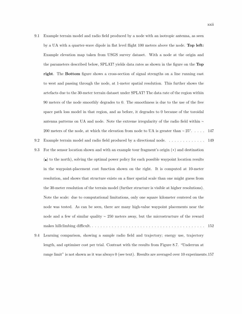
9.1 Example terrain model and radio field produced by a node with an isotropic antenna, as seen

by a UA with a quarter-wave dipole in flat level flight 100 meters above the node. Top left:

Example elevation map taken from USGS survey dataset. With a node at the origin and

the parameters described below, SPLAT! yields data rates as shown in the figure on the Top

right. The Bottom figure shows a cross-section of signal strengths on a line running east

to west and passing through the node, at 1-meter spatial resolution. This further shows the

artefacts due to the 30-meter terrain dataset under SPLAT! The data rate of the region within

90 meters of the node smoothly degrades to 0. The smoothness is due to the use of the free

space path loss model in that region, and as before, it degrades to 0 because of the toroidal

antenna patterns on UA and node. Note the extreme irregularity of the radio field within ∼

200 meters of the node, at which the elevation from node to UA is greater than ∼ 25. . . . . 147

9.2 Example terrain model and radio field produced by a directional node. . . . . . . . . . . . . . 149

9.3 For the sensor location shown and with an example tour fragment’s origin (⋆) and destination

(∎) to the north), solving the optimal power policy for each possible waypoint location results

in the waypoint-placement cost function shown on the right. It is computed at 10-meter

resolution, and shows that structure exists on a finer spatial scale than one might guess from

the 30-meter resolution of the terrain model (further structure is visible at higher resolutions).

Note the scale: due to computational limitations, only one square kilometer centered on the

node was tested. As can be seen, there are many high-value waypoint placements near the

node and a few of similar quality ∼ 250 meters away, but the microstructure of the reward

makes hillclimbing difficult. . . . . . . . . . . . . . . . . . . . . . . . . . . . . . . . . . . . . . . . . 152

9.4 Learning comparison, showing a sample radio field and trajectory; energy use, trajectory

length, and optimiser cost per trial. Contrast with the results from Figure 8.7. “Underrun at

range limit” is not shown as it was always 0 (see text). Results are averaged over 10 experiments.157

xxiii

9.5 Metapolicy learning progress over the runs (problems) used to generate Figure 9.4, compared

against the non-metapolicy PGRL learner. Shown are energy use, trajectory length, and op-

timiser cost per run over three representative intervals. “trials 1–30” reflects the performance

early in the learning of each new problem, “trials 1–100” shows aggregate performance for an

“adolescent” network, and “trials 150–300” shows performance of a mature network. For each

case, the untrained metapolicy (early runs) results in performance similar to that of PGRL

on average, whereas after training the metapolicy improves learning performance. Results are

averaged over 10 experiments. . . . . . . . . . . . . . . . . . . . . . . . . . . . . . . . . . . . . . . 158

9.6 Trajectory tracking error affects both the optimal planner and the learners. Top row: exam-

ple trajectories under the tracking error conditions σt, as shown, from an example run for each

of the three error conditions. The node locations are shown in order to illustrate some possi-

ble fields. Signal strength is given in grey so that the trajectories are visible. Middle row:

Under trajectory tracking error, the performance of all algorithms degrades slightly. Shown

are averages for the learners, but the Optimal line represents the “omniscient” optimal energy

policy—in which tracking error is perfectly anticipated (unachievable in practice). Bottom

row: when the Optimal policy cannot anticipate trajectory tracking noise, performance suf-

fers as shown. (5 samples per run per tracking error value, 21-run averages, 5 experiments, as

described in the text.) . . . . . . . . . . . . . . . . . . . . . . . . . . . . . . . . . . . . . . . . . . . 160

xxiv

9.7 Node location error: Energy use of the UA flying under an optimal planner that was given

incorrect information about node location, compared to performance curves for the learners

and Reference. With good information (left), optimal policies use significantly less energy

than the learners, which in turn substantially outperform reference. As the error increases,

the optimal plan underruns data objectives, requiring more flights and more transmission

energy, as evidenced by increased energy use. The proportional increase in trajectory length

is identical to the increase in energy use. In contrast, the learners are essentially unaffected.

(Unlike the similar figures that follow, the location error is sampled from exact distances in

random compass directions, rather than a distribution over distances.) (These graphs average

5 misinformed tests of each of runs 80–100 from 5 experiments as described in the text; the

inter-experiment variation was negligible.) . . . . . . . . . . . . . . . . . . . . . . . . . . . . . . . 163

9.8 Terrain model error. The figure on the left shows relative performance with perfect informa-

tion; that on the right, performance with the indicated error. 5 degraded samples per run,

21-run averages, over 10 experiments, as described in the text. . . . . . . . . . . . . . . . . . . 165

A.1 A poor gradient estimate slows learning, but a good gradient estimate requires many trials.

How many trials are required before the learner finds an acceptable trajectory? This measures

learning speed on the same easy problem (4 nodes, 28 policy parameters, req=30), averaged

over 100 runs. The local-credit-assignment (LCA) learner does best with about 4 trials/epoch,

and the plain REINFORCE (eR) learner prefers somewhere between 6 and 10. Error bars

show 1σ. To improve legibility we show only half of each error bar on the left graph. . . . . . 192

A.2 As Fig. A.1, with 20 nodes and 62 waypoints (124 parameters). Convergence of the LCA

estimator is still excellent at 4 trials/epoch, but it may improve slightly at higher values. . . 192

A.3 As Fig. A.1, but now a policy update is made whenever the gradient estimate changes between

trials by less than x. . . . . . . . . . . . . . . . . . . . . . . . . . . . . . . . . . . . . . . . . . . . 193

B.1 Creating new policies by regressing over old ones, on single-node problems with a data re-

quirement of 30, with the allowed trajectory extension factor φ ∈ [1,4]. . . . . . . . . . . . . . 199

xxv

B.2 Neural network regression with knowledge transfer . . . . . . . . . . . . . . . . . . . . . . . . . . 200

Chapter 1

Introduction

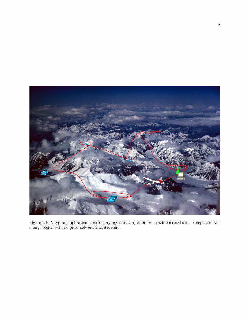
We consider the problem of collecting data from widespread stationary data sources such as ground-

based environmental sensor nodes. Such ground-based sensors can gather data unavailable to those on

aircraft or satellites; for example, continuous proximal surveillance of flora [Baghzouz et al., 2010] or fauna

[McQuillen and Brewer, 2000], or measurements that require physical interaction such as watershed runoff

[Muskett and Romanovsky, 2011]. The sensors may be far from cellular networks, have insufficient power or

size to use long-range radio or form multihop networks, and collect too much data to upload via satellite.

When latency in the network is acceptable, the data may be physically transported by a mobile network

component known as a data ferry [Zhao and Ammar, 2003] or data mule [Shah et al., 2003]. In our

approach, a fixed-wing unmanned aircraft (UA) flies over the sensors and gathers the data via a wireless

link [Jenkins et al., 2007] (e.g. Figure 1.1). We assume that the UA has a known range limit and can be

recharged/refuelled at a base station, and that the sensors may continuously generate data over long periods,

so that the UA needs to ferry the data to a collection site over repeated flights.

1.1 Problem

The general challenge is to find good control policies for the network. This work focuses on two

specific network performance goals: minimising the trajectory length flown by the UA given certain other

constraints such as acquiring a given amount of data; and minimising the energy that the nodes require

for transmitting data to the UA, which has ramifications for sensor lifetime. We divide the problem into

Aircraft Flight Optimisation and Radio Energy Optimisation layers.

2

Figure 1.1: A typical application of data ferrying: retrieving data from environmental sensors deployed overa large region with no prior network infrastructure.

3

Aircraft Flight Optimisation seeks to discover a flight path over the sensor nodes (a so-called

tour) that minimises some mission cost. We decompose this piece as follows:

Tour Design determines in what order to visit sensor nodes of known location. As the quality of node

location information diminishes, this transitions to a search.

Trajectory Optimisation identifies a trajectory that, when navigated by the UA, allows sufficient inter-

action with each node’s radio field while satisfying other constraints.

Vehicle Control determines the commands that must be sent to the aircraft’s control surfaces in order to

track a desired trajectory.

This work focuses on the Trajectory Optimisation layer. We assume that the tour is given and that the

nodes’ locations are known, albeit with some degree of imprecision, as for example when the sensors have

been deployed from an aircraft.

The interaction between planned and instantiated trajectories is affected by complex vehicle and

autopilot dynamics, may rely on careful identification of the UA system, and may be affected by external

factors such as changing payloads and weather conditions. For this reason, it is desirable to plan trajectories

with the understanding that they may not be tracked precisely. We assume a black-box autopilot that can

navigate between GPS waypoints, and that any idiosyncrasies while navigating are drawn from a stationary

distribution. We focus on the following question: How to discover the flight path that best accommodates

network demands, through an unknown radio field?

Radio Energy Optimisation consists of the following:

Radio Design chooses radio hardware and protocols to support high-efficiency communication.

Power Management varies the transmission power of nodes’ radios during interaction with the ferry

aircraft.

We assume a the existence of a reasonable solution to the Radio Design portion, as this has been addressed

elsewhere (see §2.1.1.1). We address only the Power Management layer.

4

Data can be transferred at a rate that depends on the signal-to-noise ratio (SNR) between sender

and receiver in configuration x(t) at time t. Thus, a trajectory that will collect D bytes of data satisfies

∫ R(x(t))dt ≥D, where R is the data rate supported by the SNR.

A perfect model of the system permits offline optimal planning, but such a model is difficult to acquire.

Radio system performance is a complex function of communication protocols and radio field shape. Radio

fields are shaped not just by the configuration of sending and receiving antennas, but also by reflections,

occlusions, and multipath interference, causing the radio field to be irregular and unpredictable. An aircraft

with a directional antenna will experience a signal strength that varies according to the aircraft’s position

and orientation ∈ R6, and may have a high spatial frequency. Environmental factors such as background

noise and humidity can further affect radio. These factors combine to make planning trajectories based on

predicted signal strength difficult and error-prone.

Consequently, research in data-ferried sensor networks thus far has made simplifying assumptions

about the shape of the radio field through which the UA flies. The nearly ubiquitous assumption is that

the radio field is spherically symmetrical as generated by a perfect isotropic antenna, with received signal

strength proportional to 1dϵ for distance d and path loss exponent ϵ. This simplification may be close enough

for good planning when a near-isotropic antenna is mounted high off the ground and far from environmental

features, but in other cases the difference between expected and realised signal strength can be significant,

and this degrades the quality of the solution.

In order to generate high-quality trajectories that acknowledge the complex structure of real radio

environments while eliminating the inconvenience of obtaining and maintaining accurate models suitable

for planning, this dissertation proposes a model-free learning approach for discovering control policies for

UA-ferried networks in the field. Policies can be learned quickly through direct interaction with unknown

entities, including the operating environment as well as autopilot and communication systems, which are

treated as black boxes whose specific functionality is unknown to the upper layers.

5

1.2 Thesis

UA-serviced sensor networks can learn high-performance energy-conserving policies in reasonable time

using a model-free learning approach.

This statement can be unpacked as follows:

UA-serviced sensor networks refers not just to the behaviour of the data-ferry UA, but to the learning

of policies governing various aspects of network behaviour. Chapters 4–5 are concerned only with

the optimisation of UA trajectories. Chapters 7–8 will expand the optimisation objectives to include

the sensor nodes’ radio control policies.

High performance refers to the magnitude of the improvement based on our chosen performance metrics.

Performance gains over the standard approach (reviewed in Chapter 2) are modest on simple radio

fields for which accurate information is available, but the model-free approach is well suited to deal-

ing with two real-world complications of data-ferrying scenarios: messy radio fields and inaccurate

information.

Messy radio fields reveal the first strength of model-free planning: standard approaches involve

circling the expected location of a node, whereas the best orbit point may be at some distance

from the node’s location, especially when radio fields have some irregular structure. In the

simulations presented here, this is especially true in the case of point noise sources and radio

interactions with terrain; other features of real radio fields, such as occlusions and multipath

interference, will have a similar effect.

While the learning approach shows great gains over reference planning when radio fields are

messy, further gains still are, in theory, available to model-based optimal planners. For example,

under tests of somewhat messy single-node fields, including randomly-oriented dipole antennas

and closely-spaced randomly-oriented point noise sources, we show that the model-free learners

can generally achieve ∼ 60–75% of the maximum possible gain over the conventional approach for

trajectory planning, and ∼ 70–85% of the maximum possible gain for node energy optimisation,

6

when perfect models of the systems are available. Under a more realistic terrain-based radio

simulator, the learner only achieves ∼ 50–65% of the performance gain available to an omniscient

optimal policy.

Inaccurate information can degrade solution quality for both the reference approach and the

optimal planners. When node position information is inaccurate, the performance of reference

planners degrades quickly, while the learners can adapt waypoint positions and communication

policies to optimise measured performance. For example, in the tests presented here, models

consist of all the information relevant to the planner: node position and antenna pattern in-

formation for target transmitters and point noise sources, and terrain when appropriate. This

allows model-based optimal planning to perform roughly ∼5–20% better with perfect models

than the learners could do, but modelling errors in the range of ∼ 10% were sufficient to reduce

performance below that which could be quickly learned. Under a terrain-based simulator, the

optimal planner will be shown to be extremely sensitive to misinformation, making it difficult

to achieve performance any better than that of the learners in the field.

Energy-conserving: Small or remote sensors tend to be energy-limited, making energy conservation an

important contributing factor to sensor network longevity. This dissertation begins by introducing

trajectory length minimisation, and builds towards learning policies that extend the UA’s trajectory

in order to increase contact time with the nodes, allowing them to transmit at lower power and

thus save energy. So while the techniques developed here are applicable to a variety of network

performance goals, the primary example is node energy conservation.

Reasonable time: The time taken to discover good policies varied with the quality of information available

to the learners, but over the evaluations that will be presented in this work, performance generally

significantly surpasses the conventional approach within dozens of trials and convergence generally

occurs within 30–200 trials. Is that “reasonable”? The number of tours of a sensor network depends

on several factors:

Target latency: If data become “stale”, then more tours of the network will be required. For

7

a surveillance network, the time between detecting an anomalous event and responding to it

should generally be low, and so hundreds or thousands of flights are likely to occur over a

network’s lifetime. For many scientific applications, latency is a lower priority, since the time

between gathering data and responding to it is generally greater. Some research assumes that

data are gathered and published before any response is implemented, in which case a single

tour of the nodes would meet any latency requirement. For other research, ongoing monitoring

is required. Sensor networks used in environmental risk detection (pollution, earthquakes,

volcanoes. . . ) may have various latency requirements, some of which will require thousands of

tours.

Buffers: Data storage is becoming increasingly inexpensive, but in response, data are becoming

richer. Especially if sensors gather large quantities of information, frequent collection may be

a necessity.

Backups: In harsh or hostile environments, sensors may become damaged or lost, making frequent

retrieval important. Again, this pushes the total number of tours high enough that a learning

approach that manifests large performance gains within dozens of trials is useful.

On a related note, scientific data acquisition is often accomplished by replacing technology with

manpower, using a human or graduate student (possibly in an aircraft or other vehicle) as the ferry.

This makes low latency, high bandwidth, or node-loss–tolerant data acquisition an expensive under-

taking. Consequently, many current experiments are designed assuming that low-latency monitoring

is not an option. The availability of low-cost UA-ferried data-acquisition networks would reduce the

cost of frequent data retrieval in remote environments, making new kinds of experiments feasible.

Model-free learning approach: Models allow rapid re-planning in the face of changing conditions or

network requirements, at the cost of initial and ongoing system identification time. In contrast,

learning directly on the observed performance allows the network to begin operation immediately.

The model-free optimisations used in this dissertation range from stochastic approximation to several

varieties of policy gradient reinforcement learning.

8

Few commercial products use reinforcement learning, or even stochastic approximation, while de-

ployed, often because of learning time: good policies may require thousands or millions of samples. Notable

commercial successes of reinforcement learning have involved either tasks for which ample offline training

time is available before the system goes live, or tasks that use simple policies that can be learned quickly. We

begin with the latter approach: the trajectory learner of Chapter 4 manipulates waypoints, leaving naviga-

tion and trajectory tracking to a standard autopilot; and the radio power learner of Chapter 7 manipulates

policies that, while sufficiently expressive to achieve high performance, are also sufficiently biased that they

can be learned quickly in the field. Chapter 8 makes a concession to the benefits of copious “offline” training

time by introducing a metapolicy that uses lifelong experience with past data-ferrying policy optimisations

in order to learn to improve learning speed and robustness on new problems.

This in situ approach to the optimisation of UA-ferried networks is novel, and the tools it provides

may be widely applicable. Furthermore, this work presents an integrated approach in which stochastic

approximation, reinforcement learning, and conventional off-the-shelf controllers produce useful behaviours

quickly—often within dozens of trials. A system that can learn on this timescale is both relevant to the

problem at hand and a starting point for a deployable system that integrates reinforcement learning.

1.3 Evaluation

The primary basis for comparison will be a planner that assumes a simple radio field model that is

nearly ubiquitous in data-ferry trajectory planning research. It assumes that radio fields are symmetrical

and predictable, with signal strength varying ∝ 1dϵ for distance d and path loss exponent ϵ, and that sensor

node positions are known precisely (although this knowledge may or may not be easy to acquire). This

planner will be referred to throughout the document as “Reference”.

As a further basis for comparison, we introduce optimal planners that assume perfect knowledge of

the radio environment, communication protocol quirks, and autopilot behaviour through access to the same

generative model used by the simulator. This provides a measure of how much of the theoretically possible

improvement over reference the proposed learners achieve.

Near-optimal planning is possible with slightly imperfect environmental models, but it is outside the

9

scope of this work to perform a general evaluation of the degradation in planning performance as the model’s

quality deteriorates. However, assume that a perfect model can be built in some finite amount of time. With

perfect information, optimal planning produces perfect policies, so eventually will outperform any other

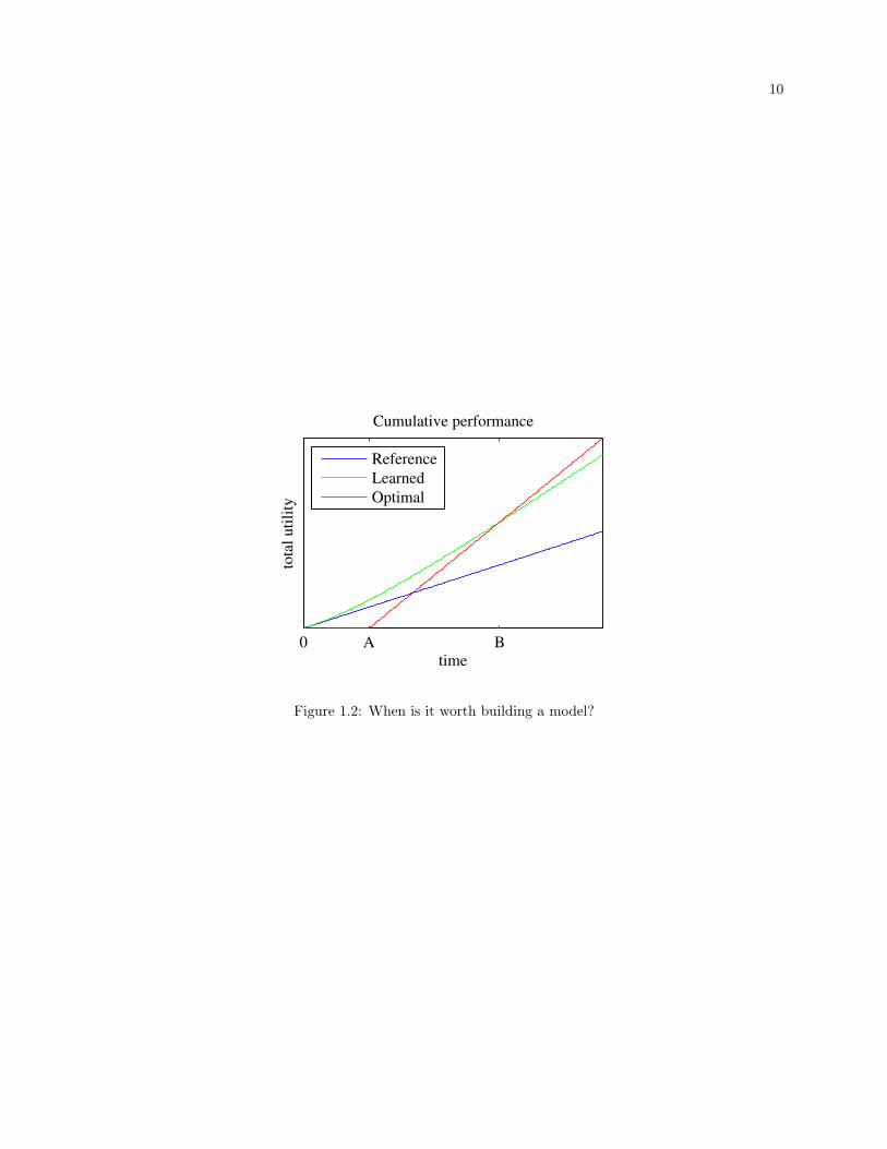
approach. What is “eventually”? Figure 1.2 is a schematic representing the accumulation of measurable

outcome—total data ferried or other total utility—over time. Assume that the network is deployed at time 0.

Reference and Learning approaches immediately begin active ferrying duties, accruing the desired outcome

(e.g. data) at similar rates, while an optimal planner begins system identification, resulting in a good model

at time A. As the learner refines its policy, it performs better and better, but never as well as the optimal

planner. By time B, the measurable outcome of the optimal network has surpassed that of the learned

network.

This is a simplification of the true case: it is possible to build a model while also ferrying data.

However, as we will see, the model must be quite accurate in order to achieve near-optimal planning, and it

is reasonable to assume that building such a high-quality model will require that the data-ferrying trajectory

make concessions to the need for acquiring data for the model. How to optimally trade off this exploration

vs. exploitation in an unknown environment is an open question, and so the simplification is a reasonable

starting point for analysis.

This dissertation argues that the learning approach is a reasonable alternative to optimal planning.

The criteria for comparison that will be used herein are:

Converged performance: As time goes to infinity, at what rate does cost or benefit accrue? Or, how do

the asymptotic slopes of the cumulative utilities in Figure 1.2 compare among the tested algorithms?

Learning speed: How quickly does the network achieve performance that is nearly as good as it will ever

be?

Network longevity requirement: It can be difficult to define total utility in a scenario-agnostic manner,

but when possible: when comparing to a model-building approach, for how long must the network

be in use for optimal planning to be the best choice?

An advantage of optimal planning not shown by the schematic is that a model permits immediate

10

0 A B

time

tota

l u

tili

ty

Cumulative performance

Reference

Learned

Optimal

Figure 1.2: When is it worth building a model?

11

generation of new policies if network requirements change, whereas model-free learning approaches require

time to adapt. On the other hand, when the environment changes sufficiently, a model-building approach

may need to expend resources updating its models. It is assumed that target applications for this work may

have a slowly varying environment (for example, seasonal foliage changes), but that demands on the network

remain fairly constant.

Algorithms are evaluated using two radio models. The primary one introduces antenna directionality

and point noise sources. Further evaluations are performed using a third-party simulator that adds terrain

interactions.

1.4 Contributions

The primary contribution of this research is the development and evaluation of a learner capable of

rapidly discovering suitable network control policies in the field without building system models. Reinforce-

ment learning is appropriate for the domain because it obviates the step of acquiring and maintaining system

models; because simple reinforcement learning techniques find good solutions quickly; and finally, because

the problem provides an interesting and useful testbed for multitask transfer learning.

The contributions are as follows:

Waypoint placement: A trajectory encoding and optimisation procedure for learning waypoint placement.

The trajectory representation is easy both for learning algorithms to manipulate and for off-the-shelf

autopilots to work with, and is optimised using stochastic approximation. The learner rapidly

discovers near-optimal trajectories (optimal + ∼ 10%) for various optimisation criteria even when

environmental information is inaccurate. Networks are optimised with either of two objectives:

Bandwidth, through learning minimum-length trajectories.

Sensor node longevity, by learning to conserve node energy reserves by trading UA flight dura-

tion against node radio transmission power.

Energy conservation: Nodes in sensor networks may be energy-limited. If the UA has excess range

available and the network is not bandwidth- or latency-limited, the nodes may transmit their data

12

at lower radio power, increasing contact time with the UA but saving node energy. We contribute a

simple energy policy to control the radio power used by the nodes for data transmission. We show

that it can be optimised at the same time as node positions, using policy gradient reinforcement

learning (PGRL) to produce near-optimal results.

Faster, more stable learning: We introduce a metapolicy that operates in parallel with the PGRL al-

gorithm, learning how to speed the learning process on new problems. The base learner optimises

waypoint placement and radio power policies. As the metapolicy gains experience with the policy

optimisation process over multiple problems, it learns to anticipate policy gradient estimates from

long-timescale information that is unavailable to the base policy, and uses this information to provide

augmentative or corrective policy updates. Learning speed is increased and sampling of high-cost

trajectories is reduced.

The metapolicy is trained on sequences of meta-level ⟨ state, action, reward ⟩ that are not

available to the base learner, allowing it to anticipate and prevent transitions into regions of

base policy space likely to lead to good or bad outcomes.

Training the metapolicy on a combination of its own generated actions and base-level PGRL

updates yields superior results to using either type of action alone.

The quality of the metapolicy’s suggestions can be monitored, allowing modulation between its

suggestions and the base gradient estimator’s updates.

Evaluation under complex radio models: The radio model used for most of the experiments introduces

features not commonly found in prior work, including antenna directionality and point noise sources.

Further tests examine the proposed planners under a realistic third-party terrain-based radio propa-

gation simulator. Results are shown to be qualitatively similar to those obtained under the simpler

radio model, lending strong support to the claim that model-free planning is robust to unexpected

features of the radio environment.

This dissertation advances the state of the art by lifting a significant restriction on the problem of

policy planning for ferried networks. The reinforcement learning approach can discover near-optimal policies

13

in reasonable time despite complex, unknown radio environments, allowing sensor networks to be rapidly

deployed in the field. Furthermore, since this domain is particularly well-suited to a reinforcement learner’s

unique capabilities, the system presented herein furnishes an interesting example of a real-world application of

reinforcement learning, including not only applications of the fairly common approaches through Chapter 7,

but also the active research question of multitask learning presented in Chapter 8.

Chapter 2

Related Work

This work contributes a reinforcement learning solution to the problem of discovering good policies

for data-ferried networks serviced by fixed-wing aircraft. §2.1 lays out the permutations of the general data

ferrying problem studied in the literature, and places the current work in context. Reinforcement learning

is used throughout, and so a brief review of the reinforcement learning methods presented here follows in

§2.2. In particular, one method falls loosely into the category of “learning to learn” or “metalearning”:

using knowledge gleaned from solving task A in order to better learn task B. §2.2 reviews metalearning in

reinforcement learning.

2.1 Data Ferrying

Using robots as data ferries is a relatively recent idea, dating to 2003 [Zhao and Ammar; Shah et al.],

although zebras were used as early as 2002 [Juang et al.]. The concept of data ferries is widely applicable,

and consequently the variety of considerations is large.

This section serves two purposes: to identify and discuss relevant research; and to present an overview

of the variety of hardware and network requirements in order to clarify the limits of the objectives of the

current work.

This portion of the review is organised as follows: §2.1.1 reviews the design goals and performance

metrics that have been used to evaluate data ferrying schemes, §2.1.2 discusses communication models,

§2.1.3 describes mobility models of both the ferry and the nodes, §2.1.4 reviews some of the capabilities of

ground-based sensor nodes. A brief discussion of what knowledge is assumed by the ferry system appears in

15

§2.1.5. Finally, §2.1.6 summarises research that applies machine learning to the data ferrying domain.

2.1.1 Objectives

Data ferrying has been considered largely due to its advantage in minimising energy consumption of

the nodes. The literature often takes energy reduction as a given and concerns itself with maximising the

data performance (§2.1.1.1). §2.1.1.2 provides a few examples of research in which energy—usually that of

the node, not the ferry—is explicitly studied.

2.1.1.1 Data-centric performance metrics

The majority of sensor network research considers metrics related to data transmission: network

throughput, latency, and packet loss.

Bandwidth is measured as the average rate of arrival of data at the hub. If this is not the same as

the total of data production rates of the sensors, then they must discard data, which may be appropriate for

some tasks. Bandwidth may be increased by reducing the UA’s tour time or increasing the data retrieved

per tour; the ratio of time spent communicating with node or basestation to time spent transporting may

be increased up to the limit of UA range, at the cost of latency.

Latency, the delay between a sensor taking a measurement and the measurement arriving at a base

station, is also sensitive to the ferry’s trajectory. The important number is the time between sampling data

from the environment and delivering it to the base station, so trajectories that visit nodes and base station

more frequently will tend to provide lower latencies than those that perform a complete tour of all nodes

before delivering the data. However, we consider only the latency minimisation that comes with reducing

the time taken for a complete tour.

While protocols are frequently discussed (e.g. [Jenkins et al., 2007; Al-Mousa, 2007; Wang et al., 2008;

Ho et al., 2010]), the primary consideration here is discovering a flight plan for the ferry. This involves:

Node location: If the nodes’ locations are unknown, the first step is usually to find them. Completely

unknown locations may indicate a grid search or some other search pattern based on expected node

distribution, and there may be parallels with animal foraging.

16

In [Detweiller et al., 2007] the ferry assumes approximate knowledge of the node’s location, and if

necessary performs a spiral search outward from there until the node is located visually or a time

limit is reached. Liu et al. [2010] represent node location as a POMDP and learn how to alter the

ferry’s trajectory to find a node that has moved. A related problem is WiFi target localisation

[Wagle and Frew, 2010], but I will argue that ferries do not need to know the exact location of each

node: Dunbabin et al. [2006] assume that the ferry can get close enough to locate a node visually,

and the approach in [Pearre, 2010; Pearre and Brown, 2010, 2011, 2012a,b] and the current work

tolerate error on the scale of the radio range.

Global tour design: In which order should the nodes be visited? The travelling-salesman (TSP) solution

is often taken to be the global tour of choice [Zhao and Ammar, 2003; Tekdas et al., 2008; Sugihara

and Gupta, 2011; Pearre and Brown, 2010; Tao et al., 2012] as it maximises bandwidth if no data

need be discarded, but when minimising latency it is suboptimal. For example, if the data hub H sits

between two nodes a and b, then the latency-minimising tour might be not Hab ∶∥ but HaHb ∶∥.1 If a

gathers data at a higher rate than b or is closer, then a better tour might be HaHaHb ∶∥ [Henkel and

Brown, 2008a], and aperiodic tours are optimal under some circumstances (there is also unpublished

research by Katz and Munakata showing faster discovery of good solutions in this space). Another

type of constraint may stem from the limited size of nodes’ buffers, in which case it may be ideal to

visit a node several times before delivering data to the hub [Somasundara et al., 2007]. A completely

different motivation appears in [Dunbabin et al., 2006]: global positioning information is expensive

to obtain in a submarine because it requires surfacing; therefore the optimal global tour minimises

the maximum inter-node segment in order to mitigate navigation errors.

Trajectory optimisation: Sugihara and Gupta [2008] assume a radio radius at which communication is

guaranteed, but shorten the tour as unexpectedly strong radio signals are found. Sugihara and

Gupta [2010] plan the ferry’s speed and current communication target given a priori knowledge of

the trajectory and communication conditions. Wichmann et al. [2012] adapt a TSP-based global

1 I borrow the repeat sign “∶∥” from musical notation, although here it may be treated as a repeat indefinitely sign.

17

tour design to the motion constraints of a fixed-wing UA, smoothing the tour with constant-radius

circles; they assume that data requirements are low enough for complete transfer under the proposed

trajectory. [Pearre, 2010; Pearre and Brown, 2010, 2011, 2012a,b] and the current work remove

assumptions about the shape of a radio field and optimises trajectories via repeated passes through

a (stationary) node’s field.

Low-level control: Aircraft autopilots generally communicate with a trajectory planner through way-

points. Precise tracking of arbitrary trajectories is not readily available in fixed-wing aircraft au-

topilots, although it is an active research area [Kendoul et al., 2009; Abbeel et al., 2010; Fang et al.,

2012]. Even the trajectories instantiated from waypoints can be unpredictable [Chao et al., 2010].

In [Dunbabin et al., 2006] the authors describe their submarine control system. They show examples

of “demand” and “actual” trajectories, and the tracking errors are frequently large. This seems to

be an opportunity to try a learning approach. However, I do not propose to solve this problem.

Other objectives are possible: sensor radio energy use (discussed in §2.1.1.2), spatial costs to the

ferry such as difficult terrain or hazardous flight conditions, or value-of-information metrics used for event

reconstruction. These objectives can be accommodated using our approach.

2.1.1.2 Energy

A primary goal of using data ferries is minimising energy. If the ferry is assumed to travel for free

(for example, because it can be recharged or refuelled at the hub or because it is mounted on a platform

that moves for other reasons), then the concern is with allowing a node to gather and transmit data for as

long as possible. Jun et al. [2007] compare ferry-assisted networks with hopping networks in simulation and

find that a ferry can reduce node energy consumption by up to 95% (further gains would be possible if their

configuration space were broader), and Tekdas et al. [2008] reach a similar conclusion on a real toy network

that uses wheeled robots as ferries. Anastasi et al. [2009a] consider energy requirements per message sent

including the overhead associated with turning a node’s radio on in order to search for a fixed-trajectory

ferry. Similarly, Ma and Yang [2007] optimise the lifetime of nodes by choosing between multi-hop node-node

18

routing and changing the ferry’s route and speed. Sugihara and Gupta [2009] examine optimal solutions

under the trade-off between energy use and latency given a fixed ferry trajectory, and Ciullo et al. [2010]

decrease a node’s transmit power as its data load rises, which allows high-data nodes to conserve energy and

low-data nodes to require less of a detour on the part of the ferry, which moves in straight lines and stops

while collecting data. In [Boloni and Turgut, 2008] a node learns whether or not to transmit to the ferry

depending on the range to the ferry—if the node expects the ferry to come closer later, then it should not

waste energy transmitting now. Taylor et al. [2009] take a different approach in which the ferry’s radio field

provides both a data channel and power for simple sensor nodes in a structural monitoring application.

I have found no work on choosing the ferry’s trajectory in order to minimise its own energy cost. The

ferry is assumed not to be the limiting factor, but minimising tour length will in general also be advantageous

for ferry energy use. The correspondence is not absolute: compare (a) an aircraft trajectory at constant

altitude and speed to (b) a trajectory that flies low and slowly while retrieving data and climbs higher to

avoid obstacles while travelling for long distances. The relationship is not simple: under (b) the ferry will

use more energy unless (a) requires the aircraft to orbit a node for a significantly longer period due to its

greater altitude.

Anastasi et al. [2009b] reviews not just data ferries but many other techniques of energy minimisation

in sensor networks.

2.1.2 Radio

The selection of communication hardware and standards constrains trajectory choice. For example,

available data transmission rates and association times affect the ability of the ferry to sense and respond

to its radio environment. Beam pattern controls range and signal isolation [Pearre and Brown, 2012b]. A

steerable antenna can offer a greater advantage [Jiang and Swindlehurst, 2010] at the cost of complexity and

weight.

If only one sensor transmits data at any given time, interference from other sensors is eliminated. But

this may not always be possible, for example when searching for sensors or comparing signal strengths; using

multiple ferries; or in the presence of sources that are not part of the sensor network. In the first two cases,

19

enhanced protocols can mitigate multi-source interference.

Computing a good trajectory through a radio field can be set up as a constrained optimisation problem:

find the shortest path such thatD bytes can be transferred. Alternatively, it could be set up as a non-episodic

unconstrained optimisation that maximises throughput or minimises latency over repetitions of the cycle.

Given a good model of the radio field, the data transfer for any control policy may be computed, and

the techniques of optimal control may be used. However, data rate is a nonlinear function with a high-

dimensional domain (§3.1), and thus a sufficiently accurate model is time-consuming to create, maintain

under even slowly changing conditions, and use.

Therefore, prior work has used a variety of simplified radio models. In Visit models, the ferry au-

tomatically exchanges all data upon visiting a node [Gu et al., 2006; Somasundara et al., 2007; Henkel

and Brown, 2008a]. Communication radius or disc models assume a mechanism for complete data transfer

below a threshold distance, possibly by permitting the ferry to hover [Zhao and Ammar, 2003; Dunbabin

et al., 2006; Bin Tariq et al., 2006; Ma and Yang, 2007; Tekdas et al., 2008; Sugihara and Gupta, 2008;

Tao et al., 2012]. A learning variant on a communication radius model is described by Sugihara and Gupta

[2011]: route planning assumes a communication radius but data may also be transmitted (at the same rate)

opportunistically, allowing planned tours to be shortened if possible.

Of greatest interest here because they are the most sophisticated models in general use are Variable-

rate models, which assume non-interfering spherically symmetrical radio fields whose power varies with range.

Radio power is computed as∝ 1dϵ for distance d and path loss exponent ϵ; this allows computation of data rate

that varies with transmission range. Henkel and Brown [2008b] present theoretical results using a distance-

dependent rate model, Carfang et al. [2010] compare the communication radius model to both smooth

and stepped variable communication rate models with optimal trajectories, approximating the behaviour of

802.11g hardware, and Brown et al. [2007]; Kung et al. [2010] and others measure real transmission losses

in UAVs and confirm that the behaviour of real stepped-rate radios can be approximated by variable-rate

models. Similarly, Stachura et al. [2009] treat a mobile tracking problem in which the probability of packet

transmission varies linearly with distance according to a function fit from data. Recently, variable-rate

communication models have been used to compute not transmission rate but transmission energy required

20

for a given rate. For example, Boloni and Turgut [2008] consider whether or not a node should transmit

when the ferry is within range, and scales the power required for transmission according to the range; similar

use of a variable-rate model to scale transmission power appears most recently in [Ren and Liang, 2012;

Wu et al., 2012]. The spherically symmetrical variable-rate assumption underlies most current trajectory

planning work, and thus serves as a basis the Reference trajectory planner that will be used throughout this

dissertation.

On a completely different note, underwater sensor networks [Detweiller et al., 2007; Erol-Kantarci

et al., 2011] tend to use sonar, which introduces a different set of constraints on communications [Zhou

et al., 2012], as well as issues of localisation [Zhou et al., 2007]. However, since underwater ferries tend to

be neutral-buoyancy and slow-moving, trajectory planning is very different from our case.

Many of these variations could be accommodated, but here we have chosen to ignore protocol details

and ties to specific hardware, and instead focus on a simple domain simulator that creates a sufficiently com-

plex radio environment to explore a versatile model-free learning approach. A recent review by Di Francesco

et al. [2011] focuses on data-collection aspects of the data-ferrying problem not discussed in this review.

2.1.3 Ferries

A ferry moves between sensors and possibly base stations, retrieving and transmitting data. The

variety of craft that have served as data ferries attests to the approach’s versatility, but it introduces variety in

the expected vehicle dynamics. The ferry may follow a regular route with few concessions to data collection,

perhaps because it is attached to a vehicle such as a bus [Chakrabarti et al., 2003]. Ferries may have a

prescribed mobility pattern designed for a specific sensor deployment [Boloni and Turgut, 2008; Kavitha,

2011], or may change trajectories over time. Our ferries are special-purpose vehicles whose trajectories may

be manipulated with no consideration for non-ferrying tasks, and whose range and refuelling requirements

are assumed to be appropriate for the application. Watts et al. [2012] review currently available robotic

aircraft.

Our intended hardware, unmanned fixed-wing aircraft, is constrained by some range, as well as max-

imum and minimum speeds, and a minimum turning radius. The values of those constants are unimportant

21

for showing the operation of these algorithms; they may be filled in with any hardware-specific values. Fixed-

wing aircraft are not the only possible choice, and other choices may be amenable to our approach given

appropriate trajectory representations and cost functions. Helicopters and quadrotors can hold a position

at some cost in energy; ground vehicles can hold a position without an energy cost, as can buoyant vehicles

in calm weather. Some vehicles can be controlled with great precision; others, such as ours, cannot, which

imposes further constraints on trajectory shapes and the accuracy with which they can be realised.

2.1.4 Sensors

Some ground-based sensors do not move once deployed. Some move without control; for example,

sensors deployed on ice floes [Richter-Menge et al., 2006], floating in bodies of water [Heery et al., 2012],

or attached to wildlife [Juang et al., 2002]. Data ferries are sometimes used to provide connectivity for

fully mobile nodes such as military ground forces [Jiang and Swindlehurst, 2010]. In this paper we assume

stationary sensors in environments that are unchanging on a timescale of a at least a few dozen tours.

Sensor energy is generally supplied by battery, which sensors may recharge by harvesting energy from

the environment [Ren and Liang, 2012]. We do not model sensor energy reserves explicitly; instead we

assume that minimising energy use is a serviceable proxy.

I will ignore work that has considered controlling the positions of the nodes in order to facilitate

communication since this compromises their primary duty and since the thrust of this research concerns

stationary nodes, but there has been some work on predicting node locations and searching for them in the

case of prediction error [Juang et al., 2002; Dunbabin et al., 2006; Liu et al., 2010].

The rate at which data are gathered by the sensors, expected sensor lifetime, and network latency all

contribute to the required data storage (buffer) capability of sensors. We assume that storage and buffers

suffice for the application and do not consider buffer state.

2.1.5 Knowledge models

Often the locations of the sensors will be approximately known—the location of a measurement is

usually important—but the accuracy requirement may be inadequate for optimal trajectory planning. It

22

is possible that each sensor knows its own location but this information is not available to the ferry until

contact, and in the case of mobile sensors or noisy GPS this information may not be static. Other times

sensors may not know their positions, and it is up to the ferry to provide approximate location information.

In other cases sensors may be known only to lie somewhere in an area, necessitating a search.

When using radio or other propagating-wave communication system, knowledge of the shape of the

radio field is likely approximate, and may change over time due to sensor mobility or environmental effects.

The interaction of radio waves with terrain leads to reflections, occlusions, and self-interference, and the

existence of other radio sources causes further difficulties. So while accurate knowledge of the radio field can

allow effective trajectory planning, the ability to accommodate vague or incorrect information is important.

We assume that the aircraft knows the identities of sensor nodes, and that it knows enough about

their positions to fly to within radio communication range of them. This information could be discovered

by a preliminary search pattern, inventory, and initial tour generation phase, but that phase of learning is

outside the scope of this work.

2.1.6 Sensor networks that learn

Of particular interest to me are applications of machine learning, and especially of reinforcement

learning, to the data ferrying problem.

Two ways of classifying optimisation criteria will be especially useful:

Hard vs. Soft constraints: A hard constraint is a property of the solution that either exists or does not.

In this paper, the notable hard constraint is that trajectories must collect the required quantity

of data. In contrast, for a soft constraint a more extreme value is always preferred. For example,

even when a trajectory is shorter than the UA’s maximum range, shorter trajectories are generally

preferred.

Global vs. Local: The tour length is a global criterion, since each action affects others and thus impacts

the whole tour. Other objectives are spatially localised; for example, radio energy used at any given

sensor depends only on decisions made in the vicinity of that sensor.

23

The first distinction is important because of the difficulty inherent in model-free learning algorithms: ful-

filment of hard constraints is not guaranteed, but must be learned quickly or ensured by a non-learning

component. The second distinction has a bearing on the scalability of the problem: the speed of optimisa-

tion of global objectives depends on the number of nodes or trajectory parameters, whereas the optimisation

of local-flavoured objectives can be largely independent of the number of nodes.

The objective of [Boloni and Turgut, 2008] is to allow each node to decide whether the ferry is close

enough to justify the energy cost of transmitting, based on the node’s past experience with the ferry and the

amount of data in the node’s buffer. When the ferry is far away and the node’s buffer is nearly full, should

the node transmit, or wait for the ferry to approach? The authors model the node’s buffer state and the

ferry’s position as a Markov Decision Process (MDP), so it relies at least on the ferry drawing its trajectories

from a stationary distribution.

Henkel and Brown [2008a] aim to solve the global tour planning problem for fixed nodes and a “visit”

radio model, using reinforcement learning. The state space is the buffer state of each node, and the action

space is the set of all ordered subsets of the set of nodes. The algorithm does learn tours that are better

than the standard TSP solution, but learning is not fast even for simple problems—they present results for

5 nodes after 20 hours of computer time, and for n nodes their action space scales as O(2n), making the

approach infeasible for large problems. This research is interesting, however, and Boyan and Moore [2001]

provide some ideas on nonlinear optimisation that may be of value in further developing such solutions.

Sugihara and Gupta [2011] first use a “communication radius” radio model and extend the TSP to

a “label-covering” problem. Then the ferry observes locations in the tour during which communication at

the same rate can be initiated earlier than expected. Using this observed information, it shortens the tour.

Learning is rapid: it converges within a couple of tours, and is guaranteed not to produce an inferior tour

as long as the minimum communication radius assumption holds.

Liu et al. [2010] assume that the nodes themselves are mobile. The ferry models node movement as

a POMDP in which position is quantised, and learns a policy for locating nodes: try the position bins that

are most likely to contain the node. If a node can not be found within a few tries, the ferry moves on to the

next node and returns later. When the node’s movement is biased towards one direction, their approach is

24

only successful when the average node speed is low relative to the learning rate. An obvious extension would

be to introduce a continuous state space and model node movement with a Kalman or particle filter. For

example, [Jiang and Swindlehurst, 2010] Kalman-filters nodes’ self-reported positions at timestep t in order

to position the aircraft optimally for communication with a directional antenna at timestep t + 1.

With a different but related goal, Dixon [2010] proposes an adaptive method of maximising network

capacity of a UA-based multi-hop relay network, measuring a gradient on the signal-to-noise-and-interference

ratio (SINR) in order to improve UA position. Notably, the work makes minimal assumptions about the

radio field’s structure, leading to a solution that is both optimal in a certain sense in the real world, and

adaptive.

2.1.7 Problem “size”

The notion of problem size can take many useful forms. There may be one sensor or thousands,

served by one ferry or by many. The ferry may need to retrieve bytes or gigabytes. The longevity of a sensor

network is another useful measure of size: in some cases a single collection run is anticipated, and in others

the network’s lifetime and the number of collection runs may be indefinite.

We assume a single ferry, up to a few dozens of sensor nodes (due only to processor limitations),

a single base station, a broad range of data requirements, and a network that is designed to collect data

continuously and be polled by the ferry at least dozens of times. The metalearner presented in Chapter 8

will assume experience with on the order of dozens of different ferried sensor networks.

2.2 Reinforcement Learning

Most reinforcement learning (RL) research deals with variants on Markov Decision Processes (MDPs)

[Bellman, 1957], which are graphs consisting of a set of states s ∈ S, a set of possible actions a ∈ A in

each state, state transition probabilities Pr(s′∣s, a) that depend on the action chosen at each timestep,

and some scalar reward (cost) function, Pr(r∣s). “Markov” refers to the (first-order) Markov property: the

transition and reward functions depend only on the current state, rather than on previous states and actions.

Reinforcement learners in an MDP strive to discover a policy—a mapping from state s to action u—that

25

maximises the expectation of total (optionally time-discounted) expected reward over time (called return);

either the total reward over an episode of finite length or a time-discounted average reward through infinite

time; some definitions of MDPs include the time discount factor and some leave it as a tunable parameter.

The majority of reinforcement learning research concerns building a function that learns the value of

performing each of a discrete set of actions from each state in the environment (see [Sutton and Barto, 1998]

for the canonical treatment). The value function, usually denoted Q(s, a), contains the expected return

to be obtained by taking action a from state s and then following a known policy. The policy can then

be: at each state, choose the highest-valued action (according to Q(s, a)), with occasional random choices

for purposes of exploration, until termination. These methods have proven powerful in some domains, but

Q(s, a) functions are not conducive to many forms of knowledge transfer.

The reinforcement learning algorithms used here are of a class known as Policy Gradient Reinforcement

Learners (PGRL). The policy is some parametrised function πθ(s) = Pr(u∣s; θ) that maps state to action

according to the policy’s parameters θ. There is no value function, but rather the learning process involves

repeatedly estimating the gradient of expected return with respect to the parameters θ and updating the

policy accordingly. An excellent overview is available in [Peters and Schaal, 2008], and further references

will be provided as the relevant algorithms are introduced.

Important practical consequences of the differences between value-function reinforcement learning

(VFRL) and PGRL are:

PGRL deals well with continuous state spaces. In VFRL, representing continuous state spaces for

use by Q(s, a) is difficult [Boyan and Moore, 1995]. PGRL sidesteps many of these difficulties, since

a poorly approximated value cannot bootstrap errors into the value function.

Continuous action spaces are naturally represented in PGRL, since the policy is simply a probability

distribution over some action space. In VFRL, continuous actions are difficult and considered rarely

(see, e.g., [van Hasselt and Wiering, 2007]).

Value-function RL is guaranteed to converge to the globally optimal solution under certain conditions,

which include discrete state and action spaces; a policy that has a nonzero probability of choosing

26

every action from every state; and an infinite number of steps. PGRL is guaranteed only to converge

to a locally optimal solution. When the reward landscape is bumpy, any nonlinear optimisation

technique may be incorporated in order to increase the probability of a globally optimal or near-

optimal solution. However, non-local search creates policies that are far from solutions that are

known to be good, which in a real system may lead to unsafe or destructive behaviours.

2.2.1 Reinforcement Metalearning

Chapter 8 will introduce a policy that operates on a policy—a “metapolicy”—and a reinforcement

learner that trains the metapolicy. “Metalearner” is not a precise term, especially in RL. It refers to a

learning algorithm that seeks to change some parameters of a lower-level learning algorithm over the course

of experience in order to increase the performance of the low-level learner [Schaul and Schmidhuber, 2010a],

but the published work on metalearning shows considerable diversity in the way in which this happens.

What follows is a brief review of the most relevant examples of reinforcement metalearning.

A simple and effective example of reinforcement metalearning seeks to learn good values for parameters

used by the base reinforcement learning algorithm. Schweighofer and Doya [2003] introduce a metalearner

that controls the RL learning rate α, exploration/exploitation trade-off parameter β, and temporal reward

discount γ. While the metapolicy does not actually control action selection, β does control the probability

of exploratory actions. The metapolicy monitors the policy by watching whether parameter modifications

help a medium-term running average of reward compared to a long-term average. [Kobayashi et al., 2009]

further develop the same idea by using the temporal difference error [Sutton and Barto, 1998] to track the

effectiveness of parameter modification.

Reinforcement metalearning is more often applied to knowledge transfer between tasks. In multitask

reinforcement learning, approaches step away from the base learner by transferring information gleaned by

one base learner to another base learner operating on a different task. Various kinds of information may

be transferred, including state-action values from past tasks [Perkins and Precup, 1999]; partial [Fernandez

and Veloso, 2006] or complete [Tanaka and Yamamura, 2003] state-action value functions Q(s, a); gener-

alised rules for what to do in state s [Madden and Howley, 2004]; important [Banerjee and Stone, 2007] or

27

mathematically interesting [Mahadevan, 2005] features of the environment; shaping rewards [Konidaris and

Barto, 2006]; or domain models [Thrun, 1995]. Reviews with further examples may be found in [Taylor and

Stone, 2009] and [Torrey and Shavlik, 2009].

The oldest example above is also one of the most interesting. Thrun’s [1995] Explanation-Based Neural

Networks (EBNNs) use neural networks for classification, and use the slopes of the networks to represent

domain “explanations”. For example, when classifying a cup, EBNN will generate a cupness manifold with

a large slope over the dimension that indicates whether the object can hold liquid, but zero slope over the

Styrofoam dimension. One important aspect of EBNN is recoverability: given an incorrect or incomplete

domain model, the importance of slope information is downgraded and re-learned, allowing the model to

improve its domain theory rather than simply refining it. Thrun applies this idea to Q-learning by training

a sensation-prediction network and a payoff-prediction network. The former is trained across tasks, and the

latter is trained only per task. The gradients of the networks with respect to state ∇sQ(s, a) are used to

quickly produce environmental models specific to new tasks. This is an elegant way of producing and using

a classical model Pr(s′∣s, a) using a large training set that spans a variety of tasks.

The review of Torrey and Shavlik [2009] discusses both reinforcement and supervised transfer learning.

In the field of supervised learning, “meta” again refers to using past data sets in order to improve classification

results on new ones (for example, to learn values for bias parameters). Various recent surveys on supervised

metalearning are available, e.g. [Pan and Yang, 2010], but supervised metalearning is not directly relevant

to this work.

2.2.2 Policy initialisation from past experience

Appendix B will explore a method of creating new parametrised policies from old ones, rather than

requiring re-learning a solution to each new problem from scratch.

Most of the extant work achieves a similar end by adapting old Q(s, a) functions to new problems.

For example, Taylor and Stone [2005] define a function ρ ∶ π1 → π2 that transforms policy π1 in domain 1 into

policy π2 in a related domain. The authors have shown that for some domains ρ can exist and can be useful

for automatically initialising a new policy, and they later [Taylor et al., 2008] proposes a method, Modeling

28

Approximate State Transitions by Exploiting Regression (MASTER), that allows automatic discovery of ρ.

However, MASTER scales exponentially in the number of state dimensions and distinct actions.

Tanaka and Yamamura [2003] describe a simple approach in which the learner is told from which

distribution MDPs are drawn. It uses measured mean and variance to adjust initial values and step sizes,

respectively, of a tabular Q(s, a) function. The variance allows a modification to Prioritized Sweeping [Moore

and Atkeson, 1993] that allows the agent to use estimates to bias the update order.

Wilson et al. [2007] describe a Bayesian multitask learner: MDPs are assumed to be drawn from a

clustered distribution, modelled with a Dirichlet process. The clusters are in any parameter space for the

MDP. Knowledge is transferred by drawing a sample of likely MDPs from the model, solving them offline,

and trying to use their optimal actions on the real MDP. The same authors extend the technique using

PGRL in [Wilson et al., 2008], in which the Dirichlet process models a distribution of roles of policy-gradient

agents learning to play the realtime strategy game Wargus. An expert assigns agents to areas of expertise,

and the mapping of learned policies to tasks generalises (by construction) to new agents who can therefore

be initialised with good policies.

The policy initialisation method introduced in Chapter B tries to initialise new policies that differ from

old only in the weights of parameters inside the reward function. While this work uses smooth parametrised

policies, the setup is similar in spirit to the Variable-reward Hierarchical Reinforcement Learning of Mehta

et al. [2008], in which the reward function consists of a weighted sum of reward features. Upon receiving a

new task with new reward weights, a Q(s, a) function is initialised from the solved task whose reward weight

vector is closest.

The most similar work to mine initialises not Q(s, a) tables but parametrised policies. [Kronander

et al., 2011] use supervised learning to regress over policy parameters of a basic motion model of hitting in

minigolf; they assume consistent examples presented by a teacher. Ijspeert et al. [2002] propose a method

of encoding trajectories for reaching motions as the time evolution of a class of differential equations, and

use metaparameters of the differential equation to change the endpoint of a motion. Their assumption that

the relationship between task outcome and metaparameters is trivial is lifted by Kober et al. [2012], which

describes a sophisticated approach suitable for tuning Ijspeert’s motor primitives over individual executions

29

of related tasks. Their approach learns a nonparametric regression across policy parameters, using prediction

variance for exploration.

Chapter 3

The Simulator

3.1 Radio Environment Model

Our goal is to evaluate the ability and limitations of model-free optimisation in a complex, unknown

radio environment. To this end we introduce a radio model that incorporates several complicating factors

that are rarely considered: variable-rate transmission, point noise sources, and anisotropic antenna patterns.

Chapter 9 will verify the developed algorithms against a third-party simulator that additionally considers

terrain and atmospheric effects; this section describes the simulator used through Chapter 8.

The signal to noise ratio at node a from node b is given by

SNRab =P (a, b)

N +∑i P (a,ni)(3.1)

P (a, b) is the power received by node a from node b, N > 0 is background noise from electronics and

environment, and ni are other transmitters or noise sources. The power between a and b is computed as

P (a, b) =P0,ad

ϵ0

∣Xa −Xb∣ϵ(3.2)

for reference transmit power P0,a ≥ 0, reference distance d0 = 1, distance between transmitter and receiver

∣Xa−Xb∣, and propagation decay ϵ. However, antenna shape and radio interactions with nearby objects make

most antennas directional, so the orientations of the antennas affect received power. We model the aircraft’s

antenna as a short dipole with gain 1.5 (1.76 dBi) oriented on the dorsal-ventral axis of the aircraft, and

approximate the resulting radio pattern as a torus. We model the nodes’ fields similarly with random fixed

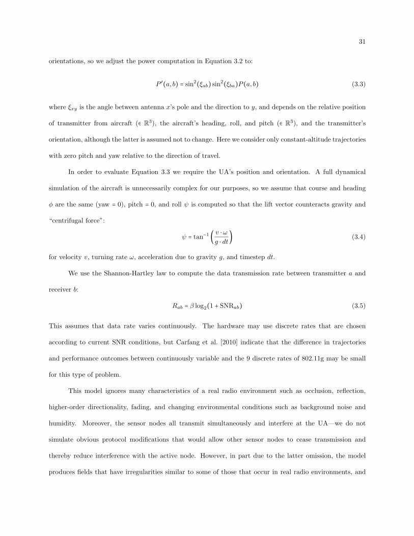
31

orientations, so we adjust the power computation in Equation 3.2 to:

P ′(a, b) = sin2(ξab) sin2(ξba)P (a, b) (3.3)

where ξxy is the angle between antenna x’s pole and the direction to y, and depends on the relative position

of transmitter from aircraft (∈ R3), the aircraft’s heading, roll, and pitch (∈ R3), and the transmitter’s

orientation, although the latter is assumed not to change. Here we consider only constant-altitude trajectories

with zero pitch and yaw relative to the direction of travel.

In order to evaluate Equation 3.3 we require the UA’s position and orientation. A full dynamical

simulation of the aircraft is unnecessarily complex for our purposes, so we assume that course and heading

ϕ are the same (yaw = 0), pitch = 0, and roll ψ is computed so that the lift vector counteracts gravity and

“centrifugal force”:

ψ = tan−1 ( v ⋅ ωg ⋅ dt

) (3.4)

for velocity v, turning rate ω, acceleration due to gravity g, and timestep dt.

We use the Shannon-Hartley law to compute the data transmission rate between transmitter a and

receiver b:

Rab = β log2(1 + SNRab) (3.5)

This assumes that data rate varies continuously. The hardware may use discrete rates that are chosen

according to current SNR conditions, but Carfang et al. [2010] indicate that the difference in trajectories

and performance outcomes between continuously variable and the 9 discrete rates of 802.11g may be small

for this type of problem.

This model ignores many characteristics of a real radio environment such as occlusion, reflection,

higher-order directionality, fading, and changing environmental conditions such as background noise and

humidity. Moreover, the sensor nodes all transmit simultaneously and interfere at the UA—we do not

simulate obvious protocol modifications that would allow other sensor nodes to cease transmission and

thereby reduce interference with the active node. However, in part due to the latter omission, the model

produces fields that have irregularities similar to some of those that occur in real radio environments, and

32

thus it meets our aim of having a complex simulation environment within which we can test whether the

aircraft can learn in situ.

3.2 Policy, Autopilot, Trajectory

The aircraft is directed to follow some trajectory by the autopilot. Two considerations drive the design

of the policy representation:

The learning algorithms that we will see in the following chapters require a representation for which

it is easy to generate variations and that can be manipulated at low computational cost.

The autopilot generally cannot perfectly track arbitrary trajectories, but it can easily work with

waypoints.

Thus the autopilot realises trajectories and the policy representation serves as the interface between the

learner and the autopilot, allowing the latter to remain ignorant of the former’s internals.

Here we introduce the three major trajectory representations for convenience. They will be reviewed

again when they are used.

3.2.1 The Reference trajectory

The non-learning Reference autopilot is similar to that used by Carfang et al. [2010]. It is provided

with estimates of the sensor nodes’ locations (although these can be difficult to discover [Wagle and Frew,

2010]), which it assumes to be correct. For each node, the UA receives data only from that node while flying

at constant speed v towards the tangent of a circle of radius radloop about the node’s nominal location. It

then circles the target node at the loop turning rate ωloop until D bytes are received, and then proceeds

to the next node. This produces the Reference trajectory. Fig. 3.1 (left) shows an example of a trajectory

generated by the reference autopilot.

33

Reference: trial 0, req [ 8 10 12 ]dist 100%, data [ 118 113 109 ]%

Waypoints: trial 96, req [ 8 10 12 ]dist 66%, data [ 118 112 108 ]%

Data−loops: trial 96, req [ 8 10 12 ]dist 77%, data [ 101 102 101 ]%

Figure 3.1: Sample trajectories plotted in space, superimposed over reference rate contours that show whatthe aircraft would see in flat level flight (not what it actually sees as it steers and banks). Six noisetransmitters, of the same signal strength as the sensors, sit at unknown locations. The aircraft starts at ⋆and passes each waypoint (˙) as described in §3.2. Actual node locations are at ; their assumed positionsare at (in this case, drawn from a Gaussian about the true positions, σ = 3). Left: Reference. Middle:Waypoints planner with 3 waypoints per node. Right: Data-loops planner with 1 waypoint locked to eachnode. Circle size is proportional to data rate. “req” is the data requirement per node (blue, green, red),“dist” is the distance travelled compared to the Reference trajectory, and “data %” shows the proportion ofthe data requirement transferred.

34

3.2.2 The Data-loops trajectory representation

The learning Data-loops autopilot assigns one waypoint to each node—we will assume that node

identities and approximate locations are known during tour initialisation, although the assignment could

instead occur on the fly as nodes are discovered. The UA flies towards the tangent of a circle of radius

radloop about the waypoint, and then if necessary circles the waypoint at that radius, exchanging data only

with the assigned node until it has collected sufficient data. Other course corrections—for example, those

made after completing data collection at a node—are of radius radmin. While not orbiting a node the UA

collects data from any node opportunistically : at each timestep, of the nodes that still have data to be

uploaded, communication is to the node with the highest observed SNR—a suboptimal greedy algorithm,

but one that performs well in practice. The true node location and the waypoint location may differ, and as

we will see, usually they will.

3.2.3 The Waypoints trajectory representation

The Waypoints representation will appear in Chapter 5 in order to explore what might be gained by

an autopilot that can fully anticipate future communication.

The learning Waypoints autopilot flies directly towards each waypoint in the sequence supplied by

the planner, adjusting its heading for the next waypoint at its maximal turning rate ω as soon as it has

passed the current one. We define “passing” a waypoint as being within the UA’s turning circle of it: ϵ = vω

(see Fig. 3.1 (middle)). We initialise trajectories of “n waypoints per node” with a waypoint at the nominal

location of each node (not including the start and end points) and n− 1 waypoints evenly spaced along each

tour segment. Because there is no intrinsic association between waypoints and nodes, the UA always collects

data opportunistically: at each timestep, of the nodes that still have data to be uploaded, communication is

to the node with the highest observed SNR. We have assumed that the protocol overhead of monitoring the

SNR and associating to each node is relatively small.

Chapter 4

Data-loops Trajectories

This chapter introduces the basic trajectory representation used throughout most of the experiments,

and evaluates the effectiveness of a simplified version of Policy Gradient Reinforcement Learning (PGRL)

for learning appropriate waypoints for data-ferrying tasks.

4.1 Waypoint placement

When minimising trajectory length, the optimal waypoint placement solves:

argminθ

d(π(θ)) subject to ∫T

0Rj(t) dt ≥Dj , ∀j ∈ nodes (4.1)

where d is the total distance1 flown by the ferry aircraft on the time interval [0, T ] for some policy π(θ)

parametrised with θ, Rj is the radio transmission rate to node j, and Dj is node j’s data requirement. The

models for radio (§3.1) and autopilot (§3.2) underlie Equation 4.1, but it is difficult to anticipate Rj at a

given aircraft position. And due to the unpredictable nature of the autopilot it is difficult to anticipate the

aircraft’s position through time in response to a set of waypoints. Thus knowing a set of waypoints permits

us to anticipate neither how far the aircraft will fly nor whether a given trajectory will satisfy the constraints.

We will discuss two solutions to this difficulty. The current chapter describes the Data-loops planner,

in which we push the constraint-satisfaction problem down to the autopilot, whose control policy guarantees

that the data constraints are satisfied. A contrasting approach, the Waypoints planner, rewrites the

constraints of Equation 4.1 as costs for the optimiser to minimise through experience, and will be developed

in Chapter 5.

1 Or, equivalently for constant speed, flight time.

36

Since Equation 4.1 cannot generally be solved directly by a UA in the field, we use a parameter

optimiser based on a Policy Gradient Reinforcement Learning (PGRL) algorithm. For waypoint placement

we use a simplified version that reduces to Simultaneous Perturbation Stochastic Approximation (SPSA)

[Sadegh and Spall, 1997; Hirokami et al., 2006]. Because the policies do not react to state, it is not strictly

correct to refer to this simplified version as “reinforcement learning”: the policies are open-loop, and a

non-learning trajectory-tracking controller (the autopilot) closes the control loop. This is not uncommon in

the PGRL literature [Kohl and Stone, 2004; Peters and Schaal, 2008; Roberts et al., 2009] but Kohl and

Stone [2004] referred to it as “a degenerate form of standard policy gradient reinforcement learning”. The

simplification is desirable because it allows a reduced policy space and thus faster learning. However, we

use the language and framework of PGRL because this makes it easy to reintroduce state dependence at the

policy level, as we will do when minimising data transmission power requirements in Chapter 7.

4.2 The Data-loops trajectory representation

The learning Data-loops autopilot assigns one waypoint to each node—we will assume that node

identities and approximate locations are known during tour initialisation, although the assignment could

instead occur on the fly as nodes are discovered. The UA flies towards the tangent of a circle of radius

radloop about the waypoint, and then if necessary circles the waypoint at that radius, exchanging data only

with the assigned node until it has collected sufficient data. Other course corrections—for example, those

made after completing data collection at a node—are of radius radmin. While not orbiting a node the UA

collects data from any node opportunistically : at each timestep, of the nodes that still have data to be

uploaded, communication is to the node with the highest observed SNR—a suboptimal greedy algorithm,

but one that performs well in practice. The true node location and the waypoint location may differ, and as

we will see, usually they will.

4.3 Gradient estimation

In PGRL, a stochastic policy π(s, u; θ) = Pr(u∣s; θ) defines the probability of choosing action u in

state s with the policy’s parameter vector θ ∈ Rn. The expectation of discounted rewards averaged over all

37

states s and actions u under a policy π(θ) is called the expected return J :

J(π(s, u; θ)) = 1

γΣE (

H

∑k=0

γkrk) (4.2)

where r is the reward received at each timestep, γ ≤ 1 is a “temporal discount” that places higher value on

rewards received sooner than on those received in the more distant future (this will be discussed further in

Chapter 6), and γΣ normalises the temporal discount weights and satisfies 1γΣ∑H

k=0 γk = 1. We will use the

common abbreviation J(θ) = J(π(s, u; θ)). The key component of PGRL is estimating the gradient of the

expected reward: gθ = ∇θJ(θ).

We break the task down down into distinct “trials”. Each consists of a complete execution of the

policy π(θ) over a bounded time interval—the aircraft flying a complete tour τ—followed by receipt of

reward r at the end. During a trial, the policy defines a probability distribution over the action chosen at

any point. Assume that the controller makes some finite number H of decisions uk at times tk, k ∈ 1 . . .H

during a trial; discretizing time in this manner makes it possible to compute the probability of a trajectory

under a policy as the product of the probabilities of each (independent) decision at each time tk. So

Pr(τ ∣θ) =∏Hk=1Pr(uk ∣sk; θ).

To optimise θ, we estimate the gradient using stochastic optimisation’s “likelihood-ratio trick” [Glynn,

1987] or reinforcement learning’s “episodic REINFORCE” (eR) [Williams, 1992] with non-discounted reward.

Each element ∇θi of the gradient is estimated as:

gθi = ⟨(H

∑k=1∇θi logPr(uk ∣sk; θ) − µ∑∇)(

H

∑k=1

γtkrk − bi)⟩ (4.3)

in which ⟨⋅⟩ is the average over some number N of trajectories, and bi is a “reward baseline” for element θi,

for which the value that most reduces the variance of the gradient estimate is computed as the inter-trial

weighted mean of rewards:

bi =⟨(∑H

k=1∇θi logPr(uk ∣sk; θ) − µ∑∇)2∑H

k=1 γtkrk⟩

(∑Hk=1∇θi logPr(uk ∣sk; θ) − µ∑∇)

2(4.4)

(see [Peters and Schaal, 2008] for a derivation), and µ∑∇ is the mean over trials of the ∑∇θi terms.2

The gist of Equation 4.3 is that when action u performed in state s produces a better-than-average reward,

2 This term does not appear in [Peters and Schaal, 2008] but reduces the variance of the “characteristic eligibility”.

38

the policy parameters θ should be adjusted to make future production of the high-reward response more

probable, and vice versa. The equation may be arrived at in several ways; for derivations see the above

references or [Peters and Schaal, 2008]. We will revisit the temporal discount factor γ in Chapter 6; for now

we use γ = 1.

Once the algorithm has computed a policy gradient estimate gθ = ∇θJ for episode e, it takes a step of

some length α in that direction,

θe+1 = θe + αgθ∣gθ ∣

(4.5)

thus altering the policy. The gradient estimation and update may be repeated until a design requirement

is met, until the policy converges to a local optimum, or forever to adapt to an environment that changes

slowly over time. If α decreases over time such that ∑∞k=0 αk > 0 and ∑∞k=0 α2k = 0, and if the environment is

static, the algorithm is guaranteed to find a locally optimal policy eventually. The theoretical guarantee of

convergence to a locally optimal policy is not available if α does not decrease to 0. That guarantee is useful,

but prevents tracking of a changing environment.

4.4 Learning waypoint placement

We consider a sequence of nodes that need to be visited in some order a, b1, . . . , bn, c that was

determined by a higher-level planner [Henkel and Brown, 2008a; Bin Tariq et al., 2006]. We will assume

that the aircraft must fly a trajectory that starts at a and ends at c and allows exchange of Dj bytes of data

with each of the n sensor nodes b1 to bn. Thus we seek the shortest path a → c subject to the constraint

that for each sensor node j, ∫ Rj(t)dt ≥Dj , in which the data rate Rj(t) is measured in flight, or simulated

as described in §3.1. In this chapter the data constraint is guaranteed by the autopilot, and so need not

be considered explicitly by the optimiser: better waypoint placement will allow the UA to receive data at a

higher rate, allowing the autopilot to progress to the next waypoint sooner.

4.4.1 Policy

Data-loops policies (§3.2.2) are implemented as sequences of constant-altitude waypoints that are

fed to the autopilot. So for m waypoints, the policy’s parameter vector θ = [x1 y1 x2 y2 . . . xm ym]T . In order

39

to be used by Equation 4.3 the controller adds noise such that Pr(τ ∣θ) can be computed. In a real system,

actuator noise or autopilot error E can be used for this purpose if ∇θ logPr(u + E ∣ θ) can be computed,

but in our simulations we simply add zero-mean Gaussian noise N (0,Σ), Σ = I, directly to the waypoint

locations at the beginning of each tour:

u = N (θ,Σ) (4.6)

Recall that for now the policy’s output does not depend on state s. Equation 4.3 requires the gradient of u

with respect to the policy parameters θ:

∇θ logPr(u∣s; θ) =1

2(Σ−1 +Σ−1T ) (u − θ) (4.7)

4.4.2 Reward

For this waypoint-placement problem our objective is to minimise tour length, so an appropriate

reward function need do no more than penalise the distance flown by the UA:

r = −d (4.8)

for trajectories of length d.

4.5 Scalability

When reward is received at the end of an episode, we encounter a version of RL’s credit assignment

problem: noise was added to the policy’s output at several points and that noise had some effect on the

reward, but we have little information as to which variations to the policy output were responsible for the

observed outcome. As the number of parameters increases, this difficulty worsens, leading to increased noise

in the gradient estimate, and therefore to increased learning time.

However, the trajectory can be decomposed such that the policy noise added to each waypoint is

linked to the local change in trajectory length in the vicinity of the corresponding node. The decomposition

is approximate since each waypoint’s position can affect the entire trajectory. Chapter 6 will provide a

thorough explanation of the decomposition as well as comparisons that show that the approximation is

indeed reasonable, and that the local decomposition is helpful for this trajectory representation. For now,

40

note that the experiments below use the local decomposition (which in Chapter 6 will be referred to as

“LCA-length”).

4.6 Optimal trajectory planning

Assume that a high-resolution model of the environment—the signal strength at every point in space

surrounding the node, for every UA orientation—has been acquired. How much could be gained by using

this model rather than the model-free learning approach presented here?

Due to the complexity of the radio environment simulator, it is difficult to compute the optimal

waypoint placement in closed form, and the simplifications that would allow a closed-form solution would

also change that solution significantly. It is possible to compute an optimal trajectory given the model,

but the computation is not particularly enlightening, since an optimal trajectory is only as good as an

autopilot’s ability to track it. As a compromise between optimality and usability, we compare generated

trajectories to the best possible trajectory that can be represented in the same way as the Data-loops

trajectory encoding—straight lines and and uniform orbits defined by a small number of waypoints, which

are far easier for autopilots to realise and which therefore constitute a more useful policy set from which to

define “optimal”.

Definition 1. Best Data-loops trajectory: the best possible trajectory that can be instantiated by the Data-

loops planner. Given the planner, the waypoint placement is globally optimal.

Definition 2. Compatible optimal trajectory: the best possible trajectory that can be represented using a

single waypoint per node3 and instantiated by an autopilot that perfectly tracks straight lines and circular

orbits of defined radius radloop.

A compatible optimal trajectory differs from a Data-loops trajectory in two key ways:

Waypoints positions are globally optimal.

The UA need not complete data transfer before leaving a node—the compatible optimal trajectory

uses its radio model to perfectly anticipate future communication.

3 As will be shown in Chapter 5, performance gains from inserting additional waypoints are insignificant.

41

These trajectories may be found by densely sampling the policy space in simulation. The UA flying a

compatible optimal trajectory may disengage from an orbit before completing transfer because it anticipates

future collection.

The amount of future data collection that is possible at any moment is difficult for the learner to

anticipate: policy exploration noise may affect data collection during a loop and exit points from loops.

Learning to anticipate future collection is therefore error-prone, and it is impossible to do without breaking

the guarantee of complete data collection on each tour. In contrast, any optimal planner can model the

environment and predict data collection on any trajectory segment. At each sampled position, the compatible

optimal planner searches for the point at which the ferry may exit a collection loop and still meet the data

requirement.

The compatible optimal policy can be computed in reasonable time for small problems. We will

compare learned and optimal solutions for single nodes.

We will compare the following trajectories:

Compatible optimal: The policy found by the search, using either a grid search or a hillclimbing search,

anticipating future collection, as described above. Because the grid’s spacing is not 0, this may not

be exact. However, grid spacing was chosen based on the observed structure of the reward landscape.

Reference: The conventional solution orbits the node’s true position. This assumes that the node’s position

is known precisely—the node may have a GPS, may have been deployed carefully, or may have been

located during a previous phase of network identification.

Best waypoint: Reference with the globally optimal waypoint position (not necessarily the node’s position).

Learned: To what solution does the learned waypoint position policy converge in 200 trials?

Of course, the comparisons shown here are only as good as the models. The trajectories are optimal in

simulation because the optimal planner has access to the same generative model as is used by the simulator,

but the simulator does not model every real-world effect with perfect detail. For example, fading, occlusion,

reflection, or diffraction may result in local optima that the model does not mimic. However, this issue

42

is unavoidable with any simulation- or model-based solution—the true optimum can only be discovered by

sampling real radio fields at arbitrarily high spatial resolution, which is not feasible. Meanwhile, this furnishes

a best-case baseline, giving some idea as to what proportion of the performance of a perfect model-based

solution the data-loops learner finds.

The data requirement affects the distance of the optimal waypoint from the node’s true position: if the

UA and node can complete the data transfer while the UA is still approaching the node, then the waypoint

can be far from the node, especially if the angle between approach and exit trajectories is small. The more

orbits that the UA must make of the waypoint, the closer, on average, the waypoint will be to the node.

However, even in the limit of high data requirements and large approach-exit angles, the optimal waypoint

position is usually at some distance from the node, and the difference in trajectory length (reward) between

optimal and reference is non-negligible.

4.7 Experiments

For each run, some number of sensor nodes are placed uniformly randomly on a 20 × 20 field. They

use dipole antennas as described in §3.1, set to random orientations. When additional point noise sources

are added, they are distributed and behave identically to the target nodes. When we introduce error “of size

e” into information about sensor node locations, we place the expected node position on a circle of radius e

about the node’s true position. Each graph shows results averaged over 100 independent runs on different

random problems.

In a typical scenario, the UA approaches each node from some direction, orbits it while collecting

data, and then flies toward the next node in some other direction. When examining single-node problems,

we will assume that the directions are uniformly distributed on the circle, and we consider the approach and

exit paths each have length 10 from the true node position.

The following definition is not precise, but will be useful for the discussion.

Definition 3. High (low) data requirement: a data requirement that requires the UA to orbit the target node

more (less) than once.

43

Some behaviours may differ between high- and low-data-requirement scenarios. In particular, waypoint

placement optimisation for high data requirements is dominated by the consideration of optimising behaviour

during the orbit, while for low data requirements the approach and exit trajectories become relatively more

important and the waypoint will often stray farther from the node’s true location in order to reduce trajectory

length.

4.7.0.1 Parameters

The aircraft flies at a constant speed v = 1 at altitude z = 3, and when course corrections are necessary

it turns at a rate of ωmax ≃ 30/s: the turning radius radmin = vω= 1.9. When orbiting a node, the turning

radius radloop = 3, yielding ωmax ≃ 20/s. We use bandwidth β = 1, and background noise N = 2. We use

a path loss exponent ϵ = 2.6 (Equation 3.2) based on the measurements done by Carfang and Frew [2012].

These generic parameters do not qualitatively affect the results, and can be replaced by appropriate values

for any given hardware (one example will be given in Chapter 9). Gradient estimates are computed after 4

trials for reasons that will be presented in Appendix A.

Waypoint placement exploration noise is 1, and the learning rate α = 0.5.

4.7.1 Data-loops vs. optimal trajectories

The compatible optimal trajectory involves a global search over the configuration space, which takes

exponential time in the number of waypoints. Even for single-node problems, the global search is too

computationally expensive to compute for every experiment, especially for multi-node problems. However,

the degree to which optimal waypoint placement for one node can affect another node is limited, so single-

node problems will give insight into the performance of the learner, and can be roughly extrapolated to the

multi-node case.

Definition 4. The improvement I(a, b) of algorithm a over b is 1 −Ďr∗a−1Ďr∗b−1 , where sr∗x is the average of the

rewards r∗x = rxropt

learned by the solution of algorithm x compared to that of the optimal solution.

This places a on a linear scale between b and opt. For example, Ěropt = 2, sra = 4, srb = 8. The

improvement I(a, b) = 23: algorithm a achieves 67% of the maximum possible improvement over algorithm b.

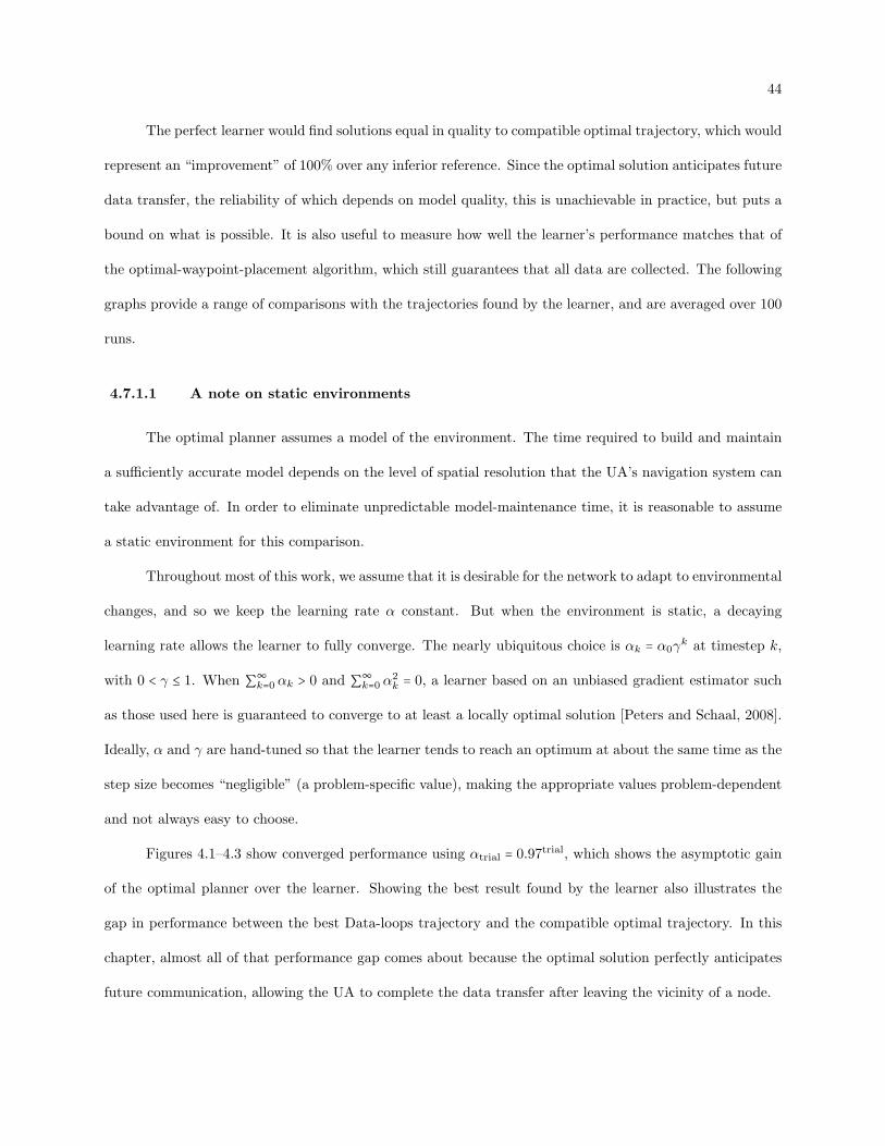
44

The perfect learner would find solutions equal in quality to compatible optimal trajectory, which would

represent an “improvement” of 100% over any inferior reference. Since the optimal solution anticipates future

data transfer, the reliability of which depends on model quality, this is unachievable in practice, but puts a

bound on what is possible. It is also useful to measure how well the learner’s performance matches that of

the optimal-waypoint-placement algorithm, which still guarantees that all data are collected. The following

graphs provide a range of comparisons with the trajectories found by the learner, and are averaged over 100

runs.

4.7.1.1 A note on static environments

The optimal planner assumes a model of the environment. The time required to build and maintain

a sufficiently accurate model depends on the level of spatial resolution that the UA’s navigation system can

take advantage of. In order to eliminate unpredictable model-maintenance time, it is reasonable to assume

a static environment for this comparison.

Throughout most of this work, we assume that it is desirable for the network to adapt to environmental

changes, and so we keep the learning rate α constant. But when the environment is static, a decaying

learning rate allows the learner to fully converge. The nearly ubiquitous choice is αk = α0γk at timestep k,

with 0 < γ ≤ 1. When ∑∞k=0 αk > 0 and ∑∞k=0 α2k = 0, a learner based on an unbiased gradient estimator such

as those used here is guaranteed to converge to at least a locally optimal solution [Peters and Schaal, 2008].

Ideally, α and γ are hand-tuned so that the learner tends to reach an optimum at about the same time as the

step size becomes “negligible” (a problem-specific value), making the appropriate values problem-dependent

and not always easy to choose.

Figures 4.1–4.3 show converged performance using αtrial = 0.97trial, which shows the asymptotic gain

of the optimal planner over the learner. Showing the best result found by the learner also illustrates the

gap in performance between the best Data-loops trajectory and the compatible optimal trajectory. In this

chapter, almost all of that performance gap comes about because the optimal solution perfectly anticipates

future communication, allowing the UA to complete the data transfer after leaving the vicinity of a node.

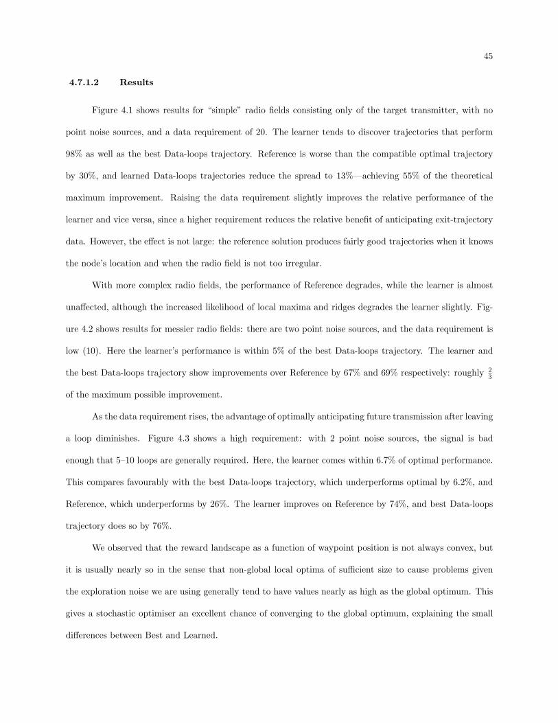
45

4.7.1.2 Results

Figure 4.1 shows results for “simple” radio fields consisting only of the target transmitter, with no

point noise sources, and a data requirement of 20. The learner tends to discover trajectories that perform

98% as well as the best Data-loops trajectory. Reference is worse than the compatible optimal trajectory

by 30%, and learned Data-loops trajectories reduce the spread to 13%—achieving 55% of the theoretical

maximum improvement. Raising the data requirement slightly improves the relative performance of the

learner and vice versa, since a higher requirement reduces the relative benefit of anticipating exit-trajectory

data. However, the effect is not large: the reference solution produces fairly good trajectories when it knows

the node’s location and when the radio field is not too irregular.

With more complex radio fields, the performance of Reference degrades, while the learner is almost

unaffected, although the increased likelihood of local maxima and ridges degrades the learner slightly. Fig-

ure 4.2 shows results for messier radio fields: there are two point noise sources, and the data requirement is

low (10). Here the learner’s performance is within 5% of the best Data-loops trajectory. The learner and

the best Data-loops trajectory show improvements over Reference by 67% and 69% respectively: roughly 23

of the maximum possible improvement.

As the data requirement rises, the advantage of optimally anticipating future transmission after leaving

a loop diminishes. Figure 4.3 shows a high requirement: with 2 point noise sources, the signal is bad

enough that 5–10 loops are generally required. Here, the learner comes within 6.7% of optimal performance.

This compares favourably with the best Data-loops trajectory, which underperforms optimal by 6.2%, and

Reference, which underperforms by 26%. The learner improves on Reference by 74%, and best Data-loops

trajectory does so by 76%.

We observed that the reward landscape as a function of waypoint position is not always convex, but

it is usually nearly so in the sense that non-global local optima of sufficient size to cause problems given

the exploration noise we are using generally tend to have values nearly as high as the global optimum. This

gives a stochastic optimiser an excellent chance of converging to the global optimum, explaining the small

differences between Best and Learned.

46

Ref Best Learned0

0.1

0.2

0.3

0.4

Mean log2(cost/optimal)

log

2(c

ost

/op

t)

Sample learned traj

Anticipating

−200

−150

−100

−50

Data−loops

−200

−150

−100

−50

Figure 4.1: Performance of learner relative to Reference and Optimal. Upper left: Performance of thewaypoint position learner for a data requirement of 20 on a field with no noise sources, relative to compatibleoptimal trajectories. Standard deviations for the log relative costs cost

optare 0.15 for Reference, 0.086 for Best,

and 0.097 for Learned. Lower left: A representation of the radio field from an example run, and the learnedtrajectory. The true node location is given by ; the waypoint is placed at ˙. Upper right: Example resultof the waypoint-placement grid search for the anticipatory planner on the example run; colourmaps showreward, and the summit (˙) represents waypoint for the compatible optimal trajectory. Lower right: Asupper right, but showing how waypoint placement affects reward for the Data-loops planner. The summitrepresents the waypoint of the best Data-loops trajectory.

47

Sample learned traj

Ref Best Learned0

0.2

0.4

0.6

0.8

Mean log2(cost/optimal)

log

2(c

ost

/op

t)

Anticipating

−70

−60

−50

−40

−30

Data−loops

−80

−70

−60

−50

−40

−30

Figure 4.2: As Figure 4.1, but with two noise sources and a data requirement of 10. Upper left: standarddeviations for the log relative costs are 0.21 for Reference, 0.15 for Best, and 0.16 for Learned. Lower leftshows that the approach and exit are from the bottom in this example. Upper right: the large high-rewardregion on the far side of the node is due to the fact that a waypoint placed in that region will be markedas “passed” as soon as sufficient data have been collected; since the optimal trajectory anticipates futurecollection, the waypoint is never reached so only its direction from the UA matters.

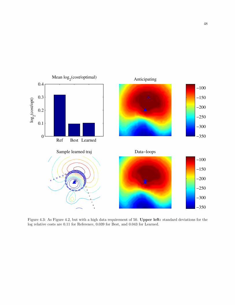
48

Sample learned traj

Ref Best Learned0

0.1

0.2

0.3

0.4

Mean log2(cost/optimal)

log

2(c

ost

/op

t)

Anticipating

−350

−300

−250

−200

−150

−100

Data−loops

−350

−300

−250

−200

−150

−100

Figure 4.3: As Figure 4.2, but with a high data requirement of 50. Upper left: standard deviations for thelog relative costs are 0.11 for Reference, 0.039 for Best, and 0.043 for Learned.

49

We are now in a position to make a preliminary evaluation of the waypoint-placement learner according

to the criteria defined in §1.3. Figure 4.4 (left) duplicates Figure 1.2 for a sample problem, although it does

not offset the cumulative performance of the optimal planner by an arbitrary amount representing system

identification time (“A” in Figure 1.2). The ratio of the asymptotic slopes of Learned and Ref is, on average,

the inverse of costopt

in Figure 4.3, but note that the slopes are computed using actual trial-by-trial performance

(including exploration) rather than the best performance described in §4.7.1.1. Figure 4.4 (right) measures

the average time taken for the optimal planner to surpass Learned and Reference, averaged over 10 problems,

suggesting that learning waypoint placements in the field with no system identification time is quite feasible.

4.7.2 Accurate network layout information

Even when the UA is given perfect knowledge of node positions, the learning planner can outperform

Reference by directing the UA to circle some point other than the sensor’s true location. How much gain is

possible? How quickly is it achieved?

Figure 4.5 shows learning on single-node problems with the data requirement req = 60. This may

be considered a high requirement because the aircraft must make several orbits in the vicinity of the node,

so the data-transfer performance is dominated by the loops rather than by the inter-waypoint segments of

straight flight (additionally, the starting and end positions are placed close to the node, yielding even less

benefit in moving the waypoint farther from the node). When the node is the only radio source in the field,

the gain is consistent but minuscule: the distance travelled averages just under 2−0.02 ≃ 0.99 of that required

by Reference, with the best waypoint location averaging about 1.6 from the sensor’s true location. When

the radio field’s complexity increases slightly due to the addition of two noise sources, the average gain is

greater due to the learner’s ability to find a trajectory that minimises interference with the target node, but

still minimal: 2−0.09 ≃ 0.94 of that required by Reference, with an average displacement of waypoint from

true node location of 2.4 (additional noise sources beyond 2 yield results very similar to the 2-noise-source

case). The chosen parameters (listed at the top of this section) result in consistent gains in a dozen trials

and final convergence in about 40 trials.

The multi-node case shows greater gains for the Data-loops planner. Figure 4.6 shows the average

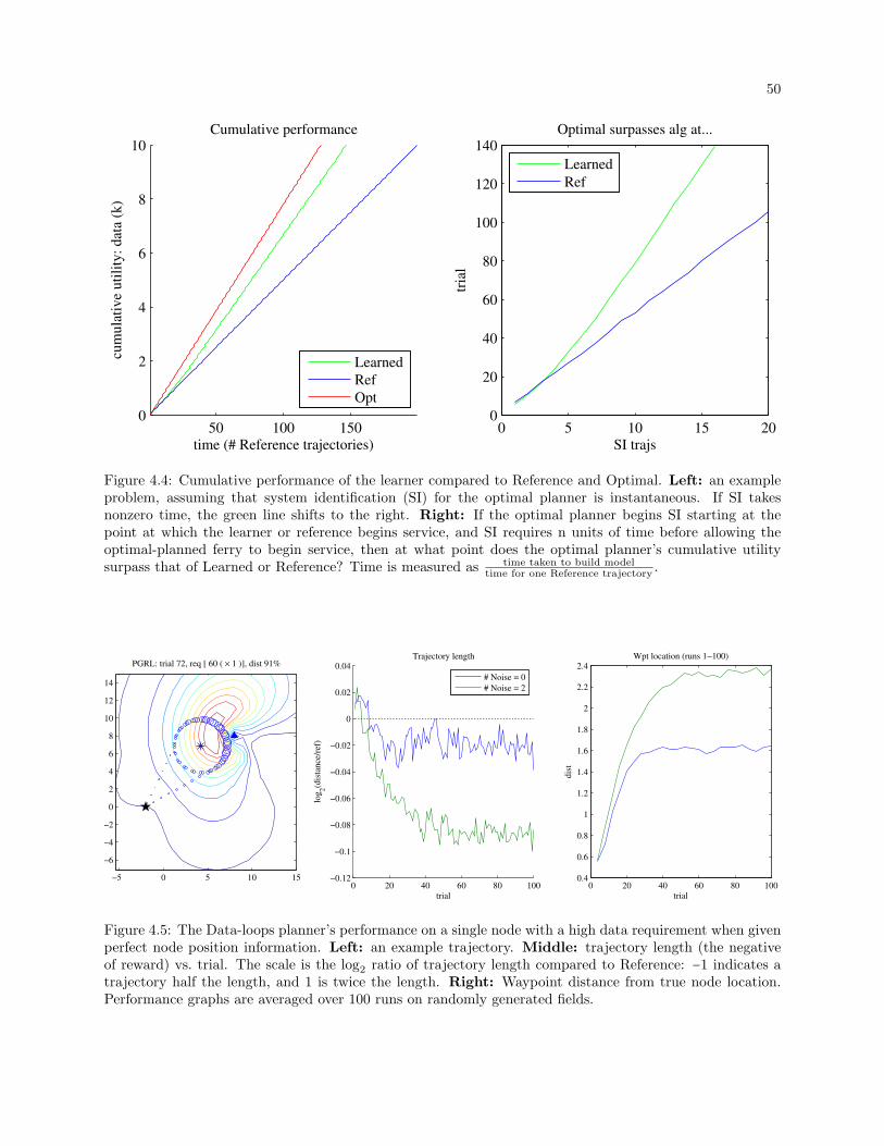
50

50 100 1500

2

4

6

8

10

time (# Reference trajectories)

cum

ula

tiv

e u

tili

ty:

dat

a (k

)Cumulative performance

0 5 10 15 200

20

40

60

80

100

120

140Optimal surpasses alg at...

SI trajstr

ial

Learned

Ref

Opt

Learned

Ref

Figure 4.4: Cumulative performance of the learner compared to Reference and Optimal. Left: an exampleproblem, assuming that system identification (SI) for the optimal planner is instantaneous. If SI takesnonzero time, the green line shifts to the right. Right: If the optimal planner begins SI starting at thepoint at which the learner or reference begins service, and SI requires n units of time before allowing theoptimal-planned ferry to begin service, then at what point does the optimal planner’s cumulative utilitysurpass that of Learned or Reference? Time is measured as time taken to build model

time for one Reference trajectory.

PGRL: trial 72, req [ 60 ( × 1 )], dist 91%

−5 0 5 10 15

−6

−4

−2

0

2

4

6

8

10

12

14

0 20 40 60 80 1000.4

0.6

0.8

1

1.2

1.4

1.6

1.8

2

2.2

2.4Wpt location (runs 1−100)

trial

dis

t

0 20 40 60 80 100−0.12

−0.1

−0.08

−0.06

−0.04

−0.02

0

0.02

0.04

trial

log

2(d

ista

nce

/ref

)

Trajectory length

# Noise = 0

# Noise = 2

Figure 4.5: The Data-loops planner’s performance on a single node with a high data requirement when givenperfect node position information. Left: an example trajectory. Middle: trajectory length (the negativeof reward) vs. trial. The scale is the log2 ratio of trajectory length compared to Reference: −1 indicates atrajectory half the length, and 1 is twice the length. Right: Waypoint distance from true node location.Performance graphs are averaged over 100 runs on randomly generated fields.

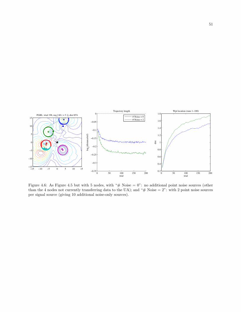
51

0 50 100 150 200−0.35

−0.3

−0.25

−0.2

−0.15

−0.1

−0.05

0

trial

log

2(d

ista

nce

/ref

)

Trajectory length

0 50 100 150 2000.2

0.4

0.6

0.8

1

1.2

1.4

1.6

1.8Wpt location (runs 1−100)

trial

dis

t

PGRL: trial 198, req [ 60 ( × 5 )], dist 85%

−15 −10 −5 0 5 10 15−15

−10

−5

0

5

10

15# Noise = 0

# Noise = 2

Figure 4.6: As Figure 4.5 but with 5 nodes, with “# Noise = 0”: no additional point noise sources (otherthan the 4 nodes not currently transferring data to the UA); and “# Noise = 2”: with 2 point noise sourcesper signal source (giving 10 additional noise-only sources).

52

learning speed, solution quality, and node–waypoint distance for randomly generated 5-node problems with

a high data requirement (req=60). Here, the trajectory length compared to Reference ranges between

2−0.17 ≃ 0.89 for the less-noisy case and 2−0.24 ≃ 0.85 when more point noise sources are added. Beyond

aiming the UA so as to minimise interference, further gains are achieved because the UA starts further from

each node, so moving the waypoint away from the node may shorten the trajectory.

In contrast, Figure 4.7 shows a requirement low enough that no looping is required, and the data

transfer sometimes completes before the UA reaches the waypoint. This situation increases the benefit of

moving the waypoint towards the origin or destination—waypoint placement can stray quite far from the

node’s true position, and gains over Reference reach 1 − 2−0.32 ≃ 1 − 0.8 ≃ 20% or more.

Why does moving the waypoint away from the node’s true location improve performance?

Radio field irregularity: The circular orbit with the highest average data rate is often not centered on

the node’s actual location, due to the planner’s ability to both maximise signal strength from the

target node and minimise signal strength from noise sources. At high (i.e. loop-dominated) data

requirements the best trajectories were those in which the waypoint positions differed from true

node positions by roughly 1.7 in the case of no point noise sources, growing to 2.5 with more noise

sources. These numbers depend on the particulars of the radio fields; for example, greater radio field

irregularity—presumably including that caused by higher-gain antenna patterns—will yield larger

node-waypoint offsets.

Wasted partial orbits: The circular orbit with the highest average data rate is suboptimal when the

data transfer completes before the loop completes. This effect is most pronounced at lower data

requirements, in which achieving the highest possible data rate throughout the loop is less important

than shortening the trajectory. For very low data requirements such as shown in Figure 4.7 the

waypoint may be moved quite far from the node’s location, resulting in a lower transmission rate

that is still sufficient for complete data transfer.

Opportunistic communication: During execution of a Reference trajectory, the aircraft communicates

with the node towards which it is flying. In contrast, the Data-loops planner allows communication

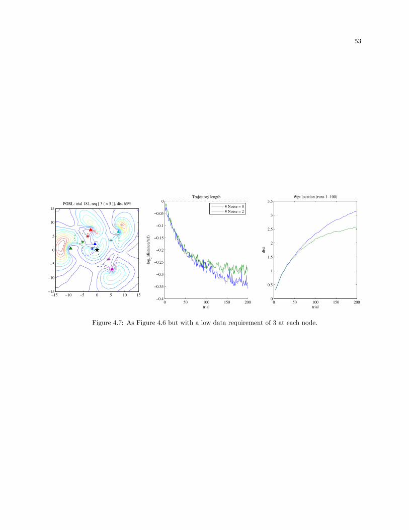
53

PGRL: trial 181, req [ 3 ( × 5 )], dist 65%

−15 −10 −5 0 5 10 15−15

−10

−5

0

5

10

15

0 50 100 150 2000

0.5

1

1.5

2

2.5

3

3.5Wpt location (runs 1−100)

trial

dis

t

0 50 100 150 200−0.4

−0.35

−0.3

−0.25

−0.2

−0.15

−0.1

−0.05

0

trial

log

2(d

ista

nce

/ref

)

Trajectory length

# Noise = 0

# Noise = 2

Figure 4.7: As Figure 4.6 but with a low data requirement of 3 at each node.

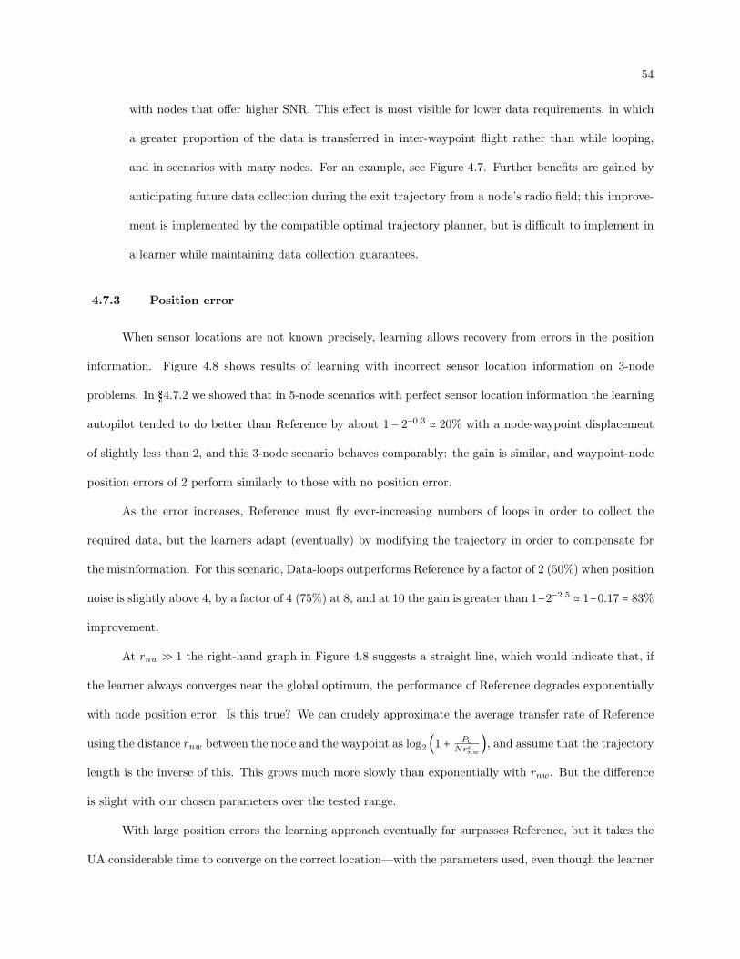
54

with nodes that offer higher SNR. This effect is most visible for lower data requirements, in which

a greater proportion of the data is transferred in inter-waypoint flight rather than while looping,

and in scenarios with many nodes. For an example, see Figure 4.7. Further benefits are gained by

anticipating future data collection during the exit trajectory from a node’s radio field; this improve-

ment is implemented by the compatible optimal trajectory planner, but is difficult to implement in

a learner while maintaining data collection guarantees.

4.7.3 Position error

When sensor locations are not known precisely, learning allows recovery from errors in the position

information. Figure 4.8 shows results of learning with incorrect sensor location information on 3-node

problems. In §4.7.2 we showed that in 5-node scenarios with perfect sensor location information the learning

autopilot tended to do better than Reference by about 1 − 2−0.3 ≃ 20% with a node-waypoint displacement

of slightly less than 2, and this 3-node scenario behaves comparably: the gain is similar, and waypoint-node

position errors of 2 perform similarly to those with no position error.

As the error increases, Reference must fly ever-increasing numbers of loops in order to collect the

required data, but the learners adapt (eventually) by modifying the trajectory in order to compensate for

the misinformation. For this scenario, Data-loops outperforms Reference by a factor of 2 (50%) when position

noise is slightly above 4, by a factor of 4 (75%) at 8, and at 10 the gain is greater than 1−2−2.5 ≃ 1−0.17 = 83%

improvement.

At rnw ≫ 1 the right-hand graph in Figure 4.8 suggests a straight line, which would indicate that, if

the learner always converges near the global optimum, the performance of Reference degrades exponentially

with node position error. Is this true? We can crudely approximate the average transfer rate of Reference

using the distance rnw between the node and the waypoint as log2 (1 + P0

Nrϵnw), and assume that the trajectory

length is the inverse of this. This grows much more slowly than exponentially with rnw. But the difference

is slight with our chosen parameters over the tested range.

With large position errors the learning approach eventually far surpasses Reference, but it takes the

UA considerable time to converge on the correct location—with the parameters used, even though the learner

55

PGRL: trial 194, req [ 20 ( × 3 )], dist 53%

−15 −10 −5 0 5 10 15−15

−10

−5

0

5

10

15

0 50 100 150 200−2.5

−2

−1.5

−1

−0.5

0

trial

log

2(d

ista

nce

/ref

)

Trajectory length

0 2 4 6 8 10−3.5

−3

−2.5

−2

−1.5

−1

−0.5

0

Position Error

bes

t d

ista

nce

, lo

g2([

alg

] /

[ R

efer

ence

])

Best distance (100 runs)

error = 0

error = 2

error = 4

error = 6

error = 8

error = 10

Figure 4.8: Trajectory quality through time as the error in node position information increases. Here weused 3 nodes, each with a requirement of 20. Each randomly generated field is 20 × 20, nodes are placeduniformly randomly, and the orientations of their dipole antennas are randomly distributed. Position erroris the radius of a circle on which nodes are placed uniformly randomly from the true node position.

56

in the error=10 case far surpasses Reference within a dozen trials, it has not yet converged. While perfectly

accurate sensor location information is not necessary and is not even beneficial, the learner performs better

when somewhat accurate information is available.

4.7.4 Antenna patterns

The learner finds trajectories that place the aircraft in a position and orientation that allow high SNR

with each of the target nodes. High-gain antennas, when oriented appropriately, allow transmission at a

higher rate or at longer range. Perhaps more importantly, if an antenna’s null can be aimed appropriately,

then it can reduce interference from other antennas or from multipath interference. A steerable antenna would

provide great benefit at the cost of hardware and controller complexity (even the smallest commercially-

available units can easily exceed the payload of a lightweight UA).

How do antenna patterns affect the quality of the trajectories found? We have assumed that both the

aircraft and the nodes use short dipole antennas as represented by Eq. 3.3 (directivity = 1.5, gain = 1.76

dBi). Here we compare the dipoles to equally efficient isotropic antennas operating at the same power, in

both aircraft and nodes. We place some number of nodes randomly on a 20 × 20 field, and each node has a

data requirement of 20.

Results are shown in Figure 4.9. The dipole is not an especially high-gain antenna, yet equipping the

aircraft with a dipole offers a large improvement over an isotropic antenna, especially in a noisier environment.

We observed this effect both for learned and for reference trajectories, and whether the nodes use dipoles or

isotropic antennas. However, equipping the nodes with dipoles had the opposite effect: whatever the UA’s

equipment and whether flying reference or learned trajectories, it was able to discover shorter trajectories

when the nodes had isotropic antennas. The best combination was a dipole on the aircraft combined with

isotropics on the nodes, especially as the sensor density increased. It should be noted, however, that while

we observed this trend over a range of conditions, we did not test across every possible configuration.

For example, it is possible that a more manoeuvrable UA could better take advantage of directional node

antennas.

More important than the preceding observation is the confirmation that the learner adapts to the

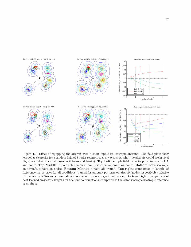
57

Iso / Iso: trial 152, req [ 20 ( × 8 )], dist 91% Di / Iso: trial 189, req [ 20 ( × 8 )], dist 83%

Iso / Di: trial 20, req [ 20 ( × 8 )], dist 108% Di / Di: trial 187, req [ 20 ( × 8 )], dist 83%

0 2 4 6 8−0.2

−0.15

−0.1

−0.05

0

0.05

0.1

0.15

0.2

Number of nodes

bes

t d

ista

nce

, lo

g2([

alg

] /

[ R

ef:

Iso

/ I

so ]

)

Reference: best distances (100 runs)

0 2 4 6 8−0.5

−0.4

−0.3

−0.2

−0.1

0

0.1

Number of nodes

bes

t d

ista

nce

, lo

g2([

alg

] /

[ R

ef:

Iso

/ I

so ]

)

Data−loops: best distances (100 runs)

Ref: Di / Iso

Ref: Iso / Di

Ref: Di / Di

Iso / Iso

Di / Iso

Iso / Di

Di / Di

Figure 4.9: Effect of equipping the aircraft with a short dipole vs. isotropic antenna. The field plots showlearned trajectories for a random field of 8 nodes (contours, as always, show what the aircraft would see in levelflight, not what it actually sees as it turns and banks). Top Left: sample field for isotropic antennas on UAand nodes. Top Middle: dipole antenna on aircraft, isotropic antennas on nodes. Bottom Left: isotropicon aircraft, dipoles on nodes. Bottom Middle: dipoles all around. Top right: comparison of lengths ofReference trajectories for all conditions (named for antenna patterns on aircraft/nodes respectively) relativeto the isotropic/isotropic case (shown as the zero), on a logarithmic scale. Bottom right: comparison ofbest learned trajectory lengths for the four combinations, compared to the same isotropic/isotropic referenceused above.

58

antenna characteristics it experiences, lending further credence to model-free approaches. As a counterex-

ample, Dixon [2010] measures SINR in order to compute a gradient on UA position, and observes that

using a dipole (or other non-isotropic) antenna pattern can destabilise the gradient estimate. In contrast, by

shunning intermediate models, the current approach does not suffer from that difficulty. Quite the reverse:

it would take full advantage of any real-world antenna pattern such as would be expected in the presence

of fuselage, landing gear, and other mechanical elements of the aircraft, or systematic noise sources on the

aircraft (e.g. due to the onboard computer). If those effects are large, the difficulty of acquiring models of

the system sufficiently accurate for near-optimal planning may increase substantially.

We leave for future work investigation of more directional antennas, laterally asymmetric patterns,

steerable antennas, patterns based on real-world measurements, and aircraft movement models designed to

take advantage of directional node antennas.

4.8 Summary

The Data-loops learner optimises a trajectory representation that is compatible with off-the-shelf

autopilots. It quickly learns trajectories that are shorter than those of the reference solution, with improve-

ments ranging from 1% up to 20% in the configuration space tested here, with greater improvement as the

radio field’s complexity increases. Learning proceeds quickly, with near-convergence in a few dozen trials,

but note that careful hand-tuning is likely to result in further learning speed gains.

The compatible optimal planner assumes a perfect model not just of node positions but of the whole

system. Over the scenarios evaluated here, the Data-loops learner was usually able to achieve 55–75% of the

maximum possible improvement. As before, more complex radio fields disproportionately hurt the reference

solution, leading to a stronger preference for the learned solution.

With inaccurate radio field models, optimally planned solutions deteriorate in quality, but the reference

solution makes the more reasonable assumption of perfect knowledge of node positions. But even this

can be difficult to achieve. In contrast, as node position information becomes inaccurate, the Data-loops

learner adapts, achieving performance close to that of an optimal planner with perfect information, while

the reference solution’s performance degrades arbitrarily.

59

Interestingly, under the studied conditions, the network benefits when the UA has a directional antenna

and the nodes do not. However, we will continue to assume that the nodes use dipole antennas throughout:

the objective is to compare a learning approach to handcoded heuristics in complex environments, and the

dipole radio pattern of our nodes serves as a proxy for the complex structure of real radio fields.

Chapter 5

Waypoints Trajectories

The Data-loops trajectory representation can reliably collect all data from nodes despite incomplete

or incorrect information, but produces trajectories inferior to those of the compatible optimal planner mainly

due to its inability to anticipate future data collection. If the nodes’ data loads are small and do not vary in

time, can a constraint-optimising trajectory encoding yield better results?

This chapter and Chapter 6 form a digression from the main thrust of the dissertation: they propose

a new trajectory representation, and show that it is slightly superior to Data-loops over a narrow range of

conditions.

5.1 The Waypoints trajectory representation

The learning Waypoints autopilot flies directly towards each waypoint in the sequence supplied by

the planner, adjusting its heading for the next waypoint at its maximal turning rate ω as soon as it has

passed the current one. We define “passing” a waypoint as being within the UA’s turning circle of it: ϵ = vω

(see Fig. 3.1 (middle)). We initialise trajectories of “n waypoints per node” with a waypoint at the nominal

location of each node (not including the start and end points) and n− 1 waypoints evenly spaced along each

tour segment. Because there is no intrinsic association between waypoints and nodes, the UA always collects

data opportunistically: at each timestep, of the nodes that still have data to be uploaded, communication is

to the node with the highest observed SNR. We have assumed that the protocol overhead of monitoring the

SNR and associating to each node is relatively small.

The consequence to performance of this trajectory encoding is that since the autopilot does not

61

wait to ensure complete data transmission from each node, the UA may fly away from a node while still

communicating with it. Thus, in exchange for running the risk of gathering insufficient data from a node,

the UA may learn trajectories that anticipate future data transfer, enabling more efficient transfer and hence

shorter trajectories.

5.2 The learner

We will apply the same learning algorithm to the Waypoints representation that we used for Data-

loops. The scalability problem alluded to in §4.5 similarly affects the Waypoints representation, and is

complicated by the fact that in order to encode more general trajectories there is no strict association

between waypoints and nodes. In Chapter 6 we will develop a local credit assignment (LCA) decomposition

that improves the optimiser’s scalability during the local-flavoured phases of the optimisation.

5.3 Reward

When a system model is not available, constraints cannot be guaranteed by the optimiser. For the

Waypoints planner we seek to fulfil them by trial and error through the gradient estimation process. So

instead of solving the constrained optimisation of Equation 4.1, or pushing the problem to a lower-level

controller as we did in Chapter 4, here we maximise the expected return (Equation 4.2) for a reward

function chosen to favour solutions that also solve Equation 4.1. Rewards (or their negatives, costs) are

assigned so that solutions that better satisfy the design objectives have higher reward (lower cost). The

constraints in Equation 4.1 differ from the corresponding summands of the reward in that the former merely

state requirements while the latter create a function at whose maximum the constraints are satisfied.

For our waypoint-placement problem we seek the shortest tour subject to the constraint of allowing

exchange of Dj bytes of data with each sensor bj , so we define a reward function that aggressively punishes

data underrun while placing a more modest cost on trajectory length:

r = −⎛⎝d + η

n

∑j=1

⎛⎝max

⎧⎪⎪⎨⎪⎪⎩(Dj + µmj

)2

− 1,0⎫⎪⎪⎬⎪⎪⎭

⎞⎠⎞⎠

(5.1)

where d is the trajectory path length, η is a weighting term chosen so that violation of a hard constraint

62

(data underrun) dominates the costs, mj is the data quantity collected from sensor node j, Dj is the data

requirement on sensor j, and µ is an optional small safety margin that helps to ensure that all data are

collected even in the presence of policy noise. When the constraint is satisfied—or for the guaranteed

collection of the Data-loops planner—the second term disappears and only trajectory length affects reward.

5.4 Experiments

We define acceptable trajectories to be those that collect the required D bytes of data, regardless of

trajectory length. The reference and Data-loops autopilots always produce acceptable trajectories, while the

Waypoints planner may take some number of trials before discovering one. While the former two planners

were judged based on the criteria of trajectory length and learning speed, Waypoints requires two more

criteria: the fraction of the trajectories that are acceptable when testing on randomly-generated problems;

and the number of trials required before the first acceptable trajectory is discovered.

Note that the reward function is a tool that allows the learner to find constraint-satisfying solutions,

and as such it is the indicator of the success of the learning algorithm. However, it often does not paint the

most informative picture of the achievement of optimisation goals. For this reason, this chapter uses the

evaluation criteria described above.

5.4.0.1 Parameters

We use the parameter values described in §4.7.0.1. In addition, we use safety factor µ = 1 and a

hard-constraint factor η = 10000 in Eq. 5.1.

5.4.1 Waypoints vs. Data-loops

Chapter 4 explored the performance that the Data-loops learner could achieve. How does the Way-

points learner compare?

Figure 5.1 shows how solution quality varies for different data requirements. In this test case (details

given in the caption) Waypoints reliably learns to outperform Reference when the data requirement is below

about 10, but as the requirement overwhelms the available transmission time the learning time grows and

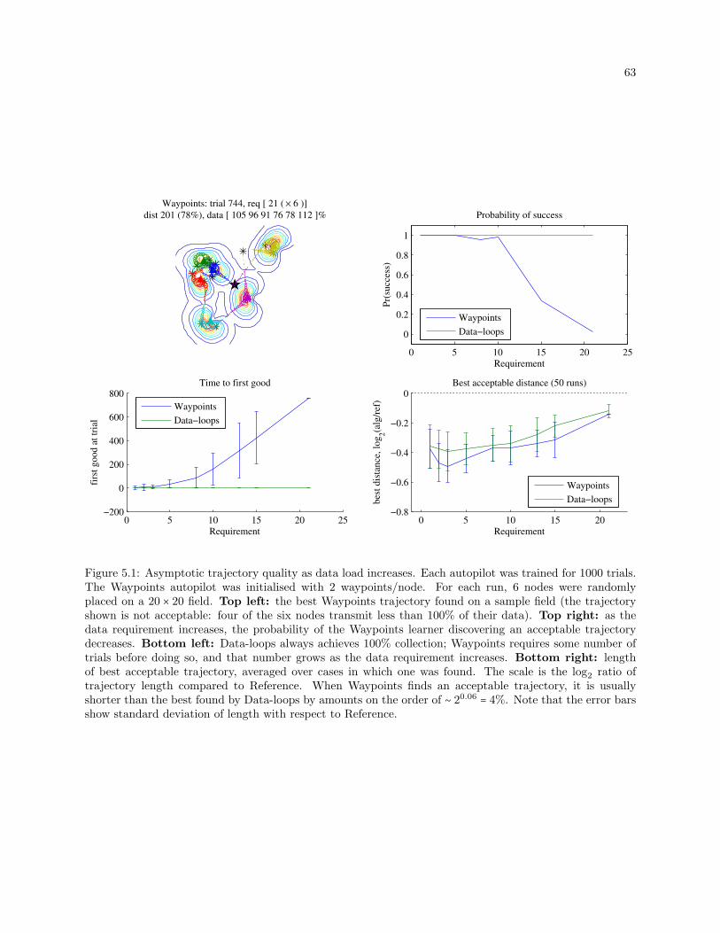
63

0 5 10 15 20−0.8

−0.6

−0.4

−0.2

0

Requirement

bes

t d

ista

nce

, lo

g2(a

lg/r

ef)

Best acceptable distance (50 runs)

0 5 10 15 20 25

0

0.2

0.4

0.6

0.8

1

Requirement

Pr(

succ

ess)

Probability of success

Waypoints: trial 744, req [ 21 ( × 6 )]

dist 201 (78%), data [ 105 96 91 76 78 112 ]%

0 5 10 15 20 25−200

0

200

400

600

800

Requirement

firs

t goo

d a

t tr

ial

Time to first good

Waypoints

Data−loops

Waypoints

Data−loops

Waypoints

Data−loops

Figure 5.1: Asymptotic trajectory quality as data load increases. Each autopilot was trained for 1000 trials.The Waypoints autopilot was initialised with 2 waypoints/node. For each run, 6 nodes were randomlyplaced on a 20 × 20 field. Top left: the best Waypoints trajectory found on a sample field (the trajectoryshown is not acceptable: four of the six nodes transmit less than 100% of their data). Top right: as thedata requirement increases, the probability of the Waypoints learner discovering an acceptable trajectorydecreases. Bottom left: Data-loops always achieves 100% collection; Waypoints requires some number oftrials before doing so, and that number grows as the data requirement increases. Bottom right: lengthof best acceptable trajectory, averaged over cases in which one was found. The scale is the log2 ratio oftrajectory length compared to Reference. When Waypoints finds an acceptable trajectory, it is usuallyshorter than the best found by Data-loops by amounts on the order of ∼ 20.06 = 4%. Note that the error barsshow standard deviation of length with respect to Reference.

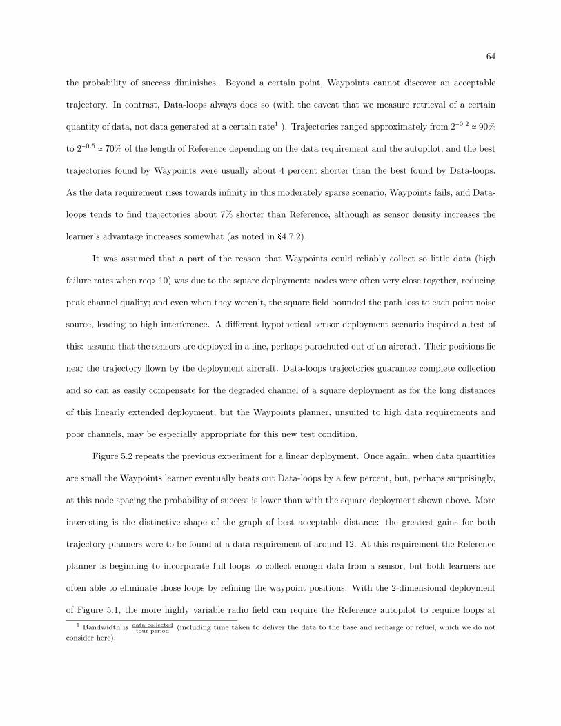
64

the probability of success diminishes. Beyond a certain point, Waypoints cannot discover an acceptable

trajectory. In contrast, Data-loops always does so (with the caveat that we measure retrieval of a certain

quantity of data, not data generated at a certain rate1 ). Trajectories ranged approximately from 2−0.2 ≃ 90%

to 2−0.5 ≃ 70% of the length of Reference depending on the data requirement and the autopilot, and the best

trajectories found by Waypoints were usually about 4 percent shorter than the best found by Data-loops.

As the data requirement rises towards infinity in this moderately sparse scenario, Waypoints fails, and Data-

loops tends to find trajectories about 7% shorter than Reference, although as sensor density increases the

learner’s advantage increases somewhat (as noted in §4.7.2).

It was assumed that a part of the reason that Waypoints could reliably collect so little data (high

failure rates when req> 10) was due to the square deployment: nodes were often very close together, reducing

peak channel quality; and even when they weren’t, the square field bounded the path loss to each point noise

source, leading to high interference. A different hypothetical sensor deployment scenario inspired a test of

this: assume that the sensors are deployed in a line, perhaps parachuted out of an aircraft. Their positions lie

near the trajectory flown by the deployment aircraft. Data-loops trajectories guarantee complete collection

and so can as easily compensate for the degraded channel of a square deployment as for the long distances

of this linearly extended deployment, but the Waypoints planner, unsuited to high data requirements and

poor channels, may be especially appropriate for this new test condition.

Figure 5.2 repeats the previous experiment for a linear deployment. Once again, when data quantities

are small the Waypoints learner eventually beats out Data-loops by a few percent, but, perhaps surprisingly,

at this node spacing the probability of success is lower than with the square deployment shown above. More

interesting is the distinctive shape of the graph of best acceptable distance: the greatest gains for both

trajectory planners were to be found at a data requirement of around 12. At this requirement the Reference

planner is beginning to incorporate full loops to collect enough data from a sensor, but both learners are

often able to eliminate those loops by refining the waypoint positions. With the 2-dimensional deployment

of Figure 5.1, the more highly variable radio field can require the Reference autopilot to require loops at

1 Bandwidth is data collectedtour period

(including time taken to deliver the data to the base and recharge or refuel, which we do not

consider here).

65

0 5 10 15 20−0.8

−0.6

−0.4

−0.2

0

0.2

Requirement

bes

t d

ista

nce

, lo

g2(a

lg/r

ef)

Best acceptable distance (50 runs)

0 5 10 15 20 25

0

0.2

0.4

0.6

0.8

1

Requirement

Pr(

succ

ess)

Probability of success

Waypoints: trial 128, req [ 10 ( × 6 )]

dist 78 (61%), data [ 105 106 112 110 113 103 ]%

0 5 10 15 20 25−200

0

200

400

600

800

1000

Requirement

firs

t g

oo

d a

t tr

ial

Time to first good

Waypoints

Data−loops

Waypoints

Data−loops

Waypoints

Data−loops

Figure 5.2: Data-loops vs. Waypoints as the data load increases, on a linear 6-node trajectory with nodesplaced every 10. Otherwise as described in Figure 5.1.

66

any point, eliminating the distinctive shape. Here, as the data requirement goes to infinity, the gain of

Data-loops over Reference approaches ∼ 4%. However, as we saw in Ch. 4, this number depends on radio

source density.

5.4.2 Position error

§5.4.1 showed that Waypoints can sometimes discover better trajectories than Data-loops. When there

is an error in node position information, given sufficient training time, this advantage is generally maintained.

The learners both optimise waypoint positions, so the initial error eventually becomes irrelevant, leaving the

difference in trajectories that is due to the different encodings.

Figure 5.3 shows the learners’ performance relative to Reference for a scenario in which Waypoints is

especially appropriate: a data requirement of 3, which is low enough to allow the UA to complete the data

transfer without having to learn how to circle the node, generally allowing the discovery of an acceptable

trajectory within a dozen trials or fewer.

Three unexpected features are visible in Figure 5.3.

(1) The advantage of the learners over Reference does not increase as steeply with position error as would

be expected from §4.7.3. Because the scale of the radio field’s irregularities tends to increase with

distance from the source, at this low requirement, it is quite probable that Reference will complete

the data transfer long before approaching a node, so the refinement of waypoint positions makes less

difference than at higher requirements.

(2) The advantage of Waypoints over Data-loops decreases as the position error increases. This is because

Waypoints has not yet converged—if more trials are allowed, Waypoints restores its advantage. This

emphasises the primary drawback of Waypoints: its learning time can be long, and large errors in

node location information exacerbate this problem.

While the best trajectories are discovered using the Waypoints representation, the average trajectory

length during early learning tends to be shorter for Data-loops. This is because of the difference

in “completion” criteria for the two representations: whereas Waypoints directs the UA to fly all

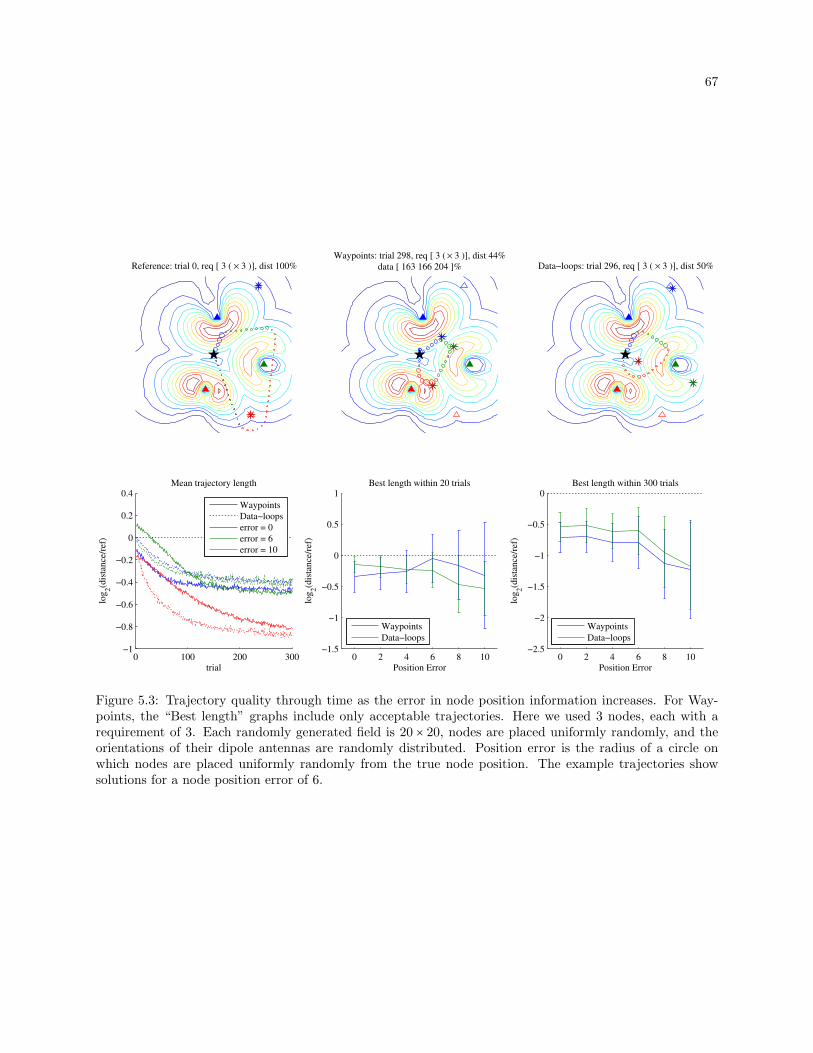
67

Reference: trial 0, req [ 3 ( × 3 )], dist 100%Waypoints: trial 298, req [ 3 ( × 3 )], dist 44%

data [ 163 166 204 ]% Data−loops: trial 296, req [ 3 ( × 3 )], dist 50%

0 100 200 300−1

−0.8

−0.6

−0.4

−0.2

0

0.2

0.4

trial

log

2(d

ista

nce

/ref

)

Mean trajectory length

0 2 4 6 8 10−2.5

−2

−1.5

−1

−0.5

0

Position Error

log

2(d

ista

nce

/ref

)

Best length within 300 trials

0 2 4 6 8 10−1.5

−1

−0.5

0

0.5

1

Position Error

log

2(d

ista

nce

/ref

)

Best length within 20 trials

Waypoints

Data−loops

error = 0

error = 6

error = 10

Waypoints

Data−loops

Waypoints

Data−loops

Figure 5.3: Trajectory quality through time as the error in node position information increases. For Way-points, the “Best length” graphs include only acceptable trajectories. Here we used 3 nodes, each with arequirement of 3. Each randomly generated field is 20 × 20, nodes are placed uniformly randomly, and theorientations of their dipole antennas are randomly distributed. Position error is the radius of a circle onwhich nodes are placed uniformly randomly from the true node position. The example trajectories showsolutions for a node position error of 6.

68

the way to each waypoint in turn, Data-loops uses each waypoint only until the data transfer is

complete, allowing it to mark waypoints as “passed” while still far from them if the data have been

collected.

Figure 5.4 shows a higher requirement of 10, which, as shown in §5.4.1, is about the highest data

requirement for which Waypoints can reliably find an acceptable trajectory given the parameters of the

scenario. Here, the unexpected outcomes of Figure 5.3 are less apparent:

Since the UA must spend more time near a node, where the radio field varies with higher spatial

frequency, the position of the waypoint becomes more important.

The advantage of Data-loops by which it can move on to waypoint n + 1 before reaching waypoint

n does not come into play unless the data transfer can be completed significantly before arriving at

waypoint n. This is not the case for the higher-requirement scenario.

5.5 Summary

The Waypoints trajectory representation has three weaknesses due to the fact that it has no inbuilt

mechanism for lingering in the vicinity of a node in order to fulfil larger data requirements.

While learning proceeds quickly, often producing trajectories that recover all the data in a few

dozen training circuits, the requirement for a long initial training time during which not all data are

collected, or during which trajectories are needlessly long, limits the domains in which the technique

is applicable.

As the data requirement grows, or, equivalently, a node’s SNR becomes too low due to interference

or power constraints, it becomes more and more difficult to learn waypoint placements that generate

the loops required to collect all the data.

If the data requirement or radio background change much from flight to flight, the learned Waypoints

trajectory will no longer be appropriate.

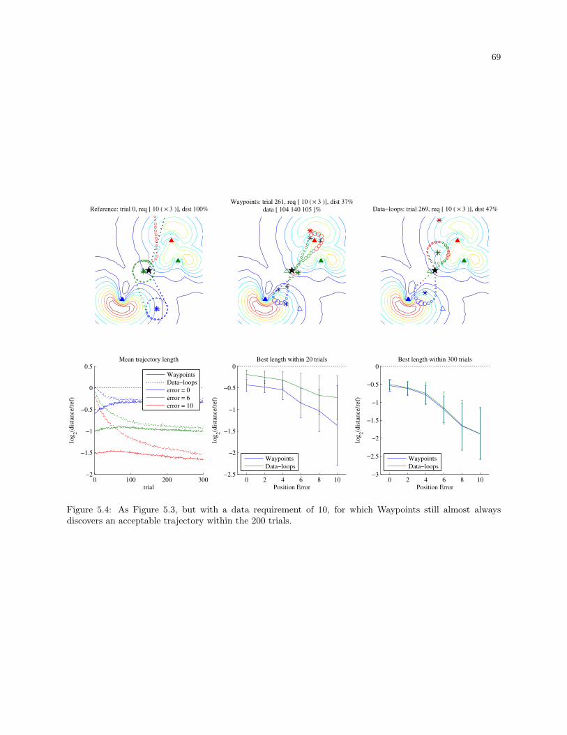
69

Reference: trial 0, req [ 10 ( × 3 )], dist 100%Waypoints: trial 261, req [ 10 ( × 3 )], dist 37%

data [ 104 140 105 ]% Data−loops: trial 269, req [ 10 ( × 3 )], dist 47%

0 100 200 300−2

−1.5

−1

−0.5

0

0.5

trial

log

2(d

ista

nce

/ref

)

Mean trajectory length

0 2 4 6 8 10−3

−2.5

−2

−1.5

−1

−0.5

0

Position Error

log

2(d

ista

nce

/ref

)Best length within 300 trials

0 2 4 6 8 10−2.5

−2

−1.5

−1

−0.5

0

Position Error

log

2(d

ista

nce

/ref

)

Best length within 20 trials

Waypoints

Data−loops

error = 0

error = 6

error = 10

Waypoints

Data−loops

Waypoints

Data−loops

Figure 5.4: As Figure 5.3, but with a data requirement of 10, for which Waypoints still almost alwaysdiscovers an acceptable trajectory within the 200 trials.

70

Against these drawbacks may be set one advantage: when data quantities are small and approximately

constant, the Waypoints planner can discover superior trajectories. For some applications, that may be

compelling, but the rest of this work will assume that in most cases the immediate guarantee of complete

collection combined with the ability to collect larger and variable quantities of data will be reason to prefer

Data-loops. However, examined in this context of static problems, when some initial learning time is feasible

and data quantities are small, a Waypoints-style encoding may be superior.

Chapter 6

Local Credit Assignment

In order to allow a wide variety of trajectory shapes, the Waypoints autopilot does not explicitly

associate waypoints with nodes. When reward is received at the end of an episode, we encounter a version of

RL’s credit assignment problem: noise was added to the policy’s output at several points and that noise

had some effect on the reward, but we have little information as to which variations to the policy output

were responsible for the observed outcome. As the number of parameters increases, this difficulty worsens,

leading to increased noise in the gradient estimate, and therefore to increased learning time.

The reward function (Equation 5.1) is made up of 1 + n summands—a cost for the optimisation

criterion d and a cost designed to create a suitable reward gradient for each of the n constraints. The policy

is made up of some number of parameters that define the locations of waypoints, so each policy parameter

can influence some subset of the n+1 reward summands. The members of the subset are no more predictable

than are the trajectory and radio interactions, but they are observable. Can the effect of exploration noise

on reward be credited to the relevant policy parameters? Can this be used to speed learning as problem size

increases?

Below we develop an approach based on such a reward decomposition. We introduce an estimate of the

relationship between policy parameters and nodes, which allows us to compute a policy gradient for each data

constraint term. This allows the policy updates to be based directly on individual constraint-violation–based

gradient estimates, rather than through the indirect mechanism by which constraint violations dominate a

monolithic reward gradient.

72

6.1 Components of the reward

In §5.3 we constructed a reward function whose purpose was to drive the learner towards desirable

solutions. Here we re-deconstruct the reward function into the components that produced the desired effect,

and attempt to optimise them separately, combining them not at the reward stage, but at the gradient-update

stage.

The reward function is designed to drive the learner towards good solutions that satisfy the constraints.

In our current example, the UA must collect as much waiting data as possible from each of the n nodes

while remaining as short as possible—leading to 1 + n terms in the reward function. Other terms could be

included in the optimisation function: for this explanation, let us consider those two types. We list one more

as an example for this discussion; it will not be considered until Chapter 7.

The trajectory length summand (d in Equation 5.1) represents a single cost. For the Waypoints

planner it is strictly correct to regard it as a global cost: each waypoint directly controls a finite

span of the trajectory length but can potentially influence the best position of any other waypoint.

However, we will see that a local approximation can be useful. When pushing the limits of an

aircraft’s range or a weather window, the trajectory length constraint could be considered hard, but

otherwise it is generally soft.

Each of the n (one per sensor node) data-acquisition summands (the arguments to Σ in Equa-

tion 5.1) is, to a first approximation, local: each waypoint’s movement affects the data requirement of

only one or two data summands and the trajectory length summand. We will consider data retrieval

to be a hard constraint: the trajectory must collect a given amount of data.

A common need is to extend sensor lifetime by reducing the energy used for data transfer. The n (one

per node) radio transmission energy summands are similar to the data-acquisition summands,

but we will treat them as soft constraints in Chapters 7–9.

While slight gains can be achieved by treating local contributions to trajectory length, here we will focus on

the latter two types of constraint due to their local flavour.

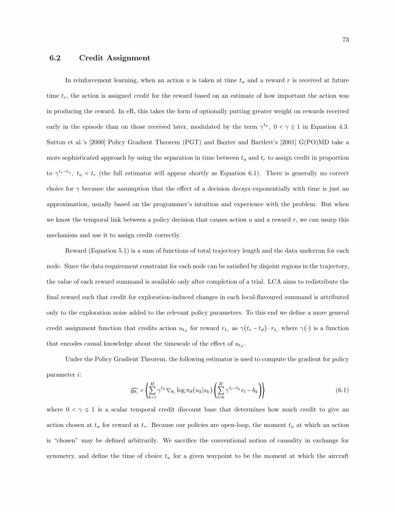
73

6.2 Credit Assignment

In reinforcement learning, when an action u is taken at time tu and a reward r is received at future

time tr, the action is assigned credit for the reward based on an estimate of how important the action was

in producing the reward. In eR, this takes the form of optionally putting greater weight on rewards received

early in the episode than on those received later, modulated by the term γtk , 0 < γ ≤ 1 in Equation 4.3.

Sutton et al.’s [2000] Policy Gradient Theorem (PGT) and Baxter and Bartlett’s [2001] G(PO)MD take a

more sophisticated approach by using the separation in time between tu and tr to assign credit in proportion

to γtr−tu , tu < tr (the full estimator will appear shortly as Equation 6.1). There is generally no correct

choice for γ because the assumption that the effect of a decision decays exponentially with time is just an

approximation, usually based on the programmer’s intuition and experience with the problem. But when

we know the temporal link between a policy decision that causes action u and a reward r, we can usurp this

mechanism and use it to assign credit correctly.

Reward (Equation 5.1) is a sum of functions of total trajectory length and the data underrun for each

node. Since the data requirement constraint for each node can be satisfied by disjoint regions in the trajectory,

the value of each reward summand is available only after completion of a trial. LCA aims to redistribute the

final reward such that credit for exploration-induced changes in each local-flavoured summand is attributed

only to the exploration noise added to the relevant policy parameters. To this end we define a more general

credit assignment function that credits action utd for reward rtr as γ(tr − td) ⋅ rtr where γ(⋅) is a function

that encodes causal knowledge about the timescale of the effect of utd .

Under the Policy Gradient Theorem, the following estimator is used to compute the gradient for policy

parameter i:

gθi = ⟨H

∑k=1

γtk∇θi logπθ(uk ∣sk)(H

∑l=kγtl−tkrl − bk)⟩ (6.1)

where 0 < γ ≤ 1 is a scalar temporal credit discount base that determines how much credit to give an

action chosen at tu for reward at tr. Because our policies are open-loop, the moment tu at which an action

is “chosen” may be defined arbitrarily. We sacrifice the conventional notion of causality in exchange for

symmetry, and define the time of choice tu for a given waypoint to be the moment at which the aircraft

74

passes the “chosen” waypoint. Thus “actions” affect not just the future as in the PGT, but also “the past”—

points in the trajectory that occur leading up to the waypoint. We modify Equation 6.1 as follows to produce

the LCA estimator:

gθi = ⟨H

∑k=1(γik∇θi logπθ(uk ∣sk) − µ∑∇)(rj

H

∑l=1γilρlj − bij)⟩ (6.2)

We have changed γ from a scalar to an arbitrary function that assigns credit at timestep k for policy

parameter (or waypoint) i, and re-inserted the variance-reducing term µ∑∇ from Equation 4.3. Since rj is

computed at the end of a trial, we introduce ρkj in order to distribute the reward received from summand

j at time tk. Finally, the indices of the reward summation can span the whole trajectory since γik will

modulate reward through time.

Redistributing reward requires that we determine the effect of each waypoint on each reward summand,

which requires that we answer the following two questions:

(1) γik: How does each waypoint i affect each timestep k along the trajectory?

(2) ρkj : How does each step along the trajectory affect each reward summand?

6.2.1 Waypoints ↔ Timesteps

Question 1 may easily be answered—approximately. When the trajectory is well-approximated by

line segments, each point in the trajectory between waypoints wi and wi+1 is affected only by those two

waypoints. (With higher-order splines such as NURBS the number of control points affecting each timestep

would be greater, but still generally a small constant.)

x(tk) = xk is the aircraft’s position at time tk. To compute the effect of exploration noise at waypoint

wi (or, equivalently, θi ∈ R2) on the aircraft’s location at time tk we must look at three cases: that in which

the aircraft has passed waypoint wi−1 and is now steering towards waypoint wi, that in which the aircraft

is orbiting wi, and that in which it has passed wi and is en route to wi+1. We define the parameter-point

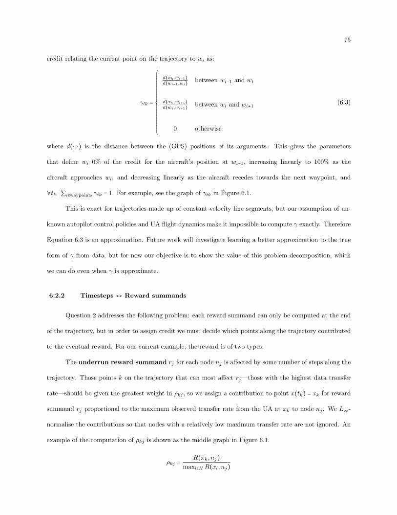
75

credit relating the current point on the trajectory to wi as:

γik =

⎧⎪⎪⎪⎪⎪⎪⎪⎪⎪⎪⎪⎪⎪⎪⎪⎪⎨⎪⎪⎪⎪⎪⎪⎪⎪⎪⎪⎪⎪⎪⎪⎪⎪⎩

d(xk,wi−1)d(wi−1,wi) between wi−1 and wi

d(xk,wi+1)d(wi,wi+1) between wi and wi+1

0 otherwise

(6.3)

where d(⋅, ⋅) is the distance between the (GPS) positions of its arguments. This gives the parameters

that define wi 0% of the credit for the aircraft’s position at wi−1, increasing linearly to 100% as the

aircraft approaches wi, and decreasing linearly as the aircraft recedes towards the next waypoint, and

∀tk ∑i∈waypoints γik = 1. For example, see the graph of γik in Figure 6.1.

This is exact for trajectories made up of constant-velocity line segments, but our assumption of un-

known autopilot control policies and UA flight dynamics make it impossible to compute γ exactly. Therefore

Equation 6.3 is an approximation. Future work will investigate learning a better approximation to the true

form of γ from data, but for now our objective is to show the value of this problem decomposition, which

we can do even when γ is approximate.

6.2.2 Timesteps ↔ Reward summands

Question 2 addresses the following problem: each reward summand can only be computed at the end

of the trajectory, but in order to assign credit we must decide which points along the trajectory contributed

to the eventual reward. For our current example, the reward is of two types:

The underrun reward summand rj for each node nj is affected by some number of steps along the

trajectory. Those points k on the trajectory that can most affect rj—those with the highest data transfer

rate—should be given the greatest weight in ρkj , so we assign a contribution to point x(tk) = xk for reward

summand rj proportional to the maximum observed transfer rate from the UA at xk to node nj . We L∞-

normalise the contributions so that nodes with a relatively low maximum transfer rate are not ignored. An

example of the computation of ρkj is shown as the middle graph in Figure 6.1.

ρkj =R(xk, nj)

maxl∈H R(xl, nj)

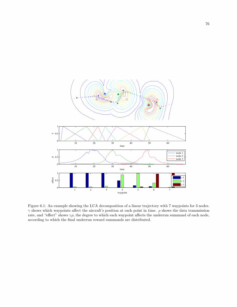
76

10 20 30 40 50 600

0.5

1

γ

time

10 20 30 40 50 600

0.5

1

time

ρ

1 2 3 4 5 6 70

0.5

1

effe

ct

waypoint

node 1

node 2

node 3

r 1

r 2

r 3

Figure 6.1: An example showing the LCA decomposition of a linear trajectory with 7 waypoints for 3 nodes.γ shows which waypoints affect the aircraft’s position at each point in time. ρ shows the data transmissionrate, and “effect” shows γρ, the degree to which each waypoint affects the underrun summand of each node,according to which the final underrun reward summands are distributed.

77

The final effect of each waypoint on each node’s reward—the product γρ in Equation 6.2—is visualised in

the final graph of Figure 6.1. The gradient due to each underrun summand is computed separately via

Equation 6.2.

6.2.3 LCA-Length

The reward function treats the tour length reward summand as a global property of the trajectory,

but it too can be decomposed by considering the portion of the trajectory length due to each waypoint.

The mechanism of LCA is overkill for this term: ρt = v∆t, and therefore Equation 6.2 reduces nearly to

Equation 6.1: the waypoints still define the same γik described in Equation 6.3 rather than the decaying

exponential assumed by Equation 6.1. For this reason we will refer to this simplified variant as LCA-length.

6.3 Combining the gradient estimates

In the example above, we have shown how to compute three different gradient estimates:

Global eR estimate from Equation 4.3.

Local underrun-based LCA estimates gu using Equation 6.2.

Local segment-length–based LCA estimate gl using Equation 6.2 or Equation 6.1.

The original reward function (Equation 5.1) balances underrun and length penalties by ensuring through η

that whenever there is underrun, the policy gradient with respect to reward is steepest in the direction that

will most reduce the hard constraint. But with the LCA decomposition, length and individual underrun

penalties are each computed from their own reward terms, producing separate policy gradient vectors. This

allows us to balance optimisation of the hard constraints against soft not through the indirect mechanism of

the monolithic reward function but rather by ensuring that hard-constraint gradients dominate the policy

update.

We create a new policy update for Equation 4.5 by combining the LCA-based gradient estimates gu

and gl in a way that ensures that wherever a hard constraint is violated (a data underrun occurs and gu is

nonzero), that update vector dominates the total update, otherwise only the LCA-length update vector gl

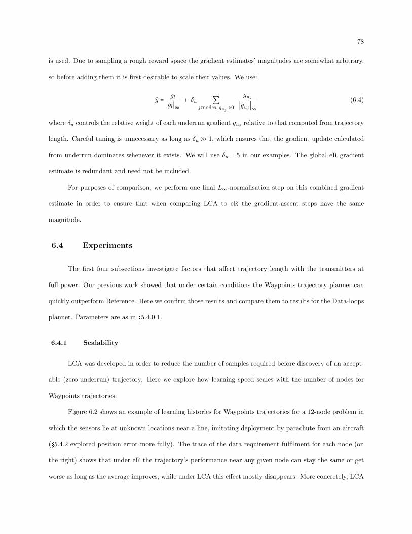
78

is used. Due to sampling a rough reward space the gradient estimates’ magnitudes are somewhat arbitrary,

so before adding them it is first desirable to scale their values. We use:

g = gl∣gl∣∞

+ δu ∑j∈nodes,∣guj

∣>0

guj

∣guj∣∞

(6.4)

where δu controls the relative weight of each underrun gradient guj relative to that computed from trajectory

length. Careful tuning is unnecessary as long as δu ≫ 1, which ensures that the gradient update calculated

from underrun dominates whenever it exists. We will use δu = 5 in our examples. The global eR gradient

estimate is redundant and need not be included.

For purposes of comparison, we perform one final L∞-normalisation step on this combined gradient

estimate in order to ensure that when comparing LCA to eR the gradient-ascent steps have the same

magnitude.

6.4 Experiments

The first four subsections investigate factors that affect trajectory length with the transmitters at

full power. Our previous work showed that under certain conditions the Waypoints trajectory planner can

quickly outperform Reference. Here we confirm those results and compare them to results for the Data-loops

planner. Parameters are as in §5.4.0.1.

6.4.1 Scalability

LCA was developed in order to reduce the number of samples required before discovery of an accept-

able (zero-underrun) trajectory. Here we explore how learning speed scales with the number of nodes for

Waypoints trajectories.

Figure 6.2 shows an example of learning histories for Waypoints trajectories for a 12-node problem in

which the sensors lie at unknown locations near a line, imitating deployment by parachute from an aircraft

(§5.4.2 explored position error more fully). The trace of the data requirement fulfilment for each node (on

the right) shows that under eR the trajectory’s performance near any given node can stay the same or get

worse as long as the average improves, while under LCA this effect mostly disappears. More concretely, LCA

79

Trial 0: length 520, data [ 46 7 50 48 32 32 30 111 24 36 17 33 ]%

eR: first acceptable at trial 360, length 627

0 100 200 300 400 5000

50

100

150

eR: constraint learning progress

trial

dat

a %

LCA: first acceptable at trial 116, length 571

0 100 200 300 400 5000

50

100

150

LCA: constraint learning progress

trial

dat

a %

Figure 6.2: LCA vs. eR: sample trajectories for 12 sensors. Left column, from top to bottom: the initialtrajectory is assumed to follow that of a deployment aircraft’s recorded path and is ignorant of actual sensorpositions (deployed every 30 units, displaced uniformly randomly on a circle of radius 12 around the expectedlocation); the first acceptable trajectory learned by eR; and the trajectory produced by LCA after the samenumber of steps. “Length” for the learned trajectories is the average length over the 100 trials after the firstacceptable trajectory is discovered. Right column: fraction of the data requirement fulfilled (here req=25for each node); each line shows the trace of data collected vs. trial number for a single node, for eR andLCA. Here we use 38 waypoints (76 parameters) for 12 sensors.

80

allows more rapid convergence to a better trajectory.

Figure 6.3 shows that LCA improves scalability of the learning system for Waypoints trajectories. eR

requires a number of trials roughly linear in the number of nodes, whereas with LCA the learning time grows

much more slowly. Perhaps more surprising is the difference in first good trajectory length between eR and

LCA. When some nodes but not others have underrun, the locality of the LCA update allows optimisation

for length on whichever waypoints bear no responsibility for underrun. This effect is most significant at

higher data requirements when the learner is required to spend significant time optimising the trajectory

in the vicinity of each node, and almost disappears at low requirements (not shown). When using LCA for

both underrun and distance, the first good trajectory tends to be slightly shorter than for LCA-underrun

only, but the difference is only significant under a narrow range of conditions. We weight the LCA update

for underrun more heavily than those for length (as described in the caption), which ensures that wherever

there is an underrun its gradient will dominate the policy update. What happens after the first acceptable

trajectory is found? Behaviour remains similar to that when using the zero-underrun trajectories generated

by Data-loops, discussed below.

6.4.2 LCA-length for Data-loops trajectories

Figure 6.4 shows how learning rate scales for Data-loops trajectories. We have shown a quasi-linear

sensor layout: the assumed sensor positions lie near a line, and the actual positions are displaced by 8 in

a uniformly random direction from where the UA believes it to lie. Because time to first good is 0 for

Data-loops, we show the quality of the trajectory after 40 trials (initial quality is nearly identical to that of

Reference, so initially log2length(Data−loops)length(Reference) = 0). While the quality of the trajectory achieved by eR after 40

trials improves over Reference less as the number of nodes increases, LCA-length achieves consistently good

performance even for large problems, in this case generally finding trajectories 2−1.5 ≃ 0.35 times the length of

Reference within 40 trials. This relatively large improvement is a consequence of providing poor information

to the trajectory planners: when the Reference planner is given incorrect information, the advantage of the

learners can be arbitrarily large.

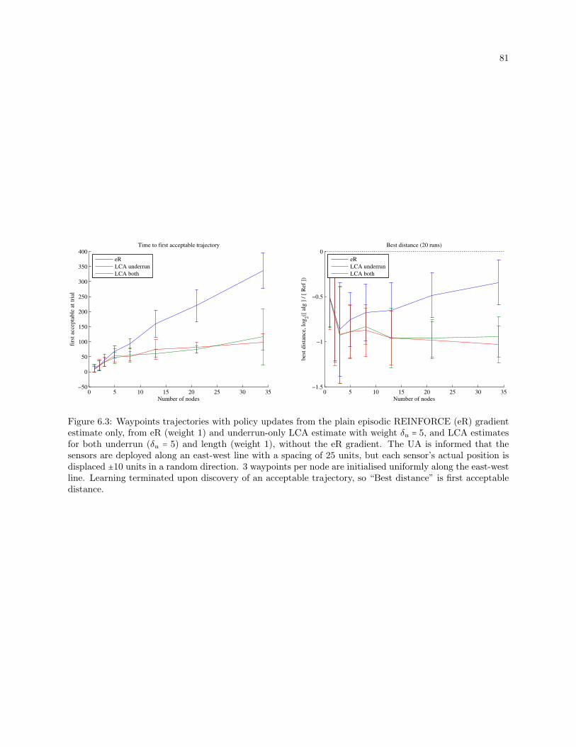
81

0 5 10 15 20 25 30 35−50

0

50

100

150

200

250

300

350

400

Number of nodes

firs

t ac

cepta

ble

at

tria

l

Time to first acceptable trajectory

0 5 10 15 20 25 30 35−1.5

−1

−0.5

0

Number of nodes

bes

t dis

tance

, lo

g2([

alg

] /

[ R

ef ]

)

Best distance (20 runs)

eR

LCA underrun

LCA both

eR

LCA underrun

LCA both

Figure 6.3: Waypoints trajectories with policy updates from the plain episodic REINFORCE (eR) gradientestimate only, from eR (weight 1) and underrun-only LCA estimate with weight δu = 5, and LCA estimatesfor both underrun (δu = 5) and length (weight 1), without the eR gradient. The UA is informed that thesensors are deployed along an east-west line with a spacing of 25 units, but each sensor’s actual position isdisplaced ±10 units in a random direction. 3 waypoints per node are initialised uniformly along the east-westline. Learning terminated upon discovery of an acceptable trajectory, so “Best distance” is first acceptabledistance.

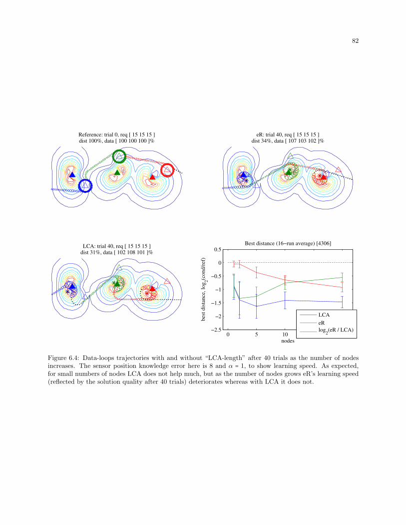
82

Reference: trial 0, req [ 15 15 15 ]dist 100%, data [ 100 100 100 ]%

LCA: trial 40, req [ 15 15 15 ]dist 31%, data [ 102 108 101 ]%

0 5 10 15 20−2.5

−2

−1.5

−1

−0.5

0

0.5

nodes

bes

t d

ista

nce

, lo

g2(c

on

d/r

ef)

Best distance (16−run average) [4306]

LCA

eR

log2(eR / LCA)

eR: trial 40, req [ 15 15 15 ]dist 34%, data [ 107 103 102 ]%

Figure 6.4: Data-loops trajectories with and without “LCA-length” after 40 trials as the number of nodesincreases. The sensor position knowledge error here is 8 and α = 1, to show learning speed. As expected,for small numbers of nodes LCA does not help much, but as the number of nodes grows eR’s learning speed(reflected by the solution quality after 40 trials) deteriorates whereas with LCA it does not.

83

6.5 Summary

When waypoints are not associated with nodes, the link between waypoint motion data collection goals

is no longer clear. The credit assignment problem leads to long learning times as problem size increases.

This chapter presented a local credit assignment (LCA) algorithm that rediscovers the link between

policy parameters and ferrying objectives, and demonstrated that LCA dramatically improves scalability to

large problems.

Chapter 7

Node Energy Management

This chapter introduces a different design goal. Assume that sensors generate data that must be

retrieved at a fixed interval that is much greater than the time required for a UA tour. Assume further that

the sensors have limited energy reserves. Tour length is treated as a hard constraint: the UA has some fixed

maximum range dmax that is greater than the range required to collect all the data, and there is no benefit

in reducing trajectory length below this point. Rather, the soft constraint is the energy used by the nodes

for data transmission. The objective is to learn a policy that not only carries the UA to the best location for

radio transmission, but also allows the sensors to transmit to the UA using the lowest possible radio power.

This is accomplished by allowing the ferry to use its excess range to increase contact time with each node,

directing the node to transmit at lower power.

Contributions:

We demonstrate the feasibility of a reinforcement learning approach for rapid discovery of energy-

saving network policies that trade UA flight time for sensor energy. The policies are learned without

a system model and despite potentially inaccurate sensor node locations, unknown radio antenna

patterns, and ignorance of the internals of the autopilot.

We show that our two independent optimisers—waypoint location and transmission power policy—

can operate simultaneously on the same sampling flights.

We show that learned policies approach optimal performance, and that the time they require to do

so is short enough to offer a reasonable alternative to an optimal planning approach.

85

7.1 Radio transmission power

The data-ferrying approach allows sensors to communicate with distal base stations without the need

for high-powered radios, but the energy that nodes spend in communicating with the ferry is still non-

negligible [Jun et al., 2007; Tekdas et al., 2008].

Theorem 1. For a continuous rate model, decreasing power increases the energy efficiency of transmission

ratepower

.

Proof. Recall the data rate from §3.1:

Rab = β log2(1 + SNRab)

The derivative of efficiency ratepower

with respect to power:

∇P1

P⋅ β log2 (1 +

P

N) = β

N P log(2) (1 + PN)−β log(1 + P

N)

P 2 log(2)

is negative whenever

P

P +N− log (P +N

N) < 0

Let f(P,N) = PP+N − log (

P+NN).

∇P f = 1

P +N− P

(P +N)2− 1

P +N

= − P

(P +N)2

which is negative for P > 0. Note that ∀N > 0, f(0,N) = 0. So:

f(0,N) > f(P,N) ∀P > 0

Therefore the derivative of ratepower

is negative: as power increases, efficiency drops.

While reducing power results in a lower energy cost per bit, it results in lower transmission rates and

longer trajectories. Given an externally defined trade-off between ferry trajectory length and the value of a

node’s energy resource, when should a sensor transmit, and at what power?

The difficulty of predicting the SNR between transmitter and aircraft again suggests reinforcement

learning. We assume that at each timestep a sensor can transmit with power P ∈ [0, Pmax]. Assume some

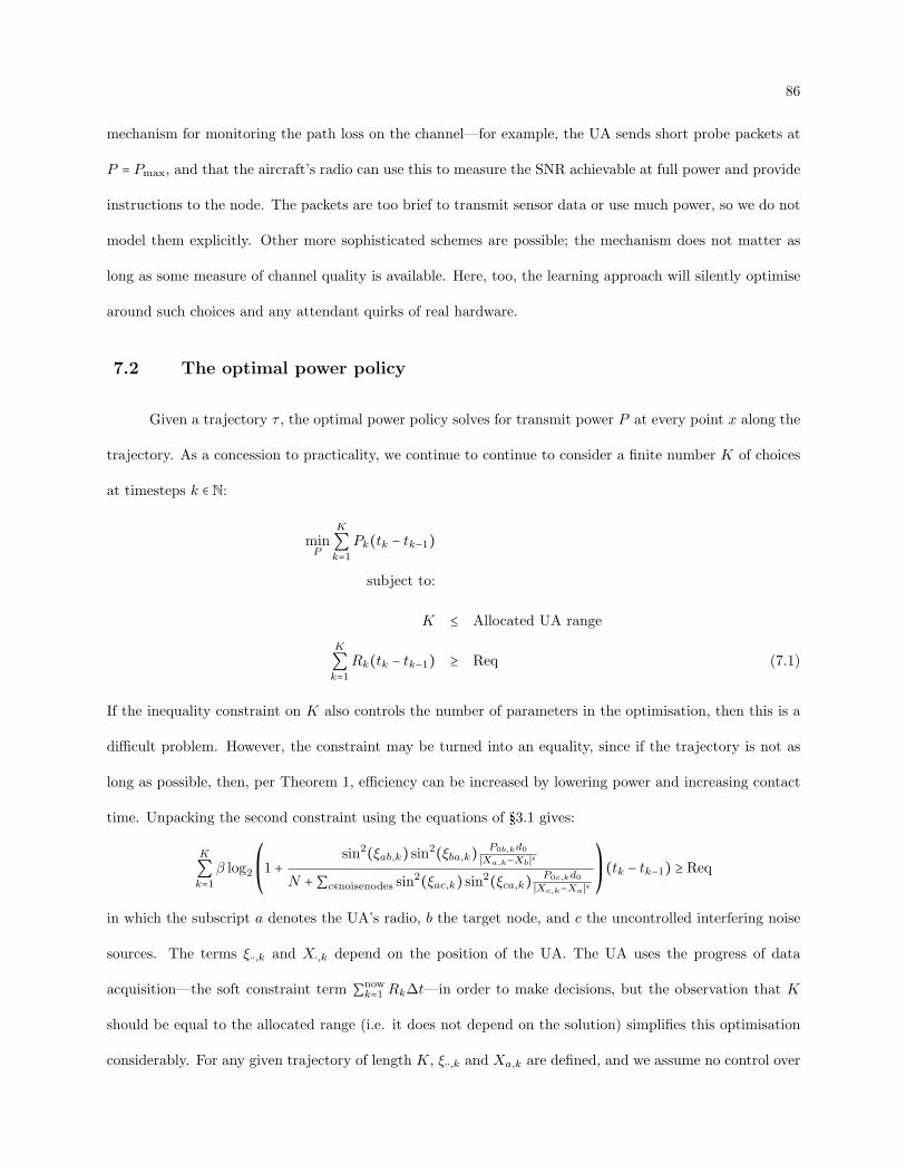
86

mechanism for monitoring the path loss on the channel—for example, the UA sends short probe packets at

P = Pmax, and that the aircraft’s radio can use this to measure the SNR achievable at full power and provide

instructions to the node. The packets are too brief to transmit sensor data or use much power, so we do not

model them explicitly. Other more sophisticated schemes are possible; the mechanism does not matter as

long as some measure of channel quality is available. Here, too, the learning approach will silently optimise

around such choices and any attendant quirks of real hardware.

7.2 The optimal power policy

Given a trajectory τ , the optimal power policy solves for transmit power P at every point x along the

trajectory. As a concession to practicality, we continue to continue to consider a finite number K of choices

at timesteps k ∈ N:

minP

K

∑k=1

Pk(tk − tk−1)

subject to:

K ≤ Allocated UA range

K

∑k=1

Rk(tk − tk−1) ≥ Req (7.1)

If the inequality constraint on K also controls the number of parameters in the optimisation, then this is a

difficult problem. However, the constraint may be turned into an equality, since if the trajectory is not as

long as possible, then, per Theorem 1, efficiency can be increased by lowering power and increasing contact

time. Unpacking the second constraint using the equations of §3.1 gives:

K

∑k=1

β log2

⎛⎜⎝1 +

sin2(ξab,k) sin2(ξba,k) P0b,kd0

∣Xa,k−Xb∣ϵ

N +∑c∈noisenodes sin2(ξac,k) sin2(ξca,k) P0c,kd0

∣Xc,k−Xa∣ϵ

⎞⎟⎠(tk − tk−1) ≥ Req

in which the subscript a denotes the UA’s radio, b the target node, and c the uncontrolled interfering noise

sources. The terms ξ⋅⋅,k and X⋅,k depend on the position of the UA. The UA uses the progress of data

acquisition—the soft constraint term ∑nowk=1 Rk∆t—in order to make decisions, but the observation that K

should be equal to the allocated range (i.e. it does not depend on the solution) simplifies this optimisation

considerably. For any given trajectory of length K, ξ⋅⋅,k and Xa,k are defined, and we assume no control over

87

the power of the noise transmitters, so P0c,k is also known. Let

Ωk =sin2(ξab,k) sin2(ξba,k)d0

∣Xa,k−Xb∣ϵ

N +∑c∈noisenodes sin2(ξac,k) sin2(ξca,k) P0c,kd0

∣Xc,k−Xa∣ϵ

Further assume uniform timestep size (for convenience and readability, but otherwise this is unnecessary).

The constraint is now:

β∆tK

∑k=1

log2 (1 +ΩkP0b,k) ≥ Req

Given a sample of Ω over the maximum-length trajectory given waypoint x, this may easily be solved

using standard nonlinear constrained optimisation tools.

Let r∗x be the reward achieved by the power policy that solves Equation 7.1 for a trajectory flown by

the autopilot given a single waypoint x. The optimal waypoint is:

x∗ = argmaxx

r∗x (7.2)

This is an unconstrained nonlinear optimisation whose objective function is the solution to a constrained

nonlinear optimisation. This can be solved by standard numerical techniques, but it is time-consuming to

solve—even the simplest one-node problems of ∼ 100 timesteps require many dozens of minutes of CPU time

in Matlab on a modern personal computer, and optimal solutions for larger problems require significant

computational resources, even with the substantial simplification that the compatible optimal trajectory

allows.

7.3 Learning

Waypoint placement is learned as described in §4.3. This operates concurrently with the power policy

optimiser described below.

7.3.1 Power Policies

In order to transmit data at a low energy cost, two conditions must be met:

Transmission should only occur when the path loss is as low as possible.

The radio should operate at the lowest power that will result in a channel of sufficient bandwidth.

88

A power policy is a function that controls the power a node uses to transmit given a reported

maximum SNR, which may be given in dB or, as shown below, as a linear ratio. We define it by two

parameters θpower = [Powertarget, Ratethreshold]T , which may be abbreviated as θp = [Pt, RT ]T or, when the

policy under discussion is unambiguous, the subscripts p on θ and π may be dropped. The desired behaviour

is to transmit at the target power Pt ≤ Pmax if and only if the probed SNR is greater than some threshold

ratio Rthreshold. Thus the policy observes state s and produces the action u (the relative transmission power)

according to its learned parameters θ:

s = SNRprobed

u =Ptarget

Pmax(7.3)

θp =

⎡⎢⎢⎢⎢⎢⎢⎢⎢⎢⎣

Ptarget

Rthreshold

⎤⎥⎥⎥⎥⎥⎥⎥⎥⎥⎦

PGRL requires that exploration noise be added to the controller’s output u, so we amend Equation 7.3

to:

u = Pnow

Pmax(7.4)

where u = Pnow = Ptarget + exploration noise, and

π(s; θ) = Pr(u∣s; θ) (7.5)

is defined by the exploration noise distribution.

Since the shape of the exploration noise distribution of u will affect results, we will compare four

exploration strategies to the handcoded heuristics. Typical actions drawn by each of the policies, sample

trajectories for each strategy, including transmit power, data rate, and transmission efficiency through time,

are illustrated in Figures 7.1 (the handcoded heuristics) and 7.2 (the learning policies).

Unlike the waypoint-placement policy, this one is closed-loop: a measurement of path loss (in this case

the SNR measured by probe packets at full power) informs the choice of action at each timestep. Thus we use

the full capabilities of the episodic REINFORCE algorithm of §4.3. This policy and the waypoint-placement

one run in parallel, using the same flights and the same PGRL algorithm to estimate their gradients.

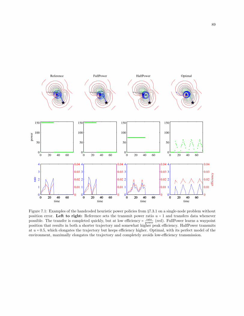
89

0 20 40 600

1

2

3

4

time

rate

0 20 40 600

1

2

3

4

time

0 20 40 600

1

2

3

4

time

0 20 40 600

1

2

3

4

time

0 20 40 600

50

100

150

po

wer

0 20 40 600

50

100

150

0 20 40 600

50

100

150

0 20 40 600

50

100

150

Reference FullPower HalfPower Optimal

0 20 40 600

0.01

0.02

0.03

0.04

0 20 40 600

0.01

0.02

0.03

0.04

0 20 40 600

0.01

0.02

0.03

0.04

0 20 40 600

0.01

0.02

0.03

0.04

effi

cien

cyFigure 7.1: Examples of the handcoded heuristic power policies from §7.3.1 on a single-node problem withoutposition error. Left to right: Reference sets the transmit power ratio u = 1 and transfers data wheneverpossible. The transfer is completed quickly, but at low efficiency = rate

power(red). FullPower learns a waypoint

position that results in both a shorter trajectory and somewhat higher peak efficiency. HalfPower transmitsat u = 0.5, which elongates the trajectory but keeps efficiency higher. Optimal, with its perfect model of theenvironment, maximally elongates the trajectory and completely avoids low-efficiency transmission.

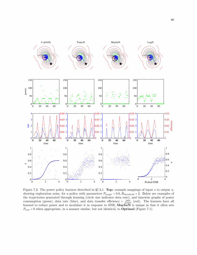
90

0 20 40 600

1

2

3

4

time

rate

0 20 40 600

1

2

3

4

time

0 20 40 600

1

2

3

4

time

0 20 40 600

1

2

3

4

time

0 20 40 600

50

100

150

po

wer

0 20 40 600

50

100

150

0 20 40 600

50

100

150

0 20 40 600

50

100

150

ε−greedy TruncN MaybeN LogN

0 20 40 600

0.01

0.02

0.03

0.04

0 20 40 600

0.01

0.02

0.03

0.04

0 20 40 600

0.01

0.02

0.03

0.04

0 20 40 600

0.01

0.02

0.03

0.04

effi

cien

cy

0 2 40

0.2

0.4

0.6

0.8

1

u

0 2 40

0.2

0.4

0.6

0.8

1

0 2 40

0.2

0.4

0.6

0.8

1

0 2 40

0.2

0.4

0.6

0.8

1

Probed SNR

u

Figure 7.2: The power policy learners described in §7.3.1. Top: example mappings of input s to output u,showing exploration noise, for a policy with parameters Ptarget = 0.6,Rthreshold = 2. Below are examples ofthe trajectories generated through learning (circle size indicates data rate), and timewise graphs of powerconsumption (green), data rate (blue), and data transfer efficiency = rate

power(red). The learners have all

learned to reduce power and to modulate it in response to SNR; MaybeN is unique in that it often setsPnow = 0 when appropriate, in a manner similar, but not identical, to Optimal (Figure 7.1).

91

In order to show that the chosen strategy can have a significant and sometimes surprising effect

on performance, comparisons will be made between learning policies with several exploration strategies,

described below. Baseline comparisons will be made to our standard Reference, which transmits at full power;

two new baseline heuristics; and to the optimal power policy described above, which uses the compatible

optimal waypoint placement from Chapter 4.

7.3.1.1 Sigmoid ϵ-Greedy (“ϵ-G”)

The policy’s output is the action u; in this case the radio power Pnow. In order to approximate the

threshold power policy described above, the ϵ-greedy policy usually sets u to the value of a sigmoid of height

Ptarget and steepness ϕ, centered on the “threshold” (now smoothed) Rthreshold. In order to add exploration

noise, with probability ϵ, the action is drawn uniformly randomly from [0 . . .1]:

Pr(u∣s; θ) =

⎧⎪⎪⎪⎪⎪⎪⎪⎨⎪⎪⎪⎪⎪⎪⎪⎩

1 with probability ϵ

Ptarget ⋅ 11+eϕ(Rthreshold−s)

otherwise

(7.6)

This exploration strategy is easy to explain and helps to set up the more complex ones below, but it

cannot be used for PGRL because it has no useful gradient—the probability of any action that does not fall

on the sigmoid is Pr(u∣s; θ) = ϵ, so ∇θπ(u∣s; θ) = 0. However, when noise is introduced into the output, it is

possible to pretend that the noise derived from some policy that has a gradient. In this case, the derivative

from §7.3.1.2 can be borrowed, which allows the algorithm to maintain the pretence that the uniform noisy

actions were instead drawn from a Gaussian. The necessity of this kludge illustrates a problem with the

exploration strategy that will be solved in the following sections, but the kludge yields interesting results.

Figure 7.2 suggests an apparent practical weakness of this exploration strategy (and the others as

well): power never drops quite to 0 even when there is no signal, because the sigmoid 11+exp(ϕ(Rthreshold−s)) > 0.

However, while the data transmitted during these drops is insignificant, so is the energy used.

92

7.3.1.2 Truncated Gaussian (“TruncN”)

ϵ-greedy draws exploratory actions from the whole range of allowed actions, and does not provide a

useful gradient. Exploration noise does produce a gradient if it is more likely to fall closer to the noise-free

(“greedy”) action (keeping exploratory actions nearer those of the noise-free policy also tends to mitigate

sudden large deviations from the greedy action, limiting their adverse effect on reward). Here we draw the

transmission power u = Pnow for each timestep from a Gaussian whose mean is taken from a sigmoid of

height Ptarget (the same sigmoid that appears in Equation 7.6):

u = N (Ptarget ⋅1

1 + eϕ(Rthreshold−s), σ) , truncated on 0 ≤ Pnow ≤ Pmax

where s = SNRprobed.

When SNRprobed = Rthreshold, the mean transmission power is 50% of Ptarget and the actual trans-

mission power Pnow is close to that. Power goes to 100% as SNRprobed increases above Rthreshold and vice

versa, thus implementing the desired behaviour with exploration. The sigmoid’s width is controlled by ϕ,

and Gaussian exploration is controlled by σ. For example, when Ptarget = Pmax and Rthreshold is small, if σ

is small then the policy mimics the full-power Data-loops policy.

Note also that even when SNRprobed ≪ Pthreshold, there is a 50% chance that the node will attempt

transmission, albeit at low power. As we will see, this exploration turns out to be important: if the

trajectory does not carry the UA into a region in which SNRprobed ⪆ Pthreshold, these low-power exploratory

transmissions create an appropriate gradient for an update.

The policy’s derivatives, used in Equation 4.3, are:

∇θ logπ(s; θ) =

⎡⎢⎢⎢⎢⎢⎢⎢⎢⎢⎢⎢⎢⎣

u− Ptarget

1+eϕ (Rthreshold−s)

σ2 (1+eϕ (Rthreshold−s))

−Ptarget ϕ eϕ (Rthreshold−s) (u− Ptarget

1+eϕ (Rthreshold−s))

σ2 (1+eϕ (Rthreshold−s))2

⎤⎥⎥⎥⎥⎥⎥⎥⎥⎥⎥⎥⎥⎦

Gradients for u > 1 and u < 0 are computed before truncation.

93

7.3.1.3 Gaussian Maybe (“MaybeN”)

At each timestep, transmission occurs with probability drawn from a sigmoid:

Pr(transmit) = 1

1 + eϕ(Rthreshold−s)(7.7)

If transmission is to occur, it is at a power drawn from a Gaussian about Ptarget:

Pnow = N (Ptarget, σ) (7.8)

This is again truncated on [0 . . . Pmax]. The policy is otherwise the same as that described in §7.3.1.2.

When transmission does occur, the policy’s derivatives are:

∇θ logπ(s; θ) =

⎡⎢⎢⎢⎢⎢⎢⎢⎢⎢⎢⎣

u−Ptarget

σ2

− ϕeϕ (Rthreshold−s)

1+eϕ (Rthreshold−s)

⎤⎥⎥⎥⎥⎥⎥⎥⎥⎥⎥⎦

Otherwise:

∇θ logπ(s; θ) =

⎡⎢⎢⎢⎢⎢⎢⎢⎢⎢⎢⎣

0

1 + ϕeϕ (Rthreshold−s)

1+eϕ (Rthreshold−s)

⎤⎥⎥⎥⎥⎥⎥⎥⎥⎥⎥⎦As before, if u is truncated, gradients are computed on the pre-truncated values.

7.3.1.4 Log-Normal exploration (“LogN”)

Is constant-sized exploration noise detrimental to exploitation? Here, noise is drawn from a log-normal

distribution, so Pnow > 0, and exploration noise scales with power. Like the previous strategies, the “target”

transmit power is drawn from a sigmoid of height Ptarget.

When the log-normal distribution’s probability density function (PDF) is defined as

Pr(u) = 1

2σ√2π

exp(− ln(u) −M2σ2

)

then the mean of the distribution is eM+σ2

2 . Since we desire a mean of Ptarget, we set

M = ln (Ptarget) −σ2

2(7.9)

= ln( P

1 + eϕ(Rthreshold−s)) − σ

2

2(7.10)

94

This yields

Pr(u∣s; θ) = lnN (ln(M), σ)

= 1

2σ√2π

exp⎛⎜⎝−ln(u) − (ln ( 1

eϕ(Rthreshold−s)) − σ2

2)

2σ2

⎞⎟⎠

∇θ Pr(u∣s; θ) =

⎡⎢⎢⎢⎢⎢⎢⎢⎢⎢⎢⎢⎣

exp(− (ln(u)−M)2

2σ2 )(ln(u)−M)

Pσ3u√2π

−ϕ exp(− (ln(u)−M)2

2σ2 +ϕ(Rthreshold−s))(ln(u)−M)

σ3u(eϕ(Rthreshold−s)+1)√2π

⎤⎥⎥⎥⎥⎥⎥⎥⎥⎥⎥⎥⎦

7.3.2 Baselines

The conventional approach is the non-learning Reference planner, reviewed here. In addition, we

introduce two new references. They use naıve power policies, but learn waypoint placement as described in

Chapter 4, allowing some performance gain over Reference that increases with increasing inaccuracy in node

location information.

7.3.2.1 Reference

Performance of each of the power policies will be shown relative to our standard Reference planner,

first introduced in §3.2.1, which circles the assumed position of each waypoint and directs the node to

transmit at full power.

7.3.2.2 Full Power learner (“FullPower”)

FullPower learns waypoint placement as described in §4.4, but always transmits at the maximum

power P = Pmax, or u = 1. This is the “Data-loops” planner, with its use of the most naıve possible power

policy spelt out.

7.3.2.3 Half Power learner (“HalfPower”)

The experiments will generally assume that the UA can safely use twice the range required for the

Reference trajectory. HalfPower learns waypoint placement as described in §4.4, but sets P = Pmax

2, or u = 1

2.

This generally increases the trajectory length by less than a factor of 2, since at each point on the trajectory,

95

HalfPower transmits more than half the data that FullPower does (since 2 ⋅ log2 (1 + x2) > log2(1+x) ∀x > 0),

but note that this is not guaranteed, since HalfPower’s lower transmission rate may require additional loops

or substantially different trajectories. In our simulations HalfPower tends to increase trajectory length by

factors in the range of ∼ 1.1–1.5, and almost never exceeds the factor-of-two distance threshold.

7.3.3 Reward

When a system model is not available, constraints cannot be guaranteed. So instead of solving the

nested optimisation given by Equations 7.1 and 7.2, we maximise the expected return (Equation 4.2) for a

reward function chosen to favour solutions that also solve Equations 7.1 and 7.2. Rewards (or their negatives,

costs) are assigned so that solutions that better satisfy the design objectives have higher reward (lower cost).

The constraints in Equation 7.1 differ from the corresponding summands of the reward in that the former

merely state requirements while the latter create a function at whose maximum the constraints are satisfied.

The reward function expresses the desiderata of solutions as a scalar quantity. We seek the policy that

allows each node to transmit at the lowest power that does not require the aircraft to exceed a maximum

desired tour length dmax, which indicates that we are nearing the endurance limit of the aircraft. The

following reward expresses the desiderata:

r = −⎛⎝max (0, d − dmax)

ϱ + ∑j∈nodes

φj

H

∑k=1

Pjk∆t⎞⎠

(7.11)

where d is the current trajectory path length, dmax is the soft maximum range of the aircraft, ϱ controls

the severity of the soft maximum distance penalty, Pjk is the transmission power of node j at timestep k of

length ∆t, and φj is a weighting for the value of energy for node j. Note that d is not penalised until the

aircraft exceeds dmax.

7.3.3.1 Local reward decomposition

Can power policies be treated locally? Since the satisfaction of performance objectives is controlled

by policies that correspond to individual nodes, if a node is added to a problem, the performance of the

policy for that node can, to a first approximation, be optimised independently of the performance of the

96

other nodes. This makes the algorithms scalable.

This need not be the case. For Waypoints trajectories, LCA (Chapter 6) was necessary in order to link

the satisfaction of local-flavoured constraints such as data underrun to waypoints that are not explicitly tied

to nodes. That the satisfaction of the constraints is a well-defined local property of portions of the trajectory

makes local credit assignment meaningful. But for the power policy under the Data-loops planner, parameters

and rewards both correspond to nodes rather than to waypoints, so the mechanism by which LCA assigns

per-node reward to influential waypoints is unnecessary.

Total trajectory length is a global property, but it can be approximately decomposed, as was done

with “LCA-Length” (§6.2.3). This pseudo-local breakdown is accomplished as follows:

The trajectory length attributable to each node is that flown while navigating towards that node’s

designated waypoint under a reference planner. Let this be called d∗j for node j.

The extra range D+ available to the UA is allocated to each node j in proportion to the value of

energy to each node: d+j =D+ ⋅φj

∑k∈nodes φk

Equation 7.11 is decomposed per node j as follows:

rj = −(max (0, dj − (d∗j + d+j ))ϱ + φj

H

∑k=1

Pjk∆t) (7.12)

where dj is the distance flown during which node j is the target of communication under the current planner

(whether or not communication actually takes place). This decomposition is somewhat simplistic, but it

allows an N -node problem to be approximately decomposed into N 1-node problems, and will be used to

produce per-node gradient estimates throughout the multi-node experiments.

7.3.4 Policy Updates

The size of the update step to Ptarget deserves special mention: the difference in trajectory length,

and hence in reward, between Pnow = x and Pnow = 2x is similar to the change in reward between Pnow = 2x

and Pnow = 4x. Furthermore, if Ptarget = 0, it becomes easy for the aircraft to circle in a region at which

SNRprobed < Rthreshold, in which case the radio is unlikely to receive any data at all, especially under the

97

MaybeN and LogN exploration policies. Therefore it is desirable to scale power down slowly. Rather than

the additive update used for most policy parameters (θx ← θx + αwx) for update vector w and learning rate

α, the policy update treats this parameter multiplicatively:

Ptarget ← Ptarget + PtargetαwP (7.13)

This is equivalent to re-writing the policy by replacing Ptarget = θ1 with Ptarget = (1 + α)θ1α , requiring θ1 ≤ 0

(or adding a squashing function in order to bound the output), and then performing conventional additive

gradient updates on θ1.

The updates for the Rate threshold Rthreshold are simply additive, as usual:

Rthreshold ← Rthreshold + αwRthreshold(7.14)

7.3.5 An example failsafe mechanism

The exploration noise produced by the learning system most often results in small changes to trajectory

length, but occasionally the exploration noise reduces power, increases the SNR threshold, or moves a

waypoint so that the new trajectory no longer results in enough time spent in regions in which SNRprobed ⪆

Rthreshold. This may require the UA to add loops in order to collect sufficient data, significantly exceeding

its trajectory limit. But it is reasonable to assume that the UA has a real physical range limit dhardmax that

is somewhat greater than the soft limit dmax. Some failsafe mechanism that brings the UA home before it

hits its hardware range limit will be necessary in practice.

By way of including some version of this concept in the results, we implement a simple failsafe that

is suitable for simulation: when the aircraft’s soft maximum range has been exceeded, radio power is set

to 100%, ensuring that the UA does not become stuck in nearly infinite loops waiting for the power policy

to allow data transfer. This can result in limited overruns of the length limit, since the UA must complete

transfer at a high rate and then return to its origin, but in the experiments the overruns are shown to be

minor. Failsafes that are more appropriate for real-world flight are not difficult to imagine, but they have

little effect upon the results, and it is outside the scope of the current work to investigate further.

98

7.4 Experiments

We explore the simultaneous optimisation of trajectory length and node energy using the Data-loops

planner. Energy use and trajectory length balance each other as specified by Equation 7.12, so in one sense

the most important performance criterion is the composite measure defined by reward (or cost). When the

learners keep trajectory length very close to the soft limit (as is most often the case), the composite reward

measure is similar to the most important design objective: energy use. However, note that cost is a function

designed to drive the optimisers towards solutions that minimise energy use subject to a length constraint.

Equation 7.12 may spike by several orders of magnitude when the length constraint is exceeded by only a

small amount, so the dual measures of energy and length, while less convenient, are more informative. A

further complication unique to the comparison to the optimal policy with degraded information—in which

case data underrun must also be considered—will be discussed in §7.4.1.1.

Throughout this chapter, a trial is one tour of the nodes, a run is some number of trials (usually 200

unless otherwise noted) on a single radio field, during which the learners are given the opportunity to adapt.

For each new run, a new random radio field is generated.

Parameters: The aircraft flies at speed v = 1 at altitude z = 3. The maximum turning rate of

ω = 20/s yields a turning radius r = vω≈ 2.9. Radios use Pmax = 150 and bandwidth β = 1, and the

background noise N = 2. Each sensor’s data requirement req = 20 unless otherwise noted. These parameters

do not qualitatively affect the results, and can be replaced by appropriate values for any given hardware.

For waypoint placement the learning rate α = 0.5 and the exploration parameter σ = 1. The power policy

uses αp = 0.1, σp = 0.1, ϕp = 3, φj = 1∀j.

7.4.1 Comparison to the optimal policy

Finding the optimal policy requires significant computational resources. Therefore the comparisons

with optimal trajectories are limited to this section. In order to furnish an informative framework against

which to compare the remaining results of this chapter, we will show results from at least the following

algorithms, introducing more as required:

99

Optimal: the baseline for this experiment uses the optimal power policy as described above. Waypoints are

placed using the compatible optimal waypoint placement defined in §4.6, but note that the chosen

waypoint maximises the energy-conservation reward (Equation 7.12).

Reference: The conventional solution orbits the node’s true position (or what it believes the true position

to be, if information is degraded), transmitting at full power.

FullPower: A Data-loops trajectory the learned locally optimal waypoint position (not necessarily the

node’s position). As was shown in §4.6, its best-trial performance tends to be very similar to that

of the compatible optimal trajectory with full power.

Learned: To what solution does a learned policy (waypoint location and power) converge (in 200 trials,

with parameters as described above)? For reasons explained in the following sections, the learning

policy used throughout §7.4.1 uses the truncated Gaussian (TruncN) exploration policy. Variants of

Learned will be introduced and tested as needed.

7.4.1.1 Revisiting Performance Comparison

Various comparisons may be made between the learners and the optimal planner, and no scalar tells

the whole story. The learners change over time, and can potentially track a changing environment at the

cost of convergence, whereas the optimal planner takes some unknown startup time to build a suitable model

for a static environment, or must take some unknown time to keep its model of a changing environment up

to date. The optimal planner and the learners have different kinds of costs that must be balanced. The

learners may be initialised with better or worse policy parameters. All of these factors and more introduce

free parameters into a performance comparison. Here we seek to measure the impact of modelling error on

energy efficiency, but first we must define the efficiency of transmission when a data underrun occurs.

When the optimal planner underestimates channel quality, it directs the nodes to use a higher transmit

power than necessary. When it overestimates, it directs the nodes to transmit at a power that is too low

to fulfil data requirements, leading to data underrun. In contrast, the Data-loops planner never permits

underrun. How should underrun be weighed against the greater power used by Data-loops? The reward

100

introduced in Chapter 5 weights these factors in order to create a gradient with which the optimiser may

learn a suitable policy, but choosing any such weighting outside the context of a real deployment scenario

makes the weighting factor arbitrary, so a different understanding of performance is required.

The opening assumption of this chapter was that maximising efficiency of data transfer is more

important than minimising latency. Underlying this assumption are others that are task-specific, but here

we compare trajectories under the following conditions:

The maximum interval between tour initiations is fixed in order to bound network latency. No other

considerations (such as data buffer overflows) will be considered.

We ignore the complicating case in which there is not enough time to recharge/refuel: we assume

that a tour takes significantly less time than the maximum interval between tour initiations.

Thus, for purposes of comparison, we reinterpret the data requirement as a maximum latency, which

follows from our assumption that the sensors generate data at a known rate. This interpretation allows us

to assume that in order to satisfy the fixed bandwidth requirement, the network compensates for a data

underrun by a mechanism such as increasing the frequency of flights by a factor of 11−underrun . We ignore

the fact that this will reduce latency as well as the available recharge/refuel time. Thus we treat underruns

simply as lower-efficiency transfer, with no further penalties. If this assumption does not hold, then optimal

planning under a degraded model is more problematic simply for want of a basis for comparison.

Other model-based approaches such as receding-horizon control may provide a different solution to

the problem of overestimating channel quality, eliminating underrun at some energy cost by increasing node

transmission power in response to unexpectedly slow uploads during a flight. The comparison method

presented above, in which underrun leads not to penalties but simply to some other “invisible” means of

satisfying the bandwidth requirement, should produce similar (not identical) results for any such underrun-

reducing method.

When is it better to use a model-free learning UA system than a model-based planner? Is it more

valuable to have an operational network immediately, or to invest time in building a model in exchange

for ultimate performance later? This question cannot be answered outside the context of a real network

101

deployment. Instead, we will assume that a perfect model is available to the optimal planner, with the

caveat that the model must be built and maintained at some cost that is not discussed here.

7.4.1.2 Quality of the power policy representation

How does the policy generated by the noisy sigmoid used as a policy representation compare against

the optimal policy? How much variation is there between the different exploration strategies?

The learned policies may produce inferior results to optimal policies for any of the following reasons:

Inadequate representation: does the two-parameter step function that the learned power policies ap-

proximate capture the important behaviour?

Exploration noise: the power policy never follows its mean behaviour, but rather modifies its output in

order to produce a gradient for learning.

Failure to discover the best trajectory: The learners may not find the optimal trajectory.

No anticipatory planning: We have assumed that the optimal planner can perfectly anticipate future

channel quality and plan accordingly. In contrast, the learned policies continue looping until all data

have been collected.

This section will explore the first item and touch on the second. To eliminate the effects of anticipatory

planning and trajectory choice, this experiment (§7.4.1.2 only) allows the learning trajectory planners to

completely determine the trajectory based on their exploration strategies, and then the optimal power policy

over the trajectory is computed. This also eliminates the risk that the trajectory discovered is suboptimal:

the same trajectories are being compared, varying only the power.

Results are summarised in Table 7.1. The TruncN exploration strategy discovers power policies that

are within 14% of Optimal. TruncN* is a variant on TruncN: the best trajectory is used, but exploration

noise is disabled in order to determine to what extent it is interfering with performance (recall that exploration

noise for waypoint placement does not happen on the timescale of a single trial, but power policy exploration

noise is added at every timestep). The similarity of performance for TruncN and TruncN* suggest that the

degree of exploration noise used does not hurt performance significantly.

102Algorithm Best cost factor std dev

TruncN 1.134 0.12

TruncN* 1.136 0.12

MaybeN 1.182 0.22

LogN 1.181 0.24

Table 7.1: Best power schedules found by different exploration strategies relative to optimal power policiesfor the same trajectory, for 30 random trajectories with a requirement of 50. “Best cost factor” is

ralgropt

: the

factor by which the cost of the best found solution exceeds that of the optimal power policy for the sametrajectory.

It may be observed from Figures 7.1–7.2 that MaybeN learns trajectories that most closely mimic

Optimal. Some of the best results are found by MaybeN, but it is not reliable. It can achieve excellent results

on easy-to-learn problems, but the low exploration noise at low SNR causes it to have difficulty learning

under some conditions as will be shown later in this chapter. LogN fared similarly poorly.

7.4.1.3 Optimal planning

Figure 7.3 shows the results on a high-data-requirement (req=50) problem, averaged over 100 runs,

and final performance is summarised in Table 7.2. Here, PGRL uses the TruncN exploration strategy for

reasons that have been touched on in §7.4.1.2 and that will be explored further in §7.4.2–7.4.4.

Optimal clearly outperforms the others when system identification time is not considered, but de-

pending on how much time is required to build an adequate model, the advantage of having an immediately

useful network may be significant. Again, the caveat is that it is possible to build a model while actively

ferrying, but that, too, is not trivial, and the optimal trade-off between exploration for model-building and

exploitation for ferrying, especially under a changing environment, is an open problem.

Because the optimal policy assumes a static environment (see §4.7.1.1), it seems fair to compare

the optimal policy with one generated using decaying learning rates. Decay was roughly hand-tuned; it

was found that the most important factor was decaying exploration noise and learning rate for waypoint

placement. These were scaled as 0.98trial, with the result that Decay significantly outperforms the other

algorithms in a mature network, although its initial learning time keeps it some distance from Optimal.

In the field, testing learning speed is less important than achieving good performance as quickly as

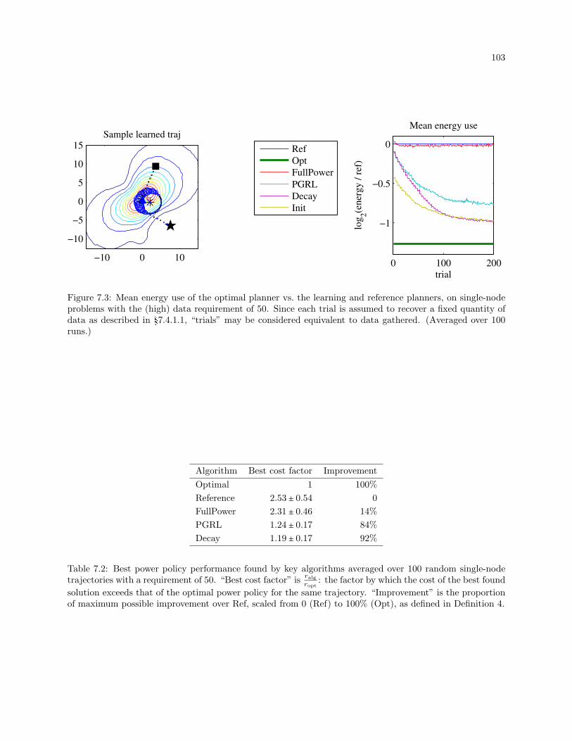
103

Sample learned traj

−10 0 10

−10

−5

0

5

10

15

0 100 200

−1

−0.5

0

trial

log

2(e

ner

gy

/ r

ef)

Mean energy use

Ref

Opt

FullPower

PGRL

Decay

Init

Figure 7.3: Mean energy use of the optimal planner vs. the learning and reference planners, on single-nodeproblems with the (high) data requirement of 50. Since each trial is assumed to recover a fixed quantity ofdata as described in §7.4.1.1, “trials” may be considered equivalent to data gathered. (Averaged over 100runs.)

Algorithm Best cost factor Improvement

Optimal 1 100%

Reference 2.53 ± 0.54 0

FullPower 2.31 ± 0.46 14%

PGRL 1.24 ± 0.17 84%

Decay 1.19 ± 0.17 92%

Table 7.2: Best power policy performance found by key algorithms averaged over 100 random single-nodetrajectories with a requirement of 50. “Best cost factor” is

ralgropt

: the factor by which the cost of the best found

solution exceeds that of the optimal power policy for the same trajectory. “Improvement” is the proportionof maximum possible improvement over Ref, scaled from 0 (Ref) to 100% (Opt), as defined in Definition 4.

104

possible. So far, the learners that we have looked at start with θp = [1 0]T , which, as will be seen in the

coming sections, leads to performance little better than Reference for the first few trials. To see the effect

of early learning speed we show a learner, Init, designed to take advantage of the observation that setting

the power to half of its maximum tends to produce safe policies, as described in §7.3.2.3. Init initialises

θp = [0.5 0]T , and thus matches the performance of HalfPower immediately, after which it learns identically

to Decay. Better initialisations are available, but will not be investigated here.

This comparison assumes that a model can be built with no energy cost, which is not possible. A more

thorough comparison could reflect the fact that a certain amount of energy is spent initially with no—or at

least significantly reduced—data transport. This would cause the cumulative performance line for Optimal

to curve similarly to the learners. However, the energy required for SNR detection should not be significant

compared to that required for data transfer, and is analogous to the posited probe packets that the learners

use to measure the channel, so it is not considered in these comparisons.

7.4.1.4 Optimal planning with imperfect models

The optimal planner achieves perfect results given a perfect model, but in practice the model will be

imperfect. These experiments are at best qualitative, since even a perfect model of the radio simulator does

not consider all real radio field effects—the true effect of modelling error tends to be larger, as Chapter 9

will suggest. The purpose of this section is to begin to answer the question: How realistic a goal is optimal

performance?

Here we assume that the optimal planner’s model consists of the position and dipole antenna orien-

tation of each radio source on the field, and uses these to predict channel quality. As a proxy for various

real-world modelling errors, the radio field model is degraded as follows: Gaussian noise of variance σ2 is

added to the nodes’ positions and their antennas’ orientations. Note the units—angles are in radians, but

distances have a scale: recall that the UA flies at altitude z = 3 and orbits at radius 3 about waypoints, so

a position error of 0.1 corresponds to a difference of about 2.5% between true and expected distances to the

node. This makes the choice of using the same σ for both noise parameters unsophisticated, but the choice

is adequate for approaching the idea of optimal planning under inaccurate models.

105

Figure 7.4 shows results over a range of σ. The performance loss is slight up to σ = 0.1, significant at

σ = 0.2, and model quality has begun to seriously impact the performance of the optimal planner by σ = 0.5,

by which time its asymptotic performance is no better than the learners’. Recall that these results are highly

dependent on the details of the simulator, and that their significance is impacted by the value placed on

immediate utility vs. initial model-building, so they serve only to illustrate the potential ability of a learning

policy optimiser to compete with an optimal planning approach.

7.4.2 Single node, no position error

The previous section provided context and a justification for a further examination of reinforcement

learning for UA-ferried sensor network design. We now turn to a more detailed look at the different learning

algorithms, and show why the learner that was compared to optimal planning in §7.4.1, using the Truncated

Gaussian (TruncN) exploration strategy, was a reasonable choice.

Figure 7.5 shows results for a single node with perfect position information. FullPower performs

very slightly better than Reference due to its learning of waypoint positions. HalfPower immediately

provides a significant improvement, with a ∼ 30% reduction in energy used, although this varies with data

requirement—for high requirements, when many orbits are required in order to achieve data collection goals

(e.g., req > 100), Half-power tends to reduce energy use by only 20% with a 60% increase in trajectory length.

The learners surpass the performance of the handcoded heuristics relatively quickly. TruncN and

MaybeN perform best, eventually allowing on the order of a ∼ 63% reduction in radio energy, although they

occasionally exceed the aircraft’s range limit (by around 0.8% on average). These length penalties bring the

average cost improvement down to ∼ 55%. ϵ-greedy converges slightly more slowly than the others.

LogN achieves the worst long-term performance. Indeed, LogN does not converge at all, as can be

seen by its ever-increasing underrun at the range limit, and by the fact that it tends to discover low-cost

trajectories around trial 70 and then to perform worse with further learning. When SNRprobed < Rthreshold,

its exploration noise, while nonzero, is of insufficient magnitude to produce a meaningful gradient estimate,

producing dynamics similar to those of a random walk in that region. This can be largely rectified by adding

non-log normal noise as in TruncN, or even uniformly distributed noise as in ϵ-greedy if the analogous

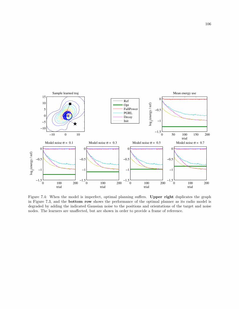
106

0 100 200−1.5

−1

−0.5

0

trial

Model noise σ = 0.1

log

2(e

ner

gy

/ r

ef)

0 100 200−1.5

−1

−0.5

0

trial

Model noise σ = 0.3

0 100 200−1.5

−1

−0.5

0

trial

Model noise σ = 0.5

0 100 200−1.5

−1

−0.5

0

trial

Model noise σ = 0.7

Sample learned traj

−10 0 10

−10

−5

0

5

10

15

Ref

Opt

FullPower

PGRL

Decay

Init

0 50 100 150 200−1.5

−1

−0.5

0

trial

log

2(e

ner

gy

/ r

ef)

Mean energy use

Figure 7.4: When the model is imperfect, optimal planning suffers. Upper right duplicates the graphin Figure 7.3, and the bottom row shows the performance of the optimal planner as its radio model isdegraded by adding the indicated Gaussian noise to the positions and orientations of the target and noisenodes. The learners are unaffected, but are shown in order to provide a frame of reference.

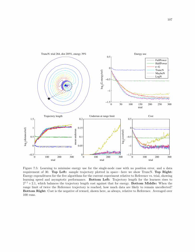
107

TruncN: trial 264, dist 205%, energy 39%

0 100 200 300−0.5

0

0.5

1

1.5

trial

log

2(d

ista

nce

/ref

)

Trajectory length

0 100 200 3000

0.05

0.1

0.15

0.2

trial

mea

n u

nd

erru

n

Underrun at range limit

0 50 100 150 200 250 300−1.5

−1

−0.5

0

0.5

trial

log

2(Σ

en

erg

y/r

ef)

Energy use

FullPower

HalfPower

ε−G

TruncN

MaybeN

LogN

0 100 200 300−1.5

−1

−0.5

0

0.5

trial

log

2(c

ost

/ref

)

Cost

Figure 7.5: Learning to minimise energy use for the single-node case with no position error, and a datarequirement of 30. Top Left: sample trajectory plotted in space—here we show TruncN. Top Right:Energy expenditures for the five algorithms for the current experiment relative to Reference vs. trial, showinglearning speed and asymptotic performance. Bottom Left: Trajectory length for the learners rises to21.1 ≃ 2.1, which balances the trajectory length cost against that for energy. Bottom Middle: When therange limit of twice the Reference trajectory is reached, how much data are likely to remain uncollected?Bottom Right: Cost is the negative of reward, shown here, as always, relative to Reference. Averaged over100 runs.

108

gradient hack (treating the random noise as if they had been generated by the log-normal distribution) is

implemented. In order to test this explanation, the effect of this hack will be shown as “LogN” in Figures 7.6–

7.7 in the following section. However, the enhancement will not be explored further, since the purpose of

discussing LogN is to introduce a reasonable-seeming but ultimately unsuccessful policy. A similar pattern

could be expected of MaybeN, but in that case, when exploration does occur, it results in a sufficiently wide

spread between Pnow and 0. More interesting is the general tendency to perform well in early trials and then

degrade over time due to some subtle policy flaw. This will be addressed in Chapter 8.

7.4.3 Position error

As can be seen in Figure 7.6, results with sensor position error (here set to error = 5) are similar

to those without. Energy savings are far better compared to Reference because while the learners adjust

the trajectory to compensate for the poor information, Reference is crippled by it. There is a large dip in

trajectory length before it begins to climb again; this is due to the relatively simple waypoint optimisation

occurring before the somewhat more complex (state-dependent) radio power policy converges.

FullPower and HalfPower do not adjust their power policies, but merely by moving the waypoint

they achieve 43% and 57% savings, and they do so quickly. The Learners do better: MaybeN learns slightly

more slowly than the others but achieves the best final result with ∼ 80% energy reduction. As described in

§7.4.2, the modified LogN is no longer unstable but still performs the worst, eventually discovering policies

that reduce energy needs by ∼ 75% and showing evidence of having not yet converged by trial 300.

7.4.4 Scalability

Because each policy parameter is linked to the performance in the vicinity of a specific node, learning

time was not expected to significantly grow with problem size. Figure 7.7 shows an 8-node problem with

position error = 5, where it can be seen that learning times are longer than for the single-node case. Much of

the effect is explained as follows: with 8 closely-spaced nodes, the radio field has become far more complex,

which causes the angle between local performance gradient and direction to local optimum to increase. This

leads to increased learning times. The effect diminishes when the nodes are separated by greater distance.

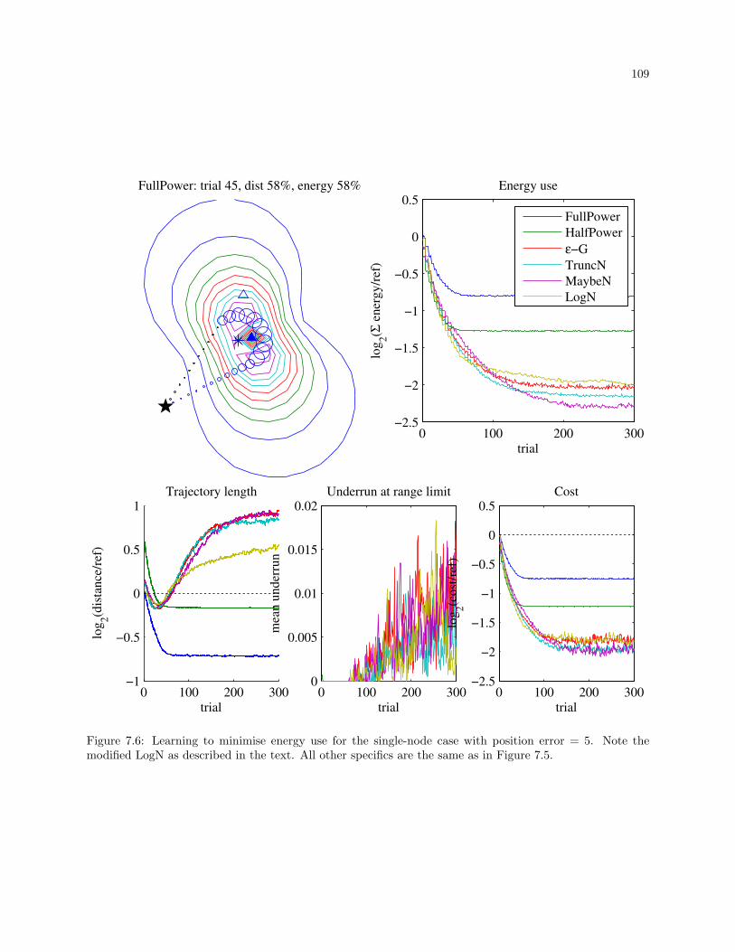
109

FullPower: trial 45, dist 58%, energy 58%

0 100 200 300−1

−0.5

0

0.5

1

trial

log

2(d

ista

nce

/ref

)

Trajectory length

0 100 200 3000

0.005

0.01

0.015

0.02

trial

mea

n u

nd

erru

n

Underrun at range limit

0 100 200 300−2.5

−2

−1.5

−1

−0.5

0

0.5

trial

log

2(Σ

en

erg

y/r

ef)

Energy use

0 100 200 300−2.5

−2

−1.5

−1

−0.5

0

0.5

trial

log

2(c

ost

/ref

)

Cost

FullPower

HalfPower

ε−G

TruncN

MaybeN

LogN

Figure 7.6: Learning to minimise energy use for the single-node case with position error = 5. Note themodified LogN as described in the text. All other specifics are the same as in Figure 7.5.

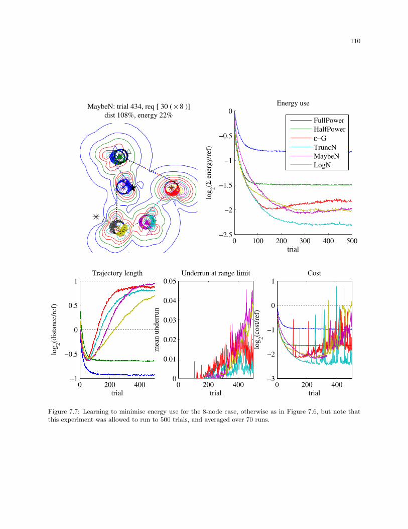
110

MaybeN: trial 434, req [ 30 ( × 8 )]

dist 108%, energy 22%

0 200 400−1

−0.5

0

0.5

1

trial

log

2(d

ista

nce

/ref

)

Trajectory length

0 200 4000

0.01

0.02

0.03

0.04

0.05

trial

mea

n u

nd

erru

n

Underrun at range limit

0 100 200 300 400 500−2.5

−2

−1.5

−1

−0.5

0

trial

log

2(Σ

en

erg

y/r

ef)

Energy use

0 200 400−3

−2

−1

0

1

trial

log

2(c

ost

/ref

)

Cost

FullPower

HalfPower

ε−G

TruncN

MaybeN

LogN

Figure 7.7: Learning to minimise energy use for the 8-node case, otherwise as in Figure 7.6, but note thatthis experiment was allowed to run to 500 trials, and averaged over 70 runs.

111

Alternatively, single-node learning performance decreases on fields with a similar number of point noise

transmitters.

In Figure 7.7, MaybeN’s performance no longer equals that of TruncN in these complex and noisy

radio fields: the scarcity of exploration steps when SNRprobed < Rthreshold mentioned in §7.4.2 becomes

problematic, preventing MaybeN from discovering good policies. TruncN maintains exploration throughout

its policy space, allowing it to reduce energy use by ∼ 80% compared to Reference with this position error.

Figure 7.7 shows one anomaly: all of the learning policies destabilise somewhat after many trials.

TruncN suffers the least from this, but like the others, it has entered a region in the policy space in which

even small policy exploration steps have a high risk of hurting performance. This will be discussed in the

next chapter.

7.5 Summary

This chapter introduced a simple node radio power policy, and a reinforcement learner that refines

the policy with experience. In order to use reinforcement learning, exploration noise must be added to the

desired policy, and four exploration algorithms were considered. Each of them can learn to represent policies

that produce nearly optimal behaviour over a given trajectory, although they differ in how well they facilitate

the learning process.

TruncN’s performance is similar to that of MaybeN in the single-node case, but is clearly superior as

radio field complexity increases—it learns as fast as any other exploration strategy, achieves the best results

by a sometimes significant margin, and is stable. Therefore it will be used henceforth.

LogN performed spectacularly poorly due to its failure to explore when SNRprobed < Rthreshold. More

than just furnishing an example of a poor policy, it shows that reasonable policies can perform well in early

trials and then find their way into regions in policy space in which the gradient estimator performs poorly. In

general, subtle flaws in policy design and parameter tuning can harm performance. Chapter 8 will introduce

a multitask learner that not only allows learners to converge more quickly, but also learns situations in

which such a policy is at risk, and, based on past experience, gently guides the gradient estimator towards

solutions that are likely to be good.

112

Most importantly, the learners were shown to perform well with respect to an optimal planner. Learn-

ing can eventually achieve near-optimal results, and although the learners take some time to converge, this

must be set against the time required by an optimal planner for system identification. If immediate deploy-

ment is important, then a reinforcement learning system may provide a viable alternative to model-based

planning.

Chapter 8

Learning to Learn Energy Policies

This chapter introduces a long-timescale reinforcement learner that learns to augment the gradient-

based policy optimisation process that occurs due to PGRL. Through observing and being allowed to interact

with the gradient-based policy optimisation process, it learns to suggest policy updates, increasing policy

learning speed. Furthermore, it allows the transfer of this knowledge of the optimisation procedure to other

instances of the problem.

The learning framework developed up to this point produces trajectories that exploit the limits of ferry

endurance. For example, when the allowable flight length is twice that of a handcoded reference trajectory

and accurate sensor location information is available, the system learns to reduce sensor communication

energy by roughly 60% after around 70 flights (subject to tuning), and when the sensor location information

is inaccurate, the learners do even better relative to non-learning approaches.

However, there is room for improvement. This chapter is concerned with three weaknesses of the

framework developed so far:

The energy policy in particular is sensitive to parameter choice and system design, and poor choices

can lead to high sampling costs or even to divergent behaviours.

Exploration noise can lead to high-cost samples. If noise is reduced, exploration suffers. Can we

learn how to steer the optimiser away from regions in which high sampling costs are likely to be

incurred?

While the learning speeds shown in previous chapters may be acceptable for some applications, faster

114

learning is preferred.

The primary contribution of this chapter is a higher-level policy that learns to speed and stabilise the learning

of new policies for unseen data-ferrying problems. This higher-level policy is trained using a variant of PGRL

on optimisation histories for the low-level policy, allowing it to anticipate updates that might lead to good

or bad outcomes several learning steps into the future.

8.1 Motivation

Chapter 7 showed that the learning energy policies can produce good behaviour, but there were some

surprises. Figure 7.5 (p. 105) showed that the lognormal power policy exploration strategy diverged even

on the simplest problem; Figure 7.7 (p. 110) demonstrated that all of the exploration strategies occasionally

produced expensive exploration steps at high trial numbers; and we will see in §8.5.3 that even without a

decaying learning rate, the choice of α is an exercise in compromise. Are these quirks specific to our chosen

domain, or do they reflect some general characteristic of policy gradient methods? The answer is: a little of

each.

Figure 8.1 shows a portion of the energy reward landscape (Equation 7.12) for trajectories looping

a typical node, assuming a fixed waypoint location. When RT is small and Ptarget is near 1, the reward

gradient on the power policy is not difficult to estimate on average, but the shallow slope, the ridges and

valleys, and the sampling noise for other policy parameters—in this case, waypoint location—lead to a noisy

estimate. But these do not account for the initial convergence and subsequent frequent high-cost samples

exhibited by the learning algorithms, all of which converge to a policy near the global optimum.

In the vicinity of the optimal solution (the crest of the hill), the energy reward function is highly

nonlinear with respect to the power policy parameters. If RT becomes too high or Ptarget becomes too low,

the aircraft must add a loop to its trajectory in order to collect all the data.

Conventional PGRL repeatedly estimates the reward gradient near the current policy and takes a

hillclimbing step. Near the optimum, policy updates or sampling can result in the learner taking a step off

the reward cliff, or “cliff-jumping”, and on many problems, the closer the power policy is to the optimum,

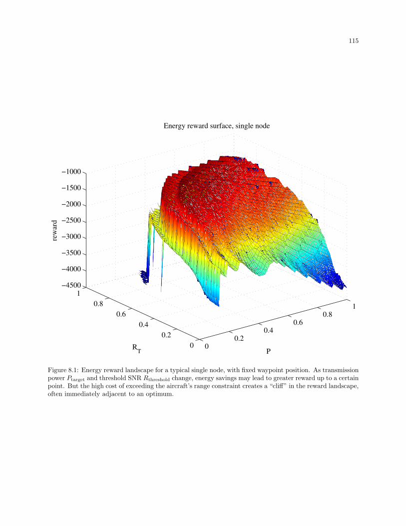
115

00.2

0.40.6

0.81

0

0.2

0.4

0.6

0.8

1−4500

−4000

−3500

−3000

−2500

−2000

−1500

−1000

P

Energy reward surface, single node

RT

rew

ard

Figure 8.1: Energy reward landscape for a typical single node, with fixed waypoint position. As transmissionpower Ptarget and threshold SNR Rthreshold change, energy savings may lead to greater reward up to a certainpoint. But the high cost of exceeding the aircraft’s range constraint creates a “cliff” in the reward landscape,often immediately adjacent to an optimum.

116

the closer it is to the cliff.

Furthermore, the cliff contains local regions in which a problematic reverse-sloped ledge structure is

apparent—it is possible for a local gradient estimate to suggest a step further off the cliff. Confidence regions

can mitigate the problem caused by policy updates, but they generally fail to re-use information acquired

during past steps (but see [Kolter et al., 2012] for a counterexample). Cliff-jumping due to the exploration

noise required by the gradient estimator is more difficult to eliminate.

8.2 Metapolicies

The problematic structure in the reward landscape motivated the development of a technique to

encode knowledge of the process of optimising on reward landscapes like ours.

The energy policy is sensitive to a state that changes over the course of a trajectory: πp(s; θp) is

chosen based on the measured SNR at each timestep. Some additional information is available only at the

end of the trajectory. Most useful in this case is an intermediate value from the computation of the the

hard limit term from Equation 7.12: the value d − dmax. Even when this term does not affect reward (i.e.

when d < dmax), it provides information that can be used to improve the policy. However, this information

is not available to πp during flight, and so it is difficult to incorporate into πp. The longer timescale of

the availability of this information makes it awkward to shoehorn into the base gradient estimator, and its

applicability to various problem configurations makes it natural to hand it to a multitask learner.

Under the reinforcement learning paradigm, this additional information can naturally be enriched over

multiple tours: the one-step return can be extended to a multi-step (discounted) return by looking not just

at the relationship between a policy update step after trajectory τk and the consequent reward on trajectory

τk+1, but between a policy update step after τk and the sequence of likely subsequent trajectories τk+[1...∞]

and the rewards that they receive.

A policy that operates on a policy is often referred to as a metapolicy. A PGRL policy π is a noisy

function that takes a state s to an action u, and learns a mapping that optimises the expectation of some

sum over time of the reward r. For the base energy learner’s policy πp, the state s is the sensed SNR at

each timestep, the action u is the radio’s output power for that timestep, and the reward is a function of the

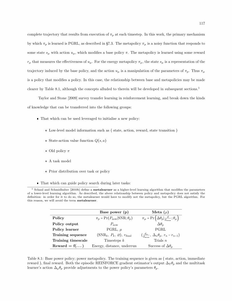
117

complete trajectory that results from execution of πp at each timestep. In this work, the primary mechanism

by which πp is learned is PGRL, as described in §7.3. The metapolicy πµ is a noisy function that responds to

some state sµ with action uµ, which modifies a base policy π. The metapolicy is learned using some reward

rµ that measures the effectiveness of uµ. For the energy metapolicy πµ, the state sµ is a representation of the

trajectory induced by the base policy, and the action uµ is a manipulation of the parameters of πp. Thus πµ

is a policy that modifies a policy. In this case, the relationship between base and metapolicies may be made

clearer by Table 8.1, although the concepts alluded to therein will be developed in subsequent sections.1

Taylor and Stone [2009] survey transfer learning in reinforcement learning, and break down the kinds

of knowledge that can be transferred into the following groups:

That which can be used leveraged to initialise a new policy:

* Low-level model information such as ⟨ state, action, reward, state transition ⟩

* State-action value function Q(s, a)

* Old policy π

* A task model

* Prior distribution over task or policy

That which can guide policy search during later tasks:

1 Schaul and Schmidhuber [2010b] define a metalearner as a higher-level learning algorithm that modifies the parametersof a lower-level learning algorithm. As described, the above relationship between policy and metapolicy does not satisfy thedefinition: in order for it to do so, the metalearner would have to modify not the metapolicy, but the PGRL algorithm. Forthis reason, we will avoid the term metalearner.

Base power (p) Meta (µ)

Policy πp = Pr(Pnow∣SNR; θp) πµ = Pr (∆θp∣ ddmax

; θµ)Policy output Pnow ∆θp

Policy learner PGRL, µ PGRL

Training sequence ⟨SNRk, Pk, ∅⟩, rfinal ⟨ dn

dmax, ∆nθp, rn − rn−1⟩

Training timescale Timesteps k Trials n

Reward = f(. . . ) Energy, distance, underrun Success of ∆θp

Table 8.1: Base power policy; power metapolicy. The training sequence is given as ⟨ state, action, immediatereward ⟩, final reward. Both the episodic REINFORCE gradient estimator’s output ∆∇θp and the multitasklearner’s action ∆µθp provide adjustments to the power policy’s parameters θp.

118

* What actions to take under certain circumstances

* Fragments of policies

* Rules or advice

* Important state features

* Shaping rewards

* Subtask definitions

In terms of that breakdown, the current chapter describes the transfer of something that is best described

as “Rules or advice”, but the rules apply not to the action taken by the policy, but to the actions taken by

the policy learner.

When a trial leads to an overly long trajectory, it is generally helpful to increase radio power or

transmit at lower detected SNR. Conversely, for a trajectory that does not use the aircraft’s full range, node

energy can be reduced without penalty (assuming the reward function given in Equation 7.12) by reducing

radio power or transmit time. The PGRL gradient estimation finds policy updates that, on average, tend

to obey these heuristics, but only as a side-effect of the gradient estimation process, and at each policy

update the sampling must discover the gradient estimate anew. Furthermore, the PGRL updates can result

in policies from which further exploration is likely to be expensive due to the microstructure and the abrupt

cliff near the global optimum.

Our goal in developing a multitask learner is to give the UA the ability to use experience with

past problems to improve learning speed and robustness on new problems and automatically capture such

heuristics. We investigate the following questions:

Can a metapolicy that encodes knowledge about optimising policies in this domain be learned through

experience?

Can such a metapolicy transfer knowledge within a problem between nodes?

Can such a metapolicy transfer knowledge between problems?

Can the metapolicy be used to speed the learning of energy-saving policies for sensor networks?

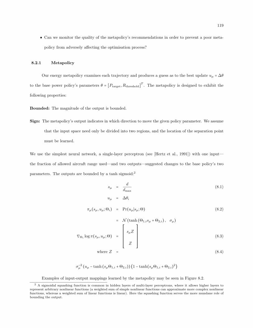
119

Can we monitor the quality of the metapolicy’s recommendations in order to prevent a poor meta-

policy from adversely affecting the optimisation process?

8.2.1 Metapolicy

Our energy metapolicy examines each trajectory and produces a guess as to the best update uµ =∆θ

to the base power policy’s parameters θ = [Ptarget,Rthreshold]T . The metapolicy is designed to exhibit the

following properties:

Bounded: The magnitude of the output is bounded.

Sign: The metapolicy’s output indicates in which direction to move the given policy parameter. We assume

that the input space need only be divided into two regions, and the location of the separation point

must be learned.

We use the simplest neural network, a single-layer perceptron (see [Hertz et al., 1991]) with one input—

the fraction of allowed aircraft range used—and two outputs—suggested changes to the base policy’s two

parameters. The outputs are bounded by a tanh sigmoid:2

sµ = d

dmax(8.1)

uµ = ∆θi

πµ(sµ, uµ;Θi) = Pr(uµ∣sµ;Θ) (8.2)

= N (tanh (Θ1,isµ +Θ2,i) , σµ)

∇Θi logπ(sµ, uµ;Θ) =

⎡⎢⎢⎢⎢⎢⎢⎢⎢⎢⎣

sµZ

Z

⎤⎥⎥⎥⎥⎥⎥⎥⎥⎥⎦

(8.3)

where Z = (8.4)

σ−2µ (uµ − tanh (sµΘ1,i +Θ2,i)) (1 − tanh(sµΘ1,i +Θ2,i)2)

Examples of input-output mappings learned by the metapolicy may be seen in Figure 8.2.

2 A sigmoidal squashing function is common in hidden layers of multi-layer perceptrons, where it allows higher layers torepresent arbitrary nonlinear functions (a weighted sum of simple nonlinear functions can approximate more complex nonlinearfunctions, whereas a weighted sum of linear functions is linear). Here the squashing function serves the more mundane role ofbounding the output.

120

0 1 2−1

−0.5

0

0.5

1

dist ratio

∆µθ

e

PGRL+µ: πµ, run 10

0 1 2−1

−0.5

0

0.5

1

dist ratio

∆µθ

ePGRL+µ: π

µ, run 30

0 1 2−1

−0.5

0

0.5

1

dist ratio∆

µθ

e

PGRL+µ: πµ, run 80

Ptarget

Rthreshold

Figure 8.2: Example visualisations of metapolicies learned for a single node. “Dist ratio” is the ratio oftrajectory length to maximum permissible length, and ∆µθp indicates the metapolicy’s suggestion for thevariation to the parameter θp ∈ Ptarget,Rthreshold. Left: πµ learned by PGRL+µ after 10 runs of 100 trials.Middle: After 30 runs, a good policy has begun to take shape. Right: A helpful metapolicy has emerged:when trajectories are too long, the energy policy’s parameter Ptarget should increase and Rthreshold shoulddecrease, and vice versa. The value of “too long” is learned with reference to possible future states andactions. Unintuitively, the value of d

dmaxabove which Rthreshold should generally decrease is higher than that

for which Ptarget should increase. This is a pattern seen in most of the learned metapolicies, although thecrossover point varies with problem parameters, and it signifies a region in which past experience suggeststhat the best update to πp is one that increases both Ptarget and Rthreshold.

121

Our purpose is not to determine the best metapolicy encoding, but rather to demonstrate that some

metapolicy encoding can speed and stabilise learning of the base policy. If the perceptual space is enriched

with other inputs or a more expressive representation is desired, other models can be used. For example, the

same inputs could be mapped using a basis function network similar to that described in §8.4.1.1. However,

more complex models, or ones with more parameters, increase the number of runs necessary for learning a

good metapolicy.

8.2.2 Metareward

The metapolicy learner’s objective is to learn a metapolicy that takes as input some observable features

of a trajectory, and outputs an “action” consisting of an improvement of the base policy’s parameters. So

our metareward rµ reflects the improvement due to the most recent policy update:

rµ = rk − rk−1 (8.5)

where rk is the base reward received on trajectory k.

8.2.3 Time-discounted credit

The metapolicy receives µ-reward (Equation 8.5) after every µ-action, and each µ-action also—to

a lesser extent—affects future µ-states and thus potential µ-rewards, so it would be appropriate to use a

time-discounted eligibility (γ < 1 in Equation 4.3). But further improvements are to be gained by using a

more sophisticated gradient estimator, which we introduce here:

8.2.3.1 G(PO)MDP

Here we drop the µ-prefix, as this section describes a well-known general technique. In reinforcement

learning, when an action u is taken at time tu and a reward r is received at future time tr, the action

is assigned credit for the reward based on an estimate of how important the action was in producing the

reward. In eR (§4.3), greater weight may be given to rewards received early in the episode than on those

received later, modulated by the term γtk , 0 < γ ≤ 1 in Equation 4.3. G(PO)MDP [Baxter and Bartlett,

122

2001] uses the separation in time between tu and tr to assign credit in proportion to γtr−tu , tu < tr. We use

G(PO)MDP as described in [Peters and Schaal, 2008]. The gradient estimator is related to Equation 4.3:

gθi = ⟨H

∑p=0(

p

∑k=0∇θi logPr(uk ∣sk; θ)) (γtprp − bi,p)⟩ (8.6)

We use the optimal baseline bi from [Peters and Schaal, 2008], which is similar to that described in Equa-

tion 4.4 but is computed for each gradient element i at every timestep k:

bi,k =⟨(∑k

j=1∇θi logPr(uj ∣sj ; θ))2γtkrk⟩

(∑Hk=1∇θi logPr(uk ∣sk; θ))

2(8.7)

In our simulations, the learning rate and ultimate performance of the metapolicy are minimally sen-

sitive to the metapolicy learner’s temporal µ-reward discount γ through a broad range, learning too much

or too little caution only when γ > ∼ 0.9 or γ < ∼ 0.2, respectively.

When γ2 is less than the threshold (0.01) described in the following section (§8.2.3.2), the ability of

the reinforcement metapolicy learner to anticipate future metarewards vanishes—i.e., the metapolicy learner

does not include discounted future rewards in its computation of expected return—it cannot see the problem

with an update that takes πp into a space from which exploration noise is likely to go off the edge of the

cliff). Thus it degrades into a single-step predictor, which, while still helpful, is less effective than the

multi-step–aware case.

8.2.3.2 Sliding trajectory windows

In the episodic formulation presented above, when γ < 1, Equation 8.6 learns from rewards received

early in the trajectory but not later, since γt drives the value of later rewards to 0. In order to apply the

estimator to non-episodic tasks, we break each trajectory into sequences of ⟨sµ, aµ, rµ⟩ with one sequence

starting at each timestep, and present those as separate trajectories to Equation 8.6. We choose sequence

length n such that γn ≥ 0.01 > γn+1: the terms beyond this threshold increase computational burden without

significantly improving accuracy.

123

8.2.4 Training

The training sequence used by the metapolicy learner consists of a gradient on the probability of

producing the meta-action from the metastate, and the resulting metareward:

∇Θ logPr(uµ,k ∣sµ,k;Θ): The gradient of the log probability of the chosen meta-action uµ after trial k.

rµ,k: The change in reward seen between trials k−1 and k, which is affected by uµ, and thus by πµ(sµ,k−1;Θ).

The gradient for the energy policy update is normalised, so the energy policy changes by an amount whose

magnitude is αp. Thus the metareward rµ is based on a meta-action of fixed size ∣∣∆θp∣∣∞ = αp. For this

reason, the metapolicy is designed to output (with the addition of exploration noise) a value mimicking

the PGRL update; hence the sigmoidal squashing function on each output variable: ∣∣uµ∣∣∞ = αp + ϵ for

exploration noise ϵ.

8.3 Three Learners

With the state and action spaces we have defined, the metapolicy can be used on its own, or in

combination with the PGRL policy updates. So we have three possible ways of learning an energy policy,

described in the next three subsections:

8.3.1 PGRL

All adjustments ∆θp to the energy policy πp(s; θp) come from the PGRL gradient estimate—∆∇θp.

This was examined in Chapter 7.

8.3.2 Pure µ

All adjustments to the energy policy come from the metapolicy, as described above. These updates

will be called ∆µθp.

The gradient estimates ∇Θ logPr(uµ∣sµ;Θ) for the metapolicy learning algorithm use action uµ from

the metapolicy’s update at the end of each trial.

124

8.3.3 Gradient-guided meta-exploration with hybrids

Changes ∆θ to the base policy’s parameters θ can be computed by the base PGRL estimator (§7.1)

after every epoch, or from the metapolicy (Equation 8.2) via uµ after every trial. When the base PGRL

estimator produces an estimate, it is used to adjust θ. But we can also pretend that it came from πµ,

and use it as uµ for the computation of ∇Θ logPr(uµ∣sµ;Θ), similarly to the fake gradient mentioned in

§7.3.1.1. Thus both the PGRL and the πµ updates and metarewards can be used to form the µ-trajectory

for Equation 8.6. This can be done in a principled way, as described in the next section.

8.4 Combining ∇∆ and ∇µ

Early in training, the metapolicy can give poor advice, leading to high-cost policies. If ample non-

mission training time is allocated, then such runs do not pose a problem. In our single-node example, roughly

30 runs of 100 trials each were required (in the single-node case) before the metapolicy reliably improved upon

PGRL. Knowledge encoded by the metapolicy can be transferred between nodes or problems, and therefore

metapolicy training time for any new scenario may be low or even nonexistent, but here we investigate

a technique for reducing the adverse effect of poor metaknowledge while training, tuning, and testing the

metapolicy in a live network.

8.4.1 Mean Squared Error of the gradient updates

If the mean squared error (MSE) between the true gradient and the various gradient estimates is

known, then the estimates can be combined as ∆θ = 1MSE∇

∆∇θ + 1MSEµ

∆µθ. Can we compute these MSEs?

8.4.1.1 MSE of PGRL gradient estimate

Episodic REINFORCE provides an unbiased estimate of the gradient [Peters and Schaal, 2008], so

the gradient estimate’s MSE is just its variance. However, even when each gradient estimate is correct, the

estimates’ variance over a trajectory is high. For example, consider the gradient estimate near an optimum.

If the learning step size α is too large, then the gradient estimate will repeatedly change sign. For this

reason, it is important to measures variance as a function of the metapolicy’s notion of “state” ( ddmax

; see

125

Equation 8.1).

In order to maintain an estimate of variance at unseen states, a simplified Gaussian Radial Basis

Function (RBF) network (with fixed basis function centres uniformly spanning the useful range of the µ-

state space (c ∈ 0,0.1 . . .2) and widths σ = 0.05) was used. The training set was the set of ⟨sµ, uµ⟩ pairs

from all runs in the current experiment, for each trial in which a PGRL update was computed (although

2 or 3 runs generally sufficed for a useful estimate). The inferred variance in the vicinity of each basis

function ϕc centered on sµ = c was the total variance of the training set weighted by the radial distance

ϕc(s) = exp (− (s−c)2

2σ2 ).

The RBF network was an expedient way of generating a suitable function approximation. If the state

space were of higher dimension, the network would be problematic and other approximation techniques, or

possibly an RBF network with adaptive means and widths, would be more appropriate.

8.4.1.2 MSE of µ gradient estimate

The metapolicy’s gradient estimates have known mean and variance, given in Equation 8.2. Since

PGRL provides an unbiased estimate of the gradient, the bias of the gradient provided by the metapolicy

can be computed as the difference between the sampled mean PGRL estimate and the mean from which the

metapolicy’s output is drawn. The mean of the PGRL gradient estimate, ⟨∆∇θp⟩, was provided by another

RBF network, identical to that described in §8.4.1, trained on the sampled PGRL gradient estimates ∆∇θp

as above. The metapolicy’s MSE is thus:

∣∣ tanh (Θ1,isµ +Θ2,i) − ⟨∆∇θ⟩ ∣∣2 + σ2µ (8.8)

8.4.2 Combining the gradient estimates

At the end of every epoch, the energy policy’s parameters θp are changed by an amount given by

the PGRL estimate: ∆∇θp. At the end of each trial, the metapolicy provides its own best guess for the

update: ∆µθ, which may correct a bad update due to ∆∇θp. The updates should be combined so that

∆θ = 1MSE∇

∆∇θ + 1MSEµ

∆µθ, which is achieved by scaling the metapolicy’s update ∆µθp by magnitude

MSE∇MSEµ

⋅ 1trials per epoch−1 and applying the result to θp after every trial on which PGRL does not produce a

126

gradient estimate.

8.4.2.1 Off-policy gradient estimates

When the metapolicy updates the policy during an epoch, PGRL is no longer being furnished with

correct information: at trial j, the policy was π(s; θ(j)), and the computed gradient of the probability of the

trajectory was ∇θ(j) logπ(s; θ(j)).

A correction should be applied to the log-probabilities of the trajectories. Tang and Abbeel [2010]

describe how to re-weight the log-probabilities of the gradients of the expected return based on importance

sampling, in which a distribution is . This was implemented here. However, the average corrections were

found to be small—on the order of one percent on average—and made essentially no difference to the results.

8.4.3 Is the true gradient the best update?

The above approach takes ∆∇θp as the ground truth, accepting updates from ∆µθp in inverse pro-

portion to their relative MSE from that “truth”. But the metapolicy learner has access to information not

available to the PGRL learner—in particular, information about the future costs likely to be incurred for any

policy update—and thus may produce better (lower-variance, or safer) policy updates than those produced

by PGRL. In the following section, we will compare the inverse-MSE weighting scheme described above

(“PGRL∝ µ”) with one that weights the terms equally (“PGRL+µ”).

8.5 Experiments

We generate random data-ferrying problems each of which consists of a random position and ori-

entation for each sensor. At each timestep the aircraft flies some distance towards the next waypoint,

measures the current channel quality (for example, measuring SNR via probe packets as described in §7.1),

and requests some data from a node at the power indicated by the power policy. A trial is a single complete

flight over the radio field. An epoch is a small number of trials, after which we estimate the policy gradients

and update the policies. A run is an attempt to optimise radio power and waypoint position policies for

a given problem, and here consists of 200 trials. For each problem we generate a new random radio field,

127

train the metapolicy from the previous run’s learning history, and re-initialise the policies to [1 0]T for each

node (yielding similar behaviour to FullPower).3 Although it is possible to adapt the metapolicy as soon as

we have enough trials to produce a gradient estimate, for simplicity we instead hold the metapolicy’s param-

eters Θ constant during each run. An experiment is a set of 100 runs, each on a different problem, during

which the metapolicies have the opportunity to adapt. For each experiment we re-initialise the metapolicy

parameters to [0]. To generate the graphs, we average over 50 experiments.

We will compare the following approaches:

Reference: the non-learning autopilot defined in §3.2.1.

Half-power learns waypoint placement, but always transmits at P = 0.5, as described in §7.3.2.3.

PGRL uses the Learning autopilot and the conventional PGRL approach described in §7.1, without the

metapolicy.

Pure µ: Since the metapolicy can modify the base energy policy directly, we can evaluate its performance

as a standalone learner. µ does not use the PGRL estimates, but learns the energy policy through

meta-PGRL only.

PGRL+µ combines the updates from PGRL and µ such that the updates have equal size per epoch: the

inverse-MSE technique described in §8.4.1.1 is not used. For reasons given in §8.4.3, this may be

superior to PGRL∝ µ.

PGRL∝ µ combines the updates from PGRL and µ as described in §8.3.3, balancing the updates according

to the MSE ratio described in §8.4.1.1.

The experiments are organised as follows: §8.5.1 details tests showing the performance of a metapolicy on

the most easily solved problems of Chapter 7. §8.5.2 briefly digresses to speculate on why the combination

of policy updates from PGRL and the metapolicy outperforms either approach alone. §8.5.3 tests the

metapolicy’s ability to compensate for poor choice of learning rates. §7.3.4 discussed the special treatment

received by one of the power policy parameters; §8.5.4 further tests the metapolicy’s ability to compensate

3 This is a reasonable choice for comparing algorithms, but the “Init” variant described in §7.4.1.3 suggests a further avenuefor exploration when performance is more important than comparison.

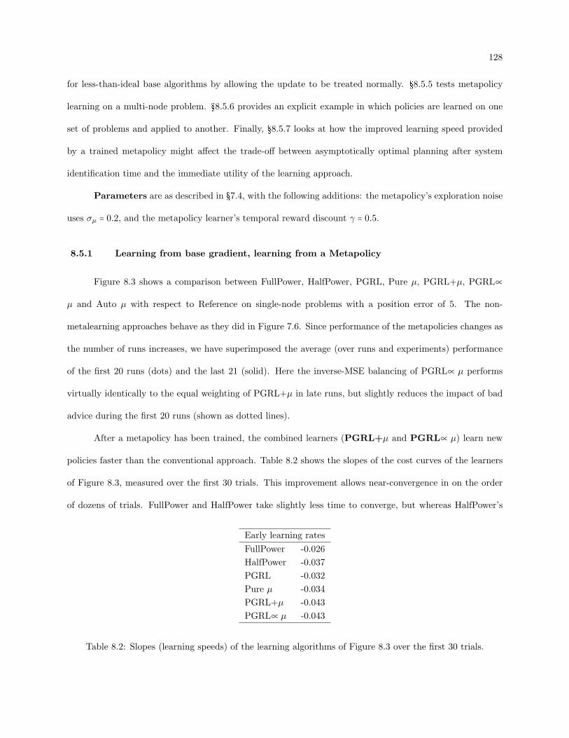
128

for less-than-ideal base algorithms by allowing the update to be treated normally. §8.5.5 tests metapolicy

learning on a multi-node problem. §8.5.6 provides an explicit example in which policies are learned on one

set of problems and applied to another. Finally, §8.5.7 looks at how the improved learning speed provided

by a trained metapolicy might affect the trade-off between asymptotically optimal planning after system

identification time and the immediate utility of the learning approach.

Parameters are as described in §7.4, with the following additions: the metapolicy’s exploration noise

uses σµ = 0.2, and the metapolicy learner’s temporal reward discount γ = 0.5.

8.5.1 Learning from base gradient, learning from a Metapolicy

Figure 8.3 shows a comparison between FullPower, HalfPower, PGRL, Pure µ, PGRL+µ, PGRL∝

µ and Auto µ with respect to Reference on single-node problems with a position error of 5. The non-

metalearning approaches behave as they did in Figure 7.6. Since performance of the metapolicies changes as

the number of runs increases, we have superimposed the average (over runs and experiments) performance

of the first 20 runs (dots) and the last 21 (solid). Here the inverse-MSE balancing of PGRL∝ µ performs

virtually identically to the equal weighting of PGRL+µ in late runs, but slightly reduces the impact of bad

advice during the first 20 runs (shown as dotted lines).

After a metapolicy has been trained, the combined learners (PGRL+µ and PGRL∝ µ) learn new

policies faster than the conventional approach. Table 8.2 shows the slopes of the cost curves of the learners

of Figure 8.3, measured over the first 30 trials. This improvement allows near-convergence in on the order

of dozens of trials. FullPower and HalfPower take slightly less time to converge, but whereas HalfPower’s

Early learning rates

FullPower -0.026

HalfPower -0.037

PGRL -0.032

Pure µ -0.034

PGRL+µ -0.043

PGRL∝ µ -0.043

Table 8.2: Slopes (learning speeds) of the learning algorithms of Figure 8.3 over the first 30 trials.

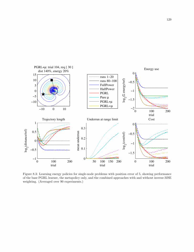
129

PGRL+µ: trial 104, req [ 30 ]

dist 140%, energy 20%

−10 0 10

−10

−5

0

5

10

15

0 100 200−1

−0.5

0

0.5

1

trial

log

2(d

ista

nce

/ref

)

Trajectory length

50 100 150 2000

0.1

0.2

0.3

trial

mea

n u

nd

erru

n

Underrun at range limit

runs 1−20

runs 80−100

FullPower

HalfPower

PGRL

Pure µ

PGRL+µ

PGRL∝µ

0 100 200−2

−1.5

−1

−0.5

0

trial

log

2(Σ

en

erg

y/r

ef)

Energy use

0 100 200

−1.5

−1

−0.5

0

trial

log

2(c

ost

/ref

)

Cost

Figure 8.3: Learning energy policies for single-node problems with position error of 5, showing performanceof the base PGRL learner, the metapolicy only, and the combined approaches with and without inverse-MSEweighting. (Averaged over 90 experiments.)

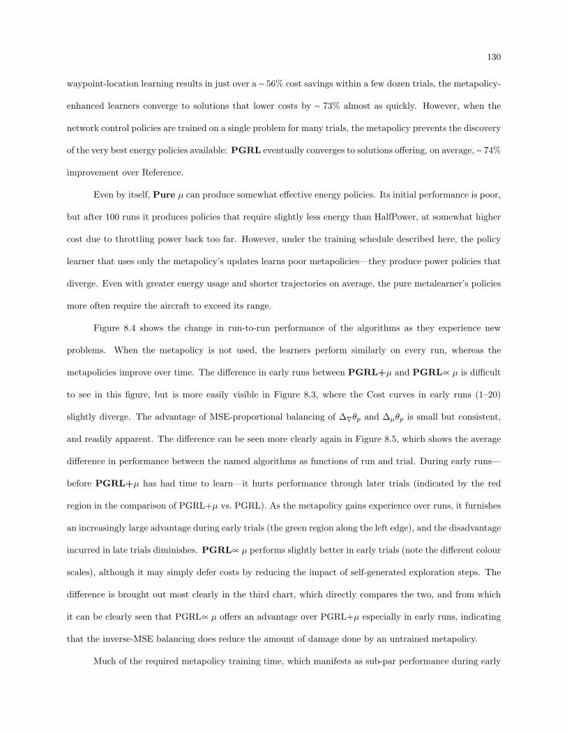
130

waypoint-location learning results in just over a ∼ 56% cost savings within a few dozen trials, the metapolicy-

enhanced learners converge to solutions that lower costs by ∼ 73% almost as quickly. However, when the

network control policies are trained on a single problem for many trials, the metapolicy prevents the discovery

of the very best energy policies available: PGRL eventually converges to solutions offering, on average, ∼ 74%

improvement over Reference.

Even by itself, Pure µ can produce somewhat effective energy policies. Its initial performance is poor,

but after 100 runs it produces policies that require slightly less energy than HalfPower, at somewhat higher

cost due to throttling power back too far. However, under the training schedule described here, the policy

learner that uses only the metapolicy’s updates learns poor metapolicies—they produce power policies that

diverge. Even with greater energy usage and shorter trajectories on average, the pure metalearner’s policies

more often require the aircraft to exceed its range.

Figure 8.4 shows the change in run-to-run performance of the algorithms as they experience new

problems. When the metapolicy is not used, the learners perform similarly on every run, whereas the

metapolicies improve over time. The difference in early runs between PGRL+µ and PGRL∝ µ is difficult

to see in this figure, but is more easily visible in Figure 8.3, where the Cost curves in early runs (1–20)

slightly diverge. The advantage of MSE-proportional balancing of ∆∇θp and ∆µθp is small but consistent,

and readily apparent. The difference can be seen more clearly again in Figure 8.5, which shows the average

difference in performance between the named algorithms as functions of run and trial. During early runs—

before PGRL+µ has had time to learn—it hurts performance through later trials (indicated by the red

region in the comparison of PGRL+µ vs. PGRL). As the metapolicy gains experience over runs, it furnishes

an increasingly large advantage during early trials (the green region along the left edge), and the disadvantage

incurred in late trials diminishes. PGRL∝ µ performs slightly better in early trials (note the different colour

scales), although it may simply defer costs by reducing the impact of self-generated exploration steps. The

difference is brought out most clearly in the third chart, which directly compares the two, and from which

it can be clearly seen that PGRL∝ µ offers an advantage over PGRL+µ especially in early runs, indicating

that the inverse-MSE balancing does reduce the amount of damage done by an untrained metapolicy.

Much of the required metapolicy training time, which manifests as sub-par performance during early

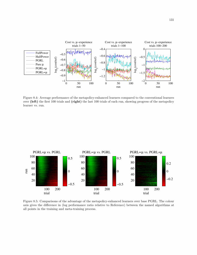
131

FullPower

HalfPower

PGRL

Pure µ

PGRL+µ

PGRL∝µ

0 50 100−1

−0.9

−0.8

−0.7

−0.6

−0.5

run

log

2(c

ost

/ref

)

Cost vs. µ−experience

trials 1−50

0 50 100

−1.2

−1

−0.8

−0.6

−0.4

run

log

2(c

ost

/ref

)

Cost vs. µ−experience

trials 1−100

0 50 100−2

−1.5

−1

−0.5

0

run

log

2(c

ost

/ref

)

Cost vs. µ−experience

trials 100−200

Figure 8.4: Average performance of the metapolicy-enhanced learners compared to the conventional learnersover (left) the first 100 trials and (right) the last 100 trials of each run, showing progress of the metapolicylearner vs. run.

PGRL+µ vs. PGRL

trial

run

100 200

20

40

60

80

100

−0.5

0

0.5

PGRL∝µ vs. PGRL

trial

100 200

20

40

60

80

100

−0.5

0

0.5

PGRL∝µ vs. PGRL+µ

trial

100 200

20

40

60

80

100

−0.2

0

0.2

Figure 8.5: Comparisons of the advantage of the metapolicy-enhanced learners over base PGRL. The colouraxis gives the difference in (log performance ratio relative to Reference) between the named algorithms atall points in the training and meta-training process.

132

runs, may be required only once in a “lifetime” due to the transferability of the converged metapolicies. Once

the metapolicies are trained, they facilitate the discovery of a good policy extremely rapidly, by aggressively

pushing policy changes that they have found in the past result in higher performance: quickly reducing energy

use until nearing the UA’s range limit and then backing off without requiring further exploration of the cliff’s

high-cost trajectories. The ability of the metapolicies to transfer knowledge about the optimisation process

has already been demonstrated—each run is on a new problem—but knowledge transfer will be investigated

further in the following sections.

8.5.2 PGRL vs. Pure µ vs. hybrids

Why do the hybrid approaches (those that combine PGRL and metapolicy updates) learn so much

faster than either pure PGRL or Pure µ alone?

Their exploration profiles (how often each chooses certain actions) differ, but the reason is not simply

greater exploration. We replaced the “actions” at the end of every epoch (the updates to base θ, either from

the Pure-µ or from the base PGRL ∇ updates (for PGRL+µ)) with equiprobable actions u ∈ [−1,1]. This

forced a similar amount of far-off-policy exploration to the PGRL+µ approach, but it did not significantly

improve Pure µ-PGRL’s performance. The accuracy of the base-∇–guided exploration is far more effective

than random exploration for rapidly learning good metapolicies.

The updates from the metapolicy combined with the updates from the base policy combine to yield

an effectively higher learning rate than that used by either approach alone. This accounts for the greater

learning speed, but cannot be duplicated simply by doubling the learning rate, which leads to faster learning

but which destabilises the learner—as will be shown in §8.5.3.

For now, we do not know the answer to this question, but look forward to answering it in future work.

8.5.3 Sensitivity to learning rates

Much published work in learning presents results after extensive hand-tuning, including hand-tuning

of decay rates for the size of the update step. Even when deployed real-world systems permit such tuning, it

is still valuable to seek techniques that allow more stable performance with suboptimal parameter choices.

133

As discussed in §4.7.1.1, reinforcement learning in static environments allows the system designer to

select a decaying learning rate, which ideally allows rapid convergence followed by stability. But this prevents

the system from adapting to dynamic environments. If the learning rate is to be held constant throughout a

network’s lifetime, to what value should it be set? A low value results in slow convergence and good ultimate

performance, while a high value facilitates rapid convergence followed by poor performance as a result of

continually overshooting the optimal parameters. Just as the relationship between policy parameters and

reward gradient must be learned, the effect of the gradient update’s step size is unpredictable and can be

complicated, and is generally chosen using some degree of trial and error. Can a metapolicy be learned that

stabilises learning when the learning rate is chosen poorly?

Figure 8.6 shows learning histories over a range of choices of the power policy learning rate αp. At

the default value αp = 0.1, base PGRL generally achieves results consistent with those discussed in §7.4.2,

with cost nearly converging by about trial 80 to a value around half that of Reference. α = 0.2 results in

convergence by trial ∼ 35, and ultimate cost that is about 40% better than Reference—significantly worse

than when using α = 0.1. Continuing to increase α yields progressively faster discovery of the best policy,

followed by poor average costs due to cliff-jumping.

The figure shows that a well-trained metapolicy (solid line) both speeds and stabilises base PGRL:

at αp = 0.1, convergence is twice as fast, nearing best performance by trial ∼ 40, although the untrained

metapolicy (dots) destabilises learning. At αp = 0.2, even over only 20 runs the almost naıve metapolicy has

learned enough to compete with PGRL alone, and the experienced metapolicy brings the final performance

almost to αp = 0.1 levels. As αp continues to climb and the base PGRL learner becomes less and less

capable of holding the policy parameters near the optimum, the metapolicy becomes relatively more and

more effective, pulling the parameters of the base learner back from the cliff.

Note that at high αp the metapolicy does not allow the discovery of the near-optimal policies that can

be found at lower learning rates, but rather keeps the policy parameters θe in a region that it has learned

produces the best long-term performance under the dynamics induced by the base PGRL algorithm.

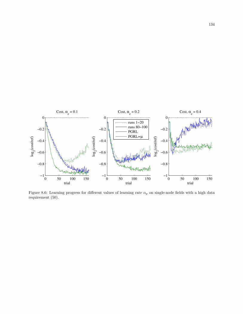
134

0 50 100 150−1

−0.8

−0.6

−0.4

−0.2

0

trial

log

2(c

ost

/ref

)

Cost, αe = 0.1

0 50 100 150−1

−0.8

−0.6

−0.4

−0.2

0

trial

log

2(c

ost

/ref

)

Cost, αe = 0.2

0 50 100 150−1

−0.8

−0.6

−0.4

−0.2

0

trial

log

2(c

ost

/ref

)

Cost, αe = 0.4

runs 1−20

runs 80−100

PGRL

PGRL∝µ

Figure 8.6: Learning progress for different values of learning rate αp on single-node fields with a high datarequirement (50).

135

8.5.4 Mitigating flaws in the policy update step

Recall the special update to the θe parameter Ptarget described in §7.3.4, which has been used up until

now. In this experiment, Ptarget does not receive the special treatment of Equation 7.13, but is updated

in the same way as Rthreshold in Equation 7.14. This results in unexpectedly large proportional changes to

Ptarget when its value is small, which in turn leads to high sampling costs and poor performance, similar to

the high-αp experiment of §8.5.3.

This experiment’s purpose is twofold:

To verify that the modification to the update rule given in §7.3.4 is justified by improved performance.

To show an additional example of the metapolicy learner’s ability to learn metapolicies that com-

pensate for imperfections in the optimisation algorithm.

Figure 8.7 shows the performance through time of the additive-update learner with and without the

assistance of a metapolicy on a single node over the course of 200 trials, using the same experimental setup

described in §8.5.1. As before, the behaviour of the metapolicy early during its training is illustrated by

performance plots over runs 1–20 (dots). We contrast this with performance over runs 80–100 (solid).

As the PGRL learner nears the optimal solution, the relatively higher learning rate drives it into a

cycle of discovering and rediscovering the cliff when random exploration steps take trajectory length over

dmax, resulting in frequent high-cost trajectories. The trained (runs 80–100) metapolicy outperforms PGRL

early in each problem (the first few trials) during which it slightly accelerates learning (cost slope = -0.039

vs. -0.032), but it has a profound effect later, where it has learned that the optimal policy should not be

approached too closely due to the likelihood of subsequent poor steps.

The higher-level time-varying behaviour shown as the metapolicy is learned can be seen in the differ-

ence between runs 1–20 and 80–100, and is shown more explicitly in Figure 8.8. As the metapolicy learner

observes the base learner solving new problems, it refines πµ, yielding performance that improves from run

to run. The graph of metapolicy’s improvement for trials 100–200 (middle figure) shows extremely rapid

learning, with helpful policies emerging after 2 runs. Improvement over early trials (left figure) emerges more

slowly. This difference is due to the difference in training signal-to-noise ratio: increasing learning speed (in

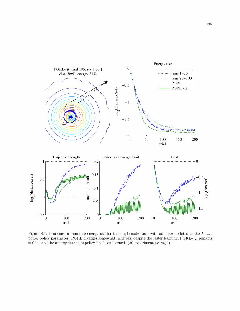
136

PGRL∝µ: trial 105, req [ 30 ]

dist 189%, energy 31%

0 100 200−0.5

0

0.5

1

trial

log

2(d

ista

nce

/ref

)

Trajectory length

0 100 2000

0.05

0.1

0.15

0.2

trial

mea

n u

nd

erru

n

Underrun at range limit

0 50 100 150 200−2

−1.5

−1

−0.5

0

trial

log

2(Σ

en

erg

y/r

ef)

Energy use

0 100 200

−1.5

−1

−0.5

0

trial

log

2(c

ost

/ref

)

Cost

runs 1−20

runs 80−100

PGRL

PGRL∝µ

Figure 8.7: Learning to minimise energy use for the single-node case, with additive updates to the Ptarget

power policy parameter. PGRL diverges somewhat, whereas, despite the faster learning, PGRL∝ µ remainsstable once the appropriate metapolicy has been learned. (50-experiment average.)

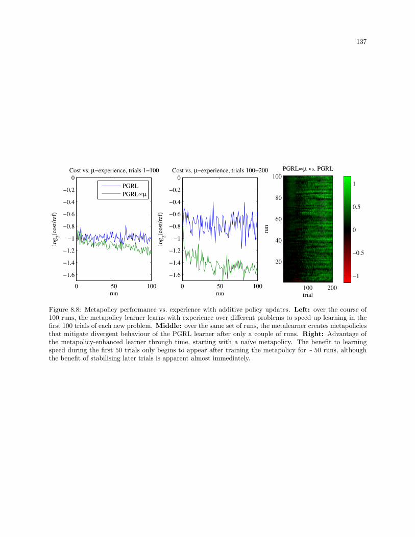
137

0 50 100

−1.6

−1.4

−1.2

−1

−0.8

−0.6

−0.4

−0.2

0

run

log

2(c

ost

/ref

)

Cost vs. µ−experience, trials 1−100

PGRL

PGRL∝µ

0 50 100

−1.6

−1.4

−1.2

−1

−0.8

−0.6

−0.4

−0.2

0

run

log

2(c

ost

/ref

)

Cost vs. µ−experience, trials 100−200 PGRL∝µ vs. PGRL

trial

run

100 200

20

40

60

80

100

−1

−0.5

0

0.5

1

Figure 8.8: Metapolicy performance vs. experience with additive policy updates. Left: over the course of100 runs, the metapolicy learner learns with experience over different problems to speed up learning in thefirst 100 trials of each new problem. Middle: over the same set of runs, the metalearner creates metapoliciesthat mitigate divergent behaviour of the PGRL learner after only a couple of runs. Right: Advantage ofthe metapolicy-enhanced learner through time, starting with a naıve metapolicy. The benefit to learningspeed during the first 50 trials only begins to appear after training the metapolicy for ∼ 50 runs, althoughthe benefit of stabilising later trials is apparent almost immediately.

138

early trials) has a smaller effect on cost than cliff-jumping (near the best policy, in late trials), leading to

faster metapolicy learning in the higher-signal region.

8.5.5 Larger problems

As the number of nodes grows, the metapolicy learner should require fewer tours: the problem can be

decomposed into n weakly interacting problems for n nodes, and the experience with optimising each node

assists with optimising the next node through the mechanism of the metapolicy.

Figure 8.9 shows the result on 3-node problems. The results are qualitatively similar to those in

§8.5.1. For PGRL+µ, one metapolicy was shared among all three nodes, learning on the locally decom-

posed optimisation runs for all of them, whereas Separate shows the result of using a separate metapolicy

“for each node” (for n-node problems, even though new nodes are placed randomly for each run, we con-

sider the metapolicy for the node in the mth position in the tour order to be the same from run to run).

Separate metapolicies display similar ultimate performance to shared metapolicies, but longer learning time,

as expected. This is especially visible in the graph of “Cost vs. µ-experience, trials 1–20” in Figure 8.9, in

which it can be seen that combining the training sets for the different nodes yields consistently faster early

metapolicy learning than using separate metapolicies.

While PGRL+µ allows performance almost as bad as Reference in early runs, later in metapolicy

training, metapolicies emerge that are notable in two ways:

The learned metapolicies improve learning speed. Initial slopes of the conventional learners and

trained (last 20 runs) metapolicy-augmented learners are shown in Table 8.3. In particular, the

trained metapolicy nearly doubles learning speed over the conventional base-learning-only approach.

Separate has not yet learned metapolicies as good as the others. This further confirms that the

metapolicies generalise well: metapolicy learning from optimisation experience on one node improves

performance on the others.

The learned metapolicies prevent discovery of the best trajectories. In the figure, PGRL converges

just beyond 200 trials and then behaves much as it does (as “TruncN”) in Figure 7.7, with the caveat

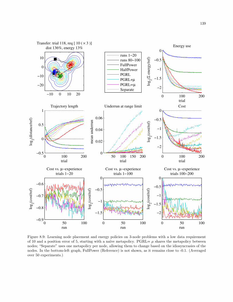
139

Transfer: trial 118, req [ 10 ( × 3 )]

dist 136%, energy 13%

−10 0 10 20

−20

−10

0

10

0 100 200−0.5

0

0.5

1

trial

log

2(d

ista

nce

/ref

)

Trajectory length

50 100 150 2000

0.02

0.04

0.06

trial

mea

n u

nd

erru

n

Underrun at range limit

runs 1−20

runs 80−100

FullPower

HalfPower

PGRL

PGRL+µ

PGRL∝µ

Separate

0 100 200

−2

−1.5

−1

−0.5

0

trial

log

2(Σ

en

erg

y/r

ef)

Energy use

0 100 200

−2

−1.5

−1

−0.5

0

trial

log

2(c

ost

/ref

)

Cost

0 50 100−0.9

−0.8

−0.7

−0.6

run

log

2(c

ost

/ref

)

Cost vs. µ−experience

trials 1−20

0 50 100

−1.5

−1

−0.5

0

run

log

2(c

ost

/ref

)

Cost vs. µ−experience

trials 1−100

0 50 100

−2

−1.5

−1

−0.5

0

run

log

2(c

ost

/ref

)

Cost vs. µ−experience

trials 100−200

Figure 8.9: Learning node placement and energy policies on 3-node problems with a low data requirementof 10 and a position error of 5, starting with a naıve metapolicy. PGRL∝ µ shares the metapolicy betweennodes; “Separate” uses one metapolicy per node, allowing them to change based on the idiosyncrasies of thenodes. In the bottom-left graph, FullPower (Reference) is not shown, as it remains close to -0.1. (Averagedover 50 experiments.)

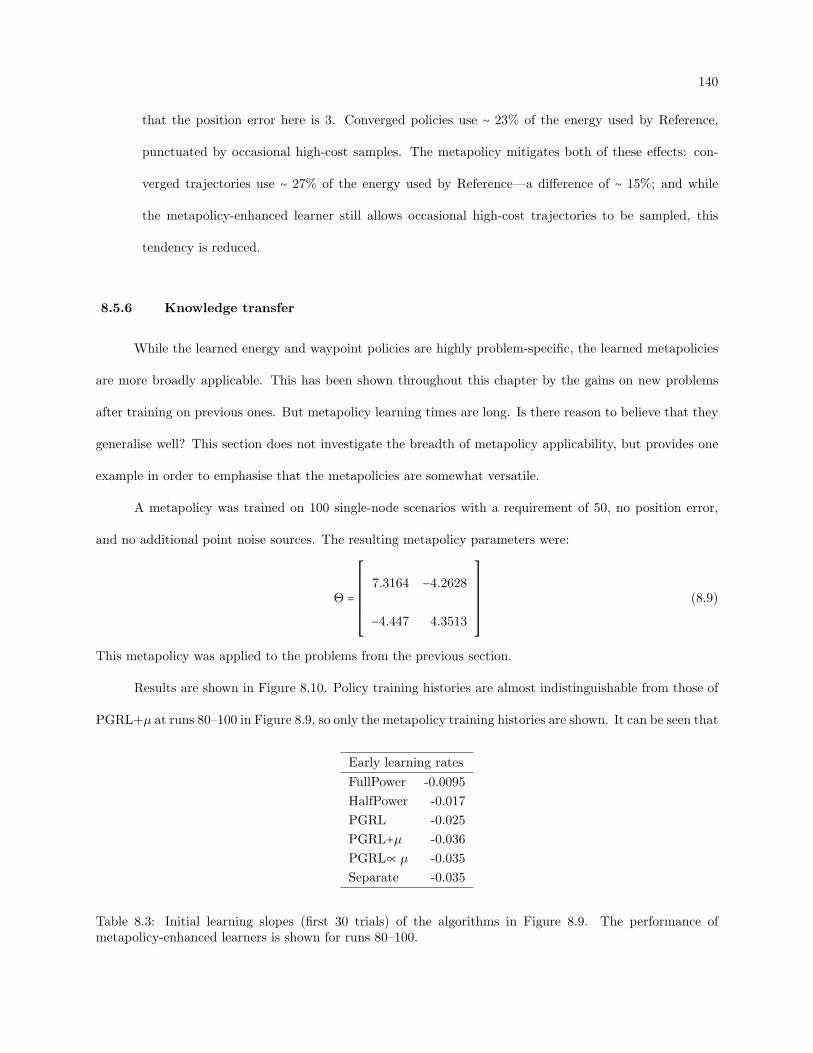
140

that the position error here is 3. Converged policies use ∼ 23% of the energy used by Reference,

punctuated by occasional high-cost samples. The metapolicy mitigates both of these effects: con-

verged trajectories use ∼ 27% of the energy used by Reference—a difference of ∼ 15%; and while

the metapolicy-enhanced learner still allows occasional high-cost trajectories to be sampled, this

tendency is reduced.

8.5.6 Knowledge transfer

While the learned energy and waypoint policies are highly problem-specific, the learned metapolicies

are more broadly applicable. This has been shown throughout this chapter by the gains on new problems

after training on previous ones. But metapolicy learning times are long. Is there reason to believe that they

generalise well? This section does not investigate the breadth of metapolicy applicability, but provides one

example in order to emphasise that the metapolicies are somewhat versatile.

A metapolicy was trained on 100 single-node scenarios with a requirement of 50, no position error,

and no additional point noise sources. The resulting metapolicy parameters were:

Θ =

⎡⎢⎢⎢⎢⎢⎢⎢⎢⎢⎣

7.3164 −4.2628

−4.447 4.3513

⎤⎥⎥⎥⎥⎥⎥⎥⎥⎥⎦

(8.9)

This metapolicy was applied to the problems from the previous section.

Results are shown in Figure 8.10. Policy training histories are almost indistinguishable from those of

PGRL+µ at runs 80–100 in Figure 8.9, so only the metapolicy training histories are shown. It can be seen that

Early learning rates

FullPower -0.0095

HalfPower -0.017

PGRL -0.025

PGRL+µ -0.036

PGRL∝ µ -0.035

Separate -0.035

Table 8.3: Initial learning slopes (first 30 trials) of the algorithms in Figure 8.9. The performance ofmetapolicy-enhanced learners is shown for runs 80–100.

141

0 50 100−0.9

−0.8

−0.7

−0.6

run

log

2(c

ost

/ref

)

Cost vs. µ−experience

trials 1−20

0 50 100−1.8

−1.6

−1.4

−1.2

−1

−0.8

run

log

2(c

ost

/ref

)

Cost vs. µ−experience

trials 1−100

0 50 100

−2

−1.5

−1

−0.5

0

run

log

2(c

ost

/ref

)

Cost vs. µ−experience

trials 100−200

PGRL

PGRL∝µ

Transfer

Figure 8.10: Transferring a single-node metapolicy to a larger field with different data requirements andincorrect node position information. To reduce clutter, only PGRL and PGRL∝ µ are shown for comparison.(This is the same set of experiments that generated Figure 8.9.)

142

in this example, transfer is successful, with the learner immediately receiving the full benefit of the metapolicy

for early trials. In late trials, the transfer learner causes higher-cost trajectories than PGRL for ∼ 10 runs,

while it adapts to the different high-risk areas in policy space of the new, more complex problem. Most

notably, initialising the metapolicy with one of approximately the right shape allows much faster metapolicy

learning. This is a promising result, suggesting broad potential for this metapolicy representation for lifelong

learning in the data-ferrying domain.

However, the generalisation has limits. For example, if we allow node data requirements to be drawn

randomly in [1 . . .10] the metapolicy is not cautious enough in its recommendations for policy updates due

to the short contact times. Similarly, adding a large number of noise nodes (10 in this case) to the radio

field in the test led to a longer retraining time. But even these modifications did not prevent the metapolicy

learner from adapting the metapolicies to the new situation, allowing them to become effective again.

8.5.7 Impact on the comparison to the optimal policy

As we saw in §7.4.1, the power policies can achieve near-optimal performance if given sufficient learning

time. The first goal of the metapolicy is to decrease that time, and, as we have seen, it does so. What effect

does the learning speed improvement have on the trade-off between the ultimate performance of an optimal

planner and the immediate utility of a model-free learning system?

Figure 8.11 duplicates Figure 7.4 from the previous chapter, replacing results from Fullpower with

those from the metapolicy-enhanced learner, PGRL∝ µ. A naıve metapolicy accomplishes nothing, so

here it was assumed that πµ was trained on 100 previous problems before being used on the ones used

to generate the graph. With the assistance of a trained metapolicy, good power policies are found more

quickly than under any other algorithm, even outperforming Init after a handful of trials in each run. The

result is of course not asymptotically superior to Optimal (Opt), but the accelerated learning would make

it significantly more difficult for Opt to overtake a metapolicy-assisted learning network if the former were

required to spend time building a model. When Opt is given even slightly degraded models, its performance

is significantly hurt, and it will probably never outperform the learner by much.

The version of PGRL∝ µ tested here does not decay learning rates, and so it would be able to track

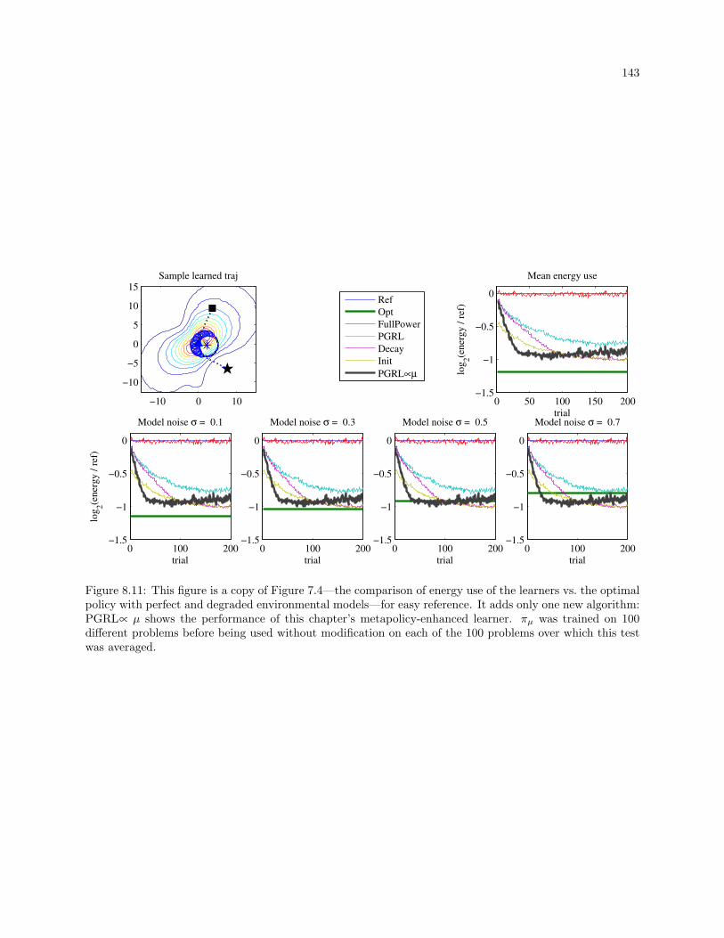
143

Sample learned traj

−10 0 10

−10

−5

0

5

10

15

0 50 100 150 200−1.5

−1

−0.5

0

trial

log

2(e

ner

gy

/ r

ef)

Mean energy use

0 100 200−1.5

−1

−0.5

0

trial

Model noise σ = 0.1

log

2(e

ner

gy

/ r

ef)

0 100 200−1.5

−1

−0.5

0

trial

Model noise σ = 0.7

0 100 200−1.5

−1

−0.5

0

trial

Model noise σ = 0.3

0 100 200−1.5

−1

−0.5

0

trial

Model noise σ = 0.5

Ref

Opt

FullPower

PGRL

Decay

Init

PGRL∝µ

Figure 8.11: This figure is a copy of Figure 7.4—the comparison of energy use of the learners vs. the optimalpolicy with perfect and degraded environmental models—for easy reference. It adds only one new algorithm:PGRL∝ µ shows the performance of this chapter’s metapolicy-enhanced learner. πµ was trained on 100different problems before being used without modification on each of the 100 problems over which this testwas averaged.

144

a changing environment. Such changes would require additional SI time of Opt, for which these graphs do

not account. Alternatively, if PGRL∝ µ were to use a decaying learning rate, it would give up versatility in

exchange for slightly higher performance.

Notwithstanding this analysis, perhaps the great advantage of optimal planning is in its adaptability

to changing requirements. If the environment is reasonably static, the optimiser can immediately produce

perfect trajectories for changing data needs, while the learners must slowly adapt. Appendix B discusses

some preliminary work on immediately adapting learned policies to new tasks.

8.6 Summary

The metapolicy learning approach introduced in this chapter uses experience with the process of

learning data-ferrying policies in order to accelerate and stabilise a conventional PGRL system learning new

problems in the domain. It is a full reinforcement learner for the metapolicy—it considers the distribution of

future discounted returns that might result from policy update steps—and it can therefore both speed policy

acquisition and keep base PGRL updates from taking the learner into hazardous regions of policy space.

This furnishes a new mechanism for approaching the global optimum of an unseen data-ferrying scenario

extremely quickly while sampling few high-cost trajectories.

A trained metapolicy can reduce the necessity of hand-tuning the system by compensating for a poor

choice of parameters. A poorly chosen exploration rate frequently produces trajectories that significantly

exceed the aircraft’s range limit. As the metapolicy incorporates experience with the base optimiser it learns

to compensate, modulating the problematic policy updates and keeping trajectory costs lower. This may be

a disadvantage if it permits a configuration error to go unnoticed.

Chapter 9

Assessment under a complex, noisy, terrain-based radio model

The radio model presented in Chapter 3 produces fields that simulate the effects of path loss, point

interference, and directionality. For these assumptions and simple ferrying scenarios (few nodes, or nodes

that are spatially well-separated), it may be possible to model the environment with sufficient accuracy to

outperform the learning approach presented here. Real radio fields are more complex—notably, they exhibit

slow and fast fading, variable path loss that depends on antennas’ relative and absolute heights above ground,

terrain composition, and atmospheric effects. Thus a real system is far more difficult to identify accurately,

and consequently may present a more compelling incentive for model-free learning. This chapter addresses

two questions:

How well does the model-free approach developed up to this point work in a more realistic radio

environment?

What level of inaccuracy can be tolerated in an optimal planner’s system model while still offering

a significant performance advantage over our model-free learning approach?

This chapter introduces SPLAT! [Magliacane, 2011], a terrain-based radio simulator that uses the

Longley-Rice propagation model [Longley and Rice, 1968], which computes path loss based on line-of-sight

distance, diffraction, and scatter using either average terrain data or, in the case of SPLAT!, actual terrain

elevation measurements. Signals interact with the ground, whose influence depends on its conductivity and

dielectric constant; atmospheric bending; polarisation; and other factors. Ground interactions in SPLAT!

are computed using a terrain model built from USGS 30-meter satellite survey data.

146

This chapter also contains a brief analysis of learning performance in the presence of random autopilot

tracking error such as might be induced by turbulent air. This is not a general investigation of wind, but

it provides a starting point for an investigation into the algorithms’ robustness to unmodelled trajectory

tracking errors.

9.1 Terrain interactions and SPLAT!

SPLAT! uses the Longley-Rice propagation model [Longley and Rice, 1968] and USGS elevation

datasets at a resolution of 30×30 meters.1 The Longley-Rice computation assumes that signals propagate at

no more than ∼ 12 above horizontal due to approximations made for ground and troposphere interactions,

and SPLAT! further restricts antenna directionality to no more than 10 above the antenna’s equator—

consistent with its design goal of predicting ground-to-ground transmissions. SPLAT! allows rotation of

the transmitting antenna’s orientation, with the assumption that the orientation will be modified by a few

degrees in order to aim the antenna at the horizon in some direction. This differs from our default assumption

that the orientations of small sensors deployed from the air might have uniformly random orientations over

the sphere.

9.1.1 Modifications to the scenario assumptions

The simulation environment provided by SPLAT! works best, and our testing goals are best achieved,

when the elevation between node and UA remains small. In order to achieve this, in this chapter we adopt

a more highly directional node antenna pattern that radiates power mostly horizontally, which reduces the

power directly above the node. This encourages the optimisers to find trajectories that interact better with

the simulator for the following reasons:

More accurate simulation results: While the Longley-Rice computation degrades somewhat gracefully

as the target elevation exceeds 12, the degradation at high elevations is significant (see Figure 9.1).

Furthermore, SPLAT! requires paths of at least 5 pixels (including sender’s and receiver’s) in order to

1 We use the “high-definition” implementation of SPLAT!, distributed as splat-hd in the SPLAT! package version 1.4.0.The earlier version uses USGS 100×100-meter datasets.

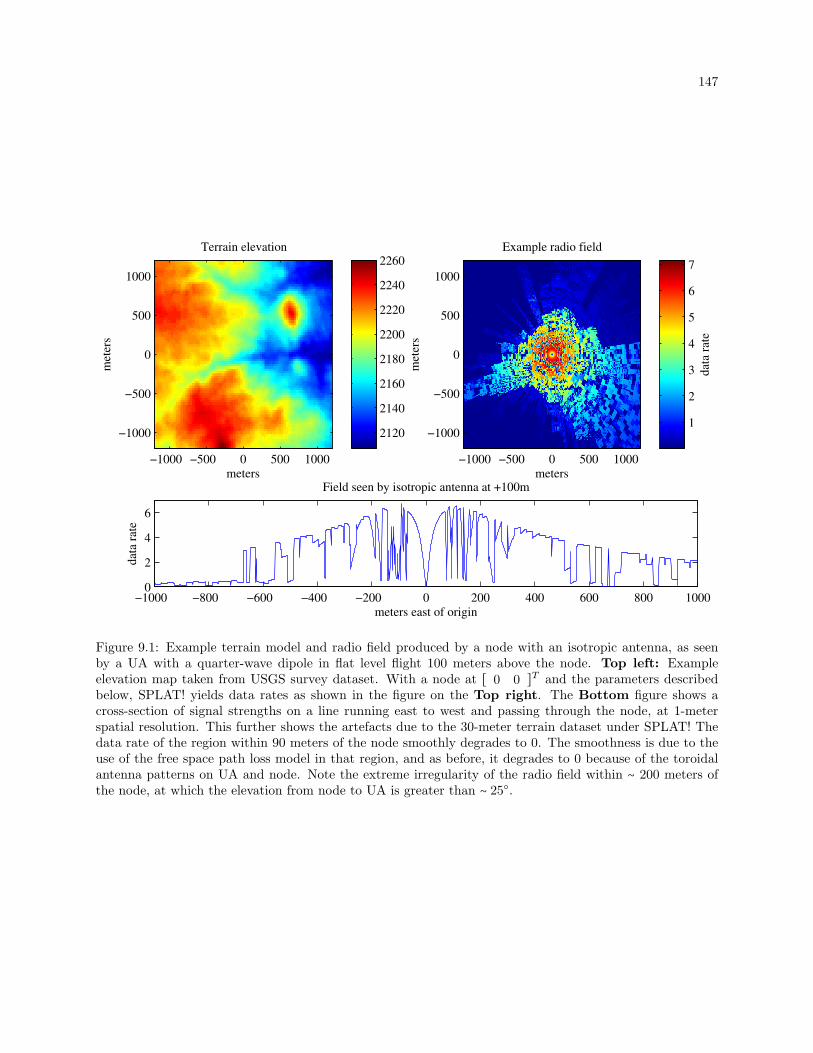
147

meters

met

ers

Terrain elevation

−1000 −500 0 500 1000

−1000

−500

0

500

1000

met

ers

2120

2140

2160

2180

2200

2220

2240

2260

meters

Example radio field

−1000 −500 0 500 1000

−1000

−500

0

500

1000

dat

a ra

te

1

2

3

4

5

6

7

−1000 −800 −600 −400 −200 0 200 400 600 800 10000

2

4

6

meters east of origin

dat

a ra

te

Field seen by isotropic antenna at +100m

Figure 9.1: Example terrain model and radio field produced by a node with an isotropic antenna, as seenby a UA with a quarter-wave dipole in flat level flight 100 meters above the node. Top left: Exampleelevation map taken from USGS survey dataset. With a node at [ 0 0 ]T and the parameters describedbelow, SPLAT! yields data rates as shown in the figure on the Top right. The Bottom figure shows across-section of signal strengths on a line running east to west and passing through the node, at 1-meterspatial resolution. This further shows the artefacts due to the 30-meter terrain dataset under SPLAT! Thedata rate of the region within 90 meters of the node smoothly degrades to 0. The smoothness is due to theuse of the free space path loss model in that region, and as before, it degrades to 0 because of the toroidalantenna patterns on UA and node. Note the extreme irregularity of the radio field within ∼ 200 meters ofthe node, at which the elevation from node to UA is greater than ∼ 25.

148

compute Longley-Rice loss—this may correspond to distances of ∼ 90–170 meters. While we modified

SPLAT! to use freespace path loss for shorter trajectories, if the UA flies either closer than ∼ 170m

or to points at which the transmission angle is too great, accuracy suffers. Therefore, encouraging

trajectories that do not encounter this region leads to more realistic simulation results.

Finding an approximate global optimum: The Longley-Rice model results in a highly complex radio

field whose spatial scale decreases and whose variance increases as the target elevation surpasses ∼ 25

above horizontal (Figure 9.1). Finding the global optimum of the resultant field is difficult, and the

results from the learner are wildly erratic for the same reason. The antenna pattern modification

creates an environment in which the optimal waypoint placement is generally not very far from the

node’s location, and results in a somewhat smoother optimisation surface. These properties are

necessary just to find a solution that is likely close to optimal in reasonable time.

Increasing the impact of terrain: The goal of this section is to compare learning to optimal planning

under a realistic terrain model. At high transmission angles, terrain has little (in reality) or no (in

this simulation environment) systematic impact upon radio patterns, reducing the interest of the

results.

Spatial resolution: Lowering the maximum transmission elevation angle while preserving a realistic flight

altitude has an additional effect: it requires that the UA use a greater turning radius. It is plausible

for a UA to have a turning radius of on the order of 30 meters, but since transmission rate is computed

on roughly this spatial scale due to the resolution of the USGS dataset, the results are difficult to

interpret. Expanding the turning radius allows the radio field to more closely approximate a realistic

spatial smoothness, while still allowing us to compare learning vs. optimal planning.

Reducing vertically radiated power both encourages the UA to find trajectories that do not stray into

the troublesome region and ensures that there is little enough power in the troublesome region that it has at

most a minor effect on results. Compare the example radio field produced by an isotropic transmitter shown

in Figure 9.1 with that produced by our directional antenna illustrated in Figure 9.2. In the latter, the UA

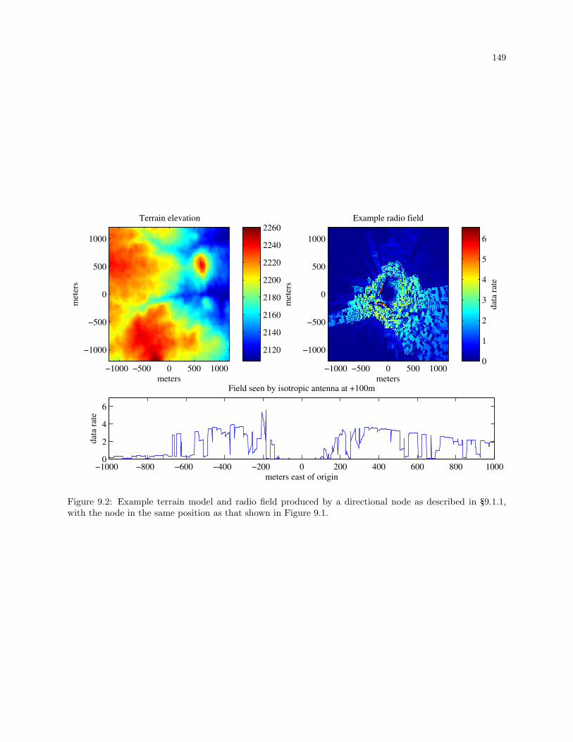
149

meters

met

ers

Terrain elevation

−1000 −500 0 500 1000

−1000

−500

0

500

1000

meters

Example radio field

−1000 −500 0 500 1000

−1000

−500

0

500

1000

−1000 −800 −600 −400 −200 0 200 400 600 800 10000

2

4

6

meters east of origin

dat

a ra

te

Field seen by isotropic antenna at +100m

met

ers

2120

2140

2160

2180

2200

2220

2240

2260

dat

a ra

te

0

1

2

3

4

5

6

Figure 9.2: Example terrain model and radio field produced by a directional node as described in §9.1.1,with the node in the same position as that shown in Figure 9.1.

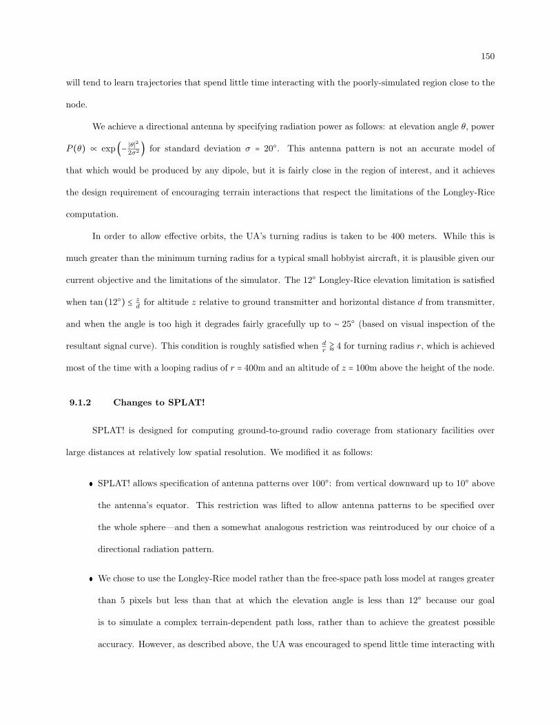
150

will tend to learn trajectories that spend little time interacting with the poorly-simulated region close to the

node.

We achieve a directional antenna by specifying radiation power as follows: at elevation angle θ, power

P (θ) ∝ exp (− ∣θ∣2

2σ2 ) for standard deviation σ = 20. This antenna pattern is not an accurate model of

that which would be produced by any dipole, but it is fairly close in the region of interest, and it achieves

the design requirement of encouraging terrain interactions that respect the limitations of the Longley-Rice

computation.

In order to allow effective orbits, the UA’s turning radius is taken to be 400 meters. While this is

much greater than the minimum turning radius for a typical small hobbyist aircraft, it is plausible given our

current objective and the limitations of the simulator. The 12 Longley-Rice elevation limitation is satisfied

when tan (12) ≤ zdfor altitude z relative to ground transmitter and horizontal distance d from transmitter,

and when the angle is too high it degrades fairly gracefully up to ∼ 25 (based on visual inspection of the

resultant signal curve). This condition is roughly satisfied when dr⪆ 4 for turning radius r, which is achieved

most of the time with a looping radius of r = 400m and an altitude of z = 100m above the height of the node.

9.1.2 Changes to SPLAT!

SPLAT! is designed for computing ground-to-ground radio coverage from stationary facilities over

large distances at relatively low spatial resolution. We modified it as follows:

SPLAT! allows specification of antenna patterns over 100: from vertical downward up to 10 above

the antenna’s equator. This restriction was lifted to allow antenna patterns to be specified over

the whole sphere—and then a somewhat analogous restriction was reintroduced by our choice of a

directional radiation pattern.

We chose to use the Longley-Rice model rather than the free-space path loss model at ranges greater

than 5 pixels but less than that at which the elevation angle is less than 12 because our goal

is to simulate a complex terrain-dependent path loss, rather than to achieve the greatest possible

accuracy. However, as described above, the UA was encouraged to spend little time interacting with

151

this region.

SPLAT! was modified to act as a server, loading data files on demand and then communicating via

IPC with the Matlab learning infrastructure developed in previous chapters.

SPLAT! has no mechanism by which to incorporate receiver antenna patterns, so directionality in the

receiver’s antenna was handled in Matlab. Since SPLAT! does not compute multipath interference (indeed,

it would be pointless to do so for the design range of radio frequencies given the limited spatial resolution

available), this should not introduce errors.

Not everything about the model can be realistic given the limitations of the available terrain datasets

and simulation environments, but once again we take the spatial properties of the terrain-based radio model

to be a good proxy for a complex radio field such as would occur, albeit in more detail and on a finer spatial

scale, in the real world.

9.2 Model-based Optimal Planning

We assume that the UA has a perfect model of the system. In this case, the systems are the SPLAT!

radio simulator and the autopilot used throughout this research. The UA uses the simulator in order to

compute an optimal policy: waypoint locations and predicted data rates perfectly determine trajectories,

and trajectories perfectly determine the optimal transmit power scaling at each timestep.

Figure 9.3 shows the quality of the optimal power policy for each possible waypoint location on

the square kilometer centered on the node. Structure can be observed at the 10-meter resolution of the

figure, and exists at still higher resolutions. This structure results in off-the-shelf hillclimbing optimisers

frequently becoming stuck in poor local optima, although some ad-hoc selection of step sizes and sampling

regions (similar to those used by PGRL as implemented here) can improve the solution. However, the local

structure tends to have relatively small amplitude in the vicinity of the global optimum, so instead of a

hillclimbing search we choose waypoint location using a grid search at 60-meter resolution. The best power

policy found using this search is usually within a few percent of the best found at higher resolution, and the

computational burden is far less.

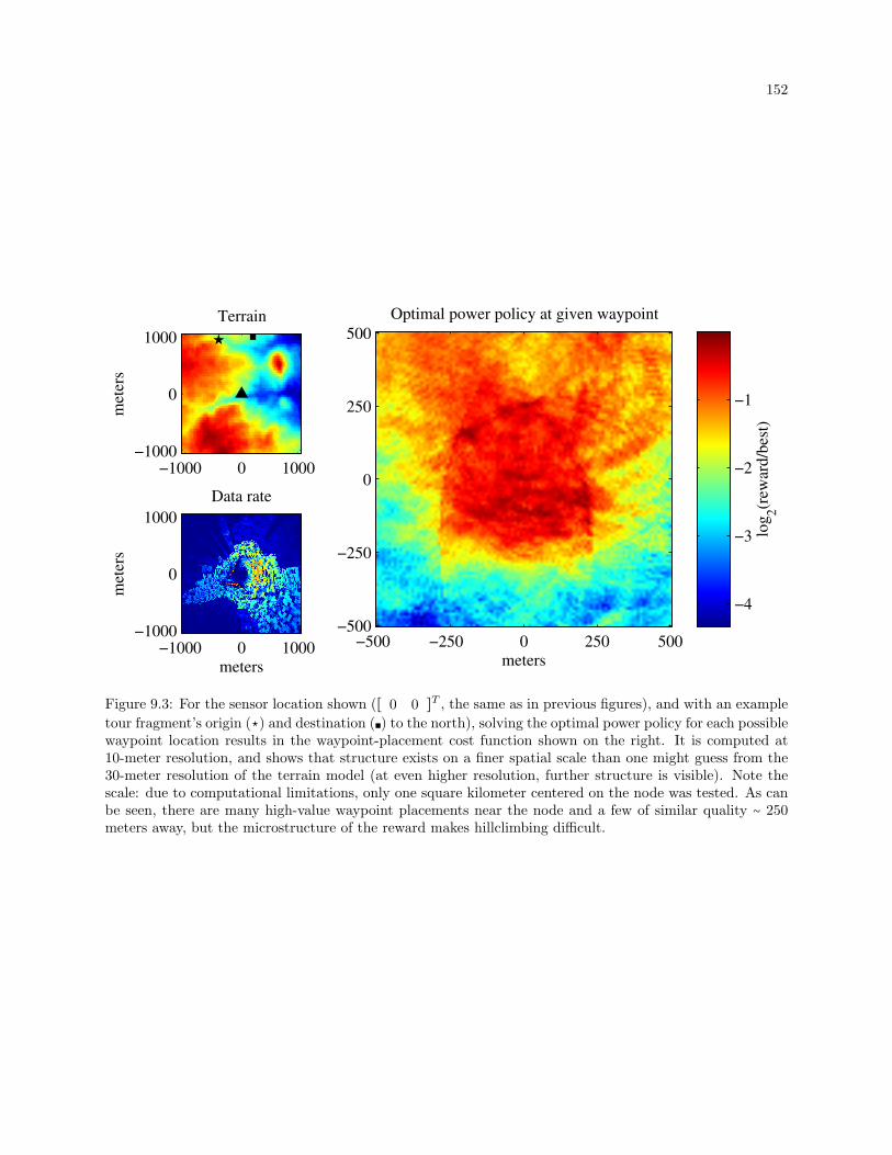
152

Terrain

met

ers

−1000 0 1000−1000

0

1000

Data rate

met

ers

meters

−1000 0 1000−1000

0

1000

Optimal power policy at given waypoint

meters

−500 −250 0 250 500−500

−250

0

250

500

log

2(r

ewar

d/b

est)

−4

−3

−2

−1

Figure 9.3: For the sensor location shown ([ 0 0 ]T , the same as in previous figures), and with an example

tour fragment’s origin (⋆) and destination (∎) to the north), solving the optimal power policy for each possiblewaypoint location results in the waypoint-placement cost function shown on the right. It is computed at10-meter resolution, and shows that structure exists on a finer spatial scale than one might guess from the30-meter resolution of the terrain model (at even higher resolution, further structure is visible). Note thescale: due to computational limitations, only one square kilometer centered on the node was tested. As canbe seen, there are many high-value waypoint placements near the node and a few of similar quality ∼ 250meters away, but the microstructure of the reward makes hillclimbing difficult.

153

With a perfect model (and infinite computational power), optimal planning finds perfect solutions.

As the model degrades, so does solution quality. The optimal planner will be tested in the presence of both

model error and unmodelled noise in the trajectory instantiated by the autopilot.

9.2.1 Stochastic autopilot tracking error

The UA’s controller does not perfectly track a trajectory; for example, slightly turbulent air leads to

small deflections, requiring constant course corrections. In order to simulate this effect, at each timestep

we alter the UA’s position [ x y ]T and heading ϕ by a small amount proportional to a number drawn

from a Gaussian with standard deviation σt. This noise renders the UA’s position and heading somewhat

unpredictable. Another consequence of these changes is that the bank angle ψ constantly changes as the UA

adjusts to correct its course. Since the UA’s antenna is directional, this leads to a random fluctuation in the

received signal strength.

Autopilot tracking error affects both the optimal planner and the learner. The learner compensates

without explicitly understanding that noise is present. An optimal planner could estimate the distribution

of each noise source and build the appropriate safety margins into the plan, but optimal planning in noisy

environments is a hard problem and is outside the scope of this work.

9.2.2 Model errors

The following data are used only by the optimal planner’s model. The learner’s strength is in its

ability to perform optimisation without this information, and so is not affected by these errors. In contrast,

it is important to evaluate the performance of the optimal planner as this information degrades.

Node: The node’s assumed position and antenna orientation are adjusted, similarly to the location error

first introduced in Chapter 4. While node location error affects Reference and the initial trajectories

of the learners, the location errors tested in this chapter are too small to make a measurable difference

for those algorithms.

Terrain: For each experiment, the optimal planner uses the USGS terrain data for planning, and for eval-

uation the elevation of each pixel (30×30-meter square) is modified by adding Gaussian noise to the

154

USGS data. We’ve assumed that the noise is uncorrelated between neighbouring pixels.

9.3 Experiments

For each run a node is uniformly randomly placed in the 1400×1400-meter square around the test

region’s center. The UA flies at a height of 100 meters above the target sensor’s assumed location for

the current run, and the test zone was chosen such that collisions with the ground are not an issue for all

permitted node placements. The test zone, as can be seen in Figure 9.1, is the area surrounding a moderately

deeply eroded river bed. This was chosen both for the interesting terrain and for the applicability to some

increasingly important water monitoring tasks. For the examples in Figures 9.1–9.3 the node is placed in

the center of the field (at [ 0 0 ]T ), which is near the bottom of the river valley.

For these experiments, only one node is used. The radio simulator’s speed precludes in-depth analysis

of more complex scenarios, but as both learning and optimal planning interact equally with the highly

spatially complex radio fields provided by SPLAT!, the mechanism of additional radio point noise sources in

order to increase spatial complexity is unnecessary.

Transfer is PGRL∝ µ with a mature metapolicy trained on a slightly different scenario (a data

requirement of 300) on 200 problems. The initial values used for Transfer were:

Θ =

⎡⎢⎢⎢⎢⎢⎢⎢⎢⎢⎣

3.71 −2.75

−3.34 2.72

⎤⎥⎥⎥⎥⎥⎥⎥⎥⎥⎦

Energy use for Optimal under degraded models is computed as described in §7.4.1.1. When model

error causes a tour to underrun data requirements, trajectory length per tour does not change, but in order

to compensate for decreased data transfer, more trajectories are flown. Thus the increase in flight time per

per unit of data collected is identical to the increase in energy use, and will not be shown.

9.3.0.1 Parameters

The parameters used by the radio simulator appear in Table 9.1, and the key ones used by the aircraft

are given in Table 9.2. These parameters were chosen in order to allow SPLAT! and the Longley-Rice model

155

to provide a reasonable simulation. Higher-resolution terrain data, a more general radio simulation model,

greater computational resources, or a re-interpretation of the results as representative of an up-scaled model

of the world, would permit the choice of different parameters. Other parameters not described below, such

as those used by the learning algorithms, are unchanged from previous chapters.

9.3.1 Perfect information

In this section, the model errors described in §9.2.2 are not used, but the trajectory tracking noise

described in §9.2.1 is present, drawn with σ = 0.05 (a 5% error in the UA’s position in each timestep).

For computation of the optimal policy, the noise is added at the time of trajectory generation and is never

recomputed during optimisation. Thus the optimal planner has perfect information about the field and the

trajectory, which happens to be less smooth than a noise-free one, allowing omniscient optimal planning—

optimal planning with complete and correct information. A moderately high data requirement of 200, which

in this scenario tends to require 2–5 orbits, is shown here; other requirements yield similar results.

Learning performance is presented in Figure 9.4, and Figure 9.5 provides further comparisons of the

progress of the metapolicy learner. PGRL eventually achieves the lowest energy use, on average, at about

35% of Reference after a few hundred trials. However, it frequently exceeds the length limit—in tests to

more than 300 trials, PGRL eventually averages just over twice the length of Reference, visible as frequent

spikes in its optimisation cost (see below). PGRL∝ µ behaves much as it did in Chapter 8: while a mature

metapolicy generally reduces energy use to only 38% of Reference, it does so much faster, achieving most of

its gain by trial 100. Trajectory length averages ∼ 160% of Reference, seldom exceeding the limit by much,

as can be seen by the much lower average cost. Once again, the metapolicy learner must observe many

scenarios in order to achieve this result: over the first 20 runs, PGRL∝ µ offers slower initial learning and

a higher-cost final result than PGRL. Unsurprisingly, Transfer provides the benefit of a mature PGRL∝ µ

immediately, generally surpassing the performance of the latter in both initial policy learning speed and

frequency of cost spikes due to its more mature policy, and continuing to improve very slightly with further

experience. Optimal averages ∼ 26% of the energy of Reference with trajectories nearly twice as long as

Reference—almost exactly 100% of the permitted length, although trajectories may occasionally be shorter

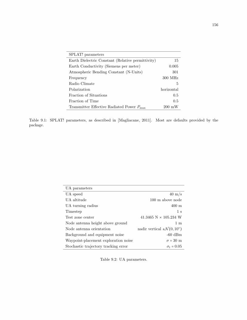
156

SPLAT! parameters

Earth Dielectric Constant (Relative permittivity) 15

Earth Conductivity (Siemens per meter) 0.005

Atmospheric Bending Constant (N-Units) 301

Frequency 300 MHz

Radio Climate 5

Polarization horizontal

Fraction of Situations 0.5

Fraction of Time 0.5

Transmitter Effective Radiated Power Pmax 200 mW

Table 9.1: SPLAT! parameters, as described in [Magliacane, 2011]. Most are defaults provided by thepackage.

UA parameters

UA speed 40 m/s

UA altitude 100 m above node

UA turning radius 400 m

Timestep 1 s

Test zone center 41.3465 N × 105.234 W

Node antenna height above ground 1 m

Node antenna orientation nadir vertical ±N (0,10)Background and equipment noise -60 dBm

Waypoint-placement exploration noise σ = 30 m

Stochastic trajectory tracking error σt = 0.05

Table 9.2: UA parameters.

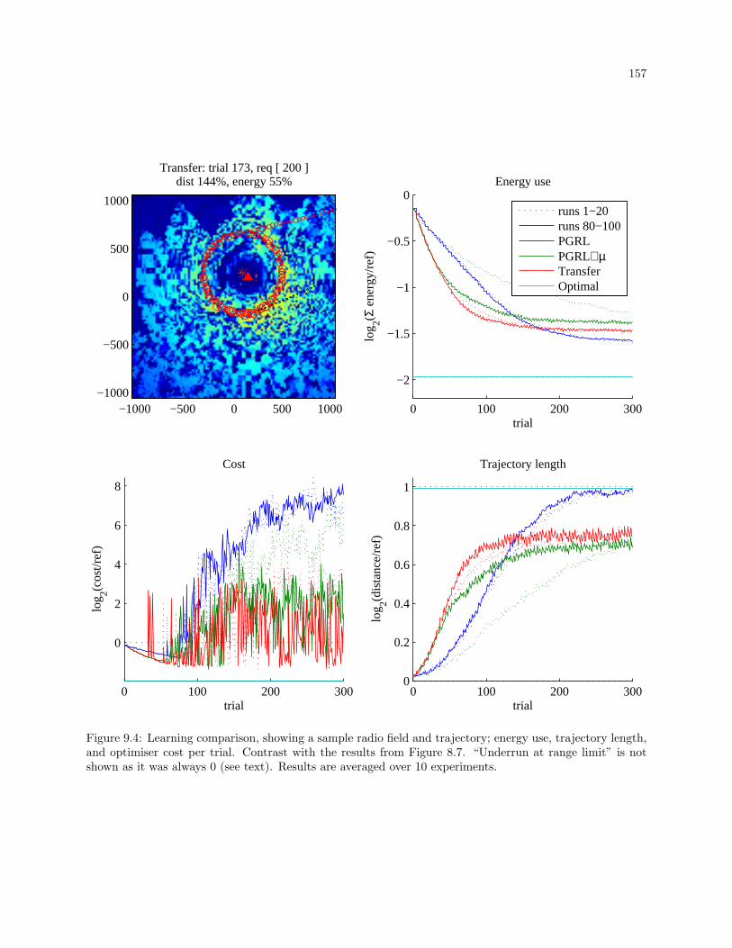
157

0 100 200 3000

0.2

0.4

0.6

0.8

1

trial

log 2(d

ista

nce/

ref)

Trajectory length

0 100 200 300

−2

−1.5

−1

−0.5

0

trial

log 2(Σ

ene

rgy/

ref)

Energy use

0 100 200 300

0

2

4

6

8

trial

log 2(c

ost/r

ef)

Cost

Transfer: trial 173, req [ 200 ]dist 144%, energy 55%

−1000 −500 0 500 1000−1000

−500

0

500

1000runs 1−20runs 80−100PGRLPGRL∝µTransferOptimal

Figure 9.4: Learning comparison, showing a sample radio field and trajectory; energy use, trajectory length,and optimiser cost per trial. Contrast with the results from Figure 8.7. “Underrun at range limit” is notshown as it was always 0 (see text). Results are averaged over 10 experiments.

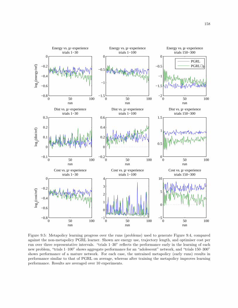
158

0 50 100−0.8

−0.6

−0.4

−0.2

0

run

log 2(c

ost/r

ef)

Cost vs. µ−experiencetrials 1−30

0 50 100−0.1

0

0.1

0.2

0.3

run

log 2(d

ist/r

ef)

Dist vs. µ−experiencetrials 1−30

0 50 100−0.8

−0.6

−0.4

−0.2

0

run

log 2(e

nerg

y/re

f)

Energy vs. µ−experiencetrials 1−30

0 50 100−1

0

1

2

3

4

run

Cost vs. µ−experiencetrials 1−100

0 50 100−0.2

0

0.2

0.4

0.6

run

Dist vs. µ−experiencetrials 1−100

0 50 100−1.5

−1

−0.5

0

run

Energy vs. µ−experiencetrials 1−100

0 50 100−5

0

5

10

run

Cost vs. µ−experiencetrials 150−300

0 50 1000

0.5

1

1.5

run

Dist vs. µ−experiencetrials 150−300

0 50 100−2

−1.5

−1

−0.5

0

run

Energy vs. µ−experiencetrials 150−300

PGRLPGRL∝µ

Figure 9.5: Metapolicy learning progress over the runs (problems) used to generate Figure 9.4, comparedagainst the non-metapolicy PGRL learner. Shown are energy use, trajectory length, and optimiser cost perrun over three representative intervals. “trials 1–30” reflects the performance early in the learning of eachnew problem, “trials 1–100” shows aggregate performance for an “adolescent” network, and “trials 150–300”shows performance of a mature network. For each case, the untrained metapolicy (early runs) results inperformance similar to that of PGRL on average, whereas after training the metapolicy improves learningperformance. Results are averaged over 10 experiments.

159

due to the discrete timesteps used by the simulator. The performance of Optimal under perfect and imperfect

models will be explored in the following sections.

As can be seen in Figure 9.5, the metapolicy learner improves the learning speed and stability of the

base learner as the former’s experience with new problems increases, but after seeing 100 problems it has

not yet converged: its performance is still improving. The Transfer algorithm shown in Figure 9.4 changes

only slightly over the same interval (not shown), and provides an idea of the performance of a more nearly

converged metapolicy.

The relationship between FullPower, HalfPower, and the learners is similar to that shown in Chapters 7

and 8. In Chapter 8 it was shown that PGRL∝ µ outperformed PGRL+µ in early runs. The effect here is

similar in both magnitude and timescale, independent of which radio simulator is used. Therefore we do not

show the latter algorithm here.

“Underrun at range limit” was shown in earlier analogous figures (e.g. Figure 7.5), and was nonzero

if the UA had to exceed its soft range limit in order to collect all the data. In these experiments, the

range limit was exceeded occasionally—otherwise there would be no push to shorten trajectories—but it was

always exceeded after the UA had exited from the data collection loop and was nearly at the destination.

The difference is due to the fact that the average variation in data collection rate varies more slowly with

distance under this simulator than under the simpler one (equivalently, the exploration noise step size is

smaller relative to the field’s decay—if background noise N were higher, the field would decay faster).

Presumably some rules for choosing exploration noise could be devised, but it would be computationally

expensive to do so and is beyond the scope of this work.

9.3.2 Trajectory tracking error

Here we test against the trajectory tracking error described in §9.2.1. Testing each dimension sepa-

rately is more than we require, so to produce Figure 9.6 we vary an error parameter σt and arbitrarily set all

three of the standard deviation variables of the inter-step tracking error [ x y ϕ ]T to σt: the first two

are in meters of error per meter travelled (unitless), and the third is in radians, but this is sufficient to give

some idea of the effect of such an error.

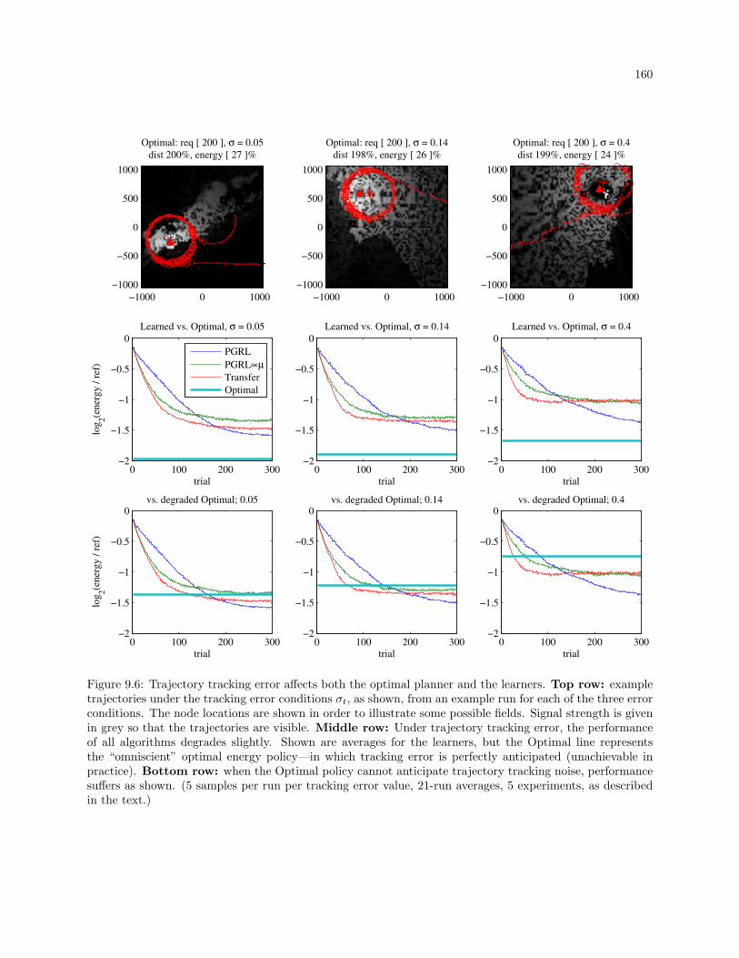
160

Optimal: req [ 200 ], σ = 0.05

dist 200%, energy [ 27 ]%

−1000 0 1000

−1000

−500

0

500

1000

0 100 200 300−2

−1.5

−1

−0.5

0

trial

log

2(e

ner

gy

/ r

ef)

Learned vs. Optimal, σ = 0.05

0 100 200 300−2

−1.5

−1

−0.5

0

trial

log

2(e

ner

gy

/ r

ef)

vs. degraded Optimal; 0.05

Optimal: req [ 200 ], σ = 0.14

dist 198%, energy [ 26 ]%

−1000 0 1000

−1000

−500

0

500

1000

0 100 200 300−2

−1.5

−1

−0.5

0

trial

Learned vs. Optimal, σ = 0.14

0 100 200 300−2

−1.5

−1

−0.5

0

trial

vs. degraded Optimal; 0.14

Optimal: req [ 200 ], σ = 0.4

dist 199%, energy [ 24 ]%

−1000 0 1000

−1000

−500

0

500

1000

0 100 200 300−2

−1.5

−1

−0.5

0

trial

Learned vs. Optimal, σ = 0.4

0 100 200 300−2

−1.5

−1

−0.5

0

trial

vs. degraded Optimal; 0.4

PGRL

PGRL∝µ

Transfer

Optimal

Figure 9.6: Trajectory tracking error affects both the optimal planner and the learners. Top row: exampletrajectories under the tracking error conditions σt, as shown, from an example run for each of the three errorconditions. The node locations are shown in order to illustrate some possible fields. Signal strength is givenin grey so that the trajectories are visible. Middle row: Under trajectory tracking error, the performanceof all algorithms degrades slightly. Shown are averages for the learners, but the Optimal line representsthe “omniscient” optimal energy policy—in which tracking error is perfectly anticipated (unachievable inpractice). Bottom row: when the Optimal policy cannot anticipate trajectory tracking noise, performancesuffers as shown. (5 samples per run per tracking error value, 21-run averages, 5 experiments, as describedin the text.)

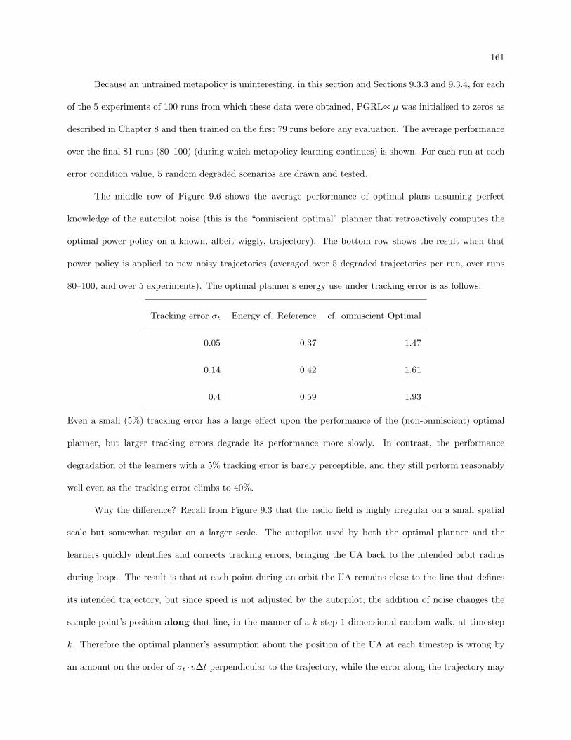
161

Because an untrained metapolicy is uninteresting, in this section and Sections 9.3.3 and 9.3.4, for each

of the 5 experiments of 100 runs from which these data were obtained, PGRL∝ µ was initialised to zeros as

described in Chapter 8 and then trained on the first 79 runs before any evaluation. The average performance

over the final 81 runs (80–100) (during which metapolicy learning continues) is shown. For each run at each

error condition value, 5 random degraded scenarios are drawn and tested.

The middle row of Figure 9.6 shows the average performance of optimal plans assuming perfect

knowledge of the autopilot noise (this is the “omniscient optimal” planner that retroactively computes the

optimal power policy on a known, albeit wiggly, trajectory). The bottom row shows the result when that

power policy is applied to new noisy trajectories (averaged over 5 degraded trajectories per run, over runs

80–100, and over 5 experiments). The optimal planner’s energy use under tracking error is as follows:

Tracking error σt Energy cf. Reference cf. omniscient Optimal

0.05 0.37 1.47

0.14 0.42 1.61

0.4 0.59 1.93

Even a small (5%) tracking error has a large effect upon the performance of the (non-omniscient) optimal

planner, but larger tracking errors degrade its performance more slowly. In contrast, the performance

degradation of the learners with a 5% tracking error is barely perceptible, and they still perform reasonably

well even as the tracking error climbs to 40%.

Why the difference? Recall from Figure 9.3 that the radio field is highly irregular on a small spatial

scale but somewhat regular on a larger scale. The autopilot used by both the optimal planner and the

learners quickly identifies and corrects tracking errors, bringing the UA back to the intended orbit radius

during loops. The result is that at each point during an orbit the UA remains close to the line that defines

its intended trajectory, but since speed is not adjusted by the autopilot, the addition of noise changes the

sample point’s position along that line, in the manner of a k-step 1-dimensional random walk, at timestep

k. Therefore the optimal planner’s assumption about the position of the UA at each timestep is wrong by

an amount on the order of σt ⋅ v∆t perpendicular to the trajectory, while the error along the trajectory may

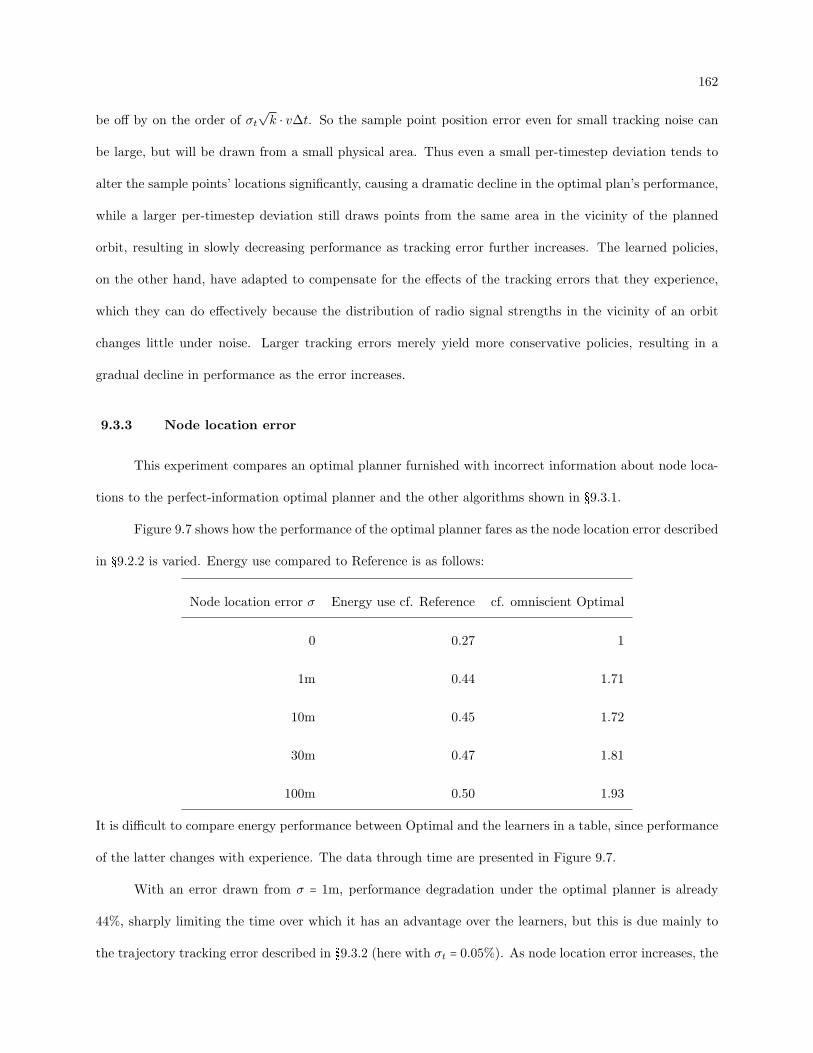
162

be off by on the order of σt√k ⋅ v∆t. So the sample point position error even for small tracking noise can

be large, but will be drawn from a small physical area. Thus even a small per-timestep deviation tends to

alter the sample points’ locations significantly, causing a dramatic decline in the optimal plan’s performance,

while a larger per-timestep deviation still draws points from the same area in the vicinity of the planned

orbit, resulting in slowly decreasing performance as tracking error further increases. The learned policies,

on the other hand, have adapted to compensate for the effects of the tracking errors that they experience,

which they can do effectively because the distribution of radio signal strengths in the vicinity of an orbit

changes little under noise. Larger tracking errors merely yield more conservative policies, resulting in a

gradual decline in performance as the error increases.

9.3.3 Node location error

This experiment compares an optimal planner furnished with incorrect information about node loca-

tions to the perfect-information optimal planner and the other algorithms shown in §9.3.1.

Figure 9.7 shows how the performance of the optimal planner fares as the node location error described

in §9.2.2 is varied. Energy use compared to Reference is as follows:

Node location error σ Energy use cf. Reference cf. omniscient Optimal

0 0.27 1

1m 0.44 1.71

10m 0.45 1.72

30m 0.47 1.81

100m 0.50 1.93

It is difficult to compare energy performance between Optimal and the learners in a table, since performance

of the latter changes with experience. The data through time are presented in Figure 9.7.

With an error drawn from σ = 1m, performance degradation under the optimal planner is already

44%, sharply limiting the time over which it has an advantage over the learners, but this is due mainly to

the trajectory tracking error described in §9.3.2 (here with σt = 0.05%). As node location error increases, the

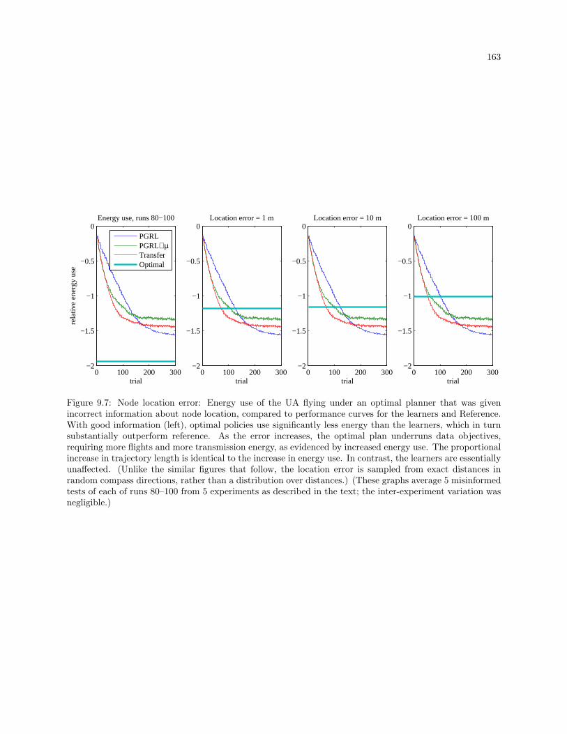
163

0 100 200 300−2

−1.5

−1

−0.5

0

trial

Location error = 1 m

0 100 200 300−2

−1.5

−1

−0.5

0

trial

Location error = 10 m

0 100 200 300−2

−1.5

−1

−0.5

0

trial

Location error = 100 m

0 100 200 300−2

−1.5

−1

−0.5

0

trial

rela

tive

ener

gy u

se

Energy use, runs 80−100

PGRLPGRL∝µTransferOptimal

Figure 9.7: Node location error: Energy use of the UA flying under an optimal planner that was givenincorrect information about node location, compared to performance curves for the learners and Reference.With good information (left), optimal policies use significantly less energy than the learners, which in turnsubstantially outperform reference. As the error increases, the optimal plan underruns data objectives,requiring more flights and more transmission energy, as evidenced by increased energy use. The proportionalincrease in trajectory length is identical to the increase in energy use. In contrast, the learners are essentiallyunaffected. (Unlike the similar figures that follow, the location error is sampled from exact distances inrandom compass directions, rather than a distribution over distances.) (These graphs average 5 misinformedtests of each of runs 80–100 from 5 experiments as described in the text; the inter-experiment variation wasnegligible.)

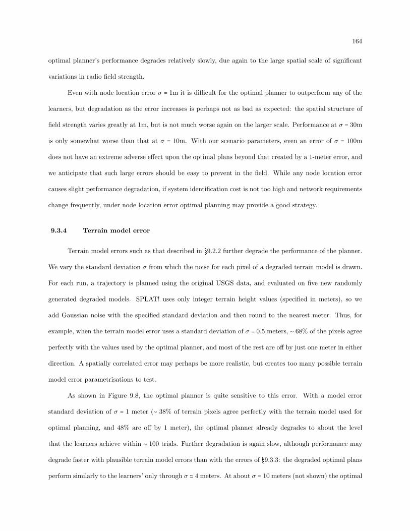
164

optimal planner’s performance degrades relatively slowly, due again to the large spatial scale of significant

variations in radio field strength.

Even with node location error σ = 1m it is difficult for the optimal planner to outperform any of the

learners, but degradation as the error increases is perhaps not as bad as expected: the spatial structure of

field strength varies greatly at 1m, but is not much worse again on the larger scale. Performance at σ = 30m

is only somewhat worse than that at σ = 10m. With our scenario parameters, even an error of σ = 100m

does not have an extreme adverse effect upon the optimal plans beyond that created by a 1-meter error, and

we anticipate that such large errors should be easy to prevent in the field. While any node location error

causes slight performance degradation, if system identification cost is not too high and network requirements

change frequently, under node location error optimal planning may provide a good strategy.

9.3.4 Terrain model error

Terrain model errors such as that described in §9.2.2 further degrade the performance of the planner.

We vary the standard deviation σ from which the noise for each pixel of a degraded terrain model is drawn.

For each run, a trajectory is planned using the original USGS data, and evaluated on five new randomly

generated degraded models. SPLAT! uses only integer terrain height values (specified in meters), so we

add Gaussian noise with the specified standard deviation and then round to the nearest meter. Thus, for

example, when the terrain model error uses a standard deviation of σ = 0.5 meters, ∼ 68% of the pixels agree

perfectly with the values used by the optimal planner, and most of the rest are off by just one meter in either

direction. A spatially correlated error may perhaps be more realistic, but creates too many possible terrain

model error parametrisations to test.

As shown in Figure 9.8, the optimal planner is quite sensitive to this error. With a model error

standard deviation of σ = 1 meter (∼ 38% of terrain pixels agree perfectly with the terrain model used for

optimal planning, and 48% are off by 1 meter), the optimal planner already degrades to about the level

that the learners achieve within ∼ 100 trials. Further degradation is again slow, although performance may

degrade faster with plausible terrain model errors than with the errors of §9.3.3: the degraded optimal plans

perform similarly to the learners’ only through σ ≃ 4 meters. At about σ = 10 meters (not shown) the optimal

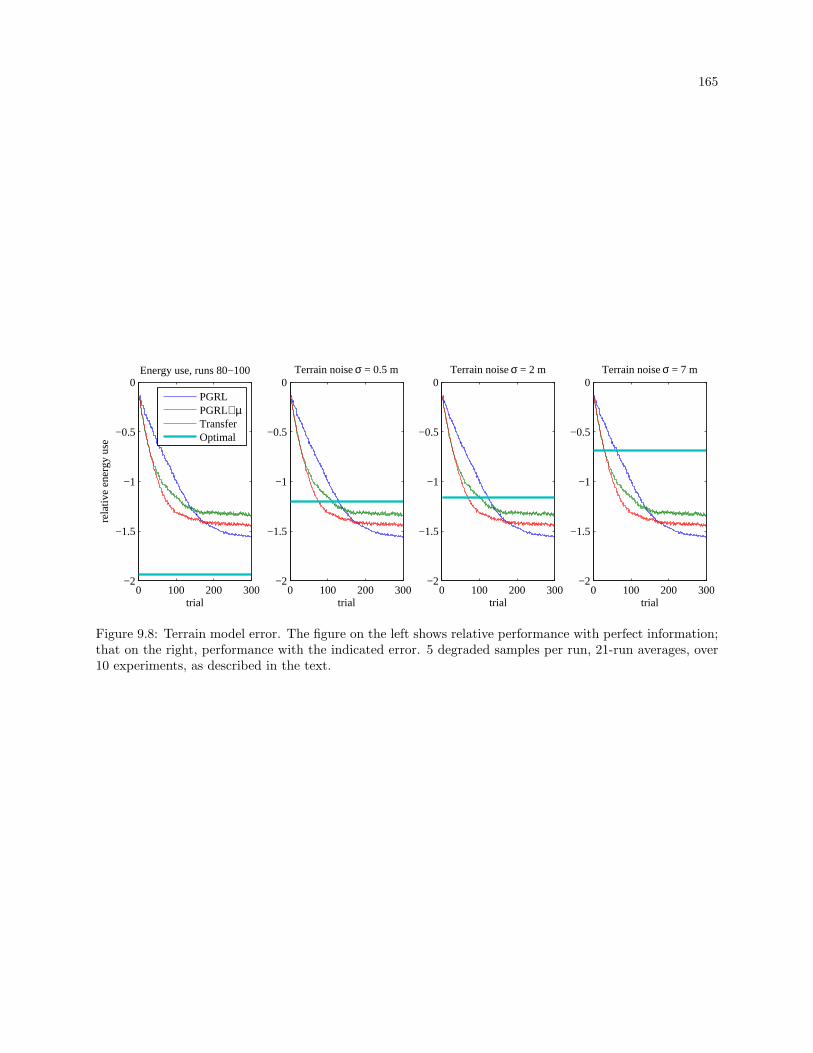
165

0 100 200 300−2

−1.5

−1

−0.5

0

trial

rela

tive

ener

gy u

se

Energy use, runs 80−100

PGRLPGRL∝µTransferOptimal

0 100 200 300−2

−1.5

−1

−0.5

0

trial

Terrain noise σ = 0.5 m

0 100 200 300−2

−1.5

−1

−0.5

0

trial

Terrain noise σ = 2 m

0 100 200 300−2

−1.5

−1

−0.5

0

trial

Terrain noise σ = 7 m

Figure 9.8: Terrain model error. The figure on the left shows relative performance with perfect information;that on the right, performance with the indicated error. 5 degraded samples per run, 21-run averages, over10 experiments, as described in the text.

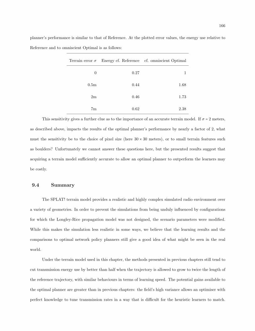
166

planner’s performance is similar to that of Reference. At the plotted error values, the energy use relative to

Reference and to omniscient Optimal is as follows:

Terrain error σ Energy cf. Reference cf. omniscient Optimal

0 0.27 1

0.5m 0.44 1.68

2m 0.46 1.73

7m 0.62 2.38

This sensitivity gives a further clue as to the importance of an accurate terrain model. If σ = 2 meters,

as described above, impacts the results of the optimal planner’s performance by nearly a factor of 2, what

must the sensitivity be to the choice of pixel size (here 30 × 30 meters), or to small terrain features such

as boulders? Unfortunately we cannot answer these questions here, but the presented results suggest that

acquiring a terrain model sufficiently accurate to allow an optimal planner to outperform the learners may

be costly.

9.4 Summary

The SPLAT! terrain model provides a realistic and highly complex simulated radio environment over

a variety of geometries. In order to prevent the simulations from being unduly influenced by configurations

for which the Longley-Rice propagation model was not designed, the scenario parameters were modified.

While this makes the simulation less realistic in some ways, we believe that the learning results and the

comparisons to optimal network policy planners still give a good idea of what might be seen in the real

world.

Under the terrain model used in this chapter, the methods presented in previous chapters still tend to

cut transmission energy use by better than half when the trajectory is allowed to grow to twice the length of

the reference trajectory, with similar behaviours in terms of learning speed. The potential gains available to

the optimal planner are greater than in previous chapters: the field’s high variance allows an optimiser with

perfect knowledge to tune transmission rates in a way that is difficult for the heuristic learners to match.

167

Thus the optimal planner often achieves a further halving of radio energy requirements, often resulting in

energy consumption of only ∼ 25% that of Reference.

However, these large gains are fragile. While the learning planners are robust to poor information

because they do not rely on it, the optimal planner’s use of terrain and UA dynamics information results in

sharply degraded performance in the presence of modelling errors. Through all modelling error types tested,

even slight errors tended to reduce the optimal plans’ performance below the level of the converged learners,

with notable sensitivity to trajectory tracking and terrain model errors.

Perhaps surprisingly, even significant errors generally degraded the optimal plans’ performance only

gradually beyond the initial reduction. This suggests that given an approximate generative model such as

was explored here, it may be desirable to use an optimal planning technique (or the presented learning

techniques using an approximate model) to initialise policies, and then to refine them further in situ using

the PGRL techniques developed here.

The optimal planner produces trajectories very close to our chosen range limit—twice the length of

the reference planner (not exactly twice the length due to the simulator’s discrete timestep). Trajectories

produced by the learners tend to be only ∼ 85% of the length limit (∼ 170% of reference length) in order

to allow for safe exploration in the presence of the observed environmental variability. So even with perfect

models, the optimal planner flies further on average than do the learners. This outcome is exacerbated under

our assumption that the optimal planner compensates for data underrun by flying its trajectory more often.

For purposes of comparison this chapter has defined flight distance (or time) as an unlimited resource, but if

this assumption does not hold, this further potential drawback of the optimal planner should be considered.

We have tested two types of environmental information errors that affect only the optimal planner,

and one that affects both the optimal planner and the learners. The latter, trajectory tracking error,

was found to degrade the optimal planner’s performance especially quickly. We tested the two types of

environment modelling error separately; picking arbitrary values for the errors and combining them would

further degrade the optimal planner, although on realistic scales terrain model error seems to dominate.

Whether a sufficiently accurate system model could be created in reasonable time depends on situation and

resources, and this chapter suggests an initial guess as to the required accuracy.

168

As noted in Chapters 7 and 8, the learners still require time to achieve good performance, which is

a handicap if the mission requirements vary frequently. This can be balanced against the optimal planner’s

handicap in the face of an imperfect system model and the corresponding cost of building and maintaining

a sufficiently accurate model. Once again, it appears that there is a place for both methods, and it may be

valuable to investigate intermediate techniques that combine the two approaches.

Chapter 10

Conclusion

UA-serviced sensor networks can achieve high performance in reasonable time using a model-free

learning approach.

This dissertation presents an investigation of model-free learning techniques for discovery of high-

performance policies for UA-ferried sensor networks. The central claim, that learning approaches can achieve

high performance in reasonable time, is evaluated on two network performance objectives: trajectory length

minimisation, and node energy conservation.

Research in data-ferried sensor networks thus far has made strict assumptions about the shape of the

radio field through which the UA flies. The most sophisticated model in common use treats the radio field

as spherically symmetrical, with received signal strength proportional to 1dϵ for distance d and path loss

exponent ϵ. A key theme of this dissertation is that, since real radio fields have more structure than this,

the oversimplification of radio field models results in poor trajectory planning. Since accurate models are

difficult to acquire and maintain, the proposed approach bypasses model-based planning in favour of learning

directly on the radio fields. The radio environment models used here introduce structure in the following

ways:

Anisotropic antennas. Node antennas are modelled as dipoles at random orientations, and the UA is

equipped with a dipole at fixed orientation, making data retrieval sensitive to UA orientation.

Interference. Nodes transmit simultaneously and interfere with each other. Protocol modifications that

could prevent this are not used, because our objective in designing the radio field simulator is to

170

provide a complex, structure-rich environment in which to test model-free learning techniques.

Terrain. Chapter 9 introduces a third-party terrain-based radio simulator based on the Longley-Rice prop-

agation model, and compares the performance of the learners to optimal planning as terrain infor-

mation is degraded.

Dropping the conventional isotropic radio model breaks conventional trajectory-planning approaches to some

degree, since their assumptions about radio field structure may be optimistic. Model-based planners can

overcome this if their models are good, but there is a trade-off between developing good models and deploying

a network that is functional immediately. Furthermore, maintaining models of sufficient accuracy may be

an ongoing endeavour in the real world.

In order to overcome this limitation of the state of the art, this dissertation proposes the use of

model-free reinforcement learning techniques. They offer the following advantages:

A model of the radio environment is unnecessary. This lifts the burden of ensuring that a model

remains sufficiently accurate throughout the lifetime of a network.

Ability to discover good (near-optimal) policies in a short time relative to the lifetime of typical

networks.

Continually adaptive. When environmental changes happen on timescales longer than the learning

rate, a model-free optimiser tracks those changes by observing the degree to which system be-

haviour affects desired outcomes. Note that this requires a departure from theoretical or controlled-

environment reinforcement learning research: decaying learning rates to 0 over time is inconsistent

with this goal.

Ability to take advantage of system idiosyncrasies. The stereotypical example throughout this docu-

ment is irregular radio fields due to interfering directional antennas, but irregularities due to terrain

are also considered. Causes of radio field irregularities include occlusions, reflections, diffraction,

noise sources, and masses of humid air. Autopilots are unpredictable. Aircraft flight dynamics

change depending on payload (including fuel), air temperature, and servo battery power. A learning

171

approach that ignores expected mechanism and instead optimises only based on observed outcome

can take advantage of unmodelled effects.

10.1 Summary

This dissertation combines several pieces in order to demonstrate a unified system for sensor network

optimisation on complex, unknown radio fields. This section reviews those pieces.

10.1.1 Trajectory optimisation

The choice of trajectory representation was dictated by two requirements: that the trajectory could

be easily manipulated by a learning algorithm, and that it could communicate naturally with off-the-shelf

autopilots. Therefore arbitrary trajectories were eschewed in favour of ones based on small numbers of

waypoints for use by a typical GPS-based navigation system. Trajectory learning is accomplished by learning

the placement of navigation waypoints using stochastic optimisation over multiple tours. The primary

trajectory representation presented here, Data-loops (Chapter 4), places one waypoint for each network

node, circling the waypoint until all data are collected. In the case of trajectory length minimisation, the

optimiser’s objective function is simply the length of the resulting trajectory.

An alternate trajectory representation, Waypoints (Chapter 5), does not associate waypoints with

nodes. Because the waypoints are not associated with the requirement to gather a certain amount of data

from a certain node, the ferry may learn to anticipate future data collection, leaving the vicinity of a

node before completing data transfer and thus achieving higher performance. In order to learn acceptable

trajectories, the objective function must be modified in order to minimise data underruns. Compared to

Data-loops, this yields trajectories whose ultimate performance may be slightly higher, with three notable

drawbacks:

Initially the trajectories may not fulfil data requirements. Significant initial learning time may be

required before the network becomes serviceable. Similarly, changing environmental conditions that

degrade the channel may reintroduce data underruns to a converged trajectory.

172

Trajectories for large data requirements or poor channels are difficult to learn.

When waypoints are not associated with nodes, a version of reinforcement learning’s credit assign-

ment problem emerges, extending learning times as nodes are added.

The third drawback was addressed in Chapter 6, which introduced the LCA algorithm to estimate credit

assignment appropriately for this task. This enhancement allows the Waypoints trajectory encoding to scale

to large networks under some circumstances, such as low data loads. However, the other drawbacks of

Waypoints are better addressed by the Data-loops representation.

Data-loops trajectories interface easily with autopilots, can be learned quickly, tend to produce near-

optimal solutions, and can continue to adapt to changing environmental conditions. Because waypoints are

associated with nodes, Data-loops trajectories decompose into local pieces that can be optimised individually,

reducing scalability concerns. The trajectory optimisation technique is, as expected, versatile, seamlessly

switching from the trajectory length minimisation of Chapter 4 to the energy-minimising tours of Chapter 7.

10.1.1.1 Trajectory optimisation contributions

The development and evaluation of a trajectory representation that is convenient both for the learner

to optimise and for the autopilot to use, and that represents domain-appropriate trajectories well.

The development and evaluation of a stochastic-approximation approach for learning the trajec-

tory representation. Tests show that the Data-loops navigation policies and the learning algorithm

are appropriate for representing trajectories for a variety of data-ferrying problems, both for learn-

ing minimal-length trajectories and for learning trajectories that support energy-optimisation radio

policies.

One unexpected experimental result from Chapter 4 deserves special notice. The UA can benefit significantly

from a directional antenna, especially in a radio field with multiple point noise sources. Trajectories were

learned that took advantage of a dipole antenna’s null in order to reduce interference despite waypoint

placement at significant distance from the target node. In a sparse radio environment, this result may still

be useful for eliminating self-interference from reflections or diffraction.

173

10.1.2 Energy optimisation

Chapter 7 introduces a more challenging network performance objective: node energy conservation

by reducing energy used for data transmission. The presented solution uses excess UA range to increase

contact time with each node, allowing data transmission at lower power and therefore higher efficiency. This

is possible if increased tour time is acceptable—if, for example, target latency is greater than the time taken

for a single tour and refuel/recharge.

10.1.2.1 Energy optimisation contributions

The development and testing of a power policy encoding that takes observed channel quality to radio

output power. A basic behaviour is proposed, to which exploration noise of various forms is added.

The exploration noise is shown to have an effect on performance, and the best strategy is shown via

simulation to allow power policies that represent behaviours that use on average ∼ 13% more energy

than an optimal policy uses on the same trajectory, while including the exploration noise necessary

to allow policy gradients to be computed.

A policy gradient reinforcement learning algorithm on the above encoding works in concert with a

waypoint position optimisation that also uses the energy-optimising objective function. This allows

the discovery of network behaviours that save ∼ 60% of energy compared to Reference, and use ∼ 15%

more energy than optimal, if permitted to extend UA range by a factor of two. This constitutes

∼ 80% of the maximum possible improvement over Reference.

The specification of an optimal power policy subject to autopilot and UA constraints, and evaluation

under the proposed radio field model.

Some additional observations do not qualify as contributions, since they were not shown conclusively, but

they are interesting:

When the model-based optimal planner’s information is degraded, it is likely to be optimistic about

data rates, in which case the planned trajectory will fail to meet data collection goals. This affects

174

the reference planner as well, but not the learning planners, which guarantee complete collection in

exchange for a slight performance penalty.

The time required to learn near-optimal trajectories depends somewhat on radio field complexity.

With limited efforts to hand-tune learning parameters, the learners tended to achieve near-optimal

performance in ⪅ 100 trials. Despite good ultimate performance, 100 trials may be excessive for

many sensor networking scenarios. Faster learning might be achieved by tuning parameters, or by

clever hacks to initialise policy parameters; for example, by immediately setting target transmit

power to the inverse of the UA’s available range factor, which is likely to lead to good trajectories

immediately.

While demonstrating the potential for learning high-performance policies, Chapter 7 revealed a pitfall

of the model-free gradient-based policy optimisation approach: the reward landscape for this domain often

contains steep cliffs near the optimal policy, and policy updates—or, more difficult to prevent, random

variations in the policy’s output due to exploration noise or environmental factors—can lead to high sampling

costs.

10.1.3 Learning to learn energy policies

The problem of steep cliffs in the reward landscape is one that well-tuned learning rate decay largely

obviates, at the expense of losing the ability to track changes in the environment. Another solution would

be for the gradient estimator to learn a model of the RF environment and avoid straying into problematic

regions of policy space, which raises open questions of model maintenance under changing conditions and of

generalisability to unseen problems, but which could be a powerful solution.

Chapter 8 introduced a different response: a high-level policy (or metapolicy) that operates in parallel

with the base policy gradient learning algorithm. This metapolicy supplements the base power policy’s

update from gradient estimation, and is trained using a variant of PGRL, and consequently can steer base

policy updates away from regions that past experience has shown might result in high sampling costs.

Once the metapolicy is trained, its output augments conventional policy learning due to the base

175

PGRL algorithm. This allows it to both speed and stabilise learning on new problems.

The metapolicy is trained using both the actions that it generates and the actions generated by the

base PGRL estimator. Its training sequence spans complete optimisation runs, allowing it to learn to respond

to policy updates that may take the policy into dangerous regions even if a policy update does not result

immediately in a high-cost trajectory. The policy’s representation is extraordinarily simple, which allows

it to be learned relatively quickly (experience optimising power policies for 20–50 nodes seems sufficient to

produce helpful metapolicies), but which also leaves open the possibility of greater performance gain with

the behaviours that a more complex policy could represent.

10.1.3.1 Metapolicy contributions

A metapolicy representation that can speed and stabilise learning on new problems by augmenting

base policy updates. The metapolicy is a vehicle for learning to learn. This is valuable in two

ways:

* Policies for new data-ferrying scenarios are learned faster based on experience with past prob-

lems.

* Certain learning parameter choices, such as inappropriate learning rates, lead to unstable be-

haviours in the learner. The metapolicy can provide corrective adjustments, reversing updates

from the gradient-based policy search that are likely to lead to high-cost trajectories.

A policy gradient reinforcement learning algorithm for the metapolicy that packages experience with

past problems in a way that teaches the metapolicy what updates to the base policy are likely to

lead to good or bad outcomes. Effective metapolicies tend to become useful after the metapolicy

learner has trained them with experience from ∼ 30–50 power policy optimisation experiences.

A technique for balancing the policy updates from the metapolicy against those from the base

gradient estimator. Assuming that the base policy’s update is an unbiased estimate of the best

update, it measures the metapolicy’s deviation from that and balances the two based on estimates

of the two estimators’ MSEs.

176

However, note that the base PGRL estimate is not generally optimal in the long term unless the

learning rate decays, which we eschew in favour of continuous adaptability to environmental changes.

Therefore the metapolicy may be underutilised when it disagrees with bad PGRL updates.

10.1.4 Evaluation under a terrain-based radio simulator

Chapter 9 introduces a third-party radio simulator, SPLAT!, which is based on the Longley-Rice

propagation model. The Longley-Rice model gives erratic results in certain configurations, so as a concession

to the simulator, we introduced modified versions of the scenario parameters in order to push trajectories

into regions for which the model was designed.

The algorithms that were developed through Chapter 8 were tested using SPLAT! as a drop-in re-

placement for our simpler radio simulator. Results were qualitatively similar to those obtained under our

radio model. More surprisingly, gains are quantitatively similar as well. For example, with the objectives of

Chapter 8, PGRL learns policies that permit a ∼ 65% energy savings within ∼ 200 trials, and that surpass the

expected performance of an optimal planner with degraded environmental information within ∼ 140 trials.

A trained metapolicy permits PGRL∝ µ to save slightly less energy (∼ 62%) but to achieve its gain far

more quickly (performing as well as a typically degraded optimal planner within ∼ 70–100 trials), and again

minimises trajectory length overruns. Policy transfer is again successful, perhaps more surprisingly since

the radio field configurations exhibit much more extreme variance due to the pronounced effect of terrain on

the radio field. Even metapolicy training proceeds similarly—on the order of 50–100 optimisation runs on

different ferrying scenarios are required before the metapolicy’s potential begins to be realised.

More important than the specifics of learning rates and ultimate gains is the comparison of the

learners to optimal planning. Under SPLAT!, the optimal planner can generally achieve much higher gains

than it can under our simpler model—often producing policies that achieve a ∼ 75% reduction in energy used

compared to Reference. However, we show that under SPLAT!, these changes are extremely fragile, and

that performance degrades to approximately the level of the learners in the presence of even slight modelling

errors.

177

10.1.4.1 Terrain-based radio simulator contributions

Modifications to SPLAT! to allow it to evaluate UA trajectories, permitting the development of

closed-loop UA and radio control policies.

Modifications to the evaluation scenarios that encourage trajectories within the range of configura-

tions for which the Longley-Rice model was intended.

Evaluation of the algorithms developed throughout this work under a realistic, complex, terrain-

based radio model, demonstrating the validity of conclusions made under a simpler model.

Evaluation of the degradation of the optimal power policy planner under modelling errors in a

realistic, complex, terrain-based radio model.

10.2 Open issues and future work

This dissertation has answered questions about the viability of model-free optimisation and reinforce-

ment learning for the optimisation of UA-ferried networks. Under some conditions, the approaches presented

here result in high performance in reasonable time. However, much work remains to be done:

10.2.1 Time-varying effects

We considered only networks of stationary or nearly stationary sensors, in environments that change

only on the timescale of multiple tours. This includes many scientific applications, such as polar ice pack

measurement, tectonic sensing, hydrology, and certain types of wildlife study, as well as some military

surveillance. However, in other applications, changing environment and requirements would require faster

re-planning than this method can accommodate.

Unpredictable time-varying interference causes special difficulties for any trajectory planner, but some-

times can be managed. A rapidly time-varying environment introduces another source of noise into the

samples used for the learners’ gradient estimates, which would slow convergence, although the gradient es-

timator would be sampling over the time-varying distribution and would therefore still converge to at least

a local optimum given the noise distribution. Environmental changes with longer timescales (over several

178

tours) would give the learner some time to adapt; depending on the rate of environmental variation and the

learning rate, the learner might effectively track the change. While it may be possible to learn to anticipate

such change, the methods presented here do not consider this case.

Analogously, model-based planners that characterised time-varying signals in the environment could

plan for the signals’ effect upon desired outcomes. This strategy is more versatile than the model-free learning

approach put forward in this dissertation, but also more time-consuming to deploy and more sensitive to

inaccuracies in the model.

10.2.2 Metapolicy training

The metapolicy of Chapter 8 learns fastest, and learns the best policies, when trained on ⟨ state,

action, reward ⟩ sets that include tuples both from when the action was generated by the base PGRL

gradient estimator and from when it was generated by the metapolicy. Removing either of those training

examples degrades metapolicy performance. In general, PGRL algorithms explore by adding noise to the

policies’ actions, but as far as we are aware, this is a unique situation in which some of the “noise” that is

added tends to maximise reward. In a higher-dimensional policy space, this might drastically improve the

quality of the estimated gradient by increasing the likelihood of exploration along the relevant direction, but

in a two-dimensional policy space, this exploration seems tenuous.

Important future work involves identifying the mechanism for the improvement; extending the result to

higher-dimensional policy spaces. Most interesting, however, will be an investigation as to whether more and

better exploration can be achieved by choosing not just one µ-action based on the base gradient estimator’s

update, but several in directions that are some function of the base update vector.

10.2.3 Real-world tests

The results presented herein are based on simulations. While even our own radio environment model

provides a more realistic testing environment than other work in the field, and while the SPLAT! simulations

provide a significantly greater level of realism, various features that have been found in real-world tests of

similar systems are absent from our model. Some, but by no means all, of these features are:

179

Radio signal strength patterns more irregular than the dipoles used here due to reflections and

self-interference.

Systematic noise such as RF noise caused by storage device writes on the UA during data upload.

Autopilot idiosyncrasies such as the rate at which navigation changes are made, including over/under-

damped controls.

UA flight patterns such as frequent nonzero roll angles due to minor course corrections in response

to wind or GPS jumps (although Chapter 9 introduced a preliminary experiment to address this).

Changing UA dynamics as its fuel load is used.

UA and radio reactions to changing weather conditions.

While it may reasonably expected that a learning algorithm’s gradient estimator will sample over any of

these effects and therefore consider it a part of the environment to be optimised around or taken advantage

of, that hope is not a certainty for two reasons:

Timescale of the effect: unmodelled effects on timescales shorter than the state/action cycle will be op-

timised over, and ones on timescales on the order of the convergence time of the learner will be

tracked as they change, but effects in intermediate timescales may cause difficulties with the gradi-

ent estimation process.

Introduction of poor local optima: the environmental model used herein tended to have few local op-

tima, and stochastic search usually approached the globally optimal solution. If effects missing from

the simulator were to drastically change the reward landscape, then the methods presented here

would be much less effective. Should this be the case, the best known solution method would prob-

ably be an accurate and complete environmental model and copious offline planning time during

which nonlinear global optimisation could be performed.

The question of what is lost in simulation, and what effect it will have upon the optimisation process, is best

answered through real-world tests.

180

10.2.4 Wind

Wind is of great interest to the UA community. The work for this dissertation included a brief

investigation into the effects of steady wind upon optimal trajectories and trajectory learning; it was found

that a perfect wind correction in the autopilot, similar to those found on commercial units, generally resulted

in only modest changes to planning and performance at windspeeds w ⪅ v2for UA flight velocity v. Data-

gathering must of course be suspended when w ⪆ v, but there may be network deployments in which the

ability to plan good trajectories close to the feasibility limit would be valuable. This might be especially

important for military surveillance, disaster monitoring, and networks in polar regions where winds tend to

remain high for long periods.

In contrast to treatment as a steady-state vector, wind may be treated as a rapidly varying field,

pushing the UA around unpredictably and causing small trajectory tracking errors. §9.2.1 briefly explored

the effect that such an input would have, and showed that while the terrain-based optimal planner is quite

sensitive to small random fluctuations in the trajectory, the learners observe the effect of planning given the

turbulence and are therefore able to compensate despite having no knowledge of the cause. Further research

could examine building spatially-localised estimates of turbulence, possibly inferring likely turbulence from

terrain features, and using such inferences to push trajectory exploration in likely-good directions.

10.2.5 Intra-trajectory learning

The waypoint placement presented herein uses a tour of the nodes as the basic unit of policy variation

because reward information is readily available after a complete tour. However, waypoint placement could

be adjusted while orbiting a node, such that the unit of policy variation is a complete circle. This would

involve the design of secondary reward-correlated signals, but could reduce waypoint placement times for

trajectories with high data requirements.

10.2.6 Dynamic network requirements

This dissertation has assumed that network requirements do not change during operation; for example,

that data are generated at a constant rate. When data loads are variable, the Data-loops trajectory planner

181

continues to collect all data, but using trajectories planned under different conditions results in subpar

performance. Other changes, such as balancing energy use among many nodes each of whose energy stores

is replenished at a variable rate, may demand model-based planning. However, for prolonged-operation

networks, Appendix B suggests an alternative: learning to adjust policies for changing data requirements.

A simple method is proposed and preliminary evaluations are performed, but a more sophisticated method

from Kober et al. [2012] appears extremely promising. Future work will compare the approach proposed in

Appendix B with that of Kober et al. [2012] and with optimal model-based planning.

10.3 Conclusion

This dissertation opens with the observation that accurate system models for UA-ferried networks are

difficult to acquire and maintain, but that inaccurate models lead to poor planning. Whereas prior research

has planned trajectories based on on oversimplified radio field models and ignored the performance penalty

caused by planning with inaccurate information, this dissertation discards models entirely, and shows that

without system models, near-optimal network policies can be learned on timescales of as few as several dozen

tours. Low or nonexistent system identification times permit rapid deployment of the network, performance

improves over time, and slow environmental changes are continually tracked by the learning algorithms.

The approach has notable weaknesses:

A period of significantly suboptimal performance exists before the learners find good solutions make

the approach infeasible for some sensor networks, especially short-lifetime networks in which there

would be few data-collection flights before decommissioning or large modifications to the network’s

geometry.

Compared to optimal planning with good models, the learning system cannot adapt instantly to

new network objectives. For example, the proposed method would not be appropriate for adaptive

sensing tasks in which data collection objectives vary widely from tour to tour.

These weaknesses rule out the proposed approach for some important applications. However, for networks

that are expected to be stable over long periods, the techniques developed in this dissertation can learn

182

policies that offer near-optimal performance without relying on system models.

This dissertation advances the state of the art by lifting a significant restriction on the problem of

policy planning for ferried networks. The reinforcement learning approach can discover near-optimal policies

in reasonable time despite complex, unknown radio environments, allowing sensor networks to be rapidly

deployed in the field. The primary problem studied here, sensor lifetime extension by learning to conserve

node energy, provides a rich testbed for algorithms and requirements. It is expected that optimisations for

other network desiderata will be amenable to the same approach, possibly requiring nothing more than the

design of appropriate policy representations.

Bibliography

Pieter Abbeel, Adam Coates, and Andrew Y. Ng. Autonomous helicopter aerobatics through apprenticeshiplearning. I. J. Robotic Res., 29(13):1608–1639, 2010.

Yamin Samir Al-Mousa. Mac/routing design for under water sensor networks. Master’s thesis, RochesterInstitute of Technology, 2007.

Giuseppe Anastasi, Marco Conti, and Mario Di Francesco. Reliable and energy-efficient data collectionin sparse sensor networks with mobile elements. Perform. Eval., 66:791–810, December 2009a. ISSN0166-5316. doi: http://dx.doi.org/10.1016/j.peva.2009.08.005.

Giuseppe Anastasi, Marco Conti, Mario Di Francesco, and Andrea Passarella. Energy conservation inwireless sensor networks: a survey. Ad Hoc Netw., 7:537–568, May 2009b. ISSN 1570-8705. doi:10.1016/j.adhoc.2008.06.003.

Malika Baghzouz, Dale A. Devitt, Lynn F. Fenstermaker, and Michael H. Young. Monitoring vegetationphenological cycles in two different semi-arid environmental settings using a ground-based ndvi system: Apotential approach to improve satellite data interpretation. Remote Sensing, 2(4):990–1013, 2010. ISSN2072-4292. doi: 10.3390/rs2040990.

Bikramjit Banerjee and Peter Stone. General game learning using knowledge transfer. In In The 20thInternational Joint Conference on Artificial Intelligence, pages 672–677, 2007.

Jonathan Baxter and Peter L. Bartlett. Infinite-horizon policy-gradient estimation. Journal of ArtificialIntelligence Research, 15:319–350, 2001.

R. Bellman. A markovian decision process. Journal of Mathematics and Mechanics, 6, 1957.

Muhammad Mukarram Bin Tariq, Mostafa Ammar, and Ellen Zegura. Message ferry route design for sparsead hoc networks with mobile nodes. In MobiHoc: Proceedings of the 7th ACM international symposiumon Mobile ad hoc networking and computing, pages 37–48, New York, NY, USA, 2006. ACM. ISBN1-59593-368-9. doi: http://doi.acm.org/10.1145/1132905.1132910.

Ladislau Boloni and Damla Turgut. Should i send now or send later? a decision-theoretic approach totransmission scheduling in sensor networks with mobile sinks. Wireless Communications and MobileComputing, 8(3):385–403, 2008.

Justin Boyan and Andrew W. Moore. Learning evaluation functions to improve optimization by local search.Journal of Machine Learning Research, 2001.

Justin A. Boyan and Andrew W. Moore. Generalization in reinforcement learning: Safely approxi-mating the value function. In G. Tesauro, D. S. Touretzky, and T. K. Leen, editors, Advances inNeural Information Processing Systems 7, pages 369–376, Cambridge, MA, 1995. The MIT Press. URLhttp://citeseer.ist.psu.edu/boyan95generalization.html.

184

Timothy X Brown, B. M. Argrow, Eric W. Frew, Cory Dixon, Daniel Henkel, J. Elston, and H. Gates.Experiments Using Small Unmanned Aircraft to Augment a Mobile Ad Hoc Network, chapter 28, pages123–145. Cambridge University Press, 2007. URL http://dx.doi.org/10.1017/CBO9780511611421.

Anthony Carfang and Eric W. Frew. Real-time estimation of wireless ground-to-air communication param-eters. In IEEE International Conference on Computing, Networking and Communications, pages 1–5,Maui, Hawaii, January 2012.

Anthony Carfang, Eric W. Frew, and Timothy X Brown. Improved delay-tolerant communication by con-sidering radio propagation in planning data ferry navigation. In Proc. AIAA Guidance, Navigation, andControl, pages 5322–5335, Toronto, Canada, August 2010. AIAA.

A. Chakrabarti, A. Sabharwal, and B. Aazhang. Using predictable observer mobility for power efficientdesign of sensor networks. In Information Processing in Sensor Networks, pages 552–552. Springer, 2003.

HaiYang Chao, YongCan Cao, and YangQuan Chen. Autopilots for small unmanned aerial vehi-cles: A survey. International Journal of Control, Automation and Systems, 8:36–44, 2010. URLhttp://dx.doi.org/10.1007/s12555-010-0105-z. 10.1007/s12555-010-0105-z.

D. Ciullo, G. Celik, and E. Modiano. Minimizing transmission energy in sensor networks via trajectorycontrol. In IEEE Symposium on Modeling and Optimization in Mobile, Ad Hoc, and Wireless Networks(WiOpt), pages 132–141, 2010.

Carrick Detweiller, Iuliu Vasilescu, and Daniela Rus. An underwater sensor network withdual communications, sensing, and mobility. In OCEANS Europe, pages 1–6, 2007. doi:http://dx.doi.org/10.1109/OCEANSE.2007.4302445.

M. Di Francesco, S.K. Das, and G. Anastasi. Data collection in wireless sensor networks with mobile elements:a survey. ACM Transactions on Sensor Networks (TOSN), 8(1):7, 2011.

Cory Dixon. Controlled Mobility of Unmanned Aircraft Chains to Optimize Network Capacity in RealisticCommunication Environments. PhD thesis, University of Colorado, 2010.

Mathew Dunbabin, Peter Corke, Iuliu Vasilescu, and Daniela Rus. Data muling over underwater wirelesssensor networks using an autonomous underwater vehicle. In Proc. of IEEE International Conference onRobotics and Automation (ICRA), pages 2091–2098, 2006.

M. Erol-Kantarci, H.T. Mouftah, and S. Oktug. A survey of architectures and localization techniques forunderwater acoustic sensor networks. Communications Surveys & Tutorials, IEEE, 13(3):487–502, 2011.

Jiancheng Fang, Cunxiao Miao, and Yuhu Du. Adaptive nonlinear path following method for fix-wing microaerial vehicle. Industrial Robot: An International Journal, 39(5):475–483, 2012.

Fernando Fernandez and Manuela Veloso. Probabilistic policy reuse in a reinforcement learning agent. InProceedings of the Fifth International Joint Conference on Autonomous Agents and Multi-Agent Systems,May 2006. URL citeseer.ist.psu.edu/andez06probabilistic.html.

P. Glynn. Likelihood ratio gradient estimation: An overview. In Proceedings of the 1987 Winter SimulationConference, pages 366–375, 1987.

Y. Gu, D. Bozdag, R. W. Brewer, and E. Ekici. Data harvesting with mobile elements in wireless sensornetworks. Computer Networks 50, 17:3449–3465, 2006.

Brendan Heery, Lorna Fitzsimons, Timothy Sullivan, James Chapman, Fiona Regan, Kim Lau, DermotBrabazon, JungHo Kim, and Dermot Diamond. Monitoring the marine environment using a low-costcolorimetric optical sensor. In The Sixth International Conference on Sensor Technologies and Applications(IARIA SensorComm), Rome, Italy, 9 2012. IARIA.

185

Daniel Henkel and Timothy X. Brown. Towards autonomous data ferry route design through reinforce-ment learning. In Proceedings of the 2008 International Symposium on a World of Wireless, Mobile andMultimedia Networks (WOWMOM), pages 1–6, Washington, DC, USA, 2008a. IEEE. ISBN 978-1-4244-2099-5. doi: http://dx.doi.org/10.1109/WOWMOM.2008.4594888.

Daniel Henkel and Timothy X Brown. On controlled node mobility in delay-tolerant networks of unmannedaerial vehicles. In International Symposium on Advance Radio Technolgoies, pages 7–16, 2008b.

John A. Hertz, Andrers S. Krogh, and Richard G. Palmer. Introduction to the Theory of Neural Computation.Perseus Books, 1991.

T. Hirokami, Y. Maeda, and H. Tsukada. Parameter estimation using simultaneous perturbation stochasticapproximation. Electrical Engineering in Japan, 154 (2), 2006.

Tu Dac Ho, Jingyu Park, and Shigeru Shimamoto. Qos constraint with prioritized frame selection cdmamac protocol for wsn employing uav. In IEEE Globecom 2010 Workshop on Wireless Networking forUnmanned Aerial Vehicles (Wi-UAV 2010), 2010.

A. Ijspeert, J. Nakanishi, and S. Schaal. Learning attractor landscapes for learning motor primitives. InAdvances in Neural Information Processing Systems, number 15, pages 1523–1530, Cambridge, MA, 2002.MIT Press.

A. Jenkins, D. Henkel, and T.X Brown. Sensor data collection through gateways in a highly mobile meshnetwork. In Proc. IEEEWireless Communications and Networking Conference (WCNC), pages 2784–2789,Hong Kong, 2007. IEEE.

Feng Jiang and Lee Swindlehurst. Dynamic uav relay positioning for the ground-to-air uplink. In IEEEGlobecom 2010 Workshop on Wireless Networking for Unmanned Aerial Vehicles (Wi-UAV 2010), 2010.

Philo Juang, Hidekazu Oki, Yong Wang, Margaret Martonosi, Li Shiuan Peh, and Daniel Ruben-stein. Energy-efficient computing for wildlife tracking: Design tradeoffs and early experienceswith zebranet. SIGOPS Oper. Syst. Rev., 36:96–107, October 2002. ISSN 0163-5980. doi:http://doi.acm.org/10.1145/635508.605408.

H. Jun, W. Zhao, M. H. Ammar, E. W. Zegura, and C. Lee. Trading latency for energy in densely deployedwireless ad hoc networks using message ferrying. Ad Hoc Netw., 5:444–461, May 2007. ISSN 1570-8705.doi: 10.1016/j.adhoc.2006.02.001.

V. Kavitha. Continuous polling with rerouting and applications to ferry assisted wireless lans. In Proceedingsof the 5th International ICST Conference on Performance Evaluation Methodologies and Tools, pages81–90. ICST (Institute for Computer Sciences, Social-Informatics and Telecommunications Engineering),2011.

Farid Kendoul, Yu Zhenyu, and Kenzo Nonami. Embedded autopilot for accurate waypoint navigation andtrajectory tracking: application to miniature rotorcraft uavs. In Proceedings of the 2009 IEEE internationalconference on Robotics and Automation, ICRA’09, pages 2332–2338, Piscataway, NJ, USA, 2009. IEEEPress. ISBN 978-1-4244-2788-8. URL http://dl.acm.org/citation.cfm?id=1703775.1703828.

Kunikazu Kobayashi, Hiroyuki Mizoue, Takashi Kuremoto, and Masanao Obayashi. A meta-learning methodbased on temporal difference error. In ChiSing Leung, Minho Lee, and JonathanH. Chan, editors, NeuralInformation Processing, volume 5863 of Lecture Notes in Computer Science, pages 530–537. SpringerBerlin Heidelberg, 2009. ISBN 978-3-642-10676-7.

Jens Kober, Andreas Wilhelm, Erhan Oztop, and Jan Peters. Reinforcement learning to adjust parametrizedmotor primitives to new situations. Auton. Robots, 33(4):361–379, 2012.

Nate Kohl and Peter Stone. Policy gradient reinforcement learning for fast quadrupedal locomotion. In inProceedings of the IEEE International Conference on Robotics and Automation, pages 2619–2624, 2004.

186

J. Zico Kolter, Zachary Jackowski, and Russ Tedrake. Design, analysis and learning control of a fully actuatedmicro wind turbine. In Proceedings of the 2012 American Control Conference (ACC), 2012.

G.D. Konidaris and A.G. Barto. Building portable options: Skill transfer in reinforcement learning. Technicalreport, University of Massachusetts Department of Computer Science, 2006.

Klas Kronander, Seyed Mohammad Khansari-Zadeh, and Aude Billard. Learning to Control Planar HittingMotions in a Minigolf-like Task. In Proceedings of the IEEE/RSJ International Conference on IntelligentRobots and Systems, 2011. (IROS 2011)., IEEE International Conference on Intelligent Robots and Sys-tems. Ieee Service Center, 445 Hoes Lane, Po Box 1331, Piscataway, Nj 08855-1331 Usa, 2011. Winner ofJTCF Novel Technology Paper Award for Amusement Culture.

HT Kung, Chit-Kwan Lin, Tsung-Han Lin, Steve Tarsa, and Dario Vlah. Measuring receiver diversity on alow-altitude uav in a ground-to-air wireless mesh network. In IEEE Globecom 2010 Workshop on WirelessNetworking for Unmanned Aerial Vehicles (Wi-UAV 2010), 2010.

C. H. Liu, T. He, K. W. Lee, K. K. Leung, and A. Swami. Dynamic control of data ferries under partialobservations. In IEEE WCNC 2010, 2010.

A. G. Longley and P. L. Rice. Prediction of tropospheric radio transmission loss over irregular terrain; acomputer method. Technical Report ESSA-TR-ERL79-ITS67, Environmental Science Services Adminis-tration, Institute for Telecommunication Sciences, Boulder, CO 80302, USA, July 1968.

Ming Ma and Yuanyuan Yang. Sencar: An energy-efficient data gathering mechanism for large-scale multihopsensor networks. IEEE Transactions on Parallel and Distributed Systems, 18:1476–1488, 2007. ISSN 1045-9219. doi: http://doi.ieeecomputersociety.org/10.1109/TPDS.2007.1070.

Michael G. Madden and Tom Howley. Transfer of experience between reinforcement learning environ-ments with progressive difficulty. Artif. Intell. Rev., 21(3-4):375–398, 2004. ISSN 0269-2821. doi:http://dx.doi.org/10.1023/B:AIRE.0000036264.95672.64.

John A. Magliacane. Splat! a terrestrial rf path analysis application for linux/unix.http://www.qsl.net/kd2bd/splat.html, March 2011. Accessed: 2013-03-08.

S. Mahadevan. Proto-value functions: Developmental reinforcement learning. In Proceedings of the 22ndinternational conference on Machine learning. ICML, 2005.

Harry L. McQuillen and Larry W. Brewer. Methodological considerations for monitoring wild bird nestsusing video technology. Journal of Field Ornithology, 71(1):167–172, 2000.

N. Mehta, S. Natarajan, P. Tadepalli, and A. Fern. Transfer in variable-reward hierarchical reinforcementlearning. Machine Learning, 73(3):289–312, 2008.

Andrew W. Moore and Christopher G. Atkeson. Prioritized sweeping: Reinforcement learning with less dataand less real time. Machine Learning, 13:103–130, 1993.

Reginald R. Muskett and Vladimir E. Romanovsky. Alaskan permafrost groundwater storage changes de-rived from grace and ground measurements. Remote Sensing, 3(2):378–397, 2011. ISSN 2072-4292. doi:10.3390/rs3020378.

S.J. Pan and Q. Yang. A survey on transfer learning. Knowledge and Data Engineering, IEEE Transactionson, 22(10):1345–1359, 2010.

Ben Pearre. Model-free trajectory optimisation for wireless data ferries. In 6th IEEE International Workshopon Performance and Management of Wireless and Mobile Networks (P2MNET), 2010.

Ben Pearre and Timothy X Brown. Fast, scalable, model-free trajectory optimization for wireless data ferries.In IEEE International Conference on Computer Communications and Networks (ICCCN), pages 370–377,2011.

187

Ben Pearre and Timothy X Brown. Self-monitoring reinforcement metalearning for energy conservationin data-ferried sensor networks. In The Sixth International Conference on Sensor Technologies andApplications (IARIA SensorComm), pages 296–305, Rome, Italy, 9 2012a. IARIA.

Ben Pearre and Timothy X. Brown. Model-free trajectory optimisation for unmanned aircraft serving asdata ferries for widespread sensors. Remote Sensing, 4(10):2971–3005, 2012b. ISSN 2072-4292. doi:10.3390/rs4102971. URL http://www.mdpi.com/2072-4292/4/10/2971.

Benjamin Pearre and Timothy Brown. Model-free trajectory optimization for wireless data ferries among mul-tiple sources. In Globecom Workshop on Wireless Networking for Unmanned Aerial Vehicles (Wi-UAV),Miami, Florida, USA, 12 2010. IEEE.

T. J. Perkins and D. Precup. Using options for knowledge transfer in reinforcement learn-ing. Technical Report UM-CS-1999-034, University of Massachusetts, , 1999. URLciteseer.ist.psu.edu/perkins99using.html.

J. Peters and S. Schaal. Reinforcement learning of motor skills with policy gradients. Neural Networks, 21(4):682–697, 2008.

Xiaojiang Ren and Weifa Liang. Delay-tolerant data gathering in energy harvesting sensor networks with amobile sink. In Global Communications Conference, Anaheim, CA, USA, 12 2012. IEEE.

J. A. Richter-Menge, D. K. Perovich, B. C. Elder, K. Claffey, I. Rigor, and M. Ortmeyer. Ice mass-balancebuoys: a tool for measuring and attributing changes in the thickness of the Arctic sea-ice cover. Annalsof Glaciology, 44:205–210, 2006. doi: 10.3189/172756406781811727.

John W. Roberts, Lionel Moret, Jun Zhang, and Russ Tedrake. Motor Learning at Intermediate ReynoldsNumber: Experiments with Policy Gradient on the Flapping Flight of a Rigid Wing., chapter From Motorto Interaction Learning in Robots. Springer, 2009.

P. Sadegh and J. Spall. Optimal random perturbations for stochastic approximation using a simultaneousperturbation gradient approximation. In Proceedings of the American Control Conference, pages 3582–3586, 1997.

T. Schaul and J. Schmidhuber. Metalearning. Scholarpedia, 5(6):4650, 2010a.

T. Schaul and J. Schmidhuber. Metalearning. Scholarpedia, 5(6):4650, 2010b.

N. Schweighofer and K. Doya. Meta-learning in reinforcement learning. Neural Networks, 16:5–9, 2003.

R.C. Shah, S. Roy, S. Jain, and W. Brunette. Data mules: Modeling a three-tier architecture for sparsesensor networks. In Sensor Network Protocols and Applications, 2003. Proceedings of the First IEEE.2003 IEEE International Workshop on, pages 30 – 41, May 2003. doi: 10.1109/SNPA.2003.1203354.

Arun A. Somasundara, Aditya Ramamoorthy, and Mani B. Srivastava. Mobile element scheduling withdynamic deadlines. IEEE Transactions on Mobile Computing, 6(4):395–410, 2007. ISSN 1536-1233. doi:http://dx.doi.org/10.1109/TMC.2007.57.

Maciej Stachura, Anthony Carfang, and Eric W. Frew. Cooperative target tracking with a communicationlimited active sensor network. In International Workshop on Robotic Wireless Sensor Networks, 2009.

R. Sugihara and R. K. Gupta. Optimizing energy-latency trade-off in sensor networks with controlledmobility. In IEEE INFOCOM Mini-conference, pages 2566–2570, 2009.

Ryo Sugihara and Rajesh K. Gupta. Improving the data delivery latency in sensor networks with con-trolled mobility. In Proc. 4th IEEE international conference on Distributed Computing in Sensor Systems,DCOSS, pages 386–399, Berlin, Heidelberg, 2008. Springer-Verlag. ISBN 978-3-540-69169-3.

188

Ryo Sugihara and Rajesh K. Gupta. Speed control and scheduling of data mules in sen-sor networks. ACM Trans. Sen. Netw., 7:4:1–4:29, August 2010. ISSN 1550-4859. doi:http://doi.acm.org/10.1145/1806895.1806899. URL http://doi.acm.org/10.1145/1806895.1806899.

Ryo Sugihara and Rajesh K. Gupta. Path planning of data mules in sensor networks. In ACM Trans. Sen.Netw., volume 8, pages 1–27, New York, USA, August 2011. ACM. doi: 10.1145/1993042.1993043.

R. S. Sutton, D. McAllester, S Singh, and Y. Mansour. Policy gradient methods for reinforcement learningwith function approximation. In Advances in Neural Information Processing Systems, pages 1057–1063,2000.

R.S. Sutton and A.G. Barto. Reinforcement Learning: An Introduction. MIT Press, Cambridge, MA, 1998.URL http://www.cs.ualberta.ca/ sutton/book/ebook/the-book.html.

Fumihide Tanaka and Masayuki Yamamura. Multitask reinforcement learning on the distribution of mdps.In Proceedings of the 2003 IEEE International Symposium on Computational Intelligence in Robotics andAutomation, pages p.1108–1113, 2003.

J. Tang and P. Abbeel. On a connection between importance sampling and the likelihood ratio policygradient. In Neural Information Processing Systems (NIPS), 2010.

Jun Tao, Liang He, Yanyan Zhuang, Jianping Pan, and Maryam Ahmadi. Sweeping and active skippingin wireless sensor networks with mobile elements. In Global Communications Conference, Anaheim, CA,USA, 12 2012. IEEE.

Matthew E. Taylor and Peter Stone. Behavior transfer for value-function-based reinforcement learning. InFrank Dignum, Virginia Dignum, Sven Koenig, Sarit Kraus, Munindar P. Singh, and Michael Wooldridge,editors, The Fourth International Joint Conference on Autonomous Agents and Multiagent Systems, pages53–59, New York, NY, July 2005. ACM Press.

Matthew E. Taylor and Peter Stone. Transfer learning for reinforcement learning domains: A survey. Journalof Machine Learning Research, 10:1633–1685, 2009.

Matthew E. Taylor, Gregory Kuhlmann, and Peter Stone. Autonomous transfer for reinforcement learning.In The Seventh International Joint Conference on Autonomous Agents and Multiagent Systems, May2008.

Stuart G Taylor, Kevin M Farinholt, Eric B Flynn, Eloi Figueiredo, David L Mascarenas, Erik A Moro,Gyuhae Park, Michael D Todd, and Charles R Farrar. A mobile-agent–based wireless sensing net-work for structural monitoring applications. Measurement Science and Technology, 20(4), 2009. URLhttp://stacks.iop.org/0957-0233/20/i=4/a=045201.

O. Tekdas, J.H. Lim, A. Terzis, and V. Isler. Using mobile robots to harvest data from sensor fields. IEEEWireless Communications special Issue on Wireless Communications in Networked Robotics, 16:22–28,2008.

S. Thrun. A lifelong learning perspective for mobile robot control. In V. Graefe, editor, Intelligent Robotsand Systems. Elsevier, 1995.

Sebastian Thrun. Explanation-based Neural Network Learning. PhD thesis, CMU, 1996.

L. Torrey and J. Shavlik. Transfer learning. In Handbook of Research on Machine Learning Applications,2009.

H. van Hasselt and M.A. Wiering. Reinforcement learning in continuous action spaces. In ApproximateDynamic Programming and Reinforcement Learning, 2007. ADPRL 2007. IEEE International Symposiumon, pages 272–279. IEEE, 2007.

189

Neeti Wagle and Eric W. Frew. A particle filter approach to wifi target localization. In AIAA Guidance,Navigation, and Control Conference, pages 2287–2298, Toronto, Canada, August 2010. AIAA.

Guoqiang Wang, Damla Turgut, Ladislau Boloni, Yongchang Ji, and Dan C. Marinescu. A mac layer protocolfor wireless networks with asymmetric links. Ad Hoc Networks, pages 424–440, 2008.

Adam C. Watts, Vincent G. Ambrosia, and Everett A. Hinkley. Unmanned aircraft systems in remote sensingand scientific research: Classification and considerations of use. Remote Sensing, 4(6):1671–1692, 2012.ISSN 2072-4292. doi: 10.3390/rs4061671.

Andrew Wichmann, Justin Chester, and Turgay Korkmaz. Smooth path construction for data mule toursin wireless sensor networks. In Global Communications Conference, Anaheim, CA, USA, 12 2012. IEEE.

R. J. Williams. Simple statistical gradient-following algorithms for connectionist reinforcement learning.Machine Learning, 8:229–256, 1992.

Aaron Wilson, Alan Fern, Soumya Ray, and Prasad Tadepalli. Multi-task reinforcement learning: ahierarchical bayesian approach. In ICML ’07: Proceedings of the 24th international conference onMachine learning, pages 1015–1022, New York, NY, USA, 2007. ACM. ISBN 978-1-59593-793-3. doi:http://doi.acm.org/10.1145/1273496.1273624.

Aaron Wilson, Alan Fern, Soumya Ray, and Prasad Tadepalli. Learning and transferring roles in multi-agentreinforcement learning. In AAAI-08 Workshop on Transfer Learning for Complex Tasks, 2008.

Fang-Jing Wu, Hsiu-Chi Hsu, and Yu-Chee Tseng. Traffic-attracted mobile relay deployment in a wirelessad hoc network. In Global Communications Conference, Anaheim, CA, USA, 12 2012. IEEE.

Wenrui Zhao and Mostafa H. Ammar. Message ferrying: Proactive routing in highly-partitioned wirelessad hoc networks. In Proceedings of the The Ninth IEEE Workshop on Future Trends of DistributedComputing Systems, FTDCS ’03, pages 308–314, Washington, DC, USA, 2003. IEEE. ISBN 0-7695-1910-5.

Z. Zhou, J. Hong Cui, and S. Zhou. Localization for large scale underwater sensor networks. In Proc. IFIPNetworking, pages 108–119, 2007.

Zhong Zhou, Zheng Peng, Jun-Hong Cui, and Zaihan Jiang. Handling triple hidden terminal problems formultichannel mac in long-delay underwater sensor networks. IEEE Transactions on Mobile Computing,11:139–154, 2012. ISSN 1536-1233. doi: http://doi.ieeecomputersociety.org/10.1109/TMC.2011.28.

Appendix A

Convergence of the gradient estimate

How many trials should be made before a gradient estimate is computed? It is common to use a

“convergence criterion” for the gradient estimate: the learner performed trials until the gradient estimate

varied by less than some threshold [Peters and Schaal, 2008]. But how should this criterion be chosen?

Fig. A.1 shows the standard episodic REINFORCE (eR) and the local-credit-assignment (LCA) learn-

ers’ performance on a 4-node problem as the number of trials per epoch is varied. Two trials per epoch—the

standard for simultaneous perturbation stochastic approximation (SPSA) [Hirokami et al., 2006]—results in

noisy gradient estimates and consequently slow convergence. The fastest learning on this problem occurs at

about 4 trials/epoch with LCA, and at somewhere between 6 and 10 trials/epoch without. At each version’s

optimal configuration LCA consistently outperforms eR by a factor of about 2. As will be seen below, this

factor does depend on the problem, and the performance gain improves as the problem complexity increases.

For a single node, 4 trials/epoch is optimal for both learners, but LCA provides no benefit (not shown). The

results for 20 nodes and 124 parameters are less extreme but qualitatively similar (Fig. A.2).

Fig. A.3 shows the same experiment, but using the convergence criterion described in [Pearre and

Brown, 2010]. A stricter criterion generally requires more trials per epoch, but apparently convergence of

the gradient estimate does not guarantee its quality. This is especially true for the eR estimator, which

performs poorly when the convergence criterion is lax—a larger update-angle threshold means that fewer

trials are required in order for the change in gradient estimate to fall below the threshold. It is gratifying

to note that LCA facilitates fast learning even when the convergence test is lax, further suggesting that its

gradient estimate is reliably better than that of the eR learner.

191

The most general conclusion from this is that neither SPSA’s standard 2 samples per update, nor a

convergence criterion, necessarily achieves the best results. However, for some problems, good results may

be achieved over a fairly large range of samplesupdate

.

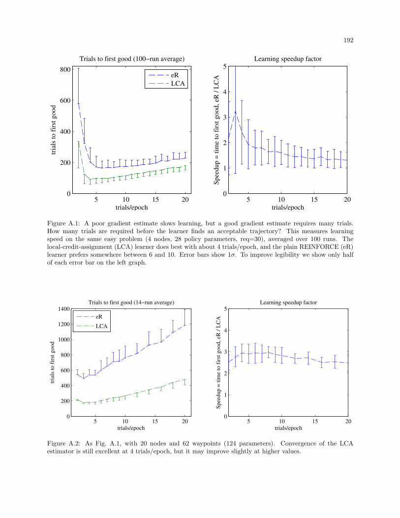
192

5 10 15 200

200

400

600

800

trials/epoch

tria

ls t

o f

irst

go

od

Trials to first good (100−run average)

5 10 15 200

1

2

3

4

5Learning speedup factor

trials/epoch

Sp

eed

up

= t

ime

to f

irst

go

od

, eR

/ L

CAeR

LCA

Figure A.1: A poor gradient estimate slows learning, but a good gradient estimate requires many trials.How many trials are required before the learner finds an acceptable trajectory? This measures learningspeed on the same easy problem (4 nodes, 28 policy parameters, req=30), averaged over 100 runs. Thelocal-credit-assignment (LCA) learner does best with about 4 trials/epoch, and the plain REINFORCE (eR)learner prefers somewhere between 6 and 10. Error bars show 1σ. To improve legibility we show only halfof each error bar on the left graph.

5 10 15 200

200

400

600

800

1000

1200

1400

trials/epoch

tria

ls t

o f

irst

go

od

Trials to first good (14−run average)

5 10 15 200

1

2

3

4

5Learning speedup factor

trials/epoch

Sp

eed

up

= t

ime

to f

irst

go

od

, eR

/ L

CAeR

LCA

Figure A.2: As Fig. A.1, with 20 nodes and 62 waypoints (124 parameters). Convergence of the LCAestimator is still excellent at 4 trials/epoch, but it may improve slightly at higher values.

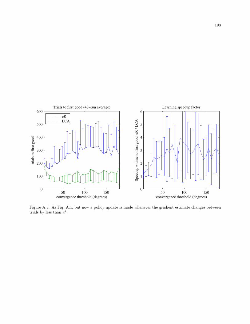
193

50 100 1500

100

200

300

400

500

600

convergence threshold (degrees)

tria

ls t

o f

irst

go

od

Trials to first good (43−run average)

eR

LCA

50 100 1500

1

2

3

4

5

6Learning speedup factor

convergence threshold (degrees)

Sp

eed

up

= t

ime

to f

irst

go

od

, eR

/ L

CA

Figure A.3: As Fig. A.1, but now a policy update is made whenever the gradient estimate changes betweentrials by less than x.

Appendix B

Creating new policies by combining old ones

B.1 Preface

This chapter grew out of an idea from the proposal. It led to promising results, but in March of this

year, Kober et al. [2012] published what I believe to be a similar, but superior, approach, which seems to

largely obviate the work done here. See §2.2.2 for context.

B.2 Introduction

Previous chapters have developed an approach for quickly discovering new policies for unseen sensor

networks. But when the requirements on a known network change, it may be unnecessary to learn a new

policy from scratch. Here we look at a case in which the values of parameters from previously learned policies

are correlated with changeable parameters in the reward function.

Consider a sensor network with some performance goal that varies occasionally, with the variable goal

expressed as a changeable parameter in the reward function. The techniques of the previous chapters can

be used to optimise trajectories for a given reward function, but here we show that the sensor networking

problem contains situations for which it is possible to interpolate between policies. This allows the learner

to immediately generate good policies for unseen tasks based on previously solved problems.

A typical policy optimisation problem is defined by an environment and by an objective communicated

to the learner by a function r(s, a) that returns a reward when the agent takes action a from state s. This

implicitly defines the parameters of an optimal controller. But it is common to desire solutions for several

195

similar problems defined by r(s, a; ξ) for some variable ξ that the agent can directly or indirectly observe

but not control. For example, ξ may be a utility function that defines the trade-off between taking the time

to collect all waiting data vs. returning just the most important data to the processing center more quickly,

in which case the data-collection trajectory (the policy) varies predictably as ξ varies. If an agent can learn

a continuum of policies π(ξ), it may immediately produce good policies for unseen values of ξ.

Changing system requirements such as these weights are not properly part of the “state” of a rein-

forcement learning system, since actions u cannot affect them. Consequently, the policy need not consider

them as state inputs. Were they to be treated as a part of the state, they would require more complex

policies, and would result in slower learning.

The example application I explore here is that of energy optimisation as the value of energy (VOE)

to each node changes over a timescale that may be a few or a few dozen trials. Our assumption is that as

the UA becomes more familiar with the class of tasks, it can use nodes’ self-reported energy states for the

previous trial (tour) to anticipate how to allocate excess range in the current trial.

The proposed approach also works at least as well for:

Changing the data requirements: set power policy and waypoint position to best regressed value for

the new requirement when the UA first comes into range.

Changing wind vector can also benefit from this approach, since it affects time spent in different

parts of an orbit, which in turn affects both waypoint placement and energy policy. (Note to self:

distance and time are no longer equivalent.)

But this is not strictly part of the framework described above: these items are not represented as changes

in the class of reward functions; it’s harder to argue that this isn’t simply part of the state vector. I have

not shown that pretending that reward parameters are “state” is inferior, although the increased expressive

richness of a policy that can accommodate this additional information is wasted if the information to which

the policy must respond varies on vastly different timescales, as is the case here. The policy gains in

complexity and therefore learning time, but does not gain in capability.

I assume that the UA can compute how much time to allocate to each node. I do not address the

196

question of optimal time allocation under uncertainty about future data requirements, although solutions

exist.

B.3 Reward functions and resource allocation

Recall the reward equation for energy optimisation:

r = −⎛⎝max(0, d − dmax)ϱ + ∑

j∈nodesφj

H

∑k=1

Pjk∆t⎞⎠

(7.12)

d is the current trajectory path length, dmax is the soft maximum range of the aircraft, ϱ controls the severity

of the soft maximum distance penalty, Pjk is the transmission power of node j at timestep k of length ∆t,

and φj is a weighting for the VOE for node j.

Assume that the VOE for each node is known at the start of a tour. Ideally we would like to learn

the relationship between the given combination of VOEs and the appropriate policy parameters for each

node. But the relationship between the power policy and the time taken to retrieve a given amount of data

is difficult to model, and treating each node’s policy separately and learning all possible combinations is

intractable. Thus we propose to decompose the reward function into n components, one corresponding to

each node, as was done in §6.2.3:

rj = −(max(0, dj − dmax,j)ϱ + φj

H

∑k=1

Pjk∆t) (B.1)

Given the VOE for each node (φj), how to determine dmax,j? While an approximation informed by

the relationship between power and data rate (given by the Shannon-Hartley law (Equation 3.5)) would be

a reasonable way to make the problem tractable, a linear approximation is even simpler, and will be used in

order to demonstrate the approach: the UA flight distance allocated to node j is:

dmax,j = (dmax − dreturn)φj

∑k∈nodes φk(B.2)

Flight distance is counted from the timestep at which the autopilot chooses the waypoint associated with

the node to that at which it chooses the next waypoint. dreturn is the portion of the trajectory flown after

the UA has collected all data from the final node but before arriving at the final destination; since its value

197

is not critical, it may be approximated as the distance between the last node’s assumed location and the

final destination.

B.4 Policy regression

The policy for each node consists of some parameters θ. So far we have considered waypoint position,

energy policy parameters, and parameters for a metapolicy to control energy policy learning. When encoun-

tering a new reward function, a new parametrised policy must be learned. Rather than initialising the new

policy parameters to values chosen by the programmer, here the parameters may be initialised based on

policies that solved other problems. When successful, this immediately yields a good policy.

We expect the optimal policies’ parameters to vary predictably with the reward functions’ parameters,

so a new policy may be constructed through regression, as follows:

Independent variable: reward function’s parameters.

Dependent variable: the values of θ corresponding to the best reward achieved for the given reward

function, which occurs on trial t∗.

Weights: A somewhat arbitrary regression weighting for the policies was chosen in order to give more weight

to solutions that earned a higher reward relative to Reference, although any other baseline would

do. Here they are given by W = rrefr− 1 for the reward received on trial t∗. Recall that all rewards

are negative, so rrefr= cref

cfor costs c, rref

r= x for policies with 1

xthe cost of reference, so W = x for

policies x + 1 times as good as reference. Policies worse than reference (W < 0) were discarded.

Following initialisation, the learning algorithms are allowed to run as described in the preceding chapters.

As with all supervised regression tasks, choosing a regression method appropriate to the task deter-

mines the method’s success. We will present three regressions for the example task:

0th-order regression: take the average parameter values.

1st-order regression: a linear least-squares fit.

198

Nonlinear nonparametric regression: a simple feedforward neural network with one hidden layer of 2

tanh neurons, trained using Levenberg-Marquardt backpropagation with Matlab R2012a’s trainlm.

When the UA has computed the permissible trajectory length dj for node j, if enough policies for

previously solved tasks exist it initialises each node’s policy by regressing the previous best values. In order

to reduce spurious regression results, the regressed value for each θi is constrained to a maximum distance

of max(θi) −min(θi) outside the supported range of the regression.

B.5 Experiments

B.5.1 Single nodes

Figure B.1 shows the results of the regression, compared to PGRL+µ from the previous section. Mean

is relatively safe, generally initialising the policies to ones of moderately low cost but frequently resulting

in range-limit underruns. Linear regression is riskier, showing occasional problems in the first few runs,

when only a handful of data point are available, but quickly learning to create new policies that significantly

outperform the others in almost all respects. Net has the potential for the highest performance, but in

this domain the representative richness afforded by the neural network is wasted, and the overfitting when

few policies are available is problematic. In contrast, PGRL+µ fails to reliably discover a metapolicy that

converges at all within 30 runs.

B.5.2 With a borrowed metapolicy

For each reward function, a policy must be generated. The better the policy that is discovered before

the task (reward function) changes again, the more likely the regression is to produce a good policy.

When the metapolicy is initialised using a typical final metapolicy from the previous chapter, learning

proceeds faster. This is a further vindication of the claim that the metapolicies can transfer optimisation

knowledge to related domains—here the domain differs in the total trajectory length available—results

improve markedly. Figure B.2 compares this result with key results from §B.5.1. Not only are the metapolicies

trained in the previous chapter still useful for speeding up learning here, but the speedup greatly improves

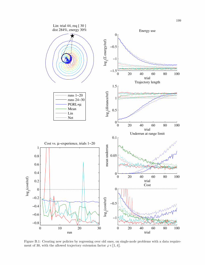
199

Lin: trial 44, req [ 30 ]dist 284%, energy 30%

0 20 40 60 80 1000

0.5

1

1.5

trial

log

2(d

ista

nce

/ref

)

Trajectory length

0 20 40 60 80 1000

0.05

0.1

trial

mea

n u

nd

erru

n

Underrun at range limit

runs 1−20

runs 24−30

PGRL+µ

Mean

Lin

Net

0 20 40 60 80 100−1.5

−1

−0.5

0

trial

log

2(Σ

en

erg

y/r

ef)

Energy use

0 10 20 30

−0.8

−0.6

−0.4

−0.2

0

0.2

0.4

0.6

0.8

1

run

log

2(c

ost

/ref

)

Cost vs. µ−experience, trials 1−20

0 20 40 60 80 100

−1

−0.5

0

trial

log

2(c

ost

/ref

)

Cost

Figure B.1: Creating new policies by regressing over old ones, on single-node problems with a data require-ment of 30, with the allowed trajectory extension factor φ ∈ [1,4].

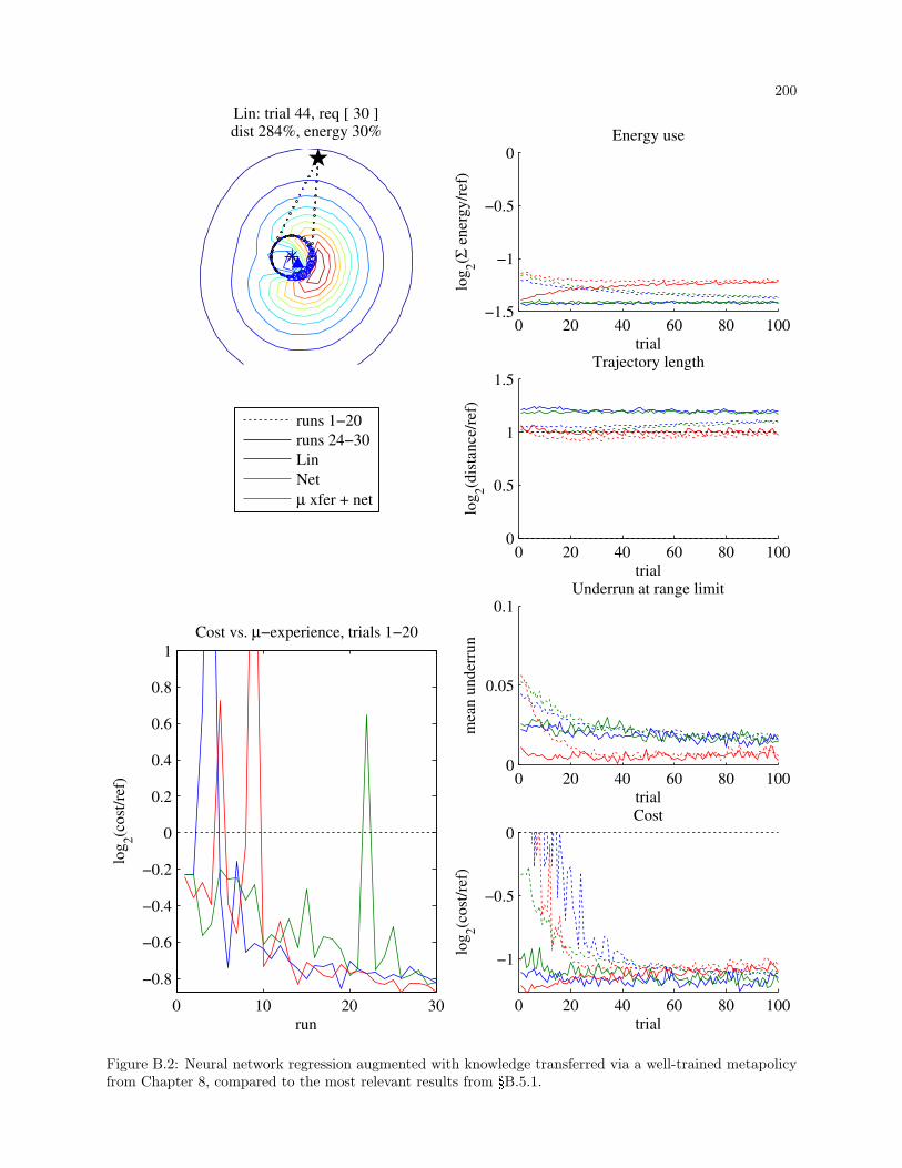
200

Lin: trial 44, req [ 30 ]dist 284%, energy 30%

0 20 40 60 80 1000

0.5

1

1.5

trial

log

2(d

ista

nce

/ref

)

Trajectory length

0 20 40 60 80 1000

0.05

0.1

trial

mea

n u

nd

erru

n

Underrun at range limit

runs 1−20

runs 24−30

Lin

Net

µ xfer + net

0 20 40 60 80 100−1.5

−1

−0.5

0

trial

log

2(Σ

en

erg

y/r

ef)

Energy use

0 10 20 30

−0.8

−0.6

−0.4

−0.2

0

0.2

0.4

0.6

0.8

1

run

log

2(c

ost

/ref

)

Cost vs. µ−experience, trials 1−20

0 20 40 60 80 100

−1

−0.5

0

trial

log

2(c

ost

/ref

)

Cost

Figure B.2: Neural network regression augmented with knowledge transferred via a well-trained metapolicyfrom Chapter 8, compared to the most relevant results from §B.5.1.

201

regression results. However, for this scenario, linear regression without metalearning speedup still performs

almost as well in the first few trials (cost graph) and better after training—the metapolicy is not perfectly

suited to the new range of tasks.

This approach may be extended to regressing across any smoothly parametrised policy. Examples

include regressing the metapolicies of Chapter 8, varying data requirements (preliminary results look good

but are not shown), and wind. In easily operable ranges of windspeed w ⪅ v2for UA velocity v, a compensating

autopilot resulted in little gain by regressing policies. However, in some domains, operability near w ≃ v

could be valuable. In preliminary tests, nonlinear policy regression was found to be extremely useful in such

scenarios.)

B.6 Summary

For the trajectory-length-allocation task, linear regression performs well. Further failsafes, such as

not attempting to create a new policy when too few old ones are available, may eliminate the occasional

high-cost policy early in training.

Linear regression is not sacred. For example, for trajectory length allocation, the waypoint placement

parameters tend to remain constant while the energy policy parameters vary roughly linearly with available

UA range. Modifying policies to accommodate wind results in nonlinear structure in both waypoint position

and energy policies, so the neural network (or any other nonlinear regression) performs best after it has a

sufficiently large library of old policies from which to draw. Careful choice of biases and basis functions

will help. A scheme in which the order of the regression varies with the amount of data available could

also be useful, but that problem is outside the scope of this research. None of these ideas is unfamiliar to

the supervised learning community; what is interesting here is simply the observation that it can indeed be

beneficial to create new policies by regressing over old ones.

Discovering that the class of tasks that an RL agent is asked to solve, given by the various reward

functions, requires policy regressions that vary in some dimensions but not in others, gives a key insight into

perception. In our example, the regression’s outputs that control the power policy parameters vary with

the inputs, but the waypoint positions don’t. In a higher-dimensional case, any inputs whose regression

202

coefficients were close to 0 (those that had no learned bearing on the policy outputs) could be considered

irrelevant. This could be considered a reinforcement-learning application of a key idea from Thrun’s [1996]

Explanation-based Neural Networks.