Model Based Prognostic Maintenance as Applied to Small Scale PVRO Systems for Remote Communities by Leah C. Kelley Bachelor of Fine Arts, Dance The Boston Conservatory, 1998 Bachelor of Engineering, Mechanical Engineering City College of New York, 2009 Master of Science, Mechanical Engineering Massachusetts Institute of Technology, 2011 Submitted to the Department of Mechanical Engineering in Partial Fulfillment of the Requirements for the Degree of Doctor of Philosophy in Mechanical Engineering at the MASSACHUSETTS INSTITUTE OF TECHNOLOGY May 2015 L.te 2\50 0 2015 Massachusetts Institute of Technology All rights reserved Signature of Author: ....................................................... Certified by: .................................................................. ARCHIVES MASSACHUSF-TTS 1NTIT[TE OF TECHNOLOLGY JUL 302015 LIBRARIES Signature redacted Department of Mechanical Engineering Mayt2 Signature redacted Steven Djbowsky Professor of Aeronautics and Astronautics & Mechanical Engineering Thesis Supervisor Signature redacted Accep ted by : ........................................................ .. ....... ----------------------------- David E. Hardt Professor of Mechanical Engineering Chairman, Committee on Graduate Studies

Welcome message from author
This document is posted to help you gain knowledge. Please leave a comment to let me know what you think about it! Share it to your friends and learn new things together.
Transcript
Model Based Prognostic Maintenance as Applied to Small ScalePVRO Systems for Remote Communities
by
Leah C. Kelley
Bachelor of Fine Arts, DanceThe Boston Conservatory, 1998
Bachelor of Engineering, Mechanical EngineeringCity College of New York, 2009
Master of Science, Mechanical EngineeringMassachusetts Institute of Technology, 2011
Submitted to the Department of Mechanical Engineeringin Partial Fulfillment of the Requirements for the Degree of
Doctor of Philosophy in Mechanical Engineering
at the
MASSACHUSETTS INSTITUTE OF TECHNOLOGY
May 2015 L.te 2\50
0 2015 Massachusetts Institute of TechnologyAll rights reserved
Signature of Author: .......................................................
Certified by: ..................................................................
ARCHIVESMASSACHUSF-TTS 1NTIT[TE
OF TECHNOLOLGY
JUL 302015
LIBRARIES
Signature redactedDepartment of Mechanical Engineering
Mayt2
Signature redactedSteven Djbowsky
Professor of Aeronautics and Astronautics & Mechanical EngineeringThesis Supervisor
Signature redactedA ccep ted b y : ........................................................ .. .. ..... -----------------------------
David E. HardtProfessor of Mechanical Engineering
Chairman, Committee on Graduate Studies


Model Based Prognostic Maintenance as Applied to Small Scale PVROSystems for Remote Communities
by
Leah C. Kelley
Submitted to the Department of Mechanical EngineeringMay 26, 2015 in Partial Fulfillment of the
Requirements for the Degree of Doctor of Philosophy inMechanical Engineering
ABSTRACT
Many systems degrade as functions of their operation and require maintenance to extendtheir productivity. When operating under steady conditions, prescheduled maintenance can beused to ensure such systems meet their required levels of productivity at lowest cost. However,using pre-scheduled maintenance on systems that degrade as functions of their operation underuncertain, varying conditions will not guarantee that they meet their productivity at lowest cost.They require maintenance schedules that accommodate changes in their operating conditions anddegradation. This research develops a prognostic maintenance methodology that ensures asystem degrading with its operation under variable, uncertain operating conditions meets itsdesired productivity at the lowest cost.
An example of a degrading system under variable, uncertain operating conditions is aphotovoltaic-powered reverse osmosis (PVRO) desalination system. PVRO desalination canprovide drinking water to remote communities in sunny areas with saline water sources. Suchsystems produce clean water and degrade as functions of their operating conditions, includingsolar radiation, water chemistry and community demand. These conditions are not constant, butvary stochastically. Maintenance (system flushing and cleaning) will extend a PVRO system'sproductivity, but requires time, chemicals and use of the clean product water. Hence, it has asubstantial impact on the total cost of water production and should be adjusted in response tovariations in operation. The community members who generally operate and maintain PVROsystems do not have the training or experience to determine the best type and timing ofmaintenance to ensure their water demand is met at lowest cost, and require a method to do so.
Here, prognostic maintenance methodology is developed and applied to community-scalePVRO desalination. Degradation (fouling) and remediation (cleaning) of the RO membranehave the largest impact on the system productivity and water cost, and hence are the focus of thisstudy. Fouling and cleaning are complex functions of water chemistry and system operation.Physics-based mathematical models of fouling and cleaning rely on two critical unknownparameters: fouling rate and cleaning effectiveness. They can be determined using systemidentification methods in real time, using measurements of the PVRO feed water pressure andclean water production rates. The identified fouling and cleaning models are combined with
3
statistical models of the expected future PV power and community water demand to predict thetype and timing of future maintenance procedures. The maintenance protocols are adjusted inreal time in response to changes in identified fouling. The prognostic algorithm developed hereis suitable for implementation on a PVRO system's embedded microcontroller.
Case studies presented here show that the prognostic maintenance methodology providesnon-expert operators with near optimal maintenance protocols when compared with conventionalperiodic scheduling, especially under varying degradation, solar radiation and demand. In thisexample study, annual maintenance happens to be nearly optimal, so the prognostic maintenancealgorithm produces a nearly annual cleaning schedule that minimizes maintenance costs. Sincethe statistical nature of this example prevents demand from being met 100% of the time, theprognostic maintenance method is used to minimize cost and water loss. On average, followingthe prognostic maintenance protocol results in less than 4% loss of water over a 5-year period atlowest cost.
Although developed in the domain of PVRO, the prognostic maintenance methodologydeveloped here is anticipated to be applicable to other systems that degrade as functions of theiroperation, including machine systems, vehicle fleets and transportation networks.
Thesis Supervisor: Steven DubowskyTitle: Professor of Aeronautics and Astronautics & Mechanical Engineering
4
ACKNOWLEDGEMENTS
I thank my advisor, Steven Dubowsky, for his guidance, support, advice and patience over thepast six years. I also thank my committee members, Professors Kamal Youcef-Toumi andOlivier L. de Weck, for their guidance, advice and encouragement.
I especially thank Amy Bilton and Huda Elasaad for their friendship, technical help and advice,ranging from developing the Matlab code for clear-sky solar radiation calculations to discussionsof physical process modeling and water quality requirements, their willingness to listen to ideasand their boundless generosity. It has been my great pleasure to assist them and ProfessorDubowsky with the implementation of the community-size PVRO system in La Mancalona,Mexico, in spite of all the insects and frogs we encountered while there. I also thank the manyother members of the Field and Space Robotics Laboratory over the past six years for theirfriendship and support, and especially our administrative assistant, Irina Gaziyeva. I thank themany friends I've made at MIT for their support and encouragement, including NevanHanumara, Folkers Rojas and others in the Precision Engineering Research Group, friends andfaculty in the Department of Mechanical Engineering, and friends from the MIT Ballroom DanceTeam and community.
I thank the Department of Defense SMART Scholarship for Service Program for its financialsupport of my PhD studies. I also acknowledge my sponsoring facility, SPAWAR SystemsCenter Pacific. I thank the W.K. Kellogg Foundation and the Fondo Para la Paz for theirfinancial support of the PVRO system installed in La Mancalona, Mexico.
Finally, I thank my family for their love, support and encouragement.
5

6

CONTENTS
ABSTR ACT ................................................................................................................................... 3
A CK N O W LED G EM ENTS ...................................................................................................... 5
CO N TEN TS................................................................................................................................... 7
FIG U R ES..................................................................................................................................... 11
TA BLES....................................................................................................................................... 13
N O M EN CLA TU RE.................................................................................................................... 15
1. IN TR O D U CTIO N ................................................................................................................... 19
1.1 M OTIVATION ................................................................................................................. 19
1.1.1 System D egradation.................................................................................................. 191.1.2 Photovoltaic Pow ered Reverse O sm osis............................................................... 22
1.2 PROBLEM STATEMENT AND A PPROACH ..................................................................... 27
1.3 THESIS CONTRIBUTIONS .............................................................................................. 291.4 THESIS ORGANIZATION................................................................................................ 30
2. BACKGROUND AND LITERATURE REVIEW .......................................................... 33
2.1 M AINTENANCE SCHEDULING ......................................................................................... 33
2.1.1 Condition-based M aintenance .............................................................................. 34
2.1.2 Prognostic M aintenance........................................................................................ 352.2 PHOTOVOLTAIC POWERED REVERSE OSMOSIS TECHNOLOGY ..................................... 37
2.2.1 PV RO Overview .................................................................................................... 382.2.2 PV RO Operation.................................................................................................... 41
2.3 FOULING AND REMEDIATION OF REVERSE O SMOSIS................................................... 43
2.3.1 Fouling Basics........................................................................................................... 43
2.3.1.1 Concentration Polarization and M ineral Scaling ........................................... 432.3.1.2 Colloidal Fouling .......................................................................................... 452.3.1.3 Biofouling ...................................................................................................... 462.3.1.4 Effects of Fouling on RO W ater Production.................................................. 48
2.3.2 M odels of RO Fouling in the Literature ............................................................... 482.3.3 Fouling M itigation ................................................................................................. 50
2.3.3.1 Pretreatm ent.................................................................................................... 512.3.3.2 M echanical Cleaning ..................................................................................... 522.3.3.3 Chem ical Cleaning ........................................................................................ 542.3.3.4 RO M em brane M aintenance .......................................................................... 57
2.4 SUMMARY...................................................................................................................... 61
3. PVRO PERFORMANCE, DEGRADATION AND REMEDIATION MODELING ... 65
3.1 RO W ATER PRODUCTION ............................................................................................ 65
7

3.2 RO D EGRADATION ..................................................................................................... 703.3 RO M EM BRANE REMEDIATION................................................................................... 71
3.3.1 System Flushing........................................................................................................ 723.3.2 Chem ical Cleaning.................................................................................................. 73
3.4 REPRESENTATIVE DEGRADATION AND REMEDIATION EXAMPLE ................................ 74
3.5 SUM M ARY...................................................................................................................... 78
4. DETERMINISTIC MAINTENANCE STUDY ............................................................... 81
4.1 PROBLEM STATEMENT ................................................................................................ 81
4.1.1 W ater Production w ith M aintenance ...................................................................... 82
4.1.2 The Optim ization ................................................................................................... 82
4.2 REPRESENTATIVE PV RO SYSTEM M ODEL.................................................................. 84
4.3 RESULTS ........................................................................................................................ 864.3.1 N om inal Case............................................................................................................ 864.3.2 Sensitivity Study ................................................................................................... 88
4.4 SUM M ARY...................................................................................................................... 90
5. PARAMETER IDENTIFICATION AND FORECASTING ............................................. 93
5.1 PARAMETER IDENTIFICATION ...................................................................................... 94
5.1.1 Fouling Param eter Identification ........................................................................... 94
5.1.2 Cleaning Effectiveness............................................................................................ 100
5.2 O PERATING CONDITION FORECASTING........................................................................ 101
5.2.1 Solar Radiation Predictions..................................................................................... 102
5.2.2 W ater Salinity V ariations........................................................................................ 104
5.2.3 System D em and ...................................................................................................... 105
5.3 PV RO M AINTENANCE FORECASTING A LGORITHM ...................................................... 107
6. PROGNOSTIC MAINTENANCE CASE STUDIES........................................................ 109
6.1 PROGNOSTIC MAINTENANCE FRAMEWORK APPLIED TO PVRO SYSTEMS ................... 109
6.2 PROBLEM D ESCRIPTION ............................................................................................... 110
6.2.1 Brackish W ater System ........................................................................................... 110
6.2.2 System Operation.................................................................................................... 113
6.2.3 Incorporating U ncertainty into Sim ulations............................................................ 114
6.2.4 Lim its on Chem ical Cleaning Frequencies............................................................. 115
6.3 CASE STUDY D ETAILS ................................................................................................. 116
6.3.1 U nknow n, Fixed Fouling ........................................................................................ 118
6.3.2 U nknow n, Slow ly V arying Fouling........................................................................ 118
6.3.3 U nknow n, Fixed Fouling w ith V arying D em and ................................................... 119
6.3.4 U nknow n, V arying Fouling w ith V arying D em and ............................................... 120
6.4 CASE STUDY RESULTS ................................................................................................. 121
8
6.4.1 Fixed Fouling Rate Parameter Results.................................................................... 121
6.4.2 Varying Fouling Rate Parameter, Fixed Water Demand Results ........................... 125
6.4.3 Fixed Fouling Rate Parameter, Varying Water Demand Results ........................... 1266.4.4 Varying Fouling Rate Parameter and Varying Water Demand Results ................. 129
6 .5 S U M M A R Y.................................................................................................................... 132
7. SUMMARY AND CONCLUSIONS................................................................................... 135
7 .1 S U M M A R Y .................................................................................................................... 13 5
7.2 SUGGESTIONS FOR FUTURE WORK............................................................................... 136
7.2.1 Future R efinem ents................................................................................................. 1367.2.2 Applications to Other Domains .............................................................................. 138
REFERENCES.......................................................................................................................... 141
APPENDIX A: RELATING SOLAR POWER TO FEED WATER PRESSURE............. 149
9

10

FIGURES
Figure 1.1: Pre-scheduled preventative maintenance: an open-loop system ............................. 19
Figure 1.2: Condition-based maintenance: a type of feedback system...................................... 21
Figure 1.3: Populations using improved drinking water sources............................................... 23
Figure 1.4: Areas with high water stress and over-exploitation of local water sources ........... 24
Figure 1.5: Annual average daily clear sky solar insolation at ground level............................ 24
Figure 1.6: A representative PVRO system ............................................................................... 25
Figure 1.7: Block diagram representation of prognostic maintenance strategy........................ 28
Figure 2.1: Cross-section of RO spiral-wound membrane; axial feed and brine flow into the page........................................................................................................................................... 3 9
Figure 2.2: Detailed view from Figure 2.1, rotated so feed flows from left to right ................ 39
Figure 2.3: Community-sized photovoltaic-powered reverse osmosis system......................... 41
Figure 2.4: Mineral scaling on a reverse osmosis membrane .................................................... 44
Figure 2.5: Colloidal fouling on an RO membrane surface...................................................... 46
Figure 2.6: Biofouling on an RO membrane surface............................................................... 47
Figure 2.7: Loosely deposited particles removed by system flushing ...................................... 53
Figure 3.1: Clean water desalination through an RO membrane............................................... 66
Figure 3.2: Short term permeate flow rate with and without system flushing........................... 75
Figure 3.3: Longer term permeate flow rate with and without system flushing........................ 76
Figure 3.4: Longer term permeate flow rate with and without chemical cleaning .................... 76
Figure 3.5: Permeate flow rate decline with and without maintenance .................................... 77
Figure 4.1: M aintenance optim ization structure ........................................................................ 83
Figure 4.2: Daily water production under optimized maintenance, compared with productionunder no maintenance and under daily flushing alone.................................................. 87
Figure 4.3: Daily water production under lower fouling rate ................................................... 89
Figure 4.4: Daily water production under high fouling rate ...................................................... 90
Figure 5.1: Measured, identified and predicted RO membrane permeability (left) and % error inpredicted permeability (right) from the brackish water RO pilot plant in Brownsville, TX........................................................................................................................................... 9 7
Figure 5.2: Measured, identified and predicted RO permeate flow rate (left), and % errorbetween predicted and measured permeate flow rates (right), for the Brownsville ROp lan t................................................................................................................................... 9 8
11
Figure 5.3: Measured and predicted RO permeate flow rate (left), and % error between predictedand measured permeate flow rates after identification (right), for La Verne, CA, RO plant......................................................................................................................................... 10 0
Figure 5.4: Solar radiation scale factor as a function of cloud fraction...................................... 103
Figure 5.5: Forecasting water production and RO membrane degradation using cloud statistics......................................................................................................................................... 1 0 4
Figure 5.6: Average monthly salinity in Mediterranean Sea near Limassol, Cyprus................. 105
Figure 5.7: Prognostic maintenance scheduler structure ............................................................ 108
Figure 6.1: Prognostic maintenance applied to a PVRO system................................................ 110
Figure 6.2: Daily cloud level assignm ent process ...................................................................... 115
Figure 6.3: Prognostic maintenance simulation structure........................................................... 117
Figure 6.4: Histograms of water loss percentage with optimal fixed maintenance (A) andseasonal m aintenance (B ) ............................................................................................... 122
Figure 6.5: Histograms of water loss percentage with aggressive (C) and sparse maintenance (D)......................................................................................................................................... 12 2
Figure 6.6: Histograms of water loss percentage with adjusted prognostic (E) and sparsemaintenance (F) under varying fouling rate parameter and fixed demand..................... 126
Figure 6.7: Histograms of water loss percentage with prognostic (G) and seasonally adjustedprognostic maintenance (H), under fixed fouling rate parameter and varying demand. 127
Figure 6.8: Histogram of water loss percentage with sparse maintenance (I)............................ 128
Figure 6.9: Histograms of water loss percentage with adjusted prognostic (J) and sparsemaintenance (K), under varying fouling rate parameter and varying water demand ..... 131
Figure A. 1: RO pressure vessel as a fluid resistance network.................................................... 150
12

TABLES
Table 3.1: RO fouling and remediation example parameters ................................................... 74
Table 4.1: Representative 1,000 L/day brackish water PVRO system parameters .................. 84
Table 4.2: System flushing and chemical cleaning parameters ................................................. 86
Table 4.3: Sensitivity study maintenance optimization results.................................................. 88
Table 5.1: Measurements available from pilot RO plant in Brownsville, TX........................... 96
Table 5.2: Measurements from the Metropolitan Water District pilot RO plant....................... 99
Table 5.3: Estimated cleaning effectiveness from measured data.............................................. 101
Table 5.4: Cloud cover conditional probabilities for La Mancalona, Mexico............................ 103
Table 6.1: Representative brackish water PVRO system parameters......................................... 111
Table 6.2: Chemical and water requirements for a single chemical cleaning ............................ 112
Table 6.3: RO m em brane and chem ical costs............................................................................. 112
Table 6.4: M aintenance process param eters ............................................................................... 113
Table 6.5: Upper limits on RO membrane permeability restoration .......................................... 116
Table 6.6: Chemical and labor costs for select cleaning frequencies ......................................... 116
Table 6.7: Fixed, pre-determined cleaning schedules................................................................. 118
Table 6.8: Seasonal portion of drinking water demand .............................................................. 120
Table 6.9: Daily climatic portion of drinking water demand...................................................... 120
Table 6.10: W ater loss results: fixed, unknown fouling rate ...................................................... 123
Table 6.11: Cleaning numbers and costs: fixed, unknown fouling rate...................................... 124
Table 6.12: Water loss and cleaning cost results: higher fixed, unknown fouling rate .............. 124
Table 6.13: Water loss results: varying, unknown fouling rate .................................................. 125
Table 6.14: Cleaning numbers and costs: varying, unknown fouling rate.................................. 126
Table 6.15: Water loss results: fixed, unknown fouling rate, varying demand .......................... 127
Table 6.16: Water loss results: varying, unknown fouling rate and varying demand ................ 129
Table 6.17: Cleaning numbers and costs: varying unknown fouling rate, varying demand....... 131
13

14
NOMENCLATURE
A, RO membrane area (in2
AS Area of the solar panels (in 2
a Forgetting factor
AOC Assimilable organic carbon
b An unknown parameter
b Estimate of unknown parameter b
C, (t) Feed water salt concentration (ppm)
Cf (t) Average of the feed and concentrate salt concentrations (ppm)
C, Concentration of total dissolved solids (ppm)
CBM Condition-based maintenance
D(I (t) Climactic-dependent component of daily drinking water demand (L)
DnOM Baseline daily drinking water demand (L)
Ds (t) Seasonal-dependent component of daily drinking water demand (L)
D,0 , (t) Total daily water demand (L)
,(t) Delta function
e Percent error
EPS extracellular polymeric substance
q Solar to electrical conversion efficiency
f Cloud fraction
FDI Fault detection and isolation
FTC Fault tolerant control
ggf Proportionality constant for system flushing effectiveness (one/bar/m 2/s)
Gcc RO membrane permeability increase due to a chemical cleaning (L/bar/m2/s 2 )
Gs RO membrane permeability increase due to one flushing cycle (L/bar/m 2/s2)
y Fouling rate (one/bar/s)
15
Fouling rate estimate (one/bar/s)
70 Initial fouling rate estimate (one/bar/s)
I (t) Instantaneous solar radiation (W/m 2
IC Clear sky solar radiation (W/m 2)
K (t) RO membrane permeability to water (L/m2/bar/s)
K, (t) Normalized RO membrane permeability to water (L/m2 /bar/s)
LSI Langlier Saturation Index
M Number of chemical cleanings over the total time of interest
MF Microfiltration
MFI Modified fouling index
MPPT Maximum power point tracking
N Number of system flushes over the total time of interest
NF Nanofiltration
NTU Nephelometric Turbidity Units
p (t) Average hydraulic pressure in the RO pressure vessel (bar)
Ph (t) Concentrate (brine) water pressure (bar)
Pf (t) Feed water pressure at the RO pressure vessel inlet (bar)
p, (t) Permeate (clean) water pressure (bar)
pf Concentration polarization factor
Plec Electricity produced by the solar panel
PHM Prognostic health monitoring
PVRO Photovoltaic-powered reverse osmosis
;r (t) Average osmotic pressure in the RO pressure vessel (bar)
rf (t) Feed water osmotic pressure (bar)
T, (t) Permeate osmotic pressure (bar)
;TW Osmotic pressure of saline water (bar)
q1 (t) Feed water flow rate (L/s)
16
q, (t) Clean water (permeate) flow rate through the RO membrane (L/s)
q, Flushing water flow rate (L/s)
QD Volume of water needed daily by a community (L)
Qdy Volume of permeate water produced in a day
Q11 Volume of permeate water used during a chemical cleaning process (L)
Qe Net clean water produced (L)
Q, Clean water produced by the RO system over a period of time (L)
Q'i Volume of permeate water used during a flushing process (L)
RO Reverse osmosis
SDI Silt density index
SDSI Stiff-Davis Saturation Index
t Time
tF Ending time
tFy Ending time of the yth water production period
ts Starting time
ts, Starting time of the yth water production period
Ats Duration of a flushing cycle
T Water temperature ('C)
TBC Total bacterial count
TDS Total dissolved solids
TFC Temperature correction factor
TOC Total organic carbon
u System measurements
UF Ultrafiltration
UV Ultraviolet
WLP Water loss percentage
y System output
Y Number of periods of water production between maintenance processes
17

18
CHAPTER
1INTRODUCTION
1.1 Motivation
1.1.1 System Degradation
Many systems degrade as a result of their operation and require maintenance to extend
their productivity. When operating under steady conditions, the degradation of a system can be
related linearly to the cumulative amount of operation, such as the number of operating hours or
operating cycles. Often, preventative maintenance is performed when a pre-determined number
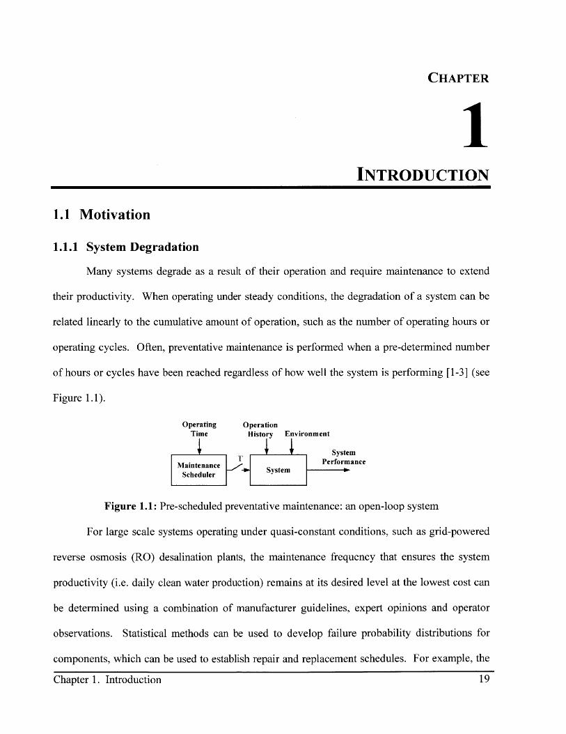
of hours or cycles have been reached regardless of how well the system is performing [1-3] (see
Figure 1.1).
Operating OperationTime History Environment
System
Maintenance Performance
Scheduler System
Figure 1.1: Pre-scheduled preventative maintenance: an open-loop system
For large scale systems operating under quasi-constant conditions, such as grid-powered
reverse osmosis (RO) desalination plants, the maintenance frequency that ensures the system
productivity (i.e. daily clean water production) remains at its desired level at the lowest cost can
be determined using a combination of manufacturer guidelines, expert opinions and operator
observations. Statistical methods can be used to develop failure probability distributions for
components, which can be used to establish repair and replacement schedules. For example, the
Chapter 1. Introduction 19
meantime between failures for a typical single-stage centrifugal pump is 1.07 years, determined
from operation data [4]. Meantime between failures for variable frequency drives can range
from 274 to 17.13 years, depending on temperature and other operating conditions [5]. A
portable tactical water purification unit has a mean time between failures of 180 operating hours
[6]. Under steady conditions, one can choose an appropriate schedule and follow it.
Determining the optimal maintenance schedules for systems operating under variable,
uncertain and stochastic conditions is much more challenging. Degradation under such
conditions is likely not constant, but a complex function of the system operation and
environmental conditions. Following a pre-determined maintenance schedule established during
steady operating conditions will likely result in sub-optimal performance in such cases. Simple
guidelines may result in too frequent or infrequent maintenance [2, 3, 7]. Performing too
frequent maintenance may sustain high productivity levels, at the expense of excess cost and
unnecessary downtime. Waiting too long to perform maintenance can result in periods of low
productivity or failure of components.
Feedback techniques have been applied to improve system reliability and decrease
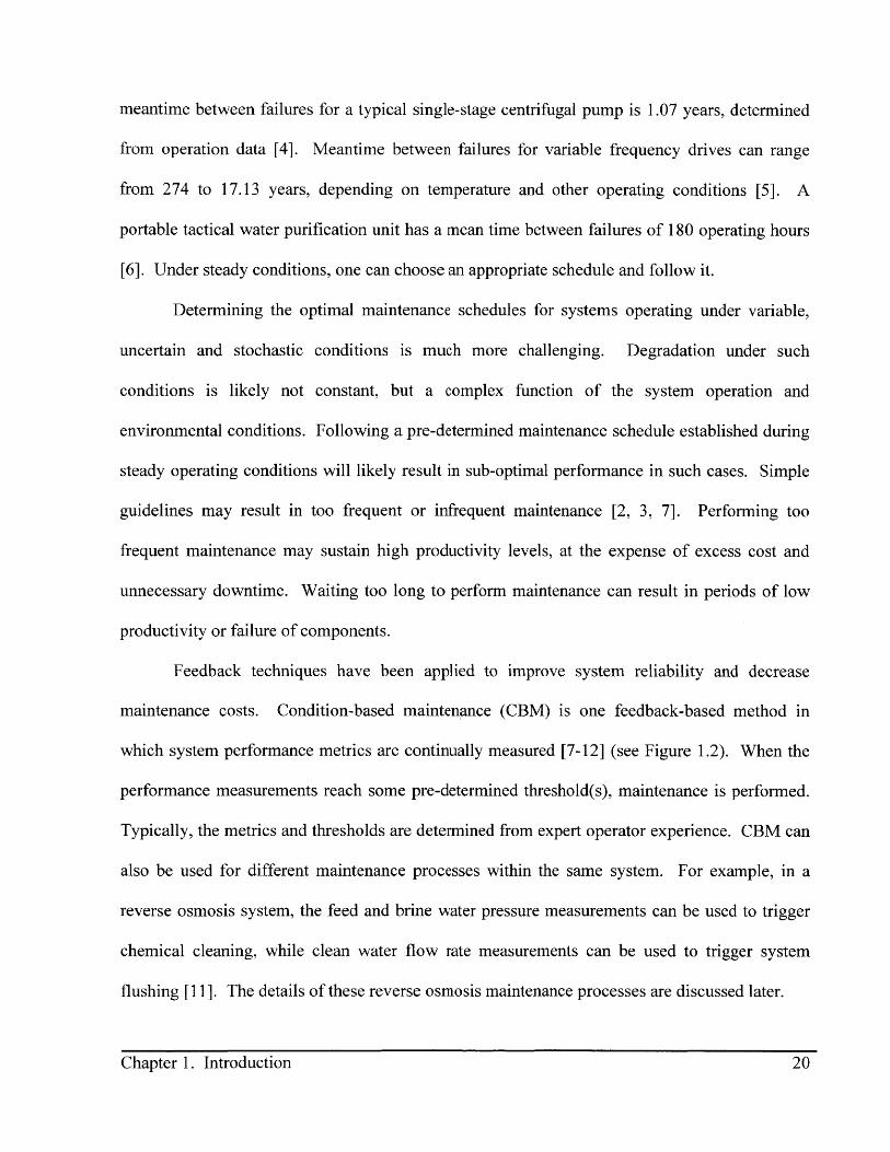
maintenance costs. Condition-based maintenance (CBM) is one feedback-based method in
which system performance metrics are continually measured [7-12] (see Figure 1.2). When the
performance measurements reach some pre-determined threshold(s), maintenance is performed.
Typically, the metrics and thresholds are determined from expert operator experience. CBM can
also be used for different maintenance processes within the same system. For example, in a
reverse osmosis system, the feed and brine water pressure measurements can be used to trigger
chemical cleaning, while clean water flow rate measurements can be used to trigger system
flushing [11]. The details of these reverse osmosis maintenance processes are discussed later.
Chapter 1. Introduction 20
OperationHistory Environment
SystemThreshold Maintenance Performance
Scheduler System
Performance Measurements
Figure 1.2: Condition-based maintenance: a type of feedback system
CBM prevents maintenance from being performed too early or too late when applied to
systems operating at fixed settings. However, it is difficult to apply CBM to systems that must
operate over a wide range of settings. Threshold levels or metrics may need to be adjusted based
on operating conditions. Expert domain knowledge may be needed to make these adjustments.
Since no planning or forecasting is included in this method, it requires that the labor and
materials for maintenance be available at the time the threshold is met.
Driving a system to the same pre-determined degraded state before performing
maintenance is not necessarily optimal, especially for systems that operate under variable
conditions. For example, a reverse osmosis membrane becomes less permeable to water as it
degrades. During periods of high water demand, one may need to clean the membranes in an RO
system earlier than during periods of low water demand. If one waits until the clean water flow
through the RO system has dropped to a fixed percentage before cleaning, the RO system may
not produce enough water during a high-demand period. Conversely, one may be able to permit
the RO membranes to degrade more during periods of low water demand while still meeting the
desired productivity. This requires changing the thresholds that trigger maintenance. If the
water demand varies unpredictably, then one may not know when to adjust the thresholds.
Failure to make the appropriate adjustments will result in either too frequent maintenance, or
failure to meet the water demand.
Chapter 1. Introduction 21
Applying pre-determined schedules or feedback-based maintenance with fixed thresholds
to a degrading system operating under highly variable, uncertain conditions will not ensure it
meets its desired level of productivity at the lowest cost. To do this, one must have knowledge
of how the system degrades and must be able to predict its future operation. Current research in
prognostics and health monitoring (PHM) of systems includes methods to predict remaining
useful life of systems and components, and methods of optimizing maintenance schedules based
on such predictions [13-19]. However, much of the research focuses on systems operating at
steady or quasi-steady points, such as industrial process machinery and power plants. A
prognostic maintenance strategy for degrading systems subject to highly variable, uncertain
operating conditions without real-time, expert operator supervision is needed.
Examples of systems that degrade as a function of their operation and that operate under
uncertain and variable conditions include fleets of automobiles, aircraft, wind turbines and
photovoltaic-powered reverse osmosis desalination (PVRO) systems. Here, a remote,
community-scale PVRO system is used as a representative application for development of an
adaptive prognostic maintenance algorithm. Such an algorithm is essential for remote PVRO
systems so that they can successfully meet their community water demands over their lifetimes
while subject to widely varying conditions and operation by non-experts.
1.1.2 Photovoltaic Powered Reverse Osmosis
Supplying the world's population with sufficient drinking water remains a global
challenge. Although 2.3 billion people gained access to improved drinking water sources
between 1990 and 2012, over 740 million people remain without access [20]. The majority of
the people without sufficient drinking water access live in Africa, Asia, Oceania and Latin
Chapter 1. Introduction 22
Chapter 1. Introduction 22
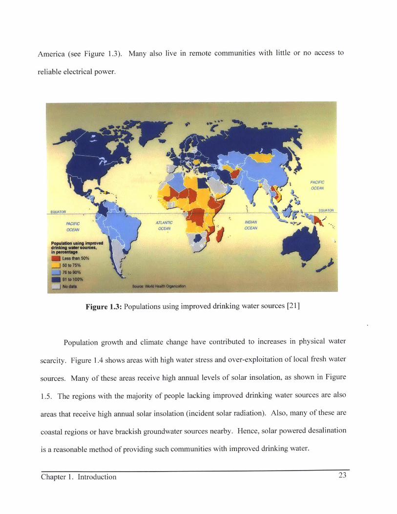
America (see Figure 1.3). Many also live in remote communities with little or no access to
reliable electrical power.
OCEAN
EQUATOR
INDIANOCEAN
Figure 1.3: Populations using improved drinking water sources [21]
Population growth and climate change have contributed to increases in physical water
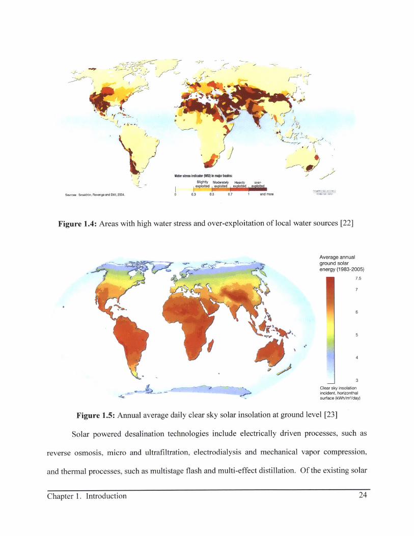
scarcity. Figure 1.4 shows areas with high water stress and over-exploitation of local fresh water
sources. Many of these areas receive high annual levels of solar insolation, as shown in Figure
1.5. The regions with the majority of people lacking improved drinking water sources are also
areas that receive high annual solar insolation (incident solar radiation). Also, many of these are
coastal regions or have brackish groundwater sources nearby. Hence, solar powered desalination
is a reasonable method of providing such communities with improved drinking water.
23Chapter 1. Introduction
Sources: SmakhtOn, Revenge and D11. 2004.
&-/
-N,
Water slresa Indicator (MIl) in m*r baina:Slightly Moderatel Heevil over-
ex loited
0 0.3 0 5 0.7 1 and more
Figure 1.4: Areas with high water stress and over-exploitation of local water sources [22]
Average annualground solarenergy (1983-2005)
7.5
7
6
5
4*13
Clear sky insolationincident, horizonthalsurface (kWh/m2/day)
Figure 1.5: Annual average daily clear sky solar insolation at ground level [23]
Solar powered desalination technologies include electrically driven processes, such as
reverse osmosis, micro and ultrafiltration, electrodialysis and mechanical vapor compression,
and thermal processes, such as multistage flash and multi-effect distillation. Of the existing solar
IA07~-
'7
ltjpp nc i If
24Chapter 1. Introduction
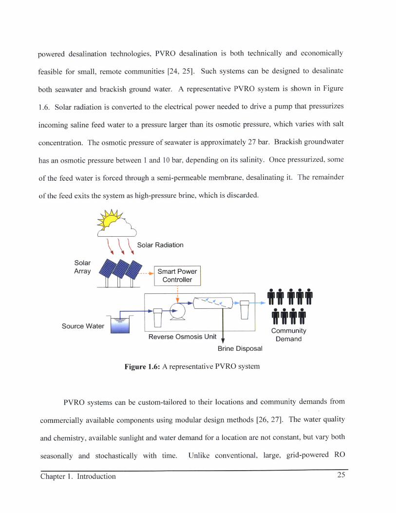
powered desalination technologies, PVRO desalination is both technically and economically
feasible for small, remote communities [24, 25]. Such systems can be designed to desalinate
both seawater and brackish ground water. A representative PVRO system is shown in Figure
1.6. Solar radiation is converted to the electrical power needed to drive a pump that pressurizes
incoming saline feed water to a pressure larger than its osmotic pressure, which varies with salt
concentration. The osmotic pressure of seawater is approximately 27 bar. Brackish groundwater
has an osmotic pressure between 1 and 10 bar, depending on its salinity. Once pressurized, some
of the feed water is forced through a semi-permeable membrane, desalinating it. The remainder
of the feed exits the system as high-pressure brine, which is discarded.
Solar Radiation
SolarArray -. , Smart Power
Controller
Source WaterCommunity
Reverse Osmosis Unit aDemandBrine Disposal
Figure 1.6: A representative PVRO system
PVRO systems can be custom-tailored to their locations and community demands from
commercially available components using modular design methods [26, 27]. The water quality
and chemistry, available sunlight and water demand for a location are not constant, but vary both
seasonally and stochastically with time. Unlike conventional, large, grid-powered RO
Chapter 1. Introduction 25
desalination plants that operate at essentially constant power, PVRO systems operate variably as
the environmental conditions change, assuming there is no local energy storage (batteries).
Degradation in RO systems is a function of their operation, so PVRO system degradation will
also vary as a function of its operating conditions. Even PVRO systems with energy storage will
experience fluctuations in their operation, although the batteries, rather than the RO membranes,
will experience greater stochastic effects.
Maintenance procedures have substantial impact on the PVRO system lifetime and water
production costs, and should be optimized so that the community water demand is met at the
lowest water production cost. Manufacturers provide basic guidelines for maintenance based on
RO membrane type, but these guidelines are intended for RO plants operating under relatively
constant conditions [28, 29]. Following such guidelines may not result in the PVRO system
meeting the community's water demand at the lowest cost. Performing maintenance too
infrequently may result in the PVRO system being unable to meet the community's daily water
demand. Performing too frequent maintenance may ensure the community's water demand is
met, but at significant cost in terms of lost product water used in maintenance, lost water
production time and labor and supply costs associated with maintenance. Operators of large RO
plants also monitor the water production and other performance metrics, and have the technical
expertise and experience needed to adjust maintenance protocols as needed. The community
members operating small PVRO systems do not generally have the expertise to determine the
type and timing of maintenance protocols that will permit the PVRO system to meet their water
demand at minimum cost.
Chapter 1. Introduction 26
Chapter 1. Introduction 26
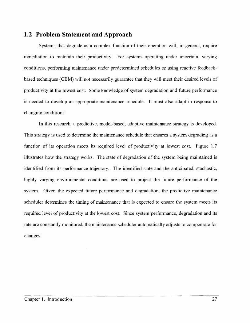
1.2 Problem Statement and Approach
Systems that degrade as a complex function of their operation will, in general, require
remediation to maintain their productivity. For systems operating under uncertain, varying
conditions, performing maintenance under predetermined schedules or using reactive feedback-
based techniques (CBM) will not necessarily guarantee that they will meet their desired levels of
productivity at the lowest cost. Some knowledge of system degradation and future performance
is needed to develop an appropriate maintenance schedule. It must also adapt in response to
changing conditions.
In this research, a predictive, model-based, adaptive maintenance strategy is developed.
This strategy is used to determine the maintenance schedule that ensures a system degrading as a
function of its operation meets its required level of productivity at lowest cost. Figure 1.7
illustrates how the strategy works. The state of degradation of the system being maintained is
identified from its performance trajectory. The identified state and the anticipated, stochastic,
highly varying environmental conditions are used to project the future performance of the
system. Given the expected future performance and degradation, the predictive maintenance
scheduler determines the timing of maintenance that is expected to ensure the system meets its
required level of productivity at the lowest cost. Since system performance, degradation and its
rate are constantly monitored, the maintenance scheduler automatically adjusts to compensate for
changes.
Chapter 1. Introduction 27
Chapter 1. Introduction 27

Anticipated Stochastic Environment
System AnticipatedModel Operation
Degradation StochasticModel Operation Stochastic
History Environment
State of Predictive System
Degradation Maintenance System Perfo ance
Scheduler
Identification 1Operation
Figure 1.7: Block diagram representation of prognostic maintenance strategy
The approach can be implemented in an algorithm as follows. A physics-based
understanding of the system performance, its degradation and the effects of remediation are used
to generate mathematical models of its behavior over time in response to system inputs.
Degradation models (Figure 1.7 upper left) are parameterized in such a way that the rate of
degradation can be identified from the system performance, using well-established system
identification techniques. Statistical methods are used to generate expectations of future system
inputs. These expectations are used in the system and degradation models to project the
expectation of future performance and degradation. These expectations, along with the
associated maintenance costs (both monetary and in terms of lost production due to system
maintenance downtime and any product required to perform the maintenance), form a
constrained optimization problem, which the maintenance scheduler solves in order to find the
schedule that maintains the desired system productivity at the lowest cost.
28Chapter 1. Introduction

This algorithm is applied to a simulated model of a community-size PVRO desalination
system, which is assumed to be operated by non-experts. The simulated model is based on an
existing, community-sized PVRO system in La Mancalona, Mexico. The basic underlying
physics of RO membrane degradation and remediation are studied and modeled in order to
determine the simplest mathematical models that sufficiently describe the RO physics. Given a
PVRO system location and size, analytical clear-sky solar radiation models are convolved with
historical cloud frequency statistics to generate expected future solar radiation levels at the
PVRO system location. The expected solar radiation and water chemistry are used in the RO
models to forecast the expected water production and RO membrane degradation. The
maintenance scheduler uses the expected production and degradation, along with the time, cost
and volume of product water required for maintenance, to determine the maintenance frequency
that is expected to sustain the PVRO system's productivity so it meets the community's daily
water demand at lowest cost. Since the optimization cost function is not closed-form, and since
the search space is relatively small, exhaustive search (full factorial) methods are used. There is
no mathematical way to prove that the solution is optimal, although full factorial methods should
yield the best solution here. Numerical case studies and Monte Carlo simulations show the
algorithm's success when compared with use of conventional maintenance.
1.3 Thesis Contributions
This thesis contributes a methodology for developing a model-based prognostic
maintenance algorithm for systems degrading as a complex function of their operation, under
varying, uncertain conditions. It combines physics-based modeling, system identification based
on operation history, and statistical models of future system inputs to predict system performance
Chapter 1. Introduction 2929Chapter 1. Introduction

and to optimize maintenance scheduling in terms of sustaining the desired productivity at the
lowest cost.
The methodology is applied to a remote, community-size PVRO system assumed to
operate without the benefit of energy storage. An automated, prognostic maintenance algorithm
is needed by PVRO system operators, who lack the expertise to determine the type and timing of
the maintenance that will ensure the community's water demand is met at lowest cost. To date,
such an algorithm does not exist for PVRO. Given a system location and design, the algorithm
estimates the degradation level and rate of the RO membrane from water pressure, flow and
salinity measurements. It also identifies cleaning effectiveness over time. It uses a clear-sky
solar-radiation model combined with weather statistics from historical data, along with the
identified degradation rate, to project future performance and degradation. It is able to predict
when the system will fail to meet community demand. By setting up a constrained optimization
problem using the identified degradation, anticipated environmental conditions, predicted
performance and costs in terms of money, production time lost and product water required, a
maintenance schedule that will result in the PVRO system meeting the community's water
demand at lowest cost is produced.
1.4 Thesis Organization
The rest of this thesis is organized as follows. Chapter 2 provides background
information and the current state of the art in prognostic maintenance and PVRO technology, RO
fouling and remediation. Chapter 3 describes the process models for RO water production,
fouling and cleaning. Chapter 4 presents a deterministic maintenance schedule optimization for
PVRO, in which the solar radiation levels, RO membrane fouling rate and remediation
effectiveness are known. The sensitivity of the optimization to changes in the fouling rate is
Chapter 1. Introduction 30
demonstrated, motivating the need to identify the fouling rate from system performance history.
Chapter 5 presents parameter identification and performance forecasting. This chapter describes
the simple method used to identify the PVRO fouling rate, the way in which weather statistics
are used to project future levels of solar radiation over time, and how the projected solar
radiation and identified fouling rate are used to forecast future PVRO system performance.
Chapter 6 presents the full prognostic maintenance algorithm as applied to a PVRO system
similar to a fielded PVRO system in La Mancalona, Mexico, in simulation. Four scenarios are
simulated, and the algorithm's performance is evaluated under each scenario. In all scenarios,
variation of solar radiation with uncertain, varying cloud cover is accounted for. The simulations
increase the uncertainty in operation by adding variation to an unknown fouling rate, as well as
seasonal and cloud-cover dependent water demand. Preliminary results indicate that prognostic
maintenance can indeed minimize the number of days a PVRO system fails to meet community
demand, assuming it is constant and/or known. Chapter 7 summarizes this research and suggests
additional directions for this research as applied both to PVRO and other types of stochastically
degrading systems.
Chapter 1. Introduction 31
Chapter 1. Introduction 31

Chapter 1. Introduction 32
CHAPTER
2BACKGROUND AND LITERATURE REVIEW
2.1 Maintenance Scheduling
System maintenance can be performed based on pre-determined schedules, in response to
measured system performance metrics or in reaction to system failures. Reactionary
maintenance, such as a repair or replacement after component failure, results in unanticipated
loss of system operating time and productivity. If the required materials and labor for
performing maintenance are not available, additional time and productivity are lost. Pre-planned
preventative maintenance reduces the likelihood of unexpected failures and ensures materials
and labor are available when needed [1-3, 7].
Historically, preventative maintenance was performed according to pre-determined
schedules generated from averaged observations of component performance, degradation and
failures by manufacturers and system operators. When using this method, a plant operator may
initially follow a component manufacturer's guidelines or empirical rules of thumb. Such
schedules may be optimal when applied to systems operating under the average conditions used
for schedule development. The operator may adjust maintenance frequency based on previous
experience or on observed system performance. For systems operating under steady conditions,
such schedule adjustments may result in cost savings and/or productivity increases, and may
result in the required productivity at lowest cost. However, the schedule adjustments may not
Chapter 2. Background and Literature Review 33Chapter 2. Background and Literature Review 33

result in the required productivity at minimal cost, as this method can also result in excess
maintenance and downtime, or may be too infrequent.
Improving preventative maintenance has been well-studied over the last several decades
[2, 3]. Much of this research is motivated by reducing operating costs of large manufacturing
facilities or large vehicle fleets, such as fleets of airplanes. The two main thrusts in this area are
condition-based maintenance (CBM) and prognostic health monitoring (PHM). These methods
are described in the next two sub-sections.
2.1.1 Condition-based Maintenance
Condition-based maintenance (CBM) can reduce maintenance costs while maintaining
acceptable system performance, and can be thought of as "just-in-time" maintenance [2, 3, 7-12,
30-35]. In CBM, maintenance is not performed at pre-defined intervals. Instead, system
performance is measured using sensors and/or by routine inspections. When the performance
measurements pass pre-determined thresholds, it is assumed that the system has degraded and
maintenance is performed. For example, the vibration amplitudes of a wind turbine drive train
may be measured over broad frequency bands. When changes in the amplitudes at specific
frequencies pass specific thresholds, system operators are notified so they can perform
maintenance on the corresponding drive train part before catastrophic failure occurs [35]. Note
that this may mean that the wind turbine still functions from a mechanical standpoint, but the
quality of its performance is no longer considered acceptable and hence the turbine has failed, or
has dropped to a performance level that anticipates failure. Diagnostics and process models can
be used in addition to sensor feedback to trigger maintenance actions.
CBM is most effectively applied to systems that run at desired operating points or within
desired operating ranges, only experiencing small fluctuations, if any. Degradation is assumed to
Chapter 2. Background and Literature Review 34

be a low-frequency, slow-moving phenomenon. Efforts have been made to extend CBM
methods to systems experiencing changing degradation rates and to incorporate uncertainty.
Environmental effects can be used to dynamically adjust CBM trigger thresholds for a non-
monotonically degrading system [34]. Instead of triggering maintenance at set thresholds,
conditional probabilistic failure models can be used to decide whether or not to perform
maintenance between inspections [36]. If maintenance should be performed, the optimal timing
within the interval between inspections can also be determined from the probabilistic failure
models. The CBM approach has been extended so that it becomes predictive rather than reactive
[30]. This extension is a type of prognostic maintenance and is discussed next.
2.1.2 Prognostic Maintenance
Prognostic maintenance and system health monitoring, also called prognostic health
monitoring (PHM), is an active research area. Similarly to CBM, system maintenance costs are
reduced by monitoring the system using sensors. However, rather than simply performing
maintenance when a particular metric reaches a pre-determined threshold, the measurements are
used to generate a data-driven or probabilistic model of system failure [3, 8, 13-19, 36-42]. Both
history-based and model-based failure prognosis have been studied. History-based methods
apply probability theory, trend modeling and pattern recognition to generate probability
distributions of the likelihood of failure [14-16, 41, 42]. For example, machine learning methods
have been applied to generate remaining useful life models for liquid natural gas pump bearings,
and have been validated experimentally [14]. Expert operator experiences may also be used to
generate a probability distribution or model to predict the likelihood and/or time of failure.
Bayesian techniques have been used to select the most likely fouling model from an assumed
pool of models to determine which one best describes the fouling of a heat exchanger in a
Chapter 2. Background and Literature Review 35
desalination plant [42]. A variety of modeling techniques are also used to generate prognostic
models. Models derived from system data include Hidden Markov Models, causal models, and
models generated by Artificial Neural Networks [3, 17-19, 36, 37, 40, 41, 43, 44]. System
physics and first principles are also used. For example, physics-based modeling has been
combined with parametric identification methods to detect faults and predict remaining useful
life of flight actuators, based on flight control command and response data [17].
The prognostic models are typically used to estimate the state of degradation or
remaining useful life of a component or system. Though much research focuses on modeling
and detecting degradation, determining how to use the models to make decisions on maintenance
timing has not been as well-studied. One method uses the degradation states predicted by
prognostic models similarly to the way pre-determined metric thresholds are used in CBM.
When the remaining useful life of a component or system has reached a certain level or state,
maintenance is performed [3, 40, 41, 45]. This technique has been applied to heavy commercial
vehicles [41], and to Rankine cycle equipment [40]. In the heavy commercial vehicle
application, rolling horizon planning is used to decide whether or not to perform maintenance at
each decision interval, and at each interval, maintenance actions are rescheduled based on the
degradation state of each component. In the Rankine cycle equipment application, maximum
likelihood Bayesian estimation is used iteratively to find the threshold of fault detection that
minimizes the total operation and maintenance costs. This threshold is adjusted over each time
step. Monte Carlo simulations of the system performance over its lifetime can be used to
determine the optimal actions for each state, as demonstrated in [45]. Another method uses a
prognostic model to compare the cost of doing nothing with the cost of preventative maintenance
over a period of time [30]. When the cost of preventative maintenance is lower than the cost of
Chapter 2. Background and Literature Review 36
doing nothing, maintenance is performed. Additional constraints can be added to the
optimization so that a certain level of system availability is also maintained.
The methods described above establish the conditions under which maintenance should
be performed, but do not produce an optimal sequence of maintenance actions and time between
them. Since most of the research in PHM is intended for application to large-scale industrial
facilities, power plants, fleets of aircraft, and other large, complex systems, specifying the type
and timing of the next maintenance action alone may be sufficient. These systems have on-site,
dedicated operators who have specialist knowledge of the systems and processes they monitor.
Smaller, remote systems may have inexperienced or no on-site operators. Those who maintain
such smaller systems need to know, in advance, the type and timing of maintenance so they can
perform it at the proper time. A prognostic maintenance algorithm that provides more than
simply the next immediate maintenance action and its timing is needed.
2.2 Photovoltaic Powered Reverse Osmosis Technology
The prognostic maintenance algorithm developed in this research is applied to
community-size, remote PVRO desalination systems operated by non-experts. Here, community-
sized systems are defined as systems that produce up to 10,000 liters of fresh water per day.
Such systems degrade as functions of their operation, and experience both seasonal and
stochastic operation, making their degradation complex. Proper maintenance can partially
restore a degraded PVRO system, extending its life. This section describes the PVRO
technology, degradation, remediation methods and current maintenance practices.
Chapter 2. Background and Literature Review 37Chapter 2. Background and Literature Review 37

2.2.1 PVRO Overview
Reverse osmosis (RO) is a membrane-separation desalination process in which electrical
power or hydrostatic potential energy is used to pressurize saline feed water to a pressure above
its osmotic pressure, and force it into a pressure vessel containing a semi-permeable polyamide
membrane that is permeable to water, but not salt. Some of the feed water flows through the
membrane, and is desalinated. The remaining concentrate (brine) is discharged from the system.
Typical RO membranes are spiral-wound, consisting of several membrane leaves
wrapped around a central channel (see Figure 2.1). Each membrane leaf is a sandwich of RO
membranes and support structures. When the feed water is pressurized above its osmotic
pressure, some of the water passes through both sides of the RO membrane leaf into its own
channels and is desalinated. This clean water (permeate) flows around the spiral radially into the
central channel, and then flows axially through the central channel and exits the pressure vessel.
Permeate flow through the RO membrane is also referred to as trans-membrane flow. The feed
water flows axially along the membrane surface and exits the pressure vessel as high pressure
brine (see Figure 2.2). The flow of (feed/brine) water axially along the membrane surface is
referred to as cross-flow. The leaves (top and bottom of Figure 2.2) are separated by meshes,
called feed channel spacers, which ensure the water channels do not collapse under pressure. In
a typical composite polyamide RO membrane, the actual semi-permeable layer is between 0.04
to 0.1 microns thick, and is supported by a substrate layer that is 40-80 microns thick. The
overall thickness of the membrane and its fabric backing is between 1,500 and 2,000 microns
thick [28]. Feed channel spacers are between 700 and 870 microns thick.
Chapter 2. Background and Literature Review 38Chapter 2. Background and Literature Review 38

Feed water- channels
RO membranesurface
Detail area
Permeate
channels
Permeateexit
Figure 2.1: Cross-section of RO spiral-wound membrane; axial feed and brineflow into the page
Feed channel Support layerspacers
Clean water.-- flow out
RO membrane
Axial feed -- Brine flow outwater flow in
RO membrane
.- - --- Clean waterflow out
Support layer
Figure 2.2: Detailed view from Figure 2.1, rotated so feed flows from left to right
RO is an energy-intensive process, requiring roughly 3-5 kWh to produce one cubic
meter of fresh water from seawater, assuming energy recovery is used, and 7-10 kWh per cubic
meter if not [24, 46]. Brackish water RO desalination requires less energy, roughly 1-3 kWh to
produce one cubic meter of fresh water with energy recovery, and 1.4-4 kWh per cubic meter
without [24, 46]. Typical operating pressures are 55 bar for seawater desalination and 15 bar for
39Chapter 2. Background and Literature Review
brackish water RO desalination [28]. Large RO plants that produce several thousand or more
cubic meters of clean water per day are typically powered from the electrical grid or using stand-
alone diesel generators. However, it has been shown that community-size RO plants, which
produce up to 10 m3 of water per day, can produce clean water at lower cost when powered by
photovoltaic panels, especially if they are located in remote areas with no electrical grid access
[24].
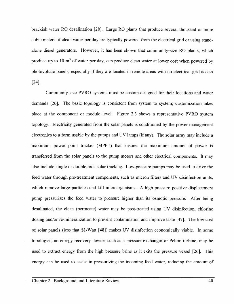
Community-size PVRO systems must be custom-designed for their locations and water
demands [26]. The basic topology is consistent from system to system; customization takes
place at the component or module level. Figure 2.3 shows a representative PVRO system
topology. Electricity generated from the solar panels is conditioned by the power management
electronics to a form usable by the pumps and UV lamps (if any). The solar array may include a
maximum power point tracker (MPPT) that ensures the maximum amount of power is
transferred from the solar panels to the pump motors and other electrical components. It may
also include single or double-axis solar tracking. Low-pressure pumps may be used to drive the
feed water through pre-treatment components, such as micron filters and UV disinfection units,
which remove large particles and kill microorganisms. A high-pressure positive displacement
pump pressurizes the feed water to pressure higher than its osmotic pressure. After being
desalinated, the clean (permeate) water may be post-treated using UV disinfection, chlorine
dosing and/or re-mineralization to prevent contamination and improve taste [47]. The low cost
of solar panels (less that $1/Watt [48]) makes UV disinfection economically viable. In some
topologies, an energy recovery device, such as a pressure exchanger or Pelton turbine, may be
used to extract energy from the high pressure brine as it exits the pressure vessel [26]. This
energy can be used to assist in pressurizing the incoming feed water, reducing the amount of
Chapter 2. Background and Literature Review 40

solar-generated electricity that must be produced. Energy recovery devices are expensive
relative to the cost of the other components in a PVRO system, so they are not always used. This
thesis assumes no battery or other form of local energy storage.
PowerSolar Management
Panels Electronics
OutflowLow Micron UV High Reverse (Demand)
Water Pressure Filter Pretreatment Pressure Osmosis -. {''- - -
Source Pump PumpClean Water Maintenance+ IValve Circulating
To Brine/ Storage & UV irPumpWastewater L- ..---- . --------
Disposal
CleaningChemicals
Figure 2.3: Community-sized photovoltaic-powered reverse osmosis system
A maintenance loop is also shown in Figure 2.3, consisting of a circulating pump and
mixing valve where cleaning chemicals can be added. Details on the maintenance processes are
discussed in Section 2.3.3, following the background presentation of PVRO operation and
degradation.
2.2.2 PVRO Operation
Operation of a PVRO system depends on whether or not large battery banks are present
in its design. The topology in Figure 2.3 does not include large battery banks for energy storage.
However, PVRO systems with batteries have been developed and tested [49-53]. Systems
utilizing batteries for energy storage can be operated at quasi-constant power. When the solar
panels produce more power than required by the RO pumps and other electrical loads, the excess
power is used to charge the batteries, provided they are not fully charged already. During
41Chapter 2. Background and Literature Review
periods of little to no sunlight, the electrical loads draw power from the batteries. Though this
simplifies the control electronics, the batteries in such systems will experience deep discharging
and cycling, shortening their life spans. Such batteries are also expensive, so the cost of their
somewhat frequent replacement contributes substantially to the overall system lifetime cost.
PVRO systems that do not include batteries require custom electronic controllers that
adjust the operating points of the RO pumps and other electrical loads based on the amount of
instantaneous power produced by the solar panels. This can be achieved by defining a set of
pump operating points corresponding to different power levels. As the power from the solar
panel changes, such as when a cloud passes overhead, an automatic controller switches to the
appropriate operating point [54]. Another method of achieving variable control is to use a
custom, computer-controlled DC-to-DC converter that automatically conditions the power as the
solar radiation changes [25].
Regardless of whether or not the PVRO system operates under fixed variable power, the
RO membrane will degrade with operation. This degradation is not constant, but is dependent on
the input water chemistry, pressure and flow rates through and along the RO membrane surfaces.
Even in large, industrial RO plants, fouling cannot be determined before the system is built and
is in operation, even when the water chemistry is analyzed a priori. In some cases, smaller RO
pilot plants are tested at sites where larger industrial plants are to be installed, in order to
experimentally determine the types and rates of fouling that are likely to occur [28, 55]. Such
experiments are impractical when installing small-scale community PVRO systems, since the
experiment would be on the same scale as the RO system itself. The fouling rates for
community-size RO systems must be determined from their operating history.
Chapter 2. Background and Literature Review 42Chapter 2. Background and Literature Review 42

2.3 Fouling and Remediation of Reverse Osmosis
Of all the components in a PVRO system, the RO membrane degradation has the largest
effect on water production and maintenance costs. It is also difficult to determine its state
visually, since it is completely enclosed in a pressure vessel. The permeate flow through a
reverse osmosis membrane is a function of the average water pressure applied at the membrane
surface, the feed water osmotic pressure and the RO membrane permeability to water. Over
time, particles, microorganisms and films will accumulate on the RO membrane surface and its
internal water channels as clean water passes through the membrane. This accumulation results
in what is called membrane fouling, which reduces the fresh water flow through the membrane
and hence RO system productivity. The fouling mechanisms, methods used to mitigate
membrane fouling, and current way maintenance is performed for most RO plants (solar or
otherwise) are discussed next.
2.3.1 Fouling Basics
2.3.1.1 Concentration Polarization and Mineral Scaling
Several mechanisms contribute to RO membrane fouling, including concentration
polarization, mineral scaling, colloidal fouling, and biofouling. As the clean water flows through
the RO membrane, the local salt concentration near the membrane surface increases above the
concentration level of the bulk feed, causing an increase in the local osmotic pressure, which in
turn slows the clean water trans-membrane flow. This phenomenon is called concentration
polarization. The increased local salt concentration level at the membrane surface also increases
the likelihood that salt crystals will form and precipitate out of solution onto the membrane
surface, forming a mineral scale (see Figure 2.4).
Chapter 2. Background and Literature Review 43Chapter 2. Background and Literature Review 43

Feed channelspacers
Concentration
polarization regions
Feed -- Brine flow outflow In 6Mineral scale
RO membrane-- 0- Permeate flow out
Increasing bulk salinity ---------------------------- + Support layer
Figure 2.4: Mineral scaling on a reverse osmosis membrane
Several types of mineral scale may form on an RO membrane surface, depending on its
water chemistry. Sparingly soluble salts, such as calcium carbonate, calcium sulfate, barium
sulfate, calcium fluoride, strontium sulfate and calcium phosphate, are examples of salts that may
precipitate out of solution and onto the membrane surface [28]. Once seeded, a crystalline layer
may grow on the RO membrane surface, forming a hard mineral scale that is difficult to remove.
Scale formation is affected by concentration polarization, pH, temperature, pressure, permeation
rate, axial flow velocity and the presence of other ions and minerals [56-58]. Surface
crystallization is favored at high operating pressures and low cross-flow (axial) velocities and
bulk crystallization is favored at high pressures and intermediate cross-flow velocities [56].
Higher concentration polarization leads to more crystal growth on the surface than to
precipitation at low cross flow rates. At high flow rates, there is more bulk crystallization and
less surface growth [57]. Experimental results from the literature show that increasing the water
temperature increases nucleation and growth rates of gypsum scale [58]. At 15 and 25*C, the
(clean water) flux decline is slow and steady, and small crystals are deposited over the entire
membrane surface. At 35'C, and at high (70%) recovery ratios (70% of the feed water is
desalinated), flux decline decreases due to higher osmotic pressure and "the entire membrane
surface [is] covered with "needle-like" crystal fragments. The crystal fragments broke off from
growing gypsum rosettes and [re-deposit] uniformly across the membrane forming a "cake layer"
Chapter 2. Background and Literature Review 44
that [causes] the massive flux decline [58]." As used here, "flux" is the permeate water
volumetric flow per unit area of the RO membrane.
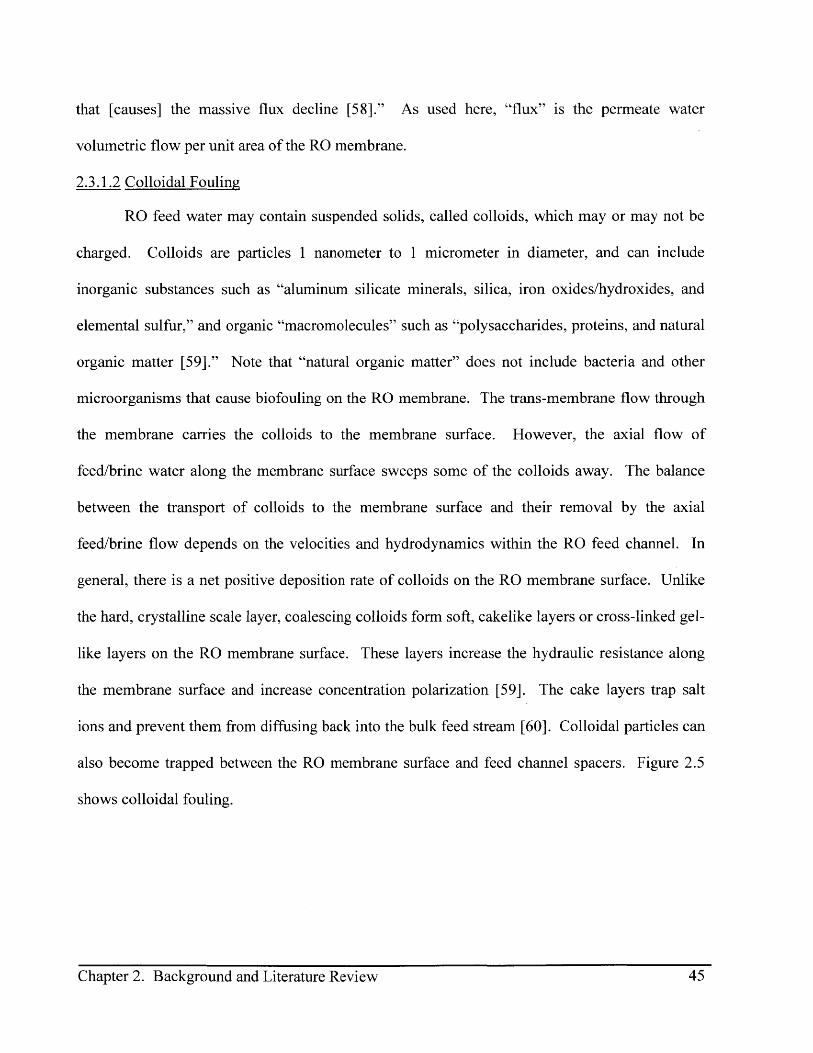
2.3.1.2 Colloidal Fouling
RO feed water may contain suspended solids, called colloids, which may or may not be
charged. Colloids are particles 1 nanometer to 1 micrometer in diameter, and can include
inorganic substances such as "aluminum silicate minerals, silica, iron oxides/hydroxides, and
elemental sulfur," and organic "macromolecules" such as "polysaccharides, proteins, and natural
organic matter [59]." Note that "natural organic matter" does not include bacteria and other
microorganisms that cause biofouling on the RO membrane. The trans-membrane flow through
the membrane carries the colloids to the membrane surface. However, the axial flow of
feed/brine water along the membrane surface sweeps some of the colloids away. The balance
between the transport of colloids to the membrane surface and their removal by the axial
feed/brine flow depends on the velocities and hydrodynamics within the RO feed channel. In
general, there is a net positive deposition rate of colloids on the RO membrane surface. Unlike
the hard, crystalline scale layer, coalescing colloids form soft, cakelike layers or cross-linked gel-
like layers on the RO membrane surface. These layers increase the hydraulic resistance along
the membrane surface and increase concentration polarization [59]. The cake layers trap salt
ions and prevent them from diffusing back into the bulk feed stream [60]. Colloidal particles can
also become trapped between the RO membrane surface and feed channel spacers. Figure 2.5
shows colloidal fouling.
Chapter 2. Background and Literature Review 45Chapter 2. Background and Literature Review 45

Feed channelspacers
Feed
flow in *- Brine flow out
Cake layerRO membrane
-- -- Permeate flow out
Support layer
Figure 2.5: Colloidal fouling on an RO membrane surface
Colloidal fouling is more severe at high permeate flux and/or low axial flow across the
RO membrane. "The greater tendency of colloidal fouling at higher flux [is] attributed to: 1)
larger permeate volume (thus greater amount of foulant "seen" by the membrane), 2) more
severe concentration polarization, and 3) greater hydrodynamic drag towards the membrane
surface [59]." The ionic strength of monovalent salts in the feed water, though not their types,
affects colloidal fouling, with higher ionic strength increasing the fouling potential [60, 61]. The
effects of water temperature on organic colloidal fouling and water production have also been
studied. Research shows that the amount of foulant on the membrane remains the same
regardless of temperature, but specific cake resistance increases with decreasing temperature,
"hence, specific cake resistance increases with increasing humic acid colloid size [62]."
2.3.1.3 Biofouling
Microorganisms and bacteria, if present in the feed water, can attach to the RO membrane
surface and feed channel spacers and grow into colonies (see Figure 2.6). Such colonies
generate an extracellular polymeric substance (EPS) that forms a biofilm over them. This layer
traps nutrients needed by the colonies as well as protects them from the axial shear fluid forces.
As the colonies grow larger, some of the bacteria detach and reattach further downstream and
Chapter 2. Background and Literature Review 46
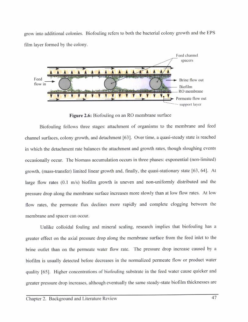
grow into additional colonies. Biofouling refers to both the bacterial colony growth and the EPS
film layer formed by the colony.
Feed channelspacers
Feedflow in
- Brine flow out
BiofilmRO membrane
Permeate flow out
support layer
Figure 2.6: Biofouling on an RO membrane surface
Biofouling follows three stages: attachment of organisms to the membrane and feed
channel surfaces, colony growth, and detachment [63]. Over time, a quasi-steady state is reached
in which the detachment rate balances the attachment and growth rates, though sloughing events
occasionally occur. The biomass accumulation occurs in three phases: exponential (non-limited)
growth, (mass-transfer) limited linear growth and, finally, the quasi-stationary state [63, 64]. At
large flow rates (0.1 m/s) biofilm growth is uneven and non-uniformly distributed and the
pressure drop along the membrane surface increases more slowly than at low flow rates. At low
flow rates, the permeate flux declines more rapidly and complete clogging between the
membrane and spacer can occur.
Unlike colloidal fouling and mineral scaling, research implies that biofouling has a
greater effect on the axial pressure drop along the membrane surface from the feed inlet to the
brine outlet than on the permeate water flow rate. The pressure drop increase caused by a
biofilm is usually detected before decreases in the normalized permeate flow or product water
quality [65]. Higher concentrations of biofouling substrate in the feed water cause quicker and
greater pressure drop increases, although eventually the same steady-state biofilm thicknesses are
-i
47Chapter 2. Background and Literature Review

achieved [66]. Higher linear flow velocities (inlet velocities about 0.1 m/s) result in higher
initial pressure drops, larger and quicker pressure drop increases and more biofouling
accumulation, though the biofilms formed are thinner than those formed under lower linear flow
velocities [63, 66].
Fouling mechanisms are not independent of one another. For example, colloidal fouling
may transport needed nutrients to the bio-colonies, promoting their growth. In such instances,
the cake layer may not be as thick, but the concentration polarization may increase since salts
become trapped in the biofilm [63]. Interactions between fouling mechanisms have received
limited study, and preliminary research suggests the interactions are complex [67-69]. Modeling
such interaction in detail has not been performed, and is also not the focus of this thesis.
2.3.1.4 Effects of Fouling on RO Water Production
Fouling decreases the water flow rate through the RO membrane and increases the
pressure drop along the RO channel. As the fouling increases, the feed water pressure required
to produce a given permeate flow rate increases. An RO unit designed to operate at constant
flow will consume more energy as it fouls. An RO unit operating at constant pressure
experiences a drop in clean water production over time as it fouls. A PVRO system operates
under varying power levels, hence varying pressure and flow rates, and so its fouling will not be
uniform over time. Understanding how these losses develop as a function of system operation is
critical for developing a maintenance plan that ensures the desired water demand is always met.
2.3.2 Models of RO Fouling in the Literature
The physics of RO fouling and scaling have been well studied, and many mathematical
models describing the effects of fouling exist [11, 59, 60, 63, 64, 70-77]. Models range in
Chapter 2. Background and Literature Review 48
complexity from simple models that describe the decrease in permeate flow rate in a constant
pressure RO plant over time, to complex, finite-difference, multi-dimensional, temporal-spatial
models of fouling based on fundamental physics and include feed channel geometry, water
chemistry and hydrodynamics.
Simple models describe the reduction in permeate water flow over time [11, 60, 70, 71].
Flux decline is described by a simple, exponential decay with time in [11, 70]. Simple models
have also been generated by fitting exponential and rational functions to empirical plant data [60,
71]. Since fouling is dependent on water chemistry and operating conditions, these models are
limited in their use to the RO systems from which they were derived. Adjusting such models to
other RO systems require data from the systems to be modeled.
Effects of colloidal fouling are commonly described using a cake growth model that
relates the increase in RO membrane resistance to permeate water flow to the cake layer
thickness [59, 72-74]. The feed water is assumed to have a "fouling potential" that is intrinsic to
it, and this is the proportionality constant between trans-membrane velocity and RO membrane
resistance to water permeation. The feed water fouling potential must be found from
experimental data [73]. The cake growth model can be used to describe the increase in RO
membrane resistance that decreases permeate flux due to mineral scale formation. A lateral
growth model describes decrease in available RO membrane area caused by mineral scale [57].
The cake growth model is an extension of an earlier resistance-in-series model [75]. In
this research, fouling by nucleation-growth mechanisms is discussed. Large particle settling is
described using Stoke's Law. Scale formation by flocculation of small particles at the RO
membrane surface is explained. A method to experimentally determine the parameters in the
cake growth model is presented. Note that all the species present in the feed water must be
Chapter 2. Background and Literature Review 49

known to use the resistance-in-series model. Additionally, the resistance will change based on
the thickness of the foulant layer as well as on changes in the operating conditions.
Another model that describes the effects of colloidal fouling is the gel-polarization model
[75]. The gel-polarization model assumes that the colloids form a gel layer on the RO membrane
surface that is more permeable to water than the RO membrane, so the permeate flow becomes a
logarithmic function of the concentration of salt species in the gel and bulk feed water layers.
The model is found to predict permeate flux "within two orders of magnitude when applied to
particulate colloidal fouling [75]."
Biofouling of RO membranes has been extensively studied and modeled. A two-
dimensional spatial, temporal model of biofouling used to numerically simulate attachment,
growth and detachment of bacterial colonies in the feed water channel of an RO membrane is
presented in [63, 76]. Three-dimensional spatial-temporal models have also been presented [64,
77]. The complexities of these models require that simulations be computed numerically using
computational fluid dynamics packages. Simulation results agree well with experimental data.
Such models are useful for determining the effects of feed channel spacers and are intended to
assist in future membrane design. However, they are too complex to be appropriate for
predicting the long-term fouling of small, remote PVRO systems.
All of the models describing fouling presented above depend on parameters that must be
determined experimentally.
2.3.3 Fouling Mitigation
Methods have been developed by researchers to mitigate RO fouling and to partially
restore RO membrane permeability. These methods include pretreatment of the feed water,
mechanical cleaning of the RO membrane, chemical cleaning of the RO membrane and
Chapter 2. Background and Literature Review 50
ultimately RO membrane replacement. Maintenance guidelines for RO systems have also been
developed.
2.3.3.1 Pretreatment
There are several methods for pretreatment of RO feed water that can reduce the colloidal
fouling and scaling rates at the RO membrane surface [28]. Filtration and flocculation remove
larger particles and organisms from the feed water. Feed water can be filtered through sand,
porous media, carbon filters, microfiltration (MF), ultrafiltration (UF) and nanofiltration (NF)
units. Flocculants can be added to the feed water in a mixing tank to induce aggregation of
smaller particles into larger clusters. The water then flows into a settling tank or clarifier to
permit the larger clusters to sink out of the RO feed water. Anti-scalants can partially prevent
mineral scale from forming by keeping the sparingly soluble salts in solution, by changing the
crystal structure of the salts as they precipitate so they form a softer layer, or by adsorbing onto
the salt crystals and imparting high anionic charges, causing the crystals to remain dispersed and
to be repelled from the anionic membrane surface [28].
Though all pretreatment methods described above can be used in remote, community-size
PVRO systems, some methods are more economical than others. Carbon, porous media, sand
and micron filters are inexpensive. Visual inspection can be used to determine whether or not
they need cleaning or replacing. MF, UF and NF filtration are more expensive, so using such
technologies for pretreatment of feed water for community-sized systems may not be cost
effective.
Biofouling can be minimized by disinfecting the feed water before it enters the RO
pressure vessel. Disinfection can be accomplished using chlorine dosing, although the feed
water must then be de-chlorinated before entering the RO pressure vessels, since chlorine can
51Chapter 2. Background and Literature Review

damage the RO membranes. Another method is using UV disinfection. The low cost of solar
panels makes solar-powered UV disinfection practical for community-sized PVRO systems, and
eliminates the need for chemical dosing and its associated costs [78].
2.3.3.2 Mechanical Cleaning
Mechanical cleaning techniques for removing foulants from RO membrane surfaces have
been developed. They include system flushing, backwashing, scouring with sponge balls, air
scouring and ultrasonic cleaning [28, 79]. In system flushing, some of the clean permeate water
flows over the RO membrane, and removes some of the loosely deposited colloids and other
particles from the feed-water side surface (see Figure 2.7). In a forward flush, flushing water
flows from the feed inlet to the brine outlet, as shown in Figure 2.7. In a backward flush,
flushing water flows from brine outlet to feed inlet. The effectiveness of system flushing has
been studied experimentally with the intent to optimize the flushing process [80]. In this case,
the optimized flushing process for a single 2.5-inch diameter, 14-inch long RO membrane was a
minute-long backward flush followed by a 5 minute forward flush, which used a total of 7% of
the permeate water produced over a single day. The amount of water required for a system flush
depends on system size, the flushing water flow rates and flushing durations specified by RO
membrane manufacturers [29, 81]. Typical flushing flow rates for 4-inch diameter RO
membranes are 23 to 38 liters per minute [81]. Flushing durations are usually 3 to 5 minutes
[28]. Flushing only removes loosely deposited particles, and cannot remove hard scales or
biofilms.
Chapter 2. Background and Literature Review 52Chapter 2. Background and Literature Review 52

Loose particles Feed channel
removed spacers
System flush (RO - System flush water
product) water in ~ &particlesout
S'-4RO membrane
Support layer
Figure 2.7: Loosely deposited particles removed by system flushing
Backwashing is similar to system flushing in that some of the clean permeate water is
used to remove loosely deposited particles. In backwashing, the flushing water is forced from
the permeate side of the membrane to the feed water side. Flushing water can be directly forced
from the permeate side to the feed side of hollow fiber RO, UF and NF membranes. Osmotic
backwashing of spiral-wound membranes can be induced by flowing feed water at pressures
lower than osmotic pressure along the RO membrane. Direct osmosis from the permeate side to
the feed side occurs. This type of osmotic backwashing can also be accomplished using
hypersaline solutions in place of the feed water. Typically, osmotic backwashing is followed by
a system flush to sweep away any loosened particles on the membrane feed water side surface
[79].
In sponge-ball cleaning, small abrasive sponges are introduced and circulated in the RO
pressure vessel. As with backwashing, sponge-ball cleaning cannot be applied to spiral-wound
RO membranes, but can be used to clean hollow fiber RO membranes [79].
Air scouring is another process typically applied to microfiltration and ultrafiltration
membranes, though it has been used to clean hollow fiber and spiral-wound RO membranes. In
air scouring, a gas/liquid mixture flows over the RO membrane surface. This two-phase flow
scours the membrane and loosens the cake layer [79]. Recent advances in RO membrane
cleaning techniques combine air scouring and chemical cleaning [82, 83]. Researchers add
Chapter 2. Background and Literature Review 53
effervescent chemicals into cleaning solutions that generate microbubbles, which provide
scouring. Using this method, researchers were able to reduce the chemical cleaning cycle
frequency from every 10 days to every 6-8 weeks in a wastewater reverse osmosis plant [83].
Chemical cleaning is discussed in the next section.
Ultrasonic de-fouling for RO membranes has been proposed and tested experimentally in
a laboratory setting [11, 79, 84]. In the experimental setup, the cross-flow RO unit is submerged
in an ultrasonic bath during the filtration process. The results show that applying ultrasound
during the RO process increases the permeate flux by at least 50% while minimally decreasing
the salt rejection [84]. The authors of this study suggest that ultrasonic cleaning can remove
calcium sulfate and organic foulants. This technique is not typically used in large RO plants.
Of the purely mechanical cleaning techniques presented above, system flushing is most
easily implemented and is most suitable for small-scale PVRO plants. The amount of permeate
water required for flushing is minimal and the cleaning duration is short. Chemical cleaning,
discussed below, is also needed in a PVRO system.
2.3.3.3 Chemical Cleaning
Chemical cleaning is a common method used to remove foulants from RO membranes.
The process consists of pre-flushing, slow circulation of cleaning chemical solution, a 30 minute
to a full-day soak, a high-flow rate recirculation of the cleaning solution for 30 to 60 minutes,
and a clean-water flush for approximately 60 minutes [28, 29, 79, 81]. The flushing, circulation
and soaking durations and flow rates used for a given RO system will depend on its size and the
type of fouling, as will the volume of permeate water needed. Cleaning chemical and RO
membrane manufacturers provide instructions by chemical cleaning type and RO system size.
The types of chemicals used for cleaning also depend on the type of fouling [28, 79, 85]. For
Chapter 2. Background and Literature Review 54

example, alkaline solutions (high pH cleaners), such as sodium hydroxide solutions, can be used
to remove sulfate scale, organic fouling, biofouling and silica. Low pH cleaners, such as
hydrochloric acid solution and sodium hydrosulfate, can be used to remove calcium carbonate
scale and iron oxide deposition, respectively. Neutral pH cleaners can be used to remove
biofilms. Typically, acid cleaning follows alkaline cleaning, since cleaning with acid first in the
presence of biofouling or organic fouling can cause irreversible damage to the membrane.
Commercial formulations of cleaning chemicals vary by manufacturer.
The effectiveness of different chemical cleaning solutions and chemical cleaning
processes applied to RO membranes has been studied [79, 80, 85-87]. One study on chemical
cleaning for RO membranes treating effluent found that chemical cleaning efficacy is highly
dependent on the temperature and the concentration of the alkaline cleaning solution used [80].
The study also found that following the chemical cleaning procedure with a system flush was
able to restore the permeate water flow rate to about 97% of its pre-fouled value. The cleaning
efficacy of alkaline solutions, acid solutions, surfactants and detergents on seawater RO
membranes fouled with calcium sulfate (90%) and calcium phosphate has been studied [87]. In
that research, alkaline cleaners combined with a chelating agent and surfactant are able to
remove most of the foulant and to restore the permeate flux to its pre-fouled flow rate. Also,
higher concentration of cleaning chemicals, longer duration of cleaning time and higher
temperatures increase the effectiveness of foulant removal, but also extend the downtime of the
system.
Though membrane manufacturers provide cleaning guidelines, independent research
points out that these guidelines are appropriate for single types of fouling and may not be
appropriate for RO systems experiencing multiple, concurrent types of fouling [86]. During a
Chapter 2. Background and Literature Review 55

case study of a brackish water 60 m3/hr RO plant, researchers define a hierarchy of foulants: 1)
silica colloids, 2) adsorbed organic compounds, 3) particulate matter (iron and aluminum
colloids), 4) microorganisms and 5) metallic oxides. They recommend that the chemical
cleaning process be structured such that it prioritizes removal of foulants according to the
hierarchy. Cleaning guidelines available from membrane manufacturers now follow the cleaning
process order presented in [86].
The cleaning effectiveness studies cited above investigate single instances of cleaning
and do not address the long-term effects of cleaning over time. The effects of long-term cleaning
(e.g., on RO membrane useful life) have not been thoroughly studied. Chemical cleaning cannot
perfectly restore the RO membrane to its original condition. Though all of the foulants may be
removed during the chemical cleaning, the foulants also cause irreversible damage, such as
surface abrasions. One optimal design study on seawater reverse osmosis systems presents a
model to capture the decline in the RO membrane permeabilities to water and salt, considering
imperfect cleaning and RO membrane replacement [88]. In this model, membrane permeability
decays exponentially. Chemical cleaning partially restores permeability; permeability is only
fully restored when the membrane is replaced. Similarly to other models in the literature, the
model presented in [88] depends on experimentally determined parameters.
After several years of operation, an RO membrane wears out due to compaction from the
high pressure feed water, from irreversible fouling, and from general deterioration. Membrane
life depends on the feed water chemistry, with lifetimes of 2-5 years typically given in the
literature, based on operator experience [28].
Chapter 2. Background and Literature Review 56Chapter 2. Background and Literature Review 56
2.3.3.4 RO Membrane Maintenance
Historically, RO plants have been maintained using conventional periodic maintenance
[11, 28, 89]. System pretreatment and maintenance procedures, including the specifics of
flushing and chemical cleaning flow rates, durations, frequencies and chemicals, are determined
by analyzing the feed water chemistry at the intended plant site during several times of the year,
prior to plant construction. The water chemistry analysis includes details of the chemical species
present and the type of biological content. The concentrations of chemical species, such as
calcium, soluble silica, barium and strontium, can be used to determine whether or not mineral
scaling is likely. The likelihood of mineral scaling can also be determined by calculating the
Langlier Saturation Index (LSI) or the Stiff-Davis Saturation Index (SDSI) of the water [28].
Both indices uses the pH and temperature of the water in addition to the concentration of total
dissolved solids (TDS), calcium hardness and alkalinity to quantify the scaling and corrosive
tendencies of the water. A positive LSI or SDSI indicates calcium carbonate scaling is likely. A
negative LSI indicates the water is corrosive and may dissolve scale. An LSI of 0 indicates the
water is chemically balanced. The LSI is used for water with TDS of up to 4,000 ppm, and is
only appropriate for low-level brackish water. The SDSI is used for water with higher TDS
concentration, including seawater.
The concentrations of metals, including iron, manganese and aluminum, along with
concentrations of hydrogen sulfide and total organic carbon (TOC), can be used to estimate
colloidal and organic fouling potentials [28]. Color, measured in color units, and water turbidity,
measured in Nephelometric Turbidity Units (NTU), are additional indicators of the fouling
potential of feed water. Industry guidelines recommend feed water have color less than 3 APHA
and turbidity less than 1 NTU. Particulate fouling potential is also measured using the Silt
Density Index (SDI). The SDI is calculated from a standardized test in which the water being
Chapter 2. Background and Literature Review 57

analyzed flows through a 0.45 micron filter pad at 30 psi. The time it takes for 500 ml of water
to flow through the filter pad is recorded initially. After 15 minutes of flow through the pad at
30 psi, an additional 500 ml of water is collected and its time is recorded. The SDI is calculated
from these measurements. An SDI above 3 indicates higher fouling potential. The SDI test can
also be performed once the RO plant has been constructed and the pretreatment system is in
place. The Modified Fouling Index (MFI) is an extension of the SDI and is also used to
determine fouling potential [90].
Additional indices for fouling potential have been developed [11, 91-94]. Estimates of
fouling potential based on RO system performance data are defined in [91, 92]. One method
tracks the change in RO membrane permeability over time and plots the volumetric clean water
production versus the ratio of current membrane permeability to starting membrane permeability
[91]. This method can be used to determine how much the system water production is affected
by the types of foulants, but doesn't provide information on how fast the ratio declines. Another
method defines a filtration coefficient that is essentially a lumped parameter of the bulk
membrane permeability of the entire RO plant, and calculates its value [92]. By calculating this
value over time, the level of fouling is determined. Molar species have also been used to
develop water fouling classifications [93, 94].
Assimilable organic carbon (AOC) measures the growth potential of microorganisms in a
water sample [28]. This can be used as an indication of the likelihood of biofouling before plant
operation. Analysis of the concentrate (brine) water stream in an RO plant can be used to
determine whether or not biofouling has occurred. Typical analysis methods are growing
cultures from the reject stream, or obtaining a total bacterial count (TBC) from a filter through
which the RO concentrate flows.
Chapter 2. Background and Literature Review 58

The above indices are measured before plant operation takes place. Although such
indices can be used to determine the types of chemicals needed for cleaning the RO membranes,
cleaning frequency and duration will need to be adjusted during plant operation.
In addition to water quality testing, a pilot plant may be constructed and operated for
several months to a year before construction of a large RO plant begins [28]. During pilot plant
operation, flushing and chemical cleaning processes determined from water quality testing can
be refined and optimized empirically. RO membranes from the pilot plant can also be autopsied
to determine the types of fouling present in the pilot system. For a large-scale RO project,
incurring such costs may be considered trivial. However, pilot plant construction and testing is
prohibitively expensive and impractical for small, community-size projects.
Optimization of periodic maintenance has been performed for RO plants during the
design stage, assuming that fouling is exponential and that regeneration is perfect after
maintenance [95-97]. Optimization of an RO system fluid network is performed in terms of total
cost and maintenance schedule, assuming perfect regeneration, in [95]. Flexible fluid RO
networks able to accommodate a given range of feed water and system performance variations
are optimized in terms of lowest annual cost, considering fouling and maintenance, in [96].
Optimization of the operation of an RO plant with a given set of membranes in terms of
minimizing its specific energy consumption and annual operating cost is performed in [97].
These studies are applied to large RO plants and do not assume large variations in operating
conditions.
Condition-based maintenance is also used in RO plants [28]. The performance metrics
for RO are the permeate flow rate and pressure drop from feed inlet to brine outlet.
Measurements are normalized to account for temperature, pressure and salinity variations, and
Chapter 2. Background and Literature Review 59

are compared with normalized plant measurements taken at either plant startup or when new RO
membranes are installed. RO process experts and manufacturer maintenance guidelines
consistently recommend that RO membranes be cleaned when the normalized permeate flow rate
drops by 10%, or when the normalized pressure drop along the RO pressure vessel increases by
15% [28, 29, 81]. Maintenance chemical suppliers and RO membrane manufacturers sell
software-based condition monitoring systems that perform the normalization calculations from
plant operating data, and that notify operators when chemical cleaning is needed. CBM is a
reasonable method of maintaining a large RO plant with staff available on hand to perform
maintenance as required, but is not suitable for remote, community-size PVRO plants. Small
PVRO plants will not have the expert staff available to perform maintenance quickly. Also,
simply defining suitable CBM metrics for a PVRO plant that operates over wide pressure and
flow ranges is challenging. It is not appropriate to use the normalized pressure drop and water
production rates, since the variability in operation may trigger maintenance when it is not yet
required.
Prognostic maintenance has been applied to RO plants. Neural network approaches have
been used to develop short-term forecasting models of RO performance [98, 99]. An approach
using radial basis functions has been used to predict performance over a two hour period based
on "transmembrane pressure, ionic strength, solution pH, particle size and elapsed filtration time
[98]." Note that this is a very short period with respect to RO membrane fouling. A neural
network approach for predicting the short term performance (i.e. the next 24 hours) of an RO
plant subject to fouling has been developed from experimental data [99]. Risk modeling and
model predictive control have been combined to determine RO plant operation that will
minimize risks [100]. The model predictive controller determines the timing of risk-mitigating
Chapter 2. Background and Literature Review 60

actions. This method has been tested in simulation. Fault detection and isolation (FDI) and fault
tolerant control (FTC) have been applied to a high recovery RO plant in simulation [101]. In this
work, the redundancy in the structure of the RO plant permits multiple flow pathways, which is
necessary for FTC. Fault tolerant control has been applied to a small-scale laboratory RO
system; however, this system treats municipal tap water, so faults resulting from fouling/scaling
are not addressed [102]. This small laboratory system also includes a reconfigurable network of
reverse osmosis pressure vessels and membranes. Implementing redundancy in community-
sized PVRO plants adds capital costs and may not be economically viable, so such an approach
is not necessarily applicable. A prognostic maintenance method for PVRO systems that will
ensure they meet their community demands at lowest cost has yet to be developed. The
development of a prognostic maintenance method is the focus of this thesis.
2.4 Summary
Prognostic health monitoring (PHM) and maintenance is an active area of research. Early
research in diagnostics of machine health led to the development of condition-based maintenance
(CBM), which has now been widely adopted in industry. CBM improves on pre-determined
periodic maintenance so that preventative maintenance is not performed when it isn't needed.
Efforts to improve CBM so that preventative maintenance can be scheduled in advance have led
to predictive condition-based maintenance and prognostic maintenance (PHM). The methods
described in the literature predict the remaining useful life of components and schedule the next
immediate maintenance action, but do not produce sequences of maintenance actions and
determine the time between them. Though sufficient for applications in which dedicated, onsite
operators with specialized knowledge are present, a prognostic method that provides non-expert
Chapter 2. Background and Literature Review 61Chapter 2. Background and Literature Review 61

operators with a sequence of maintenance actions and their timing while accounting for highly
variable and uncertain operating conditions and degradation has yet to be developed.
PVRO desalination is a representative application requiring model-based prognostic
maintenance. An RO membrane's degradation is caused by fouling, which is a complex function
of RO system operation. It is dependent on water chemistry, operating pressure and water flow
rates. When part of a PVRO system, water desalination through the RO membrane becomes a
complex function of the solar energy driving the RO process, so its degradation is even more
complex and uncertain. A PVRO system is also operated by community members who do not
have the expert knowledge to determine the maintenance strategy that will ensure community
water demand is met at the lowest cost. Following recommended maintenance guidelines from
RO membrane manufacturers will not necessarily guarantee PVRO systems meet their demand,
or may not ensure that demand is met at the lowest cost. Similarly, CBM for PVRO may also
not ensure demand is met at the lowest cost, and is also difficult to implement for PVRO systems
operating over wide power ranges.
In this research, a model-based prognostic maintenance algorithm for community sized
PVRO systems, subject to highly varying, uncertain and stochastic operating conditions is
developed. It uses probabilistic methods to handle uncertainties in future inputs, such as
incoming solar radiation and water demand. Prognostic maintenance also requires models of RO
membrane fouling and remediation. The physics of various types of RO membrane fouling have
been studied and mathematical models that describe the effects of fouling over time have been
developed. The models range from simple empirically derived models that describe the decline
in water flow, to extensive two and three dimensional models that require intensive computation.
Simple empirical models are valid for the systems from which their underlying data was sourced.
Chapter 2. Background and Literature Review 62

Even the extensive models rely on empirically derived parameters. A simple, yet valid, physics-
based model of RO fouling that can be used for prognostics is needed, and is developed here.
Chapter 2. Background and Literature Review 63Chapter 2. Background and Literature Review 63
Chapter 2. Background and Literature Review 64

CHAPTER
3PVRO PERFORMANCE, DEGRADATION AND
REMEDIATION MODELING
The development of a prognostic maintenance algorithm requires an understanding of the
physics of system degradation and remediation. The previous chapter presents the physics of RO
water production and membrane fouling, including mineral scaling, colloidal fouling and
biofouling. In this chapter, mathematical models that describe the clean water production,
degradation (fouling) and remediation of the RO membrane are presented. The degradation
model is a simplification of the cake growth model found in [72]. The simple remediation
models presented here are unique to this work. These models will be used to predict PVRO
system performance when subject to fouling.
3.1 RO Water Production
The reverse osmosis process is a function of the RO membrane permeability, osmotic
pressure and the feed water pressure. A schematic showing the flow of clean water across an RO
membrane is shown in Figure 3.1. The well-known solution-diffusion model describes the clean
water (permeate) flow rate through the RO membrane, q, (t), (L/s), [103, 104]:
e(3.1)
where-
Chapter 3. PVRO Performance, Degradation and Remediation Modeling 65
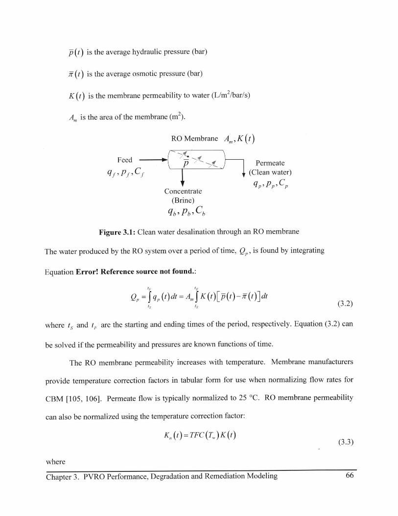
P (t) is the average hydraulic pressure (bar)
i (t) is the average osmotic pressure (bar)
K (t) is the membrane permeability to water (L/m2/bar/s)
A,, is the area of the membrane (m2).
RO Membrane AM,K(t)
Feed Feed (Permeate
qf, p, Cf (Clean water)
Concentrate q,, p,,C
(Brine)
q b Pb , Cb
Figure 3.1: Clean water desalination through an RO membrane
The water produced by the RO system over a period of time, Q,, is found by integrating
Equation Error! Reference source not found.:
tF tF
QP = qP(t~dt = Am f K (t)[(t t- 17(t})dtis is (3.2)
where ts and tF are the starting and ending times of the period, respectively. Equation (3.2) can
be solved if the permeability and pressures are known functions of time.
The RO membrane permeability increases with temperature. Membrane manufacturers
provide temperature correction factors in tabular form for use when normalizing flow rates for
CBM [105, 106]. Permeate flow is typically normalized to 25 'C. RO membrane permeability
can also be normalized using the temperature correction factor:
K,t Q) = TFC (T. ) K (t) (33
where
Chapter 3. PVRO Performance, Degradation and Remediation Modeling 66

TFC is the temperature correction factor,
T, is the water temperature inside the RO pressure vessel ('C) and
K, (t) is the normalized membrane permeability at time t.
The average hydraulic pressure is a function of the feed water pressure at the RO inlet,
axial pressure drop along the RO membrane from the feed water inlet to the brine water outlet,
and the pressure of the permeate water on the opposite side of the membrane. The upper limit on
the pressure drop for a single RO membrane element is 1 bar, according to RO membrane
manufacturer data [107]. Since the community-sized PVRO systems considered in this work are
assumed to consist of pressure vessels containing one or two RO membranes each, the average
pressure on the feed water side of the RO membranes can be calculated using:
p- -t ()+ b=t -p(W2 (3.4)
where
pf (t) is the feed water pressure at the RO inlet (bar),
Pb (t) is the pressure of the concentrate (brine) water (bar), and
p, (t) is the pressure of the permeate (clean) water (bar).
These parameters are shown in Figure 3.1. The pressure drop over a single membrane element in
a small PVRO system was measured and found to be on the order of 0.1 bar [25]. For very small
RO systems, such as those containing a single RO membrane in a single vessel, it can be
assumed that the permeate water exits the RO pressure vessel at approximately atmospheric
pressure. Also, the average water pressure on the feed water side of the single RO membrane
can be assumed to be the feed water inlet pressure, p1 (t).
Chapter 3. PVRO Performance, Degradation and Remediation Modeling 67
The osmotic pressure of water depends on its composition and temperature. An
approximate empirical relationship for osmotic pressure of saline water, r,, as a function of the
concentration of total dissolved solids and temperature is [103]:
/7 (2.654 x 10-) C, (T, +273.15)
1000 - / (3.5)
where
C, is the concentration of total dissolved solids (TDS) in ppm and
T, is the water temperature ('C).
Note that the constants in Equation (3.5) have units that are not shown.
The average osmotic pressure will depend on the concentrations of salt in the feed,
concentrate and permeate, as well as the effect of concentration polarization at the RO membrane
surface. The following equation can be used for a single RO membrane element [103]:
C~f (t)jgC( = ,z ( C~t)W]Pf (3.6)
where
/ 7f (t) is the osmotic pressure of the feed water (bar),
Cf (t) is the arithmetic average of the feed and concentrate salt concentrations (ppm),
Cf (t) is the feed salt concentration (ppm),
7t, (t) is the osmotic pressure of the permeate water (bar), and
pf is the concentration polarization factor (dimensionless).
The concentration polarization for a single RO element can be found using an empirical
relationship [103]:
Chapter 3. PVRO Performance, Degradation and Remediation Modeling 68

pf = exp 0.7 qP (t)q (t)) (3.7)
where q, (t) is feed water flow rate (L/s). The ratio of permeate flow to feed water flow is
called the recovery ratio.
In a PVRO system, the feed water pressure at the RO pressure vessel inlet will depend on
the amount of sunlight that is converted to electrical energy by the solar panels. The electricity
produced by the solar panel, P,,,,, for a given level of solar radiation can be calculated using
[108]:
Peec (t) = qI(t)A ., (3.8)
where
I(t) is the instantaneous solar radiation (W/m 2),
A,, is the area of the solar panels (M2), and
q is the solar to electrical conversion efficiency of the solar panels. This efficiency is
temperature dependent. Improving the efficiencyof a community-size PVRO system by cooling
the solar panels with the incoming feed water has been studied [108, 109].
The RO inlet pressure also depends on the efficiency of the maximum power point
tracker, if included, the efficiencies of the pumps, fluid inertia, the hydraulic resistances of the
pretreatment components, and the hydraulic resistance of the concentrate exit of the pressure
vessel. The topology of a PVRO system must be known in order to correctly model the
individual motors, pumps, filters, etc. Steady-state, physics-based models of the individual
components of a PVRO system, including the different types of motors, pumps, and energy
recovery devices, have been developed and presented in [26]. Components such as electrical
Chapter 3. PVRO Performance, Degradation and Remediation Modeling 69

motors have extremely fast dynamics relative to the RO fouling process, so steady-state models
of such components can be used when predicting long-term RO performance and fouling. Once
a PVRO system topology is established, the appropriate physics-based models and numerical
values for their parameters can be incorporated into a full system description. Measurements of
the PVRO system and component performance may need to be recorded in order to calibrate the
system models. For example, the initial RO membrane permeability can be determined from
pressure, flow, salinity and temperature measurements.
3.2 RO Degradation
As discussed in Chapter 2, RO membranes may be fouled by colloids, mineral scales and
biological colonies (biofilms). The underlying physical method of both colloidal fouling and
mineral scaling is accumulation of material on the RO membrane surface through deposition of
particles or minerals by the transmembrane flow. Even though the axial fluid velocity sweeps
some of the particles away from the RO membrane surface, there is a net deposition of particles
over time. This layer of foulant decreases the flow of clean water through the membrane. In
general, this fouling layer is not uniform. In small RO systems consisting of one or two RO
membranes within a pressure vessel, it is assumed that the variations in the fouling layer are
small, so a lumped parameter approach is justified. Using this idea, the decrease in RO
membrane permeability, dK ) , is assumed to be proportional to the transmembrane velocitydt
through it:
dK(t) = m q(3dt A, (3.9)
Chapter 3. PVRO Performance, Degradation and Remediation Modeling 70
where y is a fouling rate that represents the net deposition of particles and minerals (one/bar/s).
This approach is motivated by the modeling methods in [72, 92], where membrane resistance and
the filtration coefficient are proportional to the cake layer growth. Note that the fouling rate is
not necessarily assumed constant. It will depend on the water chemistry and on the
hydrodynamics.
Substituting Equations (3.1) and (3.3) into (3.9) describes the change in membrane
permeability as a function of the current membrane state and water pressure:
dK, (t) -dt (3.10)
Biofouling physics are more complex than those of colloidal fouling and mineral scaling,
since, in addition to deposition, bacteria grow into colonies and occasionally detach from the
membrane surface to form new colonies downstream. This can cause a time-dependent fouling
rate y(t). However, for the PVRO application here, it is assumed that UV disinfection
pretreatment effectively eliminates the biofouling risk. Hence, biofouling is considered
negligible here. For other RO applications where the risk of biofouling is higher, a more
complex fouling model that includes the growth and detachment effects can be developed and
incorporated into the prognostic model formulation.
3.3 RO Membrane Remediation
The decrease in RO membrane permeability with fouling in an RO system with
pretreatment happens slowly, on the order of weeks or months, depending on the water
chemistry. Maintenance processes occur much more quickly - on the order of minutes or hours.
When considering system performance over a membrane lifetime, maintenance processes can be
approximated using delta functions [110]. System flushing and chemical cleaning are two
Chapter 3. PVRO Performance, Degradation and Remediation Modeling 71

maintenance procedures that are likely to be used to maintain a PVRO system, and they are
modeled below.
3.3.1 System Flushing
As discussed in Chapter 2, system flushing takes place on the order of minutes and
requires approximately 7% of the total permeate water produced during a day [80]. The increase
in membrane permeability due to flushing will depend on the flushing water flow rate. A simple
model describes this change during flushing:
dK,(t)
dt (3.11)
where
g, is a proportionality constant (one/bar/m2/s), and
q, is the flushing water flow rate (L/s).
Since flushing happens on the order of minutes, Equation (3.11) can be written as:
dK" ( gfqfAtf (t -tf Gg t -t [,(dt (3.12)
where
At, is the duration of the flushing cycle, and
Gf is the increase in RO membrane permeability due to one flushing cycle (L/bar/m 2/s 2).
Again, this will be system-dependent. It will also not be known a priori, and will need to be
identified during system operation.
Chapter 3. PVRO Performance, Degradation and Remediation Modeling 72
3.3.2 Chemical Cleaning
Chemical cleaning is a much more complex process than simple flushing, and takes
several hours. This is still a rapid process compared with the rate of change in RO membrane
permeability due to fouling. Again, a delta function is used to describe the increase in RO
membrane permeability due to a chemical cleaning process:
dK, (t)
dt ((3.13)
where G, is the increase in RO membrane permeability due to a chemical cleaning cycle. This
proportionality constant will depend on the specifics of the chemical cleaning cycle, such as the
duration, flow rates during recirculation and flushing, order of chemical application, types of
foulants, etc. This parameter may also depend on the number of cleaning cycles. As with the
increase in RO membrane permeability with system flushing, G,,, the increase in RO membrane
permeability due to cleaning will also need to be identified from the system performance during
its operation.
Neither the system flush nor the chemical cleaning will result in total restoration of the
RO membrane permeability. In general, chemical cleaning will provide greater increases in
permeability, since it can remove more types of foulants. Both models rely on proportionality
constants that will not be known prior to performing maintenance. As a rough estimate,
experimental results from the literature suggest chemical cleaning followed by system flushing
can restore up to 97% of the RO membrane's permeability [80]. Though the same group of
experiments found that flushing alone can restore the RO membrane permeability by 90%, this
was limited to short-term colloidal fouling. These percentages will vary by system.
Chapter 3. PVRO Performance, Degradation and Remediation Modeling 73

3.4 Representative Degradation and Remediation Example
A representative example presents the behaviors of the above models. The operating and
initial conditions are presented in Table 3.1. It is assumed that the RO system operates for 12
hours per day and must produce 1,000 Liters each day.
Table 3.1: RO fouling and remediation example parameters [11, 71]Parameter Value
Feed pressure pf 18 bar
Feed salinity C/ 20,000 ppm
Feed temperature Tf 25 OC
Osmotic pressure ii> 11.64 bar
Initial RO membrane permeability K 4.62 x 10⁻⁴ L/bar/m 2/s
Active Area A, 7.2406 m 2
Fouling rate y 3.4614 x 10⁻⁹ one/bar/s
Minimum permeate flow rate 0.0231 L/s
System flush flow rate g, 0.57 L/s
Flushing duration Az> 5 minutes
Membrane improvement after flushing G 1 x 10- L/bar/m 2/s
Chemical cleaning water demand 7,000 L
Membrane improvement after flushing Gc( ( 4 x 10⁻⁴ L/bar/m 2/s
Table 3.1 also gives the assumed system flushing and chemical cleaning process
parameters. These values are based on experimental results from [80]. Maintenance cannot
increase the RO membrane permeability beyond its initial permeability. Therefore, in this
example, if the membrane has not degraded much and maintenance is applied, it is assumed to
restore the membrane permeability to its initial value.
RO performance under constant degradation was calculated over three years of operation
using Equations (3.1), (3.10), (3.12) and (3.13). Four cases are considered: no maintenance,
daily system flushing, monthly chemical cleaning, and daily system flushing combined with
monthly chemical cleaning.
Chapter 3. PVRO Performance, Degradation and Remediation Modeling 74

RO permeate volumetric flow rate over the first 11 days is plotted in Figure 3.2 to
compare the short-term effects of system flushing with doing no maintenance. The small
increases in RO membrane permeability from the flushing are visible in the increases in
permeate flow rate immediately following flushing. Though not huge, the daily restoration from
daily flushing results in a slower net permeate flow rate decline.
0.0615
0.061 -With daily system flushing
. 0.0605
Cz 0.06-
0 0.0595
S0.059-
S Without system flushing
0.0580.058- -
0.05750 2 4 6 8 10 12
Operating time (days)
Figure 3.2: Short term permeate flow rate with and without system flushing
Figure 3.3 shows the permeate flow rate with and without system flushing over a longer
operating period. For this representative case, the permeate flow rate drops to 30% of its initial
value after 200 days of operation without any system flushing. After approximately 180 days,
this system can no longer maintain the required 0.0231 L/s flow rate to meet the required daily
water demand. With daily system flushing, permeate production drops to 60% of its initial value
after 200 days. From the long-term perspective, one can say that the net fouling rate is reduced
by daily flushing.
Chapter 3. PVRO Performance, Degradation and Remediation Modeling 75
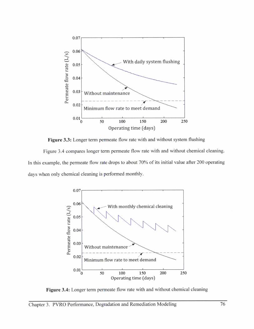
(U
40a)C)
0.07
0.06
0.05
0.04
0.03
0.02
0.0110 50 100 150 200 250
Operating time (days)
Figure 3.3: Longer term permeate flow rate with and without system flushing
Figure 3.4 compares longer term permeate flow rate with and without chemical cleaning.
In this example, the permeate flow rate drops to about 70% of its initial value after 200 operating
days when only chemical cleaning is performed monthly.
p..
U,
Figur 3.4:
0.07
0.06
0.05
0.04
0.03
0.02
I.I1I0 50 100 150 200
Operating time (days)
Longer term permeate flow rate with and without
250
chemical cleaning
Chapter 3. PVRO Performance, Degradation and Remediation Modeling
With daily system flushing
- Without maintenance
Minimum flow rate to meet demand
With monthly chemical cleaning
Without maintenance
Minimum flow rate to meet demand
76
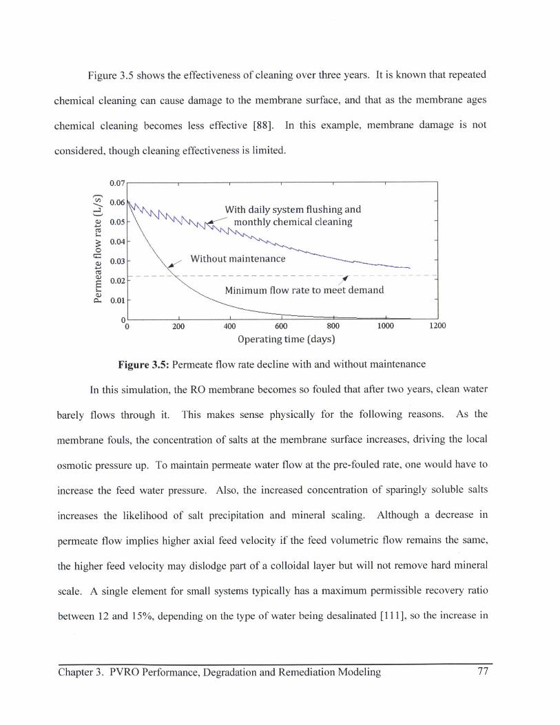
Figure 3.5 shows the effectiveness of cleaning over three years. It is known that repeated
chemical cleaning can cause damage to the membrane surface, and that as the membrane ages
chemical cleaning becomes less effective [88]. In this example, membrane damage is not
considered, though cleaning effectiveness is limited.
0.07
0.06With daily system flushing and
0.05 - ' monthly chemical cleaning
0.04-
0.03 - Without maintenance
E0.02Minimum flow rate to meet demand
A- 0.01 -
01-0 200 400 600 800 1000 1200
Operating time (days)
Figure 3.5: Permeate flow rate decline with and without maintenance
In this simulation, the RO membrane becomes so fouled that after two years, clean water
barely flows through it. This makes sense physically for the following reasons. As the
membrane fouls, the concentration of salts at the membrane surface increases, driving the local
osmotic pressure up. To maintain permeate water flow at the pre-fouled rate, one would have to
increase the feed water pressure. Also, the increased concentration of sparingly soluble salts
increases the likelihood of salt precipitation and mineral scaling. Although a decrease in
permeate flow implies higher axial feed velocity if the feed volumetric flow remains the same,
the higher feed velocity may dislodge part of a colloidal layer but will not remove hard mineral
scale. A single element for small systems typically has a maximum permissible recovery ratio
between 12 and 15%, depending on the type of water being desalinated [111], so the increase in
Chapter 3. PVRO Performance, Degradation and Remediation Modeling 77

feed water axial velocity may not be large. When completely fouled, little to no permeate water
will flow through the RO membrane, even if water still flows axially through the pressure vessel.
3.5 Summary
This chapter presents simple mathematical models that describe clean water flow rate
through an RO membrane, RO membrane water permeability decrease with fouling, and RO
membrane permeability increases with system flushing and chemical cleaning. Clean water flow
through the RO membrane is described using the well-known solution diffusion model. The
colloidal fouling and mineral scaling model assumes that the change in membrane permeability
is proportional to the transmembrane flow, and is thus a function of the RO membrane
permeability and applied water pressure. The fouling rate y encapsulates effects of water
chemistry and axial hydrodynamics, and so it will not necessarily be constant.
Maintenance processes are very fast with respect to membrane fouling, so are modeled
using delta functions that describe an impulse in foulant removal. This corresponds to a step-
change increase in RO membrane permeability. The magnitudes of the delta functions for each
type of maintenance are limited so that the membrane permeability after remediation cannot
exceed its permeability when new.
Also presented are simple models of the solar to electrical conversion of energy in a solar
panel, equations for osmotic pressure, concentration polarization, and average water pressure
within an RO pressure vessel.
The models are used to calculate the performance of an RO membrane under constant
pressure over three years under four scenarios: no maintenance, daily flushing, monthly chemical
cleaning, and combined daily flushing and monthly cleaning. The trends displayed in the
simulation results are similar to trends found in the literature for constant pressure systems [71,
Chapter 3. PVRO Performance, Degradation and Remediation Modeling 78
74]. Daily system flushing essentially reduces the long term net fouling rate. Chemical cleaning
becomes less effective over time. The next chapter demonstrates how these models are
incorporated into a deterministic maintenance optimization.
Chapter 3. PVRO Performance, Degradation and Remediation Modeling 79

80Chapter 3. PVRO Performance, Degradation and Remediation Modeling

CHAPTER
4DETERMINISTIC MAINTENANCE STUDY
The models presented in Chapter 3 can be used in a prognostic maintenance algorithm. If
the solar radiation, water chemistry, temperature, water demand, etc., over an operating period
are known, determining the maintenance protocol that maximizes water production can be
formulated as a deterministic optimization problem. This optimization is the precursor to the
prognostic maintenance algorithm for systems with substantial variation and uncertainty in their
operating conditions, such as PVRO systems.
4.1 Problem Statement
The maintenance schedule that maximizes the clean water production over the lifetime of
a typical RO membrane for a community-sized PVRO plant under fixed demand is to be
determined. It is assumed that batteries for electrical energy storage are not included in the
example system, so it will operate at varying power levels as a function of the incident solar
radiation on the photovoltaic panels. Feed water pressure, water flow rates and fouling will vary
each day. Maintenance processes include system flushing and chemical cleaning. An automatic
system flushing loop can be incorporated into the PVRO topology. The community members are
assumed to be able to chemically clean the RO membranes with proper training. Also, since the
community members are not continuously monitoring their system, a periodic maintenance
Chapter 4. Deterministic Maintenance Study 81Chapter 4. Deterministic Maintenance Study 81
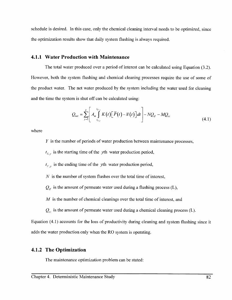
schedule is desired. In this case, only the chemical cleaning interval needs to be optimized, since
the optimization results show that daily system flushing is always required.
4.1.1 Water Production with Maintenance
The total water produced over a period of interest can be calculated using Equation (3.2).
However, both the system flushing and chemical cleaning processes require the use of some of
the product water. The net water produced by the system including the water used for cleaning
and the time the system is shut off can be calculated using:
Qnet = Am f K (t)[P(t)- rt)dt- NQf - MQ,,=1 (4.1)
where
Y is the number of periods of water production between maintenance processes,
(, is the starting time of the yth water production period,
tF,y is the ending time of the yth water production period,
N is the number of system flushes over the total time of interest,
Qf is the amount of permeate water used during a flushing process (L),
M is the number of chemical cleanings over the total time of interest, and
Q , is the amount of permeate water used during a chemical cleaning process (L).
Equation (4.1) accounts for the loss of productivity during cleaning and system flushing since it
adds the water production only when the RO system is operating.
4.1.2 The Optimization
The maintenance optimization problem can be stated:
Chapter 4. Deterministic Maintenance Study 82

Maximize QeN,M
subject to: Qd,,, QD, Equations (3.1),(3.3) --(3.8),(3.10),(3.12),(3.13) (4.2)
where
Qda, is the volume of permeate water produced in a day, and
QD is the daily volume of water needed by the community.
Figure 4.1 shows the structure of the optimization in block diagram form. A
meteorological model describing the solar radiation as a function of location and day of the year
is used to generate the daily clear-sky solar radiation.profile. The radiation profile and the water
chemistry are used to calculate water production and fouling over time using Equations (3.1),
(3.3) - (3.8), (3.10), (3.12) and (3.13), (the Fouling and Water Production Models in Figure 4.1),
along with a system dependent model that describes feed water pressure as a function of solar-
generated electrical power. These calculations are used by the maintenance optimizer to
determine the schedule which maximizes the total water production. In this study, the optimizer
performs exhaustive search by computing the total water production under every frequency and
selecting the maintenance frequency that results in the maximum water production.
SolarRadiation
Meteorological RoTime ti l Solar Radiation Fouling and Calculated
Model Water Production -- Production
Water Chemistry o Models and Fouling
Maintenance MaintenanceOptimizer Schedule
Figure 4.1: Maintenance optimization structure
Chapter 4. Deterministic Maintenance Study 83Chapter 4. Deterministic Maintenance Study 83
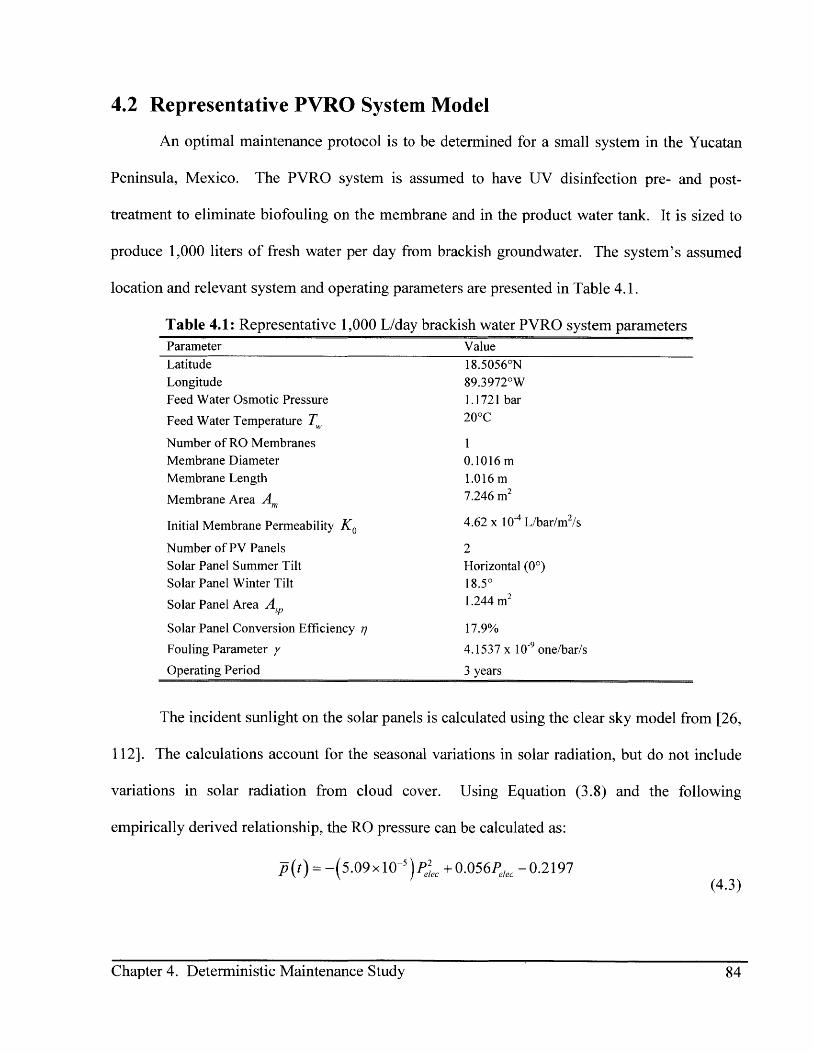
4.2 Representative PVRO System Model
An optimal maintenance protocol is to be determined for a small system in the Yucatan
Peninsula, Mexico. The PVRO system is assumed to have UV disinfection pre- and post-
treatment to eliminate biofouling on the membrane and in the product water tank. It is sized to
produce 1,000 liters of fresh water per day from brackish groundwater. The system's assumed
location and relevant system and operating parameters are presented in Table 4.1.
Table 4.1: Representative 1,000 L/day brackish water PVRO system parametersParameter Value
Latitude 18.50560 N
Longitude 89.3972"W
Feed Water Osmotic Pressure 1.1721 bar
Feed Water Temperature T. 200C
Number of RO Membranes IMembrane Diameter 0.1016 m
Membrane Length 1.016 m
Membrane Area Am 7.246 m 2
Initial Membrane Permeability Ko 4.62 x 10⁻⁴ L/bar/m 2/s
Number of PV Panels 2
Solar Panel Summer Tilt Horizontal (00)
Solar Panel Winter Tilt 18.50
Solar Panel Area AP 1.244 m2
Solar Panel Conversion Efficiency q 17.9%
Fouling Parameter y 4.1537 x 10⁻⁹ one/bar/s
Operating Period 3 years
The incident sunlight on the solar panels is calculated using the clear sky model from [26,
112]. The calculations account for the seasonal variations in solar radiation, but do not include
variations in solar radiation from cloud cover. Using Equation (3.8) and the following
empirically derived relationship, the RO pressure can be calculated as:
p (t)= (5.09 x10-P5)p +0.056P, -0.2197
Chapter 4. Deterministic Maintenance Study 84Chapter 4. Deterministic Maintenance Study 84

This empirical relationship was derived from operating data from a small-scale experimental
seawater PVRO system and scaled appropriately for a brackish water system [25].
Other assumptions are made for this example study. The solar panels are assumed to be
adjusted for the summer and winter seasons to increase the amount of solar energy collected.
The solar-to-electrical conversion efficiency is chosen based on the performance of a 215 Watt
solar panel manufactured by Suntech Power [113]. The feed water is assumed to be well water
at a constant temperature of 20'C and constant salinity, with an osmotic pressure of 1.17 bar.
The fouling rate is assumed constant, and is chosen such that if the PVRO system were operated
constantly at 80% power, its flow rate would decay exponentially with a time constant of
approximately 200 days. The community water demand is assumed constant at 1,000 L/day.
The storage of water is not accounted for. Here, it is assumed that there is a clean water storage
tank that holds the water needed for chemical cleaning and system flushing. The PVRO system
is also assumed to produce water for the entire duration of each day, and so it continues to
produce water after the daily demand is satisfied. In actual operation, one would likely turn the
system off once the water storage tank is full so as not to waste water.
The following maintenance processes are assumed. System flushing takes place for 3
minutes at a flow rate of 0.57 L/s. Chemical cleaning consists of an acid clean to remove the
calcium carbonate scale, followed by an alkaline cleaning. Table 4.2 lists the values of the
cleaning parameters. As in the constant pressure degradation example in Chapter 3, the increase
in permeability after system flushing is limited such that the post-system flush permeability is no
greater than the initial "clean membrane" permeability. The increase in membrane permeability
after chemical cleaning is limited to 97% of its original permeability to capture the effects of
Chapter 4. Deterministic Maintenance Study 85Chapter 4. Deterministic Maintenance Study 85
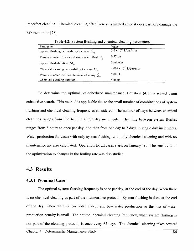
imperfect cleaning. Chemical cleaning effectiveness is limited since it does partially damage the
RO membrane [28].
Table 4.2: System flushing and chemical cleaning parametersParameter Value
System flushing permeability increase G 5.0 x 10 L/bar/m2/s
Permeate water flow rate during system flush qgf 0.57 L/s
System flush duration Ats 3 minutes
Chemical cleaning permeability increase Gc 4.009 x 10-' L/bar/m 2/s
Permeate water used for chemical cleaning Q, 5,000 L
Chemical cleaning duration 4 hours
To determine the optimal pre-scheduled maintenance, Equation (4.1) is solved using
exhaustive search. This method is applicable due to the small number of combinations of system
flushing and chemical cleaning frequencies considered. The number of days between chemical
cleanings ranges from 365 to 3 in single day increments. The time between system flushes
ranges from 3 hours to once per day, and then from one day to 7 days in single day increments.
Water production for cases with only system flushing, with only chemical cleaning and with no
maintenance are also calculated. Operation for all cases starts on January 1st. The sensitivity of
the optimization to changes in the fouling rate was also studied.
4.3 Results
4.3.1 Nominal Case
The optimal system flushing frequency is once per day, at the end of the day, when there
is no chemical cleaning as part of the maintenance protocol. System flushing is done at the end
of the day, when there is low solar energy and low water production so the loss of water
production penalty is small. The optimal chemical cleaning frequency, when system flushing is
not part of the cleaning protocol, is once every 62 days. The chemical cleaning takes several
Chapter 4. Deterministic Maintenance Study 86

hours and is assumed to be at the beginning of the day. The optimal combination of system
flushing and chemical cleanings is found to be daily system flushing with chemical cleaning
every 146 days.
The simulated daily average water production for the PVRO system for these four cases
is compared in Figure 4.2. The seasonal effects on daily water production are evident in all four
cases. Without maintenance, the daily water production declines more rapidly when the duration
of sunlight is shorter, during the winter. During the spring as the sunlight duration becomes
longer, the fouling rate is such that the daily water production remains nearly constant. In the
cases including maintenance, the daily water production increases as the sunlight duration
becomes longer, hits a local maximum during the summer, and decreases as the sunlight duration
becomes shorter.
1600Daily flushing, chemical
1400- cleaning every 146 days
1200
1000
800 -Daily flushing, no
600 .chemical cleaning
Expected demand400-
200- No maintenance
20
0 200 400 600 800 1000Operating time (days)
Figure 4.2: Daily water production under optimized maintenance, compared
with production under no maintenance and under daily flushing alone
Chapter 4. Deterministic Maintenance Study 87
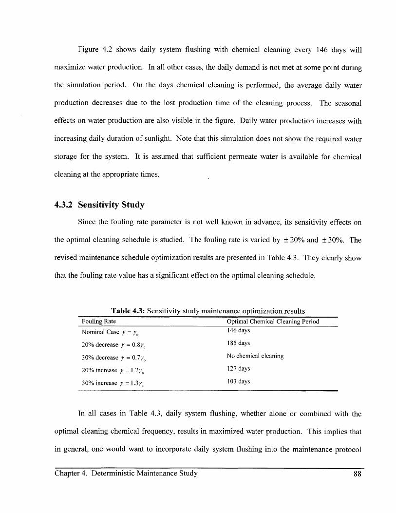
Figure 4.2 shows daily system flushing with chemical cleaning every 146 days will
maximize water production. In all other cases, the daily demand is not met at some point during
the simulation period. On the days chemical cleaning is performed, the average daily water
production decreases due to the lost production time of the cleaning process. The seasonal
effects on water production are also visible in the figure. Daily water production increases with
increasing daily duration of sunlight. Note that this simulation does not show the required water
storage for the system. It is assumed that sufficient permeate water is available for chemical
cleaning at the appropriate times.
4.3.2 Sensitivity Study
Since the fouling rate parameter is not well known in advance, its sensitivity effects on
the optimal cleaning schedule is studied. The fouling rate is varied by 20% and 30%. The
revised maintenance schedule optimization results are presented in Table 4.3. They clearly show
that the fouling rate value has a significant effect on the optimal cleaning schedule.
Table 4.3: Sensitivity study maintenance optimization resultsFouling Rate Optimal Chemical Cleaning Period
Nominal Case y = 146 days
20% decrease y = 0.8 v, 185 days
30% decrease y = 0.7v, No chemical cleaning
20% increase y = 1.27, 127 days
30% increase y = 1.3y 103 days
In all cases in Table 4.3, daily system flushing, whether alone or combined with the
optimal cleaning chemical frequency, results in maximized water production. This implies that
in general, one would want to incorporate daily system flushing into the maintenance protocol
Chapter 4. Deterministic Maintenance Study 88
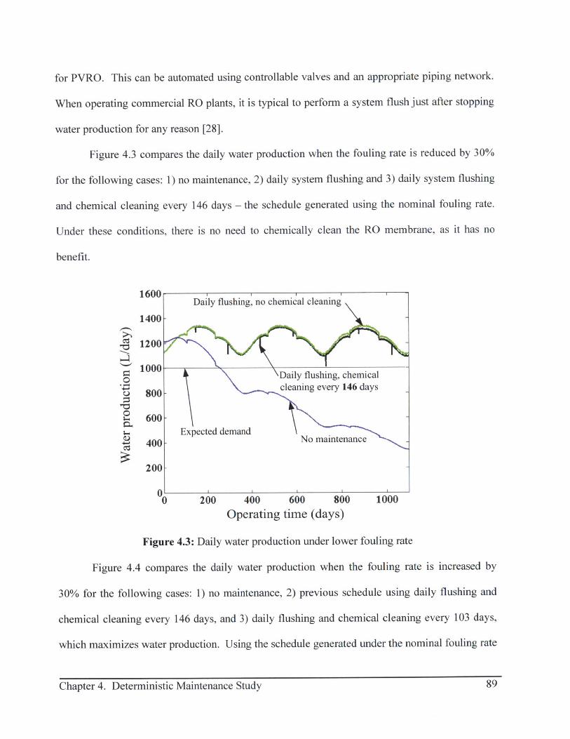
for PVRO. This can be automated using controllable valves and an appropriate piping network.
When operating commercial RO plants, it is typical to perform a system flush just after stopping
water production for any reason [28].
Figure 4.3 compares the daily water production when the fouling rate is reduced by 30%
for the following cases: 1) no maintenance, 2) daily system flushing and 3) daily system flushing
and chemical cleaning every 146 days - the schedule generated using the nominal fouling rate.
Under these conditions, there is no need to chemically clean the RO membrane, as it has no
benefit.
1600Daily flushing, no chemical cleaning
1400
1200
1000 \Daily flushing, chemical800 cleaning every 146 days
"06 600
Expected demand3 400 .No maintenance.
200-
0 200 400 600 800 1000Operating time (days)
Figure 4.3: Daily water production under lower fouling rate
Figure 4.4 compares the daily water production when the fouling rate is increased by
30% for the following cases: 1) no maintenance, 2) previous schedule using daily flushing and
chemical cleaning every 146 days, and 3) daily flushing and chemical cleaning every 103 days,
which maximizes water production. Using the schedule generated under the nominal fouling rate
89Chapter 4. Deterministic Maintenance Study
is clearly no longer optimal, since the system fails to meet the daily demand after about a year in
operation. This result demonstrates that a prognostic maintenance schedule needs to be based on
a reasonably accurate value of the fouling rate, and will need to adapt if the fouling rate changes
during the system's operation. Since the fouling rate will not be known in advance, it must be
identified from the PVRO system operation.
1600Daily flushing, chemical
1400- cleaning every 103 days
1200
10 20 40 000 10
800-Daily flushing, chemical
600O- cleaning every 146 days -Expected demand
(U 400 - -
200-No maintenance
"' 200 400 600 800 1000Operating time (days)
Figure 4.4: Daily water production under high fouling rate
4.4 Summary
A deterministic study demonstrates the use of the system models in an optimization that
finds the periodic maintenance schedule which meets the daily water demand. Results from this
optimization show that under the assumptions given, flushing the RO system daily is a
requirement for maximizing water production over the operating period. Generally, the fouling
rate will not be known before system operation starts, so it must be identified from PVRO
performance measurements over time. The optimization is sensitive to changes in the fouling
Chapter 4. Deterministic Maintenance Study 90

rate, particularly with respect to chemical cleaning, as expected, and so the maintenance
algorithm will need to be updated in response to such changes.
Chapter 4. Deterministic Maintenance Study 91Chapter 4. Deterministic Maintenance Study 91

Chapter 4. Deterministic Maintenance Study 92
CHAPTER
5
PARAMETER IDENTIFICATION AND FORECASTING
Process models often depend on parameters that cannot be calculated before operating a
system, and that change slowly over time. Such is the case with the fouling rate y in the RO
membrane fouling model presented in Chapter 3. The system operating history can be used to
identify these parameters to forecast future system performance. In this chapter, linear recursive
least squares estimation with forgetting [114] is used to identify the RO fouling rate from RO
plant performance data from the literature.
In addition to the identified unknown model parameters, forecasting requires estimates of
future system inputs, which may be both highly variable and uncertain. For example, the solar
radiation that powers a PVRO process varies both seasonally and with passing clouds.
Probabilistic descriptions of future input conditions can be generated from past data, such as
from past solar radiation and cloud histories. These descriptions are used to forecast the most
likely system performance. This chapter describes how the probabilistic descriptions of solar
radiation, including cloud cover, and of water demand are formed from available data. It also
describes how the forecasting algorithm combines the identified fouling rate and probabilistic
models to estimate future PVRO system performance.
Chapter 5: Parameter Identification and Forecasting 93Chapter 5: Parameter Identification and Forecasting 93
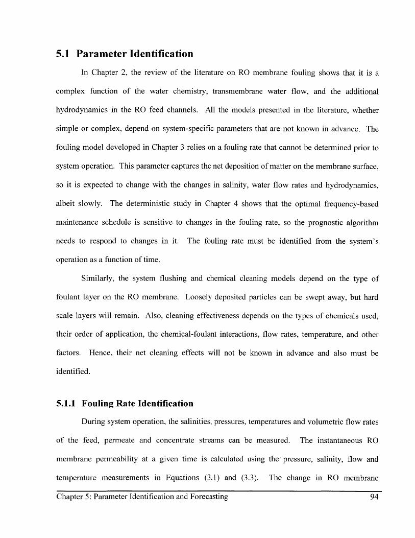
5.1 Parameter Identification
In Chapter 2, the review of the literature on RO membrane fouling shows that it is a
complex function of the water chemistry, transmembrane water flow, and the additional
hydrodynamics in the RO feed channels. All the models presented in the literature, whether
simple or complex, depend on system-specific parameters that are not known in advance. The
fouling model developed in Chapter 3 relies on a fouling rate that cannot be determined prior to
system operation. This parameter captures the net deposition of matter on the membrane surface,
so it is expected to change with the changes in salinity, water flow rates and hydrodynamics,
albeit slowly. The deterministic study in Chapter 4 shows that the optimal frequency-based
maintenance schedule is sensitive to changes in the fouling rate, so the prognostic algorithm
needs to respond to changes in it. The fouling rate must be identified from the system's
operation as a function of time.
Similarly, the system flushing and chemical cleaning models depend on the type of
foulant layer on the RO membrane. Loosely deposited particles can be swept away, but hard
scale layers will remain. Also, cleaning effectiveness depends on the types of chemicals used,
their order of application, the chemical-foulant interactions, flow rates, temperature, and other
factors. Hence, their net cleaning effects will not be known in advance and also must be
identified.
5.1.1 Fouling Rate Identification
During system operation, the salinities, pressures, temperatures and volumetric flow rates
of the feed, permeate and concentrate streams can be measured. The instantaneous RO
membrane permeability at a given time is calculated using the pressure, salinity, flow and
temperature measurements in Equations (3.1) and (3.3). The change in RO membrane
Chapter 5: Parameter Identification and Forecasting 94

permeability with time can be estimated using a difference equation, assuming measurements are
sampled at high frequency and properly calibrated. For PVRO degradation, sampling at 67
millihertz is reasonable, since RO membrane fouling occurs over several days, weeks or months.
In Equation (3.10), the fouling rate is linear with respect to the system measurements and
is in the form:
y =bu
(5.1)
dK(t )In Equation (3.10), the change in RO membrane permeability, , is output y , the fouling
dt
rate y is the unknown parameter b, and the product of the current membrane state and pressure,
-K (t)(p - Z) are the system measurements u. This structure permits the use of recursive
linear least-squares parameter estimation [114]. A forgetting factor, a , is incorporated so that
more weight is given to recent measurements and large initialization errors will be minimized.
The estimation algorithm is [114]:
R(t -1)u(t)b(t)= b(t -1)+ \2 Hy(o- b (t - 1) u(t))a + R (t -1)(u(t)) (5.2)
1 (R (t -1)u (t))2
a a + R (t -1)(u(t)) (5.3)
where R (t) is defined as:
R= Lu(tju(tt=1 (5.4)
Equation (5.3) permits the update of R without needing to store all measurements. When
initializing the recursive least squares algorithm, R0 is constrained to be positive definite.
The forgetting factor a is constrained such that
Chapter 5: Parameter Identification and Forecasting 95
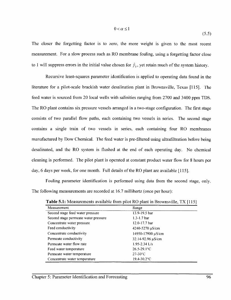
0<a 1(5.5)
The closer the forgetting factor is to zero, the more weight is given to the most recent
measurement. For a slow process such as RO membrane fouling, using a forgetting factor close
to 1 will suppress errors in the initial value chosen for 70, yet retain much of the system history.
Recursive least-squares parameter identification is applied to operating data found in the
literature for a pilot-scale brackish water desalination plant in Brownsville, Texas [115]. The
feed water is sourced from 20 local wells with salinities ranging from 2700 and 3400 ppm TDS.
The RO plant contains six pressure vessels arranged in a two-stage configuration. The first stage
consists of two parallel flow paths, each containing two vessels in series. The second stage
contains a single train of two vessels in series, each containing four RO membranes
manufactured by Dow Chemical. The feed water is pre-filtered using ultrafiltration before being
desalinated, and the RO system is flushed at the end of each operating day. No chemical
cleaning is performed. The pilot plant is operated at constant product water flow for 8 hours per
day, 6 days per week, for one month. Full details of the RO plant are available [115].
Fouling parameter identification is performed using data from the second stage, only.
The following measurements are recorded at 16.7 millihertz (once per hour):
Table 5.1: Measurements available from pilot RO plant in Brownsville, TX [115]Measurement RangeSecond stage feed water pressure 13.9-19.5 barSecond stage permeate water pressure 1.3-1.7 barConcentrate water pressure 12.0-17.7 barFeed conductivity 4240-5270 pS/cmConcentrate conductivity 14950-17900 pS/cmPermeate conductivity 32.14-92.96 pS/cmPermeate water flow rate 1.95-2.34 L/sFeed water temperature 26.5-29.1 CPermeate water temperature 27-300CConcentrate water temperature 19.4-30.20 C
Chapter 5: Parameter Identification and Forecasting 96

The temperature measurements and the temperature correlation table from Dow Chemical
are used to normalize the permeate flow data [105]. The RO membrane permeability is
calculated using the normalized permeate flow, salinity and pressure in Equations (3.1) and (3.3)
- (3.5). The change in RO membrane permeability is approximated using a difference equation.
Recursive least squares with a forgetting factor of 0.998 is applied to the data for the first 110
measurements. Here, a fouling rate of 4.6382 x 10~8 (one/bar/s) is identified. The identified
fouling rate is used to calculate an estimate of the membrane permeability and a prediction of the
RO membrane permeability over the next 70 operating hours. Figure 5.1 shows that the
predicted permeability captures the overall decline in permeability occurring during the
prediction period. Although the membrane permeability derived from the measurements is not
reproduced, possibly due to measurement noise, the identified fouling rate is acceptable for
estimating the longer-term fouling behavior. Error between measured and predicted permeability
is within 6%.
7 X 10⁻⁴ ,,,6Measured 4-
6.5 permeability + + *
+ +
6 Identification - +* .
stopped Predicted U. + + .5. permeability + + . +
0, -2- +* + * +
++ ++
Identified - ++ .
4.5 permeability +
40L 10 16 80 50 100 150 200 -POO 120 140 160 180
Operating time (hours) Operating time (hours)
Figure 5.1: Measured, identified and predicted RO membrane permeability (left) and % error in
predicted permeability (right) from the brackish water RO pilot plant in Brownsville, TX [115]
The identified fouling rate parameter, pressure, temperature and salinity measurements
are used in Equations (3.1), (3.3) - (3.5), and (3.10) to calculate RO clean water flow rate during
97Chapter 5: Parameter Identification and Forecasting
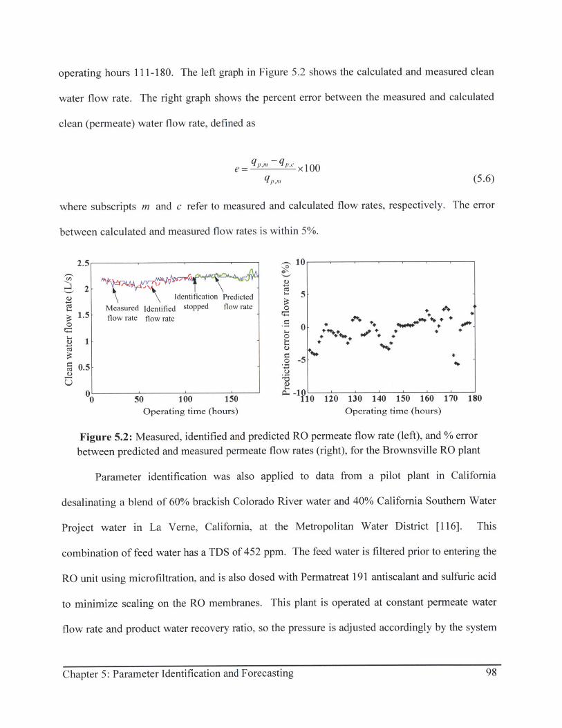
operating hours 111-180. The left graph in Figure 5.2 shows the calculated and measured clean
water flow rate. The right graph shows the percent error between the measured and calculated
clean (permeate) water flow rate, defined as
e = q''"' -' qx100q,,?, (5.6)
where subscripts m and c refer to measured and calculated flow rates, respectively. The error
between calculated and measured flow rates is within 5%.
2.5 10
Identification Predicted 5
Measured Identified stopped flow rate
1.5 flow rate flow rate A
o-50.5
00 50 100 150 10 120 130 140 150 160 170 180
Operating time (hours) Operating time (hours)
Figure 5.2: Measured, identified and predicted RO permeate flow rate (left), and % error
between predicted and measured permeate flow rates (right), for the Brownsville RO plant
Parameter identification was also applied to data from a pilot plant in California
desalinating a blend of 60% brackish Colorado River water and 40% California Southern Water
Project water in La Verne, California, at the Metropolitan Water District [116]. This
combination of feed water has a TDS of 452 ppm. The feed water is filtered prior to entering the
RO unit using microfiltration, and is also dosed with Permatreat 191 antiscalant and sulfuric acid
to minimize scaling on the RO membranes. This plant is operated at constant permeate water
flow rate and product water recovery ratio, so the pressure is adjusted accordingly by the system
98Chapter 5: Parameter Identification and Forecasting
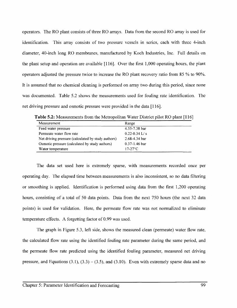
operators. The RO plant consists of three RO arrays. Data from the second RO array is used for
identification. This array consists of two pressure vessels in series, each with three 4-inch
diameter, 40-inch long RO membranes, manufactured by Koch Industries, Inc. Full details on
the plant setup and operation are available [116]. Over the first 1,000 operating hours, the plant
operators adjusted the pressure twice to increase the RO plant recovery ratio from 85 % to 90%.
It is assumed that no chemical cleaning is performed on array two during this period, since none
was documented. Table 5.2 shows the measurements used for fouling rate identification. The
net driving pressure and osmotic pressure were provided in the data [116].
Table 5.2: Measurements from the Metropolitan Water District pilot RO plant [116]Measurement RangeFeed water pressure 4.55-7.38 barPermeate water flow rate 0.22-0.34 L/ sNet driving pressure (calculated by study authors) 2.68-4.34 barOsmotic pressure (calculated by study authors) 0.37-1.46 barWater temperature 17-270 C
The data set used here is extremely sparse, with measurements recorded once per
operating day. The elapsed time between measurements is also inconsistent, so no data filtering
or smoothing is applied. Identification is performed using data from the first 1,200 operating
hours, consisting of a total of 50 data points. Data from the next 750 hours (the next 32 data
points) is used for validation. Here, the permeate flow rate was not normalized to eliminate
temperature effects. A forgetting factor of 0.99 was used.
The graph in Figure 5.3, left side, shows the measured clean (permeate) water flow rate,
the calculated flow rate using the identified fouling rate parameter during the same period, and
the permeate flow rate predicted using the identified fouling parameter, measured net driving
pressure, and Equations (3.1), (3.3) - (3.5), and (3.10). Even with extremely sparse data and no
Chapter 5: Parameter Identification and Forecasting 99Chapter 5: Parameter Identification and Forecasting 99

temperature normalization, the predicted clean water flow rate is within 5% of the measured
clean water flow rate.
N10
Measured 10
0.3. flow ratePredicted 5- +
[2 0.25 Identification flow rate , + *stopped + * +
0 0.2-~
2 0.15 Identified *flow rate
0.1 -5 -
0.05UU
0 500 1000 1500 2001 ~0 00 1400 1600 1800 2000
Operating time (hours) Operating time (hours)
Figure 5.3: Measured and predicted RO permeate flow rate (left), and % error between predicted
and measured permeate flow rates after identification (right), for La Verne, CA, RO plant [116]
The experimental results of applying the recursive least squares parameter identification
algorithm to RO pilot plant operating data imply that it is sufficient for estimating an RO
membrane fouling rate that captures the long-term decline in RO membrane permeability.
5.1.2 Cleaning Effectiveness
The simulations from Chapters 3 and 4 imply that the long-term effect of daily system
flushing is a reduced net fouling rate. The penalties in terms of lost water production time and
lost permeate water are low. If desired, the effectiveness of a single flushing process can be
directly calculated from the difference in membrane permeability before and after a flushing:
G,.= KA - K,(5.7)
where K,4 is the membrane permeability computed from the pressure and flow measurements
immediately after the flushing process, and K, is the membrane permeability just before
Chapter 5: Parameter Identification and Forecasting 100
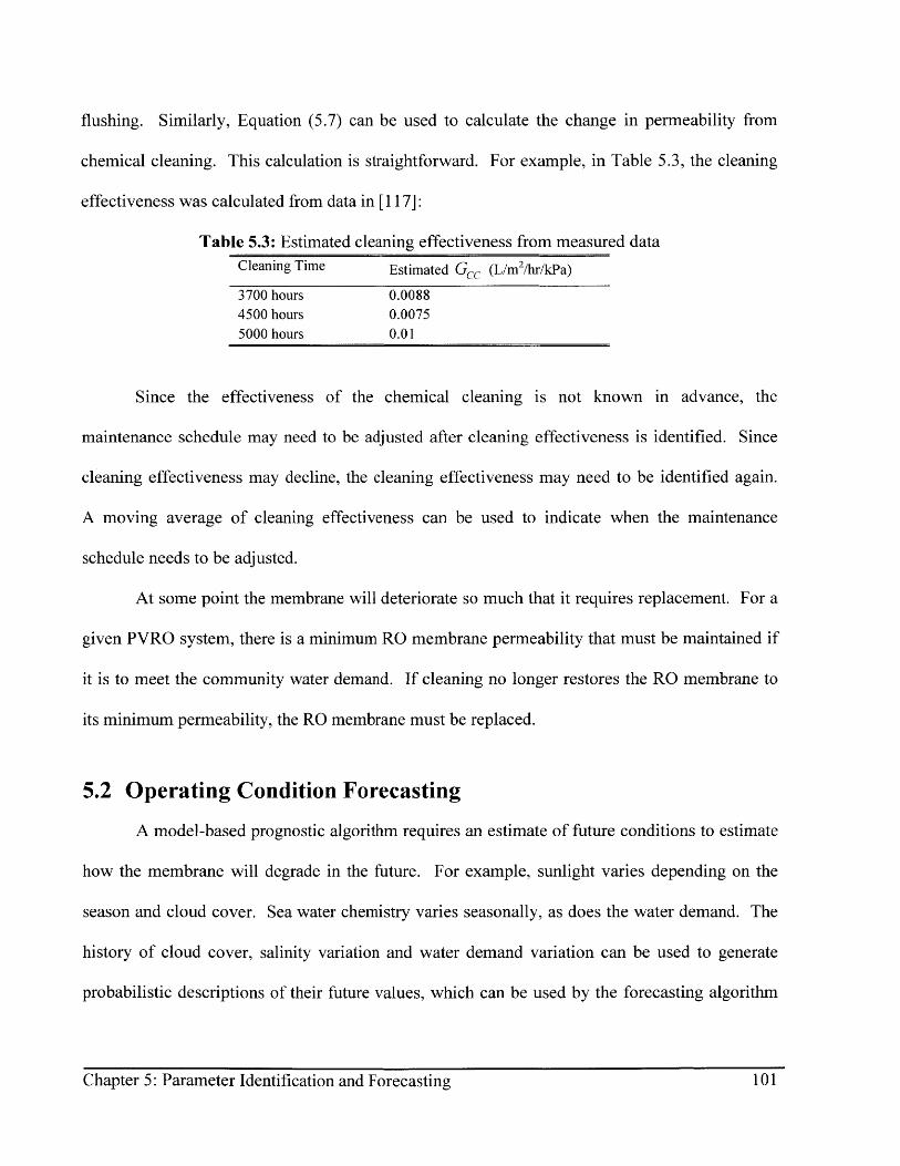
flushing. Similarly, Equation (5.7) can be used to calculate the change in permeability from
chemical cleaning. This calculation is straightforward. For example, in Table 5.3, the cleaning
effectiveness was calculated from data in [117]:
Table 5.3: Estimated cleaning effectiveness from measured dataCleaning Time Estimated GCC (L/m2 /hr/kPa)
3700 hours 0.00884500 hours 0.00755000 hours 0.01
Since the effectiveness of the chemical cleaning is not known in advance, the
maintenance schedule may need to be adjusted after cleaning effectiveness is identified. Since
cleaning effectiveness may decline, the cleaning effectiveness may need to be identified again.
A moving average of cleaning effectiveness can be used to indicate when the maintenance
schedule needs to be adjusted.
At some point the membrane will deteriorate so much that it requires replacement. For a
given PVRO system, there is a minimum RO membrane permeability that must be maintained if
it is to meet the community water demand. If cleaning no longer restores the RO membrane to
its minimum permeability, the RO membrane must be replaced.
5.2 Operating Condition Forecasting
A model-based prognostic algorithm requires an estimate of future conditions to estimate
how the membrane will degrade in the future. For example, sunlight varies depending on the
season and cloud cover. Sea water chemistry varies seasonally, as does the water demand. The
history of cloud cover, salinity variation and water demand variation can be used to generate
probabilistic descriptions of their future values, which can be used by the forecasting algorithm
Chapter 5: Parameter Identification and Forecasting 101Chapter 5: Parameter Identification and Forecasting 101

to generate the most likely forecast of future performance. Maintenance optimization is
performed using this forecast.
5.2.1 Solar Radiation Predictions
As discussed in Chapter 3, analytical models exist in the literature for calculating solar
radiation for a given time of day and day of the year for a given location, assuming clear skies
[112]. However, cloud cover statistics will greatly affect the solar radiation, so cloud cover
variation needs to be incorporated into solar radiation prediction.
Cloud cover frequency data for many locations is available from NASA [118].
Frequency data is categorized by percent cloudiness into three groups: 1) clear skies (0-10%
cloud cover), 2) broken-cloud skies (10-70% cloud cover) and 3) near-overcast skies (70-100%
cloud cover), for 3-hour intervals within a day. Using this data, a conditional probability
function dependent on the month of the year can be created:
x1,X <10%
P (X Month) x2, 10% X <70%
x3 X 70% (5.8)
where X is the percentage of cloud cover and
X + X2 + x3 =1(5.9)
For example, Table 5.4 presents the conditional probability of cloudiness given the month of the
year for La Mancalona, Mexico, created using cloud cover frequency data from NASA [118].
The rainy season in La Mancalona ranges from May through October [119]. As expected, the
probability of overcast skies is higher during these months.
Chapter 5: Parameter Identification and Forecasting 102Chapter 5: Parameter Identification and Forecasting 102

Table 5.4: Cloud cover conditional probabilities for La Mancalona, MexicoJan Feb Mar Apr May Jun Jul Aug Sept Oct Nov Dec
Clear 0.172 0.203 0.244 0.222 0.127 0.068 0.073 0.063 0.060 0.106 0.163 0.186Partly Cloudy 0.354 0.368 0.313 0.307 0.338 0.341 0.415 0.423 0.410 0.400 0.419 0.358Overcast 0.473 0.428 0.442 0.470 0.534 0.590 0.511 0.513 0.529 0.494 0.417 0.454
The probability functions are combined with the clear sky solar radiation model in the
forecasting algorithm as follows. For a given day, the clear sky solar radiation is calculated.
Calculations are then separated into three paths: clear day, partially cloudy day, and overcast
day. The solar radiation profile is scaled for the partially cloudy and overcast conditions using
the following empirical relation [120]:
I= I, (I -0.75f 3 4 ) (5.10)
where Ic is the clear sky solar radiation and f is the fraction of the sky covered by clouds.
Note that in Equation (5.10), approximately 25% of the total radiation is assumed to reach the
earth's surface. The scaling factor in Equation (5.10) is plotted in Figure 5.4.
0
1.2
1
0.8
0.6
0.4
0.2
-0 0.2 0.4 0.6 0.8
Cloud Cover Fractionf
I
Figure 5.4: Solar radiation scale factor as a function of cloud fraction
Chapter 5: Parameter Identification and Forecasting 103Chapter 5: Parameter Identification and Forecasting 103

Once the solar radiation profile is scaled, Equations (3.1) - (3.8) and (3.10), a system-
specific model relating electrical power to feed water pressure and the identified fouling rate
parameter are used to calculate the water production and RO membrane fouling over the given
day for clear, partly cloudy, and overcast conditions. The total law of probability is then applied
to produce an estimate of the water production and state of the RO membrane for that day [121].
For example, the estimate of daily water production is:
QMLE Q' 1X 1 +PCx2 + Q0x3(5.11)
where the subscripts MLE, Cl, PC and 0 refer to the maximum likelihood estimate, clear
skies, partly cloudy skies, and overcast skies, respectively, and where x,, x 2 and x3 correspond
to the probabilities that the sky is clear, partly cloudy and overcast, respectively. The forecasting
process can be repeated for as many days as needed. Figure 5.5 depicts the integration of the
solar radiation statistics into the forecasting.
Identified FoulingParameter
SolarRadiation Clear
Time Meteorological Profile Conditional Partial Clouds Fouling and Total Law of Estimated Water
Model Probability Mass P Water Production Probability 0 Production,Function Overcast Model (Averaging) Fouling
Cloud FrequencyStatistics
Figure 5.5: Forecasting water production and RO membrane degradation using cloud statistics
5.2.2 Water Salinity Variations
When desalinating brackish well water, the salinity is expected to remain fairly constant.
There may be short-term changes due to rain runoff, but these effects are short-lived. However,
seawater salinity is known to vary seasonally. For example, in the Mediterranean Sea near
Limassol, Cyprus, the average salinity at the water surface varies over the year between 38,540
Chapter 5: Parameter Identification and Forecasting 104
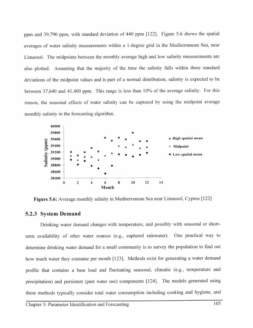
ppm and 39,790 ppm, with standard deviation of 440 ppm [122]. Figure 5.6 shows the spatial
averages of water salinity measurements within a 1-degree grid in the Mediterranean Sea, near
Limassol. The midpoints between the monthly average high and low salinity measurements are
also plotted. Assuming that the majority of the time the salinity falls within three standard
deviations of the midpoint values and is part of a normal distribution, salinity is expected to be
between 37,640 and 41,400 ppm. This range is less than 10% of the average salinity. For this
reason, the seasonal effects of water salinity can be captured by using the midpoint average
monthly salinity in the forecasting algorithm.
40000 -
39800 -
39600 - m High spatial mean
39400 AA Midpoint
A39200 - A * Low spatial mean39000 - A A
38800 -
38600 -
384000 2 4 6 8 10 12 14
Month
Figure 5.6: Average monthly salinity in Mediterranean Sea near Limassol, Cyprus [122]
5.2.3 System Demand
Drinking water demand changes with temperature, and possibly with seasonal or short-
term availability of other water sources (e.g., captured rainwater). One practical way to
determine drinking water demand for a small community is to survey the population to find out
how much water they consume per month [123]. Methods exist for generating a water demand
profile that contains a base load and fluctuating seasonal, climatic (e.g., temperature and
precipitation) and persistent (past water use) components [124]. The models generated using
these methods typically consider total water consumption including cooking and hygiene, and
105Chapter 5: Parameter Identification and Forecasting

not just drinking water requirements. Health guidelines stress the importance of increasing
drinking water intake with rising temperatures and physical exertion, so there likely are seasonal,
climatic and persistent components to drinking water consumption.
The water demand variability can be incorporated into the forecasting algorithm. It is
assumed that the total water demand D,,, (t) has the following structure:
(5.12)
where
D,,, is the baseline drinking water demand,
Dc (t) is the daily climactic-dependent component of drinking water demand and
Ds (t) is the seasonal-dependent component of drinking water demand.
The baseline drinking water demand can be determined from the number of people in the
community and the recommended daily water intake for people at rest [125]. The seasonal
component of drinking water demand can be determined from the monthly average daytime
temperatures and relative increase in water loss through perspiration associated with increasing
temperature [125]. Daily temperature will be affected by cloud cover, precipitation, etc. To
capture the associated variation in water consumption based on climatic fluctuations, this
component of the water demand can be described as a function of cloud cover. This term
becomes probabilistic. The amount of water stored in the tank at the end of the day is then
computed using the total law of probability:
QTank,MLE C(Q -D- ) x, +(Qc - D, )2 +(Q0 - Dt, ) X3 (
Chapter 5: Parameter Identification and Forecasting 106Chapter 5: Parameter Identification and Forecasting 106

where the notation tot Cl, tot PC and tot 0 refers to the total given that the sky is clear, partly
cloudy, and overcast, respectively.
5.3 PVRO Maintenance Forecasting Algorithm
The PVRO maintenance forecasting algorithm combines the recursive linear least squares
parameter estimation algorithm with the probabilistic models of cloud cover, salinity and water
demand to generate the most likely estimate of daily water production, change in RO membrane
permeability due to fouling over time, and volume of water stored in a finite tank. The volume
of this tank depends on the particular PVRO system size, the nominal volume of water needed
daily by the community, and the volume of water needed to complete a chemical cleaning cycle.
The maintenance optimizer uses Equations (4.1) and (4.2) to determine the frequency of
chemical cleanings that will 1) ensure system demand is always met and 2) will produce the
necessary water at the lowest cost. This means that the optimizer includes information on the
cost of cleaning chemicals and labor, as well as the permeate water use penalties.
The structure of the prognostic maintenance algorithm is shown in Figure 5.7. Since
chemical cleaning and system flushing affect RO membrane permeability and clean water
production, the predictor must incorporate cleaning and flushing into its computations. The
optimization process consists of an exhaustive search in which water production and RO
membrane permeability are calculated under different cleaning frequencies. The chemical
cleaning frequency that results in the lowest loss of demanded water over the forecasting period
(if any) and the least expensive cleaning costs is selected as the maintenance schedule.
Chapter 5: Parameter Identification and Forecasting 107107Chapter 5: Parameter Identification and Forecasting

Expected salinity
Expected solar power
SystemModels
Time t._
IdentificationAlgorithm
PVRO measurements(from PVRO system)
State of the RO membrane
_Water Salinity Expected salinity
Statistics Foulig andSolar Water
Sarto Production
Meteorological profile i Cnouin Epce rdco
solar power
Maintenance
Cloud Frequency FptionStatistics______
---- --- --- ---- --- --- --- ---- --- --- --- M a in ten a n ce
Operation Condition Forecasting Prediction
Expected productionand fouling
Maintenance Schedule(to PVRO system)
Prognostic Scheduler
Figure 5.7: Prognostic maintenance scheduler structure
If the fouling rate estimate and the chemical cleaning effectiveness experience very small
perturbations, then cleaning schedule only needs to be optimized once. However, if conditions
change, the deterministic optimization study results in Chapter 4 suggest that the maintenance
schedule should be adjusted accordingly. Therefore, after each chemical cleaning, the change in
cleaning effectiveness is calculated and compared with previous results, and the fouling rate
identification is restarted. If the newly identified fouling rate differs from the previously
identified fouling rate, then the maintenance optimization should be performed again using the
newly identified fouling rate. Similarly, if cleaning effectiveness decreases, the latest identified
effectiveness should be used during predictions. Chapter 6 demonstrates the use of the
prognostic maintenance algorithm as applied to a PVRO system.
Chapter 5: Parameter Identification and Forecasting 108Chapter 5: Parameter Identification and Forecasting 108

CHAPTER
6PROGNOSTIC MAINTENANCE CASE STUDIES
In this chapter, the prognostic maintenance algorithm is applied to community-sized
PVRO systems operated by non-experts, subject to variable and uncertain operating conditions,
in simulation.
6.1 Prognostic Maintenance Framework Applied to PVRO Systems
The system models, constrained maintenance optimization, parameter identification,
statistical input models and forecasting algorithm, presented in Chapters 3-5, are combined to
determine the maintenance schedule that permits a system to achieve its desired productivity at
lowest cost. Figure 6.1 illustrates how they are combined in block-diagram form to control
PVRO maintenance. The physics-based models of RO water production, degradation and
cleaning combine the fouling rate and cleaning effectiveness estimates from the parameter
identification algorithm with the expected solar radiation and water chemistry to determine the
state of the RO membrane and its degradation. The degradation predictions are used to
determine the maintenance schedule, so the community members know when to perform
maintenance. Changes in the fouling rate and cleaning effectiveness are detected by the
identification algorithm, passed through to the system models, and are used to adjust the
maintenance schedule accordingly. Note that the community operators are assumed to be
Chapter 6. Prognostic Maintenance Case Studies 109Chapter 6. Prognostic Maintenance Case Studies 109

"perfect actuators" that perform maintenance when scheduled. The impact of imperfect
maintenance is left for future work.
Shown in Detail in Figure 5.7
Expected solar radiation and water chemistry iSunlight
Water chemistry Disturbances
System RO membrane stateModels
Time Prognostic I Uncertain Water production,Scheduler I Maintenance --NoVRO Plant 1i 1 pressure, etc.
Identification ontrollerAlgorithm I - - - - - -
Measurements
Figure 6.1: Prognostic maintenance applied to a PVRO system
6.2 Problem Description
The chemical cleaning schedule for a PVRO system that ensures community water
demand is met at the lowest cost is to be determined. The PVRO system operates variably, as a
function of incident solar radiation, salinity, water demand, and water storage. It has no large
battery banks for energy storage, hence the feed water pressure, water flow rates and fouling all
vary with incident solar radiation. Maintenance processes include system flushing and chemical
cleaning. In these studies, system flushing occurs automatically at the end of an operating day.
This assumption is based both on the simulations in Chapter 4 in which daily system flushing
maximized production across all deterministic cases, and on typical intermittent operation of RO
plants [28]. The community members are assumed to have been trained to perform the chemical
cleaning.
6.2.1 Brackish Water System
The PVRO system used in this set of examples is assumed to produce 1,000 liters of
clean water per day from brackish well water, using solar power. It has a single 2.5-inch
Chapter 6. Prognostic Maintenance Case Studies 110
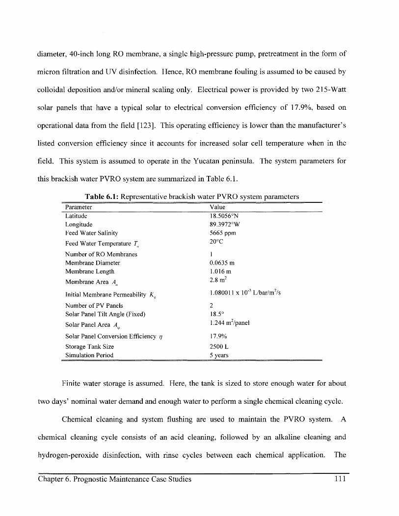
diameter, 40-inch long RO membrane, a single high-pressure pump, pretreatment in the form of
micron filtration and UV disinfection. Hence, RO membrane fouling is assumed to be caused by
colloidal deposition and/or mineral scaling only. Electrical power is provided by two 215-Watt
solar panels that have a typical solar to electrical conversion efficiency of 17.9%, based on
operational data from the field [123]. This operating efficiency is lower than the manufacturer's
listed conversion efficiency since it accounts for increased solar cell temperature when in the
field. This system is assumed to operate in the Yucatan peninsula. The system parameters for
this brackish water PVRO system are summarized in Table 6.1.
Table 6.1: Representative brackish water PVRO system parametersParameter Value
Latitude 18.50560 N
Longitude 89.39720 W
Feed Water Salinity 5665 ppm
Feed Water Temperature T 200 C
Number of RO Membranes 1
Membrane Diameter 0.0635 m
Membrane Length 1.016 m
Membrane Area A, 2.8 m2
Initial Membrane Permeability K 1.080011 x 10- L/bar/m 2/s
Number of PV Panels 2
Solar Panel Tilt Angle (Fixed) 18.50
Solar Panel Area A 1.244 m 2/panelSP
Solar Panel Conversion Efficiency q 17.9%
Storage Tank Size 2500 L
Simulation Period 5 years
Finite water storage is assumed. Here, the tank is sized to store enough water for about
two days' nominal water demand and enough water to perform a single chemical cleaning cycle.
Chemical cleaning and system flushing are used to maintain the PVRO system. A
chemical cleaning cycle consists of an acid cleaning, followed by an alkaline cleaning and
hydrogen-peroxide disinfection, with rinse cycles between each chemical application. The
Chapter 6. Prognostic Maintenance Case Studies III

amounts of chemicals and permeate water needed for a single cleaning cycle are listed in Table
6.2, and are based on manufacturers' cleaning process guidelines [29, 126-128].
Table 6.2: Chemical and water requirements for a single chemical cleaningChemical Amount Permeate for Solution Permeate for Rinse Total Permeate
Acidic Cleaner 0.95 lbs 20 L 150 L 170 LAlkaline Cleaner 0.95 lbs 20 L 150 L 170 LDisinfectant 7.5 L 292.5 L 150 L 442.5 L
The prices of the RO membrane and the chemicals needed per cleaning are listed in Table
6.3, and are based on retail prices available online [129, 130]. The exchange rate for Mexican
pesos (MEX) used here is 13 pesos to 1 USD. A chemical cleaning cycle is assumed to require 4
hours. System operators perform the chemical cleaning at a labor cost of 30 MEX per hour,
based on typical wages for rural Mexico [131].
Table 6.3: RO membrane and chemical costsComponent USD MEX
RO Membrane $197.00 2,561.00Acidic Chemicals/Cleaning $3.79 49.26Alkaline Chemicals/Cleaning $4.74 61.58Disinfectant/Cleaning $14.86 193.18
System flushing is assumed to automatically occur at the end of each operating day and
uses 45 L of permeate water (less than 5% of the nominal production). It does not require
operator labor or chemicals. Table 6.4 lists the increases in RO membrane permeability due to
maintenance processes, permeate water requirements, maintenance duration and costs. The cost
of replacing the RO membrane is six times the cost of a single chemical cleaning, including
labor. No maintenance process can restore the RO membrane to its pre-fouled permeability.
The increase in RO membrane water permeability from flushing is also limited to 99.9% of its
previously-flushed permeability. The RO membrane water permeability increase from chemical
cleaning is also limited to 97% of its pre-cleaned permeability. Thus, the permeability increases
Chapter 6. Prognostic Maintenance Case Studies 112
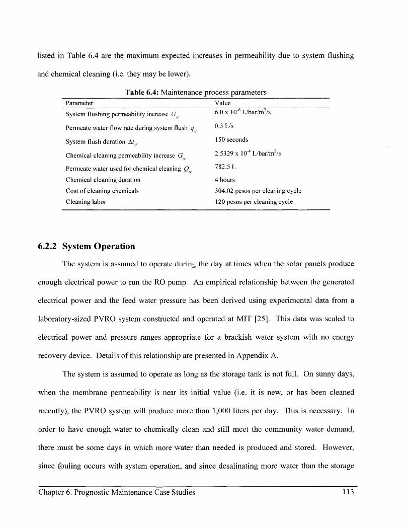
listed in Table 6.4 are the maximum expected increases in permeability due to system flushing
and chemical cleaning (i.e. they may be lower).
Table 6.4: Maintenance process parametersParameter Value
System flushing permeability increase Gf 6.0 x 10⁻⁶ LUar/m 2/s
Permeate water flow rate during system flush q, 0.3 L/s
System flush duration Ats 150 seconds
Chemical cleaning permeability increase G, 2.5329 x 10⁻⁴ L/bar/m 2/s
Permeate water used for chemical cleaning Q 782.5 L
Chemical cleaning duration 4 hours
Cost of cleaning chemicals 304.02 pesos per cleaning cycle
Cleaning labor 120 pesos per cleaning cycle
6.2.2 System Operation
The system is assumed to operate during the day at times when the solar panels produce
enough electrical power to run the RO pump. An empirical relationship between the generated
electrical power and the feed water pressure has been derived using experimental data from a
laboratory-sized PVRO system constructed and operated at MIT [25]. This data was scaled to
electrical power and pressure ranges appropriate for a brackish water system with no energy
recovery device. Details of this relationship are presented in Appendix A.
The system is assumed to operate as long as the storage tank is not full. On sunny days,
when the membrane permeability is near its initial value (i.e. it is new, or has been cleaned
recently), the PVRO system will produce more than 1,000 liters per day. This is necessary. In
order to have enough water to chemically clean and still meet the community water demand,
there must be some days in which more water than needed is produced and stored. However,
since fouling occurs with system operation, and since desalinating more water than the storage
Chapter 6. Prognostic Maintenance Case Studies 113
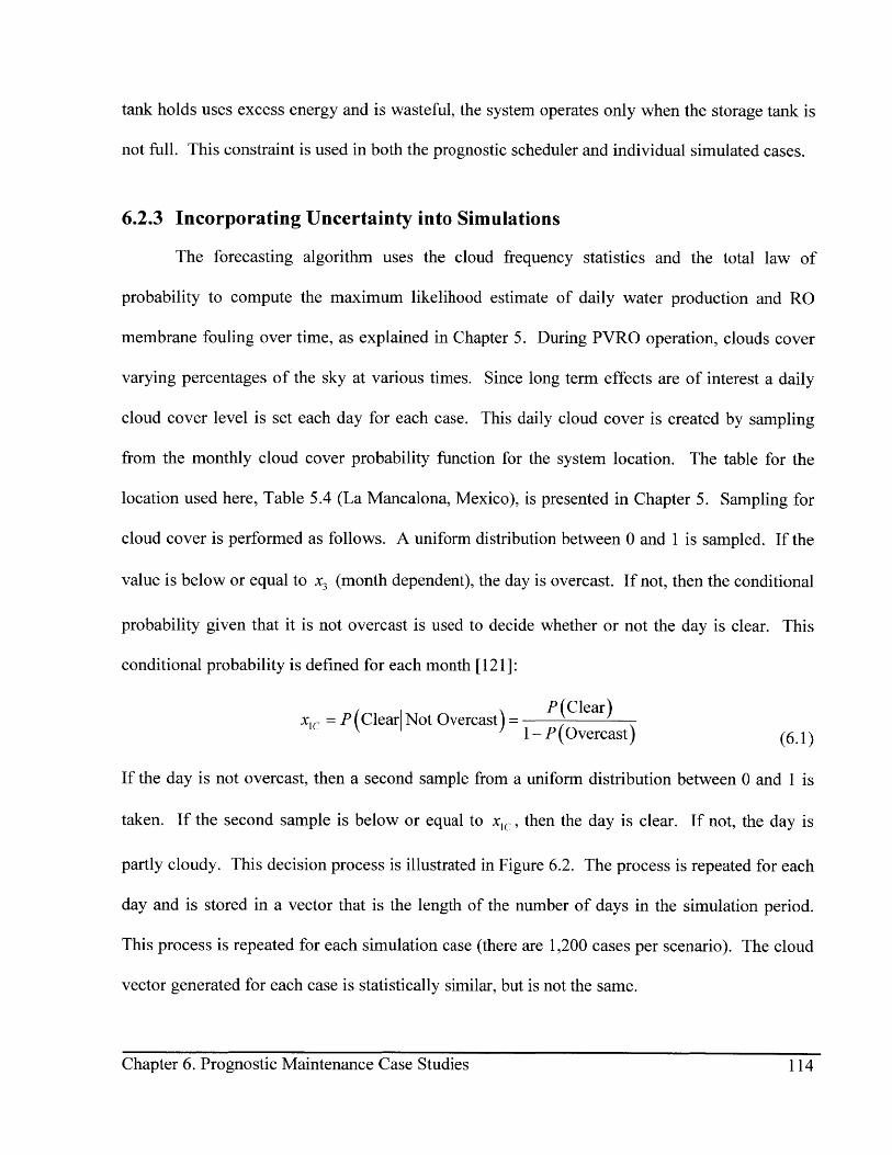
tank holds uses excess energy and is wasteful, the system operates only when the storage tank is
not full. This constraint is used in both the prognostic scheduler and individual simulated cases.
6.2.3 Incorporating Uncertainty into Simulations
The forecasting algorithm uses the cloud frequency statistics and the total law of
probability to compute the maximum likelihood estimate of daily water production and RO
membrane fouling over time, as explained in Chapter 5. During PVRO operation, clouds cover
varying percentages of the sky at various times. Since long term effects are of interest a daily
cloud cover level is set each day for each case. This daily cloud cover is created by sampling
from the monthly cloud cover probability function for the system location. The table for the
location used here, Table 5.4 (La Mancalona, Mexico), is presented in Chapter 5. Sampling for
cloud cover is performed as follows. A uniform distribution between 0 and 1 is sampled. If the
value is below or equal to x3 (month dependent), the day is overcast. If not, then the conditional
probability given that it is not overcast is used to decide whether or not the day is clear. This
conditional probability is defined for each month [121]:
xic = P (ClearNot Overcast)= P(Clear)(- P (Overcast) (6.1)
If the day is not overcast, then a second sample from a uniform distribution between 0 and 1 is
taken. If the second sample is below or equal to x(., then the day is clear. If not, the day is
partly cloudy. This decision process is illustrated in Figure 6.2. The process is repeated for each
day and is stored in a vector that is the length of the number of days in the simulation period.
This process is repeated for each simulation case (there are 1,200 cases per scenario). The cloud
vector generated for each case is statistically similar, but is not the same.
Chapter 6. Prognostic Maintenance Case Studies 114Chapter 6. Prognostic Maintenance Case Studies 114

X>. YesStart - Sample I x Overcast
No
YesSample 2 V2 xc > x >-> Clear
No4
Partly Cloudy
Figure 6.2: Daily cloud level assignment process
Once the level of cloudiness is assigned, the daily solar radiation profile is scaled using
Equation (5.10). For simplicity, cloudy day solar radiation is scaled assuming the sky is 85%
covered, and partly cloudy day solar radiation is scaled assuming the sky is 50% covered. These
cloud cover percentages result in scaling factors of 0.4785 and 0.929, respectively.
6.2.4 Limits on Chemical Cleaning Frequencies
Although the cost of one chemical cleaning is a sixth of the cost of replacing the RO
membrane, the RO membrane cannot be completely restored to its pre-fouled permeability. As
assumed here, each cleaning is capable of restoring the RO membrane permeability to at most
97% of its previously clean value. As the number of cleanings increases, the "clean"
permeability declines and eventually the RO membrane will not be permeable enough to meet
the daily demand on a clear day. Table 6.5 lists the upper limits on RO membrane permeability
after each cleaning cycle. Under the assumptions made here, the RO membrane cannot meet the
demand on a clear day after it is cleaned 9 times and should be replaced before the 9th cleaning.
The maintenance optimization in this example is constrained to solutions using fewer than 9
cleaning cycles before RO membrane replacement.
Chapter 6. Prognostic Maintenance Case Studies 115Chapter 6. Prognostic Maintenance Case Studies 115

Table 6.5: Upper limits on RO membrane permeability restorationCleaning Instance Restored Permeability (L/m 2/bar/s)
New RO Membrane 1.080011 x 10-'1 1.04761 x 10⁻³² 1.01618 x 10⁻³
3 9.857 x 10-44 9.5613 x 10⁻⁴
5 9.2744 x 10⁻⁴
6 8.9962x 10⁻⁴
7 8.7263 x 10-48 8.4645 x 10-49 8.2106 x 10⁻⁴
The economic data presented in Table 6.3 and Table 6.4 shows that the cost of replacing
an RO membrane is slightly higher than the cost of six cleaning cycles. RO membrane
replacement is not included in the optimization performed here. Chemical cleaning frequencies
that result in fewer than six cleaning cycles over the 5-year period and still meet water demand
are less expensive to implement than changing the RO membrane once during the same period.
Table 6.6 lists the 5-year chemical and labor costs for select cleaning frequencies that are less
expensive than RO membrane replacement. If the cleaning frequency that ensures demand is
met at lowest cost is shorter than 261 days, one would need to include RO membrane
replacement in the optimization.
Table 6.6: Chemical and labor costs for select cleaning frequenciesCleaning frequency range Number of cleanings in 5 years 5-year cleaning cost (pesos)366-456 days 4 1,696.16305-365 days 5 2,120.20261-304 days 6 2,544.24
6.3 Case Study Details
The prognostic algorithm performance is simulated under the following scenarios: 1)
fixed, unknown fouling rate, 2) slowly varying unknown fouling rate., 3) fixed, unknown fouling
with varying demand, and 4) slowly varying, unknown fouling and varying demand. In all
Chapter 6. Prognostic Maintenance Case Studies 116
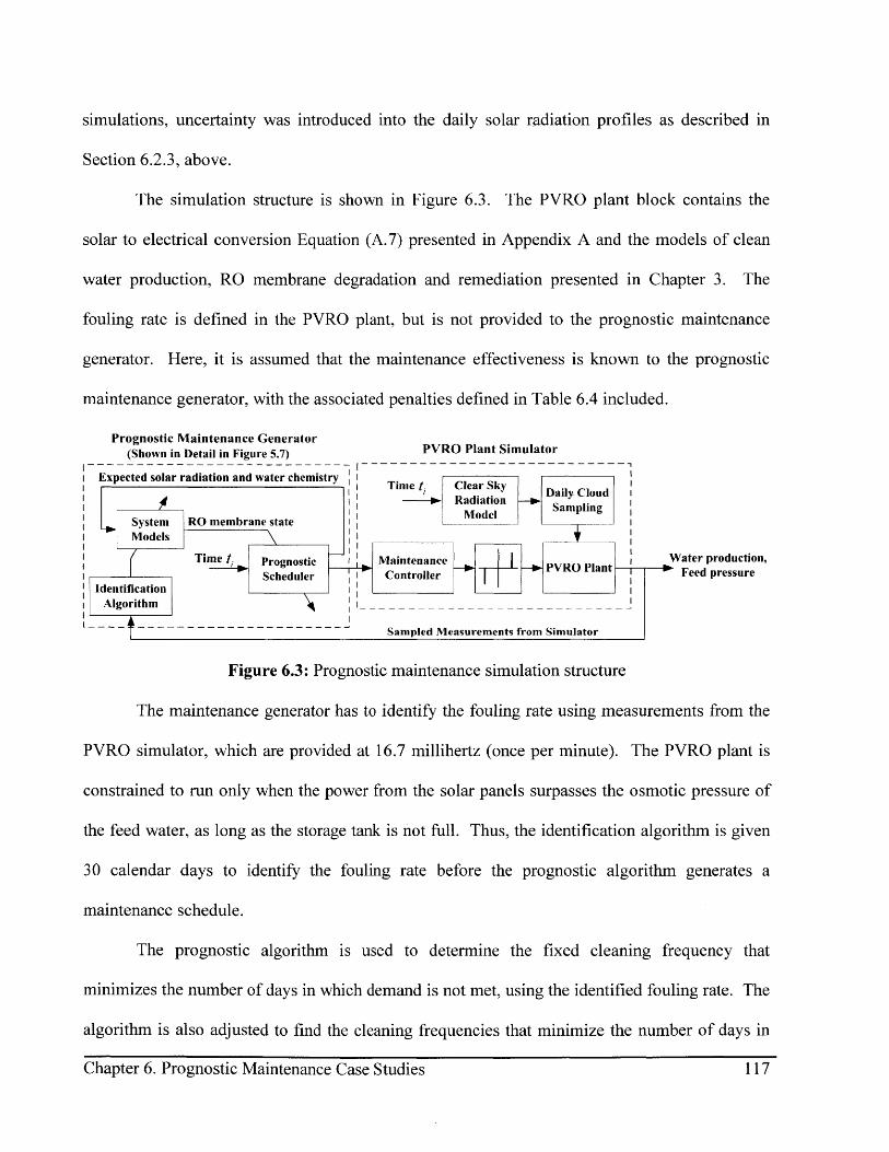
simulations, uncertainty was introduced into the daily solar radiation profiles as described in
Section 6.2.3, above.
The simulation structure is shown in Figure 6.3. The PVRO plant block contains the
solar to electrical conversion Equation (A.7) presented in Appendix A and the models of clean
water production, RO membrane degradation and remediation presented in Chapter 3. The
fouling rate is defined in the PVRO plant, but is not provided to the prognostic maintenance
generator. Here, it is assumed that the maintenance effectiveness is known to the prognostic
maintenance generator, with the associated penalties defined in Table 6.4 included.
Prognostic Maintenance Generator(Shown in Detail in Figure 5.7) PVRO Plant Simulator
i Expected solar radiation and water chemistry IRadition-->Daily Cloud
System RO membrane stateSModels
Time Prognostc Maintenance - Water production,rj Pronoti PYRO Plant T-o Feed pressure
IIdentification
I Algorithm --
Sampled Measurements from Simulator
Figure 6.3: Prognostic maintenance simulation structure
The maintenance generator has to identify the fouling rate using measurements from the
PVRO simulator, which are provided at 16.7 millihertz (once per minute). The PVRO plant is
constrained to run only when the power from the solar panels surpasses the osmotic pressure of
the feed water, as long as the storage tank is not full. Thus, the identification algorithm is given
30 calendar days to identify the fouling rate before the prognostic algorithm generates a
maintenance schedule.
The prognostic algorithm is used to determine the fixed cleaning frequency that
minimizes the number of days in which demand is not met, using the identified fouling rate. The
algorithm is also adjusted to find the cleaning frequencies that minimize the number of days in
Chapter 6. Prognostic Maintenance Case Studies 117

which demand is not met during periods of high average solar radiation and low average solar
radiation. This is accomplished by dividing up the year into two high-sun periods and two low-
sun periods, based on the clear sky solar radiation calculations for La Mancalona, assuming
latitude tilt on the solar panels as listed in Table 6.1.
6.3.1 Unknown, Fixed Fouling
In the first scenario, the RO fouling rate is constant over the 5-year period. Under this
scenario, the performance of the PVRO system when maintained using the prognostic fixed and
seasonal schedules is compared with its performance when following two pre-determined, fixed
cleaning schedules (see Table 6.7). These schedules are chosen based on manufacturer
recommendations and operator experience [28, 29]. Although condition-based maintenance is a
strategy used to maintain industrial RO plants, it is not practical for PVRO systems that do not
operate at fixed settings. A PVRO system will produce much less water on a cloudy day than on
a sunny day. Choosing a measurement threshold for CBM is difficult under such large variations
and can cause maintenance to occur too soon or too late.
Table 6.7: Fixed, pre-determined cleaning schedulesFixed Cleaning Schedule FrequencyAggressive Every 60 daysSparse Once per year
6.3.2 Unknown, Slowly Varying Fouling
In the second scenario, the fouling rate is slowly increased over time within the PVRO
plant simulator, described by:
y((t) Yo(6.2)
Chapter 6. Prognostic Maintenance Case Studies 118Chapter 6. Prognostic Maintenance Case Studies 118

where y0 is 6.5 x 10⁻⁹ (one/bar/s), bo is 3 x 10~1 (one/bar/s/day) and t is time in days. This
choice is arbitrary. Tying the fouling rate increase to operating time facilitates equal comparison
of PVRO performance across different maintenance strategies. Although one can also change
the fouling rate based on whether or not a chemical cleaning process has occurred, such changing
does not permit fair comparison across multiple maintenance strategies, since in some scenarios
fouling will occur faster than in others.
For this set of simulations, the fixed prognostic and seasonal prognostic schedules are
adjusted each time the fouling rate parameter estimate changes by more than 1% of its previous
value. This decision is also arbitrary. Optimizing the threshold under which maintenance
schedules are adjusted can be performed.
6.3.3 Unknown, Fixed Fouling with Varying Demand
The PVRO system is nominally sized to produce 1,000 L of clean water per day.
Initially, the forecasting algorithm assumes this demand is constant. In this scenario, the demand
is assumed to have fixed, seasonal and climatic components as described in Equation (5.12). The
baseline demand D,,,. is set to be 650 liters. The seasonal-dependent portion of drinking water
demand Ds (t) is defined using the average monthly temperatures in La Mancalona, obtained
from NASA [132]. As the dry-bulb temperature increases, human sweat loss increases to enable
thermoregulation. The seasonal component of the demand is generated using the average
monthly temperatures in La Mancalona and charts from the United States Department of
Agriculture [125]. The values shown in Table 6.8 are based on a population of 90 families with
5 family members each.
Chapter 6. Prognostic Maintenance Case Studies 119Chapter 6. Prognostic Maintenance Case Studies 119

Table 6.8: Seasonal portion of drinking water demandJan Feb Mar Apr May Jun Jul Aug Sept Oct Nov Dec
T C 22.4 24.1 26.4 27.8 27.9 26.9 26.4 26.5 26.3 25.2 23.9 22.5
D, (t) L/day 337.5 405 562.5 675 675 585 562.5 567 558 450 360 337.5
The daily climatic-dependent component is defined in Table 6.9. Since sunny days are
generally warmer than cloudy days, it is assumed that on cloudy days the baseline and seasonal
portions of demand do not need adjustment. The choices of increased water demand for clear
and partly cloudy skies are roughly approximated by assuming that on clear days each member
of the population will need 0.3 more liters of water, and on partly cloudy days each member will
need 0.2 more liters of water.
Table 6.9: Daily climatic portion of drinking water demandCloud Cover Dc (t)
Clear 135 L/dayPartly Cloudy 90 L/day
Overcast 0 L/day
In this set of simulations, the fouling rate is again constant, but unknown to the
prognostic algorithm.
6.3.4 Unknown, Varying Fouling with Varying Demand
In this scenario, the varying fouling rate and varying demand from Sections 6.3.2 and
6.3.3 are combined. The PVRO system performance under fixed and seasonal prognostic
maintenance and sparse cleaning is simulated and compared. Here, the fixed prognostic and
seasonal prognostic schedules are adjusted each time the fouling rate parameter estimate changes
by more than 1% of its previous value.
Chapter 6. Prognostic Maintenance Case Studies 120Chapter 6. Prognostic Maintenance Case Studies 120
6.4 Case Study Results
6.4.1 Fixed Fouling Rate Parameter Results
Under this scenario, the PVRO performance with fixed prognostic maintenance, seasonal
prognostic maintenance, aggressive maintenance and sparse maintenance is simulated 1,200
times. Due to the statistical nature of this problem and the finite size of the storage tank, the
water demand is not always met 100% of the time. Hence, the statement of this problem: Find
the minimum cost maintenance program that ensures the system will meet the community water
demand can never be met. It can only be approximated.
During the simulations, the water required by the community is subtracted from the
storage tank at the end of each day. At times when the amount of water in the tank is less than
the amount of water required by the community, the difference between the required and stored
water is recorded as a water deficit. As the simulations progress, the water deficit increases. To
evaluate performance, the water loss percentage, WLP, is defined:
WLP = Total Water Deficit x100Total Water Demand (6.3)
Histograms of the water loss percentage under the simulated maintenance strategies are shown in
Figure 6.4 and Figure 6.5. In this scenario, the fixed and sparse maintenance schedules result in
the lowest water loss. Clearly, the aggressive cleaning schedule does not perform as well, since
on average 25% of the water demand is not met. The seasonally adjusted maintenance schedule
also does result in the lowest water loss compared with PVRO performance under fixed
prognostic or sparse maintenance.
Chapter 6. Prognostic Maintenance Case Studies 121Chapter 6. Prognostic Maintenance Case Studies 121

35
30
25
20
a 15
| 10
5
t I A 1Ic il n I ItAn
350B
300-
250-
200-
150-
100-
50-
00 5 10 15 20 25 30
WLP(%) WLP(%)
Figure 6.4: Histograms of water loss percentage with optimal fixed
maintenance (A) and seasonal maintenance (B)
350C
300-
250-
200
150-
100-
50.
U,
U,
Cu
0
.0
2
150D
100
150
200
150
100
50
0
'0 5 10 15 20 25 30 "0 5 10 15 20 25 30
WLP (%) WLP(%)
Figure 6.5: Histograms of water loss percentage with aggressive (C)and sparse maintenance (D)
Table 6.10 lists the average water loss percentages and their ranges for the four simulated
maintenance strategies under an assumed fixed, unknown fouling rate. The average water loss is
minimized when the fixed prognostic maintenance strategy is used, although the PVRO system
also performs well under sparse maintenance schedule. In this scenario, the fixed maintenance
cleaning frequency always falls in the range of 305-365 days between cleanings. In some cases,
the optimal cleaning frequency determined by the prognostic scheduler is 365 days, which is the
0A
0-
0
0
0-
0
0
U,
U,
Cu
0I..
Ez
Chapter 6. Prognostic Maintenance Case Studies 122

same as the sparse cleaning frequency. Note that most RO membrane suppliers suggest that the
members will fail after about 3 to 5 years for reasons such as tearing and fabric failure. At the
end of this five-year period, one may need to replace the RO membrane anyway.
Table 6.10: Water loss results: fixed, unknown fouling rateCleaning Schedule WLP Mean WLP RangeFixed Prognostic Maintenance 2.357% [1.3876, 3.3642]Seasonal Prognostic Maintenance 4.2966% [2.0215, 6.6591]Aggressive Maintenance 24.98% [23.5403, 26.6339]Sparse Maintenance 2.5529% [1.3813, 4.1346]
This result is specific to the conditions simulated here. A different PVRO system under
faster fouling will likely require more frequent chemical cleaning. Under more frequent
chemical cleaning, adjusting the prognostic maintenance schedule in response to seasonal
changes may ensure community water demand is met more of the time.
In addition to meeting the water demand, the prognostic optimization minimizes the cost
of maintenance. Table 6.11 compares the average number of cleanings and the average
maintenance costs for each strategy over the five-year simulation period. As stated above, the
fixed maintenance cleaning frequency always falls in the range of [305-365] days between
cleanings, which always results in 5 cleanings over the simulation period. The cost of fixed
prognostic maintenance is the same as that of the sparse maintenance, and it results in lower
water loss on average. Adjusting the maintenance schedule seasonally results in a range of 4-7
cleanings over five years, so on average it costs more than simply fixing the maintenance
schedule based on the identified fouling rate parameter. For this scenario, it does not make
financial sense to seasonally adjust the cleaning schedule after it has been optimized. Finally,
the aggressive schedule is clearly too expensive and does not perform well. It is included to
Chapter 6. Prognostic Maintenance Case Studies 123

demonstrate that blindly following manufacturers' guidelines without identifying the fouling rate
parameter from the system performance may lead to expensive, sub-optimal results.
Table 6.11: Cleaning numbers and costs: fixed, unknown fouling rateCleaning Schedule Average Number of Cleanings Average Cost (MEX)Fixed Prognostic Maintenance 5 2,120.20Seasonal Prognostic Maintenance 5.1667 2,190.78Aggressive Maintenance 30 12,720.60Sparse Maintenance 5 2,120.20
The RO membrane replacement cost is assumed to be 2,561 pesos. Clearly, in this
scenario it is cheaper to perform chemical cleaning several times than to replace the RO
membrane once.
In this set of cases, a PVRO system maintained using the prognostic schedule on average
performs only slightly better than one maintained under annual chemical cleaning. For
comparison, a second set of cases under fixed, unknown fouling are simulated. The fouling rate
)/ in the PVRO plant simulator was increased by 20%, to 8.0 x 10⁻⁹ (one/bar/s) from 6.5 x 10⁻⁹
(one/bar/s). As discussed previously, the prognostic maintenance generator has to identify the
fouling rate. Results of the cases under higher, fixed unknown fouling are listed in Table 6.12.
Under the higher fouling rate, following the prognostic maintenance schedule minimizes the
water loss percentage without increasing the cleaning costs drastically. These results show that it
is advantageous to use prognostic maintenance.
Table 6.12: Water loss and cleaning cost results: higher fixed, unknown fouling rateCleaning Schedule WLP Mean WLP Range Average Number Average Cost
of Cleanings (MEX)Fixed Prognostic Maintenance 3.6% [2.4547, 4.8971] 5.8333 2,473.44Seasonal Prognostic Maintenance 9.1% [3.1497, 16.038] 5.5833 2,367.45Aggressive Maintenance 25.3% [23.898, 26.946] 30 12,720.60Sparse Maintenance 4.2% [2.700, 5.9082] 5 2,120.20
Chapter 6. Prognostic Maintenance Case Studies 124
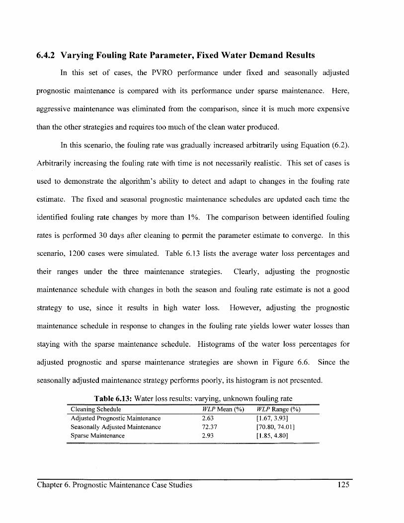
6.4.2 Varying Fouling Rate Parameter, Fixed Water Demand Results
In this set of cases, the PVRO performance under fixed and seasonally adjusted
prognostic maintenance is compared with its performance under sparse maintenance. Here,
aggressive maintenance was eliminated from the comparison, since it is much more expensive
than the other strategies and requires too much of the clean water produced.
In this scenario, the fouling rate was gradually increased arbitrarily using Equation (6.2).
Arbitrarily increasing the fouling rate with time is not necessarily realistic. This set of cases is
used to demonstrate the algorithm's ability to detect and adapt to changes in the fouling rate
estimate. The fixed and seasonal prognostic maintenance schedules are updated each time the
identified fouling rate changes by more than 1%. The comparison between identified fouling
rates is performed 30 days after cleaning to permit the parameter estimate to converge. In this
scenario, 1200 cases were simulated. Table 6.13 lists the average water loss percentages and
their ranges under the three maintenance strategies. Clearly, adjusting the prognostic
maintenance schedule with changes in both the season and fouling rate estimate is not a good
strategy to use, since it results in high water loss. However, adjusting the prognostic
maintenance schedule in response to changes in the fouling rate yields lower water losses than
staying with the sparse maintenance schedule. Histograms of the water loss percentages for
adjusted prognostic and sparse maintenance strategies are shown in Figure 6.6. Since the
seasonally adjusted maintenance strategy performs poorly, its histogram is not presented.
Table 6.13: Water loss results: varying, unknown fouling rateCleaning Schedule WLP Mean (%) WLP Range (%)Adjusted Prognostic Maintenance 2.63 [1.67, 3.93]Seasonally Adjusted Maintenance 72.37 [70.80, 74.01]Sparse Maintenance 2.93 [1.85, 4.80]
Chapter 6. Prognostic Maintenance Case Studies 125Chapter 6. Prognostic Maintenance Case Studies 125
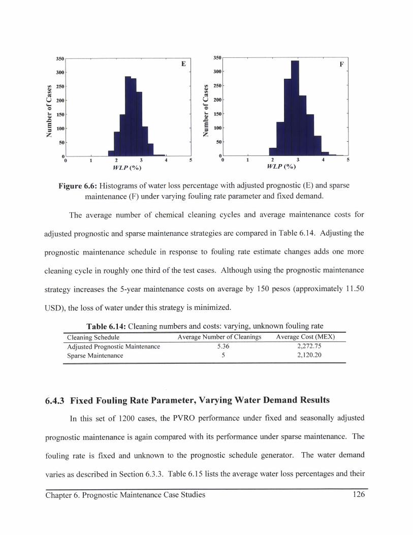
350 , 350E F
300- 300
250- 250-
200 200-
150 - - 150-
100 -100
50 50
0 00 1 2 3 4 5 0 1 2 3 4 5
WLP (%) WLP(%)
Figure 6.6: Histograms of water loss percentage with adjusted prognostic (E) and sparse
maintenance (F) under varying fouling rate parameter and fixed demand.
The average number of chemical cleaning cycles and average maintenance costs for
adjusted prognostic and sparse maintenance strategies are compared in Table 6.14. Adjusting the
prognostic maintenance schedule in response to fouling rate estimate changes adds one more
cleaning cycle in roughly one third of the test cases. Although using the prognostic maintenance
strategy increases the 5-year maintenance costs on average by 150 pesos (approximately 11.50
USD), the loss of water under this strategy is minimized.
Table 6.14: Cleaning numbers and costs: varying, unknown fouling rate
Cleaning Schedule Average Number of Cleanings Average Cost (MEX)
Adjusted Prognostic Maintenance 5.36 2,272.75Sparse Maintenance 5 2,120.20
6.4.3 Fixed Fouling Rate Parameter, Varying Water Demand Results
In this set of 1200 cases, the PVRO performance under fixed and seasonally adjusted
prognostic maintenance is again compared with its performance under sparse maintenance. The
fouling rate is fixed and unknown to the prognostic schedule generator. The water demand
varies as described in Section 6.3.3. Table 6.15 lists the average water loss percentages and their
Chapter 6. Prognostic Maintenance Case Studies 126126Chapter 6. Prognostic Maintenance Case Studies
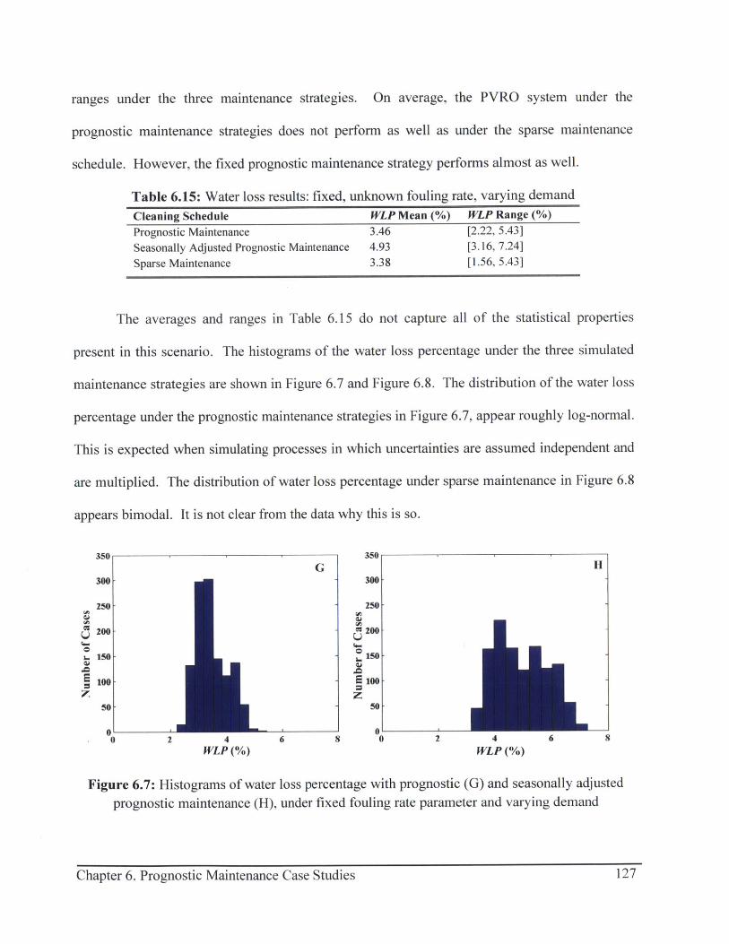
ranges under the three maintenance strategies. On average, the PVRO system under the
prognostic maintenance strategies does not perform as well as under the sparse maintenance
schedule. However, the fixed prognostic maintenance strategy performs almost as well.
Table 6.15: Water loss results: fixed, unknown fouling rate, varying demand
Cleaning Schedule WLP Mean (%) WLP Range (%)Prognostic Maintenance 3.46 [2.22, 5.43]
Seasonally Adjusted Prognostic Maintenance 4.93 [3.16, 7.24]Sparse Maintenance 3.38 [1.56, 5.43]
The averages and ranges in Table 6.15 do not capture all of the statistical properties
present in this scenario. The histograms of the water loss percentage under the three simulated
maintenance strategies are shown in Figure 6.7 and Figure 6.8. The distribution of the water loss
percentage under the prognostic maintenance strategies in Figure 6.7, appear roughly log-normal.
This is expected when simulating processes in which uncertainties are assumed independent and
are multiplied. The distribution of water loss percentage under sparse maintenance in Figure 6.8
appears bimodal. It is not clear from the data why this is so.
350 350G H
300- 300-
250- 250-CAI
~200- 1%200-Q
150 150
100- 100 -
50 50-
0 2 4 6 8 0 2 4 6 8WLP(%) WLP(%)
Figure 6.7: Histograms of water loss percentage with prognostic (G) and seasonally adjusted
prognostic maintenance (H), under fixed fouling rate parameter and varying demand
Chapter 6. Prognostic Maintenance Case Studies 127127Chapter 6. Prognostic Maintenance Case Studies

350
300-
250-
09 200-Q
150-
~10o
50-
010 2 4 6 8
WLP(%)
Figure 6.8: Histogram of water loss percentage with sparse maintenance (I)
Although the cleaning frequencies differ by maintenance strategy, the number of
cleanings in each case for each maintenance strategy is always five, so the 5-year maintenance
costs across all cases are the same: 2,120.20 pesos. The mean water loss percentage under
prognostic maintenance is less than 0.1% higher than the mean under sparse maintenance (see
Table 6.15). The sparse cleaning schedule is selected without estimating the fouling rate, based
on minimum chemical cleaning frequency guidelines from RO membrane manufacturers, and it
happens to be very close to the chemical cleaning frequencies determined by the prognostic
maintenance scheduler. Essentially, the prognostic maintenance method performs well and
essentially maintains demand at lowest cost here.
One can argue that the case study results imply that prognostic maintenance is not
necessary, and that simply following an annual cleaning schedule will result in reasonable
performance. However, recall that the fouling rate is not known a priori, is a complex function
of water chemistry and system operating conditions, and must be identified during operation.
The fouling rates for other PVRO systems will not be the same as the rates assumed here, so
following an annual schedule may result in higher water loss. In scenarios where annual
Chapter 6. Prognostic Maintenance Case Studies 128
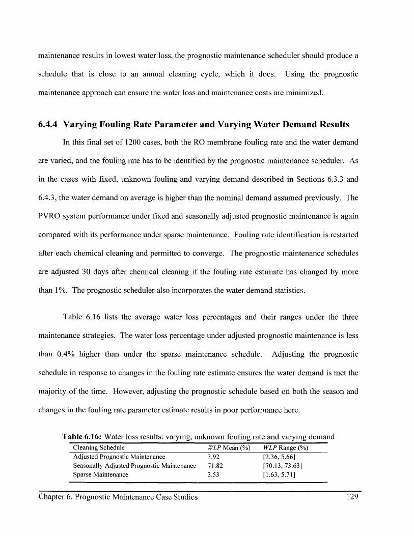
maintenance results in lowest water loss, the prognostic maintenance scheduler should produce a
schedule that is close to an annual cleaning cycle, which it does. Using the prognostic
maintenance approach can ensure the water loss and maintenance costs are minimized.
6.4.4 Varying Fouling Rate Parameter and Varying Water Demand Results
In this final set of 1200 cases, both the RO membrane fouling rate and the water demand
are varied, and the fouling rate has to be identified by the prognostic maintenance scheduler. As
in the cases with fixed, unknown fouling and varying demand described in Sections 6.3.3 and
6.4.3, the water demand on average is higher than the nominal demand assumed previously. The
PVRO system performance under fixed and seasonally adjusted prognostic maintenance is again
compared with its performance under sparse maintenance. Fouling rate identification is restarted
after each chemical cleaning and permitted to converge. The prognostic maintenance schedules
are adjusted 30 days after chemical cleaning if the fouling rate estimate has changed by more
than 1%. The prognostic scheduler also incorporates the water demand statistics.
Table 6.16 lists the average water loss percentages and their ranges under the three
maintenance strategies. The water loss percentage under adjusted prognostic maintenance is less
than 0.4% higher than under the sparse maintenance schedule. Adjusting the prognostic
schedule in response to changes in the fouling rate estimate ensures the water demand is met the
majority of the time. However, adjusting the prognostic schedule based on both the season and
changes in the fouling rate parameter estimate results in poor performance here.
Table 6.16: Water loss results: varying, unknown fouling rate and varying demandCleaning Schedule WLP Mean (%) WLP Range (%)Adjusted Prognostic Maintenance 3.92 [2.36, 5.66]Seasonally Adjusted Prognostic Maintenance 71.82 [70.13, 73.63]Sparse Maintenance 3.53 [1.63, 5.71]
Chapter 6. Prognostic Maintenance Case Studies 129

Under this scenario, the averages and ranges listed in Table 6.16 do not capture all of the
statistical properties. The histograms of the water loss percentage under adjusted prognostic and
sparse maintenance are shown in Figure 6.9. The histogram of water loss percentage under
adjusted prognostic maintenance, Figure 6.9 (J), appears log-normal. However, the water loss
percentage distribution under sparse maintenance, Figure 6.9 (K), is almost bimodal and has a
mode above 4.5%. It is not clear from the data why this is so. One possible reason for the
bimodal behavior is that the RO membrane permeability does not uniformly decline. During the
summer, the days are longer, so the PVRO system will operate for a longer period of time each
day. Since fouling generally increases with operating duration, more foulants may accumulate
per day. If the PVRO system is initially started in the summer, it may foul faster than a PVRO
system started in the winter. An annual cleaning cycle results in a "clean" RO membrane at the
same date each year, and these seasonal effects are compounded over the 5-year simulation
period.
Seasonality of water demand may also contribute to the bimodal behavior. Water use is
generally higher during dry seasons and at higher temperatures. In this case study, the period of
highest water use is at the end of the dry season in La Mancalona, in late spring (April and May).
If the RO membrane is not scheduled to be cleaned until right after this period, then the water
demand is at its highest when the RO membrane is most fouled. Conversely, if the RO
membrane is scheduled to be cleaned every March, then the RO membrane is not as fouled
during the time of greatest water demand and there is a lower probability of failing to meet
demand.
Chapter 6. Prognostic Maintenance Case Studies 130Chapter 6. Prognostic Maintenance Case Studies 130
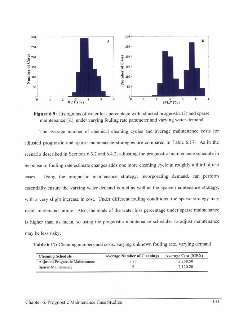
300 300J K
250 250-
S200- - 200
' 0-'' 150
5100 10o-
01 010 1 2 3 4 5 6 0 1 2 3 4 5 6
WLP (%) WLP (%)
Figure 6.9: Histograms of water loss percentage with adjusted prognostic (J) and sparse
maintenance (K), under varying fouling rate parameter and varying water demand
The average number of chemical cleaning cycles and average maintenance costs for
adjusted prognostic and sparse maintenance strategies are compared in Table 6.17. As in the
scenario described in Sections 6.3.2 and 6.4.2, adjusting the prognostic maintenance schedule in
response to fouling rate estimate changes adds one more cleaning cycle in roughly a third of test
cases. Using the prognostic maintenance strategy, incorporating demand, can perform
essentially ensure the varying water demand is met as well as the sparse maintenance strategy,
with a very slight increase in cost. Under different fouling conditions, the sparse strategy may
result in demand failure. Also, the mode of the water loss percentage under sparse maintenance
is higher than its mean, so using the prognostic maintenance scheduler to adjust maintenance
may be less risky.
Table 6.17: Cleaning numbers and costs: varying unknown fouling rate, varying demand
Cleaning Schedule Average Number of Cleanings Average Cost (MEX)
Adjusted Prognostic Maintenance 5.35 2,268.50
Sparse Maintenance 5 2,120.20
Chapter 6. Prognostic Maintenance Case Studies 131131Chapter 6. Prognostic Maintenance Case Studies
Once again, one can argue that simply following an annual cleaning schedule will result
in reasonable performance without relying on prognostic maintenance. However, the fouling
rates for other PVRO systems in other locations may differ substantially, and so annual
maintenance may result in higher water loss. Also, since the causes of the bimodal histogram in
Figure 6.9 (K) and not well understood, and since the mode of Figure 6.9 (K) is higher than its
average, following an annual schedule may result in more water loss than implied by the
average. The prognostic maintenance approach can be used to find a lowest cost maintenance
program that minimizes water loss percentage.
6.5 Summary
The prognostic maintenance algorithm is applied to a simulated PVRO system sized to
produce 1,000 L/day from brackish water under four scenarios: 1) fixed, unknown fouling rate,
2) slowly varying unknown fouling rate, 3) fixed, unknown fouling rate with varying water
demand, and 4) slowly varying, unknown fouling rate and varying water demand. The
variability in solar radiation from cloud cover is accounted for in all scenarios, as described in
Chapter 5. In this study, the water demand is not always met 100% of the time. Preliminary
results indicate that the prognostic approach ensures demand is met the majority of the time at
minimal maintenance cost under both constant fouling rate estimates and when adjusted in
response to changes in the fouling rate estimate, both with and without accounting for variations
in community water demand.
The method proposed here is intended to be general and can be applied to a broad class of
systems that degrade with operation that are stochastic in nature. Here it is applied to a solar
powered water purification system. For illustrative purposes the methodology is applied to a
representative, also though not typical, PVRO system and location as discussed in this section.
Chapter 6. Prognostic Maintenance Case Studies 132

The results are rational and in some cases somewhat counter intuitive. For example, in this
study, adjusting the maintenance schedule seasonally does not ensure demand is met at minimal
cost. This is likely due to the timing of maintenance cleanings selected by the prognostic
scheduler under the simulated conditions. The time between cleanings is between 305 and 365
days. Under these circumstances, it does not make sense to change frequencies with seasons.
Under different conditions, seasonal adjustments to the prognostic schedule may ensure demand
is met even more of the time, with minimal increases to maintenance costs.
The prognostic maintenance methodology can ensure the community water demand is
met at minimal cost by accounting for variable, stochastic operating conditions, RO membrane
degradation and cleaning effectiveness. Refinements to the prognostic scheduling optimization
algorithm, such as optimization of the threshold at which the prognostic maintenance schedule is
adjusted, can improve its performance under varying fouling and community water demand.
Chapter 6. Prognostic Maintenance Case Studies 133Chapter 6. Prognostic Maintenance Case Studies 133
Chapter 6. Prognostic Maintenance Case Studies 134
CHAPTER
7SUMMARY AND CONCLUSIONS
7.1 Summary
In this thesis, a methodology for developing a model-based prognostic maintenance
algorithm for systems degrading as complex functions of their operation, under varying,
uncertain conditions has been developed and applied to a community-sized, brackish water
PVRO desalination system in simulation. The methodology combines physics-based modeling,
system identification based on operation history and statistical models of future system inputs to
predict system performance and to optimize maintenance scheduling in terms of maintaining its
desired performance at the lowest cost.
The methodology is applied to a remote, community-scale PVRO system assumed to
operate without the benefit of energy storage. A physics-based model describing the long-term
effects of RO membrane degradation due to colloidal fouling and mineral scaling is formulated.
System flushing and chemical cleaning models are also formulated and are justified based on the
relative timescales of fouling versus flushing and cleaning. Given a system location and design,
the prognostic algorithm identifies the RO membrane permeability and fouling rate from water
pressure, flow and salinity measurements. It uses the identified fouling rate and estimated state
of the RO membrane, combined with a clear-sky solar-radiation model and historical weather
data, to project future performance and degradation. It is able to predict when the system will
fail to meet community demand. It is also able to predict the costs of applying maintenance
135Chapter 7. Summary and Conclusions

actions at different times to compare alternatives. By setting up a constrained optimization
problem using the identified fouling rate, anticipated environmental conditions, predicted
performance and costs, production time lost and product water required, a maintenance schedule
that ensures community water demand is met the majority of the time at lowest cost is generated.
Example results show that the prognostic maintenance approach can minimize the water loss
percentage at minimal cost, subject to variable operating conditions and degradation. An
optimized maintenance schedule is needed by PVRO system operators, who do not have the
expertise to determine the type and timing of the maintenance that will assure community water
demand is met at lowest cost, and the prognostic maintenance methodology can fill this need.
7.2 Suggestions for Future Work
Several directions are available for extension of this work. Refinements can be made to
the prognostic maintenance algorithm as applied to PVRO systems, both with and without
batteries. The prognostic maintenance methodology can also be applied to other degrading
systems subject to variable and uncertain operating conditions.
7.2.1 Future Refinements
Many future refinements to the prognostic maintenance algorithm as applied to PVRO
exist. The set of case studies presented in this work determine the chemical cleaning schedule
for a 5-year period. This length of time was chosen based on RO plant operator and
manufacturer experience. However, the prognostic maintenance algorithm for PVRO can be
extended so that membrane replacement can be incorporated. In the example study, the increase
in RO memhrane permeability after chemical cleaning is limited to 97/of its nrevisy11Q1r cleaned
value. After 8 cleanings, the RO membrane permeability cannot be increased enough to meet the
Chapter 7. Summary and Conclusions 136

daily water demand on a clear day, and so the RO membrane should be replaced. In general, the
limit on the number of cleanings will depend on the cleaning effectiveness and type of fouling.
Though assumptions are made for the example study, the cleaning effectiveness of a real PVRO
system can be estimated from system performance history. Limits on the number of chemical
cleanings can be calculated once the cleaning effectiveness is identified.
Biofouling is assumed negligible in the community-sized PVRO systems considered
here, since UV disinfection is assumed to effectively prevent it. Extensions of this work as
applied to reverse osmosis systems can include the modeling, identification and remediation of
biofouling.
In this work, the prognostic maintenance schedule was constrained to evenly spaced
waiting periods between chemical cleanings under the assumption that an even schedule is the
easiest for non-expert operators to follow. The operators are also assumed to follow the schedule
perfectly. These constraints can be relaxed. Permitting the days between chemical cleanings to
vary may result in a cleaning schedule that ensures community water demand is met 100% of the
time. Effectively communicating the cleaning schedule to the system operators can also be
considered.
The case studies in this work assume that battery banks are not used for energy storage,
and that the PVRO pumps operate variably as the incident sunlight fluctuates. In a PVRO
system that incorporates batteries, the RO motor/pumps run at constant power, and the batteries
mitigate the fluctuations in solar power. Battery charging and discharging, and hence its
degradation, will fluctuate with solar radiation. The prognostic algorithm will still need to
identify the RO fouling rate and determine chemical cleaning schedules. However, it will also
need to forecast battery charging, discharging and degradation. The same methodology applied
137Chapter 7. Summary and Conclusions
to a PVRO system without batteries can be applied. A suitable model of the battery bank
charging and discharging can either be found in the literature or can be developed. Unknown
parameters in such models may need to be identified, in which case parameter estimation
methods, such as recursive least squares or others [114], can be used along with measurements of
battery current, voltage and temperature. Identification methods will depend on model structure.
The solar radiation model incorporating the cloud statistics presented here can be used as an
input to the battery degradation model, and thus its degradation can be forecasted, and its
replacement schedule can be determined.
The PVRO prognostic algorithm has not yet been applied to a physical PVRO system.
This is needed to validate the prognostic maintenance approach. Field experiments will enable
further refinement of appropriate RO fouling models and their validation, refinement of demand
models, refinement of climate statistical models, and refinement of the prognostic algorithm
itself. Additionally, operators claim that cleaning an RO membrane becomes less effective over
time, based on their experiences. However, this has yet to be been studied. Such experimental
studies obviously will take years to perform, and are difficult to perform in the actual settings.
7.2.2 Applications to Other Domains
The prognostic maintenance methodology can be applied to other systems that degrade
with operation and are subject to varying, uncertain conditions, such as vehicle fleets. For
example, a fleet of military vehicles will be subject to many different road conditions,
temperatures, levels of dust, etc. Maintaining fleets of vehicles is expensive. Instead of
performing reactive or condition-based maintenance, prognostic maintenance can potentially
lower costs and facilitate better scheduling of vehicle deployment.
Chapter 7. Summary and Conclusions 138Chapter 7. Summary and Conclusions 138
Prognostic maintenance can also be applied to other solar-powered or renewable energy-
powered systems, such as systems powered by wind turbines. These may include RO processes
or other processes driven by variable, uncertain power sources, and may or may not include
energy storage. Applying this methodology can ensure such systems maintain their desired
productivity without excessive maintenance.
Chapter 7. Summary and Conclusions 139
Chapter 7. Summary and Conclusions 139

Chapter 7. Summary and Conclusions 140

REFERENCES
[1] A. Sharma, G. S. Yadava, and S. G. Deshmukh, "A literature review and future perspectives onmaintenance optimization," in Journal of Quality in Maintenance Engineering. vol. 17 Bradford: EmeraldGroup Publishing, Limited, 2011, pp. 5-25.
[2] R. Kothamasu, S. Huang, and W. VerDuin, "System health monitoring and prognostics - a review ofcurrent paradigms and practices," The International Journal ofAdvanced Manufacturing Technology, vol.28, pp. 1012-1024, 2006.
[3] A. Chen and G. S. Wu, "Real-time health prognosis and dynamic preventive maintenance policy forequipment under aging Markovian deterioration," International Journal ofProduction Research, vol. 45,pp. 3351-3379, 2007.
[4] H. P. Bloch and A. R. Budris, "Improvements Leading to Pump Mechanical Maintenance Cost Reduction,"in Pump User's Handbook: Life Extension: Fairmont Press, 2004.
[5] D. Yellamati, E. Arthur, S. James, G. Morris, T. Heydt, and E. Graf, "Predictive Reliability Models forvariable frequency drives based on application profiles," in Reliability and Maintainability Symposium(RAMS), 2013 Proceedings - Annual, 2013, pp. 1-6.
[6] "Tactical Water Purification," Knoxville, TN: Aqua-Chem, Inc., 2015. Available http://aqua-chem.com/node/22.
[7] Y. Peng, M. Dong, and M. Zuo, "Current status of machine prognostics in condition-based maintenance: areview," The International Journal ofAdvanced Manufacturing Technology, vol. 50, pp. 297-3 13, 2010.
[8] R. C. M. Yam, P. W. Tse, L. Li, and P. Tu, "Intelligent Predictive Decision Support System for Condition-Based Maintenance," The International Journal ofAdvanced Manufacturing Technology, vol. 17, pp. 383-391, 2001.
[9] W. Wang, P. A. Scarf, and M. A. J. Smith, "On the Application of a Model of Condition-BasedMaintenance," The Journal of the Operational Research Society, vol. 51, pp. 1218-1227, 2000.
[10] D. B. Durocher and G. R. Feldmeier, "Predictive versus preventive maintenance," Industry ApplicationsMagazine, IEEE, vol. 10, pp. 12-21, 2004.
[11] A. S. Bhujle, "Autonomous Control and Membrane Maintenance Optimization of Photovoltaic ReverseOsmosis Systems," SM Thesis. Cambridge, MA: Massachusetts Institute of Technology, 2013.
[12] S. R. McCormick, K. Hur, S. Santoso, A. Maitra, and A. Sundaram, "Capacitor bank predictivemaintenance and problem identification using conventional power quality monitoring systems," in PowerEngineering Society General Meeting, 2004. IEEE, 2004, pp. 1846-1850 Vol.2.
[13] V. Venkatasubramanian, "Prognostic and diagnostic monitoring of complex systems for product lifecyclemanagement: Challenges and opportunities," Computers & Chemical Engineering, vol. 29, pp. 1253-1263,2005.
[14] H.-E. Kim, A. C. C. Tan, J. Mathew, and B.-K. Choi, "Bearing fault prognosis based on health stateprobability estimation," Expert Systems with Applications, vol. 39, pp. 5200-5213, 2012.
[15] H. Lu, W. J. Kolarik, and S. S. Lu, "Real-time performance reliability prediction," Reliability, IEEETransactions on, vol. 50, pp. 353-357, 2001.
[16] H. T. Pham and B.-S. Yang, "Estimation and forecasting of machine health condition usingARMA/GARCH model," Mechanical Systems and Signal Processing, vol. 24, pp. 546-558, 2010.
[17] C. S. Byington, M. Watson, D. Edwards, and P. Stoelting, "A model-based approach to prognostics andhealth management for flight control actuators," in Aerospace Conference, 2004. Proceedings. 2004 IEEE,2004, pp. 3551-3562 Vol.6.
[18] B. Iung, M. Monnin, A. Voisin, P. Cocheteux, and E. Levrat, "Degradation state model-based prognosis forproactively maintaining product performance," CIRP Annals - Manufacturing Technology, vol. 57, pp. 49-52, 2008.
References 141

[19] Z.-J. Zhou, C.-H. Hu, W.-B. Wang, B.-C. Zhang, D.-L. Xu, and J.-F. Zheng, "Condition-based maintenanceof dynamic systems using online failure prognosis and belief rule base," Expert Systems with Applications,vol. 39, pp. 6140-6149, 2012.
[20] WHO/UNICEF, "Progress on Drinking Water and Sanitation: 2012 Update," World Health Organizationand UNICEF, Geneva, Switzerland 2012.
[21] P. Rekacewicz and E. Bournay, "Proportion of population with improved drinking water supply in 2002"Arendal, Norway: UNEP/GRID-Arendal, 2007.
[22] P. Rekacewicz, "Water Scarcity Index," in Vital Water Graphics - An Overview of the State of the World'sFresh and Marine Waters. 2nd Edition. Nairobi, Kenya: UNEP, 2008.
[23] H. Ahlenius, "Natural resource - solar power (potential) " in Environment & Poverty Times No. 5 Arendal,Norway: GRID-Arendal, 2008.
[24] A. M. Bilton, R. Wiesman, A. F. M. Arif, S. M. Zubair, and S. Dubowsky, "On the feasibility ofcommunity-scale photovoltaic-powered reverse osmosis desalination systems for remote locations,"Renewable Energy, vol. 36, pp. 3246-3256, 2011.
[25] A. M. Bilton, L. C. Kelley, and S. Dubowsky, "Photovoltaic reverse osmosis - Feasibility and a pathwayto develop technology," Desalination and Water Treatment, vol. 31, pp. 24-34, 2011.
[26] A. M. Bilton, "A Modular Design Architecture for Application to Community-Scale Photovoltaic-PoweredReverse Osmosis Systems," Ph D Thesis, Cambridge, MA: Massachusetts Institute of Technology, 2013.
[27] A. M. Bilton and S. Dubowsky, "The modular design of photovoltaic reverse osmosis systems: makingtechnology accessible to nonexperts," Desalination and Water Treatment, vol. 51, pp. 702-712, 2012.
[28] J. Kucera, Reverse Osmosis. Salem, MA: Scrivener Publishing, LLC, 2010.[29] "Cleaning Procedures for DOW FILMTEC FT30 Elements." Form No. 609-23010-0211, DOW Chemical
Company, 2011.[30] S. Lu, Y.-C. Tu, and H. Lu, "Predictive condition-based maintenance for continuously deteriorating
systems," Quality and Reliability Engineering International, vol. 23, pp. 71-81, 2007.[31] S. K. Yang, "A condition-based failure-prediction and processing-scheme for preventive maintenance,"
Reliability, IEEE Transactions on, vol. 52, pp. 373-383, 2003.[32] H. Liao and M. Rausch, "Spare part inventory control driven by condition based maintenance," in
Reliability and Maintainability Symposium (RAMS), 2010 Proceedings - Annual, 2010, pp. 1-6.[33] E. Deloux, B. Castanier, and C. Berenguer, "Predictive maintenance policy for a gradually deteriorating
system subject to stress," Reliability Engineering & System Safety, vol. 94, pp. 418-431, 2009.[34] X. Zhao, M. Fouladirad, C. Berenguer, and L. Bordes, "Condition-based inspection/replacement policies
for non-monotone deteriorating systems with environmental covariates," Reliability Engineering & SystemSafety, vol. 95, pp. 921-934, 2010.
[35] E. Becker and P. Poste, "Keeping the blades turning: Condition monitoring of wind turbine gears," Refocus,vol. 7, pp. 26-32, 2006.
[36] W. Wang and M. Carr, "A stochastic filtering based data driven approach for residual life prediction andcondition based maintenance decision making support," in Prognostics and Health ManagementConference, 2010. PHM '10., 2010, pp. 1-10.
[37] Y. Dong, Y. Gu, K. Yang, and J. Zhang, "Applying PCA to establish artificial neural network for conditionprediction on equipment in power plant," in Intelligent Control and Automation, 2004. WCICA 2004. FifthWorld Congress on, 2004, pp. 1715-1719 Vol.2.
[38] Z.-J. Zhou, C.-H. Hu, D.-L. Xu, M.-Y. Chen, and D.-H. Zhou, "A model for real-time failure prognosisbased on hidden Markov model and belief rule base," European Journal of Operational Research, vol. 207,pp. 269-283, 2010.
[39] D. Bansal, D. J. Evans, and B. Jones, "A Real-Time Predictive Maintenance System for Machine Systems -An Alternative to Expensive Motion Sensing Technology," in Sensorsfor Industry Conference, 2005, pp.39-44.
References 142
References 142

[40] P. Sadegh, J. Concha, S. Stricevic, A. Thompson, and P. J. Kootsookos, "A framework for unified design offault detection & isolation and optimal maintenance policies," in American Control Conference, 2006,2006.
[41] K. Bouvard, S. Artus, C. Berenguer, and V. Cocquempot, "Condition-based dynamic maintenanceoperations planning & grouping. Application to commercial heavy vehicles," Reliability Engineering &System Safety, vol. 96, pp. 601-610, 2011.
[42] B. Y. Yu, T. Honda, G. M. Zak, A. Mitsos, J. Lienhard, K. Mistry, S. Zubair, M. H. Sharqawy, M. Antar,and M. C. Yang, "Prognosis of Component Degradation Under Uncertainty: A Method for Early StageDesign of a Complex Engineering System," in ASME 2012 11th Biennial Conference on EngineeringSystems Design and Analysis, 2012, pp. 683-694.
[43] M. Dong, D. He, P. Banerjee, and J. Keller, "Equipment health diagnosis and prognosis using hidden semi-Markov models," The International Journal ofAdvanced Manufacturing Technology, vol. 30, pp. 738-749,2006.
[44] L. Jianhui, M. Namburu, K. Pattipati, Q. Liu, M. Kawamoto, and S. Chigusa, "Model-based prognostictechniques [maintenance applications]," in A UTOTESTCON 2003. IEEE Systems Readiness TechnologyConference. Proceedings, 2003, pp. 330-340.
[45] M. D. Le and C. M. Tan, "Optimal maintenance strategy of deteriorating system under imperfectmaintenance and inspection using mixed inspection scheduling," Reliability Engineering & System Safety,vol. 113, pp. 21-29, 2012.
[46] E. Tzen and R. Morris, "Renewable energy sources for desalination," Solar Energy, vol. 75, pp. 375-379,2003.
[47] C. Fritzmann, J. Lowenberg, T. Wintgens, and T. Melin, "State-of-the-art of reverse osmosis desalination,"Desalination, vol. 216, pp. 1-76, 2007.
[48] "PVInsights: Solar Photovoltaic (Polysilicon wafer cell and panel) Prices and Research Reports,"PVinsights Co. Ltd., 2015.
[49] A. Bermudez-Contreras, M. Thomson, and D. G. Infield, "Renewable energy powered desalination in BajaCalifornia Sur, Mexico," Desalination, vol. 220, pp. 431-440, 2008.
[50] R. Wood, "Sun- and wind-powered solar cube is a self-contained water purification system," Journal of theAmerican Water Works Association, vol. 99, pp. 38-40, 42, 2007.
[51] A. Ghermandi and R. Messalem, "Solar-driven desalination with reverse osmosis: the state of the art,"Desalination and Water Treatment, vol. 7, pp. 285-296, 2009.
[52] D. Herold and A. Neskakis, "A small PV-driven reverse osmosis desalination plant on the island of GranCanaria," Desalination, vol. 137, pp. 285-292, 2001.
[53] M. Papapetrou, C. Epp, and E. Tzen, "Autonomous desalination units based on renewable energy systems-A review of representative installations worldwide," in Solar Desalinationfor the 21st Century: Springer,2007, pp. 343-353.
[54] M. Thomson, "Reverse-Osmosis Desalination of Seawater Powered by Photovoltaics Without Batteries."vol. Thesis Leicestershire, UK: Loughborough University, 2003.
[55] M. B. Baig and A. A. Al Kutbi, "Design features of a 20 migd SWRO desalination plant, Al Jubail, SaudiArabia," Desalination, vol. 118, pp. 5-12, 1998.
[56] A. Antony, J. H. Low, S. Gray, A. E. Childress, P. Le-Clech, and G. Leslie, "Scale formation and control inhigh pressure membrane water treatment systems: A review," Journal of Membrane Science, vol. 383, pp.1-16, 2011.
[57] S. Lee and C. Lee, "Scale formation in NF/RO: mechanism and control," Water Science & Technology, vol.51, pp. 267-275, 2005.
[58] A. Jawor and E. M. V. Hoek, "Effects of feed water temperature on inorganic fouling of brackish water ROmembranes," Desalination, vol. 235, pp. 44-57, 2009.
[59] C. Y. Tang, T. H. Chong, and A. G. Fane, "Colloidal interactions and fouling of NF and RO membranes: Areview," Advances in Colloid and Interface Science, vol. 164, pp. 126-143, 2011.
References 143143References
[60] T. H. Chong, F. S. Wong, and A. G. Fane, "Implications of critical flux and cake enhanced osmoticpressure (CEOP) on colloidal fouling in reverse osmosis: Experimental observations," Journal ofMembrane Science, vol. 314, pp. 101-111, 2008.
[61] L. Song and G. Singh, "Influence of various monovalent cations and calcium ion on the colloidal foulingpotential," Journal of Colloid and Interface Science, vol. 289, pp. 479-487, 2005.
[62] X. Jin, A. Jawor, S. Kim, and E. M. V. Hoek, "Effects of feed water temperature on separation performanceand organic fouling of brackish water RO membranes," Desalination, vol. 239, pp. 346-359, 2009.
[63] A. I. Radu, J. S. Vrouwenvelder, M. C. M. van Loosdrecht, and C. Picioreanu, "Effect of flow velocity,substrate concentration and hydraulic cleaning on biofouling of reverse osmosis feed channels," ChemicalEngineering Journal, vol. 188, pp. 30-39, 2012.
[64] J. S. Vrouwenvelder, C. Picioreanu, J. C. Kruithof, and M. C. M. van Loosdrecht, "Biofouling in spiralwound membrane systems: Three-dimensional CFD model based evaluation of experimental data," Journalof Membrane Science, vol. 346, pp. 71-85, 2010.
[65] J. S. Baker and L. Y. Dudley, "Biofouling in membrane systems: A review," Desalination, vol. 118, pp. 81-89, 1998.
[66] J. S. Vrouwenvelder, C. Hinrichs, W. G. J. Van der Meer, M. C. M. Van Loosdrecht, and J. C. Kruithof,"Pressure drop increase by biofilm accumulation in spiral wound RO and NF membrane systems: role ofsubstrate concentration, flow velocity, substrate load and flow direction," Biofouling, vol. 25, pp. 543-555,2009.
[67] J. Thompson, N. Lin, E. Lyster, R. Arbel, T. Knoell, J. Gilron, and Y. Cohen, "RO membrane mineralscaling in the presence of a biofilm," Journal ofMembrane Science, vol. 415-416, pp. 181-191, 2012.
[68] J. S. Vrouwenvelder, S. A. Manolarakis, H. R. Veenendaal, and D. van der Kooij, "Biofouling potential ofchemicals used for scale control in RO and NF membranes," Desalination, vol. 132, pp. 1-10, 2000.
[69] R. Higgin, K. J. Howe, and T. M. Mayer, "Synergistic behavior between silica and alginate: Novelapproach for removing silica scale from RO membranes," Desalination, vol. 250, pp. 76-81, 2010.
[70] B. A. Qureshi, S. M. Zubair, A. K. Sheikh, A. Bhujle, and S. Dubowsky, "Design and performanceevaluation of reverse osmosis desalination systems: An enphasis on fouling modeling," Applied ThermalEngineering, vol. 60, pp. 208-217, 2013.
[71] A. Abbas and N. Al-Bastaki, "Performance decline in brackish water Film Tec spiral wound ROmembranes," Desalination, vol. 136, pp. 281-286, 2001.
[72] E. M. V. Hoek, J. Allred, T. Knoell, and B.-H. Jeong, "Modeling the effects of fouling on full-scale reverseosmosis processes," Journal of Membrane Science, vol. 314, pp. 33-49, 2008.
[73] Y. G. Lee, Y. S. Lee, D. Y. Kim, M. Park, D. R. Yang, and J. H. Kim, "A fouling model for simulatinglong-term performance of SWRO desalination process," Journal ofMembrane Science, vol. 401, pp. 282-291, 2012.
[74] K. L. Chen, L. Song, S. L. Ong, and W. J. Ng, "The development of membrane fouling in full-scale ROprocesses," Journal ofMembrane Science, vol. 232, pp. 63-72, 2004.
[75] M. Barger and R. P. Carnahan, "Fouling prediction in reverse osmosis processes," Desalination, vol. 83,pp. 3-33, 1991.
[76] A. I. Radu, J. S. Vrouwenvelder, M. C. M. van Loosdrecht, and C. Picioreanu, "Modeling the effect ofbiofilm formation on reverse osmosis performance: Flux, feed channel pressure drop and solute passage,"Journal ofMembrane Science, vol. 365, pp. 1-15, 2010.
[77] C. Picioreanu, J. S. Vrouwenvelder, and M. C. M. van Loosdrecht, "Three-dimensional modeling ofbiofouling and fluid dynamics in feed spacer channels of membrane devices," Journal ofMembraneScience, vol. 345, pp. 340-354, 2009.
[78] L. Kelley, H. Elasaad, and S. Dubowsky, "Autonomous operation and maintenance of small-scale PVROsystems for remote communities," Desalination and Water Treatment, pp. 1-13, 2014.
[,79]l J. Mvi. Arnal, B. Garcia-Fayos, and M. a. Sancho, "Membrane Cleaning," in Expanding Issues inDesalination, R. Y. Ning, Ed. Rijeka, Croatia: InTech, 2011, pp. 63-84.
[80] J. P. Chen, S. L. Kim, and Y. P. Ting, "Optimization of membrane physical and chemical cleaning by astatistically designed approach," Journal ofMembrane Science, vol. 219, pp. 27-45, 2003.
References 144
[81] Hydranautics, "Technical Service Bulletin: Foulants and Cleaning Procedures for composite polyamide ROMembrane Elements (ESPA, ESNA, CPA, LFC, NANO and SWC) ". TSB 107.22, Oceanside, CA: NittoCorporation, 2013.
[82] M. Fazel and S. Chesters, "RO membrane cleaning using microbubbles at 6,800 m3/d wastewater RO plantin UAE," Desalination and Water Treatment, pp. 1-9, 2014.
[83] S. P. Chesters, M. W. Armstrong, and M. Fazel, "Microbubble RO membrane cleaning reduces fouling onWWRO plant," Desalination and Water Treatment, pp. 1-9, 2014.
[84] D. Feng, J. S. J. van Deventer, and C. Aldrich, "Ultrasonic defouling of reverse osmosis membranes used totreat wastewater effluents," Separation and Purification Technology, vol. 50, pp. 318-323, 2006.
[85] W. S. Ang, S. Lee, and M. Elimelech, "Chemical and physical aspects of cleaning of organic-fouled reverseosmosis membranes," Journal ofMembrane Science, vol. 272, pp. 198-210, 2006.
[86] M. Luo and Z. Wang, "Complex fouling and cleaning-in-place of a reverse osmosis desalination system,"Desalination, vol. 141, pp. 15-22, 2001.
[87] S. S. Madaeni, T. Mohamamdi, and M. Kazemi Moghadam, "Chemical cleaning of reverse osmosismembranes," Desalination, vol. 134, pp. 77-82, 2001.
[88] Y.-y. Lu, Y.-d. Hu, D.-m. Xu, and L.-y. Wu, "Optimum design of reverse osmosis seawater desalinationsystem considering membrane cleaning and replacing," Journal ofMembrane Science, vol. 282, pp. 7-13,2006.
[89] S. I. Graham, R. L. Reitz, and C. E. Hickman, "Improving reverse osmosis performance through periodiccleaning," Desalination, vol. 74, pp. 113-124, 1989.
[90] J. C. Schippers and J. Verdouw, "The modified fouling index, a method of determining the foulingcharacteristics of water," Desalination, vol. 32, pp. 137-148, 1980.
[91] E. Brauns, E. Van Hoof, B. Molenberghs, C. Dotremont, W. Doyen, and R. Leysen, "A new method ofmeasuring and presenting the membrane fouling potential," Desalination, vol. 150, pp. 31-43, 2002.
[92] K. G. Tay and L. Song, "A more effective method for fouling characterization in a full-scale reverseosmosis process," Desalination, vol. 177, pp. 95-107, 2005.
[93] S. El-Manharawy and A. Hafez, "Molar ratios as a useful tool for prediction of scaling potential inside ROsystems," Desalination, vol. 136, pp. 243-254, 2001.
[94] S. El-Manharawy and A. Hafez, "A new chemical classification system of natural waters for desalinationand other industrial uses," Desalination, vol. 156, pp. 163-180, 2003.
[95] H. J. See, V. S. Vassiliadis, and D. 1. Wilson, "Optimisation of membrane regeneration scheduling inreverse osmosis networks for seawater desalination," Desalination, vol. 125, pp. 37-54, 1999.
[96] M. Zhu, M. M. El-Halwagi, and M. Al-Ahmad, "Optimal design and scheduling of flexible reverse osmosisnetworks," Journal of Membrane Science, vol. 129, pp. 161-174, 1997.
[97] K. M. Sassi and I. M. Mujtaba, "Optimal design and operation of reverse osmosis desalination process withmembrane fouling," Chemical Engineering Journal, vol. 171, pp. 582-593, 2011.
[98] H. Chen and A. S. Kim, "Prediction of permeate flux decline in crossflow membrane filtration of colloidalsuspension: a radial basis function neural network approach," Desalination, vol. 192, pp. 415-428, 2006.
[99] D. Libotean, J. Giralt, F. Giralt, R. Rallo, T. Wolfe, and Y. Cohen, "Neural network approach for modelingthe performance of reverse osmosis membrane desalting," Journal of Membrane Science, vol. 326, pp. 408-419, 2009.
[100] A. n. Zafra-Cabeza, M. A. Ridao, and E. F. Camacho, "A mixed integer quadratic programmingformulation of risk management for reverse osmosis plants," Desalination, vol. 268, pp. 46-54, 2011.
[101] C. W. McFall, A. Bartman, P. D. Christofides, and Y. Cohen, "Control and Monitoring of a High RecoveryReverse Osmosis Desalination Process," Industrial & Engineering Chemistry Research, vol. 47, pp. 6698-6710, 2008.
[102] A. Gambier, N. Blumlein, and E. Badreddin, "Real-time fault tolerant control of a Reverse Osmosisdesalination plant based on a hybrid system approach," in American Control Conference, 2009. ACC '09.,2009, pp. 1598-1603.
References 145
References 145
[103] "FILMTEC Membranes System Design: System Performance Projection." Form Number 609-02057-604Dow Chemical Corporation. Available http://www.dow.com. Accessed 13 December 2010, 2010.
[104] M. Wilf and K. Klinko, "Performance of commercial seawater membranes," Desalination, vol. 96, pp. 465-478, 1994.
[105] "Technical Manual Excerpt: Filmtec Membranes Addendum: Temperature Correction Factor." FormNumber 609-02129-804. Dow Chemical Corporation. Available http://www.dow.com. Accessed 18December 2014, 2008.
[106] "Membrane Performance Factors: Temperature Correction," Applied Membranes, Inc., 2012. Availablehttp://appliedmembranes.com Accessed 4 February 2015.
[107] "FILMTEC Membranes System Design: Membrane Systen Design Guidelines for Commercial Elements."Form Number 609-02054-0812: Dow Chemical Corporation. Available http://www.dow.com. Accessed 3February 2014, 2010.
[108] L. C. Kelley and S. Dubowsky, "Thermal control to maximize photovoltaic powered reverse osmosisdesalination systems productivity," Desalination, vol. 314, pp. 10-19, 2012.
[109] L. C. Kelley, "The Design and Control of a Thermal Management System for a Photovoltaic ReverseOsmosis System," in Mechanical Engineering. vol. SM Cambridge: Massachusetts Institute of Technology,2011.
[110] E. W. Weisstein, "Delta Function," in Math World - a Wolfram Web Resource: Wolfram Research, Inc.,2014. http://mathworld.wolfram.com/DeltaFunction.html.
[111] "FILMTEC Membranes System Design: Membrane System Design Guidelines for Commercial Elements."Form Number 609-02054-0812: Dow Chemical Corporation., 2010. Available http://www.dow.com.Accessed 3 February 2014.
[112] C. Rigollier, 0. Bauer, and L. Wald, "On the clear sky model of the ESRA -- European Solar RadiationAtlas -- with respect to the heliosat method," Solar Energy, vol. 68, pp. 33-48, 2000.
[113] "Suntech 215 Watt Polycrystalline Solar Panel," Suntech Power. EN-NA-STD-Wd-NO1.0 1-Rev 2010,2010.
[114] L. Ljung, System Identification: Theoryfor the User, 2nd ed. Upper Saddle River, NJ: Prentice-Hall, Inc.,1999.
[115] M. Chapman, F. Leitz, and A. Tiffenbach, "Variable Salinity Desalination," Denver, CO: Bureau ofReclamation, United States Department of the Interior, 2013.
[116] C. Gabelich, T. I. Yun, J. F. Green, I. H. Suffet, and W. R. Chen, "Evaluation of Precipitative Fouling forColorado River Water Desalination Using Reverse Osmosis," Denver, CO: Bureau of Reclamation, UnitedStates Department of the Interior, 2002.
[117] C. J. Gabelich, T. I. Yun, B. M. Coffey, and I. H. M. Suffet, "Pilot-scale testing of reverse osmosis usingconventional treatment and microfiltration," Desalination, vol. 154, pp. 207-223, 2003.
[118] NASA, "NASA Surface meteorology and Solar Energy: Global/Regional Data," National Aeronautics andSpace Administration, Atmospheric Science and Data Center. Available http://eosweb.larc.nasa.gov/sseAccessed 18 December 2013, 2013.
[119] "Statistics on Water in Mexico, 2010 Edition," National Water Commission of Mexico, CoyoacAn, D.F.2010.
[120] F. Kasten and G. Czeplak, "Solar and terrestrial radiation dependent on the amount and type of cloud,"Solar Energy, vol. 24, pp. 177-189, 1980.
[121] D. P. Bertsekas and J. N. Tsitsiklis, Introduction to Probability, 2nd ed. Belmont, MA Athena Scientific,2008.
[122] M. M. Zweng, J. R. Reagan, J. I. Antonov, R. A. Locarnini, A. V. Mishonov, T. P. Boyer, H. E. Garcia, 0.K. Baranova, D. R. Johnson, D.Seidov, and M. M. Biddle, "World Ocean Atlas 2013. Volume 2: Salinity,"NOAA Atlas NESDIS 74, 2013. Available: https://www.nodc.noaa.gov/OC5/woal 3/pubwoa 1 3.html.
[123] H. Elasaad, A. Bilton, L. Kelley, 0. Duayhe, and S. Dubowsky, "Field Evaluation of a Community ScaleSolar Powered Water Purification Technology: A Case Study of a Remote Mexican CommunityApplication," Submitted to Desalination, 2015.
References 146
[124] S. L. Zhou, T. A. McMahon, A. Walton, and J. Lewis, "Forecasting operational demand for an urban watersupply zone," Journal of Hydrology, vol. 259, pp. 189-202, 2002.
[125] "Water," in Dietary Reference Intakes for Water, Potassium, Sodium, Chloride, and Sulfate NationalResearch Council. Washington, DC: The National Academies Press, 2005, pp. 73-185. Accessed 14October 2014. Available: http://www.nal.usda.gov/fnic/DRI//DRIWater/73-185.pdf.
[126] "Cleaning Procedures for AM- 11: Thin Film Composite RO Membrane Acid Cleaner," AppliedMembranes, Inc., 2014. Available http://appliedmembranes.com Accessed 25 March 2015.
[127] "Cleaning Procedures for AM-22: Thin Film Composite RO Membrane Alkaline Cleaner," AppliedMembranes, Inc., 2014. Available http://appliedmembranes.com Accessed 25 March 2015.
[128] "Disinfecting Membranes and System with PS-77," Applied Membranes, Inc., 2014. Availablehttp://appliedmembranes.com Accessed 25 March 2015.
[129] "RO Membrane Cleaning & Fouling Chemicals for Scale and Organics Removal for Water Treatment,"WaterAnywhere, 2015. Available http://www.wateranywhere.com Accessed 25 March 2015.
[130] "Neutra Sul Hydrogen Peroxide - 2 - 2.5 Gallon Bottles," US Water Systems, Inc., 2015. Availablewww.uswatersystems.com Accessed 25 March 2015.
[131] D. Verner, Activities, Employment, and Wages in Rural and Semi-Urban Mexico: The World Bank, 2005.
[132] NASA, "NASA Surface meteorology and Solar Energy: Global/Regional Data," National Aeronautics andSpace Administration, Atmospheric Science and Data Center. Available http://eosweb.larc.nasa.gov/sseAccessed 26 March 2015, 2015.
References 147147References

References 148

APPENDIX
ARELATING SOLAR POWER To FEED WATER
PRESSURE
The case studies in Chapters 4 and 6 use an empirically derived equation that relates
electrical power generated by a solar panel to the feed water pressure at the RO pressure vessel
inlet. This equation is based on operating data collected from a small, laboratory-size PVRO
system constructed and operated in the Field and Space Robotics Lab at MIT [25]. This system
is designed to produce 300 liters per day of clean water from seawater, using single-axis sun
tracking and maximum power point tracking. It uses a custom-designed, computer controlled,
variable DC to DC converter to adjust the voltage applied to the motor/pumps based on the
amount of power coming from the solar panel. It also incorporates an energy recovery device,
which is how the PVRO system is able to boost the water pressure to sufficiently high pressure
for seawater desalination. Full details of this system are available [123].
The brackish water system design used in simulations in Chapters 4 and 6 is based on a
fielded PVRO system in La Mancalona, Mexico, with one major difference. The fielded system
in La Mancalona uses batteries for energy storage. The system used for these case studies is
assumed to have a custom-designed, computer controlled, variable DC to DC converter that
facilitates variable operation of the high pressure pump/motor, thus expensive batteries are not
needed.
Appendix A. Relating Solar Power to Feed Water Pressure 149149Appendix A. Relating Solar Power to Feed Water Pressure
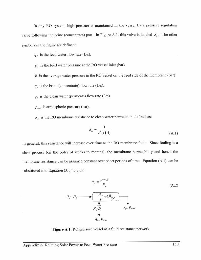
In any RO system, high pressure is maintained in the vessel by a pressure regulating
valve following the brine (concentrate) port. In Figure A. 1, this valve is labeled Rb . The other
symbols in the figure are defined:
qf is the feed water flow rate (L/s).
p1 is the feed water pressure at the RO vessel inlet (bar).
p is the average water pressure in the RO vessel on the feed side of the membrane (bar).
qb is the brine (concentrate) flow rate (L/s).
q, is the clean water (permeate) flow rate (L/s).
Patm is atmospheric pressure (bar).
Rm1 is the RO membrane resistance to clean water permeation, defined as:
R = I' K(t),Am (A.1)
In general, this resistance will increase over time as the RO membrane fouls. Since fouling is a
slow process (on the order of weeks to months), the membrane permeability and hence the
membrane resistance can be assumed constant over short periods of time. Equation (A. 1) can be
substituted into Equation (3.1) to yield:
qP =RMn (A.2)
qf qpj R
Rb qP, patm
b I Pat.t
Figure A.1: RO pressure vessel as a fluid resistance network
150Appendix A. Relating Solar Power to Feed Water Pressure

The resistance of the pressure-regulating valve, Rb, will be a function of its setting and
the flow rate of water through it [26]. At a given RO pump operating point, the brine flow is
assumed proportional to the pressure drop across the valve in Figure A.1, and an equivalent
resistance seen by the pump, ReqI can be defined as:
R - R,,Rb _ Rb
eq R, +Rb K(t)A,,Rb +1 (A.3)
The feed water volumetric flow rate q, can be calculated:
q, = PReq (A.4)
The power transferred from the solar panels to the RO fluid can be approximated by:
P1 = qff =P, elp77m ?ec (A.5)
where qp and rq, are the energy conversion efficiencies of the pump and motor, respectively
and Pe,,i is the electrical power from the solar panel, as described in Equation (3.8). Substituting
Equation (A.4) into Equation (A.5) to eliminate qf yields:
2Pf
f Req (A.6)
Both the PVRO system modeled for simulation purposes and the MIT laboratory-sized PVRO
system contain a single RO membrane element housed in a small pressure vessel. For this
reason, the average water pressure p is assumed to be approximately the same as the feed water
pressure p,.
Equation (A.6) is an approximation that is valid at constant operating points for short
periods of time. When operating a PVRO system at variable power levels for long durations of
Appendix A. Relating Solar Power to Feed Water Pressure 151

time, the flow rates and pressure levels will change since both the membrane resistance and the
pressure drop through the brine-side valve are functions of pressure and flow, respectively. With
a physical system and sensors, one can use physics-based modeling techniques to create a high-
fidelity mathematical model describing this behavior. This is impractical without a physical
system, especially when the downstream loading is both complex and unknown. Therefore, in
order to describe the conversion of electrical power to feed water pressure for long-term
simulations under variable power levels, electrical power, water flow and pressure experimental
data from MIT laboratory-sized PVRO system were scaled to electrical power, water flow and
pressure levels for a 1,000 L/day brackish water PVRO system. Since pressure is roughly
proportional to the square-root of the power, the following equation was fit to the scaled data
using the curve fitting tool in Matlab:
p = aP-' +a 2(A.7)
The curve in Equation (A.7) fits the experimental data almost perfectly (coefficient of
determination R2 value of 0.999) when the coefficients al and a2 are 1.298 and -6.182,
respectively. Another empirical relation that fits the data well (R2 value of 0.997) was found
previously, and has also been used in simulations:
Pf = (-0.7053 x 10 ) P'lc + 0.07979Ps,c + -0.8582(A.8)
Equation (A.7) captures the power-pressure relationship better at very low power levels, but
tends to over-estimate the pressure at high power (over 400 Watts from the solar panels).
Conversely, Equation (A.8) captures the high-power behavior better, but over-estimates pressure
at low power levels (below 25 Watts from the solar panels).
Appendix A. Relating Solar Power to Feed Water Pressure 152
Related Documents