Model-based energy optimization of automotive control systems

Model-Based Energy Optimizationof Automotive Control Systems

Joost-Pieter Katoen, Thomas Noll, Hao Wu†Software Modeling and Verification Group

RWTH Aachen University, Germany{katoen,noll,hao.wu}@cs.rwth-aachen.de

Thomas Santen, Dirk SeifertAdvanced Technology Labs (ATL) Europe

Microsoft Research, Aachen, Germany{thomas.santen,dirk.seifert}@microsoft.com

Abstract—Reducing the energy consumption of controllers invehicles requires sophisticated regulation mechanisms. Betterpower management can be enabled by allowing the controllerto shut down sensors, actuators or embedded control units in away that keeps the car safe and comfortable for the user, with thegoal of optimizing the (average or maximal) energy consumption.This paper proposes an approach to systematically explorethe design space of SW/HW mappings to determine energy-optimal deployments. It employs constraint-solving techniquesfor generating deployment candidates and probabilistic analysesfor computing the expected energy consumption of the respectivedeployment. The feasibility and scalability of the method isdemonstrated by several case studies.

I. INTRODUCTION

A. Problem Description

Nowadays, energy-saving activities in the transport domainmainly concentrates on the engines. But also the electroniccontrol systems in vehicles significantly contribute to theirenergy consumption. Better power management can be enabledby allowing the controller to shut down sensors, actuators orembedded control units. As vehicles have to be consideredas safety-critical systems, sophisticated regulation mechanismsare required to optimize the (average or maximal) energyconsumption while guaranteeing the user’s safety and comfortat all times. A key factor on which to base an optimizationstrategy is the operational mode of a vehicle, because not allfunctionality of a vehicle control system is used in all oper-ational modes. Examples for operational modes are: parking,driving in the city, driving on a highway, and entertainment.Operational modes can be orthogonal to one another, i.e.several modes may be active simultaneously, such as parkingand entertainment.

Software components do not work independently of oneanother. Moreover they form so called function chains, whichoperate together to perform a desired task. Among softwarecomponents we distinguish between input/output drivers andfunctional components. In a deployment step the functionchains must be mapped to existing hardware components.More precisely, input and output drivers are mapped to sen-sors and actuators, and functional components are mappedto Electronic Control Units (ECUs). Hardware and software

†Supported by ATL and RWTH Aachen University Seed Fund

Input-Driver-1 Output-Driver-1

Controller-ASensor-1

Bus

Actuator-1

Component3

Controller-B

Component1

Component2

Component4

Component5

Function-Chain-1

Function-Chain-2 Function-Chain-3

Fig. 1. An example deployment of function chains

components can be required to operate within multiple func-tion chains. That means they can be a member of manyfunction chains by consuming inputs or providing outputs forother components. Each of the different operation modes ofa car implies that a certain number of function chains are(potentially) operational and that other function chains neednot be available.

As a function chain generally consists of many softwarecomponents, all participating components are active if thefunction chain is. A hardware component must be active ifthere is an active software component in any active functionchain that is deployed to this hardware component. Shuttingdown an ECU thus disables all software components that aredeployed to this ECU or that depend on the attached sensorsand actuators.

In today’s systems the power management is quite conser-vative in disabling functionality. In this paper we present anapproach to reduce the energy consumption of an automotivecontrol system by optimizing the deployment of functionality,and subsequently exploiting the power management opportu-nities that the chosen deployment provides. In particular, ourapproach analyzes the deployment problem based on opera-tional modes and behavioral profiles, so that we can proposefunction chain deployments that allow for shutting down partsof the system while optimizing energy consumption over time(average) or to avoid peak energy consumption.

The scenario in Fig. 1 illustrates three functionchains, which are deployed to two different ECUs.Function chains can include input/output drivers, suchas Output-Driver-1. In a specific operational mode,978-3-9815370-0-0/DATE13/ c©2013 EDAA

Function-Chain-1 implicitly triggers a dependencyon Function-Chain-2, because the result of thatchain is required as an input for Component-2.Function-Chain-3 is not required to support theother chains and therefore can be put in a low-power state.An analysis of design alternatives can reveal that moving orduplicating the software component of Function-Chain-2to Controller-A will allow the system management topower down Controller-B completely in that specificoperational mode.

B. Our Optimization Approach in a Nutshell

Due to the complexity of such intelligent control systems,computer support for their design is indispensable. Our ap-proach relies on exploring the design space of embeddedsystems using the FORMULA1 tool [1], [2]. The latter is basedon model-based design and logic programming and allows forthe logical specification of non-functional requirements for thecomponents of the system. This includes e.g., schedulabilityor communication constraints. The FORMULA modeling toolcan then be used to systematically analyze the interactionsbetween and the impacts of these requirements on platformmappings and design spaces. This allows to automaticallygenerate deployment candidates, i.e., mappings of software tohardware components that satisfy the given requirements.

The FORMULA approach, however, does not allow toassess more quantitative aspects of the system, like its energyconsumption. The analysis of such properties additionallyrequires to take the timed and/or stochastic behavior of com-ponents and users into account. It is therefore necessary toextend the model-based design method towards a generate-and-test approach which comprises two steps: first, FOR-MULA generates a set of deployment candidates fulfillingthe given constraints. Second, dedicated analysis methods areapplied to evaluate the interesting quantitative properties of therespective deployment. The latter generally requires additionalinformation that FORMULA does not deal with such as usageprofiles of function chains. Given the random nature of suchprofiles in automotive embedded systems, a natural candidatefor the analysis of quantitative aspects of the SW/HW mappingare probabilistic techniques.

Fig. 2 gives a more detailed overview of our approach.The computation of the expected energy consumption (lowerbox) is essentially based on two inputs. The first is the usageprofile, specified as a discrete-time Markov chain (DTMC;upper left box) over mode configurations. The second is theset of deployment candidates (upper middle box) as providedby FORMULA. The outcome is the optimal deployment, inthe sense that the expected energy consumption (for the givenusage profile) is minimal. The procedure will be detailedfurther in this paper and will be applied to some (abstract)case studies so as to indicate its scalability and feasibility.

1http://research.microsoft.com/en-us/projects/formula/

DTMC of Mode Conf. FORMULA

ProbabilisticAnalysis

Steady-state Prob.

modeconf.

deploy.cand.

SW/HWMapping

OptimalDeployment

SW/HW Relat.Extraction

Involved HWEn. Consump.

Overall Exp. En. Consump.

Rank &Feedback

PRISMFORMULA Our Tool

Fig. 2. Overview of our approach towards energy optimization of deploymentcandidates

C. Related Work

The main novelty of our approach is the combination ofconstraint-based generation of deployment candidates withthe efficient quantitative analysis of Markov chains to anal-yse energy consumption. In our view, the constraint-basedperspective is a natural fit to deployment generation, andconceptually differs from e.g., state-based techniques suchas BIP as used in [3]. In particular, our approach allows toobtain useful information about energy optimization in anearly design phase where detailed automata-based models arenot yet at our disposal. Whereas most approaches are basedon simulation [3] or analytical techniques [4], we advocatea numerical approach to determine the maximum expectedoverall energy consumption. Energy consumption analysesof single deployments include e.g., the analysis of selectivedeactivation of ECUs in networked embedded systems [5], andprobabilistic model checking analysis [6]. Other approachesinclude e.g., the usage of non-linear convex programmingtechniques for determining optimal voltage supply [7].

II. THE FORMULA TOOL

Declarative specification languages with constraints are usedin model-driven engineering to give formal semantics, de-fine model transformations, and describe domain constraints.FORMULA (Formal Modeling Using Logic Programming andAnalysis) [1], [2] is a modern formal specification languagetargeting model-based development (MBD). The core of FOR-MULA’s approach uses algebraic data types (ADTs) andstrongly-typed constraint logic programming (CLP), whichsupport concise specifications of abstractions (domains) andmodel transformations. Specifications are understood as con-straints on relations; the logic is a class of fixpoint logic (FPL),similar to (but more general than) Datalog.

In general, logic programs have a precise execution se-mantics, so domains can be understood programmatically.However, FORMULA’s logic programs also have a preciseinterpretation as a system of first-order formulas, makingthem analyzable by existing tools. FORMULA applies thesatisfiability modulo theories (SMT) solver Z3 [8] for search.A major advantage is its model finding and design space

exploration facility. It can be used to construct system modelssatisfying complex domain constraints. The user inputs a par-tially specified model, and FORMULA searches the space ofcompleted models until it finds a globally satisfactory design.This process may be repeated to find many globally consistentdesigns. Variations on this procedure can be used to proveproperties on model transformations and to perform bounded-symbolic model checking. Specifications are composable via anovel set of operators acting on data types and logic programs.They are constructive and they make semantic guaranteesabout composite domains.

III. THE SYSTEM MODEL

This section describes the system model in detail andexplains the modeling of the usage profile.

A. System Structure

A key factor on which to base optimization strategies is theoperational mode of a system, because not every functionalityof a system is used in all modes. In turn, the functionalities or,more technically, function chains determine which (softwareand hardware) components need to be active. These entitiesare formally represented by finite sets of (operational) modes,Mod , function chains, Chn , and software and hardware com-ponents, SW and HW , respectively.

For the example system shown in Fig. 1 and using appro-priate abbreviations, we obtain the following sets. (Note thatthe figure does not visualize the modes.)• Mod = {M1,M2,M3}• Chn = {FC1,FC2,FC3}• SW = {ID1,C1, . . . ,C5,OD1}• HW = {S1,CA,CB,A1}Furthermore we need mappings that determine the relation

between modes and function chains, between function chainsand software components, and between software and hardwarecomponents. (In the following, 2S := {T | T ⊆ S} denotesthe powerset of a given set S.)• chn : Mod → 2Chn : for every m ∈ Mod , chn(m) yields

the set of function chains that are operative in mode m;• sw : Chn → 2SW : for every c ∈ Chn , sw(c) yields the

set of software components that are engaged in functionchain c (where sw(c1) and sw(c2) are not necessarilydisjoint for c1, c2 ∈ Chn); and

• dpl : SW → HW defines the deployment mapping,which determines for every s ∈ SW the hardwarecomponent dpl(s) on which software component s isrunning. We let Dpl denote the set of all such deploymentmappings.

Thus the structure of the example system is formal-ized by letting chn(M1) = {FC1,FC2}, sw(FC1) ={ID1,C1,C2,OD1}, dpl(ID1) = S1, etc.

B. Cost Parameters

In order to determine the (expected) energy consumption ofthe system for a given deployment, the following quantitativeparameters are required.

• the cycle time of the system (in ms), δ ∈ R, which de-termines the period during which its mode configurationremains unchanged;

• for every s ∈ SW , twc(s) ∈ R gives the worst-case execution time (WCET; in ms) for a single run ofsoftware component s;

• for every s ∈ SW , f (s) ∈ N gives the executionfrequency of software component s, that is, the numberof executions per cycle;

• for every h ∈ HW , Pdown /Pidle(h)/Pact(h) ∈ R re-spectively determines the power consumption of hardwarecomponent h in shutdown/idle/active state (in W). Herea hardware component is considered to be active whenit is currently executing a software component, otherwiseidle. We assume that Pdown(h) ≤ Pidle(h) ≤ Pact(h)for every h ∈ HW .

To enable proper scheduling of software components, wemoreover assume that f (s) · twc(s) ≤ δ for every s ∈ SW .

C. Behavioral Profile

With regard to the analysis of energy consumption, it isimportant to observe that operational modes can be orthogonalto each other, i.e., that several modes may be simultaneouslyactive. The overall activity of the system is therefore deter-mined by a (non-empty) set M ⊆ Mod of currently activemodes, called a mode configuration. As mentioned earlier, thisconfiguration remains constant during the execution of a singlecycle. Between cycles, however, it may change. We assumethat inter-cycle transitions can be represented by a stochasticmodel which, for a given current configuration, enumeratesall possible successor configurations that can be taken forthe next cycle, together with their associated probabilities.Clearly, the successor configurations may include the currentone. Formally, this model is a discrete-time Markov chain(DTMC), a triple (S, s0, p) where S is a countable set of stateswith initial state s0 ∈ S and p : S×S → [0, 1] is a probabilitymatrix satisfying

∑s′∈S p(s, s

′) = 1 for each s ∈ S. Thus weassume that the mode transition behavior of the given systemcan be represented by a DTMC over mode configurations, i.e.,with (finite) state space S = 2Mod \ {∅}.

For example, the diagram shown in Fig. 3 visualizes aDTMC with configurations over modes from the set Mod ={M1,M2,M3}. A possible interpretation is that M1 and M2respectively represent the parking and driving mode of thevehicle while M3 indicates the activity of the entertainmentsystem. Thus M1 and M2 exclude each other (and therefore donot occur jointly in any reachable configuration) while M3 isorthogonal to the other two modes. The initial state, {M1}, ismarked by an ingoing arrow.

IV. THE ANALYSIS

The goal of our analysis is to rank the deployment can-didates as provided by the FORMULA tool with respect totheir (expected) energy consumption. Clearly the analysis hasto employ probabilistic methods as the underlying behaviormodel, DTMCs, is of a stochastic nature. More concretely, for

M1 M2

M1M3

M2M3

0.10.4

0.1

0.4

0.4

0.1

0.1

0.4

0.1

0.10.4

0.4

0.4

0.1

0.4

0.1

Fig. 3. A DTMC over mode configurations

a given deployment candidate, the expected energy consump-tion of the system using that deployment can be determinedin the following way.

1) Compute the steady-state probabilities for all states inthe DTMC.

2) Compute the energy consumption in each of the states,and attach it as reward information to the DTMC.

3) Compute the expected overall energy consumption percycle as the expected reward.

These steps are detailed in the following.

A. Computation of Steady-State Probabilities

Evaluating the energy consumption of a system is based oncomputing the stationary distribution of the DTMC (S, s0, p).It gives the probability of being in a certain state when takinga snapshot after a very long time or, in other words, theproportion of time that the DTMC “spends” in that state inthe long run. Under certain mild assumptions regarding theDTMC (which usually apply in our setting), this distributioncan be characterized by a flow balance equation system of theform

π = π · p

which expresses that the total probability flow out of a stateis equal to the total flow into the state.

The stationary distribution, that is, the solution π of theequation system can be computed using tools such as PRISM[9], based on the given DTMC. Note that this computationis independent of the concrete deployment. It therefore needsto be done only once in the beginning of the analysis beforespecific deployment candidates are considered.

B. Energy Consumption per Mode Configuration

Knowing the stationary distribution of the DTMC, theexpected overall energy consumption per cycle with respectto a given deployment candidate can be determined by firstcomputing the energy consumption per cycle for each of themode configurations in the DTMC, and second weighting it

with the stationary probability of the respective configuration.This section describes the first step in detail.

Given the current mode configuration M ⊆ Mod (i.e., astate of the DTMC) and the deployment mapping dpl ∈ Dpl ,the maximal energy consumption in mode M per cycle withrespect to dpl can be computed as follows.

1) Determine the function chains that are operative in M :

Chn(M) :=⋃

m∈Mchn(m) ⊆ Chn.

2) Determine the engaged software components:

SW (M) :=⋃

c∈Chn(M)

sw(c) ⊆ SW .

3) Determine the engaged hardware components:

HW (M) := dpl(SW (M)) ⊆ HW .

4) For every h ∈ HW (M):a) Determine the engaged software components that

are deployed on h:

SW (h) := SW (M) ∩ dpl−1(h) ⊆ SW .

Here dpl−1 : HW → 2SW denotes the inversemapping of dpl , defined by dpl−1(h) := {s ∈SW | dpl(s) = h}.

b) For every s ∈ SW (h), determine the active timeof s (independent of mode M ):

tact(s) := f (s) · twc(s).

c) Determine the active time of h:

tact(h) :=∑

s∈SW (h)

tact(s).

5) This yields the maximal energy consumption in modeconfiguration M per cycle:

E(M) :=∑

h∈HW \HW (M) Pdown(h) · δ+

∑h∈HW (M)E(h) where

E(h) := Pact(h) · tact(h) + Pidle(h) · (δ − tact(h)).

Here, E(h) is the expected energy usage of an engaged HWcomponent expressed as weighted sum over the active timeand idle time, respectively.

C. Expected Overall Energy Consumption

The expected overall energy consumption per cycle forthe given deployment mapping can easily be obtained bycomputing the expected reward

E(dpl) =∑

M⊆Mod

π(M) · E(M)

whose minimization yields the energy-optimal deployment.

#Mode conf. #Modes #FC #SW #HW #Dpl. Comp. time4 3 3 7 4 16 1075 ms

TABLE IOVERVIEW OF THE EXAMPLE

V. EVALUATION

The analysis described in the previous section has beenimplemented in a tool that, given a set of deploymentsdetermined by FORMULA, computes the expected energyconsumption of each candidate. This section gives the result ofsome experiments to explore its capabilities. They were carriedout on a machine equipped with an 3.06 GHz Intel Core i7CPU and 5.8 GB of memory. We start with the evaluation ofthe running example, using 16 different deployments. Next weexplore the scalability of our tool by changing certain modelsize parameters during deployment generation.

A. Running Example

In this experiment, we first use FORMULA to specifyall parameters and constraints, and then generate a set ofcandidate deployments to compute their energy consumption.The parameters are those described in Section III, dealing bothwith the static part of the system structure (cf. Section III-A)and with its cost parameters (cf. Section III-B). Furthermore,FORMULA allows to specify some requirements that the gen-erated deployments should satisfy, such as the schedulabilityof the resulting system, the minimal or maximal number ofsoftware components that are mapped to one hardware compo-nent, etc. Based on this information, FORMULA generates thepossible deployments using SMT-based methods as sketchedin Section II. We again refer to [1], [2] for details.

Each deployment is exported as a 4ml file including addi-tional information for energy consumption computation, andthen our tool will import these files and extract the informationfor further processing. The steady-state probabilities of themode configurations (cf. Section IV-A) are obtained by callingthe PRISM2 model-checking tool. Based on the results, ourtool computes the expected energy consumption per cycle foreach deployment and returns the deployment with minimalenergy consumption.

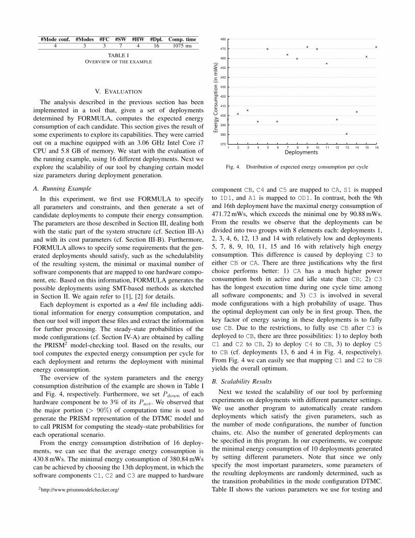
The overview of the system parameters and the energyconsumption distribution of the example are shown in Table Iand Fig. 4, respectively. Furthermore, we set Pdown of eachhardware component be to 3% of its Pact . We observed thatthe major portion (> 90%) of computation time is used togenerate the PRISM representation of the DTMC model andto call PRISM for computing the steady-state probabilities foreach operational scenario.

From the energy consumption distribution of 16 deploy-ments, we can see that the average energy consumption is430.8 mWs. The minimal energy consumption of 380.84 mWscan be achieved by choosing the 13th deployment, in which thesoftware components C1, C2 and C3 are mapped to hardware

2http://www.prismmodelchecker.org/

370

380

390

400

410

420

430

440

450

460

470

480

1 2 3 4 5 6 7 8 9 10 11 12 13 14 15 16

Ener

gy C

onsu

mpt

ion

(in m

Ws)

Deployments

Fig. 4. Distribution of expected energy consumption per cycle

component CB, C4 and C5 are mapped to CA, S1 is mappedto ID1, and A1 is mapped to OD1. In contrast, both the 9thand 16th deployment have the maximal energy consumption of471.72 mWs, which exceeds the minimal one by 90.88 mWs.From the results we observe that the deployments can bedivided into two groups with 8 elements each: deployments 1,2, 3, 4, 6, 12, 13 and 14 with relatively low and deployments5, 7, 8, 9, 10, 11, 15 and 16 with relatively high energyconsumption. This difference is caused by deploying C3 toeither CB or CA. There are three justifications why the firstchoice performs better: 1) CA has a much higher powerconsumption both in active and idle state than CB; 2) C3has the longest execution time during one cycle time amongall software components; and 3) C3 is involved in severalmode configurations with a high probability of usage. Thusthe optimal deployment can only be in first group. Then, thekey factor of energy saving in these deployments is to fullyuse CB. Due to the restrictions, to fully use CB after C3 isdeployed to CB, there are three possibilities: 1) to deploy bothC1 and C2 to CB, 2) to deploy C4 to CB, 3) to deploy C5to CB (cf. deployments 13, 6 and 4 in Fig. 4, respectively).From Fig. 4 we can easily see that mapping C1 and C2 to CByields the overall optimum.

B. Scalability Results

Next we tested the scalability of our tool by performingexperiments on deployments with different parameter settings.We use another program to automatically create randomdeployments which satisfy the given parameters, such asthe number of mode configurations, the number of functionchains, etc. Also the number of generated deployments canbe specified in this program. In our experiments, we computethe minimal energy consumption of 10 deployments generatedby setting different parameters. Note that since we onlyspecify the most important parameters, some parameters ofthe resulting deployments are randomly determined, such asthe transition probabilities in the mode configuration DTMC.Table II shows the various parameters we use for testing and

#Mode conf. #Modes #FC #SW # HW100-1000 100-1000 10-100 100-1000 100-1000

TABLE IISCALABILITY PARAMETERS

20 40 60 80

100 120 140 160 180 200 220 240 260 280 300 320 340 360 380 400 420 440 460 480 500 520 540 560

100 200 300 400 500 600 700 800 900 1000

Com

puta

tion

time

(in s

)

0

sw

md. cfmode

hw

Parameter Size

Fig. 5. Scalabilty test for configurations, modes, SW and HW components

their value ranges.The computation time distributions for different parameter

settings are shown in Fig. 5 and 6. The first successively variesthe number of mode configurations (md. cf), modes, softwarecomponents (sw) and hardware components (hw), which allincrease from 100 to 1000 in steps of 100, respectively. Here,the sizes of the non-varying parameters (mode configurations,modes, software and hardware components) are fixed to 10, 5,1000 and 10, respectively. Moreover the number of functionchains of these generated deployments is fixed to 20. Theresults indicate that the number of hardware components hasthe strongest influence on the computation time whereas theother three parameters have a similar, weaker effect.

In addition, Fig. 6 shows that the number of function chainshas an even more significant impact on the computation time.About 2122 s (≈ 35 min) are needed to find the optimaldeployment for 100 function chains whereas only 36 s arerequired for 10 chains. (The number of mode configurations,modes, software and hardware components is again fixed to10/5/1000/10.) Finally we performed a maximal test (whoseresult is not shown in the figures) by computing 10 de-ployments for 100 mode configurations, 1000 modes, 100function chains, 1000 software components and 100 hardwarecomponents. The computation takes about 5702 s (≈ 95 min),which exceeds the longest time shown in Fig. 6 by a factor ofabout 2.7.

75 150 225 300 375 450 525 600 675 750 825 900 975

1050 1125 1200 1275 1350 1425 1500 1575 1650 1725 1800 1875 1950 2025 2100 2175

10 20 30 40 50 60 70 80 90 100

Com

puta

tion

Tim

e (in

s)

fc

Parameter Size

Fig. 6. Scalabilty test on function chains

VI. CONCLUSION

This paper presented a novel combination of constraint-based deployment generation and quantitative analysis todetermine the SW/HW deployment that minimizes expectedenergy consumption. The approach has been implemented ina prototypical tool-chain using FORMULA and PRISM astool components. Our experimental results show the sensitivityon several parameters and indicate a good scalability. Furtherresearch includes the application to automotive case studies.

REFERENCES

[1] E. K. Jackson, E. Kang, M. Dahlweid, D. Seifert, and T. Santen,“Components, platforms and possibilities: Towards generic automationfor MDA,” in Proc. 10th Int. Conf. on Embedded Software (EMSOFT 10).ACM, 2010, pp. 39–48.

[2] E. K. Jackson, D. Seifert, M. Dahlweid, T. Santen, N. Bjørner, andW. Schulte, “Specifying and composing non-functional requirements inmodel-based development,” in Proc. 8th Int. Conf. on Software Compo-sition (SC 2009), ser. LNCS, vol. 5634. Springer, 2009, pp. 72–89.

[3] P. Bourgos, A. Basu, M. Bozga, S. Bensalem, J. Sifakis, and K. Huang,“Rigorous system level modeling and analysis of mixed HW/SW sys-tems,” in 9th IEEE/ACM Int. Conf. on Formal Methods and Models forCodesign (MEMOCODE 2011). IEEE, 2011, pp. 11–20.

[4] B. Theelen, M. Geilen, T. Basten, J. Voeten, S. Gheorghita, and S. Stuijk,“A scenario-aware data flow model for combined long-run average andworst-case performance analysis,” in 4th IEEE/ACM Int. Conf. on FormalMethods and Models for Codesign (MEMOCODE 2006). IEEE, 2006,pp. 185–194.

[5] C. Schmutzler, M. Simons, and J. Becker, “On demand dependentdeactivation of automotive ECUs,” in Design, Automation & Test inEurope (DATE 2012). IEEE, 2012, pp. 69–74.

[6] G. Norman, D. Parker, M. Z. Kwiatkowska, S. K. Shukla, and R. Gupta,“Using probabilistic model checking for dynamic power management,”Formal Asp. Comput., vol. 17, no. 2, pp. 160–176, 2005.

[7] X. Piao, H. Kim, Y. Cho, M. Park, S. Han, M. Park, and S. Cho, “Energyconsumption optimization of real-time embedded systems,” in Int. Conf.on Embedded Software and Systems (ICESS 2009). IEEE, 2009, pp.281–287.

[8] L. M. D. Moura and N. Bjrner, Z3: An Efficient SMT Solver, 2008.[9] M. Kwiatkowska, G. Norman, and D. Parker, “Probabilistic symbolic

model checking with PRISM: a hybrid approach,” Int. J. on SoftwareTools for Technology Transfer, vol. 6, no. 2, pp. 128–142, 2004.