Model-based Aeroservoelastic Design and Load Alleviation of Large Wind Turbines

Model-based Aeroservoelastic Design and Load

Alleviation of Large Wind Turbines

Bing Feng Ng∗, Henrik Hesse†, Rafael Palacios‡, J. Michael R. Graham§, and Eric C.Kerrigan¶

Imperial College London, South Kensington Campus, London SW7 2AZ

This paper presents an aeroservoelastic modeling approach for dynamic load alleviationin large wind turbines with trailing-edge aerodynamic surfaces. The tower, potentially on amoving base, and the rotating blades are modeled using geometrically non-linear compositebeams, which are linearized around reference conditions with arbitrarily-large structuraldisplacements. Time-domain aerodynamics are given by a linearized 3-D unsteady vortex-lattice method and the resulting dynamic aeroelastic model is written in a state-spaceformulation suitable for model reductions and control synthesis. A linear model of a singleblade is used to design a Linear-Quadratic-Gaussian regulator on its root-bending moments,which is finally shown to provide load reductions of about 20% in closed-loop on the fullwind turbine non-linear aeroelastic model.

Nomenclature

MSS Discrete mass matrix

CSSgyr Gyroscopic damping matrix

KSSgyr Gyroscopic stiffness matrix

KSSstif Stiffness matrix

Qext External forces

MSR Coupling mass matrix

CSRgyr Coupling damping matrix

η Nodal dispacements and rotationsν Rigid body velocitiesλ Lagrange multipliersAc Aerodynamic influence coefficient matrixΓ Vortex circulation strengthΦ Constraint functionφ Nonholonomic constraintx State variablew Aerodynamic downwashβ Flap deflection angleδ External disturbanceΩ Rotational speedθ Azimuth anglen Time stept TimeSub-, Superscripts(•)0 Equilibrium conditions

∗Graduate Student, Department of Aeronautics (email: [email protected]), AIAA Student Member.†Research Associate, Department of Aeronautics, AIAA Member.‡Senior Lecturer, Department of Aeronautics (email: [email protected]), AIAA Member.§Professor, Department of Aeronautics.¶Senior Lecturer, Department of Electrical and Electronic Engineering, Department of Aeronautics.

1 of 21

American Institute of Aeronautics and Astronautics

(•)b Blade representation(•)w Wake representation(•)k Collocation point representation(•)r Rotor representation(•)t Tower representation(•)s Hub representation(•)η Structural representation(•)ν Rigid body representation(•)β Flap representation(•)δ Gust representation(•)S Structural degrees of freedom(•)R Rigid body degrees of freedom˙(•) Derivative with respect to time t

AbbreviationsUVLM Unsteady Vortex-Lattice MethodFoR Frame of Referencerms Root-Mean-SquareDEL Damage Equivalent LoadRBM Root-Bending Moments

I. Introduction

The size of wind turbines has doubled each decade for the past 30 years, both in terms of tower heightand rotor diameter. The largest wind turbines in operation have rotors measuring above 120m in diameter,and rotors of up to 160m are already being developed.1 Aeroelastic effects previously not seen in smallerrotors are beginning to surface as a result of increased flexibility from the longer blades.2 This broughtabout new needs in terms of modeling requirements, as blade flexibility may have a significant effect inthe performance characteristics of turbines. It also poses new technological challenges, in particular, withrespect to an increased need for methods of load control to avoid unnecessary loadings and oscillations ofthe flexible blades that would impact their fatigue life.3

A number of design codes have been developed in recent years for aeroelastic analysis of wind turbines,including NREL’s open source FAST, DTU’s FLEX5, DTU Wind’s HAWC2, TU Delft’s DU SWAMP,and GL Garrad Hassan’s Bladed, among others .4–11 Their structural models are based on either directfinite-element solutions or assumed modes approaches, while their aerodynamics relies on blade-elementmomentum theory with various, mostly empirical, corrections to account for dynamic inflow, stall and tiploss effects.2,12 For larger and typically offshore turbines, there will be larger aeroelastic couplings, towermotions, and structural deformations on the more flexible blades, and consequently a potential for increased3-D aerodynamic effects. Hence, an alternative description based on a time-domain Unsteady Vortex-LatticeMethod (UVLM)13 formulation could provide a better characterization of the aeroelastic responses underattached flow conditions. This will be explored in this paper. As it will also be shown, such an approachcan be directly formulated in a suitable manner for model reductions, control synthesis and design.

Existing turbines are fitted with pitch control systems for speed regulation. Their actuation is howeverrelatively slow14 and their use as load alleviation system is therefore limited to low-frequency excitations.Distributed load alleviation systems, placed along the blade span, can overcome such limitations and theseconcepts, which derive from well-known solutions in air vehicles, are gaining momentum in wind turbine re-search. They can be designed to complement existing pitch control mechanisms by tackling higher frequencyloadings, or even be used to exploit aeroelastic twisting of the rotor blades. Using trailing-edge flaps for loadreduction, Frederick et al.,15 Riziotis et al.16 and Basualdo17 were able to achieve significant reduction inloadings on simple 2-D aeroelastic models, while Barlas et al.7,18 and Wilson et al.19 have demonstratedthe performance of multiple flaps on a full rotor. Concepts for conformable trailing-edge flaps20–23 and mi-crotabs24 have also shown great potential. Comparisons between various active control concepts have beenrecently investigated by various authors.1,25–27 To date, there is no commercial application of the active flapconcept on existing wind turbines, but a recent full-scale experiment was conducted by Castaignet et al.28 ona Vestas V27 wind turbine using frequency-weighted model predictive control (MPC), and demonstrated the

2 of 21


potential of trailing-edge flaps by reducing average flapwise blade root load by 14%. Also, Sandia NationalLaboratories have designed and built turbine blades equipped with aerodynamic flaps for testing.29,30

Barlas et al.7 have reviewed the most recent developments in the use of active flaps on wind turbines forload reduction, and have reported the performance predicted through the use of different control methods.A wide spectrum of numerical results was found: various authors have reported reductions in root-bendingmoments (RBM) ranging from 10% up to 30%, depending on the type of controller used and also the size anddistribution of flaps. To the best of our knowledge, the only work that involved the aeroelastic modeling ofwind turbine blades using vortex methods was by Riziotis et al.,16 who used a vortex panel code coupled witha structural module. Using PID control and trailing-edge flaps with lengths ranging between 15% and 50%span, the authors demonstrated a load reduction of up to 30% under an exponential wind shear profile. Infact, most of the works in active aeroelastic control of wind turbines has relied on classical control methods,such as PD and PID, with only a few of the more recent works considering modern control methods, suchas LQR or predictive control.7,19 This is probably because the intention has normally been to show thepotential of feedback control in enhancing the aeroelastic performance of the blades, but in a recent study,31

we have shown that PD may need up to 70% more actuation power than a robust controller under similarload reduction targets.

Within this context, this paper will extend the previous study of modeling and load alleviation on asingle rotating blade to the full wind turbine.32 It will introduce a model-based control design by firstimplementing the vortex-lattice method in an efficient state-space representation. This is subsequentlycoupled to a linearized structural dynamics description of the turbine rotor to produce a compact formsuitable for aeroservoelastic analysis. The approach will then be used to model the NREL 5-MW referenceoffshore wind turbine rotor, which is attached to the tower through Lagrange multipliers for prescribedrotations. We will then use the model to demonstrate the use of flaps in reducing the root-mean-square(rms) values of RBM, tip deflections and fatigue using LQG controllers.

II. Methodology

The aeroservoelastic modeling of wind turbines will be based upon the integrated framework for theSimulation of High Aspect Ratio Planes (SHARP), which has been developed in previous works for flexibleaircraft applications, including static aeroelastic analyses, linear stability analyses, control synthesis andnon-linear open-loop time-marching simulations.33–36 The following description provides an overview of theunderlying structural and aerodynamic models, which have been tailored in this work for application to largewind turbines.

A. Composite beam model

Taking advantage of the slenderness of the tower and blades, their structural deformations will be modeledusing a composite beam formulation written in a rotating frame of reference.37,38 In its original implemen-tation,33 the structural model can account for large static and transient deformations of the blades, whichhas been reduced to a 1-D representation in the 3-D space, using an appropriate cross-sectional analysismethodology.39 For the purpose of efficient control synthesis, this work will focus on the linearized approachthat provides a compact form of the equations of motion (EoM) around a possibly geometrically non-linearsteady-state equilibrium.

As shown in Figure 1, the deformation of the structure is described in terms of a hub-fixed (structural)reference coordinate system, S, which moves according to the hub translational and angular velocities, vS(t)and ωS(t), respectively. The global motions of the rotor blades are given by the hub rigid-body velocitiesν> =

[v>S ω>S

], with respect to an inertia frame G. To account for large blade deformations, the local

orientation of each cross section along the beam reference line is defined by a local coordinate system Band is parametrized at time t by the Cartesian Rotation Vector Ψ(s, t), where s is the arc-length along thebeam reference line.33,38 Hence, the nodal positions RS(s, t), expressed in the hub-fixed frame S, and thecross-sectional orientations, Ψ(s, t), form the independent set of variables for the structural problem.

After a finite-element discretization, the equations of motion for the structural subsystem are then ob-tained as:34,38

MSS (η) η + MSR (η) ν +Qgyr (η, η,ν) +Qstif (η) = Qext, (1)

where the discrete mass matrix MSS and the discrete gyroscopic, elastic and external generalized forces,

3 of 21


Local FoR

Inertia FoR

Hub FoR

B

S

G

RS

S S,

RS

r

Figure 1: Multi-beam configuration with the definition of reference frames for the rotor model.

Qgyr, Qstif and Qext, respectively, are obtained through a finite element discretization of the primaryvariables, with η the column matrix with all the nodal displacements and rotations. Equation (1) capturesthe possibly large deformations of the blades by balancing the discrete inertial and elastic forces with theexternal aerodynamic forces. The inertial couplings due to ν and ν, which are functions of time, areincorporated through the coupling mass matrix MSR and the gyroscopic forces Qgyr. The superscripts Sand R, denoting structural and rigid-body contributions, respectively, highlight the coupling between theblade structural dynamics and the overall (rigid-body) motion of the rotor.

To arrive at a compact state-space form of the aeroelastic EoM suitable for control synthesis, the struc-tural dynamics equations are linearized around a geometrically non-linear steady-state equilibrium condition(η0, η0 = 0,ν0). This steady-state solution is obtained by neglecting all time derivatives in Equation (1).The incremental form of the beam EoM is:

MSS (η0) ∆η + MSR (η0) ∆ν +CSSgyr (η0,ν0) ∆η +CSR

gyr (η0,ν0) ∆ν+

+[KSSgyr (η0,ν0) +KSS

stif (η0)]

∆η = ∆Qext,(2)

where the contribution to the (constant) mass, damping and stiffness matrices has been obtained throughdirect linearizion of the different generalized forces with respect to η and its time derivatives. The effects oftower oscillation is accounted for in the coupling mass and damping matrices, MSR and CSR

gyr, respectively.A detailed derivation of Equation (2) can be found in Hesse and Palacios.33 These linearized beam equationsalso preserve the rotational effect due to the prescribed angular velocity Ω through the contribution of thelinearized gyroscopic forces to the damping and stiffness matrices CSS

gyr and KSSgyr, respectively.

The resulting linear system can be cast into state-space form from which we can define an eigenvalueproblem that includes rotational effects and geometrically non-linear equilibrium deformations. At last,the state-space system is discretized in time using a standard Newmark-β discretization method40 for theintegration of the structural dynamics equations with the discrete-time unsteady aerodynamic formulation.

B. Flexible multi-body dynamics

The inclusion of tower dynamics in the modeling of large wind turbines constitutes a multi-body dynamicsproblem. Similar to the blades, the tower is modeled using beam elements and its structural dynamics aredescribed with respect to a global frame A at the tower base. The motion of this frame is further described

4 of 21


Bt

hub FoR

S

Tower Base FoR

Tower top

local FoR

AG

Inertia FoR

Figure 2: Multi-body configuration with the definition of reference frames for the combined rotor and towermodel.

with respect to the inertia frame G and parametrized through quaternions, to account for any motion ofthe tower found in floating structures. The tower and rotor are connected using Lagrange multipliers, whichconstrain the nodal velocities of the local frame Bt at the tower top to the translational and angular velocitiesof frame S fixed to the rotor hub, as shown in Figure 2. Next, the extension of the beam equations to multiplebodies is given in the context of large wind turbines assuming the problem is posed as an open kinematicchain.

The constraints between N connected flexible bodies are conveniently enforced in the weak form of theequations of motions using Lagrange multipliers.38 Starting from Hamilton’s principle, we get:

∫ t2

t1

N∑i=1

[∫Li

δTi − δUi + δWi ds

]+

N∑i=1

N∑j=1j 6=i

[δΦ>ijλij + δλ>ijΦij

] dt = 0, (3)

where Ti and Ui are the kinetic and internal energy densities, respectively, and δWi is the virtual work perunit length of body i. These virtual quantities have been defined in Refs.33,34 in terms of the infinitesimalbeam kinematics, i.e. the local beam strains and velocities. Each constraint between two connected bodies(tower and rotor) is enforced using six Lagrange multipliers λ, for three translational and three rotationalconstraints, while Φ is the corresponding constraint function. Due to the parameterization of large rotationsin the present geometrically non-linear description of flexible bodies, it is convenient to enforce the constraintsin terms of velocities, which leads to nonholonomic (bilateral) constraints, written in general as:38

Φij

(˙ηi, ηi,νi,νj

)= Φnh

ij (ηi)

˙ηiνi

νj

+ φij = 0, (4)

where ηi are the nodal displacements and rotations at the end of body i. In the context of the wind turbinemodel, i and j denote the tower and rotor degrees of freedom, respectively, and ηi corresponds to thedisplacements and rotations of tower top frame Bt, as defined in Figure 2. From the kinematic description of

5 of 21


the beam displacements and velocities in Hesse and Palacios,33 we can write the nonholonomic constraintsas:

Φnhij =

[Λ(ηi) ARC(ηi) −ACC(ηi,ν0,j)

]and

φij = ACC(ηi,ν0,j)ν0,j(t),(5)

where Λ, ARC , and ACC are transformation matrices to enforce the velocity constraints in the local frameat the end of body i. At last, ν0,j(t) accounts for possible (time-varying) prescribed velocities of body j,which will be used in this paper to introduce the (constant) angular velocity of the rotor. The resultingchange in orientation between the rotor frame S and the tower top frame Bt is accounted for in matrix ACC

which transforms the velocities of the rotor hub to the tower top frame Bt.As for a single body, a finite element discretization of the primary variables, the displacements and

rotations of all blades, finally leads to the discrete form of the augmented system equations, given as:

M (η)

η

ν

+Qgyr (η, η,ν) +Qstif (η) = Qext −Φ>nhλ− Jλ

Φnh

η

ν

+ φ = 0

. (6)

where η is the resulting column matrix with all the nodal displacements and rotations of the N bodies and

ν =[ν>1 , · · · ,ν>N

]>. Hence, Equation (6) extends the original flexible-body dynamics equations with the

additional constraints, where Φnh represents the nonholonomic quantity of all constraints and φ is the vectorof all prescribed velocities, both defined in Equation (5) for a constraint between two bodies i and j. Finally,J is the tangent matrix of all algebraic constraints defined between two bodies as J ij = ∂Φij/∂ηi. Notethat the discrete mass matrix, M, and the discrete generalized forces, Qgyr, Qstif and Qext, respectively,now include the structural and rigid-body contributions of all bodies.

The augmented equations for the coupled wind turbine problem, Equation (6), can also be linearizedaround the steady-state equilibrium with constant rotor velocity leading to a compact form of the equationscoupling the tower and rotor dynamics, written as:

MSSt 0 0 −ΛT

0 MSSr MSR

r 0

0 MRSr MRR

r ATCC(θ)

0 0 0 0

∆ηt∆ηr∆νr

∆λ

+

CSSt 0 0 0

0 CSSr CSR

r 0

0 CRSr CRR

r 0

Λ 0 −ACC(θ) 0

∆ηt∆ηr∆νr

∆λ

+

KSSt 0 0 0

0 KSSr 0 0

0 KRSr 0 0

0 0 0 0

∆ηt∆ηr

0

0

=

Qext∫Qext

0

0

,(7)

with the subscripts t and r corresponding to the tower and rotor, respectively. The prescribed rotor velocityand azimuth angles of the rotor blades at steady-state, Ω and θ = Ωt, respectively, leads to gyroscopiccontributions to the damping and stiffness matrices with non-negligible effects on the vibration frequenciesof the coupled system.32 Linearization around steady-state greatly simplifies the incremental form of theconstraint function included in the last row of Equation (7). Note however that the transformation matrixACC(θ), which projects the incremental hub velocities to the local frame Bt at the tower top, becomes aperiodic function due to the prescribed rotor velocity, Ω.

C. Unsteady aerodynamics model

The aerodynamics are modeled using the discrete-time UVLM36,41 with a prescribed helicoidal wake, whichallows non-stationary aerodynamics to be captured in low-speed, high-Reynolds-number attached-flow con-ditions for arbitrary blade kinematics. The UVLM uses vortex rings as fundamental solutions, which arelocated in lattices that represent the blades (modeled as a lifting surface) and their wakes (modeled as thinshear layers). The leading segment of the vortex ring is placed along the quarter chord of each panel. The

6 of 21


b

b

Collocation

point k

Bound Vortices

Wake Vortices

Figure 3: Typical thin lifting surface represented by the Unsteady Vortex-Lattice Method.

collocation points are then placed at the three-quarter chord where boundary conditions are imposed. Inthe current implementation, the aerodynamics of the tower is neglected.

The wake vortex is convected downstream by both the freestream velocity and also the velocity inducedby all other vortices. The influence of the latter is commonly known as wake roll-up and introduces non-linearities in the model. To obtain linear models for control methods, we could freeze the model with wakeroll-up and linearize around that point. Alternatively, the effect of wake roll-up can be ignored. In thispaper, the latter method was adopted such that the wake was assumed to be helicoidal.42

In the UVLM, Neumann boundary conditions are imposed on the lifting surface. Hence, the normalvelocity at each collocation point due to vortices (blade and wake) and motion of the blade has to be zero.This relationship is given by:

Ac,bΓn+1b +Ac,wΓn+1

w +Ac,xΓn+1x +wn+1 = 0 , (8)

where Γb and Γw denotes the bound and wake vortex rings respectively (shown in Figure 3), and Γxaccounts for circulations (both bound and wake) due to multiple blades. Ac,b, Ac,w and Ac,x are theinfluence coefficients that gives the induced normal velocity to blade surface at collocation points (resolvedusing the Biot-Savart law) due to bound and wake vortices, and n is the time step. The last term w isthe downwash at collocation points and is generated by the motion of the lifting surface wb (the blade),rigid body motions wν (such as the deflection of the tower), the actuators wβ (such as trailing-edge flaps)and external disturbances wδ (such as gusts). The downwash are all in the same time step and the firsttwo contributions wb and wν will disappear in the process of coupling with the structural dynamics. Thelast two contributions wβ and wδ will appear as inputs to the system and in order for the final equationsof motion to be in explicit form, they are written in time step n instead of n + 1, assuming effects on thesolution will be minimal if time steps are kept small:

wn+1 = wn+1b +wn+1

ν +wnβ +wn

δ . (9)

In particular, the downwash due to motion of the lifting surface wb is mapped from the structural beammodel of the rotor blades and can be represented using:

wn+1b =

[T∆η T∆η

] [∆ηr∆η

]n+1

, (10)

where T∆η and T∆η project the contribution of the nodal displacements ∆η and velocities ∆η onto theaerodynamic lifting surface as downwash terms.

7 of 21


S

Structural beam nodesAerodynamic panel collocation point

Figure 4: Coupling between fluid and structure. Structural displacements and velocities are mapped ontoaerodynamic collocation points as downwash. Pressures on the aerodynamic panels are mapped onto struc-tural nodes as forces and moments.

The downwash due to rigid body motion of the rotor is expressed as:

wn+1r = T∆ν(θ)∆νn+1

r , (11)

where in the context of the wind turbine, T∆ν is varying with the azimuth location θ of the rotor bladeswith respect to the tower.

Pressure distribution across each panel on the lifting surface can be computed using the unsteadyBernoulli equation,41 from which the aerodynamic forces in each panel are obtained. This can be expressedin compact form as:

∆Pn+1k = Φn+1

k Γn+1b + Φn

kΓnb , (12)

where Γn+1b contains circulation strengths of all vortex rings on the lifting surface.

Since the UVLM is based on thin wing theory, special care is needed to obtain the leading-edge suction.43

In steady flow, pressure forces in the direction of flow are canceled by leading-edge suction, arising in zerodrag, which is commonly known as the d’Alembert’s paradox. In the case of unsteady flow, drag may bepresent and an approximation given by Katz et al.41 is used, expressed compactly as:

Dn+1k = Υn+1

k Γn+1b + Υn

kΓnb , (13)

D. Aeroelastic equations

The continuous-time structural equations of motion of the wind turbine are discretized using the Newmark-β method and the blades are subsequently coupled with the discrete-time UVLM. As each lifting surfaceis comprised of panels while the structure is modeled using beams that run along the span of the blades,aerodynamic loads are mapped onto the beam nodes as shown in Figure 4.

In the coupled model description, the structural beams representing the rotor blades are linearized arounda prescribed rotational velocity, and non-linearity enters the system through the constraint equation (4),which is azimuth dependent in the transformation matrix. The UVLM is also linear in the rotor descriptionbut the coupling term in Equation 11 injects an azimuth dependent downwash due to tower deflection onto thepanel collocation points. The aeroelastic formulation accommodates for rotor anisotropy such as imbalanceand also external anisotropy pertaining to operating conditions such as wind shear, rotor imbalance, yawerror and gravity.44

With each bound and wake circulation in the UVLM model representing a state, the coupled equations ofmotion are huge, causing simulation to be computationally expensive. Furthermore, the rotation of the rotorimposes non-linearity in both the constrained structural equations of motion and the coupling terms withaerodynamics, rendering model reduction on the final aeroelastic system infeasible. Hence, the structuraland UVLM models are reduced separately prior to coupling. Firstly, the structural degrees of freedom aretruncated using classical modal decomposition40 on individual beams. Next, the UVLM model is reducedthrough balanced truncation which Hesse and Palacios45 have demonstrated its effectiveness in reducinglarge flexible aircraft models.

8 of 21


The resulting equations of motion between the constrained structural model and UVLM provide the fullaeroelastic system in state-space representation.35 The equations can be written in the standard form:

xn+1 = A(θn)xn +Bwnβ +Gwn

δ ,

yn = Cxn +Dwnβ +Hwn

δ ,(14)

where the state matrix A is a function of the azimuth angle θ, which defines the orientations of the rotorblades with respect to the tower at each time step n. The state vector that completely defines the aeroelasticsystem is:

xT =[∆ΓTb ∆ΓTw | ∆ηTt ∆ηTt ∆ηTr ∆ηTr | ∆νT ∆λT

], (15)

containing the aerodynamics, structures and rigid body states. The inputs to Equation (14) are from thedownwash terms in Equation (9). Note that the downwash due to motion of lifting surface wb and rigidbody motion wν does not appear, since it is coupled to the structural dynamics. The control input wβ

represents the downwash due to flap motion and the external disturbance wδ is the downwash due to gust.The output vector, y, includes the desired output (e.g., blade root-bending moments, tip deflection, towertop deflection).

III. Closed-loop model

The control input for Equation (14) contains the flap deflection angle β(t) and its time derivative. Hence,a double integrator46 is introduced such that the control input is now the flap acceleration, β(t). The inflowspeed to the rotor is constant and disturbance enters the system in the form of turbulence in the longitudinaldirection that is assumed to be homogeneous in the rotor disk. It is simulated by passing white Gaussiannoise through a filter such that the signal output will have a von Karman turbulence spectrum that is notaffected by the mean flow field of the rotor. A simplified closed-loop block diagram of the aeroelastic modelis illustrated in Figure 5. In the same figure, wδ represents the external disturbance (Gaussian) that ispassed through the von Karman filter to produce the turbulence signal δ, and v accounts for any externalmeasurement noise.

Due to the characteristics of the disturbance (Gaussian), LQG controls will be considered in this pa-per. For a Gaussian disturbance, a LQG controller minimizes the expected value of the quadratic costfunction:47,48

J = limN→∞

1

N

N−1∑n=0

((xn)

TQxn +

(βn)T

Rβn), (16)

where Q and R are appropriately chosen weighting matrices.Performance will be measured in terms of the percentage reduction in rms values of blade flapwise RBM

as well as tip deflections, while keeping maximum flap deflection angles and rates within the prescribed limits.Fatigue will also be measured using the percentage reduction in Damage Equivalent Load (DEL).49,50

IV. Numerical results

The aeroelastic code SHARP has been extensively verified in the context of flexible aircraft aeroelasticityand flight dynamics.36 Ng et al.32 extended it to problems with a single rotating blade, in which gyroscopiceffects have been compared to analytical solutions51 and flutter speeds have been investigated. Additionalstudies are presented here for the full wind turbine including coupling of rotor and tower.

A. NREL 5-MW reference wind turbine

Using the structural formulation described above, the NREL 5-MW reference wind turbine is modeled.The tower and blades with cross sectional properties described in Jonkman et al.52 are modeled as beamsconnected through Lagrange multipliers. The nacelle and hub are modeled as point masses on the tower topat prescribed offset locations. As for the drivetrain, it is modeled as a beam with a single element connectingthe tower to the rotor hub. The rotor and shaft are pitched at 5 as documented. A graphical representation

9 of 21


Aeroelastic

Model

Double

Integrator

System

(Gaussian)

Controller

von Karman

Turbulence filter

Figure 5: Closed-loop block diagram.

Hub

Nacelle

Generator

High-speed shaft

Low-speed

shaft

Main

bearing Gearbox

Tower

Blade

Yaw bearing

87.6 m

1.96 m

61.5 m

1.5 m

5.02 m

90 m5 deg

1.91 m

Hub mass - 59,780 kg

Hub inertia about shaft - 115,926 kgm2

Nacelle mass - 240,000 kg

Nacelle inertia about yaw axis - 2,607,890 kgm2

Yaw axis

CG of hub

CG of nacelle

1.75 m

1.9 m

3.87 m

6 m

Figure 6: The NREL 5-MW offshore wind turbine.52 The gearbox and generator are merged with the nacelleas a single point mass in the modeling, but are shown here for completeness.

of the NREL 5-MW wind turbine is shown in Figure 6, describing the locations and dimensions of variouscomponents based on our interpretation of the written turbine description in Jonkman et al.52

For the aerodynamics model, vortex panels are placed on the outer 80% span of the blade and a helicoidalwake profile42 is prescribed to enable a linear UVLM representation, as shown in Figure 7. The inboard

10 of 21


Figure 7: Aerodynamic model of NREL 5-MW reference wind turbine rotor with prescribed helicoidal wake.(For the purpose of clarity in visualization of wake profile, 4 chordwise panels (instead of 10) are used togenerate the figure.)

segment of the blade with cylindrical cross-sections is not modeled here but can be included as additionaldrag forces. The aerodynamic forces as a result of the pre-twist in the NREL 5-MW reference wind turbinecan be modeled as additional downwash on the lifting surface.

In all the cases that follows, unless otherwise stated, the model of the NREL 5-MW wind turbine rotorand tower is used. The operating conditions are under rated inflow of 11 m/s, time step of 0.007 seconds,Tip Speed Ratio (TSR) of around 7 and turbulence intensity of 10%.

B. Numerical implementation and validation

The implementation of the aeroelastic code to model a single NREL 5-MW wind turbine blade has beenperformed in a previous study.32 Progressing from the single rotating blade to the full rotor, we will firstinvestigate the effects of wake interactions due to the presence of multiple surfaces on the aerodynamic loads.Next, the Lagrange multipliers are verified to ensure that the constraints between the tower and rotor areimplemented correctly. This will be done by comparing the response of the turbine to static loads as wellas matching the natural frequencies of the full wind turbine in parked conditions with Jonkman et al.52

Finally, we will study the effects of tower flexibility on the frequency response of the system and the effectsof rotation on individual blades.

Firstly, in modeling the rotor, three similar NREL 5-MW blades are placed at 120 azimuth from eachother with cross influence of circulation included in the UVLM model. The effect of the multiple liftingsurfaces is to generate additional backflow from the rotating wake, potentially reducing loads on the blades.Figure 4 shows the flapwise aerodynamic load on one of the blades in the full rotor subject to an impulsivelystarted gust and the vertical dotted lines indicate each time the blade have rotated 120. It is evident thatin the transient stage, each time the blade passes through the wake shed by another blade or by itself, theaerodynamic loads are reduced. Also plotted on the same figure is a single rotating blade for comparison,showing a slight reduce in load when it passes by its own shed wake after a full rotation. In steady state,the loads in the full rotor configuration are about 15% lower than in a single rotating blade.

Next, the Lagrange multipliers constraining the tower and rotor in the augmented structural equationsof motion were validated, where the kinematic results for the constrained problem compared well to a multi-beam configuration of the turbine with similar properties. The natural frequencies of the full wind turbine

11 of 21


00.85

0.9

0.95

1

no. of cycles

Norm

alis

ed f

lapw

ise a

ero

dynam

ic loads Single blade

Full rotor

1 2 3

Figure 8: Normalized flapwise aerodynamic loads for a single rotating blade and for the full rotor, subjectedto an impulsively started gust. (Vertical dotted lines indicate each time a blade have rotated 120)

Table 1: Full system natural frequencies (Hz) of the NREL 5-MW wind turbine (stationary) for structuraldiscretization of (a) 10 tower elements and 48 elements on each blade (same as documentation52) and (b)10 tower elements and 12 elements on each blade (interpolated blade properties).

Mode Description FAST52 ADAMS52 SHARP SHARP

(10t, 48b) (10t, 12b)

1 1st Tower Fore-Aft 0.324 0.320 0.320 0.321

2 1st Tower Side-to-Side 0.312 0.316 0.315 0.316

3 1st Drivetrain Torsion 0.621 0.609 0.611 0.617

4 1st Blade Asymmetric Flapwise Yaw (FY) 0.667 0.630 0.641 0.662

5 1st Blade Asymmetric Flapwise Pitch (FP) 0.668 0.669 0.670 0.693

6 1st Blade Collective Flap 0.699 0.701 0.703 0.726

7 1st Blade Asymmetric Edgewise Pitch (EP) 1.080 1.074 1.082 1.091

8 1st Blade Asymmetric Edgewise Yaw (EY) 1.090 1.090 1.096 1.105

9 2nd Blade Asymmetric Flapwise Yaw (FY) 1.933 1.651 1.729 1.793

10 2nd Blade Asymmetric Flapwise Pitch (FP) 1.922 1.856 1.878 1.955

11 2nd Blade Collective Flap 2.021 1.960 1.973 2.061

12 2nd Tower Fore-Aft 2.900 2.860 2.913 2.931

13 2nd Tower Side-to-Side 2.936 2.941 3.029 3.040

with rotor and tower connected through the Lagrange multipliers in parked configuration are then computedusing the same discretization as in Jonkman et al.52 of 10 tower elements and 48 elements for each of theblades. They are listed in the second last column of Table 1 and match very closely to those using FASTand ADAMS.52 The corresponding mode shapes are shown in Figure 9, showing low frequency modes beingdominated by tower motion as well as blade out-of-plane flapping.

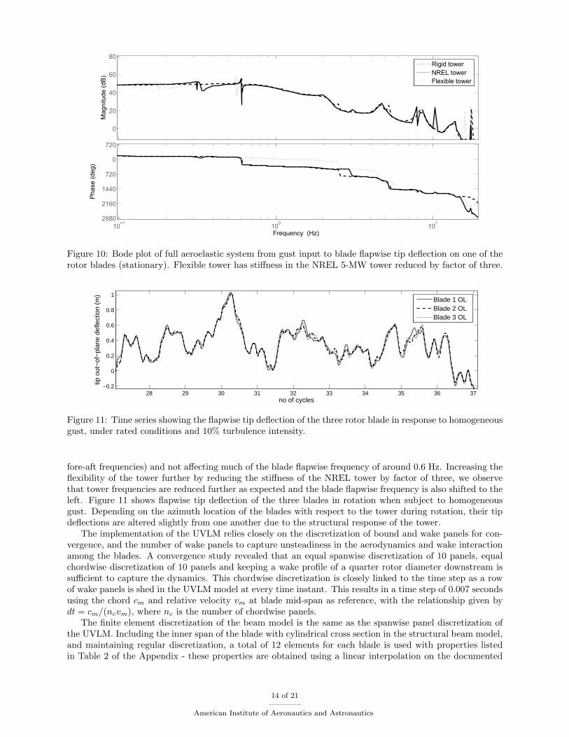
Next, we study the effects of tower flexibility on the overall structural response of the wind turbine.Figure 10 shows the Bode diagram from gust input to blade flapwise tip deflection for a stationary turbinewith different degrees of tower flexibility. Comparing the solid (NREL tower) and dashed lines (rigid tower),it is evident that the tower introduces dynamics around 0.3 Hz and 2.9 Hz (the first and second tower

12 of 21


(a) 1st Tower Side-Side (0.315 Hz) (b) 1st Tower Fore-Aft (0.320 Hz) (c) 1st Drivetrain Torsion (0.611 Hz)

(d) 1st Blade Asym FY (0.641 Hz) (e) 1st Blade Asym FP (0.670 Hz) (f) 1st Blade Collective Flap (0.703 Hz)

(g) 1st Blade Asym EP (1.082 Hz) (h) 1st Blade Asym EY (1.096 Hz) (i) 2nd Blade Asym FY (1.729 Hz)

(j) 2nd Blade Asym FP (1.879 Hz) (k) 2nd Blade Collective Flap (1.973 Hz) (l) 2nd Drivetrain Torsion (2.316 Hz)

Figure 9: Stationary mode shapes of the NREL 5-MW reference wind turbine in parked configuration.

13 of 21


0

20

40

60

80

Magnitude (

dB

)

101

100

101

2880

2160

1440

720

0

720

Phase (

deg)

Frequency (Hz)

Rigid tower

NREL tower

Flexible tower

Figure 10: Bode plot of full aeroelastic system from gust input to blade flapwise tip deflection on one of therotor blades (stationary). Flexible tower has stiffness in the NREL 5-MW tower reduced by factor of three.

28 29 30 31 32 33 34 35 36 37−0.2

0

0.2

0.4

0.6

0.8

1

no of cycles

tip o

ut−

of−

plan

e de

flect

ion

(m)

Blade 1 OLBlade 2 OLBlade 3 OL

Figure 11: Time series showing the flapwise tip deflection of the three rotor blade in response to homogeneousgust, under rated conditions and 10% turbulence intensity.

fore-aft frequencies) and not affecting much of the blade flapwise frequency of around 0.6 Hz. Increasing theflexibility of the tower further by reducing the stiffness of the NREL tower by factor of three, we observethat tower frequencies are reduced further as expected and the blade flapwise frequency is also shifted to theleft. Figure 11 shows flapwise tip deflection of the three blades in rotation when subject to homogeneousgust. Depending on the azimuth location of the blades with respect to the tower during rotation, their tipdeflections are altered slightly from one another due to the structural response of the tower.

The implementation of the UVLM relies closely on the discretization of bound and wake panels for con-vergence, and the number of wake panels to capture unsteadiness in the aerodynamics and wake interactionamong the blades. A convergence study revealed that an equal spanwise discretization of 10 panels, equalchordwise discretization of 10 panels and keeping a wake profile of a quarter rotor diameter downstream issufficient to capture the dynamics. This chordwise discretization is closely linked to the time step as a rowof wake panels is shed in the UVLM model at every time instant. This results in a time step of 0.007 secondsusing the chord cm and relative velocity vm at blade mid-span as reference, with the relationship given bydt = cm/(ncvm), where nc is the number of chordwise panels.

The finite element discretization of the beam model is the same as the spanwise panel discretization ofthe UVLM. Including the inner span of the blade with cylindrical cross section in the structural beam model,and maintaining regular discretization, a total of 12 elements for each blade is used with properties listedin Table 2 of the Appendix - these properties are obtained using a linear interpolation on the documented

14 of 21


0 20 40 60 80 100 120 140 160 180 20010

6

105

104

103

102

101

100

No. of states

Sta

te r

ela

tive e

nerg

y

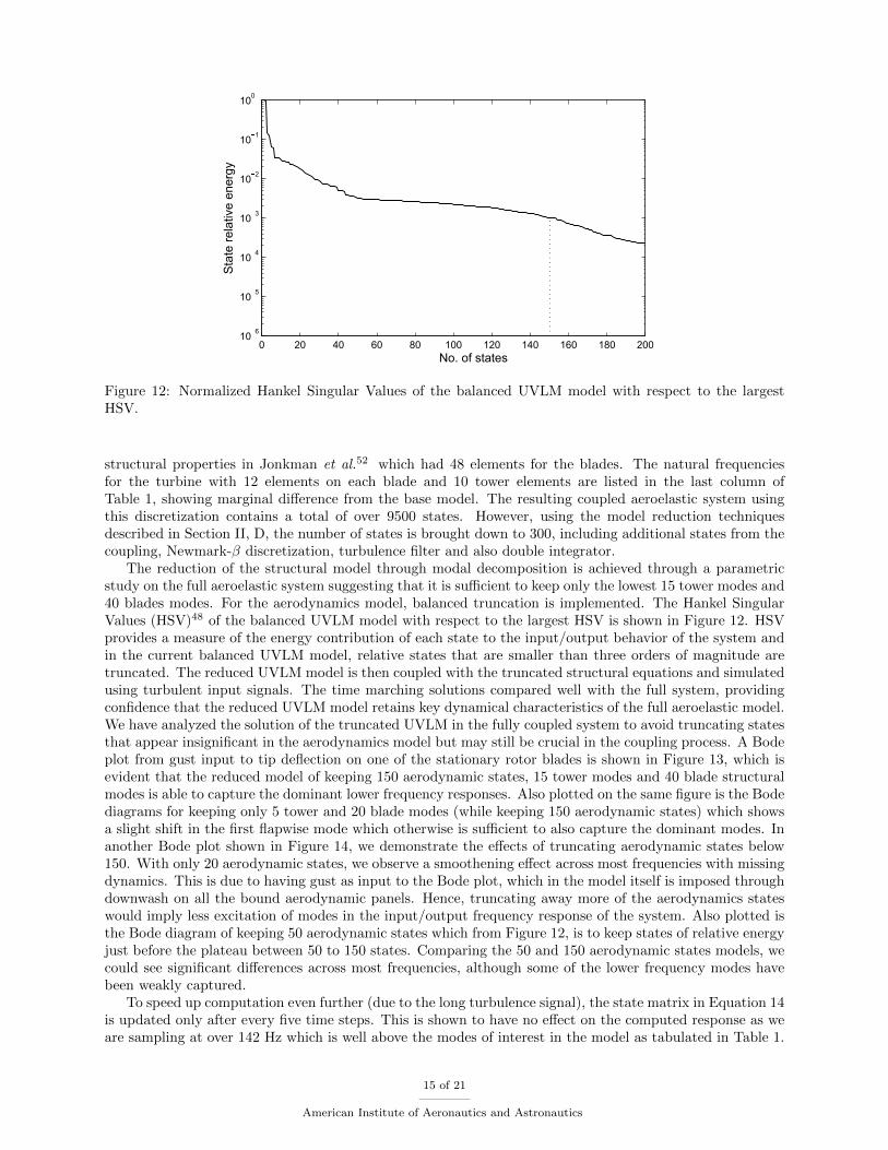
Figure 12: Normalized Hankel Singular Values of the balanced UVLM model with respect to the largestHSV.

structural properties in Jonkman et al.52 which had 48 elements for the blades. The natural frequenciesfor the turbine with 12 elements on each blade and 10 tower elements are listed in the last column ofTable 1, showing marginal difference from the base model. The resulting coupled aeroelastic system usingthis discretization contains a total of over 9500 states. However, using the model reduction techniquesdescribed in Section II, D, the number of states is brought down to 300, including additional states from thecoupling, Newmark-β discretization, turbulence filter and also double integrator.

The reduction of the structural model through modal decomposition is achieved through a parametricstudy on the full aeroelastic system suggesting that it is sufficient to keep only the lowest 15 tower modes and40 blades modes. For the aerodynamics model, balanced truncation is implemented. The Hankel SingularValues (HSV)48 of the balanced UVLM model with respect to the largest HSV is shown in Figure 12. HSVprovides a measure of the energy contribution of each state to the input/output behavior of the system andin the current balanced UVLM model, relative states that are smaller than three orders of magnitude aretruncated. The reduced UVLM model is then coupled with the truncated structural equations and simulatedusing turbulent input signals. The time marching solutions compared well with the full system, providingconfidence that the reduced UVLM model retains key dynamical characteristics of the full aeroelastic model.We have analyzed the solution of the truncated UVLM in the fully coupled system to avoid truncating statesthat appear insignificant in the aerodynamics model but may still be crucial in the coupling process. A Bodeplot from gust input to tip deflection on one of the stationary rotor blades is shown in Figure 13, which isevident that the reduced model of keeping 150 aerodynamic states, 15 tower modes and 40 blade structuralmodes is able to capture the dominant lower frequency responses. Also plotted on the same figure is the Bodediagrams for keeping only 5 tower and 20 blade modes (while keeping 150 aerodynamic states) which showsa slight shift in the first flapwise mode which otherwise is sufficient to also capture the dominant modes. Inanother Bode plot shown in Figure 14, we demonstrate the effects of truncating aerodynamic states below150. With only 20 aerodynamic states, we observe a smoothening effect across most frequencies with missingdynamics. This is due to having gust as input to the Bode plot, which in the model itself is imposed throughdownwash on all the bound aerodynamic panels. Hence, truncating away more of the aerodynamics stateswould imply less excitation of modes in the input/output frequency response of the system. Also plotted isthe Bode diagram of keeping 50 aerodynamic states which from Figure 12, is to keep states of relative energyjust before the plateau between 50 to 150 states. Comparing the 50 and 150 aerodynamic states models, wecould see significant differences across most frequencies, although some of the lower frequency modes havebeen weakly captured.

To speed up computation even further (due to the long turbulence signal), the state matrix in Equation 14is updated only after every five time steps. This is shown to have no effect on the computed response as weare sampling at over 142 Hz which is well above the modes of interest in the model as tabulated in Table 1.

15 of 21


20

40

60

Magnitude (

dB

)

101

100

101

2880

2160

1440

720

0

720

Phase (

deg)

Frequency (Hz)

5 tower, 20 blade modes

15 tower, 40 blade modes

Full system

Figure 13: Bode plot from gust input to blade flapwise tip deflection on one of the rotor blades (stationary).Comparing full model with reduced models of (a) 5 tower and 20 blade structural modes, 150 aero states,(b) 15 tower and 40 blade structural modes, 150 aero states.

0

20

40

60

Magnitude (

dB

)

101

100

101

2880

1440

0

1440

Phase (

deg)

Frequency (Hz)

20 aero states

50 aero states

150 aero states

Full system

Figure 14: Bode plot from gust input to blade flapwise tip deflection on one of the rotor blades (stationary).Comparing effect of reducing aerodynamic states (20, 50 and 150), all with 15 tower and 40 blade structuralmodes.

Also, with the rotor blades returning to the same azimuth location after each round of rotation, all thestate matrices in the first rotation can be stored and extracted for use in subsequent loops. These methods,including model reductions in the structures and aerodynamics as described, helped to save computationtime by more than two orders of magnitude with minimal impact in the accuracy of the simulations.

C. Gust load alleviation

The model of the 5-MW NREL reference wind turbine is fitted with one flap on each blade and simulated.Based on a previous study,32 a flap occupying 20% of the span of the lifting surface and 10% of the localchord is chosen and located at a mean position of 80% span. This location is found to provide the largestreductions in RBM and tip deflection and agrees with the flap sizing used in Refs.7,16 Better performances

16 of 21


could be expected with multiple and distributed flaps7,19 but since we are assuming a homogeneous gustmodel, a single flap will be sufficient.

Five statistically significant turbulence signals of 20 length scales each are generated for the simulation.The variance for the LQG controller is taken from the turbulence intensity (standard deviation) and theweights on states Q in Equation (16) are increased relative to R until either the flap deflection angle or ratelimits of |β| ≤ 10 and |β| ≤ 100/s reported by Berg et al.53 are encountered.

The controller is synthesized from a clamped single rotor blade described in a rotating frame and writtenin linear state-space representation.32 Also, the von Karman turbulence filter is included in the systemshown in Figure 5 (dotted block) for controller synthesis, thus enabling the controller to have knowledge ofthe disturbance spectrum. When placed in closed-loop with the full turbine model, it forms a distributedcontrol system in which three independent controllers act on the flaps on the three blades.

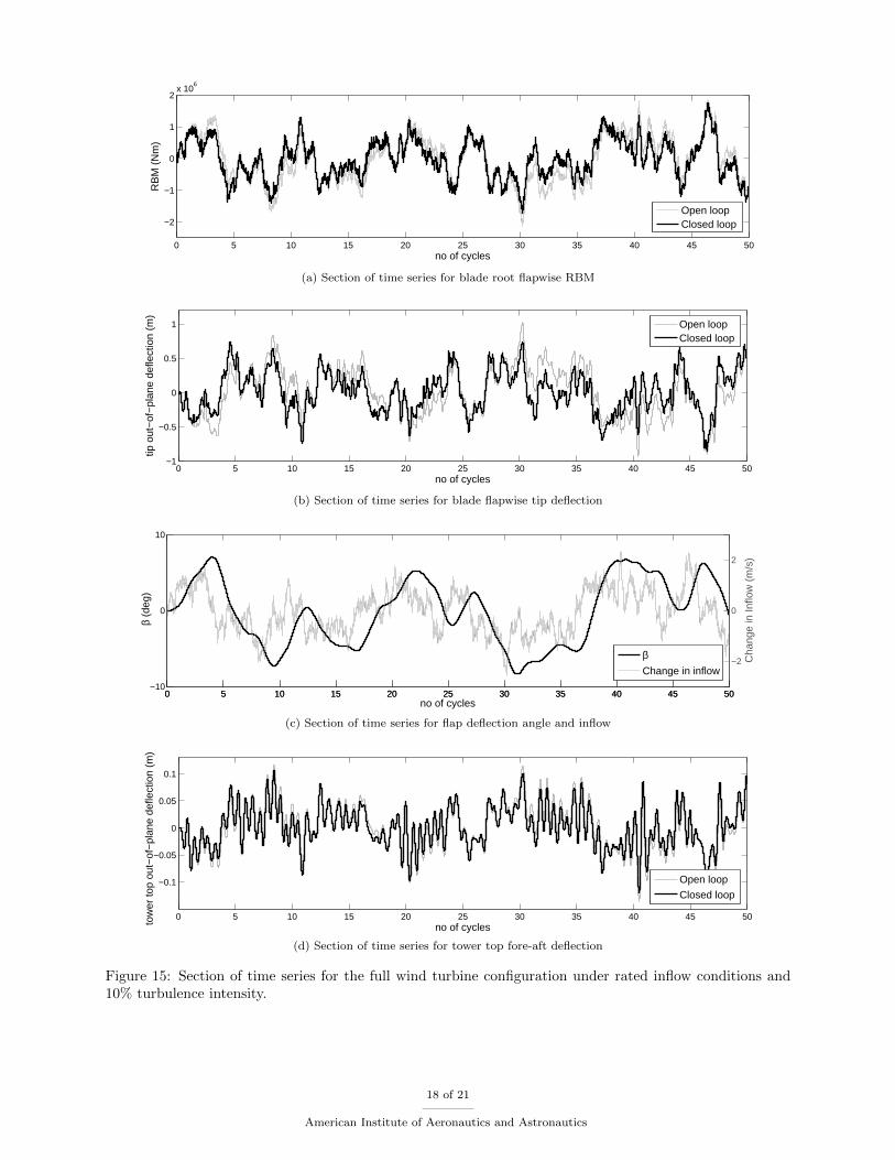
Using blade RBM feedback, on average, we are observing around 22% rms reduction in RBM and 23%rms reduction in tip deflection. The limit on the flap deflection angle of ±10 is met while the limit on flapdeflection rate was less of a concern as it was well below ±100/s. The Damage Equivalent Load (DEL) wasreduced by 17%. For the fatigue analysis, a S-N slope of 10 is selected, typical for composite materials.49,50

A section of the time series for the RBM and tip deflections on the three blades is shown in Figure 15aand Figure 15b respectively, where it is evident that peaks are reduced in the closed-loop system. Theflap deflection angle β is shown in Figure 15c which are within prescribed limits. On the same figure, thefluctuation of the inflow is also plotted in which we observe a phase lag in the response of the flaps to theinflow turbulence. The tower top out-of-plane deflection is plotted in Figure 15d, showing the additionalbenefits of flaps in reducing tower loads as well. As mentioned, the control model had with it the structureof the von Karman turbulence filter. Interestingly, the closed-loop performance deteriorated slightly by 10%when the control model had the filter removed.

The results were similar when a centralized control method was adopted in which the control model wasa rotor with three blades rigidly clamped at the hub. This would now include aerodynamics cross-influencedue to multiple surfaces but does not have any structural interaction between the blades due to the rigidjoint. Hence, the closed-loop performance is similar to the original case, except for a smaller amplitude ofloads due to aerodynamic backflow.

In an effort to enhance the performance of the control action, the single rotating blade model used forcontroller synthesis was also augmented with rigid body motion at its root, which can be representative oftower motions. The controller synthesized from this model was then placed in closed-loop with the full windturbine model. However, despite efforts in adjusting the relative importance of the gust against rigid bodymotions in the model, the results were no better than the base case controller synthesized without rigid bodymotions, indicating gust disturbance dominating the response of the system.

A final study compared the results with a controller synthesized from the full wind turbine model at aninstantaneous arbitrary azimuth location. As observed previously in Figure 11, the response of the threeblades in rotation is relatively similar, despite the non-linearity imposed through different azimuth location ofthe rotor blades with respect to the tower. The resulting closed-loop performance was less than 5% differentfrom previous cases, further demonstrating the dominance of gust disturbance and that it is sufficient to usea single rotating blade for controller synthesis.

V. Conclusions

The aeroelastic response and gust load alleviation of a large wind turbine using active control surfacesis presented using a model-based aeroservoelastic tool, coupling composite beam models and unsteady aero-dynamics in a state-space description. The finite-element solution of the rotor blades are linearized aroundlarge geometrically non-linear rotating steady-state equilibriums. The connection between the rotor hub andtower, including prescribed angular velocities are enforced through velocities with the Lagrange multipliers.The aerodynamics modeled through the Unsteady Vortex-Lattice Method allows the response of large flexibleblades to be captured with better fidelity than blade-element momentum theory and control surfaces to bemodeled directly. While the standard UVLM implementation have a relatively large computation cost, thestate-space representation presented here can be coupled to any structural model easily, allows for standardmodel reduction techniques and provides a computationally efficient route for control synthesis as illustrated.Through modal decomposition of the structural equations of motion and balanced model truncation of theaerodynamics, the size of the resulting coupled aeroelastic model can be reduced to speed up computation

17 of 21


0 5 10 15 20 25 30 35 40 45 50

−2

−1

0

1

2x 10

6

no of cycles

RB

M (

Nm

)

Open loopClosed loop

(a) Section of time series for blade root flapwise RBM

0 5 10 15 20 25 30 35 40 45 50−1

−0.5

0

0.5

1

no of cycles

tip o

ut−

of−

plan

e de

flect

ion

(m)

Open loopClosed loop

(b) Section of time series for blade flapwise tip deflection

0 5 10 15 20 25 30 35 40 45 50−10

0

10

β (d

eg)

no of cycles

0 5 10 15 20 25 30 35 40 45 50

−2

0

2

Cha

nge

in In

flow

(m

/s)

βChange in inflow

(c) Section of time series for flap deflection angle and inflow

0 5 10 15 20 25 30 35 40 45 50

−0.1

−0.05

0

0.05

0.1

no of cyclestow

er to

p ou

t−of

−pl

ane

defle

ctio

n (m

)

Open loop

Closed loop

(d) Section of time series for tower top fore-aft deflection

Figure 15: Section of time series for the full wind turbine configuration under rated inflow conditions and10% turbulence intensity.

18 of 21


time by more than two orders of magnitude, This includes making use of similarity in the cyclic behavior ofthe wind turbine in which system matrices in one rotation can be stored and reloaded.

Using the aeroelastic formulation presented, the NREL 5-MW offshore reference wind turbine is mod-eled and validated. Subsequently, the turbine blades are attached with trailing-edge flaps and using LQGcontrollers with RBM feedback, an average rms reduction of 22% for RBM, 23% for tip deflection and DELreduction of 17% is observed, with flap deflections angles kept within the limits of ±10. The current de-scription of the model can be extended to include cyclic loads such as gravity, wind shear, base excitationand also the use of multiple flaps modeled directly in the UVLM model, which will be considered in a furtherwork.

Appendix

The interpolated blade structural properties with 12 elements is shown in Table 2.

Table 2: Interpolated blade structural properties for NREL 5-MW wind turbine.

Node Radius StrTwst MassDen FlpStff EdgStff GJStff EAStff FlpIner EdgIner EdgcgOf

(m) () (kg/m) (N·m2) (N·m2) (N·m2) (N) (Kg·m) (Kg·m) (m)

1 1.50 13.31 678.94 1.81×1010 1.81×1010 5.56×109 9.73×109 972.86 973.04 0.0002

2 6.63 13.31 475.27 7.36×109 1.04×1010 2.37×109 5.57×109 464.34 649.09 0.0647

3 11.75 13.31 445.61 4.67×109 7.18×109 8.48×108 4.17×109 288.05 546.22 0.1614

4 16.88 11.01 364.77 2.37×109 4.93×109 3.07×108 2.99×109 146.92 450.87 0.2580

5 22.00 9.59 343.65 1.80×109 4.20×109 2.25×108 2.33×109 107.14 357.59 0.2028

6 27.13 8.11 313.06 1.17×109 3.54×109 1.52×108 1.71×109 67.48 275.76 0.1580

7 32.25 6.55 271.80 6.37×108 2.67×109 7.70×107 1.13×109 34.82 191.03 0.1326

8 37.38 5.06 234.32 3.29×108 1.90×109 4.77×107 7.85×108 18.05 138.83 0.1396

9 42.50 3.63 180.95 1.53×108 1.26×109 2.44×107 5.36×108 8.75 98.31 0.2038

10 47.63 2.52 145.71 9.15×107 8.03×108 1.64×107 3.78×108 5.22 70.39 0.2257

11 52.75 1.53 107.00 5.47×107 4.81×108 8.46×106 2.25×108 3.02 42.01 0.2102

12 57.88 0.54 75.25 2.97×107 2.10×108 5.69×106 1.07×108 1.65 19.74 0.1487

13 63.00 0 10.32 1.70×105 5.01×106 1.90×105 3.53×106 0.02 0.68 0.0518

Acknowledgments

The first author would like to acknowledge the funding support from the Singapore Energy InnovationProgramme Office. The work of the second author is sponsored by the UK Engineering and Physical SciencesResearch Council (EPSRC) and is gratefully acknowledged.

References

1Barlas, T. K. and van Kuik, G. A. M., “Review of state of the art in smart rotor control research for wind turbines,”Progress in Aerospace Sciences, Vol. 46, No. 1, 2010, pp. 1–27.

2Hansen, M., Sørensen, J. N., Voutsinas, S. G., Sørensen, N., and Madsen, H. A., “State of the art in wind turbineaerodynamics and aeroelasticity,” Progress in Aerospace Sciences, Vol. 42, No. 4, 2006, pp. 285–330.

3Wang, H., Barthelmie, R. J., Pryor, S. C., and Kim, H. G., “A new turbulence model for offshore wind turbine standards,”Wind Energy, 2013.

4Jonkman, J. M. and Buhl Jr., M. L., “FAST User’s guide,” Tech. rep., NREL/EL-500-38230, 2005.5Øye, S., “FLEX4 simulation of wind turbine dynamics,” Proceedings of the IEA 28th Meeting of Experts on State of the

Art of Aeroelastic Codes for Wind Turbine Calculations, Lyngby, Denmark, 1996, pp. 71–76.6Larsen, T. J. and Hansen, A. M., “How 2 HAWC2, the user’s manual,” Tech. rep., Risø-R-1597(ver. 4-3)(EN), 2012.7Barlas, T. K., van der Veen, G. J., and van Kuik, G. A. M., “Model predictive control for wind turbines with distributed

active flaps: Incorporating inflow signals and actuator constraints,” Wind Energy, Vol. 15, No. 5, 2012, pp. 757–771.8Bossanyi, E. A., “GH Bladed theory manual,” Tech. rep., 282/BR/009, 2003.9Jonkman, J. and Musial, W., “Offshore code Comparison collaboration (OC3) for IEA Task 23 offshore wind technology

and deployment,” Tech. rep., NREL/TP-5000-48191, 2010.10Passon, P., Kuhn, M., Butterfield, S., Jonkman, J., Camp, T., and Larsen, T. J., “OC3 - Benchmark exercise of aero-

elastic offshore wind turbine codes,” Journal of Physics Conference Series, Vol. 75: 012071, 2007.

19 of 21


11Ahlstrom, A., Aeroelastic simulation of wind turbine dynamics, Ph.D. thesis, 2005.12Hansen, M., Gaunaa, M., and Madsen, H. A., “A Beddoes-Leishman type dynamic stall model in state-space and indicial

formulations,” Tech. rep., Risø-R-1354(EN), 2004.13Voutsinas, S. G., “Vortex methods in aeronautics: How to make things work,” International Journal of Computational

Fluid Dynamics, Vol. 20, No. 1, 2006, pp. 3–18.14Bossanyi, E. A., “Individual blade pitch control for load reduction,” Wind Energy, Vol. 6, No. 2, 2003, pp. 119–128.15Frederick, M., Kerrigan, E. C., and Graham, J. M. R., “Gust alleviation using rapidly deployed trailing-edge flaps,”

Journal of Wind Engineering and Industrial Aerodynamics, Vol. 98, No. 12, 2010, pp. 712–723.16Riziotis, V. A. and Voutsinas, S., “Aero-elastic modelling of the active flap concept for load control,” Proceedings of the

EWEC , Brussels, Belgium, 2008.17Basualdo, S., “Load alleviation on wind turbine blades using variable airfoil geometry,” Wind Engineering, Vol. 29, No. 2,

2005, pp. 169–182.18Barlas, T. K. and van Kuik, G. A. M., “Aeroelastic modelling and comparison of advanced active flap control concepts

for load reduction on the UPWIND 5MW wind turbine,” Proceedings of the EWEC , Marseille, France, 2009.19Wilson, D. G., Resor, B. R., Berg, D. E., Barlas, T. K., and van Kuik, G. A. M., “Active aerodynamic blade distributed

flap control design procedure for load reduction on the UPWIND 5MW wind turbine,” Proceedings of the 48th AIAA AerospaceSciences Meeting, Orlando, FL, USA, 2010.

20Andersen, P. B., Gaunaa, M., Bak, C., and Buhl, T., “Load alleviation on wind turbine blades using variable airfoilgeometry,” Proceedings of the EWEC , Athens, Greece, 2006.

21Andersen, P. B., Henriksen, L., Gaunaa, M., Bak, C., and Buhl, T., “Deformable trailing edge flaps for modern megawattwind turbine controllers using strain gauge sensors,” Wind Energy, Vol. 13, No. 2-3, 2010, pp. 193–206.

22Buhl, T., Gaunaa, M., and Bak, C., “Potential load reduction using airfoils with variable trailing edge geometry,” Journalof Solar Energy Engineering, Vol. 127, No. 4, 2005, pp. 503–516.

23Gaunaa, M., “Unsteady 2D potential-Flow forces on a thin variable geometry airfoil undergoing arbitary motion,” Tech.rep., Risø-R-1478(EN), 2006.

24van Dam, C. P., Chow, R., Zayas, J. R., and Berg, D. E., “Computational investigations of small deploying tabs andflaps for aerodynamic load control,” Journal of Physics, Vol. 75: 012027, 2007.

25Marrant, B. A. H. and van Holten, T., “Concept study of smart rotor blades for large offshore wind turbines.” Proceedingsof OWEMES 2006 , Rome, Italy, 2006.

26Wilson, D. G., Berg, D. E., Barone, M. F., Berg, J. C., Resor, B. R., and Lobitz, D. W., “Active aerodynamics bladecontrol design for load reduction on large wind turbines,” Proceedings of the EWEC , Marseille, France, 2009.

27Lackner, M. A. and van Kuik, G., “A comparison of smart rotor control approaches using trailing edge flaps and individualpitch control,” Proceedings of the 47th AIAA Aerospace Sciences Meeting, Orlando, FL, USA, 2009.

28Castaignet, D., Barlas, T., Buhl, T., Poulsen, N. K., Wedel-Heinen, J. J., Olesen, N. A., Bak, C., and Kim, T., “Full-scaletest of trailing edge flaps on a Vestas V27 wind turbine: Active load reduction and system identification,” Wind Energy, 2013.

29Berg, D. E., Berg, J. C., Wilson, D. G., White, J., Resor, B. R., and Rumsey, M. A., “Design, fabrication, assembly andinitial testing of a SMART rotor,” Proceedings of the 29th ASME Wind Energy Symposium, Orlando, FL, USA, 2011.

30Berg, J. C., Berg, D. E., and White, J., “Fabrication, integration, and initial testing of a SMART rotor,” Proceedings ofthe 50th AIAA Aerospace Sciences Meeting, Nashville, TN, USA, 2012.

31Ng, B. F., Palacios, R., Graham, J. M. R., and Kerrigan, E. C., “Robust control synthesis for gust load alleviation fromlarge aeroelastic models with relaxation of spatial discretisation,” Proceedings of the EWEC , Copenhagen, Denmark, 2012.

32Ng, B. F., Hesse, H., Palacios, R., Graham, J. M. R., and Kerrigan, E. C., “Aeroservoelastic modeling and load alleviationof very large wind turbine blades,” AWEA Windpower , Chicago, IL, 2013.

33Hesse, H. and Palacios, R., “Consistent structural linearisation in flexible-body dynamics with large rigid-body motion,”Computers and Structures, Vol. 110-111, No. 0, 2012, pp. 1–14.

34Palacios, R., Murua, J., and Cook, R., “Structural and aerodynamic models in the nonlinear flight dynamics of veryflexible aircraft,” AIAA Journal , Vol. 48, No. 11, 2010, pp. 2559–2648.

35Murua, J., Palacios, R., and Graham, J. M. R., “Applications of the unsteady vortex-lattice method in aircraft aeroelas-ticity and flight dynamics,” Progress in Aerospace Sciences, Vol. 55, 2012, pp. 46–72.

36Murua, J., Palacios, R., and Graham, J. M. R., “Assessment of wake-tail interference effects on the dynamics of flexibleaircraft,” AIAA Journal , Vol. 50, No. 7, 2012, pp. 1575–1585.

37Simo, J. C. and Vu-Quoc, L., “On the dynamics in space of rods undergoing large motions - A geometrically exactapproach,” Computer Methods in Applied Mechanics and Engineering, Vol. 66, No. 2, 1988, pp. 125–161.

38Geradin, M. and Cardona, A., Flexible multibody dynamics: A finite element approach, John Wiley, Chichester, England;New York, 2001.

39Palacios, R. and Cesnik, C., “Cross-sectional analysis of non-homogeneous anisotropic active slender structures.” AIAAJournal , Vol. 43, No. 12, 2005, pp. 2624–2638.

40Geradin, M. and Rixen, D., Mechanical vibrations: Theory and application to structural dynamics, John Wiley, Chich-ester, England; New York, 2nd ed., 1997.

41Katz, J. and Plotkin, A., Low speed aerodynamics, Cambridge aerospace series, Cambridge University Press, Cambridge,UK; New York, 2nd ed., 2001.

42Chattot, J.-J., “Helicoidal vortex model for wind turbine aeroelastic simulation,” Computers and Structures, Vol. 85,No. 11-14, 2007, pp. 1072–1079.

43Simpson, R. J. S., Palacios, R., and Murua, J., “Induced drag calculations in the unsteady vortex-lattice method,” AIAAJournal , Vol. 51, No. 7, 2013, pp. 1775–1779.

20 of 21


44Skjoldan, P. F., Aeroelastic modal dynamics of wind turbines including anisotropic effects, Ph.D. thesis, TechnicalUniversity of Denmark, 2011.

45Hesse, H. and Palacios, R., “Reduced-order aeroelastic models for the dynamics of maneuvering flexible aircraft,” AIAAJournal , , No. 1, 2014.

46Astrom, K. J. and Murray, R. M., Feedback systems: An introduction for scientists and engineers, Princeton UniversityPress, Princeton; Oxford, UK, 2008.

47Maciejowski, J. M., Multivariable feedback design, Addison-Wesley, Wokingham, 1989.48Skogestad, S. and Postlethwaite, I., Multivariable feedback control: Analysis and design, John Wiley, Chichester, England;

Hoboken, NJ, 2nd ed., 2005.49Freebury, G. and Musial, W., “Determining equivalent damage loading for full-scale wind turbine blade fatigue tests,”

Proceedings of the 19th American Society of Mechanical Engineers Wind Energy Symposium, Reno, Nevada, 2000.50Hendriks, H. B. and Bulder, B. H., “Fatigue equivalent load cycle method - A general method to compare the fatigue

loading of different load spectrums,” Tech. rep., ECN-C-95-074, 1995.51Bielawa, R. L., Rotary wing structural dynamics and aeroelasticity, American Institute of Aeronautics and Astronautics,

2006.52Jonkman, J., Butterfield, S., Musial, W., and Scott, G., “Definition of a 5-MW wind turbine for offshore system devel-

opment,” Tech. rep., NREL/TP-500-38060, 2009.53Berg, D. E., Wilson, D. G., Resor, B. R., Barone, M. F., and Berg, J. C., “Active aerodynamic blade load control impacts

on utility-scale wind turbines,” Proceedings of the AWEA Windpower , Chicago, IL, USA, 2009.

21 of 21


Model-based Aeroservoelastic Design and Load Alleviation of Large Wind Turbines

Documents