Modal Logic - Uppsala Universityhedin/TillLog/LectureNotesAL.pdf · Modal Logic (Lecture Notes for Applied Logic) Anton Hedin October 2, 2008 Contents 1 Introduction 2 2 Basic Modal

Modal Logic(Lecture Notes for Applied Logic)

Anton Hedin

October 2, 2008

Contents

1 Introduction 2

2 Basic Modal Logic 3

2.1 Syntax . . . . . . . . . . . . . . . . . . . . . . . . . . . . . . . 3

2.2 Semantics . . . . . . . . . . . . . . . . . . . . . . . . . . . . . 4

3 Engineering of Modal Logics 9

3.1 Frame correspondence . . . . . . . . . . . . . . . . . . . . . . 11

3.2 Normal modal logics . . . . . . . . . . . . . . . . . . . . . . . 15

4 Neighborhood Semantics: A remark on normal modal logics 20

5 Intuitionistic Propositional Calculus 23

6 Generalizing the basic framework 29

1

1 Introduction

In (classical) propositional and predicate logic, every formula is either trueor false in any model. But there are situations were we need to distinguishbetween different modes of truth, such as necessarily true, known to be true,believed to be true and always true in the future (with respect to time). Forexample, consider the sentence

”The math department is located on thefourth floor of the Angstrom building”.

It expresses something that is true today, but was false some years ago.Moreover, it might be false again some time in the future. Another example,whose mode of truth is more stable with respect to time, is

”The Earth has exactly one moon”.

The sentence expresses something that is true and maybe will be true forever in the future, but it is not necessarily true in the sense that there mightas well have been two moons, or none for that matter (since we know this ispossible for planets). However, most people would consider the statement

”The square root of 9 is 3”

as expressing something that is both necessarily true as well as always true.But it does not enjoy all modes of truth, for example it may not be believedto be true (for example by someone who is mistaken) or known to be true(for example by someone that hasn’t learned mathematics).

There are also more practical examples were reasoning about different modesof truth is helpful. For example, think of a multi-agent system in computerscience. There, each agent may have different knowledge about the systemand even about other agents knowledge. In such a scenario a sentence is’necessarily’ true when known. It should be clear that not every sentenceneeds to be necessarily true in this sense.

In the examples given above we are using the same way of reasoning. Asentence ϕ, if true, will be so with respect to the current state of affairs, i.e.

2

how the world actually is, but (depending on ϕ) we might be able to conceiveof a state of affairs (a different world) were ϕ is false, and if this is the caseϕ will not be necessarily true. These states of affairs can be points in timeas in the first example, possible worlds as in the second example or states ofknowledge of a person/agent as in the last two examples.

We will develop a general framework in which we will be able to reason aboutsituations as the ones above. First we take a look at basic modal logic.

2 Basic Modal Logic

2.1 Syntax

The language of Basic Modal Logic is an extension of classical propositionallogic. What we add are two unary connectives � and ♦. We have a set Atomsof propositional letters p, q, r, . . ., also called atomic formulas or atoms.

Definition 1. Formulas of basic modal logic are given by the following rule

ϕ ::= ⊥ | > | p | ¬ϕ | (ϕ ∧ ϕ) | (ϕ ∨ ϕ) | (ϕ→ ϕ) | (ϕ⇔ ϕ) | �ϕ | ♦ϕ.

where p is any atomic formula.

Examples of well formed formulas (wffs) are (q ∧ ¬♦p) and (�p → ♦�(r ∨�>)), while p�¬ → ♦p or ∨p�q are clearly non-wffs!

Just as in predicate logic, the unary connectives bind most closely so thatfor example �p ∨ r is read as (�p) ∨ r and not �(p ∨ r).

The new connectives � and ♦ are read ’box’ and ’diamond’ respectively,and are dual of each other similarly to how ∀ and ∃ are dual of each otherin predicate logic (we will return to this later). And just as ∀ and ∃ areread as ’for every’ and ’there exists’ respectively, we will also want to givespecial readings for box and diamond. Although the readings will be differentdepending on the situation we want to study, i.e. what mode of truth we areinterested in. For example in case we want to study necessity and possibility(as in the case of the second sentence above), � is read as ’necessarily’ and

3

♦ as ’possibly’. In such a logic there are some formulas we might regardas being correct principles, for example �ϕ → ♦ϕ ’whatever is necessary ispossible’ or ϕ→ ♦ϕ ’whatever is, is possible’. However, other formulas maybe harder to decide. Should ϕ → �♦ϕ ’whatever is, is necessarily possible’be regarded as a general truth about necessity and possibility? A precisesemantics will bring clarity to questions like these.

Remark 2.1. We could just as well have defined a formula ϕ by the following(shorter) rule

ϕ ::= ⊥ | p | ¬ϕ | (ϕ ∧ ϕ) | (ϕ→ ϕ) | �ϕ,

and then, as is usually done, define the rest of the connectives from the onesgiven. In this case, diamond would be defined as ♦ := ¬�¬.

2.2 Semantics

We now want to give some mathematical content to our suggestive discussionabove. A model in propositional logic is simply a valuation function assigningtruth values to the set of atoms, i.e. a function

ν : Atoms→ {>,⊥}.

As we’ve hinted at in the discussion, we now want to consider models inwhich an atom can have different truth values at different states. Therefore:

Definition 2. A model,M, in basic modal logic is a triple (W,R,L), where

• W is a set of states or worlds,

• R is a relation R ⊆ W ×W ,

• and L is a function L : W → P(Atoms), called the labelling function.

These models are called Kripke models after Saul Kripke who was the firstto introduce them in the 1950s. Intuitively w ∈ W is a possible world andR is an accessibility relation between worlds. That is, wRw′ (which we willuse as shorthand for (w,w′) ∈ R) means that w′ is accessible from w. Thisintuition will be made more precise in the next definition. But first someexamples.

4

Example 1. Although the definition of a Kripke model might look somewhatcomplicated, we can use an easy graphical notation for such a model: SupposeM = (W,R,L) is a Kripke model where

W = {x1, x2, x3, x4, x5},R = {(x1, x2), (x1, x4), (x2, x2), (x2, x3),

(x3, x2), (x3, x4), (x5, x5), (x5, x2), (x5, x4)}

and

L(xi) =

{p, q, r}, i = 1{p}, i = 2{p, r}, i = 3{r}, i = 4∅, i = 5

Then we can picture M as follows:

gfed`abc{p, q, r}

ONMLHIJK{p}_^]\XYZ[{p, r}

ONMLHIJK{r}

/.-,()*+∅��������

((ggtt

LL�������������

VV

--

ff

//

x1

x2 x3

x4

x5

Where an arrow xi → xj means that xiRxj.

Example 2. A Kripke model M = (W,R,L) can be used to describe howtruth values vary over time. A common example is when W = N and R isthe ordinary ordering ≤ of the natural numbers.

0 // 1 // 2 // . . . // n // . . .

Then we can think of W as a set of points in time and R as the relation ofbeing ahead in time. Then L(t) will describe the truth values of propositionsat time t ∈ W .

5

Example 3. If we consider the model ({∗}, ∅, L), we see that it is in fact justan ordinary model for propositional logic (when restricting our attention toformulas of propositional logic). Namely, we can define an ordinary valuationfunction V : Atoms→ {>,⊥} by

V (p) =

{>, if p ∈ L(∗)⊥, if p 6∈ L(∗)

Now we will define what it means for a formula to be true at a state in amodel.

Definition 3. LetM = (W,R,L) be a model in basic modal logic. Supposex ∈ W and ϕ is a formula. We will define when ϕ is true in the world x. Thisis done via a satisfaction relation x ϕ by structural induction on ϕ:

• x >

• x 6 ⊥

• x p iff p ∈ L(x)

• x ¬ϕ iff x 6 ϕ

• x ϕ ∧ ψ iff x ϕ and x ψ

• x ϕ ∨ ψ iff x ϕ or x ψ

• x ϕ→ ψ iff x ψ whenever x ϕ

• x ϕ↔ ψ iff x ϕ iff x ψ

• x �ϕ iff for each y ∈ W with xRy we have y ϕ

• x ♦ϕ iff there exists y ∈ W such that xRy and y ϕ

When x ϕ, we say that ’x satisfies/forces ϕ’ or ’ϕ is true in world x/atstate x’.

6

The first eight clauses are straightforward from propositional logic, the onlydifference being that an atom p can be true at many worlds x. The interestingcases are the ones for box and diamond. For �ϕ to be true at x, ϕ musthold at every world y related to x, and for ♦ϕ to be true at x there must beat least one world y related to x such that ϕ is true at y. Note that � and♦ act a bit like the quantifiers ∀ and ∃, but quantifiers over states instead ofvariables. The above interpretation of the logical constants of basic modallogic is usually called possible worlds semantics.

Example 4. Consider the model of example 1. According to definition 3 wehave

x2 �p

since x2Ry implies that y = x2 or y = x3 and we have both x2 p andx3 p, i.e. p ∈ L(x2) and p ∈ L(x3). Moreover we have

x1 |= ♦(r ∧�q)

since x1Rx4 and x4 r and x4 �q since there is no y ∈ W such that x4Ry.

Definition 4. A modelM = (W,R,L) is said to satisfy a formula ϕ if everystate in the model satisfies it. Thus, we write M |= ϕ if and only if x ϕfor every x ∈ W .

Example 5. Again considering the model M of example 1 we see that forexample the modal formula r ∨ ♦p is satisfied by M: x1, x3, x4 r andx2, x5 ♦p.

Next we define semantic entailment.

Definition 5. Let Γ be set of formulas. Then we say that Γ semanticallyentails a formula ϕ if for any world x in any model M = (W,R,L) we havex ϕ whenever x ψ for every ψ ∈ Γ. In that case we write Γ |= ϕ.

We will say that two formulas ϕ and ψ are semantically equivalent when theysemantically entail each other, and then we write ϕ ≡ ψ.

Example 6. We have already seen that � acts as a universal quantifier onworlds while ♦ acts as an existential quantifier on worlds. Therefore it maynot be so surprising that we have the following semantical equivalences:

�ϕ ≡ ¬♦¬ϕ

7

♦ϕ ≡ ¬�¬ϕ

How can we see this? Well, let M = (W,R,L) be an arbitrary model andlet x ∈ W be any world. Suppose x �ϕ, then y ϕ for every y ∈ Wsuch that xRy. So there cannot exist a world y ∈ W such that xRy andy ¬ϕ, but then x 6 ♦¬ϕ. Hence x ¬♦¬ϕ. Conversely, if x ¬♦¬ϕthen x 6 ♦¬ϕ so that there is no world y such that xRy and y ¬ϕ. Hence,for any y ∈ W such that xRy, we must have y ϕ. But then x �ϕ. Hence�ϕ ≡ ¬♦¬ϕ. The second equivalence follows easily from the first one.

Example 7. It is also not surprising that � distributes over ∧ and that ♦distributes over ∨ but not the other way around. That is

�(ϕ ∧ ψ) ≡ (�ϕ ∧�ψ)

♦(ϕ ∨ ψ) ≡ (♦ϕ ∨ ψ)

but�((ϕ ∨ ψ) 6≡ (�ϕ ∨�ψ)

♦(ϕ ∧ ψ) 6≡ (♦ϕ ∧ ♦ψ).

For the first equivalence, let M = (W,R,L) be an arbitrary model and letx ∈ W be any world. Suppose x �(ϕ∧ψ), then for every y such that xRy,y ϕ and y ψ. But then of course x �ϕ and x �ψ, i.e. x �ϕ∧�ψ.Likewise, if x �ϕ∧�ψ, then for every y such that xRy, y ϕ and y ψ,i.e. y ϕ ∧ ψ and hence x �(ϕ ∧ ψ).

To see that �(ϕ ∨ ψ) 6≡ �ϕ ∨�ψ, we consider the following kripke model:

/.-,()*+∅

GFED@ABC{q} GFED@ABC{p}RR LL

y z

x

We see that x �(p∨q), since y p∨q and z p∨q. However x 6 �p∨�qsince y 6 p and z 6 q.

Exercise 1. Show that ♦(ϕ∨ψ) ≡ (♦ϕ∨ψ) and that ♦(ϕ∧ψ) 6≡ (♦ϕ∧♦ψ).

8

Now, we need a notion of validity. In our case this will mean not just beingtrue with respect to every valuation, but also with respect to every underlyingrelational structure (W,R). More precisely we have

Definition 6. We say that a formula ϕ is valid if it is true in every world ofevery model. We denote this by |= ϕ.

From the results in example 6 and 7 we have that the following formulas arevalid

♦ϕ↔ ¬�¬ϕ

�(ϕ ∧ ψ)↔ (�ϕ ∧�ψ)

♦(ϕ ∨ ψ)↔ ♦ϕ ∨ ♦ψ

Another important formula which can be seen to be valid is the following

�(ϕ→ ψ)→ (�ϕ→ �ψ).

This formula (formula scheme to be more precise) is called K (honoring S.Kripke). To see that K is valid, let M = (W,R,L) be any model and letx ∈ W be some world inM. Assume that x �(ϕ→ ψ) and x �ϕ. Thisholds if and only if for every y ∈ W such that xRy, we have y ϕ→ ψ andy ϕ which implies that y ψ for every y such that xRy. But this on theother hand holds if and only if x �ψ. Hence x �(ϕ → ψ) → (�ϕ →�ψ), which shows that K is valid.

Exercise 2. Is the converse of the K formula valid? That is, do we have

|= (�ϕ→ �ψ)→ �(ϕ→ ψ) ?

3 Engineering of Modal Logics

As we discussed in the introduction we are interested in modeling situationswere we need to distinguish between different modes of truth. And as we sawthe applications can vary from temporal to epistemological. The framework

9

for basic modal logic is quite general (although it can be further generalizedas we will see later) and can be refined to yield the properties appropriate forthe intended application. We will concentrate on three different applications:logic of necessity, temporal logic and logic of knowledge. That is, we willengineer the basic framework to fit the following readings of �ϕ:

• It is necessarily true that ϕ

• It will always be true that ϕ

• Agent A knows ϕ.

We know that ♦ϕ ≡ ¬�¬ϕ, so the reading of ♦ϕ in each situation is givenautomatically by that of �ϕ:

• It is not necessarily true that not ϕ≡ It is possible that not not ϕ≡ It is possible that ϕ.

• It will not always be true that not ϕ≡ At some point in the future not ϕ will not hold≡ At some point in the future ϕ will hold.

• Agent A does not know not ϕ≡ As far as A knows, ϕ could be the case≡ ϕ is consistent with A’s knowledge.

Exercise 3. Suppose we want to interpret �ϕ as ”We have a proof of ϕ”.What would the corresponding interpretation of ♦ϕ be?

In the last section we saw some examples of valid formulas, i.e. formulasthat are satisfied in every model. Many other formulas, of course, are not.Some examples are �ϕ → ϕ, �ϕ → ��ϕ and ♦> (Why?). However, if wewant to study the logic of necessity we would like the first of these, �ϕ→ ϕ(’What is necessarily true is also true’), to be valid, in the case that �ϕ isread ’Agent A knows ϕ’ we might want �ϕ→ ��ϕ (’If A knows ϕ, A alsoknows that he/she/it knows ϕ’) to be valid, and in the case of temporal logicwe might want ♦> (’There is always a future world’) to be valid.

10

So for each situation, or reading of �, we would like to restrict the class ofmodels so that the desired formulas are valid (with respect to this restrictedclass of models).

Now, each reading of � also provides some corresponding reading of theaccessibility relation xRy:

• y is a possible world according to the information at x

• y is in the future of x

• y could be the actual world according to A’s knowledge at x.

Exercise 4. Consider again the interpretation in exercise 3. Can you sayanything about the accessibility relation xRy in this case?

The question now is what properties the relation R should have in the variouscases. In the first case for example, is it desirable that R be reflexive? Well,this would mean that at each world x, x itself is a possible world. So theanswer seems to be yes. We may note a similarity to the argument validatingthe formula �ϕ → ϕ under the same reading of �. In fact, there is a closeconnection between this formula and the property of reflexivity. In the nextsection we will see that some elementary classes of models correspond tosimple formulas in basic modal logic. This will yield a connection betweenwhat formulas should be valid and what general structure the models shouldhave in each situation.

3.1 Frame correspondence

We start with some definitions.

Definition 7. A structure (W,R) with W a non-empty set and R a binaryrelation on W , is called a frame and is denoted F .

A frame F is the underlying structure of any model M, and so from anymodel we can extract a frame by simply forgetting about the labeling func-tion.

11

Definition 8. A formula ϕ is valid on a frame F , written F |= ϕ, if forevery labelling function L and each x ∈ W we have M, x ϕ, where M =(W,R,L).

Remark 3.1. We defined validity of a formula ϕ, |= ϕ, by saying that ϕ is trueat every state of every model, but we could equivalently say that a formulaϕ is valid when F |= ϕ for all frames F .

Example 8. Consider the following frame F :

•

•

•99

��

ee

??������������� ��?????????????

x1

x2

x3

Then we have, F |= �ϕ → ϕ. Why is this? Well, let L be any labellingfunction on F and let x be any state of F . If x �ϕ then y ϕ for everyy in F such that x is related to y. But, every state in F is related to itself,i.e. F has a reflexive accessibility relation. Hence x ϕ, and so we indeedhave F |= �ϕ→ ϕ.

This is a special case of the following result:

Proposition 3.2. Let F = (W,R) be a frame, then

1. R is reflexive if and only if F |= �ϕ→ ϕ,

2. R is transitive if and only if F |= �ϕ→ ��ϕ.

Proof. (1): Suppose R is reflexive and let L be a labelling function on F sothat we get a model M = (W,R,L). We want to show that M |= �ϕ→ ϕ,so let x ∈ W be any state such that x �ϕ. Since R is reflexive, we havexRx and hence x ϕ. But then we have x �ϕ → ϕ, and F |= �ϕ → ϕsince x was arbitrary.

12

Conversely, suppose F |= �ϕ→ ϕ. In particular, we then have F |= �p→ p.Now, let x ∈ W and let L be a labelling function such that p 6∈ L(x) andp ∈ L(y) for each y ∈ W with xRy. Suppose we don’t have xRx, thenx �p. But then, since F satisfies �p → p we also must have x p. Butthis is a contradiction to the assumption that p 6∈ L(x). Hence, it must bethe case that xRx. Since x was arbitrary this shows that R is reflexive.

(2): Suppose R is transitive. Let L be a labelling function and M =(W,R,L). We want to show that M |= �ϕ → ��ϕ. So let x ∈ W beany state such that x �ϕ. We then need to show that for every y ∈ Wsuch that xRy and every z ∈ W such that yRz we have z ϕ, i.e. x ��ϕ.But if xRy and yRz then xRz since R is transitive, and together with x �ϕwe then have z ϕ. Hence x ��ϕ. This shows that F |= �ϕ→ ��ϕ.

Conversely, suppose F |= �ϕ → ��ϕ, In particular, we then have F |=�p → ��p. Let x, y, z ∈ W be such that xRy and yRz, we want to showxRz. Let L be a labelling function such that p 6∈ L(z) but p ∈ L(w) forall other worlds w. Suppose we don’t have xRz, then x �p and hencex ��p since F |= �p → ��p. But then y �p, since xRy, and z p,since yRz, which contradicts our assumption that p 6∈ L(z). Hence, we musthave xRz. This shows that R is transitive.

For other applications there might be other properties of R that are desir-able. And in many cases these properties will, as above, correspond to someformula. The following table gives some such correspondences

T: Frame-validity of �ϕ→ ϕ corresponds to reflexivity of R.

B: Frame-validity of ϕ→ �♦ϕ corresponds to symmetry of R.

D: Frame-validity of �ϕ→ ♦ϕ corresponds to R being serial.

4: Frame-validity of �ϕ→ ��ϕ corresponds to transitivity of R.

13

5: Frame-validity of ♦ϕ→ �♦ϕ corresponds to R being Euclidean.

The first symbol on each line is the commonly used name of the correspondingmodal formula (cf. axiom K).

Definition 9. We say that a BML formula ϕ defines a property P of a frameF = (W,R) if F |= ϕ if and only if R has the property P .

Exercise 5. Show that both ♦> and D : �ϕ→ ♦ϕ defines the same property.

Example 9. We will prove the last of the correspondences above, that F |=♦ϕ→ �♦ϕ if and only if R is Euclidean. The relation R is Euclidean if forevery x, y, z ∈ W , xRy and xRz implies that yRz. First, suppose that R isEuclidean. Let L be any labelling function on F and let x ∈ W such thatx ♦ϕ. Then there is z ∈ W with xRz and z ϕ. Now suppose y ∈ Wwith xRy, then yRz since R is Euclidean. But then we have y ♦ϕ, andhence x �♦ϕ, i.e. x ♦ϕ→ �♦ϕ.

We prove the converse by contraposition. Assume F is non-Euclidean, thenthere must be states x, y, z ∈ W such that xRy, xRz but not yRz. We willtry to falsify 5 in x by finding a labelling function L such that x ♦p andx 6 �♦p. That is, we have to make p true at some R-successor of x andfalse at all R-successors of some R-successor of x. Let L be given by

p ∈ L(w) iff it is not the case that yRw

then p ∈ L(z) while {w | yRw} ∩ {w | p ∈ L(w)} = ∅. Now clearly y 6 ♦p,so that x 6 �♦p. On the other hand, since we have z p and xRz, we havex ♦p. Hence, F 6|= ♦ϕ→ �♦ϕ.

Exercise 6. Prove the remaining frame correspondences in the list.

Exercise 7. Can you find a modal formula that defines linearity? R is linearif it is reflexive, transitive and satisfies (∀x, y)(xRy ∨ yRx).

We now have a way of deciding what formulas of basic modal logic shouldbe included as axioms in our logic: On the one hand we are guided by thereading of the unary connectives � and ♦, and on the other hand by thedesired properties of models.

14

For example, say we want to interpret � as the temporal connective Alwaysin the future. Then we have already argued that we would like to have theformula ♦> as an axiom. Furthermore it would be reasonable to consideronly transitive models, which would simply mean that if y is ahead in timeof x and z is ahead in time of y, then z is also ahead in time of x. So we addthe formula 4 as an axiom.

So how could logics for our three readings of �ϕ look like? Before we caninvestigate this further we need a proper definition of what we mean by alogic.

3.2 Normal modal logics

Given a class of frames F, we denote by ΛF the set of formulas valid onevery frame in F. So for example, if F is the class of all reflexive frames, weknow that �ϕ → ϕ ∈ ΛF. Now, are there syntactic mechanisms capable ofgenerating ΛF? And are such mechanisms able to cope with the associatedsemantic consequence relation?

We are going to define a Hilbert-style axiom system called K, which is a’minimal’ system for reasoning about frames.

Definition 10. A K-proof is a finite sequence of formulas, each of whichis an axiom, or follows from one or more earlier items in the sequence byapplying a rule of proof. The axioms of K are all instances of propositionaltautologies and:

K: �(ϕ→ ψ)→ (�ϕ→ �ψ),

Dual: ♦ϕ↔ ¬�¬ϕ.

The rules of proof of K are:

• Modus ponens : given ϕ and ϕ→ ψ, prove ψ.

• Uniform substitution: given ϕ, prove ψ, where ψ is obtained from ϕby replacing proposition letters in ϕ by arbitrary formulas.

15

• Rule of necessitation: given ϕ, prove �ϕ.

A formula ϕ is K-provable if it occurs as the last item of some K-proof, inthis case we write `K ϕ.

The definition needs some explaining. Adding all propositional tautologiesof course yields a very large axiom set and we could have chosen a smallset of tautologies capable of generating the rest by using the rules of proof.However, we are not at the moment interested in having a minimal generatingset of axioms.

Modus ponens preserves validity. That is, if |= ϕ and |= ϕ→ ψ then also |= ψso it is a correct rule for reasoning about frames. Furthermore, modus ponenspreserves global truth (if M |= ϕ and M |= ϕ → ψ then also M |= ψ) andsatisfiability (if M, x ϕ and M, x ϕ → ψ then also M, x ψ). Thus,modus ponens is also a correct rule for reasoning about models, both globallyand locally.

Uniform substitution mirrors the fact that validity has nothing to do withparticular assignments: if a formula is valid, this does not depend on theparticular values its propositional symbols have, thus we should be free touniformly replace any propositional symbol with an arbitrary formula. Uni-form substitution preserves validity (why?), but neither global truth norsatisfiability. For example q is obtainable from p by uniform substitution butjust because p is globally true in some model it does not follow that the sameis true for q.

The K axiom lets us transform a boxed formula�(ϕ→ ψ) into an implication�ϕ → �ψ. It is sometimes called the distribution axiom. And as we havealready seen, K is valid on all frames.

The reason for having the Dual axiom is that we did not define ♦ using box.We saw earlier that it is a valid formula scheme.

The rule of necessitation might look somewhat odd, since clearly ϕ→ �ϕ isnot valid. However, the rule of necessitation preserves validity; if ϕ is valid,then also �ϕ is valid. Similarly, it preserves global truth; if M |= ϕ thenM |= �ϕ (why?).

Exercise 8. Show that all the rules above preserve validity. Which of the

16

rules preserves global and/or local truth?

K is the minimal modal Hilbert system in the following sense: All its axiomsare valid and all the rules of inference preserve validity, hence all K-provableformulas are valid. That is K is sound with respect to the class of all frames.Moreover, the converse is also true: if a formula of basic modal logic is valid,then it is K-provable. The proof of this fact is way beyond the scope of thepresent presentation.

Example 10. The formula (�p ∧�q)→ �(p ∧ q) is valid on any frame, soit should be K-provable, and indeed it is. Consider the following sequenceof formulas

Tautology

1. ` p→ (q → (p ∧ q))

Generalization: 1

2. ` �(p→ (q → (p ∧ q)))

K axiom

3. ` �(p→ q)→ (�p→ �q)

Uniform Substitution: 3

4. ` �(p→ (q → (p ∧ q)))→ (�p→ �(q → (p ∧ q)))

Modus Ponens: 2,4

5. ` �p→ �(q → (p ∧ q))

Uniform Substitution: 3

6. ` �(q → (p ∧ q))→ (�q → �(p ∧ q))

Propositional Logic: 5,6

17

7. ` �p→ (�q → �(p ∧ q))

Propositional Logic: 7

8. ` (�p ∧�q)→ �(p ∧ q)

As a matter of fact we have cheated a bit here; some of the steps are missing.So this is not a K-proof in the strict sense, although we see that it is possibleto fill in the gaps (from 6 to 8) in order to get a complete proof.

Suppose now that we are interested in validity only on transitive frames.Then we know the formula �ϕ → ��ϕ is valid on this class of frames,and hence we would like to be able to derive it. But the system K is toweak for this, since it only derives valid formulas (that is, formulas validon all frames) and �ϕ → ��ϕ is not valid. However, we can simply add�ϕ → ��ϕ to K as an axiom, we then obtain the Hilbert system K4. Itis then possible to show that K4 is sound and complete with respect to theclass of all transitive frames. That is, K4 generates precisely the formulasvalid on transitive frames. More generally we may add any set of modalformulas Γ as axioms to K and obtain an axiom system KΓ.

We will now introduce the concept of a normal modal logic.

Definition 11. A normal modal logic L is a set of formulas of basic modallogic, with the following properties:

(1) L contains all tautologies

(2) L contains all instances of the formula scheme K:

�(ϕ→ ψ)→ (�ϕ→ �ψ)

(3) L contains all instances of the formula scheme Dual:

♦ϕ↔ ¬�¬ϕ

(4) L is closed under uniform substitution and modus ponens.

18

(5) L is closed under the rule of necessitation.

We call the smallest normal modal logic K, and it just contains propositionallogic and all instances of axiom K, together with all formulas that you getby applying conditions (3)-(5) above.

Now, to ”build” a modal logic, first choose the formula schemes that youwould like to have in it, these will be the axioms of the logic. Then close itunder the conditions of the definition.

In the case �ϕ is read ’It is necessarily true that ϕ’ we may (as we discussedearlier) want �ϕ→ ♦ϕ and ϕ→ ♦ϕ to be in our logic L. Then we can see,by frame correspondence, that every model of L will have a serial accessibilityrelation R. Moreover, R must be reflexive since ϕ → ♦ϕ ≡ �ϕ → ϕ. Apossible name for L could then be KTD.

If we instead look at the case when �ϕ is read ’It will always be true thatϕ’. In this case we may, as we discussed earlier, want to add the formula ♦>.Moreover we may want the present to be part of the future and thereforeadd �ϕ→ ϕ. Then we get a logic, whose models are reflexive and satisfy forevery x ∈ W there is y ∈ W such that xRy. We may of course want furtherrefinements depending on the situation we want to model.

The last case we will look at in some more detail.

Example 11 (The modal Logic KT45). Here �ϕ is read ’Agent A knows ϕ’.A logic commonly used in this situation is KT45, which means that we addto K the formula schemes T : �ϕ→ ϕ, 4 : �ϕ→ ��ϕ and 5 : ♦ϕ→ �♦ϕ,and close under the conditions of the definition. The axioms T , 4 and 5 tellus that

T. Truth: the agent A knows only true things.

4. Positive introspection: if the agent A knows something, then he/she/itknows that he/she/it knows it.

5. Negative introspection: if the agent A doesn’t know something, thenhe/she/it knows that he/she/it doesn’t know it.

19

The K axiom tells us that the agents knowledge is closed under logical con-sequence. These properties represent idealizations of knowledge, and KT45might not be appropriate in some, or even many, situations.

What we do know, is that the semantics for KT45 must consider only frameswhere the accessibility relation is reflexive (T), transitive (4) and Euclidean(5). In fact one can prove that such a relation must be an equivalence relation,i.e. reflexive, transitive and symmetric. Hence we know that B : ϕ → �♦ϕis true in every model of KT45.

Exercise 9. Show that in a frame, F = (W,R), for KT45 the accessibilityrelation R must be an equivalence relation.

4 Neighborhood Semantics: A remark on nor-

mal modal logics

When we introduced the Hilbert system K, the motivation for having theformula

(K): �(ϕ→ ψ)→ (�ϕ→ �ψ),

as an axiom was simply its validity with respect to the class of all frames.

Removing (K) from the set of axioms would also yield a type of modal logic.However, then the Kripke style semantics would no longer be the right se-mantics (simply because of the validity of (K) in this semantics).

One possible semantics, in which (K) is no longer valid, is called neighborhoodsemantics.

Definition 12. A neighborhood frame is a pair (W,N), where W is a setand N is a map

N : W → P(P(W )).

N is called a neighborhood function and assigns to each w ∈ W a set N(w)of neighborhoods of w.

20

A model is as before a frame together with a labelling of the states withatoms.

Definition 13. A neighborhood model is a neighborhood frame (W,N) to-gether with a labelling function

L : W → P(Atoms).

Now, the truth of boxed formulas �ϕ at a state w will be interpreted as ϕbeing true in a neighborhood of w.

Definition 14. We define that a formula ϕ of BML is true at a state w ina modelM = (W,N,L) by induction on ϕ, and denote this asM, w ϕ (orrather w ϕ when the model M is understood),

• x >

• x 6 ⊥

• x p iff p ∈ L(x)

• x ¬ϕ iff x 6 ϕ

• x ϕ ∧ ψ iff x ϕ and x ψ

• x ϕ ∨ ψ iff x ϕ or x ψ

• x ϕ→ ψ iff x ψ whenever x ϕ

• x ϕ↔ ψ iff x ϕ ⇔ x ψ

• x �ϕ iff ϕM ∈ N(x)

• x ♦ϕ iff W \ ϕM 6∈ N(x)

Here ϕM := {y ∈ W | M, y ϕ} and is called the truth set of ϕ.

Example 12. Consider the neighborhood model M = (W,N,L) with W ={w1, w2, w3}, N(w1) = {{w2, w3}, {w1}}, N(wi) = ∅ for i = 2, 3 and L(w1) ={p}, L(w2) = {q}, L(w3) = ∅.

21

w1 w2 w3

������������

////////////

{{w2, w3}, {w1}} ∅

Then (p→ q)M = {w | w p→ q} = {w2, w3} ∈ N(w1) and hence we havew1 �(p → q). We also have w1 �p, since pM = {w1} ∈ N(w1). Butw1 6 �q since qM = {w2} 6∈ N(w1), and we have

w1 6 �(p→ q)→ (�p→ �q).

So (K) is not satisfied in M.

Exercise 10. Show that to every Kripke model K = (M,R,L) there corre-sponds an equivalent neighborhood model N = (W,N,L) where N : W →P(P(W )) given by

N(w) := {ϕK | K, w �ϕ}.

(By equivalent we mean that for all w ∈ W : K, w ψ iff N , w ψ).

Is the converse true? That is, given a neighborhood model N can we find anequivalent Kripke model K?

Thus, neighborhood semantics generalizes the possible worlds semantics.

As before we may speak of frame correspondence.

Definition 15. We say that a BML formula ϕ defines a property P of aneighborhood frame F = (W,N) if F |= ϕ if and only if N has the propertyP .

Recall that on Kripke frames the two formulas ♦> and �ϕ→ ♦ϕ define thesame property: seriality. For neighborhood frames this is no longer the case.

22

Lemma 1. Let F = (W,N) be a neighborhood frame. Then

(i) F |= ♦> if and only if ∅ 6∈ N(w) for all w ∈ W .

(ii) F |= �ϕ → ♦ϕ if and only if N(w) is proper (i.e. If U ∈ N(w)implies U c 6∈ N(w)).

Proof. (i) follows directly from the definition of truth for formulas ♦ϕ.

(ii) Suppose N(w) is proper for every w ∈ W and let L be an arbitrarylabelling function on F . Let w ∈ W such that w �ϕ, then ϕM ∈ N(w).Hence W \ ϕM = (ϕM)c 6∈ N(w) and we have w ♦ϕ. Hence F |= �ϕ →♦ϕ.

Conversely, suppose F |= �ϕ → ♦ϕ and that for some w ∈ W there isU ∈ N(w) such that also U c ∈ N(w). Define a labelling function L bysetting p ∈ L(x) if and only if x ∈ U . Then pM = U and we have w �p.But since W \ pM = U c ∈ N(w) we have w 6 ♦p. This contradicts theassumption that F |= �ϕ → ♦ϕ. We conclude that N(w) is proper for allw ∈ W .

Exercise 11. Find properties that are defined by the following formulas:

(1) �ϕ→ ϕ,

(2) �ϕ→ ��ϕ,

(3) �⊥,

(4) ¬�ϕ→ �¬�ϕ,

(5) ♦ϕ→ �ϕ.

5 Intuitionistic Propositional Calculus

We will in this section see how modal logic provides a semantics for intu-itionistic propositional logic (IPC).

23

Recall that IPC is a propositional logic without the rule of reductio ad ab-surdum, i.e. ¬¬ϕ → ϕ is not derivable. We will actually prove this in amoment, but first we need to define the syntax and a proof system for IPC.

Definition 16. Formulas ϕ of IPC are given by the following rule

ϕ ::= ⊥ | p | ϕ ∧ ϕ | ϕ ∨ ϕ | ϕ→ ϕ

Where p is an arbitrary propositional symbol in Atoms - the set of proposi-tional symbols. Negation ¬ϕ is defined as ϕ→ ⊥.

A system of natural deduction IPC is given by:

(A) ϕ1, . . . , ϕn ` ϕi

(⊥)Γ ` ⊥

Γ ` ϕ

(∧I)Γ ` ϕ Γ ` ψ

Γ ` ϕ ∧ ψ(∧E)

Γ ` ϕ ∧ ψ

Γ ` ϕ

Γ ` ϕ ∧ ψ

Γ ` ψ

(∨I)Γ ` ϕ

Γ ` ϕ ∨ ψ

Γ ` ψ

Γ ` ϕ ∨ ψ(∨E)

Γ ` ϕ ∨ ψ Γ, ϕ ` χ Γ, ψ ` χ

Γ ` χ

(→ I)Γ, ϕ ` ψ

Γ ` ϕ→ ψ(→ E)

Γ ` ϕ Γ ` ϕ→ ψ

Γ ` ψ

Where Γ ` ϕ means that ϕ is derivable under assumptions Γ = ϕ1, . . . , ϕn.When Γ is empty we simply write ` ϕ.

Example 13. We show ` ϕ→ (¬ϕ→ ψ):

ϕ,¬ϕ ` ϕ ϕ,¬ϕ ` ¬ϕ→E

ϕ,¬ϕ ` ⊥⊥

ϕ,¬ϕ ` ψ→I

ϕ ` ¬ϕ→ ψ→I

` ϕ→ (¬ϕ→ ψ)

24

Exercise 12. Give a derivation for ` (ϕ→ ψ)→ (¬ψ → ¬ϕ).

Even though IPC does not have any modal operators, we can give meaning tothe logical constants with a Kripke style semantics. As in the case of modallogics, a model for IPC will consist of a frame (W,R) and a labelling functionL : W → P(Atoms). We will think of the elements of W as ’informationstates’ or ’bundles of data’, that can be incomplete in the sense that thecollected data at some state is possibly not enough to decide the truth valueof every statement that can be expressed in the language. Compare this tothe classical situation where every statement is either true or false at anystate.

The accessibility relation R is going to be a reflexive partial order and wewill read iRj as

”Information state j can still be reached once the information of state i isalready acquired”

We want to think of states iRj as j being a state where we have acquiredmore (or at least the same) knowledge than in i. For this to hold formallywe need a forcing relation satisfying

iRj =⇒ (i ϕ =⇒ j ϕ).

We can only enforce this for atoms in our definition, but we will see that theproperty carries over to arbitrary formulas of IPC.

Definition 17. A model for IPC is a Kripke model (W,R,L) such that

(i) R is a reflexive partial order and,

(ii) L satisfies: If iRj then L(i) ⊆ L(j).

Truth at a state in a model for IPC is defined as usual by an induction onformulas:

• i 6 ⊥,

25

• i ϕ ∧ ψ iff i ϕ and i ψ,

• i ϕ ∨ ψ iff i ϕ or i ψ,

• i ϕ→ ψ iff for all j ∈ W such that iRj we have j 6 ϕ or j ψ.

Exercise 13. Show that i ¬ϕ if and only if j 6 ϕ for all j such that iRj.Remember that ¬ϕ ≡ ϕ→ ⊥.

We note that i 6 ϕ only means that no verification of ϕ have been found yetas opposed to i ¬ϕ meaning that we will never be able to find one.

We will now prove that knowledge or truth is preserved by the relation R.

Lemma 2. Let i, j ∈ W and ϕ be a formula of IPC. Then i ϕ and iRjimplies j ϕ.

Proof. By induction on the complexity of ϕ.

The base case, i.e. ϕ = p atomic, follows by the definition of a model ofIPC. The cases ϕ = ⊥ and ϕ = ϕ1 ∧ ϕ2 are straightforward and so we jumpdirectly to the interesting case: ϕ = ϕ1 → ϕ2.

Suppose i ϕ1 → ϕ2, then k 6 ϕ1 or k ϕ2 for all k such that iRk. Butthen k 6 ϕ1 or k ϕ2 for all k such that jRk since iRj and R is transitive.But this just means that j ϕ1 → ϕ2.

Exercise 14. Fill in the gaps in the above proof.

As usual we would like our deduction system to be sound, i.e. it should onlybe able to derive true formulas (with respect to the semantics just given). IfΓ = ϕ1, . . . , ϕn, then we mean byM |= Γ→ ϕ, thatM |= (ϕ1∧· · ·∧ϕn)→ ϕ.

Theorem 5.1 (Soundness). The semantics given above is sound. That is, ifM = (W,R,L) is a model for IPC, then

Γ ` ϕ =⇒M |= Γ→ ϕ.

Proof. We use induction on the length of the derivation of Γ ` ϕ.

The base case ϕ ∈ Γ is trivial, and the cases involving ∧ and ∨ are straight-forward so we will only address the case of implication introduction (→ I)

26

and leave the rest as an exercise. Suppose therefore we haveM |= Γ, ϕ→ ψ.Let i in M be arbitrary such that i Γ, i.e. i ϕ1 ∧ · · · ∧ ϕn. Then let jbe such that iRj and j ϕ. By lemma (2) we have that also j Γ and soj ψ. But this just means that i ϕ→ ψ, i.e. M |= Γ→ (ϕ→ ψ).

Exercise 15. Fill in the gaps in the above proof.

The soundness theorem can be used to show that certain formulas of IPCare not derivable by the construction of models not satisfying them. This isjust the contrapositive statement of the theorem:

M 6|= Γ→ ϕ =⇒ Γ 6` ϕ.

Example 14. ` p ∨ ¬p is not derivable in IPC. Consider the Kripke modelM:

•

•OO

0

1 p

That is 0R1, 1 p and 0 6 p. Then 0 p∨¬p if and only if 0 p or o ¬p.But 0 6 p and 0 ¬p would imply 1 6 p. Hence we must have 0 6 p ∨ ¬p.Therefore M 6|= p ∨ ¬p.

Similarly we can show that 6` ¬¬p→ p. Consider again the modelM above.We have 0 ¬¬p, i.e. 0 ¬p→ ⊥, since 0 6 ¬p and 1 6 ¬p. But 0 6 p, so0 6 ¬¬p→ p. Therefore M 6|= ¬¬p→ p.

Exercise 16. Show that 6` (p→ q) ∨ (q → p) in IPC.

Remark 5.2. One can prove that IPC is complete with respects to the Kripkesemantics given above, and moreover that it is complete with respect to theclass of all finite Kripke models, i.e. IPC has the finite model property : If6` ϕ then there is a finite model M such that M 6|= ϕ.

We will now describe the connection to the framework of basic modal logic.This is done via a translation (·)∗ : IPC → BML, defined by

• p∗ = �p, for all p ∈ Atoms,

27

• ⊥∗ = ⊥

• (ϕ ∧ ψ)∗ = ϕ∗ ∧ ψ∗,

• (ϕ ∨ ψ)∗ = ϕ∗ ∨ ψ∗,

• (ϕ→ ψ)∗ = �(ϕ∗ → ψ∗).

Note here that in the last bullet the implication used on the left hand sideis the implication of IPC while the implication on the right hand side is theone of BML.

The frames, (W,R), for IPC has a reflexive and transitive accessibility re-lation R, so we could guess that the right semantics for IPC∗ is somethinglike the one for the normal modal logic KT4, i.e. the normal modal logic Kwith the formula (T), corresponding to reflexivity, and the formula (4), cor-responding to transitivity, added as axioms. That is, we guess that the classof models appropriate for KT4 is also appropriate for IPC∗. As a matter offact we have.

Proposition 5.3. `IPC ϕ if and only if `KT4 ϕ∗.

Proof. We will only sketch a proof of the right to left direction. The otherdirection is left, since a proof would take us beyond the scope of these notes.

(⇐): Suppose 6`IPC ϕ, then there is a finite model (W,R,L) such that forsome i0 ∈ W , i0 6 ϕ. Now, (W,R,L) can be considered a model of BML,where we have a forcing relation ∗ for the BML language (i.e. i ∗ ψ, forBML formulas ψ, is defined as in section 2.2).

We claim that i ∗ ψ∗ if and only if i ψ for all IPC formulas ψ. Theni0 6 ϕ implies i0 6 ∗ ϕ∗, and we have 6`KT4 ϕ

∗.

The claim is proved using induction on the complexity of ψ, and as alwayswe only prove one case and leave the rest as exercise. Suppose ψ = ψ1 → ψ2

and i ψ, then for all j such that iRj we have that j ψ1 implies ψ2.But this is just j ∗ ψ∗1 → ψ∗2 for all j with iRj, that is i �(ψ∗1 → ψ∗),where �(ψ∗1 → ψ∗) = ψ∗. The converse direction is similar.

28

Now, since KT4 is complete with respect to the class of all reflexive andtransitive frames (chapter 4.3 in [1]) the same is true for IPC∗.

6 Generalizing the basic framework

So far our three examples have been quite simple. For example, in the caseof temporal logic we only had the possibility to talk about truth in the futurewhile it is natural to also want to be able to talk about truth in the past. Inthe case where we read �ϕ as ’agent A knows ϕ’, we could only handle oneagent, whereas in a practical situation we would like to be able to model asituation with more than one agent. So let us generalize the basic frameworkwe have developed so far. First, there seems to be no good reason to restrictourselves to languages with only one ’box’. Second, there seems no goodreason to restrict ourselves to unary modalities.

Definition 18. A modal similarity type is a pair τ = (O, ρ) where O is anon-empty set, and ρ is a function O → N. The elements of O are calledmodal operators ; and are denoted O0,O1, . . .. The function ρ assigns to eachoperator O ∈ O a finite arity, indicating the number of arguments O can beapplied to. We keep the word box for unary operators and denote them �ior [ i ] for i in some index set.

Definition 19. A modal language is now given by a modal similarity typeτ = (O, ρ) and a set Atoms of propositional letters. A formula in thislanguage is given by the rule:

ϕ ::= p | ⊥ | ¬ϕ | ϕ ∧ ϕ | ϕ→ ϕ | O(ϕ, . . . , ϕ)

where the number of arguments that O takes is ρ(O) and p ∈ Atoms.

The dual 4 of O is defined as 4(ϕ1, . . . , ϕn) := ¬O(¬ϕ1 . . . ,¬ϕn), whenρ(O) = n. The dual of a box is called a diamond, and is denoted ♦i or 〈i〉

Models will now have to encompass an accessibility relation for each modaloperator.

29

Definition 20. Let τ be a modal similarity type. A τ -frame is a tuple Fconsisting of

(i) A set W of worlds

(ii) for each n ≥ 0, and each n-ary modal operator O in the similarity typeτ an (n+ 1)-ary relation RO.

A τ -model M is simply a τ -frame F together with a labelling function L,that is M = (F , L).

The notion of a formula ϕ being satisfied in a world x in a model M =(W, {RO | O ∈ τ}, L), denoted M, x ϕ is defined inductively. The onlycase different from basic modal logic being the modal case:

M, x O(ϕ1, . . . , ϕn) iff for every y1, . . . , yn ∈ W with (x, y1, . . . , y2) ∈ RO

we have for each i that M, yi ϕi.

Example 15. If we have a modal language with two unary modalities �1

and �2, a model will have two corresponding binary relations R1 and R2 andcould look as follows:

gfed`abc{p, q, r}

ONMLHIJK{p}_^]\XYZ[{p, r}

ONMLHIJK{r}

/.-,()*+∅1

��������

1((

2

gg

1

tt

1

LL�������������

2

VV

2 --

1ff

2 //

x1

x2 x3

x4

x5

So the underlying frame is a labeled transition system

Example 16 (The Basic Temporal Language). The basic temporal language(BTL) is built using a set of unary operators O = {[G], [H]} where theintended interpretation of a formula [G]ϕ is ’ϕ will always be true in thefuture’ and the intended interpretation of a formula [H]ϕ is ’ϕ has always

30

been true in the past’. Their dual are denoted 〈F 〉 and 〈P 〉 respectively.With this language we can express many more things than with our previoustemporal language. For example: 〈P 〉ϕ → [G]〈P 〉ϕ says that ’whatever hashappened will always have happened’. We will often write just the boxedletter to denote the modality, e.g. G instead of [G].

Since we now have two unary operators, a model for the language will haveto be based on a frame with two binary relations, RG and RH . But since weare interested in modeling time we don’t want them to be any two binaryrelations, rather we want them to be converse. That is, xRGy if and only ifyRHx. Let us denote the converse of a relation R by R. We will call a modelof the form (W,R, R, L) a bidirectional model, and similarly the underlyingframe is called a bidirectional frame. In this case we usually write F = (W,R)

Exercise 17. Try to give a formula characterizing bidirectional frames.

Example 17. Consider again the the basic temporal language, and supposewe want to consider dense (bidirectional) frames F = (W,R). That is, Rsatisfies

(∀x, y ∈ W )(xRy → (∃z ∈ W )(xRz ∧ zRy)).

Can we characterize this property by a formula in BTL?

We may think as follows: If the formula Fϕ holds at time t0, then there is atime t1 such that t0Rt1 and where ϕ holds. If the frame is dense, we shouldbe able to find t2 such that t0Rt2 and t2Rt1, and hence also FFϕ should holdat t0.

• •

•

//

??��

��

��

�� ��?

??

??

??

?

t0 Fϕ

t0 FFϕt1 ϕ

t2 Fϕ

So let us try with the formula

Fϕ→ FFϕ.

31

Suppose F is dense and suppose t Fp under some arbitrary labellingfunction L. Then there is a state t′ ∈ W such that tRt′ and t′ p. But asF is dense there is s ∈ W such that tRs and sRt′. So s Fp and t FFp.

Conversely, suppose that F is a frame such that F |= Fϕ → FFϕ, andsuppose t ∈ W has an R-successor t′. Let L be the minimal labelling functiondefined by

L(t′) = {p}.

Then we have M, t Fp, where M = F , L = (W,R,L). Since F |= Fp →FFp we must have t FFp. This means there is a state s ∈ W such thattRs and s Fp. But as t′ is the only state where p holds, we must havesRt′, and hence s is the intermediate state we were looking for.

Example 18. Suppose we want to model a multi-agent situation, where wehave a finite set S = {1, . . . , n} of agents. We let O = {�1, . . . ,�n}. �iϕwill now be interpreted as ’Agent i knows ϕ’. And so we can have formulas�i(�j p∧�kq) saying ’Agent i knows that Agent j knows p and that Agentk knows q’.

A model for this language is of the form M = (W, {R1, . . . , Rn}, L) whereRi is the accessibility relation corresponding to �i. This means that theunderlying frame is a labeled transition system.

The following example is a good example of how general the new frameworkis.

Example 19 (Propositional Dynamic Logic). The language of propositionaldynamic logic (PDL) has an infinite set of boxes. Each of these boxes hasthe form [π], where π denotes a (non-deterministic) program. The intendedmeaning of [π]ϕ is ’every execution of π from the present state leads to astate bearing the information ϕ’. The dual assertion 〈π〉ϕ states that ’someterminating execution of π from the present state leads to a state bearingthe information ϕ’. Now, a very simple idea is going to ensure that PDLis highly expressive: we will make the inductive structure of the programsexplicit in PDL’s syntax.

Suppose we have fixed some set of basic programs a, b, c, . . ., so that we havethe basic modalities [a], [b], [c], . . . at our disposal. Then we can build morecomplex programs π over this basis, using the following rules

32

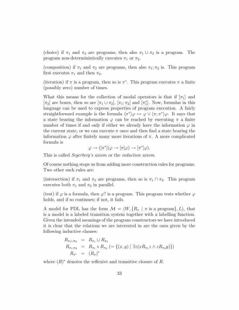
(choice) if π1 and π2 are programs, then also π1 ∪ π2 is a program. Theprogram non-deterministically executes π1 or π2.

(composition) if π1 and π2 are programs, then also π1; π2 is. This programfirst executes π1 and then π2.

(iteration) if π is a program, then so is π∗. This program executes π a finite(possibly zero) number of times.

What this means for the collection of modal operators is that if [π1] and[π2] are boxes, then so are [π1 ∪ π2], [π1; π2] and [π∗1]. Now, formulas in thislanguage can be used to express properties of program execution. A fairlystraightforward example is the formula 〈π∗〉ϕ ↔ ϕ ∨ 〈π; π∗〉ϕ. It says thata state bearing the information ϕ can be reached by executing π a finitenumber of times if and only if either we already have the information ϕ inthe current state, or we can execute π once and then find a state bearing theinformation ϕ after finitely many more iterations of π. A more complicatedformula is

ϕ→ ([π∗](ϕ→ [π]ϕ)→ [π∗]ϕ).

This is called Segerberg’s axiom or the induction axiom.

Of course nothing stops us from adding more construction rules for programs.Two other such rules are:

(intersection) if π1 and π2 are programs, then so is π1 ∩ π2. This programexecutes both π1 and π2 in parallel.

(test) if ϕ is a formula, then ϕ? is a program. This program tests whether ϕholds, and if so continues; if not, it fails.

A model for PDL has the form M = (W, {Rπ | π is a program}, L), thatis a model is a labeled transition system together with a labelling function.Given the intended meanings of the program constructors we have introducedit is clear that the relations we are interested in are the ones given by thefollowing inductive clauses:

Rπ1∪π2 = Rπ1 ∪Rπ2

Rπ1;π2 = Rπ1 ◦Rπ2 (= {(x, y) | ∃z(xRπ1z ∧ zRπ2y)})Rπ∗ = (Rπ)∗

where (R)∗ denotes the reflexive and transitive closure of R.

33

Example 20. PDL can be interpreted on any transition system (W,Rπ)π∈Π.Such a system is called a regular frame if the relations satisfy the conditions ofexample 19. One can show that a frame F is regular if and only if F |= ∆∪Γwhere

∆ := {p→ ([π∗](p→ [π]p)→ [π∗]p), 〈π∗〉p↔ (p ∨ 〈π〉〈π∗〉p) | π ∈ Π},

and

Γ := {〈π1; π2〉p↔ 〈π1〉〈π2〉p, 〈π1 ∪ π2〉p↔ 〈π1〉p ∨ 〈π2〉p | πi ∈ Π}.

Exercise 18. Show that regular frames are characterized by the formulas in∆ and Γ, given in example 20

References

[1] Patrick Blackburn, Marteen de Rijke and Yde Venema,Modal Logic. Cambridge Tracts in Theoretical Computer Science(53) 2004.

[2] Dirk van Dalen,Logic and Structure. Third edition. Universitext. Springer-Verlag,Berlin, 1994.

[3] Michael R. A. Huth and Mark D. Ryan,Logic in Computer Science, Modelling and reasoning about sys-tems. Cambridge university press 2000.

[4] Dick de Jongh, Frank Veltman,Intensional Logics. Course notes,http://staff.science.uva.nl/∼veltman/papers/FVeltman-intlog.pdf

[5] Erik Palmgren,Konstruktiv Logik, U.U.D.M. Lecture Notes 2002:LN1http://www.math.uu.se/∼palmgren/tillog/klogik02.ps

34