Mobile Money and Monetary Policy in East African … · Mobile Money and Monetary Policy in East African Countries Christopher S. Adam and S ebastien E. J. Walker University of Oxford

Mobile Money and Monetary Policy in EastAfrican Countries

Christopher S. Adam and Sebastien E. J. Walker∗

University of Oxford

April 14, 2015

Abstract

As mobile phones have spread at breakneck speed in East African countries, so toohas their use for accessing basic financial services. ‘M-Pesa’ in Kenya is the best-known of such ‘mobile money’ products, but is now one amongst many others avail-able in East Africa. The dramatic benefits of mobile money at the microeconomiclevel have been widely documented, but its macroeconomic impacts have so far at-tracted little formal investigation despite the interest and concerns of the region’spolicymakers. We model the emergence of mobile money (MM) by introducing anincreasingly advanced remittance payment technology into a Dynamic StochasticGeneral Equilibrium (DSGE) framework with two sectors (rural and urban pro-ducer households). Despite initial concerns that mobile money would underminethe conduct of monetary policy, our results suggest that MM should increase themacroeconomic stability of the countries in which it is widespread, with benefitsgoing mainly to rural (and thus lower-income) households. Our results also suggestthat as financial innovations help to reduce the incompleteness of markets, the mon-etary authorities may be able usefully to shift their focus from headline inflation tocore inflation. These results add to the case for policymakers to continue supportingand encouraging the further spread of MM in East African Countries and beyond.Our findings also suggest that policymakers should work with mobile network oper-ators to enable cross-border transfers amongst East African Community countriesahead of the planned East African Monetary Union.

Keywords: Mobile money, financial innovations, remittances, East Africa, mone-tary policy, DSGE models

∗Emails: [email protected] and [email protected]. The authorsgratefully acknowledge funding from the Bill and Melinda Gates Foundation; support from InternationalGrowth Centre staff in Tanzania and Uganda; assistance from staff at the Central Bank of Kenya, theBank of Tanzania, and the Bank of Uganda; help from staff at mobile network operators and otherorganisations in Kenya, Tanzania, and Uganda; and comments from participants at the Mobile Moneyand the Economy conference in Kampala, February 2015. We are indebted to Rahul Anand for sharinghis code. The usual disclaimer applies. Comments are welcome.

1

Contents

1 Introduction 3

2 Background 4

3 The Model 73.1 The Anand and Prasad (2010) model . . . . . . . . . . . . . . . . . . 83.2 Introducing remittances . . . . . . . . . . . . . . . . . . . . . . . . . 83.3 Monetary policy rules . . . . . . . . . . . . . . . . . . . . . . . . . . 10

4 Simulations 104.1 Calibration . . . . . . . . . . . . . . . . . . . . . . . . . . . . . . . . 104.2 Results . . . . . . . . . . . . . . . . . . . . . . . . . . . . . . . . . . . 12

5 Conclusions 15

Appendix 1 Formal outline of the Anand and Prasad model 17

Appendix 2 List of variables and parameters 23

References 24

2

1 Introduction

On Saturday the 21st of September 2013, members of the Islamist group al-Shababattacked the Westgate Mall in Nairobi, resulting in a bloodbath. On the followingday, Safaricom, the mobile operator and market leader in mobile money servicesin Kenya, launched a special zero-rated number for Kenyans to send donations tohelp the victims of the attack using its M-Pesa service. By noon on the followingMonday, KSh36 million (over US$400,000) were donated by some 100,000 Kenyansthrough that channel alone.1 This is one particularly striking example of the impactof mobile money in East Africa; it is, however, one example amongst many.

We use ‘mobile money’ (‘MM’) as a catch-all term to include all financial ser-vices provided via mobile network operators (MNOs); these services mainly involveenabling users to store money on their MM accounts and to transfer them to otherusers, although credit and savings products are increasingly being offered by someMNOs. MM, which is hugely popular in Kenya, Tanzania, and Uganda, allows anurban worker to send money to her pensionless parents living in a distant village,and thus to avoid the costs, delays, and risks of taking cash in person or of sendingit with a bus driver. Rural people who do not have access to bank branches nowhave a secure place to store their savings – the alternative is to store money literally‘under the mattress’ (if they have one) or in the form of livestock, with all the riskswhich these saving technologies entail. The ability instantly and securely to sendmoney to pay for goods and services; to contribute to the cost of a funeral; or toprovide liquidity to farm tenants who need to invest in new tools potentially helpsto channel funds to where they are the most useful, whether it be for consumptionor investment purposes. MM can therefore help households to smooth their con-sumption when faced with an income shock, or to invest when they face liquidityconstraints.

That MM is having a profound impact on these countries at the microeconomiclevel is relatively clear. For example, it can help to increase saving among individualswith little or no access to formal financial services by providing them with a rudi-mentary bank account (Morawczynski and Pickens, 2009); by facilitating depositsinto informal saving group accounts (Wilson, 2010); or by simply allowing users tokeep their savings hidden from friends or relatives who might ask them for money(Jack and Suri, 2011). MM can also reinforce informal insurance networks: Jackand Suri’s (2014) study of M-Pesa in Kenya finds that while income shocks reduceconsumption by 7% for non-users the consumption of user households is unaffected,so that the latter are in effect fully insured on average. However, far less clear arethe macroeconomic consequences and policy implications of the widespread use ofMM.

Work by Weil et al. (2012) offers a preliminary assessment of the impact ofM-Pesa on the behaviour of monetary aggregates in Kenya. They conclude thatthe monetary policy implications of MM are currently nugatory in Kenya (andare likely to be equally small in Tanzania and Uganda). These conclusions aretentative, however, not least because the diffusion rate for MM was still relativelymodest at the time of their study. They acknowledge, however, that “developmentsand innovations in this space could fuel the growth of MM such that it reaches levelswhere it could have [significant] implications for monetary policy”.

1http://www.businessdailyafrica.com/Donations-to-Safaricom-fund-/-/539546/2004568/-/h3kdr9/-/index.html.

3

Misati et al. (2010) find that financial innovation seems to have weakened themonetary transmission mechanism, but do not distinguish the effect of MM fromthat of other innovations. Macha (2013) conducts a study in the spirit of Weilet al.’s (2012) for Tanzania, and finds a clear coincidence of the instability of themoney demand parameter estimates with the introduction of MM. He concludesthat MM has an impact on money demand and hence on the velocity of money,although, unlike Weil et al. for Kenya, in insignificant magnitudes. Ndirandgu andNyamongo (2015) update and extend the Weil et al. analysis on Kenya. Theyfind that the fast pace of financial development in Kenya has not caused structuralshifts in the long-run money demand relation, and has therefore not underminedthe conduct of monetary policy in Kenya.

Aron et al.’s (2015) econometric work investigates inflation forecasting modelsfor Uganda, with a notable focus on the potential impact of mobile money. The au-thors estimate models to forecast the 1-month and 3-month ahead rate of inflationfor food prices, non-food prices, and energy prices. They test a wide range of possibledeterminants, and allow for the possibility of structural breaks and non-linearitiesin the relationship between these determinants and inflation. An important de-velopment compared to research looking at similar issues in the recent past is theinclusion of rainfall shocks as a possible determinant. The authors find only tenta-tive evidence that mobile money may exert some downward pressure on inflation,possibly reflecting positive impacts on productivity.

In this paper we investigate the impact of MM on the macroeconomy by focus-ing on what has so far been the main service provided to users: a secure, instan-taneous, and inexpensive means of sending remittances. We build on the modelof Anand and Prasad (2010) and introduce into it an increasingly advanced remit-tance technology. The model combines rural food-producing households with urbannon-food-producing households, and only the latter are able to save and borrow tosmooth their consumption. This model is useful for our purposes as it was devel-oped to analyse monetary policy in low-income dualistic economies similar to thoseof East African countries. The remittance channel we incorporate allows the urbanhouseholds to insure the rural households against income fluctuations.

Contrary to initial concerns that mobile money would undermine the conduct ofmonetary policy, our simulations predict that MM should bring material macroe-conomic benefits in the form of greater stability of the overall economy, with thebenefits accruing mainly to rural (and thus lower-income) households. Our resultsalso suggest that as financial innovations help to reduce the incompleteness of mar-kets the monetary authorities may find it useful to target core inflation rather thanheadline inflation, or at least be more comfortable about accommodating first-roundnon-core price shocks in the absence of core price shocks. These results add to thecase for policymakers to continue supporting and encouraging the further spreadof MM in East African Countries and beyond. Our findings also suggest that pol-icymakers should work with MNOs to enable cross-border transfers amongst EastAfrican Community countries ahead of the planned East African Monetary Union.

2 Background

Assessing the impact of mobile money on monetary policy is of particular relevanceat the current time in East Africa. Since the mid-1990s the three largest economiesin the region, Kenya, Tanzania, and Uganda have enjoyed high and stable growth

4

while maintaining annual inflation in the single digits for most of the last twentyyears. Even when inflation rates moved sharply above the central banks’ inflationtargets of 5 percent, as they did in 2009-11 when world and regional food pricesspiked, concerted policy action by the central banks brought inflation back to target.Much of this success, particularly in the early years, was due to close adherence toconventional reserve money programmes which seeks to exploit the relative stabilityof the private sector demand for money to target inflation through monetary targets.The conventional reserve money targeting approach starts from a simple monetaristor quantity theory of money. The ‘quantity equation’ is given by

Mtvt = PtYt, (1)

where Mt is the quantity of money; vt is the transactions velocity of money, whichmeasures the rate at which money circulates in the economy, which is determinedby the private sectors demand for money; Pt is the average price per transaction;and Yt is a measure of the number of transactions in a given period. In practicalapplications, it is common to use real GDP as a proxy for the number of transactions.Assuming that velocity is stable and predictable, then the path of nominal GDP,PtYt, is a predictable function of the quantity of money. Two further assumptionsturn the quantity theory into an operational monetary policy strategy. The first isthe relationship between the quantity of money, Mt, and ‘reserve money’ (or insidemoney), Ht, the component of the money supply under the control of the centralbank. This relationship is summarised by the money multiplier (mt)

Mt = mtHt (2)

The second is that the authorities can project real output, Yt. With these assump-tion we can express inflation (the growth rate of prices) as

Pt = Ht − Yt + (m+ v)t (3)

where χ denotes the growth rate of a variable χ. Hence, conditional on an expectedgrowth of real output, targeting reserve money will anchor inflation if and only if thegrowth rates of the money multiplier and the velocity of circulation are constant(or at least predictable). If either or both are unstable, reserve money targetingbecomes ineffective. The recent instability of both in Kenya, Uganda, and Tanzania– ascribed by the central banks to the effects of information and communicationtechnology-driven financial innovation, including the emergence of mobile money –has been instrumental in all three countries embarking upon a delicate transitionfrom conventional ‘reserve money targeting’ approaches towards what is being called‘flexible monetary targeting’, under which the authorities will seek to rely muchmore heavily on price- rather than quantity-based instruments of monetary policy(IMF, 2014 and O’Connell, 2013). The effectiveness of price-based monetary policydepends critically on the central banks being able to identify the key channels ofthe underlying monetary transmission mechanism and, crucially, how it is affectedby these aspects of financial innovation.

The emphasis on the velocity of money and the money multiplier in previousresearch may be natural in a monetary-targeting framework, but it is not clear thatthis is warranted as the main instrument becomes a policy interest rate. With thetransition towards price-based instruments of monetary policy, the quantity of re-serve money in circulation becomes a second-order consideration: it is essentially

5

demand-driven. Increasingly important is the depth of financial markets, and theproportion of firms and households which are (gross) borrowers or savers and there-fore sensitive to interest rates. MM is clearly increasing the number of householdsand small businesses which use formal financial services, whether directly by provid-ing access to such services, or indirectly by acting as a complement to or otherwiseencouraging users to access bank services. The upshot is that households and smallbusinesses are increasingly likely to earn interest on their savings and to borrowto smooth consumption or fund investment; as a result, these agents are also in-creasingly likely to be affected by the interest rates set by monetary policy makers.However, the extent of this impact is as yet unknown.

One result is nonetheless undisputed. There is no reason for the introduction ofmobile money to be ‘fundamentally’ inflationary (or indeed disinflationary). Rather,its macroeconomic impact depends critically on how monetary policy adapts to whatis one financial innovation amongst others, including ATMs, debit and credit cards,agency banking, real-time gross settlement systems (RTGSs), etc., as expoundedbelow (section 2.1). In summary, any MM balances are fully backed by money de-posited by MNOs in a bank, so no ‘new’ money is created by the MNOs. Banks canuse these additional funds to increase their lending, which does create new money,but this is no different from the way in which banks use ordinary deposits. Demom-bynes and Thegeya (2012) distinguish between two types of mobile savings: (1)‘basic mobile savings’, where households store balances on M-Pesa-type MM sys-tems earning no interest, as one might use a current (bank) account for savings; and(2) ‘bank-integrated mobile savings’, where an account accessible via mobile phoneyields interest on savings, and might enable users to apply for credit. Even whereMM services provide credit or interest on savings, these remain services providedby banks to which MNOs give access.

Financial innovations always change the velocity of money and the money mul-tiplier by altering the cost of liquidity services and the costs and benefits facingcompanies, banks, and households. It is important to understand and take intoaccount these evolutions in the conduct of monetary policy regardless of the par-ticular framework in place. However, while the technology is new, monetary eco-nomics has always been about such innovations, as was the case with the 1980sdebate about financial innovation undermining monetary targeting in high-incomecountries (HICs); therefore, MM does not represent anything new in a fundamen-tal sense when seen through the lens of a monetary economist. Central banks inKenya, Tanzania, and Uganda have generally supported, and often encouraged, theintroduction and development of MM; one of their reasons for doing so is the hopethat a greater proportion of households in the formal financial system will assist theconduct of monetary policy.

Furthermore, MM is not distributionally neutral, as its benefits accrue dispro-portionately to lower-income households. Evidence from Kenya (Aker and Mbiti,2010) suggests that higher-income and urban households are more likely to use MMthan lower-income and rural households, but it seems that the former use it asa complement to other formal financial services, while for the latter it may be theonly formal financial service available (Mbiti and Weil, 2011). Moreover, if a higher-income urban worker makes an MM transfer to her lower-income rural family, theyare clearly both using MM, but it seems fair to say that it is the lower-income re-cipient who derives the greatest benefit from the service. MM is ‘pro-poor’ insofaras it helps hand-to-mouth (‘Keynesian’) and shock-prone households with highly

6

seasonal incomes to smooth their consumption (e.g., by providing a saving tech-nology or reinforcing informal insurance networks), and helps liquidity-constrainedfirms (e.g., small-scale farms) to invest. Therefore, even if rural households do notthemselves save or borrow, the ability to receive MM transfers also enables them toinvest and smooth their consumption, and is therefore likely to have positive effectson economic growth and stability. The result is plausibly to lessen the challengesfacing monetary- and fiscal-policy makers, notably when it comes to stabilising foodprices (possibly through subsidies, for example), but this remains to be established.

While all of the above-mentioned macroeconomic effects of MM are likely to bematerial, it may still take some time for their full effect to be felt (and measured),particularly in Uganda and Tanzania where MM penetration has lagged behindKenya. One important implication of this is that identification of the impact ofMM on the effectiveness of monetary policy through conventional econometric anal-ysis is unlikely to be particularly illuminating. Indeed, given the breakneck pace atwhich the MM market is developing, a backward-looking empirical study will daterather quickly. We therefore favour an alternative methodological approach which isinformed by, but not wholly dependent on, careful econometric analysis of the avail-able data. We develop a theoretical model which captures the clear microeconomiccharacteristics of MM within an aggregate macroeconomic structure embodying thekey structural characteristics of our East African economies. We use the model toassess how the spread of MM technologies modifies the properties of the monetarypolicy regimes currently being developed by the countries of the region.

Our model is based on that of Anand and Prasad (2010), which was devel-oped to evaluate optimal monetary policy rules in economies with many of thestructural characteristics of low-income countries, including: dualism in productioncombined with a prevalence of agricultural or climatic shocks; high levels of subsis-tence consumption; and low levels of financial inclusion. Our framework includestwo household types, rural and urban, which respectively produce two goods: foodand non-food output. The rural households are subsistence farmers, who are highlyvulnerable to supply-side shocks, and who would therefore reap large welfare gainsif they were able to smooth their consumption, but do not have access to any savingtechnology (let alone credit). Remittances are sent from urban to rural householdsusing a costly remittance technology. Financial innovations reduce the cost of send-ing remittances to rural households and increase urban households’ inclination todo so.

3 The Model

Figure 1 below shows the overall structure of the Anand and Prasad (2010) model.To the left of the dashed line is the rural food-producing sector, and to the right isthe urban non-food producing sector. The bold line shows the remittance transfersfrom urban to rural households which we add to the original model.

7

Figure 1. Model overview

LABOUR

FOOD

NON-FOOD

WAGES

WAGES

LABOUR

CREDIT/SAVINGS INTEREST RATE REMITTANCES/

MOBILE MONEY

TRANSFER

FOOD HHs NON-FOOD HHs

NON-FOOD FIRMS FOOD FIRMS

BOND MARKET

CENTRAL BANK

3.1 The Anand and Prasad (2010) model

A proportion of households, which works in the food production sector (“ruralhouseholds”), cannot save or borrow at all and therefore consumes its entire incomeeach period. The remaining households, which work in non-food production (“urbanhouseholds”), have access to perfect capital markets and smooth their consumptionfollowing a standard Euler equation. Households in each sector sell their labourexclusively to firms in their respective sectors, and labour is the only factor of pro-duction; output in each sector is linear in labour and is subject to sector-specificproductivity shocks. Households in each sector consume both food and non-foodgoods. Monetary policy affects the economy through the consumption Euler equa-tion which applies to non-food sector households.

Anand and Prasad (2010) find that the central bank maximises welfare withan interest rate rule whose arguments are headline (rather than core) inflation, theoutput gap, and the lag of the interest rate. Their results are driven by the factthat credit-constrained households’ consumption is insensitive to the interest rateand is determined entirely by their real income, which is increasing in food prices.Therefore, if the central bank targets core inflation, thereby ignoring food pricesin its interest rate decision, aggregate demand may move in the opposite directionfrom that intended by monetary-policy makers. A formal outline of the Anand andPrasad (2010) is given in Appendix 1.

3.2 Introducing remittances

In the original Anand and Prasad model the rural household’s consumption at timet is given by

Cft = xf,t (yf,t − C∗) , (4)

8

where Cft is a composite of food and non-food consumption2; xf,t is the relative priceof food3; yf,t is food production per rural firm; and C∗ is the minimum amount offood consumption required for subsistence. Rural households’ composite consump-tion is thus equal to earnings from producing food less the cost of subsistence foodconsumption.

Let us now define Ωt as the rural households’ earned income net of the cost ofsubsistence food consumption, so that

Ωt = xf,t (yf,t − C∗) . (5)

We introduce remittances from urban to rural households which include a steady-state component (a regular transfer such as a pension) and an insurance componentwhich increases as Ωt falls below its steady-state value. The remittance paymentmt (in units of real composite consumption) is given by

mt = m exp[−κ(Ωt/Ω− 1

)], (6)

where exp[·] is the exponential function, χ denotes the steady-state value of a vari-able χt, and κ is the elasticity of remittances with respect to deviations of Ωt fromits steady state. This insurance transfer increases rapidly as the rural household’searned income falls, but decreases somewhat in good times.

To capture the cost of sending a remittance, we assume that a certain amountof the transfer sent ‘melts’ away before it reaches the recipient. Let the grossmelt rate in the steady state be 1 + µ, where µ > 0, so that the steady-stateamount of money received by the remittance beneficiary is m/(1 + µ). To ensurethat our results are comparable across economies with different assumed remittancetechnologies we assume that the steady state is the same in each case. The differentremittance technologies will instead affect our model economy outside of the steadystate through (1) the elasticity parameter κ and (2) a variable ‘melt’ rate out ofsteady state. We assume that the proportion of the remittance lost before it reachesthe recipient is weakly decreasing in the amount sent; in other words, the larger theamount sent the smaller the cost per (real) Shilling. Without loss of generality, weassume that the parameter κ reflects the speed at which the melt rate falls with theamount sent. Let the amount received by the remittance recipient, for an amountsent mt, then be

mt

(1 + µ)(mtm )

−κ . (7)

So as mt rises above its steady-state value m, the amount which melts away falls,and does so at a faster rate for a greater value of κ.

In our simulations, a more ‘advanced’ remittance technology will be associatedwith a higher κ; the greater κ, the more remittances will be sent to rural householdsfor a given fall in earned income, and the lower the marginal cost of sending theremittances (as measured by the melt rate). We can motivate the existence of aninvariant melt rate in the steady state by appealing to fixed costs of using any re-mittance technology (identifying a suitable bus driver, purchasing a mobile phone,etc.), while the decreasing marginal cost of remittances conveniently mirrors the

2The f superscript denotes consumption by food-producing, i.e., rural households3The f subscript denotes price of food.

9

tiered fee structure of mobile money transfers. A more advanced remittance tech-nology will also make urban households more inclined to send remittances thanks toits greater speed, convenience, and security. With remittances built into the Anandand Prasad model, our rural households’ demand for composite consumption is thengiven by

Cft = xf,t (yf,t − C∗) +mt

(1 + µ)(mtm )

−κ . (8)

The full list of model equations in terms of stationary variables used for our simu-lations is given in Appendix 2.

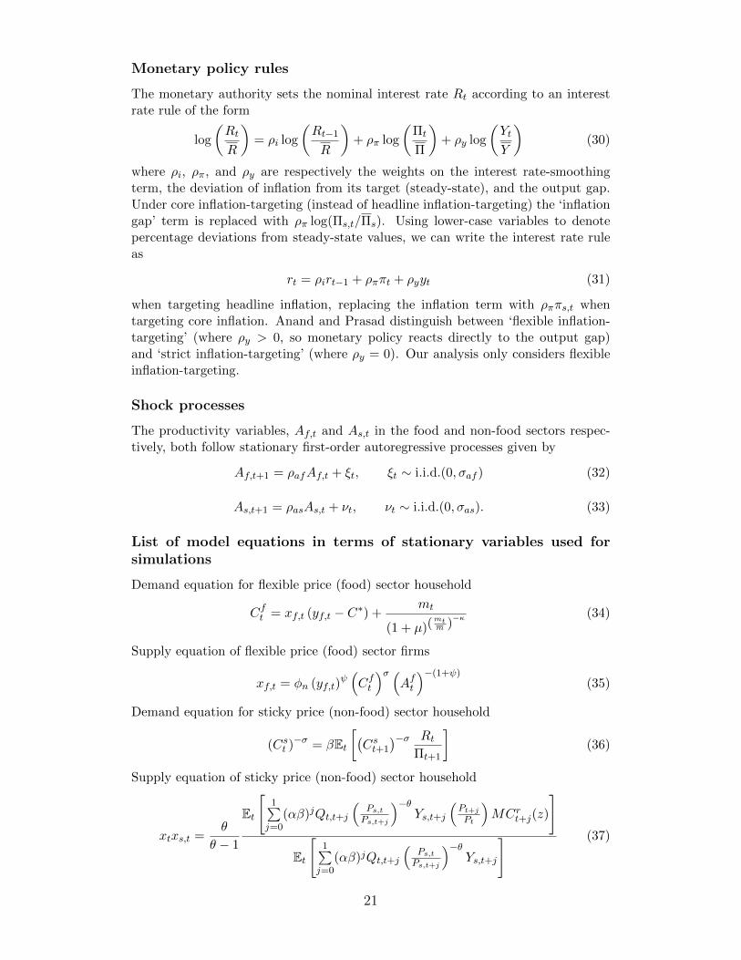
3.3 Monetary policy rules

The monetary authority follows an interest rate rule of the form

rt = ρirt−1 + ρππt + ρyyt, (9)

where the lower case variables are expressed in percentage deviations from theirsteady-state values; rt is the nominal interest rate; πt is headline inflation; yt isGDP; and ρi, ρπ, and ρy are respectively the weights on the interest rate-smoothingterm, the deviation of inflation from its target (the steady-state value), and theoutput gap. We consider two versions of this rule depending on whether the centralbank targets headline inflation or core inflation, where the latter is denoted by πs,t.

4 Simulations

In this section we simulate the calibrated model over 16 quarters (4 years) to as-sess the impact of introducing mobile money into the economy, and to comparethe performance of headline- and core-inflation-targeting as increasingly advancedremittance technologies are introduced. We compare the volatilities of the mainvariables of interest under headline- and core-inflation-targeting and under threedifferent remittance technologies (‘no remittances’, ‘constrained remittances’, and‘mobile money’).

4.1 Calibration

Our calibration follows that of Anand and Prasad with a few exceptions – the valuesare listed in Table 1. The number of urban households is normalised to 1, and weset the number of rural households, λ, to 2 so as better to reflect the structure of anEast African economy. We set the inverse of the Frisch elasticity of labour supply,ψ, to 10 following Berg et al. (2012), implying an inelastic labour supply consistentwith the estimates of Goldberg (2015) from Malawi. We set the persistence of thefood productivity shock, ρaf , to 0.75, implying a fairly persistent shock. We set theweight on the output gap in the interest rate rule, γY , to 1 so that the central bankresponds more to the output gap.

10

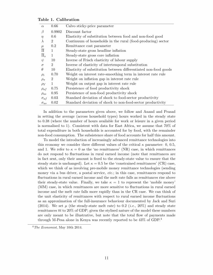
Table 1. Calibration

α 0.66 Calvo sticky-price parameter

β 0.9902 Discount factorη 0.6 Elasticity of substitution between food and non-food goodλ 2 Continuum of households in the rural (food-producing) sectorµ 0.2 Remittance cost parameter

Π 1 Steady-state gross headline inflation

Πs 1 Steady-state gross core inflationψ 10 Inverse of Frisch elasticity of labour supplyσ 2 Inverse of elasticity of intertemporal substitutionθ 10 Elasticity of substitution between differentiated non-food goodsρi 0.70 Weight on interest rate-smoothing term in interest rate ruleρπ 2 Weight on inflation gap in interest rate ruleρY 1 Weight on output gap in interest rate ruleρaf 0.75 Persistence of food productivity shockρas 0.95 Persistence of non-food productivity shockσaf 0.03 Standard deviation of shock to food-sector productivityσas 0.02 Standard deviation of shock to non-food-sector productivity

In addition to the parameters given above, we follow and Anand and Prasadin setting the average (across household types) hours worked in the steady stateto 0.38 (where the number of hours available for work or leisure in a given periodis normalised to 1). Consistent with data for East Africa, we assume that 70% oftotal expenditure in both households is accounted for by food, with the remaindernon-food consumption. The subsistence share of food accounts for half this amount.

To model the introduction of increasingly advanced remittance technologies intothis economy we consider three different values of the critical κ parameter: 0, 0.5,and 1. We refer to κ = 0 as the ‘no remittances’ (NR) case, in which remittancesdo not respond to fluctuations in rural earned income (note that remittances arein fact sent, only their amount is fixed to the steady-state value to ensure that thesteady state is unchanged). Let κ = 0.5 be the ‘constrained remittances’ (CR) case,which we think of as involving pre-mobile money remittance technologies (sendingmoney via a bus driver, a postal service, etc.; in this case, remittances respond tofluctuations in rural earned income and the melt rate falls as remittances rise abovetheir steady-state value. Finally, we take κ = 1 to represent the ‘mobile money’(MM) case, in which remittances are more sensitive to fluctuations in rural earnedincome and the melt rate falls more rapidly than in the CR case. We can think ofthe unit elasticity of remittances with respect to rural earned income fluctuationsas an approximation of the full-insurance behaviour documented by Jack and Suri(2014). We set µ (the steady-state melt rate) to 0.2 (i.e., 20%) and steady stateremittances m to 20% of GDP; given the stylised nature of the model these numbersare only meant to be illustrative, but note that the total flow of payments madethrough M-Pesa alone in Kenya was recently reported to be 43% of GDP.4

4The Economist, May 10th 2014.

11

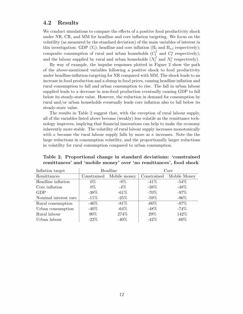
4.2 Results

We conduct simulations to compare the effects of a positive food productivity shockunder NR, CR, and MM for headline and core inflation targeting. We focus on thevolatility (as measured by the standard deviation) of the main variables of interest inthis investigation: GDP (Yt); headline and core inflation (Πt and Πs,t respectively);

composite consumption of rural and urban households (Cft and Cst respectively);

and the labour supplied by rural and urban households (Nft and N s

t respectively).By way of example, the impulse responses plotted in Figure 2 show the path

of the above-mentioned variables following a positive shock to food productivityunder headline-inflation-targeting for NR compared with MM. The shock leads to anincrease in food production and a slump in food prices, causing headline inflation andrural consumption to fall and urban consumption to rise. The fall in urban laboursupplied leads to a decrease in non-food production eventually causing GDP to fallbelow its steady-state value. However, the reduction in demand for consumption byrural and/or urban households eventually leads core inflation also to fall below itssteady-state value.

The results in Table 2 suggest that, with the exception of rural labour supply,all of the variables listed above become (weakly) less volatile as the remittance tech-nology improves, implying that financial innovations can help to make the economyinherently more stable. The volatility of rural labour supply increases monotonicallywith κ because the rural labour supply falls by more as κ increases. Note the thelarge reductions in consumption volatility, and the proportionally larger reductionsin volatility for rural consumption compared to urban consumption.

Table 2. Proportional change in standard deviations: ‘constrainedremittances’ and ‘mobile money’ over ‘no remittances’, food shock

Inflation target Headline Core

Remittances Constrained Mobile money Constrained Mobile Money

Headline inflation 0% -8% -41% -54%Core inflation 0% -4% -38% -48%GDP -38% -61% -70% -97%Nominal interest rate -11% -25% -59% -86%

Rural consumption -46% -81% -60% -87%Urban consumption -40% -64% -48% -74%Rural labour 90% 274% 29% 142%Urban labour -22% -40% -42% -60%

12

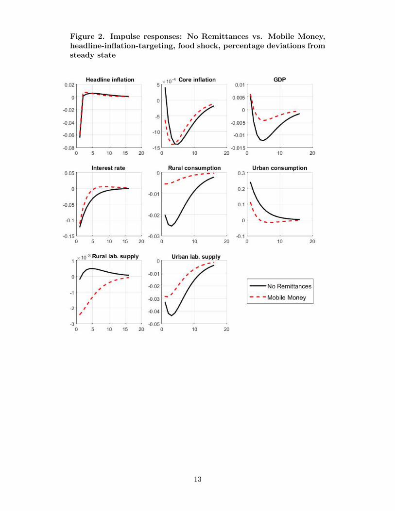
Figure 2. Impulse responses: No Remittances vs. Mobile Money,headline-inflation-targeting, food shock, percentage deviations fromsteady state

13

The results in Table 3 indicate that GDP volatility is reduced by targetingcore rather than headline inflation under CR and MM. Headline inflation is morevolatile when targeting core inflation for each of the remittance technologies, butthis difference shrinks as the remittance technology becomes more advanced. Coreinflation volatility is reduced when targeting core inflation under CR and MM.Urban consumption is less volatile for each of the remittance technologies whentargeting core inflation, which is a consequence of the standard result that whenmarkets are complete it is optimal to target core inflation; but rural consumption,and both rural and urban labour supplied become less volatile under core inflation-targeting in the MM case. These results suggest that as financial innovations helpto reduce the incompleteness of markets the monetary authorities may find it usefulto target core inflation rather than headline inflation; at a minimum, the monetaryauthorities should be more comfortable about accommodating first-round non-coreprice shocks in the absence of core price shocks.

Table 3. Proportional change in standard deviations: headline- overcore-inflation-targeting, food shock

Remittances No Remittances Constrained Mobile Money

Headline inflation -59% -30% -17%Core inflation -34% 7% 24%GDP -34% 36% 682%Nominal interest rate 58% 244% 758%

Rural consumption -29% -5% 4%Urban consumption 2% 16% 41%Rural labour -34% -3% 2%Urban labour -30% -4% 5%

We now consider the effects of a shock to non-food productivity. The resultsin Table 4 are qualitatively similar to those in the case of the food productivityshock (Table 2), and suggest that more advanced remittance technologies also helpto increase the inherent stability of the economy when it is subject to a non-foodproductivity shock. A notable difference is that the volatility of urban consumptionincreases dramatically when more advanced remittances technologies are introduced;this arises from the fact that a positive non-food technology shock increases the con-sumption of both household types in the absence of remittances (NR). But as wemove to CR and MM rural consumption rises by less and urban consumption risesby more because the amount of remittances sent falls as rural earned income rises(due to higher food prices). In quantitative terms, the effects of more advanced re-mittance technologies on the volatility of inflation and GDP are materially smallerthan in the case of the food-productivity shock, in some cases by orders of magni-tude; this is consistent with the notion that the benefits of mobile money accruedisproportionately to rural (and as a rule, lower-income) households.

14

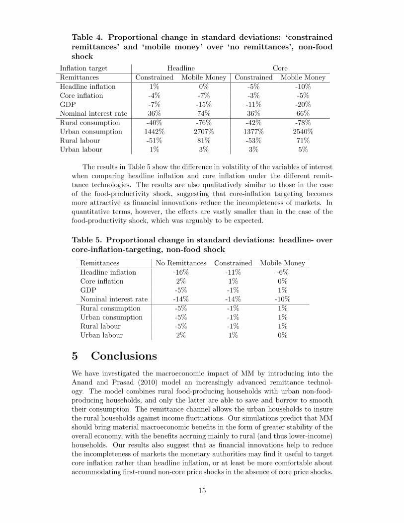
Table 4. Proportional change in standard deviations: ‘constrainedremittances’ and ‘mobile money’ over ‘no remittances’, non-foodshock

Inflation target Headline Core

Remittances Constrained Mobile Money Constrained Mobile Money

Headline inflation 1% 0% -5% -10%Core inflation -4% -7% -3% -5%GDP -7% -15% -11% -20%Nominal interest rate 36% 74% 36% 66%

Rural consumption -40% -76% -42% -78%Urban consumption 1442% 2707% 1377% 2540%Rural labour -51% 81% -53% 71%Urban labour 1% 3% 3% 5%

The results in Table 5 show the difference in volatility of the variables of interestwhen comparing headline inflation and core inflation under the different remit-tance technologies. The results are also qualitatively similar to those in the caseof the food-productivity shock, suggesting that core-inflation targeting becomesmore attractive as financial innovations reduce the incompleteness of markets. Inquantitative terms, however, the effects are vastly smaller than in the case of thefood-productivity shock, which was arguably to be expected.

Table 5. Proportional change in standard deviations: headline- overcore-inflation-targeting, non-food shock

Remittances No Remittances Constrained Mobile Money

Headline inflation -16% -11% -6%Core inflation 2% 1% 0%GDP -5% -1% 1%Nominal interest rate -14% -14% -10%

Rural consumption -5% -1% 1%Urban consumption -5% -1% 1%Rural labour -5% -1% 1%Urban labour 2% 1% 0%

5 Conclusions

We have investigated the macroeconomic impact of MM by introducing into theAnand and Prasad (2010) model an increasingly advanced remittance technol-ogy. The model combines rural food-producing households with urban non-food-producing households, and only the latter are able to save and borrow to smooththeir consumption. The remittance channel allows the urban households to insurethe rural households against income fluctuations. Our simulations predict that MMshould bring material macroeconomic benefits in the form of greater stability of theoverall economy, with the benefits accruing mainly to rural (and thus lower-income)households. Our results also suggest that as financial innovations help to reducethe incompleteness of markets the monetary authorities may find it useful to targetcore inflation rather than headline inflation, or at least be more comfortable aboutaccommodating first-round non-core price shocks in the absence of core price shocks.

15

Our results add to the case for policymakers to continue supporting and en-couraging the further spread of MM in East African Countries and beyond. Ourfindings also suggest that policymakers should work with MNOs to enable cross-border transfers amongst East African Community (EAC) countries ahead of theplanned East African Monetary Union. As East African countries progress towardsthe Monetary Union planned for 2024, risk sharing-mechanisms will be critical forits members to withstand country-specific shocks (Aisen et al., 2015). As the EACcountries seek further to integrate their economies, the EAC Common Market Pro-tocol notably establishes that governments should guarantee the free movement ofworkers and their dependents across the EAC (ibid.). Risk-sharing across the re-gion will be enhanced if workers away from their home countries are able to sendremittances back to their relatives more easily thanks to MM. Cross-border MMtransfers could also increase regional labour mobility well in advance of the creationof the Monetary Union if workers are more willing to migrate safe in the knowledgethat they can straightforwardly remit funds to their dependents.

MM may also have fiscal implications because of its potential impact on taxrevenue. Typically narrow tax bases in LICs make it tempting for governments tobring MM and other mobile phone-related products and services into the tax net.While the low elasticity of demand for MM services means that direct taxation ofMM services may be efficient, it is likely to be regressive. There may, however, beprogressive if indirect ways in which MM could broaden the tax base available toLIC governments. It is now possible in Kenya, Rwanda, Tanzania, and Ugandato pay taxes using MM; and as mobile-based transactions, transfers, and savingsreplace those in cash and kind, revenue authorities ought to be more able to detecttax evasion. These two considerations could lead to lower tax evasion by alteringthe cost-benefit analysis involved in deciding whether or not to pay taxes, andtherefore to a greater amount of tax revenue for a given amount of economic activity.Moreover, this effect would become all the more important as MM increases theamount of economic activity in a country. A possible extension to our analysis wouldfocus on such fiscal issues. Another extension to our analysis would be to modelthe introduction of basic savings and credit products for low-income households,in light of the increasingly widespread availability of such products to the hithertounbanked thanks to MM platforms.

16

Appendix 1. Formal outline of the Anand and

Prasad model

Households

The economy is inhabited by 1+λ infinitely lived households, where λ is the numberof rural households and the number of urban households is normalised to 1. Thereis no labour mobility across sectors. Households are indexed by i, where i = f forrural (“f lexible-price sector”) households and i = s for urban (“sticky-price sector”)households. Household i maximises

E0

∞∑t=0

βt[u(Cit , N

it

)](1)

where β is the discount factor, Cit is the composite consumption (of food and non-food goods) by household i, and N i

t is the quantity of labour supplied by householdi. Instantaneous utility is given by

u(Cit , N

it

)=

(Cit)1−σ

1− σ− φn

(N it

)1−ψ1− ψ

, (2)

where σ is the inverse of the elasticity of intertemporal substitution, ψ is the inverseof the Frisch elasticity of labour supply, and φn is a scaling factor (on disutility fromlabour supplied). Composite consumption is defined by

Cit =

[γ

1η(Cif,t − C∗

)1− 1η + (1− γ)

1η(Cis,t

)1− 1η

] 1

1− 1η , (3)

where Cif,t is household i’s consumption of food and Cis,t is its consumption ofnon-food goods; the parameter C∗ is the minimum amount of food required forsubsistence5; γ is the weight on food in the consumption index; and η is the elasticityof substitution between food and non-food goods. Food goods are homogeneous,while non-food consumption is a continuum of differentiated goods given by

Cis,t =

[∫ 1

0cit(z)

θ−1θ dz

] θθ−1

, (4)

where θ is the elasticity of substitution between any two differentiated non-foodgoods and cit(z) is household i’s consumption of the non-food good produced byfirm z with z ∈ (0, 1).

Production in both sectors is linear in labour and each household owns one firm.Food production per firm (in that sector) is

yf,t = Af,tNft , (5)

where Af,t is exogenous productivity in the food sector and Nf,t is labour employedin food production. Similarly, non-food production by firm z is

ys,t(z) = As,tNst (z), (6)

with analogously defined variables.

5This subsistence threshold does not bind, but alters the elasticity of substitution between food andnon-food items and the marginal utility of food and non-food consumption.

17

Rural consumption

Rural households are excluded from financial markets, and must therefore consumetheir entire income every period in a hand-to-mouth (‘Keynesian’) fashion. A rep-resentative household maximises its expected intertemporal utility subject to thebudget constraint

Pf,tCff,t + Ps,tC

fs,t = W f

t Nft , (7)

where Pf,t is the price of food, Ps,t is the price index for non-food goods, and W ft

is the nominal wage in the food sector. The consumer price index (CPI), which is

the price of composite consumption Cft , is given by

Pt =[γ (Pf,t)

1−η + (1− γ)(Ps,t)1−η] 1

1−η. (8)

The budget constraint can then be written

PtCft = W f

t Nft − Pf,tC∗, (9)

so that the cost of composite consumption is equal to earnings each period net ofthe cost of subsistence consumption (of food).

The rural household’s demand for food is given by

Cff,t = γ

(Pf,tPt

)−ηCft + C∗, (10)

and its demand for non-food goods by

Cfs,t = (1− γ)

(Ps,tPt

)−ηCft , (11)

where Ps,t is the Dixit-Stiglitz price index given by

Ps,t =

[∫ 1

0Xt(z)

1−θdz

] 11−θ

, (12)

with Xt(z) the price of differentiated good z. Demand for each differentiated goodis

cft (z) =

[Xt(z)

Ps,t

]−θCfs,t. (13)

Finally, the first-order condition for the labour supply is

φn

(Nft

)ψ(Cft

)−σ =W ft

Pt. (14)

18

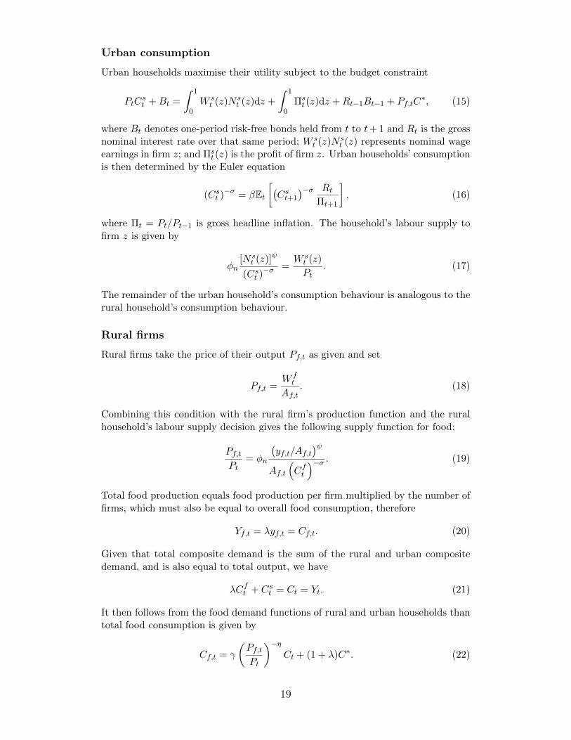
Urban consumption

Urban households maximise their utility subject to the budget constraint

PtCst +Bt =

∫ 1

0W st (z)N s

t (z)dz +

∫ 1

0Πst (z)dz +Rt−1Bt−1 + Pf,tC

∗, (15)

where Bt denotes one-period risk-free bonds held from t to t+ 1 and Rt is the grossnominal interest rate over that same period; W s

t (z)N st (z) represents nominal wage

earnings in firm z; and Πst (z) is the profit of firm z. Urban households’ consumption

is then determined by the Euler equation

(Cst )−σ = βEt[(Cst+1

)−σ RtΠt+1

], (16)

where Πt = Pt/Pt−1 is gross headline inflation. The household’s labour supply tofirm z is given by

φn[N s

t (z)]ψ

(Cst )−σ=W st (z)

Pt. (17)

The remainder of the urban household’s consumption behaviour is analogous to therural household’s consumption behaviour.

Rural firms

Rural firms take the price of their output Pf,t as given and set

Pf,t =W ft

Af,t. (18)

Combining this condition with the rural firm’s production function and the ruralhousehold’s labour supply decision gives the following supply function for food:

Pf,tPt

= φn

(yf,t/Af,t

)ψAf,t

(Cft

)−σ . (19)

Total food production equals food production per firm multiplied by the number offirms, which must also be equal to overall food consumption, therefore

Yf,t = λyf,t = Cf,t. (20)

Given that total composite demand is the sum of the rural and urban compositedemand, and is also equal to total output, we have

λCft + Cst = Ct = Yt. (21)

It then follows from the food demand functions of rural and urban households thantotal food consumption is given by

Cf,t = γ

(Pf,tPt

)−ηCt + (1 + λ)C∗. (22)

19

Urban firms

Non-food producing firms set prices in a Calvo fashion with a probability α of notbeing able to change their prices in a given period. Firm z chooses price Xt(z) tomaximise

Et

∞∑j=0

(αβ)jQt,t+j

Xt(z)yt,t+j(z)− TCt,t+j

[yt,t+j(z)

] , (23)

where Qt,t+j is the stochastic discount factor, yt,t+j is the output of firm z in periodt+j when it has set its price in period t, and TCt,t+j [·] is the total cost of producingthis output, with

Qt,t+j = βi(Cst+jCst

)−σPtPt+j

(24)

and

yt,t+j(z) =

[Xt(z)

Ps,t+j

]−θYs,t+j . (25)

The non-food sector price index is

Ps,t =[α(Ps,t−1)

1−θ + (1− α)X1−θt (z)

]1/(1−θ). (26)

The first-order condition for this optimisation problem is

Et

∞∑j=0

(αβ)jQt,t+jyt,t+j(z)Xt(z)−

θ

θ − 1MCrt+j(z)

= 0, (27)

where MCrt+j(z) is the real marginal cost given by

MCrt+j(z) =MCt+j(z)

Pt+j= φn

[yt,t+j(z)/As,t+j

]ψAs,t+j

(Cst+j

)−σ ; (28)

and θ/(θ−1) is the constant mark-up over the marginal cost, given that MCt,t+j =MCt+j : the marginal cost does not depend on the level of production given thatoutput is linear in labour.

Inflation and relative prices

The relative price of food is xf,t = Pf,t/Pt; the relative price of non-food goodsis xs,t = Ps,t/Pt; and the relative price charged by firms which can change theirprice at time t is xt = Xt/Ps,t. Gross non-food inflation (i.e., gross core inflation) isΠs,t = Ps,t/Ps,t−1. Finally, the relation between headline inflation and core inflationis given by

xs,t =Πs,txs,t−1

Πt. (29)

20

Monetary policy rules

The monetary authority sets the nominal interest rate Rt according to an interestrate rule of the form

log

(Rt

R

)= ρi log

(Rt−1

R

)+ ρπ log

(Πt

Π

)+ ρy log

(Yt

Y

)(30)

where ρi, ρπ, and ρy are respectively the weights on the interest rate-smoothingterm, the deviation of inflation from its target (steady-state), and the output gap.Under core inflation-targeting (instead of headline inflation-targeting) the ‘inflationgap’ term is replaced with ρπ log(Πs,t/Πs). Using lower-case variables to denotepercentage deviations from steady-state values, we can write the interest rate ruleas

rt = ρirt−1 + ρππt + ρyyt (31)

when targeting headline inflation, replacing the inflation term with ρππs,t whentargeting core inflation. Anand and Prasad distinguish between ‘flexible inflation-targeting’ (where ρy > 0, so monetary policy reacts directly to the output gap)and ‘strict inflation-targeting’ (where ρy = 0). Our analysis only considers flexibleinflation-targeting.

Shock processes

The productivity variables, Af,t and As,t in the food and non-food sectors respec-tively, both follow stationary first-order autoregressive processes given by

Af,t+1 = ρafAf,t + ξt, ξt ∼ i.i.d.(0, σaf ) (32)

As,t+1 = ρasAs,t + νt, νt ∼ i.i.d.(0, σas). (33)

List of model equations in terms of stationary variables used forsimulations

Demand equation for flexible price (food) sector household

Cft = xf,t (yf,t − C∗) +mt

(1 + µ)(mtm )

−κ (34)

Supply equation of flexible price (food) sector firms

xf,t = φn (yf,t)ψ(Cft

)σ (Aft

)−(1+ψ)(35)

Demand equation for sticky price (non-food) sector household

(Cst )−σ = βEt[(Cst+1

)−σ RtΠt+1

](36)

Supply equation of sticky price (non-food) sector household

xtxs,t =θ

θ − 1

Et

[1∑j=0

(αβ)jQt,t+j

(Ps,tPs,t+j

)−θYs,t+j

(Pt+jPt

)MCrt+j(z)

]

Et

[1∑j=0

(αβ)jQt,t+j

(Ps,tPs,t+j

)−θYs,t+j

] (37)

21

Price index in non-food sector

1 =[α(Πs,t)

−(1−θ) + (1− α)x1−θt

]1/(1−θ)(38)

Real marginal cost in the sticky price sector

MCrt (z) = φn [ys,t(z)]ψ (Cst )σ (As,t)

−(1+ψ) = φn

[(xt)

−θYs,t

]ψ(Cst )σ(As,t)

−(1+ψ) (39)

Market clearing equation for flexible price good

Yf,t = λyf,t = Cf,t = γ(xf,t)−ηCt + (1 + λ)C∗ (40)

Market clearing condition for sticky price good

Ys,t = Cs,t = (1− γ)(xs,t)−ηCt (41)

Aggregate price index

1 =[γ(xf,t)

(1−η) + (1− γ)(xs,t)1−η]1/(1−η)

(42)

Relation between headline and sticky price inflation

xs,t =Πs,txs,t−1

Πt(43)

Aggregation equation

λCft + Cst = Ct = Yt (44)

Rural household income (net of subsistence consumption) before receiving remit-tance

Ωt = xf,tyf,t − xf,tC∗ (45)

Remittance payment

mt = m exp[−κ(Ωt/Ω− 1

)](46)

Monetary policy rule 1: Core Inflation-Targeting

log

(Rt

R

)= ρi log

(Rt−1

R

)+ ρπ log

(Πs,t

Πs

)+ ρy log

(Yt

Y

)(47)

Monetary policy rule 2: Headline Inflation-Targeting

log

(Rt

R

)= ρi log

(Rt−1

R

)+ ρπ log

(Πt

Π

)+ ρy log

(Yt

Y

)(48)

Food productivity process

Af,t+1 = ρafAf,t + ξt, ξt ∼ i.i.d.(0, σaf ) (49)

Non-food productivity process

As,t+1 = ρasAs,t + νt, νt ∼ i.i.d.(0, σas) (50)

22

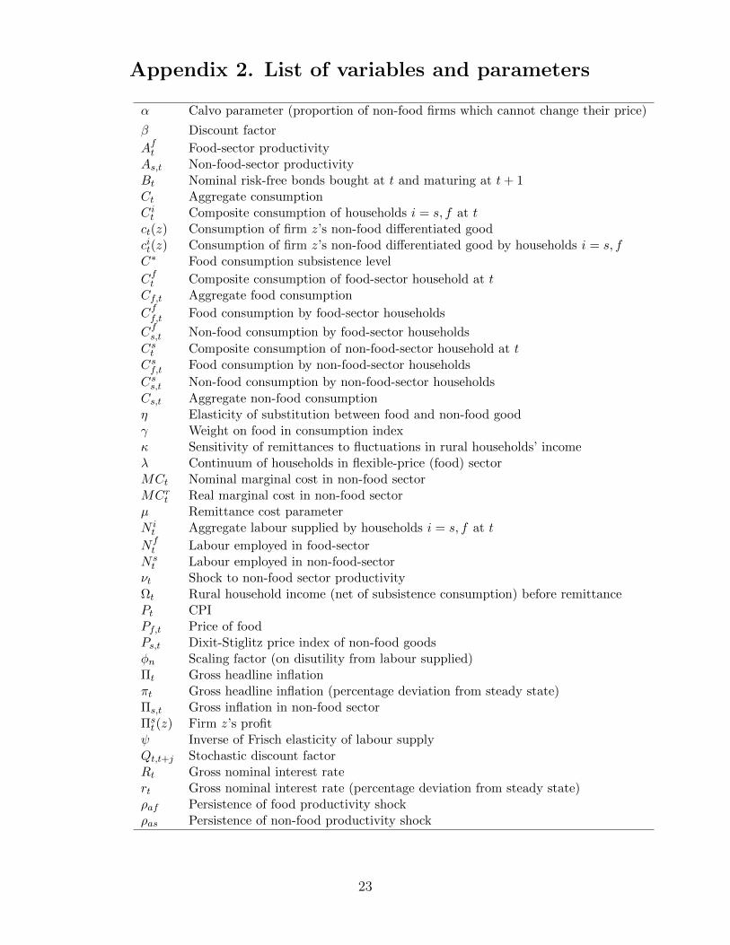
Appendix 2. List of variables and parameters

α Calvo parameter (proportion of non-food firms which cannot change their price)

β Discount factor

Aft Food-sector productivityAs,t Non-food-sector productivityBt Nominal risk-free bonds bought at t and maturing at t+ 1Ct Aggregate consumptionCit Composite consumption of households i = s, f at tct(z) Consumption of firm z’s non-food differentiated goodcit(z) Consumption of firm z’s non-food differentiated good by households i = s, fC∗ Food consumption subsistence level

Cft Composite consumption of food-sector household at tCf,t Aggregate food consumption

Cff,t Food consumption by food-sector households

Cfs,t Non-food consumption by food-sector households

Cst Composite consumption of non-food-sector household at tCsf,t Food consumption by non-food-sector households

Css,t Non-food consumption by non-food-sector households

Cs,t Aggregate non-food consumptionη Elasticity of substitution between food and non-food goodγ Weight on food in consumption indexκ Sensitivity of remittances to fluctuations in rural households’ incomeλ Continuum of households in flexible-price (food) sectorMCt Nominal marginal cost in non-food sectorMCrt Real marginal cost in non-food sectorµ Remittance cost parameterN it Aggregate labour supplied by households i = s, f at t

Nft Labour employed in food-sector

N st Labour employed in non-food-sector

νt Shock to non-food sector productivityΩt Rural household income (net of subsistence consumption) before remittancePt CPIPf,t Price of foodPs,t Dixit-Stiglitz price index of non-food goodsφn Scaling factor (on disutility from labour supplied)Πt Gross headline inflationπt Gross headline inflation (percentage deviation from steady state)Πs,t Gross inflation in non-food sectorΠst (z) Firm z’s profit

ψ Inverse of Frisch elasticity of labour supplyQt,t+j Stochastic discount factorRt Gross nominal interest ratert Gross nominal interest rate (percentage deviation from steady state)ρaf Persistence of food productivity shockρas Persistence of non-food productivity shock

23

ρi Weight on interest rate-smoothing term in interest rate rule

ρπ Weight on inflation gap in interest rate ruleρY Weight on output gap in interest rate ruleσ Inverse of elasticity of intertemporal substitutionσaf Standard deviation of shock to food-sector productivityσas Standard deviation of shock to non-food-sector productivityθ Elasticity of substitution between differentiated non-food goodsTCt,t+j [yt,t+j(z)] Total cost of producing yt,t+j(z)u(·) Instantaneous utility functionV it Expected lifetime utility for i = f, s

W ft Nominal wage in food sector

W st (z) Nominal paid by non-food sector firm z

Xt(z) Price of differentiated non-food good zxt Relative price desired by non-food firms t: Xt/Ps,txf,t Relative price of food: Pf,t/Ptxs,t Relative price of non-food goods: Pf,t/Ptξt Shock to food-sector productivityYt GDPyt GDP (percentage deviation from steady state)yt,t+j(z) Firm z non-food production at t+ j given price set at tYf,t Aggregate food productionyf,t Food production per food-sector firmYs,t Aggregate non-food productionys,t(z) Non-food production by firm zz Index for firms in non-food sector

References

Aisen, A., Alper, E., Drummond, P.F.N., Fuli., E., and Walker, S.E.J., (2015). Onthe Road to East African Community Monetary Union: Asymmetric Shocks,the Exchange Rate, and Risk Sharing Mechanisms. Forthcoming as IMF Work-ing Paper.

Aker, J. and Mbiti, I., (2010). Mobile Phones and Economic Development in Africa.Journal of Economic Perspectives. 24(3). 207-232.

Anand, R. and Prasad, E.S., (2010). Optimal Price Indices for Targeting InflationUnder Incomplete Markets. IMF Working Paper 10/200.

Aron, J., (2015). ‘Leapfrogging’: a Survey of the Nature and Economic Implicationsof Mobile Money. CSAE Working Paper.

Aron, J., Muellbauer, J., and Sebudde, R., (2015). The Determinants of Inflationin Uganda: Forward-looking Models. CSAE Working Paper.

Berg, A., Portillo, R., Yang, S.-C.S., and Zanna, L.-F., (2012). Public Investmentin Resource-Abundant Developing Countries. IMF Working Paper 12/274.

Demombynes, G. and Thegeya, A., (2012). Kenya’s Mobile Revolution and thePromise of Mobile Savings. World Bank Policy Research Working Paper 5988.

Goldberg, J., (2015). Kwacha Gonna Do? Experimental Evidence about LaborSupply in Rural Malawi. Mimeo.

24

IMF, (2014). Conditionality in Evolving Monetary Policy Regimes. IMF PolicyPaper.

Jack, W. and Suri, T., (2011). Mobile Money: the Economics of M-Pesa. NBERWorking Paper 16721.

Jack, W. and Suri, T., (2014). Risk Sharing and Transactions Costs: Evidence fromKenya’s Mobile Money Revolution. American Economic Review. 104(1). 183-223.

Macha, D.P., (2013). Mobile Financial Services in Tanzania: State of the Art andPotentials for Financial Inclusion. University of Dar es Salaam doctoral thesis.

Mbiti, I. and Weil, D., (2011). Mobile Banking: The impact of M-Pesa in Kenya.NBER Working Paper 17129.

Misati, N.K., Njoroge, L.K., Kamau, A.W., and Shem, A.O., (2010). Financialinnovation and monetary policy transmission in Kenya. International ResearchJournal of Finance and Economics. 50. 123-136.

Morawczynski, O., and Pickens, M., (2009). Poor people using mobile financialservices – Observations on customer usage and impact from M-Pesa. CGAPBrief.

Ndirangu, L. and Nyamongo, E.M., (2015). Financial Innovations and Their Impli-cations for Monetary Policy in Kenya. Journal of African Economies. 24(Sup-plement 1). i46-i71.

O’Connell, S., (2013). Modernizing the monetary policy framework in Tanzania.Presentation at the 2013 IGC Growth Week.

Weil, D., Mbiti, I., and Mwega, F., (2012). The implications of innovations in thefinancial sector on the conduct of monetary policy in East Africa. InternationalGrowth Centre Working Paper 12/0460.

Wilson, K., (2010). Jipange Sasa – A Little Heaven of Local Savings, Hot Tech-nologies, and Formal Finance. In Wilson, K., Harper, M., and Griffith, M.,(eds.), 2010. Financial Promise for the Poor – How Groups Build Microsavings.Sterling, VA: Kumarian Press.

25