Mobile Demand Forecasting via Deep Graph-Sequence ...

IEEE INTERNET OF THINGS JOURNAL, VOL. 5, NO. 4, AUGUST 2018 3091

Mobile Demand Forecasting via DeepGraph-Sequence SpatiotemporalModeling in Cellular Networks

Luoyang Fang, Student Member, IEEE, Xiang Cheng , Senior Member, IEEE,

Haonan Wang, and Liuqing Yang , Fellow, IEEE

Abstract—The demand forecasting plays a crucial role in thepredictive physical and virtualized network management in cel-lular networks, which can effectively reduce both the capitaland operational expenditures by fully exploiting the networkinfrastructure. In this paper, we study the per-cell demand fore-casting in cellular networks. The success of demand forecastingrelies on the effective modeling of both the spatial and tem-poral aspects of the per-cell demand time series. However, themain challenge of the spatial relevancy modeling in the per-celldemand forecasting is the irregular spatial distribution of cells ina network, where applying grid-based models (e.g., convolutionalneural networks) would lead to degradation of spatial granular-ity. In this paper, we propose to model the spatial relevancyamong cells by a dependency graph based on spatial distancesamong cells without the loss of spatial granularity. Such spatialdistance-based graph modeling is confirmed by the spatiotempo-ral analysis via semivariogram, which suggests that the relevancybetween any two cells declines as their spatial distance increases.Hence, the graph convolutional networks and long short-termmemory (LSTM) from deep learning are employed to modelthe spatial and temporal aspects, respectively. In addition, thedeep graph-sequence model, graph convolutional LSTM, is fur-ther employed to simultaneously characterize both the spatialand temporal aspects of mobile demand forecasting. Experimentsdemonstrate that our proposed graph-sequence demand fore-casting model could achieve a superior forecasting performancecompared with the other two proposed models as well as the tra-ditional auto regression integrated moving average time seriesmodel.

Index Terms—Communication system traffic, mobile learning,statistical learning.

Manuscript received February 10, 2018; revised April 3, 2018; acceptedApril 19, 2018. Date of publication May 1, 2018; date of current versionAugust 9, 2018. This work was supported in part by the National NaturalScience Foundation of China under Grant 61622101 and Grant 61571020,in part by the National Science and Technology Major Project under Grant2018ZX03001031, and in part by the National Science Foundation underGrant DMS-1521746 and Grant DMS-1737795. (Corresponding author:Xiang Cheng.)

L. Fang and L. Yang are with the Department of Electrical and ComputerEngineering, Colorado State University, Fort Collins, CO 80523 USA (e-mail:[email protected]; [email protected]).

X. Cheng is with the State Key Laboratory of Advanced OpticalCommunication Systems and Networks, School of Electronics Engineeringand Computer Science, Peking University, Beijing 100871, China (e-mail:[email protected]).

H. Wang is with the Department of Statistics, Colorado State University,Fort Collins, CO 80523 USA (e-mail: [email protected]).

Digital Object Identifier 10.1109/JIOT.2018.2832071

I. INTRODUCTION

W ITH the explosive growth of wireless data trafficand large-scale penetration of mobile devices into

our everyday life, the massive data generated from mobiledevices and mobile networks, termed as mobile big data [1],could significantly reveal the human activity patterns, whichis valuable in both data-driven personalized applications anddata-driven public services. In [2], one of the highlighted char-acteristics of mobile big data is its spatiotemporal feature.In fact, the cell towers or base stations of a mobile networkspatially distributed in an area could be regarded as sensors,recording the location of the network subscribers without theproactive location update via GPS by subscribers.

The mobile big data collected by mobile network opera-tors can also benefit the management of mobile networks.In fact, mobile big data could help uncover and understanduser’ behavior patterns [3] via effective data mining tech-niques, which could benefit to the resource-constraint networkoptimization, from network planning, network traffic monitor-ing to network management. In recent years, self-organizingnetworks (SONs) is widely studied to automatically manageand organize networks without manual intervention [4], [5].One motivation to employ SONs in cellular networks is thereduction of network operational expenditures and capitalexpenditures, which requires full exploitation of the capabilityof network infrastructure. The demand forecasting will play animportant role of providing predictive knowledge [6] in vari-ous cellular SON functions, especially for the future cellularnetworks with the virtualization and cloudization of networkfunctions [7], [8].

In addition, the studied mobile demand forecasting is notonly a critical problem in cellular networks, but also closelyrelated to the domain of Internet of Things (IoT). First, eachbase station of cellular networks can be regarded as an IoTdevice to track and monitor network subscribers’ behaviorin terms of the aggregated traffic demands. This makes thestudied demand forecasting a widely useful IoT application.Second, the interconnection between IoT devices and controlcenters will be realized by the machine-type communicationsin cellular networks via various low power wide area networktechnologies [9], where the IoT-type traffic demand forecast-ing in cellular networks will be critical to facilitate an efficientnetwork resource schedule and management for IoT services,

2327-4662 c© 2018 IEEE. Personal use is permitted, but republication/redistribution requires IEEE permission.See http://www.ieee.org/publications_standards/publications/rights/index.html for more information.

https://orcid.org/0000-0002-5943-0326

https://orcid.org/0000-0003-0231-6837

3092 IEEE INTERNET OF THINGS JOURNAL, VOL. 5, NO. 4, AUGUST 2018

especially in the context of service-oriented network operationin 5G networks [10]. Third, the proposed graph-sequencemodels of mobile demand forecasting may be extended toother forecasting problems in the domain of IoT, e.g., IoT-enabled load forecasting in smart grid [11], [12] and air qualityforecasting [13].

In this paper, we study the mobile demand forecasting, thefoundation of predictive mobile network management. In theliterature, the mobile traffic/demand forecasting schemes havebeen studied for traffic apprehension and prediction via theHolt–Winter’s exponential smoothing technique [14], informa-tion theory [15], and the seasonal auto regression integratedmoving average (ARIMA) model [16]. However, all thesedemand forecasting models only consider the temporal aspectvia various time series models without taking into accountthe spatial relevancy of cells. Models of mobile demand fore-casting accounting for the spatial relevancy have been recentlystudied based on deep learning [17], [18]. In these models, thetemporal aspect of demand time series is commonly studiedvia the recurrent neural networks (RNNs), while the spatialrelevancy is captured by various grid-based spatial models.

However, the main challenge of applying grid-based spatialmodels to per-cell demand forecasting is the irregular spatialdistribution of cells in the real-world setting. Generally, thecell towers are distributed in a network covered area accord-ing to the population density. That is, the distance between twocell towers is about 500 m. in the urban area, but can reach2000 m in the rural area. Hence, grid-based models [17], [18]do note directly apply. To utilize the grid-based models, onefirst needs to redivide the network covered area into a uni-form square grid, and then predict the aggregated demands ofmultiple cell towers residing in each lattice. Such spatial arearedivision and demand aggregation will lead to the loss of thespatial granularity and will significantly limit the applicationsto future cellular network management that requires variablespatial granularity.

To this end, we propose a flexible graph-based spatialmodel for the per-cell demand forecasting without any spatialresolution degradation and data aggregation. First, we realizethat the spatiotemporal analysis of the per-cell demand timeseries via the semivariogram [19] reveals that the relevancybetween the demands of two cells relies on the spatial dis-tance of the two cells. That is, the dependency level of twocells would decrease when their spatial distance increases.Hence, we can build a dependency graph characterizing therelevancy of cells based on their spatial distances. In otherswords, the per-cell demands generated at each cell tower couldbe regarded as signals generated at the vertices of a graph.In addition, not only the recent demand history is applied toforecast the future demands, but also the periodic history [e.g.,day(s) ahead demands] are considered in order to obtain anaccurate demand predictor.

With the dependency graph formulation, the recently devel-oped graph convolutional networks (GCNs) [20], [21] and thelong short-term memory (LSTM) neural networks [22] areemployed to characterize the spatial aspect and the temporalaspect for demand forecasting, respectively. The LSTM is agated version of RNNs in deep learning, which is well known

for its good performance on sequence modeling. In GCNs, thegraph convolution operation, originated from signal process-ing theory on graphs [23]–[25], is employed to replace thematrix multiplication in the feedforward neural networks. Thepower of graph convolution results from the ideas of parametersharing and sparse interaction as in the traditional convolu-tional neural networks [26]. The sparse interaction in per-celldemand prediction means that the demand prediction of onecell is only related to itself and its nearest neighbors in thedependency graph. The parameter sharing assumes that themodel parameters are shared across all cells of the network.

In this paper, we first formulate the demand forecastingproblem as a one-step ahead demand prediction problem. Thedemand forecasts after one step in the future are dynam-ically generated by the one-step ahead predictor. Threemodels, namely the spatial-only (GCNs), the temporal-only(LSTM), and the spatiotemporal [graph convolutional LSTM(GCLSTM)], are studied. The GCLSTM [27] is the modelreplacing the matrix multiplication operation with the graphconvolution operation in LSTM, inspired by the convolutionalLSTM [28]. Compared with GCLSTM, LSTM without theembedded spatial information will predict the demand of onecell based on all other cells in the network, which wouldlead to an inferior generalization performance. Experimentsshow that the temporal-only LSTM could achieve a supe-rior performance for the very-short-term demand forecastingfor its much larger model capacity, but rapidly deteriorateswhen the forecast horizon increases. This results from theinferior generalization performance of LSTM and the accu-mulated errors in the generated predicts. The GCLSTM withthe spatial and the temporal aspects modeled will generallyhave a superior forecast performance except for the very-short-term one. Main contributions of this paper are summarized asfollows.

1) To the best of the authors’ knowledge, this is the firstwork modeling the spatial relevancy among cells by adependency graph. The graph-based spatial modelingcould completely retain the spatial granularity withoutany data aggregation.

2) The periodicity of the per-cell demand time series isexplicitly taken into account by adding past periodicobservations as input features in our studied modelsso that the accuracy of demand forecasting could beenhanced without significantly increasing model size.

3) The graph convolutional and RNNs are proposed tosimultaneously characterize both the spatial and tem-poral attributes with parameter sharing, which couldlead to a superior generalization performance of demandforecasting.

The rest of this paper is organized as follows. In Section II, thestudied dataset is described and the per-cell demand is defined.The per-cell demand forecasting problem in Section III isidentified with the spatial and temporal aspects modeled.In Section IV, three demand prediction models based onGCN, LSTM, and GCLSTM are proposed. In Section V,experiment results are compared to demonstrate the superiorperformance of GCLSTM. Finally, concluding remarks aremade in Section VI.

FANG et al.: MOBILE DEMAND FORECASTING VIA DEEP GRAPH-SEQUENCE SPATIOTEMPORAL MODELING IN CELLULAR NETWORKS 3093

Fig. 1. Cell distribution heatmap.

II. DATASET

A. Signaling Dataset

The signaling data is collected near the radio accessnetworks in a cellular network, which records communicationevents as well as location update events on all active sub-scribers in mobile networks. Data fields of the signaling datainclude: 1) subscriber’s anonymized identifier; 2) time stamp(e.g., 20160101184312); 3) location coordinates (i.e., the lon-gitude and latitude of cell towers); 4) event type; and 5) celltype (i.e., small cell or macro cell). The longitude and lati-tude coordinates where the cell tower is located are accurateto 6 decimal places and time stamps are accurate to seconds.The signaling data logs event type as well as the directionof the event (e.g., initiating a call or being called). In thestudied dataset, more than 6000 cells in total including smalland macro cells with millions of subscribers are recorded inthe studied dataset, as shown in Fig. 1. In the studied dataset,the average daily active subscribers is about three million. Thetime period of the studied signaling data is 104 days, fromAugust 22, 2016 to December 3, 2016.

B. Per-Cell Demands

Based on the studied signaling dataset, two categories ofservice demands could be extracted, namely communicationdemands and tracking demands. The communication demandsincluding the first 4 events on calls and texts recorded inthe signaling dataset, to forecast which is the very task ofthis paper. The tracking demands could be obtained basedon the location update events, which is closely related tocrowd mobility. The location update frequency is once perhour, which may be too coarse to exactly describe the crowdflow, especially in the urban area (where cells are denselydistributed). Hence, we focus on the communication demandforecasting in this paper.

With the spatiotemporal information of each eventrecorded, we define the per-cell demand as the number ofcommunication events occurring within a cell during an eventcounting time window �T. Hence, a per-cell demand timeseries could be generated as follows:

[xn

t , xnt−1, xn

t−2, . . . , xnt−l+1, . . .

](1)

where xnt = ln(1+cn

t ) denotes the per-cell demand within timewindow [t−�T, t), where cn

t is the number of communication

events of the nth cell. Here, we utilize the commonly usedlogarithm function ln(1+x) to convent the integer event num-ber domain to the real number domain of demands. In thispaper, we mainly study the demand forecasting in terms ofthe 10-min counting time windows, i.e., �T = 10.

It can be clearly observed that small cells are denselydeployed in the studied urban area (green areas as shown inFig. 1). In a heterogeneous cellular networks, small cells aredesigned to assist their corresponding macro cell by offloadingdata traffic, whose coverage is also relatively much smallerthan that of macro cells. As a result, the communicationdemands of small cells is sparse, which is not of interest inthis paper. Hence, we aggregate the demand of small cellsto its corresponding macro cell, which is determined by theirspatially closest macro cell based on the location information(i.e., the longitude and latitude of cell towers). In other words,we study the per-cell aggregated demands within a spatial areacovered by a macro cell.

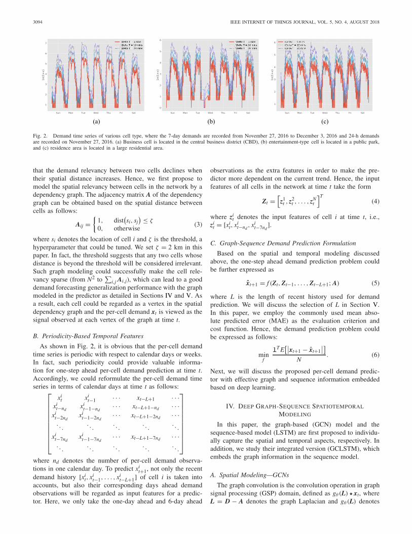
In Fig. 2, the per-cell demands with different cell types areillustrated, namely business, entertainment, and residence. Ineach subfigure, three demand time series with different count-ing time window are plotted, �T = 5 min, �T = 10 min,and �T = 20 min. One can easily observe that the largecounting time window could significantly reduce the noise ofthe per-cell demand time series, as the larger counting timewindow acts like a smoothing filter applied on the one gener-ated by the small counting time window. However, such noisereduction is at the cost of lowering the temporal resolution ofdemand time series. In addition, it can be easily observed thatper-cell demands are strongly periodic in terms of calendardays, regardless of cell types. Another periodic effect, that thedemands during weekends is obviously less than those duringweekdays, could be observed from the demand time seriesof the business type [Fig. 2(a)]. Such effects would inspirethe feature engineering for demand forecasting, which will bediscussed in detail later.

III. DEMAND PREDICTION PROBLEM FORMULATION

With the definition of per-cell demands, the demand fore-casting is aimed to predict the per-cell demands of all cells ina mobile network based on its history. In this paper, demandforecasting is studied as the one-step ahead prediction problemas follows:

xt+1 = f (xt, xt−1, . . . , xt−l+1, . . .) (2)

where xt = [x1t , x2

t , . . . , xNt ]T denotes the per-cell demands of

cells across the covered area at time t and N is the total numberof macro cells in the network. Hence, the prediction problemessentially amounts to the estimation of a function or predictorf based on the collected history data and the knowledge ofcell locations. In this section, we will discuss the one-stepahead demand prediction with the innovative spatiotemporalmodeling.

A. Graph-Based Spatial Formulation

By the spatiotemporal analysis of multiple per-cell demandtime series (see Section V-B, Appendix B), it can be concluded


(a) (b) (c)

Fig. 2. Demand time series of various cell type, where the 7-day demands are recorded from November 27, 2016 to December 3, 2016 and 24-h demandsare recorded on November 27, 2016. (a) Business cell is located in the central business district (CBD), (b) entertainment-type cell is located in a public park,and (c) residence area is located in a large residential area.

that the demand relevancy between two cells declines whentheir spatial distance increases. Hence, we first propose tomodel the spatial relevancy between cells in the network by adependency graph. The adjacency matrix A of the dependencygraph can be obtained based on the spatial distance betweencells as follows:

Aij ={

1, dist(si, sj

) ≤ ζ

0, otherwise(3)

where si denotes the location of cell i and ζ is the threshold, ahyperparameter that could be tuned. We set ζ = 2 km in thispaper. In fact, the threshold suggests that any two cells whosedistance is beyond the threshold will be considered irrelevant.Such graph modeling could successfully make the cell rele-vancy sparse (from N2 to

∑i,j Ai,j), which can lead to a good

demand forecasting generalization performance with the graphmodeled in the predictor as detailed in Sections IV and V. Asa result, each cell could be regarded as a vertex in the spatialdependency graph and the per-cell demand xt is viewed as thesignal observed at each vertex of the graph at time t.

B. Periodicity-Based Temporal Features

As shown in Fig. 2, it is obvious that the per-cell demandtime series is periodic with respect to calendar days or weeks.In fact, such periodicity could provide valuable informa-tion for one-step ahead per-cell demand prediction at time t.Accordingly, we could reformulate the per-cell demand timeseries in terms of calendar days at time t as follows:

⎡

⎢⎢⎢⎢⎢⎢⎢⎢⎢⎣

xit xi

t−1 · · · xt−L+1 · · ·xi

t−ndxi

t−1−nd· · · xt−L+1−nd · · ·

xit−2nd

xit−1−2nd

· · · xt−L+1−2nd · · ·. . .

. . .. . .

. . .. . .

xit−7nd

xit−1−7nd

· · · xt−L+1−7nd · · ·. . .

. . .. . .

. . .. . .

⎤

⎥⎥⎥⎥⎥⎥⎥⎥⎥⎦

where nd denotes the number of per-cell demand observa-tions in one calendar day. To predict xi

t+1, not only the recentdemand history [xi

t, xit−1, . . . , xi

t−L+1] of cell i is taken intoaccounts, but also their corresponding days ahead demandobservations will be regarded as input features for a predic-tor. Here, we only take the one-day ahead and 6-day ahead

observations as the extra features in order to make the pre-dictor more dependent on the current trend. Hence, the inputfeatures of all cells in the network at time t take the form

Zt =[z1

t , z2t , . . . , zN

t

]T(4)

where zit denotes the input features of cell i at time t, i.e.,

zit = [xi

t, xit−nd

, xit−7nd

].

C. Graph-Sequence Demand Prediction Formulation

Based on the spatial and temporal modeling discussedabove, the one-step ahead demand prediction problem couldbe further expressed as

xt+1 = f (Zt, Zt−1, . . . , Zt−L+1; A) (5)

where L is the length of recent history used for demandprediction. We will discuss the selection of L in Section V.In this paper, we employ the commonly used mean abso-lute predicted error (MAE) as the evaluation criterion andcost function. Hence, the demand prediction problem couldbe expressed as follows:

minf

�T E

[∣∣xt+1 − xt+1∣∣]

N. (6)

Next, we will discuss the proposed per-cell demand predic-tor with effective graph and sequence information embeddedbased on deep learning.

IV. DEEP GRAPH-SEQUENCE SPATIOTEMPORAL

MODELING

In this paper, the graph-based (GCN) model and thesequence-based model (LSTM) are first proposed to individu-ally capture the spatial and temporal aspects, respectively. Inaddition, we study their integrated version (GCLSTM), whichembeds the graph information in the sequence model.

A. Spatial Modeling—GCNs

The graph convolution is the convolution operation in graphsignal processing (GSP) domain, defined as gθ (L) � xt, whereL = D − A denotes the graph Laplacian and gθ (L) denotes


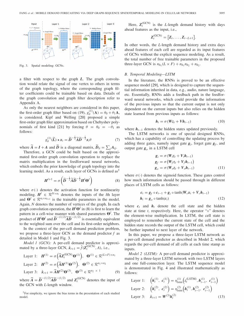
Fig. 3. Spatial modeling: GCNs.

a filter with respect to the graph L. The graph convolu-tion would relate the signal of one vertex to others in termsof the graph topology, where the corresponding graph fil-ter coefficients could be trainable based on data. Details ofthe graph convolution and graph filter description refer toAppendix A.

As only the nearest neighbors are considered in this paper,the first-order graph filter based on (19), g(1)

θ (�) = θ0 + θ1�,is considered. Kipf and Welling [20] proposed a simplefirst-order graph filer approximation based on Chebyshev poly-nomials of first kind [21] by forcing θ = θ0 = −θ1 asfollows:

g(1)θ (L) � xt = D

− 12 AD

− 12 xtθ (7)

where A = I + A and D is a diagonal matrix, Dii = ∑j Aij.

Therefore, a GCN could be built based on the approxi-mated first-order graph convolution operation to replace thematrix multiplication in the feedforward neural networks,which embeds the prior knowledge of graph topology into thelearning model. As a result, each layer of GCNs is defined as1

Hl+1 = σ

(D

− 12 AD

− 12 Hl�l

)(8)

where σ(·) denotes the activation function for nonlinearitymodeling. Hl ∈ RN×nl denotes the inputs of the lth layerand �l ∈ Rnl×nl+1 is the trainable parameters in the model.Again, N denotes the number of vertices of the graph. In eachgraph convolution operation, the Hl�l in (8) is first to learn thepattern in a cell-wise manner with shared parameters �l. Theproduct of Hl�l and D

−(1/2)AD

−(1/2)is essentially equivalent

to the weighted sum over the cell and its first-order neighbors.In the context of the per-cell demand prediction problem,

we propose a three-layer GCN as the demand predictor f asdetailed in Model 1 and Fig. 3.

Model 1 (GCN): A per-cell demand predictor is approxi-mated by a three-layer GCN, xt+1 = f (Z(GCN)

t , A), i.e.,

Layer 1: H(1) = σ(

AZ(GCN)t �(1)

), �(1) ∈ R(L×F)×n1

Layer 2: H(2) = σ(

AH(1)�(2)), �(2) ∈ Rn1×n2

Layer 3: xt+1 = AH(2)�(3), �(3) ∈ Rn2 × 1 (9)

where A = D−(1/2)

AD−(1/2)

and Z(GCN)t denotes the input of

the GCN with L-length window.

1For simplicity, we ignore the bias terms in the presentation of each studiedmodel.

Here, Z(GCN)t is the L-length demand history with days

ahead features as the input, i.e.,

Z(GCN)t = [

Zt, . . . , Zt−L+1].

In other words, the L-length demand history and extra daysahead features of each cell are regarded as its input featuresof GCNs without the explicit sequence modeling. As a result,the total number of free trainable parameters in the proposedthree-layer GCN is nh1(L × F) + nh1nh2 + nh2 .

B. Temporal Modeling—LSTM

In the literature, the RNNs is proved to be an effectivesequence model [29], which is designed to capture the sequen-tial information inherited in data, e.g., audio, nature language,etc. Essentially, RNNs adds a feedback path in the feedfor-ward neural networks, which could provide the informationof the previous inputs so that the current output is not onlydependent on the current inputs but also relies on the hiddenstate learned from previous inputs as follows:

ht = σ(Wzt + Vht−1) (10)

where ht−1 denotes the hidden states updated previously.The LSTM networks is one of special designed RNNs,

which has a capability of controlling the updating process byadding three gates, namely input gate gi, forget gate gf , andoutput gate go in a LSTM cell

gi = σ(Wizt + Viht−1)

gf = σ(Wf zt + Vf ht−1

)

go = σ(Wozt + Voht−1) (11)

where σ(·) denotes the sigmoid function. These gates controlhow much information should be passed through in differentplaces of LSTM cells as follows:

ct = gf ◦ ct−1 + gi ◦ tanh(Wcxt + Vcht−1)

ht = go ◦ tanh(ct) (12)

where ct and ht denote the cell state and the hiddenstate at time t, respectively. Here, the operator “◦” denotesthe element-wise multiplication. In LSTM, the cell state isemployed to remember the current state of the cell and thehidden state records the output of the LSTM cell, which couldbe further inputted to next layer of the network.

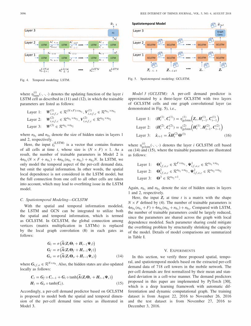
In this paper, we propose a three-layer LSTM network asa per-cell demand predictor as described in Model 2, whichregards the per-cell demand of all cells at each time stamp asinputs.

Model 2 (LSTM): A per-cell demand predictor is approxi-mated by a three-layer LSTM network with two LSTM layersand one full-connection layer. The LSTM sequence modelis demonstrated in Fig. 4 and illustrated mathematically asfollows:

Layer 1:(

h(1)t , c(1)

t

)= η

(1)lstm

(z(LSTM)

t , h(1)t−1, c(1)

t−1

)

Layer 2:(

h(2)t , c(2)

t

)= η

(2)lstm

(h(1)

t , h(2)t−1, c(2)

t−1

)

Layer 3: xt+1 = W(3)h(2)t (13)


Fig. 4. Temporal modeling: LSTM.

where η(i)lstm(·, ·, ·) denotes the updating function of the layer i

LSTM cell as described in (11) and (12), in which the trainableparameters are listed as follows:

Layer 1: W(1)i,o,f ,c ∈ R(N×F)×nh1 , V(1)

i,o,f ,c ∈ Rnh1×nh1

Layer 2: W(2)i,o,f ,c ∈ Rnh1×nh2 , V(2)

i,o,f ,c ∈ Rnh2×nh2

Layer 3: W(3) ∈ Rnh1×nh2

where nh1 and nh2 denote the size of hidden states in layers 1and 2, respectively.

Here, the input z(LSTM)t is a vector that contains features

of all cells at time t, whose size is (N × F) × 1. As aresult, the number of trainable parameters in Model 2 is4nh1(N × F + nh1) + 4nh2(nh1 + nh2) + nh2N. In LSTM, weonly model the temporal aspect of the per-cell demand data,but omit the spatial information. In other words, the spatiallocal dependence is not considered in the LSTM model, butthe full connection from one cell to all other cells are takeninto account, which may lead to overfitting issue in the LSTMmodel.

C. Spatiotemporal Modeling—GCLSTM

With the spatial and temporal information modeled,the LSTM and GCN can be integrated to utilize boththe spatial and temporal information, which is termedas GCLSTM. In GCLSTM, the global connection amongvertices (matrix multiplication in LSTMs) is replacedby the local graph convolution (8) in each gates asfollows:

Gi = σ(A(Zt�i + Ht−1� i)

)

Gf = σ(A(Zt�f + Ht−1� f )

)

Go = σ(A(Zt�o + Ht−1�o)

)(14)

where Gi,f ,o ∈ RN×nh . Also, the hidden states are also updatedlocally as follows:

Ct = Gf ◦ Ct−1 + Gi ◦ tanh(A(Zt�c + Ht−1�c)

)

Ht = Go ◦ tanh(Ct). (15)

Accordingly, a per-cell demand predictor based on GCLSTMis proposed to model both the spatial and temporal dimen-sion of the per-cell demand time series as illustrated inModel 3.

Fig. 5. Spatiotemporal modeling: GCLSTM.

Model 3 (GCLSTM): A per-cell demand predictor isapproximated by a three-layer GCLSTM with two layersof GCLSTM cells and one graph convolutional layer (asdemonstrated in Fig. 5), i.e.,

Layer 1: (H(1)t , C(1)

t ) = η(1)gclstm

(Zt, H(1)

t−1, C(1)t−1

)

Layer 2: (H(2)t , C(2)

t ) = η(2)gclstm

(H(1)

t , H(2)t−1, C(2)

t−1

)

Layer 3: xt+1 = AH(2)t �(3) (16)

where η(i)gclstm(·, ·, ·) denotes the layer i GCLSTM cell based

on (14) and (15), where the trainable parameters are illustratedas follows:

Layer 1: �1i,f ,o,c ∈ RF×nh1 ,�1

i,f ,o,c ∈ Rnh1×nh1

Layer 2: �2i,f ,o,c ∈ Rnh1×nh2 ,�2

i,f ,o,c ∈ Rnh2×nh2

Layer 3: �3 ∈ Rnh2×1.

Again, nh1 and nh2 denote the size of hidden states in layers1 and 2, respectively.

Here, the input Zt at time t is a matrix with the shapeN × F defined by (4). The number of trainable parameters is4nh1(nh1 + F)+ 4nh2(nh2 + nh1)+ nh2. Compared with LSTM,the number of trainable parameters could be largely reduced,since the parameters are shared across the graph with localdependence modeled. Such parameter sharing could mitigatethe overfitting problem by structurally shrinking the capacityof the model. Details of model comparisons are summarizedin Table I.

V. EXPERIMENTS

In this section, we verify three proposed spatial, tempo-ral, and spatiotemporal models based on the extracted per-celldemand data of 718 cell towers in the mobile network. Theper-cell demands are first normalized by their mean and stan-dard deviation in a cell-wise manner. The demand predictorsproposed in this paper are implemented by PyTorch [30],which is a deep learning framework with automatic dif-ferentiation and dynamic computational graph. The trainingdataset is from August 22, 2016 to November 26, 2016and the test dataset is from November 27, 2016 toDecember 3, 2016.


TABLE ICOMPARISONS OF THREE PER-CELL DEMAND PREDICTION MODELS

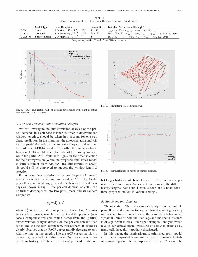
Fig. 6. ACF and partial ACF of demand time series with event countingtime windows �T = 10 min.

A. Per-Cell Demands Autocorrelation Analysis

We first investigate the autocorrelation analysis of the per-cell demands in a cell-wise manner, in order to determine thewindow length L should be taken into account for one-stepahead prediction. In the literature, the autocorrelation analysisand its partial derivative are commonly adopted to determinethe order of ARIMA model. Specially, the autocorrelationfunction (ACF) would decide the order of the moving average,while the partial ACF could shed lights on the order selectionfor the autoregression. While the proposed time series modelis quite different from ARIMA, the autocorrelation analy-sis could still be employed to suggest the window-length Lselection.

Fig. 6 shows the correlation analysis on the per-cell demandtime series with the counting time window, �T = 10. As theper-cell demand is strongly periodic with respect to calendardays as shown in Fig. 2, the per-cell demand of cell i canbe further decomposed into two parts, mean and its randomcomponent

xid = xi

d + εi

where xid is the periodic component. Hence, Fig. 6 shows

two kinds of curves, namely the direct and the periodic (sea-sonal) component reduced, which demonstrate the (partial)autocorrelation analysis directly on the per-cell demand timeseries and the random component, respectively. It could beclearly observed that the PACF curves rapidly decrease to zerowith the time lag increased, while the ACF curves are slowlydecreasing, especially the direct one. One can conclude thatone hour history is sufficient for one-step ahead prediction,

Fig. 7. Spatiotemporal semivariogram.

Fig. 8. Semivariogram in terms of spatial distance.

but longer history could benefit to capture the random compo-nent in the time series. As a result, we compare the differenthistory lengths (half-hour, 1-hour, 2-hour, and 3-hour) for allthree proposed models in various settings.

B. Spatiotemporal Analysis

The objective of the spatiotemporal analysis on the multipleper-cell demand signals is to evaluate how demand signals varyin space and time. In other words, the correlation between twosignals in terms of both the time lags and the spatial distanceis of significant interest. Such spatiotemporal analysis wouldlead to our critical spatial modeling of demands observed bymany cells irregularly spatially distributed.

In this paper, the semivariogram, originated from spatialstatistics, is employed to analyze the per-cell demands. Detailsof semivariogram refer to Appendix B. Fig. 7 shows the


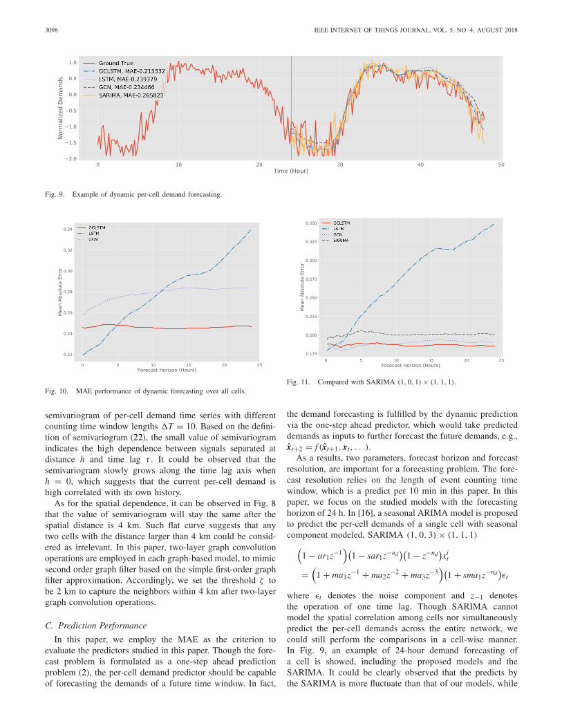
Fig. 9. Example of dynamic per-cell demand forecasting.

Fig. 10. MAE performance of dynamic forecasting over all cells.

semivariogram of per-cell demand time series with differentcounting time window lengths �T = 10. Based on the defini-tion of semivariogram (22), the small value of semivariogramindicates the high dependence between signals separated atdistance h and time lag τ . It could be observed that thesemivariogram slowly grows along the time lag axis whenh = 0, which suggests that the current per-cell demand ishigh correlated with its own history.

As for the spatial dependence, it can be observed in Fig. 8that the value of semivariogram will stay the same after thespatial distance is 4 km. Such flat curve suggests that anytwo cells with the distance larger than 4 km could be consid-ered as irrelevant. In this paper, two-layer graph convolutionoperations are employed in each graph-based model, to mimicsecond order graph filter based on the simple first-order graphfilter approximation. Accordingly, we set the threshold ζ tobe 2 km to capture the neighbors within 4 km after two-layergraph convolution operations.

C. Prediction Performance

In this paper, we employ the MAE as the criterion toevaluate the predictors studied in this paper. Though the fore-cast problem is formulated as a one-step ahead predictionproblem (2), the per-cell demand predictor should be capableof forecasting the demands of a future time window. In fact,

Fig. 11. Compared with SARIMA (1, 0, 1) × (1, 1, 1).

the demand forecasting is fulfilled by the dynamic predictionvia the one-step ahead predictor, which would take predicteddemands as inputs to further forecast the future demands, e.g.,xt+2 = f (xt+1, xt, . . .).

As a results, two parameters, forecast horizon and forecastresolution, are important for a forecasting problem. The fore-cast resolution relies on the length of event counting timewindow, which is a predict per 10 min in this paper. In thispaper, we focus on the studied models with the forecastinghorizon of 24 h. In [16], a seasonal ARIMA model is proposedto predict the per-cell demands of a single cell with seasonalcomponent modeled, SARIMA (1, 0, 3) × (1, 1, 1)

(1 − ar1z−1

)(1 − sar1z−nd

)(1 − z−nd

)xi

t

=(

1 + ma1z−1 + ma2z−2 + ma3z−3)(

1 + sma1z−nd)εt

where εt denotes the noise component and z−1 denotesthe operation of one time lag. Though SARIMA cannotmodel the spatial correlation among cells nor simultaneouslypredict the per-cell demands across the entire network, wecould still perform the comparisons in a cell-wise manner.In Fig. 9, an example of 24-hour demand forecasting ofa cell is showed, including the proposed models and theSARIMA. It could be clearly observed that the predicts bythe SARIMA is more fluctuate than that of our models, while


(a) (b) (c)

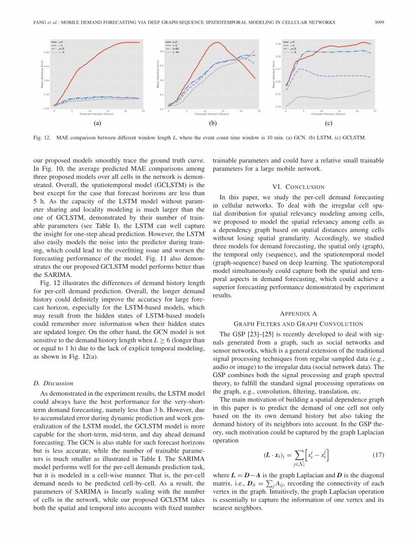
Fig. 12. MAE comparison between different window length L, where the event count time window is 10 min. (a) GCN. (b) LSTM. (c) GCLSTM.

our proposed models smoothly trace the ground truth curve.In Fig. 10, the average predicted MAE comparisons amongthree proposed models over all cells in the network is demon-strated. Overall, the spatiotemporal model (GCLSTM) is thebest except for the case that forecast horizons are less than5 h. As the capacity of the LSTM model without param-eter sharing and locality modeling is much larger than theone of GCLSTM, demonstrated by their number of train-able parameters (see Table I), the LSTM can well capturethe insight for one-step ahead prediction. However, the LSTMalso easily models the noise into the predictor during train-ing, which could lead to the overfitting issue and worsen theforecasting performance of the model. Fig. 11 also demon-strates the our proposed GCLSTM model performs better thanthe SARIMA.

Fig. 12 illustrates the differences of demand history lengthfor per-cell demand prediction. Overall, the longer demandhistory could definitely improve the accuracy for large fore-cast horizon, especially for the LSTM-based models, whichmay result from the hidden states of LSTM-based modelscould remember more information when their hidden statesare updated longer. On the other hand, the GCN model is notsensitive to the demand history length when L ≥ 6 (longer thanor equal to 1 h) due to the lack of explicit temporal modeling,as shown in Fig. 12(a).

D. Discussion

As demonstrated in the experiment results, the LSTM modelcould always have the best performance for the very-short-term demand forecasting, namely less than 3 h. However, dueto accumulated error during dynamic prediction and week gen-eralization of the LSTM model, the GCLSTM model is morecapable for the short-term, mid-term, and day ahead demandforecasting. The GCN is also stable for such forecast horizonsbut is less accurate, while the number of trainable parame-ters is much smaller as illustrated in Table I. The SARIMAmodel performs well for the per-cell demands prediction task,but it is modeled in a cell-wise manner. That is, the per-celldemand needs to be predicted cell-by-cell. As a result, theparameters of SARIMA is linearly scaling with the numberof cells in the network, while our proposed GCLSTM takesboth the spatial and temporal into accounts with fixed number

trainable parameters and could have a relative small trainableparameters for a large mobile network.

VI. CONCLUSION

In this paper, we study the per-cell demand forecastingin cellular networks. To deal with the irregular cell spa-tial distribution for spatial relevancy modeling among cells,we proposed to model the spatial relevancy among cells asa dependency graph based on spatial distances among cellswithout losing spatial granularity. Accordingly, we studiedthree models for demand forecasting, the spatial only (graph),the temporal only (sequence), and the spatiotemporal model(graph-sequence) based on deep learning. The spatiotemporalmodel simultaneously could capture both the spatial and tem-poral aspects in demand forecasting, which could achieve asuperior forecasting performance demonstrated by experimentresults.

APPENDIX A

GRAPH FILTERS AND GRAPH CONVOLUTION

The GSP [23]–[25] is recently developed to deal with sig-nals generated from a graph, such as social networks andsensor networks, which is a general extension of the traditionalsignal processing techniques from regular sampled data (e.g.,audio or image) to the irregular data (social network data). TheGSP combines both the signal processing and graph spectraltheory, to fulfill the standard signal processing operations onthe graph, e.g., convolution, filtering, translation, etc.

The main motivation of building a spatial dependence graphin this paper is to predict the demand of one cell not onlybased on the its own demand history but also taking thedemand history of its neighbors into account. In the GSP the-ory, such motivation could be captured by the graph Laplacianoperation

(L · xt)i =∑

j∈Ni

[xi

t − xjt

](17)

where L = D−A is the graph Laplacian and D is the diagonalmatrix, i.e., Dii = ∑

j Aij, recording the connectivity of eachvertex in the graph. Intuitively, the graph Laplacian operationis essentially to capture the information of one vertex and itsnearest neighbors.


Analogous to the filter design in the traditional signal pro-cessing, a graph filter could be expressed as polynomials interms of the graph Laplacian [23]

gθ

(L) = θ0I + θ1L + θ2L

2 + · · · + θK LK

(18)

where L is the normalized graph Laplacian, i.e., L = I −D−(1/2)AD−(1/2). And θk is the filter coefficient of tap k. Theorder of graph filters would determine the order of neighborsof vertices in the graph affected by the filter.

By the eigendecomposition on the graph Laplacian, L =UUT , any graph signal could be transformed to the cor-responding graph spectral domain, X = Ux, analogous tothe discrete Fourier transform [23]–[25], where the eigen-vectors U are viewed as a basis. As a result, the graphfilter could be further expressed in the graph spectraldomain

gθ (�) = θ0 + θ1� + θ2�2 + · · · + θK�K . (19)

Hence, the graph convolution operation gθ (L) ∗ xt can becalculated as multiplication operations in the graph spectraldomain

gθ

(L)� xt = Ugθ (�)UTxt. (20)

APPENDIX B

SPATIOTEMPORAL SEMIVARIOGRAM

The per-cell demand time series (1) could be furtherexpressed in terms of both the spatial and temporal aspects asfollows:

z(sn, t) = xnt (21)

where sn represents the detailed spatial information of the nthcell (i.e., location coordinates). The semivariogram γ (h) is afunction to describe the spatial dependence of two stochasticprocesses generated in two locations sn and sm separated at hdistance

γ (h) = E[(z(sn) − z(sm))2

∣∣∣ dist (sn, sm) = h

].

With the temporal dependence considered, the time lag τ

should be further considered atop the spatial variogramγ (h)

γ (h, τ ) = E[(z(s, t) − z(s + h, t + τ ))2

].

However, the cell towers are distributed irregularly in thecovered area according to the population density. Hence,we analyze the multiple per-cell demand processes in termsof the empirical spatiotemporal semivariogram [19], [31] asfollows:

γ (h(l), τ ) = 1

|N (h(l), τ )|×

∑

(n,m,t,t′)∈N (h(l),τ )

[z(sn, t) − z

(sm, t′

)]2(22)

where

N (h(l), τ ) = {(n, m, t, t′

)|dist (sn, sm) ∈ h(l),∣∣t − t′

∣∣ = τ}.

The N (h(l), τ ) is a set to collect any signal pairs spatiallyseparated at distance within the distance tolerance h(l) andtemporally separated at τ . The distance tolerance h(l) isemployed to discretize the continuous spatial distance. In thispaper, we utilize a linear uniform discretization with the spa-tial resolution 0.5 km. As a result, h(l) = [(l − 1) × 0.5,

l × 0.5).

REFERENCES

[1] X. Cheng, L. Fang, X. Hong, and L. Yang, “Exploiting mobile bigdata: Sources, features, and applications,” IEEE Netw., vol. 31, no. 1,pp. 72–79, Jan./Feb. 2017.

[2] X. Cheng, L. Fang, L. Yang, and S. Cui, “Mobile big data: Thefuel for data-driven wireless,” IEEE Internet Things J., vol. 4, no. 5,pp. 1489–1516, Oct. 2017.

[3] F. Malandrino, C.-F. Chiasserini, and S. Kirkpatrick, “Understanding thepresent and future of cellular networks through crowdsourced traces,”in Proc. 18th Int. Symp. World Wireless Mobile Multimedia Netw.(WoWMoM), Macau, China, Jun. 2017, pp. 1–9.

[4] M. Peng, D. Liang, Y. Wei, J. Li, and H.-H. Chen, “Self-configurationand self-optimization in LTE-advanced heterogeneous networks,” IEEECommun. Mag., vol. 51, no. 5, pp. 36–45, May 2013.

[5] O. G. Aliu, A. Imran, M. A. Imran, and B. Evans, “A survey of selforganisation in future cellular networks,” IEEE Commun. Surveys Tuts.,vol. 15, no. 1, pp. 336–361, 1st Quart., 2013.

[6] R. Li et al., “Intelligent 5G: When cellular networks meet artificialintelligence,” IEEE Wireless Commun., vol. 24, no. 5, pp. 175–183,Oct. 2017.

[7] E. J. Kitindi, S. Fu, Y. Jia, A. Kabir, and Y. Wang, “Wireless networkvirtualization with SDN and C-RAN for 5G networks: Requirements,opportunities, and challenges,” IEEE Access, vol. 5, pp. 19099–19115,2017.

[8] H. Zhang et al., “Network slicing based 5G and future mobile networks:Mobility, resource management, and challenges,” IEEE Commun. Mag.,vol. 55, no. 8, pp. 138–145, Aug. 2017.

[9] U. Raza, P. Kulkarni, and M. Sooriyabandara, “Low power wide areanetworks: An overview,” IEEE Commun. Surveys Tuts., vol. 19, no. 2,pp. 855–873, 2nd Quart., 2017.

[10] Z. Chang, Z. Zhou, S. Zhou, T. Chen, and T. Ristaniemi, “Towardsservice-oriented 5G: Virtualizing the networks for everything-as-a-service,” IEEE Access, vol. 6, pp. 1480–1489, 2017.

[11] L. Li, K. Ota, and M. Dong, “When weather matters: Iot-based electricalload forecasting for smart grid,” IEEE Commun. Mag., vol. 55, no. 10,pp. 46–51, Oct. 2017.

[12] A. Y. Saber and T. Khandelwal, “IoT based online load forecasting,”in Proc. IEEE Green Technol. Conf. (GreenTech), Denver, CO, USA,Mar. 2017, pp. 189–194.

[13] C. Xiaojun, L. Xianpeng, and X. Peng, “IoT-based air pollution mon-itoring and forecasting system,” in Proc. Int. Conf. Comput. Comput.Sci. (ICCCS), Noida, India, Jan. 2015, pp. 257–260.

[14] D. Tikunov and T. Nishimura, “Traffic prediction for mobile networkusing Holt–Winter’s exponential smoothing,” in Proc. 15th Int. Conf.Softw. Telecommun. Comput. Netw., Dubrovnik, Croatia, Sep. 2007,pp. 1–5.

[15] R. Li, Z. Zhao, X. Zhou, J. Palicot, and H. Zhang, “The predictionanalysis of cellular radio access network traffic: From entropy theory tonetworking practice,” IEEE Commun. Mag., vol. 52, no. 6, pp. 234–240,Jun. 2014.

[16] F. Xu et al., “Big data driven mobile traffic understanding and fore-casting: A time series approach,” IEEE Trans. Services Comput., vol. 9,no. 5, pp. 796–805, Sep./Oct. 2016.

[17] J. Zhang, Y. Zheng, D. Qi, R. Li, and X. Yi, “Dnn-based predictionmodel for spatio-temporal data,” in Proc. 24th ACM SIGSPATIAL Int.Conf. Adv. Geograph. Inf. Syst., Burlingame, CA, USA, Oct./Nov. 2016,pp. 1–4.

[18] J. Wang et al., “Spatiotemporal modeling and prediction in cellularnetworks: A big data enabled deep learning approach,” in Proc. IEEEConf. Comput. Commun. (INFOCOM), Atlanta, GA, USA, May 2017,pp. 1–9.

[19] N. Cressie and H.-C. Huang, “Classes of nonseparable, spatio-temporalstationary covariance functions,” J. Amer. Stat. Assoc., vol. 94, no. 448,pp. 1330–1339, 1999.


[20] T. N. Kipf and M. Welling, “Semi-supervised classification withgraph convolutional networks,” in Proc. ICLR, Paris, France,Apr. 2017, pp. 1–14.

[21] M. Defferrard, X. Bresson, and P. Vandergheynst, “Convolutional neu-ral networks on graphs with fast localized spectral filtering,” in Proc.Conf. Neural Inf. Process. Syst. (NIPS), Barcelona, Spain, Dec. 2016,pp. 3844–3852.

[22] S. Hochreiter and J. Schmidhuber, “Long short-term memory,” NeuralComput., vol. 9, no. 8, pp. 1735–1780, Nov. 1997.

[23] A. Sandryhaila and J. M. F. Moura, “Discrete signal processing ongraphs,” IEEE Trans. Signal Process., vol. 61, no. 7, pp. 1644–1656,Apr. 2013.

[24] D. I. Shuman, S. K. Narang, P. Frossard, A. Ortega, andP. Vandergheynst, “The emerging field of signal processing on graphs:Extending high-dimensional data analysis to networks and other irreg-ular domains,” IEEE Signal Process. Mag., vol. 30, no. 3, pp. 83–98,May 2013.

[25] A. Sandryhaila and J. M. F. Moura, “Big data analysis with signal pro-cessing on graphs: Representation and processing of massive data setswith irregular structure,” IEEE Signal Process. Mag., vol. 31, no. 5,pp. 80–90, Sep. 2014.

[26] I. Goodfellow, Y. Bengio, and A. Courville, Deep Learning. Cambridge,MA, USA: MIT Press, 2016.

[27] Y. Seo, M. Defferrard, P. Vandergheynst, and X. Bresson, “Structuredsequence modeling with graph convolutional recurrent networks,” eprintarXiv:1612.07659.

[28] X. Shi et al., “Convolutional LSTM network: A machine learningapproach for precipitation nowcasting,” in Proc. Conf. Neural Inf.Process. Syst. (NIPS), Montreal, QC, Canada, Dec. 2015, pp. 802–810.

[29] Y. LeCun, Y. Bengio, and G. Hinton, “Deep learning,” Nature, vol. 521,no. 7553, pp. 436–444, May 2015.

[30] A. Paszke et al., “Automatic differentiation in PyTorch,” in Proc. 31stConf. Neural Inf. Process. Syst. (NIPS), Long Beach, CA, USA,Dec. 2017, pp. 1–4.

[31] X. Jian, R. A. Olea, and Y.-S. Yu, “Semivariogram modeling by weightedleast squares,” Comput. Geosci., vol. 22, no. 4, pp. 387–397, May 1996.

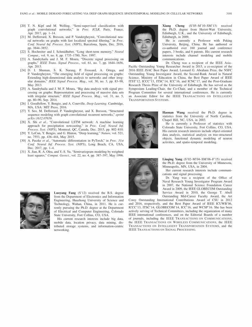
Luoyang Fang (S’12) received the B.S. degreefrom the Department of Electronics and InformationEngineering, Huazhong University of Science andTechnology, Wuhan, China, in 2011. He is cur-rently pursuing the Ph.D. degree at the Departmentof Electrical and Computer Engineering, ColoradoState University, Fort Collins, CO, USA.

His current research interests include big data,mobile data, location privacy, data mining, dis-tributed storage systems, and information-centricnetworking.

Xiang Cheng (S’05–M’10–SM’13) receivedthe Ph.D. degree from Heriot-Watt University,Edinburgh, U.K., and the University of Edinburgh,Edinburgh, in 2009,

He is currently a Professor with PekingUniversity, Beijing, China. He has authored orco-authored over 160 journal and conferencepapers, 3 books, and 6 patents. His current researchinterests include channel modeling and mobilecommunications.

Dr. Cheng was a recipient of the IEEE Asia–Pacific Outstanding Young Researcher Award in 2015, a co-recipient of the2016 IEEE JSAC Best Paper Award, Leonard G. Abraham Prize, the NSFCOutstanding Young Investigator Award, the Second-Rank Award in NaturalScience, Ministry of Education in China, the Best Paper Award of IEEEITST’12, ICCC’13, ITSC’14, ICC’16, and ICNC’17, and the Post-GraduateResearch Thesis Prize of the University of Edinburgh. He has served as theSymposium Leading-Chair, the Co-Chair, and a member of the TechnicalProgram Committee for several international conferences. He is currentlyan Associate Editor for the IEEE TRANSACTIONS ON INTELLIGENT

TRANSPORTATION SYSTEMS.

Haonan Wang received the Ph.D. degree instatistics from the University of North Carolina,Chapel Hill, NC, USA, in 2003.

He is currently a Professor of statistics withColorado State University, Fort Collins, CO, USA.His current research interests include object-orienteddata analysis, statistical analysis on tree-structuredobjects, functional dynamic modeling of neuronactivities, and spatio-temporal modeling.

Liuqing Yang (S’02–M’04–SM’06–F’15) receivedthe Ph.D. degree from the University of Minnesota,Minneapolis, MN, USA, in 2004.

Her current research interests include communi-cations and signal processing.

Dr. Yang was a recipient of the Office ofNaval Research Young Investigator Program Awardin 2007, the National Science Foundation CareerAward in 2009, the IEEE GLOBECOM OutstandingService Award in 2010, the George T. AbellOutstanding Mid-Career Faculty Award, the Art

Corey Outstanding International Contributions Award of CSU in 2012and 2016, respectively, and the Best Paper Award of IEEE ICUWB’06,ICCC’13, ITSC’14, GLOBECOM’14, ICC’16, and WCSP’16. She has beenactively serving of Technical Committees, including the organization of manyIEEE international conferences, and on the Editorial Boards of a numberof journals, including the IEEE TRANSACTIONS ON COMMUNICATIONS,the IEEE TRANSACTIONS ON WIRELESS COMMUNICATIONS, the IEEETRANSACTIONS ON INTELLIGENT TRANSPORTATION SYSTEMS, and theIEEE TRANSACTIONS ON SIGNAL PROCESSING.

Mobile Demand Forecasting via Deep Graph-Sequence ...

Documents