Mobile Computing Systems -- Introduction - ECE

Chapter 1 Introduction

Ivan Marsic • Rutgers University 2

1.1 Information, Computation, and Communication

Conceptually, computing can be seen as: USER ⇔ COMP.SYS ⇔ ENVIRONMENT

Work has become more abstract. Workers no longer make physical contact with the objects with which they deal; rather, they accomplish tasks through the medium of an information system.

[It is also often true that once a job is computerized it is made routine and unchallenging, while at the same time it demands focused attention and abstract comprehension. Needless to say, that is a bad combination!]

If any of the players is mobile relative to each other during the time of system use, we are dealing with an instance of mobile computing. Three types of mobility: mobility of the user; mobility of the device; and, since they can be accessed from any point, mobility of services. P.25, [Brown et al. 2002].

System is distributed if it consists of independent components, connected by communication links.

Distribution often does not matter from the viewpoint of the task at hand; it matters only from the system developer’s viewpoint. However, there are instances where system distribution alters the way the task is performed.

1.1.1 Functions and Processes

Relations For two sets of elements, A and B, the Cartesian product A and B is defined as the set of pairs of their elements:

{ }BbAabaBA ∈∧∈=× ),(

A unary operation R on a set A is defined to be a subset of A, R ⊆ A. An n-ary relation R on A, for n > 1, is a subset of the n-fold Cartesian product, R ⊆ A × A × … × A. Binary relations play a particularly important role, and we often write R(a, b) or aRb to mean the same as (a, b) ∈ R. For example, in the case of ordering relations we write a < b rather than (a, b) ∈ <.

There are several properties that apply to binary relations. Let R denote any binary relation on a set A. We say:

R is reflexive if (∀ a ∈ A) (aRa)

R is symmetric if (∀ a, b ∈ A) (aRb ⇒ bRa)

R is antisymmetric if (∀ a, b ∈ A) [(aRb ∧ a ≠ b) ⇒ ¬(bRa)]

Chapter 1 • Introduction 3

R is connected if (∀ a, b ∈ A) [(a ≠ b) ⇒ (aRb ∨ bRa)]

R is transitive if (∀ a, b, c ∈ A) [(aRb ∧ bRc) ⇒ (aRc)]

Of course, not all binary relations have all of the above properties. For example, a partial ordering of a set A, usually denoted by the symbol ≤, is a binary relation on A which is reflexive, antisymmetric, and transitive. A partially ordered set, or poset, is the ordered pair (A, ≤).

Functions Let R be an (n + 1)-ary relation on a set A. The domain of R is defined to be the set

dom(R) = {a | ∃b[(a, b) ∈ R]}

The range of R is defined to be the set

ran(R) = {b | ∃a[(a, b) ∈ R]}

If n = 1, so that R is a binary relation consisting of ordered pairs, then dom(R) is the set of first components of members of R, and ran(R) the set of second components. Likewise, if n > 1, the elements of R are still ordered pairs, only now the domain of R consists not of elements of A but of the n-fold product A × A × … × A.

A function is a relation that uniquely associates members of one set with members of another set. More formally, an n-ary function on a set A is and (n + 1)-ary relation, R, on A such that for every a ∈ dom(R) there is exactly one b ∈ ran(R) such that (a, b) ∈ R. As before, if R is an n-ary function on A and a1, a2, …, an, b ∈ A, we write R(a1, …, an) = b instead of (a1, …, an, b) ∈ R.

We write

f : A → B

to denote that f is a function such that dom(f) = A and ran(f) ⊆ B. Notice that if f : A → B, then f ⊆ A × B. A function is therefore a many-to-one (or sometimes one-to-one) relation. We also say that f is a mapping from one domain A into another domain B. Each domain represents a set of possible values, with A being the set of possible values upon which the function operates and B the set of possible values that can be produced by the function.

In the correct notation, the symbol f or f(⋅) refers to the function itself, while f(x) refers to the value taken by the function when evaluated at a point x. The dot (⋅) is meant to indicate that the function f takes a single argument, i.e., it is a unary function.

Processes A process is a naturally occurring or designed sequence of operations or events, possibly taking up time, space, expertise or other resource, which produces some outcome. A process may be identified by the changes it creates in the properties of one or more objects under its influence.

A function may be thought of as a computer program or mechanical device that takes the characteristics of its input and produces output with its own characteristics. Every process may be defined functionally and every process may be defined as one or more functions.

Ivan Marsic • Rutgers University 4

0

5 10 15 20

0 1 2 3 4 5 6 7 8 9 10 11 12 13 14 15arrivals per time unit (n)

perc

ent o

f occ

urre

nces

(%)

Figure 1-1. The histogram of the number of arrivals per unit of time (τ = 1) for a Poisson process with average arrival rate λ = 5.

An example random process that will appear later in the text is Poisson process. It is usually employed to model arrivals of people or physical events as occurring at random points in time. Poisson process is a counting process for which the times between successive events are independent and identically distributed exponential random variables. For a Poisson process, the number of arrivals in any interval of length τ is Poisson distributed with parameter λ⋅τ. That is, for all t, τ > 0,

{ } ,...1,0,!)()()( ===−+ − n

nentAtAP

nλττ λτ (1.1)

The average number of arrivals within an interval of length τ is λτ (based on the mean of the Poisson distribution). This leads to the interpretation of λ as an arrival rate (average number of arrivals per unit time). An example of the Poisson distribution is shown in Figure 1-1.

This model is not entirely realistic for many types of sessions and there is a great amount of literature which shows that it fails particularly at modeling the LAN traffic. However, such simple models provide insight into major tradeoffs involved in network design, and these tradeoffs are often obscured in more realistic and complex models.

Markov process is a random process with the property that the probabilities of occurrence of the various possible outputs depend upon one or more of the preceding outputs.

1.1.2 Information and Entropy Information theory considers the transmission of messages from source to receiver. Claude E. Shannon (1916-2001), who invented information theory in 1948, viewed information as being the resolution of uncertainty. It is the part of a message that is unknown to and cannot be foreseen by the receiver. “Information” in information theory is related to the element of surprise on behalf of the receiver, which is result of uncertainty, or unexpectedness. This concurs with the intuitive notion that the whole idea of information is to “inform” or transfer knowledge. If you are told something that you already know, you are not given information—there is nothing new added to your store of knowledge. Moreover, even if you are told something that you can deduce from other things that you know, you are not given information. The essence of information is in the novelty—the contrasting from that previously known, and from that which may be expected based upon what is formerly known.

Chapter 1 • Introduction 5

Sources:

Receiver

Book

Die

Coin

{Head, Tail}

{1, 2, 3, 4, 5, 6}

Letters, Letter-combinations, Words, …

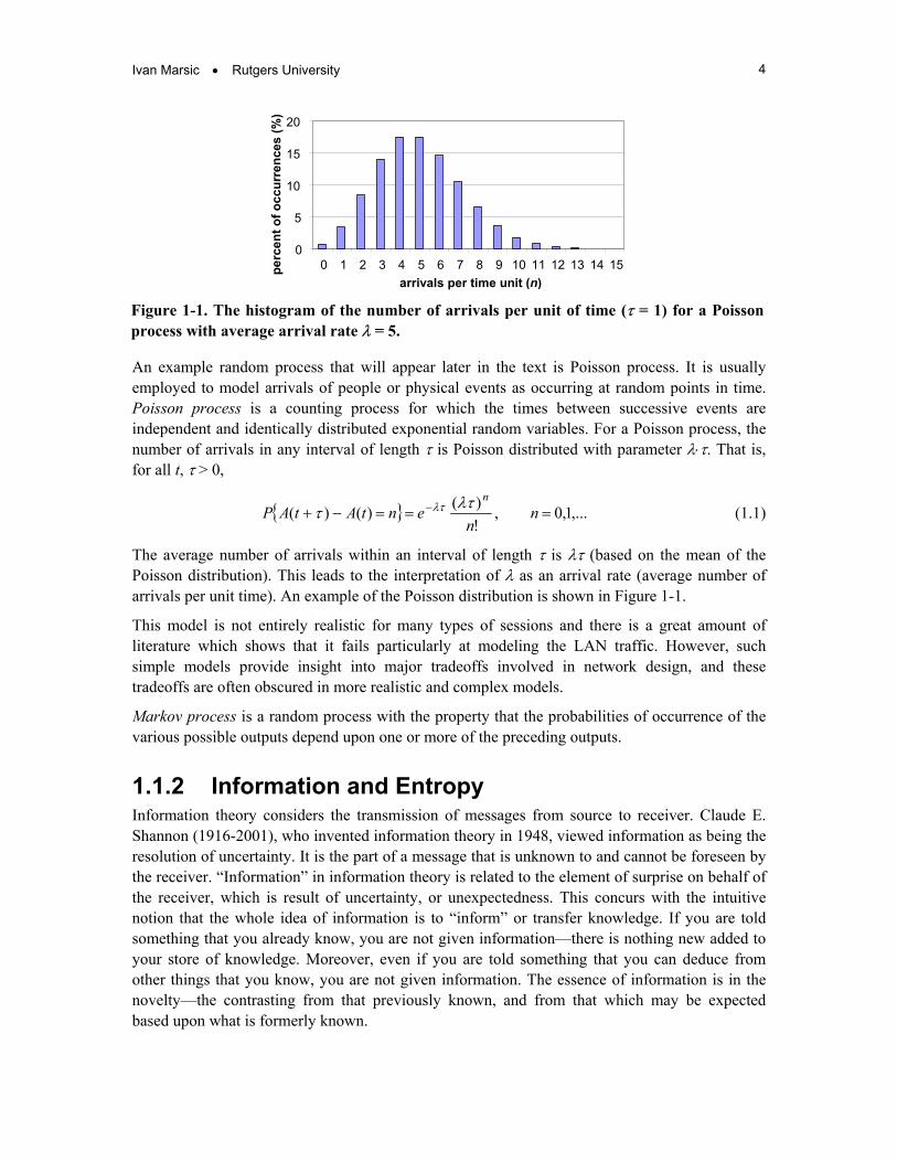
Figure 1-2. Example information sources.

Representation Symbols represent physical objects or abstract concepts. For example, the pips on the six sides of a die can be represented as {“1”, “2”, “3”, “4”, “5”, “6”} or {“I”, “II”, “III”, “IV”, “V”, “VI”} or {“001”, “010”, “011”, “100”, “101”, “110”} or {“one”, “two”, “three”, “four”, “five”, “six”}. All of these represent differently one aspect of a die: the pip count on different sides. Rolling a die can be considered an information source generating a sequence of symbols or events. Example information sources are given in Figure 1-2.

How is it possible for a lower level process to use smaller number of symbols to communicate larger number of symbols of a higher-level? – Only by reducing the rate. (Compute the entropy of each level/source.)

If a “higher-level” process generates more different symbols, but at a lower rate than a “lower-level” process (with less number of different symbols, but higher rate), and communicates with another higher-level process, then the higher-level process is represented in terms of the lower one.

Information Measure The measure of information must lie in the amount of surprise that resides in the unexpected or uncertain portion of the data received. The more unexpected the information content of a message, the greater the surprise, and hence more information.

As the unit of information we take the simplest uncertain event with only two outcomes, for example, the single throw of a fair coin. The outcome of such an even is a binary choice, the answer to a single “yes” or “no” question. This can be represented with a single binary digit or

Ivan Marsic • Rutgers University 6

bit1, which can take the values “0” or “1.” Each “information bit” is the answer to a single yes/no question, posed according to the best possible strategy for the given situation. Obviously, the best possible strategy depends on what the recipient already knows.

For example, assume that we are receiving a stream of messages from tossing a biased coin such that the “Head” outcome is much more likely than “Tail.” If we do not know about the bias, it is equally profitable, on the average, to ask whether it is “Tail” as is “Head.” However, if we know about the bias, it is more profitable to ask first whether the outcome is “Head” since this saves us lots of questions, on the average.

The average information per message from an information source is called the source’s entropy. It is the minimum number of yes/no questions required on the average to arrive at the given data, knowing everything that we do know. If a source M emits messages m1, m2, …, mn, with probabilities P(m1), P(m2), …, P(mn), respectively, then the entropy H(M) of the source is the average number of binary digits per message2:

H(M) = ( )∑ = ⋅− ni ii mPmP1 2 )(log)( = ( ))(1log)( 21 i

ni i mPmP ⋅∑ = bits per symbol (1.2)

(We assume that each message contains a single symbol.) This minimum average number of information bits (entropy) has real world significance, since it determines the minimum required capacity for communication and storage of information. The number of bits of information is the fundamental uncertainty associated with it.

Interestingly, the Shannon’s recommended strategy implied by (1.2) is to choose those questions to ask for which the answers “yes” and “no” are about equally likely. For example, when determining the result of spinning a roulette wheel with 38 equiprobable choices, it is not the best strategy to ask whether an individual number, such as “17” appeared, since the probability of obtaining “yes” is only 1/38, whereas probability of “no” is 37/38. On the other hand, asking whether the result is one of the first 19 numbers gives “yes” with the probability ½ (same for “no”). In the former case, one needs to ask 19 yes/no questions, on the average. Conversely, in the latter case, one always obtains the right answer by asking exactly 6 yes/no questions.

The source is modeled as a random, independent identically distributed (iid) symbol sequence.

Ergodic process (Pierce, p.81) – probabilities do not change over time

Ergodic: of or relating to a process in which a sequence or sizable sample is equally representative of the whole (as in regard to statistical parameter)

— from PRINCIPIA CYBERNETICA WEB (http://pespmc1.vub.ac.be/ASC/ERGODIC.html)

1 The term “bit” was coined by statistician John W. Tukey (1915-2000) in 1949 during a lunchtime conversation at Bell Labs. He is also credited with introducing the terms “byte,” “software,” and “cepstrum” (the Fourier transform of the logarithm of the Fourier transform).

2 In case your calculator does not support binary logarithms, )2(log)(log)(log

10102

xx =

Chapter 1 • Introduction 7

"2" (0.01)

"1" (0.05)

"3" (0.05)

"4" (0.05)

"5" (0.25)

"6" (0.59)

(0.06)

(0.10)

(0.16)

(0.41)

(1.00)

0

10

0

1

0

1

01

1

Path for “4”:“0011"

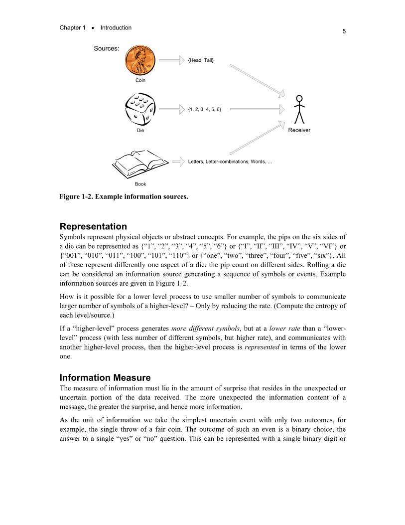
Figure 1-3. Huffman code tree for a biased die. See text for details.

Source Coding Source coding is also called data compression.

Let us assume that the source generates symbols by rolling a die. If the die is unbiased, the probability distribution of symbols is uniform, P(Xi) = 1/6 ≈ 0.1667; i = 1, …, 6. The source entropy in this case is H(M) ≈ 2.585.

Let us now assume that the die is biased, e.g., by embedding a concealed piece of metal, so that the new probabilities are as shown in Figure 1-3, in the lower left corner where the symbols are listed on the left and the probabilities are shown in parentheses. The source entropy in this case is H(M′) ≈ 1.664.

If we merely assigned a binary number to each symbol, we would need 3 bits to transmit each symbol. How can we encode the symbols more efficiently? One way is to use Huffman coding, as illustrated in the following example.

Example 1.1 Huffman Code

We start by rank-ordering the messages from least probable to most probable, see Figure 1-3. In constructing the code, we first find the two lowest probabilities, in our case 0.01 for symbol “2” and of the three symbols with the probability 0.05 we pick arbitrarily “1.” We draw lines to the point marked (0.06), which is the probability of either “2” or “1.” From now on, we disregard the individual probabilities connected by the lines and look again for the two lowest probabilities, which are 0.05 for both “3” and “4.” Again draw lines to the right to a point marked (0.10), which is their sum. The lowest remaining probabilities are now 0.06 and 0.10, so we draw a line connecting them, to obtain a point marked (0.16). We proceed thus until paths run from each symbol to a common point to the right, the point marked (1.00).

To obtain the codes for the symbols, we label each lower path going to the left from a point 1 and each upper path 0. The code for a given symbol is then the sequence of digits encountered going left from the common point 1.00 to the symbol in question. The codes are listed in Table 1-1.

Ivan Marsic • Rutgers University 8

Table 1-1 Summary of Huffman code for a biased die. P is the probability of the symbol, N is the number of digits in its codeword, and N⋅P is the average number of bits needed to encode the particular symbol.

Symbol P Code N N⋅P "1" 0.05 "0001" 4 0.20 "2" 0.01 "0000" 4 0. 04 "3" 0.05 "0010" 4 0.20 "4" 0.05 "0011" 4 0.20 "5" 0.25 "01" 2 0.50 "6" 0.59 "1" 1 0.59

Average number of bits per symbol: 1.73

Although most symbols require four binary digits to per symbol, the savings comes from the fact that they occur very rarely and we use only one or two digits for the most frequent symbols. In Table 1-1, the probability of a symbol times the number of digits in the code gives the average number of digits per symbol in a long message due to the use of that particular symbol. If we add the products of these probabilities, we obtain the average number of digits per symbol, which is 1.73. This is a little larger than the entropy per symbol, which was given above as 1.664, but it is smaller number of digits than the 3 digits per symbol we would have used if we had merely assigned a different 3-digit code to each symbol.

Comments As already pointed out, the amount of information a source generates depends on what the observer chooses to watch and on the observer’s prior knowledge. Thus, there is a built-in element of subjectivity in the process of information measurement and there is no absolute amount of entropy associated with information source.

Some authors, e.g., Lucky [1988: p. 9] contend that creation of information does not require natural resources. This author respectfully disagrees; cf. Maxwell’s daemon [Leff & Rex 1990; 2003]. But, see also [Landauer 1991] on the Landauer’s principle and the cost of forgetting. The idea is that information invariably encodes on real, physical objects, ranging from wooden abacuses (papyrus) to sheets of paper to semiconducting computer chips to neurons in the brain. Being physical, information is subject to the laws of physics. Landauer in 1961 succeeded in locating the precise point in any computation in which energy is converted to heat and carried away as waste.

See Technomanifestos, p. 16, Wiener’s comment “information is unsuited to being commodity.” Also, see [von Baeyer 2003: p. 25]. Cf. A. Boucouvalas, value of information with time.

[ Shouldn’t human limitations of 50 bps be seen in this (see section on Representation) light? I.e., the conversion is not proper, since humans can generate many high-level symbols although at a particular moment they may be generating only 50 bps. ]

Information theory started with a simple structure—sources and channels. There were simple examples—iid sources, binary channels and Gaussian channels. The structure has grown, but

Chapter 1 • Introduction 9

Information

Source Transmitter Receiver

Noise Source

Destination Communication Channel

Figure 1-4. Shannon’s diagram of the communication process.

almost as a tree—it displays chunking property, hierarchical abstraction, well known in cognitive psychology. One can still start at the bottom and quickly get anywhere. As the old branches die off and new ones start, they do not affect each other or the rest of the tree—the alterations are strictly confined at the conceptual level.

Re: complexity, see Pierce on complexity of melodies and recognizability of author's style, whether in music, poetry, or painting. Maximum information content would be that of random noise, but they seek a simple but unique pattern.

1.1.3 Communication Ideally, a channel should accept messages at the input, transmit them, and deliver unaltered at the output. An important concept is the rate of information transmission. Every physical channel has a finite upper limit on the amount of information that it can transmit per unit of time.

Another important aspect is noise—noise reduces the channel capacity and, moreover, does do in a non-deterministic way. In other words, some transmitted messages will not reach destination and we cannot know beforehand which ones will be impaired nor how.

The overall communication process suggested by Shannon’s theory of information works as follows (Figure 1-4). First, we should seek by a complex encoding to represent the message from the source by the smallest number of binary digits possible—the source’s entropy. This will produce a nonredundant stream of binary digits. This process is usually called “compression” of information. The reason for compression is to adjust the messages to the limited channel capacity—the smaller the messages, the more of them can be transmitted per unit of time. We are then faced with the problem of transmitting a nonredundant stream of binary digits without error over a noisy channel. To do this, we encode the nonredundant message digits into a redundant stream of signal digits (symbols), which is called error-control encoding. Thus, we remove redundancy from the messages produced by the message source and then add the right sort of redundancy to produce signal with immunity against noise of a particular channel type. Shannon has shown that it is possible to achieve error-free communication by adding suitable redundancy [Shannon & Weaver 1949].

One can relatively easily admit that removing redundancy from source information by source coding helps communication, since it reduces the quantity of data that needs to be transmitted without losing valuable information. However, adding new redundancy may at first look suspicious. Even if this can be admitted as a means to harden the signal against noise impairments, the question arises of the best way of adding the redundancy in channel coding, in the sense that it guarantees achieving maximum transmission capacity in the presence of noise. An analogy shown in Figure 1-5 may help in understanding this. Here, we remove the pods

Ivan Marsic • Rutgers University 10

Beans (Redundancy = pods)

Beans (No redundancy)

Beans (No redundancy)

Beans (Redundancy = can)

Erroneous Communication Channel

Source Coding

ChannelCoding

Figure 1-5. An analogy for redundancy manipulation in communication. Bean pods are not the “right” kind of redundancy for bean transport, whereas metal cans are. See text for details.

(source coding) in order to ship as many beans as possible. We then add cans to protect the beans from damage in transportation.

If process (channel) loss takes known form or can be modeled, we can represent the loss as an additional variable (noise). Suppose that we transmit a sequence of bits over the channel, and errors occur where marked “X”:

Source Data: 0 1 0 0 1 1 0 0 1 0 1 1 0 1 1 Errors: X_________________X_____X__________________ Received Data: 1 1 0 0 1 1 1 0 0 0 1 1 0 1 1

In order to reconstruct the original data we would have to know the error locations. These could be represented as a sequence of bits with 0 for “no error” and 1 for “error,” as follows:

Error Locations: 1 0 0 0 0 0 1 0 1 0 0 0 0 0 0 If we only knew this sequence, we would know which bits had to be changed (inverted), and we could repair the received data. It is the result of the uncertainty added during transit by the communications channel. How much information does it take to learn this sequence and repair the data? We can quantify this by employing entropy. In the case of independent binary symbols, we obtain:

H(N) = − [Pe ⋅ log2(Pe) + (1−Pe) ⋅ log2(1−Pe)]

where Pe is the probability of the symbol 1, representing an error. [We assume that Pe is the same regardless of whether 0 or 1 is sent; this is called binary symmetric channel.]

It is as if the received binary digits are “missing” H(N) bits of information. This leads us to an intuition about the channel capacity to transmit information. For a binary symmetric channel with independent error events the capacity is:

C = 1 − H(N) = 1 + Pe ⋅ log2(Pe) + (1−Pe) ⋅ log2(1−Pe) bits per binary digit (1.3)

This intuition will be substantiated more formally below.

Chapter 1 • Introduction 11

“1"

“0"

“1"

1−Pe

1−Pe

Pe

Pe

(a)

“1"

“2"

“3"

“4"

“5"

“6"

“1"

“2"

“3"

“4"

“5"

“6"(b)

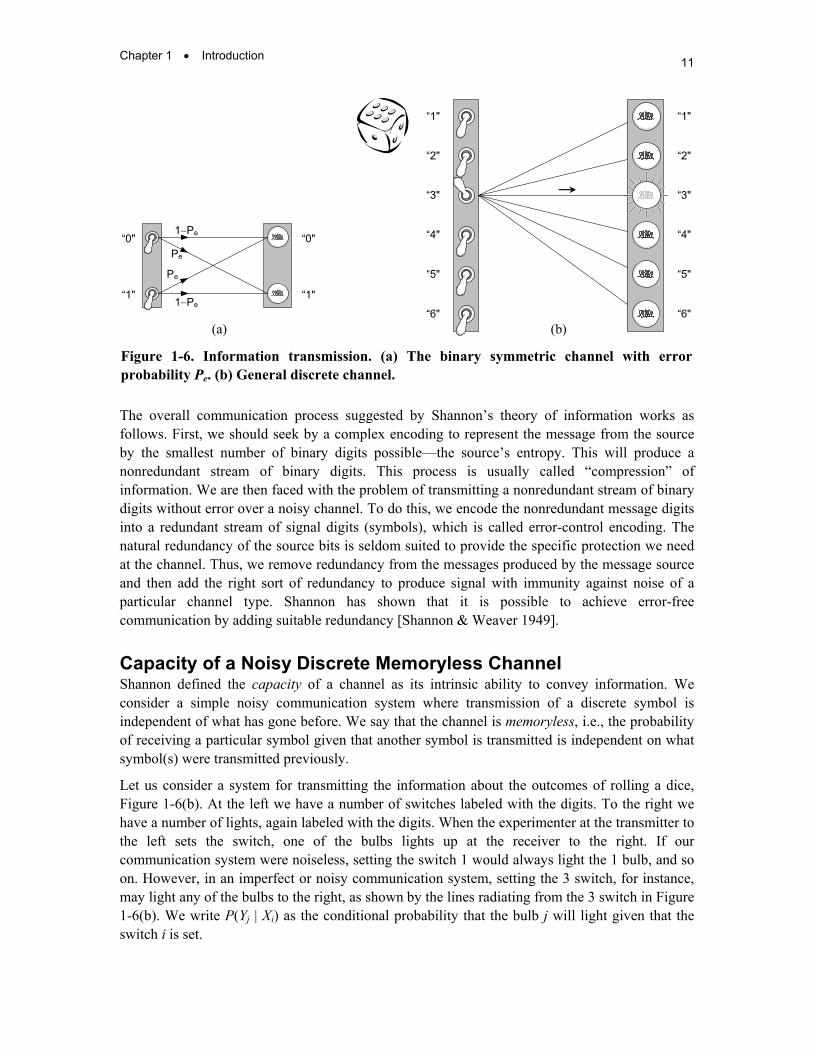
Figure 1-6. Information transmission. (a) The binary symmetric channel with errorprobability Pe. (b) General discrete channel.

“0"

The overall communication process suggested by Shannon’s theory of information works as follows. First, we should seek by a complex encoding to represent the message from the source by the smallest number of binary digits possible—the source’s entropy. This will produce a nonredundant stream of binary digits. This process is usually called “compression” of information. We are then faced with the problem of transmitting a nonredundant stream of binary digits without error over a noisy channel. To do this, we encode the nonredundant message digits into a redundant stream of signal digits (symbols), which is called error-control encoding. The natural redundancy of the source bits is seldom suited to provide the specific protection we need at the channel. Thus, we remove redundancy from the messages produced by the message source and then add the right sort of redundancy to produce signal with immunity against noise of a particular channel type. Shannon has shown that it is possible to achieve error-free communication by adding suitable redundancy [Shannon & Weaver 1949].

Capacity of a Noisy Discrete Memoryless Channel Shannon defined the capacity of a channel as its intrinsic ability to convey information. We consider a simple noisy communication system where transmission of a discrete symbol is independent of what has gone before. We say that the channel is memoryless, i.e., the probability of receiving a particular symbol given that another symbol is transmitted is independent on what symbol(s) were transmitted previously.

Let us consider a system for transmitting the information about the outcomes of rolling a dice, Figure 1-6(b). At the left we have a number of switches labeled with the digits. To the right we have a number of lights, again labeled with the digits. When the experimenter at the transmitter to the left sets the switch, one of the bulbs lights up at the receiver to the right. If our communication system were noiseless, setting the switch 1 would always light the 1 bulb, and so on. However, in an imperfect or noisy communication system, setting the 3 switch, for instance, may light any of the bulbs to the right, as shown by the lines radiating from the 3 switch in Figure 1-6(b). We write P(Yj | Xi) as the conditional probability that the bulb j will light given that the switch i is set.

Ivan Marsic • Rutgers University 12

YXH(X)

P(Yj | Xi)Observer 1

Observer 2

H(Y)

H(X,Y) = H(X) + H(Y|X) = H(Y) + H(X|Y)

Observer 3

(a)

H(X | Y) H(Y | X)

H(X) H(Y)

I(X; Y)

H(X, Y)

(b)

Figure 1-7. (a) Average information of the whole communication system seen by Observer 3. (b) Diagrammatic summary of relations between various averages of information.

We know from Eq. (1.2) that the entropy of the source X, the rate at which the message source generates information, is

H(X) = ( )∑ = ⋅− ni ii XPXP1 2 )(log)(

We can regard the output of the receiver as another source, Y, as seen by Observer 2 in Figure 1-7. The number of lights need not be equal to the number n of switches, but we will assume that it is, so the entropy of the output at the receiver is

H(Y) = ( )∑ = ⋅− nj jj YPYP1 2 )(log)(

We know that H(X) depends only on the input of the communication channel and H(Y) depends both on the input to the channel and on the errors made in transmission.

Now imagine an observer that can simultaneously see both the transmitter and the receiver (Observer 3 in Figure 1-7(a)) and detect how often certain combinations of X and Y occur; say, how often 3 is sent and 4 is received. Or, knowing the statistics of the message source and the statistics of the noisy channel, we can compute such probabilities. From these, we can compute the average uncertainty of the communication system as a whole by joint probabilities of occurrence of the combination of input and output symbols:

H(X, Y) = ( ) ( )( )jini

nj ji YXPYXP ,log, 21 1 ⋅∑ ∑= =−

Since a symbol at the transmitter can result in different symbols at the receiver, we can think of each transmitter symbol as a source. Thus, given that we know the input to the channel is the symbol Xi, we can define conditional or relative entropy like so

H(Y | Xi) = ( )∑ = ⋅− nj ijij XYPXYP1 2 )|(log)|(

and for any channel input, we multiply the uncertainty for a given input by the probability that that input will occur and sum over all inputs

H(Y | X) = ( ) ( ) ( ) ( ) (( )ijijni

nj i

ni ii XYPXYPXPXYHXP |log|| 21 11 ⋅⋅−=⋅− ∑ ∑∑ = == )

Finally, we have that the combined average information of the whole system is

Chapter 1 • Introduction 13

H(X, Y) = H(X) + H(Y | X) (1.4)

That is, the uncertainty of sending Xi and receiving Yj is the uncertainty of sending Xi plus the uncertainty of receiving Yj when Xi is sent.

We can similarly derive

H(X, Y) = H(Y) + H(X | Y) (1.5)

which means that the uncertainty of receiving Yj and sending Xi is the uncertainty of receiving Yj plus the uncertainty that Xi was sent when Yj was received. Here, H(X | Y) is the uncertainty as to which symbol was transmitted when a given symbol is received.

Figure 1-7(b) summarizes the relations between various entropies in the system. One important quantity is the average mutual information between the source X and receiver Y, I(X; Y), which is the average information that is successfully conveyed. As shown,

I(X; Y) = H(X) − H(X | Y) = H(Y) − H(Y | X) (1.6)

We can read this equation to mean that the average mutual information (known to both source and receiver) is what is known (statistically) to one side minus what is lost in transmission due to the noise. The quantity H(X | Y), the average amount of information lost because of noise, is called equivocation of the communication channel. One possible interpretation of the equivocation is that it is the additional average information needed for correction of channel errors. The average uncertainty about the received symbol when the transmitted symbol is known, H(Y | X), is known as the average error due to channel noise.

If we take I(X; Y), H(X), and H(X | Y) as entropies in bits per second, then I(X; Y) represents the rate of transmission of information over the channel. From Eq. (1.6) the rate of transmission of information is the source rate or entropy less the equivocation. Or, in other words, it is the entropy of the message as sent less the uncertainty of the recipient as to what message was sent.

The channel capacity C is the maximum rate of transmission of information over the channel; hence it is the maximum value of I(X; Y) with respect to the variations of the transmitted symbol probabilities P(Xi). In other words, we keep choosing the message source so as to make the transmission rate as large as possible for a given channel. Of course, if the entropy of a source X exceeds the channel capacity, the excess information, H(X) − C, is lost in transmission by default.

The simplest case, but a very important one, is the binary symmetric channel (BSC) for which the probability of an error is Pe and of correct transmission is (1 − Pe), regardless of what bit (0 or 1) is sent (Figure 1-6(a)). The capacity of such a binary channel can be easily derived analytically, as given by Eq. (1.3) above.

We notice that, in general, finding the maximal value of I(X; Y), i.e., the channel capacity, is very difficult to perform. We will see an example in Chapter 3.

Channel Coding for Error-Control Shannon’s fundamental theorem for a noisy channel states that

Let a discrete channel have a capacity C and a discrete source the entropy per second H. If H < C there exists a coding system such that the output of the source can be transmitted over the channel with an arbitrary small frequency of errors (or an arbitrary small equivocation). If H > C it is possible to

Ivan Marsic • Rutgers University 14

CommunicationChannel

CommunicationChannel Blocks:

Bits:

Figure 1-8. Bits vs. blocks: It is only the transmitter and receiver mutual convention—there is no difference in their appearance on the channel.

encode the source so that the equivocation is less than H − C + ε, where ε is arbitrarily small. There is no method of encoding which gives an equivocation less than H − C.

Notice that the theorem does not promise eliminating the errors altogether—it only says that the error rate can be made vanishingly small—even then the errors could still happen, but with an extremely low probability. It also does not specify how to develop the code with such a property.

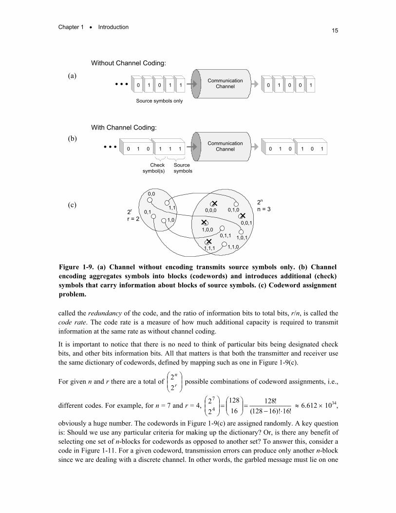
Clearly, considering individual symbols cannot help us detect occurrence of an error. Individual symbols are atomic and cannot contain any other information except about self. For example, for the binary channel in Figure 1-6(a), it is impossible to detect an error by looking just at the last received binary digit. To do so, we need to introduce redundancy. Redundancy essentially means that instead of considering the transmission of individual symbols, we consider the transmission of blocks or sequences of symbols, Figure 1-8. In such a block, some symbols carry the information from the transmitting source and other symbols carry information about the source-information-carrying symbols. The latter are called check symbols, see Figure 1-9(b). The check symbols help the receiver to detect errors inside their blocks and perhaps even correct it or the receiver could notify the transmitter that the block was garbled, and ask for a retransmission.

For the sake of simplicity, assume that we deal with binary symbols, 0 and 1. A sequence of 0’s and 1’s of length n is called (binary) n-block. Each transmitted n-block is made up of r binary digits representing the source messages and the remaining (n − r) are check digits. There are 2n possible different n-blocks shown as points of sets in Figure 1-9(c). We need only 2r different n-blocks to transmit all possible source sequences of length r. Since r < n, the transmitter and receiver can agree and select 2r different n-blocks as valid sequences, also called codewords. A dictionary of codewords is called code. The remaining 2n − r sequences they declare as invalid. Of course, the transmitter will always send only codewords, so when receiver receives an invalid n-block, it knows that an error occurred and can try to repair it or request retransmission. This is illustrated in Figure 1-10.

Code is established by a prior mutual agreement of the transmitter and receiver and a copy of it (a “dictionary”) is placed at both of them. This is known as a priori shared context—a prerequisite for any communication to happen.

Notice also that channel coding effectively reduces the source transmission rate, since check bits consume some of the channel capacity. The ratio of redundant bits to information bits, (n − r)/r, is

Chapter 1 • Introduction 15

Communication Channel 1101 0 1 0 0 1 0

Communication Channel

Without Channel Coding:

With Channel Coding:

1 1 1 0 1 0

Source symbols only

Source symbols

Checksymbol(s)

1 0 1 0 1 0

(a)

(b)

2r r = 2

0,0

0,11,1

1,0

0,0,0 0,1,0

1,0,00,1,1

1,1,0

1,0,1

1,1,1

0,0,1

2n n = 3

(c)

Figure 1-9. (a) Channel without encoding transmits source symbols only. (b) Channelencoding aggregates symbols into blocks (codewords) and introduces additional (check)symbols that carry information about blocks of source symbols. (c) Codeword assignmentproblem.

called the redundancy of the code, and the ratio of information bits to total bits, r/n, is called the code rate. The code rate is a measure of how much additional capacity is required to transmit information at the same rate as without channel coding.

It is important to notice that there is no need to think of particular bits being designated check bits, and other bits information bits. All that matters is that both the transmitter and receiver use the same dictionary of codewords, defined by mapping such as one in Figure 1-9(c).

For given n and r there are a total of possible combinations of codeword assignments, i.e.,

different codes. For example, for n = 7 and r = 4,

r

n

22

!16)!16128(!128

16128

22

4

7

⋅−=

=

≈ 6.612 × 1034,

obviously a huge number. The codewords in Figure 1-9(c) are assigned randomly. A key question is: Should we use any particular criteria for making up the dictionary? Or, is there any benefit of selecting one set of n-blocks for codewords as opposed to another set? To answer this, consider a code in Figure 1-11. For a given codeword, transmission errors can produce only another n-block since we are dealing with a discrete channel. In other words, the garbled message must lie on one

Ivan Marsic • Rutgers University 16

CommunicationChannel

Noise

Without channel coding:

With channel coding:

Illegal block!! (Transmitter agreed never

to send such a block)

Noise

Undetected!! (Receiver has no means

to detect this error)

Dictionary of Codewords

Dictionaryof Codewords

Figure 1-10. Channel coding helps the receiver detect errors. Notice that both transmitterand receiver have a copy of the codeword dictionary, i.e., the code. (Transmitter substitutesthe codewords as per Figure 1-9(c).)

of the vertices of the unit cube in Euclidean n-dimensional space—it cannot lie at any other point in the space. Therefore, the distance between two vertices is measured as the minimum number of edges that must be traversed on a path from one vertex to another. This is called Hamming distance and it basically counts the number of bits in which two n-blocks differ. For instance, dH(101, 011) = 2, while dH(101, 010) = 3.

The minimum distance of a code dmin is the minimum of the Hamming

distances between any two nonidentical codewords of the code. [Notice that dH(cwi, cwj) ≥ 1 for any two codewords cwi, cwj, i ≠ j, so as soon as a distance of 1 is detected, we know that dmin = 1.] For the code shown in Figure 1-11(a), dmin = 2. As illustrated in Figure 1-11(b), any single-digit error will lead to an illegal n-block, so the receiver will be able to detect all the single-digit errors. Conversely, the minimum distance for the code in Figure 1-9(c) is one, since it takes only one bit to change the codeword 010 into 110 or 011. In this case, the receiver cannot detect all single-digit errors. Clearly, some codes are better than others.

( 1222

2 1 −⋅=

− rrr )

While single-error detection is possible with a code whose dmin is two, single-error correction is only possible with a code whose minimum distance is at least three. One example is shown in Figure 1-11(c). If a maximum of one error is assumed to occur in the transmission of a single codeword, then the error can be found and the receiver can determine exactly which codeword has been sent. The codeword which differs from the received n-block in the fewest number of bits is assumed to be the one transmi8tted. (Such receiver is sometimes termed a “maximum-likelihood” receiver.) However, the correcting ability disappears if two errors occur in the same codeword. It can be shown that for a given positive integer t, if a code satisfies dmin ≥ 2t, then all errors of (t − 1) bits or less can be corrected and errors of t bits can be detected but not, in general, corrected.

Chapter 1 • Introduction 17

x

y

z

(1,0,1)

(0,0,0)

(1,1,0)

(0,1,1)

1

1

1

(a)

(1,0,1) (1,1,1)

(0,0,1)

(1,0,0)

(b)

(1,0,1)

(0,1,0)

(0,0,1)

(1,0,0)

(c)

(0,0,0)

(1,1,1)

dmin = 3dmin = 2(1,1,0)

(0,1,1)

Figure 1-11. (a) A code with four codewords of length three, indicated by black circles. (b) Three possible 3-blocks formed by a single error in the transmission of the codeword 101.(c) A code with two codewords of length three and six possible 3-blocks formed by single or double error in the transmission of the codeword 000.

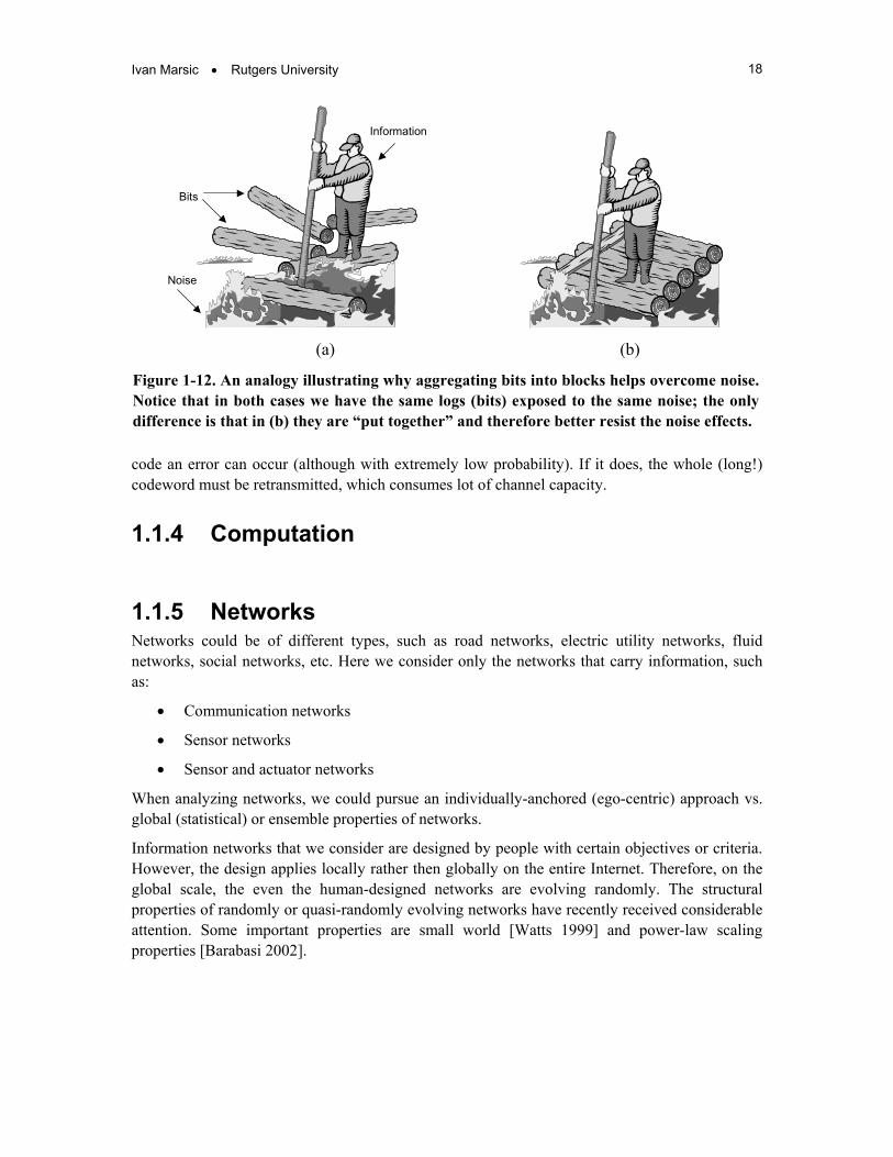
Code Size vs. Noise Longer codes are better than shorter codes and the reason is as follows. When designing a code, we need to decide on code redundancy, (n − r)/r, and code rate, r/n. This in turn is based on the decision on how many errors the code should be able to detect/correct and with what certainty. Errors are probabilistic events and to tell anything certain about them requires a large number of observations (to validate the relative frequencies and ultimately ensure that the law of large numbers takes effect). An analogy with a log raft in Figure 1-12 is useful to keep in mind when considering the grounds for bit aggregation as a means of increasing the noise resistance of messages.

It is easier for the receiver to cope with errors when longer codes are used, similar as with people being able to easier correct letter-errors in longer words in spoken language. Another example is when solving a crosswords puzzle—it is easier to guess the correct word when given longer word with the same proportion of missing letters as in a shorter one.

For example, if somebody gives you a coin and asks whether this is a fair coin, you would probably say: I need to toss it a number of times before I know this with any certainty. You cannot figure this out from two or three tosses only; you need something on the order of a hundred tosses or more. The more times you perform the experiment, the higher the certainty about the coin’s fairness.

Likewise, assuming that we know Pe, we need a long block of bits to know with certainty how many bits will be in error at the receiver. If Pe = 0.13, then for a 100-block we are reasonably confident that 13 will be in error, and for a transmission of a 1000-block we are much more confident that 130 will be in error. But, for a 2- or 3-block, we cannot say how many will be in error with any confidence. Therefore, when messages are n-blocks with large n, we can with high confidence say how many bits will be in error. Accordingly, if we choose the appropriate length code, we can with high confidence claim that it has the power to detect/correct such-and-such number of transmission errors.

By this logic, we could infer that the longer the code the better it is. However, there are some other reasons why the codewords should be of limited length. For example, even with the longest

Ivan Marsic • Rutgers University 18

(a) (b)

Bits

Information

Noise

Figure 1-12. An analogy illustrating why aggregating bits into blocks helps overcome noise.Notice that in both cases we have the same logs (bits) exposed to the same noise; the onlydifference is that in (b) they are “put together” and therefore better resist the noise effects.

code an error can occur (although with extremely low probability). If it does, the whole (long!) codeword must be retransmitted, which consumes lot of channel capacity.

1.1.4 Computation

1.1.5 Networks Networks could be of different types, such as road networks, electric utility networks, fluid networks, social networks, etc. Here we consider only the networks that carry information, such as:

• Communication networks

• Sensor networks

• Sensor and actuator networks

When analyzing networks, we could pursue an individually-anchored (ego-centric) approach vs. global (statistical) or ensemble properties of networks.

Information networks that we consider are designed by people with certain objectives or criteria. However, the design applies locally rather then globally on the entire Internet. Therefore, on the global scale, the even the human-designed networks are evolving randomly. The structural properties of randomly or quasi-randomly evolving networks have recently received considerable attention. Some important properties are small world [Watts 1999] and power-law scaling properties [Barabasi 2002].

Chapter 1 • Introduction 19

(a) (b)

Hosts: N = 6 Lines: N×(N−1) = 30

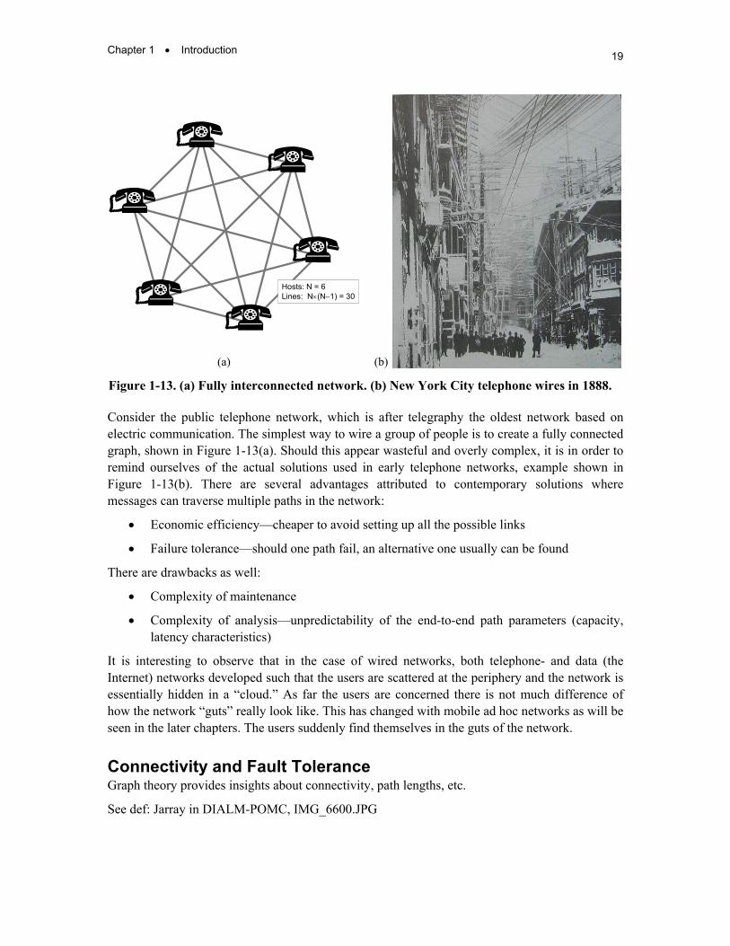
Figure 1-13. (a) Fully interconnected network. (b) New York City telephone wires in 1888.

Consider the public telephone network, which is after telegraphy the oldest network based on electric communication. The simplest way to wire a group of people is to create a fully connected graph, shown in Figure 1-13(a). Should this appear wasteful and overly complex, it is in order to remind ourselves of the actual solutions used in early telephone networks, example shown in Figure 1-13(b). There are several advantages attributed to contemporary solutions where messages can traverse multiple paths in the network:

• Economic efficiency—cheaper to avoid setting up all the possible links

• Failure tolerance—should one path fail, an alternative one usually can be found

There are drawbacks as well:

• Complexity of maintenance

• Complexity of analysis—unpredictability of the end-to-end path parameters (capacity, latency characteristics)

It is interesting to observe that in the case of wired networks, both telephone- and data (the Internet) networks developed such that the users are scattered at the periphery and the network is essentially hidden in a “cloud.” As far the users are concerned there is not much difference of how the network “guts” really look like. This has changed with mobile ad hoc networks as will be seen in the later chapters. The users suddenly find themselves in the guts of the network.

Connectivity and Fault Tolerance Graph theory provides insights about connectivity, path lengths, etc.

See def: Jarray in DIALM-POMC, IMG_6600.JPG

Ivan Marsic • Rutgers University 20

R = 1 R = 1.5 R = 2

R = 3 R = 4

R′ = 3 R′ = 4

R′ = 6 R′ = 8 Figure 1-14. Redundancy levels. From: [Baran 1964]

Paul Baran considered in 1964 theoretically best architecture for survivability of data networks. This considers only network graph topology and no qualities are assigned to nodes and links.

Incidentally, the real Internet developed quite differently, see e.g., Figure 1-14.

See also [Pastor-Satorras & Vespignani, 2004; Dorogovtsev & Mendes, 2003]

Fault tolerance is important for survivability (i.e., connectivity), but also for selecting sleeping nodes in power saving algorithms; see Lee in MobiCom’04, p. 275. We need to preserve connectivity after selected set of nodes in a sensor network goes to sleep mode.

Capacity

Delay Effect of node/link failures on delay

Chapter 1 • Introduction 21

1.2 Summary and Bibliographical Notes

Today it is clear that digital communication, digital networks, and computer systems are part of a major force changing the way we think and live. As we design most effective and efficient conduits to transmit maximum amount of information at maximum speed, we should keep in mind the purpose of communication, the greater picture of human activities that are being supported by the communication.

Simple models are important that let us understand the main issues. A good model should be simple enough to provide intuition. It should be extendable, i.e., more realistic features can be added without violating the central idea of the model. It need not (and should not) model all aspects of the real problem. See also [Watts 1999] explanation of rationale for modeling in Small Worlds. The purpose of modeling, as of layering, is to divide and conquer—solve puzzles about toy models of real things. [demonstrate] how real [communication] systems can be viewed as elaborations of these simple models.

Simple but generalizable examples (and counter-examples) are critical.

In basic terms, Shannon’s information theory addresses two issues of practical importance: the efficient encoding of a source message and its reliable transmission over a noisy channel. Both issues are of fundamental importance to the study of wireless communications, which in turn is fundamental for mobile computing. More will be said about wireless communications in Chapters 3 and 4.

1.2.1 Bibliography [Shannon & Weaver 1949] is the original text that introduced information theory and it is still as fresh a read as at the time when it appeared. An introductory review of information theory is available in [Pierce 1980] and [Lucky 1989]. [Cover & Thomas 1991] offers a comprehensive formal, yet relatively accessible, treatment of the subject.

Losee [1997] offers a useful framework for thinking about discipline independent abstract model of information, although in a somewhat disorganized manner flawed with occasional technical inaccuracies. [von Baeyer 2003] gives an interesting perspective on the nature of information, including the emerging field of quantum information.

See also [Moss & Wiesenfeld 1995] on interesting aspects of noise.

[Milburn 1998] offers a popular account of quantum computing.

A very accessible review of the inner workings of computers is available in [Petzold 1999]; an expert would enjoy reading it as much as a novice.

Ivan Marsic • Rutgers University 22

Problems

Section 1.1 1.1 Let Xi represent an available alphabet of the symbols a, b, c, …, N in total number, and

consider long sequences of these symbols generated by a stationary random process. Let the probabilities of occurrence of the various symbols be Pa, Pb, …, PN. In a typical sequence of S symbols the symbol a will occur approximately S⋅Pa times, b approximately S⋅Pb times, and so on. What is the probability that a typical sequence will occur?

1.2 Consider experimenting with the circuit shown in Figure 1-15, which is faulty so that on the average it behaves as shown in the following table:

Observation Open & Unlit Open & Lit Closed & Unlit Closed & Lit Probability 0.99 0.01 0.20 0.80

An observation informs about what was done to the switch and how the bulb behaved. You can assume that the experimenter will make the switch OPEN or CLOSED with equal probability, i.e., either way happens 50% of the time. If you think of the experiment as an information source, each observation corresponding to one message, what is the source’s entropy? Design a Huffman code tree for the source. Hint: The table of probabilities is really stating the conditional probabilities.

Switch {Open, Closed}

Bulb {Unlit, Lit}

Figure 1-15. Faulty circuit experiment. (See Problem 1.2)

Chapter 1 • Introduction 23

0 0

0

0 0

0

0 0

1

1 1

1

1 1

1

0

0

0

0

0

0

0

0

0

1

1

1

1

1

1

0 0

0

0

0 0

0 1 1

1

1 1

1 1

1

0

0

0 0

0 0

0

1

1 1

1

1

1

1

1

0

0

0 0

0

0

0

0

1

1

1

1

1

1

1

0

0

0

0

0

0

1 1

1 1

1

1 1

1

1

0

0

0

0

0

0

1 1

1

1

1

1

1

1

1

0

0

0

0

0 0

0

1

1

1

1

1

1 1

1

0

0 0

0

0

0

0

0

1 1

1

1

1

1

1

0

0

0 0

0 0

1

1 1

1 1

1

1

1

1

Figure 1-16. Catalog of patterns for Problem 1.3.

“0"

“1"

“0"

“1"

1

1/2

1/2 Figure 1-17. Discrete memoryless channel for Problems 1.4 and 1.5.

1.3 Assume a stream of 0’s and 1’s originating from a source with probabilities x and (1 − x), respectively. What is the source entropy? Now suppose that you are told that the incoming bits should be organized in 5 × 3 matrices and that the only possible patterns are those ten shown in Figure 1-16, appearing with equal probability. What is now the source entropy? Determine also the numerical value of x.

1.4 Consider the discrete memoryless channel in Figure 1-17. Where input symbol “0” is received without error and the symbol “1” is received as a “0” with probability 1/2 and as a “1” with probability 1/2. The probability that a “0” is sent P(“0”) = 1/4 and a “1” is sent with probability P(“1”)=3/4. Determine the maximum likelihood (ML) decision rule for the above channel and the associated probability of a decision error. (Show your work) Hint: You should express your decision rule as how you would decode a received 0 and how you would decode a received 1. Also, the probability of a decision error is the average probability of error over both input symbols.

1.5 Find the capacity of the discrete memoryless channel in Figure 1-17. What is the average information conveyed per symbol, I(X; Y)?

1.6 A noisy discrete communication channel has a transmitter alphabet of N equiprobable symbols xi. There is no intersymbol influence; that is, successive transmitted symbols are independent. There is a probability p/N that any given incorrect symbol yj (j ≠ i) in the receiver alphabet (consisting of the same N symbols) will be received. Find an expression for the average transmitted information per symbol, I(X; Y), as a function of p. Simplify this for N 1. (Check these by substituting p = 0 and p = 1.)

Ivan Marsic • Rutgers University 24

"0"

"1"

1−Pe

Pe

1−Pe

Pe

"0"

"1"

"0"

"1"

1−Pe

Pe

1−Pe

Pe

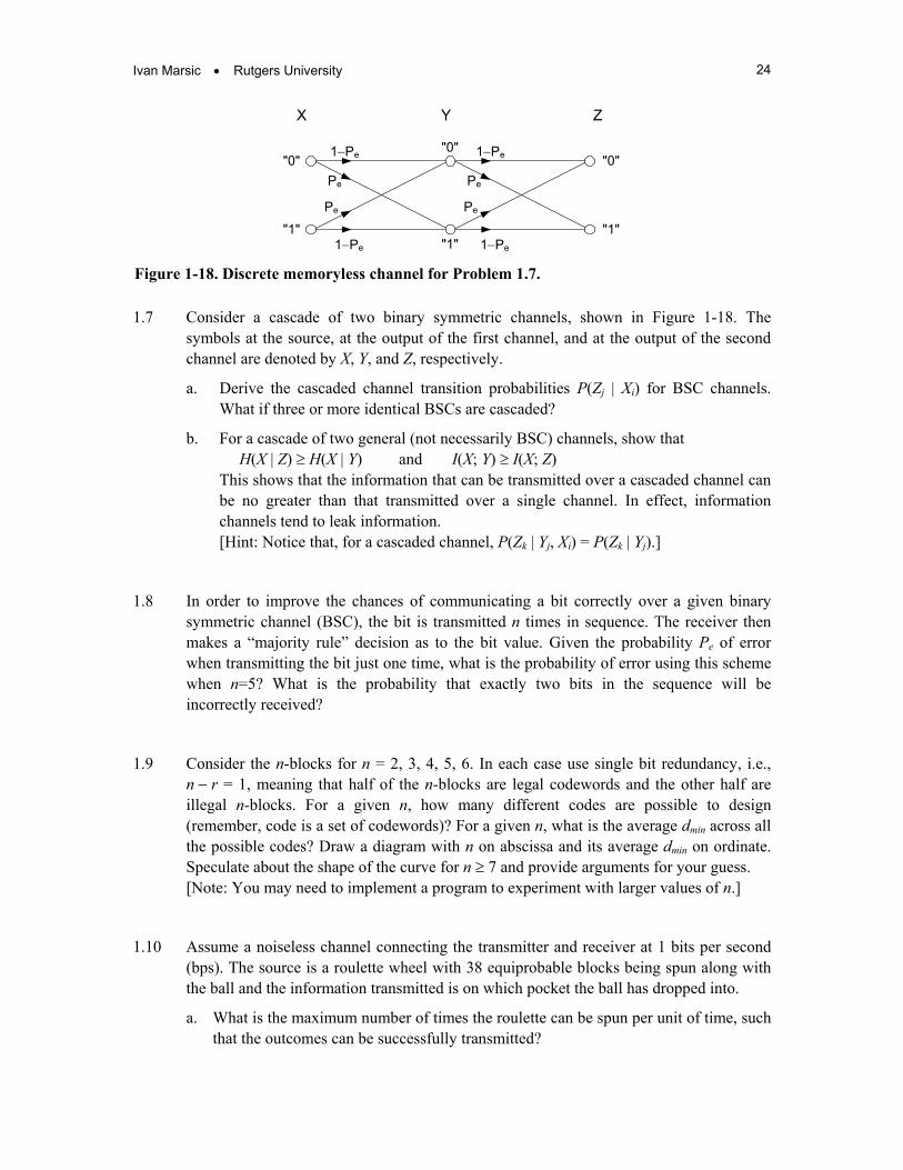
X Y Z

Figure 1-18. Discrete memoryless channel for Problem 1.7.

1.7 Consider a cascade of two binary symmetric channels, shown in Figure 1-18. The symbols at the source, at the output of the first channel, and at the output of the second channel are denoted by X, Y, and Z, respectively.

a. Derive the cascaded channel transition probabilities P(Zj | Xi) for BSC channels. What if three or more identical BSCs are cascaded?

b. For a cascade of two general (not necessarily BSC) channels, show that H(X | Z) ≥ H(X | Y) and I(X; Y) ≥ I(X; Z) This shows that the information that can be transmitted over a cascaded channel can be no greater than that transmitted over a single channel. In effect, information channels tend to leak information. [Hint: Notice that, for a cascaded channel, P(Zk | Yj, Xi) = P(Zk | Yj).]

1.8 In order to improve the chances of communicating a bit correctly over a given binary symmetric channel (BSC), the bit is transmitted n times in sequence. The receiver then makes a “majority rule” decision as to the bit value. Given the probability Pe of error when transmitting the bit just one time, what is the probability of error using this scheme when n=5? What is the probability that exactly two bits in the sequence will be incorrectly received?

1.9 Consider the n-blocks for n = 2, 3, 4, 5, 6. In each case use single bit redundancy, i.e., n − r = 1, meaning that half of the n-blocks are legal codewords and the other half are illegal n-blocks. For a given n, how many different codes are possible to design (remember, code is a set of codewords)? For a given n, what is the average dmin across all the possible codes? Draw a diagram with n on abscissa and its average dmin on ordinate. Speculate about the shape of the curve for n ≥ 7 and provide arguments for your guess. [Note: You may need to implement a program to experiment with larger values of n.]

1.10 Assume a noiseless channel connecting the transmitter and receiver at 1 bits per second (bps). The source is a roulette wheel with 38 equiprobable blocks being spun along with the ball and the information transmitted is on which pocket the ball has dropped into.

a. What is the maximum number of times the roulette can be spun per unit of time, such that the outcomes can be successfully transmitted?

Chapter 1 • Introduction 25

b. How does this change if a noisy channel with bit error probability Pe = 0.001 is employed? Discuss under what conditions it is appropriate to assume a BSC.

1.11 Consider a source which generates messages with four information bits (m0, m1, m2, and m3) and it adds three check bits (c0, c1, and c2) to them calculated such that c0 = m0 ⊕ m1 ⊕ m3 c1 = m0 ⊕ m2 ⊕ m3 c2 = m1 ⊕ m2 ⊕ m3 where ⊕ symbolizes modulo 2 addition. The encoded 7-bit messages are transmitted in the order: t0 t1 t2 t3 t4 t5 t6 = c0 c1 m0 c2 m1 m2 m3 and this is called Hamming code. The receiver recalculates the check bit equations the same way as the receiver. Show that:

a. If no transmission errors have occurred the check bits at the receiver are c0 = c1 = c2 = 0. The only other way this can occur is if three errors or more occur. Assuming that Pe < ½ show that no errors if more likely than three or more errors. Hence, if the parity check equations are satisfied at the receiver, it is most likely that no errors occurred.

b. If an odd number of errors occur, the check equations at the receiver will fail.

c. If 1 error occurs, the check equations will fail (not be satisfied). For instance, if an error occurs in the 6th transmitted digit (t5 = m2), the check bits are c0 = 0, c1 = c2 = 1. The error syndrome c2 c1 c0 = 110, the binary number 6! Again, this syndrome is most likely caused by an error in the 6th digit, and making that decision means that we are most likely correct. This is what is called error correction. It is equivalent to maximum likelihood decision making.

1.12 … another problem …

Ivan Marsic • Rutgers University 26

References 1. R. Azuma, Y. Baillot, R. Behringer, S., K. Feiner, S. Julier, and B. MacIntyre, “Recent advances in

augmented reality,” IEEE Computer Graphics and Applications, vol. 21, no. 6, pp. 34-47, November/December 2001.

2. G. Banavar, J. Beck, E. Gluzberg, J. Munson, J. Sussman, and D. Zukowski, “An application model for pervasive computing,” Proceedings of the Sixth Annual ACM/IEEE International Conference on Mobile Computing and Networking (Mobicom 2000), Boston, MA, pp. 266-274, 2000.

3. A.-L. Barabasi, Linked: How Everything Is Connected to Everything Else and What It Means, Cambridge, MA: Perseus Publishing, 2002.

4. P. Baran, “Introduction to Distributed Communications Network,” RAND Corporation, Memorandum RM-3420-PR, August 1964. Online at: http://www.rand.org/publications/RM/baran.list.html

5. V. Belloti and A. S. Bly. “Walking away from the desktop computer: Distributed collaboration and mobility in a product design team,” Proceedings of the ACM Conference on Computer Supported Cooperative Work (CSCW-1996), Boston, MA, pp. 209-218, November 1996.

6. T. Berners-Lee and M. Fischetti. Weaving the Web: The Original Design and Ultimate Destiny of the World Wide Web by Its Inventor. Harper-Collins Publishers, San Francisco, CA, 1999. Online information at: http://www.w3.org/People/Berners-Lee/

7. B. Brown, N. Green, and Richard Harper (Eds.), Wireless World: Social and Interactional Aspects of the Mobile Age, Springer-Verlag, London, 2002.

8. T. M. Cover and J. A. Thomas, Elements of Information Theory, New York, NY: John Wiley & Sons, Inc., 1991.

9. S. N. Dorogovtsev and J. F. F. Mendes, Evolution of Networks: From Biological Nets to the Internet and WWW, Oxford, UK: Oxford University Press, 2003.

10. A. Ephremides and B. Hajek, “Information theory and communication networks: An unconsummated union,” IEEE Transactions on Information Theory, vol. 44, no. 6, pp. 2416-2434, October 1998.

11. S. K. Feiner, “Augmented reality: A new way of seeing,” Scientific American, vol. 286, no. 4, pp. 34-41, April 2002. Online at: http://www.sciam.com/article.cfm?articleID=0006378C-CDE1-1CC6-B4A8809EC588EEDF

12. S. K. Feiner, H. Fuchs, T. Kanade, G. Klinker, P. Milgram, and H. Tamura, Mixed reality: Where real and virtual worlds meet. Proc. 26th Int’l Conf. on Computer Graphics and Interactive Techniques, ACM SIGGRAPH 99 Conference Abstracts and Applications, Los Angeles, CA, pp.156-158, August 1999.

13. W. W. Gibbs, “As we may live: Computer scientists build a dream house to test their vision of our future,” Scientific American, November 2000. Online at: http://www.sciam.com/article.cfm?articleID=000B8F57-1635-1C73-9B81809EC588EF21&pageNumber=1&catID=2

14. C. D. Green, “Charles Babbage, the Analytical Engine, and the possibility of a 19th-century cognitive science,” Online at: http://www.yorku.ca/christo/papers/Babbage-CogSci.htm

15. J. Y. Halpern and Y. Moses, “Knowledge and common knowledge in a distributed environment,” Proceedings of the 3rd Annual ACM Symposium on Principles of Distributed Computing (PODC'84), Vancouver, British Columbia, Canada, pp. 50-61, 1984.

Chapter 1 • Introduction 27

16. A. C. Huang, B. C. Ling, and A. Fox, “What is appliance computing?” Proceedings of the Workshop on Application Models and Programming Tools for Ubiquitous Computing (UbiTools '01), in conjunction with UBICOMP 2001, Atlanta, GA, September 2001. Online at: http://swig.stanford.edu/pub/publications/ads/ubicomp01.pdf

17. A. C. Huang, B. C. Ling, S. Ponnekanti, and A. Fox. Pervasive computing: What is it good for? Proceedings of the Workshop on Mobile Data Management (MobiDE), in conjunction with ACM MobiCom '99, Seattle, WA, September 1999. http://swig.stanford.edu/public/projects/papers/mobicom99.pdf

18. A. Jesdanun (Associated Press), “Instant-message wars heat up,” Wired News, April 26, 2004. Online at: http://www.wired.com/news/technology/0,1282,63224,00.html?tw=wn_techhead_8

19. B. Joy, “Why the future doesn’t need us,” Wired, vol. 8, no. 4, April 2000. Online at: http://www.wired.com/wired/archive/8.04/joy_pr.html

20. K. Kelly, New Rules for the New Economy: 10 Radical Strategies for a Connected World, Penguin Books, 1999.

21. R. Landauer, “Information is physical,” Physics Today, pp. 23-??, May 1991.

22. H. S. Leff and A. F. Rex, Maxwell’s Demon: Entropy, Information, Computing, Bristol, UK: Institute of Physics (IOP) Publishing, 1990.

23. H. S. Leff and A. F. Rex, Maxwell’s Demon 2: Entropy, Classical and Quantum Information, Computing, Bristol, UK: Institute of Physics (IOP) Publishing, 2003.

24. R. M. Losee, “A discipline independent definition of information,” Journal of the American Society For Information Science, vol. 48, no. 3, pp. 254-269, 1997.

25. R. W. Lucky, Silicon Dreams: Information, Man, and Machine, New York, NY: St. Martin’s Press, 1989.

26. T. Mansfield, S. Kaplan, G. Fitzpatrick, T. Phelps, M. Fitzpatrick, and R. Taylor. Toward locales: supporting collaboration with Orbit. Journal of Information and Software Technology, Vol. 41, No. 6, pp. 367-382, 1999.

27. C. Marvin, When Old Technologies Were New, Oxford, UK: Oxford University Press, 1988.

28. F. Mattern, The vision and technical foundations of ubiquitous computing. UPGRADE, Vol. II, No. 5, October 2001. Online at: http://citeseer.nj.nec.com/504566.html

29. G. J. Milburn, The Feynman Processor, Perseus Books, 1998.

30. K. B. Miller Telephone theory and practice, Vol. 1: Theory and elements, New York, NY: McGraw-Hill Book Co., 1930.

31. MIT Project Oxygen Publications. Online at: http://oxygen.lcs.mit.edu/Publications/

32. F. Moss and K. Wiesenfeld, “The benefits of background noise,” Scientific American, pp. 66, August 1995.

33. R. Pastor-Satorras and A. Vespignani, Evolution and Structure of the Internet: A Statistical Physics Approach, Cambridge, UK: Cambridge University Press, 2004.

34. C. Petzold, Code: The Hidden Language of Computer Hardware and Software, Redmond, WA: Microsoft Press, 1999. Check online at: http://www.charlespetzold.com/code/

35. J. R. Pierce, An Introduction to Information Theory: Symbols, Signals, and Noise, New York, NY: Dover Publications, Inc., 1980.

36. D. P. Reed and D. Weinberger, “Reed’s law: An interview,” Journal of the Hyperlinked Organization, January 19, 2001. Online at: http://www.hyperorg.com/backissues/joho-jan19-01.html#reed See also Reed’s Locus: Group Forming Networks Resource Page, Online at: http://www.reed.com/gfn/

Ivan Marsic • Rutgers University 28

37. M. Satyanarayanan. Fundamental challenges in mobile computing. Proceedings of the 15th ACM Symposium on Principles of Distributed Computing, Philadelphia, PA, May 1996. Online at: http://www-2.cs.cmu.edu/~coda/docdir/podc95.pdf

38. C. E. Shannon and W. Weaver, The Mathematical Theory of Communication. University of Illinois Press, Urbana, IL, 1949.

39. C. Shirky, “Why Oprah will never talk to you. Ever.,” Wired, vol. 12, no.8, pp.52-55, August 2004.

40. S. Singhal and M. Zyda, Networked Virtual Environments—Design and Implementation. New York, NY: Addison-Wesley, 1999.

41. P. Virilio, Polar Inertia, London, UK: Sage Publications, 1999.

42. H. C. von Baeyer, Information: The New Language of Science, Cambridge, MA: Harvard University Press, 2003.

43. D. J. Watts, Small Worlds: The Dynamics of Networks between Order and Randomness, Princeton, NJ: Princeton University Press, 1999.

44. M. Weiser. The computer for the 21st century. Scientific American, Vol. 265, No. 9, pp. 66-75, September 1991. Draft copy at http://www.ubiq.com/hypertext/weiser/UbiHome.html