MNRAS ATEX style le v3 - arXiv.org e-Print archive · PDF fileMNRAS 000,1{10(2017) Preprint 19 December 2017 Compiled using MNRAS LATEX style le v3.0 Testing Star Formation Laws in

MNRAS 000, 1–12 (2018) Preprint 9 April 2018 Compiled using MNRAS LATEX style file v3.0

Testing Star Formation Laws in a Starburst Galaxy AtRedshift 3 Resolved with ALMA

P. Sharda2,3,4?, C. Federrath1, E. da Cunha1, A. M. Swinbank5,6 and S. Dye71Research School of Astronomy and Astrophysics, The Australian National University, Canberra, ACT 2611, Australia2Department of Physics, Birla Institute of Technology and Science, Pilani, Rajasthan 333031, India3Department of Electrical and Electronics Engineering, Birla Institute of Technology and Science, Pilani, Rajasthan 333031, India4Department of Physics and Astronomy, University of Exeter, Stoker Road, Exeter EX4 4QL, UK5Institute for Computational Cosmology, Durham University, Durham DH1 3LE, UK6Centre for Extragalactic Astronomy, Department of Physics, Durham University, Durham, DH1 3LE, UK7School of Physics and Astronomy, University of Nottingham, University Park, Nottingham NG7 2RD, UK

Accepted 2018 March 26. Received 2018 March 26; in original form 2017 December 11

ABSTRACTUsing high-resolution (sub-kiloparsec scale) data obtained by ALMA, we analyze thestar formation rate (SFR), gas content and kinematics in SDP 81, a gravitationally-lensed starburst galaxy at redshift 3. We estimate the SFR surface density (ΣSFR)in the brightest clump of this galaxy to be 357+135

−85 M yr−1 kpc−2, over an area of

0.07 ± 0.02 kpc2. Using the intensity-weighted velocity of CO (5-4), we measure theturbulent velocity dispersion in the plane-of-the-sky and find σv,turb = 37 ± 5 km s−1

for the clump, in good agreement with previous estimates along the line of sight,corrected for beam smearing. Our measurements of gas surface density, freefall timeand turbulent Mach number allow us to compare the theoretical SFR from variousstar formation models with that observed, revealing that the role of turbulence iscrucial to explaining the observed SFR in this clump. While the Kennicutt Schmidt(KS) relation predicts an SFR surface density of ΣSFR,KS = 52 ± 17 M yr−1 kpc−2,the single-freefall model by Krumholz, Dekel and McKee (KDM) predicts ΣSFR,KDM =

106 ± 37 M yr−1 kpc−2. In contrast, the multi-freefall (turbulence) model by Salim,

Federrath and Kewley (SFK) gives ΣSFR,SFK = 491+139−194 M yr−1 kpc−2. Although the

SFK relation overestimates the SFR in this clump (possibly due to the negligence ofmagnetic fields), it provides the best prediction among the available models. Finally,we compare the star formation and gas properties of this galaxy to local star-formingregions and find that the SFK relation provides the best estimates of SFR in bothlocal and high-redshift galaxies.

Key words: Stars: formation – Submillimetre: galaxies – Galaxy: evolution – Galaxy:kinematics and dynamics – Turbulence

1 INTRODUCTION

Numerous star formation relations have been proposed in aquest to universalize the theory of star formation, by link-ing the star formation rate (SFR) with the mass of gas, itsfreefall time, virial parameter, magnetic field strength andturbulence (Silk 1997; Kennicutt 1998a; Elmegreen 2002;Shi et al. 2011; Krumholz et al. 2012 (hereafter, KDM12);Renaud et al. 2012; Escala 2015; Elmegreen & Hunter2015; Salim et al. 2015 (hereafter, SFK15); Elmegreen 2015;Nguyen-Luong et al. 2016; Miettinen et al. 2017). While

? E-mail: [email protected] (PS)

these relations have been shown to be valid for star-formingregions in the Milky Way and local galaxies (Bigiel et al.2008), the lack of spatial resolution has limited us in testingthem on high-redshift sources with z > 1. Thanks to the highspatial resolution of ALMA, several high-redshift galaxiesemitting in the submillimeter (sub-mm) regime have beendetected and resolved over the last few years (Decarli et al.2016; Spilker et al. 2016; Lu et al. 2017; Danielson et al. 2017;Brisbin et al. 2017), particularly if they are gravitationally-lensed by a foreground source (Smail et al. 1997, 2002; Heza-veh et al. 2013; Johnson et al. 2017; Bradac et al. 2017; La-porte et al. 2017; Wong et al. 2017; Fudamoto et al. 2017).These galaxies are known to be rigorous sites of dusty star

© 2018 The Authors

arX

iv:1

712.

0366

1v4

[as

tro-

ph.G

A]

5 A

pr 2

018

2 P. Sharda et al.

formation where molecular gas plays a key role in modify-ing the structure of clusters where star formation occurs.Tracing molecular gas in these regions can give us valuableinsight on the star formation characteristics of these galax-ies since it is now known that molecular gas has a strongcorrelation with SFR whereas atomic gas does not (Wong &Blitz 2002; Bigiel et al. 2008; Blanc et al. 2009).

J090311.6+003906 (hereafter, referred to as SDP 81)was detected as a lensed galaxy in the H − AT L AS surveyof bright submillimeter galaxies (SMGs) by Negrello et al.(2010) where the redshift was measured as z = 3.042 ± 0.001through ground based CO measurements. It falls in thepopular definition of SMGs where the 850 µm flux densityS850 > 3 mJy and infrared luminosity LIR & 1012 L (Kovacset al. 2006; Coppin et al. 2008; Hayward et al. 2011). SDP 81has also been established to be a dusty star-forming galaxyin previous works (Negrello et al. 2014; Swinbank et al. 2015(hereafter, S15); Dye et al. 2015; Hatsukade et al. 2015; Ry-bak et al. 2015a,b; Tamura et al. 2015; Wong et al. 2015;Hezaveh et al. 2016; Inoue et al. 2016). Even though thereare significant uncertainties in determining the stellar massof SDP 81, we note that it lies 1-2 orders of magnitude abovethe main sequence on the stellar mass − star formation rate(M?−SFR) plane (Speagle et al. 2014; Schreiber et al. 2015;Chang et al. 2015; Guo et al. 2015). Thus, SDP 81 falls underthe category of extreme starburst galaxies and is an idealcandidate to test star formation relations. This is furtherconfirmed by the position of SDP 81 on the star formationrate − gas mass (SFR −Mgas) plane (Sargent et al. 2014).

Our goal in this work is to extract the SFR in individ-ual clumps of this galaxy and compare it with that predictedby existing star formation relations. We refer to clumps asgiant star-forming regions (Genzel et al. 2006; Elmegreenet al. 2009; Bournaud et al. 2014) substantially more mas-sive and star-forming than typical molecular clouds in theMilky Way (Cowie et al. 1995; Van den Bergh et al. 1996;Shapiro et al. 2010), and possibly showing high star forma-tion efficiencies (Freundlich et al. 2013; Zanella et al. 2015;Cibinel et al. 2017). The paper is organized as follows: inSection 2, we summarize data reduction through lens mod-eling to create source plane reconstructed images (Dye et al.2015). This section also identifies different clumps in thisgalaxy extracted by S15. Section 3 follows the dust spectralenergy distribution (SED) fitting of a modified blackbody(MBB) and estimation of SFR surface density in the galaxy.We describe the kinematic analysis of CO (5-4) used to esti-mate the Mach number in Section 4. In Section 5, we presentour estimates of the local gas mass and freefall time in thegalaxy. Finally, we put all these parameters together to testvarious star formation relations and compare with the SFRsurface density deduced through dust SED fitting in Section6. We summarize our findings in Section 7.

We adopt the ΛCDM cosmology with H0 =

72 km s−1 Mpc−1, Ωm = 0.27, ΩΛ = 1-Ωm and a ChabrierIMF (Chabrier 2003). The luminosity distance and scalelength corresponding to these parameters is 25.9 Gpc and7.69 kpc arcsec−1, respectively, for z ≈ 3.042 (Wright 2006).

2 DATA REDUCTION AND ANALYSIS

ALMA observations of SDP 81 (RA = 09h03m11.57s, Dec =+0039′06.6′′) were taken during Science Verification cyclein October 2014. In the calibrated data1, the lensed galaxyis seen in the form of an Einstein ring, with two arcs onthe eastern and western sides (Dye et al. 2014; ALMA Part-nership et al. 2015). Through uν tapering, a resolution of∼ 150 × 120 mas was achieved in the three bands (see Ta-bles 1 and 3 of ALMA Partnership et al. (2015) for observedfluxes and noise levels). The CO (5-4) velocity cubes werebinned to a velocity resolution of 21 km s−1 (ALMA Partner-ship et al. 2015).

We use the source plane reconstructed images of contin-uum emissions (in ALMA Bands 4, 6 and 7, correspondingto λobs = 2.0, 1.3 and 1.0 mm, respectively) and CO (5-4)flux and velocity, created by S15, using the lensing modelby Dye et al. (2015). This model was used in the imageplane with the semi-linear inversion method (Warren & Dye2003) worked upon by Nightingale & Dye (2015). The av-erage luminosity weighted magnification factors derived byDye et al. (2015) for the continuum in band 6 and 7 are15.8 ± 0.7 and 16.0 ± 0.7 respectively. This magnification isrepresentative of a higher resolution by a factor of ∼ 30 (sub-kpc scale) than that in the typical non-lensed case (Ikarashiet al. 2015; Simpson et al. 2015).

S15 identified 5 molecular clumps from the continuumemission maps where intense star formation is taking place(see Figure 1 in their paper), using a signal to local noise(SNR) cutoff at 5σ. Of these clumps, only clumps A and Bhave sufficient resolution (number of pixels) to perform thekinematic analysis to estimate the turbulent velocity disper-sion (see Figure 1). The horizontally elongated structure ofclump B rules out the possibility of a spherical approxima-tion to its volume which we otherwise cannot estimate, notto mention that its location does not correlate well with theCO (5-4) flux map. Clump A, on the other hand, has a strongcorrelation with CO (5-4) flux and appears symmetric, asseen in Figure 1. Hence, we restrict our analysis to clump Ain this work. We notice that clump A likely coincides withthe center of the galaxy and might be its nucleus/formingcore. Thus, it might be significantly different in origin fromclumps residing in the outer regions of the disk.

3 MEASUREMENT OF THE STARFORMATION RATE

We estimate the SFR surface density (ΣSFR) in clump A byfitting a modified blackbody (MBB) spectrum to the con-tinuum emission from dust in the three ALMA bands. Themodified blackbody spectral law can be written as:

Sν = Nν

(2hν3

c2

)1

ehν/kBT − 1νβem , (1)

where ν is the rest-frame frequency, Sν is the flux den-sity of the clump, Nν is the normalization parameter (in-cludes dust opacity), T is the dust temperature and βem is

1 https://almascience.nao.ac.jp/alma-data/

science-verification

MNRAS 000, 1–12 (2018)

IV Submission Clean Testing Star Formation Laws on SDP 81 Using ALMA 3

Figure 1. Source reconstructed image of continuum flux in

ALMA band 7 (λobs = 1.0 mm), created using CASA (McMullin

et al. 2007). The contours depict clumps A, B, C, D and E, takenfrom Figure 1 of S15. We do not use clumps B, C, D and E in this

work because they do not allow for accurate estimates of kinemat-ics and volume densities from the plane-of-the-sky projection.

the emissivity index (βem = 0 corresponds to a blackbody)(Draine & Lee 1984; Da Cunha et al. 2010b). Since clump Alies near the center of the galaxy where the background con-tribution may be high, we subtract the underlying (disc)CO emission from clump A. For background subtraction, wemask the clump A and then smooth the image by convolv-ing it with a large Gaussian kernel. Then, we subtract thesmoothed image from the original image to get the back-ground subtracted image. In order to ensure that we do notover or under-subtract, we reiterate this procedure multipletimes with different kernels.

The flux density can be integrated over the whole in-frared (IR) range (8–1000 µm) to get dust luminosity (Hu-mason et al. 1956; Oke & Sandage 1968; Hogg et al. 2002):

LFIR =4πDL

2

1 + z

∫ 1000 µm

8 µmSν dν , (2)

where LFIR is the far infrared luminosity of the clump,DL is the luminosity distance to SDP 81 and Sν is the fluxdensity of the clump. However, the available ALMA observa-tions are insufficient to simultaneously constrain the dust pa-rameters – T , βem, and LFIR. Therefore, we fix βem = 1.5, 2.0and 2.5, which are the typically used values for starburstgalaxies (Hildebrand 1983; Blain et al. 2003; Casey 2012;Smith et al. 2013). We also include observed fluxes at variousother wavelengths in the infrared regime, reported in Table

2 of Negrello et al. (2014), which covers a longer wavelengthbaseline (λobs = 350 − 2000 mm). Then, using a two-step fit-ting process: 1.) we fit the galaxy-integrated fluxes to con-strain T and βem; 2) we then adopt the ’galaxy-wide’ T andβem to fit clump A and determine its far infrared luminosity.The conditions of individual clumps might be very differ-ent as compared to the whole galaxy. We lack the spatialresolution for a proper decomposition of the various clumpsand assume that the clump conditions (of clump A) are iden-tical to the galaxy-wide properties, while being aware thatthis might not be the case. We include the systematic un-certainty arising from this assumption in our calculation ofthe far infrared luminosity.

We derive a best-fit temperature T = 39 ± 2 K forβem = 2.5, where we use Monte Carlo (MC) simulations (bymodeling the uncertainties in the observed fluxes accordingto a Gaussian distribution) to find the bestfit MBB (Ogilvie1984; Johnson et al. 2013). The uncertainty on T arises fromthe inclusion of the flux at 350 µm (from SPIRE observa-tions, Griffin et al. 2010) which falls partially under the coldtemperature dominated regime (see Figure 6 of Dye et al.2015). Figure 2 shows the best-fit MBB we find for clump Afrom the fits, along with the 1σ uncertainty range we de-rive from the 1σ uncertainty of the far infrared luminosity(LFIR) obtained using MC error propagation.

We obtain nearly identical values of (T, βem) from thetwo fitting methods we use: pixel-by-pixel and whole clump.In the pixel-by-pixel algorithm, we find the SFR in eachpixel by fitting the MBB using the best-fit (T, βem) values.Then, we sum the SFRs from each pixel to get SFR for thewhole clump. On the contrary, in the whole clump fittingalgorithm, we first sum the fluxes from each pixel and thenfind the SFR by fitting the MBB using the best-fit (T, βem)values. The SFRs we obtain from both the methods agreewell with each other, within ± 3%.

Using equation 2, we derive LFIR =(2.25+0.95

−0.47)× 1011 L

for clump A, where the uncertainty includes statistical as wellas systematic errors. The observed SFR surface density wefind using the LFIR − SFR relation from Kennicutt (1998a)is ΣSFR = 555+197

−120 M yr−1 kpc−2. Since this relation used aSalpeter IMF (Salpeter 1955), we adjust its coefficient bya factor of 1.6 downward to adopt to ”the Chabrier IMF”(Chabrier 2003) to be consistent throughout our work (DaCunha et al. 2010a,b). The resulting SFR surface density weget is ΣSFR = 357+135

−85 M yr−1 kpc−2. These values are repre-sentative of intense star formation and are expected for thecentral regions of high-redshift starburst galaxies (Cibinelet al. 2017; Canameras et al. 2017).

To reinforce our estimation of flux densities in the threeALMA bands as obtained after background subtraction, wealso model the fluxes using an n-Sersic profile (R1/n) forthe disc, with a Gaussian added to it for clump A (Sersic1968; Caon et al. 1993; Ciotti & Bertin 1999; Trujillo et al.2001; Aceves et al. 2006). The Sersic index (n) we obtainfor λobs = 1.0 mm continuum is n ∼ 0.5. Although our re-sult is lower than the median value reported in Hodge et al.2016 (n ≈ 1 ± 0.2, see also Paulino-Afonso et al. 2018), itis consistent with the Sersic indices found in several high-redshift galaxies (see Table 1 of Hodge et al. 2016). Throughthis composite profile, the fluxes we obtain for clump A forthe three bands are similar to those obtained through back-ground subtraction discussed above, within ±12%. Since this

MNRAS 000, 1–12 (2018)

4 P. Sharda et al.

Figure 2. SED fit applied to clump A with T = 39 K, βem = 2.5 (pa-rameters obtained from SED fit of data from SPIRE (Griffin et al.

2010), SMA (Bussmann et al. 2013), MAMBO (Negrello et al.

2010) and ALMA (ALMA Partnership et al. 2015)). Observedfluxes for the three ALMA bands are shown in blue. Dashed lines

indicate the 1σ uncertainty range of the fit.

difference in flux densities is negligible, the resulting LFIRand ΣSFR from this method are similar to those quotedabove, within the uncertainties.

3.1 Gas Mass and Clump Size from ContinuumEmission

Apart from the SFR surface density, one can also estimatethe gas mass (Mgas) and size of the clump (R) using theSED fits and continuum maps, respectively. Since we havean excellent coverage of the Rayleigh-Jeans regime, we useour best-fit MBB to estimate the dust mass of clump A byusing equation 6 of Magdis et al. (2012) and appropriaterest-frame dust mass absorption coefficients for the threeALMA bands, from Table 6 of Li & Draine (2001). Then,we use a typical gas-to-dust conversion ratio of 150 to getthe gas mass in this clump (Dunne et al. 2000; Dye et al.2015; Brisbin et al. 2017). For the three ALMA bands, thegas masses we thereby obtain are Mgas = (2.3−4.9)×108 M.This is consistent with the value of Mgas we obtain fromCO (5-4) (as we discuss in detail in Section 5).

We use the composite disc profile (n-Sersic disc + Gaus-sian clump, as discussed in Section 3) to find an estimate ofthe size of clump A. Since the clump is defined using theλobs = 1.0 mm continuum obtained from ALMA, we usethe best-fit composite disc profile at this wavelength andfind the size of this clump by assuming that its diameteris equal to the full width at half maximum of the compos-ite profile (i.e., FWHM = 2 R). Correspondingly, we obtainR ∼ 0.16 kpc for clump A. This is in good agreement withthe size of clump A we find in Section 5 by summing up thepixels belonging to clump A, as we report in Table 1.

4 MACH NUMBER ESTIMATION

Supersonic turbulence is a key ingredient to star formationbecause it can compress interstellar gas which leads to theformation of dense cores. On the other hand, it can suppress

the global collapse of the clouds, thus significantly reducingthe SFR (Elmegreen & Scalo 2004; Mac Low & Klessen 2004;McKee & Ostriker 2007; Hennebelle & Falgarone 2012). Theroot mean square (RMS) sonic Mach number associated withturbulence in star-forming regions is given by:

M =σv,turb

cs, (3)

where σv,turb is the turbulent velocity dispersion and csis the sound speed. cs ∝

√T , where T is the gas temper-

ature. It is difficult to estimate the gas temperature withthe current data, however, we can assume it to be between10–100 K. This assumption is valid for gas temperatures indense molecular clouds (Gao & Solomon 2004; Solomon &Vanden Bout 2005; Wu et al. 2005; Battersby et al. 2014;Immer et al. 2016; Krieger et al. 2017). Using the relationfor isothermal sound speed from Federrath et al. (2016) for amean molecular weight of 2.33 (Kauffmann et al. 2008) andTgas ≈ 10 K, the sound speed is ∼ 0.2 km s−1 whereas it is

∼ 0.6 km s−1 for Tgas ≈ 100 K; so we assume the sound speed

to be in the range 0.2 − 0.6 km s−1.The CO (5-4) velocity map after source plane recon-

struction shows a clear, large-scale gradient running diag-onally, as we show in Figure 3 (also, Figure 1 of S15). Thissystematic gradient can be associated with the rotational orshear motion of the gas. To extract the small-scale turbu-lent features in this clump, we fit a large-scale gradient tothe clump and subtract it; similar to the analysis of turbu-lent velocity dispersion done on the central molecular zone(CMZ) cloud Brick by Federrath et al. (2016). For this pur-pose, we use the PLANEFIT routine in IDL which performs aleast-squares fit of a plane to set of (x, y, z) points. In thiscase, this set is a position-position-velocity (PPV) cube withx and y being the position coordinates of pixels formingclump A, and z being the CO (5-4) velocity of each pixel. Weuse the standard deviation of residuals after gradient sub-traction as the turbulent velocity dispersion:

σv,turb =

√√√√1

N − 1

N∑i=1

((vbgs − vfg

)− µ

)2

, (4)

where N is the number of pixels or resolution elements,vbgs is the pixel velocity before gradient subtraction, vfg isthe velocity of the fitted gradient and µ is the mean of resid-uals after gradient subtraction (i.e., µ =< (vbgs − vfg) >).

The turbulent velocity before subtracting the gradientis σv,bgs = 80±10 km s−1. From the gradient subtraction algo-rithm, we obtain the turbulent velocity dispersion in clump Aas σv,turb = 37± 5 km s−1, where the 1σ error is the standarddeviation calculated using (Lehmann & Casella 1998):

sσv = σv ·Γ( N−1

2)

Γ(N/2) ·

√√√N − 1

2−

(Γ(N/2)Γ( N−1

2) )2

, (5)

where Γ(N) is the Gamma function. We also find the un-certainty on σv,turb through MC simulations and note thatthe result is consistent with the value we obtain from theanalytical equation, within ±8 %. Figure 3 shows the veloc-ity field across clump A before gradient subtraction, fitted

MNRAS 000, 1–12 (2018)

IV Submission Clean Testing Star Formation Laws on SDP 81 Using ALMA 5

gradient velocities and velocity field after gradient subtrac-tion. By construction, the residuals after gradient subtrac-tion are evenly spread around 0, as is also clear from thePDF of σv,turb plotted in Figure 4. From Figure 4, we notethat the distribution of velocities (in the pixels of clump A)before gradient subtraction is highly non-Gaussian and bi-modal, while that of the velocities after gradient subtractionis more consistent with a Gaussian distribution. However,due to low-number statistics, it is hard to infer much infor-mation from this distribution; some non-Gaussian contribu-tions may still remain after gradient subtraction, becauseit only removes the largest-scale mode of systematic shearor rotation. Nonetheless, this distribution is in agreementwith velocity PDFs obtained for simulations of supersonicturbulence which are also Gaussian in nature (Klessen 2000;Federrath 2013) and the non-Gaussian components can arisefrom small-scale rotational or shear modes, or due to the in-trinsic features of turbulence (see Section 3.2.2 of Federrathet al. (2016) and references therein). Additionally, we notethat the width of the Gaussian we fit for the PDF of veloc-ities after gradient subtraction matches well with what wefind using the data (i.e., σv,turb(fit) ≈ σv,turb(data)).

We also note that the turbulent velocity dispersion wecalculate is in agreement with the velocity dispersion of30 ± 9 km s−1 calculated by S15 for this clump using the 2nd

moment map (i.e., the dispersion along the line of sight, aftercorrection for beam smearing). The velocity dispersion wecalculate is in the plane of the sky. A consensus between ve-locity dispersions using the two methods imply that clump Acan be considered isotropic and it is fair to approximate itas a sphere.

Using this turbulent velocity dispersion, we obtain aturbulent Mach numberM = 96± 28. Although this is quitehigh compared to nearby galaxies (see Kennicutt & Evans(2012) and references therein), it falls in the range of Machnumbers associated with starburst galaxies (Gao & Solomon2004; Bouche et al. 2007; Cresci et al. 2009; Forster Schreiberet al. 2009; Tacconi et al. 2010). Given the high redshift ofSDP 81 and previous works highlighting intense star forma-tion, it is not unusual to obtain Mach numbers near 100.In fact, it implies that the role of turbulence becomes moreimportant at the epoch near the maximum star formationin the history of the Universe (Springel & Hernquist 2003;Madau & Dickinson 2014; Falgarone et al. 2017).

4.1 Resolution Check for Gradient Fit andSubtraction Algorithm

The gradient fit and subtraction algorithm works accuratelyonly if the resolution is sufficient. For the CMZ cloud Brick,the resolution scale was in sub-parsecs (Federrath et al.2016) whereas it is in sub-kiloparsecs for SDP 81. We checkif the low number of resolution elements in our data affectsour measurements, since the velocity dispersion calculatedmight vary by more than 20% if sufficient number of pix-els are not available to resolve the clump. To investigatewhether we have enough pixels to be operating in the sat-urated regime (where velocity dispersion does not changeby more than 20% when the number of resolution elementsare altered), we perform a resolution degradation on clump Aby creating artificial ’superpixels’ (merging nearby pixels to

make a bigger pixel) and then applying the gradient fit sub-traction algorithm.

For the first degradation (1/4 resolution), we merge fournearby pixels into one (making a square shape, see Figure 5).While the center of a superpixel is the centroid of the fourconstituent pixels, its CO (5-4) velocity is the flux-weightedaverage of CO (5-4) velocities in the constituent pixels:

vspix =

(∑4i=1(Si vi)∑4i=1 Si

), (6)

where vspix is the velocity of the superpixel, Si is the flux

of the ith constituent pixel and vi is its velocity. At placeswhere pixels belonging to the clump A cannot make a squareby themselves, we use pixels from outside the clump, butmask their flux to be 0. Thus, for such constituent pixels,Si = 0, so these pixels do not contribute to the sums inequation 6.

We do this process twice: decreasing the resolution to(1/4) and (1/16) of the original resolution. This results in atotal of 11 and 4 superpixels after the first and second resolu-tion degradation, respectively. Figure 6 shows the turbulentvelocity dispersions we get at the three resolutions. We fita growing exponential of the form A0(1 − e−N/N0 ) (where,N is the number of resolution elements) to this data. Sincedecreasing the resolution by (1/4) does not alter the velocitydispersion by & 20% (as we notice from Figure 6), we con-firm that we have enough pixels to resolve this clump withacceptable accuracy.

5 GAS MASS AND FREEFALL TIME FROMCO (5-4)

The total gas mass is an essential parameter which goesin all the star formation relations we test in a later sec-tion (see Section 6). It can be estimated by following theCO (1-0) emission in the star-forming region (Carilli & Blain2002; Pety et al. 2013; McNamara et al. 2014; Scoville et al.2017). From Figure 1 in Rybak et al. (2015b), and that inDye et al. (2015), we notice that there is a significant pres-ence of CO (1-0) emission at the position of clump A. How-ever, the CO (1-0) data was obtained by the Karl G. JanskyVery Large Array (VLA) at a lower resolution than ALMA(Valtchanov et al. 2011) and cannot be used for kinematicanalysis. Thus, we rely on ALMA observations of CO (5-4)transition (observed at a frequency of 142.57 GHz in ALMABand 4), to estimate the gas mass of clump A. It should benoted that CO (5-4) is generally a poor tracer of the totaldiffuse molecular gas, but is bright and easily observable athigh redshift (Daddi et al. 2015; Lu et al. 2015; Yang et al.2017).

We follow the Solomon et al. (1992a,b) relation betweenline luminosity and integrated flux density of CO (5-4):

L′C O (5−4) = 3.25 × 107 Sv ∆ vDL

2

ν2obs(1 + z)3

, (7)

where L′C O (5−4) is the line luminosity in K km s−1 pc2,

Sv∆v is the velocity integrated flux density of CO (5-4) af-ter subtraction of background emission, in Jy km s−1, DL is

MNRAS 000, 1–12 (2018)

6 P. Sharda et al.

Figure 3. Left Panel: Centroid CO (5-4) velocity (in km s−1) in the pixels of clump A before gradient subtraction. The size of each pixelis ∼ 0.05 kpc. Middle Panel: Fitted large-scale gradient to the clump. Right Panel: Velocity of CO (5-4) in the clump after gradient

subtraction. The last panel isolates the turbulent velocities in the plane of the sky. The turbulent velocity dispersion obtained for clump Ais σv, turb = 37 ± 5 km s−1, using which the Mach number calculated is M = σv, turb/cs = 96 ± 28.

−100 0 80

vbgs (km s−1)

0.000

0.005

0.010

0.015

0.020

0.025

0.030

0.035

0.040

PDF(v

bgs)

Before Gradient Subtraction

σv,bgs(data) = 79.9 kms−1

Data

−100 0 100

vturb (km s−1)

0.000

0.002

0.004

0.006

0.008

0.010

0.012

0.014

0.016

PDF(v

turb)

After Gradient Subtraction

σv,turb(fit) = 36.6 kms−1

σv,turb(data) = 37.2 kms−1

GaussianFit

Data

Figure 4. PDFs of CO (5-4) velocities of the pixels in clump A before and after gradient subtraction. The distribution of velocities beforegradient subtraction (vbgs) is bimodal; that of velocities after gradient subtraction (vturb) resembles a Gaussian distribution, however,

much information cannot be ascertained due to low number of statistics. The width of the Gaussian we fit (right panel) and the data are

similar, thus reinforcing the estimate of turbulent velocity dispersion σv, turb = 37 ± 5 km s−1.

MNRAS 000, 1–12 (2018)

IV Submission Clean Testing Star Formation Laws on SDP 81 Using ALMA 7

ClumpA

Figure 5. First resolution degradation through creation of 11 su-

perpixels, by merging nearby pixels using a flux-weighted averag-ing method (see equation 6). Thick lines denote the boundaries of

superpixels whereas thinner lines denote the boundaries of pixels.Red dots depict the center of superpixels and purple dots depict

the center of pixels. Pixels belonging to clump A are shown in blue;

they are the same as those shown in Figure 3. Pixels outside theclump are shown in white. Arrows show the movement of a pixel

when it is merged with other pixels to create a superpixel.

the luminosity distance in Mpc and νobs is the observed fre-quency of transition in GHz. The line luminosity we obtainis L′C O (5−4) = (5.04 ± 1.10) × 108 K km s−1 pc2. Since the tran-

sition we observe with ALMA at z ≈ 3 is higher than theground (1-0) transition, we introduce an appropriate line ra-tio factor (defined as the ratio of line luminosity of CO (5-4)to that of CO (1-0)), r54 = 0.28 ± 0.05. This value was de-rived for clump A by S15, where the authors use velocity andmagnification maps from the lens model prepared by Dyeet al. (2015). This value falls in the typical range of valuesof r54 for SMGs (see Carilli & Walter (2013) and referencestherein).

To get the gas mass from the line luminosity, we usean appropriate CO to H2 conversion factor αCO. Althoughthere is a high uncertainty in the value of this factor fornearby as well as high-redshift galaxies (Papadopoulos et al.2012; Narayanan et al. 2012), the suggested values basedon observations of SMGs lie in the range ∼ 0.8–1.0 M per(K km s−1 pc2) (Downes & Solomon 1998; Solomon & VandenBout 2005; Tacconi et al. 2008; Magdis et al. 2011; Hodgeet al. 2012; Carilli & Walter 2013; Bolatto et al. 2013; Both-well et al. 2013), which is less by a factor of ∼ 4 than thetypical value used for Milky Way clouds and nearby galax-ies. Dye et al. (2015) used a conversion factor of unity (inthe same units) for SDP 81, while Hatsukade et al. (2015)used a value of 0.8. Further, we notice that clump A falls ontop of the starburst sequence of the Σgas−ΣSFR relation pop-ulated by local ultra-luminous infrared galaxies (ULIRGs)

Figure 6. Turbulent velocity dispersion at different resolutions,

fitted with a growing exponential function of the form A0 (1 −e−N/N0 ), where N is the number of resolution elements. N0 ∼ 7for the best fit model, which implies the velocity dispersion does

not change by more than 5% for N & 20.

and SMGs (Daddi et al. 2010). This further justifies thechoice of αCO ∼ 0.8 − 1 M per (K km s−1pc2).

Keeping these studies in mind, we assume αCO ≈ 0.9 ±0.2 M per (K km s−1pc2), which suggests an H2 mass of(4.5 ± 1.0) × 108 M 2. Accounting for the contribution tothe gas by He, we further increase the H2 mass obtainedso far by 36% to get the total gas mass for clump A as(6.2±1.4)×108 M. This value is in good agreement with thegas mass found out using SED fitting in Section 3. The gassurface density we derive is Σgas = (8.6± 1.9) × 109 M kpc−2,where we calculate and sum the area of all pixels which con-stitute clump A 3. Moreover, the size of clump A we obtain inthis manner is R ∼ 0.15 ± 0.02 kpc, in excellent agreementwith the size we find through composite disc profile fitting inSection 3.1. Assuming clump A to be spherical (see section 4for a discussion on the validity of this assumption), we calcu-late its density to be ρ = Mgas/V = (2.9 ± 0.6) × 10−21 g cm−3,where V is the volume of the spherical clump.

To establish whether the cloud could be collapsing, weestimate the virial parameter αvir, which is the ratio of twicethe kinetic energy to the gravitational energy (Federrath &Klessen 2012). Using the definition from Bertoldi & McKee(1992), the virial parameter can also be given by:

αvir =5σ2

v,tot4πGR2ρ

, (8)

where, the velocity dispersion σtot is the total thermaland turbulent velocity dispersion including the shear com-ponent (i.e., turbulent velocity dispersion before gradientsubtraction, σv,bgs). However, in this clump, since the tur-bulent velocity dispersion σv,bgs cs, it implies that the to-tal velocity dispersion can be approximated as σv,tot ≈ σv,bgs

2 This gas mass is essentially in agreement as that obtained byS15 for clump A. However, due to a typographical error, the gasmasses reported in the last column of table 1 of S15 have to be

rearranged. The gas masses reported are in the order D-C-A-B-E.3 The size of 1 pixel is ∼ 0.05 kpc. There are 32 pixels in this

clump.

MNRAS 000, 1–12 (2018)

8 P. Sharda et al.

(Krumholz & McKee 2005; Federrath & Klessen 2012). Thevirial parameter we thus obtain is αvir = 0.63± 0.13 < 1, im-plying the cloud is strongly gravitationally bound and likelyundergoing collapse. For such a cloud, the freefall time canbe given by (Hennebelle & Chabrier 2011, 2013; Chabrieret al. 2014):

tff =

√3π

32Gρ, (9)

where G is the gravitational constant. From this equa-tion, we obtain a freefall time of 1.3 ± 0.1 Myr. This value isin agreement with freefall times calculated for other high zstarbursts (see Table 4 of Krumholz et al. 2013).

We summarize all the parameters going into predictionsof SFR surface density in various star formation relations inTable 1.

6 COMPARISON OF OBSERVED SFRSURFACE DENSITY WITH THEORETICALPREDICTIONS BY K98, KDM12 AND SFK15

We compare the SFR surface density obtained throughdust SED fitting with star formation relations proposed fornearby and high-redshift galaxies in Figure 7. The proba-bility density function (PDF) of the measured SFR surfacedensity in clump A is shown as the solid line, and we compareit with the predictions of SFR surface density by three pop-ular star formation relations in the same plot. These PDFswere calculated using Monte Carlo simulations with a sam-ple size of 100,000 and included systematic errors on theSFR surface densities.

The Kennicutt-Schmidt (KS or K98) relation is givenby (Schmidt 1959; Kennicutt 1998b):

ΣSFR = 2.53 × 10−4Σgas

1.4±0.15 , (10)

The distribution of SFR surface density (ΣSFR) obtainedusing equation 10 is shown as the dotted line in Figure 7.The mean SFR surface density we calculate from the KSrelation is ΣSFR = 84 ± 27 M yr−1 kpc−2. Since equation 10is based on the Salpeter IMF, we correct the SFR surfacedensity for a Chabrier IMF (similar to that done in section3) and obtain ΣSFR = 52±17 M yr−1 kpc−2.4 We find that theKS relation underestimates SFR surface density by a factor& 3.3, with respect to the observed SFR surface densityin this clump, even when the 1σ uncertainty is taken intoaccount. Numerous studies discuss the breakdown of the KSrelation on the scales of ∼ 100 pc in local (Onodera et al.2010; Shi et al. 2011; Becerra & Escala 2014; Xu et al. 2015)and high-redshift environments (Bouche et al. 2007; Daddiet al. 2010; Genzel et al. 2010).

Krumholz, Dekel and McKee (KDM12) showed that theSFR does not only depend on gas surface density but also

4 This distribution does not take into account the uncertainty

on the power law index in equation 10 because we notice that it

becomes highly skewed when this uncertainty is randomized. Inthat case, the 16th and 84th percentile values of ΣSFR are 1 and

133 M yr−1 kpc−2, respectively.

Figure 7. Probability distribution function (PDF) of ΣSFR es-timated from dust SED fitting (solid curve) and those predicted

from K98 (dotted curve, equation 10), KDM12 (dot-dashed curve,

equation 11) and SFK15 (dashed curve, equation 12) relations.The PDFs were calculated using MC simulations with a sample

size of 100,000.

Table 1. Results for Clump A in SDP 81 (see Figure 1) with mean

and 1σ errors.

Parameter Value

βem 2.5T 39 ± 2 KLFIR

(2.3+1.0−0.5

)× 1011 L

ΣSFR (observed)a 357+135−85 M yr−1 kpc−2

A (7.2 ± 1.5) × 10−2 kpc2

R (1.5 ± 0.2) × 10−1 kpcσ(b)v,bgs

80 ± 10 km s−1

σ(c)v,turb

37 ± 5 km s−1

cs 0.4 ± 0.2 km s−1

M 96 ± 28b 0.4

Sv,CO (5−4)v(d) 8.4 ± 1.8 mJy km s−1

L′C O (1−0) (1.4 ± 0.1) × 108 K km s−1 pc2

r54 0.28 ± 0.05L′C O (5−4) (5.0 ± 1.1) × 108 K km s−1 pc2

αCO 0.9 ± 0.2 M (K km s−1 pc2)−1

Mgas (6.2 ± 1.4) × 108 MΣgas (8.6 ± 1.9) × 109 M kpc−2

ρ (2.9 ± 0.6) × 10−21 g cm−3

αvir 0.6 ± 0.1tff (1.3 ± 0.1) × 106 yrΣSFR (K98) (a,e) 52 ± 17 Myr−1 kpc−2

ΣSFR (KDM12) (f) 106 ± 37 Myr−1 kpc−2

ΣSFR (SFK15) (g) 491+139−194 Myr−1 kpc−2

(a)Corrected for Chabrier IMF.(b)Large-scale velocity dispersion before gradient subtraction.(c)Turbulent velocity dispersion after gradient subtraction.(d)Integrated CO (5-4) flux after background subtraction.(e)16th and 84th percentiles are 37 and 64 M yr−1 kpc−2.(f)16th and 84th percentiles are 74 and 132 M yr−1 kpc−2.(g) Errors represent the 16th and 84th percentiles.

MNRAS 000, 1–12 (2018)

IV Submission Clean Testing Star Formation Laws on SDP 81 Using ALMA 9

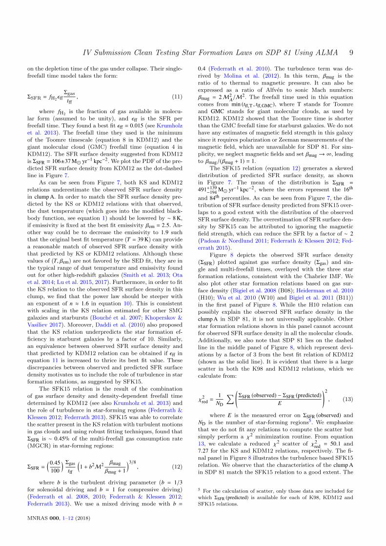
on the depletion time of the gas under collapse. Their single-freefall time model takes the form:

ΣSFR = fH2εffΣgas

tff, (11)

where fH2 is the fraction of gas available in molecu-lar form (assumed to be unity), and εff is the SFR perfreefall time. They found a best fit εff = 0.015 (see Krumholzet al. 2013). The freefall time they used is the minimumof the Toomre timescale (equation 8 in KDM12) and thegiant molecular cloud (GMC) freefall time (equation 4 inKDM12). The SFR surface density suggested from KDM12is ΣSFR = 106±37 M yr−1 kpc−2. We plot the PDF of the pre-dicted SFR surface density from KDM12 as the dot-dashedline in Figure 7.

As can be seen from Figure 7, both KS and KDM12relations underestimate the observed SFR surface densityin clump A. In order to match the SFR surface density pre-dicted by the KS or KDM12 relations with that observed,the dust temperature (which goes into the modified black-body function, see equation 1) should be lowered by ∼ 8 K,if emissivity is fixed at the best fit emissivity βem = 2.5. An-other way could be to decrease the emissivity to 1.9 suchthat the original best fit temperature (T = 39 K) can providea reasonable match of observed SFR surface density withthat predicted by KS or KDM12 relations. Although thesevalues of (T, βem) are not favored by the SED fit, they are inthe typical range of dust temperature and emissivity foundout for other high-redshift galaxies (Smith et al. 2013; Otaet al. 2014; Lu et al. 2015, 2017). Furthermore, in order to fitthe KS relation to the observed SFR surface density in thisclump, we find that the power law should be steeper withan exponent of n ≈ 1.6 in equation 10). This is consistentwith scaling in the KS relation estimated for other SMGgalaxies and starbursts (Bouche et al. 2007; Khoperskov &Vasiliev 2017). Moreover, Daddi et al. (2010) also proposedthat the KS relation underpredicts the star formation ef-ficiency in starburst galaxies by a factor of 10. Similarly,an equivalence between observed SFR surface density andthat predicted by KDM12 relation can be obtained if εff inequation 11 is increased to thrice its best fit value. Thesediscrepancies between observed and predicted SFR surfacedensity motivates us to include the role of turbulence in starformation relations, as suggested by SFK15.

The SFK15 relation is the result of the combinationof gas surface density and density-dependent freefall timedetermined by KDM12 (see also Krumholz et al. 2013) andthe role of turbulence in star-forming regions (Federrath &Klessen 2012; Federrath 2013). SFK15 was able to correlatethe scatter present in the KS relation with turbulent motionsin gas clouds and using robust fitting techniques, found thatΣSFR is ∼ 0.45% of the multi-freefall gas consumption rate(MGCR) in star-forming regions:

ΣSFR =( 0.45

100

) Σgastff

(1 + b2M2 βmag

βmag + 1

)3/8, (12)

where b is the turbulent driving parameter (b = 1/3for solenoidal driving and b = 1 for compressive driving)(Federrath et al. 2008, 2010; Federrath & Klessen 2012;Federrath 2013). We use a mixed driving mode with b =

0.4 (Federrath et al. 2010). The turbulence term was de-rived by Molina et al. (2012). In this term, βmag is theratio of to thermal to magnetic pressure. It can also beexpressed as a ratio of Alfven to sonic Mach numbers:βmag = 2M2

A/M2. The freefall time used in this equation

comes from min (tff,T , tff,GMC), where T stands for Toomreand GMC stands for giant molecular clouds, as used byKDM12. KDM12 showed that the Toomre time is shorterthan the GMC freefall time for starburst galaxies. We do nothave any estimates of magnetic field strength in this galaxysince it requires polarization or Zeeman measurements of themagnetic field, which are unavailable for SDP 81. For sim-plicity, we neglect magnetic fields and set βmag →∞, leadingto βmag/(βmag + 1) = 1.

The SFK15 relation (equation 12) generates a skeweddistribution of predicted SFR surface density, as shownin Figure 7. The mean of the distribution is ΣSFR =

491+139−194 M yr−1 kpc−2, where the errors represent the 16th

and 84th percentiles. As can be seen from Figure 7, the dis-tribution of SFR surface density predicted from SFK15 over-laps to a good extent with the distribution of the observedSFR surface density. The overestimation of SFR surface den-sity by SFK15 can be attributed to ignoring the magneticfield strength, which can reduce the SFR by a factor of ∼ 2(Padoan & Nordlund 2011; Federrath & Klessen 2012; Fed-errath 2015).

Figure 8 depicts the observed SFR surface density(ΣSFR) plotted against gas surface density (Σgas) and sin-gle and multi-freefall times, overlayed with the three starformation relations, consistent with the Chabrier IMF. Wealso plot other star formation relations based on gas sur-face density (Bigiel et al. 2008 (B08); Heiderman et al. 2010(H10); Wu et al. 2010 (W10) and Bigiel et al. 2011 (B11))in the first panel of Figure 8. While the H10 relation canpossibly explain the observed SFR surface density in theclump A in SDP 81, it is not universally applicable. Otherstar formation relations shown in this panel cannot accountfor observed SFR surface density in all the molecular clouds.Additionally, we also note that SDP 81 lies on the dashedline in the middle panel of Figure 8, which represent devi-ations by a factor of 3 from the best fit relation of KDM12(shown as the solid line). It is evident that there is a largescatter in both the K98 and KDM12 relations, which wecalculate from:

χ2red =

1ND

∑ (ΣSFR (observed) − ΣSFR (predicted)

E

)2

, (13)

where E is the measured error on ΣSFR (observed) andND is the number of star-forming regions5. We emphasizethat we do not fit any relations to compute the scatter butsimply perform a χ2 minimization routine. From equation13, we calculate a reduced χ2 scatter of χ2

red = 50.1 and7.27 for the KS and KDM12 relations, respectively. The fi-nal panel in Figure 8 illustrates the turbulence based SFK15relation. We observe that the characteristics of the clump Ain SDP 81 match the SFK15 relation to a good extent. The

5 For the calculation of scatter, only those data are included forwhich ΣSFR (predicted) is available for each of K98, KDM12 and

SFK15 relations.

MNRAS 000, 1–12 (2018)

10 P. Sharda et al.

0 1 2 3 4 5

log10 Σgas [M⊙ pc−2]

−4

−2

0

2

4

6

log 1

0Σ

SFR

[M⊙

yr−1

kpc−

2] SDP 81

−2 −1 0 1 2 3 4 5

log10 (Σgas/t)single-ff [M⊙ pc−2 Myr−1]

SDP 81

−1 0 1 2 3 4 5log10 (Σgas/t)multi-ff [M⊙ pc−2 Myr−1]

SDP 81

F16 CMZ ‘Brick’W10 Clumps (lower limit)L10 Clouds (Aκ ≥ 0.8 mag)K98 Starbursts (z∼ 0)K98 Disks (z∼ 0)H10 Flat SED YSOs

H10 Class I YSOsH10 Class I YSOs (upper limit)H10 Flat SED YSOs (upper limit)H10 C2D+GB CloudsH10 Taurus

G11 CloudsL10 Clouds (Aκ ≥ 0.1 mag)J16 LMCJ16 SMCSDP 81 (This Work)

K98B08W10B11H10

KDM12 SFK15

Figure 8. Left-panel: Observations of ΣSFR (SFR surface density) in local clouds, plotted against gas surface density. The data is extracted

from Heiderman et al. 2010 (H10), Lada et al. 2010 (L10), Wu et al. 2010 (W10), Gutermuth et al. 2011 (G11) and Jameson et al. 2016(J16). Data for the Brick molecular cloud in the central molecular zone (CMZ) is taken from Federrath et al. 2016 (F16). The K98 (disks

and starbursts) data were adjusted in KDM12, Krumholz et al. (2013) and Federrath (2013) to the Chabrier IMF, similar to that done

for the high-redshift data by Daddi et al. (2010). The systematic difference between starbursts and the original K98 relation is due todifferent αCO conversion factors used for starbursts and disks (see Section 2 of Daddi et al. 2010 and Figure 1 of Federrath 2013). SFR

relations proposed by Kennicutt 1998b (K98, corrected for Chabrier IMF), Bigiel et al. 2008 (B08), Bigiel et al. 2011 (B11), Wu et al.

2010 (W10) and Heiderman et al. 2010 (H10) are also shown. Middle-panel: Observations of ΣSFR plotted against the single-freefall time.Solid line depicts the best fit model from KDM12, with εff = 0.015 (see Krumholz et al. (2013)); dashed lines illustrate deviations by a

factor of 3 from the best fit. Right-panel: Observations of ΣSFR plotted against the turbulence based multi-freefall model proposed bySalim et al. 2015 (SFK15). Solid line represents equation 12. Clump A analyzed in this work is marked with an arrow in all the three

panels. The scatter obtained through a χ2 minimization routine for K98, KDM12 and SFK15 relations is 50.1, 7.27 and 1.25, respectively.

scatter we obtain for the SFK15 relation is 1.25. It has sig-nificantly reduced as compared to the scatter from KS andKDM12 relations because the SFK15 relation includes sys-tematic variations in the Mach number, as were establishedby Federrath (2013). This highlights the role of turbulencein star-forming regions (Federrath & Klessen 2012; Kraljicet al. 2014). The validity of the multi-freefall star formationrelation has been previously supported in an independentwork by Braun & Schmidt (2015).

7 CONCLUSIONS

Using high-resolution (sub-kpc) ALMA data of SDP 81 –a high-redshift (z ∼ 3) lensed galaxy, we have measuredthe SFR surface density in its biggest and most isotropicclump revealed by the lensing analysis of Dye et al. (2015).Through dust SED fitting by a modified blackbody spectrumof this clump (clump A in S15), we find the best fit dust tem-perature to be 39 K when an emissivity index βem = 2.5 isused. We determine the corresponding SFR surface densityof this clump as ΣSFR = 357 ± 9 M yr−1 kpc−2, which is inthe sub-Eddington limit for starburst galaxies at the given

redshift. Taking into account the systematic errors resultingfrom partially cold temperature dominated flux and assum-ing that this clump has conditions similar to those in thewhole galaxy, we obtain ΣSFR = 357+135

−85 M yr−1 kpc−2.Using CO (5-4) flux and velocity data for this galaxy,

we obtain a turbulent velocity dispersion of σv,turb = 37 ±5 km s−1, corresponding to a turbulent Mach number M =

96±28. This is somewhat higher than the typical Mach num-bers found for local galaxies, but is in agreement with thoseestimated for high-redshift starbursts. The turbulent veloc-ity dispersion that goes into estimating this Mach numberis obtained from large-scale gradient subtraction from theCO (5-4) velocity, which is in good agreement with the ve-locity dispersion obtained along the line of sight by S15 aftercorrecting for beam smearing. Using an appropriate CO toH2 conversion factor for this galaxy, we find the gas massin the clump we study to be (6.2 ± 1.4) × 108 M, which isin agreement with that found out using the best-fit modi-fied blackbody function and the dynamical mass obtainedfor this clump (S15).

On testing star-forming relations based on gas mass,freefall times and turbulence (available in literature), we findthat the KS relation underpredicts the observed SFR surface

MNRAS 000, 1–12 (2018)

IV Submission Clean Testing Star Formation Laws on SDP 81 Using ALMA 11

density in this clump (ΣSFR,KS = 52 ± 17 M yr−1 kpc−2) bya factor & 3.3, which can be corrected for if the dust tem-perature is lowered while keeping the emissivity the same orvice-versa. It is also clear that the other star formation rela-tions as plotted in first panel of Figure 8 are not universallyapplicable. Further, the freefall time based KDM12 relationalso underestimates the observed SFR surface density in thisclump, giving ΣSFR,KDM = 106 ± 37 M yr−1 kpc−2; however,it can explain the observed SFR if deviations up to a factorof 3 from its best fit model are considered. We also find thatthe large scatter present in these star formation relations canbe explained by turbulence acting in this clump. The turbu-lence regulated multi-freefall model by SFK15 predicts theSFR surface density as ΣSFR,SFK = 491+139

−194 M yr−1 kpc−2.The overestimation of SFR surface density by SFK15 can beattributed to ignoring magnetic fields while calculating theSFR through equation 12. Our findings emphasize the roleof turbulence giving rise to the multi-freefall model of theSFR and its consistency with the observed SFR in molecularclouds in local as well as high-redshift galaxies.

ACKNOWLEDGEMENTS

The authors thank the anonymous referee for commentswhich significantly helped to improve the paper. P.S. ac-knowledges travel support from the International Pro-grammes and Collaboration Division, BITS Pilani, India6.C.F. acknowledges funding provided by the Australian Re-search Council’s Discovery Projects (grants DP150104329and DP170100603), the ANU Futures Scheme, and theAustralia-Germany Joint Research Cooperation Scheme(UA-DAAD). E. dC. gratefully acknowledges the AustralianResearch Council for funding support as the recipient of aFuture Fellowship (FT150100079). S.D. is a Rutherford Fel-low supported by the UK STFC. The authors also acknowl-edge the use of WebPlot Digitizer, an extremely useful onlineimage-data mapping tool7.

This paper uses data from ALMA programADS/JAO.ALMA #2011.0.00016.SV. ALMA is a partner-ship of ESO, NSF (USA), NINS (Japan), NRC (Canada),NSC and ASIAA (Taiwan), and KASI (Republic of Korea)and the Republic of Chile. The JAO is operated by ESO,AUI/NRAO and NAOJ.

REFERENCES

ALMA Partnership et al., 2015, ApJ, 808, L4

Aceves H., Velazquez H., Cruz F., 2006, MNRAS, 373, 632

Battersby C., Bally J., Dunham M., Ginsburg A., Longmore S.,Darling J., 2014, ApJ, 786, 116

Becerra F., Escala A., 2014, ApJ, 786, 56

Bertoldi F., McKee C. F., 1992, ApJ, 395, 140

Bigiel F., Leroy A., Walter F., Brinks E., de Blok W. J. G.,Madore B., Thornley M. D., 2008, AJ, 136, 2846

Bigiel F., et al., 2011, ApJ, 730, L13

Blain A. W., Barnard V. E., Chapman S. C., 2003, MNRAS, 338,733

6 www.bits-pilani.ac.in/university/ipcd/home7 https://automeris.io/WebPlotDigitizer/index.html

Blanc G. A., Heiderman A., Gebhardt K., Evans II N. J., Adams

J., 2009, ApJ, 704, 842

Bolatto A. D., Wolfire M., Leroy A. K., 2013, ARA&A, 51, 207

Bothwell M. S., et al., 2013, MNRAS, 429, 3047

Bouche N., et al., 2007, ApJ, 671, 303

Bournaud F., et al., 2014, ApJ, 780, 57

Bradac M., et al., 2017, ApJ, 836, L2

Braun H., Schmidt W., 2015, MNRAS, 454, 1545

Brisbin D., et al., 2017, A&A, 608, A15

Bussmann R. S., et al., 2013, ApJ, 779, 25

Canameras R., et al., 2017, A&A, 604, A117

Caon N., Capaccioli M., D’Onofrio M., 1993, MNRAS, 265, 1013

Carilli C. L., Blain A. W., 2002, ApJ, 569, 605

Carilli C. L., Walter F., 2013, ARA&A, 51, 105

Casey C. M., 2012, MNRAS, 425, 3094

Chabrier G., 2003, ApJ, 586, L133

Chabrier G., Hennebelle P., Charlot S., 2014, ApJ, 796, 75

Chang Y.-Y., van der Wel A., da Cunha E., Rix H.-W., 2015,ApJS, 219, 8

Cibinel A., et al., 2017, MNRAS, 469, 4683

Ciotti L., Bertin G., 1999, A&A, 352, 447

Coppin K., et al., 2008, MNRAS, 384, 1597

Cowie L. L., Hu E. M., Songaila A., 1995, AJ, 110, 1576

Cresci G., et al., 2009, ApJ, 697, 115

Da Cunha E., Eminian C., Charlot S., Blaizot J., 2010a, MNRAS,403, 1894

Da Cunha E., Charmandaris V., Dıaz-Santos T., Armus L., Mar-

shall J. A., Elbaz D., 2010b, A&A, 523, A78

Daddi E., et al., 2010, ApJ, 714, L118

Daddi E., et al., 2015, A&A, 577, A46

Danielson A. L. R., et al., 2017, ApJ, 840, 78

Decarli R., et al., 2016, ApJ, 833, 70

Downes D., Solomon P. M., 1998, ApJ, 507, 615

Draine B. T., Lee H. M., 1984, ApJ, 285, 89

Dunne L., Eales S., Edmunds M., Ivison R., Alexander P.,

Clements D. L., 2000, MNRAS, 315, 115

Dye S., et al., 2014, MNRAS, 440, 2013

Dye S., et al., 2015, MNRAS, 452, 2258

Elmegreen B. G., 2002, ApJ, 577, 206

Elmegreen B. G., 2015, ApJ, 814, L30

Elmegreen B. G., Hunter D. A., 2015, ApJ, 805, 145

Elmegreen B. G., Scalo J., 2004, ARA&A, 42, 211

Elmegreen D. M., Elmegreen B. G., Marcus M. T., Shahinyan K.,

Yau A., Petersen M., 2009, ApJ, 701, 306

Escala A., 2015, ApJ, 804, 54

Falgarone E., et al., 2017, Nature, 548, 430

Federrath C., 2013, MNRAS, 436, 3167

Federrath C., 2015, MNRAS, 450, 4035

Federrath C., Klessen R. S., 2012, ApJ, 761, 156

Federrath C., Klessen R. S., Schmidt W., 2008, ApJ, 688, L79

Federrath C., Roman-Duval J., Klessen R. S., Schmidt W., Mac

Low M.-M., 2010, A&A, 512, A81

Federrath C., et al., 2016, ApJ, 832, 143

Forster Schreiber N. M., et al., 2009, ApJ, 706, 1364

Freundlich J., et al., 2013, A&A, 553, A130

Fudamoto Y., et al., 2017, MNRAS, 472, 2028

Gao Y., Solomon P. M., 2004, ApJ, 606, 271

Genzel R., et al., 2006, Nature, 442, 786

Genzel R., et al., 2010, MNRAS, 407, 2091

Griffin M. J., et al., 2010, A&A, 518, L3

Guo K., Zheng X. Z., Wang T., Fu H., 2015, ApJ, 808, L49

Gutermuth R. A., Pipher J. L., Megeath S. T., Myers P. C., AllenL. E., Allen T. S., 2011, ApJ, 739, 84

Hatsukade B., Tamura Y., Iono D., Matsuda Y., Hayashi M.,Oguri M., 2015, PASJ, 67, 93

Hayward C. C., Keres D., Jonsson P., Narayanan D., Cox T. J.,

Hernquist L., 2011, ApJ, 743, 159

MNRAS 000, 1–12 (2018)

12 P. Sharda et al.

Heiderman A., Evans II N. J., Allen L. E., Huard T., Heyer M.,

2010, ApJ, 723, 1019

Hennebelle P., Chabrier G., 2011, ApJ, 743, L29

Hennebelle P., Chabrier G., 2013, ApJ, 770, 150

Hennebelle P., Falgarone E., 2012, A&ARv, 20, 55

Hezaveh Y. D., et al., 2013, ApJ, 767, 132

Hezaveh Y. D., et al., 2016, ApJ, 823, 37

Hildebrand R. H., 1983, QJRAS, 24, 267

Hodge J. A., Carilli C. L., Walter F., de Blok W. J. G., RiechersD., Daddi E., Lentati L., 2012, ApJ, 760, 11

Hodge J. A., et al., 2016, ApJ, 833, 103

Hogg D. W., Baldry I. K., Blanton M. R., Eisenstein D. J., 2002,

ArXiv Astrophysics e-prints,

Humason M. L., Mayall N. U., Sandage A. R., 1956, AJ, 61, 97

Ikarashi S., et al., 2015, ApJ, 810, 133

Immer K., Kauffmann J., Pillai T., Ginsburg A., Menten K. M.,

2016, A&A, 595, A94

Inoue K. T., Minezaki T., Matsushita S., Chiba M., 2016, MN-

RAS, 457, 2936

Jameson K. E., et al., 2016, ApJ, 825, 12

Johnson S., Wilson G., Tang Y., AzTEC Team 2013, in AmericanAstronomical Society Meeting Abstracts #221. p. 431.03

Johnson T. L., et al., 2017, ApJ, 843, L21

Kauffmann J., Bertoldi F., Bourke T. L., Evans II N. J., Lee

C. W., 2008, A&A, 487, 993

Kennicutt Jr. R. C., 1998a, ARA&A, 36, 189

Kennicutt Jr. R. C., 1998b, ApJ, 498, 541

Kennicutt R. C., Evans N. J., 2012, ARA&A, 50, 531

Khoperskov S. A., Vasiliev E. O., 2017, MNRAS, 468, 920

Klessen R. S., 2000, ApJ, 535, 869

Kovacs A., Chapman S. C., Dowell C. D., Blain A. W., Ivison

R. J., Smail I., Phillips T. G., 2006, ApJ, 650, 592

Kraljic K., Renaud F., Bournaud F., Combes F., Elmegreen B.,

Emsellem E., Teyssier R., 2014, ApJ, 784, 112

Krieger N., et al., 2017, ApJ, 850, 77

Krumholz M. R., McKee C. F., 2005, ApJ, 630, 250

Krumholz M. R., Dekel A., McKee C. F., 2012, ApJ, 745, 69

Krumholz M. R., Dekel A., McKee C. F., 2013, ApJ, 779, 89

Lada C. J., Lombardi M., Alves J. F., 2010, ApJ, 724, 687

Laporte N., et al., 2017, ApJ, 837, L21

Lehmann E., Casella G., 1998, Theory of Point Estimation.

Springer Verlag

Li A., Draine B. T., 2001, ApJ, 554, 778

Lu N., et al., 2015, ApJ, 802, L11

Lu N., et al., 2017, ApJ, 842, L16

Mac Low M.-M., Klessen R. S., 2004, Reviews of Modern Physics,

76, 125

Madau P., Dickinson M., 2014, ARA&A, 52, 415

Magdis G. E., et al., 2011, ApJ, 740, L15

Magdis G. E., et al., 2012, ApJ, 760, 6

McKee C. F., Ostriker E. C., 2007, ARA&A, 45, 565

McMullin J. P., Waters B., Schiebel D., Young W., Golap K.,2007, in Shaw R. A., Hill F., Bell D. J., eds, AstronomicalSociety of the Pacific Conference Series Vol. 376, AstronomicalData Analysis Software and Systems XVI. p. 127

McNamara B. R., et al., 2014, ApJ, 785, 44

Miettinen O., Delvecchio I., Smolcic V., Aravena M., Brisbin D.,Karim A., 2017, A&A, 602, L9

Molina F. Z., Glover S. C. O., Federrath C., Klessen R. S., 2012,

MNRAS, 423, 2680

Narayanan D., Krumholz M. R., Ostriker E. C., Hernquist L.,

2012, MNRAS, 421, 3127

Negrello M., et al., 2010, Science, 330, 800

Negrello M., et al., 2014, MNRAS, 440, 1999

Nguyen-Luong Q., et al., 2016, ApJ, 833, 23

Nightingale J. W., Dye S., 2015, MNRAS, 452, 2940

Ogilvie J., 1984, Computers & Chemistry, 8, 205

Oke J. B., Sandage A., 1968, ApJ, 154, 21

Onodera S., et al., 2010, ApJ, 722, L127

Ota K., et al., 2014, ApJ, 792, 34

Padoan P., Nordlund A., 2011, ApJ, 730, 40Papadopoulos P. P., van der Werf P. P., Xilouris E. M., Isaak

K. G., Gao Y., Muhle S., 2012, MNRAS, 426, 2601

Paulino-Afonso A., et al., 2018, MNRAS,Pety J., et al., 2013, ApJ, 779, 43

Renaud F., Kraljic K., Bournaud F., 2012, ApJ, 760, L16

Rybak M., McKean J. P., Vegetti S., Andreani P., White S. D. M.,2015a, MNRAS, 451, L40

Rybak M., Vegetti S., McKean J. P., Andreani P., White S. D. M.,

2015b, MNRAS, 453, L26Salim D. M., Federrath C., Kewley L. J., 2015, ApJ, 806, L36

Salpeter E. E., 1955, ApJ, 121, 161Sargent M. T., et al., 2014, ApJ, 793, 19

Schmidt M., 1959, ApJ, 129, 243

Schreiber C., et al., 2015, A&A, 575, A74Scoville N., et al., 2017, ApJ, 836, 66

Sersic J. L., 1968, Atlas de Galaxias Australes

Shapiro K. L., Genzel R., Forster Schreiber N. M., 2010, MNRAS,403, L36

Shi Y., Helou G., Yan L., Armus L., Wu Y., Papovich C., Stierwalt

S., 2011, ApJ, 733, 87Silk J., 1997, ApJ, 481, 703

Simpson J. M., et al., 2015, ApJ, 799, 81

Smail I., Ivison R. J., Blain A. W., 1997, ApJ, 490, L5Smail I., Ivison R. J., Blain A. W., Kneib J.-P., 2002, MNRAS,

331, 495Smith D. J. B., et al., 2013, MNRAS, 436, 2435

Solomon P. M., Vanden Bout P. A., 2005, ARA&A, 43, 677

Solomon P. M., Radford S. J. E., Downes D., 1992a, Nature, 356,318

Solomon P. M., Downes D., Radford S. J. E., 1992b, ApJ, 398,

L29Speagle J. S., Steinhardt C. L., Capak P. L., Silverman J. D.,

2014, ApJS, 214, 15

Spilker J. S., et al., 2016, ApJ, 826, 112Springel V., Hernquist L., 2003, MNRAS, 339, 312

Swinbank A. M., et al., 2015, ApJ, 806, 5

Tacconi L. J., et al., 2008, ApJ, 680, 246Tacconi L. J., et al., 2010, Nature, 463, 781Tamura Y., Oguri M., Iono D., Hatsukade B., Matsuda Y.,

Hayashi M., 2015, PASJ, 67, 72Trujillo I., Graham A. W., Caon N., 2001, MNRAS, 326, 869

Valtchanov I., et al., 2011, MNRAS, 415, 3473Van den Bergh S., Abraham R. G., Ellis R. S., Tanvir N. R.,

Santiago B. X., Glazebrook K. G., 1996, AJ, 112, 359

Warren S. J., Dye S., 2003, ApJ, 590, 673Wong T., Blitz L., 2002, ApJ, 569, 157

Wong K. C., Suyu S. H., Matsushita S., 2015, ApJ, 811, 115Wong K. C., Ishida T., Tamura Y., Suyu S. H.and Oguri M.,

Matsushita S., 2017, ApJ, 843, L35

Wright E. L., 2006, PASP, 118, 1711

Wu J., Evans II N. J., Gao Y., Solomon P. M., Shirley Y. L.,Vanden Bout P. A., 2005, ApJ, 635, L173

Wu J., Evans II N. J., Shirley Y. L., Knez C., 2010, ApJS, 188,313

Xu C. K., et al., 2015, ApJ, 799, 11

Yang C., et al., 2017, A&A, 608, A144Zanella A., et al., 2015, Nature, 521, 54

MNRAS 000, 1–12 (2018)