MMA831 - DOS 3 - Simon Campbell & Mark Liu

MMA 831 – Marketing Analytics Queens School of Business Simon Campbell & Mark Liu

1

MMA831 Marketing Analytics

Dr. Ceren Kolsarici

DOS 3 Assignment July 10th, 2015

Simon Campbell & Mark Liu

Order of files:

Filename Pages Comments and/or Instructions MMA831 – DOS 3 – Simon Campbell & Mark Liu 12 Page count includes title page + exhibits

Additional Comments:


2

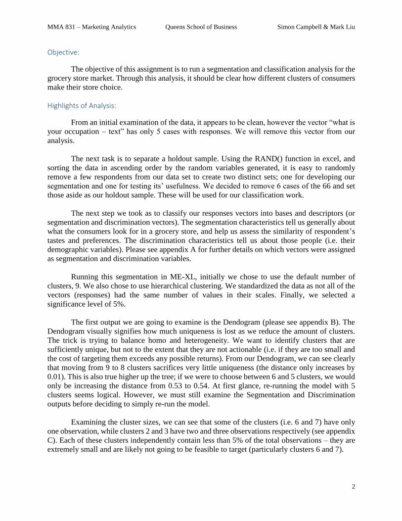
Objective:

The objective of this assignment is to run a segmentation and classification analysis for the

grocery store market. Through this analysis, it should be clear how different clusters of consumers

make their store choice.

Highlights of Analysis:

From an initial examination of the data, it appears to be clean, however the vector “what is

your occupation – text” has only 5 cases with responses. We will remove this vector from our

analysis.

The next task is to separate a holdout sample. Using the RAND() function in excel, and

sorting the data in ascending order by the random variables generated, it is easy to randomly

remove a few respondents from our data set to create two distinct sets; one for developing our

segmentation and one for testing its’ usefulness. We decided to remove 6 cases of the 66 and set

those aside as our holdout sample. These will be used for our classification work.

The next step we took as to classify our responses vectors into bases and descriptors (or

segmentation and discrimination vectors). The segmentation characteristics tell us generally about

what the consumers look for in a grocery store, and help us assess the similarity of respondent’s

tastes and preferences. The discrimination characteristics tell us about those people (i.e. their

demographic variables). Please see appendix A for further details on which vectors were assigned

as segmentation and discrimination variables.

Running this segmentation in ME-XL, initially we chose to use the default number of

clusters, 9. We also chose to use hierarchical clustering. We standardized the data as not all of the

vectors (responses) had the same number of values in their scales. Finally, we selected a

significance level of 5%.

The first output we are going to examine is the Dendogram (please see appendix B). The

Dendogram visually signifies how much uniqueness is lost as we reduce the amount of clusters.

The trick is trying to balance homo and heterogeneity. We want to identify clusters that are

sufficiently unique, but not to the extent that they are not actionable (i.e. if they are too small and

the cost of targeting them exceeds any possible returns). From our Dendogram, we can see clearly

that moving from 9 to 8 clusters sacrifices very little uniqueness (the distance only increases by

0.01). This is also true higher up the tree; if we were to choose between 6 and 5 clusters, we would

only be increasing the distance from 0.53 to 0.54. At first glance, re-running the model with 5

clusters seems logical. However, we must still examine the Segmentation and Discrimination

outputs before deciding to simply re-run the model.

Examining the cluster sizes, we can see that some of the clusters (i.e. 6 and 7) have only

one observation, while clusters 2 and 3 have two and three observations respectively (see appendix

C). Each of these clusters independently contain less than 5% of the total observations – they are

extremely small and are likely not going to be feasible to target (particularly clusters 6 and 7).


3

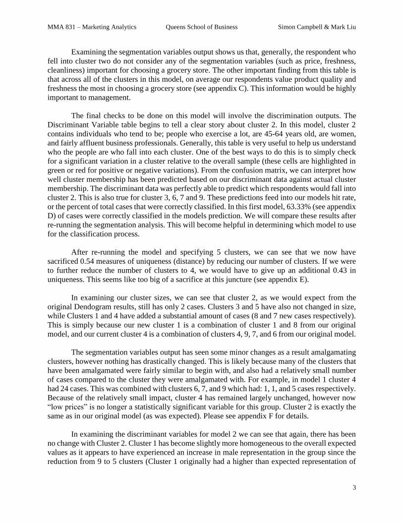
Examining the segmentation variables output shows us that, generally, the respondent who

fell into cluster two do not consider any of the segmentation variables (such as price, freshness,

cleanliness) important for choosing a grocery store. The other important finding from this table is

that across all of the clusters in this model, on average our respondents value product quality and

freshness the most in choosing a grocery store (see appendix C). This information would be highly

important to management.

The final checks to be done on this model will involve the discrimination outputs. The

Discriminant Variable table begins to tell a clear story about cluster 2. In this model, cluster 2

contains individuals who tend to be; people who exercise a lot, are 45-64 years old, are women,

and fairly affluent business professionals. Generally, this table is very useful to help us understand

who the people are who fall into each cluster. One of the best ways to do this is to simply check

for a significant variation in a cluster relative to the overall sample (these cells are highlighted in

green or red for positive or negative variations). From the confusion matrix, we can interpret how

well cluster membership has been predicted based on our discriminant data against actual cluster

membership. The discriminant data was perfectly able to predict which respondents would fall into

cluster 2. This is also true for cluster 3, 6, 7 and 9. These predictions feed into our models hit rate,

or the percent of total cases that were correctly classified. In this first model, 63.33% (see appendix

D) of cases were correctly classified in the models prediction. We will compare these results after

re-running the segmentation analysis. This will become helpful in determining which model to use

for the classification process.

After re-running the model and specifying 5 clusters, we can see that we now have

sacrificed 0.54 measures of uniqueness (distance) by reducing our number of clusters. If we were

to further reduce the number of clusters to 4, we would have to give up an additional 0.43 in

uniqueness. This seems like too big of a sacrifice at this juncture (see appendix E).

In examining our cluster sizes, we can see that cluster 2, as we would expect from the

original Dendogram results, still has only 2 cases. Clusters 3 and 5 have also not changed in size,

while Clusters 1 and 4 have added a substantial amount of cases (8 and 7 new cases respectively).

This is simply because our new cluster 1 is a combination of cluster 1 and 8 from our original

model, and our current cluster 4 is a combination of clusters 4, 9, 7, and 6 from our original model.

The segmentation variables output has seen some minor changes as a result amalgamating

clusters, however nothing has drastically changed. This is likely because many of the clusters that

have been amalgamated were fairly similar to begin with, and also had a relatively small number

of cases compared to the cluster they were amalgamated with. For example, in model 1 cluster 4

had 24 cases. This was combined with clusters 6, 7, and 9 which had: 1, 1, and 5 cases respectively.

Because of the relatively small impact, cluster 4 has remained largely unchanged, however now

“low prices” is no longer a statistically significant variable for this group. Cluster 2 is exactly the

same as in our original model (as was expected). Please see appendix F for details.

In examining the discriminant variables for model 2 we can see that again, there has been

no change with Cluster 2. Cluster 1 has become slightly more homogeneous to the overall expected

values as it appears to have experienced an increase in male representation in the group since the

reduction from 9 to 5 clusters (Cluster 1 originally had a higher than expected representation of


4

females). Clusters 3, 4 and 5 have not had any impactful changes. Overall, the ability of our

discriminant data to predict cluster membership (hit rate) has improved to 65% (see appendix G

for details).

The final process that will be run is a classification in order to evaluate the usefulness of

this segmentation model against our holdout data. As determined by our discriminant variables,

we can determine which segment each of the 6 holdout cases will fall into. Our classified data

indicates that 5 cases would fall into cluster 5, while 1 would fall into cluster 6 (see appendix H).

To verify the accuracy of these predictions, we will now return our holdout data to our testing set

and re-run the same model including these cases. We will then be able to measure the accuracy of

these predictions.

Re-running the model with the 6 additional cases had a surprising result. Only 2 out of the

6 predictions turned out to be correct. However, two of the cases which were predicted to become

members of cluster 5 became members of cluster 4. When comparing these clusters in the new

segmentation and discrimination results (which were generated by re-running the model while

including the 6 additional cases), we can see that from a discrimination perspective, cluster 4 and

5 are quite similar. They do deviate from one another in terms of the store variables that they

consider important, but their demographics are essentially the same (see appendix H).

This segmentation and classification analysis will be highly valuable to the managers of

the grocery chain. The results will have a significant impact on deciding which segments to target,

and this will have very important implications for not only marketing decisions, but also

assortment and merchandising. At this time, the sample is far too small to base any significant

targeting choices against any of the segments. Increasing the sample size and re-running the

segmentation and classification process will make the outputs far more generalizable and robust.

It is unlikely that the Category Managers are likely to make significant changes in assortment or

promotion planning based on these results at this time.

Despite this, these results do begin to provide insight into what variables are most important

to people when choosing a grocery store. More specifically, we are able to begin to see how

different demographic segments choose where to shop.


5

Appendix A: Classifying Segmentation and Discrimination variables

Responses to the following questions will be considered segmentation variables for the purposes of this analysis:

Please rate how important each attribute is in your choice of grocery store:

o Price

o Freshness

o Choice variety

o Healthiness

o Organic alternatives

o Convenient store layout

o Store location

o Product quality

o Service quality

o Return policy

o Cleanliness

o Busyness

Responses to the following questions will be considered discrimination variables for the purposes of this analysis:

Please indicate how much you agree / disagree with the following statements:

o I am a very active person

o I DO NOT exercise regularly

o I consider myself physically fit

o I eat healthy

o I consider myself a healthy person

o I ear poorly

Of all of the food you ate last week, what proportion was fruits

and vegetables

How many hours of exercise related / physical activity would you estimate you did last week

How would you classify your neighbourhood

What is your gender

How old are you

How many occupants live in your household

What is your marital status

What is your occupation

What is your highest finished degree

What is the annual income of you / your household

These variables are highly positively

correlated (0.86). Because of this “I

consider myself a healthy person” was not

included in any of the models run.


6

Appendix B: Model 1 – Dendogram

The original model had 9 clusters. We can see from this Dendogram that there is very little uniqueness sacrificed by

moving between 6 and 5 clusters. There is, however, significant uniqueness lost when moving from 5 to 4 clusters.

This insight was important in helping us determine that 5 clusters would be appropriate for this scenario.


7

Appendix C: Model 1 – Segmentation output details

The first table (“Size / Cluster”) lets us see the number of cases (respondents) who were

segmented into each cluster in our original model (as well as the clusters proportion of

respondents). We can see that cluster 6 and 7 have one respondent each while clusters 2 and 3

have two and three respondents respectively. The model will certainly not be actionable with so

few respondents in clusters. It is clear that we need fewer clusters to try and make the results

more actionable.

The second table (“Segmentation variable / Cluster”) indicates how the overall sample responded

on average to each of the segmentation variables, as well as how the average of how respondents

within specific clusters responded. Cluster responses which are statistically significantly

different from the overall sample are highlighted. We can see that overall, product quality and

freshness are the most important variables to this sample. Also, the respondents in Cluster 2 rated

each variable to be of much lower importance to them than the average of the overall sample.

Clusters 3 and 5 both rated several variables to be more important to them than the average of the

overall sample.

Size / Cluster Overall Cluster 1 Cluster 2 Cluster 3 Cluster 4 Cluster 5 Cluster 6 Cluster 7 Cluster 8 Cluster 9

Number of observations 60 8 2 3 24 8 1 1 8 5

Proportion 1 0.133 0.033 0.05 0.4 0.133 0.017 0.017 0.133 0.083

Segmentation variable / Cluster Overall Cluster 1 Cluster 2 Cluster 3 Cluster 4 Cluster 5 Cluster 6 Cluster 7 Cluster 8 Cluster 9

Please rate how important each / attribute is in your choice of grocery store. / -Low Prices 5.72 5.62 3 3.67 6.42 6 7 6 5.38 4.6

Please rate how important each / attribute is in your choice of grocery store. / -Freshness 6.17 6.88 1 7 6.29 6.75 7 5 6.5 4.6

Please rate how important each / attribute is in your choice of grocery store. / -Choice Variety 5.72 5.88 2 7 5.71 5.88 7 4 6.12 5.4

Please rate how important each / attribute is in your choice of grocery store. / -Healthiness 5.7 5.5 2 7 5.5 6.62 4 5 6.5 5.4

Please rate how important each / attribute is in your choice of grocery store. / -Organic Alternatives 3.68 1.62 1.5 6.67 3.58 5.5 1 2 3.25 5.2

Please rate how important each / attribute is in your choice of grocery store. / -Convenient Store Layout 4.93 5.88 1 6.67 4.54 6.25 1 4 5.12 4.4

Please rate how important each / attribute is in your choice of grocery store. / -Store Location 5.97 6.38 1 7 5.83 6.62 1 6 6.88 5.8

Please rate how important each / attribute is in your choice of grocery store. / -Product Quality 6.28 6.88 2 7 6 7 7 5 6.62 6.4

Please rate how important each / attribute is in your choice of grocery store. / -Service Quality 4.52 5.62 2.5 6.67 4.08 6.12 2 1 3.38 4.8

Please rate how important each / attribute is in your choice of grocery store. / -Return Policy 3.47 2.75 4 1.67 3.79 5.5 2 2 1.38 4.6

Please rate how important each / attribute is in your choice of grocery store. / -Cleanliness 5.65 6.12 1.5 7 5.33 6.75 5 2 6.25 5.4

Please rate how important each / attribute is in your choice of grocery store. / -Busyness 4.65 6 4 2.33 4.54 4.62 7 1 5.12 4.2


8

Appendix D: Model 1 – Discrimination output details

The first table (“Discriminant variable / Cluster”) lets us see the demographic makeup of the

sample, and for each individual cluster. As with the “Segmentation variable / Cluster” output

above, cells are highlighted based on statistically significant differences from the Overall

column.

The second table is our confusion matrix. This shows us how well cluster membership has been

predicted based on our discriminant data against actual cluster membership. This output also

shows us the overall effectiveness of the model at predicting cluster membership, which in this

case is 63.33%.

Discriminant variable / Cluster Overall Cluster 1 Cluster 2 Cluster 3 Cluster 4 Cluster 5 Cluster 6 Cluster 7 Cluster 8 Cluster 9

How would you classify your / neighbourhood? / 1.75 1.625 2 1.333 1.833 1.875 2 1 1.75 1.6

What is your gender? / 1.667 2 2 1.667 1.5 1.75 2 1 1.75 1.6

How old are you? / 1.683 1.875 3 1.667 1.417 2.125 4 1 1.375 1.6

How many occupants in your household / including yourself? / 3.283 2.375 3.5 3.333 3.667 2.75 4 5 2.875 3.8

What is your marital status / 3.983 4 1.5 3 4.25 4.25 2 5 4.625 3

What is your occupation? / 4.783 4.625 3 4 5 5.25 3 5 5 4.4

What is your highest finished / degree? 3.233 3.5 3.5 4 2.958 3.125 4 3 3.125 3.8

What is the annual income of your / household? 2.75 3.125 4 4.333 2.292 2.875 6 1 1.75 4

Please indicate how much you agree / or disagree with the following statements / -I am a very active person 5.35 5.5 6 7 5.208 5.125 7 6 5.125 4.8

Please indicate how much you agree / or disagree with the following statements / -I Do Not exercise regularly 2.85 3 3.5 1 3.083 3.375 1 2 2.375 2.8

Please indicate how much you agree / or disagree with the following statements / -I consider myself physically fit 5.217 4.875 5.5 7 5.125 5 7 6 5.375 4.6

Please indicate how much you agree / or disagree with the following statements / -I eat healthy 5.483 5.625 5.5 7 5.333 5.5 7 5 5.375 5

Please indicate how much you agree / or disagree with the following statements / -I eat poorly 2.383 2.625 2 1 2.583 2.25 1 3 2.625 2

/ / / Of all the food you ate last week, / what proportion were fruits and vegetables. 5.283 5.25 4.5 4.667 5.458 4.75 8 4 5.5 5.4

/ / / / / How many hours of exercise related / physical activity would you estimate you did last we... 4.467 4.5 7 5.667 4.5 3.625 4 4 4.375 4.2

Actual / Predicted cluster Cluster 1 Cluster 2 Cluster 3 Cluster 4 Cluster 5 Cluster 6 Cluster 7 Cluster 8 Cluster 9

Cluster 1 62.50% 12.50% 00.00% 00.00% 12.50% 00.00% 00.00% 12.50% 00.00%

Cluster 2 00.00% 100.00% 00.00% 00.00% 00.00% 00.00% 00.00% 00.00% 00.00%

Cluster 3 00.00% 00.00% 100.00% 00.00% 00.00% 00.00% 00.00% 00.00% 00.00%

Cluster 4 08.30% 00.00% 08.30% 54.20% 08.30% 00.00% 00.00% 16.70% 04.20%

Cluster 5 12.50% 00.00% 00.00% 12.50% 62.50% 00.00% 00.00% 12.50% 00.00%

Cluster 6 00.00% 00.00% 00.00% 00.00% 00.00% 100.00% 00.00% 00.00% 00.00%

Cluster 7 00.00% 00.00% 00.00% 00.00% 00.00% 00.00% 100.00% 00.00% 00.00%

Cluster 8 12.50% 00.00% 12.50% 12.50% 12.50% 00.00% 12.50% 37.50% 00.00%

Cluster 9 00.00% 00.00% 00.00% 00.00% 00.00% 00.00% 00.00% 00.00% 100.00%

Hit Rate (percent of total cases correctly classified) 63.33%


9

Appendix E: Model 2 – Dendogram

The Dendogram output from our second model (Model 2) shows us that if we were to decrease

to 4 clusters, we would have to sacrifice an additional 0.43 distance-units of uniqueness. This

was important in our decisions to retain 5 clusters.


10

Appendix F: Model 2 – Segmentation output details

The first table (“Size / Cluster”) lets us see the number of cases (respondents) who were

segmented into each cluster in our second model (as well as the clusters proportion of

respondents). Cluster 2 has remained the same while Clusters 1 and 5 have added cases.

The second table (“Segmentation variable / Cluster”) indicates how the overall sample responded

on average to each of the segmentation variables, as well as how the average of how respondents

within specific clusters responded. We can see that again, Cluster 2 has not changed (as we

would expect). Cluster 4 has become slightly more homogeneous and no longer has any

significant deviation from the overall sample. Cluster 3 and 5 both have significant differences

from the overall sample.

Size / Cluster Overall Cluster 1 Cluster 2 Cluster 3 Cluster 4 Cluster 5

Number of

observations60 16 2 3 31 8

Proportion 1 0.267 0.033 0.05 0.517 0.133

Segmentation variable / Cluster Overall Cluster 1 Cluster 2 Cluster 3 Cluster 4 Cluster 5

Please rate how important each / attribute is in your choice of grocery store. / -Low Prices 5.72 5.5 3 3.67 6.13 6

Please rate how important each / attribute is in your choice of grocery store. / -Freshness 6.17 6.69 1 7 6 6.75

Please rate how important each / attribute is in your choice of grocery store. / -Choice Variety 5.72 6 2 7 5.65 5.88

Please rate how important each / attribute is in your choice of grocery store. / -Healthiness 5.7 6 2 7 5.42 6.62

Please rate how important each / attribute is in your choice of grocery store. / -Organic Alternatives 3.68 2.44 1.5 6.67 3.71 5.5

Please rate how important each / attribute is in your choice of grocery store. / -Convenient Store Layout 4.93 5.5 1 6.67 4.39 6.25

Please rate how important each / attribute is in your choice of grocery store. / -Store Location 5.97 6.62 1 7 5.68 6.62

Please rate how important each / attribute is in your choice of grocery store. / -Product Quality 6.28 6.75 2 7 6.06 7

Please rate how important each / attribute is in your choice of grocery store. / -Service Quality 4.52 4.5 2.5 6.67 4.03 6.12

Please rate how important each / attribute is in your choice of grocery store. / -Return Policy 3.47 2.06 4 1.67 3.81 5.5

Please rate how important each / attribute is in your choice of grocery store. / -Cleanliness 5.65 6.19 1.5 7 5.23 6.75

Please rate how important each / attribute is in your choice of grocery store. / -Busyness 4.65 5.56 4 2.33 4.45 4.62


11

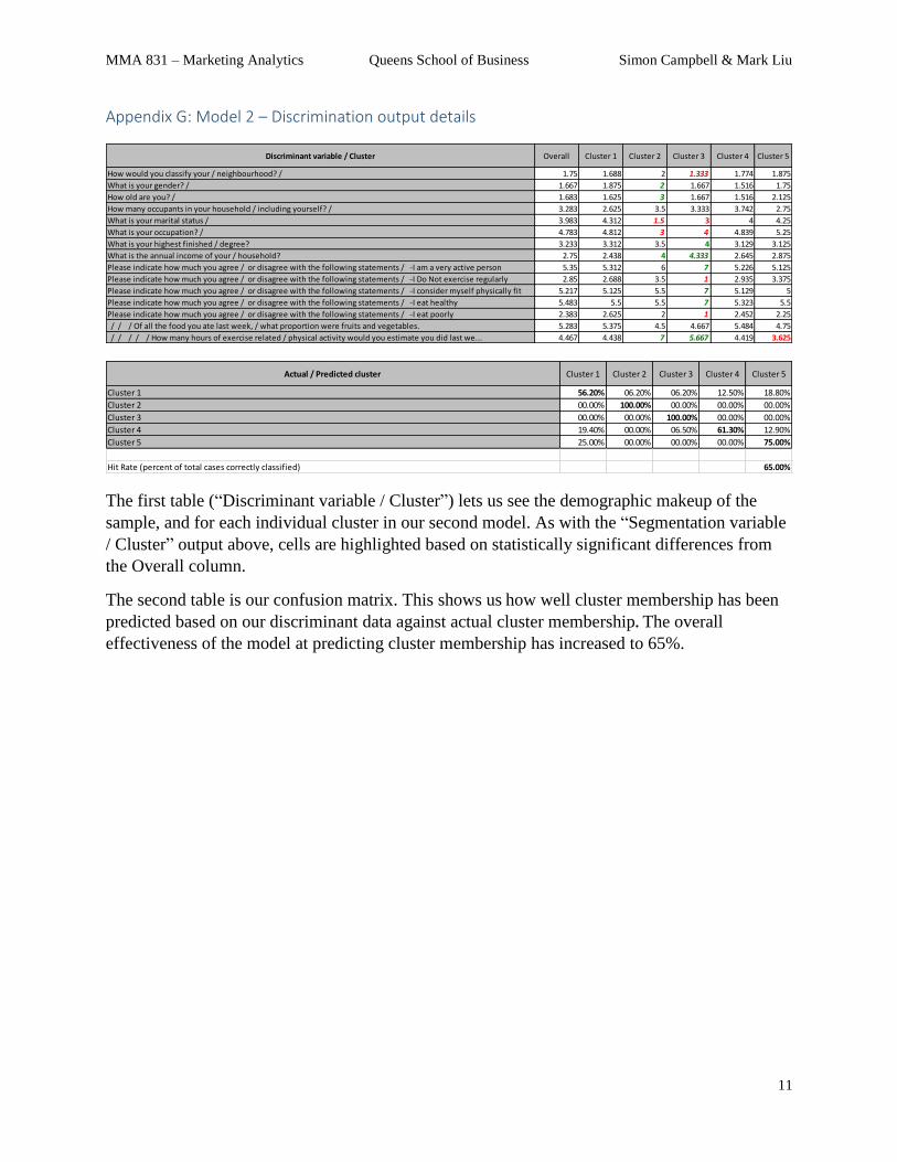
Appendix G: Model 2 – Discrimination output details

The first table (“Discriminant variable / Cluster”) lets us see the demographic makeup of the

sample, and for each individual cluster in our second model. As with the “Segmentation variable

/ Cluster” output above, cells are highlighted based on statistically significant differences from

the Overall column.

The second table is our confusion matrix. This shows us how well cluster membership has been

predicted based on our discriminant data against actual cluster membership. The overall

effectiveness of the model at predicting cluster membership has increased to 65%.

Discriminant variable / Cluster Overall Cluster 1 Cluster 2 Cluster 3 Cluster 4 Cluster 5

How would you classify your / neighbourhood? / 1.75 1.688 2 1.333 1.774 1.875

What is your gender? / 1.667 1.875 2 1.667 1.516 1.75

How old are you? / 1.683 1.625 3 1.667 1.516 2.125

How many occupants in your household / including yourself? / 3.283 2.625 3.5 3.333 3.742 2.75

What is your marital status / 3.983 4.312 1.5 3 4 4.25

What is your occupation? / 4.783 4.812 3 4 4.839 5.25

What is your highest finished / degree? 3.233 3.312 3.5 4 3.129 3.125

What is the annual income of your / household? 2.75 2.438 4 4.333 2.645 2.875

Please indicate how much you agree / or disagree with the following statements / -I am a very active person 5.35 5.312 6 7 5.226 5.125

Please indicate how much you agree / or disagree with the following statements / -I Do Not exercise regularly 2.85 2.688 3.5 1 2.935 3.375

Please indicate how much you agree / or disagree with the following statements / -I consider myself physically fit 5.217 5.125 5.5 7 5.129 5

Please indicate how much you agree / or disagree with the following statements / -I eat healthy 5.483 5.5 5.5 7 5.323 5.5

Please indicate how much you agree / or disagree with the following statements / -I eat poorly 2.383 2.625 2 1 2.452 2.25

/ / / Of all the food you ate last week, / what proportion were fruits and vegetables. 5.283 5.375 4.5 4.667 5.484 4.75

/ / / / / How many hours of exercise related / physical activity would you estimate you did last we... 4.467 4.438 7 5.667 4.419 3.625

Actual / Predicted cluster Cluster 1 Cluster 2 Cluster 3 Cluster 4 Cluster 5

Cluster 1 56.20% 06.20% 06.20% 12.50% 18.80%

Cluster 2 00.00% 100.00% 00.00% 00.00% 00.00%

Cluster 3 00.00% 00.00% 100.00% 00.00% 00.00%

Cluster 4 19.40% 00.00% 06.50% 61.30% 12.90%

Cluster 5 25.00% 00.00% 00.00% 00.00% 75.00%

Hit Rate (percent of total cases correctly classified) 65.00%


12

Appendix H: Model 2 – Classified data

The table above is an output from our classification

exercise. The column to the far right indicates what

cluster the holdout cases are predicted to fall into

based on each cases responses to our discrimination

variables.

After replacing these cases into our sample and re-

running the model, we can see in the table to the

right that many of the cases actually fell into a

different cluster than expected.

Below we have the Discriminant and Segmentation outputs from the model with the replaced

holdout sample. We compared this to the results from Model 2 and found that Cluster 4 and 5 are

very similar demographically, however they have slightly different results for what they look for

in a grocery store. Because of this, the model was able to recognize that 2 of the cases predicted

to land in Cluster 5, actually had a better match with Cluster 4.

Respondents /

Discriminant variables

and predicted cluster

Please

indicate

how much

you agree /

or disagree

with the

following

statements

/ -I am a

very active

person

Please

indicate

how much

you agree /

or disagree

with the

following

statements

/ -I Do Not

exercise

regularly

Please

indicate

how much

you agree /

or disagree

with the

following

statements

/ -I

consider

myself

physically

fit

Please

indicate

how much

you agree /

or disagree

with the

following

statements

/ -I eat

healthy

Please

indicate

how much

you agree /

or disagree

with the

following

statements

/ -I eat

poorly

/ / / Of

all the

food you

ate last

week, /

what

proportion

were fruits

and

vegetables

.

/ / / /

/ How

many

hours of

exercise

related /

physical

activity

would you

estimate

you did

last we...

How would

you

classify

your /

neighbour

hood? /

What is

your

gender? /

How old

are you? /

How many

occupants

in your

household

/ including

yourself? /

What is

your

marital

status /

What is

your

occupation

? /

What is

your

highest

finished /

degree?

What is the

annual

income of

your /

household

?

Predicted

Cluster

R_7UPkfMgtI15JjU1 5 3 5 5 3 6 5 1 2 2 2 1 3 5 5 5

R_8uJOlGRsGYqpIHP 3 5 4 6 2 7 3 1 1 2 3 2 4 6 5 2

R_55yIdOmwKbSKVlr 6 2 7 6 2 8 6 2 2 3 2 2 8 3 5 5

R_afmAmpRW8tDTAHj 4 3 3 5 3 8 4 2 1 2 3 2 4 6 6 5

R_7Nx2c3mWHxACXI1 7 7 7 7 7 11 7 3 1 4 1 5 7 6 6 5

R_2Qndw0rq8Yo4MCc 6 2 5 6 3 9 5 1 2 2 1 5 3 4 3 5

Observation / Cluster solutionWith 5

clusters

Predicted

Cluster

Membership

R_7UPkfMgtI15JjU1 1 5

R_8uJOlGRsGYqpIHP 5 2

R_55yIdOmwKbSKVlr 4 5

R_afmAmpRW8tDTAHj 5 5

R_7Nx2c3mWHxACXI1 4 5

R_2Qndw0rq8Yo4MCc 5 5

Discriminant variable / Cluster Overall Cluster 1 Cluster 2 Cluster 3 Cluster 4 Cluster 5

Please indicate how much you agree / or disagree with the following statements / -I am a very active person 5.333 5.5 6 5.636 5.25 5

Please indicate how much you agree / or disagree with the following statements / -I Do Not exercise regularly 2.924 2.9 3.5 2.727 3.062 2.636

Please indicate how much you agree / or disagree with the following statements / -I consider myself physically fit 5.212 5 5.5 5.545 5.219 5

Please indicate how much you agree / or disagree with the following statements / -I eat healthy 5.515 5.5 5.5 5.909 5.375 5.545

Please indicate how much you agree / or disagree with the following statements / -I eat poorly 2.47 2.6 2 1.909 2.594 2.636

/ / / Of all the food you ate last week, / what proportion were fruits and vegetables. 5.545 5.4 4.5 4.727 5.781 6

/ / / / / How many hours of exercise related / physical activity would you estimate you did last we... 4.515 4.7 7 4.182 4.531 4.182

How would you classify your / neighbourhood? / 1.742 1.6 2 1.727 1.844 1.545

What is your gender? / 1.652 2 2 1.727 1.531 1.545

How old are you? / 1.758 1.9 3 2 1.656 1.455

How many occupants in your household / including yourself? / 3.167 2.3 3.5 2.909 3.594 2.909

What is your marital status / 3.879 3.8 1.5 3.909 3.938 4.182

What is your occupation? / 4.788 4.5 3 4.909 5 4.636

What is your highest finished / degree? 3.394 3.8 3.5 3.364 3.25 3.455

What is the annual income of your / household? 2.955 3.1 4 3.273 2.75 2.909

Segmentation variable / Cluster Overall Cluster 1 Cluster 2 Cluster 3 Cluster 4 Cluster 5

Please rate how important each / attribute is in your choice of grocery store. / -Low Prices 5.68 5.8 3 5.36 6.19 4.91

Please rate how important each / attribute is in your choice of grocery store. / -Freshness 6.17 6.8 1 6.82 5.97 6.45

Please rate how important each / attribute is in your choice of grocery store. / -Choice Variety 5.73 5.8 2 6.18 5.62 6.18

Please rate how important each / attribute is in your choice of grocery store. / -Healthiness 5.67 5.4 2 6.73 5.31 6.55

Please rate how important each / attribute is in your choice of grocery store. / -Organic Alternatives 3.79 1.5 1.5 5.82 3.69 4.55

Please rate how important each / attribute is in your choice of grocery store. / -Convenient Store Layout 4.83 5.8 1 6.36 4.41 4.36

Please rate how important each / attribute is in your choice of grocery store. / -Store Location 5.85 6.4 1 6.73 5.59 6.09

Please rate how important each / attribute is in your choice of grocery store. / -Product Quality 6.27 6.9 2 7 6 6.55

Please rate how important each / attribute is in your choice of grocery store. / -Service Quality 4.56 5.4 2.5 6.27 4.16 3.64

Please rate how important each / attribute is in your choice of grocery store. / -Return Policy 3.5 2.9 4 4.45 3.81 2.09

Please rate how important each / attribute is in your choice of grocery store. / -Cleanliness 5.67 6 1.5 6.82 5.22 6.27

Please rate how important each / attribute is in your choice of grocery store. / -Busyness 4.65 5.9 4 4 4.41 5

MMA831 - DOS 3 - Simon Campbell & Mark Liu

Documents

segmentation characteristics

discrimination vectors

default number of clusters

responses vectors

vectors responses

discrimination variables

classification analysis

data set