THÈSE DE DOCTORAT DE L’ÉCOLE NORMALE SUPÉRIEURE Spécialité : Physique École doctorale : “Physique en Île-de-France” réalisée au Laboratoire Kastler Brossel présentée par Marion Delehaye pour obtenir le grade de : DOCTEUR DE L’ÉCOLE NORMALE SUPÉRIEURE Sujet de la thèse : Mixtures of superfluids soutenue le 8 Avril 2016 devant le jury composé de : M. Frédéric Chevy Directeur de thèse M. David Guéry-Odelin Rapporteur M. Takis Kontos Examinateur M me Anna Minguzzi Rapportrice M. Christophe Salomon Membre invité M. Sandro Stringari Examinateur

Welcome message from author
This document is posted to help you gain knowledge. Please leave a comment to let me know what you think about it! Share it to your friends and learn new things together.
Transcript

THÈSE DE DOCTORATDE L’ÉCOLE NORMALE SUPÉRIEURE
Spécialité : Physique
École doctorale : “Physique en Île-de-France”
réalisée
au Laboratoire Kastler Brossel
présentée par
Marion Delehaye
pour obtenir le grade de :
DOCTEUR DE L’ÉCOLE NORMALE SUPÉRIEURE
Sujet de la thèse :
Mixtures of superfluids
soutenue le 8 Avril 2016
devant le jury composé de :
M. Frédéric Chevy Directeur de thèseM. David Guéry-Odelin RapporteurM. Takis Kontos ExaminateurMme Anna Minguzzi RapportriceM. Christophe Salomon Membre invitéM. Sandro Stringari Examinateur

Contents
Introduction 1
1 Superfluidity 11
1.1 Superfluids . . . . . . . . . . . . . . . . . . . . . . . . . . . . . . . . . . 111.1.1 Historical approach . . . . . . . . . . . . . . . . . . . . . . . . . . 111.1.2 Properties of superfluid helium and superfluid atomic gases . . . 12
1.2 Bosons and fermions . . . . . . . . . . . . . . . . . . . . . . . . . . . . . 141.2.1 Quantum statistics . . . . . . . . . . . . . . . . . . . . . . . . . . 141.2.2 Low-temperature behavior . . . . . . . . . . . . . . . . . . . . . . 14
1.3 Superfluidity in ultracold atomic gases . . . . . . . . . . . . . . . . . . . 171.3.1 Interactions and scattering length . . . . . . . . . . . . . . . . . 171.3.2 Bose-Einstein Condensates . . . . . . . . . . . . . . . . . . . . . 191.3.3 Fermi superfluids . . . . . . . . . . . . . . . . . . . . . . . . . . . 22
2 Lithium Machine and Double Degeneracy 25
2.1 General description . . . . . . . . . . . . . . . . . . . . . . . . . . . . . . 262.2 Lithium . . . . . . . . . . . . . . . . . . . . . . . . . . . . . . . . . . . . 26
2.2.1 The atom of lithium . . . . . . . . . . . . . . . . . . . . . . . . . 262.2.2 Atomic structure . . . . . . . . . . . . . . . . . . . . . . . . . . . 282.2.3 Feshbach resonances . . . . . . . . . . . . . . . . . . . . . . . . . 28
2.3 Loading the MOT . . . . . . . . . . . . . . . . . . . . . . . . . . . . . . 332.3.1 Oven . . . . . . . . . . . . . . . . . . . . . . . . . . . . . . . . . . 342.3.2 Zeeman slower . . . . . . . . . . . . . . . . . . . . . . . . . . . . 342.3.3 MOT . . . . . . . . . . . . . . . . . . . . . . . . . . . . . . . . . 362.3.4 Laser system . . . . . . . . . . . . . . . . . . . . . . . . . . . . . 36
2.4 Magnetic trap, transport, and RF evaporation . . . . . . . . . . . . . . . 372.4.1 Optical pumping . . . . . . . . . . . . . . . . . . . . . . . . . . . 372.4.2 Magnetic trap and transport . . . . . . . . . . . . . . . . . . . . 382.4.3 Ioffe-Pritchard trap . . . . . . . . . . . . . . . . . . . . . . . . . . 382.4.4 RF evaporation . . . . . . . . . . . . . . . . . . . . . . . . . . . . 40
2.5 Optical trap . . . . . . . . . . . . . . . . . . . . . . . . . . . . . . . . . . 412.5.1 Generalities on optical traps . . . . . . . . . . . . . . . . . . . . . 412.5.2 Loading the hybrid trap . . . . . . . . . . . . . . . . . . . . . . . 412.5.3 Mixture preparation . . . . . . . . . . . . . . . . . . . . . . . . . 422.5.4 Evaporation . . . . . . . . . . . . . . . . . . . . . . . . . . . . . . 43
i

ii CONTENTS
2.5.5 Summary . . . . . . . . . . . . . . . . . . . . . . . . . . . . . . . 432.6 Imaging . . . . . . . . . . . . . . . . . . . . . . . . . . . . . . . . . . . . 44
2.6.1 Absorption imaging . . . . . . . . . . . . . . . . . . . . . . . . . 442.6.2 Imaging system . . . . . . . . . . . . . . . . . . . . . . . . . . . . 452.6.3 Image processing . . . . . . . . . . . . . . . . . . . . . . . . . . . 46
2.7 Double Degeneracy . . . . . . . . . . . . . . . . . . . . . . . . . . . . . . 472.7.1 Bosons . . . . . . . . . . . . . . . . . . . . . . . . . . . . . . . . . 472.7.2 Fermions . . . . . . . . . . . . . . . . . . . . . . . . . . . . . . . 49
2.8 Conclusion . . . . . . . . . . . . . . . . . . . . . . . . . . . . . . . . . . 50
3 Collective modes of the mixture 53
3.1 Dipole modes excitation . . . . . . . . . . . . . . . . . . . . . . . . . . . 553.1.1 The mixture . . . . . . . . . . . . . . . . . . . . . . . . . . . . . 553.1.2 Selective excitation of dipole modes . . . . . . . . . . . . . . . . 563.1.3 Kohn’s theorem . . . . . . . . . . . . . . . . . . . . . . . . . . . . 57
3.2 Low temperature, low amplitude . . . . . . . . . . . . . . . . . . . . . . 583.2.1 Experiments . . . . . . . . . . . . . . . . . . . . . . . . . . . . . 583.2.2 Bose-Fermi interaction . . . . . . . . . . . . . . . . . . . . . . . . 603.2.3 Sum-rule approach . . . . . . . . . . . . . . . . . . . . . . . . . . 623.2.4 Two coupled-oscillators model . . . . . . . . . . . . . . . . . . . . 65
3.3 Low temperature, high amplitude . . . . . . . . . . . . . . . . . . . . . . 663.3.1 Experiments . . . . . . . . . . . . . . . . . . . . . . . . . . . . . 663.3.2 Landau criterion for superfluidity . . . . . . . . . . . . . . . . . . 683.3.3 Critical velocity . . . . . . . . . . . . . . . . . . . . . . . . . . . . 703.3.4 Discussion . . . . . . . . . . . . . . . . . . . . . . . . . . . . . . . 73
3.4 High temperature, moderate amplitude . . . . . . . . . . . . . . . . . . 743.4.1 Experiments . . . . . . . . . . . . . . . . . . . . . . . . . . . . . 743.4.2 Frequency analysis . . . . . . . . . . . . . . . . . . . . . . . . . . 753.4.3 Damping . . . . . . . . . . . . . . . . . . . . . . . . . . . . . . . 773.4.4 Two coupled-oscillator model . . . . . . . . . . . . . . . . . . . . 793.4.5 Zeno-like model . . . . . . . . . . . . . . . . . . . . . . . . . . . . 793.4.6 At the origin of the frequency shift . . . . . . . . . . . . . . . . . 82
3.5 Advanced data analysis: PCA . . . . . . . . . . . . . . . . . . . . . . . . 833.6 Quadrupole modes . . . . . . . . . . . . . . . . . . . . . . . . . . . . . . 873.7 Conclusion . . . . . . . . . . . . . . . . . . . . . . . . . . . . . . . . . . 89
4 Imbalanced gases and flat bottom trap 91
4.1 Superfluidity in imbalanced Fermi gases . . . . . . . . . . . . . . . . . . 934.1.1 Fermions in a box . . . . . . . . . . . . . . . . . . . . . . . . . . 934.1.2 Fermions in a harmonic trap . . . . . . . . . . . . . . . . . . . . 954.1.3 Application: another evidence of superfluidity . . . . . . . . . . . 97
4.2 Realization of a flat bottom trap . . . . . . . . . . . . . . . . . . . . . . 984.2.1 Prediction . . . . . . . . . . . . . . . . . . . . . . . . . . . . . . . 984.2.2 Experimental conditions . . . . . . . . . . . . . . . . . . . . . . . 99
4.3 Critical polarizations in a flat bottom trap . . . . . . . . . . . . . . . . . 1034.3.1 Bosons and fermions in a box . . . . . . . . . . . . . . . . . . . . 103

CONTENTS iii
4.3.2 Bosons and fermions in a harmonic trap . . . . . . . . . . . . . . 1054.3.3 Breakdown of FBT prediction . . . . . . . . . . . . . . . . . . . . 108
4.4 Experiments on imbalanced Fermi gases in a FBT . . . . . . . . . . . . 1084.4.1 Bosonic Thomas-Fermi radius . . . . . . . . . . . . . . . . . . . . 1114.4.2 First observations . . . . . . . . . . . . . . . . . . . . . . . . . . 1114.4.3 Reconstruction Methods . . . . . . . . . . . . . . . . . . . . . . . 1124.4.4 Evidence for a superfluid shell . . . . . . . . . . . . . . . . . . . 1154.4.5 Parameters influencing the superfluid shell on the BEC side . . . 1184.4.6 Parameters influencing the superfluid shell on the BCS side . . . 1224.4.7 Portrait of the superfluid shell . . . . . . . . . . . . . . . . . . . 124
4.5 Conclusion . . . . . . . . . . . . . . . . . . . . . . . . . . . . . . . . . . 125
5 New Lithium Machine 129
5.1 Overview . . . . . . . . . . . . . . . . . . . . . . . . . . . . . . . . . . . 1305.1.1 “Cahier des charges” . . . . . . . . . . . . . . . . . . . . . . . . . 1305.1.2 D1 cooling . . . . . . . . . . . . . . . . . . . . . . . . . . . . . . 1315.1.3 Experimental sequence . . . . . . . . . . . . . . . . . . . . . . . . 133
5.2 Mechanical setup . . . . . . . . . . . . . . . . . . . . . . . . . . . . . . . 1345.2.1 Oven . . . . . . . . . . . . . . . . . . . . . . . . . . . . . . . . . . 1355.2.2 Vacuum system . . . . . . . . . . . . . . . . . . . . . . . . . . . . 1355.2.3 Cells and optical transport . . . . . . . . . . . . . . . . . . . . . 136
5.3 Laser setup . . . . . . . . . . . . . . . . . . . . . . . . . . . . . . . . . . 1375.3.1 Laser Scheme . . . . . . . . . . . . . . . . . . . . . . . . . . . . . 1375.3.2 Optical realization . . . . . . . . . . . . . . . . . . . . . . . . . . 1375.3.3 Mechanical installation . . . . . . . . . . . . . . . . . . . . . . . 141
5.4 Magnetic fields . . . . . . . . . . . . . . . . . . . . . . . . . . . . . . . . 1435.4.1 Zeeman slower . . . . . . . . . . . . . . . . . . . . . . . . . . . . 1435.4.2 Compensation coils . . . . . . . . . . . . . . . . . . . . . . . . . . 1455.4.3 MOT-Feshbach coils . . . . . . . . . . . . . . . . . . . . . . . . . 1465.4.4 Science cell magnetic fields . . . . . . . . . . . . . . . . . . . . . 148
5.5 Security and computer control . . . . . . . . . . . . . . . . . . . . . . . 1485.6 Conclusion . . . . . . . . . . . . . . . . . . . . . . . . . . . . . . . . . . 148
Conclusion 149
Appendices 151
A Consistency check of FBT analysis . . . . . . . . . . . . . . . . . . . . . 153B Cicero for Lithium: User’s Manuel . . . . . . . . . . . . . . . . . . . . . 155
B.1 Introduction - Caution . . . . . . . . . . . . . . . . . . . . . . . . 155B.2 Configuration of Atticus . . . . . . . . . . . . . . . . . . . . . . . 155B.3 Changes made to the software . . . . . . . . . . . . . . . . . . . . 157
C Publications and preprints . . . . . . . . . . . . . . . . . . . . . . . . . . 161C.1 Λ-enhanced sub-Doppler cooling of lithium atoms in D1 gray
molasses . . . . . . . . . . . . . . . 162C.2 A mixture of Bose and Fermi superfluids . . . . . . 172

iv CONTENTS
C.3 Chandrasekhar-Clogston limit and critical polarization in a Fermi-Bose superfluid mixture . . . . . . . . . . . 186
C.4 Critical velocity and dissipation of an ultracold Bose-Fermi coun-terflow . . . . . . . . . . . . . . . . 192
C.5 Universal loss dynamics in a unitary Bose gas . . . . . 204
Bibliography 215

Introduction
“What kind of computer are we going to use to simulate physics?” Richard Feynmanasked in 19821, before adding, about quantum mechanics, “I want to talk about thepossibility that there is to be an exact simulation, that the computer will do exactly thesame as nature”. That is, to simulate accurately and efficiently quantum physics, oneneeds a quantum computer2. Those quantum computers are still under development3,but the idea arose to simulate quantum matter with quantum systems that share thesame Hamiltonian. Such quantum systems can be either composed of ultracold atoms4
photonic5 or ionic6.Even though cold atoms can be used to simulate long-elusive particles, such as the
Higgs mode7 or Weyl fermions8, most of the quantum simulation is focused on aspectsrelated to condensed matter.
Superfluidity in quantum fluids
At low temperature, matter is dominated by quantum effects. In condensed matter,they manifest themselves in a spectacular way via superfluidity.
Superconductivity
The first superfluidity effects were discovered with the superconductivity of mercury in1911. In superconductors, electrons feel effective attractive interactions mediated byphonons and form Cooper pairs, as was explained in Bardeen-Cooper-Schrieffer (BCS)theory (citation needed). The superfluid character of the Cooper pairs leads to theobserved absence of electric resistance.
Helium
In 1937, Kapitza9, Allen and Misener10 discovered that the viscosity of helium 4 belowthe phase transition temperature of 2.2 K was exactly zero. This was interpreted11 asthe condensation predicted by Bose and Einstein of bosonic 4He. Years later, in 1972,helium 3 was also found to undergo a phase transition, at a temperature of 2.6 mK,
1[Feynman, 1982]2[Lloyd, 1996]3[Ladd et al., 2010]4[Bloch et al., 2012, Bloch et
al., 2008]
5[Aspuru-Guzik and Walther,2012]6[Blatt and Roos, 2012]7[Endres et al., 2012]8[Suchet et al., 2015]
9[Kapitza, 1938]10[Allen and Misener, 1938]11[Tisza, 1938, London,1938, Landau, 1941, Tisza,1947]
1

2 Introduction
below which it was superfluid12. Here, the superfluidity was interpreted13 as relyingon the formation of pairs of fermionic 3He.
Ultracold atoms
For the new quantum fluids that ultracold gases were about fifteen years ago, withthe first Bose-Einstein condensate in 199514 and the degenerate Fermi gas in 199915,evidences of superfluidity were searched intensively. Among the spectacular effects ofsuperfluidity are phase coherence16, the presence of vortices and the existence of acritical velocity for dissipation, and that were these effects that attracted most effortsin the cold atom community. Vortices are due to the quantization of circulation inquantum fluids and can be seen via the presence of zero-density lines within the gas.The existence of a critical velocity is a completely different phenomenon and is basedon Landau’s criterion to create excitations in a quantum fluid flow that lead to dis-sipation. For Bose-Einstein condensates, both vortices17 and critical velocity18 wereobserved in the early 2000s. For fermions, the observation of vortices at MIT19 pro-vided indisputable proofs on the superfluidity of these systems for various interactionstrengths. The critical velocity for fermions was also measured with different probingtechniques20.
It is also worth mentioning the recent realization of Bose-Einstein condensates ofpolaritons [Amo et al., 2009, Balili et al., 2007] and magnons [Nikuni et al., 2000,Demokritov et al., 2006], that are also superfluids.
Quantum simulation with ultracold atoms
Hubbard models
In was noticed in the early days of ultracold atoms that the high purity of theirenvironment and their controllability made them systems of choice to simulate variouscondensed-matter Hamiltonians21. Observation of superfluidity in ultracold gases wasa prelude to quantum simulation of environments that challenge it. Among them isthe Hubbard model, that predicts a phase transition between a superfluid state and aMott insulating state for particles in a lattice when the depth of the lattice is varied.The first realizations of the Bose-Hubbard Hamiltonian (with bosons in an opticallattice)22 paved the way for theoretical and experimental studies of Fermi-Hubbard23
and Bose-Fermi Hubbard24 models. Cold atoms provide unique tools, such as singlesite and single atom resolution25, that would correspond to imaging directly single
12[Osheroff et al.,1972a, Osheroff et al., 1972b]13[Leggett, 1975]14[Anderson et al.,1995, Davis et al., 1995a]15[DeMarco and Jin, 1999]16[Bloch et al., 2000]17[Matthews et al.,1999, Madison et al.,2000, Abo-Shaeer et al., 2001]
18[Raman et al., 1999, Onofrioet al., 2000, Fedichev andShlyapnikov, 2001]19[Zwierlein et al.,2005, Zwierlein et al., 2006a]20[Miller et al., 2007, Weimeret al., 2015, Delehaye et al.,2015]21[Fisher et al., 1989, Jakschet al., 1998, Jaksch and
Zoller, 2005]22[Greiner et al., 2002, Will et
al., 2010]23[Köhl et al.,2005, Strohmaier et al.,2007, Jordens et al.,2008, Schneider et al., 2008]24[Günter et al.,2006, Ospelkaus et al., 2006]25[Bakr et al., 2009]

Introduction 3
electrons in a solid. The possibility to visualize directly single-site population givesaccess to the correlation functions and enables precise study of the quantum phasetransition between superfluid and Mott insulator. Some controllable disorder26 canalso be added to the Bose-Hubbard model in various dimensions to study Andersonlocalization, the localization of particles and subsequent loss of superfluidity due todisorder.
Charged matter in magnetic fields
More recently, the challenge of simulating the behavior of charged matter in magneticfields with neutral atoms was also addressed27. Since cold atoms are neutral, theyare not accelerated by magnetic fields. It is thus required to apply so-called artificialgauge fields. One of the realization of artificial gauge fields consists in implementinga global rotation Ω of the gas. The resulting Coriolis force 2MΩ ∧ v (where M isthe mass of the system and v its speed) has the same mathematical structure as theLorentz force qv ∧B28, where q is the charge of the particle. Another possibility is touse artificial gauge fields, where a specific laser scheme is designed to imprint a Berryphase (similar to the phase acquired by a particle evolving in a magnetic field) on atomsin bulk phases29 or in optical lattices30. This led for instance to the realization of theHofstadter Hamiltonian31. Another opportunity offered by these synthetic magneticfields is the possibility to reach fractional quantum Hall regime for ultracold atomsunder a strong artificial magnetic field.
Transport properties
Since the starting point of most cold atom experiments is a system at equilibrium ina trapping potential, one natural way to investigate transport properties is to modifythe trapping potential and observe the response of the system to this perturbation32.However, one key observable of solid-state physics, electric conduction, can not besimulated with this technique because it requires two reservoirs and a channel con-necting them. Conduction was observed by engineering such a system with opticalpotential and realizing a population imbalance between the two reservoirs so that theparticles would go from one to the other through the channel33, both in the ballisticand diffusive regime.
Dipolar gases
The first atoms that were cooled to quantum degeneracy were alkali. They haveno dipolar magnetic moment and only interact with short-range contact interactions.One workaround to study the effect of long-range interactions is the use of Rydbergatoms [Schauß et al., 2012, Weimer et al., 2008, Pohl et al., 2010]. Another one relies26[Roati et al., 2008, Billy et
al., 2008, Kondov et al.,2011, Gurarie et al.,2009, Schreiber et al., 2015]27[Bloch et al., 2008, Dalibardet al., 2011, Goldman et al.,2014]
28[Madison et al., 2000]29[Lin et al., 2009, Wang et
al., 2012, Cheuk et al., 2012]30[Aidelsburger et al.,2011, Struck et al.,2013, Miyake et al., 2013]
31[Aidelsburger et al., 2013]32[Jin et al., 1996, Ben Dahanet al., 1996, Ott et al.,2004, Sommer et al.,2011, Schneider et al., 2012]33[Brantut et al., 2012]

4 Introduction
on dipolar gases, that exhibit long-range, anisotropic interactions34. They may chal-lenge the stability of a Bose-Einstein condensate35, or lead to Rosensweig instability36.Antiferromagnetism can also be simulated37.
Fermi gases with tunable interactions
Ultracold gases can also predict the properties of systems hard to reach experimentally,such as neutron stars for instance38. Neutron stars are strongly interacting Fermisystems at a temperature T ∼ 106 K well below their Fermi temperature TF ∼ 1012 K,their behavior is similar to that of an ultracold strongly interacting Fermi gas, and theknowledge of the equation of state of the ultracold Fermi gas gives access to that ofa layer of the neutron star. Strongly interacting Fermi gases gather several fermionicspecies (for instance, atoms in two different spin-states noted ↑ and ↓). Those twofermionic species may interact with each other, and the lengthscale characterizing theinteraction is the scattering length aff . The interaction strength is then given by kFaff ,where kF is the Fermi wave-vector. For large values of |kFaff |, the system is saidstrongly interacting, and the |kFaff | → ∞ limit is called unitarity. For 1/kFaff ≫ 1(“BEC regime”), fermions form tightly-bound pairs with bosonic character that mayundergo Bose-Einstein condensation, while for 1/kFaff ≪ −1(“BCS regime”), fermionsform Cooper pairs. Superfluidity is possible in the whole BEC-BCS crossover, and ischaracterized by pairing between spin-↑ and spin-↓ fermions.
For fermions, the equation of state is thus a function of three parameters: the tem-perature, the interaction strength, and the ratio between the two spin-populations1.It has been obtained in three dimensions2, as a function of temperature at unitar-ity39, as a function of interaction strength at zero temperature40, and as a functionof spin imbalance. When considering spin-imbalanced gases, one key parameter isthe population imbalance above which superfluidity is lost. This issue, known as theClogston-Chandrasekhar limit, was first addressed in41, and has been investigated boththeoretically42 and experimentally43.
For spin-imbalanced Fermi system, several exotic, long-elusive phases have been
1For bosons the equation of state is a function only of temperature and interaction strength. It hasbeen measured as a function of temperature in three dimensions [Ensher et al., 1996, Gerbier et al.,2004b, Gerbier et al., 2004a], in two dimensions [Hung et al., 2011, Rath et al., 2010, Yefsah et al.,2011] and in one dimension [van Amerongen et al., 2008, Armijo et al., 2011]. The study of ultracoldgases in more than three dimensions is now considered [Boada et al., 2012, Celi et al., 2014, Zeng et
al., 2015, Price et al., 2015], by seeing the spin degrees of freedom of the atoms as a discrete extradimension.
2In two dimensions, the equation of state of fermions has been measured recently [Boettcher et al.,2016, Fenech et al., 2016].
34[Lahaye et al., 2009]35[Lahaye et al., 2007, Lahayeet al., 2008, Ferrier-Barbut et
al., 2016]36[Kadau et al., 2016]37[Simon et al., 2011, Greif et
al., 2015]
38[Ho, 2004, Gezerlis andCarlson, 2008]39[Thomas et al.,2005, Stewart et al., 2006, Luoet al., 2007, Nascimbène et
al., 2010, Horikoshi et al.,2010, Ku et al., 2012]40[Shin, 2008, Bulgac andForbes, 2007, Navon et al.,
2010]41[Clogston,1962, Chandrasekhar, 1962]42[Bausmerth et al.,2009, Chevy, 2006, Lobo et
al., 2006]43[Zwierlein et al.,2006a, Navon et al., 2010]

Introduction 5
predicted. Among them is the FFLO phase44, characterized, with other properties,by Cooper pairs with non-zero momentum and a spatially varying order parameter.Despite intensive experimental effort, no irrefutable proof of their observation couldbe seen, even though some evidence have been put forward45. In three dimensions,they are predicted to appear only in a narrow range of parameters (see Figure 0.1 and[Sheehy and Radzihovsky, 2007] for a review), so their signature is mainly smearedout when the system is trapped in a harmonic potential, as it is usually the case forultracold gases3. The ongoing development of uniform trapping potentials is thus verypromising for the observation of FFLO phases.
Figure 0.1: Mean-field phase diagram of imbalanced Fermi gases, as a function ofinverse scattering length and local spin polarization imbalance P , showing regimes ofmagnetized (imbalanced) superfluid (SFM ), FFLO (in red, bounded by PFFLO andPc2) and normal Fermi liquid, taken from [Radzihovsky and Sheehy, 2010].
Uniform systems
Harmonic traps were very practical to measure the equation of state of ultracold sys-tems. Indeed, the atomic density varies spatially and explores a finite range on a singlecloud, giving access to many points of the equation of state curve from a single exper-imental realization. However, the search for phases that appear in a narrow range ofphase diagram is made challenging, because they would appear only in a small portionof the cloud’s volume. This would not be the case in box potentials, where the poten-tial and hence the atomic density is constant on a finite volume (the ‘box’). It wouldthen be possible to “zoom in” into the parameter subspace of interest. Box potentials
3One way to circumvent this problem is to go to lower dimensions: in one dimensional systems,FFLO phase occupies a larger portion of the phase diagram[Liao et al., 2010, Mizushima et al., 2005,Orso, 2007, Hu et al., 2007, Guan et al., 2007, Parish et al., 2007, Feiguin and Heidrich-Meisner, 2007,Casula et al., 2008, Kakashvili and Bolech, 2009], allowing possible experimental detection [Kinnunenet al., 2006, Edge and Cooper, 2009].
44[Fulde and Ferrell,1964, Larkin and
Ovchinnikov, 1964] 45[Kontos et al., 2001]

6 Introduction
were initially reported in46, then more recently in47, where they have already providedthe opportunity to study critical phenomena, such as Kibble-Zurek mechanism48.
Bose-Fermi mixtures
State of the art
After the discovery of superfluidity in 3He, one natural question that arose was whetheris was possible to make a mixture with the two known superfluids, 3He and 4He.It turns out that strong interactions between the two species downshift the criticaltemperature for superfluidity to about 50µK, while the coldest temperature reachedin mixtures of liquid helium is so far 100µK49. That question thus remained open forabout 50 years before we could realize such a Bose-Fermi superfluid mixture with coldatoms.
In cold atoms, many mixtures with bosons and fermions have been realized, alsobecause initially one of the methods to cool fermions was via sympathetic coolingwith bosons. But none of the mixtures was showing simultaneously Bose and Fermisuperfluidity: either the bosons were condensed but the fermions were not superfluid(for instance because there was only one fermionic spin-state, or because the criticaltemperature for superfluidity was too low), or the fermions were superfluid but theBose gas not condensed (because of too few atoms for instance).
MixturesBosons Fermions Reference
7Li 6Li [Schreck et al., 2001b, Truscott et al., 2001]23Na 6Li [Hadzibabic et al., 2002]87Rb 40K [Roati et al., 2002]87Rb 6Li [Silber et al., 2005]4He∗ 3He∗ [McNamara et al., 2006]87Rb 6Li-40K [Taglieber et al., 2008]
85,97Rb 6Li [Deh et al., 2008, Deh et al., 2010]84,86,88Sr 87Sr [Tey et al., 2010, Stellmer et al., 2013]
174Yb 6Li [Hara et al., 2011, Hansen et al., 2011]170,174Yb 173Yb [Sugawa et al., 2011]
41K 40K-6Li [Wu et al., 2011]162Dy 161Dy [Lu et al., 2012]23Na 40K [Park et al., 2012]133Cs 6Li [Repp et al., 2013]
Reported degenerate Bose-Fermi mixtures
46[Meyrath et al., 2005]47[Gaunt et al., 2013, Cormanet al., 2014]
48[Chomaz et al., 2014, Navonet al., 2015]
49[Tuoriniemi et al.,2002, Rysti et al., 2012]

Introduction 7
Superfluid mixture
Our experiment had already produced mixtures of a Bose-Einstein Condensate andof a degenerate Fermi gas50, and cold bosons in the presence of superfluid fermions51.We were able to realize a double superfluid Bose-Fermi mixture of fermionic 6Li andbosonic 7Li by choosing the right combination of atomic states to make use of the 6LiFeshbach resonance in a magnetic field range where the Bose-Einstein of 7Li is stable52.
The report of our superfluid mixture raised very fast new questions regarding thevalidity of Landau’s argument in the case of a Bose-Fermi superfluid counterflow53.During my PhD, we addressed a few of them, such as the measurement of the criticalvelocity of the mixture or the effect of finite temperature. We also studied, both theo-retically and experimentally, the robustness of fermionic superfluidity with respect tospin-population imbalance, in the presence of the Bose gas. Indeed, another propertyof the Bose-Fermi system was the opportunity to create a flat bottom potential. Pre-viously reported uniform potentials54 use repulsive laser sheets to create a box for theatoms. The approach that we propose is completely different. It uses the repulsiveinteractions between bosons and fermions to compensate the curvature of the harmonictrap for the Fermi cloud. The flatness of the trap can be set by the precise tuningof Bose-Bose interactions through a Feshbach Resonance. The effective trapping po-tential for the Fermi gas then has a flat bottom and opens the possibility to probeClogston-Chandrasekhar limit in homogeneous systems.
Outline of this thesis
My first contribution to research within the group was to take data regarding thelifetime and three-body losses of the unitary Bose gas55 (see Appendix C.5). Afteran interlude for the implementation a new cooling technique on lithium based of D1
cooling56 (see Appendix C.1), we turned to the production of a superfluid Bose-Fermimixture57 (see Appendix C.2) and the study of its properties58 (see Appendix C.3).This form the central part of my PhD work. Among the properties of this novelsystem, we have focused both on its superfluidity and critical velocity, and on theimplementation of a proposal realized in collaboration with the Trento group59 (seeAppendix C.2).
This thesis is organized the following way:
• chapter 1 is dedicated to an introduction to the subject of superfluidity. It givesa brief overview of the major steps in history of superfluidity, then details someof its most spectacular physical manifestations. It then turns to the subject ofquantum gases, and to the relation between their interactions and superfluidity.
• chapter 2 describes the lithium machine on which all of the results given inthis PhD were obtained. It was thoroughly described in several PhD theses from
50[Schreck et al., 2001b]51[Nascimbène et al., 2010]52[Ferrier-Barbut et al., 2014]53[Castin et al., 2015, Abad et
al., 2015, Zheng and Zhai,2014, Wen and Li, 2014, Shen
and Zheng, 2015, Chevy, 2015]54[Meyrath et al.,2005, Gaunt et al.,2013, Corman et al., 2014]
55[Rem et al., 2013, Eismannet al., 2015]56[Grier et al., 2013]57[Ferrier-Barbut et al., 2014]58[Delehaye et al., 2015]59[Ferrier-Barbut et al., 2014]
8 Introduction
students before me60, so I only go briefly over the different steps that lead to therealization of a Bose-Fermi superfluid mixture61.
• chapter 3 concerns the study of the Bose-Fermi counterflow. It details theinitiation of the counterflow, its mean-field study, the measurement of the criticalvelocity in the BEC-BEC crossover, and the observation of an unexpected phase-locking of the two clouds at unitarity when increasing the temperature.
• chapter 4 is dedicated to the study of imbalanced Fermi gases in a flat bottomtrap. It explains the theoretical prediction and the conditions to implement it onour experiment. First results show evidence for a novel superfluid phase with ashell structure that topologically differs from the standard bulk Fermi superfluidproduced so far.
• chapter 5 describes the new lithium experiment, currently under construction.It gives details on the desired properties of the new experiment, as well as on itstechnical mechanical drawing, planned laser system and magnetic fields configu-rations.
60[Schreck, 2002, Tarruell, 2008] 61[Ferrier-Barbut et al., 2014]

Introduction 9

10 Introduction
Chapter 1
Superfluidity
1.1 Superfluids . . . . . . . . . . . . . . . . . . . . . . . . . . . . 11
1.1.1 Historical approach . . . . . . . . . . . . . . . . . . . . . . . . 11
1.1.2 Properties of superfluid helium and superfluid atomic gases . 12
1.2 Bosons and fermions . . . . . . . . . . . . . . . . . . . . . . 14
1.2.1 Quantum statistics . . . . . . . . . . . . . . . . . . . . . . . . 14
1.2.2 Low-temperature behavior . . . . . . . . . . . . . . . . . . . . 14
1.3 Superfluidity in ultracold atomic gases . . . . . . . . . . . 17
1.3.1 Interactions and scattering length . . . . . . . . . . . . . . . 17
1.3.2 Bose-Einstein Condensates . . . . . . . . . . . . . . . . . . . 19
1.3.3 Fermi superfluids . . . . . . . . . . . . . . . . . . . . . . . . . 22
1.1 Superfluids
1.1.1 Historical approach
The adventure of superfluidity began with the liquefaction of helium in 1908 by theDutch physicist Heike Kamerlingh Onnes: via a succession of compressions and ex-pansions of gaseous 4He (3He was still unknown back then), he managed to reachtemperatures as low as 1.5 K, while 4He undergoes liquefaction at 4.2 K. Having sucha cold reservoir of liquid allowed him to cool down different kind of materials, and thisis how he discovered the superconductivity of mercury in 1911: below a temperatureof 4.2 K, the resistivity of mercury drops to exactly zero. In 1937, Kapitza [Kapitza,1938], Allen and Misener [Allen and Misener, 1938] discovered that liquid 4He un-derwent a phase transition at 2.2 K between type I helium (above 2.2 K) and typeII helium (below 2.2 K), the viscosity of which was found to be zero. These lacks ofelectric resistance and viscosity are deeply connected, and while superfluidity in 4Hewas quickly associated to the Bose-Einstein condensation of bosonic 4He atoms and atheory proposed by Tisza, London and Landau [Tisza, 1938, London, 1938, Landau,
11

12 Chapter 1. Superfluidity
1941, Tisza, 1947] in 1941, superconductivity relies on the creation of Cooper pairs be-tween electrons, as detailed in Bardeen-Cooper-Schrieffer (BCS) theory. Years after,in 1972, Lee, Osheroff and Richardson [Osheroff et al., 1972a, Osheroff et al., 1972b]showed that 3He also becomes superfluid below 2.6 mK. Such a low transition tem-perature is due to the necessity to form pairs of fermionic 3He so that it can becomesuperfluid. A theory presented by Leggett [Leggett, 1975] adapted BCS theory to thep-wave pairing occurring in 3He.
Along the years superconductivity was discovered in many different materials, witheven some materials showing unconventional superconductivity, which is not perfectlyunderstood yet. However, at the very low temperatures needed to reach superfluidity,most materials are solid, and no other superfluid was discovered until the first real-ization, in 1995, of Bose-Einstein condensates (BECs) in ultracold atoms [Andersonet al., 1995, Davis et al., 1995a]. During the past 20 years, intense experimental andtheoretical efforts have been dedicated to the study of the superfluid’s properties inultracold atoms, but before moving to this point I will give a brief overview of themacroscopic properties of superfluids.
1.1.2 Properties of superfluid helium and superfluid atomic gases
Historically, the existence of superfluidity in helium was unexpected. It came outwhen Kapitza, Allen and Misener measured the viscosity of helium below 2.2 K throughcapillary tubes and found out it had a “non-viscous” character [Wilks and Betts, 1987].A two-fluids model was proposed by Landau [Landau, 1941] and Tisza [Tisza, 1938],in which helium below 2.2 K was composed of two fluids, one is called the normal fluidand behaves like a Newtonian fluid, the other one is superfluid, has no viscosity andcarries no entropy.
A number of very specific properties have been demonstrated for superfluid helium,some of which also have been observed in the field of ultracold gases:
• superfluid flow. The flow rate of liquid helium through capillary tubes tendsto increase with decreasing temperature below 2.2 K. This is also the case forcold atoms superfluids: it is possible to build an experiment with two reservoirsconnected by a small channel and measure the resistance of the flow throughit [Stadler et al., 2012]. A theory proposed by Landau [Landau, 1941] connectsthe superfluid flow to the fact that it is not possible to create excitations in thesuperfluid below a certain critical velocity. The existence of such a critical ve-locity has been demonstrated in [Onofrio et al., 2000, Raman et al., 1999], eventhough this evidence was more qualitative than quantitative, and will be the sub-ject of our investigations in chapter 3. Landau’s criterion will be demonstratedin subsection 3.3.2.
• siphon effect. Driven by surface tension, a fluid may wet the walls of its contain-ers, and for normal fluids the velocity of the film is limited by viscosity. In thecase of superfluids, since the viscosity is zero, the flow is much higher. Superfluidhelium may thus escape an open container.
• phase coherence. Superfluids are described by a single macroscopic wave functionψ(r). This single wave function implies phase coherence for the superfluid, and

1.1. Superfluids 13
this was evidenced by the interferences of condensates [Andrews et al., 1997b,Bloch et al., 2000].
• heat transport. Superfluid helium does not transport heat by conduction butonly by convection. The superfluid component goes from cold places to hot placeswhile the normal component goes the other way. This process is actually veryefficient, leading to a high thermal conductivity. This results in the spectacularfountain effect: by blocking the flow of the normal component, any temperaturegradient can be rapidly turned into a pressure gradient of the superfluid, thatmay form a fountain. Similar experiments, showing particle flow under a pressuregradient, have also been demonstrated in ultracold atoms [Brantut et al., 2013].
• second sound. It is possible to create entropy waves, in which the density ofthe normal and superfluid components oscillate with opposite phases. Theseentropy waves are associated to temperature waves that lead to the specificheat transport described above. It is analogous to the conventional sound (‘firstsound’) except that instead of being associated to an isentropic density wave,it is an isobaric entropy-wave, hence its name of ‘second sound’. Evidence offirst and second sound have been given in both 4He and 3He, but also in coldatom experiments [Andrews et al., 1997a, Stamper-Kurn et al., 1998, Hou et al.,2013, Sidorenkov et al., 2013].
• vortices. They are typical evidence for superfluidity. Indeed, the wave functionthat describes the superfluid can be separated into a module and a phase: ψ(r) =|ψ(r)|eiφ(r), and the velocity of the superfluid is proportional to the gradient ofthe phase φ:
v =~
m∇φ,
where m is the mass of the particles composing the superfluid. Since the phasecannot be multivalued, this leads to [Onsager, 1949, Feynman, 1953, Feynman,1954]
˛
v · dl = 2πn~
m,
where n is an integer. If the density is always strictly positive, the only possiblevalue for n is zero. Having a non-zero value for n, which means having a non-zero circulation, necessarily implies the existence of lines of zero density, calledvortices. The number of quanta n associated to each vortex is called its charge.To vortices of equal charge repel each other, this is why vortices will arrangethemselves into lattices called Abrikosov lattices. Vortices have been observed inthe 1950’s after their theoretical prediction in superfluid helium [Hall and Vinen,1956a, Rayfield and Reif, 1964]. As an obvious proof for superfluidity, they werealso sought for and evidenced in the early days of ultracold atoms [Matthews etal., 1999, Madison et al., 2000, Abo-Shaeer et al., 2001, Zwierlein et al., 2005],and it was demonstrated as well that vortices were quantized and arranged them-selves in lattices.
I will now give more details on the nature of the particles that form the superfluids,and on the mechanisms connected to superfluidity.

14 Chapter 1. Superfluidity
1.2 Bosons and fermions
1.2.1 Quantum statistics
Particles that form our universe can be sorted into two categories: bosons and fermions.Fermions have a half-integer spin and are the building bricks of matter: protons, neu-trons and electrons are fermions. Bosons have an integer spin and gauge bosons, suchas the photon or the famous Higgs boson mediate the interactions between particles.An assembly of fermions, such as an atom composed of protons, neutrons and elec-trons, may either have a fermionic nature if its total spin is half integer, that is if it iscomposed of an odd number of fermions, or rather a bosonic nature if it is composedof an even number of fermions, leading to an integer spin. For instance, 4He and 7Liare bosons, while 3He and 6Li are fermions.
Bosons and fermions obey different statistics. Indistinguishable bosons will followthe Bose-Einstein statistics, where the population ni in a state of energy εi with de-generacy gi for an ensemble of indistinguishable bosons of chemical potential µ is givenby:
ni(εi) =gi
e(εi−µ)/kBT − 1,
where T is the temperature and kB the Boltzmann’s constant. On the other hand,indistinguishable fermions with the same chemical potential µ obey the Fermi-Diracstatistics and
ni(εi) =gi
e(εi−µ)/kBT + 1.
Form this equation, we can see that ni ≤ gi: two identical fermions cannot occupy thesame energy state. This is a reformulation of Pauli principle that applies to electrons.In the high temperature or low-density limit, these two distributions lead to the sameMaxwell-Boltzmann statistics:
ni(εi) =gi
e(εi−µ)/kBT.
The first implication of this result is straightforward: to observe the effect of thequantum nature of particles, it will be necessary to go to low temperature and relativelyhigh atomic densities. Indeed, quantum effects start to appear when the interparticledistance n−1/3 is on the order on the size of the wave packet describing each particle.The size of this wave packet is given by the thermal De Broglie wavelength λth =√
~2
2πmkBT . When nλ3th & 1, the description in terms of independent particles is not
relevant any more an one has to take into account quantum mechanics and quantumstatistics.
1.2.2 Low-temperature behavior
At low temperature, bosons will macroscopically accumulate in the lowest energy stateand there will be a phase transition towards a Bose-Einstein condensate (BEC). For a

1.2. Bosons and fermions 15
uniform non-interacting system, the transition temperature is given by:
Tc =1
(g3/2(1))2/3
2π~2
mbkBn
2/3b ,
where nb is the density of bosons, mb their mass and gn(z) is the polylogarithmgn(z) =
∑∞k=1 z
k/kn. When the system is not uniform but in a harmonic trap withaverage trap frequency ω and total number of atoms Nb, this transition temperatureis given by:
Tc =1
(g3/2(1))1/3
~ω
kBN
1/3b .
The behavior of fermions is very different. At low temperature, identical fermions forma Fermi Sea, with one particle per energy state. Typical temperature at which Fermistatistics start to take over thermal effects is the Fermi temperature TF. For a uniformnon-interacting system, the Fermi temperature is given by:
TF =~
2
2kBmf(3π2)2/3n
2/3f ,
with nf the fermion density and mf their mass. In a harmonic trap the Fermi temper-ature is given by
TF =~ω
kB(6Nf)1/3.
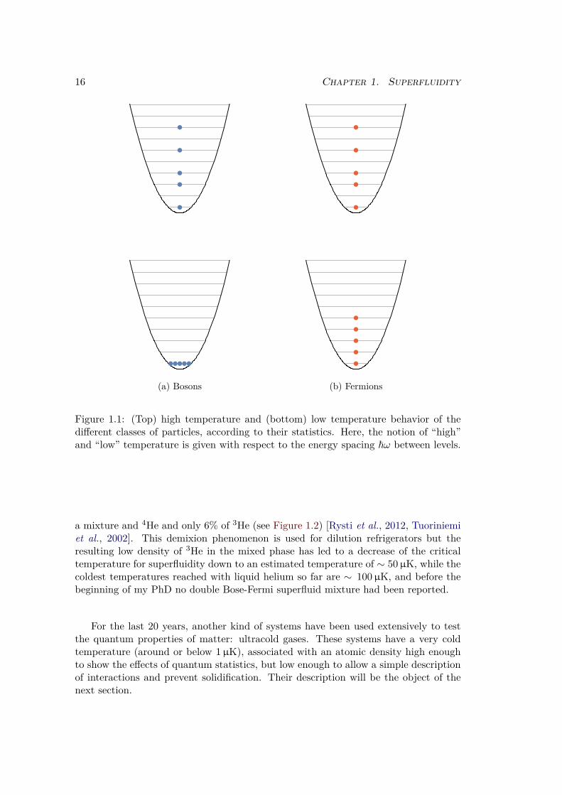
These different behaviors are summed up on Figure 1.1.In liquid helium 4He, interactions are everything but negligible, but the transi-
tion towards superfluidity occurs at a temperature relatively close to the critical onefor Bose-Einstein condensation for a system of non-interacting bosons with the samedensity (3.2 K). Indeed, the superfluidity of 4He can be interpreted as a Bose-Einsteincondensation of interacting bosons.
As for 3He, the origin of its superfluidity is more complex. Indeed, 3He is a fermion,and identical fermions cannot occupy the same energy state. However, two fermionsthat differ, by the value of their spin for example, can be paired up and form a com-posite boson. This is what happens for 3He, and since the critical temperature forpair formation is much smaller than the critical temperature for condensation, thisexplains the very low temperature for superfluidity in 3He (2.6 mK). For supercon-ductivity, this phenomenon is also at play, and electrons pair up in momentum spaceto form Cooper pairs thanks to attractive interactions mediated by the phonons ofcrystalline structure.
The quantum nature of particles thus has an important role for explaining differentbehaviors and phenomena observed in condensed matter. However, one of the difficul-ties in the quantitative understanding and modeling of condensed matter is its density:strong interactions between particles lead to behaviors that are very complicated topredict theoretically. In addition, these interactions can also lead to demixion withinthe superfluid. For instance, while (as indicated above) both 3He and 4He have beensuccessfully cooled down to superfluidity, this has not been the case so far for themixture of 3He and 4He. Indeed, strong interactions between 3He and 4He lead to aphase separation of the system into two phases, one of pure 3He, and the second one of
16 Chapter 1. Superfluidity
(a) Bosons (b) Fermions
Figure 1.1: (Top) high temperature and (bottom) low temperature behavior of thedifferent classes of particles, according to their statistics. Here, the notion of “high”and “low” temperature is given with respect to the energy spacing ~ω between levels.
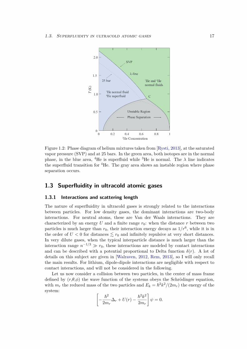
a mixture and 4He and only 6% of 3He (see Figure 1.2) [Rysti et al., 2012, Tuoriniemiet al., 2002]. This demixion phenomenon is used for dilution refrigerators but theresulting low density of 3He in the mixed phase has led to a decrease of the criticaltemperature for superfluidity down to an estimated temperature of ∼ 50µK, while thecoldest temperatures reached with liquid helium so far are ∼ 100µK, and before thebeginning of my PhD no double Bose-Fermi superfluid mixture had been reported.
For the last 20 years, another kind of systems have been used extensively to testthe quantum properties of matter: ultracold gases. These systems have a very coldtemperature (around or below 1µK), associated with an atomic density high enoughto show the effects of quantum statistics, but low enough to allow a simple descriptionof interactions and prevent solidification. Their description will be the object of thenext section.
1.3. Superfluidity in ultracold atomic gases 17
Figure 1.2: Phase diagram of helium mixtures taken from [Rysti, 2013], at the saturatedvapor pressure (SVP) and at 25 bars. In the green area, both isotopes are in the normalphase, in the blue area, 4He is superfluid while 3He is normal. The λ line indicatesthe superfluid transition for 4He. The gray area shows an instable region where phaseseparation occurs.
1.3 Superfluidity in ultracold atomic gases
1.3.1 Interactions and scattering length
The nature of superfluidity in ultracold gases is strongly related to the interactionsbetween particles. For low density gases, the dominant interactions are two-bodyinteractions. For neutral atoms, these are Van der Waals interactions. They arecharacterized by an energy U and a finite range r0: when the distance r between twoparticles is much larger than r0, their interaction energy decays as 1/r6, while it is inthe order of U < 0 for distances . r0 and infinitely repulsive at very short distances.In very dilute gases, when the typical interparticle distance is much larger than theinteraction range n−1/3 ≫ r0, these interactions are modeled by contact interactionsand can be described with a potential proportional to Delta function δ(r). A lot ofdetails on this subject are given in [Walraven, 2012, Rem, 2013], so I will only recallthe main results. For lithium, dipole-dipole interactions are negligible with respect tocontact interactions, and will not be considered in the following.
Let us now consider a collision between two particles, in the center of mass framedefined by (r,θ,φ) the wave function of the systems obeys the Schrödinger equation,with mr the reduced mass of the two particles and Ek = ~
2k2/(2mr) the energy of thesystem:
[
− ~2
2mr∆r + U(r)− ~
2k2
2mr
]
ψ = 0.

18 Chapter 1. Superfluidity
This equation can be solved into
ψ = ψ0 + fk(θ)eikr
r,
where fk(θ) is the scattering amplitude, equal to:
fk(θ) =1k
∞∑
l=0
√
4π(2l + 1)Y 0l (θ)eiδl sin δl,
with Y ml (θ,φ) the spherical harmonics and δl a phase acquired by the wave function
due to the interaction potential. δl is typically very dependent on the details of theinteraction potential. l is a quantum number describing the scattering. For symmetryreasons, for identical bosons, l is necessarily even, while it is odd for identical fermionswith in particular δ0 = 0. There are no restrictions on l for distinguishable particles.Different values of l correspond to different effective scattering potentials Ul, and foreach potential Ul it is possible to define a classical turning point rl, correspond to thedistance at which incoming classical particles with energy E = ~
2k2/(2m) would havea zero kinetic energy. We have:
rl =
√
l(l + 1)k
.
In the low energy limit, corresponding to the low-temperature limit, k → 0, and theresult is that particles scattering with l > 0 feel a repulsive barrier, and the phaseshift δl>0 actually vanishes, δl>0 = 0. We will in the following only consider l = 0scattering, also called s-wave scattering, according to spectroscopic vocabulary. Foridentical fermions, since δ0 = 0, there is thus no collisions in the low temperature limit.For bosons or distinguishable particles, fk is equal to
fk(θ) =1keiδ0 sin δ0,
and we define the scattering length a as:
a = − limk→0
fk = − limk→0
δ0
k.
It is the scattering length that accounts for most scattering properties. To the firstorder in k, the scattering amplitude can be expressed as:
fk(θ) =−a
1 + ika.
The total scattering cross-section σk, equal to σk = 2π´ 2π
0 dθ sin θ|fk(θ) + fk(π− θ)|2,can also be expressed in terms of k:
σk = 4πa2
1 + k2a2
for distinguishable particles, and
σk = 8πa2
1 + k2a2

1.3. Superfluidity in ultracold atomic gases 19
for indistinguishable particles. In the limit of small scattering length, the interactionstrength of the system can be written as:
g =2π~2a
mr.
Let us now discuss the different interaction cases:
• Between two identical fermions, only p-wave interaction occurs and the scatteringcross-section drops to zero as T 2.
• Between two identical bosons, the scattering length abb can take any value. Forsmall values of abb, the interaction energy is given by gbbnb where gbb = 4π~2abb
mb
is the interaction strength. For negative values of abb, interactions are attractiveand may lead to a collapse of the gas for large atom number [Bradley et al.,1997, Sackett et al., 1999, Gerton et al., 2000, Donley et al., 2001, Roberts etal., 2001]. Large values of abb correspond to strong interactions between bosons.This will not be discussed in this thesis, but at the beginning of my PhD weperformed experiments relating the lifetime of a Bose gas with abb → ∞ to thetemperature [Rem et al., 2013, Eismann et al., 2015, Rem, 2013]. In the regimeof the diverging scattering length, called the unitary limit, some predictionswere made by Efimov [Efimov, 1970] regarding the existence of a three-bodybound state for specific values of the two-body scattering length [Kraemer et al.,2006, Berninger et al., 2011], with some log-periodic properties [Huang et al.,2014, Tung et al., 2014, Pires et al., 2014].
• Between two distinguishable fermions, for example between two fermions withdifferent spin states, the scattering length aff can take any value. The regimewhere aff → ∞ is also called the unitary regime, where the scattering cross-section take its maximum value 8π/k2. For fermions, the case aff > 0 correspondsto strong attraction between fermions and leads to the formation of moleculeswith binding energy − ~
2
mfa2ff
. Being formed of two fermions, these molecules
have an integer spin and bosonic behavior. The case aff < 0 corresponds toweak attraction between fermions, as in the Bardeen-Cooper-Schrieffer theoryfor superconductivity. The fermion-fermion interactions will be discussed withmore details in subsection 1.3.3.
• It may also be relevant to consider interactions between a boson and a fermion.In this case, the two colliding particles are obviously distinguishable, and thescattering length abf may take any value.
Let us now look at the effects of interactions on low-temperature gases.
1.3.2 Bose-Einstein Condensates
Realizing a Bose-Einstein condensate (BEC) of ultracold atoms had been a longstand-ing goal in the atomic physics community. This requires to obtain a combinationof temperature and densities such that nλ3
th & 1. A Bose-Einstein condensate withcondensed matter thus requires temperature on the order of 1 K. However, except for

20 Chapter 1. Superfluidity
helium, all other atomic elements undergo solidification at temperatures well above1 K, preventing condensation. Realizing a gaseous BEC thus requires to go to very lowdensities, typically 1014 − 1015 cm−3. At such low densities, the rate of inelastic colli-sions (proportional to n2) is strongly suppressed, with a typical timescale on the orderof a few seconds or minutes. The gas is thus chemically metastable. The rate of elasticcollisions (proportional to n) is still high enough to ensure thermal equilibrium. Thecounterpart is that the Bose-Einstein condensation occurs at even lower temperatures,on the order of 1µK. Advanced cooling and trapping techniques were developed overthe years by the atomic physics community with notably the Nobel Prize in Physics of1997 attributed to W.D. Phillips, S. Chu and C. Cohen Tannoudji “for developmentof methods to cool and trap atoms with laser light”.
The first BECs were realized in 1995 in the teams of E.A. Cornell and C.E. Wieman,and of W. Ketterle, also awarded with the Nobel prize in 2001. They were producedin harmonic traps, and evidence for their production were given by a narrow peak inthe velocity distribution.
To obtain the density distribution in the general case (and for simplicity here inthe T = 0 limit), one should integrate the Gross-Pitaevskii equation:
i~dψ
dt= − ~
2
2mb∆ψ + U(r)ψ + gbb|ψ|2ψ,
where ψ is the wave-function of the BEC, and gbb = 4π~2abb/mb. The terms of theright-hand-side of the equation account respectively for kinetic energy, trapping energy,and interaction energy.
One has to make a distinction between two different regimes: the ideal-gas limit,and the Thomas-Fermi limit. In the ideal gas limit, interactions are negligible withrespect to the trapping potential energies (nbgbb ≪ ~ωx,y,z). If we call U(r) =12mb(ω2
xx2 +ω2
yy2 +ω2
zz2) the harmonic trapping potential, the system is described by
the Schrödinger equation:
i~dψ
dt= − ~
2
2mb∆ψ + U(r)ψ
The BEC wave function is the ground state of the harmonic oscillator and
nb(r) =Nb
π3/2
e−x2/l2ho,x
lho,x
e−y2/l2ho,y
lho,y
e−z2/l2ho,z
lho,z,
where lho,α=x,y,z =√
~
mωαare the harmonic oscillator lengths and Nb the atom num-
ber in the BEC. However, non-interacting BECs are difficult to produce because lowcollision rate leads to a poor thermalization, and in most cases interactions are notnegligible.
In the limit of strong interactions, called the Thomas-Fermi limit, the kinetic energyterm in Schrödinger equation is neglected, and the wave-function obeys:
i~dψ
dt= U(r)ψ + gbb|ψ|2ψ.

1.3. Superfluidity in ultracold atomic gases 21
The atomic density is then
nb(r) =158π
Nb
lT F,x lT F,y lT F,zmax
(
1−(
x2
l2T F,x
+y2
l2T F,y
+z2
l2T F,z
)
,0
)
,
where lT F,α=x,y,z =√
2µb
mω2α
are the Thomas-Fermi radii of the cloud and µb its chemicalpotential. The density distribution thus has a parabolic shape. This expression canbe integrated and inverted to express µb as a function of the other parameters: µ5/2
b =15~2m
1/2b
25/2 Nbωabb, with ω = (ωxωyωz)1/3 the geometric mean of the trapping frequencies.A common technique to image BECs is to release them from the trap, and let themexpand for a few milliseconds of time of flight ttof before imaging them. For cigar-shape harmonic traps as it is the case for our experiment, with ωx ≈ ωy ≈ ωρ ≫ ωz,the initial half-lengths of the BEC x0(t = 0), y0(t = 0), z0(t = 0) are within a ratioz0(0) = ωρ
ωzx0(0) = ωρ
ωzy0(0) and evolve as:
x0(t) = x0(0)√
1 + τ2, (1.1)
y0(t) = y0(0)√
1 + τ2,
z0(t) = z0(0)
(
1 +ω2
z
ω2ρ
(
τ arctan τ − ln√
1 + τ2))
,
where τ = ωρttof . This leads to the inversion of the ellipticity of the clouds for long timeof flights (typically ∼ 10− 100 ms), and allows to measure the velocity distribution oftrapped clouds. In our experiments, we will only use very short time of flights (. 5 ms),so that the cloud does not have time to expand axially. In experiments, we do nothave access to the 3D local density distribution of atoms, but rather to the integrateddensity along one or two directions. The density distributions vary then as:
n(y,z) ∝ max
(
1− y2
l2T F,y
− z2
l2T F,z
,0
)3/2
,
for densities integrated along x direction, and
n(z) ∝ max
(
1− z2
l2T F,z
,0
)2
,
for densities integrated along x and y.Let us now discuss the influence of interactions on BECs. A BEC with attractive
interactions (abb < 0) is unstable and collapses on itself above a critical atom number,on the order of 1000 atoms [Bradley et al., 1997, Sackett et al., 1999, Gerton et al.,2000, Donley et al., 2001, Roberts et al., 2001]. A purely non-interacting BEC is stable,but the absence of collisions prevents thermalization between particles. It is also notsuperfluid because its critical velocity for superfluidity vanishes. For weakly interactingBECs with abb > 0, it was shown [Bogoliubov, 1947] that they have an excitationspectrum compatible with Landau’s criterion for superfluidity and are thus superfluids.This was evidenced by numerous experiments; among the most convincing ones arethose showing the existence of quantized vortices [Matthews et al., 1999, Madison etal., 2000, Abo-Shaeer et al., 2001] and critical velocity [Raman et al., 1999, Onofrio etal., 2000] in a stirred BEC.

22 Chapter 1. Superfluidity
1.3.3 Fermi superfluids
The realization of Fermi degenerate gases (1999) and Fermi superfluids (2004) wasachieved after the first BECs. Fermions are difficult to cool because Pauli principleforbids s-wave collisions, thus preventing thermalization between identical fermions atlow temperature. Standard evaporative cooling techniques cannot be used. There aretwo options to realize the last cooling stages: either by sympathetic cooling, for which abosonic and a fermionic gas are hold in the same trap, and fermions thermalize with thebosons that are evaporatively cooled [Schreck et al., 2001b]. The other option consistsin trapping two fermionic states between which collisions are allowed [DeMarco andJin, 1999]. At the unitary limit, this option has proven to be very efficient, since thescattering cross-section is large and unitary limited.
Two-component Fermi clouds can then be prepared at temperatures well below theFermi energy. The question of whether they are superfluids then depends on the valueof the scattering length. An important parameter for Fermi gases is kFaff , where kF is
the Fermi wave vector of the gas, defined as ~2k2
F2mf
= EF.
For values of aff such that 1kFaff
≫ 1, the system is said to be on the BEC limit.Indeed, strong attraction between fermions lead them to form pairs that then have abosonic behavior and can undergo Bose-Einstein condensation [Zwierlein et al., 2003,Zwierlein et al., 2004].
For values of aff such that 1kFaff
≪ −1, the system is said to be on the BCS limit.Indeed, weak attraction between fermions lead them to form Cooper-like pairs, as de-scribed by the Bardeen-Cooper-Schrieffer (BCS) theory. Pairing occurs in momentumspace, between two particles with opposite momentum.
For values of aff such that∣∣∣
1kFaff
∣∣∣ ≪ 1, the system is said to be unitary. Since the
scattering length, characteristic length for the interactions, diverges, the only relevantlength left in the problem is the interparticle distance n−1/3, and results obtained forsuch a system are applicable for any system with resonant interactions. This is howneutron stars and other complex systems can be simulated with ultracold atoms [Blochet al., 2012]. The equation of state of a unitary Fermi gas at finite temperature hasbeen obtained in [Nascimbène et al., 2010].
(a) BEC regime (b) BCS regime (c) Unitary regime
Figure 1.3: Representation of the three limit regimes of the BEC-BCS crossover.Fermionic pairs are circled in blue. On the BEC side, the typical pair size is smallerthan the interparticle distance, while it is larger on the BCS side. At unitarity, bothlengths are comparable.

1.3. Superfluidity in ultracold atomic gases 23
These three regime span the so-called BEC-BCS crossover. They are representedon Figure 1.3. Superfluidity has been proven in the whole crossover, via the existenceof vortices [Zwierlein et al., 2005], and of a critical velocity [Miller et al., 2007, Weimeret al., 2015, Delehaye et al., 2015]. The nature of the superfluid varies in the crossover,from tightly bound molecules to Cooper pairs [Veeravalli et al., 2008]. A sketch of thisis shown on Figure 1.3. The critical temperature for superfluidity varies as well as afunction of 1/kFaff , from a roughly constant value on the BEC side to an exponentiallysmall value on the BCS side, with a maximum close to 1/kFaff = 0 [Haussmann et al.,2007].
In many experiments, fermions were mixed with bosons, that provided both acooling agent and a convenient thermometer, but it was not until 2014 [Ferrier-Barbutet al., 2014] that a Bose-Fermi superfluid mixture was produced in our group with 6Li(fermions) and 7Li (bosons) atoms. Other fermions involved in Bose-Fermi mixturesare 40K, 87Sr, 173Yb, 161Dy and 53Cr, but so far Fermi superfluids were produced onlywith 6Li and 40K.

24 Chapter 1. Superfluidity

Chapter 2
Lithium Machine and Double Degen-
eracy
2.1 General description . . . . . . . . . . . . . . . . . . . . . . . 26
2.2 Lithium . . . . . . . . . . . . . . . . . . . . . . . . . . . . . . 26
2.2.1 The atom of lithium . . . . . . . . . . . . . . . . . . . . . . . 26
2.2.2 Atomic structure . . . . . . . . . . . . . . . . . . . . . . . . . 28
2.2.3 Feshbach resonances . . . . . . . . . . . . . . . . . . . . . . . 28
2.3 Loading the MOT . . . . . . . . . . . . . . . . . . . . . . . . 33
2.3.1 Oven . . . . . . . . . . . . . . . . . . . . . . . . . . . . . . . . 34
2.3.2 Zeeman slower . . . . . . . . . . . . . . . . . . . . . . . . . . 34
2.3.3 MOT . . . . . . . . . . . . . . . . . . . . . . . . . . . . . . . 36
2.3.4 Laser system . . . . . . . . . . . . . . . . . . . . . . . . . . . 36
2.4 Magnetic trap, transport, and RF evaporation . . . . . . . 37
2.4.1 Optical pumping . . . . . . . . . . . . . . . . . . . . . . . . . 37
2.4.2 Magnetic trap and transport . . . . . . . . . . . . . . . . . . 38
2.4.3 Ioffe-Pritchard trap . . . . . . . . . . . . . . . . . . . . . . . . 38
2.4.4 RF evaporation . . . . . . . . . . . . . . . . . . . . . . . . . . 40
2.5 Optical trap . . . . . . . . . . . . . . . . . . . . . . . . . . . . 41
2.5.1 Generalities on optical traps . . . . . . . . . . . . . . . . . . . 41
2.5.2 Loading the hybrid trap . . . . . . . . . . . . . . . . . . . . . 41
2.5.3 Mixture preparation . . . . . . . . . . . . . . . . . . . . . . . 42
2.5.4 Evaporation . . . . . . . . . . . . . . . . . . . . . . . . . . . . 43
2.5.5 Summary . . . . . . . . . . . . . . . . . . . . . . . . . . . . . 43
2.6 Imaging . . . . . . . . . . . . . . . . . . . . . . . . . . . . . . 44
2.6.1 Absorption imaging . . . . . . . . . . . . . . . . . . . . . . . 44
2.6.2 Imaging system . . . . . . . . . . . . . . . . . . . . . . . . . . 45
2.6.3 Image processing . . . . . . . . . . . . . . . . . . . . . . . . . 46
2.7 Double Degeneracy . . . . . . . . . . . . . . . . . . . . . . . 47
2.7.1 Bosons . . . . . . . . . . . . . . . . . . . . . . . . . . . . . . . 47
25
26 Chapter 2. Lithium Machine and Double Degeneracy
2.7.2 Fermions . . . . . . . . . . . . . . . . . . . . . . . . . . . . . 49
2.8 Conclusion . . . . . . . . . . . . . . . . . . . . . . . . . . . . 50
In our group, we produce ultracold gases of both fermionic and bosonic lithium (6Liand 7Li). In this chapter I will present the historical machine that we use to producethese ultracold gases. It was built by Florian Schreck in 1999 [Schreck, 2002] andrebuilt by Leticia Tarruell in 2004 [Tarruell, 2008]. All of the results described in thisPhD have been obtained with this experiments. Since it has already been describedwith great details in [Schreck, 2002, Tarruell, 2008, Nascimbène, 2010], and no majorchange to the experiment has been made since then, I will not go into deep detailsand refer the interested reader to the PhD theses cited above. First I will give a shortoverview of the main steps of the experiment, then present some specificities of lithiumsuch as the existence of Feshbach resonances, before using these properties to describethe different steps of the experiment.
2.1 General description
For many cold-atom experiments, an initial Magneto-Optical Trap (MOT) stage isfollowed by direct loading of another trap, either optical or magnetic, where evaporativecooling can be performed. However, in the case of lithium, due to a small hyperfinesplitting of the excited states, the temperature at the end of the MOT stage is usually1
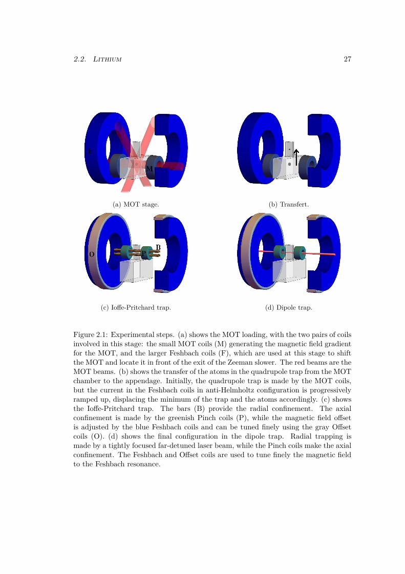
not low enough to load efficiently an optical dipole trap directly after the MOT. Toovercome this issue, we transport the cloud to a small appendage allowing for strongmagnetic gradients. Atoms are transfered in a magnetic Ioffe-Pritchard trap where wedo a first evaporative cooling stage of 7Li, that sympathetically cools down 6Li. Atomsare then transfered into an optical dipole trap where some additional evaporativecooling stages are performed. 6Li atoms are cooled down very efficiently and theysympathetically cool 7Li. At the end of this second evaporative cooling stage, physicsexperiment are performed in a hybrid optical-magnetic trap. The different stages ofthe experiment are shown in Figure 2.1 and will be discussed later in this chapter.
2.2 Lithium
2.2.1 The atom of lithium
Lithium is an alkali with atomic number Z = 3. Its electronic ground state configura-tion is [He]1s1. It has two natural isotopes: 6Li (natural abundance 7.5%) and 7Li (nat-ural abundance 72.5%) and one artificial isotope, 8Li with a half-life of 0.838 s. In thefollowing, we will focus on 6Li and 7Li. Lithium is highly reactive with water and needsspecial care when manipulating to avoid the reaction Li + H2O→ Li+ + HO− + 1/2H2.6Li has six nucleons and three electrons, it is thus a fermion, while 7Li, with seven
1In the case of very large number of atoms and very powerful dipole trap this is however possible,as in the group of Chris Vale in Melbourne, Australia.
2.2. Lithium 27
(a) MOT stage. (b) Transfert.
(c) Ioffe-Pritchard trap. (d) Dipole trap.
Figure 2.1: Experimental steps. (a) shows the MOT loading, with the two pairs of coilsinvolved in this stage: the small MOT coils (M) generating the magnetic field gradientfor the MOT, and the larger Feshbach coils (F), which are used at this stage to shiftthe MOT and locate it in front of the exit of the Zeeman slower. The red beams are theMOT beams. (b) shows the transfer of the atoms in the quadrupole trap from the MOTchamber to the appendage. Initially, the quadrupole trap is made by the MOT coils,but the current in the Feshbach coils in anti-Helmholtz configuration is progressivelyramped up, displacing the minimum of the trap and the atoms accordingly. (c) showsthe Ioffe-Pritchard trap. The bars (B) provide the radial confinement. The axialconfinement is made by the greenish Pinch coils (P), while the magnetic field offsetis adjusted by the blue Feshbach coils and can be tuned finely using the gray Offsetcoils (O). (d) shows the final configuration in the dipole trap. Radial trapping ismade by a tightly focused far-detuned laser beam, while the Pinch coils make the axialconfinement. The Feshbach and Offset coils are used to tune finely the magnetic fieldto the Feshbach resonance.

28 Chapter 2. Lithium Machine and Double Degeneracy
nucleons and three electrons, is a boson. Some of its physical properties are given in[Gehm, 2003].
2.2.2 Atomic structure
Like all alkali atoms, since it only has one valence electron, the atomic structure of Li isquite simple. It is different for each isotope, and is given in Figure 2.2. The ground stateis 22S1/2, and its two lowest excited states are 22P1/2 and 22P3/2. The 22S1/2 → 22P1/2
and the 22S1/2 → 22P3/2 transitions are both in the red, at a wavelength of λ = 671 nm.Reasonably high optical power at 671 nm is available from commercial sources. Thenext excited state, 32P3/2 (not shown in Figure 2.2), can be reached from the groundstate with UV light at λ = 323 nm [Duarte et al., 2011], though we don’t use it in theexperiment. The fine splitting between the 22P1/2 and the 22P3/2 is equal to 10.5 GHz,which is also equal to the isotopic shift. This results in a fortuitous coincidence betweenthe D1 lines of 7Li and the D2 lines of 6Li that is used for the design of the laser system.The fine splitting (∆hf) is indicated in Figure 2.2, as well as the hyperfine splitting. Forthe 22P3/2 (D2 transition from ground state), the hyperfine states cannot be resolvedbecause the width of all excited states is Γ = 5.9 MHz.
Due to the Zeeman effect, the energy of these levels changes when varying themagnetic field B. For the J = 1/2 states, it is possible to solve the perturbationHamiltonian exactly, and one obtains the Breit-Rabi formula [Breit and Rabi, 1931]:
E(mF ) =− ahf
4+gIµB
~mFB
±ahf
(
I + 12
)
2
√√√√√1 +
2µB(gI − gJ)
ahf~
(
I + 12
)2mFB +µ2
B(gI − gJ)2
a2hf~
2(
I + 12
)2B2.
Here mF is the magnetic moment −F ≤ mF ≤ F , ahf is the magnetic dipole momentfor the ground state 22S1/2 and gI (resp. gJ) are the nucleic (resp. electronic) Landég-factor. Their values and other relevant quantities are shown in Table 2.1 for bothisotopes.
This is used to calculate the evolution of the energy of the ground state 22S1/2 sub-levels for both 6Li and 7Li, as shown in Figure 2.3 and Figure 2.42. Please note thatat zero magnetic field (as in Figure 2.2) the Zeeman sub-levels are degenerate. Thenotations introduced in Figure 2.3 and Figure 2.4 will be used in the following to referto the atomic states. Atoms whose energy decreases when increasing the magnetic fieldare called high field seekers, those whose energy increases with magnetic are called lowfield seekers.
2.2.3 Feshbach resonances
The atom of lithium has a very important property: the interatomic interaction can betuned via the use of Feshbach resonances. As indicated in chapter 1, low interactionsbetween atoms are characterized at low energy by the scattering length a between theseatoms. For atoms showing Feshbach resonances, the scattering length can be tuned
2Courtesy from Daniel Suchet

2.2. Lithium 29
S/
P/
P/
S/
P/
P/
=/
=/
=/
=/
=/
=/
=/
=
=
=
=
=
=
=
=
7Licooling
7Lirepumping
6Licooling
6Lirepumping
6Li 7Li
2:λ=6
70,9616nm
1:λ=6
70,9767nm
2:λ=6
70,9774nm
1:λ=6
70,9925nm
Δ f=
Δ f=
Figure 2.2: Schematic representation of 6Li and 7Li atomic structure. Only the firsttwo excited states are shown. The excited state fine splitting is 10.5 GHz for bothisotopes. The wavelengths for the atomic transitions are shown in red, and the green,blue, yellow and dark gray indicate the transitions used to cool the atoms with theZeeman slower and the MOT. The color code for the cooling and repumping frequenciescorrespond to the one we use on the experiment, except that the ‘white’ is shown indark gray here. The width of the excited states is 5.9 MHz.

30 Chapter 2. Lithium Machine and Double Degeneracy
Isotopic properties 6Li 7LiNatural abundance 7.59% 92.4%
Mass 9.99 · 10−27 kg 11.65 · 10−27 kgTotal electronic spin S 1/2 1/2
Total nuclear spin I 1 3/2Hyperfine coupling constant ahf 152.14 MHz 401.75 MHz
Electronic g-factor for ground state gS 2.0023010 2.0023010Nuclear g-factor gI −0.448 · 10−3 −1.182 · 10−3
D1 transition frequency 446.7896 THz 446.8001 THzD2 transition frequency 446.7996 THz 446.8102 THzExcited state linewidth 5.9 MHz 5.9 MHz
Hyperfine splitting of ground state 228 MHz 803.5 MHz
Table 2.1: Some atomic properties of Li
|f ⟩=|=/mF=+/⟩|f ⟩=|=/mF=-/⟩|f ⟩=|=/mF=-/⟩
|f ⟩=|=/mF=-/⟩|f ⟩=|=/mF=+/⟩|f ⟩=|=/mF=+/⟩
=/
=/
-
-
-
()
Δ(
)
Figure 2.3: Energy of the Zeeman sub-levels of the ground state 22S1/2 of 6Li as afunction of magnetic field. The magnetic field vector is chosen as the quantizationaxis.
simply by varying the magnetic field. This property is used both to cool efficiently theatoms and to probe strongly-interacting many-body physics.
The principle of the Feshbach resonances is the following [Walraven, 2012, Dalibard,

2.2. Lithium 31
|b⟩=|=mF=+⟩|b⟩=|=mF= ⟩|b⟩=|=mF=-⟩|b⟩=|=mF=-⟩
|b⟩=|=mF=-⟩|b⟩=|=mF= ⟩|b⟩=|=mF=+⟩|b⟩=|=mF=+⟩
=
=
-
-
()
Δ(
)
Figure 2.4: Energy of the Zeeman sub-levels of the ground state 22S1/2 of 7Li as afunction of magnetic field. The magnetic field vector is chosen as the quantizationaxis.
1999]: consider a collision between two atoms. Each atom has several internal states,and each combination of states is associated to an interaction potential (displayed inFigure 2.5 in the center-of-mass frame). In the general case, the potentials may havebound states. If the only accessible states of a certain potential are bound states, thenthis potential is called a “closed channel”. This is the case of the potential shown inblue in Figure 2.5. However, if scattering levels are accessible for this pair of atoms, thepotential is called an “open channel”,as it is the case for the potential shown in pinkin Figure 2.5. Since the internal states of the particles may change during a collision,these potentials are coupled to each other. Now, in the low energy physics that applywith cold atoms, if two particles collide, they come from a scattering state from anopen channel (then called the “entrance channel”) with an energy E slightly higherthan the dissociation limit of the entrance channel. They interact during the collision,and may go away again from each other. But if there was a level of the closed channelwhose energy was very close to 0 (the energy of the colliding particles), its couplingto the open channel strongly affects the collisional properties of the system, such thatthe scattering length diverges.
And as it turns out, since the internal states depend on the magnetic field, forsome atoms it is possible to tune the energy of the bound channel with respect tothat of the open channel by varying the magnetic field. In other words, we can changethe scattering properties and more particularly the scattering length with the magneticfield. This phenomenon is called a Feshbach resonance [Feshbach, 1958]. In the vicinityof the resonance, a good approximation for the scattering length is given by
a(B) = abg
(
1 +∆B
B −Bres
)

32 Chapter 2. Lithium Machine and Double Degeneracy
open channel
closed channel
0 1 2 3 4 5
-0.6
-0.4
-0.2
0.0
0.2
0.4
()
()
Figure 2.5: Schematic representation of the level crossing that leads to a Feshbachresonance. The blue curve represents a closed channel and its energy states, the pinkcurve an open channel with its energy states, in arbitrary units. We can see that thehighest energy state of the closed channel is very close to zero, the dissociation energyof the open channel. If one of the potentials is sensitive to magnetic field (say theopen channel for instance), it is possible to bring them to the same energy, and thisresults into a resonance phenomenon and a divergence of the scattering length. Thisphenomenon is known as a Feshbach resonance.
where abg is the collisional background scattering length, ∆B the width of the reso-nance, and Bres the magnetic field at resonance.
This phenomenon of Feshbach resonance may appear between two identical bosons,as it is the case for 7Li. 7Li shows a number of Feshbach resonances, some of whichare given in Table 2.2. They have been used in our group to vary the interactionswithin the gas, and to study beyond mean-field effects [Navon et al., 2010], three-bodylosses and Efimov physics [Rem et al., 2013, Eismann et al., 2015]. For 6Li, there is nos-wave collisions for identical fermions3. However, for fermions in two different spinstates, the scattering length may vary and encounter Feshbach resonances, as it is thecase for 6Li. Some of the relevant Feshbach resonances for 6Li are given in Table 2.2.There also exists Feshbach resonances between 6Li and 7Li (see Table 2.3), and eventhough we do not exploit them in the current experiment, we plan to use them withthe new machine4. For the whole range of magnetic fields that we used, the scatteringlength between 6Li and 7Li is roughly equal for all spin states and its value is 40.8 a0,where a0 = 52.9 pm is the Bohr radius.
3And the colder the atoms, the more p-wave collisions can be neglected.4Some of these resonances require to trap low-field seeking states, with a crossed-dipole trap for
instance, currently not implemented in the experiment. The other resonances are around 400 G, buttheir narrowness (they are only a few mG wide) makes them challenging to study with the currentexperiment.

2.3. Loading the MOT 33
Atomic levels abg(a0) Bres (G) ∆B (G)|1b〉 -20.98 738.2 171|2b〉 -18.24 845.5 -4.52
893.7 237.8|1f〉 − |2f〉 -1582 832.2 262.3|1f〉 − |3f〉 -1770 690.43 166.6|2f〉 − |3f〉 -1642 811.2 200.2
Table 2.2: List of Feshbach resonance parameters for the atomic states used in theexperiment, with the notations for the Zeeman states defined in Figure 2.3 and Fig-ure 2.4, from [Chin et al., 2010].
Atomic levels |1f〉 |2f〉 |3f〉 |4f〉 |5f〉 |6f〉|1b〉 230 270 310 530 530 535
550 578 610|2b〉 310 330 380 660 670 680
600 610 660|3b〉 360 390 730 820
670 700|4b〉 450 800
770|5b〉 690 740|6b〉 750 805 860|7b〉 750 800 830|8b〉 700 750 810
Table 2.3: Indications of the magnetic fields (in G) for the Feshbach resonances betweenthe different states of 6Li and 7Li, with the notations for the Zeeman states definedin Figure 2.3 and Figure 2.4. The given magnetic fields are ±10 G approximations.All of the resonances below 500 G have a width below 5 G. However, there are somesufficiently wide resonances between |3b〉 and |4f〉, |5f〉, and between |6b〉 and |1f〉, |2f〉.They are indicated in blue.
2.3 Loading the MOT
The first step of every cold atom experiment is to load a magneto-optical trap (MOT).This trap relies on the use of near-resonant laser beams that acts both as a molassesto slow down the atoms and as a trapping force so that they can be trapped in thelocal minimum of a potential created by a magnetic field. Atoms are thus trappedboth in real space and in momentum space. The source of atoms is usually either anoven (as it is the case here) or a dispenser. They produce a hot atomic vapor that,depending on the atomic species, may be loaded directly into the MOT (for cesium forinstance), or has to be slowed down (as for lithium). Here this is done by a Zeemanslower, but a 2D MOT [Dieckmann et al., 1998] have been used successfully in other
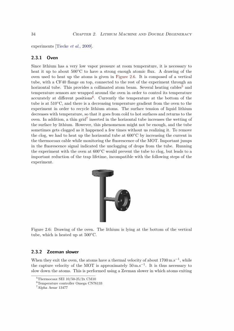
34 Chapter 2. Lithium Machine and Double Degeneracy
experiments [Tiecke et al., 2009].
2.3.1 Oven
Since lithium has a very low vapor pressure at room temperature, it is necessary toheat it up to about 500C to have a strong enough atomic flux. A drawing of theoven used to heat up the atoms is given in Figure 2.6. It is composed of a verticaltube, with a CF40 flange on top, connected to the rest of the experiment through anhorizontal tube. This provides a collimated atom beam. Several heating cables5 andtemperature sensors are wrapped around the oven in order to control its temperatureaccurately at different positions6. Currently the temperature at the bottom of thetube is at 510C, and there is a decreasing temperature gradient from the oven to theexperiment in order to recycle lithium atoms. The surface tension of liquid lithiumdecreases with temperature, so that it goes from cold to hot surfaces and returns to theoven. In addition, a thin grid7 inserted in the horizontal tube increases the wetting ofthe surface by lithium. However, this phenomenon might not be enough, and the tubesometimes gets clogged as it happened a few times without us realizing it. To removethe clog, we had to heat up the horizontal tube at 600C by increasing the current inthe thermocoax cable while monitoring the fluorescence of the MOT. Important jumpsin the fluorescence signal indicated the unclogging of drops from the tube. Runningthe experiment with the oven at 600C would prevent the tube to clog, but leads to aimportant reduction of the trap lifetime, incompatible with the following steps of theexperiment.
Figure 2.6: Drawing of the oven. The lithium is lying at the bottom of the verticaltube, which is heated up at 500C.
2.3.2 Zeeman slower
When they exit the oven, the atoms have a thermal velocity of about 1700 m.s−1, whilethe capture velocity of the MOT is approximately 50 m.s−1. It is thus necessary toslow down the atoms. This is performed using a Zeeman slower in which atoms exiting
5Thermocoax SEI 10/50-25/2x CM106Temperature controller Omega CN761337Alpha Aesar 13477

2.3. Loading the MOT 35
the oven are slowed down by a counter-propagating laser beam. But as soon as theatoms are slowed down, the Doppler effect brings them out of resonance with the laserbeam. A Zeeman slower uses Zeeman effect to get rid of this problem, and creates amagnetic field that compensates the change in resonance frequency of the atoms. Toget a constant deceleration, the magnetic field has to vary with the square-root of thedistance traveled by the atomic beam. Several designs can be used and in our case weuse a spin-flip Zeeman slower, in which the magnetic field goes from +800 G at theentrance of the Zeeman slower to −200 G at the exit. This configuration ensures thatthe laser beams used in the Zeeman slower will be off-resonant for atoms in the MOTand reduces power consumption and heating. Considering now the laser beams, herewe have four frequencies mixed together: two principal and two repumpers.
• The principal light for 6Li, on the D2 line from F = 3/2 to F ′ = 5/2, slows down6Li atoms (shown in green in Figure 2.2).
• The repumper light for 6Li is necessary to recycle the atoms falling into theF = 1/2 level of the ground state. This repumper light is on the D1 line of 6Li(shown in blue in Figure 2.2).
• The principal light for 7Li, on the D2 line from F = 2 to F ′ = 3 slows down 7Liatoms (shown in yellow in Figure 2.2).
• A repumper is also needed for 7Li, to recycle atoms that fell in the F = 1 levelof the ground state, but we cannot use its D1 lines because it would affect 6Li.Repumping is thus made on the D2 line, between F = 1 and F ′ = 2 (shown ingray in Figure 2.2).
All four laser frequencies are recombined on a single mirror just before being sent intothe Zeeman slower tube. The detunings used in the experiment are given in Table 2.4.The detuning of the beams is very robust and almost never needs to be re-optimized8.
7Li Principal -390 MHz7Li Repumper -400 MHz6Li Principal -390 MHz
6Li Repumper -375 MHz
Table 2.4: Detunings used for the Zeeman slower, with respect to the transitionsindicated in Figure 2.2. The detunings are quite large because the magnetic field isvaried from +800 G to −200 G between the two ends of the Zeeman slower and thebeams are resonant with the atoms when they are in the area with B ≃ 0, where theystill have a velocity of about 250 m.s−1.
8Even though a small drift of the alignment may require some minor adjustments from time totime.

36 Chapter 2. Lithium Machine and Double Degeneracy
2.3.3 MOT
At the end of the Zeeman slower, atoms are slow enough to be captured in a magneto-optical trap. It is composed of three pairs of counter-propagating laser beams, orthog-onal to each other, and of a magnetic field gradient. The combination of laser beamsand of the magnetic field traps atoms in real and momentum space. A reading onoptical molasses and magneto-optical traps was given by Jean Dalibard at Collège deFrance, year 2014-2015 (lecture notes are available in French). We have a dual-speciesMOT, and the laser frequencies used follow the same constraints as for the Zeemanslower. The four frequencies (Principal and Repumper for each isotope) are recom-bined on four beam-splitter cubes, resulting into four beams containing each frequency.Three of these beams are the MOT beams and are sent on the atoms, and the lastone is sent on a Fabry-Perot for frequency monitoring. The magnetic field gradientis provided by a pair of coils called the MOT coils, and the MOT is shifted upwardto be located in front of the exit of the Zeeman slower by another pair of coils calledthe Feshbach coils, see Figure 2.1a. We load the MOT for about one minute. At theend of the loading stage, we typically have 4 · 107 6Li atoms and 109 7Li atoms at atemperature of 3 mK. We then switch off the Feshbach coils (that brought the centerof the magnetic trap in front of the Zeeman slower) to do the ‘Shift MOT’. Then theMOT is compressed (CMOT) by bringing the lasers closer to resonance and reducingthe repumper beam intensities. This increases atomic density and decreases tempera-ture, ensuring an increase of the phase-space density and a better loading into the nexttrap, purely magnetic. Detunings and magnetic field gradients for MOT and CMOTstages are summed up in Table 2.5. The detunings have to be re-optimized from timeto time due to slow drifts. After the CMOT, we have Nb ∼ 109, Nf ∼ 4 · 107 atoms ata temperature of T = 600µK.
MOT CMOT7Li Principal -49 MHz -30 MHz
7Li Repumper -38 MHz -21 MHz6Li Principal -35 MHz -8 MHz
6Li Repumper -12 MHz -7 MHzGradient 25 G/cm 25 G/cm
Table 2.5: Detunings and magnetic field gradients used for the MOT and CMOT. Val-ues from May 2015. The detunings are given with respect to the transitions indicatedin Figure 2.2.
2.3.4 Laser system
The frequencies are generated by three master lasers that are locked on atomic transi-tions. However, these master lasers produce a relatively low optical power which hasto be amplified before being sent on the atoms. We use slave diodes9 that are injectedwith a few hundreds of µW and output about 150 mW. These are low-cost diodes
9Hitachi HL6545MG, now available from Thorlabs

2.4. Magnetic trap, transport, and RF evaporation 37
manufactured for DVD players, but their natural output wavelength is approximately660 nm, so they have to be heated at 70C to emit at 670 nm. The lifetime of thesediode is rather short (a few months), so we use optical fibers to be able to replacethem without realigning the rest of the experiment. We have one diode for each of thefrequencies for both the Zeeman slower and the MOT, each of them delivering a totalpower of 40-50 mW on the atoms. We also have two more pre-amplifying slave diodesafter the master laser on the D2 of each isotope. In addition, a high atom numberof 7Li turned out to be critical for the realization of a double-superfluid mixture, wethus had to increase the optical power at the 7Li principal frequencies both for theMOT and the Zeeman slower using Tapered Amplifiers(TAs)10. They are seeded with10-20 mW and produce up to 500 mW of output power, with results in 100-150 mW ofpower available on the atoms11. This cascade of light sources ensures enough opticalpower to perform the experiment, at the price of a relatively poor shot-to-shot stability.
2.4 Magnetic trap, transport, and RF evaporation
2.4.1 Optical pumping
Before loading the atoms into a magnetic trap, we have to prepare them in the rightspin states: since Maxwell’s equations prevent a local maximum of static magneticfield, we can only trap atoms polarized in low-field seeking states. Since we alsowant them to be stable against spin-exchange collisions, the only acceptable states are|F = 2,mF = +2〉 for 7Li and |F = 3/2,mF = +3/2〉 for 6Li (indicated as |8b〉 and |6f〉in Figure 2.4 and Figure 2.3, respectively). However, at the end of the CMOT stage,atoms are in F = 1/2 (for 6Li) and F = 1 (for 7Li), and are evenly distributed in theZeeman sub-levels |1f〉, |2f〉 and |1b〉, |2b〉, |3b〉12. It is thus necessary to perform anoptical pumping stage.
Optical pumping is realized with a beam with σ+ light, with respect to a weak(≈10 G) guiding magnetic field, in which two frequencies are mixed. One of the fre-quencies is used to transfer 7Li from F = 1 to F = 2 via the F ′ = 2 state of the D2
transition and realizes the so-called ‘hyperfine’ pumping for 7Li. It is tuned to theF = 1→ F ′ = 2 transition at zero magnetic field. The other frequency has two roles:first, it pumps the 7Li atoms of the F = 2 manifold to |F = 2,mF = 2〉 state throughthe F ′ = 2 state of the D1 transition and realizes the ‘Zeeman’ optical pumping for7Li. The pumping is made on the D1 transition in order not to disturb the hyper-fine pumping. Second, it also pumps 6Li atoms from the F = 1/2 to the F = 3/2manifold, via the F ′ = 3/2 state of the D2 transition, for the hyperfine pumping of6Li. The detuning for that frequency results from a compromise between these tworoles, and simultaneous optimization of 6Li and 7Li atom numbers leads to a detuningof −45 MHz for the F = 2 → F ′ = 2 D1 transition for 7Li and of +25 MHz for the
10We use TA chips from Toptica installed in a home-designed mount.11180 mW in the best conditions. The high fraction of lost power is due to a non-gaussian output
mode of the Tapered Amplifier which makes its coupling into a polarization-maintaining single modefiber challenging. In addition, the total output power slowly decays from 500 mW to 300 mW.
12During CMOT, the intensities of the repumpers are decreased to zero. Atoms thus accumulate inthe F = 1/2 (for 6Li) and F = 1 (for 7Li) states.

38 Chapter 2. Lithium Machine and Double Degeneracy
F = 1/2 → F ′ = 3/2 D1 transition for 6Li. There is no Zeeman optical pumping for6Li because the number of 6Li atoms is not critical at that stage of the experiment.The full optical pumping sequence lasts 300µs, long enough to give time to magneticfields to stabilize, but short enough not to heat up the clouds. A summary of theoptical pumping parameters is given in Table 2.6. Its efficiency is about ∼ 60%.
Isotope Pumping type Transition Detuning (MHz)7Li Hyperfine D2 F = 1→ F ′ = 2 0
Zeeman D1 F = 1→ F ′ = 2 -456Li Hyperfine D2 F = 1/2→ F ′ = 3/2 +25
Zeeman
Table 2.6: Parameters for the optical pumping. The detunings are given with respectto the transitions indicated in Figure 2.2.
2.4.2 Magnetic trap and transport
2.4.2.1 Magnetic trap
Once the atoms are prepared in the right magnetic states, they are loaded into aquadrupole magnetic trap. The trap is realized by the MOT coils with current inopposite directions (as in anti-Helmholtz configuration) and is ramped on in 2 ms.Since the same coils are used for the MOT stage and for the quadrupole trap, at theend of the MOT the atoms are already at the center of the quadrupole trap. Weuse the maximum available current of 500 A, leading to a magnetic field gradient of335 G.cm−1. The number of trapped atoms are Nf = 7 · 107 and Nb = 7 · 108 at atemperature of ∼ 2 mK. Loading efficiency is about 60 %.
2.4.2.2 Magnetic transport
The clouds now have to be transported inside the appendage, an additional very thinpart of the cell that allow the realization of very strong magnetic field gradients. Thisis done by moving the center of the magnetic trap: the Feshbach coils, whose center islocated inside the appendage, are ramped on in anti-Helmholtz configuration while thecurrent of the MOT coils is decreased to zero in 500 ms. The current in the MOT coilsis finally reversed to give a final push to the atoms and center them in the appendage.The overall efficiency of the transfer is about 40 %, mainly because part of the cloudis cut by the walls of the appendage. A scheme of this stage is given in Figure 2.1b.
2.4.3 Ioffe-Pritchard trap
The simplest trapping magnetic configuration is the quadrupole trap realized usinganti-Helmholtz coils in which atoms are confined near the magnetic field zero. However,this design suffers from Majorana losses when temperature is decreased: close to azero of magnetic field, atoms might undergo a spin flip and go from a low-field seeking

2.4. Magnetic trap, transport, and RF evaporation 39
trapped state to a high-field seeking anti-trapped state... To overcome this issue, severalpossibilities have been used in the cold atom community:
• The Time Orbiting Potential (TOP) trap, where the minimum of the magneticfield is rotated fast enough so that the atoms don’t notice, and see on average anon-zero magnetic field minimum [Petrich et al., 1995, Anderson et al., 1995].
• The plug, where the position of the magnetic field zero is plugged by a blue-detuned laser beam that repel the atoms from the center [Davis et al., 1995a].
• The Ioffe-Pritchard trap, which have a non-zero minimum, and is the solutionthat was used in our experiment [Pritchard, 1983].
In our experiment, the Ioffe-Pritchard trap is made of four bars parallel to the zdirection that realize a tight radial confinement, of a pair of coils called the PinchCoils to realize the axial confinement. Another pair of coils (that turns out to be theFeshbach coils used for the magnetic transport) is used to tune the bias field, so thatthe bias field is high enough to prevent Majorana losses, and low enough not to reducethe radial confinement. It can be finely adjusted using a third pair of coils called Offsetcoils. A scheme of the trap is given in Figure 2.1c.
The loading of the Ioffe-Pritchard trap is not so straightforward due to the differentshapes of the traps: the quadrupole trap at the end of the transport has an aspectratio of 2, the axial direction z being more confined than the radial ones x and y, whilethe cloud in the Ioffe-Pritchard trap will have an elongated, cigar-like shape with amuch higher aspect-ratio. To ensure good loading efficiency, the cloud is deformed atthe end of the transport by switching on the current in the bars. This has to be doneabruptly to avoid any cancellation of the confinement in one of the radial directions13.The pinch coils are then ramped up while decreasing the quadrupole to ensure thataxial confinement is always present. The efficiency of the transfer in the Ioffe-Pritchardtrap is hard to evaluate because we cannot count reliably the atoms at this stage: theclouds are too dense.
2.4.3.1 Doppler cooling
After the Ioffe-Pritchard trap loading, the atoms have a temperature of 3 mK. Unfor-tunately, the collisional scattering cross-section for 7Li vanishes for a relative collisionenergy of 6 mK and at 3 mK it is still too low to ensure efficient evaporation. It is thusnecessary to add another cooling stage of 7Li.
A single beam with σ+ polarization slightly red-detuned from the the D2 transition|F = 2,mF = 2〉 → |F ′ = 3,m′
F = 3〉 of 7Li is thus sent on the atoms. This beam coolsin one direction, and thermalization in the other directions is ensured by the collisionsin the quadrupole trap [Suchet et al., 2015]. Doppler cooling is made in two stages of1 s, and the trap is re-compressed between the first and the second stage by increasingthe bias field to optimize overall cooling. At the end of the Doppler cooling, the
13The 3D quadrupole made by the Feshbach coils have a magnetic field given by B = b′(−xex−yey +2zez) while the 2D quadrupole made by the bars have a magnetic field given by B = G(xex − yey),with b′ and G positive. When increasing the bars’ current, G increases, and when G = b′, there is nomore confinement in the x direction.

40 Chapter 2. Lithium Machine and Double Degeneracy
temperature is about 300µK, at the price of 25% atom loss, and the collision rate ofabout ∼ 15 s−1 is now sufficiently high to allow efficient evaporative cooling [Schrecket al., 2001a]. The efficiency of the Doppler cooling is very sensitive to the detuning,which itself is function of the magnetic fields. In practice, the optimization is empiricaland has to be redone daily.
2.4.4 RF evaporation
Evaporative cooling consists in removing the hottest atoms from an assembly of atomsand in letting the remaining atoms thermalize at a lower temperature [Ketterle andDruten, 1996]. Since the hot atoms are at the tail of the Maxwell-Boltzmann distri-bution, they carry a significant amount of energy, and this loss of hot atoms actuallyleads to an increase of phase-space density. There exist two main situations to performevaporative cooling: either in a magnetic trap, where a finely tuned RF signal transfersthe hot atoms from a trapped to an anti-trapped state [Hess, 1986, Masuhara et al.,1988, Anderson et al., 1995, Davis et al., 1995a], or in an optical trap, where the depthof the potential can be lowered so that the hot atoms escape the trap. The latter will beused later in the experiment, and the former is the one used here. This is the last cool-ing stage of 7Li, that will sympathetically cool 6Li: Pauli blocking prevents collisionsbetween fermions in the same spin state, but collisions between 6Li and 7Li are allowedand are frequent enough to ensure good thermalization between 6Li and 7Li. This stageis realized in the Ioffe-Pritchard trap with a low bias field and radio-frequency (RF)field [Pritchard et al., 1989, Davis et al., 1995b] that transfer the hottest 7Li atomsfrom the trapped |F = 2,mF = 2〉 state to the anti-trapped |F = 1,mF = 1〉 state. Inthe process, the remaining 7Li atoms thermalize together and cool as well the 6Liatoms. The evolution of the RF frequency with respect to time follows approximatelya decaying exponential and goes from 1050 MHz down to 840 MHz in 22 s. At the endof this stage, the temperature is T = 12µK, with Nf = 2 · 106 and Nb = 6 · 105, witha phase-space density of 10−1 for 6Li and 2 · 10−2 for 7Li and it is possible to load theatoms into an optical dipole trap for the final cooling stages. The evolution of the RFfrequency as a function of time during evaporation ramp is shown in Figure 2.7.
0 5 10 15 20
0
50
100
150
200
()
(
)
Figure 2.7: RF frequency as a function of time during radio-frequency (RF) evaporativecooling.

2.5. Optical trap 41
2.5 Optical trap
The final trap is a cigar-shaped trap composed of a far-detuned (λ = 1070 nm) opticaldipole trap14 that provides the radial trapping, and of a magnetic trap that providesaxial trapping. A bias field of about 800-1000 G is also applied to be in the vicinity ofFeshbach resonances. This final trap is represented in Figure 2.1d.
2.5.1 Generalities on optical traps
In the presence of a laser beam with frequency close to an atomic transition, atomsexperience an AC Stark Shift proportional to the laser’s intensity, and this correspondsto a potential of
V (r) =~Γ2
8δI(r)Is
,
where Γ is the natural linewidth of the transition (Γ = 5,9 MHz in the case of Li), δis the detuning of the laser with respect to the transition (δ = −2π · 1.67 · 1014 Hz fora λ0 = 1070 nm laser beam for a transition at λ = 670 nm), I(r) is the laser beamintensity, and Is is the saturation intensity (here for the D2 line of Li the representativesaturation intensity is Is = 2.5 mW.cm−2). For a TEM00 laser beam at the output ofan optical fiber, the mode is Gaussian and
I(x,y,z) =2P
πw20(1 + z2/z2
R)exp
(
− 2(x2 + y2)w2
0(1 + z2/z2R)
)
,
where P is the total laser power, w0 is the beam waist (w0 = 27(2)µm in our exper-iment), and zR = πw2
0/λ0 is the Rayleigh range (zR = 2,1 mm here). Close to thebottom of the trap, at the first-order approximation, the potential is harmonic with
V (x,y,z) = −U0 +12mω2
r (x2 + y2) +12mω2
zz2,
with
U0 =~γ2P
4πδIsw20
,
ωr =
√
4U0
mw20
,
ωz =1
2πλ0
w20
ωr.
2.5.2 Loading the hybrid trap
The geometry of the final hybrid optical-magnetic trap is similar to that of the Ioffe-Pritchard trap, so no sophisticated mode-matching preparation is needed here. Wesimply ramp up the optical trap power up to 40% of its maximum power while rampingdown the current in the Ioffe-Pritchard bars. The loading efficiency is about 80% and
14IPG laser 120 W

42 Chapter 2. Lithium Machine and Double Degeneracy
Nf = 1.8 ·106 and Nb = 5 ·105 after loading. The optical trap power is then about 8 W,with a waist of w0 = 27(2)µm, leading to trap frequencies of ωr ≃ 2π · 8 kHz for theradial direction and ωz ≃ 2π · 75 Hz for the axial direction15. At high laser power, theaxial confinement provided by the dipole trap is sufficient to trap the atoms, but thisis not the case any more at low trap power, where it falls below 1 Hz. Some extra axialconfinement is needed, and this is realized via a magnetic trap. To axially trap atoms,there are two possibilities: either a global minimum of the magnetic field (to trap low-field seekers), or a saddle point with a maximum in the axial direction and a minimumin the radial direction (to trap high-field seekers if radial confinement is obtained byother means). The atomic levels that we want to use for 6Li are high field seekers, sothe second option is preferred: the radial confinement is made by the optical trap. Itis thus possible to tune independently the radial and the axial confinement. To obtainsuch a saddle point, we use two pairs of coils: the curve coils (already used in the Ioffe-Pritchard trap) produce a magnetic curvature of 1.0 G.(cm2)−1.A−1 and a bias fieldof 2.28 G.A−1. The Feshbach coils, with current in the other direction, produce a biasfield of −2.28 G.A−1 and a very small curvature of −0.080 G.cm−2.A−1. By imposinga large current in the Feshbach coils, the minimum of magnetic field becomes negative,and becomes a maximum in amplitude, trapping the high-field seeking states. Withthis configuration, it is thus possible to trap high-field seekers states at a bias field of832 G, in the vicinity of the Feshbach resonance.
2.5.3 Mixture preparation
Once the atoms are loaded into the optical dipole trap, we ramp up the optical trappower to its maximum value and transfer the atoms to the high-field seekers states,F = 1 for 7Li and F = 1/2 for 6Li. This is done using adiabatic passage. We applytwo RF frequencies, of 827 MHz (for 7Li) and 240 MHz (for 6Li) and vary the biasmagnetic field from 13 G to 4 G in 50 ms, crossing the resonance and transferring theatoms into the desired states. This RF transfer is very robust and never needs to bere-optimized.
Ultimately, we want to have 7Li atoms in the |2b〉 state and the 6Li atoms in amixture of the |1f〉 and the |2f〉 state, while so far the atoms are in |1b〉 and |1f〉,respectively. We first prepare 7Li. The transfer has to be done at a magnetic fieldbelow 738 G to avoid crossing of the Feshbach resonance of the |1b〉 state. We increasethe current in the Feshbach coils up to a magnetic field of 656 G, and perform anotherRAP, but this time varying the RF frequency from 170.9 MHz tp 170.7 MHz, crossingagain the resonance since the frequency of the transition |1b〉 → |2b〉 is 170.8 MHz atthat magnetic field. The ramp is long enough (10 ms) to ensure a complete transferof 7Li atoms into the |2b〉 state. To prepare the 6Li atoms into the desired states,the magnetic field is further ramped to 835 G, very close to the Feshbach resonanceat 832 G. We then perform a last RF sweep from 76.30 MHz and 76.25 MHz (aroundthe transition frequency of |1f〉 and |2f〉), but instead of doing an adiabatic passage,
15We have to operate the laser at full power to obtain a clean TEM00 output mode. To reduce thispower to lower intensities, we first use a Brewster plate that reflects most of the laser power so thatthe maximum optical power that can be sent on the atoms is about 20 W. We finally adjust the powerduring the experimental sequence with a high-power Acousto-Optic Modulator (AOM).

2.5. Optical trap 43
we make a partial Landau Zener sweep: the sweep time is too short for a full transfer,only part of the atoms are transferred from |1f〉 to |2f〉. We can thus control the ratioof |1f〉 with respect to |2f〉 by varying the sweep time. The fermionic polarization, orsimply polarization, is defined as
P =N↑ −N↓N↑ +N↓
,
where |↑〉 = |1f〉 or |2f〉 is the atomic state with the highest number of atoms N↑ and|↓〉 the one with the smallest atom number N↓. The transfer efficiency is subject tofluctuations and the sweep time has to be re-optimized from time to time. A summaryof the different RF pulses is shown in Table 2.7.
Isotope B (G) νRF (MHz) Action7Li 13→ 4 827 |8b〉 → |1b〉6Li 13→ 4 240 |6f〉 → |1f〉7Li 656 170.9→ 170.7 |1b〉 → |2b〉6Li 835 76.30→ 76.25 |1f〉 → (|1f〉+ |2f〉)
Table 2.7: Summary of the RF sweeps performed to prepare the mixture.
2.5.4 Evaporation
After the mixture preparation, the magnetic field is held at 835 G and the opticalevaporation is performed by ramping down the dipole trap power. We now haveNb = 2 · 105 bosons and Nf = 1.5 · 106 fermions. The unitary Fermi gas has there avery high collisional cross section and the evaporation is very efficient. The evaporationramp lasts for 3.2 s, the evolution of the laser power as a function of time duringevaporation is shown in Figure 2.8. At the end of the evaporation we have typicallyNb = 10−20·103, Nf = 60−100·103 for a temperature . 80 nK. 7Li is sympatheticallycooled during the process. To ensure complete thermalization between 6Li and 7Li,one needs to wait about 1 s after the end of the evaporation before performing furtherexperiments on the mixture.
When we want to perform experiments at 860 G with bosons in the |2b〉 state, wehave to evaporate at 860 G in order not to cross the 7Li Feshbach resonance at 845 Gwith a cold cloud. The evaporation ramp is then slightly longer to allow for enoughthermalization.
2.5.5 Summary
By means of different magnetic and optical traps, we are thus able to produce ultracoldsamples of bosons and fermions. A summary of atom numbers and temperaturesat each step is given in Table 2.8. The bosons are condensed into a Bose-EinsteinCondensate (BEC), as it is obvious from the clear peak in the density profiles. Thesuperfluidity of the fermions is harder to demonstrate, but several proofs will be givenin the following chapters (chapter 3 and chapter 4). The data obtained on the clouds are

44 Chapter 2. Lithium Machine and Double Degeneracy
0.0 0.5 1.0 1.5 2.0 2.5 3.0 3.5
0
10
20
30
40
50
()
(%
)
Figure 2.8: Laser power as a function of time during optical evaporative cooling.
taken in the form of absorption images of the cloud. This technique will be describedin the next section.
MOT CMOT Quadrupole RF evaporation optical evaporation optical evaporation(end) (beginning) (end)
Nb 109 109 4 · 108 6 · 105 2 · 105 20 · 103
Nf 4 · 107 4 · 107 2 · 107 6 · 106 1.5 · 106 200 · 103
T 3 mK 600µK 2 mK 12µK 40µK 80 nK
Table 2.8: Summary of typical atom numbers and temperatures at the different stagesof the experiment.
2.6 Imaging
2.6.1 Absorption imaging
We use standard in situ absorption imaging to image the clouds by shining on itresonant light. Atoms absorb the photons and the shadow of the cloud is captured bya camera (“absorption image”). The atoms that absorbed a photon are now excitedand escape the trap. Another image is then taken after a wait time of 10-20 ms withoutthe atoms (“reference image”). A scheme of the imaging process is shown in Figure 2.9.
If we note y the imaging direction, Ia(x,z) the intensity of the absorption image inthe x− z plane, and Ir(x,z) that of the reference image. The optical density OD(x,z)is then given by
OD(x,z) = − ln(Ia(x,z)Ir(x,z)
)
,
and the optical density is itself related to the number of atoms via the relation
OD(x,z) = σ
ˆ
dyn(x,y,z),
where n(x,y,z) is the atomic density of the cloud and σ the absorption cross-section ofone atom. The cross-section at resonance is known as a function of Clebsch-Gordan

2.6. Imaging 45
Figure 2.9: Imaging process: a resonant beam is shone on the atoms, their shadowis cast on a camera (“absorption image”), before a second image, without the atoms(“reference image”) is taken. The cloud is shown here in purple, the CCD camera isthe blue-and-white grid, and the imaging beam is shown in red.
coefficients and can be calculated. However, because of complex optical pumping-likephenomena and of some experimental difficulties (such as the relatively large spec-tral bandwidth of the laser, on the order of a few hundred kilohertz, some polariza-tion fluctuations, or the acceleration of detected atoms increased by the lightness oflithium), the scattering cross-section is reduced and we have to calibrate it experimen-tally. This has been done by measuring the Thomas-Fermi radius for both bosons andfermions: the relation between the total atom number and the Thomas-Fermi radius iswell known, and this procedure gives access to the imaging correction factor [Ferrier-Barbut, 2014]. We only image in the linear absorption regime, when the optical densityis . 1, so that no additional correction to the atom number needs to be taken intoaccount [Reinaudi et al., 2007]. A consequence of this low-intensity imaging is that wecannot image very dense clouds. This can be circumvented using a short time-of-flight,as will be discussed below.
2.6.2 Imaging system
Our imaging system allows to image in two orthogonal directions. One of the imagingdirections is along the dipole trap direction z, while the other one is along y. Imagingin the z direction requires some time of flight to reduce the optical density (typically onthe order of 4 ms), while imaging in the y direction can be done in situ, even thoughwe usually have a very short time of flight (on the order of 100µs) to reduce theoptical density. However, the radial dimensions of the cloud are on the order of theimaging resolution, about 5µm and no information is lost by integration also along the
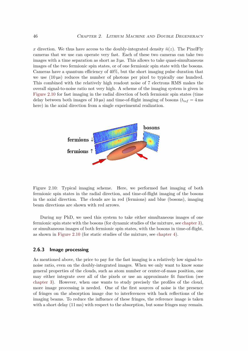
46 Chapter 2. Lithium Machine and Double Degeneracy
x direction. We thus have access to the doubly-integrated density n(z). The PixelFlycameras that we use can operate very fast. Each of these two cameras can take twoimages with a time separation as short as 3µs. This allows to take quasi-simultaneousimages of the two fermionic spin states, or of one fermionic spin state with the bosons.Cameras have a quantum efficiency of 40%, but the short imaging pulse duration thatwe use (10µs) reduces the number of photons per pixel to typically one hundred.This combined with the relatively high readout noise of 7 electrons RMS makes theoverall signal-to-noise ratio not very high. A scheme of the imaging system is given inFigure 2.10 for fast imaging in the radial direction of both fermionic spin states (timedelay between both images of 10µs) and time-of-flight imaging of bosons (ttof = 4 mshere) in the axial direction from a single experimental realization.
Figure 2.10: Typical imaging scheme. Here, we performed fast imaging of bothfermionic spin states in the radial direction, and time-of-flight imaging of the bosonsin the axial direction. The clouds are in red (fermions) and blue (bosons), imagingbeam directions are shown with red arrows.
During my PhD, we used this system to take either simultaneous images of onefermionic spin state with the bosons (for dynamic studies of the mixture, see chapter 3),or simultaneous images of both fermionic spin states, with the bosons in time-of-flight,as shown in Figure 2.10 (for static studies of the mixture, see chapter 4).
2.6.3 Image processing
As mentioned above, the price to pay for the fast imaging is a relatively low signal-to-noise ratio, even on the doubly-integrated images. When we only want to know somegeneral properties of the clouds, such as atom number or center-of-mass position, onemay either integrate over all of the pixels or use an approximate fit function (seechapter 3). However, when one wants to study precisely the profiles of the cloud,more image processing is needed. One of the first sources of noise is the presenceof fringes on the absorption image due to interferences with back reflections of theimaging beams. To reduce the influence of these fringes, the reference image is takenwith a short delay (11 ms) with respect to the absorption, but some fringes may remain.
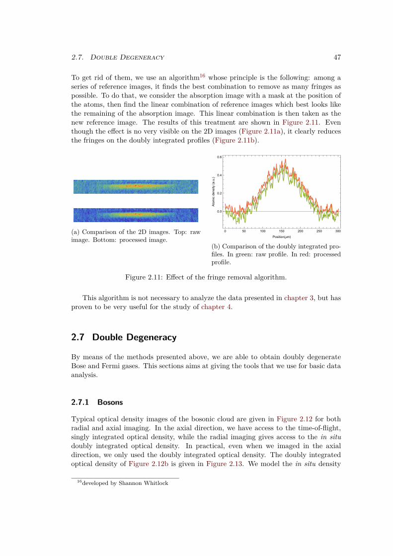
2.7. Double Degeneracy 47
To get rid of them, we use an algorithm16 whose principle is the following: among aseries of reference images, it finds the best combination to remove as many fringes aspossible. To do that, we consider the absorption image with a mask at the position ofthe atoms, then find the linear combination of reference images which best looks likethe remaining of the absorption image. This linear combination is then taken as thenew reference image. The results of this treatment are shown in Figure 2.11. Eventhough the effect is no very visible on the 2D images (Figure 2.11a), it clearly reducesthe fringes on the doubly integrated profiles (Figure 2.11b).
(a) Comparison of the 2D images. Top: rawimage. Bottom: processed image.
0 50 100 150 200 250 300
0.0
0.2
0.4
0.6
Position(μm)
Atomicdensity(a.u.)
(b) Comparison of the doubly integrated pro-files. In green: raw profile. In red: processedprofile.
Figure 2.11: Effect of the fringe removal algorithm.
This algorithm is not necessary to analyze the data presented in chapter 3, but hasproven to be very useful for the study of chapter 4.
2.7 Double Degeneracy
By means of the methods presented above, we are able to obtain doubly degenerateBose and Fermi gases. This sections aims at giving the tools that we use for basic dataanalysis.
2.7.1 Bosons
Typical optical density images of the bosonic cloud are given in Figure 2.12 for bothradial and axial imaging. In the axial direction, we have access to the time-of-flight,singly integrated optical density, while the radial imaging gives access to the in situdoubly integrated optical density. In practical, even when we imaged in the axialdirection, we only used the doubly integrated optical density. The doubly integratedoptical density of Figure 2.12b is given in Figure 2.13. We model the in situ density
16developed by Shannon Whitlock

48 Chapter 2. Lithium Machine and Double Degeneracy
(a) Axial direction.Time of flight 4 ms.
(b) Radial direction.Time of flight 100µs.
Figure 2.12: Singly integrated optical density images of bosonic clouds.
profile of a thermal cloud at temperature T by17
nth(z) = nth(0) exp
(
−(z − z0)2
z2th
)
, (2.1)
where z0 is the position of the center of the cloud, and zth its thermal width, given by
kBT =12mbω
2zz
2th.
The measurement of the width of the thermal cloud thus gives access to the tempera-ture of the whole cloud.
In the Thomas-Fermi limit, the doubly-integrated profile of the condensate can bedescribed by
nc(z) = nc(0) max
(
1− (z − z0)2
l2T F,z
)2
,0
, (2.2)
where lT F,z =√
2µb
mbω2z
is the Thomas-Fermi radius of the cloud and has already beendefined in subsection 1.3.2. Density profiles of partly condensed clouds can be fittedusing a bimodal fit, taking into account the thermal cloud with equation (2.1) and thecondensate with equation (2.2). This gives access to both the temperature, via thegaussian fit, and to the condensed fraction Nc/Nb. The relation between condensedfraction and temperature, Nc/Nb = 1− (T/Tc,b)3, provides a consistency check of thetemperature measurement.
Figure 2.13 shows the doubly integrated of a relatively hot cloud and its associatedbimodal fit, corresponding to a temperature of 230 nK.
For our coldest clouds, no thermal fraction is visible (see Figure 2.14 for instance),and we assure that the condensed fraction is above 90 %. This implies that the tem-perature is below 80 nK.
17Even though a description by a polylog function would be more accurate, this one gives similarresults and converges faster.

2.7. Double Degeneracy 49
(l)
(l
- )
Figure 2.13: Doubly integrated density profile of a relatively hot bosonic cloud. Blueline: experimental profile. Dashed black line: bimodal fit of the density distribution.Here, the temperature extracted from the thermal cloud width is 233 nK, while thecondensed fraction is ∼ 50 %, corresponding to a temperature of 238 nK.
-
(l)
(l
- )
Figure 2.14: Doubly integrated density profile of a cold bosonic cloud. Blue line:experimental profile. Dashed black line: bimodal fit of the density distribution. Nothermal fraction is visible, corresponding to a cloud at a temperature below 80 nK.
2.7.2 Fermions
The shape of the density profile of a two-component Fermi cloud depends on the inter-action strength kFaff : on the deep BEC side, the density profile will be the same as thatof an atomic BEC, while at unitarity it will have the same shape as a non-interactingFermi gas, but there is no analytical expression in the general case. Moreover, thereis no obvious modification of the profile when crossing the critical temperature forsuperfluidity, as it was the case for the bosons with the appearance of the BEC peak.However, in the regimes studied in this thesis, we stayed relatively close to unitar-ity (|1/kFaff < 1), and the profile of the Fermi gas could be well described by theThomas-Fermi profile of a unitary Fermi gas:
nf(z) = nf(0) max
(
1− (z − z0)2
l2T F,z
)5/2
,0
,
where here the Thomas-Fermi radius lT F,z is given by lT F,z = ξ1/4√
2EFmfω2
z. An example
of the fit of the profile is given in Figure 2.15. The Fermi cloud profile does not giveaccess to its temperature, but since it is in equilibrium with the bosonic cloud, theyhave the same temperature. The Bose gas thus acts as a thermometer for the Fermigas. As a result, the temperature for cold Fermi gases is below 80 nK, which is below

50 Chapter 2. Lithium Machine and Double Degeneracy
the critical temperature for superfluidity at unitarity Tc,f = 0.19TF = 170 nK. TheFermi cloud is thus superfluid.
(l)
(l
- )
Figure 2.15: Doubly integrated density profile of a fermionic cloud. Red line: experi-mental profile. Dashed black line: Thomas-Fermi fit of the density distribution.
2.8 Conclusion
In this chapter we have presented the lithium experiment. Some visitor in the labonce said that “this experiment contain[ed] every textbook cooling stage” used in coldatoms. This is not such a big exaggeration. Learning how to run the machine is thusa tough task, but is a good way to learn how to cool and trap atoms. The majorspecificity of this experiment is the use of crossed-thermalization in two evaporativecooling stages, the first one where 7Li cools 6Li, and the second one where 6Li cools 7Li.This way, we could obtain a double Bose-Fermi superfluid mixture of 6Li and 7Li whichwas a long sought goal of the helium community. As will be described in chapter 3,we could for instance probe the effect of the Bose-Fermi interaction on the collectiveexcitations of the mixture and use this interaction to explore the critical velocity ofthe superfluid mixture. However, some of the parts of this lithium experiment start tobe very old, and it was time to build a new experiment that would be more versatileand reliable. I started this project during my PhD and it is describe in chapter 5.

2.8. Conclusion 51

52 Chapter 2. Lithium Machine and Double Degeneracy

Chapter 3
Collective modes of the mixture
3.1 Dipole modes excitation . . . . . . . . . . . . . . . . . . . . 55
3.1.1 The mixture . . . . . . . . . . . . . . . . . . . . . . . . . . . 55
3.1.2 Selective excitation of dipole modes . . . . . . . . . . . . . . 56
3.1.3 Kohn’s theorem . . . . . . . . . . . . . . . . . . . . . . . . . . 57
3.2 Low temperature, low amplitude . . . . . . . . . . . . . . . 58
3.2.1 Experiments . . . . . . . . . . . . . . . . . . . . . . . . . . . 58
3.2.2 Bose-Fermi interaction . . . . . . . . . . . . . . . . . . . . . . 60
3.2.3 Sum-rule approach . . . . . . . . . . . . . . . . . . . . . . . . 62
3.2.4 Two coupled-oscillators model . . . . . . . . . . . . . . . . . . 65
3.3 Low temperature, high amplitude . . . . . . . . . . . . . . 66
3.3.1 Experiments . . . . . . . . . . . . . . . . . . . . . . . . . . . 66
3.3.2 Landau criterion for superfluidity . . . . . . . . . . . . . . . . 68
3.3.3 Critical velocity . . . . . . . . . . . . . . . . . . . . . . . . . . 70
3.3.4 Discussion . . . . . . . . . . . . . . . . . . . . . . . . . . . . . 73
3.4 High temperature, moderate amplitude . . . . . . . . . . . 74
3.4.1 Experiments . . . . . . . . . . . . . . . . . . . . . . . . . . . 74
3.4.2 Frequency analysis . . . . . . . . . . . . . . . . . . . . . . . . 75
3.4.3 Damping . . . . . . . . . . . . . . . . . . . . . . . . . . . . . 77
3.4.4 Two coupled-oscillator model . . . . . . . . . . . . . . . . . . 79
3.4.5 Zeno-like model . . . . . . . . . . . . . . . . . . . . . . . . . . 79
3.4.6 At the origin of the frequency shift . . . . . . . . . . . . . . . 82
3.5 Advanced data analysis: PCA . . . . . . . . . . . . . . . . . 83
3.6 Quadrupole modes . . . . . . . . . . . . . . . . . . . . . . . . 87
3.7 Conclusion . . . . . . . . . . . . . . . . . . . . . . . . . . . . 89
The first proof of superfluidity in liquid helium was given in 1938 by Allen andMisener [Allen and Misener, 1938], and by Kapitza [Kapitza, 1938], by measuring theviscosity of a flow in a capillary tube and finding that it did not obey Poiseuille law.
53

54 Chapter 3. Collective modes of the mixture
It was soon followed by other striking effects, such as the fountain effect [Allen andJones, 1938], or the presence of vortices [Hall and Vinen, 1956b]. Similar phenomenawere also observed for superfluid 3He [Osheroff et al., 1972b, Osheroff et al., 1972a].Years later, after the first realization of Bose-Einstein Condensates [Anderson et al.,1995, Davis et al., 1995a] in ultracold atoms, phase-coherence was observed [Andrews etal., 1997b, Bloch et al., 2000], and the presence of vortices in rotating clouds provideda proof of the superfluidity of these atomic ensembles [Madison et al., 2000], as well asthe existence of a critical velocity [Raman et al., 1999]. When Fermi superfluids wererealized [DeMarco and Jin, 1999], first evidences of their superfluidity were provided bythe appearance of a molecular BEC after projection of the Fermi gas onto a moleculargas [Regal et al., 2004b]. Later, the observation of vortices [Zwierlein et al., 2005] andcritical velocity [Miller et al., 2007] were a definitive proof. Since then, other proofs ofsuperfluidity for ultracold gases have been put forward, such as the existence of secondsound [Sidorenkov et al., 2013].
In his original argument [Landau, 1957], Landau showed that an impurity movingin a superfluid cannot create any excitations below a certain critical velocity vc (seesubsection 3.3.2), such that:
vc = minp
(ε(p)p
)
,
where ε(p) is the dispersion relation of the superfluid. This prediction was successfullydemonstrated in superfluid helium [Wilks and Betts, 1987]. Another way to probesuperfluidity for cold atoms was thus to consider an impurity moving inside a Fermisuperfluid or inside a BEC, and to observe the onset of dissipation for these systems.For bosons, critical velocity was measured both in 3D [Raman et al., 1999] and in2D [Desbuquois et al., 2012] using a stirring laser as an impurity: a bosonic cloudis prepared at low temperature and stirred using a laser. Above a certain stirringvelocity, an onset of heating is observed and this defines the critical velocity. Insteadof a stirring laser beam, other experiments used moving atomic impurities in a staticBEC [Chikkatur et al., 2000] to probe the critical velocity. Experiments with twoBECs flowing into each other have shown that the critical velocity between them wasvery small [Hall et al., 1998], and that their motion was damped. In Fermi gases, thecritical velocity has been probed as well, but the measured critical velocity proved tobe ≈ 40% below Landau’s prediction [Miller et al., 2007, Weimer et al., 2015].
The first realization in our group of a Bose-Fermi superfluid mixture raised newquestions regarding the behavior of a rotating Bose and Fermi superfluid mixture [Wenand Li, 2014], the effect of interactions between BEC’s and Fermi superfluid’s quasi-particle on their lifetime [Zheng and Zhai, 2014], the damping rate of the counter-flow [Shen and Zheng, 2015, Chevy, 2015], or the critical velocity of the mixture [Abadet al., 2015, Castin et al., 2015]. Experimentally, the mixture provided a new approachto measure the critical velocity, because the Bose superfluid, of relatively small size,serves as (quasi) local probe of the Fermi superfluid.
In this chapter we describe the measurement of the critical velocity of a Bose-Fermisuperfluid mixture, through the study of its counterflow. We create a Bose-Fermisuperfluid in a harmonic trap as explained in chapter 2, and we excite the dipolemodes of the system, leading to oscillations of the BEC and of the Fermi superfluid.The long-lived oscillations of the system are an evidence for the double superfluidity

3.1. Dipole modes excitation 55
and more proofs will be put forward in the following. In a first series of experiments, weshow that the (weak) interactions between 6Li and 7Li is does not prevent superfluidity,unlike in 3He-4He mixtures. The reported observation of long-lived oscillations allowfor precise frequency measurement and provide insightful information on the localpotential, which results in a new method to measure the equation of state. A secondset of experiments is dedicated to the exploration of the limits of superfluidity. Therelative critical velocity between the two clouds is investigated by studying the onsetof dissipation in the BEC-BCS crossover. The measured critical velocity is comparedto both theory [Landau, 1957, Castin et al., 2015] and experiments [Miller et al.,2007, Weimer et al., 2015]. In a third set of experiments, the robustness of superfluidityas a function of temperature is probed. We use a more sophisticated frequency analysisto ensure model-free measurement of the frequencies. We observe an unexpected phase-locking of the oscillations and explain it by a Zeno-like model.
3.1 Dipole modes excitation
3.1.1 The mixture
At the end of evaporation, the system is composed of a mixture of ultracold bosonsin |2b〉 state and fermions with equal number of atoms in |1f〉 and |2f〉 states. Wetypically have Nf = 60− 100 · 103 and Nb = 10− 29 · 103 at a temperature . 80 nK1.Both clouds are in the same hybrid magnetic-optical trap and feel the same trappingpotentials2. Radial confinement is made by the optical trap (with a trapping frequencyof νr = 470 Hz), and axial confinement is made mainly by the magnetic trap (with atrapping frequency of about νz = 15 Hz)3. The resulting trap is thus cylindrico-symmetric. Despite the high aspect-ratio of this cigar-shaped trap, the dynamics arestill 3D, since T ≫ ~ωr/kB ≈ 20 nK (where ωr = 2πνr and ωz = 2πνz). An externalmagnetic field in the range of 700 to 900 G allows us to set the superfluid at the vicinityof the multiples Feshbach resonances (at 846 and 894 G for 7Li and at 832 G for 6Li).This way, the bias field and the magnetic field curvature responsible for axial trappingcan be tuned independently. In the experiments reported here, the axial confinementis held constant, while the bias field was varied to tune the interaction strength 1/kFaff
between -0.4 and 0.8.In such superfluid mixtures the Bose gas can serve as an excellent thermometer by
taking advantage of the thermal fraction in the wings of the clouds. However, in theregime of parameters considered here the condensate fraction is typically above 90 %,such that the thermal component is barely detectable. In this case, we can still inferan upper bound on the temperature. Indeed, for an ideal4 Bose gas in a harmonic
1It is possible to have hotter clouds with more atoms simply by stopping the optical evaporationat a higher optical power.
2But not the same trapping frequency as they have different masses.3The magnetic trapping frequency is 15 Hz, the optical trapping frequency is about 1 − 2 Hz. The
trapping frequencies of the two species are within a ratio ωf/ωb =√
mb/mf because both isotopes arein the same potential.
4Here, the Bose-Bose scattering length is typically . 100 aB so the Bose gas is not ideal, but the
corrections to Tc,b due to the interactions are negligible. Indeed,∆Tc,b
Tc,b
= 1.3abbn1/3b ≪ 1 [Pitaevskii
and Stringari, 2003].

56 Chapter 3. Collective modes of the mixture
trap the condensed fractionN0/N is given by N0/N = 1 − (T/Tc,b)3. We can deduce
that T ≤ 0.5Tc,b, where Tc,b = 0.94 ~ωbN1/3b /kB is the critical temperature for Bose-
Einstein condensation, and the upper bound for the temperature is T ≤ 80 nK. Thecritical temperature for BEC (resp. Fermi superfluid at unitarity) is Tc,b = 200 nK(resp. Tc,f = 0.19TF = 170 nK), so both clouds are clearly in the superfluid regime.
We mainly studied the center-of-mass oscillations of the Bose-Fermi mixture byexciting the oscillation mode (called the “dipole mode”) in the harmonic trap. Theposition of the center-of-mass of both the bosonic and the fermionic cloud is recordedas a function of time. Those measurement were repeated for various sets of parameters,including:
• The bias magnetic field. This modifies both the fermion-fermion interactionand the boson-boson interaction via Feshbach resonances. As we will see, thisis mostly the modification of the fermion-fermion interaction that affects theoscillations.
• The amplitude of the oscillations. Since the oscillation frequency of the cloudis roughly constant, this also affects the velocity of the clouds in the trap, andtheir relative velocity when they oscillate at different frequencies.
• The temperature of the clouds. Sine both clouds are at thermal equilibrium,they have the same temperature.
We performed three different kind of experiments, the corresponding parametersare shown in Table 3.1.
Description in Magnetic field oscillation amplitude Temperature Quantity measuredsection 3.2 varied small low frequencysection 3.3 varied varied low dampingsection 3.4 835 G moderate varied frequency, (damping)
Table 3.1: Summary of the parameter space studied in the oscillation experiments.
3.1.2 Selective excitation of dipole modes
We excite the dipole modes of the system by displacing the centers of mass of bothclouds. The centers of the magnetic and of the optical trap are different, so to excitethe dipole modes of the system, we increase the optical trap power by typically a factor3, and this displaces axially the minimum of the hybrid trap, and thus the cloud bya distance d. This is made with a timescale of 150 ms≥ 1/νz,1/νr in order to beadiabatic. The optical trap power is then reduced to its initial value, which bringsback the center of the trap to its initial position, with a timescale of 20 ms, greaterthan the inverse of the radial frequency, not to excite the radial modes, but smallerthan the inverse of the axial frequency, to excite the dipole modes. A scheme of theexcitation process is shown on Figure 3.1.
The clouds thus acquire some velocity and oscillate in the trap. We let themevolve during a variable time t before imaging them with double in situ imaging (see

3.1. Dipole modes excitation 57
1
2
Figure 3.1: Scheme of the excitation process: first slowly displace the trap by a distanced, then release the cloud into the initial trap.
subsection 2.6.1) and measuring their position. With this process, the compressionis very small, and the axial Thomas-Fermi radius of the clouds is modified by lessthan 10%. We neglect it in a first approximation. In section 3.6 we show that themodifications of the radii are periodic, which shows that quadrupole modes are slightlyexcited.
3.1.3 Kohn’s theorem
It is very well known that the motion of a single particle in a harmonic trap is asinusoid of radial frequency
√
k/m, where m is the mass of the particle and −kr therestoring force. For N identical non-interacting particles, the result is obviously thesame, and all particles oscillate at the frequency
√
k/m. One may wonder how thisresult is affected by the interactions. When considering only the center-of-mass of theparticle ensemble, we can write (with ri the position of particle i and F (ri − rj) theinteraction force between two particles in ri and rj):
mri = −kri +∑
j
F (ri − rj).
The center-of-mass position rCoM thus obeys:
mrCoM = −krCoM +1N
∑
i,j
F (ri − rj).
Newton’s third law implies that∑
i,j F (ri−rj) = 0, so the center-of-mass oscillation ofidentical particles in a harmonic trap is independent of the interactions. It was demon-strated here in the classical regime, but this result also holds in the quantum regime.

58 Chapter 3. Collective modes of the mixture
Regarding the evolution of the shape of the ensemble, this problem was originally ad-dressed by Kohn in [Kohn, 1961], who showed that for a gas of electrons in a uniformand constant magnetic field, the response to an uniform electric field ~E = ~E0 cosωtwas independent of the interactions between the electrons. Its extension in [Brey et al.,1989] generalized this result to the case of identical particles in a harmonic trap. Later,in [Dobson, 1994] the "harmonic potential theorem" demonstrates the rigid transportof of the many-body wavefunction.
In our system, we have interacting atoms and not electrons, but the same resultshold. For an interacting, single species, atomic gas in a harmonic trap, the oscillationsare undamped and at a constant frequency without modification of the shape of thecloud, whatever the interactions between atoms are. This is indeed what we observe inour experiments, with either bosons alone or fermions alone in the trap (see Figure 3.2for instance for an example with bosons). The axial magnetic trap that we use is veryharmonic, and there is (as also shown in Figure 3.2) no anharmonic terms that wouldlead to damping.
-
-
()
(μ)
Figure 3.2: Axial center-of-mass oscillations of the BEC alone in the harmonic trap.We see long-lived oscillations with a frequency of 16.08(2) Hz for an initial oscillationamplitude of 140µm.
3.2 Low temperature, low amplitude
3.2.1 Experiments
We first studied dipole modes of the clouds at low temperature, and for a small ampli-tude displacement. We typically displace the clouds by less than 100µm. Imaging thecloud at constant time intervals during the oscillations allowed us to sketch a movieof the oscillations, which is shown on Figure 3.3, and displays long-lived undampedoscillations of the mixture.
In the following, we will note ωb (resp. ωf) the oscillation frequency of the bosons(resp. fermions) in the mixture, and ωb (resp. ωf) the oscillation frequency of thebosons (resp. fermions) alone in the trap. Since there is no visible damping on atimescale of about 4 seconds, precision frequency measurements are possible.
In our experiment, we measure at unitarity ωb = 2π × 15.27(1) Hz and ωf =2π × 16.80(2) Hz. The ratio ωf/ωb = 1.10 is the expected value, slightly above the

3.2. Low temperature, low amplitude 59
50
0Μ
m5
00Μ
m
0 ms 100 ms 200 ms 300 ms 400 ms 500 ms
HaL
50 100 1501.
1.
50 100 1501.
1.
Ω t
Ω tz
z
HbL
æ
æ
æ
æ
æ
æ
æ
æ
æ
æ
0.0 0.2 0.4 0.6 0.80
1
2
3
4
5
HL
HcLFigure 3.3: Center-of-mass oscillations of a Fermi superfluid (top) and of a Bose-Einstein Condensate (bottom) at a magnetic field of 835 G. The oscillation period of6Li (resp. 7Li) is 59.7(1) ms (resp. 66.6(1) ms).
mass ratio√
mb/mf =√
7/6 = 1.08 because of magnetic corrections5. However,when we excite the dipole modes of the superfluid mixture, what we observe is slightlydifferent (see Figure 3.4).
0
- 1
1
z b
0 100 200 300 400
0
- 1
1
z f
ωftFigure 3.4: Evolution of the centers of mass of the mixture at low temperature (≈100 nK), and for low-amplitude oscillations (d ≤ 50µm). Solid lines are fits to thedata using equations (3.8) and (3.9).
First, the oscillation frequency for the bosons is down-shifted to ωb = 2π ×15.00(2) Hz while ωf ≈ ωf . Second, we see a beat associated to an amplitude modula-
5The magnetic fields that we use in the experiment are all above 750 G so both clouds are in thedeep Paschen-Back regime and their energy dependence with magnetic field is ∂E/∂B ≈ µB. The
clouds are thus almost in the same trapping potential and ωb/ωf =√
6/7. If we take into accountthe corrections to energy dependence with magnetic field, this ratio is slightly modified and we obtainωb/ωf ≈ 1.10 between 780 G and 880 G.

60 Chapter 3. Collective modes of the mixture
tion of about 25% at a frequency ωf − ωb.
3.2.2 Bose-Fermi interaction
To understand the origin of the frequency shift of the bosons, let us first note that thenumber of bosons is much smaller than the number of fermions: Nb ≪ Nf . We canthus treat the BEC as an impurity immersed in a Fermi superfluid. Similarly to whatwill be used in subsection 4.2.1 and to [Lobo et al., 2006], we can say that the BECfeels now an effective potential
Veff(r) = V (r) + gbfnf(r),
where the gbfnf(r) takes into account the mean-field interaction between the bosonsand the fermions. If we now make a first-order approximation and neglect the back-action of the bosons on the fermions6, the fermionic density nf(r) is given by the localdensity approximation, where µf(r) is the local chemical potential of the fermions andµ0
f the global fermionic chemical potential
nf(r) = n(0)f (µf(r)) = n
(0)f (µ0
f − V (r)), (3.1)
where n(0)f (µ) is the equation of state of the Fermi superfluid, known at unitarity for
T 6= 0 [Nascimbène et al., 2010] and at T = 0 in the whole BEC-BCS crossover [Navonet al., 2010]. If we now take into account the fact that the oscillation amplitude issmall and that the BEC always remains close to the center of the superfluid, we canmake a Taylor-expansion of equation (3.1) and obtain:
nf(r) = n(0)f (µf(r)) = n
(0)f (µ0
f )− ∂n(0)f
∂µfV (r) = nf(r = 0)− dn
(0)f
dµf
∣∣∣∣∣µf(r=0)
V (r).
The effective potential thus reads
Veff(r) = gbfnf(r = 0) + V (r)
1− gbfdn
(0)f
dµf
∣∣∣∣∣µf(r=0)
(3.2)
From equation(3.2), we see that the potential remains harmonic, but its frequency isnow given by:
ωb = ωb
1− 12gbf
dn
(0)f
dµf
∣∣∣∣∣µf(r=0)
.
Since gbf > 0 and dn(0)f
dµf> 0, we expect a downshift of the oscillation frequency,
consistent with our observations. The value of this downshift can be calculated. Indeed,
the value of dn(0)f
dµ
∣∣∣∣r=0
is known at unitarity from experiment and theory: the equation
of state of a unitary Fermi gas is given by
µf = ξ~
2
2mf(3π2nf)2/3,
6This is justified because of the small Nb/Nf ratio. As it is shown in chapter 4, when the numberof bosons is comparable to the number of fermions, it can strongly affect the Fermi cloud’s profile.

3.2. Low temperature, low amplitude 61
where ξ = 0.38(1) is the Bertsch parameter. This leads to
nf =1
3π2
(2mfµf
ξ~2
)3/2
.
dn(0)f
dµ
∣∣∣∣∣µf(r=0)
=mf
π2~2
kF
ξ5/4,
with kF the Fermi wave-vector of the Fermi gas. It can also be calculated in the BEC-BCS crossover from the equation of state [Navon et al., 2010, Astrakharchik et al.,2004, Carlson et al., 2003]. We can introduce the relative frequency shift δωb
ωb= ωb−ωb
ωb:
δωb
ωb=
12gbf
dn(0)f
dµf
∣∣∣∣∣µf(r=0)
. (3.3)
At unitarity, the predicted oscillation frequency is thus 14.97(2) Hz, very close to ourmeasured frequency.
We can extend the study to the whole BEC-BCS crossover and measure the fre-quency shift for different magnetic fields between 860 G and 780 G (corresponding to1/kFaff between -0.4 and 0.8), we obtain the results shown on Figure 3.5 and com-pare them to equation (3.3). We can see very good agreement between theory andexperiments, and this could be used as another method to measure the equation ofstate. Collective modes can provide precision measurements to probe the equilibriumproperties of a many-body system, as was already done in [Tey et al., 2013].
æ
ææ
æ
æ
æ
æ
æ
æ
ææ
æ
æ
æ
æ
æ
-0.4 -0.2 0.0 0.2 0.4 0.6 0.80
1
2
3
4
1kFaf
∆ΩbΩb
kFabf
Figure 3.5: Evolution of the frequency shift of the dipole mode in the BEC-BCScrossover. Experiment (red dots) and theory (blue line) from the equation of state(equation (3.3) and [Navon et al., 2010]), ideal Fermi gas (dashed line) and MITprediction at unitarity [Ku et al., 2012] (blue triangle).

62 Chapter 3. Collective modes of the mixture
3.2.3 Sum-rule approach
3.2.3.1 Method
These results can also be found using a sum-rule approach [Stringari, 2004, Miyakawaet al., 2000, Banerjee, 2007]. The dynamics of the system can be described using aHamiltonian
H =∑
i,j
(
p2f,i
2mf+p2
b,j
2mb
)
+ U(rf,i,rb,j), (3.4)
where U is the total (trap+interaction) potential energy of the system. We note |n〉and En the eigenstates and eigenvalues of the Hamiltonian. The ground state is |0〉with energy E0. If we now consider an excitation operator Ff (resp. Fb) affecting thefermions (resp. the bosons) and define
F (cf ,cb) = cf Ff + cbFb (3.5)
the excitation operator for both species, depending on the mixing coefficients cf andcb. We can define the moments (‘sum-rules’) by
Sk =∑
n
(En − E0)k∣∣∣〈n|F |0〉
∣∣∣
2.
In particular, S1 and S−1 are defined as:
S1 =∑
n
(En − E0)∣∣∣〈n|F |0〉
∣∣∣
2,
S−1 =∑
n
1En − E0
∣∣∣〈n|F |0〉
∣∣∣
2.
Assuming then that the system is mainly described by its ground state and twofirst excited states leads to
(E1 − E0)2 ≤ S1
S−1≤ (E2 − E0)2
~2ω2
1 ≤S1
S−1≤ ~
2ω22
and the extrema of S1/S−1 with respect to cf and cb give access to approximate valuesfor excitation energies and frequencies of the system (or more precisely, to the upperbound for the lowest one and to the lower bound for the highest one).
3.2.3.2 Displacement of the cloud
To push the calculation further, it is necessary to calculate S1 and S−1. Using closurerelation, S1 can be re-written as
S1 = 〈0|F HF |0〉 = −12〈0|[[H,F ],F ]|0〉.

3.2. Low temperature, low amplitude 63
If F affects only the position degrees of freedom, as it is the case for the excitationdescribed in subsection 3.1.2, and if H has the form H = p2
2m + V (r), then S1 can becalculated exactly. The axial displacement of the system can be described by choosing
Ff =Nf∑
i=1
zf,i (3.6)
(resp.Fb =Nb∑
j=1
zb,j), (3.7)
where zα=(f,b),i is the position along z of the i-th atom, and the Hamiltonian is givenby equation (3.4). In this case, using the fact that [[p2
z,z],z] = 2~2, we have:
S1 = −12〈0|[[H,F ],F ]|0〉
= −12
(
c2f 〈0|[[H,Ff ],Ff ]|0〉+ c2
b〈0|[[H,Fb],Fb]|0〉)
= −12
(
Nf2~2
2mf+Nb
2~2
2mb
)
= −(
~2
2mfNfc
2f +
~2
2mbNbc
2b
)
S−1 can be calculated using perturbation theory: consider a perturbed HamiltonianH ′ = H − k F , where k is the restoring force of the trap. The first-order perturbationtheory gives access to the eigenstates |n′〉 of the perturbed system and
|0′〉 = |0〉+∑
n
〈n| F |0〉En − E0
|n〉 ,
which leads to:
〈0′| F |0′〉 = 〈0| F |0〉+ 2k∑
n
| 〈0| F |n〉 |2En − E0
= 〈0| F |0〉+ 2kS−1.
So S−1 = 12k (0′F |0′〉 − 〈0| F |0〉), and F is given by equation (3.5) and equations (3.6)
and (3.7). Using Taylor expansion, 〈0′| zα,i |0′〉 can be expressed as:
〈0′| zα,i |0′〉 = 〈0| zα,i |0〉+∑
β=b,f
∂ 〈0| zα,i |0〉∂dβ
.
Noting 〈zα〉 = 〈0| zα,i |0〉 the center of mass of specie α =b,f, this leads to:
S−1 =12k
∑
α,β
Nαcαcβ∂〈zα〉∂dβ
.
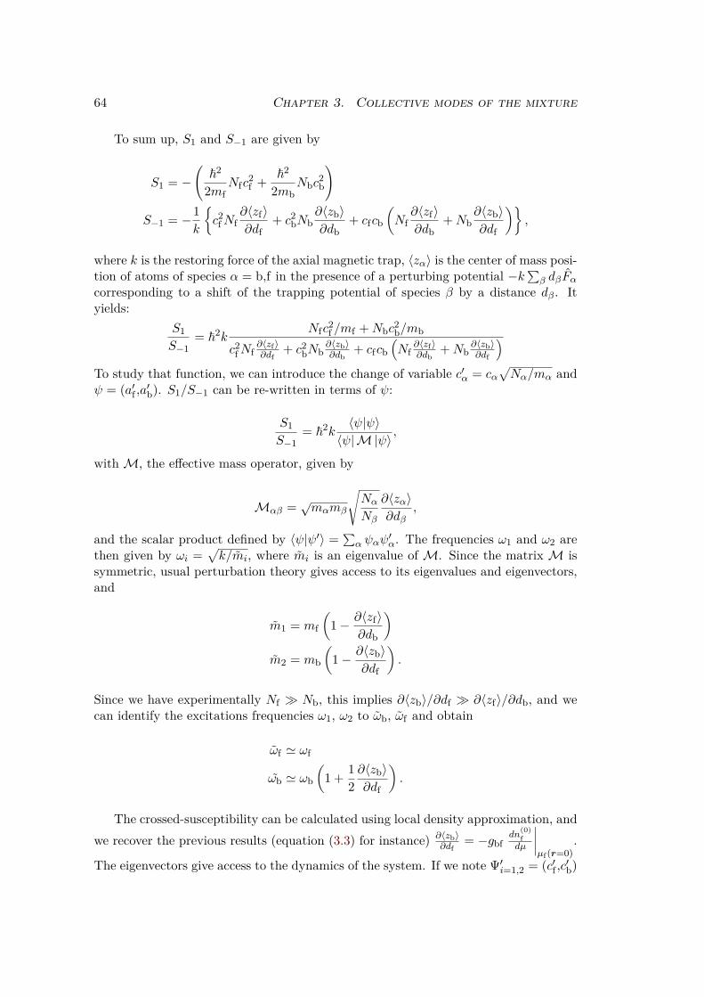
64 Chapter 3. Collective modes of the mixture
To sum up, S1 and S−1 are given by
S1 = −(
~2
2mfNfc
2f +
~2
2mbNbc
2b
)
S−1 = −1k
c2fNf
∂〈zf〉∂df
+ c2bNb
∂〈zb〉∂db
+ cfcb
(
Nf∂〈zf〉∂db
+Nb∂〈zb〉∂df
)
,
where k is the restoring force of the axial magnetic trap, 〈zα〉 is the center of mass posi-tion of atoms of species α = b,f in the presence of a perturbing potential −k∑β dβFα
corresponding to a shift of the trapping potential of species β by a distance dβ. Ityields:
S1
S−1= ~
2kNfc
2f /mf +Nbc
2b/mb
c2fNf
∂〈zf〉∂df
+ c2bNb
∂〈zb〉∂db
+ cfcb
(
Nf∂〈zf〉∂db
+Nb∂〈zb〉∂df
)
To study that function, we can introduce the change of variable c′α = cα
√
Nα/mα andψ = (a′
f ,a′b). S1/S−1 can be re-written in terms of ψ:
S1
S−1= ~
2k〈ψ|ψ〉〈ψ|M |ψ〉 ,
with M, the effective mass operator, given by
Mαβ =√mαmβ
√
Nα
Nβ
∂〈zα〉∂dβ
,
and the scalar product defined by 〈ψ|ψ′〉 =∑
α ψαψ′α. The frequencies ω1 and ω2 are
then given by ωi =√
k/mi, where mi is an eigenvalue of M. Since the matrix M issymmetric, usual perturbation theory gives access to its eigenvalues and eigenvectors,and
m1 = mf
(
1− ∂〈zf〉∂db
)
m2 = mb
(
1− ∂〈zb〉∂df
)
.
Since we have experimentally Nf ≫ Nb, this implies ∂〈zb〉/∂df ≫ ∂〈zf〉/∂db, and wecan identify the excitations frequencies ω1, ω2 to ωb, ωf and obtain
ωf ≃ ωf
ωb ≃ ωb
(
1 +12∂〈zb〉∂df
)
.
The crossed-susceptibility can be calculated using local density approximation, and
we recover the previous results (equation (3.3) for instance) ∂〈zb〉∂df
= −gbfdn
(0)f
dµ
∣∣∣∣µf(r=0)
.
The eigenvectors give access to the dynamics of the system. If we note Ψ′i=1,2 = (c′
f ,c′b)

3.2. Low temperature, low amplitude 65
the eigenvectors associated to eigenvalues ω1 and ω2, with perturbation theory we get
Ψ′1 =
(1√
mfmb
mf−mb
√NbNf
∂〉zb〉∂df
)
Ψ′2 =
( √mfmb
mb−mf
√NbNf
∂〉zb〉∂df
1
)
,
and the vectors Ψi=1,2 = (cf ,cb) corresponding to the excitation operator F are
Ψ1 =√mf
Nf
(
1mb
mf−mb
∂〉zb〉∂df
)
Ψ2 =√mb
Nb
(mf
mb−mf
NbNf
∂〉zb〉∂df
1
)
.
It is now possible to express the initial condition zf(t = 0) = zb(t = 0) = d on the(Ψ1,Ψ2) basis, and since the evolution of the eigenvector Ψi occurs at a frequency ωi,in the experimentally relevant situation it is possible to obtain the time evolution ofthe system as
zf(t) = d[(1− ερ) cos(ωft) + ρε cos(ωbt)], (3.8)
zb(t) = d[−ε cos(ωft) + (1 + ε) cos(ωbt)]., (3.9)
with ρ = Nb/Nf ≪ 1 and
ε =mb
mb −mf
∂〈zb〉df
.
The second factor in the expression of ε might be rather small, the first factor isactually quite large ( mb
mb−mf= 14), and the value of ε is ε = 0.25. This actually makes
the amplitude modulation very visible on the center-of-mass oscillations of the bosoniccloud. These functions perfectly fit the data, as shown in Figure 3.4. More detailson the calculations can be found in supplementary materials of [Ferrier-Barbut et al.,2014]. This approach validates the description in terms of harmonic oscillators thatwill be used in the next paragraph.
3.2.4 Two coupled-oscillators model
To understand the amplitude modulation, it is necessary to take into account the back-action of the bosons on the fermions. A scheme of the system is given in Figure 3.6.
We now obtain the following system:
Mf zf = −Kfzf −Kbf(zf − zb) (3.10)
Mbzb = −Kbzb −Kbf(zb − zf), (3.11)
where Mb = Nbmb (resp. Mf = Nfmf) is the total mass of the bosonic (resp.fermionic) cloud, Kb = Mbω
2b (resp. Kf = Mfω
2f ) is the spring constant of the axial

66 Chapter 3. Collective modes of the mixture
Kb Kbf Kf
Figure 3.6: Schematic representation of the system. The fermions (on the right) andthe bosons (on the left) are represented by two oscillators with spring constants Kf
and Kb, and are coupled with a spring constant Kbf .
magnetic confinement for the bosons (resp. fermions), and Kbf is a phenomenologicalweak coupling constant describing the mean-field interaction between the bosons andthe fermions. To be consistent with the previous description, we take Kbf = −2Kb
δωbωb
.We can now solve equations (3.10) and (3.11) with initial condition zf(t = 0) = zb(t =0) = d. We note ρ = Nb/Nf(≪ 1) and ε = 2mb
mb−mf
(ωb−ωb
ωb
)
. We get, as before,
ωf ≈ ωf
ωb = ωb
(
1− Kbf
2Kb
)
zf = d[(1− ερ) cos(ωft) + ερ cos(ωbt)] (3.12)
zb = d[−ε cos(ωft) + (1 + ε) cos(ωbt)]. (3.13)
Our system is analogous to a two-coupled-pendulum system which mass would beclose. This almost exact tuning of the two oscillators leads to the observed strongmodulation of the oscillations.
The adequacy of the T = 0 mean-field model, the absence of dissipation and thecoherent energy exchange between the two gases provide another evidence for thesuperfluid character of the two clouds. Limits of superfluidity can be studied in moredetails by varying the amplitude of the oscillations, as shown below.
3.3 Low temperature, high amplitude
3.3.1 Experiments
As it was shown previously, the two clouds oscillate in the trap with different frequen-cies. They gradually get out of phase and acquire some relative velocity with respectto each other, whose maximum value is given by (ωb + ωf)d. By varying the value of d,we can thus tune the relative velocity between the two clouds and study the propertiesof the counterflow. One striking feature is that, though for low relative velocities weobserve no damping (as discussed in section 3.2), above a certain critical velocity thereis an onset of dissipation (see Figure 3.7). The relative motion is damped down toa value where their relative velocities are smaller than the critical velocity, and theythen reach a steady-state regime similar to that of section 3.2.
We can make a phenomenological fit of the data using the functions defined inequations (3.12) and (3.13) in the limit of ρ → 0 and with ε fixed, but using a time-

3.3. Low temperature, high amplitude 67
0
- 1
1
z b
0 100 200 300
0
- 1
1
z f
ωftFigure 3.7: Center of mass oscillations at low temperature (≈ 100 nK) for a highinitial amplitude (d ≈ 150µm). The oscillations are initially damped, until the relativevelocity drops below the critical velocity. Then a steady-state regime is reached andlower amplitude oscillations are long-lived.
dependent amplitude:
d(t) = d1 + d2e−γbt
for the bosons and
d(t) = d1 + d2e−γft
for the fermions. Due to the high number of parameters, the fit procedure is thefollowing. We first fit te center-of-mass oscillation of the fermions with the function(d1 + d2e
−γft) cos(ωft). From this, we extract ωf ≈ ωf , that we use to fit the center-of-mass oscillations of the bosons with (d1 + d2e
−γbt)(−ε cos(ωft) + (1 + ε) cos(ωbt)).The value of γb can be extracted for different relative velocities and plotted as afunction of vmax/vF, where vmax is the maximum relative velocity between the twoclouds (see Figure 3.8). This shows clear evidence for a critical velocity, which cannow be measured.
One may wonder what happens to coefficients d1 and d2 when damping is small.There actually may exist two time scales in the time evolution of the center-of-mass.The first one, corresponds to damping due to friction between bosons and fermions, andthis is the one we want to measure in this experiment. The other timescale correspondsto residual damping due to some small anharmonicities of the trap, with a timescaleof 5 to 20 s. For high relative velocity between the two clouds, the first timescale isshort, leading to high values of γb, on the order of a few s−1. The residual dampingis then neglected. However, for low relative velocity, both timescale have the samemagnitude, and the measured γb corresponds to some convolution between them. It isthen over-evaluated. In any case, d2 always has a finite value and γb can be measured.

68 Chapter 3. Collective modes of the mixture
æ
æ
æ
æ
æ
æ
æ
à
à
à
à
à
à
à
à
à
ààì ìì
ìì
ìì
ì
0.0 0.2 0.4 0.6 0.8 1.00
1
2
3
4
5
6
7
vmaxvF
ΓBHs-1L
1kFaF = -0.421kFaF = 01kFaF = 0.68
Figure 3.8: Damping rate of the bosons as a function of the relative velocity betweenthe two clouds in the BEC-BCS crossover. Magnetic fields are 780 G (1/kFaff = 0.68),832 G (1/kFaff = 0) and +880 G (1/kFaff = −0.42).
Another way to obtain the critical velocity would have been to extract the ampli-tude d1 of the long-lived oscillations: the oscillation amplitude goes from d1 + d2 forshort evolution times down to d1. Since after a few γ−1
b , γ−1f there is no more damping
of the oscillations, their relative velocity is necessarily below the critical velocity. Un-fortunately, this procedure turned out to be hard to set up, because the value of d1 isvery sensitive to the fitted value of γb and γf , itself subject to noise. The final relativevelocity of the two clouds was not constant for all dataset at a given magnetic field,even though it was always below the critical velocity. More studies are needed to goforward on this subject.
It was also tempting to use as well γf to study the critical velocity. However, thedamping rate of the fermionic oscillations seems to be influenced by the ratio Nf/Nb,which is hard to keep constant, even within a dataset. No clear tendency on γf couldbe evidenced, but this could be the subject of future studies.
Another question that may be raised is where does the energy dissipated by frictiongoes. It turns out that it is dissipated by residual evaporation, leading to a loss ofatoms. This also results into an evolution of the ratio Nf/Nb as a function of time, asmentioned above.
3.3.2 Landau criterion for superfluidity
Here, we will first derive the historical Landau criterion for an impurity inside a su-perfluid, then its extension by Castin et al. [Castin et al., 2015]. Let us consider animpurity of mass m moving with a velocity v inside a superfluid. It may dissipateenergy by creating excitations of momentum p in the superfluid and reach a velocityv′. Let us note ε(p) the dispersion relation of the excitations. Conservation laws lead

3.3. Low temperature, high amplitude 69
to:
mv2
2= m
v′2
2+ ε(p)
mv = mv′ + p
Thus
v · p =p2
2m+ ε(p)
and
v ≥
p2
2m + ε(p)p
.
A necessary condition for excitation shedding is v > vc, where
vc = minp
p2
2m + ε(p)p
This sets a lower bound for the velocity needed to create excitations in a superfluid.For an impurity with a very large mass m→∞, this can be simplified as
vc = minp
(ε(p)p
)
In the case where the superfluid is a homogeneous weakly-interacting BEC, the exci-tations are phonons. Since the phonon dispersion relation is linear, εb(p) = cs
bp, thecritical velocity is simply the sound velocity cs
b:
vc = csb =
√
gn/m.
In the case where the superfluid is a strongly interacting Fermi gas, there exist twoexcitation branches. One of them is phonon-like with bosonic statistics[Minguzzi etal., 2001], and at low momentum its dispersion relation εb
f (p) is given by
εbf (p) =
p→0pcs
f ,
where csf is the sound velocity in the Fermi cloud. The second branch is associated
to pair-breaking and has fermionic statistics [Combescot et al., 2006]. Its dispersionrelation is given by
εff (p) =
√(p2
2mf− µ
)2
+ ∆2
At unitarity and on the BEC side of the resonance, the critical velocity is given bythe sound velocity, whereas on the BCS side, the pair-breaking excitations domi-nate [Combescot et al., 2006].
If we now consider a Fermi cloud and take as an impurity a BEC, the situation isquite similar. If we note εb the dispersion relation of the BEC, Mb the mass of the BEC

70 Chapter 3. Collective modes of the mixture
and εσf , with σ = f (for pair-breaking excitations) or b (for phonon-like excitations)
that of the fermions. The conservation laws lead to
Mbv2
2= Mb
v′2
2+ εb(p) + εσ
f (q) + p · v
Mbv = Mbv′ + p + q,
where p (resp. q) is the momentum of the excitation created in the BEC (resp. Fermisuperfluid), and p · v is the Doppler shift of the excitation in the BEC. The lowestrelative velocity allowing the creation of excitations corresponds to v = v′ and thecritical velocity is then given by7
vc = minσ=f,b
p
(εb(p) + εσ
f (p)p
)
,
and on the BEC side of the resonance, this can be further simplified in
vc = csb + cs
f ,
the sum of the sound velocities for both superfluids. This formula, obtained in thecase of homogeneous systems flowing into each other at a constant velocity, is quiteremarkable because it was unexpected. A naive answer would be that the criticalvelocity should be somehow the minimum of the two critical velocities, for instance.The results presented in subsection 3.3.3 and Figure 3.10 show that the adaptation ofLandau’s argument is indeed accurate.
3.3.3 Critical velocity
We measure γb as a function of vmax/vF for six different values of 1/kFaff in the BEC-BCS crossover and we can extract the critical velocity using a phenomenological fitshown on Figure 3.8:
γb = Aθ(v − vc)(v − vc
vF
)α
where vF is the Fermi velocity defined as 1/2mfv2F = EF = ~ωf(6Nf)1/3 and θ(x) is the
Heaviside function defined as
θ(x) =
0 if x < 0
1 if x > 0.
Since there is currently no theoretical prediction for the behavior of γb as a function ofvmax/vF for harmonically trapped gases, on Figure 3.8 we chose to fit with α = 1 (asother previous studies [Miller et al., 2007, Weimer et al., 2015]) because it is consistentwith a χ2 test8. To avoid any loss of generality, the systematic influence of such a
7This is actually a rough estimate: for σ = f , corresponding to the pair-breaking excitations of theFermi superfluid, it is only possible to create pairs of excitations that may have different momenta q1
and q2, not necessarily in the same direction.8We measured the distance between the points and the fit function for different values of α between
0.5 and 2 and the minimum distance was always reached for values close to α = 1.

3.3. Low temperature, high amplitude 71
choice is evaluated by letting α vary between 0.5 and 2 for all of our dataset (seeFigure 3.9), this gives us lower and higher bounds for the measured critical velocity.We attract the reader’s attention on the low damping rate on the BCS side, and onthe small critical velocity on the BEC side.
æ
æ
æ
æ
æ
æ
æ
0.0 0.2 0.4 0.6 0.80
1
2
3
4
5
6
vmaxvF
ΓBHs-1L
1kFaF = 0.68
æ
æ
ææ
æ
æ
æ
0.0 0.2 0.4 0.6 0.80
1
2
3
4
5
6
vmaxvF
ΓBHs-1L
1kFaF = 0.39
æ ææ
æ
æ
æ
æ
æ
æ
0.0 0.2 0.4 0.6 0.80
1
2
3
4
5
6
vmaxvF
ΓBHs-1L
1kFaF = 0.18
æ
æ
æ
æ
æ
æ
æ
æ
æ
ææ
0.0 0.2 0.4 0.6 0.80
1
2
3
4
5
6
vmaxvF
ΓBHs-1L
1kFaF = 0
æ
æ
ææææ
æ
0.0 0.2 0.4 0.6 0.80
1
2
3
4
5
6
vmaxvF
ΓBHs-1L
1kFaF = -0.26
æ ææ
ææ
ææ
æ
0.0 0.2 0.4 0.6 0.80
1
2
3
4
5
6
vmaxvF
ΓBHs-1L
1kFaF = -0.42
Figure 3.9: Damping rates of the center of mass oscillations versus maximal relativevelocity in the BEC-BCS crossover in unit of the Fermi velocity vF. Red line: fit withα = 1. Orange zone: region spanned by the fitting function when varying α from 0.5to 2. BEC limit corresponds to 1/kFaff ≫ 1 and BCS limit to 1/kFaff ≪ −1.
All of the parameters used to extract vc in the BEC-BCS crossover are given inTable 3.2.
B (G) 780 800 816 832 860 880af(a0) 6.4× 10³ 11.3× 10³ 24.0× 10³ ∞ −16.5× 10³ −10.3× 10³
1/kFaff 0.68± 0.07 0.39± 0.01 0.18± 0.02 0± 0.002 −0.26± 0.05 −0.42± 0.03ab(a0) 21.3 30.8 43.3 69.5 76.0 259
csb(10−2vF) 9.6± 1.4 9.4± 0.14 11.0± 1.6 11.1± 1.7 11.4± 1.7 15.1± 2.2vc/vF 0.17+0.06
−0.10 0.38+0.02−0.04 0.35+0.04
−0.11 0.42+0.08−0.14 0.54+0.02
−0.06 0.40+0.10−0.20
A(s−1) 14.8± 1.4 85± 32 24.6± 4.3 17.3± 3.6 30± 11 2.9± 0.5vc/c
sf 0.53+0.19
−0.31 1.11+0.06−0.12 0.99+0.11
−0.31 1.17+0.22−0.39 1.46+0.05
−0.16 1.05+0.26−0.53
Table 3.2: Experimental parameters, sound velocity at the center of the Bose gas in anelongated geometry cs
b =√
µb/2mb, critical velocity vc/vF, damping rate A(s−1), andvc/c
sf for α = 1 in the BEC-BCS crossover. The typical number of bosons and fermions
are constant in the crossover and are respectively 2.5± 0.5× 10⁴ and 2.5± 0.5× 10⁵.
The extracted critical velocity as a function of 1/kFafff is displayed on Figure 3.10,as well as the sound velocity for an elongated Fermi gas cs
f calculated by integrationover the transverse direction [Capuzzi et al., 2006, Luo et al., 2007, Astrakharchik,
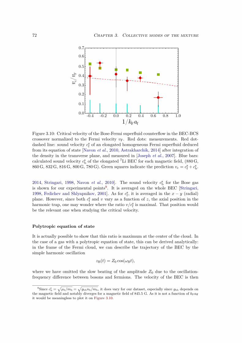
72 Chapter 3. Collective modes of the mixture
v c/v F
1/kFaf0.0
0.1
0.2
0.3
0.4
0.5
0.6
0.7
-0.4 -0.2 0.0 0.2 0.4 0.6 0.8 1.0
Figure 3.10: Critical velocity of the Bose-Fermi superfluid counterflow in the BEC-BCScrossover normalized to the Fermi velocity vF. Red dots: measurements. Red dot-dashed line: sound velocity cs
f of an elongated homogeneous Fermi superfluid deducedfrom its equation of state [Navon et al., 2010, Astrakharchik, 2014] after integration ofthe density in the transverse plane, and measured in [Joseph et al., 2007]. Blue bars:calculated sound velocity cs
b of the elongated 7Li BEC for each magnetic field, (880 G,860 G, 832 G, 816 G, 800 G, 780 G). Green squares indicate the prediction vc = cs
f + csb.
2014, Stringari, 1998, Navon et al., 2010]. The sound velocity csb for the Bose gas
is shown for our experimental points9. It is averaged on the whole BEC [Stringari,1998, Fedichev and Shlyapnikov, 2001]. As for cs
f , it is averaged in the x − y (radial)plane. However, since both cs
f and v vary as a function of z, the axial position in theharmonic trap, one may wonder where the ratio v/cs
f is maximal. That position wouldbe the relevant one when studying the critical velocity.
Polytropic equation of state
It is actually possible to show that this ratio is maximum at the center of the cloud. Inthe case of a gas with a polytropic equation of state, this can be derived analytically:in the frame of the Fermi cloud, we can describe the trajectory of the BEC by thesimple harmonic oscillation
zB(t) = Z0 cos(ωBt),
where we have omitted the slow beating of the amplitude Z0 due to the oscillation-frequency difference between bosons and fermions. The velocity of the BEC is then
9Since csb =
õb/mb =
√gbbnb/mb, it does vary for our dataset, especially since gbb depends on
the magnetic field and notably diverges for a magnetic field of 845.5 G. As it is not a function of kFaff
it would be meaningless to plot it on Figure 3.10.

3.3. Low temperature, high amplitude 73
v(z) = −Z0ωB sin(ωBt), hence(
v(z)v(z = 0)
)2
=
(
1− z2
Z20
)
,
For a polytropic equation of state, the local sound velocity in the Fermi cloud is givenby [Capuzzi et al., 2006]
cFs (z)2 =
γ
γ + 1µF(z)mF
cFs (z)2 =
γ
γ + 1µF(0)mF
(
1− z2
z2TF
)
,
where zTF is the Thomas-Fermi radius of the cloud, and the local chemical potentialµF(z) was obtained using the local density approximation. Combining equations 3.3.3and 3.15, we then obtain
vB(z)2
cFs (z)2
=vB(z = 0)2
cFs (z = 0)2
1− z2/Z20
1− z2/z2TF
,
which is maximum for z = 0 when Z0 ≤ zTF. In the general case, numerical calculationscan be performed using the equation of state. Example of such calculations at unitarityare shown in Figure 3.11 (where the gas is still polytropic) and are consistent with theabove analytical results.
v
(μ)
(a) cs
f(z) and v(z) in the Fermi cloud
frame
(μ)
v/cs f
(b) Ratio v(z)/cs
f(z) in the Fermi cloud
frame
Figure 3.11: Calculated csf(z), v(z) (left) and ratio v(z)/cs
f(z) (right) using the equationof state, for a Z0 = 100µm displacement of the BEC in a Fermi cloud withNf = 300·103
atoms at unitarity. The curves obtained for different magnetic fields show similarevolution.
Our measured critical velocity is consistent with Castin et al. prediction [Castin etal., 2015], but a χ2 test on our results does not discriminate between a critical velocityequal to Castin et al. prediction and to the sound velocity of the fermions.
3.3.4 Discussion
One may wonder the origin of the anomalously small value for the critical velocityat 780 G. It turns out that inelastic losses increase on the BEC side of a fermionic

74 Chapter 3. Collective modes of the mixture
Feshbach resonance and heat up the system [Regal et al., 2004a]. This is confirmedby the fact that we were unable to take data at 760 G due to a strong reduction ofthe lifetime of the mixture. This hypothesis is also supported by the presence of aclearly visible pedestal in the density profiles of the BEC taken at 780 G. At thisvalue of the magnetic field, we measure a ∼ 60% condensed fraction, correspondingto a temperature T/Tc,b ∼ 0.5. Even though the two clouds are still superfluids asdemonstrated by the critical behavior around vc, the increased temperature could beresponsible for the decrease of vc.
It is actually surprising how high the critical velocity is, especially when comparingto other experiments performed in this direction [Weimer et al., 2015, Miller et al.,2007]. The first point is that the BEC is completely contained in the Fermi superfluidand probes only its central (superfluid) part and not the outer (non-superfluid) wings,in strong opposition with the one of the other reported experiments [Weimer et al.,2015] where the probe was a laser beam piercing the whole cloud, including its non-superfluid parts In the other reported experiments [Miller et al., 2007], the probe is a20,60µm moving lattice in a cloud with Thomas Fermi radii of 63,91,82µm. Thesize of the lattice is thus smaller but comparable to the size of te cloud and it mayprobe as well its non-superfluid part. Second, the BEC is much smaller than the Fermicloud (Thomas-Fermi radii of 73, 3, 3µm to compare with 350, 13, 13µm), so itallows to probe locally the cloud. Third, the interaction between bosons and fermionsis weak, so the presence of the BEC does not causes strong density modulation forthe fermions and thus limits vortex shedding. The production of vortices is known tobe one of the factors reducing the critical velocity in other experiments [Singh et al.,2015].
3.4 High temperature, moderate amplitude
3.4.1 Experiments
We now study finite-temperature effects in the Bose-Fermi counterflow. To have hotterclouds, we stop the evaporation at a higher optical power10. We thus have moreatoms, and the radial trap frequencies are different for each temperature, but sincethey scale as
√U , where U is the optical power, they can be inferred from the low-
power trap frequencies without us having to re-measure them. The temperature canbe measured using the profile of the Bose gas: either by using the condensed fraction(scaling as (T/Tc,b)3), for temperature below the transition temperature for Bose-Einstein Condensation, or by fitting the thermal pedestal with a Gaussian functionwhose width gives the temperature of the cloud, for temperatures above the transitiontemperature. A typical measurement for the high-temperature oscillations is shownon Figure 3.12.
We see two remarkable features here: first, the oscillation is damped down to zeroamplitude for both clouds, while the fermions had not been affected in the previous
10We first tried to evaporate at low temperature and then re-compress the cloud, in order to keepthe atom number constant, but this proved to cause strong shot-to-shot fluctuations and forced us touse another method.

3.4. High temperature, moderate amplitude 75
0
- 1
1
z b
0 50 100
0
- 1
1
z f
ωftFigure 3.12: Center of mass oscillations at high temperature (T/TF = 0.4) for a mod-erate initial displacement (z0 = 80µm). Bosonic and fermionic motions are dampedwith the same damping constant, and phase-locking is observed. The dashed lines areguides to the eye.
experiments, second the two clouds are locked in phase to a high degree and oscillateat almost the same frequency, which turns out to be the frequency of the fermions.
3.4.2 Frequency analysis
Since the data points were taken at non-evenly spaced time positions11, it is not possibleto perform standard Fourier analysis, such as Fast Fourier Transform. Instead, we haveused a Lomb-Scargle algorithm (or ‘least-square analysis’) which measures the weightof the projection of data points on sines and cosines of fixed frequency.
For N data points hi = h(ti)i=1,...,N taken at times ti, the periogram is definedas
PN (ω) =1
2σ2
[∑
j(hj − h) cosω(tj − τ)]2∑
j cos2 ω(tj − τ)
+[∑
j(hj − h) sinω(tj − τ)]2∑
j sin2 ω(tj − τ)
where τ is defined as
tan(2ωτ) =
∑
j sin 2ωtj∑
j cos 2ωtj;
11The best compromise between the duration of the experimental acquisition and the precision ofthe frequency measurement was reached by taking several series of points spaced by approximatelyone quarter of an oscillation period, typically series of 6 points spaced by ∼ 15 ms, each series being∼ 500 ms apart from each other. This way, a first approximation of the period is given by closelyspaced points, and it is refined by the existence of points farther separated without having to spanprecisely the whole ∼ 5 s range.

76 Chapter 3. Collective modes of the mixture
its role is to make the periogram independent of the time origin.
h =1N
N∑
i=1
hi
and
σ =1
N − 1
N∑
i=1
(hi − h)2
are the mean and the variance of hii. The periogram, or power spectrum, gives accessto the statistical significance (ie the probability of rejecting the null hypothesis whenit is true) of each of the evaluated frequencies. In other words, the significance is therisk (between 0 and 1) that the measured frequency does not have a physical meaningbut rather is some artifact resulting from the noise. For all of the data presented here,this ‘risk’ is below 1.5%. Noting
Pmax = maxω
PN (ω),
the significance is proportional to e−Pmax , and here a value of 10 for the power representstypically a significance of 0.002.
νb/νf
(a) T/TFF = 0.03(2)
νb/νf
(b) T/TFF = 0.32(2)
Figure 3.13: Lomb Scargle periogram of the position of the bosons for both a cold (left)sample and a hotter (right) sample. A value of 10 for the powers represents typicallya significance of 0.002 (see text).
This analysis applied to our data points is shown on Figure 3.13 for both a cold anda hot sample. It shows a clear peak for a value of ωb/ωf ≈
√
6/7 at low temperature,as expected, but the peak is shifted toward 1 at higher temperatures. We can gatherall of the periograms obtained at different temperatures, and the result is displayedon Figure 3.14. We can see that up to a temperature T ≈ 0.34 TF, corresponding toT ≈ Tc,b, the bosons oscillate at a frequency ωb ≈
√
6/7 ωf that one expects for sucha mixture at low temperature, but that above that temperature, bosons are locked onthe fermions. It is remarkable that the shift in frequency happens close to the criticaltemperature for the bosons, while the superfluidity of the fermions was long gone.
It is possible to provide error bars for the determined frequencies, for instance bymeasuring the upper and the lower bounds for which the statistical significance is 10

3.4. High temperature, moderate amplitude 77
Figure 3.14: Power spectrum of the oscillations for different temperatures, obtainedusing the Lomb-Scargle algorithm of the center-of-mass displacement. Above T ≈Tc,B ≈ 0.34 TF > Tc,F, oscillations of the Bose and Fermi clouds become locked togetherat ωF.
times larger than that of the central frequency. This corresponds to a 10% uncertaintyon ωb. This is shown on Figure 3.15.
3.4.3 Damping
For each temperature, we can extract the damping rate γb. Using the functions definedin equation (3.13) and (3.12), with as before
d(t) = d1 + d2e−γb,ft, (3.16)
for clouds at temperatures T < 0.34TF, and
zb(t) = d0e−γbt cos(ωft)
zf(t) = d0e−γft cos(ωft)
for clouds at temperatures T > 0.34TF because the oscillations are then damped tozero amplitude, and fixing the frequencies to those extracted from the Lomb-Scarglealgoritm (see subsection 3.4.2), we can obtain the evolution of the damping rate as afunction of temperature, as shown on Figure 3.16.
The fact that the damping rate reaches a maximum at the temperature at whichthe phase-locking of the two clouds occur is consistent with results from a two coupledoscillator model that will be discussed below.

78 Chapter 3. Collective modes of the mixture
0.0 0.1 0.2 0.3 0.4 0.5 0.6
0.85
0.90
0.95
1.00
1.05
1.10
/
ω /ω
Figure 3.15: Ratio ωb/ωf as a function of T/TF. The bottom dashed line indicates theprediction from the mean-field model of section 3.2. The top dashed line correspondsto ωb/ωf = 1. The blue dots correspond to situations where both the Fermi and theBose clouds are superfluids, the yellow squares to a situation where the bosons are stillsuperfluids but not the fermions, and for the green open diamonds, both clouds are inthe normal phase.
0.0 0.1 0.2 0.3 0.4 0.5 0.60
1
2
3
4
5
T/TF
γ(s-1)
Figure 3.16: Damping rate of the oscillations of the bosons as a function of temperaturein units of Fermi temperature. Horizontal error bars are mainly statistical and refer touncertainties on temperature, and vertical error bars are fit uncertainties. This figureis preliminary because we have no evidence that γ is only a function of TF and not ofatom numbers or densities, that were not kept constant for this dataset.
From T = 0 to 0.34TF, damping increases as T/TF increases: the fact that theclouds have a relative velocity and some friction leads to an increase of damping up toT = 0.34TF. Above this temperature, friction is so high that both clouds oscillate atthe same frequency and are (almost) perfectly in phase ((ωf − ωb)/ωb ≈ 0.2%). Thisleads to a reduction of damping at higher temperatures.

3.4. High temperature, moderate amplitude 79
3.4.4 Two coupled-oscillator model
We can re-use the model of coupled oscillators introduced in subsection 3.2.4 andextend it to the case where there is friction between the two clouds. We introduce afriction parameter Γ, and the motion equations now are
Mf zf = −Kfzf −Kbf(zf − zb)− Γ(zf − zb)
Mbzb = −Kbzb −Kbf(zb − zf)− Γ(zb − zf).
These equations can be solved analytically. For different values of Γ, we fit the evolutionof zb using equations (3.13) with d(t) as in equation (3.16), and extract the values ofωb and γb. They are represented on figure Figure 3.17.
0.001 0.005 0.010 0.050 0.100 0.500
0.95
0.96
0.97
0.98
0.99
Γ
ω b/ω f
(a)
0.001 0.005 0.010 0.050 0.100 0.500
0.000
0.005
0.010
0.015
0.020
Γ
γ b/ω f
(b)
Figure 3.17: Evolution of ωb (a) and γb (b) as a function of Γ, the friction parameter,for a ratio Mf/Mb = 10. Phase locking accurs when Γ & Γ0 = 0.06, which correspondsto a maximum of dissipation between the clouds. Above Γ0, the damping is reducedbecause the clouds stay in phase.
Assuming that friction is increased when increasing the temperature, the resultsfrom the damped coupled-oscillator model are in qualitative agreement with our data,where we had indeed noticed the presence of a maximum in damping. Note that sincethe number of atoms was not kept constant within the datasets, nor the ratio betweenbosons and fermions, this would require more data to be fully exploited. It is also verydifficult to infer the value of Γ from the theory, and this prevents further comparisonwith the experiment.
3.4.5 Zeno-like model
The classical coupled oscillator model given above can be completed by a quantumphenomenological description using a Zeno-like model. Let us now consider that thebosons and the fermions are two coupled quantum harmonic oscillators. If we neglectthe interspecies interaction and consider that all of the particles have the same massm, the system is described by the Hamiltonian:
H = Hf +Hb,

80 Chapter 3. Collective modes of the mixture
where Hα=f,b is defined as:
Hα =P 2
α
2Mα+Mαω
2Z2α
2+Hαint,
with Pα the total momentum of the cloud, Zα the position of its center of mass andMα = Nαm its total mass. Hαint affects only the internal variable and commutes withZα and Pα. The oscillations of the fermions and that of the bosons are then associatedto two quantum numbers nf and nb, coupled to thermal baths described by φf and φb.We can thus describe the state of the system as |nf ,nb,φ〉, where φ = φf ,φb.
Alternatively, we can make a change of variable, and use
P = Pf + Pb,
Z = (MfZf +MbZb)/M,
p = µ(Pf/Mf − Pb/Mb),
z = Zf − Zb,
M = Mf +Mb,
Mr = MfMb/M.
With these new variables, the Hamiltonian of the system now reads
H =P 2
2M+Mω2Z2
2+
p2
2Mr+Mrω
2z2
2+H int
f +H intb ,
and the motion can now be described by two new quantum numbers, N and n,where N represents the number of quanta of the global center of mass motion (bosonsand fermions), and n the number of quanta of the relative motion. The state of thesystem is now described by |N,n,ϕ〉. The initial state, where both clouds are displacedand released together in the trap, corresponds to |N0,n = 0,ϕ〉. If both atomic specieshad the same mass, and without interactions, the clouds would remain in-phase, andwe would stay in the |N,n = 0,ϕ〉 state.
Lets now add the interspecies interactions. They are described by the Hamiltonian
Hb,f =∑
i≤Nf ,j≤Nb
U(zf,i − zb,j),
where zα,i is the z-position of the i-th particle of species α. This Hamiltonian commuteswith P and Z and therefore only couples to the relative variables z and p. It inducesa coupling between the relative motion and the thermal bath.
Lets us switch back off the interactions and consider the mass difference betweenthe two species. If the species α has a mass mα = m + ǫαδm/2, with ǫf = −1 andǫb = +1, its add to the Hamiltonian a kinetic energy term
δHK = −δm2m
∑
i,α
ǫαp2
i,α
2m,
where the center-of-mass contribution can be isolated and that can be re-written as
δHK = −δm2m
(
P 2b
2Mb− P 2
f
2Mb
)
+ δH intK ,
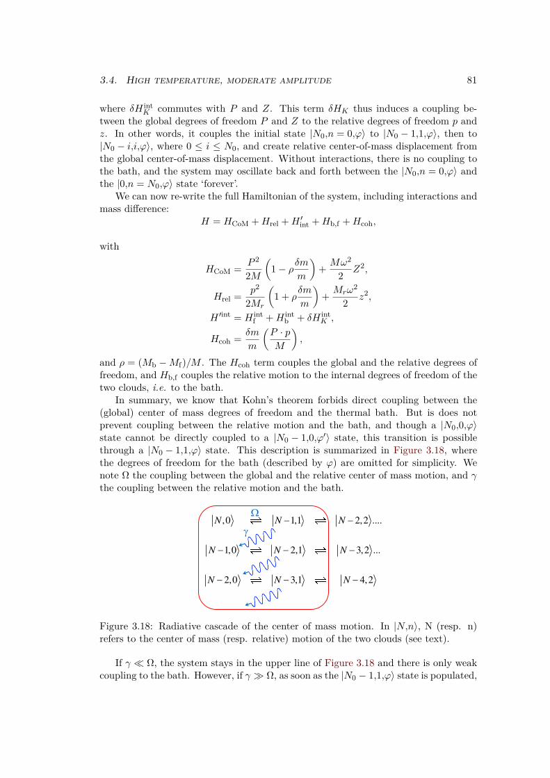
3.4. High temperature, moderate amplitude 81
where δH intK commutes with P and Z. This term δHK thus induces a coupling be-
tween the global degrees of freedom P and Z to the relative degrees of freedom p andz. In other words, it couples the initial state |N0,n = 0,ϕ〉 to |N0 − 1,1,ϕ〉, then to|N0 − i,i,ϕ〉, where 0 ≤ i ≤ N0, and create relative center-of-mass displacement fromthe global center-of-mass displacement. Without interactions, there is no coupling tothe bath, and the system may oscillate back and forth between the |N0,n = 0,ϕ〉 andthe |0,n = N0,ϕ〉 state ‘forever’.
We can now re-write the full Hamiltonian of the system, including interactions andmass difference:
H = HCoM +Hrel +H ′int +Hb,f +Hcoh,
with
HCoM =P 2
2M
(
1− ρδmm
)
+Mω2
2Z2,
Hrel =p2
2Mr
(
1 + ρδm
m
)
+Mrω
2
2z2,
H ′int = H intf +H int
b + δH intK ,
Hcoh =δm
m
(P · pM
)
,
and ρ = (Mb −Mf)/M . The Hcoh term couples the global and the relative degrees offreedom, and Hb,f couples the relative motion to the internal degrees of freedom of thetwo clouds, i.e. to the bath.
In summary, we know that Kohn’s theorem forbids direct coupling between the(global) center of mass degrees of freedom and the thermal bath. But is does notprevent coupling between the relative motion and the bath, and though a |N0,0,ϕ〉state cannot be directly coupled to a |N0 − 1,0,ϕ′〉 state, this transition is possiblethrough a |N0 − 1,1,ϕ〉 state. This description is summarized in Figure 3.18, wherethe degrees of freedom for the bath (described by ϕ) are omitted for simplicity. Wenote Ω the coupling between the global and the relative center of mass motion, and γthe coupling between the relative motion and the bath.
,0 1,1 2,2 ....
1,0 2,1 3,2 ...
2,0 3,1 4,2
N N N
N N N
N N N
g
W
Figure 3.18: Radiative cascade of the center of mass motion. In |N,n〉, N (resp. n)refers to the center of mass (resp. relative) motion of the two clouds (see text).
If γ ≪ Ω, the system stays in the upper line of Figure 3.18 and there is only weakcoupling to the bath. However, if γ ≫ Ω, as soon as the |N0 − 1,1,ϕ〉 state is populated,

82 Chapter 3. Collective modes of the mixture
it decays into the |N0 − 1,0,ϕ′〉 state, so that the relative motion is frozen (n ≡ 0) andthe oscillations are damped (N → 0). Here, Ω = ωf − ωb, but γ may depend ontemperature (but is hard to calculate in such a complex system), and this is thenconsistent with our observations. At high temperature, we can eliminate adiabaticallythe excited states of the relative motion, similarly to optical pumping in quantumoptics, and the system evolves in the |N,0,ϕ〉 manifold.
This model provides a quantum interpretation of the origin of friction between thetwo clouds. It can be mapped on a Caldeira-Leggett [Caldeira and Leggett, 1983] usedto study how dissipation arises for a quantum system interacting with a bath, exceptthat for our system the bandwidth for the frequency distribution of the bath is narrow,while it is large and continuous for the Caldeira-Leggett model [Onofrio and Sundaram,2015]. The phenomenon observed here are reminiscent to the synchronization of twospins immersed in a thermal bath predicted in [Orth et al., 2010, Henriet and Hur,2015] and may simulate decoherence in quantum networks [Chou et al., 2008] or heattransport in crystals [Zürcher and Talkner, 1990].
3.4.6 At the origin of the frequency shift
A complementary analysis of the motion of the two clouds can be made by consider-ing in the analysis that the BEC and its thermal fraction oscillate separately duringof the oscillations. We can fit the data of the high temperature oscillations allowingtwo different values for the center-of-mass of the BEC zBEC and for that of the ther-mal fraction zthermal. Obviously, the determination of zthermal at low temperature ischallenging because the thermal pedestal is very small, while that of zBEC is not de-fined above Tc,b. For intermediate temperatures, however, we can perform the spectralanalysis of zBEC and zthermal separately with the periogram. They are displayed inFigure 3.19 for different temperatures. Results are striking: while the BEC oscillatesat ωb, the thermal fraction oscillates at ωf . When the temperature is increased, theBEC reduces and the thermal fraction increases, and the weight of their respectivefrequencies on the global oscillation of the bosonic cloud varies accordingly. This ex-plains the shift from ωb to ωf when increasing the temperature. The observation ofout of phase oscillations of the thermal cloud and the BEC can be compared to secondsound experiments presented in [Andrews et al., 1997a, Stamper-Kurn et al., 1998],where a partly condensed cloud was oscillating in a harmonic trap. They set in motiononly the thermal cloud, that dragged the oscillations of the condensate with dampedout-of-phase oscillations at a frequency ∼ 5% smaller than the trap frequency. Here,in the presence of fermions, the out-of-phase oscillation seems to be long-lived, at afrequency fixed by the trapping frequencies of the system.
However, what we do not understand so far is why the oscillation frequency of thebosonic thermal fraction is ωf : for the fermions, the thermal cloud is a non-superfluidmoving impurity and the critical velocity should be cs
f . For the data presented here,the initial amplitude was 50µm for an oscillation frequency of 18 Hz. The maximumrelative velocity between the clouds is then vmax = 11 mm.s−1, while cs
f = 17 mm.s−1
in our experimental conditions. As a result, there should be no friction between thesuperfluid Fermi cloud and the thermal fraction and it is surprising that the thermalfraction oscillates at ωf even below Tc,f = 0.2TF (as in Figure 3.19b). It also has to be

3.5. Advanced data analysis: PCA 83
taken into account the fact that the superfluid fraction of the Fermi gas also shrinkstowards the center of the trap, and that the thermal fraction of the Bose gas, spatiallyextended, is likely to explore the non-superfluid part of the Fermi gas. Further studiescould be performed on this subject, for instance using the finite temperature equation-of-state of the Fermi gas from [Nascimbène et al., 2010] to know the spatial positionof the Fermi superfluid.
3.5 Advanced data analysis: PCA
It is also possible to use a more sophisticated analysis technique to analyze the data ofthe dipole modes. This provides a second analysis technique to confirm the previousstudy. It has the advantage of being fully model-independent. The analysis techniqueused here is based on Principal Component Analysis (PCA)12 and has been used anddescribed in a very pedagogical way in [Dubessy et al., 2014]. PCA is a well-knownimage analysis technique used in various fields. It allows to study correlations betweena set of images and works in the following way:
• The studied system is a set of images (2D images as in [Dubessy et al., 2014], or1D profiles, as it will be the case here).
• The average image (AI) of the dataset is computed and subtracted from all ofthe images. We then obtain a new ensemble of images.
• Then the covariance matrix of this new ensemble is computed and diagonalized.The eigenstates represent the directions along which there is variation from theaverage image AI, and their associated eigenvalues the relative weight of thesevariations. These eigenstates, called Principal Components (PCs), represent typ-ically variations in position, atom number, shape of the cloud, etc. Any kind ofvariation may show up in the PCs, provided that it concerns enough images andthat its variation from the mean is noticeable.
In other words, the PCA consists in a change of basis for the description of theimages. Instead of describing an image via its decomposition on the basis of the pixels(1 0 . . . 0),(0 1 0 . . . 0) . . . (0 . . . 0 1), we look for another basis AI, PC1, PC2, . . . PCn−1that would allow an accurate description of all of the images of the dataset using aminimum number of vectors from the basis, and any image of the dataset ID can beprojected on the principal components:
ID = c0AI +n−1∑
i=1
ciPCi,
with c0 ≥ c1 ≥ c2 ≥ c3 ≥ · · · ≥ cn−1. In practical, the first PCs are sufficient todescribe each image quite accurately, with typically |ci|2
∑n−1
i=0|ci|2
< 1% for i ≥ 5. It is
actually a very powerful way to increase the signal-to-noise ratio of a dataset: sincemost of the physical information is contained in only the first PCs, all of the following
12I would like to thank Romain Dubessy who took the time to come to the ENS to explain me thesubtleties of the PCA.

84 Chapter 3. Collective modes of the mixture
0
ω/ωf
(a) T/TF = 0.06(2)
ω/ωf
(b) T/TF = 0.13(2)
ω/ωf
(c) T/TF = 0.23(2)
ω/ωf
(d) T/TF = 0.26(2)
ω/ωf
(e) T/TF = 0.32(2)
ω/ωf
(f) T/TF = 0.34(2)
Figure 3.19: Spectral analysis of the oscillations of the BEC (blue) and of the ther-mal fraction (green) for different temperatures. Vertical dashed lines correspond toω/ωf =
√
6/7 and to ω/ωf = 1. It is clear that the oscillation of the thermal fractionoccurs at ωf while that of the BEC occurs at ωb. For low temperatures, the thermalfraction is very small and it is hard to determine accurately its position, while for hightemperatures the BEC is almost gone and it is also hard to locate it accurately, whichexplains the low resolution of the frequency determination in those cases.
PCs represent mainly noise, and it is possible to reconstruct a less noisy image ID′ by

3.5. Advanced data analysis: PCA 85
projecting on the truncated basis [Desbuquois, 2013]:
ID′ = c0AI +5∑
i=1
ciPCi.
The first PCs given by the algorithm for an oscillating BEC in a harmonic trap areshown on Figure 3.20. The average image AI is shown on Figure 3.20a. As expected,we identify the first PC (Figure 3.20b) as describing the center-of-mass oscillationof the BEC. If the cloud was at rest, the second PC (Figure 3.20c) would representcompression and dilatation of the cloud. Here, it is a reminiscence of the center-of-massoscillation: since the center-of-mass oscillation was strongly excited, its contributionto the second PC13 is dominant over the compression and dilatation excitation, onlyweakly excited. The third PC (Figure 3.20d) represents atom number fluctuations: itsshape is similar to the shape of the cloud. The fourth PC (Figure 3.20e) is anotherreminiscence of the center-of-mass oscillation.
Since the PCA algorithm is very fast, it can be used for an efficient analysis of thedipole mode. Once the Principal Component associated to the dipole-mode excitationis identified, each profile can be projected onto this component, and the scalar productbetween the PC and the profile tells ‘how much the cloud is on the right or on theleft’ for all times. We can then perform some spectral analysis (using for example theLomb-Scargle algorithm) to obtain the oscillation frequency. For the dipole mode withthe first PC, this method is very precise (see for instance Figure 3.21).
We can use this method to calculate again the shift of the bosonic frequency due tothe presence of fermions as in section 3.2. The calculated shift is given in Figure 3.22,very similar to Figure 3.5. For this study, the bare oscillation frequency of the bosonswas inferred from the oscillation frequency of the fermions in the mixture, ωb =
√
6/7ωf
instead of being obtained from interleaved measurements of bosons alone oscillations,as it was the case for data of Figure 3.5.
It is tempting to apply the same procedure to the second PC to study compression.However, as it can be demonstrated from numerical simulation, the second PC reflectsboth the compression of the cloud and the oscillations of the center-of-mass. Since herethe most excited mode is the dipole mode, its contribution dominates the quadrupole-like Principal Component and, consistently, the spectral analysis of this componentmainly shows contributions at 2ωf and 2ωb.
13Indeed, since the density of the cloud is n(x − a(t)), when we do a Taylor expansion for a smallcenter-of-mass oscillation this leads:
n(x − a(t)) = n(x)
− a(t)n′(x)
+a2(t)
2n′′(x)
− . . . .
For a harmonic oscillation, a(t) = a0 cos(ωt), and the term + a2(t)2
n′′(x) have indeed the second PCshape and oscillates at 2ω.
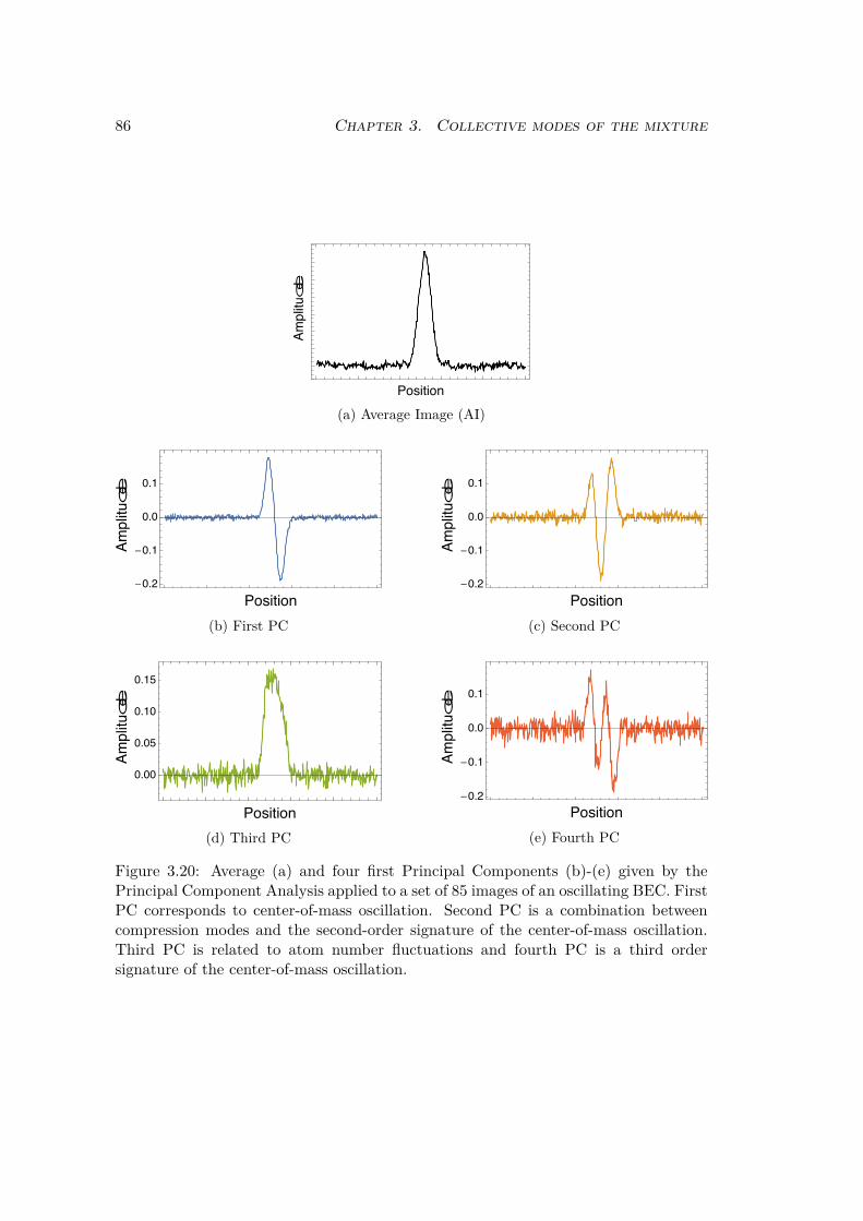
86 Chapter 3. Collective modes of the mixture
(a) Average Image (AI)
-
-
(b) First PC
-
-
(c) Second PC
(d) Third PC
-
-
(e) Fourth PC
Figure 3.20: Average (a) and four first Principal Components (b)-(e) given by thePrincipal Component Analysis applied to a set of 85 images of an oscillating BEC. FirstPC corresponds to center-of-mass oscillation. Second PC is a combination betweencompression modes and the second-order signature of the center-of-mass oscillation.Third PC is related to atom number fluctuations and fourth PC is a third ordersignature of the center-of-mass oscillation.

3.6. Quadrupole modes 87
() -
(a) Lomb Scargle periogram for thefermions.
() -
(b) Lomb Scargle periogram for thebosons.
Figure 3.21: Lomb-Scargle periogram of the projection of each profile on the PrincipalComponent showing the dipole mode. Here, ωf = 2π · 16.80(5)rad.s−1 and ωb =2π · 14.95(5)rad.s−1. Since this is a statistical analysis, the uncertainties are directlyrelated to the total number of images in the dataset. Here, we had 35 images.
- -
kF af
δω b/ω b
kFa
Figure 3.22: Green squares: shift of the bosonic frequency due to the presence of thefermions, calculated using the PCA and Lomb-Scargle algorithm. Red dots: data ofFigure 3.5, extracted with the standard method. Blue line: theory, as in Figure 3.5.
3.6 Quadrupole modes
We wanted to see whether it was possible to extract information about the compressionmodes of the mixture using the dataset taken to study critical velocity. Even thoughit was not possible to use the PCA here for the reasons mentioned above, we couldextract the Thomas-Fermi radius of each of the profiles, for different times, and performa spectral analysis on them.
It was checked (see [Ferrier-Barbut, 2014]) that this Thomas-Fermi radius had lessthan 10% fluctuations and that they were mainly due to atom number fluctuations.However, it is possible to use the Lomb algorithm to get the spectral distribution ofthe time evolution of these radii. For the bosons, a frequency does not always ap-

88 Chapter 3. Collective modes of the mixture
pear in the spectrum and it seems that any periodic variation of the width of thecloud is smeared out by atom number fluctuations and it is not possible the com-pare breathing or higher-order modes to their expected behavior [Guéry-Odelin etal., 1999, Guéry-Odelin and Stringari, 1999, Guéry-Odelin and Trizac, 2015]. How-ever, for the fermions, there is a much clearer signal (see Figure 3.23a), and it ispossible to extract the frequency of the axial quadrupole mode ωQ
f and to draw theratio ωQ
f /ωf as a function of 1/kFaff in the BEC-BCS crossover, displayed in Fig-ure 3.23b. They are compared to the hydrodynamic prediction in elongated harmonictraps: ωQ
f =√
(3γ + 2)/(γ + 1)ωf [Vichi and Stringari, 1999, Astrakharchik et al.,2005, Combescot et al., 2006, Amoruso et al., 1999, Hu et al., 2004], where γ is thepolytropic exponent of the equation of state14. This leads to ωQ
f /ωf =√
5/2 ≈ 1.581on the BEC side and ωQ
f /ωf =√
12/5 ≈ 1.549 at unitarity and on the BCS side. Thishas been measured in the BEC-BCS crossover [Bartenstein et al., 2004a, Altmeyer etal., 2007]. These values are indicated as dashed lines in Figure 3.23b.
() -
(a)
- -
kF af
ω Qf ω Df
(b)
Figure 3.23: (a) Lomb-Scargle periogram of the time evolution of the Thomas-Fermiradius of the fermions. There is a clear peak at 24.11 Hz. (b) Evolution of the ratioωQ
f /ωf as a function of 1/kFaff in the BEC-BCS crossover. The dashed lines are thepredictions for the molecular BEC (1/kFaff ≫ 1): ωQ
f /ωf =√
5/2 ≈ 1.581 and atunitarity and on the BCS side (1/kFaff = 0 and 1/kFaff ≪ −1): ωQ
f /ωf =√
12/5 ≈1.549. Green squares: measurements of quadrupole frequency for fermions alone, takenfrom [Bartenstein et al., 2004a]. Blue circles: measurements of quadrupole frequencyof the fermions in the presence of bosons, with the method explained above.
The values reported here are in good agreement with previous measurements fromthe Innsbruck group. They appear slightly downshifted but compatible with the com-bined error bars. This could be an effect of the presence of bosons in the trap butfurther studies would be needed on this subject.
14γ = 1 for the molecular BEC and γ = 2/3 in the unitary limit and on the BCS side [Stringari,2007, Bartenstein et al., 2004b].

3.7. Conclusion 89
3.7 Conclusion
We have studied the Bose-Fermi counterflow in various regimes of parameters, at lowand high temperature and in the BEC-BCS crossover. The low temperature studybelow the critical velocity showed that one could measure precisely equilibrium quan-tities (the equation of state) using collective excitations. With respect to measuringthe critical velocity, the use of the BEC as a local probe within the Fermi cloud allowsfor more sensitive measurement compared to earlier cases, which were subject to av-eraging effects over the trap inhomogeneities [Miller et al., 2007, Weimer et al., 2015].Finally, the phase-locking of the oscillations at higher temperatures arises from thedissipation between the two clouds. What is remarkable here is that the phase lockingdoes not result from high dissipation: the friction coefficient is still low compared tothe individual oscillation frequencies, but is comparable to the frequency difference.Several questions remain open: so far, we have no full explanation for the high criticalvelocity that we measure, even though several reasons have been suggested. On an-other subject, it has been predicted that each component of the mixture conserves itsinherent first sound while only a single second sound should exist, common to the wholesuperfluid mixture [Volovik et al., 1975]. It would be very nice to perform experimentsin this direction.

90 Chapter 3. Collective modes of the mixture

Chapter 4
Imbalanced gases and flat bottom
trap
4.1 Superfluidity in imbalanced Fermi gases . . . . . . . . . . . 93
4.1.1 Fermions in a box . . . . . . . . . . . . . . . . . . . . . . . . 93
4.1.2 Fermions in a harmonic trap . . . . . . . . . . . . . . . . . . 95
4.1.3 Application: another evidence of superfluidity . . . . . . . . . 97
4.2 Realization of a flat bottom trap . . . . . . . . . . . . . . . 98
4.2.1 Prediction . . . . . . . . . . . . . . . . . . . . . . . . . . . . . 98
4.2.2 Experimental conditions . . . . . . . . . . . . . . . . . . . . . 99
4.3 Critical polarizations in a flat bottom trap . . . . . . . . . 103
4.3.1 Bosons and fermions in a box . . . . . . . . . . . . . . . . . . 103
4.3.2 Bosons and fermions in a harmonic trap . . . . . . . . . . . . 105
4.3.3 Breakdown of FBT prediction . . . . . . . . . . . . . . . . . . 108
4.4 Experiments on imbalanced Fermi gases in a FBT . . . . 108
4.4.1 Bosonic Thomas-Fermi radius . . . . . . . . . . . . . . . . . . 111
4.4.2 First observations . . . . . . . . . . . . . . . . . . . . . . . . 111
4.4.3 Reconstruction Methods . . . . . . . . . . . . . . . . . . . . . 112
4.4.4 Evidence for a superfluid shell . . . . . . . . . . . . . . . . . 115
4.4.5 Parameters influencing the superfluid shell on the BEC side . 118
4.4.6 Parameters influencing the superfluid shell on the BCS side . 122
4.4.7 Portrait of the superfluid shell . . . . . . . . . . . . . . . . . 124
4.5 Conclusion . . . . . . . . . . . . . . . . . . . . . . . . . . . . 125
In the previous chapter we studied the robustness of the Fermi superfluid againsta counter propagating “obstacle”. While in the latter investigation we challenged theFermi superfluid by using the BEC as a dynamical perturbation, we now explore an-other pathway to compete with the fermionic superfluidity, in equilibrium. To thisend we tune the relative spin population of the fermionic component, while the Bose
91

92 Chapter 4. Imbalanced gases and flat bottom trap
superfluid now serves as potential shaper. The effect of spin imbalance in Fermi gaseshas been long-studied both experimentally and theoretically. In fact, this topic is stilla subject of debate and covers scope which extends to solid state condensed-matter.In particular, this question is formally tightly connected to the one of superconduc-tors in the presence of an external magnetic field. There, the practical difficulty risesfrom the fact that Meissner effect expels magnetic field from a superconductor (sofor a type I superconductor, the value of the magnetic field is strictly zero withinthe material while for a type II superconductor, a magnetic field may exist, but itis then constrained into filaments which are in the normal state). Superconductingregions and regions with a non-zero magnetic field do not intersect, and there is noCooper pairs in non-zero magnetic field regions. In ultracold atoms, it is sufficientto prepare a different number of atoms in two long-lived spin states, labeled ↑ and↓. As the spin population n↑,↓ is tied to a chemical potential µ↑,↓, the energy costfor adding or removing a fermion is different for a spin ↑ with respect to a spin ↓.The difference ∆µ = µ↑ − µ↓, therefore obviously plays the role of magnetic field.The Fermi gas is then called spin-imbalanced and singlet pairing is frustrated sinceit requires equal numbers of up and down particles. The question is how robustis superfluidity with respect to this imbalance? It has been addressed theoreticallyvery soon after the development of the BCS theory, by Clogston [Clogston, 1962] andChandrasekhar [Chandrasekhar, 1962]. In the condensed matter context, the questionregarded the maximum magnetic field that could be imposed on a superconductor with-out breaking superconductivity. Indeed, such a magnetic field imposes a populationimbalance between the two spin states involved in BCS theory. It was demonstratedthat the pairing that resulted in superconductivity was indeed stable against a finitepopulation imbalance caused by the magnetic field, but the value of this critical im-balance was only known in the BCS limit and is exponentially small as the BCS gap.Aside from the BCS limit, both the value of this population imbalance and what hap-pened to the gas above this imbalance was unknown. As a result, when ultracoldsuperfluid Fermi gases were first realized in 2003 [Jochim et al., 2003, Zwierlein etal., 2003, Greiner et al., 2003, Bourdel et al., 2004], this issue was soon investigated,both at MIT [Zwierlein et al., 2006a, Zwierlein et al., 2006b, Shin et al., 2006, Shin etal., 2008, Shin, 2008] and at Rice University [Partridge et al., 2006a, Partridge et al.,2006b]. There were some discrepancies between these two experiments that could besolved afterwards, but they paved the way towards a better understanding of imbal-anced Fermi gases. Another very important (and still unanswered) question is whetherother types of pairing are conceivable. Several possibilities have been put forward, suchas the long-sought Fulde–Ferrell–Larkin–Ovchinnikov (FFLO) phases, where there ispairing between particles with momenta of different amplitudes, resulting in a Cooperpair with non-zero momentum q. This leads to a spatially modulated order parame-ter with wavevector q. One of the main issues with the observation of FFLO phasesis that they are predicted to appear only in a narrow range of parameter space, seeFigure 0.1, and that ultracold Fermi gases are usually prepared in harmonic traps.This implies that the favorable conditions for FFLO could be reached only for a smallfraction of the atoms and that any visible effect would be smeared out by neighboringregions of the cloud. Other possibilities, also predicted to appear in a narrow range ofparameters, include gapless superfluid state [Liu and Wilczek, 2003] or a state with a

4.1. Superfluidity in imbalanced Fermi gases 93
deformed Fermi surface [Müther and Sedrakian, 2002]. The use of a uniform trap (a‘box’) would allow to zoom in for a small window of parameters.
During my PhD, we developed an idea to create a locally uniform trap for the Fermigas using the repulsive interaction with the bosons. This chapter will be dedicated tothe description of imbalanced gases and to the realization of the flat bottom trap.In a first section, I will give known results about superfluidity in imbalanced Fermigases and explain how we used them to give another proof of the superfluidity of theultracold Bose-Fermi mixture. Then, in a second section, I will detail a way to imprinta flat bottom trap (FBT) on the Fermi gas, and discuss its consequences in terms ofcritical polarization in a third section. Finally, in a fourth section, I will detail therealization of such a FBT in our experiment and give preliminary results.
4.1 Superfluidity in imbalanced Fermi gases
Firstly, let us restrict ourselves to the case of a two-component Fermi gas. The twocomponents studied here are two of the Zeeman sub-levels of the same atom and havein particular the same mass. We will first describe the gas in a box, that is a gas whichdensity is spatially uniform, and then expand the results to a gas in a harmonic trapwhich is more realistic experimentally.
4.1.1 Fermions in a box
In the case of an imbalanced Fermi gas in a box, the system will phase-separate intoa fully paired superfluid phase, a normal phase and, possibly, in a very narrow rangeof parameters, in a FFLO phase, see Figure 0.1. They can be described by atomicdensities ns for the density of the superfluid, n↑ for that of the majority componentin the normal phase, and n↓ for that of the minority component in the normal phase.The two phases have different densities and the ratio n↓/n↑ in the normal phase isfixed by equilibrium conditions.
Let us first consider the superfluid phase (labeled by s). In a superfluid fermions arepaired into Cooper pairs (for weakly attractive systems) or molecules (in the stronglyattractive regime). For all interaction strengths, the densities of both species in thesuperfluid phase are thus equal and will be noted ns. On the BCS limit, the chemicalpotential of the gas is known: µ = εF, where εF is the Fermi energy of a uniform non-interacting Fermi gas: εF = ~
2
2mf(6π2ns)2/3. On the BEC limit, it is known as well and
is simply the mean-field interaction of the composite molecules shifted by the moleculebinding energy: µ = − ~
2
2mfa2ff
+ π~2affnsmf
. At unitarity, the scattering length diverges, so
the only remaining energy scale in the system is the Fermi energy εF and the lengthscale is the inter-particle distance n−1/3 . As a result, the energy of a superfluidFermi gas at unitarity has to be proportional to the energy of a noninteracting Fermigas 3
5εF [Heiselberg, 2001], with proportionality factor the Bertsch parameter ξ =0.38(1) [Ku et al., 2012, Zürn et al., 2013, Zwerger, 2012, Navon et al., 2010]. Theenergy density es of the superfluid at unitarity can thus be written as:
es[ns] ≡ ξ65
~2
2mf(6π2ns)2/3ns = ξ
65εFns, (4.1)

94 Chapter 4. Imbalanced gases and flat bottom trap
the factor 2 being due to the two components.Regarding the normal phase, it is relevant to use the notion of fermionic polaron,
introduced in [Chevy, 2006, Lobo et al., 2006]. The polaron is a quasi-particle ofeffective mass m∗ composed of a one atom of the minority component (↓) accompaniedby its interaction with the majority component (↑). If only ↑ atoms were present,the energy density of the system would be the one of a noninteracting Fermi gas:en[n↑, n↓ = 0] ≡ 3
5εF↑n↑, with εF↑ = ~2
2mf(6π2n↑)2/3. Now, if we add some ↓ atoms,
and note their binding energy Ebind with the Fermi gas of ↑ particles, we have Ebind =−3/5εF↑A. Finally, with ε∗
F↓ = ~2
2m∗ (6π2n↓)2/3 the Fermi energy of the polaron of massm∗, if several quasi-particles are present, they will have an energy density 3
5ε∗F↓n↓ =
35εF↑n↑
mf
m∗ x5/3. We can then write the energy density en of the normal phase as [Loboet al., 2006]:
en[n↑, n↓] ≡ 35εF↑n↑
(
1− 53Ax+
mf
m∗ x5/3)
, (4.2)
where x = n↓/n↑ is the ratio between the densities of the minority and majoritycomponents. The description of the system in terms of majority atoms with non-interacting polarons is only valid for low ↓ densities with respect to ↑ densities. Thisimplies x≪ 1. At higher x, the effect of interactions between quasi-particles also haveto be taken into account [Pilati and Giorgini, 2008, Recati et al., 2008], this is doneby adding an extra term Fx2 in the above equation ((4.2)):
en[n↑, n↓] ≡ 35εF↑n↑
(
1− 53Ax+
mf
m∗ x5/3 + Fx2
)
(4.3)
≡ 35εF↑n↑ǫ(x).
The values of ξ, A, mf/m∗ and F = (5/9)A2 have been measured [Navon et al.,
2010] and calculated [Prokof’ev and Svistunov, 2008, Combescot and Giraud, 2008,Mora and Chevy, 2010] at unitarity: ξ = 0.38, A = 0.615 and m∗/mf = 1.20. Thoughthe above functions are strictly valid only at unitarity, we used them also aroundunitarity for specific values of 1/kFaff , using approximate values given in Table 4.1.
1/kFaff 0 0.2 −0.25B (G) 832.2 817 854F 0.21 0.25 0.1553A 1.025 1.118 0.866ξ 0.37 0.22 0.54
m∗/mf 1.20 1.30 1.12
Table 4.1: Summary of the values used to study the imbalanced mixture, extractedfrom [Navon et al., 2010, Mora and Chevy, 2010]
Starting with a normal phase with x = 0, adding ↓ atoms will increase x and forx = xc there will be a first-order phase transition between a pure normal phase anda system with phase separated superfluid and normal states. At unitarity, matching

4.1. Superfluidity in imbalanced Fermi gases 95
the pressures and the chemical potentials at the interface leads to x = 0.4 [Recatiet al., 2008, Lobo et al., 2006]. This varies in the BEC-BCS crossover [Shin et al.,2006, Navon et al., 2010]: on the BEC side, pairing is very robust, and xc → 1, whileit decreases on the BCS side. The limit above which superfluidity is destroyed by a toolarge imbalance between the two species is called the Clogston Chandrasekhar limit.In the condensed matter context where the imbalance was caused by a magnetic field,it was convenient to use, instead of the density ratio, the local polarization, defined as
p =n↑ − n↓n↑ + n↓
,
which is also widely used in the cold atom community. The polarization p can be ex-pressed as a function of the density ratio x, p = 1−x
1+x , and the Clogston Chandrasekharcritical ratio xc = 0.4 at unitarity corresponds to a critical local polarization pc = 43%.
4.1.2 Fermions in a harmonic trap
Uniform systems are easier to handle theoretically, but the ultracold Fermi gases re-alized experimentally are usually trapped by harmonic potentials, either optical ormagnetic1. One can re-apply the results obtained above for a uniform system to thecase of a harmonic trap using the LDA. Local Density Approximation, or LDA, is anapproximation that states that a cloud trapped by a potential V (r) can be seen aslocally homogeneous at position r with a chemical potential µ − V (r). This approxi-mation is valid only if the trapping potential varies slowly enough so that the cloud canfollow its variations. Its violation in some experiments due to sharp boundaries [Par-tridge et al., 2006a, Partridge et al., 2006b, De Silva and Mueller, 2006b, Baur et al.,2009] leads to the study of surface tension effects. In a harmonic trap, the local densi-ties vary, hence the local polarization p and density ratio x vary as well. As a result,instead of the local quantities x and p, we rather use the total polarization P , thatinvolves the total numbers of atoms of each species N↓ and N↑ in the trap:
P =N↑ −N↓N↑ +N↓
.
Applying the results of subsection 4.1.1 to a harmonic trap implies that the phaseseparation found in the homogeneous system translates into a layered structure in atrap. If the polarization is small, the cloud will separate in three concentric parts (seeFigure 4.1a):
• A fully paired superfluid core: in the center of the cloud, there is a superfluid,that can be characterized by the presence of vortices [Zwierlein et al., 2006a]. Itimplies the equality of the local atomic densities: n↑ = n↓.
• A partially polarized non-superfluid phase, where n↑ > n↓
• A fully polarized phase, where n↓ = 0, and the ↑ atoms obey the ideal Fermi gaslaws.
1Box potentials are becoming more and more popular [Gaunt et al., 2013, Corman et al., 2014].

96 Chapter 4. Imbalanced gases and flat bottom trap
When the polarization increases, the central superfluid part shrinks, and when it istoo high (above 76% for a unitary Fermi gas [Nascimbène et al., 2009, Zwierlein et al.,2006a, Shin et al., 2006]), there is no more superfluid part, the central part of the cloudis partially polarized and is surrounded by a fully polarized phase (see Figure 4.1b).In this whole chapter, the calculations were made in the isotropic case and at unitarityfor a gas with the same mean trapping frequency ω. Adapting them to our cigar-shaped experiment thus requires a re-scaling of the length scales. For all the theorycurves, results will be plotted in terms of the averaged oscillator length lho =
√
~/mω,while the experimental data that will be shown below will be given in terms of axialharmonic oscillator length aho =
√
~/mωz. For the values of ωz and ωr that we havein the experiment, lho = 3.6µm and aho = 9.8µm. Note the density jump in theminority density at the boundary of the superfluid, corresponding exactly to xc fromthe homogeneous case.
n↑n↓n↑-n↓
n↑n ↓
(a) Below the critical polarization, a super-fluid lies in the center of the cloud.
n↑n↓n↑-n↓
n↑n ↓
(b) Above the critical polarization, there isno superfluid any more.
Figure 4.1: Calculated density profiles (top) and schematic representation (bottom)of an imbalanced Fermi gas in a spherical harmonic trap. Red (resp. yellow) curvesrepresent the density of the majority ↑ (resp. minority ↓) component, and the greencurve represents the density difference n↑ − n↓. In purple is the superfluid (SF) phasewhere n↑ = n↓, in faded yellow-to-red is the partially polarized (PP) phase withn↑ > n↓, and in red is the fully polarized (FP) phase where n↓ = 0. Distance is givenin units of harmonic oscillator length lho and densities in units of l−3
ho .

4.1. Superfluidity in imbalanced Fermi gases 97
4.1.3 Application: another evidence of superfluidity in the Bose-Fermi
mixture
The superfluid is associated to pairing, which implies a local equality between ↑ and↓ densities: n↑ = n↓. Experimentally, we only have access to doubly integrated
densities n(z), but it can be shown that dn(z)z dz = −2π ω2
zω2
ρn(z), provided the poten-
tial has ellipsoidal symmetry and verifies some weak local density approximation: itrequires that iso-potential lines correspond to iso-density lines. This hypothesis isresembles the LDA hypothesis but is weaker. The relation creates a direct link be-tween n(z) and n(z). The ellipsoidal symmetry implies that n(x,y,z) is actually a
function of r =√
ω2xx2+ω2
yy2+ω2zz2
ω , and, with ωρ defined as ωρ = ω1/2x ω
1/2y and ρ as
ω2ρρ
2 = ωxx2 + ωyy
2,
n(z) =ˆ
dx dy n
r =
√
ω2xx
2 + ω2yy
2 + ω2zz
2
ω
(ω = ω1/3x ω
1/3y ω
1/3z )
n(z) = πω2
ω2ρ
ˆ
ds n(s) (s =ω2
ρ
ω2 ρ2 + ω2
zω2 z
2, ds = 2ω2
ρ
ω2 ρ dρ+ 2ω2z
ω2 z dz)
dn(z)ds
= −π ω2
ω2ρ
n(s)
dn(z)z dz
= −2πω2
z
ω2ρ
n(z),
where the ω2z
ω2ρ
term accounts for the fact that the potential is not spherical but ellip-soidal.
As a result, if we consider the density difference, n↑−n↓ = 0 implies d(n↑−n↓)dz (z) =
0, i.e. there is a plateau in the density difference, hereafter called the superfluidplateau. We use this result to provide another evidence of the superfluidity of the Bose-Fermi mixture. We prepared a BEC with an imbalanced Fermi superfluid at unitarity,and image both clouds with the simultaneous triple imaging technique explained insubsection 2.6.2. While the peak of the Bose-Einstein Condensation was clearly visible,the density difference of the two fermionic spin states showed a plateau, indicatingsuperfluidity for both species (see Figure 4.2).
In this section, we have shown that an imbalanced Fermi gas phase separates intoa superfluid and a normal phase. In a harmonic trap, this results in a cloud withconcentric layers, the inner one being superfluid if the polarization is low enough.Although these results were obtained at unitarity, they can be extended in the BEC-BCS crossover, and we successfully used them to provide another evidence of thesuperfluidity of the Bose-Fermi mixture that we produced. Indeed, we observe a fullypaired Fermi gas at the center of the trap. If this itself is not a definitive proof ofsuperfluidity, it was shown with the observation of vortices in [Zwierlein et al., 2006a]that fully paired regions in spin-imbalanced Fermi gases were superfluid.

98 Chapter 4. Imbalanced gases and flat bottom trap
-
(a)
(a
- )
(a)
(a
- )
Figure 4.2: Doubly integrated density profiles of bosons and fermions resulting fromtriple simultaneous imaging described in subsection 2.6.2. In blue are the bosons, inred the majority ↑ component of the fermions, in yellow the minority ↓ component andin green their density difference. Bosons are imaged axially, fermions radially. Thomas-Fermi fit of the bosonic profile is shown in dashed blue line. The superfluid plateau inthe density difference is indicated with a dark green dashed line. It implies the localequality n↑ = n↓ and is associated to pairing and superfluidity. Here, Nf = 180 · 103,Nb = 38 · 103, and P = 24% at 817 G. Units are in terms of harmonic oscillator lengthof the axial direction aho = 9.8µm in our experiment.
In the next sections, we will discuss how we can use the BEC to create an effectiveflat bottom trap (FBT) for the fermions, then discuss the effect of that specific trapon the Clogston-Chandrasekhar limits of the Fermi gas.
4.2 Realization of a flat bottom trap
In the limit of low atom number for bosons, we have shown in chapter 3 that therewere no drastic change in the Fermi cloud’s behavior due to the presence of bosons andthat for instance the dipole mode frequency of the fermions was barely modified whenNb ≪ Nf and that the superfluidity of the Fermi cloud was not deeply affected by thepresence of bosons. On the other hand, we have seen that even for high bosonic atomnumber, the Fermi cloud could still show concentric layers of phases with differentpolarization, see Figure 4.2. However, fermions and bosons do have a (weak) repulsiveinteraction that will induce an energy shift of gbfnf (for the bosons) and gbfnb (forthe fermions). Since the density of the Bose gas is much higher that that of the Fermigas, we will focus of the effective trapping potential felt by the fermions (the effectivetrapping potential for the bosons is barely modified) [Mølmer, 1998, Amoruso et al.,1998].
4.2.1 Prediction
Let us consider a mixture of a Bose-Einstein Condensate and a two components (notedagain ↑ and ↓) Fermi gas, in the vicinity of a Feshbach resonance for the Fermi gas.Here, both gases are confined by a harmonic trap with the same potential V (r) =

4.2. Realization of a flat bottom trap 99
1/2mαω2αr
2, where α = b or f for bosons or fermions, respectively2. If we assumemean-field Bose-Bose and Bose-Fermi interactions, using the LDA, the local energydensity E can be written as:
E =gbb
2n2
b + gbfnb(n↑ + n↓) + e[n↑,n↓],
where gbb = 4π~2abb/mb and gbf = 2π~2abf(1/mb + 1/mf) (within Born approxima-tion [Zhang et al., 2014]) are the coupling constants for Bose-Bose and Bose-Fermiinteractions, respectively, and we assume that the Bose-Fermi scattering length is thesame for both Fermi gas components. e[n↑,n↓] refers to the Fermi-Fermi interaction. Itis a complicated function in the general case, but is known at unitarity for a balanced(n↑ = n↓ = nf/2) superfluid Fermi gas, as defined in equation (4.1). For a spin-polarized Fermi gas at unitarity, the interaction energy is given by [Chevy, 2006, Loboet al., 2006] equation (4.3), and this can be extended in the BEC-BCS crossover fromthe equation of state with appropriate coefficients (given in Table 4.1).
It is now possible to obtain the chemical potentials as:
µσ=↑,↓ = wσ[n↑,n↓] + gbfnb + V (r) (4.4)
µb = gbbnb + gbf(n↑ + n↓) + V (r), (4.5)
where wσ[n↑,n↓] = ∂e[n↑,n↓]∂nσ
is the pressure equation of state of the fermions. Atunitarity for a spin-balanced Fermi gas, wσ = ξεFσ.
If we now replace nb in equation (4.4) by its value from equation (4.5), we get:
µσ = wσ[n↑,n↓] +g2
bf
gbb(n↑ + n↓) + V (r)
(
1− gbf
gbb
)
+gbf
gbbµb (4.6)
µb = gbbnb + gbf(n↑ + n↓) + V (r).
With equation (4.6), we see that for gbf = gbb, n↑ and n↓ do not depend on r anymore: the repulsive interaction with the bosons compensates exactly the harmonicconfining potential and the density of fermions is uniform anywhere where the bosonsare present. The influence of gbf/gbb is shown on Figure 4.3.
We see that at the condition gbb = gbf , the potential felt by the fermions is flatclose to the center of the trap. This means that the 3D effective potential for thefermions is composed of a ellipsoidal region where the potential is uniform, surroundedby a truncated harmonic potential. The center of the trap is an ellipsoidal ‘box’.
4.2.2 Experimental conditions
The question now is how to realize the condition gbf = gbb. We want the BEC to bestable, which requires abb > 0, and the possibility for the Fermi gas to be superfluid,which requires to be close to a Feshbach resonance for the Fermi cloud.
2In reality, the trap is not isotropic but is rather cigar-shaped with an aspect ratio of ∼ 20. However,it does not matter here because in first approximation the two clouds feel the same potential, bothradially and axially.

100 Chapter 4. Imbalanced gases and flat bottom trap
-R b R b
gg
=
(a) gbf/gbb = 0.5, thefermions still feel some har-monic trapping potential,but its frequency is smallerthan in the bare trap.
-R b R b
gg
=
(b) gbf/gbb = 1, thefermions experience a flatpotential in the whole vol-ume occupied by the bosonsand should be uniform.
-R b R b
gg
=
(c) gbf/gbb = 2, the fermionsare anti-trapped close to thecenter of the trap, we expecta peak fermion density closeto r = RTF,b.
Figure 4.3: Shape of the potential felt by the fermions for different values of gbf/gbb.
4.2.2.1 Conditions for the magnetic field
In our system, the bosons are 7Li, the fermions are 6Li in two different spin states.The Bose-Fermi interaction is fixed with a scattering length of abf = 40.8 a0, constantfor a large range of magnetic fields, and equal for all Bose and Fermi spin-statescombinations considered here. However, 7Li has a number of Feshbach resonances (seeTable 2.2), and both for |1b〉 and |2b〉 states it is possible to find a magnetic field whereabb = 44.2 a0, that is where gbf = gbb. However, to be close to a Feshbach resonancefor 6Li, it is favorable to use |2b〉 and a |1f〉 − |2f〉 mixture. Then, one can choosebetween two different magnetic fields to achieve the condition gbf = gbb: B = 816.8 Gand B = 854.2 G, these two possibilities being around the broad Feshbach resonancefor 6Li (at B = 832.2 G). They are shown on Figure 4.4 as purple dots. Thus, it willthen be possible to have either a BEC superfluid (with our experimental conditions,for a magnetic field of B = 816.8 G, this corresponds to kFaff = 5 i.e. 1/kFaff = 0.2) ora BCS superfluid (for a magnetic field of B = 854.2 G, this corresponds to kFaff = −4i.e. 1/kFaff = −0.25) in a flat potential. This makes this combination an excitingplayground to study the physics of Fermi superfluid in a flat trap.
4.2.2.2 Robustness of the flat trap
It is an important question to know the sensitivity of the flat bottom trap with re-spect to magnetic field variations: it is impossible experimentally to be exactly at themagnetic field where gbf = gbb. Typically in our experiment we may have . 0.1 Gday-to-day fluctuations. To quantify this effect, we compare the residual anti-trappingenergy ∆ defined on Figure 4.5 to the chemical potential of the fermions µf in the caseof a balanced gas. The results are shown on Figure 4.6, for two different ranges ofmagnetic field. One can see that, on a 0.3 G interval around the target chemical po-tential, ∆/µf varies by less than 0.5%, to be compared for instance with gap energy atunitarity of 0.4 εF, or with critical temperature for superfluidity of 0.2TF. A residualtrapping or anti-trapping energy on the order of 0.5 % of µf thus seems small enoughto say that the flat potential conditions are verified.
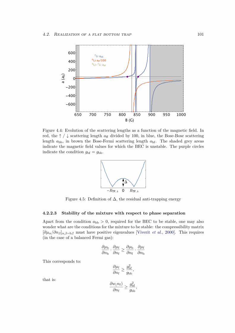
4.2. Realization of a flat bottom trap 101
---
()
(
)
/-
Figure 4.4: Evolution of the scattering lengths as a function of the magnetic field. Inred, the ↑ / ↓ scattering length aff divided by 100, in blue, the Bose-Bose scatteringlength abb, in brown the Bose-Fermi scattering length abf . The shaded grey areasindicate the magnetic field values for which the BEC is unstable. The purple circlesindicate the condition gbf = gbb.
-R b R b
ΔFigure 4.5: Definition of ∆, the residual anti-trapping energy
4.2.2.3 Stability of the mixture with respect to phase separation
Apart from the condition abb > 0, required for the BEC to be stable, one may alsowonder what are the conditions for the mixture to be stable: the compressibility matrix[∂µα/∂nβ]α,β=b,f must have positive eigenvalues [Viverit et al., 2000]. This requires(in the case of a balanced Fermi gas):
∂µb
∂nb· ∂µf
∂nf≥ ∂µb
∂nf· ∂µf
∂nb
This corresponds to:∂µf
∂nf≥ g2
bf
gbb,
that is:∂w(nf)
∂nf≥ g2
bf
gbb,

102 Chapter 4. Imbalanced gases and flat bottom trap
-
-
()
Δ/μ F
-
-
-
()
Δ/μ F
Figure 4.6: Variations of ∆/µf for different ranges of magnetic fields around the con-dition gb = gbf .
At unitarity, this leads to nf ≤ 2.7 · 1016 cm−3, which is well verified with our experi-mental parameters (nf < 1014 cm−3), and this will remain the case for gbf = gbb.
However, if we wanted to study phase-separation between the components of themixture, it would be possible to go towards a magnetic field where abb goes to zero.For the |2b〉 state that we are using, abb = 0 at B = 850 G and at B = 578 G [Shotanet al., 2014]. The phase separation occurs when abb is still positive, ie before reachingabb = 0 that leads to the collapse of the condensate. Close to B = 850 G, the phaseseparation occurs about 50 mG away from abb = 0 and preliminary data that we tookthere show mainly the collapse of the BEC. Towards B = 578 G, phase separationshould occur below 730 G [Ferrier-Barbut, 2014], well before the collapse of the BEC,but this is then in the deep BEC regime for the fermions and their lifetime is reduced.We plan to do more experiments to investigate this possibility of phase separation tomake a connection with what is happening in 4He-3He mixtures.
4.2.2.4 Deviations from Paschen-Back regime
In the range [800 G-900 G], 7Li is not fully in the Paschen-Back regime. This results in aslightly different magnetic trapping for 7Li and 6Li: Vb,ax = βVf,ax, with β = 0.96 < 1.The optical trapping stays the same for both isotopes3. This results in the axialtrapping (mainly magnetic) being different for both isotopes while the radial trapping(mainly optical) is the same. Equation (4.6) can be re-written as:
µσ = wσ[n↑,n↓] +g2
bf
gbb(n↑ + n↓) + Vf(r)−
gbf
gbbVb(r) +
gbf
gbbµb.
It is not possible any more to cancel harmonic trapping simultaneously in all threedirections. For gbb = gbf (at magnetic fields of 816.8 G and 854.2 G), this results in aresidual axial trapping with a frequency ω′
f ≈√
1− β ωf ≈ 3 Hz for the fermions.Alternatively, when gbb = βgbf (for magnetic fields of 815.2 G and 854.0 G), ax-
ial trapping is canceled and the residual radial potential is anti-trapping, with anti-trapping frequencies of 74 Hz. The minima of potential would then follow the surface ofa cylinder. To evaluate how important these deviations are from the true flat-bottom
3The isotopic shift is 10.5 GHz while the laser frequency is 3.0·1014 Hz, leading to a relative differencebetween the two optical trapping potentials of 3 · 10−5.

4.3. Critical polarizations in a flat bottom trap 103
trap, one can evaluate the size of ∆, as it was defined in subsubsection 4.2.2.2, withrespect to the fermions chemical potential µf . We have:
∆µf
=12mfω
′2f R
2TF,b
µf
=µb
µf
ω′2f
ω2b
mf
mb
= (1− β)µb
µf
. 10−4
At 816.8 G, the trap is thus radially flat, and has a small residual trapping potentialof 3 Hz. However, the above calculation shows that the corresponding change in energyis small compared to the chemical potential of the fermions, and it was neglected inboth the theoretical calculations and the analysis.
At 854 G, the trap is axially flat, with some anti-trapping at a frequency of about74 Hz. Still from the above calculations, the resulting energy change is also small withrespect to µf and was also neglected.
In the following, we will always consider that the bottom of the trap is flat, andhas ellipsoidal symmetry.
4.3 Critical polarizations in a flat bottom trap
4.3.1 Bosons and fermions in a box
If we turn back to the situation of a spin-polarized Fermi gas in a box described insubsection 4.1.1, in the presence of bosons, the situation is a bit modified [Ozawa etal., 2014]. The Fermi gas is still separated into a normal and a superfluid phase, an wenote nbn (resp. nbs) the densities of bosons in the normal (resp. superfluid) phase ofthe fermions. We can write the total energy densities Es and En of the superfluid andnormal phase:
Es =gbb
2n2
bs + 2gbfnbsns + es[ns],
En =gbb
2n2
bn + gbfnbn(n↑ + n↓) + en[n↑, n↓]
At unitarity, we recall equations (4.1) and (4.3) for the energy of fermions in thesuperfluid and the normal phases (with x defined as previously x ≡ n↓/n↑):
es[ns] ≡ ξ65
~2
2mf(6π2ns)2/3ns
en[n↑, n↓] ≡ 35εF↑n↑
1− 53Ax+
mf
m∗ x5/3 + Fx2
︸ ︷︷ ︸
ǫ(x)
≡ 35εF↑n↑ǫ(x),
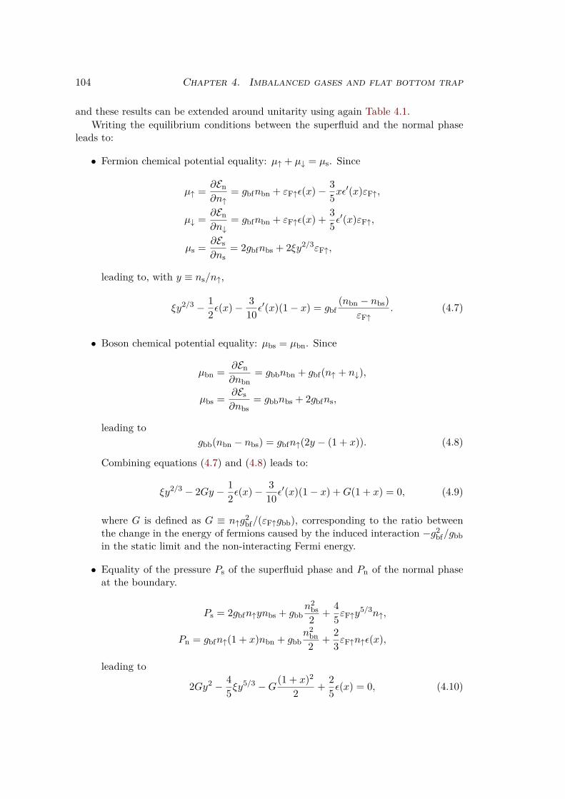
104 Chapter 4. Imbalanced gases and flat bottom trap
and these results can be extended around unitarity using again Table 4.1.Writing the equilibrium conditions between the superfluid and the normal phase
leads to:
• Fermion chemical potential equality: µ↑ + µ↓ = µs. Since
µ↑ =∂En
∂n↑= gbfnbn + εF↑ǫ(x)− 3
5xǫ′(x)εF↑,
µ↓ =∂En
∂n↓= gbfnbn + εF↑ǫ(x) +
35ǫ′(x)εF↑,
µs =∂Es
∂ns= 2gbfnbs + 2ξy2/3εF↑,
leading to, with y ≡ ns/n↑,
ξy2/3 − 12ǫ(x)− 3
10ǫ′(x)(1− x) = gbf
(nbn − nbs)εF↑
. (4.7)
• Boson chemical potential equality: µbs = µbn. Since
µbn =∂En
∂nbn= gbbnbn + gbf(n↑ + n↓),
µbs =∂Es
∂nbs= gbbnbs + 2gbfns,
leading togbb(nbn − nbs) = gbfn↑(2y − (1 + x)). (4.8)
Combining equations (4.7) and (4.8) leads to:
ξy2/3 − 2Gy − 12ǫ(x)− 3
10ǫ′(x)(1− x) +G(1 + x) = 0, (4.9)
where G is defined as G ≡ n↑g2bf/(εF↑gbb), corresponding to the ratio between
the change in the energy of fermions caused by the induced interaction −g2bf/gbb
in the static limit and the non-interacting Fermi energy.
• Equality of the pressure Ps of the superfluid phase and Pn of the normal phaseat the boundary.
Ps = 2gbfn↑ynbs + gbbn2
bs
2+
45εF↑y
5/3n↑,
Pn = gbfn↑(1 + x)nbn + gbbn2
bn
2+
23εF↑n↑ǫ(x),
leading to
2Gy2 − 45ξy5/3 −G(1 + x)2
2+
25ǫ(x) = 0, (4.10)
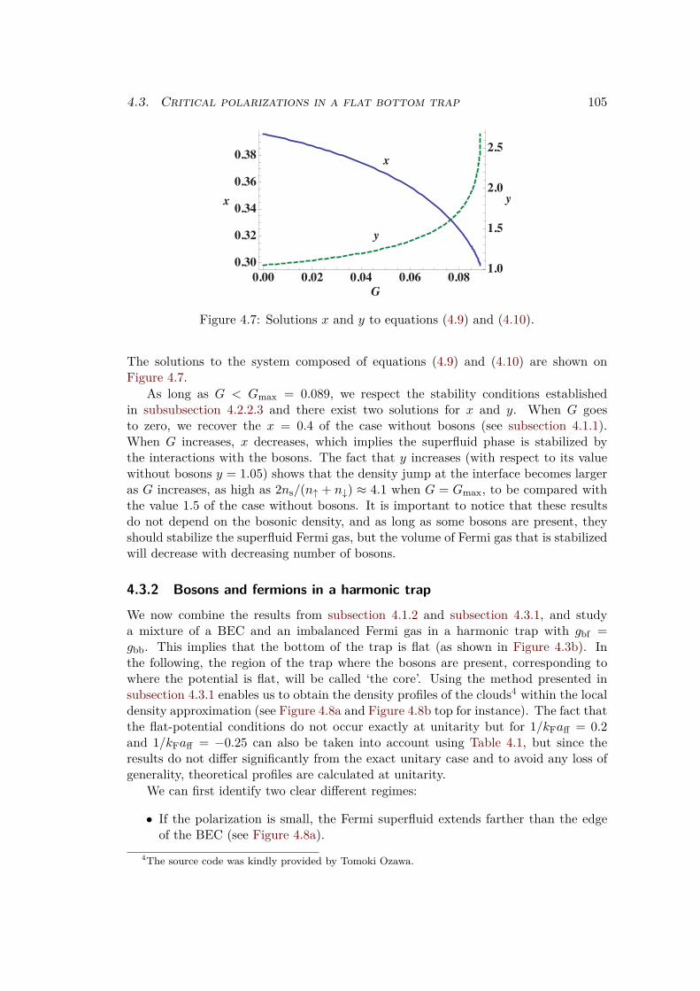
4.3. Critical polarizations in a flat bottom trap 105
0.00 0.02 0.04 0.06 0.08
0.30
0.32
0.34
0.36
0.38
1.0
1.5
2.0
2.5
x y
G
x
y
Figure 4.7: Solutions x and y to equations (4.9) and (4.10).
The solutions to the system composed of equations (4.9) and (4.10) are shown onFigure 4.7.
As long as G < Gmax = 0.089, we respect the stability conditions establishedin subsubsection 4.2.2.3 and there exist two solutions for x and y. When G goesto zero, we recover the x = 0.4 of the case without bosons (see subsection 4.1.1).When G increases, x decreases, which implies the superfluid phase is stabilized bythe interactions with the bosons. The fact that y increases (with respect to its valuewithout bosons y = 1.05) shows that the density jump at the interface becomes largeras G increases, as high as 2ns/(n↑ + n↓) ≈ 4.1 when G = Gmax, to be compared withthe value 1.5 of the case without bosons. It is important to notice that these resultsdo not depend on the bosonic density, and as long as some bosons are present, theyshould stabilize the superfluid Fermi gas, but the volume of Fermi gas that is stabilizedwill decrease with decreasing number of bosons.
4.3.2 Bosons and fermions in a harmonic trap
We now combine the results from subsection 4.1.2 and subsection 4.3.1, and studya mixture of a BEC and an imbalanced Fermi gas in a harmonic trap with gbf =gbb. This implies that the bottom of the trap is flat (as shown in Figure 4.3b). Inthe following, the region of the trap where the bosons are present, corresponding towhere the potential is flat, will be called ‘the core’. Using the method presented insubsection 4.3.1 enables us to obtain the density profiles of the clouds4 within the localdensity approximation (see Figure 4.8a and Figure 4.8b top for instance). The fact thatthe flat-potential conditions do not occur exactly at unitarity but for 1/kFaff = 0.2and 1/kFaff = −0.25 can also be taken into account using Table 4.1, but since theresults do not differ significantly from the exact unitary case and to avoid any loss ofgenerality, theoretical profiles are calculated at unitarity.
We can first identify two clear different regimes:
• If the polarization is small, the Fermi superfluid extends farther than the edgeof the BEC (see Figure 4.8a).
4The source code was kindly provided by Tomoki Ozawa.

106 Chapter 4. Imbalanced gases and flat bottom trap
• If the polarization is large, the Fermi gas in the core will be all in the normalphase, thereby one expects a uniform partially polarized gas, surrounded by anon-uniform partially polarized phase, and then by a fully polarized phase (seeFigure 4.8b).
nb
n↑n↓nb
n↑n ↓
(a) For low polarization, a uniform super-fluid (USF) lies in the core region.
n↑n↓nb
n↑n ↓
nb
(b) For high polarization, the core region isoccupied by a uniform partially polarized(UPP) phase.
Figure 4.8: Schematic representation of an imbalanced Fermi gas in a flat bottom trap.In purple is the superfluid (SF) phase, in faded yellow-to-red is the partially polarized(PP) phase, and in red is the fully polarized (FP) phase. The ‘core’ region, occupiedby the bosons - hence the flat trap area - is circled in blue.
We can now define two critical situations:
(i) The superfluid occupies the whole core, but does not extend out of it.
(ii) The core is occupied by a partially polarized phase such that the ratio n↓/n↑ inthe core is equal to the critical ratio for superfluidity (defined previously as x).
The radial density profiles corresponding to these situations are shown in Figure 4.9.The critical polarization for each of these situations can be computed as a func-
tion of Nf/Nb and depends only weakly on Nb. At unitarity, they are displayed onFigure 4.10a. They can also be computed for the two values of kFaff correspondingto our experimental realizations (namely kFaff = 5 and kFaff = −4), and the re-sults are shown on Figure 4.10b and Figure 4.10c, respectively. We notice that, for

4.3. Critical polarizations in a flat bottom trap 107
n↑n↓nb
n↑n ↓
nb
(a) Critical situation (i): the superfluid(with n↑ = n↓) occupies the whole coreand does not expand out of it.
n↑n↓nb
n↑n ↓
nb
(b) Critical situation (ii): the partially po-larized phase in the core is such as n↓/n↑ =0.40, the critical ratio for superfluidity.
(c) Representation of critical situation (i). (d) Representation of critical situation (ii).
Figure 4.9: The two critical situations evoked in the text. The bosonic density is shownin blue, the spin-up density in red and the spin-down density in yellow. Calculationswere made at unitarity, for Nb = 80 · 103, Nf = 150 · 103, and the correspondingpolarizations are P = 64% (a) and P = 75% (b). The radius r is given in units ofharmonic oscillator length lho and the densities of atoms in units of 1/l3ho, and gbb =gbf = 10−3lhomb/mf . (c) and (d) are 3D representation of the situations described in(a) and (b) respectively.
108 Chapter 4. Imbalanced gases and flat bottom trap
Nf/Nb →∞, we retrieve the critical polarization for superfluidity in a harmonic trap.For all three cases, we notice that there is a non-zero range of polarization for whichthe core can neither be entirely superfluid nor entirely partially polarized. There isthus a phase-separation inside the core which is then ‘non-homogeneous’.
4.3.3 Breakdown of flat bottom trap prediction
The obvious question now is: what happens in the dashed region of Figure 4.10?There exist two ways to get there: either starting from the critical situation of (i) andincreasing the polarization, or starting from the critical situation of (ii) and decreasingthe polarization. We then have coexistence of the superfluid and of the normal phasein the core region. Many scenarios are eligible, including exotic phases such as FFLOphases [Hu and Liu, 2006, Bulgac and Forbes, 2008, Radzihovsky and Sheehy, 2010].
If we restrict ourselves to simple scenarios which respect the ellipsoidal symmetryand have a limited number of Superfluid-Normal boundaries, we can suppose the coreis separated into a normal phase and a superfluid phase, with either the superfluidphase at the center of the core, and the normal phase around it (Superfluid-Normalscenario, as in Figure 4.11a), or a central normal phase, and a superfluid around it inthe core, and a non-homogeneous normal phase (Normal-Superfluid-Normal scenario,as in Figure 4.11b). The question is then whether the superfluid lies at the center ofthe cloud like a ‘Kernel’ (Superfluid-Normal scenario), or whether it has the shape ofa ‘Shell’ around a normal phase (Normal-Superfluid-Normal scenario).
It is experimentally feasible to be both in the flat potential conditions and closeto the unitary regime, and we can also vary the polarization. We only have accessto the doubly-integrated profiles and not to the radial profiles, but the two scenariosexplained previously have very different signatures in the doubly integrated profiles (seeFigure 4.11c and Figure 4.11d). It should be possible to identify them experimentally.
4.4 Experiments on imbalanced Fermi gases in a flat bottom
trap
The rich variety of phenomena presented above led us to run the experiment at themagnetic fields for which a FBT was expected.
We took data for different total atom numbers and polarizations, using simultane-ous triple imaging, with both fermionic spin states imaged transversally in situ and thebosons imaged axially after ttof = 4 ms of time-of-flight. We have taken 1135 imagesat 817 G and 288 images at 854 G with Bose-Fermi mixture, and 405 images at 817 Gwith fermions alone, that we took for comparison purposes. In the Bose-Fermi mixture,the BEC density profile was found to be very close to a Thomas-Fermi distribution,despite the presence of fermions. On the other hand, as expected, the distribution ofthe Fermi component appears to be qualitatively affected by the presence of the BEC.

4.4. Experiments on imbalanced Fermi gases in a FBT 109
(a) At unitarity
Superfluid core
Normal core
Non-homogeneous core
1
ff= 0
N/N
(b) BEC side
Superfluid core
Normal core
Non-homogeneous core
1
ff= 0.2
N/N
(c) BCS side
Superfluid core
Normal core
Non-homogeneous core
1
ff= -0.25
N/N
Figure 4.10: Critical polarizations for the core to be entirely normal (yellow area) orentirely superfluid (purple area), for different values of 1
kFaffin the BEC-BCS crossover.
The intermediate area of inhomogeneous core is in dashed purple-and-yellow.

110 Chapter 4. Imbalanced gases and flat bottom trap
n↑n↓nb
n↑n ↓
nb
(a) Superfluid-Normal scenario, radial den-sity profile.
n↑n↓nb
n↑n ↓
nb
(b) Normal-Superfluid-Normal scenario,radial density profile.
n↑n↓n↑-n↓
(c) Superfluid-Normal scenario, doubly-integrated density profile.
n↑n↓n↑-n↓
(d) Normal-Superfluid-Normal scenario,doubly-integrated density profile.
(e) 3D representation of Superfluid-Normal scenario.
(f) 3D representation of Normal-Superfluid-Normal scenario.
Figure 4.11: Two possible scenarios involving a phase separation in the core. Thecalculations were made assuming an equal volume of superfluid and of normal phasein the core for these figures. The numbers of atoms are Nf = 144 · 103, Nb = 80 · 103
with P = 0.69. (a) and (b) figures show the radial density profiles, and (c) and (d) thecorresponding doubly-integrated density profiles. Majority fermions (↑) are shown inred, minority (↓) in yellow, the difference (n↑ − n↓) in green and bosons in blue. (e)and (f) are 3D representations of the two situations.

4.4. Experiments on imbalanced Fermi gases in a FBT 111
4.4.1 Bosonic Thomas-Fermi radius
Since the fermionic density is essentially uniform, the shape of the BEC remains aparabola5. The fermions are imaged in situ and rapidly blown away from the trap,so the BEC expands during time-of-flight as usual6. We can make a Thomas-Fermifit of the bosonic profile and use it to extract the Thomas-Fermi radius after time offlight ttof , RTF,tof . In the case of cigar-shaped traps, it is related to the in situ axialThomas-Fermi radius RTF,b by the relation [Castin and Dum, 1996]:
RTF,b =1√
1 + ωrttof
ωr
ωzRTF,tof .
This expression is valid when any confinement is switched off at t = 0. In our case,we only switch off the optical dipole trap, that realizes mainly the radial confinement,and let the magnetic trap on. During the time of flight, the atoms feels some weakenedtrapping potential in the axial direction (with a new trapping frequency ωz,tof ∼ 2π ·14 Hz), and some anti-trapping potential in the radial direction (with a new frequencyωr,tof ∼ i2π · 7 Hz). The time evolution of the Thomas-Fermi radius are now given by:
RTF,z(t = ttof) = λz(ttof)RTF,z(t = 0),
RTF,r(t = ttof) = λr(ttof)RTF,r(t = 0),
where the λj=r,z obey [Castin and Dum, 1996]:
λr(t) =ω2
r
λz(t)λ3r(t)− ω2
r,tofλr(t),
λz(t) =ω2
z
λ2z(t)λ2
r(t)− ω2
z,tofλz(t).
These equations can be solved numerically, and we find that for a time of flight of 4 ms,λr(ttof) = 11.9 and λz(ttof) = 0.96. These values can be compared with λr = 11.9 andλz = 1.01, obtained assuming true time of flight, with equations (1.1). The correctionon λr is below our error bars. From the measured time of flight radius in the radialdirection RTF,r(ttof), we obtain the in situ radial Thomas-Fermi radius RTF,r(t =0) = RTF,r(ttof)/λr(ttof), then the in situ axial Thomas-Fermi radius RTF,z(t = 0) =RTF,r(t = 0)ωr/ωz. The Thomas-Fermi radius along the axial direction of the BECcan now be compared to the fermions characteristic lengths.
4.4.2 First observations
One first observation is that the peak density of the fermions is reduced by the presenceof the bosons with respect to a cloud without bosons with the same number of fermions,as it can already be seen on Figure 4.12. This very simple effect shows that the bosonsdo impose some repulsive potential on the fermions, whose density is reduced withrespect to a cloud in a simple harmonic trap. However, that effect is not straightforwardto quantify, due to the double integration in the two radial directions.
5If there is a density jump in the fermionic density, the BEC is not strictly a parabola, but dueto the high nb/nf ratio (see section 4.2), this effect is barely visible on theoretical profiles (see bluecurves in Figure 4.11a and Figure 4.11b), and not visible at all in our profiles.
6We checked the the bosonic cloud was not displaced during its time and flight, and thus not pushedby escaping fermions.
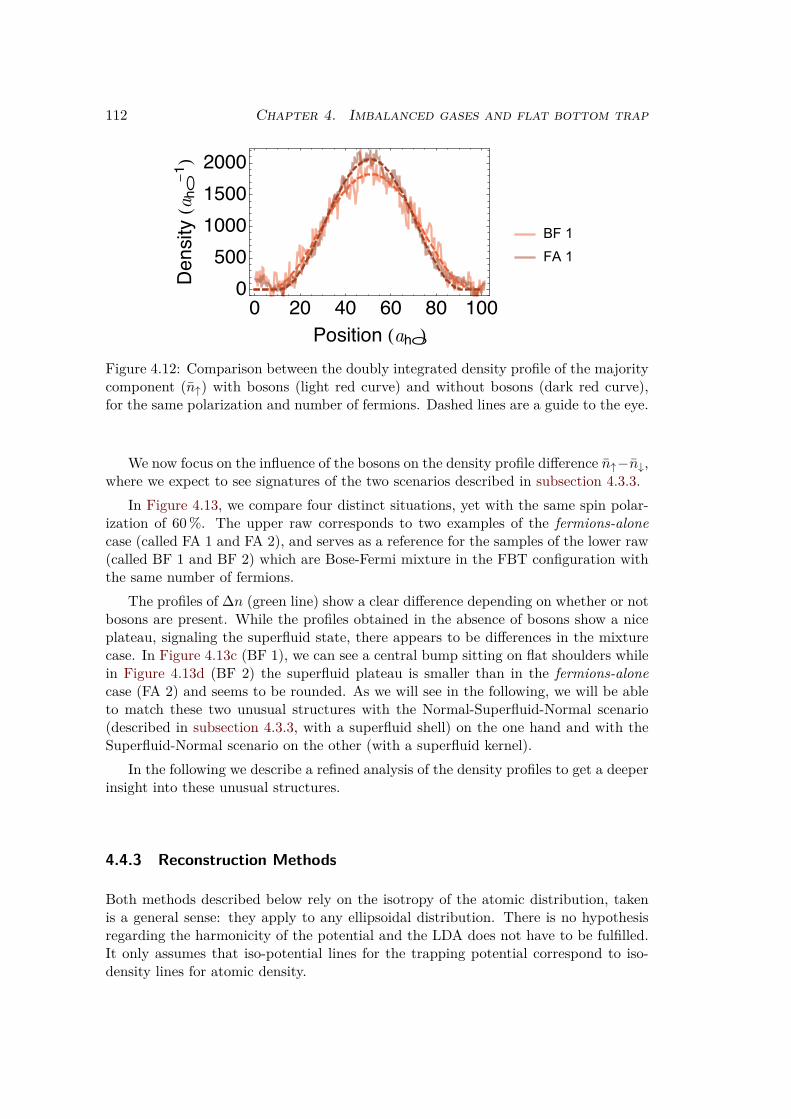
112 Chapter 4. Imbalanced gases and flat bottom trap
(a)
(a
- )
BF 1
FA 1
Figure 4.12: Comparison between the doubly integrated density profile of the majoritycomponent (n↑) with bosons (light red curve) and without bosons (dark red curve),for the same polarization and number of fermions. Dashed lines are a guide to the eye.
We now focus on the influence of the bosons on the density profile difference n↑−n↓,where we expect to see signatures of the two scenarios described in subsection 4.3.3.
In Figure 4.13, we compare four distinct situations, yet with the same spin polar-ization of 60 %. The upper raw corresponds to two examples of the fermions-alonecase (called FA 1 and FA 2), and serves as a reference for the samples of the lower raw(called BF 1 and BF 2) which are Bose-Fermi mixture in the FBT configuration withthe same number of fermions.
The profiles of ∆n (green line) show a clear difference depending on whether or notbosons are present. While the profiles obtained in the absence of bosons show a niceplateau, signaling the superfluid state, there appears to be differences in the mixturecase. In Figure 4.13c (BF 1), we can see a central bump sitting on flat shoulders whilein Figure 4.13d (BF 2) the superfluid plateau is smaller than in the fermions-alonecase (FA 2) and seems to be rounded. As we will see in the following, we will be ableto match these two unusual structures with the Normal-Superfluid-Normal scenario(described in subsection 4.3.3, with a superfluid shell) on the one hand and with theSuperfluid-Normal scenario on the other (with a superfluid kernel).
In the following we describe a refined analysis of the density profiles to get a deeperinsight into these unusual structures.
4.4.3 Reconstruction Methods
Both methods described below rely on the isotropy of the atomic distribution, takenis a general sense: they apply to any ellipsoidal distribution. There is no hypothesisregarding the harmonicity of the potential and the LDA does not have to be fulfilled.It only assumes that iso-potential lines for the trapping potential correspond to iso-density lines for atomic density.

4.4. Experiments on imbalanced Fermi gases in a FBT 113
FA 1
(a)
(a
- )
(a) Nf = 180 · 103, no bosons.
FA 2
(a)
(a
- )
(b) Nf = 125 · 103, no bosons.
BF 1
(a)
(a
- )
(c) Nb = 63 · 103, Nf = 180 · 103.
BF 2
(a)
(a
- )
(d) Nb = 88 · 103, Nf = 125 · 103.
Figure 4.13: Examples of doubly-integrated density profiles for a polarization of 60%.The top figures correspond to Fermi clouds prepared without bosons, while the bottomfigures to Bose-Fermi mixtures. Red curve is the density of the majority component,yellow curve that of the minority component and the green curve to the density dif-ference. The blue-dashed curve represents the reconstructed bosonic density fromthe time-of-flight image in another direction (when bosons are present). Units are interms of harmonic oscillator length in the axial direction. These clouds were preparedat 817 G.
Double inverse Abel transform
The first method that we used is based on the Abel transform. It was used in [Bulgacand Forbes, 2007, Shin et al., 2008, Shin, 2008, Horikoshi et al., 2010, Van Houckeet al., 2012] to extract the equation of state. It relies on a mathematical transformthat physically corresponds to the integration of an axially symmetric image along onedirection. Indeed, if we consider a function f(ρ) in the x−y plane with ρ =
√
x2 + y2,then F (y) is the integration of this function along x:
F (y) =ˆ ∞
−∞f
(√
x2 + y2
)
dx dx = ρ dρ√ρ2−y2
F (y) = 2ˆ ∞
y
f(ρ)ρ dρ√
ρ2 − y2.
This can easily be extended to a cylindrico-symmetric function f(ρ,z) in the xyz

114 Chapter 4. Imbalanced gases and flat bottom trap
space, with still ρ =√
x2 + y2:
F (y,z) =ˆ ∞
−∞f(ρ,z) dx = 2
ˆ ∞
y
f(ρ,z)ρ dρ√
ρ2 − y2.
But now if f was spherically-symmetric with f(ρ,z) = f(r =√
ρ2 + z2) = f(r =√
x2 + y2 + z2), then the function F (y,z) = F (√
y2 + z2) has radial symmetry andcan be integrated along y. We obtain:
F =ˆ ∞
−∞F
(√
y2 + z2
)
dy.
A representation of these two steps are given on Figure 4.14.
(a) Integration along x.
⇒
(b) Integration along y.
⇒
(c) Resulting 1D profile.
Figure 4.14: Schematic description of the two integration steps that lead to the doubleAbel transform. (a): integration of f(r) along the x direction to obtain F (y,z). (b):F (R) = F (y,z) integrated along the y direction to obtain F(z). (c): F(z), doubly-integrated density profile.
The fact that here the potential is ellipsoidal but not spherical is not a problembecause we just need to change the scaling of the z axis (for instance), with z ← ωz
ωrz.
Here, the doubly-integrated density profiles would correspond to F(z), and singly-integrated density profiles and radial density profiles can be reconstructed iterativelyusing the inverse Abel transform:
F (R =√
y2 + z2) = − 1π
ˆ ∞
R
dF(z)dz
dz√z2 −R2
f(ρ =√
x2 + y2,z) = − 1π
ˆ ∞
ρ
dF (y,z)dy
dy√
y2 − ρ2
Although it is mathematically exact, this method implies to take second derivativesof the experimental profiles which is quite noisy. Moreover the division by
√z2 −R2
and√
y2 − ρ2 implies a division by zero close to the center of the cloud, and thisamplifies the noise. It was thus impossible in our case to apply directly this methodand we had to pre-process the data in order to use this analysis. Before discussingthe pre-processing, I will give another mathematical relation between the radial profileand the doubly-integrated profile, based on a method proposed in [Fuchs et al., 2003,De Silva and Mueller, 2006a, Cheng and Yip, 2007, Ho and Zhou, 2009] and used in ourgroup [Nascimbène, 2010] to obtain the equation of state of the Fermi gas [Nascimbèneet al., 2010, Navon et al., 2010]. It turns out to give the same results with much lessamplification of the noise.

4.4. Experiments on imbalanced Fermi gases in a FBT 115
Weak LDA method
This method shares the same hypothesis with the previous one : ellipsoidal potential,non-necessarily harmonic. It was shown in subsection 4.1.3 that:
dn(z)z dz
= −2πω2
z
ω2ρ
n(z),
under some weak-LDA hypothesis, namely that the iso-potential lines correspond tothe iso-density lines.
This relation only involves one derivative, and one division by z, such that thenoise is strongly reduced with respect to the double-inverse Abel transform.
However, the experimental data is still too noisy to obtain a clear signal withthe derivative. Several pre-processing methods can be used to smooth the profiles.To remain as model-free as possible, we chose to use high-order polynomials to fitthe experimental profiles7. These polynomials can then be processed using eitherweak LDA method, or inverse-Abel transform. An example of the fit with 16th orderpolynomials is shown in Figure 4.15. Discussions on the choice of the order polynomialare presented in Appendix A.
4.4.4 Evidence for a superfluid shell
The results of Abel Transform and weak LDA method are presented in Figure 4.16from which we draw the following conclusions: as expected, the inverse Abel method ismuch noisier than the weak LDA method (this is amplified by the discretization of thepolynomial, necessary for the Abel integrals to converge properly). In the following,we will thus restrict ourselves to the weak LDA method. The numerical computationis also much faster.
Regarding the shape of the profiles, we can make additional remarks:
• For the fermions alone (FA) (see Figure 4.16d and Figure 4.16b), the radial den-sity of the difference n↑(z)−n↓(z) always has a minimum near z = 0. The densityjump at the boundary of the superfluid and normal phase (as on Figure 4.1a)that one would expect is not seen here because of the C∞ polynomials used forthe analysis.
• For the image with fermions and bosons (BF) (see Figure 4.16c and Figure 4.16a),the radial density of the difference n↑(z)−n↓(z) shows a minimum at a distancez 6= 0, close to the Thomas-Fermi radius of the bosons, shown in dashed bluelines. This is not the case for all BF images, some show a minimum for thedensity difference near z = 0, as shown on Figure 4.17.
These two different behaviors are very reminiscent of the two proposals made insubsection 4.3.3 regarding what could happen between the two critical polarizationsin the FBT. These images and others suggest that:
7It is clear that polynomials are C∞ functions and will not represent the corner points of Fig-ure 4.11c and Figure 4.11d. However, we considered that using piecewise functions as fit functionswould not provide an objective criteria to discriminate between these two scenarios.

116 Chapter 4. Imbalanced gases and flat bottom trap
FA 1
(a)
(a
- )
(a) Nf = 180 · 103, no bosons.
FA 2
(a)
(a
- )
(b) Nf = 125 · 103, no bosons.
BF 1
(a)
(a
- )
(c) Nb = 63 · 103, Nf = 180 · 103.
BF 2
(a)
(a
- )
(d) Nb = 88 · 103, Nf = 125 · 103.
Figure 4.15: Example of the polynomial fits on the doubly-integrated density profilespresented on Figure 4.13 The polarization is 60 % for all images. Top row: Thomas-Fermi fits applied to the fermions-alone (FA) cases. Bottom row: polynomial fitapplied to the Bose-Fermi mixtures (BF). Red: n↑(z), yellow: n↓(z), green: n↑(z) −n↓(z). Dashed thick lines: fits; thin solid lines: experimental data. Dashed blueline: reconstructed BEC profile. Vertical blue dashed lines indicate the Thomas-Fermiradius of the BEC when present.
• When there are no bosons, there is no FBT and the superfluid always lies at thecenter of the cloud, as expected (see Figure 4.1a).
• For Figure 4.17a, there is a superfluid in the FBT that is forming as a shell arounda partially polarized phase, like in the Normal-Superfluid-Normal scenario (seeFigure 4.11b and Figure 4.11f).
• For Figure 4.17b, there is a superfluid at the center of the FBT, surrounded by apartially polarized phase, like in the Superfluid-Normal scenario (see Figure 4.11aand Figure 4.11e).
The fact that the minima in the radial density differences n↑−n↓ do not always goto zero is a numerical artifact resulting from the polynomial fit: having a radial densitygoing precisely to zero requires a perfect cancellation the polynomial’s derivative, whichis not favored because the doubly integrated density profile is decreasing from thecenter. The radial density going precisely to zero thus requires the cancellation ofboth the first and second derivative (inflexion point). The same kind of arguments

4.4. Experiments on imbalanced Fermi gases in a FBT 117
BF 3
(a)
(a
- )
(a)
(a
- )
(a) Nf = 126 ·103, Nb = 63 ·103, P = 64%,with weak LDA method.
FA 3
(a)
(a
- )
(a)
(a
- )
(b) Nf = 126 · 103, Nb = 0, P = 64%, withweak LDA method
BF 3
(a)
(a
- )
(c) Nf = 126 ·103, Nb = 63 ·103, P = 64%,with inverse Abel transform.
FA 3
(a)
(a
- )
(d) Nf = 126 · 103, Nb = 0, P = 64%, withinverse Abel transform.
Figure 4.16: Comparison of typical radial profiles n(z) obtained with weak LDAmethod (figures (a) and (b)) and inverse Abel transform (figures (c) and (d)), forfermionic clouds with (figures (a) and (c)) and without (figures (b) and (d)) bosons.Red: n↑(z), yellow: n↓(z), green: n↑(z)−n↓(z). Insets: doubly-integrated density pro-files with their polynomial fits. Vertical blue dashed lines indicate the Thomas-Fermiradius of the BEC.
BF 1
(a)
(a
- )
(a) Nb = 63 · 103, Nf = 180 · 103.
BF 2
(a)
(a
- )
(b) Nb = 88 · 103, Nf = 125 · 103.
Figure 4.17: Reconstructed radial density profiles of two systems with similar atomsnumbers and a polarization of 60 %, that show different behaviors for the radial densitydifference.

118 Chapter 4. Imbalanced gases and flat bottom trap
explains also why the minimum is local and does not extend on a broader area: thepolynomial would have to be flat on a wide area, and this is not possible with apolynomial with order greater than one. Some numerical errors may also lead toa negative radial density difference for the SNN scenario as in Figure 4.17b. Theinfluence of the order of the polynomial and a consistency check on theoretical profilesare given in Appendix A.
From the above analysis, we believe that a minimum in the reconstructed profileof the density difference indicates the presence of a superfluid located around theminimum. Two situations can be discriminated:
• Either there is a superfluid kernel, surrounded by an unpaired normal phase. Inthis case, the radial density difference has a minimum near r = 0.
• Either there is a superfluid shell, surrounding and surrounded by a normal phase.In this case, the radial density difference has a minimum close to r = RT F,b.
• If the minimum is reached for r = RT F,↑, there is no superfluid and the cloud isentirely normal.
To evaluate the validity of these assumptions, we show the histogram of the reparti-tion of rmin/RT F,b at 817 G (see Figure 4.18a). It is clearly bimodal, with a first groupof data around rmin/RT F,b = 0 (corresponding to a superfluid kernel), and another onearound rmin/RT F,b ≈ 0.8 (corresponding to a superfluid shell). In addition, we plot(n↑−n↓)(r=rmin)
(n↑−n↓)(r=0) as a function of rminRT F,b
in Figure 4.18b. When (n↑−n↓)(r=rmin)(n↑−n↓)(r=0) = 1, the
minimum is located precisely at r = 0. Otherwise, this ratio indicates the depth ofthe minimum. We can see that the closer to RT F,b the minimum is, the deeper it is.Similar results were obtained for images taken at 854 G. This result can be interpretedas a signature that the superfluid shell, when it is present, is located close to RT F,b.
The criteria used to attribute a superfluid kernel, a superfluid shell, or a non-superfluid character are thus the followings:
• If there is a minimum at r = 0, there is a superfluid kernel.
• If there is a minimum between 0.5RT F,b and 1.5RT F,b and the density difference
ratio (n↑−n↓)(r=rmin)(n↑−n↓)(r=0) is smaller than 0.68, there is a superfluid shell.
• Else, if no minimum is present, or if it is not deep enough, there is no superfluid.
4.4.5 Parameters influencing the superfluid shell on the BEC side
4.4.5.1 Presence of bosons
Once the criteria have been proposed, it is important to check whether they are perti-nent and whether we can recover well-established results. We thus apply this methodto images without bosons, hence without a flat bottom trap. We expect to see only
8The value of 0.6 is chosen because the histogram as a function of(n↑−n↓)(r=rmin)
(n↑−n↓)(r=0)reveals a minimum
at 0.7. Values above 0.8 correspond to superfluid kernels, and below 0.6 to superfluid shells.

4.4. Experiments on imbalanced Fermi gases in a FBT 119
rRb
(a)
rRb
(n↑-n↓)(r
=r)
(n↑-n↓)(r
=)
(b)
Figure 4.18: (a) Histogram of the values of rmin/RT F,b at 817 G. The distributionis strongly bimodal. Black solid line is a Gaussian fit of the data centered aroundrmin/RT F,b = 0.8. Central value is 0.8 and standard deviation 0.2. (b) Evolutionof (n↑ − n↓)(r = rmin)/(n↑ − n↓)(r = 0) as a function of rmin/RT F,b for images at817 G. This shows two different behaviors: either the points are close to (n↑−n↓)(r =rmin)/(n↑ − n↓)(r = 0) = 1, rmin/RT F,b = 0 (509 points are superimposed here), orrather towards (n↑ − n↓)(r = rmin)/(n↑ − n↓)(r = 0) . 0.8, rmin/RT F,b ≈ 0.6 ∼ 1.1(423 points in this area, for a total of 1135 images).
superfluid kernels up to the Clogston-Chandrasekhar limit (76 % at unitarity, ∼ 90 %at 817 G and ∼ 57 % at 854 G).
At 817 G, we can check that all images with a polarization below 90 % show asuperfluid kernel. The result of this analysis is shown in Figure 4.19.
(%)
Shell
Kernel
Non-superfluid
Figure 4.19: Probability of having a superfluid shell (blue), a superfluid kernel (yellow),or no superfluid (green), as a function of polarization. Data correspond to 405 imagestaken at 817 G (1/kFaff = 0.2), without bosons. Shaded areas show 95 % confidenceinterval.
The fact that nearly 100 % of the images without bosons show a superfluid kerneland no shell below the critical polarization validates the approach given above. Therise of the non superfluid curve around 85 % indicates the expected breakdown of
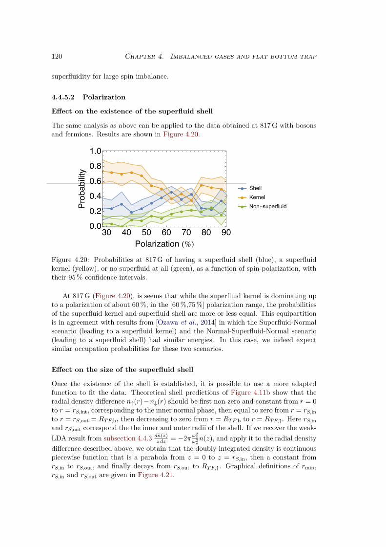
120 Chapter 4. Imbalanced gases and flat bottom trap
superfluidity for large spin-imbalance.
4.4.5.2 Polarization
Effect on the existence of the superfluid shell
The same analysis as above can be applied to the data obtained at 817 G with bosonsand fermions. Results are shown in Figure 4.20.
(%)
Shell
Kernel
Non-superfluid
Figure 4.20: Probabilities at 817 G of having a superfluid shell (blue), a superfluidkernel (yellow), or no superfluid at all (green), as a function of spin-polarization, withtheir 95 % confidence intervals.
At 817 G (Figure 4.20), is seems that while the superfluid kernel is dominating upto a polarization of about 60 %, in the [60 %,75 %] polarization range, the probabilitiesof the superfluid kernel and superfluid shell are more or less equal. This equipartitionis in agreement with results from [Ozawa et al., 2014] in which the Superfluid-Normalscenario (leading to a superfluid kernel) and the Normal-Superfluid-Normal scenario(leading to a superfluid shell) had similar energies. In this case, we indeed expectsimilar occupation probabilities for these two scenarios.
Effect on the size of the superfluid shell
Once the existence of the shell is established, it is possible to use a more adaptedfunction to fit the data. Theoretical shell predictions of Figure 4.11b show that theradial density difference n↑(r)−n↓(r) should be first non-zero and constant from r = 0to r = rS,int, corresponding to the inner normal phase, then equal to zero from r = rS,in
to r = rS,out = RT F,b, then decreasing to zero from r = RT F,b to r = RT F,↑. Here rS,in
and rS,out correspond the the inner and outer radii of the shell. If we recover the weak-
LDA result from subsection 4.4.3 dn(z)z dz = −2π ω2
zω2
ρn(z), and apply it to the radial density
difference described above, we obtain that the doubly integrated density is continuouspiecewise function that is a parabola from z = 0 to z = rS,in, then a constant fromrS,in to rS,out, and finally decays from rS,out to RT F,↑. Graphical definitions of rmin,rS,in and rS,out are given in Figure 4.21.
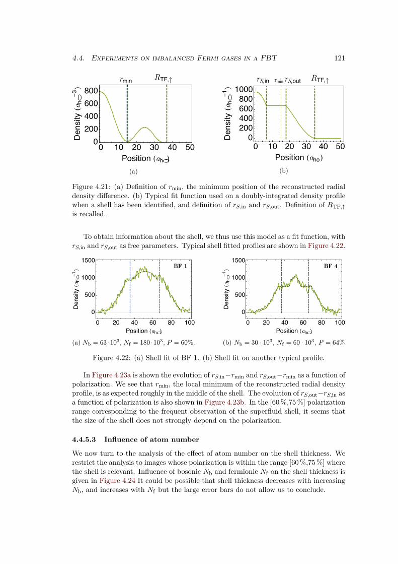
4.4. Experiments on imbalanced Fermi gases in a FBT 121
r R
(a)
(a
- )
(a)
rSrS R
(a)
(a
- )
(b)
Figure 4.21: (a) Definition of rmin, the minimum position of the reconstructed radialdensity difference. (b) Typical fit function used on a doubly-integrated density profilewhen a shell has been identified, and definition of rS,in and rS,out. Definition of RTF,↑is recalled.
To obtain information about the shell, we thus use this model as a fit function, withrS,in and rS,out as free parameters. Typical shell fitted profiles are shown in Figure 4.22.
BF 1
(a)
(a
- )
(a) Nb = 63 ·103, Nf = 180 ·103, P = 60%.
BF 4
(a)
(a
- )
(b) Nb = 30 · 103, Nf = 60 · 103, P = 64%
Figure 4.22: (a) Shell fit of BF 1. (b) Shell fit on another typical profile.
In Figure 4.23a is shown the evolution of rS,in−rmin and rS,out−rmin as a function ofpolarization. We see that rmin, the local minimum of the reconstructed radial densityprofile, is as expected roughly in the middle of the shell. The evolution of rS,out−rS,in asa function of polarization is also shown in Figure 4.23b. In the [60 %,75 %] polarizationrange corresponding to the frequent observation of the superfluid shell, it seems thatthe size of the shell does not strongly depend on the polarization.
4.4.5.3 Influence of atom number
We now turn to the analysis of the effect of atom number on the shell thickness. Werestrict the analysis to images whose polarization is within the range [60 %,75 %] wherethe shell is relevant. Influence of bosonic Nb and fermionic Nf on the shell thickness isgiven in Figure 4.24 It could be possible that shell thickness decreases with increasingNb, and increases with Nf but the large error bars do not allow us to conclude.

122 Chapter 4. Imbalanced gases and flat bottom trap
---
rS-r(a)
- - -
(a)
rS-rS
(a)
(b)
Figure 4.23: (a) Evolution of rS,in−rmin (green diamonds), rS,out−rmin (yellow squares)and rS,TF,b − rmin (blue dots) as a function of polarization. rmin is the local minimumof the reconstructed radial density profile, rS,in is the inner radius of the shell, andrS,out its outer radius. (b) Evolution of the shell thickness rS,out − rS,in as a functionof polarization. Error bars correspond to one standard deviation. aho = 9.8µm is theharmonic oscillator length in the axial direction.
Nb
rS-rS
(a)
(a)
Nf
rS-rS
(a)
(b)
Figure 4.24: (a) Evolution of rS,out − rS,in as a function of bosonic atom numberNb, restricted to the [60 %,75 %] polarization range. (b) Evolution of rS,out − rS,in
as a function of fermionic atom number Nf , restricted to the [60 %,75 %] polarizationrange. Dashed lines: linear fits. Dotted lines: mean values. Error bars correspond toone standard deviation.
4.4.6 Parameters influencing the superfluid shell on the BCS side
The same analysis can be performed at 854 G, on the BCS side. This magnetic fieldis of particular interest because the interaction parameter 1/kFaff ≈ −0.25, close tothe predicted FFLO conditions (see Figure 0.1). Similar behavior as for 817 G can beobserved, with hints both for shells and for kernels (see for instance Figure 4.25a for ashell and Figure 4.25b for a kernel).
The same reconstruction procedure leads to reconstructed radial density profilesshown in Figure 4.25c and Figure 4.25d. As before, depending of the existence of aminimum close to r = 0 (as in Figure 4.25d), or for a finite r close to RT F,b (as in

4.4. Experiments on imbalanced Fermi gases in a FBT 123
BF 1BCS
(a)
(a
- )
(a)
BF 2BCS
(a)
(a
- )
(b)
BF 1BCS
(a)
(a
- )
(c)
BF 2BCS
(a)
(a
- )
(d)
BF 1BCS
(a)
(a
- )
(e)Shell example at 854 G
BF 2BCS
(a)
(a
- )
(f)Kernel example at 854 G
Figure 4.25: (a) Typical density difference showing the existence of a superfluid shellat 854 G. Here Nf = 110 · 103, Nb = 38 · 103 and P = 52 %. (b) Typical densitydifference showing the existence of a superfluid kernel at 854 G. Here Nf = 90 · 103,Nb = 38 · 103 and P = 48 %. (c) and (d) Corresponding reconstructed radial densityprofiles with weak LDA method. (e) and (f) Green dashed curves: piecewise functionsused to extract the position and thickness of the superfluid shell (e) or the extensionof the plateau (f). Red and yellow dashed curves are guides to the eye for the doubly-integrated density of the majority (red curve) and minority (yellow curve) components.Vertical dashed blue lines indicate the Thomas-Fermi radius of the condensate.

124 Chapter 4. Imbalanced gases and flat bottom trap
Figure 4.25c), we use an adapted piecewise function to know the position and extensionof the superfluid plateau. Fits using such piecewise functions on the profiles are shownin Figure 4.25e (for a shell) and Figure 4.25f (for a kernel).
Here again, the contrast of the minimum of the density difference (see green curvesin Figure 4.25c and Figure 4.25d) can be plotted as a function of its position, and asbefore we find that the minimum is either located close to r = 0 or close to r = RT F,b,see Figure 4.26b, and the same criteria are used to discriminate between a superfluidkernel, a superfluid shell, or no superfluid at all.
rRb
(a)
rRb
(n↑-n↓)(r
=r)
(n↑-n↓)(r
=)
(b)
Figure 4.26: (a) Histogram of the values of rmin/RT F,b. The distribution is stronglybimodal. Black solid line is a Gaussian fit of the data centered around rmin/RT F,b =0.9. Central value is 0.9 and standard deviation 0.25. (b) Evolution of (n↑ − n↓)(r =rmin)/(n↑ − n↓)(r = 0) as a function of rmin/RT F,b for images at 854 G. This showstwo different behaviors: either the points are close to (n↑ − n↓)(r = rmin)/(n↑ −n↓)(r = 0) = 1, rmin/RT F,b = 0 (41 points are superimposed here), or rather towards(n↑ − n↓)(r = rmin)/(n↑ − n↓)(r = 0) . 0.8, rmin/RT F,b ≈ 0.6 ∼ 1.1 (165 points in thisarea, for a total of 288 images).
However, at 854 G the analysis is not statistically conclusive, see Figure 4.27. Thiscan be due to a lower number of images (288 instead of 1135). Another explanationwould rely on the relative sharpness of the FBT condition (see subsubsection 4.2.2.2).Indeed, the dataset gathers images taken on different days, and since the FBT conditionis sharper at 854 G than it is at 817 G, it is also possible that day-to-day magnetic fieldfluctuations drove the system back and forth across the gbb = gbf condition, or simplythat we made a small mistake in the magnetic field calibration that drove us awayfrom the FBT condition and into the anti-trapping regime (see Figure 4.3c). Thiswould explain the apparent prevalence of the superfluid shell in Figure 4.27. We planto investigate this situation in much greater detail.
The dependence of the shell parameters at 854 G with the polarization and atomnumbers are shown in FF. They do not differ significantly from the that at 817 G.
4.4.7 Portrait of the superfluid shell
With the information gathered above, we can draw a portrait of the superfluid shell.It is presented in Table 4.2.
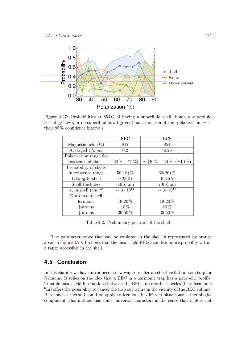
4.5. Conclusion 125
(%)
Shell
Kernel
Non-superfluid
Figure 4.27: Probabilities at 854 G of having a superfluid shell (blue), a superfluidkernel (yellow), or no superfluid at all (green), as a function of spin-polarization, withtheir 95 % confidence intervals.
BEC BCSMagnetic field (G) 817 854Averaged 1/kFaff 0.2 -0.25
Polarization range forexistence of shells [60 %− 75 %] ∼ [40 %− 60 %] (±10 %)
Probability of shellsin existence range 50(10) % 60(20) %
1/kFaff in shell 0.25(5) -0.34(5)Shell thickness 50(5)µm 70(5)µm
ns in shell (cm−3) ∼ 3 · 1011 ∼ 3 · 1011
% atoms in shellfermions 10-20 % 10-20 %↑-atoms 10 % 10 %↓-atoms 30-50 % 30-50 %
Table 4.2: Preliminary portrait of the shell
The parameter range that can be explored in the shell in represented by orangeareas in Figure 4.29. It shows that the mean-field FFLO conditions are probably withina range accessible in the shell.
4.5 Conclusion
In this chapter we have introduced a new way to realize an effective flat bottom trap forfermions. It relies on the idea that a BEC in a harmonic trap has a parabolic profile.Tunable mean-field interactions between the BEC and another species (here fermionic6Li) offers the possibility to cancel the trap curvature in the vicinity of the BEC volume.Here, such a method could be apply to fermions in different situations: either single-component This method has some universal character, in the sense that it does not

126 Chapter 4. Imbalanced gases and flat bottom trap
-
-
rS-r(a)
- - -
(a)
rS-rS
(a)
(b)
Nb
rS-rS
(a)
(c)
Nf
rS-rS
(a)
(d)
Figure 4.28: (a) Evolution at 854 G of rS,in − rmin (green diamonds), rS,out − rmin
(yellow squares) and rS,TF,b−rmin (blue dots) as a function of polarization. rmin is thelocal minimum of the reconstructed radial density profile, rS,in is the inner radius of theshell, and rS,out its outer radius. (b) Evolution of the shell thickness rS,out − rS,in as afunction of polarization. (c) (resp. (d)) Evolution of rS,out−rS,in as a function of bosonnumber Nb (resp. fermion number Nf), restricted to the [40 %,60 %] polarization range.Dashed line is a linear fit, dotted line is the mean value of the shell thickness. Errorbars correspond to one standard deviation. aho = 9.8µm is the harmonic oscillatorlength in the axial direction.
depend on the situation of the other species and can be applied, for instance, to both asingle-component Fermi gas or to a two-component Fermi gas (spin-imbalanced or not).Since the Bose-Fermi scattering length of ∼ 41a0 is mainly identical for all spin-statesand independent of the magnetic field in a broad range (∼ 700−900 G) while the boson-boson scattering length encounters several Feshbach resonances, several combinationsof states can be chosen, leading to different values for the interaction parameter 1/kFaff .In collaboration with the Trento group, we predicted that for a spin-imbalanced Fermigas at unitarity in such a flat bottom trap, the Clogston-Chandrasekhar limit wouldbe modified and that some new topological superfluid phases, such as a shell-shapedsuperfluid, could arise. The experimental implementation of the flat bottom trap,for two magnetic fields (817 G, on the BEC side and 854 G, on the BCS side) closeto unitarity |1/kFaff | . 0.25 and the numerical reconstruction of the radial profilesfrom one-dimensional absorption images were realized. At 817 G, in the [60% − 75%]polarization range, the repeated presence of a minimum in the reconstructed radial

4.5. Conclusion 127
Figure 4.29: Mean-field phase diagram for FFLO phases, taken from [Radzihovskyand Sheehy, 2010]. The areas indicated in bright orange correspond to the areasexplored with the experiments presented here. The faint orange areas correspond toa range of interaction parameters accessible within the homogeneous area. Adaptedfrom [Radzihovsky and Sheehy, 2010]
density difference was interpreted as an evidence for a superfluid shell. This superfluidshell could be seen only in images with a BEC, and is clearly made possible only bythe presence of the bosons. This novel phase is consistent with mean-field theoreticalpredictions. It does not provide direct proof of the flat bottom trap, for instance itcould be enhanced by a small anti-trapping potential in the BEC volume. This wouldincrease the fermionic density close to the bosonic Thomas-Fermi radius and favorthe shell. The currently ongoing detailed study of the role of gbb/gbf will clarify thissituation and bring better knowledge of the flat bottom trap. Also the 854 G conditionon the BCS side of the resonance deserves much more detailed studies.

128 Chapter 4. Imbalanced gases and flat bottom trap
Chapter 5
New Lithium Machine
5.1 Overview . . . . . . . . . . . . . . . . . . . . . . . . . . . . . 130
5.1.1 “Cahier des charges” . . . . . . . . . . . . . . . . . . . . . . . 130
5.1.2 D1 cooling . . . . . . . . . . . . . . . . . . . . . . . . . . . . 131
5.1.3 Experimental sequence . . . . . . . . . . . . . . . . . . . . . . 133
5.2 Mechanical setup . . . . . . . . . . . . . . . . . . . . . . . . . 134
5.2.1 Oven . . . . . . . . . . . . . . . . . . . . . . . . . . . . . . . . 135
5.2.2 Vacuum system . . . . . . . . . . . . . . . . . . . . . . . . . . 135
5.2.3 Cells and optical transport . . . . . . . . . . . . . . . . . . . 136
5.3 Laser setup . . . . . . . . . . . . . . . . . . . . . . . . . . . . 137
5.3.1 Laser Scheme . . . . . . . . . . . . . . . . . . . . . . . . . . . 137
5.3.2 Optical realization . . . . . . . . . . . . . . . . . . . . . . . . 137
5.3.3 Mechanical installation . . . . . . . . . . . . . . . . . . . . . 141
5.4 Magnetic fields . . . . . . . . . . . . . . . . . . . . . . . . . . 143
5.4.1 Zeeman slower . . . . . . . . . . . . . . . . . . . . . . . . . . 143
5.4.2 Compensation coils . . . . . . . . . . . . . . . . . . . . . . . . 145
5.4.3 MOT-Feshbach coils . . . . . . . . . . . . . . . . . . . . . . . 146
5.4.4 Science cell magnetic fields . . . . . . . . . . . . . . . . . . . 148
5.5 Security and computer control . . . . . . . . . . . . . . . . 148
5.6 Conclusion . . . . . . . . . . . . . . . . . . . . . . . . . . . . 148
During the first half of my PhD, I had been doing several side projects to improvethe old lithium machine: adapt Cicero (a control software for cold atoms experiments)to the specificities of our experiment1, build a whole new laser system that would notrely on slave laser diodes, to increase laser power and run-to-run stability, preparesome beams for transverse cooling of the atoms flux before the Zeeman slower, etc.Finally, since some of the parts of the historical lithium experiment started to be very
1The historical experiment built by Florian Schreck was using Digital-to-Analog Converters (DAC)to generate analog signals.
129

130 Chapter 5. New Lithium Machine
old, and even though the two water leaks could be fixed and the broken coil replaced,a control computer under MS DOS and 10 slave lasers appeared as good reasonsto, instead of upgrading the experiment, build a complete upgraded experiment thatwould be more versatile, more reliable, and would take advantage of a new techniqueunveiled in our group: sub-Doppler D1 cooling. Using it, it is possible to skip all of themagnetically trapped stages of the previous experiment and have (hopefully) a muchsimpler experimental sequence. When it became unavoidable that our lab would beclose for a few months due to major construction work taking place at the ENS, wedecided to use this period to start building the new experiment.
The goals are still to be able to produce a superfluid mixture of 7Li and 6Li su-perfluids, but with a faster experimental sequence, more reliable, with less day-to-dayrealignment, and a better optical access. This will enable us further push superfluiditystudies in tailored optical potentials and to search for the famous FFLO phase in spinimbalanced systems.
This chapter is organized as follow: first, I will give the ideas at the root of thenew experiment, then describe its mechanical organization, its laser system, and finallywrite a few words about computer control and security circuit. The building is on itsway but not over, so this document does not intend to give all of the details of the newexperiment.
5.1 Overview
5.1.1 “Cahier des charges”
The design of the new experiment has to obey several requirements, and to provideimprovements with respect to the old one. Requirements are listed below, with aproposal for their realization.
• Ultracold mixtures of 6Li and 7Li. This is the main specificity of our experiment,which led to the first realization of a double Bose-Fermi superfluid mixture, andthere is a lot of experimental competences in the group regarding this point. Wewill use a 50/50 mixture of 6Li and 7Li in the oven.
• Fast sequence. This used to be a limitation of the old experiment, with ≥ 30 sof MOT loading and ≥ 20 s of RF evaporation. The repetition rate was at mostone sequence per minute, usually more like one sequence every two minutes. Theplan is to have a 20 s sequence, with a fast MOT loading and no RF evaporation(that will be replaced by D1 cooling).
• High optical access to do science. For this we need two chambers. One for theMOT and other pre-cooling stages (“MOT chamber”), and one for the actualphysics experiments (“science chamber”). We already had a similar situationwith the previous experiment, with the appendage acting as the science chamber,but optical access was strongly reduced by the presence of the Ioffe bars.
• Mechanical stability. On the old lithium experiment, all of the optics weremounted on high posts, and the MOT mirrors were held on high pillars. Here,

5.1. Overview 131
we plan to use low posts for the optical tables, and to mount the MOT and D1
cooling optics very close to the atoms, directly on the MOT chamber.
• Laser stability. With 10 slave diodes, this was always a big problem as well. Tocircumvent it, we plan to use no diode except for two of the three master lasers,and amplify the optical power with Tapered Amplifiers (TAs)2.
• Day-to-day stability. Within the new lab, it will be possible to have the exper-iment in one room, and to have the computer control on the other side of thewall. This way, perturbations of the experiment are minimized, with less dust,vibrations, etc.
• Relatively simple. With a limited number of traps, and using always 6Li to cooldown 7Li, the experiment should be easier to handle.
• Versatile. We want to be able to study different aspects of the physics of ultracoldgases, be able to install lattices, low-dimensions traps, or an imaging system witha very good resolution, etc. For this, the space around the science cell is so farcompletely empty. We also plan to do the computer control of the experimentwith Cicero, a very convenient and practical software for cold atoms experimentsdesigned by Aviv Kesheet at MIT. It will be much easier to make changes in theexperimental sequence than with the historical software working with MS-DOScomputers...
The requirements and their solutions have been exposed, and we plan ambitious im-provements of the experiment. Most of the points rely on a specific cooling technique,called gray molasses D1 cooling. Let us now detail a bit more about it before movingto the provisional experimental sequence.
5.1.2 D1 cooling
In the old experiment, the temperature at the end of the CMOT stage is about 600µK.Even though it has been made successfully by other groups [Fuchs et al., 2007], it isvery hard to load directly a MOT of lithium into an optical dipole trap. Indeed, forthe case of lithium (and conversely potassium), the temperature obtained at the end ofthe MOT stage are typically much higher than for other alcali atoms such as sodium,cesium or rubidium. Indeed, the naive temperature limit for a two-level atom in anoptical molasses is the Doppler temperature TD = ~Γ/2KB, where Γ is the widthof the excited state. However, the first realization of optical molasses and magneto-optical traps [Chu et al., 1985, Chu et al., 1986, Lett et al., 1988] showed that thetemperatures reached were well below TD. This could be explained later by takinginto account a three-level structure for the atoms and polarization gradients for thelasers [Dalibard and Cohen-Tannoudji, 1989, Ungar et al., 1989], and this effect is nowknown as Sisyphus cooling. It is widely used in different gray molasses schemes [Chu,
2TAs are optical amplifiers composed of a tapered-shaped gain medium. When they are seededwith properly aligned single mode frequency laser, the re-emit amplified light at the same frequency, atthe price of a relatively poor spatial mode (max. 50 % coupling efficiency) and a background pedestalover a few nanometers in the frequency spectrum.

132 Chapter 5. New Lithium Machine
1991, Weidemüller et al., 1994, Boiron et al., 1998, Aspect et al., 1988, Grynberg andCourtois, 1994, Boiron et al., 1995]. On the contrary, the efficiency of Sisyphus coolingis strongly reduced for D2 lines of lithium because excited states are not resolved: thetotal hyperfine splittings of 4.5 MHz for 7Li and 18.0 MHz for 6Li are comparable withtheir natural linewidth of Γ = 5.9 MHz.
Gray molasses were designed based on Sisyphus cooling more than 20 years ago,but it was rediscovered only recently by Fermix, the other team of the Ultracold Fermigroup at LKB [Fernandes et al., 2012]. Its principle is the following: consider a near-resonant laser beam (with detuning ∆) applied to a Λ-like three-level atom with twodegenerate ground states and one excited state, and assume that one of the groundstate is dark while the other one is bright. Which state is dark or bright depends onthe atomic transition and of the light polarization, this may even vary in space (if thepolarization varies). The dark state is transparent for the laser and is not coupled tothe excited state, but may be coupled to the bright state via motional coupling. Thebright state however is coupled to the excited state by the laser and will undergo a lightshift proportional to the laser’s intensity. If the light comes from counter-propagatingbeams, the resulting light intensity will be a standing wave and the light shift will beperiodic: δE = ~Ω(r)2
4∆ , with Ω(r) the Rabi frequency associated to the standing wave,proportional to the square root of the light’s intensity. In the dressed atom picturethat we will use in the following, since the excited to which the bright state is coupledhave a finite linewidth Γ, the bright state also have some effective width Γ′ = ΓΩ(r)2
∆2 .This is summed up in Figure 5.1.
dark state
bright state
excited state
Figure 5.1: Scheme of the Sisyphus cooling for ∆ > 0 in the dressed atom picture. Thedark state is shown in black, the bright state in blue, with its light shift and effectivelinewidth, and the excited state in gray.
The cooling process is now described for the case of a blue-detuned laser beam:∆ > 0 (here a red-detuned laser beam, with ∆ < 0 would lead to heating). Anatom in a dark state may be transferred to the bright state due to motional coupling.

5.1. Overview 133
This happens when the energy difference between the dark and the bright state is thesmallest, that is in the valleys of the bright state’s potential. The atom then climbsthe valley, and its probability to be pumped into the excited state increases as thelinewidth of the bright state increases, and is maximal at the top of the hills. Once itis pumped into the excited state, it may decay via spontaneous emission to the darkstate, with a net loss of energy, so that the cloud is cooled down. Another circle maystart again.
This method can be applied to any system with a dark state in the ground statesmanifold (this is the case for any transition F → F ′ ≤ F ), provided that the excitedstate can be resolved. We thus have to use the D1 line. We have successfully imple-mented this technique on the F = 2 → F ′ = 2 transition of the D1 line of 7Li andobtained temperatures of 50µK, more than ten time smaller than in the standard cool-ing sequence and with the same atomic density[Grier et al., 2013]. The crucial pointis that, now direct loading of an optical dipole trap can be achieved with a reasonabledipole trap power of ∼ 20 Watts focused over 40µm [Burchianti et al., 2014]. Ourcolleagues from Fermix experiment applied it simultaneously to 6Li and 40K [Sieverset al., 2015]. It is now used in many other groups, such as Mumbai group [Nath et al.,2013], Institut d’Optique group [Salomon et al., 2013], LENS group [Burchianti et al.,2014], Ketterle group at MIT (private communication), and others.
5.1.3 Experimental sequence
The organization for the new experimental sequence is the following. We plan to keepon having 6Li and 7Li mixtures. Both species exit the same oven, are slowed down byan inverted Zeeman slower, and then trapped into a MOT. The MOT should have more6Li than 7Li atoms with a loading rate on the order of 10 seconds. After this, we runa compressed MOT (CMOT) to increase phase-space density. A gray molasses shouldthen be imposed to the cloud. Here, some uncertainties remain: a D1 blue-detunedmolasses will cool down 6Li atoms, but we haven’t decided yet how we will cool down7Li atoms. So far, we have three options:
• If the thermalization with 6Li is sufficiently efficient and no further cooling willbe needed.
• If not, we can try to implement a blue-detuned D1 molasses on 7Li. However,due to a coincidence between 7Li D1 line and 6Li D2 line, this may heat up 6Li.
• The efficiency of far red detuned lithium cooling has also been demonstratedin [Hamilton et al., 2014]. This can also be implemented in the new experiment.
• In the last case, we can implement a UV-MOT cooling stage, as was shown in[Duarte et al., 2011]. This technique is the least-favored one, because it requiresspecial optics and a coherent source at 323 nm, a wavelength range where poweris still limited.
After this D1 cooling stage, the phase-space density will be high enough to allow directloading into a far-detuned 200 W optical dipole trap for both species to perform opticaltransport into the science cell. We plan to do optical transport with focus-tunable

134 Chapter 5. New Lithium Machine
lenses, as was demonstrated in [Léonard et al., 2014]. This tunable lens is sensitiveto temperature variations and might be subject to thermal lensing. To overcome this,we plan to do a pre-evaporation stage with the two lowest spin states of 6Li beforetransport3, in a dipole trap different from the one that we will use for optical transport.Since at low magnetic fields, the scattering length between 6Li Zeeman sub-levels isvery small, we need to go at a magnetic field of 300 G. There, the scattering lengthbetween the spin states is around −300 aB, which allows efficient evaporation. The7Li is sympathetically cooled by 6Li, with interspecies scattering length of ∼ 40 aB.Some optical pumping on 7Li might be realized at this stage to ensure state purityof 7Li. In the science cell, we ramp up the magnetic field up to ≈ 800 G and resumethe evaporation of 6Li down to quantum degeneracy. We then have several projects inmind, for instance using the high optical access and spatial resolution of the sciencecell to load the atoms in a flat potential, as was demonstrated in [Gaunt et al., 2013],and investigate the phase diagram of strongly correlated fermions with and withoutspin polarization.
5.2 Mechanical setup
The mechanical design of the new experiment is represented in Figure 5.2. It will bedetailed in the following sections.
Figure 5.2: Scheme of the new Li experiment. The oven is at the extreme left, SAESpumps are in red, in blue is the atomic beam block rotating mount and motor. Themain cell is the MOT chamber and the science cell is in light blue at the back of theMOT cell.
3After the D1 cooling stage, 6Li atoms will be naturally in the two-lowest-spin states of the system:|F = 1/2,mF = ±1/2〉.

5.2. Mechanical setup 135
5.2.1 Oven
The oven is composed of a T-like tube4, the same as the one on Figure 2.6. Lithiumwill be inserted from the top and heated up at 510C in order to get a high vaporpressure. There will be a 50/50 mixture of 6Li and 7Li in the oven. In the previousexperiment, the horizontal part of the tube tended to clog with lithium, leading to lowatomic flux and low atom number in the MOT. The tube can be unblocked by heatingit up for a while, but the major problem consisted in the fact that we never knewwhether the tube was blocked or the experiment just not working so well. To preventthis in the new experiment, viewports to monitor the atom flux have been planned.A rotatable stepper motor5 (in blue on Figure 5.2) will be used to block the atomicjet when the experiment is not running or after the loading stage of an experimentalsequence.
5.2.2 Vacuum system
To ensure a good vacuum in the experiment, we have chosen the following scheme :
• Two turbo pumps can be placed at each end of the experimental apparatus,which will allow the opening of the part containing the oven (to reload or changeit) and the part containing the last window of the Zeeman slower (to clean it)without breaking the vacuum of the two main cells. They will not be presentduring the day-to-day run of the experiment and are not indicated in Figure 5.2,only their connexions are shown.
• One 40 L.s−1 ion pump6 will be placed close to the oven.
• Two 200 L.s−1 SAES pumps7 will be placed afterwards to ensure differentialpumping stages.
• One 500 L.s−1 SAES pump8 will pump directly on the MOT chamber
• A last 200 L.s−1 SAES pump9 will ensure a differential pumping stage betweenthe MOT chamber and the science chamber.
To improve the pumping efficiency of the SAES pumps, we chose to connect themto larger tubes: the flanges of NEXTORR D200-5 is CF40 and that of NEXTORRD500-5 is CF63. We will use zero-length reducers10 to connect them to custom-madetees and crosses11 so that they can pumps into CF63 and CF100 tubes respectively.
4custom-made from MDC-Vacuum5Brimrose BRM-275 670002-036Agilent Technologies StarCell Vaclon Plus 407NEXTORR D200-5. These pumps are hybrid between ion pumps and getters and have a very
high pumping efficiency for H2.8NEXTORR D500-5.9NEXTORR D200-5.
10Lesker RF600x450 and RF450x275M11MDC Vacuum ZCRT40-63, ZCRT63-100, ZCRT40-63-Conical, ZCRX6-2-63-4-40

136 Chapter 5. New Lithium Machine
5.2.3 Cells and optical transport
We have decided to use a two-cell setup for the new experiment, with some opticaltransport between them. This solution has several advantages: a better vacuum in thescience cell, and a better optical access to ensure a high versatility to the new experi-ment. The MOT cell12 has numerous viewports and we plan to dedicate each of themto a specific function (MOT beams, D1 cooling, Zeeman slower, imaging, fluorescence,optical transport, ...). The use of each viewport will be detailed in subsection 5.3.3.The science cell13 is the place where we will produce and study quantum degenerategases. The plan is to have two facing microscopes to have a high spatial resolutionand to be able to imprint custom-made potential on the atoms. The thin 3 mm wallsallow the use of some semi-custom commercial microscope.
There will be a ≈ 20 cm optical transport between those two cells. Optical trans-port is usually performed using a corner mirror on an extremely stable translationstage. However, a new option have been developed recently in Tilman Esslinger’sgroup [Léonard et al., 2014] using focus-tunable lenses14. These lenses are composedof some optical fluid inside a sealed deformable polymer membrane that has a diskshape. A flat ring applied on the outer part of the lens with more or less pressurepushes more or less the fluid towards the center, making use of the membrane elastic-ity. This changes the curvature radius of the lens and, as a result, its focal length. Aschematic representation is given on Figure 5.3. To ensure best working conditions,it is only needed to hold the lens horizontally (so that gravity deforms the membranehomogeneously), and to use a highly stable current controller. The whole system isextremely cost-efficient.
Figure 5.3: Scheme of the process used to change the focal length of the lens. Thegray outer rim is pushed downwards and the liquid is pushed inwards. Making use ofthe membrane’s elasticity, the curvature radius is changed, which modifies the focallength. On the left, the tunable lens is tuned to a large focal length, on the right to asmall one.
The lens is actually being tested15, and even though we have not fully decided theoptical scheme yet, it is likely that we will load the atoms in a first very powerfuldipole trap16 to make a pre-evaporation, then load them into a second weaker dipoletrap that will go through to tunable lens system to transport them. We will probablyuse a combination of two focus-tunable lenses in order to be able to move the focal
12Kimball Physics MCF450-SphCube-E6C8A1213custom-made from ColdQuanta. It is a 25x25x60 mm glass-cell with 3 mm thick walls, AR coatings
inside and outside, and a 2 wedge at the end to avoid standing waves during optical transport.14Optotune15Thanks to Thomas Reimann, who takes care of the realization of the optical transport part.16Made by a 300 W laser from IPG photonics, YURT-300-LP-WC

5.3. Laser setup 137
point of the beam without changing its waist nor moving the lens.
5.3 Laser setup
To cool the Li gases to degeneracy, we will use both the D1 and D2 lines of eachisotope. Since there is a coincidence between the D1 of 7Li and the D2 of 6Li (whichare distant only by 20 MHz), and since the hyperfine splitting for the ground stateis at most 800 MHz (for 7Li), we only need three master laser to generate all of thefrequencies used in the experiment, the other frequencies are derived from that of themaster’s lasers using Acouto-Optic-Modulators (AOMs) and Electro-Optic-Modulators(EOMs). We already had one solid-state laser at 670 nm providing a laser power of800 mW and two Toptica17 lasers producing a laser power of 500 mW each. The planin the new experiment is to have a vast majority of 6Li atoms in the MOT and to use6Li to evaporatively cool 7Li, so most of the optical power will be dedicated to 6Li.
5.3.1 Laser Scheme
The frequencies needed for the new experiment are given in Table 5.1. Proposed laserschemes are shown in Figure 5.5, Figure 5.4 and Figure 5.6. The ideas that led tothis design are the following: laser power has always been a problem, so we want toreuse as much of the optical power as possible. As a result, light for applications thathappen at different times in the experiment can be derived from the same sources(e.g. MOT beams and imaging beams can be derived from the same sources becausewhen we image the clouds the MOT is switched off). Some very precise calculationsof the transition frequencies for lithium were realized in [Sansonetti et al., 2011], andthe frequencies listed in Table 5.1 are given with respect to center-of-gravity (cog) ofthe D1 and D2 lines. These centers-of-gravity are within a few megahertz from thecrossovers which serve as experimental reference points.
5.3.2 Optical realization
We need three master lasers: one for the D2 line of each isotope and one for the D1
line of 6Li. The two master lasers for the D2 line of each isotope will be producedfrom Toptica BoosTA system. It is composed of one master diode, producing a powerof about 10 mW, that can be locked onto an atomic frequency and whose power isamplified by a Tapered Amplifier (TA) up to 500 mW. However, the TA output modeis not a Gaussian TEM00 mode, and injecting it properly into a fiber requires someappropriate beam shaping and may be challenging. In practical, about half of thepower is lost by fiber injection. For the D1 line of 6Li, we plan to use a solid-statelaser built by our group [Eismann et al., 2012]. This laser has a total output power of800 mW in a Gaussian TEM00 mode and was already used in our group for D1 coolingof 7Li [Grier et al., 2013]. Another version [Eismann et al., 2013, Kretschmar et al.,2016] has a total output power of more than 2 W. Since D1 cooling requires a lot of
17TA Pro at 670 nm

138 Chapter 5. New Lithium Machine
CO D2 6Li
-2x150 MHz
AOM
200 MHz
AOM
140 MHz
AOM
760 MHz
AOM
+2x130 MHz
-1 0
6P ZS
6P MOT
AOM
-2x80 MHz
AOM
+2x140 MHz
EOM
800 MHz
D1 7
0 +1
TA
AOM
-120 MHz
TA
AOM
200 MHz
AOM
250 MHz
0-1
AOM
2x200 MHz
AOM
2x200 MHz
LFI 6 OP 6
0 +1AOM
-2x70 MHz
AOM
+2x100 MHz
HF2 6HF1 6
0-1
Figure 5.4: Proposed laser scheme for the D2 lines of 6Li for the new experiment.Golden boxes correspond to Zeeman slowing light, silver boxes to MOT light, bluecases to D1 cooling light, red cases to imaging light and dashed cases to (so far)optional beams.

5.3. Laser setup 139
CO D1 6Li
-2x90 MHz
AOM
80 MHz
AOM
+2x130 MHz
AOM
-2x120 MHz
EOM
228 MHz
+1
6R ZS
6 D1
6R MOT
AOM
+200 MHz
0
Figure 5.5: Proposed laser scheme for the D1 lines of 6Li for the new experiment. Samecolor code as for Figure 5.4.

140 Chapter 5. New Lithium Machine
CO D2 7Li
-2x150 MHz
AOM
80 MHz
AOM
200 MHz
AOM
200 MHz
AOM
-2x225 MHz
-1 0
AOM
-2x130 MHz
AOM
+2x250 MHz
0 +1
TA
EOM
800 MHz
TA
AOM
-2x110 MHz
+1
0
LFI 7
AOM
-2x120 MHz
AOM
-2x210 MHz
HF1 7HF2 7
7 ZS
7 MOT
EOM
800 MHz
AOM
+120 MHz
OP 7
Figure 5.6: Proposed laser scheme for the D2 lines of 7Li for the new experiment. Samecolor code as for Figure 5.4.

5.3. Laser setup 141
Function Reference Detuning (MHz)(with respect to cog)
7Li P ZS D27Li −753.3
7Li R ZS D27Li +53.5
7Li P MOT D27Li −443.5
7Li R MOT D27Li +363.5
LFI 7Li D27Li −403.5
HFI1 7Li D27Li −623.5
HFI2 7Li D27Li −803.5
OP 7Li D27Li +403.5
7Li P D1 D17Li −355.9
D26Li +125
7Li R D1 D17Li +447.7
D26Li +928.6
6Li P ZS D26Li −464.1
6Li P MOT D26Li −154.1
LFI 6Li D26Li −114.1
HFI1 6Li D26Li −1314.1
HFI2 6Li D26Li −1394.1
OP 6Li D26Li +104.1
6Li R ZS D16Li −222.9
6Li R MOT D16Li +87.1
6Li P D1 D16Li −101.1
6Li R D1 D16Li +127.1
Table 5.1: Light frequencies needed for the new experiment. Here the letter ‘P’ standsfor Principal, ‘R’ for Repumper. Frequencies are given with respect to the centers ofgravity (cog) of the Li D lines.
optical power18, this repartition seems to be the best choice, even though it wouldhave been nice to have some narrow-linewidth light on the D2 lines for imaging19 toimprove imaging resolution.
The light emitted by the three master lasers is then split and sent through AOMsand EOMs to reach the right frequency, and the lights for the MOT and the Zeemanslowing beam are finally re-amplified by TAs before being combined and sent to theatoms.
5.3.3 Mechanical installation
The laser setup around the MOT cell is given on Figure 5.7.
18We want to be able to illuminate the clouds with an intensity of several tens of Isat =2.54 mW/cm−2 (typically I ≈ 50Isat) on the whole volume of the Compressed MOT.
19The solid-state lasers can easily be stabilized to sub-100 kHz linewidth while that of diode lasersor TAs is usually of several 100 kHz.

142 Chapter 5. New Lithium Machine
Figure 5.7: Laser arrangement around the MOT cell. The horizontal red beam is theZeeman beam. The faint red beams are the MOT beams. The orange beams will beused for D1 cooling. The yellow beams will be used for absorption and fluorescenceimaging. The green beam will be used for optical transport into the science cell. Theblue beams are for an optional blue MOT. One of the yellow or blue beams will alsobe used (with dichroic optics) for the high-power dipole trap and pre-evaporation inorder to use low-power optics on the optical transport path (the tunable lens can onlyhandle a few watts of optical power, not the few tens of watts needed for an efficientloading in the optical dipole trap).
We have also developed a compact design20 to install MOT beams and D1 coolingbeams directly on the MOT chamber: the MOT CF63 windows and the D1 CF16windows are fixed on the cell using four long setscrews, on which we plan to use extranuts to fix some adaptation plates to support a beam-guide system 21. A photo of the
20with the help of Cedric Enesa.21Beam Guide system, with mixed elements from Radiant Dyes (RD) and from Thorlabs(Th).
• For the MOT input: RD fiber plate / RD plate with f ′ = 8 mm aspheric lens to collimate fiberoutput / RD support with polarizing beam splitter (PBS) cube to clean the polarization / RDplate with f ′ = 8 mm aspheric lens - first lens of telescope / RD plate with λ/4 wave plate /RD to Th adapters / Th plate with f ′ = 100 mm lens - last lens of telescope / Th to Kimballcell adapter.
• And MOT retro-reflexion: Th to Kimball cell adapter / Th plate with λ/4 wave plate / Thplate with mirror.
• For D1 input: RD fiber plate / RD plate with f ′ = 8 mm aspheric lens to collimate fiber output/ RD support with polarizing beam splitter (PBS) cube to clean the polarization / RD platewith λ/4 wave plate / RD to Kimball cell adapter.
• And D1 retro-reflexion: RD to Kimball cell adapter / RD plate with λ/4 wave plate / RD plate

5.4. Magnetic fields 143
partially-mounted MOT chamber with the setscrews apparent is shown on Figure 5.8.
Figure 5.8: Photo of the partially-mounted MOT chamber. The white plastic coversare only to protect flanges and viewports from dust and chocks until construction isachieved. The long setscrews are very visible both on CF63 (MOT beams) and CF16(D1 cooling beams) flanges. One adapter plate is installed on the top CF63 viewport.The yellow plug is where the Zeeman slower will be installed.
A scheme of the designed beam guides is shown on Figure 5.9.We expect this cage mount to be simple to align, very stable, with a compact
design.
5.4 Magnetic fields
A number of different magnetic fields have to be imposed on the atoms to slow andcool them. The first one, the Zeeman slower field, has already been evoked in theprevious sections. It is described in more details here. However, it imposes a straymagnetic field in the MOT cell that has to be compensated for a proper operation ofthe MOT, as well as other stray magnetic fields, such as the Earth’s field. The mainideas for the MOT coils will then be discussed, before writing a few words about theprospective magnetic fields of the science cell region.
5.4.1 Zeeman slower
The Zeeman slower22 aims at slowing the atoms exiting the oven with an averagevelocity of 1400 m/s down to a velocity of about 50 m/s, at which they can be capturedby a Magneto-Optical Trap. We chose to implement a Zeeman Slower in a spin-flipconfiguration, i. e. the magnetic field produced by the Zeeman slower crosses zerobefore the end of the tube (see Figure 5.12). This has several advantages: a smallerabsolute magnetic field value leading to a smaller power consumption, and it also
with mirror.
22designed by Shuwei Jin
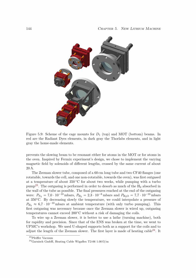
144 Chapter 5. New Lithium Machine
Figure 5.9: Scheme of the cage mounts for D1 (top) and MOT (bottom) beams. Inred are the Radiant Dyes elements, in dark gray the Thorlabs elements, and in lightgray the home-made elements.
prevents the slowing beam to be resonant either for atoms in the MOT or for atoms inthe oven. Inspired by Fermix experiment’s design, we chose to implement the varyingmagnetic field by solenoids of different lengths, crossed by the same current of about20 A.
The Zeeman slower tube, composed of a 60 cm long tube and two CF40 flanges (onerotatable, towards the cell, and one non-rotatable, towards the oven), was first outgasedat a temperature of about 350 C for about two weeks, while pumping with a turbopump23. The outgasing is performed in order to desorb as much of the H2 absorbed inthe wall of the tube as possible. The final pressures reached at the end of the outgasingwere: PN2 = 7,0 · 10−10 mbars, PH2 = 2,3 · 10−8 mbars and PH2O = 7,7 · 10−10 mbarsat 350C. By decreasing slowly the temperature, we could interpolate a pressure ofPH2 ≈ 6,7 · 10−10 mbars at ambient temperature (with only turbo pumping). Thisfirst outgasing was necessary because once the Zeeman slower is wired up, outgasingtemperatures cannot exceed 200C without a risk of damaging the coils.
To wire up a Zeeman slower, it is better to use a lathe (turning machine), bothfor rapidity and precision. Since that of the ENS was broken at the time, we went toUPMC’s workshop. We used U-shaped supports both as a support for the coils and toadjust the length of the Zeeman slower. The first layer is made of heating cable24. It
23Pfeiffer Vacuum24Garnisch GmbH, Heating Cable Wigaflex T2-06 1.00 Ω/m

5.4. Magnetic fields 145
will be used for a second outgasing of the Zeeman slower, up to 200C. Temperaturewill be monitored thanks to three thermocouples (one in the center, two on the sides)that go up to 400C. This first layer is then covered with Kapton tape to avoidheating of the coils during the outgasing phase. Then follow two layers of annealedhollow copper tube for cooling25. We then wrapped the whole tube in aluminum foil inorder to even the tube surface for wiring of the electric layers. The wire for the coils26
has a rectangular shape for easy wiring. A scheme of the Zeeman slower is displayedin ??. We first wired up the inverted Zeeman slower (8 layers of 9 turns) and wired upa spare 9th layer for security. A picture of the Zeeman slower is shown on Figure 5.11.We could test the magnetic field produced by the Zeeman slower using a gauss-meter,and the results are displayed on Figure 5.12 for a current of I = 20 A. The agreementbetween expected and measured variation is very satisfactory.
Figure 5.10: Schematic cut of the Zeeman Slower. The CF40 tube walls are indicatedin gray. The heating layer for the second outgasing is shown in red, the cooling layersin blue, and the coils in gold.
5.4.2 Compensation coils
5.4.2.1 For the Zeeman slower
The end of the Zeeman slower results in a non-zero magnetic field (B ≈ 4 G) in themiddle of the MOT chamber, which is a problem for the MOT. To compensate forthis, a compensation coil will be winded up on the other side of the cell and its currentadjusted to ensure a zero magnetic field at the center of the chamber. The support forthe coil will be fixed directly around the CF40 flange opposite of the Zeeman slower.
5.4.2.2 In 3 directions
Around the 6 CF63 windows for the MOT beams, we plan to have six small coils inorder to compensate for any residual stray magnetic field. They should be able togenerate a magnetic field of about 2 G in any direction. Their support will also be
25Euralliage, outer diameter 6 mm, inner diameter 4 mm.26APX, CL H 1.60x2.50 GR2 DIN 355, width: 2.5 mm (+2×0.17 mm insulation), thickness: 1.6 mm
(+2 × 0.12 mm insulation)

146 Chapter 5. New Lithium Machine
Figure 5.11: Picture of the Zeeman Slower
-
()
()(=)
Figure 5.12: Measured magnetic field in the Zeeman Slower (blue dots) and expectedvariation of the magnetic field (green curve). Dimensions are not respected.
fixed directly around the CF63 view-ports. Their current will be adjustable separatelyand optimized directly on the MOT position and fluorescence.
5.4.3 MOT-Feshbach coils
Now that we have the possibility of zeroing the bias magnetic field in the MOT cham-ber, we can turn to the realization of the magnetic gradient for the MOT. Due to thehigh volume of the MOT chamber it is not possible to put the coils very close to it, sowe use high current and water cooled wires.
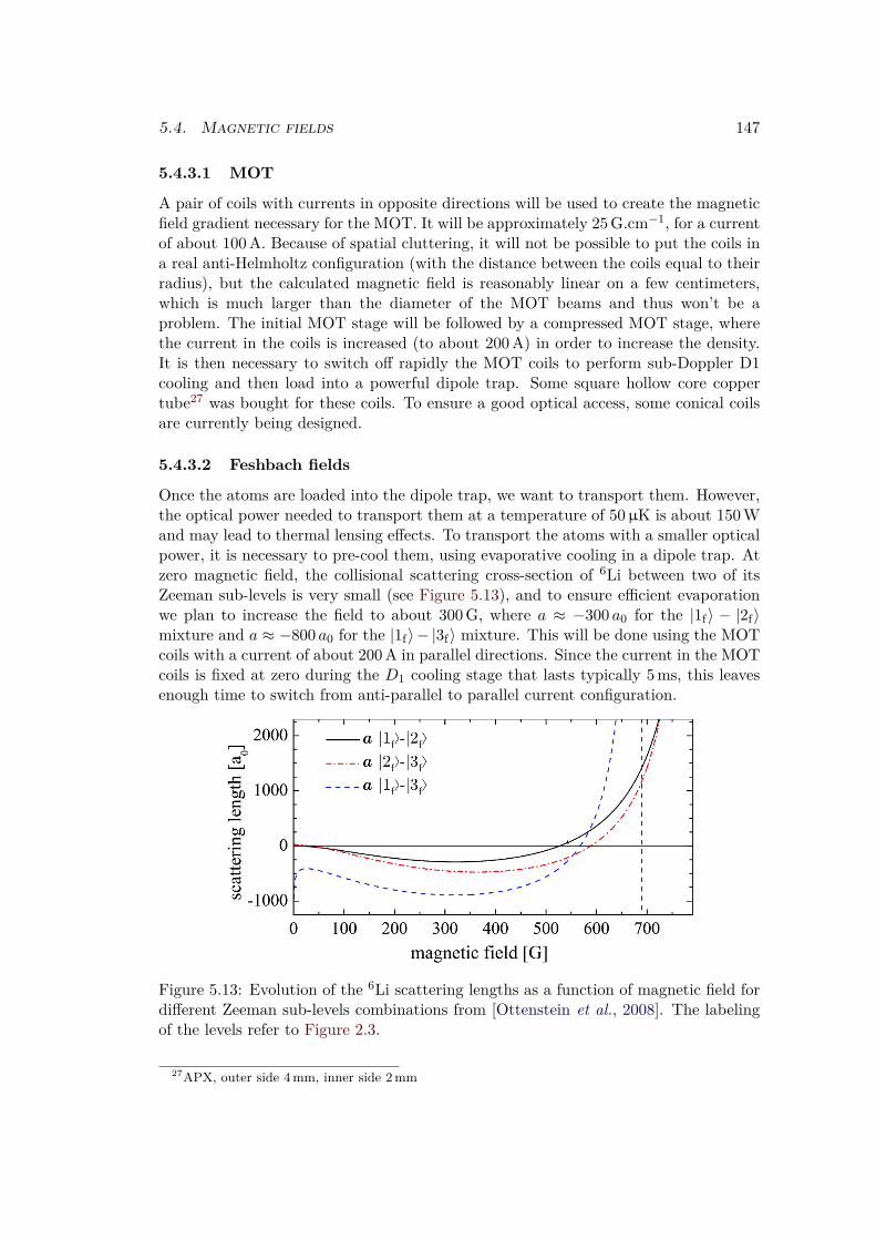
5.4. Magnetic fields 147
5.4.3.1 MOT
A pair of coils with currents in opposite directions will be used to create the magneticfield gradient necessary for the MOT. It will be approximately 25 G.cm−1, for a currentof about 100 A. Because of spatial cluttering, it will not be possible to put the coils ina real anti-Helmholtz configuration (with the distance between the coils equal to theirradius), but the calculated magnetic field is reasonably linear on a few centimeters,which is much larger than the diameter of the MOT beams and thus won’t be aproblem. The initial MOT stage will be followed by a compressed MOT stage, wherethe current in the coils is increased (to about 200 A) in order to increase the density.It is then necessary to switch off rapidly the MOT coils to perform sub-Doppler D1cooling and then load into a powerful dipole trap. Some square hollow core coppertube27 was bought for these coils. To ensure a good optical access, some conical coilsare currently being designed.
5.4.3.2 Feshbach fields
Once the atoms are loaded into the dipole trap, we want to transport them. However,the optical power needed to transport them at a temperature of 50µK is about 150 Wand may lead to thermal lensing effects. To transport the atoms with a smaller opticalpower, it is necessary to pre-cool them, using evaporative cooling in a dipole trap. Atzero magnetic field, the collisional scattering cross-section of 6Li between two of itsZeeman sub-levels is very small (see Figure 5.13), and to ensure efficient evaporationwe plan to increase the field to about 300 G, where a ≈ −300 a0 for the |1f〉 − |2f〉mixture and a ≈ −800 a0 for the |1f〉− |3f〉 mixture. This will be done using the MOTcoils with a current of about 200 A in parallel directions. Since the current in the MOTcoils is fixed at zero during the D1 cooling stage that lasts typically 5 ms, this leavesenough time to switch from anti-parallel to parallel current configuration.
Figure 5.13: Evolution of the 6Li scattering lengths as a function of magnetic field fordifferent Zeeman sub-levels combinations from [Ottenstein et al., 2008]. The labelingof the levels refer to Figure 2.3.
27APX, outer side 4 mm, inner side 2 mm

148 Chapter 5. New Lithium Machine
5.4.4 Science cell magnetic fields
The goals for the science cell magnetic fields is to be able to generate magnetic field ofup to 1000 G in order to exploit the Feshbach resonances of both 6Li and 7Li, and tobe able to generate a variable curvature to use a hybrid magnetic-optical trap. For theFeshbach field we need a pair of coils in Helmholtz configuration, and for the curvaturewe only have to be in a non-Helmholtz configuration. The plan is thus to have a pairof coils in Helmholtz configuration quite close to the cell, maybe conical, with an innerdiameter large enough to have the microscopes going through. Here also, the conicaldesign would reduce spatial cluttering and leave a better optical access. Anotherindependent pair of coils, probably farther away from the cell, will be designed for thecurvature field. In the previous lithium experiment, a clever design of the coils wasmade so that the bias field of the Feshbach coils (in G.A−1) was the opposite of that ofthe curvature coils [Tarruell, 2008]. This resulted in the axial confinement being veryeasy to tune. We are currently designing a similar solution for the new experiment.
5.5 Security and computer control
A security box28 will be used to monitor the temperatures of the critical elementsof the experiment: Zeeman slower, oven, coils, etc. and to overlook the water fluxthat is supposed to cool them. In case the temperature gets too high or the flux toolow, the currents will be shut down. The computer control will be made by Cicero,a software developed at MIT. It is composed of two sub-softwares, Atticus, whichdeals with communication between the computer and the experiment through NationalInstrument cards, and Cicero itself, to design the experimental sequence. During myPhD, I modified Cicero so that it can address Digital to Analog Converters (DACs);the corresponding user’s manual is given in Appendix B. It is a very powerful andconvenient software, with the a good ability of dealing with the different time scalesused in an ultracold atom experiment.
5.6 Conclusion
The historical lithium experiment has proven its capability to give and produce greatresults. However, its heavy day-to-day maintainability makes it poorly competitivewith respect to numerous new experiment worldwide. The project of building a com-plete new one instead of renewing it allowed the construction to be made in parallelwith the running of the old experiment. We could make use of the full man power ofthe Ultracold Fermi gases group (including Fermix team) during the shut down due toconstruction work, and they were really a great help for the project. From my personalpoint of view, it was very exciting and rich to start building a new experiment once Imastered the old one. The possibilities opened by the new experiment are numerousand I hope that the future PhD students will take advantage of them.
28Designed by Mihail Rabinovic.

Conclusion
Summary
The realization during my PhD of the first superfluid Bose-Fermi mixture opened a vastfield of investigation regarding the physics of the mixture. Due to the weak interactionbetween the Bose and the Fermi cloud, the BEC acts both as a sensitive probe and asa precision tool on the Fermi cloud.
Firstly, we investigated the properties of the Bose-Fermi counterflow. In the super-fluid regime, the mean-field effect of the Fermi gas on the BEC is probed with precisionspectroscopy measurements, in very good agreement with calculations. For a high-velocity counterflow, the Bose gas acts as a local probe to measure the critical velocityof the mixture. Our results are in agreement with Landau’s criterion[Castin et al., 2015]for superfluidity, in contrast with previous experiments[Miller et al., 2007, Weimer etal., 2015]. At high temperature, we observe an unexpected synchronization of thetwo thermal clouds, associated to a reduction of dissipation. Further experiments willmake use of the out-of-phase motion of the BEC and its thermal fraction to explorethe second sound of the mixture, predicted to be common to both components.
Second, we explored the opportunity to use the BEC as a precision tool to engineera flat-bottom trapping potential for the fermions and investigated the effect of sucha trap on Clogston-Chandrasekhar limit. We predicted the existence of a finite rangeof polarization for which a shell-shaped superfluid was energetically possible, and weprovided first experimental evidences of the observation of such a shell. It topologicallydiffers both from the habitual bulk superfluids and from toroidal superfluids reportedin Bose systems [Ramanathan et al., 2011, Wright et al., 2013b, Wright et al., 2013a,Mathey et al., 2014, Yakimenko et al., 2015]. This flat bottom trap can also be used toprepare uniform spin-imbalanced Fermi gases and search for the FFLO phase, whichparameters seem to be within the reach of our experimental realizations.
Perspectives
Regarding the superfluid shell in the Bose-Fermi mixture, a remaining open questionconcerns the dynamics of the shell formation, and the response of the system to aquench of the potential shape. This could be investigated using rapid magnetic fieldramps.
The existence of Feshbach resonances between 6Li and 7Li makes possible the re-alization of a superfluid Bose-Fermi mixture with one of the Fermi gas components
149

150 Conclusion
strongly interacting with the Bose gas29. This may have an influence on superfluidityand on Clogston-Chandrasekhar limit, making it an intriguing system to study.
Lastly, the ongoing construction of a new experiment opens the way to studies ofother properties of the mixture. The implementation of a box potential will enable usto obtain homogeneous Bose-Fermi mixtures, in which we plan to study for instancevortex formation and organization. Indeed, for such a Bose-Fermi mixture, the vorticesare expected to arrange in a square lattices, as it is the case for some Bose-Bosemixtures [Ho and Shenoy, 1996, Liu et al., 2014, Kuopanportti et al., 2012, Jezek etal., 2004] and in contrast with hexagonal Abrikosov lattices encountered for single Boseor Fermi superfluids. We also plan to take advantage of the box potential to measurethe critical velocity of a uniform Fermi gas and compare it with Landau’s criterion.Up to date, there are only few box potentials for fermions30, and the playground isvast.
29With |1f〉, |2f〉 and |4b〉 at 800 G for instance, see Table 2.2.30Martin Zwierlein at MIT is currently implementing one.

Appendices
151


Appendix A
Consistency check of FBT analy-sis
When doing the polynomial fit to the data, we evaluated the influence of using a non-adequate function to fit the density profiles and the influence of the order of the poly-nomial. We used simulated profiles from Normal-Superfluid-Normal and Superfluid-Normal scenarios that we fitted using polynomials of various order. Results are shownon Figure A.1.
A compromise has to be found between a too small order leading to an imprecisedescription, and a too high order where the polynomial starts to fit the noise leading tooscillations. We chose to use polynomials of order n = 16. The fact that the minimumin the density difference does not go to zero for the NSN scenario is very visible onthe analysis of the theoretical profile, as well as the fact that for the SNN scenario thedensity difference may be negative close to z = 0.
153

154
n↑n↓n↑-n↓
n↑n↓n↑-n↓
BF 1
(a)
(a
- )
BF 2
(a)
(a
- )
(a)
(a)
(
- )
(a)
(
- )
-
(a)
(
)
-
(a)
(
)
(b) n = 12.
(a)
(
- )
(a)
(
- )
-
(a)
(
)
-
(a)
(
)
(c) n = 16.
(a)
(
- )
(a)
(
- )
-
(a)
(
)
-
(a)
(
)
(d) n = 20.
(a)
(
- )
(a)
(
- )
-
(a)
(
)
-
(a)
(
)
(e) n = 24.
Figure A.1: Influence of the order n of the polynomials used to fit the data. Theleft column are the doubly integrated density profiles. First raw: theoretical profilesfor NSN scenario. Second raw: theoretical profiles for SNN scenario. Third raw:Nf = 180 · 103, Nb = 63 · 103, P = 60%. Fourth raw: Nf = 125 · 103, Nb = 88 · 103,P = 60%. The ↑ density is represented in red, the ↓ in yellow, the density differencein green, and the blue vertical dashed lines indicate the Thomas-Fermi radius of theBEC. Here the densities are given in terms of the averaged harmonic oscillator length√
~
mω .

Appendix B
Cicero for LithiumUser’s Manuel
B.1 Introduction - Caution
Introduction
This is meant to be a manual explaining the main changes done to the software Ciceroin order to have it running on the Lithium Experiment that uses Digital to AnalogConverter boxes.
Caution
• Do not name a device using capital letters. The only capital letter should be the‘D’ of ‘Devbanane’.
• Do not try to run Cicero for Lithium without a FPGA variable timebase. Thiswill not work.
• The function ‘Output Now’ that could be used to check whether Digital or Analogchannels were working is not fully implemented with DAC channels. (‘Outputnow’ is a static method, and since we can’t address several DACs simultaneously,it cannot be adapted easily).
B.2 Configuration of Atticus
I give here the step-by-step procedure to install Cicero with at least on digital carddedicated to DAC outputs.
Start by configuring Atticus as explained in Aviv Kesheet’s manual. For the FPGA:
• Install FPGA XEM3001 drivers, and run software FrontPanel.
• Click on ’Configure PLL button’ and set the frequency of CLK1 to the desiredfrequency as master clock. A suitable choice is 10MHz
155

156
• Click on EEPROM Write and Apply buttons to store these settings.
• Wire the variable frequency clock (bus JP2 pin 17) and its ground (bus JP2 pin19) to the PFI4 of ONE of the NI cards
For the server :
• set UseOpalKellyFPGA to True
• In the connections menu, set a connection between PFI4 (source) and PXI _Trig7(destination) - this is because the Trig terminals are shared between the cards-,and between PFI4 (source) and PFI0(destination) - this part is to isolate thestrobe for DAC devices.
In the FPGA menu :
• set UsingVariableTimebase to True
• set MySampleClockSource to DerivedFromMaster
• set the SampleClockRate to the frequency of the master clock (ex : 10000000 for10MHz)
For all of the NI devices,
• set MySampleClockSource to External
• set SampleClockExternalSource to PXI _Trig7 (or as defined in the devices con-figuration, so that it is linkable to the clock)
• set SampleClockRate to the FPGA sample clock rate
• set UsingVariableTimebase to True
• set SoftTriggerLast to False
• set StartTriggerType to SoftwareTrigger
Now you have to dedicate one of the digital cards to be DAC card. The DAC cardwill not be able to output digital signals any more. For this card:
• set DACChannelsEnabled to True, AnalogChannelsEnabled to False and Digi-talChannelsEnabled to False.
• The digforDAC Channels should appear in the list of Hardware channels. Theseare digital channels that will be used to output the DAC commands Use thebutton ‘Exclude Channels’ to get rid of the DigforDAC channels that won’t beused for DAC Address nor DAC Value.
• In the ServerSettings, edit the ChannelsforAddress and ChannelsforValue listswith the desired digforDAC channels.
• Be careful, you need exactly 8 channels for address and 16 channels for value.The order is important.

B. Cicero for Lithium: User’s Manuel 157
• Be careful, the bits are rather mixed up in the DAC boxes. The first 8 bits ofthe bus are for Address, then the next 3 bits are lost, then the next 8 bits arefor Value, another 3 bits are lost, the next 8 ones are also for Value, and the last2 are lost again.
• Now you can see 28 DAC channels appear in the channels list. Exclude theunused ones. The binary address of DAC boxes is either 110xxxxx or 10xxxxxx,depending on the generation, which means that you may use channels from 128(10000000) to 223 (11011111) (the values given here refer to the old lithiumexperiment).
• The DAC channels will now appear in Cicero Word Generator. You can boundthem to logical channels in the Add Logical Channel menu, give them a conversionequation, and all of the features available for Analog Channels in Cicero.
B.3 Changes made to the software
To deal with DAC channels, one need to start with Atticus, and tell it DAC channelsexist, and how to create and configure them. Then I had to add in Cicero some codeso that DAC channels can be programmed and dealt with. After that, i had to explainAtticus how to output the DAC values.
Atticus 1
First of all, i added two channel types to the preset types (that were digital, analog,series, gpib) : digforDAC and DAC. The digforDAC is for a real physical channel(ex:port1, line0), while the DAC channel is somehow a virtual channel, made by thecombination of digforDAC channels with the right value. Then, i allowed some of thedigital card to be specified as being ‘digforDAC’. Usually, when a card is programmed,its channels appear in the physical channels list. When a card has its ‘digforDACcha-nnelsEnabled’, its channels also appear in the channels list. You can allow some ofthem to be channels for DAC address, and some to be Channels for DAC value. Atthe end of the sequence, the computer will parse through the channels and tell eachof the ChannelsforAddress which value it has to output. Well, once you’ve got someChannels for Address (say, x), the corresponding number of DAC channels (2x) willappear in the list of available channels. This is the list that will be read by CiceroWord Generator, so i strongly recommend that you remove all of the unused DACchannels from this list in order to avoid mistakes.
Cicero
The DAC channels are now created, and Cicero will see them. Not much change hasbeen made in Cicero itself, I just looked for the occurrences of ’analog’ and copiedthem into ’DAC’. The data concerning the sequence is produced the same way asbefore. However, on producing the buffers, i had to change a few things, but this wasmade in DataStructures.

158
DataStructures
How it is done : basically, all of the timesteps of the sequence are saved with
• Which analog channel is on during this timestep ? What are the associatedwaveforms ? What is the precision required ?
• Which DAC channel is on during this timestep ? What are the associated wave-forms ? What is the precision required ?
• Which digital channel is on or off ? Is there pulses ?
Before, the computer had this precision required that more or less set the mainperiod of this step and just had to check if a channel had to be switch on or off inthe middle of a period. This was used to generate the VariableTimebase data, whichconsists in a dictionary of timesteps, to which are linked a list of ‘segments’, eachsegment being characterized by a number of counts (= its length divided by the mastersampleclock period). Then this dictionary is given to a function which calculates thevalues the channels have to take for each segment, and this is the buffer generation.Each segment corresponds to one line of the buffer, it’s one ‘clic’ of the clock.
Now, it is divided in several steps.
1. The first step is still the same, working together with the DAC and analogchannels, and taking the precision as the minimum of the two required precisions,the computer generates a ‘primary’ variable timebase.
2. Then, it generates the DAC buffer the same way the analog buffer was generatedpreviously. The trouble is, during a ramp for example, several DAC channels(let’s say 2) may have to change their value at the same time, and this can’t bedone because we need all of the channels of the digforDAC card to address oneDAC channel. So the computer has to talk to a channel, then quickly talk to theother one.
3. So the next step is to look into the DAC buffer, to find for which segments atleast two DAC channels have to change, which are the DAC channels involved,and then split the segment into the necessary number of new segments so that thecomputer talks to all of the channels without delaying the rest of the sequence.This outputs a dictionary that links the ‘bad’ segments to the DAC channelsthat change in it. A way of skipping this step would be to force the computer toaddress all of the 40 DACs at each segment, but we decided this would increasethe buffer size too much.
4. Then, i have to generate this new timebase splitting the segments of the first onewhen needed. We have to define how fast the computer switches between theDAC channels, and this can’t be arbitrary low (see below, about strobe). Thistime is called ‘Time needed to update Bus’ or ‘TimeBusUpdate’ in the code.
5. To produce the new DAC buffer, we can’t use the same function as before withthe new timebase segments dictionary because we would meet the same problemas before with several DACs changing their value at the same time. We have to
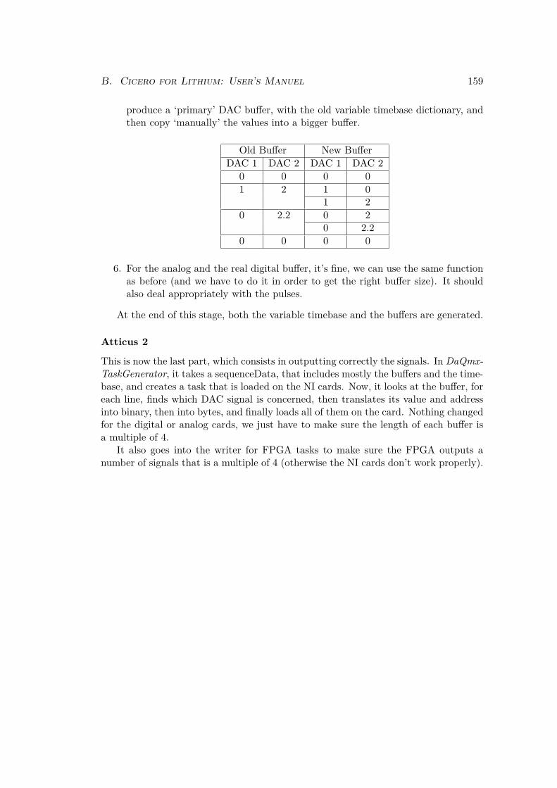
B. Cicero for Lithium: User’s Manuel 159
produce a ‘primary’ DAC buffer, with the old variable timebase dictionary, andthen copy ‘manually’ the values into a bigger buffer.
Old Buffer New BufferDAC 1 DAC 2 DAC 1 DAC 2
0 0 0 01 2 1 0
1 20 2.2 0 2
0 2.20 0 0 0
6. For the analog and the real digital buffer, it’s fine, we can use the same functionas before (and we have to do it in order to get the right buffer size). It shouldalso deal appropriately with the pulses.
At the end of this stage, both the variable timebase and the buffers are generated.
Atticus 2
This is now the last part, which consists in outputting correctly the signals. In DaQmx-TaskGenerator, it takes a sequenceData, that includes mostly the buffers and the time-base, and creates a task that is loaded on the NI cards. Now, it looks at the buffer, foreach line, finds which DAC signal is concerned, then translates its value and addressinto binary, then into bytes, and finally loads all of them on the card. Nothing changedfor the digital or analog cards, we just have to make sure the length of each buffer isa multiple of 4.
It also goes into the writer for FPGA tasks to make sure the FPGA outputs anumber of signals that is a multiple of 4 (otherwise the NI cards don’t work properly).

160

Appendix C
Publications and preprints
• “Λ-enhanced sub-Doppler cooling of lithium atoms in D1 gray molasses”,Andrew T. Grier, Igor Ferrier-Barbut, Benno S. Rem, Marion Delehaye, LevKhaykovich, Frédéric Chevy, and Christophe SalomonPhysical Review A 87, 063411 (2013)
• “A mixture of Bose and Fermi superfluids”,Igor Ferrier-Barbut, Marion Delehaye, Sébastien Laurent, Andrew T. Grier,Matthieu Pierce, Benno S. Rem, Frédéric Chevy, and Christophe SalomonScience 345, 1035-1038 (2014)
• “Chandrasekhar-Clogston limit and critical polarization in a Fermi-Bose super-fluid mixture”,Tomoki Ozawa, Alessio Recati, Marion Delehaye, Frédéric Chevy, and SandroStringariPhysical Review A 90, 043608 (2014)
• “Critical velocity and dissipation of an ultracold Bose-Fermi counterflow”,Marion Delehaye, Sébastien Laurent, Igor Ferrier-Barbut, Shuwei Jin, FrédéricChevy, and Christophe SalomonPhysical Review Letters 115, 265303 (2015)
• “Universal loss dynamics in a unitary Bose gas”,Ulrich Eismann, Lev Khaykovich, Sébastien Laurent, Igor Ferrier-Barbut, BennoS. Rem, Andrew T. Grier, Marion Delehaye, Frédéric Chevy, Christophe Sa-lomon, Li-Chung Ha, and Cheng ChinSubmitted to Physical Review X
161

162
C.1 Λ-enhanced sub-Doppler cooling of lithium atoms inD1 gray molasses
Andrew T. Grier, Igor Ferrier-Barbut, Benno S. Rem, MarionDelehaye, Lev Khaykovich, Frédéric Chevy, and Christophe
Salomon
Physical Review A 87, 063411 (2013)

PHYSICAL REVIEW A 87, 063411 (2013)
-enhanced sub-Doppler cooling of lithium atoms in D1 gray molasses
Andrew T. Grier,1,* Igor Ferrier-Barbut,1 Benno S. Rem,1 Marion Delehaye,1 Lev Khaykovich,2
Frederic Chevy,1 and Christophe Salomon1
1Laboratoire Kastler-Brossel, Ecole Normale Superieure, CNRS and UPMC, 24 rue Lhomond, 75005 Paris, France2Department of Physics, Bar-Ilan University, Ramat-Gan 52900, Israel
(Received 26 April 2013; published 12 June 2013)
Following the bichromatic sub-Doppler cooling scheme on the D1 line of 40K recently demonstrated
in Fernandes et al. [Europhys. Lett. 100, 63001 (2012)], we introduce a similar technique for 7Li atoms and obtain
temperatures of 60 μK while capturing all of the 5 × 10⁸ atoms present from the previous stage. We investigate
the influence of the detuning between the the two cooling frequencies and observe a threefold decrease of the
temperature when the Raman condition is fulfilled. We interpret this effect as arising from extra cooling due
to long-lived coherences between hyperfine states. Solving the optical Bloch equations for a simplified -type
three-level system we identify the presence of an efficient cooling force near the Raman condition. After transfer
into a quadrupole magnetic trap, we measure a phase space density of ∼10−5. This laser cooling offers a promising
route for fast evaporation of lithium atoms to quantum degeneracy in optical or magnetic traps.
DOI: 10.1103/PhysRevA.87.063411 PACS number(s): 37.10.De, 32.80.Wr, 67.85.−d
I. INTRODUCTION
Lithium is enjoying widespread popularity in the cold-atom
trapping community thanks to the tunability of its two-body
interactions and its lightness. Both the fermionic and the
bosonic isotopes of lithium feature broad, magnetically tunable
Feshbach resonances in a number of hyperfine states [1].
The presence of these broad resonances makes lithium
an attractive candidate for studies of both the Fermi- and
Bose-Hubbard models [2] and the strongly correlated regime
for bulk dilute gases of Fermi [3] or Bose [4–6] character. Its
small mass and correspondingly large photon-recoil energy
are favorable factors for large area atom interferometers [7]
and precision frequency measurements of the recoil energy
and fine structure constant [8]. Under the tight-binding
lattice model, lithium’s large photon-recoil energy leads to a
larger tunneling rate and faster time scale for superexchange
processes, allowing for easier access to spin-dominated
regimes [9]. Finally, lithium’s small mass reduces the heating
due to nonadiabatic parts of the collision between ultracold
atoms and Paul-trapped ions. This feature, together with Pauli
suppression of atom-ion three-body recombination events
involving 6Li [10], potentially allows one to reach the s-wave
regime of ion-atom collisions [11].
However, lithium, like potassium, is harder to cool using
optical transitions than the other alkali-metal atoms. The
excited-state structure of the D2 transition in lithium lacks the
separation between hyperfine states for standard sub-Doppler
cooling techniques such as polarization gradient cooling
[12–14] to work efficiently. Recently, it has been shown by
the Rice group that cooling on the narrow 2S1/2 → 3P3/2
transition produces lithium clouds near 60 μK, about half
the D2-line Doppler cooling limit [15], and can be used for
fast all-optical production of a 6Li quantum degenerate Fermi
gas. However, this approach requires special optics and a
coherent source at 323 nm, a wavelength range where power
is still limited. Another route is to use the three-level structure
of the atom as implemented previously in neutral atoms
*Corresponding author: [email protected]
and trapped ions [16–22]. The three-level structure offers
the possibility of using dark states to achieve temperatures
below the standard Doppler limit, as evidenced by the use
of velocity-selective coherent population trapping (VSCPT)
to produce atomic clouds with subrecoil temperatures [23]. In
another application, electromagnetically induced transparency
has been used to demonstrate robust cooling of a single ion to
its motional ground state [19,24].
In this paper, we implement three-dimensional bichromatic
sub-Doppler laser cooling of 7Li atoms on the D1 transition.
Figure 1 presents the 7Li level scheme and the detunings
of the two cooling lasers that are applied to the atoms after
the magneto-optical trapping phase. Our method combines
a gray molasses cooling scheme on the |F = 2〉 → |F ′ =2〉 transition [25,26] with phase-coherent addressing of the
|F = 1〉 → |F ′ = 2〉 transition, creating VSCPT-like dark
states at the two-photon resonance. Instead of UV laser
sources, the method uses laser light that is conveniently
produced at 671 nm by semiconductor laser sources or solid-
state lasers [27,28] with sufficient power. This enables us to
capture all of the ≃5 × 10⁸ atoms from a MOT and cool them
to 60 μK in a duration of 2 ms.
We investigate the influence of the relative detuning
between the two cooling lasers and observe a threefold
decrease of the temperature in a narrow frequency range
around the exact Raman condition. We show that extra cooling
arises due to long-lived coherences between hyperfine states.
We develop a simple theoretical model for a sub-Doppler
cooling mechanism which occurs in atoms with a -type
three-level structure, in this case, the F = 1, F = 2, and
F ′ = 2 manifolds of the D1 transition in 7Li. The main physical
cooling mechanism is contained in a 1D bichromatic lattice
model. We first give a perturbative solution to the model and
then verify the validity of this approach with a continued
fraction solution to the optical Bloch equations (OBEs).
II. EXPERIMENT
The stage preceding D1 sub-Doppler cooling is a com-
pressed magneto-optical trap (CMOT) in which, starting
from a standard MOT optimized for total atom number, the
063411-11050-2947/2013/87(6)/063411(8) ©2013 American Physical Society
C. Publications and preprints 163

ANDREW T. GRIER et al. PHYSICAL REVIEW A 87, 063411 (2013)
FIG. 1. (Color online) The D1 line for 7Li. The cooling scheme
has a strong coupling laser (principal beam, black solid arrow) δ2
blue detuned from the |F = 2〉 → |F ′ = 2〉 transition and a weak
coupling laser (repumper, gray solid arrow) δ1 blue detuned from
the |F = 1〉 → |F ′ = 2〉 transition. The repumper is generated from
the principal beam by an electro-optical modulator operating at a
frequency 803.5 + δ/2π MHz, where δ = δ1 − δ2.
frequency of the cooling laser is quickly brought close to
resonance while the repumping laser intensity is diminished
in order to increase the sample’s phase space density [29].
The CMOT delivers 5 × 10⁸ 7Li atoms at a temperature of
600 μK. The atoms are distributed throughout the F = 1
manifold in a spatial volume of 800 μm 1/e width. Before
starting our D1 molasses cooling, we wait 200 μs to allow any
transient magnetic fields to decay to below 0.1 G. The light
used for D1 cooling is generated by a solid-state laser presented
in [27]. The laser is locked at frequency ω2, detuned from
the |F = 2〉 → |F ′ = 2〉 D1 transition in 7Li by δ2. It is
then sent through a resonant electro-optical modulator (EOM)
operating at a frequency near the hyperfine splitting in7Li, νEOM = 803.5 MHz + δ/2π . This generates a small-
amplitude sideband, typically a few percent of the carrier,
at frequency ω1. We define the detuning of this frequency
from the |F = 1〉 → |F ′ = 2〉 transition as δ1 (such that
δ = δ1 − δ2), as shown in Fig. 1. Using about 150 mW of
671-nm light we perform a three-dimensional D1 molasses
as in [25], with three pairs of σ+ − σ− counterpropagating
beams. The beams are of 3.4-mm waist and the intensity
(I ) of each beam is I 45Isat, where Isat = 2.54 mW/cm2
is the saturation intensity of the D2 cycling transition in
lithium.
We capture all of the atoms present after the CMOT stage
into the D1 gray molasses. The 1/e lifetime of atoms in the
molasses is 50 ms. After being cooled for 1.5–2.0 ms, the
temperature is as low as 40 μK without optical pumping or
60 μK after optical pumping into the |F = 2,mF = 2〉 state
for imaging and subsequent magnetic trapping. In contrast
with [25], we find no further reduction in the steady-state
temperature by slowly lowering the light intensities after the
initial 2.0 ms.
During the molasses phase, we find a very weak dependence
on the principal laser detuning for 3Ŵ δ2 6Ŵ. For the
remainder of this article, we use a principal laser detuning of
δ2 = 4.5Ŵ = 2π × 26.4 MHz. In Fig. 2(a), the temperature
dependence upon the repumper detuning is displayed for
(a)
(b) (c)
FIG. 2. (Color online) (a) Typical temperature of the cloud as
a function of the repumper detuning for a fixed principal beam
detuned at δ1 = 4.5Ŵ = 2π × 26.4 MHz. The dashed vertical line
indicates the position of the resonance with transition |F = 2〉 →|F ′ = 2〉, the dotted horizontal line shows the typical temperature of
a MOT. (b) Magnification of the region near the Raman condition
with well-aligned cooling beams and zeroed magnetic offset fields.
(c) Minimum cloud temperature as a function of repumper power.
typical conditions. For −9 δ/Ŵ −6, the temperature
drops from 600 μK (the CMOT temperature) to 200 μK as gray
molasses cooling gains in efficiency when the weak repumper
comes closer to resonance. For −6 δ/Ŵ −1, the cloud
temperature stays essentially constant but, in a narrow range
near the position of the exact Raman condition (δ = 0), one
notices a sharp drop of the temperature. For δ slightly blue
of the Raman condition, a strong heating of the cloud occurs,
accompanied by a sharp decrease in the number of cooled
atoms. Finally for δ Ŵ, the temperature drops again to a level
much below the initial MOT temperature until the repumper
detuning becomes too large to produce significant cooling
below the CMOT temperature.
Figures 2(b) and 2(c) show the sensitivity of the temperature
minimum to repumper deviation from the Raman condition
and repumper power, respectively. The temperature reaches
60 μK in a ±500-kHz interval around the Raman resonance
condition. After taking the data for Fig. 2(a), the magnetic field
zeroing and beam alignment were improved, which accounts
for the frequency offset and higher temperature shown in
Fig. 2(a) relative to Figs. 2(b) and 2(c). The strong influence
of the repumper around the Raman condition with a sudden
change from cooling to heating for small and positive Raman
detunings motivated the study of the bichromatic-lattice effects
induced by the -type level configuration which is presented
in the next section.
III. MODEL FOR HYPERFINE RAMAN COHERENCE
EFFECTS ON THE COOLING EFFICIENCY
In order to understand how the addition of the second
manifold of ground states modifies the gray molasses scheme,
063411-2
164

-ENHANCED SUB-DOPPLER COOLING OF . . . PHYSICAL REVIEW A 87, 063411 (2013)
FIG. 3. The level scheme. An intense standing wave with Rabi
frequency 2 and a weaker standing wave with Rabi frequency 1,
detuning δ1, illuminate an atom with three levels in a configuration.
we analyze a one-dimensional model based on a -type
three-level system schematically represented in Fig. 3.
A. The model
This model includes only the F = 1,2 hyperfine ground
states and the F ′ = 2 excited state ignoring the Zeeman
degeneracy; hence, standard gray molasses cooling [26] does
not appear in this model. The states are addressed by two
standing waves with nearly the same frequency ω1 ≃ ω2 ≃ω = kc but spatially shifted by a phase φ. The principal
cooling transition F = 2 → F ′ = 2 is labeled here and below
as transition 2, between states |2〉 and |3〉 with a Rabi frequency
2 = Ŵ√
I/2Isat, where I is the laser light intensity and Isat the
saturation intensity on this transition. The repumper transition
is labeled 1, between states |1〉 and |3〉 with Rabi frequency
1 much smaller than 2.
The corresponding Hamiltonian for the light-atom interac-
tion in the rotating wave approximation (at ω) is
Ha.l. = h2cos(kz) (|2〉〈3| + H.c.)
+ h1 cos(kz + φ) (|1〉〈3| + H.c.)
+ hδ2|2〉〈2| + hδ1|1〉〈1|. (1)
The usual formalism used to compute the atom’s dynamics
is to consider the light force as a Langevin force. Its mean value
is F(v), and the fluctuations around this mean will give rise to
diffusion in momentum space, characterized by the diffusion
coefficient Dp(v) 0. In order to calculate an equilibrium
temperature, one needs F(v) and Dp(v). In the limit of small
velocities the force reads
F(v) ≃ −α v, (2)
with α the friction coefficient. If α > 0 the force is a
cooling force; in the opposite case it produces heating. For
a cooling force the limiting temperature in this regime is
given by
kBT ≃ Dp(0)/α. (3)
However, since our model (1) is a gross simplification of the
physical system, we do not expect to be able to quantitatively
predict a steady-state temperature. Instead, in order to reveal
the physical mechanisms in action, we only calculate the force
F(v) and the excited state population ρ33. Restricting our
analysis to the force and photon scattering rate, Ŵρ33, suffices
to determine whether the action of the weak repumper serves
to heat or cool the atomic ensemble.
From (1) the mean light force on the atoms is computed by
taking the quantum average of the gradient of the potential,
F = 〈−∇Ha.l.〉 = −Tr[ ρ Ha.l.], with ρ the density matrix,
yielding the wavelength-averaged force F ,
F(v) =k
2π
∫ 2πk
0
dz F (z,v), (4)
F(v) =hk2
π
∫ 2πk
0
dz sin(kz)(2Reρ23 + 1Reρ12). (5)
The spontaneous emission rate averaged over the standing
wave is simply given by the linewidth of the excited state
multiplied by its population:
Ŵ′ =k
2π
∫ 2πk
0
dz Ŵ ρ33. (6)
So, both the force and the spontaneous emission rate are
functions of the density matrix ρ, the evolution of which is
given by the OBEs,
id
dtρ =
1
h[HAL,ρ] + i
(
dρ
dt
)
spont. emis.
. (7)
As we are focusing on the sub-Doppler regime, we assume
v ≪ Ŵ/k, (8)
with v being the velocity. The inequality holds for T ≪ 13 mK
for lithium. This inequality allows us to replace the full time
derivative in the left-hand side of (7) by a partial spatial
derivative times the atomic velocity,
d
dt→ v
∂
∂z.
Using the notation i(z) = i cos(z + φi) and setting h =k = 1 from here on,
iv∂ρ22
∂z= −2i2(z) Im(ρ23) + i
Ŵ
2ρ33, (9)
iv∂ρ11
∂z= −2i1(z) Im(ρ13) + i
Ŵ
2ρ33, (10)
iv∂ρ23
∂z=
(
δ2 − iŴ
2
)
ρ23 + 2(z) (ρ33 − ρ22) − 1(z)ρ21,
(11)
iv∂ρ13
∂z=
(
δ1 − iŴ
2
)
ρ13 + 1(z) (ρ33 − ρ11) − 2(z)ρ12,
(12)
iv∂ρ21
∂z= (δ2 − δ1)ρ21 + 2(z)ρ31 − 2(z)ρ23. (13)
The solution of these equations yields the expression of
F(v) and Ŵ′. This semiclassical model is valid only for veloc-
ities above the recoil velocity vrec = hk/m (corresponding to
a temperature mvrec/kB of about 6 μK for lithium). Different
theoretical studies [17,18,20,22,30,31] as well as experiments
[16,32] have been performed on such a configuration
in standing waves or similar systems. However, in our 7Li
experiment, we have the situation in which the configuration
is coupled to a gray molasses scheme which involves a different
set of dark states. This fixes the laser light parameters to
values that motivate our theoretical exploration. Thus, we
063411-3
C. Publications and preprints 165

ANDREW T. GRIER et al. PHYSICAL REVIEW A 87, 063411 (2013)
concentrate on the situation corresponding to the conditions of
our experiment.
To solve the OBEs (9)–(13), we first introduce a per-
turbative approach that enables us to point out the relevant
physical mechanisms. We further extend the analysis by an
exact approach in terms of continued fractions.
B. Perturbative approach
In our perturbative approach we choose a Rabi frequency
2 between 2Ŵ and 4Ŵ and 1 ≪ Ŵ,2,δ2 as the ratio of
the repumper to principal laser power is very small, typically
(1/2)2 0.03, under our experimental conditions. We
further simplify the approach by considering only the in-phase
situation φ = 0; any finite phase would lead to divergencies of
the perturbative approach at the nodes of wave 1. The validity
of these assumptions are discussed in Sec. III C.
We perform an expansion in powers of the Rabi frequency
1 and the atomic velocity such that the complete expansion
reads
ρij =∑
n,l
ρ(n,l)i,j (1)n(v)l . (14)
This expansion of ρ allows us to recursively solve the OBEs.
Using an expansion similar to Eq. (14) for the force, we find
α = −∞
∑
n=0
F (n,1)(1)n. (15)
We plug the perturbative solution of the OBEs into Eq. (5) and
find, to the lowest order (n = 2) in 1,
α ≃ −(1)2
2π
∫ 2π
0
dz sin(z)(
2Re ρ(2,1)23 + Re ρ
(1,1)13
)
. (16)
The spontaneous emission rate to lowest order in v and 1
reads
Ŵ′ = Ŵ(1)2
2π
∫ 2π
0
dz ρ(2,0)33 . (17)
Figure 4 presents the results from (15) and (17) compared
with the experimental data. It shows that indeed a narrow
cooling force appears near the Raman resonance condition
and that the photon scattering rate vanishes at exact res-
onance, hinting at an increase of cooling efficiency with
respect to the gray molasses Sisyphus cooling mechanism
which achieves a temperature near 200 μK over a broad
range. The strong heating peak for small, positive repumper
detuning is also a consequence of the negative value of
α, and the heating peak shifts towards higher frequency
and broadens for larger intensities of the principal laser. In
contrast, the friction coefficient and scattering rate in the
range −6 δ/Ŵ −3, which correspond to a repumper near
resonance, do not seem to significantly affect the measured
temperature.
To gain further physical insight into this cooling near the
Raman condition, it is useful to work in the dressed-atom
picture. Given the weak repumping intensity, we first ignore
its effect and consider only the dressing of the states |2〉 and
|3〉 by the strong pump with Rabi frequency 2. This dressing
FIG. 4. (Color online) Comparison of experimental data with
the perturbative approach results for a detuning of the pump δ2 =2π × 26.4 MHz = 4.5Ŵ. (a) Temperature versus repumper detuning,
experiment; we indicate the MOT temparature by the dotted line.
Panels (b) and (c) show, respectively, the friction coefficient α and
photon scattering rate Ŵ′ for 2 = 3.4Ŵ (red dashed curve) and 2.1Ŵ
(blue solid curve). The intensity ratio (1/2)2 is 0.02. The vertical
dashed line indicates the position of δ1 = 0.
gives rise to an Autler-Townes doublet structure which follows
the spatial modulation of the standing wave:
|2′〉 ∝ |2〉 − i2(z)/δ2|3〉, (18)
|3′〉 ∝ −i2(z)/δ2|2〉 + |3〉. (19)
Since the pump is relatively far detuned (in the conditions
of Fig. 4 2/δ2 0.45), the broad state |3′〉 carries little |2〉character. Conversely, the narrow state |2′〉 is mostly state
|2〉. It follows that |3′〉 has a lifetime Ŵ|3′〉 ≃ Ŵ, while |2′〉is relatively long lived with a spatially dependent linewidth
Ŵ|2′〉 = Ŵ(2(z)/δ2)2, which is always Ŵ/6 for the param-
eters chosen here. In order to reintroduce the effects of the
repumping radiation, we note that the position in δ of the
broad state is δ|3′〉 ≃ −δ2 − 2(z)2/δ2 and the narrow state
δ|2′〉 ≃ 2(z)2/δ2. As coherent population transfer between
|1〉 and |2′〉 does not change the ensemble temperature, we
consider only events which couple atoms out of |2′〉 to |1〉through spontaneous decay and therefore scale with Ŵ|2′〉.The rates of coupling from |1〉 into the dressed states can
be approximated by the two-level absorption rates:
γ|1〉→|2′〉 ∼1(z)2
2
Ŵ|2′〉(z)
[Ŵ|2′〉(z)/2]2 + [δ − δ|2′〉(z)]2, (20)
γ|1〉→|3′〉 ∼1(z)2
2
Ŵ
(Ŵ/2)2 + [δ − δ|3′〉(z)]2. (21)
Finally, these results are valid only in the limit |δ| > Ŵ22/δ
22
(see, e.g., [33]) when state |1〉 is weakly coupled to the radiative
cascade. Near the Raman resonance, the dressed state family
contains a dark state which bears an infinite lifetime under the
assumptions made in this section but is, in reality, limited by
063411-4
166

-ENHANCED SUB-DOPPLER COOLING OF . . . PHYSICAL REVIEW A 87, 063411 (2013)
FIG. 5. (Color online) The cascade of levels dressed by transition
2 with a schematical representation of state |1〉. Traces show typical
cycles of atoms pumped from |1〉 and back depending on the detuning
of wave 1. The detuning of the repumper modulates the entry point
into the cascade of the dressed states, leading either (a) heating or (b)
cooling processes.
off-resonant excitations and motional coupling. This dark state
reads
|NC〉 = (2|1〉 − 1|2〉)/
√
21 + 2
2, (22)
which we must add in by hand.
Using this toy model, we now explain the features of Fig. 4
and Fig. 2. Figure 5 represents the cascade of dressed levels
where each doublet is separated by one pump photon. It gives
rise, for example, to the well-known Mollow triplet. Condition
(8) states that if an atom falls in state |3′〉 it will rapidly decay to
|2′〉 without traveling a significant distance. However, the atom
will remain in |2′〉 long enough to sample the spatial variation
of the standing wave and gain or lose energy depending on the
difference of light shift between the entry and the departure
points, as in most sub-Doppler cooling schemes.
Let us first analyze the spontaneous emission rate shown
in Fig. 4(c). It reaches two maxima, the first one for δ ∼ δ|3′〉
and the second one for δ ∼ δ|2′〉, and it goes to exactly zero at
δ = 0. The two maxima are simply due to scattering off the
states |2′〉 and |3′〉. At δ = 0, Ŵ′ goes to zero due to coherent
population trapping in |NC〉. It is the presence of this dark state
which leads to the reduced scattering rate of photons around
δ = 0 and the suppression of the final temperature of the gas
in the region around the Raman condition.
The friction coefficient, Fig. 4(b), displays a more com-
plicated structure with variations in δ. It shows a dispersive
shape around δ|3′〉, remains positive in the range δ|3′〉 < δ < 0,
diverges at δ = 0, and reaches negative values for δ > 0 up
to δ|2′〉, where it drops to negligible values. This structure for
α can be explained using our toy model. Let us consider the
different scenarios corresponding to both sides of δ near 0,
they follow formally from Eqs. (20) and (21) and the spatially
varying linewidth of |2′〉.For the case of the repumper tuned slightly blue of the
narrow doublet state, δ > δ|2′〉, shown in Fig. 5(a), the atoms
are pumped directly from |1〉 into |2′〉. However, this pumping
happens preferentially at the antinodes of the standing wave
as the repumper intensity is greatest, the linewidth of |2′〉 is
the largest, and the light shift minimizes the detuning of the
repumper from the |1〉 → |2′〉 transition for the φ = 0 case
considered here. On average, the atoms exit this state at a
point with a smaller light shift through a spontaneous emission
process either into the cascade of dressed states or directly back
to |1〉. As a result, we expect heating and α < 0 in this region.
For repumper detunings between δ|3′〉 and 0, Fig. 5(b), we
predict cooling. For this region, the atoms are initially pumped
into |3′〉. Here the light shift modifies the relative detuning,
favoring coupling near the nodes of the light. Spontaneous
decay drops the atoms near the nodes of the longer-lived |2′〉,and they travel up the potential hill into regions of larger light
shift before decaying, yielding cooling and a positive α. These
sign changes of α and the decreased scattering rate due to |NC〉in the vicinity of the Raman condition explain the features of
our perturbative model.
We conclude this section by stating that the experimentally
observed change of sign of the force close to the Raman
condition is well described in our perturbative model. The
model further reveals the importance of Raman coherence and
the existence of a dark state. The dark state together with
the friction coefficient associated with cycles represented in
trace 5(b) correspond to a cooling mechanism analogous to
that of gray molasses. In this way, the bichromatic system
provides an additional gray molasses scheme involving both
hyperfine states which complements the gray molasses cooling
scheme on the principal transition. On the other hand, when the
friction coefficient is negative in the vicinity of the two-photon
resonance, it turns into a heating mechanism that overcomes
the standard gray molasses operating on the F = 2 → F ′ = 2
transition.
The perturbative approach successfully revealed the mech-
anisms giving rise to the experimentally observed additional
cooling. However, it also possesses some shortcomings. First,
the divergence of α at δ = 0 is not physical; the assumption
that 1 is the smallest scale in the problem breaks down when
δ → 0. Alternatively, it can be seen as the failure of our model
based on nondegenerate perturbative theory in the region
where |1〉 and |2〉 become degenerate when dressed with ω1 and
ω2, respectively. Second, we have only addressed the φ = 0
case. Since the experiment was done in three dimensions with
three pairs of counterpropagating beams, the relative phase
063411-5
C. Publications and preprints 167

ANDREW T. GRIER et al. PHYSICAL REVIEW A 87, 063411 (2013)
FIG. 6. (Color online) Comparison of results using the perturba-
tive calculation (dashed), and the continued fractions (solid) for the
φ = 0 case, with the same parameters as in Fig. 4 and 2 = 2.1Ŵ.
between the two frequencies varies spatially, and we must test
if the picture derived at φ = 0 holds when averaging over all
phases. In order to address these limitations and confirm the
predictions of the perturbative approach, we now present a
continued-fractions solution to the OBEs which does not rely
on 1 being a small parameter.
C. Continued fractions approach
The limitations listed above can be addressed by using a
more general approach, namely, an expansion of the density
matrix in Fourier harmonics:
ρij =n=+∞∑
n=−∞ρ
(n)ij einkz. (23)
Injecting this expansion in (9)–(13) yields recursive rela-
tions between different Fourier components of ρ. Kozachiov
et al. [17,30] express the solutions of these relations for a
generalized system in terms of continued fractions. Here
we use their results to numerically solve the Bloch equations.
We then compute the force F(v) to arbitrary order of 1 and
extract α by means of a linear fit to the small-v region. We
then compute F(v) and the photon scattering rate Ŵ′ averaged
over the phase between the two standing waves.
Figure 6 compares α(δ) obtained through the continued-
fractions approach with the results of the perturbative expan-
sion for the φ = 0 case. The continued-fractions approach has
removed the divergence at δ = 0 and α crosses zero linearly.
The overall friction coefficient is reduced but the two methods
show qualitative agreement in the range of δ considered. At
the Raman condition the interaction with light is canceled due
to the presence of |NC〉; thus, the diffusion coefficient Dp in
momentum space also cancels. To lowest order, the diffusion
and friction coefficients scale as
Dp ≃ δ2, (24)
α ≃ δ; (25)
according to (3) the temperature scales as
T ≃ δ. (26)
Through this qualitative scaling argument, we show that
even though the light action on the atoms is suppressed
FIG. 7. (Color online) 〈F〉φ in units of 1/hkŴ as a function of v
for different values of δ around δ = 0. The horizontal scale is in units
of the thermal velocity at T = 200 μK, vth =√
kBT/m.
when approaching the Raman condition, we expect that the
temperature will drop when approaching from the δ < 0 side,
completing the physical picture derived in the previous section.
Next, we analyze how a randomized phase between the
repumping and principal standing waves, φ, modifies F(v). In
order to take this into account, we calculate the phase-averaged
force:
〈F(v)〉φ =1
2π
∫ 2π
0
F(v,φ) dφ. (27)
In Fig. 7, the phase-averaged force is plotted for various
detunings near the Raman condition. It can be seen that a
cooling force is present for small detunings, qualitatively
in agreement with our perturbative model and with the
experimental data. The force, however, changes sign to heating
for small blue detuning, close to δ = 0.6 Ŵ, also in qualitative
agreement with the experimental data. We note that the
cooling slope very close to zero velocity in the δ = 0.8 Ŵ
plot corresponds to a velocity on the order of or below the
single-photon recoil velocity, i.e., is nonphysical.
Finally, for the φ = 0 case, |NC〉 varies in space and
the motion of the atoms can couple atoms out of |NC〉even at the Raman condition. In Fig. 8 we verify that the
rate of photon scattering retains a minimum near the δ = 0
region after averaging over φ by plotting 〈Ŵ′〉φ = Ŵ〈ρ33〉φcalculated with the continued fractions approach. Overall, the
friction coefficient α and photon scattering rate Ŵ′ confirm
the existence of a cooling force associated with a decrease in
photon scattering in the vicinity of the Raman condition for
the 1D bichromatic standing-wave model. Thus, the continued
fractions calculation has confirmed the physical mechanisms
revealed by the perturbative expansion and that the lowest
063411-6
168

-ENHANCED SUB-DOPPLER COOLING OF . . . PHYSICAL REVIEW A 87, 063411 (2013)
FIG. 8. (Color online) Continued fractions solution of the photon
scattering rate Ŵ′ = Ŵ ρ33 averaged over all relative phases of the
repumper and principal standing waves as a function of the two-
photon detuning δ. Velocity-dependent effects are taken into account
here by computing an average of 〈Ŵ′〉φ(v) weighed by a Maxwell-
Boltzmann velocity distribution at 200 μK.
temperatures should be expected close to δ = 0, as seen in the
experiment.
IV. CONCLUSION
In this study, using bichromatic laser light near 670 nm,
we have demonstrated sub-Doppler cooling of 7Li atoms
down to 60 μK with near unity capture efficiency from a
magneto-optical trap. Solving the OBEs for a simplified
level structure, we have analyzed the detuning dependence
of the cooling force and photon scattering rate. Our analysis
shows that the lowest temperatures are expected for a detuning
of the repumping light near the Raman condition, in agreement
with our measurements. There the configuration adds a
new set of long-lived dark states that strongly enhance the
cooling efficiency. For 7Li, this addition results in a threefold
reduction of the steady-state temperature in comparison with
an incoherently repumped gray molasses scheme. This atomic
cloud at 60 μK is an ideal starting point for direct loading into a
dipole trap, where one of the broad Feshbach resonances in the
lowest-energy states of 7Li or 6Li could be used to efficiently
cool the atoms to quantum degeneracy [15,34]. Alternatively,
when the atoms are loaded into a quadrupole magnetic trap,
we measure a phase space density of ≃10−5. This -enhanced
sub-Doppler cooling in a D1 gray molasses is general and
should occur in all alkali metals. Notably, we have observed its
signature in a number of the alkali-metal isotopes not amenable
to polarization gradient cooling: 7Li (this work), 40K [25], and6Li [35].
ACKNOWLEDGMENTS
We acknowledge fruitful discussions with Y. Castin, J.
Dalibard S. Wu, F. Sievers, N. Kretzschmar, D. R. Fernandes,
M. Schleier-Smith, and I. Leroux and support from Region
Ile de France (IFRAF-C’Nano), EU (ERC advanced grant
Ferlodim), Institut de France (Louis D. Foundation), and
Institut Universitaire de France.
[1] C. Chin, R. Grimm, P. Julienne, and E. Tiesinga, Rev. Mod.
Phys. 82, 1225 (2010).
[2] I. Bloch, J. Dalibard, and W. Zwerger, Rev. Mod. Phys. 80, 885
(2008).
[3] S. Nascimbene, N. Navon, K. J. Jiang, F. Chevy, and C. Salomon,
Nature (London) 463, 1057 (2010).
[4] N. Navon, S. Piatecki, K. Gunter, B. Rem, T. C. Nguyen,
F. Chevy, W. Krauth, and C. Salomon, Phys. Rev. Lett. 107,
135301 (2011).
[5] R. J. Wild, P. Makotyn, J. M. Pino, E. A. Cornell, and D. S. Jin,
Phys. Rev. Lett. 108, 145305 (2012).
[6] B. S. Rem, A. T. Grier, I. Ferrier-Barbut, U. Eismann, T. Langen,
N. Navon, L. Khaykovich, F. Werner, D. S. Petrov, F. Chevy
et al., Phys. Rev. Lett. 110, 163202 (2013).
[7] S. Lepoutre, A. Gauguet, G. Trenec, M. Buchner, and J. Vigue,
Phys. Rev. Lett. 109, 120404 (2012).
[8] R. Bouchendira, P. Clade, S. Guellati-Khelifa, F. Nez, and
F. Biraben, Phys. Rev. Lett. 106, 080801 (2011).
[9] T. Esslinger, Annu. Rev. Condens. Matter Phys. 1, 129
(2010).
[10] A. Harter, A. Krukow, A. Brunner, W. Schnitzler, S. Schmid,
and J. H. Denschlag, Phys. Rev. Lett. 109, 123201 (2012).
[11] M. Cetina, A. T. Grier, and V. Vuletic, Phys. Rev. Lett. 109,
253201 (2012).
[12] J. Dalibard and C. Cohen-Tannoudji, J. Opt. Soc. Am. B 6, 2023
(1989).
[13] P. D. Lett, W. D. Phillips, S. L. Rolston, C. E. Tanner, R. N.
Watts, and C. I. Westbrook, J. Opt. Soc. Am. B 6, 2084 (1989).
[14] D. S. Weiss, E. Riis, Y. Shevy, P. J. Ungar, and S. Chu, J. Opt.
Soc. Am. B 6, 2072 (1989).
[15] P. M. Duarte, R. A. Hart, J. M. Hitchcock, T. A. Corcovilos,
T. L. Yang, A. Reed, and R. G. Hulet, Phys. Rev. A 84, 061406
(2011).
[16] R. Gupta, C. Xie, S. Padua, H. Batelaan, and H. Metcalf, Phys.
Rev. Lett. 71, 3087 (1993).
[17] D. V. Kosachiov, Y. V. Rozhdestvensky, and G. Nienhuis, J. Opt.
Soc. Am. B 14, 535 (1997).
[18] M. Drewsen, Phys. Rev. A 51, 1407 (1995).
[19] C. F. Roos, D. Leibfried, A. Mundt, F. Schmidt-Kaler, J. Eschner,
and R. Blatt, Phys. Rev. Lett. 85, 5547 (2000).
[20] G. Grynberg and J.-Y. Courtois, Europhys. Lett. 27, 41
(1994).
[21] G. Morigi and E. Arimondo, Phys. Rev. A 75, 051404 (2007).
[22] J. W. Dunn, J. W. Thomsen, C. H. Greene, and F. C. Cruz, Phys.
Rev. A 76, 011401 (2007).
[23] A. Aspect, E. Arimondo, R. Kaiser, N. Vansteenkiste, and
C. Cohen-Tannoudji, Phys. Rev. Lett. 61, 826 (1988).
[24] G. Morigi, J. Eschner, and C. H. Keitel, Phys. Rev. Lett. 85,
4458 (2000).
[25] D. R. Fernandes, F. Sievers, N. Kretzschmar, S. Wu,
C. Salomon, and F. Chevy, Europhys. Lett. 100, 63001
(2012).
063411-7
C. Publications and preprints 169
ANDREW T. GRIER et al. PHYSICAL REVIEW A 87, 063411 (2013)
[26] M. Weidemuller, T. Esslinger, M. A. Ol’shaniı, A. Hemmerich,
and T. W. Hansch, Europhys. Lett. 27, 109 (1994).
[27] U. Eismann, F. Gerbier, C. Canalias, A. Zukauskas, G. Trenec, J.
Vigue, F. Chevy, and C. Salomon, Appl. Phys. B 106, 25 (2011).
[28] U. Eismann, A. Bergschneider, F. Sievers, N. Kretzschmar,
C. Salomon, and F. Chevy, Opt. Express 21, 9091 (2013).
[29] M.-O. Mewes, G. Ferrari, F. Schreck, A. Sinatra, and C.
Salomon, Phys. Rev. A 61, 011403 (1999).
[30] D. V. Kosachev and Y. V. Rozhdestvenskii, J. Exp. Theor. Phys.
79, 856 (1994).
[31] C. Menotti, G. Morigi, J. H. Muller, and E. Arimondo, Phys.
Rev. A 56, 4327 (1997).
[32] N. Malossi, S. Damkjær, P. L. Hansen, L. B. Jacobsen,
L. Kindt, S. Sauge, J. W. Thomsen, F. C. Cruz, M. Allegrini,
and E. Arimondo, Phys. Rev. A 72, 051403 (2005).
[33] E. Arimondo, in Progress in Optics, Vol. 35 (Elsevier,
Amsterdam, 1996), pp. 257–354.
[34] N. Gross and L. Khaykovich, Phys. Rev. A 77, 023604 (2008).
[35] F. Sievers, N. Kretzschmar, S. Wu, et al. (private
communication).
063411-8
170

C. Publications and preprints 171
172
C.2 A mixture of Bose and Fermi superfluids
Igor Ferrier-Barbut, Marion Delehaye, Sébastien Laurent, AndrewT. Grier, Matthieu Pierce, Benno S. Rem, Frédéric Chevy, and
Christophe Salomon
Science 345, 1035-1038 (2014)

collisions. An analysis with some similarities to
ours for the bright debris disk of HD 172555
(20) found that dust created in a hypervelocity
impact will have a size slope of ~ –4, in agreement
with the fits of (10) to the IR spectrum of ID8.
After the exponential decay is removed from
the data (“detrending”), the light curves at both
wavelengths appear to be quasi-periodic. The
regular recovery of the disk flux and lack of ex-
traordinary stellar activity essentially eliminate
coronal mass ejection (21) as a possible driver of
the disk variability. We employed the SigSpec al-
gorithm (22) to search for complex patterns in
the detrended, post-impact 2013 light curve. The
analysis identified two significant frequencies with
comparable amplitudes, whose periods are P1 =
25.4 T 1.1 days and P2 = 34.0 T 1.5 days (Fig. 3A)
and are sufficient to qualitatively reproducemost
of the observed light curve features (Fig. 3B).
The quoted uncertainties (23) do not account for
systematic effects due to the detrending and thus
are lower limits to the real errors. Other peakswith
longer periods in the periodogram are aliases or
possibly reflect long-term deviation from the ex-
ponential decay. These artifacts make it difficult
to determine whether there are weak real signals
near those frequencies.
We now describe the most plausible inter-
pretation of this light curve that we have found.
The two identified periods have a peak-to-peak
amplitude of ~6 × 10⁻³
in fractional luminosity,
which provides a critical constraint for models of
the ID8 disk. In terms of sky coverage at the disk
distance inferred from the IR SED, such an am-
plitude requires the disappearance and reappear-
ance every ~30days of the equivalent of an opaque,
stellar-facing “dust panel” of radius ~110 Jupiter
radii. One possibility is that the disk flux perio-
dicity arises from recurring geometry that changes
the amount of dust that we can see. At the time
of the impact, fragments get a range of kick ve-
locities when escaping into interplanetary space.
This will cause Keplerian shear of the cloud (24),
leading to an expanding debris concentration
along the original orbit (supplementary text). If
the ID8 planetary system is roughly edge-on, the
longest dimension of the concentration will be
parallel to our line of sight at the greatest elon-
gations and orthogonal to the line of sight near
conjunctions to the star. This would cause the
optical depth of the debris to vary within an
orbital period, in a range on the order of 1 to 10
according to the estimated disk mass and par-
ticle sizes. Our numerical simulations of such dust
concentrations onmoderately eccentric orbits are
able to produce periodic light curves with strong
overtones. P2 and P1 should have a 3:2 ratio if
they are the first- and second-order overtones of
a fundamental, which is consistent with the mea-
surements within the expected larger errors (<2s
or better). In this case, the genuine period should
be 70.8 T 5.2 days (lower-limit errors), a value
where it may have been submerged in the perio-
dogram artifacts. This period corresponds to a
semimajor axis of ~0.33 astronomical units, which
is consistent with the temperature and distance
suggested by the spectral models (10).
Despite the peculiarities of ID8, it is not a
unique system. In 2012 and 2013, we monitored
four other “extreme debris disks” (with disk frac-
tional luminosity ≥10−2) around solar-like stars
with ages of 10 to 120My. Various degrees of IR
variations were detected in all of them. The
specific characteristics of ID8 in the time domain,
including the yearly exponential decay, addition-
al more rapid weekly to monthly changes, and
color variations, are also seen in other systems.
This opens up the time domain as a new dimen-
sion for the study of terrestrial planet formation
and collisions outside the solar system. The var-
iability of many extreme debris disks in the era
of the final buildup of terrestrial planets may
provide new possibilities for understanding the
early solar system and the formation of habitable
planets (25).
REFERENCES AND NOTES
1. R. Helled et al., in Protostars and Planets VI, H. Beuther,R. Klessen, C. Dullemond, T. Henning, Eds. (Univ. of ArizonaPress, Tucson, AZ, 2014), in press; available at http://arxiv.org/abs/1311.1142.
2. M. C. Wyatt, Annu. Rev. Astron. Astrophys. 46, 339–383 (2008).3. K. Righter, D. P. O’Brien, Proc. Natl. Acad. Sci. U.S.A. 108,
19165–19170 (2011).4. S. N. Raymond, E. Kokubo, A. Morbidelli, R. Morishima,
K. J. Walsh, in Protostars and Planets VI, H. Beuther,R. Klessen, C. Dullemond, T. Henning, Eds. (Univ. of ArizonaPress, Tucson, AZ, 2014), in press; available at http://arxiv.org/abs/1312.1689.
5. R. M. Canup, Annu. Rev. Astron. Astrophys. 42, 441–475 (2004).6. M. Ćuk, S. T. Stewart, Science 338, 1047–1052 (2012).7. R. M. Canup, Science 338, 1052–1055 (2012).8. H. Y. A. Meng et al., Astrophys. J. 751, L17–L21 (2012).9. D. R. Soderblom, L. A. Hillenbrand, R. D. Jeffries, E. E. Mamajek,
T. Naylor, in Protostars and Planets VI, H. Beuther, R. Klessen,C. Dullemond, T. Henning, Eds. (Univ. of Arizona Press, Tucson,AZ, 2014), in press; available at http://arxiv.org/abs/1311.7024.
10. J. Olofsson et al., Astron. Astrophys. 542, 90–115 (2012).11. P. Artymowicz, Astrophys. J. 335, L79–L82 (1988).12. G. G. Fazio et al., Astrophys. J. Suppl. Ser. 154, 10–17
(2004).13. D. Jewitt, H. Matthews, Astron. J. 117, 1056–1062 (1999).14. J. A. M. McDonnell et al., Nature 321, 338–341 (1986).15. D. Perez-Becker, E. Chiang, Mon. Not. R. Astron. Soc. 433,
2294–2309 (2013).16. P. H. Warren, Geochim. Cosmochim. Acta 72, 3562–3585
(2008).17. B. C. Johnson, H. J. Melosh, Icarus 217, 416–430 (2012).18. M. C. Wyatt, W. R. F. Dent, Mon. Not. R. Astron. Soc. 334,
589–607 (2002).19. B. Zuckerman, I. Song, Astrophys. J. 758, 77–86 (2012).20. B. C. Johnson et al., Astrophys. J. 761, 45–57 (2012).21. R. Osten et al., Astrophys. J. 765, L44–L46 (2013).22. P. Reegen, Astron. Astrophys. 467, 1353–1371 (2007).23. T. Kallinger, P. Reegen, W. W. Weiss, Astron. Astrophys. 481,
571–574 (2008).24. S. J. Kenyon, B. C. Bromley, Astron. J. 130, 269–279 (2005).25. S. Elser, B. Moore, J. Stadel, R. Morishima, Icarus 214,
357–365 (2011).26. T. Naylor et al., Mon. Not. R. Astron. Soc. 335, 291–310 (2002).27. R. D. Jeffries, T. Naylor, C. R. Devey, E. J. Totten, Mon. Not.
R. Astron. Soc. 351, 1401–1422 (2004).
ACKNOWLEDGMENTS
H.Y.A.M, K.Y.L.S., and G.H.R. thank R. Malhotra and A. Gáspár forvaluable discussions. This work is based on observations madewith the Spitzer Space Telescope, which is operated by the JetPropulsion Laboratory (JPL), California Institute of Technology,under a contract with NASA. Support for this work was providedby NASA through an award issued by JPL/Caltech and by NASAgrant NNX13AE74G. All data are publicly available through theNASA/IPAC Infrared Science Archive.
SUPPLEMENTARY MATERIALS
www.sciencemag.org/content/345/6200/1032/suppl/DC1Supplementary TextFigs. S1 to S4References (28–45)
23 April 2014; accepted 15 July 201410.1126/science.1255153
SUPERFLUIDITY
A mixture of Bose and Fermi superf luidsI. Ferrier-Barbut,* M. Delehaye, S. Laurent, A. T. Grier,† M. Pierce,
B. S. Rem,‡ F. Chevy, C. Salomon
Superconductivity and superfluidity of fermionic and bosonic systems are remarkable
many-body quantum phenomena. In liquid helium and dilute gases, Bose and Fermi
superfluidity has been observed separately, but producingamixture inwhich both the fermionic
and the bosonic components are superfluid is challenging. Here we report on the observation
of such a mixture with dilute gases of two lithium isotopes, lithium-6 and lithium-7.We probe
the collective dynamics of this system by exciting center-of-mass oscillations that exhibit
extremely low damping below a certain critical velocity. Using high-precision spectroscopy
of these modes, we observe coherent energy exchange and measure the coupling between
the two superfluids. Our observations can be captured theoretically using a sum-rule
approach that we interpret in terms of two coupled oscillators.
In recent years, ultracold atoms have emerged
as a unique tool to engineer and study quantum
many-body systems. Examples include weakly
interacting Bose-Einstein condensates (1, 2),
two-dimensional gases (3), and the superfluid-
Mott insulator transition (4) in the case of bosonic
atoms, and the crossover between Bose-Einstein
condensation (BEC) and fermionic superfluidity
described by the the theory of Bardeen, Cooper,
and Schrieffer (BCS) for fermionic atoms (5). Mix-
tures of Bose-Einstein condensates were produced
shortly after the observation of BEC (2), and a
BEC mixed with a single-spin state Fermi sea
was originally observed in (6, 7). However, realizing
a mixture in which both fermionic and bosonic
species are superfluid has been experimentally
challenging. This has also been a long-sought goal
in liquid helium, where superfluidity was achieved
separately in both bosonic4He and fermionic
3He.
The double superfluid should undergo a transition
SCIENCE sciencemag.org 29 AUGUST 2014 • VOL 345 ISSUE 6200 1035
RESEARCH | REPORTS
on O
cto
ber
21, 2015
ww
w.s
cie
ncem
ag.o
rgD
ow
nlo
aded fro
m
on O
cto
ber
21, 2015
ww
w.s
cie
ncem
ag.o
rgD
ow
nlo
aded fro
m
on O
cto
ber
21, 2015
ww
w.s
cie
ncem
ag.o
rgD
ow
nlo
aded fro
m
on O
cto
ber
21, 2015
ww
w.s
cie
ncem
ag.o
rgD
ow
nlo
aded fro
m
C. Publications and preprints 173

between s-wave and p-wave Cooper pairs as the3He dilution is varied (8). However, because of
strong interactions between the two isotopes,3He-
4He mixtures contain only a small fraction
of3He (typically 6%) which, so far, has prevented
attainment of simultaneous superfluidity for the
two species (8, 9).
Here we report on the production of a Bose-
Fermi mixture of quantum gases in which both
species are superfluid. Our system is an ultracold
gas of fermionic6Li in two spin states mixed with
7Li bosons and confined in an optical dipole trap.
Using radio-frequency pulses, we prepare6Li atoms
in their two lowest hyperfine states j1f ⟩ and j2f ⟩,whereas
7Li is spin polarized in the second-to-
lowest state j2b⟩ (10). For this combination of states,
in the vicinity of the6Li Feshbach resonance at a
magnetic field of 832 G (11), the scattering length
of the bosonic isotope ab = 70a0 (a0 is the Bohr
radius) is positive, preventing collapse of the BEC.
The boson-fermion interaction is characterized by
a scattering length abf ¼ 40:8a0 that does not
depend on magnetic field in the parameter range
studied here. At resonance, the Fermi gas exhibits
a unitary limited collision rate, and lowering the
optical dipole trap depth leads to extremely ef-
ficient evaporation. Owing to a large excess of6Li atoms with respect to
7Li, the Bose gas is sym-
pathetically driven to quantum degeneracy.
The two clouds reach the superfluid regime
after a 4-s evaporation ramp (10). As the7Li Bose
gas is weakly interacting, the onset of BEC is
detected by the growth of a narrow peak in the
density profile of the cloud. From previous studies
on atomic Bose-Einstein condensates, we con-
clude that the7Li BEC is in a superfluid phase.
Superfluidity in a unitary Fermi gas is notori-
ously more difficult to detect because of the
absence of any qualitative modification of the
density profile at the phase transition. To dem-
onstrate the superfluidity of the fermionic com-
ponent of the cloud, we slightly imbalance the
two spin populations. In an imbalanced gas, the
cloud is organized in concentric layers, with a
fully paired superfluid region at its center, where
Cooper pairing maintains equal spin popula-
tions. This6Li superfluid core can be detected
by the presence of a plateau in the doubly in-
tegrated density difference (12). Examples of
density profiles of the bosonic and fermionic
superfluids are shown in Fig. 1, where both the
Bose-Einstein condensate (blue circles) and the
plateau (black diamonds in the inset) are clearly
visible. Our coldest samples contain Nb ¼ 4 104
7Li atoms and Nf ¼ 3:5 105
6Li atoms. The
absence of a thermal fraction in the bosonic cloud
indicates a temperature below 0.5Tc,b, where
kBTc;b ¼ 0:94ℏwbN1=3b is the critical temperature
of the7Li bosons, and wb (wf ) is the geometric
mean trapping frequency for7Li (
6Li). Com-
bined with the observation of the6Li plateau,
this implies that the Fermi cloud is also super-
fluid with a temperature below 0:8Tc;f . Here,
Tc;f is the critical temperature for superfluid-
ity of a spin-balanced, harmonically trapped
Fermi gas at unitarity, Tc;f ¼ 0:19TF (13), and
kBTF ¼ ℏwfð3NfÞ1=3 is the Fermi temperature.
The superfluid mixture is very stable, with a
lifetime exceeding 7 s for our coldest samples.
As seen in Fig. 1, the Bose-Fermi interaction is
too weak to alter significantly the density pro-
files of the two species (14). To probe the inter-
action between the two superfluids, we study the
dynamics of the mass centers of the two isotopes
(dipole modes), a scheme used previously for the
study of mixtures of Bose-Einstein condensates
(15, 16),mixtures of Bose-Einstein condensates and
spin-polarized Fermi seas (17), spin diffusion in
Fermi gases (18), or integrability in one-dimensional
systems (19). In a purely harmonic trap and in
the absence of interspecies interactions, the di-
polemode of each species is undamped and can
therefore be measured over long time spans to
achieve a high-frequency resolution and detect
small perturbations of the system. We excite the
dipole modes by shifting the initial position of
the6Li and
7Li clouds by a displacement d along
the weak direction z of the trap (10). We then
release themand let themevolve during a variable
time t, after which we measure their positions. By
monitoring the cloud oscillations during up to 4 s,
we determine their frequencies with high precision
(Dww
≲ 2 10−3Þ: In the absence of the other spe-
cies, the oscillation frequencies of 6Li and 7Li are,
respectively, wf ¼ 2p 16:80ð2Þ Hz and wb ¼
2p 15:27ð1Þ Hz. In the axial direction, the con-
finement is mostly magnetic, and at high mag-
netic field, both species are in the Paschen-Back
regime, where the electronic and nuclear spin
degrees of freedomare decoupled. In this regime,
the magnetic confinement mostly results from
the electronic spin and is therefore almost iden-
tical for the two isotopes. The ratio wf=wb is then
very close to the expected valueffiffiffiffiffiffiffiffi
7=6p
≃ 1:08based on the ratio of the atomic masses (20).
Contrary to the large damping observed in the
Bose-Bose mixtures (15), we observe long-lived
oscillations of the Bose-Fermi superfluid mixture
at frequencies (wb, wf ). These oscillations extend
over more than 4 s with undetectable damping
(Fig. 2 and fig. S2). This very weak dissipation
is only observed when the initial displacement
d is below 100 mm, corresponding to a maxi-
mum relative velocity vmax ¼ ðwb þ wfÞd below
18 mm/s ≃ 0:4 vF, where vF ¼ffiffiffiffiffiffiffiffiffiffiffiffiffiffiffiffiffiffiffiffiffi
2kBTF=mf
p
. In
this situation, the BEC explores only the central
part of the much broader Fermi cloud. When
vmax > vc ¼ 0:42þ0:05−0:11 vF ¼ 20þ2
−5 mm/s, we ob-
serve a sharp onset of damping and heating of
the BEC compatible with the Landau criterion for
breakdown of superfuidity (Fig. 2C) (10). For com-
parison, the sound velocity of an elongated Fermi
gas at its center is vs0 ¼ x1=4vF=
ffiffiffi
5p
¼ 17 mm/s
(21), where x ¼ 0:38 is the Bertsch parameter
(5, 13). The measured critical velocity vc is very
close to vs0 and is clearly above the BEC sound
velocity of ≃5 mm/s at its center.
Two striking phenomena are furthermore ob-
served. First, whereas the frequency wf of6Li
oscillations is almost unchanged from the value
in the absence of7Li, that of
7Li is downshifted
1036 29 AUGUST 2014 • VOL 345 ISSUE 6200 sciencemag.org SCIENCE
Laboratoire Kastler-Brossel, École Normale Supérieure,Collège de France, CNRS and UPMC, 24 rue Lhomond,75005 Paris, France.*Corresponding author. E-mail: [email protected] †Presentaddress: Van Swinderen Institute, University of Groningen,Faculty of Mathematics and Natural Sciences, Zernikelaan 25, 9747AA Groningen, Netherlands. ‡Present address: Institut fürLaserphysik, Universität Hamburg, Luruper Chaussee 149, Building69, D-22761 Hamburg, Germany.
0 100 200 300 400 500 600
0
50
100
150
200
z
n,n
0 100 200 300 400 500 600 700
0
50
100
150
200
z µm
nµ
m1
Fig. 1. Density profiles in the double superfluid regime. Nb ¼ 4 104 7Li atoms and Nf ¼ 3:5 105 6Li
atoms are confined in a trap at a temperature below 130 nK. The density profiles nb (blue circles) and
nf;↑(red squares) are doubly integrated over the two transverse directions.The blue (red) solid line is a fit
to the 7Li (6Li) distribution by a mean-field (unitary Fermi gas) EoS in the Thomas-Fermi approximation.
Inset: Spin-imbalanced Fermi gas (Nf;↑ ¼ 2 105, Nf;↓ ¼ 8 104) in thermal equilibrium with a BEC.
Red circles: nf;↑; green squares: nf;↓; black diamonds: difference nf;↑−nf;↓. The plateau (black dashed line)
indicates superfluid pairing (12). Gray solid line: Thomas-Fermi profile of a noninteracting Fermi gas for the
fully spin-polarized outer shell prolonged by the partially polarized normal phase (gray dashed line).
RESEARCH | REPORTS
174

to wb ¼ 2p 15:00ð2Þ Hz. Second, the ampli-
tude of oscillations of the bosonic species displays
a beat at a frequency ≃ðwf − wbÞ=ð2pÞ, reveal-ing coherent energy transfer between the two
clouds (Fig. 2B). To interpret the frequency shift
of the7Li atoms, we note that Nb ≪ Nf ; which
allows us to treat the BEC as a mesoscopic im-
purity immersed in a Fermi superfluid. Similar-
ly to the Fermi polaron case (22), the effective
potential seen by the bosons is the sum of the
trapping potential V ðrÞ and the mean-field in-
teraction gbfnfðrÞ, where nf is the total fermion
density, gbf ¼ 2pℏ2abf =mbf , and mbf ¼ mbmf
mbþmfis
the6Li/
7Li reduced mass. Neglecting at first
the back-action of the bosons on the fermions,
we can assume that nf is given by the local-density-
approximation result nfðrÞ ¼ nð0Þf ðm0f − V ðrÞÞ,
where nð0Þf ðmÞ is the stationary equation of state
(EoS) of the Fermi gas. Because the Bose-Einstein
condensate is much smaller than the Fermi cloud
(Fig. 2A), V ðrÞ is smaller than m0f over the BEC
volume. We can thus expand nð0Þf , and we get
VeffðrÞ ¼ gbfnfð0Þ þ V ðrÞ 1 − gbfdn
ð0Þf
dmf
!
r¼0
" #
ð1ÞWe observe that the effective potential is still har-
monic and the rescaled frequency is given by
wb ≃ wb 1 −1
2gbf
dnð0Þf
dmf
!
r¼0
!
ð2Þ
For a unitary Fermi gas, the chemical potential is
related to the density by mf ¼ xℏ2ð3p2nfÞ2=3=2mf .
In theweakly coupled limit,wegetdwb
wb¼ wb − wb
wb¼
13kFabf
7px5=4, whereℏkF ¼
ffiffiffiffiffiffiffiffiffiffiffiffiffiffiffiffiffiffiffiffiffiffiffiffiffiffiffiffiffiffi
2ℏmfwfð3NfÞ1=3q
is theFermi
momentum of a noninteracting harmonically
trapped Fermi gas. Using our experimental pa-
rameters kF ¼ 4:6 106 m−1, we predict a value
wb ≃ 2p 14:97 Hz, in very good agreement with
the observed value 15.00(2)Hz.
To understand the amplitude modulation, we
now take into account the back-action on the
fermions. A fully quantum formalism using a
sum-rule approach (23–25) leads to a coupled
oscillator model in which the positions of the
two clouds obey the following equations (10)
Mf::z f ¼ −Kfzf − Kbfðzf − zbÞ ð3Þ
Mb::zb ¼ −Kbzb − Kbfðzb − zfÞ ð4Þ
whereMb ¼ Nbmb (Mf ¼ Nfmf ) is the total mass
of the7Li (
6Li) cloud, Kb ¼ Mbw
2b ðKf ¼ Mfw
2f Þ
is the spring constant of the axial magnetic con-
finement, and Kbf is a phenomenological (weak)
coupling constant describing the mean-field in-
teraction between the two isotopes. To recov-
er the correct frequency shift (Eq. 2), we take
Kbf ¼ 2Kbdwb
wb: Solving these equations with the
initial condition zfð0Þ ¼ zbð0Þ ¼ d, and defining
r ¼ Nb=Nf and e ¼ 2mb
mb−mf
wb − wb
wb
, in the limit
r; e ≪ 1 we get
zf ¼ d½ð1 − erÞcosðwf tÞ þ ercosðwbtÞ ð5Þ
zb ¼ d½−ecosðwftÞ þ ð1þ eÞcosðwbtÞ ð6Þ
The predictions of Eqs. 5 and 6 agree well with
experiment (Fig. 2B). Interestingly, the peak-to-
peak modulation of the amplitude of7Li is much
larger than the relative frequency shift, a conse-
quence of the almost exact tuning of the two
oscillators (up to a factorffiffiffiffiffiffiffiffi
6=7p
). Thus, the mass
prefactor in the expression for e is large (=14) and
leads to e ≃ 0:25 at unitarity. This results in
efficient energy transfer between the two modes
despite their weak coupling, as observed.
We now extend our study of the Bose-Fermi
superfluid mixture to the BEC-BCS crossover by
tuning the magnetic field away from the reso-
nance value Bf ¼ 832 G. We explore a region
from 860 G down to 780 G where 1=kFaf spansthe interval ½−0:4;þ0:8. In this whole domain,
except in a narrow region between 845 and
850 G where the boson-boson scattering length
SCIENCE sciencemag.org 29 AUGUST 2014 • VOL 345 ISSUE 6200 1037
50
0µ
m5
00
µm
0 ms 100 ms 200 ms 300 ms 400 ms 500 ms
50 100 150
1.
1.
50 100 1501.
1.
ωft
ωftzb
z f
0.0 0.2 0.4 0.6 0.80
1
2
3
4
5
vmax vF
γs
1
Fig. 2. Coupled oscillations of the superfluid mixture. (A) Center-of-mass
oscillations. The oscillations are shown over the first 500 ms at a magnetic
field of 835 G for a Fermi superfluid (top) and a Bose superfluid (bottom).The
oscillation period of 6Li (7Li) is 59.7(1) ms [66.6(1) ms], leading to a
dephasing of π near 300 ms. These oscillations persist for more than 4 s
with no visible damping.The maximum relative velocity between the two clouds
is 1.8 cm/s. (B) Coupled oscillations. Symbols: Center-of-mass oscillation of7Li (top) and 6Li (bottom) displaying coherent energy exchange between both
superfluids. Solid lines: Theory for an initial displacement d of 100 mm at a
magnetic field of 835 G; see text. (C) Critical damping. Symbols: Damping
rate (blue circles) of the amplitude of the center-of-mass oscillations of the7Li BEC as a function of the maximal relative velocity between the two
superfluids normalized to the Fermi velocity of the 6Li gas. Data taken at
832 G. From these data and using a fit function given in (10) (solid line), we
extract vc ¼ 0:42þ0:05−0:11 vF. The red dashed line shows the speed of sound of an
elongated unitary Fermi superfluid v0s ¼ x1=4vF=
ffiffiffi
5p
¼ 0:35vF (20).
RESEARCH | REPORTS
C. Publications and preprints 175

is negative, the mixture is stable and the damp-
ing extremely small.
The frequency shift of the BEC (Eq. 2) now
probes the derivative of the EoS nfðmfÞ in the BEC-
BCS crossover. In the zero-temperature limit and
under the local density approximation, Eq. 2
obeys the universal scaling dwb
wb¼ kFabf f
1kFaf
In Fig. 3, we compare our measurements to
the prediction for the function f obtained from the
zero-temperature EoS measured in (26). On the
BCS side, (1=kFaf < 0), the frequency shift is re-
duced and tends to that of a noninteracting
Fermi gas. Far on the BEC side ð1=kFaf ≫ 1Þ, wecan compute the frequency shift using the EoS
of a weakly interacting gas of dimers. Within the
mean-field approximation, we have dnf
dmf¼ 2mf
pℏ2add,
where add ¼ 0:6af is the dimer-dimer scatter-
ing length. This expression explains the increase
in the frequency shift when af is reduced, i.e.,
moving toward the BEC side [see (10) for the
effect of Lee-Huang-Yang quantum correction].
The excellent agreement between experiment
and our model confirms that precision measure-
ments of collective modes are a sensitive dynamical
probe of equilibrium properties of many-body quan-
tum systems (27). Our approach can be extended to
the study of higher-order excitations. In particular,
although there are two first sound modes, one for
each atomic species, we expect only one second
sound for the superfluid mixture (28) if cross-
thermalization is fast enough. In addition, the
origin of the critical velocity for the relative motion
of Bose and Fermi superfluids is an intriguing ques-
tion that can be further explored in our system.
Finally, a richer phase diagram may be revealed
when Nb=Nf is increased (29) or when the super-
fluid mixture is loaded in an optical lattice (30).
REFERENCES AND NOTES
1. W. Ketterle, Rev. Mod. Phys. 74, 1131–1151 (2002).2. E. A. Cornell, C. E. Wieman, Rev. Mod. Phys. 74, 875–893 (2002).3. Z. Hadzibabic, P. Krüger, M. Cheneau, B. Battelier, J. Dalibard,
Nature 441, 1118–1121 (2006).
4. M. Greiner, O. Mandel, T. Esslinger, T. W. Hänsch, I. Bloch,Nature 415, 39–44 (2002).
5. W. Zwerger, Ed., The BCS-BEC Crossover and the Unitary Fermi Gas,vol. 836 of Lecture Notes in Physics (Springer, Berlin, 2012).
6. F. Schreck et al., Phys. Rev. Lett. 87, 080403 (2001).7. A. G. Truscott, K. E. Strecker, W. I. McAlexander, G. B. Partridge,
R. G. Hulet, Science 291, 2570–2572 (2001).8. J. Rysti, J. Tuoriniemi, A. Salmela, Phys. Rev. B 85, 134529 (2012).9. J. Tuoriniemi et al., J. Low Temp. Phys. 129, 531–545 (2002).10. See supplementary materials on Science Online.11. G. Zürn et al., Phys. Rev. Lett. 110, 135301 (2013).12. T. De Silva, E. Mueller, Phys. Rev. A 73, 051602 (2006).13. M. J. H. Ku, A. T. Sommer, L. W. Cheuk, M. W. Zwierlein,
Science 335, 563–567 (2012).
14. K. Mølmer, Phys. Rev. Lett. 80, 1804–1807 (1998).15. D. S. Hall, M. R. Matthews, J. R. Ensher, C. E. Wieman,
E. A. Cornell, Phys. Rev. Lett. 81, 1539–1542 (1998).16. P. Maddaloni, M. Modugno, C. Fort, F. Minardi, M. Inguscio,
Phys. Rev. Lett. 85, 2413–2417 (2000).17. F. Ferlaino et al., J. Opt. B Quantum Semiclassical Opt. 5,
S3–S8 (2003).18. A. Sommer, M. Ku, G. Roati, M. W. Zwierlein, Nature 472,
201–204 (2011).19. T. Kinoshita, T. Wenger, D. S. Weiss, Nature 440, 900–903
(2006).20. Because of a slight deviation from the Paschen-Back regime
for 7Li, this ratio is 1.1 instead of 1.08.21. Y. Hou, L. Pitaevskii, S. Stringari, Phys. Rev. A 88, 043630 (2013).22. C. Lobo, A. Recati, S. Giorgini, S. Stringari, Phys. Rev. Lett. 97,
200403 (2006).23. S. Stringari, J. Phys. IV France 116, 47–66 (2004).24. T. Miyakawa, T. Suzuki, H. Yabu, Phys. Rev. A 62, 063613 (2000).25. A. Banerjee, Phys. Rev. A 76, 023611 (2007).26. N. Navon, S. Nascimbène, F. Chevy, C. Salomon, Science 328,
729–732 (2010).27. M. K. Tey et al., Phys. Rev. Lett. 110, 055303 (2013).28. G. Volovik, V. Mineev, I. Khalatnikov, Sov. Phys. JETP 69, 675
(1975).29. T. Ozawa, A. Recati, S. Stringari, http://arxiv.org/abs/1405.7187
(2014).30. A. B. Kuklov, B. V. Svistunov, Phys. Rev. Lett. 90, 100401 (2003).
ACKNOWLEDGMENTS
We thank S. Stringari and Y. Castin for fruitful discussions andS. Balibar, J. Dalibard, F. Gerbier, S. Nascimbène, C. Cohen-Tannoudji,and M. Schleier-Smith for critical reading of the manuscript.We acknowledge support from the European Research CouncilFerlodim and Thermodynamix, the Ile de France Nano-K(contract Atomix), and Institut de France Louis D. Prize.
SUPPLEMENTARY MATERIALS
www.sciencemag.org/content/345/6200/1035/suppl/DC1Materials and MethodsFigs. S1 to S4References (31–34)
29 April 2014; accepted 30 June 2014Published online 17 July 2014;10.1126/science.1255380
EARTHQUAKE DYNAMICS
Strength of stick-slip and creepingsubduction megathrusts from heatflow observationsXiang Gao1 and Kelin Wang2,3*
Subduction faults, called megathrusts, can generate large and hazardous earthquakes.The
mode of slip and seismicity of a megathrust is controlled by the structural complexity of the
fault zone. However, the relative strength of a megathrust based on the mode of slip is far from
clear.The fault strength affects surface heat flow by frictional heating during slip.We model
heat-flow data for a number of subduction zones to determine the fault strength.We find that
smooth megathrusts that produce great earthquakes tend to be weaker and therefore
dissipate less heat than geometrically rough megathrusts that slip mainly by creeping.
Subduction megathrusts that primarily ex-
hibit stick-slip behavior can produce great
earthquakes, but some megathrusts are ob-
served to creep while producing small and
moderate-size earthquakes. The relation-
ship between seismogenesis and strength of sub-
duction megathrust is far from clear. Faults that
produce great earthquakes are commonly thought
of as being stronger than those that creep (1).
Megathrusts that are presently locked to build
up stress for future great earthquakes are thus
described as being “strongly coupled.” However,
some studies have proposed strong creeping
megathrusts because of the geometric irregular-
ities of very rugged subducted sea floor (2, 3).
Contrary to a widely held belief, geodetic and
seismic evidence shows that very rough subduct-
ing sea floor promotes megathrust creep (2). All
1038 29 AUGUST 2014 • VOL 345 ISSUE 6200 sciencemag.org SCIENCE
0.4 0.2 0.0 0.2 0.4 0.6 0.80
1
2
3
4
1 kFaf
δωb ωb
kFabf
Fig. 3. Dipole mode frequency shift in the BEC-BCS crossover. Red circles: Experiment. Blue line:
zero-temperature prediction from the equation of state of (26); dashed line: ideal Fermi gas. Blue
triangle: prediction from (13). Error bars include systematic and statistical errors at 1 SD.
RESEARCH | REPORTS
176

Supplementary material to
A Mixture of Bose and Fermi Superfluids
I. Ferrier-Barbut, M. Delehaye, S. Laurent, A. T. Grier, M. Pierce, B. S. Rem, F. Chevy, and C. Salomon
Laboratoire Kastler-Brossel, Ecole Normale Superieure,
College de France, CNRS and UPMC, 24 rue Lhomond, 75005 Paris, France
Feshbach Resonances
The Bose-Fermi mixture is composed of a 7Li cloud prepared in the |2b〉 state, which connects to the|F = 1,mf = 0〉 state at low field, together with a 6Li gas in the two lowest energy states |1f〉 and |2f〉connecting to |F = 1/2,mf = 1/2〉 and |F = 1/2,mf = −1/2〉 respectively.In Fig. S1 we present the relevant s-wave scattering lengths characterizing the 7Li-7Li, 6Li-6Li and 6Li-7Li interactions in the 700 G-1000 G magnetic field region of interest. 7Li, |2b〉 exhibits two Feshbachresonances located at 845.5 G and 894 G. For fermionic 6Li, the two spin-states |1f〉, |2f〉 exhibit one verybroad s-wave resonance at 832.18 G. Note the 1/100 vertical scale for 6Li in Fig. S1. The scattering lengthsare taken from (11,31) in units of Bohr radius a0 as a function of magnetic field B in gauss:
af(B) = −1582
(1− −262.3
B − 832.18
)(S1)
ab(B) = −18.24
(1− −237.8
B − 893.95
)(1− 4.518
B − 845.54
)(S2)
For the inter-isotope interaction, coupled-channel calculations by S. Kokkelmans provide a scattering
length abf = 40.8 a0 independent of the magnetic field in this region.
700 750 800 850 900 950 1000
-600
-400
-200
0
200
400
600
B HGL
aHa
0L
ab
abf
af100
Figure S1: Magnetic field dependence of the different scattering lengths ab (blue), af (red), and abf (dashed
gray). abf = 40.8 a0 is independent of B. Note the 1/100 vertical scale for 6Li.
1
C. Publications and preprints 177

Experimental set-up, mixture preparation
The apparatus and early stages of our experiment have been described in (32). Initially 7Li (resp. 6Li)
atoms are cooled to 40µK in a Ioffe-Pritchard trap in the |F = 2,mf = 2〉 (resp. |F = 3/2,mf = 3/2〉)states at a bias field of 12.9 G. The trapping potential for the mixture is a hybrid trap composed of an optical
dipole trap (wavelength 1.07µm) with waist 27µm superimposed with a magnetic curvature in which the
bias magnetic field remains freely adjustable. About 3× 10⁵ 7Li and 2× 10⁶ 6Li atoms are transferred in a
300µK deep optical dipole trap. They are then transferred to their absolute ground state |F = 1,mf = 1〉and |F = 1/2,mf = 1/2〉 by a rapid adiabatic passage (RAP) using two 50 ms radio-frequency (RF) pulses
and a sweep of the magnetic bias down to 4.3 G. These states connect at high magnetic field respectively to
|1b〉 and |1f〉. We revert the magnetic curvature in order to provide an axial confining potential, the ground
states being high-field-seeking states. The bias field is ramped in 100 ms to 656 G where we transfer 7Li
to the state |2b〉 by a RAP done by an RF pulse with a frequency sweep from 170.9 MHz to 170.7 MHz
in 5 ms. The field is ramped in 100 ms to 835 G where a mixture of 6Li in its two lowest energy states
|1f〉 and |2f〉 is prepared with an RF sweep between 76.35 MHz and 76.25 MHz. The duration of this
sweep varies the Landau-Zener efficiency of the transfer offering control of the spin polarization of the 6Li
mixture. Initial conditions for evaporation at this field are 1.5 × 10⁵ 7Li and 1.5 × 10⁶ 6Li at 30µK in a
300µK deep trap. The evaporation of the mixture is done near unitarity for the fermions providing high
collision rate. In 3 s the laser power is reduced by a factor 100 and 7Li is sympathetically cooled by 6Li
with high efficiency; the phase-space density increases to BEC by a factor ∼ 2 × 10⁴ for a factor of ten
loss in 7Li atoms. To confirm this sympathetic cooling scheme we have also performed the evaporation
at 850 G where the 7Li scattering length vanishes, demonstrating that 7Li can be cooled down solely by
thermalisation with 6Li. At the end of evaporation, we typically wait 700 ms at constant dipole trap power
to ensure thermal equilibrium between both species.
The trapping potential is cylindrically symmetric, with axial (transverse) frequency ωz (ωρ). The BEC
phase transition is observed at a temperature of 700 nK. Our studies are performed in a shallow trap with
frequencies:
• ωρ,b = 2π × 550(20) Hz, ωρ,f = 2π × 595(20) Hz
• ωz,b = 2π × 15.27 Hz, ωz,f = 2π × 16.8 Hz.
These frequencies are measured by single species center-of-mass oscillations at a field of 832G.
Typical atoms numbers areNb = 4×10⁴ 7Li atoms andNf = 3.5×10⁵ 6Li in a spin-balanced mixture.
The critical temperature for 7Li Bose-Einstein condensation is Tc,b = ~ωb
kB(Nb/ζ(3))
1/3 = 260 nK and the
Fermi temperature for 6Li TF = ~ωf
kB(3Nf)
1/3 = 880 nK. To our experimental precision, the condensed
fraction N0
Nis higher than 0.8, implying Tb
Tc,b. 0.5. With Tf . Tb, we have Tf
TF. 0.15 = 0.8Tc,f . This
temperature upper bound indicates fermionic superfluidity, in agreement with the direct observation of the
superfluid core in the spin-imbalanced gas shown in Fig. 1 in the main text and the extremely low damping
observed for small relative oscillations between both isotopes.
The large imbalance in isotope population Nf/Nb ≃ 10 results from our cooling strategy. At the cost of a
small loss in 6Li numbers, we can also get samples containing Nb ≃ Nf,↑ ≃ Nf,↓ ≃ 105.To excite the dipole mode of the two superfluids, we take advantage of the fact that the axial position of
the waist of the dipole trap laser beam is slightly off-centered with respect to the minimum of the axial
magnetic confinement. In order to displace the center of the atomic clouds, we slowly increase the laser
power of the dipole trap by a variable factor (between 1.1 and 2). This results in axial displacement and
radial compression of both clouds. The intensity ramp is done in tup = 150 ms, i.e slow compared to the
2
178

trap periods. We then return the laser power to its initial value in tdown = 20 ms, fast compared to the axial
trap period but slow compared to the radial period, avoiding excitation of radial collective modes. The
center of mass positions of both clouds are measured by recording in situ images at variable delays after
the axial excitation, up to 4 seconds. Examples of center-of-mass oscillations over a time span of more
than 3.5 s are shown in Fig S2.
ææ
æ
æ
æ
æ
æ
æ
æ
æ
æ
æ
æ
æ
æ
æ
æ
æ
æ
æ
0 500 1000 1500 2000
-50
0
50
t HmsL
cente
rHΜ
mL
(a)
æ
æ
æ
æ
æ
æ
æ
ææ
æ
æ
æ
æ
æ
æ
æ æ
æ
æ
æ
æ
æ
æ
æ
æ
æ
æ
æ
æ
æ
æ
ææ
æ
æ
0 500 1000 1500 2000
-50
0
50
t HmsL
cen
terHΜ
mL
(b)
æææ
ææ
æ
æ
æ
æ
æ
æ
æ
æ
æ
æ
æ
æ
ææ
æ
æ
æ
æ
æææ
æ
æ
æ
æ
æ
æ
ææ
æ
æ
æ
æ
ææ
æ
æ
æ
æ
ææ
æ
æ
æ
ææææ
æ
æ
æ
æ
ææ
æ
æ
ææ
æ
æ
æ
æ
ææ
æ
æ
æ
æ
æ
ææ
æ
ææ
æ
æ
æ
æ
æ
æ
æ
æ
æ
æ
æ
æ
æ
æ
æ
æ
æ
æ
æ
æ
æ
æ
æ
æ
æ
æ
æ
ææ
æ
æ
æ
æ
æ
æ
æ
æ
æ
æ
æ
æ
æ
æ
æ
ææ
æ
æ
æ
æ
æ
æ
æ
æ
0 500 1000 1500 2000 2500 3000 3500-100
-50
0
50
100
t HmsL
cente
rHΜ
mL
(c)
ææ
æ
ææ
æ
ææ
æ
æ
æ
æ
æ
æ
æ
æ
æ
ææ
æ
æ
æ
æ
ææ
æ
æ
æ
æ
æ
æ
æ
ææ
æ
æ
ææ
æ
æ
æ
æ
æ
æ
æ
æ
æ
æ
æ
æ
æ
æ
æ
æ
æ
æ
æ
ææ
ææ
æ
æ
æ
æ
æ
æ
æ
ææ
æ
æ
æ
æ
æ
æ
æ
æ
æ
æ
æ
æ
æ
æ
æ
æ
æ
æ
æ
æ
æ
æ
æ
æ
æ
æ
æ
æ
ææ
æ
æ
æ
æ
æ
æ
æ
æ
æ
æ
æ
ææ
æ
æææ
ææ
æ
æ
æ
æ
æ
æ
æ
æ
æ
æ
æ
ææ
æ
0 500 1000 1500 2000 2500 3000 3500-100
-50
0
50
100
t HmsL
cente
rHΜ
mL
(d)
Figure S2: Examples of center-of-mass oscillations. 7Li bosons alone at 832 G (a), 7Li bosons in the
presence of 6Li fermions at 832G (b). 4 second time span for the evolution of 7Li bosons (c) mixed
with 6Li fermions (d) at 835 G. The coherent energy exchange between 7Li and 6Li superfluids with no
detectable damping is clearly visible.
Critical velocity measurement
When we increase the initial amplitude d0 of the oscillations above ≃ 100µm, we observe first strong
damping of the 7Li BEC oscillations inside the Fermi cloud followed by long-lived oscillations at a lower
amplitude, as shown in Fig. S3. To verify that this damping is not due to trap anharmonicity for large
displacements, we measured oscillations of the BEC in the absence of fermions. For a displacement of
d = 120µm, which corresponds to a velocity of v ≃ 0.45vF in the presence of the Fermi cloud, we found
a characteristic damping rate of γ = 0.05 s−1. For a much larger initial displacement d = 275µm (v ≃ vF)
we observe an influence of trap anharmonicity with an effective damping rate γ = 0.26 s−1. Both of these
rates are much smaller than the measured rates in presence of the Fermi cloud for velocities above 0.4 vFas shown in Fig. 2(c) in main text.
The observed behavior is compatible with a critical velocity vc for relative motion, resulting in damping
for velocities above vc at early times and then undamped oscillations when the velocity is smaller than
3
C. Publications and preprints 179

vc. We fit our data with Eq. (7) from main text and an amplitude d = d0 exp(−γt) + d′ where d′ is the
amplitude for the long-lived final oscillations. γ is then a damping rate extracted from each data set. Its
variation against maximal relative velocity between the two clouds is shown in Fig. 2(c) of main text. To
extract a critical velocity we use a simple model:
γ(v) = Θ(v − vc)A ((v − vc)/vF)α
(S3)
where Θ(x) is the Heaviside function, A and α are free parameters. By fitting Eq. (S3), we obtain a critical
velocity vc = 0.42+0.05−0.11 vF, an exponent α = 0.95+0.8
−0.3, close to 1, and A = 17(9) s−1. This function is
plotted in solid blue curve in Fig. 2(c) of main text. vc is very close to the sound velocity of an elongated
Fermi gas v′s =ξ1/4√
5vF = 0.35 vF (21). For comparison, in a nearly isotropic trap and a moving 1D lattice,
the MIT group found a critical velocity vc = 0.32 vF (33).
æ
æ
æ
æ
æ
æ
æ
ææ
æ
æ
æ
æ
æ
æ
ææ
æ
æ
æ
æ
æ
æ
æ
æ
æ
æ
æ
æ
æ
æ
æ
æ
æææ
æ
ææ
æ
æ
0 500 1000 1500 2000 2500 3000 3500
-200
-100
0
100
200
t HmsL
cen
terHΜ
mL
Figure S3: Example of dipole oscillations of the 7Li BEC for a large initial amplitude (blue circles). The
blue solid line is a fit to equation (7) from main text with a phenomenological damping rate γ = 3.1s−1.
BEC mean-field and Lee-Huang-Yang limit
Here we evaluate the frequency shift δωb/ωb given by
δωb
ωb
≃ 1
2gbf
(dn
(0)f
dµf
)
r=0
, (S4)
in the limit where the Fermi superfluid is a molecular BEC of composite Fermi-Fermi dimers. The dimers
have a mass md = 2mf and a binding energy Ed = ~2/mda
2d, where ad = 0.6 af is the dimer-dimer
scattering length (34). The Lee-Huang-Yang EoS for the molecular BEC reads
nd =µd
gd
1− 32
3√π
õda3dgdd
(S5)
where nd = nf/2 is the density of dimers, µd = 2µf +Ed their chemical potential, and gdd = 4π~2ad/md
the coupling constant for the dimer-dimer interaction. Then we have ddµf
= 2 ddµd
and thus
dn(0)f
dµf
=4
gd
1− 16√
π
õda3dgdd
. (S6)
4
180
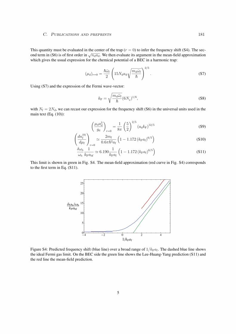
This quantity must be evaluated in the center of the trap (r = 0) to infer the frequency shift (S4). The sec-
ond term in (S6) is of first order in√ndad. We then evaluate its argument in the mean-field approximation
which gives the usual expression for the chemical potential of a BEC in a harmonic trap:
(µd)r=0 =~ωf
2
(15Ndad
√mdωf
~
)2/5
. (S7)
Using (S7) and the expression of the Fermi wave-vector:
kF =
√mdωf
~(6N
d)1/6, (S8)
with Nf = 2Nd, we can recast our expression for the frequency shift (S6) in the universal units used in the
main text (Eq. (10)):
(µda
3d
gd
)
r=0
=1
8π
(5
2
)2/5
(adkF)12/5
(S9)
(dn
(0)f
dµf
)
r=0
≃ 2mf
0.6π~2af
(1− 1.172 (kFaf)
6/5)
(S10)
δωb
ωb
1
kFabf≃ 6.190
1
kFaf
(1− 1.172 (kFaf)
6/5)
(S11)
This limit is shown in green in Fig. S4. The mean-field approximation (red curve in Fig. S4) corresponds
to the first term in Eq. (S11).
-4 -2 0 2 40
5
10
15
20
25
1kFaf
∆ΩbΩbkFabf
Figure S4: Predicted frequency shift (blue line) over a broad range of 1/kFaf . The dashed blue line shows
the ideal Fermi gas limit. On the BEC side the green line shows the Lee-Huang-Yang prediction (S11) and
the red line the mean-field prediction.
5
C. Publications and preprints 181

Derivation of the coupled oscillator model using the sum-rule approach
We describe the dynamics of the system by a Hamiltonian
H =∑
i,α
[p2α,i2mα
]+ U(rα,i), (S12)
where α = b, f labels the isotopes, and U describes the total (trap+interaction) potential energy of the
cloud.
Consider the operators Fα =∑Nα
i=1 zα,i, where zα,i is the position along z of the i-th atom of species
α = b, f and take F (af , ab) =∑
α aαFα an excitation operator depending on two mixing coefficients (aα).We introduce the moments Sp defined by
Sp =∑
n
(En − E0)p∣∣∣〈n|F |0〉
∣∣∣2
,
where |n〉 and En are the eigenvectors and the eigenvalues of the Hamiltonian H (by definition |0〉 is the
ground state and E0 is its energy). Using the Closure Relation and first order perturbation theory, S1 and
S−1 can be calculated exactly and we have
S1 = −∑
α
~2
mα
Nαa2α (S13)
S−1 = −1
k
∑
α,β
aαaβNα∂〈zα〉∂bβ
(S14)
where k is the restoring force of the axial magnetic trap and 〈zα〉 is the center of mass position of atoms α
in the presence of a perturbing potential −k∑β bβFα corresponding to a shift of the trapping potential of
species β by a distance bβ . 〈zα〉 satisfies two useful conditions. First, using Hellmann-Feynman’s theorem,
the matrix Nα∂bβ〈zα〉 = ∂2bαbβH is symmetric. Secondly, if we shift the two traps by the same quantify
bβ = b, the center of mass of the two clouds move by 〈zα〉 = b. Differentiating this constraint with respect
to b yields the condition∑
β ∂bβ〈zα〉 = 1.
Experimentally, we observe that only two modes are excited by the displacement of the trap center.
We label |n = 1〉 and |n = 2〉 the corresponding modes and we take ~ωn = En−E0, with, by convention,
ω1 ≤ ω2. We thus have for any set of mixing parameters (af , ab),
~2ω2
1 ≤ S1
S−1
≤ ~2ω2
2. (S15)
To find the values of the two frequencies ω1 and ω2, one thus simply has to find the extrema of S1/S−1
with respect to af and ab. Using the sum rules (S13) and (S14), we see that
S1
S−1
= ~2k
∑αNα/mαa
2α∑
α,β Nαaαaβ∂〈zα〉∂bβ
. (S16)
This expression can be formally simplified by taking a′α = aα√Nα/mα and ψ = (a′f , a
′b). We then have
S1
S−1
= ~2k
〈ψ|ψ〉〈ψ|Mψ〉 , (S17)
6
182

where the scalar product is defined by 〈ψ|ψ′〉 =∑α ψαψ′α and the effective-mass operator is given by
Mαβ =√mαmβ
√Nα
Nβ
∂〈zα〉∂bβ
. (S18)
With these notations, the frequencies ωi=1,2 are given by ωi =√k/mi, where mi is an eigenvalue of M.
In the weak-coupling limit, the cross-terms ∂bβ〈zα〉 (α 6= β) are small and using their symmetryproperties, we can write M as M0 +M1 with
M0 =
(mf 00 mb
)(S19)
M1 =
−mf
∂〈zf〉∂bb
√mfmb
√Nb
Nf
∂〈zb〉∂bf√
mfmb
√Nb
Nf
∂〈zb〉∂bf
−mb∂〈zb〉∂bf
(S20)
Since the matrix M is symmetric we can use the usual perturbation theory to calculate its eigenvalues and
eigenvectors. We have to first order
m1 = mf
(1− ∂〈zf〉
∂bb
)(S21)
m2 = mb
(1− ∂〈zb〉
∂bf
)(S22)
Using the symmetry of Nα∂bβ〈zα〉, we see that in the experimentally relevant limit Nf ≫ Nb, we have
∂bf 〈zb〉 ≫ ∂bb〈zf〉. Thus the frequency of 6Li is essentially not affected by the coupling between the two
species. To leading order, we can identify ω1 (ω2) with ωb (ωf) and we have
ωf ≃ ωf (S23)
ωb ≃ ωb
(1 +
1
2
∂〈zb〉∂bf
)(S24)
To calculate the frequency ωb we need to know the crossed-susceptibility ∂bf 〈zb〉. Since this is in
equilibrium quantity, we can calculate it using the local-density approximation. We then obtain
∂〈zb〉∂bf
=kgbfNb
∫d3rz2
(∂nf
∂µf
)(∂nb
∂µb
)(S25)
In the limit Nb ≪ Nf , the bosonic cloud is much smaller than the fermionic cloud. We can therefore
approximate this expression by
∂〈zb〉∂bf
≃ kgbfNb
(∂nf
∂µf
)
0
∫d3rz2
(∂nb
∂µb
)(S26)
where the index zero indicates that the derivative is calculated at the center of the trap. The integral can be
calculated exactly and we finally obtain
∂〈zb〉∂bf
= gbf
(∂nf
∂µf
)
0
, (S27)
7
C. Publications and preprints 183

where we recover Eq. (2) from main text.
To get the dynamics of the system after the excitation, we need to calculate the eigenvectors of the
matrix M. Note ψ′i = (a′i,f , a
′i,b) the eigenvector associated to the eigenvalue ωi. Using once more first
order perturbation theory, we have
ψ′1 =
(1
√mfmb
mf−mb
√Nb
Nf
∂〈zb〉∂bf
)(S28)
ψ′2 =
( √mfmb
mb−mf
√Nb
Nf
∂〈zb〉∂bf
1
), (S29)
from which we deduce the vectors ψi=1,2 = (ai,f , ai,b) giving the excitation operator F (ai,f , ai,b). More
precisely
ψ1 =
√mf
Nf
(1
mb
mf−mb
∂〈zb〉∂bf
)(S30)
ψ2 =
√mb
Nb
(mf
mb−mf
Nb
Nf
∂〈zb〉∂bf
1
). (S31)
Note d the initial displacement of the two species and expand the initial condition Z = (zf(0), zb(0)) =
(d, d) over the basis ψ1, ψ2 as Z =∑
i ciψi. Since by construction the operator F (ai,f , ai,b) excitessolely the mode ωi we must have at time t Z(t) =
∑i ci cos(ωit)ψi (we assume that the initial velocities
are zero). After a straightforward calculation, we get
zf(t) = d
[(1− ερη) cos(ω1t) + ηρε(1 + ε) cos(ω2t)
1 + ε2ρη
](S32)
zb(t) = d
[−ε(1− ερη) cos(ω1t) + (1 + ε) cos(ω2t)
1 + ε2ρη
](S33)
with ρ = Nb/Nf , ε = mb/(mb −mf)∂bf 〈zb〉 and η = mf/mb. In experimentally relevant situations, we
have ε≪ 1, ρ≪ 1 and η ≃ 1. We can thus approximate the previous equations by
zf(t) ≃ d [(1− ερ) cos(ωft) + ρε cos(ωbt)] (S34)
zb(t) ≃ d [−ε cos(ωft) + (1 + ε) cos(ωbt)] , (S35)
and where according to Eq. (S24), we can take
ε =2mb
mb −mf
(ωb − ωb
ωb
). (S36)
References
31. N. Gross, Z. Shotan, O. Machtey, S. Kokkelmans, L. Khaykovich, Comptes Rendus Physique 12, 4
(2011).
32. S. Nascimbene, et al., Phys. Rev. Lett. 103, 170402 (2009).
33. D. Miller, et al., Phys. Rev. Lett. 99, 070402 (2007).
34. D. Petrov, C. Salomon, G. Shlyapnikov, Phys. Rev. Lett. 93, 090404 (2004).
8
184

C. Publications and preprints 185

186
C.3 Chandrasekhar-Clogston limit and critical polariza-tion in a Fermi-Bose superfluid mixture
Tomoki Ozawa, Alessio Recati, Marion Delehaye, Frédéric Chevy,and Sandro Stringari
Physical Review A 90, 043608 (2014)

PHYSICAL REVIEW A 90, 043608 (2014)
Chandrasekhar-Clogston limit and critical polarization in a Fermi-Bose superfluid mixture
Tomoki Ozawa,1 Alessio Recati,1 Marion Delehaye,2 Frederic Chevy,2 and Sandro Stringari1
1INO-CNR BEC Center and Dipartimento di Fisica, Universita di Trento, I-38123 Povo, Italy2Laboratoire Kastler-Brossel, Ecole Normale Superieure, CNRS and UPMC, 24 rue Lhomond, 75005 Paris, France
(Received 28 May 2014; published 8 October 2014)
We study mixtures of a population-imbalanced, strongly interacting Fermi gas and of a Bose-Einstein condensed
gas at zero temperature. In the homogeneous case, we find that the Chandrasekhar-Clogston critical polarization
for the onset of instability of Fermi superfluidity is enhanced due to the interaction with the bosons. Predictions for
the critical polarization are also given in the trapped case, with a special focus on the situation of equal Fermi-Bose
and Bose-Bose coupling constants, where the density of fermions becomes flat in the center of the trap. This
regime can be realized experimentally using Feshbach resonances and is well suited to investigate the emergence
of exotic configurations, such as the occurrence of spin domains or the Fulde-Ferrell-Larkin-Ovchinnikov (FFLO)
phase.
DOI: 10.1103/PhysRevA.90.043608 PACS number(s): 67.85.Pq, 03.75.Mn, 03.75.Ss, 05.30.Fk
I. INTRODUCTION
The property of fermions interacting with a Bose fluid has
been a longstanding subject of research in condensed matter
physics, dating back to the study of 3He −4He mixtures [1].
With the recent development of research activity in ultracold
gases, it is now possible to experimentally create mixtures of
degenerate bosonic and fermionic atomic gases [2–11]. Very
recently, the first experimental realization of a superfluid Bose-
Fermi mixture was reported [12], the Fermi gas being at the
unitarity limit.
There are several theoretical works on mixtures of super-
fluid Bose gases interacting with spin-1/2 Fermi gases
[13–17], but the behavior of coexisting superfluid Fermi and
Bose gases in the case of strong Fermi-Fermi interaction has
not yet been considered in the literature. Furthermore, since
spin-imbalanced fermions are predicted to give rise to exotic
phases such as the Fulde-Ferrell-Larkin-Ovchinnikov (FFLO)
phase [18–20], it is of great interest to investigate how their
behavior is modified by the interaction with bosons.
In this paper, we show that in a homogeneous configura-
tion the Chandrasekhar-Clogston critical polarization for the
breakdown of superfluidity is larger than in the absence of
the bosonic component [21]. We then consider the case of a
harmonically trapped configuration: when the Bose-Bose and
Bose-Fermi interactions are equal, the fermionic density in the
region of coexistence with bosons becomes flat, because the
interaction with bosons exactly compensates the external
trapping potential [22]. We investigate the phase diagram of
the trapped gas when the fermion imbalance is varied and
show that, for a finite range of polarization, the fermionic
density in the Bose-Fermi coexistence region can become
inhomogeneous.
II. HOMOGENEOUS SYSTEM
The balanced unitary Fermi gas is known to be fully
superfluid at zero temperature. As one increases the polar-
ization, it has been observed that the system phase separates
into a balanced superfluid phase and an imbalanced normal
phase [23]. The two phases have different densities, and the
equilibrium conditions between the two phases fix the ratio x
between the density of the minority species over the density
of the majority species in the normal phase, which determines
the Chandrasekhar-Clogston limit. At zero temperature, this
critical ratio turns out to be, at unitarity, x ≈ 0.4 [21,24,25].
As we show, this value is modified by the interaction with
bosons. We assume that the Fermi gas is phase separated into
a superfluid phase with density ns for both species and a normal
phase with density n↑ and n↓ for the spin-up (majority) and
spin-down (minority) fermions, respectively. The density of
the coexisting bosons in the Fermi superfluid phase is nbs and
that in the normal phase is nbn. Later we discuss the stability
conditions for such configurations. We assume that both the
bosonic and fermionic species can be described within the local
density approximation and both the Bose-Bose and the
Bose-Fermi interactions are weak enough to be treated within
the mean-field approximation. Then the energy density in the
superfluid phase (Es) and in the normal phase (En) takes the
form
Es =gbb
2n2
bs + 2gbf nbsns + es[ns],
(1)
En =gbb
2n2
bn + gbf nbn(n↑ + n↓) + en[n↑,n↓],
where gbb ≡ 4π2abb/mb, assumed to be positive, and gbf ≡
2π2abf /mr are, respectively, the Bose-Bose and spin-
independent Bose-Fermi interaction coupling constants. The
Bose-Bose and Bose-Fermi scattering lengths are abb and abf ,
respectively, and mr ≡ mbmf /(mb + mf ), where mb and mf
are the boson and fermion masses, respectively. The Fermi
energy density in the superfluid phase is given by the universal
form
es[ns] ≡ ξ6
5
2
2mf
(6π2ns)2/3ns, (2)
where ξ = 0.370 [25–27] is the Bertsch parameter. For the
normal phase we use the expansion in the parameter x ≡
n↓/n↑ introduced in [21]:
en[n↑,n↓] ≡3
5ǫF↑n↑
(
1 −5
3Ax +
mf
m∗x5/3 + Fx2
)
≡3
5ǫF↑n↑ǫ(x), (3)
1050-2947/2014/90(4)/043608(5) 043608-1 ©2014 American Physical Society
C. Publications and preprints 187

OZAWA, RECATI, DELEHAYE, CHEVY, AND STRINGARI PHYSICAL REVIEW A 90, 043608 (2014)
0.00 0.02 0.04 0.06 0.08
0.30
0.32
0.34
0.36
0.38
1.0
1.5
2.0
2.5
x y
G
x
y
FIG. 1. (Color online) Critical ratios x ≡ n↓/n↑ (solid blue line
with left axis) and y ≡ ns/n↑ (dotted green line with right axis) as a
function of G ≡ n↑g2bf /ǫF↑gbb.
where ǫF↑ ≡ (2/2mf )(6π2n↑)2/3 is the noninteracting Fermi
energy of the majority species, and for the parameters in
ǫ(x) we use A = 0.615, m∗/mf = 1.20, and F = (5/9)A2,
determined by diagramatic methods and Monte-Carlo cal-
culations [28–30]. Using different sets of parameters would
not change our results significantly. The equilibrium between
the two phases is determined by matching the pressure and
the chemical potentials for both bosons and fermions at the
interface, which leads to the following conditions for x and
y ≡ ns/n↑:
ξy2/3 − 2Gy −1
2ǫ(x) −
3
10ǫ′(x)(1 − x) + G(1 + x) = 0,
2Gy2 −4
5ξy5/3 − G
(1 + x)2
2+
2
5ǫ(x) = 0,
(4)
where ǫ′(x) ≡ dǫ(x)/dx and G ≡ n↑g2bf /(ǫF↑gbb) is a dimen-
sionless parameter independent of the bosonic density. As a
consequence, also the critical ratios x and y are independent
of the boson density, provided there are background bosons
with nonzero densities in both phases. The parameter G
has an important physical meaning, corresponding to the
ratio between the change in the energy of fermions caused
by the induced interaction −g2bf /gbb in the static limit and
the noninteracting Fermi energy. The existence of two real
solutions for x and y for (4) is ensured for 0 G Gmax ≈
0.089, and in Fig. 1 we plot the resulting values of x and y
as a function of G. When G = 0, the critical ratio x ≈ 0.40
coincides with the value obtained in the absence of Bose-Fermi
interaction (gbf = 0). As G becomes larger, the value of x
decreases, reaching the minimum value of x ≈ 0.30, which
means that the superfluid phase of fermions is stabilized by
the interaction with bosons. The ratio y, on the other hand,
increases with G, reaching the maximum value of y ≈ 2.68,
which implies that the density jump at the interface of the
two phases becomes larger; the maximum value of the jump,
corresponding to G = Gmax, is 2ns/(n↑ + n↓) ≈ 4.1, to be
compared with the value ≈1.5 when G = 0.
The nonexistence of real solutions when G > Gmax is
related to the occurrence of dynamical instability in the
fermionic superfluid phase caused by the interaction with
bosons. The dynamical stability of the superfluid phase
requires that the following inequality be obeyed [31]:
δ2es[ns]
δn2s
− 4g2
bf
gbb
> 0, (5)
which is equivalent to imposing ξ/3y1/3 > G. We have
checked that the condition for having real solutions for x and
y coincides with the one ensuring dynamical stability. If G
becomes larger than Gmax, the superfluid Fermi gas and the
Bose gas are expected to phase separate.
III. TRAPPED SYSTEM
Let us now consider the case of a trapped quantum mixture.
In the absence of bosons, it is known that as one introduces a
small imbalance between the two species, the central part of
the trap remains superfluid and the outer shell is turned into a
normal state [21,23]. When the imbalance is large enough, the
whole Fermi gas is in the normal state.
In the presence of bosons, the situation can change
significantly. The energy of a highly polarized Fermi gas
interacting with a BEC gas is given, within the local density
approximation (LDA), by
E =
∫
r<Rb
d3r
gbb
2n2
b(r) + [Vb(r) − μb]nb(r)
+ gbf nb(r)[n↑(r) + n↓(r)] + en[n↑(r),n↓(r)]
+ [Vf (r) − μ↑]n↑(r) + [Vf (r) − μ↓]n↓(r)
+
∫
Rb<r
d3ren[n↑(r),n↓(r)] + [Vf (r) − μ↑]n↑(r)
+ [Vf (r) − μ↓]n↓(r), (6)
where Rb is the radius at which the boson density vanishes,
and Vb(r) and Vf (r) are the harmonic traps for bosons and
fermions, respectively [32]. The densities of boson, spin-up
fermion, and spin-down fermion are nb(r), n↑(r), and n↓(r),
respectively, and the corresponding chemical potentials are
labeled, respectively, with μb, μ↑, and μ↓.
Taking the variation of the energy with respect to nb(r),
n↑(r), and n↓(r) in the Bose-Fermi coexistence region r < Rb,
which is hereafter referred to as the “core” region, one obtains
the following equations:
nb(r) = μb − Vb(r) − gbf [n↑(r) + n↓(r)]/gbb,
δen
δnσ
+ Vf (r) −gbf
gbb
Vb(r) +gbf
gbb
μb − μσ
−(
g2bf /gbb
)
[n↑(r) + n↓(r)] = 0, (7)
where σ = ↑,↓. The second equation explicitly reveals that,
if gbf Vb(r) = gbbVf (r), the fermion densities are not affected
by the presence of the trap and take a constant value inside
the core [22]. This follows from the fact that the effect of
the trap on the fermions is exactly canceled by the mean-field
interaction with bosons [33]. Conversely, the bosonic density
is not affected by the presence of fermions and, choosing
an external potential of harmonic form, the bosonic density,
for r < Rb, takes an inverted parabola profile, whose shape
is solely determined by the total number of bosons and the
043608-2
188

CHANDRASEKHAR-CLOGSTON LIMIT AND CRITICAL . . . PHYSICAL REVIEW A 90, 043608 (2014)
Bose-Bose coupling constant gbb. If instead gbf Vb > gbbVf ,
the fermions feel an antitrapping potential in the core region
and their density will increases when one moves away from
the center.
When the imbalance is small, most of the fermions are
in the superfluid phase and one can write down a similar
energy functional as (6), but the region r < Rb is filled with
the superfluid phase, while the region r > Rb is divided into an
inner superfluid phase and an outer normal phase. One obtains
the following conditions analogous to Eq. (7):
nb(r) = [μb − Vb(r) − 2gbf ns(r)]/gbb,
δes
δns
+ 2
(
Vf (r) −gbf
gbb
Vb(r)
)
+ 2gbf
gbb
μb − (μ↑ + μ↓)
− 4(g2bf /gbb)ns(r) = 0, (8)
in the core. As in the highly polarized case, one can see that in
this region the fermions exhibit a flat density distribution when
gbf Vb(r) = gbbVf (r). The equilibrium between the superfluid
phase and the normal phase in the tail is determined by match-
ing the pressure and the chemical potentials at the interface,
and the critical ratio x = n↓/n↑ is equal to 0.40, which is the
value predicted in the absence of bosons [21,24,25].
For concreteness we provide predictions for the mixture
of 7Li bosons and 6Li fermions reported in [12] where
V (r) ≡ Vb(r) = Vf (r), and we focus on the special case gbf =
gbb. This condition gbb = gbf [corresponding to abb/abf =
(mb + mf )/2mf ], together with that of unitarity for the Fermi
component, are achievable for a magnetic field of B = 817 G,
leading to a fermion-fermion scattering length of 25800aB and
to a boson-boson scattering length abb = 44.2aB , the average
Fermi momentum being kF = 106 ∼ 107m−1.
The density profile of the fermions (both inside and outside
the core) can be obtained by solving (7) or (8) and similar
equations for the region r > Rb. In Fig. 2, we plot two
density distributions for fixed values of Nb = 105 and N↑ =
1.5 × 10⁵ but with two different values of N↓. We choose
abb = 10−3lhomb/mf , where lho ≡√
/mf ωf is the harmonic
0 2 4 6 8 10 12 140
10
20
30
40
50
0
100
200
300
400
500
600
700
nf
nb
n↑
n↓
nb
r
(a)The whole system is normal
0
100
200
300
400
500
600
700
0 2 4 6 8 10 12 140
10
20
30
40
50
nf
nbn
↑
n↓n
b
r
(b)The core is all superfluid
FIG. 2. (Color online) Local 3D density profile of the two op-
posite limits where the inhomogeneous phase in the core is about
to appear. We fix Nb = 105 and N↑ = 1.5 × 10⁵. The solid (blue)
lines are spin-up fermions, the dotted (green) lines are spin-down
fermions, and the dash-dotted (red) lines are bosons. The left axis is
for the fermion densities and the right axis is for the boson density.
The number of spin-down fermions is (a) N↓ = 0.22 × 10⁵ and (b)
N↓ = 0.33 × 10⁵. The length is in units of lho, and the density of
particles is in units of 1/l3ho.
0.0 0.5 1.0 1.5 2.0N f /Nb
0.2
0.4
0.6
0.8
1.0
P
Normal Phase
Super
×
FIG. 3. (Color online) Critical polarizations for entering the in-
homogeneous core as a function of Nf /Nb for Nb = 105 (solid blue
lines) and Nb = 104 (dashed red lines). The cross corresponds to the
situation of Fig. 4.
oscillator length corresponding to a fermionic trap frequency
ωf = 2π × 420 Hz. Figure 2(a) corresponds to the smallest
value of total polarization of the gas [P ≡ (N↑ − N↓)/(N↑ +
N↓) = 0.74] compatible with the absence of superfluidity,
where the ratio n↓/n↑ in the core is equal to the critical value
determined by Eq. (4) for the value of G in the core region.
A smaller value of P would correspond to the onset of a
superfluid region in the core. Figure 2(b) instead corresponds
to the largest value of total polarization (P = 0.63) compatible
with the presence of a superfluid phase occupying the whole
core region. A larger value of P would correspond to the onset
of a normal region in the core (see also Fig. 3).
For intermediate values of the population imbalance,
coexistence of the superfluid and the normal phase takes
place in the core region, giving rise to inhomogeneity and
new interesting physics. Inhomogeneity in the core can be
reached either by starting with a balanced superfluid gas
and gradually decreasing the number of minority fermions
until the normal part enters the core, or by starting with a
completely polarized gas and gradually increasing the number
of minority fermions until a superfluid phase region in the
core is favorable. In Fig. 3, the two critical polarizations
for entering the inhomogeneous core phase are plotted as a
function of Nf /Nb, where Nf ≡ N↑ + N↓, for two different
values of Nb. The upper region corresponds to the phase with
the whole system being normal [Fig. 2(a)], and the lower region
corresponds to the whole core being superfluid [Fig. 2(b)].
The region between the lines represents the inhomogeneous
core phase. We observe that the critical polarization as a
function of Nf /Nb is not very sensitive to the number of
bosons. The two critical polarization lines approach the value
0.8 as Nf /Nb → ∞. This asymptotic value corresponds to
the critical polarization for the onset of superfluidity in the
absence of bosons [24].
We now discuss the possible scenarios characterizing the
inhomogeneous phase for intermediate values of population
imbalance (see Fig. 3). The simplest possibility, hereafter
called the superfluid-normal (S-N) scenario, is that the core is
phase separated into a central superfluid and an outer normal
phase. The equilibrium condition between the superfluid phase
and the normal phase turns out to be determined by the same
conditions (4) holding for the homogeneous mixture. Another
043608-3
C. Publications and preprints 189
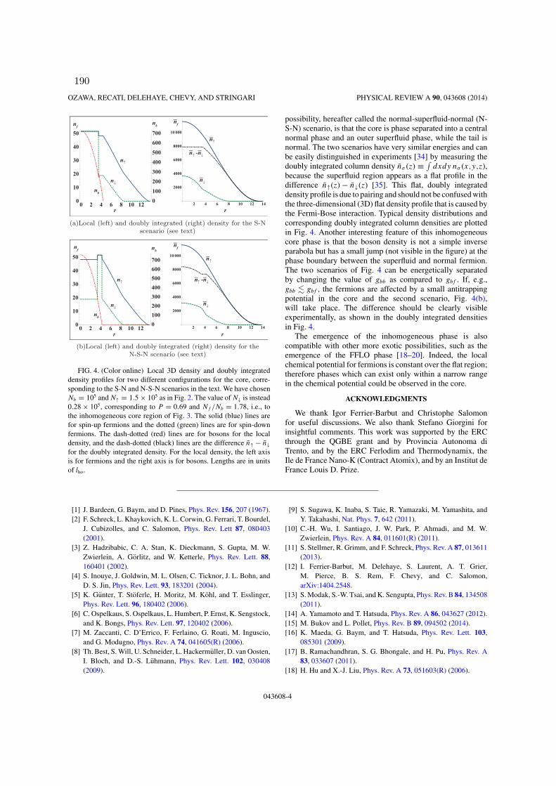
OZAWA, RECATI, DELEHAYE, CHEVY, AND STRINGARI PHYSICAL REVIEW A 90, 043608 (2014)
0 2 4 6 8 10 120
10
20
30
40
50
0
100
200
300
400
500
600
700
2 4 6 8 10 12 14
2000
4000
6000
8000
10 000
nf
nb
rr
nf
n↑
nb
n↓
n↑
n↑-n
↓
n↓
(a)Local (left) and doubly integrated (right) density for the S-Nscenario (see text)
0 2 4 6 8 10 120
10
20
30
40
50
0
100
200
300
400
500
600
700
2 4 6 8 10 12 14
2000
4000
6000
8000
10 000
rr
nf n
b
nf
n↑
n↓
nb
n↑
n↑-n
↓
n↓
(b)Local (left) and doubly integrated (right) density for theN-S-N scenario (see text)
FIG. 4. (Color online) Local 3D density and doubly integrated
density profiles for two different configurations for the core, corre-
sponding to the S-N and N-S-N scenarios in the text. We have chosen
Nb = 105 and N↑ = 1.5 × 10⁵ as in Fig. 2. The value of N↓ is instead
0.28 × 10⁵, corresponding to P = 0.69 and Nf /Nb = 1.78, i.e., to
the inhomogeneous core region of Fig. 3. The solid (blue) lines are
for spin-up fermions and the dotted (green) lines are for spin-down
fermions. The dash-dotted (red) lines are for bosons for the local
density, and the dash-dotted (black) lines are the difference n↑ − n↓
for the doubly integrated density. For the local density, the left axis
is for fermions and the right axis is for bosons. Lengths are in units
of lho.
possibility, hereafter called the normal-superfluid-normal (N-
S-N) scenario, is that the core is phase separated into a central
normal phase and an outer superfluid phase, while the tail is
normal. The two scenarios have very similar energies and can
be easily distinguished in experiments [34] by measuring the
doubly integrated column density nσ (z) ≡∫
dxdy nσ (x,y,z),
because the superfluid region appears as a flat profile in the
difference n↑(z) − n↓(z) [35]. This flat, doubly integrated
density profile is due to pairing and should not be confused with
the three-dimensional (3D) flat density profile that is caused by
the Fermi-Bose interaction. Typical density distributions and
corresponding doubly integrated column densities are plotted
in Fig. 4. Another interesting feature of this inhomogeneous
core phase is that the boson density is not a simple inverse
parabola but has a small jump (not visible in the figure) at the
phase boundary between the superfluid and normal fermion.
The two scenarios of Fig. 4 can be energetically separated
by changing the value of gbb as compared to gbf . If, e.g.,
gbb gbf , the fermions are affected by a small antitrapping
potential in the core and the second scenario, Fig. 4(b),
will take place. The difference should be clearly visible
experimentally, as shown in the doubly integrated densities
in Fig. 4.
The emergence of the inhomogeneous phase is also
compatible with other more exotic possibilities, such as the
emergence of the FFLO phase [18–20]. Indeed, the local
chemical potential for fermions is constant over the flat region;
therefore phases which can exist only within a narrow range
in the chemical potential could be observed in the core.
ACKNOWLEDGMENTS
We thank Igor Ferrier-Barbut and Christophe Salomon
for useful discussions. We also thank Stefano Giorgini for
insightful comments. This work was supported by the ERC
through the QGBE grant and by Provincia Autonoma di
Trento, and by the ERC Ferlodim and Thermodynamix, the
Ile de France Nano-K (Contract Atomix), and by an Institut de
France Louis D. Prize.
[1] J. Bardeen, G. Baym, and D. Pines, Phys. Rev. 156, 207 (1967).
[2] F. Schreck, L. Khaykovich, K. L. Corwin, G. Ferrari, T. Bourdel,
J. Cubizolles, and C. Salomon, Phys. Rev. Lett 87, 080403
(2001).
[3] Z. Hadzibabic, C. A. Stan, K. Dieckmann, S. Gupta, M. W.
Zwierlein, A. Gorlitz, and W. Ketterle, Phys. Rev. Lett. 88,
160401 (2002).
[4] S. Inouye, J. Goldwin, M. L. Olsen, C. Ticknor, J. L. Bohn, and
D. S. Jin, Phys. Rev. Lett. 93, 183201 (2004).
[5] K. Gunter, T. Stoferle, H. Moritz, M. Kohl, and T. Esslinger,
Phys. Rev. Lett. 96, 180402 (2006).
[6] C. Ospelkaus, S. Ospelkaus, L. Humbert, P. Ernst, K. Sengstock,
and K. Bongs, Phys. Rev. Lett. 97, 120402 (2006).
[7] M. Zaccanti, C. D’Errico, F. Ferlaino, G. Roati, M. Inguscio,
and G. Modugno, Phys. Rev. A 74, 041605(R) (2006).
[8] Th. Best, S. Will, U. Schneider, L. Hackermuller, D. van Oosten,
I. Bloch, and D.-S. Luhmann, Phys. Rev. Lett. 102, 030408
(2009).
[9] S. Sugawa, K. Inaba, S. Taie, R. Yamazaki, M. Yamashita, and
Y. Takahashi, Nat. Phys. 7, 642 (2011).
[10] C.-H. Wu, I. Santiago, J. W. Park, P. Ahmadi, and M. W.
Zwierlein, Phys. Rev. A 84, 011601(R) (2011).
[11] S. Stellmer, R. Grimm, and F. Schreck, Phys. Rev. A 87, 013611
(2013).
[12] I. Ferrier-Barbut, M. Delehaye, S. Laurent, A. T. Grier,
M. Pierce, B. S. Rem, F. Chevy, and C. Salomon,
arXiv:1404.2548.
[13] S. Modak, S.-W. Tsai, and K. Sengupta, Phys. Rev. B 84, 134508
(2011).
[14] A. Yamamoto and T. Hatsuda, Phys. Rev. A 86, 043627 (2012).
[15] M. Bukov and L. Pollet, Phys. Rev. B 89, 094502 (2014).
[16] K. Maeda, G. Baym, and T. Hatsuda, Phys. Rev. Lett. 103,
085301 (2009).
[17] B. Ramachandhran, S. G. Bhongale, and H. Pu, Phys. Rev. A
83, 033607 (2011).
[18] H. Hu and X.-J. Liu, Phys. Rev. A 73, 051603(R) (2006).
043608-4
190

CHANDRASEKHAR-CLOGSTON LIMIT AND CRITICAL . . . PHYSICAL REVIEW A 90, 043608 (2014)
[19] A. Bulgac and M. McNeil Forbes, Phys. Rev. Lett. 101, 215301
(2008).
[20] L. Radzihovsky and D. E. Sheehy, Rep. Prog. Phys. 73, 076501
(2010).
[21] A. Recati, C. Lobo, and S. Stringari, Phys. Rev. A 78, 023633
(2008).
[22] K. Mølmer, Phys. Rev. Lett. 80, 1804 (1998).
[23] Y. Shin, C. H. Schunck, A. Schirotzek, and W. Ketterle, Nature
(London) 451, 689 (2008).
[24] C. Lobo, A. Recati, S. Giorgini, and S. Stringari, Phys. Rev.
Lett. 97, 200403 (2006).
[25] The BCS-BEC Crossover and the Unitary Fermi Gas, edited by
W. Zwerger (Springer-Verlag, Berlin, 2012).
[26] M. J. H. Ku, A. T. Sommer, L. W. Cheuk, and M. W. Zwierlein,
Science 335, 563 (2012).
[27] G. Zurn, T. Lompe, A. N. Wenz, S. Jochim, P. S. Julienne, and
J. M. Hutson, Phys. Rev. Lett. 110, 135301 (2013).
[28] N. Prokof’ev and B. Svistunov, Phys. Rev. B 77, 020408(R)
(2008).
[29] R. Combescot and S. Giraud, Phys. Rev. Lett. 101, 050404
(2008).
[30] C. Mora and F. Chevy, Phys. Rev. Lett. 104, 230402
(2010).
[31] L. Viverit, C. J. Pethick, and H. Smith, Phys. Rev. A 61, 053605
(2000).
[32] In the following, without loss of generality, we use an isotropic
potential.
[33] The cancellation effect disappears when the number of bosons
is not large enough to apply LDA.
[34] An experimental measurement of the local 3D density would
require a more sophisticated 3D reconstruction of the density
based on inverse Abel transformation [23].
[35] T. N. De Silva and E. J. Mueller, Phys. Rev. A 73, 051602
(2006).
043608-5
C. Publications and preprints 191

192
C.4 Critical velocity and dissipation of an ultracold Bose-Fermi counterflow
Marion Delehaye, Sébastien Laurent, Igor Ferrier-Barbut, ShuweiJin, Frédéric Chevy, and Christophe Salomon
Physical Review Letters 115, 265303 (2015)
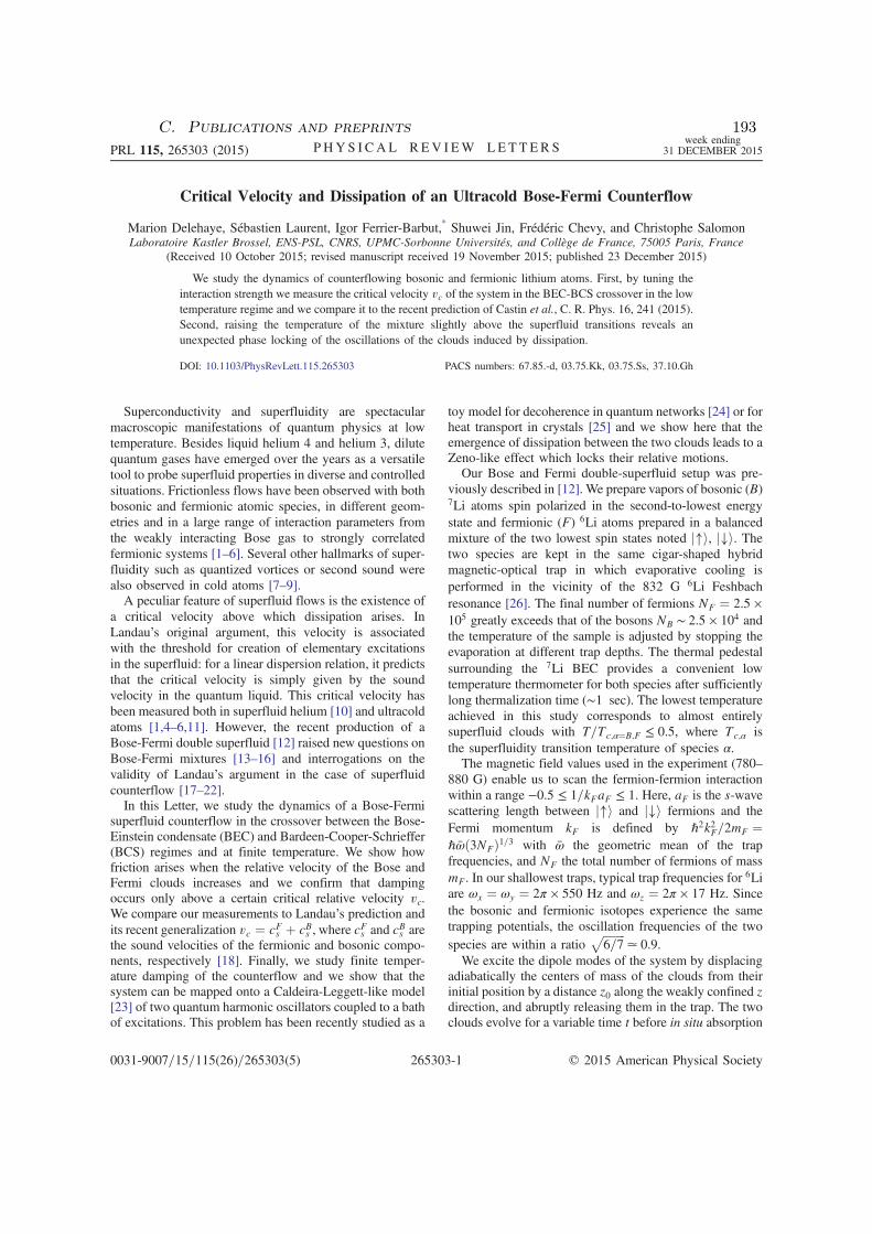
Critical Velocity and Dissipation of an Ultracold Bose-Fermi Counterflow
Marion Delehaye, Sébastien Laurent, Igor Ferrier-Barbut,*Shuwei Jin, Frédéric Chevy, and Christophe Salomon
Laboratoire Kastler Brossel, ENS-PSL, CNRS, UPMC-Sorbonne Universités, and Collège de France, 75005 Paris, France
(Received 10 October 2015; revised manuscript received 19 November 2015; published 23 December 2015)
We study the dynamics of counterflowing bosonic and fermionic lithium atoms. First, by tuning the
interaction strength we measure the critical velocity vc of the system in the BEC-BCS crossover in the low
temperature regime and we compare it to the recent prediction of Castin et al., C. R. Phys. 16, 241 (2015).
Second, raising the temperature of the mixture slightly above the superfluid transitions reveals an
unexpected phase locking of the oscillations of the clouds induced by dissipation.
DOI: 10.1103/PhysRevLett.115.265303 PACS numbers: 67.85.-d, 03.75.Kk, 03.75.Ss, 37.10.Gh
Superconductivity and superfluidity are spectacular
macroscopic manifestations of quantum physics at low
temperature. Besides liquid helium 4 and helium 3, dilute
quantum gases have emerged over the years as a versatile
tool to probe superfluid properties in diverse and controlled
situations. Frictionless flows have been observed with both
bosonic and fermionic atomic species, in different geom-
etries and in a large range of interaction parameters from
the weakly interacting Bose gas to strongly correlated
fermionic systems [1–6]. Several other hallmarks of super-
fluidity such as quantized vortices or second sound were
also observed in cold atoms [7–9].
A peculiar feature of superfluid flows is the existence of
a critical velocity above which dissipation arises. In
Landau’s original argument, this velocity is associated
with the threshold for creation of elementary excitations
in the superfluid: for a linear dispersion relation, it predicts
that the critical velocity is simply given by the sound
velocity in the quantum liquid. This critical velocity has
been measured both in superfluid helium [10] and ultracold
atoms [1,4–6,11]. However, the recent production of a
Bose-Fermi double superfluid [12] raised new questions on
Bose-Fermi mixtures [13–16] and interrogations on the
validity of Landau’s argument in the case of superfluid
counterflow [17–22].
In this Letter, we study the dynamics of a Bose-Fermi
superfluid counterflow in the crossover between the Bose-
Einstein condensate (BEC) and Bardeen-Cooper-Schrieffer
(BCS) regimes and at finite temperature. We show how
friction arises when the relative velocity of the Bose and
Fermi clouds increases and we confirm that damping
occurs only above a certain critical relative velocity vc.We compare our measurements to Landau’s prediction and
its recent generalization vc ¼ cFs þ cBs , where cFs and cBs are
the sound velocities of the fermionic and bosonic compo-
nents, respectively [18]. Finally, we study finite temper-
ature damping of the counterflow and we show that the
system can be mapped onto a Caldeira-Leggett-like model
[23] of two quantum harmonic oscillators coupled to a bath
of excitations. This problem has been recently studied as a
toy model for decoherence in quantum networks [24] or for
heat transport in crystals [25] and we show here that the
emergence of dissipation between the two clouds leads to a
Zeno-like effect which locks their relative motions.
Our Bose and Fermi double-superfluid setup was pre-
viously described in [12]. We prepare vapors of bosonic (B)7Li atoms spin polarized in the second-to-lowest energy
state and fermionic (F) 6Li atoms prepared in a balanced
mixture of the two lowest spin states noted j↑i, j↓i. Thetwo species are kept in the same cigar-shaped hybrid
magnetic-optical trap in which evaporative cooling is
performed in the vicinity of the 832 G 6Li Feshbach
resonance [26]. The final number of fermions NF ¼ 2.5 ×
105 greatly exceeds that of the bosons NB ∼ 2.5 × 10⁴ and
the temperature of the sample is adjusted by stopping the
evaporation at different trap depths. The thermal pedestal
surrounding the 7Li BEC provides a convenient low
temperature thermometer for both species after sufficiently
long thermalization time (∼1 sec). The lowest temperature
achieved in this study corresponds to almost entirely
superfluid clouds with T=Tc;α¼B;F ≤ 0.5, where Tc;α is
the superfluidity transition temperature of species α.
The magnetic field values used in the experiment (780–
880 G) enable us to scan the fermion-fermion interaction
within a range −0.5 ≤ 1=kFaF ≤ 1. Here, aF is the s-wave
scattering length between j↑i and j↓i fermions and the
Fermi momentum kF is defined by ℏ2k2F=2mF ¼
ℏωð3NFÞ1=3 with ω the geometric mean of the trap
frequencies, and NF the total number of fermions of mass
mF. In our shallowest traps, typical trap frequencies for6Li
are ωx ¼ ωy ¼ 2π × 550 Hz and ωz ¼ 2π × 17 Hz. Since
the bosonic and fermionic isotopes experience the same
trapping potentials, the oscillation frequencies of the two
species are within a ratioffiffiffiffiffiffiffiffi
6=7p
≃ 0.9.
We excite the dipole modes of the system by displacing
adiabatically the centers of mass of the clouds from their
initial position by a distance z0 along the weakly confined zdirection, and abruptly releasing them in the trap. The two
clouds evolve for a variable time t before in situ absorption
PRL 115, 265303 (2015) P HY S I CA L R EV I EW LE T T ER Sweek ending
31 DECEMBER 2015
0031-9007=15=115(26)=265303(5) 265303-1 © 2015 American Physical Society
C. Publications and preprints 193

images perpendicular to the z direction are taken. The
measurement of their doubly integrated density profiles
gives access to axial positions and atom numbers of both
species. Typical time evolutions of the centers of mass are
shown in Fig. 1 for different parameter values. Since the
Bose and Fermi components oscillate at different frequen-
cies, they oscillate in quadrature after a few periods. By
changing z0, we can thus tune the maximum relative
velocity between the two clouds and probe the critical
superfluid counterflow.
As shown in Fig. 1(a), the superfluid counterflow
exhibits no visible damping on a ≃5 s time scale for very
low temperature and small initial displacement. A striking
feature is the beat note on the 7Li oscillation amplitude due
to the coherent mean-field coupling to the 6Li cloud [12].
For larger relative velocities, 7Li oscillations are initially
damped [Fig. 1(b)] until a steady-state regime as in
Fig. 1(a) is reached. We fit the time evolution of the cloud
position using the phenomenological law
zBðtÞ ¼ dðtÞ½a cosðωBtÞ þ b cosðωFtÞ;
dðtÞ ¼ d1 þ d2 expð−γBtÞ: ð1Þ
We measure the damping rate γB as a function of
relative velocity for six different values of magnetic field,
exploring a large region of the crossover going from the
BCS (1=kFaF ¼ −0.42, B ¼ 880 G) to the BEC side
(1=kFaF ¼ 0.68, B ¼ 780 G), see Fig. 2. For these mag-
netic field values, the Bose gas remains in the weakly
interacting (repulsive) regime and the Bose-Fermi scatter-
ing length is aBF ≃ 41a0, constant in this magnetic field
range, and equal for both j↑i and j↓i spin states.
We extract the critical velocity vc using an ad hoc power-law fitting function γB ¼ AΘðv − vcÞ½ðv − vcÞ=vF
α, where
Θ is the Heaviside function and vF is the Fermi velocity
given by vF ¼ ℏkF=mF. For details, see [27]. vc in the
BEC-BCS crossover is displayed in Fig. 3 (red dots)
and compared to the predictions of Landau and Castin
et al. [18]. In this latter work, dissipation arises by the
creation of excitation pairs and yields a critical velocity
FIG. 1 (color online). Center-of-mass oscillations of bosons
(blue, top) and fermions (red, bottom), for different sets of
parameters at unitarity. Solid lines: fits using Eq. (1) for the
bosons and a similar equation for the fermions. (a) T=TF ¼ 0.03,
T=Tc;b ≤ 0.5, z0 ¼ 10 μm. Superfluid regime, no damping is
observed and ωB ¼ 2π × 15.41ð1Þ Hz ≈ffiffiffiffiffiffiffiffi
6=7p
ωF. The observed
beating at ωF − ωB is due to coherent energy exchange between
the clouds. (b) T=TF ¼ 0.03 and z0 ¼ 150 μm. For a larger initial
displacement, initial damping (γB ¼ 2.4 s−1) is followed by
steady-state evolution. ωB ¼ 2π × 14.2ð1Þ Hz ≈ffiffiffiffiffiffiffiffi
6=7p
ωF.
(c) T=TF ¼ 0.4 and z0 ¼ 80 μm. At higher temperature, phase
locking of the two frequencies is observed with ωF ≈ ωB ¼2π × 17.9ð3Þ Hz and γB ¼ γF ¼ 1.4ð5Þ s−1.
FIG. 2 (color online). Damping rate of the center-of-mass
oscillations versus maximal relative velocity in the BEC-BCS
crossover in units of the Fermi velocity vF. Dark blue dots, BEC
side (780 G) 1=kFaF ¼ 0.68; red squares, unitarity (832.2 G)
1=kFaF ¼ 0; light blue diamonds, BCS side (880 G)
1=kFaF ¼ −0.42. Power law fits with thresholds provide the
critical velocity (solid lines).
PRL 115, 265303 (2015) P HY S I CA L R EV I EW LE T T ER Sweek ending
31 DECEMBER 2015
265303-2
194

vc ¼ Minp
σ¼f;b
f½ϵBðpÞ þ ϵFσ ðpÞ=½pg. In this expression, ϵBðpÞ
denotes the dispersion relation of excitations in the BEC
and ϵFσ ðpÞ refers to the two possible branches of the Fermi
superfluid, phononlike (σ ¼ b), and threshold for pair
breaking excitations (σ ¼ f) [28]. For homogeneous gases,
at unitarity and on the BEC side of the crossover, this
critical relative velocity turns out to be simply the sum of
the respective sound velocities of the Bose and Fermi
superfluids, vc ¼ cFs þ cBs . We thus plot in Fig. 3 the
calculated sound velocities of both superfluids in an
elongated geometry obtained by integration over the trans-
verse direction [29–33] (red dashed line cFs , blue bars cBs ).
Typically, cBs contributes ≃20%–25% to the sum shown as
green squares in Fig. 3. Around unitarity and on the BCS
side of the resonance, our experimental data are consistent
with this interpretation as well as with a critical velocity
vc ¼ cFs that one would expect by considering the BEC as a
single impurity moving inside the fermionic superfluid. By
contrast, we clearly exclude the bosonic sound velocity as a
threshold for dissipation.
Our measured critical velocities are significantly higher
than those previously reported in pure fermionic systems
which, for all interaction strengths, were lower than
Landau’s criterion [4,6]. The main difference with our
study is the use of focused laser beams instead of a BEC as
a moving obstacle. In [6], the laser beam is piercing the
whole cloud including its nonsuperfluid part where the
density is low, and its potential may create a strong density
modulation of the superfluid. These effects make a direct
comparison to Landau criterion difficult [35]. On the
contrary, in our system the size of the BEC (Thomas
Fermi radii of 73; 3; 3 μm) is much smaller than the typical
size of the Fermi cloud (350; 13; 13 μm around unitarity).
For oscillation amplitudes up to 200 μm the BEC probes
only the superfluid core of the fermionic cloud. During its
oscillatory motion along z the Bose gas may explore the
edges of the Fermi superfluid where the density is smaller.
However, it is easy to check that the ratio v=cFs is maximum
when the centers of the two clouds coincide [27]. Finally, as
the mean-field interaction between the two clouds is very
small [27] our BEC acts as a weakly interacting local probe
of the Fermi superfluid.
On the BEC side of the resonance (780 G), however, we
observe a strong reduction of the measured critical velocity
compared to the predicted values. The effect is strikingly
seen in Fig. 2, dark blue dots (see also Supplemental
Material [27]). This anomalously small value for positive
scattering lengths is consistent with previous measurements
[4,6]. Its origin is still unclear but several explanations can
be put forward [35]. First, it is well known that vortex
shedding can strongly reduce superfluid critical velocity.
However, this mechanism requires a strong perturbation.
The density of the Bose gas and the mean-field interaction
between the two clouds are probably too small for vortex
generation through a collective nucleation process. Second,
inelastic losses increase on the BEC side of a fermionic
Feshbach resonance and heat up the system [36]. This
hypothesis is supported by the presence of a clearly visible
pedestal in the density profiles of the BEC taken at 780 G.
At this value of the magnetic field, we measure a ≃60%
condensed fraction, corresponding to a temperature
T=Tc;B ≃ 0.5. Even though the two clouds are still super-
fluids as demonstrated by the critical behavior around vc,
the increased temperature could be responsible for the
decrease of vc.We now present results of experiments performed at a
higher temperature (0.03≲ T=TF ≲ 0.5) for B ¼ 835 G.
For low temperatures (T=TF ≤ 0.2), the two clouds remain
weakly coupled and, as observed in Fig. 4, the bosonic and
fermionic components oscillate at frequencies in the
expected ratio ≃0.9≃ffiffiffiffiffiffiffiffi
6=7p
. A new feature emerges for
T ≳ Tc;B ≈ 0.34TF > Tc;F where both gases are in the
normal phase. In this “high” temperature regime, the
two clouds are locked in phase: 7Li oscillates at 6Li
frequency (Fig. 4) and the two components are equally
damped [Fig. 1(c)]. This remarkable behavior can be
understood as a Zeno effect arising from the increased
dissipation between the two components. Indeed, the
system can be described as a set of two harmonic oscillators
describing, respectively, the macroscopic motion of the
global center of mass of the system (Kohn’s mode [37]) and
the relative motion of the two clouds [27]. These two
degrees of freedom are themselves coupled to the “bath” of
FIG. 3 (color online). Critical velocity of the Bose-Fermi
superfluid counterflow in the BEC-BCS crossover normalized
to the Fermi velocity vF. Red dots, measurements. Red dot-
dashed line, sound velocity cFs of an elongated homogeneous
Fermi superfluid calculated from its equation of state [29,30] after
integration of the density in the transverse plane, and also
measured in [34]. Blue bars, calculated sound velocity cBs of
the elongated 7Li BEC for each magnetic field (880, 860, 832,
816, 800, 780 G). Green squares indicate the prediction
vc ¼ cFs þ cBs . Error bars and cBs are discussed in [27].
PRL 115, 265303 (2015) P HY S I CA L R EV I EW LE T T ER Sweek ending
31 DECEMBER 2015
265303-3
C. Publications and preprints 195
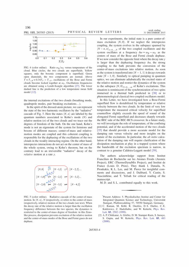
the internal excitations of the two clouds (breathing mode,
quadrupole modes, pair breaking excitations…).
In the spirit of the dressed-atom picture, we can represent
the state of the two harmonic oscillators by the “radiative”
cascade of Fig. 5. Here the states jN; ni are labeled by the
quantum numbers associated to Kohn’s mode (N) and
relative motion (n) of the two clouds and we trace out the
degrees of freedom of the bath. On the one hand, Kohn’s
mode is not an eigenstate of the system for fermions and
bosons of different masses; center-of-mass and relative-
motion modes are coupled and this coherent coupling is
responsible for the dephasing of the oscillations of the two
clouds in the weakly interacting regime. On the other hand,
interspecies interactions do not act on the center of mass of
the whole system, owing to Kohn’s theorem, but on the
contrary lead to an irreversible “radiative” decay of the
relative motion at a rate γ.
In our experiments, the initial state is a pure center-of-
mass excitation jN; 0i. If we neglect the interspecies
coupling, the system evolves in the subspace spanned by
jN − n; nin¼0;…;N of the two coupled oscillators and the
system oscillates at a frequency δω≃ ωB − ωF as the
centers of mass of the Bose and Fermi clouds dephase.
If we now consider the opposite limit where the decay rate γ
is larger than the dephasing frequency δω, the strong
coupling to the bath prevents the conversion of the
center-of-mass excitations into relative motion. As soon
as the system is transferred into jN − 1; 1i it decays towardsstate jN − 1; 0i. Similarly to optical pumping in quantum
optics, we can eliminate adiabatically the excited states of
the relative motion and restrict the dynamics of the system
to the subspace jN; 0iN¼0;…;∞ of Kohn’s excitations. This
situation is reminiscent of the synchronization of two spins
immersed in a thermal bath predicted in [38] or to
phenomenological classical two-coupled oscillators model.
In this Letter, we have investigated how a Bose-Fermi
superfluid flow is destabilized by temperature or relative
velocity between the two clouds. In the limit of very low
temperature the measured critical velocity for superfluid
counterflow slightly exceeds the speed of sound of the
elongated Fermi superfluid and decreases sharply towards
the BEC side of the BEC-BCS crossover. In a future study,
we will investigate the role of temperature, of the confining
potential, and of the accelerated motion of the two clouds
[35] that should provide a more accurate model for the
damping rate versus velocity and more insights on the
nature of the excitations. In particular, the ab initio calcu-
lation of the damping rate will require clarification of the
dissipation mechanism at play in a trapped system where
the bandwidth of the excitation spectrum is narrow, in
contrast to a genuine Caldeira-Leggett model [39].
The authors acknowledge support from Institut
Francilien de Recherche sur les Atomes Froids (Atomix
Project), ERC (ThermoDynaMix Project), and Institut de
France (Louis D. Prize). They thank I. Danaila, N.
Proukakis, K. L. Lee, and M. Pierce for insightful com-
ments and discussions, and J. Dalibard, Y. Castin, S.
Nascimbène, and T. Yefsah for critical reading of the
manuscript.
M. D. and S. L. contributed equally to this work.
*Present Address: 5. Physikalisches Institut and Center for
Integrated Quantum Science and Technology, Universität
Stuttgart, Pfaffenwaldring 57, 70550 Stuttgart, Germany.
[1] C. Raman, M. Köhl, R. Onofrio, D. S. Durfee, C. E.
Kuklewicz, Z. Hadzibabic, and W. Ketterle, Phys. Rev.
Lett. 83, 2502 (1999).
[2] A. P. Chikkatur, A. Görlitz, D. M. Stamper-Kurn, S. Inouye,
S. Gupta, and W. Ketterle, Phys. Rev. Lett. 85, 483
(2000).
FIG. 4 (color online). Ratio ωB=ωF versus temperature of the
cloud. Blue circles, the two clouds are superfluids. Yellow
squares, only the bosonic component is superfluid. Green
open diamonds, the two components are normal. Above
T ≈ Tc;B ≈ 0.34TF > Tc;F, oscillations of the Bose and Fermi
clouds become locked together at ωF. Oscillations frequencies
are obtained using a Lomb-Scargle algorithm [27]. The lower
dashed line is the prediction of a low temperature mean field
model [12].
FIG. 5 (color online). Radiative cascade of the center-of-mass
motion. In jN; ni, N (respectively, n) refers to the center-of-mass
(respectively, relative) motion of the two clouds (see text). When
the decay rate of the relative motion is larger than the oscillation
frequency difference between the two species, the dynamics is
restricted to the center-of-mass degree of freedom: in this Zeno-
like process, dissipation prevents excitation of the relative motion
and the center-of-mass modes of the Bose and Fermi gases do not
dephase.
PRL 115, 265303 (2015) P HY S I CA L R EV I EW LE T T ER Sweek ending
31 DECEMBER 2015
265303-4
196
[3] C. Ryu, M. F. Andersen, P. Cladé, V. Natarajan, K.
Helmerson, and W. D. Phillips, Phys. Rev. Lett. 99,
260401 (2007).
[4] D. E. Miller, J. K. Chin, C. A. Stan, Y. Liu, W. Setiawan, C.
Sanner, andW. Ketterle, Phys. Rev. Lett. 99, 070402 (2007).
[5] R. Desbuquois, L. Chomaz, T. Yefsah, J. Léonard, J.
Beugnon, C. Weitenberg, and J. Dalibard, Nat. Phys. 8,
645 (2012).
[6] W. Weimer, K. Morgener, V. P. Singh, J. Siegl, K. Hueck, N.
Luick, L. Mathey, and H. Moritz, Phys. Rev. Lett. 114,
095301 (2015).
[7] K.W. Madison, F. Chevy, W. Wohlleben, and J. Dalibard,
Phys. Rev. Lett. 84, 806 (2000).
[8] M. Zwierlein, J. Abo-Shaeer, A. Schirotzek, C. Schunck,
and W. Ketterle, Nature (London) 435, 1047 (2005).
[9] L. A. Sidorenkov, M. K. Tey, R. Grimm, Y.-H. Hou, L.
Pitaevskii, and S. Stringari, Nature (London) 498, 78
(2013).
[10] J. Wilks and D. Betts, An Introduction to Liquid Helium
(Oxford Science Publications, Clarendon Press, Oxford,
1987).
[11] D. Dries, S. E. Pollack, J. M. Hitchcock, and R. G. Hulet,
Phys. Rev. A 82, 033603 (2010).
[12] I. Ferrier-Barbut, M. Delehaye, S. Laurent, A. T. Grier, M.
Pierce, B. S. Rem, F. Chevy, and C. Salomon, Science 345,
1035 (2014).
[13] T. Ozawa, A. Recati, M. Delehaye, F. Chevy, and S.
Stringari, Phys. Rev. A 90, 043608 (2014).
[14] R. Zhang, W. Zhang, H. Zhai, and P. Zhang, Phys. Rev. A
90, 063614 (2014).
[15] X. Cui, Phys. Rev. A 90, 041603 (2014).
[16] J. J. Kinnunen and G.M. Bruun, Phys. Rev. A 91, 041605
(2015).
[17] M. Abad, A. Recati, S. Stringari, and F. Chevy, Eur. Phys. J.
D 69, 126 (2015).
[18] Y. Castin, I. Ferrier-Barbut, and C. Salomon, C.R. Phys. 16,
241 (2015).
[19] W. Zheng and H. Zhai, Phys. Rev. Lett. 113, 265304 (2014).
[20] L. Wen and J. Li, Phys. Rev. A 90, 053621 (2014).
[21] F. Chevy, Phys. Rev. A 91, 063606 (2015).
[22] H. Shen and W. Zheng, Phys. Rev. A 92, 033620 (2015).
[23] A. O. Caldeira and A. J. Leggett, Physica (Amsterdam)
121A, 587 (1983).
[24] C.-H. Chou, T. Yu, and B. L. Hu, Phys. Rev. E 77, 011112
(2008).
[25] U. Zürcher and P. Talkner, Phys. Rev. A 42, 3267
(1990).
[26] G. Zürn, T. Lompe, A. N. Wenz, S. Jochim, P. S. Julienne,
and J. M. Hutson, Phys. Rev. Lett. 110, 135301 (2013).
[27] See Supplemental Material at http://link.aps.org/
supplemental/10.1103/PhysRevLett.115.265303 for extra
comments and discussion.
[28] R. Combescot, M. Y. Kagan, and S. Stringari, Phys. Rev. A
74, 042717 (2006).
[29] N. Navon, S. Nascimbène, F. Chevy, and C. Salomon,
Science 328, 729 (2010).
[30] G. Astrakharchik, Ph.D thesis, University of Trento, 2004,
arXiv:1412.4529.
[31] S. Stringari, Phys. Rev. A 58, 2385 (1998).
[32] P. Capuzzi, P. Vignolo, F. Federici, and M. P. Tosi, Phys.
Rev. A 73, 021603 (2006).
[33] L. Luo, B. Clancy, J. Joseph, J. Kinast, and J. E. Thomas,
Phys. Rev. Lett. 98, 080402 (2007).
[34] J. Joseph, B. Clancy, L. Luo, J. Kinast, A. Turlapov, and
J. E. Thomas, Phys. Rev. Lett. 98, 170401 (2007).
[35] V. P. Singh, W. Weimer, K. Morgener, J. Siegl, K. Hueck, N.
Luick, H. Moritz, and L. Mathey, arXiv:1509.02168.
[36] C. A. Regal, M. Greiner, and D. S. Jin, Phys. Rev. Lett. 92,
083201 (2004).
[37] W. Kohn, Phys. Rev. 123, 1242 (1961).
[38] P. P. Orth, D. Roosen, W. Hofstetter, and K. Le Hur, Phys.
Rev. B 82, 144423 (2010).
[39] R. Onofrio and B. Sundaram, Phys. Rev. A 92, 033422
(2015).
PRL 115, 265303 (2015) P HY S I CA L R EV I EW LE T T ER Sweek ending
31 DECEMBER 2015
265303-5
C. Publications and preprints 197

1
Supplemental Information
DAMPING RATES IN THE BEC-BCS CROSSOVER
All the center of mass (CoM) damping rates measured in the BEC-BCS crossover and their respective fittingfunctions to extract vc are shown in Fig. 1. As indicated in the main text the fit function is γB = AΘ(v − vc)((v −vc)/vF)
α, where Θ is the Heaviside function and vF is the Fermi velocity. The χ2 test reveals that most of our data isconsistent with α = 1 as in [1, 2]. Due to the current absence of theoretical prediction for α in a trapped system, weallow α to vary between 0.5 and 2, and this induces a systematic correlation between the extracted α and vc that weinclude in our error bars on vc shown in Fig. 3 of main text. The fit results for α = 1 are displayed in Tab. I alongwith experimental parameters to produce Fig. 3 of main text. The error bars given for vc give the span of vc whenchanging α from 0.5 to 2 in the fit function. Note the strong decrease of the damping rate towards the BCS regime.
In addition, cBs depends on the Bose-Bose scattering length which varies with magnetic field and in particulardiverges for a magnetic field of 845.5G (corresponding to 1/kFaF = −0.13). We therefore show only the values of cBsat the six magnetic field values used in our experiments.
Following [3] the Bose-Fermi coupling can be characterized by the quantity ∆ =√
∂µB
∂nF
∂µF
∂nB/∂µB
∂nB
∂µF
∂nF. As ∆ increases,
the interspecies interactions affect more and more the properties of the system and for ∆ = 1, the mixture isdynamically unstable at rest and demixes. For measurements presented here we typically have ∆ ≃ 15%.
æ
æ
æ
æ
æ
æ
æ
0.0 0.2 0.4 0.6 0.80
1
2
3
4
5
6
vmaxvF
ΓBHs-1L
1kFaF = 0.68
æ
æ
ææ
æ
æ
æ
0.0 0.2 0.4 0.6 0.80
1
2
3
4
5
6
vmaxvF
ΓBHs-1L
1kFaF = 0.39
æ ææ
æ
æ
æ
æ
æ
æ
0.0 0.2 0.4 0.6 0.80
1
2
3
4
5
6
vmaxvF
ΓBHs-1L
1kFaF = 0.18
æ
æ
æ
æ
æ
æ
æ
æ
æ
ææ
0.0 0.2 0.4 0.6 0.80
1
2
3
4
5
6
vmaxvF
ΓBHs-1L
1kFaF = 0
æ
æ
ææææ
æ
0.0 0.2 0.4 0.6 0.80
1
2
3
4
5
6
vmaxvF
ΓBHs-1L
1kFaF = -0.26
æ ææ
ææ
ææ
æ
0.0 0.2 0.4 0.6 0.80
1
2
3
4
5
6
vmaxvF
ΓBHs-1L
1kFaF = -0.42
FIG. 1: Damping rates of the center of mass oscillations versus maximal relative velocity in the BEC-BCS crossover in unit ofthe Fermi velocity vF. Red line: fit with α = 1. Orange zone: region spanned by the fitting function when varying α from 0.5to 2.
198

2
B (G) 780 800 816 832 860 880
aF(a0) 6.4× 10³ 11.3× 10³ 24.0× 10³ ∞ − 16.5× 10³ − 10.3× 10³
1/kFaF 0.68± 0.07 0.39± 0.01 0.18± 0.02 0± 0.002 − 0.26± 0.05 − 0.42± 0.03
aB(a0) 21.3 30.8 43.3 69.5 76.0 259
cB(10−2vF) 9.6± 1.4 9.4± 0.14 11.0± 1.6 11.1± 1.7 11.4± 1.7 15.1± 2.2
vc/vF 0.17+0.06−0.10 0.38+0.02
−0.04 0.35+0.04−0.11 0.42+0.08
−0.14 0.54+0.02−0.06 0.40+0.10
−0.20
A(s−1) 14.8± 1.4 85± 32 24.6± 4.3 17.3± 3.6 30± 11 2.9± 0.5
vc/cFs 0.53+0.19
−0.31 1.11+0.06−0.12 0.99+0.11
−0.31 1.17+0.22−0.39 1.46+0.05
−0.16 1.05+0.26−0.53
TABLE I: Experimental parameters, sound velocity at the center of the Bose gas in an elongated geometry cB =√
µB/2mB,
critical velocity vc/vF, damping rate A(s−1), and vc/cFs for α = 1 in the BEC-BCS crossover. The typical number of bosons
and fermions are constant in the crossover and are respectively 2.5± 0.5× 10⁴ and 2.5± 0.5× 10⁵.
EVOLUTION OF THE VELOCITIES IN THE TRAP
We demonstrate here that for a Bose-Fermi superfluid mixture oscillating in a harmonic trap, the ratio v/cFs ismaximum when the centers of two clouds coincide. This can be demonstrated in the general case using the equationof state in the BEC-BCS crossover [4], but we will derive it here for the simpler case of a polytropic equation of state.
In the frame of the Fermi cloud, we can describe the trajectory of the BEC by the simple harmonic oscillation
zB(t) = Z0 cos(ωBt), (1)
where we have omitted the slow beating of the amplitude Z0 due to the oscillation-frequency difference between bosonsand fermions. The velocity of the BEC is then v(z) = −Z0ωB sin(ωBt), hence
(v(z)
v(z = 0)
)2
=
(1− z2
Z20
), (2)
For a polytropic equation of state, the local sound velocity in the Fermi cloud is given by [5]
cFs (z)2 =
γ
γ + 1
µF(z)
mF(3)
cFs (z)2 =
γ
γ + 1
µF(0)
mF
(1− z2
z2TF
), (4)
where zTF is the Thomas-Fermi radius of the cloud, and the local chemical potential µF(z) was obtained using thelocal density approximation. Combining equations 2 and 4, we then obtain
v(z)2
cFs (z)2=
v(z = 0)2
cFs (z = 0)21− z2/Z2
0
1− z2/z2TF
, (5)
which is maximum for z = 0 when Z0 ≤ zTF.
LOMB-SCARGLE ALGORITHM
We use the fit-free Lomb-Scargle periodogram - or Least Square Spectral Analysis - to extract the spectral com-ponents of the oscillations for different temperatures [6, 7]. This method is an adaptation of the Fourier transformto the case of unevenly spaced data. For N data points hi = h(ti)i=1,...,N taken at times ti, the periodogram isdefined as
PN (ω) =1
2σ2
[∑
j(hj − h) cosω(tj − τ)]2∑
j cos2 ω(tj − τ)
+[∑
j(hj − h) sinω(tj − τ)]2∑
j sin2 ω(tj − τ)
(6)
C. Publications and preprints 199

3
FIG. 2: Power spectrum of the oscillations for different temperatures, obtained using the Lomb-Scargle algorithm of the center-of-mass displacement. Above T ≈ Tc,B ≈ 0.34TF > Tc,F, oscillations of the Bose and Fermi clouds become locked together atωF. A value of 10 for the power represents typically a significance of 0.002.
where τ is given by tan(2ωτ) =∑
jsin 2ωtj
∑jcos 2ωtj
making the periodogram independent of the time origin. h = 1N
∑Ni=1 hi
and σ = 1N−1
∑Ni=1(hi − h)2 are the mean and the variance of hii. The periodogram, or power spectrum (see Fig.
2), gives access to the statistical significance (ie the probability of rejecting the null hypothesis when it is true) ofeach of the evaluated frequencies: noting Pmax = max
ωPN (ω), the signifiance is proportional to e−Pmax , and here a
value of 10 for the power represents typically a significance of 0.002. Fig. ?? of the main text displays the set ofmaxima of Fig. 2; error bars correspond to a significance increased by a factor of 10.
RADIATIVE CASCADE MODEL
Consider a mixture of two atomic species labeled by α = 1, 2 of identical masses m and confined in identicalharmonic traps. According to Kohn’s theorem [8], the single-species Hamiltonian can always be written as
Hα =P 2α
2Mα+
Mαω2X2
α
2+H
(α)int , (7)
where Pα is the total momentum of cloud α, Xα the position of its center of mass and Mα = Nαm its total mass (Nα
being the number of atoms). H(α)int acts only on the internal excitation modes of the cloud and commutes with the
center-of-mass variables.Neglecting interspecies interactions, the total Hamiltonian of the system can be written asH = H1+H2. Introducing
the center of mass/relative variables, we have then
H = H1 +H2 =P 2
2M+
Mω2X2
2+
p2
2µ+
µω2x2
2+H
(1)int +H
(2)int , (8)
200
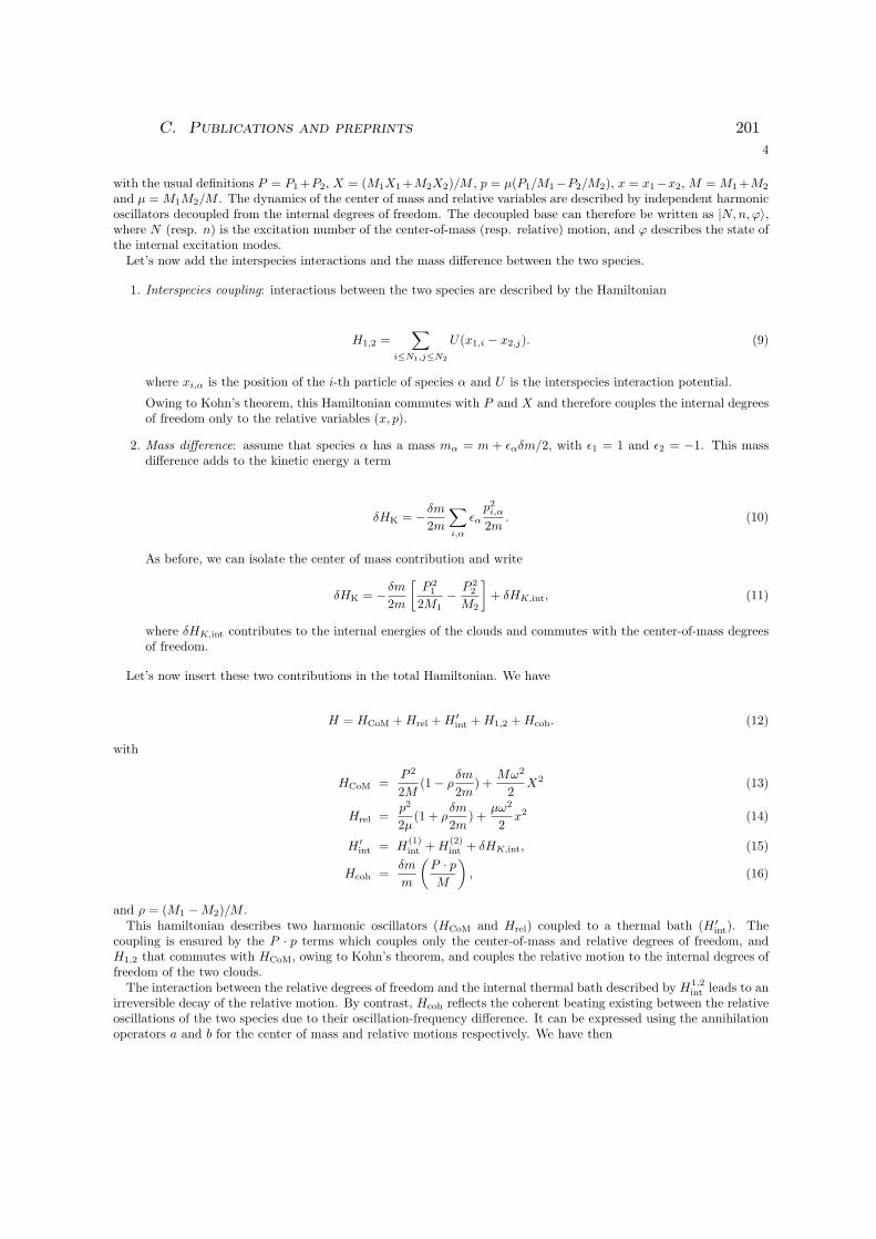
4
with the usual definitions P = P1+P2, X = (M1X1+M2X2)/M , p = µ(P1/M1−P2/M2), x = x1−x2, M = M1+M2
and µ = M1M2/M . The dynamics of the center of mass and relative variables are described by independent harmonicoscillators decoupled from the internal degrees of freedom. The decoupled base can therefore be written as |N,n, ϕ〉,where N (resp. n) is the excitation number of the center-of-mass (resp. relative) motion, and ϕ describes the state ofthe internal excitation modes.
Let’s now add the interspecies interactions and the mass difference between the two species.
1. Interspecies coupling: interactions between the two species are described by the Hamiltonian
H1,2 =∑
i≤N1,j≤N2
U(x1,i − x2,j). (9)
where xi,α is the position of the i-th particle of species α and U is the interspecies interaction potential.
Owing to Kohn’s theorem, this Hamiltonian commutes with P and X and therefore couples the internal degreesof freedom only to the relative variables (x, p).
2. Mass difference: assume that species α has a mass mα = m + ǫαδm/2, with ǫ1 = 1 and ǫ2 = −1. This massdifference adds to the kinetic energy a term
δHK = −δm
2m
∑
i,α
ǫαp2i,α2m
. (10)
As before, we can isolate the center of mass contribution and write
δHK = −δm
2m
[P 21
2M1− P 2
2
M2
]+ δHK,int, (11)
where δHK,int contributes to the internal energies of the clouds and commutes with the center-of-mass degreesof freedom.
Let’s now insert these two contributions in the total Hamiltonian. We have
H = HCoM +Hrel +H ′int +H1,2 +Hcoh. (12)
with
HCoM =P 2
2M(1− ρ
δm
2m) +
Mω2
2X2 (13)
Hrel =p2
2µ(1 + ρ
δm
2m) +
µω2
2x2 (14)
H ′int = H
(1)int +H
(2)int + δHK,int, (15)
Hcoh =δm
m
(P · pM
), (16)
and ρ = (M1 −M2)/M .This hamiltonian describes two harmonic oscillators (HCoM and Hrel) coupled to a thermal bath (H ′
int). Thecoupling is ensured by the P · p terms which couples only the center-of-mass and relative degrees of freedom, andH1,2 that commutes with HCoM, owing to Kohn’s theorem, and couples the relative motion to the internal degrees offreedom of the two clouds.
The interaction between the relative degrees of freedom and the internal thermal bath described by H1,2int leads to an
irreversible decay of the relative motion. By contrast, Hcoh reflects the coherent beating existing between the relativeoscillations of the two species due to their oscillation-frequency difference. It can be expressed using the annihilationoperators a and b for the center of mass and relative motions respectively. We have then
C. Publications and preprints 201

5
Hcoh = −δm
m~ω
õ
M
(a− a†
) (b− b†
). (17)
Using the rotating wave approximation, one can eliminate the non resonant terms and one finally gets
Hcoh ≃ δm
2m~ω
õ
M
(a†b+ ab†
). (18)
This Hamiltonian is similar to the generalized Caldeira-Leggett model [9] used in solid state physics to study heattransport by phonons in a crystal. The absence of coupling between the bath and Kohn’s mode generalizes to thedecomposition used in [10] for a bilinear coupling between the harmonic oscillators and the bath.
In the experiment, we excite the center of mass motion and the initial state is |N, 0, ϕ〉. The coherent couplingtransfers the system to the state |N − 1, 1, ϕ〉. If the coupling to the bath is strong, the relative motion decaysvery fast and the system falls into a state |N − 1, 0, ϕ′〉 (actually, since several states of the bath are involved, it ismore appropriate to describe the state of the two harmonic oscillators by a density matrix rather than a well-definedquantum state). In this case, just like for optical pumping, we can adiabatically eliminate the intermediate state|N − 1, 1, ϕ〉 and consider that the dynamics occurs only in the sub-space |N, 0, ϕ〉, where the relative motion is neverexcited and the centers of mass of the two clouds are locked. In some sense, this freezing of the system state in a puremotion of its center of mass can be considered as a manifestation of the quantum Zeno effect.
[1] D. E. Miller, J. K. Chin, C. A. Stan, Y. Liu, W. Setiawan, C. Sanner, and W. Ketterle, Phys. Rev. Lett. 99, 070402 (2007),URL http://link.aps.org/doi/10.1103/PhysRevLett.99.070402.
[2] W. Weimer, K. Morgener, V. P. Singh, J. Siegl, K. Hueck, N. Luick, L. Mathey, and H. Moritz, Phys. Rev. Lett. 114,095301 (2015), URL http://link.aps.org/doi/10.1103/PhysRevLett.114.095301.
[3] M. Abad, A. Recati, S. Stringari, and F. Chevy, Eur. Phys. J. D 69, 126 (2015), URL http://dx.doi.org/10.1140/epjd/
e2015-50851-y.[4] N. Navon, S. Nascimbene, F. Chevy, and C. Salomon, Science 328, 729 (2010),
http://www.sciencemag.org/content/328/5979/729.full.pdf, URL http://www.sciencemag.org/content/328/5979/
729.abstract.[5] P. Capuzzi, P. Vignolo, F. Federici, and M. P. Tosi, Phys. Rev. A 73, 021603 (2006), URL http://link.aps.org/doi/
10.1103/PhysRevA.73.021603.[6] N. Lomb, Astrophysics and Space Science 39, 447 (1976), ISSN 0004-640X, URL http://dx.doi.org/10.1007/
BF00648343.[7] J. Scargle, Astrophysical Journal 263, 835 (1982), URL http://articles.adsabs.harvard.edu/full/1982ApJ...263.
.835S.[8] W. Kohn, Phys. Rev. 123, 1242 (1961), URL http://link.aps.org/doi/10.1103/PhysRev.123.1242.[9] A. O. Caldeira and A. J. Leggett, Physica A: Statistical mechanics and its Applications 121, 587 (1983).
[10] C.-H. Chou, T. Yu, and B. L. Hu, Phys. Rev. E 77, 011112 (2008), URL http://link.aps.org/doi/10.1103/PhysRevE.
77.011112.
202

C. Publications and preprints 203

204
C.5 Universal loss dynamics in a unitary Bose gas
Ulrich Eismann, Lev Khaykovich, Sébastien Laurent, IgorFerrier-Barbut, Benno S. Rem, Andrew T. Grier, Marion
Delehaye, Frédéric Chevy, Christophe Salomon, Li-Chung Ha, andCheng Chin
Submitted to Physical Review X
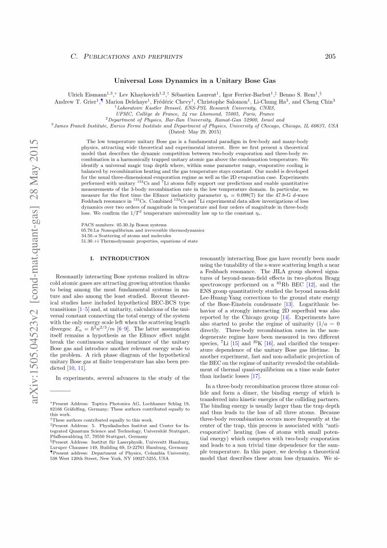
Universal Loss Dynamics in a Unitary Bose Gas
Ulrich Eismann1,3,∗ Lev Khaykovich1,2,† Sebastien Laurent1, Igor Ferrier-Barbut1,‡ Benno S. Rem1,§
Andrew T. Grier1,¶ Marion Delehaye1, Frederic Chevy1, Christophe Salomon1, Li-Chung Ha3, and Cheng Chin31Laboratoire Kastler Brossel, ENS-PSL Research University, CNRS,
UPMC, College de France, 24 rue Lhomond, 75005, Paris, France2Department of Physics, Bar-Ilan University, Ramat-Gan 52900, Israel and
3James Franck Institute, Enrico Fermi Institute and Department of Physics, University of Chicago, Chicago, IL 60637, USA
(Dated: May 29, 2015)
The low temperature unitary Bose gas is a fundamental paradigm in few-body and many-bodyphysics, attracting wide theoretical and experimental interest. Here we first present a theoreticalmodel that describes the dynamic competition between two-body evaporation and three-body re-combination in a harmonically trapped unitary atomic gas above the condensation temperature. Weidentify a universal magic trap depth where, within some parameter range, evaporative cooling isbalanced by recombination heating and the gas temperature stays constant. Our model is developedfor the usual three-dimensional evaporation regime as well as the 2D evaporation case. Experimentsperformed with unitary 133Cs and 7Li atoms fully support our predictions and enable quantitativemeasurements of the 3-body recombination rate in the low temperature domain. In particular, wemeasure for the first time the Efimov inelasticity parameter η∗ = 0.098(7) for the 47.8-G d-waveFeshbach resonance in 133Cs. Combined 133Cs and 7Li experimental data allow investigations of lossdynamics over two orders of magnitude in temperature and four orders of magnitude in three-bodyloss. We confirm the 1/T 2 temperature universality law up to the constant η∗.
PACS numbers: 05.30.Jp Boson systems05.70.Ln Nonequilibrium and irreversible thermodynamics34.50.-s Scattering of atoms and molecules51.30.+i Thermodynamic properties, equations of state
I. INTRODUCTION
Resonantly interacting Bose systems realized in ultra-cold atomic gases are attracting growing attention thanksto being among the most fundamental systems in na-ture and also among the least studied. Recent theoret-ical studies have included hypothetical BEC-BCS typetransitions [1–5] and, at unitarity, calculations of the uni-versal constant connecting the total energy of the systemwith the only energy scale left when the scattering lengthdiverges: En = ~
2n2/3/m [6–9]. The latter assumptionitself remains a hypothesis as the Efimov effect mightbreak the continuous scaling invariance of the unitaryBose gas and introduce another relevant energy scale tothe problem. A rich phase diagram of the hypotheticalunitary Bose gas at finite temperature has also been pre-dicted [10, 11].
In experiments, several advances in the study of the
∗Present Address: Toptica Photonics AG, Lochhamer Schlag 19,82166 Grafelfing, Germany; These authors contributed equally tothis work.†These authors contributed equally to this work.‡Present Address: 5. Physikalisches Institut and Center for In-tegrated Quantum Science and Technology, Universitat Stuttgart,Pfaffenwaldring 57, 70550 Stuttgart, Germany§Present Address: Institut fur Laserphysik, Universitt Hamburg,Luruper Chaussee 149, Building 69, D-22761 Hamburg, Germany¶Present address: Department of Physics, Columbia University,538 West 120th Street, New York, NY 10027-5255, USA
resonantly interacting Bose gas have recently been madeusing the tunability of the s-wave scattering length a neara Feshbach resonance. The JILA group showed signa-tures of beyond-mean-field effects in two-photon Braggspectroscopy performed on a 85Rb BEC [12], and theENS group quantitatively studied the beyond mean-fieldLee-Huang-Yang corrections to the ground state energyof the Bose-Einstein condensate [13]. Logarithmic be-havior of a strongly interacting 2D superfluid was alsoreported by the Chicago group [14]. Experiments havealso started to probe the regime of unitarity (1/a = 0directly. Three-body recombination rates in the non-degenerate regime have been measured in two differentspecies, 7Li [15] and 39K [16], and clarified the temper-ature dependence of the unitary Bose gas lifetime. Inanother experiment, fast and non-adiabatic projection ofthe BEC on the regime of unitarity revealed the establish-ment of thermal quasi-equilibrium on a time scale fasterthan inelastic losses [17].
In a three-body recombination process three atoms col-lide and form a dimer, the binding energy of which istransferred into kinetic energies of the colliding partners.The binding energy is usually larger than the trap depthand thus leads to the loss of all three atoms. Becausethree-body recombination occurs more frequently at thecenter of the trap, this process is associated with “anti-evaporative” heating (loss of atoms with small poten-tial energy) which competes with two-body evaporationand leads to a non trivial time dependence for the sam-ple temperature. In this paper, we develop a theoreticalmodel that describes these atom loss dynamics. We si-
arX
iv:1
50
5.0
45
23
v2
[c
on
d-m
at.q
uan
t-g
as]
28
May
20
15
C. Publications and preprints 205
2
multaneously take into account two and three-body lossesto quantitatively determine each of these contributions.We predict the existence of a magic value for the trap-depth-over-temperature ratio where residual evaporationcompensates for three-body loss heating and maintainsthe gas temperature constant within some range of pa-rameters. We then apply our model to analyze the lossdynamics of 133Cs and 7Li unitary Bose gases preparedat various temperatures and atom numbers. Compar-ing measurements in these two different atomic specieswe find the dynamics to be universal, i.e. in both sys-tems the three-body loss rate is found to scale universallywith temperature. Excellent agreement between theoryand experiment confirms that the dynamic evolution ofthe unitary Bose gas above the condensation tempera-ture can be well modelled by the combination of two andthree-body interaction processes.
II. MODEL
A former study developed for measuring three-bodydecay in trapped 133Cs [18] atoms has proposed a modelto describe the time evolution of the atom number N andthe temperature T taking into account the three-body re-combination induced loss and the heating associated withit. This model is valid in the limit of deep trapping poten-tials (trapping depth much larger than the atom’s tem-perature) and for temperature independent losses. Herewe generalize this model to include evaporation inducedcooling and the associated atom loss, as well as the tem-perature dependence of the three-body loss rate.
A. Rate equation for atom number
The locally defined three-body recombination rateL3n
3(r)/3 leads, through integration over the whole vol-ume, to the loss rate of atoms:
dN
dt= −3
∫L3n
3(r)
3d3r = −L3〈n2〉N, (1)
where the factor of 3 in front on the integral reflects thefact that all 3 atoms are lost per each recombinationevent. In the following, we neglect single-atom lossesdue to collisions with the background gas and we assumethat two-body inelastic collisions are forbidden, a condi-tion which is fulfilled for atoms polarized in the absoluteground state.
An expression for the three-body recombination losscoefficient at unitarity for a non-degenerate gas has beendeveloped in Ref. [15]. Averaged over the thermal distri-bution it reads:
L3 =72
√3π2
~(1− e−4η∗
)
mk6th
×∫ ∞
0
(1− |s11|2
)e−k2/k2
thk dk
|1 + (kR0)−2is0e−2η∗s11|2, (2)
where kth =√mkBT/~, R0 is the three-body parame-
ter, and the Efimov inelasticity parameter η∗ character-izes the strength of the short range inelastic processes.Here, ~ is the reduced Planck’s constant, kB is the Boltz-mann’s constant, and s0 = 1.00624 for three identicalbosons [19]. The matrix element s11 relates the incom-ing to outgoing wave amplitudes in the Efimov scatteringchannel and shows the emerging discrete scaling symme-try in the problem (see for example Ref. [20]). Details aregiven in the supplementary material to Ref. [15] for thecalculation of s11(ka), where a is the scattering lengthand k is the relative wavenumber of the colliding part-ners. Because of its numerically small value for threeidentical bosons at unitarity, we can set |s11| = 0 and L3
is well approximated by:
L3 ≈ ~5
m336
√3π2 1− e−4η∗
(kBT )2=
λ3
T 2, (3)
where λ3 is a temperature-independent constant. Assum-ing a harmonic trapping potential, we directly expressthe average square density 〈n2〉 through N and T . Incombination with Eq. (3), Eq. (1) is represented as:
dN
dt= −γ3
N3
T 5, (4)
where
γ3 = λ3
(mω2
2√3πkB
)3
, (5)
with ω being the geometric mean of the angular frequen-cies in the trap.
To model the loss of atoms induced by evaporation, weconsider time evolution of the phase-space density distri-bution of a classical gas:
f(r,p) =n0λdB
3
(2π~)3e−U(r)/kBT e−p2/2mkBT , (6)
which obeys the Boltzmann equation. Here n0 is thecentral peak density of atoms, λdB = (2π~2/mkBT )
1/2
is the thermal de Broglie wavelength, and U(r) is theexternal trapping potential. The normalization con-stant is fixed by the total number of atoms, such that∫f(r,p)d3p d3r = N .If the gas is trapped in a 3-D trap with a potential
depth U , the collision integral in the Boltzmann equationcan be evaluated analytically [21]. Indeed, the low-energycollisional cross-section
σ(k) =8π
k2 + a−2(7)
reduces at unitarity to a simple dependence on the rel-ative momentum of colliding partners: σ(k) = 8π/k2.However, not every collision leads to a loss of atoms dueto evaporation. Consider
η = U/kBT. (8)
206

3
In the case of η ≫ 1, such loss is associated with atransfer of large amount of energy to the atom whichultimately leads to the energy independent cross-section.This can be understood with a simple argument [22]. As-sume that two atoms collide with the initial momenta p1
and p2. After the collision they emerge with the mo-menta p3 and p4, and if one of them acquires a mo-mentum |p3| &
√2mU . Then, |p4| is necessarily smaller
than the most probable momentum of atoms in the gasand |p3| ≫ |p4|. In the center of mass coordinates theabsolute value of the relative momentum is preserved,so that 1
2 |p1 − p2| = 12 |p3 − p4| ≈ 1
2 |p3|. Assuming
|p3| =√2mU , we get |p1 − p2| =
√2mU . Substituting
the relative momentum in the center of mass coordinate,~k = 1
2 (p1 − p2), to the unitary form of the collisionalcross-section, we find the latter is energy independent:
σU =16π~2
mU, (9)
and the rate-equation for the atom number can be writ-ten as:
dN
dt= −ΓevN, Γev = n0σUve
−η Vev
Ve. (10)
The peak density is n0 = N/Ve, where Ve is the effec-tive volume of the sample. In the harmonic trap Ve can
be related to ω and the temperature T : Ve =(2πkBTmω2
)3/2.
The ratio of the evaporative and effective volumes is de-fined by [21]:
Vev
Ve= η − 4R (3, η) , (11)
where R(a, η) = P (a+1,η)P (a,η) and P (a, η) is the incomplete
Gamma function
P (a, η) =
∫ η
0ua−1e−udu∫∞
0ua−1e−udu
.
Finally, taking into account both three-body recombi-nation loss (see Eqs. (4),(5)) and evaporative loss, we canexpress the total atom number loss rate equation as:
dN
dt= −γ3
N3
T 5− γ2e
−η Vev
Ve
N2
T, (12)
where
γ2 =16
π
~2ω3
kBU. (13)
Note that η and the ratio of the evaporative and effec-tive volumes explicitly depend on temperature and γ2 istemperature independent.
B. Rate equation for temperature
1. ‘Anti-evaporation’ and recombination heating
Ref. [18] points out that in each three-body recom-bination event a loss of an atom is associated with anexcess of kBT of energy that remains in the sample.This mechanism is caused by the fact that recombina-tion events occur mainly at the center of the trap wherethe density of atoms is highest and it is known as ‘anti-evaporation’ heating. We now show that the unitarylimit is more ‘anti-evaporative’ than the regime of finitescattering lengths considered in ref. [18] where L3 is tem-perature independent. We separate center of mass andrelative motions of the colliding atoms and express thetotal loss of energy per three-body recombination eventas following:
E3b = −∫
L3n3(r)
3(〈Ecm〉+ 3U(r))
+n3(r)
3〈L3(k)Ek〉
d3r. (14)
The first two terms in the parenthesis represent the meancenter-of-mass kinetic energy 〈Ecm〉 = 〈P 2
cm〉/2M andthe local potential energy 3U(r) per each recombinationtriple. M = 3m is the total mass of the three-bodysystem. The last term stands for thermal averaging ofthe three-body coefficient over the relative kinetic energyEk = (~k)2/2µ where µ is the reduced mass.Averaging the kinetic energy of the center of mass mo-
tion over the phase space density distribution (Eq. (6))gives 〈Ecm〉 = 3
2kBT . Then the integration over this termis straightforward and using Eq. (1) we have:
−∫
L3n3(r)
3〈Ecm〉d3r =
1
2kBTN (15)
The integration over the second term can be easilyevaluated as well:
−∫
3L3
3n3(r)U(r)d3r =
1
2kBTN (16)
To evaluate the third term we recall the averaged overthe thermal distribution expression of the three-body re-combination rate in Eq. (2). Now its integrand has tobe supplemented with the loss of the relative kinetic en-ergy per recombination event Ek. Keeping the limit ofEq. (3) this averaging can be easily evaluated to give〈L3(k)Ek〉 = L3kBT . Finally, the last term in Eq. (14)gives:
−∫
n3(r)
3〈L3(k)Ek〉d3r =
1
3kBTN (17)
Finally, getting together all the terms, the lost energy perlost atom in a three-body recombination event becomes:
E3b
N=
4
3kBT. (18)
C. Publications and preprints 207

4
This expression shows that unitarity limit is more‘anti-evaporative’ than the regime of finite scatteringlength (k|a| ≤ 1). As the mean energy per atom in theharmonic trap is 3kBT , at unitarity each escaped atomleaves behind (3 − 4/3)kBT = (5/3)kBT of the excessenergy as compared to 1kBT when L3 is energy indepen-dent. In the latter case, thermal averaging of the relativekinetic energy gives 〈Ek〉 = 3kBT , thus E3b/N = 2kBT .
Eq. (18) is readily transformed into the rate equationfor the rise of temperature per lost atom using the factthat E3b = 3NkBT in the harmonic trap and Eq. (4):
dT
dt=
5
3
T
3γ3
N2
T 5. (19)
Another heating mechanism pointed out in Ref. [18]is associated with the creation of weakly bound dimerswhose binding energy is smaller than the depth of thepotential. In such a case, the three-body recombinationproducts stay in the trap and the binding energy is con-verted into heat.
In the unitary limit, this mechanism causes no heat-ing. In fact in this regime, as shown in the supplementarymaterial to Ref. [15], the atoms and dimers are in chem-ical equilibrium with each other, e.g. the rate of dimerformation is equal to the dissociation rate. We thereforeexclude this mechanism from our considerations.
2. Evaporative cooling
“Anti-evaporative” heating can be compensated byevaporative cooling. The energy loss per evaporatedatom is expressed as:
E = N (η + κ) kBT (20)
where κ in a harmonic trap is [21]:
κ = 1− P (5, η)
P (3, η)
Ve
Vev, (21)
with 0 < κ < 1.In a harmonic trap, the average energy per atom is
3kBT = EN . Taking the derivative of this equation and
combining it with Eq. (20) we get:
3T
T=
N
N(η + κ− 3) . (22)
From Eqs. (10) and (22), evaporative cooling is expressedas:
3dT
dt= −Γev (η + κ− 3)T, (23)
This equation can be presented in a similar manner as inthe previous section:
dT
dt= −γ2e
−η Vev
Ve(η + κ− 3)
N
T
T
3, (24)
0.1 1
0.7
0.8
0.9
1.0
1.1
T/T
in
N/Nin
in=6
in=8.2
in=9
in=10
FIG. 1: N-T phase space representation of ‘anti-evaporation’heating and evaporative cooling dynamics for different valuesof the initial ηin parameter. The “magic” ηm satisfies thecondition dT/dN = 0. For lower values of ηin the “magic”ηm is not reached during the evolution of the gas.The figure isdrawn for experimental parameters of 133Cs atoms presentedin Sec. III. For these conditions ηm coincides with ηin ≈ 8.
where, as before, the temperature dependence remains inη.
Finally, combining the two processes of recombinationheating (Eq. (19)) and evaporative cooling (Eq. (24)) weget:
dT
dt=
T
3
(5
3γ3
N2
T 5− γ2e
−η Vev
Ve(η + κ− 3)
N
T
). (25)
Eqs. (12) and (25) form a set of coupled rate equationsthat describe the atom loss dynamics.
C. N-T dynamics and the “magic” ηm
To study atom number and temperature dynamics wesolve Eqs. (12) and (25) numerically for different initialvalues of η, referred to as ηin from here on. As an illus-tration, γ2 and γ3 are evaluated based on parameters ofthe 133Cs experiment discussed in Sec. III. The systemdynamics in N − T phase space is represented in Fig. 1.All represented values of ηin lead to a decrease in temper-ature for small atom numbers indicating that evaporativecooling always wins for asymptotic times where the atomdensity becomes small. This weakens the three-body re-combination event rate and effectively extinguishes theheating mechanism altogether. Large values of the initialηin cause initial heating of the system which is followedby a flattening of the temperature dependence at a cer-tain atom number (grey dashed and dark yellow dottedlines) that defines the “magic” ηm. In Fig. 1 the solid
208

5
æ
ææà
à
0.000 0.002 0.004 0.006 0.008 0.0106
7
8
9
10
11
Α
Ηm
FIG. 2: Universal plot ηm vs α = N(~ω/kBT )3(1 − e−4η∗)
(bue curve). The blue solid circles correspond to the resultsobtained for 133Cs in Fig. 3(a) with η∗ = 0.098. The redsolid squares correspond to the 7Li data of Fig. 3(c) withη∗ = 0.21.
green line represents the special case when ηm = ηin. Ex-perimentally, η(T,N) is tuned to satisfy this special casefor a given initial temperature and atom number. Asit is seen in Fig. 1, lower initial values of ηin can neverreach the necessary condition for ηm in their subsequentdynamics (orange dotted-dashed line).
The value of ηm(T,N) is found by solving the equationdT/dN = 0, i.e. when T (N) becomes independent onthe atom number up to the first order in N . From thegeneral structure of this equation, we see that ηm is solelyfunction of the dimensionless parameter
α = N
(~ω
kBT
)3 (1− e−4η∗
). (26)
Up to a factor (1−e−4η∗), ηm depends only on the phase-space densityN(~ω/kBT )
3 of the cloud. We plot in Fig. 2the dependence of ηm vs α. Since our approach is validonly in the non-quantum degenerate regime where themomentum distribution is a Gaussian, we restricted theplot to small (and experimentally relevant) values of α.
D. 2D evaporation
The above model was developed to explain 3D isother-mal evaporation in a harmonic trap and experiments with133Cs presented below correspond to this situation. Ourmodel can also be extended to 2D isothermal evapora-tion, as realized in the 7Li gas studied in Ref. [15] andpresented below. In this setup, the atoms were trapped ina combined trap consisting of optical confinement in theradial direction and magnetic confinement in the axial di-rection. Evaporation was performed by lowering the laser
beam power which did not lower the axial (essentially in-finite) trap depth due to the magnetic confinement. Sucha scenario realizes a 2D evaporation scheme. Here, we ex-plore the consequences of having 2D evaporation. In theexperimental section we will show the validity of theseresults with the evolution of a unitary 7Li gas.
Lower dimensional evaporation is, in general, less ef-ficient than its 3D counterpart. 1D evaporation can benearly totally solved analytically and it has been an in-tense subject of interest in the context of evaporativecooling of magnetically trapped hydrogen atoms [21, 23,24]. In contrast, analytically solving the 2D evaporationscheme is infeasible in practice. It also poses a ratherdifficult questions considering ergodicity of motion in thetrap [25]. The only practical way to treat 2D evapora-tion is Monte Carlo simulations which were performedin Ref. [25] to describe evaporation of an atomic beam.However, as noted in Ref. [25], these simulations followamazingly well a simple theoretical consideration whichleaves the evaporation dynamics as in 3D but introducesan ’effective’ η parameter to take into account its 2Dcharacter.
The consideration is as following. In the 3D evapo-ration model, the cutting energy ǫc is introduced in theHeaviside function that is multiplied with the classicalphase-space distribution of Eq. (6) [21]. For the 2Dscheme this Heaviside function is Y (ǫc − ǫ⊥), where ǫcis the 2D truncation energy and ǫ⊥ is the radial energyof atoms in the trap, the only direction in which atomscan escape. Now we simply add and subtract the axialenergy of atoms in the trap and introduce an effective 3Dtruncation energy as following:
Y (ǫc − ǫ⊥) = Y ((ǫc + ǫz)− (ǫ⊥ + ǫz)) = Y (ǫeffc − ǫtot),(27)
where ǫtot is the total energy of atoms in the trap andthe effective truncation energy is given ǫeffc = ǫc + ǫz ≃ǫc+kBT where we replaced ǫz by its mean value kBT in aharmonic trap. The model then suggests that the evapo-ration dynamics follows the same functional form as thewell established 3D model, but requires a modification ofthe evaporation parameter (8):
ηeff = η + 1, (28)
Then, the experimentally provided 2D η should be com-pared with the theoretically found 3D ηeff reduced by 1(i.e. ηeff − 1).
III. EXPERIMENTS
In this section, we present experimental T (N) trajec-tories of unitary 133Cs and 7Li gases, and show that theirdynamics are given by the coupled Eqns. (12) and (25).The 133Cs Feshbach resonance at 47.8 Gauss and the7Li Feshbach resonance at 737.8 Gauss have very sim-ilar resonance strength parameter sres = 0.67 and 0.80
C. Publications and preprints 209

6
respectively [26, 27]) and are in the intermediate cou-pling regime (neither in the broad nor narrow resonanceregime). We first confirm the existence of a “magic” ηmfor unitarity-limited losses for both species, with either3D or 2D evaporation. Then we will use the unitarity-limited three-body loss and the theory presented here todetermine the Efimov inelasticity parameter of the nar-row 47.8-G resonance in 133Cs which was not measuredbefore.
A. N − T fits
We prepare the initial samples at Tin and Nin as de-scribed in the Supplementary Materials. We measure theatom number N(t) and the temperature T (t) from in-
situ absorption images taken after a variable hold time t.In Fig. 3(a), we present typical results for the evolutionT (N) of the atom number and temperature of the gases,and we furthermore treat the hold time t as a param-eter. We also plot the relative temperature T/Tin as afunction of the relative atom number N/Nin for the samedata in Fig. 3(b), and for 7Li in Fig. 3(c). We then per-form a coupled least-squares fit of the atom number andtemperature trajectories, Eqs. (12) and (25), to the data.We note that with our independent knowledge of the ge-ometric mean of the trapping frequencies, ω, the onlyfree fit parameters apart from initial temperature andatom number are the trap depth U and the temperature-independent loss constant λ3. The solid lines are thefits (see Supplementary Materials) to our theory model,which describe the experimental data well for a large va-riety of initial temperatures, atom numbers and relativetrap depth. We are able to experimentally realize the fullpredicted behavior of rising, falling and constant-to-first-order temperatures.
B. Magic η
The existence of maxima in the T −N plots confirmsthe existence of a “magic” relative trap depth ηm, wherethe first-order time derivative of the sample temperaturevanishes. Using the knowledge of η∗ for both 133Cs and7Li, we can compare the observed values of ηm to the pre-diction of Fig. 2 (note that in the case of 7Li, we plot ηeffmthat enters into the effective 3D evaporation model). Wesee that for both the 3D evaporation 133Cs data and 2Devaporation 7Li data, the agreement between experimentand theory is remarkable.
Furthermore, in the Supplemental Materials we showthat from the three-body loss coefficients and the evap-oration model, we can predict the trap depth, which isfound in good agreement with the value deduced fromthe laser power, beam waist, and atom polarizability.
Number7of7atoms7N7
0 .3 0 .4 0 .5 0 .6 0 .8 1 .0
inRel.7number7of7atoms7N/N
(a)7
(b)
(c)70 .3 0 .4 0 .5 0 .6 0 .8 1 .0
inRel.7number7of7atoms7N/N
207000 407000 607000 807000 10070000
inR
el.7te
mper
ature
7T/T
1.3
1.2
1.1
1.0
0.9
0.8
0.7
inR
el.7te
mper
ature
7T/T
1.2
1.1
1.0
0.9
0.8
0.7
Tem
per
ature
7T in
7nK
400
350
300
250
200
150
100
10.910.07.45.85.0
η in
10.910.07.45.85.0
η in
9.6
8.5
8.2
η in
FIG. 3: (Color online) Evolution of the unitary 133Cs gasin (a) absolute and (b) relative numbers. The solid lines arefits of the data using the theory presented here, and the fittedinitial relative trap depth ηin = U/kBTin is given in the legend.Error bars are statistical. The condition for (dT/dN)|t=0 isexpected for ηin ≈ ηm ≈ 8.2, very close to the measured datafor ηin = 7.4 (green lines in a) and b)). (c) Evolution of theunitary 7Li gas. The solid lines are fits of the data usingour 2D evaporation model, and the fitted initial relative trapdepth ηin = U/kBTin is given in the legend. Error bars arestatistical. In 2D evaporation, ηin ≈ ηeff
m = ηm + 1 = 8.5 isrequired to meet the (dT/dN)|t=0 condition, and is found inexcellent agreement with the measured value 8.5 (green linein c)), see text.
210

7
C. Universality of the three-body loss
As the last application we now show the validity of theL3 ∝ T−2 law for the tree-body loss of unitary 7Li and133Cs Bose gases. Because both species are situated atthe extreme ends of the (stable) alkaline group, they havea large mass ratio of 133/7 = 19 and the temperaturerange is varied over two orders of magnitude from 0.1µKto 10µK. We determine the three-body loss coefficientsλ3 from fits to decay curves such as shown in Fig.3. Wepresent in Fig. 4 the results for the rate coefficient L3,which varies over approximately two orders of magnitudefor both species. In order to emphasize universality, theloss data is plotted as a function of (m/mH)
3T 2in, where
mH is the hydrogen mass. In this representation, theunitary limit for any species collapses to a single universalline (dotted line in Fig. 4, cf. Eq. (3)).
ì
ì
ì
ì
ì
ì
ìì
ì
ì
ìì
ì
ìì ì
ì
æ
ææ
æ
æ
æ
æ
æ
æ
æ
æ
æ
æææ
æ
ææ
ææ
æ
æ
æ
ææ
ææ
ææ
æ
æ
æ
æ
æ
ææ
æ
ææ
1000 104
105
106
10-24
10-23
10-22
10-21
10-20
m3Tin
2in mH
3 ΜK2
L3in
cm
6s
FIG. 4: (Color online) The magnitude of three-body loss rateat unitarity for 7Li (red) and 133Cs (blue) with the respective±1 standard deviation (shaded areas). On the horizontalaxis, masses are scaled to the hydrogen atom mass mH. Thedashed line represents the unitary limit (Eq. (3) with η∗ →∞). Solid lines are predictions of universal theory [15] withη∗ = 0.21 for 7Li and η∗ = 0.098(7) for 133Cs, see text. Thedata confirms the universality of the L3 ∝ T−2 law.
For 7Li, we cover the 1-10µK temperature range.We find for the temperature-independent loss coefficientλ3 = 3.0(3) × 10−20 cm6µK2s−1, very close to the uni-tary limit λmax
3 ≈ 2.7×10⁻²⁰ cm6µK2s−1. It is also closeto the value λ3 = 2.5(3) × 10−20 cm6µK2s−1 found in[15] with a restricted set of data, and to the predicionfrom Eq. (2) with η∗ = 0.21 from [28] (red solid line inFig. 4). We cannot measure η∗ here because the 7Li datacoincides with the unitary limit.
Furthermore the quality of the 133Cs temperature andatom number data enables us to directly measure thepreviously unknown η∗ parameter of the 47.8-G Fesh-bach resonance. The standard technique for obtainingη∗ is measuring the three-body loss rate L3(a, T → 0) asa function of scattering length in the zero-temperaturelimit, and subsequent fitting of the resulting spectrum to
universal theory. However, for a given experimental mag-netic field stability, this method becomes hard to put intopractice for narrow resonances like the 47.8-G resonancein 133Cs. Instead, we use the fits to our theory model inorder to obtain η∗ from λ3. We cover the 0.1-1µK rangeand find λ3 = 1.27(7)× 10−24 cm6µK2s−1. Plugging thisnumber into Eq. (3), we deduce a value for the Efimovinelasticity parameter η∗ = 0.098(7). The correspondingcurve is the blue line in Fig. 4 and is significantly be-low the unitary line because of the smallness of η∗. Thisnew value is comparable to the Efimov inelasticity pa-rameter found for other resonances in 133Cs, in the range0.06...0.19 [29, 30].
The plot of the full theoretical expression Eq. (2) forL3(m
3T 2) in Fig. 4 (full lines) requires an additional pa-rameter describing three-body scattering around this Fes-hbach resonance, the so-called three-body parameter. Itcan be represented by the location of the first Efimov
resonance position a(1)− [31]. Because of the lack of ex-
perimental knowledge for the 47.8-G resonance, we take
the quasi-universal value a(1)− = −9.73(3)rvdW, rvdW be-
ing the van-der-Waals radius, for which theoretical ex-planations have been given recently [31–33]. The theorycurve then displays log-periodic oscillations with a tem-perature period set by the Efimov state energy spacingof exp(2π/s0) ≈ 515, where s0 = 1.00624, and with a
phase given by a(1)− . The relative peak-to-peak ampli-
tude is 7% for 133Cs. As seen in Fig. 4, such oscillationscannot be resolved in the experimental data because oflimited signal-to-noise and the limited range of tempera-ture. The predicted contrast of these oscillations for 7Liis even smaller (∼ 6%). This is a general property of thesystem of three identical bosons due to the smallness of|s11| [15].
IV. CONCLUSIONS
In this article, we developed a general theoreticalmodel for the coupled time dynamics of atom numberand temperature of the 3D harmonically trapped unitaryBose gas in the non-degenerate regime. The theory takesfull account of evaporative loss and the related coolingmechanism, as well as of the universal three-body lossand heating. It is furthermore extended to the specialcase of 2D evaporation. We predict and experimentallyverify the existence of a “magic” trap depth, where thetime derivative of temperature vanishes both in 3D and2D evaporation.
We compare our model to two different set of experi-ments with lithium and cesium with vastly different massand temperature ranges. The data illustrates the univer-sal T−2 scaling over 2 orders of magnitude in temper-ature, and we obtain an experimental value of the Efi-mov inelasticity parameter for the 47.8-G resonance in133Cs. The theory further enables an independent deter-mination of the trap depth. The agreement found here
C. Publications and preprints 211

8
with standard methods shows that it can be used in morecomplex trap geometries (crossed dipole traps, or hybridmagnetic-optical traps) where the actual trap depth isoften not easy to measure.
In future work it would be highly interesting to probethe discrete symmetry of the unitary Bose gas by reveal-ing the 7% log-periodic modulation of the three-body losscoefficient expected over a factor 515 energy range.
Acknowledgments
We would like to thank the Institut de France (Louis
D. award), the region Ile de France DIM nanoK/IFRAF(ATOMIX project), and the European Research Coun-cil ERC (ThermoDynaMix grant) for support. We ac-knowledge support from the NSF-MRSEC program, NSFGrant No. PHY-1206095, and Army Research OfficeMultidisciplinary University Research Initiative (ARO-MURI) Grant No. W911NF-14-1-0003. L.-C. H. is sup-ported by the Grainger Fellowship and the Taiwan Gov-ernment Scholarship. We also acknowledge the supportfrom the France-Chicago Center.
[1] Y.-W. Lee and Y.-L. Lee. Quantum phase transition inan atomic bose gas near a feshbach resonance. Phys. Rev.B, 70:224506, 2004.
[2] M. W. .J. Romans, R. A. Duine, S. Sashdev, and H. T. C.Stoof. Quantum phase transition in an atomic bose gaswith a feshbach resonance. Phys. Rev. Lett., 93:020405,2004.
[3] L. Radzihovsky, P. B. Weichmann, and J. I. Park. Su-perfluidity and phase transitions in a resonant bose gas.Annals of Physics, 323:2376, 2008.
[4] A. Koetsier, P. Massignan, R. A. Duine, and H. T. C.Stoof. Strongly interacting bose gas: Nosieres andschmitt-rink theory and beyond. Phys. Rev. A,79:063609, 2009.
[5] F. Cooper, C.-C. Chien, B. Mihaila, J. F. Dawson,and E. Timmermans. Non-perturbative predictionsfor cold atom bose gases with tunable interactions.Phys. Rev. Lett., 105:240402, 2010.
[6] S. Cowell, H. Heiselberg, I. E. Mazets, J. Morales, V. R.Pandharipande, and C. J. Pethick. Cold bose gaseswith large scattering length. Phys. Rev. Lett., 88:210403,2002.
[7] J. L. Song and F. Zhou. Ground state proper-ties of cold bosonic atoms at large scattering lengths.Phys. Rev. Lett., 103:025302, 2009.
[8] Y.-L. Lee and Y.-W. Lee. Universality and stability fora dilute bose gas with a feshbach resonance. Phys. Rev.
A, 81:063613, 2010.[9] J. M. Diederix, T. C. F van Heijst, and H. T. C Stoof.
Ground state of a resonantly interacting bose gas. Phys.Rev. A, 84:033618, 2011.
[10] Weiran Li and Tin-Lun Ho. Bose gases near unitarity.Phys. Rev. Lett., 108:195301, May 2012.
[11] Swann Piatecki andWerner Krauth. Efimov-driven phasetransitions of the unitary bose gas. Nat. Commun.,5:3503, 2014.
[12] S.B. Papp, J. M. Pino, R. J. Wild, S. Ronen, C.E. Wie-mann, D. S. Jin, and E. A. Cornell. Bragg spectroscopyof a strongly interacting 85rb bose-einstein condensate.Phys. Rev. Lett., 101:135301, 2008.
[13] N. Navon, S. Piatecki, K. Gunter, B. Rem, T. C. Nguyen,F. Chevy, W. Krauth, and C. Salomon. Dynamics andthermodynamics of the low-temperature strongly inter-acting bose gas. Phys. Rev. Lett., 107:135301, 2011.
[14] Li-Chung Ha, Chen-Lung Hung, Xibo Zhang, Ulrich Eis-
mann, Shih-Kuang Tung, and Cheng Chin. Strongly in-teracting two-dimensional bose gases. Phys. Rev. Lett.,110:145302, Apr 2013.
[15] B. Rem, A. T. Grier, I. Ferrier-Barbut, U. Eismann,T. Langen, N. Navon, L. Khaykovich, F. Werner, D. S.Petrov, F. Chevy, and C. Salomon. Lifetime of thebose gas with resonant interactions. Phys. Rev. Lett.,110:163202, 2013.
[16] R. J. Fletcher, A. L. Gaunt, N. Navon, R. P. Smith, andZ. Hadzibabic. Stability of a unitary bose gas. Phys. Rev.Lett., 111:125303, 2013.
[17] P. Makotyn, C. E. Klauss, D. L. Goldberg, E. A. Cornell,and D. S. Jin. Universal dynamics of a degenerate unitarybose gas. Nat. Physics, 10:116, 2014.
[18] T. Weber, J. Herbig, M. Mark, H.-C. Nagerl, andR. Grimm. Three-body recombination at large scatter-ing lengths in an ultracold atomic gas. Phys. Rev. Lett.,91:123201, 2003.
[19] V. Efimov. Energy levels arising from resonant two-body forces in a three-body system. Physics Letters B,33(8):563–564, 1970.
[20] S.-K. Tung, K. Jimenez-Garcıa, J. Johansen, C. V.Parker, and C. Chin. Phys. Rev. Lett., 113:240402, 2014.
[21] O. J. Luiten, M. W. Reynolds, and J. T. M. Walraven.Kinetic theory of the evaporative cooling of a trappedgas. Phys. Rev. A, 53:381, 1996.
[22] L. Luo, B. Clancy, J. Joseph, J. Kinast, A. Turlapov, andJ. E. Thomas. New J. Phys., 8:213, 2006.
[23] E. L. Surkov, J. T. M. Walraven, and G. V. Shlyapnikov.Collisionless motion and evaporative cooling of atoms inmagnetic traps. Phys. Rev. A, 53:3403, 1996.
[24] P. W. H. Pinkse, A. Mosk, M. Weidemuller, M. W.Reynolds, T. W. Hijmans, and J. T. M. Walraven. One-dimensional evaporative cooling of magnetically trappedatomic hydrogen. Phys. Rev. A, 57:4747, 1998.
[25] E. Mandonnet, A. Minguzzi, R. Dum, I. Carusotto,Y. Castin, and J. Dalibard. Evaporative cooling of anatomic beam. Eur. Phys. J D, 10:9, 2000.
[26] A. D. Lange, K. Pilch, A. Prantner, F. Ferlaino, B. En-geser, H.-C. Nagerl, R. Grimm, and C. Chin. Determi-nation of atomic scattering lengths from measurementsof molecular binding energies near feshbach resonances.Phys. Rev. A, 79:013622, Jan 2009.
[27] C. Chin, R. Grimm, P. Julienne, and E. Tiesinga.Rev. Mod. Phys., 82:1225, 2010.
212

9
[28] N. Gross, Z. Shotan, S.J.J.M.F. Kokkelmans, andL. Khaykovich. Phys. Rev. Lett., 105:103203, 2010.
[29] T. Kraemer, M. Mark, P. Waldburger, J.G. Danzl,C. Chin, B. Engeser, A.D. Lange, K. Pilch, A. Jaakkola,H.-C. Nagerl, and R. Grimm. Nature, 440:315–318, 2006.
[30] M. Berninger, A. Zenesini, B. Huang, W. Harm, H.-C.Nagerl, F. Ferlaino, R. Grimm, P.S. Julienne, and J.M.Hutson. Phys. Rev. Lett., 107:120401, 2011.
[31] Cheng Chin. Universal scaling of efimov resonancepositions in cold atom systems. arXiv preprint
arXiv:1111.1484, 2011.[32] Jia Wang, J. P. D’Incao, B. D. Esry, and Chris H. Greene.
Origin of the three-body parameter universality in efimovphysics. Phys. Rev. Lett., 108:263001, Jun 2012.
[33] Pascal Naidon, Shimpei Endo, and Masahito Ueda. Mi-
croscopic origin and universality classes of the efimovthree-body parameter. Phys. Rev. Lett., 112:105301, Mar2014.
[34] Chen-Lung Hung, Xibo Zhang, Nathan Gemelke, andCheng Chin. Accelerating evaporative cooling of atomsinto Bose-Einstein condensation in optical traps. Phys
Rev A, 78(1):011604, July 2008.[35] Chen-Lung Hung. private communication. 2013.[36] Chen-Lung Hung, Xibo Zhang, Li-Chung Ha, Shih-
Kuang Tung, Nathan Gemelke, and Cheng Chin. Ex-tracting density–density correlations from in situ im-ages of atomic quantum gases. New Journal of Physics,13(7):075019, 2011.
C. Publications and preprints 213

214

Bibliography
[Abad et al., 2015] M. Abad, A. Recati, S. Stringari and F. Chevy. “Counter-flowinstability of a quantum mixture of two superfluids”. The European Physical JournalD, vol. 69, no. 5, 126 (2015) (cited pages 7, 54)
[Abo-Shaeer et al., 2001] J. R. Abo-Shaeer, C. Raman, J. M. Vogels and W. Ketterle.“Observation of Vortex Lattices in Bose-Einstein Condensates”. Science, vol. 292,no. 5516, pp. 476–479 (2001) (cited pages 2, 13, 21)
[Aidelsburger et al., 2011] M. Aidelsburger, M. Atala, S. Nascimbène, S. Trotzky, Y.-A. Chen and I. Bloch. “Experimental Realization of Strong Effective Magnetic Fieldsin an Optical Lattice”. Phys. Rev. Lett., vol. 107, p. 255301 (2011) (cited page 3)
[Aidelsburger et al., 2013] M. Aidelsburger, M. Atala, M. Lohse, J. T. Barreiro,B. Paredes and I. Bloch. “Realization of the Hofstadter Hamiltonian with UltracoldAtoms in Optical Lattices”. Phys. Rev. Lett., vol. 111, p. 185301 (2013) (cited page3)
[Allen and Jones, 1938] J. F. Allen and H. Jones. “New Phenomena Connected withHeat Flow in Helium II”. Nature, vol. 141, pp. 243–244 (1938) (cited page 54)
[Allen and Misener, 1938] J. F. Allen and A. D. Misener. “Flow of Liquid Helium II”.Nature, vol. 141, pp. 75–75 (1938) (cited pages 1, 11, 53)
[Altmeyer et al., 2007] A. Altmeyer, S. Riedl, C. Kohstall, M. Wright, R. Geursen,M. Bartenstein, C. Chin, J. Hecker-Denschlag and R. Grimm. “Precision Mea-surements of Collective Oscillations in the BEC-BCS Crossover”. Phys. Rev. Lett.,vol. 98, no. 4, 040401 (2007) (cited page 88)
[Amo et al., 2009] A. Amo, J. Lefrère, S. Pigeon, C. Adrados, C. Ciuti, I. Carusotto,R. Houdré, E. Giacobino and A. Bramati. “Superfluidity of polaritons in semicon-ductor microcavities”. Nature Physics, vol. 5, no. 11, pp. 805–810 (2009) (citedpage 2)
[Amoruso et al., 1998] M. Amoruso, A. Minguzzi, S. Stringari, M. Tosi and L. Vichi.“Temperature-dependent density profiles of trapped boson-fermion mixtures”. TheEuropean Physical Journal D-Atomic, Molecular, Optical and Plasma Physics,vol. 4, no. 3, pp. 261–265 (1998) (cited page 98)
215

216 Bibliography
[Amoruso et al., 1999] M. Amoruso, I. Meccoli, A. Minguzzi and M. Tosi. “Collectiveexcitations of a degenerate Fermi vapour in a magnetic trap”. The European PhysicalJournal D-Atomic, Molecular, Optical and Plasma Physics, vol. 7, no. 3, pp. 441–447 (1999) (cited page 88)
[Anderson et al., 1995] M. H. Anderson, J. R. Ensher, M. R. Matthews, C. E. Wiemanand E. A. Cornell. “Observation of Bose-Einstein Condensation in a Dilute AtomicVapor”. Science, vol. 269, no. 5221, pp. 198–201 (1995) (cited pages 2, 12, 39, 40,54)
[Andrews et al., 1997a] M. R. Andrews, D. M. Kurn, H.-J. Miesner, D. S. Durfee,C. G. Townsend, S. Inouye and W. Ketterle. “Propagation of Sound in a Bose-Einstein Condensate”. Phys. Rev. Lett., vol. 79, pp. 553–556 (1997) (cited pages13, 82)
[Andrews et al., 1997b] M. R. Andrews, C. G. Townsend, H.-J. Miesner, D. S. Durfee,D. M. Kurn and W. Ketterle. “Observation of Interference Between Two BoseCondensates”. Science, vol. 275, no. 5300, pp. 637–641 (1997) (cited pages 13, 54)
[Armijo et al., 2011] J. Armijo, T. Jacqmin, K. Kheruntsyan and I. Bouchoule. “Map-ping out the quasicondensate transition through the dimensional crossover from oneto three dimensions”. Phys. Rev. A, vol. 83, p. 021605 (2011) (cited page 4)
[Aspect et al., 1988] A. Aspect, E. Arimondo, R. Kaiser, N. Vansteenkiste andC. Cohen-Tannoudji. “Laser Cooling below the One-Photon Recoil Energy byVelocity-Selective Coherent Population Trapping”. Phys. Rev. Lett., vol. 61, pp.826–829 (1988) (cited page 132)
[Aspuru-Guzik and Walther, 2012] A. Aspuru-Guzik and P. Walther. “Photonic quan-tum simulators”. Nature Physics, vol. 8, no. 4, pp. 285–291 (2012) (cited page 1)
[Astrakharchik, 2014] G. Astrakharchik. Quantum Monte Carlo study of ultracoldgases. Ph.D. thesis, University of Trento (2014) (cited page 72)
[Astrakharchik et al., 2004] G. E. Astrakharchik, J. Boronat, J. Casulleras andS. Giorgini. “Equation of State of a Fermi Gas in the BEC-BCS Crossover: AQuantum Monte Carlo Study”. Phys. Rev. Lett., vol. 93, p. 200404 (2004) (citedpage 61)
[Astrakharchik et al., 2005] G. E. Astrakharchik, R. Combescot, X. Leyronas andS. Stringari. “Equation of State and Collective Frequencies of a Trapped FermiGas Along the BEC-Unitarity Crossover”. Phys. Rev. Lett., vol. 95, p. 030404(2005) (cited page 88)
[Bakr et al., 2009] W. S. Bakr, J. I. Gillen, A. Peng, S. Folling and M. Greiner. “Aquantum gas microscope for detecting single atoms in a Hubbard-regime opticallattice”. Nature, vol. 462, no. 7269, pp. 74–77 (2009) (cited page 2)
[Balili et al., 2007] R. Balili, V. Hartwell, D. Snoke, L. Pfeiffer and K. West. “Bose-Einstein Condensation of Microcavity Polaritons in a Trap”. Science, vol. 316, no.5827, pp. 1007–1010 (2007) (cited page 2)
217
[Banerjee, 2007] A. Banerjee. “Collective oscillations of a Bose-Fermi mixture: Effectof unequal masses of Bose and Fermi particles”. Phys. Rev. A, vol. 76, p. 023611(2007) (cited page 62)
[Bartenstein et al., 2004a] M. Bartenstein, A. Altmeyer, S. Riedl, S. Jochim, C. Chin,J. H. Denschlag and R. Grimm. “Collective Excitations of a Degenerate Gas at theBEC-BCS Crossover”. Phys. Rev. Lett., vol. 92, p. 203201 (2004) (cited page 88)
[Bartenstein et al., 2004b] M. Bartenstein, A. Altmeyer, S. Riedl, S. Jochim, C. Chin,J. Hecker Denschlag and R. Grimm. “Crossover from a Molecular Bose-EinsteinCondensate to a Degenerate Fermi Gas”. Phys. Rev. Lett., vol. 92, no. 12, p.120401 (2004) (cited page 88)
[Baur et al., 2009] S. K. Baur, S. Basu, T. N. De Silva and E. J. Mueller. “Theory ofthe normal-superfluid interface in population-imbalanced Fermi gases”. Phys. Rev.A, vol. 79, p. 063628 (2009) (cited page 95)
[Bausmerth et al., 2009] I. Bausmerth, A. Recati and S. Stringari. “Chandrasekhar-Clogston limit and phase separation in Fermi mixtures at unitarity”. Phys. Rev. A,vol. 79, p. 043622 (2009) (cited page 4)
[Ben Dahan et al., 1996] M. Ben Dahan, E. Peik, J. Reichel, Y. Castin and C. Sa-lomon. “Bloch Oscillations of Atoms in an Optical Potential”. Phys. Rev. Lett.,vol. 76, pp. 4508–4511 (1996) (cited page 3)
[Berninger et al., 2011] M. Berninger, A. Zenesini, B. Huang, W. Harm, H.-C. Nägerl,F. Ferlaino, R. Grimm, P. S. Julienne and J. M. Hutson. “Universality of the Three-Body Parameter for Efimov States in Ultracold Cesium”. Phys. Rev. Lett., vol. 107,p. 120401 (2011) (cited page 19)
[Billy et al., 2008] J. Billy, V. Josse, Z. Zuo, A. Bernard, B. Hambrecht, P. Lugan,D. Clement, L. Sanchez-Palencia, P. Bouyer and A. Aspect. “Direct observation ofAnderson localization of matter waves in a controlled disorder”. Nature, vol. 453,no. 7197, pp. 891–894 (2008) (cited page 3)
[Blatt and Roos, 2012] R. Blatt and C. F. Roos. “Quantum simulations with trappedions”. Nature Physics, vol. 8, no. 4, pp. 277–284 (2012) (cited page 1)
[Bloch et al., 2000] I. Bloch, T. W. Hansch and T. Esslinger. “Measurement of thespatial coherence of a trapped Bose gas at the phase transition”. Nature, vol. 403,no. 6766, p. 166 (2000) (cited pages 2, 13, 54)
[Bloch et al., 2008] I. Bloch, J. Dalibard and W. Zwerger. “Many-body physics withultracold gases”. Rev. Mod. Phys., vol. 80, pp. 885–964 (2008) (cited pages 1, 3)
[Bloch et al., 2012] I. Bloch, J. Dalibard and S. Nascimbène. “Quantum Simulationswith ultracold quantum gases”. Nature Physics, vol. 8, no. 4, pp. 267–276 (2012)(cited pages 1, 22)

218 Bibliography
[Boada et al., 2012] O. Boada, A. Celi, J. I. Latorre and M. Lewenstein. “QuantumSimulation of an Extra Dimension”. Phys. Rev. Lett., vol. 108, p. 133001 (2012)(cited page 4)
[Boettcher et al., 2016] I. Boettcher, L. Bayha, D. Kedar, P. A. Murthy, M. Neidig,M. G. Ries, A. N. Wenz, G. Zürn, S. Jochim and T. Enss. “Equation of State ofUltracold Fermions in the 2D BEC-BCS Crossover Region”. Phys. Rev. Lett., vol.
116, p. 045303 (2016) (cited page 4)
[Bogoliubov, 1947] N. Bogoliubov. “On the Theory of Superfluidity”. Journal ofPhysics (USSR), vol. 11, no. 1, pp. 23–32 (1947) (cited page 21)
[Boiron et al., 1995] D. Boiron, C. Triché, D. R. Meacher, P. Verkerk and G. Grynberg.“Three-dimensional cooling of cesium atoms in four-beam gray optical molasses”.Phys. Rev. A, vol. 52, pp. R3425–R3428 (1995) (cited page 132)
[Boiron et al., 1998] D. Boiron, A. Michaud, J. M. Fournier, L. Simard, M. Sprenger,G. Grynberg and C. Salomon. “Cold and dense cesium clouds in far-detuned dipoletraps”. Phys. Rev. A, vol. 57, pp. R4106–R4109 (1998) (cited page 132)
[Bourdel et al., 2004] T. Bourdel, L. Khaykovich, J. Cubizolles, J. Zhang, F. Chevy,M. Teichmann, L. Tarruell, S. J. J. M. F. Kokkelmans and C. Salomon. “Experi-mental Study of the BEC-BCS Crossover Region in Lithium 6”. Phys. Rev. Lett.,vol. 93, p. 050401 (2004) (cited page 92)
[Bradley et al., 1997] C. C. Bradley, C. A. Sackett and R. G. Hulet. “Bose-EinsteinCondensation of Lithium: Observation of Limited Condensate Number”. Phys. Rev.Lett., vol. 78, pp. 985–989 (1997) (cited pages 19, 21)
[Brantut et al., 2012] J.-P. Brantut, J. Meineke, D. Stadler, S. Krinner andT. Esslinger. “Conduction of Ultracold Fermions Through a Mesoscopic Channel”.Science, vol. 337, no. 6098, pp. 1069–1071 (2012) (cited page 3)
[Brantut et al., 2013] J.-P. Brantut, C. Grenier, J. Meineke, D. Stadler, S. Krinner,C. Kollath, T. Esslinger and A. Georges. “A Thermoelectric Heat Engine withUltracold Atoms”. Science, vol. 342, no. 6159, pp. 713–715 (2013) (cited page 13)
[Breit and Rabi, 1931] G. Breit and I. I. Rabi. “Measurement of Nuclear Spin”. Phys.Rev., vol. 38, pp. 2082–2083 (1931) (cited page 28)
[Brey et al., 1989] L. Brey, N. F. Johnson and B. I. Halperin. “Optical and magneto-optical absorption in parabolic quantum wells”. Phys. Rev. B, vol. 40, pp. 10647–10649 (1989) (cited page 58)
[Bulgac and Forbes, 2007] A. Bulgac and M. M. Forbes. “Zero-temperature thermo-dynamics of asymmetric Fermi gases at unitarity”. Phys. Rev. A, vol. 75, p. 031605(2007) (cited pages 4, 113)
[Bulgac and Forbes, 2008] A. Bulgac and M. Forbes. “Unitary Fermi Supersolid: TheLarkin-Ovchinnikov Phase”. Physical Review Letters, vol. 101, p. 215301 (2008)(cited page 108)

219
[Burchianti et al., 2014] A. Burchianti, G. Valtolina, J. A. Seman, E. Pace, M. De Pas,M. Inguscio, M. Zaccanti and G. Roati. “Efficient all-optical production of large 6Liquantum gases using D1 gray-molasses cooling”. Phys. Rev. A, vol. 90, p. 043408(2014) (cited page 133)
[Caldeira and Leggett, 1983] A. O. Caldeira and A. J. Leggett. “Path integral ap-proach to quantum Brownian motion”. Physica A: Statistical Mechanics and itsApplications, vol. 121, no. 3, pp. 587 – 616 (1983) (cited page 82)
[Capuzzi et al., 2006] P. Capuzzi, P. Vignolo, F. Federici and M. P. Tosi. “Soundpropagation in elongated superfluid fermionic clouds”. Phys. Rev. A, vol. 73, p.021603 (2006) (cited pages 72, 73)
[Carlson et al., 2003] J. Carlson, S.-Y. Chang, V. R. Pandharipande and K. E.Schmidt. “Superfluid Fermi Gases with Large Scattering Length”. Phys. Rev. Lett.,vol. 91, p. 050401 (2003) (cited page 61)
[Castin and Dum, 1996] Y. Castin and R. Dum. “Bose-Einstein Condensates in TimeDependent Traps”. Phys. Rev. Lett., vol. 77, pp. 5315–5319 (1996) (cited page 111)
[Castin et al., 2015] Y. Castin, I. Ferrier-Barbut and C. Salomon. “La vitesse cri-tique de Landau d’une particule dans un superfluide de fermions”. Comptes RendusPhysique, vol. 16, no. 2, pp. 241–253 (2015) (cited pages 7, 54, 55, 68, 73, 149)
[Casula et al., 2008] M. Casula, D. M. Ceperley and E. J. Mueller. “Quantum MonteCarlo study of one-dimensional trapped fermions with attractive contact interac-tions”. Phys. Rev. A, vol. 78, p. 033607 (2008) (cited page 5)
[Celi et al., 2014] A. Celi, P. Massignan, J. Ruseckas, N. Goldman, I. B. Spielman,G. Juzeliunas and M. Lewenstein. “Synthetic Gauge Fields in Synthetic Dimensions”.Phys. Rev. Lett., vol. 112, p. 043001 (2014) (cited page 4)
[Chandrasekhar, 1962] B. Chandrasekhar. “A note on the maximum critical field ofhigh-field superconductors”. App. Phys. Lett., vol. 1, no. 1, pp. 7–8 (1962) (citedpages 4, 92)
[Cheng and Yip, 2007] C.-H. Cheng and S.-K. Yip. “Trapped resonant fermions abovethe superfluid transition temperature”. Phys. Rev. B, vol. 75, p. 014526 (2007)(cited page 114)
[Cheuk et al., 2012] L. W. Cheuk, A. T. Sommer, Z. Hadzibabic, T. Yefsah, W. S.Bakr and M. W. Zwierlein. “Spin-Injection Spectroscopy of a Spin-Orbit CoupledFermi Gas”. Phys. Rev. Lett., vol. 109, p. 095302 (2012) (cited page 3)
[Chevy, 2006] F. Chevy. “Universal phase diagram of a strongly interacting Fermi gaswith unbalanced spin populations”. Phys. Rev. A, vol. 74, p. 063628 (2006) (citedpages 4, 94, 99)
[Chevy, 2015] F. Chevy. “Counterflow in a doubly superfluid mixture of bosons andfermions”. Phys. Rev. A, vol. 91, p. 063606 (2015) (cited pages 7, 54)

220 Bibliography
[Chikkatur et al., 2000] A. P. Chikkatur, A. Görlitz, D. M. Stamper-Kurn, S. Inouye,S. Gupta and W. Ketterle. “Suppression and Enhancement of Impurity Scatteringin a Bose-Einstein Condensate”. Phys. Rev. Lett., vol. 85, pp. 483–486 (2000) (citedpage 54)
[Chin et al., 2010] C. Chin, R. Grimm, P. Julienne and E. Tiesinga. “Feshbach reso-nances in ultracold gases”. Rev. Mod. Phys., vol. 82, pp. 1225–1286 (2010) (citedpage 33)
[Chomaz et al., 2014] L. Chomaz, L. Corman, T. Bienaimé, R. Desbuquois, C. Weit-enberg, S. Nascimbène, J. Beugnon and J. Dalibard. “Emergence of coherence viatransverse condensation in a uniform quasi-two-dimensional Bose gas”. Nature Com-munications, vol. 6, no. 6162 (2014) (cited page 6)
[Chou et al., 2008] C.-H. Chou, T. Yu and B. L. Hu. “Exact master equation andquantum decoherence of two coupled harmonic oscillators in a general environment”.Phys. Rev. E, vol. 77, p. 011112 (2008) (cited page 82)
[Chu, 1991] S. Chu. “Laser Manipulation of Atoms and Particles”. Science, vol. 253,no. 5022, pp. 861–866 (1991) (cited page 132)
[Chu et al., 1985] S. Chu, L. Hollberg, J. E. Bjorkholm, A. Cable and A. Ashkin.“Three-dimensional viscous confinement and cooling of atoms by resonance radiationpressure”. Phys. Rev. Lett., vol. 55, pp. 48–51 (1985) (cited page 131)
[Chu et al., 1986] S. Chu, J. E. Bjorkholm, A. Ashkin and A. Cable. “ExperimentalObservation of Optically Trapped Atoms”. Phys. Rev. Lett., vol. 57, pp. 314–317(1986) (cited page 131)
[Clogston, 1962] A. M. Clogston. “Upper Limit for the Critical Field in Hard Super-conductors”. Phys. Rev. Lett., vol. 9, pp. 266–267 (1962) (cited pages 4, 92)
[Combescot and Giraud, 2008] R. Combescot and S. Giraud. “Normal state of highlypolarized Fermi gases: full many-body treatment.” Physical Review Letters, vol.
101, p. 050404 (2008) (cited page 94)
[Combescot et al., 2006] R. Combescot, M. Y. Kagan and S. Stringari. “Collectivemode of homogeneous superfluid Fermi gases in the BEC-BCS crossover”. PhysicalReview A, vol. 74, p. 042717 (2006) (cited pages 69, 88)
[Corman et al., 2014] L. Corman, L. Chomaz, T. Bienaimé, R. Desbuquois, C. Weiten-berg, S. Nascimbène, J. Dalibard and J. Beugnon. “Quench-Induced Supercurrentsin an Annular Bose Gas”. Phys. Rev. Lett., vol. 113, p. 135302 (2014) (cited pages6, 7, 95)
[Dalibard and Cohen-Tannoudji, 1989] J. Dalibard and C. Cohen-Tannoudji. “Lasercooling below the Doppler limit by polarization gradients: simple theoretical mod-els”. J. Opt. Soc. Am. B, vol. 6, no. 11, pp. 2023–2045 (1989) (cited page 131)
221
[Dalibard, 1999] J. Dalibard. “Collisional dynamics of ultra-cold atomic gases”. InM Inguscio, S Stringari and C Wieman, editors, “Proceedings of the InternationalSchool of Physics “Enrico Fermi”, 1998, Bose-Einstein Condensation in AtomicGases”, Course CXL, pp. 321–349. Società Italiana di Fisica, IOS Press (1999) (citedpage 31)
[Dalibard et al., 2011] J. Dalibard, F. Gerbier, G. Juzeliunas and P. Öhberg. “Collo-quium : Artificial gauge potentials for neutral atoms”. Rev. Mod. Phys., vol. 83,pp. 1523–1543 (2011) (cited page 3)
[Davis et al., 1995a] K. B. Davis, M. O. Mewes, M. R. Andrews, N. J. van Druten,D. S. Durfee, D. M. Kurn and W. Ketterle. “Bose-Einstein Condensation in a Gasof Sodium Atoms”. Phys. Rev. Lett., vol. 75, pp. 3969–3973 (1995) (cited pages 2,12, 39, 40, 54)
[Davis et al., 1995b] K. B. Davis, M.-O. Mewes, M. A. Joffe, M. R. Andrews andW. Ketterle. “Evaporative Cooling of Sodium Atoms”. Phys. Rev. Lett., vol. 74,pp. 5202–5205 (1995) (cited page 40)
[De Silva and Mueller, 2006a] T. N. De Silva and E. J. Mueller. “Profiles of near-resonant population-imbalanced trapped Fermi gases”. Phys. Rev. A, vol. 73, p.051602 (2006) (cited page 114)
[De Silva and Mueller, 2006b] T. N. De Silva and E. J. Mueller. “Surface Tension inUnitary Fermi Gases with Population Imbalance”. Phys. Rev. Lett., vol. 97, p.070402 (2006) (cited page 95)
[Deh et al., 2008] B. Deh, C. Marzok, C. Zimmermann and P. W. Courteille. “Fesh-bach resonances in mixtures of ultracold 6Li and 87Rb gases”. Phys. Rev. A, vol. 77,p. 010701 (2008) (cited page 6)
[Deh et al., 2010] B. Deh, W. Gunton, B. G. Klappauf, Z. Li, M. Semczuk, J. Van Don-gen and K. W. Madison. “Giant Feshbach resonances in 6Li-85Rb mixtures”. Phys.Rev. A, vol. 82, p. 020701 (2010) (cited page 6)
[Delehaye et al., 2015] M. Delehaye, S. Laurent, I. Ferrier-Barbut, S. Jin, F. Chevyand C. Salomon. “Critical Velocity and Dissipation of an Ultracold Bose-FermiCounterflow”. Phys. Rev. Lett., vol. 115, p. 265303 (2015) (cited pages 2, 7, 23)
[DeMarco and Jin, 1999] B. DeMarco and D. S. Jin. “Onset of Fermi Degeneracy ina Trapped Atomic Gas”. Science, vol. 285, no. 5434, pp. 1703–1706 (1999) (citedpages 2, 22, 54)
[Demokritov et al., 2006] S. Demokritov, V. Demidov, O. Dzyapko, G. Melkov,A. Serga, B. Hillebrands and A. Slavin. “Bose–Einstein condensation of quasi-equilibrium magnons at room temperature under pumping”. Nature, vol. 443, no.7110, pp. 430–433 (2006) (cited page 2)
[Desbuquois, 2013] R. Desbuquois. Thermal and superfluid properties of thetwo–dimensional Bose gas. Ph.D. thesis, Université Paris IV (2013) (cited page85)

222 Bibliography
[Desbuquois et al., 2012] R. Desbuquois, L. Chomaz, T. Yefsah, J. Léonard,J. Beugnon, C. Weitenberg and J. Dalibard. “Superfluid behaviour of a two-dimensional Bose gas”. Nature Physics, vol. 8, no. 9, pp. 645–648 (2012) (citedpage 54)
[Dieckmann et al., 1998] K. Dieckmann, R. J. C. Spreeuw, M. Weidemüller andJ. T. M. Walraven. “Two-dimensional magneto-optical trap as a source of slowatoms”. Phys. Rev. A, vol. 58, pp. 3891–3895 (1998) (cited page 33)
[Dobson, 1994] J. F. Dobson. “Harmonic-Potential Theorem: Implications for Ap-proximate Many-Body Theories”. Phys. Rev. Lett., vol. 73, pp. 2244–2247 (1994)(cited page 58)
[Donley et al., 2001] E. A. Donley, N. R. Claussen, S. L. Cornish, J. L. Roberts, E. A.Cornell and C. E. Wieman. “Dynamics of collapsing and exploding Bose-Einsteincondensates”. Nature, vol. 412, no. 6844, pp. 295–299 (2001) (cited pages 19, 21)
[Duarte et al., 2011] P. M. Duarte, R. A. Hart, J. M. Hitchcock, T. A. Corcovilos,T.-L. Yang, A. Reed and R. G. Hulet. “All-optical production of a lithium quantumgas using narrow-line laser cooling”. Phys. Rev. A, vol. 84, p. 061406 (2011) (citedpages 28, 133)
[Dubessy et al., 2014] R. Dubessy, C. D. Rossi, T. Badr, L. Longchambon and H. Per-rin. “Imaging the collective excitations of an ultracold gas using statistical corre-lations”. New Journal of Physics, vol. 16, no. 12, p. 122001 (2014) (cited page83)
[Edge and Cooper, 2009] J. M. Edge and N. R. Cooper. “Signature of the Fulde-Ferrell-Larkin-Ovchinnikov Phase in the Collective Modes of a Trapped UltracoldFermi Gas”. Phys. Rev. Lett., vol. 103, p. 065301 (2009) (cited page 5)
[Efimov, 1970] V. Efimov. “Energy levels arising from resonant two-body forces in athree-body system”. Physics Letters B, vol. 33, no. 8, pp. 563–564 (1970) (citedpage 19)
[Eismann et al., 2012] U. Eismann, F. Gerbier, C. Canalias, A. Zukauskas, G. Trénec,J. Vigué, F. Chevy and C. Salomon. “An all-solid-state laser source at 671 nm forcold-atom experiments with lithium”. Applied Physics B, vol. 106, no. 1, pp. 25–36(2012) (cited page 137)
[Eismann et al., 2013] U. Eismann, A. Bergschneider, F. Sievers, N. Kretzschmar,C. Salomon and F. Chevy. “2.1-watts intracavity-frequency-doubled all-solid-statelight source at 671 nm for laser cooling of lithium”. Opt. Express, vol. 21, no. 7,pp. 9091–9102 (2013) (cited page 137)
[Eismann et al., 2015] U. Eismann, L. Khaykovich, S. Laurent, I. Ferrier-Barbut, B. S.Rem, A. T. Grier, M. Delehaye, F. Chevy, C. Salomon, L.-C. Ha and C. Chin.“Universal Loss Dynamics in a Unitary Bose Gas”. Submitted to PRX (2015) (citedpages 7, 19, 32)

223
[Endres et al., 2012] M. Endres, T. Fukuhara, D. Pekker, M. Cheneau, P. Schauss,C. Gross, E. Demler, S. Kuhr and I. Bloch. “The ‘Higgs’ amplitude mode at thetwo-dimensional superfluid/Mott insulator transition”. Nature, vol. 487, no. 7408,pp. 454–458 (2012) (cited page 1)
[Ensher et al., 1996] J. R. Ensher, D. S. Jin, M. R. Matthews, C. E. Wieman and E. A.Cornell. “Bose-Einstein Condensation in a Dilute Gas: Measurement of Energy andGround-State Occupation”. Phys. Rev. Lett., vol. 77, pp. 4984–4987 (1996) (citedpage 4)
[Fedichev and Shlyapnikov, 2001] P. Fedichev and G. Shlyapnikov. “Critical velocityin cylindrical Bose-Einstein condensates”. Physical Review A, vol. 63, p. 045601(2001) (cited pages 2, 72)
[Feiguin and Heidrich-Meisner, 2007] A. E. Feiguin and F. Heidrich-Meisner. “Pairingstates of a polarized Fermi gas trapped in a one-dimensional optical lattice”. Phys.Rev. B, vol. 76, p. 220508 (2007) (cited page 5)
[Fenech et al., 2016] K. Fenech, P. Dyke, T. Peppler, M. G. Lingham, S. Hoinka, H. Huand C. J. Vale. “Thermodynamics of an Attractive 2D Fermi Gas”. Phys. Rev. Lett.,vol. 116, p. 045302 (2016) (cited page 4)
[Fernandes et al., 2012] D. R. Fernandes, F. Sievers, N. Kretzschmar, S. Wu, C. Sa-lomon and F. Chevy. “Sub-Doppler laser cooling of fermionic 40K atoms in three-dimensional gray optical molasses”. EPL (Europhysics Letters), vol. 100, no. 6, p.63001 (2012) (cited page 132)
[Ferrier-Barbut, 2014] I. Ferrier-Barbut. Mixtures of Bose and Fermi Superfluids.Ph.D. thesis, École Normale Supérieure (2014) (cited pages 45, 87, 102)
[Ferrier-Barbut et al., 2014] I. Ferrier-Barbut, M. Delehaye, S. Laurent, A. T. Grier,M. Pierce, B. S. Rem, F. Chevy and C. Salomon. “A mixture of Bose and Fermisuperfluids”. Science, vol. 345, no. 6200, pp. 1035–1038 (2014) (cited pages 7, 8,23, 65)
[Ferrier-Barbut et al., 2016] I. Ferrier-Barbut, H. Kadau, M. Schmitt, M. Wenzeland T. Pfau. “Observation of quantum droplets in a strongly dipolar Bose gas”.arXiv:1601.03318 (2016) (cited page 4)
[Feshbach, 1958] H. Feshbach. “Unified theory of nuclear reactions”. Annals of Physics,vol. 5, no. 4, pp. 357 – 390 (1958) (cited page 31)
[Feynman, 1953] R. P. Feynman. “Atomic Theory of the λ Transition in Helium”.Phys. Rev., vol. 91, pp. 1291–1301 (1953) (cited page 13)
[Feynman, 1954] R. P. Feynman. “Atomic Theory of the Two-Fluid Model of LiquidHelium”. Phys. Rev., vol. 94, pp. 262–277 (1954) (cited page 13)
[Feynman, 1982] R. P. Feynman. “Simulating physics with computers”. InternationalJournal of Theoretical Physics, vol. 21, no. 6, pp. 467–488 (1982) (cited page 1)

224 Bibliography
[Fisher et al., 1989] M. P. A. Fisher, P. B. Weichman, G. Grinstein and D. S. Fisher.“Boson localization and the superfluid-insulator transition”. Phys. Rev. B, vol. 40,pp. 546–570 (1989) (cited page 2)
[Fuchs et al., 2003] J. N. Fuchs, X. Leyronas and R. Combescot. “Hydrodynamicmodes of a one-dimensional trapped Bose gas”. Phys. Rev. A, vol. 68, p. 043610(2003) (cited page 114)
[Fuchs et al., 2007] J. Fuchs, G. J. Duffy, G. Veeravalli, P. Dyke, M. Bartenstein, C. J.Vale, P. Hannaford and W. J. Rowlands. “Molecular Bose–Einstein condensation ina versatile low power crossed dipole trap”. Journal of Physics B: Atomic, Molecularand Optical Physics, vol. 40, no. 20, p. 4109 (2007) (cited page 131)
[Fulde and Ferrell, 1964] P. Fulde and R. Ferrell. “Superconductivity in a strong spin-exchange field”. Phys. Rev, vol. 135, p. A550 (1964) (cited page 5)
[Gaunt et al., 2013] A. L. Gaunt, T. F. Schmidutz, I. Gotlibovych, R. P. Smith andZ. Hadzibabic. “Bose-Einstein Condensation of Atoms in a Uniform Potential”.Phys. Rev. Lett., vol. 110, p. 200406 (2013) (cited pages 6, 7, 95, 134)
[Gehm, 2003] M. E. Gehm. “Properties of 6Li”. Unpublished (2003) (cited page 28)
[Gerbier et al., 2004a] F. Gerbier, J. H. Thywissen, S. Richard, M. Hugbart, P. Bouyerand A. Aspect. “Critical Temperature of a Trapped, Weakly Interacting Bose Gas”.Phys. Rev. Lett., vol. 92, p. 030405 (2004) (cited page 4)
[Gerbier et al., 2004b] F. Gerbier, J. H. Thywissen, S. Richard, M. Hugbart, P. Bouyerand A. Aspect. “Experimental study of the thermodynamics of an interactingtrapped Bose-Einstein condensed gas”. Phys. Rev. A, vol. 70, p. 013607 (2004)(cited page 4)
[Gerton et al., 2000] J. M. Gerton, D. Strekalov, I. Prodan and R. G. Hulet. “Directobservation of growth and collapse of a Bose-Einstein condensate with attractiveinteractions”. Nature, vol. 408, no. 6813, pp. 692–695 (2000) (cited pages 19, 21)
[Gezerlis and Carlson, 2008] A. Gezerlis and J. Carlson. “Strongly paired fermions:Cold atoms and neutron matter”. Phys. Rev. C, vol. 77, p. 032801 (2008) (citedpage 4)
[Goldman et al., 2014] N. Goldman, G. Juzeliunas, P. Öhberg and I. B. Spielman.“Light-induced gauge fields for ultracold atoms”. Reports on Progress in Physics,vol. 77, no. 12, p. 126401 (2014) (cited page 3)
[Greif et al., 2015] D. Greif, G. Jotzu, M. Messer, R. Desbuquois and T. Esslinger.“Formation and Dynamics of Antiferromagnetic Correlations in Tunable OpticalLattices”. Phys. Rev. Lett., vol. 115, p. 260401 (2015) (cited page 4)
[Greiner et al., 2002] M. Greiner, O. Mandel, T. Esslinger, T. Hänsch and I. Bloch.“Quantum phase transition from a superfluid to a Mott insulator in a gas of ultracoldatoms”. Nature, vol. 415, no. 6867, pp. 39–44 (2002) (cited page 2)

225
[Greiner et al., 2003] M. Greiner, C. Regal and D. Jin. “Emergence of a molecularBose-Einstein condensate from a Fermi gas”. Nature, vol. 426, no. 6966, pp. 537–540 (2003) (cited page 92)
[Grier et al., 2013] A. T. Grier, I. Ferrier-Barbut, B. S. Rem, M. Delehaye,L. Khaykovich, F. Chevy and C. Salomon. “Λ-enhanced sub-Doppler cooling oflithium atoms in D1 gray molasses”. Phys. Rev. A, vol. 87, p. 063411 (2013) (citedpages 7, 133, 137)
[Grynberg and Courtois, 1994] G. Grynberg and J. Courtois. “Proposal for a magneto-optical lattice for trapping atoms in nearly-dark states”. EPL (Europhysics Letters),vol. 27, no. 1, p. 41 (1994) (cited page 132)
[Guan et al., 2007] X. W. Guan, M. T. Batchelor, C. Lee and M. Bortz. “Phase tran-sitions and pairing signature in strongly attractive Fermi atomic gases”. Phys. Rev.B, vol. 76, p. 085120 (2007) (cited page 5)
[Guéry-Odelin and Stringari, 1999] D. Guéry-Odelin and S. Stringari. “Scissors Modeand Superfluidity of a Trapped Bose-Einstein Condensed Gas”. Phys. Rev. Lett.,vol. 83, pp. 4452–4455 (1999) (cited page 88)
[Guéry-Odelin and Trizac, 2015] D. Guéry-Odelin and E. Trizac. “Ultracold atoms:Boltzmann avenged”. Nature Physics, vol. 11, no. 12, pp. 988–988 (2015) (citedpage 88)
[Guéry-Odelin et al., 1999] D. Guéry-Odelin, F. Zambelli, J. Dalibard and S. Stringari.“Collective oscillations of a classical gas confined in harmonic traps”. Phys. Rev. A,vol. 60, pp. 4851–4856 (1999) (cited page 88)
[Günter et al., 2006] K. Günter, T. Stöferle, H. Moritz, M. Köhl and T. Esslinger.“Bose-Fermi Mixtures in a Three-Dimensional Optical Lattice”. Phys. Rev. Lett.,vol. 96, p. 180402 (2006) (cited page 2)
[Gurarie et al., 2009] V. Gurarie, L. Pollet, N. V. Prokof’ev, B. V. Svistunov andM. Troyer. “Phase diagram of the disordered Bose-Hubbard model”. Phys. Rev. B,vol. 80, p. 214519 (2009) (cited page 3)
[Hadzibabic et al., 2002] Z. Hadzibabic, C. A. Stan, K. Dieckmann, S. Gupta, M. W.Zwierlein, A. Görlitz and W. Ketterle. “Two-Species Mixture of Quantum Degener-ate Bose and Fermi Gases”. Phys. Rev. Lett., vol. 88, p. 160401 (2002) (cited page6)
[Hall and Vinen, 1956a] H. E. Hall and W. F. Vinen. “The Rotation of Liquid HeliumII. II. The Theory of Mutual Friction in Uniformly Rotating Helium II”. Proceedingsof the Royal Society of London A: Mathematical, Physical and Engineering Sciences,vol. 238, no. 1213, pp. 215–234 (1956) (cited page 13)
[Hall and Vinen, 1956b] H. E. Hall and W. F. Vinen. “The Rotation of Liquid HeliumII. II. The Theory of Mutual Friction in Uniformly Rotating Helium II”. Proceedingsof the Royal Society of London Series A, vol. 238, pp. 215–234 (1956) (cited page54)

226 Bibliography
[Hall et al., 1998] D. S. Hall, M. R. Matthews, J. R. Ensher, C. E. Wieman and E. A.Cornell. “Dynamics of Component Separation in a Binary Mixture of Bose-EinsteinCondensates”. Phys. Rev. Lett., vol. 81, pp. 1539–1542 (1998) (cited page 54)
[Hamilton et al., 2014] P. Hamilton, G. Kim, T. Joshi, B. Mukherjee, D. Tiarks andH. Müller. “Sisyphus cooling of lithium”. Phys. Rev. A, vol. 89, p. 023409 (2014)(cited page 133)
[Hansen et al., 2011] A. H. Hansen, A. Khramov, W. H. Dowd, A. O. Jamison, V. V.Ivanov and S. Gupta. “Quantum degenerate mixture of ytterbium and lithiumatoms”. Phys. Rev. A, vol. 84, p. 011606 (2011) (cited page 6)
[Hara et al., 2011] H. Hara, Y. Takasu, Y. Yamaoka, J. M. Doyle and Y. Takahashi.“Quantum Degenerate Mixtures of Alkali and Alkaline-Earth-Like Atoms”. Phys.Rev. Lett., vol. 106, p. 205304 (2011) (cited page 6)
[Haussmann et al., 2007] R. Haussmann, W. Rantner, S. Cerrito and W. Zwerger.“Thermodynamics of the BCS-BEC crossover”. Phys. Rev. A, vol. 75, p. 023610(2007) (cited page 23)
[Heiselberg, 2001] H. Heiselberg. “Fermi systems with long scattering lengths”. Phys.Rev. A, vol. 63, p. 043606 (2001) (cited page 93)
[Henriet and Hur, 2015] L. Henriet and K. L. Hur. “Quantum sweeps, synchronization,and Kibble-Zurek physics in dissipative quantum spin systems”. ArXiv e-prints, ,no. arXiv:1502.06863 (2015) (cited page 82)
[Hess, 1986] H. F. Hess. “Evaporative cooling of magnetically trapped and compressedspin-polarized hydrogen”. Phys. Rev. B, vol. 34, pp. 3476–3479 (1986) (cited page40)
[Ho and Shenoy, 1996] T.-L. Ho and V. B. Shenoy. “Binary Mixtures of Bose Conden-sates of Alkali Atoms”. Phys. Rev. Lett., vol. 77, pp. 3276–3279 (1996) (cited page150)
[Ho and Zhou, 2009] T. Ho and Q. Zhou. “Obtaining phase diagram and thermo-dynamic quantities of bulk systems from the densities of trapped gases”. NaturePhysics, vol. 6, no. 2, pp. 131–134 (2009) (cited page 114)
[Ho, 2004] T.-L. Ho. “Universal Thermodynamics of Degenerate Quantum Gases inthe Unitarity Limit”. Phys. Rev. Lett., vol. 92, p. 090402 (2004) (cited page 4)
[Horikoshi et al., 2010] M. Horikoshi, S. Nakajima, M. Ueda and T. Mukaiyama.“Measurement of Universal Thermodynamic Functions for a Unitary Fermi Gas”.Science, vol. 327, no. 5964, pp. 442–445 (2010) (cited pages 4, 113)
[Hou et al., 2013] Y.-H. Hou, L. P. Pitaevskii and S. Stringari. “First and secondsound in a highly elongated Fermi gas at unitarity”. Phys. Rev. A, vol. 88, p.043630 (2013) (cited page 13)
227
[Hu and Liu, 2006] H. Hu and X. Liu. “Mean-field phase diagrams of imbalancedFermi gases near a Feshbach resonance”. Physical Review A, vol. 73, p. 051603(2006) (cited page 108)
[Huang et al., 2014] B. Huang, L. A. Sidorenkov, R. Grimm and J. M. Hutson. “Ob-servation of the Second Triatomic Resonance in Efimov’s Scenario”. Phys. Rev. Lett.,vol. 112, p. 190401 (2014) (cited page 19)
[Hu et al., 2004] H. Hu, A. Minguzzi, X.-J. Liu and M. P. Tosi. “Collective Modes andBallistic Expansion of a Fermi Gas in the BCS-BEC Crossover”. Phys. Rev. Lett.,vol. 93, p. 190403 (2004) (cited page 88)
[Hu et al., 2007] H. Hu, X.-J. Liu and P. D. Drummond. “Phase Diagram of a StronglyInteracting Polarized Fermi Gas in One Dimension”. Phys. Rev. Lett., vol. 98, p.070403 (2007) (cited page 5)
[Hung et al., 2011] C.-L. Hung, X. Zhang, N. Gemelke and C. Chin. “Observation ofscale invariance and universality in two-dimensional Bose gases”. Nature, vol. 470,no. 7333, pp. 236–239 (2011) (cited page 4)
[Jaksch and Zoller, 2005] D. Jaksch and P. Zoller. “The cold atom Hubbard toolbox”.Annals of Physics, vol. 315, no. 1, pp. 52 – 79 (2005). Special Issue (cited page 2)
[Jaksch et al., 1998] D. Jaksch, C. Bruder, J. I. Cirac, C. W. Gardiner and P. Zoller.“Cold Bosonic Atoms in Optical Lattices”. Phys. Rev. Lett., vol. 81, no. 15, pp.3108–3111 (1998) (cited page 2)
[Jezek et al., 2004] D. M. Jezek, M. Barranco, M. Guilleumas, R. Mayol and M. Pi.“K-Rb Fermi-Bose mixtures: Vortex states and sag”. Phys. Rev. A, vol. 70, p.043630 (2004) (cited page 150)
[Jin et al., 1996] D. S. Jin, J. R. Ensher, M. R. Matthews, C. E. Wieman and E. A.Cornell. “Collective Excitations of a Bose-Einstein Condensate in a Dilute Gas”.Phys. Rev. Lett., vol. 77, pp. 420–423 (1996) (cited page 3)
[Jochim et al., 2003] S. Jochim, M. Bartenstein, A. Altmeyer, G. Hendl, S. Riedl,C. Chin, J. Hecker Denschlag and R. Grimm. “Bose-Einstein condensation ofmolecules”. Science, vol. 302, no. 5653, p. 2101 (2003) (cited page 92)
[Jordens et al., 2008] R. Jordens, N. Strohmaier, K. Gunter, H. Moritz andT. Esslinger. “A Mott insulator of fermionic atoms in an optical lattice”. Nature,vol. 455, no. 7210, pp. 204–207 (2008) (cited page 2)
[Joseph et al., 2007] J. Joseph, B. Clancy, L. Luo, J. Kinast, A. Turlapov and J. E.Thomas. “Measurement of Sound Velocity in a Fermi Gas near a Feshbach Reso-nance”. Phys. Rev. Lett., vol. 98, p. 170401 (2007) (cited page 72)
[Kadau et al., 2016] H. Kadau, M. Schmitt, M. Wenzel, C. Wink, T. Maier, I. Ferrier-Barbut and T. Pfau. “Observing the Rosensweig instability of a quantum ferrofluid”.Nature (2016) (cited page 4)

228 Bibliography
[Kakashvili and Bolech, 2009] P. Kakashvili and C. J. Bolech. “Paired states in spin-imbalanced atomic Fermi gases in one dimension”. Phys. Rev. A, vol. 79, p. 041603(2009) (cited page 5)
[Kapitza, 1938] P. Kapitza. “Viscosity of Liquid Helium below the λ-Point”. Nature,vol. 141, p. 74 (1938) (cited pages 1, 11, 53)
[Ketterle and Druten, 1996] W. Ketterle and N. V. Druten. “Evaporative Cooling ofTrapped Atoms”. vol. 37 of Advances In Atomic, Molecular, and Optical Physics,pp. 181 – 236. Academic Press (1996) (cited page 40)
[Kinnunen et al., 2006] J. Kinnunen, L. M. Jensen and P. Törmä. “Strongly Inter-acting Fermi Gases with Density Imbalance”. Phys. Rev. Lett., vol. 96, p. 110403(2006) (cited page 5)
[Köhl et al., 2005] M. Köhl, H. Moritz, T. Stöferle, K. Günter and T. Esslinger.“Fermionic Atoms in a Three Dimensional Optical Lattice: Observing Fermi Sur-faces, Dynamics, and Interactions”. Phys. Rev. Lett., vol. 94, p. 080403 (2005)(cited page 2)
[Kohn, 1961] W. Kohn. “Cyclotron Resonance and de Haas-van Alphen Oscillationsof an Interacting Electron Gas”. Phys. Rev., vol. 123, pp. 1242–1244 (1961) (citedpage 58)
[Kondov et al., 2011] S. S. Kondov, W. R. McGehee, J. J. Zirbel and B. DeMarco.“Three-Dimensional Anderson Localization of Ultracold Matter”. Science, vol. 334,no. 6052, pp. 66–68 (2011) (cited page 3)
[Kontos et al., 2001] T. Kontos, M. Aprili, J. Lesueur and X. Grison. “InhomogeneousSuperconductivity Induced in a Ferromagnet by Proximity Effect”. Phys. Rev. Lett.,vol. 86, pp. 304–307 (2001) (cited page 5)
[Kraemer et al., 2006] T. Kraemer, M. Mark, P. Waldburger, J. G. Danzl, C. Chin,B. Engeser, A. D. Lange, K. Pilch, A. Jaakkola, H.-C. Nägerl and R. Grimm. “Ev-idence for Efimov quantum states in an ultracold gas of caesium atoms”. Nature,vol. 440, no. 7082, pp. 315–318 (2006) (cited page 19)
[Kretschmar et al., 2016] N. Kretschmar, U. Eismann, F. Sievers, F. Chevy and C. Sa-lomon. “Multiwatt-level second harmonic generation in ppZn:LN ridge waveguide”.in preparation (2016) (cited page 137)
[Ku et al., 2012] M. J. H. Ku, A. T. Sommer, L. W. Cheuk and M. W. Zwierlein.“Revealing the Superfluid Lambda Transition in the Universal Thermodynamics ofa Unitary Fermi Gas”. Science, vol. 335, no. 6068, pp. 563–567 (2012) (cited pages4, 61, 93)
[Kuopanportti et al., 2012] P. Kuopanportti, J. A. M. Huhtamäki and M. Möttönen.“Exotic vortex lattices in two-species Bose-Einstein condensates”. Phys. Rev. A,vol. 85, p. 043613 (2012) (cited page 150)

229
[Ladd et al., 2010] T. D. Ladd, F. Jelezko, R. Laflamme, Y. Nakamura, C. Monroeand J. L. O/’Brien. “Quantum Computers”. Nature, vol. 464, no. 7285, pp. 45–53(2010) (cited page 1)
[Lahaye et al., 2007] T. Lahaye, T. Koch, B. Frohlich, M. Fattori, J. Metz, A. Gries-maier, S. Giovanazzi and T. Pfau. “Strong dipolar effects in a quantum ferrofluid”.Nature, vol. 448, no. 7154, pp. 672–675 (2007) (cited page 4)
[Lahaye et al., 2008] T. Lahaye, J. Metz, B. Fröhlich, T. Koch, M. Meister, A. Gries-maier, T. Pfau, H. Saito, Y. Kawaguchi and M. Ueda. “d-Wave Collapse and Explo-sion of a Dipolar Bose-Einstein Condensate”. Phys. Rev. Lett., vol. 101, p. 080401(2008) (cited page 4)
[Lahaye et al., 2009] T. Lahaye, C. Menotti, L. Santos, M. Lewenstein and T. Pfau.“The physics of dipolar bosonic quantum gases”. Reports on Progress in Physics,vol. 72, no. 12, p. 126401 (2009) (cited page 4)
[Landau, 1941] L. Landau. “Theory of the Superfluidity of Helium II”. Phys. Rev.,vol. 60, pp. 356–358 (1941) (cited pages 1, 12)
[Landau, 1957] L. Landau. “The theory of a Fermi liquid”. Sov. Phys. JETP, vol. 3,no. 6, pp. 920–925 (1957) (cited pages 54, 55)
[Larkin and Ovchinnikov, 1964] A. Larkin and Y. Ovchinnikov. “Nonuniform state ofsuperconductors”. Zh. Eksp. Teor. Fiz, vol. 47, p. 1136 (1964) (cited page 5)
[Leggett, 1975] A. J. Leggett. “A theoretical description of the new phases of liquid3He”. Rev. Mod. Phys., vol. 47, pp. 331–414 (1975) (cited pages 2, 12)
[Léonard et al., 2014] J. Léonard, M. Lee, A. Morales, T. M. Karg, T. Esslinger andT. Donner. “Optical transport and manipulation of an ultracold atomic cloud usingfocus-tunable lenses”. New Journal of Physics, vol. 16, no. 9, p. 093028 (2014)(cited pages 134, 136)
[Lett et al., 1988] P. D. Lett, R. N. Watts, C. I. Westbrook, W. D. Phillips, P. L.Gould and H. J. Metcalf. “Observation of Atoms Laser Cooled below the DopplerLimit”. Phys. Rev. Lett., vol. 61, pp. 169–172 (1988) (cited page 131)
[Liao et al., 2010] Y. Liao, A. Rittner, T. Paprotta, W. Li, G. Partridge, R. Hulet,S. Baur and E. Mueller. “Spin-Imbalance in a One-Dimensional Fermi Gas”. Nature,vol. 467, no. 7315, pp. 567–569 (2010) (cited page 5)
[Lin et al., 2009] Y.-J. Lin, R. L. Compton, K. Jimenez-Garcia, J. V. Porto and I. B.Spielman. “Synthetic magnetic fields for ultracold neutral atoms”. Nature, vol. 462,no. 7273, pp. 628–632 (2009) (cited page 3)
[Liu and Wilczek, 2003] W. V. Liu and F. Wilczek. “Interior Gap Superfluidity”. Phys.Rev. Lett., vol. 90, p. 047002 (2003) (cited page 92)
230 Bibliography
[Liu et al., 2014] C.-F. Liu, H. Fan, S.-C. Gou and W.-M. Liu. “Crystallized and amor-phous vortices in rotating atomic-molecular Bose-Einstein condensates”. ScientificReports, vol. 4, no. 4224 (2014) (cited page 150)
[Lloyd, 1996] S. Lloyd. “Universal Quantum Simulators”. Science, vol. 273, no. 5278,pp. 1073–1078 (1996) (cited page 1)
[Lobo et al., 2006] C. Lobo, A. Recati, S. Giorgini and S. Stringari. “Normal stateof a polarized Fermi gas at unitarity”. Phys. Rev. Lett., vol. 97, p. 200403 (2006)(cited pages 4, 60, 94, 95, 99)
[London, 1938] F. London. “The λ-Phenomenon of Liquid Helium and the Bose-Einstein Degeneracy”. Nature, vol. 141, pp. 643–644 (1938) (cited pages 1, 12)
[Lu et al., 2012] M. Lu, N. Q. Burdick and B. L. Lev. “Quantum Degenerate DipolarFermi Gas”. Phys. Rev. Lett., vol. 108, p. 215301 (2012) (cited page 6)
[Luo et al., 2007] L. Luo, B. Clancy, J. Joseph, J. Kinast and J. Thomas. “Measure-ment of the entropy and critical temperature of a strongly interacting Fermi gas”.Physical Review Letters, vol. 98, p. 080402 (2007) (cited pages 4, 72)
[Madison et al., 2000] K. Madison, F. Chevy, W. Wohlleben and J. Dalibard. “Vortexformation in a stirred Bose-Einstein condensate”. Physical Review Letters, vol. 84,pp. 806–809 (2000) (cited pages 2, 3, 13, 21, 54)
[Masuhara et al., 1988] N. Masuhara, J. M. Doyle, J. C. Sandberg, D. Kleppner, T. J.Greytak, H. F. Hess and G. P. Kochanski. “Evaporative Cooling of Spin-PolarizedAtomic Hydrogen”. Phys. Rev. Lett., vol. 61, pp. 935–938 (1988) (cited page 40)
[Mathey et al., 2014] A. C. Mathey, C. W. Clark and L. Mathey. “Decay of a superfluidcurrent of ultracold atoms in a toroidal trap”. Phys. Rev. A, vol. 90, p. 023604 (2014)(cited page 149)
[Matthews et al., 1999] M. R. Matthews, B. P. Anderson, P. C. Haljan, D. S. Hall,C. E. Wieman and E. A. Cornell. “Vortices in a Bose-Einstein Condensate”. Phys.Rev. Lett., vol. 83, pp. 2498–2501 (1999) (cited pages 2, 13, 21)
[McNamara et al., 2006] J. M. McNamara, T. Jeltes, A. S. Tychkov, W. Hogervorstand W. Vassen. “Degenerate Bose-Fermi Mixture of Metastable Atoms”. Phys. Rev.Lett., vol. 97, p. 080404 (2006) (cited page 6)
[Meyrath et al., 2005] T. P. Meyrath, F. Schreck, J. L. Hanssen, C.-S. Chuu and M. G.Raizen. “Bose-Einstein condensate in a box”. Phys. Rev. A, vol. 71, p. 041604 (2005)(cited pages 6, 7)
[Miller et al., 2007] D. E. Miller, J. K. Chin, C. A. Stan, Y. Liu, W. Setiawan, C. San-ner and W. Ketterle. “Critical Velocity for Superfluid Flow across the BEC-BCSCrossover”. Physical Review Letters, vol. 99, p. 070402 (2007) (cited pages 2, 23,54, 55, 70, 74, 89, 149)

231
[Minguzzi et al., 2001] A. Minguzzi, G. Ferrari and Y. Castin. “Dynamic structurefactor of a superfluid Fermi gas”. The European Physical Journal D-Atomic, Molec-ular, Optical and Plasma Physics, vol. 17, no. 1, pp. 49–55 (2001) (cited page69)
[Miyakawa et al., 2000] T. Miyakawa, T. Suzuki and H. Yabu. “Sum-rule approach tocollective oscillations of a boson-fermion mixed condensate of alkali-metal atoms”.Phys. Rev. A, vol. 62, p. 063613 (2000) (cited page 62)
[Miyake et al., 2013] H. Miyake, G. A. Siviloglou, C. J. Kennedy, W. C. Burton andW. Ketterle. “Realizing the Harper Hamiltonian with Laser-Assisted Tunneling inOptical Lattices”. Phys. Rev. Lett., vol. 111, p. 185302 (2013) (cited page 3)
[Mizushima et al., 2005] T. Mizushima, K. Machida and M. Ichioka. “Direct Imagingof Spatially Modulated Superfluid Phases in Atomic Fermion Systems”. Phys. Rev.Lett., vol. 94, p. 060404 (2005) (cited page 5)
[Mølmer, 1998] K. Mølmer. “Bose Condensates and Fermi Gases at Zero Tempera-ture”. Phys. Rev. Lett., vol. 80, pp. 1804–1807 (1998) (cited page 98)
[Mora and Chevy, 2010] C. Mora and F. Chevy. “Normal Phase of an ImbalancedFermi Gas”. Phys. Rev. Lett., vol. 104, no. 23, p. 230402 (2010) (cited page 94)
[Müther and Sedrakian, 2002] H. Müther and A. Sedrakian. “Spontaneous Breakingof Rotational Symmetry in Superconductors”. Phys. Rev. Lett., vol. 88, p. 252503(2002) (cited page 93)
[Nascimbène, 2010] S. Nascimbène. Thermodynamics of ultracold Fermi gases. Ph.D.thesis, University Pierre et Marie Curie, Paris VI (2010) (cited pages 26, 114)
[Nascimbène et al., 2009] S. Nascimbène, N. Navon, K. Jiang, L. Tarruell, M. Teich-mann, J. McKeever, F. Chevy and C. Salomon. “Collective Oscillations of an Imbal-anced Fermi Gas: Axial Compression Modes and Polaron Effective Mass”. PhysicalReview Letters, vol. 103, p. 170402 (2009) (cited page 96)
[Nascimbène et al., 2010] S. Nascimbène, N. Navon, K. Jiang, F. Chevy and C. Sa-lomon. “Exploring the Thermodynamics of a Universal Fermi Gas”. Nature, vol.
463, no. 7284, pp. 1057–1060 (2010) (cited pages 4, 7, 22, 60, 83, 114)
[Nath et al., 2013] D. Nath, R. K. Easwaran, G. Rajalakshmi and C. S. Unnikrishnan.“Quantum-interference-enhanced deep sub-Doppler cooling of 39K atoms in graymolasses”. Phys. Rev. A, vol. 88, p. 053407 (2013) (cited page 133)
[Navon et al., 2010] N. Navon, S. Nascimbène, F. Chevy and C. Salomon. “The Equa-tion of State of a Low-Temperature Fermi Gas with Tunable Interactions”. Science,vol. 328, no. 5979, pp. 729–732 (2010) (cited pages 4, 32, 60, 61, 72, 93, 94, 95,114)
[Navon et al., 2015] N. Navon, A. L. Gaunt, R. P. Smith and Z. Hadzibabic. “Criticaldynamics of spontaneous symmetry breaking in a homogeneous Bose gas”. Science,vol. 347, no. 6218, pp. 167–170 (2015) (cited page 6)

232 Bibliography
[Nikuni et al., 2000] T. Nikuni, M. Oshikawa, A. Oosawa and H. Tanaka. “Bose-Einstein Condensation of Dilute Magnons in tlcucl3”. Phys. Rev. Lett., vol. 84, pp.5868–5871 (2000) (cited page 2)
[Onofrio and Sundaram, 2015] R. Onofrio and B. Sundaram. “Effective microscopicmodels for sympathetic cooling of atomic gases”. Phys. Rev. A, vol. 92, p. 033422(2015) (cited page 82)
[Onofrio et al., 2000] R. Onofrio, C. Raman, J. M. Vogels, J. R. Abo-Shaeer, A. P.Chikkatur and W. Ketterle. “Observation of Superfluid Flow in a Bose-EinsteinCondensed Gas”. Phys. Rev. Lett., vol. 85, pp. 2228–2231 (2000) (cited pages 2,12, 21)
[Onsager, 1949] L. Onsager. “Statistical hydrodynamics”. Il Nuovo Cimento (1943-1954), vol. 6, no. 2, pp. 279–287 (1949) (cited page 13)
[Orso, 2007] G. Orso. “Attractive Fermi Gases with Unequal Spin Populations inHighly Elongated Traps”. Phys. Rev. Lett., vol. 98, p. 070402 (2007) (cited page5)
[Orth et al., 2010] P. P. Orth, D. Roosen, W. Hofstetter and K. Le Hur. “Dynamics,synchronization, and quantum phase transitions of two dissipative spins”. Phys. Rev.B, vol. 82, p. 144423 (2010) (cited page 82)
[Osheroff et al., 1972a] D. D. Osheroff, W. J. Gully, R. C. Richardson and D. M. Lee.“New Magnetic Phenomena in Liquid he3 below 3 mK”. Phys. Rev. Lett., vol. 29,pp. 920–923 (1972) (cited pages 2, 12, 54)
[Osheroff et al., 1972b] D. D. Osheroff, R. C. Richardson and D. M. Lee. “Evidencefor a New Phase of Solid he3”. Phys. Rev. Lett., vol. 28, pp. 885–888 (1972) (citedpages 2, 12, 54)
[Ospelkaus et al., 2006] S. Ospelkaus, C. Ospelkaus, O. Wille, M. Succo, P. Ernst,K. Sengstock and K. Bongs. “Localization of Bosonic Atoms by Fermionic Impuritiesin a Three-Dimensional Optical Lattice”. Phys. Rev. Lett., vol. 96, p. 180403 (2006)(cited page 2)
[Ott et al., 2004] H. Ott, E. de Mirandes, F. Ferlaino, G. Roati, G. Modugno andM. Inguscio. “Collisionally Induced Transport in Periodic Potentials”. Phys. Rev.Lett., vol. 92, p. 160601 (2004) (cited page 3)
[Ottenstein et al., 2008] T. B. Ottenstein, T. Lompe, M. Kohnen, A. N. Wenz andS. Jochim. “Collisional Stability of a Three-Component Degenerate Fermi Gas”.Phys. Rev. Lett., vol. 101, p. 203202 (2008) (cited page 147)
[Ozawa et al., 2014] T. Ozawa, A. Recati, M. Delehaye, F. Chevy and S. Stringari.“Chandrasekhar-Clogston limit and critical polarization in a Fermi-Bose superfluidmixture”. Phys. Rev. A, vol. 90, p. 043608 (2014) (cited pages 103, 120)

233
[Parish et al., 2007] M. M. Parish, S. K. Baur, E. J. Mueller and D. A. Huse. “Quasi-One-Dimensional Polarized Fermi Superfluids”. Phys. Rev. Lett., vol. 99, p. 250403(2007) (cited page 5)
[Park et al., 2012] J. W. Park, C.-H. Wu, I. Santiago, T. G. Tiecke, S. Will, P. Ahmadiand M. W. Zwierlein. “Quantum degenerate Bose-Fermi mixture of chemicallydifferent atomic species with widely tunable interactions”. Phys. Rev. A, vol. 85,p. 051602 (2012) (cited page 6)
[Partridge et al., 2006a] G. B. Partridge, W. Li, R. I. Kamar, Y.-a. Liao and R. G.Hulet. “Pairing and Phase Separation in a Polarized Fermi Gas”. Science, vol. 311,no. 5760, pp. 503–505 (2006) (cited pages 92, 95)
[Partridge et al., 2006b] G. B. Partridge, W. Li, Y. A. Liao, R. G. Hulet, M. Haqueand H. T. C. Stoof. “Deformation of a Trapped Fermi Gas with Unequal SpinPopulations”. Phys. Rev. Lett., vol. 97, p. 190407 (2006) (cited pages 92, 95)
[Petrich et al., 1995] W. Petrich, M. H. Anderson, J. R. Ensher and E. A. Cor-nell. “Stable, Tightly Confining Magnetic Trap for Evaporative Cooling of NeutralAtoms”. Phys. Rev. Lett., vol. 74, pp. 3352–3355 (1995) (cited page 39)
[Pilati and Giorgini, 2008] S. Pilati and S. Giorgini. “Phase Separation in a PolarizedFermi Gas at Zero Temperature”. Phys. Rev. Lett., vol. 100, p. 030401 (2008)(cited page 94)
[Pires et al., 2014] R. Pires, J. Ulmanis, S. Häfner, M. Repp, A. Arias, E. D. Kuhnleand M. Weidemüller. “Observation of Efimov Resonances in a Mixture with ExtremeMass Imbalance”. Phys. Rev. Lett., vol. 112, p. 250404 (2014) (cited page 19)
[Pitaevskii and Stringari, 2003] L. Pitaevskii and S. Stringari. Bose-Einstein Conden-sation. Clarendon Press (2003) (cited page 55)
[Pohl et al., 2010] T. Pohl, E. Demler and M. D. Lukin. “Dynamical Crystallizationin the Dipole Blockade of Ultracold Atoms”. Phys. Rev. Lett., vol. 104, p. 043002(2010) (cited page 3)
[Price et al., 2015] H. M. Price, O. Zilberberg, T. Ozawa, I. Carusotto and N. Gold-man. “Four-Dimensional Quantum Hall Effect with Ultracold Atoms”. Phys. Rev.Lett., vol. 115, p. 195303 (2015) (cited page 4)
[Pritchard, 1983] D. E. Pritchard. “Cooling Neutral Atoms in a Magnetic Trap forPrecision Spectroscopy”. Phys. Rev. Lett., vol. 51, pp. 1336–1339 (1983) (citedpage 39)
[Pritchard et al., 1989] D. Pritchard, K. Helmerson and A. Martin. “About RF evap-oration”. Atomic physics, p. 179. World Scientific (1989) (cited page 40)
[Prokof’ev and Svistunov, 2008] N. Prokof’ev and B. Svistunov. “Fermi-polaron prob-lem: Diagrammatic Monte Carlo method for divergent sign-alternating series”. Phys.Rev. B, vol. 77, no. 2, 020408 (2008) (cited page 94)

234 Bibliography
[Radzihovsky and Sheehy, 2010] L. Radzihovsky and D. E. Sheehy. “ImbalancedFeshbach-resonant Fermi gases”. Reports on Progress in Physics, vol. 73, no. 7,p. 076501 (2010) (cited pages 5, 108, 127)
[Ramanathan et al., 2011] A. Ramanathan, K. C. Wright, S. R. Muniz, M. Zelan,W. T. Hill, C. J. Lobb, K. Helmerson, W. D. Phillips and G. K. Campbell. “Su-perflow in a Toroidal Bose-Einstein Condensate: An Atom Circuit with a TunableWeak Link”. Phys. Rev. Lett., vol. 106, p. 130401 (2011) (cited page 149)
[Raman et al., 1999] C. Raman, M. Köhl, R. Onofrio, D. S. Durfee, C. E. Kuklewicz,Z. Hadzibabic and W. Ketterle. “Evidence for a Critical Velocity in a Bose-EinsteinCondensed Gas”. Phys. Rev. Lett., vol. 83, pp. 2502–2505 (1999) (cited pages 2,12, 21, 54)
[Rath et al., 2010] S. P. Rath, T. Yefsah, K. J. Günter, M. Cheneau, R. Desbuquois,M. Holzmann, W. Krauth and J. Dalibard. “Equilibrium state of a trapped two-dimensional Bose gas”. Phys. Rev. A, vol. 82, p. 013609 (2010) (cited page 4)
[Rayfield and Reif, 1964] G. W. Rayfield and F. Reif. “Quantized Vortex Rings inSuperfluid Helium”. Phys. Rev., vol. 136, pp. A1194–A1208 (1964) (cited page 13)
[Recati et al., 2008] A. Recati, C. Lobo and S. Stringari. “Role of interactions in spin-polarized atomic Fermi gases at unitarity”. Phys. Rev. A, vol. 78, p. 023633 (2008)(cited pages 94, 95)
[Regal et al., 2004a] C. A. Regal, M. Greiner and D. S. Jin. “Lifetime of Molecule-Atom Mixtures near a Feshbach Resonance inˆ40 K”. Phys. Rev. Lett., vol. 92,p. 083201 (2004) (cited page 74)
[Regal et al., 2004b] C. A. Regal, M. Greiner and D. S. Jin. “Observation of ResonanceCondensation of Fermionic Atom Pairs”. Phys. Rev. Lett., vol. 92, p. 040403 (2004)(cited page 54)
[Reinaudi et al., 2007] G. Reinaudi, T. Lahaye, Z. Wang and D. Guéry-Odelin.“Strong saturation absorption imaging of dense clouds of ultracold atoms”. Opt.Lett., vol. 32, no. 21, pp. 3143–3145 (2007) (cited page 45)
[Rem, 2013] B. S. Rem. The Road to the Unitary Bose Gas. Ph.D. thesis, ÉcoleNormale Supérieure (2013) (cited pages 17, 19)
[Rem et al., 2013] B. S. Rem, A. T. Grier, I. Ferrier-Barbut, U. Eismann, T. Langen,N. Navon, L. Khaykovich, F. Werner, D. S. Petrov, F. Chevy and C. Salomon.“Lifetime of the Bose Gas with Resonant Interactions”. Phys. Rev. Lett., vol. 110,p. 163202 (2013) (cited pages 7, 19, 32)
[Repp et al., 2013] M. Repp, R. Pires, J. Ulmanis, R. Heck, E. D. Kuhnle, M. Wei-demüller and E. Tiemann. “Observation of interspecies 6Li-133Cs Feshbach reso-nances”. Phys. Rev. A, vol. 87, p. 010701 (2013) (cited page 6)
235
[Roati et al., 2002] G. Roati, F. Riboli, G. Modugno and M. Inguscio. “Fermi-BoseQuantum Degenerate 40K-87Rb Mixture with Attractive Interaction”. Phys. Rev.Lett., vol. 89, p. 150403 (2002) (cited page 6)
[Roati et al., 2008] G. Roati, C. D/’Errico, L. Fallani, M. Fattori, C. Fort, M. Za-ccanti, G. Modugno, M. Modugno and M. Inguscio. “Anderson localization of anon-interacting Bose-Einstein condensate”. Nature, vol. 453, no. 7197, pp. 895–898(2008) (cited page 3)
[Roberts et al., 2001] J. L. Roberts, N. R. Claussen, S. L. Cornish, E. A. Donley, E. A.Cornell and C. E. Wieman. “Controlled Collapse of a Bose-Einstein Condensate”.Phys. Rev. Lett., vol. 86, pp. 4211–4214 (2001) (cited pages 19, 21)
[Rysti, 2013] J. Rysti. Microscopic and Macroscopic Studies of Liquid and Solid He-lium Mixtures. Ph.D. thesis, Aalto University (2013) (cited page 17)
[Rysti et al., 2012] J. Rysti, J. Tuoriniemi and A. Salmela. “Effective 3He interactionsin dilute 3He-4He mixtures”. Phys. Rev. B, vol. 85, p. 134529 (2012) (cited pages6, 16)
[Sackett et al., 1999] C. A. Sackett, J. M. Gerton, M. Welling and R. G. Hulet. “Mea-surements of Collective Collapse in a Bose-Einstein Condensate with AttractiveInteractions”. Phys. Rev. Lett., vol. 82, pp. 876–879 (1999) (cited pages 19, 21)
[Salomon et al., 2013] G. Salomon, L. Fouché, P. Wang, A. Aspect, P. Bouyer andT. Bourdel. “Gray-molasses cooling of 39K to a high phase-space density”. EPL(Europhysics Letters), vol. 104, no. 6, p. 63002 (2013) (cited page 133)
[Sansonetti et al., 2011] C. J. Sansonetti, C. E. Simien, J. D. Gillaspy, J. N. Tan, S. M.Brewer, R. C. Brown, S. Wu and J. V. Porto. “Absolute Transition Frequencies andQuantum Interference in a Frequency Comb Based Measurement of the 6,7Li DLines”. Phys. Rev. Lett., vol. 107, p. 023001 (2011) (cited page 137)
[Schauß et al., 2012] P. Schauß, M. Cheneau, M. Endres, T. Fukuhara, S. Hild, A. Om-ran, T. Pohl, C. Gross, S. Kuhr and I. Bloch. “Observation of spatially orderedstructures in a two-dimensional Rydberg gas”. Nature, vol. 491, no. 7422, pp.87–91 (2012) (cited page 3)
[Schneider et al., 2008] U. Schneider, L. Hackermüller, S. Will, T. Best, I. Bloch, T. A.Costi, R. W. Helmes, D. Rasch and A. Rosch. “Metallic and Insulating Phases ofRepulsively Interacting Fermions in a 3D Optical Lattice”. Science, vol. 322, no.5907, pp. 1520–1525 (2008) (cited page 2)
[Schneider et al., 2012] U. Schneider, L. Hackermuller, J. P. Ronzheimer, S. Will,S. Braun, T. Best, I. Bloch, S. Demler, Eugeneand Mandt, D. Rasch and A. Rosch.“Fermionic transport and out-of-equilibrium dynamics in a homogeneous Hubbardmodel with ultracold atoms”. Nature Physics, vol. 8, no. 3, pp. 213–218 (2012)(cited page 3)

236 Bibliography
[Schreck, 2002] F. Schreck. Mixtures of ultracold gases: Fermi sea and Bose-Einsteincondensate of Lithium isotopes. Ph.D. thesis, University Pierre et Marie Curie, ParisVI (2002) (cited pages 8, 26)
[Schreck et al., 2001a] F. Schreck, G. Ferrari, K. L. Corwin, J. Cubizolles,L. Khaykovich, M.-O. Mewes and C. Salomon. “Sympathetic cooling of bosonicand fermionic lithium gases towards quantum degeneracy”. Phys. Rev. A, vol. 64,p. 011402 (2001) (cited page 40)
[Schreck et al., 2001b] F. Schreck, L. Khaykovich, K. L. Corwin, G. Ferrari, T. Bour-del, J. Cubizolles and C. Salomon. “Quasipure Bose-Einstein Condensate Immersedin a Fermi Sea”. Phys. Rev. Lett., vol. 87, p. 080403 (2001) (cited pages 6, 7, 22)
[Schreiber et al., 2015] M. Schreiber, S. S. Hodgman, P. Bordia, H. P. Lüschen, M. H.Fischer, R. Vosk, E. Altman, U. Schneider and I. Bloch. “Observation of many-bodylocalization of interacting fermions in a quasirandom optical lattice”. Science, vol.
349, no. 6250, pp. 842–845 (2015) (cited page 3)
[Sheehy and Radzihovsky, 2007] D. E. Sheehy and L. Radzihovsky. “BEC–BCScrossover, phase transitions and phase separation in polarized resonantly-paired su-perfluids”. Annals of Physics, vol. 322, no. 8, pp. 1790 – 1924 (2007) (cited page5)
[Shen and Zheng, 2015] H. Shen and W. Zheng. “Landau damping in a mixture ofBose and Fermi superfluids”. Phys. Rev. A, vol. 92, p. 033620 (2015) (cited pages7, 54)
[Shin, 2008] Y.-i. Shin. “Determination of the equation of state of a polarized Fermigas at unitarity”. Phys. Rev. A, vol. 77, p. 041603 (2008) (cited pages 4, 92, 113)
[Shin et al., 2006] Y. Shin, M. Zwierlein, C. Schunck, A. Schirotzek and W. Ketterle.“Observation of phase separation in a strongly interacting imbalanced Fermi gas”.Physical Review Letters, vol. 97, p. 030401 (2006) (cited pages 92, 95, 96)
[Shin et al., 2008] Y. Shin, C. Schunck, A. Schirotzek and W. Ketterle. “Phase dia-gram of a two-component Fermi gas with resonant interactions”. Nature, vol. 451,no. 7179, pp. 689–693 (2008) (cited pages 92, 113)
[Shotan et al., 2014] Z. Shotan, O. Machtey, S. Kokkelmans and L. Khaykovich.“Three-Body Recombination at Vanishing Scattering Lengths in an Ultracold BoseGas”. Phys. Rev. Lett., vol. 113, p. 053202 (2014) (cited page 102)
[Sidorenkov et al., 2013] L. A. Sidorenkov, M. K. Tey, R. Grimm, Y.-H. Hou,L. Pitaevskii and S. Stringari. “Second sound and the superfluid fraction in a Fermigas with resonant interactions”. Nature, vol. 498, no. 7452, pp. 78–81 (2013) (citedpages 13, 54)
[Sievers et al., 2015] F. Sievers, N. Kretzschmar, D. R. Fernandes, D. Suchet, M. Ra-binovic, S. Wu, C. V. Parker, L. Khaykovich, C. Salomon and F. Chevy. “Simul-taneous sub-Doppler laser cooling of fermionic 6Li and 40K on the D1 line: Theoryand experiment”. Phys. Rev. A, vol. 91, p. 023426 (2015) (cited page 133)

237
[Silber et al., 2005] C. Silber, S. Günther, C. Marzok, B. Deh, P. W. Courteille andC. Zimmermann. “Quantum-Degenerate Mixture of Fermionic Lithium and BosonicRubidium Gases”. Phys. Rev. Lett., vol. 95, p. 170408 (2005) (cited page 6)
[Simon et al., 2011] J. Simon, W. S. Bakr, R. Ma, M. E. Tai, P. M. Preiss andM. Greiner. “Quantum simulation of antiferromagnetic spin chains in an opticallattice”. Nature, vol. 472, no. 7343, pp. 307–312 (2011) (cited page 4)
[Singh et al., 2015] V. P. Singh, W. Weimer, K. Morgener, J. Siegl, K. Hueck, N. Luick,H. Moritz and L. Mathey. “Probing superfluidity of Bose-Einstein condensates vialaser stirring”. arXiv preprint arXiv:1509.02168 (2015) (cited page 74)
[Sommer et al., 2011] A. Sommer, M. Ku, G. Roati and M. W. Zwierlein. “Universalspin transport in a strongly interacting Fermi gas”. Nature, vol. 472, no. 7342, pp.201–204 (2011) (cited page 3)
[Stadler et al., 2012] D. Stadler, S. Krinner, J. Meineke, J.-P. Brantut andT. Esslinger. “Observing the drop of resistance in the flow of a superfluid Fermigas”. Nature, vol. 491, no. 7426, pp. 736–739 (2012) (cited page 12)
[Stamper-Kurn et al., 1998] D. M. Stamper-Kurn, H.-J. Miesner, S. Inouye, M. R.Andrews and W. Ketterle. “Collisionless and Hydrodynamic Excitations of a Bose-Einstein Condensate”. Phys. Rev. Lett., vol. 81, pp. 500–503 (1998) (cited pages13, 82)
[Stellmer et al., 2013] S. Stellmer, R. Grimm and F. Schreck. “Production of quantum-degenerate strontium gases”. Phys. Rev. A, vol. 87, p. 013611 (2013) (cited page6)
[Stewart et al., 2006] J. T. Stewart, J. P. Gaebler, C. A. Regal and D. S. Jin. “PotentialEnergy of a 40K Fermi Gas in the BCS-BEC Crossover”. Phys. Rev. Lett., vol. 97,p. 220406 (2006) (cited page 4)
[Stringari, 1998] S. Stringari. “Dynamics of Bose-Einstein condensed gases in highlydeformed traps”. Physical Review A, vol. 58, pp. 2385–2388 (1998) (cited page 72)
[Stringari, 2004] S. Stringari. “Sum rules and the collective oscillations of a quantumgas”. J. Phys. IV France, vol. 116, pp. 47–66 (2004) (cited page 62)
[Stringari, 2007] S. Stringari. “Dynamics and Superfluidity of an ultracold Fermi gas”.In “Ultra-cold Fermi gases”, (2007) (cited page 88)
[Strohmaier et al., 2007] N. Strohmaier, Y. Takasu, K. Günter, R. Jördens, M. Köhl,H. Moritz and T. Esslinger. “Interaction-Controlled Transport of an Ultracold FermiGas”. Phys. Rev. Lett., vol. 99, p. 220601 (2007) (cited page 2)
[Struck et al., 2013] J. Struck, M. Weinberg, C. Olschlager, P. Windpassinger, J. Si-monet, K. Sengstock, R. Hoppner, P. Hauke, A. Eckardt, M. Lewenstein andL. Mathey. “Engineering Ising-XY spin-models in a triangular lattice using tun-able artificial gauge fields”. Nature Physics, vol. 9, no. 11, pp. 738–743 (2013)(cited page 3)

238 Bibliography
[Suchet et al., 2015] D. Suchet, M. Rabinovic, T. Reimann, N. Kretschmar, F. Sievers,C. Salomon, J. Lau, O. Goulko, C. Lobo and F. Chevy. “Quasi-thermalizationof non-interacting particles in a quadrupole potential: Analog simulation of Weylfermions”. ArXiv e-prints (2015) (cited pages 1, 39)
[Sugawa et al., 2011] S. Sugawa, K. Inaba, S. Taie, R. Yamazaki, M. Yamashita andY. Takahashi. “Interaction and filling-induced quantum phases of dual Mott insu-lators of bosons and fermions”. Nature Physics, vol. 7, no. 8, pp. 642–648 (2011)(cited page 6)
[Taglieber et al., 2008] M. Taglieber, A. Voigt, T. Aoki, T. Hänsch and K. Dieck-mann. “Quantum degenerate two-species Fermi-Fermi mixture coexisting with aBose-Einstein condensate”. Phys. Rev. Lett., vol. 100, p. 010401 (2008) (cited page6)
[Tarruell, 2008] L. Tarruell. Superfluidity in an ultracold Fermi gas. Ph.D. thesis,University Pierre et Marie Curie, Paris VI (2008) (cited pages 8, 26, 148)
[Tey et al., 2010] M. K. Tey, S. Stellmer, R. Grimm and F. Schreck. “Double-degenerate Bose-Fermi mixture of strontium”. Phys. Rev. A, vol. 82, p. 011608(2010) (cited page 6)
[Tey et al., 2013] M. K. Tey, L. A. Sidorenkov, E. R. S. Guajardo, R. Grimm, M. J. H.Ku, M. W. Zwierlein, Y.-H. Hou, L. Pitaevskii and S. Stringari. “Collective Modesin a Unitary Fermi Gas across the Superfluid Phase Transition”. Phys. Rev. Lett.,vol. 110, p. 055303 (2013) (cited page 61)
[Thomas et al., 2005] J. E. Thomas, J. Kinast and A. Turlapov. “Virial Theorem andUniversality in a Unitary Fermi Gas”. Phys. Rev. Lett., vol. 95, p. 120402 (2005)(cited page 4)
[Tiecke et al., 2009] T. G. Tiecke, S. D. Gensemer, A. Ludewig and J. T. M. Walraven.“High-flux two-dimensional magneto-optical-trap source for cold lithium atoms”.Phys. Rev. A, vol. 80, p. 013409 (2009) (cited page 34)
[Tisza, 1938] L. Tisza. “Transport Phenomena in Helium II”. Nature, vol. 141, pp.913–913 (1938) (cited pages 1, 12)
[Tisza, 1947] L. Tisza. “The Theory of Liquid Helium”. Phys. Rev., vol. 72, pp.838–854 (1947) (cited pages 1, 12)
[Truscott et al., 2001] A. G. Truscott, K. E. Strecker, W. I. McAlexander, G. B. Par-tridge and R. G. Hulet. “Observation of Fermi pressure in a gas of trapped atoms”.Science, vol. 291, no. 5513, pp. 2570–2572 (2001) (cited page 6)
[Tung et al., 2014] S.-K. Tung, K. Jiménez-García, J. Johansen, C. V. Parker andC. Chin. “Geometric Scaling of Efimov States in a 6Li-133Cs Mixture”. Phys. Rev.Lett., vol. 113, p. 240402 (2014) (cited page 19)

239
[Tuoriniemi et al., 2002] J. Tuoriniemi, J. Martikainen, E. Pentti, A. Sebedash,S. Boldarev and G. Pickett. “Towards Superfluidity of 3He Diluted by 4He”. Journalof Low Temperature Physics, vol. 129, no. 5-6, pp. 531–545 (2002) (cited pages 6,16)
[Ungar et al., 1989] P. J. Ungar, D. S. Weiss, E. Riis and S. Chu. “Optical molassesand multilevel atoms: theory”. J. Opt. Soc. Am. B, vol. 6, no. 11, pp. 2058–2071(1989) (cited page 131)
[van Amerongen et al., 2008] A. H. van Amerongen, J. J. P. van Es, P. Wicke, K. V.Kheruntsyan and N. J. van Druten. “Yang-Yang Thermodynamics on an AtomChip”. Phys. Rev. Lett., vol. 100, p. 090402 (2008) (cited page 4)
[Van Houcke et al., 2012] K. Van Houcke, F. Werner, E. Kozik, N. Prokofíev, B. Svis-tunov, M. Ku, A. Sommer, L. Cheuk, A. Schirotzek and M. Zwierlein. “Feynmandiagrams versus Fermi-gas Feynman emulator”. Nature Physics, vol. 8, no. 5, pp.366–370 (2012) (cited page 113)
[Veeravalli et al., 2008] G. Veeravalli, E. Kuhnle, P. Dyke and C. J. Vale. “BraggSpectroscopy of a Strongly Interacting Fermi Gas”. Phys. Rev. Lett., vol. 101, p.250403 (2008) (cited page 23)
[Vichi and Stringari, 1999] L. Vichi and S. Stringari. “Collective oscillations of aninteracting trapped Fermi gas”. Phys. Rev. A, vol. 60, no. 6, pp. 4734–4737 (1999)(cited page 88)
[Viverit et al., 2000] L. Viverit, C. J. Pethick and H. Smith. “Zero-temperature phasediagram of binary boson-fermion mixtures”. Phys. Rev. A, vol. 61, p. 053605 (2000)(cited page 101)
[Volovik et al., 1975] G. Volovik, V. Mineev and I. Khalatnikov. “Theory of solutionsof a superfluid Fermi liquid in a superfluid Bose liquid”. Zh. Eksp. Teor. Fiz, vol. 69,pp. 675–687 (1975) (cited page 89)
[Walraven, 2012] J. T. M. Walraven. “Elements of quantum gases: collisions andstatistics”. In “Les Houches School”, (2012) (cited pages 17, 31)
[Wang et al., 2012] P. Wang, Z.-Q. Yu, Z. Fu, J. Miao, L. Huang, S. Chai, H. Zhaiand J. Zhang. “Spin-Orbit Coupled Degenerate Fermi Gases”. Phys. Rev. Lett., vol.
109, p. 095301 (2012) (cited page 3)
[Weidemüller et al., 1994] M. Weidemüller, T. Esslinger, M. A. Ol’shanii, A. Hem-merich and T. W. Hänsch. “A Novel Scheme for Efficient Cooling below the PhotonRecoil Limit”. EPL (Europhysics Letters), vol. 27, no. 2, p. 109 (1994) (cited page132)
[Weimer et al., 2008] H. Weimer, R. Löw, T. Pfau and H. P. Büchler. “QuantumCritical Behavior in Strongly Interacting Rydberg Gases”. Phys. Rev. Lett., vol.
101, p. 250601 (2008) (cited page 3)

240 Bibliography
[Weimer et al., 2015] W. Weimer, K. Morgener, V. P. Singh, J. Siegl, K. Hueck,N. Luick, L. Mathey and H. Moritz. “Critical Velocity in the BEC-BCS Crossover”.Phys. Rev. Lett., vol. 114, p. 095301 (2015) (cited pages 2, 23, 54, 55, 70, 74, 89,149)
[Wen and Li, 2014] L. Wen and J. Li. “Structure and dynamics of a rotating superfluidBose-Fermi mixture”. Physical Review A, vol. 90, p. 053621 (2014) (cited pages 7,54)
[Wilks and Betts, 1987] J. Wilks and D. Betts. An introduction to liquid helium. Ox-ford science publications. Clarendon Press (1987). ISBN 9780198514718 (cited pages12, 54)
[Will et al., 2010] S. Will, T. Best, U. Schneider, L. Hackermuller, D.-S. Luhmann andI. Bloch. “Time-resolved observation of coherent multi-body interactions in quantumphase revivals”. Nature, vol. 465, no. 7295, pp. 197–201 (2010) (cited page 2)
[Wright et al., 2013a] K. C. Wright, R. B. Blakestad, C. J. Lobb, W. D. Phillips andG. K. Campbell. “Driving Phase Slips in a Superfluid Atom Circuit with a RotatingWeak Link”. Phys. Rev. Lett., vol. 110, p. 025302 (2013) (cited page 149)
[Wright et al., 2013b] K. C. Wright, R. B. Blakestad, C. J. Lobb, W. D. Phillips andG. K. Campbell. “Threshold for creating excitations in a stirred superfluid ring”.Phys. Rev. A, vol. 88, p. 063633 (2013) (cited page 149)
[Wu et al., 2011] C.-H. Wu, I. Santiago, J. W. Park, P. Ahmadi and M. W. Zwierlein.“Strongly Interacting Isotopic Bose-Fermi Mixture Immersed in a Fermi Sea”. Phys.Rev. A, vol. 84, p. 011601 (2011) (cited page 6)
[Yakimenko et al., 2015] A. I. Yakimenko, K. O. Isaieva, S. I. Vilchinskii and E. A.Ostrovskaya. “Vortex excitation in a stirred toroidal Bose-Einstein condensate”.Phys. Rev. A, vol. 91, p. 023607 (2015) (cited page 149)
[Yefsah et al., 2011] T. Yefsah, R. Desbuquois, L. Chomaz, K. J. Günter and J. Dal-ibard. “Exploring the Thermodynamics of a Two-Dimensional Bose Gas”. Phys.Rev. Lett., vol. 107, p. 130401 (2011) (cited page 4)
[Zeng et al., 2015] T.-S. Zeng, C. Wang and H. Zhai. “Charge Pumping of InteractingFermion Atoms in the Synthetic Dimension”. Phys. Rev. Lett., vol. 115, p. 095302(2015) (cited page 4)
[Zhang et al., 2014] R. Zhang, W. Zhang, H. Zhai and P. Zhang. “Calibration of theinteraction energy between Bose and Fermi superfluids”. Phys. Rev. A, vol. 90, p.063614 (2014) (cited page 99)
[Zheng and Zhai, 2014] W. Zheng and H. Zhai. “Quasiparticle Lifetime in a Mixtureof Bose and Fermi Superfluids”. Physical Review Letters, vol. 113, p. 265304 (2014)(cited pages 7, 54)

241
[Zürcher and Talkner, 1990] U. Zürcher and P. Talkner. “Quantum-mechanical har-monic chain attached to heat baths. I. Equilibrium properties”. Phys. Rev. A,vol. 42, pp. 3267–3277 (1990) (cited page 82)
[Zürn et al., 2013] G. Zürn, T. Lompe, A. N. Wenz, S. Jochim, P. S. Julienne andJ. M. Hutson. “Precise Characterization of 6Li Feshbach Resonances Using Trap-Sideband-Resolved RF Spectroscopy of Weakly Bound Molecules”. Phys. Rev. Lett.,vol. 110, p. 135301 (2013) (cited page 93)
[Zwerger, 2012] W. Zwerger, editor. The BCS-BEC Crossover and the Unitary FermiGas, vol. 836 of Lecture Notes in Physics. Springer, Berlin (2012) (cited page 93)
[Zwierlein et al., 2003] M. Zwierlein, C. Stan, C. Schunck, S. Raupach, S. Gupta,Z. Hadzibabic and W. Ketterle. “Observation of Bose-Einstein Condensation ofMolecules”. Phys. Rev. Lett., vol. 91, no. 25, p. 250401 (2003) (cited pages 22, 92)
[Zwierlein et al., 2004] M. W. Zwierlein, C. A. Stan, C. H. Schunck, S. M. F. Raupach,A. J. Kerman and W. Ketterle. “Condensation of Pairs of Fermionic Atoms near aFeshbach Resonance”. Phys. Rev. Lett., vol. 92, p. 120403 (2004) (cited page 22)
[Zwierlein et al., 2005] M. W. Zwierlein, J. R. Abo-Shaeer, A. Schirotzek, C. H.Schunck and W. Ketterle. “Vortices and superfluidity in a strongly interactingFermi gas”. Nature, vol. 435, no. 7045, pp. 1047–1051 (2005) (cited pages 2, 13,23, 54)
[Zwierlein et al., 2006a] M. Zwierlein, A. Schirotzek, C. Schunck and W. Ketterle.“Fermionic superfluidity with imbalanced spin populations”. Science, vol. 311, no.5760, pp. 492–496 (2006) (cited pages 2, 4, 92, 95, 96, 97)
[Zwierlein et al., 2006b] M. Zwierlein, C. Schunck, A. Schirotzek and W. Ketterle.“Direct observation of the superfluid phase transition in ultracold Fermi gases”.Nature, vol. 442, no. 7098, pp. 54–58 (2006) (cited page 92)

Marion Delehaye 8 Avril 2016
Sujet : Mélanges de superfluides
Résumé : Les atomes froids sont des outils formidables pour explorer la physique dela matière condensée. En effet, le haut degré de contrôle que nous avons sur leur envi-ronnement offre la possibilité de les utiliser comme simulateurs quantiques, voire mêmede réaliser des systèmes encore hors d’atteinte en matière condensée. Nous avons ainsiréalisé le premier mélange superfluide de bosons et de fermions, avec deux isotopes dulithium. Nous avons ensuite étudié les manifestations de la superfluidité dans ce mélange,au moyen d’un contre-flot entre bosons et fermions. Ceci a donné accès notamment à lamesure de la vitesse critique dans le crossover BEC-BCS, et a mis en évidence l’existenced’une synchronisation inattendue entre les deux espèces à haute température. Nos étudesdu mélange on également été axées sur la possibilité d’utiliser la répulsion bosons-fermionspour compenser l’effet du piège harmonique sur les fermions. Le potentiel effectif subi parles fermions est alors un potentiel à fond plat, et la densité de fermions est uniforme dansun volume situé au centre du piège. Des études théoriques ont prédit que dans cette sit-uation un superfluide “en coquille” (à la différence des cœurs superfluides habituellementrencontrés) est énergétiquement possible. Dans la région de densité uniforme, il devientpossible de chercher à observer la phase FFLO.
Cette thèse est rédigée en langue anglaise.
Mots clés : atomes froids, superfluidité, mélanges Bose-Fermi, vitesse critique, limite deClogston-Chandrasekhar, piège uniforme
Subject : Mixtures of superfluids
Abstract : Ultracold atoms are unique tools to explore the physics of condensed matter.Indeed, the high degree of control that we have on their environment offerts the possibilityto use them as quantum simulators, and even to simultate systems that are still outof reach in condensed matter. We thus realize the first Bose-Fermi superfluid mixture,with two lithium isotopes. We study the expression of superfluidity in the mixture witha Bose-Fermi counterflow. This gives access to the measure of the critical velocity inthe BEC-BCS crossover, and highlights the existence of an unexpected synchronizationbetween the two clouds at high temperature. We also focused on the possibility to usethe Bose-Fermi repulsion to compensate the effect of the harmonic trap on fermions. Thepotential effectively felt by the fermions is thus flat, and their density is uniform in a finitevolume located close to the center of the trap. Theoretical studies predicted that in thissituation a superfluid with a shell structure is energetically possible. The uniform densityregion also opens the way to the search of FFLO phases.
This thesis is written in English.
Keywords : quantum gases, superfluidity, Bose-Fermi mixtures, critical velocity, Clogston-Chandrasekhar limit, uniform trap
Related Documents