Mixed Models for Longitudinal Data: An Applied Introduction · 2019-03-29 · Mixed Models for Longitudinal Data: An Applied Introduction Don Hedeker Department of Public Health Sciences

Mixed Models for Longitudinal Data:An Applied Introduction

Don HedekerDepartment of Public Health Sciences

Biological Sciences DivisionUniversity of Chicago

[email protected]

Hedeker, D. (2004). An introduction to growth modeling. In D. Kaplan (Ed.), Quantitative Method-

ology for the Social Sciences. Thousand Oaks CA: Sage.

Hedeker, D. & Gibbons, R.D. (2006). Longitudinal Data Analysis, chapters 4 & 5. Wiley.

This work was supported by National Institute of Mental Health Contract N44MH32056.

1

2-level model for longitudinal data

yini×1

= Xini×p

βp×1

+ Zini×r

υir×1

+ εini×1

i = 1 . . . N individualsj = 1 . . . ni observations for individual i

yi = ni × 1 response vector for individual i

Xi = ni × p design matrix for the fixed effects

β = p× 1 vector of unknown fixed parameters

Zi = ni × r design matrix for the random effects

υi = r × 1 vector of unknown random effects ∼ N (0,Συ)

εi = ni × 1 residual vector ∼ N (0, σ2Ini)

2

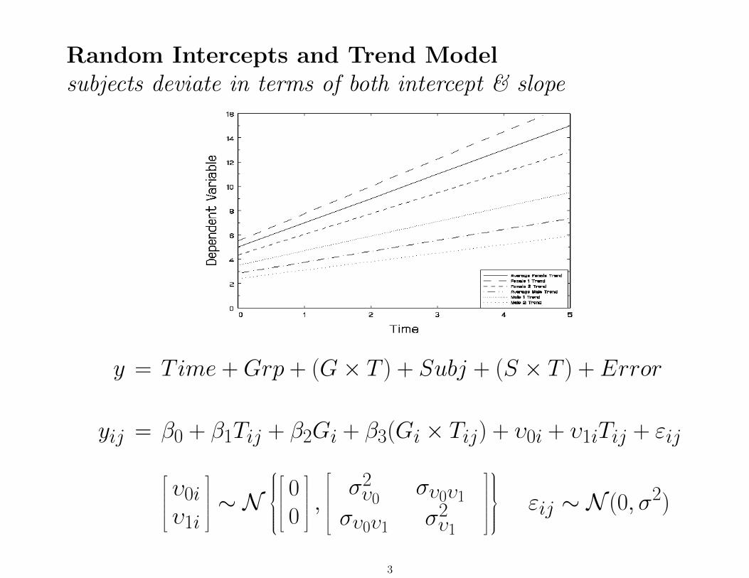
Random Intercepts and Trend Modelsubjects deviate in terms of both intercept & slope

y = Time + Grp + (G× T ) + Subj + (S × T ) + Error

yij = β0 + β1Tij + β2Gi + β3(Gi × Tij) + υ0i + υ1iTij + εij

υ0iυ1i

∼ N

00

,σ2υ0

συ0υ1

συ0υ1 σ2υ1

εij ∼ N (0, σ2)

3

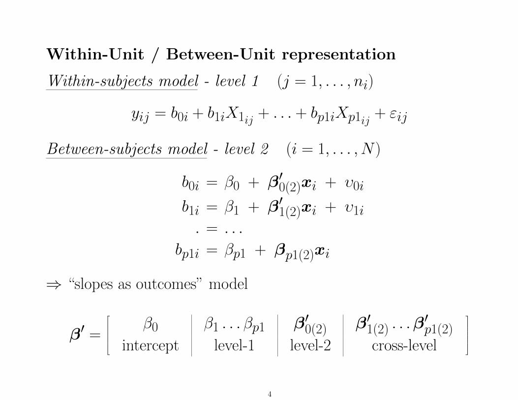
Within-Unit / Between-Unit representation

Within-subjects model - level 1 (j = 1, . . . , ni)

yij = b0i + b1iX1ij + . . . + bp1iXp1ij + εij

Between-subjects model - level 2 (i = 1, . . . , N)

b0i = β0 + β′0(2)xi + υ0i

b1i = β1 + β′1(2)xi + υ1i

. = . . .

bp1i = βp1 + βp1(2)xi

⇒ “slopes as outcomes” model

β′ =

β0 β1 . . . βp1 β′0(2) β′1(2) . . .β

′p1(2)

intercept level-1 level-2 cross-level

4

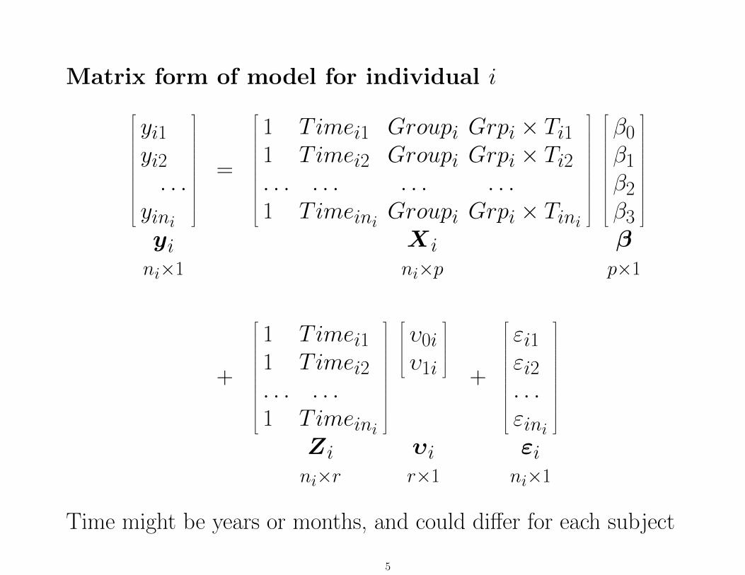
Matrix form of model for individual i

yi1yi2. . .

yini

yini×1

=

1 Timei1 Groupi Grpi × Ti11 Timei2 Groupi Grpi × Ti2. . . . . . . . . . . .1 Timeini Groupi Grpi × Tini

Xini×p

β0β1β2β3

βp×1

+

1 Timei11 Timei2. . . . . .1 Timeini

Zini×r

υ0iυ1i

υir×1

+

εi1εi2. . .εini

εini×1

Time might be years or months, and could differ for each subject

5

The conditional variance-covariance matrix is now of the form:

• Σyi = ZiΣυZ′i + σ2Ini

For example, with r = 2, n = 3, and Z ′i =

1 1 10 1 2

the conditional variance-covariance Σyi = σ2Ini+

σ2υ0

σ2υ0

+ συ0υ1 σ2υ0

+ 2συ0υ1

σ2υ0

+ συ0υ1 σ2υ0

+ 2συ0υ1 + σ2υ1

σ2υ0

+ 3συ0υ1 + 2σ2υ1

σ2υ0

+ 2συ0υ1 σ2υ0

+ 3συ0υ1 + 2σ2υ1

σ2υ0

+ 4συ0υ1 + 4σ2υ1

• variances and covariances change across time

More general models allow autocorrelated errors, εi ∼ N (0, σ2Ωi),where Ω might represent AR or MA process

6

Example: Drug Plasma Levels and Clinical Response

Riesby and associates (Riesby et al., 1977) examined therelationship between Imipramine (IMI) and Desipramine (DMI)plasma levels and clinical response in 66 depressed inpatients(37 endogenous and 29 non-endogenous)

Drug-Washoutday0 day7 day14 day21 day28 day35wk 0 wk 1 wk 2 wk 3 wk 4 wk 5

HamiltonDepression HD1 HD2 HD3 HD4 HD5 HD6

Diagnosis Dx

IMI IMI3 IMI4 IMI5 IMI6DMI DMI3 DMI4 DMI5 DMI6

n 61 63 65 65 63 58

7

outcome variable - Hamilton Depression Scores (HD)

independent variables - Dx, IMI and DMI

•Dx - endogenous (=1) or non-endogenous (=0)

• IMI (imipramine) drug-plasma levels (µg/l)

– antidepressant given 225 mg/day, weeks 3-6

•DMI (desipramine) drug-plasma levels (µg/l)

– metabolite of imipramine

8

Descriptive Statistics

Observed HDRS Means, n, and sdWashout

wk 0 wk 1 wk 2 wk 3 wk 4 wk 5Endog 24.0 23.0 19.3 17.3 14.5 12.6n 33 34 37 36 34 31

Non-Endog 22.8 20.5 17.0 15.3 12.6 11.2n 28 29 28 29 29 27

pooled sd 4.5 4.7 5.5 6.4 7.0 7.2

9

Correlations: n = 46 and 46 ≤ n ≤ 66

wk 0 wk 1 wk 2 wk 3 wk 4 wk 5week 0 1.0 .49 .41 .33 .23 .18week 1 .49 1.0 .49 .41 .31 .22week 2 .42 .49 1.0 .74 .67 .46week 3 .44 .51 .73 1.0 .82 .57week 4 .30 .35 .68 .78 1.0 .65week 5 .22 .23 .53 .62 .72 1.0

10

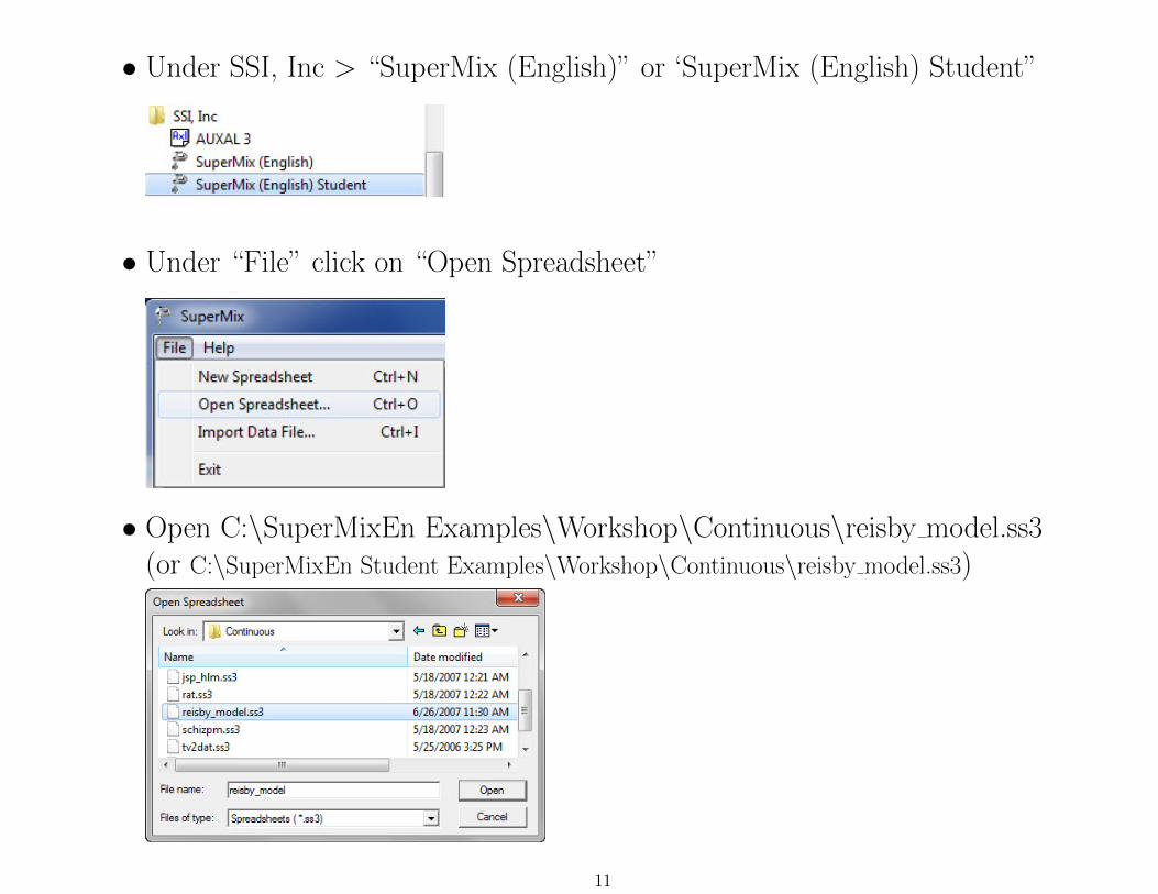
• Under SSI, Inc > “SuperMix (English)” or ‘SuperMix (English) Student”

• Under “File” click on “Open Spreadsheet”

• Open C:\SuperMixEn Examples\Workshop\Continuous\reisby model.ss3(or C:\SuperMixEn Student Examples\Workshop\Continuous\reisby model.ss3)

11

c:\SuperMixEn Examples\Workshop\Continuous\reisby model.ss3

12

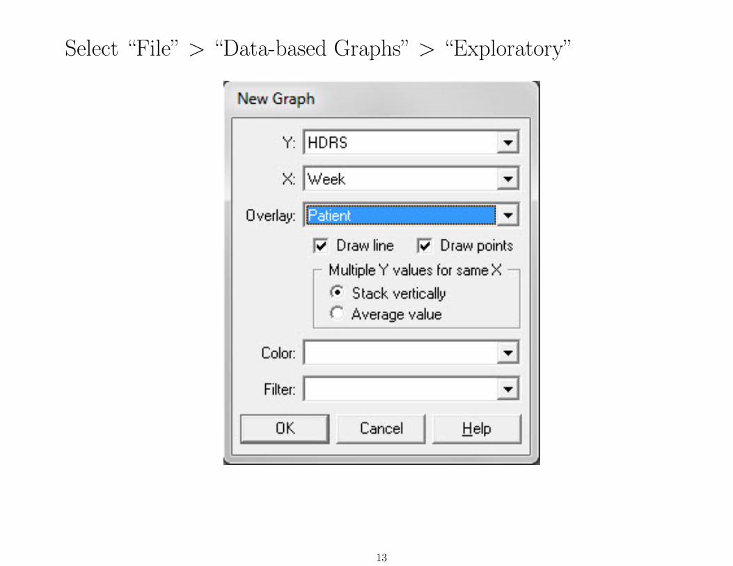
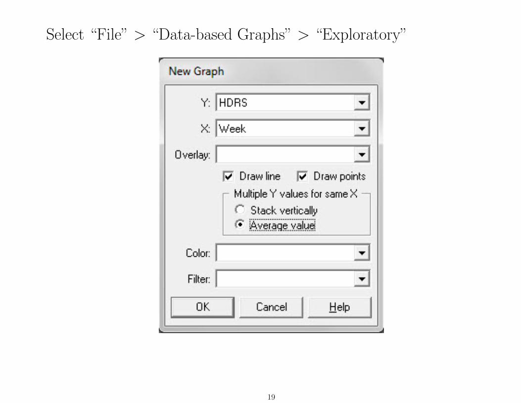
Select “File” > “Data-based Graphs” > “Exploratory”

13

• increasing variance across time

• general linear decline over time

14

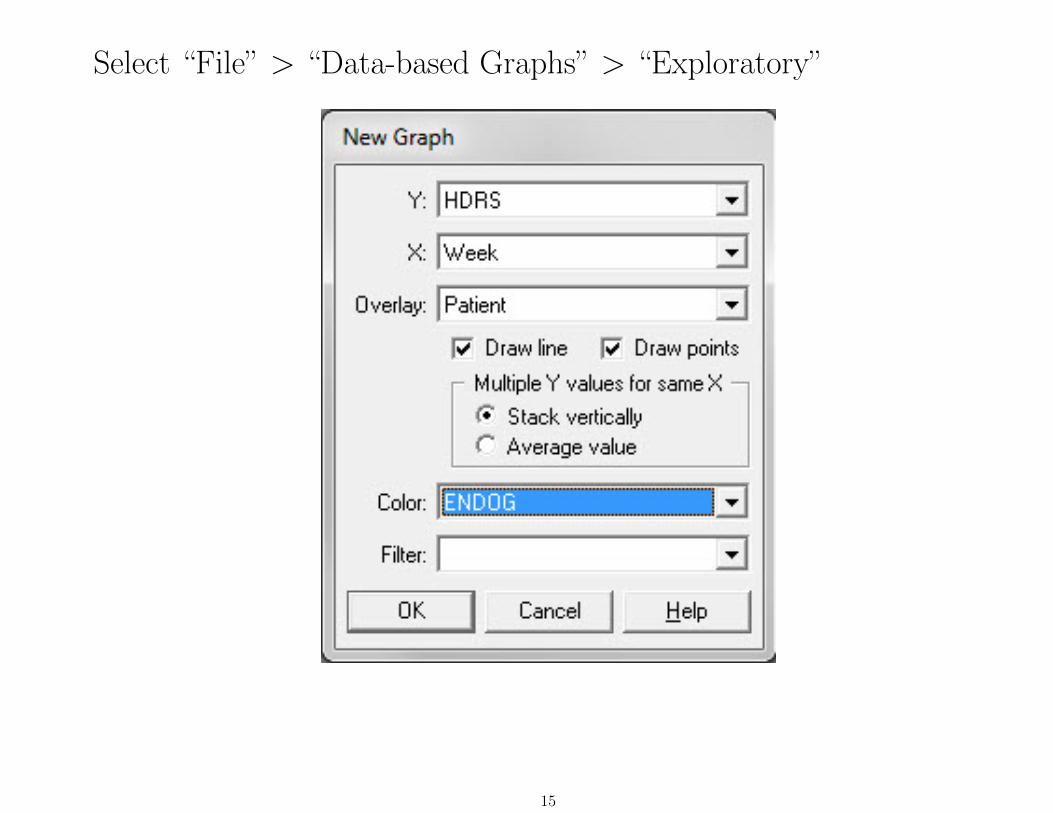
Select “File” > “Data-based Graphs” > “Exploratory”

15

• Plot of Endogenous and Non-Endogenous patients

16

Select “File” > “Data-based Graphs” > “Exploratory”

⇒ Produces plots for each subject

17

18

Select “File” > “Data-based Graphs” > “Exploratory”

19

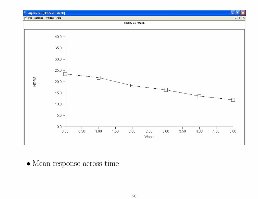
•Mean response across time

20

Select “File” > “Data-based Graphs” > “Univariate”

21

22

Select “File” > “Data-based Graphs” > “Bivariate”

23

24

Examination of HD across all weeks

HDi1

HDi2

. . .HDini

yini×1

=

1 WEEKi1

1 WEEKi2

. . . . . .1 WEEKini

X i

ni×p

β0β1

βp×1

+

1 WEEKi1

1 WEEKi2

. . . . . .1 WEEKini

Z i

ni×r

υ0iυ1i

υir×1

+

εi1εi2. . .εini

εini×1

where max(ni) = 6, and X ′i = Z ′i =

1 1 1 1 1 10 1 2 3 4 5

25

Within-subjects and between-subjects components

Within-subjects model

HDij = b0i + b1iTimeij + Eijyij = b0i + b1ixij + εij

i = 1 . . . 66 patientsj = 1 . . . ni observations (max = 6) for patient i

b0i = week 0 HD level for patient ib1i = weekly change in HD for patient i

Between-subjects models

b0i = β0 + υ0ib1i = β1 + υ1i

β0 = average week 0 HD levelβ1 = average HD weekly improvementυ0i = individual deviation from average interceptυ1i = individual deviation from average improvement

26

Under “File” click on “Open Existing Model Setup”

Open C:\SuperMixEn Examples\Workshop\Continuous\reisby.mum(or C:\SuperMixEn Student Examples\Workshop\Continuous\reisby.mum)

27

28

29

30

31

Empirical Bayes Estimates of Random EffectsSelect “Analysis” > “View Level-2 Bayes Results”

ID, random effect number, estimate, variance, name

32

Select “File” > “Model-based Graphs” > “Equations’

33

Empirical Bayes estimates of Subject Trends

34

Select “File” > “Model-based Graphs” > “Confidence Intervals’

35

Confidence Intervals for Subject Week Effects

36

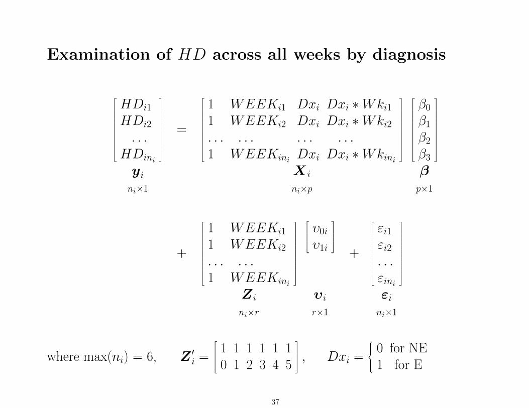
Examination of HD across all weeks by diagnosis

HDi1

HDi2

. . .HDini

yini×1

=

1 WEEKi1 Dxi Dxi ∗Wki11 WEEKi2 Dxi Dxi ∗Wki2. . . . . . . . . . . .1 WEEKini Dxi Dxi ∗Wkini

X i

ni×p

β0β1β2β3

βp×1

+

1 WEEKi1

1 WEEKi2

. . . . . .1 WEEKini

Z i

ni×r

υ0iυ1i

υir×1

+

εi1εi2. . .εini

εini×1

where max(ni) = 6, Z ′i =

1 1 1 1 1 10 1 2 3 4 5

, Dxi =

0 for NE1 for E

37

Within-subjects and between-subjects components

Within-subjects model

HDij = b0i + b1iTimeij + Eij

b0i = week 0 HD level for patient ib1i = weekly change in HD for patient i

Between-subjects models

b0i = β0 + β2Dxi + υ0ib1i = β1 + β3Dxi + υ1i

β0 = average week 0 HD level for NE patients (Dxi = 0)β1 = average HD weekly improvement for NE patients (Dxi = 0)β2 = average week 0 HD difference for E patientsβ3 = average HD weekly improvement difference for endogenous patientsυ0i = individual deviation from average interceptυ1i = individual deviation from average improvement

38

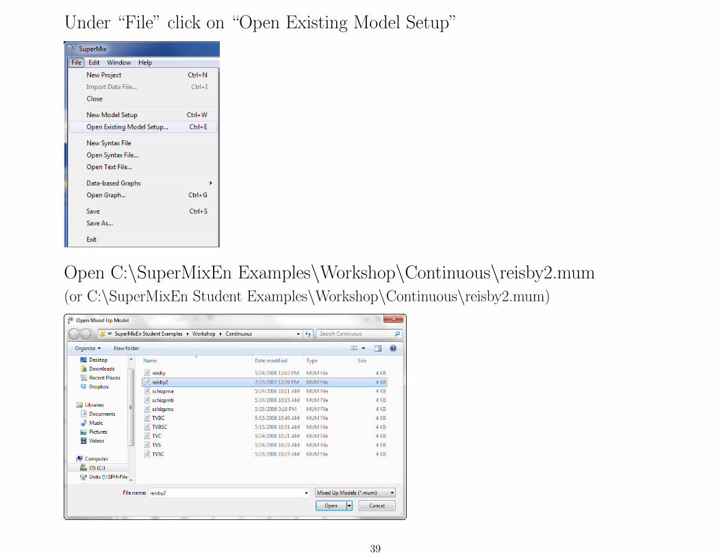
Under “File” click on “Open Existing Model Setup”

Open C:\SuperMixEn Examples\Workshop\Continuous\reisby2.mum(or C:\SuperMixEn Student Examples\Workshop\Continuous\reisby2.mum)

39

40

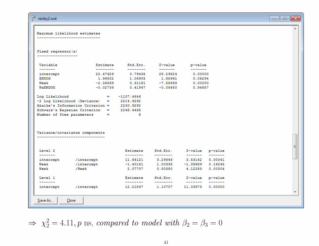
⇒ χ22 = 4.11, p ns, compared to model with β2 = β3 = 0

41

Select “File” > “Model-based Graphs” > “Trends”(sorry, but “Trends” is not include in the student edition)

42

⇒ Endogenous group by time interaction is non-significant; groupsare about 2 points different at all timepoints

43

Select “File” > “Model-based Graphs” > “Residuals”

44

45

Linear Transforms

Fixed part of model:

HDij = β0 + β1Endog + β2Week + β3(Endog ×Week)

in terms of the Endogenous group effect

(β1 + β3Week)Endog

For example, the estimated group effect at the end of the study is

β1 + 5β3

H0 : β1 + 5β3 = 0; null that groups are equivalent at the study’s end

z =β1 + 5β3

SE(β1 + 5β3)46

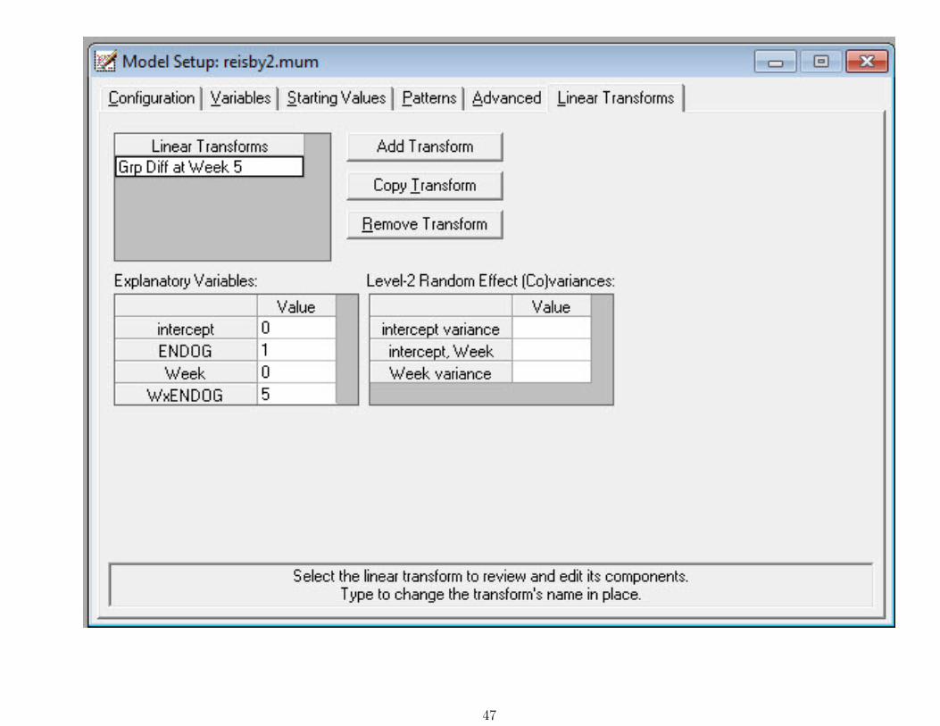
47

48

HD across 4 weeks by plasma drug-levels

HDi1

HDi2

. . .HDini

yini×1

=

1 WEEKi1 lnIMIi1 lnDMIi11 WEEKi2 lnIMIi2 lnDMIi2. . . . . . . . . . . .1 WEEKini lnIMIini lnDMIini

X i

ni×p

β0β1β2β3

βp×1

+

1 WEEKi1

1 WEEKi2

. . . . . .1 WEEKini

Z i

ni×r

υ0iυ1i

υir×1

+

εi1εi2. . .εini

εini×1

where max(ni) = 4, and Z ′i =

1 1 1 10 1 2 3

49

Within-subjects and between-subjects components

Within-subjects model

HDij = b0i + b1iTij + b2i ln IMIij + b3i lnDMIij + Eij

b0i = week 2 HD level for patient i with both ln IMI and lnDMI = 0b1i = weekly change in HD for patient ib2i = change in HD due to ln IMIb3i = change in HD due to lnDMI

Between-subjects models

b0i = β0 + υ0ib1i = β1 + υ1ib2i = β2b3i = β3

50

β0 = average week 2 HD level for subjects with ln drug values of 0β1 = average HD weekly improvementβ2 = average HD difference for unit change in ln IMIβ3 = average HD difference for unit change in lnDMIυ0i = individual intercept deviation from modelυ1i = individual slope deviation from model

Here, week 2 is the actual study week (i.e., one week after the drug washoutperiod), which is coded as 0 in this analysis of the last four study timepoints

51

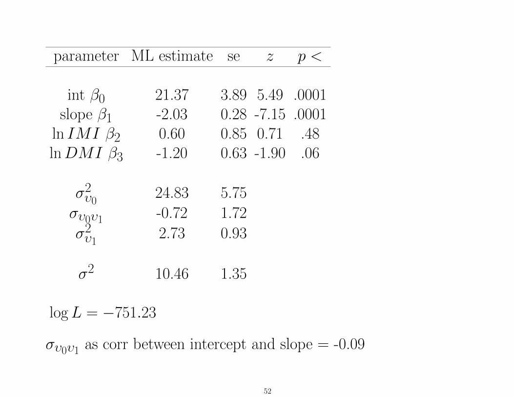
parameter ML estimate se z p <

int β0 21.37 3.89 5.49 .0001slope β1 -2.03 0.28 -7.15 .0001

ln IMI β2 0.60 0.85 0.71 .48lnDMI β3 -1.20 0.63 -1.90 .06

σ2υ0

24.83 5.75

συ0υ1 -0.72 1.72

σ2υ1

2.73 0.93

σ2 10.46 1.35

logL = −751.23

συ0υ1 as corr between intercept and slope = -0.09

52

parameter estimate se p <

HD total score

intercept β0 10.97 4.44 .013

slope β1 -1.99 0.28 .0001

Baseline HD β2 0.54 0.14 .0001

ln IMI β3 0.54 0.78 .49

ln DMI β4 -1.63 0.59 .006

σ2υ0 17.82 4.55

συ0υ1 0.08 1.53

σ2υ1 2.74 0.94

σ2 10.50 1.36

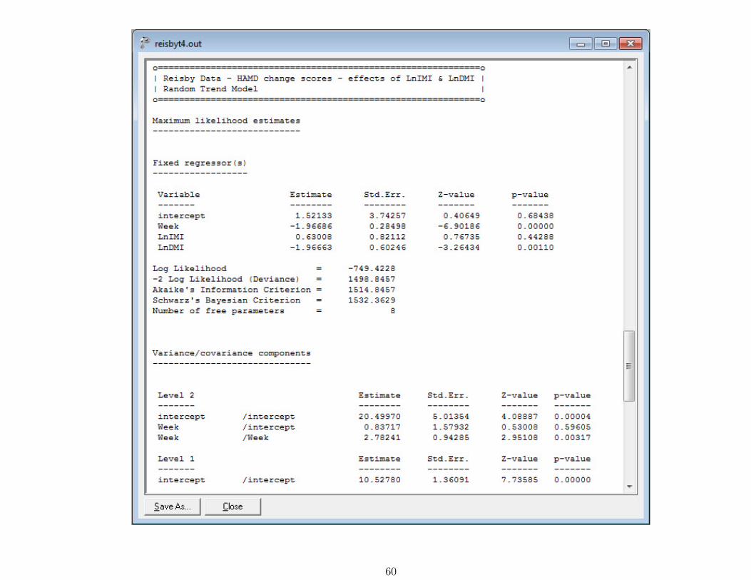
HD change from baseline

intercept β0 1.52 3.74 ns

slope β1 -1.97 0.28 .0001

ln IMI β3 0.63 0.82 ns

ln DMI β4 -1.97 0.60 .001

σ2υ0 20.50 5.01

συ0υ1 0.84 1.58

σ2υ1 2.78 0.94

σ2 10.53 1.36

53

Correlation between HD scoresand plasma levels (ln units)

HD total scoreweek 2 week 3 week 4 week 5

IMI -0.034 -0.034 -0.003 -0.189DMI -0.178 -0.075 -0.250∗ -0.293∗

HD change from baselineweek 2 week 3 week 4 week 5

IMI -0.025 -0.100 -0.034 -0.250DMI -0.350∗ -0.274∗ -0.348∗ -0.401∗

∗p < 0.05

54

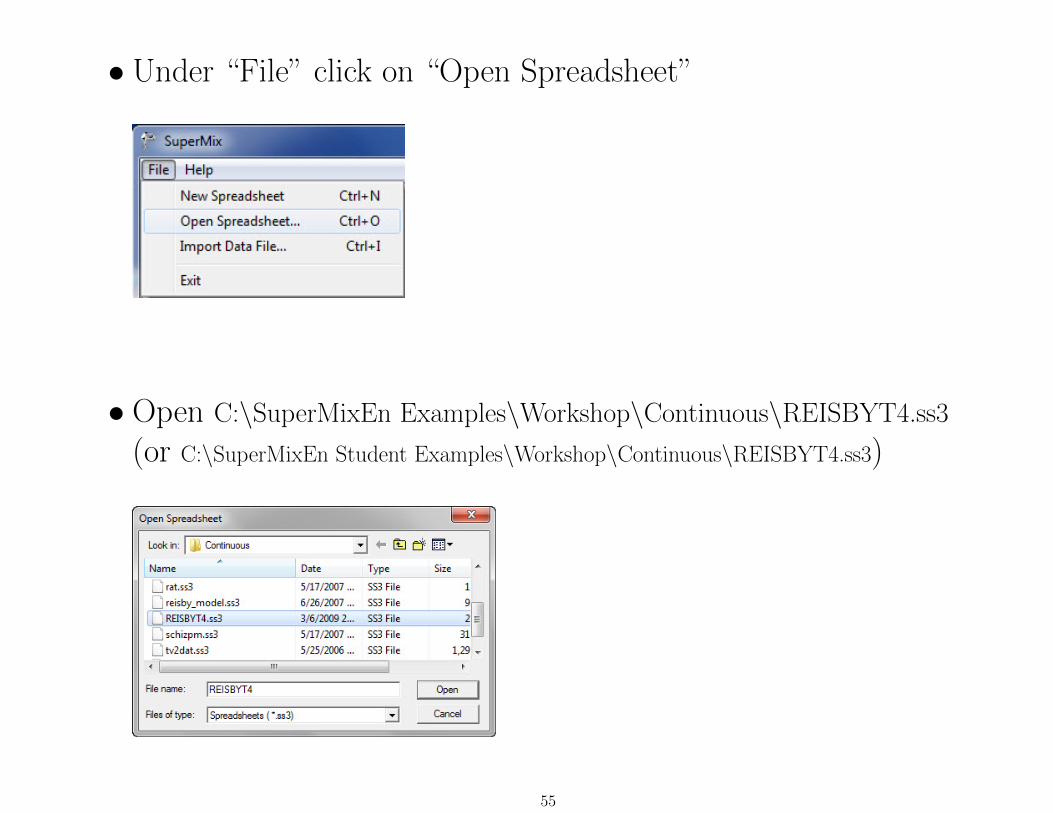
• Under “File” click on “Open Spreadsheet”

• Open C:\SuperMixEn Examples\Workshop\Continuous\REISBYT4.ss3

(or C:\SuperMixEn Student Examples\Workshop\Continuous\REISBYT4.ss3)

55

56

Under “File” click on “Open Existing Model Setup”

Open C:\SuperMixEn Examples\Workshop\Continuous\reisbyt4.mum

(or C:\SuperMixEn Student Examples\Workshop\Continuous\reisbyt4.mum)

57

58

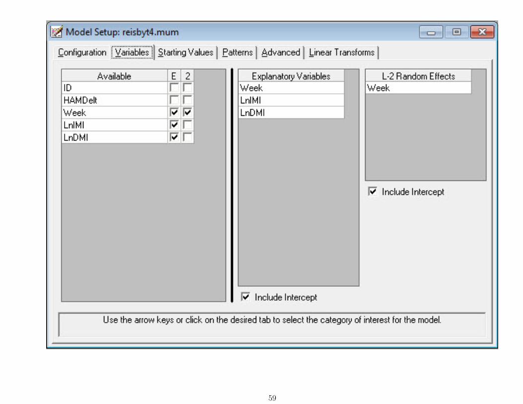
59

60

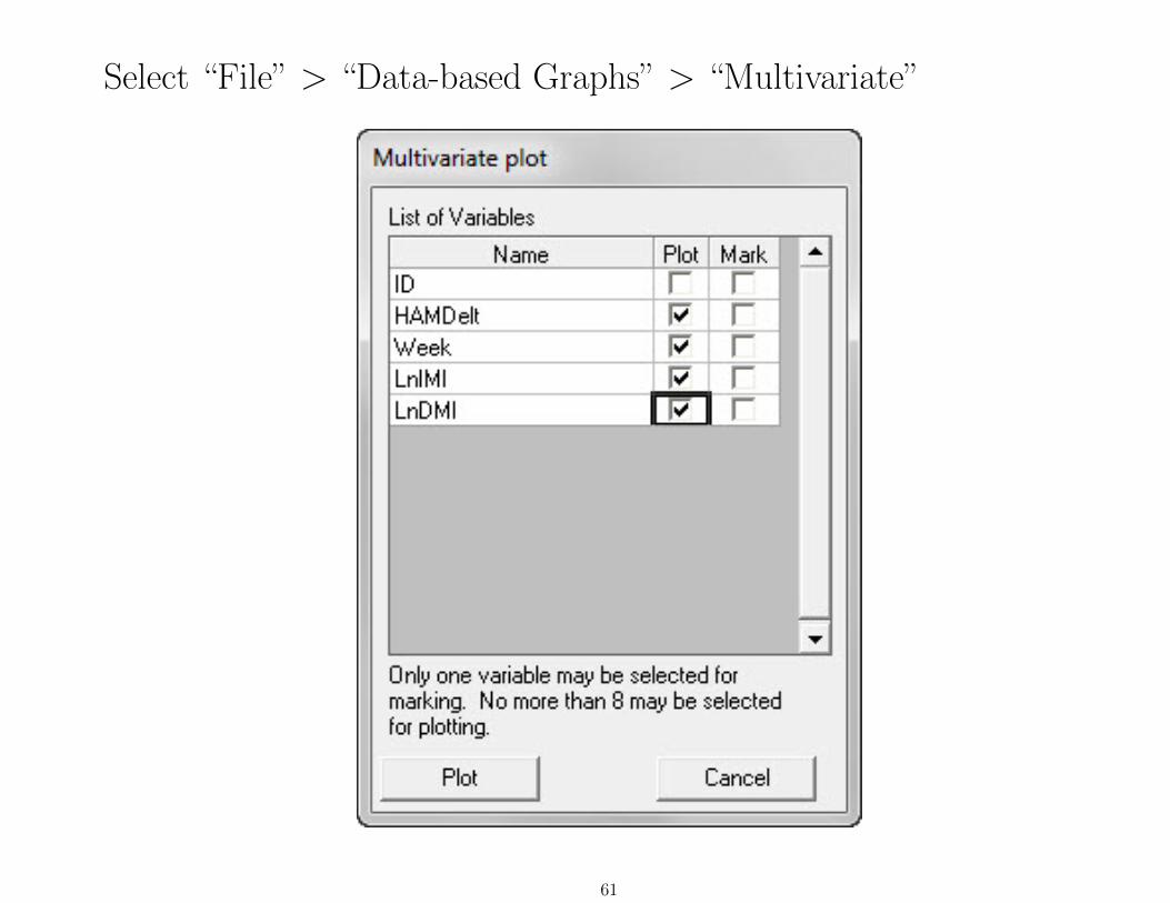
Select “File” > “Data-based Graphs” > “Multivariate”

61

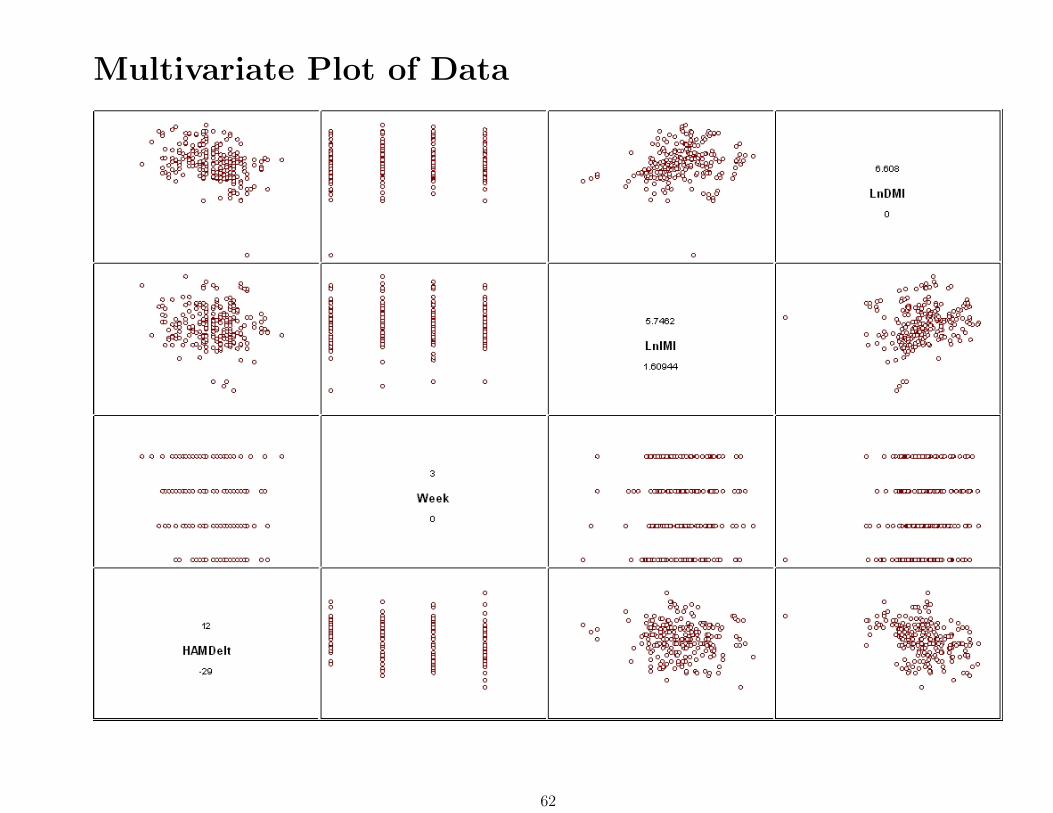
Multivariate Plot of Data

62

Multivariate Plot of Data without DMI outlier

63

Analysis on HD change with and without DMI outlierwith outlier without outlier

parameter estimate se p < estimate se p <intercept β0 1.52 3.74 ns 2.76 3.95 nsslope β1 -1.97 0.28 .0001 -1.96 0.28 .0001ln IMI β3 0.63 0.82 ns 0.72 0.83 nsln DMI β4 -1.97 0.60 .001 -2.30 0.70 .0009

σ2υ0

20.50 5.01 20.53 5.04

συ0υ1 0.84 1.58 0.72 1.59

σ2υ1

2.78 0.94 2.77 0.94

σ2 10.53 1.36 10.56 1.37

64

Summary

• Spreadsheet allows some data manipulation

– add/delete columns or rows

– transformations of variables (abs, exp, ln, sqrt, square)

– summary statistics of variables (average, median, min, max,mode)

– can create interaction terms and grand-mean centered variables

• Various kinds of data-based and model-based plots

• Up to 3-level models with full likelihood estimation (andempirical Bayes estimation of random effects)

• Linear transforms of parameter estimates

• Non-normal outcomes: binary, ordinal, nominal, and counts

65