Mixed-Model Assembly Line Scheduling Using the … · Mixed-Model Assembly Line Scheduling ... line balancing that adequately assigns operators to tasks is another ... moving windows

0

Mixed-Model Assembly Line SchedulingUsing the Lagrangian Relaxation Technique

Yuanhui Zhang, Peter B. [email protected], [email protected]. of Electrical and Systems Engineering

University of ConnecticutStorrs, CT 06269-2157, USA

Kiyoshi Yoneda, Toshiyuki Kano, Yuji [email protected], [email protected], [email protected]

Systems & Software Engineering LabToshiba Corporation, 70, Yanagi-cho, Saiwai-ku

Kawasaki-shi, 210 Japan

Abstract

The increasing market demand for product variety forces manufacturers to design mixed-

model assembly lines on which different product models can be switched back and forth and

mixed together with little changeover costs. This paper describes the design and implementation

of an optimization-based scheduling algorithm for mixed-model compressor assembly lines of

Toshiba with complicated component supply requirements. A separable integer optimization

formulation is obtained by treating compressor lots going through a properly balanced line as

undergoing a single operation, and the scheduling goal is to delivery products just in time while

avoiding possible component shortage. The problem is solved by using Lagrangian relaxation

(LR). Several generic defects of LR leading to slow algorithm convergence are identified based on

geometrical insights, and are overcome by perturbing/changing problem parameters. Numerical

testing shows that near-optimal schedules are efficiently obtained, convergence is significantly

improved, and the method is effective for practical problems. The system is currently under

deployment at Toshiba.

Keywords: Optimization-Based Scheduling, Mixed-Model Assembly Lines, LagrangianRelaxation.

1

1. Introduction

Mixed-Model Assembly Line Scheduling

The increasing market demand for product diversity forces manufacturers to consider

switching from the mass batch production of a small number of product types to small-lot

production of many varieties. The old paradigm of assembling a single item to inventory and

changing models while selling off inventory has been replaced by mixed-model assembly lines

where quick changeovers between models occur frequently without significant setup costs. A

simplified mixed-model assembly configuration with two lines is shown in Figure 1.

AssemblyOperations

ComponentsProductLots

Line 1

Line 2

Figure 1. Mixed-Model Assembly Lines

In the assembly operations, many types of components are required from fabrication shops or

from suppliers. To apply the paradigm of producing the right products at the right time with low

inventory to component fabrications as well, better coordination between the assembly and

fabrications is needed. One way to coordinate them is to limit the consumption of key components

at the assembly to certain values. Otherwise, assembly lines may have to be stopped because of

starvation when the capacities of component fabrications are exceeded. In addition to component

2

consumption requirements, line balancing that adequately assigns operators to tasks is another

important issue to avoid bottlenecks and to smooth the flow of products.

Literature Review

In the mixed-model scheduling literature, the key premise is that both assembly lines and

component fabrications will operate smoothly if uniform or linear consumption of components

over time can be achieved ([7],[8]). Heuristics have been developed to schedule mixed-model

assembly lines to minimize the deviations of actual consumption from linear consumption. In an

earlier work by Toyota (goal chasing method), the total deviation from linear consumption is

considered [8]. Variations of the heuristics to consider the maximum deviation are presented in

[9]. In [3], [7] and [10], these heuristic rules have been refined and algorithm efficiency has been

improved. Important goals such as meeting due dates and reducing finished goods inventory,

however, are seldom addressed in the mixed model scheduling literature, and the quality of

schedules generated by the heuristics may be questionable. An efficient optimization-based

approach with quantifiable quality is therefore highly desirable for the daily scheduling of mixed-

model assembly lines.

Overview of the Paper

This paper describes the design and implementation of an optimization-based scheduling

algorithm for the assembly of Toshiba’s compressors, core of air conditioners and refrigerant

equipment. In the shop, a lot can be processed on one of several lines with different processing

rates. Assembly lines are properly balanced, and a compressor lot going through a line can be

conceived of as undergoing a single operation. Since lots may be generated by splitting large

orders, multiple lots may have the same set of parameters (processing requirements, due date,

priority, etc.), and this will cause difficulties in the solution process. The objective is to determine

3

the appropriate lines and launch sequences for all the lots to meet their due dates just in time while

avoiding possible component starvation. An integer optimization formulation is presented in

Section 2. The limits on component supply are formulated as a series of time windows within

each of them the consumption cannot exceed a certain value. These constraints are additive in

terms of basic decision variables. Together with the additive objective function and linear

assembly line capacity constraints, they result in a “separable” formulation.

Because of the combinatorial nature of integer optimization, it is very difficult to obtain

optimal schedules for practical problems within a limited amount of computation time. In Section

3, a solution methodology based on a synergistic combination of Lagrangian relaxation (LR) and

heuristics is developed following Luh and Hoitomt [5] to generate near-optimal solutions with

quantifiable quality. The convergence of the method is significantly affected by the existence of

identical lots, multiple alternative lines, and the large number of component supply constraints. In

Section 4, two structural difficulties leading to slow convergence are identified and analyzed based

on geometric characteristics of the dual function. To overcome these difficulties, perturbations or

modifications of original problem parameters are used to achieve better convergence. Numerical

results in Section 5 show that the performance of the algorithm is substantially improved, and

near-optimal results can be efficiently obtained for problems of practical sizes. In Section 6, the

deployment of the method at Toshiba and the experiences learned are highlighted. The system is

currently under deployment at Toshiba.

2. Problem Formulation

The formulation to be presented next is built on our previous work for job shop scheduling

[5] with the component supply requirements as the new feature. A list of symbols used is provided

in Appendix A for easy reference.

4

2.1 General Description

Assembly Lines. There are a total of H assembly lines indexed by h, 0 ≤ h ≤ H-1. A compressor

lot goes through several operations on a line with components assembled at various operations as

shown in Figure 2. Since assembly lines are assumed to be properly balanced and the time for

each operation is very short, a lot going through a line can be conceived of as undergoing a single

operation.

Inspection

Just in Time orOver Due, NextStage Production

Finished Early,Finished GoodsInventory

Assembly LineOperations

….Oper 1 Oper 2 Oper N

ComponentSupply 1

ComponentSupply 2

ComponentSupply N

Figure 2. Compressor Assembly Line

Product Models. There are a total of G product models. Model g, 0 ≤ g ≤ G-1, can be processed

on one of several lines with different production rates. The rate of model g on line h is denoted by

rhg, which is the number of pieces that can be finished in one time unit. All the lines that can

process model g form an integer set Hg.

Lots. There are a total of I lots to schedule. Lot i, 0 ≤ i ≤ I-1, consists of multiple products of the

same model gi and has a given lot size Si. The processing time of the lot equals the lot size Si

divided by ihgr , the production rate of the model on line h.

Component Supply. Not all the components used in the assembly have supply limits, and the

number of key component types with supply limit is denoted as J. The key component types

5

needed by model g form an integer set Pg, and one product of model g requires njg type j

components, j ∈ Pg.

As mentioned in Section 1, component supply has its capacity, and even consumption of

components is critical for the smooth operation of assembly lines and component fabrications. A

conventional way to handle this is to limit the total number of pieces per type consumed over fixed

and non-overlapping windows. Component consumption, however, may burst across adjacent

windows. In this paper, moving windows starting at the beginning of every day and spanning over

several days are used to smooth component consumption. Moving windows increase the number

of constraints, but can reduce the bursting of component consumption. In Figure 3, the

consumption bursts from Day 4 to Day 7 while satisfying fixed weekly window supply constraints

(Day 1 to Day 5 and Day 6 to Day 10). However, if moving windows are used, this consumption

pattern will not be allowed.

500 500 500 500

1 Day

Moving Window Size = 5

5 6 10

0 0 0 0 00

Supply = 1000

4 7

Figure 3. Component Supply Moving Windows

Time Step Reduction. In the shop, there are about 600 lots to be scheduled over a one-month

period with a required time resolution of 0.1 hour. In view of the long scheduling horizon as

compared to the time resolution, the “time step reduction technique” is used to control the

computational requirements following [6]. The horizon is divided into T “resolution increments”

indexed by t, 0 ≤ t ≤ T-1, and R resolution increments aggregated into an “enumeration step”

indexed by k, 0≤ k ≤ K, with T = R×K. An operation requires a fractional but quantized line

6

utilization, and multiple operations are allowed to “share” an assembly line within an enumeration

step. An enumeration step may be a shift or a day, depending on the applications.

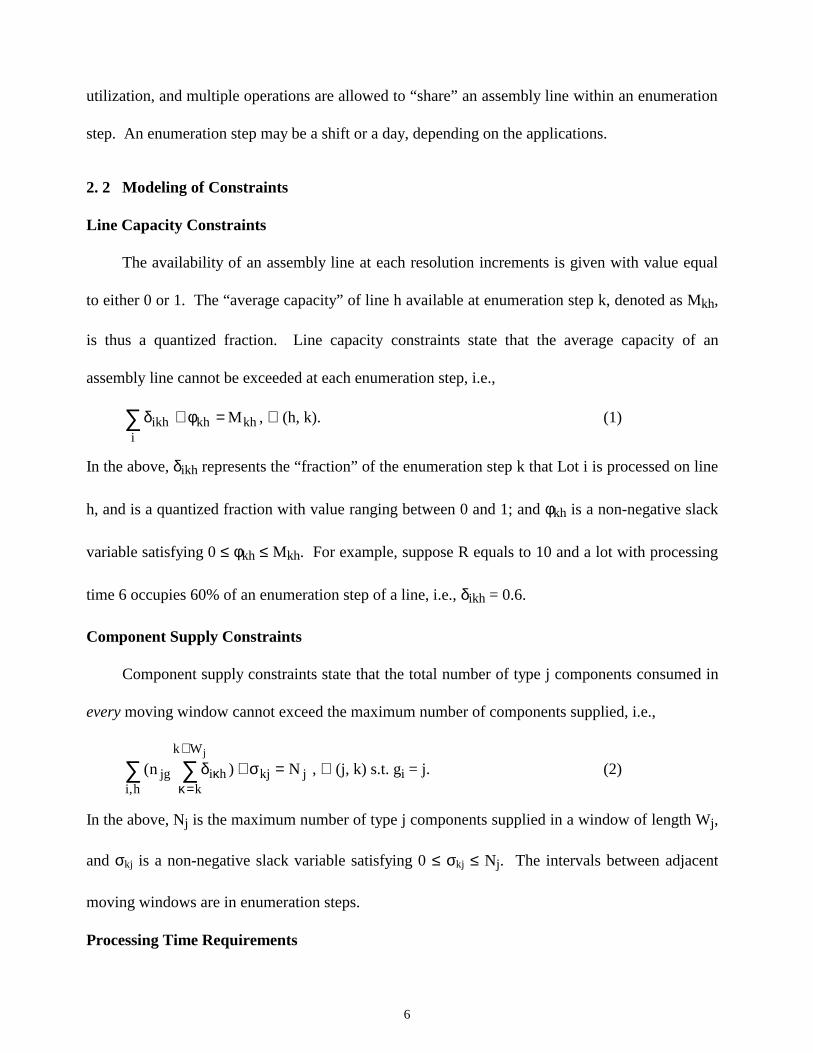
2. 2 Modeling of Constraints

Line Capacity Constraints

The availability of an assembly line at each resolution increments is given with value equal

to either 0 or 1. The “average capacity” of line h available at enumeration step k, denoted as Mkh,

is thus a quantized fraction. Line capacity constraints state that the average capacity of an

assembly line cannot be exceeded at each enumeration step, i.e.,

khkhi

ikh M =φ+δ∑ , ∀ (h, k). (1)

In the above, δikh represents the “fraction” of the enumeration step k that Lot i is processed on line

h, and is a quantized fraction with value ranging between 0 and 1; and φkh is a non-negative slack

variable satisfying 0 ≤ φkh ≤ Mkh. For example, suppose R equals to 10 and a lot with processing

time 6 occupies 60% of an enumeration step of a line, i.e., δikh = 0.6.

Component Supply Constraints

Component supply constraints state that the total number of type j components consumed in

every moving window cannot exceed the maximum number of components supplied, i.e.,

jkjh,i

Wk

khijg N)n(

j

=σ+δ∑ ∑+

=κκ , ∀ (j, k) s.t. gi = j. (2)

In the above, Nj is the maximum number of type j components supplied in a window of length Wj,

and σkj is a non-negative slack variable satisfying 0 ≤ σkj ≤ Nj. The intervals between adjacent

moving windows are in enumeration steps.

Processing Time Requirements

7

Processing time requirements state that the completion time of an operation equals the

beginning time plus the required processing time, i.e.,

cih = bih + tih - 1. (3)

In the above, the processing time of Lot i on line h is given in resolution unit by tih = Si / ihgr .

The beginning time refers to the start of a discrete resolution unit while the completion time refers

to the end of a discrete resolution unit, therefore, the term -1 is required in (3).

2.3 Objective Function

Each lot has a given due date. If it finishes too late, it cannot be delivered on time. If it

finishes too early, it has to be stored as inventory. The objective of scheduling is to meet the

products’ due dates just in time while avoiding component starvation, and this is represented by

the following tardiness and early completion penalties:

J ∑ ρ+≡i

ii2ii ]VTw[ . (4)

Since product delivery is at the end of a shift, the tardiness of Lot i, Ti, is defined as the number of

shifts the completion time passes the given due date, i.e.,

−

≡ 0 ,

T

d

T

cmaxT

s

i

s

ii , where Ts is

the number of resolution units in a shift, and x is the “floor function” returning the integer

portion of x. Similarly, Vi is the number of shifts that a lot finishes earlier than its due date, and is

related to the level of finished goods inventory. Parameters wi and ρi are weights associated with

tardiness and early completion penalties, respectively. Since meeting due dates is usually more

important than low inventory, wi is larger than ρi, and tardiness penalty takes quadratic form in

contrast to the linear early completion penalty in (4). These penalties thus define a window in

which a lot can be scheduled without any penalties.

8

2.4 Overall Problem

The overall problem is to minimize the weighted tardiness and early completion penalties (4)

subject to assembly line capacity constraints, component supply constraints, and processing time

requirements (1-3). Decision variables are assembly line to be used {h ∈ Hg}, lot beginning times

{bi}, and slack variables. Once these variables are determined, other variables can be easily

derived. Since the objective function and all coupling constraints are additive in terms of basic

decision variables, the problem formulation is “separable,” with line capacity and component

supply constraints as “coupling constraints.” Lagrangian relaxation can therefore be effectively

used to solve it, as will be presented in next section.

3. Solution Methodology

Similar to the pricing concept of a market economy, Lagrangian relaxation replaces coupling

line capacity and component supply constraints by the payment of certain prices (i.e., Lagrange

multipliers) for the use of assembly line and components at each time unit. The “relaxed problem”

can then be decomposed into many smaller subproblems, one for each lot. These subproblems are

much easier to solve as compared to the original problem, and solutions can be efficiently obtained

by enumeration. The prices or multipliers are iteratively adjusted based on the degrees of

constraint violation following again the market economy principle (i.e., increase prices for over-

utilized time units and reduce prices for under-utilized time units). Subproblems are then re-

solved based on the new set of multipliers. In mathematical terms, a “dual function” is maximized

in the multiplier updating process, and values of the dual function serve as lower bounds to the

optimal feasible cost. At the termination of such price updating iterations, a few constraints may

still be violated. Simple heuristics are then applied to adjust subproblem solutions to form a

feasible schedule satisfying all constraints. Optimization and heuristics thus operate in a

9

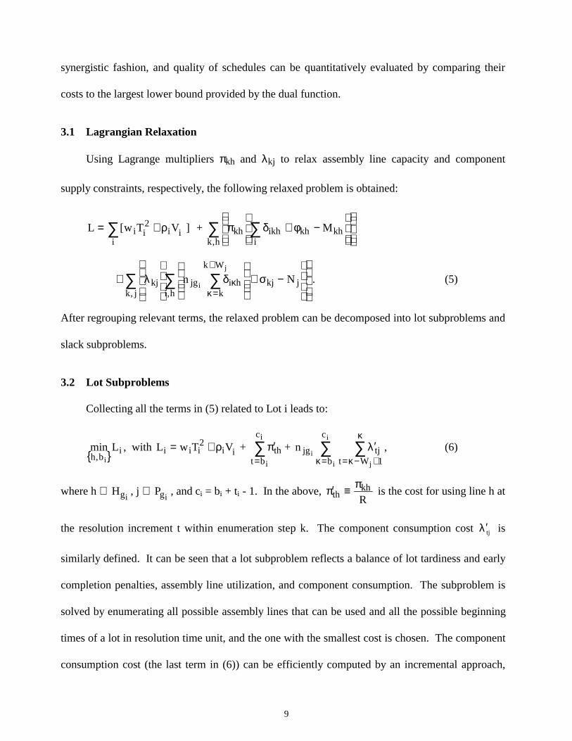
synergistic fashion, and quality of schedules can be quantitatively evaluated by comparing their

costs to the largest lower bound provided by the dual function.

3.1 Lagrangian Relaxation

Using Lagrange multipliers πkh and λkj to relax assembly line capacity and component

supply constraints, respectively, the following relaxed problem is obtained:

∑ ρ+=i

ii2ii ]V Tw[ L + ∑ ∑

−φ+δπ

h,kkhkh

iikhkh M

∑ ∑ ∑

−σ+

δλ+

+

=κκ

j,k h,ijkj

Wk

khijgkj N n

j

i. (5)

After regrouping relevant terms, the relaxed problem can be decomposed into lot subproblems and

slack subproblems.

3.2 Lot Subproblems

Collecting all the terms in (5) related to Lot i leads to:

{ } ib,h

Lmini

, with ii2iii VTw L ρ+= + ∑

=π′

i

i

c

btth + ∑ ∑

=κ

κ

+−κ=λ′

i

i j

i

c

b 1Wttjjgn , (6)

where h ∈ igH , j ∈

igP , and ci = bi + ti - 1. In the above, R

khth

π≡π′ is the cost for using line h at

the resolution increment t within enumeration step k. The component consumption cost tjλ′ is

similarly defined. It can be seen that a lot subproblem reflects a balance of lot tardiness and early

completion penalties, assembly line utilization, and component consumption. The subproblem is

solved by enumerating all possible assembly lines that can be used and all the possible beginning

times of a lot in resolution time unit, and the one with the smallest cost is chosen. The component

consumption cost (the last term in (6)) can be efficiently computed by an incremental approach,

10

i.e., the cost associated with bi is derived from the cost associated with bi - 1 by adding one term

and subtracting one term.

3.3 Slack Subproblems

Collecting all the terms in (5) related to slack variables leads to:

{ } s,

Lminkjkh σφ

, with ∑∑ σλ+φπ≡j,k

kjkjh,k

khkhs L . (7)

The solution to the above subproblem is:

<π

=φ;otherwise ,0

,0if,M khkh

kh and <λ

=σ.otherwise,0

,0if,N kjj

kj

3.4 Solving the Dual Problem

After subproblems have been solved, the Lagrange multipliers are updated based on the

degrees of constraint violation. Let *iL denote the minimal lot subproblem cost for Lot i and *

sL

the minimum slack subproblem cost, then the high level dual problem is obtained as

{ } NMLLD with ,D maxj,k

jkjh,k

khkh*s

i

*i

, kjkh∑∑∑ λ−π−+≡

λπ. (8)

The dual function D is concave, piece-wise linear, and consists of many facets. The

subgradient method is commonly used for this kind of non-differentiable optimization. The

subgradients with respect to multipliers πkh and λkj can be calculated by

gkh = khkhi

*ikh M −φ+δ∑ , and (9.a)

gkj =∑ ∑ −σ+

δ

+

=κκ

h,ijkj

Wk

k

*hi

pjg N n

pj

i, (9.b)

respectively, where gkh and gkj are elements of the subgradients, and { *ikhδ } are associated with

subproblem solutions.

11

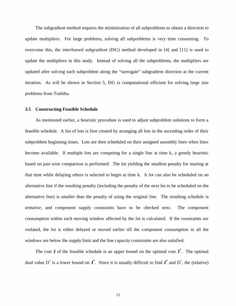
The subgradient method requires the minimization of all subproblems to obtain a direction to

update multipliers. For large problems, solving all subproblems is very time consuming. To

overcome this, the interleaved subgradient (ISG) method developed in [4] and [11] is used to

update the multipliers in this study. Instead of solving all the subproblems, the multipliers are

updated after solving each subproblem along the “surrogate” subgradient direction at the current

iteration. As will be shown in Section 5, ISG is computational efficient for solving large size

problems from Toshiba.

3.5 Constructing Feasible Schedule

As mentioned earlier, a heuristic procedure is used to adjust subproblem solutions to form a

feasible schedule. A list of lots is first created by arranging all lots in the ascending order of their

subproblem beginning times. Lots are then scheduled on their assigned assembly lines when lines

become available. If multiple lots are competing for a single line at time k, a greedy heuristic

based on pair-wise comparison is performed. The lot yielding the smallest penalty for starting at

that time while delaying others is selected to begin at time k. A lot can also be scheduled on an

alternative line if the resulting penalty (including the penalty of the next lot to be scheduled on the

alternative line) is smaller than the penalty of using the original line. The resulting schedule is

tentative, and component supply constraints have to be checked next. The component

consumption within each moving window affected by the lot is calculated. If the constraints are

violated, the lot is either delayed or moved earlier till the component consumption in all the

windows are below the supply limit and the line capacity constraints are also satisfied.

The cost J of the feasible schedule is an upper bound on the optimal cost J*. The optimal

dual value D* is a lower bound on J*. Since it is usually difficult to find J* and D*, the (relative)

12

duality gap (J-D)/D is often used as a measure of the quality of a feasible schedule. The algorithm

will stop after a given number of iterations or the duality gap is within an acceptable range.

4. Geometric Insights

As mentioned earlier, the dual function D is concave, piece-wise linear, and consists of many

facets. The sharp ridges of the hyper-surface of the dual function will cause convergence

difficulties. In this section, the impact of sharp ridges is illustrated, and two major causes of sharp

ridges are identified and remedied by perturbing problem parameters and by adding penalties for

the use of slow lines.

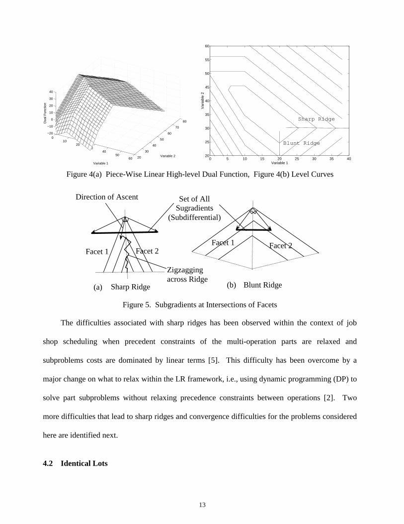
4.1 Geometric Characteristic at the High Level

Consider a simple problem with one assembly line and three lots with t1 = t2 = t3 = 3, d1 = d2

= 3, d3 = 4, w1 = w2 = 1, ρ1 = ρ2 = 0, and K=13. The dual function in terms of two variables π3

and π4 is plotted in Figure 4(a), and the corresponding level curves is shown in Figure 4(b). Each

facet of the dual function corresponds to one set of subproblem solutions. For points on a ridge

(intersection of two or multiple facets), only subgradients exists. If the angle formed by the level

curves of a ridge is acute, the ridge is “sharp”; otherwise, the ridge is “blunt” as shown in Figure

4(b) and in Figure 5. From Figure 5, the subdifferential (i.e., the set of all subgradients) at a point

on a sharp ridge is “larger” than the subdifferential associated with a point on a blunt ridge, and

conversely, the existence of a sharp ridge can be inferred from the “size” of the subdifferential. A

subgradient at a sharp ridge may not be an ascending direction to update the multipliers, and only

the subgradients within the angle formed by the level curves are ascending directions as shown in

Figure 5(a). Even if an ascending direction is obtained for a point on a sharp ridge, zigzagging

across ridges may occur as illustrated also in Figure 5(a).

13

010

2030

4050

60 20

30

40

50

60

70

80

−20

−10

0

10

20

30

40

Variable 1

Variable 2

Dua

l Fun

ctio

n

0 5 10 15 20 25 30 35 4020

25

30

35

40

45

50

55

60

Variable 1

Var

iabl

e 2

Sharp Ridge

Blunt Ridge

Figure 4(a) Piece-Wise Linear High-level Dual Function, Figure 4(b) Level Curves

Set of AllSugradients

(Subdifferential)

Sharp Ridge

Facet 2Facet 1

(a)

Facet 2Facet 1

(b)

Direction of Ascent

Blunt Ridge

Zigzaggingacross Ridge

Figure 5. Subgradients at Intersections of Facets

The difficulties associated with sharp ridges has been observed within the context of job

shop scheduling when precedent constraints of the multi-operation parts are relaxed and

subproblems costs are dominated by linear terms [5]. This difficulty has been overcome by a

major change on what to relax within the LR framework, i.e., using dynamic programming (DP) to

solve part subproblems without relaxing precedence constraints between operations [2]. Two

more difficulties that lead to sharp ridges and convergence difficulties for the problems considered

here are identified next.

4.2 Identical Lots

14

As described in Section 1, there are many identical lots in the shop having the same due date,

weight, and processing requirements. These identical lots have the same subproblem solution for

any given set of multipliers. As multipliers are updated, their solutions move together as blubs,

causing major changes in line utilization. This in turn implies major changes in the subgradients

calculated from (9), and often leads to sharp ridges as shown in Figure 6 depicting the dual as a

function of two variables π2 and π3 for a simple problem with two identical lots on one assembly

line (t1 = t2 = 3, d1 = d2 = 3, w1 = w2 = 1, ρ1 = ρ2 = 0, and K=10).

0

5

10

15

20

−10

−5

0

5

10−5

0

5

10

15

Variable 1Variable 2 0 2 4 6 8 10 12 14 16 18

−10

−8

−6

−4

−2

0

2

4

6

8

Variable 1

Var

iabl

e 2

Figure 6. Dual Function and Level Curve of Original Problem

The basic idea to overcome this difficulty is to smooth the dual function by eliminating

identical parts through perturbing the original problem parameters. Less sharp ridges, less

zigzagging, and better algorithm convergence can then be obtained. The tardiness weights are

slightly perturbed (w1 = 0.95, w2 = 1.05) for the simple example in Figure 6, essentially

eliminating the blubs as can be seen in Figure 7. Although the original problem has been changed

by the perturbation, a good schedule for the perturbed problem is usually a good schedule for the

original problem in view of the small levels of disturbance introduced as will be illustrated in

Example 3 of Section 5.

15

0

5

10

15

20

−10

−5

0

5

10−10

−5

0

5

10

Variable 1Variable 2 0 2 4 6 8 10 12 14 16 18

−10

−8

−6

−4

−2

0

2

4

6

8

Variable 1

Var

iabl

e 2

Figure 7. Dual Function and Level Curve of Perturbed Problem

4.3 Alternative Resources

As mentioned in Section 1, there are multiple assembly lines with overlapping capabilities

but having different processing rates. A subproblem may have multiple equivalent solutions using

different lines, especially at the initial stage of iterations when many line capacity multipliers take

zero value. Similar to but different from the case with identical lots, multiple equivalent solutions

increase the number of elements in subdifferentials, and very often lead to sharp ridges. Because

of poor search directions caused by sharp ridges, the dual value starting at zero may plummet into

deep negative values.

Due Date

TardinessPenalty

Tight Window

(a) Single Line

Loose WindowLoose Window

Use Fastest Line

b c

Due Date

Tight Window

(b) Multiple Lines

Figure 8. Penalty Windows of a Lot

16

The idea to resolve this difficulty is that if every subproblem has a unique solution, then the

subgradient is unique, becomes the gradient, and an ascending direction. A unique solution can be

achieved by introducing tight penalty windows. For the single line case, a tight penalty window

means penalty is zero only when each lot finishes exactly at due date as shown in Figure 8(a). For

the multiple line case, a tight window is obtained by penalizing the use of slower assembly lines as

shown by the solid line in Figure 8(b). With tight windows, subproblem solutions will be unique

at the first iteration when multipliers take zero value. At later iterations, multiple equivalent

subproblem solutions are also less likely to occur than the original case because tight windows

differentiate the lines. The geometric characteristics of the high level optimization are therefore

much improved, leading to better convergence of the algorithm. The negative dual values at initial

stages are also eliminated as will be illustrated in Example 2 of Section 5.

5. Testing Results

The method has been implemented using the object-oriented programming language C++

and tested on a Pentium Pro 200 personal computer. Testing results for small problems are

presented first in Example 1 to demonstrate the impact of component supply constraints. The

benefit of tight penalty windows on the algorithm convergence is shown next in Example 2. In

Example 3, large data sets taken from the factory are tested to show the effectiveness of the

method for solving practical problems. Example 3 also demonstrates that better geometric

characteristics obtained by slightly perturbing the original problems will result in better algorithm

convergence and feasible schedules. Finally, in Example 4, the schedules for a real data set is

compared with the manually prepared schedule currently used by the factory, and the impact of

early completion penalty and component windows is also illustrated. In all the examples,

multipliers talk zero value at initial stage.

17

Example 1

In this example, two assembly lines are always available throughout the entire time horizon

of 27 time units. Five lots are to be assembled with one key component type as summarized in

Table 1. The numbers of multipliers for line capacity and component supply constraints are 54

and 31, respectively.

The moving window size for the component is 6 (i.e., Wj =6), and only one piece is needed

for each product (i.e., 1jgn =

2jgn =1). Three cases are examined with the supply limits assumed

to be 60, 80 and 100, respectively, with the corresponding schedules S1.1, S1.2, and S1.3. It can

be verified that the component supply constraints are satisfied. In fact, all three schedules obtained

are optimal as can be verified by exhaustive search.

Table 1: Data and Results for Example 1

Schedule (bi)Lot Model njg MachType

Si tih ρi wi di

S1.1 S1.2 S1.31 1 1 1 40 4 0.5 1.0 0 3 0 02 2 1 2 60 6 0.5 1.0 15 13 10 103 1 1 1 40 4 0.5 1.0 1 7 5 44 2 1 2 30 3 0.5 1.0 0 0 0 05 1 1 1 20 2 0.5 1.0 10 11 9 9

Example 2

A realistic data set corresponding to a scheduling horizon of one week is used. There are

122 lots to be scheduled on five assembly lines, which may not always be available. The supplies

of five key component types are considered, and the component supply is not very tight for this

particular data set. Many lots can be processed on multiple (e.g., four) lines, and the processing

rate of the fastest line could be five times of that of the slowest line.

18

-3000

-2000

-1000

0

1000

2000

3000

4000

5000

0 10 20 30 40 50

Iteration Number

Dual Cost

Tight Penalty Window

Loose Penalty Window

Figure 9. Convergence of Example 2 with Tight and Loose Penalty Window

The dual costs for the original problem with loose penalty windows and the modified

problem with tight penalty windows are plotted in Figure 9 for comparison. It can be seen that

tight windows eliminate negative dual values and improve algorithm convergence at early

iterations. (Although the ISG method is used to update multipliers, the exact dual is computed in

Figure 9 by solving all the lot subproblems to show algorithm convergence in the dual space.)

Example 3

This example draws data from the assembly shop of Toshiba with 400 lots to be scheduled.

The shop configuration is similar to that of Example 2 with the same number of assembly lines

and component types considered. Also, component supply is not tight for this data set, and lots

can be processed on multiple lines. There are about 20 major orders, each corresponding to 20 to

30 identical lots. Tight penalty windows demonstrated in Example 2 are used. The time horizon

is 3580, and this results in 1780 multipliers with enumeration step of 20.

19

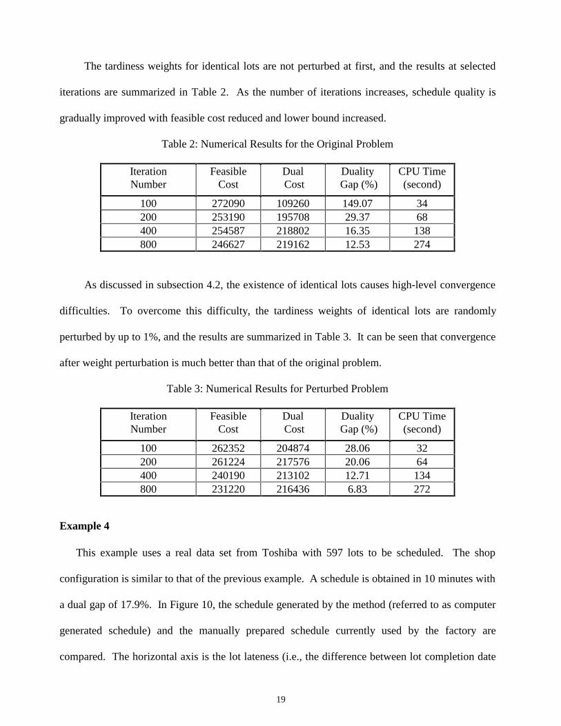
The tardiness weights for identical lots are not perturbed at first, and the results at selected

iterations are summarized in Table 2. As the number of iterations increases, schedule quality is

gradually improved with feasible cost reduced and lower bound increased.

Table 2: Numerical Results for the Original Problem

IterationNumber

FeasibleCost

Dual Cost

Duality Gap (%)

CPU Time(second)

100 272090 109260 149.07 34200 253190 195708 29.37 68400 254587 218802 16.35 138800 246627 219162 12.53 274

As discussed in subsection 4.2, the existence of identical lots causes high-level convergence

difficulties. To overcome this difficulty, the tardiness weights of identical lots are randomly

perturbed by up to 1%, and the results are summarized in Table 3. It can be seen that convergence

after weight perturbation is much better than that of the original problem.

Table 3: Numerical Results for Perturbed Problem

IterationNumber

FeasibleCost

Dual Cost

Duality Gap (%)

CPU Time(second)

100 262352 204874 28.06 32200 261224 217576 20.06 64400 240190 213102 12.71 134800 231220 216436 6.83 272

Example 4

This example uses a real data set from Toshiba with 597 lots to be scheduled. The shop

configuration is similar to that of the previous example. A schedule is obtained in 10 minutes with

a dual gap of 17.9%. In Figure 10, the schedule generated by the method (referred to as computer

generated schedule) and the manually prepared schedule currently used by the factory are

compared. The horizontal axis is the lot lateness (i.e., the difference between lot completion date

20

and due date) in days, and the vertical axis is the number of lots having the same lateness. It can

be seen that the computer generated schedule has more lots finishing at or near their due dates than

the manually prepared schedule. However, it should be mentioned that the lots far from the due

dates in the manually prepared schedule could be unimportant lots, whereas lots are assumed to

have equal weights in the computer generated schedule. Because of the ongoing refinement of lot

weights from three levels to four levels, the weights are not available for the computer generated

schedule at the time of this writing.

0

50

100

150

200

250

300

<-10 -8 -6 -4 -2 0 2 4 6 8 >10 <-4 -2 0 2 >4Lateness (Completion Date minus Due Date in Days)

Nu

mb

er o

f L

ots

Manually Prepared Schedule

Computer Generated Schedule

Figure 10. Comparison of Manually Prepared and Computer Generated Schedules

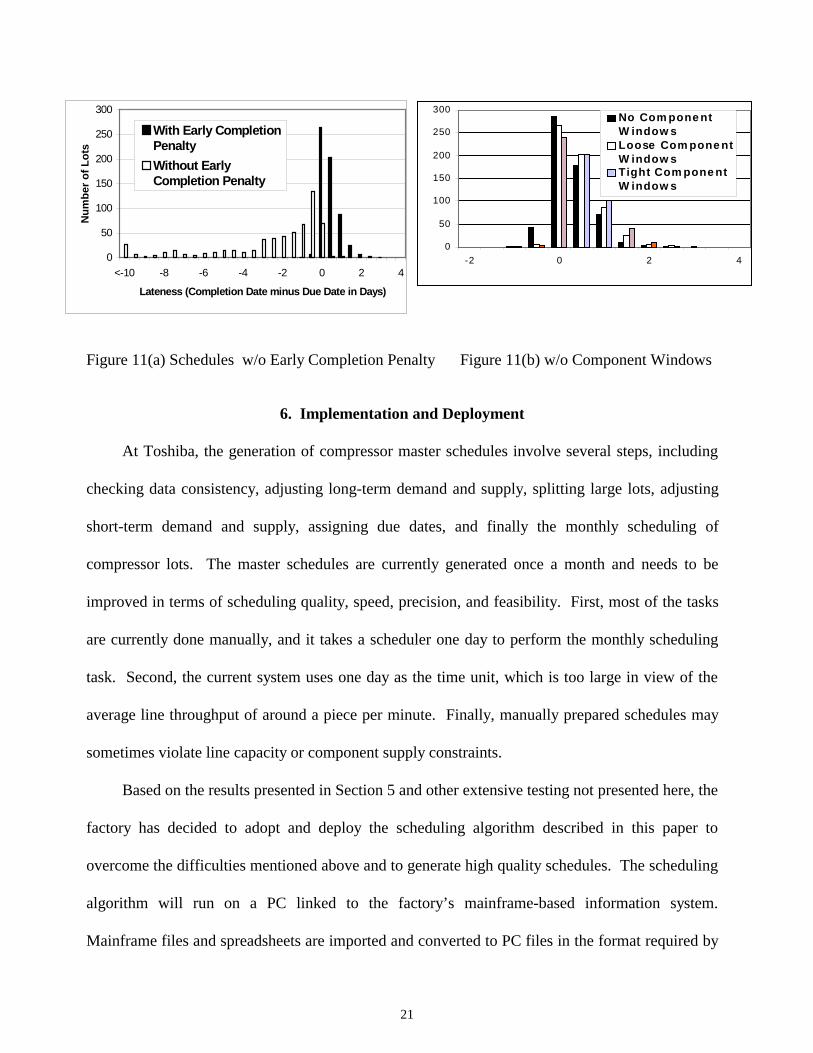
The above lateness comparison can also be used to illustrate the impact of early completion

penalty and component windows constraints. In Figure 11(a), schedules with and without early

completion penalties are compared. It can be seen that, without early completion penalties, many

lots finish earlier than the due dates and this results in large amount of finished goods inventory.

The schedules corresponding to three levels (weekly consumption of 50,000, 24,000, and 10,000

of a key component type) of component windows are compared in Figure 11(b). It can be seen

that the number of late lots increases when tighter component consumption is imposed.

21

Figure 11(a) Schedules w/o Early Completion Penalty Figure 11(b) w/o Component Windows

6. Implementation and Deployment

At Toshiba, the generation of compressor master schedules involve several steps, including

checking data consistency, adjusting long-term demand and supply, splitting large lots, adjusting

short-term demand and supply, assigning due dates, and finally the monthly scheduling of

compressor lots. The master schedules are currently generated once a month and needs to be

improved in terms of scheduling quality, speed, precision, and feasibility. First, most of the tasks

are currently done manually, and it takes a scheduler one day to perform the monthly scheduling

task. Second, the current system uses one day as the time unit, which is too large in view of the

average line throughput of around a piece per minute. Finally, manually prepared schedules may

sometimes violate line capacity or component supply constraints.

Based on the results presented in Section 5 and other extensive testing not presented here, the

factory has decided to adopt and deploy the scheduling algorithm described in this paper to

overcome the difficulties mentioned above and to generate high quality schedules. The scheduling

algorithm will run on a PC linked to the factory’s mainframe-based information system.

Mainframe files and spreadsheets are imported and converted to PC files in the format required by

0

50

100

150

200

250

300

-2 0 2 4

No Com pone ntW indow sLoose Com pone ntW indow sTight Com pone ntW indow s

0

50

100

150

200

250

300

<-10 -8 -6 -4 -2 0 2 4

Lateness (Completion Date minus Due Date in Days)

Nu

mb

er o

f L

ots

With Early CompletionPenalty

Without EarlyCompletion Penalty

22

the scheduling algorithm. A graphical user interface developed by Toshiba serves as a front end,

and presents scheduling results in terms of Gantt chart and statistics such as the total processing

times and utilization of lines. As illustrated in Section 5, it takes only a few minutes for the

scheduling algorithm to generate high quality schedules that meet products’ due dates just in time

while satisfying all the constraints. By using 0.1 hour as the time unit, the production of

compressor can be precisely controlled. In addition, the core database is being restructured to

provide accurate and consistent data for the scheduling algorithm and automate other tasks in the

generation of the master schedules. With deployment of the scheduling algorithm and speed up of

related tasks, the factory will be able to generate master schedules multiple times per month.

During the implementation and deployment, many lessons are learned. First, it is critical to

understand and analyze the factory requirements at the problem formulation stage. At the

beginning of this project, a requirement from the factory was that compressor lots of same model

needed to be separated by a certain time interval. This requirement, however, was identified later

to be similar to component supply constraints but seeing from a different angle. By concentrating

on the component supply, problem formulation and the solution methodology were simplified.

Second, the lack of data consistency is a common problem in integrating the scheduling software

with the existing information system, and a data consistency checker should save considerable

efforts in later debugging. Third, timely communication is very important especially in such a

collaborative project involving many parties, including Toshiba’s research laboratory, the factory,

and the UConn. The collaboration is not easy because of the long distance among the parties,

different time zones, and the different languages and culture. The project as a whole can still

benefit from improved interaction among the parties.

23

7. Conclusions

A separable formulation for mixed-model compressor assembly line scheduling and the

resolution of the scheduling problem has been presented. The complicated component supply

requirements are effectively handled to avoid component shortage. Based on geometrical insights,

generic defects of LR leading to slow algorithm convergence are identified and overcome by

perturbing/changing problem parameters. Numerical testing shows that near-optimal schedules are

efficiently obtained, convergence is significantly improved, and the method is effective for

practical problems.

Acknowledgment

This work was supported in part by Toshiba Corporation and National Science Foundation

Grant DMI-9813176. The authors would like to thank Dr. Shinsuke Tamura of Toshia’s Systems

& Software Engineering Laboratory, Mr. Ling Gou of Delta Technology Incorporation, and Mr.

Xing Zhao of University of Connecticut for their contributions to this project.

Appendix A: A List of Symbols

bi Beginning time of Lot i, decision variables;

ci Completion time of Lot i;

di Due date of Lot i, given;

D Dual function;

gi Product model type of Lot i, given;

Hg Integer set of all the lines that can be used to process model g;

i Lot index from 1 to I;

I Total number of lots, given;

j Component type index from 1 to J;

J Total number of component type, given;

J Objective function;

K Time horizon in resolution step, given;

24

Mkh Number of type h lines available at time k, fraction between 0-1;

njg Number of type j components needed by one type g lot within one time unit, given;

Nj Maximum number of type j components that can be supplied during Wj;

Pg Integer set of all the component types needed by the model g;

rhg Number of model g products can be finished on machine type h within one time unit;

R Number of resolution units in an enumeration step;

Si Lot size of Lot i, integer, given;

ti Processing time of Lot i integer, given;

Ti Tardiness of Lot i;

Ts Number of resolution time units in a shift;

Vi Early completion penalty of Lot i;

wi Tardiness weight of Lot i, real number, given;

Wj Window size for component type j, given;

ρi Early completion weight of Lot i, real number, given;

δikh 0-1 variable equals 1 if Lot i is active on machine h at time k and 0 otherwise ;

λkj Lagrange multipliers for constraints of component type j at enumeration step k;

πkh Lagrange multipliers for constraints of machine type h at enumeration step k;

σkj Non-negative slack variable of component supply constraints, 0 ≤ σkh ≤ pjN ;

φkh Non-negative slack variable of machine type constraints, 0 ≤ φkh ≤ Mkh.

References

[1] Bertsekas, D. P. (1995) Nonlinear Programming, Athena Scientific.

[2] Chen, H., Chu, C., Proth, J. M., (1995) A More Efficient Lagrangian Relaxation Approach to

Job Shop Scheduling Problems. Proceeding of IEEE Conference on Robotics and

Automation, 496-501.

[3] Inman, R. R. and Bulfin, R. L. (1991) Sequencing JIT Mixed-model Assembly Lines.

Management Science, 37 (7), 901-904.

25

[4] Kaskavelis, C. A. and Caramanis, M. C., Efficient Lagrangian Relaxation Algorithms for

Real-Life-Size Job-Shop Scheduling Problems. To appear in IIE Transactions on

Scheduling and Logistics.

[5] Luh, P. B. and Hoitomt, D. J. (1993) Scheduling of Manufacturing Systems Using the

Lagrangian Relaxation Technique. IEEE Transactions on Automatic Control, 38 (7), 1066-

1088.

[6] Luh, P. B., Gou, L., Zhang, Y., Nagahora, T., Tsuji, M., Yoneda, K., Hasegawa, T., Kyoya,

Y. and Kano, T. (1998) Job Shop Scheduling with Group-dependent Setups, Finite Buffers,

and Long Time Horizon. Annals of Operations Research, 76, 233-259.

[7] Miltenburg, G. J. (1989) Level Schedules for Mixed-Model Assembly Lines in Just-In-Time

Production System. Management Science, 35 (2), 192-207.

[8] Monden, Y. (1993) Toyota Production System, Norcross, GA: Industrial Engineering and

Management Press.

[9] Stein, G. and Yeomans, J. S. (1996) Optimal Level Schedules in Mixed-model, Multi-level

JIT Assembly Systems with Pegging. European Journal of Operational Research, 22 (1),

38-45.

[10] Sumichrast, R. T., Russel, R. S. and Taylor, B. W. (1992) A Comparative Analysis of

Sequencing Procedures for Mixed-model Assembly Lines in a Just-in-time Production

System. International Journal of Production Research, 30 (1), 199-214.

[11] Zhao, X., Luh, P. B. and Wang, J. (1999) The Surrogate Gradient Algorithm for Lagrangian

Relaxation Method. To appear in Journal of Optimization Theory and Applications, March

1999.