Mitigation of oceanic tidal aliasing errors in space and time simultaneously using different repeat sub-satellite tracks from pendulum-type gravimetric mission candidate

1

A summary of the Paper:

“Mitigation of oceanic tidal aliasing errors in space and time simultaneously using

different repeat sub-satellite tracks from pendulum-type gravimetric mission

candidate”

Acta Geophysica (2015), doi.10.2478/s11600-014-0251-4

Basem Elsaka1,2

, Karl-Heinz Ilk3 and Abdulaziz Alothman

1

1- Space and Aviation Research Institute, King Abdulaziz City for Science and

Technology (KACST), Riyadh, Saudi Arabia.

2- National Research Institute of Astronomy and Geophysics (NRIAG), Helwan,

Cairo, Egypt.

3- Institute of Geodesy and Geoinformation, University of Bonn, Germany.

Corresponding Author:

Dr. Basem Elsaka,

Center of Excellence for Lunar and Near Earth Objects Science,

King Abdulaziz City for Science and Technology (KACST),

P.O.Box 6086,

Riyadh 11442, Saudi Arabia,

Tel: +966 503805697 | Fax: +966 114814572

2

Abstract

This contribution investigates two different ways for mitigating the aliasing errors

in ocean tides. This is done on the one hand by sampling the satellite observations in

another direction using the pendulum satellite mission configuration. On the other hand, a

mitigation of the temporal aliasing errors in the ocean tides can be achieved by using a

suitable repeat period of the sub-satellite tracks.

The findings show firstly that it is very beneficial for minimizing the aliasing

errors in ocean tides to use pendulum configuration; secondly optimizing the orbital

parameter to get shorter repeat orbit mode can be effective in minimizing the aliasing

errors. This paper recommends the pendulum as a candidate for future gravity mission to

be launched in longer repeating orbit mode with shorter ‘sub-cycle’ repeat periods to

improve the temporal resolution of the satellite mission.

Keywords. Gravity field recovery. Repeat sub-satellite tracks. Ocean tides aliasing.

3

1. Introduction:

The products that the twin-satellite GRACE (Gravity Recovery and Climate Experiment)

mission (Tapley et al., 2004) has provided in the form of numerous model series such as

the EIGEN and ITG-GRACE series (e.g., Förste et al., 2008 and Mayer-Gürr et al., 2010,

respectively) have not yet matched pre-mission expectations in terms of error level and

error isotropy. The main limitation of the quality of the resolved temporal gravity field

estimates is mostly controlled not only by instrument noise, but also the anisotropy of

spatial sampling and temporal aliasing errors (i.e., the errors in modeling of mass

variations due to the high frequency signals such as non-tidal atmospheric oceanic masses

and the oceanic tides). The latter effects are related to the GRACE orbital configuration

because of the inhomogeneous sampling in time and space. Therefore, to minimize the

errors in the temporal gravity field models, e.g., ocean tides, one has to optimize and/or

improve the determination of the gravitational signal spatially and temporally. On the

one hand, a spatially homogeneous sampling can be achieved via the selection of an

alternative mission type whose satellite observables are sensitive in other directions (e.g.,

radial and/or cross-track) compared to the GRACE along-track observable. On the other

hand, adjusting the orbit and formation parameters can improve the temporal sampling of

the mission. These parameters include the orbital altitude, the inter-satellite distance, the

inclination, the repeat mode of sub-satellite tracks (as projected satellite orbits on the

Earth’s surface) and, of course, the choice of the number of satellites and satellite links to

create a possible multi-satellite/formation mission. By means of an appropriate choice of

these parameters, isotropy can be enlarged and aliasing effects (the most problematic

issue of GRACE mission) can be reduced.

It should be mentioned here that there are common approaches for reducing the

temporal aliasing effects, such as smoothing techniques with Gaussian and/or de-

correlation filters (see, e.g., Wahr et al., 2004, Swenson and Wahr, 2006 and Kusche,

2007). However, it was found that the impact of such filters is partially undesirable as a

part of the desired gravity signal is smoothed besides the errors.

It is important first to mention that a variety of studies was published in the

previous years which have investigated the performance of the basic types of satellite

formation missions, e.g. pendulum, cartwheel and LISA (see, e.g., Sharifi et al., 2007,

4

Sneeuw et al., 2008, Wiese et al., 2009, Elsaka et al., 2012 and Elsaka et al., 2014a). All

these studies have found that the latter three missions would provide a lower error

spectrum with improved isotropy. In addition, the arrangement of a second, inclined

satellite pair in the so-called “Bender design” was studied by Bender et al. (2008), Visser

et al. (2010) Wiese et al. (2011a), Wiese et al. (2012) and Elsaka et al. (2014b). All of the

above-mentioned studies show a common result that a significant increase in accuracy

and sensitivity is expected when a future formation will be flown in an alternative

configuration, different from the GRACE leader-follower scheme. Furthermore, Visser et

al. (2010), Wiese et al. (2011b) and Elsaka (2014) have studied the feasibility of

estimating low resolution gravity fields at short periods via a single and double pairs of

satellites similar to GRACE to reduce the effect of temporal aliasing errors from mass

variations with large spatial scales.

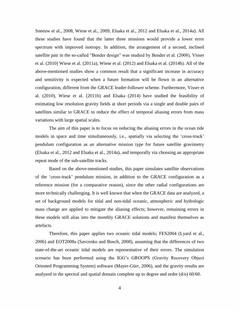
The aim of this paper is to focus on reducing the aliasing errors in the ocean tide

models in space and time simultaneously, i.e., spatially via selecting the ‘cross-track’

pendulum configuration as an alternative mission type for future satellite gravimetry

(Elsaka et al., 2012 and Elsaka et al., 2014a), and temporally via choosing an appropriate

repeat mode of the sub-satellite tracks.

Based on the above-mentioned studies, this paper simulates satellite observations

of the ‘cross-track’ pendulum mission, in addition to the GRACE configuration as a

reference mission (for a comparative reason), since the other radial configurations are

more technically challenging. It is well known that when the GRACE data are analyzed, a

set of background models for tidal and non-tidal oceanic, atmospheric and hydrologic

mass change are applied to mitigate the aliasing effects; however, remaining errors in

these models still alias into the monthly GRACE solutions and manifest themselves as

artefacts.

Therefore, this paper applies two oceanic tidal models; FES2004 (Lyard et al.,

2006) and EOT2008a (Savcenko and Bosch, 2008), assuming that the differences of two

state-of-the-art oceanic tidal models are representative of their errors. The simulation

scenario has been performed using the IGG’s GROOPS (Gravity Recovery Object

Oriented Programming System) software (Mayer-Gürr, 2006), and the gravity results are

analyzed in the spectral and spatial domain complete up to degree and order (d/o) 60/60.

5

This paper is organized as follows: in section 2, a review concerning the

computation of the repeat periods of sub-satellite tracks and the applied repeat modes in

this contribution is outlined. The pendulum mission configuration is discussed in section

3. The simulation strategy used for the gravity field analysis is introduced in section 4.

The gravity field solutions in terms of ocean tide aliasing errors are presented in section

5. Finally, on this basis, a relevant conclusion is outlined in section 6.

2. Computation of the repeat period of sub-satellite tracks

Repeat sub-satellite track means simply that the sub-satellite track retraces itself exactly

after a certain time. If the satellite orbit should repeat itself whilst the Earth was not

rotating or the satellite orbital plane was fixed in the Earth’s fixed frame, the two satellite

crossings at the equator would occur at the same site. Since neither Earth rotation nor the

precession of the orbital plane can be neglected, the shift between two ascending nodes

takes place. Because the precession of the ascending nodes is much slower than the

Earth's rotation, a nodal day differs slightly from a solar day, and in case of a sun-

synchronous orbit (e.g., i = 95°) they are equal (see Bezdek et al., 2009). The nodal day

corresponds to the time that the Earth takes to complete one revolution with respect to the

orbital plane, while the solar day corresponds to the time required for the Earth to

complete one revolution with respect to the Sun-Earth line.

Taking the Earth’s rotation rate ( ) with respect to the satellite’s orbital plane,

the notion of a nodal period (Pn) is therefore orbit-dependent and is defined as (after Rees

2001)

2 2,

( )nP

[1]

where is the angular velocity of the Earth and is the precession rate of the

satellite’s line of node. After an integer number () of Earth rotations in the time required

for the satellite to make an integral number of orbits (), the condition in Eq. [1] can be

written as

( ) 2 .nP

[2]

6

The nodal period is equal to the Keplerian period if the perturbations were absent.

However, in presence of perturbations, the secular change in the satellite’s argument of

perigee and the secular change in the satellite's mean anomaly M must be taken into

account (i.e., Pn = 2 /( )M ). Thus Eq. [2] can be rewritten in terms of the classical

orbital elements as

22 ,

( ) ( )nP

M

[3]

and hence,

( ) ( ) .M [4]

Equation [4] represents the repeat period condition and establishes the synchronicity

between the Earth rotation and the satellite rotation in a way that the satellite completes

nodal revolutions while the Earth performs rotations. The three secular changes, ,

M and , in Eq. [2] are calculated according to Kaula (1966) as

2

20

2 2 2

2220

2 2 2

2220

2 2 3/ 2

3dcos ,

dt 2 (1 )

3d(1 5cos ) ,

dt 4 (1 )

3dM(3cos 1) ,

dt 2 (1 )

nC Ri

a e

nC Ri

a e

nC Rn i

a e

[5]

where n is the satellite’s mean motion, C20 is the second zonal term of the geopotential, R

is the Earth’s radius, a is the orbital semi-major axis, and e is the orbital eccentricity.

When the Earth takes approximately 365.25 days to orbit around the Sun, this means that

it performs exactly 1.002737925 rev (i.e., 1+1/365.25) per day. In this way, the duration

of the sidereal day becomes exactly 23.9345 hours and the Earth’s angular velocity reads

-52 / 23.9345x60x60=7.2921x10 rad/s.

The repeat period condition (Eq. [3]) is related to the mean motion of the satellite,

after neglecting the term e2 (due to its small value) in Eq. [5], using the nodal period of

the satellite 2 /( )M , and the nodal day 2 /( ) , as

( ) ( ) .n M

[6]

7

After one inserts the secular rates calculated from Eq. [5] into Eq. [4], the ratio β/α can be

easily computed. Eq. [6] reads for the first order in J2 (where J2 is the normalized

coefficient20 5C ) according to Bezdek et al. (2009) as

2

2

2

31 4cos cos 1 .

2

Rn j i i

a

[7]

The ratio β/α in Eq. [7] depends on the orbital inclination and altitude. In this paper, an

eccentricity e = 0.001 and an inclination of i = 89.5° for both pendulum and GRACE

configurations are selected, so one can focus here on the change of repeat sub-satellite

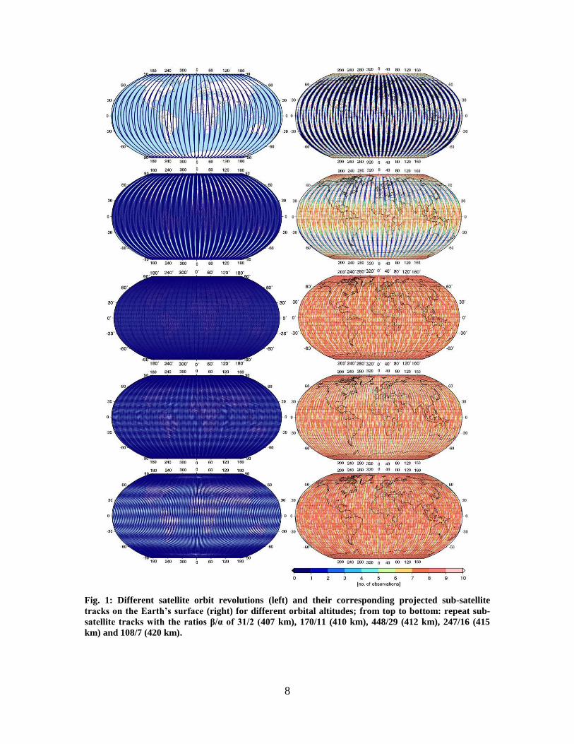
tracks according to different orbital altitudes. Figure 1 shows different satellite orbits

revolutions and their projected sub-satellite tracks on an Earth’s map with the ratio β/α

equal to 31/2, 170/11, 448/29, 247/16 and 108/7, corresponding to the orbital altitudes of

407 km, 410 km, 212 km, 415 km and 420 km, respectively.

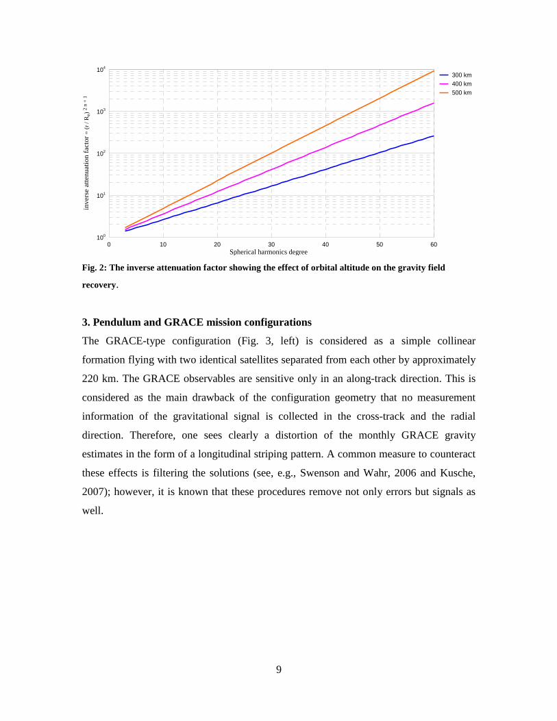
The selection of those orbital altitudes is based on the fact that the gravitational

signal rapidly decays due to the so-called inverse attenuation factor, [r/Re]2n+1

, which is a

function of the spherical harmonic degree n. The term r stands for the orbit altitude and

Re stands for the Earth’s radius. The exponent n indicates that the higher the orbital

altitude (and consequently the larger the r), the worse the resolution of the gravity field

recovery (see e.g., Fig. 2).

Therefore, nearby orbital altitudes between 407 km and 420 km are selected here

in order to achieve different repeat modes without affecting the strength of the

gravitational signal. The selected orbital altitudes represent different sub-satellite tracks

that cover the Earth, insufficiently and sufficiently, as shown in Fig. 1.

8

Fig. 1: Different satellite orbit revolutions (left) and their corresponding projected sub-satellite

tracks on the Earth’s surface (right) for different orbital altitudes; from top to bottom: repeat sub-

satellite tracks with the ratios β/α of 31/2 (407 km), 170/11 (410 km), 448/29 (412 km), 247/16 (415

km) and 108/7 (420 km).

9

0 10 20 30 40 50 60

Spherical harmonics degree

100

101

102

103

104

invers

e a

tten

uati

on

facto

r =

(r

/ R

e) 2

n +

1

300 km

400 km

500 km

Fig. 2: The inverse attenuation factor showing the effect of orbital altitude on the gravity field

recovery.

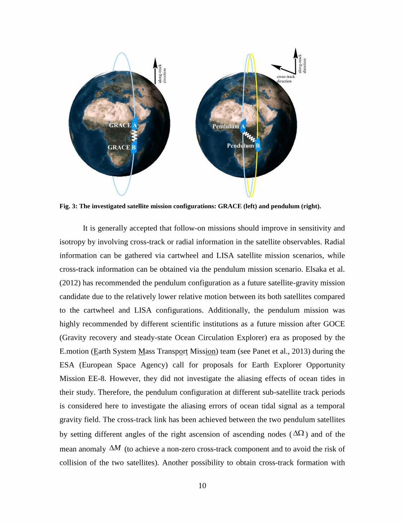
3. Pendulum and GRACE mission configurations

The GRACE-type configuration (Fig. 3, left) is considered as a simple collinear

formation flying with two identical satellites separated from each other by approximately

220 km. The GRACE observables are sensitive only in an along-track direction. This is

considered as the main drawback of the configuration geometry that no measurement

information of the gravitational signal is collected in the cross-track and the radial

direction. Therefore, one sees clearly a distortion of the monthly GRACE gravity

estimates in the form of a longitudinal striping pattern. A common measure to counteract

these effects is filtering the solutions (see, e.g., Swenson and Wahr, 2006 and Kusche,

2007); however, it is known that these procedures remove not only errors but signals as

well.

10

Fig. 3: The investigated satellite mission configurations: GRACE (left) and pendulum (right).

It is generally accepted that follow-on missions should improve in sensitivity and

isotropy by involving cross-track or radial information in the satellite observables. Radial

information can be gathered via cartwheel and LISA satellite mission scenarios, while

cross-track information can be obtained via the pendulum mission scenario. Elsaka et al.

(2012) has recommended the pendulum configuration as a future satellite-gravity mission

candidate due to the relatively lower relative motion between its both satellites compared

to the cartwheel and LISA configurations. Additionally, the pendulum mission was

highly recommended by different scientific institutions as a future mission after GOCE

(Gravity recovery and steady-state Ocean Circulation Explorer) era as proposed by the

E.motion (Earth System Mass Transport Mission) team (see Panet et al., 2013) during the

ESA (European Space Agency) call for proposals for Earth Explorer Opportunity

Mission EE-8. However, they did not investigate the aliasing effects of ocean tides in

their study. Therefore, the pendulum configuration at different sub-satellite track periods

is considered here to investigate the aliasing errors of ocean tidal signal as a temporal

gravity field. The cross-track link has been achieved between the two pendulum satellites

by setting different angles of the right ascension of ascending nodes ( ) and of the

mean anomaly M (to achieve a non-zero cross-track component and to avoid the risk of

collision of the two satellites). Another possibility to obtain cross-track formation with

11

non-zero differential inclination is also achievable. However, this option is not

guaranteed, since a non-trivial solution of the linear equation system exists (Sneeuw et al.

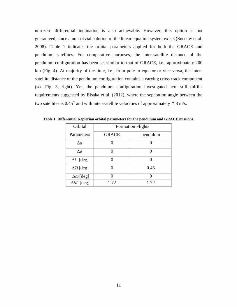
2008). Table 1 indicates the orbital parameters applied for both the GRACE and

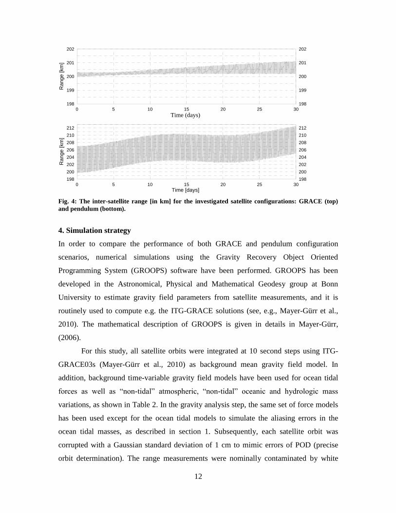
pendulum satellites. For comparative purposes, the inter-satellite distance of the

pendulum configuration has been set similar to that of GRACE, i.e., approximately 200

km (Fig. 4). At majority of the time, i.e., from pole to equator or vice versa, the inter-

satellite distance of the pendulum configuration contains a varying cross-track component

(see Fig. 3, right). Yet, the pendulum configuration investigated here still fulfills

requirements suggested by Elsaka et al. (2012), where the separation angle between the

two satellites is 0.45 and with inter-satellite velocities of approximately 8 m/s.

Table 1. Differential Keplerian orbital parameters for the pendulum and GRACE missions.

Orbital

Parameters

Formation Flights

GRACE pendulum

a 0 0

e 0 0

i [deg] 0 0

[deg] 0 0.45

[deg] 0 0

M [deg] 1.72 1.72

12

0 5 10 15 20 25 30

Time (days)

198

199

200

201

202

Ran

ge [

km

]

198

199

200

201

202

0 5 10 15 20 25 30

Time [days]

198

200

202

204

206

208

210

212

Ran

ge [

km

]

198

200

202

204

206

208

210

212

Fig. 4: The inter-satellite range [in km] for the investigated satellite configurations: GRACE (top)

and pendulum (bottom).

4. Simulation strategy

In order to compare the performance of both GRACE and pendulum configuration

scenarios, numerical simulations using the Gravity Recovery Object Oriented

Programming System (GROOPS) software have been performed. GROOPS has been

developed in the Astronomical, Physical and Mathematical Geodesy group at Bonn

University to estimate gravity field parameters from satellite measurements, and it is

routinely used to compute e.g. the ITG-GRACE solutions (see, e.g., Mayer-Gürr et al.,

2010). The mathematical description of GROOPS is given in details in Mayer-Gürr,

(2006).

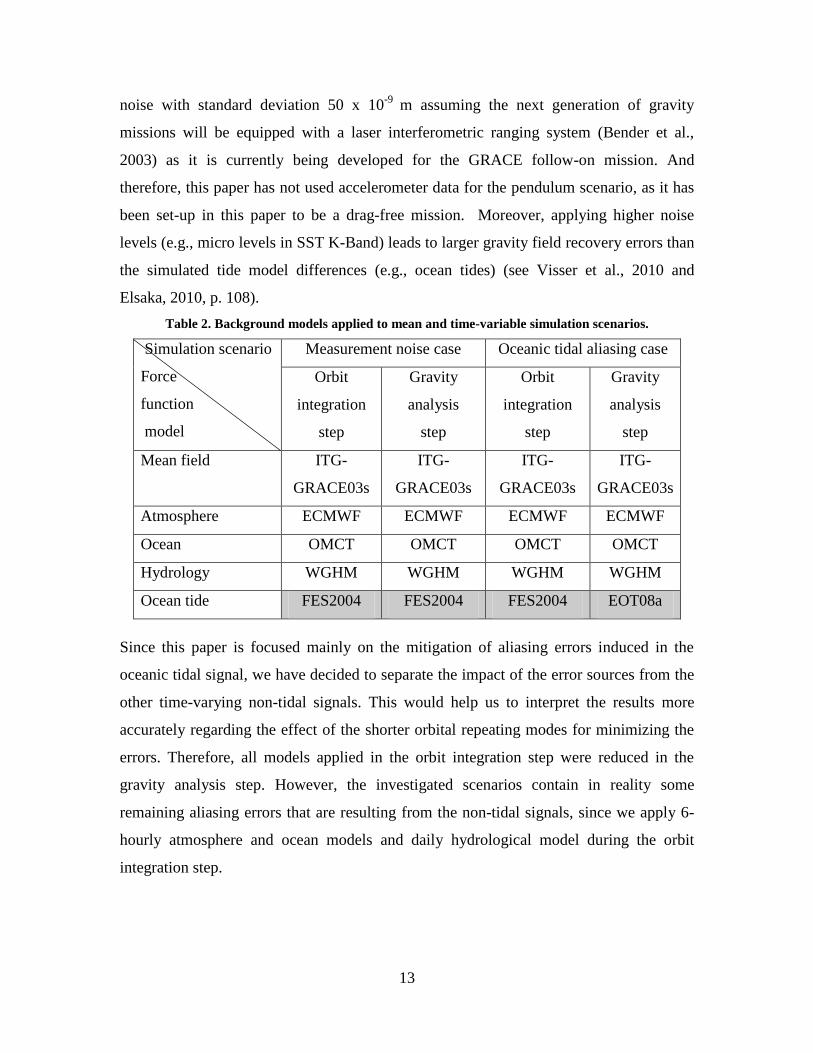
For this study, all satellite orbits were integrated at 10 second steps using ITG-

GRACE03s (Mayer-Gürr et al., 2010) as background mean gravity field model. In

addition, background time-variable gravity field models have been used for ocean tidal

forces as well as “non-tidal” atmospheric, “non-tidal” oceanic and hydrologic mass

variations, as shown in Table 2. In the gravity analysis step, the same set of force models

has been used except for the ocean tidal models to simulate the aliasing errors in the

ocean tidal masses, as described in section 1. Subsequently, each satellite orbit was

corrupted with a Gaussian standard deviation of 1 cm to mimic errors of POD (precise

orbit determination). The range measurements were nominally contaminated by white

13

noise with standard deviation 50 x 10-9

m assuming the next generation of gravity

missions will be equipped with a laser interferometric ranging system (Bender et al.,

2003) as it is currently being developed for the GRACE follow-on mission. And

therefore, this paper has not used accelerometer data for the pendulum scenario, as it has

been set-up in this paper to be a drag-free mission. Moreover, applying higher noise

levels (e.g., micro levels in SST K-Band) leads to larger gravity field recovery errors than

the simulated tide model differences (e.g., ocean tides) (see Visser et al., 2010 and

Elsaka, 2010, p. 108).

Table 2. Background models applied to mean and time-variable simulation scenarios.

Simulation scenario

Force

function

model

Measurement noise case Oceanic tidal aliasing case

Orbit

integration

step

Gravity

analysis

step

Orbit

integration

step

Gravity

analysis

step

Mean field ITG-

GRACE03s

ITG-

GRACE03s

ITG-

GRACE03s

ITG-

GRACE03s

Atmosphere ECMWF ECMWF ECMWF ECMWF

Ocean OMCT OMCT OMCT OMCT

Hydrology WGHM WGHM WGHM WGHM

Ocean tide FES2004 FES2004 FES2004 EOT08a

Since this paper is focused mainly on the mitigation of aliasing errors induced in the

oceanic tidal signal, we have decided to separate the impact of the error sources from the

other time-varying non-tidal signals. This would help us to interpret the results more

accurately regarding the effect of the shorter orbital repeating modes for minimizing the

errors. Therefore, all models applied in the orbit integration step were reduced in the

gravity analysis step. However, the investigated scenarios contain in reality some

remaining aliasing errors that are resulting from the non-tidal signals, since we apply 6-

hourly atmosphere and ocean models and daily hydrological model during the orbit

integration step.

14

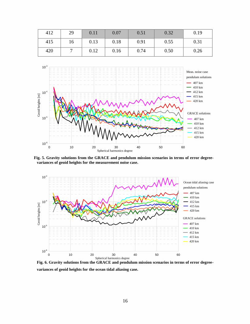
5. Results

The results are provided in the ‘long-to-medium’ spectral domain in terms of spherical

harmonic coefficients up to degree/order (d/o) 60/60. The gravity field estimates are

further visualized in terms of error degree-variances of the geoid heights, as shown in

Figs. 5 and 6 for the measurement noise and oceanic tidal aliasing scenarios, respectively.

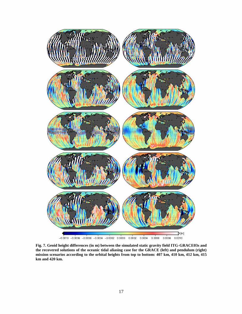
In the spatial domain, geoid error maps are constructed in Fig. 7 for the oceanic tidal

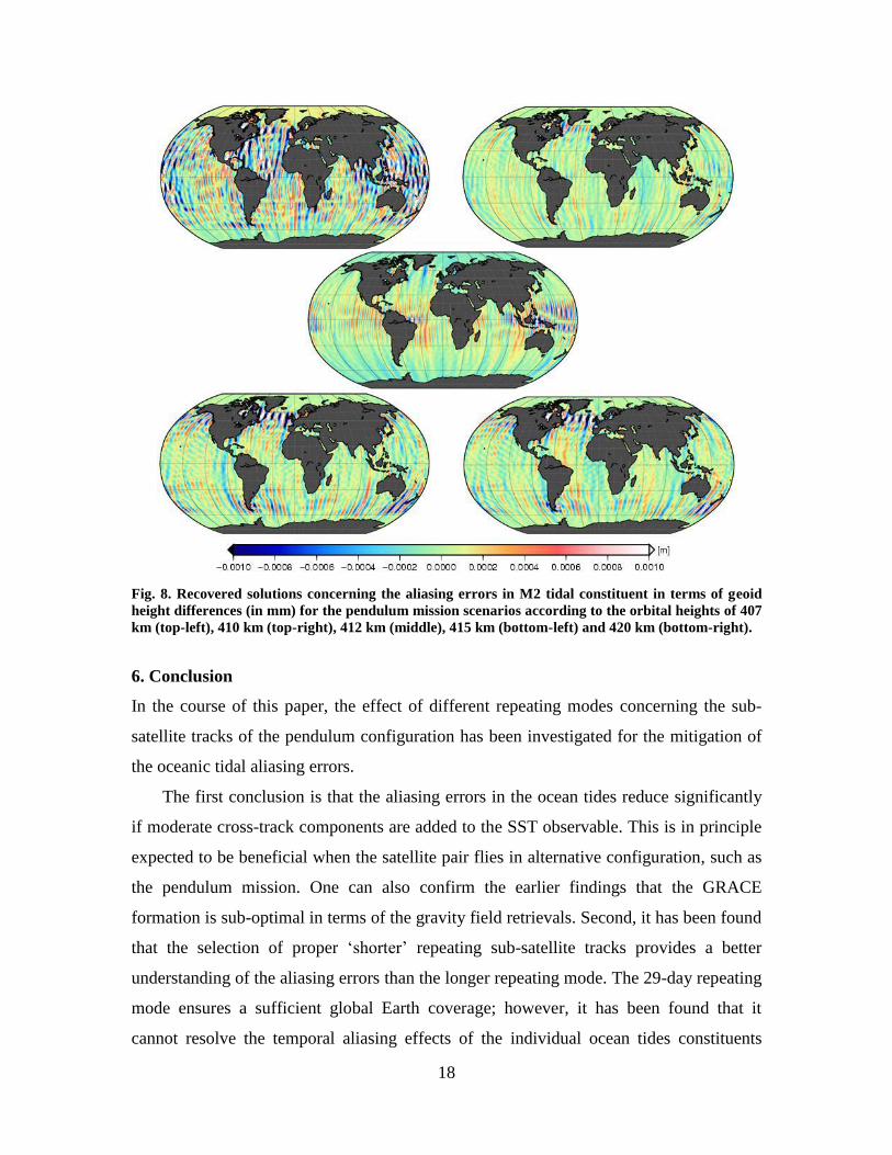
aliasing case. Moreover, Fig. 8 shows the gravity field solutions of the aliasing case

considering only the individual semi-diurnal M2 tidal constituent determined by the

pendulum configuration. The corresponding statistics in terms of global root mean square

(RMS) values are given separately in Table 3. All error curves shown in Figs. 5 and 6 are

obtained from the difference between outputs (estimates) and input (true model, i.e., ITG-

GRACE03s). This means that the mean field based on ITG-GRACE03s had to be

removed from the monthly recovered solution in order to obtain the residual monthly

gravity signal, due to the simulated error of the ocean tides signal.

As expected, all estimated solutions for the pendulum mission scenario perform

approximately a half to one full order of magnitude (Table 3) better than the GRACE

reference solution, in particular, at the medium wavelength range, as seen in Fig. 5 for the

measurement noise case. However, Table 3 shows that the GRACE solutions at orbital

heights of 410, 415 and 420 km surpass those determined by the pendulum scenario. The

reason is clearly identified in Fig. 5 that the pendulum configuration recover the

harmonic coefficients at the long wavelength range (up to d/o 8) worse than the GRACE

configuration. Yet the pendulum surpasses GRACE within the remaining long as well as

medium range (i.e., from d/o 9 up to d/o 60). According to the oceanic tidal aliasing case

(Fig. 6), the pendulum solutions outperform the GRACE ones. This can be clearly seen in

Table 3 and spatially on the Earth’s map in Fig. 7, which shows the global geoid height

errors. The reason for this performance is that the pendulum configuration adds

measurement information in the cross-track directions, and hence it helps in improving

the retrieval of the mean and temporal gravity signal.

The north-south striping pattern has been obviously reduced via the pendulum

gravity estimates in comparison to the GRACE reference solutions, which display a

stronger striping pattern, as expected (see Fig. 7). This means that the pendulum

15

configuration would not only be able to reduce aliasing errors but also to resolve the

temporal signal better.

According to the performance of the gravity field retrievals concerning the different

repeating modes of sub-satellite tracks, one finds that the 29-day repeating mode provides

the least oceanic tidal aliasing errors for both GRACE and pendulum configurations. This

is due to the sufficient satellite observables and the adequate Earth coverage. Strong

improvements have been found also for the 11-day repeating for mitigating the aliasing

errors as seen in Table 3, which behaves similar to the 29-day repeating.

Since the pendulum configuration provides the least oceanic tidal aliasing errors, it

has been additionally examined here how different repeating modes could mitigate the

aliasing errors of the individual tides. For this case, the semi-diurnal M2 tidal constituent

was selected. One can find here that both the 29-day and 11-day repeating still result in

similar improvements; however, the 11-day repeating outperforms the 29-day repeating.

This can be seen in Fig. 8 showing that the M2 aliasing errors have been minimized by

the 11-day repeating mode better than by the other repeating modes.

One can infer that although the 29-day solution may be the best choice for

minimizing the temporal aliasing errors, its temporal resolution is still not enough to

resolve errors in the individual temporal signals. Therefore, it is recommended that the

pendulum, as a candidate for a future gravity mission for detecting the temporal

variations of the Earth’s gravity field, is flown in a 29-day repeating mode allowing

sufficient satellite observations with, e.g., 11-day sub-cycle repeating at the same time to

allowing a better understanding of the temporal variations of the individual time-varying

signals.

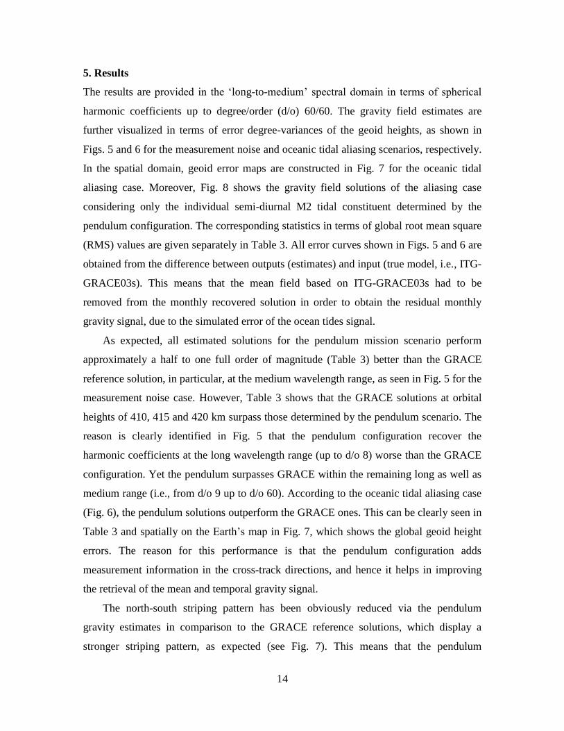
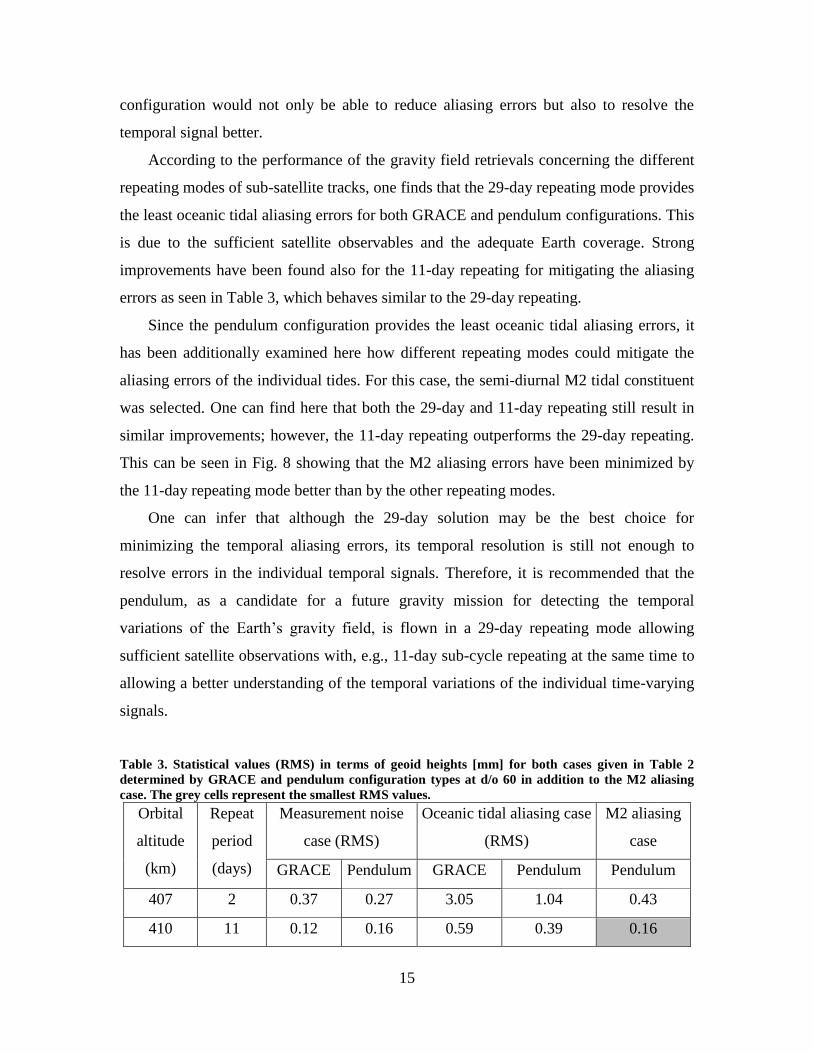
Table 3. Statistical values (RMS) in terms of geoid heights [mm] for both cases given in Table 2

determined by GRACE and pendulum configuration types at d/o 60 in addition to the M2 aliasing

case. The grey cells represent the smallest RMS values.

Orbital

altitude

(km)

Repeat

period

(days)

Measurement noise

case (RMS)

Oceanic tidal aliasing case

(RMS)

M2 aliasing

case

GRACE Pendulum GRACE Pendulum Pendulum

407 2 0.37 0.27 3.05 1.04 0.43

410 11 0.12 0.16 0.59 0.39 0.16

16

412 29 0.11 0.07 0.51 0.32 0.19

415 16 0.13 0.18 0.91 0.55 0.31

420 7 0.12 0.16 0.74 0.50 0.26

0 10 20 30 40 50 60Spherical harmonics degree

10-6

10-5

10-4

10-3

Geo

id h

eights

[m

]

GRACE solutions

407 km

410 km

412 km

415 km

420 km

Meas. noise case

pendulum solutions

407 km

410 km

412 km

415 km

420 km

Fig. 5. Gravity solutions from the GRACE and pendulum mission scenarios in terms of error degree-

variances of geoid heights for the measurement noise case.

0 10 20 30 40 50 60Spherical harmonics degree

10-6

10-5

10-4

10-3

Geo

id h

eights

[m

]

Ocean tidal aliasing case

pendulum solutions

407 km

410 km

412 km

415 km

420 km

GRACE solutions

407 km

410 km

412 km

415 km

420 km

Fig. 6. Gravity solutions from the GRACE and pendulum mission scenarios in terms of error degree-

variances of geoid heights for the ocean tidal aliasing case.

17

Fig. 7. Geoid height differences (in m) between the simulated static gravity field ITG-GRACE03s and

the recovered solutions of the oceanic tidal aliasing case for the GRACE (left) and pendulum (right)

mission scenarios according to the orbital heights from top to bottom: 407 km, 410 km, 412 km, 415

km and 420 km.

18

Fig. 8. Recovered solutions concerning the aliasing errors in M2 tidal constituent in terms of geoid

height differences (in mm) for the pendulum mission scenarios according to the orbital heights of 407

km (top-left), 410 km (top-right), 412 km (middle), 415 km (bottom-left) and 420 km (bottom-right).

6. Conclusion

In the course of this paper, the effect of different repeating modes concerning the sub-

satellite tracks of the pendulum configuration has been investigated for the mitigation of

the oceanic tidal aliasing errors.

The first conclusion is that the aliasing errors in the ocean tides reduce significantly

if moderate cross-track components are added to the SST observable. This is in principle

expected to be beneficial when the satellite pair flies in alternative configuration, such as

the pendulum mission. One can also confirm the earlier findings that the GRACE

formation is sub-optimal in terms of the gravity field retrievals. Second, it has been found

that the selection of proper ‘shorter’ repeating sub-satellite tracks provides a better

understanding of the aliasing errors than the longer repeating mode. The 29-day repeating

mode ensures a sufficient global Earth coverage; however, it has been found that it

cannot resolve the temporal aliasing effects of the individual ocean tides constituents

19

(e.g., M2 semi-diurnal signal). On the other hand, the 11-day repeating mode could

resolve the ocean tidal aliasing errors of individual constituents better.

Finally, it is recommended that a future gravity mission is launched in an orbital

altitude of 29-day repeating cycle implementing at the same time 11-day repeating sub-

cycle, which would support the detection of mass variations at higher temporal

frequencies.

Acknowledgement:

The authors would like firstly to thank the Managing Editor, Dr. Z. Wisniewski, for his

efforts during the publication process of this manuscript and would like also to thank the

reviewers for their valuable comment. The financial support of King Abdulaziz City for

Science and Technology (KACST) is gratefully acknowledged.

References

Bender, P., Hall, J., Ye, J., Klipstein, W. (2003) Satellite–satellite laser links for future

gravity missions. Space Sci. Rev. 108: 377–384.

Bender, P. , Wiese, D. and Nerem, R. (2008) A possible dual-GRACE mission with 90

degree and 63 degree inclination orbits, paper presented at Third International

Symposium on Formation Flying, Eur. Space Agency, Noordwijk, Netherlands, 23–

25 April.

Bezdek, A., Klokocnik J., Kostelecky J., Floberghagen R. and Gruber, Ch. (2009)

Simulation of free fall and resonances in the GOCE mission. Journal of

Geodynamics, Vol. 48, Issue 1:47-53.

Elsaka, B., (2010) Simulated satellite formation flights for detecting the temporal

variations of the earth’s gravity field. Ph.D. Dissertation. University of Bonn,

Germany.

Elsaka, B., (2014) Sub-month Gravity Field Recovery from Simulated Multi-GRACE

Type. . Acta Geophys. Vol. 62, no. 1, pp. 241-258, doi: 10.2478/s11600-013-0170-9.

Elsaka, B., Kusche, J. and Ilk, K.-H. (2012) Recovery of the Earth’s gravity field from

formation-flying satellites: Temporal aliasing issues. Advances in Space Research,

50: 1534-1552, doi: 10.1016/j.asr.2012.07.016.

20

Elsaka, B., Raimondo, J.-C., Brieden, Ph., Reubelt, T., Kusche, J., Flechtner, F.,

Iran Pour, S., Sneeuw, N. and Müller, J. (2014a) Comparing Seven Candidate

Mission Configurations for Temporal Gravity Retrieval through Full-Scale Numerical

Simulation. Journal of Geodesy, 88, 31-43, doi: 10.1007/s00190-013-0665-9.

Elsaka, B., Forootan, E. and Alothman, A. (2014b) Improving the recovery of monthly

regional water storage using one year simulated observations of two pairs of GRACE-

type satellite gravimetry constellation. Journal of Applied Geophysics, Vol. 109, Pp.

195–209, doi: 10.1016/j.jappgeo.2014.07.026.

Förste, C., Schmidt, R., Stubenvoll, R., Flechtner, F., Meyer, U., König, R., Neu-

mayer, H., Biancale, R., Lemoine, J., Bruinsma, S., Loyer, S., Barthelmes, F. and

Esselborn, S. (2008) The GeoForschungsZentrum Potsdam/Groupe de Recherche de

Ge-odesie Spatiale satellite-only and combined gravity field models: EIGEN-GL04S1

and EIGEN-GL04C. J Geod, 82, 6, 331-346, doi: 10.1007/s00190-007-0183-8.

Kaula, W. M. (1966) Theory of Satellite Geodesy. Blaisdell Puplishing Company,

Waltham, Massachusetts. Toronto. London. Republished, 2000 by Dover

Puplications, Inc. Mineola, New York.

Kusche, J. (2007) Approximate decorrelation and non-isotropic smoothing of time-

variable GRACE-type gravity field models. Journal of Geodesy, Vol. 81:733-749.

Lyard, F., Lefèvre, F., Letellier, T. and Francis, O. (2006) Modelling the global ocean

tides: a modern insight from FES2004, Ocean Dynamics, 56, 394-415.

Mayer-Gürr, T. (2006) Gravitationsfeldbestimmung aus der Analyse kurzer Bahnbögen

am Beispiel der Satellitenmissionen CHAMP und GRACE. Ph.D. Dissertation,

University of Bonn, Germany.

Mayer-Gürr, T., Eicker, A., Kurtenbach, E., and Ilk, K.H. (2010) ITG-GRACE:

Global Static and Temporal Gravity Field Models from GRACE Data. In: Flechtner,

F., Gruber, Th., Gntner, A., Mandea, M., Rothacher, M., Schne, T., Wickert, J. (Eds.),

System Earth via Geodetic-Geophysical Space Techniques, Springer, Berlin, pp.159-

168.

Panet, I., Flury, J., Biancale, R., Gruber, T., Johannessen, J., van den broeke, M. R.,

van Dam, T., Gegout, P., Hughes, C.-W., Ramillien, G., Sasgen, I., Seoane, L.,

Thomas, M. (2013) Earth System Mass Transport Mission (e.motion): A Concept for

21

Future Earth Gravity Field Measurements from Space. Surveys in Geophysics: Vol

34, Issue 2, pp 141-163, doi: 10.1007/s10712-012-9209-8.

Rees, W. G. (2001) Physical Principles of Remote Sensing. Cambridge University Press.

2nd edition, Cambridge, United Kingdom.

Savcenko, R. and Bosch, W. (2008) EOT08a – empirical ocean tide model from mul-ti-

mission satellite altimetry. Report No. 81, Deutsches Geodätisches Forschung-

sinstitut (DGFI), München.

Sharifi, M., Sneeuw, N., and Keller, W. (2007) Gravity Recovery capability of four

generic satellite formations. In Proc. Kilicoglu, A. and R. forsberg (Eds.), Gravity

Field of the Earth. General Command of Mapping, ISSN 1300-5790, Special issue 18,

211–216.

Sneeuw, N., Sharifi, M., and Keller, W. (2008) Gravity Recovery from Formation

Flight Missions. Xu, Peiliang, Jingnan Liu and Athanasios Dermanis (Eds.), VI

Hotine-Marussi Symposium on Theoretical and Computational Geodesy, Vol. 132,

Springer, Berlin Heidelberg, 29–34.

Swenson, S. and Wahr, J. (2006) Post-processing removal of correlated errors in

GRACE data, Geophysical Research Letters, 33, L08, 402, doi: 10.1029/2005GL025,

285.

Tapley, B., Bettadpur, S., Watkins, M. and Reigber, Ch. (2004) The Gravity Recovery

and Climate Experiment: Mission Overview and Early Results. Geophysical Research

Letters, Vol. 31, doi: 10.1029/2004GL019920.

Visser, P., Sneeuw, N., Reubelt, T., Losch, M. and van Dam, T. (2010), Space-borne

gravimetric satellite constellations and ocean tides: aliasing effects. Geophys. J. Int.,

181, 789–805, doi: 10.1111/j.1365-246X. 2010.04557.x.

Wahr, J., Swenson, S., Zlotnicki, V. and Velicogna, I. (2004) Time variable gravity

from GRACE: First results. Geophys. Res. Lett., 31, L11501, doi: 10.1029/2004GL

019779.

Wiese, D., Folkner, W. and Nerem, R. (2009) Alternative mission architectures for a

gravity recovery satellite mission. Journal of Geodesy, doi: 10.1007/s00190-008-

0274-1.

22

Wiese, D., Nerem, R. and Han, S.-C. (2011a) Expected improvements in determining

continental hydrology, ice mass variations, ocean bottom pressure signals, and

earthquakes using two pairs of dedicated satellites for temporal gravity recovery.

Journal of Geophysical Research, Vol. 116, B11 405, doi: 10.1029/2011JB008375.

Wiese, D., Visser, P. and Nerem, R. (2011b) Estimating low resolution gravity fields at

short time intervals to reduce temporal aliasing errors. Advances in Space Research,

48: 1094-1107, doi: 10.1016/j.asr.2012.07.016.

Wiese, D., Nerem, R. and Lemoine, F. (2012) Design considerations for a dedicated

gravity recovery satellite mission consisting of two pairs of satellites. Journal of

Geodesy, 86:81-98, doi: 10.1007/s00190-011-0493-8.