Mitigating Disruption Cascades in Supply Networks Nitin Bakshi London Business School, Regent’s Park, London NW1 4SA, United Kingdom, [email protected] Shyam Mohan London Business School, Regent’s Park, London NW1 4SA, United Kingdom, [email protected] The losses to supply chains from disasters such as the Tohuku earthquake in Japan and Thai floods in 2011 arise not only through direct damage at firms, but also from the interruption of normal operations due to lack of supply; that is, due to disruption cascades from suppliers in the adjacent tiers and beyond. To curtail such losses, firms can make ex ante investments in mitigation and recovery strategies. However, given the complexity of the network topology, the assessment and mitigation of disruption risk pose formidable managerial challenges. In this paper, we address these challenges by analyzing an investment game for a given network structure, in which firms’ investments in risk mitigation are best responses to their suppliers’ investments. We determine the equilibrium payoffs in both decentralized and centralized settings and find that, under either setting, the investment and payoff of a firm typically depend only on the properties of its extended local neighborhood; that is, up to its tier-2 suppliers, thus making knowledge of the remaining network structure redundant. We also characterize the efficiency gap (difference between centralized and decentralized payoffs) in terms of the network structure. To resolve the efficiency gap, we then exploit the network topology to propose a coordinating payment-transfer mechanism that induces firms to make efficient investments in a decentralized manner. Key words : supply chain management; network games; cascades; disruption risk History : October 7, 2015 1. Introduction The interruption of normal operations at one or more firms in a supply chain can cascade through the network and wreak economic havoc. Examples of events that can trigger such cas- cades include natural disasters, labour strikes, bankruptcy filings, industrial accidents, and qual- ity failures. Modern-day supply chains have proven to be particularly vulnerable to disruptions due to their global, interconnected and complex nature. For instance, the triple disaster of the earthquake/tsunami/nuclear-accident that struck Japan in 2011 resulted in economic losses esti- mated at $210 billion, of which only about $35 billion are insured losses. The disruption of the interconnected supply chains lasted for more than 6 months, and affected multiple industries such as automobile, electronics, steel, tire and rubber, chemicals, consumer goods, and even Disney theme parks (Airmic 2013). We emphasize two features of disruption cascades in supply networks which serve to amplify the resulting economic damages. First, a noteworthy characteristic of disruption cascades is the ripple 1

Welcome message from author
This document is posted to help you gain knowledge. Please leave a comment to let me know what you think about it! Share it to your friends and learn new things together.
Transcript

Mitigating Disruption Cascades in Supply Networks
Nitin BakshiLondon Business School, Regent’s Park, London NW1 4SA, United Kingdom, [email protected]
Shyam MohanLondon Business School, Regent’s Park, London NW1 4SA, United Kingdom, [email protected]
The losses to supply chains from disasters such as the Tohuku earthquake in Japan and Thai floods in 2011
arise not only through direct damage at firms, but also from the interruption of normal operations due
to lack of supply; that is, due to disruption cascades from suppliers in the adjacent tiers and beyond. To
curtail such losses, firms can make ex ante investments in mitigation and recovery strategies. However, given
the complexity of the network topology, the assessment and mitigation of disruption risk pose formidable
managerial challenges. In this paper, we address these challenges by analyzing an investment game for a
given network structure, in which firms’ investments in risk mitigation are best responses to their suppliers’
investments. We determine the equilibrium payoffs in both decentralized and centralized settings and find
that, under either setting, the investment and payoff of a firm typically depend only on the properties of
its extended local neighborhood; that is, up to its tier-2 suppliers, thus making knowledge of the remaining
network structure redundant. We also characterize the efficiency gap (difference between centralized and
decentralized payoffs) in terms of the network structure. To resolve the efficiency gap, we then exploit the
network topology to propose a coordinating payment-transfer mechanism that induces firms to make efficient
investments in a decentralized manner.
Key words : supply chain management; network games; cascades; disruption risk
History : October 7, 2015
1. Introduction
The interruption of normal operations at one or more firms in a supply chain can cascade
through the network and wreak economic havoc. Examples of events that can trigger such cas-
cades include natural disasters, labour strikes, bankruptcy filings, industrial accidents, and qual-
ity failures. Modern-day supply chains have proven to be particularly vulnerable to disruptions
due to their global, interconnected and complex nature. For instance, the triple disaster of the
earthquake/tsunami/nuclear-accident that struck Japan in 2011 resulted in economic losses esti-
mated at $210 billion, of which only about $35 billion are insured losses. The disruption of the
interconnected supply chains lasted for more than 6 months, and affected multiple industries such
as automobile, electronics, steel, tire and rubber, chemicals, consumer goods, and even Disney
theme parks (Airmic 2013).
We emphasize two features of disruption cascades in supply networks which serve to amplify the
resulting economic damages. First, a noteworthy characteristic of disruption cascades is the ripple
1

Bakshi and Shyam: Mitigating Disruption Cascades in Supply Networks2 Article submitted to ; manuscript no.
effect : disruptions to a firm’s operations not only affect its immediate buyers, who cannot produce
anymore, but based on the same principle often propagate along the supply chain to disrupt firms
further away in the network. As per a survey by the Business Continuity Institute, nearly 40% of
all supply-chain disruptions originate from the second tier and 10% of disruptions originate from
beyond the second tier (Business Continuity Institute 2013). In the aftermath of the Japanese
disaster, multiple instances of the ripple effect, due to single-sourcing of parts somewhere deep
in the automobile supply chain, prompted this quote from Dave Andrea, senior Vice President
of the Original Equipment Suppliers Association, “What vehicle manufacturers are finding are
parts within parts... within parts that are sourced from a single-source [Japanese] manufacturer.”
(Financial Times 2011).
Second, inherent to supply chains is the critical component property. It refers to the feature that
the shortage of any one input from a set of complementary inputs, is enough to completely stall a
production line; this is true regardless of the size of the supplier or the value of the input in short
supply. An example which illustrates this property pertains to the disruption in manufacturing
of Xirallic, a pigment used in metallic car paints (The Wall Street Journal 2011). As of 2011,
the only plant in the world producing Xirallic (belonging to the German firm, Merck KGaA) was
located in Onahama in Japan, and this was severely damaged by the Tohuku earthquake and
accompanying tsunami. Although a mere pigment for paint, Xirallic was an essential part of the
bill-of-materials. Its shortage idled plants and consequently the production volume of firms like
Toyota Motor Corporation, Nissan, Ford and Chrysler had to be cut by up to 20%.
The twin-features of the ripple effect and the critical component property form an economically
lethal combination. However, firms can mitigate the risk from disruptions. On the one hand, firms
can invest to reduce the probability of being directly disrupted by a trigger event; e.g., a man-
ufacturing firm wanting to reduce the threat of fire-based damages to its plant, could invest in
equipment maintenance, installation of fire alarms and sprinkler systems; or alternatively, the firm
could also invest in spare capacity to which production can be shifted in the event of an unforeseen
disaster (FM Global 2010). On the other hand, firms can also invest in measures that counter the
ripple effect; i.e., the likelihood of being disrupted by their suppliers. For example, firms can invest
in inventory to buffer against temporary interruptions in supply, or they can identify avenues for
alternate supply for a disrupted component (Tomlin 2006).
Thus, managing disruption cascades in supply networks involves two major challenges for practi-
tioners: (i) developing long-term strategies for risk mitigation; and (ii) prioritizing the allocation of
resources by “bang-for-buck”. Furthermore, firms have to make strategic investment and resource
allocation decisions well before the actual onset of a disaster. In the words of John Baranski, former

Bakshi and Shyam: Mitigating Disruption Cascades in Supply NetworksArticle submitted to ; manuscript no. 3
Vice President of Smiths Medical, a leading supplier of medical equipment that undertook com-
prehensive risk mitigation in its supply chain, “We were eager to develop long-term risk mitigation
strategies to support our business [...] We also wanted insight into... practical ways to prioritize
our response and allocate our resources.”(FM Global 2011). Such strategic choices are the main
determinants of supply chain resilience, which we define as the negative of the sum of expected
losses across all firms in the supply chain network, given firms have invested optimally.
A major hurdle in making optimal investments to achieve resilience is the ability to map out the
entire network and to capture the characteristics and capabilities of all firms. In order to manage
its supply chain risk better, in 2012 Toyota embarked on a major project to map out its entire
supply chain network. The company quickly realized that more than half of its trusted supplier
base was unwilling to provide visibility into their suppliers due to competitive reasons (Supply
Chain Digest 2012). Similar challenges in mapping out the network are faced by many other firms
attempting to manage risk in their supply chains (Supply Chain Digest 2013).
In order to capture the supply-chain features and practitioner priorities (i.e., investment in risk
mitigation) described above, we create a stylized model of a given network of firms, where different
suppliers to a firm supply complementary inputs. Firms make a one-time strategic decision regard-
ing how much to invest to mitigate the probability of being disrupted either directly, or indirectly
via disruption cascades. Investment decisions are determined in equilibrium as the solution to a
game in which firms’ investments are best responses to the investments of their suppliers.
We then analyze this model to shed light on the following questions that pertain to making long-
term efficient investments in a network setting: (1) What are the informational requirements for
making the optimal investments in risk mitigation, and specifically, how does the network structure
relate to the investment decisions? (2) How does the network structure influence the efficiency gap,
i.e., the difference in aggregate supply-chain payoff between centralized and decentralized decision
making? (3) What strategies can mitigate the efficiency gap?
Our main findings are four-fold. First, we characterize the equilibrium outcome in the decen-
tralized and the centralized settings and find that a firm’s total investment, allocation decisions,
and payoff, typically depend only on properties of its extended local neighborhood, that is, up to
its tier-2 suppliers. This limited dependence, irrespective of a firm’s relative importance in the
network, draws an interesting contrast with the extant literature which has highlighted that sys-
tematically important nodes are typically identified using global network metrics such as centrality
(e.g., Acemoglu et al. 2013, Acemoglu et al. 2015).1 This contrast can be attributed to the fact that
we consider endogenous investment in a game of strategic substitutes, whereby a firm’s suppliers
1 A global metric requires knowledge of the entire network structure.

Bakshi and Shyam: Mitigating Disruption Cascades in Supply Networks4 Article submitted to ; manuscript no.
invest to protect themselves from disruptions cascading down from their own suppliers, and thus in
turn essentially insulate the focal firm from risk posed by firms in higher tiers. A crucial implication
is that optimal risk mitigation requires knowledge only of the extended local neighborhood. More-
over, we find that in the decentralized setting, the expected loss to a firm on account of disruptions
is equal to an elementary graph property, namely, the weighted in-degree; while in the centralized
case, it reduces to the difference between weighted in- and out-degrees of the firm.2 Thus, we are
able to quantify supply chain resilience and establish its relationship to network topology.
Second, we are able to relate the efficiency gap to the network structure, in particular, to the
distribution of the in-degree and the out-degree for networks. We find that inefficiency tends to be
higher when the distribution for in-degree is such that more assembly stars (e.g., one assembler,
multiple suppliers) are likely to exist in the network; the inefficiency tends to be lower when
the distribution of out-degree is such that more distribution stars (e.g., one warehouse, multiple
retailers) are likely to exist; and the inefficiency is intermediate relative to the previous two cases for
networks with more degree balance, e.g., linear network. As such, we offer guidance regarding which
kinds of networks warrant an alternate approach to decentralized investment in risk mitigation.
Third, as a possible means to reduce the efficiency gap, we characterize the positive externalities
induced by a firm’s investment on the payoff of other firms whose relative position in the net-
work could be arbitrary. Such a characterization helps identify opportunities for collaborative risk
mitigation, such as the joint investment by western retailers in improving the safety conditions at
textile factories in Bangladesh in the aftermath of numerous safety incidents (Bloomberg 2013).
Finally, if investments are verifiable, we find that a coordinating payment-transfer mechanism
can ensure that first-best investments are incentive compatible for individual firms, i.e., efficient
investments can be made in a decentralized manner; we exploit our network characterization to
calculate such payments.
The rest of the paper is divided as follows. In Section 2 we review the literature in economics
and operations dealing with problems related to ours. In Section 3, we present our model and state
our assumptions. In Sections 4 and 5, we analyze the investment game in the decentralized and
the centralized setting, respectively. In Section 6, we propose a mechanism to induce firms to make
efficient investments in the decentralized setting. Although, for simplicity, in the main model we
focus on complementary inputs and the interior solution, in Section 7 we discuss extensions that
relax these assumptions. We conclude in Section 8.
2 The in-degree of a firm corresponds to the number of suppliers it has, while the out-degree of a firm corresponds tothe number of buyers it has.

Bakshi and Shyam: Mitigating Disruption Cascades in Supply NetworksArticle submitted to ; manuscript no. 5
2. Literature Survey
Our work is related to three streams of literature - management of disruption risk in supply chain
networks; games on networks; and contagion in financial and economic networks. We discuss each
in turn.
2.1. Disruption risk in supply chain networks
The importance of studying disruptions to supply-chain networks and their impact on business has
been highlighted qualitatively in Kleindorfer and Saad (2005) and Netessine (2009). The former
provides a conceptual framework for understanding the general area, while the latter highlights
the need for new approaches that support a network-based view of supply chain management.
Subsequently, a few papers have adopted a network perspective for the problem of supply chain
disruptions. Bimpikis et al. (2015) characterize the supply equilibrium (in terms of price and quan-
tity decisions) to rank network structures in terms of the profit, welfare and the consumer surplus
that they generate. Ang et al. (2015) and Bimpikis et al. (2014) use a Principal-Agent framework
to show how the problem of moral hazard leads to suboptimal configurations in multi-tier supply
chains. DeCroix (2013) proposes heuristic solutions for determining the optimal inventory policy
for a general assembly system facing disruption risk. However, the above papers are quite limited
in terms of the type of network topologies they can handle, either because they have a different
focus or due to tractability issues.
To get around the problem of tractability, a few papers have used simulation and computational
techniques to tackle to problem of disruption cascades. For instance, Kim et al. (2015) use a
simulation-based approach to relate network structure to resilience and find that a power-law
distribution of degrees gives rise to the most resilient topologies. In a recent work, Schmidt et al.
(2015) adopt a computational approach to study risk mitigation for Ford’s internal supply chain:
Given a particular node is disrupted for a length of time equal to its TTR (time to recover), the
authors provide linear programs to numerically determine the production quantities and inventories
to be held at different supplier locations that minimize the economic impact of the disruption. In
contrast, we analytically study disruption cascades in inter-firm (external) supply chains, wherein
firms make long-term strategic choices pertaining to mitigation and recovery capability.
Recently, a few empirical papers have also documented the significance and severity of disruption
cascades in supply chains, most notably, Barrot and Sauvagnat (2014), Tahbaz-Salehi et al. (2015)
and Wu and Birge (2014). A related idea is explored in Osadchiy et al. (2015) who empirically
study how the supply chain network structure relates to propagation of systematic risk ; the latter
is defined as the correlation coefficient of sales change with market return.
Within operations management, the phenomenon of disruption cascades in networks is also
studied in the literature on reliability of complex networked systems; see for example Barlow and

Bakshi and Shyam: Mitigating Disruption Cascades in Supply Networks6 Article submitted to ; manuscript no.
Proschan (1996). A recent example from this literature is Kim and Tomlin (2013) who develop
a game-theoretic model for capturing risk mitigation and loss sharing between subsystems, under
investments in failure prevention and recovery capacity. A key differentiating feature of this setting
is that either the entire system fails or it does not, whereas in supply disruption cascades not all
firms are necessarily affected: losses may be limited to a few firms that are affected due to the
ripple effect.
2.2. Games on networks
The literature on games on networks is vast and comprises papers published over the last 20 years.
For a detailed summary of this area, we refer the reader to Jackson (2010), Goyal (2012) and Jackson
and Zenou (2014). Games on networks have been studied in a number of different contexts. One
way to broadly classify such games is as either games involving strategic complements, or as games
involving strategic substitutes, based on whether the marginal utility of a player’s effort increases or
decreases, respectively, when neighbors increase their effort. Our game of endogenous investment to
mitigate disruption risk demonstrates the property of strategic substitutes, as increased investment
from neighboring firms encourages free-riding behaviour for a firm. A well-studied problem in
economics exhibiting strategic substitutes is that of provision of public goods to a network of
individuals (Elliott and Golub (2013), Bramoulle and Kranton (2007), Bramoulle et al. (2014)). A
related theme is that of risk sharing using mutual insurance amongst a population of individuals
(Bloch et al. (2008)).
While most studies of economic networks assume that all firms have complete knowledge of the
network, this assumption is relaxed in Galeotti et al. (2010) where individuals know only about
themselves and have a belief over the degrees of their neighbors. The authors study equilibrium
actions under strategic substitutes and complements and draw the connection between network
topology and equilibrium actions. de Martı and Zenou (2013) also characterize Bayesian Nash
equilibrium in a network game of strategic complementarities and relate the centralities to the
efforts of agents.
The focus in this literature is not on disruptions and how they cascade through a network, hence,
the modeling approach and resulting insights are quite distinct from ours.
2.3. Contagion in financial and economic networks
Another problem that has characteristics that are similar to supply chain disruptions is contagion
in financial networks. Although the problem of contagion had been identified earlier (e.g., Eisen-
berg and Noe 2001), post the financial crisis of 2008, several papers in the literature study the
relationship between network structure, financial contagion and vulnerability of banks. Elliott et al.
(2014) brings out the trade-offs between integration (increased dependence on counter-parties) and

Bakshi and Shyam: Mitigating Disruption Cascades in Supply NetworksArticle submitted to ; manuscript no. 7
diversification (increased number of counter-parties per bank) and the counter-balancing effects of
integration and diversification on cascading defaults in a financial network. Acemoglu et al. (2015)
propose a model which sheds light on the robust-yet-fragile property of financial networks. When
shocks to assets are small in magnitude, a connected network enhances stability and mitigates
default risk; however, as shocks increase in magnitude, connections serve as channels of propaga-
tion of shocks and defaults through the financial network. The authors then characterize network
structure that ensure stability of the financial system. Supply chain disruptions differ from financial
contagion in two ways. First, in supply chains, due to bill-of-material considerations, firms cannot
choose to source from or supply to any arbitrary firm in the network simply because it reduces
their disruption probabilities. Such a realignment is possible in the case of interbank lending among
banks. Second, in financial networks there is typically no parallel to link-based investments (aimed
to prevent propagation of disruptions) that are common in supply chain networks.3
Finally, it is worth noting an influential strand in the economics literature that uses a passive
(non game-theoretic) approach, in contrast to our strategic approach, to study how intersectoral
linkages in an economy can amplify and cascade productivity shocks (e.g., Acemoglu et al. 2012,
Gabaix 2011).
3. Model Description3.1. Network structure and disruption probabilities
We consider a stylized one-shot model that lasts for a finite duration. A supply chain network
comprising N firms is represented by a directed acyclic graph G(V,E); the firms are nodes in V
and there is an edge i→ j ∈E whenever firm i is a supplier to firm j. Let Ni be the set of suppliers
to firm i, with cardinality of the set denoted by |Ni|. We also assume that the |Ni| suppliers
supply complementary components to firm i; i.e., normal operations of firm i might potentially be
disrupted if any one of its |Ni| suppliers is disrupted.
Firms can maintain inventory for each of the components procured from suppliers. We say that
a previously functioning firm is disrupted by a cascade if one of its suppliers is disrupted and
the firm is not able to make alternate supply arrangements (via contingency measures) before
its inventory has depleted. Further, consistent with our stylized one-shot treatment, we assume
that once disrupted, the firm cannot resume normal operations in the horizon of interest. This
is reasonable in the case of low-probability, high-consequence triggers. For example, in 2000, a
fire in a plant of Phillips Electronics disrupted the supply of chips to Nokia and Ericsson, two of
their buyers. However, Nokia avoided losses by recovering in three days, having managed to find
3 A notable exception in this regard is Zawadowski (2013) which models an entangled financial system in which anindividual bank may invest in counterparty insurance to prevent the cascading of failures. However, the analysistherein is still distinct from our work due to the absence of bill-of-material considerations.

Bakshi and Shyam: Mitigating Disruption Cascades in Supply Networks8 Article submitted to ; manuscript no.
alternative suppliers, while Ericsson, whose contingency measures did not quite kick in on time,
ceded 3% in market share and incurred quarterly economic losses of $570 million, owing to the parts
shortage that resulted from the disruption ( Chopra and Sodhi 2014 and Sheffi et al. 2005). Once
short-term contingency measures fail, the process of setting up an alternative supplier is typically
very time consuming. According to (Cormican and Cunningham 2007), on average, it takes firms
six months to one year to qualify a new supplier. In keeping with these general principles, following
the Japanese disaster in 2011, Toyota set a target time of two weeks for its suppliers to recover
from any disruptions, beyond which it reckoned that the damages incurred would be severe (Supply
Chain Digest 2012).
In the absence of any investment in risk mitigation, firm i has a baseline idiosyncratic disruption
probability θ0i , which is the probability of being disrupted by trigger events originating outside
the supply chain. In addition, firms also face potential disruptions from their suppliers. These
disruptions are intrinsic to the supply chain and could be caused by suppliers being unable to meet
demand, possibly due to an external disruption to themselves, or a disruption, in turn, of one of
their suppliers. We denote by θij, the baseline conditional probability that firm j gets disrupted
given its supplier i is disrupted, so θij = 0 if i /∈Nj. Thus, the probability of firm i being disrupted
by an external disruption to firm j ∈Ni is θ0jθji. Note that a firm should be previously operational
in order to be disrupted, and once disrupted it does not recover in the horizon of interest. Hence,
firm i can be disrupted either externally or by one of its suppliers in exactly one of |Ni|+1 possible
ways; in other words, under our assumption of no recovery, these events are mutually exclusive or
disjoint.
If w is the vector of probabilities of disruption to firms in the network, then wi = θ0i +∑
j∈Niwjθji,
or in matrix notation, w = (I−Θ>)−1θ0, where Θ = [θij] and θ0 = [θ0i ]. To ensure model consistency,
we assume I−Θ> is invertible and 0< (I−Θ>)−1θ0 < 1.4
3.2. Investment in risk mitigation
In our model, we seek to endogenize the probabilities of disruption by expressing them as a function
of investment made by firms that strive to minimize expected losses. A firm i allots an amount yi
to reduce expected losses in its supply chain. This investment yi is divided into |Ni|+ 1 parts: y0i
and yji, j ∈Ni. The node investment y0i is made with a view to reducing the firm’s external dis-
ruption risks. Examples of such investment include equipment maintenance, and installation of fire
alarms and sprinkler systems, hardening of buildings against damage from earthquakes or floods,
maintaining spare production capacity, etc. The link investment yji is targeted to minimize the
4 A sufficient condition for 0< (I−Θ>)−1θ0 < 1 is that∑i θ
0i < 1, but note that θ0 is not a probability vector; it
constitutes individual probabilities of firms getting disrupted externally.

Bakshi and Shyam: Mitigating Disruption Cascades in Supply NetworksArticle submitted to ; manuscript no. 9
risk of cascading disruptions from the suppliers. Holding inventory, and maintaining the capability
to quickly identify alternate suppliers with spare capacity are often mentioned examples of such
operational measures (e.g., PR Newswire 2000, Reuters 2012, Tomlin 2006).
These two investments work as follows. The initiation of alternate supply arrangements before
depletion of inventory helps avoid disruption. Correspondingly, a larger inventory level offers a firm
greater time (or equivalently, greater chance) to start sourcing from a contingent supplier and avoid
disruption. Representing operational strategies, such as holding inventory and making contingent
supply arrangements, as investments helps us formulate a parsimonious model that allows us to
focus on network effects in supply disruption cascades.
We denote by p0i (y
0i ) and pji(yji), respectively, the probability of external disruption to firm i,
and the conditional probability of firm j disrupting i, given firm j is disrupted. We assume an
exponential dependence between the investments and probabilities, i.e., p0i (yi) = θ0
i e−y0i /α
0i , and
pji = θjie−yji/αji , where α0
i , αji > 0 ∀i, j. Besides being tractable, the exponential form is useful for
two reasons: one, it captures a monotonically decreasing trend of probability with investments, and
two, it exhibits a decreasing marginal reduction in probability with increasing investment.5
To obtain a given disruption probability, a link with a greater αji requires a greater investment.
For a fixed level of investment on link (j, i), higher αji is indicative of a greater conditional prob-
ability of firm i being disrupted given firm j is disrupted. Such a link property is often a function
of the characteristics of both firms: i as well as j. To illustrate, the difficulty of finding alternate
supply may be a function of not only the type of component in question (a property of firm i’s
bill-of-materials), but also a function of the willingness of firm j to share its expertise/technology
in manufacturing this component with potential replacement suppliers. We refer to α as inverse
sensitivity, which captures its role in mediating the impact of investment on disruption probability
and observe that α for a particular node or link is equal to the amount of investment necessary to
bring down the disruption probability across the node or link by about 63% (= 1− 1/e).
Based on these inverse sensitivities, we define measures of weighted in-degree and out-degree for
firms in our model. Many useful results in the later sections of this paper will be expressed in terms
of these quantities.
Definition 1 (Weighted in-degree). For any firm i, the weighted in-degree d−i is repre-
sented as the sum of its node-specific inverse sensitivity and the inverse sensitivities of all its
incoming links, i.e., d−i = α0i +∑
j∈Niαji.
5 This specific functional form also stems from logistic regression (see, for example, Bakshi and Kleindorfer 2009or Greene 2008), wherein the probability of disruption p is modeled as a function of the investment level y,log (p/(1− p)) = a− y
α, a and α being non-negative constants. The exponential function is justified, since p� 1 for
rare events.

Bakshi and Shyam: Mitigating Disruption Cascades in Supply Networks10 Article submitted to ; manuscript no.
Definition 2 (Weighted out-degree). For any firm i, the weighted out-degree d+i is the
sum of inverse sensitivities of all its outgoing links, i.e., d+i =
∑j∈V αij1i∈Nj .
Note that we use weighted in-degree to include not only the inverse sensitivities of incoming links
to i, but also the inverse sensitivity of node i itself. The latter corresponds to the responsiveness of
external disruption probability of firm i to investment y0i . We also assume that, for any firm, the
parameters θ and α and the firm’s investments are common knowledge; every firm knows what its
suppliers invest and the disruption probabilities resulting from their investment decisions.
3.3. Losses for firms
Business Continuity Institute (2012) surveyed firms that had suffered major supply chain disrup-
tions and identified a number of potential consequences: loss in productivity, increased cost of
working, lost sales, loss in reputation and market share, or the fall in share value following the
disruption. (For an empirical study on this topic, we refer the reader to Hendricks and Singhal
2005.) We denote by li the loss incurred by firm i were it to be disrupted; hence, liwi is the expected
loss of firm i in the event of a disruption in the time horizon of interest.
4. Decentralized decision-making4.1. Investment decision and equilibrium characterization
In this section, we shall consider firms making decentralized decisions regarding optimal investments
for risk mitigation. Firms are faced with two questions pertaining to optimal investments: firstly,
what is the optimal amount of total investment, given the probabilities of disruption; and secondly,
how to allocate this investment across the node and all incoming links, with a view to protecting
itself from the various possible sources of disruption. The optimal investment for a firm depends
on its losses in the event of a disruption, the inverse sensitivity of the links from its suppliers, and
its position in the overall network.
Given firm i’s total investment, yi, we first address the problem of optimal allocation of this
investment using the following program. Here the optimal disruption probability of firm i, wi, is a
function of the corresponding probabilities wj for firms j ∈Ni and yi. We note that the following
problem is equivalent to minimizing the expected losses liwi with an investment budget yi.6
wi(yi,wj, j ∈Ni) = miny0i+
∑j∈Ni
yji=yi
y0i ,yji≥0
θ0i e−y0i /α
0i +
∑j∈Ni
wjθjie−yji/αji (ALLOC)
For simplicity in exposition, going forward, we focus on the interior solution to the above opti-
mization problem, i.e., when there is non-zero investment (at least 1 pence) on all nodes and links.
6 For convenience in exposition, we abuse notation slightly to represent the probability of disruption for firm i, bothbefore and after optimal allocation, by wi. Similar notation scheme is used for the investments y0i and yji.

Bakshi and Shyam: Mitigating Disruption Cascades in Supply NetworksArticle submitted to ; manuscript no. 11
We discuss the boundary cases in Section 7 and show that our key insights continue to hold. The
interior solution to ALLOC is characterized in the following proposition.
Proposition 1 (Optimal allocation). For a given investment level yi > 0, the necessary and
sufficient conditions for an interior solution to the allocation problem, in which y0i > 0 and yji >
0, ∀j ∈Ni are respectively given by:
yi >d−i log
(α0i
θ0i
)−α0
i log
(α0i
θ0i
)−∑j∈Ni
αji log
(αjiwjθji
),
yi >d−i log
(αjiwjθji
)−α0
i log
(α0i
θ0i
)−∑j∈Ni
αji log
(αjiwjθji
).
(1)
The interior solution is unique, and the corresponding disruption probability of firm i is a contin-
uous and piecewise convex function in yi and is given by the following expression:
wi(yi,wj, j ∈Ni) = d−i exp
(− yid−i
)(θ0i
α0i
) α0i
d−i Πj∈Ni
(wjθjiαji
)αji
d−i . (2)
Clearly, ALLOC is a convex program in the investments (y0i , yji, j ∈Ni), where the total budget
of firm i, yi, is allocated towards reducing both idiosyncratic risk of firm i and the cascading risk
from neighboring firms. Proposition 1 shows that wi is a continuous and piecewise (decreasing)
exponential function in yi. As yi is increased from 0, it becomes optimal to invest in certain links or
the node; for sufficiently high yi, there is non-zero investment at optimum on all nodes and links,
which is the interior solution. The conditions in (1) ensure that the optimal solution is interior.
Using (2), we observe that, at the interior solution, the disruption probability wi is exponentially
decreasing in the investment yi, the rate of the exponent being the inverse of the weighted in-degree,
1/d−i . It can also be shown that wi is non-decreasing in the parameters θ0i , α
0i , θji, and αji, j ∈Ni.
Given the solution to the implicit equation (2), firm i’s problem reduces to the determination of
the optimal total investment yi. Firm i’s payoff in such a case can be written as follows.
maxyi
Ui(yi) =−liwi− yi s.t. (1) and (2) hold. (DECEN)
We are interested in analyzing the solution to the game G(V,{yi},{Ui}, i ∈ V ), where each firm
i∈ V chooses an investment level to maximize its payoff, and the optimal solution depends on the
corresponding investments made by the firm’s suppliers. The players of the game are the firms
(nodes) in the network; they choose investments, yi, such that (1) is satisfied, and the payoffs are
given by Ui(yi, yj, j ∈Ni) =−liwi(yi, yj)−yi. We have assumed that firms have complete knowledge
of the network. We now solve the problem DECEN and present the solution of the decentralized
problem in the proposition below.

Bakshi and Shyam: Mitigating Disruption Cascades in Supply Networks12 Article submitted to ; manuscript no.
Proposition 2 (Solution of decentralized problem). A unique interior solution is
achieved when the loss li is greater than a threshold, i.e., li >max
(α0i
θ0i,maxj∈Ni
ljαji
θjid−j
), and at the
interior solution, the equilibrium outcome in the decentralized problem DECEN can be expressed
as follows:
• Optimal investment of firm i is given by:
y∗i (wj, j ∈Ni) = d−i log(li)−∑j∈Ni
αji log
(αjiwjθji
)−α0
i log
(α0i
θ0i
), (3)
where the equilibrium disruption probability wi for firm i is:
w∗i (w∗j , j ∈Ni) = d−i /li. (4)
• The link and node disruption probabilities at equilibrium are: p∗ji =αjiliw∗j
and p0∗i =
α0ili
.
Proposition 2 characterizes the equilibrium investments and the disruption probabilities in the
interior solution, which is ensured (using (1), (3), and (4)) if the loss li is greater than a threshold
that depends only on model primitives: li >max(α0i
θ0i,maxj∈Ni
αjiw∗j θji
), where w∗j = d−j /lj. We find
that the equilibrium investments are proportional to the firm’s own losses, but inversely propor-
tional to the suppliers’ losses. That is, if a firm sources from suppliers that face severe losses in the
event of a disruption, then the firm’s own incentive to invest in risk mitigation is reduced, as such
suppliers are bound to invest more themselves. Also, we note that a firm’s equilibrium investment
increases both with its own in-degree and with its suppliers’ in-degree.
We make two crucial observations about the equilibrium outcome. First, we note that the equi-
librium investments of a firm depend only on the properties of its extended local neighborhood,
i.e., up to its tier-2 suppliers. This observation is in contrast to much of the existing literature on
networks in which measures such as eigenvector centrality, bottleneck centrality (Acemoglu et al.
2013) or harmonic distance (Acemoglu et al. 2015) determine, in some sense, the systemically
important nodes which merit higher investments. These measures are global, as their computation
entails knowledge of the entire network structure. By comparison, we find that firm i’s investment
y∗i depends on the losses and inverse sensitivities of firm i and its suppliers; suppliers’ inverse
sensitivity calls for knowledge of second-tier suppliers (as explained in § 3.2). This turns out to
be the case because of the following reason. Since investments are endogenous in our setting, and
the supply chain networks we consider are directed and acyclic (therefore disruptions cascade from
an initially disrupted firm down to its buyers, and so on), at equilibrium, it suffices for firm i
to only consider the disruption probabilities of its immediate suppliers, as these suppliers would
have accounted for the risk due to disruption cascades from higher tiers into their own optimal
investment decisions, and thereby largely shielded the focal firm i from these risks.

Bakshi and Shyam: Mitigating Disruption Cascades in Supply NetworksArticle submitted to ; manuscript no. 13
Second, from (4) we see that the expected losses liwi for firm i is equal to its weighted in-degree.
Regardless of a firm’s initial disruption probabilities or its “global” position in the network or
the investment decisions of its suppliers, the expected losses depend only on a firm-specific model
primitive.
Equation (4) also helps us get a handle on the relationship between supply-chain resilience and
network structure. Since we define resilience of the supply chain as the negative of the total expected
losses, resilience turns out to be the negative of the sum of weighted in-degrees of all firms in the
network. This result conforms to the intuition that, as supply chains become more interconnected
(the bill-of-materials of firms becomes more complex), they become less resilient. However, recall
that our model has considered only complementary inputs thus far. When connectivity increases
by the addition of more substitutes, it is likely to reduce the total expected losses and enhance
resilience. We discuss the model in the presence of substitutes in §7.
The two observations together imply that a firm’s equilibrium payoff depends only the properties
of its extended local neighborhood (up to tier 2). This has important implications for practice. As
discussed in Section 1, a major hurdle to effective supply risk management is the ability to map out
the entire network and to capture the characteristics and capabilities of all firms in it. In 2012, when
Toyota tried to map its supplier network, it faced push-back from more than half of the firms in its
supplier base; they were unwilling to provide visibility into their suppliers for competitive reasons
(Supply Chain Digest 2012). A more recent update suggests that Toyota has been able to identify
75% of its tier-2 suppliers and 40% of tier-3 vendors through an online census (Automotive News
2014). Our results show that, if losses and inverse sensitivities of suppliers are known precisely, it
is not necessary to know the entire network to make equilibrium investment decisions. However,
network information may still be quite useful if the system is not in equilibrium, as we illustrate
in the next subsection.
4.2. Dependence of positive externalities on network structure
We now look at the dependence of disruption probabilities of one firm on the investments of
other firms in the network. The off-equilibrium characterization of such a dependence helps us to
identify opportunities for firms to engage in joint or collaborative risk mitigation. The qualitative
importance of such cooperation in supply chains has been noted in the literature. For example,
Kleindorfer and Saad (2005) observe that, ‘[...] cooperation, coordination, and collaboration have to
prevail both cross-functionally within the firm, and across supply chain partners. Non-cooperative
strategies in managing disruption risks are too costly, and leave synergies unexploited.’ Coalitions
formed to engage in joint risk mitigation are also observed in practice: in 2013, Wal-Mart Inc.,
Gap Retail Inc. and 17 other North American retailers set up a $42 million fund to improve safety

Bakshi and Shyam: Mitigating Disruption Cascades in Supply Networks14 Article submitted to ; manuscript no.
conditions in the factories of Bangladesh. Earlier in the year, European retailers including H&M
and Inditex pledged $60 million over five years for ensuring plant safety in Bangladesh. These
measures were a follow-up to the twin disasters of a fire and building collapse in two factories that
were producing for western retailers (Bloomberg 2013).
For the next two results, Lemma 1 and Proposition 3, we assume that the investments made by
firms satisfy condition (1) for an interior solution, and so the dependence of wi on yi as evinced by
(2) holds. To analyze the positive externalities of a firm’s investment, we begin by stating a lemma,
which characterizes the posterior conditional probabilities of disruption, i.e., probability that a
particular supplier caused a disruption, given a firm is disrupted. These posterior probabilities turn
out to be a straightforward function of the inverse sensitivities.
Lemma 1 (Posterior probabilities). Provided firm i is disrupted, the conditional probability
that it has been disrupted by firm j, where j ∈Ni, is aij :=αji
d−i. Further, if A = [aij] and aii = 0 for
all i, the matrix B = (I−A)−1 exists and is unique. Moreover, the (i, j)th entry in B is the sum,
over paths from j to i, of conditional probabilities that disruption has cascaded from j to i over
these paths, given firm i is disrupted.
The above lemma characterizes the posterior probability that firm i was disrupted by firm
j, conditioned on i being disrupted. Importantly, we use the A matrix that emerges from the
lemma as a weighted adjacency matrix to capture the network interactions in our model. Next, we
consider the classic examples of assembly star (e.g., multiple suppliers, one assembler) and linear
topologies to illustrate the above lemma.
Examples: assembly star and linear topologies
0
1
23
N -1
Figure 1 An assembly star (also called hub-and-spoke) supply chain; all spoke firms are suppliers to the hub firm.
1 2 3 N
Figure 2 A linear supply chain where each firm is a supplier to the firm towards its right.

Bakshi and Shyam: Mitigating Disruption Cascades in Supply NetworksArticle submitted to ; manuscript no. 15
In our example we assume that the inverse sensitivities are the same for all nodes (and equal
to αn) and same for all links (and equal to αl). In the absence of investment, the probabilities of
external disruption to firms, and the conditional probabilities of transmission of disruption are θn
and θl, respectively. For the star and linear networks, the A and B matrices of Lemma 1 can then
be expressed as follows.
Aassemblystar =
0 αl
(αn+(N−1)αl)
αl(αn+(N−1)αl)
· · · αl(αn+(N−1)αl)
0 0 0 · · · 00 0 0 · · · 0...
. . .. . .
. . ....
0 0 0 · · · 0
Bassemblystar = (I−Aassembly
star )−1 =
1 αl
(αn+(N−1)αl)
αl(αn+(N−1)αl)
· · · αl(αn+(N−1)αl)
0 1 0 · · · 00 0 1 · · · 0...
. . .. . .
. . ....
0 0 0 · · · 1
Alinear =
0 0 0 · · · 0αl
αl+αn0 0 · · · 0
0 αlαl+αn
0 · · · 0...
. . .. . .
. . ....
0 0 · · · αlαl+αn
0
Blinear = (I−Alinear)−1 =
1 0 0 · · · 0αl
αl+αn1 0 · · · 0(
αlαl+αn
)2αl
αl+αn1 · · · 0
.... . .
. . .. . .
...(αl
αl+αn
)N−1 (αl
αl+αn
)N−2
· · · αlαl+αn
1
We find that, in an assembly star network, the matrix (I−Aassembly
star )−1 = I + Aassemblystar . In other
words, there are no cascades beyond the first tier, and the first order connections wholly determine
the posterior probabilities of disruption of the assembling firm. In contrast, in a serial supply
chain, given the most downstream firm is disrupted, any of the N − 1 firms could have potentially
initiated the disruption, and the entries in the B matrix help us evaluate the corresponding posterior
probabilities. It can be seen that (I−Alinear)−1 =
∑N−1
k=0 Aklinear; the cascade in the network could
be of length at most N − 1. Though we have presented two simple examples, it is clear that the B
matrix can be evaluated similarly for any arbitrary network topology.
From the structure of B, we find that distance between two firms is not the sole determinant of
the likelihood of disruption cascading from one to another. To see this, consider the example shown

Bakshi and Shyam: Mitigating Disruption Cascades in Supply Networks16 Article submitted to ; manuscript no.
1
2
3 41 5 5
Figure 3 A network of four firms; the node sensitivities are set to 1 for all firms and the link inverse sensitivities
are indicated along the edges.
in Figure 3. Here, given firm 2 is disrupted, the probability that firm 4, which is two tiers away from
firm 2, caused the disruption (the probability can be computed to be 25/36) is greater than the
corresponding probability from firm 1 (which is 0.5), which is closer to firm 2. Hence, probabilities
of disruption cascades are not only a function of tier-distance, but also of the sensitivities of the
intervening nodes and links.
With the definitions of the A and B matrices in place, the following proposition highlights the
positive externalities a firm’s investment has on the rest of the network, based on the network
structure. Specifically, the proposition characterizes the reduction in disruption probability of firm
j with respect to investment by firm i.
Proposition 3 (Positive externalities). The percentage change in disruption probabilities of
firms with respect to a change in investment by firm i can be represented as a vector, δ(i) = −1
d−iBi,
where δ(i)j =
∂ log(wj)
∂yi, j = 1,2, . . . ,N and Bi is the ith column of the B matrix.
The elements in B are all positive, thus there is a non-negative change in disruption probability
of a firm when any other firm in its upstream network makes a positive investment. In other words,
the investment game G(V,{yi},{Ui}, i ∈ V ) is a game of strategic substitutes. This can be seen
using Proposition 3 and by noting that ∂2Ui∂yi∂yj
≤ 0 for all i, j.
Proposition 3 gives us quite a few insights about disruption cascades in networks. It characterizes
the benefit firms gain by investing in other firms that can potentially cause a disruption. Consider
the example of three firms, 1 2 and 3; with 1 supplying to 2, and 2 supplying to 3, and let all of
the inverse sensitivity terms be set to 1. It can be seen that ∂l1w1∂y1
=−l1w1, ∂l2w2∂y1
=−l2w2/2 and
∂l3w3∂y1
=−l3w3/4. Thus, when firms 2 and 3 face high risk from firm 1, but firm 1 does not make
an adequate investment to mitigate disruptions, it is beneficial for these firms to step in to invest
in firm 1. As can be seen in the case of firm 3, in addition to investing in reducing the disruption
probability from their immediate suppliers, it is also beneficial for firms to invest in their second-tier
suppliers and beyond, if those upstream nodes’ identities and the risk they pose are known. The
result also suggests the role that collaborative investment and coalitions can play in supply chains.
Suppose all the firms have invested the equilibrium amounts defined in Proposition 2. There is still
scope for reducing risk further, if a group of firms is willing to form a coalition aimed at mutual risk

Bakshi and Shyam: Mitigating Disruption Cascades in Supply NetworksArticle submitted to ; manuscript no. 17
mitigation. There may be investment by the coalition if the cumulative marginal benefit is greater
than the marginal cost. In the above example, at the decentralized equilibrium, l1w1 = d−1 = 1;
l2w2 = d−2 = 2; and l3w3 = d−3 = 2. The marginal benefit of investment for firm 1 equals 1 (which
equals marginal cost), which by itself would not induce additional investment. However, if firms 1
and 2 form a coalition, then the total marginal benefit (due to investment in firm 1) to both firms
at equilibrium is 2, creating scope for risk mitigation through joint investment.
We now proceed to characterize the centralized solution to the investment problem, for which
the results of this section serve as building blocks.
5. Centralized decision making
In this section, we characterize the inefficiency associated with decentralized decision making, by
benchmarking it against a setting where the central planner makes optimal investment decisions
on behalf of the firms. We consider the problem of a central planner whose objective is to minimize
the aggregate expected losses of all firms. The payoff of the central planner will be Ucen(yi, i∈ V ) =∑i(−liwi − yi). For this problem and the remainder of this section, we continue to focus on the
interior solution where the investments in nodes and links are nonzero at optimum; this is ensured
by the constraints in CEN.
maxyi,∀i
Ucen(yi, i∈ V ) =∑i∈V
(−liwi− yi) s.t. (1) and (2) hold for all i. (CEN)
Before proceeding to the solution to the central planner’s problem, we define a measure which
is a useful characterization of centrality in our problem setting.
Definition 3 (Weighted Bonacich centrality). For a (weighted) adjacency matrix M∈
Rn×n and weight vector l ∈Rn, the vector ρ∈Rn of Katz-Bonacich centrality measures for different
nodes is given by ρ(l,M) = l>(I−M)−1, provided (I−M)−1 is well-defined and non-negative.
Bonacich centrality is a common centrality measure that arises in many network settings to rank
nodes based on their relative importance. In the words of Jackson (2010), this measure “presumes
that the power or prestige of a node is simply a weighted sum of the walks that emanate from it.”
In our context, the Bonacich centrality of a firm corresponds to the expected losses incurred by
the network, when there is an external disruption to the firm.
5.1. Key players in the network
Firstly, we shall characterize the relative efficacy of investment in different firms and examine the
relationship between key players in the network and their position in the network. The central
planner is interested in identifying those firms for which investment will generate the greatest
improvement in the overall supply-chain resilience. For the central planner’s problem, this notion

Bakshi and Shyam: Mitigating Disruption Cascades in Supply Networks18 Article submitted to ; manuscript no.
is analogous to the off-equilibrium prioritization studied in Proposition 3 for the decentralized
setting. The following proposition answers this question in terms of two model parameters, the
losses, li, and the sensitivities, αis.
Proposition 4 (Key players in the network). The change in the centralized payoff with
respect to investment in firm i is ∂Ucen∂yi
= ρi(l,A)
d−i.
The numerator, ρi(l,A) = [l>(I−A)−1]i represents the conditional expected losses incurred by
the network due to disruption to firm i.7 The proposition tells us that the relative impact of
investment in different firms can be expressed as a ratio of a measure of centrality of the firm,
which is the negative externality that a disruption to the firm causes to other firms in the network,
to the in-degree of the firm, which is a measure of the efficacy of investing in the firm.
5.2. Optimal investments and payoffs
The following proposition characterizes the optimal solution of the central planner. Similar to the
decentralized case, we derive expressions for expected losses, optimal investments and payoff for
the central planner.
Define matrix A such that aij = aijd−i . Let γi = d−i log(d−i )−α0
i log(α0i /θ
0i )−
∑j∈Ni
αji log(αji/θji),
γ = [γi];∼wi = log(li/(d
−i − d+
i )),∼w = [
∼wi]; and D− = diag(d−i ). Also let a ◦ b be a vector whose
entries are element-wise products of vectors a and b.
Proposition 5 (Central planner’s problem). The central planner’s problem CEN is con-
vex; and the unique optimal solution to the central planner’s problem is interior (the inequalities in
(1) are satisfied), if and only if, for all i, d−i >d+i , and li >max
(α0i
θ0i,maxj∈Ni
αjilj
θji(d−i −d
+i )
). Moreover,
at the interior optimum:
• For every firm i, the weighted centrality ρi(l ◦w∗,A) is equal to the weighted in-degree, d−i ;
• The expected loss for firm i is: liw∗i = d−i − d+
i ;
• The vector of optimal investments made by the central planner, y∗cen = (D−− A)∼w+γ.
Before we discuss the findings in Proposition 5, we investigate the conditions for the interior
solution. The condition d−i > d+i entails that the weighted in-degree must be greater than the
weighted out-degree for all firms. This condition is satisfied for all nodes, if, for example, αn (the
inverse sensitivity for a node) is considerably higher than αl (the inverse sensitivity for a link).
Protecting against external disruptions is in general more difficult than warding off disruptions from
suppliers and hence, we can expect link disruption probabilities to respond better to investment
than node disruption probabilities. Under such circumstances, αn >αl is a reasonable assumption.
7 We can contrast this with the central planner’s problem in Proposition 5, where the centrality ρi(l ◦w,A) is equalto the unconditional expected losses due to firm i’s disruption.

Bakshi and Shyam: Mitigating Disruption Cascades in Supply NetworksArticle submitted to ; manuscript no. 19
The other condition, li > max(α0i
θ0i,maxj∈Ni
αjilj
θji(d−i −d
+i )
), is similar to the conditions on losses for
firms in decentralized settings, but for the fact that the d−i term has been replaced with d−i − d+i .
Since the central planner’s problem is a joint maximization over many variables, the conditions on
losses for an interior solution are more stringent than in the decentralized case.
Turning to the findings in the proposition, firstly, we note that the weighted centrality is equal
to the in-degree d−i for every firm. The weighted centrality measure of firm i is a measure of the
expected losses to the network resulting from a disruption to i, i.e., ρ(l◦w,A)=(l◦w)>(I−A)−1 =∑j ljwjBji, where Bji is the sum of probabilities of the various paths of disruption from i to j,
given j is disrupted. We can contrast this result with that from the decentralized solution, where
the in-degree of a firm is equal only to its own expected losses. In the centralized setting, however,
the optimal investment in firm i also accounts for the (negative) externality that firm i imposes on
the entire network.
Further, we also find that the expected losses for a firm in this problem are equal to the difference
of the weighted in- and out-degrees. Hence, the expected losses are lower for all firms in the cen-
tralized case, except for firms that are not others’ suppliers, e.g., firms that meet end-user demand.
This observation brings a new perspective to the relationship between supply-chain resilience and
network structure. While in the decentralized case, more connections are always bad for a firm,
as they increase the firm’s in-degree; in the centralized case, an increase in connections does not
matter as long as there is sufficient balance between the in- and out-degrees of a firm. However,
we note that the reduction in expected losses in the centralized solution comes at the expense of
increased investment.
Our next problem is to quantify absolute inefficiency, which we define to be the difference
between the centralized payoff and the cumulative equilibrium payoffs in the decentralized solution.
5.3. Dependence of inefficiency on network structure
The following corollary to Propositions 2 and 5 characterizes the difference between the centralized
and decentralized payoffs as a function of the network structure.
Corollary 1 (Comparison of decentralized and centralized payoffs). The differences
in the aggregate investments and firm payoffs in the centralized and decentralized settings, when
the solutions are interior, are as follows:
• ycen−ydecen = (D−− A)wd, where wdi =− log(
1− d+id−i
),
• The inefficiency ∆ is given by: ∆ =Ucen−∑
i∈V Ui =∑
i∈V d+i +
∑i∈V (d−i −d+
i ) log(
1− d+id−i
).
To understand the relationship between inefficiency and network structure, we begin by consid-
ering three standard topologies: a star-shaped assembly network (Figure 1), a star-shaped distribu-
tion network (network as in Figure 1 but with the links reversed), and a linear network (Figure 2).

Bakshi and Shyam: Mitigating Disruption Cascades in Supply Networks20 Article submitted to ; manuscript no.
To make these networks comparable, we assume they have equal numbers of nodes (|V |) and
equal numbers of edges (|E|). We also set the node and link inverse sensitivities to be αn and αl,
respectively, for all nodes and links.
Proposition 6 (Star versus Linear). When the solutions are interior, the relationship
between the inefficiencies of the assembly star, linear, and distribution star networks with identical
values for sensitivities, and identical number of nodes and links, is given by: ∆assemblystar ≥∆linear ≥
∆dist.star .
A rough intuition for the above result is as follows. In an assembly star, the hub (assembly)
node has a large in-degree. In the decentralized setting, each of the spoke (supplier) nodes makes
investment decisions while ignoring the externality it imposes on the assembly node. This leads
to a great deal of aggregate inefficiency in the network. By contrast, in a distribution star, the
hub node acts only as a supplier to each spoke node, therefore it is not exposed to risk from their
decisions. It is however true that for this topology, relative to the assembly star, the spoke nodes
are exposed to risk due to underinvestment by the hub node, but that is still only one link that
they have to worry about. Based on this intuition, we find that overall, the inefficiency associated
with the assembly star is always higher than the inefficiency associated with the distribution star,
with the linear network giving rise to a level of inefficiency that lies in between the two extremes.
Using the result in Proposition 6, one might conjecture that in more complicated network topolo-
gies, the greater the tendency to encounter assembly stars, the greater is the inefficiency; and
greater the tendency to encounter distribution stars, the lower is the inefficiency; with more linear
topologies resulting in intermediate levels of inefficiency. In the next section we introduce analysis
using the methodology of random graphs that allows us to investigate this conjecture.
5.4. Sensitivity analysis of inefficiency
In this subsection, we study the dependence of inefficiency on different network characteristics.
While our analysis thus far has provided an exact characterization of inefficiency for a given network
structure, a complete characterization of the relationship calls for an understanding of the variation
of inefficiency as a function of common graph properties, such as connectivity, size, parameters
of degree distributions, etc. A useful tool for this purpose is the theory of random graphs, which
provides us with guidelines on generating random instances of graphs possessing desired properties.
The average inefficiency over such instances can be used to glean insights on the variation of
inefficiency with the graph property of interest. While we have conducted extensive numerical
analyses to generate insight, for brevity, we report only one illustrative set of results for each graph
property that we investigate.

Bakshi and Shyam: Mitigating Disruption Cascades in Supply NetworksArticle submitted to ; manuscript no. 21
We first examine how inefficiency changes with network size (|V |) and connectivity, which we
define to be the ratio, |E|/|V |. We use the Erdos-Renyi model to generate random graphs with a
specific number of nodes and edges, wherein we pick a graph uniformly at random from the set
of ‘candidate’ graphs. As before, in order to zero in on the effects of network structure, we fix the
inverse sensitivity parameters to be same for all nodes (αn = 10) and links (αl = 1). We generate
instances of connected and directed random graphs with |V |= 30 and plot average inefficiency of
these instances as a function of connectivity.8 The result of our simulations is shown in Figure 4(a).
In Figure 4(b), we plot the average inefficiency as a function of |V |, while keeping connectivity fixed
at 2.5. The increasing trend in both these figures motivates us to make the following observation.
Observation 1. The average inefficiency increases with |V | (for fixed |E|/|V |) and with |E|/|V |
for fixed |V |.
In our second task, we consider a parametrized family of graphs and study the dependence of
inefficiency on the parameters. Recent empirical studies on supply chain networks (for example,
Wu and Birge (2014)) observe a power law trend in the in- and out-degree distributions of nodes
in supply chains. The power law trend is commonly observed in the literature of networks when
there is preferential attachment; that is, if we ‘grow’ supply chains from scratch, a new supplier
is more likely to supply to a buyer with many existing suppliers, and a new buyer is likely to
buy from a supplier already supplying to many firms. In line with this observation, we assume
power law distributions for the (weighted) in- and out-degrees and calculate the dependence of
the average inefficiency on the power-law exponents. For the power law, we assume a generalized
Pareto distribution on all positive reals. Ideally, we require a discrete distribution for the degrees
over integers (which for the power law is given by the zeta distribution), but we opt for a continuous
distribution to keep the analysis simple. The generalized Pareto distribution is defined (Rachev
et al. 2010, p. 281), using two parameters, ρ0x and ξx, which are, respectively, the probability of
having a firm having an in- or out-degree of zero and the power-law exponent (ξx ≥ 0). Moreover,
the threshold tx is αn and zero for in- and out-degree distributions, respectively.
f(dx) = ρ0x
(1 +
ρ0x(dx− tx)
ξx
)−1−ξx
, dx ≥ tx and x= {in,out}
Average inefficiency can then be computed by evaluating a double integral, i.e., integrating
∆ over the in- and out-degree distributions. From Corollary 1, each node’s contribution to ∆ is
d+i + (d−i − d+
i ) log(
1− d+id−i
). Using the distributions, we numerically calculate the average per-node
inefficiency as a function of the in- and out-degree exponents and plot the relations in Figure 5. To
make sense of the average inefficiency, we vary the in- and out-degree exponents and plot the change
8 Random graphs were generated in Mathematica using the RandomGraph command.

Bakshi and Shyam: Mitigating Disruption Cascades in Supply Networks22 Article submitted to ; manuscript no.
in average inefficiency, keeping other model parameters fixed. We note that there can potentially
be parameter values for which no corresponding graph exists (Chen et al. 2013) – constructing
random graphs, given in- and out- degree distributions, is known to be a challenging graph-theoretic
problem – and hence, our approach to calculating the average inefficiency can be viewed as one
involving numerical relaxations of the graph structure.
Observation 2. Average inefficiency increases with an increasing in-degree exponent and
decreases with an increasing out-degree exponent.
To interpret this observation, we need to draw the connection between the in- and out-degree
exponents and network structure. A high in-degree exponent means that the probability distri-
bution of the in-degree is more heavily concentrated on smaller numbers of nodes, i.e., there are
many nodes with very low in-degree, and the number of nodes with high in-degree is very small.
An extreme example of this will be the assembly star topology, where the spoke nodes have an
in-degree of αn and the hub node is the only one with an in-degree of αn+(N −1)αl. On the other
hand, a low in-degree exponent will ensure that the in-degrees are more or less the same for all
firms; the linear network being a case in point. Similarly, an example for high out-degree exponent
is that of a star-shaped distribution network (in contrast to the star-shaped assembly network in
the case of the high in-degree exponent), where a single hub firm supplies to many spoke firms.
In the previous section, intuition from Proposition 6 had led us to conjecture that inefficiency in
complex networks would depend on whether the network would be more likely to contain assembly
stars, distribution stars, etc. The result in Observation 2 is broadly consistent with this conjecture.
Figure 6 provides the overall summary of this section.
2.5 3.0 3.5 4.0 4.50
1
2
3
4
|E|/|V|
Inefficiency
Δ
|V|=: 20
(a)
20 25 30 35 400.0
0.5
1.0
1.5
2.0
2.5
|V|
Inefficiency
Δ
|E|/|V|=: 2.5
(b)
Figure 4 Variation of average inefficiency ∆ (and the 95% confidence interval) as a function of graph connectivity
(#edges/#nodes) and as a function of graph size (#nodes). The parameter values are αn = 10, αl = 1
and the averages were computed over 1000 instances.
Our final observation concerns the variation of inefficiency with inverse sensitivity parameters,
and can be deduced analytically from Corollary 1. The intuition involved is simple as well. As αn

Bakshi and Shyam: Mitigating Disruption Cascades in Supply NetworksArticle submitted to ; manuscript no. 23
2 4 6 8 10
2.555
2.560
2.565
2.570
2.575
ξin
Inefficiency
Δ
ξout = 3
(a)
2 4 6 8 100.0
0.5
1.0
1.5
2.0
2.5
ξout
Inefficiency
Δ
ξin = 3
(b)
Figure 5 Variation of average inefficiency ∆ with in-degree and out-degree exponents, ξin and ξout. The param-
eter values are αn = 10, αl = 1, ρ0in = ρ0out = 0.4.
Inefficiency ∆
Increasing ξout Increasing ξin
0
1
23
N -1
0 1 2 N -1
0
1
23
N -1
Figure 6 Inefficiency and graph structure. The average inefficiency increases with ξin and decreases with ξout.
increases, the problem of investing in nodes to reduce disruption cascades becomes more difficult,
compared to that of investing in links to prevent external disruptions. Since both the decentralized
and centralized problems are equivalent in the absence of cascades, the inefficiency decreases with
increases αn. A similar argument can explain the variation with αl.
Observation 3. Average inefficiency decreases with αn (for fixed αl) and increases with αl (for
fixed αn).
6. Coordination
In the previous section we saw how the efficiency gap between the centralized and decentralized
outcomes depends on network structure. When this gap is large, then one means to reduce it is
to identify and exploit the collaborative investment opportunities that exist, as explained in §4.2.
Such collaboration can be found in practice as well. In this section, we study mechanisms that
completely bridge the gap between the centralized and decentralized solutions, i.e., they achieve
coordination. For the purposes of this discussion, we assume that the investments in risk mitigation
yi are verifiable and, hence, contractible. We then find that coordination in a network setting is

Bakshi and Shyam: Mitigating Disruption Cascades in Supply Networks24 Article submitted to ; manuscript no.
achievable using a simple payment-transfer mechanism. We define a firm k to be downstream to
a firm i as long as there exists a directed path from firm i to firm k. As part of the mechanism,
every firm i receives a payment from each of its downstream firms, where the payment is contingent
on the investment made by firm i. The exact compensation can be easily determined using the
characterization of externalities presented in Proposition 3.
Proposition 7 (Coordinating mechanism). Let Di be the set of downstream firms with
respect to firm i. Then a downstream firm k ∈Di makes the payment Qki(yi) to firm i, given by,
Qki(yi) =lk(I−A)−1
ki
d−i
∫ yi
yi
wk(yi)dyi,
where yi is the investment of firm i in the decentralized setting. In such a case, the optimal invest-
ments coincide with those of the centralized solution.
The above mechanism ensures that an upstream firm is compensated by each of its downstream
firms for any positive externalities of its investment. Once this compensation is contractually guar-
anteed, then the upstream firm finds it incentive compatible to invest efficiently.
In order to understand this outcome better, it is helpful to understand the relationship between
the payment Qki(yi) and the network structure. From our definition of centrality, the numerator in
the expression in Proposition 7 can be seen to be the change in the unconditional expected losses of
downstream firm k as a function of the investment yi. If firm i is unlikely to cause a disruption to
firm k, then both the term (I−A)−1ki and the integral term will be small, and so will the payment
Qki. The payment is also inversely proportional to the weighted in-degree of firm i. This factor is
used to discount the payment if the responsiveness of firm i’s disruption probabilities to investment
is small due to the high inverse sensitivity factors. Also the payment increases linearly with the
loss suffered by firm k, and firms that suffer high losses as a result of disruption will compensate
other firms even for marginal reductions in their disruption probabilities.
We note that the above mechanism is effectively a decentralized alternative to Pigouvian taxes
(Pigou 1920). Recall that a Pigouvian tax is a tax levied on industries for negative externalities
they create for society. A pollution tax, for example, is a Pigouvian tax as pollution is a negative
externality from a factory on its environment. Similarly alcohol businesses are also taxed more
for the adverse effects they have on society. The positive externalities of firms’ investments in
our model entail a Pigouvian subsidy (as opposed to tax) (e.g., Helsley and Zenou 2014). The
Pigouvian subsidy to firm i in our model is equal to the sum of the payments made by other firms
to i, i.e.,∑
k∈DiQki. We note that Pigouvian taxes or subsidies are reliant on a central planner to
operationalize them, and it is not obvious which entity could play the role of the central planner
in our setting.

Bakshi and Shyam: Mitigating Disruption Cascades in Supply NetworksArticle submitted to ; manuscript no. 25
The decentralized mechanism in Proposition 7 does not suffer from the above “drawback”; instead
it relies on firms writing legally binding contracts with each other in a decentralized fashion.
Further, we note that not only does the mechanism described in Proposition 7 ensure the first-best
outcome, it does not impose any restrictions on how the firms may bargain to split the pie. In
other words, Pareto improvement can be ensured by arriving at a split of the surplus that satisfies
each firm’s participation criterion (e.g., doing better than its outside option).
7. Extensions
In this section, we relax some of the assumptions of the model, and describe the corresponding
implications.
7.1. Budget constraints
In our analysis, we have not placed any restrictions on firms’ availability of funds; firms are able
to invest as much in risk mitigation as determined by their first-order conditions. We relax this
restriction here and analyze the changes in the decentralized equilibrium.
Suppose a firm is budget-constrained and is unable to make the entire investment as governed by
the first-order conditions. Mathematically, the lower bound dictated by (1) holds, but in addition,
there is an upper bound yi ≤ bi, that caps the investment made by firm i. We can see that the
expected losses in equilibrium in this scenario depend on both the equilibrium investment in the
absence of budget, y∗i , and the budget bi. We consider two cases: firstly if bi ≥ y∗i , the budget
will not be binding, the firm will invest y∗i as before, and our insights and results carry through.
On the contrary, suppose bi < y∗i , then let k = y∗i /bi. In this case, the budget bi is the optimal
investment for firm i, as the objective function monotonically increases until the equilibrium point.
At optimum, the expected loss liw∗i = kd−i . That is, the expected loss, and hence payoff, still
depends only on three local factors of firm i - budget, weighted in-degree, and the equilibrium
investment in the absence of a budget. This logic can be extended to the case where multiple firms
in the network are budget constrained. Starting with firms with no suppliers, the logic described
above is adequate. Thereafter, the argument can be recursively applied to firms that are further
down the network to show that the expected losses and total payoff depend only on properties of
the extended local neighborhood, which now include information about the budget constraints on
nodes in this neighborhood. Thus, we conclude that the presence of budgetary constraints does
not alter our core insight that just local network information is relevant for the firm’s investment
decision.

Bakshi and Shyam: Mitigating Disruption Cascades in Supply Networks26 Article submitted to ; manuscript no.
7.2. Constraints on interior solution
Throughout our analysis, we have focused on the interior solution, i.e., the investment that firm i
makes is large enough to ensure that all link and node investments are strictly positive (at least 1
pence). We now examine the effect of relaxing this assumption. Firm i invests an amount which
maximizes its payoff, and this investment might result in zero investment along one or more links
or on the node. Mathematically, our problem DECEN reduces to a piecewise-convex optimization
problem. To solve this, we need to determine the optimal investment in the various ‘pieces’ and take
the maximum of these local maxima. To study the behaviour of such a maximum, let us consider
the form of the disruption probability wi at the optimum point. Let the equilibrium investments
be zero on links j→ i and k→ i. From the proof for Proposition 1 in the Appendix, we find that
the disruption probability
wi =∑l∈{j,k}
wlθli + d−i exp
(− yid−i
)(θ0i
α0i
) α0i
d−i Πl∈Ni\{j,k}
(wlθliαl
) αl
d−i ,
where d−i = α0i +∑
l∈Ni\{j,k}αl. The simplified first-order conditions yield the equilibrium: li(w
∗i −∑
l∈{j,k}w∗l θli) = d−i . Thus, we identify the following change in intuition from the case of interior
solution: along links where no investment has been made, the second-tier firms play the role of the
first-tier firms. In terms of information requirements for optimal decision making, for the example
provided here, firm i would need to know the weighted in-degree of all of the suppliers to firms j
and k, in addition to the weighted in-degrees and losses of its other suppliers. Besides, the weighted
in-degree of firm i excludes the inverse sensitivities on links j→ i and k→ i. Therefore we conclude
that our main insights continue to hold when the assumption of an interior solution is relaxed.
7.3. Substitutes
While the main focus of the model is on disruptions from complementary products, in the real
world, a firm will dual source some components. We find that there are two ways by which the
model can be used to incorporate substitutes. Firstly, suppose we relax the assumption that the
inputs to any node in G(V,E) supply complementary components. Then the essence of substitutes
can be captured by assigning low values to the inverse sensitivities of links along which alternate
suppliers are available. However, such a modeling approach has its downside: it does not capture
the risk that arises when two suppliers providing substitute products have a common second-tier
supplier. Disruption risk in such diamond-shaped networks has been analysed in depth in Ang
et al. (2015). If we assume that the events of cascading disruptions from different suppliers to i
are independent, then the disruption probability wi when all suppliers j ∈Ni provide substitute
components can be seen to be:

Bakshi and Shyam: Mitigating Disruption Cascades in Supply NetworksArticle submitted to ; manuscript no. 27
wi(yi,wj, j ∈Ni) = miny0i+
∑j∈Ni
yji=yi
y0i ,yji≥0
θ0i e−y0i /α
0i + Πj∈Niθjie
−yji/αji
In the presence of substitutes, firm i is disrupted only when all its suppliers are disrupted; the
independence assumption calls for the replacement of the summation over suppliers j ∈Ni in our
original formulation with a product. With such a formulation, under some simplifying assumptions,
our existing results can be readily extended to incorporate the presence of dual sourcing.
8. Conclusion
In this paper, we considered the impact of network structure on optimal decision making to min-
imize the threat of disruptions in supply chain networks. We studied the optimal solution under
both decentralized and centralized decision making settings, and we found that for making optimal
decisions, a firm requires information only about its extended local neighborhood, i.e., up to its
tier-2 suppliers. By characterizing the positive externalities of one firm’s investment on another
firm’s payoff, we were able to develop a scheme to identify opportunities for collaborative risk
management. We were also able to analytically characterize supply-chain resilience, as well as
the absolute inefficiency that arises due to decentralized investment, and to relate these metrics
to network topology. Finally, we identified a coordinating mechanism that allows firms to invest
efficiently.
We believe there are a few potentially rewarding directions to take this work forward. For
instance, while the coordination mechanism we identify is able to achieve first-best, it also requires
complete knowledge of the network, and assumes it is costless for firms to interact with each other
across the network. It would be interesting to examine how coordination might be achieved with
limited network visibility (e.g., firms only know about their adjacent tiers). Alternately, in the
presence of transaction costs that are incurred when interacting with firms that are “far away” in
the network, it might yet be feasible for a small subset of firms to engage in cooperative risk mitiga-
tion. An interesting question in this regard is about the formation of stable and optimal coalitions
in the network, i.e., which firms should form coalitions and how do these coalitions depend on the
network structure? Another promising avenue for research pertains to the dynamic treatment of
disruptions. Our model incorporates a one-shot treatment, but the real mechanics of disruptions
are dynamic, as firms could recover and be disrupted by a second supplier. Capturing the entire
dynamics of disruptions evolving over time presents considerable challenge; however, such a model
could generate useful insights on optimal operational decisions to be made during the course of
disruptions.

Bakshi and Shyam: Mitigating Disruption Cascades in Supply Networks28 Article submitted to ; manuscript no.
References
Acemoglu, Daron, Vasco M Carvalho, Asuman Ozdaglar, Alireza Tahbaz-Salehi. 2012. The network origins
of aggregate fluctuations. Econometrica 80(5) 1977–2016.
Acemoglu, Daron, Azarakhsh Malekian, Asuman Ozdaglar. 2013. Network security and contagion. Tech.
rep., National Bureau of Economic Research.
Acemoglu, Daron, Asuman Ozdaglar, Alireza Tahbaz-Salehi. 2015. Systemic risk and stability in financial
networks. American Economic Review 105(2) 564–608.
Airmic. 2013. Supply Chain Failures URL http://www.airmic.com/sites/default/files/supply chain failures
2013 FINAL web.pdf.
Ang, Erjie, Dan Iancu, Robert Swinney. 2015. Disruption risk and optimal sourcing in multi-tier supply
networks. Working paper .
Automotive News. 2014. Toyota asks suppliers for disaster plans. URL http://www.autonews.com/article/
20140804/OEM10/308049947/toyota-asks-suppliers-for-disaster-plans.
Bakshi, Nitin, Paul Kleindorfer. 2009. Co-opetition and investment for supply-chain resilience. Production
and Operations Management 18(6) 583–603.
Barlow, Richard E, Frank Proschan. 1996. Mathematical theory of reliability , vol. 17. Siam.
Barrot, Jean-Noel, Julien Sauvagnat. 2014. Input specificity and the propagation of idiosyncratic shocks in
production networks. Working paper .
Bimpikis, Kostas, Ozan Candogan, Shayan Ehsani. 2015. Supply disruptions and optimal network structures.
Working paper .
Bimpikis, Kostas, Douglas Fearing, Alireza Tahbaz-Salehi. 2014. Multi-sourcing and miscoordination in
supply chain networks. Tech. rep.
Bloch, Francis, Garance Genicot, Debraj Ray. 2008. Informal insurance in social networks. Journal of
Economic Theory 143(1) 36–58.
Bloomberg. 2013. Wal-mart to gap group starts $42 million bangladesh fund URL http://www.bloomberg.
com/news/articles/2013-07-10/wal-mart-to-gap-group-starts-42-million-bangladesh-fund.
Bramoulle, Yann, Rachel Kranton. 2007. Public goods in networks. Journal of Economic Theory 135(1)
478–494.
Bramoulle, Yann, Rachel Kranton, Martin D’amours. 2014. Strategic interaction and networks. The Amer-
ican Economic Review 104(3) 898–930.
Business Continuity Institute. 2012. Supply Chain Resilience URL http://www.thebci.org/index.php/
businesscontinuity/doc download/35-supply-chain-resilience-survey-2012.
Business Continuity Institute. 2013. Supply Chain Resilience URL http://www.thebci.org/index.php/
supply-chain-continuity/doc download/62-supply-chain-resilience-2013.

Bakshi and Shyam: Mitigating Disruption Cascades in Supply NetworksArticle submitted to ; manuscript no. 29
Chen, Ningyuan, Mariana Olvera-Cravioto, et al. 2013. Directed random graphs with given degree distribu-
tions. Stochastic Systems 3(1) 147–186.
Chopra, Sunil, Manmohan Sodhi. 2014. Reducing the risk of supply chain disruptions. MIT Sloan Manage-
ment Review 73–80.
Cormican, Kathryn, Michael Cunningham. 2007. Supplier performance evaluation: lessons from a large
multinational organisation. Journal of Manufacturing Technology Management 18(4) 352–366.
de Martı, Joan, Yves Zenou. 2013. Network games with incomplete information. Tech. rep. URL http:
//papers.ssrn.com/sol3/papers.cfm?abstract id=2535427.
DeCroix, Gregory A. 2013. Inventory management for an assembly system subject to supply disruptions.
Management Science 59(9) 2079–2092.
Eisenberg, Larry, Thomas H Noe. 2001. Systemic risk in financial systems. Management Science 47(2)
236–249.
Elliott, Matthew, Benjamin Golub. 2013. A network approach to public goods. Proceedings of the fourteenth
ACM conference on Electronic commerce. ACM, 377–378.
Elliott, Matthew, Benjamin Golub, Matthew O Jackson. 2014. Financial networks and contagion. American
Economic Review 104(10) 3115–53.
Financial Times. 2011. Car components hit by japan aftershock URL http://www.ft.com/cms/s/0/
9ac4d7e2-595f-11e0-bc39-00144feab49a.html.
FM Global. 2010. Flirting with Natural Disasters - Why companies risk it all? URL www.fmglobal.com/
assets/pdf/P10168.pdf.
FM Global. 2011. In Case of Emergency. URL http://www.fmglobalreason.com/article/case-emergency.
Gabaix, Xavier. 2011. The granular origins of aggregate fluctuations. Econometrica 79(3) 733–772.
Galeotti, Andrea, Sanjeev Goyal, Matthew O Jackson, Fernando Vega-Redondo, Leeat Yariv. 2010. Network
games. The review of economic studies 77(1) 218–244.
Goyal, Sanjeev. 2012. Connections: an introduction to the economics of networks. Princeton University
Press.
Greene, William H. 2008. Econometric analysis. Granite Hill Publishers.
Helsley, Robert W, Yves Zenou. 2014. Social networks and interactions in cities. Journal of Economic Theory
150 426–466.
Hendricks, Kevin B, Vinod R Singhal. 2005. An empirical analysis of the effect of supply chain disruptions on
long-run stock price performance and equity risk of the firm. Production and Operations management
14(1) 35–52.
Jackson, Matthew O. 2010. Social and economic networks. Princeton University Press.

Bakshi and Shyam: Mitigating Disruption Cascades in Supply Networks30 Article submitted to ; manuscript no.
Jackson, Matthew O, Yves Zenou. 2014. Games on networks. Handbook of game theory 4 95–164.
Kim, Sang-Hyun, Brian Tomlin. 2013. Guilt by association: Strategic failure prevention and recovery capacity
investments. Management Science 59(7) 1631–1649.
Kim, Yusoon, Yi-Su Chen, Kevin Linderman. 2015. Supply network disruption and resilience: A network
structural perspective. Journal of Operations Management 33 43–59.
Kleindorfer, Paul R, Germaine H Saad. 2005. Managing disruption risks in supply chains. Production and
Operations Management 14(1) 53–68.
Netessine, Serguei. 2009. Supply webs: Managing, organizing, and capitalizing on global networks of suppliers.
The Network Challenge: Strategy, Profit, and Risk In an Interlinked World, 1st ed., Pearson Prentice
Hall, Upper Saddle River, New Jersey 225–241.
Osadchiy, Nikolay, Vishal Gaur, Sridhar Seshadri. 2015. Systematic risk in supply chain networks. Manage-
ment Science Forthcoming.
Pigou, Arthur Cecil. 1920. The economics of welfare. Palgrave Macmillan.
PR Newswire. 2000. Semiconductor Manufacturers Weigh Wafer-Cleaning Options as
Hydroxylamine Shortage Is Imminent. URL http://www.prnewswire.com/news-releases/
semiconductor-manufacturers-weigh-wafer-cleaning-options-as-hydroxylamine-shortage-is-imminent-73698632.
html.
Rachev, Svetlozar T, Markus Hoechstoetter, Frank J Fabozzi, Sergio M Focardi, et al. 2010. Probability and
Statistics for Finance, vol. 176. John Wiley & Sons.
Reuters. 2012. Dupont, Dow to help global automakers avoid output crunch. URL http://www.reuters.com/
article/2012/04/20/us-autos-resin-idUSBRE83J05A20120420.
Schmidt, William, David Simchi-Levi, Yehua Wei, Peter Zhang. 2015. Identifying risks and mitigating
disruptions in the automotive supply chain. Interfaces Forthcoming.
Sheffi, Yossi, et al. 2005. The resilient enterprise: overcoming vulnerability for competitive advantage. MIT
Press Books 1.
Supply Chain Digest. 2012. Global supply chain news: Toyota taking massive effort to reduce its supply
chain risk in japan URL http://www.scdigest.com/ontarget/12-03-07-2.php?cid=5576.
Supply Chain Digest. 2013. 2013 priorities: Mapping and modeling your supply chain URL http://www.
scdigest.com/assets/FIRSTTHOUGHTS/13-01-15.php?cid=6737.
Tahbaz-Salehi, Alireza, Vasco Carvalho, Makoto Nirei, Yukiko Saito. 2015. Supply chain disruptions: Evi-
dence from the great east japan earthquake. Working paper .
The Wall Street Journal. 2011. Quake still rattles suppliers URL http://online.wsj.com/news/articles/
SB10001424053111904563904576586040856135596.

Bakshi and Shyam: Mitigating Disruption Cascades in Supply NetworksArticle submitted to ; manuscript no. 31
Tomlin, Brian. 2006. On the value of mitigation and contingency strategies for managing supply chain
disruption risks. Management Science 52(5) 639–657.
Wu, Jing, John Birge. 2014. Supply chain network structure and firm returns. Working paper .
Zawadowski, Adam. 2013. Entangled financial systems. Review of Financial Studies hht008.

Bakshi and Shyam: Mitigating Disruption Cascades in Supply Networks32 Article submitted to ; manuscript no.
Appendix A: Proofs of results
Proof of Proposition 1:
We shall solve the optimisation problem by assuming the inequalities are not strict, and later get conditions
for interior solution. Clearly the objective function is convex in the investments (y0i , yji, j ∈ Ni) and the
constraint set is compact. The first-order KKT conditions are necessary and sufficient for optimality. We
now characterize the unique global minimum by solving the first-order conditions. The Lagrangian of the
problem can then be written as:
L(λ, y0i , yji, j ∈Ni) = θ0i e−y0i /α
0i +
∑j∈Ni
wjθjie−yji/αji +λ(y0i +
∑j∈Ni
yji− yi),
where λ∈R is the Lagrange multiplier. The first order conditions for interior solution is:
λ= (θ0i /α0i )e−y0i
∗/α0i = (wjθji/αji)e
−y∗ji/αji .
For an optimal interior solution (y0i∗> 0 and y∗ji > 0, ∀j ∈ Ni), we need: θ0i /α
0i > λ and wjθji/αji > λ.
Under this condition, λ can be evaluated from the equality constraint as:
yi =−α0i log(
λα0i
θ0i)−
∑j∈Ni
αji log(λαjiwjθji
)
log(λ) =−yi +α0
i log(α0i /θ
0i ) +
∑j∈Ni
αji log(αji/(wjθji))
α0i +∑
j∈Niαji
Subsequently, the optimal investments y0i and yji, j ∈Ni can then be computed as follows.
y0i∗
= α0i
(log
(θ0iαi0
)+yi +α0
i log(α0i
θ0i
) +∑
j∈Niαji log(
αji
wjθji)
α0i +∑
j∈Niαji
)
y∗ji = αji
(log
(θjiwjαji
)+yi +α0
i log(α0i
θ0i
) +∑
j∈Niαji log(
αji
wjθji)
α0i +∑
j∈Niαji
)Under the sufficient conditions for interior solution, the disruption probability wi reduces to:
wi = (α0i +
∑j∈Ni
αji) exp
−yi−α0i log(
θ0iα0i)−∑
j∈Niαji log(
wjθji
αji)
α0i +∑
j∈Niαji
wi = d−i exp
(−yid−i
)Πj∈Ni
(wjθjiαji
)αji
d−i
(θ0iα0i
)α0i /(d
−i)
To complete the discussion in Section 7 on interior solution, we compute the optimal wi when the solution is
not in the interior, that is, if y0i∗
or y∗ji are zero. For this, we adopt an iterative approach, where we recompute
λ every time we find the sufficient conditions are not met. This procedure is detailed in Algorithm 1. Let us
sort the quantities θ0i /α0i , wjθji/αji as an ascending sequence of numbers a(j), j = 0,1, . . . , |Ni|. Let α(j) be
the α-term in the denominator of the number a(j), e.g., if a(p) =wkθki/αk where k ∈Ni, then α(p) = αk.
l∗ is the number of avenues of investment of firm i (out of the node and Ni links) that have zero investment
at optimum. If l∗ = 0, then the optimal solution is in the interior and all links and the node receive positive
investment at optimum. However, as yi decreases, l∗ increases from 0 and the interior solution can no longer
be satisfied. For example, if l∗ = 1, and a(0) =wkθki/αk, then there is no investment on the link k→ i in the

Bakshi and Shyam: Mitigating Disruption Cascades in Supply NetworksArticle submitted to ; manuscript no. 33
Algorithm 1 Finding optimal y0i∗, y∗ji, j ∈Ni, given yi
1: procedure
2: for l= 0 to |Ni| − 1 do
3: Compute log(λ) =−yi+∑N−1k=l
α(k)| log(a(k))|∑N−1k=l
α(k)
4: If λ< a(l), break;
5: end for
6: l∗ = l;
7: y∗(m) = 0 for m= 0,1, . . . , l∗− 1;
8: y∗(m) = α(m) log(a(m)/λ) for m= l∗, l∗+ 1, . . . , |Ni|;
9: Define κl =∑|Ni|
k=l α(k);
10: w∗i =∑l−1
k=0 a(k)α(k) +κl exp(−yi/κl)Π|Ni|k=laα(k)/κl
(k) ;
11: end procedure
optimal solution (i.e., y∗ki = 0), but non-zero investment in the node and the rest of the links. The continuity
and piecewise-convexity properties can be inferred from the functional form of w∗i , which can be computed
from the expression for log(λ).
Sensitivity analysis: wi on αji: For completeness, we provide a sensitivity analysis of wi on αji, j ∈Ni.
wi(yi,wj , j ∈Ni) = d−i exp
(− yid−i
)(θ0iα0i
) α0i
d−i Πj∈Ni
(wjθjiαji
)αji
d−i
log(wi) = log(d−)− yid−i
+α0i
d−ilog
(θ0iα0i
)+∑j∈Ni
αjid−i
log
(wjθjiαji
)(5)
∂ logwi∂αji
=yi−α0
i log(θ0i /α0i )−
∑j∈Ni
αji log(wkθki/αk)
(d−i )2+
1
di− log(wjθji/αji)
=log(li) + log(wjθji/αji)
d−i
Since li > log(wjθji/αji) in an interior solution, the disruption probability increases with increase in αji. The
dependence of wi on θs and α0i can be similarly proved using Equation 5.
Proof of Proposition 2:
For an investment of yi, the payoff of firm i is given by Ui =−liwi− yi. The optimal investment yi to be
made by the firm is derived from first-order conditions as −li ∂wi∂yi= 1. Since the positive externalities of a
firm’s investment does not impact its suppliers,∂wj
∂yi= 0 for all j ∈Ni. From the result in Proposition 1, we
note that the form of the payoff function is Ui =−a exp(−byi)− yi with a, b > 0. For such a payoff function,
the optimal investment y∗i = log(ab) if ab > 1 and zero otherwise. The optimal investment y∗i can be written
as follows.
y∗i =
d−i log(li) +∑
j∈Niαji log
(w∗j θjiαji
)+α0
i log(θ0i /α0i ), if li >Πj∈Ni
(αji
w∗jθji
)αji/d−i (α0i
θ0i
)α0i /d−i
0, otherwise
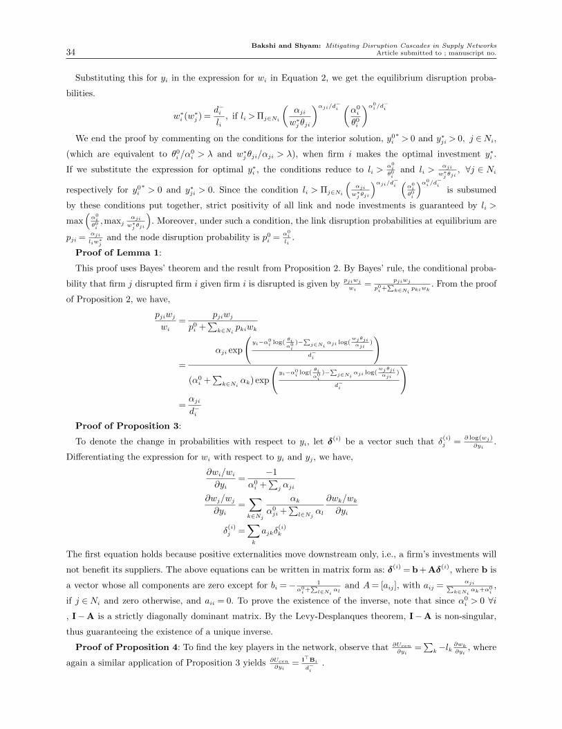
Bakshi and Shyam: Mitigating Disruption Cascades in Supply Networks34 Article submitted to ; manuscript no.
Substituting this for yi in the expression for wi in Equation 2, we get the equilibrium disruption proba-
bilities.
w∗i (w∗j ) =
d−ili, if li >Πj∈Ni
(αjiw∗j θji
)αji/d−i (α0i
θ0i
)α0i /d−i
We end the proof by commenting on the conditions for the interior solution, y0i∗> 0 and y∗ji > 0, j ∈Ni,
(which are equivalent to θ0i /α0i > λ and w∗j θji/αji > λ), when firm i makes the optimal investment y∗i .
If we substitute the expression for optimal y∗i , the conditions reduce to li >α0i
θ0i
and li >αji
w∗jθji, ∀j ∈ Ni
respectively for y0i∗> 0 and y∗ji > 0. Since the condition li > Πj∈Ni
(αji
w∗jθji
)αji/d−i (α0i
θ0i
)α0i /d−i
is subsumed
by these conditions put together, strict positivity of all link and node investments is guaranteed by li >
max(α0i
θ0i,maxj
αji
w∗jθji
). Moreover, under such a condition, the link disruption probabilities at equilibrium are
pji =αji
liw∗j
and the node disruption probability is p0i =α0i
li.
Proof of Lemma 1:
This proof uses Bayes’ theorem and the result from Proposition 2. By Bayes’ rule, the conditional proba-
bility that firm j disrupted firm i given firm i is disrupted is given bypjiwj
wi=
pjiwj
p0i+∑k∈Ni
pkiwk. From the proof
of Proposition 2, we have,
pjiwjwi
=pjiwj
p0i +∑
k∈Nipkiwk
=
αji exp
(yi−α0
i log(θiα0i
)−∑j∈Ni
αji log(wjθjiαji
)
d−i
)
(α0i +∑
k∈Niαk) exp
(yi−α0
ilog(
θiα0i
)−∑j∈Ni
αji log(wjθjiαji
)
d−i
)=αjid−i
Proof of Proposition 3:
To denote the change in probabilities with respect to yi, let δ(i) be a vector such that δ(i)j =
∂ log(wj)
∂yi.
Differentiating the expression for wi with respect to yi and yj , we have,
∂wi/wi∂yi
=−1
α0i +∑
jαji
∂wj/wj∂yi
=∑k∈Nj
αkα0ji +
∑l∈Nj
αl
∂wk/wk∂yi
δ(i)j =
∑k
ajkδ(i)k
The first equation holds because positive externalities move downstream only, i.e., a firm’s investments will
not benefit its suppliers. The above equations can be written in matrix form as: δ(i) = b + Aδ(i), where b is
a vector whose all components are zero except for bi =− 1α0i+∑l∈Ni
αland A= [aij ], with aij =
αji∑k∈Ni
αk+α0i,
if j ∈Ni and zero otherwise, and aii = 0. To prove the existence of the inverse, note that since α0i > 0 ∀i
, I−A is a strictly diagonally dominant matrix. By the Levy-Desplanques theorem, I−A is non-singular,
thus guaranteeing the existence of a unique inverse.
Proof of Proposition 4: To find the key players in the network, observe that ∂Ucen∂yi
=∑
k−lk ∂wk∂yi
, where
again a similar application of Proposition 3 yields ∂Ucen∂yi
= l>Bid−i
.

Bakshi and Shyam: Mitigating Disruption Cascades in Supply NetworksArticle submitted to ; manuscript no. 35
Proof of Proposition 5: We first prove that the central planner’s problem CEN is convex. To this end, we
show that each of the wis are convex functions of y. To see this, take logarithm of wi in Equation 2, and find
that log(wi)s can be expressed as a linear function of the yis, i.e., log(wi) =∑
j∈Niαji/d
−i log(wj)+bi−yi/d−i ,
for some constant bi. Writing this in the form of a matrix, log(w) = A log(w) + b− y, where yi = yi/d−i .
Since I−A is invertible, log(wi) can be expressed as an affine function of the yis, and consequently wi =
ai exp(∑
jbijyj), for some ais and bijs. The convexity of these functions ensures the convexity of the objective
function. Since log(w)s are affine functions of y, the inequalities in Equation 1 define a convex set. Hence
the central planner’s problem is a convex optimisation problem.
The central planner’s payoff function is
Ucen =∑i
(−liwi− yi)
with constraints in Equation 1. The first-order KKT conditions are∑k
lk∂wk∂yi
+ 1−λi = 0,
for i= 1,2, . . . ,N . From the proof of Proposition 3, we have that
∂wk/wk∂yi
=−Bki/d−i =−(I−A)−1ki /d
−i .
Plugging this in the FOC, we have ∑k
lkwk(I−A)−1ki = d−i (1−λi), ∀i.
Moreover for an interior solution with y > 0, (l ◦w)>B = (l ◦w)>(I−A)−1 = d−>. Simplifying this gets
us
liwi = [(I−A)>d−]i = α0i +
∑j∈Ni
αji−αi∑j∈V
1i∈Nj = d−i − d+i ,
for all i. In other words, when the weighted out-degree of all firms is less than the weighted in-degree of
all firms, the expected loss for all firms is equal to the difference between the two in the central planner’s
optimal solution.
Since CEN is convex, the first-order conditions are necessary and sufficient. A solution to the first-order
conditions exists if and only if liw∗i = d−i − d+i > 0. When node inverse sensitivities are lower than their link
counterparts, firms may invest only in nodes, thus rendering an interior solution suboptimal. Substituting
the optimal w∗i in the Equation 1 gives us the condition on the loss terms to guarantee an interior solution.
For part (ii), we use our definition of centrality ρi =∑
klkwkBki.
To find the optimal investments in part (iii), note:
y∗i cen = d−i log(d−i /wi) +∑j∈Ni
αji log
(wjθjiαji
)+α0
i log(θ0i /α0i )
= γi− d−i log(wi) +∑j∈Ni
αji log(wj)

Bakshi and Shyam: Mitigating Disruption Cascades in Supply Networks36 Article submitted to ; manuscript no.
Substituting w∗i =d−i−d+
i
liand simplifying, we find ycen = (D− − A)
∼w+ γ. Proof of Proposition 6: The
inefficiencies of star and linear topologies are as follows.
∆assemblystar = |E|αl + |E|(αn−αl) log
(1− αl
αn
)∆line = |E|αl + (αn−αl) log
(1− αl
αn
)+ (|E| − 1)αn log
(1− αl
αn +αl
)To prove the result, we need to show: (αn − αl) log
(1− αl
αn
)≥ αn log
(1− αl
αn+αl
). Since αn > αl by the
requirement of interior solution in the central planner’s problem, divide both sides by αn and set z = αl/αn.
Now we are left with comparing two functions f(z) = − log(1 + z) and g(z) = (1− z) log(1− z). It is easy
to see that f(z) ≤ g(z) for 0 ≤ z ≤ 1. The argument can be extended to the star distribution network by
observing that ∆diststar = |E|αl + (αn + |E|αl) log
(1− |E|αl
αn
).
Proof of Proposition 7: The decentralised equilibrium for firm i is: −∂liwi/∂yi = 1. The social planner
decides the investment on firm i based on: −∑
k∂lkwk/∂yi = 1. The coordination is achieved if each firm i
can solve the social planner’s problem when deciding optimal investment.
The payoff for firm i in the presence of the given payment mechanism is:
Ui(y) =−liwi− yi−∑l∈Ui
Qil(yl) +∑k∈Di
Qki(yi).
The convexity arguments presented in the proof of Proposition 1 hold, and firm i’s investment is determined
by the FOC: −∂liwi/∂yi +∑
k∈Di∂Qki/∂yi = 1. Since ∂Qki
∂yi=
lkwk(I−A)−1ki
d−i
, using the result of Proposition 3,
we find that ∂Qki/∂yi =−∂lkwk/∂yi.
Since ∂Qki∂yi
= 0 for all k ∈Ui, the FOC of firm i matches with that of the social planner with regard to yi.
Related Documents