Mitigating counterparty risk - bundesbank.de · risk mitigation is taking place in the OTC market despite the high level of collateraliza- tion indicated by recent studies, and that

Discussion PaperDeutsche BundesbankNo 35/2018

Mitigating counterparty risk

Yalin Gündüz

Discussion Papers represent the authors‘ personal opinions and do notnecessarily reflect the views of the Deutsche Bundesbank or the Eurosystem.

Editorial Board:

Deutsche Bundesbank, Wilhelm-Epstein-Straße 14, 60431 Frankfurt am Main,

Postfach 10 06 02, 60006 Frankfurt am Main

Tel +49 69 9566-0

Please address all orders in writing to: Deutsche Bundesbank,

Press and Public Relations Division, at the above address or via fax +49 69 9566-3077

Internet http://www.bundesbank.de

Reproduction permitted only if source is stated.

ISBN 978–3–95729–498–2 (Printversion)

ISBN 978–3–95729–499–9 (Internetversion)

Daniel Foos

Thomas Kick

Malte Knüppel

Jochen Mankart

Christoph Memmel

Panagiota Tzamourani

Non-technical summary

Research Question

We investigate whether financial institutions that are active buyers of credit protection

from a specific counterparty through a purchase of a credit default swap (CDS) protect

themselves by purchasing credit protection on their counterparties. This paper provides

initial evidence that banks and financial institutions do so by purchasing additional CDS

whose reference entity is their counterparty and manage their counterparty risk on weekly

or monthly horizons as evidenced by the transaction-level and position-level information

from the Depository Trust and Clearing Corporation (DTCC).

Contribution

The current regulatory frameworks explicitly formulate that protection purchase on the

counterparty would diminish the regulatory capital requirement, by alleviating the orig-

inal contribution to risk-weighted assets. We argue that these regulatory capital relief

motives that are put forward by Basel III and its European implementation, the Capital

Requirements Regulation, accentuate such mitigation of counterparty risk. We show that

risk mitigation is taking place in the OTC market despite the high level of collateraliza-

tion indicated by recent studies, and that purchasing protection on the reference entities

of counterparties seems to be a reliable method in circumstances where collateral alone

do not provide sufficient protection.

Results and Policy Recommendations

Trading-intensive dealer banks are found to be more active in hedging, both over short and

longer horizons, whereas non-dealer banks appear to manage this risk only over longer,

monthly intervals. Higher stock return and CDS price volatility, lower past stock returns,

and higher CDS prices of the counterparty are shown to be positively related with the

hedging behavior against the counterparty. The sample banks are also shown to mitigate

their counterparty risk by even avoiding wrong-way hedging; in other words, the results

are robust even when the hedging activity from those banks who belong to the same

countries are omitted. Moreover, banks that have a relatively higher exposure to their

counterparties are shown to hedge their counterparty risk more, especially when they have

a lower Tier 1 core capital ratio, thus being relatively less capitalized. Overall, it is in the

best interest of regulatory authorities to set the right incentives for market participants

and clearing houses through an optimal design of the capital regulation of CDSs.

Nichttechnische Zusammenfassung

Fragestellung

Untersucht wird, ob Finanzinstitute, die bei einem bestimmten Geschaftspartner Siche-

rungsinstrumente in Form von Credit Default Swaps (CDS) kaufen, auch ihre Kontrahen-

tenausfallrisiken gegenuber diesem Geschaftspartner absichern, indem sie zusatzliche CDS abschließen, deren Referenzschuldner der Geschaftspartner des Ursprungsgeschafts

ist. Im vorliegenden Forschungspapier werden erste Belege dafur vorgestellt, dass Banken

und Finanzinstitute ihr Kontrahentenrisiko auf wochentlicher bzw. monatlicher Basis

steuern. Grundlage der Untersuchung sind Transaktions- und Positionsdaten der

Depository Trust and Clearing Corporation (DTCC).

Beitrag

Das geltende aufsichtsrechtliche Regelwerk sieht explizit vor, dass sich durch den Erwerb

von Sicherungsinstrumenten, die sich auf den Geschaftspartner beziehen, die Eigenkapi-

talanforderung verringert, indem der ursprungliche Beitrag zu den risikogewichteten Akti-

va niedriger ausfallt. Diese in Basel III und seiner europaischen Umsetzung, der Eigenka-

pitalverordnung (CRR), enthaltenen Vorgaben verstarken unserer Argumentation zufolge

eine derartige Minderung des Kontrahentenrisikos. Wir zeigen, dass die Risikominderung

am OTC-Markt trotz des in aktuellen Studien aufgezeigten hohen Besicherungsgrades

erfolgt und dass der Eingang eines auf den Referenzschuldner des Geschaftspartners bezo-

genen Absicherungsgeschafts eine verlassliche Methode zu sein scheint, wenn die gestellte

Sicherheit alleine keine ausreichende Risikominderung erlaubt.

Ergebnisse

Handelsaktive Dealer-Banken sind unseren Forschungsergebnissen zufolge sowohl uber

kurze als auch uber langere Zeitraume aktiver im Hedging, wahrend andere Banken die-

ses Risiko eher in langeren, monatlichen Intervallen steuern. Eine hohere Aktienkurs- und

CDS-Volatilitat, niedrigere Aktienrendite und ein hoherer CDS-Spread des Geschaftspart-

ners fuhren zu einer Zunahme der Hedging-Aktivitaten gegenuber dem Geschaftspartner.

Ferner mindern die betrachteten Banken der Stichprobe ihr Kontrahentenrisiko auch da-

durch, dass sie Korrelationsrisiken durch “wrong-way Hedging” vermeiden; dementspre-

chend sind die Ergebnisse auch dann robust, wenn die Hedging-Aktivitaten bezogen auf

Banken aus denselben Landern ausgenommen werden. Daruber hinaus wird gezeigt, dass

Banken, die ein relativ hoheres Exposure gegenuber ihrem Kontrahenten haben, ihr Kon-

trahentenrisiko starker absichern, insbesondere wenn sie eine niedrigere Kernkapitalquote

haben und daher weniger kapitalisiert sind. Insgesamt liegt es im eigenen Interesse der Regulierungsbehorden, durch die Ausgestaltung der CDS-bezogenen Eigenkapitalanfor-

derungen die richtigen Anreize fur das Verhalten von Marktteilnehmern und Clearingstel-

len zu setzen.

Bundesbank Discussion Paper No 35/2018

Mitigating Counterparty Risk∗

Yalin GunduzDeutsche Bundesbank

August 14, 2018

Abstract

This paper provides initial evidence on counterparty risk-mitigation activities offinancial institutions on the basis of Depository Trust and Clearing Corporation’s(DTCC) proprietary bilateral credit default swap transactions and positions. Weshow that financial institutions that are active buyers of protection from a spe-cific counterparty undertake successive contracts and purchase protection writtenon them, even avoiding wrong-way risk mitigation. Higher stock return and CDSprice volatility, lower past stock returns, and higher CDS prices of the counter-party are shown to have an increasing effect on the hedging behaviour against thecounterparty. As the current regulatory frameworks explicitly formulate any pro-tection purchase on the counterparty would diminish the required capital, this typeof risk mitigation could follow regulatory capital relief motives and provides a viablehedging instrument beyond receiving coverage through collateral.

Keywords: Credit default swaps, DTCC, OTC markets, hedging, Basel III, CRR.

JEL classification: G11, G21, G23.

∗Yalin Gunduz is a financial economist at the Deutsche Bundesbank, Wilhelm Epstein Strasse14, 60431 Frankfurt, Germany. Tel: +49 (69) 9566-8163, Fax: +49 (69) 9566-4275, E-mail:[email protected]. The author would like to thank Viral Acharya, Patrick Augustin, Evange-los Benos, Boele Bonthuis, Greg Duffee, Falko Fecht, Peter Feldhutter, Daniel Foos (the editor), AndrasFulop, Michael Imerman, Tobias Kreuter, Christoph Memmel, Antonio Mello, Martin Oehmke, GiovanniPetrella, Xiaoling Pu, Emil Siriwardane, Mick Swartz, Henok Tewolde; conference participants at theAmerican Finance Association 2018, Philadelphia; European Banking Authority Policy Research Work-shop 2017, London; Annual Workshop of ESCB Research Cluster 2017, Athens; Financial ManagementAssociation 2016, Las Vegas; European Finance Association 2016, Oslo; Western Economic Association2016, Portland; Midwest Finance Association 2016, Atlanta; Southwestern Finance Association 2016, Ok-lahoma City; International Dauphine-ESSEC-SMU Systemic Risk 2015, Singapore; seminar participantsat the US Commodity Futures Trading Commission (CFTC), US Office of Financial Research, ShandongUniversity, Free University Amsterdam and the Research Council of the Deutsche Bundesbank for help-ful feedback. The author would also like to specially thank to the trade repositories team of DTCC forproviding the transactions and positions data. The views expressed in this paper are those of the authorand do not necessarily coincide with the views of the Deutsche Bundesbank or the Eurosystem.

1 Introduction

The past decade has witnessed the emergence of counterparty credit risk as one of the

potential factors contributing to the systemic nature of the global financial crisis. The

Lehman default spread initial fear as to whether this would trigger a “domino effect”

among major dealers that are involved in a bilateral relationship through financial deriva-

tives, including credit default swaps (CDSs).1 The market for CDSs is a perfect labora-

tory for analyzing how counterparty risk is priced and managed within a system of major

dealers. The systemic role of CDSs was of particular interest during the financial cri-

sis, as the market was criticized for creating a highly dependent default structure among

participants. Nevertheless, extensive government support and supervisory actions have

prevented a systemic breakdown of the financial system.2 Although the recent introduc-

tion of central counterparties (CCPs) as a post-crisis market infrastructure has already

eliminated counterparty risk in centrally cleared trades, many financial products, such

as single-name CDSs are still not mandated to be centrally cleared: There still exists

a major bilateral trading volume between counterparties in the over-the-counter (OTC)

market.3 What remains from the peak period of the crisis is the need to take a closer look

at counterparty credit risk-taking activities of global actors in order to see whether fears

1J.P. Morgan was the pioneer developer of the product in the 1990s, which was initially thought ofas an instrument for hedging the credit risk associated with loans and bonds. The company initiatedan annual payment to the European Bank for Reconstruction and Development (EBRD), making itpossible for the credit risk of a credit line extended to Exxon to be transferred to the EBRD. Whenthe Federal Reserve issued a statement in 1996 suggesting hedging with credit derivatives as a means ofreducing necessary capital, this provided a further catalyst for market development. The CDS market hasgrown significantly since 2001, as the trading of corporate or sovereign-specific default risk through creditderivatives has spread globally. See Augustin, Subrahmanyam, Tang, and Wang (2014) and Augustin,Subrahmanyam, Tang, and Wang (2016) for reviews on the market.

2The all-time peak value of global outstanding notional amounts of CDSs in 2007 gradually reducedduring and after the crisis as a result of bilateral netting, trade compression and maturing contracts; seeStulz (2010) for an evaluation of the CDS market during the global financial crisis.

3The G20 Pittsburgh meetings in 2009 had an agenda item on regulating OTC derivatives markets inorder to create a sound financial architecture after the global financial crisis. Thanks to the “Big Bang”and “Small Bang” protocols issued in 2009, the credit default swap markets currently possess widelyaccepted trading standards. Nevertheless, neither U.S. nor European regulators have yet mandatedcentral clearing of single-name CDSs as of date. Bellia, Panzica, Pelizzon, and Peltonen (2018) documentthat among all transactions in 2016 on German, French and Italian sovereign CDSs, only 48% werecentrally cleared, whereas 42% were not cleared despite being eligible for central clearing.

1

of a systemic breakdown were substantiated.4

In this paper we provide extensive empirical evidence that CDS market participants

actively manage their counterparty risk. We make use of the Depository Trust & Clearing

Corporation’s (DTCC) proprietary dataset on CDS transactions and outstanding posi-

tions between November 2006 and February 2012 in order to explore the hedging behavior

of banks and financial institutions participating in the OTC market. Specifically, we in-

vestigate whether banks or financial institutions that are active buyers of protection from

a global counterparty purchase protection against these counterparties’ credit risk. Our

rich dataset enables us to identify whether (and how) banks active in the CDS market

mitigate their counterparty credit risk positions against global dealers.

The key results are as follows. First, we find evidence that counterparty risk is hedged

over weekly and/or monthly horizons. The banks and financial institutions in our dataset

purchase protection on global financial counterparties once they are protection buyers

from them. In line with previous literature, the economic significance of our results

indicates a hedge proportion of 4-15% on the counterparty, implying that the high degree

of collateralization diminishes the need to fully mitigate counterparty risk. This hedge

proportion should also be read as the extent to which the purchaser of protection would

like to cover any unhedged losses in excess of margin calls of the underlying.

All specifications with this transaction-level dataset provide robust results even with

the inclusion of time (week/month) fixed effects or counterparty-time (week/month) pair

fixed effects that control for any aggregate factors, which may simultaneously drive pro-

tection bought from the counterparty today and protection bought on the counterparty

in the future. These ensure that accounting for counterparty-specific time-variant effects

does not alter the results, and addresses any endogeneity concerns by showing that the

results are not driven by confounding counterparty-specific or aggregate factors in certain

weeks or months.

Second, the dealers in the dataset exhibit a different counterparty risk-mitigation

4Counterparty risk has been empirically shown to have major contagion effects also in credit markets,for instance as in Jorion and Zhang (2009).

2

behavior to that of non-dealers. Non-dealers, which are typically small and medium-sized

banks, are identified as actively hedging their counterparty risk only at longer, monthly

intervals, whereas dealers are shown to be managing this risk by hedging over both short

and longer horizons. These results can be interpreted by considering the accumulation

of counterparty risk to be slower for non-dealers in comparison to that of dealers. Non-

dealers might have certain thresholds or ratios for the open interest, and this might be the

reason why they hedge less frequently. A similar possibility might be the lower frequency

of risk management activities at non-dealer institutions, which fix hedging action deadlines

during less frequent meetings.

Third, we utilize also a position-level dataset in order to carve out the causal effects of

shocks on the CDS prices of all reference entities traded between the bank-counterparty

pairs. The individual price changes of the underlyings in the inventories of our banks

create an aggregate exogenous effect on the counterparty risk of the dealer which our

banks have these positions with. This identification strategy enables us to show that the

results are robust each time a price shock increases the risk of the global dealers for our

sample banks.

Fourth, we consider if our banks and financial institutions avoid “wrong-way risk”,

which arises when banks intend to mitigate their counterparty risk through the purchase

of protection on their counterparty from a third party that is highly correlated with their

initial counterparty. In a systemic view, it would not be optimal to purchase protection

from this third party on the initial counterparty, since they may jointly enter into trouble.

We show that our financial institutions avoid this type of wrong-way risk mitigation by

purchasing protection from counterparties that do not belong to the same country as the

global dealer on which protection is sought. This indeed provides evidence on the careful

risk management policies of financial institutions.

Finally, interacting the Tier 1 core capital ratios of our sample banks with the pro-

tection purchase activity indicates that mitigation of counterparty risk is consistent with

regulatory capital relief motives, since banks that are relatively less capitalized and make

3

a relatively larger net purchase from their counterparties are shown to mitigate their

counterparty risk to a higher extent. This motive could naturally follow the Basel III reg-

ulations and its European implementation, the Capital Requirements Regulation (CRR),

which explicitly incentivize purchasing protection on counterparties as a way of risk mit-

igation.

Overall, the focus on bilateral OTC activity enables us to identify this mitigation

whenever it takes place in the absence of a central counterparty. Given that single-name

CDSs have not yet been mandated to be centrally cleared by any regulation, the paper

points to the additional cost of bilateral OTC trading. Non-centrally cleared single-name

CDSs still represent an important share of the global activity, which holds back the phe-

nomenon documented in this paper to be outdated. Even if the introduction of central

clearing has phased out the creation of further counterparty risk to a certain degree, it

did not eliminate the necessity of regularly mitigating it; such that the Basel III and the

European CRR formulate any protection purchase on the counterparty to be subtracted

from the credit exposure for regulatory capital calculation.

Related Literature

By providing initial evidence of counterparty risk-mitigating activities at the contract

level, this paper adds to the scarce empirical literature. This has been made possible by

the DTCC dataset, which enables us to uniquely identify the protection purchase activities

on the counterparties to which our banks are most heavily exposed. Arora, Gandhi, and

Longstaff (2012) was the first study to focus on the price effects of counterparty risk.

They showed that as the credit risk of 14 major CDS dealers increases, the price at which

these dealers sell protection decreases. Nevertheless, the effect in question is of negligible

magnitude. The CDS price of the dealers needs to increase by 645 basis points for it to

cause a one basis point price decline of the CDS sold. The authors document the market

practice of full collateralization in the CDS market as a key reason for this extremely

small effect. In this paper, we provide significant evidence of managing counterparty risk-

4

mitigation activities that go beyond the prevailing emphasis on collateralization in the

market, and extend the results of Arora et al. on pricing to management of counterparty

risk.

In a similar effort, a recent paper by Du, Gadgil, Gordy, and Vega (2016) confirms

the findings of Arora et al. (2012), demonstrating that counterparty risk does not affect

any CDS contract pricing. On the other hand, they provide evidence indicating that

the participants prefer to trade with counterparties whose default risk is low and less

correlated with those of the underlying entities. Our paper complements their findings

on showing the financial institutions’ preference to hedge counterparties with lower past

stock returns, higher stock return volatility and higher CDS volatility, while they avoid

wrong-way risk mitigation. Interestingly, their finding that central clearing is associated

with lower spreads contradicts the results of Loon and Zhong (2014), who attribute the

higher spreads to the added value of central clearing to the mitigation of counterparty

risk. Overall, our paper adds to the growing literature on bilateral counterparty risk-

taking activities through its insights based on OTC transactions in the DTCC dataset.

There is also a growing body of theoretical analysis that draws attention to regulatory

capital relief motives of banks for purchasing protection through CDS. Klingler and Lando

(2018) concentrate only on sovereign states as counterparties and build a model to argue

that banks find it necessary to purchase CDS written on their sovereign counterparties

in order to hedge their counterparty risk. Our analysis provides granular evidence that

the authors’ theory could be well extended to any counterparty, since Basel III and CRR

regulations do not limit capital relief for any type of counterparty. Yorulmazer (2013)

focuses in his model also on the regulatory capital relief through CDS purchases. He

draws attention to adverse effects of these incentives that lead to excessive risk-taking.

Our study takes up the debate on these regulatory motives and aims at providing first

empirical evidence on risk mitigation.5

5Other important analyses on counterparty risk include Cooper and Mello (1991), Duffie and Huang(1996), Jarrow and Yu (2001), Hull and White (2001), Kraft and Steffensen (2007), Thompson (2010)and Morkoetter, Pleus, and Westerfeld (2012). More recently, Duffie and Zhu (2011), Biais, Heider, andHoerova (2016), Acharya and Bisin (2014) and Duffie, Scheicher, and Vuillemey (2015) have studied the

5

Finally, our paper contributes to the expanding strand of literature that utilizes DTCC

data to analyze various features of credit default swaps, although they do not focus di-

rectly on counterparty risk. As outlined by Augustin et al. (2014), the CDS literature is

growing; however there is a recent tendency to utilize transaction and position-level data

to the extent of availability. In one of the first papers with CDS transaction data from

the DTCC, Gehde-Trapp, Gunduz, and Nasev (2015) consider whether microstructural

frictions are priced in CDS transactions. They find that larger transactions have a higher

price impact and that traders charge higher premiums not for compensating asymmetric

information, but rather as a price for liquidity provision. In effect, buy-side investors

are charged higher prices than major CDS dealers for demanding liquidity. Siriwardane

(2016) also uses transaction-based DTCC data and examines how capital fluctuations of

large protection sellers are an important determinant of CDS spreads. Oehmke and Za-

wadowski (2017) explain net notional CDS outstanding by bonds outstanding of the same

entity through the usage of aggregate public DTCC information, in order to interpret

hedging and speculation effects. Recently, Biswas, Nikolova, and Stahel (2015) estimate

transaction costs showing that effective spreads are larger for actively traded CDS. The

transaction costs of the bonds they reference are not necessarily higher in terms of the

effective spreads; for large trade sizes, trading bonds is cheaper. Focusing on an entirely

different research question, Gunduz, Ongena, Tumer-Alkan, and Yu (2017) couple pro-

prietary CDS positions from DTCC with a credit register containing bilateral bank-firm

credit exposures, concluding that there has been an increase in hedging activity with CDS

for credit lending relationships to riskier firms following the Small Bang event.

This paper is organized as follows. Section 2 introduces the counterparty risk that

exists in OTC markets. In Section 3, we provide a description of our DTCC transaction

and position-level datasets. Next, in Section 4, we present our empirical results, which

provide evidence of the counterparty risk-mitigation activities in OTC markets. Section

5 sets out our conclusions.

impact of central clearing.

6

2 Counterparty Risk in the CDS Market

A single-name CDS trade can be thought of as an act of purchasing protection against

the default of a certain underlying reference entity from a protection seller, who contrarily

is interested in increasing its credit risk exposure on the entity. Once both parties have

agreed on a credit risk transfer, the protection buyer is basically insured against the default

of the reference entity, whereas now the seller of the protection bears the default risk. If

a “credit event” in line with the circumstances of default according to the protocols of

the International Swaps and Derivatives Association (ISDA) occurs prior to the contract

maturity, the seller is obliged to transfer the full notional amount in exchange for post-

default deliverable bonds of the reference entity. Meanwhile, the buyer of the contract

makes quarterly installments to the seller, so-called “CDS premium” payments, as a

typical insurance fee. Figure 1 shows the basic structure of a CDS transaction.

Figure 1: A typical CDS transaction that transfers the underlying reference entity’s defaultrisk.

The risk of the protection buyer not receiving the notional payment due to financial

constraints of the seller, even if the reference entity defaults, can be referred to as the

“counterparty risk” in CDS contracts. If the counterparty faces financial difficulties in

7

parallel to the reference entity, there is a danger that the buyer of the initial protection will

not receive his notional payment. Nevertheless, counterparty risk persists not just during

a credit event relating to the reference entity but at any time when the counterparty is

in financial trouble, since marking-to-market agreements and the need to post additional

collateral can threaten its position as a viable reverse side of the contract. In order to

assess their expected loss from the default of their counterparties, financial institutions

calculate their credit valuation adjustment, or CVA, which is counterparty-specific and is

a product of the probability of default, loss given default and expected net exposure for

the counterparty. An increase in CVA is deducted from the reported income of dealers,

so that there is a general interest in keeping the counterparty-specific credit exposure at

lower levels. This counterparty-specific credit risk has also been introduced as a capital

charge under the Basel III regulations that are published in December 2010 and updated in

June 2011, as part of the set of risk management measures taken by the Basel Committee

of Banking Supervision in response to the global financial crisis (Basel Committee on

Banking Supervision (2011)).

How can the buyer protect himself against the possibility of deteriorating counterparty

credibility? Typically, ISDA master agreements and protocols provide a framework for

a healthy bilateral relationship between transacting parties. Most importantly, the high

degree of collateralization in the CDS market secures the system against any derailing.

In this paper, we specifically look at the counterparty risk-mitigation activity of buyers

of protection who might prefer to actively manage their risk above and beyond master

agreements and collateralization. Specifically, we investigate whether German banks that

are active buyers of CDS protection from one global counterparty undertake successive

contracts and purchase protection written on these global players. Providing significant

evidence on mitigation of counterparty risk even only on bilateral CDS exposures indi-

cates that a much higher degree of counterparty risk mitigation should be taking place if

exposures from interest rate and FX swaps were included.

Our analysis has implications for the degree of hedging CVA accounts as well, since any

8

counterparty-specific credit risk exposure, including interest rate or FX swaps, needs to be

mitigated for accounting purposes. Besides risk-mitigation motives, there is a regulatory

incentive following Basel III (Basel Committee on Banking Supervision (2011)) and its

European implementation, the CRR (Capital Requirements Regulation (CRR) (2013)).

According to Basel III, banks can alleviate the contribution to risk-weighted assets that

arises through any counterparty credit risk exposure by purchasing protection on their

counterparties. Similarly, CRR Article 386 specifically refers to the mitigation of CVA

risk such that banks and financial institutions could also get capital relief from regulatory

requirements through purchasing a single-name or index CDS on their counterparties,

since any protection purchase on the counterparty is subtracted from the exposure for

regulatory CVA capital calculation (CRR, Article 384). Given that the capital charge

arising from the exposure to the new counterparty is only contingent to the default of the

initial counterparty, this type of mitigation is a regulatory desired way to diversify risk,

even if the rating implied capital surcharge of the initial and new counterparty are similar.

The evidence we provide is an indication that hedging of counterparty risk follows not

only risk-mitigation motives but regulatory capital relief motives as well.

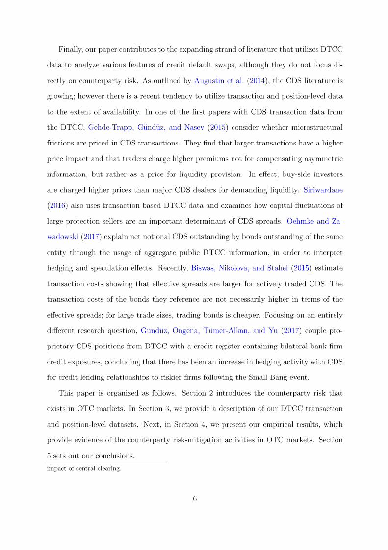
Figure 2 provides an illustrative example of possible time t+1 activity for Bank AAA,

which faces the counterparty risk of Bank BBB after a trade at time t.

Testing whether Bank AAA actively takes action to mitigate counterparty risk of Bank

BBB at t+1 is central to our analysis. Such an investigation could not have been made in

the past, as bilateral transaction data on CDS has only recently become available through

trade repositories. Our proprietary DTCC data on CDS transactions is presented in the

next section.

9

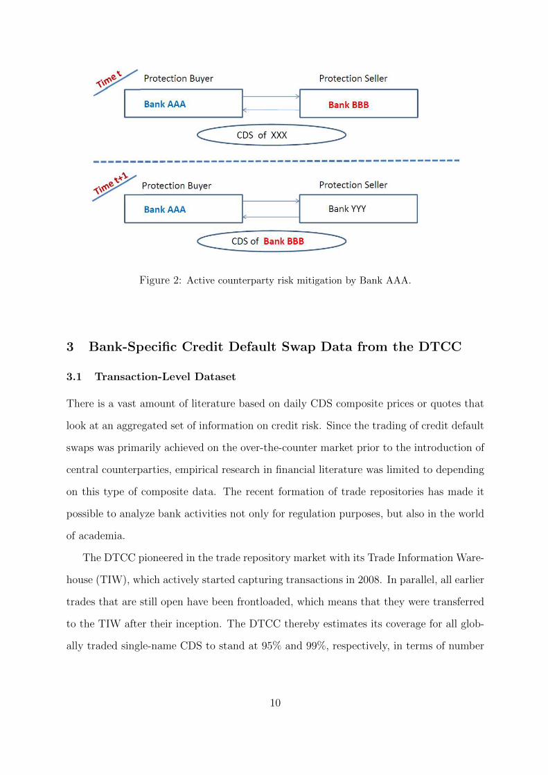
Figure 2: Active counterparty risk mitigation by Bank AAA.

3 Bank-Specific Credit Default Swap Data from the DTCC

3.1 Transaction-Level Dataset

There is a vast amount of literature based on daily CDS composite prices or quotes that

look at an aggregated set of information on credit risk. Since the trading of credit default

swaps was primarily achieved on the over-the-counter market prior to the introduction of

central counterparties, empirical research in financial literature was limited to depending

on this type of composite data. The recent formation of trade repositories has made it

possible to analyze bank activities not only for regulation purposes, but also in the world

of academia.

The DTCC pioneered in the trade repository market with its Trade Information Ware-

house (TIW), which actively started capturing transactions in 2008. In parallel, all earlier

trades that are still open have been frontloaded, which means that they were transferred

to the TIW after their inception. The DTCC thereby estimates its coverage for all glob-

ally traded single-name CDS to stand at 95% and 99%, respectively, in terms of number

10

of contracts and notional amounts (Gunduz et al. (2017)). A summary of the growing

academic literature using TIW data of the DTCC can be found in Acharya, Gunduz, and

Johnson (2018).

The DTCC provided access to all CDS transactions of German banks and financial

institutions, as well as the positions associated with these transactions. Our baseline

transaction-level dataset encompasses all new trades from November 2006 to February

2012. These are the actual new CDS transactions bought (sold) by German financial

institutions from (to) any global counterparty, as well as any CDS contracts bought or

sold on these counterparties where they are a reference entity. The DTCC tags financial

institutions in the CDS market as “dealer” or “buyside”. Prior research shows that coun-

terparties tagged as “dealers” by the DTCC are either on the buy (85%) or the sell side

(89%) of a CDS trade. The full universe of TIW positions confirms this high concentra-

tion (89% for being on the buy or sell side) with publicly available data (Gunduz et al.

(2017)). Since our sample includes all the trading activity with these global dealers, it is

highly representative of the global CDS trading which is known to have dealer dominance.

Moreover, focusing on dealers as the counterparties for German financial institutions has

the advantage of avoiding the usage of transactions by counterparties that rarely trade

and/or are rarely traded as a reference entity.

A group of 25 German banks and financial institutions reside in our sample, the aim

being to look at their counterparty risk-mitigation behavior. Their names could not be

explicitly mentioned due to confidentiality reasons. On the other hand, Table 1 consists

of the 21 counterparties that DTCC tags as global dealers.6,7

All of the new CDS protection bought from these dealers, as well as all of the new

CDS bought on these dealers as reference entities, will be investigated concurrently in

6It should be noted that these include the G14 dealers: Bank of America-Merrill Lynch, BarclaysCapital, BNP Paribas, Citi, Credit Suisse, Deutsche Bank, Goldman Sachs, HSBC, JP Morgan, MorganStanley, RBS, Societe Generale, UBS, and Wells Fargo Bank. Peltonen, Scheicher, and Vuillemey (2014)provide empirical evidence that the CDS market is centered around G14 dealers.

7It should be noted that Deutsche Bank AG and Commerzbank AG are present in both samples. Forour purposes, they will serve as German banks when their counterparty risk-taking behavior on dealers isbeing investigated, and as dealers against other German banks and financial institutions whenever theyact as counterparties for the remaining 23 institutions included in our German sample.

11

Table 1: List of 21 global dealers in our sample that act as counterparties.

Banco Santander, S.A.Bank of America CorporationBarclays Bank PLCBNP ParibasCitigroup Inc.Commerzbank AGCredit Agricole SACredit Suisse GroupDeutsche Bank AGHSBC Bank PLCJPMorgan Chase & Co.Lehman Brothers Holdings Inc.Morgan StanleyNatixisNomura Holdings, Inc.Royal Bank of Scotland Group PLCSociete GeneraleThe Goldman Sachs Group, Inc.UBS AGUniCredit S.p.A.Wells Fargo & Co.

this study. Figures 3 and 4 shed light on the time series development of the counterparty

risk-taking and mitigation activities of German banks on global dealers. In Figure 3,

it can be seen that purchasing protection from dealers reached an all-time high of 600

new contracts during the week of September 15-19, 2008, at the peak of the subprime

mortgage crisis when Lehman Brothers defaulted, and then partly slowed down towards

the end of our sample period. We term this type of transactions as “SEL”, where the

global counterparty acts as the seller of the contract. Similarly, Figure 4 shows that

purchasing protection on dealers reached a value of 235 new contracts during the same

week in which Lehman Brothers defaulted, but as the tensions in the financial markets

eased, the number of new contracts purchased on global counterparties decreased as well.

In the following, we will term these type of transactions as “RED”, where the global

counterparty acts as the reference entity of the contract.8

8The RED abbreviation comes from Markit company’s notation for “Reference Entity Database”

12

Figure 3: Time series development of weekly aggregate protection purchases from a globaldealer counterparty (SEL-type transactions).

Figure 4: Time series development of weekly aggregate protection purchases on a global dealercounterparty (RED-type transactions).

Table 2 shows basic statistics of the transaction dataset from the perspective of Ger-

man financial institutions. Although we will initially focus on protection purchase from

global dealers, the protection sold to these dealers is important to arrive at a net purchas-

13

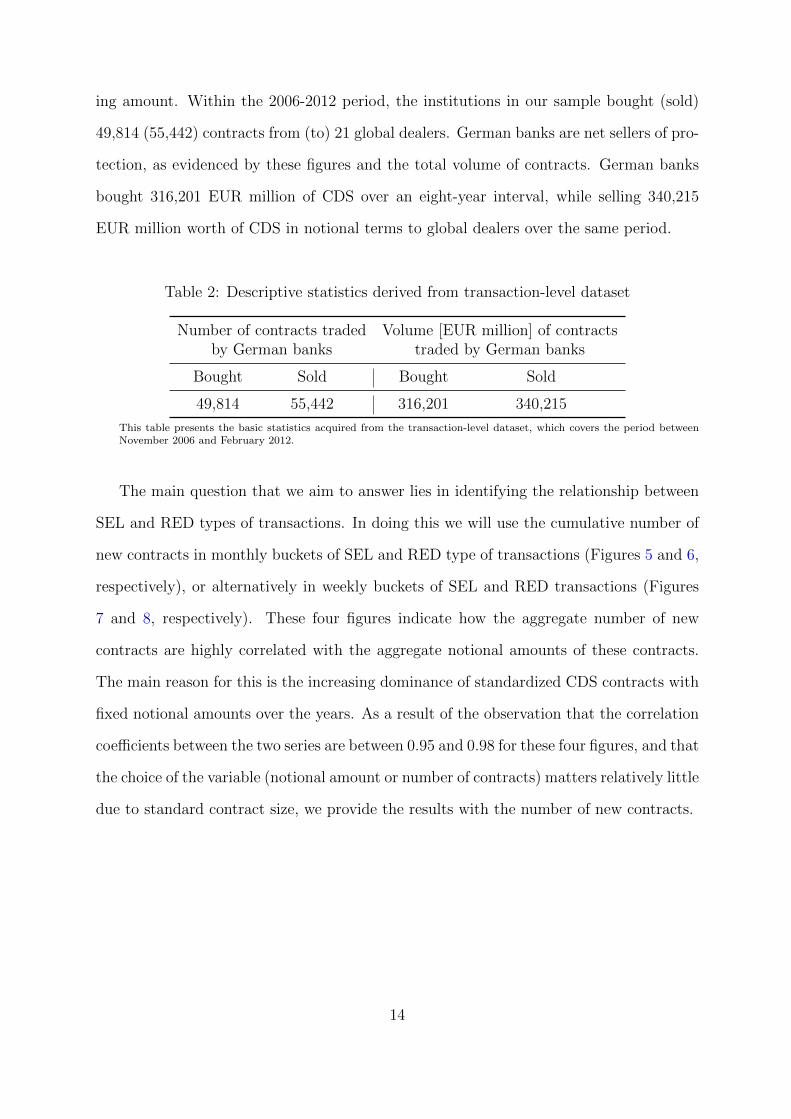
ing amount. Within the 2006-2012 period, the institutions in our sample bought (sold)

49,814 (55,442) contracts from (to) 21 global dealers. German banks are net sellers of pro-

tection, as evidenced by these figures and the total volume of contracts. German banks

bought 316,201 EUR million of CDS over an eight-year interval, while selling 340,215

EUR million worth of CDS in notional terms to global dealers over the same period.

Table 2: Descriptive statistics derived from transaction-level dataset

Number of contracts traded Volume [EUR million] of contractsby German banks traded by German banks

Bought Sold Bought Sold

49,814 55,442 316,201 340,215

This table presents the basic statistics acquired from the transaction-level dataset, which covers the period betweenNovember 2006 and February 2012.

The main question that we aim to answer lies in identifying the relationship between

SEL and RED types of transactions. In doing this we will use the cumulative number of

new contracts in monthly buckets of SEL and RED type of transactions (Figures 5 and 6,

respectively), or alternatively in weekly buckets of SEL and RED transactions (Figures

7 and 8, respectively). These four figures indicate how the aggregate number of new

contracts are highly correlated with the aggregate notional amounts of these contracts.

The main reason for this is the increasing dominance of standardized CDS contracts with

fixed notional amounts over the years. As a result of the observation that the correlation

coefficients between the two series are between 0.95 and 0.98 for these four figures, and that

the choice of the variable (notional amount or number of contracts) matters relatively little

due to standard contract size, we provide the results with the number of new contracts.

14

Figure 5: Volume and number of transaction in which protection is purchased from a globaldealer counterparty (SEL-type), aggregated in monthly buckets.

Figure 6: Volume and number of transaction in which protection is purchased on a global dealercounterparty (RED-type), aggregated in monthly buckets.

15

Figure 7: Volume and number of transaction in which protection is purchased from a globaldealer counterparty (SEL-type), aggregated in weekly buckets.

Figure 8: Volume and number of transaction in which protection is purchased on a global dealercounterparty (RED-type), aggregated in weekly buckets.

16

The balance sheet and financial characteristics of the 21 global dealers that act as

counterparties are presented in Table 3. In addition to our main interest, that is, whether

SEL type of transactions are followed by RED transactions, we would also like to un-

derstand whether certain financial features of the global dealers cause German banks to

undertake more hedging of their risk. It can be seen that the global dealers in our sample

have quite a large asset size (an average of 1.2 EUR trillion), are highly leveraged, and do

not have liquidity constraints in the median. Since our observation period encompasses

the subprime mortgage crisis, the very high maximum values for stock volatility and CDS

price levels coincide with the peak of the financial crisis in 2008. Although some global

counterparties may be safe, as a minimum CDS price of 4 bps indicates, an average CDS

price value of 122 bps and a standard devaition of 88 bps show that the variation in dealer

riskiness is quite high.

Table 3: Summary statistics for financial variables of 21 global dealers

VARIABLES N Mean S.D. Min p10 p50 p90 Max

Total Assets (EUR billion) 5,019 1,208.90 549.50 156.35 544.56 1,147.22 1,917.66 3,027.84Capital Structure 5,019 0.95 0.02 0.89 0.91 0.95 0.97 0.99Current Ratio 5,019 1.17 0.56 0.26 0.63 1.07 1.81 4.77Stock Return (%) 5,019 -0.14 2.11 -42.98 -1.87 -0.11 1.61 16.75Stock Volatility 5,019 1.48 2.07 0.01 0.16 0.82 3.51 25.24CDS Volatility (bps) 5,019 7.10 13.71 0.01 0.87 4.28 14.42 411.00CDS Price (bps) 5,019 122.61 89.67 4.28 28.87 106.33 222.41 1,182.35

This table contains summary statistics for financial variables of 21 global dealers as counterparties. Listed in the table areweekly summary statistics (number of observations, mean, standard deviation, minimum, 10th, 50th and 90th percentiles,and maximum) in the sample period between November 2006 and February 2012. Quarterly values for Total Assets, CaptialStructure and Current Ratio are repeated in this table as weekly observations, since the following regression analyses makesuse of weekly data points. Total Assets of the 21 global counterparties are in billion euros. Capital Structure is definedas total liabilities divided by total assets. Current Ratio is defined as one-year liquid assets (marketable securities, othershort-term investments, cash and cash-near items) over one-year liabilities (short-term borrowing, securities sold as repos,short-term liabilities and customer accounts). Stock Return and Stock Volatility are defined as geometric average of tradingweek stock return and the standard deviation of trading week stock returns of the global counterparty, respectively. CDSVolatility is the standard deviation of CDS price levels of the trading week, whereas CDS price is the arithmetic averageCDS spread level of the same week. Data sources are Bankscope, Bloomberg and Markit.

3.2 Position-Level Dataset

The position-level dataset from DTCC provides an alternative answer to the research

question. In contrast to the “flow” information provided by the transaction-level dataset,

the position-level dataset contains “stock” information. These snapshots encompass the

17

January 2008 to February 2012 weekly CDS positions of all the above-mentioned 25

financial institutions. Although the DTCC started building its database in 2008, the

position dataset contains all the prior transactions that are frontloaded as well. Moreover,

this dataset serves as a perfect tool for testing the robustness of the transaction-level

results, since all other types of CDS transactions, such as assignments, amendments,

and terminations are now embedded in the information in the number of open contracts.

Moreover, the maturity of each new transaction is automatically accounted for when all

open trades in the position level dataset are considered.

Table 4 Panel A provides basic descriptive statistics on the weekly average number of

open contracts of banks and institutions in our sample on dealer banks as the underlying,

and on dealer banks as the counterparty. Although the confidential nature of the data

does not allow for the disclosure of bank-level statistics, the aggregated statistics already

show the proportional dominance of dealer banks acting as a counterparty, as opposed to

their credit risk being traded by the institutions in our sample. In an average week there

are 710 (698) open CDS contracts where the dealer bank acted as a seller (buyer) against

our 25 institutions, whereas these institutions traded the credit risk of dealers by only 42

(41) open CDS contracts by buying (selling) their CDS where they are a reference entity.

Similarly, Panel B of Table 4 presents statistics on the weekly average of the total

volume of open contracts for the financial institutions in our sample. It is evident that

German banks do not predominantly take long or short positions on dealer banks as the

underlying on aggregate terms, since the average long volume (351.19 EUR million) and

the average short volume (353.56 EUR million) are not far apart. On the other hand, the

German banks are net sellers of protection to 21 global dealers, indulging in a net selling

of 255.38 EUR million when weekly average volumes of open contracts are considered.

Naturally, our position-level dataset only enables tracking of CDS positions in the

form of weekly snapshots. These might not reveal actual risk-taking activity, as contracts

that mature automatically drop from this dataset, thus lowering the respective number

and volume of contracts. Although it may be argued that maturing bought contracts

18

Table 4: Descriptive statistics derived from position-level dataset

Panel A: Weekly average of number of open contracts by German banks

Dealer Bank as Counterparty Dealer Bank as Underlying

Bought From Sold To Bought On Sold On

Mean 710.32 697.53 42.06 41.07p5 0 0 0 0p50 19 28 3 6p95 2865 2904 274 243

Panel B: Weekly average of total volume [EUR million] of open contracts

Dealer Bank as Counterparty Dealer Bank as Underlying

Bought From Sold To Net Bought On Sold On Net

Mean 7,414.61 7,670.00 -255.38 351.19 353.56 -2.37p5 0.00 0.00 -2,318.82 0.00 0.00 -191.20p50 182.00 282.29 -18.30 30.00 55.00 -10.00p95 33,137.88 33,695.65 1,187.27 1,867.48 1,772.78 297.83

This table presents the basic statistics acquired from the position-level dataset, which covers the period betweenJanuary 2008 and February 2012.

would, on average, be equivalent to maturing sold contracts, the position-level dataset

will be an ideal tool to be utilized in Section 4.3 for a better identification through price

shocks to the individual position with the counterparty. All in all, both datasets will be

important sources for understanding risk-taking activities by the financial institutions in

our sample. The findings from the two datasets would complement each other in this

manner.

4 Empirical Analysis

4.1 Evidence of Risk Mitigation from Baseline Transaction Datasets

We are initially interested in the trading activity in weekly or monthly terms. Our se-

lection of alternative time intervals overlaps with the margin period at risk for CVA

calculation. The so-called “cure period” is the time that elapses between when the coun-

terparty ceases to respond to margin calls and the financial institution is able to hedge

19

this uncovered risk. This can be regarded as the actual grace period in which no collat-

eral is posted and the institution is exposed to naked counterparty risk, and therefore the

institution takes action in order to cover remaining exposure. In practice, a cure period of

10 to 25 business days is typical.9 It is initially hypothesized that the banks and financial

institutions in our sample undertake trading activity in the form of CDS purchasing on

a global counterparty as an underlying entity following a month of CDS purchases from

that same global counterparty. By collecting the flow information in monthly buckets (a

time interval of 20 business days), any successive hedging activity can be identified at

rolling intervals.10 The first specification we examine is as follows:

4∑k=1

REDi,j,t+k = a0 + a1

3∑k=0

SELi,j,t−k + a2Xj,t + FE + εi,j,t (1)

where SEL is the cumulative number of contracts bought by the German bank i when

the counterparty j acts as a seller between (and including) weeks t = −3 and t = 0,

and RED is the cumulative number of contracts bought by the German bank i where

the counterparty j is a reference entity between (and including) weeks t = 1 and t =

4. We expect a positive coefficient for a1 if the banks i aim at hedging their risk on

counterparties j on monthly rolling horizons. Vector X represents the counterparty-

specific variables such as total assets, capital structure, current ratio (of their last quarter),

geometric average stock return and volatility (in their last month), and average CDS

price and volatility (in their last month). All specifications are alternatively tested using

bank fixed effects, counterparty fixed effects and bank-counterparty pair fixed effects. In

this way, we are able to address any idiosyncratic effects arising from our banks and

their counterparties. In addition, all specifications include time (month) fixed effects

or counterparty-time (month) pair fixed effects in order to control for any aggregate

9In a recent study, Andersen, Pykthin, and Sokol (2017) calibrate their counterparty risk model witha margin period at risk assumption of 10 business days for the benchmark case, and 15 business days forthe conservative case.

10In this way, the rolling methodology could also capture any chain of consecutive hedging on eachnext counterparty.

20

factors that may simultaneously drive protection bought from the counterparty today

and protection bought on the counterparty in the future. As a robustness, we also add

the lagged value of the protection purchased on the counterparty as a regressor in order

to obtain a dynamic setup, which controls for serial correlation that might arise due to

institutions buying protection in one week being likely to buy protection in the following

week. All errors are clustered at the bank level or alternatively at the bank-counterparty

pair level.

Table 5 presents the results of the baseline dataset of monthly cumulative rolling

transactions. The main variable of interest, the monthly lagged cumulative new trans-

actions of protection bought from the counterparty, is positive, and always significant in

explaining the following month’s cumulative new protections bought on the counterparty.

Even the highly constraining bank-counterparty pair fixed effect (with more than 200

dummies) in specifications (4),(5),(10) and (11) does not diminish the significance of the

main variable of interest. It is important to underline that the significance is also persis-

tent, regardless of whether the errors are clustered at bank level (with 24-25 clusters) or

bank-counterparty pair level (with more than 200 clusters).11 Finally, the a1 parameter,

which is significantly positive even in specifications (6) and (7), ensures that accounting

for counterparty-specific time-variant effects does not alter the results, and addresses any

endogeneity concerns by showing that the results are not driven by counterparty-specific

or aggregate factors in certain months.12,13

11When there is a small number of clusters, or when there are very unbalanced cluster sizes, the inferenceusing the cluster-robust estimator may be biased. As long as bank-level clustering is undertaken, ourdealer banks have a higher number of observations than non-dealer banks, which makes it necessary tocheck the robustness of the results to bank-counterparty pair clustering.

12An alternative specification that was looked at used the net (bought - sold) number of new trans-actions traded with/on the counterparty. The main variable of interest was still significantly positive,and the magnitude was naturally lower. The results are therefore robust when protections sold to/on thecounterparty are considered.

13Notice that our panel is not balanced. We set absent RED type of activity of a bank on a dealer to azero value, whereas we set absent SEL type of activity of a bank with a dealer to a missing observation.The reasoning behind this choice is that absent RED activity contributes the analysis with useful infor-mation, such that our banks that initially purchase CDS from global dealers might eventually purchaseor may not purchase CDS on these counterparties (non-zero or zero hedging activity). Therefore, includ-ing absent RED activity as a zero value in the panel biases our results downwards, but is economicallynecessary. In undocumented results, our main finding is shown to be robust when only observations ofnon-zero hedging activity are utilized (by setting all absent RED activity to missing values), albeit with

21

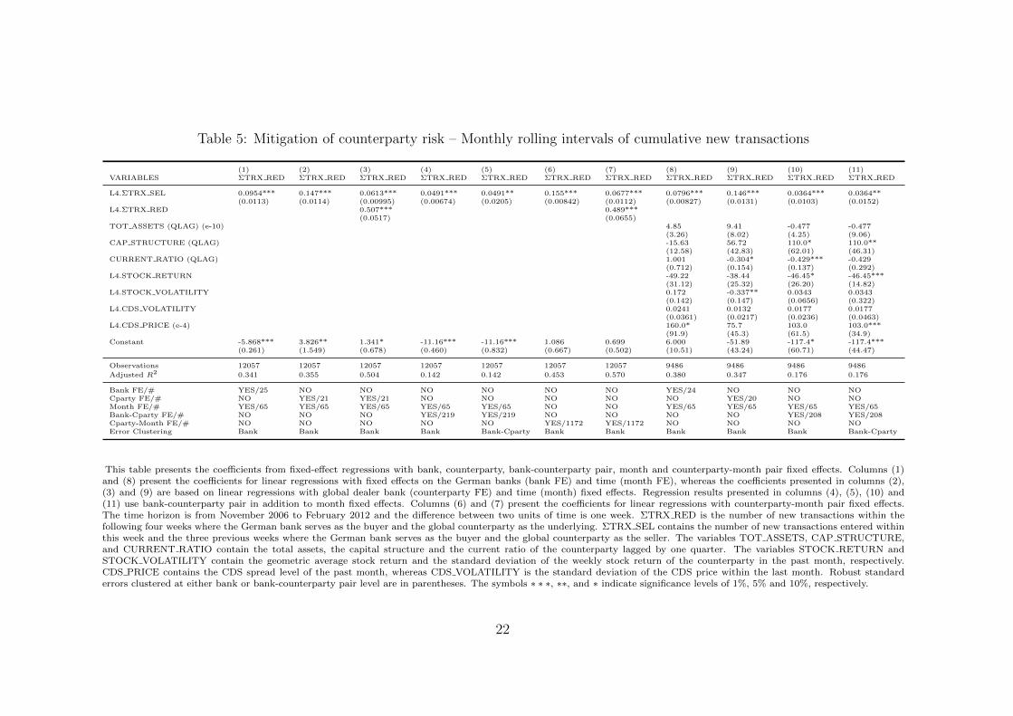
Table 5: Mitigation of counterparty risk – Monthly rolling intervals of cumulative new transactions

(1) (2) (3) (4) (5) (6) (7) (8) (9) (10) (11)VARIABLES ΣTRX RED ΣTRX RED ΣTRX RED ΣTRX RED ΣTRX RED ΣTRX RED ΣTRX RED ΣTRX RED ΣTRX RED ΣTRX RED ΣTRX RED

L4.ΣTRX SEL 0.0954*** 0.147*** 0.0613*** 0.0491*** 0.0491** 0.155*** 0.0677*** 0.0796*** 0.146*** 0.0364*** 0.0364**(0.0113) (0.0114) (0.00995) (0.00674) (0.0205) (0.00842) (0.0112) (0.00827) (0.0131) (0.0103) (0.0152)

L4.ΣTRX RED 0.507*** 0.489***(0.0517) (0.0655)

TOT ASSETS (QLAG) (e-10) 4.85 9.41 -0.477 -0.477(3.26) (8.02) (4.25) (9.06)

CAP STRUCTURE (QLAG) -15.63 56.72 110.0* 110.0**(12.58) (42.83) (62.01) (46.31)

CURRENT RATIO (QLAG) 1.001 -0.304* -0.429*** -0.429(0.712) (0.154) (0.137) (0.292)

L4.STOCK RETURN -49.22 -38.44 -46.45* -46.45***(31.12) (25.32) (26.20) (14.82)

L4.STOCK VOLATILITY 0.172 -0.337** 0.0343 0.0343(0.142) (0.147) (0.0656) (0.322)

L4.CDS VOLATILITY 0.0241 0.0132 0.0177 0.0177(0.0361) (0.0217) (0.0236) (0.0463)

L4.CDS PRICE (e-4) 160.0* 75.7 103.0 103.0***(91.9) (45.3) (61.5) (34.9)

Constant -5.868*** 3.826** 1.341* -11.16*** -11.16*** 1.086 0.699 6.000 -51.89 -117.4* -117.4***(0.261) (1.549) (0.678) (0.460) (0.832) (0.667) (0.502) (10.51) (43.24) (60.71) (44.47)

Observations 12057 12057 12057 12057 12057 12057 12057 9486 9486 9486 9486

Adjusted R2 0.341 0.355 0.504 0.142 0.142 0.453 0.570 0.380 0.347 0.176 0.176

Bank FE/# YES/25 NO NO NO NO NO NO YES/24 NO NO NOCparty FE/# NO YES/21 YES/21 NO NO NO NO NO YES/20 NO NOMonth FE/# YES/65 YES/65 YES/65 YES/65 YES/65 NO NO YES/65 YES/65 YES/65 YES/65Bank-Cparty FE/# NO NO NO YES/219 YES/219 NO NO NO NO YES/208 YES/208Cparty-Month FE/# NO NO NO NO NO YES/1172 YES/1172 NO NO NO NOError Clustering Bank Bank Bank Bank Bank-Cparty Bank Bank Bank Bank Bank Bank-Cparty

This table presents the coefficients from fixed-effect regressions with bank, counterparty, bank-counterparty pair, month and counterparty-month pair fixed effects. Columns (1)and (8) present the coefficients for linear regressions with fixed effects on the German banks (bank FE) and time (month FE), whereas the coefficients presented in columns (2),(3) and (9) are based on linear regressions with global dealer bank (counterparty FE) and time (month) fixed effects. Regression results presented in columns (4), (5), (10) and(11) use bank-counterparty pair in addition to month fixed effects. Columns (6) and (7) present the coefficients for linear regressions with counterparty-month pair fixed effects.The time horizon is from November 2006 to February 2012 and the difference between two units of time is one week. ΣTRX RED is the number of new transactions within thefollowing four weeks where the German bank serves as the buyer and the global counterparty as the underlying. ΣTRX SEL contains the number of new transactions entered withinthis week and the three previous weeks where the German bank serves as the buyer and the global counterparty as the seller. The variables TOT ASSETS, CAP STRUCTURE,and CURRENT RATIO contain the total assets, the capital structure and the current ratio of the counterparty lagged by one quarter. The variables STOCK RETURN andSTOCK VOLATILITY contain the geometric average stock return and the standard deviation of the weekly stock return of the counterparty in the past month, respectively.CDS PRICE contains the CDS spread level of the past month, whereas CDS VOLATILITY is the standard deviation of the CDS price within the last month. Robust standarderrors clustered at either bank or bank-counterparty pair level are in parentheses. The symbols ∗ ∗ ∗, ∗∗, and ∗ indicate significance levels of 1%, 5% and 10%, respectively.

22

Moreover, what we may refer to as the “hedge proportion” is at economically rea-

sonable levels. For each contract bought from counterparties, 4 − 15% of contracts are

bought on the counterparties. These values provide a good estimate for the counterparty

risk-mitigation activity beyond any usage of collateral and any expected retained amount

due to recovery in case of a default. The high extent of collateralization in the CDS mar-

ket is documented in Arora et al. (2012), such that collateral agreements were included

in 74% of CDS contracts that were executed in 2008. The economic significance of the

hedge proportion can be interpreted in terms of the expected recovery from the underlying

and the non-collateralized portion for an average trade. A standard assumption for the

average recovery of a corporate bond would be at the 40% level. Hence, the buyer of the

CDS would receive 60% of the notional amount as a payoff from the seller, in case of a

default of the reference entity. With a back-of-the-envelope calculation, if the buyer of

the CDS has received collateral for 74% of the contracts with the seller, counterparty risk

could be further hedged for a remaining 15.6% of the contracts, which is a value close to

the maximum hedge proportion revealed by our coefficients.

Given that the transaction-level data enables a fine picture of risk-taking activity, one

can consider a weekly cumulation of buckets with a view to identify short-term trading

activities. This exercise would practically refer to a margin period of risk of five business

days.

REDi,j,t+1 = a0 + a1SELi,j,t + a2Xj,t + FE + εi,j,t (2)

The specification in Equation (2) would collect all transactions on weekly horizons.

All other variables are identical to the first specification. The results in Table 6 mirror the

findings in Table 5 such that new transactions of protections bought from the counter-

party positively explain the following week’s new protections bought on the counterparty.

In Table 6, all 11 specifications (with an exception of specifications (6) and (7)) include

higher economic significance. On the other hand, absent SEL transactions do not contribute the analysis,since if banks had not initially purchased any CDS from the global dealers, there would occur no hedgingactivity to investigate at all.

23

Table 6: Mitigation of counterparty risk – Weekly intervals of new transactions

(1) (2) (3) (4) (5) (6) (7) (8) (9) (10) (11)VARIABLES TRX RED TRX RED TRX RED TRX RED TRX RED TRX RED TRX RED TRX RED TRX RED TRX RED TRX RED

L.TRX SEL 0.0607*** 0.0891*** 0.0423** 0.0317*** 0.0317** 0.114*** 0.0428*** 0.0496*** 0.0643*** 0.0269*** 0.0269**(0.0213) (0.0220) (0.0182) (0.00977) (0.0147) (0.0197) (0.0140) (0.0154) (0.0178) (0.00869) (0.0115)

L.TRX RED 0.424*** 0.519***(0.0556) (0.0244)

TOT ASSETS (QLAG) (e-10) 2.78*** 6.22*** 2.21 2.21(0.882) (1.53) (2.12) (3.19)

CAP STRUCTURE (QLAG) -6.796** 23.21 41.80*** 41.80***(2.871) (17.56) (12.45) (13.24)

CURRENT RATIO (QLAG) 0.379** -0.164*** -0.203*** -0.203*(0.154) (0.0520) (0.0342) (0.123)

T1 CAPITAL (QLAG) (%) 0.0833 0.713*** 0.215** 0.215***(0.0835) (0.166) (0.0926) (0.0624)

L.STOCK RETURN -3.768 -3.452** -2.134* -2.134(2.330) (1.246) (1.011) (5.707)

L.STOCK VOLATILITY 0.101 0.0460 0.0988* 0.0988(0.0708) (0.0562) (0.0545) (0.0764)

L.CDS VOLATILITY 0.00810 0.00458 0.00557 0.00557(0.0103) (0.00670) (0.00675) (0.00763)

L.CDS PRICE (e-4) 103.0** 76.9** 83.0** 83.0***(37.1) (30.5) (29.5) (24.7)

Constant -2.296*** -0.0318 -0.103 -2.730*** -2.730*** 0.578 0.344* 2.709 -26.90 -43.87*** -43.87***(0.118) (0.752) (0.460) (0.106) (0.104) (0.370) (0.198) (2.195) (18.12) (12.36) (12.81)

Observations 6725 6725 6725 6725 6725 6725 6725 5019 5019 5019 5019

Adjusted R2 0.191 0.212 0.349 0.112 0.112 0.138 0.386 0.254 0.265 0.162 0.162

Bank FE/# YES/25 NO NO NO NO NO NO YES/16 NO NO NOCparty FE/# NO YES/21 YES/21 NO NO NO NO NO YES/20 NO NOWeek FE/# YES/275 YES/275 YES/275 YES/275 YES/275 NO NO YES/275 YES/275 YES/275 YES/275Bank-Cparty FE/# NO NO NO YES/221 YES/221 NO NO NO NO YES/166 YES/166Cparty-Week FE/# NO NO NO NO NO YES/4075 YES/4075 NO NO NO NOError Clustering Bank Bank Bank Bank Bank-Cparty Bank Bank Bank Bank Bank Bank-Cparty

This table presents the coefficients from fixed-effect regressions with bank, counterparty, bank-counterparty pair, week and counterparty-week pair fixed effects. Columns (1) and(8) present the coefficients for linear regressions with fixed effects on the German banks (bank FE) and time (week FE), whereas the coefficients presented in columns (2), (3) and(9) are based on linear regressions with global dealer bank (counterparty FE) and time (week) fixed effects. Regression results presented in columns (4), (5), (10) and (11) usebank-counterparty pair in addition to week fixed effects. Columns (6) and (7) present the coefficients for linear regressions with counterparty-week pair fixed effects. The time horizonis from November 2006 to February 2012 and the difference between two units of time is one week. TRX RED is the number of new transactions within the current week where theGerman bank serves as the buyer and the counterparty is the underlying. TRX SEL contains the number of new transactions entered within the past week where the German bankserves as the buyer and the counterparty as the seller. T1 CAPITAL is the Tier 1 core capital ratio of the German bank in percentages retrieved from the Bundesbank’s regulatorydatabase lagged by one quarter. The variables STOCK RETURN and STOCK VOLATILITY contain the geometric average stock return and the standard deviation of the weeklystock return of the counterparty in the past week, respectively. CDS PRICE contains the CDS spread level of the past week, whereas CDS VOLATILITY is the standard deviationof the CDS price within the last week. All other variables are defined similarly as in Table 5. Robust standard errors clustered at either bank or bank-counterparty pair level are inparentheses. The symbols ∗ ∗ ∗, ∗∗, and ∗ indicate significance levels of 1%, 5% and 10%, respectively.

24

time(week) fixed effects in order to control for any confounding factors that may simul-

taneously drive protection bought from the counterparty today and protection bought

on the counterparty in the following weeks. Specifications (6) and (7) alternatively pro-

vide the results with counterparty-week fixed effects, which control for the changes in the

characteristics of the counterparty. The a1 parameter, which is robustly positive in all

11 cases, once again confirms that accounting for time-variant effects does not alter the

results, and that the results are not driven by counterparty-specific or aggregate shocks

in certain weeks.

The regressions with the weekly baseline dataset deliver further interesting observa-

tions. The full specifications ((8)-(11)) reveal that protection purchase activity is prevalent

on counterparties that have a larger asset size. While the evidence on the current ratio

and leverage is not conclusive, German banks that have a higher Tier 1 core capital ratio

purchase more protection on their counterparties. Moreover, a decrease in the past week’s

stock returns and a higher stock return volatility leads to increased protection purchase

on the counterparty. Most importantly, there is strong evidence that the CDSs of riskier

counterparties are purchased more. These intuitive results contribute to the analysis of

counterparty risk mitigation.

These results with the weekly intervals signal that the margin period at risk might

be as short as five business days. Further analysis in the Internet Appendix I1 provides

evidence that a longer cure period could also be justified through the second and third

weekly lags of the main explanatory variable explaining the purchasing protection on the

counterparty, as suggested in the literature.

An interesting extension to Table 6 is to include interacting variables with the pro-

tection bought from the counterparty. These interaction terms would show which at-

tributes of the counterparty complement the explanation of the hedging behavior of our

financial institutions. Table 7 provides this analysis based on bank, counterparty, and

bank-counterparty pair fixed effects, in addition to the time (week) fixed effects in each

specification. The interacting variables indicate that lower past stock returns and in-

25

creased stock volatility of the counterparty encourage the banks to purchase more CDS

protection on these counterparties, possibly as insurance during turbulent times that the

counterparty might be facing. The CDS price volatility of the counterparty has a similar

effect on protection purchasing on these counterparties. All these variables indicate a

higher degree of risk mitigation by the financial institutions.

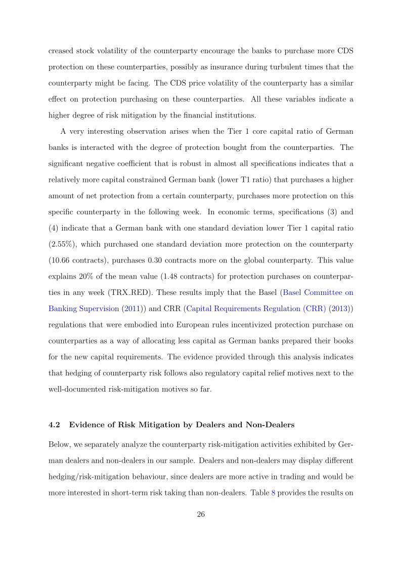
A very interesting observation arises when the Tier 1 core capital ratio of German

banks is interacted with the degree of protection bought from the counterparties. The

significant negative coefficient that is robust in almost all specifications indicates that a

relatively more capital constrained German bank (lower T1 ratio) that purchases a higher

amount of net protection from a certain counterparty, purchases more protection on this

specific counterparty in the following week. In economic terms, specifications (3) and

(4) indicate that a German bank with one standard deviation lower Tier 1 capital ratio

(2.55%), which purchased one standard deviation more protection on the counterparty

(10.66 contracts), purchases 0.30 contracts more on the global counterparty. This value

explains 20% of the mean value (1.48 contracts) for protection purchases on counterpar-

ties in any week (TRX RED). These results imply that the Basel (Basel Committee on

Banking Supervision (2011)) and CRR (Capital Requirements Regulation (CRR) (2013))

regulations that were embodied into European rules incentivized protection purchase on

counterparties as a way of allocating less capital as German banks prepared their books

for the new capital requirements. The evidence provided through this analysis indicates

that hedging of counterparty risk follows also regulatory capital relief motives next to the

well-documented risk-mitigation motives so far.

4.2 Evidence of Risk Mitigation by Dealers and Non-Dealers

Below, we separately analyze the counterparty risk-mitigation activities exhibited by Ger-

man dealers and non-dealers in our sample. Dealers and non-dealers may display different

hedging/risk-mitigation behaviour, since dealers are more active in trading and would be

more interested in short-term risk taking than non-dealers. Table 8 provides the results on

26

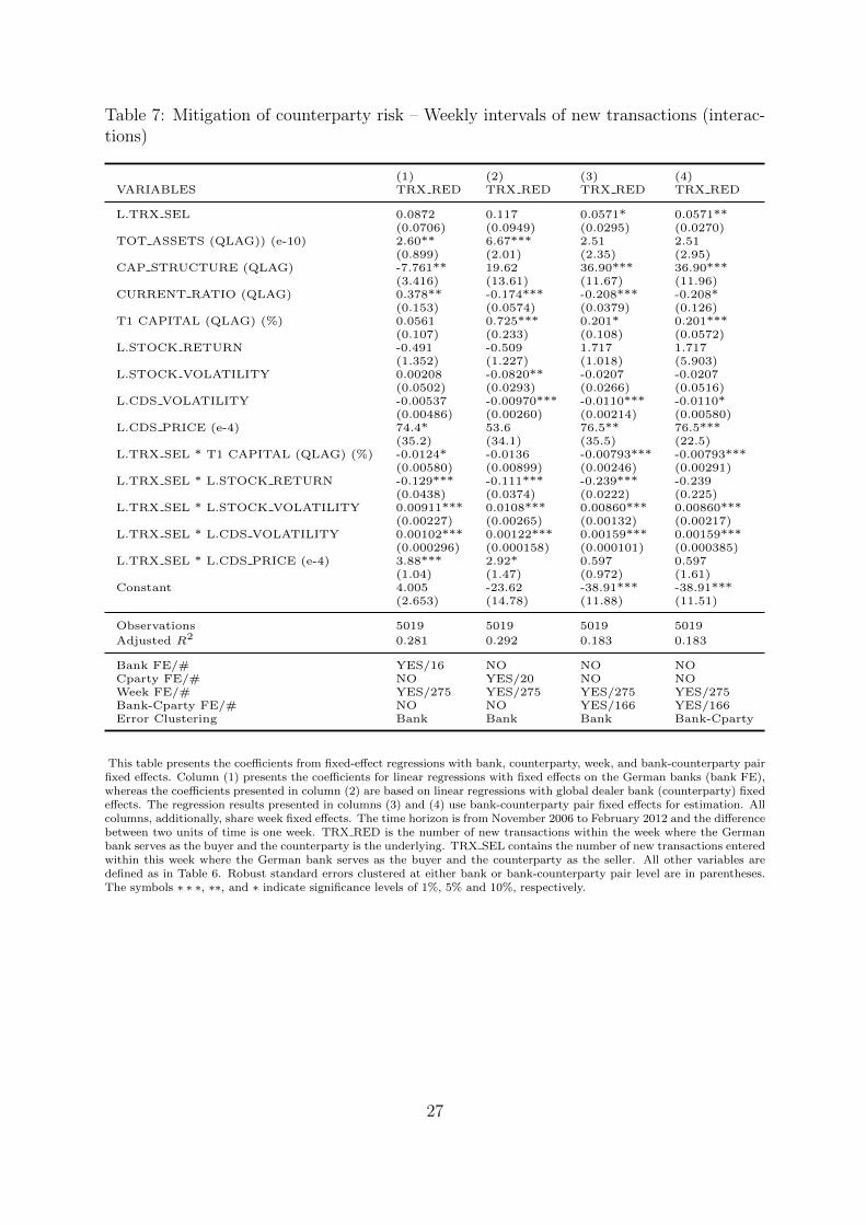
Table 7: Mitigation of counterparty risk – Weekly intervals of new transactions (interac-tions)

(1) (2) (3) (4)VARIABLES TRX RED TRX RED TRX RED TRX RED

L.TRX SEL 0.0872 0.117 0.0571* 0.0571**(0.0706) (0.0949) (0.0295) (0.0270)

TOT ASSETS (QLAG)) (e-10) 2.60** 6.67*** 2.51 2.51(0.899) (2.01) (2.35) (2.95)

CAP STRUCTURE (QLAG) -7.761** 19.62 36.90*** 36.90***(3.416) (13.61) (11.67) (11.96)

CURRENT RATIO (QLAG) 0.378** -0.174*** -0.208*** -0.208*(0.153) (0.0574) (0.0379) (0.126)

T1 CAPITAL (QLAG) (%) 0.0561 0.725*** 0.201* 0.201***(0.107) (0.233) (0.108) (0.0572)

L.STOCK RETURN -0.491 -0.509 1.717 1.717(1.352) (1.227) (1.018) (5.903)

L.STOCK VOLATILITY 0.00208 -0.0820** -0.0207 -0.0207(0.0502) (0.0293) (0.0266) (0.0516)

L.CDS VOLATILITY -0.00537 -0.00970*** -0.0110*** -0.0110*(0.00486) (0.00260) (0.00214) (0.00580)

L.CDS PRICE (e-4) 74.4* 53.6 76.5** 76.5***(35.2) (34.1) (35.5) (22.5)

L.TRX SEL * T1 CAPITAL (QLAG) (%) -0.0124* -0.0136 -0.00793*** -0.00793***(0.00580) (0.00899) (0.00246) (0.00291)

L.TRX SEL * L.STOCK RETURN -0.129*** -0.111*** -0.239*** -0.239(0.0438) (0.0374) (0.0222) (0.225)

L.TRX SEL * L.STOCK VOLATILITY 0.00911*** 0.0108*** 0.00860*** 0.00860***(0.00227) (0.00265) (0.00132) (0.00217)

L.TRX SEL * L.CDS VOLATILITY 0.00102*** 0.00122*** 0.00159*** 0.00159***(0.000296) (0.000158) (0.000101) (0.000385)

L.TRX SEL * L.CDS PRICE (e-4) 3.88*** 2.92* 0.597 0.597(1.04) (1.47) (0.972) (1.61)

Constant 4.005 -23.62 -38.91*** -38.91***(2.653) (14.78) (11.88) (11.51)

Observations 5019 5019 5019 5019

Adjusted R2 0.281 0.292 0.183 0.183

Bank FE/# YES/16 NO NO NOCparty FE/# NO YES/20 NO NOWeek FE/# YES/275 YES/275 YES/275 YES/275Bank-Cparty FE/# NO NO YES/166 YES/166Error Clustering Bank Bank Bank Bank-Cparty

This table presents the coefficients from fixed-effect regressions with bank, counterparty, week, and bank-counterparty pairfixed effects. Column (1) presents the coefficients for linear regressions with fixed effects on the German banks (bank FE),whereas the coefficients presented in column (2) are based on linear regressions with global dealer bank (counterparty) fixedeffects. The regression results presented in columns (3) and (4) use bank-counterparty pair fixed effects for estimation. Allcolumns, additionally, share week fixed effects. The time horizon is from November 2006 to February 2012 and the differencebetween two units of time is one week. TRX RED is the number of new transactions within the week where the Germanbank serves as the buyer and the counterparty is the underlying. TRX SEL contains the number of new transactions enteredwithin this week where the German bank serves as the buyer and the counterparty as the seller. All other variables aredefined as in Table 6. Robust standard errors clustered at either bank or bank-counterparty pair level are in parentheses.The symbols ∗ ∗ ∗, ∗∗, and ∗ indicate significance levels of 1%, 5% and 10%, respectively.

27

weekly new transactions from Equation (2), separating German dealers and non-dealers

in Panels A and B, respectively.

Panel A of Table 8 presents the risk-mitigation activity of dealers. The weekly lagged

new transactions of protections bought from the counterparty remain partly significant

in explaining the following week’s new protections bought on the counterparty. Most im-

portantly, the coefficient of interest is highly significant in specification (5), which utilizes

the very strong counterparty-week fixed effects in order to control for any endogeneity.

Higher leverage, lower past stock returns and higher CDS price levels of the counterparty

lead to increased protection purchases on the respective counterparty by German deal-

ers. On the other hand, we see a different picture when we look at Panel B. There is

no evidence of hedging behaviour by non-dealers in weekly intervals, which is observed

from the insignificant TRX SEL coefficient. Since non-dealers are active in CDS trad-

ing markets to a lesser degree, this finding overlaps with the intuition that non-dealers

might not be active in counterparty risk-taking and mitigation on such short horizons.

Still, higher leverage and short-term past stock performance seem to be decisive for non-

dealers’ decisions regarding the purchase of CDSs on respective global dealers. The lower

the past performance of the global player, the greater the extent of protection bought on

counterparties by non-dealers.

Table 9 replicates the setup used in Table 8, but this time with monthly intervals. The

interesting insight provided by Table 9 Panel B is that, unlike the results with the weekly

intervals in Table 8, non-dealers are shown to be more active in mitigating their risk on

monthly horizons. This result builds on the insignificance of the short-term mitigation

effects shown in Table 8, and indicates that since non-dealers are active in CDS trading

markets to a lesser degree, they might be managing their counterparty risk-taking and

mitigation on longer horizons. On the other hand, in Panel A of Table 9, we observe

that the dealers are to a certain degree still active with respect to risk mitigation over

longer periods. This result can be interpreted as indicating that the risk-taking activity

of dealers spans both short and longer horizons as revealed by Panels A in Tables 8 and

28

9.

Table 8: Mitigation of counterparty risk – Weekly intervals of new transactions, dealers v non-dealers

(1) (2) (3) (4) (5) (6) (7) (8) (9)VARIABLES TRX RED TRX RED TRX RED TRX RED TRX RED TRX RED TRX RED TRX RED TRX RED

Panel A. German banks and investment firms acting as dealers

L.TRX SEL 0.0802** 0.0909 0.0372 0.0372* 0.141*** 0.0638 0.0901 0.0322 0.0322**(0.00521) (0.0595) (0.0182) (0.0194) (1.32e-09) (0.0165) (0.0682) (0.0250) (0.0158)

TOT ASSETS (QLAG) (e-10) 2.73 7.25** 3.91 3.91(1.11) (0.283) (2.59) (3.60)

CAP STRUCTURE (QLAG) -8.533 30.01 45.08 45.08***(3.642) (30.01) (15.68) (12.45)

CURRENT RATIO (QLAG) 0.496 -0.128 -0.218 -0.218(0.174) (0.0243) (0.0394) (0.142)

L.STOCK RETURN -3.079 -2.831** -1.072 -1.072(3.338) (0.0993) (0.999) (8.351)

L.STOCK VOLATILITY 0.144 0.0720 0.124 0.124(0.113) (0.114) (0.0780) (0.0829)

L.CDS VOLATILITY 0.0155 0.0101 0.0102 0.0102(0.0148) (0.00946) (0.00835) (0.00928)

L.CDS PRICE (e-4) 116.0 86.5 88.6 88.6***(45.4) (36.1) (35.9) (25.6)

Constant -1.851* -0.751 -2.234** -2.234*** 0.654 4.623 -29.97 -45.68 -45.68***(0.166) (1.484) (0.175) (0.111) (0.509) (2.652) (30.19) (15.58) (12.10)

Observations 4862 4862 4862 4862 4862 3851 3851 3851 3851

Adjusted R2 0.173 0.250 0.140 0.140 0.052 0.255 0.270 0.187 0.187

Bank FE/# YES/2 NO NO NO NO YES/2 NO NO NOCparty FE/# NO YES/21 NO NO NO NO YES/20 NO NOWeek FE/# YES/275 YES/275 YES/275 YES/275 NO YES/275 YES/275 YES/275 YES/275Bank-Cparty FE/# NO NO YES/40 YES/40 NO NO NO YES/38 YES/38Week-Cparty FE/# NO NO NO NO YES/3927 NO NO NO NOError Clustering Bank Bank Bank Bank-Cparty Bank Bank Bank Bank Bank-Cparty

Panel B. German banks and investment firms acting as non-dealers

L.TRX SEL -0.00000567 0.000316 0.000104 0.000104 -0.00246 0.000145 0.000144 -0.000128 -0.000128(0.000254) (0.000555) (0.000331) (0.000267) (0.0120) (0.000218) (0.000452) (0.000384) (0.000419)

TOT ASSETS (QLAG) (e-10) -0.185 -0.406 -0.440 -0.440(0.113) (0.285) (0.285) (0.792)

CAP STRUCTURE (QLAG) 0.734*** 4.956*** 4.093*** 4.093(0.260) (1.669) (1.344) (2.886)

CURRENT RATIO (QLAG) 0.0431* 0.0103 0.0205 0.0205(0.0231) (0.0185) (0.0204) (0.0267)

L.STOCK RETURN -2.234** -2.083** -2.020** -2.020*(0.939) (0.915) (0.890) (1.199)

L.STOCK VOLATILITY -0.00141 -0.0106 -0.00887 -0.00887(0.00503) (0.00662) (0.00558) (0.00944)

L.CDS VOLATILITY 0.00389 0.00349 0.00401 0.00401(0.00301) (0.00294) (0.00320) (0.00289)

L.CDS PRICE (e-4) -2.67 -3.38 -4.31 -4.31(4.15) (6.12) (7.35) (5.35)

Constant -0.161*** 0.0337** -0.0398*** -0.0398*** 0.0740** -0.759*** -4.443*** -3.723*** -3.723(0.00814) (0.0157) (0.00700) (0.0107) (0.0286) (0.227) (1.488) (1.283) (2.724)

Observations 1863 1863 1863 1863 1863 1467 1467 1467 1467

Adjusted R2 0.016 0.006 0.001 0.001 -0.026 0.061 0.040 0.042 0.042

Bank FE/# YES/23 NO NO NO NO YES/23 NO NO NOCparty FE/# NO YES/19 NO NO NO NO YES/18 NO NOWeek FE/# YES/254 YES/254 YES/254 YES/254 NO YES/247 YES/247 YES/247 YES/247Bank-Cparty FE/# NO NO YES/181 YES/181 NO NO NO YES/170 YES/170Week-Cparty FE/# NO NO NO NO YES/1328 NO NO NO NOError Clustering Bank Bank Bank Bank-Cparty Bank Bank Bank Bank Bank-Cparty

29

Table 9: Mitigation of counterparty risk – Monthly rolling intervals of cumulative new transactions, dealers v non-dealers

(1) (2) (3) (4) (5) (6) (7) (8) (9)VARIABLES Σ TRX RED Σ TRX RED Σ TRX RED Σ TRX RED Σ TRX RED Σ TRX RED Σ TRX RED Σ TRX RED Σ TRX RED

Panel A. German banks and investment firms that are dealers

L4.Σ TRX SEL 0.102** 0.132 0.0445 0.0445* 0.159 0.0783 0.131 0.0299 0.0299*(0.00583) (0.0574) (0.0228) (0.0240) (0.0282) (0.0223) (0.0686) (0.0327) (0.0176)

TOT ASSETS (QLAG) (e-10) 8.89 24.1 10.9 10.9(5.07) (7.03) (8.78) (12.8)

CAP STRUCTURE (QLAG) -25.69 90.88 144.1 144.1***(22.78) (101.6) (97.23) (51.38)

CURRENT RATIO (QLAG) 2.048 -0.105** -0.338 -0.338(1.158) (0.00251) (0.0990) (0.425)

L4.STOCK RETURN -85.57 -75.44 -69.82 -69.82***(55.74) (41.18) (40.59) (22.40)

L4.STOCK VOLATILITY 0.316 -0.315 0.0595 0.0595(0.394) (0.143) (0.182) (0.416)

L4.CDS VOLATILITY 0.0470 0.0151 0.0191 0.0191(0.0855) (0.0449) (0.0464) (0.0686)

L4.CDS PRICE (e-4) 252.0 161.0 176.0 176.0***(151.0) (92.3) (99.3) (48.2)

Constant -5.034** 0.539 -9.339* -9.339*** 2.000 13.14 -89.72 -149.2 -149.2***(0.368) (5.200) (0.940) (0.793) (1.810) (17.77) (103.9) (95.96) (49.54)

Observations 6832 6832 6832 6832 6832 5400 5400 5400 5400

Adjusted R2 0.298 0.383 0.195 0.195 0.533 0.369 0.387 0.245 0.245

Bank FE/# YES/2 NO NO NO NO YES/2 NO NO NOCparty FE/# NO YES/21 NO NO NO NO YES/20 NO NOMonth FE/# YES/65 YES/65 YES/65 YES/65 NO YES/65 YES/65 YES/65 YES/65Bank-Cparty FE/# NO NO YES/40 YES/40 NO NO NO YES/38 YES/38Month-Cparty FE/# NO NO NO NO YES/1158 NO NO NO NOError Clustering Bank Bank Bank Bank-Cparty Bank Bank Bank Bank Bank-Cparty

Panel B. German banks and investment firms that are non-dealers

L4.Σ TRX SEL 0.00704*** 0.00758*** 0.00745*** 0.00745*** 0.0110*** 0.00714*** 0.00741*** 0.00731*** 0.00731***(0.000782) (0.000555) (0.000444) (0.000855) (0.000960) (0.000269) (0.000527) (0.000399) (0.000793)

TOT ASSETS (QLAG) (e-10) -0.276 -1.62 -1.74 -1.74(0.326) (1.04) (1.49) (1.88)

CAP STRUCTURE (QLAG) 0.397 7.972 9.756 9.756(1.609) (5.716) (6.147) (7.272)

CURRENT RATIO (QLAG) -0.0164 -0.0369* -0.0324*** -0.0324(0.0436) (0.0198) (0.0111) (0.0254)

L4.STOCK RETURN -5.299*** -4.505*** -4.957*** -4.957***(1.771) (1.362) (1.399) (1.749)

L4.STOCK VOLATILITY 0.0263* 0.00882 0.0192 0.0192(0.0143) (0.0231) (0.0241) (0.0271)

L4.CDS VOLATILITY 0.000504 0.00148 0.000166 0.000166(0.00208) (0.00221) (0.00185) (0.00256)

L4.CDS PRICE (e-4) 0.660 -6.46 -5.59 -5.59(3.74) (7.89) (8.12) (6.83)

Constant -0.272* 0.0386 0.0581 0.0581 0.173** -0.447 -7.188 -8.750 -8.750(0.137) (0.132) (0.0661) (0.0594) (0.0676) (1.465) (5.259) (5.588) (6.760)

Observations 5225 5225 5225 5225 5225 4086 4086 4086 4086

Adjusted R2 0.114 0.085 0.066 0.066 0.324 0.152 0.120 0.108 0.108

Bank FE/# YES/23 NO NO NO NO YES/23 NO NO NOCparty FE/# NO YES/19 NO NO NO NO YES/18 NO NOMonth FE/# YES/63 YES/63 YES/63 YES/63 NO YES/63 YES/63 YES/63 YES/63Bank-Cparty FE/# NO NO YES/179 YES/179 NO NO NO YES/170 YES/170Month-Cparty FE/# NO NO NO NO YES/709 NO NO NO NOError Clustering Bank Bank Bank Bank-Cparty Bank Bank Bank Bank Bank-Cparty

30

One way to interpret the results in Tables 8 and 9 is that the accumulation of counter-

party risk might be slower for non-dealers in comparison to that of dealers. Non-dealers

might be waiting to hedge until the open interest hits a certain level or ratio, and this

might be the reason why they hedge less frequently. Another possibility might be the

lower frequency of risk management meetings at non-dealer institutions, which could fix

hedging action deadlines to a less frequent extent.

4.3 Identification through an Exogenous Shock on the Underlying

The previous two subsections made use of the transaction-level CDS dataset together with

bank, counterparty or bank-counterparty pair fixed effects, and relied on time (week/-

month) or counterparty-time pair fixed effects to address any endogeneity that could have

been caused by aggregate or counterparty-specific time-variant factors, which may simul-

taneously drive protection bought from the global dealer today and protection bought on

the global dealer on a future week or month.

An alternative robust way to address this issue is to make use of price shocks on

underlyings, whose protection are being purchased by our sample banks and financial

institutions from the global counterparties at the SEL time step. An ideal identification

could be achieved through looking at the CDS price change of each underlying u in all

trading activities between the German banks and their counterparties, and multiplying

this value with the current net position of the same bank i with the same counterparty j

on this underlying u (“NETSELPOS”). The value in Equation 3 could be viewed as an

individual shock (“INDSHOCK”) to the counterparty risk of the bank with respect to a

given underlying u.

INDSHOCKi,j,u,t = NETSELPOSi,j,u,t−1 ∗ (CDS PRICEu,t − CDS PRICEu,t−1)

(3)

In order to reach the aggregate shock to the counterparty risk of a bank with respect

31

to all underlyings, the individual shocks in Equation 3 could be aggregated across all

underlyings u that are traded between a bank-counterparty pair.

SHOCKi,j,t =u∑INDSHOCKi,j,u,t (4)

The variable SHOCKi,j,t provides a valuable exogenous shock on counterparty risk

of bank i on counterparty j, which enables the consecutive actions of bank i on trading

the CDS of counterparty j to be independently interpreted from any endogeneity. Ta-

ble 10 Panel A introduces ΣSHOCKi,j,t as a new explanatory variable, where the past

four weeks of price shocks on all underlyings are aggregated. In the first (second) part

of the panel the dependent variable is the cumulative number of new protection con-

tracts,“TRX RED” (cumulative volume of new protection, “VOL RED”) purchased on

the counterparty during the immediately following four weeks. We make use of the fol-

lowing specifications in Equations 5 and 6, alternatively with (1) bank and month FE, (2)

counterparty and month FE, and (3) counterparty-month pair FE. The fourth and fifth

specifications add the typical counterparty-specific controls that were used previously into

specifications (1) and (2).

4∑k=1

TRX REDi,j,t+k = a0 + a1

3∑k=0

SHOCKi,j,t−k + a2Xj,t + FE + εi,j,t (5)

4∑k=1

V OL REDi,j,t+k = a0 + a1

3∑k=0

SHOCKi,j,t−k + a2Xj,t + FE + εi,j,t (6)

The results in Table 10 Panel A indicate that both dependent variables, number of

new contracts and notional amount purchased on the counterparty, are explained by the

exogenous increase in the counterparty risk of the global dealer, revealed by the price

shock on the CDS underlyings in prior weeks. In economic terms, a 100 bps aggregate

CDS price deterioration (increase) in 10 EUR billion of an aggregate net sold position

to the counterparty results in purchase of 3.25-6.69 additional contracts bought on the

counterparty in order to mitigate the counterparty risk emerging from the price shock.

32

Table 10: Mitigation of counterparty risk – Identification through an Exogenous Shock

Panel A. Monthly rolling intervals of new transactions

(1) (2) (3) (4) (5)VARIABLES Σ TRX RED Σ TRX RED Σ TRX RED Σ TRX RED Σ TRX RED

Σ SHOCK 0.0325*** 0.0371* 0.0669*** 0.0339*** 0.0497*(0.0014) (0.019) (0.0086) (0.0053) (0.024)

Observations 6230 6230 6230 4021 4021

Adjusted R2 0.238 0.225 0.340 0.362 0.277

(1) (2) (3) (4) (5)VARIABLES Σ VOL RED Σ VOL RED Σ VOL RED Σ VOL RED Σ VOL RED

Σ SHOCK 0.185*** 0.211 0.387*** 0.159*** 0.270(0.016) (0.148) (0.048) (0.030) (0.176)

Observations 6230 6230 6230 4021 4021

Adjusted R2 0.259 0.229 0.341 0.383 0.271

Controls NO NO NO YES YESBank FE/# YES/8 NO NO YES/6 NOCparty FE/# NO YES/21 NO NO YES/20Month FE/# YES/50 YES/50 NO YES/49 YES/49Cparty-Month FE/# NO NO YES/982 NO NO

Panel B. Weekly intervals of new transactions

(1) (2) (3) (4) (5)VARIABLES TRX RED TRX RED TRX RED TRX RED TRX RED

SHOCK 0.00286 0.00576*** 0.0197*** 0.00679** 0.0110**(0.0031) (0.0020) (0.0046) (0.0030) (0.0044)

Observations 11087 11087 11087 6525 6525

Adjusted R2 0.162 0.079 0.108 0.226 0.110

(1) (2) (3) (4) (5)VARIABLES VOL RED VOL RED VOL RED VOL RED VOL RED

SHOCK 0.0169 0.0376*** 0.112*** 0.0199 0.0504*(0.014) (0.0093) (0.022) (0.015) (0.027)

Observations 11087 11087 11087 6525 6525

Adjusted R2 0.166 0.080 0.060 0.225 0.101

Controls NO NO NO YES YESBank FE/# YES/25 NO NO YES/19 NOCparty FE/# NO YES/21 NO NO YES/20Week FE/# YES/214 YES/214 NO YES/213 YES/213Cparty-Week FE/# NO NO YES/4272 NO NO

This table presents the coefficients from fixed-effect regressions with bank, counterparty, time (month or week) andcounterparty-time pair fixed effects. Column (1) and (4) present the coefficients for linear regressions with fixed effectson the German banks (bank FE), whereas the coefficients presented in column (2) and (5) are based on linear regressionswith international dealer bank (counterparty) fixed effects, all sharing, in addition, time fixed effects. The regression resultspresented in columns (3) use counterparty-time pair fixed effects for estimation. The time horizon is from November 2006to February 2012 and the difference between two units of time is one week. In Panel A, Σ TRX RED is the number while ΣVOL RED is the volume of new transactions within the following four weeks, where the German bank serves as the buyerand the counterparty is the underlying. Σ SHOCK is the cumulative product between NETSELPOS and ∆ RED PRICEfrom the first to the fourth lag. In Panel B, TRX RED is the number while VOL RED is the volume of new transactionswithin the week, where the German bank serves as the buyer and the counterparty is the underlying. SHOCK is composedof lagged NETSELPOS times ∆ RED PRICE. All the other variables are defined as in Table 5 and 6 and are not tabulatedfor brevity. Robust standard errors clustered at bank level are in parentheses. The symbols ∗ ∗ ∗, ∗∗, and ∗ indicatesignificance levels of 1%, 5% and 10%, respectively.

33

Similarly, the second part of Panel A reveals that the same conditions result in a protection

purchase of 18.5-38.7 EUR million on the counterparty.14

Panel B shows the effects of weekly price shocks on our sample banks’ behaviour on

purchase of protection on the counterparty (Equations 7 and 8). The same pattern of

mitigation of counterparty risk due to exogenous price shocks on the underlying are once

again observed, albeit at a lesser economic extent.

TRX REDi,j,t+1 = a0 + a1SHOCKi,j,t + a2Xj,t + FE + εi,j,t (7)

V OL REDi,j,t+1 = a0 + a1SHOCKi,j,t + a2Xj,t + FE + εi,j,t (8)

Overall, the findings in this section underline once again the robustness of the results

when an exogenous shock is used for a better identification.

4.4 Robustness

This section provides the results for alternative monthly and weekly specifications. We

specifically look at whether German banks hedge their counterparty risk from correct

parties (no wrong-way risk), and whether results are robust when (i) contemporaneous

months and weeks of hedging activity are analyzed, and (ii) non-overlapping monthly

specifications are used.15 Table 11 reports the results of these checks by tabulating only

the main variable of interest for monthly and weekly specifications in Panels A and B,

respectively.

4.4.1 Wrong-Way Risk

“Wrong-way risk” arises when banks intend to mitigate their counterparty risk through the

purchase of protection on their counterparty from a third party that is highly correlated

14A one standard deviation shock would have a value of 62.8 billion, which is a value close to thisscenario.

15In undocumented results, our main finding is shown to be also robust when only observations ofnon-zero hedging activity are utilized.

34

Table 11: Robustness checks

Panel A. Monthly rolling intervals of new transactions

(1) (2) (3) (4) (5) (6) (7) (8) (9)VARIABLES Σ TRX RED Σ TRX RED Σ TRX RED Σ TRX RED Σ TRX RED Σ TRX RED Σ TRX RED Σ TRX RED Σ TRX RED

Baseline (Table 5): L4.Σ TRX SEL 0.104*** 0.147*** 0.0694*** 0.0694*** 0.148*** 0.0873*** 0.146*** 0.0472** 0.0472***Case 1 (No WWR): L4.Σ TRX SEL 0.0398*** 0.0798*** 0.0205*** 0.0205* 0.0849*** 0.0265*** 0.0726*** 0.0106 0.0106Case 2 (Contemporaneous Month): Σ TRX SEL 0.124*** 0.168*** 0.0892*** 0.0892*** 0.180*** 0.116*** 0.182*** 0.0830*** 0.0830**Case 3 (Non-Overlapping Months): L4.Σ TRX SEL 0.101*** 0.151*** 0.0557*** 0.0557** 0.162*** 0.0863*** 0.151*** 0.0442*** 0.0442**

Controls NO NO NO NO NO YES YES YES YESBank FE YES NO NO NO NO YES NO NO NOCounterparty FE NO YES NO NO NO NO YES NO NOTime (Month or Week) FE YES YES YES YES NO YES YES YES YESBank-Cparty FE NO NO YES YES NO NO NO YES YESCparty-Time FE NO NO NO NO YES NO NO NO NOError Clustering Bank Bank Bank Bank-Cparty Bank Bank Bank Bank Bank-Cparty

Panel B. Weekly intervals of new transactions

(1) (2) (3) (4) (5) (6) (7) (8) (9)VARIABLES TRX RED TRX RED TRX RED TRX RED TRX RED TRX RED TRX RED TRX RED TRX RED

Baseline (Table 6): L.TRX SEL 0.0607*** 0.0891*** 0.0317*** 0.0317** 0.114*** 0.0496*** 0.0858*** 0.0359** 0.0359**Case 1 (No WWR): L.TRX SEL 0.0215*** 0.0437*** 0.00855** 0.00855 0.0587*** 0.0141*** 0.0380*** 0.00457 0.00457Case 2 (Contemporaneous Week): TRX SEL 0.0848*** 0.110*** 0.0584*** 0.0584*** 0.138*** 0.0841*** 0.129*** 0.0543*** 0.0543***

Controls NO NO NO NO NO YES YES YES YESBank FE YES NO NO NO NO YES NO NO NOCounterparty FE NO YES NO NO NO NO YES NO NOTime (Month or Week) FE YES YES YES YES NO YES YES YES YESBank-Cparty FE NO NO YES YES NO NO NO YES YESCparty-Time FE NO NO NO NO YES NO NO NO NOError Clustering Bank Bank Bank Bank-Cparty Bank Bank Bank Bank Bank-Cparty

This table presents the coefficients from fixed-effect regressions with bank, counterparty, time (month or week), bank-counterparty and counterparty-time pair fixed effects. Columns(1) and (6) present the coefficients for linear regressions with fixed effects on the German banks (bank FE), whereas the coefficients presented in columns (2) and (7) are basedon linear regressions with international dealer bank (counterparty) fixed effects, both sets of regressions sharing, in addition, time fixed effects. Regression results presented incolumns (3), (4), (8) and (9) use bank-counterparty pair fixed effects for estimation in addition to time fixed effects. Column (5) presents the coefficient for linear regression withcounterparty-time pair fixed effect. The time horizon is from November 2006 to February 2012 and the difference between two units of time is one week. In Panel A, Σ TRX REDis the number of new transactions within the following four weeks where the German bank serves as the buyer and the counterparty is the underlying. L4.Σ TRX SEL containsthe number of new transactions entered within this week and the three previous weeks where the German bank serves as the buyer and the counterparty as the seller. In Panel B,TRX RED is the number of new transactions within the current week where the German bank serves as the buyer and the counterparty is the underlying. L.TRX SEL contains thenumber of new transactions entered within the past week where the German bank serves as the buyer and the counterparty as the seller. All the other variables are defined as inTable 5 (for Panel A) and 6 (for Panel B) and are not tabulated for brevity. Robust standard errors clustered at either bank or bank-counterparty pair level. The symbols ∗ ∗ ∗, ∗∗,and ∗ indicate significance levels of 1%, 5% and 10%, respectively.

35

with their initial counterparty. For instance, if a German bank purchases protection on

a Japanese counterparty from another Japanese third party, it can be suggested that

wrong-way risk mitigation occurs. In order to see whether German financial institutions

mitigate counterparty risk keeping in mind the need to avoid wrong-way risk, we remove

all the same country hedging activity and see if the results still hold. Hence, all protection

purchases on, e.g., US dealers, from another US financial institution, are removed from the

sample. Cases 1 in Panels A and B of Table 11 show that although the hedge proportion is

lower, there is indeed significant evidence for German financial institutions to be avoiding

wrong-way risk mitigation.

4.4.2 Contemporaneous months and weeks

It could be argued that risk-mitigation activity takes place directly in the same weeks or

months whenever counterparty risk occurs, due to immediate reaction of the dealer desks.

Cases 2 in Panels A and B of Table 11 provide evidence that risk mitigation takes place

even in the contemporaneous months and weeks. Interestingly, the hedge proportion is

much higher when compared to baseline results in Tables 5 and 6, which gives rise to the

possibility that risk mitigation is immediately undertaken as well.

4.4.3 Non-overlapping months

One argument could be that the results might be spurious due to autocorrelated usage of

weeks in monthly rolling intervals. If overlapping weeks are rolled over, double counting

of information might emerge. In order to avoid this concern, Case 3 in Panel A of Table

11 generates results with non-overlapping rolling of monthly intervals. The coefficients of

interest indicate an even slightly higher hedge proportion in some specifications compared

to the baseline results in Table 5.

5 Conclusion and Policy Implications

This paper provides initial evidence of counterparty risk-mitigation activity on the part

of financial institutions. Our sample banks and financial institutions manage their coun-

36

terparty risk on weekly or monthly horizons as evidenced both by transaction-level and

position-level information. Trading-intensive dealer banks are found to be more active in

hedging, over both short and longer horizons, whereas non-dealer banks appear to manage

this risk only over longer, monthly intervals. Higher stock return and CDS price volatility,

lower past stock returns, and higher CDS prices of the counterparty are shown to boost

hedging behaviour on the counterparty. The sample banks are also shown to mitigate

their counterparty risk by keeping in mind to avoid wrong-way hedging. Finally, we fur-

ther document the robustness of our main finding through identifying the risk mitigation

activity when an exogenous price shock increases the counterparty risk of our sample

banks.

The analysis provided in this study has implications regarding the ongoing debate on

regulating the OTC market and further phasing in central clearing, which would seem-

ingly eliminate the necessity of bilateral trading and diminish counterparty risk. However,

given that single-name CDSs are still not mandated to be centrally cleared by any reg-

ulator, there still exists a major bilateral trading volume between counterparties in the

OTC market, which holds back the phenomenon documented in this paper to be out-

dated. We show that risk-mitigation is taking place in the OTC market despite the high

level of collateralization indicated by recent studies, and that purchasing protection on

the reference entities of counterparties seems to be a reliable method in circumstances

where collateral alone provides insufficient protection. Players in the market are able to

tentatively hedge their counterparty risk through CDSs in the OTC market regardless of

whether they are a central clearing member. Given that we are able to show evidence

on hedging in the CDS market that encompasses only a part of counterparty risk-taking

activity, we expect that even a much higher degree of counterparty risk mitigation could

be evidenced if exposures from interest rate and FX swaps were included. Altogether, the

analysis in the paper points to an additional cost of bilateral OTC trading in the absence

of central clearing, which has not been articulated in the literature.

We argue in this study that regulatory capital relief motives could actively accentu-

37

ate this type of risk mitigation. Banks that have a relatively higher exposure to their

counterparties are shown to hedge their counterparty risk more, especially when they

have a lower Tier 1 core capital ratio, thus being relatively less capitalized. Since Basel

III and its European implementation, the CRR, explicitly formulate that any protection

purchase on the counterparty would diminish the required regulatory CVA capital, future

work should study whether such an incentive might create adverse effects that lead to

excessive risk-taking by relatively less capitalized banks. In the end, it is in the best in-

terest of regulators to set the right incentives for market participants and clearing houses

to ensure an optimal design of the capital regulation of CDSs.

38

References

Acharya, V. and A. Bisin (2014). Counterparty risk externality: Centralized versus over-the-counter markets. Journal of Economic Theory 149, 153–182.

Acharya, V. V., Y. Gunduz, and T. C. Johnson (2018). Bank use of sovereign CDS in theEurozone crisis: Hedging and risk incentives. Deutsche Bundesbank Discussion PaperNo:26/2018, EFA 2017 Mannheim Meetings Paper .

Andersen, L., M. Pykthin, and A. Sokol (2017). Rethinking the margin period of risk.Journal of Credit Risk 13(1), 1–45.

Arora, N., P. Gandhi, and F. A. Longstaff (2012). Counterparty credit risk and the creditdefault swap market. Journal of Financial Economics 103, 280–293.

Augustin, P., M. G. Subrahmanyam, D. Y. Tang, and S. Q. Wang (2014). Credit defaultswaps: A survey. Foundations and Trends in Finance 9, 1–196.

Augustin, P., M. G. Subrahmanyam, D. Y. Tang, and S. Q. Wang (2016). Credit defaultswaps: Past, present and future. Annual Review of Financial Economics 8, 175–196.

Basel Committee on Banking Supervision (2011). Basel III: A Global regulatory frame-work for more resilient banks and banking systems. Technical report, Bank for Inter-national Settlements.

Bellia, M., R. Panzica, L. Pelizzon, and T. Peltonen (2018). The Demand for centralclearing: To clear or not to clear, that is the question. SAFE Working paper No:193,Goethe University Frankfurt.

Biais, B., F. Heider, and M. Hoerova (2016). Risk-sharing or risk-taking? counterpartyrisk, incentives, and margins. The Journal of Finance, 71(4), 1669–1698.

Biswas, G., S. Nikolova, and C. W. Stahel (2015). The Transaction costs of tradingcorporate credit. AFA 2015 Boston Meetings Paper .

Capital Requirements Regulation (CRR) (2013). Regulation (EU) no. 575/2013 of theEuropean Parliament and of the Council. Official Journal of the European Union.

Cooper, I. and A. Mello (1991). The Default risk of swaps. The Journal of Finance 46 (2),597–620.

Du, W., S. Gadgil, M. B. Gordy, and C. Vega (2016). Counterparty risk and counterpartychoice in the credit default swap market. Board of Governors of the Federal Reserve Sys-tem Finance and Economics Discussion Series 087, AFA 2016 San Francisco MeetingsPaper .

Duffie, D. and M. Huang (1996). Swap rates and credit quality. The Journal of Fi-nance 51 (3), 921–949.

Duffie, D., M. Scheicher, and G. Vuillemey (2015). Central clearing and collateral demand.Journal of Financial Economics 116 (2), 237–256.

39

Duffie, D. and H. Zhu (2011). Does a central clearing counterparty reduce counterpartyrisk? Review of Asset Pricing Studies 1 (1), 74–95.

Gehde-Trapp, M., Y. Gunduz, and J. Nasev (2015). The Liquidity premium in CDStransaction prices: Do frictions matter? Journal of Banking & Finance, 61, 184–205.

Gunduz, Y., S. Ongena, G. Tumer-Alkan, and Y. Yu (2017). CDS and credit: Testingthe small bang theory of the financial universe with micro data. Deutsche BundesbankDiscussion Paper No:16/2017, AFA 2017 Chicago Meetings Paper .

Hull, J. and A. White (2001). Valuing credit default swaps II: Modeling default correla-tions. Journal of Derivatives 8, 12–22.

Jarrow, R. A. and F. Yu (2001). Counterparty risk and the pricing of defaultable securities.The Journal of Finance 56 (5), 1765–1799.

Jorion, P. and G. Zhang (2009). Credit contagion from counterparty risk. The Journalof Finance 64(5), 2053–2087.

Klingler, S. and D. Lando (2018). Safe-haven CDS premia. Review of Financial Studies 31,1855–1895.

Kraft, H. and M. Steffensen (2007). Bankruptcy, counterparty risk, and contagion. Reviewof Finance 11, 209–252.

Loon, Y. C. and Z. K. Zhong (2014). The Impact of central clearing on counterpartyrisk, liquidity, and trading: Evidence from the credit default swap market. Journal ofFinancial Economics 112, 91–115.

Morkoetter, S., J. Pleus, and S. Westerfeld (2012). The Impact of counterparty risk oncredit default swap pricing dynamics. Journal of Credit Risk 8(1), 63–88.

Oehmke, M. and A. Zawadowski (2017). The Anatomy of the CDS market. Review ofFinancial Studies, 30(1), 80–119.

Peltonen, T. A., M. Scheicher, and G. Vuillemey (2014). The Network structure of theCDS market and its determinants. Journal of Financial Stability 13, 118–133.

Siriwardane, E. N. (2016). Limited investment capital and credit spreads. The Journalof Finance, forthcoming .

Stulz, R. M. (2010). Credit default swaps and the credit crisis. Journal of EconomicPerspectives 24(1), 73–92.

Thompson, J. R. (2010). Counterparty risk in financial contracts: Should the insuredworry about the insurer? Quarterly Journal of Economics 123(3), 1195–1252.

Yorulmazer, T. (2013). Has financial innovation made the world riskier? CDS, regulatoryarbitrage and systemic risk. Federal Reserve Bank of New York Working paper .

40

Internet Appendix to

Mitigating Counterparty Risk

41

Table I1: Mitigation of counterparty risk – Weekly intervals of new transactions with additional lags

(1) (2) (3) (4) (5) (6) (7) (8) (9)VARIABLES TRX RED TRX RED TRX RED TRX RED TRX RED TRX RED TRX RED TRX RED TRX RED

L.TRX SEL 0.0369*** 0.0405* 0.0165* 0.0165 0.000269 0.0289*** 0.0263 0.0137 0.0137(0.00406) (0.0182) (0.00746) (0.0125) (0.0184) (0.00659) (0.0176) (0.00895) (0.00974)

L2.TRX SEL 0.0289*** 0.0329** 0.0122*** 0.0122 0.0250 0.0229*** 0.0191** 0.00990*** 0.00990(0.00244) (0.0103) (0.00103) (0.0100) (0.0204) (0.00126) (0.00569) (0.00134) (0.00749)

L3.TRX SEL 0.0171*** 0.0216 -0.00422* -0.00422 0.143*** 0.00441*** 0.000616 -0.0122*** -0.0122(0.000456) (0.0149) (0.00211) (0.00727) (0.0130) (0.000379) (0.00996) (0.000939) (0.00738)

TOT ASSETS (QLAG) (e-10) 2.25*** 9.07*** 5.17*** 5.17(0.373) (2.30) (0.450) (3.64)

CAP STRUCTURE (QLAG) -8.720*** 42.47** 54.56*** 54.56***(1.090) (13.31) (1.542) (10.26)

CURRENT RATIO (QLAG) 0.552*** -0.151*** -0.209*** -0.209(0.0247) (0.0373) (0.0554) (0.160)

T1 CAPITAL (QLAG) 0.0143 1.126*** 0.551** 0.551**(0.152) (0.290) (0.206) (0.215)

L.STOCK RETURN -3.184 0.391 1.420 1.420(2.097) (3.107) (2.460) (12.15)

L.STOCK VOLATILITY 0.205*** 0.172** 0.198*** 0.198***(0.0563) (0.0606) (0.0230) (0.0481)

L.CDS VOLATILITY 0.0211*** 0.0129*** 0.0131*** 0.0131*(0.000594) (0.000799) (0.00106) (0.00727)

L.CDS PRICE 0.0151*** 0.0120*** 0.0119*** 0.0119***(0.00138) (0.000568) (0.000512) (0.00260)

Constant -3.903*** -0.0658 -0.986*** -0.986 0.524** 4.876** -48.88*** -58.55*** -58.55***(0.724) (0.368) (0.0337) (1.144) (0.227) (1.709) (13.33) (2.443) (10.19)

Observations 3630 3630 3630 3630 3630 2812 2812 2812 2812

Adjusted R2 0.182 0.288 0.176 0.176 0.215 0.291 0.348 0.247 0.247

Bank FE/# YES/10 NO NO NO NO YES/8 NO NO NOCparty FE/# NO YES/20 NO NO NO NO YES/19 NO NOWeek FE/# YES/266 YES/266 YES/266 YES/266 NO YES/266 YES/266 YES/266 YES/266Bank-Cparty FE/# NO NO YES/78 YES/78 NO NO NO YES/71 YES/71Cparty-Week FE/# NO NO NO NO YES/3209 NO NO NO NOError Clustering Bank Bank Bank Bank-Cparty Bank Bank Bank Bank Bank-Cparty

This table presents the coefficients from fixed-effect regressions with bank, counterparty, bank-counterparty pair, week and counterparty-week pair fixed effects. Columns (1) and(6) present the coefficients for linear regressions with fixed effects on the German banks (bank FE) and time (week FE), whereas the coefficients presented in columns (2) and(7) are based on linear regressions with global dealer bank (counterparty FE) and time (week) fixed effects. Regression results presented in columns (3), (4), (8) and (9) usebank-counterparty pair in addition to week fixed effects. Column (5) presents the coefficient for linear regression with counterparty-week pair fixed effect. The time horizon is fromNovember 2006 to February 2012 and the difference between two units of time is one week. TRX RED is the number of new transactions within the current week where the Germanbank serves as the buyer and the counterparty is the underlying. L.TRX SEL, L2.TRX SEL, L3.TRX SEL contain the number of new transactions entered in which the Germanbank serves as the buyer and the counterparty as the seller within the past week, the week before (two weeks ago), and the earlier week (three weeks ago), respectively. All othervariables are defined similarly as in Table 6. Robust standard errors clustered at either bank or bank-counterparty pair level are in parentheses. The symbols ∗∗ ∗, ∗∗, and ∗ indicatesignificance levels of 1%, 5% and 10%, respectively.

42