Missing Data Problems in Machine Learning by Benjamin M. Marlin A thesis submitted in conformity with the requirements for the degree of Doctor of Philosophy Graduate Department of Computer Science University of Toronto Copyright c 2008 by Benjamin M. Marlin

Welcome message from author
This document is posted to help you gain knowledge. Please leave a comment to let me know what you think about it! Share it to your friends and learn new things together.
Transcript

Missing Data Problems in Machine Learning
by
Benjamin M. Marlin
A thesis submitted in conformity with the requirements
for the degree of Doctor of Philosophy
Graduate Department of Computer Science
University of Toronto
Copyright c© 2008 by Benjamin M. Marlin

Abstract
Missing Data Problems in Machine Learning
Benjamin M. Marlin
Doctor of Philosophy
Graduate Department of Computer Science
University of Toronto
2008
Learning, inference, and prediction in the presence of missing data are pervasive problems in
machine learning and statistical data analysis. This thesis focuses on the problems of collab-
orative prediction with non-random missing data and classification with missing features. We
begin by presenting and elaborating on the theory of missing data due to Little and Rubin. We
place a particular emphasis on the missing at random assumption in the multivariate setting
with arbitrary patterns of missing data. We derive inference and prediction methods in the
presence of random missing data for a variety of probabilistic models including finite mixture
models, Dirichlet process mixture models, and factor analysis.
Based on this foundation, we develop several novel models and inference procedures for both
the collaborative prediction problem and the problem of classification with missing features.
We develop models and methods for collaborative prediction with non-random missing data by
combining standard models for complete data with models of the missing data process. Using
a novel recommender system data set and experimental protocol, we show that each proposed
method achieves a substantial increase in rating prediction performance compared to models
that assume missing ratings are missing at random.
We describe several strategies for classification with missing features including the use of
generative classifiers, and the combination of standard discriminative classifiers with single im-
putation, multiple imputation, classification in subspaces, and an approach based on modifying
the classifier input representation to include response indicators. Results on real and synthetic
data sets show that in some cases performance gains over baseline methods can be achieved by
methods that do not learn a detailed model of the feature space.
ii

Acknowledgements
I’ve been privileged to enjoy the support and encouragement of many people during the course
of this work. I’ll start by thanking my thesis supervisor, Rich Zemel. I’ve learned a great deal
of machine learning from Rich, and have benefitted from his skill and intuition at modelling
difficult problems. I’d also like to thank Sam Roweis, who essentially co-supervised much of my
PhD research. His enthusiasm for machine learning is insatiable, and his support of this work
has been greatly appreciated.
I have benefitted from the advice of a terrific PhD committee including Geoff Hinton and
Brendan Frey, as well as Rich and Sam. Rich, Sam, Geoff, and Brendan were all instrumental
in helping me to pare down a long list of interesting problems to arrive at the present contents
of this thesis. I’ve appreciated their helpful comments and thoughtful questions throughout
the research and thesis writing process. I would like to extend a special thanks to my external
examiner, Zoubin Ghahramani, for his thorough reading of this thesis. His detailed comments,
questions, and suggestions have helped to significantly improve this thesis.
During the course of this work I have also been very fortunate to collaborate with Malcolm
Slaney at Yahoo! Research. I’m very grateful to Malcolm for championing our projects within
Yahoo!, and to many other people at Yahoo! who were involved in our work including Sandra
Barnat, Todd Beaupre, Josh Deinsen, Eric Gottschalk, Matt Fukuda, Kristen Jower-Ho, Brian
McGuiness, Mike Mull, Peter Shafton, Zack Steinkamp, and David Tseng. I would like to
thank Dennis DeCoste, who co-supervised me at Yahoo! for a short time, for his continuing
interest in this work. Malcolm also helped to coordinate the release of the Yahoo! data set
used in this thesis. Malcolm, Rich, and I would like to extend our thanks to Ron Brachman,
David Pennock, John Langford, and Lauren McDonnell at Yahoo!, as well as Fred Zhu from
the University’s Office of Intellectual Property for their efforts in approving the data release
and putting together a data use agreement.
I would like to acknowledge the generous funding of this work provided by the University
of Toronto Fellowships program, the Ontario Graduate Scholarships program, and the Natural
Sciences and Engineering Research Council Canada Graduate Scholarships program. This work
wouldn’t have been possible without the support of these programs.
On the personal side, I’d like to thank all my lab mates and friends at the University for
good company and interesting discussions over the years including Matt Beal, Miguel Carreira-
Perpinan, Stephen Fung, Inmar Givoni, Jenn Listgarten, Ted Meeds, Roland Memisevic, Andriy
Mnih, Quaid Morris, Rama Natarajan, David Ross, Horst Samulowitz, Rus Salakhutdinov, Nati
Srebro, Liam Stewart, Danny Tarlow, and Max Welling. I’m very grateful to Bruce and Maura
Rowat, for providing me with a home away from home during my final semester of courses in
Toronto. I’m also grateful to Horst Samulowitz, Nati Srebro and Eli Thomas, Sam Roweis, and
iii

Ted Meeds for the use of spare rooms/floor space on numerous visits to the University.
I’d like to thank my Mom for never giving up on trying to understand exactly what this
thesis is all about, and my Dad for teaching me that you can fix anything with hard work and
the right tools. I’d like to thank the whole family for providing a great deal of support, and for
their enthusiasm at the prospect of me finishing the 22nd grade. Finally, I’m incredibly grateful
to my wife Krisztina for reminding me to eat and sleep when things were on a roll, for love
and encouragement when things weren’t going well, for always being ready to drop everything
and get away from it all when I needed a break, and for understanding all the late nights and
weekends that went into finishing this thesis.
iv
Contents
1 Introduction 1
1.1 Outline and Contributions . . . . . . . . . . . . . . . . . . . . . . . . . . . . . . . 2
1.2 Notation . . . . . . . . . . . . . . . . . . . . . . . . . . . . . . . . . . . . . . . . . 4
1.2.1 Notation for Missing Data . . . . . . . . . . . . . . . . . . . . . . . . . . . 4
1.2.2 Notation and Conventions for Vector and Matrix Calculus . . . . . . . . . 5
2 Decision Theory, Inference, and Learning 7
2.1 Optimal Prediction and Minimizing Expected Loss . . . . . . . . . . . . . . . . . 7
2.2 The Bayesian Framework . . . . . . . . . . . . . . . . . . . . . . . . . . . . . . . 8
2.2.1 Bayesian Approximation to the Prediction Function . . . . . . . . . . . . 9
2.2.2 Bayesian Computation . . . . . . . . . . . . . . . . . . . . . . . . . . . . . 9
2.2.3 Practical Considerations . . . . . . . . . . . . . . . . . . . . . . . . . . . . 11
2.3 The Maximum a Posteriori Framework . . . . . . . . . . . . . . . . . . . . . . . . 11
2.3.1 MAP Approximation to The Prediction Function . . . . . . . . . . . . . . 11
2.3.2 MAP Computation . . . . . . . . . . . . . . . . . . . . . . . . . . . . . . . 12
2.4 The Direct Function Approximation Framework . . . . . . . . . . . . . . . . . . . 13
2.4.1 Function Approximation as Optimization . . . . . . . . . . . . . . . . . . 13
2.4.2 Function Approximation and Regularization . . . . . . . . . . . . . . . . . 14
2.5 Empirical Evaluation Procedures . . . . . . . . . . . . . . . . . . . . . . . . . . . 15
2.5.1 Training Loss . . . . . . . . . . . . . . . . . . . . . . . . . . . . . . . . . . 15
2.5.2 Validation Loss . . . . . . . . . . . . . . . . . . . . . . . . . . . . . . . . . 15
2.5.3 Cross Validation Loss . . . . . . . . . . . . . . . . . . . . . . . . . . . . . 16
3 A Theory of Missing Data 17
3.1 Categories of Missing Data . . . . . . . . . . . . . . . . . . . . . . . . . . . . . . 17
3.2 The Missing at Random Assumption and Multivariate Data . . . . . . . . . . . . 18
3.3 Impact of Incomplete Data on Inference . . . . . . . . . . . . . . . . . . . . . . . 20
3.4 Missing Data, Inference, and Model Misspecification . . . . . . . . . . . . . . . . 21
v
4 Unsupervised Learning With Random Missing Data 25
4.1 Finite Mixture Models . . . . . . . . . . . . . . . . . . . . . . . . . . . . . . . . . 25
4.1.1 Maximum A Posteriori Estimation . . . . . . . . . . . . . . . . . . . . . . 27
4.1.2 Predictive Distribution . . . . . . . . . . . . . . . . . . . . . . . . . . . . . 29
4.2 Dirichlet Process Mixture Models . . . . . . . . . . . . . . . . . . . . . . . . . . . 29
4.2.1 Properties of The Dirichlet Process . . . . . . . . . . . . . . . . . . . . . . 30
4.2.2 Bayesian Inference and the Conjugate Gibbs Sampler . . . . . . . . . . . 32
4.2.3 Bayesian Inference and the Collapsed Gibbs Sampler . . . . . . . . . . . . 34
4.2.4 Predictive Distribution and the Conjugate Gibbs Sampler . . . . . . . . . 35
4.2.5 Predictive Distribution and the Collapsed Gibbs Sampler . . . . . . . . . 36
4.3 Factor Analysis and Probabilistic Principal Components Analysis . . . . . . . . . 37
4.3.1 Joint, Conditional, and Marginal Distributions . . . . . . . . . . . . . . . 38
4.3.2 Maximum Likelihood Estimation . . . . . . . . . . . . . . . . . . . . . . . 39
4.3.3 Predictive Distribution . . . . . . . . . . . . . . . . . . . . . . . . . . . . . 41
4.4 Mixtures of Factor Analyzers . . . . . . . . . . . . . . . . . . . . . . . . . . . . . 42
4.4.1 Joint, Conditional, and Marginal Distributions . . . . . . . . . . . . . . . 42
4.4.2 Maximum Likelihood Estimation . . . . . . . . . . . . . . . . . . . . . . . 42
4.4.3 Predictive Distribution . . . . . . . . . . . . . . . . . . . . . . . . . . . . . 45
5 Unsupervised Learning with Non-Random Missing Data 46
5.1 The Yahoo! Music Data Set . . . . . . . . . . . . . . . . . . . . . . . . . . . . . . 47
5.1.1 User Survey . . . . . . . . . . . . . . . . . . . . . . . . . . . . . . . . . . . 48
5.1.2 Rating Data Analysis . . . . . . . . . . . . . . . . . . . . . . . . . . . . . 49
5.1.3 Experimental Protocols for Rating Prediction . . . . . . . . . . . . . . . . 51
5.2 The Jester Data Set . . . . . . . . . . . . . . . . . . . . . . . . . . . . . . . . . . 52
5.2.1 Experimental Protocols for Rating Prediction . . . . . . . . . . . . . . . . 52
5.3 Test Items and Additional Notation for Missing Data . . . . . . . . . . . . . . . . 54
5.4 The Finite Mixture/CPT-v Model . . . . . . . . . . . . . . . . . . . . . . . . . . 54
5.4.1 Conditional Identifiability . . . . . . . . . . . . . . . . . . . . . . . . . . . 56
5.4.2 Maximum A Posteriori Estimation . . . . . . . . . . . . . . . . . . . . . . 59
5.4.3 Rating Prediction . . . . . . . . . . . . . . . . . . . . . . . . . . . . . . . 63
5.4.4 Experimentation and Results . . . . . . . . . . . . . . . . . . . . . . . . . 63
5.5 The Dirichlet Process Mixture/CPT-v Model . . . . . . . . . . . . . . . . . . . . 68
5.5.1 An Auxiliary Variable Gibbs Sampler . . . . . . . . . . . . . . . . . . . . 69
5.5.2 Rating Prediction for Training Cases . . . . . . . . . . . . . . . . . . . . . 72
5.5.3 Rating Prediction for Novel Cases . . . . . . . . . . . . . . . . . . . . . . 73
vi
5.5.4 Experimentation and Results . . . . . . . . . . . . . . . . . . . . . . . . . 74
5.6 The Finite Mixture/Logit-vd Model . . . . . . . . . . . . . . . . . . . . . . . . . 75
5.6.1 Maximum A Posteriori Estimation . . . . . . . . . . . . . . . . . . . . . . 77
5.6.2 Rating Prediction . . . . . . . . . . . . . . . . . . . . . . . . . . . . . . . 79
5.6.3 Experimentation and Results . . . . . . . . . . . . . . . . . . . . . . . . . 81
5.7 Restricted Boltzmann Machines . . . . . . . . . . . . . . . . . . . . . . . . . . . . 82
5.7.1 Restricted Boltzmann Machines and Complete Data . . . . . . . . . . . . 82
5.7.2 Conditional Restricted Boltzmann Machines and Missing Data . . . . . . 85
5.7.3 Conditional Restricted Boltzmann Machines and Non User-Selected Items 89
5.7.4 Experimentation and Results . . . . . . . . . . . . . . . . . . . . . . . . . 92
5.8 Comparison of Results and Discussion . . . . . . . . . . . . . . . . . . . . . . . . 94
6 Classification With Missing Data 99
6.1 Frameworks for Classification With Missing Features . . . . . . . . . . . . . . . . 99
6.1.1 Generative Classifiers . . . . . . . . . . . . . . . . . . . . . . . . . . . . . 100
6.1.2 Case Deletion . . . . . . . . . . . . . . . . . . . . . . . . . . . . . . . . . . 100
6.1.3 Classification and Imputation . . . . . . . . . . . . . . . . . . . . . . . . . 100
6.1.4 Classification in Sub-spaces: Reduced Models . . . . . . . . . . . . . . . . 101
6.1.5 A Framework for Classification with Response Indicators . . . . . . . . . 102
6.2 Linear Discriminant Analysis . . . . . . . . . . . . . . . . . . . . . . . . . . . . . 102
6.2.1 Fisher’s Linear Discriminant Analysis . . . . . . . . . . . . . . . . . . . . 102
6.2.2 Linear Discriminant Analysis as Maximum Probability Classification . . . 104
6.2.3 Quadratic Discriminant Analysis . . . . . . . . . . . . . . . . . . . . . . . 104
6.2.4 Regularized Discriminant Analysis . . . . . . . . . . . . . . . . . . . . . . 105
6.2.5 LDA and Missing Data . . . . . . . . . . . . . . . . . . . . . . . . . . . . 107
6.2.6 Discriminatively Trained LDA and Missing Data . . . . . . . . . . . . . . 108
6.2.7 Synthetic Data Experiments and Results . . . . . . . . . . . . . . . . . . 112
6.3 Logistic Regression . . . . . . . . . . . . . . . . . . . . . . . . . . . . . . . . . . . 114
6.3.1 The Logistic Regression Model . . . . . . . . . . . . . . . . . . . . . . . . 114
6.3.2 Maximum Likelihood Estimation for Logistic Regression . . . . . . . . . . 115
6.3.3 Regularization for Logistic Regression . . . . . . . . . . . . . . . . . . . . 116
6.3.4 Logistic Regression and Missing Data . . . . . . . . . . . . . . . . . . . . 116
6.3.5 An Equivalence Between Missing Data Strategies for Linear Classification 118
6.3.6 Synthetic Data Experiments and Results . . . . . . . . . . . . . . . . . . 119
6.4 Perceptrons and Support Vector Machines . . . . . . . . . . . . . . . . . . . . . . 124
6.4.1 Perceptrons . . . . . . . . . . . . . . . . . . . . . . . . . . . . . . . . . . . 124
vii
6.4.2 Hard Margin Support Vector Machines . . . . . . . . . . . . . . . . . . . . 125
6.4.3 Soft Margin Support Vector Machines . . . . . . . . . . . . . . . . . . . . 126
6.4.4 Soft Margin Support Vector Machine via Loss + Penalty . . . . . . . . . 126
6.5 Basis Expansion and Kernel Methods . . . . . . . . . . . . . . . . . . . . . . . . 127
6.5.1 Basis Expansion . . . . . . . . . . . . . . . . . . . . . . . . . . . . . . . . 128
6.5.2 Kernel Methods . . . . . . . . . . . . . . . . . . . . . . . . . . . . . . . . 128
6.5.3 Kernel Support Vector Machines and Kernel Logistic Regression . . . . . 129
6.5.4 Kernels For Missing Data Classification . . . . . . . . . . . . . . . . . . . 130
6.5.5 Synthetic Data Experiments and Results . . . . . . . . . . . . . . . . . . 133
6.6 Neural Networks . . . . . . . . . . . . . . . . . . . . . . . . . . . . . . . . . . . . 135
6.6.1 Feed-Forward Neural Network Architecture . . . . . . . . . . . . . . . . . 135
6.6.2 One Hidden Layer Neural Networks for Classification . . . . . . . . . . . . 136
6.6.3 Special Cases of Feed-Forward Neural Networks . . . . . . . . . . . . . . . 137
6.6.4 Regularization in Neural Networks . . . . . . . . . . . . . . . . . . . . . . 137
6.6.5 Neural Network Classification and Missing Data . . . . . . . . . . . . . . 138
6.6.6 Synthetic Data Experiments and Results . . . . . . . . . . . . . . . . . . 139
6.7 Real Data Experiments and Results . . . . . . . . . . . . . . . . . . . . . . . . . 140
6.7.1 Hepatitis Data Set . . . . . . . . . . . . . . . . . . . . . . . . . . . . . . . 140
6.7.2 Thyroid - AllHypo Data Set . . . . . . . . . . . . . . . . . . . . . . . . . . 141
6.7.3 Thyroid - Sick Data Set . . . . . . . . . . . . . . . . . . . . . . . . . . . . 142
6.7.4 MNIST Data Set . . . . . . . . . . . . . . . . . . . . . . . . . . . . . . . . 143
7 Conclusions 146
7.1 Unsupervised Learning with Non-Random Missing Data . . . . . . . . . . . . . . 146
7.2 Classification with Missing Features . . . . . . . . . . . . . . . . . . . . . . . . . 148
Bibliography 150
viii
Chapter 1
Introduction
Missing data occur in a wide array of application domains for a variety of reasons. A sensor in
a remote sensor network may be damaged and cease to transmit data. Certain regions of a gene
microarray may fail to yield measurements of the underlying gene expressions due to scratches,
finger prints, dust, or manufacturing defects. Participants in a clinical study may drop out
during the course of the study leading to missing observations at subsequent time points. A
doctor may not order all applicable tests while diagnosing a patient. Users of a recommender
system rate an extremely small fraction of the available books, movies, or songs, leading to
massive amounts of missing data.
Abstractly, we may consider a random process underlying the generation of incomplete data
sets. This generative process can be decomposed into a complete data process that generates
complete data sets, and a missing data process that determines which elements of the complete
data set will be missing. In the examples given above, the hypothetical complete data set would
include measurements from every sensor in a remote sensor network, the result of every medical
test relevant to a particular medical condition for every patient, and the rating of every user
for every item in a recommender system. The missing data process is sometimes referred to
as the missing data mechanism, the observation process, or the selection process. We might
imagine that a remote sensor is less likely to transmit data if its operational temperate range
is exceeded, that a doctor is less likely to order a test that is invasive, and that a user of a
recommender system is less likely to rate a given item if the user does not like that item.
The analysis of missing data processes leads to a theory of missing data in terms of its
impact on learning, inference, and prediction. This theory draws a distinction between two
fundamental categories of missing data: data that is missing at random and data that is not
missing at random. When data is missing at random, the missing data process can be ignored
and inference can be based on the observed data only. The resulting computations are tractable
in many common generative models. When data is not missing at random, ignoring the missing
1
Chapter 1. Introduction 2
data process leads to a systematic bias in standard algorithms for unsupervised learning, in-
ference, and prediction. An intuitive example of a process that violates the missing at random
assumption is one where the probability of observing the value of a particular feature depends
on the value of that feature. All forms of missing data are problematic in the classification
setting since standard discriminative classifiers do not include a model of the feature space. As
a result, most discriminative classifiers have no natural ability to deal with missing data.
1.1 Outline and Contributions
The focus of this thesis is the development of models and algorithms for learning, inference, and
prediction in the presence of missing data. The two main problems we study are collaborative
prediction with non-random missing data, and classification with missing features. We begin
Chapter 2 with a discussion of decision theory as a framework for understanding different learn-
ing and inference paradigms including Bayesian inference, maximum a posteriori estimation,
maximum likelihood estimation, and regularized function approximation. We review particu-
lar algorithms and principles including the Metropolis-Hastings algorithm, the Gibbs sampler,
and the Expectation Maximization algorithm. We also discuss procedures for estimating the
performance of prediction methods.
Chapter 3 introduces the theory of missing data due to Little and Rubin. We present
formal definitions of the three main classes of missing data. We present a detailed investigation
of the missing at random assumption in the multivariate case with arbitrary patterns of missing
data. We argue that the missing at random assumption is best understood in terms of a set
of symmetries imposed on the missing data process. We review the impact of random and
non-random missing data on probabilistic inference. We present a study of the effect of data
model misspecification on inference in the presence of random missing data. We demonstrate
that using an incorrect data model can lead to biased inference and learning even when data is
missing at random in the underlying generative process.
Chapter 4 introduces unsupervised learning models in the random missing data setting in-
cluding finite multinomial mixtures, Dirichlet Process multinomial mixtures, factor analysis,
and probabilistic principal component analysis. We present maximum a posteriori learning in
finite mixture models with missing data. We derive conjugate and collapsed Gibbs samplers for
the Dirichlet Process multinomial mixture model with missing data. We derive complete expec-
tation maximization algorithms for factor analysis, probabilistic principal components analysis,
mixtures of factor analyzers, and mixtures of probabilistic principal components analyzers with
missing data.
Chapter 5 focuses on the problem of unsupervised learning for collaborative prediction when
Chapter 1. Introduction 3
missing data may violate the missing at random assumption. Collaborative prediction problems
like rating prediction in recommender systems are typically solved using unsupervised learning
methods. As discussed in Chapter 3, the results of learning and prediction will be biased if the
missing at random assumption is violated. We discuss compelling new evidence in the form
of a novel user study and the analysis of a new collaborative filtering data set which strongly
suggests that the missing at random assumption does not hold in the recommender system
domain.
We present four novel models for unsupervised learning with non-random missing data that
build on the models and inference procedures for random missing data presented in Chapter
4. These models include the combination of the finite multinomial mixture model and the
Dirichlet Process multinomial mixture model with a simple missing data mechanism where
the probability that a rating is missing depends only on the value of that rating. We refer
to this mechanism as CPT-v since it is parameterized using a simple conditional probability
table. We prove that the parameters of the CPT-v missing data mechanism are conditionally
identifiable even though the mixture data models are not identifiable. We also combine the
finite multinomial mixture model with a more flexible missing data model that we refer to as
Logit-vd. The Logit-vd model allows for response probabilities that differ depending on both
the underlying rating value, and the identity of the item. The name Logit-vd derives from the
fact that the missing data mechanism is represented using an additive logistic model. We review
modified contrastive divergence learning for restricted Boltzmann machines with missing data,
and offer a new derivation of these learning methods as standard contrastive divergence in an
alternative model. The final model we consider is a conditional Restricted Boltzmann Machine
that includes energy terms that can account for non-random missing data effects similar to the
CPT-v model.
We show that traditional experimental protocols and testing procedures for collaborative
prediction implicity assume missing ratings are missing at random. We show that these pro-
cedures fail to detect the effects of non-random missing ratings. To correct this problem we
introduce novel experimental protocols and testing procedures specifically designed for col-
laborative prediction with non-random missing data. Our empirical results show that rating
prediction methods based on models that incorporate an explicit non-random missing data
mechanism achieve 25% to 40% lower error rates than methods that assume the missing at
random assumption holds. To put these results in perspective, the best models studied in our
previous work on collaborative filtering achieve approximately 15% lower error rates relative
to the simplest models we considered [52, p. 107-108]. We also compare the methods studied
in terms of ranking performance, and again show that methods that model the missing data
mechanism achieve better ranking performance than methods that treat missing data as if it is
Chapter 1. Introduction 4
missing at random.
In Chapter 6 we consider the problem of classification with missing features. We begin
with a discussion of general strategies for dealing with missing data in the classification setting.
We consider the application of generative classifiers where missing data can be analytically
integrated out of the model. We derive a variation of Fisher’s linear discriminant analysis for
missing data that uses a factor analysis model for the covariance matrix. We then derive a
novel discriminative learning procedure for the classifier based on maximizing the conditional
probability of the labels given the observed data.
We study the application of logistic regression, multi-layer neural networks, and kernel
classifiers in conjunction with several frameworks for converting a discriminative classifier into
a classifier for incomplete data cases. We consider the use of various imputation methods
including multiple imputation. For data sets with a limited number of patterns of missing
data, we consider a reduced model approach that learns a separate classifier for each pattern
of missing data. Finally, we consider an approach based on modifying the input representation
of a discriminative classifier in such a way that the classification function depends only on the
observed feature values, and which features are observed. Results on real and synthetic data
sets show that in some cases performance gains over baseline methods can be achieved without
learning detailed models of the input space.
1.2 Notation
We use capital letters to denote random variables, and lowercase letters to denote instantiations
of random variables. We use a bold typeface to indicate vector and matrix quantities, and a
plain typeface to indicate scalar quantities.
When describing data sets we denote the total number of feature dimensions by D, and the
total number of data cases by N . We denote the feature vector for data case n by xn, and
individual feature values by xdn. In the classification setting we denote the total number of
classes by C. We denote the class variable for data case n by yn, and assume it takes the values
{1,−1} in the binary case, and {1, ..., C} in the multi-class case.
We use square bracket notation [s] to represent an indicator function that takes the value 1
if the statement s is true, and 0 if the statement s is false. For example, [xdn = v] would take
the value 1 if xdn is equal to v, and 0 otherwise.
1.2.1 Notation for Missing Data
Following the standard representation for missing data due to Little and Rubin [49], we intro-
duce a companion vector of response indicators for data case n denoted rn. rdn is 1 if xdn is
Chapter 1. Introduction 5
observed, and rdn is 0 if xdn is not observed. We denote the number of observed data dimensions
in data case n by Dn. In addition to the response indicator vector, we introduce a vector on
of length Dn listing the dimensions of xn that are observed. We define oin = d if∑d
j=1 rjn = i
and rdn = 1. In other words, oin = d if d is the ith observed dimension of xn. We introduce a
corresponding vector mn of length D −Dn listing the dimensions of xn that are missing. We
define min = d if∑d
j=1(1− rjn) = i and (1− rdn) = 1. In other words, min = d if d is the ith
missing dimension of xn.
We use superscripts to denote sub-vectors and sub-matrices. For example, xonn denotes the
sub-vector of xn corresponding to the observed elements of xn. The element-wise definition of
xonn is xon
in = xoinn. Similarly, if Σ is a D×D matrix then, for example, Σonmn is the sub-matrix
of Σ obtained by selecting the rows corresponding to the observed dimensions of xn, and the
columns corresponding to the missing dimensions of xn. The element-wise definition of Σonmn
is Σonmn
ij = Σoinmjn. For simplicity we will often use the notation xo and Σom in place of xon
n
or Σonmn when it is clear which pattern of observed or missing entries is intended.
Projection matrices are another very useful tool for dealing with sub-vectors and sub-
matrices induced by missing data. We define the projection matrix Hon where Ho
ijn = [ojn = i].
The matrix Hon projects a vector from the Dn dimensional space corresponding to the observed
dimensions of xn to the full D dimensional feature space. The missing dimensions are filled
with zeros. Similarly, we define the projection matrix Hmn such that Hm
ijn = [mjn = i]. The
matrix Hmn projects a vector from the (D−Dn) dimensional space corresponding to the missing
dimensions of xn to the full D dimensional feature space. The observed dimensions are filled
with zeros. As we will see later, these projection matrices arise naturally when taking matrix
and vector derivatives of the form ∂Σonmn/∂Σ.
1.2.2 Notation and Conventions for Vector and Matrix Calculus
Throughout this work we will be deriving optimization algorithms that require the closed-form
or iterative solution of a set of gradient equations. The gradient equations are derived using
matrix calculus. In this section we review the matrix calculus conventions used in this work.
First, we assume that all vectors are column vectors unless explicitly stated otherwise. We
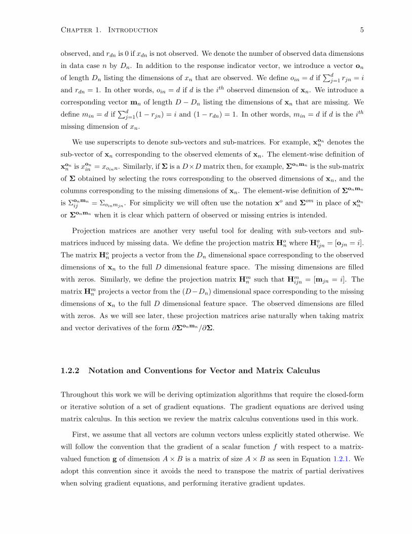
will follow the convention that the gradient of a scalar function f with respect to a matrix-
valued function g of dimension A×B is a matrix of size A×B as seen in Equation 1.2.1. We
adopt this convention since it avoids the need to transpose the matrix of partial derivatives
when solving gradient equations, and performing iterative gradient updates.
Chapter 1. Introduction 6
∂f
∂g=
∂f∂g11
∂f∂g12
· · · ∂f∂g1B
∂f∂g21
∂f∂g22
· · · ∂f∂g2B
......
. . ....
∂f∂gA1
∂f∂gA2
· · · ∂f∂gAB
(1.2.1)
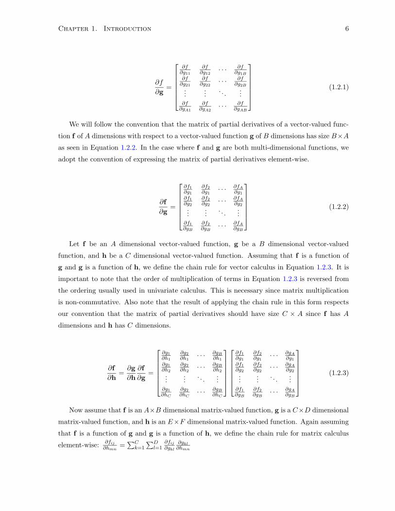
We will follow the convention that the matrix of partial derivatives of a vector-valued func-
tion f of A dimensions with respect to a vector-valued function g of B dimensions has size B×Aas seen in Equation 1.2.2. In the case where f and g are both multi-dimensional functions, we
adopt the convention of expressing the matrix of partial derivatives element-wise.
∂f
∂g=
∂f1
∂g1
∂f2
∂g1· · · ∂fA
∂g1
∂f1
∂g2
∂f2
∂g2· · · ∂fA
∂g2
......
. . ....
∂f1
∂gB
∂f2
∂gB· · · ∂fA
∂gB
(1.2.2)
Let f be an A dimensional vector-valued function, g be a B dimensional vector-valued
function, and h be a C dimensional vector-valued function. Assuming that f is a function of
g and g is a function of h, we define the chain rule for vector calculus in Equation 1.2.3. It is
important to note that the order of multiplication of terms in Equation 1.2.3 is reversed from
the ordering usually used in univariate calculus. This is necessary since matrix multiplication
is non-commutative. Also note that the result of applying the chain rule in this form respects
our convention that the matrix of partial derivatives should have size C × A since f has A
dimensions and h has C dimensions.
∂f
∂h=∂g
∂h
∂f
∂g=
∂g1
∂h1
∂g2
∂h1· · · ∂gB
∂h1
∂g1
∂h2
∂g2
∂h2· · · ∂gB
∂h2
......
. . ....
∂g1
∂hC
∂g2
∂hC· · · ∂gB
∂hC
∂f1
∂g1
∂f2
∂g1· · · ∂gA
∂g1
∂f1
∂g2
∂f2
∂g2· · · ∂gA
∂g2
......
. . ....
∂f1
∂gB
∂f2
∂gB· · · ∂gA
∂gB
(1.2.3)
Now assume that f is an A×B dimensional matrix-valued function, g is a C×D dimensional
matrix-valued function, and h is an E×F dimensional matrix-valued function. Again assuming
that f is a function of g and g is a function of h, we define the chain rule for matrix calculus
element-wise:∂fij
∂hmn=∑C
k=1
∑Dl=1
∂fij
∂gkl
∂gkl
∂hmn
Chapter 2
Decision Theory, Inference, and
Learning
This chapter introduces the learning and inference frameworks used in this thesis. We adopt
a decision-theoretic perspective based on a general prediction problem where we are given a
set of pairs {yn,xn}, n = 1, ..., N along with a loss function l(y, y). The goal is to estimate
a prediction function or decision rule f(x) that achieves the lowest possible loss on future
examples. In the collaborative prediction case, yn corresponds to a subset of the values in xmn ,
and xn is replaced by xon. In the classification with missing features case, yn takes a single
categorical value, and xn is replaced with xon.
We begin by reviewing decision making and the Bayes optimal prediction function. We then
turn to the Bayesian inference framework and introduce Markov chain Monte Carlo (MCMC)
methods including the Metropolis Hastings algorithm and the Gibbs sampler. We present the
Maximum a Posteriori principle as an approximation to Bayesian inference, and review the
Expectation Maximization algorithm. We discuss a direct function approximation framework
that includes neural networks, and logistic regression. We briefly review empirical evaluation
procedures for estimating expected loss.
2.1 Optimal Prediction and Minimizing Expected Loss
We assume that there is a fixed but unknown generative probability distribution pG(y,x) over
pairs (y,x). The goal of the prediction problem can be formally stated as selecting a prediction
function f(x) that achieves the lowest possible expected loss on examples drawn from pG(y,x).
The expected loss of a prediction function f(x) under the generative distribution pG(y,x) is
defined in equation 2.1.1.
7

Chapter 2. Decision Theory, Inference, and Learning 8
EpG[l(y, f(x))] =
∫ ∫l(y, f(x))pG(y,x)dydx (2.1.1)
The theoretical minimum value of the expected loss is known as the Bayes optimal loss
or the Bayes error rate. The Bayes optimal loss is achieved by the Bayes optimal prediction
function shown in Equation 2.1.2 [57, p. 174]. The Bayes optimal prediction fO(x) given a
vector x is equal to the value y that minimizes the expectation of the loss taken with respect
to the conditional distribution pG(y|x). The Bayes optimal loss is expressed in Equation 2.1.3.
fO(x) = arg miny
∫l(y, y)pG(y|x)dy (2.1.2)
EpG[l(y, fO(x))] =
∫ ∫l(y, fO(x))pG(y,x)dydx (2.1.3)
Prediction frameworks differ in how they approximate the Bayes optimal prediction function.
Bayesian methods are closest in spirit to the Bayes optimal prediction rule and replace pG(y|x)
in Equation 2.1.2 with the posterior distribution over a set of models distributions. Maximum a
posteriori approximations replace pG(y|x) in Equation 2.1.2 with the single model distribution
that attains the highest posterior probability among a given set of model distributions. The
classical maximum likelihood principle replaces pG(y|x) in Equation 2.1.2 with the single model
distribution with the highest likelihood given the training data. Direct function approximation
frameworks including neural networks and logistic regression avoid approximating the predictive
distribution pG(y|x) by directly approximating the optimal prediction function.
2.2 The Bayesian Framework
The Bayesian solution to the prediction problem consists of specifying a family of probability
distributions (a model), and assigning a prior probability to each distribution in the family.
Once the sample of data is observed, the posterior predictive distribution is computed and sub-
stituted for the unknown pG(y|x). To make this concrete, assume that the model is parametric
with parameter θ. Each distribution in the model family has the form pM (y|x, θ) for some
value of θ. The prior probability of each distribution in the set can then be given as a prior
probability q(θ) on the parameter θ.
Chapter 2. Decision Theory, Inference, and Learning 9
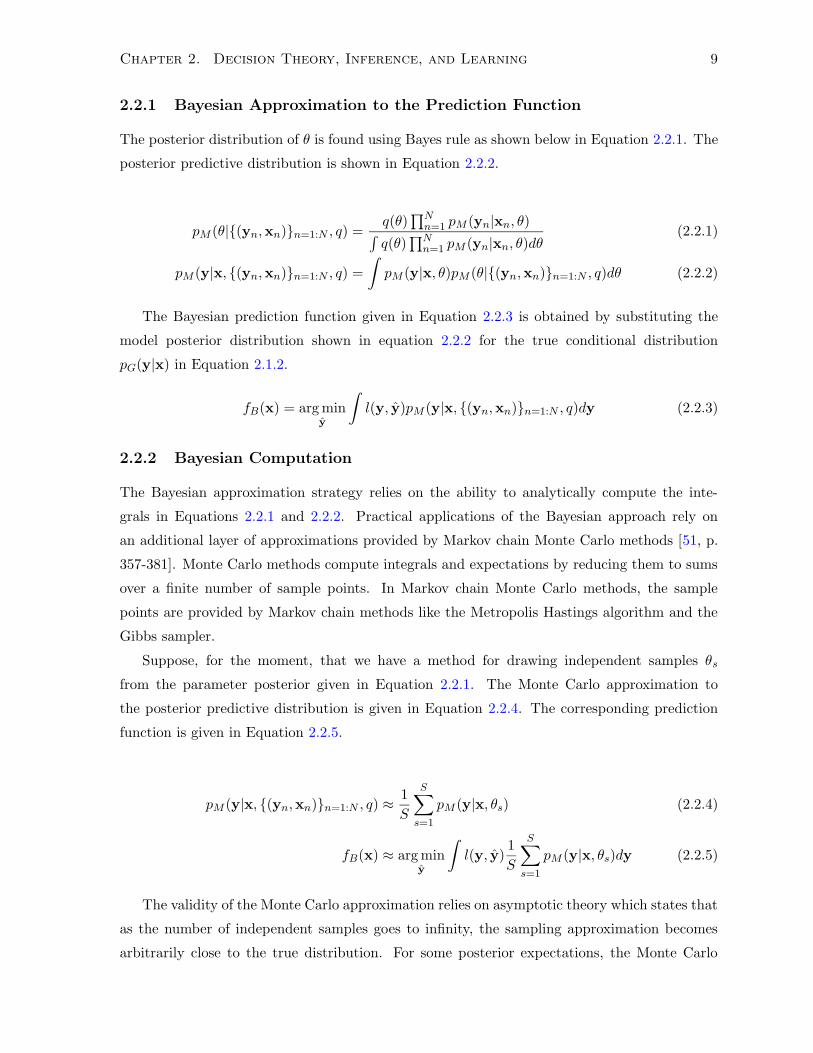
2.2.1 Bayesian Approximation to the Prediction Function
The posterior distribution of θ is found using Bayes rule as shown below in Equation 2.2.1. The
posterior predictive distribution is shown in Equation 2.2.2.
pM (θ|{(yn,xn)}n=1:N , q) =q(θ)
∏Nn=1 pM (yn|xn, θ)∫
q(θ)∏N
n=1 pM (yn|xn, θ)dθ(2.2.1)
pM (y|x, {(yn,xn)}n=1:N , q) =
∫pM (y|x, θ)pM (θ|{(yn,xn)}n=1:N , q)dθ (2.2.2)
The Bayesian prediction function given in Equation 2.2.3 is obtained by substituting the
model posterior distribution shown in equation 2.2.2 for the true conditional distribution
pG(y|x) in Equation 2.1.2.
fB(x) = arg miny
∫l(y, y)pM (y|x, {(yn,xn)}n=1:N , q)dy (2.2.3)
2.2.2 Bayesian Computation
The Bayesian approximation strategy relies on the ability to analytically compute the inte-
grals in Equations 2.2.1 and 2.2.2. Practical applications of the Bayesian approach rely on
an additional layer of approximations provided by Markov chain Monte Carlo methods [51, p.
357-381]. Monte Carlo methods compute integrals and expectations by reducing them to sums
over a finite number of sample points. In Markov chain Monte Carlo methods, the sample
points are provided by Markov chain methods like the Metropolis Hastings algorithm and the
Gibbs sampler.
Suppose, for the moment, that we have a method for drawing independent samples θs
from the parameter posterior given in Equation 2.2.1. The Monte Carlo approximation to
the posterior predictive distribution is given in Equation 2.2.4. The corresponding prediction
function is given in Equation 2.2.5.
pM (y|x, {(yn,xn)}n=1:N , q) ≈1
S
S∑
s=1
pM (y|x, θs) (2.2.4)
fB(x) ≈ arg miny
∫l(y, y)
1
S
S∑
s=1
pM (y|x, θs)dy (2.2.5)
The validity of the Monte Carlo approximation relies on asymptotic theory which states that
as the number of independent samples goes to infinity, the sampling approximation becomes
arbitrarily close to the true distribution. For some posterior expectations, the Monte Carlo

Chapter 2. Decision Theory, Inference, and Learning 10
approximation can be quite accurate using only a small number of samples [51, p. 357].
In practice it is not possible to draw independent samples θs from an arbitrary posterior
distribution. Markov chain sampling methods define a Markov chain where the state at time t
is the parameter vector θt, and the equilibrium distribution is the posterior distribution of θ.
Samples are obtained by starting the Markov chain in a random initial state, and running it
for a sufficient number of steps to reach equilibrium. If sufficient iterations are allowed between
samples at equilibrium, the samples will be approximately independent draws from the model
posterior [25, p. 287].
The Metropolis-Hastings Algorithm
For simplicity we will drop the dependence on the data and write the posterior distribution on θ
as p(θ). The Metropolis-Hastings algorithm requires the specification of a proposal distribution
p′(θnew|θt) that gives the probability of transitioning to the state θnew from the current state
θt. The algorithm proceeds by sampling a candidate value θnew from p′(θnew|θt), and setting
θt+1 to θnew with probability at+1, and θt with probability 1 − at+1. The probability at+1 is
called the acceptance probability and is defined below [25, p. 291].
at+1 = max
(1,p(θnew)p′(θt|θnew)
p(θt)p′(θnew|θt)
)(2.2.6)
θt+1 ←{θnew With probability at+1
θt otherwise(2.2.7)
A useful property of the Metropolis-Hastings method is that the normalizing factor in the
posterior cancels out in the acceptance ratio. As a result, it suffices to compute the posterior
up to a constant of proportionality. Asymptotic convergence of the Markov chain defined by
the Metropolis-Hastings updates to the posterior distribution p(θ) is guaranteed if p′(θ′|θ) > 0
for all θ′, θ [51, p. 366].
The Gibbs Sampler
The Gibbs sampler is a particular form of Metropolis-Hastings algorithm based on updating
each parameter θk in the parameter vector θ according to its posterior distribution given the
remaining parameters. The utility of the Gibbs sampler stems from the fact that in structured
models it is often possible to sample efficiently from the posterior distribution of a single pa-
rameter or a small group of parameters, even when it is not possible to sample efficiently from
the complete posterior. A single round of Gibbs updates is described below [25, p. 287].
Chapter 2. Decision Theory, Inference, and Learning 11
θ1t+1 ∼ p(θ1|θ2t, ..., θKt, {(yn,xn)}n=1:N )
...
θKt+1 ∼ p(θK |θ1t+1, ..., θK−1t+1, {(yn,xn)}n=1:N )
Since the proposal distribution for each update is based on the actual conditional distri-
bution for each parameter, the acceptance ratio for the Gibbs proposal distribution is always
equal to 1, and the proposal is always accepted.
2.2.3 Practical Considerations
Assuming the required regularity conditions hold for the Markov chain implementing a given
posterior distribution, one still needs to know both how long to simulate the Markov chain
before equilibrium is reached and how long to wait between samples. As MacKay indicates,
lower bounds on time to equilibrium can sometimes be established, but precisely predicting
time to equilibrium is a difficult problem [51, p. 379]. In general, it is not possible to guarantee
that equilibrium has been reached in a running simulation. It could always be the case that if
the simulation were run for additional steps, a new set of states with high posterior probability
could be found. Nevertheless, the use of approximate Bayesian methods based on pragmatic
choices for the number of samples and the length of the simulation can lead to good results in
practice.
2.3 The Maximum a Posteriori Framework
The maximum a posteriori (MAP) approach to the prediction problem is based on selecting
the single distribution with highest posterior probability from a family of probability distribu-
tions given a set of observations and a prior distribution. The classical maximum likelihood
framework developed by Fisher [19] is based on selecting the single distribution with the high-
est likelihood given the data. We restrict our discussion to the more general case of MAP
estimation.
2.3.1 MAP Approximation to The Prediction Function
Again assume that we have a family of distributions indexed by a parameter θ such that each
distribution in the family has the form pM (y|x, θ) with prior probability q(θ). The posterior
distribution of θ is again found using Bayes rule as shown below. θMAP is set to a value of θ

Chapter 2. Decision Theory, Inference, and Learning 12
that obtains maximum posterior probability. Note that in general several different parameter
vectors θ could attain the same maximum value of the posterior probability.
pM (θ|{(yn,xn)}n=1:N , q) =q(θ)
∏Nn=1 pM (yn|xn, θ)∫
q(θ)∏N
n=1 pM (yn|xn, θ)dθ(2.3.1)
θMAP = arg maxθ
pM (θ|{(yn,xn)}n=1:N , q) (2.3.2)
The maximum a posteriori prediction function is obtained by substituting the single dis-
tribution pM (y|x, θMAP ) for pG(y|x) in Equation 2.1.2. The maximum a posterior prediction
function fMAP is shown in Equation 2.3.3.
fMAP (x) = arg miny
∫l(y, y)P (y|x, θMAP )dy (2.3.3)
2.3.2 MAP Computation
Computation of the maximum a posteriori parameters θMAP is accomplished through opti-
mization of the posterior probability. Assuming that all first order partial derivatives of the
posterior distribution with respect to the parameters exist, the value of θMAP can be found by
solving the following set of gradient equations. Note that the normalization term is constant
with respect to θ, and has been omitted below.
∂
∂θkq(θ)
N∏
n=1
pM (yn|xn, θ) = 0 ... for all K (2.3.4)
For more complex models, the system of equations must be solved using non-linear numerical
optimization techniques such as gradient ascent, conjugate gradient, or Newton methods [62].
It is important to note that these are all local optimization methods in the sense that they
return a solution consisting of a parameter vector θ∗ that is only guaranteed to be optimal in
a local neighbourhood. In many practical situations it is not possible to fully implement the
MAP principle. Instead, the best locally optimal set of parameters found using random restarts
of the optimization procedure is substituted for θMAP . The error in such an approximation is
impossible to determine in general. Nevertheless, these methods are often found to work well
in practice.
The Expectation Maximization Algorithm
The Expectation Maximization (EM) algorithm due to Dempster, Laird and Rubin is an itera-
tive numerical procedure for finding maximum a posteriori parameter estimates [17]. It is useful

Chapter 2. Decision Theory, Inference, and Learning 13
when the probability pM (yn|xn, θ) is obtained by integrating over latent or unobserved variables
Z. For example, a finite mixture distribution has the form∑K
k=1 p(yn|xn, Z = k, θ)p(Z = k|θ).The EM algorithm proceeds by randomly initializing the parameters to θ0. On each iteration
t, the posterior probability of the missing variables Z is computed for each data case n given
the values of the observed variables and the current parameters. In the maximization step, θt+1
is set to the value which maximizes the expected complete log posterior. These two updates
are iterated as shown below until the posterior converges.
E-Step: qn(z) ← p(y|z,x, θt)p(z|θt)∑z p(y|z,x, θt)p(z|θt)
M-Step: θt+1 ← arg maxθ
N∑
n=1
∑
z
qn(z) log (p(y|z,x, θ)p(z|θ)) + log(q(θ))
The primary advantage of the Expectation Maximization algorithm over other general iter-
ative optimization procedures is that each iteration is guaranteed to improve the value of the
log posterior. General optimization techniques require the use of line search or backtracking to
provide a similar guarantee. Of course, like any general optimization technique, the Expectation
Maximization procedure returns a locally optimal solution.
2.4 The Direct Function Approximation Framework
In the Bayesian and MAP frameworks, the main idea is to approximate the true conditional
distribution pG(y|x) using an alternative predictive distribution inferred from a sample of data.
The alternative predictive distribution is then used to derive a prediction function. The al-
ternative approach is to circumvent the estimation of a predictive distribution pM (y|x, θ), and
instead directly approximate the prediction function.
Direct function approximation is used with models like perceptrons [63], neural networks
[7], and support vector machines [10]. The direct function approximation approach to the
prediction problem requires defining a family of functions, and specifying a rule for choosing
the best function given a sample of data.
2.4.1 Function Approximation as Optimization
Suppose that the set of functions is parametric with typical elements of the form fθ(x), where
θ is the parameter vector. The rule for choosing the best value of θ given the sample of N
observed pairs (yn,xn) is normally described as the solution to a minimization problem as
shown in Equation 2.4.1. The objective function L maps each function fθ to a real-valued
score.
Chapter 2. Decision Theory, Inference, and Learning 14
θ∗ = arg minθ
L(fθ, {yn,xn}n=1:N ) (2.4.1)
Given a loss function l, the most straightforward objective function is the empirical loss
given by Equation 2.4.2. Optimizing the empirical loss function selects a function fθ with the
minimum loss on the training set. Note that this function need not be unique.
LE(fθ, {yn,xn}n=1:N ) =1
N
N∑
n=1
l(yn, fθ(xn)) (2.4.2)
2.4.2 Function Approximation and Regularization
The empirical loss function LE is often a poor estimator of the expected loss EpG[l(y, fθ(x))]
due to overfitting the training data. Regularization methods modify the empirical loss in a way
that penalizes complex functions. Let g(θ) be a function that assigns a real value to each fθ
depending on its complexity for a given notion of complexity. We assume that g(θ) decreases
as the complexity of fθ increases. Equation 2.4.3 gives a regularized objective function LR
with parameter λ controlling the trade-off between fitting the training data and penalizing the
complexity of the functions.
LR(fθ, {yn,xn}n=1:N ) =1
N
N∑
n=1
l(yn, fθ(xn)) + λg(θ) (2.4.3)
Subset selection, more commonly known as feature selection in the machine learning com-
munity, is a form of regularization that trades off between loss on the training set and the
number of features used by the model. Hoerl’s ridge regression uses a quadratic regularization
function of the form g(θ) = θT θ [38]. Ridge regression is more commonly referred to as “weight
decay” or L2 regularization in the machine learning literature [35]. Tibshirani’s “lasso” corre-
sponds to the penalty function g(θ) =∑K
k=1 |θk| [72]. This regularization function is known in
machine learning research as L1 regularization. L2 regularization has the advantage that the
regularized objective function remains continuous and differentiable if the original loss func-
tion is continuous and differentiable. Subset selection requires a search over subsets of features
that can be costly to perform. L1 regularization introduces discontinuities in the regularized
objective function, which require specialized optimization methods.
Chapter 2. Decision Theory, Inference, and Learning 15
2.5 Empirical Evaluation Procedures
While theoretical justifications can be given for each of the prediction frameworks discussed
in this chapter, in practice, the underlying assumptions are almost never known to hold with
certainty. As a result, the performance of prediction methods must be established through the
use of empirical evaluation procedures that estimate expected loss. There are several possible
estimates for expected loss including training set loss, loss on a held out validation set, and
cross validation loss.
2.5.1 Training Loss
The training loss can sometimes give an accurate estimate of the expected prediction loss, but
in most cases will be overly optimistic. Denote the training set by DT = {yn,xn|n = 1, ..., N},and a function estimated based on DT by fθ|DT
. The training loss of the function fθ|DTis given
in Equation 2.5.1.
LT (fθ|DT, DT ) =
1
N
N∑
n=1
l(yn, fθ|DT(xn)) (2.5.1)
In a classification setting with a limited number of input patterns x, the training loss can
be an accurate estimate of the expected loss if all patterns are seen during training. In a
classification setting where the number of possible input patterns is infinite, a method that
achieves zero training loss can have expected loss arbitrarily close to that of random guessing.
2.5.2 Validation Loss
The most straightforward, unbiased estimate of the expected loss is obtained by randomly
partitioning the available data into a training set DT = {yn,xn|n = 1, ..., NT } and a validation
set DV = {yn,xn|n = 1, ..., NV }. The function fθ|DTis selected based on the training set DT
only. The loss is assessed on the validation set DV .
LV (fθ|DT, DV ) =
1
NV
NV∑
n=1
l(yn, fθ|DT(xn)) (2.5.2)
The variance of validation loss as an estimate of expected loss can be lowered by increasing
the size of the validation set. This exposes the obvious drawback of validation loss: using
a separate validation set necessitates a reduction in the available training data. When large
Chapter 2. Decision Theory, Inference, and Learning 16
amounts of training data are available, this may not be problematic. With small and medium
sized samples, we might hope to make more effective use of the available data.
2.5.3 Cross Validation Loss
Cross validation loss provides an estimate of the expected loss that can be nearly unbiased
[32, p. 215]. To compute the cross validation loss, the available data is randomly partitioned
into K equally sized blocks D1, ..., DK . We define the data set D−k =⋃
l 6=k Dl. For each k, a
function fθ|D−kis selected based on the training set D−k, and evaluated on the validation set
Dk. The loss values obtained by testing on each Dk are averaged together to obtain the cross
validation loss [71]. The cross validation loss is defined in Equation 2.5.3. For convenience we
define fkθ|D = fθ|D−k
, and introduce an indexing function κ(n), which maps data case indices
1, ..., N to the corresponding block indices 1, ...,K.
LCV (fθ|D, D) =1
N
N∑
n=1
l(yn, fκ(n)θ|D (xn)) (2.5.3)
By alternately holding out several small subsets of data for testing, we are able to use more
data for training each model. Cross validation can also be used as a method for selecting free
parameters in learning algorithms by evaluating the cross validation loss of several alternative
parameter sets.
Chapter 3
A Theory of Missing Data
In this chapter we review the theory of missing data due to Little and Rubin [49]. We formally
introduce the classes of missing data. We present a detailed analysis of the missing at random
assumption in the case of multivariate missing data. We review the effect of different types
of missing data on probabilistic inference. Finally, we highlight the impact of data model
misspecification on inference with missing data.
3.1 Categories of Missing Data
There are essentially two ways to factorize the joint distribution of the data, the latent variables,
and the response indicators as far as the response indicators are concerned. In the first case
the joint distribution is factorized as P (R|X,Z, µ)P (X,Z|θ). P (R|X,Z, µ) is referred to as the
missing data model, and P (X,Z|θ) is referred to as the complete data model. The intuition is
that the response probability depends on the true values of the data vector and latent variables.
In the second factorization the conditioning is reversed, and the joint distribution is written
as P (X,Z|R, ϑ)P (R|ν). The intuition is that each pattern of missing data specifies a different
distribution for the data and latent variables. [49, p. 219]. In this chapter and throughout most
of this work, we adopt the first factorization, but it is important to note that the alternative
factorization is equally valid.
In the classification scheme proposed by Little and Rubin, the first category of missing
data is called “missing completely at random” or MCAR. Data is MCAR when the response
indicator variables R are independent of the data variables X and the latent variables Z. The
MCAR condition can be succinctly expressed by the relation P (R|X,Z, µ) = P (R|µ).
The second category of missing data is called “missing at random” or MAR. The MAR
condition is frequently written as P (R = r|X = x,Z = z, µ) = P (R = r|Xo = xo, µ) for all xm,
z, and µ [49, p. 12]. It is intended to express the fact that the probability of response can not
17
Chapter 3. A Theory of Missing Data 18
depend on missing data values or latent variables. A precise definition of the MAR condition
requires the introduction of additional notation. Define a function f(x, r) = v such that vd = xd
if rd = 1, and vd = ∅ if rd = 0. The function f() maps a data vector and response indicator
vector into an alternative representation where the missing dimensions of x are replaced with
the symbol ∅. Given x and r we compute v, and consider the set C = {(x′, z′)|P (X = x′,Z =
z′) > 0, f(x′, r) = v}. The set C contains all pairs (x′, z′) with non-zero probability where x′
agrees with x on the observed dimensions specified by r.
The missing dimensions of x are missing at random for a fixed response vector r if P (R =
r|X = x′,Z = z′, µ) is constant for all (x′, z′) in the set C, and all values of the parameter µ
[64, p. 582]. In other words, given the values of the observed dimensions, the probability of the
response vector is the same regardless of the values we fill in for the missing dimensions and
latent variables.
The last class of missing data is referred to by several names including “non-ignorable” (NI)
and “not missing at random” (NMAR). Data is NMAR when the response indicator variable
R depends on either the unobserved values contained in xm, or the unobserved values of the
latent variables z. It may also depend on the observed data variables xo. A simple example
of NMAR occurs when the probability that a particular data dimension is missing depends on
the value of that data dimension.
3.2 The Missing at Random Assumption and Multivariate Data
The interpretation and implications of the missing at random assumption can be quite subtle
in the multivariate setting with arbitrary patterns of missing data. In many of the examples
considered by Little and Rubin it is assumed that the data vector can be partitioned into two
parts where the first part is subject to non-response, and the second part is always observed.
If we define the always observed sub-vector to be xa, then a missing data model of the form
P (R = r|Xa = xa, µ) satisfies the missing at random condition.
In the multivariate setting with arbitrary patterns of missing data, we find it more intuitive
to think of the missing at random condition as imposing constraints on the parameters of the
conditional distribution P (R = r|X = x, µ). Recall that the precise definition of the missing at
random assumption states that for a fixed value of r, P (R = r|X = x′, µ) must take the same
value for any complete vector x′ that agrees with the observed dimensions of x as specified by
r.
In the case where x is a vector of discrete values, we can parameterize the conditional
distribution as P (R = r|X = x′, µ) = µrx′ . The missing at random assumption then specifies
constraints on the parameters µrx′ . In particular, if u and w are complete vectors that both
Chapter 3. A Theory of Missing Data 19
X\R 0 0 0 1 1 0 1 1
0 0 α β γ 1− α− β − γ0 1 α δ γ 1− α− δ − γ1 0 α β λ 1− α− β − λ1 1 α δ λ 1− α− δ − λ
Table 3.1: Restrictions imposed on the parameterization of P (R = r|X = x) by the MARcondition.
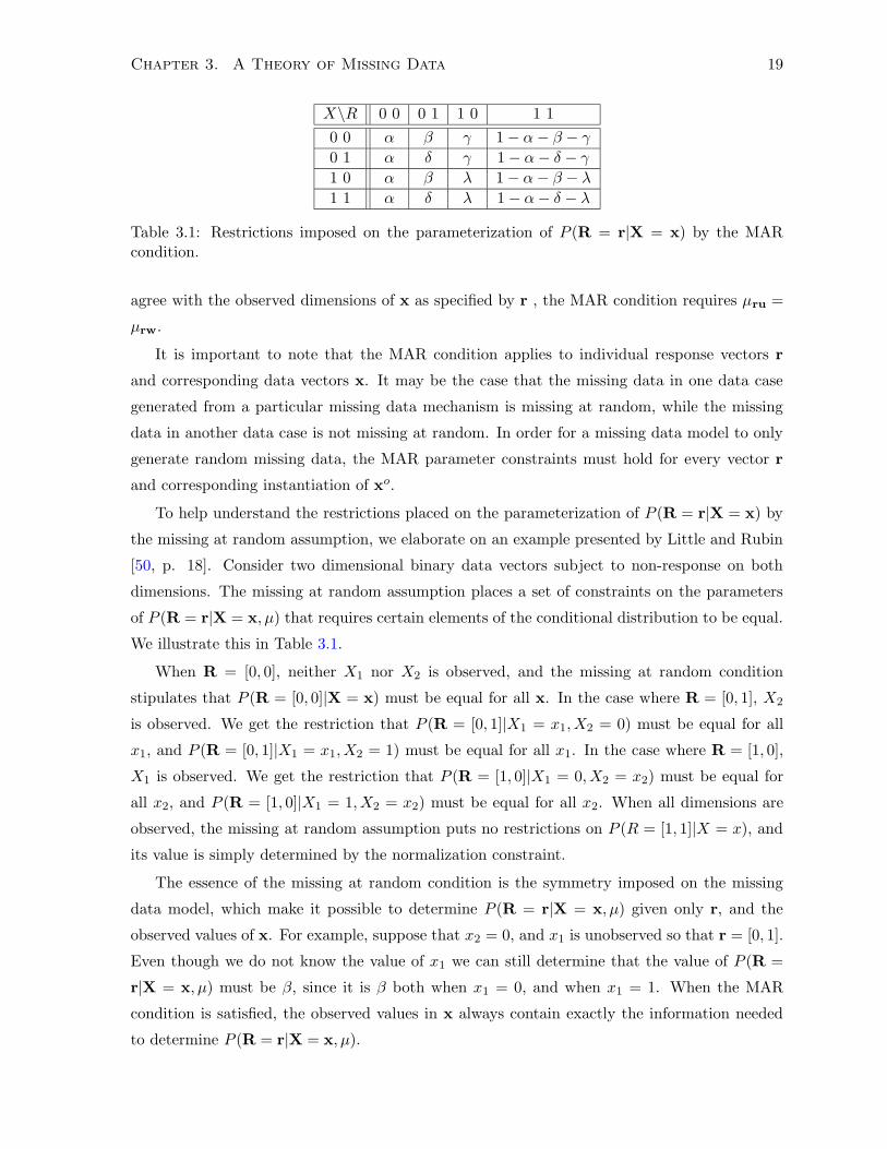
agree with the observed dimensions of x as specified by r , the MAR condition requires µru =
µrw.
It is important to note that the MAR condition applies to individual response vectors r
and corresponding data vectors x. It may be the case that the missing data in one data case
generated from a particular missing data mechanism is missing at random, while the missing
data in another data case is not missing at random. In order for a missing data model to only
generate random missing data, the MAR parameter constraints must hold for every vector r
and corresponding instantiation of xo.
To help understand the restrictions placed on the parameterization of P (R = r|X = x) by
the missing at random assumption, we elaborate on an example presented by Little and Rubin
[50, p. 18]. Consider two dimensional binary data vectors subject to non-response on both
dimensions. The missing at random assumption places a set of constraints on the parameters
of P (R = r|X = x, µ) that requires certain elements of the conditional distribution to be equal.
We illustrate this in Table 3.1.
When R = [0, 0], neither X1 nor X2 is observed, and the missing at random condition
stipulates that P (R = [0, 0]|X = x) must be equal for all x. In the case where R = [0, 1], X2
is observed. We get the restriction that P (R = [0, 1]|X1 = x1, X2 = 0) must be equal for all
x1, and P (R = [0, 1]|X1 = x1, X2 = 1) must be equal for all x1. In the case where R = [1, 0],
X1 is observed. We get the restriction that P (R = [1, 0]|X1 = 0, X2 = x2) must be equal for
all x2, and P (R = [1, 0]|X1 = 1, X2 = x2) must be equal for all x2. When all dimensions are
observed, the missing at random assumption puts no restrictions on P (R = [1, 1]|X = x), and
its value is simply determined by the normalization constraint.
The essence of the missing at random condition is the symmetry imposed on the missing
data model, which make it possible to determine P (R = r|X = x, µ) given only r, and the
observed values of x. For example, suppose that x2 = 0, and x1 is unobserved so that r = [0, 1].
Even though we do not know the value of x1 we can still determine that the value of P (R =
r|X = x, µ) must be β, since it is β both when x1 = 0, and when x1 = 1. When the MAR
condition is satisfied, the observed values in x always contain exactly the information needed
to determine P (R = r|X = x, µ).

Chapter 3. A Theory of Missing Data 20
From a modeling perspective, it makes more sense to assert that the random variable R1
either depends on the random variable X1, or is independent of the random variable X1. If
R1 is always dependent on X1, and X1 is missing in a given data case, then X1 will not be
missing at random. This makes parameter estimation more difficult. On the other hand, the
MAR assumption allows R1 to depend on X1 for some values of R1, and not for others. This is
convenient, but unnatural and difficult to justify. Little and Rubin acknowledge that assuming
the missing at random condition in a multivariate setting with arbitrary patterns of missing
data is not very realistic, but can sometimes lead to reasonable results if there are sufficient
observed covariates to do a reasonable job of predicting the response patterns [50, p. 19].
3.3 Impact of Incomplete Data on Inference
Rubin considered the impact of incomplete data on Bayesian inference [64, p. 587]. These
results are also contained in the more recent text by Schafer [67, p. 17]. In this section we
describe the effect of random missing data on Bayesian inference, and contrast it with the effect
of non-random missing data. The results for maximum likelihood and maximum a posteriori
inference are analogous, and discussed at length by Little and Rubin [49, p. 89].
Consider a joint parametric model over data variables, latent variables, and response indi-
cators of the form P (R|X,Z, µ)P (X,Z|θ), and assume the prior distribution is factorized as
P (θ|ω)P (µ|η). The posterior distribution P (θ|{xn, rn}1:N , ω, η) on θ given a sample of incom-
plete data vectors xn, n = 1, ..., N , and the prior parameters is given in Equation 3.3.1.
P (θ|{xn, rn}1:N , ω, η) ∝ P (θ|ω)
∫P (µ|η)
N∏
n=1
∫ ∫P (xo
n,xm, z|θ)P (rn|xo
n,xm, z, µ)dxmdzdµ
(3.3.1)
Without making any simplifying assumptions, the missing data and complete data models
are coupled together by the integration over both the missing data values, and the latent
variable values. Under the missing at random or missing completely at random conditions,
P (rn|xon,x
m, z, µ) is constant for all values of xm and z when we fix rn and xon. As a result,
the posterior on θ is completely independent of rn, µ and η, and the missing data model
can be removed from the posterior. The integration over missing data values then reduces to
marginalization within the complete data model only. The result of these simplifications is the
observed data posterior shown in Equation 3.3.2.
P obs(θ|{xn, rn}1:N , ω) ∝ P (θ|ω)N∏
n=1
∫P (xo
n, z|θ)dz (3.3.2)
Chapter 3. A Theory of Missing Data 21
x P (x) P (R = [0, 0]|x) P (R = [0, 1]|x) P (R = [1, 0]|x) P (R = [1, 1]|x)
0 0 a α β γ 1− α− β − γ0 1 b α δ γ 1− α− δ − γ1 0 c α β λ 1− α− β − λ1 1 d α δ λ 1− α− δ − λ
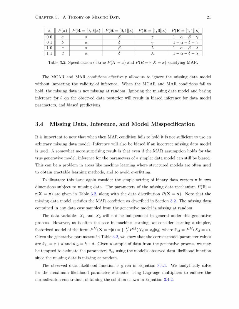
Table 3.2: Specification of true P (X = x) and P (R = r|X = x) satisfying MAR.
The MCAR and MAR conditions effectively allow us to ignore the missing data model
without impacting the validity of inference. When the MCAR and MAR conditions fail to
hold, the missing data is not missing at random. Ignoring the missing data model and basing
inference for θ on the observed data posterior will result in biased inference for data model
parameters, and biased predictions.
3.4 Missing Data, Inference, and Model Misspecification
It is important to note that when then MAR condition fails to hold it is not sufficient to use an
arbitrary missing data model. Inference will also be biased if an incorrect missing data model
is used. A somewhat more surprising result is that even if the MAR assumption holds for the
true generative model, inference for the parameters of a simpler data model can still be biased.
This can be a problem in areas like machine learning where structured models are often used
to obtain tractable learning methods, and to avoid overfitting.
To illustrate this issue again consider the simple setting of binary data vectors x in two
dimensions subject to missing data. The parameters of the missing data mechanism P (R =
r|X = x) are given in Table 3.2, along with the data distribution P (X = x). Note that the
missing data model satisfies the MAR condition as described in Section 3.2. The missing data
contained in any data case sampled from the generative model is missing at random.
The data variables X1 and X2 will not be independent in general under this generative
process. However, as is often the case in machine learning, we consider learning a simpler,
factorized model of the form PM (X = x|θ) =∏D
d PM (Xd = xd|θd) where θvd = PM (Xd = v).
Given the generative parameters in Table 3.2, we know that the correct model parameter values
are θ11 = c + d and θ12 = b + d. Given a sample of data from the generative process, we may
be tempted to estimate the parameters θvd using the model’s observed data likelihood function
since the missing data is missing at random.
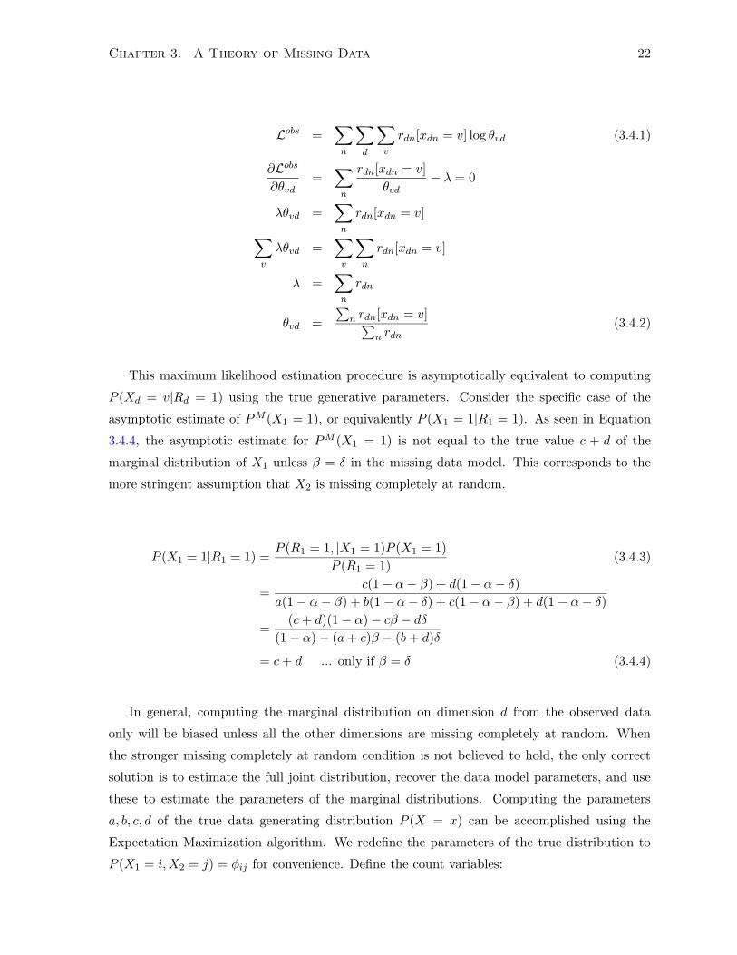
The observed data likelihood function is given in Equation 3.4.1. We analytically solve
for the maximum likelihood parameter estimates using Lagrange multipliers to enforce the
normalization constraints, obtaining the solution shown in Equation 3.4.2.
Chapter 3. A Theory of Missing Data 22
Lobs =∑
n
∑
d
∑
v
rdn[xdn = v] log θvd (3.4.1)
∂Lobs
∂θvd=
∑
n
rdn[xdn = v]
θvd− λ = 0
λθvd =∑
n
rdn[xdn = v]
∑
v
λθvd =∑
v
∑
n
rdn[xdn = v]
λ =∑
n
rdn
θvd =
∑n rdn[xdn = v]∑
n rdn(3.4.2)
This maximum likelihood estimation procedure is asymptotically equivalent to computing
P (Xd = v|Rd = 1) using the true generative parameters. Consider the specific case of the
asymptotic estimate of PM (X1 = 1), or equivalently P (X1 = 1|R1 = 1). As seen in Equation
3.4.4, the asymptotic estimate for PM (X1 = 1) is not equal to the true value c + d of the
marginal distribution of X1 unless β = δ in the missing data model. This corresponds to the
more stringent assumption that X2 is missing completely at random.
P (X1 = 1|R1 = 1) =P (R1 = 1, |X1 = 1)P (X1 = 1)
P (R1 = 1)(3.4.3)
=c(1− α− β) + d(1− α− δ)
a(1− α− β) + b(1− α− δ) + c(1− α− β) + d(1− α− δ)
=(c+ d)(1− α)− cβ − dδ
(1− α)− (a+ c)β − (b+ d)δ
= c+ d ... only if β = δ (3.4.4)
In general, computing the marginal distribution on dimension d from the observed data
only will be biased unless all the other dimensions are missing completely at random. When
the stronger missing completely at random condition is not believed to hold, the only correct
solution is to estimate the full joint distribution, recover the data model parameters, and use
these to estimate the parameters of the marginal distributions. Computing the parameters
a, b, c, d of the true data generating distribution P (X = x) can be accomplished using the
Expectation Maximization algorithm. We redefine the parameters of the true distribution to
P (X1 = i,X2 = j) = φij for convenience. Define the count variables:
Chapter 3. A Theory of Missing Data 23
β − δ True P (X1 = 1) Est. P (X1 = 1) True P (X1 = 1|R1 = 1) Est. PM (X1 = 1)
0.5 0.8000 0.7999± 0.0007 0.7961 0.7961± 0.0007
1.0 0.8000 0.8004± 0.0006 0.7917 0.7923± 0.0006
1.5 0.8000 0.7996± 0.0006 0.7868 0.7860± 0.0007
2.0 0.8000 0.8011± 0.0007 0.7812 0.7826± 0.0008
2.5 0.8000 0.7990± 0.0007 0.7750 0.7737± 0.0008
3.0 0.8000 0.8000± 0.0007 0.7679 0.7679± 0.0007
3.5 0.8000 0.7994± 0.0008 0.7596 0.7582± 0.0009
4.0 0.8000 0.7999± 0.0009 0.7500 0.7501± 0.0010
4.5 0.8000 0.7992± 0.0010 0.7386 0.7379± 0.0010
5.0 0.8000 0.7986± 0.0010 0.7250 0.7241± 0.0010
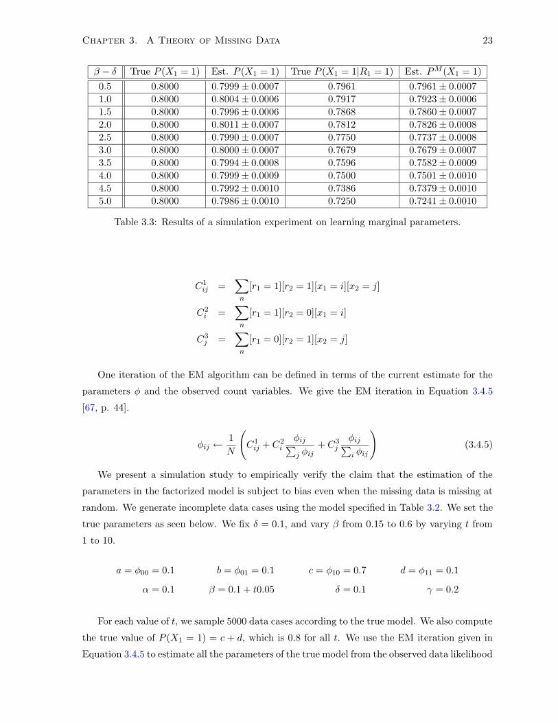
Table 3.3: Results of a simulation experiment on learning marginal parameters.
C1ij =
∑
n
[r1 = 1][r2 = 1][x1 = i][x2 = j]
C2i =
∑
n
[r1 = 1][r2 = 0][x1 = i]
C3j =
∑
n
[r1 = 0][r2 = 1][x2 = j]
One iteration of the EM algorithm can be defined in terms of the current estimate for the
parameters φ and the observed count variables. We give the EM iteration in Equation 3.4.5
[67, p. 44].
φij ←1
N
(C1
ij + C2i
φij∑j φij
+ C3j
φij∑i φij
)(3.4.5)
We present a simulation study to empirically verify the claim that the estimation of the
parameters in the factorized model is subject to bias even when the missing data is missing at
random. We generate incomplete data cases using the model specified in Table 3.2. We set the
true parameters as seen below. We fix δ = 0.1, and vary β from 0.15 to 0.6 by varying t from
1 to 10.
a = φ00 = 0.1 b = φ01 = 0.1 c = φ10 = 0.7 d = φ11 = 0.1
α = 0.1 β = 0.1 + t0.05 δ = 0.1 γ = 0.2
For each value of t, we sample 5000 data cases according to the true model. We also compute
the true value of P (X1 = 1) = c + d, which is 0.8 for all t. We use the EM iteration given in
Equation 3.4.5 to estimate all the parameters of the true model from the observed data likelihood

Chapter 3. A Theory of Missing Data 24
under the true model. The estimated parameters c and d are then used to estimate P (X1 = 1)
as c + d for each t. Next, the true value of the observed data marginal P (X1 = 1|R1 = 1) is
computed for each t according to Equation 3.4.3. Finally, we use the observed data likelihood
under the factorized model to compute an estimate θ11 of PM (X1 = 1) according to Equation
3.4.2. The entire experiment is repeated 100 times for each value of t. The average results are
reported in Table 3.3, along with the standard error of the mean for estimated quantities.
The results show that as the true value of the β parameter diverges from the true value of
the δ parameter, the estimated parameter θ11 as given by Equation 3.4.2 diverges from the true
value of P (X1 = 1). In addition, the estimate θ11 is approximately equal to the true value of
P (X1 = 1|R1 = 1) as claimed. Finally, the results also show that estimating all the parameters
of the true data model using EM and then estimating P (X1 = 1) as c+ d is not subject to bias
as claimed.
It is important to realize that in order for parameter estimation to be unbiased, it is not
sufficient for missing data to be missing at random with respect to a true underlying data
model. Inference in models that make independence assumptions not present in the underlying
generative process for complete data may be biased unless more stringent assumptions on the
missing data process hold.

Chapter 4
Unsupervised Learning With
Random Missing Data
In this chapter we present unsupervised learning methods under the missing at random as-
sumption. We discuss several types of probabilistic mixture models for categorical data in-
cluding finite mixture models and Dirichlet process mixture models. We present a collapsed
Gibbs sampler for the Multinomial/Dirichlet process mixture model with random missing data.
We review linear Gaussian latent variable models including probabilistic principal components
analysis and factor analysis. We present expectation maximization algorithms for single factor
analysis models and mixtures of factor analysis models with randomly missing data.
The models and methods presented in this chapter provide a starting point for the devel-
opment of novel models and methods for both unsupervised learning with non-random missing
data, and classification with missing features. Experimental results using the methods described
in this chapter are presented in Chapters 5 and 6.
4.1 Finite Mixture Models
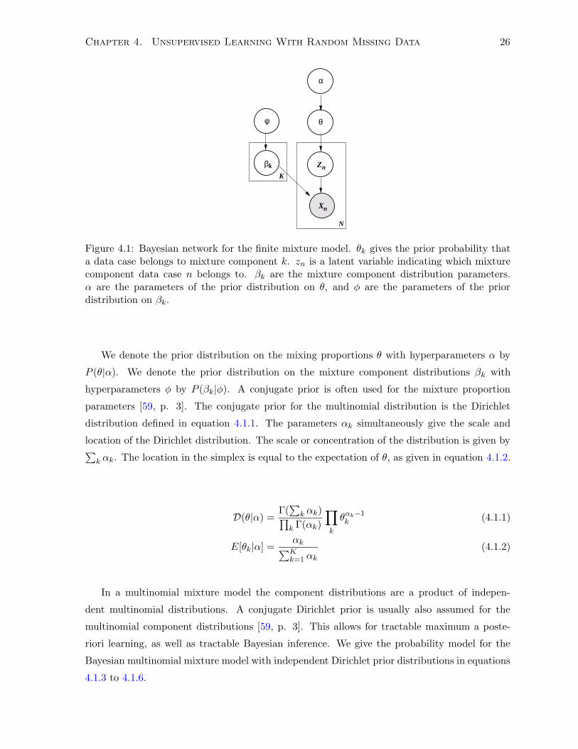
A Bayesian network representation of the finite mixture model is given in figure 4.1. We
assume that the data random variables Xn are vectors of length D that are subject to random
missing data. We assume that there are K mixture components. The random variables Zn are
mixture component indicator variables. They indicate which mixture component is associated
with each data case, and take values on the discrete set {1, ...,K}. In practice the random
variables Zn are not observed, and are referred to as latent variables. The parameters of the
mixture component distributions are denoted by βk. The mixing proportions θk give the prior
probability of observing a data case from each of the K mixture components. The mixing
proportions satisfy the constraints∑
k θk = 1, and θk > 0 ∀k.
25
Chapter 4. Unsupervised Learning With Random Missing Data 26
φ
βk
K
α
θ
N
Z
Xn
n
Figure 4.1: Bayesian network for the finite mixture model. θk gives the prior probability thata data case belongs to mixture component k. zn is a latent variable indicating which mixturecomponent data case n belongs to. βk are the mixture component distribution parameters.α are the parameters of the prior distribution on θ, and φ are the parameters of the priordistribution on βk.
We denote the prior distribution on the mixing proportions θ with hyperparameters α by
P (θ|α). We denote the prior distribution on the mixture component distributions βk with
hyperparameters φ by P (βk|φ). A conjugate prior is often used for the mixture proportion
parameters [59, p. 3]. The conjugate prior for the multinomial distribution is the Dirichlet
distribution defined in equation 4.1.1. The parameters αk simultaneously give the scale and
location of the Dirichlet distribution. The scale or concentration of the distribution is given by∑
k αk. The location in the simplex is equal to the expectation of θ, as given in equation 4.1.2.
D(θ|α) =Γ(∑
k αk)∏k Γ(αk)
∏
k
θαk−1k (4.1.1)
E[θk|α] =αk∑K
k=1 αk
(4.1.2)
In a multinomial mixture model the component distributions are a product of indepen-
dent multinomial distributions. A conjugate Dirichlet prior is usually also assumed for the
multinomial component distributions [59, p. 3]. This allows for tractable maximum a poste-
riori learning, as well as tractable Bayesian inference. We give the probability model for the
Bayesian multinomial mixture model with independent Dirichlet prior distributions in equations
4.1.3 to 4.1.6.
Chapter 4. Unsupervised Learning With Random Missing Data 27
P (θ|α) = D(θ|α) (4.1.3)
P (βdk|φdk) = D(βdk|φdk) (4.1.4)
P (Zn = k|θ) = θk (4.1.5)
P (Xn = xn|Zn = k, β) =D∏
d=1
V∏
v=1
β[xdn=v]vdk (4.1.6)
We give the posterior probability of the parameters β and θ given the prior and a set of N
data cases in Equation 4.1.7. We assume the missing at random condition holds.
P (β, θ|{xn, rn}1:N , α, φ) ∝ Γ(∑K
k=1 αk)∏Kk=1 Γ(αk)
K∏
k=1
θαk−1k ·
D∏
d=1
Γ(∑V
v=1 φvdk)∏Vv=1 Γ(φvdk)
V∏
v=1
βφvdk−1vdk
·N∏
n=1
K∑
k=1
θk
D∏
d=1
V∏
v=1
β[rdn=1][xdn=v]vdk (4.1.7)
4.1.1 Maximum A Posteriori Estimation
The maximum a posteriori principle states that we should select the parameters θ and β with
maximum posterior probability. The optimal parameters of the Bayesian multinomial mixture
model can not be found analytically, but an efficient expectation maximization algorithm can
be derived assuming missing data is missing at random. We give the derivation in equations
4.1.8 to 4.1.11. We first find the posterior distribution over the latent variable zn for each data
case n. Note that the posterior only depends on the observed data dimensions as specified by
[rdn = 1].
P (Zn = k|xn, rn, β, θ) = qn(k) =θk∏D
d=1
∏Vv=1 β
[rdn=1][xdn=v]vdk∑K
k′=1 θk′
∏Dd=1
∏Vv=1 β
[rdn=1][xdn=v]vdk′
(4.1.8)
Next we form the expected complete log posterior function E[logP(θ, β|{xn, rn}1:N , α, φ)]
using the posterior probability of the latent variables, and the complete log posterior of the
parameters. The expectation is taken with respect to the latent mixture indicators only. The
missing data is analytically integrated out of the complete log posterior under the MAR as-
sumption.
Chapter 4. Unsupervised Learning With Random Missing Data 28
E[logP(θ, β|{xn, rn}n=1:N , α, φ)] = log Γ(K∑
k=1
αk)−K∑
k=1
log Γ(αk) +K∑
k=1
(αk − 1) log θk
+
K∑
k=1
D∑
d=1
log Γ(
V∑
v=1
φvdk)−V∑
v=1
log Γ(φvdk) +
V∑
v=1
(φvdk − 1) log βvdk
+N∑
n=1
K∑
k=1
qn(k)
(log θk +
D∑
d=1
V∑
v=1
[rdn = 1][xdn = v] log βvdk
)(4.1.9)
Finally, we find the partial derivatives of the expected complete log posterior with respect to
the multinomial parameters θ, and β. We solve the resulting gradient equations using Lagrange
multipliers to enforce the normalization constraint on the multinomial parameters. The update
for θ is given in Equation 4.1.10.
∂E[logP]
∂θk=αk − 1 +
∑Nn=1 qn(k)
θk− λ = 0
θkλ = αk − 1 +N∑
n=1
qn(k)
K∑
k=1
θkλ =K∑
k=1
(αk − 1) +N∑
n=1
qn(k)
λ = N −K +K∑
k=1
αk
θk =αk − 1 +
∑Nn=1 qn(k)
N −K +∑K
k=1 αk
(4.1.10)
The update for βdk is given in Equation 4.1.11.
∂E[logP]
∂βvdk=φvnk − 1 +
∑Nn=1 qn(k)[rdn = 1][xdn = v]
βvdk− λ = 0
βvdkλ = φvnk − 1 +N∑
n=1
qn(k)[rdn = 1][xdn = v]
V∑
v=1
βvdkλ =V∑
v=1
(φvnk − 1) +N∑
n=1
qn(k)[rdn = 1][xdn = v]
λ =N∑
n=1
qn(k)[rdn = 1]− V +V∑
v=1
φvdk
Chapter 4. Unsupervised Learning With Random Missing Data 29
βvdk =φvdk − 1 +
∑Nn=1 qn(k)[rdn = 1][xdn = v]
∑Nn=1 qn(k)[rdn = 1]− V +
∑Vv=1 φvdk
(4.1.11)
We give the expectation maximization algorithm for the Bayesian multinomial mixture
model under the missing at random assumption in Equations 4.1.12 to 4.1.14.
E-Step: qn(k)← θk∏D
d=1
∏Vv=1 β
[rdn=1][xdn=v]vdk∑K
k′=1 θk′
∏Dd=1
∏Vv=1 β
[rdn=1][xdn=v]vdk′
(4.1.12)
M-Step: θk ←αk − 1 +
∑Nn=1 qn(k)
N −K +∑K
k=1 αk
(4.1.13)
βvdk ←φvdk − 1 +
∑Nn=1 qn(k)[rdn = 1][xdn = v]
∑Nn=1 qn(k)[rdn = 1]− V +
∑Vv=1 φvdk
(4.1.14)
Efficient Markov chain Monte Carlo inference methods can also be derived for the finite
mixture model [59, p. 3]. However, with very little additional computational effort these same
methods can be used to perform inference in a mixture model with an unbounded number of
mixture components, as we describe in Section 4.2.
4.1.2 Predictive Distribution
Once the model parameters β and θ are learned, the finite mixture model can be used to make
predictions for the unobserved values in a data case. The posterior predictive distribution is
given in Equation 4.1.15.
P (xdn = v|xn, rn, β, θ) =K∑
k=1
P (xdn = v|zn = k, β)P (zn = k|xn, rn, β, θ)
=
K∑
k=1
βvdkθk
∏Dd=1
∏Vv=1 β
[rdn=1][xdn=v]vdk∑K
k′=1 θk′
∏Dd=1
∏Vv=1 β
[rdn=1][xdn=v]vdk′
(4.1.15)
4.2 Dirichlet Process Mixture Models
The Dirichlet process mixture model is represented as a Bayesian network in figure 4.2. To
sample a complete data set from a DP mixture model we begin by sampling a random distri-
bution φ from DP(αφ0). For each data case n we sample a value βn from φ, and a value of xn
from P (X|βn). Unlike the finite mixture model, the number of mixture components is not fixed
a priori. As more data is sampled from the model, an unlimited number of mixture components
may appear. Data cases n and n′ are said to belong to the same mixture component if βn = βn′ .
We give the probability model for the DP mixture in equations 4.2.1 to 4.2.3.
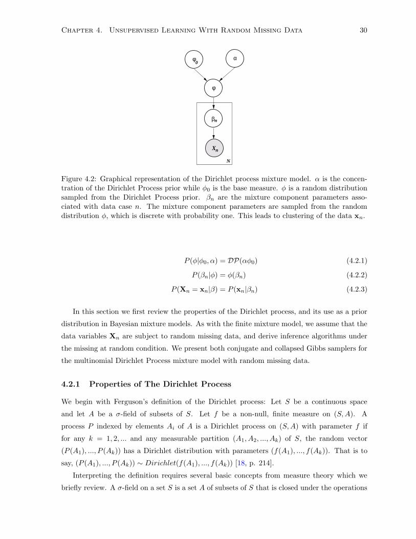
Chapter 4. Unsupervised Learning With Random Missing Data 30
φ0
α
N
nβ
φ
Xn
Figure 4.2: Graphical representation of the Dirichlet process mixture model. α is the concen-tration of the Dirichlet Process prior while φ0 is the base measure. φ is a random distributionsampled from the Dirichlet Process prior. βn are the mixture component parameters asso-ciated with data case n. The mixture component parameters are sampled from the randomdistribution φ, which is discrete with probability one. This leads to clustering of the data xn.
P (φ|φ0, α) = DP(αφ0) (4.2.1)
P (βn|φ) = φ(βn) (4.2.2)
P (Xn = xn|β) = P (xn|βn) (4.2.3)
In this section we first review the properties of the Dirichlet process, and its use as a prior
distribution in Bayesian mixture models. As with the finite mixture model, we assume that the
data variables Xn are subject to random missing data, and derive inference algorithms under
the missing at random condition. We present both conjugate and collapsed Gibbs samplers for
the multinomial Dirichlet Process mixture model with random missing data.
4.2.1 Properties of The Dirichlet Process
We begin with Ferguson’s definition of the Dirichlet process: Let S be a continuous space
and let A be a σ-field of subsets of S. Let f be a non-null, finite measure on (S,A). A
process P indexed by elements Ai of A is a Dirichlet process on (S,A) with parameter f if
for any k = 1, 2, ... and any measurable partition (A1, A2, ..., Ak) of S, the random vector
(P (A1), ..., P (Ak)) has a Dirichlet distribution with parameters (f(A1), ..., f(Ak)). That is to
say, (P (A1), ..., P (Ak)) ∼ Dirichlet(f(A1), ..., f(Ak)) [18, p. 214].
Interpreting the definition requires several basic concepts from measure theory which we
briefly review. A σ-field on a set S is a set A of subsets of S that is closed under the operations
Chapter 4. Unsupervised Learning With Random Missing Data 31
of complementation, and countably infinite unions. A measure f is a function mapping any
element of the σ-field A to the positive real line which satisfies f(∅) = 0 and for every collection
A1, A2, ... of non-overlapping elements of A, f(∪∞i=0Ai) =∑∞
i=0 f(Ai).
Suppose that β is a continuous random variable, and the space of β is S. Normally the
base measure f consists of the product of a scalar variable α, and a probability distribution φ0
on β [60]. The definition states that a random probability distribution φ on β is distributed
according to the Dirichlet process DP(αφ0) if for any partition (A1, A2, ..., Ak) of S, (φ(β ∈A1), ..., φ(β ∈ AK)) ∼ Dirichlet(αφ0(A1), ..., αφ0(AK)).
In the case of a Dirichlet process mixture model, we assume that the observed data variable
X is generated according to a parametric distribution P (X|β). The parameter β is in turn
distributed according to a random distribution P (β|φ) = φ(β). The random distribution φ is
drawn from a Dirichlet process prior DP(αφ0).
Ferguson’s definition of the Dirichlet process is useful for establishing some important prop-
erties of the Dirichlet process. For example, suppose that we observe a set of draws β1, ..., βN−1
from φ. Let A1, ..., AK be any partition of the space S of β for any K. Let δβnbe a distribu-
tion concentrated at location βn. The posterior distribution of φ given β1, ..., βN−1 is shown in
equation 4.2.4, as derived by Ferguson [18, p. 217]. From the posterior distribution on φ we
can find the posterior distribution on βN+1 given the values of the previous draws as seen in
equation 4.2.5 [60, p. 3].
P (φ|α, φ0, β1, ..., βN−1) = DP(αφ0 +N−1∑
n=1
δβn) (4.2.4)
P (βN |α, φ0, β1, ..., βN−1) =αφ0(βN )
N − 1 + α+
∑Nn=1 δβn
(βN )
N − 1 + α(4.2.5)
This last equation shows that when we draw a series of values for β from the Dirichlet process
prior, we may either draw a value equal to one of the previous draws, or draw a new value from
the base distribution φ0. Further, it can be shown that a draw φ from the Dirichlet process is
discrete with probability one [18, p. 219]. This means that φ consists of a countably infinite
collection of point masses in the space of β, and there is a non-zero probability of drawing the
same value β multiple times. In terms of the Dirichlet process mixture, this property implies
that a series of data points xn drawn from the DP mixture will tend to form clusters.
Suppose we introduce a set of indicator variables zn along with βn and xn. We begin by
setting z1 = 0. During sampling we set zn = zj if βn = βj , 1 < j < n. If βn is not equal to any
of β1, .., βn−1, we set zn to the next available value 1 + max(z1, ..., zn−1). The sampling process
on the indicator variables induced by the Dirichlet process is known as the Chinese Restaurant
Chapter 4. Unsupervised Learning With Random Missing Data 32
Process or CRP [2, p. 92]. The probability distribution of zN given the N −1 previous samples
can be obtained from equation 4.2.5.
If zj = zN = k for some j 6= N P (zN = k|α, z1, ..., zN−1) =
∑N−1i=1 [zi = k]
N − 1 + α(4.2.6)
P (zN 6= zj ∀ j 6= N |α, z1, ..., zN−1) =α
N − 1 + α(4.2.7)
Using the CRP, we can draw a sample of N data points from the Dirichlet process prior
in two stages. First we sample a partition of the data points from the CRP as represented by
the indicator variables zn. Let the partition consists of K clusters. Next, for each cluster k, a
single parameter vector βk is sampled from the base distribution φ0 for that cluster.
We can also use the definition of the CRP, and its relationship to the Dirichlet process, to
derive the joint distribution of a sample of indicator variables z1, ..., zN , as well as a sample of
parameter values β1, ..., βN . To simplify the notation suppose again that the partition has K
blocks or clusters. Let the unique values of z be zu(1), ..., zu(K), and the corresponding unique
values of β be βu(1), ..., βu(K). We introduce count variables ck to indicate the number of zn
equal to zu(k).
P (z1, ..., zN |α) = P (z1|α) · · ·P (zN |α, z1, ..., zN−1)
=
∏Kk=1 α
∏ck−1i=1 i
∏Nn=1 n− 1 + α
=αKΓ(α)
∏Kk=1 Γ(ck)
Γ(N + α)(4.2.8)
P (β1, ..., βN |α, φ0) = P (β1|α, φ0) · · ·P (βN |α, φ0, β1, ..., βN−1)
=αKΓ(α)
∏Kk=1 Γ(ck)
Γ(N + α)
K∏
k=1
φ0(βu(k)) (4.2.9)
It is clear from the form of equations 4.2.8 and 4.2.9 that the joint probability of the z’s
and the joint probability of the β’s are both independent of their ordering. This property is
called exchangeability. Under exchangeability we can assume that any element in the sampled
sequence is the last element, and thus use 4.2.6 or 4.2.5 to compute the conditional probabilities
needed for Gibbs sampling [2, p. 6].
4.2.2 Bayesian Inference and the Conjugate Gibbs Sampler
As we have seen, the Dirichlet Process provides a very flexible prior distribution for mixture
models. Unlike finite mixture models, the Dirichlet process mixture model can produce an
unlimited number of clusters as the amount of data increases. Conditioned on a fixed sample
Chapter 4. Unsupervised Learning With Random Missing Data 33
of data, the Dirichlet process mixture model is able to automatically adapt the number of
clusters. The Dirichlet process mixture model can better reflect uncertainty about the number
of components underlying the data, and eliminates the need to perform an explicit search for
a single, optimal number of components. In this section we derive a Gibbs sampler for the
Dirichlet process mixture model assuming conjugate priors [60, p. 4].
To complete our definition of the multinomial Dirichlet Process mixture model, we must
specify the base distribution φ0. A conjugate Gibbs sampler can be derived using an indepen-
dent product of Dirichlet distributions as the base distribution. Recall that this base distri-
bution is the same as the conjugate prior on mixture component parameters used in the finite
multinomial mixture model.
P (β|φ0) =D∏
d=1
D(βd|φd0) (4.2.10)
The state of the Gibbs sampler consists of the mixture component indicators z1, ..., zN
and the parameters of the occupied mixture component distributions β1, ..., βK . Of course,
the mixture contains an infinite number of components, but we do not explicitly represent
components that have no data cases assigned to them. The number of occupied components K
changes as new components are occupied, and old components are abandoned.
We begin by deriving the posterior probability of the mixture indicator zn, given the re-
maining indicator variables z−n, and the observed data. This conditional distribution can be
derived from the Chinese Restaurant Process and the observed data likelihood obtained by
analytically summing over missing data under the missing at random assumption.
If zj = zn = k for some j 6= n P (zn = k|z−n,xn, β, α, φ0)
∝ P (zn = k|z−n, α)P (xn|rn, βk)
∝∑N
i6=n[zi = k]
N − 1 + α
D∏
d=1
V∏
v=1
βvdk[rdn=1][xdn=v] (4.2.11)
P (zn 6= zj ∀ j 6= n|z−n,xn, α, φ0) ∝ P (zn 6= zj∀ j 6= n|z−n, α)P (xn|rn, φ0)
∝ α
N − 1 + α
∫P (xn|rn, β)P (β|φ0)dβ
∝ α
N − 1 + α
D∏
d=1
V∏
v=1
(φvd0∑V
v=1 φvd0
)[rdn=1][xdn=v]
(4.2.12)
The probabilities in equations 4.2.11 and 4.2.12 have very intuitive interpretations. Equation
4.2.11 simply states that zn is assigned to a component k, and there exists another data case
j different from n that is also assigned to component k. The probability of this event depends

Chapter 4. Unsupervised Learning With Random Missing Data 34
on the number of data cases assigned to component k, and the probability of the observed data
xon under component k.
The event expressed in equation 4.2.12 as (zn 6= zj ∀ j 6= n) is the event that data case n is
assigned to a previously unoccupied component. The probability of this event depends only on
the concentration parameter α, and the marginal probability of xon under the base distribution.
Increasing the concentration parameter increases the prior probability of forming new clusters.
The marginal probability of assigning data case n to an unoccupied component is given by the
integral of P (xon|β) with respect to the base distribution. This integral is tractable when the
base distribution is conjugate to the parameter β. If a new component is created while updating
the zn, it is randomly initialized by sampling from the base distribution.
Once all of the data cases have been assigned to mixture components, the update for the
occupied component distribution parameters is identical to the finite mixture case. Here we
use the count variables cvdk =∑N
n=1[zn = k][rdn = 1][xdn = v] to simplify the notation.
P (βvdk|z,x, φ0) ∝N∏
n=1
P (xdn|βdk)P (βdk|φd0)
∝N∏
n=1
V∏
v=1
βvdk[rdn=1][xdn=v][zn=k] ·
V∏
v=1
βφvd0−1vdk
= D(c1dk + φ1d0, ..., cV dk + φV d0) (4.2.13)
The conjugate Gibbs sampler for the multinomial/Dirichlet process mixture model alter-
nates between sequentially assigning each data case to a mixture component, creating new
components as needed, and updating the parameters associated with each occupied mixture
component.
4.2.3 Bayesian Inference and the Collapsed Gibbs Sampler
In this section we derive a collapsed Gibbs sampler for the multinomial Dirichlet Process mixture
model under the missing at random assumption. To form the collapsed Gibbs sampler we
analytically integrate the β parameters out of the model, leaving only the mixture indicators
[59, p. 4]. This integration is tractable in the conjugate multinomial/Dirichlet setting. The
primary advantage of the collapsed Gibbs sampler is that the size of the state of the underlying
Markov chain is greatly reduced. We give the Gibbs updates below. For convenience we
introduce the count variables c−nk =
∑Ni6=n[zi = k] and c−n
vdk =∑N
i6=n[zi = k][rdi = 1][xdi = v].
Note that the count variables must be recomputed after each Gibbs update.
Chapter 4. Unsupervised Learning With Random Missing Data 35
If zj = zn = k for some j 6= n P (zn = k|z−n,x, α, φ0)
∝ c−nk
N − 1 + α
D∏
d=1
V∏
v=1
(c−nvdk + φvd0∑V
v=1 c−nvdk + φvd0
)[rdn=1][xdn=v]
(4.2.14)
P (zn 6= zj ∀j 6= n |z−n, xn, α, φ0) ∝α
N − 1 + α
D∏
d=1
V∏
v=1
(φvd0∑V
v=1 φvd0
)[rdn=1][xdn=v]
(4.2.15)
To run the collapsed Gibbs sampler we simply iterate through the data cases, updating each
mixture indicator in turn. A careful implementation where the count variable are cached and
updated instead of recomputed from scratch can lead to significant computational savings.
4.2.4 Predictive Distribution and the Conjugate Gibbs Sampler
Running the conjugate Gibbs sampler produces a set of samples zsn, βs
k for each data case n and
each occupied mixture component k. Denote the number of occupied mixture components in
sample s by Ks. The posterior predictive distribution for data case n is obtained by averaging
the predictions made by the mixture component data case n belongs to in each sample s. Note
that we assume the data dimension d we make a prediction for is not one of the observed data
dimensions.
P (xdn = v|{xoi , ri}i=1:N , φ0, α) =
1
S
S∑
s=1
Ks∑
k=1
[zsn = k]βs
vdk (4.2.16)
If a data case is not included in the Dirichlet process mixture simulation, it is still possible to
make predictions for that data case. This is a useful procedure if we need to make predictions
for additional data cases and wish to avoid re-running a complete simulation. One method
to accomplish this is to convert each sample from the Dirichlet process mixture into a finite
mixture model with parameters θ and β as shown below. This procedure is closely related to
the finite mixture model approximations to the Dirichlet Process mixture model studied by
Ishwaran and Zarepour [41].
θsk =
∑Nn=1
[zn=k]N+α ... k ≤ Ks
αN+α ... k = Ks + 1
βsvdk =
βsvdk ... k ≤ Ks
φvd0∑Vv=1
φvd0
... k = Ks + 1
Chapter 4. Unsupervised Learning With Random Missing Data 36
To compute the predictive distribution for a novel data case x∗, we average the predictive
distribution under each of the finite mixture models as seen in Equation 4.2.17. The predictive
distribution within a single finite mixture model is computed according to Equation 4.1.15.
P (xd∗ = v|xo∗, r∗, β, θ) =
1
S
S∑
s=1
Ks+1∑
k=1
βsvdk
θk∏D
d=1
∏Vv=1 β
[rd∗=1][xd∗=v]vdk∑K
k′=1 θk′
∏Dd=1
∏Vv=1 β
[rd∗=1][xd∗=v]vdk′
(4.2.17)
If our original simulation was based on a large number of data cases, the present approxima-
tion will be quite close to the predictive distribution obtain by including the novel data point
in the simulation. The reason is that a single data point can not have a large effect on either
the partitioning of the data points, or the sampling of the parameter values. If we use this
scheme to independently make predictions for a large number of novel data points, the results
may differ significantly from including all such novel data points in the simulation.
4.2.5 Predictive Distribution and the Collapsed Gibbs Sampler
Computing the predictive distribution for a training case using samples from the collapsed
Gibbs sampler requires additional steps. This is because the state of the collapsed Gibbs
sampler consists only of mixture indicator variables zn. The posterior distribution on βdk
for an occupied cluster with index k in sample s is Dirichlet, and its parameters are trivial
to compute given the training data and mixture indicators. We again use count variables
cvdk =∑N
n=1[zn = k][rdn = 1][xdn = v].
P (βdk|{zsn,xn, rn}n=1:N , φ0) = D(φ10 + c1dk, ..., φV 0 + cV dk) (4.2.18)
A particular value βsk could be sampled from this posterior distribution in order to compute
the predictive distribution. However, this introduces unnecessary variance. A better option is
to set βsk to the mean of the posterior. This is a form of Rao-Blackwellization in the sense of
Gelfand and Smith [24].
βsvdk =
φv0 + cvdk∑Vv=1 φv0 + cvdk
(4.2.19)
The predictive distribution for training cases can now be calculated as seen in Equation
4.2.20. The predictive distribution for novel data cases can be found using the same approxi-
mation scheme as described for the conjugate Gibbs sampler in Equation 4.2.17.
P (xdn = v|{xoi , ri}i=1:N , φ0, α) =
1
S
S∑
s=1
Ks∑
k=1
[zsn = k]βs
vdk (4.2.20)
Chapter 4. Unsupervised Learning With Random Missing Data 37
4.3 Factor Analysis and Probabilistic Principal Components
Analysis
The generative process underlying factor analysis asserts that the observed data cases x1, ...,xN
are generated using a two step process. First, a continuous Q-dimensional latent vector tn is
sampled for each data case n from a zero-mean Gaussian with unit variance. Next, xn is sampled
from a D-dimensional Gaussian distribution with mean µ+ Λtn, and covariance matrix Ψ [73,
p. 612]. Λ is a D×Q matrix referred to as the factor loading matrix. Each dimension q of the
latent space is referred to as a factor.
The main feature of factor analysis is that the covariance matrix Ψ is constrained to be
diagonal. This means that conditioned on the latent vector tn, the dimensions of xn are
independent. We summarize the factor analysis model below.
P (tn) =1
(2π)Q/2exp(−1
2tTn tn) (4.3.1)
P (xn|tn,Λ,Ψ, µ) =1
|2πΨ|1/2exp(−1
2(xn − µ− Λtn)T Ψ−1(xn − µ− Λtn)) (4.3.2)
Probabilistic principal components analysis is a linear Gaussian generative model for con-
tinuous data vectors [73]. The model asserts that each D dimensional observed data vector xn
is generated by first sampling a Q dimensional vector tn from a unit-variance, zero-mean Gaus-
sian distribution. The observed data vector xn is then sampled from a Gaussian distribution
with mean µ+ Λtn and covariance matrix σ2I. We summarize the probabilistic model below.
P (tn) =1
(2π)Q/2exp(−1
2tTn tn) (4.3.3)
P (xn|tn,Λ, σ, µ) =1
(2πσ2)D/2exp(− 1
2σ2(xn − µ− Λtn)T (xn − µ− Λtn)) (4.3.4)
Probabilistic PCA is thus subsumed by factor analysis since the spherical covariance matrix
σ2I is a special case of the diagonal covariance matrix used in factor analysis. Fitting the two
models will, of course, lead to different latent factors, and different factor loading matrices.
It is insightful to compare the two models based on what data transformations each model is
invariant to. Probabilistic PCA is invariant to rotations of the observed data since the covari-
ance matrix is assumed to be spherical. By contrast, factor analysis is invariant to independent
scaling along different input dimensions since the covariance matrix is diagonal [73, p. 615].
Probabilistic principal components analysis is also closely related to classical principal com-
Chapter 4. Unsupervised Learning With Random Missing Data 38
ponents analysis. Classical PCA finds a linear projection from D dimensions to Q dimensions
that retains the maximum amount of variance [43]. Given a set of N data vectors x1, ...,xN in
D dimensions, the goal of PCA is to obtain a set of vectors t1, ..., tN in Q dimensions satisfying
the relationship tn = W (xn − x), where x is the mean of the data vectors, and t1, ..., tN retain
the maximum amount of variance. The matrix W is called the projection matrix, and is of size
Q × D. The rows of W are constrained to be orthonormal. It can be shown that the matrix
W that yields the desired projection is given by the Q leading eigenvectors of the empirical
covariance matrix [73, p. 611].
Probabilistic PCA and classical PCA are related by the fact that classical PCA is the zero-
noise limit of probabilistic PCA. As a result, the optimal probabilistic PCA factor loading
matrix Λ is the transpose of classical PCA’s optimal W matrix, and can be found using eigen-
decomposition of the empirical covariance matrix if there is no missing data. The optimal factor
loading matrix in factor analysis can not be found in this way [73, p. 619]. For the remainder
of this section we develop the more general case of a diagonal covariance matrix Ψ.
4.3.1 Joint, Conditional, and Marginal Distributions
The joint probability of xn and tn is Gaussian. This means that all marginal and conditional
distributions are also Gaussian, and can be obtained from the joint distribution using standard
Gaussian marginalization and conditioning formulas. The parameters of the joint distribution
can be deduced from the Gaussian conditioning formula that computes P (xn|tn) from P (xn, tn).
P([xn, tn]T |µ,Λ,Ψ
)= N
([µx
µt
],
[Σxx Σxt
Σtx Σtt
])= N
([µ
0
],
[Ψ + ΛΛT Λ
ΛT I
])(4.3.5)
Both probabilistic PCA and factor analysis are similar to classical PCA in that they can
also be used for dimensionality reduction. Dimensionality reduction is achieved by inferring
the most likely latent vector tn for each observed data vector xn using Bayes rule. However,
unlike classical PCA, probabilistic PCA and factor analysis can infer latent factors vectors given
incomplete input vectors, assuming the missing at random condition holds. The posterior prob-
ability of tn given xn can be found by applying the Gaussian conditioning and marginalization
formulas to Equation 4.3.5.
P (tn|xon, µ,Λ,Ψ) = N (µtn|xo
n,Σtn|xo
n) (4.3.6)
µtn|xon
= ΛoT (Σooxx)−1(xo
n − µo)
Σtn|xon
= I − ΛoT (Σooxx)−1Λo

Chapter 4. Unsupervised Learning With Random Missing Data 39
Probabilistic PCA and factor analysis can also be thought of as providing a structured
approximation to the empirical covariance matrix. This view is obtained by integrating over
the unobserved latent vectors tn to obtain the marginal distribution on xn. This operation is
trivial given the joint distribution of xn and tn.
P (xn|Λ, σ, µ) = N (xn;µx,Σxx) = N (xn;µ,Ψ + ΛΛT )
The estimated covariance matrix Σxx = Ψ + ΛΛT can be used in place of the empirical
covariance matrix, and can result in significant savings in both computation time, and the
space required to store model parameters. The factor analysis model parameters Ψ, Λ, and
µ can be estimated using and expectation maximization algorithm as discussed in the next
section.
4.3.2 Maximum Likelihood Estimation
In this section we derive an expectation maximization algorithm for factor analysis and prob-
abilistic principal components analysis assuming the missing at random condition holds. The
maximum likelihood principle states that we should select the parameters µ, Λ, Ψ that have
the highest likelihood given the observed data. Two distinct maximum likelihood EM algo-
rithms can be obtained depending on whether the missing data is integrated out analytically
before forming the expected complete log likelihood, or treated along with the latent vectors tn
within the EM algorithm itself. Neither approach has a clear advantage. Solving the gradient
equations in the M-Step is significantly easier when EM is used to deal with the missing data;
however, the E-step is more difficult since joint expectations of missing data values and latent
variables are required.
Below, we derive an EM algorithm where the missing data is handled along with the latent
factors. This approach is closely related to the handling of missing data when learning a
full covariance Gaussian or mixture of full covariance Gaussians [27, 28]. The alternative EM
algorithm for factor analysis is given by Canny [11]. We begin by forming the complete log-
likelihood.
L(Λ,Ψ, µ|xn, tn) = logP (tn) + logP (xn|tn,Λ,Ψ, µ)
= −1
2log(|2πΨ|)− 1
2(xn − µ− Λtn)T Ψ−1(xn − µ− Λtn)
− Q
2log(2π)− 1
2tTn tn (4.3.7)
Chapter 4. Unsupervised Learning With Random Missing Data 40
The E-step requires the conditional distribution of the unobserved variables tn and xmn
given the observed variables xon. This distribution is obtained from the joint using the Gaussian
conditioning formula as seen below.
qn(t,xm) = P ([tn,xmn ]T |xo
n, µ,Λ,Ψ) = N
[µtn|xo
n
µxmn |xo
n
],
Σtn|xo
nΣtnxm
n |xon
ΣTtnxm
n |xon
Σxmn |xo
n
(4.3.8)
µtn|xon
= ΛoT (Σooxx)−1(xo
n − µo) µxmn |xo
n= µm + Σmo
xx (Σooxx)−1(xo
n − µo)
Σtn|xon
= Σtt − Σotx(Σoo
xx)−1Σoxt Σxm
n |xon
= Σmmxx − Σmo
xx (Σooxx)−1Σom
xx
Σtnxmn |xo
n= Σm
tx − Σotx(Σoo
xx)−1Σomxx
We form the expected complete log likelihood function using the posterior distribution
qn(t,xm), and the complete log likelihood function.
E[L(Λ,Ψ, µ|xn, tn, zn)] =N∑
n=1
∫ ∫qn(t,xm)(logP (tn) + logP (xn|tn,Λ,Ψ, µ))dxm
n dtn
=N∑
n=1
−1
2log(|2πΨ|)− 1
2Eqn [(xn − µ− Λtn)T Ψ−1(xn − µ− Λtn)]
− Q
2log(2π)− 1
2Eqn [tT
n tn] (4.3.9)
We derive the maximum likelihood parameter estimates for µ, and Λ, which are identical for
both factor analysis and probabilistic PCA. We derive the update for both the diagonal factor
analysis covariance matrix Ψ, and the spherical probabilistic PCA covariance matrix σ2I. We
assume the missing at random condition holds throughout the derivation. We introduce the
notation Ad: to refer to the dth row vector of a matrix A. The element-wise definition of Ad: is
(Ad:)j = Adj .
∂E[L(Λ,Ψ, µ|xn, tn)]
∂µ=
N∑
n=1
−2Ψ−1Eqn [xn] + 2Ψ−1ΛEqn [tn] + 2Ψ−1µ = 0
µ =1
N
N∑
n=1
Eqn [xn]− ΛEqn [tn] (4.3.10)
Chapter 4. Unsupervised Learning With Random Missing Data 41
∂E[L(Λ, σ, µ|xn, tn)]
∂Λ=
N∑
n=1
−2Ψ−1Eqn [(xn − µ)tTn ] + 2Ψ−1ΛEqn [tnt
tn]
ΛN∑
n=1
Eqn [tnttn] =
N∑
n=1
Eqn [xntTn ]− µEqn [tT
n ]
Λ =
(N∑
n=1
Eqn [xntTn ]− µEqn [tn]T
)(N∑
n=1
Eqn [tntTn ]
)−1
(4.3.11)
∂E[L(Λ,Ψ, µ|xn, tn)]
∂Ψdd=
N∑
n=1
− 1
2Ψdd+
1
2Ψ2dd
Eqn [(xdn − µd − Λd:tn)T (xdn − µd − Λd:tn)]
Ψdd =1
N
N∑
n=1
Eqn [xnxTn ]dd + µ2
d + Λd:Eqn [tntTn ]ΛT
d:
− 2µdEqn [xn]d − 2Λd:Eqn [xntTn ]Td: + 2µdΛd:Eqn [tn] (4.3.12)
∂E[L(Λ, σ, µ|xn, tn)]
∂σ2=
N∑
n=1
− 1
2σ2+
1
2σ4Eqn [(xn − µ− Λtn)T (xn − µ− Λtn)]
σ2 =1
N
N∑
n=1
tr(Eqn [xnxTn ]) + µTµ+ tr(ΛT ΛEqn [tnt
Tn ])
− 2µTEqn [xn]− 2tr(ΛEqn [tnxTn ]) + 2µT ΛEqn [tn] (4.3.13)
The M-step updates can be expressed in terms of only five expectations derived from Equa-
tion 4.3.8. Namely, Eqn [xn] = [µxmn |xo
n,xo
n], Eqn [tn] = µtn|xon, Eqn [tnt
Tn ] = Σtn|xo
n+ µtn|xo
nµT
tn|xon,
as well as Eqn [xnxTn ] and Eqn [xnt
Tn ] shown below.
Eqn [xnxTn ] =
(Σxm
n |xon
+ µxmn |xo
nµT
xmn |xo
n) µxm
n |xon(xo
n)T
xon(µxm
n |xon)T xo
n(xon)T
Eqn [xnt
Tn ] =
Σxm
n tn|xon
+ µxmn |xo
nµT
tn|xon
xonµ
Ttn|xo
n
4.3.3 Predictive Distribution
A learned factor analysis model can be used to calculate the posterior predictive distribution
on the missing data dimensions xmn given the observed data dimension xo
n. The posterior
predictive distribution is Gaussian as seen in equation 4.3.14. The parameters are µxmn |xo
n=
µm + Σmoxx (Σoo
xx)−1(xon − µo), Σxm
n |xon
= Σmmxx − Σmo
xx (Σooxx)−1Σom
xx , and Σxx = Ψ + ΛΛT .
P (xmn |xo
n,Λ, µ,Ψ) = N (µxmn |xo
n,Σxm
n |xon) (4.3.14)
Chapter 4. Unsupervised Learning With Random Missing Data 42
4.4 Mixtures of Factor Analyzers
A mixture of factor analyzers is a finite mixture model where the mixture component distribu-
tions are factor analysis models [37, 26, 45, 74]. The generative process for the mixture of factor
analyzers starts by selecting one of the K factor analysis models in the mixture according to
the discrete probability distribution P (zn = k) = θk. Once a mixture component is selected,
the generative process is identical to the generative process in a single factor analysis model. A
low dimensional latent vector tn is sampled from a zero mean, unit variance Gaussian distribu-
tion. A data case xn is then sampled according to a Gaussian distribution with mean given by
µk +Λktn, and covariance matrix is given by Ψk. We summarize the mixture of factor analyzers
model below.
P (zn = k) = θk (4.4.1)
P (tn) =1
(2π)Q/2exp(−1
2tTn tn) (4.4.2)
P (xn|zn = k, tn,Λ,Ψ, µ) =1
|2πΨk|1/2exp(−1
2(xn − µk − Λktn)T Ψ−1
k (xn − µk − Λktn))
(4.4.3)
4.4.1 Joint, Conditional, and Marginal Distributions
The joint probability of xn and tn given zn = k is Gaussian as in a single factor analysis model.
We give this probability in Equation 4.4.4.
P([xn, tn]T |zn = k, µ,Λ,Ψ
)= N
([µxk
µt
],
[Σxxk Σxtk
Σtxk Σttk
])= N
([µk
0
],
[Ψk + ΛkΛ
Tk Λk
ΛTk I
])
(4.4.4)
The probability of a data case xn given a choice of mixture component zn = k is obtained
by marginalizing over tn with zn fixed.
P (xn|zn = k,Λ, σ, µ) = N (xn;µxk,Σxxk) = N (xn;µk,Ψk + ΛkΛTk )
4.4.2 Maximum Likelihood Estimation
The parameters of the mixture of factor analyzers model are found using an Expectation Max-
imization algorithm. The E-step for the mixture of factor analyzers first computes the prob-
ability that each data case belongs to each mixture component. The remainder of the E-step
Chapter 4. Unsupervised Learning With Random Missing Data 43
consists of estimating expectations within each component model. The computation within
each component model is identical to the E-step in a single factor analysis model. The M-step
in the mixture of factor analyzers model updates the parameters of each component model
according to that component’s responsibility for each data case.
Below, we derive an EM algorithm where the missing data is handled along with the latent
factors, and mixture indicators. The derivation for mixtures of factor analyzers with missing
data is closely related to the derivation for mixtures of factor analyzers with complete data [26],
as well as the derivation of full covariance mixtures of Gaussians with missing data [28]. We
begin by forming the complete log-likelihood.
L(Λ,Ψ, µ, θ|xn, tn, zn) =K∑
k=1
[zn = k](logP (zn = k|θ) + logP (tn) + logP (xn|tn,Λk,Ψk, µk))
=K∑
k=1
[zn = k]
(−1
2(xn − µk − Λktn)T Ψ−1
k (xn − µk − Λktn)
+ log θk −1
2log(|2πΨk|)−
Q
2log(2π)− 1
2tTn tn
)(4.4.5)
The E-step requires the distribution of the unobserved variables zn, tn and xmn given the
observed variables xon. This distribution can be factorized as seen in Equation 4.4.6.
qn(tn,xmn , zn) = P (tn,x
mn |zn,xo
n, µ,Λ,Ψ)P (zn|xon, µ,Λ,Ψ, θ) (4.4.6)
= qnzn(tn,xmn )qn(zn)
qn(k) ∝ θk1
|2π(Ψok + Λo
kΛoTk )| exp(−1
2(xo
n − µok)
T (Ψok + Λo
kΛoTk )−1(xo
n − µok))
qnk(tn,xmn ) = N
[µtn|xo
nk
µxmn |xo
nk
],
Σtn|xo
nk Σtnxmn |xo
nk
ΣTtnxm
n |xonk Σxm
n |xonk
The parameters of the normal distribution specified by qnk(tn,xmn ) are given below.
µtn|xonk = ΛoT
k (Σooxxk)
−1(xon − µo
k) µxmn |xo
nk = µmk + Σmo
xxk(Σooxxk)
−1(xon − µo
k)
Σtn|xonk = Σtt − Σo
txk(Σooxxk)
−1Σoxtk Σxm
n |xonk = Σmm
xxk − Σmoxxk(Σ
ooxxk)
−1Σomxxk
Σtnxmn |xo
nk = Σmtxk − Σo
txk(Σooxxk)
−1Σomxxk
We form the expected complete log likelihood function using the posterior distribution
qn(zn)qnzn(t,xm), and the complete log likelihood function.

Chapter 4. Unsupervised Learning With Random Missing Data 44
E[L(Λ,Ψ, µ, θ|x, t, z)] =N∑
n=1
K∑
zn=1
∫ ∫qn(zn)qnzn(t,xm)L(Λ,Ψ, µ, θ|xn, tn, zn)dxm
n dtn
=N∑
n=1
K∑
k=1
Eqn [zn = k]
(−1
2Eqnk
[(xn − µk − Λktn)T Ψ−1k (xn − µk − Λktn)]
+ log θk −1
2log(|2πΨk|)−
Q
2log(2π)− 1
2Eqnk
[tTn tn]
)(4.4.7)
We give the maximum likelihood updates for θ, µ, Λ, and Ψ below. The derivation for θ is
identical to the general finite mixture case. The derivations for µ, Λ, and Ψ are the same as for
a single factor analysis model, except that each data case is weighted by the factor qn(k).
θk =
∑Nn=1 qn(k)
N(4.4.8)
µk =1
∑Nn=1 qn(k)
N∑
n=1
qn(k)(Eqnk[xn]− ΛkEqnk
[tn]) (4.4.9)
Λk =
(N∑
n=1
qn(k)(Eqnk[xnt
Tn ]− µkEqnk
[tn]T )
)(N∑
n=1
qn(k)Eqnk[tnt
Tn ]
)−1
(4.4.10)
Ψdd =1
∑Nn=1 qn(k)
N∑
n=1
qn(k)(Eqnk
[xnxTn ]dd + µ2
dk + Λd:kEqnk[tnt
Tn ]ΛT
d:k
−2µdkEqnk[xn]d − 2Λd:kEqnk
[xntTn ]Td: + 2µdkΛd:kEqnk
[tn])
(4.4.11)
σ2 =1
∑Nn=1 qn(k)
N∑
n=1
qn(k)(tr(Eqnk
[xnxTn ]) + µT
k µk + tr(ΛTk ΛkEqnk
[tntTn ])
−2µTkEqnk
[xn]− 2tr(ΛEqnk[tnx
Tn ]) + 2µT
k ΛkEqn [tn])
(4.4.12)
The M-step updates can again be expressed in terms of only five expectations. Namely,
Eqnk[xn], Eqnk
[tn], Eqnk[xnx
Tn ], Eqnk
[tntTn ], and Eqnk
[xntTn ]. These expectations can be derived
from Equation 4.4.6 as shown below.
Eqnk[tn] = µtn|xo
nk Eqnk[xn] = [µxm
n |xonk,x
on] Eqnk
[tntTn ] = Σtn|xo
nk + µtn|xonkµ
Ttn|xo
nk
Chapter 4. Unsupervised Learning With Random Missing Data 45
Eqnk[xnx
Tn ] =
(Σxm
n |xonk + µxm
n |xonkµ
Txm
n |xonk) µxm
n |xonk(x
on)T
xon(µxm
n |xonk)
T xon(xo
n)T
Eqnk[xnt
Tn ] =
Σxm
n tn|xonk + µxm
n |xonkµ
Ttn|xo
nk
xonµ
Ttn|xo
nk
4.4.3 Predictive Distribution
A learned mixture of factor analyzers model can be used to calculate the posterior predictive
distribution of the missing data dimensions xmn given the observed data dimensions xo
n. The
posterior predictive distribution is a mixture Gaussians, and can be computed in two steps
as seen in Equation 4.4.13 where µxmn |xo
nk = µmk + Σmo
xxk(Σooxxk)
−1(xon − µo
k), Σxmn |xo
nk = Σmmxxk −
Σmoxxk(Σ
ooxxk)
−1Σomxxk, and Σxxk = Ψk + ΛkΛ
Tk .
P (xmn |xo
n,Λ, µ,Ψ) =
K∑
k=1
qn(k)N (µxmn |xo
nk,Σxmn |xo
nk) (4.4.13)
qn(k) ∝ θk1
|2πΣooxxk|
exp(−1
2(xo
n − µok)
T (Σooxxk)
−1(xon − µo
k))

Chapter 5
Unsupervised Learning with
Non-Random Missing Data
This chapter presents work on unsupervised learning with non-random missing data. We use
collaborative prediction as a motivating example throughout this chapter. In a typical collab-
orative filtering system users assign ratings to items, and the system uses information from
all users to recommend previously unseen items that each user might like or find useful. One
approach to recommendation is to predict the ratings for all unrated items, and then recom-
mend the items with the highest predicted ratings. Collaborative filtering research has focused
almost exclusively on developing new models and new learning procedures to improve rating
prediction performance [16, 30, 33, 39, 52].
A critical assumption behind both learning methods and testing procedures is that the
missing ratings are missing at random. As discussed in Section 3.1, one way to violate the
missing at random condition is for the value of a variable to affect the probability that the
variable is missing. In the collaborative filtering setting this translates into the statement that
the rating value for a particular item affects the probability that the rating value will be missing.
In an internet based movie recommendation system, for example, users may be less likely to
enter ratings for movies they do not like since they avoid seeing such movies in the first place.
This would create a systematic bias towards observing ratings with higher values.
As discussed in Section 3.3, the presence of non-random missing data can introduce a
systematic bias into the learned parameters of parametric and semi-parametric models such
as mixture models [9], matrix factorization models [16], and other specialized probabilistic
models [52]. It is important to note that the presence of non-random missing data introduces
a complementary bias into the standard testing procedure for rating prediction experiments [9]
[33] [52, p.90]. Models are typically learned on one subset of the observed data, and tested on a
different subset of the observed data. If the distribution of the observed data is different from
46
Chapter 5. Unsupervised Learning with Non-Random Missing Data 47
the distribution of the complete data for any reason, the estimated error on observed test data
can be an arbitrarily poor estimate of the error on the complete data. Marlin, Roweis, and
Zemel confirm this using experiments on synthetic data [54].
In this chapter we begin by describing an online user study and rating data collection
experiment based on Yahoo! Music’s LaunchCast internet radio service. The data collection
experiment was designed to gather information about how users choose which items they rate.
The initial empirical work performed by Marlin et al. used a proprietary data set derived from
this data collection experiment [53]. This work uses a slightly different data set that is publicly
available through the Yahoo! Research Alliance Webscope data sharing program under the
name ydata-ymusic-rating-study-v1 0.
We present an analysis of this new data set, which includes survey responses, and ratings
for randomly chosen songs. We describe methods for learning and prediction with non-random
missing data based on Bayesian mixture models, Dirichlet Process mixture models, and re-
stricted Boltzmann machines. We introduce a new experimental protocol for rating prediction
based on training models using user-selected items, and testing models using randomly selected
items. Experimental results show that incorporating a simple, explicit model of the missing
data mechanism can lead to significant improvements in prediction error as well as rank loss
compared to. Experiments are performed both on data from the Yahoo! LaunchCast study,
and synthetic data based on the Jester data set [30].
5.1 The Yahoo! Music Data Set
To properly assess the impact of the missing at random assumption on rating prediction, we
require a test set consisting of ratings that are a random sample of the ratings contained in the
complete data matrix for a given set of users. In this section we describe a study conducted in
conjunction with Yahoo! Music’s LaunchCast Radio service to collect such a data set.
LaunchCast radio is a free, customizable streaming music service where users can influence
the music played on their personal station by supplying ratings for songs. The LaunchCast
Radio player interface allows the user enter a rating for the currently playing song using a five
point scale. Users can also enter ratings for artists and albums.
Data was collected from LaunchCast Radio users between August 22, 2006 and September
12, 2006. Users based in the US were able to join the study by clicking on a link in the
LaunchCast player. Both the survey responses and rating data were collected through the
study’s web site. A total of 35, 786 users participated in the study. The results reported in
this paper are based on a random subset of 5400 survey participants and 10, 000 non-survey
participants who had at least 10 existing ratings in the LaunchCast rating database.
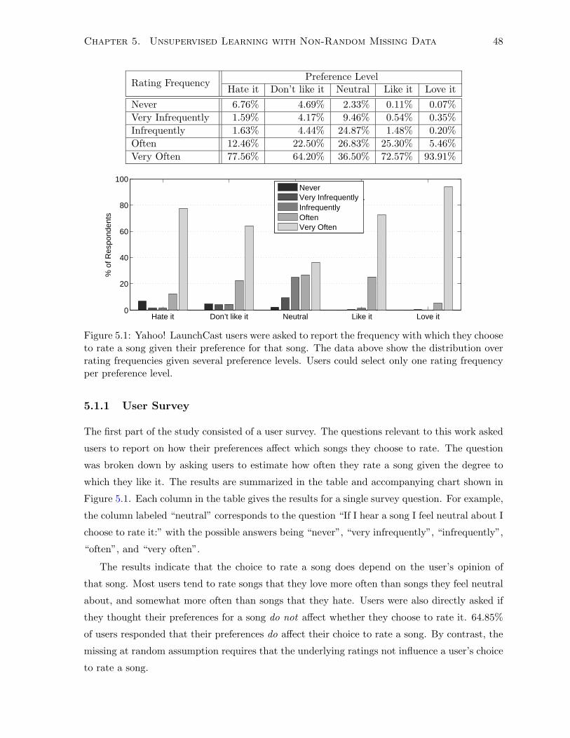
Chapter 5. Unsupervised Learning with Non-Random Missing Data 48
Rating FrequencyPreference Level
Hate it Don’t like it Neutral Like it Love it
Never 6.76% 4.69% 2.33% 0.11% 0.07%
Very Infrequently 1.59% 4.17% 9.46% 0.54% 0.35%
Infrequently 1.63% 4.44% 24.87% 1.48% 0.20%
Often 12.46% 22.50% 26.83% 25.30% 5.46%
Very Often 77.56% 64.20% 36.50% 72.57% 93.91%
Hate it Don’t like it Neutral Like it Love it0
20
40
60
80
100
% o
f Res
pond
ents
NeverVery Infrequently .InfrequentlyOftenVery Often
Figure 5.1: Yahoo! LaunchCast users were asked to report the frequency with which they chooseto rate a song given their preference for that song. The data above show the distribution overrating frequencies given several preference levels. Users could select only one rating frequencyper preference level.
5.1.1 User Survey
The first part of the study consisted of a user survey. The questions relevant to this work asked
users to report on how their preferences affect which songs they choose to rate. The question
was broken down by asking users to estimate how often they rate a song given the degree to
which they like it. The results are summarized in the table and accompanying chart shown in
Figure 5.1. Each column in the table gives the results for a single survey question. For example,
the column labeled “neutral” corresponds to the question “If I hear a song I feel neutral about I
choose to rate it:” with the possible answers being “never”, “very infrequently”, “infrequently”,
“often”, and “very often”.
The results indicate that the choice to rate a song does depend on the user’s opinion of
that song. Most users tend to rate songs that they love more often than songs they feel neutral
about, and somewhat more often than songs that they hate. Users were also directly asked if
they thought their preferences for a song do not affect whether they choose to rate it. 64.85%
of users responded that their preferences do affect their choice to rate a song. By contrast, the
missing at random assumption requires that the underlying ratings not influence a user’s choice
to rate a song.
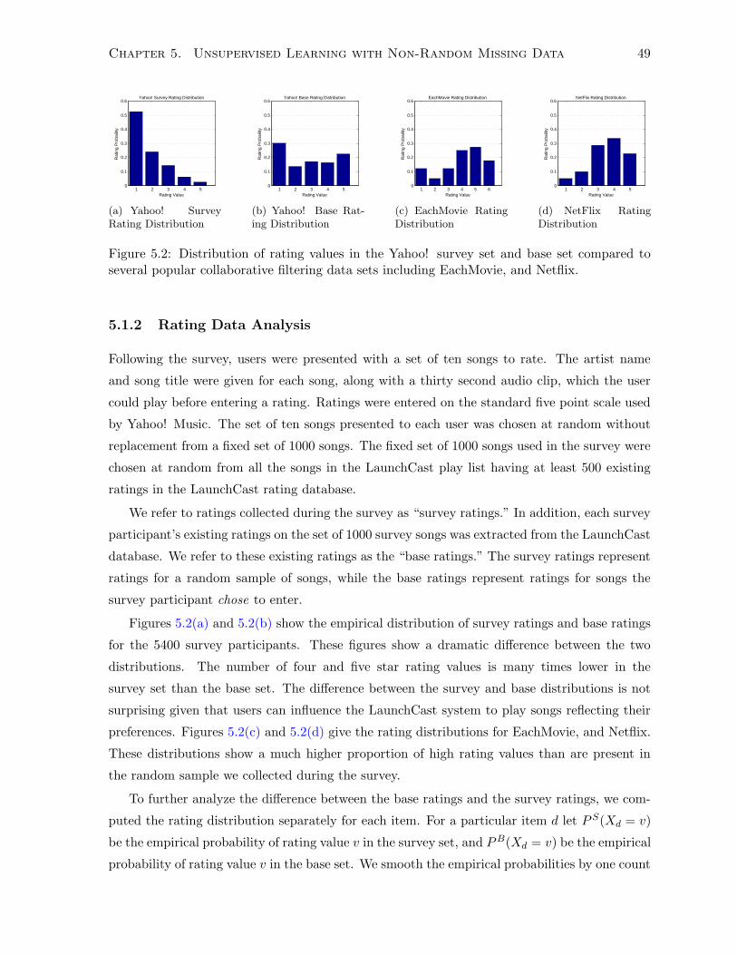
Chapter 5. Unsupervised Learning with Non-Random Missing Data 49
1 2 3 4 50
0.1
0.2
0.3
0.4
0.5
0.6
Rating Value
Rat
ing
Pro
baili
ty
Yahoo! Survey Rating Distribution
(a) Yahoo! SurveyRating Distribution
1 2 3 4 50
0.1
0.2
0.3
0.4
0.5
0.6
Rating Value
Rat
ing
Pro
baili
ty
Yahoo! Base Rating Distribution
(b) Yahoo! Base Rat-ing Distribution
1 2 3 4 5 60
0.1
0.2
0.3
0.4
0.5
0.6
Rating Value
Rat
ing
Pro
baili
ty
EachMovie Rating Distribution
(c) EachMovie RatingDistribution
1 2 3 4 50
0.1
0.2
0.3
0.4
0.5
0.6
Rating Value
Rat
ing
Pro
baili
ty
NetFlix Rating Distribution
(d) NetFlix RatingDistribution
Figure 5.2: Distribution of rating values in the Yahoo! survey set and base set compared toseveral popular collaborative filtering data sets including EachMovie, and Netflix.
5.1.2 Rating Data Analysis
Following the survey, users were presented with a set of ten songs to rate. The artist name
and song title were given for each song, along with a thirty second audio clip, which the user
could play before entering a rating. Ratings were entered on the standard five point scale used
by Yahoo! Music. The set of ten songs presented to each user was chosen at random without
replacement from a fixed set of 1000 songs. The fixed set of 1000 songs used in the survey were
chosen at random from all the songs in the LaunchCast play list having at least 500 existing
ratings in the LaunchCast rating database.
We refer to ratings collected during the survey as “survey ratings.” In addition, each survey
participant’s existing ratings on the set of 1000 survey songs was extracted from the LaunchCast
database. We refer to these existing ratings as the “base ratings.” The survey ratings represent
ratings for a random sample of songs, while the base ratings represent ratings for songs the
survey participant chose to enter.
Figures 5.2(a) and 5.2(b) show the empirical distribution of survey ratings and base ratings
for the 5400 survey participants. These figures show a dramatic difference between the two
distributions. The number of four and five star rating values is many times lower in the
survey set than the base set. The difference between the survey and base distributions is not
surprising given that users can influence the LaunchCast system to play songs reflecting their
preferences. Figures 5.2(c) and 5.2(d) give the rating distributions for EachMovie, and Netflix.
These distributions show a much higher proportion of high rating values than are present in
the random sample we collected during the survey.
To further analyze the difference between the base ratings and the survey ratings, we com-
puted the rating distribution separately for each item. For a particular item d let P S(Xd = v)
be the empirical probability of rating value v in the survey set, and PB(Xd = v) be the empirical
probability of rating value v in the base set. We smooth the empirical probabilities by one count
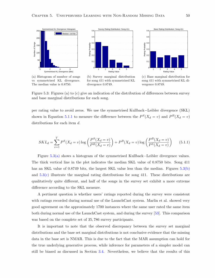
Chapter 5. Unsupervised Learning with Non-Random Missing Data 50
0 2 4 60
50
100
150
200
250Symmetrised KL Divergence Histogram
Num
ber
of S
ongs
Symmetrised KL Divergence (Bits)
Median: 0.8750
(a) Histogram of number of songsvs symmetrised KL divergence.The median value is 0.8750.
1 2 3 4 50
0.1
0.2
0.3
0.4
0.5
0.6
Rating Value
Rat
ing
Pro
baili
ty
Survey Rating Distribution: Song 411
(b) Survey marginal distributionfor song 411 with symmetrised KLdivergence 0.8749.
1 2 3 4 50
0.1
0.2
0.3
0.4
0.5
0.6
Rating Value
Rat
ing
Pro
baili
ty
Base Rating Distribution: Song 411
(c) Base marginal distribution forsong 411 with symmetrised KL di-vergence 0.8749.
Figure 5.3: Figures (a) to (c) give an indication of the distribution of differences between surveyand base marginal distributions for each song.
per rating value to avoid zeros. We use the symmetrised Kullback−Leibler divergence (SKL)
shown in Equation 5.1.1 to measure the difference between the P S(Xd = v) and PB(Xd = v)
distributions for each item d.
SKLd =V∑
v=1
PS(Xd = v) log
(PS(Xd = v)
PB(Xd = v)
)+ PB(Xd = v) log
(PB(Xd = v)
PS(Xd = v)
)(5.1.1)
Figure 5.3(a) shows a histogram of the symmetrised Kullback−Leibler divergence values.
The thick vertical line in the plot indicates the median SKL value of 0.8750 bits. Song 411
has an SKL value of 0.8749 bits, the largest SKL value less than the median. Figures 5.3(b)
and 5.3(c) illustrate the marginal rating distributions for song 411. These distributions are
qualitatively quite different, and half of the songs in the survey set exhibit a more extreme
difference according to the SKL measure.
A pertinent question is whether users’ ratings reported during the survey were consistent
with ratings recorded during normal use of the LaunchCast system. Marlin et al. showed very
good agreement on the approximately 1700 instances where the same user rated the same item
both during normal use of the LaunchCast system, and during the survey [53]. This comparison
was based on the complete set of 35, 786 survey participants.
It is important to note that the observed discrepancy between the survey set marginal
distributions and the base set marginal distributions is not conclusive evidence that the missing
data in the base set is NMAR. This is due to the fact that the MAR assumption can hold for
the true underlying generative process, while inference for parameters of a simpler model can
still be biased as discussed in Section 3.4. Nevertheless, we believe that the results of this
Chapter 5. Unsupervised Learning with Non-Random Missing Data 51
analysis combined with the results of the user survey provide compelling evidence against the
MAR assumption.
5.1.3 Experimental Protocols for Rating Prediction
The rating data set used in the experiments is based on the 1000 survey songs and a set of 15, 400
users. The set of 15, 400 users consists of a random selection of 10, 000 non-survey participants
with at least 10 existing ratings on the set of 1000 survey songs, and a random selection of 5400
survey participants with at least 10 existing ratings on the set of 1000 survey songs. We chose to
enforce a minimum number of existing ratings per user so that rating prediction methods would
have at least 10 observations on which to base predictions. Non-survey users were included to
provide more training data to the learning methods.
In this work we follow an experimental protocol based on a five fold cross validation as-
sessment of both the weak and strong generalization performance of rating prediction methods
[52, p. 14]. We consider the prediction of ratings for both user-selected and randomly selected
songs. Preparing the data set for this empirical protocol involves several steps. We begin by
randomly partitioning the 5400 survey users into five blocks of 1080 users each. Each block
is used as a set of test users in turn. The ratings for the test users are further divided into
observed ratings, test ratings for user selected items, and test ratings for randomly selected
items. The observed ratings consist of all but one of the user selected ratings for each user.
The test ratings for user selected items consist of exactly one rating for a user selected item per
user. The observed ratings consist of the remaining user selected ratings for each user. The
test ratings for randomly selected items consist of the 10 ratings for randomly selected items
collected for each user during the survey. Any overlapping ratings in the user selected and
randomly selected sets were removed from the user selected set before the Yahoo! data was
publicly released. Note that these ratings should have been preserved in both rating sets, but
the effect of removing them from the user selected set is small.
Of the 4320 survey users from the remaining four blocks, 400 users are selected at random to
form a hold out set. The set of training users consists of the remaining 3920 survey users, and all
of the 10, 000 non-survey users. The training user ratings are divided into observed ratings, test
ratings for user selected items, and test ratings for randomly selected items. The survey users in
the training set have one test rating for a user selected item, and 10 test ratings for randomly
selected items. The non-survey users have one test rating for a user selected item, and no
test ratings for randomly selected items. Each set of training users has approximately 250, 000
observed ratings, while each set of test users has approximately 25, 000 observed ratings.
Unless otherwise specified, models are trained using the training users’ observed ratings. We
use normalized mean absolute error as the error measure for collaborative prediction [52, p. 15].
Chapter 5. Unsupervised Learning with Non-Random Missing Data 52
Given a predictive distribution over the V rating values, we predict the median rating value.
The weak generalization error for user-selected items is computed by predicting the value of each
training user’s user-selected test items. The weak generalization error for randomly selected
items is computed by predicting the value of each training user’s randomly-selected test items.
The strong generalization error for user-selected items is computed by predicting the value of
each test user’s user-selected test items. The strong generalization error for randomly selected
items is computed by predicting the value of each test user’s randomly-selected test items.
The novel aspect of this protocol stems from the division of the rating data into three sets
of ratings. The observed ratings for each user are ratings for user-selected items. Thus, the user
selected test items come from the same distribution as the observed ratings, and both rating sets
are subject to the same unknown missing data mechanism. The ratings for randomly selected
test items come from a known selection mechanism where missing data is missing completely
at random.
If missing data is missing at random in the user selected items, we would not expect to see
a large difference in prediction performance on the randomly selected and user selected test
items. If missing data is not missing at random, we would expect methods that incorrectly
assume the MAR condition to perform poorly on the randomly selected test items compared
to the user-selected test items.
5.2 The Jester Data Set
The Jester recommender system was established as part of a research project on collaborative
filtering methods [30]. The system allows a user to rate jokes, and then recommends other
jokes the user might like. Jester is unique among the available collaborative filtering data sets
in that it contains a dense subset of ten items that all users were required to rate upon joining
the system. We extracted 15000 completely observed ratings vectors from the Jester gauge
set. Each rating vector consists of ratings for all ten of the gauge set items. The ratings were
mapped from the original continuous rating scale to 5 discrete rating values.
5.2.1 Experimental Protocols for Rating Prediction
Artificial missing data was added to the Jester data set using a synthetic missing data mech-
anism. The missing data model we use has the form P (rdn = 1|xdn = v, µv(s)) = µv(s). The
function µv(s) = s(v − 3) + 0.5. As s increases from 0 to 0.25, high rating values have an
increasing chance of being observed, and low rating values have an increasing chance of being
missing. We applied this missing data mechanism to the Jester ratings using the five sets of
missing data model parameters pictured in Figure 5.4, and obtained five data sets with artifi-
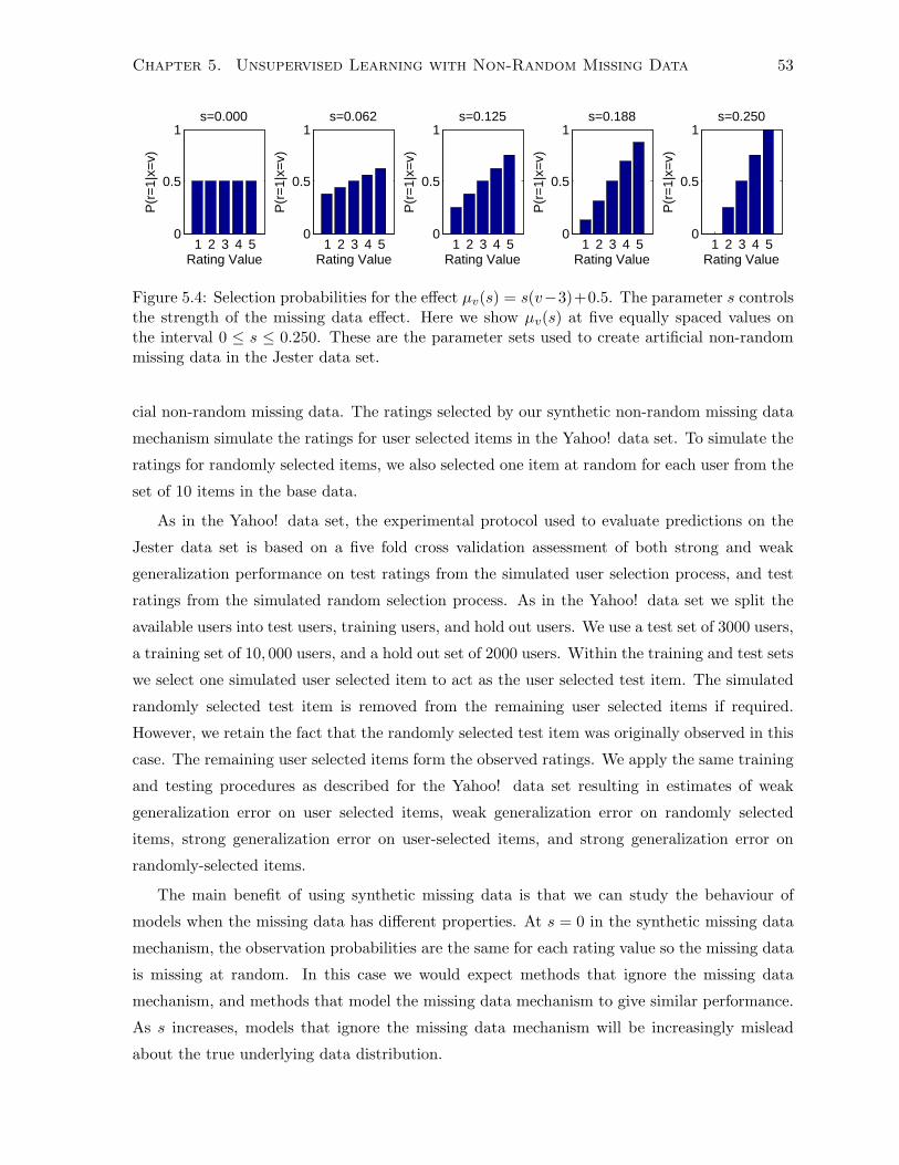
Chapter 5. Unsupervised Learning with Non-Random Missing Data 53
1 2 3 4 50
0.5
1s=0.000
Rating Value
P(r
=1|
x=v)
1 2 3 4 50
0.5
1s=0.062
Rating Value
P(r
=1|
x=v)
1 2 3 4 50
0.5
1s=0.125
Rating Value
P(r
=1|
x=v)
1 2 3 4 50
0.5
1s=0.188
Rating Value
P(r
=1|
x=v)
1 2 3 4 50
0.5
1s=0.250
Rating Value
P(r
=1|
x=v)
Figure 5.4: Selection probabilities for the effect µv(s) = s(v−3)+0.5. The parameter s controlsthe strength of the missing data effect. Here we show µv(s) at five equally spaced values onthe interval 0 ≤ s ≤ 0.250. These are the parameter sets used to create artificial non-randommissing data in the Jester data set.
cial non-random missing data. The ratings selected by our synthetic non-random missing data
mechanism simulate the ratings for user selected items in the Yahoo! data set. To simulate the
ratings for randomly selected items, we also selected one item at random for each user from the
set of 10 items in the base data.
As in the Yahoo! data set, the experimental protocol used to evaluate predictions on the
Jester data set is based on a five fold cross validation assessment of both strong and weak
generalization performance on test ratings from the simulated user selection process, and test
ratings from the simulated random selection process. As in the Yahoo! data set we split the
available users into test users, training users, and hold out users. We use a test set of 3000 users,
a training set of 10, 000 users, and a hold out set of 2000 users. Within the training and test sets
we select one simulated user selected item to act as the user selected test item. The simulated
randomly selected test item is removed from the remaining user selected items if required.
However, we retain the fact that the randomly selected test item was originally observed in this
case. The remaining user selected items form the observed ratings. We apply the same training
and testing procedures as described for the Yahoo! data set resulting in estimates of weak
generalization error on user selected items, weak generalization error on randomly selected
items, strong generalization error on user-selected items, and strong generalization error on
randomly-selected items.
The main benefit of using synthetic missing data is that we can study the behaviour of
models when the missing data has different properties. At s = 0 in the synthetic missing data
mechanism, the observation probabilities are the same for each rating value so the missing data
is missing at random. In this case we would expect methods that ignore the missing data
mechanism, and methods that model the missing data mechanism to give similar performance.
As s increases, models that ignore the missing data mechanism will be increasingly mislead
about the true underlying data distribution.

Chapter 5. Unsupervised Learning with Non-Random Missing Data 54
5.3 Test Items and Additional Notation for Missing Data
The act of removing user selected items from the training data to use as test items effectively
introduces an additional source of missing data. Missing training data that results from held
out test items must be treated differently than the missing data that results from the natural
missing data process. For example, suppose item d was originally selected and rated by user n.
The training data would contain rdn = 1 and xdn = v. Now suppose that item d is chosen as a
test item for user n. We must remove the value xdn = v from the training data. However, it is
not correct to set rdn = 0 in the training data since user n originally selected item d.
Keeping track of the two sources of missing data in the training data requires the use of
additional notation. We define rdn = 1 to mean that user n originally selected and rated item
d. We define adn = 1 to mean that the rating value xdn is available for use during training or
inference. If rdn = 1 and adn = 1 this implies that user n originally selected and rated item d,
and that the rating for item d is available during training and inference. This is the normal
situation during learning. If rdn = 1 and adn = 0 this implies that user n originally selected
and rated item d, but the rating for item d is not available during training or inference. This
situation occurs when xdn is removed from the training set because item d is used as a test
rating. If rdn = 0 and adn = 1 this implies that user n originally did not select and rate item d,
but the rating for item d is available. This situation generally arises when we predict the value
of a randomly selected test item. It also occurs in some of the specialized training procedures
we consider. Finally, rdn = 0 and adn = 0 implies that item d was not originally selected and
rated by user n, and that the rating value is not available for learning.
5.4 The Finite Mixture/CPT-v Model
The CPT-v missing data model was proposed by Marlin, Roweis, and Zemel as a highly simpli-
fied non-random missing data model for collaborative filtering [54]. The CPT-v missing data
model captures the intuition that a user’s preference for an item affects whether they choose
to rate that item or not. The model assumes that the choice to rate each item is independent,
and the probability of rating a single item, given the user’s rating for the item is v, is Bernoulli
distributed with parameter µv. Marlin et al. combine the CPT-v missing data model with a
finite mixture data model [54, 53]. Figure 5.5 shows a graphical representation of the CPT-v
missing data model combined with the finite multinomial mixture data model. We give the
corresponding probabilistic model in equations 5.4.1 to 5.4.6.
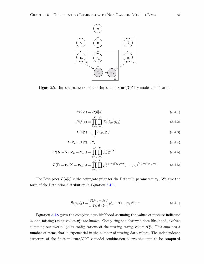
Chapter 5. Unsupervised Learning with Non-Random Missing Data 55
θφ
βk
K
ξ
Zn
X
N
v
V
R
µ
v
nn
α
Figure 5.5: Bayesian network for the Bayesian mixture/CPT-v model combination.
P (θ|α) = D(θ|α) (5.4.1)
P (β|φ) =K∏
k=1
D∏
d=1
D(βdk|φdk) (5.4.2)
P (µ|ξ) =∏
v
B(µv|ξv) (5.4.3)
P (Zn = k|θ) = θk (5.4.4)
P (X = xn|Zn = k, β) =D∏
d=1
V∏
v=1
β[xdn=v]vdk (5.4.5)
P (R = rn|X = xn, µ) =D∏
d=1
V∏
v=1
µ[rdn=1][xdn=v]v (1− µv)
[rdn=0][xim=v] (5.4.6)
The Beta prior P (µ|ξ) is the conjugate prior for the Bernoulli parameters µv. We give the
form of the Beta prior distribution in Equation 5.4.7.
B(µv|ξv) =Γ(ξ0v + ξ1v)
Γ(ξ0v)Γ(ξ1v)µξ1v−1
v (1− µv)ξ0v−1 (5.4.7)
Equation 5.4.8 gives the complete data likelihood assuming the values of mixture indicator
zn and missing rating values xmn are known. Computing the observed data likelihood involves
summing out over all joint configurations of the missing rating values xmn . This sum has a
number of terms that is exponential in the number of missing data values. The independence
structure of the finite mixture/CPT-v model combination allows this sum to be computed

Chapter 5. Unsupervised Learning with Non-Random Missing Data 56
efficiently as seen in Equation 5.4.9. Unlike the missing at random case, both the missing
rating values and response indicators contribute to the likelihood.
P (zn,xn, rn|β, θ, µ) =
K∏
k=1
(θk
D∏
d=1
V∏
v=1
(µ[rdn=1]
v (1− µv)[rdn=0]βvdk
)[xdn=v])[zn=k]
(5.4.8)
P (xon, rn|β, θ, µ) =
∑
xm
K∑
k=1
θk
D∏
d=1
V∏
v=1
(µ[rdn=1]
v (1− µv)[rdn=0]βvdk
)
=K∑
k=1
θk
(D∏
d=1
V∏
v=1
(µvβvdk)[rdn=1][xdn=v]
)
V∑
xm1
=1
· · ·V∑
xmD
=1
D∏
d=1
V∏
v=1
((1− µv)βvdk)[rdn=0][xm
d=v]
=K∑
k=1
θk
(D∏
d=1
V∏
v=1
(µvβvdk)[rdn=1][xdn=v]
)(D∏
d=1
V∑
v=1
((1− µv)βvdk)[rdn=0]
)
=K∑
k=1
θk
D∏
d=1
(V∏
v=1
(µvβvdk)[xdn=v])
)[rdn=1]( V∑
v=1
(1− µv)βvdk
)[rdn=0]
(5.4.9)
5.4.1 Conditional Identifiability
The CPT-v missing data model has the interesting property that its parameters are condition-
ally identifiable even when the multinomial mixture model parameters are not identifiable. The
proof builds on the work of Glonek, who studied the problem of non-random missing data for
a single binary variable in the classification setting [29]. We first review Glonek’s proof, and
then extend the proof method to the CPT-v missing data mechanism.
Binary Classification with Non-Random Missing Labels
Consider a binary classification task with fully observed binary predictors x, and a single
binary class variable y subject to nonignorable nonresponse. The data model is a conditional
model parameterized by πx = P (Y = 1|X = x), while the selection model is parameterized by
µy = P (R = 1|Y = y) where R is a binary response indicator. Thus, the model consists of the
predictor or feature variables X, the binary class variable Y , and the binary response indicator
variable R.
Glonek defines the variable w to be categorical with values from the set {0, 1,∅} where ∅
indicates that the value of y was not observed [29]. Thus, the single variable w replaces the
combination of variables y, and r. Note that regardless of the data and selection models in
question, all that is ever observed in the data are the values of the random variables w, and the
Chapter 5. Unsupervised Learning with Non-Random Missing Data 57
predictors x. We can now define the distribution over the observed variables φwx = P (W =
w|X = x).
A necessary condition for identifiability is that the number of degrees of freedom in the
observed variable distributions exceed the number of degrees of freedom in the model parame-
ters. If the total number of different configurations of the predictor variables x is M , then the
number of degrees of freedom in the observed variable distributions will be 2M since w is a
three-valued variable with the constraint that the values sum to one. The number of degrees
of freedom in the model parameters will be M + 2, and the condition is satisfied if M ≥ 2.
Glonek formulates a precise characterization of global identifiability, which we now recount.
Suppose we have at least two distinct settings of the predictor variables, and for two particular
settings of the predictor variables x1 and x2 we have πx16= πx2
. We relate the observed
distributions to the model parameters as follows:
φ0x1= µ0(1− πx1
) φ1x1= µ1(πx1
) φ0x2= µ0(1− πx2
) φ1x2= µ1(πx2
)
Noting that φ0x1/µ0+φ1x1
/µ1 = (1−πx1)+πx1
= 1 and φ0x2/µ0+φ1x2
/µ1 = (1−πx2)+πx2
=
1 we can reduce the above set of equations to the following linear system for 1/µ0 and 1/µ1.
[φ0x1
φ1x1
φ0x2φ1x2
][1µ0
1µ1
]=
[1
1
](5.4.10)
Subject to the conditions πx16= πx2
and µ0, µ1 > 0, the above matrix is invertible. As a
result, the above system has a unique solution for µ0, µ1, and all of the π′s.
CPT-v and Conditional Identifiability
In the collaborative filtering case the observed variables are denoted wd, and take values on the
extended set {1, ..., V,∅} where ∅ again denotes the observation that xd is missing. Thus wd
replaces xd and rd. We denote the parameters of the joint distribution of the observed variables
by φw. This distribution has V D − 1 free parameters. We relate the parameters of the joint
distribution to the parameters of the model distribution as seen in Equation 5.4.11.
φw =
K∑
k=1
θk
D∏
d=1
(V∏
v=1
(µvβvdk)[wd=v]
)[wd 6=∅]( V∑
v=1
(1− µv)βvdk
)[wd=∅]
(5.4.11)
Before describing the general case, we consider a specific instance where V = 2, D = 2,K =
2. We list the φ functions for several configuration of the observed variables.
Chapter 5. Unsupervised Learning with Non-Random Missing Data 58
φ11 =K∑
k=1
θkµ1β11kµ1β12k φ21 =K∑
k=1
θkµ2β21kµ1β12k
φ12 =K∑
k=1
θkµ1β11kµ2β22k φ22 =K∑
k=1
θkµ2β21kµ2β22k
φ1∅ =K∑
k=1
θkµ1β11k(V∑
v=1
(1− µv)βv2k) φ2∅ =K∑
k=1
θkµ2β21k(V∑
v=1
(1− µv)βv2k)
φ∅1 =K∑
k=1
θk(V∑
v=1
(1− µv)βv1k)µ1β12k φ∅2 =K∑
k=1
θk(V∑
v=1
(1− µv)βv1k)µ2β22k
We show that µ1 and µ2 are uniquely determined using an argument similar to that used
by Glonek. Consider the system of linear equations derived from the full set of φ values given
previously.
Φ
[1µ1
1µ2
]=
[(φ11 + φ12 + φ1∅) (φ21 + φ22 + φ2∅)
(φ11 + φ21 + φ∅1) (φ12 + φ22 + φ∅2)
][1µ1
1µ2
]=
[1
1
](5.4.12)
This system will have a unique solution for µ1 and µ2 assuming both are greater than 0, and
the matrix Φ of sums of φ coefficients is non-singular. We note that the entry Φ(d, v) is equal
to the marginal observed probability P (wd = v). This result is easily extended to the general
case when D ≥ V by defining Φ(d, v) as follows:
Φ(d, v) =∑
x1
· · ·∑
xd−1
∑
xd+1
· · ·∑
xD
φx1···xd−1vxd+1···xD(5.4.13)
As before the relation∑
v Φ(d, v)/µv = 1 holds. Suppose that for some set of V data
dimensions, the corresponding matrix Φ is nonsingular. Without loss of generality we can
assume it is the first V dimensions of the data. Under these conditions, the following system
has a unique solution, and the CPT-v selection model parameters are uniquely identified.
Φ11 Φ12 · · · Φ1V
Φ21 Φ22 · · · Φ2V
.... . .
...
ΦV 1 ΦV 2 · · · ΦV V
1µ0
1µ1
...
1µV
=
1
1...
1
(5.4.14)
The matrix Φ may have an interesting interpretation as far as inferring the selection model
parameters from data is concerned. Consider the case where data is generated exactly from a
CPT-v selection model paired with a multinomial mixture model. In this case we can directly
estimate the Φdv coefficients from the data, and they will be correct up to sampling error. We
can select a suitable set of V items and compute estimate for the µv parameters. However, in
Chapter 5. Unsupervised Learning with Non-Random Missing Data 59
the presence of deviations from the CPT-v model, the estimates obtained from this procedure
may not be probabilities.
It is a well known fact of linear algebra that the condition number of a linear system,
the ratio of largest to smallest singular value of the coefficient matrix, is an indication of the
sensitivity of the system. If the coefficient matrix has high condition number, then small changes
to the coefficients can result is large changes in the solution to the system. If we construct a
non-singular matrix Φ from a sample of data and see that the condition number of the matrix
is high, this is an indication that the selection model parameters could be highly sensitive to
the particular data sample used to estimate them. On the other hand, if the condition number
is low, the selection model parameters should be fairly invariant to the particular data sample
used to estimate them.
5.4.2 Maximum A Posteriori Estimation
The principal of maximum a posteriori probability states that we should select the parameters
θ, β, and µ with maximum posterior probability. As in the case of the finite Bayesian mixture
model, maximum a posteriori estimation can be accomplished using an expectation maximiza-
tion algorithm. To derive the expectation maximization algorithm we first require the posterior
distribution of the mixture indicator variable zn and the missing ratings xmn given the observed
data xon, the response indicators rn and the parameters θ, β, µ. At this point, we also introduce
the available rating indicators an to properly account for held out test data during inference and
learning. To help simplify the notation, we introduce the auxiliary variables γdkn in Equation
5.4.15. The posterior distribution is denoted qn(k,xmn ) and given in Equation 5.4.16.
γdkn =
(V∏
v=1
(βvdkµv)[xdn=v]
)[rdn=1][adn=1]( V∏
v=1
(βvdk(1− µv))[x=v]
)[rdn=0][adn=1]
·(
V∑
v=1
βvdkµv
)[rdn=1][adn=0]( V∑
v=1
βvdk(1− µv)
)[rdn=0][adn=0]
(5.4.15)
qn(k,xmn ) = P (zn = k,xm
n |xon, rn,an, θ, β, µ) =
P (zn = k,xmn ,x
on, rn|an, θ, β, µ)
P (xon, rn|an, θ, β, µ)
=
θk
D∏
d=1
V∏
v=1
(µvβvdk)[rdn=1][xdn=v]((1− µv)βvdk)
[rdn=0][xdn=v]
K∑
k=1
θk
D∏
d=1
γdkn
(5.4.16)
Chapter 5. Unsupervised Learning with Non-Random Missing Data 60
This posterior distribution has a number of terms that is again exponential in the number
of missing data values. We form the expected complete log posterior shown below based on the
missing data posterior distribution qn(k,xmn ) given in Equation 5.4.16, the complete likelihood
given in Equation 5.4.8, and the prior distribution. As we will see, the required expectations
are functions of at most two variables, and can be efficiently computed.
E[logP(β, θ, µ|{xn, rn,an}n=1:N , α, φ, ξ)] = log Γ(K∑
k=1
αk)−K∑
k=1
log Γ(αk) +K∑
k=1
(αk − 1) log θk
+K∑
k=1
D∑
d=1
log Γ(V∑
v=1
φvdk)−V∑
v=1
log Γ(φvdk) +V∑
v=1
(φvdk − 1) log βvdk
+V∑
v=1
log Γ(ξ0v + ξ1v)− log Γ(ξ0v)− log Γ(ξ1v) + (ξ1v − 1) log µv + (ξ0v − 1) log(1− µv)
+N∑
n=1
K∑
k=1
∑
xmn
qn(k,xmn )[zn = k] log θk
+N∑
n=1
K∑
k=1
∑
xmn
D∑
d=1
V∑
v=1
qn(k,xmn )[zn = k][xdn = v][rdn = 1][adn = 1](log βvdk + log µv)
+N∑
n=1
K∑
k=1
∑
xmn
D∑
d=1
V∑
v=1
qn(k,xmn )[zn = k][xdn = v][rdn = 1][adn = 0](log βvdk + log µv)
+N∑
n=1
K∑
k=1
∑
xmn
D∑
d=1
V∑
v=1
qn(k,xmn )[zn = k][xdn = v][rdn = 0][adn = 0](log βvdk + log(1− µv))
(5.4.17)
The expected complete log posterior can be simplified significantly. First, we note that the
term∑
xmnqn(k,xm
n )[zn = k] log θk depends only on k and not on xmn . This is also true for the
term qn(k,xmn )[zn = k][xdn = v][rdn = 1][adn = 1](log βvdk + log µv) since xdn is not missing
when rdn = 1 and adn = 1. We can sum qn(k,xmn ) over xm
n to obtain the simplified posterior
term qn(k) as seen below. This yields the simplified factors of the form qn(k)[zn = k] log θk,
and qn(k)[zn = k][xdn = v][rdn = 1][adn = 1](log βvdk + log µv).
qn(k) = P (zn = k|xon, rn,an, θ, β, µ) =
P (zn = k,xon, rn|an, θ, β, µ)
P (xon, rn|an, θ, β, µ)
=θk
∏Dd=1 γdkn∑K
k=1 θk∏D
d=1 γdkn
Terms where [adn = 0] can also be simplified since they depend on exactly one missing data
value. Assume that dimension d is missing, we can sum out over the remaining missing data
dimensions to obtain a simplified posterior factor of the form qn(k, v, d) as seen in Equation
5.4.18. The value of qn(k, v, d) is simple to compute given the value of qn(k).
Chapter 5. Unsupervised Learning with Non-Random Missing Data 61
qn(k, v, d) = P (zn = k, xdn = v,xon, rn|an, θ, β, µ)
= qn(k)
(µvβvdk∑V
v′=1 µv′βv′dk
)[rdn=1][adn=0]((1− µv)βvdk∑V
v′=1(1− µv′)βv′dk
)[rdn=0][adn=0]
(5.4.18)
Another useful posterior probability is the probability that a missing rating takes value v.
We denote this distribution by qn(v, d). This distribution can be obtained from qn(k, v, d) by
marginalizing over k.
qn(v, d) = P (xdn = v,xon, rn|an, θ, β, µ) =
K∑
k=1
qn(k, v, d)
We rewrite the expected complete log posterior using the simplified posterior distributions.
It is clear from this form that the expected complete log posterior depends only on a relatively
small set of local posterior factors, all of which can be efficiently computed.
E[logP(β, θ, µ|{xn, rn,an}n=1:N , α, φ, ξ)] = log Γ(K∑
k=1
αk)−K∑
k=1
log Γ(αk) +K∑
k=1
(αk − 1) log θk
+
K∑
k=1
D∑
d=1
log Γ(
V∑
v=1
φvdk)−V∑
v=1
log Γ(φvdk) +
V∑
v=1
(φvdk − 1) log βvdk
+V∑
v=1
log Γ(ξ0v + ξ1v)− log Γ(ξ0v)− log Γ(ξ1v) + (ξ1v − 1) log µv + (ξ0v − 1) log(1− µv)
+N∑
n=1
K∑
k=1
qn(k)[zn = k] log θk
+N∑
n=1
K∑
k=1
qn(k)D∑
d=1
V∑
v=1
[zn = k][xdn = v][rdn = 1][adn = 1](log βvdk + log µv)
+N∑
n=1
K∑
k=1
D∑
d=1
V∑
v=1
qn(k, v, d)[zn = k][rdn = 1][adn = 0](log βvdk + log(µv))
+N∑
n=1
K∑
k=1
D∑
d=1
V∑
v=1
qn(k, v, d)[zn = k][rdn = 0][adn = 0](log βvdk + log(1− µv)) (5.4.19)
Finally, we find the partial derivatives of the expected complete log posterior with respect
to the multinomial parameters θ, β, and the Bernoulli parameters µv. We solve the result-

Chapter 5. Unsupervised Learning with Non-Random Missing Data 62
ing gradient equations using Lagrange multipliers to enforce normalization constraints. The
derivation for θ is identical to the finite mixture case.
∂E[logP]
∂θk=αk − 1 +
∑Nn=1 qn(k)
θk− λ = 0
θkλ = αk − 1 +N∑
n=1
pn(k)
K∑
k=1
θkλ =K∑
k=1
(αk − 1) +N∑
n=1
qn(k)
λ = N −K +K∑
k=1
αk
θk =αk − 1 +
∑Nn=1 qn(k)
N −K +∑K
k=1 αk
(5.4.20)
The update for βvdk takes into account both the expected number of observed ratings of
value v explained by component k, and the expected number of missing ratings of value v
explained by component k.
∂E[logP]
∂βvdk=φvnk − 1
βvdk+
∑Nn=1 qn(k)[adn = 1][xdn = v]
βvdk(5.4.21)
+
∑Nn=1 qn(v, d, k)[adn = 0]
βvdk− λ = 0
βvdkλ = φvnk − 1 +N∑
n=1
qn(k)[adn = 1][xdn = v] + qn(k, v, d)[adn = 0]
λ =V∑
v=1
(φvnk − 1) +N∑
n=1
qn(k)
βvdk =φvdk − 1 +
∑Nn=1 qn(k)[adn = 1][xdn = v] + qn(k, v, d)[adn = 0]∑N
n=1 qn(k)− V +∑V
v=1 φvdk
(5.4.22)
The update for µv is given by the ratio of the number of observed ratings with value v to
the total number of observed and expected ratings with value v.
∂E[logP]
∂µv=ξ1v − 1
µv+
∑Nn=1
∑Dd=1[rdn = 1][adn = 1][xdn = v] + qn(v, d)[rdn = 1][adn = 0]
µv
− ξ0v − 1
(1− µv)−∑N
n=1
∑Dd=1 qn(v, d)[rdn = 0][adn = 0]
(1− µv)= 0
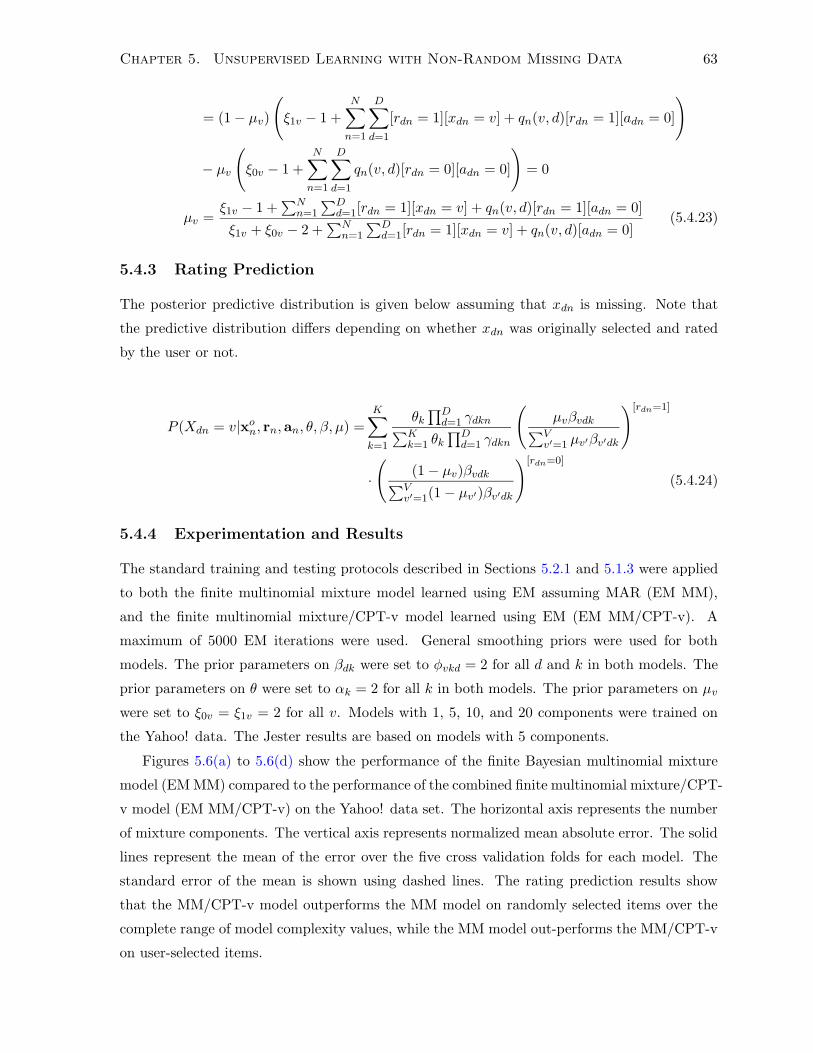
Chapter 5. Unsupervised Learning with Non-Random Missing Data 63
= (1− µv)
(ξ1v − 1 +
N∑
n=1
D∑
d=1
[rdn = 1][xdn = v] + qn(v, d)[rdn = 1][adn = 0]
)
− µv
(ξ0v − 1 +
N∑
n=1
D∑
d=1
qn(v, d)[rdn = 0][adn = 0]
)= 0
µv =ξ1v − 1 +
∑Nn=1
∑Dd=1[rdn = 1][xdn = v] + qn(v, d)[rdn = 1][adn = 0]
ξ1v + ξ0v − 2 +∑N
n=1
∑Dd=1[rdn = 1][xdn = v] + qn(v, d)[adn = 0]
(5.4.23)
5.4.3 Rating Prediction
The posterior predictive distribution is given below assuming that xdn is missing. Note that
the predictive distribution differs depending on whether xdn was originally selected and rated
by the user or not.
P (Xdn = v|xon, rn,an, θ, β, µ) =
K∑
k=1
θk∏D
d=1 γdkn∑Kk=1 θk
∏Dd=1 γdkn
(µvβvdk∑V
v′=1 µv′βv′dk
)[rdn=1]
·(
(1− µv)βvdk∑Vv′=1(1− µv′)βv′dk
)[rdn=0]
(5.4.24)
5.4.4 Experimentation and Results
The standard training and testing protocols described in Sections 5.2.1 and 5.1.3 were applied
to both the finite multinomial mixture model learned using EM assuming MAR (EM MM),
and the finite multinomial mixture/CPT-v model learned using EM (EM MM/CPT-v). A
maximum of 5000 EM iterations were used. General smoothing priors were used for both
models. The prior parameters on βdk were set to φvkd = 2 for all d and k in both models. The
prior parameters on θ were set to αk = 2 for all k in both models. The prior parameters on µv
were set to ξ0v = ξ1v = 2 for all v. Models with 1, 5, 10, and 20 components were trained on
the Yahoo! data. The Jester results are based on models with 5 components.
Figures 5.6(a) to 5.6(d) show the performance of the finite Bayesian multinomial mixture
model (EM MM) compared to the performance of the combined finite multinomial mixture/CPT-
v model (EM MM/CPT-v) on the Yahoo! data set. The horizontal axis represents the number
of mixture components. The vertical axis represents normalized mean absolute error. The solid
lines represent the mean of the error over the five cross validation folds for each model. The
standard error of the mean is shown using dashed lines. The rating prediction results show
that the MM/CPT-v model outperforms the MM model on randomly selected items over the
complete range of model complexity values, while the MM model out-performs the MM/CPT-v
on user-selected items.

Chapter 5. Unsupervised Learning with Non-Random Missing Data 64
0 5 10 15 200.4
0.5
0.6
0.7
0.8
0.9
1
1.1Weak Rand MAE vs Model Complexity
Model Complexity
MA
E
EM MMEM MM/CPT−v
(a) Weak generalization on randomly selected itemsfrom the Yahoo! data set.
0 5 10 15 200.4
0.5
0.6
0.7
0.8
0.9
1
1.1Weak User MAE vs Model Complexity
Model Complexity
MA
E
(b) Weak generalization on user selected items fromthe Yahoo! data set.
0 5 10 15 200.4
0.5
0.6
0.7
0.8
0.9
1
1.1Strong Rand MAE vs Model Complexity
Model Complexity
MA
E
(c) Strong generalization on randomly selected itemsfrom the Yahoo! data set.
0 5 10 15 200.4
0.5
0.6
0.7
0.8
0.9
1
1.1Strong User MAE vs Model Complexity
Model Complexity
MA
E
(d) Strong generalization on user selected items fromthe Yahoo! data set.
Figure 5.6: Figures 5.6(a) to 5.6(d) show the performance of the finite multinomial mixturemodel learned using EM assuming MAR (EM MM) compared to the performance of the com-bined finite multinomial mixture/CPT-v model learned using EM (EM MM/CPT-v) on theYahoo! data set. The horizontal axis represents the number of mixture components. The ver-tical axis represents normalized mean absolute error. The rating prediction results show thatthe MM/CPT-v model vastly outperforms the MM model on randomly selected items over arange of model complexity values.
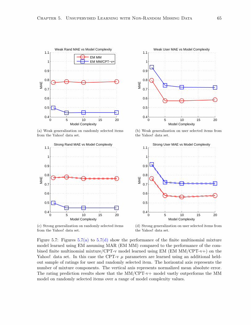
Chapter 5. Unsupervised Learning with Non-Random Missing Data 65
0 5 10 15 200.4
0.5
0.6
0.7
0.8
0.9
1
1.1Weak Rand MAE vs Model Complexity
Model Complexity
MA
E
EM MMEM MM/CPT−v+
(a) Weak generalization on randomly selected itemsfrom the Yahoo! data set.
0 5 10 15 200.4
0.5
0.6
0.7
0.8
0.9
1
1.1Weak User MAE vs Model Complexity
Model Complexity
MA
E
(b) Weak generalization on user selected items fromthe Yahoo! data set.
0 5 10 15 200.4
0.5
0.6
0.7
0.8
0.9
1
1.1Strong Rand MAE vs Model Complexity
Model Complexity
MA
E
(c) Strong generalization on randomly selected itemsfrom the Yahoo! data set.
0 5 10 15 200.4
0.5
0.6
0.7
0.8
0.9
1
1.1Strong User MAE vs Model Complexity
Model Complexity
MA
E
(d) Strong generalization on user selected items fromthe Yahoo! data set.
Figure 5.7: Figures 5.7(a) to 5.7(d) show the performance of the finite multinomial mixturemodel learned using EM assuming MAR (EM MM) compared to the performance of the com-bined finite multinomial mixture/CPT-v model learned using EM (EM MM/CPT-v+) on theYahoo! data set. In this case the CPT-v µ parameters are learned using an additional held-out sample of ratings for user and randomly selected item. The horizontal axis represents thenumber of mixture components. The vertical axis represents normalized mean absolute error.The rating prediction results show that the MM/CPT-v+ model vastly outperforms the MMmodel on randomly selected items over a range of model complexity values.
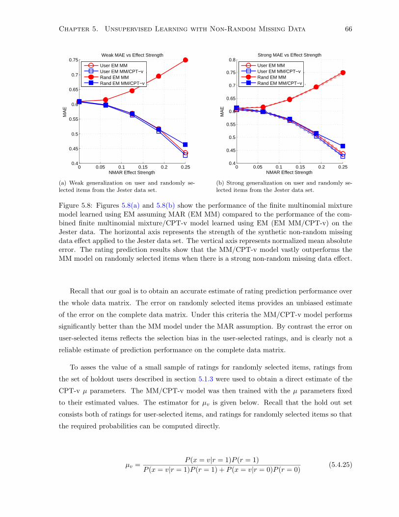
Chapter 5. Unsupervised Learning with Non-Random Missing Data 66
0 0.05 0.1 0.15 0.2 0.250.4
0.45
0.5
0.55
0.6
0.65
0.7
0.75Weak MAE vs Effect Strength
NMAR Effect Strength
MA
E
User EM MMUser EM MM/CPT−v .Rand EM MMRand EM MM/CPT−v .
(a) Weak generalization on user and randomly se-lected items from the Jester data set.
0 0.05 0.1 0.15 0.2 0.250.4
0.45
0.5
0.55
0.6
0.65
0.7
0.75
0.8Strong MAE vs Effect Strength
NMAR Effect Strength
MA
E
User EM MMUser EM MM/CPT−v .Rand EM MMRand EM MM/CPT−v .
(b) Strong generalization on user and randomly se-lected items from the Jester data set.
Figure 5.8: Figures 5.8(a) and 5.8(b) show the performance of the finite multinomial mixturemodel learned using EM assuming MAR (EM MM) compared to the performance of the com-bined finite multinomial mixture/CPT-v model learned using EM (EM MM/CPT-v) on theJester data. The horizontal axis represents the strength of the synthetic non-random missingdata effect applied to the Jester data set. The vertical axis represents normalized mean absoluteerror. The rating prediction results show that the MM/CPT-v model vastly outperforms theMM model on randomly selected items when there is a strong non-random missing data effect.
Recall that our goal is to obtain an accurate estimate of rating prediction performance over
the whole data matrix. The error on randomly selected items provides an unbiased estimate
of the error on the complete data matrix. Under this criteria the MM/CPT-v model performs
significantly better than the MM model under the MAR assumption. By contrast the error on
user-selected items reflects the selection bias in the user-selected ratings, and is clearly not a
reliable estimate of prediction performance on the complete data matrix.
To asses the value of a small sample of ratings for randomly selected items, ratings from
the set of holdout users described in section 5.1.3 were used to obtain a direct estimate of the
CPT-v µ parameters. The MM/CPT-v model was then trained with the µ parameters fixed
to their estimated values. The estimator for µv is given below. Recall that the hold out set
consists both of ratings for user-selected items, and ratings for randomly selected items so that
the required probabilities can be computed directly.
µv =P (x = v|r = 1)P (r = 1)
P (x = v|r = 1)P (r = 1) + P (x = v|r = 0)P (r = 0)(5.4.25)
Chapter 5. Unsupervised Learning with Non-Random Missing Data 67
P (r = 1) ≈ (1/DN)
N∑
n=1
D∑
d=1
[rdn = 1] (5.4.26)
P (r = 0) ≈ (1/DN)N∑
n=1
D∑
d=1
[rdn = 0] (5.4.27)
P (x = v|r = 1) ≈∑N
n=1
∑Dd=1[xdn = v][rdn = 1][adn = 1]
∑Nn=1
∑Dd=1[rdn = 1][adn = 1]
(5.4.28)
P (x = v|r = 0) ≈∑N
n=1
∑Dd=1[xdn = v][rdn = 0][adn = 1]
∑Nn=1
∑Dd=1[rdn = 1][adn = 0]
(5.4.29)
Figures 5.7(a) to 5.7(d) give a comparison between CPT-v trained using this modified
protocol (EM MM/CPT-v+), and the baseline multinomial mixture model assuming MAR (EM
MM). The rating prediction results again show that the MM/CPT-v+ model vastly outperforms
the MM model on randomly selected items. Learning the CPT-v parameters on held-out data
also yields significantly better performance than jointly learning the CPT-v parameters and
mixture model parameters using the EM algorithm. This demonstrates that a small number of
ratings for randomly selected items can yield a significant benefit.
Figures 5.8(a) and 5.8(b) show the performance of the finite multinomial mixture model
learned using EM assuming MAR (EM MM) compared to the performance of the combined
finite multinomial mixture/CPT-v model learned using EM (EM MM/CPT-v) on the Jester
data. The standard training protocol where both missing data parameters and mixture model
parameters are jointly learned was used for the MM/CPT-v model. The horizontal axis repre-
sents the strength of the synthetic non-random missing data effect applied to the Jester data
set. The vertical axis represents normalized mean absolute error. The rating prediction results
show that the MM/CPT-v model vastly outperforms the MM model on randomly selected items
when there is a strong non-random missing data effect. The two models perform similarly when
missing data is missing at random.
It is interesting to note that the error on randomly-selected items actually goes down in all
of these experiments as the effect strength increases. This is due to the fact that we condition on
the value of rdn when making predictions for xdn. As the effect strength increases the prediction
problem become easier because the value of rdn carries a significant amount of information about
the value of xdn. The error on user-selected items shows a similar trend for the MM model,
which assuming MAR . The explanation for the MM model is that the distribution of ratings
for user-selected items becomes increasingly concentrated on high rating values as the effect
strength increases. The user-selected rating values thus become easier to predict.
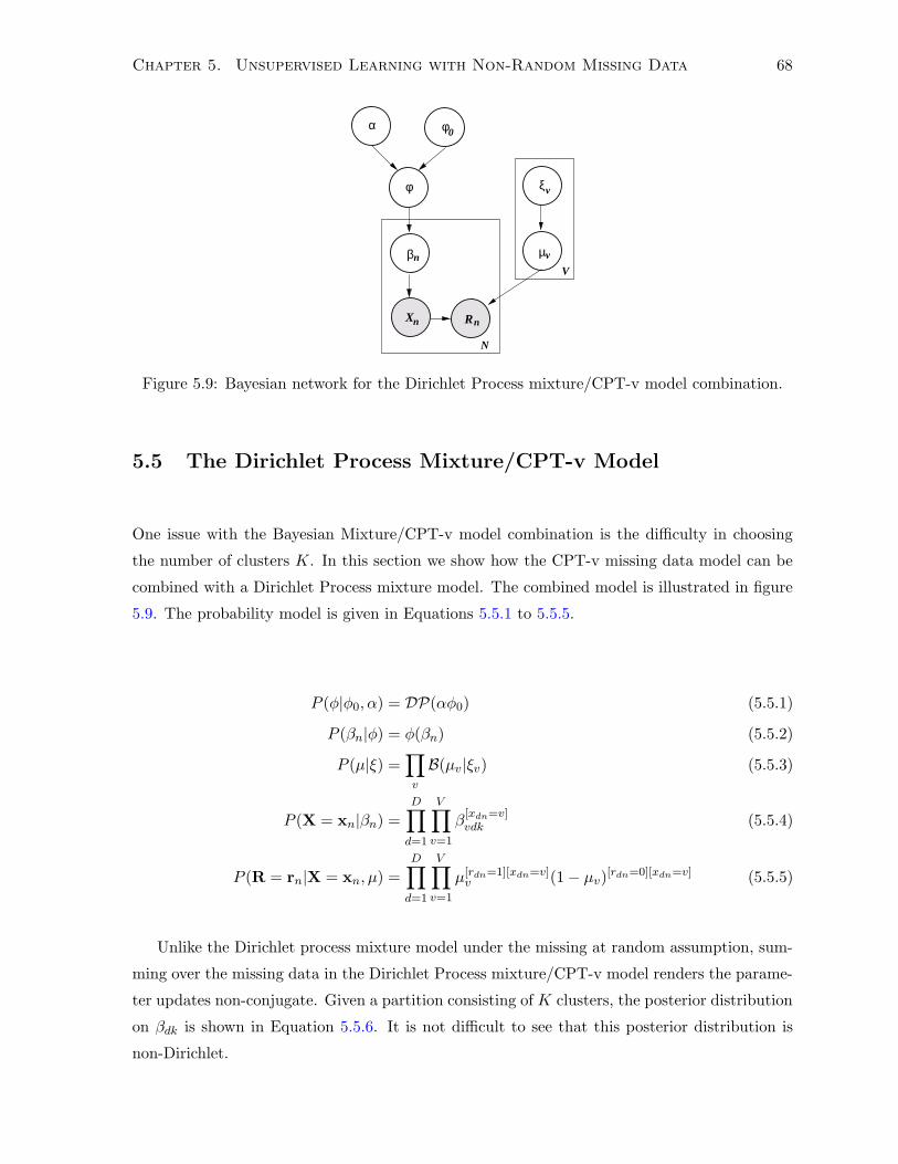
Chapter 5. Unsupervised Learning with Non-Random Missing Data 68
φ
βn
α φ0
X
N
v
V
R
µ
v
nn
ξ
Figure 5.9: Bayesian network for the Dirichlet Process mixture/CPT-v model combination.
5.5 The Dirichlet Process Mixture/CPT-v Model
One issue with the Bayesian Mixture/CPT-v model combination is the difficulty in choosing
the number of clusters K. In this section we show how the CPT-v missing data model can be
combined with a Dirichlet Process mixture model. The combined model is illustrated in figure
5.9. The probability model is given in Equations 5.5.1 to 5.5.5.
P (φ|φ0, α) = DP(αφ0) (5.5.1)
P (βn|φ) = φ(βn) (5.5.2)
P (µ|ξ) =∏
v
B(µv|ξv) (5.5.3)
P (X = xn|βn) =D∏
d=1
V∏
v=1
β[xdn=v]vdk (5.5.4)
P (R = rn|X = xn, µ) =D∏
d=1
V∏
v=1
µ[rdn=1][xdn=v]v (1− µv)
[rdn=0][xdn=v] (5.5.5)
Unlike the Dirichlet process mixture model under the missing at random assumption, sum-
ming over the missing data in the Dirichlet Process mixture/CPT-v model renders the parame-
ter updates non-conjugate. Given a partition consisting of K clusters, the posterior distribution
on βdk is shown in Equation 5.5.6. It is not difficult to see that this posterior distribution is
non-Dirichlet.

Chapter 5. Unsupervised Learning with Non-Random Missing Data 69
P (βdk| {xn, rn,an, zn}n=1:N , µ, φ0)
∝N∏
n=1
(V∏
v=1
β[xdn=v][rdn=1][adn=1][zn=k]vdk
)·(
V∑
v=1
µvβvdk
)[rdn=1][adn=0][zn=k]
·(
V∑
v=1
(1− µv)βvdk
)[rdn=0][adn=0][zn=k]( V∏
v=1
βφvd0−1vdk
)(5.5.6)
The straightforward approach to avoiding non-conjugate parameter sampling is to sample all
of the missing data values given the current partition and parameter values. With the missing
data values included in the state of the Gibbs sampler, the Gibbs updates consist of sampling
from Dirichlet, Beta, or discrete distributions. While simple, this sampling scheme is not
practical in the collaborative filtering case. First, sampling all of the missing data means that
the space complexity of the inference algorithm scales with the size of the complete data matrix
instead of the number of observed ratings. Second, introducing millions of additional state
variables into the Gibbs sampler has a severely detrimental affect on mixing time, rendering
the naive sampler effectively useless.
5.5.1 An Auxiliary Variable Gibbs Sampler
In this section we describe an exact auxiliary variable sampler for the Dirichlet Process mixture/CPT-
v model. The sampler exploits two key properties of the combined model. First, the missing
data can be analytically summed over when assigning a data case to a mixture component.
This includes the case of assignment to a previously unrepresented component. Second, the
parameter updates for βvdk and µv depend only on counts of observed and missing rating val-
ues. It is possible to exactly sample the missing rating counts as auxiliary variables without
simultaneously storing the missing ratings for each user.
We give the cluster assignment updates in Equations 5.5.7 and 5.5.9. Equation 5.5.7 gives
the probability that data case n is assigned to occupied cluster k. This probability can be
viewed as the product of a prior term, and a likelihood term. The prior component of the
update probability follows from the Chinese Restaurant Process, and depends only on the
concentration parameter, and the number of data cases assigned to each occupied component.
The likelihood component of equation 5.5.7 is obtained by summing over missing data values
as in the finite mixture case.
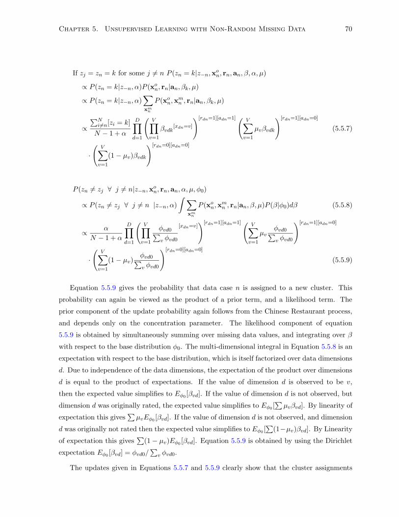
Chapter 5. Unsupervised Learning with Non-Random Missing Data 70
If zj = zn = k for some j 6= n P (zn = k|z−n,xon, rn,an, β, α, µ)
∝ P (zn = k|z−n, α)P (xon, rn|an, βk, µ)
∝ P (zn = k|z−n, α)∑
xmn
P (xon,x
mn , rn|an, βk, µ)
∝∑N
i6=n[zi = k]
N − 1 + α
D∏
d=1
(V∏
v=1
βvdk[xdn=v]
)[rdn=1][adn=1]( V∑
v=1
µvβvdk
)[rdn=1][adn=0]
(5.5.7)
·(
V∑
v=1
(1− µv)βvdk
)[rdn=0][adn=0]
P (zn 6= zj ∀ j 6= n|z−n,xon, rn,an, α, µ, φ0)
∝ P (zn 6= zj ∀ j 6= n |z−n, α)
∫ ∑
xmn
P (xon,x
mn , rn|an, β, µ)P (β|φ0)dβ (5.5.8)
∝ α
N − 1 + α
D∏
d=1
(V∏
v=1
φvd0∑v φvd0
[xdn=v])[rdn=1][adn=1]( V∑
v=1
µvφvd0∑v φvd0
)[rdn=1][adn=0]
·(
V∑
v=1
(1− µv)φvd0∑v φvd0
)[rdn=0][adn=0]
(5.5.9)
Equation 5.5.9 gives the probability that data case n is assigned to a new cluster. This
probability can again be viewed as the product of a prior term, and a likelihood term. The
prior component of the update probability again follows from the Chinese Restaurant process,
and depends only on the concentration parameter. The likelihood component of equation
5.5.9 is obtained by simultaneously summing over missing data values, and integrating over β
with respect to the base distribution φ0. The multi-dimensional integral in Equation 5.5.8 is an
expectation with respect to the base distribution, which is itself factorized over data dimensions
d. Due to independence of the data dimensions, the expectation of the product over dimensions
d is equal to the product of expectations. If the value of dimension d is observed to be v,
then the expected value simplifies to Eφ0[βvd]. If the value of dimension d is not observed, but
dimension d was originally rated, the expected value simplifies to Eφ0[∑µvβvd]. By linearity of
expectation this gives∑µvEφ0
[βvd]. If the value of dimension d is not observed, and dimension
d was originally not rated then the expected value simplifies to Eφ0[∑
(1−µv)βvd]. By Linearity
of expectation this gives∑
(1− µv)Eφ0[βvd]. Equation 5.5.9 is obtained by using the Dirichlet
expectation Eφ0[βvd] = φvd0/
∑v φvd0.
The updates given in Equations 5.5.7 and 5.5.9 clearly show that the cluster assignments
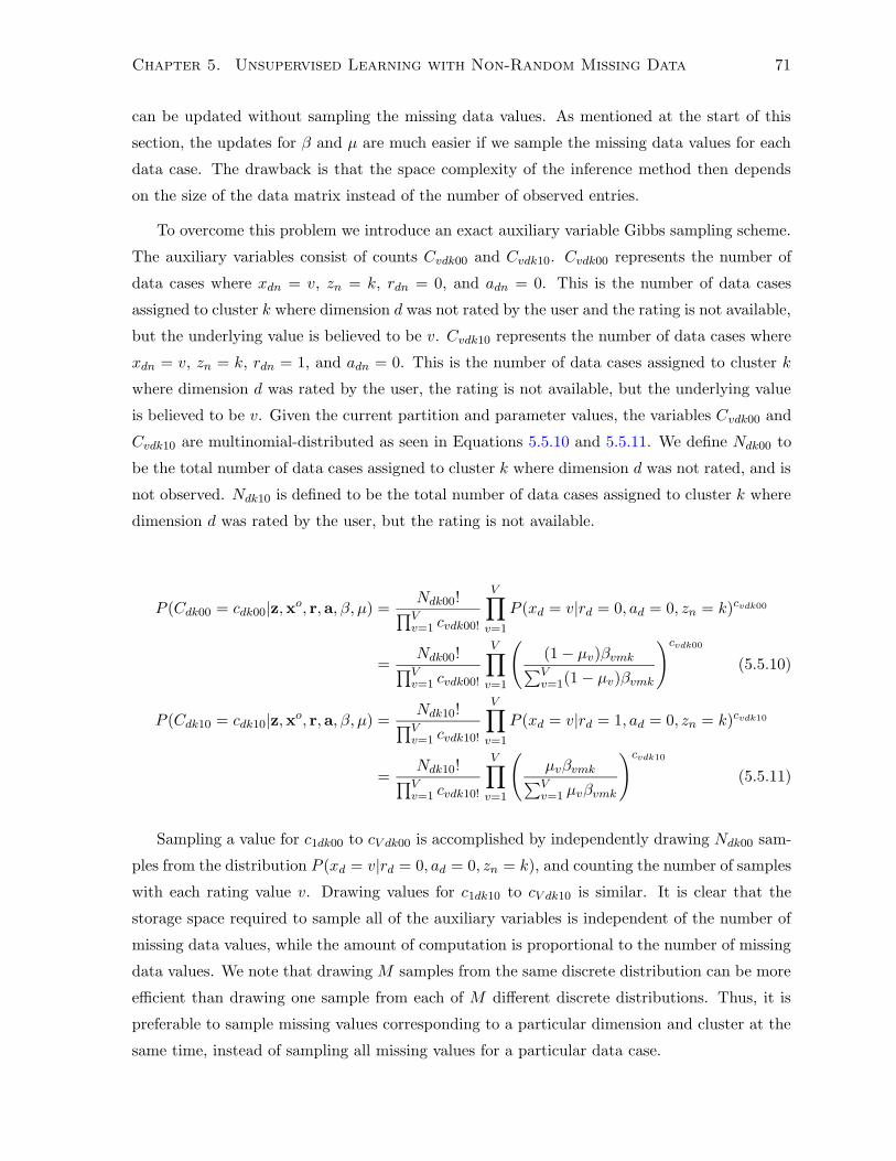
Chapter 5. Unsupervised Learning with Non-Random Missing Data 71
can be updated without sampling the missing data values. As mentioned at the start of this
section, the updates for β and µ are much easier if we sample the missing data values for each
data case. The drawback is that the space complexity of the inference method then depends
on the size of the data matrix instead of the number of observed entries.
To overcome this problem we introduce an exact auxiliary variable Gibbs sampling scheme.
The auxiliary variables consist of counts Cvdk00 and Cvdk10. Cvdk00 represents the number of
data cases where xdn = v, zn = k, rdn = 0, and adn = 0. This is the number of data cases
assigned to cluster k where dimension d was not rated by the user and the rating is not available,
but the underlying value is believed to be v. Cvdk10 represents the number of data cases where
xdn = v, zn = k, rdn = 1, and adn = 0. This is the number of data cases assigned to cluster k
where dimension d was rated by the user, the rating is not available, but the underlying value
is believed to be v. Given the current partition and parameter values, the variables Cvdk00 and
Cvdk10 are multinomial-distributed as seen in Equations 5.5.10 and 5.5.11. We define Ndk00 to
be the total number of data cases assigned to cluster k where dimension d was not rated, and is
not observed. Ndk10 is defined to be the total number of data cases assigned to cluster k where
dimension d was rated by the user, but the rating is not available.
P (Cdk00 = cdk00|z,xo, r,a, β, µ) =Ndk00!∏V
v=1 cvdk00!
V∏
v=1
P (xd = v|rd = 0, ad = 0, zn = k)cvdk00
=Ndk00!∏V
v=1 cvdk00!
V∏
v=1
((1− µv)βvmk∑Vv=1(1− µv)βvmk
)cvdk00
(5.5.10)
P (Cdk10 = cdk10|z,xo, r,a, β, µ) =Ndk10!∏V
v=1 cvdk10!
V∏
v=1
P (xd = v|rd = 1, ad = 0, zn = k)cvdk10
=Ndk10!∏V
v=1 cvdk10!
V∏
v=1
(µvβvmk∑V
v=1 µvβvmk
)cvdk10
(5.5.11)
Sampling a value for c1dk00 to cV dk00 is accomplished by independently drawing Ndk00 sam-
ples from the distribution P (xd = v|rd = 0, ad = 0, zn = k), and counting the number of samples
with each rating value v. Drawing values for c1dk10 to cV dk10 is similar. It is clear that the
storage space required to sample all of the auxiliary variables is independent of the number of
missing data values, while the amount of computation is proportional to the number of missing
data values. We note that drawing M samples from the same discrete distribution can be more
efficient than drawing one sample from each of M different discrete distributions. Thus, it is
preferable to sample missing values corresponding to a particular dimension and cluster at the
same time, instead of sampling all missing values for a particular data case.
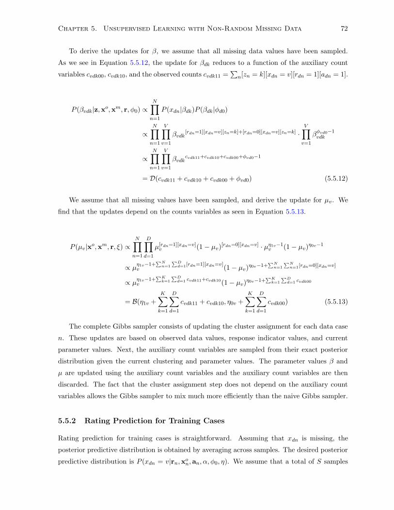
Chapter 5. Unsupervised Learning with Non-Random Missing Data 72
To derive the updates for β, we assume that all missing data values have been sampled.
As we see in Equation 5.5.12, the update for βdk reduces to a function of the auxiliary count
variables cvdk00, cvdk10, and the observed counts cvdk11 =∑
n[zn = k][xdn = v][rdn = 1][adn = 1].
P (βvdk|z,xo,xm, r, φ0) ∝N∏
n=1
P (xdn|βdk)P (βdk|φd0)
∝N∏
n=1
V∏
v=1
βvdk[rdn=1][xdn=v][zn=k]+[rdn=0][xdn=v][zn=k] ·
V∏
v=1
βφvd0−1vdk
∝N∏
n=1
V∏
v=1
βvdkcvdk11+cvdk10+cvdk00+φvd0−1
= D(cvdk11 + cvdk10 + cvdk00 + φvd0) (5.5.12)
We assume that all missing values have been sampled, and derive the update for µv. We
find that the updates depend on the counts variables as seen in Equation 5.5.13.
P (µv|xo,xm, r, ξ) ∝N∏
n=1
D∏
d=1
µ[rdn=1][xdn=v]v (1− µv)
[rdn=0][xdn=v] · µη1v−1v (1− µv)
η0v−1
∝ µη1v−1+∑N
n=1
∑Dd=1
[rdn=1][xdn=v]v (1− µv)
η0v−1+∑N
n=1
∑Nn=1
[rdn=0][xdn=v]
∝ µη1v−1+∑K
k=1
∑Dd=1
cvdk11+cvdk10
v (1− µv)η0v−1+
∑Kk=1
∑Dd=1
cvdk00
= B(η1v +
K∑
k=1
D∑
d=1
cvdk11 + cvdk10, η0v +
K∑
k=1
D∑
d=1
cvdk00) (5.5.13)
The complete Gibbs sampler consists of updating the cluster assignment for each data case
n. These updates are based on observed data values, response indicator values, and current
parameter values. Next, the auxiliary count variables are sampled from their exact posterior
distribution given the current clustering and parameter values. The parameter values β and
µ are updated using the auxiliary count variables and the auxiliary count variables are then
discarded. The fact that the cluster assignment step does not depend on the auxiliary count
variables allows the Gibbs sampler to mix much more efficiently than the naive Gibbs sampler.
5.5.2 Rating Prediction for Training Cases
Rating prediction for training cases is straightforward. Assuming that xdn is missing, the
posterior predictive distribution is obtained by averaging across samples. The desired posterior
predictive distribution is P (xdn = v|rn,xon,an, α, φ0, η). We assume that a total of S samples
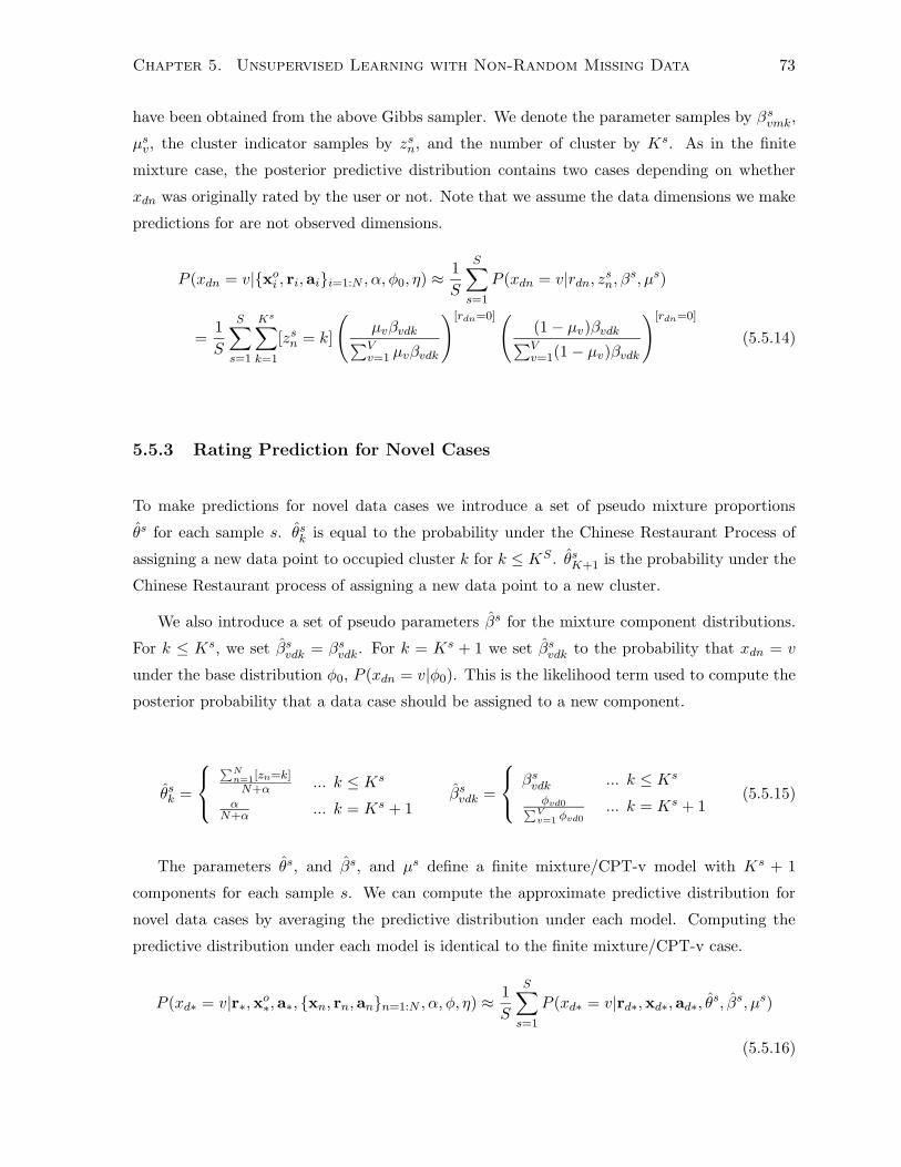
Chapter 5. Unsupervised Learning with Non-Random Missing Data 73
have been obtained from the above Gibbs sampler. We denote the parameter samples by βsvmk,
µsv, the cluster indicator samples by zs
n, and the number of cluster by Ks. As in the finite
mixture case, the posterior predictive distribution contains two cases depending on whether
xdn was originally rated by the user or not. Note that we assume the data dimensions we make
predictions for are not observed dimensions.
P (xdn = v|{xoi , ri,ai}i=1:N , α, φ0, η) ≈
1
S
S∑
s=1
P (xdn = v|rdn, zsn, β
s, µs)
=1
S
S∑
s=1
Ks∑
k=1
[zsn = k]
(µvβvdk∑V
v=1 µvβvdk
)[rdn=0]((1− µv)βvdk∑Vv=1(1− µv)βvdk
)[rdn=0]
(5.5.14)
5.5.3 Rating Prediction for Novel Cases
To make predictions for novel data cases we introduce a set of pseudo mixture proportions
θs for each sample s. θsk is equal to the probability under the Chinese Restaurant Process of
assigning a new data point to occupied cluster k for k ≤ KS . θsK+1 is the probability under the
Chinese Restaurant process of assigning a new data point to a new cluster.
We also introduce a set of pseudo parameters βs for the mixture component distributions.
For k ≤ Ks, we set βsvdk = βs
vdk. For k = Ks + 1 we set βsvdk to the probability that xdn = v
under the base distribution φ0, P (xdn = v|φ0). This is the likelihood term used to compute the
posterior probability that a data case should be assigned to a new component.
θsk =
∑Nn=1
[zn=k]N+α ... k ≤ Ks
αN+α ... k = Ks + 1
βsvdk =
βsvdk ... k ≤ Ks
φvd0∑Vv=1
φvd0
... k = Ks + 1(5.5.15)
The parameters θs, and βs, and µs define a finite mixture/CPT-v model with Ks + 1
components for each sample s. We can compute the approximate predictive distribution for
novel data cases by averaging the predictive distribution under each model. Computing the
predictive distribution under each model is identical to the finite mixture/CPT-v case.
P (xd∗ = v|r∗,xo∗,a∗, {xn, rn,an}n=1:N , α, φ, η) ≈
1
S
S∑
s=1
P (xd∗ = v|rd∗,xd∗,ad∗, θs, βs, µs)
(5.5.16)
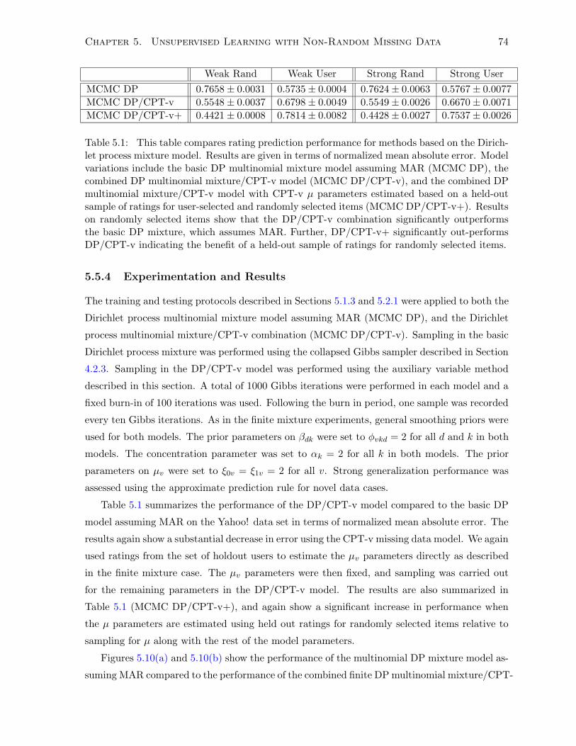
Chapter 5. Unsupervised Learning with Non-Random Missing Data 74
Weak Rand Weak User Strong Rand Strong User
MCMC DP 0.7658± 0.0031 0.5735± 0.0004 0.7624± 0.0063 0.5767± 0.0077
MCMC DP/CPT-v 0.5548± 0.0037 0.6798± 0.0049 0.5549± 0.0026 0.6670± 0.0071
MCMC DP/CPT-v+ 0.4421± 0.0008 0.7814± 0.0082 0.4428± 0.0027 0.7537± 0.0026
Table 5.1: This table compares rating prediction performance for methods based on the Dirich-let process mixture model. Results are given in terms of normalized mean absolute error. Modelvariations include the basic DP multinomial mixture model assuming MAR (MCMC DP), thecombined DP multinomial mixture/CPT-v model (MCMC DP/CPT-v), and the combined DPmultinomial mixture/CPT-v model with CPT-v µ parameters estimated based on a held-outsample of ratings for user-selected and randomly selected items (MCMC DP/CPT-v+). Resultson randomly selected items show that the DP/CPT-v combination significantly outperformsthe basic DP mixture, which assumes MAR. Further, DP/CPT-v+ significantly out-performsDP/CPT-v indicating the benefit of a held-out sample of ratings for randomly selected items.
5.5.4 Experimentation and Results
The training and testing protocols described in Sections 5.1.3 and 5.2.1 were applied to both the
Dirichlet process multinomial mixture model assuming MAR (MCMC DP), and the Dirichlet
process multinomial mixture/CPT-v combination (MCMC DP/CPT-v). Sampling in the basic
Dirichlet process mixture was performed using the collapsed Gibbs sampler described in Section
4.2.3. Sampling in the DP/CPT-v model was performed using the auxiliary variable method
described in this section. A total of 1000 Gibbs iterations were performed in each model and a
fixed burn-in of 100 iterations was used. Following the burn in period, one sample was recorded
every ten Gibbs iterations. As in the finite mixture experiments, general smoothing priors were
used for both models. The prior parameters on βdk were set to φvkd = 2 for all d and k in both
models. The concentration parameter was set to αk = 2 for all k in both models. The prior
parameters on µv were set to ξ0v = ξ1v = 2 for all v. Strong generalization performance was
assessed using the approximate prediction rule for novel data cases.
Table 5.1 summarizes the performance of the DP/CPT-v model compared to the basic DP
model assuming MAR on the Yahoo! data set in terms of normalized mean absolute error. The
results again show a substantial decrease in error using the CPT-v missing data model. We again
used ratings from the set of holdout users to estimate the µv parameters directly as described
in the finite mixture case. The µv parameters were then fixed, and sampling was carried out
for the remaining parameters in the DP/CPT-v model. The results are also summarized in
Table 5.1 (MCMC DP/CPT-v+), and again show a significant increase in performance when
the µ parameters are estimated using held out ratings for randomly selected items relative to
sampling for µ along with the rest of the model parameters.
Figures 5.10(a) and 5.10(b) show the performance of the multinomial DP mixture model as-
suming MAR compared to the performance of the combined finite DP multinomial mixture/CPT-
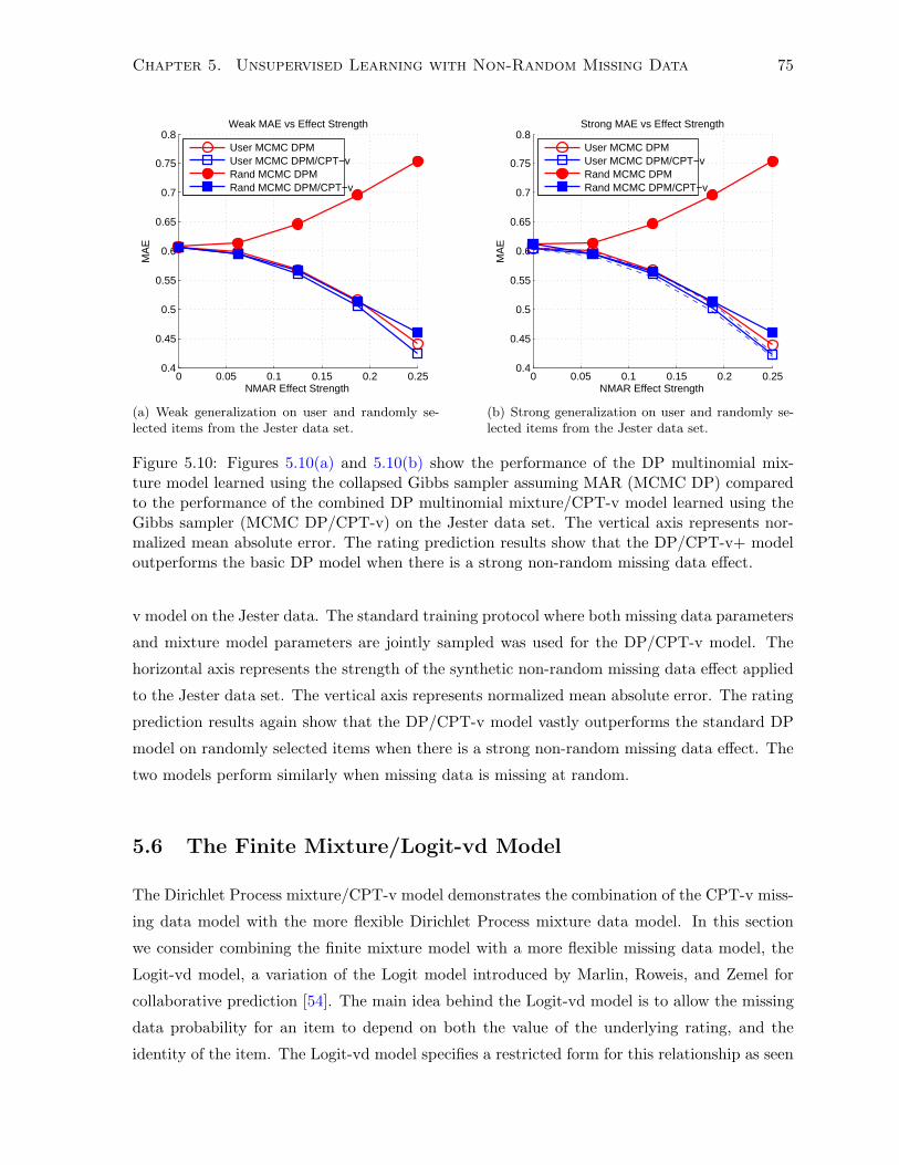
Chapter 5. Unsupervised Learning with Non-Random Missing Data 75
0 0.05 0.1 0.15 0.2 0.250.4
0.45
0.5
0.55
0.6
0.65
0.7
0.75
0.8Weak MAE vs Effect Strength
NMAR Effect Strength
MA
E
User MCMC DPMUser MCMC DPM/CPT−vRand MCMC DPMRand MCMC DPM/CPT−v
(a) Weak generalization on user and randomly se-lected items from the Jester data set.
0 0.05 0.1 0.15 0.2 0.250.4
0.45
0.5
0.55
0.6
0.65
0.7
0.75
0.8Strong MAE vs Effect Strength
NMAR Effect Strength
MA
E
User MCMC DPMUser MCMC DPM/CPT−vRand MCMC DPMRand MCMC DPM/CPT−v
(b) Strong generalization on user and randomly se-lected items from the Jester data set.
Figure 5.10: Figures 5.10(a) and 5.10(b) show the performance of the DP multinomial mix-ture model learned using the collapsed Gibbs sampler assuming MAR (MCMC DP) comparedto the performance of the combined DP multinomial mixture/CPT-v model learned using theGibbs sampler (MCMC DP/CPT-v) on the Jester data set. The vertical axis represents nor-malized mean absolute error. The rating prediction results show that the DP/CPT-v+ modeloutperforms the basic DP model when there is a strong non-random missing data effect.
v model on the Jester data. The standard training protocol where both missing data parameters
and mixture model parameters are jointly sampled was used for the DP/CPT-v model. The
horizontal axis represents the strength of the synthetic non-random missing data effect applied
to the Jester data set. The vertical axis represents normalized mean absolute error. The rating
prediction results again show that the DP/CPT-v model vastly outperforms the standard DP
model on randomly selected items when there is a strong non-random missing data effect. The
two models perform similarly when missing data is missing at random.
5.6 The Finite Mixture/Logit-vd Model
The Dirichlet Process mixture/CPT-v model demonstrates the combination of the CPT-v miss-
ing data model with the more flexible Dirichlet Process mixture data model. In this section
we consider combining the finite mixture model with a more flexible missing data model, the
Logit-vd model, a variation of the Logit model introduced by Marlin, Roweis, and Zemel for
collaborative prediction [54]. The main idea behind the Logit-vd model is to allow the missing
data probability for an item to depend on both the value of the underlying rating, and the
identity of the item. The Logit-vd model specifies a restricted form for this relationship as seen
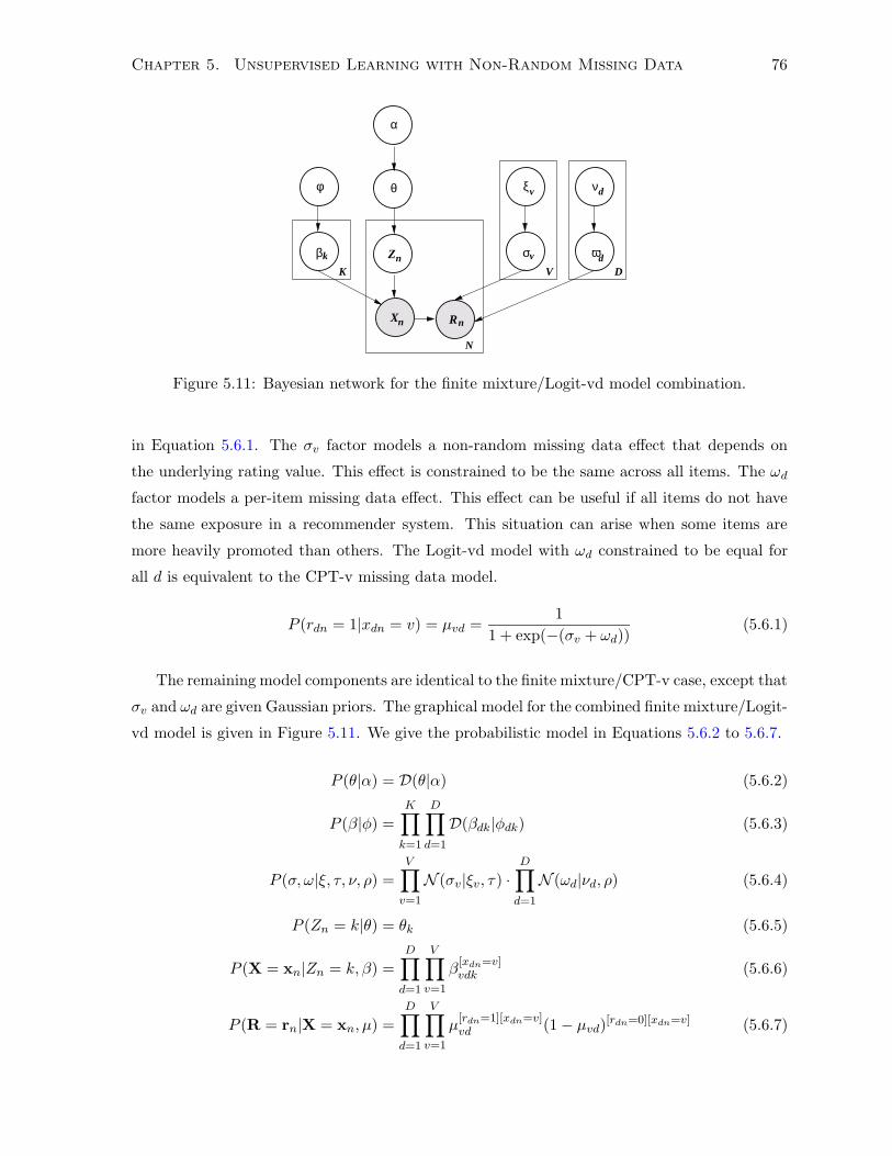
Chapter 5. Unsupervised Learning with Non-Random Missing Data 76
θφ
βk
K
ξ ν
Zn
X
N
Rnn
v
V
v
σ ωD
d
d
α
Figure 5.11: Bayesian network for the finite mixture/Logit-vd model combination.
in Equation 5.6.1. The σv factor models a non-random missing data effect that depends on
the underlying rating value. This effect is constrained to be the same across all items. The ωd
factor models a per-item missing data effect. This effect can be useful if all items do not have
the same exposure in a recommender system. This situation can arise when some items are
more heavily promoted than others. The Logit-vd model with ωd constrained to be equal for
all d is equivalent to the CPT-v missing data model.
P (rdn = 1|xdn = v) = µvd =1
1 + exp(−(σv + ωd))(5.6.1)
The remaining model components are identical to the finite mixture/CPT-v case, except that
σv and ωd are given Gaussian priors. The graphical model for the combined finite mixture/Logit-
vd model is given in Figure 5.11. We give the probabilistic model in Equations 5.6.2 to 5.6.7.
P (θ|α) = D(θ|α) (5.6.2)
P (β|φ) =
K∏
k=1
D∏
d=1
D(βdk|φdk) (5.6.3)
P (σ, ω|ξ, τ, ν, ρ) =V∏
v=1
N (σv|ξv, τ) ·D∏
d=1
N (ωd|νd, ρ) (5.6.4)
P (Zn = k|θ) = θk (5.6.5)
P (X = xn|Zn = k, β) =D∏
d=1
V∏
v=1
β[xdn=v]vdk (5.6.6)
P (R = rn|X = xn, µ) =D∏
d=1
V∏
v=1
µ[rdn=1][xdn=v]vd (1− µvd)
[rdn=0][xdn=v] (5.6.7)
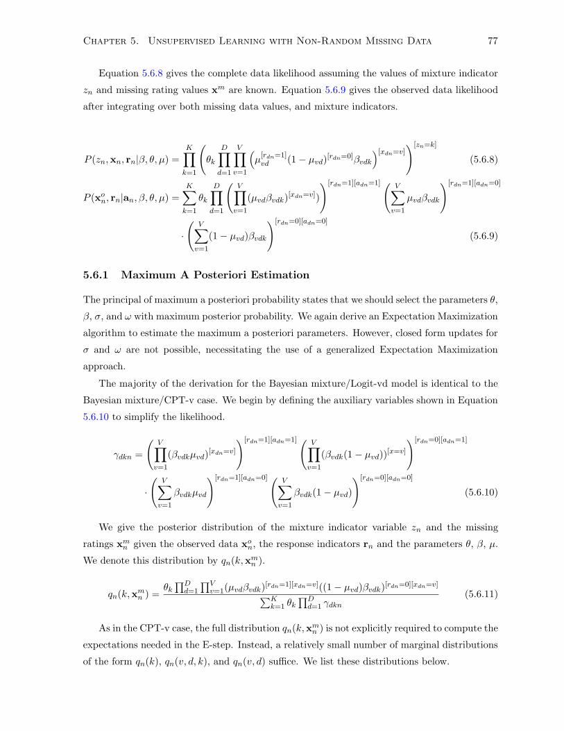
Chapter 5. Unsupervised Learning with Non-Random Missing Data 77
Equation 5.6.8 gives the complete data likelihood assuming the values of mixture indicator
zn and missing rating values xm are known. Equation 5.6.9 gives the observed data likelihood
after integrating over both missing data values, and mixture indicators.
P (zn,xn, rn|β, θ, µ) =K∏
k=1
(θk
D∏
d=1
V∏
v=1
(µ
[rdn=1]vd (1− µvd)
[rdn=0]βvdk
)[xdn=v])[zn=k]
(5.6.8)
P (xon, rn|an, β, θ, µ) =
K∑
k=1
θk
D∏
d=1
(V∏
v=1
(µvdβvdk)[xdn=v])
)[rdn=1][adn=1]( V∑
v=1
µvdβvdk
)[rdn=1][adn=0]
·(
V∑
v=1
(1− µvd)βvdk
)[rdn=0][adn=0]
(5.6.9)
5.6.1 Maximum A Posteriori Estimation
The principal of maximum a posteriori probability states that we should select the parameters θ,
β, σ, and ω with maximum posterior probability. We again derive an Expectation Maximization
algorithm to estimate the maximum a posteriori parameters. However, closed form updates for
σ and ω are not possible, necessitating the use of a generalized Expectation Maximization
approach.
The majority of the derivation for the Bayesian mixture/Logit-vd model is identical to the
Bayesian mixture/CPT-v case. We begin by defining the auxiliary variables shown in Equation
5.6.10 to simplify the likelihood.
γdkn =
(V∏
v=1
(βvdkµvd)[xdn=v]
)[rdn=1][adn=1]( V∏
v=1
(βvdk(1− µvd))[x=v]
)[rdn=0][adn=1]
·(
V∑
v=1
βvdkµvd
)[rdn=1][adn=0]( V∑
v=1
βvdk(1− µvd)
)[rdn=0][adn=0]
(5.6.10)
We give the posterior distribution of the mixture indicator variable zn and the missing
ratings xmn given the observed data xo
n, the response indicators rn and the parameters θ, β, µ.
We denote this distribution by qn(k,xmn ).
qn(k,xmn ) =
θk∏D
d=1
∏Vv=1(µvdβvdk)
[rdn=1][xdn=v]((1− µvd)βvdk)[rdn=0][xdn=v]
∑Kk=1 θk
∏Dd=1 γdkn
(5.6.11)
As in the CPT-v case, the full distribution qn(k,xmn ) is not explicitly required to compute the
expectations needed in the E-step. Instead, a relatively small number of marginal distributions
of the form qn(k), qn(v, d, k), and qn(v, d) suffice. We list these distributions below.
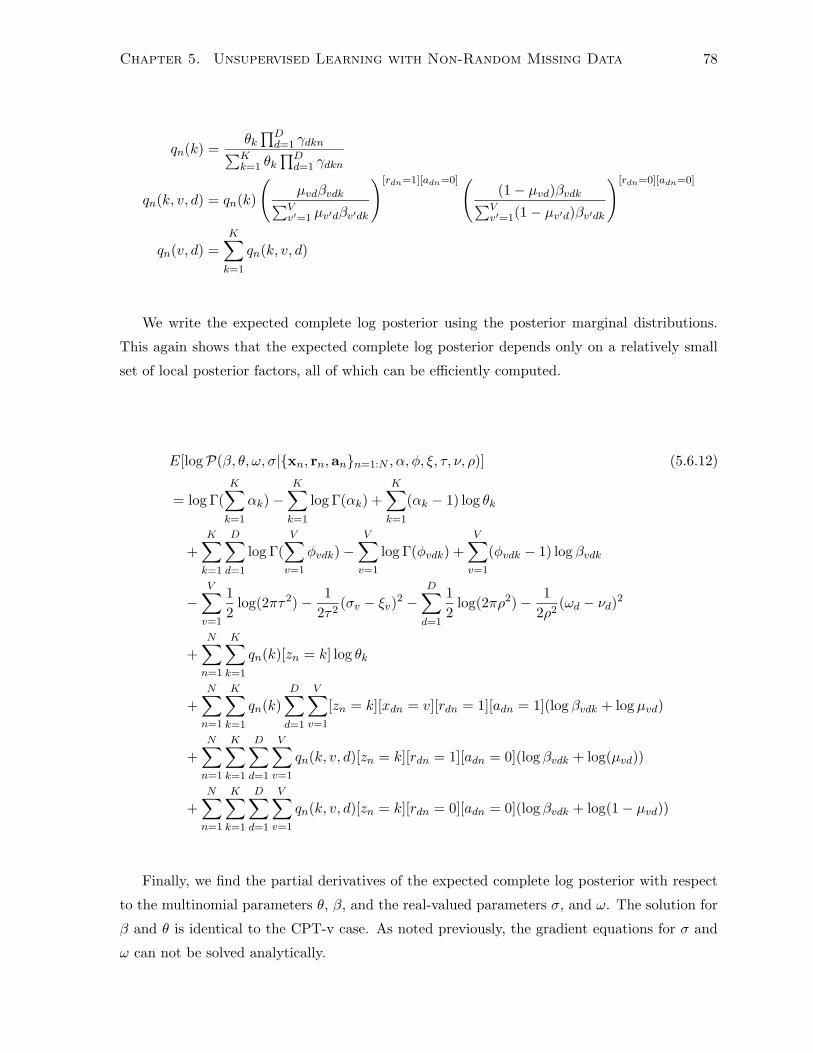
Chapter 5. Unsupervised Learning with Non-Random Missing Data 78
qn(k) =θk∏D
d=1 γdkn∑Kk=1 θk
∏Dd=1 γdkn
qn(k, v, d) = qn(k)
(µvdβvdk∑V
v′=1 µv′dβv′dk
)[rdn=1][adn=0]((1− µvd)βvdk∑V
v′=1(1− µv′d)βv′dk
)[rdn=0][adn=0]
qn(v, d) =K∑
k=1
qn(k, v, d)
We write the expected complete log posterior using the posterior marginal distributions.
This again shows that the expected complete log posterior depends only on a relatively small
set of local posterior factors, all of which can be efficiently computed.
E[logP(β, θ, ω, σ|{xn, rn,an}n=1:N , α, φ, ξ, τ, ν, ρ)] (5.6.12)
= log Γ(K∑
k=1
αk)−K∑
k=1
log Γ(αk) +K∑
k=1
(αk − 1) log θk
+K∑
k=1
D∑
d=1
log Γ(V∑
v=1
φvdk)−V∑
v=1
log Γ(φvdk) +V∑
v=1
(φvdk − 1) log βvdk
−V∑
v=1
1
2log(2πτ 2)− 1
2τ2(σv − ξv)2 −
D∑
d=1
1
2log(2πρ2)− 1
2ρ2(ωd − νd)
2
+
N∑
n=1
K∑
k=1
qn(k)[zn = k] log θk
+N∑
n=1
K∑
k=1
qn(k)D∑
d=1
V∑
v=1
[zn = k][xdn = v][rdn = 1][adn = 1](log βvdk + logµvd)
+N∑
n=1
K∑
k=1
D∑
d=1
V∑
v=1
qn(k, v, d)[zn = k][rdn = 1][adn = 0](log βvdk + log(µvd))
+N∑
n=1
K∑
k=1
D∑
d=1
V∑
v=1
qn(k, v, d)[zn = k][rdn = 0][adn = 0](log βvdk + log(1− µvd))
Finally, we find the partial derivatives of the expected complete log posterior with respect
to the multinomial parameters θ, β, and the real-valued parameters σ, and ω. The solution for
β and θ is identical to the CPT-v case. As noted previously, the gradient equations for σ and
ω can not be solved analytically.

Chapter 5. Unsupervised Learning with Non-Random Missing Data 79
∂E[logP]
∂θk=αk − 1 +
∑Nn=1 qn(k)
θk− λ = 0
θk =αk − 1 +
∑Nn=1 qn(k)
N −K +∑K
k=1 αk
(5.6.13)
∂E[logP]
∂βvdk=φvnk − 1
βvdk+
∑Nn=1 qn(k)[adn = 1][xdn = v]
βvdk
+
∑Nn=1 qn(v, d, k)[adn = 0]
βvdk− λ = 0
βvdk =φvdk − 1 +
∑Nn=1 qn(k)[adn = 1][xdn = v] + qn(k, v, d)[adn = 0]∑N
n=1 qn(k)− V +∑V
v=1 φvdk
(5.6.14)
∂E[logP]
∂µvd=
∑Nn=1[rdn = 1][adn = 1][xdn = v] + qn(v, d)[rdn = 1][adn = 0]
µvd
−∑N
n=1 qn(v, d)[rdn = 0][adn = 0]
(1− µvd)= 0 (5.6.15)
∂E[logP]
∂σv=
D∑
d=1
∂E[logP]
∂µvd
∂µvd
∂σv− 1
τ2(σv − ξv) = 0
=D∑
d=1
N∑
n=1
∂E[logP]
∂µvdµvd(1− µvd)−
1
τ2(σv − ξv) (5.6.16)
∂E[logP]
∂ωd=
V∑
v=1
∂E[logP]
∂µvd
∂µvd
∂ωd− 1
γ2(ωd − νd) = 0
=V∑
v=1
N∑
n=1
∂E[logP]
∂µvdµvd(1− µvd)−
1
ρ2(ωd − νd) (5.6.17)
5.6.2 Rating Prediction
The posterior predictive distribution for the finite mixture/Logit-vd model is identical to the
finite mixture/CPT-v case. The only difference is the definition of the µvd and γvdk auxiliary
variables.
P (Xdn = v|xn, rn,an, θ, β, µ) =K∑
k=1
θk∏D
d=1 γdkn∑Kk=1 θk
∏Dd=1 γdkn
(µvdβvdk∑V
v′=1 µv′dβv′dk
)[rdn=1]
·(
(1− µvd)βvdk∑Vv′=1(1− µv′d)βv′dk
)[rdn=0]
(5.6.18)
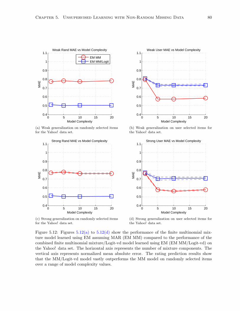
Chapter 5. Unsupervised Learning with Non-Random Missing Data 80
0 5 10 15 200.4
0.5
0.6
0.7
0.8
0.9
1
1.1Weak Rand MAE vs Model Complexity
Model Complexity
MA
E
EM MMEM MM/Logit
(a) Weak generalization on randomly selected itemsfor the Yahoo! data set.
0 5 10 15 200.4
0.5
0.6
0.7
0.8
0.9
1
1.1Weak User MAE vs Model Complexity
Model Complexity
MA
E
(b) Weak generalization on user selected items forthe Yahoo! data set.
0 5 10 15 200.4
0.5
0.6
0.7
0.8
0.9
1
1.1Strong Rand MAE vs Model Complexity
Model Complexity
MA
E
(c) Strong generalization on randomly selected itemsfor the Yahoo! data set.
0 5 10 15 200.4
0.5
0.6
0.7
0.8
0.9
1
1.1Strong User MAE vs Model Complexity
Model Complexity
MA
E
(d) Strong generalization on user selected items forthe Yahoo! data set.
Figure 5.12: Figures 5.12(a) to 5.12(d) show the performance of the finite multinomial mix-ture model learned using EM assuming MAR (EM MM) compared to the performance of thecombined finite multinomial mixture/Logit-vd model learned using EM (EM MM/Logit-vd) onthe Yahoo! data set. The horizontal axis represents the number of mixture components. Thevertical axis represents normalized mean absolute error. The rating prediction results showthat the MM/Logit-vd model vastly outperforms the MM model on randomly selected itemsover a range of model complexity values.

Chapter 5. Unsupervised Learning with Non-Random Missing Data 81
0 0.05 0.1 0.15 0.2 0.250.4
0.45
0.5
0.55
0.6
0.65
0.7
0.75Weak MAE vs Effect Strength
NMAR Effect Strength
MA
E
User EM MMUser EM MM/LogitRand EM MMRand EM MM/Logit
(a) Weak generalization on randomly selected itemsfor the Jester data set.
0 0.05 0.1 0.15 0.2 0.250.4
0.45
0.5
0.55
0.6
0.65
0.7
0.75
0.8Strong MAE vs Effect Strength
NMAR Effect Strength
MA
E
User EM MMUser EM MM/LogitRand EM MMRand EM MM/Logit
(b) Strong generalization on randomly selecteditems for the Jester data set.
Figure 5.13: Figures 5.12(a) to 5.12(d) show the performance of the finite multinomial mixturemodel learned using EM assuming MAR (EM MM) compared to the performance of the com-bined finite multinomial mixture/Logit-vd model learned using EM (EM MM/Logit-vd). Thehorizontal axis represents non-random missing data effect strength. The vertical axis representsnormalized mean absolute error. The rating prediction results show that the MM/Logit-vdmodel vastly outperforms the MM model on randomly selected items as the effect strengthincreases.
5.6.3 Experimentation and Results
The standard training and testing protocols described in Sections 5.2.1 and 5.1.3 were applied
to both the finite multinomial mixture model learned using EM assuming MAR (EM MM),
and the finite multinomial mixture/Logit-vd model learned using EM (EM MM/Logit). A
maximum of 5000 EM iterations were used to train each model. General smoothing priors were
used for both models. The prior parameters on βdk were set to φvkd = 2 for all d and k in both
models. The prior parameters on θ were set to αk = 2 for all k in both models. A zero mean
Gaussian prior was used on both σv and ωd with a standard deviation of 10. The σv parameters
were all initialized to the same small random value. The ωd parameters were each initialized to
a different small random value. Models with 1, 5, 10, and 20 components were trained on the
Yahoo! data. The Jester results are based on models with 5 components.
Figures 5.12(a) to 5.12(d) show the performance of the finite multinomial mixture model
assuming MAR (EM MM) compared to the performance of the combined finite multinomial
mixture/Logit-vd model (EM MM/Logit) on the Yahoo! data set. The horizontal axis rep-
resents the number of mixture components. The vertical axis represents normalized mean
absolute error. The solid lines represent the mean of the error over the five cross validation
Chapter 5. Unsupervised Learning with Non-Random Missing Data 82
folds for each model. The standard error of the mean is shown using dashed lines. The rating
prediction results show that the MM/Logit-v model outperforms the MM model on randomly
selected items over the complete range of model complexity values.
Figures 5.13(a) and 5.13(b) show the performance of the finite multinomial mixture model
learned using EM assuming MAR (EM MM) compared to the performance of the combined
finite multinomial mixture/Logit-vd model learned using EM (EM MM/Logit) on the Jester
data. The horizontal axis represents the strength of the synthetic non-random missing data
effect applied to the Jester data set. The vertical axis represents normalized mean absolute error.
The rating prediction results show that the MM/Logit-vd model significantly outperforms the
MM model on randomly selected items when there is a strong non-random missing data effect.
The two models perform similarly when missing data is missing at random.
5.7 Restricted Boltzmann Machines
In this section we present restricted Boltzmann machines (RBMs) for complete data, and two
types of conditional RBMs that can efficiently cope with missing data. Unlike the other mod-
els considered to this point, the conditional RBM models do not follow the data model/selection
model factorization P (X)P (R|X). Instead, they follow the alternative factorization P (R)P (X|R).
Since our only interest is making predictions for missing data values given the corresponding re-
sponse indicators, the distribution P (R) is not needed. Therefore, the conditional RBM models
specify only the distribution P (X|R).
We begin this section by reviewing RBMs for complete data. We then present a new
interpretation of the conditional RBM model for missing data due to Salakhutdinov, Minh, and
Hinton [65]. We extend the basic conditional RBM model and devise a new training protocol
to better deal with prediction for non user-selected items. Finally, we present an empirical
comparison of the two conditional RBM models for missing data.
5.7.1 Restricted Boltzmann Machines and Complete Data
Boltzmann machines are a sub-class of Markov Random fields. A Boltzmann machine is typi-
cally organized into one layer of visible units or observed variables, and multiple layers of hidden
units or latent variables. A Boltzmann machine typically has connections between units in sub-
sequent layers, as well as between units in the same layer [34]. Restricted Boltzmann Machines
are a sub-class of Boltzmann Machines with one layer of hidden units, and no connections
between units in the same layer [70].
The joint probability distribution over the data xn and the hidden units zn defined by a
Restricted Boltzmann machine is specified in terms of an energy function E(xn, zn) as seen in
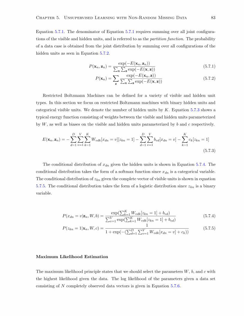
Chapter 5. Unsupervised Learning with Non-Random Missing Data 83
Equation 5.7.1. The denominator of Equation 5.7.1 requires summing over all joint configura-
tions of the visible and hidden units, and is referred to as the partition function. The probability
of a data case is obtained from the joint distribution by summing over all configurations of the
hidden units as seen in Equation 5.7.2.
P (xn, zn) =exp(−E(xn, zn))∑x
∑z exp(−E(x, z))
(5.7.1)
P (xn) =∑
z
exp(−E(xn, z))∑x
∑z exp(−E(x, z))
(5.7.2)
Restricted Boltzmann Machines can be defined for a variety of visible and hidden unit
types. In this section we focus on restricted Boltzmann machines with binary hidden units and
categorical visible units. We denote the number of hidden units by K. Equation 5.7.3 shows a
typical energy function consisting of weights between the visible and hidden units parameterized
by W , as well as biases on the visible and hidden units parameterized by b and c respectively.
E(xn, zn) = −D∑
d=1
V∑
v=1
K∑
k=1
Wvdk[xdn = v][zkn = 1]−D∑
d=1
V∑
v=1
bvd[xdn = v]−K∑
k=1
ck[zkn = 1]
(5.7.3)
The conditional distribution of xdn given the hidden units is shown in Equation 5.7.4. The
conditional distribution takes the form of a softmax function since xdn is a categorical variable.
The conditional distribution of zkn given the complete vector of visible units is shown in equation
5.7.5. The conditional distribution takes the form of a logistic distribution since zkn is a binary
variable.
P (xdn = v|zn,W, b) =exp(
∑Kk=1Wvdk[zkn = 1] + bvd)∑V
v=1 exp(∑K
k=1Wvdk[zkn = 1] + bvd)(5.7.4)
P (zkn = 1|xn,W, c) =1
1 + exp(−(∑D
d=1
∑Vv=1Wvdk[xdn = v] + ck))
(5.7.5)
Maximum Likelihood Estimation
The maximum likelihood principle states that we should select the parameters W , b, and c with
the highest likelihood given the data. The log likelihood of the parameters given a data set
consisting of N completely observed data vectors is given in Equation 5.7.6.
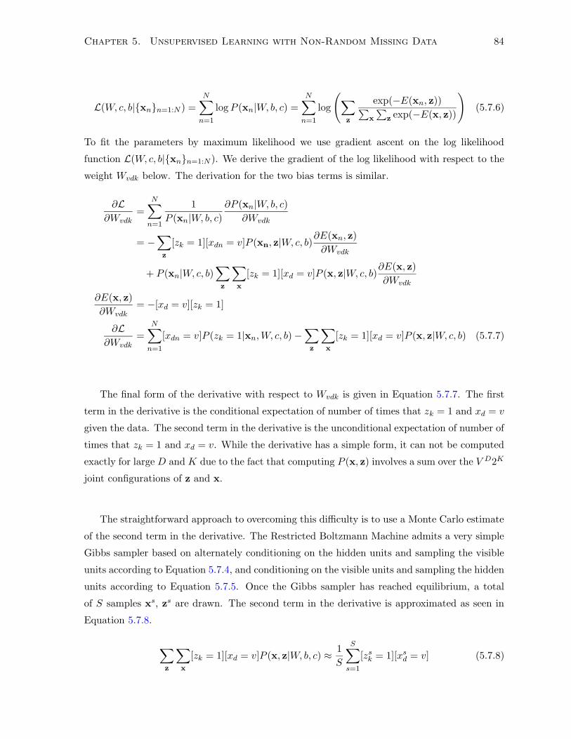
Chapter 5. Unsupervised Learning with Non-Random Missing Data 84
L(W, c, b|{xn}n=1:N ) =N∑
n=1
logP (xn|W, b, c) =N∑
n=1
log
(∑
z
exp(−E(xn, z))∑x
∑z exp(−E(x, z))
)(5.7.6)
To fit the parameters by maximum likelihood we use gradient ascent on the log likelihood
function L(W, c, b|{xn}n=1:N ). We derive the gradient of the log likelihood with respect to the
weight Wvdk below. The derivation for the two bias terms is similar.
∂L∂Wvdk
=N∑
n=1
1
P (xn|W, b, c)∂P (xn|W, b, c)
∂Wvdk
= −∑
z
[zk = 1][xdn = v]P (xn, z|W, c, b)∂E(xn, z)
∂Wvdk
+ P (xn|W, c, b)∑
z
∑
x
[zk = 1][xd = v]P (x, z|W, c, b)∂E(x, z)
∂Wvdk
∂E(x, z)
∂Wvdk= −[xd = v][zk = 1]
∂L∂Wvdk
=
N∑
n=1
[xdn = v]P (zk = 1|xn,W, c, b)−∑
z
∑
x
[zk = 1][xd = v]P (x, z|W, c, b) (5.7.7)
The final form of the derivative with respect to Wvdk is given in Equation 5.7.7. The first
term in the derivative is the conditional expectation of number of times that zk = 1 and xd = v
given the data. The second term in the derivative is the unconditional expectation of number of
times that zk = 1 and xd = v. While the derivative has a simple form, it can not be computed
exactly for large D and K due to the fact that computing P (x, z) involves a sum over the V D2K
joint configurations of z and x.
The straightforward approach to overcoming this difficulty is to use a Monte Carlo estimate
of the second term in the derivative. The Restricted Boltzmann Machine admits a very simple
Gibbs sampler based on alternately conditioning on the hidden units and sampling the visible
units according to Equation 5.7.4, and conditioning on the visible units and sampling the hidden
units according to Equation 5.7.5. Once the Gibbs sampler has reached equilibrium, a total
of S samples xs, zs are drawn. The second term in the derivative is approximated as seen in
Equation 5.7.8.
∑
z
∑
x
[zk = 1][xd = v]P (x, z|W, b, c) ≈ 1
S
S∑
s=1
[zsk = 1][xs
d = v] (5.7.8)
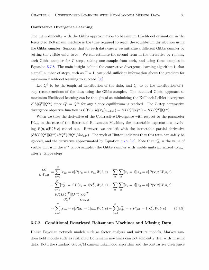
Chapter 5. Unsupervised Learning with Non-Random Missing Data 85
Contrastive Divergence Learning
The main difficulty with the Gibbs approximation to Maximum Likelihood estimation in the
Restricted Boltzmann machine is the time required to reach the equilibrium distribution using
the Gibbs sampler. Suppose that for each data case n we initialize a different Gibbs sampler by
setting the visible units to xn. We can estimate the second term in the derivative by running
each Gibbs sampler for T steps, taking one sample from each, and using these samples in
Equation 5.7.8. The main insight behind the contrastive divergence learning algorithm is that
a small number of steps, such as T = 1, can yield sufficient information about the gradient for
maximum likelihood learning to succeed [36].
Let Q0 to be the empirical distribution of the data, and Qt to be the distribution of t-
step reconstructions of the data using the Gibbs sampler. The standard Gibbs approach to
maximum likelihood learning can be thought of as minimizing the Kullback-Leibler divergence
KL(Q0||Q∞) since Qt = Q∞ for any t once equilibrium is reached. The T -step contrastive
divergence objective function is C(W, c, b|{xn}n=1:N ) = KL(Q0||Q∞)−KL(QT ||Q∞).
When we take the derivative of the Contrastive Divergence with respect to the parameter
Wvdk in the case of the Restricted Boltzmann Machine, the intractable expectations involv-
ing P (x, z|W, b, c) cancel out. However, we are left with the intractable partial derivative
(∂KL(QT ||Q∞)/∂QT )(∂QT /∂wvdk). The work of Hinton indicates that this term can safely be
ignored, and the derivative approximated by Equation 5.7.9 [36]. Note that xTdn is the value of
visible unit d in the nth Gibbs sampler (the Gibbs sampler with visible units initialized to xn)
after T Gibbs steps.
∂C∂Wvdk
=N∑
n=1
[xdn = v]P (zk = 1|xn,W, b, c)−∑
z
∑
x
[zk = 1][xd = v]P (x, z|W, b, c)
−N∑
n=1
[xTdn = v]P (zk = 1|xT
n ,W, b, c) +∑
z
∑
x
[zk = 1][xd = v]P (x, z|W, b, c)
− ∂KL(QT ||Q∞)
∂QT
∂QT
∂wvdk
≈N∑
n=1
[xdn = v]P (zk = 1|xn,W, b, c)−N∑
n=1
[xTdn = v]P (zk = 1|xT
n ,W, b, c) (5.7.9)
5.7.2 Conditional Restricted Boltzmann Machines and Missing Data
Unlike Bayesian network models such as factor analysis and mixture models, Markov ran-
dom field models such as restricted Boltzmann machines can not efficiently deal with missing
data. Both the standard Gibbs/Maximum Likelihood algorithm and the contrastive divergence
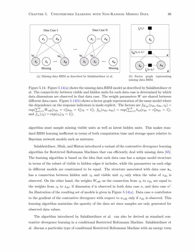
Chapter 5. Unsupervised Learning with Non-Random Missing Data 86
X1 XD
ZKZ1
X1
WDW1 W1 W2
...
...
...
X2...
...
X2 XD
Data Case 1 Data Case N
Missing Missing
ZKZ1
(a) Missing data RBM as described by Salakhutdinov et al.
d Ad
Zk
K
D
f (z )c kk
Wdkf (x ,r ,z )d d k
dbd df (x ,a )
X
(b) Factor graph representingmissing data RBM.
Figure 5.14: Figure 5.14(a) shows the missing data RBM model as described by Salakhutdinov etal. The connectivity between visible and hidden units for each data case is determined by whichdata dimensions are observed in that data case. The weight parameters W are shared betweendifferent data cases. Figure 5.14(b) shows a factor graph representation of the same model wherethe dependence on the response indicators is made explicit. The factors are fWdk
(xdn, adn, zk) =
exp(∑V
v=1Wvdk[xdn = v][adn = 1][zk = 1]), fbd(xdn, adn) = exp(
∑Vv=1 bvd[xdn = v][adn = 1]),
and fck(zk) = exp(ck[zk = 1]).
algorithm must sample missing visible units as well as latent hidden units. This makes stan-
dard RBM learning inefficient in terms of both computation time and storage space relative to
Bayesian network models such as mixtures.
Salakhutdinov, Minh, and Hinton introduced a variant of the contrastive divergence learning
algorithm for Restricted Boltzmann Machines that can efficiently deal with missing data [65].
The learning algorithm is based on the idea that each data case has a unique model structure
in terms of the subset of visible to hidden edges it includes, while the parameters on each edge
in different models are constrained to be equal. The structure associated with data case xn
has a connection between hidden unit zk and visible unit xd only when the value of xdn is
observed. On the other hand, the weights Wvdk on the connection from zk to xdn are equal to
the weights from zk to xdn′ if dimension d is observed in both data case n, and data case n′.
An illustration of the resulting set of models is given in Figure 5.14(a). Data case n contributes
to the gradient of the contrastive divergence with respect to wvdk only if xdn is observed. This
learning algorithm maintains the sparsity of the data set since samples are only generated for
observed data values.
The algorithm introduced by Salakhutdinov et al. can also be derived as standard con-
trastive divergence learning in a conditional Restricted Boltzmann Machine. Salakhutdinov et
al. discuss a particular type of conditional Restricted Boltzmann Machine with an energy term

Chapter 5. Unsupervised Learning with Non-Random Missing Data 87
of the form Vdk[adn = 1][zk = 1]. However, the basic learning algorithm discussed above also
implicitly conditions on the available rating indicators adn. Making this conditioning explicit
clarifies the description of the model and the learning algorithm.
We provide a factor graph representation of the basic conditional RBM model for missing
data in Figure 5.14(b). The key difference between the conditional RBM for missing data
and the standard RBM is the definition of the energy function. The energy function for the
conditional RBM is given in Equation 5.7.10. Note that [xdn = v] only appears in the energy
function multiplied by [adn = 1]. Whenever xdn is not available adn = 0, and the value of
[xdn = v][adn = 1] is zero for all v. This is equivalent to removing all edges starting at xdn in
a standard RBM. Note that the basic conditional RBM model does not differentiate between
user-selected and non-user selected ratings.
E(xon, zn,an) = −
D∑
d=1
V∑
v=1
K∑
k=1
Wvdk[xdn = v][zkn = 1][adn = 1]−D∑
d=1
V∑
v=1
bvd[xdn = v][adn = 1]
−K∑
k=1
ck[zkn = 1] (5.7.10)
Equation 5.7.11 shows the joint probability of the visible and hidden units conditioned on
the response indicators. Equation 5.7.12 shows the probability of the visible units conditioned
on the response indicators.
P (xon, zn|an) =
∑
xmn
exp(−E(xn, zn,an))∑x
∑z exp(−E(x, z,an))
=exp(−E(xo
n, zn,an))∑xo
∑z exp(−E(xo, z,an))
(5.7.11)
P (xon) =
∑
z
exp(−E(xon, z,an))∑
xo
∑z exp(−E(xo, z,an))
(5.7.12)
It is important to note that missing values xdn can be analytically summed out of Equation
5.7.11 since they make no contribution to the energy function. As a result, the normalization in
the partition function is taken with respect to the observed variables xo only. The conditional
RBM is similar to mixture models under the missing at random assumption in the sense that we
can ignore missing data values during learning and inference. However, the conditional RBM
model does not satisfy the missing at random condition.
Assume for the moment that we are in the simple setting where all observed ratings are
available during inference so that a = r. The conditional RBM has the property that for any
response pattern r, and any two data vectors x1 and x2 such that xo1 = xo
2, P (x1|r) = P (x2|r).This is precisely the property needed to ignore missing data during inference and learning.
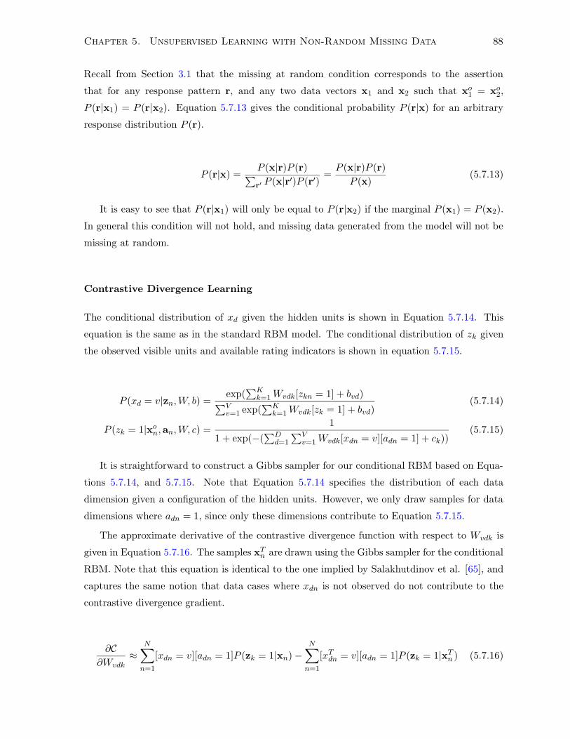
Chapter 5. Unsupervised Learning with Non-Random Missing Data 88
Recall from Section 3.1 that the missing at random condition corresponds to the assertion
that for any response pattern r, and any two data vectors x1 and x2 such that xo1 = xo
2,
P (r|x1) = P (r|x2). Equation 5.7.13 gives the conditional probability P (r|x) for an arbitrary
response distribution P (r).
P (r|x) =P (x|r)P (r)∑r′ P (x|r′)P (r′)
=P (x|r)P (r)
P (x)(5.7.13)
It is easy to see that P (r|x1) will only be equal to P (r|x2) if the marginal P (x1) = P (x2).
In general this condition will not hold, and missing data generated from the model will not be
missing at random.
Contrastive Divergence Learning
The conditional distribution of xd given the hidden units is shown in Equation 5.7.14. This
equation is the same as in the standard RBM model. The conditional distribution of zk given
the observed visible units and available rating indicators is shown in equation 5.7.15.
P (xd = v|zn,W, b) =exp(
∑Kk=1Wvdk[zkn = 1] + bvd)∑V
v=1 exp(∑K
k=1Wvdk[zk = 1] + bvd)(5.7.14)
P (zk = 1|xon,an,W, c) =
1
1 + exp(−(∑D
d=1
∑Vv=1Wvdk[xdn = v][adn = 1] + ck))
(5.7.15)
It is straightforward to construct a Gibbs sampler for our conditional RBM based on Equa-
tions 5.7.14, and 5.7.15. Note that Equation 5.7.14 specifies the distribution of each data
dimension given a configuration of the hidden units. However, we only draw samples for data
dimensions where adn = 1, since only these dimensions contribute to Equation 5.7.15.
The approximate derivative of the contrastive divergence function with respect to Wvdk is
given in Equation 5.7.16. The samples xTn are drawn using the Gibbs sampler for the conditional
RBM. Note that this equation is identical to the one implied by Salakhutdinov et al. [65], and
captures the same notion that data cases where xdn is not observed do not contribute to the
contrastive divergence gradient.
∂C∂Wvdk
≈N∑
n=1
[xdn = v][adn = 1]P (zk = 1|xn)−N∑
n=1
[xTdn = v][adn = 1]P (zk = 1|xT
n ) (5.7.16)
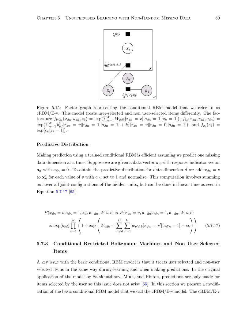
Chapter 5. Unsupervised Learning with Non-Random Missing Data 89
Xd
Ad
Rdf (x ,r ,a )d d ddb
K
f (z )c kk
Wdk
D
d d kf (x ,a ,z )
Zk
Figure 5.15: Factor graph representing the conditional RBM model that we refer to ascRBM/E-v. This model treats user-selected and non user-selected items differently. The fac-tors are fWdk
(xdn, adn, zk) = exp(∑V
v=1Wvdk[xdn = v][adn = 1][zk = 1]), fbd(xdn, rdn, adn) =
exp(∑V
v=1 b1vd[xdn = v][rdn = 1][adn = 1] + b0v[xdn = v][rdn = 0][adn = 1]), and fck
(zk) =exp(ck[zk = 1]).
Predictive Distribution
Making prediction using a trained conditional RBM is efficient assuming we predict one missing
data dimension at a time. Suppose we are given a data vector xn with response indicator vector
an with adn = 0. To obtain the predictive distribution for data dimension d we add xdn = v
to xon for each value of v with adn set to 1 and normalize. This computation involves summing
out over all joint configurations of the hidden units, but can be done in linear time as seen in
Equation 5.7.17 [65].
P (xdn = v|adn = 1,xon,a−dn,W, b, c) ∝ P (xdn = v,x−dn|adn = 1,a−dn,W, b, c)
∝ exp(bvd)K∏
k=1
1 + exp
Wvdk +
D∑
d′ 6=d
V∑
v′=1
wv′d′k[xd′n = v′][ad′n = 1] + ck
(5.7.17)
5.7.3 Conditional Restricted Boltzmann Machines and Non User-Selected
Items
A key issue with the basic conditional RBM model is that it treats user selected and non-user
selected items in the same way during learning and when making predictions. In the original
application of the model by Salakhutdinov, Minh, and Hinton, predictions are only made for
items selected by the user so this issue does not arise [65]. In this section we present a modifi-
cation of the basic conditional RBM model that we call the cRBM/E-v model. The cRBM/E-v
Chapter 5. Unsupervised Learning with Non-Random Missing Data 90
learning procedure requires training ratings for both user-selected items and randomly selected
items. Unlike the basic conditional RBM model, the cRBM/E-v model treats user-selected and
non user-selected items differently using energy terms that depend on the response indicators
rn as well as the available rating indicators an. The trained cRBM/E-v model makes differ-
ent predictions for user-selected and non user-selected items in a way that is similar to the
mixture/CPT-v model. This allows the cRBM/E-v model to better deal with prediction for
non user-selected items than the basic cRBM model.
Equation 5.7.18 defines cRBM/E-v model. We have a contribution to the energy of Wvdk if
zk = 1, xdn = 1 and adn = 1. This term is included both when rdn = 1 and rdn = 0. We have
a contribution to the energy of b1vd if xdn = v, adn = 1, and rdn = 1. We have a contribution
to the energy of b0v if xdn = v, adn = 1, and rdn = 0. To train the model we require data that
includes observations of the form adn = 1 and rdn = 0. This situation corresponds to having
rating observations for items that the user did not select. Both the Yahoo! Rating Study data
set and the Jester data set with synthetic missing data include observations of this form.
E(xon, zn, rn,an) = −
D∑
d=1
V∑
v=1
K∑
k=1
Wvdk[xd = v][zk = 1][adn = 1]−K∑
k=1
ck[zk = 1]
−D∑
d=1
V∑
v=1
b1vd[xd = v][rdn = 1][adn = 1] + b0v[xd = v][rdn = 0][adn = 1]
(5.7.18)
The additional bias term b0v has an equivalent role to the µv parameter in the CPT-v
model. This particular model form was selected since we anticipate a training regime where
ratings for user selected items are abundant, while ratings for randomly selected items are
significantly more scarce. If this were not the case the model could be easily enhanced by
including additional factors in the energy function. Note that we do not include a factor of the
from Vdk[rdn = 1][adn = 1][zk = 1] as used by Salakhutdinov et al. since we have a relatively
small number of observations where rdn = 1 and adn = 0 [65]. The focus of our model is the
complementary case where rdn = 0 and adn = 1.
Contrastive Divergence Learning
The conditional distribution of xdn given the hidden units is shown in Equation 5.7.19. The
conditional distribution of zk given the observed visible units and response indicators is shown
in equation 5.7.20.
Chapter 5. Unsupervised Learning with Non-Random Missing Data 91
P (xdn = v|rdn, adn, z,W, b) =exp(
∑Kk=1Wvdk[zk = 1] + b1vd[rdn = 1] + b0v[rdn = 0])
∑Vv=1 exp(
∑Kk=1Wvdk[zk = 1] + b1vd[rdn = 1] + b0v[rdn = 0])
(5.7.19)
P (zk = 1|xon, rn,an,W, c) =
1
1 + exp(−(∑D
d=1
∑Vv=1Wvdk[xdn = v][adn = 1] + ck))
(5.7.20)
It is straightforward to construct a Gibbs sampler for the cRBM/E-v model based on Equa-
tions 5.7.19, and 5.7.20. Note that the predictive distribution for xdn in Equation 5.7.19 is
different depending on whether the user selected the item or not.
The approximate derivative of the contrastive divergence function with respect to Wvdk is
given in Equation 5.7.21. The samples xTn are drawn using the Gibbs sampler for the cRBM/E-
v specified in Equations 5.7.19, and 5.7.20. Note that items rated under each rating source
contribute to the contrastive divergence gradients. For completeness, we also give the gradients
with respect to b1vd, b0v, and ck.
∂C(x|r,a,W, b, c)∂Wvdk
≈N∑
n=1
[xdn = v][adn = 1]P (zkn = 1|xn,W, b, c)
−N∑
n=1
[xTdn = v][adn = 1]P (zkn = 1|xT
n ,W, b, c) (5.7.21)
∂C(x|r,a,W, b, c)∂ck
≈N∑
n=1
(P (zkn = 1|xn,W, b, c)− P (zkn = 1|xT
n ,W, b, c))
(5.7.22)
∂C(x|r,a,W, b, c)∂b1vd
≈N∑
n=1
[rdn = 1][adn = 1]([xdn = v]− P (xT
dn = v|W, b, c))
(5.7.23)
∂C(x|r,a,W, b, c)∂b0v
≈N∑
n=1
D∑
d=1
[rdn = 0][adn = 1]([xdn = v]− P (xT
dn = v|W, b, c))
(5.7.24)
Rating Prediction
Making predictions using a trained cRBM/E-v model remains efficient assuming we predict one
missing rating at a time. The predictive distribution again includes two cases corresponding
to whether the item was originally selected by the user or not. The difference between the
two cases comes down to whether the bias term b1vd is used, corresponding to an item that was
selected by the user, or whether the bias term b0v is used, corresponding to an item not selected
by the user. This conditional RBM model can learn and exploit rating patterns such as items
not selected by the user tend to have lower ratings than items selected by the user.

Chapter 5. Unsupervised Learning with Non-Random Missing Data 92
P (xdn = v|xon, rn,an,W, b, c) ∝ P (xdn = v,xo
n|rn,an,W, b, c)
∝ exp(b1vd[rdn = 1]) exp(b0v[rdn = 0])
·K∏
k=1
1 + exp
Wvdk +
D∑
d′ 6=d
V∑
v′=1
Wv′d′k[xd′n = v′][adn = 1] + ck
(5.7.25)
5.7.4 Experimentation and Results
The training and testing protocols described in Sections 5.2.1 and 5.1.3 were applied to both
the basic conditional RBM model (cRBM), and the conditional RBM/E-v model (cRBM/E-v).
A total of 1000 iterations of contrastive divergence learning was performed for each model. It-
eration i of the contrastive divergence algorithm used a Gibbs burn-in of di/200e steps followed
by the collection of di/200e samples. A small amount of weight decay was used with regular-
ization parameter set to 0.0001. The cRBM/E-v model was trained on the set of training users
combined with the set of held out users. Models with 1, 5, 10, and 20 hidden units were trained
on the Yahoo! data. The Jester results are based on models with 5 hidden units.
Figures 5.16(a) to 5.16(d) show the performance of the basic conditional RBM model
(cRBM) compared to the conditional RBM/E-v model (cRBM/E-v). The horizontal axis repre-
sents the number of hidden units. The vertical axis represents normalized mean absolute error.
The solid lines represent the mean of the error over the five cross validation folds for each model.
The standard error of the mean is shown using dashed lines. The results show a substantial
decrease in error on randomly selected items using the cRBM/E-v model. However, the error
on randomly selected items increases as the number of components increases, while the error on
user-selected items decreases. This is likely due to the fact a relatively small number of ratings
for randomly selected items was added to a much larger data set of ratings for user-selected
items. The gradient for the W parameter is thus dominated by contributions from user selected
ratings, and appears to over fit these ratings as the number of hidden units increases.
Figures 5.17(a) and 5.17(b) show the performance of the basic conditional RBM model
(cRBM) compared to the performance of the conditional RBM/E-v model (cRBM/E-v) on the
Jester data. The horizontal axis represents the strength of the synthetic non-random missing
data effect applied to the Jester data set. The vertical axis represents normalized mean absolute
error. The rating prediction results show that the cRBM/E-v model out performs the basic
cRBM model when the non-random missing data effect strength is significant.
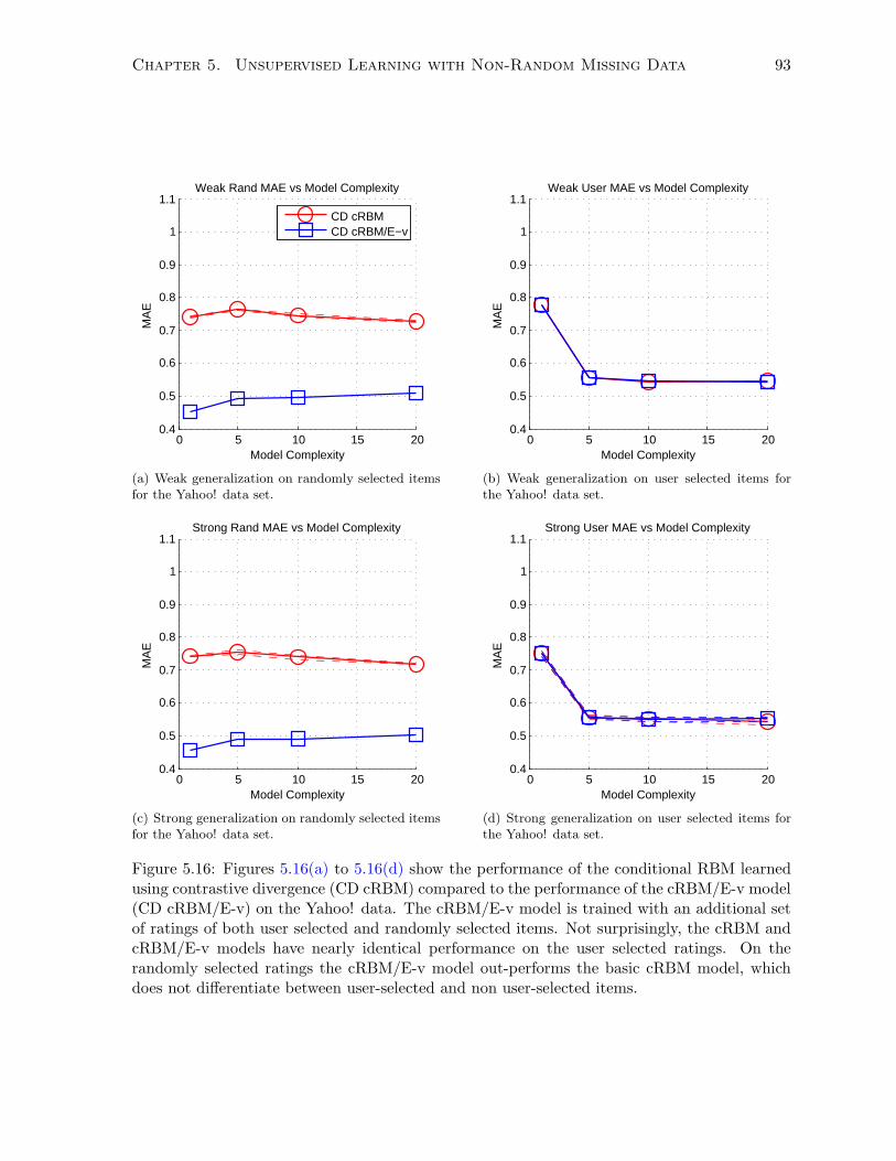
Chapter 5. Unsupervised Learning with Non-Random Missing Data 93
0 5 10 15 200.4
0.5
0.6
0.7
0.8
0.9
1
1.1Weak Rand MAE vs Model Complexity
Model Complexity
MA
E
CD cRBMCD cRBM/E−v
(a) Weak generalization on randomly selected itemsfor the Yahoo! data set.
0 5 10 15 200.4
0.5
0.6
0.7
0.8
0.9
1
1.1Weak User MAE vs Model Complexity
Model Complexity
MA
E
(b) Weak generalization on user selected items forthe Yahoo! data set.
0 5 10 15 200.4
0.5
0.6
0.7
0.8
0.9
1
1.1Strong Rand MAE vs Model Complexity
Model Complexity
MA
E
(c) Strong generalization on randomly selected itemsfor the Yahoo! data set.
0 5 10 15 200.4
0.5
0.6
0.7
0.8
0.9
1
1.1Strong User MAE vs Model Complexity
Model Complexity
MA
E
(d) Strong generalization on user selected items forthe Yahoo! data set.
Figure 5.16: Figures 5.16(a) to 5.16(d) show the performance of the conditional RBM learnedusing contrastive divergence (CD cRBM) compared to the performance of the cRBM/E-v model(CD cRBM/E-v) on the Yahoo! data. The cRBM/E-v model is trained with an additional setof ratings of both user selected and randomly selected items. Not surprisingly, the cRBM andcRBM/E-v models have nearly identical performance on the user selected ratings. On therandomly selected ratings the cRBM/E-v model out-performs the basic cRBM model, whichdoes not differentiate between user-selected and non user-selected items.
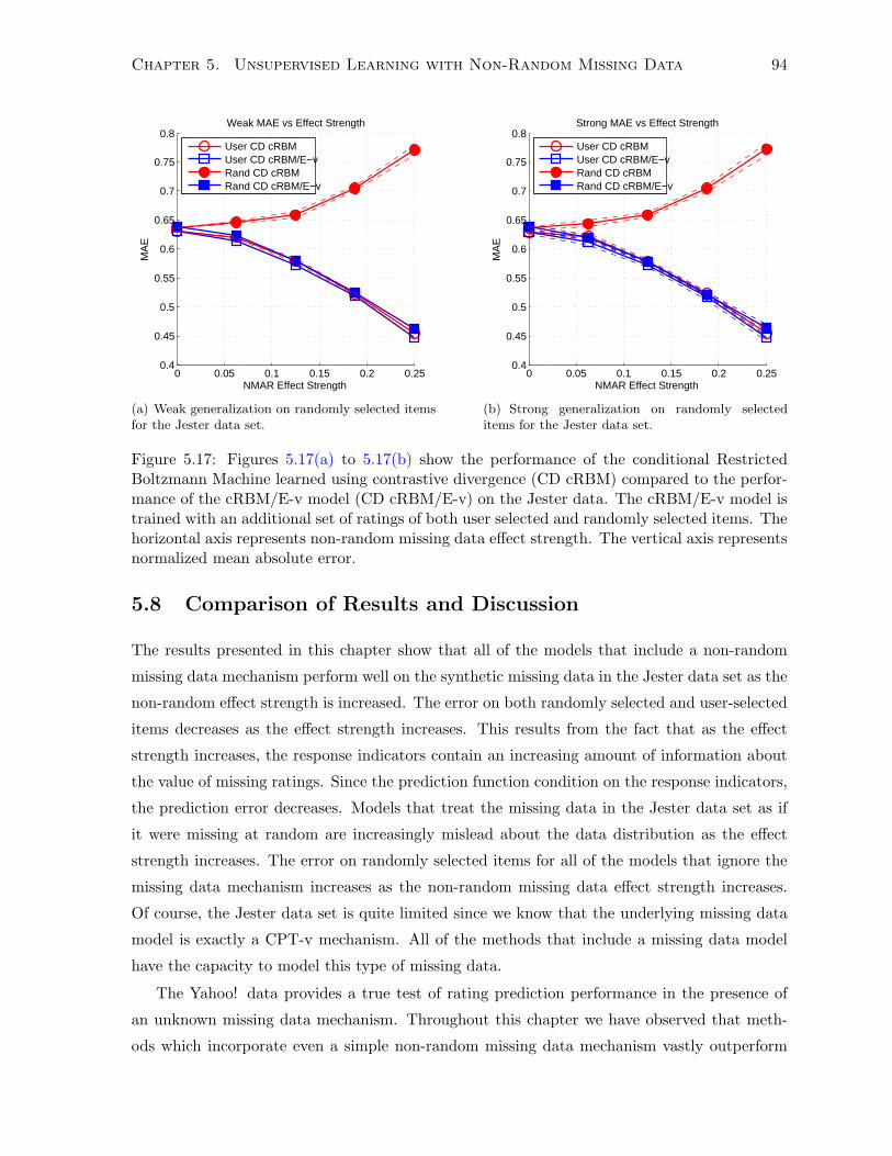
Chapter 5. Unsupervised Learning with Non-Random Missing Data 94
0 0.05 0.1 0.15 0.2 0.250.4
0.45
0.5
0.55
0.6
0.65
0.7
0.75
0.8Weak MAE vs Effect Strength
NMAR Effect Strength
MA
E
User CD cRBMUser CD cRBM/E−vRand CD cRBMRand CD cRBM/E−v
(a) Weak generalization on randomly selected itemsfor the Jester data set.
0 0.05 0.1 0.15 0.2 0.250.4
0.45
0.5
0.55
0.6
0.65
0.7
0.75
0.8Strong MAE vs Effect Strength
NMAR Effect Strength
MA
E
User CD cRBMUser CD cRBM/E−vRand CD cRBMRand CD cRBM/E−v
(b) Strong generalization on randomly selecteditems for the Jester data set.
Figure 5.17: Figures 5.17(a) to 5.17(b) show the performance of the conditional RestrictedBoltzmann Machine learned using contrastive divergence (CD cRBM) compared to the perfor-mance of the cRBM/E-v model (CD cRBM/E-v) on the Jester data. The cRBM/E-v model istrained with an additional set of ratings of both user selected and randomly selected items. Thehorizontal axis represents non-random missing data effect strength. The vertical axis representsnormalized mean absolute error.
5.8 Comparison of Results and Discussion
The results presented in this chapter show that all of the models that include a non-random
missing data mechanism perform well on the synthetic missing data in the Jester data set as the
non-random effect strength is increased. The error on both randomly selected and user-selected
items decreases as the effect strength increases. This results from the fact that as the effect
strength increases, the response indicators contain an increasing amount of information about
the value of missing ratings. Since the prediction function condition on the response indicators,
the prediction error decreases. Models that treat the missing data in the Jester data set as if
it were missing at random are increasingly mislead about the data distribution as the effect
strength increases. The error on randomly selected items for all of the models that ignore the
missing data mechanism increases as the non-random missing data effect strength increases.
Of course, the Jester data set is quite limited since we know that the underlying missing data
model is exactly a CPT-v mechanism. All of the methods that include a missing data model
have the capacity to model this type of missing data.
The Yahoo! data provides a true test of rating prediction performance in the presence of
an unknown missing data mechanism. Throughout this chapter we have observed that meth-
ods which incorporate even a simple non-random missing data mechanism vastly outperform
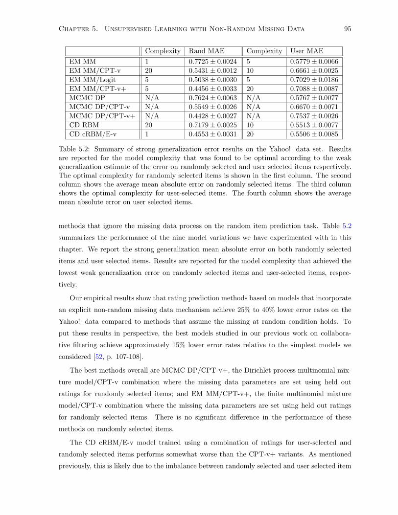
Chapter 5. Unsupervised Learning with Non-Random Missing Data 95
Complexity Rand MAE Complexity User MAE
EM MM 1 0.7725± 0.0024 5 0.5779± 0.0066
EM MM/CPT-v 20 0.5431± 0.0012 10 0.6661± 0.0025
EM MM/Logit 5 0.5038± 0.0030 5 0.7029± 0.0186
EM MM/CPT-v+ 5 0.4456± 0.0033 20 0.7088± 0.0087
MCMC DP N/A 0.7624± 0.0063 N/A 0.5767± 0.0077
MCMC DP/CPT-v N/A 0.5549± 0.0026 N/A 0.6670± 0.0071
MCMC DP/CPT-v+ N/A 0.4428± 0.0027 N/A 0.7537± 0.0026
CD RBM 20 0.7179± 0.0025 10 0.5513± 0.0077
CD cRBM/E-v 1 0.4553± 0.0031 20 0.5506± 0.0085
Table 5.2: Summary of strong generalization error results on the Yahoo! data set. Resultsare reported for the model complexity that was found to be optimal according to the weakgeneralization estimate of the error on randomly selected and user selected items respectively.The optimal complexity for randomly selected items is shown in the first column. The secondcolumn shows the average mean absolute error on randomly selected items. The third columnshows the optimal complexity for user-selected items. The fourth column shows the averagemean absolute error on user selected items.
methods that ignore the missing data process on the random item prediction task. Table 5.2
summarizes the performance of the nine model variations we have experimented with in this
chapter. We report the strong generalization mean absolute error on both randomly selected
items and user selected items. Results are reported for the model complexity that achieved the
lowest weak generalization error on randomly selected items and user-selected items, respec-
tively.
Our empirical results show that rating prediction methods based on models that incorporate
an explicit non-random missing data mechanism achieve 25% to 40% lower error rates on the
Yahoo! data compared to methods that assume the missing at random condition holds. To
put these results in perspective, the best models studied in our previous work on collabora-
tive filtering achieve approximately 15% lower error rates relative to the simplest models we
considered [52, p. 107-108].
The best methods overall are MCMC DP/CPT-v+, the Dirichlet process multinomial mix-
ture model/CPT-v combination where the missing data parameters are set using held out
ratings for randomly selected items; and EM MM/CPT-v+, the finite multinomial mixture
model/CPT-v combination where the missing data parameters are set using held out ratings
for randomly selected items. There is no significant difference in the performance of these
methods on randomly selected items.
The CD cRBM/E-v model trained using a combination of ratings for user-selected and
randomly selected items performs somewhat worse than the CPT-v+ variants. As mentioned
previously, this is likely due to the imbalance between randomly selected and user selected item

Chapter 5. Unsupervised Learning with Non-Random Missing Data 96
K=1 K=5 K=10 K=20
EM MM 0.8153± 0.0007 0.8135± 0.0006 0.8106± 0.0005 0.8073± 0.0006
EM MM/CPT-v 0.8257± 0.0006 0.8325± 0.0006 0.8353± 0.0006 0.8356± 0.0008
EM MM/Logit 0.8251± 0.0005 0.8385± 0.0003 0.8384± 0.0005 0.8381± 0.0010
EM MM/CPT-v+ 0.8282± 0.0003 0.8337± 0.0007 0.8355± 0.0008 0.8367± 0.0007
MCMC DP 0.8167± 0.0007 0.8167± 0.0007 0.8167± 0.0007 0.8167± 0.0007
MCMC DP/CPT-v 0.8259± 0.0010 0.8259± 0.0010 0.8259± 0.0010 0.8259± 0.0010
MCMC DP/CPT-v+ 0.8320± 0.0011 0.8320± 0.0011 0.8320± 0.0011 0.8320± 0.0011
CD cRBM 0.8104± 0.0007 0.8154± 0.0012 0.8174± 0.0010 0.8183± 0.0011
CD cRBM/E-v 0.8211± 0.0007 0.8185± 0.0010 0.8220± 0.0011 0.8210± 0.0009
Table 5.3: Summary of weak generalization ranking results on the Yahoo! data set in terms ofaverage NDCG score on randomly selected items. Results are reported for model complexityvalues from K = 1 to K = 20. Note that the performance of the Dirichlet process models isindependent of K.
during training. It may be possible to improve the performance of the cRBM/E-v model by
altering the gradients to balance the contribution from randomly selected and user-selected
items. It may also be interesting to consider an energy function with more flexibility in terms
of modeling the missing data process.
Of the models that are trained only on user-selected items, the MM/Logit model obtained
significantly lower error than the models incorporating a CPT-v type missing data model. It
appears that the additional flexibility in the MM/Logit model helps to learn a better model.
We note that some instability in the MM/Logit model was noticed when the σv parameters
are not all initialized to the same value. Initializing all the σv to the same small random
value appears to lead to good performance. We also experimented with a DP/Logit model
combination. However, the complete lack of conjugacy created by the logistic function makes
inference much more difficult when compared to the DP/CPT-v case. The development of a
suitable DP/Logit sampling framework is an interesting area for future work.
The MM/CPT-v and DP/CPT-v models again have approximately equal performance when
trained only on user selected items. As was observed by Marlin et al. [53], the MM/CPT-v
model converges to a solution where almost all of the missing data is explained as having been
generated by the second rating value. It was hoped that giving the model more flexibility
during training by moving to a Dirichlet process based mixture and full Bayesian inference
might alleviate this problem. However, the DP/CPT-v model appears to be prone to the same
type of problem on this data set. The development of the auxiliary variable Gibbs sampler
for the DP/CPT-v model is still quite interesting. The naive approach of sampling missing
data values and performing cluster assignments on the basis of the completed data cases is
completely ineffective since it vastly increases the state space of the Gibbs chain. An interesting
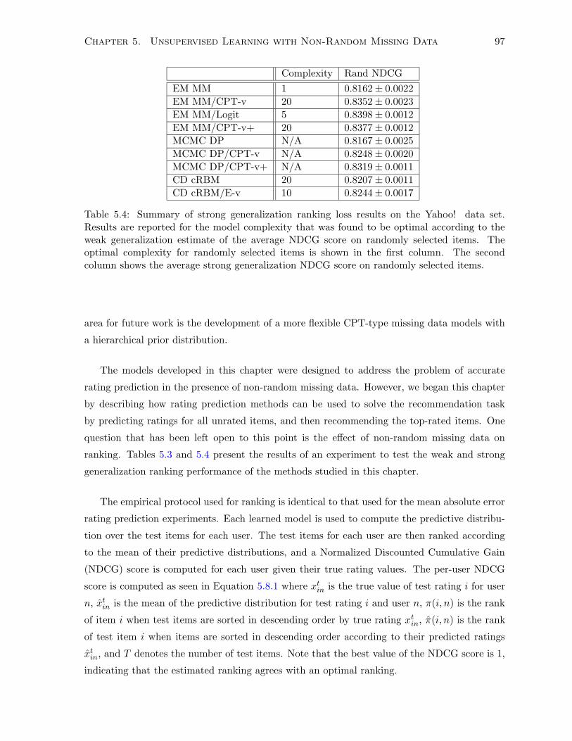
Chapter 5. Unsupervised Learning with Non-Random Missing Data 97
Complexity Rand NDCG
EM MM 1 0.8162± 0.0022
EM MM/CPT-v 20 0.8352± 0.0023
EM MM/Logit 5 0.8398± 0.0012
EM MM/CPT-v+ 20 0.8377± 0.0012
MCMC DP N/A 0.8167± 0.0025
MCMC DP/CPT-v N/A 0.8248± 0.0020
MCMC DP/CPT-v+ N/A 0.8319± 0.0011
CD cRBM 20 0.8207± 0.0011
CD cRBM/E-v 10 0.8244± 0.0017
Table 5.4: Summary of strong generalization ranking loss results on the Yahoo! data set.Results are reported for the model complexity that was found to be optimal according to theweak generalization estimate of the average NDCG score on randomly selected items. Theoptimal complexity for randomly selected items is shown in the first column. The secondcolumn shows the average strong generalization NDCG score on randomly selected items.
area for future work is the development of a more flexible CPT-type missing data models with
a hierarchical prior distribution.
The models developed in this chapter were designed to address the problem of accurate
rating prediction in the presence of non-random missing data. However, we began this chapter
by describing how rating prediction methods can be used to solve the recommendation task
by predicting ratings for all unrated items, and then recommending the top-rated items. One
question that has been left open to this point is the effect of non-random missing data on
ranking. Tables 5.3 and 5.4 present the results of an experiment to test the weak and strong
generalization ranking performance of the methods studied in this chapter.
The empirical protocol used for ranking is identical to that used for the mean absolute error
rating prediction experiments. Each learned model is used to compute the predictive distribu-
tion over the test items for each user. The test items for each user are then ranked according
to the mean of their predictive distributions, and a Normalized Discounted Cumulative Gain
(NDCG) score is computed for each user given their true rating values. The per-user NDCG
score is computed as seen in Equation 5.8.1 where xtin is the true value of test rating i for user
n, xtin is the mean of the predictive distribution for test rating i and user n, π(i, n) is the rank
of item i when test items are sorted in descending order by true rating xtin, π(i, n) is the rank
of test item i when items are sorted in descending order according to their predicted ratings
xtin, and T denotes the number of test items. Note that the best value of the NDCG score is 1,
indicating that the estimated ranking agrees with an optimal ranking.

Chapter 5. Unsupervised Learning with Non-Random Missing Data 98
NDCG(n) =
∑Ti=1(2
xtin − 1)/ log(1 + π(i, n))
∑Ti=1(2
xtin − 1)/ log(1 + π(i, n))
(5.8.1)
In this experiment we perform mean prediction to rank the ten randomly selected test items
for each survey participant in the Yahoo! data set. The weak generalization results are reported
in Table 5.4 for model complexity values from 1 to 20. The best complexity level for each model
based on the weak generalization NDCG score was determined from Table 5.3. The complexity
level and corresponding strong generalization NDCG score is reported in Table 5.4. These
results show small but significant improvements in average NDCG when the underlying rating
prediction methods learn a model of the missing data mechanism.
An interesting avenue for future research is to consider models that both take into account a
model of the missing data process, and directly optimize a rank loss measure. This is closely re-
lated to the recent work of Weimer, Karatzoglou, Le, and Smola on training matrix factorization
methods for collaborative filtering based on a relaxation of the NDCG score [77].
Chapter 6
Classification With Missing Data
This chapter explores a variety of strategies for performing classification with missing feature
values. The classification setting is particularly affected by the presence of missing feature
values since most discriminative learning approaches including logistic regression, support vector
machines, and neural networks have no natural ability to deal with missing input features. Our
main interest is in classification methods that can both learn from data cases with missing
features, and make predictions for data cases with missing features.
We begin with an overview of strategies for dealing with missing data in classification. Gen-
erative classifiers learn a joint model of labels and features. Generative classifier do have a
natural ability to learn from incomplete data cases and to make predictions when features are
missing. We then discuss several strategies that can be applied to any discriminative classifier
including case deletion, imputation, and classification in subspaces. Finally, we discuss a frame-
work for classification from incomplete data based on augmenting the input representation of
complete data classifiers with a vector of response indicators.
We consider Linear Discriminant Analysis as an example of a generative classifier. We
present both maximum likelihood and maximum conditional likelihood learning methods for
a regularized Linear Discriminant Analysis model with missing data. We review several dis-
criminative classification methods including logistic regression, multi-layer neural networks, and
kernel logistic regression. We consider applying these methods to classification with missing
data using imputation, reduced models, and the response indicator framework.
6.1 Frameworks for Classification With Missing Features
Generative classifiers have a natural ability to deal with missing data through marginalization.
This makes them well suited for dealing with random missing data. The most well known
methods for dealing with missing data in discriminative classifiers are case deletion, imputation,
99
Chapter 6. Classification With Missing Data 100
and learning in subspaces. All of these methods can be applied in conjunction with any classifier
that operates on complete data. In this section we discuss these methods for dealing with
missing data. We also discuss a different strategy for converting a complete data classifier into
a classifier that can operate on incomplete data cases by augmenting the input representation
with response indicators.
6.1.1 Generative Classifiers
Generative classifiers model the joint distribution of labels and features. If any feature values
are missing they can be marginalized over when classifying data cases. In class conditional
models like the Naive Bayes classifier and Linear Discriminant Analysis, the marginalization
operation can be performed efficiently. Missing data must also be dealt with during learning.
This typically requires an application of the Expectation Maximization algorithm. However,
generative classifiers require making explicit assumptions about the feature space distribution,
while discriminative classifiers do not.
6.1.2 Case Deletion
In case deletion any data case with missing features values is discarded from the data set,
and standard methods for complete data are run on the remaining data cases. Case deletion
discards valuable information about features that are observed, and its use is generally not
recommended [49]. Case deletion can be appropriate if there is a relatively small amount of
missing data, and only complete data cases are permitted at test time. The particular missing
data scenario we are interested in requires the ability to classify incomplete data vectors, so
case deletion can not be applied.
6.1.3 Classification and Imputation
Imputation is a strategy for dealing with missing data that is widely used in the statistical
community. In unconditional mean imputation, the mean of feature d is computed using the
data cases where feature d is observed [49, p.44]. The mean value for feature d is then used as
the value for feature d in data cases where feature d is not observed. In regression imputation, a
set of regression models of missing features given observed features is learned. Missing features
are filled in using predicted values from the learned regression model [49, p. 61].
Regression and mean imputation belong to the class of single imputation methods. In both
cases a single completion of the data set is formed by imputing exactly one value for each
unobserved variable. Multiple imputation is an alternative to single imputation procedures [49,
p. 255]. As the name implies, multiple completions of a data set are formed by imputing several

Chapter 6. Classification With Missing Data 101
values for each missing variable. In its most basic form, the imputed values are sampled from
a simplified imputation model and standard methods are used on each complete data set. The
principal advantage of multiple imputation over single imputation is that multiple imputation
better reflects the variability due to missing values. Sophisticated forms of multiple imputation
are closely related to approximate Bayesian techniques like Markov chain Monte Carlo methods,
and can be viewed as an approximation to integrating out the missing data with respect to an
auxiliary distribution over the feature space.
The key to imputation techniques is selecting an appropriate model of the input space to
sample from. This is rarely the case in single imputation where imputing zeros is common.
A standard practice in multiple imputation is to fit a gaussian distribution to each class, and
sample multiple completions of the missing features conditioned on the observed features. More
flexible imputation models for real valued data are often based on mixtures of Gaussians [75].
In high dimensions, learning a mixture of probabilistic principal components analysis or factor
analysis models may be more appropriate.
The advantage of imputation methods is that they can be used in conjunction with any
complete data classifier. The main disadvantage is that learning one or more imputation mod-
els can be a costly operation. In addition, using multiple imputations leads to maintaining
an ensemble of classifiers at test time. Combining multiple imputation with cross validation
requires training and evaluating many individual classifiers.
6.1.4 Classification in Sub-spaces: Reduced Models
Perhaps the most straightforward method for dealing with missing data is to learn a different
classifier for each pattern of observed values. Sharpe and Solly studied the diagnosis of thyroid
disease with neural networks under this framework, which they refer to as the network reduction
approach [69]. The advantage of this approach is that standard discriminative learning methods
can be applied to learn each model. Sharpe and Solly found that learning one neural network
classifier for each subspace of observed features led to better classification performance than
using neural network regression imputation combined with a single neural network classifier
taking all features as inputs.
As Tresp et al. point out, the main drawback of the reduced model approach is that the
number of different patterns of missing features is exponential in the number of features [75].
In Sharpe and Solly’s case, the data set contained four inputs, and only four different patterns
of missing features, making the entire approach feasible [69, p. 74].

Chapter 6. Classification With Missing Data 102
6.1.5 A Framework for Classification with Response Indicators
An alternative to imputation and subspace classification is to augment the input to a standard
classifier with a vector of response indicators. The input representation xn = [xn � rn, rn]
can be thought of as an encoding for xon. Here � signifies elementwise multiplication. A
trained classifier can be thought of as computing a decision function of the form f(xon). In
logistic regression, multi-layer neural networks, and some kernel-based classifiers, substituting
xn for xn is the only modification required. This framework was studied in conjunction with
certain SVM models by Chechik et al. [13], although they focus on the problem of structurally
incomplete data cases. Structurally incomplete data cases arise when certain feature values are
undefined for some data cases. This is semantically different than the missing data we consider
here.
6.2 Linear Discriminant Analysis
In this section we present Linear Discriminant Analysis, and its application to classification
with missing features. We begin by reviewing Fisher’s original conception of Linear Discrimi-
nant Analysis. We then describe the relationship between Fisher’s view and a view based on
maximum probability classification in a class conditional Gaussian model. We discuss several
extensions of LDA including Quadratic Discriminant Analysis (QDA), and Regularized Dis-
criminant Analysis (RDA). We introduce a new method for missing data classification based
on generative training of a linear discriminant analysis model with a factor analysis-style co-
variance matrix. Finally, we present a discriminative training method for the same model that
maximizes the conditional probability of labels given features.
6.2.1 Fisher’s Linear Discriminant Analysis
In the original binary classification setting, Fisher motivates the objective function for linear
discriminant analysis by arguing for two criteria. The first criteria is that the means of the two
classes µ1, µ−1 should be maximally separated by the choice of the discriminant direction w
as expressed in Equation 6.2.1. The second criteria is that the chosen w should minimize the
within-class scatter S of the two classes as expressed in Equation 6.2.2. The definition of the
scatter matrix S is given in Equation 6.2.3 [20] [55, p. 63].
f1(w) = wT (µ1 − µ−1) (6.2.1)
f2(w) = wTSw (6.2.2)

Chapter 6. Classification With Missing Data 103
S =
N∑
n=1
∑
c∈{−1,1}
[yn = c](xn − µc)(xn − µc)T (6.2.3)
µc =1
Nc
N∑
n=1
[yn = c]xn (6.2.4)
Fisher proposes choosing w to maximize the objective function shown in Equation 6.2.5,
which is the ratio of the square of mean separation to scatter in the direction w.
f(w) =f1(w)2
f2(w)=
wT (µ1 − µ−1)(µ1 − µ−1)Tw
wTSw(6.2.5)
To find the best w∗ we must differentiate f(w) with respect to w and solve for w. However,
it is useful to note that the objective function f(w) is invariant to the rescaling of w. As a
result we can always rescale an optimal w such that f2(w) = 1. We can then transform the
optimization of f(w) into a constrained problem with a simplified objective function as seen in
Equation 6.2.6.
w∗ = maxw
wT (µ1 − µ−1)(µ1 − µ−1)Tw (6.2.6)
st wTSw = 1
To solve the constrained optimization problem we take the derivative of the objective func-
tion, and introduce a Lagrange multiplier along with the derivative of the constraint leading to
equation 6.2.7. Isolating λw under the assumption that S is invertible shows that w is given
by the solution to a generalized eigenvalue problem.
(µ1 − µ−1)(µ1 − µ−1)Tw − λSw = 0 (6.2.7)
S−1(µ1 − µ−1)(µ1 − µ−1)Tw = λw (6.2.8)
This problem can be solved by inspection if we note that the result of multiplying any
vector w by the matrix on the left hand side of Equation 6.2.8 is a vector proportional to
S−1(µ1−µ−1). As a result, S−1(µ1−µ−1) is the only eigenvector, and the only possible solution
to the generalized eigenvalue problem. We can thus conclude that w∗ = S−1(µ1 − µ−1).
If we assume that the midpoint between the projections of the two means should separate
the two classes, we can derive a simple formula for the optimal bias term b∗ given the optimal
weight vector w∗as seen in Equation 6.2.9. A data case xn is assigned to class 1 if w∗Txn+b > 0.
Chapter 6. Classification With Missing Data 104
b∗ =1
2(w∗T
µ1 + w∗Tµ−1) =
1
2(µ1 − µ−1)
TS−1(µ1 + µ−1) (6.2.9)
6.2.2 Linear Discriminant Analysis as Maximum Probability Classification
Welch was the first to note that Fisher’s linear discriminant can be derived from the class pos-
terior distribution in a class conditional Gaussian model with shared covariance, and different
means [78]. This approach is more clearly motivated by the idea of maximum probability clas-
sification, and has become the standard derivation for linear discriminant analysis [55, p. 59].
The model is described in Equations 6.2.10 and 6.2.11. The posterior class probability is given
in equation 6.2.12, which we work into a form that depends only on a linear function of the
data.
P (Yn = c) = θc (6.2.10)
P (Xn = xn|Yn = c) = |2πΣ|−1/2 exp
(−1
2(xn − µc)
TΣ−1(xn − µc)
)(6.2.11)
P (Yn = 1|Xn = xn) =θ1|2πΣ|−1/2 exp
(−1
2(xn − µ1)TΣ−1(xn − µ1)
)∑
c∈−1,1 θc|2πΣ|−1/2 exp(−1
2(xn − µc)TΣ−1(xn − µc)
) (6.2.12)
=1
1 + exp (wTxn + b)(6.2.13)
w = (µ1 − µ−1)TΣ−1 (6.2.14)
b =1
2(µ1 − µ−1)
TΣ−1(µ1 + µ−1) +1
2log(θ1/θ−1) (6.2.15)
It is now easy to see that the discriminant function P (Yn = c|Xn = xn) > 0.5 is exactly
equivalent to Fisher’s discriminant function in the case where θ1 = θ−1 = 0.5. The fact that
Fisher’s discriminant function is defined in terms of the scatter matrix S as opposed to the
shared covariance matrix Σ makes no difference since the two are related by a scalar constant.
6.2.3 Quadratic Discriminant Analysis
Quadratic Discriminant Analysis is the natural extension of Fisher’s Linear Discriminant to
the case where each class has a different covariance matrix. In this case the class posterior
distribution obviously does not reduce to a linear function of the data. Instead, the decision
surface is quadratic [55, p. 52]. We give the probability model for Quadratic Discriminant
Analysis in equations 6.2.16 and 6.2.17. The class posterior is given in equation 6.2.18. As in
the linear case, the classification rule is to assign a vector xn to the class under which it has
maximum posterior probability.
Chapter 6. Classification With Missing Data 105
P (Yn = c) = θc (6.2.16)
P (Xn = xn|Yn = c) = |2πΣc|−1/2 exp
(−1
2(xn − µc)
TΣ−1c (xn − µc)
)(6.2.17)
P (Yn = 1|Xn = xn) =θ1|2πΣc|−1/2 exp
(−1
2(xn − µ1)TΣ−1
c (xn − µ1))
∑c∈−1,1 θc|2πΣc|−1/2 exp
(−1
2(xn − µc)TΣ−1
c (xn − µc)) (6.2.18)
6.2.4 Regularized Discriminant Analysis
In this section we discuss regularization strategies for Linear and Quadratic discriminant analy-
sis. The main issue is that computing an accurate estimate of the required covariance matrices
can be difficult when data is high dimensional and scarce. It is well known that the sampling
variation of the standard covariance estimate goes up as the number of data cases goes down,
and that when Nc < D all of the covariance parameters are not identifiable for class c [55, p.
130].
Friedman presents an insightful demonstration of the effect this has on the discrimina-
tion function based on spectral analysis of the covariance matrix [23]. Assume that εd are
the eigenvalues of Σ, and that vd are the corresponding eigenvectors. We have that Σ−1 =∑D
d=1 vdvTd /εd. This shows that the spectral decomposition of Σ−1 is dominated by the smallest
eigenvalues of Σ−1.
Unsupervised Covariance Shrinkage
As Friedman claims, the eigenvalues of the sample covariance matrix tend to have a systematic
bias, with the small eigenvalues biased low, and the large eigenvalues biased high [23]. Not
surprisingly, the first techniques used to regularize covariance matrix estimates were based on
attempts to correct the bias in the eigenvalue spectrum. Regularized estimates of the form
αΣc + βI were introduced to effectively shrink the eigenvalues towards a central value [58].
However, the optimal trade-off between the empirical covariance Σc and the identity matrix
I was sometimes left as an open problem, or set by optimizing a loss function unrelated to
classification performance [55, p. 131].
Supervised Covariance Shrinkage
Friedman introduced the first covariance regularization method for the quadratic case based on
minimizing a cross-validation estimate of prediction error [23] [55, p. 144]. The basic idea is to
shrink the per-class covariance matrices towards the pooled covariance matrix by introducing a
trade-off parameter α. That estimate is further shrunk towards a multiple of the identity matrix

Chapter 6. Classification With Missing Data 106
through the introduction of a second trade-off parameter γ. We give the definition of Friedman’s
per-class covariance matrix estimate in equation 6.2.19 where Σc is the standard estimate of
the per-class covariance matrix, and Σ is the standard estimate of the pooled covariance matrix
[23].
Σc = γ(αΣc + (1− α)Σ) +(1− γ)D
tr(Σ)I (6.2.19)
Friedman performs leave-one-out cross-validation over a grid of possible α and γ values
with classification error as the objective function to choose the optimal α and γ. A specialized
updating procedure is used during training to avoid the otherwise quadratic cost of computing
a new set of covariance estimates when classifying each data case for each value of α and γ.
Restricted Eigen-Decomposition Covariance Models
Bensmail and Celeux introduced a regularization method called Eigenvalue Decomposition Dis-
criminant Analysis that is based on a group of 14 different covariance approximations [6]. Each
approximation is formed by imposing different symmetries on the eigen-decompositions of the
class covariance matrices. Bensmail and Celeux propose a slightly refined eigen-decomposition
of the form Σc = λcVcεcVTc where Vc is the matrix of eigenvectors, λc = |Σc|1/D, and εc is
the matrix of eigenvalues normalized such that |εc| = 1. Under this decomposition, λc controls
the volume of the covariance matrix, Vc controls the orientation, and εc controls the shape [6].
The group of models proposed by Bensmail and Celeux includes simpler models of the form
Σc = λcBc for Bc diagonal, and Σc = λcI
Regularization is achieved by tying the parameters of the decompositions across classes. For
example, the model Σc = λcVεcVT allows the volume and shape to differ across classes, but
restricts the orientation parameters to be the same for all classes. Bensmail and Celeux, like
Friedman, select the single model that minimizes a cross-validation estimate of classification
error [6].
It is interesting to note that Bensmail and Celeux do not consider covariance models based
on retaining only K of the D eigenvalue-eigenvector pairs. It is well known that retaining only
the largest K eigenvalues and eigenvectors of a covariance matrix leads to an optimal rank K
approximation in the squared error sense. This is essentially classical Principal Components
Analysis [43]. Of course, classical PCA can not be directly applied as a covariance approxima-
tion since it results in a singular matrix for K < D. However, this is easily overcome by adding
in a multiple of the identity matrix.
The Probabilistic Principal Components Analysis framework advanced by Tipping and
Bishop and described in Section 4.3 provides just such a covariance approximation. Indeed,
Chapter 6. Classification With Missing Data 107
Tipping and Bishop consider the application of the PPCA covariance approximation to the dis-
criminant analysis problem with complete data, and show that it leads to improved classification
error relative to spherical, diagonal, and full covariance matrices [73, p. 618].
6.2.5 LDA and Missing Data
As a generative model, Linear Discriminant Analysis has a natural ability to deal with missing
input features. The class conditional probability of a data vector with missing input features is
given in Equation 6.2.20. The posterior probability of each class given a data case with missing
features is shown in Equation 6.2.21.
P (Xon = xo
n|Yn = c) = |2πΣoo|−1/2 exp
(−1
2(xo
n − µoc)
T (Σoo)−1(xon − µo
c)
)(6.2.20)
P (Y = c|Xon = xo
n) =θc|2πΣoo|−1/2 exp
(−1
2(xon − µo
c)T (Σoo)−1(xo
n − µoc))
∑c θc|2πΣoo|−1/2 exp
(−1
2(xon − µo
c)T (Σoo)−1(xo
n − µoc)) (6.2.21)
Maximum Likelihood Estimation
The maximum likelihood estimate of the mean parameters is computed from incomplete data
as shown in Equation 6.2.22.
µdc =
∑Nn=1[yn = c][rdn = 1]xdn∑N
n=1[yn = c][rdn = 1](6.2.22)
The parameters of the full covariance matrix can be estimated using the Expectation Maxi-
mization algorithm. However, when data vectors are high dimensional and there are a relatively
small number of data cases, it is preferable to use a structured covariance approximation. A
variety of structured covariance approximations were discussed in Section 6.2.4. We choose to
use a factor analysis-like covariance matrix of the form ΛΛT + Ψ with Ψ diagonal. We call this
model LDA-FA for Linear Discriminant Analysis with Factor Analysis covariance. The factor
analysis covariance model is slightly more general than the PPCA covariance model used by
Tipping and Bishop in their LDA experiments [73, p. 618]. Note that while Tipping and Bishop
also consider learning PPCA models with missing data, they do not consider the simultaneous
application of PPCA to linear discriminant analysis with missing data.
The factor analysis covariance parameters are learned by first centering the training data
by subtracting off the appropriate class mean as seen in Equation 6.2.23, and then applying the
Expectation Maximization algorithm for factor analysis with missing data as derived in Section
4.3.2. The dimensionality of the latent factors Q is a free parameter that must be set using
cross validation.

Chapter 6. Classification With Missing Data 108
xdn =C∑
c=1
[yn = c][rdn](xdn − µdc) (6.2.23)
6.2.6 Discriminatively Trained LDA and Missing Data
One of the main drawbacks of generatively trained classification methods is that they tend
to be very sensitive to violations of the underlying modeling assumptions. In this section we
consider a discriminative training procedure for the LDA-FA model described in the previous
section. The main insight is that we can fit the LDA-FA model parameters by maximizing the
conditional probability of the labels given the incomplete features instead of maximizing the
joint probability of the labels and the incomplete features. This training procedure is closely
related to the minimum classification error factor analysis algorithm introduced by Saul and
Rahim for complete data [66].
The posterior class probabilities given an incomplete feature vector are again given by
Equation 6.2.21. The objective function used during training is the conditional log likelihood
as shown in Equation 6.2.24.
L =N∑
n=1
C∑
c=1
[yn = c] log(P cn) (6.2.24)
P cn =
Acn∑
c′ Ac′n
Acn = θc|2πΣoo|−1/2 exp
(−1
2(xo
n − µoc)
T (Σoo)−1(xon − µo
c)
)
Conditional Maximum Likelihood Estimation
We derive a maximum conditional likelihood learning algorithm for the LDA-FA model in this
section. We optimize the average conditional log likelihood with respect to the parameters
θ, µ, Λ, and Ψ using non-linear optimization. We first transform the parameters θ and Ψ to
eliminate constraints. θ represent the parameters of a discrete distribution with normalization
and positivity constraints, while ψii simply has to be positive since it is a variance parameter.
We use the mappings shown below.
Ψii = exp(φii) θc =exp(ωc)∑c exp(ωc)
We begin by computing the partial derivative of the conditional log likelihood with respect
Chapter 6. Classification With Missing Data 109
to the current posterior class probabilities P kn , and the partial derivative of the posterior class
probability with respect to Akn.
∂L∂P k
n
= [yn = k]1
P kn
∂P kn
∂P kn
∂Aln
=
([k = l]∑
k Akn
− Akn
(∑
k Akn)
2
)∂Al
n (6.2.25)
We compute the partial derivative of Aln with respect to θj , and the partial derivative of θj
with respect to ωc. We use the chain rule to find the partial derivative of the conditional log
likelihood with respect to ωc.
∂Aln
∂θj= [l = j]
Aln
θj(6.2.26)
∂θj
∂ωc= [j = c]θc − θjθc (6.2.27)
∂L∂ωc
=N∑
n=1
C∑
k=1
C∑
l=1
C∑
j=1
∂L∂P k
n
∂P kn
∂Aln
∂Aln
∂θj
∂θj
∂ωc
=N∑
n=1
C∑
k=1
C∑
l=1
C∑
j=1
[yn = k]1
P kn
([k = l]∑
k Akn
− Akn
(∑
k Akn)
2
)([j = c]θc − θjθc)
=N∑
n=1
C∑
c=1
([yn = c]− P cn) (6.2.28)
We compute the partial derivative of Aln with respect to µc, and use the chain rule to
find the partial derivative of the conditional log likelihood with respect to µc. The projection
matrix Hon was introduced in Section 1.2.1. Recall that Ho
n projects the observed dimensions
of xon back into D dimension such that the missing dimensions are filled in with zeros. These
projection matrices arise naturally when taking the derivative of a sub-matrix or sub-vector
with respect to a full dimensional matrix or vector. Also recall that on refers to the vector of
observed dimensions for data case xn such that oin = d if d is the ith observed dimension of xn.
∂Aln
∂µonc
= [l = c]Acn(−1
2)(2(Σonon)−1(µon
c − xonn ))
(6.2.29)
∂µonc
∂µc
= Hon, Ho
ijn = [ojn = i] (6.2.30)

Chapter 6. Classification With Missing Data 110
∂L∂µc
=
N∑
n=1
C∑
k=1
∂L∂P k
n
C∑
l=1
∂P kn
∂Aln
∂µonc
∂µc
∂Aln
∂µonc
=N∑
n=1
C∑
k=1
[yn = k]1
P kn
C∑
l=1
([k = l]∑
k Akn
− Akn
(∑
k Akn)
2
)[l = c](−Ac
n)Hon(Σonon)−1(µon
c − xonn )
=N∑
n=1
1
P ynn
([yn = c]∑
k Akn
− Aynn
(∑
k Akn)
2
)Ho
n(−Acn)(Σonon)−1(µon
c − xonn )
=N∑
n=1
([yn = c]− P cn)Ho
n(Σonon)−1(xonn − µ
onc ) (6.2.31)
We compute the partial derivative of Aln with respect to Σonon , the partial derivative of
Σonon with respect to Σ, and the partial derivative of Σ with respect to Λ. We apply the chain
rule to obtain the partial derivative of the conditional log likelihood with respect to Λ.
∂Aln
∂Σonon=
1
2Al
n
((Σonon)−1(µon
l − xonn )(µon
l − xonn )T (Σonon)−1 − (Σonon)−1
)(6.2.32)
∂Σonon
ij
∂Σst= [oin = s][ojn = t] (6.2.33)
∂Σst
∂Λab= [s = a]Λtb + [t = a]Λsb (6.2.34)
∂Σonon
ij
∂Λab=
D∑
s=1
D∑
t=1
[oin = s][ojn = t] ([s = a]Λtb + [t = a]Λsb)
= [oin = a]D∑
t=1
[ojn = t]Λtb + [ojn = a]D∑
s=1
[oin = s]Λsb (6.2.35)
∂Aln
∂Λab=
Dn∑
i=1
Dn∑
j=1
∂Aln
∂Σonon
ij
∂Σonon
ij
∂Λab
=
Dn∑
i=1
Dn∑
j=1
∂Aln
∂Σonon
ij
([oin = a]
D∑
t=1
[ojn = t]Λtb + [ojn = a]D∑
s=1
[oin = s]Λsb
)
= 2
Dn∑
i=1
Dn∑
j=1
∂Aln
∂Σonon
ij
[oin = a]D∑
t=1
[ojn = t]Λtb
= 2D∑
t=1
Dn∑
i=1
Dn∑
j=1
[oin = a]∂Al
n
∂Σonon
ij
[ojn = t]
Λtb
Chapter 6. Classification With Missing Data 111
∂Aln
∂Λ= 2Ho
n
∂Aln
∂Σonon
ij
(Hon)TΛ (6.2.36)
∂L∂Λ
=N∑
n=1
C∑
k=1
∂L∂P k
n
C∑
l=1
∂P kn
∂Aln
∂Aln
∂Λ
=N∑
n=1
C∑
k=1
[yn = k]1
P kn
C∑
l=1
([k = l]∑
k Akn
− Akn
(∑
k Akn)
2
)(6.2.37)
·Hon
(Al
n
((Σonon)−1(µon
l − xonn )(µon
l − xonn )T (Σonon)−1 − (Σonon)−1
))(Ho
n)TΛ
=N∑
n=1
C∑
c=1
([yn = c]− P cn)(Ho
n(Σonon)−1(µonc − xon
n )(µonc − xon
n )T (Σonon)−1(Hon)T
−Hon(Σonon)−1(Ho
n)T)Λ (6.2.38)
Finally, we compute the partial derivative of the conditional log likelihood with respect to
φ by computing the partial derivative of Σ with respect to φ and applying the chain rule.
∂Σst
∂φaa= [s = a][t = a]Ψaa (6.2.39)
∂Σonon
ij
∂φaa=
D∑
s=1
D∑
t=1
[oin = s][ojn = t][s = a][t = a]Ψaa = [oin = a][ojn = a]Ψaa (6.2.40)
∂Aln
∂φaa=
Dn∑
i=1
Dn∑
j=1
∂Aln
∂Σonon
ij
∂Σonon
ij
∂Φaa=
Dn∑
i=1
Dn∑
j=1
∂Aln
∂Σonon
ij
([oin = a][ojn = a])Ψaa (6.2.41)
∂Aln
∂φ= diag
(Ho
n
∂Aln
∂Σonon
ij
(Hon)T)Ψ (6.2.42)
∂L∂φ
=N∑
n=1
C∑
k=1
∂L∂P k
n
C∑
l=1
∂P kn
∂Aln
∂Aln
∂φ
=1
2
N∑
n=1
C∑
c=1
([yn = c]− P cn)diag
(Ho
n(Σonon)−1(µonc − xon
n )(µonc − xon
n )T (Σonon)−1(Hon)T
−Hon(Σonon)−1(Ho
n)T)Ψ (6.2.43)
In addition to controlling the complexity of the classifier through the latent dimensionality
of the covariance model, it can also be useful to apply the equivalent of weight decay. The hy-
perplane separator for class c is given by µcT Σ. Instead of regularizing µc and Σ independently,
we can regularize the norm of the hyperplane using an L2 penalty of the form −0.5λµcT ΣΣµc.
The additional gradient terms can easily be computed.

Chapter 6. Classification With Missing Data 112
Simple Mix Overlap
Loss Err(%) Loss Err(%) Loss Err(%)
LDA-FA Gen 0.0449 1.75 0.3028 20.50 0.2902 13.50
LDA-FA Dis 0.0494 2.00 0.0992 3.25 0.2886 13.75
Table 6.1: Summary of illustrative results for generative and discriminatively trained LDA-FAmodels. We report the log loss (average negative log probability of the correct class), as wellas the average classification error.
6.2.7 Synthetic Data Experiments and Results
Experiments were performed on three synthetic data sets to illustrate the properties of genera-
tive and discriminative training for the LDA-FA model. The first data set was sampled from a
class conditional Gaussian model with equal class proportions, class means located at [-1.5,-1.5]
and [1.5,1.5], and spherical covariance matrix with variance 0.5. 100 training cases were sam-
pled from each class for training, and a separate set of 200 cases from each class was sampled
for testing. Missing data was created by randomly sampling the three response patterns [1, 1],
[0, 1], and [1, 0] each with probability 1/3. We refer to this as the “Simple” data set. It is
pictured in Figure 6.1(a).
The second data set was sampled from a class condition model where one class is Gaussian
with mean [−2,−2], and the other class is a mixture of Gaussians with one mean at [−1,−1],
and the other mean at [2, 2]. A spherical covariance matrix with variance 0.1 was used for both
classes. A total of 100 training cases were sampled from each class for training, and a separate
set of 200 cases from each class was sampled for testing. Missing data was created by randomly
sampling the three response patterns [1, 1], [0, 1], and [1, 0] each with probability 1/3. We refer
to this as the “Mix” data set. It is pictured in Figure 6.1(d).
The third data set was sampled from a class condition Gaussian model with one class mean
at [−0.3, 0.8], and the other class mean at [0.3,−0.8]. A full covariance matrix was used with
variance terms equal to 0.5, and covariance terms equal to 0.45. 100 training cases were sampled
from each class for training, and a separate set of 200 cases from each class was sampled for
testing. Missing data was created by randomly sampling the three response patterns [1, 1],
[0, 1], and [1, 0] each with probability 1/3. We refer to this as the “Overlap” data set. It is
pictured in Figure 6.1(g).
The generative LDA-FA learning algorithm has one free parameter: the dimensionality of
the latent space. In the experiments that follow we fix the latent dimensionality in both the
generative and discriminative learning procedures to one since this setting is sufficient to learn
any two dimensional covariance matrix. The regularization parameter in the discriminative
training algorithm is set by a five fold cross validation search over the range 10−2 to 10−5.

Chapter 6. Classification With Missing Data 113
−2 0 2
−3
−2
−1
0
1
2
3
(a) Training Data - Simple
−2 0 2
−3
−2
−1
0
1
2
3
(b) Generative LDA-FA
−2 0 2
−3
−2
−1
0
1
2
3
(c) Discriminative LDA-FA
−2 0 2
−3
−2
−1
0
1
2
3
(d) Training Data - Mix
−2 0 2
−3
−2
−1
0
1
2
3
(e) Generative LDA-FA
−2 0 2
−3
−2
−1
0
1
2
3
(f) Discriminative LDA-FA
−2 0 2
−3
−2
−1
0
1
2
3
(g) Training Data - Overlap
−2 0 2
−3
−2
−1
0
1
2
3
(h) Generative LDA-FA
−2 0 2
−3
−2
−1
0
1
2
3
(i) Discriminative LDA-FA
Figure 6.1: The first column of figures shows the training data. The second column of figuresshows the classification function learned by the generatively trained LDA-FA model. The thirdcolumn of figures shows the classification function learned by the discriminatively trained LDA-FA model. Data cases missing the horizontal dimension are shown in the left panel in each figure.Data cases missing the vertical dimension are shown in the bottom panel. Complete data casesare shown in the main panel. Both discriminative and generative training perform well on theSimple data set shown in the first row of figures. The Mix data set shown in the second rowof figures violates the LDA generative model assumptions. Generative training performs verypoorly on the data set while discriminative training does much better. The Overlap data setshown in the third row is fundamentally difficult because the two classes overlap when eitherdata dimension is missing.
Chapter 6. Classification With Missing Data 114
Each method was run for a maximum of 1000 training iterations.
The results are presented in Figure 6.1 and summarized in Table 6.1. The first column
in Figure 6.1 shows a plot of each training set. Data cases missing the horizontal dimension
are shown in the left panel in each figure. Data cases missing the vertical dimension are
shown in the bottom panel. Complete data cases are shown in the main panel. The second
column in Figure 6.1 shows the classification function learned by the generatively trained LDA-
FA model. The third column in Figure 6.1 shows the classification function learned by the
discriminatively trained LDA-FA model. The intensity of the plot represents the conditional
probability P (y|x). The dark contour line represents P (y|x) = 0.5. The two lighter contour
lines represent P (y|x) = 0.25 and P (y|x) = 0.75.
The results show that both discriminative and generative training perform well on the Simple
data set. The Mix data set violates the class conditional Gaussian assumption underlying
the LDA-FA generative model. Generative training performs very poorly on the data set.
Discriminative training obtains an error rate that is nearly six times lower than generative
training, and a loss that is three times lower. The Overlap data set is fundamentally more
difficult than the Simple and Mix data sets due to the fact that there is large overlap between
the classes when either data dimension is missing. In such cases no classifier can perform well.
6.3 Logistic Regression
Logistic Regression is a statistical method for modeling the relationship between a binary or
categorical class variable, and a vector of features variables or covariates. The name logistic
regression comes from the use of the logistic function f(x) = 1/(1+exp(−x)) as a map from the
real line to the interval [0, 1]. In this section we review binary and multi-class logistic regression
including model fitting, regularization, and the relationship between Logistic Regression and
Linear Discriminant Analysis. We consider the application of logistic regression with missing
data in conjunction with imputation, reduced models, and the response indicator framework.
6.3.1 The Logistic Regression Model
In the two class case the linear logistic regression model takes the form shown in equation 6.3.1
where w is a D dimensional vector referred to as the weight vector, and b is a scalar referred
to as the bias [40, p. 31]. The multi-class case generalizes the binary case by introducing one
weight vector wc and bias bc for each class [40, p. 260] [55, p. 255]. Without loss of generality
we may assume that wC = 0 and bC = 0 since the multiclass logistic regression model is over-
parameterized when C distinct sets of parameters are used. We give the multi-class model in
equation 6.3.2.
Chapter 6. Classification With Missing Data 115
P (Y = 1|X = xn) =1
1 + exp(−(wTxn + b))(6.3.1)
P (Y = c|X = xn) =exp(wT
c xn + bc)∑Cc′=1 exp(wT
c′xn + bc′)(6.3.2)
In the binary case, the negative log probability of a single observation can also be expressed
in terms of the logistic loss function as shown in equation 6.3.3 [68, p. 63].
− logP (Y = yn|X = xn) = − log
([yn = 1] + [yn = −1] exp(−(wTxn + b))
1 + exp(−(wTxn + b))
)
= − log
(1
1 + exp(−yn(wTxn + b))
)
= log(1 + exp(−yn(wTxn + b)) (6.3.3)
6.3.2 Maximum Likelihood Estimation for Logistic Regression
Maximum likelihood estimation is the standard approach to estimating parameters for logistic
regression. Equation 6.3.4 shows the log likelihood function for logistic regression. Maximizing
the likelihood function involves solving a set of gradient equations. We derive the gradient with
respect to wk and bk in Equations 6.3.5 to 6.3.9. We introduce the notation pcn = P (Y =
c|X = xn) to simplify the derivation.
L =N∑
n=1
C∑
c=1
[yn = c] log(pcn) (6.3.4)
∂L∂pcn
= 1/pcn (6.3.5)
∂pcn
∂wk= (pcnpkn − [c = k]pcn)xn (6.3.6)
∂L∂wk
=N∑
n=1
C∑
c=1
[yn = c](1/pcn)(pcnpkn − [c = k]pcn)xn =N∑
n=1
(pkn − [yn = k])xn (6.3.7)
∂pcn
∂bk= (pcnpkn − [c = k]pcn) (6.3.8)
∂L∂bk
=N∑
n=1
C∑
c=1
[yn = c](1/pcn)(pcnpkn − [c = k]pcn) =N∑
n=1
(pkn − [yn = k]) (6.3.9)
Maximizing the likelihood function requires the use of an iterative, non-linear optimization
algorithm since a closed form solution of the gradient equations is not possible. Conjugate

Chapter 6. Classification With Missing Data 116
gradient methods have the advantage of only needing the first order derivatives given above.
A Newton-Raphson method also requires the matrix of second derivatives. The log likelihood
function for linear logistic regression is strictly convex. The likelihood equations have a unique,
finite-valued solution except for a small number of special cases related to a lack of overlap
between the class distributions [1, p. 195] [55, p. 264 ]. Details can be found in Agresti [1, p.
194], Hosmer and Lemeshow [40, p. 263 ], and Mclachlan [55, p. 263 ].
6.3.3 Regularization for Logistic Regression
Regularization is an important issue when learning logistic regression parameters. The two
main regularizers used with logistic regression are L2 regularization and L1 regularization. L2
regularized logistic regression has the advantage that the derivatives of the regularized objective
function remain continuous. This means that standard, unconstrained optimization methods
can still be used to find the optimal weight vector. On the other hand, the L1 regularized
logistic regression objective function has discontinuous gradients if any component of the weight
vector is 0. This means that standard, unconstrained optimization methods can not be reliably
applied.
An advantage of L1 regularized logistic regression over L2 is that the L1 penalty tends to
set weight parameters exactly to zero, while the L2 penalty does not. This means that the
L1 regularizer is accomplishing both feature selection and regularization simultaneously. For
example, Ng demonstrated that the L1 logistic regression formulation performs much better
than L2 logistic regression in situations with many irrelevant features [61]. Tibshirani notes
that in the linear regression case L1 performs better than L2 when there are a small number of
large effects, and a moderate number of moderate effects [72]. In both cases the L1 penalty is
able to ignore irrelevant or low-quality features.
These are important properties in machine learning where large-scale problems with many
features of unknown quality are considered. As a result, several specialized methods for solving
L1 regularized logistic regression have been proposed. Boyd has proposed a customized interior
point method [8]. Lee et al. present a method based on a modification of iteratively re-weighted
least squares [48]. Andrew and Gao present a modified limited-memory quasi-Newton method
suitable for very large problems [4].
6.3.4 Logistic Regression and Missing Data
In this section we discuss the application of imputation, reduced models, and the response
indicator framework to linear logistic regression with missing data.
Chapter 6. Classification With Missing Data 117
Imputation
The application of zero imputation and mean imputation is straightforward. To apply multiple
imputation using S imputations per data case we first learn S separate imputation models
P s(x) from the incomplete training data set xon, n = 1, ..., N . For each data case n and each
imputation model s we compute P s(xmn |xo
n), and sample a value for xmns to form the complete
training data case xns = [xon,x
mns]. Note that we could also learn a single imputation model and
draw S samples from that single model. We choose to learn multiple imputation models to help
address the problem of multiple modes when learning imputation models such as mixtures.
For each of the S imputed data sets we learn a separate logistic regression model of the
form P s(y|x). To classify a novel incomplete data case xo∗, we sample S completions of the
data case x∗s, s = 1, ..., S. We compute the predictive distribution P s(y|x∗s) under each of
the S imputation models, and average them together to obtain the final imputation predictive
distribution P (y|xo∗).
P (y|xo∗) =
1
S
S∑
s=1
P s(y|x∗s) (6.3.10)
When combining multiple imputation with cross validation we learn the imputation models,
and sample the imputed data sets before applying cross validation. This shortcut saves a large
amount of computation. The imputation models learned before splitting the data into cross
validation sets will tend to be somewhat more accurate than imputation models learned for
a particular cross validation fold, since there is more training data available in the first case.
However, the imputation models do not have access to labels during training, and the complete
multiple imputation learning procedure could be viewed as a form of transductive learning.
Williams et al. introduced a scheme for incomplete data classification in a probit regression
model that closely approximates logistic regression. The advantage of the probit link function
is that is allows an approximation to analytically integrating over missing data with respect to
an auxiliary Gaussian mixture feature space model [79]. However, the approach can only be
applied in the binary classification setting, a limitation that does not apply to general multiple
imputation.
Reduced Models
The application of reduced models to logistic regression is again straightforward. One important
detail is that during training of a particular reduced model corresponding to the response
pattern r, we include data case n in the training set if for all d where rd = 1, rdn = 1. In other

Chapter 6. Classification With Missing Data 118
words, we include as training data all cases that match the response pattern exactly, as well as
all cases that match the response pattern, and have additional dimensions observed. Of course,
the model for response pattern r is trained only on the dimensions where rd = 1. At test time
we compute the predictive distribution for a novel data case xo∗ using the reduced model that
corresponds exactly to the novel data case’s response pattern r∗.
Response Indicator Framework
The response indicator framework can be applied to linear logistic regression by providing it
with data vectors of the form x = [x� r, r]. The resulting model for P (Y = 1|x, r) is given in
equation 6.3.11 where wd is the weight on feature d, vd is the weight on response indicator rd,
and b is the bias. The objective function used to train the model is given in equation 6.3.12. It
is easy to see that unobserved dimensions of x do not contribute to the classification function,
or the objective function.
P (Y =1|x, r) =1
1 + exp(−(b+∑D
d=1 rd(wdxdn + vd))(6.3.11)
F =N∑
n=1
log(1 + exp(−yn(b+D∑
d=D
rd(wdxnd + vd))) + λ(wTw + vTv) (6.3.12)
Learning the parameters of the response augmented logistic regression model is straightfor-
ward, and can be accomplished using any first or second order non-linear optimization method.
Note that the optimization problem remains convex.
6.3.5 An Equivalence Between Missing Data Strategies for Linear Classifi-
cation
Anderson was likely the first to note that the logistic regression model is much more general than
the linear discriminant analysis model since it can also exactly represent the posterior of several
other model classes [3] [55, p. 256]. Jordan showed that all exponential family models with
shared dispersion parameters lead to class posteriors that can be represented exactly by linear
logistic regression [44]. Banerjee has proven that the log-odds ratio of the class posteriors will
be linear if and only if the class conditional distributions belong to the same exponential family,
yielding a full characterization of the posterior distributions representable by logistic regression
[5]. This implies that logistic regression and linear discriminant analysis are equivalent when
the assumptions underlying LDA are satisfied. In fact, some early work on multivariate logistic
regression models used linear discriminant estimates due to computational requirements of
Chapter 6. Classification With Missing Data 119
obtaining direct estimates of the logistic regression model parameters [40, p. 43].
The relationship between logistic regression and linear discriminant analysis extends to the
missing data setting as well. Under the class conditional gaussian/shared covariance assump-
tion, the predictive distribution obtained from linear disclaimant analysis is asymptotically
equivalent to the predictive distribution given by a combination of logistic regression and re-
duced models.
The true predictive distribution in a particular sub-space is given by P (Y = y|xo). Un-
der the class conditional Gaussian/shared covariance assumption the predictive distribution is
calculated as seen below.
P (Y = y|xo) =
∫xm P (xo,xm|Y = y)P (Y = y)dxm
∑y
∫xm P (xo,xm|Y = y)P (Y = y)dxm
(6.3.13)
=P (xo|Y = y)P (Y = y)∑y′ P (xo|Y = y′)P (Y = y′)
(6.3.14)
=N (xo;µo
y,Σoo)P (Y = y)∑
y′ N (xo;µoy′ ,Σoo)P (Y = y′)
(6.3.15)
Since the LDA parameter estimates are asymptotically unbiased, the estimated predictive
distribution PLDA(Y = y|xo, µ, Σ) will be equal to the true predictive distribution in the limit.
We know that logistic regression can exactly represent the predictive distribution of any class
conditional Gaussian model with shared covariance, and that the logistic regression objective
function is convex. As a result, the predictive distribution P LR(Y = y|xo, w, b) learned in each
observed data subspace will also be equal to the true predictive distribution in the limit.
Of course, when the class conditional Gaussian/shared covariance assumption is violated
the two approaches can lead to very different predictive distributions. The generative linear
discriminants approach makes much more stringent assumptions about the structure of the
input space, while the logistic regression/reduced models approach makes no such assumptions.
6.3.6 Synthetic Data Experiments and Results
Illustrative experiments comparing different strategies for missing data classification with linear
logistic regression were performed using the “Simple”, “Mix”, and “Overlap” data sets intro-
duced in Section 6.2.7. We compare logistic regression combined with zero imputation, mean
imputation, multiple imputation, reduced models, and the response indicator framework. The
imputation model used is a mixture of factor analyzers with latent dimensionality Q = 1. We
present results using one, two, and three mixture components. For each data set and each
number of mixture components we learn five separate imputation models using the Expecta-
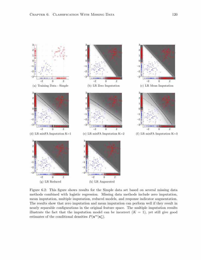
Chapter 6. Classification With Missing Data 120
−2 0 2
−3
−2
−1
0
1
2
3
(a) Training Data - Simple
−2 0 2
−3
−2
−1
0
1
2
3
(b) LR Zero Imputation
−2 0 2
−3
−2
−1
0
1
2
3
(c) LR Mean Imputation
−2 0 2
−3
−2
−1
0
1
2
3
(d) LR mixFA Imputation K=1
−2 0 2
−3
−2
−1
0
1
2
3
(e) LR mixFA Imputation K=2
−2 0 2
−3
−2
−1
0
1
2
3
(f) LR mixFA Imputation K=3
−2 0 2
−3
−2
−1
0
1
2
3
(g) LR Reduced
−2 0 2
−3
−2
−1
0
1
2
3
(h) LR Augmented
Figure 6.2: This figure shows results for the Simple data set based on several missing datamethods combined with logistic regression. Missing data methods include zero imputation,mean imputation, multiple imputation, reduced models, and response indicator augmentation.The results show that zero imputation and mean imputation can perform well if they result innearly separable configurations in the original feature space. The multiple imputation resultsillustrate the fact that the imputation model can be incorrect (K = 1), yet still give goodestimates of the conditional densities P (xm|xo
n).
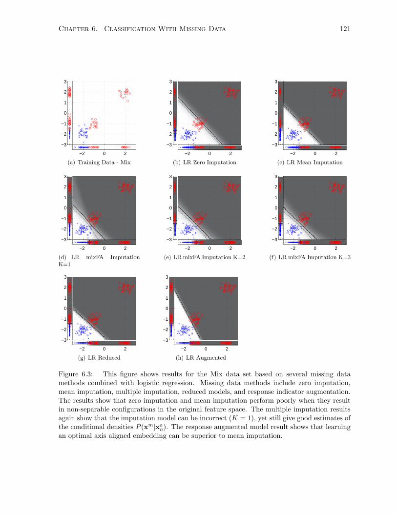
Chapter 6. Classification With Missing Data 121
−2 0 2
−3
−2
−1
0
1
2
3
(a) Training Data - Mix
−2 0 2
−3
−2
−1
0
1
2
3
(b) LR Zero Imputation
−2 0 2
−3
−2
−1
0
1
2
3
(c) LR Mean Imputation
−2 0 2
−3
−2
−1
0
1
2
3
(d) LR mixFA ImputationK=1
−2 0 2
−3
−2
−1
0
1
2
3
(e) LR mixFA Imputation K=2
−2 0 2
−3
−2
−1
0
1
2
3
(f) LR mixFA Imputation K=3
−2 0 2
−3
−2
−1
0
1
2
3
(g) LR Reduced
−2 0 2
−3
−2
−1
0
1
2
3
(h) LR Augmented
Figure 6.3: This figure shows results for the Mix data set based on several missing datamethods combined with logistic regression. Missing data methods include zero imputation,mean imputation, multiple imputation, reduced models, and response indicator augmentation.The results show that zero imputation and mean imputation perform poorly when they resultin non-separable configurations in the original feature space. The multiple imputation resultsagain show that the imputation model can be incorrect (K = 1), yet still give good estimates ofthe conditional densities P (xm|xo
n). The response augmented model result shows that learningan optimal axis aligned embedding can be superior to mean imputation.
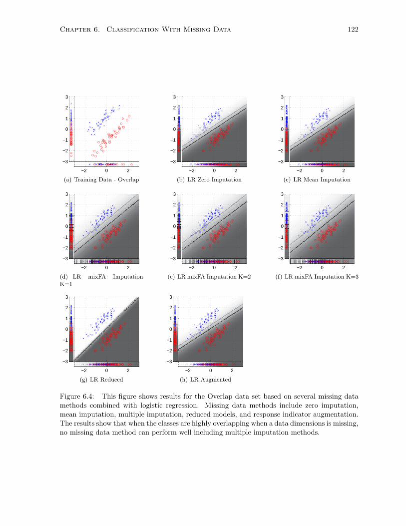
Chapter 6. Classification With Missing Data 122
−2 0 2
−3
−2
−1
0
1
2
3
(a) Training Data - Overlap
−2 0 2
−3
−2
−1
0
1
2
3
(b) LR Zero Imputation
−2 0 2
−3
−2
−1
0
1
2
3
(c) LR Mean Imputation
−2 0 2
−3
−2
−1
0
1
2
3
(d) LR mixFA ImputationK=1
−2 0 2
−3
−2
−1
0
1
2
3
(e) LR mixFA Imputation K=2
−2 0 2
−3
−2
−1
0
1
2
3
(f) LR mixFA Imputation K=3
−2 0 2
−3
−2
−1
0
1
2
3
(g) LR Reduced
−2 0 2
−3
−2
−1
0
1
2
3
(h) LR Augmented
Figure 6.4: This figure shows results for the Overlap data set based on several missing datamethods combined with logistic regression. Missing data methods include zero imputation,mean imputation, multiple imputation, reduced models, and response indicator augmentation.The results show that when the classes are highly overlapping when a data dimensions is missing,no missing data method can perform well including multiple imputation methods.
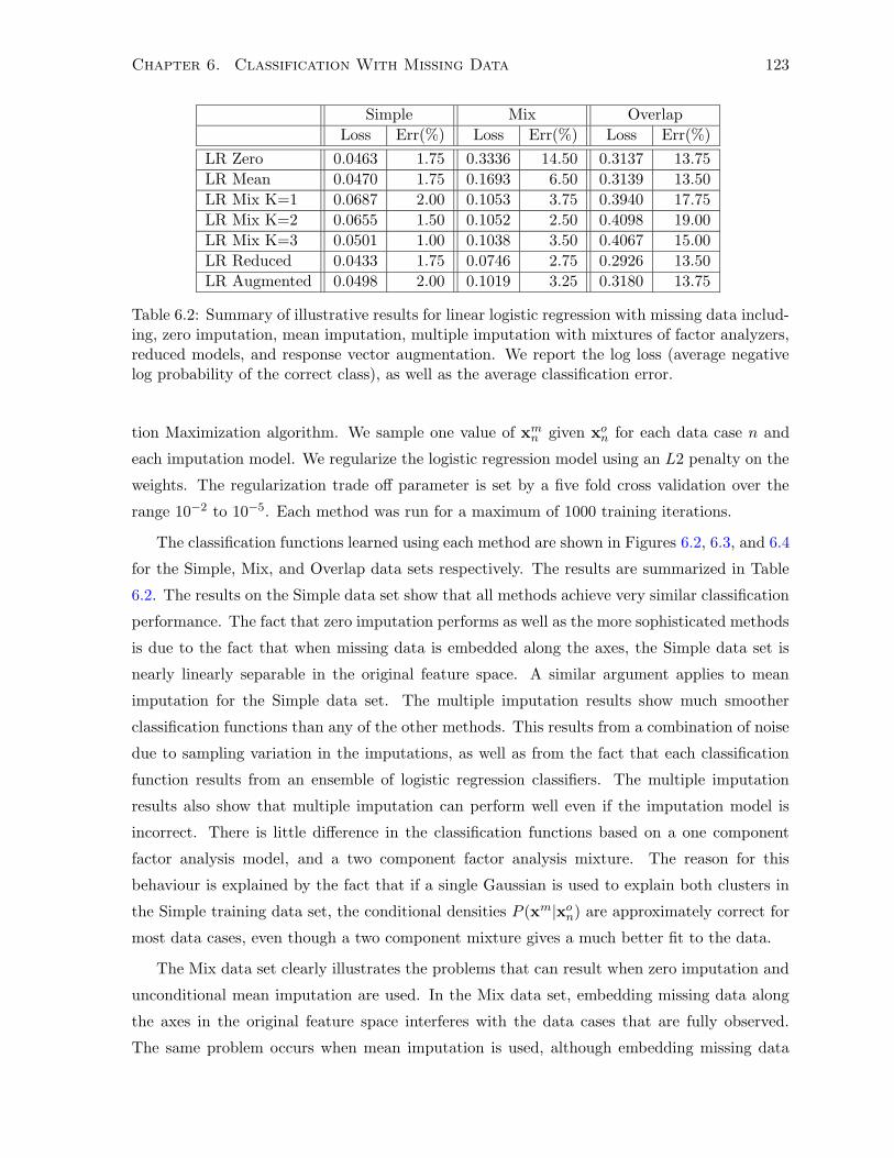
Chapter 6. Classification With Missing Data 123
Simple Mix Overlap
Loss Err(%) Loss Err(%) Loss Err(%)
LR Zero 0.0463 1.75 0.3336 14.50 0.3137 13.75
LR Mean 0.0470 1.75 0.1693 6.50 0.3139 13.50
LR Mix K=1 0.0687 2.00 0.1053 3.75 0.3940 17.75
LR Mix K=2 0.0655 1.50 0.1052 2.50 0.4098 19.00
LR Mix K=3 0.0501 1.00 0.1038 3.50 0.4067 15.00
LR Reduced 0.0433 1.75 0.0746 2.75 0.2926 13.50
LR Augmented 0.0498 2.00 0.1019 3.25 0.3180 13.75
Table 6.2: Summary of illustrative results for linear logistic regression with missing data includ-ing, zero imputation, mean imputation, multiple imputation with mixtures of factor analyzers,reduced models, and response vector augmentation. We report the log loss (average negativelog probability of the correct class), as well as the average classification error.
tion Maximization algorithm. We sample one value of xmn given xo
n for each data case n and
each imputation model. We regularize the logistic regression model using an L2 penalty on the
weights. The regularization trade off parameter is set by a five fold cross validation over the
range 10−2 to 10−5. Each method was run for a maximum of 1000 training iterations.
The classification functions learned using each method are shown in Figures 6.2, 6.3, and 6.4
for the Simple, Mix, and Overlap data sets respectively. The results are summarized in Table
6.2. The results on the Simple data set show that all methods achieve very similar classification
performance. The fact that zero imputation performs as well as the more sophisticated methods
is due to the fact that when missing data is embedded along the axes, the Simple data set is
nearly linearly separable in the original feature space. A similar argument applies to mean
imputation for the Simple data set. The multiple imputation results show much smoother
classification functions than any of the other methods. This results from a combination of noise
due to sampling variation in the imputations, as well as from the fact that each classification
function results from an ensemble of logistic regression classifiers. The multiple imputation
results also show that multiple imputation can perform well even if the imputation model is
incorrect. There is little difference in the classification functions based on a one component
factor analysis model, and a two component factor analysis mixture. The reason for this
behaviour is explained by the fact that if a single Gaussian is used to explain both clusters in
the Simple training data set, the conditional densities P (xm|xon) are approximately correct for
most data cases, even though a two component mixture gives a much better fit to the data.
The Mix data set clearly illustrates the problems that can result when zero imputation and
unconditional mean imputation are used. In the Mix data set, embedding missing data along
the axes in the original feature space interferes with the data cases that are fully observed.
The same problem occurs when mean imputation is used, although embedding missing data
Chapter 6. Classification With Missing Data 124
cases along the mean values is somewhat better than embedding along the axes. Multiple
imputation again works well with one, two, or three clusters. The explanation is the same as
for the Simple data set: the conditional densities P (xm|xon) are correct for most data points.
Comparing the response indicator framework to unconditional mean estimation shows that the
two are not equivalent. The response indicator framework essentially learns the optimal axis
aligned embedding of the missing data at the same time it learns the classification function.
This results in improved accuracy relative to unconditional mean estimation.
The Overlap data set again illustrates the fact that if the classes overlap significantly when
some data dimensions are missing, no classification method can perform well. Any axis aligned
embedding of the missing data into the original feature space results in a highly non-separable
arrangement of data points. This adversely affects zero imputation, mean imputation, and the
response indicator framework. Even when an appropriate number of mixture components are
used, the conditional densities P (xm|xon) are highly bimodal for most data cases. Sampling will
place data points in one cluster or the other essentially at random.
6.4 Perceptrons and Support Vector Machines
Both Linear Discriminant Analysis and Logistic Regression are examples of hyperplane clas-
sifiers. A potential drawback of these methods is that neither directly optimizes classification
error as an objective function. Linear discriminant analysis optimizes the joint probability of
features and labels, while logistic regression optimizes the conditional probability of labels given
features. In this section we review perceptrons and support vector machines. The classical per-
ceptron is a hyperplane classifier that attempts to directly minimize classification error. The
support vector machine is a hyperplane classifier that selects an optimal hyperplane by trading
off classification error against a complexity penalty.
6.4.1 Perceptrons
The perceptron is a binary linear classifier that chooses a hyperplane by directly optimizing
classification error, as seen in Equation 6.4.1 [63]. The original perceptron learning rule intro-
duced by Rosenblatt is a stochastic gradient descent algorithm [63]. Data cases are presented
one at a time, and the corrections to the parameters shown in Equation 6.4.2 is made if the
current data case is misclassified. The parameter α is a learning rate.
Chapter 6. Classification With Missing Data 125
fPct(w, b) =N∑
n=1
1
2|yn − sgn(wTxn + b)| (6.4.1)
w← w + αynxn (6.4.2)
b← b+ αyn (6.4.3)
The algorithm is run until a pass through the complete training set results in no updates
to the parameters. The interpretation of the single-layer perceptron in terms of a separating
hyperplane, along with the limitations this implied, was only understood later by Minsky and
Papert [56].
Rosenblatt’s perceptron learning algorithm is guaranteed to converge in a finite number of
steps if the training data is linearly separable [32, p. 108]. However, the solution that is returned
is essentially an arbitrary member of the set of all hyperplanes yielding perfect classification
of the training data. The hyperplane obtained when the perceptron learning algorithm halts
depends on the initial parameter values, as well as the order in which that training cases are
presented. The non-uniqueness of the solution in the separable case can be eliminated by
requiring that the hyperplane satisfy additional optimality constraints. This is the approach
taken by the support vector machine classifier discussed in the following section.
If the training data is not linearly separable the perceptron learning algorithm will not
converge, and cycles will develop in the parameter values. Several methods have been developed
to deal with the problem of non-separable training sets including Freund and Schapire’s voted
perceptron method [21], and the soft margin support vector machine.
6.4.2 Hard Margin Support Vector Machines
As mentioned in the previous section, there is an infinite set of hyperplanes that can perfectly
classify a separable data set. The hyperplane returned by the perceptron learning rule is
essentially a random member of this set. The optimal separating hyperplane, as defined by
Vapnik, is the one that maximizes the minimum distance of any training data point to the
separating hyperplane as seen in equation 6.4.4 [76].
Since the same decision rule results if the parameters w and b are multiplied by a constant,
any scaling of the optimal w can be used. In this case w and b are scaled such that ||w|| = 1.
Equation 6.4.5 gives an alternate formulation for the optimal hyperplane problem. The utility
of this formulation is that it is a standard, convex quadratic optimization problem subject to
linear constraints.

Chapter 6. Classification With Missing Data 126
fPH (w, b) = max
w,bmin
nyn(wTxn + b) ... st ||w|| = 1 (6.4.4)
= minw,b
1
2||w||2 ... st ∀n yn(wTxn + b) ≥ 1 (6.4.5)
6.4.3 Soft Margin Support Vector Machines
The main issue with the hard margin formulation of the support vector machine is that it is
only useful in the case where the data is perfectly separable. One solution to this problem is
to modify the constraints in equation 6.4.5 to the form yn(wTxn + b) ≥ (1 − ηn) where ηn is
a non-negative slack variable [32, p. 373]. This essentially relaxes the constraints, and ensures
that the primal optimization problem always has a feasible solution. Penalizing the use of slack
leads to the optimization problem in Equation 6.4.6. S is a free tradeoff parameter.
fS(w, b,η) = minw,b
1
2||w||2 + S
N∑
n=1
ηn ... st ∀n yn(wTxn + b) ≥ (1− ηn), ηn > 0 (6.4.6)
6.4.4 Soft Margin Support Vector Machine via Loss + Penalty
The standard derivation for the soft margin support vector machine tends to obscures the rela-
tionship between the support vector machine and logistic regression. The soft margin support
vector machine can also be derived in an alternative regularization framework using a partic-
ular loss function and penalty term [32, p. 380]. As we noted previously, regularized logistic
regression can be derived from a combination of the logistic loss function shown in equation
6.3.3, and an L1 or L2 penalty term on the weight vector. The soft margin support vector
machine can be derived from a combination of the hinge loss shown in equation 6.4.7, and an
L2 penalty on the weight vector.
LH(yn,wTxn + b) = [1− yn(wTxn + b)]+ (6.4.7)
[a]+ = max(a, 0); (6.4.8)
The primal objective function is given in Equation 6.4.9. Since the loss term is discontinuous
this optimization problem is difficult to solve directly. In the second step below we introduce
a set of auxiliary variables ηn to represent the value of the hinge loss function for each data
case. We constrain these variables to be exactly equal to the corresponding hinge loss values.
The formulation now has a continuous objective function with the discontinuity moved into
the constraints. In the final step we recognize that the equality constraints can be replaced by
Chapter 6. Classification With Missing Data 127
linear inequality constraints, and that the larger of the two inequalities will be saturated at the
minimum. If that was not the case we could lower the value of ηn for some n and reduce the
objective function further, contradicting the fact that we are at a minimum.
fS′(w, b) = minw,b
N∑
n=1
[1− yn(wTxn + b)]+γ||w||2 (6.4.9)
fS′(w, b,η) = minw,b,η
N∑
n=1
ηn + γ||w||2
st ∀n ηn =
{1− yn(wTxn + b) ... 1− yn(wTxn + b) > 0
0 ... 1− yn(wTxn + b) ≤ 0(6.4.10)
= minw,b
N∑
n=1
ηn + γ||w||2 ... st ∀n ηn ≥ 1− yn(wTxn + b), ηn ≥ 0 (6.4.11)
It is easy to see that the final form of the optimization problem derived from Equation 6.4.9
is equivalent to the soft margin support vector machine formulation given in Equation 6.4.6
for equivalent choices of the tradeoff parameters γ and S. In this work we focus on the use of
logistic regression instead of SVMs. Do to the similarity between support vector machines an
logistic regression, we expect results to generalize well from logistic regression to SVMs.
6.5 Basis Expansion and Kernel Methods
The classification methods we have considered to this point allow for a very limited class of
decision surfaces. Linear discriminant analysis, linear logistic regression, perceptrons, and linear
support vector machines all have decision surfaces described by hyperplanes. Of the methods we
have discussed, only quadratic discriminant analysis and some forms of regularized discriminant
analysis have non-linear decision surfaces.
In statistics the restrictions imposed by linear models are often overcome through the use of
higher order interaction terms [15, p. 191]. Consider the case when the feature vector x is two
dimensional, for example. Linear logistic regression finds the hyperplane w1x1 +w2x2 + b that
maximizes the conditional probability of the labels. If there is a strong interaction between x1
and x2, then an interaction term of the from x1x2 can be included and an optimal hyperplane
of the form w1x1 + w2x2 + w3x1x2 + b will be found. Basis expansions and kernel methods
generalize this basic strategy for converting a linear classifier into a non-linear classifier. The
resulting learning algorithms are often convex for a fixed basis expansion or kernel function.
Chapter 6. Classification With Missing Data 128
6.5.1 Basis Expansion
The idea of interaction terms can be generalized by replacing the original feature vector x
with a derived feature vector z = [φ1(x), ..., φM (x)]. Each φi(x) is a function that maps a
D dimensional vector to a scalar value. More generally, we can assume that there exists a
mapping z = Φ(x) that maps D dimensional feature vectors to M dimensional derived feature
vectors. Normally M will be greater than D, in which case the vector z is referred to as a basis
expansion of x [32, p. 115].
Under the assumption that the function Φ(x) is fixed, the vector zn can be computed for
each xn. Standard methods for fitting linear models can then be applied to the data in the
expanded basis. The result is a model that is linear in the expanded basis. However, if any of
the basis functions φi(x) are non-linear, the resulting model will be non-linear in the original
features x. This is a useful way to obtain non-linear models while retaining the ease of fitting
linear models. The obvious problem with this approach is that it assumes an appropriate set
of basis functions is known a priori.
6.5.2 Kernel Methods
In many linear classification models the optimal parameters can be expressed in terms of a
linear combination of data cases. As a result, the corresponding classification rule depends only
on inner products between data vectors. In the case of logistic regression and perceptrons, it
is clear from the optimization algorithm that the resulting optimal weight parameters can be
expressed as a linear combination of data vectors. In the case of support vector machines, an
analysis of the dual optimization problem shows that the optimal parameters can be expressed
as a linear combination of data vectors.
When a basis expansion is introduced, the optimal weight vector depends only on a linear
combination of the expanded vectors Φ(xn). The fact that the optimal parameters depend only
on inner products between the Φ(xn) means we never need to explicitly compute the value
of Φ(xn) for a single data case in isolation. It suffices to have a kernel function K(xi,xj) =
Φ(xi)T Φ(xj) that returns the required inner products. Further, it is possible to directly specify
a kernel function, and prove that it corresponds to an inner product under some mapping Φ(·),without explicitly constructing that mapping Φ(·).
In order for a kernel function to correspond to a valid inner product for some mapping Φ(·)it suffices for the kernel function to be positive definite. A kernel K(·, ·) is positive definite if
for any N and any x1, ...,xN , the induced Gram matrix Kij = K(xi,xj) is positive definite. A
real-valued N ×N Gram matrix K is positive definite if it is symmetric, and for any choice of
vector v ∈ RN the quadratic form vTKv ≥ 0 [68, p. 30].
Chapter 6. Classification With Missing Data 129
6.5.3 Kernel Support Vector Machines and Kernel Logistic Regression
In the kernel support vector machine we replace the optimal weights by the optimal linear
combination of expanded data vectors Φ(xn): w =∑N
n=1 αnynΦ(xn). This leads to a decision
surface based only on the corresponding kernel function K(·, ·) as seen in equation 6.5.1.
wT Φ(xn) + b =N∑
n′=1
αn′yn′Φ(xn′)T Φ(xn) + b =N∑
n′=1
αn′yn′K(xn′ ,xn) + b (6.5.1)
The optimal weight vector and decision surface for binary kernel logistic regression can also
be expressed as seen in Equation 6.5.1. However, the optimal parameters are found by mini-
mizing a regularized logistic loss function. In Equation 6.5.2 we shown the objective function
for L2 regularized kernel logistic regression in the multiclass case.
fL(α) = minα−
N∑
n=1
C∑
c=1
[yn = c] log
(exp(
∑Nn′=1 αn′cK(xn′ ,xn) + bc)
exp(∑C
c′=1
∑Nn′=1 αn′c′K(xn′ ,xn) + bc′)
)+ γ
C∑
c=1
αTc Kαc
(6.5.2)
One of the main advantages of the kernel support vector machine is that a number of αn
are usually exactly zero. This is a result of the hinge loss being exactly equal to zero for data
cases on the correct side of the margin. L2 regularized kernel logistic regression does not share
this property. In general all data cases will have non-zero αn.
An advantage of kernel logistic regression is that it naturally estimates classification prob-
abilities while kernel support vector machines do not. Under certain conditions, kernel logistic
regression also has margin maximizing properties similar to kernel support vector machines
[80]. As we have shown, kernel logistic regression naturally generalizes to the multiclass set-
ting simply by replacing the logistic loss by a loss function derived from the softmax function.
We perform experiments exclusively with kernel logistic regression, although we again expect
similar results using kernel support vector machines.
The primal L2 regularized kernel logistic regression optimization problem is unconstrained,
and can be solved directly using first or second order non-linear optimization methods. The
dual Sequential Minimal Optimization (SMO) method for kernel logistic regression developed by
Keerthi et al. reportedly achieves significant increases in speed compared to standard first and
second order optimization methods applied to the primal optimization problem [46]. However,
the SMO method has only been developed for the binary classification case. We use a simple
primal optimization method in all experiments.

Chapter 6. Classification With Missing Data 130
6.5.4 Kernels For Missing Data Classification
The main problem in the application of kernel methods is the choice of an appropriate kernel
function. In the present context this choice is complicated by the fact that the kernel function
must be defined even in the presence of missing feature values. To make the dependence on the
response indicators explicit we consider kernels of the form K(xi, ri,xj , rj).
Linear Kernels
The linear kernel Kol shown in equation 6.5.3 is a positive definite kernel since it corresponds
to the standard inner product in RD when the data vector and response indicator vector are
mapped to x� r. � denotes the element-wise product. This mapping simply replaces missing
values by zeros, and is one of the kernel studied by Chechik et al. [13].
Kol (xi, ri,xj , rj) =
∑
d
rdirdjxdixdj (6.5.3)
The explicit representation of missing data in terms of response indicators leads us immedi-
ately to the new linear kernel Ko+rl shown in equation 6.5.4. Again, this kernel can immediately
be seen as positive definite since it corresponds to the standard inner product in R2D when the
data vector and response indicator vector are mapped to [x � r,√γr]. Performing kernel lo-
gistic regression using the linear kernel Kol corresponds to performing linear logistic regression
combined with zero imputation. Performing kernel logistic regression using the linear kernel
Ko+rl corresponds to performing logistic regression under the response indicator framework.
Ko+rl (xi, ri,xj , rj) =
∑
d
rdirdjxdixdj + γrdirdj (6.5.4)
Polynomial Kernels
Given these two positive definite linear kernels, we can obtain a pair of more interesting positive
definite inhomogeneous polynomial kernels through the usual construction [68, p. 46 ]. The
kernels are given in equations 6.5.5 and 6.5.6. Positive definiteness of Kop and Ko+r
p follows
from the positive definiteness of Kol and Ko+r
l . Chechik et al. have also studied the Kop kernel
[13].
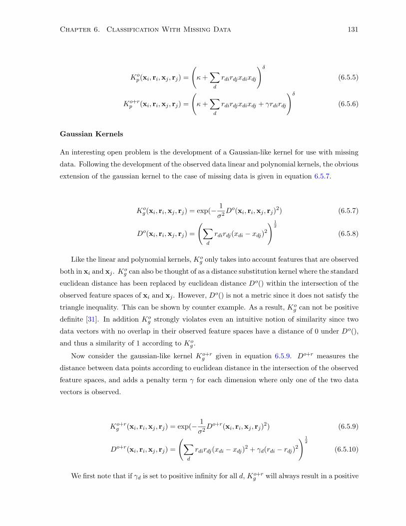
Chapter 6. Classification With Missing Data 131
Kop(xi, ri,xj , rj) =
(κ+
∑
d
rdirdjxdixdj
)δ
(6.5.5)
Ko+rp (xi, ri,xj , rj) =
(κ+
∑
d
rdirdjxdixdj + γrdirdj
)δ
(6.5.6)
Gaussian Kernels
An interesting open problem is the development of a Gaussian-like kernel for use with missing
data. Following the development of the observed data linear and polynomial kernels, the obvious
extension of the gaussian kernel to the case of missing data is given in equation 6.5.7.
Kog (xi, ri,xj , rj) = exp(− 1
σ2Do(xi, ri,xj , rj)
2) (6.5.7)
Do(xi, ri,xj , rj) =
(∑
d
rdirdj(xdi − xdj)2
) 1
2
(6.5.8)
Like the linear and polynomial kernels, Kog only takes into account features that are observed
both in xi and xj . Kog can also be thought of as a distance substitution kernel where the standard
euclidean distance has been replaced by euclidean distance Do() within the intersection of the
observed feature spaces of xi and xj . However, Do() is not a metric since it does not satisfy the
triangle inequality. This can be shown by counter example. As a result, Kog can not be positive
definite [31]. In addition Kog strongly violates even an intuitive notion of similarity since two
data vectors with no overlap in their observed feature spaces have a distance of 0 under Do(),
and thus a similarity of 1 according to Kog .
Now consider the gaussian-like kernel Ko+rg given in equation 6.5.9. Do+r measures the
distance between data points according to euclidean distance in the intersection of the observed
feature spaces, and adds a penalty term γ for each dimension where only one of the two data
vectors is observed.
Ko+rg (xi, ri,xj , rj) = exp(− 1
σ2Do+r(xi, ri,xj , rj)
2) (6.5.9)
Do+r(xi, ri,xj , rj) =
(∑
d
rdirdj(xdi − xdj)2 + γd(rdi − rdj)2
) 1
2
(6.5.10)
We first note that if γd is set to positive infinity for all d, Ko+rg will always result in a positive

Chapter 6. Classification With Missing Data 132
XOR
Loss Err(%)
pKLR Zero 0.3660 25.75
pKLR Mean 0.3660 26.50
pKLR Mix 0.2046 5.75
pKLR Reduced 0.1345 6.25
pKLR Augmented 0.1467 5.50
gKLR Zero 0.1932 7.00
gKLR Mean 0.2271 8.25
gKLR Mix 0.2055 5.25
gKLR Reduced 0.1402 5.75
gKLR Augmented 0.1677 5.25
Table 6.3: Summary of illustrative results for kernel logistic regression combined with zeroimputation, mean imputation, multiple imputation, reduced models, and the response indicatorframework. We report the log loss (average negative log probability of the correct class), aswell as the average classification error.
definite kernel matrix. For any two data points that are defined in the same feature subspace,
the value of Ko+rg is equal to the standard Gaussian Kernel applied in that sub-space. For any
two data points that are defined in different subspaces, the value of Ko+rg will be 0. Permuting
the kernel matrix so that all the rows and columns corresponding to data points from the same
subspace are contiguous results in a block diagonal matrix where each block is positive definite.
As a result, the complete Kernel matrix is positive definite.
Performing kernel logistic regression using theKo+rg kernel with γd =∞ has some interesting
properties. First, since the Ko+rg kernel matrix is block diagonal, using it to perform kernel
logistic regression is similar to separately computing a kernel logistic regression classifier in each
observed data subspace using only the data specifically from that sub-space. This is closely
related to the reduced models approach of Sharp and Solly [69].
The negative side of using the Ko+rg kernel with γd = ∞ is that there is no regularization
across feature subspaces. In the extreme case of a data set with every data point in a unique
subspace, no regularization would be achieved at all. The solution to this problem is to consider
Ko+rg for general γ, but it can again be shown that Do+r fails to satisfy the triangle inequality in
general. However, it may be possible to construct a positive definite kernel matrix using a small
values of γd for a fixed data set, even though the kernel function is not positive definite. Another
option is to construct the kernel matrix and explicitly test if it is positive definite. Indefinite
kernel matrices can be made positive semi-definite by modifying the eigen-decomposition to
eliminate negative eigen values.
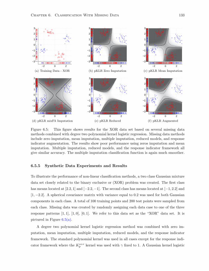
Chapter 6. Classification With Missing Data 133
−2 0 2
−3
−2
−1
0
1
2
3
(a) Training Data - XOR
−2 0 2
−3
−2
−1
0
1
2
3
(b) pKLR Zero Imputation
−2 0 2
−3
−2
−1
0
1
2
3
(c) pKLR Mean Imputation
−2 0 2
−3
−2
−1
0
1
2
3
(d) pKLR mixFA Imputation
−2 0 2
−3
−2
−1
0
1
2
3
(e) pKLR Reduced
−2 0 2
−3
−2
−1
0
1
2
3
(f) pKLR Augmented
Figure 6.5: This figure shows results for the XOR data set based on several missing datamethods combined with degree two polynomial kernel logistic regression. Missing data methodsinclude zero imputation, mean imputation, multiple imputation, reduced models, and responseindicator augmentation. The results show poor performance using zeros imputation and meanimputation. Multiple imputation, reduced models, and the response indicator framework allgive similar accuracy. The multiple imputation classification function is again much smoother.
6.5.5 Synthetic Data Experiments and Results
To illustrate the performance of non-linear classification methods, a two class Gaussian mixture
data set closely related to the binary exclusive or (XOR) problem was created. The first class
has means located at [2.2, 1] and [−2.2,−1]. The second class has means located at [−1, 2.2] and
[1,−2.2]. A spherical covariance matrix with variance equal to 0.2 was used for both Gaussian
components in each class. A total of 100 training points and 200 test points were sampled from
each class. Missing data was created by randomly assigning each data case to one of the three
response patterns [1, 1], [1, 0], [0, 1]. We refer to this data set as the “XOR” data set. It is
pictured in Figure 6.5(a).
A degree two polynomial kernel logistic regression method was combined with zero im-
putation, mean imputation, multiple imputation, reduced models, and the response indicator
framework. The standard polynomial kernel was used in all cases except for the response indi-
cator framework where the Ko+rp kernel was used with γ fixed to 1. A Gaussian kernel logistic
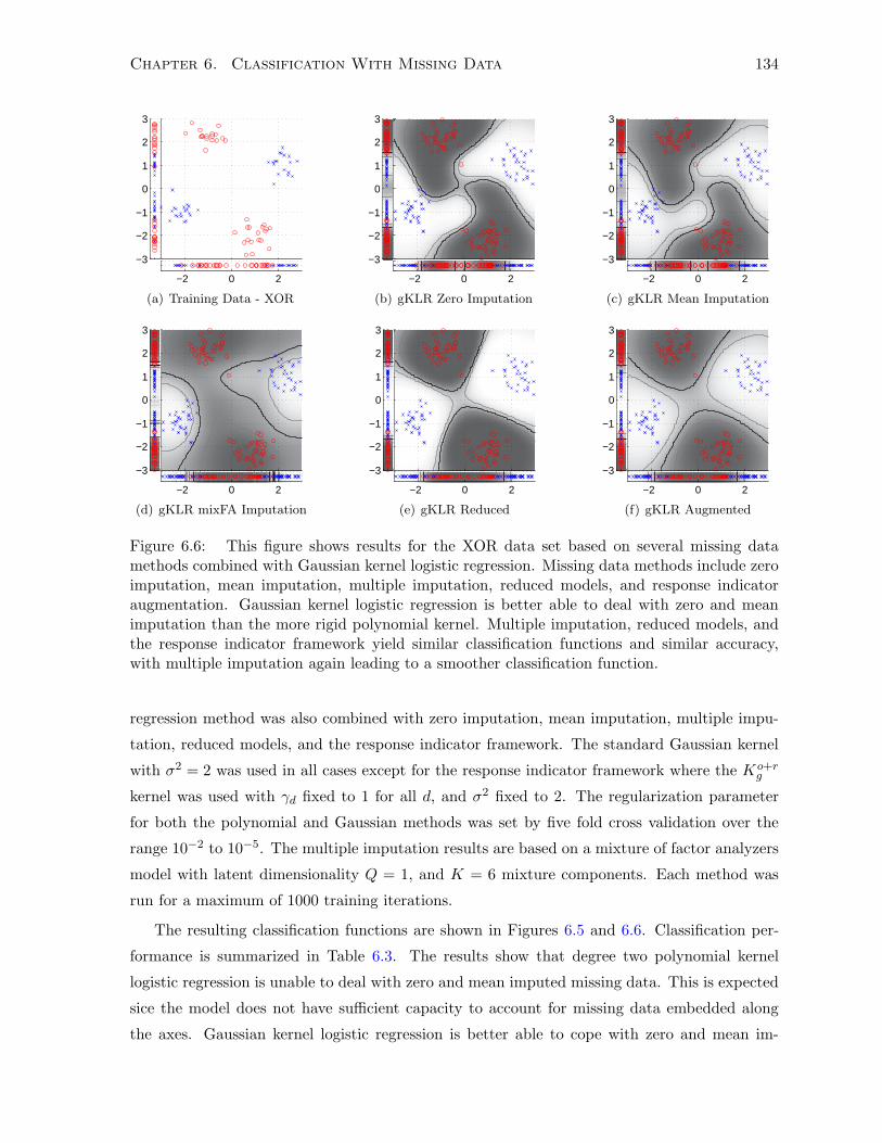
Chapter 6. Classification With Missing Data 134
−2 0 2
−3
−2
−1
0
1
2
3
(a) Training Data - XOR
−2 0 2
−3
−2
−1
0
1
2
3
(b) gKLR Zero Imputation
−2 0 2
−3
−2
−1
0
1
2
3
(c) gKLR Mean Imputation
−2 0 2
−3
−2
−1
0
1
2
3
(d) gKLR mixFA Imputation
−2 0 2
−3
−2
−1
0
1
2
3
(e) gKLR Reduced
−2 0 2
−3
−2
−1
0
1
2
3
(f) gKLR Augmented
Figure 6.6: This figure shows results for the XOR data set based on several missing datamethods combined with Gaussian kernel logistic regression. Missing data methods include zeroimputation, mean imputation, multiple imputation, reduced models, and response indicatoraugmentation. Gaussian kernel logistic regression is better able to deal with zero and meanimputation than the more rigid polynomial kernel. Multiple imputation, reduced models, andthe response indicator framework yield similar classification functions and similar accuracy,with multiple imputation again leading to a smoother classification function.
regression method was also combined with zero imputation, mean imputation, multiple impu-
tation, reduced models, and the response indicator framework. The standard Gaussian kernel
with σ2 = 2 was used in all cases except for the response indicator framework where the Ko+rg
kernel was used with γd fixed to 1 for all d, and σ2 fixed to 2. The regularization parameter
for both the polynomial and Gaussian methods was set by five fold cross validation over the
range 10−2 to 10−5. The multiple imputation results are based on a mixture of factor analyzers
model with latent dimensionality Q = 1, and K = 6 mixture components. Each method was
run for a maximum of 1000 training iterations.
The resulting classification functions are shown in Figures 6.5 and 6.6. Classification per-
formance is summarized in Table 6.3. The results show that degree two polynomial kernel
logistic regression is unable to deal with zero and mean imputed missing data. This is expected
sice the model does not have sufficient capacity to account for missing data embedded along
the axes. Gaussian kernel logistic regression is better able to cope with zero and mean im-
Chapter 6. Classification With Missing Data 135
puted missing data, but it is clear that both of these imputation strategies adversely affect the
resulting classification function. Polynomial kernel regression does have sufficient capacity to
accurately classify the Mix data set when the imputations are more accurate, or reduced mod-
els are used. Polynomial kernel logistic regression also works well in this case when response
indicator augmentation is used. A similar pattern holds for Gaussian kernel logistic regression
where multiple imputation, reduced models, and the response indicator framework yield similar
results and similar classification functions.
6.6 Neural Networks
Neural networks are a biologically inspired computational framework where a number of simple
computational units, the neurons, are connected together to compute a more complex function.
Neural networks can be characterized by the topology of the network, the dynamics of the
network, and the activation function computed at each node. The key property of neural
networks is that the activation function computed at each node is a parametric function. In
the classification setting, neural networks learn to classify inputs by adapting the parameters
associated with each node in the network. In this section we review sigmoid multi-layer feed-
forward neural networks, and their application to classification with missing data.
6.6.1 Feed-Forward Neural Network Architecture
The network topology of a feed-forward neural network is constrained to be a directed acyclic
graph. The nodes are typically arranged in one or more layers, with connections between layers,
but not within layers. The first layer is called the input layer, and the last layer is called the
output layer. Any intermediate layers are referred to as hidden layers. The parents of a node
in the network are referred to as that node’s inputs. We will assume that each layer is fully
connected to the subsequent layer. At time step t each node in layer t computes its output
value by applying its local activation function to its inputs. The assumption that the network
topology is a directed acyclic graph insures that the input values needed at each time step have
already been computed, and are not affected by computations at higher levels in the network.
The activation function computed at each node is typically a function of a linear combination
of its inputs. In this case the directed edges connecting nodes in the network can be thought
of as having weights. Typical functions applied to the linear combination of inputs include the
identity, sign, logistic or sigmoid, and hyperbolic tangent functions.
Chapter 6. Classification With Missing Data 136
6.6.2 One Hidden Layer Neural Networks for Classification
In this section we develop a learning algorithm for feed forward neural networks with one hidden
layer. We denote the inputs by xdn, the first layer activations by A1kn, the hidden unit values
by hkn, the second layer activations by A2cn, and the outputs by ycn. We denote the number
of nodes in the hidden layer by K. The first layer weight from input dimension d to hidden
unit k is denoted W 1dk. The second layer weight from hidden unit k to output unit c is denoted
by W 2kc. We denote the hidden unit biases by b1k, and the output unit biases by b2c . We select
a sigmoid or logistic activation function σ(·) for the hidden units as shown in Equation 6.6.1.
We assume a multiclass classification setting and choose a softmax activation function at the
output layer coupled with a cross-entropy objective function as shown in Equation 6.6.2.
σ(x) =1
1 + exp−x (6.6.1)
L = −N∑
n=1
C∑
c=1
[yn = c] log(ycn) (6.6.2)
The output of a feed forward neural network is computed using a forward pass through the
network from the input layer to the output layer as seen in Equation 6.6.3.
A1kn =
D∑
d=1
W 1dkxdn + b1k (6.6.3)
hkn = σ(A1kn) (6.6.4)
A2cn =
K∑
k=1
W 2kchkn + b2c (6.6.5)
ycn =exp(A2
cn)∑C
c′=1 exp(A2c′n)
(6.6.6)
The parameters of the network are adapted using gradient descent on the objective function
given in Equation 6.6.2. The back-propagation algorithm [32, p. 353] is an efficient method
for computing the required gradients by exploiting the structure of the network. The weights
are fixed and a forward pass is used to compute and store the activation, hidden unit, and
output values. The derivatives with respect to the weights, biases, and activation values are
then computed and stored using a backward pass through the network. The gradients for the
current network are given in Equations 6.6.7 to 6.6.11.
Chapter 6. Classification With Missing Data 137
∂L∂A2
cn
= ycn − [yn = c] (6.6.7)
∂L∂W 2
kc
=N∑
n=1
∂L∂A2
cn
∂A2cn
∂W 2kc
=N∑
n=1
(ycn − [yn = c])hkn (6.6.8)
∂L∂b2c
=N∑
n=1
∂L∂A2
cn
∂A2cn
∂b2c=
N∑
n=1
(ycn − [yn = c]) (6.6.9)
∂L∂W 1
dk
=
N∑
n=1
C∑
c=1
∂L∂A2
cn
∂A2cn
∂hkn
∂hkn
∂A1kn
∂A1kn
∂W 1dk
=
N∑
n=1
C∑
c=1
∂L∂A2
cn
W 2kchkn(1− hkn)xdn (6.6.10)
∂L∂b1k
=
N∑
n=1
C∑
c=1
∂L∂A2
cn
∂A2cn
∂hkn
∂hkn
∂A1kn
∂A1kn
∂b1k=
N∑
n=1
C∑
c=1
∂L∂A2
cn
W 2kchkn(1− hkn) (6.6.11)
6.6.3 Special Cases of Feed-Forward Neural Networks
Rosenblatt’s perceptron discussed in Section 6.4.1 is considered to be the earliest example of a
feed-forward neural network [63]. The network consists of the input layer, and one output node.
The activation function at the output node is the sign of a linear combination of the inputs.
The loss function used by the perceptron is classification error. Since the activation function
used by the perceptron has a discontinuous first derivative, the back-propagation algorithm can
not be used. Instead, the Perceptron Learning Rule adapts the weights or connection strengths
in the network in response to classification errors.
Logistic regression discussed in Section 6.3 can also be interpreted in terms of a neural
network. In the multi-class case logistic regression corresponds to a network with an input
layer, an output layer with C nodes, and no hidden layer. The activation function used at each
output is the softmax function. The loss function used is cross-entropy.
6.6.4 Regularization in Neural Networks
Several regularization techniques are commonly used to improve neural network learning. Weight
decay corresponds placing an L2 penalty on the network weights w. L1 regularization is less
commonly used with neural networks due to the discontinuity in the penalty function.
Momentum is a heuristic optimization strategy that modifies the current gradient by mixing
in a portion of the previous gradient. The use of momentum in gradient descent is often
motivated by a physical analogy to a ball rolling down a hill. If the ball has no momentum it
will be trapped by any local minimum, no matter how shallow. If the ball has momentum it can
skip over shallow local minima, and continue down the hill until it falls into a deep minimum.
Early stopping is a heuristic optimization technique used to avoid over-fitting in neural net-
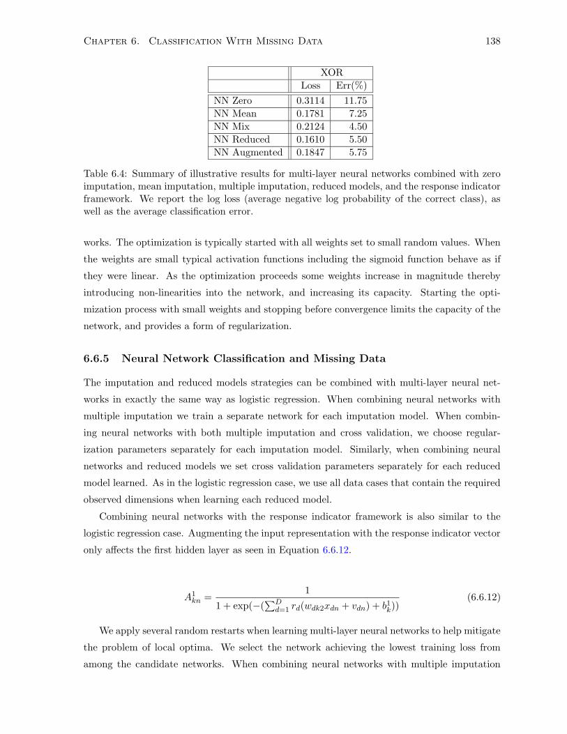
Chapter 6. Classification With Missing Data 138
XOR
Loss Err(%)
NN Zero 0.3114 11.75
NN Mean 0.1781 7.25
NN Mix 0.2124 4.50
NN Reduced 0.1610 5.50
NN Augmented 0.1847 5.75
Table 6.4: Summary of illustrative results for multi-layer neural networks combined with zeroimputation, mean imputation, multiple imputation, reduced models, and the response indicatorframework. We report the log loss (average negative log probability of the correct class), aswell as the average classification error.
works. The optimization is typically started with all weights set to small random values. When
the weights are small typical activation functions including the sigmoid function behave as if
they were linear. As the optimization proceeds some weights increase in magnitude thereby
introducing non-linearities into the network, and increasing its capacity. Starting the opti-
mization process with small weights and stopping before convergence limits the capacity of the
network, and provides a form of regularization.
6.6.5 Neural Network Classification and Missing Data
The imputation and reduced models strategies can be combined with multi-layer neural net-
works in exactly the same way as logistic regression. When combining neural networks with
multiple imputation we train a separate network for each imputation model. When combin-
ing neural networks with both multiple imputation and cross validation, we choose regular-
ization parameters separately for each imputation model. Similarly, when combining neural
networks and reduced models we set cross validation parameters separately for each reduced
model learned. As in the logistic regression case, we use all data cases that contain the required
observed dimensions when learning each reduced model.
Combining neural networks with the response indicator framework is also similar to the
logistic regression case. Augmenting the input representation with the response indicator vector
only affects the first hidden layer as seen in Equation 6.6.12.
A1kn =
1
1 + exp(−(∑D
d=1 rd(wdk2xdn + vdn) + b1k))(6.6.12)
We apply several random restarts when learning multi-layer neural networks to help mitigate
the problem of local optima. We select the network achieving the lowest training loss from
among the candidate networks. When combining neural networks with multiple imputation
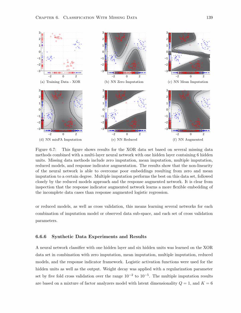
Chapter 6. Classification With Missing Data 139
−2 0 2
−3
−2
−1
0
1
2
3
(a) Training Data - XOR
−2 0 2
−3
−2
−1
0
1
2
3
(b) NN Zero Imputation
−2 0 2
−3
−2
−1
0
1
2
3
(c) NN Mean Imputation
−2 0 2
−3
−2
−1
0
1
2
3
(d) NN mixFA Imputation
−2 0 2
−3
−2
−1
0
1
2
3
(e) NN Reduced
−2 0 2
−3
−2
−1
0
1
2
3
(f) NN Augmented
Figure 6.7: This figure shows results for the XOR data set based on several missing datamethods combined with a multi-layer neural network with one hidden layer containing 6 hiddenunits. Missing data methods include zero imputation, mean imputation, multiple imputation,reduced models, and response indicator augmentation. The results show that the non-linearityof the neural network is able to overcome poor embeddings resulting from zero and meanimputation to a certain degree. Multiple imputation performs the best on this data set, followedclosely by the reduced models approach and the response augmented network. It is clear frominspection that the response indicator augmented network learns a more flexible embedding ofthe incomplete data cases than response augmented logistic regression.
or reduced models, as well as cross validation, this means learning several networks for each
combination of imputation model or observed data sub-space, and each set of cross validation
parameters.
6.6.6 Synthetic Data Experiments and Results
A neural network classifier with one hidden layer and six hidden units was learned on the XOR
data set in combination with zero imputation, mean imputation, multiple imputation, reduced
models, and the response indicator framework. Logistic activation functions were used for the
hidden units as well as the output. Weight decay was applied with a regularization parameter
set by five fold cross validation over the range 10−2 to 10−5. The multiple imputation results
are based on a mixture of factor analyzers model with latent dimensionality Q = 1, and K = 6
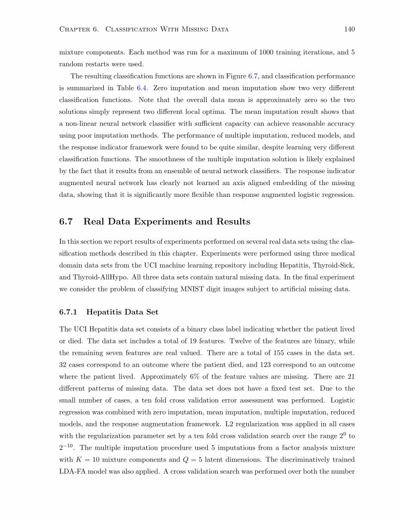
Chapter 6. Classification With Missing Data 140
mixture components. Each method was run for a maximum of 1000 training iterations, and 5
random restarts were used.
The resulting classification functions are shown in Figure 6.7, and classification performance
is summarized in Table 6.4. Zero imputation and mean imputation show two very different
classification functions. Note that the overall data mean is approximately zero so the two
solutions simply represent two different local optima. The mean imputation result shows that
a non-linear neural network classifier with sufficient capacity can achieve reasonable accuracy
using poor imputation methods. The performance of multiple imputation, reduced models, and
the response indicator framework were found to be quite similar, despite learning very different
classification functions. The smoothness of the multiple imputation solution is likely explained
by the fact that it results from an ensemble of neural network classifiers. The response indicator
augmented neural network has clearly not learned an axis aligned embedding of the missing
data, showing that it is significantly more flexible than response augmented logistic regression.
6.7 Real Data Experiments and Results
In this section we report results of experiments performed on several real data sets using the clas-
sification methods described in this chapter. Experiments were performed using three medical
domain data sets from the UCI machine learning repository including Hepatitis, Thyroid-Sick,
and Thyroid-AllHypo. All three data sets contain natural missing data. In the final experiment
we consider the problem of classifying MNIST digit images subject to artificial missing data.
6.7.1 Hepatitis Data Set
The UCI Hepatitis data set consists of a binary class label indicating whether the patient lived
or died. The data set includes a total of 19 features. Twelve of the features are binary, while
the remaining seven features are real valued. There are a total of 155 cases in the data set.
32 cases correspond to an outcome where the patient died, and 123 correspond to an outcome
where the patient lived. Approximately 6% of the feature values are missing. There are 21
different patterns of missing data. The data set does not have a fixed test set. Due to the
small number of cases, a ten fold cross validation error assessment was performed. Logistic
regression was combined with zero imputation, mean imputation, multiple imputation, reduced
models, and the response augmentation framework. L2 regularization was applied in all cases
with the regularization parameter set by a ten fold cross validation search over the range 20 to
2−10. The multiple imputation procedure used 5 imputations from a factor analysis mixture
with K = 10 mixture components and Q = 5 latent dimensions. The discriminatively trained
LDA-FA model was also applied. A cross validation search was performed over both the number

Chapter 6. Classification With Missing Data 141
Hepatitis
Loss Err(%)
LR Zero 0.4012± 0.0439 20.67± 2.71
LR Mean 0.4064± 0.0576 18.00± 2.82
LR MixFA 0.3517± 0.0506 13.33± 3.44
LR Reduced 0.4443± 0.0720 19.33± 3.78
LR Augmented 0.5812± 0.1258 19.33± 4.27
LDA-FA Dis 0.4312± 0.0720 20.00± 3.98
Table 6.5: Results on the UCI Hepatitis Data set.
of latent dimensions, and the value of the regularization parameter. Latent dimensions in the
range 1 to 15 were tried, as were regularization parameters in the range 20 to 2−10.
The results of this experiment are presented in Table 6.5. For the most part, the methods
have approximately equal performance in terms of both the log loss, and classification error.
The one interesting result in this data set is the combination of multiple imputation and logistic
regression, which obtains a much lower value of the log loss as well as the classification error
rate. This may seem surprising since there are a significant number of binary features in the
Hepatitis data set, and the imputation model assumes features are continuous. However, most
of the missing attributes in the data set are real valued.
6.7.2 Thyroid - AllHypo Data Set
The UCI Thyroid-AllHypo data set consists of four classes: Primary Hypothyroid, Compensated
Hypothyroid, Secondary Hypothyroid and Negative. We perform the standard prediction task,
which consists of discriminating between the negative class and the remaining classes. We used
five continuous feature variables: FTI, T4U, TT4, T3, and TSH. There are a total of 2659
training cases and a total of 934 test cases. The test data set contains 863 negative cases
and 71 positive cases. Approximately 7% of feature values are missing. There are 15 different
patterns of missing data.
Logistic regression was combined with zero imputation, mean imputation, multiple imputa-
tion, reduced models, and the response augmentation framework. L2 regularization was applied
in all cases with the regularization parameter set by five fold cross validation search over the
range 20 to 2−10. The multiple imputation procedure used 5 imputations from a factor analysis
mixture with K = 4 mixture components and Q = 3 latent dimensions. A sigmoid neural
network with one hidden layer was combined with mean imputation, multiple imputation, re-
duced models, and the response augmentation framework. L2 regularization was applied in all
cases with the regularization parameter set by five fold cross validation search over the range
20 to 2−10. The hidden layer was fixed to 3 hidden units. The discriminatively trained LDA-FA
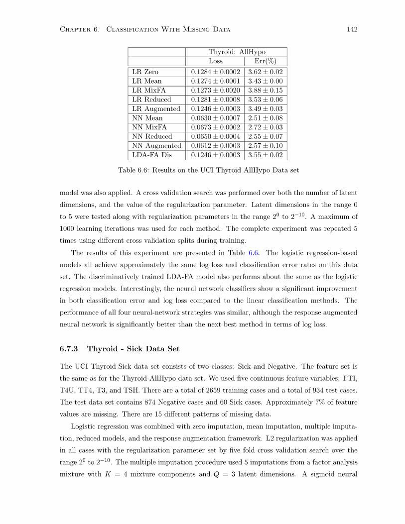
Chapter 6. Classification With Missing Data 142
Thyroid: AllHypo
Loss Err(%)
LR Zero 0.1284± 0.0002 3.62± 0.02
LR Mean 0.1274± 0.0001 3.43± 0.00
LR MixFA 0.1273± 0.0020 3.88± 0.15
LR Reduced 0.1281± 0.0008 3.53± 0.06
LR Augmented 0.1246± 0.0003 3.49± 0.03
NN Mean 0.0630± 0.0007 2.51± 0.08
NN MixFA 0.0673± 0.0002 2.72± 0.03
NN Reduced 0.0650± 0.0004 2.55± 0.07
NN Augmented 0.0612± 0.0003 2.57± 0.10
LDA-FA Dis 0.1246± 0.0003 3.55± 0.02
Table 6.6: Results on the UCI Thyroid AllHypo Data set
model was also applied. A cross validation search was performed over both the number of latent
dimensions, and the value of the regularization parameter. Latent dimensions in the range 0
to 5 were tested along with regularization parameters in the range 20 to 2−10. A maximum of
1000 learning iterations was used for each method. The complete experiment was repeated 5
times using different cross validation splits during training.
The results of this experiment are presented in Table 6.6. The logistic regression-based
models all achieve approximately the same log loss and classification error rates on this data
set. The discriminatively trained LDA-FA model also performs about the same as the logistic
regression models. Interestingly, the neural network classifiers show a significant improvement
in both classification error and log loss compared to the linear classification methods. The
performance of all four neural-network strategies was similar, although the response augmented
neural network is significantly better than the next best method in terms of log loss.
6.7.3 Thyroid - Sick Data Set
The UCI Thyroid-Sick data set consists of two classes: Sick and Negative. The feature set is
the same as for the Thyroid-AllHypo data set. We used five continuous feature variables: FTI,
T4U, TT4, T3, and TSH. There are a total of 2659 training cases and a total of 934 test cases.
The test data set contains 874 Negative cases and 60 Sick cases. Approximately 7% of feature
values are missing. There are 15 different patterns of missing data.
Logistic regression was combined with zero imputation, mean imputation, multiple imputa-
tion, reduced models, and the response augmentation framework. L2 regularization was applied
in all cases with the regularization parameter set by five fold cross validation search over the
range 20 to 2−10. The multiple imputation procedure used 5 imputations from a factor analysis
mixture with K = 4 mixture components and Q = 3 latent dimensions. A sigmoid neural
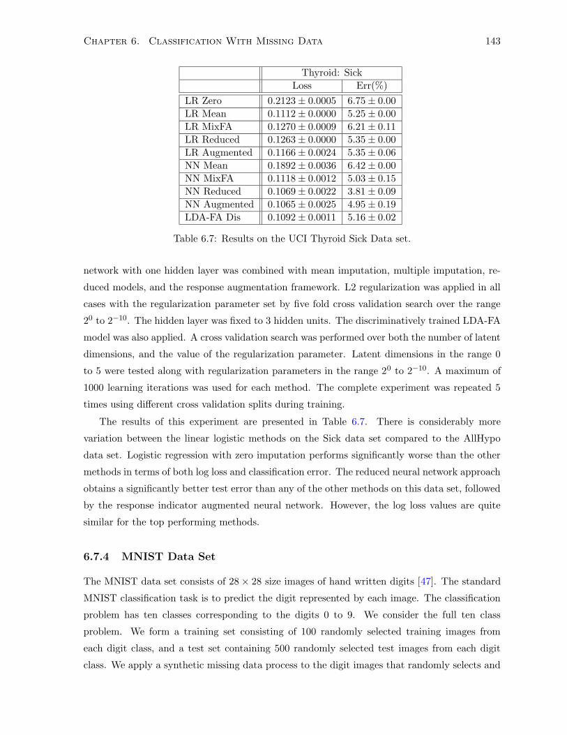
Chapter 6. Classification With Missing Data 143
Thyroid: Sick
Loss Err(%)
LR Zero 0.2123± 0.0005 6.75± 0.00
LR Mean 0.1112± 0.0000 5.25± 0.00
LR MixFA 0.1270± 0.0009 6.21± 0.11
LR Reduced 0.1263± 0.0000 5.35± 0.00
LR Augmented 0.1166± 0.0024 5.35± 0.06
NN Mean 0.1892± 0.0036 6.42± 0.00
NN MixFA 0.1118± 0.0012 5.03± 0.15
NN Reduced 0.1069± 0.0022 3.81± 0.09
NN Augmented 0.1065± 0.0025 4.95± 0.19
LDA-FA Dis 0.1092± 0.0011 5.16± 0.02
Table 6.7: Results on the UCI Thyroid Sick Data set.
network with one hidden layer was combined with mean imputation, multiple imputation, re-
duced models, and the response augmentation framework. L2 regularization was applied in all
cases with the regularization parameter set by five fold cross validation search over the range
20 to 2−10. The hidden layer was fixed to 3 hidden units. The discriminatively trained LDA-FA
model was also applied. A cross validation search was performed over both the number of latent
dimensions, and the value of the regularization parameter. Latent dimensions in the range 0
to 5 were tested along with regularization parameters in the range 20 to 2−10. A maximum of
1000 learning iterations was used for each method. The complete experiment was repeated 5
times using different cross validation splits during training.
The results of this experiment are presented in Table 6.7. There is considerably more
variation between the linear logistic methods on the Sick data set compared to the AllHypo
data set. Logistic regression with zero imputation performs significantly worse than the other
methods in terms of both log loss and classification error. The reduced neural network approach
obtains a significantly better test error than any of the other methods on this data set, followed
by the response indicator augmented neural network. However, the log loss values are quite
similar for the top performing methods.
6.7.4 MNIST Data Set
The MNIST data set consists of 28× 28 size images of hand written digits [47]. The standard
MNIST classification task is to predict the digit represented by each image. The classification
problem has ten classes corresponding to the digits 0 to 9. We consider the full ten class
problem. We form a training set consisting of 100 randomly selected training images from
each digit class, and a test set containing 500 randomly selected test images from each digit
class. We apply a synthetic missing data process to the digit images that randomly selects and
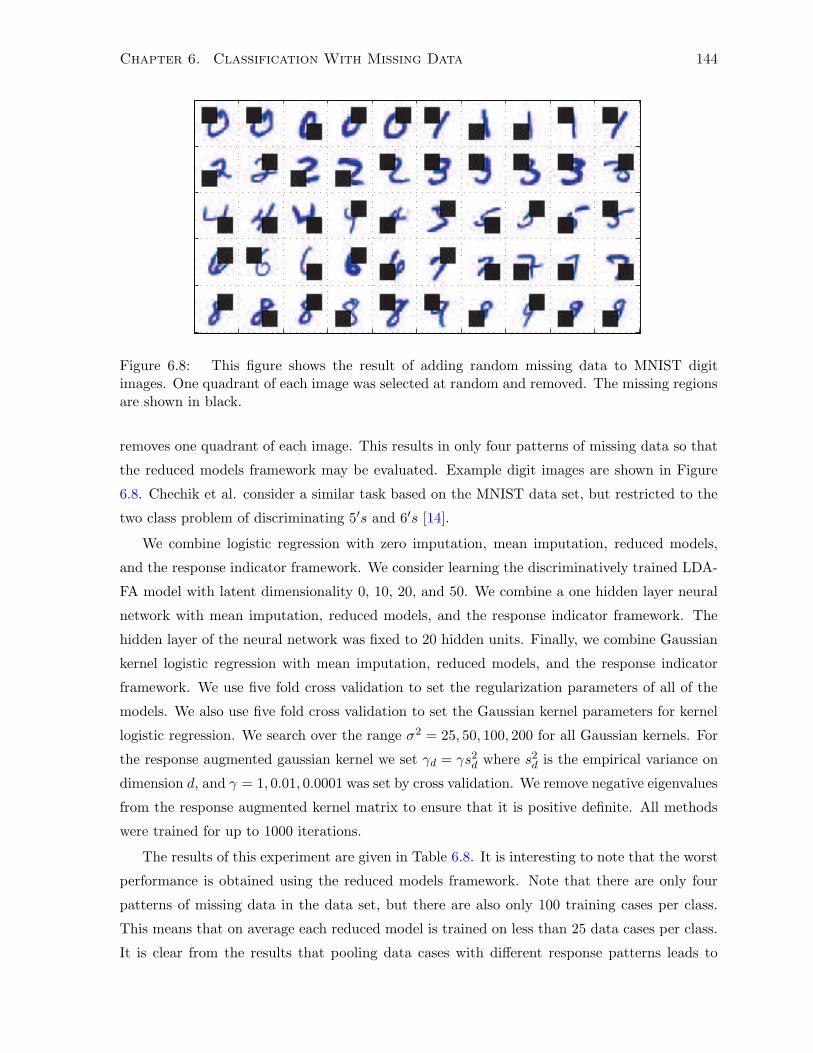
Chapter 6. Classification With Missing Data 144
Figure 6.8: This figure shows the result of adding random missing data to MNIST digitimages. One quadrant of each image was selected at random and removed. The missing regionsare shown in black.
removes one quadrant of each image. This results in only four patterns of missing data so that
the reduced models framework may be evaluated. Example digit images are shown in Figure
6.8. Chechik et al. consider a similar task based on the MNIST data set, but restricted to the
two class problem of discriminating 5′s and 6′s [14].
We combine logistic regression with zero imputation, mean imputation, reduced models,
and the response indicator framework. We consider learning the discriminatively trained LDA-
FA model with latent dimensionality 0, 10, 20, and 50. We combine a one hidden layer neural
network with mean imputation, reduced models, and the response indicator framework. The
hidden layer of the neural network was fixed to 20 hidden units. Finally, we combine Gaussian
kernel logistic regression with mean imputation, reduced models, and the response indicator
framework. We use five fold cross validation to set the regularization parameters of all of the
models. We also use five fold cross validation to set the Gaussian kernel parameters for kernel
logistic regression. We search over the range σ2 = 25, 50, 100, 200 for all Gaussian kernels. For
the response augmented gaussian kernel we set γd = γs2d where s2d is the empirical variance on
dimension d, and γ = 1, 0.01, 0.0001 was set by cross validation. We remove negative eigenvalues
from the response augmented kernel matrix to ensure that it is positive definite. All methods
were trained for up to 1000 iterations.
The results of this experiment are given in Table 6.8. It is interesting to note that the worst
performance is obtained using the reduced models framework. Note that there are only four
patterns of missing data in the data set, but there are also only 100 training cases per class.
This means that on average each reduced model is trained on less than 25 data cases per class.
It is clear from the results that pooling data cases with different response patterns leads to
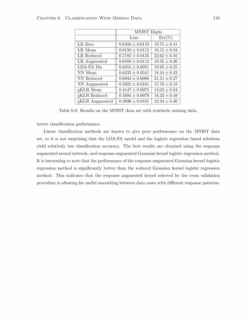
Chapter 6. Classification With Missing Data 145
MNIST Digits
Loss Err(%)
LR Zero 0.6350± 0.0110 19.75± 0.41
LR Mean 0.6150± 0.0112 19.15± 0.34
LR Reduced 0.7182± 0.0135 22.62± 0.45
LR Augmented 0.6160± 0.0112 19.35± 0.36
LDA-FA Dis 0.6355± 0.0051 19.95± 0.25
NN Mean 0.6235± 0.0541 18.34± 0.42
NN Reduced 0.6944± 0.0088 21.51± 0.27
NN Augmented 0.5925± 0.0161 17.76± 0.18
gKLR Mean 0.4147± 0.0075 13.02± 0.24
gKLR Reduced 0.5694± 0.0079 18.32± 0.49
gKLR Augmented 0.3896± 0.0101 12.34± 0.46
Table 6.8: Results on the MNIST data set with synthetic missing data.
better classification performance.
Linear classification methods are known to give poor performance on the MNIST data
set, so it is not surprising that the LDA-FA model and the logistic regression based solutions
yield relatively low classification accuracy. The best results are obtained using the response
augmented neural network, and response augmented Gaussian kernel logistic regression method.
It is interesting to note that the performance of the response augmented Gaussian kernel logistic
regression method is significantly better than the reduced Gaussian kernel logistic regression
method. This indicates that the response augmented kernel selected by the cross validation
procedure is allowing for useful smoothing between data cases with different response patterns.
Chapter 7
Conclusions
Learning, inference, and prediction in the presence of missing data are pervasive problems in
machine learning and statistical data analysis. This thesis focuses on the problems of collab-
orative prediction with non-random missing data and classification with missing features. We
have presented new experimental protocols, new data sets, and new models and algorithms for
learning, inference, and prediction. In this final chapter we present concluding remarks and
indicate directions for future research.
7.1 Unsupervised Learning with Non-Random Missing Data
In the first half of this thesis, we describe a framework for collaborative prediction in the presence
of non-random missing data. The framework is based on combining probabilistic models for
complete data with probabilistic models of the non-random missing data process. These missing
data models capture simple non-random effects by allowing the response probability for each
data dimension to depend on the underlying feature values. Models and prediction methods
were tested both on the novel Yahoo! music data set with natural missing data and the Jester
data set with synthetic missing data.
Our results show that incorporating a model of the missing data process results in substantial
improvements in predictive performance on randomly selected items compared to models that
ignore the missing data process. Our results show that training and testing only on ratings
for user selected items can vastly overestimate prediction performance on randomly selected
items. Our analysis also shows that the availability of even a small sample of ratings for
randomly selected items can have a large impact on rating prediction performance. Rating
prediction performance is also important if recommendations are derived from predicted ratings.
Our initial results evaluating rankings produced by rating prediction methods also show that
modeling the missing data mechanism results in improved ranking performance.
146
Chapter 7. Conclusions 147
There are many interesting future directions for modeling and learning with non-random
missing data within the collaborative filtering domain. The development of more flexible miss-
ing data models for the collaborative filtering domain remains an important and challenging
problem. The key assumption of the CPT-v model is that the choice to rate an item depends
only on the underlying rating value. The Logit-vd model loosens that assumption by allowing
the choice to also depend on the identity of the item. Of course, one might speculate that there
are any number of other factors involved in the choice to rate an item. The identity of the user
is likely to be important for several reasons. First, some users may be inherently more inter-
ested in rating items than other users. Second, different users may differ in their probability of
response for a given underlying preference level. This necessitates the introduction of different
missing data probabilities for different users, or classes of users.
The assumption that the choice to rate each item is independent of all of the other items
given the underlying rating value and item identity may also be questionable. It could be
interesting to consider removing this assumption and allowing response probabilities to directly
depend on higher level user tastes or preferences, as captured by latent variables. A related
issue is that current models strictly assume that the user chooses not to rate all of the unrated
items. This assumption is certainly flawed in the case of new users where we know that the
number of ratings the user has entered is limited by the amount of time the user has spent
using the recommender system. The assumption also may not hold for users who are not aware
that certain items are available in the recommender system.
A further implicit assumption is that all users in the recommender system use the rating
scale in the same way. This is not necessarily the case, and has the potential to introduce an
additional ambiguity when interpreting rating data. How might one go about deciding whether
a particular user selects items to rate completely at random and then only uses the extreme
one star and five star rating values, or whether the same user only rates items he thinks are
one star or five star items? In both cases all of the observations will be either one star or five
star ratings, but the two situation have very different interpretations.
Relaxing the assumptions behind the CPT-v and Logit-vd models in one or more of the
ways we have described here has the potential to result in more flexible selection models.
However, a crucial problem is the development of suitable learning, inference, and prediction
methods. Likely candidates for dealing with more flexible selection models are hierarchical and
semi-parametric Bayesian modeling and inference. However, the need for practical methods
to operate in an online setting raises significant questions about computational efficiency of
prediction procedures.
A complimentary approach to dealing with more complex selection models is to collect
additional information that will facilitate learning and inference. An approach to dealing with
Chapter 7. Conclusions 148
the problem of new users and users who may not be aware of certain items is to explicitly record
all of the items that each user views, listens to, reads, or purchases, regardless of whether ratings
are supplied for the items. The fact that a user listened to a particular song and chose not to
rate it is significantly more informative than simply knowing that a user did not rate a song.
An interesting alternative to the data model/selection framework is the conditional re-
stricted Boltzmann machine framework. The key to the RBM framework is the availability
of training ratings for items the user did not choose to rate. In this work, a random sample
of ratings was used to provide these ratings. It is doubtless that many users would object to
rating random items. However, it is certainly the case that some users are willing to provide
this type of data as evidenced by the more than 35, 000 users who participated in the Yahoo!
study.
The main avenues for further research with the conditional RBM model revolve around
the definition of the energy function. Like the CPT-v selection model, the cRBM/E-v model
specifies a fairly strict relationship between the ratings of user-selected and non user-selected
items when making predictions. Any number of additional terms may be included and their
effect on prediction accuracy assessed. An interesting line of inquiry would be to study the effect
of the amount of ratings for non-user selected items on the ability to learn conditional RBM
models with differently parameterized energy functions. We have also previously mentioned
the possibility of re-weighting the contrastive divergence gradients to help balance different
numbers of user-selected and non-user selected items.
7.2 Classification with Missing Features
In the second half of this thesis, we consider the problem of classification with missing features.
We consider several strategies for performing incomplete data classification including the use of
generative classification models, and the combination of standard discriminative methods with
imputation, reduced models, and response indicator augmentation. We introduce a generative
classifier for incomplete data based on linear discriminant analysis combined with a factor
analysis covariance model. We compare imputation, reduced models, and response indicator
augmentation combined with logistic regression, multi-layer neural networks, and kernel logistic
regression. We show that response augmentation has interesting properties when combined with
non-linear classifiers.
Synthetic data results illustrate the fact that zero imputation and unconditional mean im-
putation rarely work well with linear classifiers. With sufficient capacity, non-linear classifiers
can sometimes overcome poor imputation procedures. Multiple imputation was shown to work
well so long as the conditional distribution of missing data given observed data is approximately
Chapter 7. Conclusions 149
correct. The reduced models approach was also shown to work well when there is sufficient data
to reliably estimate a model for each response pattern. The synthetic data results illustrate
the important fact that if classes significantly overlap in a given observed data sub-space, no
classification method can perform well including multiple imputation and reduced models.
Results on real medical domain data show that many of the methods yield classification
accuracy that is not significantly better than baseline methods like zero imputation and mean
imputation. This may be partly due to the fact that the medical domain data sets do not
contain a large amount of missing data, and partly due to the fact that the medical domain
data sets are strongly imbalanced. Looking at the bigger picture; however, the best method on
each data set performs quite well in absolute terms.
The most interesting classification results were seen in the MNIST experiment. The MNIST
experiment used a relatively small number of high dimensional data cases with a significant
amount of missing data in each data case. The novel response augmented Gaussian kernel
logistic regression method obtained the best results in the MNIST experiment, followed by
Gaussian kernel logistic regression combined with mean imputation. In general, the classifica-
tion results show that learning a detailed model of the feature space can often be avoided and
good classification performance can still be obtained.
In terms of future research directions, it may be useful to consider other approaches for
dealing with the indefinite augmented Gaussian kernel. The present strategy of removing
negative eigenvalues from the kernel matrix is a fairly costly operation. Another option is to
consider other Gaussian-like kernels that are positive definite. Bhattacharya kernels, a special
case of probability product kernels [42], can be constructed to resemble the augmented Gaussian
kernel using relatively simple Gaussian or class conditional Gaussian models of the feature space,
and are always positive definite. A completely different classification framework that we have
not explored here, but might be amenable to dealing with missing features is boosting [22].
It would be quite interesting to consider an application of boosting using response augmented
decision stumps as the weak learners.
Semi-supervised learning deals with the problem of learning classifiers from both labeled
and unlabeled data [12]. The significance of semi-supervised learning stems from the fact that
in some domains there is an abundance of unlabeled data while labeled data is quite scarce. The
semi-supervised learning framework can be extended by simultaneously allowing missing data
in the features as well as the labels. Semi-supervised learning can also be made more difficult if
missing data in the labels or features is not missing at random. Semi-supervised learning along
with these variations provides yet another source of very interesting missing data problems in
machine learning.

Bibliography
[1] Alan Agresti. Categorical Data Analysis (Second Edition). John Wiley and Sons, 2002.
116
[2] D. Aldous. Exchangeability and Related Topics. In Proceedings of the Ecole d’Ete de
Probabilities de Saint-Flour XIII, Pages 1–198. Springer, 1985. 32
[3] J. A. Anderson. Separate Sample Logistic Discrimination. Biometrika, 59(1):19–35, 1972.
118
[4] Galen Andrew and Jianfeng Gao. Scalable Training of L1-Regularized Log-Linear Models.
In Proceedings of the 24th International Conference on Machine Learning, 2007. 116
[5] A. Banerjee. An Analysis of Logistic Models: Exponential Family Connections and Online
Performance. In SIAM International Conference on Data Mining, 2002. 118
[6] Halima Bensmail and Gilles Celeux. Regularized Gaussian Discriminant Analysis Through
Eigenvalue Decomposition. Journal of the American Statistical Association, 91(463):1743–
1748, 1996. 106
[7] C. M. Bishop. Neural Networks for Pattern Recognition. Oxford University Press, 1995.
13
[8] Stephen Boyd. An Interior-Point Method for Large-Scale L1-Regularized Logistic Regres-
sion. Journal of Machine Learning Research, 8:1519–1555, 2007. 116
[9] John S. Breese, David Heckerman, and Carl Kadie. Empirical Analysis of Predictive
Algorithms for Collaborative Filtering. In Proceedings of the Fourteenth Annual Conference
on Uncertainty in Artificial Intelligence, Pages 43–52, July 1998. 46
[10] Christopher J. C. Burges. A Tutorial on Support Vector Machines for Pattern Recognition.
Data Mining and Knowledge Discovery, 2(2):121–167, 1998. 13
150

Bibliography 151
[11] John Canny. Collaborative Filtering with Privacy via Factor Analysis. In Proceedings of
the 25th Annual International ACM SIGIR Conference on Research and Development in
Information Retrieval, Pages 238–245. ACM Press, 2002. 39
[12] O. Chapelle, B. Scholkopf, and A. Zien, editors. Semi-Supervised Learning. MIT Press,
Cambridge, MA, 2006. 149
[13] Gal Chechik, Geremy Heitz, Gal Elidan, Pieter Abbeel, and Daphne Koller. Max-Margin
Classification of Incomplete Data. In Advances in Neural Information Processing Systems
19, 2006. 102, 130
[14] Gal Chechik, Geremy Heitz, Gal Elidan, Pieter Abbeel, and Daphne Koller. Max-Margin
Classification of Data with Absent Features. Journal of Machine Learning Research, 9:1–
27, 2007. 144
[15] D. R. Cox and E. J. Snell. Analysis of Binary Data. Chapman Hall, second edition, 1989.
127
[16] Dennis Decoste. Collaborative Prediction Using Ensembles of Maximum Margin Matrix
Factorizations. In Proceedings of the 23rd International Conference on Machine Learning,
Pages 249–256, 2006. 46
[17] A.P. Dempster, N.M. Laird, and D.B. Rubin. Maximum Likelihood From Incomplete Data
Via the EM Algorithm. Journal of the Royal Statistical Society, Series B, 39(1):1–38, 1977.
12
[18] Thomas S. Ferguson. A Bayesian Analysis of Some Nonparametric Problems. The Annals
of Statistics, 1(2):209–230, 1973. 30, 31
[19] R. A. Fisher. On the Mathematical Foundations of Theoretical Statistics. Philosphical
Transactions of the Royal Society of London Series A, 1922. 11
[20] R.A. Fisher. The Use of Multiple Measurements in Taxonomic Problems. The Annual
Eugenics, 7:179–188, 1936. 102
[21] Y. Freund and R. E. Schapire. Large Margin Classification Using the Perceptron Algorithm.
In Proceedings of the 11th Annual Conference on Computational Learning Theory (Colt’
98), 1998. 125
[22] Yoav Freund and Robert E. Schapire. A Decision-Theoretic Generalization of On-Line
Learning and an Application to Boosting. Journal of Computer and System Sciences,
55(1):119–139, 1997. 149

Bibliography 152
[23] Jerome H. Friedman. Regularized Discriminant Analysis. Journal of the American Statis-
tical Association, 84:165–175, 1989. 105, 106
[24] Alan E. Gelfand and Adrian F. M. Smith. Sampling-Based Approaches to Calculating
Marginal Densities. Journal of the American Statistical Association, 85(410):398–409,
1990. 36
[25] Andrew Gelman, John B. Carlin, Hal S. Stern, and Donald B. Rubin. Bayesian Data
Analysis, Second Edition. Chapman & Hall/CRC, 2003. 10
[26] Zoubin Ghahramani and Geoffrey E. Hinton. The EM Algorithm for Mixtures of Factor
Analyzers. Technical Report CRG-TR-96-1, University of Toronto, 1996. 42, 43
[27] Zoubin Ghahramani and Michael I. Jordan. Learning From Incomplete Data. Techni-
cal Report CBCL-108, Center for Biological and Computational Learning. Massachusetts
Institute of Technology, 1994. 39
[28] Zoubin Ghahramani and Michael I. Jordan. Supervised learning from incomplete data
via an EM approach. In Jack D. Cowan, Gerald Tesauro, and Joshua Alspector, editors,
Advances in Neural Information Processing Systems, Volume 6, Pages 120–127, 1994. 39,
43
[29] G.F.V. Glonek. On Identifiability in Models for Incomplete Binary Data. Statistics and
Probability Letters, 41:191–197, 1999. 56
[30] Ken Goldberg, Theresa Roeder, Dhruv Gupta, and Chris Perkins. Eigentaste: A Constant
Time Collaborative Filtering Algorithm. Information Retrieval Journal, 4(2):133–151, July
2001. 46, 47, 52
[31] B. Haasdonk and C. Bahlmann. Learning with Distance Substitution Kernels. Pattern
Recognition - Proceedings of the 26th DAGM Symposium, 2004. 131
[32] T. Hastie, R. Tibshirani, and J. H. Friedman. The Elements of Statistical Learning.
Springer, 2001. 16, 125, 126, 128, 136
[33] J. L. Herlocker, J. A. Konstan, A. Borchers, and J. Riedl. An Algorithmic Framework for
Performing Collaborative Filtering. In Proceedings of the 22nd Annual International ACM
SIGIR Conference on Research and Development in Information Retrieval, Pages 230–237,
1999. 46
[34] G. E. Hinton and T. J. Sejnowski. Parallel Distributed Processing, Volume 1: Foundations,
Chapter: Learning and Relearning in Boltzmann Machines, Pages 194–281. MIT Press,
1986. 82
Bibliography 153
[35] Geoffrey E. Hinton. Parle Parallel Architectures and Languages Europe, Volume 258, Pages
1–13. Springer Berlin, 1987. 14
[36] Geoffrey E. Hinton. Training Products of Experts by Minimizing Contrastive Divergence.
Neural Computation, 14(8):1771–1800, 2002. 85
[37] Geoffrey E Hinton, Michael Revow, and Peter Dayan. Recognizing Handwritten Digits
Using Mixtures of Linear Models. In G. Tesauro, D. Touretzky, and T. Leen, editors,
Advances in Neural Information Processing Systems, Volume 7, Pages 1015–1022, 1995.
42
[38] Arthur E. Hoerl and Robert W. Kennard. Ridge Regression: Biased Estimation for
Nonorthogonal Problems. Technometrics, 12(1):55–67, 1970. 14
[39] Thomas Hofmann and Jan Puzicha. Latent Class Models for Collaborative Filtering. In
Proceedings of the International Joint Conference in Artificial Intelligence, 1999. 46
[40] David W. Hosmer and Stanley Lemeshow. Applied Logistic Regression, Second Edition.
John Wiley and Sons, 2000. 114, 116, 119
[41] Hemant Ishwaran and Mahmoud Zarepour. Exact and Approximate Sum Representations
for the Dirichlet Process. The Canadian Journal of Statistics, 30(2):269–283, 2002. 35
[42] Tony Jebara, Risi Kondor, and Andrew Howard. Probability Product Kernels. Journal of
Machine Learning Research, 5:819–844, 2004. 149
[43] Ian T. Jolliffe. Principal Component Analysis. Springer-Verlag, 2002. 38, 106
[44] M. Jordan. Why the Logistic Function? A Tutorial Discussion on Probabilities and Neural
Networks. Technical Report 9503, MIT Computational Cognitive Science, 1995. 118
[45] Michael I. Jordan, Michael J. Kearns, and Sara A. Solla, editors. Using Mixtures of Factor
Analyzers for Segmentation and Pose Estimation. The MIT Press, 1998. 42
[46] S. S. Keerthi, K. B. Duan, S. K. Shevade, and A. N. Poo. A Fast Dual Algorithm for
Kernel Logistic Regression. Machine Learning, 61(1-3):151–165, 2005. 129
[47] Y. Lecun, L. Bottou, Y. Bengio, and P. Haffner. Gradient-Based Learning Applied to
Document Recognition. Proceedings of the IEEE, 86(11):2278–2324, 1998. 143
[48] Su-In Lee, Honglak Lee, Pieter Abbeel, and Andrew Y. Ng. Efficient L1 Regularized Lo-
gistic Regression. In Proceedings of the Twenty-First Conference on Artificial Intelligence,
2006. 116

Bibliography 154
[49] Roderick J. A. Little and Donald B. Rubin. Statistical Analysis with Missing Data. John
Wiley and Sons, Inc., 1987. 4, 17, 20, 100
[50] Roderick J. A. Little and Donald B. Rubin. Statistical Analysis with Missing Data. Wiley,
second edition, 2002. 19, 20
[51] David J. C. Mackay. Information Theory, Inference, and Learning Algorithms. Cambridge
University Press, 2003. 9, 10, 11
[52] Benjamin Marlin. Collaborative Filtering: A Machine Learning Perspective. Master’s
thesis, University of Toronto, January 2004. 3, 46, 51, 95
[53] Benjamin Marlin, Richard S. Zemel, Sam T. Roweis, and Malcom Slaney. Collaborative
Filtering and the Missing at Random Assumption. In Uncertainty in Artificial Intelligence:
Proceedings of the 23rd Conference (Submitted), 2007. 47, 50, 54, 96
[54] Benjamin M. Marlin, Sam T. Roweis, and Richard S. Zemel. Unsupervised Learning
with Non-Ignorable Missing Data. In Proceedings of the Tenth International Workshop on
Artificial Intelligence and Statistics (AISTAT 2005), 2005. 47, 54, 75
[55] Geoffrey J. Mclachlan. Discriminant Analysis and Statistical Pattern Recognition. John
Wiley and Sons, 1992. 102, 104, 105, 114, 116, 118
[56] M. Minsky and S. Papert. Perceptron. MIT Press, 1969. 125
[57] Tom M. Mitchell. Machine Learning. Mcgraw-Hill, New York, 1997. 8
[58] A. Mkhadri, G. Celeux, and A. Nasroallah. Regularization in Discriminant Analysis: An
Overview. Computational Statistics and Data Analysis, 23(3):403–423, 1997. 105
[59] Radford M. Neal. Bayesian Mixture Modeling By Monte Carlo Simulation. Technical
Report CRG-TR-91-2, University of Toronto. Department of Computer Science, 1991. 26,
29, 34
[60] Radford M. Neal. Markov Chain Sampling Methods for Dirichlet Process Mixture Models.
Technical Report 9815, University of Toronto. Department of Statistics, 1998. 31, 33
[61] Andrew Y. Ng. Feature Selection, L1 vs. L2 Regularization, and Rotational Invariance.
In Proceedings of the Twenty-First International Conference on Machine Learning. ACM
Press, 2004. 116
[62] Jorge Nocedal and Stephen J. Wright. Numerical Optimization. Springer-Verlag, 1999. 12
Bibliography 155
[63] Frank Rosenblatt. The Perceptron: A Probabilistic Model for Information Storage and
Organization in the Brain. Psychological Review, 58(6):386–408, 1958. 13, 124, 137
[64] Donald B. Rubin. Inference and Missing Data. Biometrika, 64(3):581–592, 1976. 18, 20
[65] Ruslan Salakhutdinov, Andriy Mnih, and Geoffrey Hinton. Restricted Boltzmann Machines
for Collaborative Filtering. In Proceedings of the 24th International Conference on Machine
Learning, Pages 249–256, 2007. 82, 86, 88, 89, 90
[66] L. Saul and M. Rahim. Maximum Likelihood and Minimum Classification Error Factor
Analysis for Automatic Speech Recognition. IEEE Transactions on Speech and Audio
Processing, 8(2):115–125, 1999. 108
[67] J. L. Schafer. Analysis of Incomplete Multivariate Data. Chapman and Hall, 1997. 20, 23
[68] Bernhard Scholkopf and Alexander J. Smola. Learning with Kernels. MIT Press, Cam-
bridge, Massachusetts, 2002. 115, 128, 130
[69] P.K. Sharpe and R.J. Solly. Dealing with Missing Values in Neural Network-Based Diag-
nostic Systems. Neural Computing and Applications, 3:73–77, 1995. 101, 132
[70] P. Smolensky. Parallel Distributed Processing, Volume 1: Foundations, Chapter: Informa-
tion Processing in Dynamical Systems: Foundations of Harmony Theory, Pages 194–281.
MIT Press, 1986. 82
[71] M. Stone. Cross-Validatory Choice and Assessment of Statistical Predictions. Journal of
the Royal Statistical Society. Series B (Methodological), 36(2):111–147, 1974. 16
[72] Robert Tibshirani. Regression Shrinkage and Selection Via the Lasso. Journal of the Royal
Statistical Society. Series B (Methodological), 58(1):267–288, 1996. 14, 116
[73] M. E. Tipping and C. M. Bishop. Probabilistic Principal Component Analysis. Journal of
the Royal Statistical Society, 61(3):611–622, 1999. 37, 38, 107
[74] Michael E. Tipping and Christopher M. Bishop. Mixtures of Probabilistic Principal Com-
ponent Analysers. Neural Computation, 11(2):443–482, 1999. 42
[75] Volker Tresp, Subutai Ahmad, and Ralph Neuneier. Training Neural Networks with Defi-
cient Data. In Advances in Neural Information Processing Systems 6, 1994. 101
[76] Vladimir N. Vapnik. The Nature of Statistical Learning Theory. Springer-Verlag, 1995.
125

Bibliography 156
[77] Markus Weimer, Alexandros Karatzoglou, Quoc Le, and Alex Smola. COFI RANK -
Maximum Margin Matrix Factorization for Collaborative Ranking. In J.C. Platt, D. Koller,
Y. Singer, and S. Roweis, editors, Advances in Neural Information Processing Systems 20,
Pages 1593–1600, Cambridge, MA, 2008. MIT Press. 98
[78] B. L. Welch. Note on Discriminant Functions. Biometrika, 31(1):218–220, 1939. 104
[79] D. Williams, X. Liao, Y. Xue, and L. Carin. Incomplete-Data Classification Using Logistic
Regression. In Proceedings of the 22nd International Conference on Machine Learning
(ICML), 2005. 117
[80] Ji Zhu and Trevor Hastie. Kernel Logistic Regression and the Import Vector Machine.
Journal of Computional and Graphical Statistics, 14(1):185–205, 2005. 129
Related Documents


