GE Energy Consulting Minnesota Renewable Energy Integration and Transmission Study Final Report Prepared for: The Minnesota Utilities and Transmission Companies The Minnesota Department of Commerce Prepared by: GE Energy Consulting, with contributions by: – The Minnesota Utilities and Transmission Companies – Excel Engineering, Inc. – MISO In Collaboration with MISO October 31, 2014

Welcome message from author
This document is posted to help you gain knowledge. Please leave a comment to let me know what you think about it! Share it to your friends and learn new things together.
Transcript

GE Energy Consulting
Minnesota Renewable Energy Integration and Transmission Study
Final Report
Prepared for
The Minnesota Utilities and Transmission Companies
The Minnesota Department of Commerce
Prepared by
GE Energy Consulting with contributions by
ndash The Minnesota Utilities and Transmission Companies
ndash Excel Engineering Inc
ndash MISO
In Collaboration with MISO
October 31 2014
Updates
GE Energy Consulting MRITS Final Report
Legal Notices
This report was prepared by General Electric International Inc (GE) as an account of work sponsored by Great River Energy which was serving as a representative of the Minnesota Utilities and Transmission Companies Neither Great River Energy nor GE nor any person acting on behalf of either
1 Makes any warranty or representation expressed or implied with respect to the use of anyinformation contained in this report or that the use of any information apparatus methodor process disclosed in the report may not infringe privately owned rights
2 Assumes any liabilities with respect to the use of or for damage resulting from the use of anyinformation apparatus method or process disclosed in this report
Legal Notice i
Revision Date Update By r1 January 5 2015 Table 2-1 corrected typos mjsjea
Tables 3-1 and 3-2 clarified column headings jeamjs
October 31 2014
In 2013 the Minnesota Legislature adopted a requirement for a Renewable Energy Integration and Transmission Study1 (MRITS) MRITS is an engineering study of increasing the Minnesota Renewable Energy Standard to 40 by 2030 and to higher proportions thereafter while maintaining system reliability
Background MRITS builds upon prior renewable integration studies and related technical work and is coordinated with recent and current regional power system study work Over summer 2013 Commerce reviewed prior and current related studies and worked with stakeholders and study participants to identify key issues In fall 2013 Commerce held a stakeholder meeting to discuss the objectives scope schedule and process The study began in November 2013 and was completed in October 2014
Study details MRITS is focused on the reliability impacts of increased levels of variable renewables (wind and solar generation) and the associated costs of those impacts The study scope was developed from statutory guidance stakeholder input and technical study team refinement MRITS incorporates three core and interrelated analyses 1) Power flow analysis for development of a conceptual transmission plan which includes transmission necessary for generation interconnection and delivery and for access to regional geographic diversity and system flexibility 2) Production simulation analysis which evaluates hour-by-hour operational performance for an entire year including reserve violations unserved load wind solar curtailments thermal cycling and ramp rate and ramp range and to screen for challenging time periods and 3) Dynamics analysis which includes transient stability analysis and weak system strength analysis The broad study scope and the aggressive schedule have been very significant challenges
Technical team The MN utilities and transmission companies in coordination with MISO conducted the engineering study The Department of Commerce directed the study The Minnesota utilities and transmission companies engaged early in the study development and through the active participation of the companiesrsquo most experienced planning and operations engineers worked hard and constructively throughout the year to accomplish in collaboration with MISO a successful and timely completion of the study A preeminent technical study team of highly skilled local regional and national engineering organizations was assembled to work collaboratively on the analysis This included major contributions from the Minnesota utilities and transmission companies (siting conceptual transmission plan) Excel Engineering Inc (power flow analysis conceptual transmission plan) MISO (production simulation analysis) and GE
1 MN Laws 2013 Chapter 85 HF 729 Article 12 Section 4 MPUC Docket No CI-13-486
Energy Consulting (operational performance analysis dynamics analysis mitigations and solutions study report) Great River Energy (GRE) provided key early and ongoing study leadership GRErsquos Gordon Pietsch organized and coordinated full participation by the Minnesota utilities and transmission companies and GRErsquos Jared Alholinna led the technical study team ndash both worked tirelessly and effectively to ensure the best most knowledgeable most experienced engineers were organized funded focused and coordinated throughout the study
Study review The study has greatly benefited from extensive ongoing review and guidance by an expert Technical Review Committee (TRC) The Department of Commerce appointed and led the TRC which included engineers with experience and expertise in electric transmission system engineering electric power system operations and renewable energy generation technology Seven TRC meetings four full day and three half day were held throughout the course of the study to review and discuss the study methods and assumptions scenarios model development results and key findings With excellent input from the utilities and transmission companies MISO renewables specialists and national experts consensus was reached on overall study methods and assumptions on the scenarios to be studied on the modeling approach and on the results and key findings
Key findings The analytical results from this study show that the addition of wind and solar (variable renewable) generation to supply 40 of Minnesotarsquos annual electric retail sales can be reliably accommodated by the electric power system The MRITS operational and dynamics analyses results show that with upgrades to existing transmission the power system can be successfully operated for all hours of the year (no unserved load no reserve violations and minimal curtailment of renewable energy) with wind and solar resources increased to achieve 40 renewable energy in Minnesota and with current renewable energy standards fully implemented in neighboring MISO NorthCentral states Further analysis would be needed to ensure system reliability at 50 of Minnesotarsquos annual electric retail sales from variable renewables With wind and solar resources increased to achieve 50 renewable energy in Minnesota and 25 renewable energy in MISO North Central (10 above current renewable energy standards in neighboring states) MRITS production simulation results show that with significant transmission upgrades and expansions in the five state area the power system can be successfully operated for all hours of the year (no unserved load no reserve violations and minimal curtailment of renewable energy) Due to study schedule limitations no dynamic analysis was performed for 50 renewable energy in Minnesota (Scenarios 2 and 2a) and this analysis is necessary to ensure system reliability
Thank you to all of the study participants for an extraordinary and collaborative effort and for successful completion of a ground breaking study
Sincerely
William Grant Deputy Commissioner Division of Energy Resources
GE Energy Consulting MRITS Final Report
Technical Study Team
Jared Alholinna PE (Great River Energy) ndash Technical Study Team Lead
GE Energy Consulting (GE) ndash operating performance dynamics mitigations solutions
Douglas Welsh Durga Gautam Robert DAquila
Richard Piwko Eknath Vittal Slobodan Pajic
Gary Jordan Nicholas Miller
Excel Engineering Inc ndash power flow analysis transmission conceptual plan
Michael Cronier PE LaShel Marvig PE
MISO ndash technical coordination models data production simulation analysis
Jordan Bakke Brandon Heath Cody Doll
Aditya Jayam Prabhakar
Technical Study Team participants ndash weekly coordination calls ongoing technical study participation with Excel Engineering General Electric and MISO
Kevin Demeny American Transmission Company
Steve Porter PE Dairyland Power Cooperative
Richa Singhal Great River Energy
Jeff Eddy ITC Midwest
David Jacobson Manitoba Hydro
Scott Hoberg PE Minnesota Power
Andrew Kienitz Minnesota Power
George Sweezy PE Minnesota Power
Christian Winter PE Minnesota Power
Aaron Vander Vorst PE Minnkota Power Cooperative
John Weber Missouri River Energy Services
Matt Schuerger PE MN Department of Commerce
Lise Trudeau MN Department of Commerce
Michael Riewer Otter Tail Power
Jason Weiers PE Otter Tail Power
Andrew Lucero PE Representing CMMPA
Steve Beuning Xcel Energy
Jarred Cooley Xcel Energy
Amanda King Xcel Energy
Dean Schiro PE Xcel Energy
Technical Study Team iii
GE Energy Consulting MRITS Final Report
Technical Review Committee (TRC) Representing
Mark Ahlstrom CEO Wind Logics
Steve Beuning Director Market Operations Xcel Energy
Jeff Eddy Manager Planning ITC Holdings
Brendan Kirby Consultant Grid Integration amp Reliability NREL
Mark Mitchell Director of Operations and COO SMMPA
Michael Milligan Principal Researcher Grid Integration NREL
Dale Osborn Consulting Advisor Policy amp Economic MISO
Studies
Rhonda Peters Principal InterTran Energy Wind on the Wires
Gordon Pietsch Director Transmission Planning amp Great River Energy
Operations
Larry Schedin PE Principal LLS Resources MN Chamber of Commerce
Dean Schiro PE Manager Real Time Planning Xcel Energy
Matt Schuerger PE - Technical Advisor - TRC Chair MN Department of Commerce
Glen Skarbakka PE Consultant Skarbakka LLC
Charlie Smith Executive Director Utility Variable Generation Integration Group
George Sweezy PE Manager System Performance amp Minnesota Power
Planning
Jason Weiers PE Manager Delivery Planning Otter Tail Power
Terry Wolf Manager Transmission Services Missouri River Energy Services
Observers
Cezar Panait PE Regulatory Engineer MN Public Utilities Commission
Lise Trudeau Engineer MN Department of Commerce
Technical Review Committee iv
GE Energy Consulting MRITS Final Report
TABLE OF CONTENTS
1 EXECUTIVE SUMMARY 1-1
11 Background 1-1
12 Study Objectives and Overall Approach 1-2
13 Development of Study Scenarios 1-3
14 Development of Transmission Conceptual Plans 1-4
15 Evaluation of Operational Performance 1-4
16 Dynamic Performance Analysis 1-5
17 Key Findings 1-6 171 General Conclusions for 40 RE Penetration in Minnesota 1-6 172 General Conclusions for 50 RE Penetration in Minnesota 1-7 173 Annual Energy in the Minnesota-Centric Region 1-7 174 Cycling of Thermal Plants 1-8 175 Curtailment of Wind and Solar Energy 1-9 176 Other Operational Issues 1-10 177 System Stability Voltage Support Dynamic Reactive R eserves 1-10 178 Weak System Issues 1-11 179 Mitigations 1-12
2 PROJECT OVERVIEW 2-1
21 Background 2-1
22 Objectives 2-1
23 Study Timeline 2-2
24 Study Scope 2-2
25 Study Scenarios 2-5
3 WIND AND SOLAR GENERATION SITING 3-1
31 Siting for Wind Resources 3-2 311 Minnesota Wind 3-3 312 MISO (non-MN) Wind 3-3
32 MISO Wind Reassignment 3-9
33 Siting of PV Solar Resources 3-11 331 Minnesota PV Solar 3-11 332 Non-Minnesota PV Solar 3-16
GE Energy Consulting MRITS Final Report
4 TRANSMISSION SYSTEM CONCEPTUAL PLANS 4-1
41 Study Assumptions and Methodology 4-1 411 Study Procedure 4-1 412 Models Employed 4-2 413 Baseline M odel 4-4 414 S1 Model (Added beyond Baseline) 4-4 415 S2 Model (Added beyond S1) 4-5
42 Results 4-5 421 SCED MISO Footprint 4-5 422 Scenario 2 4-12
43 Conceptual Transmission Conclusions 4-21
5 DYNAMIC SIMULATION MODEL 5-1
51 Data Sources and Benchmarking of Dynamic Models 5-1
52 Dynamic Load Model 5-2
53 2028 Study Data Sets 5-4
54 Dynamic Models for Renewables 5-4
55 Monitoring Models and Performance Metrics 5-5
6 PRODUCTION SIMULATION MODEL 6-1
61 Overview of Production Simulations 6-1
62 PLEXOS Overview 6-1
63 MRITS Production Simulation Model ndash Source Dataset 6-1 631 Baseline S cenario 6-5 632 Scenarios 1 and 2 6-5 633 Capacity Credit for Wind and Solar Resources 6-6 634 Forecast Uncertainty 6-8
7 OPERATIONAL PERFORMANCE RESULTS 7-1
71 Scenarios for Production Simulation Analysis 7-1
72 Annual Energy 7-2 721 Aggregate Wind and Solar Plant Capacity and Power Output 7-7 722 Comparisons of Generation Fleet Utilization for Study Scenarios 7-9
73 Wind and Solar Curtailment 7-12
74 Thermal Plant Cycling 7-15 741 Coal Units 7-15 742 Combined-Cycle Units 7-19
GE Energy Consulting MRITS Final Report
75 MISO Ramp-Range and Ramp-Rate Capability 7-19
76 Carbon Emissions 7-23
77 Screening Metrics for StabilityControl Issues 7-23 771 Percent Non-Synchronous Generation ( NS) 7-23 772 Percent Renewable Pe netration ( RE) 7-25 773 Transmission Interface L oading 7-25 774 Analysis of Percent Non-Synchronous Generation 7-27 775 Percent Renewable Pe netration Analysis 7-31 776 Transmission Interface L oading 7-32
78 Selection of Operating Conditions for Dynamic Analysis 7-34
8 DYNAMIC SIMULATION RESULTS 8-1
81 Dynamic Performance Study Conditions 8-1
82 Voltage Regulation amp Stability Analysis 8-9 821 Disturbances 8-9 822 Overall Results 8-10 823 High NS conditions 8-11 824 High RE conditions 8-18 825 High Transfer Conditions 8-19
83 Reactive Reserves 8-25
84 Weak Grid Analysis 8-26 841 Composite Short Circuit Ratio Concepts 8-26 842 Identifying Weak Regions 8-28 843 Southwestern Minnesota CSCR 8-29 844 Mitigation through WindPV Inverter Controls 8-30 845 Low CSCR Mitigation 8-30
9 KEY FINDINGS 9-1
91 General Conclusions for 40 RE Penetration in Minnesota 9-1
92 General Conclusions for 50 RE Penetration in Minnesota 9-1
93 Annual Energy in the Minnesota-Centric Region 9-2
94 Cycling of Thermal Plants 9-3
95 Curtailment of Wind and Solar Energy 9-4
96 Other Operational Issues 9-5
97 System Stability Voltage Support Dynamic Reactive Reserves 9-5
98 Weak System Issues 9-6
GE Energy Consulting MRITS Final Report
99 Mitigations 9-7
10 REFERENCES 10-1
11 Appendices 11-1
GE Energy Consulting MRITS Final Report
LIST OF FIGURES
Figure 1-1 Annual Energy by Type in Minnesota-Centric Region for Study Scenarios 1-8 Figure 2-1 Flowchart of Project Tasks 2-4 Figure 3-1 RGOS Wind Zones 3-4 Figure 3-2 MN amp Non MN Scenario 1 Wind Siting 3-8 Figure 3-3 RGOS Wind Zones wMN amp Non MN Scenario 2 3-9 Figure 3-4 Wind Shift from the 4 Most-Congested to the 10 Least-Congested Sites 3-10 Figure 3-5 United States Photovoltaic Solar Resource (portion of) 3-12 Figure 3-6 MN Solar for Utility Locations - Baseline 3-14 Figure 3-7 MN Solar for Utility Locations - All Scenarios 3-14 Figure 3-8 MN Distributed PV Sites 3-16 Figure 3-9 Locations of Non-MN Solar - Utility Locations 3-19 Figure 4-1 Bus Angles from MRITS2028-S70-R17-Basea SCED Model 4-7 Figure 4-2 Bus Angles from MRITS2028-S70-R20-S1 Model0 4-8 Figure 4-3 S1 Transmission Mitigation Map 4-11 Figure 4-4 Bus Angles from MRITS2028-S70-R19-S2 Model 4-12 Figure 4-5 S2 Transmission Expansion Map 4-13 Figure 4-6 Bus Angles from MRITS2028-S70-R19-S2-Trans Model 4-14 Figure 4-7 Bus Angles from MRITS2028-S70-R19-S2-Trans-R2-SCED-A-T4B10 Model 4-15 Figure 4-8 Transmission Mitigation Map 4-17 Figure 4-9 Map of S2 Transmission Mitigations from Production Cost Analysis 4-18 Figure 4-10 HVDC Transmission Map 4-19 Figure 5-1 GE PSLF Composite Load Model CMPLDW 5-3 Figure 5-2 Renewable generation topology in powerflow Model 5-5 Figure 5-3 Geographical subregions 5-6 Figure 5-4 Voltage performance metrics 5-8 Figure 6-1 Study Footprint 6-2 Figure 6-2 MISOrsquos Market Footprint 6-2 Figure 6-3 State Renewable Portfolio Standard Policies used in the MTEP13 Model 6-3 Figure 6-4 MISOrsquos MTEP13 BAU capacity additions and coal Retirements 6-4 Figure 6-5 Illustration of site specific renewable output 6-5 Figure 6-6 Resource Capacity Changes for Scenarios 1 and 2 6-6 Figure 6-7 Plot of Wind Capacity Credit versus Penetration Level from MISO Report 6-7 Figure 6-8 Scatter Plot of Wind versus Solar Output 6-8 Figure 6-9 Sample of Hourly Forecast and Actual Wind Site Output (1st week of July) 6-9 Figure 6-10 Sample of Hourly Forecast and Actual Solar Site Output (1st week of July)) 6-10 Figure 6-11 Sample Minnesota Load Output (1st week of July) 6-11 Figure 7-1 Minnesota-Centric footprint for production simulation (Plexos) Analysis 7-2 Figure 7-2 Annual generation in TWh by unit type for Minnesota-Centric region 7-4
GE Energy Consulting MRITS Final Report
Figure 7-3 Annual Committed Capacity and Dispatch Energy 7-5 Figure 7-4 Annual Load and Net Load Duration Curves for Minnesota-Centric Region 7-6 Figure 7-5 Annual Duration Curves of Energy Imports for Minnesota-Centric Region 7-7 Figure 7-6 Duration Curves of Aggregate Wind Plant Capacity 7-8 Figure 7-7 Duration Curves of Aggregate Solar Plant Capacity 7-8 Figure 7-8 Annual Duration Curves of Solar Curtailment for Minnesota-Centric Region 7-13 Figure 7-9 Annual Duration Curves of Wind Curtailment for Minnesota-Centric Region 7-14 Figure 7-10 Wind Curtailment by Hour of Day for Minnesota-Centric Region 7-14 Figure 7-11 Coal Unit Total Annual Starts for Baseline Scenario 1 and Scenario 2 7-16 Figure 7-12 Coal Unit Total Annual Starts for Scenario 1 and Scenario 1a 7-17 Figure 7-13 Coal Unit Total Annual Starts for Scenario 2 and Scenario 2a 7-17 Figure 7-14 Coal Unit Total Annual Starts for Scenario 1a and Scenario 2a 7-18 Figure 7-15 Coal Unit Annual ldquoOperationalrdquo Starts due to Economic Commitment 7-18 Figure 7-16 Combined-Cycle Unit Total Annual Starts 7-19 Figure 7-17 Annual Duration Curve of Range-Up Capability 7-20 Figure 7-18 Annual Duration Curve of Ramp-Rate-Up Capability 7-20 Figure 7-19 Annual Duration Curve of Range-Down Capability 7-21 Figure 7-20 Annual Duration Curve of Ramp-Rate-Down Capability 7-21 Figure 7-21 Scatter Plot of Ramp-Rate Down Capability 7-22 Figure 7-22 Geographic Footprint of Minnesota-Centric Region for NS Metric 7-24 Figure 7-23 NDEX Transmission Interface 7-25 Figure 7-24 Buffalo Ridge Outlet Lines 7-26 Figure 7-25 MWEX Transmission Interface 7-27 Figure 7-26 Baseline NS Duration Curves 7-28 Figure 7-27 Scenario 1 NS Duration Curves 7-28 Figure 7-28 Scenario 1 (solid) and 1a (dashed) NS Duration Curves 7-29 Figure 7-29 Scenario 2 NS Duration Curves 7-29 Figure 7-30 Scenario 2 (solid) and 2a (dashed) NS Duration Curves 7-30 Figure 7-31 RE Penetration for the Minnesota-Centric Region 7-31 Figure 7-32 NDEX Total Loading for Scenario 1 and Scenario 1a 7-32 Figure 7-33 Buffalo Ridge Outlet Loading for Scenario 1 and Scenario 1a 7-33 Figure 7-34 MWEX Total Loading for Scenario 1 and Scenario 1a 7-33 Figure 7-35 Load Duration Curve and NS for the Minnesota-Centric Region 7-34 Figure 7-36 Chronological Load and NS for the Minnesota-Centric Region 7-35 Figure 7-37 Filtered Load and NS to the Fall Shoulder-Load Window 7-36 Figure 7-38 Further Filter Fall Shoulder Hours for Scenario 1 Stability Analysis 7-37 Figure 7-39 NDEX Interface Screening for Scenario 1 and Scenario 1a 7-39 Figure 7-40 Buffalo Ridge Outlet Interface Screening for Scenario 1 and Scenario 1a 7-39 Figure 7-41 MWEX Interface Screening for Scenario 1 and Scenario 1a 7-40 Figure 7-42 Case 2 Stability Screening for Scenario 1 and Scenario 1a 7-40
GE Energy Consulting MRITS Final Report
Figure 8-1 Minnesota Centric Dispatch (MW) By Unit Type 8-4 Figure 8-2 Minnesota Centric Percentage Generation Dispatch by Type 8-5 Figure 8-3 Minnesota Centric Commitment (MVA) by Unit Type 8-6 Figure 8-4 Percentage of On-line Non- vs Synchronous MVA 8-6 Figure 8-5 Percentage of online non- and synchronous MVA by Sub-Region 8-7 Figure 8-6 Online MVA of synchronous and non-synch Generation by Region 8-8 Figure 8-7 Dynamic Reactive Reserves of synchronous and non-synch Generation 8-8 Figure 8-8 Case 1 Terminal King Fault Active and Reactive Response 8-12 Figure 8-9 Case 1 Terminal King fault Voltage Magnitude 8-13 Figure 8-10 Case 2 Trip DEERCK fault Active and Reactive Response 8-14 Figure 8-11 Case 2 Trip DEERCK fault Voltage Magnitude 8-15 Figure 8-12 Case 3 AG3 fault Active and Reactive Response 8-16 Figure 8-13 Case 3 AG3 fault Voltage Magnitude 8-17 Figure 8-14 Case 4 NAD fault Active and Reactive Response 8-18 Figure 8-15 Case 4 NAD fault Voltage Magnitude 8-19 Figure 8-16 Case 5 AG1_v2 fault Active and Reactive Response 8-20 Figure 8-17 Case 5 AG1_v2 fault Voltage Magnitude 8-21 Figure 8-18 Case 6 SHEAS fault Active and Reactive Response 8-22 Figure 8-19 Case 6 SHEAS fault Voltage Magnitude 8-23 Figure 8-20 Case 7 BRIGGS fault Active and Reactive Response 8-24 Figure 8-21 Case 7 BRIGGS fault Voltage Magnitude 8-25 Figure 8-22 Example of composite short-circuit MVA at Multiple Wind Plants 8-27 Figure 8-23 SC MVA vs Voltage Regulation Ratio 8-29 Figure 9-1 Annual Energy by Type in Minnesota-Centric Region for St udy Scenarios 9-3
LIST OF TABLES
Table 1-1 Study Scenarios 1-3 Table 1-2 Wind and Solar Curtailment for Study Scenarios 1-10 Table 2-1 Wind and Solar Resource Allocations for Study Scenarios 2-6 Table 3-1 Minnesota-Centric Wind and Solar Amounts to be Sited 3-1 Table 3-2 Non-MN-Centric Wind and Solar Amounts to be Sited 3-1 Table 3-3 Key assumptions for Wind amp Solar Build-Outs 3-2 Table 3-4 MISO Wind Locations-Baseline 3-5 Table 3-5 Incremental Minnesota-Centric Wind Locations for Scenarios 1amp2 3-6 Table 3-6 Minnesota-Centric Wind Siting 3-6 Table 3-7 Non Minnesota MISO Wind Locations- Scenario 1 amp 2 3-7 Table 3-8 Non-MN MISO Wind Siting 3-8 Table 3-9 Wind Shift from the 4 Most-Congested to the 10 Least-Congested Sites 3-10
GE Energy Consulting MRITS Final Report
Table 3-10 Minnesota Utility PV Sites for Study Scenarios 3-13 Table 3-11 MN Distributed PV Sites for Study Scenarios 3-15 Table 3-12 Non-MN Solar for Utility Locations 3-17 Table 3-13 Non-MN Distributed Solar for St udy Scenarios 3-18 Table 4-1 S1 Transmission Mitigation 4-9 Table 4-2 S2 Transmission Expansion 4-13 Table 4-3 S2 Transmission Mitigation 4-16 Table 4-4 S2 Transmission Mitigations from Production Cost Analysis 4-18 Table 4-5 S2 AC Transmission Mitigations required with HVDC Option 4-20 Table 4-6 Scenario Transmission Cost Breakdown 4-22 Table 5-1 Benchmark Contingencies 5-2 Table 5-2 Non-industrial Load Types 5-3 Table 5-3 Industrial Load Types 5-4 Table 5-4 Sub region assignment 5-7 Table 7-1 Study Scenarios 7-1 Table 7-2 Major Assumptions for Production Simulation Analysis of Study Scenarios 7-1 Table 7-3 Annual Load Wind and Solar Energy for Minnesota-Centric Region 7-3 Table 7-4 Comparison of Minnesota-Centric Generation Fleet Utilization 7-10 Table 7-5 Comparison of Minnesota-Centric Generation Fleet Utilization 7-11 Table 7-6 Annual Wind and Solar Energy Curtailment 7-13 Table 7-7 CO2 Emissions for the Minnesota-Centric Region 7-23 Table 7-8 Maximum and Minimum NS Values 7-30 Table 7-9 Stability Cases for Scenario 1 7-38 Table 8-1 Stability Case Description 8-2 Table 8-2 Fault Description for Stability Analysis 8-9 Table 8-3 Transient Stability Analysis Results 8-10 Table 8-4 S1 Renewable Generation in SW Minnesota (Total MW Rating) 8-32 Table 9-1 Wind and Solar Curtailment for Study Scenarios 9-5
GE Energy Consulting MRITS Final Report
Nomenclature
BAU Business as Usual
CC or CCGT Combined Cycle Gas Turbine
CEMS Continuous Emissions Monitoring Systems
CF Capacity Factor
CO2 Carbon Dioxide
CSCR Composite Short-Circuit Ratio
CV Capacity Value
DA Day-Ahead
DIR Dispatchable Intermittent Resource
DPV Distributed Photovoltaic Generation Resource
DR Demand Response
DSM Demand Side Management
EI Eastern Interconnection
EMTP Electro-Magnetic Transients Program
ERGIS Eastern Renewable Generation Integration Study (by NREL)
EWITS Eastern Wind Integration and Transmission Study (by NREL)
FERC Federal Energy Regulatory Commission
GE General Electric International Inc GE Energy Consulting
GT Gas Turbine
GW Gigawatt
GWh Gigawatt Hour
HA Hour Ahead
HVDC High-Voltage Direct-Current
kV kilovolt
kW kilowatt
kWh kilowatt-hour
LBA Local Balancing Authority
LMP Locational Marginal Prices
MRITS Minnesota Renewable Energy Integration and Transmission Study
MTEP MISO Transmission Expansion Plan
MVA Megavolt Ampere
MVP Multi-Value Project
MW Megawatts
MWh Megawatt Hour
NERC North American Electric Reliability Corporation
NOMENCLATURE 1
GE Energy Consulting MRITS Final Report
Nomenclature
NOx Nitrogen Oxides
NREL National Renewable Energy Laboratory
NS Non-Synchronous
OampM Operation amp Maintenance
PJM PJM Interconnection LLC
POI Point of Interconnection
PPA Power Purchase Agreement
PSCAD Manitoba HVDC Research Centrersquos Electro-Magnetic Transients Simulation program (Power System Computer Aided Design)
PSH Pumped Storage Hydro
PV Photovoltaic
RE Renewable Energy
REC Renewable Energy Credit
RES Renewable Energy Standard
RGOS Regional Generation Outlet Study
RPS Renewable Portfolio Standard
SCED Security Constrained Economic Dispatch
SCR Short-Circuit Ratio
SCUC Security Constrained Unit Commitment
SES Solar Energy Standard
SOx Sulfur Oxides
ST Steam Turbine
STATCOM Static Compensator
SVC Static Var Compensator
TPL NERCrsquos Transmission Planning Standard
TRC Technical Review Committee
TWh Terawatt Hour (1000 Megawatt hours)
VOC Variable Operating Cost
WTG Wind Turbine-Generator
ZVRT Zero-Voltage Ride-Through
NOMENCLATURE 2
GE Energy Consulting MRITS Final Report
1 EXECUTIVE SUMMARY
11 Background
In 2013 the Minnesota Legislature adopted a requirement for a Renewable Energy Integration and Transmission Study1 (MRITS) The MN utilities and transmission companies in coordination with MISO conducted the engineering study The Department of Commerce directed the study and appointed and led the Technical Review Committee (TRC) It is an engineering study of increasing the Minnesota Renewable Energy Standard to 40 by 2030 and to higher proportions thereafter while maintaining system reliability The final study includes 1) A conceptual plan for transmission for generation interconnection and delivery and for access to regional geographic diversity and regional supply and demand side flexibility and 2) Identification and development of potential solutions to any critical issues encountered
All utilities with Minnesota retail electric sales and all Minnesota transmission companies participated andor were represented in the study Eight Minnesota Local Balancing Authorities are represented and over 85 of the Minnesota retail sales are in the four largest Local Balancing Authorities (LBA) Xcel Energy (NSP) Great River Energy Minnesota Power and Otter Tail Power The study area is within the NERC reliability region Midwest Reliability Organization (MRO) Nearly all of the Minnesota retail sales are within the Midcontinent Independent System Operator (MISO) The Local Balancing Authorities within MISO including the Minnesota LBAs are functionally consolidated
Prior studies of relevance include the 2006 Minnesota Wind Integration Study2 the 2007 Minnesota Transmission for Renewable Energy Standard Study3 the 2009 Minnesota RES Update Corridor and Capacity Validation Studies the 2008 and 2009 Statewide Studies of Dispersed Renewable Generation4 the 2010 Regional Generation Outlet Study the 2011 Multi Value Project Portfolio Study the 2013 Minnesota Biennial Transmission Project Report5 the 2013 MISO Transmission Expansion Plan and recent and ongoing MISO transmission expansion planning work6
1 MN Laws 2013 Chapter 85 HF 729 Article 12 Section 4 MPUC Docket No CI-13-486
2 2006 MN Wind Integration Study Prepared for the MPUC Nov 2006
Final Report Volumes I amp II Final Report Presentation httpwwwpucstatemnusPUCelectricity013752 3 ldquoMinnesota RES Update Study Technical Reportrdquo March 2009 ldquoRES Transmission Reportrdquo November 2007
ldquoSouthwest Twin Cities ndash Granite Falls Transmission Upgrade Study Technical Reportrdquo March 2009
ldquoCapacity Validation Study Reportrdquo March 2009 httpwwwminnelectranscomreportshtml 4
Dispersed Renewable Generation Studies June 2008 and September 2009
httpmngovcommerceenergytopicsresourcesReports-DataEnergy-Reportsjsp 5
httpwwwminnelectranscom November 1 2013 6
httpswwwmisoenergyorgPlanningTransmissionExpansionPlanningPagesTransmissionExpansionPlanningaspx
EXECUTIVE SUMMARY 1-1
GE Energy Consulting MRITS Final Report
12 Study Objectives and Overall Approach
The study objectives are listed below
1 Evaluate the impacts on reliability and costs associated with increasing Renewable Energy to 40 of Minnesota retail electric energy sales by 2030 and to higher proportions thereafter
2 Develop a conceptual plan for transmission necessary for access to regional geographic diversity and regional system flexibility
3 Identify and develop options to manage the impacts of the renewable energy resources
4 Build upon prior wind integration studies and related technical work Coordinate with recent and current regional power system study work
5 Produce meaningful broadly supported results through a technically rigorous inclusive study process
This study is focused on the reliability impacts of increased levels of variable renewables (wind and solar generation) and the associated costs of those impacts
MRITS builds upon prior wind integration studies and related technical work and is coordinated with recent and current regional power system study work The study scope was developed from statutory guidance stakeholder input and technical study team refinement
MRITS incorporates three core and interrelated analyses 1) Power flow analysis for development of a conceptual transmission plan which includes transmission necessary for generation interconnection and delivery and for access to regional geographic diversity and regional supply and demand side flexibility 2) Production simulation analysis for evaluation of operational performance including reserve violations unserved load wind solar curtailments thermal cycling and ramp rate and ramp range and to screen for challenging time periods and 3) Dynamics analysis which includes transient stability analysis and weak system strength analysis
The MRITS study area is Minnesota-centric which focuses on the combined operating areas of the Minnesota utilities and transmission companies in the context of the MISO NorthCentral areas and the neighboring regions to the west and north
The base study models (baseline and scenarios) are coordinated with and consistent with MISO models and databases including dispatch to the MISO market Additional options were considered in Task 7 (Identify amp Develop Mitigations Solutions) as needed
The key study tasks are
Develop Study Scenarios Site Wind and Solar Generation (Lead contributors Minnesota Utilities Minnesota Department of Commerce)
Perform Production Simulation Analysis (Lead Contributor MISO)
Perform Power Flow Analysis Develop Transmission Conceptual Plan (Lead Contributors Minnesota Utilities amp Transmission Owners Excel Engineering)
Evaluate Operational Performance (Lead Contributor GE Energy Consulting)
EXECUTIVE SUMMARY 1-2
GE Energy Consulting MRITS Final Report
Screen for Challenging Periods (Lead Contributor GE Energy Consulting)
Evaluate stability related issues including transient stability performance voltage regulation performance adequacy of dynamic reactive support and weak system strength issues (Lead Contributor GE Energy Consulting)
Identify and Develop Mitigations and Solutions (Lead Contributor GE Energy Consulting)
13 Development of Study Scenarios
The Baseline scenario has sufficient renewable energy generation to satisfy the current renewable energy standards and solar energy standards for all states in the study region For Minnesota the Baseline scenario was based on current Minnesota utility plans to meet the Minnesota Renewable Energy Standard (RES) and the Solar Energy Standard (SES) with renewable energy (wind solar small hydro biomass etc) from the Minnesota-centric area and incorporates refinements from the technical study team For non-Minnesota MISO states in the study footprint the Baseline scenario was based on the prior approved 2013 MISO Transmission Expansion Plan (MTEP13)
Scenario 1 builds on the Baseline scenario by adding incremental wind and solar (variable renewables) generation to the Baseline model to supply a total of 40 of Minnesota annual electric retail sales from renewables in the study year and with all states at full implementation of their current RESs
Scenario 2 builds on Scenario 1 by adding incremental wind and solar generation to the Scenario 1 model to supply 50 of Minnesota electric retail sales from total renewables and by further adding incremental wind and solar generation to supply an additional 10 of the non-Minnesota MISO North Central retail electric sales from total renewables (ie to increase the MISO footprint renewables 10 above full implementation of the current RESs)
Table 1-1 Study Scenarios
Scenario Minnesota RE Penetration
MISO Wind amp Solar Penetration (including Minnesota)
Baseline 285 140
Scenario 1 400 150
Scenario 2 500 250
Note MISO has an additional 3 renewable energy penetration in all scenarios from existing small biomass and small hydro
The horizon year for this study was 2028 (to represent 2030 conditions) System load levels for Minnesota and MISO regions were scaled up from present levels by an assumed annual growth rate of 05 for Minnesota and 075 for the rest of MISO North Central
All scenarios including the Baseline required more wind and solar generation than what is already installed on the grid Therefore the study team used a combination of windsolar resource maps and windsolar profile data (from NREL) to guide selection of sites for prospective future wind and solar plants with cumulative capacities consistent with the renewable energy targets for each study scenario Wind Plant sites were distributed among several of MISOrsquos renewable energy zones
EXECUTIVE SUMMARY 1-3
GE Energy Consulting MRITS Final Report
(originally developed in the MISO Regional Generation Outlet Study and used in the Multi-Value Project Portfolio study)
14 Development of Transmission Conceptual Plans
A conceptual transmission plan was developed for each of the study scenarios System reliability was determined through traditional transmission planning methods criteria and assumptions Steady state performance characteristics were evaluated with the system intact as well as under powerflow contingency conditions (N-1 outages and selected multiple contingency outages per NERC TPL Category C2 amp C5)
The Baseline scenario started with a transmission model that was consistent with the 2013 MTEP 2023 model This Baseline transmission model incorporates planned transmission lines including the CapX2020 Group I lines and the MISO Multi-Value Project (MVP) portfolio A very limited number of facilities were overloaded in the Baseline Scenario
For Scenario 1 a total of 54 transmission mitigations were added to accommodate the increased wind and solar generation These mitigations included transmission line upgrades transformer additionsreplacements and changes to substation terminal equipment with a total estimated cost of $373M No new transmission lines were required
In Scenario 2 a total of 17245 MW of new windsolar generation was added to increase Minnesota renewable energy penetration to 50 and MISO renewable energy penetration to 25 A total of 9 new transmission lines and 30 transmission upgrades were added to the Scenario 1 transmission system with a total estimate cost of an additional $26B Note that an undetermined portion of the Scenario 2 transmission expansions and upgrades are associated with increasing MISOrsquos renewable penetration from 15 to 25
Note that for the development of transmission conceptual plans the new wind and solar resources were connected to high voltage transmission buses The actual connection processes will likely require additional plant-specific interconnection facilities for the new wind and solar plants
15 Evaluation of Operational Performance
Operational performance of the electric power grid with increased levels of renewable generation was analyzed using production simulation analysis which simulates hourly operation of the system for an entire year The PLEXOS simulation tool uses a Day-Ahead Security Constrained Unit Commitment (SCUC) and Real-Time Security Constrained Economic Dispatch (SCED) interleaved market dispatch solution This type of modeling accurately captures the forecast uncertainties realized between a Day-Ahead and Real-Time markets Modeling of forecast uncertainty becomes increasingly important when dealing with high levels of wind and solar generation because the output tends to be more stochastic in nature
MISO used the 2013 MTEP Business as Usual (BAU) dataset as a starting point for the Baseline Scenario with modifications to the system load level to reflect the 2028 horizon year for this study The BAU future is considered the status quo future and continues current economic trends The MTEP futures are created by MISO and vetted by the MISO Planning Advisory Committee (PAC) stakeholder committee Information for the production modeling dataset is sourced from Ventyx
EXECUTIVE SUMMARY 1-4
GE Energy Consulting MRITS Final Report
and updated through an extensive MISO process to bring it into line with the most current data and expected future conditions Coal unit retirements totaling 126 GW were included in the model per MISOrsquos anticipated effects of prior EPA regulations
Future EPA regulations such as the recently proposed Clean Power Plan (111d) which is still in development are not modeled nor considered in this study The model footprint includes all areas in the Eastern Interconnect with the exception of Florida ISO New England and Eastern Canada
For the Scenarios 1 and 2 new wind and solar generation was added at the locations determined in the siting task and transmission system upgradesexpansions were added per the conceptual transmission plans
One aspect of the BAU set of assumptions is that many coal plants within MISO will continue to operate as they do now That is the plants remain on-line when economic market signals would have initiated a brief period of decommitment and effectively act as ldquomust-runrdquo units In order to examine the sensitivity to changing this assumption and to the assumption of coal unit retirements Scenarios 1a and 2a were added to the production simulation analysis as sensitivity cases relative to Scenarios 1 and 2 Scenarios 1a and 2a included the following changes in assumptions
All coal units were economically committed
Nine additional coal units in the Minnesota-centric region were assumed to be available (These units were assumed unavailable in Scenarios 1 and 2)
Forced outage modeling of conventional generation was included
The production simulation results were analyzed to assess system operational performance with respect to the following parameters annual energy production by type of generating resource renewable energy resource utilization and curtailment cycling duty of thermal plants adequacy of ramping capability of the MISO generation fleet and risk of reserve violations and unserved load For Scenario 1 the results were also screened to select challenging operating conditions for dynamic performance and these operating points were subsequently analyzed with fault simulations in the dynamics task
16 Dynamic Performance Analysis
A dynamic simulation model was developed to perform transient stability analysis of the study scenarios A series of dynamic data files were provided by the Minnesota utilities based on the MTEP 2013 dataset As with the power flow and production system models new wind and solar generation was added at the locations determined in the siting task and transmission system upgradesexpansions were added per the conceptual transmission plans In order to capture possible fault-induced delayed recovery issues caused by reduced levels of synchronous generation the load models in the Minnesota-Centric region were refined to include a more detailed representation of load composition including dynamic characteristics
New utility-scale wind and solar photovoltaic (PV) plant models were consistent with current NERC and FERC minimum requirements (eg voltage regulation power factor voltage ride-through) Full commercial technical capability (eg synthetic inertia frequency response) was not modeled Distributed PV was modeled as lumped generation at locations (per the siting task) with no reactive power or voltage regulation capability
EXECUTIVE SUMMARY 1-5
GE Energy Consulting MRITS Final Report
New wind plants were split roughly 5050 between Type 3 (double fed asynchronous generator (DFAG) and Type 4 (full converter)
A representative number of regional power system fault conditions were simulated to stress the system in different ways
Faults known to be severe challenges to system transient stability from numerous past stability studies
Faults in regions with high concentrations of wind and solar plants where voltage recovery is highly dependent on the reactive power support from wind and solar plants
Faults affecting major transmission interfaces during periods of high power transfer
The results of all dynamic simulation cases were screened with respect to a set of performance criteria including angular stability oscillatory stability voltage dips and voltage recovery
Weak system issues were also investigated using the dynamic system models When the ac system impedance is high relative to the aggregate rating of wind and solar generation in a given region the internal controllers and regulators within wind and solar inverters become less stable If the system is excessively weak control instabilities may occur Composite short-circuit ratio analysis was conducted to determine system strength in the study scenarios with respect to emerging industry understanding of this issue
17 Key Findings
This study examined two levels of increased wind and solar generation for Minnesota 40 (represented by Scenarios 1 and 1a) and 50 (represented by Scenarios 2 and 2a) In the 40 Minnesota Scenario MISO NorthCentral is at 15 (current state RESs) The 50 Minnesota Scenario also included an increase of 10 (to 25) in the MISO NorthCentral region Production simulation was used to examine annual hourly operation of the MISO NorthCentral system for all four of these scenarios Transient and dynamic stability analysis was conducted for Scenarios 1 and 1a but not on Scenarios 2 and 2a
171 General Conclusions for 40 RE Penetration in Minnesota
With wind and solar resources increased to achieve 40 renewable energy for Minnesota and 15 renewable energy for MISO NorthCentral production simulation and transientdynamic stability analysis results indicate that the system can be successfully operated for all hours of the year with no unserved load no reserve violations and minimal curtailment of renewable energy This assumes sufficient transmission mitigations as described in Section 14 to accommodate the additional wind and solar resources
This is operationally achievable with most coal plants operated as baseload must-run units similar to existing operating practice It is also achievable if all coal plants are economically committed per MISO market signals but additional analysis would be required to better understand implications tradeoffs and mitigations related to increased cycling duty
EXECUTIVE SUMMARY 1-6
GE Energy Consulting MRITS Final Report
Dynamic simulation results indicate that there are no fundamental system-wide dynamic stability or voltage regulation issues introduced by the renewable generation assumed in Scenario 1 and 1a This assumes
New wind turbine generators are a mixture of Type 3 and Type 4 turbines with standard controls
The new wind and utility-scale solar generation is compliant with present minimum performance requirements (ie they provide voltage regulationreactive support and have zero-voltage ride through capability)
Local-area issues are addressed through normal generator interconnection requirements
172 General Conclusions for 50 RE Penetration in Minnesota
With wind and solar resources increased to achieve 50 renewable energy in Minnesota and 25 renewable energy in MISO production simulation results indicate that the system can be successfully operated for all hours of the year with no unserved load no reserve violations and minimal curtailment of renewable energy This assumes sufficient transmission upgrades expansions and mitigations to accommodate the additional wind and solar resources
This is operationally achievable with most coal plants operated as baseload must-run units similar to existing operating practice It is also achievable if all coal plants are economically committed per MISO market signals but additional analysis would be required to better understand implications tradeoffs and mitigations related to increased cycling duty
No dynamic analysis was performed for the study scenarios with 50 renewable energy for Minnesota (Scenarios 2 and 2a) due to study schedule limitations and this analysis is necessary to ensure system reliability
173 Annual Energy in the Minnesota-Centric Region
Figure 1-1 shows the annual load and generation energy by type for the Minnesota-Centric region Comparing Scenarios 1 and 1a (40 MN renewables) with the Baseline
Wind and solar energy increases by 85 TWh all of which contributes to bringing the State of Minnesota from 285 RE penetration to 40 RE penetration
There is very little change in energy from conventional generation resources
Most of the increase in wind and solar energy is balanced by a decrease in imports The Minnesota-Centric region goes from a net importer to a net exporter
Comparing Scenarios 2 and 2a (50 MN renewables) with Scenarios 1 and 1a (40 MN renewables)
Wind and solar energy increases by 20 TWh Of this total 48 TWh brings the State of Minnesota from 40 to 50 RE penetration and the remainder contributes to bringing MISO from 15 to 25 RE penetration
Most of the increase in wind and solar energy in the Minnesota-Centric region is balanced by a decrease in coal generation and an increase in net exports to neighboring regions
Gas-fired combined-cycle generation declines from 50 TWh in Scenario 1 to 30 TWh in Scenario 2
EXECUTIVE SUMMARY 1-7
GE Energy Consulting MRITS Final Report
Figure 1-1 Annual Energy by Type in Minnesota-Centric Region for Study Scenarios
174 Cycling of Thermal Plants
Most coal plants were originally designed for baseload operation that is they were intended to operate continuously with only a few startstop cycles in a year (mostly due to scheduled or forced outages) Increased cycling duty could increase wear and tear on these units with corresponding increases in maintenance requirements Many coal plants in MISO presently are designated by the plantrsquos owner to operate as ldquomust-runrdquo in order to avoid startstop cycles that would occur if they were economically committed by the market
Scenarios S1a and S2a assumed that all coal plants in MISO are subject to economic commitmentdispatch (ie not must-run) based on day-ahead forecasts of load wind and solar energy within MISO Production simulation results show significant coal plant cycling due to economic market signals
Small coal units (below 300 MW rating) could have an additional 100 to 200 starts per year beyond those due to forced or planned outages
Large coal units (above 300 MW) could have an additional 20 to 100 starts per year
EXECUTIVE SUMMARY 1-8
GE Energy Consulting MRITS Final Report
Scenarios S1 and S2 assumed almost all coal plants would continue to operate as they do today Coal units were on-line all year (except for scheduled maintenance periods) and were not decommitted during periods of low market prices The results of these scenarios confirmed that the coal units could remain must-run with minor impacts on overall operation of the Minnesota-Centric region Coal plant owners could choose to continue the must-run practice to avoid the detrimental impacts of increased cycling as wind and solar penetration increases Doing so would likely incur some additional operational costs when energy prices fall below a plantrsquos breakeven point Wind curtailment would also be about 05 higher than if the coal plants were economically committed
An attractive solution to the coal plant cycling issue may exist between the two bookend cases analyzed in this study Scenarios 1a and 2a assumed that unit commitment was determined on a day-ahead basis using day-ahead forecasts of wind and solar energy The result was a high number of startstop cycles of coal plants sometimes with down-times of less than 2 days If the unit commitment process was modified to use a longer term forward market (say 3 to 5 days ahead) then coal plant owners could adjust their operational strategy to consider decommitting units when prolonged periods of high windsolar generation and low system loads are forecasted A forward market would depend on longer term forecasts of wind solar and load energy consistent with the look-ahead period of the market Although such forecasts would be somewhat less accurate than day-ahead forecasts the quality of the forecasts would likely be adequate to support such unit commitment decisions
This study did not examine the economic or wear-and-tear impacts of increased cycling on coal units Further information on this topic can be found in the NREL Western Wind and Solar Integration Study Phase 2 report7 and the PJM Renewable Integration Study report8
Combined-cycle (CC) units are better able to accommodate cycling duties than coal plants Simulation results show that combined cycle units in the Minnesota-Centric region experience from 50 to 200 startstop cycles per year Cycling of CC units declines slightly as wind and solar penetration increases This decline is primarily due to a decrease in CC plant utilization as wind and solar energy increases
175 Curtailment of Wind and Solar Energy
In general a small amount of curtailment is to be expected in any system with a significant level of wind and solar generation There are some operating conditions where it is economically efficient to accept a small amount of curtailment (ie mitigation of that curtailment would be disproportionately expensive and not justifiable)
Overall curtailment in the Minnesota-Centric region is relatively small in all study scenarios as shown in Table 1-2 Wind curtailment in Baseline and Scenario 1 is primarily due to local transmission congestion at a few wind plants This congestion could be mitigated by transmission modifications if economically justifiable
Wind curtailment in Scenario 2 is due to system-wide operational limits during nighttime hours when many baseload generators are dispatched to their minimum output levels This type of curtailment could be reduced by decommitting some baseload generation via economic market
7 httpwwwnrelgovelectricitytransmissionwestern_windhtml
8 httpwwwpjmcomcommittees-and-groupstask-forcesirtfprisaspx
EXECUTIVE SUMMARY 1-9
GE Energy Consulting MRITS Final Report
signals The effectiveness of this mitigation option is illustrated by comparing Scenario 2 (coal units must-run) with Scenario 2a (economic coal commitment) Wind curtailment decreases from 214 to 160 (reduction of 332 GWh of wind curtailment) Solar curtailment decreases from 042 to 024 (reduction of 12 GWh of solar curtailment)
Table 1-2 Wind and Solar Curtailment for Study Scenarios
Scenario Baseline Scenario 1 Scenario 1a Scenario 2 Scenario 2a
Wind Curtailment 042 100 159 214 160
Solar Curtailment 009 000 023 042 024
Note Curtailment is calculated as a percentage of available annual wind or solar energy
176 Other Operational Issues
No significant transmission system congestion was observed in any of the study scenarios with the assumed transmission upgrades and expansions Transmission contingency conditions were considered in both the powerflow analysis used to develop the conceptual transmission system and the security-constrained economic dispatch in the production simulation analysis
Ramp-range-up and ramp-rate-up capability of the MISO conventional generation fleet increases with increased penetration of wind and solar generation Conventional generation is generally dispatched down rather than decommitted when wind and solar energy is available which gives those generators more headroom for ramping up if needed
Ramp-range-down and ramp-rate-down capability of the MISO conventional generation fleet decreases with increased penetration of wind and solar generation In Scenario 2 there are 500 hours when ramp-rate-down capability of the conventional generation fleet falls below 100 MWmin Periods of low ramp-down capability coincide with periods of high wind and solar generation Wind and solar generators are capable of providing ramp-down capability during these periods MISOrsquos existing Dispatchable Intermittent Resource (DIR) process already enables this for wind generators It is anticipated that MISO would expand the DIR program to include solar plants in the future
177 System Stability Voltage Support Dynamic Reactive Reserves
No angular stability oscillatory stability or wide-spread voltage recovery issues were observed over the range of tested study conditions The 16 dynamic disturbances used in stability simulations included key traditional faultsoutages as well as faultsoutages in areas with high concentrations of renewables and high inter-area transmission flows System operating conditions included light load shoulder load and peak load cases each with the highest percent renewable generation periods in the Minnesota-Centric region
Overall dynamic reactive reserves are sufficient and all disturbances examined for Scenarios 1 and 1a show acceptable voltage recovery The South amp Central and Northern Minnesota regions get the majority of their dynamic reactive support from synchronous generation Maintaining sufficient dynamic reserves in these regions is critical both for local and system-wide stability
EXECUTIVE SUMMARY 1-10
GE Energy Consulting MRITS Final Report
Southwest Minnesota South Dakota and at times Iowa get a significant portion of dynamic reactive support from wind and solar resources Wind and Solar resources contribute significantly to voltage supportdynamic reactive reserves The fast response of windsolar inverters helps voltage recovery following transmission system faults However these are current-source devices with little or no overload capability Their reactive output decreases when they reach a limit (low voltage and high current)
Synchronous machines (either generators or synchronous condensers) on the other hand are voltage-source devices with high overload capability This characteristic will strengthen the system voltage allowing better utilization of the dynamic capability of renewable generation The mitigation methods discussed below namely stiffening the ac system through new transmission or synchronous machines will also address this concern
Local load areas such as the Silver Bay and Taconite Harbor area require reactive support from synchronous machines due to the high level of heavy industrial loads If all existing synchronous generation in this region is off line (ie due to retirement or decommitment) reinforcements such as new transmission or synchronous condensers would be required to support the load
Dynamic simulation results indicate that it is critical to maintain sufficient system strength and dynamic reserves to support high flows on the Northern Minnesota 500 kV lines and Manitoba high-voltage direct-current (HVDC) lines Insufficient system strength and reactive support will limit Manitoba exports to the US Existing transmission expansion plans as modeled in this analysis address these issues and are sufficient for the anticipated levels of Manitoba exports
The Manitoba HVDC ties and the 500 kV transmission system in Northern Minnesota require reactive support from synchronous generators the Dorsey and Riel synchronous condensers and the Forbes static var compensator (SVC) to maintain the expected level of Manitoba exports Without sufficient reactive reserves the system could be unstable for nearby transmission disturbances The current transmission plans as modeled in this analysis address this issue
178 Weak System Issues
Composite Short-Circuit Ratio (CSCR) is an indicator of the ability of an ac transmission system to support stable operation of inverter-based generation A system with a higher CSCR is considered strong and a system with a lower CSCR is considered to be weak CSCR is calculated as the ratio of the composite short-circuit MVA at the points of interconnection (POI) of all windsolar plants in a given area to the combined MW rating of all those wind and solar generation resources
Low CSCR operating conditions can lead to control instabilities in inverter-based equipment (Wind Solar PV HVDC and SVC) Instabilities of this nature will generally manifest as growing voltagecurrent oscillations at the most affected wind or solar plants In the worst conditions (ie very low CSCR) oscillations could become more wide-spread and eventually lead to loss of generation andor damage to renewable generation equipment if not adequately protected against such events
This is a relatively new area off concern within the industry The issue has emerged as the penetration of wind generation has grown Understanding of the fundamental stability issues is rapidly growing as more wind plants are being installed in regions with weak ac systems
EXECUTIVE SUMMARY 1-11
GE Energy Consulting MRITS Final Report
Equipment vendors transmission planners and consultants are all working to gain a better understanding of the issues Modeling and simulation tools have already been developed to enable detailed analysis of the phenomena Wind and solar inverter control systems are being modified to improve weak system performance
Synchronous machines (either generators or synchronous condensers) contribute short-circuit strength to the transmission system and therefore increase CSCR Therefore system operating conditions with more synchronous generators online will have higher CSCR Also stronger transmission ties (additional transmission lines or transformers or lower impedance transformers) between synchronous generation and regions of wind and solar generation will increase CSCR SVCs and STATCOMs do not contribute short-circuit current and because they are electronic converter based devices with internal control systems similar to windsolar inverters their presence in a weak system region could further reduce the effective CSCR and exacerbate the control system stability issues that occur in weak system conditions
There are two general situations where weak system issues generally need to be assessed
Local pockets of a few wind and solar plants in regions with limited transmission and no nearby synchronous generation (eg plants in North Dakota fed from Pillsbury 230 kV near Fargo)
Larger areas such as Southwest Minnesota (Buffalo Ridge area) with a very high concentration of wind and solar plants and no nearby synchronous generation
This study examined the sensitivity of weak system issues in Southwest Minnesota Observations are as follows
The trouble spots identified in this analysis are not very sensitive to existing synchronous generation commitment While there is very little synchronous generation within the area the region is supported by a strong networked 345 kV transmission grid Primary short circuit strength is from a wide range of base-load units in neighboring areas and interconnected via the 345 kV transmission network Commitment decommittment or outages of individual synchronous generators do not have significant impact on CSCR in these identified areas
Transmission outages will lower system strength and make the issue worse When performing CSCR and weak system assessments as wind and solar penetration increases it will be prudent to consider normal and design-criteria outages at a minimum (ie outage conditions consistent with MISO reliability assessment practices)
179 Mitigations
There are two approaches to improving windsolar inverter control stability in weak system conditions
To improve the inverter controls either by carefully tuning the equipment control functions or modifying the control functions to be more compatible with weak system conditions With this approach windsolar plants can tolerate lower CSCR conditions
To strengthen the ac system resulting in increased short-circuit MVA at the locations of the windsolar plants This approach increases CSCR
EXECUTIVE SUMMARY 1-12
GE Energy Consulting MRITS Final Report
The approaches are complementary so the ultimate solution for a particular region would likely be a combination of both
Mitigation through WindPV Inverter Controls
Standard inverter controls and setting procedures may not be sufficient for weak system applications Loop gains of internal control functions inherently increase when system impedance increases thereby reducing the stability margin of the controllers Developers and equipment vendors must be made aware when new plants are being proposed for weak system regions so they can designtune controls to address the issue Wind plant vendors have made significant progress in designing wind and solar plant control systems that are compatible with weak system applications
This approach becomes somewhat more difficult when there are windsolar plants from multiple vendors in one region The level of analysis requires detailed modeling of all affected wind plants at a level of detail that requires the use of proprietary control design information from the vendors Vendors are very reluctant to share such data except with independent consultants who can guarantee strict data security However this approach is gaining traction and a few projects have made effective implementations The key to success is that project developers and equipment vendors must be informed beforehand that a given wind or solar plant will be installed at a weak system location This enables the appropriate control design studies to be initiated before the project is installed
In the event that such control-based approaches are not sufficient it would be possible to further improve weak system performance by employing one or more of the system-level mitigations discussed below
Mitigation by Strengthening the AC System
CSCR analysis of the Southwest Minnesota region shows that synchronous condensers located near the wind and solar plants would be a very effective mitigation for weak system issues Synchronous condensers are synchronous machines that have the same voltage control and dynamic reactive power capabilities as synchronous generators Synchronous condensers are not connected to prime movers (eg steam turbines or combustion turbines) so they do not generate power
Other approaches that reduce ac system impedance could also offer some benefit
Additional transmission lines between the windsolar plants and synchronous generation plants
Lower impedance transformers including windsolar plant interconnection transformers
Series capacitors on transmission lines could be used to increase CSCR and to improve the transmission systemrsquos capability to transfer energy out of regions with high concentrations of wind and solar resources However series capacitors create subsynchronous frequency resonances in the transmission system which affect the performance of control systems within wind and solar plants These resonances introduce an additional challenge to windsolar plant control designs which must maintain stable operation in the presence of the resonant conditionsMitigation through
EXECUTIVE SUMMARY 1-13
GE Energy Consulting MRITS Final Report
ldquomust-runrdquo operating rules for existing generation was found to be not very effective The plants with synchronous generators are not located close enough to effected windsolar plants
EXECUTIVE SUMMARY 1-14
GE Energy Consulting MRITS Final Report
2 PROJECT OVERVIEW
21 Background
In 2013 the Minnesota Legislature adopted a requirement for a Renewable Energy Integration and Transmission Study1 (MRITS) The MN utilities and transmission companies in coordination with MISO conducted the engineering study The Department of Commerce directed the study and appointed and led the Technical Review Committee (TRC) It is an engineering study of increasing the Minnesota Renewable Energy Standard to 40 by 2030 and to higher proportions thereafter while maintaining system reliability
The final study includes
1 A conceptual plan for transmission for generation interconnection and delivery and for access to regional geographic diversity and regional supply and system flexibility and
2 Identification and development of potential solutions to any critical issues encountered
All utilities with Minnesota retail electric sales and all Minnesota transmission companies participated andor were represented in the study Eight Minnesota Local Balancing Authorities are represented and over 85 of the Minnesota retail sales are in the four largest Local Balancing Authorities Xcel Energy (NSP) Great River Energy Minnesota Power and Otter Tail Power The study area is within the NERC reliability region Midwest Reliability Organization (MRO) Nearly all of the Minnesota retail sales are within the Midcontinent Independent System Operator (MISO) The Local Balancing Authorities within MISO including the Minnesota LBAs are functionally consolidated
Prior studies of relevance include the 2006 Minnesota Wind Integration Study2 the 2007 Minnesota Transmission for Renewable Energy Standard Study3 the 2009 Minnesota RES Update Corridor and Capacity Validation Studies the 2008 and 2009 Statewide Studies of Dispersed Renewable Generation4 the 2010 Regional Generation Outlet Study the 2011 Multi Value Project Portfolio Study the 2013 Minnesota Biennial Transmission Project Report5 the 2013 MISO Transmission Expansion Plan and recent and ongoing MISO transmission expansion planning work6
22 Objectives
1 Evaluate the impacts on reliability and costs associated with increasing Renewable Energy to 40 of Minnesota retail electric energy sales by 2030 and to higher proportions thereafter
1 MN Laws 2013 Chapter 85 HF 729 Article 12 Section 4 MPUC Docket No CI-13-486
2 2006 MN Wind Integration Study Prepared for the MPUC Nov 2006 Final Report Volumes I amp II Final Report
Presentation httpwwwpucstatemnusPUCelectricity013752 3
ldquoMinnesota RES Update Study Technical Reportrdquo March 2009 ldquoRES Transmission Reportrdquo November 2007
ldquoSouthwest Twin Cities ndash Granite Falls Transmission Upgrade Study Technical Reportrdquo March 2009
ldquoCapacity Validation Study Reportrdquo March 2009 httpwwwminnelectranscomreportshtml 4
Dispersed Renewable Generation Studies June 2008 and September 2009
httpmngovcommerceenergytopicsresourcesReports-DataEnergy-Reportsjsp 5
httpwwwminnelectranscom November 1 2013 6
httpswwwmisoenergyorgPlanningTransmissionExpansionPlanningPagesTransmissionExpansionPlanningaspx
PROJECT OVERVIEW 2-1
GE Energy Consulting MRITS Final Report
2
3
4
5
Develop a conceptual plan for transmission necessary for access to regional geographic diversity and regional system flexibility
Identify and develop options to manage the impacts of the renewable energy resources
Build upon prior wind integration studies and related technical work Coordinate with recent and current regional power system study work
Produce meaningful broadly supported results through a technically rigorous inclusive study process
23 Study Timeline
June ndash August 2013
Commerce Reviewed prior and current studies and worked with stakeholders and study participants to identify key issues began development of a draft technical study scope and accepted recommendations of qualified Technical Review Committee (TRC) members
September 2013
Commerce Held a stakeholder meeting to discuss the objectives scope schedule and process Commerce appointed the Technical Review Committee
September October 2013
Commerce in consultation with the MN utilities finalized the study scope
October 2013
The MN utilities in consultation with Commerce identified the technical study team
November 2013 ndash October 2014
The study was completed The Technical Review Committee has reviewed all technical work in this study on an ongoing basis throughout the study
24 Study Scope
This study is focused on the reliability impacts of increased levels of variable renewables (wind and solar generation) and the associated costs of those impacts
MRITS builds upon prior wind integration studies and related technical work and is coordinated with recent and current regional power system study work The study scope was developed from statutory guidance stakeholder input and technical study team refinement
MRITS incorporates three core and interrelated analyses 1) Power flow analysis for development of a conceptual transmission plan which includes transmission necessary for generation interconnection and delivery and for access to regional geographic diversity and regional supply and demand side flexibility 2) Production simulation analysis for evaluation of operational performance including reserve violations unserved load wind solar curtailments thermal cycling and ramp rate and ramp range and to screen for challenging time periods and 3) Dynamics analysis which includes transient stability analysis and weak system strength analysis
PROJECT OVERVIEW 2-2
GE Energy Consulting MRITS Final Report
The MRITS study area is Minnesota-centric which focuses on the combined operating areas of the Minnesota utilities and transmission companies in the context of the MISO NorthCentral areas and the neighboring regions to the west and north
The base study models (baseline and scenarios) are coordinated with and consistent with MISO models and databases including dispatch to the MISO market Additional options were considered in Task 7 (Identify amp Develop Mitigations Solutions) as needed
The key study tasks are
Develop Study Scenarios Site Wind and Solar Generation (Task 1)
Perform Production Simulation Analysis (Tasks 2 and 4)
Perform Power Flow Analysis Develop Transmission Conceptual Plan (Task 3)
Evaluate Operational Performance (Task 6a)
Screen for Challenging Periods Perform Dynamics Analysis (Task 5 and 6b)
Identify and Develop Mitigations and Solutions (Task 7)
The study task flow chart is shown in Figure 2-1
PROJECT OVERVIEW 2-3
GE Energy Consulting MRITS Final Report
Figure 2-1 Flowchart of Project Tasks
PROJECT OVERVIEW 2-4
GE Energy Consulting MRITS Final Report
25 Study Scenarios
The MRITS study scenarios were developed from statutory guidance stakeholder input and technical study team refinement
The study year of 2028 was selected to help ensure that all models and system data were coordinated with and are consistent with MISO MTEP13 models and databases It was also thought that 2028 was suitably near to 2030 as written in legislation especially considering the difficulty in projecting an accurate load forecast fifteen years into the future
Each of the study scenarios builds on the prior scenario starting with the Baseline The Baseline scenario has sufficient renewable energy generation to satisfy the current renewable energy standards and solar energy standards for all states in the study region For Minnesota the Baseline scenario was based on current Minnesota utility plans to meet the Minnesota Renewable Energy Standard (RES) and the Solar Energy Standard (SES) with renewable energy (wind solar small hydro biomass etc) from the Minnesota-centric area and incorporates refinements from the technical study team For non-Minnesota MISO states in the study footprint the Baseline scenario was based on the prior approved 2013 MISO Transmission Expansion Plan (MTEP13)
1 Scenario 1 builds on the Baseline scenario by adding incremental wind and solar (variable renewables) generation to the Baseline model to supply a total of 40 of Minnesota annual electric retail sales from renewables in the study year with all states at full implementation of their current RESs
2 Scenario 2 builds on Scenario 1 by adding incremental wind and solar generation to the Scenario 1 model to supply 50 of Minnesota electric retail sales from total renewables and by further adding incremental wind and solar generation to supply an additional 10 of the non-Minnesota MISO North Central retail electric sales from total renewables (ie to increase the MISO footprint renewables 10 above full implementation the current RESs)
Model Minnesota MISO NorthCentral (includes MN)
Baseline 285 140
Scenario 1 400 150
Scenario 2 500 250
Within each of the scenarios the allocation of the RES was further divided between wind and solar resources and within the solar allocation was divided between centralized utility sized solar (UPV) and distributed small PV (DPV)
It was assumed that the growth in energy sales for Minnesota and MISO (includes Minnesota) would increase by 05 and 075 respectively Given these assumptions and the allocation of resources for each scenario Table 2-1 describes the amount of additional wind and solar resources included in the models
PROJECT OVERVIEW 2-5
Table 2-1 Wind and Solar Resource Allocations for Study Scenarios
2013013 2028
MN Retail Sales (GWH) 66093 71227
Wind MW
PV MWac
Minnesota-centric
Wind (MW)
Total
Incremental
Total
Incremental
Existing + signed GIA
8922 UPVV PV
Baseline 5590 457 361 96
Scenario 1 7521 1931 1371 723 191
Scenario 2
8131 610
4557 2756
430
2013013 2028
MISO Retail Sales (GWH)
498000 557000
Wind MW PV MWac
MISO (includes Minnesota) Wind (MW) Total Incremental Total Incremental
Existing + signed GIA 15320 UPVV PV
Baseline 22229 6900 1509 1413 96
24160 1931 2442 723 210Scenario 1 37796 13636 8643 5636 565 Scenario 2
GE Energy Consulting MRITS Final Report
PROJECT OVERVIEW 2-6
Note that Minnesota Baseline renewable percenta ge includes qualifying sm all hydro and biomass
MISO retail sales and percentages are MISO North and Central (they do not include MISO South)
Minnesota wind generation was sited Minnesota-centric (Minnesota North Dakota South Dakota and northern Iowa) Minnesota solar generation was sited in Minnesota eastern South Dakota and northern Iowa MISO wind and solar generation was sited per the MISO Transmission Expansion Planning assumptions The generation siting process and assumptions are described in greater detail in subsequent sections of this report
3 WIND AND SOLAR GENERATION SITING
Per the project plan this task foc used on select ing sites for wind and solar resources to meet the requirements of the study scenarios Minnesota wind and solar resource s were sited in the Minnesota-centric area (MN ND SD northern I owa) based on existing wind and solar planned wind and solar (including those with si gned Interco nnection Agreements wind sites in MVP portfoli o planning) and MN utility announced projects Wind and solar resources in the interconnection queues also helped inform the siting selection process
MISO future wind and solar was sit ed per MTEP guidelines (eg at expanded RGOS zones on a pro rata basis)
As described in the previous chap ter th ere a re significant amounts of new wind and solar generation
to locate in Minnesota and within MISO f or th e study scenarios Table 3-1 and Table 3-2 sh ow the Minnesota and MISO wind and solar build-outs f or the Baseline Scenario 1 and Scenario 2 cases to be
studied Ta ble 3-3 shows the key assumptions that were used during the build-out process
Table 3-1 Minnesota-Centric Wi nd and Solar Amounts to be Sited
3186
Wind MW
Utility
PV
Distributed
PV
Total
Increm PV
361 96 457
1931 723 191 914
610 2756 430
Minnesota Centric
PV MWac
Incremental Incremental
Baseline
Scenario 1
Scenario 2
Table 3-2 Non-MN-Centric Wind and Solar Amounts to be Sited
3015
Wind MW
Utility
PV
Distributed
PV
Total
Increm PV
6900 1052 0 1052
0 0 19 19
13026 2880 135
Non-MN MISO
PV MWac
Incremental Incremental
Baseline
Scenario 1
Scenario 2
GE Energy Consulting MRITS Final Report
WIND AND SOLAR GENERATION SITING 3-1
GE Energy Consulting MRITS Final Report
Table 3-3 Key assumptions for Wind amp Solar Build-Outs
Wind
Annual Ann CF Ann CF
Capacity MWhac MWhac
Factor fraction MWac fraction MWac
Minnesota MN
38 existing
38 80 18 20 17 Baseline
42 80 18 20 17 S1
42 85 18 15 17 S2
MISO MISO
32 existing
37 90 17 10 16 Baseline
37 90 17 10 16 S1
37 90 17 10 16 S2
PV assumptions
- S1 20 distributed 80 centralized
- S2 15 distributed 85 centralized
- MN Centralized Fixed module inverter = 125
- MISO Centralized FixedampTracker (1-axis) module inverter = 1
DC to AC derate 081
- All Distributed Fixed module inverter = 1
DC to AC derate 081
122013
Utility
Scale PV
Residential amp
Commercial PV
DPV
Distributed
CPV
Central
Annual Capacity Factor (AC)
Annual Capacity Factor (AC)
31 Siting for Wind Resources
The wind profile data used in this study were derived from existing wind data sets from NREL The data set are for the years 2004 2005 and 2006 and was initially developed for Eastern Wind Integration and Transmission Study (EWITS) and updated for Eastern Renewable Generation Integration Study (ERGIS) on hourly and 10 minutes intervals MISO had been using the data set year 2005 but downloaded and updated their data using the updated ERGIS 2006 data set
MISO also added recently signed Generation Interconnection Agreements for Xcel Energy and MidAmerican Energy Company (MEC) wind generation projects and these reduced the MN ND amp IA futureproxy wind to compensate for the addition MISO also minimized wind siting at RGOS Zones
WIND AND SOLAR GENERATION SITING 3-2
GE Energy Consulting MRITS Final Report
MN-E MN-H MN-L WI-F and allowed non-MN MISO wind to serve non-Minnesota MISO state RPSs to include MN sited wind generation The MISO wind was then prorated on the projected 2018 2023 and 2028 additions Bus names and bus numbers were corrected accordingly
311 Minnesota Wind
Minnesota Wind is intended to serve the Minnesota RES and is sited in the Minnesota-centric area which includes all of Minnesota parts of North Dakota and South Dakota as well as northern Iowa
A For the Baseline Model
MTEP13 siting principles which uses the current MISO state RPSs and corresponding wind siting including the existing and planned wind sites (Table 3-4)
B For Scenario 1
Adding 1931 MW into the Minnesota-centric area and sited per Minnesota wind resource and consistent with expanded MISO renewable energy (MVPRGOS) zones (see Table 3-5) Xcel Energy had recently signed Generation Interconnection Agreements for four wind plants totaling 750 MW and this was included in the 1931 MW and these locations are shown in green in Figure 3-2
C For Scenario 2
Minnesota wind for Scenario 2 was increased by 610 MW above what was in Scenario 1 See Table 3-6
312 MISO (non-MN) Wind
Non-MN Wind is intended to serve the MISO state RPSs for states other than Minnesota The wind resources are sited per MTEP wind resource in the MISO footprint including in the Minnesota-Centric Area
A For Baseline
Beyond the wind included in the MTEP 2013 models which includes the existing and planned wind projects in MISO 6900 MW was added MISO wide to meet the current MISO state RPSs (including MN) This is shown in Table 3-2
B For Scenario 1
No non-MN MISO wind was added
C For Scenario 2
Beyond the Baseline 13026 MW of non-Minnesota wind was added baseline in the RGOS zones primarily in Iowa Illinois Indiana and Michigan (see Table 3-8) MEC had recently signed generation interconnection agreements for four wind plants totaling 9326 MW and this was included in the 13026 MW total These four locations are shown in green in Figure 3-3
WIND AND SOLAR GENERATION SITING 3-3
GE Energy Consulting MRITS Final Report
Figure 3-1 RGOS Wind Zones
WIND AND SOLAR GENERATION SITING 3-4
GE Energy Consulting MRITS Final Report
Table 3-4 MISO Wind Locations-Baseline
2018 2023 2028
IA-B SHELDON 610 23 63 239 934IA-F SHELDON 675 23 61 233 992IA-G RAUN 805 21 56 214 1096IA-H GRIMES 415 17 45 170 647IA-I GRIMES 383 10 26 101 520IA-J WEBSTER 1735 1 4 14 1754IL-F BROKAW 891 126 48 21 1085IL-K PAWNEE 420 94 71 0 585IN-E WESTWD 350 11 30 115 507IN-K HORTVL 200 15 40 154 409MI-B REESE 305 378 0 0 683MI-C WYATT 233 345 0 0 579MI-D WYATT 112 278 0 0 390MI-E REESE 333 378 0 0 711MI-F WYATT 32 378 0 0 410MI-I PALISADES 191 0 0 191
MN-B LYON COUNTY 985 6 16 60 1066MN-E CHANARAMBIE 891 891MN-H LAKEFIELD 553 553MN-K HUNTLEY 1251 14 36 140 1441MN-L PLEASANT VALLEY 813 813MO-A ATCHISON T 146 224 0 0 370MO-C ADAIR 314 0 0 314MT-A BAKER 200 11 28 107 345ND-G GRE-MCHENRY 780 16 41 156 994ND-K ELLENDALE 171 13 34 130 348ND-M GRE-RAMSEY 887 4 12 48 952SD-H BIG STONE SOUTH (West of) 23 63 239 324SD-J BIG STONE SOUTH 40 23 61 232 355SD-L BROOKINGS 207 23 63 239 531WI-B DUBUQUE CTY 121 18 49 186 374WI-D NORTH APPLETON 267 20 54 203 543WI-F 5206 0 0 0 521
Totals 15329 3000 900 3000 22229
RGOS
ZoneBus Name
MISO - Baseline Wind
Additions (MW)
Existing
and
Signed
GIAs
(MW)
Total wind amounts
in Baseline Scenario
(MW)
WIND AND SOLAR GENERATION SITING 3-5
GE Energy Consulting MRITS Final Report
Table 3-5 Incremental Minnesota-Centric Wind Locations for Scenarios 1amp2
IA-B SHELDON 125 50 175IA-J WEBSTER 75 10 85
MN-B LYON COUNTY 218 191 409MN-E CHANARAMBIE 50 50MN-H LAKEFIELD 125 125MN-K HUNTLEY 150 129 279MN-L PLEASANT VALLEY 75 75MN ODELL (G826) 200 200MN PLEASANT VALLEY (J278) 200 200
ND-G GRE-MCHENRY 0 80 80ND-K ELLENDALE 50 50ND-M GRE-RAMSEY 25 30 55
ND BORDERS (J290) 150 150ND COURTNEY (J262J263) 200 200
SD-H BIG STONE SOUTH (West of) 50 50SD-J BIG STONE SOUTH 108 50 158SD-L BROOKINGS 130 70 200
Totals 1931 610 2541
Incremental MN
wind for Scenario 2
Total Scenario 1 amp 2
Incremental MN
wind
RGOS Zone Bus NameIncremental MN
Wind for Scenario 1
Table 3-6 Minnesota-Centric Wind Siting
WIND AND SOLAR GENERATION SITING 3-6
GE Energy Consulting MRITS Final Report
Table 3-7 Non Minnesota MISO Wind Locations- Scenario 1 amp 2
Incremental Non-
MN Wind for
Scenario 1
Incremental Non-
MN Wind for
Scenario 2
IA-B SHELDON 361IA-F SHELDON 397IA-G RAUN 350IA-H GRIMES 240IA-I GRIMES 67IA-J WEBSTER 25IA HIGHLAND (R39) 500IA LUNDGREN (R42) 250IA VIENNA II (H009) 44IA WELLSBURG (H021) 1386
IL-F BROKAW 398IL-K PAWNEE 345IN-E WESTWD 329IN-K HORTVL 425MI-B REESE 736MI-C WYATT 676MI-D WYATT 552MI-E REESE 736MI-F WYATT 736MI-I PALISADES 391
MN-K HUNTLEY 261MO-A ATCHISON T 453MO-C ADAIR 620MT-A BAKER 309ND-G GRE-MCHENRY 353ND-K ELLENDALE 367ND-M GRE-RAMSEY 130SD-H BIG STONE SOUTH (West of) 638SD-J BIG STONE SOUTH 571SD-L BROOKINGS 568WI-B DUBUQUE CTY 507WI-D NORTH APPLETON 550WI-F 0
Totals 0 13026
RGOS
ZoneBus Name
WIND AND SOLAR GENERATION SITING 3-7
GE Energy Consulting MRITS Final Report
Table 3-8 Non-MN MISO Wind Siting
Figure 3-2 MN amp Non MN Scenario 1 Wind Siting
WIND AND SOLAR GENERATION SITING 3-8
GE Energy Consulting MRITS Final Report
Figure 3-3 RGOS Wind Zones wMN amp Non MN Scenario 2
32 MISO Wind Reassignment
The Non-MN MISO wind was sited per as described in the previous section However after the production simulation analysis showed significant amounts of wind congestion at some plants in western MISO it was decided to relocate some of this congested wind sites to less congested areas A portion of the wind generation was moved from the ldquoTop 4rdquo congested sites and reassigned to the ldquoBottom 10rdquo least congested sites
This reassigned generation only involved the non-MN MISO wind and this generally relocated the wind generation to the south and east locations with lower capacity factor As a result of the placing this generation at sites with lower capacity factors or reduced average wind speeds the wind nameplate had to be increased in order to maintain the equivalent wind energy prior to and after the shift
Table 3-9 displays the shifted sites nameplate capacity and annual energy outputs Figure 3-4 shows the locations of the wind sites that were shifted the sites in red represent the 4 most congested sites The wind resources from these locations were shifted to the sites shown in yellow
WIND AND SOLAR GENERATION SITING 3-9
GE Energy Consulting MRITS Final Report
Table 3-9 Wind Shift from the 4 Most-Congested to the 10 Least-Congested Sites
Zone Company
Basecase
(MW)
S1
(MW)
S2
(MW)
Basecase
Curtailment
(GWh)
S1
Curtailment
(GWh)
S2
Curtailment
(GWh)
S2 Capacity
Adjustment (MW)
S2 Energy
Adjustment
(GWh)
SD-H1 OTP 324 374 1012 257 09 12266 (311) (1229)ND-K1 MDU 177 227 595 50 263 8952 (293) (898)IA-G1 MEC 292 292 642 06 17 4956 (129) (499)MN-K1 Alliant West 190 340 731 37 309 4444 (118) (447)IA-B1 Alliant West - Interstate Power amp Light 984 449 853 - 32 3403 (851) (3293)
H0091 MEC - - 44 - - 03 83 329H0211 Alliant West - - 139 - - 01 97 329IL-F1 Ameren IL 194 194 591 - - - 106 329IN-E1 Duke Energy IN 157 157 486 - - - 103 329MI-C1 Detroit Edison 345 345 1022 - - - 111 329MI-B1 Detroit Edison 378 378 1114 - - - 89 329MI-F1 Detroit Edison 378 378 1114 - - - 98 329MI-E1 Detroit Edison 378 378 1114 - - - 80 329MI-I1 Consumers Energy 191 191 582 - - - 84 329MI-D1 Detroit Edison 278 278 830 - - - 96 329
947 3293
Net 96 0
Figure 3-4 Wind Shift from the 4 Most-Congested to the 10 Least-Congested Sites
WIND AND SOLAR GENERATION SITING 3-10
GE Energy Consulting MRITS Final Report
33 Siting of PV Solar Resources
The Non-Minnesota MISO photovoltaic solar data set came from the ERGIS hourly solar data For Minnesota solar data NREL developed additional 2006 hourly solar power data with 10 km resolution which allow the siting of additional utility-scale solar in Minnesota that was not present in the ERGIS data
For utility-scale solar plants in Minnesota the data was processed to create individual solar plants simulating a 1251 module-to-inverter ratio This was done to approximate the additional solar panels that are used to reduce the losses and increase the capacity factor of utility-scale solar plants by having the capacity of the photovoltaic panels exceed the capacity of the inverter This process involved setting the ac rating at 80 of the dc nameplate rating and clipping the output to the ac rating (For example the raw values for a 50 MWdc PV plant were limited to 40 MWac to create a 40 MW plant for the study) The capacity values were revised accordingly so they reflect the ac bus bar values
The ERGIS data already contained values for the utility-scale solar plants outside of Minnesota and the distributed solar (both inside and outside of Minnesota) These values reflected typical losses due to inverter efficiency and other factors The distributed solar dc to ac losses varied from 79 to 85 with an average of 82 Non-Minnesota utility-scale solar losses varied from 77 to 89 with an average of 83 However the assumed annual energy numbers remain the same because the ac ratings are based on the maximum output value for each site rather than the dc values
331 Minnesota PV Solar
The solar generation added in the Minnesota-Centric area was split between Distributed PV and Centralized utility scale PV on a 2080 basis for the Baseline and Scenario 1 and a 1585 split for Scenario 2 respectively The 15 solar mandate enacted in 2013 legislation dictated that at least 10 of the solar was to be distributed but the splits were determined in the stakeholder study scoping process The distributed PV was assumed to be sited at load centers
The Centralized utility scale PV was spread by solar resource largely over the southern half of Minnesota however there was some sited in the northern portion of the state as utilities in the northern part of the state indicated that they would prefer to site closer to their service territory even knowing that the energy output would be slightly less than the southwest portion of the state Note there is an approximately 10 decrease in solar resource strength from the south west corner of MN to Duluth MN in the north east The solar strength does not follow an intuitive rule where further south equals stronger solar strength but rather the solar strength gradient generally follows a NW to SE line such that Alexandria MN has about the same solar value as the Twin Cities This is shown in Figure 3-5
WIND AND SOLAR GENERATION SITING 3-11
GE Energy Consulting MRITS Final Report
Figure 3-5 United States Photovoltaic Solar Resource (portion of)
For the Baseline scenario a total of 457 MWac PV was added with 96 MW being distributed and 361 MW classified and sited as Utility scale solar
For Scenario 1 a total of 914 MWac PV was added with 191 MW being distributed and 723 MW classified and sited as Utility scale solar
For Scenario 2 a total of 3186 MWac PV was added with 430 MW being distributed and 2756 MW classified and sited as Utility scale solar
These solar generation amounts are shown in Table 3-10 and Table 3-11 The locations are shown in Figure 3-6 Figure 3-7 and Figure 3-8
WIND AND SOLAR GENERATION SITING 3-12
GE Energy Consulting MRITS Final Report
Table 3-10 Minnesota Utility PV Sites for Study Scenarios
Location Baseline Scenario 1 Scenario 2 Total at
each site
Riverton 230 2 5 5 12Badoura 230 3 8 10 21Hubbard 230 5 10 15 30Wing River 230 5 10 15 30Alexandria 345 20 20 50 90Quarry 345 30 80 110Chub Lake 345 20 20 100 140Prairie Island 345 30 100 130North Rochester 345 30 100 130Byron 345 20 20 100 140Pleasant Valley 345 20 30 100 150Sheas Lake 345 20 30 100 150Owatanna 115 50 50Wilmarth 345 50 100 150Adams 345 20 30 100 150Hayward 161 51 51Cedar Mountain 345 20 30 100 150Willmar 230 80 80Big Stone South 345 20 30 100 150Hazel 345 20 30 100 150Lyon County 345 20 30 100 150Fort Ridgley 115 50 50Chanarambie 115 50 50Fox Lake 161 50 50Winnebago(Huntley) 345 30 40 100 170Brookings 345 26 40 100 166West New Ulm 115 50 50Lakefield 345 30 40 100 170Pipestone 115 50 50Nobles 345 30 40 100 170Split Rock 345 30 40 150 220Ledyard IA 345 40 200 240Obrien IA 345 40 200 240
Totals 361 723 2756 3840
WIND AND SOLAR GENERATION SITING 3-13
GE Energy Consulting MRITS Final Report
Figure 3-6 MN Solar for Utility Locations - Baseline Figure 3-7 MN Solar for Utility Locations - All Scenarios
WIND AND SOLAR GENERATION SITING 3-14
GE Energy Consulting MRITS Final Report
Table 3-11 MN Distributed PV Sites for Study Scenarios
Location Baseline Scenario 1 Scenario 2Total at
each site
NORTHERN HILLS 4 6 15 25SOUTH FARIBAULT 2 4 9 15CANNON FALLS 3 9 21 33INVER HILLS 6 12 28 46BLUE LAKE 4 9 18 31GRE-MCLEOD 3 5 13 21TERMINAL 9 34 30 73PARKERS LAKE 14 24 92 130AS KING 8 14 32 54BLAINE 3 6 14 23COON CREEK 8 10 24 42DICKINSON 4 7 16 27ELM CREEK 2 4 9 15KOLMAN LAKE 4 7 16 27BLAINE 4 7 16 27ELK RIVER 4 7 16 27ELM CREEK 2 4 9 15CHISAGO 4 7 16 27SHERBURNE CTY 3 5 13 21RUSH CITY 2 3 7 12PAYNESVILLE 3 7 16 26
Totals 96 191 430 717
MW (AC)
WIND AND SOLAR GENERATION SITING 3-15
GE Energy Consulting MRITS Final Report
Figure 3-8 MN Distributed PV Sites
332 Non-Minnesota PV Solar
MISO solar was sited at ERGIS solar data set locations with a fixed 1090 split between Distributed PV and Central utility scale PV and this split was also determined in the stakeholder study scoping process
For the Baseline no solar was added
For Scenario 1 a total of 19 MWac of distributed PV was added
For Scenario 2 a total of 3015 MWac PV was added with 135 MW being distributed and 2880 MW classified and sited as Utility scale solar
These solar generation amounts are shown in Table 3-12 and Table 3-13 The locations are shown in Figure 3-9
WIND AND SOLAR GENERATION SITING 3-16
GE Energy Consulting MRITS Final Report
Table 3-12 Non-MN Solar for Utility Locations
State Baseline Scenario 1 Scenario 2
Total at each site
MW (AC)
Michigan 126 0 189 315
Indiana 239 0 521 681
Illinois 188 0 377 572
Iowa 39 0 55 94
Missouri 431 0 1583 2079
Arkansas 7 0 39 48
Kentucky 22 0 116 143
Totals 1052 0 2880 3932
WIND AND SOLAR GENERATION SITING 3-17
GE Energy Consulting MRITS Final Report
Table 3-13 Non-MN Distributed Solar for Study Scenarios
Baseline Scenario 1 Scenario 2 Sub-totals Totals
City
Detroit 0 1 6 7Flint 0 0 4 4Grand Rapids 0 1 6 7Ann Arbor 0 1 6 7Lansing 0 1 5 6Indianapolis 0 1 6 7Evansville 0 1 6 7Fort Wayne 0 1 6 7South Bend 0 0 5 5Rockford 0 1 7 8Champaign 0 1 6 7Peoria 0 0 3 3Springfield 0 1 3 4Milwaukee 0 0 6 6Madison 0 0 4 4Kenosha 0 1 4 5Green Bay 0 1 6 7Des Moines 0 1 6 7Cedar Rapids 0 1 5 6Sioux City 0 1 5 6Davenport 0 1 6 7St Louis 0 1 6 7St Charles 0 1 6 7St Peters 0 1 6 7OFallon 0 0 6 8
Totals 0 19 135 154 154
IN
Location
MW (AC)
IL
Wi
IA
MO
MI
27
31
26
22
22
26
WIND AND SOLAR GENERATION SITING 3-18
GE Energy Consulting MRITS Final Report
Figure 3-9 Locations of Non-MN Solar - Utility Locations
WIND AND SOLAR GENERATION SITING 3-19
GE Energy Consulting MRITS Final Report
4 TRANSMISSION SYSTEM CONCEPTUAL PLANS
In 2013 the Minnesota Legislation adopted a requirement that all electrical utilities and transmission companies in the state of Minnesota to conduct an engineering study to evaluate the impacts of raising Renewable Energy Standard (RES) to 40 by the year 2030 and to higher proportions thereafter This Minnesota Renewable Energy Integration and Transmission Study reviewed the impacts on reliability and costs including necessary transmission network upgrades of increasing the RES while maintaining system reliability As part of this study Excel Engineering Inc was asked to help by performing a Transmission System Conceptual Plan Study This portion of the study was designed to use powerflow analysis to evaluate certain transmission configurations alongside the production modeling
41 Study Assumptions and Methodology
411 Study Procedure
The Siemens Power Technologies Inc ldquoPSSErdquo digital computer powerflow simulation program was used for the steady state thermal analysis to identify the limiting facilities (lines or transformers) which were encountered as the power injection (generation output) was added at the sites of interest per the MRITS Wind-Solar Siting Beyond the initial load scale-up to configure the models to 2028 the analysis described in this report is based on the ldquogeneration to generationrdquo method of modeling new generation resources consistent with MISO evaluation practice beyond the initial load scale-up to configure the models to 2028 The ldquogeneration to generationrdquo method involves adding new generation and simultaneously backing down or turning off an equal amount of existing generation to keep the system balanced where generation equals load (plus system losses)
A conceptual transmission plan was developed with respect to the Baseline and each scenario System reliability was determined by technical analyses performed under traditional transmission planning methods criteria and assumptions Performance characteristics to be addressed include the steady-state performance of the following
Contingency Analysis (powerflow)
bull System Intact
bull N-1
bull Common Structures Breaker failure (NERC TPL Category C2 amp C5)
The local balancing authority areas indicated below were monitored and evaluated for contingency analysis
Greater than 300 kV
bull Wisconsin Electric Power
bull ITC Midwest
bull MidAmerican Energy Company
bull Montana Dakota Utilities
bull American Transmission Company
TRANSMISSION SYSTEM CONCEPTUAL PLANS 4-1
GE Energy Consulting MRITS Final Report
Greater than 200 kV
bull Southern Manitoba Area
o Facilities South of Winnipeg Brandon to US border
Greater than 100 kV
bull Xcel Energy
bull Minnesota Power
bull Southern Minnesota Municipal Power Agency
bull Great River Energy
bull Otter Tail Power
bull Western Area Power Administration
bull Dairyland Power Cooperative
bull ITC Midwest (facilities in Minnesota)
o Northern Iowa Area Facilities North of Sioux City Fort Dodge Iowa Falls Waterloo Dubuque into Minnesota
412 Models Employed
The study base models used were the 2023 Summer Off-peak (70 load) case and 2023 Summer Peak case from the 2013 MTEP series of models These models represent the transmission system as it is presently anticipated to be configured in the year 2023 The models were then modified to create a 2028 Baseline model representation with the following additions
All CapX2020 Group 1 Projects1
bull Monticello-Quarry-Alexandria-Bison (Fargo) 345 kV line
bull Brookings Co-Lyon Co-Cedar Mountain-Helena-Chub Lake (Lake Marion)-Hampton Corner 345 kV Lyon Co-Hazel Creek 345 kV
bull Hampton Corner-North Rochester-North La Crosse 345 kV line
bull Wilton-Cass Lake-Boswell 230 kV line
All MISO Multi Value Projects (MVPs) approved in 2011
bull Big Stone South-Brookings 345 kV line
bull Brookings Co-Lyon Co-Cedar Mountain-Helena-Chubb Lake (Lake Marion)-Hampton Corner 345 kV Lyon Co-Hazel Creek 345 kV (same as shown in CapX2020 Group 1 Projects)
bull Lakefield Jct-Huntley-Ledyard-Kossuth-OBrien amp Kossuth-Webster 345 kV lines
bull Ledyard-Colby-Killdeer-Blackhawk-Hazelton 345 kV line
bull Briggs Road-North Madison-Cardinal amp Dubuque Co-Spring Green-Cardinal 345-kV lines
bull Ellendale-Big Stone South 345 kV line
bull Ottumwa-Adair 345 kV line
bull Adair-Maywood-Palmyra 345 kV line
bull Palymra-Maywood-Merleman-Meredosia-Ipava amp Meredosia-Pawnee 345 kV lines
bull Pawnee-Pana-345 kV Line
bull Pana-Mt Zion-Kansas-Sugar Creek 345 kV line
bull Reynolds-Burr Oak-Hiple 345 kV
1 httpwwwcapx2020com accessed 9252014
TRANSMISSION SYSTEM CONCEPTUAL PLANS 4-2
GE Energy Consulting MRITS Final Report
bull Michigan Thumb Loop Expansion 345 kV line
bull Reynolds-Greentown 765 kV line
bull Pleasant Prairie-Zion Energy Center 345 kV line
bull Fargo-Maple Ridge-Oak Grove 345 kV Line
bull Sidney-Rising 345 kV line
Other Transmission Projects
bull MTEP Appendix A Projects with In-Service date Prior to 2023
bull Manitoba Hydro Bipole III
bull Antelope Valley Station-Charlie Creek-Williston-Tioga 345 kV
bull Hazleton-Salem 345 kV
bull Dorsey-Iron Range 500 kV (Great Northern Transmission Line)
bull Increase Square Butte HVDC to 550 MW
bull Center - Prairie 345 kV line
bull Transmission Owners transmission changes
o Winger-Thief River Falls 230 kV line
4121 Load Scaling
The load was scaled up in the following areas to get to the 2028 proposed levels
For Minnesota Utilities
bull 05 Annually
bull 590 MW
For other MISO North and Central Utilities
bull 075 Annually
bull 3460 MW
4122 Generation Additions
The following generation was included All In-service andor signed Generator Interconnection Agreements at the start of the analysis
bull Minnesota Powerrsquos-Bison Wind 600 MW
bull Manitoba Hydrorsquos Keeyask Hydro 695 MW bull Transmission Ownerrsquos generation changes
All generation added from the MRITS Wind-Solar Siting were added by the following dispatch criteria of their nameplate value
Summer Peak Model
bull Wind ndash 20
bull Solar ndash 60
Summer Off-Peak Model
bull Wind ndash 90
bull Solar ndash 60
TRANSMISSION SYSTEM CONCEPTUAL PLANS 4-3
GE Energy Consulting MRITS Final Report
The following switched shunt capacitors were added to all models at the following buses for additional voltage support This was a broad and major addition necessary to build the Baseline model with the load and generation additions to keep the system near 10 pu voltage in order to help meet existing MISO NorthCentral state RPSs
Switched shunt capacitors were added to all models at the following buses
bull 400 MVAR Adams 345 kV bus
bull 300 MVAR Blackhawk 345 kV bus
bull 200 MVAR Blue Lake 230 kV bus
bull 300 MVAR Colby 345 kV bus
bull 300 MVAR Eau Claire 345 kV bus
413 Baseline Model
The following amounts of generation were added to the MTEP13 2023 models to obtain a Baseline model which meets the current MN RES and other MISO state RPSs
4131 MRITS Wind-Solar Siting
Added beyond MTEP13 2023 models
bull Total wind ndash 6900 MW
bull Total Solar ndash 1509 MW
bull MN Utility PV ndash 361 MW
bull MN Distributed PV ndash 96 MW
bull Non-MN Utility PV ndash 1052 MW
bull Non-MN Distributed PV ndash 0 MW
Incremental Total ndash 8409 MW
414 S1 Model (Added beyond Baseline)
The following amounts of generation were added to the Baseline models to obtain an S1 model which would meet a 40 MN RES standard and existing RPSs in other MISO NorthCentral states
4141 MRITS Wind-Solar Siting
bull Total wind ndash 1931 MW
bull MN Wind ndash 1931 MW
bull Non-MN Wind ndash 0 MW
bull Total Solar ndash 933 MW
bull MN Utility PV ndash 723 MW
bull MN Distributed PV ndash 191 MW
bull Non-MN Utility PV ndash 0 MW
bull Non-MN Distributed PV ndash 19 MW
Incremental Total ndash 2864 MW
TRANSMISSION SYSTEM CONCEPTUAL PLANS 4-4
GE Energy Consulting MRITS Final Report
415 S2 Model (Added beyond S1)
The following amounts of generation were added to the S1 models to obtain an S2 model which would meet a 50 MN RES standard and a 10 RPS increase in other MISO states
4151 MRITS Wind-Solar Siting
Total wind ndash 13636 MW
MN Wind ndash 610 MW
Non-MN Wind ndash 13026 MW
Total Solar ndash 6201 MW
MN Utility PV ndash 3840 MW
MN Distributed PV ndash 717 MW
Non-MN Utility PV ndash 3932 MW
Non-MN Distributed PV ndash 154 MW
Incremental Total ndash 19837 MW
42 Results
421 SCED MISO Footprint
4211 Generation Dispatch Methodology
The models were built while incorporating the wind generation and solar generation within the MISO North and Central footprint Some wind generation was added using the Security Constrained Economic Dispatch (SCED) which is similar to what is done when MISO creates a base MTEP model and this allows for generation re-dispatch for mitigating overloads The SCED method determines how the generation resources participating in the market would be dispatched based on economics and reliability where the most cost effective resources are dispatched while maintaining system reliability This effectively allowed the low-cost wind generation to remain on the system while other more expensive generation sources are turned down when needed to alleviate congestion The remainder of the new generation added in the Baseline S1 and S2 was dispatched in a manner consistent with the MISO Generation Interconnection studies and designated ldquoFootprint Dispatchrdquo and is described as essentially scaling the whole footprint up and down to keep the swing bus within a certain range after the project under study was added It is assumed that the swing bus is set based on where it started in the pre-project case
One of the purposes of the Multi-Value Project (MVP) portfolio was to provide delivery of wind resources needed to meet the MISO state Renewable Portfolio Standards (RPSs) Thus it was decided that for the Baseline case the 6900 MW (3000+900+3000) deemed the ldquoMulti Value Project windrdquo and which was required to meet the existing MN RES and other MISO state RPSs would be dispatched in a SCED methodology and will utilize the MVPs for delivery into the MISO market Once the Baseline model had been established by using SCED to alleviate constraints the MISO footprint dispatch methodology was used to offset renewable generation additions in the S1 and S2 scenarios
TRANSMISSION SYSTEM CONCEPTUAL PLANS 4-5
GE Energy Consulting MRITS Final Report
4212 Baseline
The Baseline models were built incorporating the wind generation of 6900 MW dispatched by Security Constrained Economic Dispatch (SCED) methodology and the solar generation of 1509 MW dispatched across the MISO North and Central footprint This process first involved adding the 6900 MW of RGOS wind in 20 and 90 (of nameplate) dispatch amounts to the 2028 Summer Peak and Summer Off Peak models respectively and then having MISO run the SCED on these models Wind plants were modeled at a plusmn095 power factor at the point of interconnection to the transmission system
MISO performed the SCED on the models and provided the generation changes for the insertion of 6900 MW of Baseline wind generation These SCED models were then adjusted by adding750 MW of new hydro in Manitoba and then dispatching it to WPS (367 MW) and MP (383 MW) along with the 1509 MW of Solar using the ldquoFootprint Dispatchrdquo method which yields the Baseline model Note the 367 amp 383 MW of hydro add up to 750 MW and are contractual amounts associated with the Great Northern Dorsey to Iron Range 500 kV project
The following two Baseline models then were created
S70 - Summer Off-Peak (70) Baseline MRITS2028-S70-R17-Baseasav
SUM - Summer Peak Baseline MRITS2028-SUM-R17-Baseasav
Figure 4-1 shows how the bus angles for the Off-Peak condition in the Upper Midwest after generation was added from the original 2013 MTEP 2023 model to the Baseline In examining the bus angle figure the larger the phase angle difference between points indicates higher power transfers lower stability margins and more operational issues such as closing in lines after outages etc
A very limited number of facilities were overloaded in the Baseline Scenario so it was determined to be a good starting point for the study See the Appendix for the full listing (available upon request from GRE)
TRANSMISSION SYSTEM CONCEPTUAL PLANS 4-6
GE Energy Consulting MRITS Final Report
Figure 4-1 Bus Angles from MRITS2028-S70-R17-Basea SCED Model
4213 Scenario S1
Similar to some of the generation in Baseline all of Scenario S1 generation was dispatched to the MISO footprint and the following models were created for S1 Scenario
S70 - Summer Off-Peak (70) S1 MRITS2028-S70-R20-S1sav
SUM - Summer Peak S1 MRITS2028-SUM-R20-S1sav
Figure 4-2 shows how the bus angles change during the Off-Peak condition in the Upper Midwest as the generation was added from Baseline to S1
As shown in the Bus Angle figure a bus angle change when moving from Northwest to Southeast is a little more extreme than in the Baseline model
TRANSMISSION SYSTEM CONCEPTUAL PLANS 4-7
GE Energy Consulting MRITS Final Report
Figure 4-2 Bus Angles from MRITS2028-S70-R20-S1 Model0
TRANSMISSION SYSTEM CONCEPTUAL PLANS 4-8
GE Energy Consulting MRITS Final Report
Table 4-1 lists mitigation for identified overloads which were required for the S1 Scenario See Appendices B4 and B6 for the full listing All costs associated in this report are based on 2014 planning level cost estimates with a plusmn30 margin of error
Table 4-1 S1 Transmission Mitigation
Branch Possible Mitigation COST ($M)
Brookings Co-White 345 kV line WAPA terminal equipment- 1800 MVA 050
Cedarsauk-Edgewater 345 kV line ATC uprate- 750 MVA 100
Helena-Scott Co 345 kV line XEL rebuild as double circuit 3000
Ottumwa-Montezuma 345 kV line ITC uprate- 956 MVA 100
Split Rock-White 345 kV line WAPA terminal equipment- 1195 MVA 100
Riverton-Mud Lake 230 kV line GRE uprate- 383MVA 900
98L Tap-Hilltop 230 kV line MP rebuild - 400 MVA 1120
Panther-Mcleod 230 kV line XEL uprate- 391 020
Willmar-Granite Falls 230 kV line GRE rebuild 391MVA 5000
Hankinson-Wahpeton 230 kV line OTP uprate- 361 MVA 030
Briggs Road-Mayfair 161 kV line XEL rebuild- 400 MVA 1000
Drager-Grand Junction 161 kV line CBPC rebuild- 326 MVA 3750
Boone Jct-Fort Dodge 161 kV line MEC CIPCO rebuild- 326 MVA 6250
Hazleton-Dundee 161 kV line ITC terminal equipment- 326 MVA 020
Liberty-Dundee 161 kV line ITC rebuild- 326 MVA 650
Wabaco-Rochester 161 kV line DPC rebuild - 400 MVA 1090
43L Tap-Laskin 138 kV line MP rebuild - 200 MVA 300
Wilmarth-Swan Lake 115 kV line XEL terminal equipment- 144 MVA 020
Wilmarth-Eastwood 115 kV line XEL uprate- 310 MVA 300
Souris-Velva Tap 115 kV line XEL terminal equipment- 144 MVA 020
Monticello-Oakwood 115 kV line XEL rebuild- 310 MVA 1200
Black Dog-Wilson 115 kV line XEL terminal equipment- 310 MVA 020
Chisago-Lindstrom 115 kV line XEL upgrade- 400 MVA 050
Scott Tap-Scott Co 115 kV line XEL Rebuild- 310 MVA 200
Hassan-Oakwood 115 kV line XL rebuild- 310 MVA 700
Velva Tap-McHenry 115 kV line XEL terminal equipment- 144 MVA 020
Hibbard-Winter St 115 kV line MP rebuild - 240 MVA 300
Etco-Forbes 115 kV line MP rebuild - 200 MVA 300
Forbes-Iron Tap 115 kV line MP rebuild - 200 MVA 300
Hibbing-44L Tap 115 kV line MP terminal equipment- 80 MVA 020
TRANSMISSION SYSTEM CONCEPTUAL PLANS 4-9
GE Energy Consulting MRITS Final Report
Branch Possible Mitigation COST ($M)
Iron Tap-Tbird 115 kV line MP rebuild - 200 MVA 300
Tbird-37L Tap 115 kV line MP rebuild - 200 MVA 300
Blackberry-Panasa Naswak 115kV MP upgrade- 240 MVA 216
Rugby OTP-Rugby CPC 115 kV line OTP rebuild - 200 MVA 100
Halliday-Beulah 115 kV line WAPA terminal equipmentshy 144 MVA 020
Rugby-Rugby CPC 115 kV line BEPC rebuild - 200 MVA 100
Johnson Jct-Morris 115 kV line GRE terminal equipment- 99 MVA 020
Johnson Jct-Ortonville 115 kV line OTPMRES rebuild - 200 MVA 1600
Fort Randall-Spencer 115 kV line WAPA terminal equipment 144 MVA 020
Blaisdell-Palermo 115 kV line BEPC rebuild - 200 MVA 800
Logan-SW Minot 115 kV line BEPC rebuild - 200 MVA 700
Hazel Creek 345230 kV Tx 6 XEL add 2nd 336 MVA transformer 600
Stone Lake 345161 kV Tx 9 XEL replace with 448 MVA transformer 750
Eau Claire 345161 kV Tx 9 amp 10 XEL replace BOTH with 448 MVA transformers 1500
Lyon Co 345115 kV Tx 1 XEL add 2nd 448 MVA transformer 750
McHenry 230115 kV Tx 1 GRE replace with 187 MVA transformer 200
LaCrosse 16169 kV Tx 1 amp 2 XEL replace BOTH with 112 MVA transformers 320
Marshland 16169 kV Tx 1 amp 2 XEL replace BOTH with 112 MVA transformers 320
Gravel Isle 16169 kV Tx 5 amp 6 XEL replace BOTH with 112 MVA transformers 320
West Faribault 11569 kV Tx 1 amp 2 XEL replace BOTH with 140 MVA transformers 360
Paynesville 11569 kV Tx 1 amp 2 XEL replace with 70 MVA transformer 280
Prentice 11569 kV Tx 5 XEL replace with 70 MVA transformer 140
Holcombe 11569 kV Tx 1 DPC replace with 70 MVA transformer 140
Glendale 11569 kV Tx 1 amp 2 GRE replace Both with 112 MVA BOTH transformers 320
Add breakers at Arrowhead 115kV bus 200
Total Cost 37306
To mitigate the contingencies that remove the full 115 kV bus sections install a breaker-and-half scheme
TRANSMISSION SYSTEM CONCEPTUAL PLANS 4-10
GE Energy Consulting MRITS Final Report
The map in Figure 4-3 shows all the mitigation required to fix the transmission concerns for dispatching S1 generation to the MISO Footprint The mitigations are spread throughout the study region
Figure 4-3 S1 Transmission Mitigation Map
The S1 powerflow cases were repeated to verify transmission upgrade results and ensure that the mitigations didnrsquot cause subsequent cascading issue on the system These mitigations are considered conceptual at this point and thus have not been optimized where for example one upgrade or a new facility may alleviate one or more of the identified overloads Thus further study would be required for the identification of the most practicable upgrade to alleviate these violations These 54 mitigations could create a challenge in scheduling and coordinating outages for the construction time necessary to upgrade the facilities
4214 S2 Scenario
The S2 Scenario generation could not be added or dispatched to the MISO footprint similar to Scenario 1 without making some changes andor additions to the Scenario 1 models primary due to the large amount of renewable generation (17245 MW) being added to the model The generation addition created an extensive number of violations during system intact conditions along with some extreme contingencies that were difficult to solve
TRANSMISSION SYSTEM CONCEPTUAL PLANS 4-11
GE Energy Consulting MRITS Final Report
Figure 4-4 shows an extreme difference in how the bus angles change during the Off-Peak condition in the Upper Midwest as the generation is added from S1 to S2
Figure 4-4 Bus Angles from MRITS2028-S70-R19-S2 Model
422 Scenario 2
4221 Transmission Expansion
In order to get the additional S2 17245 MW of generation necessary to increase the MN RES to 50 and MISO states collectively to 25 into the case the transmission expansion projects shown in were included These expansions are also shown on the map in Figure 4-5
Figure 4-6 shows how the bus angles change during the Off-Peak condition in the Upper Midwest when added the S2 Transmission Expansion The change occurs mostly in the area east and southeast of Minnesota
The cases used with these changes were
S70 - Summer Off-Peak (70) S2 MRITS2028-S70-R19-S2-Transsav
SUM - Summer Peak S2 MRITS2028-SUM-R19-S2-Transsav
TRANSMISSION SYSTEM CONCEPTUAL PLANS 4-12
GE Energy Consulting MRITS Final Report
Table 4-2 S2 Transmission Expansion
Branch COST ($M)
Corridor Project (rebuilding existing 230 kV line to 345 kV) Hazel Creek-Panther-Mcleod-Blue Lake double circuit 345 kV line
46600
Iron Range-Arrowhead 345 kV line 18200
Sheldon-Eau Claire-Alma-Adams-Killdeer 345 kV line 70000
Blackhawk-Montezuma 345 kV line 19600
Big Stone South-Hazel Creek 345 kV line 20000
Bison-Alexandria-Quarry-Monticello 345 kV line 2(dbl circuit CapX2020) 20410
Brookings Co-Lyon Co 345 kV line 2(dbl circuit CapX2020) 5800
Helena-Chub Lake-Hampton 345 kV line 2(dbl circuit CapX2020) 4700
Hampton-North Rochester-Alma 345 kV line 2(dbl circuit CapX2020) 7500
Total Cost $212810
Figure 4-5 S2 Transmission Expansion Map
TRANSMISSION SYSTEM CONCEPTUAL PLANS 4-13
GE Energy Consulting MRITS Final Report
Figure 4-6 Bus Angles from MRITS2028-S70-R19-S2-Trans Model
4222 SCED and Top 4 to Bottom 10
Even after the transmission expansion was added to the models there were still concerns with the amount of equipment overload violations in the model along with some outages not allowing the model to solve The MRITS task force decided to perform SCED on the S2 cases with the S1 mitigation and the S2 transmission expansion MISO performed the SCED on models The cases used for the S2 results were
S70 - Summer Off-Peak (70) S2 MRITS2028-S70-R19-S2-Trans-R2-SCED-Asav
SUM - Summer Peak S2 MRITS2028-SUM-R19-S2-Trans-R2-SCED-Asav
Based on the Production Cost Modeling results it was noted that several of the wind generation sites from the MRITS Wind-Solar Siting were causing overloads in the thermal case were also congested and thus restricted in the production modeling The MRITS TRC decided that the top 4 congested non-Minnesota centric generation sites would have generation reduced and moved to the bottom 10 least congested non-Minnesota centric generation sites (T4B10) (as described in the Siting Section) The resulting new S2 cases were
S70 - Summer Off-Peak (70) S2 MRITS2028-S70-R19-S2-Trans-R2-SCED-A-T4B10sav
SUM - Summer Peak S2 MRITS2028-SUM-R19-S2-Trans-R2-SCED-A-T4B10sav
TRANSMISSION SYSTEM CONCEPTUAL PLANS 4-14
GE Energy Consulting MRITS Final Report
Figure 4-7 shows how the bus angles change during the Off-Peak condition in the Upper Midwest when the S2 Transmission Expansion is added with SCED of S2 generation and the Top4-Bottom10
Figure 4-7 Bus Angles from MRITS2028-S70-R19-S2-Trans-R2-SCED-A-T4B10 Model
In addition to the S2 Transmission Expansions ($2128B from) and moving some wind generation from the top 4 congested sites to the bottom 10 least congested non-Minnesota centric generation sites steady state thermal analysis results identified transmission mitigation for the S2 The S2 additional mitigations are shown in Table 4-3 The locations are shown in Figure 4-8 See the Appendix for the full listing (available upon request from GRE)
TRANSMISSION SYSTEM CONCEPTUAL PLANS 4-15
GE Energy Consulting MRITS Final Report
Table 4-3 S2 Transmission Mitigation
Branch Possible Mitigation COST ($M)
Gardner Park-Sheldon 345 kV line ATC uprate to 1219 MVA 1000
Sioux City-Twin Church 230 kV line NPPD rebuild 390 MVA 3776
McHenry-Coal Creek Tap 230 kV line GRE rebuild 450 MVA 7808
Lakefield-Dickenson Co 161 kV line ITC Rebuild 400 MVA 2675
Triboji-Dickenson Co 161 kV line ITC Rebuild 400 MVA 300
Huntley-Freeborn 161 kV line ITC Rebuild 400 MVA 4788
Webster-Wright 161 kV line MEC Rebuild 400 MVA 1475
Alma-Lufkin 161 kV line DPC Rebuild - 400 MVA 3150
La Crosse-Mayfair 161 kV line XEL Rebuild 400 MVA 463
Devils Lake-Ramsey 115 kV line GRE Uprate 120 MVA 050
Velva Tap-GRE McHenry 115 kV line XEL Rebuild310 MVA 520
Souris-Velva Tap 115 kV line XEL Rebuild310 MVA 1960
Sheldon Pump-Osprey 115 kV line XEL Rebuild310 MVA 2090
Osprey-Hawkin 115 kV line XEL Rebuild 310 MVA 1400
Hutch McLeod-Hutchinson 3M 115 kV line GRE Rebuild 310 MVA 520
Hutch Muni-Hutchinson 3M 115 kV line GRE Rebuild 310 MVA 110
Sioux City 345230 kV Tx 1 WAPA replace with a 2x336 MVA transformer 1200
Stone Lake 345161 kV Tx 9 XEL modified S1 mitigation but adding a 2nd
336 MVA transformer rather than replacing -
GRE McHenry 230115 kV Tx 1 GRE replace with 224 MVA transformer 400
GRE Spring Creek 16169 kV Tx 2 GRE replace BOTH with 112 MVA transformers
320
Prairie 11569 kV Tx 2 MPC add 69 kV breakers 200
GRE St Boni 11569 kV Tx 1 GRE replace with 112 MVA transformer 160
Split Rock 345115 kV Tx 11 XEL add 3rd 448 MVA transformer 750
Total Cost 35114
TRANSMISSION SYSTEM CONCEPTUAL PLANS 4-16
GE Energy Consulting MRITS Final Report
As seen in Figure 4-8 the mitigations are spread throughout the study region and there is a recognition that there may have been more system overloads outside the study monitor area
Figure 4-8 Transmission Mitigation Map
The S2 powerflow cases were repeated to verify transmission upgrade results The transmission expansions and mitigations are considered high-level and conceptual at this point and thus have not been intensively analyzed and compared with other alternative mitigations nor have the projects been optimized where for example one upgrade or a new facility may alleviate one or more of the identified overloads
Thus further study would be required for the identification of the most practicable expansion or upgrade to alleviate these specific violations or widespread grid issues These upgrades would require coordination with study and validation by MISO and other utilities These 9 expansions and 23 mitigations could create a challenge in scheduling and coordinating outages for the construction time necessary to upgrade and build the facilities
4223 Production Cost Mitigation
Following the steady state power flow modeling which produced the transmission expansions and mitigations Production Cost Modeling was performed to determine if any additional transmission facilities should be upgrades to help alleviate market congestion This generation siting shift assisted in producing a more reliable and efficient market system Table 4-4 lists mitigations from the production cost analysis See the Appendix for the full listing (available upon request from GRE)
TRANSMISSION SYSTEM CONCEPTUAL PLANS 4-17
GE Energy Consulting MRITS Final Report
Table 4-4 S2 Transmission Mitigations from Production Cost Analysis
Branch Possible Mitigation COST ($M)
Blackhawk SW Yd-Colley Rd 138 kV line ATC Rebuild- 400 MVA 195
Adams 16169 kV Tx 1 112MVA ITC replace with 112 MVA transformer 160
Huntley (Winnebago) 16169 kV Tx 1 70 MVA ITC replace with 70 MVA transformer 140
NW Beloit-Paddock 138 kV line ATC Rebuild- 400 MVA 315
Hankinson-Wahpeton 230 kV line OTP Rebuild- 430 MVA 4080
Wapello Co-Jeff 161 kV line ITC Rebuild- 400 MVA 3390
Blue Earth Tap-Huntley (Winnebago) 161 kV line ITC Rebuild- 400 MVA 525
Total Cost 8805
Figure 4-9 Map of S2 Transmission Mitigations from Production Cost Analysis
4224 HVDC Transmission
Given the large number and magnitude of 345 kV mitigations identified for Scenario 2 it was decided to conduct a mitigation sensitivity using a HVDC design to deliver the non-MN MISO wind located in western MISO to eastern MISO This HVDC multi-terminal line design was guided by Bus Angles shown in Figure 4-4 in order to connect the HVDC terminals to the extreme angle differences (Red and Blue) The HVDC line was approximately 800 miles long and operated at 600 kVdc with two converter buses located at Brookings County and OrsquoBrien County and two invertor buses located Breed (Sullivan) and Dumont
TRANSMISSION SYSTEM CONCEPTUAL PLANS 4-18
GE Energy Consulting MRITS Final Report
All runs were done only on the off-peak (S70) case and were not optimized in any form but to be used as a reference The line was tested at 2000 2500 3000 and 3500 MW The cases used in the review were
2000 MW MRITS2028-S70-R19-S2-HVDC-2000sav
2500 MW MRITS2028-S70-R19-S2-HVDC-2500sav
3000 MW MRITS2028-S70-R19-S2-HVDC-3000sav
3500 MW MRITS2028-S70-R19-S2-HVDC-3500sav
Figure 4-10 is a map showing the HVDC line location and the four terminals (red dots)
Figure 4-10 HVDC Transmission Map
The HVDC line transferred a significant amount of power from the converter terminals in the west where a major amount of the MRITS Wind-Solar Siting were located at or near those terminals If future wind would be developed further away from the HVDC terminals the HVDC Transmission Expansion option would not be as efficient at transferring power from Western MISO to Eastern MISO and other transmission upgrades would likely be needed to get the new wind to the HVDC terminals Contingency or Outage of the HVDC line as full two-pole or partial single pole was not evaluated during this study These outages would require an extensive study and thus was not conducted We do know from previous work in this study that the ac transmission system could not accommodate all the S2 generation without some additional transmission so some level of generation runbacktripping or ac transmission expansion would be required in the case of a single or double pole HVDC outage The estimated cost for a four terminal 3500 MW HVDC for this distance would be approximately $3 Billion See the Appendix for the full listing (available from GRE upon request)
TRANSMISSION SYSTEM CONCEPTUAL PLANS 4-19
GE Energy Consulting MRITS Final Report
An undetermined portion of the HVDC estimated cost could be allocated to central and eastern portions of MISO to help meet their respective RPSs
Table 4-5 lists the ac transmission mitigation required beyond S1 mitigation and the HVDC at 3500 MW This is an increase in $280M of mitigation beyond the S1 mitigations This table does not include mitigations for the outage of the HVDC
Table 4-5 S2 AC Transmission Mitigations required with HVDC Option
Branch Violation Contingency COST ($M)
Hazelton-Mitchell Co 345 kV line ITC MEC Upgrade- 1464 MVA 20160
McHenry-Coal Creek Tap 230 kV line GRE upgrade- 637 MVA 7808
McHenry-Balta 230 kV line GRE upgrade- 480 MVA 6944
Big Stone-Big Stone South 230 kV line OTP upgradeshy 831 MVA 500
Oakes-Ellendale 230 kV line OTP upgrade- 480 MVA 3840
Blair-Watertown 230 kV line WAPA upgrade- 480 MVA 4640
Briggs Road-Mayfair 161 kV line XEL upgrade- 434 MVA 1000
Lacrosse-Mayfair 161 kV line XEL upgrade- 434 MVA 463
Wheaton-Elk Mound 161 kV line XEL upgrade-434 MVA 450
Beaver Creek-Adams 161 kV line DPC upgrade- 434 MVA 1888
Wabacco-Alma 161 kV line DPC upgrade- 434 MVA 2538
Swan Lake-Fort Ridgely 11 kV line 5 XEL upgrade- 232 MVA 1320
Franklin-Redwood Falls 115 kV line XEL upgrade- 232 MVA 1280
MN Valley-Redwood Falls 115 kV line XEL upgrade- 232 MVA 2780
Lawrence Creek-Shafter 115 kV line XEL upgrade- 350 MVA 610
Lindstrom-Shafer 115 kV line XEL upgrade- 319 MVA 280
Big Stone-Highway 12 115 kV line OTP upgrade- 319 MVA 200
Highway 12-Ortonville 115 kV line OTP upgrade- 319 MVA 450
Hoot Lake-Fergus Falls 115 kV line OTP upgrade- 232 MVA 420
OTP Forman-WAPA Forman 115 kV line OTP upgrade- 232 MVA 020
Devils Lake SE-Ramsey 115 kV line OTP upgrade- 232 MVA 020
Aberdeen Jct-Ellendale 115 kV line NWE upgrade- 232 MVA 3900
Iron Range 500230 Tx MP upgrade- 1043 MVA 000
Forman 230115 Tx WAPA replace w 180 MVA transformer 200
Big Stone South 345230 Tx 1 amp 2 OTP replace BOTH w 800 MVA transformer 1500
Big Stone South 230115 Tx OTP replace with 390 MVA transformer 600
Total Cost 63060
TRANSMISSION SYSTEM CONCEPTUAL PLANS 4-20
GE Energy Consulting MRITS Final Report
43 Conceptual Transmission Conclusions
The model building for the steady state thermal analysis involved significant transmission and generation additions and load increases to reflect the Baseline assumptions of the present MISO state RPSs in a 2028-2030 timeframe along with the planned transmission and generation build-outs
The generation dispatch involved a combination of methodologies to best represent the future system grid which accommodated the lowest fuel cost generation units and future contracts while maintaining system reliability
The Scenario 1 Transmission Mitigations as identified with steady state thermal powerflow analysis to accommodate an increase wind and solar generation necessary to increase the MN RES to 40 involved 54 facilities with a total estimated cost of $373M
The Scenario 1 mitigations are considered conceptual at this point and thus have not been optimized and thus further study would be required for the upgradingmitigation of these violations These 54 mitigations could create a challenge in scheduling and coordinating outages for the construction time necessary to upgrade the facilities
To reliably accommodate the addition of 17245 MW of Scenario 2 generation necessary to increase the MN RES to 50 and MISO states collectively to 25 into the case and alleviate widespread system issues a significant amount of transmission expansions were identified and included in the S2 models These expansions involved 9 facilities with a total estimated cost of $2128M
Even with the S2 expansions identified above there were still concerns with the high number of facility overloads and violations it was noted that several of the wind generation sites from the MRITS Wind-Solar Siting were causing market congestion and it was decided that the top 4 congested non-Minnesota centric generation sites would have generation reduced and moved to the bottom 10 least congested non-Minnesota centric generation sites (T4B10) This generation siting shift assisted in producing a more reliable and efficient market system
In addition to the S2 Expansions and moving some wind generation from the top 4 congested sites to the bottom 10 least congested non-Minnesota centric generation sites steady state thermal powerflow analysis still identified Scenario 2 Transmission Mitigations involving 23 facilities with a total estimated cost of $351M
The Production Cost Modeling amp Analysis showed market congestion caused by the overload of several facilities These congestion points in the MN Centric area were selected for mitigation and these involved 7 facilities with a total estimated cost of $88M
The total Scenario 2 expansions and upgrades involved 39 projects at an estimated cost of $2567M The cost of the Scenario 1 mitigations should be added to the S2 costs in order to accommodate a MN RES of 50 and a MISO collective RPS of 25 It should be noted that an undetermined portion the S2 transmission expansions and upgrades are likely due to the non-MN MISO renewables and not exclusively for the MN renewables No effort was made to separate these costs into those assigned to MN Renewables and those to non-MN MISO renewables
TRANSMISSION SYSTEM CONCEPTUAL PLANS 4-21
GE Energy Consulting MRITS Final Report
Table 4-6 Scenario Transmission Cost Breakdown
Expansion
Costs ($M)
Mitigation
Costs ($M)
Market
Mitigation
Costs ($M)
Total Costs
($M)
Scenario 1 $0 $373 $0 $373
Scenario 2 $2128 $351 $88 $2567
An alternative to the above expansions and mitigations a high level HVDC line was tested as a sensitivity The modeled 600 kV HVDC line was about 800 miles long and with converter buses located at southeastern South Dakota and northwest Iowa and two inverter buses located northern and southern Indiana The estimated cost of this HVDC project was approximately $3B and still required 26 mitigations with an estimate cost of approximately $631M for a total HVDC portfolio cost of approximately $36B which is approximately a 40 increase over the ac mitigation portfolio)
The transmission expansions and mitigations are considered high-level and conceptual at this point and thus have not been intensively analyzed nor optimized thus further study would be required for the identification of the most practicable expansion or upgrade and would likely change as the wind is actually developed These upgrades would require coordination with MISO and other utilities These transmission expansions and mitigations could create a challenge in scheduling and coordinating outages for the construction time necessary to upgrade and build the facilities
This study builds upon several previous state mandated renewable related studies and the analysis and results have demonstrated the regional nature and benefits of the grid and the operating market
TRANSMISSION SYSTEM CONCEPTUAL PLANS 4-22
GE Energy Consulting MRITS Final Report
5 DYNAMIC SIMULATION MODEL
This section documents the data source for the dynamic modeling benchmarking of the model modifications made to represent the future high-renewable scenarios and criteria for evaluating stability simulations
51 Data Sources and Benchmarking of Dynamic Models
The original data for dynamic analysis provided by the Minnesota utilities was based on an MTEP 2013 data set The following files were provided
Powerflow data in PSSE raw data format 2023_SH_2013DPP_August_Pre-DPPraw
Case comments
2023 SHOULDER LOAD CASE
AUG 2013 DPP BASE CASE PRE DPP
Dynamic data in PSSE dyre data format 2018_final_2dyr
Contingency description files provided in PSSE response file (idv) format
These files were converted to GE PSLF format and tested by simulating the benchmark contingencies listed in Table 5-1 Simulations were compared to results obtained using a similar database in PSSE Simulation results were reviewed with the MRITS Technical Team After some minor modifications to the dynamic data (adding mechanically switched capacitor models) the benchmarking results were deemed acceptable
Note that the PSLF model does not include custom HVDC controls Rather it represents a typical HVDC system Simulation results were reviewed by Technical Team members to ensure that the simulated HVDC response represented expected response In particular commutation failure and blocking was reviewed for disturbances near the HVDC terminals
DYNAMIC SIMULATION MODEL 5-1
GE Energy Consulting MRITS Final Report
Table 5-1 Benchmark Contingencies
Name Description
EI2 CU HVDC Permanent Bipole fault with tripping of both Coal Creek units
AG1 SLG fault with breaker fail at Leland Olds on the Ft Thompson 345 kV line
AG3 3 phase fault at Leland Olds on Ft Thompson 345 kV line Clear both ends of the line in 4 cycles
NAD 4cycles 3 phase fault on the Dorsey to Forbes 500 kV line D602F at Forbes Runback bi-poles that terminate at Dorsey
PCS SLG fault t with breaker fail at King with 8P6 stuck Trips King-EauClaire-Arpin and King-Chisago 345 kV line
52 Dynamic Load Model
After obtaining acceptable benchmarking results the dynamic data set was modified to include a more detailed representation of the study area loads The objective of adding a dynamic load model was to capture possible fault-induced delayed voltage recovery issues caused by reduced synchronous generation
The GE PSLF composite load model CMPLDW was added at all loads greater than 5 MW throughout MISO The topology of the composite load (shown in Figure 5-1) is intended to give more realistic representation of dynamic load behavior than present practice The model adds distribution transformer and feeder for each load The load is then modeled at the distribution bus as a composite of different induction motors electronic load and static load
In order to develop parameters for the load model the Minnesota utilities classified all loads in their service territory Classifications for non-industrial loads are shown in Table 5-2 Classifications for industrial loads are shown in Table 5-3 Loads not identified by the Minnesota utility were assumed to be either power mixed residentialcommercial or power plant auxiliary Power plant auxiliary loads were assumed if the load was at a generator bus with a rated voltage less than 30 kV
The load characteristics used for each individual load were based on the load type using the WECC parameters In total the CMPLDW model was added to 2045 loads (378 GW for the shoulder period) Note that a different set of parameters was used for the light and shoulder load cases and the peak load case This was intended to represent the higher level of motor load particularly air conditioning during the summer peak load than during spring and fall
The parameters of the four equivalent motors are particularly important for dynamics as the tendency for motor groups to stall (or not) during major voltage depressions has a substantial impact on system stability One of the key features of the composite load model includes the ability to control whether stalled motors trip (by contactors opening) or continue to stay attached drawing starting current Since the motor stalling behavior in the composite load has such a major and acutely non-linear effect on stability results for this study all motor tripping in the composite model is disabled This is very conservative and it allows for simpler and more illuminating comparison between dynamic simulation cases
DYNAMIC SIMULATION MODEL 5-2
GE Energy Consulting MRITS Final Report
Figure 5-1 GE PSLF Composite Load Model CMPLDW
Table 5-2 Non-industrial Load Types
ID Feeder Type Residential Commercial Industrial Agricultural
RES Residential 70 to 85 15 to 30 0 0
COM Commercial 10 to 20 80 to 90 0 0
MIX Mixed 40 to 60 40 to 60 0 to 20 0
RAG Rural 40 30 10 20
DYNAMIC SIMULATION MODEL 5-3
GE Energy Consulting MRITS Final Report
Table 5-3 Industrial Load Types
ID Feeder Type
IND_PCH Petro-Chemical Plant
IND_PMK Paper Mill ndash Kraft process
IND_PMT Paper Mill ndash Thermo-mechanical process
IND_ASM Aluminum Smelter
IND_SML Steel Mill
IND_MIN Mining operation
IND_SCD Semiconductor Plant
IND_SRF Server Farm
IND_OTH Industrial ndash Other
AGR_IRR Agricultural irrigation loads
AGR_PMP Large pumping stations with synchronous motors
PPA_AUX Power Plant Auxiliary
53 2028 Study Data Sets
The original MTEP data set represented a 2023 shoulder load condition This data set was modified to establish the 2028 light load shoulder load and peak load cases This involved adjusting the load in the MISO areas appropriately to represent 2028 conditions and adding the conceptual transmission plans identified in the thermal and voltage analysis In going from shoulder load 2023 to 2028 a 05 annual load growth was assumed for Minnesota and 075 annual load growth was assumed for rest of the MISO The load in the 2028 shoulder case was then modified to develop a 2028 light load and 2028 peak load case The new wind and solar generation for each scenario (baseline S1 and S2) were then added to the 2028 cases
54 Dynamic Models for Renewables
The powerflow topology was modified to interconnect the new wind and utility-scale PV plants and distributed PV These new plants have two transformations one for the substation transformer and an equivalent for the unit transformer (from collector voltage to inverter voltage) with an intervening equivalent of the collector system The arrangement is shown in Figure 5-2
For dynamic modeling the utility-scale PV plants are modeled with full four quadrant dynamic models (based on the Type 4 wind turbine generator [WTG] model) with voltage regulation and zero-voltage ride-through (ZVRT) The utility-scale PV plants are modeled with a power factor of plusmn090 at the inverter transformer This gives an MVA rating of 111 times the plant MW rating and reactive capability of plusmn0436pu based on the MVA rating New wind plants were split roughly 5050 between Type 3 double fed asynchronous generator (DFAG) and Type 4 (full converter) with voltage regulation and ZVRT The new wind plants are modeled with a power factor of plusmn090 at the 690V
DYNAMIC SIMULATION MODEL 5-4
GE Energy Consulting MRITS Final Report
bus This gives an MVA rating of 111 times the plant MW rating and reactive capability of plusmn0436pu based on the MVA rating Both wind and utility-scale PV were set to regulate the 690 V terminal bus Although advanced WTG controls such as inertial response and frequency response were available in the models they were assumed to be inactive Furthermore they were not required for mitigation during the dynamic analysis task
Distributed PV was modeled as lumped generation in central locations based on the siting work The distributed PV was modeled with no reactivevoltage regulation capability The ability of the distributed PV generation (DPV) to ride through voltage and frequency excursions is handled by a separate logic The model allows selection of different levels of voltage and frequency excursion that will result in the DPV blocking A further part of the logic allows specification of how much DPV will recover if the excursion returns within the user input bounds The result is a high level of flexibility for modeling fault ride-through However the model does not support user input time delays on the blocking functions and so is limited in its ability to reflect deliberate time thresholds for tripping (eg of the type in NERC low voltage ride through (LVRT) and IEEE 1547 standards)
Voltage ride through settings used for the DPV maintained full PV output between 090 pu and 110 pu voltage Between 090 pu and 088 pu voltage the DPV active power is run back linearly to zero Below 088 pu voltage the PV is blocked When voltage recovers above 09 pu the active power is restored Similar logic is used for high voltage conditions between 11 and 12 pu
Frequency ride throughblocking was modeled similar to voltage ride throughblocking The DPV retains full output between 5970Hz and 6030 Hz Between 5970 Hz and 5950 Hz the DPV active power runs back and is fully blocked below 595 Hz However unlike the voltage ride-through function the PV active power does not recover after being blocked due to high or low frequency There were no time delays model for the voltage or frequency ride throughblocking logic
Figure 5-2 Renewable generation topology in powerflow Model
55 Monitoring Models and Performance Metrics
In order to quantify the effect of increased renewable generation on the system performance several sets of metrics are developed The metrics are geared towards identifying first swing stability power swing damping and voltage response and recovery following a fault Rotor angle of generators in the entire Eastern Interconnect are monitored to ensure if the system is transiently stable following each disturbance Voltages are monitored for 220 kV and above buses throughout MISO
In addition a region-wide monitoring approach is used to identify issues that are not apparent from traditional stability plots In this regard a new dynamic model is developed to monitor regional performance Regional metrics include measures such as total rated MVA rated MW actual MW
DYNAMIC SIMULATION MODEL 5-5
GE Energy Consulting MRITS Final Report
and MVAR and reactive reserves for on-line synchronous generation and renewable generation System measures such as regional load and interface flows are also monitored The regional synchronous generation provides information about the short circuit strength of the region while the regional load and generator reactive power provides the understanding about regional voltage recovery following a disturbance The percentage non-synchronous generation is also calculated from these measurements These metrics are monitored dynamically and used to compare the high renewable system performance under various load conditions
The geographical sub-regions and corresponding boundaries are defined based on the group of geographically coherent machines regardless of ownership and state boundaries Altogether ten geographical subregions are defined for the study wherein six subregions constitute Minnesota Centric Region Figure 5-3 shows the geographical subregion mapping with the regions shaded green being the Minnesota-Centric region The assignment was confirmed after discussion with Technical Team members The subregion assignment is used to evaluate the production simulation (Plexos) output for challenging periods as well as for obtaining the regional metrics for dynamic simulation The geographical subregion is assigned to every generator in the entire Eastern Interconnect Furthermore all equipment including buses generators loads lines transformers are assigned subregion based on where they fit in the map shown in Figure 5-3 Table 5-4 lists the subregions and the names used to identify them
Figure 5-3 Geographical subregions
DYNAMIC SIMULATION MODEL 5-6
GE Energy Consulting MRITS Final Report
Table 5-4 Sub region assignment
Sub-Region No Name
1 Iowa
2 North Dakota
3 Northern Minnesota
4 South Dakota
5 South amp Central Minnesota
6 SW Minnesota
7 Nebraska
8 Wisconsin amp Illinois
9 Manitoba
10 Outside
A generic impedance relay model is used on all 220 kV and above the transmission lines throughout Eastern Interconnect This model is used only for monitoring purpose and will not trip the lines in response to post fault voltage and current
The instantaneous primary protection zone (Zone 1) is set to cover 85 of the primary line length Zone 2 protection is delayed by 05 seconds and set for 125 of the primary line length This model was used to identify possible system separation and voltage collapse issues in regions that were not explicitly monitored
Figure 5-4 shows voltage performance criteria used by WECC Worst conditions analysis is carried out to identify critical buses with respect to voltage dip and fault induced delayed voltage recovery All 220 kV and above buses throughout MISO are monitored With the idea of capturing large post fault transient voltage dip buses with voltage dip below 20 of initial value for more than 20 cycles are identified Another criterion is used to screen buses with voltage below 07 pu after fault clearing In order not to capture low voltage during stuck breaker faults where the fault clearing times are longer the latter criterion is applied 015 sec after fault application
DYNAMIC SIMULATION MODEL 5-7
GE Energy Consulting MRITS Final Report
Figure 5-4 Voltage performance metrics
DYNAMIC SIMULATION MODEL 5-8
GE Energy Consulting MRITS Final Report
6 PRODUCTION SIMULATION MODEL
61 Overview of Production Simulations
The Minnesota Renewable Energy Integration and Transmission Study (MRITS) analyzed three scenarios (Baseline S1 and S2) The baseline scenario represents the generation transmission and market system in 2028 if current industry and economic trends continue S1 represents a future where baseline trends continue along with Minnesota increasing its renewable penetration to 40 along with small Non-MN distributed solar in MISO S2 represents a future where baseline trends continue along with Minnesota increasing its renewable penetration to 50 and MISO NorthCentral increases its renewable penetration to 25
PLEXOStrade an integrated energy model was used to do the production simulations The PLEXOS model was constructed from the existing 2013 MTEP Business As Usual (BAU) dataset for the study year 2028 Then S1 was built from the Baseline by adding new wind and solar generation and transmission upgrades and S2 was built from S1 by adding yet more wind and solar generation removing some expansion gas generation and adding additional transmission
62 PLEXOS Overview
PLEXOS was chosen because it can utilize a Day-Ahead Security Constrained Unit Commitment (SCUC) and Real-Time Security Constrained Economic Dispatch (SCED) interleaved market dispatch solution This type of interleaved modeling with one simulation feeding into the other more accurately captures the forecast uncertainties realized between a Day-Ahead and Real-Time markets Modeling the forecast uncertainty becomes increasingly important when dealing with significant levels of wind resource output which tends to be more stochastic in nature
Performing an economic production simulation was a principal aspect of the MRITS study to correctly model how the MISO system operates The vast amount of hourly output such an analysis generates can be crucial in understanding which time periods are the most significant to analyze further It also provides valuable insight into transmission system utilization power system flows and renewable unit curtailment
63 MRITS Production Simulation Model ndash Source Dataset
MISO used the 2013 MTEP Business as Usual (BAU) future as the source dataset (starting point) for the MRITS analysis The BAU future is considered the status quo future and continues current economic trends This future models the power system as it exists today with reference values and trends Renewable portfolio standards vary by state and 126 GW of coal unit retirements are modeled The MTEP futures are created by MISO and vetted by the MISO Planning Advisory Committee (PAC) stakeholder committee Information for the dataset is sourced from Ventyx and updated through an extensive internal MISO process to bring it into line with the most current data
The PLEXOS model footprint includes all areas in the Eastern Interconnect with the exception of Florida ISO New England and Eastern Canada as shown in Figure 6-1 Figure 6-2 shows the MISO market footprint MISO is modeled using membership information dated as of January 2014
PRODUCTION SIMULATION MODEL 6-1
GE Energy Consulting MRITS Final Report
Figure 6-1 Study Footprint
Figure 6-2 MISOrsquos Market Footprint
PRODUCTION SIMULATION MODEL 6-2
GE Energy Consulting MRITS Final Report
As part of the MTEP BAU future development process capacity was added to meet the various planning reserve margin requirements Renewable resources were added to meet the various state renewable portfolio standards shown in Figure 6-3 throughout the Eastern Interconnect
Also between 2013 and 2028 24900 MW of capacity was added to MISO to meet the planning reserve margin (142) and 12200 MW of coal was retired in MISO due to the forecasted effects of prior EPA regulations as shown in Figure 6-4 This does not include coal plant retirements that may result from the EPArsquos proposed Clean Power Plan (111d)
Capacity additions include wind and demand side resources to meet state mandates along with gas units because of the low natural gas price Demand and Energy Growth Rate was 106 and all prices escalate at an inflation rate of 25
Wind and solar plant output was modeled at specific locations with each site having a unique historically based output as demonstrated in Figure 6-5 1
Figure 6-3 State Renewable Portfolio Standard Policies used in the MTEP13 Model
1 httpwwwdsireusaorgsummarymapsindexcfmee=0ampRE=0
PRODUCTION SIMULATION MODEL 6-3
GE Energy Consulting MRITS Final Report
Figure 6-4 MISOrsquos MTEP13 BAU capacity additions and coal Retirements
before changes were made as shown in Figure 6-6 (2013-2028)
PRODUCTION SIMULATION MODEL 6-4
GE Energy Consulting MRITS Final Report
Figure 6-5 Illustration of site specific renewable output
631 Baseline Scenario
MRITS held slightly different assumptions than the 2013 MTEP BAU future thus the baseline database needed to be modified to reflect these new assumptions Wind resources used the same assumptions that the MTEP BAU future did but solar units were adjusted The forecasted solar units totaling 1725 MW in MISO were removed and 1509 MW of new solar generation was added to the Baseline model per MRITS assumptions
The siting locations of these units were also changed to reflect a more realistic distribution of solar resources which is explained in the Siting Section A proxy expansion hydro unit in Manitoba Hydro was removed and replaced with Keeyask a 695MW unit that has become certain (approved and under construction) since the 2013 MTEP models were built The 500kV Great Northern transmission line was also added to deliver this hydro power
632 Scenarios 1 and 2
Scenario 1 and 2 had different capacity assumptions than the baseline case did so a new capacity expansion was done to reflect these different assumptions Renewable capacity was increased and thermal capacity was decreased to maintain the same capacity reserve margins as shown in Figure 6-6 The treatment of capacity credit for wind and solar resources is discussed in the following subsection
Thermal capacity was not reduced for Scenario 1 because capacity reserves were slightly over the requirement in 2028 given the lumpiness of capacity additions in other words the generation is not
PRODUCTION SIMULATION MODEL 6-5
GE Energy Consulting MRITS Final Report
added in smooth incremental amounts but rather the generation is added in larger blocks In scenario 2 enough renewables were added to warrant the reduction in thermal capacity
Figure 6-6 Resource Capacity Changes for Scenarios 1 and 2
633 Capacity Credit for Wind and Solar Resources
A capacity credit value was needed for the wind and solar renewables in order to perform the resource forecasting capacity expansion For each of those resource types a currently developed MISO process was utilized to determine what capacity value to use for the MRITS study
The resulting capacity credit values were
Baseline and S1 Wind 141
S2 Wind 118
Solar 40
6331 Wind Capacity Value
For the wind capacity credit this study referred to the MISO report2 findings
Both the Baseline and Scenario1 models used the value of 141 of nameplate Those cases both have levels of wind energy penetration 14 and 152 respectively which are close to the current MISO system amount of 13 installed
2Planning Year 2014-2015 Wind Capacity Credit
httpswwwmisoenergyorgLibraryRepositoryStudyLOLE201420Wind20Capacity20Reportpdf
PRODUCTION SIMULATION MODEL 6-6
GE Energy Consulting MRITS Final Report
But for Scenario 2 which had a significant increase in the MISO penetration of wind to 238 the Figure 6-7 from the report3 was used to interpolate a capacity value of 118 for wind In the higher wind penetration regions 15+ as the figure shows the wind capacity credit decreases due to a saturation of wind energy during peak times Note that the figure shows only the 20 GW and 30 GW penetration data points and these were converted to 212 and 318 penetration respectively based on the 94298 MW 2013 MISO Peak Load used for that figure
6332 Solar Capacity Value
For the solar capacity value this study referred to the MISO Resource Adequacy Business Practice Manual4 rules for non-wind intermittent resources The manual5 indicates that the following be used
ldquoIntermittent Generation and Dispatchable Intermittent Resources that are not powered by wind must supply MISO with the most recent consecutive three years of hourly net output (in MW) for hours 1500 ndash 1700 EST from June July and August For new resources or resources on qualified extended outage where data does not exist for some or all of the previous 36 historical months a minimum of 30 consecutive daysrsquo worth of historical data during June July or August for the hours of 1500 - 1700 EST must be providedrdquo
So using only data during that prescribed time period and the 2006 NREL solar set of information provided for the sites used in the MRITS study a capacity value of 40 of solar nameplate was calculated based on the capacity factor deterministic approach
Figure 6-7 Plot of Wind Capacity Credit versus Penetration Level from MISO Report
3 httpswwwmisoenergyorgLibraryRepositoryStudyLOLE201420Wind20Capacity20Reportpdf
4 httpswwwmisoenergyorg_layoutsMISOECMRedirectaspxID=19206
5 Ibid Section 4221 (page-34)
PRODUCTION SIMULATION MODEL 6-7
GE Energy Consulting MRITS Final Report
The 40 capacity factor for solar was used in the resource forecasting step when determining which and how many other non-renewable resources to add to maintain the planning reserve margin in the future year
For the load-flow analysis it was decided to further stress the transmission system with a higher value of solar output beyond its capacity factor rating A scatter plot of wind vs solar output was compiled which can be seen in Figure 6-8 This figure shows that when the wind output is in the range of 20 as during peak load-flow type conditions or when itrsquos at a 90 range during off-peak load-flow type conditions solar output could be in the high range of 60 Based on that high range level value 60 was chosen as the load-flow assumption level for solar
Figure 6-8 Scatter Plot of Wind versus Solar Output
634 Forecast Uncertainty
The MRITS study incorporates wind solar and load uncertainty to more accurately reflect the challenges associated with large scale renewable integration Renewable profiles were provided by the National Renewable Energy Lab (NREL)
Wind uses the NREL EWITS wind dataset Unit commitment uses the 4-hour ahead wind profile
Dispatch uses the actual wind site output
Solar uses the NREL ERGIS solar dataset Unit commitment uses a MISO aggregate solar profile
Dispatch uses the actual solar site output
Load uses historic load data Unit commitment uses a stochastic load profile
Dispatch uses the historic actual profiles
PRODUCTION SIMULATION MODEL 6-8
GE Energy Consulting MRITS Final Report
6341 Wind
All 2006 wind data comes from the NREL EWITS wind data set Two separate wind forecasts were considered the Next Day (ND) and the 4-hour ahead (4HR) as shown in Figure 6-9 The plot shows normalized traces of hourly wind power for one week The 4 hour wind forecast provided by NREL was used as this more accurately approximates the final generation commitment MISO would have going into the Real Time market The Actual output is the estimated wind that was actually produced for the given hour as provided by NREL6
Figure 6-9 Sample of Hourly Forecast and Actual Wind Site Output (1st week of July)
6 httpwwwnrelgovelectricitytransmissionwind_integration_datasethtml
PRODUCTION SIMULATION MODEL 6-9
GE Energy Consulting MRITS Final Report
6342 Solar
Actual real time solar data comes from NREL It is a combination of Eastern Renewable Generation Integration Study (ERGIS) data for non-Minnesota sites and newly created data for Minnesota sites The forecast is created by summing all profiles together and creating a single shape for the entire region This shape is scaled back down to the size of each individual solar site
The forecast will take into account wide spread cloudiness since it is the aggregate of the actual profiles but spotty clouding will be washed out because of the aggregation The solar arc can be perfectly forecasted but cloud cover creates the uncertainty in the forecast
Figure 6-10 shows the output of 2 Solar Sites and demonstrates the differences between individual locations and how they each compare to the forecast Solar output is shown as a percentage of its Direct Current rating
Figure 6-10 Sample of Hourly Forecast and Actual Solar Site Output (1st week of July))
PRODUCTION SIMULATION MODEL 6-10
GE Energy Consulting MRITS Final Report
6343 Load
Actual load profiles are historic 2006 shapes Forecasts are created by compiling statistics from the MISO market between 2008 and 2011 and applying those to the actual shapes A random draw was done using these statistics to simulate the historic differences between the forecast and the actual load The day-ahead load forecast was used and not a 4-hour forecast because the day-ahead is a discrete and separate forecast while the 4 hour is simply a snapshot of the rolling forecast
Figure 6-11 shows a sample of load for a week along with the random draw forecast which was used for this study
Figure 6-11 Sample Minnesota Load Output (1st week of July)
PRODUCTION SIMULATION MODEL 6-11
GE Energy Consulting MRITS Final Report
7 OPERATIONAL PERFORMANCE RESULTS
71 Scenarios for Production Simulation Analysis
As described in Chapter 2 the study was designed to evaluate scenarios with three levels of renewable energy (RE) penetration in Minnesota (see Table 7-1) These 3 levels of RE penetration were analyzed with five production simulation cases Two of the five cases had different assumptions for coal plant commitment forced outage modeling coal unit retirements and modeling of the Missouri River hydro plants The modeling assumptions for each case are summarized in Table 7-2 Scenario 1a is a sensitivity case with respect to Scenario 1 That is Scenarios 1 and 1a have the same renewable energy penetration but with different system operating assumptions Similarly Scenario 2a is a sensitivity case with respect to Scenario 2 Thus the original three scenarios expanded to five scenarios for this aspect of the technical analysis
Table 7-1 Study Scenarios
Scenario Minnesota RE Penetration MISO Wind amp Solar Penetration (including MN)
Baseline 285 140
Scenario 1 400 150
Scenario 2 500 250
Note MISO has an additional 3 renewable energy penetration in all scenarios from existing small biomass and small hydro
Table 7-2 Major Assumptions for Production Simulation Analysis of Study Scenarios
Baseline Scenario 1 Scenario 1a Scenario 2 Scenario 2a
Coal plants modeling Must-run (MR) or Security-Constrained Economic Commitment (SCEC)
MR MR SCEC MR SCEC
Forced outages included in generation modeling
No No Yes No Yes
Nine Minnesota-Centric coal units retired
Yes Yes No Yes No
Improved modeling of Missouri River hydro generation
No No Yes Yes Yes
Minnesota load is served by a group of utilities and cooperatives with service territories that extend beyond the boundaries of the State of Minnesota Therefore the results of the production simulation analysis are summarized for the ldquoMinnesota-Centric Regionrdquo which consists of all generating resources operated by and system loads served by the Minnesota utilities
OPERATIONAL PERFORMANCE RESULTS 7-1
GE Energy Consulting MRITS Final Report
Figure 7-1 shows a map of the Minnesota-Centric Region The dots represent generating stations owned and operated by the Minnesota Utilities The individual utilities are listed in the figure
Figure 7-1 Minnesota-Centric footprint for production simulation (Plexos) Analysis Dots indicate generating plants owned by Minnesota Utilities
72 Annual Energy
Table 7-3 shows annual load wind and solar energy for the Minnesota-Centric region for the study scenarios The system load energy is of course the same for all scenarios The bottom two rows show the MW rating of assumed wind and solar generation resources in the Minnesota-Centric region which increase from the Baseline to Scenarios 11a and then further increase to the values in Scenarios 22a
Note that the wind and solar energy penetration levels shown in this table are for the Minnesota-Centric Region and not specifically for the State of Minnesota The amount of wind and solar generation resources included in the system models was calculated to meet the Minnesota RE penetrations specified in the study objectives (see Chapter 3)
OPERATIONAL PERFORMANCE RESULTS 7-2
GE Energy Consulting MRITS Final Report
In the production simulation analysis the energy is summarized by ldquoownerrdquo (ie the utility which owns the bus where the generation is connected) consistent with the operation of the system Therefore the wind and solar energy penetration levels shown in the table are calculated for the entire Minnesota-Centric region which includes all generating resources operated by and system loads served by the Minnesota utilities
The results show that wind and solar curtailment is relatively small in all the scenarios The levels of curtailment are considered to be within reason and not sufficient to be of concern Experience from grid operations and from other renewable integration studies has shown that it is not economically justifiable to eliminate all causes of curtailment for all hours of the year A small amount of curtailment is to be expected for any system
Further analysis of wind and solar curtailment is presented in a subsequent section of this report
Table 7-3 Annual Load Wind and Solar Energy for Minnesota-Centric Region
Baseline Scenario 1 Scenario 1a Scenario 2 Scenario 2a
Load Energy (MWh) 147807020 147807020 147807020 147807020 147807020
Available Wind Energy (MWh) 37286193 45753928 45753928 61789277 61789277
Delivered Wind Energy (MWh) 37129632 45298460 45025066 60467557 60799826
Curtailed Wind Energy (MWh) 156561 455468 728862 1321700 989451
Curtailed Wind Energy 042 100 159 214 160
Available Solar Energy (MWh) 702562 2002969 2002969 6870164 6870164
Delivered Solar Energy (MWh) 701936 2002869 1998268 6841300 6853503
Curtailed Solar Energy (MWh) 626 100 4701 28864 16661
Curtailed Solar Energy 009 000 023 042 024
Wind Penetration 2512 3065 3046 4091 4113
Solar Penetration 048 136 135 463 464
Wind+Solar Penetration 2560 3200 3181 4554 4577
MW Rating of Wind Fleet 11039 12970 12970 18140 18140
MW Rating of Solar Fleet 470 1367 1367 4588 4588
OPERATIONAL PERFORMANCE RESULTS 7-3
GE Energy Consulting MRITS Final Report
Figure 7-2 Annual generation in TWh by unit type for Minnesota-Centric region
Figure 7-2 shows the annual load and generation energy by type for the Minnesota-Centric region Comparing Scenarios 1 and 1a (40 MN renewables) with the Baseline
Wind and solar energy increases by 85 TWh all of which contributes to bringing Minnesota from 285 RE penetration to 40 RE penetration
There is very little change in energy from conventional generation resources
Most of the increase in wind and solar energy is balanced by a decrease in imports
The slight reduction in nuclear energy in Scenario 1a is due to forced outages
Comparing Scenarios 2 and 2a (50 MN renewables) with Scenarios 1 and 1a (40 MN renewables)
Wind and solar energy increases by 20 TWh Of this total 48 TWh brings Minnesota from 40 to 50 RE penetration and the remainder contributes to bringing MISO from 15 to 25 RE penetration
Most of the increase in wind and solar energy in the Minnesota-Centric region is balanced by a decrease in coal generation and imports from neighboring regions
OPERATIONAL PERFORMANCE RESULTS 7-4
GE Energy Consulting MRITS Final Report
Gas-fired combined-cycle generation declines from 50 TWh in Scenario 1 to 30 TWh in Scenario 2
Figure 7-3 Annual Committed Capacity and Dispatch Energy for Coal and Combined-Cycle Units in the Minnesota-Centric Region
The left side of Figure 7-3 shows annual committed capacity and dispatched energy for coal units In this figure the total height of each bar indicates total annual coal unit committed capacity for the Minnesota-Centric Region This is calculated by multiplying the hours online by the unit rating for each coal unit and then totaling the values for all coal units The light-blue segment of each bar is the energy dispatched (generated) from the coal units (ie the sum of energy output for all hours for all coal units) Comparing the Baseline with Scenarios 1 and 1a there is no significant difference in coal unit commitment or dispatch In Scenario 2 the dispatched energy from the coal units declines relative to the previous scenarios due to the increase in wind and solar generation However the coal fleet commitment remains nearly the same because many coal units in Scenario 2 are assumed to be must-run and are not decommitted during periods of high wind and solar generation In Scenario 2a all coal units are economically committeddecommitted per market signals so the overall commitment of the coal fleet is lower than in Scenario 2 Note that the coal fleet dispatch in Scenario 2a is higher than Scenario 2 This is because Scenario 2 assumes that 9 coal units in the Minnesota-Centric region would be retired and Scenario 2a assumes that those units would be available to operate
OPERATIONAL PERFORMANCE RESULTS 7-5
GE Energy Consulting MRITS Final Report
The right side of Figure 7-3 shows similar information for the combined-cycle fleet Comparing Scenarios 1 and 1a with Scenarios 2 and 2a it is evident that utilization of the combined cycle fleet declines as wind and solar energy increases
The figure also indicates that CC fleet operation is more efficient in Scenario 1a (with coal units economically committed) than in Scenario 1 (with coal units assumed to be must-run) That is the dispatched CC fleet energy output is a higher percentage of the CC fleet commitment A similar observation can be made by comparing Scenario 2a with Scenario 2
Figure 7-4 Annual Load and Net Load Duration Curves for Minnesota-Centric Region
The annual load and net load1 duration curves for the Minnesota-Centric region are shown in Figure 7-4 for the different scenarios (Note the net loads for scenarios 1a and 2a are essentially unchanged from scenarios 1 and 2 and are not shown here) The areas between the curves represents the impact of the increasing renewable energy penetrations The addition of over 11000 MW of renewable capacity from the Baseline Scenario to Scenario 2 reduced the peak net load by less than 800 MW while the minimum load was reduced by over 3500 MW The entire fleet of almost 23000 MW of renewable capacity reduced the net peak load by about 3000 MW while the minimum load was reduced by slightly more than 11000 MW
1 Net load is calculated as hourly load energy minus wind and solar generation
OPERATIONAL PERFORMANCE RESULTS 7-6
GE Energy Consulting MRITS Final Report
It is this fact that makes the cycling capability and minimum stable operating points of the conventional generation critical factors in the analysis
The timing of the renewable energy is also reflected in Figure 7-5 which shows the annual duration curves of the net energy imports for the Minnesota-Centric region The overall region is initially a net importer for the year but the increasing amounts of renewable energy shifts it to a net exporter However it can be seen that there is little change in the peak imports while the maximum exports increase from a little over 3500 MW to 6650 MW
Figure 7-5 Annual Duration Curves of Energy Imports for Minnesota-Centric Region
721 Aggregate Wind and Solar Plant Capacity and Power Output
The dashed curves in Figure 7-6 show duration curves of the aggregate wind energy from all wind plants in the Minnesota-Centric region Comparing the curves for the three scenarios shows the increase in wind energy from the Baseline to Scenario 1 to Scenario 2 The solid lines are duration curves of the aggregate ratings of the wind plants on-line If a wind plant has no power output then it is considered to be off-line with its power converters idle If a wind plant is producing power then it is considered to be on-line and all of its wind turbines and power converters are in-service and connected to the power grid The flat shapes of these curves indicate that nearly all of the wind plants are on-line for nearly all hours of the year The importance of this observation is discussed further in Section 771 ( non-synchronous generation and its impact on relative system strength)
Figure 7-7 is a similar plot for PV solar plants The solid curves showing aggregate capacity on-line are essentially flat at full fleet rating for the daytime hours and flat at zero for nighttime hours
OPERATIONAL PERFORMANCE RESULTS 7-7
GE Energy Consulting MRITS Final Report
Figure 7-6 Duration Curves of Aggregate Wind Plant Capacity On-Line and Aggregate Wind Plant Power Output for Minnesota-Centric Region
Figure 7-7 Duration Curves of Aggregate Solar Plant Capacity On-Line and Aggregate Solar Plant Power Output for Minnesota-Centric Region
OPERATIONAL PERFORMANCE RESULTS 7-8
GE Energy Consulting MRITS Final Report
Comparisons of Generation Fleet Utilization for Study ScenariosTable 7-4 gives a more detailed breakdown of the commitment and dispatch by generation type for Scenarios 1 and 1a As explained earlier the ldquoMWh Committedrdquo reflects the entire rating of the plants whenever they are on line while the ldquoMWh Dispatchedrdquo only reflects the actual energy output The column ldquoCFrdquo is the capacity factor which is the energy output divided by the capacity of the fleet times 8784 hours in the year The next column ldquoOnline CFrdquo is the average capacity factor over just those hours when the units are on The clearest example of these terms is with the Combined Cycle units (CC) While the overall capacity factor only change slightly between the two scenarios from 15 to 16 the online CF or average operating level increased from 59 to 74 reflecting a much more efficient level of operation when the coal plants are permitted to cycle Note only units that operated at some time during the year were counted in the fleet so the capacities could change slightly between scenariosTable 7-5 shows a similar comparison for Scenarios 2 and 2a Allowing the coal plants to cycle reduced their average capacity factors from 69 to only 58 but their average level of operation increased from 76 to 85 The combined cycle units also increased the overall efficiency of their operation
OPERATIONAL PERFORMANCE RESULTS 7-9
GE Energy Consulting MRITS Final Report
Table 7-4 Comparison of Minnesota-Centric Generation Fleet Utilization Scenarios 1 and 1a
S1 S1a
Δ (S1a-S1)
Change in
Dispatch Unit Type Total MWh Committed
Total MWh Dispatched CF
Online CF
Total MWh Committed
Total MWh Dispatched CF
Online CF
Wind 113516032 45298460 40 40 112894006 45025066 40 40 (273394) -1
ST Coal 76285799 69984409 65 92 75904870 70043841 65 92 59432 0
CT Gas 428220 187010 0 44 2281544 1503340 2 66 1316330 704
CC 8478103 5024030 15 59 7134913 5266709 16 74 242680 5
Nuclear 20209392 20036836 96 99 19414416 19246693 93 99 (790143) -4
Solar PV 5175211 2002869 15 39 5164167 1998268 15 39 (4600) 0
Conventional Hydro
1817899 1225371 30 67 4110912 1606155 39 39 380784 31
ST Renewable 3965527 3952032 99 100 2808218 2783508 70 99 (1168524) -30
ST Gas 184918 82764 6 45 173067 78786 6 46 (3978) -5
ST Other 641604 635462 92 99 614174 607706 88 99 (27756) 0
IC Renewable 226844 226138 100 100 158898 157210 69 99 (68929) -31
IC Gas 2826 1742 1 62 2443 1975 2 81 233 13
Grand Total 230932414 148657123 - - 230662037 148319353 - - (337770) 0
OPERATIONAL PERFORMANCE RESULTS 7-10
GE Energy Consulting MRITS Final Report
Table 7-5 Comparison of Minnesota-Centric Generation Fleet Utilization Scenarios 2 and 2a
S2 S2a
Δ (S2a-S2)
Change in Dispatch Unit Type
Total MWh Committed
Total MWh Dispatched CF
Online CF
Total MWh Committed
Total MWh Dispatched CF
Online CF
Wind 157339652 60467557 38 38 157943346 60799827 38 38 332270 1
ST Coal 75987045 57743667 69 76 72743109 62072265 58 85 4328598 8
CT Gas 388393 175805 0 45 1241682 867191 1 70 691387 393
Solar PV 17666794 6841300 17 39 17694013 6853504 17 39 12203 0
CC 5375617 3052716 11 57 4823291 3344478 10 69 291762 10
Nuclear 20207026 20036836 96 99 19414416 19246693 93 99 (790143) -4
Conventional Hydro
4110444 1606234 39 39 4110912 1606218 39 39 (16) 0
ST Renewable 3974220 3715592 93 93 2808218 2708547 68 96 (1007045) -27
ST Gas 184170 82437 6 45 172413 77529 6 45 (4908) -6
ST Other 641526 632029 92 99 614174 606931 88 99 (25098) -4
IC Renewable 227041 212182 93 93 158898 153244 67 96 (58938) -28
IC Gas 2068 1215 1 59 1534 1177 1 77 (38) -3
Grand Total 286103995 154567570 - - 281727049 158338290 - - 3770720 2
OPERATIONAL PERFORMANCE RESULTS 7-11
GE Energy Consulting MRITS Final Report
73 Wind and Solar Curtailment
Curtailment of wind or solar generation occurs when the system is not able to accommodate all of the wind and solar generation in a given hour The two most common reasons for curtailment are
The available power at particular wind or solar plant (or group of plants) is higher than the capacity of transmission lines transmitting the power to the bulk grid This is often referred to as ldquolocal congestionrdquo Given that the system operates with security-constrained economic dispatch the limitation could reflect an N-1 andor a prior outage condition
The aggregate wind and solar power generation over a wide area exceeds what the grid can accommodate even after all committed conventional power plants are dispatched at their minimum power levels and regional exports are maximized This is sometimes referred to as a ldquominimum generationrdquo condition
In general a small amount of curtailment is to be expected in any system with a significant level of wind and solar generation There will be occasional operating conditions where it is economically efficient to accept a small amount of curtailment (ie where mitigation of that curtailment would be disproportionately expensive and not justifiable)
Table 7-6 shows annual curtailment of wind and solar energy as a percentage of the total available wind and solar energy In all scenarios the level of curtailment in the Minnesota-Centric region is relatively small Figure 7-8 shows annual duration curves of hourly solar curtailment An inset in the figure shows an expanded view of the hours with the most curtailment Curtailment occurs for only a very few hours of the year Scenario 2 has the most curtailment of solar energy more than 800 MW is curtailed during the worst hour Further investigation of curtailment by plant revealed that the majority of all solar energy curtailment in Scenario 2 occurred in only two specific plants indicating that it is likely caused by local congestion Nonetheless only 3 of total available solar energy is curtailed in these plants
Figure 7-9 shows annual duration curves of hourly wind curtailment In the Baseline and Scenario 1 there are a few hours where wind curtailment approaches 1000 MW But for the rest of the year curtailment is very low In Scenario 2 there are several hours where wind curtailment exceeds 3000 MW Figure 7-10 shows total curtailed wind energy by hour of day In all scenarios there is higher curtailment in nighttime hours (when many baseload generators are dispatched to their minimum output levels) than in daytime or evening hours The trend most prominent in Scenario 2 This suggests that a portion of the overall curtailment is likely due to system-wide minimum generation conditions This type of curtailment could be reduced by decommitting some baseload generation via economic market signals The effectiveness of this mitigation option is illustrated by comparing Scenario 2 (coal units must-run) with Scenario 2a (economic coal commitment) Wind curtailment decreases from 214 to 160 (a reduction of 332 GWh)
Figure 7-10 also illustrates that there is some wind curtailment during daytime and evening hours when conventional generation could likely be dispatched down if needed This suggests that a portion of the wind curtailment is due to local transmission congestion at wind plants In fact further investigation revealed that the majority of wind curtailment in the Baseline and Scenario 1 occurred in just a few wind plants This cause for curtailment could be mitigated by transmission modifications if economically justifiable
OPERATIONAL PERFORMANCE RESULTS 7-12
GE Energy Consulting MRITS Final Report
Table 7-6 Annual Wind and Solar Energy Curtailment
Baseline Scenario 1 Scenario 1a Scenario 2 Scenario 2a
Wind Curtailment 042 100 159 214 160
Solar Curtailment 009 000 023 042 024
Figure 7-8 Annual Duration Curves of Solar Curtailment for Minnesota-Centric Region
OPERATIONAL PERFORMANCE RESULTS 7-13
GE Energy Consulting MRITS Final Report
Figure 7-9 Annual Duration Curves of Wind Curtailment for Minnesota-Centric Region
Figure 7-10 Wind Curtailment by Hour of Day for Minnesota-Centric Region
OPERATIONAL PERFORMANCE RESULTS 7-14
GE Energy Consulting MRITS Final Report
74 Thermal Plant Cycling
741 Coal Units
Shutting down and then restarting generating units is called ldquocyclingrdquo Increased cycling of conventional generation is a natural side effect of increased wind and solar generation Some conventional generators are shut down during periods of high wind and solar energy production and then restarted afterwards
Some types of units are designed to withstand multiple shutdownstartup cycles (eg combustion turbines hydro generators combined cycle units) However most coal plants were originally designed for baseload operation that is they were intended to operate continuously with only a few startstop cycles in a year (mostly due to scheduled or forced outages) Increased cycling duty could impact wear and tear on these units with corresponding impacts on maintenance requirements
Many coal plants in MISO presently are designated by the plantrsquos owner to operate as ldquomust-runrdquo to avoid startstop cycles that would occur if they were economically committed by the market Figure 7-11 through Figure 7-15 illustrate the amount of cycling for coal plants in the Minnesota-Centric region
Figure 7-11 shows total annual starts plotted as a function of unit rating for Baseline Scenario 1 and Scenario 2 In these scenarios all but three coal units were assumed to be must-run consistent with existing operating practices for those units Hence those units show only one start per year following a scheduled maintenance period The three economically committed coal units experienced from 50 to 230 starts per year
Figure 7-12 shows total annual starts for Scenarios 1 (with must-run assumption) and Scenario 1a (with economic commitment and forced outages) In Scenario 1a coal units experience significantly more cycling duty than in Scenario 1 The plot also shows a general trend where smaller coal units have more annual starts than larger units
Figure 7-13 shows a similar comparison for Scenarios 2 and 2a The trends are similar to the pervious figure
Figure 7-14 shows a comparison of total annual starts for Scenarios 1a and 2a In both scenarios the coal unit modeling assumptions are the same (economic commitment forced outages) The only difference is that Scenario 2a has higher wind and solar penetration than Scenario 1a The plot shows that nearly all coal units experience higher cycling duty when the penetration of wind and solar energy increases
The previous figures showed total annual starts due to scheduled outages forced outages and economic commitment Figure 7-15 shows only ldquooperationalrdquo starts due to economic commitment This figure enables a direct comparison of how increased wind and solar penetration affects the cycling duty if the coal units are economically committed by the energy market Cycling duty increases significantly on nearly all coal units
OPERATIONAL PERFORMANCE RESULTS 7-15
GE Energy Consulting MRITS Final Report
Note on Coal Plant Modeling In this study coal plants were modeled using data that was derived from the publically available Ventyx dataset and further vetted by MISO for use in their production simulation analysis studies Data affecting plant cycling (minimum down time startup time startup cost etc) are representative values for the types of plants modeled A more thorough analysis of coal plant cycling performance would require use of proprietary plant specific data for individual coal units which was beyond the scope of this study
Figure 7-11 Coal Unit Total Annual Starts for Baseline Scenario 1 and Scenario 2
OPERATIONAL PERFORMANCE RESULTS 7-16
GE Energy Consulting MRITS Final Report
Figure 7-12 Coal Unit Total Annual Starts for Scenario 1 and Scenario 1a
Figure 7-13 Coal Unit Total Annual Starts for Scenario 2 and Scenario 2a
OPERATIONAL PERFORMANCE RESULTS 7-17
GE Energy Consulting MRITS Final Report
Figure 7-14 Coal Unit Total Annual Starts for Scenario 1a and Scenario 2a
Figure 7-15 Coal Unit Annual ldquoOperationalrdquo Starts due to Economic Commitment
for Scenario 1a and Scenario 2a
OPERATIONAL PERFORMANCE RESULTS 7-18
GE Energy Consulting MRITS Final Report
742 Combined-Cycle Units
Combined-cycle (CC) units are better able to accommodate cycling duties than coal plants Figure 7-16 is a plot of annual CC unit starts for all 5 scenarios The data shows that some CC units in the Minnesota-Centric region experience as many as 200 startstop cycles per year while other units experience only a few cycles per year In general cycling of CC units declines slightly as wind and solar penetration increases This decline is primarily due to a decrease in CC plant utilization as wind and solar energy increases
Figure 7-16 Combined-Cycle Unit Total Annual Starts for Baseline Scenario 1 Scenario 1a Scenario 2 and Scenario 2a
75 MISO Ramp-Range and Ramp-Rate Capability
Ramp-range and ramp-rate capabilities of a balancing arearsquos conventional generation fleet are measures of its ability to accommodate the variability and uncertainty associated with wind and solar generation (ie the fleetrsquos ability to follow changes in wind plant output or to compensate for forecast errors in system load and windsolar energy production This analysis was conducted for all of MISO Central-North since this capability is only relevant for a balancing area
Figure 7-17 shows range-up capability for the MISO conventional generation fleet for the Baseline Scenario 1 and Scenario 2 Figure 7-18 shows ramp-rate up capability for the same scenarios Ramp-range-up and ramp-rate-up capability of the MISO conventional generation fleet increases with increased penetration of wind and solar generation Conventional generation is generally dispatched down rather than decommitted when wind and solar energy is available which gives those generators more headroom for ramping up if needed
OPERATIONAL PERFORMANCE RESULTS 7-19
GE Energy Consulting MRITS Final Report
Figure 7-19 shows range-down capability for the MISO conventional generation fleet for the Baseline Scenario 1 and Scenario 2 Figure 7-20 shows ramp-rate down capability for the same scenarios Ramp-range-down and ramp-rate-down capability of the MISO conventional generation fleet decreases with increased penetration of wind and solar generation In Scenario 2 there are 500 hours when ramp-rate-down capability of the conventional generation fleet falls below 100 MWmin As shown in Figure 7-21 periods of low ramp-down capability coincide with periods of high wind and solar generation (see regions within red boxes) Wind and solar generators are capable of providing additional ramp-down capability to MISO during these periods MISOrsquos existing Dispatchable Intermittent Resource (DIR) process already enables this for wind generators It is anticipated that MISO would expand the DIR program to include solar plants in the future
Figure 7-17 Annual Duration Curve of Range-Up Capability
for Conventional Generation within MISO Central-North
Figure 7-18 Annual Duration Curve of Ramp-Rate-Up Capability
for Conventional Generation within MISO Central-North
OPERATIONAL PERFORMANCE RESULTS 7-20
GE Energy Consulting MRITS Final Report
Figure 7-19 Annual Duration Curve of Range-Down Capability
for Conventional Generation within MISO Central-North
Figure 7-20 Annual Duration Curve of Ramp-Rate-Down Capability
for Conventional Generation within MISO Central-North
OPERATIONAL PERFORMANCE RESULTS 7-21
GE Energy Consulting MRITS Final Report
Figure 7-21 Scatter Plot of Ramp-Rate Down Capability of MISO Conventional Generation Fleet vs Wind Generation in Minnesota-Centric Region
OPERATIONAL PERFORMANCE RESULTS 7-22
GE Energy Consulting MRITS Final Report
76 Carbon Emissions
Table 7-7 shows total annual carbon emissions for the study scenarios Overall the CO2 emissions are closely related to the amount of ST Coal committed in the system Scenario 1a has nine more coal plants than Scenario 1 As a result Scenario 1a has a higher level of CO2 emissions Similarly Scenario 2a has higher CO2 than Scenario 2 because of the nine additional coal plants
Table 7-7 CO2 Emissions for the Minnesota-Centric Region
Baseline S1 S1a S2 S2a
Tons of CO2 83627254 82055702 84027816 67882045 73991430
Reduction Versus Baseline (Tons CO2) 1571551 (400562) 15745209 9635823
77 Screening Metrics for StabilityControl Issues
The results of the production simulation analysis were screened to select challenging operating conditions for dynamic performance and these operating points were subsequently analyzed with fault simulations in the dynamics task This section describes the three screening metrics and the process for selecting specific system operating conditions for dynamic simulation analysis
771 Percent Non-Synchronous Generation ( NS)
In order to assess the stability of the power system focusing only on generation owned by the Minnesota utilities was no longer sufficient To evaluate stability issues it is necessary to consider all generation located within the geographic area of interest Thus for this metric the definition of the Minnesota-Centric region was modified to include all generation regardless of owner or type within the regions shown in Figure 7-22 The Minnesota-Centric region for calculating non-synchronous (NS) is defined by the shaded area of the figure and includes six sub-regions Northern Minnesota South and Central Minnesota Southwest Minnesota North Dakota South Dakota and Iowa Based on the physical location of the generation the NS metric was calculated for the Minnesota-Centric region and the six sub-regions
OPERATIONAL PERFORMANCE RESULTS 7-23
GE Energy Consulting MRITS Final Report
Figure 7-22 Geographic Footprint of Minnesota-Centric Region for NS Metric
The NS metric is the ratio of non-synchronous inverter-based generation (ie wind and solar) MW rating to the total generation (ie wind solar and all conventional generation) MW rating within a given geographic boundary
119879119900119905119886119897 119900119899119897119894119899119890 119908119894119899119889 + 119904119900119897119886119903 119872119882 119903119886119905119894119899119892 119873119878 =
119879119900119905119886119897 119900119899119897119894119899119890 119892119890119899119890119903119886119905119894119900119899 119872119882 119903119886119905119894119899119892
This metric is an indicator of ac system strength or weakness Synchronous generators are pure voltage sources and therefore contribute short-circuit current and support the ldquostrengthrdquo of the ac transmission system Inverter-based generators do not contribute to system strength Inverter-based generators depend on the system strength provided by synchronous machines (either generators or synchronous condensers) to operate in a stable manner Low NS indicates strong system conditions and high NS indicates potentially weak system conditions Hence this metric can be used to identify periods of weak system conditions for further evaluation using dynamic analysis methods
HVDC converters are also affected by system strength in a similar manner HVDC converters have similar internal controls that can experience degraded stability under weak system conditions However given the scope of this study the analysis reported here only considers weak system issues related to wind and solar generation
OPERATIONAL PERFORMANCE RESULTS 7-24
GE Energy Consulting MRITS Final Report
772 Percent Renewable Penetration ( RE)
The RE metric is the ratio of all wind and solar generation MW output to the total MW output of all generation (including wind and solar) within a given geographic boundary
119882119894119899119889 + 119878119900119897119886119903 119872119882 119889119894119904119901119886119905119888119893119890119889 119877119864 =
119879119900119905119886119897 119866119890119899119890119903119886119905119894119900119899 119872119882 119889119894119904119901119886119905119888119893119890119889
This metric was applied to the Minnesota-Centric region as defined in Figure 7-1 The RE metric was selected as it is one of the traditional metrics used to identify periods of the year where there are high levels of renewable generation supplying the load in the system and where the dynamic performance of the overall system is more dependent on the dynamic performance of the wind and solar resources
773 Transmission Interface Loading
This metric was used to identify periods of high loading on three interfaces that are important to the dynamic performance of the Minnesota region High loading on these interfaces stresses the overall transmission system and provides appropriate operating conditions for testing system resilience to transmission system faults
North Dakota Export (NDEX) This interface consisted of 23 lines that provided most of the power transfer out of the North Dakota sub-region The geographic representation of this interface is seen in Figure 7-23
Figure 7-23 NDEX Transmission Interface
OPERATIONAL PERFORMANCE RESULTS 7-25
GE Energy Consulting MRITS Final Report
Buffalo Ridge Outlet This interface consisted of four selected transmission lines that transfer energy out of the wind rich Buffalo Ridge region The physical location of the lines is seen in Figure 7-24
Figure 7-24 Buffalo Ridge Outlet Lines
OPERATIONAL PERFORMANCE RESULTS 7-26
GE Energy Consulting MRITS Final Report
Minnesota-Wisconsin Export (MWEX) This interface monitored the flows across three major transmission lines from Minnesota into Wisconsin(see Figure 7-25)
Figure 7-25 MWEX Transmission Interface
774 Analysis of Percent Non-Synchronous Generation
The NS metric was calculated for each hour of the year and plotted as duration curves for the Minnesota-Centric region as well as its six subregions (per Figure 7-22) The results are plotted in Figure 7-26 through Figure 7-30
The NS varies greatly across the five scenarios The general trend is that NS gradually increases from the Baseline (Figure 7-26) to Scenario 1 (Figure 7-27) and finally to Scenario 2 (Figure 7-29) This correlates with the increased wind and solar generation displacing some of the conventional synchronous generation in the region With lower levels of conventional plant online the NS values increase on average
OPERATIONAL PERFORMANCE RESULTS 7-27
GE Energy Consulting MRITS Final Report
Different trends are observed when comparing Scenario 1 with Scenario 1a (Figure 7-28) In Scenario 1a there were nine additional coal plants (existing plants not retired) all of the coal plants were given more operational flexibility (ie not must-run) and the forced outage rates of the conventional plants were enforced As a result the tails of the duration curves show significant differences The periods of higher NS and lower NS both increase These same trends can be observed by comparing Scenario 2 with Scenario 2a in Figure 7-30 Table 7-8 provides the maxima and minima of NS for each of the scenarios studied
Figure 7-26 Baseline NS Duration Curves
Figure 7-27 Scenario 1 NS Duration Curves
OPERATIONAL PERFORMANCE RESULTS 7-28
GE Energy Consulting MRITS Final Report
Figure 7-28 Scenario 1 (solid) and 1a (dashed) NS Duration Curves
Figure 7-29 Scenario 2 NS Duration Curves
OPERATIONAL PERFORMANCE RESULTS 7-29
GE Energy Consulting MRITS Final Report
Figure 7-30 Scenario 2 (solid) and 2a (dashed) NS Duration Curves
Table 7-8 Maximum and Minimum NS Values
Scenario Minnesota
Centric Northern
Minnesota
South amp Central
Minnesota Southwest Minnesota
North Dakota
South Dakota Iowa
Baseline Max 64
Min 42
Max 51
Min 22
Max 22
Min 6
Max 100
Min 95
Max 53
Min 34
Max 99
Min 67
Max 85
Min 53
Scenario 1 Max 67
Min 45
Max 53
Min 28
Max 34
Min 6
Max 100
Min 99
Max 56
Min 33
Max 95
Min 51
Max 85
Min 54
Scenario 1a Max 70
Min 40
Max 56
Min 0
Max 38
Min 0
Max 100
Min 85
Max 70
Min 25
Max 93
Min 37
Max 90
Min 50
Scenario 2 Max 75
Min 52
Max 50
Min 0
Max 48
Min 0
Max 100
Min 99
Max 64
Min 14
Max 96
Min 47
Max 88
Min 62
Scenario 2a Max 83
Min 52
Max 62
Min 0
Max 66
Min 9
Max 100
Min 90
Max 93
Min 25
Max 96
Min 45
Max 97
Min 44
OPERATIONAL PERFORMANCE RESULTS 7-30
GE Energy Consulting MRITS Final Report
775 Percent Renewable Penetration Analysis
Figure 7-31 shows duration curves of the RE metric for the Minnesota Centric region for all five scenarios The general trend from Baseline to Scenario 1 to Scenario 2 is an increase in the RE penetration as the wind and solar levels increase and conventional generation is backed down to accommodate the increased output
Scenario 1a has a slightly higher RE than Scenario 1 consistent with the change in NS between the two scenarios Conversely Scenario 2a has a significantly lower RE than Scenario 2 This is contrary to NS which is higher for Scenario 2a than Scenario 2 This is primarily related to the changes in modeling assumptions for the coal units In Scenario 2a where coal units are economically committed fewer MW of ST Coal and CC generation are committed over the course of the year but when a plant is committed it is run at a higher capacity factor This behavior is documented in Section 74 where the transition from Scenario 2 to Scenario 2a sees fewer TWh of ST Coal and CC generation being committed but the dispatched TWh increasing
Figure 7-31 RE Penetration for the Minnesota-Centric Region
OPERATIONAL PERFORMANCE RESULTS 7-31
GE Energy Consulting MRITS Final Report
776 Transmission Interface Loading
During periods of high transmission interface loading the grid could be more vulnerable to power swings after transmission system faults
In Figure 7-32 through Figure 7-34 the interface loading duration curves are compared for Scenario 1 and Scenario 1a These were the only two scenarios that were analyzed as they were the only ones that were studied for the dynamic analysis
For each of the three interfaces an increase in interface loading is observed as the dispatch and commitment moves from Scenario 1 to Scenario 1a for the NDEX (Figure 7-32) and MWEX (Figure 7-34) interfaces This is due to the fact that there is an overall increase in the ST Coal in the subshyregions close to the interfaces Both NDEX and MWEX see increases due to additional coal energy in North Dakota and Northern Minnesota from plants that were retired in Scenario 1 but were part of the ST Coal fleet in Scenario 1a The Buffalo Ridge Outlet flow (Figure 7-33) is nearly the same in Scenarios 1 and 1a because these lines are primarily loaded with wind and solar power which is nearly the same in both scenarios
Figure 7-32 NDEX Total Loading for Scenario 1 and Scenario 1a
OPERATIONAL PERFORMANCE RESULTS 7-32
GE Energy Consulting MRITS Final Report
Figure 7-33 Buffalo Ridge Outlet Loading for Scenario 1 and Scenario 1a
Figure 7-34 MWEX Total Loading for Scenario 1 and Scenario 1a
OPERATIONAL PERFORMANCE RESULTS 7-33
GE Energy Consulting MRITS Final Report
78 Selection of Operating Conditions for Dynamic Analysis
Using the three metrics described in the previous section seven stability cases were selected for each of the two studied scenarios Scenario 1 and Scenario 1a for a total of 14 cases First they were screened based on the Scenario 1 data followed by a secondary screening and adjustment if necessary based on the Scenario 1a data
This section describes the process of using the metrics to identify the stability cases The goal of the screen process was to filter down the 8784 hours of operation from the production simulation results into small groups of hours with common operating conditions that would facilitate in building a commitment and dispatch in the appropriate power flow case
The first metric used to screen for stability cases was the NS measure The following process was used to identify appropriate cases to feed into the dynamic stability assessment
1 The hourly NS data for the scenario is plotted against the load duration curve for the Minnesota-Centric region The load curve is segmented into 3 regions (peak shoulder light) that correspond to the power flow cases (Figure 7-35) This provided system load levels that would serve as filters for the next step
Figure 7-35 Load Duration Curve and NS for the Minnesota-Centric Region
OPERATIONAL PERFORMANCE RESULTS 7-34
GE Energy Consulting MRITS Final Report
2 Next the load and corresponding hourly NS values were plotted chronologically (as in Figure 7-36) Once again loading levels that corresponded to the power flow cases (peak shoulder light) were identified and used to refine the loading windows in hours with similar characteristics
Figure 7-36 Chronological Load and NS for the Minnesota-Centric Region
OPERATIONAL PERFORMANCE RESULTS 7-35
GE Energy Consulting MRITS Final Report
3 To identify a group of hours with similar operating conditions the data was filter by time of year (fall) system load level (shoulder) and highest NS (gt55) The result was 118 hours that satisfied the criteria (Figure 7-37)
Figure 7-37 Filtered Load and NS to the Fall Shoulder-Load Window
4 These 118 hours were then sorted by time of day to ensure that the hours with online solar (daytime hours) were captured and allowed for consistent hours in the commitment and dispatch (Figure 7-38) This resulted in 15 hours where the commitment and dispatch had very high NS levels during a very small window
OPERATIONAL PERFORMANCE RESULTS 7-36
GE Energy Consulting MRITS Final Report
Figure 7-38 Further Filter Fall Shoulder Hours for Scenario 1 Stability Analysis
OPERATIONAL PERFORMANCE RESULTS 7-37
Through this same methodology a further two stability cases were selected for the NS case that corresponded to the peak load and light load periods and a high RE case that corresponded to a light load period Three additional cases were selected using the interface loading metric for a total of seven Scenario 1 stability cases (Table 7-9)
Table 7-9 Stability Cases for Scenario 1
Case Criteria Load Day Night Notes
1 High NS
2 High NS
3 High NS
4 High RE Penetration
High Transmission Loading 5
NDEX
High Transmission Loading 6
Buffalo Ridge Outlet
High Transmission Loading 7
MWEX
Shoulder Day
Light Night
Peak Day
Light Night
Shoulder Night
Shoulder Night
Light Day
55 - 64 NS 5 days in Nov 11am ndash 1pm
NS gt 60 April 2-8 12am-7am
46 - 51 NS July 21-27 2pm-7pm
RE gt 55 Avg 71 Oct 1 5-7 12am - 7am
Path Loadinggt1900 MW Oct 25 ndash 30
Path Loadinggt2800 MW May 20 ndash 22
Path Loadinggt1400 MW June 8 11 14
GE Energy Consulting MRITS Final Report
Next the seven cases were re-screened to ensure that the commitment and dispatch windows still corresponded to the limits of the defined stability metrics For the interface loading metric the three cases for Scenario 1 corresponded with the new data for Scenario 1a for the NDEX (Figure 7-39) Buffalo Ridge Outlet (Figure 7-40) and the MWEX (Figure 7-41) interfaces
For the NDEX interface the period highlighted in Figure 7-39 indicates an interface loading greater than 1900 MW For the Buffalo Ridge Outlet interface the highlighted period in Figure 7-40 indicates an interface loading greater than 2800 MW Finally for the MWEX interface the highlighted period in Figure 7-41 indicates an interface loading greater than 1400 MW These values are based on the highest observed flows on the interfaces and do not correlate with a particular stability limit for the system
OPERATIONAL PERFORMANCE RESULTS 7-38
GE Energy Consulting MRITS Final Report
Figure 7-39 NDEX Interface Screening for Scenario 1 and Scenario 1a
Figure 7-40 Buffalo Ridge Outlet Interface Screening for Scenario 1 and Scenario 1a
OPERATIONAL PERFORMANCE RESULTS 7-39
GE Energy Consulting MRITS Final Report
Figure 7-41 MWEX Interface Screening for Scenario 1 and Scenario 1a
For the remaining four cases Cases 1 3 and 4 showed close correlation between Scenario 1 and Scenario 1a As a result the dispatches between these cases were compared and the power flow for the cases was adjusted according to the new Scenario 1a commitment and dispatch Case 2 was the only case that required an adjustment of the stability window
As seen in Figure 7-42 a new peak in NS for the light load case was observed around hour 3000 in Scenario 1a As such the methodology described previously in this section was applied and new commitment and dispatch for Case 2 was developed based on the Scenario 1a data Overall the new commitment and dispatch from Scenario 1a for Case 2 resulted in a net increase of 1288 MW of non-synchronous generation commitments
Figure 7-42 Case 2 Stability Screening for Scenario 1 and Scenario 1a
OPERATIONAL PERFORMANCE RESULTS 7-40
GE Energy Consulting MRITS Final Report
8 DYNAMIC SIMULATION RESULTS
The objective of this analysis was to tests the dynamic performance of the system under the most challenging system conditions observed in the scenario S1 and S1a production simulation analysis with respect to renewable generation
The dynamic study cases developed for the S1 analysis represent a full spectrum of operating conditions cover light load shoulder load and peak load Every wind plant was on line for each of the study cases All PV plants and distributed PV were on line for daytime cases and off line for nighttime cases Renewable generation levels were set based on the production simulation results for the condition being simulated
The cases cover a wide range of synchronous generation commitment and dispatch due to the different screening metrics used to select challenging hours In addition two different production simulation runs were used (S1 and S1a) with their different assumptions on must-run status generation retirement and forced outages The study cases represent hours with lower than average commitment and dispatch of synchronous generation giving a high percentage of renewable energy and non-synchronous generation on line These cases also stress several critical interfaces and transfer paths with high Manitoba Hydro exports and high Buffalo Ridge Outlet NDEX and MWEX interface flows
81 Dynamic Performance Study Conditions
Power flow study cases were developed for the seven different system conditions described in the previous section The commitment and dispatch of all generators (both conventional and renewable) throughout and outside of MISO was set based on unit operation during the corresponding hours in the production simulation analysis Conventional units that were on line less than 25 of the sample hours were decommitted in the power flow case Conventional units on line more than 25 of the sample hours were committed and operated at or above their average dispatch for those hours Renewable generation was committed and dispatched based on the average of the sample hours from production simulation
These dynamic study cases listed in Table 8-1 include three light load three shoulder load and one peak load condition Case 4 was used to test high MWEX transfers at light load The table lists the case number from the production simulation analysis the stability case name the selection criteria load level and comments The notes include the percentage of non-synchronous generation (NS) and percentage of renewable energy (RE) for the Minnesota-centric region These are calculates as
119879119900119905119886119897 119900119899119897119894119899119890 119908119894119899119889 + 119878119900119897119886119903 119872119882 119903119886119905119894119899119892 119873119878 =
119879119900119905119886119897 119900119899119897119894119899119890 119892119890119899119890119903119886119905119894119900119899 119872119882 119903119886119905119894119899119892
and
119882119894119899119889 + 119878119900119897119886119903 119872119882 119889119894119904119901119886119905119888119893119890119889 119877119864 =
119879119900119905119886119897 119866119890119899119890119903119886119905119894119900119899 119872119882 119889119894119904119901119886119905119888119893119890119889
DYNAMIC SIMULATION RESULTS 8-1
The notes also include information on high transmission loading where applicable Note that analysis of high MWEX loading (case 7 light load) was performed using the light load case with high percentage of renewable energy (case 4) since this case has very high MWEX loading Additional contingencies on the highest loaded MWEX lines were simulated to focus on the impact of high transfers
Table 8-1 Stability Case Description
Case Name Criteria Load Notes
1 S1_SH_D01
2 S1_LL_D02
3 S1_PK_D03
4 S1_LL_D04
5 S1_SH_D05
6 S1_SH_D06
7 S1_LL_D04
High NS
High NS
High NS
High RE Penetration
High Transmission Loading NDEX
High Transmission Loading Buffalo Ridge Outlet
High Transmission Loading MWEX
Shoulder
Light
Peak
Light
Shoulder
Shoulder
Light
49 NS Generation 37 Renewable Energy
48 NS Generation 36 Renewable Energy
37 NS Generation 21 Renewable Energy
47 NS Generation 40 Renewable Energy
47 NS Generation 37 Renewable Energy 2334 MW NDEX Loading
48 NS Generation 41 Renewable Energy
SW Minn Renewables at 95 Pmax
47 NS Generation 40 Renewable Energy
2424 MW MWEX Loading
GE Energy Consulting MRITS Final Report
Note Case 4 has MWEX loading above 1400 MW (max value from production simulation) The impact of MWEX loading was tested using this case subject to additional contingencies on MWEX lines
The MW dispatch of all Minnesota-centric generation is illustrated in Figure 8-1 This bar graph shows the total on-line generation in MW by type for each of the six study cases Figure 8-2 shows the same information but in the form of pie charts of the percentage of generation by type This is similar to the percent renewable energy measure (RE) used for the production simulation screening The dispatches are shown in order of increasing generation from light load to shoulder load to peak load
The reporting of RE for the stability cases is lower than that reported in the production simulation analysis due to differences in the grouping of generation However the generation dispatch for each case matches the average dispatch for the selected time period in the production analysis
DYNAMIC SIMULATION RESULTS 8-2
GE Energy Consulting MRITS Final Report
Figure 8-3 shows the total MVA of committed Minnesota-centric generation by type for the six study cases This measure sums the rated MVA of each on-line unit It does not consider the MW output of the machine only if the unit is on-line or not Figure 8-4 presents the same information but groups the generation as synchronous and inverter-based The inverter-based generation us made up of all wind solar PV and distributed PV since most of this generation is power electronic inverter based Inverter-based generation is also referred to as non-synchronous This figure shows the rated MVA of each type as a percentage of total on-line MVA This measure is similar to the percent non-synchronous generation (NS) used for production simulation screening Note that HVDC converter stations are not included in the calculation of percent non-synchronous
The measure of NS for the light and shoulder load study cases is between 47 and 48 across the Minnesota-centric area The measure of NS for the peak load case is 37 These measures are lower than the NS reported in the production simulation analysis This difference is due to three factors
1 These calculations are based on the sum of rated MVA of on-line generators where the production simulation analysis is based on the sum of rated MW In general a synchronous machine will have a higher MVA rating than a wind or PV plant with the same MW capability This will lower the measure of percent non-synchronous
2 There are over 2700 MVA of synchronous units that were not included in the NS calculations for production simulation but are included in the calculations for stability analysis This includes the two Quad Cities nuclear units (1068 MVA each)
3 Over 4600 MW of the renewable generation added for Baseline and S1 scenarios was located at buses outside the Minnesota-centric footprint These are modeled and included in the stability analysis but not accounted for in calculating the NS measure
While the calculation of NS differs between the production simulation and stability cases the actual commitmentdispatch in the stability simulations matches that of the production simulation
Figure 8-5 shows the percentage of on-line synchronous and non-synchronous generation (based on rated MVA) for each of the six regions in the Minnesota-centric footprint for each study case The same information is shown in Figure 8-6 but shown as total MVA SW Minnesota is nearly 100 non-synchronous generation for all of the dispatches South Dakota averages over 60 NS and is as high as 80 NS for the two light load cases Iowa and North Dakoda have between 40 NS and 50 NS across the cases and Northern Central and South Minnesota have 20 or less NS
Figure 8-7 shows the dynamic reactive reserves from synchronous non-synchronous and static var compensator SVC (labeled ldquoOtherrdquo) sources for each region The dynamic reactive reserves are calculated as the difference in the maximum reactive capability minus the reactive output of a unit This calculation does not include mechanically switched capacitors
The dynamic reactive reserves closely follow the on-line MVA for each region The renewable generation provides a significant portion of the dynamic reactive reserves in Iowa North and South Dakota All of the reactive reserves in SW Minnesota are from renewable generation sources The plusmn60 MVAr SVC at Lake Yankton was not included in this analysis
DYNAMIC SIMULATION RESULTS 8-3
GE Energy Consulting MRITS Final Report
The reactive reserves in Northern Minnesota are from synchronous generators and the Forbes SVC The SVC is critical to supporting imports from Manitoba Hydro (MH) One objective in developing the power flow cases was to maintain over 350 MVAr of dynamic reserves from the SVC This was achieved using the mechanically switched shunt capacitors associated with the SVC
Figure 8-1 Minnesota Centric Dispatch (MW) By Unit Type
DYNAMIC SIMULATION RESULTS 8-4
GE Energy Consulting MRITS Final Report
Figure 8-2 Minnesota Centric Percentage Generation Dispatch by Type
DYNAMIC SIMULATION RESULTS 8-5
GE Energy Consulting MRITS Final Report
Figure 8-3 Minnesota Centric Commitment (MVA) by Unit Type
Figure 8-4 Percentage of On-line Non- vs Synchronous MVA
DYNAMIC SIMULATION RESULTS 8-6
GE Energy Consulting MRITS Final Report
Figure 8-5 Percentage of online non- and synchronous MVA by Sub-Region
DYNAMIC SIMULATION RESULTS 8-7
GE Energy Consulting MRITS Final Report
Figure 8-6 Online MVA of synchronous and non-synch Generation by Region
Figure 8-7 Dynamic Reactive Reserves of synchronous and non-synch Generation
by Region
DYNAMIC SIMULATION RESULTS 8-8
GE Energy Consulting MRITS Final Report
82 Voltage Regulation amp Stability Analysis
821 Disturbances
This study considers a wide range of contingencies listed in Table 8-2 The list of faults covers reference disturbances disturbances in areas with low short circuit strength and faults along transmission interfaces Faults 1 through 5 are established contingencies that test the traditional stability limitations of the system Faults 6 through 10 (LSC1 through LSC5) and 16 were selected based on the weak system (low short circuit strength) analysis These lines have the highest contribution to short circuit strength of the SW Minnesota region Fault 11 tests the stability and voltage recovery of the Twin Cities area and Fault 12 tests a fault with generation tripping near SW Minnesota Faults 13 through 16 were developed for high transmission loading cases (cases 5 through 7) only
Table 8-2 Fault Description for Stability Analysis
No Fault Name Description
1 EI2 CU HVDC Permanent Bipole fault with tripping of both Coal Creek units
2 AG1 SLG fault with breaker fail at Leland Olds on the Ft Thompson 345 kV line
3 AG3 3 phase fault at Leland Olds on Ft Thompson 345 kV line Clear both ends of the line in 4 cycles
4 NAD 4cycles 3 phase fault on the Dorsey to Forbes 500 kV line D602F at Forbes Runback bi-poles that terminate at Dorsey
5 PCS SLG fault t with breaker fail at King with 8P6 stuck Trips King-EauClaire-Arpin and King-Chisago 345 kV line
6 LSC1 3Φ Fault at Nobles on Lakefield Jct 345 kV line clear both ends of the line in 4 cycles
7 LSC2 3Φ Fault at Fallow on Grimes 345 kV line clear both ends of the line in 4 cycles
8 LSC3 3Φ Fault at Brookings Co on Big Stone South 345 kV line clear both ends of the line in 4 cycles
9 LSC4 3Φ Fault at Split Rock on White 345 kV line clear both ends of the line in 4 cycles
10 LSC5 3Φ Fault at Split Rock on Sioux City 345 kV line clear both ends of the line in 4 cycles
11 Trip_DEERCK 3Φ Fault at Deer Creek 345 kV bus clear fault in 4 cycles followed by tripping Deer Creek CC generator
12 Term_King 3Φ Fault at KOLMNLK3 on Terminal 345 kV line clear both ends of the line in 4 cycles
13 AG1_v2 Single-line-to-ground fault with breaker fail at Leland Olds on the Groton 3 345 kV line
14 AG3_v2 Three-phase fault at Leland Olds on the Groton 3 345 kV line Clear both ends of the line in 4 cycles
15 briggs Three-phase fault at Briggs on the NMA 345 kV line Clear both ends of the line in 4 cycles
16 sheas Three-phase fault at SHEAS LK3 on the HELENA 3 345 kV line Clear both ends of the line in 4 cycles
DYNAMIC SIMULATION RESULTS 8-9
GE Energy Consulting MRITS Final Report
822 Overall Results
Transient stability analysis evaluated system response to all fault listed in Table 8-2 Faults 1 through 12 were tested on all cases while faults 13 through 16 were tested on high transmission loading cases (cases 5 through 7) only
All stability simulations were evaluated using the criteria describe in Section 5 This includes first swing and angular stability possible system separation and cascading outage conditions based on operation of the system-wide generic impedance relay and post-fault voltage recovery Transient response was considered stable if all units maintain stable response voltage recovery meets testing criteria and there were no inadvertent impedance relay operations The results of transient stability analysis are summarized in the Table 8-3 All tested scenarios produce transiently stable response with acceptable voltage recovery
Table 8-3 Transient Stability Analysis Results
No Fault Name Case 1 Case 2 Case 3 Case 4 Case 5 Case 6 Case 7
1 EI2 stable stable stable stable stable stable stable
2 AG1 stable stable stable stable stable stable stable
3 AG3 stable stable stable stable stable stable stable
4 NAD stable stable stable stable stable stable stable
5 PCS stable stable stable stable stable stable stable
6 LSC1 stable stable stable stable stable stable stable
7 LSC2 stable stable stable stable stable stable stable
8 LSC3 stable stable stable stable stable stable stable
9 LSC4 stable stable stable stable stable stable stable
10 LSC5 stable stable stable stable stable stable stable
11 Trip_DEERCK stable stable stable stable stable stable stable
12 Term_King stable stable stable stable stable stable stable
13 AG1_v2 NT NT NT NT stable NT NT
14 AG3_v2 NT NT NT NT stable NT NT
15 briggs NT NT NT NT NT NT stable
16 sheas NT NT NT NT NT stable NT
NT is ldquoNot Testedrdquo
For transient stability analysis in this study new monitoring signals are introduced These signals include dynamic monitoring of total active and reactive output of different types of generation (ie synchronous wind PV) and load for each of Minnesota footprint regions The plots of selected traces of transient stability simulations are presented in the sections below
DYNAMIC SIMULATION RESULTS 8-10
GE Energy Consulting MRITS Final Report
Transient stability cases are grouped into three categories based on criteria used for their development The categories are
1 High percentage non-synchronous condition
2 High percentage of renewable conditions
3 High transfer conditions
In the following section the system response to selected faults is presented for each category of dispatch conditions
823 High NS conditions
The cases developed for high percentage of non-synchronous generation in Minnesota footprint are case 1 case 2 and case 3 The faults selected to represent system response on these cases are
Case 1 Terminal King fault (3Φ Fault at KOLMNLK3 on Terminal 345 kV line clear both ends of the line in 4 cycles)
Case 2 Trip DEERCK fault (3Φ Fault at Deer Creek 345 kV bus clear fault in 4 cycles followed by tripping Deer Creek CC generator)
Case 3 AG3 fault (3 phase fault at Leland Olds on Ft Thompson 345 kV line Clear both ends of the line in 4 cycles)
This section lists plots of total Minnesota footprint as well as Minnesota-centric regions system generation and load response The plots of system generation include active (left column) and reactive (right column) power of all synchronous generation wind generation PV plus DGPV and load The plots show the total generationload for the Minnesota-centric region and the six subshyregions Also post fault voltage recovery of bus voltages close to a fault are presented
DYNAMIC SIMULATION RESULTS 8-11
GE Energy Consulting MRITS Final Report
Figure 8-8 Case 1 Terminal King Fault Active and Reactive Response
DYNAMIC SIMULATION RESULTS 8-12
GE Energy Consulting MRITS Final Report
Figure 8-9 Case 1 Terminal King fault Voltage Magnitude
DYNAMIC SIMULATION RESULTS 8-13
GE Energy Consulting MRITS Final Report
Figure 8-10 Case 2 Trip DEERCK fault Active and Reactive Response
DYNAMIC SIMULATION RESULTS 8-14
GE Energy Consulting MRITS Final Report
Figure 8-11 Case 2 Trip DEERCK fault Voltage Magnitude
DYNAMIC SIMULATION RESULTS 8-15
GE Energy Consulting MRITS Final Report
Figure 8-12 Case 3 AG3 fault Active and Reactive Response
DYNAMIC SIMULATION RESULTS 8-16
GE Energy Consulting MRITS Final Report
Figure 8-13 Case 3 AG3 fault Voltage Magnitude
DYNAMIC SIMULATION RESULTS 8-17
GE Energy Consulting MRITS Final Report
824 High RE conditions
The case developed to reflect high percentage of renewable penetration in Minnesota footprint is case 4 This is a light load case representing dispatch in early October during night hours between 12am and 7am The fault selected is NAD fault (4cycles 3 phase fault on the Dorsey to Forbes 500 kV line D602F at Forbes Runback bi-poles that terminate at Dorsey) Minnesota footprint generation and load response to a NAD fault is presented in Figure 8-14 Voltage recovery at 500 kV buses
Figure 8-14 Case 4 NAD fault Active and Reactive Response
DYNAMIC SIMULATION RESULTS 8-18
GE Energy Consulting MRITS Final Report
Figure 8-15 Case 4 NAD fault Voltage Magnitude
825 High Transfer Conditions
The case developed to reflect high transmission loading on NDEX Buffalo Ridge Outlet and MWEX interfaces are case 5 case 6 and case 7 respectively The faults selected to represent system response on these cases are
1 Case 5 AG1_v2 (Single-line-to-ground fault with breaker fail at Leland Olds on the Groton 3 345 kV line)
2 Case 6 SHEAS (Three-phase fault at SHEAS LK3 on the HELENA 3 345 kV line Clear both ends of the line in 4 cycles)
3 Case 7 BRIGS (Three-phase fault at Briggs on the NMA 345 kV line Clear both ends of the line in 4 cycles)
Plots of Minnesota footprint area generation and load response as well as post fault voltage recovery is presented in Figure 8-16 through Figure 8-21
DYNAMIC SIMULATION RESULTS 8-19
GE Energy Consulting MRITS Final Report
Figure 8-16 Case 5 AG1_v2 fault Active and Reactive Response
DYNAMIC SIMULATION RESULTS 8-20
GE Energy Consulting MRITS Final Report
Figure 8-17 Case 5 AG1_v2 fault Voltage Magnitude
DYNAMIC SIMULATION RESULTS 8-21
GE Energy Consulting MRITS Final Report
Figure 8-18 Case 6 SHEAS fault Active and Reactive Response
DYNAMIC SIMULATION RESULTS 8-22
GE Energy Consulting MRITS Final Report
Figure 8-19 Case 6 SHEAS fault Voltage Magnitude
DYNAMIC SIMULATION RESULTS 8-23
GE Energy Consulting MRITS Final Report
Figure 8-20 Case 7 BRIGGS fault Active and Reactive Response
DYNAMIC SIMULATION RESULTS 8-24
GE Energy Consulting MRITS Final Report
Figure 8-21 Case 7 BRIGGS fault Voltage Magnitude
83 Reactive Reserves
The dynamic reactive reserves for all test cases (plotted in Figure 8-7) were sufficient to maintain system stability and allow for acceptable voltage recovery Both the transient voltage dip and post-transient voltages recovered met all screening criteria
Sensitivity analysis was performed on two areas to test the response with lower dynamic reactive reserves The first sensitivity was performed on a localized load pocket When developing the power flow cases low voltage and power flow convergence issues were observed in the Tac Harbor Silver Bay area of Northern Minnesota This area has a significant amount of industrial load including over 75 MW of large synchronous motor load Some of the production simulation hours had all Silver Bay and Tac Harbor units turned off In most cases the power flow failed to converge with these units turned off If the power flow did solve with the generators off voltages were well below 10 pu
With all local generation off line the Tac Harbor synchronous motors will be dynamically unstable for faults in the area Turning on some units either as generators or synchronous condensers will stabilized the motors Though not tested it is likely that new transmission andor a static var compensator (SVC) would also stabilize the motors
DYNAMIC SIMULATION RESULTS 8-25
GE Energy Consulting MRITS Final Report
The second sensitivity was performed on the Manitoba Hydro (MH) HVDC ties and the 500 kV lines from MH to Minnesota The 2028 power flow cases modeled a new HVDC tie into the Riel station along with reinforcements to the existing 500 kV system near the Iron Range These reinforcements are intended to support higher MH exports The HVDC inverter stations at Dorsey and Riel have several synchronous condensers to provide short circuit strength and reactive support The S1_SH_D01 case has 2975 MW of MH exports As noted above all test disturbances are stable with acceptable post-fault voltage recovery for all of the test cases
Several sensitivity simulations were performed on the shoulder load case (S1_SH_D01) with the Riel condensers turned off and the Dorsey condensers modeled with fixed field voltage Modeling the Dorsey condensers with fixed field voltages allowed them to provide short circuit strength but not regulate voltages Under these sensitivity test conditions faults in Central Minnesota on the Terminal-King line caused a wide-spread instability In order to stabilize this case the MH exports had to be reduced by more than 500 MW
This sensitivity analysis showed that localized dynamic reactive power support is critical to maintaining system stability The current plans as modeled in this study address this issue and are sufficient for the anticipated levels of MH exports The current practice of operating the Silver Bay andor Tac Harbor generators to support the local industrial load provides strong local area voltage
84 Weak Grid Analysis
As wind penetration increases and market commitment of synchronous resources decreases there is a point where the grid is no longer strong enough (ie the impedance is too high) to support stable operation of the power electronic converters within the wind generators and PV plants This can happen for single machines as well as for groups of machines in a wind plant and groups of wind plants in a region
This is an emerging issue Very few systems have faced this issue in actual operation (eg a few events in Texas before the transmission system was reinforced) Very few transmission engineers understand this issue in depth as it has its roots within the lowest-level internal controllers of the wind and solar power electronic converter equipment Knowledge of this issue is built upon converter performance tests and detailed analysis using transient simulation tools such asPower Systems Computer Aided Design (PSCAD) and ElectroMagnetic Transients Program (EMTP) Since such tools and analytical methods are not well suited to studying large-scale risks for many plants over wide geographic areas the challenge is to take what is learned from detailed analysis of a few plants and extend that learning across larger regions using more practical methods
841 Composite Short Circuit Ratio Concepts
Short Circuit Ratio (SCR) is a method used to screen for weak grid conditions near power electronic converters This method has been used for decades to screen for weak grid conditions near HVDC converters and is currently being applied to wind plants SCR is the ratio of the available system strength (measured in short circuit MVA) to the MW rating of the wind or PV plant
While SCR is well established and trusted for HVDC and single-plant wind projects it is not well suited for areas with multiple wind and solar plants in close proximity For such cases the industry is moving towards the Composite Short Circuit Ratio (CSCR) of all plants together
DYNAMIC SIMULATION RESULTS 8-26
GE Energy Consulting MRITS Final Report
Like SCR this is the ratio of available short circuit MVA to plant MW rating However it accounts for multiple nearby plants by taking the ratio of composite short circuit MVA to that total MW rating of all plants
The composite short circuit MVA is calculated by tying together the buses at the low side of the interconnection transformers of all wind andor PV plants creating a ldquocompositerdquo bus The short circuit MVA is then calculated at the composite bus through normal fault calculation methods CSCR is the ratio of the composite short circuit MVA to the total MW rating of all the wind and PV plants This is shown in Figure 8-22 The wind and PV plants are assumed to have no fault current contribution when calculating CSCR
Figure 8-22 Example of composite short-circuit MVA at Multiple Wind Plants
CSCR is calculated for normal and contingency conditions and considers generation off line Unlike normal fault calculations where the object is to determine the strongest system condition and highest fault current CSCR calculations are intended to determine the weakest conditions the wind and PV will be expected to operate under
Based on current wind turbine generator technology a system with a CSCR above about 25 to 3 is considered strong The wind plants should not have control instability issues CSCR below about 17 to 15 is considered weak CSCR below 10 would likely require mitigation either at the plant through control tuning by strengthening the system (eg new transmission or synchronous machines) or a combination of both There is less experience with an acceptable CSCR level for PV plants
DYNAMIC SIMULATION RESULTS 8-27
GE Energy Consulting MRITS Final Report
842 Identifying Weak Regions
One of the challenges in evaluating weak grid issues for this study was identifying regions of the Minnesota system and the groups of wind and PV plants within those regions that could have low CSCR The approach used for this analysis was to find relatively weak regions where voltage regulation was impacted more by wind and PV than by synchronous generation
A measure of voltage regulation ratio was developed as the ratio of Thevenin impedance looking into the terminals of all synchronous generation to the Thevenin impedance looking into the terminals of all wind and PV generation The Thevenin impedance was calculated taking the MVA rating of each unit into account A low Thevenin impedance indicates a bus with strong voltage regulation and a high impedance indicates less voltage regulation Since the voltage regulation ratio was defined as synchronous to non-synchronous Thevenin impedance a ratio greater than 10 points to a bus with higher control from wind and PV than from synchronous generation This corresponds to the regional measure of NS but on a substation level
The voltage regulation ratio was calculated at all 230 kV and above Minnesota-centric buses The total short circuit MVA was also calculated at the same buses These two measures were then plotted for all buses and used to identify possible weak system areas with high renewables This is shown in Figure 8-23 Each point in the plot represents a transmission bus color coded by the six Minnesota-centric sub-regions This plots is for n-0 transmission condition for the shoulder load case 1 dispatch (S1_SH_D01) as this cases had the overall highest percent non-synchronous generation
Three clusters of buses are highlighted on the plot Quad Cities 345 kV bus has 16000MVA of short circuit strength and a voltage regulation ratio less than 05 This is to be expected since both Quad Cities nuclear generating units are in service and dominate the voltage regulation at the transmission bus
The Ashtabula plant in North Dakota is fed from Pillsbury 230 kV near Fargo This group of 230 kV buses highlighted in the upper left corner of the plot has a voltage regulation ratio above 30 and 710 MVA of short circuit strength This is clearly a system dominated by wind generation with little short circuit strength The three Ashtabula wind sites have a total capacity of 377 MW This gives a CSCR of 188 under n-0 transmission conditions (710MVA377MW) This is in the range of concern particularly since the CSCR would likely be lower with transmission outages
The transmission buses in SW Minnesota are shown with orange circles Four 345 kV buses are highlighted Obrien Nobles Huntley and Lakefield These buses have a relatively high short circuit strength (5000 to 7000 MVA) but also have a high voltage regulation ratio (15 to 20) These buses are in the Buffalo Ridge area The high voltage regulation ratio is due to the large amount of renewables in SW Minnesota (4344 MW total for S1) The short circuit strength is due to the strong 345 kV transmission around the area connecting it to synchronous generation to the west south and east System strength and CSCR calculations in this region are presented in the next section
The analysis was also used to identify additional contingencies for the stability analysis Critical transmission lines were identified based on initial loading (ie power flow in the base condition) and on the fault current contribution for faults on 345 kV buses around the Buffalo Ridge area Tripping transmission lines that provide the highest fault current and have the highest initial loading will be
DYNAMIC SIMULATION RESULTS 8-28
GE Energy Consulting MRITS Final Report
most challenging from a weak-system and a transient disruption standpoint Outages identified from the weak system analysis are identified as LSC1 through LSC5 and SHEAS in Table 8-2
Figure 8-23 SC MVA vs Voltage Regulation Ratio
for Minnesota-Centric Transmission Buses
843 Southwestern Minnesota CSCR
As discussed above the SW Minnesota region has a high concentration of renewable generation and relatively high short circuit strength under normal operating conditions In total the region has 4344 MW of renewable generation capacity for the S1 system The rated MW of each plant in this area is listed in Table 8-4 New PV and New Wind represent renewable generation added for the baseline and S1 scenarios
The CSCR for the composite of all of the SW Minnesota renewable generation was calculated by tying the low side of the interconnection transformers together with all renewable generation disconnected For the S1_SH_D01 case the CSCR is 9040 MVA over 4344 MW or 208 This is in the caution region
The CSCR was calculated with generation throughout the Minnesota-centric region decommitted In general no single generator had a significant impact on CSCR The greatest reduction was seen for decommitting both Prairie Island units (two 659 MVA nuclear units northeast of Buffalo Ridge)
DYNAMIC SIMULATION RESULTS 8-29
GE Energy Consulting MRITS Final Report
With both of these units off line CSCR drops to from 208 to 200 Decommitting Neal 4 (711 MVA unit near Buffalo Ridge) reduced CSCR to 204
Other decommitted units evaluated include Streeter Ames Coal Creek Big Stone Willmar Heskett JP Madgett Stanton and King These units were selected based on their commitment across all six stability cases and their operation in all of the selected hours With all of these units off line CSCR drops from 208 to 199 This is not a significant drop in CSCR given the number of units decommitted Sensitivity analysis was conducted where Hydro units at Garrison Big Bend and Oahe were decommitted These units had very little measurable impact on CSCR in the SW Minnesota region
Transmission outages play a larger role in CSCR than individual generator status Loss of the Sheas Lake to Helena 345 kV lines decreases the CSCR from 208 to 190 All other transmission outages tested has much less impact on CSCR For example loss of the Nobles-Lakefield or White-Split Rock 345 kV lines will only reduce the CSCR from 208 to 207 Several other transmission contingencies were studied but none had a significant impact on CSCR
844 Mitigation through WindPV Inverter Controls
Standard inverter controls and setting procedures may not be sufficient for weak system applications Loop gains of internal control functions inherently increase when system impedance increases thereby reducing the stability margin of the controllers Developers and equipment vendors must be made aware when new plants are being proposed for weak system regions so they can designtune controls to address the issue Wind plant vendors have made significant progress in designing wind and solar plant control systems that are compatible with weak system applications
This approach becomes somewhat more difficult when there are windsolar plants from multiple vendors in one region The level of analysis requires detailed modeling of all affected wind plants at a level of detail that requires the use of proprietary control design information from the vendors Vendors are very reluctant to share such data except with independent consultants who can guarantee strict data security However this approach is gaining traction and a few projects have made effective implementations The key to success is that project developers and equipment vendors must be informed beforehand that a given wind or solar plant will be installed at a weak system location This enables the appropriate control design studies to be initiated before the project is installed
In the event that such control-based approaches are not sufficient it would be possible to further improve weak system performance by employing one or more of the system-level mitigations discussed below
845 Low CSCR Mitigation
Committing additional generation will increase CSCR but the increase is not drastic unless large blocks of units are put on line For example committing all coal units rated above 50 MVA in the MN centric footprint (7160 MVA total) increases the CSCR from 208 to 218 This is a very modest increase for such a large amount of committed generation Therefore mitigating low CSCR issues through commitment of existing generation is not a reasonable solution
DYNAMIC SIMULATION RESULTS 8-30
GE Energy Consulting MRITS Final Report
Two more reasonable methods available to increase CSCR in SW Minnesota are
1 Add new synchronous machines either generators or condensers in the SW Minnesota region
2 Lower the impedance between the region and the surrounding synchronous generation through new transmission new 345115 kV transformers or lower impedance transformers at the renewable generation sites
Analysis considered the impact of adding synchronous condensers at several 345 kV and 115 kV buses in the Buffalo Ridge region
Synchronous condensers are synchronous machines that have the same voltage control and dynamic reactive power capabilities as synchronous generators Synchronous condensers are not connected to prime movers (eg steam turbines or combustion turbines) so they do not generate power
Adding the condensers at the 115 kV level had the greatest increase in CSCR since they were placed electrically closer to the renewable sites than on the higher voltage buses For example adding a 500 MVA of synchronous condensers at Lyon Co 115 kV and another 500 MVA at Nobles 115 kV increased the CSCR to 24 Moving the condensers to the 345 kV buses had a much lower improvement in CSCR
Adding new transmission particularly in the Sheas Lake area will increase CSCR Similarly lower impedance transformers on the grid or in the renewable plants will increase CSCR However the benefits are likely to be modest
DYNAMIC SIMULATION RESULTS 8-31
GE Energy Consulting MRITS Final Report
Table 8-4 S1 Renewable Generation in SW Minnesota (Total MW Rating)
DYNAMIC SIMULATION RESULTS 8-32
GE Energy Consulting MRITS Final Report
9 KEY FINDINGS
This study examined two levels of increased wind and solar generation for Minnesota 40 (represented by Scenarios 1 and 1a) and 50 (represented by Scenarios 2 and 2a) In the 40 Minnesota Scenario MISO NorthCentral is at 15 (current state RESs) The 50 Minnesota Scenario also included an increase of 10 (to 25) in the MISO NorthCentral region Production simulation was used to examine annual hourly operation of the MISO NorthCentral system for all four of these scenarios Transient and dynamic stability analysis was conducted for Scenarios 1 and 1a but not on Scenarios 2 and 2a
91 General Conclusions for 40 RE Penetration in Minnesota
With wind and solar resources increased to achieve 40 renewable energy for Minnesota and 15 renewable energy for MISO NorthCentral production simulation and transientdynamic stability analysis results indicate that the system can be successfully operated for all hours of the year with no unserved load no reserve violations and minimal curtailment of renewable energy This assumes sufficient transmission mitigations as described in Chapter 4 to accommodate the additional wind and solar resources
This is operationally achievable with most coal plants operated as baseload must-run units similar to existing operating practice It is also achievable if all coal plants are economically committed per MISO market signals but additional analysis would be required to better understand implications tradeoffs and mitigations related to increased cycling duty
Dynamic simulation results indicate that there are no fundamental system-wide dynamic stability or voltage regulation issues introduced by the renewable generation assumed in Scenario 1 and 1a This assumes
New wind turbine generators are a mixture of Type 3 and Type 4 turbines with standard controls
The new wind and utility-scale solar generation is compliant with present minimum performance requirements (ie they provide voltage regulationreactive support and have zero-voltage ride through capability)
Local-area issues are addressed through normal generator interconnection requirements
92 General Conclusions for 50 RE Penetration in Minnesota
With wind and solar resources increased to achieve 50 renewable energy in Minnesota and 25 renewable energy in MISO production simulation results indicate that the system can be successfully operated for all hours of the year with no unserved load no reserve violations and minimal curtailment of renewable energy This assumes sufficient transmission upgrades expansions and mitigations to accommodate the additional wind and solar resources
This is operationally achievable with most coal plants operated as baseload must-run units similar to existing operating practice It is also achievable if all coal plants are economically committed per MISO market signals but additional analysis would be required to better understand implications tradeoffs and mitigations related to increased cycling duty
KEY FINDINGS 9-1
GE Energy Consulting MRITS Final Report
No dynamic analysis was performed for the study scenarios with 50 renewable energy for Minnesota (Scenarios 2 and 2a) due to study schedule limitations and this analysis is necessary to ensure system reliability
93 Annual Energy in the Minnesota-Centric Region
Figure 9-1 shows the annual load and generation energy by type for the Minnesota-Centric region Comparing Scenarios 1 and 1a (40 MN renewables) with the Baseline
Wind and solar energy increases by 85 TWh all of which contributes to bringing the State of Minnesota from 285 RE penetration to 40 RE penetration
There is very little change in energy from conventional generation resources
Most of the increase in wind and solar energy is balanced by a decrease in imports The Minnesota-Centric region goes from a net importer to a net exporter
Comparing Scenarios 2 and 2a (50 MN renewables) with Scenarios 1 and 1a (40 MN renewables)
Wind and solar energy increases by 20 TWh Of this total 48 TWh brings the State of Minnesota from 40 to 50 RE penetration and the remainder contributes to bringing MISO from 15 to 25 RE penetration
Most of the increase in wind and solar energy in the Minnesota-Centric region is balanced by a decrease in coal generation and an increase in net exports to neighboring regions
Gas-fired combined-cycle generation declines from 50 TWh in Scenario 1 to 30 TWh in Scenario 2
KEY FINDINGS 9-2
GE Energy Consulting MRITS Final Report
Figure 9-1 Annual Energy by Type in Minnesota-Centric Region for Study Scenarios
94 Cycling of Thermal Plants
Most coal plants were originally designed for baseload operation that is they were intended to operate continuously with only a few startstop cycles in a year (mostly due to scheduled or forced outages) Increased cycling duty could increase wear and tear on these units with corresponding increases in maintenance requirements Many coal plants in MISO presently are designated by the plantrsquos owner to operate as ldquomust-runrdquo in order to avoid startstop cycles that would occur if they were economically committed by the market
Scenarios S1a and S2a assumed that all coal plants in MISO are subject to economic commitmentdispatch (ie not must-run) based on day-ahead forecasts of load wind and solar energy within MISO Production simulation results show significant coal plant cycling due to economic market signals
Small coal units (below 300 MW rating) could have an additional 100 to 200 starts per year beyond those due to forced or planned outages
Large coal units (above 300 MW) could have an additional 20 to 100 starts per year
Scenarios S1 and S2 assumed almost all coal plants would continue to operate as they do today Coal units were on-line all year (except for scheduled maintenance periods) and were not decommitted during periods of low market prices The results of these scenarios confirmed that the coal units could remain must-run with minor impacts on overall operation of the Minnesota-Centric
KEY FINDINGS 9-3
GE Energy Consulting MRITS Final Report
region Coal plant owners could choose to continue the must-run practice to avoid the detrimental impacts of increased cycling as wind and solar penetration increases Doing so would likely incur some additional operational costs when energy prices fall below a plantrsquos breakeven point Wind curtailment would also be about 05 higher than if the coal plants were economically committed
An attractive solution to the coal plant cycling issue may exist between the two bookend cases analyzed in this study Scenarios 1a and 2a assumed that unit commitment was determined on a day-ahead basis using day-ahead forecasts of wind and solar energy The result was a high number of startstop cycles of coal plants sometimes with down-times of less than 2 days If the unit commitment process was modified to use a longer term forward market (say 3 to 5 days ahead) then coal plant owners could adjust their operational strategy to consider decommitting units when prolonged periods of high windsolar generation and low system loads are forecasted A forward market would depend on longer term forecasts of wind solar and load energy consistent with the look-ahead period of the market Although such forecasts would be somewhat less accurate than day-ahead forecasts the quality of the forecasts would likely be adequate to support such unit commitment decisions
This study did not examine the economic or wear-and-tear impacts of increased cycling on coal units Further information on this topic can be found in the NREL Western Wind and Solar Integration Study Phase 2 report1 and the PJM Renewable Integration Study report2
Combined-cycle (CC) units are better able to accommodate cycling duties than coal plants Simulation results show that combined cycle units in the Minnesota-Centric region experience from 50 to 200 startstop cycles per year Cycling of CC units declines slightly as wind and solar penetration increases This decline is primarily due to a decrease in CC plant utilization as wind and solar energy increases
95 Curtailment of Wind and Solar Energy
In general a small amount of curtailment is to be expected in any system with a significant level of wind and solar generation There are some operating conditions where it is economically efficient to accept a small amount of curtailment (ie mitigation of that curtailment would be disproportionately expensive and not justifiable)
Overall curtailment in the Minnesota-Centric region is relatively small in all study scenarios as shown in Table 9-1 Wind curtailment in Baseline and Scenario 1 is primarily due to local transmission congestion at a few wind plants This congestion could be mitigated by transmission modifications if economically justifiable
Wind curtailment in Scenario 2 is due to system-wide operational limits during nighttime hours when many baseload generators are dispatched to their minimum output levels This type of curtailment could be reduced by decommitting some baseload generation via economic market signals The effectiveness of this mitigation option is illustrated by comparing Scenario 2 (coal units must-run) with Scenario 2a (economic coal commitment) Wind curtailment decreases from 214 to 160 (reduction of 332 GWh of wind curtailment) Solar curtailment decreases from 042 to 024 (reduction of 12 GWh of solar curtailment)
1 httpwwwnrelgovelectricitytransmissionwestern_windhtml
2 httpwwwpjmcomcommittees-and-groupstask-forcesirtfprisaspx
KEY FINDINGS 9-4
GE Energy Consulting MRITS Final Report
Table 9-1 Wind and Solar Curtailment for Study Scenarios
Scenario Baseline Scenario 1 Scenario 1a Scenario 2 Scenario 2a
Wind Curtailment 042 100 159 214 160
Solar Curtailment 009 000 023 042 024
Note Curtailment is calculated as a percentage of available annual wind or solar energy
96 Other Operational Issues
No significant transmission system congestion was observed in any of the study scenarios with the assumed transmission upgrades and expansions Transmission contingency conditions were considered in both the powerflow analysis used to develop the conceptual transmission system and the security-constrained economic dispatch in the production simulation analysis
Ramp-range-up and ramp-rate-up capability of the MISO conventional generation fleet increases with increased penetration of wind and solar generation Conventional generation is generally dispatched down rather than decommitted when wind and solar energy is available which gives those generators more headroom for ramping up if needed
Ramp-range-down and ramp-rate-down capability of the MISO conventional generation fleet decreases with increased penetration of wind and solar generation In Scenario 2 there are 500 hours when ramp-rate-down capability of the conventional generation fleet falls below 100 MWmin Periods of low ramp-down capability coincide with periods of high wind and solar generation Wind and solar generators are capable of providing ramp-down capability during these periods MISOrsquos existing Dispatchable Intermittent Resource (DIR) process already enables this for wind generators It is anticipated that MISO would expand the DIR program to include solar plants in the future
97 System Stability Voltage Support Dynamic Reactive Reserves
No angular stability oscillatory stability or wide-spread voltage recovery issues were observed over the range of tested study conditions The 16 dynamic disturbances used in stability simulations included key traditional faultsoutages as well as faultsoutages in areas with high concentrations of renewables and high inter-area transmission flows System operating conditions included light load shoulder load and peak load cases each with the highest percent renewable generation periods in the Minnesota-Centric region
Overall dynamic reactive reserves are sufficient and all disturbances examined for Scenarios 1 and 1a show acceptable voltage recovery The SouthCentral and Northern Minnesota regions get the majority of their dynamic reactive support from synchronous generation Maintaining sufficient dynamic reserves in these regions is critical both for local and system-wide stability
Southwest Minnesota South Dakota and at times Iowa get a significant portion of dynamic reactive support from wind and solar resources Wind and Solar resources contribute significantly to voltage supportdynamic reactive reserves The fast response of windsolar inverters helps voltage recovery following transmission system faults However these are current-source devices with little or no overload capability Their reactive output decreases when they reach a limit (low voltage and high current)
KEY FINDINGS 9-5
GE Energy Consulting MRITS Final Report
Synchronous machines (either generators or synchronous condensers) on the other hand are voltage-source devices with high overload capability This characteristic will strengthen the system voltage allowing better utilization of the dynamic capability of renewable generation The mitigation methods discussed below namely stiffening the ac system through new transmission or synchronous machines will also address this concern
Local load areas such as the Silver Bay and Taconite Harbor area require reactive support from synchronous machines due to the high level of heavy industrial loads If all existing synchronous generation in this region is off line (ie due to retirement or decommitment) reinforcements such as new transmission or synchronous condensers would be required to support the load
Dynamic simulation results indicate that it is critical to maintain sufficient system strength and dynamic reserves to support high flows on the Northern Minnesota 500 kV lines and Manitoba high-voltage direct-current (HVDC) lines Insufficient system strength and reactive support will limit Manitoba exports to the US Existing transmission expansion plans as modeled in this analysis address these issues and are sufficient for the anticipated levels of Manitoba exports
The Manitoba HVDC ties and the 500 kV transmission system in Northern Minnesota require reactive support from synchronous generators the Dorsey and Riel synchronous condensers and the Forbes SVC to maintain the expected level of Manitoba exports Without sufficient reactive reserves the system could be unstable for nearby transmission disturbances The current transmission plans as modeled in this analysis address this issue
98 Weak System Issues
Composite Short-Circuit Ratio (CSCR) is an indicator of the ability of an ac transmission system to support stable operation of inverter-based generation A system with a higher CSCR is considered strong and a system with a lower CSCR is considered to be weak CSCR is calculated as the ratio of the composite short-circuit MVA at the points of interconnection (POI) of all windsolar plants in a given area to the combined MW rating of all those wind and solar generation resources
Low CSCR operating conditions can lead to control instabilities in inverter-based equipment (Wind Solar PV HVDC and SVC) Instabilities of this nature will generally manifest as growing voltagecurrent oscillations at the most affected wind or solar plants In the worst conditions (ie very low CSCR) oscillations could become more wide-spread and eventually lead to loss of generation andor damage to renewable generation equipment if not adequately protected against such events
This is a relatively new area off concern within the industry The issue has emerged as the penetration of wind generation has grown Understanding of the fundamental stability issues is rapidly growing as more wind plants are being installed in regions with weak ac systems Equipment vendors transmission planners and consultants are all working to gain a better understanding of the issues Modeling and simulation tools have already been developed to enable detailed analysis of the phenomena Wind and solar inverter control systems are being modified to improve weak system performance
KEY FINDINGS 9-6
GE Energy Consulting MRITS Final Report
Synchronous machines (either generators or synchronous condensers) contribute short-circuit strength to the transmission system and therefore increase CSCR Therefore system operating conditions with more synchronous generators online will have higher CSCR Also stronger transmission ties (additional transmission lines or transformers or lower impedance transformers) between synchronous generation and regions of wind and solar generation will increase CSCR SVCs and STATCOMs do not contribute short-circuit current and because they are electronic converter based devices with internal control systems similar to windsolar inverters their presence in a weak system region could further reduce the effective CSCR and exacerbate the control system stability issues that occur in weak system conditions
There are two general situations where weak system issues generally need to be assessed
Local pockets of a few wind and solar plants in regions with limited transmission and no nearby synchronous generation (eg plants in North Dakota fed from Pillsbury 230 kV near Fargo)
Larger areas such as Southwest Minnesota (Buffalo Ridge area) with a very high concentration of wind and solar plants and no nearby synchronous generation
This study examined the sensitivity of weak system issues in Southwest Minnesota Observations are as follows
The trouble spots identified in this analysis are not very sensitive to existing synchronous generation commitment While there is very little synchronous generation within the area the region is supported by a strong networked 345 kV transmission grid Primary short circuit strength is from a wide range of base-load units in neighboring areas and interconnected via the 345 kV transmission network Commitment decommittment or outages of individual synchronous generators do not have significant impact on CSCR in these identified areas
Transmission outages will lower system strength and make the issue worse When performing CSCR and weak system assessments as wind and solar penetration increases it will be prudent to consider normal and design-criteria outages at a minimum (ie outage conditions consistent with MISO reliability assessment practices)
99 Mitigations
There are two approaches to improving windsolar inverter control stability in weak system conditions
To improve the inverter controls either by carefully tuning the equipment control functions or modifying the control functions to be more compatible with weak system conditions With this approach windsolar plants can tolerate lower CSCR conditions
To strengthen the ac system resulting in increased short-circuit MVA at the locations of the windsolar plants This approach increases CSCR
The approaches are complementary so the ultimate solution for a particular region would likely be a combination of both
KEY FINDINGS 9-7
GE Energy Consulting MRITS Final Report
Mitigation through WindPV Inverter Controls
Standard inverter controls and setting procedures may not be sufficient for weak system applications Loop gains of internal control functions inherently increase when system impedance increases thereby reducing the stability margin of the controllers Developers and equipment vendors must be made aware when new plants are being proposed for weak system regions so they can designtune controls to address the issue Wind plant vendors have made significant progress in designing wind and solar plant control systems that are compatible with weak system applications
This approach becomes somewhat more difficult when there are windsolar plants from multiple vendors in one region The level of analysis requires detailed modeling of all affected wind plants at a level of detail that requires the use of proprietary control design information from the vendors Vendors are very reluctant to share such data except with independent consultants who can guarantee strict data security However this approach is gaining traction and a few projects have made effective implementations The key to success is that project developers and equipment vendors must be informed beforehand that a given wind or solar plant will be installed at a weak system location This enables the appropriate control design studies to be initiated before the project is installed
In the event that such control-based approaches are not sufficient it would be possible to further improve weak system performance by employing one or more of the system-level mitigations discussed below
Mitigation by Strengthening the AC System
CSCR analysis of the Southwest Minnesota region shows that synchronous condensers located near the wind and solar plants would be a very effective mitigation for weak system issues Synchronous condensers are synchronous machines that have the same voltage control and dynamic reactive power capabilities as synchronous generators Synchronous condensers are not connected to prime movers (eg steam turbines or combustion turbines) so they do not generate power
Other approaches that reduce ac system impedance could also offer some benefit
Additional transmission lines between the windsolar plants and synchronous generation plants
Lower impedance transformers including windsolar plant interconnection transformers
Series capacitors on transmission lines could be used to increase CSCR and to improve the transmission systemrsquos capability to transfer energy out of regions with high concentrations of wind and solar resources However series capacitors create subsynchronous frequency resonances in the transmission system which affect the performance of control systems within wind and solar plants These resonances introduce an additional challenge to windsolar plant control designs which must maintain stable operation in the presence of the resonant conditionsMitigation through ldquomust-runrdquo operating rules for existing generation was found to be not very effective The plants with synchronous generators are not located close enough to effected windsolar plants
KEY FINDINGS 9-8
GE Energy Consulting MRITS Final Report
10 REFERENCES
1 NERC Integration of Variable Generation Task Force (IVGTF) ldquoSpecial Assessment 2012 ndash Requirements for Interconnection of Variable Generationrdquo September 2012 httpwwwnerccomfilesIVGTF_Task_1-3pdf
2 NREL ldquoWestern Wind and Solar Integration Studyrdquo httpwwwnrelgovwindsystemsintegrationpdfs2010wwsis_final_reportpdf
3 NREL ldquoWestern Wind and Solar Integration Study Executive Summaryrdquo httpwwwnrelgovwindsystemsintegrationpdfs2010wwsis_executive_summarypdf
4 The Western Wind and Solar Integration Study Phase 2 wwwnrelgovdocsfy12osti56217pdflthttpwwwnrelgovdocsfy12osti56217pdf
5 New England ISO ldquoNew England Wind Integration Studyrdquo httpwwwisoshynecomcommitteescomm_wkgrpsprtcpnts_commpacreports2010newis_reportpdf
6 Ontario Power Authority Independent Electricity System Operator Canadian Wind Energy Associationrsquos ldquoOntario Wind Integration Studyrdquo httpwwwpowerauthorityoncaStorage282321_OPA_Report_finalpdf
7 California Energy Commissionrsquos Intermittency Analysis Project Study ldquoAppendix B - Impact of Intermittent Generation on Operation of California Power Gridrdquo httpwwwenergycagov2007publicationsCEC-500-2007-081CEC-500-2007-081shyAPBPDF
8 New York State Energy Research and Development Authorityrsquos ldquoThe Effects of Integrating Wind Power on Transmission System Planning Reliability and Operationsrdquo httpwwwnyserdaorgpublicationswind_integration_reportpdf
9 Hawaiian Electric Company Hawaii Natural Energy Institute ldquoOahu Wind Integration Studyrdquo wwwhneihawaiiedu
REFERENCES 10-1
GE Energy Consulting MRITS Final Report
11 APPENDICES
Appendix A1 ndash AC Input Files
Appendix A2 ndash Powerflow Case Flow Info
Appendix A3 ndash Bus Angle Diagrams
Appendix A4 ndash Contingency Analysis Spreadsheets
Appendix A5 ndash Maps
Appendix A6 ndash Transmission Costs
Appendix A7 ndash HVDC
Note The Appendices are available upon request from Great River Energy
APPENDIX 11-1

GE Energy Consulting MRITS Final Report
TABLE OF CONTENTS
1 EXECUTIVE SUMMARY 1-1
11 Background 1-1
12 Study Objectives and Overall Approach 1-2
13 Development of Study Scenarios 1-3
14 Development of Transmission Conceptual Plans 1-4
15 Evaluation of Operational Performance 1-4
16 Dynamic Performance Analysis 1-5
17 Key Findings 1-6 171 General Conclusions for 40 RE Penetration in Minnesota 1-6 172 General Conclusions for 50 RE Penetration in Minnesota 1-7 173 Annual Energy in the Minnesota-Centric Region 1-7 174 Cycling of Thermal Plants 1-8 175 Curtailment of Wind and Solar Energy 1-9 176 Other Operational Issues 1-10 177 System Stability Voltage Support Dynamic Reactive R eserves 1-10 178 Weak System Issues 1-11 179 Mitigations 1-12
2 PROJECT OVERVIEW 2-1
21 Background 2-1
22 Objectives 2-1
23 Study Timeline 2-2
24 Study Scope 2-2
25 Study Scenarios 2-5
3 WIND AND SOLAR GENERATION SITING 3-1
31 Siting for Wind Resources 3-2 311 Minnesota Wind 3-3 312 MISO (non-MN) Wind 3-3
32 MISO Wind Reassignment 3-9
33 Siting of PV Solar Resources 3-11 331 Minnesota PV Solar 3-11 332 Non-Minnesota PV Solar 3-16
GE Energy Consulting MRITS Final Report
4 TRANSMISSION SYSTEM CONCEPTUAL PLANS 4-1
41 Study Assumptions and Methodology 4-1 411 Study Procedure 4-1 412 Models Employed 4-2 413 Baseline M odel 4-4 414 S1 Model (Added beyond Baseline) 4-4 415 S2 Model (Added beyond S1) 4-5
42 Results 4-5 421 SCED MISO Footprint 4-5 422 Scenario 2 4-12
43 Conceptual Transmission Conclusions 4-21
5 DYNAMIC SIMULATION MODEL 5-1
51 Data Sources and Benchmarking of Dynamic Models 5-1
52 Dynamic Load Model 5-2
53 2028 Study Data Sets 5-4
54 Dynamic Models for Renewables 5-4
55 Monitoring Models and Performance Metrics 5-5
6 PRODUCTION SIMULATION MODEL 6-1
61 Overview of Production Simulations 6-1
62 PLEXOS Overview 6-1
63 MRITS Production Simulation Model ndash Source Dataset 6-1 631 Baseline S cenario 6-5 632 Scenarios 1 and 2 6-5 633 Capacity Credit for Wind and Solar Resources 6-6 634 Forecast Uncertainty 6-8
7 OPERATIONAL PERFORMANCE RESULTS 7-1
71 Scenarios for Production Simulation Analysis 7-1
72 Annual Energy 7-2 721 Aggregate Wind and Solar Plant Capacity and Power Output 7-7 722 Comparisons of Generation Fleet Utilization for Study Scenarios 7-9
73 Wind and Solar Curtailment 7-12
74 Thermal Plant Cycling 7-15 741 Coal Units 7-15 742 Combined-Cycle Units 7-19
GE Energy Consulting MRITS Final Report
75 MISO Ramp-Range and Ramp-Rate Capability 7-19
76 Carbon Emissions 7-23
77 Screening Metrics for StabilityControl Issues 7-23 771 Percent Non-Synchronous Generation ( NS) 7-23 772 Percent Renewable Pe netration ( RE) 7-25 773 Transmission Interface L oading 7-25 774 Analysis of Percent Non-Synchronous Generation 7-27 775 Percent Renewable Pe netration Analysis 7-31 776 Transmission Interface L oading 7-32
78 Selection of Operating Conditions for Dynamic Analysis 7-34
8 DYNAMIC SIMULATION RESULTS 8-1
81 Dynamic Performance Study Conditions 8-1
82 Voltage Regulation amp Stability Analysis 8-9 821 Disturbances 8-9 822 Overall Results 8-10 823 High NS conditions 8-11 824 High RE conditions 8-18 825 High Transfer Conditions 8-19
83 Reactive Reserves 8-25
84 Weak Grid Analysis 8-26 841 Composite Short Circuit Ratio Concepts 8-26 842 Identifying Weak Regions 8-28 843 Southwestern Minnesota CSCR 8-29 844 Mitigation through WindPV Inverter Controls 8-30 845 Low CSCR Mitigation 8-30
9 KEY FINDINGS 9-1
91 General Conclusions for 40 RE Penetration in Minnesota 9-1
92 General Conclusions for 50 RE Penetration in Minnesota 9-1
93 Annual Energy in the Minnesota-Centric Region 9-2
94 Cycling of Thermal Plants 9-3
95 Curtailment of Wind and Solar Energy 9-4
96 Other Operational Issues 9-5
97 System Stability Voltage Support Dynamic Reactive Reserves 9-5
98 Weak System Issues 9-6
GE Energy Consulting MRITS Final Report
99 Mitigations 9-7
10 REFERENCES 10-1
11 Appendices 11-1
GE Energy Consulting MRITS Final Report
LIST OF FIGURES
Figure 1-1 Annual Energy by Type in Minnesota-Centric Region for Study Scenarios 1-8 Figure 2-1 Flowchart of Project Tasks 2-4 Figure 3-1 RGOS Wind Zones 3-4 Figure 3-2 MN amp Non MN Scenario 1 Wind Siting 3-8 Figure 3-3 RGOS Wind Zones wMN amp Non MN Scenario 2 3-9 Figure 3-4 Wind Shift from the 4 Most-Congested to the 10 Least-Congested Sites 3-10 Figure 3-5 United States Photovoltaic Solar Resource (portion of) 3-12 Figure 3-6 MN Solar for Utility Locations - Baseline 3-14 Figure 3-7 MN Solar for Utility Locations - All Scenarios 3-14 Figure 3-8 MN Distributed PV Sites 3-16 Figure 3-9 Locations of Non-MN Solar - Utility Locations 3-19 Figure 4-1 Bus Angles from MRITS2028-S70-R17-Basea SCED Model 4-7 Figure 4-2 Bus Angles from MRITS2028-S70-R20-S1 Model0 4-8 Figure 4-3 S1 Transmission Mitigation Map 4-11 Figure 4-4 Bus Angles from MRITS2028-S70-R19-S2 Model 4-12 Figure 4-5 S2 Transmission Expansion Map 4-13 Figure 4-6 Bus Angles from MRITS2028-S70-R19-S2-Trans Model 4-14 Figure 4-7 Bus Angles from MRITS2028-S70-R19-S2-Trans-R2-SCED-A-T4B10 Model 4-15 Figure 4-8 Transmission Mitigation Map 4-17 Figure 4-9 Map of S2 Transmission Mitigations from Production Cost Analysis 4-18 Figure 4-10 HVDC Transmission Map 4-19 Figure 5-1 GE PSLF Composite Load Model CMPLDW 5-3 Figure 5-2 Renewable generation topology in powerflow Model 5-5 Figure 5-3 Geographical subregions 5-6 Figure 5-4 Voltage performance metrics 5-8 Figure 6-1 Study Footprint 6-2 Figure 6-2 MISOrsquos Market Footprint 6-2 Figure 6-3 State Renewable Portfolio Standard Policies used in the MTEP13 Model 6-3 Figure 6-4 MISOrsquos MTEP13 BAU capacity additions and coal Retirements 6-4 Figure 6-5 Illustration of site specific renewable output 6-5 Figure 6-6 Resource Capacity Changes for Scenarios 1 and 2 6-6 Figure 6-7 Plot of Wind Capacity Credit versus Penetration Level from MISO Report 6-7 Figure 6-8 Scatter Plot of Wind versus Solar Output 6-8 Figure 6-9 Sample of Hourly Forecast and Actual Wind Site Output (1st week of July) 6-9 Figure 6-10 Sample of Hourly Forecast and Actual Solar Site Output (1st week of July)) 6-10 Figure 6-11 Sample Minnesota Load Output (1st week of July) 6-11 Figure 7-1 Minnesota-Centric footprint for production simulation (Plexos) Analysis 7-2 Figure 7-2 Annual generation in TWh by unit type for Minnesota-Centric region 7-4
GE Energy Consulting MRITS Final Report
Figure 7-3 Annual Committed Capacity and Dispatch Energy 7-5 Figure 7-4 Annual Load and Net Load Duration Curves for Minnesota-Centric Region 7-6 Figure 7-5 Annual Duration Curves of Energy Imports for Minnesota-Centric Region 7-7 Figure 7-6 Duration Curves of Aggregate Wind Plant Capacity 7-8 Figure 7-7 Duration Curves of Aggregate Solar Plant Capacity 7-8 Figure 7-8 Annual Duration Curves of Solar Curtailment for Minnesota-Centric Region 7-13 Figure 7-9 Annual Duration Curves of Wind Curtailment for Minnesota-Centric Region 7-14 Figure 7-10 Wind Curtailment by Hour of Day for Minnesota-Centric Region 7-14 Figure 7-11 Coal Unit Total Annual Starts for Baseline Scenario 1 and Scenario 2 7-16 Figure 7-12 Coal Unit Total Annual Starts for Scenario 1 and Scenario 1a 7-17 Figure 7-13 Coal Unit Total Annual Starts for Scenario 2 and Scenario 2a 7-17 Figure 7-14 Coal Unit Total Annual Starts for Scenario 1a and Scenario 2a 7-18 Figure 7-15 Coal Unit Annual ldquoOperationalrdquo Starts due to Economic Commitment 7-18 Figure 7-16 Combined-Cycle Unit Total Annual Starts 7-19 Figure 7-17 Annual Duration Curve of Range-Up Capability 7-20 Figure 7-18 Annual Duration Curve of Ramp-Rate-Up Capability 7-20 Figure 7-19 Annual Duration Curve of Range-Down Capability 7-21 Figure 7-20 Annual Duration Curve of Ramp-Rate-Down Capability 7-21 Figure 7-21 Scatter Plot of Ramp-Rate Down Capability 7-22 Figure 7-22 Geographic Footprint of Minnesota-Centric Region for NS Metric 7-24 Figure 7-23 NDEX Transmission Interface 7-25 Figure 7-24 Buffalo Ridge Outlet Lines 7-26 Figure 7-25 MWEX Transmission Interface 7-27 Figure 7-26 Baseline NS Duration Curves 7-28 Figure 7-27 Scenario 1 NS Duration Curves 7-28 Figure 7-28 Scenario 1 (solid) and 1a (dashed) NS Duration Curves 7-29 Figure 7-29 Scenario 2 NS Duration Curves 7-29 Figure 7-30 Scenario 2 (solid) and 2a (dashed) NS Duration Curves 7-30 Figure 7-31 RE Penetration for the Minnesota-Centric Region 7-31 Figure 7-32 NDEX Total Loading for Scenario 1 and Scenario 1a 7-32 Figure 7-33 Buffalo Ridge Outlet Loading for Scenario 1 and Scenario 1a 7-33 Figure 7-34 MWEX Total Loading for Scenario 1 and Scenario 1a 7-33 Figure 7-35 Load Duration Curve and NS for the Minnesota-Centric Region 7-34 Figure 7-36 Chronological Load and NS for the Minnesota-Centric Region 7-35 Figure 7-37 Filtered Load and NS to the Fall Shoulder-Load Window 7-36 Figure 7-38 Further Filter Fall Shoulder Hours for Scenario 1 Stability Analysis 7-37 Figure 7-39 NDEX Interface Screening for Scenario 1 and Scenario 1a 7-39 Figure 7-40 Buffalo Ridge Outlet Interface Screening for Scenario 1 and Scenario 1a 7-39 Figure 7-41 MWEX Interface Screening for Scenario 1 and Scenario 1a 7-40 Figure 7-42 Case 2 Stability Screening for Scenario 1 and Scenario 1a 7-40
GE Energy Consulting MRITS Final Report
Figure 8-1 Minnesota Centric Dispatch (MW) By Unit Type 8-4 Figure 8-2 Minnesota Centric Percentage Generation Dispatch by Type 8-5 Figure 8-3 Minnesota Centric Commitment (MVA) by Unit Type 8-6 Figure 8-4 Percentage of On-line Non- vs Synchronous MVA 8-6 Figure 8-5 Percentage of online non- and synchronous MVA by Sub-Region 8-7 Figure 8-6 Online MVA of synchronous and non-synch Generation by Region 8-8 Figure 8-7 Dynamic Reactive Reserves of synchronous and non-synch Generation 8-8 Figure 8-8 Case 1 Terminal King Fault Active and Reactive Response 8-12 Figure 8-9 Case 1 Terminal King fault Voltage Magnitude 8-13 Figure 8-10 Case 2 Trip DEERCK fault Active and Reactive Response 8-14 Figure 8-11 Case 2 Trip DEERCK fault Voltage Magnitude 8-15 Figure 8-12 Case 3 AG3 fault Active and Reactive Response 8-16 Figure 8-13 Case 3 AG3 fault Voltage Magnitude 8-17 Figure 8-14 Case 4 NAD fault Active and Reactive Response 8-18 Figure 8-15 Case 4 NAD fault Voltage Magnitude 8-19 Figure 8-16 Case 5 AG1_v2 fault Active and Reactive Response 8-20 Figure 8-17 Case 5 AG1_v2 fault Voltage Magnitude 8-21 Figure 8-18 Case 6 SHEAS fault Active and Reactive Response 8-22 Figure 8-19 Case 6 SHEAS fault Voltage Magnitude 8-23 Figure 8-20 Case 7 BRIGGS fault Active and Reactive Response 8-24 Figure 8-21 Case 7 BRIGGS fault Voltage Magnitude 8-25 Figure 8-22 Example of composite short-circuit MVA at Multiple Wind Plants 8-27 Figure 8-23 SC MVA vs Voltage Regulation Ratio 8-29 Figure 9-1 Annual Energy by Type in Minnesota-Centric Region for St udy Scenarios 9-3
LIST OF TABLES
Table 1-1 Study Scenarios 1-3 Table 1-2 Wind and Solar Curtailment for Study Scenarios 1-10 Table 2-1 Wind and Solar Resource Allocations for Study Scenarios 2-6 Table 3-1 Minnesota-Centric Wind and Solar Amounts to be Sited 3-1 Table 3-2 Non-MN-Centric Wind and Solar Amounts to be Sited 3-1 Table 3-3 Key assumptions for Wind amp Solar Build-Outs 3-2 Table 3-4 MISO Wind Locations-Baseline 3-5 Table 3-5 Incremental Minnesota-Centric Wind Locations for Scenarios 1amp2 3-6 Table 3-6 Minnesota-Centric Wind Siting 3-6 Table 3-7 Non Minnesota MISO Wind Locations- Scenario 1 amp 2 3-7 Table 3-8 Non-MN MISO Wind Siting 3-8 Table 3-9 Wind Shift from the 4 Most-Congested to the 10 Least-Congested Sites 3-10
GE Energy Consulting MRITS Final Report
Table 3-10 Minnesota Utility PV Sites for Study Scenarios 3-13 Table 3-11 MN Distributed PV Sites for Study Scenarios 3-15 Table 3-12 Non-MN Solar for Utility Locations 3-17 Table 3-13 Non-MN Distributed Solar for St udy Scenarios 3-18 Table 4-1 S1 Transmission Mitigation 4-9 Table 4-2 S2 Transmission Expansion 4-13 Table 4-3 S2 Transmission Mitigation 4-16 Table 4-4 S2 Transmission Mitigations from Production Cost Analysis 4-18 Table 4-5 S2 AC Transmission Mitigations required with HVDC Option 4-20 Table 4-6 Scenario Transmission Cost Breakdown 4-22 Table 5-1 Benchmark Contingencies 5-2 Table 5-2 Non-industrial Load Types 5-3 Table 5-3 Industrial Load Types 5-4 Table 5-4 Sub region assignment 5-7 Table 7-1 Study Scenarios 7-1 Table 7-2 Major Assumptions for Production Simulation Analysis of Study Scenarios 7-1 Table 7-3 Annual Load Wind and Solar Energy for Minnesota-Centric Region 7-3 Table 7-4 Comparison of Minnesota-Centric Generation Fleet Utilization 7-10 Table 7-5 Comparison of Minnesota-Centric Generation Fleet Utilization 7-11 Table 7-6 Annual Wind and Solar Energy Curtailment 7-13 Table 7-7 CO2 Emissions for the Minnesota-Centric Region 7-23 Table 7-8 Maximum and Minimum NS Values 7-30 Table 7-9 Stability Cases for Scenario 1 7-38 Table 8-1 Stability Case Description 8-2 Table 8-2 Fault Description for Stability Analysis 8-9 Table 8-3 Transient Stability Analysis Results 8-10 Table 8-4 S1 Renewable Generation in SW Minnesota (Total MW Rating) 8-32 Table 9-1 Wind and Solar Curtailment for Study Scenarios 9-5
GE Energy Consulting MRITS Final Report
Nomenclature
BAU Business as Usual
CC or CCGT Combined Cycle Gas Turbine
CEMS Continuous Emissions Monitoring Systems
CF Capacity Factor
CO2 Carbon Dioxide
CSCR Composite Short-Circuit Ratio
CV Capacity Value
DA Day-Ahead
DIR Dispatchable Intermittent Resource
DPV Distributed Photovoltaic Generation Resource
DR Demand Response
DSM Demand Side Management
EI Eastern Interconnection
EMTP Electro-Magnetic Transients Program
ERGIS Eastern Renewable Generation Integration Study (by NREL)
EWITS Eastern Wind Integration and Transmission Study (by NREL)
FERC Federal Energy Regulatory Commission
GE General Electric International Inc GE Energy Consulting
GT Gas Turbine
GW Gigawatt
GWh Gigawatt Hour
HA Hour Ahead
HVDC High-Voltage Direct-Current
kV kilovolt
kW kilowatt
kWh kilowatt-hour
LBA Local Balancing Authority
LMP Locational Marginal Prices
MRITS Minnesota Renewable Energy Integration and Transmission Study
MTEP MISO Transmission Expansion Plan
MVA Megavolt Ampere
MVP Multi-Value Project
MW Megawatts
MWh Megawatt Hour
NERC North American Electric Reliability Corporation
NOMENCLATURE 1
GE Energy Consulting MRITS Final Report
Nomenclature
NOx Nitrogen Oxides
NREL National Renewable Energy Laboratory
NS Non-Synchronous
OampM Operation amp Maintenance
PJM PJM Interconnection LLC
POI Point of Interconnection
PPA Power Purchase Agreement
PSCAD Manitoba HVDC Research Centrersquos Electro-Magnetic Transients Simulation program (Power System Computer Aided Design)
PSH Pumped Storage Hydro
PV Photovoltaic
RE Renewable Energy
REC Renewable Energy Credit
RES Renewable Energy Standard
RGOS Regional Generation Outlet Study
RPS Renewable Portfolio Standard
SCED Security Constrained Economic Dispatch
SCR Short-Circuit Ratio
SCUC Security Constrained Unit Commitment
SES Solar Energy Standard
SOx Sulfur Oxides
ST Steam Turbine
STATCOM Static Compensator
SVC Static Var Compensator
TPL NERCrsquos Transmission Planning Standard
TRC Technical Review Committee
TWh Terawatt Hour (1000 Megawatt hours)
VOC Variable Operating Cost
WTG Wind Turbine-Generator
ZVRT Zero-Voltage Ride-Through
NOMENCLATURE 2
GE Energy Consulting MRITS Final Report
1 EXECUTIVE SUMMARY
11 Background
In 2013 the Minnesota Legislature adopted a requirement for a Renewable Energy Integration and Transmission Study1 (MRITS) The MN utilities and transmission companies in coordination with MISO conducted the engineering study The Department of Commerce directed the study and appointed and led the Technical Review Committee (TRC) It is an engineering study of increasing the Minnesota Renewable Energy Standard to 40 by 2030 and to higher proportions thereafter while maintaining system reliability The final study includes 1) A conceptual plan for transmission for generation interconnection and delivery and for access to regional geographic diversity and regional supply and demand side flexibility and 2) Identification and development of potential solutions to any critical issues encountered
All utilities with Minnesota retail electric sales and all Minnesota transmission companies participated andor were represented in the study Eight Minnesota Local Balancing Authorities are represented and over 85 of the Minnesota retail sales are in the four largest Local Balancing Authorities (LBA) Xcel Energy (NSP) Great River Energy Minnesota Power and Otter Tail Power The study area is within the NERC reliability region Midwest Reliability Organization (MRO) Nearly all of the Minnesota retail sales are within the Midcontinent Independent System Operator (MISO) The Local Balancing Authorities within MISO including the Minnesota LBAs are functionally consolidated
Prior studies of relevance include the 2006 Minnesota Wind Integration Study2 the 2007 Minnesota Transmission for Renewable Energy Standard Study3 the 2009 Minnesota RES Update Corridor and Capacity Validation Studies the 2008 and 2009 Statewide Studies of Dispersed Renewable Generation4 the 2010 Regional Generation Outlet Study the 2011 Multi Value Project Portfolio Study the 2013 Minnesota Biennial Transmission Project Report5 the 2013 MISO Transmission Expansion Plan and recent and ongoing MISO transmission expansion planning work6
1 MN Laws 2013 Chapter 85 HF 729 Article 12 Section 4 MPUC Docket No CI-13-486
2 2006 MN Wind Integration Study Prepared for the MPUC Nov 2006
Final Report Volumes I amp II Final Report Presentation httpwwwpucstatemnusPUCelectricity013752 3 ldquoMinnesota RES Update Study Technical Reportrdquo March 2009 ldquoRES Transmission Reportrdquo November 2007
ldquoSouthwest Twin Cities ndash Granite Falls Transmission Upgrade Study Technical Reportrdquo March 2009
ldquoCapacity Validation Study Reportrdquo March 2009 httpwwwminnelectranscomreportshtml 4
Dispersed Renewable Generation Studies June 2008 and September 2009
httpmngovcommerceenergytopicsresourcesReports-DataEnergy-Reportsjsp 5
httpwwwminnelectranscom November 1 2013 6
httpswwwmisoenergyorgPlanningTransmissionExpansionPlanningPagesTransmissionExpansionPlanningaspx
EXECUTIVE SUMMARY 1-1
GE Energy Consulting MRITS Final Report
12 Study Objectives and Overall Approach
The study objectives are listed below
1 Evaluate the impacts on reliability and costs associated with increasing Renewable Energy to 40 of Minnesota retail electric energy sales by 2030 and to higher proportions thereafter
2 Develop a conceptual plan for transmission necessary for access to regional geographic diversity and regional system flexibility
3 Identify and develop options to manage the impacts of the renewable energy resources
4 Build upon prior wind integration studies and related technical work Coordinate with recent and current regional power system study work
5 Produce meaningful broadly supported results through a technically rigorous inclusive study process
This study is focused on the reliability impacts of increased levels of variable renewables (wind and solar generation) and the associated costs of those impacts
MRITS builds upon prior wind integration studies and related technical work and is coordinated with recent and current regional power system study work The study scope was developed from statutory guidance stakeholder input and technical study team refinement
MRITS incorporates three core and interrelated analyses 1) Power flow analysis for development of a conceptual transmission plan which includes transmission necessary for generation interconnection and delivery and for access to regional geographic diversity and regional supply and demand side flexibility 2) Production simulation analysis for evaluation of operational performance including reserve violations unserved load wind solar curtailments thermal cycling and ramp rate and ramp range and to screen for challenging time periods and 3) Dynamics analysis which includes transient stability analysis and weak system strength analysis
The MRITS study area is Minnesota-centric which focuses on the combined operating areas of the Minnesota utilities and transmission companies in the context of the MISO NorthCentral areas and the neighboring regions to the west and north
The base study models (baseline and scenarios) are coordinated with and consistent with MISO models and databases including dispatch to the MISO market Additional options were considered in Task 7 (Identify amp Develop Mitigations Solutions) as needed
The key study tasks are
Develop Study Scenarios Site Wind and Solar Generation (Lead contributors Minnesota Utilities Minnesota Department of Commerce)
Perform Production Simulation Analysis (Lead Contributor MISO)
Perform Power Flow Analysis Develop Transmission Conceptual Plan (Lead Contributors Minnesota Utilities amp Transmission Owners Excel Engineering)
Evaluate Operational Performance (Lead Contributor GE Energy Consulting)
EXECUTIVE SUMMARY 1-2
GE Energy Consulting MRITS Final Report
Screen for Challenging Periods (Lead Contributor GE Energy Consulting)
Evaluate stability related issues including transient stability performance voltage regulation performance adequacy of dynamic reactive support and weak system strength issues (Lead Contributor GE Energy Consulting)
Identify and Develop Mitigations and Solutions (Lead Contributor GE Energy Consulting)
13 Development of Study Scenarios
The Baseline scenario has sufficient renewable energy generation to satisfy the current renewable energy standards and solar energy standards for all states in the study region For Minnesota the Baseline scenario was based on current Minnesota utility plans to meet the Minnesota Renewable Energy Standard (RES) and the Solar Energy Standard (SES) with renewable energy (wind solar small hydro biomass etc) from the Minnesota-centric area and incorporates refinements from the technical study team For non-Minnesota MISO states in the study footprint the Baseline scenario was based on the prior approved 2013 MISO Transmission Expansion Plan (MTEP13)
Scenario 1 builds on the Baseline scenario by adding incremental wind and solar (variable renewables) generation to the Baseline model to supply a total of 40 of Minnesota annual electric retail sales from renewables in the study year and with all states at full implementation of their current RESs
Scenario 2 builds on Scenario 1 by adding incremental wind and solar generation to the Scenario 1 model to supply 50 of Minnesota electric retail sales from total renewables and by further adding incremental wind and solar generation to supply an additional 10 of the non-Minnesota MISO North Central retail electric sales from total renewables (ie to increase the MISO footprint renewables 10 above full implementation of the current RESs)
Table 1-1 Study Scenarios
Scenario Minnesota RE Penetration
MISO Wind amp Solar Penetration (including Minnesota)
Baseline 285 140
Scenario 1 400 150
Scenario 2 500 250
Note MISO has an additional 3 renewable energy penetration in all scenarios from existing small biomass and small hydro
The horizon year for this study was 2028 (to represent 2030 conditions) System load levels for Minnesota and MISO regions were scaled up from present levels by an assumed annual growth rate of 05 for Minnesota and 075 for the rest of MISO North Central
All scenarios including the Baseline required more wind and solar generation than what is already installed on the grid Therefore the study team used a combination of windsolar resource maps and windsolar profile data (from NREL) to guide selection of sites for prospective future wind and solar plants with cumulative capacities consistent with the renewable energy targets for each study scenario Wind Plant sites were distributed among several of MISOrsquos renewable energy zones
EXECUTIVE SUMMARY 1-3
GE Energy Consulting MRITS Final Report
(originally developed in the MISO Regional Generation Outlet Study and used in the Multi-Value Project Portfolio study)
14 Development of Transmission Conceptual Plans
A conceptual transmission plan was developed for each of the study scenarios System reliability was determined through traditional transmission planning methods criteria and assumptions Steady state performance characteristics were evaluated with the system intact as well as under powerflow contingency conditions (N-1 outages and selected multiple contingency outages per NERC TPL Category C2 amp C5)
The Baseline scenario started with a transmission model that was consistent with the 2013 MTEP 2023 model This Baseline transmission model incorporates planned transmission lines including the CapX2020 Group I lines and the MISO Multi-Value Project (MVP) portfolio A very limited number of facilities were overloaded in the Baseline Scenario
For Scenario 1 a total of 54 transmission mitigations were added to accommodate the increased wind and solar generation These mitigations included transmission line upgrades transformer additionsreplacements and changes to substation terminal equipment with a total estimated cost of $373M No new transmission lines were required
In Scenario 2 a total of 17245 MW of new windsolar generation was added to increase Minnesota renewable energy penetration to 50 and MISO renewable energy penetration to 25 A total of 9 new transmission lines and 30 transmission upgrades were added to the Scenario 1 transmission system with a total estimate cost of an additional $26B Note that an undetermined portion of the Scenario 2 transmission expansions and upgrades are associated with increasing MISOrsquos renewable penetration from 15 to 25
Note that for the development of transmission conceptual plans the new wind and solar resources were connected to high voltage transmission buses The actual connection processes will likely require additional plant-specific interconnection facilities for the new wind and solar plants
15 Evaluation of Operational Performance
Operational performance of the electric power grid with increased levels of renewable generation was analyzed using production simulation analysis which simulates hourly operation of the system for an entire year The PLEXOS simulation tool uses a Day-Ahead Security Constrained Unit Commitment (SCUC) and Real-Time Security Constrained Economic Dispatch (SCED) interleaved market dispatch solution This type of modeling accurately captures the forecast uncertainties realized between a Day-Ahead and Real-Time markets Modeling of forecast uncertainty becomes increasingly important when dealing with high levels of wind and solar generation because the output tends to be more stochastic in nature
MISO used the 2013 MTEP Business as Usual (BAU) dataset as a starting point for the Baseline Scenario with modifications to the system load level to reflect the 2028 horizon year for this study The BAU future is considered the status quo future and continues current economic trends The MTEP futures are created by MISO and vetted by the MISO Planning Advisory Committee (PAC) stakeholder committee Information for the production modeling dataset is sourced from Ventyx
EXECUTIVE SUMMARY 1-4
GE Energy Consulting MRITS Final Report
and updated through an extensive MISO process to bring it into line with the most current data and expected future conditions Coal unit retirements totaling 126 GW were included in the model per MISOrsquos anticipated effects of prior EPA regulations
Future EPA regulations such as the recently proposed Clean Power Plan (111d) which is still in development are not modeled nor considered in this study The model footprint includes all areas in the Eastern Interconnect with the exception of Florida ISO New England and Eastern Canada
For the Scenarios 1 and 2 new wind and solar generation was added at the locations determined in the siting task and transmission system upgradesexpansions were added per the conceptual transmission plans
One aspect of the BAU set of assumptions is that many coal plants within MISO will continue to operate as they do now That is the plants remain on-line when economic market signals would have initiated a brief period of decommitment and effectively act as ldquomust-runrdquo units In order to examine the sensitivity to changing this assumption and to the assumption of coal unit retirements Scenarios 1a and 2a were added to the production simulation analysis as sensitivity cases relative to Scenarios 1 and 2 Scenarios 1a and 2a included the following changes in assumptions
All coal units were economically committed
Nine additional coal units in the Minnesota-centric region were assumed to be available (These units were assumed unavailable in Scenarios 1 and 2)
Forced outage modeling of conventional generation was included
The production simulation results were analyzed to assess system operational performance with respect to the following parameters annual energy production by type of generating resource renewable energy resource utilization and curtailment cycling duty of thermal plants adequacy of ramping capability of the MISO generation fleet and risk of reserve violations and unserved load For Scenario 1 the results were also screened to select challenging operating conditions for dynamic performance and these operating points were subsequently analyzed with fault simulations in the dynamics task
16 Dynamic Performance Analysis
A dynamic simulation model was developed to perform transient stability analysis of the study scenarios A series of dynamic data files were provided by the Minnesota utilities based on the MTEP 2013 dataset As with the power flow and production system models new wind and solar generation was added at the locations determined in the siting task and transmission system upgradesexpansions were added per the conceptual transmission plans In order to capture possible fault-induced delayed recovery issues caused by reduced levels of synchronous generation the load models in the Minnesota-Centric region were refined to include a more detailed representation of load composition including dynamic characteristics
New utility-scale wind and solar photovoltaic (PV) plant models were consistent with current NERC and FERC minimum requirements (eg voltage regulation power factor voltage ride-through) Full commercial technical capability (eg synthetic inertia frequency response) was not modeled Distributed PV was modeled as lumped generation at locations (per the siting task) with no reactive power or voltage regulation capability
EXECUTIVE SUMMARY 1-5
GE Energy Consulting MRITS Final Report
New wind plants were split roughly 5050 between Type 3 (double fed asynchronous generator (DFAG) and Type 4 (full converter)
A representative number of regional power system fault conditions were simulated to stress the system in different ways
Faults known to be severe challenges to system transient stability from numerous past stability studies
Faults in regions with high concentrations of wind and solar plants where voltage recovery is highly dependent on the reactive power support from wind and solar plants
Faults affecting major transmission interfaces during periods of high power transfer
The results of all dynamic simulation cases were screened with respect to a set of performance criteria including angular stability oscillatory stability voltage dips and voltage recovery
Weak system issues were also investigated using the dynamic system models When the ac system impedance is high relative to the aggregate rating of wind and solar generation in a given region the internal controllers and regulators within wind and solar inverters become less stable If the system is excessively weak control instabilities may occur Composite short-circuit ratio analysis was conducted to determine system strength in the study scenarios with respect to emerging industry understanding of this issue
17 Key Findings
This study examined two levels of increased wind and solar generation for Minnesota 40 (represented by Scenarios 1 and 1a) and 50 (represented by Scenarios 2 and 2a) In the 40 Minnesota Scenario MISO NorthCentral is at 15 (current state RESs) The 50 Minnesota Scenario also included an increase of 10 (to 25) in the MISO NorthCentral region Production simulation was used to examine annual hourly operation of the MISO NorthCentral system for all four of these scenarios Transient and dynamic stability analysis was conducted for Scenarios 1 and 1a but not on Scenarios 2 and 2a
171 General Conclusions for 40 RE Penetration in Minnesota
With wind and solar resources increased to achieve 40 renewable energy for Minnesota and 15 renewable energy for MISO NorthCentral production simulation and transientdynamic stability analysis results indicate that the system can be successfully operated for all hours of the year with no unserved load no reserve violations and minimal curtailment of renewable energy This assumes sufficient transmission mitigations as described in Section 14 to accommodate the additional wind and solar resources
This is operationally achievable with most coal plants operated as baseload must-run units similar to existing operating practice It is also achievable if all coal plants are economically committed per MISO market signals but additional analysis would be required to better understand implications tradeoffs and mitigations related to increased cycling duty
EXECUTIVE SUMMARY 1-6
GE Energy Consulting MRITS Final Report
Dynamic simulation results indicate that there are no fundamental system-wide dynamic stability or voltage regulation issues introduced by the renewable generation assumed in Scenario 1 and 1a This assumes
New wind turbine generators are a mixture of Type 3 and Type 4 turbines with standard controls
The new wind and utility-scale solar generation is compliant with present minimum performance requirements (ie they provide voltage regulationreactive support and have zero-voltage ride through capability)
Local-area issues are addressed through normal generator interconnection requirements
172 General Conclusions for 50 RE Penetration in Minnesota
With wind and solar resources increased to achieve 50 renewable energy in Minnesota and 25 renewable energy in MISO production simulation results indicate that the system can be successfully operated for all hours of the year with no unserved load no reserve violations and minimal curtailment of renewable energy This assumes sufficient transmission upgrades expansions and mitigations to accommodate the additional wind and solar resources
This is operationally achievable with most coal plants operated as baseload must-run units similar to existing operating practice It is also achievable if all coal plants are economically committed per MISO market signals but additional analysis would be required to better understand implications tradeoffs and mitigations related to increased cycling duty
No dynamic analysis was performed for the study scenarios with 50 renewable energy for Minnesota (Scenarios 2 and 2a) due to study schedule limitations and this analysis is necessary to ensure system reliability
173 Annual Energy in the Minnesota-Centric Region
Figure 1-1 shows the annual load and generation energy by type for the Minnesota-Centric region Comparing Scenarios 1 and 1a (40 MN renewables) with the Baseline
Wind and solar energy increases by 85 TWh all of which contributes to bringing the State of Minnesota from 285 RE penetration to 40 RE penetration
There is very little change in energy from conventional generation resources
Most of the increase in wind and solar energy is balanced by a decrease in imports The Minnesota-Centric region goes from a net importer to a net exporter
Comparing Scenarios 2 and 2a (50 MN renewables) with Scenarios 1 and 1a (40 MN renewables)
Wind and solar energy increases by 20 TWh Of this total 48 TWh brings the State of Minnesota from 40 to 50 RE penetration and the remainder contributes to bringing MISO from 15 to 25 RE penetration
Most of the increase in wind and solar energy in the Minnesota-Centric region is balanced by a decrease in coal generation and an increase in net exports to neighboring regions
Gas-fired combined-cycle generation declines from 50 TWh in Scenario 1 to 30 TWh in Scenario 2
EXECUTIVE SUMMARY 1-7
GE Energy Consulting MRITS Final Report
Figure 1-1 Annual Energy by Type in Minnesota-Centric Region for Study Scenarios
174 Cycling of Thermal Plants
Most coal plants were originally designed for baseload operation that is they were intended to operate continuously with only a few startstop cycles in a year (mostly due to scheduled or forced outages) Increased cycling duty could increase wear and tear on these units with corresponding increases in maintenance requirements Many coal plants in MISO presently are designated by the plantrsquos owner to operate as ldquomust-runrdquo in order to avoid startstop cycles that would occur if they were economically committed by the market
Scenarios S1a and S2a assumed that all coal plants in MISO are subject to economic commitmentdispatch (ie not must-run) based on day-ahead forecasts of load wind and solar energy within MISO Production simulation results show significant coal plant cycling due to economic market signals
Small coal units (below 300 MW rating) could have an additional 100 to 200 starts per year beyond those due to forced or planned outages
Large coal units (above 300 MW) could have an additional 20 to 100 starts per year
EXECUTIVE SUMMARY 1-8
GE Energy Consulting MRITS Final Report
Scenarios S1 and S2 assumed almost all coal plants would continue to operate as they do today Coal units were on-line all year (except for scheduled maintenance periods) and were not decommitted during periods of low market prices The results of these scenarios confirmed that the coal units could remain must-run with minor impacts on overall operation of the Minnesota-Centric region Coal plant owners could choose to continue the must-run practice to avoid the detrimental impacts of increased cycling as wind and solar penetration increases Doing so would likely incur some additional operational costs when energy prices fall below a plantrsquos breakeven point Wind curtailment would also be about 05 higher than if the coal plants were economically committed
An attractive solution to the coal plant cycling issue may exist between the two bookend cases analyzed in this study Scenarios 1a and 2a assumed that unit commitment was determined on a day-ahead basis using day-ahead forecasts of wind and solar energy The result was a high number of startstop cycles of coal plants sometimes with down-times of less than 2 days If the unit commitment process was modified to use a longer term forward market (say 3 to 5 days ahead) then coal plant owners could adjust their operational strategy to consider decommitting units when prolonged periods of high windsolar generation and low system loads are forecasted A forward market would depend on longer term forecasts of wind solar and load energy consistent with the look-ahead period of the market Although such forecasts would be somewhat less accurate than day-ahead forecasts the quality of the forecasts would likely be adequate to support such unit commitment decisions
This study did not examine the economic or wear-and-tear impacts of increased cycling on coal units Further information on this topic can be found in the NREL Western Wind and Solar Integration Study Phase 2 report7 and the PJM Renewable Integration Study report8
Combined-cycle (CC) units are better able to accommodate cycling duties than coal plants Simulation results show that combined cycle units in the Minnesota-Centric region experience from 50 to 200 startstop cycles per year Cycling of CC units declines slightly as wind and solar penetration increases This decline is primarily due to a decrease in CC plant utilization as wind and solar energy increases
175 Curtailment of Wind and Solar Energy
In general a small amount of curtailment is to be expected in any system with a significant level of wind and solar generation There are some operating conditions where it is economically efficient to accept a small amount of curtailment (ie mitigation of that curtailment would be disproportionately expensive and not justifiable)
Overall curtailment in the Minnesota-Centric region is relatively small in all study scenarios as shown in Table 1-2 Wind curtailment in Baseline and Scenario 1 is primarily due to local transmission congestion at a few wind plants This congestion could be mitigated by transmission modifications if economically justifiable
Wind curtailment in Scenario 2 is due to system-wide operational limits during nighttime hours when many baseload generators are dispatched to their minimum output levels This type of curtailment could be reduced by decommitting some baseload generation via economic market
7 httpwwwnrelgovelectricitytransmissionwestern_windhtml
8 httpwwwpjmcomcommittees-and-groupstask-forcesirtfprisaspx
EXECUTIVE SUMMARY 1-9
GE Energy Consulting MRITS Final Report
signals The effectiveness of this mitigation option is illustrated by comparing Scenario 2 (coal units must-run) with Scenario 2a (economic coal commitment) Wind curtailment decreases from 214 to 160 (reduction of 332 GWh of wind curtailment) Solar curtailment decreases from 042 to 024 (reduction of 12 GWh of solar curtailment)
Table 1-2 Wind and Solar Curtailment for Study Scenarios
Scenario Baseline Scenario 1 Scenario 1a Scenario 2 Scenario 2a
Wind Curtailment 042 100 159 214 160
Solar Curtailment 009 000 023 042 024
Note Curtailment is calculated as a percentage of available annual wind or solar energy
176 Other Operational Issues
No significant transmission system congestion was observed in any of the study scenarios with the assumed transmission upgrades and expansions Transmission contingency conditions were considered in both the powerflow analysis used to develop the conceptual transmission system and the security-constrained economic dispatch in the production simulation analysis
Ramp-range-up and ramp-rate-up capability of the MISO conventional generation fleet increases with increased penetration of wind and solar generation Conventional generation is generally dispatched down rather than decommitted when wind and solar energy is available which gives those generators more headroom for ramping up if needed
Ramp-range-down and ramp-rate-down capability of the MISO conventional generation fleet decreases with increased penetration of wind and solar generation In Scenario 2 there are 500 hours when ramp-rate-down capability of the conventional generation fleet falls below 100 MWmin Periods of low ramp-down capability coincide with periods of high wind and solar generation Wind and solar generators are capable of providing ramp-down capability during these periods MISOrsquos existing Dispatchable Intermittent Resource (DIR) process already enables this for wind generators It is anticipated that MISO would expand the DIR program to include solar plants in the future
177 System Stability Voltage Support Dynamic Reactive Reserves
No angular stability oscillatory stability or wide-spread voltage recovery issues were observed over the range of tested study conditions The 16 dynamic disturbances used in stability simulations included key traditional faultsoutages as well as faultsoutages in areas with high concentrations of renewables and high inter-area transmission flows System operating conditions included light load shoulder load and peak load cases each with the highest percent renewable generation periods in the Minnesota-Centric region
Overall dynamic reactive reserves are sufficient and all disturbances examined for Scenarios 1 and 1a show acceptable voltage recovery The South amp Central and Northern Minnesota regions get the majority of their dynamic reactive support from synchronous generation Maintaining sufficient dynamic reserves in these regions is critical both for local and system-wide stability
EXECUTIVE SUMMARY 1-10
GE Energy Consulting MRITS Final Report
Southwest Minnesota South Dakota and at times Iowa get a significant portion of dynamic reactive support from wind and solar resources Wind and Solar resources contribute significantly to voltage supportdynamic reactive reserves The fast response of windsolar inverters helps voltage recovery following transmission system faults However these are current-source devices with little or no overload capability Their reactive output decreases when they reach a limit (low voltage and high current)
Synchronous machines (either generators or synchronous condensers) on the other hand are voltage-source devices with high overload capability This characteristic will strengthen the system voltage allowing better utilization of the dynamic capability of renewable generation The mitigation methods discussed below namely stiffening the ac system through new transmission or synchronous machines will also address this concern
Local load areas such as the Silver Bay and Taconite Harbor area require reactive support from synchronous machines due to the high level of heavy industrial loads If all existing synchronous generation in this region is off line (ie due to retirement or decommitment) reinforcements such as new transmission or synchronous condensers would be required to support the load
Dynamic simulation results indicate that it is critical to maintain sufficient system strength and dynamic reserves to support high flows on the Northern Minnesota 500 kV lines and Manitoba high-voltage direct-current (HVDC) lines Insufficient system strength and reactive support will limit Manitoba exports to the US Existing transmission expansion plans as modeled in this analysis address these issues and are sufficient for the anticipated levels of Manitoba exports
The Manitoba HVDC ties and the 500 kV transmission system in Northern Minnesota require reactive support from synchronous generators the Dorsey and Riel synchronous condensers and the Forbes static var compensator (SVC) to maintain the expected level of Manitoba exports Without sufficient reactive reserves the system could be unstable for nearby transmission disturbances The current transmission plans as modeled in this analysis address this issue
178 Weak System Issues
Composite Short-Circuit Ratio (CSCR) is an indicator of the ability of an ac transmission system to support stable operation of inverter-based generation A system with a higher CSCR is considered strong and a system with a lower CSCR is considered to be weak CSCR is calculated as the ratio of the composite short-circuit MVA at the points of interconnection (POI) of all windsolar plants in a given area to the combined MW rating of all those wind and solar generation resources
Low CSCR operating conditions can lead to control instabilities in inverter-based equipment (Wind Solar PV HVDC and SVC) Instabilities of this nature will generally manifest as growing voltagecurrent oscillations at the most affected wind or solar plants In the worst conditions (ie very low CSCR) oscillations could become more wide-spread and eventually lead to loss of generation andor damage to renewable generation equipment if not adequately protected against such events
This is a relatively new area off concern within the industry The issue has emerged as the penetration of wind generation has grown Understanding of the fundamental stability issues is rapidly growing as more wind plants are being installed in regions with weak ac systems
EXECUTIVE SUMMARY 1-11
GE Energy Consulting MRITS Final Report
Equipment vendors transmission planners and consultants are all working to gain a better understanding of the issues Modeling and simulation tools have already been developed to enable detailed analysis of the phenomena Wind and solar inverter control systems are being modified to improve weak system performance
Synchronous machines (either generators or synchronous condensers) contribute short-circuit strength to the transmission system and therefore increase CSCR Therefore system operating conditions with more synchronous generators online will have higher CSCR Also stronger transmission ties (additional transmission lines or transformers or lower impedance transformers) between synchronous generation and regions of wind and solar generation will increase CSCR SVCs and STATCOMs do not contribute short-circuit current and because they are electronic converter based devices with internal control systems similar to windsolar inverters their presence in a weak system region could further reduce the effective CSCR and exacerbate the control system stability issues that occur in weak system conditions
There are two general situations where weak system issues generally need to be assessed
Local pockets of a few wind and solar plants in regions with limited transmission and no nearby synchronous generation (eg plants in North Dakota fed from Pillsbury 230 kV near Fargo)
Larger areas such as Southwest Minnesota (Buffalo Ridge area) with a very high concentration of wind and solar plants and no nearby synchronous generation
This study examined the sensitivity of weak system issues in Southwest Minnesota Observations are as follows
The trouble spots identified in this analysis are not very sensitive to existing synchronous generation commitment While there is very little synchronous generation within the area the region is supported by a strong networked 345 kV transmission grid Primary short circuit strength is from a wide range of base-load units in neighboring areas and interconnected via the 345 kV transmission network Commitment decommittment or outages of individual synchronous generators do not have significant impact on CSCR in these identified areas
Transmission outages will lower system strength and make the issue worse When performing CSCR and weak system assessments as wind and solar penetration increases it will be prudent to consider normal and design-criteria outages at a minimum (ie outage conditions consistent with MISO reliability assessment practices)
179 Mitigations
There are two approaches to improving windsolar inverter control stability in weak system conditions
To improve the inverter controls either by carefully tuning the equipment control functions or modifying the control functions to be more compatible with weak system conditions With this approach windsolar plants can tolerate lower CSCR conditions
To strengthen the ac system resulting in increased short-circuit MVA at the locations of the windsolar plants This approach increases CSCR
EXECUTIVE SUMMARY 1-12
GE Energy Consulting MRITS Final Report
The approaches are complementary so the ultimate solution for a particular region would likely be a combination of both
Mitigation through WindPV Inverter Controls
Standard inverter controls and setting procedures may not be sufficient for weak system applications Loop gains of internal control functions inherently increase when system impedance increases thereby reducing the stability margin of the controllers Developers and equipment vendors must be made aware when new plants are being proposed for weak system regions so they can designtune controls to address the issue Wind plant vendors have made significant progress in designing wind and solar plant control systems that are compatible with weak system applications
This approach becomes somewhat more difficult when there are windsolar plants from multiple vendors in one region The level of analysis requires detailed modeling of all affected wind plants at a level of detail that requires the use of proprietary control design information from the vendors Vendors are very reluctant to share such data except with independent consultants who can guarantee strict data security However this approach is gaining traction and a few projects have made effective implementations The key to success is that project developers and equipment vendors must be informed beforehand that a given wind or solar plant will be installed at a weak system location This enables the appropriate control design studies to be initiated before the project is installed
In the event that such control-based approaches are not sufficient it would be possible to further improve weak system performance by employing one or more of the system-level mitigations discussed below
Mitigation by Strengthening the AC System
CSCR analysis of the Southwest Minnesota region shows that synchronous condensers located near the wind and solar plants would be a very effective mitigation for weak system issues Synchronous condensers are synchronous machines that have the same voltage control and dynamic reactive power capabilities as synchronous generators Synchronous condensers are not connected to prime movers (eg steam turbines or combustion turbines) so they do not generate power
Other approaches that reduce ac system impedance could also offer some benefit
Additional transmission lines between the windsolar plants and synchronous generation plants
Lower impedance transformers including windsolar plant interconnection transformers
Series capacitors on transmission lines could be used to increase CSCR and to improve the transmission systemrsquos capability to transfer energy out of regions with high concentrations of wind and solar resources However series capacitors create subsynchronous frequency resonances in the transmission system which affect the performance of control systems within wind and solar plants These resonances introduce an additional challenge to windsolar plant control designs which must maintain stable operation in the presence of the resonant conditionsMitigation through
EXECUTIVE SUMMARY 1-13
GE Energy Consulting MRITS Final Report
ldquomust-runrdquo operating rules for existing generation was found to be not very effective The plants with synchronous generators are not located close enough to effected windsolar plants
EXECUTIVE SUMMARY 1-14
GE Energy Consulting MRITS Final Report
2 PROJECT OVERVIEW
21 Background
In 2013 the Minnesota Legislature adopted a requirement for a Renewable Energy Integration and Transmission Study1 (MRITS) The MN utilities and transmission companies in coordination with MISO conducted the engineering study The Department of Commerce directed the study and appointed and led the Technical Review Committee (TRC) It is an engineering study of increasing the Minnesota Renewable Energy Standard to 40 by 2030 and to higher proportions thereafter while maintaining system reliability
The final study includes
1 A conceptual plan for transmission for generation interconnection and delivery and for access to regional geographic diversity and regional supply and system flexibility and
2 Identification and development of potential solutions to any critical issues encountered
All utilities with Minnesota retail electric sales and all Minnesota transmission companies participated andor were represented in the study Eight Minnesota Local Balancing Authorities are represented and over 85 of the Minnesota retail sales are in the four largest Local Balancing Authorities Xcel Energy (NSP) Great River Energy Minnesota Power and Otter Tail Power The study area is within the NERC reliability region Midwest Reliability Organization (MRO) Nearly all of the Minnesota retail sales are within the Midcontinent Independent System Operator (MISO) The Local Balancing Authorities within MISO including the Minnesota LBAs are functionally consolidated
Prior studies of relevance include the 2006 Minnesota Wind Integration Study2 the 2007 Minnesota Transmission for Renewable Energy Standard Study3 the 2009 Minnesota RES Update Corridor and Capacity Validation Studies the 2008 and 2009 Statewide Studies of Dispersed Renewable Generation4 the 2010 Regional Generation Outlet Study the 2011 Multi Value Project Portfolio Study the 2013 Minnesota Biennial Transmission Project Report5 the 2013 MISO Transmission Expansion Plan and recent and ongoing MISO transmission expansion planning work6
22 Objectives
1 Evaluate the impacts on reliability and costs associated with increasing Renewable Energy to 40 of Minnesota retail electric energy sales by 2030 and to higher proportions thereafter
1 MN Laws 2013 Chapter 85 HF 729 Article 12 Section 4 MPUC Docket No CI-13-486
2 2006 MN Wind Integration Study Prepared for the MPUC Nov 2006 Final Report Volumes I amp II Final Report
Presentation httpwwwpucstatemnusPUCelectricity013752 3
ldquoMinnesota RES Update Study Technical Reportrdquo March 2009 ldquoRES Transmission Reportrdquo November 2007
ldquoSouthwest Twin Cities ndash Granite Falls Transmission Upgrade Study Technical Reportrdquo March 2009
ldquoCapacity Validation Study Reportrdquo March 2009 httpwwwminnelectranscomreportshtml 4
Dispersed Renewable Generation Studies June 2008 and September 2009
httpmngovcommerceenergytopicsresourcesReports-DataEnergy-Reportsjsp 5
httpwwwminnelectranscom November 1 2013 6
httpswwwmisoenergyorgPlanningTransmissionExpansionPlanningPagesTransmissionExpansionPlanningaspx
PROJECT OVERVIEW 2-1
GE Energy Consulting MRITS Final Report
2
3
4
5
Develop a conceptual plan for transmission necessary for access to regional geographic diversity and regional system flexibility
Identify and develop options to manage the impacts of the renewable energy resources
Build upon prior wind integration studies and related technical work Coordinate with recent and current regional power system study work
Produce meaningful broadly supported results through a technically rigorous inclusive study process
23 Study Timeline
June ndash August 2013
Commerce Reviewed prior and current studies and worked with stakeholders and study participants to identify key issues began development of a draft technical study scope and accepted recommendations of qualified Technical Review Committee (TRC) members
September 2013
Commerce Held a stakeholder meeting to discuss the objectives scope schedule and process Commerce appointed the Technical Review Committee
September October 2013
Commerce in consultation with the MN utilities finalized the study scope
October 2013
The MN utilities in consultation with Commerce identified the technical study team
November 2013 ndash October 2014
The study was completed The Technical Review Committee has reviewed all technical work in this study on an ongoing basis throughout the study
24 Study Scope
This study is focused on the reliability impacts of increased levels of variable renewables (wind and solar generation) and the associated costs of those impacts
MRITS builds upon prior wind integration studies and related technical work and is coordinated with recent and current regional power system study work The study scope was developed from statutory guidance stakeholder input and technical study team refinement
MRITS incorporates three core and interrelated analyses 1) Power flow analysis for development of a conceptual transmission plan which includes transmission necessary for generation interconnection and delivery and for access to regional geographic diversity and regional supply and demand side flexibility 2) Production simulation analysis for evaluation of operational performance including reserve violations unserved load wind solar curtailments thermal cycling and ramp rate and ramp range and to screen for challenging time periods and 3) Dynamics analysis which includes transient stability analysis and weak system strength analysis
PROJECT OVERVIEW 2-2
GE Energy Consulting MRITS Final Report
The MRITS study area is Minnesota-centric which focuses on the combined operating areas of the Minnesota utilities and transmission companies in the context of the MISO NorthCentral areas and the neighboring regions to the west and north
The base study models (baseline and scenarios) are coordinated with and consistent with MISO models and databases including dispatch to the MISO market Additional options were considered in Task 7 (Identify amp Develop Mitigations Solutions) as needed
The key study tasks are
Develop Study Scenarios Site Wind and Solar Generation (Task 1)
Perform Production Simulation Analysis (Tasks 2 and 4)
Perform Power Flow Analysis Develop Transmission Conceptual Plan (Task 3)
Evaluate Operational Performance (Task 6a)
Screen for Challenging Periods Perform Dynamics Analysis (Task 5 and 6b)
Identify and Develop Mitigations and Solutions (Task 7)
The study task flow chart is shown in Figure 2-1
PROJECT OVERVIEW 2-3
GE Energy Consulting MRITS Final Report
Figure 2-1 Flowchart of Project Tasks
PROJECT OVERVIEW 2-4
GE Energy Consulting MRITS Final Report
25 Study Scenarios
The MRITS study scenarios were developed from statutory guidance stakeholder input and technical study team refinement
The study year of 2028 was selected to help ensure that all models and system data were coordinated with and are consistent with MISO MTEP13 models and databases It was also thought that 2028 was suitably near to 2030 as written in legislation especially considering the difficulty in projecting an accurate load forecast fifteen years into the future
Each of the study scenarios builds on the prior scenario starting with the Baseline The Baseline scenario has sufficient renewable energy generation to satisfy the current renewable energy standards and solar energy standards for all states in the study region For Minnesota the Baseline scenario was based on current Minnesota utility plans to meet the Minnesota Renewable Energy Standard (RES) and the Solar Energy Standard (SES) with renewable energy (wind solar small hydro biomass etc) from the Minnesota-centric area and incorporates refinements from the technical study team For non-Minnesota MISO states in the study footprint the Baseline scenario was based on the prior approved 2013 MISO Transmission Expansion Plan (MTEP13)
1 Scenario 1 builds on the Baseline scenario by adding incremental wind and solar (variable renewables) generation to the Baseline model to supply a total of 40 of Minnesota annual electric retail sales from renewables in the study year with all states at full implementation of their current RESs
2 Scenario 2 builds on Scenario 1 by adding incremental wind and solar generation to the Scenario 1 model to supply 50 of Minnesota electric retail sales from total renewables and by further adding incremental wind and solar generation to supply an additional 10 of the non-Minnesota MISO North Central retail electric sales from total renewables (ie to increase the MISO footprint renewables 10 above full implementation the current RESs)
Model Minnesota MISO NorthCentral (includes MN)
Baseline 285 140
Scenario 1 400 150
Scenario 2 500 250
Within each of the scenarios the allocation of the RES was further divided between wind and solar resources and within the solar allocation was divided between centralized utility sized solar (UPV) and distributed small PV (DPV)
It was assumed that the growth in energy sales for Minnesota and MISO (includes Minnesota) would increase by 05 and 075 respectively Given these assumptions and the allocation of resources for each scenario Table 2-1 describes the amount of additional wind and solar resources included in the models
PROJECT OVERVIEW 2-5
Table 2-1 Wind and Solar Resource Allocations for Study Scenarios
2013013 2028
MN Retail Sales (GWH) 66093 71227
Wind MW
PV MWac
Minnesota-centric
Wind (MW)
Total
Incremental
Total
Incremental
Existing + signed GIA
8922 UPVV PV
Baseline 5590 457 361 96
Scenario 1 7521 1931 1371 723 191
Scenario 2
8131 610
4557 2756
430
2013013 2028
MISO Retail Sales (GWH)
498000 557000
Wind MW PV MWac
MISO (includes Minnesota) Wind (MW) Total Incremental Total Incremental
Existing + signed GIA 15320 UPVV PV
Baseline 22229 6900 1509 1413 96
24160 1931 2442 723 210Scenario 1 37796 13636 8643 5636 565 Scenario 2
GE Energy Consulting MRITS Final Report
PROJECT OVERVIEW 2-6
Note that Minnesota Baseline renewable percenta ge includes qualifying sm all hydro and biomass
MISO retail sales and percentages are MISO North and Central (they do not include MISO South)
Minnesota wind generation was sited Minnesota-centric (Minnesota North Dakota South Dakota and northern Iowa) Minnesota solar generation was sited in Minnesota eastern South Dakota and northern Iowa MISO wind and solar generation was sited per the MISO Transmission Expansion Planning assumptions The generation siting process and assumptions are described in greater detail in subsequent sections of this report
3 WIND AND SOLAR GENERATION SITING
Per the project plan this task foc used on select ing sites for wind and solar resources to meet the requirements of the study scenarios Minnesota wind and solar resource s were sited in the Minnesota-centric area (MN ND SD northern I owa) based on existing wind and solar planned wind and solar (including those with si gned Interco nnection Agreements wind sites in MVP portfoli o planning) and MN utility announced projects Wind and solar resources in the interconnection queues also helped inform the siting selection process
MISO future wind and solar was sit ed per MTEP guidelines (eg at expanded RGOS zones on a pro rata basis)
As described in the previous chap ter th ere a re significant amounts of new wind and solar generation
to locate in Minnesota and within MISO f or th e study scenarios Table 3-1 and Table 3-2 sh ow the Minnesota and MISO wind and solar build-outs f or the Baseline Scenario 1 and Scenario 2 cases to be
studied Ta ble 3-3 shows the key assumptions that were used during the build-out process
Table 3-1 Minnesota-Centric Wi nd and Solar Amounts to be Sited
3186
Wind MW
Utility
PV
Distributed
PV
Total
Increm PV
361 96 457
1931 723 191 914
610 2756 430
Minnesota Centric
PV MWac
Incremental Incremental
Baseline
Scenario 1
Scenario 2
Table 3-2 Non-MN-Centric Wind and Solar Amounts to be Sited
3015
Wind MW
Utility
PV
Distributed
PV
Total
Increm PV
6900 1052 0 1052
0 0 19 19
13026 2880 135
Non-MN MISO
PV MWac
Incremental Incremental
Baseline
Scenario 1
Scenario 2
GE Energy Consulting MRITS Final Report
WIND AND SOLAR GENERATION SITING 3-1
GE Energy Consulting MRITS Final Report
Table 3-3 Key assumptions for Wind amp Solar Build-Outs
Wind
Annual Ann CF Ann CF
Capacity MWhac MWhac
Factor fraction MWac fraction MWac
Minnesota MN
38 existing
38 80 18 20 17 Baseline
42 80 18 20 17 S1
42 85 18 15 17 S2
MISO MISO
32 existing
37 90 17 10 16 Baseline
37 90 17 10 16 S1
37 90 17 10 16 S2
PV assumptions
- S1 20 distributed 80 centralized
- S2 15 distributed 85 centralized
- MN Centralized Fixed module inverter = 125
- MISO Centralized FixedampTracker (1-axis) module inverter = 1
DC to AC derate 081
- All Distributed Fixed module inverter = 1
DC to AC derate 081
122013
Utility
Scale PV
Residential amp
Commercial PV
DPV
Distributed
CPV
Central
Annual Capacity Factor (AC)
Annual Capacity Factor (AC)
31 Siting for Wind Resources
The wind profile data used in this study were derived from existing wind data sets from NREL The data set are for the years 2004 2005 and 2006 and was initially developed for Eastern Wind Integration and Transmission Study (EWITS) and updated for Eastern Renewable Generation Integration Study (ERGIS) on hourly and 10 minutes intervals MISO had been using the data set year 2005 but downloaded and updated their data using the updated ERGIS 2006 data set
MISO also added recently signed Generation Interconnection Agreements for Xcel Energy and MidAmerican Energy Company (MEC) wind generation projects and these reduced the MN ND amp IA futureproxy wind to compensate for the addition MISO also minimized wind siting at RGOS Zones
WIND AND SOLAR GENERATION SITING 3-2
GE Energy Consulting MRITS Final Report
MN-E MN-H MN-L WI-F and allowed non-MN MISO wind to serve non-Minnesota MISO state RPSs to include MN sited wind generation The MISO wind was then prorated on the projected 2018 2023 and 2028 additions Bus names and bus numbers were corrected accordingly
311 Minnesota Wind
Minnesota Wind is intended to serve the Minnesota RES and is sited in the Minnesota-centric area which includes all of Minnesota parts of North Dakota and South Dakota as well as northern Iowa
A For the Baseline Model
MTEP13 siting principles which uses the current MISO state RPSs and corresponding wind siting including the existing and planned wind sites (Table 3-4)
B For Scenario 1
Adding 1931 MW into the Minnesota-centric area and sited per Minnesota wind resource and consistent with expanded MISO renewable energy (MVPRGOS) zones (see Table 3-5) Xcel Energy had recently signed Generation Interconnection Agreements for four wind plants totaling 750 MW and this was included in the 1931 MW and these locations are shown in green in Figure 3-2
C For Scenario 2
Minnesota wind for Scenario 2 was increased by 610 MW above what was in Scenario 1 See Table 3-6
312 MISO (non-MN) Wind
Non-MN Wind is intended to serve the MISO state RPSs for states other than Minnesota The wind resources are sited per MTEP wind resource in the MISO footprint including in the Minnesota-Centric Area
A For Baseline
Beyond the wind included in the MTEP 2013 models which includes the existing and planned wind projects in MISO 6900 MW was added MISO wide to meet the current MISO state RPSs (including MN) This is shown in Table 3-2
B For Scenario 1
No non-MN MISO wind was added
C For Scenario 2
Beyond the Baseline 13026 MW of non-Minnesota wind was added baseline in the RGOS zones primarily in Iowa Illinois Indiana and Michigan (see Table 3-8) MEC had recently signed generation interconnection agreements for four wind plants totaling 9326 MW and this was included in the 13026 MW total These four locations are shown in green in Figure 3-3
WIND AND SOLAR GENERATION SITING 3-3
GE Energy Consulting MRITS Final Report
Figure 3-1 RGOS Wind Zones
WIND AND SOLAR GENERATION SITING 3-4
GE Energy Consulting MRITS Final Report
Table 3-4 MISO Wind Locations-Baseline
2018 2023 2028
IA-B SHELDON 610 23 63 239 934IA-F SHELDON 675 23 61 233 992IA-G RAUN 805 21 56 214 1096IA-H GRIMES 415 17 45 170 647IA-I GRIMES 383 10 26 101 520IA-J WEBSTER 1735 1 4 14 1754IL-F BROKAW 891 126 48 21 1085IL-K PAWNEE 420 94 71 0 585IN-E WESTWD 350 11 30 115 507IN-K HORTVL 200 15 40 154 409MI-B REESE 305 378 0 0 683MI-C WYATT 233 345 0 0 579MI-D WYATT 112 278 0 0 390MI-E REESE 333 378 0 0 711MI-F WYATT 32 378 0 0 410MI-I PALISADES 191 0 0 191
MN-B LYON COUNTY 985 6 16 60 1066MN-E CHANARAMBIE 891 891MN-H LAKEFIELD 553 553MN-K HUNTLEY 1251 14 36 140 1441MN-L PLEASANT VALLEY 813 813MO-A ATCHISON T 146 224 0 0 370MO-C ADAIR 314 0 0 314MT-A BAKER 200 11 28 107 345ND-G GRE-MCHENRY 780 16 41 156 994ND-K ELLENDALE 171 13 34 130 348ND-M GRE-RAMSEY 887 4 12 48 952SD-H BIG STONE SOUTH (West of) 23 63 239 324SD-J BIG STONE SOUTH 40 23 61 232 355SD-L BROOKINGS 207 23 63 239 531WI-B DUBUQUE CTY 121 18 49 186 374WI-D NORTH APPLETON 267 20 54 203 543WI-F 5206 0 0 0 521
Totals 15329 3000 900 3000 22229
RGOS
ZoneBus Name
MISO - Baseline Wind
Additions (MW)
Existing
and
Signed
GIAs
(MW)
Total wind amounts
in Baseline Scenario
(MW)
WIND AND SOLAR GENERATION SITING 3-5
GE Energy Consulting MRITS Final Report
Table 3-5 Incremental Minnesota-Centric Wind Locations for Scenarios 1amp2
IA-B SHELDON 125 50 175IA-J WEBSTER 75 10 85
MN-B LYON COUNTY 218 191 409MN-E CHANARAMBIE 50 50MN-H LAKEFIELD 125 125MN-K HUNTLEY 150 129 279MN-L PLEASANT VALLEY 75 75MN ODELL (G826) 200 200MN PLEASANT VALLEY (J278) 200 200
ND-G GRE-MCHENRY 0 80 80ND-K ELLENDALE 50 50ND-M GRE-RAMSEY 25 30 55
ND BORDERS (J290) 150 150ND COURTNEY (J262J263) 200 200
SD-H BIG STONE SOUTH (West of) 50 50SD-J BIG STONE SOUTH 108 50 158SD-L BROOKINGS 130 70 200
Totals 1931 610 2541
Incremental MN
wind for Scenario 2
Total Scenario 1 amp 2
Incremental MN
wind
RGOS Zone Bus NameIncremental MN
Wind for Scenario 1
Table 3-6 Minnesota-Centric Wind Siting
WIND AND SOLAR GENERATION SITING 3-6
GE Energy Consulting MRITS Final Report
Table 3-7 Non Minnesota MISO Wind Locations- Scenario 1 amp 2
Incremental Non-
MN Wind for
Scenario 1
Incremental Non-
MN Wind for
Scenario 2
IA-B SHELDON 361IA-F SHELDON 397IA-G RAUN 350IA-H GRIMES 240IA-I GRIMES 67IA-J WEBSTER 25IA HIGHLAND (R39) 500IA LUNDGREN (R42) 250IA VIENNA II (H009) 44IA WELLSBURG (H021) 1386
IL-F BROKAW 398IL-K PAWNEE 345IN-E WESTWD 329IN-K HORTVL 425MI-B REESE 736MI-C WYATT 676MI-D WYATT 552MI-E REESE 736MI-F WYATT 736MI-I PALISADES 391
MN-K HUNTLEY 261MO-A ATCHISON T 453MO-C ADAIR 620MT-A BAKER 309ND-G GRE-MCHENRY 353ND-K ELLENDALE 367ND-M GRE-RAMSEY 130SD-H BIG STONE SOUTH (West of) 638SD-J BIG STONE SOUTH 571SD-L BROOKINGS 568WI-B DUBUQUE CTY 507WI-D NORTH APPLETON 550WI-F 0
Totals 0 13026
RGOS
ZoneBus Name
WIND AND SOLAR GENERATION SITING 3-7
GE Energy Consulting MRITS Final Report
Table 3-8 Non-MN MISO Wind Siting
Figure 3-2 MN amp Non MN Scenario 1 Wind Siting
WIND AND SOLAR GENERATION SITING 3-8
GE Energy Consulting MRITS Final Report
Figure 3-3 RGOS Wind Zones wMN amp Non MN Scenario 2
32 MISO Wind Reassignment
The Non-MN MISO wind was sited per as described in the previous section However after the production simulation analysis showed significant amounts of wind congestion at some plants in western MISO it was decided to relocate some of this congested wind sites to less congested areas A portion of the wind generation was moved from the ldquoTop 4rdquo congested sites and reassigned to the ldquoBottom 10rdquo least congested sites
This reassigned generation only involved the non-MN MISO wind and this generally relocated the wind generation to the south and east locations with lower capacity factor As a result of the placing this generation at sites with lower capacity factors or reduced average wind speeds the wind nameplate had to be increased in order to maintain the equivalent wind energy prior to and after the shift
Table 3-9 displays the shifted sites nameplate capacity and annual energy outputs Figure 3-4 shows the locations of the wind sites that were shifted the sites in red represent the 4 most congested sites The wind resources from these locations were shifted to the sites shown in yellow
WIND AND SOLAR GENERATION SITING 3-9
GE Energy Consulting MRITS Final Report
Table 3-9 Wind Shift from the 4 Most-Congested to the 10 Least-Congested Sites
Zone Company
Basecase
(MW)
S1
(MW)
S2
(MW)
Basecase
Curtailment
(GWh)
S1
Curtailment
(GWh)
S2
Curtailment
(GWh)
S2 Capacity
Adjustment (MW)
S2 Energy
Adjustment
(GWh)
SD-H1 OTP 324 374 1012 257 09 12266 (311) (1229)ND-K1 MDU 177 227 595 50 263 8952 (293) (898)IA-G1 MEC 292 292 642 06 17 4956 (129) (499)MN-K1 Alliant West 190 340 731 37 309 4444 (118) (447)IA-B1 Alliant West - Interstate Power amp Light 984 449 853 - 32 3403 (851) (3293)
H0091 MEC - - 44 - - 03 83 329H0211 Alliant West - - 139 - - 01 97 329IL-F1 Ameren IL 194 194 591 - - - 106 329IN-E1 Duke Energy IN 157 157 486 - - - 103 329MI-C1 Detroit Edison 345 345 1022 - - - 111 329MI-B1 Detroit Edison 378 378 1114 - - - 89 329MI-F1 Detroit Edison 378 378 1114 - - - 98 329MI-E1 Detroit Edison 378 378 1114 - - - 80 329MI-I1 Consumers Energy 191 191 582 - - - 84 329MI-D1 Detroit Edison 278 278 830 - - - 96 329
947 3293
Net 96 0
Figure 3-4 Wind Shift from the 4 Most-Congested to the 10 Least-Congested Sites
WIND AND SOLAR GENERATION SITING 3-10
GE Energy Consulting MRITS Final Report
33 Siting of PV Solar Resources
The Non-Minnesota MISO photovoltaic solar data set came from the ERGIS hourly solar data For Minnesota solar data NREL developed additional 2006 hourly solar power data with 10 km resolution which allow the siting of additional utility-scale solar in Minnesota that was not present in the ERGIS data
For utility-scale solar plants in Minnesota the data was processed to create individual solar plants simulating a 1251 module-to-inverter ratio This was done to approximate the additional solar panels that are used to reduce the losses and increase the capacity factor of utility-scale solar plants by having the capacity of the photovoltaic panels exceed the capacity of the inverter This process involved setting the ac rating at 80 of the dc nameplate rating and clipping the output to the ac rating (For example the raw values for a 50 MWdc PV plant were limited to 40 MWac to create a 40 MW plant for the study) The capacity values were revised accordingly so they reflect the ac bus bar values
The ERGIS data already contained values for the utility-scale solar plants outside of Minnesota and the distributed solar (both inside and outside of Minnesota) These values reflected typical losses due to inverter efficiency and other factors The distributed solar dc to ac losses varied from 79 to 85 with an average of 82 Non-Minnesota utility-scale solar losses varied from 77 to 89 with an average of 83 However the assumed annual energy numbers remain the same because the ac ratings are based on the maximum output value for each site rather than the dc values
331 Minnesota PV Solar
The solar generation added in the Minnesota-Centric area was split between Distributed PV and Centralized utility scale PV on a 2080 basis for the Baseline and Scenario 1 and a 1585 split for Scenario 2 respectively The 15 solar mandate enacted in 2013 legislation dictated that at least 10 of the solar was to be distributed but the splits were determined in the stakeholder study scoping process The distributed PV was assumed to be sited at load centers
The Centralized utility scale PV was spread by solar resource largely over the southern half of Minnesota however there was some sited in the northern portion of the state as utilities in the northern part of the state indicated that they would prefer to site closer to their service territory even knowing that the energy output would be slightly less than the southwest portion of the state Note there is an approximately 10 decrease in solar resource strength from the south west corner of MN to Duluth MN in the north east The solar strength does not follow an intuitive rule where further south equals stronger solar strength but rather the solar strength gradient generally follows a NW to SE line such that Alexandria MN has about the same solar value as the Twin Cities This is shown in Figure 3-5
WIND AND SOLAR GENERATION SITING 3-11
GE Energy Consulting MRITS Final Report
Figure 3-5 United States Photovoltaic Solar Resource (portion of)
For the Baseline scenario a total of 457 MWac PV was added with 96 MW being distributed and 361 MW classified and sited as Utility scale solar
For Scenario 1 a total of 914 MWac PV was added with 191 MW being distributed and 723 MW classified and sited as Utility scale solar
For Scenario 2 a total of 3186 MWac PV was added with 430 MW being distributed and 2756 MW classified and sited as Utility scale solar
These solar generation amounts are shown in Table 3-10 and Table 3-11 The locations are shown in Figure 3-6 Figure 3-7 and Figure 3-8
WIND AND SOLAR GENERATION SITING 3-12
GE Energy Consulting MRITS Final Report
Table 3-10 Minnesota Utility PV Sites for Study Scenarios
Location Baseline Scenario 1 Scenario 2 Total at
each site
Riverton 230 2 5 5 12Badoura 230 3 8 10 21Hubbard 230 5 10 15 30Wing River 230 5 10 15 30Alexandria 345 20 20 50 90Quarry 345 30 80 110Chub Lake 345 20 20 100 140Prairie Island 345 30 100 130North Rochester 345 30 100 130Byron 345 20 20 100 140Pleasant Valley 345 20 30 100 150Sheas Lake 345 20 30 100 150Owatanna 115 50 50Wilmarth 345 50 100 150Adams 345 20 30 100 150Hayward 161 51 51Cedar Mountain 345 20 30 100 150Willmar 230 80 80Big Stone South 345 20 30 100 150Hazel 345 20 30 100 150Lyon County 345 20 30 100 150Fort Ridgley 115 50 50Chanarambie 115 50 50Fox Lake 161 50 50Winnebago(Huntley) 345 30 40 100 170Brookings 345 26 40 100 166West New Ulm 115 50 50Lakefield 345 30 40 100 170Pipestone 115 50 50Nobles 345 30 40 100 170Split Rock 345 30 40 150 220Ledyard IA 345 40 200 240Obrien IA 345 40 200 240
Totals 361 723 2756 3840
WIND AND SOLAR GENERATION SITING 3-13
GE Energy Consulting MRITS Final Report
Figure 3-6 MN Solar for Utility Locations - Baseline Figure 3-7 MN Solar for Utility Locations - All Scenarios
WIND AND SOLAR GENERATION SITING 3-14
GE Energy Consulting MRITS Final Report
Table 3-11 MN Distributed PV Sites for Study Scenarios
Location Baseline Scenario 1 Scenario 2Total at
each site
NORTHERN HILLS 4 6 15 25SOUTH FARIBAULT 2 4 9 15CANNON FALLS 3 9 21 33INVER HILLS 6 12 28 46BLUE LAKE 4 9 18 31GRE-MCLEOD 3 5 13 21TERMINAL 9 34 30 73PARKERS LAKE 14 24 92 130AS KING 8 14 32 54BLAINE 3 6 14 23COON CREEK 8 10 24 42DICKINSON 4 7 16 27ELM CREEK 2 4 9 15KOLMAN LAKE 4 7 16 27BLAINE 4 7 16 27ELK RIVER 4 7 16 27ELM CREEK 2 4 9 15CHISAGO 4 7 16 27SHERBURNE CTY 3 5 13 21RUSH CITY 2 3 7 12PAYNESVILLE 3 7 16 26
Totals 96 191 430 717
MW (AC)
WIND AND SOLAR GENERATION SITING 3-15
GE Energy Consulting MRITS Final Report
Figure 3-8 MN Distributed PV Sites
332 Non-Minnesota PV Solar
MISO solar was sited at ERGIS solar data set locations with a fixed 1090 split between Distributed PV and Central utility scale PV and this split was also determined in the stakeholder study scoping process
For the Baseline no solar was added
For Scenario 1 a total of 19 MWac of distributed PV was added
For Scenario 2 a total of 3015 MWac PV was added with 135 MW being distributed and 2880 MW classified and sited as Utility scale solar
These solar generation amounts are shown in Table 3-12 and Table 3-13 The locations are shown in Figure 3-9
WIND AND SOLAR GENERATION SITING 3-16
GE Energy Consulting MRITS Final Report
Table 3-12 Non-MN Solar for Utility Locations
State Baseline Scenario 1 Scenario 2
Total at each site
MW (AC)
Michigan 126 0 189 315
Indiana 239 0 521 681
Illinois 188 0 377 572
Iowa 39 0 55 94
Missouri 431 0 1583 2079
Arkansas 7 0 39 48
Kentucky 22 0 116 143
Totals 1052 0 2880 3932
WIND AND SOLAR GENERATION SITING 3-17
GE Energy Consulting MRITS Final Report
Table 3-13 Non-MN Distributed Solar for Study Scenarios
Baseline Scenario 1 Scenario 2 Sub-totals Totals
City
Detroit 0 1 6 7Flint 0 0 4 4Grand Rapids 0 1 6 7Ann Arbor 0 1 6 7Lansing 0 1 5 6Indianapolis 0 1 6 7Evansville 0 1 6 7Fort Wayne 0 1 6 7South Bend 0 0 5 5Rockford 0 1 7 8Champaign 0 1 6 7Peoria 0 0 3 3Springfield 0 1 3 4Milwaukee 0 0 6 6Madison 0 0 4 4Kenosha 0 1 4 5Green Bay 0 1 6 7Des Moines 0 1 6 7Cedar Rapids 0 1 5 6Sioux City 0 1 5 6Davenport 0 1 6 7St Louis 0 1 6 7St Charles 0 1 6 7St Peters 0 1 6 7OFallon 0 0 6 8
Totals 0 19 135 154 154
IN
Location
MW (AC)
IL
Wi
IA
MO
MI
27
31
26
22
22
26
WIND AND SOLAR GENERATION SITING 3-18
GE Energy Consulting MRITS Final Report
Figure 3-9 Locations of Non-MN Solar - Utility Locations
WIND AND SOLAR GENERATION SITING 3-19
GE Energy Consulting MRITS Final Report
4 TRANSMISSION SYSTEM CONCEPTUAL PLANS
In 2013 the Minnesota Legislation adopted a requirement that all electrical utilities and transmission companies in the state of Minnesota to conduct an engineering study to evaluate the impacts of raising Renewable Energy Standard (RES) to 40 by the year 2030 and to higher proportions thereafter This Minnesota Renewable Energy Integration and Transmission Study reviewed the impacts on reliability and costs including necessary transmission network upgrades of increasing the RES while maintaining system reliability As part of this study Excel Engineering Inc was asked to help by performing a Transmission System Conceptual Plan Study This portion of the study was designed to use powerflow analysis to evaluate certain transmission configurations alongside the production modeling
41 Study Assumptions and Methodology
411 Study Procedure
The Siemens Power Technologies Inc ldquoPSSErdquo digital computer powerflow simulation program was used for the steady state thermal analysis to identify the limiting facilities (lines or transformers) which were encountered as the power injection (generation output) was added at the sites of interest per the MRITS Wind-Solar Siting Beyond the initial load scale-up to configure the models to 2028 the analysis described in this report is based on the ldquogeneration to generationrdquo method of modeling new generation resources consistent with MISO evaluation practice beyond the initial load scale-up to configure the models to 2028 The ldquogeneration to generationrdquo method involves adding new generation and simultaneously backing down or turning off an equal amount of existing generation to keep the system balanced where generation equals load (plus system losses)
A conceptual transmission plan was developed with respect to the Baseline and each scenario System reliability was determined by technical analyses performed under traditional transmission planning methods criteria and assumptions Performance characteristics to be addressed include the steady-state performance of the following
Contingency Analysis (powerflow)
bull System Intact
bull N-1
bull Common Structures Breaker failure (NERC TPL Category C2 amp C5)
The local balancing authority areas indicated below were monitored and evaluated for contingency analysis
Greater than 300 kV
bull Wisconsin Electric Power
bull ITC Midwest
bull MidAmerican Energy Company
bull Montana Dakota Utilities
bull American Transmission Company
TRANSMISSION SYSTEM CONCEPTUAL PLANS 4-1
GE Energy Consulting MRITS Final Report
Greater than 200 kV
bull Southern Manitoba Area
o Facilities South of Winnipeg Brandon to US border
Greater than 100 kV
bull Xcel Energy
bull Minnesota Power
bull Southern Minnesota Municipal Power Agency
bull Great River Energy
bull Otter Tail Power
bull Western Area Power Administration
bull Dairyland Power Cooperative
bull ITC Midwest (facilities in Minnesota)
o Northern Iowa Area Facilities North of Sioux City Fort Dodge Iowa Falls Waterloo Dubuque into Minnesota
412 Models Employed
The study base models used were the 2023 Summer Off-peak (70 load) case and 2023 Summer Peak case from the 2013 MTEP series of models These models represent the transmission system as it is presently anticipated to be configured in the year 2023 The models were then modified to create a 2028 Baseline model representation with the following additions
All CapX2020 Group 1 Projects1
bull Monticello-Quarry-Alexandria-Bison (Fargo) 345 kV line
bull Brookings Co-Lyon Co-Cedar Mountain-Helena-Chub Lake (Lake Marion)-Hampton Corner 345 kV Lyon Co-Hazel Creek 345 kV
bull Hampton Corner-North Rochester-North La Crosse 345 kV line
bull Wilton-Cass Lake-Boswell 230 kV line
All MISO Multi Value Projects (MVPs) approved in 2011
bull Big Stone South-Brookings 345 kV line
bull Brookings Co-Lyon Co-Cedar Mountain-Helena-Chubb Lake (Lake Marion)-Hampton Corner 345 kV Lyon Co-Hazel Creek 345 kV (same as shown in CapX2020 Group 1 Projects)
bull Lakefield Jct-Huntley-Ledyard-Kossuth-OBrien amp Kossuth-Webster 345 kV lines
bull Ledyard-Colby-Killdeer-Blackhawk-Hazelton 345 kV line
bull Briggs Road-North Madison-Cardinal amp Dubuque Co-Spring Green-Cardinal 345-kV lines
bull Ellendale-Big Stone South 345 kV line
bull Ottumwa-Adair 345 kV line
bull Adair-Maywood-Palmyra 345 kV line
bull Palymra-Maywood-Merleman-Meredosia-Ipava amp Meredosia-Pawnee 345 kV lines
bull Pawnee-Pana-345 kV Line
bull Pana-Mt Zion-Kansas-Sugar Creek 345 kV line
bull Reynolds-Burr Oak-Hiple 345 kV
1 httpwwwcapx2020com accessed 9252014
TRANSMISSION SYSTEM CONCEPTUAL PLANS 4-2
GE Energy Consulting MRITS Final Report
bull Michigan Thumb Loop Expansion 345 kV line
bull Reynolds-Greentown 765 kV line
bull Pleasant Prairie-Zion Energy Center 345 kV line
bull Fargo-Maple Ridge-Oak Grove 345 kV Line
bull Sidney-Rising 345 kV line
Other Transmission Projects
bull MTEP Appendix A Projects with In-Service date Prior to 2023
bull Manitoba Hydro Bipole III
bull Antelope Valley Station-Charlie Creek-Williston-Tioga 345 kV
bull Hazleton-Salem 345 kV
bull Dorsey-Iron Range 500 kV (Great Northern Transmission Line)
bull Increase Square Butte HVDC to 550 MW
bull Center - Prairie 345 kV line
bull Transmission Owners transmission changes
o Winger-Thief River Falls 230 kV line
4121 Load Scaling
The load was scaled up in the following areas to get to the 2028 proposed levels
For Minnesota Utilities
bull 05 Annually
bull 590 MW
For other MISO North and Central Utilities
bull 075 Annually
bull 3460 MW
4122 Generation Additions
The following generation was included All In-service andor signed Generator Interconnection Agreements at the start of the analysis
bull Minnesota Powerrsquos-Bison Wind 600 MW
bull Manitoba Hydrorsquos Keeyask Hydro 695 MW bull Transmission Ownerrsquos generation changes
All generation added from the MRITS Wind-Solar Siting were added by the following dispatch criteria of their nameplate value
Summer Peak Model
bull Wind ndash 20
bull Solar ndash 60
Summer Off-Peak Model
bull Wind ndash 90
bull Solar ndash 60
TRANSMISSION SYSTEM CONCEPTUAL PLANS 4-3
GE Energy Consulting MRITS Final Report
The following switched shunt capacitors were added to all models at the following buses for additional voltage support This was a broad and major addition necessary to build the Baseline model with the load and generation additions to keep the system near 10 pu voltage in order to help meet existing MISO NorthCentral state RPSs
Switched shunt capacitors were added to all models at the following buses
bull 400 MVAR Adams 345 kV bus
bull 300 MVAR Blackhawk 345 kV bus
bull 200 MVAR Blue Lake 230 kV bus
bull 300 MVAR Colby 345 kV bus
bull 300 MVAR Eau Claire 345 kV bus
413 Baseline Model
The following amounts of generation were added to the MTEP13 2023 models to obtain a Baseline model which meets the current MN RES and other MISO state RPSs
4131 MRITS Wind-Solar Siting
Added beyond MTEP13 2023 models
bull Total wind ndash 6900 MW
bull Total Solar ndash 1509 MW
bull MN Utility PV ndash 361 MW
bull MN Distributed PV ndash 96 MW
bull Non-MN Utility PV ndash 1052 MW
bull Non-MN Distributed PV ndash 0 MW
Incremental Total ndash 8409 MW
414 S1 Model (Added beyond Baseline)
The following amounts of generation were added to the Baseline models to obtain an S1 model which would meet a 40 MN RES standard and existing RPSs in other MISO NorthCentral states
4141 MRITS Wind-Solar Siting
bull Total wind ndash 1931 MW
bull MN Wind ndash 1931 MW
bull Non-MN Wind ndash 0 MW
bull Total Solar ndash 933 MW
bull MN Utility PV ndash 723 MW
bull MN Distributed PV ndash 191 MW
bull Non-MN Utility PV ndash 0 MW
bull Non-MN Distributed PV ndash 19 MW
Incremental Total ndash 2864 MW
TRANSMISSION SYSTEM CONCEPTUAL PLANS 4-4
GE Energy Consulting MRITS Final Report
415 S2 Model (Added beyond S1)
The following amounts of generation were added to the S1 models to obtain an S2 model which would meet a 50 MN RES standard and a 10 RPS increase in other MISO states
4151 MRITS Wind-Solar Siting
Total wind ndash 13636 MW
MN Wind ndash 610 MW
Non-MN Wind ndash 13026 MW
Total Solar ndash 6201 MW
MN Utility PV ndash 3840 MW
MN Distributed PV ndash 717 MW
Non-MN Utility PV ndash 3932 MW
Non-MN Distributed PV ndash 154 MW
Incremental Total ndash 19837 MW
42 Results
421 SCED MISO Footprint
4211 Generation Dispatch Methodology
The models were built while incorporating the wind generation and solar generation within the MISO North and Central footprint Some wind generation was added using the Security Constrained Economic Dispatch (SCED) which is similar to what is done when MISO creates a base MTEP model and this allows for generation re-dispatch for mitigating overloads The SCED method determines how the generation resources participating in the market would be dispatched based on economics and reliability where the most cost effective resources are dispatched while maintaining system reliability This effectively allowed the low-cost wind generation to remain on the system while other more expensive generation sources are turned down when needed to alleviate congestion The remainder of the new generation added in the Baseline S1 and S2 was dispatched in a manner consistent with the MISO Generation Interconnection studies and designated ldquoFootprint Dispatchrdquo and is described as essentially scaling the whole footprint up and down to keep the swing bus within a certain range after the project under study was added It is assumed that the swing bus is set based on where it started in the pre-project case
One of the purposes of the Multi-Value Project (MVP) portfolio was to provide delivery of wind resources needed to meet the MISO state Renewable Portfolio Standards (RPSs) Thus it was decided that for the Baseline case the 6900 MW (3000+900+3000) deemed the ldquoMulti Value Project windrdquo and which was required to meet the existing MN RES and other MISO state RPSs would be dispatched in a SCED methodology and will utilize the MVPs for delivery into the MISO market Once the Baseline model had been established by using SCED to alleviate constraints the MISO footprint dispatch methodology was used to offset renewable generation additions in the S1 and S2 scenarios
TRANSMISSION SYSTEM CONCEPTUAL PLANS 4-5
GE Energy Consulting MRITS Final Report
4212 Baseline
The Baseline models were built incorporating the wind generation of 6900 MW dispatched by Security Constrained Economic Dispatch (SCED) methodology and the solar generation of 1509 MW dispatched across the MISO North and Central footprint This process first involved adding the 6900 MW of RGOS wind in 20 and 90 (of nameplate) dispatch amounts to the 2028 Summer Peak and Summer Off Peak models respectively and then having MISO run the SCED on these models Wind plants were modeled at a plusmn095 power factor at the point of interconnection to the transmission system
MISO performed the SCED on the models and provided the generation changes for the insertion of 6900 MW of Baseline wind generation These SCED models were then adjusted by adding750 MW of new hydro in Manitoba and then dispatching it to WPS (367 MW) and MP (383 MW) along with the 1509 MW of Solar using the ldquoFootprint Dispatchrdquo method which yields the Baseline model Note the 367 amp 383 MW of hydro add up to 750 MW and are contractual amounts associated with the Great Northern Dorsey to Iron Range 500 kV project
The following two Baseline models then were created
S70 - Summer Off-Peak (70) Baseline MRITS2028-S70-R17-Baseasav
SUM - Summer Peak Baseline MRITS2028-SUM-R17-Baseasav
Figure 4-1 shows how the bus angles for the Off-Peak condition in the Upper Midwest after generation was added from the original 2013 MTEP 2023 model to the Baseline In examining the bus angle figure the larger the phase angle difference between points indicates higher power transfers lower stability margins and more operational issues such as closing in lines after outages etc
A very limited number of facilities were overloaded in the Baseline Scenario so it was determined to be a good starting point for the study See the Appendix for the full listing (available upon request from GRE)
TRANSMISSION SYSTEM CONCEPTUAL PLANS 4-6
GE Energy Consulting MRITS Final Report
Figure 4-1 Bus Angles from MRITS2028-S70-R17-Basea SCED Model
4213 Scenario S1
Similar to some of the generation in Baseline all of Scenario S1 generation was dispatched to the MISO footprint and the following models were created for S1 Scenario
S70 - Summer Off-Peak (70) S1 MRITS2028-S70-R20-S1sav
SUM - Summer Peak S1 MRITS2028-SUM-R20-S1sav
Figure 4-2 shows how the bus angles change during the Off-Peak condition in the Upper Midwest as the generation was added from Baseline to S1
As shown in the Bus Angle figure a bus angle change when moving from Northwest to Southeast is a little more extreme than in the Baseline model
TRANSMISSION SYSTEM CONCEPTUAL PLANS 4-7
GE Energy Consulting MRITS Final Report
Figure 4-2 Bus Angles from MRITS2028-S70-R20-S1 Model0
TRANSMISSION SYSTEM CONCEPTUAL PLANS 4-8
GE Energy Consulting MRITS Final Report
Table 4-1 lists mitigation for identified overloads which were required for the S1 Scenario See Appendices B4 and B6 for the full listing All costs associated in this report are based on 2014 planning level cost estimates with a plusmn30 margin of error
Table 4-1 S1 Transmission Mitigation
Branch Possible Mitigation COST ($M)
Brookings Co-White 345 kV line WAPA terminal equipment- 1800 MVA 050
Cedarsauk-Edgewater 345 kV line ATC uprate- 750 MVA 100
Helena-Scott Co 345 kV line XEL rebuild as double circuit 3000
Ottumwa-Montezuma 345 kV line ITC uprate- 956 MVA 100
Split Rock-White 345 kV line WAPA terminal equipment- 1195 MVA 100
Riverton-Mud Lake 230 kV line GRE uprate- 383MVA 900
98L Tap-Hilltop 230 kV line MP rebuild - 400 MVA 1120
Panther-Mcleod 230 kV line XEL uprate- 391 020
Willmar-Granite Falls 230 kV line GRE rebuild 391MVA 5000
Hankinson-Wahpeton 230 kV line OTP uprate- 361 MVA 030
Briggs Road-Mayfair 161 kV line XEL rebuild- 400 MVA 1000
Drager-Grand Junction 161 kV line CBPC rebuild- 326 MVA 3750
Boone Jct-Fort Dodge 161 kV line MEC CIPCO rebuild- 326 MVA 6250
Hazleton-Dundee 161 kV line ITC terminal equipment- 326 MVA 020
Liberty-Dundee 161 kV line ITC rebuild- 326 MVA 650
Wabaco-Rochester 161 kV line DPC rebuild - 400 MVA 1090
43L Tap-Laskin 138 kV line MP rebuild - 200 MVA 300
Wilmarth-Swan Lake 115 kV line XEL terminal equipment- 144 MVA 020
Wilmarth-Eastwood 115 kV line XEL uprate- 310 MVA 300
Souris-Velva Tap 115 kV line XEL terminal equipment- 144 MVA 020
Monticello-Oakwood 115 kV line XEL rebuild- 310 MVA 1200
Black Dog-Wilson 115 kV line XEL terminal equipment- 310 MVA 020
Chisago-Lindstrom 115 kV line XEL upgrade- 400 MVA 050
Scott Tap-Scott Co 115 kV line XEL Rebuild- 310 MVA 200
Hassan-Oakwood 115 kV line XL rebuild- 310 MVA 700
Velva Tap-McHenry 115 kV line XEL terminal equipment- 144 MVA 020
Hibbard-Winter St 115 kV line MP rebuild - 240 MVA 300
Etco-Forbes 115 kV line MP rebuild - 200 MVA 300
Forbes-Iron Tap 115 kV line MP rebuild - 200 MVA 300
Hibbing-44L Tap 115 kV line MP terminal equipment- 80 MVA 020
TRANSMISSION SYSTEM CONCEPTUAL PLANS 4-9
GE Energy Consulting MRITS Final Report
Branch Possible Mitigation COST ($M)
Iron Tap-Tbird 115 kV line MP rebuild - 200 MVA 300
Tbird-37L Tap 115 kV line MP rebuild - 200 MVA 300
Blackberry-Panasa Naswak 115kV MP upgrade- 240 MVA 216
Rugby OTP-Rugby CPC 115 kV line OTP rebuild - 200 MVA 100
Halliday-Beulah 115 kV line WAPA terminal equipmentshy 144 MVA 020
Rugby-Rugby CPC 115 kV line BEPC rebuild - 200 MVA 100
Johnson Jct-Morris 115 kV line GRE terminal equipment- 99 MVA 020
Johnson Jct-Ortonville 115 kV line OTPMRES rebuild - 200 MVA 1600
Fort Randall-Spencer 115 kV line WAPA terminal equipment 144 MVA 020
Blaisdell-Palermo 115 kV line BEPC rebuild - 200 MVA 800
Logan-SW Minot 115 kV line BEPC rebuild - 200 MVA 700
Hazel Creek 345230 kV Tx 6 XEL add 2nd 336 MVA transformer 600
Stone Lake 345161 kV Tx 9 XEL replace with 448 MVA transformer 750
Eau Claire 345161 kV Tx 9 amp 10 XEL replace BOTH with 448 MVA transformers 1500
Lyon Co 345115 kV Tx 1 XEL add 2nd 448 MVA transformer 750
McHenry 230115 kV Tx 1 GRE replace with 187 MVA transformer 200
LaCrosse 16169 kV Tx 1 amp 2 XEL replace BOTH with 112 MVA transformers 320
Marshland 16169 kV Tx 1 amp 2 XEL replace BOTH with 112 MVA transformers 320
Gravel Isle 16169 kV Tx 5 amp 6 XEL replace BOTH with 112 MVA transformers 320
West Faribault 11569 kV Tx 1 amp 2 XEL replace BOTH with 140 MVA transformers 360
Paynesville 11569 kV Tx 1 amp 2 XEL replace with 70 MVA transformer 280
Prentice 11569 kV Tx 5 XEL replace with 70 MVA transformer 140
Holcombe 11569 kV Tx 1 DPC replace with 70 MVA transformer 140
Glendale 11569 kV Tx 1 amp 2 GRE replace Both with 112 MVA BOTH transformers 320
Add breakers at Arrowhead 115kV bus 200
Total Cost 37306
To mitigate the contingencies that remove the full 115 kV bus sections install a breaker-and-half scheme
TRANSMISSION SYSTEM CONCEPTUAL PLANS 4-10
GE Energy Consulting MRITS Final Report
The map in Figure 4-3 shows all the mitigation required to fix the transmission concerns for dispatching S1 generation to the MISO Footprint The mitigations are spread throughout the study region
Figure 4-3 S1 Transmission Mitigation Map
The S1 powerflow cases were repeated to verify transmission upgrade results and ensure that the mitigations didnrsquot cause subsequent cascading issue on the system These mitigations are considered conceptual at this point and thus have not been optimized where for example one upgrade or a new facility may alleviate one or more of the identified overloads Thus further study would be required for the identification of the most practicable upgrade to alleviate these violations These 54 mitigations could create a challenge in scheduling and coordinating outages for the construction time necessary to upgrade the facilities
4214 S2 Scenario
The S2 Scenario generation could not be added or dispatched to the MISO footprint similar to Scenario 1 without making some changes andor additions to the Scenario 1 models primary due to the large amount of renewable generation (17245 MW) being added to the model The generation addition created an extensive number of violations during system intact conditions along with some extreme contingencies that were difficult to solve
TRANSMISSION SYSTEM CONCEPTUAL PLANS 4-11
GE Energy Consulting MRITS Final Report
Figure 4-4 shows an extreme difference in how the bus angles change during the Off-Peak condition in the Upper Midwest as the generation is added from S1 to S2
Figure 4-4 Bus Angles from MRITS2028-S70-R19-S2 Model
422 Scenario 2
4221 Transmission Expansion
In order to get the additional S2 17245 MW of generation necessary to increase the MN RES to 50 and MISO states collectively to 25 into the case the transmission expansion projects shown in were included These expansions are also shown on the map in Figure 4-5
Figure 4-6 shows how the bus angles change during the Off-Peak condition in the Upper Midwest when added the S2 Transmission Expansion The change occurs mostly in the area east and southeast of Minnesota
The cases used with these changes were
S70 - Summer Off-Peak (70) S2 MRITS2028-S70-R19-S2-Transsav
SUM - Summer Peak S2 MRITS2028-SUM-R19-S2-Transsav
TRANSMISSION SYSTEM CONCEPTUAL PLANS 4-12
GE Energy Consulting MRITS Final Report
Table 4-2 S2 Transmission Expansion
Branch COST ($M)
Corridor Project (rebuilding existing 230 kV line to 345 kV) Hazel Creek-Panther-Mcleod-Blue Lake double circuit 345 kV line
46600
Iron Range-Arrowhead 345 kV line 18200
Sheldon-Eau Claire-Alma-Adams-Killdeer 345 kV line 70000
Blackhawk-Montezuma 345 kV line 19600
Big Stone South-Hazel Creek 345 kV line 20000
Bison-Alexandria-Quarry-Monticello 345 kV line 2(dbl circuit CapX2020) 20410
Brookings Co-Lyon Co 345 kV line 2(dbl circuit CapX2020) 5800
Helena-Chub Lake-Hampton 345 kV line 2(dbl circuit CapX2020) 4700
Hampton-North Rochester-Alma 345 kV line 2(dbl circuit CapX2020) 7500
Total Cost $212810
Figure 4-5 S2 Transmission Expansion Map
TRANSMISSION SYSTEM CONCEPTUAL PLANS 4-13
GE Energy Consulting MRITS Final Report
Figure 4-6 Bus Angles from MRITS2028-S70-R19-S2-Trans Model
4222 SCED and Top 4 to Bottom 10
Even after the transmission expansion was added to the models there were still concerns with the amount of equipment overload violations in the model along with some outages not allowing the model to solve The MRITS task force decided to perform SCED on the S2 cases with the S1 mitigation and the S2 transmission expansion MISO performed the SCED on models The cases used for the S2 results were
S70 - Summer Off-Peak (70) S2 MRITS2028-S70-R19-S2-Trans-R2-SCED-Asav
SUM - Summer Peak S2 MRITS2028-SUM-R19-S2-Trans-R2-SCED-Asav
Based on the Production Cost Modeling results it was noted that several of the wind generation sites from the MRITS Wind-Solar Siting were causing overloads in the thermal case were also congested and thus restricted in the production modeling The MRITS TRC decided that the top 4 congested non-Minnesota centric generation sites would have generation reduced and moved to the bottom 10 least congested non-Minnesota centric generation sites (T4B10) (as described in the Siting Section) The resulting new S2 cases were
S70 - Summer Off-Peak (70) S2 MRITS2028-S70-R19-S2-Trans-R2-SCED-A-T4B10sav
SUM - Summer Peak S2 MRITS2028-SUM-R19-S2-Trans-R2-SCED-A-T4B10sav
TRANSMISSION SYSTEM CONCEPTUAL PLANS 4-14
GE Energy Consulting MRITS Final Report
Figure 4-7 shows how the bus angles change during the Off-Peak condition in the Upper Midwest when the S2 Transmission Expansion is added with SCED of S2 generation and the Top4-Bottom10
Figure 4-7 Bus Angles from MRITS2028-S70-R19-S2-Trans-R2-SCED-A-T4B10 Model
In addition to the S2 Transmission Expansions ($2128B from) and moving some wind generation from the top 4 congested sites to the bottom 10 least congested non-Minnesota centric generation sites steady state thermal analysis results identified transmission mitigation for the S2 The S2 additional mitigations are shown in Table 4-3 The locations are shown in Figure 4-8 See the Appendix for the full listing (available upon request from GRE)
TRANSMISSION SYSTEM CONCEPTUAL PLANS 4-15
GE Energy Consulting MRITS Final Report
Table 4-3 S2 Transmission Mitigation
Branch Possible Mitigation COST ($M)
Gardner Park-Sheldon 345 kV line ATC uprate to 1219 MVA 1000
Sioux City-Twin Church 230 kV line NPPD rebuild 390 MVA 3776
McHenry-Coal Creek Tap 230 kV line GRE rebuild 450 MVA 7808
Lakefield-Dickenson Co 161 kV line ITC Rebuild 400 MVA 2675
Triboji-Dickenson Co 161 kV line ITC Rebuild 400 MVA 300
Huntley-Freeborn 161 kV line ITC Rebuild 400 MVA 4788
Webster-Wright 161 kV line MEC Rebuild 400 MVA 1475
Alma-Lufkin 161 kV line DPC Rebuild - 400 MVA 3150
La Crosse-Mayfair 161 kV line XEL Rebuild 400 MVA 463
Devils Lake-Ramsey 115 kV line GRE Uprate 120 MVA 050
Velva Tap-GRE McHenry 115 kV line XEL Rebuild310 MVA 520
Souris-Velva Tap 115 kV line XEL Rebuild310 MVA 1960
Sheldon Pump-Osprey 115 kV line XEL Rebuild310 MVA 2090
Osprey-Hawkin 115 kV line XEL Rebuild 310 MVA 1400
Hutch McLeod-Hutchinson 3M 115 kV line GRE Rebuild 310 MVA 520
Hutch Muni-Hutchinson 3M 115 kV line GRE Rebuild 310 MVA 110
Sioux City 345230 kV Tx 1 WAPA replace with a 2x336 MVA transformer 1200
Stone Lake 345161 kV Tx 9 XEL modified S1 mitigation but adding a 2nd
336 MVA transformer rather than replacing -
GRE McHenry 230115 kV Tx 1 GRE replace with 224 MVA transformer 400
GRE Spring Creek 16169 kV Tx 2 GRE replace BOTH with 112 MVA transformers
320
Prairie 11569 kV Tx 2 MPC add 69 kV breakers 200
GRE St Boni 11569 kV Tx 1 GRE replace with 112 MVA transformer 160
Split Rock 345115 kV Tx 11 XEL add 3rd 448 MVA transformer 750
Total Cost 35114
TRANSMISSION SYSTEM CONCEPTUAL PLANS 4-16
GE Energy Consulting MRITS Final Report
As seen in Figure 4-8 the mitigations are spread throughout the study region and there is a recognition that there may have been more system overloads outside the study monitor area
Figure 4-8 Transmission Mitigation Map
The S2 powerflow cases were repeated to verify transmission upgrade results The transmission expansions and mitigations are considered high-level and conceptual at this point and thus have not been intensively analyzed and compared with other alternative mitigations nor have the projects been optimized where for example one upgrade or a new facility may alleviate one or more of the identified overloads
Thus further study would be required for the identification of the most practicable expansion or upgrade to alleviate these specific violations or widespread grid issues These upgrades would require coordination with study and validation by MISO and other utilities These 9 expansions and 23 mitigations could create a challenge in scheduling and coordinating outages for the construction time necessary to upgrade and build the facilities
4223 Production Cost Mitigation
Following the steady state power flow modeling which produced the transmission expansions and mitigations Production Cost Modeling was performed to determine if any additional transmission facilities should be upgrades to help alleviate market congestion This generation siting shift assisted in producing a more reliable and efficient market system Table 4-4 lists mitigations from the production cost analysis See the Appendix for the full listing (available upon request from GRE)
TRANSMISSION SYSTEM CONCEPTUAL PLANS 4-17
GE Energy Consulting MRITS Final Report
Table 4-4 S2 Transmission Mitigations from Production Cost Analysis
Branch Possible Mitigation COST ($M)
Blackhawk SW Yd-Colley Rd 138 kV line ATC Rebuild- 400 MVA 195
Adams 16169 kV Tx 1 112MVA ITC replace with 112 MVA transformer 160
Huntley (Winnebago) 16169 kV Tx 1 70 MVA ITC replace with 70 MVA transformer 140
NW Beloit-Paddock 138 kV line ATC Rebuild- 400 MVA 315
Hankinson-Wahpeton 230 kV line OTP Rebuild- 430 MVA 4080
Wapello Co-Jeff 161 kV line ITC Rebuild- 400 MVA 3390
Blue Earth Tap-Huntley (Winnebago) 161 kV line ITC Rebuild- 400 MVA 525
Total Cost 8805
Figure 4-9 Map of S2 Transmission Mitigations from Production Cost Analysis
4224 HVDC Transmission
Given the large number and magnitude of 345 kV mitigations identified for Scenario 2 it was decided to conduct a mitigation sensitivity using a HVDC design to deliver the non-MN MISO wind located in western MISO to eastern MISO This HVDC multi-terminal line design was guided by Bus Angles shown in Figure 4-4 in order to connect the HVDC terminals to the extreme angle differences (Red and Blue) The HVDC line was approximately 800 miles long and operated at 600 kVdc with two converter buses located at Brookings County and OrsquoBrien County and two invertor buses located Breed (Sullivan) and Dumont
TRANSMISSION SYSTEM CONCEPTUAL PLANS 4-18
GE Energy Consulting MRITS Final Report
All runs were done only on the off-peak (S70) case and were not optimized in any form but to be used as a reference The line was tested at 2000 2500 3000 and 3500 MW The cases used in the review were
2000 MW MRITS2028-S70-R19-S2-HVDC-2000sav
2500 MW MRITS2028-S70-R19-S2-HVDC-2500sav
3000 MW MRITS2028-S70-R19-S2-HVDC-3000sav
3500 MW MRITS2028-S70-R19-S2-HVDC-3500sav
Figure 4-10 is a map showing the HVDC line location and the four terminals (red dots)
Figure 4-10 HVDC Transmission Map
The HVDC line transferred a significant amount of power from the converter terminals in the west where a major amount of the MRITS Wind-Solar Siting were located at or near those terminals If future wind would be developed further away from the HVDC terminals the HVDC Transmission Expansion option would not be as efficient at transferring power from Western MISO to Eastern MISO and other transmission upgrades would likely be needed to get the new wind to the HVDC terminals Contingency or Outage of the HVDC line as full two-pole or partial single pole was not evaluated during this study These outages would require an extensive study and thus was not conducted We do know from previous work in this study that the ac transmission system could not accommodate all the S2 generation without some additional transmission so some level of generation runbacktripping or ac transmission expansion would be required in the case of a single or double pole HVDC outage The estimated cost for a four terminal 3500 MW HVDC for this distance would be approximately $3 Billion See the Appendix for the full listing (available from GRE upon request)
TRANSMISSION SYSTEM CONCEPTUAL PLANS 4-19
GE Energy Consulting MRITS Final Report
An undetermined portion of the HVDC estimated cost could be allocated to central and eastern portions of MISO to help meet their respective RPSs
Table 4-5 lists the ac transmission mitigation required beyond S1 mitigation and the HVDC at 3500 MW This is an increase in $280M of mitigation beyond the S1 mitigations This table does not include mitigations for the outage of the HVDC
Table 4-5 S2 AC Transmission Mitigations required with HVDC Option
Branch Violation Contingency COST ($M)
Hazelton-Mitchell Co 345 kV line ITC MEC Upgrade- 1464 MVA 20160
McHenry-Coal Creek Tap 230 kV line GRE upgrade- 637 MVA 7808
McHenry-Balta 230 kV line GRE upgrade- 480 MVA 6944
Big Stone-Big Stone South 230 kV line OTP upgradeshy 831 MVA 500
Oakes-Ellendale 230 kV line OTP upgrade- 480 MVA 3840
Blair-Watertown 230 kV line WAPA upgrade- 480 MVA 4640
Briggs Road-Mayfair 161 kV line XEL upgrade- 434 MVA 1000
Lacrosse-Mayfair 161 kV line XEL upgrade- 434 MVA 463
Wheaton-Elk Mound 161 kV line XEL upgrade-434 MVA 450
Beaver Creek-Adams 161 kV line DPC upgrade- 434 MVA 1888
Wabacco-Alma 161 kV line DPC upgrade- 434 MVA 2538
Swan Lake-Fort Ridgely 11 kV line 5 XEL upgrade- 232 MVA 1320
Franklin-Redwood Falls 115 kV line XEL upgrade- 232 MVA 1280
MN Valley-Redwood Falls 115 kV line XEL upgrade- 232 MVA 2780
Lawrence Creek-Shafter 115 kV line XEL upgrade- 350 MVA 610
Lindstrom-Shafer 115 kV line XEL upgrade- 319 MVA 280
Big Stone-Highway 12 115 kV line OTP upgrade- 319 MVA 200
Highway 12-Ortonville 115 kV line OTP upgrade- 319 MVA 450
Hoot Lake-Fergus Falls 115 kV line OTP upgrade- 232 MVA 420
OTP Forman-WAPA Forman 115 kV line OTP upgrade- 232 MVA 020
Devils Lake SE-Ramsey 115 kV line OTP upgrade- 232 MVA 020
Aberdeen Jct-Ellendale 115 kV line NWE upgrade- 232 MVA 3900
Iron Range 500230 Tx MP upgrade- 1043 MVA 000
Forman 230115 Tx WAPA replace w 180 MVA transformer 200
Big Stone South 345230 Tx 1 amp 2 OTP replace BOTH w 800 MVA transformer 1500
Big Stone South 230115 Tx OTP replace with 390 MVA transformer 600
Total Cost 63060
TRANSMISSION SYSTEM CONCEPTUAL PLANS 4-20
GE Energy Consulting MRITS Final Report
43 Conceptual Transmission Conclusions
The model building for the steady state thermal analysis involved significant transmission and generation additions and load increases to reflect the Baseline assumptions of the present MISO state RPSs in a 2028-2030 timeframe along with the planned transmission and generation build-outs
The generation dispatch involved a combination of methodologies to best represent the future system grid which accommodated the lowest fuel cost generation units and future contracts while maintaining system reliability
The Scenario 1 Transmission Mitigations as identified with steady state thermal powerflow analysis to accommodate an increase wind and solar generation necessary to increase the MN RES to 40 involved 54 facilities with a total estimated cost of $373M
The Scenario 1 mitigations are considered conceptual at this point and thus have not been optimized and thus further study would be required for the upgradingmitigation of these violations These 54 mitigations could create a challenge in scheduling and coordinating outages for the construction time necessary to upgrade the facilities
To reliably accommodate the addition of 17245 MW of Scenario 2 generation necessary to increase the MN RES to 50 and MISO states collectively to 25 into the case and alleviate widespread system issues a significant amount of transmission expansions were identified and included in the S2 models These expansions involved 9 facilities with a total estimated cost of $2128M
Even with the S2 expansions identified above there were still concerns with the high number of facility overloads and violations it was noted that several of the wind generation sites from the MRITS Wind-Solar Siting were causing market congestion and it was decided that the top 4 congested non-Minnesota centric generation sites would have generation reduced and moved to the bottom 10 least congested non-Minnesota centric generation sites (T4B10) This generation siting shift assisted in producing a more reliable and efficient market system
In addition to the S2 Expansions and moving some wind generation from the top 4 congested sites to the bottom 10 least congested non-Minnesota centric generation sites steady state thermal powerflow analysis still identified Scenario 2 Transmission Mitigations involving 23 facilities with a total estimated cost of $351M
The Production Cost Modeling amp Analysis showed market congestion caused by the overload of several facilities These congestion points in the MN Centric area were selected for mitigation and these involved 7 facilities with a total estimated cost of $88M
The total Scenario 2 expansions and upgrades involved 39 projects at an estimated cost of $2567M The cost of the Scenario 1 mitigations should be added to the S2 costs in order to accommodate a MN RES of 50 and a MISO collective RPS of 25 It should be noted that an undetermined portion the S2 transmission expansions and upgrades are likely due to the non-MN MISO renewables and not exclusively for the MN renewables No effort was made to separate these costs into those assigned to MN Renewables and those to non-MN MISO renewables
TRANSMISSION SYSTEM CONCEPTUAL PLANS 4-21
GE Energy Consulting MRITS Final Report
Table 4-6 Scenario Transmission Cost Breakdown
Expansion
Costs ($M)
Mitigation
Costs ($M)
Market
Mitigation
Costs ($M)
Total Costs
($M)
Scenario 1 $0 $373 $0 $373
Scenario 2 $2128 $351 $88 $2567
An alternative to the above expansions and mitigations a high level HVDC line was tested as a sensitivity The modeled 600 kV HVDC line was about 800 miles long and with converter buses located at southeastern South Dakota and northwest Iowa and two inverter buses located northern and southern Indiana The estimated cost of this HVDC project was approximately $3B and still required 26 mitigations with an estimate cost of approximately $631M for a total HVDC portfolio cost of approximately $36B which is approximately a 40 increase over the ac mitigation portfolio)
The transmission expansions and mitigations are considered high-level and conceptual at this point and thus have not been intensively analyzed nor optimized thus further study would be required for the identification of the most practicable expansion or upgrade and would likely change as the wind is actually developed These upgrades would require coordination with MISO and other utilities These transmission expansions and mitigations could create a challenge in scheduling and coordinating outages for the construction time necessary to upgrade and build the facilities
This study builds upon several previous state mandated renewable related studies and the analysis and results have demonstrated the regional nature and benefits of the grid and the operating market
TRANSMISSION SYSTEM CONCEPTUAL PLANS 4-22
GE Energy Consulting MRITS Final Report
5 DYNAMIC SIMULATION MODEL
This section documents the data source for the dynamic modeling benchmarking of the model modifications made to represent the future high-renewable scenarios and criteria for evaluating stability simulations
51 Data Sources and Benchmarking of Dynamic Models
The original data for dynamic analysis provided by the Minnesota utilities was based on an MTEP 2013 data set The following files were provided
Powerflow data in PSSE raw data format 2023_SH_2013DPP_August_Pre-DPPraw
Case comments
2023 SHOULDER LOAD CASE
AUG 2013 DPP BASE CASE PRE DPP
Dynamic data in PSSE dyre data format 2018_final_2dyr
Contingency description files provided in PSSE response file (idv) format
These files were converted to GE PSLF format and tested by simulating the benchmark contingencies listed in Table 5-1 Simulations were compared to results obtained using a similar database in PSSE Simulation results were reviewed with the MRITS Technical Team After some minor modifications to the dynamic data (adding mechanically switched capacitor models) the benchmarking results were deemed acceptable
Note that the PSLF model does not include custom HVDC controls Rather it represents a typical HVDC system Simulation results were reviewed by Technical Team members to ensure that the simulated HVDC response represented expected response In particular commutation failure and blocking was reviewed for disturbances near the HVDC terminals
DYNAMIC SIMULATION MODEL 5-1
GE Energy Consulting MRITS Final Report
Table 5-1 Benchmark Contingencies
Name Description
EI2 CU HVDC Permanent Bipole fault with tripping of both Coal Creek units
AG1 SLG fault with breaker fail at Leland Olds on the Ft Thompson 345 kV line
AG3 3 phase fault at Leland Olds on Ft Thompson 345 kV line Clear both ends of the line in 4 cycles
NAD 4cycles 3 phase fault on the Dorsey to Forbes 500 kV line D602F at Forbes Runback bi-poles that terminate at Dorsey
PCS SLG fault t with breaker fail at King with 8P6 stuck Trips King-EauClaire-Arpin and King-Chisago 345 kV line
52 Dynamic Load Model
After obtaining acceptable benchmarking results the dynamic data set was modified to include a more detailed representation of the study area loads The objective of adding a dynamic load model was to capture possible fault-induced delayed voltage recovery issues caused by reduced synchronous generation
The GE PSLF composite load model CMPLDW was added at all loads greater than 5 MW throughout MISO The topology of the composite load (shown in Figure 5-1) is intended to give more realistic representation of dynamic load behavior than present practice The model adds distribution transformer and feeder for each load The load is then modeled at the distribution bus as a composite of different induction motors electronic load and static load
In order to develop parameters for the load model the Minnesota utilities classified all loads in their service territory Classifications for non-industrial loads are shown in Table 5-2 Classifications for industrial loads are shown in Table 5-3 Loads not identified by the Minnesota utility were assumed to be either power mixed residentialcommercial or power plant auxiliary Power plant auxiliary loads were assumed if the load was at a generator bus with a rated voltage less than 30 kV
The load characteristics used for each individual load were based on the load type using the WECC parameters In total the CMPLDW model was added to 2045 loads (378 GW for the shoulder period) Note that a different set of parameters was used for the light and shoulder load cases and the peak load case This was intended to represent the higher level of motor load particularly air conditioning during the summer peak load than during spring and fall
The parameters of the four equivalent motors are particularly important for dynamics as the tendency for motor groups to stall (or not) during major voltage depressions has a substantial impact on system stability One of the key features of the composite load model includes the ability to control whether stalled motors trip (by contactors opening) or continue to stay attached drawing starting current Since the motor stalling behavior in the composite load has such a major and acutely non-linear effect on stability results for this study all motor tripping in the composite model is disabled This is very conservative and it allows for simpler and more illuminating comparison between dynamic simulation cases
DYNAMIC SIMULATION MODEL 5-2
GE Energy Consulting MRITS Final Report
Figure 5-1 GE PSLF Composite Load Model CMPLDW
Table 5-2 Non-industrial Load Types
ID Feeder Type Residential Commercial Industrial Agricultural
RES Residential 70 to 85 15 to 30 0 0
COM Commercial 10 to 20 80 to 90 0 0
MIX Mixed 40 to 60 40 to 60 0 to 20 0
RAG Rural 40 30 10 20
DYNAMIC SIMULATION MODEL 5-3
GE Energy Consulting MRITS Final Report
Table 5-3 Industrial Load Types
ID Feeder Type
IND_PCH Petro-Chemical Plant
IND_PMK Paper Mill ndash Kraft process
IND_PMT Paper Mill ndash Thermo-mechanical process
IND_ASM Aluminum Smelter
IND_SML Steel Mill
IND_MIN Mining operation
IND_SCD Semiconductor Plant
IND_SRF Server Farm
IND_OTH Industrial ndash Other
AGR_IRR Agricultural irrigation loads
AGR_PMP Large pumping stations with synchronous motors
PPA_AUX Power Plant Auxiliary
53 2028 Study Data Sets
The original MTEP data set represented a 2023 shoulder load condition This data set was modified to establish the 2028 light load shoulder load and peak load cases This involved adjusting the load in the MISO areas appropriately to represent 2028 conditions and adding the conceptual transmission plans identified in the thermal and voltage analysis In going from shoulder load 2023 to 2028 a 05 annual load growth was assumed for Minnesota and 075 annual load growth was assumed for rest of the MISO The load in the 2028 shoulder case was then modified to develop a 2028 light load and 2028 peak load case The new wind and solar generation for each scenario (baseline S1 and S2) were then added to the 2028 cases
54 Dynamic Models for Renewables
The powerflow topology was modified to interconnect the new wind and utility-scale PV plants and distributed PV These new plants have two transformations one for the substation transformer and an equivalent for the unit transformer (from collector voltage to inverter voltage) with an intervening equivalent of the collector system The arrangement is shown in Figure 5-2
For dynamic modeling the utility-scale PV plants are modeled with full four quadrant dynamic models (based on the Type 4 wind turbine generator [WTG] model) with voltage regulation and zero-voltage ride-through (ZVRT) The utility-scale PV plants are modeled with a power factor of plusmn090 at the inverter transformer This gives an MVA rating of 111 times the plant MW rating and reactive capability of plusmn0436pu based on the MVA rating New wind plants were split roughly 5050 between Type 3 double fed asynchronous generator (DFAG) and Type 4 (full converter) with voltage regulation and ZVRT The new wind plants are modeled with a power factor of plusmn090 at the 690V
DYNAMIC SIMULATION MODEL 5-4
GE Energy Consulting MRITS Final Report
bus This gives an MVA rating of 111 times the plant MW rating and reactive capability of plusmn0436pu based on the MVA rating Both wind and utility-scale PV were set to regulate the 690 V terminal bus Although advanced WTG controls such as inertial response and frequency response were available in the models they were assumed to be inactive Furthermore they were not required for mitigation during the dynamic analysis task
Distributed PV was modeled as lumped generation in central locations based on the siting work The distributed PV was modeled with no reactivevoltage regulation capability The ability of the distributed PV generation (DPV) to ride through voltage and frequency excursions is handled by a separate logic The model allows selection of different levels of voltage and frequency excursion that will result in the DPV blocking A further part of the logic allows specification of how much DPV will recover if the excursion returns within the user input bounds The result is a high level of flexibility for modeling fault ride-through However the model does not support user input time delays on the blocking functions and so is limited in its ability to reflect deliberate time thresholds for tripping (eg of the type in NERC low voltage ride through (LVRT) and IEEE 1547 standards)
Voltage ride through settings used for the DPV maintained full PV output between 090 pu and 110 pu voltage Between 090 pu and 088 pu voltage the DPV active power is run back linearly to zero Below 088 pu voltage the PV is blocked When voltage recovers above 09 pu the active power is restored Similar logic is used for high voltage conditions between 11 and 12 pu
Frequency ride throughblocking was modeled similar to voltage ride throughblocking The DPV retains full output between 5970Hz and 6030 Hz Between 5970 Hz and 5950 Hz the DPV active power runs back and is fully blocked below 595 Hz However unlike the voltage ride-through function the PV active power does not recover after being blocked due to high or low frequency There were no time delays model for the voltage or frequency ride throughblocking logic
Figure 5-2 Renewable generation topology in powerflow Model
55 Monitoring Models and Performance Metrics
In order to quantify the effect of increased renewable generation on the system performance several sets of metrics are developed The metrics are geared towards identifying first swing stability power swing damping and voltage response and recovery following a fault Rotor angle of generators in the entire Eastern Interconnect are monitored to ensure if the system is transiently stable following each disturbance Voltages are monitored for 220 kV and above buses throughout MISO
In addition a region-wide monitoring approach is used to identify issues that are not apparent from traditional stability plots In this regard a new dynamic model is developed to monitor regional performance Regional metrics include measures such as total rated MVA rated MW actual MW
DYNAMIC SIMULATION MODEL 5-5
GE Energy Consulting MRITS Final Report
and MVAR and reactive reserves for on-line synchronous generation and renewable generation System measures such as regional load and interface flows are also monitored The regional synchronous generation provides information about the short circuit strength of the region while the regional load and generator reactive power provides the understanding about regional voltage recovery following a disturbance The percentage non-synchronous generation is also calculated from these measurements These metrics are monitored dynamically and used to compare the high renewable system performance under various load conditions
The geographical sub-regions and corresponding boundaries are defined based on the group of geographically coherent machines regardless of ownership and state boundaries Altogether ten geographical subregions are defined for the study wherein six subregions constitute Minnesota Centric Region Figure 5-3 shows the geographical subregion mapping with the regions shaded green being the Minnesota-Centric region The assignment was confirmed after discussion with Technical Team members The subregion assignment is used to evaluate the production simulation (Plexos) output for challenging periods as well as for obtaining the regional metrics for dynamic simulation The geographical subregion is assigned to every generator in the entire Eastern Interconnect Furthermore all equipment including buses generators loads lines transformers are assigned subregion based on where they fit in the map shown in Figure 5-3 Table 5-4 lists the subregions and the names used to identify them
Figure 5-3 Geographical subregions
DYNAMIC SIMULATION MODEL 5-6
GE Energy Consulting MRITS Final Report
Table 5-4 Sub region assignment
Sub-Region No Name
1 Iowa
2 North Dakota
3 Northern Minnesota
4 South Dakota
5 South amp Central Minnesota
6 SW Minnesota
7 Nebraska
8 Wisconsin amp Illinois
9 Manitoba
10 Outside
A generic impedance relay model is used on all 220 kV and above the transmission lines throughout Eastern Interconnect This model is used only for monitoring purpose and will not trip the lines in response to post fault voltage and current
The instantaneous primary protection zone (Zone 1) is set to cover 85 of the primary line length Zone 2 protection is delayed by 05 seconds and set for 125 of the primary line length This model was used to identify possible system separation and voltage collapse issues in regions that were not explicitly monitored
Figure 5-4 shows voltage performance criteria used by WECC Worst conditions analysis is carried out to identify critical buses with respect to voltage dip and fault induced delayed voltage recovery All 220 kV and above buses throughout MISO are monitored With the idea of capturing large post fault transient voltage dip buses with voltage dip below 20 of initial value for more than 20 cycles are identified Another criterion is used to screen buses with voltage below 07 pu after fault clearing In order not to capture low voltage during stuck breaker faults where the fault clearing times are longer the latter criterion is applied 015 sec after fault application
DYNAMIC SIMULATION MODEL 5-7
GE Energy Consulting MRITS Final Report
Figure 5-4 Voltage performance metrics
DYNAMIC SIMULATION MODEL 5-8
GE Energy Consulting MRITS Final Report
6 PRODUCTION SIMULATION MODEL
61 Overview of Production Simulations
The Minnesota Renewable Energy Integration and Transmission Study (MRITS) analyzed three scenarios (Baseline S1 and S2) The baseline scenario represents the generation transmission and market system in 2028 if current industry and economic trends continue S1 represents a future where baseline trends continue along with Minnesota increasing its renewable penetration to 40 along with small Non-MN distributed solar in MISO S2 represents a future where baseline trends continue along with Minnesota increasing its renewable penetration to 50 and MISO NorthCentral increases its renewable penetration to 25
PLEXOStrade an integrated energy model was used to do the production simulations The PLEXOS model was constructed from the existing 2013 MTEP Business As Usual (BAU) dataset for the study year 2028 Then S1 was built from the Baseline by adding new wind and solar generation and transmission upgrades and S2 was built from S1 by adding yet more wind and solar generation removing some expansion gas generation and adding additional transmission
62 PLEXOS Overview
PLEXOS was chosen because it can utilize a Day-Ahead Security Constrained Unit Commitment (SCUC) and Real-Time Security Constrained Economic Dispatch (SCED) interleaved market dispatch solution This type of interleaved modeling with one simulation feeding into the other more accurately captures the forecast uncertainties realized between a Day-Ahead and Real-Time markets Modeling the forecast uncertainty becomes increasingly important when dealing with significant levels of wind resource output which tends to be more stochastic in nature
Performing an economic production simulation was a principal aspect of the MRITS study to correctly model how the MISO system operates The vast amount of hourly output such an analysis generates can be crucial in understanding which time periods are the most significant to analyze further It also provides valuable insight into transmission system utilization power system flows and renewable unit curtailment
63 MRITS Production Simulation Model ndash Source Dataset
MISO used the 2013 MTEP Business as Usual (BAU) future as the source dataset (starting point) for the MRITS analysis The BAU future is considered the status quo future and continues current economic trends This future models the power system as it exists today with reference values and trends Renewable portfolio standards vary by state and 126 GW of coal unit retirements are modeled The MTEP futures are created by MISO and vetted by the MISO Planning Advisory Committee (PAC) stakeholder committee Information for the dataset is sourced from Ventyx and updated through an extensive internal MISO process to bring it into line with the most current data
The PLEXOS model footprint includes all areas in the Eastern Interconnect with the exception of Florida ISO New England and Eastern Canada as shown in Figure 6-1 Figure 6-2 shows the MISO market footprint MISO is modeled using membership information dated as of January 2014
PRODUCTION SIMULATION MODEL 6-1
GE Energy Consulting MRITS Final Report
Figure 6-1 Study Footprint
Figure 6-2 MISOrsquos Market Footprint
PRODUCTION SIMULATION MODEL 6-2
GE Energy Consulting MRITS Final Report
As part of the MTEP BAU future development process capacity was added to meet the various planning reserve margin requirements Renewable resources were added to meet the various state renewable portfolio standards shown in Figure 6-3 throughout the Eastern Interconnect
Also between 2013 and 2028 24900 MW of capacity was added to MISO to meet the planning reserve margin (142) and 12200 MW of coal was retired in MISO due to the forecasted effects of prior EPA regulations as shown in Figure 6-4 This does not include coal plant retirements that may result from the EPArsquos proposed Clean Power Plan (111d)
Capacity additions include wind and demand side resources to meet state mandates along with gas units because of the low natural gas price Demand and Energy Growth Rate was 106 and all prices escalate at an inflation rate of 25
Wind and solar plant output was modeled at specific locations with each site having a unique historically based output as demonstrated in Figure 6-5 1
Figure 6-3 State Renewable Portfolio Standard Policies used in the MTEP13 Model
1 httpwwwdsireusaorgsummarymapsindexcfmee=0ampRE=0
PRODUCTION SIMULATION MODEL 6-3
GE Energy Consulting MRITS Final Report
Figure 6-4 MISOrsquos MTEP13 BAU capacity additions and coal Retirements
before changes were made as shown in Figure 6-6 (2013-2028)
PRODUCTION SIMULATION MODEL 6-4
GE Energy Consulting MRITS Final Report
Figure 6-5 Illustration of site specific renewable output
631 Baseline Scenario
MRITS held slightly different assumptions than the 2013 MTEP BAU future thus the baseline database needed to be modified to reflect these new assumptions Wind resources used the same assumptions that the MTEP BAU future did but solar units were adjusted The forecasted solar units totaling 1725 MW in MISO were removed and 1509 MW of new solar generation was added to the Baseline model per MRITS assumptions
The siting locations of these units were also changed to reflect a more realistic distribution of solar resources which is explained in the Siting Section A proxy expansion hydro unit in Manitoba Hydro was removed and replaced with Keeyask a 695MW unit that has become certain (approved and under construction) since the 2013 MTEP models were built The 500kV Great Northern transmission line was also added to deliver this hydro power
632 Scenarios 1 and 2
Scenario 1 and 2 had different capacity assumptions than the baseline case did so a new capacity expansion was done to reflect these different assumptions Renewable capacity was increased and thermal capacity was decreased to maintain the same capacity reserve margins as shown in Figure 6-6 The treatment of capacity credit for wind and solar resources is discussed in the following subsection
Thermal capacity was not reduced for Scenario 1 because capacity reserves were slightly over the requirement in 2028 given the lumpiness of capacity additions in other words the generation is not
PRODUCTION SIMULATION MODEL 6-5
GE Energy Consulting MRITS Final Report
added in smooth incremental amounts but rather the generation is added in larger blocks In scenario 2 enough renewables were added to warrant the reduction in thermal capacity
Figure 6-6 Resource Capacity Changes for Scenarios 1 and 2
633 Capacity Credit for Wind and Solar Resources
A capacity credit value was needed for the wind and solar renewables in order to perform the resource forecasting capacity expansion For each of those resource types a currently developed MISO process was utilized to determine what capacity value to use for the MRITS study
The resulting capacity credit values were
Baseline and S1 Wind 141
S2 Wind 118
Solar 40
6331 Wind Capacity Value
For the wind capacity credit this study referred to the MISO report2 findings
Both the Baseline and Scenario1 models used the value of 141 of nameplate Those cases both have levels of wind energy penetration 14 and 152 respectively which are close to the current MISO system amount of 13 installed
2Planning Year 2014-2015 Wind Capacity Credit
httpswwwmisoenergyorgLibraryRepositoryStudyLOLE201420Wind20Capacity20Reportpdf
PRODUCTION SIMULATION MODEL 6-6
GE Energy Consulting MRITS Final Report
But for Scenario 2 which had a significant increase in the MISO penetration of wind to 238 the Figure 6-7 from the report3 was used to interpolate a capacity value of 118 for wind In the higher wind penetration regions 15+ as the figure shows the wind capacity credit decreases due to a saturation of wind energy during peak times Note that the figure shows only the 20 GW and 30 GW penetration data points and these were converted to 212 and 318 penetration respectively based on the 94298 MW 2013 MISO Peak Load used for that figure
6332 Solar Capacity Value
For the solar capacity value this study referred to the MISO Resource Adequacy Business Practice Manual4 rules for non-wind intermittent resources The manual5 indicates that the following be used
ldquoIntermittent Generation and Dispatchable Intermittent Resources that are not powered by wind must supply MISO with the most recent consecutive three years of hourly net output (in MW) for hours 1500 ndash 1700 EST from June July and August For new resources or resources on qualified extended outage where data does not exist for some or all of the previous 36 historical months a minimum of 30 consecutive daysrsquo worth of historical data during June July or August for the hours of 1500 - 1700 EST must be providedrdquo
So using only data during that prescribed time period and the 2006 NREL solar set of information provided for the sites used in the MRITS study a capacity value of 40 of solar nameplate was calculated based on the capacity factor deterministic approach
Figure 6-7 Plot of Wind Capacity Credit versus Penetration Level from MISO Report
3 httpswwwmisoenergyorgLibraryRepositoryStudyLOLE201420Wind20Capacity20Reportpdf
4 httpswwwmisoenergyorg_layoutsMISOECMRedirectaspxID=19206
5 Ibid Section 4221 (page-34)
PRODUCTION SIMULATION MODEL 6-7
GE Energy Consulting MRITS Final Report
The 40 capacity factor for solar was used in the resource forecasting step when determining which and how many other non-renewable resources to add to maintain the planning reserve margin in the future year
For the load-flow analysis it was decided to further stress the transmission system with a higher value of solar output beyond its capacity factor rating A scatter plot of wind vs solar output was compiled which can be seen in Figure 6-8 This figure shows that when the wind output is in the range of 20 as during peak load-flow type conditions or when itrsquos at a 90 range during off-peak load-flow type conditions solar output could be in the high range of 60 Based on that high range level value 60 was chosen as the load-flow assumption level for solar
Figure 6-8 Scatter Plot of Wind versus Solar Output
634 Forecast Uncertainty
The MRITS study incorporates wind solar and load uncertainty to more accurately reflect the challenges associated with large scale renewable integration Renewable profiles were provided by the National Renewable Energy Lab (NREL)
Wind uses the NREL EWITS wind dataset Unit commitment uses the 4-hour ahead wind profile
Dispatch uses the actual wind site output
Solar uses the NREL ERGIS solar dataset Unit commitment uses a MISO aggregate solar profile
Dispatch uses the actual solar site output
Load uses historic load data Unit commitment uses a stochastic load profile
Dispatch uses the historic actual profiles
PRODUCTION SIMULATION MODEL 6-8
GE Energy Consulting MRITS Final Report
6341 Wind
All 2006 wind data comes from the NREL EWITS wind data set Two separate wind forecasts were considered the Next Day (ND) and the 4-hour ahead (4HR) as shown in Figure 6-9 The plot shows normalized traces of hourly wind power for one week The 4 hour wind forecast provided by NREL was used as this more accurately approximates the final generation commitment MISO would have going into the Real Time market The Actual output is the estimated wind that was actually produced for the given hour as provided by NREL6
Figure 6-9 Sample of Hourly Forecast and Actual Wind Site Output (1st week of July)
6 httpwwwnrelgovelectricitytransmissionwind_integration_datasethtml
PRODUCTION SIMULATION MODEL 6-9
GE Energy Consulting MRITS Final Report
6342 Solar
Actual real time solar data comes from NREL It is a combination of Eastern Renewable Generation Integration Study (ERGIS) data for non-Minnesota sites and newly created data for Minnesota sites The forecast is created by summing all profiles together and creating a single shape for the entire region This shape is scaled back down to the size of each individual solar site
The forecast will take into account wide spread cloudiness since it is the aggregate of the actual profiles but spotty clouding will be washed out because of the aggregation The solar arc can be perfectly forecasted but cloud cover creates the uncertainty in the forecast
Figure 6-10 shows the output of 2 Solar Sites and demonstrates the differences between individual locations and how they each compare to the forecast Solar output is shown as a percentage of its Direct Current rating
Figure 6-10 Sample of Hourly Forecast and Actual Solar Site Output (1st week of July))
PRODUCTION SIMULATION MODEL 6-10
GE Energy Consulting MRITS Final Report
6343 Load
Actual load profiles are historic 2006 shapes Forecasts are created by compiling statistics from the MISO market between 2008 and 2011 and applying those to the actual shapes A random draw was done using these statistics to simulate the historic differences between the forecast and the actual load The day-ahead load forecast was used and not a 4-hour forecast because the day-ahead is a discrete and separate forecast while the 4 hour is simply a snapshot of the rolling forecast
Figure 6-11 shows a sample of load for a week along with the random draw forecast which was used for this study
Figure 6-11 Sample Minnesota Load Output (1st week of July)
PRODUCTION SIMULATION MODEL 6-11
GE Energy Consulting MRITS Final Report
7 OPERATIONAL PERFORMANCE RESULTS
71 Scenarios for Production Simulation Analysis
As described in Chapter 2 the study was designed to evaluate scenarios with three levels of renewable energy (RE) penetration in Minnesota (see Table 7-1) These 3 levels of RE penetration were analyzed with five production simulation cases Two of the five cases had different assumptions for coal plant commitment forced outage modeling coal unit retirements and modeling of the Missouri River hydro plants The modeling assumptions for each case are summarized in Table 7-2 Scenario 1a is a sensitivity case with respect to Scenario 1 That is Scenarios 1 and 1a have the same renewable energy penetration but with different system operating assumptions Similarly Scenario 2a is a sensitivity case with respect to Scenario 2 Thus the original three scenarios expanded to five scenarios for this aspect of the technical analysis
Table 7-1 Study Scenarios
Scenario Minnesota RE Penetration MISO Wind amp Solar Penetration (including MN)
Baseline 285 140
Scenario 1 400 150
Scenario 2 500 250
Note MISO has an additional 3 renewable energy penetration in all scenarios from existing small biomass and small hydro
Table 7-2 Major Assumptions for Production Simulation Analysis of Study Scenarios
Baseline Scenario 1 Scenario 1a Scenario 2 Scenario 2a
Coal plants modeling Must-run (MR) or Security-Constrained Economic Commitment (SCEC)
MR MR SCEC MR SCEC
Forced outages included in generation modeling
No No Yes No Yes
Nine Minnesota-Centric coal units retired
Yes Yes No Yes No
Improved modeling of Missouri River hydro generation
No No Yes Yes Yes
Minnesota load is served by a group of utilities and cooperatives with service territories that extend beyond the boundaries of the State of Minnesota Therefore the results of the production simulation analysis are summarized for the ldquoMinnesota-Centric Regionrdquo which consists of all generating resources operated by and system loads served by the Minnesota utilities
OPERATIONAL PERFORMANCE RESULTS 7-1
GE Energy Consulting MRITS Final Report
Figure 7-1 shows a map of the Minnesota-Centric Region The dots represent generating stations owned and operated by the Minnesota Utilities The individual utilities are listed in the figure
Figure 7-1 Minnesota-Centric footprint for production simulation (Plexos) Analysis Dots indicate generating plants owned by Minnesota Utilities
72 Annual Energy
Table 7-3 shows annual load wind and solar energy for the Minnesota-Centric region for the study scenarios The system load energy is of course the same for all scenarios The bottom two rows show the MW rating of assumed wind and solar generation resources in the Minnesota-Centric region which increase from the Baseline to Scenarios 11a and then further increase to the values in Scenarios 22a
Note that the wind and solar energy penetration levels shown in this table are for the Minnesota-Centric Region and not specifically for the State of Minnesota The amount of wind and solar generation resources included in the system models was calculated to meet the Minnesota RE penetrations specified in the study objectives (see Chapter 3)
OPERATIONAL PERFORMANCE RESULTS 7-2
GE Energy Consulting MRITS Final Report
In the production simulation analysis the energy is summarized by ldquoownerrdquo (ie the utility which owns the bus where the generation is connected) consistent with the operation of the system Therefore the wind and solar energy penetration levels shown in the table are calculated for the entire Minnesota-Centric region which includes all generating resources operated by and system loads served by the Minnesota utilities
The results show that wind and solar curtailment is relatively small in all the scenarios The levels of curtailment are considered to be within reason and not sufficient to be of concern Experience from grid operations and from other renewable integration studies has shown that it is not economically justifiable to eliminate all causes of curtailment for all hours of the year A small amount of curtailment is to be expected for any system
Further analysis of wind and solar curtailment is presented in a subsequent section of this report
Table 7-3 Annual Load Wind and Solar Energy for Minnesota-Centric Region
Baseline Scenario 1 Scenario 1a Scenario 2 Scenario 2a
Load Energy (MWh) 147807020 147807020 147807020 147807020 147807020
Available Wind Energy (MWh) 37286193 45753928 45753928 61789277 61789277
Delivered Wind Energy (MWh) 37129632 45298460 45025066 60467557 60799826
Curtailed Wind Energy (MWh) 156561 455468 728862 1321700 989451
Curtailed Wind Energy 042 100 159 214 160
Available Solar Energy (MWh) 702562 2002969 2002969 6870164 6870164
Delivered Solar Energy (MWh) 701936 2002869 1998268 6841300 6853503
Curtailed Solar Energy (MWh) 626 100 4701 28864 16661
Curtailed Solar Energy 009 000 023 042 024
Wind Penetration 2512 3065 3046 4091 4113
Solar Penetration 048 136 135 463 464
Wind+Solar Penetration 2560 3200 3181 4554 4577
MW Rating of Wind Fleet 11039 12970 12970 18140 18140
MW Rating of Solar Fleet 470 1367 1367 4588 4588
OPERATIONAL PERFORMANCE RESULTS 7-3
GE Energy Consulting MRITS Final Report
Figure 7-2 Annual generation in TWh by unit type for Minnesota-Centric region
Figure 7-2 shows the annual load and generation energy by type for the Minnesota-Centric region Comparing Scenarios 1 and 1a (40 MN renewables) with the Baseline
Wind and solar energy increases by 85 TWh all of which contributes to bringing Minnesota from 285 RE penetration to 40 RE penetration
There is very little change in energy from conventional generation resources
Most of the increase in wind and solar energy is balanced by a decrease in imports
The slight reduction in nuclear energy in Scenario 1a is due to forced outages
Comparing Scenarios 2 and 2a (50 MN renewables) with Scenarios 1 and 1a (40 MN renewables)
Wind and solar energy increases by 20 TWh Of this total 48 TWh brings Minnesota from 40 to 50 RE penetration and the remainder contributes to bringing MISO from 15 to 25 RE penetration
Most of the increase in wind and solar energy in the Minnesota-Centric region is balanced by a decrease in coal generation and imports from neighboring regions
OPERATIONAL PERFORMANCE RESULTS 7-4
GE Energy Consulting MRITS Final Report
Gas-fired combined-cycle generation declines from 50 TWh in Scenario 1 to 30 TWh in Scenario 2
Figure 7-3 Annual Committed Capacity and Dispatch Energy for Coal and Combined-Cycle Units in the Minnesota-Centric Region
The left side of Figure 7-3 shows annual committed capacity and dispatched energy for coal units In this figure the total height of each bar indicates total annual coal unit committed capacity for the Minnesota-Centric Region This is calculated by multiplying the hours online by the unit rating for each coal unit and then totaling the values for all coal units The light-blue segment of each bar is the energy dispatched (generated) from the coal units (ie the sum of energy output for all hours for all coal units) Comparing the Baseline with Scenarios 1 and 1a there is no significant difference in coal unit commitment or dispatch In Scenario 2 the dispatched energy from the coal units declines relative to the previous scenarios due to the increase in wind and solar generation However the coal fleet commitment remains nearly the same because many coal units in Scenario 2 are assumed to be must-run and are not decommitted during periods of high wind and solar generation In Scenario 2a all coal units are economically committeddecommitted per market signals so the overall commitment of the coal fleet is lower than in Scenario 2 Note that the coal fleet dispatch in Scenario 2a is higher than Scenario 2 This is because Scenario 2 assumes that 9 coal units in the Minnesota-Centric region would be retired and Scenario 2a assumes that those units would be available to operate
OPERATIONAL PERFORMANCE RESULTS 7-5
GE Energy Consulting MRITS Final Report
The right side of Figure 7-3 shows similar information for the combined-cycle fleet Comparing Scenarios 1 and 1a with Scenarios 2 and 2a it is evident that utilization of the combined cycle fleet declines as wind and solar energy increases
The figure also indicates that CC fleet operation is more efficient in Scenario 1a (with coal units economically committed) than in Scenario 1 (with coal units assumed to be must-run) That is the dispatched CC fleet energy output is a higher percentage of the CC fleet commitment A similar observation can be made by comparing Scenario 2a with Scenario 2
Figure 7-4 Annual Load and Net Load Duration Curves for Minnesota-Centric Region
The annual load and net load1 duration curves for the Minnesota-Centric region are shown in Figure 7-4 for the different scenarios (Note the net loads for scenarios 1a and 2a are essentially unchanged from scenarios 1 and 2 and are not shown here) The areas between the curves represents the impact of the increasing renewable energy penetrations The addition of over 11000 MW of renewable capacity from the Baseline Scenario to Scenario 2 reduced the peak net load by less than 800 MW while the minimum load was reduced by over 3500 MW The entire fleet of almost 23000 MW of renewable capacity reduced the net peak load by about 3000 MW while the minimum load was reduced by slightly more than 11000 MW
1 Net load is calculated as hourly load energy minus wind and solar generation
OPERATIONAL PERFORMANCE RESULTS 7-6
GE Energy Consulting MRITS Final Report
It is this fact that makes the cycling capability and minimum stable operating points of the conventional generation critical factors in the analysis
The timing of the renewable energy is also reflected in Figure 7-5 which shows the annual duration curves of the net energy imports for the Minnesota-Centric region The overall region is initially a net importer for the year but the increasing amounts of renewable energy shifts it to a net exporter However it can be seen that there is little change in the peak imports while the maximum exports increase from a little over 3500 MW to 6650 MW
Figure 7-5 Annual Duration Curves of Energy Imports for Minnesota-Centric Region
721 Aggregate Wind and Solar Plant Capacity and Power Output
The dashed curves in Figure 7-6 show duration curves of the aggregate wind energy from all wind plants in the Minnesota-Centric region Comparing the curves for the three scenarios shows the increase in wind energy from the Baseline to Scenario 1 to Scenario 2 The solid lines are duration curves of the aggregate ratings of the wind plants on-line If a wind plant has no power output then it is considered to be off-line with its power converters idle If a wind plant is producing power then it is considered to be on-line and all of its wind turbines and power converters are in-service and connected to the power grid The flat shapes of these curves indicate that nearly all of the wind plants are on-line for nearly all hours of the year The importance of this observation is discussed further in Section 771 ( non-synchronous generation and its impact on relative system strength)
Figure 7-7 is a similar plot for PV solar plants The solid curves showing aggregate capacity on-line are essentially flat at full fleet rating for the daytime hours and flat at zero for nighttime hours
OPERATIONAL PERFORMANCE RESULTS 7-7
GE Energy Consulting MRITS Final Report
Figure 7-6 Duration Curves of Aggregate Wind Plant Capacity On-Line and Aggregate Wind Plant Power Output for Minnesota-Centric Region
Figure 7-7 Duration Curves of Aggregate Solar Plant Capacity On-Line and Aggregate Solar Plant Power Output for Minnesota-Centric Region
OPERATIONAL PERFORMANCE RESULTS 7-8
GE Energy Consulting MRITS Final Report
Comparisons of Generation Fleet Utilization for Study ScenariosTable 7-4 gives a more detailed breakdown of the commitment and dispatch by generation type for Scenarios 1 and 1a As explained earlier the ldquoMWh Committedrdquo reflects the entire rating of the plants whenever they are on line while the ldquoMWh Dispatchedrdquo only reflects the actual energy output The column ldquoCFrdquo is the capacity factor which is the energy output divided by the capacity of the fleet times 8784 hours in the year The next column ldquoOnline CFrdquo is the average capacity factor over just those hours when the units are on The clearest example of these terms is with the Combined Cycle units (CC) While the overall capacity factor only change slightly between the two scenarios from 15 to 16 the online CF or average operating level increased from 59 to 74 reflecting a much more efficient level of operation when the coal plants are permitted to cycle Note only units that operated at some time during the year were counted in the fleet so the capacities could change slightly between scenariosTable 7-5 shows a similar comparison for Scenarios 2 and 2a Allowing the coal plants to cycle reduced their average capacity factors from 69 to only 58 but their average level of operation increased from 76 to 85 The combined cycle units also increased the overall efficiency of their operation
OPERATIONAL PERFORMANCE RESULTS 7-9
GE Energy Consulting MRITS Final Report
Table 7-4 Comparison of Minnesota-Centric Generation Fleet Utilization Scenarios 1 and 1a
S1 S1a
Δ (S1a-S1)
Change in
Dispatch Unit Type Total MWh Committed
Total MWh Dispatched CF
Online CF
Total MWh Committed
Total MWh Dispatched CF
Online CF
Wind 113516032 45298460 40 40 112894006 45025066 40 40 (273394) -1
ST Coal 76285799 69984409 65 92 75904870 70043841 65 92 59432 0
CT Gas 428220 187010 0 44 2281544 1503340 2 66 1316330 704
CC 8478103 5024030 15 59 7134913 5266709 16 74 242680 5
Nuclear 20209392 20036836 96 99 19414416 19246693 93 99 (790143) -4
Solar PV 5175211 2002869 15 39 5164167 1998268 15 39 (4600) 0
Conventional Hydro
1817899 1225371 30 67 4110912 1606155 39 39 380784 31
ST Renewable 3965527 3952032 99 100 2808218 2783508 70 99 (1168524) -30
ST Gas 184918 82764 6 45 173067 78786 6 46 (3978) -5
ST Other 641604 635462 92 99 614174 607706 88 99 (27756) 0
IC Renewable 226844 226138 100 100 158898 157210 69 99 (68929) -31
IC Gas 2826 1742 1 62 2443 1975 2 81 233 13
Grand Total 230932414 148657123 - - 230662037 148319353 - - (337770) 0
OPERATIONAL PERFORMANCE RESULTS 7-10
GE Energy Consulting MRITS Final Report
Table 7-5 Comparison of Minnesota-Centric Generation Fleet Utilization Scenarios 2 and 2a
S2 S2a
Δ (S2a-S2)
Change in Dispatch Unit Type
Total MWh Committed
Total MWh Dispatched CF
Online CF
Total MWh Committed
Total MWh Dispatched CF
Online CF
Wind 157339652 60467557 38 38 157943346 60799827 38 38 332270 1
ST Coal 75987045 57743667 69 76 72743109 62072265 58 85 4328598 8
CT Gas 388393 175805 0 45 1241682 867191 1 70 691387 393
Solar PV 17666794 6841300 17 39 17694013 6853504 17 39 12203 0
CC 5375617 3052716 11 57 4823291 3344478 10 69 291762 10
Nuclear 20207026 20036836 96 99 19414416 19246693 93 99 (790143) -4
Conventional Hydro
4110444 1606234 39 39 4110912 1606218 39 39 (16) 0
ST Renewable 3974220 3715592 93 93 2808218 2708547 68 96 (1007045) -27
ST Gas 184170 82437 6 45 172413 77529 6 45 (4908) -6
ST Other 641526 632029 92 99 614174 606931 88 99 (25098) -4
IC Renewable 227041 212182 93 93 158898 153244 67 96 (58938) -28
IC Gas 2068 1215 1 59 1534 1177 1 77 (38) -3
Grand Total 286103995 154567570 - - 281727049 158338290 - - 3770720 2
OPERATIONAL PERFORMANCE RESULTS 7-11
GE Energy Consulting MRITS Final Report
73 Wind and Solar Curtailment
Curtailment of wind or solar generation occurs when the system is not able to accommodate all of the wind and solar generation in a given hour The two most common reasons for curtailment are
The available power at particular wind or solar plant (or group of plants) is higher than the capacity of transmission lines transmitting the power to the bulk grid This is often referred to as ldquolocal congestionrdquo Given that the system operates with security-constrained economic dispatch the limitation could reflect an N-1 andor a prior outage condition
The aggregate wind and solar power generation over a wide area exceeds what the grid can accommodate even after all committed conventional power plants are dispatched at their minimum power levels and regional exports are maximized This is sometimes referred to as a ldquominimum generationrdquo condition
In general a small amount of curtailment is to be expected in any system with a significant level of wind and solar generation There will be occasional operating conditions where it is economically efficient to accept a small amount of curtailment (ie where mitigation of that curtailment would be disproportionately expensive and not justifiable)
Table 7-6 shows annual curtailment of wind and solar energy as a percentage of the total available wind and solar energy In all scenarios the level of curtailment in the Minnesota-Centric region is relatively small Figure 7-8 shows annual duration curves of hourly solar curtailment An inset in the figure shows an expanded view of the hours with the most curtailment Curtailment occurs for only a very few hours of the year Scenario 2 has the most curtailment of solar energy more than 800 MW is curtailed during the worst hour Further investigation of curtailment by plant revealed that the majority of all solar energy curtailment in Scenario 2 occurred in only two specific plants indicating that it is likely caused by local congestion Nonetheless only 3 of total available solar energy is curtailed in these plants
Figure 7-9 shows annual duration curves of hourly wind curtailment In the Baseline and Scenario 1 there are a few hours where wind curtailment approaches 1000 MW But for the rest of the year curtailment is very low In Scenario 2 there are several hours where wind curtailment exceeds 3000 MW Figure 7-10 shows total curtailed wind energy by hour of day In all scenarios there is higher curtailment in nighttime hours (when many baseload generators are dispatched to their minimum output levels) than in daytime or evening hours The trend most prominent in Scenario 2 This suggests that a portion of the overall curtailment is likely due to system-wide minimum generation conditions This type of curtailment could be reduced by decommitting some baseload generation via economic market signals The effectiveness of this mitigation option is illustrated by comparing Scenario 2 (coal units must-run) with Scenario 2a (economic coal commitment) Wind curtailment decreases from 214 to 160 (a reduction of 332 GWh)
Figure 7-10 also illustrates that there is some wind curtailment during daytime and evening hours when conventional generation could likely be dispatched down if needed This suggests that a portion of the wind curtailment is due to local transmission congestion at wind plants In fact further investigation revealed that the majority of wind curtailment in the Baseline and Scenario 1 occurred in just a few wind plants This cause for curtailment could be mitigated by transmission modifications if economically justifiable
OPERATIONAL PERFORMANCE RESULTS 7-12
GE Energy Consulting MRITS Final Report
Table 7-6 Annual Wind and Solar Energy Curtailment
Baseline Scenario 1 Scenario 1a Scenario 2 Scenario 2a
Wind Curtailment 042 100 159 214 160
Solar Curtailment 009 000 023 042 024
Figure 7-8 Annual Duration Curves of Solar Curtailment for Minnesota-Centric Region
OPERATIONAL PERFORMANCE RESULTS 7-13
GE Energy Consulting MRITS Final Report
Figure 7-9 Annual Duration Curves of Wind Curtailment for Minnesota-Centric Region
Figure 7-10 Wind Curtailment by Hour of Day for Minnesota-Centric Region
OPERATIONAL PERFORMANCE RESULTS 7-14
GE Energy Consulting MRITS Final Report
74 Thermal Plant Cycling
741 Coal Units
Shutting down and then restarting generating units is called ldquocyclingrdquo Increased cycling of conventional generation is a natural side effect of increased wind and solar generation Some conventional generators are shut down during periods of high wind and solar energy production and then restarted afterwards
Some types of units are designed to withstand multiple shutdownstartup cycles (eg combustion turbines hydro generators combined cycle units) However most coal plants were originally designed for baseload operation that is they were intended to operate continuously with only a few startstop cycles in a year (mostly due to scheduled or forced outages) Increased cycling duty could impact wear and tear on these units with corresponding impacts on maintenance requirements
Many coal plants in MISO presently are designated by the plantrsquos owner to operate as ldquomust-runrdquo to avoid startstop cycles that would occur if they were economically committed by the market Figure 7-11 through Figure 7-15 illustrate the amount of cycling for coal plants in the Minnesota-Centric region
Figure 7-11 shows total annual starts plotted as a function of unit rating for Baseline Scenario 1 and Scenario 2 In these scenarios all but three coal units were assumed to be must-run consistent with existing operating practices for those units Hence those units show only one start per year following a scheduled maintenance period The three economically committed coal units experienced from 50 to 230 starts per year
Figure 7-12 shows total annual starts for Scenarios 1 (with must-run assumption) and Scenario 1a (with economic commitment and forced outages) In Scenario 1a coal units experience significantly more cycling duty than in Scenario 1 The plot also shows a general trend where smaller coal units have more annual starts than larger units
Figure 7-13 shows a similar comparison for Scenarios 2 and 2a The trends are similar to the pervious figure
Figure 7-14 shows a comparison of total annual starts for Scenarios 1a and 2a In both scenarios the coal unit modeling assumptions are the same (economic commitment forced outages) The only difference is that Scenario 2a has higher wind and solar penetration than Scenario 1a The plot shows that nearly all coal units experience higher cycling duty when the penetration of wind and solar energy increases
The previous figures showed total annual starts due to scheduled outages forced outages and economic commitment Figure 7-15 shows only ldquooperationalrdquo starts due to economic commitment This figure enables a direct comparison of how increased wind and solar penetration affects the cycling duty if the coal units are economically committed by the energy market Cycling duty increases significantly on nearly all coal units
OPERATIONAL PERFORMANCE RESULTS 7-15
GE Energy Consulting MRITS Final Report
Note on Coal Plant Modeling In this study coal plants were modeled using data that was derived from the publically available Ventyx dataset and further vetted by MISO for use in their production simulation analysis studies Data affecting plant cycling (minimum down time startup time startup cost etc) are representative values for the types of plants modeled A more thorough analysis of coal plant cycling performance would require use of proprietary plant specific data for individual coal units which was beyond the scope of this study
Figure 7-11 Coal Unit Total Annual Starts for Baseline Scenario 1 and Scenario 2
OPERATIONAL PERFORMANCE RESULTS 7-16
GE Energy Consulting MRITS Final Report
Figure 7-12 Coal Unit Total Annual Starts for Scenario 1 and Scenario 1a
Figure 7-13 Coal Unit Total Annual Starts for Scenario 2 and Scenario 2a
OPERATIONAL PERFORMANCE RESULTS 7-17
GE Energy Consulting MRITS Final Report
Figure 7-14 Coal Unit Total Annual Starts for Scenario 1a and Scenario 2a
Figure 7-15 Coal Unit Annual ldquoOperationalrdquo Starts due to Economic Commitment
for Scenario 1a and Scenario 2a
OPERATIONAL PERFORMANCE RESULTS 7-18
GE Energy Consulting MRITS Final Report
742 Combined-Cycle Units
Combined-cycle (CC) units are better able to accommodate cycling duties than coal plants Figure 7-16 is a plot of annual CC unit starts for all 5 scenarios The data shows that some CC units in the Minnesota-Centric region experience as many as 200 startstop cycles per year while other units experience only a few cycles per year In general cycling of CC units declines slightly as wind and solar penetration increases This decline is primarily due to a decrease in CC plant utilization as wind and solar energy increases
Figure 7-16 Combined-Cycle Unit Total Annual Starts for Baseline Scenario 1 Scenario 1a Scenario 2 and Scenario 2a
75 MISO Ramp-Range and Ramp-Rate Capability
Ramp-range and ramp-rate capabilities of a balancing arearsquos conventional generation fleet are measures of its ability to accommodate the variability and uncertainty associated with wind and solar generation (ie the fleetrsquos ability to follow changes in wind plant output or to compensate for forecast errors in system load and windsolar energy production This analysis was conducted for all of MISO Central-North since this capability is only relevant for a balancing area
Figure 7-17 shows range-up capability for the MISO conventional generation fleet for the Baseline Scenario 1 and Scenario 2 Figure 7-18 shows ramp-rate up capability for the same scenarios Ramp-range-up and ramp-rate-up capability of the MISO conventional generation fleet increases with increased penetration of wind and solar generation Conventional generation is generally dispatched down rather than decommitted when wind and solar energy is available which gives those generators more headroom for ramping up if needed
OPERATIONAL PERFORMANCE RESULTS 7-19
GE Energy Consulting MRITS Final Report
Figure 7-19 shows range-down capability for the MISO conventional generation fleet for the Baseline Scenario 1 and Scenario 2 Figure 7-20 shows ramp-rate down capability for the same scenarios Ramp-range-down and ramp-rate-down capability of the MISO conventional generation fleet decreases with increased penetration of wind and solar generation In Scenario 2 there are 500 hours when ramp-rate-down capability of the conventional generation fleet falls below 100 MWmin As shown in Figure 7-21 periods of low ramp-down capability coincide with periods of high wind and solar generation (see regions within red boxes) Wind and solar generators are capable of providing additional ramp-down capability to MISO during these periods MISOrsquos existing Dispatchable Intermittent Resource (DIR) process already enables this for wind generators It is anticipated that MISO would expand the DIR program to include solar plants in the future
Figure 7-17 Annual Duration Curve of Range-Up Capability
for Conventional Generation within MISO Central-North
Figure 7-18 Annual Duration Curve of Ramp-Rate-Up Capability
for Conventional Generation within MISO Central-North
OPERATIONAL PERFORMANCE RESULTS 7-20
GE Energy Consulting MRITS Final Report
Figure 7-19 Annual Duration Curve of Range-Down Capability
for Conventional Generation within MISO Central-North
Figure 7-20 Annual Duration Curve of Ramp-Rate-Down Capability
for Conventional Generation within MISO Central-North
OPERATIONAL PERFORMANCE RESULTS 7-21
GE Energy Consulting MRITS Final Report
Figure 7-21 Scatter Plot of Ramp-Rate Down Capability of MISO Conventional Generation Fleet vs Wind Generation in Minnesota-Centric Region
OPERATIONAL PERFORMANCE RESULTS 7-22
GE Energy Consulting MRITS Final Report
76 Carbon Emissions
Table 7-7 shows total annual carbon emissions for the study scenarios Overall the CO2 emissions are closely related to the amount of ST Coal committed in the system Scenario 1a has nine more coal plants than Scenario 1 As a result Scenario 1a has a higher level of CO2 emissions Similarly Scenario 2a has higher CO2 than Scenario 2 because of the nine additional coal plants
Table 7-7 CO2 Emissions for the Minnesota-Centric Region
Baseline S1 S1a S2 S2a
Tons of CO2 83627254 82055702 84027816 67882045 73991430
Reduction Versus Baseline (Tons CO2) 1571551 (400562) 15745209 9635823
77 Screening Metrics for StabilityControl Issues
The results of the production simulation analysis were screened to select challenging operating conditions for dynamic performance and these operating points were subsequently analyzed with fault simulations in the dynamics task This section describes the three screening metrics and the process for selecting specific system operating conditions for dynamic simulation analysis
771 Percent Non-Synchronous Generation ( NS)
In order to assess the stability of the power system focusing only on generation owned by the Minnesota utilities was no longer sufficient To evaluate stability issues it is necessary to consider all generation located within the geographic area of interest Thus for this metric the definition of the Minnesota-Centric region was modified to include all generation regardless of owner or type within the regions shown in Figure 7-22 The Minnesota-Centric region for calculating non-synchronous (NS) is defined by the shaded area of the figure and includes six sub-regions Northern Minnesota South and Central Minnesota Southwest Minnesota North Dakota South Dakota and Iowa Based on the physical location of the generation the NS metric was calculated for the Minnesota-Centric region and the six sub-regions
OPERATIONAL PERFORMANCE RESULTS 7-23
GE Energy Consulting MRITS Final Report
Figure 7-22 Geographic Footprint of Minnesota-Centric Region for NS Metric
The NS metric is the ratio of non-synchronous inverter-based generation (ie wind and solar) MW rating to the total generation (ie wind solar and all conventional generation) MW rating within a given geographic boundary
119879119900119905119886119897 119900119899119897119894119899119890 119908119894119899119889 + 119904119900119897119886119903 119872119882 119903119886119905119894119899119892 119873119878 =
119879119900119905119886119897 119900119899119897119894119899119890 119892119890119899119890119903119886119905119894119900119899 119872119882 119903119886119905119894119899119892
This metric is an indicator of ac system strength or weakness Synchronous generators are pure voltage sources and therefore contribute short-circuit current and support the ldquostrengthrdquo of the ac transmission system Inverter-based generators do not contribute to system strength Inverter-based generators depend on the system strength provided by synchronous machines (either generators or synchronous condensers) to operate in a stable manner Low NS indicates strong system conditions and high NS indicates potentially weak system conditions Hence this metric can be used to identify periods of weak system conditions for further evaluation using dynamic analysis methods
HVDC converters are also affected by system strength in a similar manner HVDC converters have similar internal controls that can experience degraded stability under weak system conditions However given the scope of this study the analysis reported here only considers weak system issues related to wind and solar generation
OPERATIONAL PERFORMANCE RESULTS 7-24
GE Energy Consulting MRITS Final Report
772 Percent Renewable Penetration ( RE)
The RE metric is the ratio of all wind and solar generation MW output to the total MW output of all generation (including wind and solar) within a given geographic boundary
119882119894119899119889 + 119878119900119897119886119903 119872119882 119889119894119904119901119886119905119888119893119890119889 119877119864 =
119879119900119905119886119897 119866119890119899119890119903119886119905119894119900119899 119872119882 119889119894119904119901119886119905119888119893119890119889
This metric was applied to the Minnesota-Centric region as defined in Figure 7-1 The RE metric was selected as it is one of the traditional metrics used to identify periods of the year where there are high levels of renewable generation supplying the load in the system and where the dynamic performance of the overall system is more dependent on the dynamic performance of the wind and solar resources
773 Transmission Interface Loading
This metric was used to identify periods of high loading on three interfaces that are important to the dynamic performance of the Minnesota region High loading on these interfaces stresses the overall transmission system and provides appropriate operating conditions for testing system resilience to transmission system faults
North Dakota Export (NDEX) This interface consisted of 23 lines that provided most of the power transfer out of the North Dakota sub-region The geographic representation of this interface is seen in Figure 7-23
Figure 7-23 NDEX Transmission Interface
OPERATIONAL PERFORMANCE RESULTS 7-25
GE Energy Consulting MRITS Final Report
Buffalo Ridge Outlet This interface consisted of four selected transmission lines that transfer energy out of the wind rich Buffalo Ridge region The physical location of the lines is seen in Figure 7-24
Figure 7-24 Buffalo Ridge Outlet Lines
OPERATIONAL PERFORMANCE RESULTS 7-26
GE Energy Consulting MRITS Final Report
Minnesota-Wisconsin Export (MWEX) This interface monitored the flows across three major transmission lines from Minnesota into Wisconsin(see Figure 7-25)
Figure 7-25 MWEX Transmission Interface
774 Analysis of Percent Non-Synchronous Generation
The NS metric was calculated for each hour of the year and plotted as duration curves for the Minnesota-Centric region as well as its six subregions (per Figure 7-22) The results are plotted in Figure 7-26 through Figure 7-30
The NS varies greatly across the five scenarios The general trend is that NS gradually increases from the Baseline (Figure 7-26) to Scenario 1 (Figure 7-27) and finally to Scenario 2 (Figure 7-29) This correlates with the increased wind and solar generation displacing some of the conventional synchronous generation in the region With lower levels of conventional plant online the NS values increase on average
OPERATIONAL PERFORMANCE RESULTS 7-27
GE Energy Consulting MRITS Final Report
Different trends are observed when comparing Scenario 1 with Scenario 1a (Figure 7-28) In Scenario 1a there were nine additional coal plants (existing plants not retired) all of the coal plants were given more operational flexibility (ie not must-run) and the forced outage rates of the conventional plants were enforced As a result the tails of the duration curves show significant differences The periods of higher NS and lower NS both increase These same trends can be observed by comparing Scenario 2 with Scenario 2a in Figure 7-30 Table 7-8 provides the maxima and minima of NS for each of the scenarios studied
Figure 7-26 Baseline NS Duration Curves
Figure 7-27 Scenario 1 NS Duration Curves
OPERATIONAL PERFORMANCE RESULTS 7-28
GE Energy Consulting MRITS Final Report
Figure 7-28 Scenario 1 (solid) and 1a (dashed) NS Duration Curves
Figure 7-29 Scenario 2 NS Duration Curves
OPERATIONAL PERFORMANCE RESULTS 7-29
GE Energy Consulting MRITS Final Report
Figure 7-30 Scenario 2 (solid) and 2a (dashed) NS Duration Curves
Table 7-8 Maximum and Minimum NS Values
Scenario Minnesota
Centric Northern
Minnesota
South amp Central
Minnesota Southwest Minnesota
North Dakota
South Dakota Iowa
Baseline Max 64
Min 42
Max 51
Min 22
Max 22
Min 6
Max 100
Min 95
Max 53
Min 34
Max 99
Min 67
Max 85
Min 53
Scenario 1 Max 67
Min 45
Max 53
Min 28
Max 34
Min 6
Max 100
Min 99
Max 56
Min 33
Max 95
Min 51
Max 85
Min 54
Scenario 1a Max 70
Min 40
Max 56
Min 0
Max 38
Min 0
Max 100
Min 85
Max 70
Min 25
Max 93
Min 37
Max 90
Min 50
Scenario 2 Max 75
Min 52
Max 50
Min 0
Max 48
Min 0
Max 100
Min 99
Max 64
Min 14
Max 96
Min 47
Max 88
Min 62
Scenario 2a Max 83
Min 52
Max 62
Min 0
Max 66
Min 9
Max 100
Min 90
Max 93
Min 25
Max 96
Min 45
Max 97
Min 44
OPERATIONAL PERFORMANCE RESULTS 7-30
GE Energy Consulting MRITS Final Report
775 Percent Renewable Penetration Analysis
Figure 7-31 shows duration curves of the RE metric for the Minnesota Centric region for all five scenarios The general trend from Baseline to Scenario 1 to Scenario 2 is an increase in the RE penetration as the wind and solar levels increase and conventional generation is backed down to accommodate the increased output
Scenario 1a has a slightly higher RE than Scenario 1 consistent with the change in NS between the two scenarios Conversely Scenario 2a has a significantly lower RE than Scenario 2 This is contrary to NS which is higher for Scenario 2a than Scenario 2 This is primarily related to the changes in modeling assumptions for the coal units In Scenario 2a where coal units are economically committed fewer MW of ST Coal and CC generation are committed over the course of the year but when a plant is committed it is run at a higher capacity factor This behavior is documented in Section 74 where the transition from Scenario 2 to Scenario 2a sees fewer TWh of ST Coal and CC generation being committed but the dispatched TWh increasing
Figure 7-31 RE Penetration for the Minnesota-Centric Region
OPERATIONAL PERFORMANCE RESULTS 7-31
GE Energy Consulting MRITS Final Report
776 Transmission Interface Loading
During periods of high transmission interface loading the grid could be more vulnerable to power swings after transmission system faults
In Figure 7-32 through Figure 7-34 the interface loading duration curves are compared for Scenario 1 and Scenario 1a These were the only two scenarios that were analyzed as they were the only ones that were studied for the dynamic analysis
For each of the three interfaces an increase in interface loading is observed as the dispatch and commitment moves from Scenario 1 to Scenario 1a for the NDEX (Figure 7-32) and MWEX (Figure 7-34) interfaces This is due to the fact that there is an overall increase in the ST Coal in the subshyregions close to the interfaces Both NDEX and MWEX see increases due to additional coal energy in North Dakota and Northern Minnesota from plants that were retired in Scenario 1 but were part of the ST Coal fleet in Scenario 1a The Buffalo Ridge Outlet flow (Figure 7-33) is nearly the same in Scenarios 1 and 1a because these lines are primarily loaded with wind and solar power which is nearly the same in both scenarios
Figure 7-32 NDEX Total Loading for Scenario 1 and Scenario 1a
OPERATIONAL PERFORMANCE RESULTS 7-32
GE Energy Consulting MRITS Final Report
Figure 7-33 Buffalo Ridge Outlet Loading for Scenario 1 and Scenario 1a
Figure 7-34 MWEX Total Loading for Scenario 1 and Scenario 1a
OPERATIONAL PERFORMANCE RESULTS 7-33
GE Energy Consulting MRITS Final Report
78 Selection of Operating Conditions for Dynamic Analysis
Using the three metrics described in the previous section seven stability cases were selected for each of the two studied scenarios Scenario 1 and Scenario 1a for a total of 14 cases First they were screened based on the Scenario 1 data followed by a secondary screening and adjustment if necessary based on the Scenario 1a data
This section describes the process of using the metrics to identify the stability cases The goal of the screen process was to filter down the 8784 hours of operation from the production simulation results into small groups of hours with common operating conditions that would facilitate in building a commitment and dispatch in the appropriate power flow case
The first metric used to screen for stability cases was the NS measure The following process was used to identify appropriate cases to feed into the dynamic stability assessment
1 The hourly NS data for the scenario is plotted against the load duration curve for the Minnesota-Centric region The load curve is segmented into 3 regions (peak shoulder light) that correspond to the power flow cases (Figure 7-35) This provided system load levels that would serve as filters for the next step
Figure 7-35 Load Duration Curve and NS for the Minnesota-Centric Region
OPERATIONAL PERFORMANCE RESULTS 7-34
GE Energy Consulting MRITS Final Report
2 Next the load and corresponding hourly NS values were plotted chronologically (as in Figure 7-36) Once again loading levels that corresponded to the power flow cases (peak shoulder light) were identified and used to refine the loading windows in hours with similar characteristics
Figure 7-36 Chronological Load and NS for the Minnesota-Centric Region
OPERATIONAL PERFORMANCE RESULTS 7-35
GE Energy Consulting MRITS Final Report
3 To identify a group of hours with similar operating conditions the data was filter by time of year (fall) system load level (shoulder) and highest NS (gt55) The result was 118 hours that satisfied the criteria (Figure 7-37)
Figure 7-37 Filtered Load and NS to the Fall Shoulder-Load Window
4 These 118 hours were then sorted by time of day to ensure that the hours with online solar (daytime hours) were captured and allowed for consistent hours in the commitment and dispatch (Figure 7-38) This resulted in 15 hours where the commitment and dispatch had very high NS levels during a very small window
OPERATIONAL PERFORMANCE RESULTS 7-36
GE Energy Consulting MRITS Final Report
Figure 7-38 Further Filter Fall Shoulder Hours for Scenario 1 Stability Analysis
OPERATIONAL PERFORMANCE RESULTS 7-37
Through this same methodology a further two stability cases were selected for the NS case that corresponded to the peak load and light load periods and a high RE case that corresponded to a light load period Three additional cases were selected using the interface loading metric for a total of seven Scenario 1 stability cases (Table 7-9)
Table 7-9 Stability Cases for Scenario 1
Case Criteria Load Day Night Notes
1 High NS
2 High NS
3 High NS
4 High RE Penetration
High Transmission Loading 5
NDEX
High Transmission Loading 6
Buffalo Ridge Outlet
High Transmission Loading 7
MWEX
Shoulder Day
Light Night
Peak Day
Light Night
Shoulder Night
Shoulder Night
Light Day
55 - 64 NS 5 days in Nov 11am ndash 1pm
NS gt 60 April 2-8 12am-7am
46 - 51 NS July 21-27 2pm-7pm
RE gt 55 Avg 71 Oct 1 5-7 12am - 7am
Path Loadinggt1900 MW Oct 25 ndash 30
Path Loadinggt2800 MW May 20 ndash 22
Path Loadinggt1400 MW June 8 11 14
GE Energy Consulting MRITS Final Report
Next the seven cases were re-screened to ensure that the commitment and dispatch windows still corresponded to the limits of the defined stability metrics For the interface loading metric the three cases for Scenario 1 corresponded with the new data for Scenario 1a for the NDEX (Figure 7-39) Buffalo Ridge Outlet (Figure 7-40) and the MWEX (Figure 7-41) interfaces
For the NDEX interface the period highlighted in Figure 7-39 indicates an interface loading greater than 1900 MW For the Buffalo Ridge Outlet interface the highlighted period in Figure 7-40 indicates an interface loading greater than 2800 MW Finally for the MWEX interface the highlighted period in Figure 7-41 indicates an interface loading greater than 1400 MW These values are based on the highest observed flows on the interfaces and do not correlate with a particular stability limit for the system
OPERATIONAL PERFORMANCE RESULTS 7-38
GE Energy Consulting MRITS Final Report
Figure 7-39 NDEX Interface Screening for Scenario 1 and Scenario 1a
Figure 7-40 Buffalo Ridge Outlet Interface Screening for Scenario 1 and Scenario 1a
OPERATIONAL PERFORMANCE RESULTS 7-39
GE Energy Consulting MRITS Final Report
Figure 7-41 MWEX Interface Screening for Scenario 1 and Scenario 1a
For the remaining four cases Cases 1 3 and 4 showed close correlation between Scenario 1 and Scenario 1a As a result the dispatches between these cases were compared and the power flow for the cases was adjusted according to the new Scenario 1a commitment and dispatch Case 2 was the only case that required an adjustment of the stability window
As seen in Figure 7-42 a new peak in NS for the light load case was observed around hour 3000 in Scenario 1a As such the methodology described previously in this section was applied and new commitment and dispatch for Case 2 was developed based on the Scenario 1a data Overall the new commitment and dispatch from Scenario 1a for Case 2 resulted in a net increase of 1288 MW of non-synchronous generation commitments
Figure 7-42 Case 2 Stability Screening for Scenario 1 and Scenario 1a
OPERATIONAL PERFORMANCE RESULTS 7-40
GE Energy Consulting MRITS Final Report
8 DYNAMIC SIMULATION RESULTS
The objective of this analysis was to tests the dynamic performance of the system under the most challenging system conditions observed in the scenario S1 and S1a production simulation analysis with respect to renewable generation
The dynamic study cases developed for the S1 analysis represent a full spectrum of operating conditions cover light load shoulder load and peak load Every wind plant was on line for each of the study cases All PV plants and distributed PV were on line for daytime cases and off line for nighttime cases Renewable generation levels were set based on the production simulation results for the condition being simulated
The cases cover a wide range of synchronous generation commitment and dispatch due to the different screening metrics used to select challenging hours In addition two different production simulation runs were used (S1 and S1a) with their different assumptions on must-run status generation retirement and forced outages The study cases represent hours with lower than average commitment and dispatch of synchronous generation giving a high percentage of renewable energy and non-synchronous generation on line These cases also stress several critical interfaces and transfer paths with high Manitoba Hydro exports and high Buffalo Ridge Outlet NDEX and MWEX interface flows
81 Dynamic Performance Study Conditions
Power flow study cases were developed for the seven different system conditions described in the previous section The commitment and dispatch of all generators (both conventional and renewable) throughout and outside of MISO was set based on unit operation during the corresponding hours in the production simulation analysis Conventional units that were on line less than 25 of the sample hours were decommitted in the power flow case Conventional units on line more than 25 of the sample hours were committed and operated at or above their average dispatch for those hours Renewable generation was committed and dispatched based on the average of the sample hours from production simulation
These dynamic study cases listed in Table 8-1 include three light load three shoulder load and one peak load condition Case 4 was used to test high MWEX transfers at light load The table lists the case number from the production simulation analysis the stability case name the selection criteria load level and comments The notes include the percentage of non-synchronous generation (NS) and percentage of renewable energy (RE) for the Minnesota-centric region These are calculates as
119879119900119905119886119897 119900119899119897119894119899119890 119908119894119899119889 + 119878119900119897119886119903 119872119882 119903119886119905119894119899119892 119873119878 =
119879119900119905119886119897 119900119899119897119894119899119890 119892119890119899119890119903119886119905119894119900119899 119872119882 119903119886119905119894119899119892
and
119882119894119899119889 + 119878119900119897119886119903 119872119882 119889119894119904119901119886119905119888119893119890119889 119877119864 =
119879119900119905119886119897 119866119890119899119890119903119886119905119894119900119899 119872119882 119889119894119904119901119886119905119888119893119890119889
DYNAMIC SIMULATION RESULTS 8-1
The notes also include information on high transmission loading where applicable Note that analysis of high MWEX loading (case 7 light load) was performed using the light load case with high percentage of renewable energy (case 4) since this case has very high MWEX loading Additional contingencies on the highest loaded MWEX lines were simulated to focus on the impact of high transfers
Table 8-1 Stability Case Description
Case Name Criteria Load Notes
1 S1_SH_D01
2 S1_LL_D02
3 S1_PK_D03
4 S1_LL_D04
5 S1_SH_D05
6 S1_SH_D06
7 S1_LL_D04
High NS
High NS
High NS
High RE Penetration
High Transmission Loading NDEX
High Transmission Loading Buffalo Ridge Outlet
High Transmission Loading MWEX
Shoulder
Light
Peak
Light
Shoulder
Shoulder
Light
49 NS Generation 37 Renewable Energy
48 NS Generation 36 Renewable Energy
37 NS Generation 21 Renewable Energy
47 NS Generation 40 Renewable Energy
47 NS Generation 37 Renewable Energy 2334 MW NDEX Loading
48 NS Generation 41 Renewable Energy
SW Minn Renewables at 95 Pmax
47 NS Generation 40 Renewable Energy
2424 MW MWEX Loading
GE Energy Consulting MRITS Final Report
Note Case 4 has MWEX loading above 1400 MW (max value from production simulation) The impact of MWEX loading was tested using this case subject to additional contingencies on MWEX lines
The MW dispatch of all Minnesota-centric generation is illustrated in Figure 8-1 This bar graph shows the total on-line generation in MW by type for each of the six study cases Figure 8-2 shows the same information but in the form of pie charts of the percentage of generation by type This is similar to the percent renewable energy measure (RE) used for the production simulation screening The dispatches are shown in order of increasing generation from light load to shoulder load to peak load
The reporting of RE for the stability cases is lower than that reported in the production simulation analysis due to differences in the grouping of generation However the generation dispatch for each case matches the average dispatch for the selected time period in the production analysis
DYNAMIC SIMULATION RESULTS 8-2
GE Energy Consulting MRITS Final Report
Figure 8-3 shows the total MVA of committed Minnesota-centric generation by type for the six study cases This measure sums the rated MVA of each on-line unit It does not consider the MW output of the machine only if the unit is on-line or not Figure 8-4 presents the same information but groups the generation as synchronous and inverter-based The inverter-based generation us made up of all wind solar PV and distributed PV since most of this generation is power electronic inverter based Inverter-based generation is also referred to as non-synchronous This figure shows the rated MVA of each type as a percentage of total on-line MVA This measure is similar to the percent non-synchronous generation (NS) used for production simulation screening Note that HVDC converter stations are not included in the calculation of percent non-synchronous
The measure of NS for the light and shoulder load study cases is between 47 and 48 across the Minnesota-centric area The measure of NS for the peak load case is 37 These measures are lower than the NS reported in the production simulation analysis This difference is due to three factors
1 These calculations are based on the sum of rated MVA of on-line generators where the production simulation analysis is based on the sum of rated MW In general a synchronous machine will have a higher MVA rating than a wind or PV plant with the same MW capability This will lower the measure of percent non-synchronous
2 There are over 2700 MVA of synchronous units that were not included in the NS calculations for production simulation but are included in the calculations for stability analysis This includes the two Quad Cities nuclear units (1068 MVA each)
3 Over 4600 MW of the renewable generation added for Baseline and S1 scenarios was located at buses outside the Minnesota-centric footprint These are modeled and included in the stability analysis but not accounted for in calculating the NS measure
While the calculation of NS differs between the production simulation and stability cases the actual commitmentdispatch in the stability simulations matches that of the production simulation
Figure 8-5 shows the percentage of on-line synchronous and non-synchronous generation (based on rated MVA) for each of the six regions in the Minnesota-centric footprint for each study case The same information is shown in Figure 8-6 but shown as total MVA SW Minnesota is nearly 100 non-synchronous generation for all of the dispatches South Dakota averages over 60 NS and is as high as 80 NS for the two light load cases Iowa and North Dakoda have between 40 NS and 50 NS across the cases and Northern Central and South Minnesota have 20 or less NS
Figure 8-7 shows the dynamic reactive reserves from synchronous non-synchronous and static var compensator SVC (labeled ldquoOtherrdquo) sources for each region The dynamic reactive reserves are calculated as the difference in the maximum reactive capability minus the reactive output of a unit This calculation does not include mechanically switched capacitors
The dynamic reactive reserves closely follow the on-line MVA for each region The renewable generation provides a significant portion of the dynamic reactive reserves in Iowa North and South Dakota All of the reactive reserves in SW Minnesota are from renewable generation sources The plusmn60 MVAr SVC at Lake Yankton was not included in this analysis
DYNAMIC SIMULATION RESULTS 8-3
GE Energy Consulting MRITS Final Report
The reactive reserves in Northern Minnesota are from synchronous generators and the Forbes SVC The SVC is critical to supporting imports from Manitoba Hydro (MH) One objective in developing the power flow cases was to maintain over 350 MVAr of dynamic reserves from the SVC This was achieved using the mechanically switched shunt capacitors associated with the SVC
Figure 8-1 Minnesota Centric Dispatch (MW) By Unit Type
DYNAMIC SIMULATION RESULTS 8-4
GE Energy Consulting MRITS Final Report
Figure 8-2 Minnesota Centric Percentage Generation Dispatch by Type
DYNAMIC SIMULATION RESULTS 8-5
GE Energy Consulting MRITS Final Report
Figure 8-3 Minnesota Centric Commitment (MVA) by Unit Type
Figure 8-4 Percentage of On-line Non- vs Synchronous MVA
DYNAMIC SIMULATION RESULTS 8-6
GE Energy Consulting MRITS Final Report
Figure 8-5 Percentage of online non- and synchronous MVA by Sub-Region
DYNAMIC SIMULATION RESULTS 8-7
GE Energy Consulting MRITS Final Report
Figure 8-6 Online MVA of synchronous and non-synch Generation by Region
Figure 8-7 Dynamic Reactive Reserves of synchronous and non-synch Generation
by Region
DYNAMIC SIMULATION RESULTS 8-8
GE Energy Consulting MRITS Final Report
82 Voltage Regulation amp Stability Analysis
821 Disturbances
This study considers a wide range of contingencies listed in Table 8-2 The list of faults covers reference disturbances disturbances in areas with low short circuit strength and faults along transmission interfaces Faults 1 through 5 are established contingencies that test the traditional stability limitations of the system Faults 6 through 10 (LSC1 through LSC5) and 16 were selected based on the weak system (low short circuit strength) analysis These lines have the highest contribution to short circuit strength of the SW Minnesota region Fault 11 tests the stability and voltage recovery of the Twin Cities area and Fault 12 tests a fault with generation tripping near SW Minnesota Faults 13 through 16 were developed for high transmission loading cases (cases 5 through 7) only
Table 8-2 Fault Description for Stability Analysis
No Fault Name Description
1 EI2 CU HVDC Permanent Bipole fault with tripping of both Coal Creek units
2 AG1 SLG fault with breaker fail at Leland Olds on the Ft Thompson 345 kV line
3 AG3 3 phase fault at Leland Olds on Ft Thompson 345 kV line Clear both ends of the line in 4 cycles
4 NAD 4cycles 3 phase fault on the Dorsey to Forbes 500 kV line D602F at Forbes Runback bi-poles that terminate at Dorsey
5 PCS SLG fault t with breaker fail at King with 8P6 stuck Trips King-EauClaire-Arpin and King-Chisago 345 kV line
6 LSC1 3Φ Fault at Nobles on Lakefield Jct 345 kV line clear both ends of the line in 4 cycles
7 LSC2 3Φ Fault at Fallow on Grimes 345 kV line clear both ends of the line in 4 cycles
8 LSC3 3Φ Fault at Brookings Co on Big Stone South 345 kV line clear both ends of the line in 4 cycles
9 LSC4 3Φ Fault at Split Rock on White 345 kV line clear both ends of the line in 4 cycles
10 LSC5 3Φ Fault at Split Rock on Sioux City 345 kV line clear both ends of the line in 4 cycles
11 Trip_DEERCK 3Φ Fault at Deer Creek 345 kV bus clear fault in 4 cycles followed by tripping Deer Creek CC generator
12 Term_King 3Φ Fault at KOLMNLK3 on Terminal 345 kV line clear both ends of the line in 4 cycles
13 AG1_v2 Single-line-to-ground fault with breaker fail at Leland Olds on the Groton 3 345 kV line
14 AG3_v2 Three-phase fault at Leland Olds on the Groton 3 345 kV line Clear both ends of the line in 4 cycles
15 briggs Three-phase fault at Briggs on the NMA 345 kV line Clear both ends of the line in 4 cycles
16 sheas Three-phase fault at SHEAS LK3 on the HELENA 3 345 kV line Clear both ends of the line in 4 cycles
DYNAMIC SIMULATION RESULTS 8-9
GE Energy Consulting MRITS Final Report
822 Overall Results
Transient stability analysis evaluated system response to all fault listed in Table 8-2 Faults 1 through 12 were tested on all cases while faults 13 through 16 were tested on high transmission loading cases (cases 5 through 7) only
All stability simulations were evaluated using the criteria describe in Section 5 This includes first swing and angular stability possible system separation and cascading outage conditions based on operation of the system-wide generic impedance relay and post-fault voltage recovery Transient response was considered stable if all units maintain stable response voltage recovery meets testing criteria and there were no inadvertent impedance relay operations The results of transient stability analysis are summarized in the Table 8-3 All tested scenarios produce transiently stable response with acceptable voltage recovery
Table 8-3 Transient Stability Analysis Results
No Fault Name Case 1 Case 2 Case 3 Case 4 Case 5 Case 6 Case 7
1 EI2 stable stable stable stable stable stable stable
2 AG1 stable stable stable stable stable stable stable
3 AG3 stable stable stable stable stable stable stable
4 NAD stable stable stable stable stable stable stable
5 PCS stable stable stable stable stable stable stable
6 LSC1 stable stable stable stable stable stable stable
7 LSC2 stable stable stable stable stable stable stable
8 LSC3 stable stable stable stable stable stable stable
9 LSC4 stable stable stable stable stable stable stable
10 LSC5 stable stable stable stable stable stable stable
11 Trip_DEERCK stable stable stable stable stable stable stable
12 Term_King stable stable stable stable stable stable stable
13 AG1_v2 NT NT NT NT stable NT NT
14 AG3_v2 NT NT NT NT stable NT NT
15 briggs NT NT NT NT NT NT stable
16 sheas NT NT NT NT NT stable NT
NT is ldquoNot Testedrdquo
For transient stability analysis in this study new monitoring signals are introduced These signals include dynamic monitoring of total active and reactive output of different types of generation (ie synchronous wind PV) and load for each of Minnesota footprint regions The plots of selected traces of transient stability simulations are presented in the sections below
DYNAMIC SIMULATION RESULTS 8-10
GE Energy Consulting MRITS Final Report
Transient stability cases are grouped into three categories based on criteria used for their development The categories are
1 High percentage non-synchronous condition
2 High percentage of renewable conditions
3 High transfer conditions
In the following section the system response to selected faults is presented for each category of dispatch conditions
823 High NS conditions
The cases developed for high percentage of non-synchronous generation in Minnesota footprint are case 1 case 2 and case 3 The faults selected to represent system response on these cases are
Case 1 Terminal King fault (3Φ Fault at KOLMNLK3 on Terminal 345 kV line clear both ends of the line in 4 cycles)
Case 2 Trip DEERCK fault (3Φ Fault at Deer Creek 345 kV bus clear fault in 4 cycles followed by tripping Deer Creek CC generator)
Case 3 AG3 fault (3 phase fault at Leland Olds on Ft Thompson 345 kV line Clear both ends of the line in 4 cycles)
This section lists plots of total Minnesota footprint as well as Minnesota-centric regions system generation and load response The plots of system generation include active (left column) and reactive (right column) power of all synchronous generation wind generation PV plus DGPV and load The plots show the total generationload for the Minnesota-centric region and the six subshyregions Also post fault voltage recovery of bus voltages close to a fault are presented
DYNAMIC SIMULATION RESULTS 8-11
GE Energy Consulting MRITS Final Report
Figure 8-8 Case 1 Terminal King Fault Active and Reactive Response
DYNAMIC SIMULATION RESULTS 8-12
GE Energy Consulting MRITS Final Report
Figure 8-9 Case 1 Terminal King fault Voltage Magnitude
DYNAMIC SIMULATION RESULTS 8-13
GE Energy Consulting MRITS Final Report
Figure 8-10 Case 2 Trip DEERCK fault Active and Reactive Response
DYNAMIC SIMULATION RESULTS 8-14
GE Energy Consulting MRITS Final Report
Figure 8-11 Case 2 Trip DEERCK fault Voltage Magnitude
DYNAMIC SIMULATION RESULTS 8-15
GE Energy Consulting MRITS Final Report
Figure 8-12 Case 3 AG3 fault Active and Reactive Response
DYNAMIC SIMULATION RESULTS 8-16
GE Energy Consulting MRITS Final Report
Figure 8-13 Case 3 AG3 fault Voltage Magnitude
DYNAMIC SIMULATION RESULTS 8-17
GE Energy Consulting MRITS Final Report
824 High RE conditions
The case developed to reflect high percentage of renewable penetration in Minnesota footprint is case 4 This is a light load case representing dispatch in early October during night hours between 12am and 7am The fault selected is NAD fault (4cycles 3 phase fault on the Dorsey to Forbes 500 kV line D602F at Forbes Runback bi-poles that terminate at Dorsey) Minnesota footprint generation and load response to a NAD fault is presented in Figure 8-14 Voltage recovery at 500 kV buses
Figure 8-14 Case 4 NAD fault Active and Reactive Response
DYNAMIC SIMULATION RESULTS 8-18
GE Energy Consulting MRITS Final Report
Figure 8-15 Case 4 NAD fault Voltage Magnitude
825 High Transfer Conditions
The case developed to reflect high transmission loading on NDEX Buffalo Ridge Outlet and MWEX interfaces are case 5 case 6 and case 7 respectively The faults selected to represent system response on these cases are
1 Case 5 AG1_v2 (Single-line-to-ground fault with breaker fail at Leland Olds on the Groton 3 345 kV line)
2 Case 6 SHEAS (Three-phase fault at SHEAS LK3 on the HELENA 3 345 kV line Clear both ends of the line in 4 cycles)
3 Case 7 BRIGS (Three-phase fault at Briggs on the NMA 345 kV line Clear both ends of the line in 4 cycles)
Plots of Minnesota footprint area generation and load response as well as post fault voltage recovery is presented in Figure 8-16 through Figure 8-21
DYNAMIC SIMULATION RESULTS 8-19
GE Energy Consulting MRITS Final Report
Figure 8-16 Case 5 AG1_v2 fault Active and Reactive Response
DYNAMIC SIMULATION RESULTS 8-20
GE Energy Consulting MRITS Final Report
Figure 8-17 Case 5 AG1_v2 fault Voltage Magnitude
DYNAMIC SIMULATION RESULTS 8-21
GE Energy Consulting MRITS Final Report
Figure 8-18 Case 6 SHEAS fault Active and Reactive Response
DYNAMIC SIMULATION RESULTS 8-22
GE Energy Consulting MRITS Final Report
Figure 8-19 Case 6 SHEAS fault Voltage Magnitude
DYNAMIC SIMULATION RESULTS 8-23
GE Energy Consulting MRITS Final Report
Figure 8-20 Case 7 BRIGGS fault Active and Reactive Response
DYNAMIC SIMULATION RESULTS 8-24
GE Energy Consulting MRITS Final Report
Figure 8-21 Case 7 BRIGGS fault Voltage Magnitude
83 Reactive Reserves
The dynamic reactive reserves for all test cases (plotted in Figure 8-7) were sufficient to maintain system stability and allow for acceptable voltage recovery Both the transient voltage dip and post-transient voltages recovered met all screening criteria
Sensitivity analysis was performed on two areas to test the response with lower dynamic reactive reserves The first sensitivity was performed on a localized load pocket When developing the power flow cases low voltage and power flow convergence issues were observed in the Tac Harbor Silver Bay area of Northern Minnesota This area has a significant amount of industrial load including over 75 MW of large synchronous motor load Some of the production simulation hours had all Silver Bay and Tac Harbor units turned off In most cases the power flow failed to converge with these units turned off If the power flow did solve with the generators off voltages were well below 10 pu
With all local generation off line the Tac Harbor synchronous motors will be dynamically unstable for faults in the area Turning on some units either as generators or synchronous condensers will stabilized the motors Though not tested it is likely that new transmission andor a static var compensator (SVC) would also stabilize the motors
DYNAMIC SIMULATION RESULTS 8-25
GE Energy Consulting MRITS Final Report
The second sensitivity was performed on the Manitoba Hydro (MH) HVDC ties and the 500 kV lines from MH to Minnesota The 2028 power flow cases modeled a new HVDC tie into the Riel station along with reinforcements to the existing 500 kV system near the Iron Range These reinforcements are intended to support higher MH exports The HVDC inverter stations at Dorsey and Riel have several synchronous condensers to provide short circuit strength and reactive support The S1_SH_D01 case has 2975 MW of MH exports As noted above all test disturbances are stable with acceptable post-fault voltage recovery for all of the test cases
Several sensitivity simulations were performed on the shoulder load case (S1_SH_D01) with the Riel condensers turned off and the Dorsey condensers modeled with fixed field voltage Modeling the Dorsey condensers with fixed field voltages allowed them to provide short circuit strength but not regulate voltages Under these sensitivity test conditions faults in Central Minnesota on the Terminal-King line caused a wide-spread instability In order to stabilize this case the MH exports had to be reduced by more than 500 MW
This sensitivity analysis showed that localized dynamic reactive power support is critical to maintaining system stability The current plans as modeled in this study address this issue and are sufficient for the anticipated levels of MH exports The current practice of operating the Silver Bay andor Tac Harbor generators to support the local industrial load provides strong local area voltage
84 Weak Grid Analysis
As wind penetration increases and market commitment of synchronous resources decreases there is a point where the grid is no longer strong enough (ie the impedance is too high) to support stable operation of the power electronic converters within the wind generators and PV plants This can happen for single machines as well as for groups of machines in a wind plant and groups of wind plants in a region
This is an emerging issue Very few systems have faced this issue in actual operation (eg a few events in Texas before the transmission system was reinforced) Very few transmission engineers understand this issue in depth as it has its roots within the lowest-level internal controllers of the wind and solar power electronic converter equipment Knowledge of this issue is built upon converter performance tests and detailed analysis using transient simulation tools such asPower Systems Computer Aided Design (PSCAD) and ElectroMagnetic Transients Program (EMTP) Since such tools and analytical methods are not well suited to studying large-scale risks for many plants over wide geographic areas the challenge is to take what is learned from detailed analysis of a few plants and extend that learning across larger regions using more practical methods
841 Composite Short Circuit Ratio Concepts
Short Circuit Ratio (SCR) is a method used to screen for weak grid conditions near power electronic converters This method has been used for decades to screen for weak grid conditions near HVDC converters and is currently being applied to wind plants SCR is the ratio of the available system strength (measured in short circuit MVA) to the MW rating of the wind or PV plant
While SCR is well established and trusted for HVDC and single-plant wind projects it is not well suited for areas with multiple wind and solar plants in close proximity For such cases the industry is moving towards the Composite Short Circuit Ratio (CSCR) of all plants together
DYNAMIC SIMULATION RESULTS 8-26
GE Energy Consulting MRITS Final Report
Like SCR this is the ratio of available short circuit MVA to plant MW rating However it accounts for multiple nearby plants by taking the ratio of composite short circuit MVA to that total MW rating of all plants
The composite short circuit MVA is calculated by tying together the buses at the low side of the interconnection transformers of all wind andor PV plants creating a ldquocompositerdquo bus The short circuit MVA is then calculated at the composite bus through normal fault calculation methods CSCR is the ratio of the composite short circuit MVA to the total MW rating of all the wind and PV plants This is shown in Figure 8-22 The wind and PV plants are assumed to have no fault current contribution when calculating CSCR
Figure 8-22 Example of composite short-circuit MVA at Multiple Wind Plants
CSCR is calculated for normal and contingency conditions and considers generation off line Unlike normal fault calculations where the object is to determine the strongest system condition and highest fault current CSCR calculations are intended to determine the weakest conditions the wind and PV will be expected to operate under
Based on current wind turbine generator technology a system with a CSCR above about 25 to 3 is considered strong The wind plants should not have control instability issues CSCR below about 17 to 15 is considered weak CSCR below 10 would likely require mitigation either at the plant through control tuning by strengthening the system (eg new transmission or synchronous machines) or a combination of both There is less experience with an acceptable CSCR level for PV plants
DYNAMIC SIMULATION RESULTS 8-27
GE Energy Consulting MRITS Final Report
842 Identifying Weak Regions
One of the challenges in evaluating weak grid issues for this study was identifying regions of the Minnesota system and the groups of wind and PV plants within those regions that could have low CSCR The approach used for this analysis was to find relatively weak regions where voltage regulation was impacted more by wind and PV than by synchronous generation
A measure of voltage regulation ratio was developed as the ratio of Thevenin impedance looking into the terminals of all synchronous generation to the Thevenin impedance looking into the terminals of all wind and PV generation The Thevenin impedance was calculated taking the MVA rating of each unit into account A low Thevenin impedance indicates a bus with strong voltage regulation and a high impedance indicates less voltage regulation Since the voltage regulation ratio was defined as synchronous to non-synchronous Thevenin impedance a ratio greater than 10 points to a bus with higher control from wind and PV than from synchronous generation This corresponds to the regional measure of NS but on a substation level
The voltage regulation ratio was calculated at all 230 kV and above Minnesota-centric buses The total short circuit MVA was also calculated at the same buses These two measures were then plotted for all buses and used to identify possible weak system areas with high renewables This is shown in Figure 8-23 Each point in the plot represents a transmission bus color coded by the six Minnesota-centric sub-regions This plots is for n-0 transmission condition for the shoulder load case 1 dispatch (S1_SH_D01) as this cases had the overall highest percent non-synchronous generation
Three clusters of buses are highlighted on the plot Quad Cities 345 kV bus has 16000MVA of short circuit strength and a voltage regulation ratio less than 05 This is to be expected since both Quad Cities nuclear generating units are in service and dominate the voltage regulation at the transmission bus
The Ashtabula plant in North Dakota is fed from Pillsbury 230 kV near Fargo This group of 230 kV buses highlighted in the upper left corner of the plot has a voltage regulation ratio above 30 and 710 MVA of short circuit strength This is clearly a system dominated by wind generation with little short circuit strength The three Ashtabula wind sites have a total capacity of 377 MW This gives a CSCR of 188 under n-0 transmission conditions (710MVA377MW) This is in the range of concern particularly since the CSCR would likely be lower with transmission outages
The transmission buses in SW Minnesota are shown with orange circles Four 345 kV buses are highlighted Obrien Nobles Huntley and Lakefield These buses have a relatively high short circuit strength (5000 to 7000 MVA) but also have a high voltage regulation ratio (15 to 20) These buses are in the Buffalo Ridge area The high voltage regulation ratio is due to the large amount of renewables in SW Minnesota (4344 MW total for S1) The short circuit strength is due to the strong 345 kV transmission around the area connecting it to synchronous generation to the west south and east System strength and CSCR calculations in this region are presented in the next section
The analysis was also used to identify additional contingencies for the stability analysis Critical transmission lines were identified based on initial loading (ie power flow in the base condition) and on the fault current contribution for faults on 345 kV buses around the Buffalo Ridge area Tripping transmission lines that provide the highest fault current and have the highest initial loading will be
DYNAMIC SIMULATION RESULTS 8-28
GE Energy Consulting MRITS Final Report
most challenging from a weak-system and a transient disruption standpoint Outages identified from the weak system analysis are identified as LSC1 through LSC5 and SHEAS in Table 8-2
Figure 8-23 SC MVA vs Voltage Regulation Ratio
for Minnesota-Centric Transmission Buses
843 Southwestern Minnesota CSCR
As discussed above the SW Minnesota region has a high concentration of renewable generation and relatively high short circuit strength under normal operating conditions In total the region has 4344 MW of renewable generation capacity for the S1 system The rated MW of each plant in this area is listed in Table 8-4 New PV and New Wind represent renewable generation added for the baseline and S1 scenarios
The CSCR for the composite of all of the SW Minnesota renewable generation was calculated by tying the low side of the interconnection transformers together with all renewable generation disconnected For the S1_SH_D01 case the CSCR is 9040 MVA over 4344 MW or 208 This is in the caution region
The CSCR was calculated with generation throughout the Minnesota-centric region decommitted In general no single generator had a significant impact on CSCR The greatest reduction was seen for decommitting both Prairie Island units (two 659 MVA nuclear units northeast of Buffalo Ridge)
DYNAMIC SIMULATION RESULTS 8-29
GE Energy Consulting MRITS Final Report
With both of these units off line CSCR drops to from 208 to 200 Decommitting Neal 4 (711 MVA unit near Buffalo Ridge) reduced CSCR to 204
Other decommitted units evaluated include Streeter Ames Coal Creek Big Stone Willmar Heskett JP Madgett Stanton and King These units were selected based on their commitment across all six stability cases and their operation in all of the selected hours With all of these units off line CSCR drops from 208 to 199 This is not a significant drop in CSCR given the number of units decommitted Sensitivity analysis was conducted where Hydro units at Garrison Big Bend and Oahe were decommitted These units had very little measurable impact on CSCR in the SW Minnesota region
Transmission outages play a larger role in CSCR than individual generator status Loss of the Sheas Lake to Helena 345 kV lines decreases the CSCR from 208 to 190 All other transmission outages tested has much less impact on CSCR For example loss of the Nobles-Lakefield or White-Split Rock 345 kV lines will only reduce the CSCR from 208 to 207 Several other transmission contingencies were studied but none had a significant impact on CSCR
844 Mitigation through WindPV Inverter Controls
Standard inverter controls and setting procedures may not be sufficient for weak system applications Loop gains of internal control functions inherently increase when system impedance increases thereby reducing the stability margin of the controllers Developers and equipment vendors must be made aware when new plants are being proposed for weak system regions so they can designtune controls to address the issue Wind plant vendors have made significant progress in designing wind and solar plant control systems that are compatible with weak system applications
This approach becomes somewhat more difficult when there are windsolar plants from multiple vendors in one region The level of analysis requires detailed modeling of all affected wind plants at a level of detail that requires the use of proprietary control design information from the vendors Vendors are very reluctant to share such data except with independent consultants who can guarantee strict data security However this approach is gaining traction and a few projects have made effective implementations The key to success is that project developers and equipment vendors must be informed beforehand that a given wind or solar plant will be installed at a weak system location This enables the appropriate control design studies to be initiated before the project is installed
In the event that such control-based approaches are not sufficient it would be possible to further improve weak system performance by employing one or more of the system-level mitigations discussed below
845 Low CSCR Mitigation
Committing additional generation will increase CSCR but the increase is not drastic unless large blocks of units are put on line For example committing all coal units rated above 50 MVA in the MN centric footprint (7160 MVA total) increases the CSCR from 208 to 218 This is a very modest increase for such a large amount of committed generation Therefore mitigating low CSCR issues through commitment of existing generation is not a reasonable solution
DYNAMIC SIMULATION RESULTS 8-30
GE Energy Consulting MRITS Final Report
Two more reasonable methods available to increase CSCR in SW Minnesota are
1 Add new synchronous machines either generators or condensers in the SW Minnesota region
2 Lower the impedance between the region and the surrounding synchronous generation through new transmission new 345115 kV transformers or lower impedance transformers at the renewable generation sites
Analysis considered the impact of adding synchronous condensers at several 345 kV and 115 kV buses in the Buffalo Ridge region
Synchronous condensers are synchronous machines that have the same voltage control and dynamic reactive power capabilities as synchronous generators Synchronous condensers are not connected to prime movers (eg steam turbines or combustion turbines) so they do not generate power
Adding the condensers at the 115 kV level had the greatest increase in CSCR since they were placed electrically closer to the renewable sites than on the higher voltage buses For example adding a 500 MVA of synchronous condensers at Lyon Co 115 kV and another 500 MVA at Nobles 115 kV increased the CSCR to 24 Moving the condensers to the 345 kV buses had a much lower improvement in CSCR
Adding new transmission particularly in the Sheas Lake area will increase CSCR Similarly lower impedance transformers on the grid or in the renewable plants will increase CSCR However the benefits are likely to be modest
DYNAMIC SIMULATION RESULTS 8-31
GE Energy Consulting MRITS Final Report
Table 8-4 S1 Renewable Generation in SW Minnesota (Total MW Rating)
DYNAMIC SIMULATION RESULTS 8-32
GE Energy Consulting MRITS Final Report
9 KEY FINDINGS
This study examined two levels of increased wind and solar generation for Minnesota 40 (represented by Scenarios 1 and 1a) and 50 (represented by Scenarios 2 and 2a) In the 40 Minnesota Scenario MISO NorthCentral is at 15 (current state RESs) The 50 Minnesota Scenario also included an increase of 10 (to 25) in the MISO NorthCentral region Production simulation was used to examine annual hourly operation of the MISO NorthCentral system for all four of these scenarios Transient and dynamic stability analysis was conducted for Scenarios 1 and 1a but not on Scenarios 2 and 2a
91 General Conclusions for 40 RE Penetration in Minnesota
With wind and solar resources increased to achieve 40 renewable energy for Minnesota and 15 renewable energy for MISO NorthCentral production simulation and transientdynamic stability analysis results indicate that the system can be successfully operated for all hours of the year with no unserved load no reserve violations and minimal curtailment of renewable energy This assumes sufficient transmission mitigations as described in Chapter 4 to accommodate the additional wind and solar resources
This is operationally achievable with most coal plants operated as baseload must-run units similar to existing operating practice It is also achievable if all coal plants are economically committed per MISO market signals but additional analysis would be required to better understand implications tradeoffs and mitigations related to increased cycling duty
Dynamic simulation results indicate that there are no fundamental system-wide dynamic stability or voltage regulation issues introduced by the renewable generation assumed in Scenario 1 and 1a This assumes
New wind turbine generators are a mixture of Type 3 and Type 4 turbines with standard controls
The new wind and utility-scale solar generation is compliant with present minimum performance requirements (ie they provide voltage regulationreactive support and have zero-voltage ride through capability)
Local-area issues are addressed through normal generator interconnection requirements
92 General Conclusions for 50 RE Penetration in Minnesota
With wind and solar resources increased to achieve 50 renewable energy in Minnesota and 25 renewable energy in MISO production simulation results indicate that the system can be successfully operated for all hours of the year with no unserved load no reserve violations and minimal curtailment of renewable energy This assumes sufficient transmission upgrades expansions and mitigations to accommodate the additional wind and solar resources
This is operationally achievable with most coal plants operated as baseload must-run units similar to existing operating practice It is also achievable if all coal plants are economically committed per MISO market signals but additional analysis would be required to better understand implications tradeoffs and mitigations related to increased cycling duty
KEY FINDINGS 9-1
GE Energy Consulting MRITS Final Report
No dynamic analysis was performed for the study scenarios with 50 renewable energy for Minnesota (Scenarios 2 and 2a) due to study schedule limitations and this analysis is necessary to ensure system reliability
93 Annual Energy in the Minnesota-Centric Region
Figure 9-1 shows the annual load and generation energy by type for the Minnesota-Centric region Comparing Scenarios 1 and 1a (40 MN renewables) with the Baseline
Wind and solar energy increases by 85 TWh all of which contributes to bringing the State of Minnesota from 285 RE penetration to 40 RE penetration
There is very little change in energy from conventional generation resources
Most of the increase in wind and solar energy is balanced by a decrease in imports The Minnesota-Centric region goes from a net importer to a net exporter
Comparing Scenarios 2 and 2a (50 MN renewables) with Scenarios 1 and 1a (40 MN renewables)
Wind and solar energy increases by 20 TWh Of this total 48 TWh brings the State of Minnesota from 40 to 50 RE penetration and the remainder contributes to bringing MISO from 15 to 25 RE penetration
Most of the increase in wind and solar energy in the Minnesota-Centric region is balanced by a decrease in coal generation and an increase in net exports to neighboring regions
Gas-fired combined-cycle generation declines from 50 TWh in Scenario 1 to 30 TWh in Scenario 2
KEY FINDINGS 9-2
GE Energy Consulting MRITS Final Report
Figure 9-1 Annual Energy by Type in Minnesota-Centric Region for Study Scenarios
94 Cycling of Thermal Plants
Most coal plants were originally designed for baseload operation that is they were intended to operate continuously with only a few startstop cycles in a year (mostly due to scheduled or forced outages) Increased cycling duty could increase wear and tear on these units with corresponding increases in maintenance requirements Many coal plants in MISO presently are designated by the plantrsquos owner to operate as ldquomust-runrdquo in order to avoid startstop cycles that would occur if they were economically committed by the market
Scenarios S1a and S2a assumed that all coal plants in MISO are subject to economic commitmentdispatch (ie not must-run) based on day-ahead forecasts of load wind and solar energy within MISO Production simulation results show significant coal plant cycling due to economic market signals
Small coal units (below 300 MW rating) could have an additional 100 to 200 starts per year beyond those due to forced or planned outages
Large coal units (above 300 MW) could have an additional 20 to 100 starts per year
Scenarios S1 and S2 assumed almost all coal plants would continue to operate as they do today Coal units were on-line all year (except for scheduled maintenance periods) and were not decommitted during periods of low market prices The results of these scenarios confirmed that the coal units could remain must-run with minor impacts on overall operation of the Minnesota-Centric
KEY FINDINGS 9-3
GE Energy Consulting MRITS Final Report
region Coal plant owners could choose to continue the must-run practice to avoid the detrimental impacts of increased cycling as wind and solar penetration increases Doing so would likely incur some additional operational costs when energy prices fall below a plantrsquos breakeven point Wind curtailment would also be about 05 higher than if the coal plants were economically committed
An attractive solution to the coal plant cycling issue may exist between the two bookend cases analyzed in this study Scenarios 1a and 2a assumed that unit commitment was determined on a day-ahead basis using day-ahead forecasts of wind and solar energy The result was a high number of startstop cycles of coal plants sometimes with down-times of less than 2 days If the unit commitment process was modified to use a longer term forward market (say 3 to 5 days ahead) then coal plant owners could adjust their operational strategy to consider decommitting units when prolonged periods of high windsolar generation and low system loads are forecasted A forward market would depend on longer term forecasts of wind solar and load energy consistent with the look-ahead period of the market Although such forecasts would be somewhat less accurate than day-ahead forecasts the quality of the forecasts would likely be adequate to support such unit commitment decisions
This study did not examine the economic or wear-and-tear impacts of increased cycling on coal units Further information on this topic can be found in the NREL Western Wind and Solar Integration Study Phase 2 report1 and the PJM Renewable Integration Study report2
Combined-cycle (CC) units are better able to accommodate cycling duties than coal plants Simulation results show that combined cycle units in the Minnesota-Centric region experience from 50 to 200 startstop cycles per year Cycling of CC units declines slightly as wind and solar penetration increases This decline is primarily due to a decrease in CC plant utilization as wind and solar energy increases
95 Curtailment of Wind and Solar Energy
In general a small amount of curtailment is to be expected in any system with a significant level of wind and solar generation There are some operating conditions where it is economically efficient to accept a small amount of curtailment (ie mitigation of that curtailment would be disproportionately expensive and not justifiable)
Overall curtailment in the Minnesota-Centric region is relatively small in all study scenarios as shown in Table 9-1 Wind curtailment in Baseline and Scenario 1 is primarily due to local transmission congestion at a few wind plants This congestion could be mitigated by transmission modifications if economically justifiable
Wind curtailment in Scenario 2 is due to system-wide operational limits during nighttime hours when many baseload generators are dispatched to their minimum output levels This type of curtailment could be reduced by decommitting some baseload generation via economic market signals The effectiveness of this mitigation option is illustrated by comparing Scenario 2 (coal units must-run) with Scenario 2a (economic coal commitment) Wind curtailment decreases from 214 to 160 (reduction of 332 GWh of wind curtailment) Solar curtailment decreases from 042 to 024 (reduction of 12 GWh of solar curtailment)
1 httpwwwnrelgovelectricitytransmissionwestern_windhtml
2 httpwwwpjmcomcommittees-and-groupstask-forcesirtfprisaspx
KEY FINDINGS 9-4
GE Energy Consulting MRITS Final Report
Table 9-1 Wind and Solar Curtailment for Study Scenarios
Scenario Baseline Scenario 1 Scenario 1a Scenario 2 Scenario 2a
Wind Curtailment 042 100 159 214 160
Solar Curtailment 009 000 023 042 024
Note Curtailment is calculated as a percentage of available annual wind or solar energy
96 Other Operational Issues
No significant transmission system congestion was observed in any of the study scenarios with the assumed transmission upgrades and expansions Transmission contingency conditions were considered in both the powerflow analysis used to develop the conceptual transmission system and the security-constrained economic dispatch in the production simulation analysis
Ramp-range-up and ramp-rate-up capability of the MISO conventional generation fleet increases with increased penetration of wind and solar generation Conventional generation is generally dispatched down rather than decommitted when wind and solar energy is available which gives those generators more headroom for ramping up if needed
Ramp-range-down and ramp-rate-down capability of the MISO conventional generation fleet decreases with increased penetration of wind and solar generation In Scenario 2 there are 500 hours when ramp-rate-down capability of the conventional generation fleet falls below 100 MWmin Periods of low ramp-down capability coincide with periods of high wind and solar generation Wind and solar generators are capable of providing ramp-down capability during these periods MISOrsquos existing Dispatchable Intermittent Resource (DIR) process already enables this for wind generators It is anticipated that MISO would expand the DIR program to include solar plants in the future
97 System Stability Voltage Support Dynamic Reactive Reserves
No angular stability oscillatory stability or wide-spread voltage recovery issues were observed over the range of tested study conditions The 16 dynamic disturbances used in stability simulations included key traditional faultsoutages as well as faultsoutages in areas with high concentrations of renewables and high inter-area transmission flows System operating conditions included light load shoulder load and peak load cases each with the highest percent renewable generation periods in the Minnesota-Centric region
Overall dynamic reactive reserves are sufficient and all disturbances examined for Scenarios 1 and 1a show acceptable voltage recovery The SouthCentral and Northern Minnesota regions get the majority of their dynamic reactive support from synchronous generation Maintaining sufficient dynamic reserves in these regions is critical both for local and system-wide stability
Southwest Minnesota South Dakota and at times Iowa get a significant portion of dynamic reactive support from wind and solar resources Wind and Solar resources contribute significantly to voltage supportdynamic reactive reserves The fast response of windsolar inverters helps voltage recovery following transmission system faults However these are current-source devices with little or no overload capability Their reactive output decreases when they reach a limit (low voltage and high current)
KEY FINDINGS 9-5
GE Energy Consulting MRITS Final Report
Synchronous machines (either generators or synchronous condensers) on the other hand are voltage-source devices with high overload capability This characteristic will strengthen the system voltage allowing better utilization of the dynamic capability of renewable generation The mitigation methods discussed below namely stiffening the ac system through new transmission or synchronous machines will also address this concern
Local load areas such as the Silver Bay and Taconite Harbor area require reactive support from synchronous machines due to the high level of heavy industrial loads If all existing synchronous generation in this region is off line (ie due to retirement or decommitment) reinforcements such as new transmission or synchronous condensers would be required to support the load
Dynamic simulation results indicate that it is critical to maintain sufficient system strength and dynamic reserves to support high flows on the Northern Minnesota 500 kV lines and Manitoba high-voltage direct-current (HVDC) lines Insufficient system strength and reactive support will limit Manitoba exports to the US Existing transmission expansion plans as modeled in this analysis address these issues and are sufficient for the anticipated levels of Manitoba exports
The Manitoba HVDC ties and the 500 kV transmission system in Northern Minnesota require reactive support from synchronous generators the Dorsey and Riel synchronous condensers and the Forbes SVC to maintain the expected level of Manitoba exports Without sufficient reactive reserves the system could be unstable for nearby transmission disturbances The current transmission plans as modeled in this analysis address this issue
98 Weak System Issues
Composite Short-Circuit Ratio (CSCR) is an indicator of the ability of an ac transmission system to support stable operation of inverter-based generation A system with a higher CSCR is considered strong and a system with a lower CSCR is considered to be weak CSCR is calculated as the ratio of the composite short-circuit MVA at the points of interconnection (POI) of all windsolar plants in a given area to the combined MW rating of all those wind and solar generation resources
Low CSCR operating conditions can lead to control instabilities in inverter-based equipment (Wind Solar PV HVDC and SVC) Instabilities of this nature will generally manifest as growing voltagecurrent oscillations at the most affected wind or solar plants In the worst conditions (ie very low CSCR) oscillations could become more wide-spread and eventually lead to loss of generation andor damage to renewable generation equipment if not adequately protected against such events
This is a relatively new area off concern within the industry The issue has emerged as the penetration of wind generation has grown Understanding of the fundamental stability issues is rapidly growing as more wind plants are being installed in regions with weak ac systems Equipment vendors transmission planners and consultants are all working to gain a better understanding of the issues Modeling and simulation tools have already been developed to enable detailed analysis of the phenomena Wind and solar inverter control systems are being modified to improve weak system performance
KEY FINDINGS 9-6
GE Energy Consulting MRITS Final Report
Synchronous machines (either generators or synchronous condensers) contribute short-circuit strength to the transmission system and therefore increase CSCR Therefore system operating conditions with more synchronous generators online will have higher CSCR Also stronger transmission ties (additional transmission lines or transformers or lower impedance transformers) between synchronous generation and regions of wind and solar generation will increase CSCR SVCs and STATCOMs do not contribute short-circuit current and because they are electronic converter based devices with internal control systems similar to windsolar inverters their presence in a weak system region could further reduce the effective CSCR and exacerbate the control system stability issues that occur in weak system conditions
There are two general situations where weak system issues generally need to be assessed
Local pockets of a few wind and solar plants in regions with limited transmission and no nearby synchronous generation (eg plants in North Dakota fed from Pillsbury 230 kV near Fargo)
Larger areas such as Southwest Minnesota (Buffalo Ridge area) with a very high concentration of wind and solar plants and no nearby synchronous generation
This study examined the sensitivity of weak system issues in Southwest Minnesota Observations are as follows
The trouble spots identified in this analysis are not very sensitive to existing synchronous generation commitment While there is very little synchronous generation within the area the region is supported by a strong networked 345 kV transmission grid Primary short circuit strength is from a wide range of base-load units in neighboring areas and interconnected via the 345 kV transmission network Commitment decommittment or outages of individual synchronous generators do not have significant impact on CSCR in these identified areas
Transmission outages will lower system strength and make the issue worse When performing CSCR and weak system assessments as wind and solar penetration increases it will be prudent to consider normal and design-criteria outages at a minimum (ie outage conditions consistent with MISO reliability assessment practices)
99 Mitigations
There are two approaches to improving windsolar inverter control stability in weak system conditions
To improve the inverter controls either by carefully tuning the equipment control functions or modifying the control functions to be more compatible with weak system conditions With this approach windsolar plants can tolerate lower CSCR conditions
To strengthen the ac system resulting in increased short-circuit MVA at the locations of the windsolar plants This approach increases CSCR
The approaches are complementary so the ultimate solution for a particular region would likely be a combination of both
KEY FINDINGS 9-7
GE Energy Consulting MRITS Final Report
Mitigation through WindPV Inverter Controls
Standard inverter controls and setting procedures may not be sufficient for weak system applications Loop gains of internal control functions inherently increase when system impedance increases thereby reducing the stability margin of the controllers Developers and equipment vendors must be made aware when new plants are being proposed for weak system regions so they can designtune controls to address the issue Wind plant vendors have made significant progress in designing wind and solar plant control systems that are compatible with weak system applications
This approach becomes somewhat more difficult when there are windsolar plants from multiple vendors in one region The level of analysis requires detailed modeling of all affected wind plants at a level of detail that requires the use of proprietary control design information from the vendors Vendors are very reluctant to share such data except with independent consultants who can guarantee strict data security However this approach is gaining traction and a few projects have made effective implementations The key to success is that project developers and equipment vendors must be informed beforehand that a given wind or solar plant will be installed at a weak system location This enables the appropriate control design studies to be initiated before the project is installed
In the event that such control-based approaches are not sufficient it would be possible to further improve weak system performance by employing one or more of the system-level mitigations discussed below
Mitigation by Strengthening the AC System
CSCR analysis of the Southwest Minnesota region shows that synchronous condensers located near the wind and solar plants would be a very effective mitigation for weak system issues Synchronous condensers are synchronous machines that have the same voltage control and dynamic reactive power capabilities as synchronous generators Synchronous condensers are not connected to prime movers (eg steam turbines or combustion turbines) so they do not generate power
Other approaches that reduce ac system impedance could also offer some benefit
Additional transmission lines between the windsolar plants and synchronous generation plants
Lower impedance transformers including windsolar plant interconnection transformers
Series capacitors on transmission lines could be used to increase CSCR and to improve the transmission systemrsquos capability to transfer energy out of regions with high concentrations of wind and solar resources However series capacitors create subsynchronous frequency resonances in the transmission system which affect the performance of control systems within wind and solar plants These resonances introduce an additional challenge to windsolar plant control designs which must maintain stable operation in the presence of the resonant conditionsMitigation through ldquomust-runrdquo operating rules for existing generation was found to be not very effective The plants with synchronous generators are not located close enough to effected windsolar plants
KEY FINDINGS 9-8
GE Energy Consulting MRITS Final Report
10 REFERENCES
1 NERC Integration of Variable Generation Task Force (IVGTF) ldquoSpecial Assessment 2012 ndash Requirements for Interconnection of Variable Generationrdquo September 2012 httpwwwnerccomfilesIVGTF_Task_1-3pdf
2 NREL ldquoWestern Wind and Solar Integration Studyrdquo httpwwwnrelgovwindsystemsintegrationpdfs2010wwsis_final_reportpdf
3 NREL ldquoWestern Wind and Solar Integration Study Executive Summaryrdquo httpwwwnrelgovwindsystemsintegrationpdfs2010wwsis_executive_summarypdf
4 The Western Wind and Solar Integration Study Phase 2 wwwnrelgovdocsfy12osti56217pdflthttpwwwnrelgovdocsfy12osti56217pdf
5 New England ISO ldquoNew England Wind Integration Studyrdquo httpwwwisoshynecomcommitteescomm_wkgrpsprtcpnts_commpacreports2010newis_reportpdf
6 Ontario Power Authority Independent Electricity System Operator Canadian Wind Energy Associationrsquos ldquoOntario Wind Integration Studyrdquo httpwwwpowerauthorityoncaStorage282321_OPA_Report_finalpdf
7 California Energy Commissionrsquos Intermittency Analysis Project Study ldquoAppendix B - Impact of Intermittent Generation on Operation of California Power Gridrdquo httpwwwenergycagov2007publicationsCEC-500-2007-081CEC-500-2007-081shyAPBPDF
8 New York State Energy Research and Development Authorityrsquos ldquoThe Effects of Integrating Wind Power on Transmission System Planning Reliability and Operationsrdquo httpwwwnyserdaorgpublicationswind_integration_reportpdf
9 Hawaiian Electric Company Hawaii Natural Energy Institute ldquoOahu Wind Integration Studyrdquo wwwhneihawaiiedu
REFERENCES 10-1
GE Energy Consulting MRITS Final Report
11 APPENDICES
Appendix A1 ndash AC Input Files
Appendix A2 ndash Powerflow Case Flow Info
Appendix A3 ndash Bus Angle Diagrams
Appendix A4 ndash Contingency Analysis Spreadsheets
Appendix A5 ndash Maps
Appendix A6 ndash Transmission Costs
Appendix A7 ndash HVDC
Note The Appendices are available upon request from Great River Energy
APPENDIX 11-1
GE Energy Consulting MRITS Final Report
4 TRANSMISSION SYSTEM CONCEPTUAL PLANS 4-1
41 Study Assumptions and Methodology 4-1 411 Study Procedure 4-1 412 Models Employed 4-2 413 Baseline M odel 4-4 414 S1 Model (Added beyond Baseline) 4-4 415 S2 Model (Added beyond S1) 4-5
42 Results 4-5 421 SCED MISO Footprint 4-5 422 Scenario 2 4-12
43 Conceptual Transmission Conclusions 4-21
5 DYNAMIC SIMULATION MODEL 5-1
51 Data Sources and Benchmarking of Dynamic Models 5-1
52 Dynamic Load Model 5-2
53 2028 Study Data Sets 5-4
54 Dynamic Models for Renewables 5-4
55 Monitoring Models and Performance Metrics 5-5
6 PRODUCTION SIMULATION MODEL 6-1
61 Overview of Production Simulations 6-1
62 PLEXOS Overview 6-1
63 MRITS Production Simulation Model ndash Source Dataset 6-1 631 Baseline S cenario 6-5 632 Scenarios 1 and 2 6-5 633 Capacity Credit for Wind and Solar Resources 6-6 634 Forecast Uncertainty 6-8
7 OPERATIONAL PERFORMANCE RESULTS 7-1
71 Scenarios for Production Simulation Analysis 7-1
72 Annual Energy 7-2 721 Aggregate Wind and Solar Plant Capacity and Power Output 7-7 722 Comparisons of Generation Fleet Utilization for Study Scenarios 7-9
73 Wind and Solar Curtailment 7-12
74 Thermal Plant Cycling 7-15 741 Coal Units 7-15 742 Combined-Cycle Units 7-19
GE Energy Consulting MRITS Final Report
75 MISO Ramp-Range and Ramp-Rate Capability 7-19
76 Carbon Emissions 7-23
77 Screening Metrics for StabilityControl Issues 7-23 771 Percent Non-Synchronous Generation ( NS) 7-23 772 Percent Renewable Pe netration ( RE) 7-25 773 Transmission Interface L oading 7-25 774 Analysis of Percent Non-Synchronous Generation 7-27 775 Percent Renewable Pe netration Analysis 7-31 776 Transmission Interface L oading 7-32
78 Selection of Operating Conditions for Dynamic Analysis 7-34
8 DYNAMIC SIMULATION RESULTS 8-1
81 Dynamic Performance Study Conditions 8-1
82 Voltage Regulation amp Stability Analysis 8-9 821 Disturbances 8-9 822 Overall Results 8-10 823 High NS conditions 8-11 824 High RE conditions 8-18 825 High Transfer Conditions 8-19
83 Reactive Reserves 8-25
84 Weak Grid Analysis 8-26 841 Composite Short Circuit Ratio Concepts 8-26 842 Identifying Weak Regions 8-28 843 Southwestern Minnesota CSCR 8-29 844 Mitigation through WindPV Inverter Controls 8-30 845 Low CSCR Mitigation 8-30
9 KEY FINDINGS 9-1
91 General Conclusions for 40 RE Penetration in Minnesota 9-1
92 General Conclusions for 50 RE Penetration in Minnesota 9-1
93 Annual Energy in the Minnesota-Centric Region 9-2
94 Cycling of Thermal Plants 9-3
95 Curtailment of Wind and Solar Energy 9-4
96 Other Operational Issues 9-5
97 System Stability Voltage Support Dynamic Reactive Reserves 9-5
98 Weak System Issues 9-6
GE Energy Consulting MRITS Final Report
99 Mitigations 9-7
10 REFERENCES 10-1
11 Appendices 11-1
GE Energy Consulting MRITS Final Report
LIST OF FIGURES
Figure 1-1 Annual Energy by Type in Minnesota-Centric Region for Study Scenarios 1-8 Figure 2-1 Flowchart of Project Tasks 2-4 Figure 3-1 RGOS Wind Zones 3-4 Figure 3-2 MN amp Non MN Scenario 1 Wind Siting 3-8 Figure 3-3 RGOS Wind Zones wMN amp Non MN Scenario 2 3-9 Figure 3-4 Wind Shift from the 4 Most-Congested to the 10 Least-Congested Sites 3-10 Figure 3-5 United States Photovoltaic Solar Resource (portion of) 3-12 Figure 3-6 MN Solar for Utility Locations - Baseline 3-14 Figure 3-7 MN Solar for Utility Locations - All Scenarios 3-14 Figure 3-8 MN Distributed PV Sites 3-16 Figure 3-9 Locations of Non-MN Solar - Utility Locations 3-19 Figure 4-1 Bus Angles from MRITS2028-S70-R17-Basea SCED Model 4-7 Figure 4-2 Bus Angles from MRITS2028-S70-R20-S1 Model0 4-8 Figure 4-3 S1 Transmission Mitigation Map 4-11 Figure 4-4 Bus Angles from MRITS2028-S70-R19-S2 Model 4-12 Figure 4-5 S2 Transmission Expansion Map 4-13 Figure 4-6 Bus Angles from MRITS2028-S70-R19-S2-Trans Model 4-14 Figure 4-7 Bus Angles from MRITS2028-S70-R19-S2-Trans-R2-SCED-A-T4B10 Model 4-15 Figure 4-8 Transmission Mitigation Map 4-17 Figure 4-9 Map of S2 Transmission Mitigations from Production Cost Analysis 4-18 Figure 4-10 HVDC Transmission Map 4-19 Figure 5-1 GE PSLF Composite Load Model CMPLDW 5-3 Figure 5-2 Renewable generation topology in powerflow Model 5-5 Figure 5-3 Geographical subregions 5-6 Figure 5-4 Voltage performance metrics 5-8 Figure 6-1 Study Footprint 6-2 Figure 6-2 MISOrsquos Market Footprint 6-2 Figure 6-3 State Renewable Portfolio Standard Policies used in the MTEP13 Model 6-3 Figure 6-4 MISOrsquos MTEP13 BAU capacity additions and coal Retirements 6-4 Figure 6-5 Illustration of site specific renewable output 6-5 Figure 6-6 Resource Capacity Changes for Scenarios 1 and 2 6-6 Figure 6-7 Plot of Wind Capacity Credit versus Penetration Level from MISO Report 6-7 Figure 6-8 Scatter Plot of Wind versus Solar Output 6-8 Figure 6-9 Sample of Hourly Forecast and Actual Wind Site Output (1st week of July) 6-9 Figure 6-10 Sample of Hourly Forecast and Actual Solar Site Output (1st week of July)) 6-10 Figure 6-11 Sample Minnesota Load Output (1st week of July) 6-11 Figure 7-1 Minnesota-Centric footprint for production simulation (Plexos) Analysis 7-2 Figure 7-2 Annual generation in TWh by unit type for Minnesota-Centric region 7-4
GE Energy Consulting MRITS Final Report
Figure 7-3 Annual Committed Capacity and Dispatch Energy 7-5 Figure 7-4 Annual Load and Net Load Duration Curves for Minnesota-Centric Region 7-6 Figure 7-5 Annual Duration Curves of Energy Imports for Minnesota-Centric Region 7-7 Figure 7-6 Duration Curves of Aggregate Wind Plant Capacity 7-8 Figure 7-7 Duration Curves of Aggregate Solar Plant Capacity 7-8 Figure 7-8 Annual Duration Curves of Solar Curtailment for Minnesota-Centric Region 7-13 Figure 7-9 Annual Duration Curves of Wind Curtailment for Minnesota-Centric Region 7-14 Figure 7-10 Wind Curtailment by Hour of Day for Minnesota-Centric Region 7-14 Figure 7-11 Coal Unit Total Annual Starts for Baseline Scenario 1 and Scenario 2 7-16 Figure 7-12 Coal Unit Total Annual Starts for Scenario 1 and Scenario 1a 7-17 Figure 7-13 Coal Unit Total Annual Starts for Scenario 2 and Scenario 2a 7-17 Figure 7-14 Coal Unit Total Annual Starts for Scenario 1a and Scenario 2a 7-18 Figure 7-15 Coal Unit Annual ldquoOperationalrdquo Starts due to Economic Commitment 7-18 Figure 7-16 Combined-Cycle Unit Total Annual Starts 7-19 Figure 7-17 Annual Duration Curve of Range-Up Capability 7-20 Figure 7-18 Annual Duration Curve of Ramp-Rate-Up Capability 7-20 Figure 7-19 Annual Duration Curve of Range-Down Capability 7-21 Figure 7-20 Annual Duration Curve of Ramp-Rate-Down Capability 7-21 Figure 7-21 Scatter Plot of Ramp-Rate Down Capability 7-22 Figure 7-22 Geographic Footprint of Minnesota-Centric Region for NS Metric 7-24 Figure 7-23 NDEX Transmission Interface 7-25 Figure 7-24 Buffalo Ridge Outlet Lines 7-26 Figure 7-25 MWEX Transmission Interface 7-27 Figure 7-26 Baseline NS Duration Curves 7-28 Figure 7-27 Scenario 1 NS Duration Curves 7-28 Figure 7-28 Scenario 1 (solid) and 1a (dashed) NS Duration Curves 7-29 Figure 7-29 Scenario 2 NS Duration Curves 7-29 Figure 7-30 Scenario 2 (solid) and 2a (dashed) NS Duration Curves 7-30 Figure 7-31 RE Penetration for the Minnesota-Centric Region 7-31 Figure 7-32 NDEX Total Loading for Scenario 1 and Scenario 1a 7-32 Figure 7-33 Buffalo Ridge Outlet Loading for Scenario 1 and Scenario 1a 7-33 Figure 7-34 MWEX Total Loading for Scenario 1 and Scenario 1a 7-33 Figure 7-35 Load Duration Curve and NS for the Minnesota-Centric Region 7-34 Figure 7-36 Chronological Load and NS for the Minnesota-Centric Region 7-35 Figure 7-37 Filtered Load and NS to the Fall Shoulder-Load Window 7-36 Figure 7-38 Further Filter Fall Shoulder Hours for Scenario 1 Stability Analysis 7-37 Figure 7-39 NDEX Interface Screening for Scenario 1 and Scenario 1a 7-39 Figure 7-40 Buffalo Ridge Outlet Interface Screening for Scenario 1 and Scenario 1a 7-39 Figure 7-41 MWEX Interface Screening for Scenario 1 and Scenario 1a 7-40 Figure 7-42 Case 2 Stability Screening for Scenario 1 and Scenario 1a 7-40
GE Energy Consulting MRITS Final Report
Figure 8-1 Minnesota Centric Dispatch (MW) By Unit Type 8-4 Figure 8-2 Minnesota Centric Percentage Generation Dispatch by Type 8-5 Figure 8-3 Minnesota Centric Commitment (MVA) by Unit Type 8-6 Figure 8-4 Percentage of On-line Non- vs Synchronous MVA 8-6 Figure 8-5 Percentage of online non- and synchronous MVA by Sub-Region 8-7 Figure 8-6 Online MVA of synchronous and non-synch Generation by Region 8-8 Figure 8-7 Dynamic Reactive Reserves of synchronous and non-synch Generation 8-8 Figure 8-8 Case 1 Terminal King Fault Active and Reactive Response 8-12 Figure 8-9 Case 1 Terminal King fault Voltage Magnitude 8-13 Figure 8-10 Case 2 Trip DEERCK fault Active and Reactive Response 8-14 Figure 8-11 Case 2 Trip DEERCK fault Voltage Magnitude 8-15 Figure 8-12 Case 3 AG3 fault Active and Reactive Response 8-16 Figure 8-13 Case 3 AG3 fault Voltage Magnitude 8-17 Figure 8-14 Case 4 NAD fault Active and Reactive Response 8-18 Figure 8-15 Case 4 NAD fault Voltage Magnitude 8-19 Figure 8-16 Case 5 AG1_v2 fault Active and Reactive Response 8-20 Figure 8-17 Case 5 AG1_v2 fault Voltage Magnitude 8-21 Figure 8-18 Case 6 SHEAS fault Active and Reactive Response 8-22 Figure 8-19 Case 6 SHEAS fault Voltage Magnitude 8-23 Figure 8-20 Case 7 BRIGGS fault Active and Reactive Response 8-24 Figure 8-21 Case 7 BRIGGS fault Voltage Magnitude 8-25 Figure 8-22 Example of composite short-circuit MVA at Multiple Wind Plants 8-27 Figure 8-23 SC MVA vs Voltage Regulation Ratio 8-29 Figure 9-1 Annual Energy by Type in Minnesota-Centric Region for St udy Scenarios 9-3
LIST OF TABLES
Table 1-1 Study Scenarios 1-3 Table 1-2 Wind and Solar Curtailment for Study Scenarios 1-10 Table 2-1 Wind and Solar Resource Allocations for Study Scenarios 2-6 Table 3-1 Minnesota-Centric Wind and Solar Amounts to be Sited 3-1 Table 3-2 Non-MN-Centric Wind and Solar Amounts to be Sited 3-1 Table 3-3 Key assumptions for Wind amp Solar Build-Outs 3-2 Table 3-4 MISO Wind Locations-Baseline 3-5 Table 3-5 Incremental Minnesota-Centric Wind Locations for Scenarios 1amp2 3-6 Table 3-6 Minnesota-Centric Wind Siting 3-6 Table 3-7 Non Minnesota MISO Wind Locations- Scenario 1 amp 2 3-7 Table 3-8 Non-MN MISO Wind Siting 3-8 Table 3-9 Wind Shift from the 4 Most-Congested to the 10 Least-Congested Sites 3-10
GE Energy Consulting MRITS Final Report
Table 3-10 Minnesota Utility PV Sites for Study Scenarios 3-13 Table 3-11 MN Distributed PV Sites for Study Scenarios 3-15 Table 3-12 Non-MN Solar for Utility Locations 3-17 Table 3-13 Non-MN Distributed Solar for St udy Scenarios 3-18 Table 4-1 S1 Transmission Mitigation 4-9 Table 4-2 S2 Transmission Expansion 4-13 Table 4-3 S2 Transmission Mitigation 4-16 Table 4-4 S2 Transmission Mitigations from Production Cost Analysis 4-18 Table 4-5 S2 AC Transmission Mitigations required with HVDC Option 4-20 Table 4-6 Scenario Transmission Cost Breakdown 4-22 Table 5-1 Benchmark Contingencies 5-2 Table 5-2 Non-industrial Load Types 5-3 Table 5-3 Industrial Load Types 5-4 Table 5-4 Sub region assignment 5-7 Table 7-1 Study Scenarios 7-1 Table 7-2 Major Assumptions for Production Simulation Analysis of Study Scenarios 7-1 Table 7-3 Annual Load Wind and Solar Energy for Minnesota-Centric Region 7-3 Table 7-4 Comparison of Minnesota-Centric Generation Fleet Utilization 7-10 Table 7-5 Comparison of Minnesota-Centric Generation Fleet Utilization 7-11 Table 7-6 Annual Wind and Solar Energy Curtailment 7-13 Table 7-7 CO2 Emissions for the Minnesota-Centric Region 7-23 Table 7-8 Maximum and Minimum NS Values 7-30 Table 7-9 Stability Cases for Scenario 1 7-38 Table 8-1 Stability Case Description 8-2 Table 8-2 Fault Description for Stability Analysis 8-9 Table 8-3 Transient Stability Analysis Results 8-10 Table 8-4 S1 Renewable Generation in SW Minnesota (Total MW Rating) 8-32 Table 9-1 Wind and Solar Curtailment for Study Scenarios 9-5
GE Energy Consulting MRITS Final Report
Nomenclature
BAU Business as Usual
CC or CCGT Combined Cycle Gas Turbine
CEMS Continuous Emissions Monitoring Systems
CF Capacity Factor
CO2 Carbon Dioxide
CSCR Composite Short-Circuit Ratio
CV Capacity Value
DA Day-Ahead
DIR Dispatchable Intermittent Resource
DPV Distributed Photovoltaic Generation Resource
DR Demand Response
DSM Demand Side Management
EI Eastern Interconnection
EMTP Electro-Magnetic Transients Program
ERGIS Eastern Renewable Generation Integration Study (by NREL)
EWITS Eastern Wind Integration and Transmission Study (by NREL)
FERC Federal Energy Regulatory Commission
GE General Electric International Inc GE Energy Consulting
GT Gas Turbine
GW Gigawatt
GWh Gigawatt Hour
HA Hour Ahead
HVDC High-Voltage Direct-Current
kV kilovolt
kW kilowatt
kWh kilowatt-hour
LBA Local Balancing Authority
LMP Locational Marginal Prices
MRITS Minnesota Renewable Energy Integration and Transmission Study
MTEP MISO Transmission Expansion Plan
MVA Megavolt Ampere
MVP Multi-Value Project
MW Megawatts
MWh Megawatt Hour
NERC North American Electric Reliability Corporation
NOMENCLATURE 1
GE Energy Consulting MRITS Final Report
Nomenclature
NOx Nitrogen Oxides
NREL National Renewable Energy Laboratory
NS Non-Synchronous
OampM Operation amp Maintenance
PJM PJM Interconnection LLC
POI Point of Interconnection
PPA Power Purchase Agreement
PSCAD Manitoba HVDC Research Centrersquos Electro-Magnetic Transients Simulation program (Power System Computer Aided Design)
PSH Pumped Storage Hydro
PV Photovoltaic
RE Renewable Energy
REC Renewable Energy Credit
RES Renewable Energy Standard
RGOS Regional Generation Outlet Study
RPS Renewable Portfolio Standard
SCED Security Constrained Economic Dispatch
SCR Short-Circuit Ratio
SCUC Security Constrained Unit Commitment
SES Solar Energy Standard
SOx Sulfur Oxides
ST Steam Turbine
STATCOM Static Compensator
SVC Static Var Compensator
TPL NERCrsquos Transmission Planning Standard
TRC Technical Review Committee
TWh Terawatt Hour (1000 Megawatt hours)
VOC Variable Operating Cost
WTG Wind Turbine-Generator
ZVRT Zero-Voltage Ride-Through
NOMENCLATURE 2
GE Energy Consulting MRITS Final Report
1 EXECUTIVE SUMMARY
11 Background
In 2013 the Minnesota Legislature adopted a requirement for a Renewable Energy Integration and Transmission Study1 (MRITS) The MN utilities and transmission companies in coordination with MISO conducted the engineering study The Department of Commerce directed the study and appointed and led the Technical Review Committee (TRC) It is an engineering study of increasing the Minnesota Renewable Energy Standard to 40 by 2030 and to higher proportions thereafter while maintaining system reliability The final study includes 1) A conceptual plan for transmission for generation interconnection and delivery and for access to regional geographic diversity and regional supply and demand side flexibility and 2) Identification and development of potential solutions to any critical issues encountered
All utilities with Minnesota retail electric sales and all Minnesota transmission companies participated andor were represented in the study Eight Minnesota Local Balancing Authorities are represented and over 85 of the Minnesota retail sales are in the four largest Local Balancing Authorities (LBA) Xcel Energy (NSP) Great River Energy Minnesota Power and Otter Tail Power The study area is within the NERC reliability region Midwest Reliability Organization (MRO) Nearly all of the Minnesota retail sales are within the Midcontinent Independent System Operator (MISO) The Local Balancing Authorities within MISO including the Minnesota LBAs are functionally consolidated
Prior studies of relevance include the 2006 Minnesota Wind Integration Study2 the 2007 Minnesota Transmission for Renewable Energy Standard Study3 the 2009 Minnesota RES Update Corridor and Capacity Validation Studies the 2008 and 2009 Statewide Studies of Dispersed Renewable Generation4 the 2010 Regional Generation Outlet Study the 2011 Multi Value Project Portfolio Study the 2013 Minnesota Biennial Transmission Project Report5 the 2013 MISO Transmission Expansion Plan and recent and ongoing MISO transmission expansion planning work6
1 MN Laws 2013 Chapter 85 HF 729 Article 12 Section 4 MPUC Docket No CI-13-486
2 2006 MN Wind Integration Study Prepared for the MPUC Nov 2006
Final Report Volumes I amp II Final Report Presentation httpwwwpucstatemnusPUCelectricity013752 3 ldquoMinnesota RES Update Study Technical Reportrdquo March 2009 ldquoRES Transmission Reportrdquo November 2007
ldquoSouthwest Twin Cities ndash Granite Falls Transmission Upgrade Study Technical Reportrdquo March 2009
ldquoCapacity Validation Study Reportrdquo March 2009 httpwwwminnelectranscomreportshtml 4
Dispersed Renewable Generation Studies June 2008 and September 2009
httpmngovcommerceenergytopicsresourcesReports-DataEnergy-Reportsjsp 5
httpwwwminnelectranscom November 1 2013 6
httpswwwmisoenergyorgPlanningTransmissionExpansionPlanningPagesTransmissionExpansionPlanningaspx
EXECUTIVE SUMMARY 1-1
GE Energy Consulting MRITS Final Report
12 Study Objectives and Overall Approach
The study objectives are listed below
1 Evaluate the impacts on reliability and costs associated with increasing Renewable Energy to 40 of Minnesota retail electric energy sales by 2030 and to higher proportions thereafter
2 Develop a conceptual plan for transmission necessary for access to regional geographic diversity and regional system flexibility
3 Identify and develop options to manage the impacts of the renewable energy resources
4 Build upon prior wind integration studies and related technical work Coordinate with recent and current regional power system study work
5 Produce meaningful broadly supported results through a technically rigorous inclusive study process
This study is focused on the reliability impacts of increased levels of variable renewables (wind and solar generation) and the associated costs of those impacts
MRITS builds upon prior wind integration studies and related technical work and is coordinated with recent and current regional power system study work The study scope was developed from statutory guidance stakeholder input and technical study team refinement
MRITS incorporates three core and interrelated analyses 1) Power flow analysis for development of a conceptual transmission plan which includes transmission necessary for generation interconnection and delivery and for access to regional geographic diversity and regional supply and demand side flexibility 2) Production simulation analysis for evaluation of operational performance including reserve violations unserved load wind solar curtailments thermal cycling and ramp rate and ramp range and to screen for challenging time periods and 3) Dynamics analysis which includes transient stability analysis and weak system strength analysis
The MRITS study area is Minnesota-centric which focuses on the combined operating areas of the Minnesota utilities and transmission companies in the context of the MISO NorthCentral areas and the neighboring regions to the west and north
The base study models (baseline and scenarios) are coordinated with and consistent with MISO models and databases including dispatch to the MISO market Additional options were considered in Task 7 (Identify amp Develop Mitigations Solutions) as needed
The key study tasks are
Develop Study Scenarios Site Wind and Solar Generation (Lead contributors Minnesota Utilities Minnesota Department of Commerce)
Perform Production Simulation Analysis (Lead Contributor MISO)
Perform Power Flow Analysis Develop Transmission Conceptual Plan (Lead Contributors Minnesota Utilities amp Transmission Owners Excel Engineering)
Evaluate Operational Performance (Lead Contributor GE Energy Consulting)
EXECUTIVE SUMMARY 1-2
GE Energy Consulting MRITS Final Report
Screen for Challenging Periods (Lead Contributor GE Energy Consulting)
Evaluate stability related issues including transient stability performance voltage regulation performance adequacy of dynamic reactive support and weak system strength issues (Lead Contributor GE Energy Consulting)
Identify and Develop Mitigations and Solutions (Lead Contributor GE Energy Consulting)
13 Development of Study Scenarios
The Baseline scenario has sufficient renewable energy generation to satisfy the current renewable energy standards and solar energy standards for all states in the study region For Minnesota the Baseline scenario was based on current Minnesota utility plans to meet the Minnesota Renewable Energy Standard (RES) and the Solar Energy Standard (SES) with renewable energy (wind solar small hydro biomass etc) from the Minnesota-centric area and incorporates refinements from the technical study team For non-Minnesota MISO states in the study footprint the Baseline scenario was based on the prior approved 2013 MISO Transmission Expansion Plan (MTEP13)
Scenario 1 builds on the Baseline scenario by adding incremental wind and solar (variable renewables) generation to the Baseline model to supply a total of 40 of Minnesota annual electric retail sales from renewables in the study year and with all states at full implementation of their current RESs
Scenario 2 builds on Scenario 1 by adding incremental wind and solar generation to the Scenario 1 model to supply 50 of Minnesota electric retail sales from total renewables and by further adding incremental wind and solar generation to supply an additional 10 of the non-Minnesota MISO North Central retail electric sales from total renewables (ie to increase the MISO footprint renewables 10 above full implementation of the current RESs)
Table 1-1 Study Scenarios
Scenario Minnesota RE Penetration
MISO Wind amp Solar Penetration (including Minnesota)
Baseline 285 140
Scenario 1 400 150
Scenario 2 500 250
Note MISO has an additional 3 renewable energy penetration in all scenarios from existing small biomass and small hydro
The horizon year for this study was 2028 (to represent 2030 conditions) System load levels for Minnesota and MISO regions were scaled up from present levels by an assumed annual growth rate of 05 for Minnesota and 075 for the rest of MISO North Central
All scenarios including the Baseline required more wind and solar generation than what is already installed on the grid Therefore the study team used a combination of windsolar resource maps and windsolar profile data (from NREL) to guide selection of sites for prospective future wind and solar plants with cumulative capacities consistent with the renewable energy targets for each study scenario Wind Plant sites were distributed among several of MISOrsquos renewable energy zones
EXECUTIVE SUMMARY 1-3
GE Energy Consulting MRITS Final Report
(originally developed in the MISO Regional Generation Outlet Study and used in the Multi-Value Project Portfolio study)
14 Development of Transmission Conceptual Plans
A conceptual transmission plan was developed for each of the study scenarios System reliability was determined through traditional transmission planning methods criteria and assumptions Steady state performance characteristics were evaluated with the system intact as well as under powerflow contingency conditions (N-1 outages and selected multiple contingency outages per NERC TPL Category C2 amp C5)
The Baseline scenario started with a transmission model that was consistent with the 2013 MTEP 2023 model This Baseline transmission model incorporates planned transmission lines including the CapX2020 Group I lines and the MISO Multi-Value Project (MVP) portfolio A very limited number of facilities were overloaded in the Baseline Scenario
For Scenario 1 a total of 54 transmission mitigations were added to accommodate the increased wind and solar generation These mitigations included transmission line upgrades transformer additionsreplacements and changes to substation terminal equipment with a total estimated cost of $373M No new transmission lines were required
In Scenario 2 a total of 17245 MW of new windsolar generation was added to increase Minnesota renewable energy penetration to 50 and MISO renewable energy penetration to 25 A total of 9 new transmission lines and 30 transmission upgrades were added to the Scenario 1 transmission system with a total estimate cost of an additional $26B Note that an undetermined portion of the Scenario 2 transmission expansions and upgrades are associated with increasing MISOrsquos renewable penetration from 15 to 25
Note that for the development of transmission conceptual plans the new wind and solar resources were connected to high voltage transmission buses The actual connection processes will likely require additional plant-specific interconnection facilities for the new wind and solar plants
15 Evaluation of Operational Performance
Operational performance of the electric power grid with increased levels of renewable generation was analyzed using production simulation analysis which simulates hourly operation of the system for an entire year The PLEXOS simulation tool uses a Day-Ahead Security Constrained Unit Commitment (SCUC) and Real-Time Security Constrained Economic Dispatch (SCED) interleaved market dispatch solution This type of modeling accurately captures the forecast uncertainties realized between a Day-Ahead and Real-Time markets Modeling of forecast uncertainty becomes increasingly important when dealing with high levels of wind and solar generation because the output tends to be more stochastic in nature
MISO used the 2013 MTEP Business as Usual (BAU) dataset as a starting point for the Baseline Scenario with modifications to the system load level to reflect the 2028 horizon year for this study The BAU future is considered the status quo future and continues current economic trends The MTEP futures are created by MISO and vetted by the MISO Planning Advisory Committee (PAC) stakeholder committee Information for the production modeling dataset is sourced from Ventyx
EXECUTIVE SUMMARY 1-4
GE Energy Consulting MRITS Final Report
and updated through an extensive MISO process to bring it into line with the most current data and expected future conditions Coal unit retirements totaling 126 GW were included in the model per MISOrsquos anticipated effects of prior EPA regulations
Future EPA regulations such as the recently proposed Clean Power Plan (111d) which is still in development are not modeled nor considered in this study The model footprint includes all areas in the Eastern Interconnect with the exception of Florida ISO New England and Eastern Canada
For the Scenarios 1 and 2 new wind and solar generation was added at the locations determined in the siting task and transmission system upgradesexpansions were added per the conceptual transmission plans
One aspect of the BAU set of assumptions is that many coal plants within MISO will continue to operate as they do now That is the plants remain on-line when economic market signals would have initiated a brief period of decommitment and effectively act as ldquomust-runrdquo units In order to examine the sensitivity to changing this assumption and to the assumption of coal unit retirements Scenarios 1a and 2a were added to the production simulation analysis as sensitivity cases relative to Scenarios 1 and 2 Scenarios 1a and 2a included the following changes in assumptions
All coal units were economically committed
Nine additional coal units in the Minnesota-centric region were assumed to be available (These units were assumed unavailable in Scenarios 1 and 2)
Forced outage modeling of conventional generation was included
The production simulation results were analyzed to assess system operational performance with respect to the following parameters annual energy production by type of generating resource renewable energy resource utilization and curtailment cycling duty of thermal plants adequacy of ramping capability of the MISO generation fleet and risk of reserve violations and unserved load For Scenario 1 the results were also screened to select challenging operating conditions for dynamic performance and these operating points were subsequently analyzed with fault simulations in the dynamics task
16 Dynamic Performance Analysis
A dynamic simulation model was developed to perform transient stability analysis of the study scenarios A series of dynamic data files were provided by the Minnesota utilities based on the MTEP 2013 dataset As with the power flow and production system models new wind and solar generation was added at the locations determined in the siting task and transmission system upgradesexpansions were added per the conceptual transmission plans In order to capture possible fault-induced delayed recovery issues caused by reduced levels of synchronous generation the load models in the Minnesota-Centric region were refined to include a more detailed representation of load composition including dynamic characteristics
New utility-scale wind and solar photovoltaic (PV) plant models were consistent with current NERC and FERC minimum requirements (eg voltage regulation power factor voltage ride-through) Full commercial technical capability (eg synthetic inertia frequency response) was not modeled Distributed PV was modeled as lumped generation at locations (per the siting task) with no reactive power or voltage regulation capability
EXECUTIVE SUMMARY 1-5
GE Energy Consulting MRITS Final Report
New wind plants were split roughly 5050 between Type 3 (double fed asynchronous generator (DFAG) and Type 4 (full converter)
A representative number of regional power system fault conditions were simulated to stress the system in different ways
Faults known to be severe challenges to system transient stability from numerous past stability studies
Faults in regions with high concentrations of wind and solar plants where voltage recovery is highly dependent on the reactive power support from wind and solar plants
Faults affecting major transmission interfaces during periods of high power transfer
The results of all dynamic simulation cases were screened with respect to a set of performance criteria including angular stability oscillatory stability voltage dips and voltage recovery
Weak system issues were also investigated using the dynamic system models When the ac system impedance is high relative to the aggregate rating of wind and solar generation in a given region the internal controllers and regulators within wind and solar inverters become less stable If the system is excessively weak control instabilities may occur Composite short-circuit ratio analysis was conducted to determine system strength in the study scenarios with respect to emerging industry understanding of this issue
17 Key Findings
This study examined two levels of increased wind and solar generation for Minnesota 40 (represented by Scenarios 1 and 1a) and 50 (represented by Scenarios 2 and 2a) In the 40 Minnesota Scenario MISO NorthCentral is at 15 (current state RESs) The 50 Minnesota Scenario also included an increase of 10 (to 25) in the MISO NorthCentral region Production simulation was used to examine annual hourly operation of the MISO NorthCentral system for all four of these scenarios Transient and dynamic stability analysis was conducted for Scenarios 1 and 1a but not on Scenarios 2 and 2a
171 General Conclusions for 40 RE Penetration in Minnesota
With wind and solar resources increased to achieve 40 renewable energy for Minnesota and 15 renewable energy for MISO NorthCentral production simulation and transientdynamic stability analysis results indicate that the system can be successfully operated for all hours of the year with no unserved load no reserve violations and minimal curtailment of renewable energy This assumes sufficient transmission mitigations as described in Section 14 to accommodate the additional wind and solar resources
This is operationally achievable with most coal plants operated as baseload must-run units similar to existing operating practice It is also achievable if all coal plants are economically committed per MISO market signals but additional analysis would be required to better understand implications tradeoffs and mitigations related to increased cycling duty
EXECUTIVE SUMMARY 1-6
GE Energy Consulting MRITS Final Report
Dynamic simulation results indicate that there are no fundamental system-wide dynamic stability or voltage regulation issues introduced by the renewable generation assumed in Scenario 1 and 1a This assumes
New wind turbine generators are a mixture of Type 3 and Type 4 turbines with standard controls
The new wind and utility-scale solar generation is compliant with present minimum performance requirements (ie they provide voltage regulationreactive support and have zero-voltage ride through capability)
Local-area issues are addressed through normal generator interconnection requirements
172 General Conclusions for 50 RE Penetration in Minnesota
With wind and solar resources increased to achieve 50 renewable energy in Minnesota and 25 renewable energy in MISO production simulation results indicate that the system can be successfully operated for all hours of the year with no unserved load no reserve violations and minimal curtailment of renewable energy This assumes sufficient transmission upgrades expansions and mitigations to accommodate the additional wind and solar resources
This is operationally achievable with most coal plants operated as baseload must-run units similar to existing operating practice It is also achievable if all coal plants are economically committed per MISO market signals but additional analysis would be required to better understand implications tradeoffs and mitigations related to increased cycling duty
No dynamic analysis was performed for the study scenarios with 50 renewable energy for Minnesota (Scenarios 2 and 2a) due to study schedule limitations and this analysis is necessary to ensure system reliability
173 Annual Energy in the Minnesota-Centric Region
Figure 1-1 shows the annual load and generation energy by type for the Minnesota-Centric region Comparing Scenarios 1 and 1a (40 MN renewables) with the Baseline
Wind and solar energy increases by 85 TWh all of which contributes to bringing the State of Minnesota from 285 RE penetration to 40 RE penetration
There is very little change in energy from conventional generation resources
Most of the increase in wind and solar energy is balanced by a decrease in imports The Minnesota-Centric region goes from a net importer to a net exporter
Comparing Scenarios 2 and 2a (50 MN renewables) with Scenarios 1 and 1a (40 MN renewables)
Wind and solar energy increases by 20 TWh Of this total 48 TWh brings the State of Minnesota from 40 to 50 RE penetration and the remainder contributes to bringing MISO from 15 to 25 RE penetration
Most of the increase in wind and solar energy in the Minnesota-Centric region is balanced by a decrease in coal generation and an increase in net exports to neighboring regions
Gas-fired combined-cycle generation declines from 50 TWh in Scenario 1 to 30 TWh in Scenario 2
EXECUTIVE SUMMARY 1-7
GE Energy Consulting MRITS Final Report
Figure 1-1 Annual Energy by Type in Minnesota-Centric Region for Study Scenarios
174 Cycling of Thermal Plants
Most coal plants were originally designed for baseload operation that is they were intended to operate continuously with only a few startstop cycles in a year (mostly due to scheduled or forced outages) Increased cycling duty could increase wear and tear on these units with corresponding increases in maintenance requirements Many coal plants in MISO presently are designated by the plantrsquos owner to operate as ldquomust-runrdquo in order to avoid startstop cycles that would occur if they were economically committed by the market
Scenarios S1a and S2a assumed that all coal plants in MISO are subject to economic commitmentdispatch (ie not must-run) based on day-ahead forecasts of load wind and solar energy within MISO Production simulation results show significant coal plant cycling due to economic market signals
Small coal units (below 300 MW rating) could have an additional 100 to 200 starts per year beyond those due to forced or planned outages
Large coal units (above 300 MW) could have an additional 20 to 100 starts per year
EXECUTIVE SUMMARY 1-8
GE Energy Consulting MRITS Final Report
Scenarios S1 and S2 assumed almost all coal plants would continue to operate as they do today Coal units were on-line all year (except for scheduled maintenance periods) and were not decommitted during periods of low market prices The results of these scenarios confirmed that the coal units could remain must-run with minor impacts on overall operation of the Minnesota-Centric region Coal plant owners could choose to continue the must-run practice to avoid the detrimental impacts of increased cycling as wind and solar penetration increases Doing so would likely incur some additional operational costs when energy prices fall below a plantrsquos breakeven point Wind curtailment would also be about 05 higher than if the coal plants were economically committed
An attractive solution to the coal plant cycling issue may exist between the two bookend cases analyzed in this study Scenarios 1a and 2a assumed that unit commitment was determined on a day-ahead basis using day-ahead forecasts of wind and solar energy The result was a high number of startstop cycles of coal plants sometimes with down-times of less than 2 days If the unit commitment process was modified to use a longer term forward market (say 3 to 5 days ahead) then coal plant owners could adjust their operational strategy to consider decommitting units when prolonged periods of high windsolar generation and low system loads are forecasted A forward market would depend on longer term forecasts of wind solar and load energy consistent with the look-ahead period of the market Although such forecasts would be somewhat less accurate than day-ahead forecasts the quality of the forecasts would likely be adequate to support such unit commitment decisions
This study did not examine the economic or wear-and-tear impacts of increased cycling on coal units Further information on this topic can be found in the NREL Western Wind and Solar Integration Study Phase 2 report7 and the PJM Renewable Integration Study report8
Combined-cycle (CC) units are better able to accommodate cycling duties than coal plants Simulation results show that combined cycle units in the Minnesota-Centric region experience from 50 to 200 startstop cycles per year Cycling of CC units declines slightly as wind and solar penetration increases This decline is primarily due to a decrease in CC plant utilization as wind and solar energy increases
175 Curtailment of Wind and Solar Energy
In general a small amount of curtailment is to be expected in any system with a significant level of wind and solar generation There are some operating conditions where it is economically efficient to accept a small amount of curtailment (ie mitigation of that curtailment would be disproportionately expensive and not justifiable)
Overall curtailment in the Minnesota-Centric region is relatively small in all study scenarios as shown in Table 1-2 Wind curtailment in Baseline and Scenario 1 is primarily due to local transmission congestion at a few wind plants This congestion could be mitigated by transmission modifications if economically justifiable
Wind curtailment in Scenario 2 is due to system-wide operational limits during nighttime hours when many baseload generators are dispatched to their minimum output levels This type of curtailment could be reduced by decommitting some baseload generation via economic market
7 httpwwwnrelgovelectricitytransmissionwestern_windhtml
8 httpwwwpjmcomcommittees-and-groupstask-forcesirtfprisaspx
EXECUTIVE SUMMARY 1-9
GE Energy Consulting MRITS Final Report
signals The effectiveness of this mitigation option is illustrated by comparing Scenario 2 (coal units must-run) with Scenario 2a (economic coal commitment) Wind curtailment decreases from 214 to 160 (reduction of 332 GWh of wind curtailment) Solar curtailment decreases from 042 to 024 (reduction of 12 GWh of solar curtailment)
Table 1-2 Wind and Solar Curtailment for Study Scenarios
Scenario Baseline Scenario 1 Scenario 1a Scenario 2 Scenario 2a
Wind Curtailment 042 100 159 214 160
Solar Curtailment 009 000 023 042 024
Note Curtailment is calculated as a percentage of available annual wind or solar energy
176 Other Operational Issues
No significant transmission system congestion was observed in any of the study scenarios with the assumed transmission upgrades and expansions Transmission contingency conditions were considered in both the powerflow analysis used to develop the conceptual transmission system and the security-constrained economic dispatch in the production simulation analysis
Ramp-range-up and ramp-rate-up capability of the MISO conventional generation fleet increases with increased penetration of wind and solar generation Conventional generation is generally dispatched down rather than decommitted when wind and solar energy is available which gives those generators more headroom for ramping up if needed
Ramp-range-down and ramp-rate-down capability of the MISO conventional generation fleet decreases with increased penetration of wind and solar generation In Scenario 2 there are 500 hours when ramp-rate-down capability of the conventional generation fleet falls below 100 MWmin Periods of low ramp-down capability coincide with periods of high wind and solar generation Wind and solar generators are capable of providing ramp-down capability during these periods MISOrsquos existing Dispatchable Intermittent Resource (DIR) process already enables this for wind generators It is anticipated that MISO would expand the DIR program to include solar plants in the future
177 System Stability Voltage Support Dynamic Reactive Reserves
No angular stability oscillatory stability or wide-spread voltage recovery issues were observed over the range of tested study conditions The 16 dynamic disturbances used in stability simulations included key traditional faultsoutages as well as faultsoutages in areas with high concentrations of renewables and high inter-area transmission flows System operating conditions included light load shoulder load and peak load cases each with the highest percent renewable generation periods in the Minnesota-Centric region
Overall dynamic reactive reserves are sufficient and all disturbances examined for Scenarios 1 and 1a show acceptable voltage recovery The South amp Central and Northern Minnesota regions get the majority of their dynamic reactive support from synchronous generation Maintaining sufficient dynamic reserves in these regions is critical both for local and system-wide stability
EXECUTIVE SUMMARY 1-10
GE Energy Consulting MRITS Final Report
Southwest Minnesota South Dakota and at times Iowa get a significant portion of dynamic reactive support from wind and solar resources Wind and Solar resources contribute significantly to voltage supportdynamic reactive reserves The fast response of windsolar inverters helps voltage recovery following transmission system faults However these are current-source devices with little or no overload capability Their reactive output decreases when they reach a limit (low voltage and high current)
Synchronous machines (either generators or synchronous condensers) on the other hand are voltage-source devices with high overload capability This characteristic will strengthen the system voltage allowing better utilization of the dynamic capability of renewable generation The mitigation methods discussed below namely stiffening the ac system through new transmission or synchronous machines will also address this concern
Local load areas such as the Silver Bay and Taconite Harbor area require reactive support from synchronous machines due to the high level of heavy industrial loads If all existing synchronous generation in this region is off line (ie due to retirement or decommitment) reinforcements such as new transmission or synchronous condensers would be required to support the load
Dynamic simulation results indicate that it is critical to maintain sufficient system strength and dynamic reserves to support high flows on the Northern Minnesota 500 kV lines and Manitoba high-voltage direct-current (HVDC) lines Insufficient system strength and reactive support will limit Manitoba exports to the US Existing transmission expansion plans as modeled in this analysis address these issues and are sufficient for the anticipated levels of Manitoba exports
The Manitoba HVDC ties and the 500 kV transmission system in Northern Minnesota require reactive support from synchronous generators the Dorsey and Riel synchronous condensers and the Forbes static var compensator (SVC) to maintain the expected level of Manitoba exports Without sufficient reactive reserves the system could be unstable for nearby transmission disturbances The current transmission plans as modeled in this analysis address this issue
178 Weak System Issues
Composite Short-Circuit Ratio (CSCR) is an indicator of the ability of an ac transmission system to support stable operation of inverter-based generation A system with a higher CSCR is considered strong and a system with a lower CSCR is considered to be weak CSCR is calculated as the ratio of the composite short-circuit MVA at the points of interconnection (POI) of all windsolar plants in a given area to the combined MW rating of all those wind and solar generation resources
Low CSCR operating conditions can lead to control instabilities in inverter-based equipment (Wind Solar PV HVDC and SVC) Instabilities of this nature will generally manifest as growing voltagecurrent oscillations at the most affected wind or solar plants In the worst conditions (ie very low CSCR) oscillations could become more wide-spread and eventually lead to loss of generation andor damage to renewable generation equipment if not adequately protected against such events
This is a relatively new area off concern within the industry The issue has emerged as the penetration of wind generation has grown Understanding of the fundamental stability issues is rapidly growing as more wind plants are being installed in regions with weak ac systems
EXECUTIVE SUMMARY 1-11
GE Energy Consulting MRITS Final Report
Equipment vendors transmission planners and consultants are all working to gain a better understanding of the issues Modeling and simulation tools have already been developed to enable detailed analysis of the phenomena Wind and solar inverter control systems are being modified to improve weak system performance
Synchronous machines (either generators or synchronous condensers) contribute short-circuit strength to the transmission system and therefore increase CSCR Therefore system operating conditions with more synchronous generators online will have higher CSCR Also stronger transmission ties (additional transmission lines or transformers or lower impedance transformers) between synchronous generation and regions of wind and solar generation will increase CSCR SVCs and STATCOMs do not contribute short-circuit current and because they are electronic converter based devices with internal control systems similar to windsolar inverters their presence in a weak system region could further reduce the effective CSCR and exacerbate the control system stability issues that occur in weak system conditions
There are two general situations where weak system issues generally need to be assessed
Local pockets of a few wind and solar plants in regions with limited transmission and no nearby synchronous generation (eg plants in North Dakota fed from Pillsbury 230 kV near Fargo)
Larger areas such as Southwest Minnesota (Buffalo Ridge area) with a very high concentration of wind and solar plants and no nearby synchronous generation
This study examined the sensitivity of weak system issues in Southwest Minnesota Observations are as follows
The trouble spots identified in this analysis are not very sensitive to existing synchronous generation commitment While there is very little synchronous generation within the area the region is supported by a strong networked 345 kV transmission grid Primary short circuit strength is from a wide range of base-load units in neighboring areas and interconnected via the 345 kV transmission network Commitment decommittment or outages of individual synchronous generators do not have significant impact on CSCR in these identified areas
Transmission outages will lower system strength and make the issue worse When performing CSCR and weak system assessments as wind and solar penetration increases it will be prudent to consider normal and design-criteria outages at a minimum (ie outage conditions consistent with MISO reliability assessment practices)
179 Mitigations
There are two approaches to improving windsolar inverter control stability in weak system conditions
To improve the inverter controls either by carefully tuning the equipment control functions or modifying the control functions to be more compatible with weak system conditions With this approach windsolar plants can tolerate lower CSCR conditions
To strengthen the ac system resulting in increased short-circuit MVA at the locations of the windsolar plants This approach increases CSCR
EXECUTIVE SUMMARY 1-12
GE Energy Consulting MRITS Final Report
The approaches are complementary so the ultimate solution for a particular region would likely be a combination of both
Mitigation through WindPV Inverter Controls
Standard inverter controls and setting procedures may not be sufficient for weak system applications Loop gains of internal control functions inherently increase when system impedance increases thereby reducing the stability margin of the controllers Developers and equipment vendors must be made aware when new plants are being proposed for weak system regions so they can designtune controls to address the issue Wind plant vendors have made significant progress in designing wind and solar plant control systems that are compatible with weak system applications
This approach becomes somewhat more difficult when there are windsolar plants from multiple vendors in one region The level of analysis requires detailed modeling of all affected wind plants at a level of detail that requires the use of proprietary control design information from the vendors Vendors are very reluctant to share such data except with independent consultants who can guarantee strict data security However this approach is gaining traction and a few projects have made effective implementations The key to success is that project developers and equipment vendors must be informed beforehand that a given wind or solar plant will be installed at a weak system location This enables the appropriate control design studies to be initiated before the project is installed
In the event that such control-based approaches are not sufficient it would be possible to further improve weak system performance by employing one or more of the system-level mitigations discussed below
Mitigation by Strengthening the AC System
CSCR analysis of the Southwest Minnesota region shows that synchronous condensers located near the wind and solar plants would be a very effective mitigation for weak system issues Synchronous condensers are synchronous machines that have the same voltage control and dynamic reactive power capabilities as synchronous generators Synchronous condensers are not connected to prime movers (eg steam turbines or combustion turbines) so they do not generate power
Other approaches that reduce ac system impedance could also offer some benefit
Additional transmission lines between the windsolar plants and synchronous generation plants
Lower impedance transformers including windsolar plant interconnection transformers
Series capacitors on transmission lines could be used to increase CSCR and to improve the transmission systemrsquos capability to transfer energy out of regions with high concentrations of wind and solar resources However series capacitors create subsynchronous frequency resonances in the transmission system which affect the performance of control systems within wind and solar plants These resonances introduce an additional challenge to windsolar plant control designs which must maintain stable operation in the presence of the resonant conditionsMitigation through
EXECUTIVE SUMMARY 1-13
GE Energy Consulting MRITS Final Report
ldquomust-runrdquo operating rules for existing generation was found to be not very effective The plants with synchronous generators are not located close enough to effected windsolar plants
EXECUTIVE SUMMARY 1-14
GE Energy Consulting MRITS Final Report
2 PROJECT OVERVIEW
21 Background
In 2013 the Minnesota Legislature adopted a requirement for a Renewable Energy Integration and Transmission Study1 (MRITS) The MN utilities and transmission companies in coordination with MISO conducted the engineering study The Department of Commerce directed the study and appointed and led the Technical Review Committee (TRC) It is an engineering study of increasing the Minnesota Renewable Energy Standard to 40 by 2030 and to higher proportions thereafter while maintaining system reliability
The final study includes
1 A conceptual plan for transmission for generation interconnection and delivery and for access to regional geographic diversity and regional supply and system flexibility and
2 Identification and development of potential solutions to any critical issues encountered
All utilities with Minnesota retail electric sales and all Minnesota transmission companies participated andor were represented in the study Eight Minnesota Local Balancing Authorities are represented and over 85 of the Minnesota retail sales are in the four largest Local Balancing Authorities Xcel Energy (NSP) Great River Energy Minnesota Power and Otter Tail Power The study area is within the NERC reliability region Midwest Reliability Organization (MRO) Nearly all of the Minnesota retail sales are within the Midcontinent Independent System Operator (MISO) The Local Balancing Authorities within MISO including the Minnesota LBAs are functionally consolidated
Prior studies of relevance include the 2006 Minnesota Wind Integration Study2 the 2007 Minnesota Transmission for Renewable Energy Standard Study3 the 2009 Minnesota RES Update Corridor and Capacity Validation Studies the 2008 and 2009 Statewide Studies of Dispersed Renewable Generation4 the 2010 Regional Generation Outlet Study the 2011 Multi Value Project Portfolio Study the 2013 Minnesota Biennial Transmission Project Report5 the 2013 MISO Transmission Expansion Plan and recent and ongoing MISO transmission expansion planning work6
22 Objectives
1 Evaluate the impacts on reliability and costs associated with increasing Renewable Energy to 40 of Minnesota retail electric energy sales by 2030 and to higher proportions thereafter
1 MN Laws 2013 Chapter 85 HF 729 Article 12 Section 4 MPUC Docket No CI-13-486
2 2006 MN Wind Integration Study Prepared for the MPUC Nov 2006 Final Report Volumes I amp II Final Report
Presentation httpwwwpucstatemnusPUCelectricity013752 3
ldquoMinnesota RES Update Study Technical Reportrdquo March 2009 ldquoRES Transmission Reportrdquo November 2007
ldquoSouthwest Twin Cities ndash Granite Falls Transmission Upgrade Study Technical Reportrdquo March 2009
ldquoCapacity Validation Study Reportrdquo March 2009 httpwwwminnelectranscomreportshtml 4
Dispersed Renewable Generation Studies June 2008 and September 2009
httpmngovcommerceenergytopicsresourcesReports-DataEnergy-Reportsjsp 5
httpwwwminnelectranscom November 1 2013 6
httpswwwmisoenergyorgPlanningTransmissionExpansionPlanningPagesTransmissionExpansionPlanningaspx
PROJECT OVERVIEW 2-1
GE Energy Consulting MRITS Final Report
2
3
4
5
Develop a conceptual plan for transmission necessary for access to regional geographic diversity and regional system flexibility
Identify and develop options to manage the impacts of the renewable energy resources
Build upon prior wind integration studies and related technical work Coordinate with recent and current regional power system study work
Produce meaningful broadly supported results through a technically rigorous inclusive study process
23 Study Timeline
June ndash August 2013
Commerce Reviewed prior and current studies and worked with stakeholders and study participants to identify key issues began development of a draft technical study scope and accepted recommendations of qualified Technical Review Committee (TRC) members
September 2013
Commerce Held a stakeholder meeting to discuss the objectives scope schedule and process Commerce appointed the Technical Review Committee
September October 2013
Commerce in consultation with the MN utilities finalized the study scope
October 2013
The MN utilities in consultation with Commerce identified the technical study team
November 2013 ndash October 2014
The study was completed The Technical Review Committee has reviewed all technical work in this study on an ongoing basis throughout the study
24 Study Scope
This study is focused on the reliability impacts of increased levels of variable renewables (wind and solar generation) and the associated costs of those impacts
MRITS builds upon prior wind integration studies and related technical work and is coordinated with recent and current regional power system study work The study scope was developed from statutory guidance stakeholder input and technical study team refinement
MRITS incorporates three core and interrelated analyses 1) Power flow analysis for development of a conceptual transmission plan which includes transmission necessary for generation interconnection and delivery and for access to regional geographic diversity and regional supply and demand side flexibility 2) Production simulation analysis for evaluation of operational performance including reserve violations unserved load wind solar curtailments thermal cycling and ramp rate and ramp range and to screen for challenging time periods and 3) Dynamics analysis which includes transient stability analysis and weak system strength analysis
PROJECT OVERVIEW 2-2
GE Energy Consulting MRITS Final Report
The MRITS study area is Minnesota-centric which focuses on the combined operating areas of the Minnesota utilities and transmission companies in the context of the MISO NorthCentral areas and the neighboring regions to the west and north
The base study models (baseline and scenarios) are coordinated with and consistent with MISO models and databases including dispatch to the MISO market Additional options were considered in Task 7 (Identify amp Develop Mitigations Solutions) as needed
The key study tasks are
Develop Study Scenarios Site Wind and Solar Generation (Task 1)
Perform Production Simulation Analysis (Tasks 2 and 4)
Perform Power Flow Analysis Develop Transmission Conceptual Plan (Task 3)
Evaluate Operational Performance (Task 6a)
Screen for Challenging Periods Perform Dynamics Analysis (Task 5 and 6b)
Identify and Develop Mitigations and Solutions (Task 7)
The study task flow chart is shown in Figure 2-1
PROJECT OVERVIEW 2-3
GE Energy Consulting MRITS Final Report
Figure 2-1 Flowchart of Project Tasks
PROJECT OVERVIEW 2-4
GE Energy Consulting MRITS Final Report
25 Study Scenarios
The MRITS study scenarios were developed from statutory guidance stakeholder input and technical study team refinement
The study year of 2028 was selected to help ensure that all models and system data were coordinated with and are consistent with MISO MTEP13 models and databases It was also thought that 2028 was suitably near to 2030 as written in legislation especially considering the difficulty in projecting an accurate load forecast fifteen years into the future
Each of the study scenarios builds on the prior scenario starting with the Baseline The Baseline scenario has sufficient renewable energy generation to satisfy the current renewable energy standards and solar energy standards for all states in the study region For Minnesota the Baseline scenario was based on current Minnesota utility plans to meet the Minnesota Renewable Energy Standard (RES) and the Solar Energy Standard (SES) with renewable energy (wind solar small hydro biomass etc) from the Minnesota-centric area and incorporates refinements from the technical study team For non-Minnesota MISO states in the study footprint the Baseline scenario was based on the prior approved 2013 MISO Transmission Expansion Plan (MTEP13)
1 Scenario 1 builds on the Baseline scenario by adding incremental wind and solar (variable renewables) generation to the Baseline model to supply a total of 40 of Minnesota annual electric retail sales from renewables in the study year with all states at full implementation of their current RESs
2 Scenario 2 builds on Scenario 1 by adding incremental wind and solar generation to the Scenario 1 model to supply 50 of Minnesota electric retail sales from total renewables and by further adding incremental wind and solar generation to supply an additional 10 of the non-Minnesota MISO North Central retail electric sales from total renewables (ie to increase the MISO footprint renewables 10 above full implementation the current RESs)
Model Minnesota MISO NorthCentral (includes MN)
Baseline 285 140
Scenario 1 400 150
Scenario 2 500 250
Within each of the scenarios the allocation of the RES was further divided between wind and solar resources and within the solar allocation was divided between centralized utility sized solar (UPV) and distributed small PV (DPV)
It was assumed that the growth in energy sales for Minnesota and MISO (includes Minnesota) would increase by 05 and 075 respectively Given these assumptions and the allocation of resources for each scenario Table 2-1 describes the amount of additional wind and solar resources included in the models
PROJECT OVERVIEW 2-5
Table 2-1 Wind and Solar Resource Allocations for Study Scenarios
2013013 2028
MN Retail Sales (GWH) 66093 71227
Wind MW
PV MWac
Minnesota-centric
Wind (MW)
Total
Incremental
Total
Incremental
Existing + signed GIA
8922 UPVV PV
Baseline 5590 457 361 96
Scenario 1 7521 1931 1371 723 191
Scenario 2
8131 610
4557 2756
430
2013013 2028
MISO Retail Sales (GWH)
498000 557000
Wind MW PV MWac
MISO (includes Minnesota) Wind (MW) Total Incremental Total Incremental
Existing + signed GIA 15320 UPVV PV
Baseline 22229 6900 1509 1413 96
24160 1931 2442 723 210Scenario 1 37796 13636 8643 5636 565 Scenario 2
GE Energy Consulting MRITS Final Report
PROJECT OVERVIEW 2-6
Note that Minnesota Baseline renewable percenta ge includes qualifying sm all hydro and biomass
MISO retail sales and percentages are MISO North and Central (they do not include MISO South)
Minnesota wind generation was sited Minnesota-centric (Minnesota North Dakota South Dakota and northern Iowa) Minnesota solar generation was sited in Minnesota eastern South Dakota and northern Iowa MISO wind and solar generation was sited per the MISO Transmission Expansion Planning assumptions The generation siting process and assumptions are described in greater detail in subsequent sections of this report
3 WIND AND SOLAR GENERATION SITING
Per the project plan this task foc used on select ing sites for wind and solar resources to meet the requirements of the study scenarios Minnesota wind and solar resource s were sited in the Minnesota-centric area (MN ND SD northern I owa) based on existing wind and solar planned wind and solar (including those with si gned Interco nnection Agreements wind sites in MVP portfoli o planning) and MN utility announced projects Wind and solar resources in the interconnection queues also helped inform the siting selection process
MISO future wind and solar was sit ed per MTEP guidelines (eg at expanded RGOS zones on a pro rata basis)
As described in the previous chap ter th ere a re significant amounts of new wind and solar generation
to locate in Minnesota and within MISO f or th e study scenarios Table 3-1 and Table 3-2 sh ow the Minnesota and MISO wind and solar build-outs f or the Baseline Scenario 1 and Scenario 2 cases to be
studied Ta ble 3-3 shows the key assumptions that were used during the build-out process
Table 3-1 Minnesota-Centric Wi nd and Solar Amounts to be Sited
3186
Wind MW
Utility
PV
Distributed
PV
Total
Increm PV
361 96 457
1931 723 191 914
610 2756 430
Minnesota Centric
PV MWac
Incremental Incremental
Baseline
Scenario 1
Scenario 2
Table 3-2 Non-MN-Centric Wind and Solar Amounts to be Sited
3015
Wind MW
Utility
PV
Distributed
PV
Total
Increm PV
6900 1052 0 1052
0 0 19 19
13026 2880 135
Non-MN MISO
PV MWac
Incremental Incremental
Baseline
Scenario 1
Scenario 2
GE Energy Consulting MRITS Final Report
WIND AND SOLAR GENERATION SITING 3-1
GE Energy Consulting MRITS Final Report
Table 3-3 Key assumptions for Wind amp Solar Build-Outs
Wind
Annual Ann CF Ann CF
Capacity MWhac MWhac
Factor fraction MWac fraction MWac
Minnesota MN
38 existing
38 80 18 20 17 Baseline
42 80 18 20 17 S1
42 85 18 15 17 S2
MISO MISO
32 existing
37 90 17 10 16 Baseline
37 90 17 10 16 S1
37 90 17 10 16 S2
PV assumptions
- S1 20 distributed 80 centralized
- S2 15 distributed 85 centralized
- MN Centralized Fixed module inverter = 125
- MISO Centralized FixedampTracker (1-axis) module inverter = 1
DC to AC derate 081
- All Distributed Fixed module inverter = 1
DC to AC derate 081
122013
Utility
Scale PV
Residential amp
Commercial PV
DPV
Distributed
CPV
Central
Annual Capacity Factor (AC)
Annual Capacity Factor (AC)
31 Siting for Wind Resources
The wind profile data used in this study were derived from existing wind data sets from NREL The data set are for the years 2004 2005 and 2006 and was initially developed for Eastern Wind Integration and Transmission Study (EWITS) and updated for Eastern Renewable Generation Integration Study (ERGIS) on hourly and 10 minutes intervals MISO had been using the data set year 2005 but downloaded and updated their data using the updated ERGIS 2006 data set
MISO also added recently signed Generation Interconnection Agreements for Xcel Energy and MidAmerican Energy Company (MEC) wind generation projects and these reduced the MN ND amp IA futureproxy wind to compensate for the addition MISO also minimized wind siting at RGOS Zones
WIND AND SOLAR GENERATION SITING 3-2
GE Energy Consulting MRITS Final Report
MN-E MN-H MN-L WI-F and allowed non-MN MISO wind to serve non-Minnesota MISO state RPSs to include MN sited wind generation The MISO wind was then prorated on the projected 2018 2023 and 2028 additions Bus names and bus numbers were corrected accordingly
311 Minnesota Wind
Minnesota Wind is intended to serve the Minnesota RES and is sited in the Minnesota-centric area which includes all of Minnesota parts of North Dakota and South Dakota as well as northern Iowa
A For the Baseline Model
MTEP13 siting principles which uses the current MISO state RPSs and corresponding wind siting including the existing and planned wind sites (Table 3-4)
B For Scenario 1
Adding 1931 MW into the Minnesota-centric area and sited per Minnesota wind resource and consistent with expanded MISO renewable energy (MVPRGOS) zones (see Table 3-5) Xcel Energy had recently signed Generation Interconnection Agreements for four wind plants totaling 750 MW and this was included in the 1931 MW and these locations are shown in green in Figure 3-2
C For Scenario 2
Minnesota wind for Scenario 2 was increased by 610 MW above what was in Scenario 1 See Table 3-6
312 MISO (non-MN) Wind
Non-MN Wind is intended to serve the MISO state RPSs for states other than Minnesota The wind resources are sited per MTEP wind resource in the MISO footprint including in the Minnesota-Centric Area
A For Baseline
Beyond the wind included in the MTEP 2013 models which includes the existing and planned wind projects in MISO 6900 MW was added MISO wide to meet the current MISO state RPSs (including MN) This is shown in Table 3-2
B For Scenario 1
No non-MN MISO wind was added
C For Scenario 2
Beyond the Baseline 13026 MW of non-Minnesota wind was added baseline in the RGOS zones primarily in Iowa Illinois Indiana and Michigan (see Table 3-8) MEC had recently signed generation interconnection agreements for four wind plants totaling 9326 MW and this was included in the 13026 MW total These four locations are shown in green in Figure 3-3
WIND AND SOLAR GENERATION SITING 3-3
GE Energy Consulting MRITS Final Report
Figure 3-1 RGOS Wind Zones
WIND AND SOLAR GENERATION SITING 3-4
GE Energy Consulting MRITS Final Report
Table 3-4 MISO Wind Locations-Baseline
2018 2023 2028
IA-B SHELDON 610 23 63 239 934IA-F SHELDON 675 23 61 233 992IA-G RAUN 805 21 56 214 1096IA-H GRIMES 415 17 45 170 647IA-I GRIMES 383 10 26 101 520IA-J WEBSTER 1735 1 4 14 1754IL-F BROKAW 891 126 48 21 1085IL-K PAWNEE 420 94 71 0 585IN-E WESTWD 350 11 30 115 507IN-K HORTVL 200 15 40 154 409MI-B REESE 305 378 0 0 683MI-C WYATT 233 345 0 0 579MI-D WYATT 112 278 0 0 390MI-E REESE 333 378 0 0 711MI-F WYATT 32 378 0 0 410MI-I PALISADES 191 0 0 191
MN-B LYON COUNTY 985 6 16 60 1066MN-E CHANARAMBIE 891 891MN-H LAKEFIELD 553 553MN-K HUNTLEY 1251 14 36 140 1441MN-L PLEASANT VALLEY 813 813MO-A ATCHISON T 146 224 0 0 370MO-C ADAIR 314 0 0 314MT-A BAKER 200 11 28 107 345ND-G GRE-MCHENRY 780 16 41 156 994ND-K ELLENDALE 171 13 34 130 348ND-M GRE-RAMSEY 887 4 12 48 952SD-H BIG STONE SOUTH (West of) 23 63 239 324SD-J BIG STONE SOUTH 40 23 61 232 355SD-L BROOKINGS 207 23 63 239 531WI-B DUBUQUE CTY 121 18 49 186 374WI-D NORTH APPLETON 267 20 54 203 543WI-F 5206 0 0 0 521
Totals 15329 3000 900 3000 22229
RGOS
ZoneBus Name
MISO - Baseline Wind
Additions (MW)
Existing
and
Signed
GIAs
(MW)
Total wind amounts
in Baseline Scenario
(MW)
WIND AND SOLAR GENERATION SITING 3-5
GE Energy Consulting MRITS Final Report
Table 3-5 Incremental Minnesota-Centric Wind Locations for Scenarios 1amp2
IA-B SHELDON 125 50 175IA-J WEBSTER 75 10 85
MN-B LYON COUNTY 218 191 409MN-E CHANARAMBIE 50 50MN-H LAKEFIELD 125 125MN-K HUNTLEY 150 129 279MN-L PLEASANT VALLEY 75 75MN ODELL (G826) 200 200MN PLEASANT VALLEY (J278) 200 200
ND-G GRE-MCHENRY 0 80 80ND-K ELLENDALE 50 50ND-M GRE-RAMSEY 25 30 55
ND BORDERS (J290) 150 150ND COURTNEY (J262J263) 200 200
SD-H BIG STONE SOUTH (West of) 50 50SD-J BIG STONE SOUTH 108 50 158SD-L BROOKINGS 130 70 200
Totals 1931 610 2541
Incremental MN
wind for Scenario 2
Total Scenario 1 amp 2
Incremental MN
wind
RGOS Zone Bus NameIncremental MN
Wind for Scenario 1
Table 3-6 Minnesota-Centric Wind Siting
WIND AND SOLAR GENERATION SITING 3-6
GE Energy Consulting MRITS Final Report
Table 3-7 Non Minnesota MISO Wind Locations- Scenario 1 amp 2
Incremental Non-
MN Wind for
Scenario 1
Incremental Non-
MN Wind for
Scenario 2
IA-B SHELDON 361IA-F SHELDON 397IA-G RAUN 350IA-H GRIMES 240IA-I GRIMES 67IA-J WEBSTER 25IA HIGHLAND (R39) 500IA LUNDGREN (R42) 250IA VIENNA II (H009) 44IA WELLSBURG (H021) 1386
IL-F BROKAW 398IL-K PAWNEE 345IN-E WESTWD 329IN-K HORTVL 425MI-B REESE 736MI-C WYATT 676MI-D WYATT 552MI-E REESE 736MI-F WYATT 736MI-I PALISADES 391
MN-K HUNTLEY 261MO-A ATCHISON T 453MO-C ADAIR 620MT-A BAKER 309ND-G GRE-MCHENRY 353ND-K ELLENDALE 367ND-M GRE-RAMSEY 130SD-H BIG STONE SOUTH (West of) 638SD-J BIG STONE SOUTH 571SD-L BROOKINGS 568WI-B DUBUQUE CTY 507WI-D NORTH APPLETON 550WI-F 0
Totals 0 13026
RGOS
ZoneBus Name
WIND AND SOLAR GENERATION SITING 3-7
GE Energy Consulting MRITS Final Report
Table 3-8 Non-MN MISO Wind Siting
Figure 3-2 MN amp Non MN Scenario 1 Wind Siting
WIND AND SOLAR GENERATION SITING 3-8
GE Energy Consulting MRITS Final Report
Figure 3-3 RGOS Wind Zones wMN amp Non MN Scenario 2
32 MISO Wind Reassignment
The Non-MN MISO wind was sited per as described in the previous section However after the production simulation analysis showed significant amounts of wind congestion at some plants in western MISO it was decided to relocate some of this congested wind sites to less congested areas A portion of the wind generation was moved from the ldquoTop 4rdquo congested sites and reassigned to the ldquoBottom 10rdquo least congested sites
This reassigned generation only involved the non-MN MISO wind and this generally relocated the wind generation to the south and east locations with lower capacity factor As a result of the placing this generation at sites with lower capacity factors or reduced average wind speeds the wind nameplate had to be increased in order to maintain the equivalent wind energy prior to and after the shift
Table 3-9 displays the shifted sites nameplate capacity and annual energy outputs Figure 3-4 shows the locations of the wind sites that were shifted the sites in red represent the 4 most congested sites The wind resources from these locations were shifted to the sites shown in yellow
WIND AND SOLAR GENERATION SITING 3-9
GE Energy Consulting MRITS Final Report
Table 3-9 Wind Shift from the 4 Most-Congested to the 10 Least-Congested Sites
Zone Company
Basecase
(MW)
S1
(MW)
S2
(MW)
Basecase
Curtailment
(GWh)
S1
Curtailment
(GWh)
S2
Curtailment
(GWh)
S2 Capacity
Adjustment (MW)
S2 Energy
Adjustment
(GWh)
SD-H1 OTP 324 374 1012 257 09 12266 (311) (1229)ND-K1 MDU 177 227 595 50 263 8952 (293) (898)IA-G1 MEC 292 292 642 06 17 4956 (129) (499)MN-K1 Alliant West 190 340 731 37 309 4444 (118) (447)IA-B1 Alliant West - Interstate Power amp Light 984 449 853 - 32 3403 (851) (3293)
H0091 MEC - - 44 - - 03 83 329H0211 Alliant West - - 139 - - 01 97 329IL-F1 Ameren IL 194 194 591 - - - 106 329IN-E1 Duke Energy IN 157 157 486 - - - 103 329MI-C1 Detroit Edison 345 345 1022 - - - 111 329MI-B1 Detroit Edison 378 378 1114 - - - 89 329MI-F1 Detroit Edison 378 378 1114 - - - 98 329MI-E1 Detroit Edison 378 378 1114 - - - 80 329MI-I1 Consumers Energy 191 191 582 - - - 84 329MI-D1 Detroit Edison 278 278 830 - - - 96 329
947 3293
Net 96 0
Figure 3-4 Wind Shift from the 4 Most-Congested to the 10 Least-Congested Sites
WIND AND SOLAR GENERATION SITING 3-10
GE Energy Consulting MRITS Final Report
33 Siting of PV Solar Resources
The Non-Minnesota MISO photovoltaic solar data set came from the ERGIS hourly solar data For Minnesota solar data NREL developed additional 2006 hourly solar power data with 10 km resolution which allow the siting of additional utility-scale solar in Minnesota that was not present in the ERGIS data
For utility-scale solar plants in Minnesota the data was processed to create individual solar plants simulating a 1251 module-to-inverter ratio This was done to approximate the additional solar panels that are used to reduce the losses and increase the capacity factor of utility-scale solar plants by having the capacity of the photovoltaic panels exceed the capacity of the inverter This process involved setting the ac rating at 80 of the dc nameplate rating and clipping the output to the ac rating (For example the raw values for a 50 MWdc PV plant were limited to 40 MWac to create a 40 MW plant for the study) The capacity values were revised accordingly so they reflect the ac bus bar values
The ERGIS data already contained values for the utility-scale solar plants outside of Minnesota and the distributed solar (both inside and outside of Minnesota) These values reflected typical losses due to inverter efficiency and other factors The distributed solar dc to ac losses varied from 79 to 85 with an average of 82 Non-Minnesota utility-scale solar losses varied from 77 to 89 with an average of 83 However the assumed annual energy numbers remain the same because the ac ratings are based on the maximum output value for each site rather than the dc values
331 Minnesota PV Solar
The solar generation added in the Minnesota-Centric area was split between Distributed PV and Centralized utility scale PV on a 2080 basis for the Baseline and Scenario 1 and a 1585 split for Scenario 2 respectively The 15 solar mandate enacted in 2013 legislation dictated that at least 10 of the solar was to be distributed but the splits were determined in the stakeholder study scoping process The distributed PV was assumed to be sited at load centers
The Centralized utility scale PV was spread by solar resource largely over the southern half of Minnesota however there was some sited in the northern portion of the state as utilities in the northern part of the state indicated that they would prefer to site closer to their service territory even knowing that the energy output would be slightly less than the southwest portion of the state Note there is an approximately 10 decrease in solar resource strength from the south west corner of MN to Duluth MN in the north east The solar strength does not follow an intuitive rule where further south equals stronger solar strength but rather the solar strength gradient generally follows a NW to SE line such that Alexandria MN has about the same solar value as the Twin Cities This is shown in Figure 3-5
WIND AND SOLAR GENERATION SITING 3-11
GE Energy Consulting MRITS Final Report
Figure 3-5 United States Photovoltaic Solar Resource (portion of)
For the Baseline scenario a total of 457 MWac PV was added with 96 MW being distributed and 361 MW classified and sited as Utility scale solar
For Scenario 1 a total of 914 MWac PV was added with 191 MW being distributed and 723 MW classified and sited as Utility scale solar
For Scenario 2 a total of 3186 MWac PV was added with 430 MW being distributed and 2756 MW classified and sited as Utility scale solar
These solar generation amounts are shown in Table 3-10 and Table 3-11 The locations are shown in Figure 3-6 Figure 3-7 and Figure 3-8
WIND AND SOLAR GENERATION SITING 3-12
GE Energy Consulting MRITS Final Report
Table 3-10 Minnesota Utility PV Sites for Study Scenarios
Location Baseline Scenario 1 Scenario 2 Total at
each site
Riverton 230 2 5 5 12Badoura 230 3 8 10 21Hubbard 230 5 10 15 30Wing River 230 5 10 15 30Alexandria 345 20 20 50 90Quarry 345 30 80 110Chub Lake 345 20 20 100 140Prairie Island 345 30 100 130North Rochester 345 30 100 130Byron 345 20 20 100 140Pleasant Valley 345 20 30 100 150Sheas Lake 345 20 30 100 150Owatanna 115 50 50Wilmarth 345 50 100 150Adams 345 20 30 100 150Hayward 161 51 51Cedar Mountain 345 20 30 100 150Willmar 230 80 80Big Stone South 345 20 30 100 150Hazel 345 20 30 100 150Lyon County 345 20 30 100 150Fort Ridgley 115 50 50Chanarambie 115 50 50Fox Lake 161 50 50Winnebago(Huntley) 345 30 40 100 170Brookings 345 26 40 100 166West New Ulm 115 50 50Lakefield 345 30 40 100 170Pipestone 115 50 50Nobles 345 30 40 100 170Split Rock 345 30 40 150 220Ledyard IA 345 40 200 240Obrien IA 345 40 200 240
Totals 361 723 2756 3840
WIND AND SOLAR GENERATION SITING 3-13
GE Energy Consulting MRITS Final Report
Figure 3-6 MN Solar for Utility Locations - Baseline Figure 3-7 MN Solar for Utility Locations - All Scenarios
WIND AND SOLAR GENERATION SITING 3-14
GE Energy Consulting MRITS Final Report
Table 3-11 MN Distributed PV Sites for Study Scenarios
Location Baseline Scenario 1 Scenario 2Total at
each site
NORTHERN HILLS 4 6 15 25SOUTH FARIBAULT 2 4 9 15CANNON FALLS 3 9 21 33INVER HILLS 6 12 28 46BLUE LAKE 4 9 18 31GRE-MCLEOD 3 5 13 21TERMINAL 9 34 30 73PARKERS LAKE 14 24 92 130AS KING 8 14 32 54BLAINE 3 6 14 23COON CREEK 8 10 24 42DICKINSON 4 7 16 27ELM CREEK 2 4 9 15KOLMAN LAKE 4 7 16 27BLAINE 4 7 16 27ELK RIVER 4 7 16 27ELM CREEK 2 4 9 15CHISAGO 4 7 16 27SHERBURNE CTY 3 5 13 21RUSH CITY 2 3 7 12PAYNESVILLE 3 7 16 26
Totals 96 191 430 717
MW (AC)
WIND AND SOLAR GENERATION SITING 3-15
GE Energy Consulting MRITS Final Report
Figure 3-8 MN Distributed PV Sites
332 Non-Minnesota PV Solar
MISO solar was sited at ERGIS solar data set locations with a fixed 1090 split between Distributed PV and Central utility scale PV and this split was also determined in the stakeholder study scoping process
For the Baseline no solar was added
For Scenario 1 a total of 19 MWac of distributed PV was added
For Scenario 2 a total of 3015 MWac PV was added with 135 MW being distributed and 2880 MW classified and sited as Utility scale solar
These solar generation amounts are shown in Table 3-12 and Table 3-13 The locations are shown in Figure 3-9
WIND AND SOLAR GENERATION SITING 3-16
GE Energy Consulting MRITS Final Report
Table 3-12 Non-MN Solar for Utility Locations
State Baseline Scenario 1 Scenario 2
Total at each site
MW (AC)
Michigan 126 0 189 315
Indiana 239 0 521 681
Illinois 188 0 377 572
Iowa 39 0 55 94
Missouri 431 0 1583 2079
Arkansas 7 0 39 48
Kentucky 22 0 116 143
Totals 1052 0 2880 3932
WIND AND SOLAR GENERATION SITING 3-17
GE Energy Consulting MRITS Final Report
Table 3-13 Non-MN Distributed Solar for Study Scenarios
Baseline Scenario 1 Scenario 2 Sub-totals Totals
City
Detroit 0 1 6 7Flint 0 0 4 4Grand Rapids 0 1 6 7Ann Arbor 0 1 6 7Lansing 0 1 5 6Indianapolis 0 1 6 7Evansville 0 1 6 7Fort Wayne 0 1 6 7South Bend 0 0 5 5Rockford 0 1 7 8Champaign 0 1 6 7Peoria 0 0 3 3Springfield 0 1 3 4Milwaukee 0 0 6 6Madison 0 0 4 4Kenosha 0 1 4 5Green Bay 0 1 6 7Des Moines 0 1 6 7Cedar Rapids 0 1 5 6Sioux City 0 1 5 6Davenport 0 1 6 7St Louis 0 1 6 7St Charles 0 1 6 7St Peters 0 1 6 7OFallon 0 0 6 8
Totals 0 19 135 154 154
IN
Location
MW (AC)
IL
Wi
IA
MO
MI
27
31
26
22
22
26
WIND AND SOLAR GENERATION SITING 3-18
GE Energy Consulting MRITS Final Report
Figure 3-9 Locations of Non-MN Solar - Utility Locations
WIND AND SOLAR GENERATION SITING 3-19
GE Energy Consulting MRITS Final Report
4 TRANSMISSION SYSTEM CONCEPTUAL PLANS
In 2013 the Minnesota Legislation adopted a requirement that all electrical utilities and transmission companies in the state of Minnesota to conduct an engineering study to evaluate the impacts of raising Renewable Energy Standard (RES) to 40 by the year 2030 and to higher proportions thereafter This Minnesota Renewable Energy Integration and Transmission Study reviewed the impacts on reliability and costs including necessary transmission network upgrades of increasing the RES while maintaining system reliability As part of this study Excel Engineering Inc was asked to help by performing a Transmission System Conceptual Plan Study This portion of the study was designed to use powerflow analysis to evaluate certain transmission configurations alongside the production modeling
41 Study Assumptions and Methodology
411 Study Procedure
The Siemens Power Technologies Inc ldquoPSSErdquo digital computer powerflow simulation program was used for the steady state thermal analysis to identify the limiting facilities (lines or transformers) which were encountered as the power injection (generation output) was added at the sites of interest per the MRITS Wind-Solar Siting Beyond the initial load scale-up to configure the models to 2028 the analysis described in this report is based on the ldquogeneration to generationrdquo method of modeling new generation resources consistent with MISO evaluation practice beyond the initial load scale-up to configure the models to 2028 The ldquogeneration to generationrdquo method involves adding new generation and simultaneously backing down or turning off an equal amount of existing generation to keep the system balanced where generation equals load (plus system losses)
A conceptual transmission plan was developed with respect to the Baseline and each scenario System reliability was determined by technical analyses performed under traditional transmission planning methods criteria and assumptions Performance characteristics to be addressed include the steady-state performance of the following
Contingency Analysis (powerflow)
bull System Intact
bull N-1
bull Common Structures Breaker failure (NERC TPL Category C2 amp C5)
The local balancing authority areas indicated below were monitored and evaluated for contingency analysis
Greater than 300 kV
bull Wisconsin Electric Power
bull ITC Midwest
bull MidAmerican Energy Company
bull Montana Dakota Utilities
bull American Transmission Company
TRANSMISSION SYSTEM CONCEPTUAL PLANS 4-1
GE Energy Consulting MRITS Final Report
Greater than 200 kV
bull Southern Manitoba Area
o Facilities South of Winnipeg Brandon to US border
Greater than 100 kV
bull Xcel Energy
bull Minnesota Power
bull Southern Minnesota Municipal Power Agency
bull Great River Energy
bull Otter Tail Power
bull Western Area Power Administration
bull Dairyland Power Cooperative
bull ITC Midwest (facilities in Minnesota)
o Northern Iowa Area Facilities North of Sioux City Fort Dodge Iowa Falls Waterloo Dubuque into Minnesota
412 Models Employed
The study base models used were the 2023 Summer Off-peak (70 load) case and 2023 Summer Peak case from the 2013 MTEP series of models These models represent the transmission system as it is presently anticipated to be configured in the year 2023 The models were then modified to create a 2028 Baseline model representation with the following additions
All CapX2020 Group 1 Projects1
bull Monticello-Quarry-Alexandria-Bison (Fargo) 345 kV line
bull Brookings Co-Lyon Co-Cedar Mountain-Helena-Chub Lake (Lake Marion)-Hampton Corner 345 kV Lyon Co-Hazel Creek 345 kV
bull Hampton Corner-North Rochester-North La Crosse 345 kV line
bull Wilton-Cass Lake-Boswell 230 kV line
All MISO Multi Value Projects (MVPs) approved in 2011
bull Big Stone South-Brookings 345 kV line
bull Brookings Co-Lyon Co-Cedar Mountain-Helena-Chubb Lake (Lake Marion)-Hampton Corner 345 kV Lyon Co-Hazel Creek 345 kV (same as shown in CapX2020 Group 1 Projects)
bull Lakefield Jct-Huntley-Ledyard-Kossuth-OBrien amp Kossuth-Webster 345 kV lines
bull Ledyard-Colby-Killdeer-Blackhawk-Hazelton 345 kV line
bull Briggs Road-North Madison-Cardinal amp Dubuque Co-Spring Green-Cardinal 345-kV lines
bull Ellendale-Big Stone South 345 kV line
bull Ottumwa-Adair 345 kV line
bull Adair-Maywood-Palmyra 345 kV line
bull Palymra-Maywood-Merleman-Meredosia-Ipava amp Meredosia-Pawnee 345 kV lines
bull Pawnee-Pana-345 kV Line
bull Pana-Mt Zion-Kansas-Sugar Creek 345 kV line
bull Reynolds-Burr Oak-Hiple 345 kV
1 httpwwwcapx2020com accessed 9252014
TRANSMISSION SYSTEM CONCEPTUAL PLANS 4-2
GE Energy Consulting MRITS Final Report
bull Michigan Thumb Loop Expansion 345 kV line
bull Reynolds-Greentown 765 kV line
bull Pleasant Prairie-Zion Energy Center 345 kV line
bull Fargo-Maple Ridge-Oak Grove 345 kV Line
bull Sidney-Rising 345 kV line
Other Transmission Projects
bull MTEP Appendix A Projects with In-Service date Prior to 2023
bull Manitoba Hydro Bipole III
bull Antelope Valley Station-Charlie Creek-Williston-Tioga 345 kV
bull Hazleton-Salem 345 kV
bull Dorsey-Iron Range 500 kV (Great Northern Transmission Line)
bull Increase Square Butte HVDC to 550 MW
bull Center - Prairie 345 kV line
bull Transmission Owners transmission changes
o Winger-Thief River Falls 230 kV line
4121 Load Scaling
The load was scaled up in the following areas to get to the 2028 proposed levels
For Minnesota Utilities
bull 05 Annually
bull 590 MW
For other MISO North and Central Utilities
bull 075 Annually
bull 3460 MW
4122 Generation Additions
The following generation was included All In-service andor signed Generator Interconnection Agreements at the start of the analysis
bull Minnesota Powerrsquos-Bison Wind 600 MW
bull Manitoba Hydrorsquos Keeyask Hydro 695 MW bull Transmission Ownerrsquos generation changes
All generation added from the MRITS Wind-Solar Siting were added by the following dispatch criteria of their nameplate value
Summer Peak Model
bull Wind ndash 20
bull Solar ndash 60
Summer Off-Peak Model
bull Wind ndash 90
bull Solar ndash 60
TRANSMISSION SYSTEM CONCEPTUAL PLANS 4-3
GE Energy Consulting MRITS Final Report
The following switched shunt capacitors were added to all models at the following buses for additional voltage support This was a broad and major addition necessary to build the Baseline model with the load and generation additions to keep the system near 10 pu voltage in order to help meet existing MISO NorthCentral state RPSs
Switched shunt capacitors were added to all models at the following buses
bull 400 MVAR Adams 345 kV bus
bull 300 MVAR Blackhawk 345 kV bus
bull 200 MVAR Blue Lake 230 kV bus
bull 300 MVAR Colby 345 kV bus
bull 300 MVAR Eau Claire 345 kV bus
413 Baseline Model
The following amounts of generation were added to the MTEP13 2023 models to obtain a Baseline model which meets the current MN RES and other MISO state RPSs
4131 MRITS Wind-Solar Siting
Added beyond MTEP13 2023 models
bull Total wind ndash 6900 MW
bull Total Solar ndash 1509 MW
bull MN Utility PV ndash 361 MW
bull MN Distributed PV ndash 96 MW
bull Non-MN Utility PV ndash 1052 MW
bull Non-MN Distributed PV ndash 0 MW
Incremental Total ndash 8409 MW
414 S1 Model (Added beyond Baseline)
The following amounts of generation were added to the Baseline models to obtain an S1 model which would meet a 40 MN RES standard and existing RPSs in other MISO NorthCentral states
4141 MRITS Wind-Solar Siting
bull Total wind ndash 1931 MW
bull MN Wind ndash 1931 MW
bull Non-MN Wind ndash 0 MW
bull Total Solar ndash 933 MW
bull MN Utility PV ndash 723 MW
bull MN Distributed PV ndash 191 MW
bull Non-MN Utility PV ndash 0 MW
bull Non-MN Distributed PV ndash 19 MW
Incremental Total ndash 2864 MW
TRANSMISSION SYSTEM CONCEPTUAL PLANS 4-4
GE Energy Consulting MRITS Final Report
415 S2 Model (Added beyond S1)
The following amounts of generation were added to the S1 models to obtain an S2 model which would meet a 50 MN RES standard and a 10 RPS increase in other MISO states
4151 MRITS Wind-Solar Siting
Total wind ndash 13636 MW
MN Wind ndash 610 MW
Non-MN Wind ndash 13026 MW
Total Solar ndash 6201 MW
MN Utility PV ndash 3840 MW
MN Distributed PV ndash 717 MW
Non-MN Utility PV ndash 3932 MW
Non-MN Distributed PV ndash 154 MW
Incremental Total ndash 19837 MW
42 Results
421 SCED MISO Footprint
4211 Generation Dispatch Methodology
The models were built while incorporating the wind generation and solar generation within the MISO North and Central footprint Some wind generation was added using the Security Constrained Economic Dispatch (SCED) which is similar to what is done when MISO creates a base MTEP model and this allows for generation re-dispatch for mitigating overloads The SCED method determines how the generation resources participating in the market would be dispatched based on economics and reliability where the most cost effective resources are dispatched while maintaining system reliability This effectively allowed the low-cost wind generation to remain on the system while other more expensive generation sources are turned down when needed to alleviate congestion The remainder of the new generation added in the Baseline S1 and S2 was dispatched in a manner consistent with the MISO Generation Interconnection studies and designated ldquoFootprint Dispatchrdquo and is described as essentially scaling the whole footprint up and down to keep the swing bus within a certain range after the project under study was added It is assumed that the swing bus is set based on where it started in the pre-project case
One of the purposes of the Multi-Value Project (MVP) portfolio was to provide delivery of wind resources needed to meet the MISO state Renewable Portfolio Standards (RPSs) Thus it was decided that for the Baseline case the 6900 MW (3000+900+3000) deemed the ldquoMulti Value Project windrdquo and which was required to meet the existing MN RES and other MISO state RPSs would be dispatched in a SCED methodology and will utilize the MVPs for delivery into the MISO market Once the Baseline model had been established by using SCED to alleviate constraints the MISO footprint dispatch methodology was used to offset renewable generation additions in the S1 and S2 scenarios
TRANSMISSION SYSTEM CONCEPTUAL PLANS 4-5
GE Energy Consulting MRITS Final Report
4212 Baseline
The Baseline models were built incorporating the wind generation of 6900 MW dispatched by Security Constrained Economic Dispatch (SCED) methodology and the solar generation of 1509 MW dispatched across the MISO North and Central footprint This process first involved adding the 6900 MW of RGOS wind in 20 and 90 (of nameplate) dispatch amounts to the 2028 Summer Peak and Summer Off Peak models respectively and then having MISO run the SCED on these models Wind plants were modeled at a plusmn095 power factor at the point of interconnection to the transmission system
MISO performed the SCED on the models and provided the generation changes for the insertion of 6900 MW of Baseline wind generation These SCED models were then adjusted by adding750 MW of new hydro in Manitoba and then dispatching it to WPS (367 MW) and MP (383 MW) along with the 1509 MW of Solar using the ldquoFootprint Dispatchrdquo method which yields the Baseline model Note the 367 amp 383 MW of hydro add up to 750 MW and are contractual amounts associated with the Great Northern Dorsey to Iron Range 500 kV project
The following two Baseline models then were created
S70 - Summer Off-Peak (70) Baseline MRITS2028-S70-R17-Baseasav
SUM - Summer Peak Baseline MRITS2028-SUM-R17-Baseasav
Figure 4-1 shows how the bus angles for the Off-Peak condition in the Upper Midwest after generation was added from the original 2013 MTEP 2023 model to the Baseline In examining the bus angle figure the larger the phase angle difference between points indicates higher power transfers lower stability margins and more operational issues such as closing in lines after outages etc
A very limited number of facilities were overloaded in the Baseline Scenario so it was determined to be a good starting point for the study See the Appendix for the full listing (available upon request from GRE)
TRANSMISSION SYSTEM CONCEPTUAL PLANS 4-6
GE Energy Consulting MRITS Final Report
Figure 4-1 Bus Angles from MRITS2028-S70-R17-Basea SCED Model
4213 Scenario S1
Similar to some of the generation in Baseline all of Scenario S1 generation was dispatched to the MISO footprint and the following models were created for S1 Scenario
S70 - Summer Off-Peak (70) S1 MRITS2028-S70-R20-S1sav
SUM - Summer Peak S1 MRITS2028-SUM-R20-S1sav
Figure 4-2 shows how the bus angles change during the Off-Peak condition in the Upper Midwest as the generation was added from Baseline to S1
As shown in the Bus Angle figure a bus angle change when moving from Northwest to Southeast is a little more extreme than in the Baseline model
TRANSMISSION SYSTEM CONCEPTUAL PLANS 4-7
GE Energy Consulting MRITS Final Report
Figure 4-2 Bus Angles from MRITS2028-S70-R20-S1 Model0
TRANSMISSION SYSTEM CONCEPTUAL PLANS 4-8
GE Energy Consulting MRITS Final Report
Table 4-1 lists mitigation for identified overloads which were required for the S1 Scenario See Appendices B4 and B6 for the full listing All costs associated in this report are based on 2014 planning level cost estimates with a plusmn30 margin of error
Table 4-1 S1 Transmission Mitigation
Branch Possible Mitigation COST ($M)
Brookings Co-White 345 kV line WAPA terminal equipment- 1800 MVA 050
Cedarsauk-Edgewater 345 kV line ATC uprate- 750 MVA 100
Helena-Scott Co 345 kV line XEL rebuild as double circuit 3000
Ottumwa-Montezuma 345 kV line ITC uprate- 956 MVA 100
Split Rock-White 345 kV line WAPA terminal equipment- 1195 MVA 100
Riverton-Mud Lake 230 kV line GRE uprate- 383MVA 900
98L Tap-Hilltop 230 kV line MP rebuild - 400 MVA 1120
Panther-Mcleod 230 kV line XEL uprate- 391 020
Willmar-Granite Falls 230 kV line GRE rebuild 391MVA 5000
Hankinson-Wahpeton 230 kV line OTP uprate- 361 MVA 030
Briggs Road-Mayfair 161 kV line XEL rebuild- 400 MVA 1000
Drager-Grand Junction 161 kV line CBPC rebuild- 326 MVA 3750
Boone Jct-Fort Dodge 161 kV line MEC CIPCO rebuild- 326 MVA 6250
Hazleton-Dundee 161 kV line ITC terminal equipment- 326 MVA 020
Liberty-Dundee 161 kV line ITC rebuild- 326 MVA 650
Wabaco-Rochester 161 kV line DPC rebuild - 400 MVA 1090
43L Tap-Laskin 138 kV line MP rebuild - 200 MVA 300
Wilmarth-Swan Lake 115 kV line XEL terminal equipment- 144 MVA 020
Wilmarth-Eastwood 115 kV line XEL uprate- 310 MVA 300
Souris-Velva Tap 115 kV line XEL terminal equipment- 144 MVA 020
Monticello-Oakwood 115 kV line XEL rebuild- 310 MVA 1200
Black Dog-Wilson 115 kV line XEL terminal equipment- 310 MVA 020
Chisago-Lindstrom 115 kV line XEL upgrade- 400 MVA 050
Scott Tap-Scott Co 115 kV line XEL Rebuild- 310 MVA 200
Hassan-Oakwood 115 kV line XL rebuild- 310 MVA 700
Velva Tap-McHenry 115 kV line XEL terminal equipment- 144 MVA 020
Hibbard-Winter St 115 kV line MP rebuild - 240 MVA 300
Etco-Forbes 115 kV line MP rebuild - 200 MVA 300
Forbes-Iron Tap 115 kV line MP rebuild - 200 MVA 300
Hibbing-44L Tap 115 kV line MP terminal equipment- 80 MVA 020
TRANSMISSION SYSTEM CONCEPTUAL PLANS 4-9
GE Energy Consulting MRITS Final Report
Branch Possible Mitigation COST ($M)
Iron Tap-Tbird 115 kV line MP rebuild - 200 MVA 300
Tbird-37L Tap 115 kV line MP rebuild - 200 MVA 300
Blackberry-Panasa Naswak 115kV MP upgrade- 240 MVA 216
Rugby OTP-Rugby CPC 115 kV line OTP rebuild - 200 MVA 100
Halliday-Beulah 115 kV line WAPA terminal equipmentshy 144 MVA 020
Rugby-Rugby CPC 115 kV line BEPC rebuild - 200 MVA 100
Johnson Jct-Morris 115 kV line GRE terminal equipment- 99 MVA 020
Johnson Jct-Ortonville 115 kV line OTPMRES rebuild - 200 MVA 1600
Fort Randall-Spencer 115 kV line WAPA terminal equipment 144 MVA 020
Blaisdell-Palermo 115 kV line BEPC rebuild - 200 MVA 800
Logan-SW Minot 115 kV line BEPC rebuild - 200 MVA 700
Hazel Creek 345230 kV Tx 6 XEL add 2nd 336 MVA transformer 600
Stone Lake 345161 kV Tx 9 XEL replace with 448 MVA transformer 750
Eau Claire 345161 kV Tx 9 amp 10 XEL replace BOTH with 448 MVA transformers 1500
Lyon Co 345115 kV Tx 1 XEL add 2nd 448 MVA transformer 750
McHenry 230115 kV Tx 1 GRE replace with 187 MVA transformer 200
LaCrosse 16169 kV Tx 1 amp 2 XEL replace BOTH with 112 MVA transformers 320
Marshland 16169 kV Tx 1 amp 2 XEL replace BOTH with 112 MVA transformers 320
Gravel Isle 16169 kV Tx 5 amp 6 XEL replace BOTH with 112 MVA transformers 320
West Faribault 11569 kV Tx 1 amp 2 XEL replace BOTH with 140 MVA transformers 360
Paynesville 11569 kV Tx 1 amp 2 XEL replace with 70 MVA transformer 280
Prentice 11569 kV Tx 5 XEL replace with 70 MVA transformer 140
Holcombe 11569 kV Tx 1 DPC replace with 70 MVA transformer 140
Glendale 11569 kV Tx 1 amp 2 GRE replace Both with 112 MVA BOTH transformers 320
Add breakers at Arrowhead 115kV bus 200
Total Cost 37306
To mitigate the contingencies that remove the full 115 kV bus sections install a breaker-and-half scheme
TRANSMISSION SYSTEM CONCEPTUAL PLANS 4-10
GE Energy Consulting MRITS Final Report
The map in Figure 4-3 shows all the mitigation required to fix the transmission concerns for dispatching S1 generation to the MISO Footprint The mitigations are spread throughout the study region
Figure 4-3 S1 Transmission Mitigation Map
The S1 powerflow cases were repeated to verify transmission upgrade results and ensure that the mitigations didnrsquot cause subsequent cascading issue on the system These mitigations are considered conceptual at this point and thus have not been optimized where for example one upgrade or a new facility may alleviate one or more of the identified overloads Thus further study would be required for the identification of the most practicable upgrade to alleviate these violations These 54 mitigations could create a challenge in scheduling and coordinating outages for the construction time necessary to upgrade the facilities
4214 S2 Scenario
The S2 Scenario generation could not be added or dispatched to the MISO footprint similar to Scenario 1 without making some changes andor additions to the Scenario 1 models primary due to the large amount of renewable generation (17245 MW) being added to the model The generation addition created an extensive number of violations during system intact conditions along with some extreme contingencies that were difficult to solve
TRANSMISSION SYSTEM CONCEPTUAL PLANS 4-11
GE Energy Consulting MRITS Final Report
Figure 4-4 shows an extreme difference in how the bus angles change during the Off-Peak condition in the Upper Midwest as the generation is added from S1 to S2
Figure 4-4 Bus Angles from MRITS2028-S70-R19-S2 Model
422 Scenario 2
4221 Transmission Expansion
In order to get the additional S2 17245 MW of generation necessary to increase the MN RES to 50 and MISO states collectively to 25 into the case the transmission expansion projects shown in were included These expansions are also shown on the map in Figure 4-5
Figure 4-6 shows how the bus angles change during the Off-Peak condition in the Upper Midwest when added the S2 Transmission Expansion The change occurs mostly in the area east and southeast of Minnesota
The cases used with these changes were
S70 - Summer Off-Peak (70) S2 MRITS2028-S70-R19-S2-Transsav
SUM - Summer Peak S2 MRITS2028-SUM-R19-S2-Transsav
TRANSMISSION SYSTEM CONCEPTUAL PLANS 4-12
GE Energy Consulting MRITS Final Report
Table 4-2 S2 Transmission Expansion
Branch COST ($M)
Corridor Project (rebuilding existing 230 kV line to 345 kV) Hazel Creek-Panther-Mcleod-Blue Lake double circuit 345 kV line
46600
Iron Range-Arrowhead 345 kV line 18200
Sheldon-Eau Claire-Alma-Adams-Killdeer 345 kV line 70000
Blackhawk-Montezuma 345 kV line 19600
Big Stone South-Hazel Creek 345 kV line 20000
Bison-Alexandria-Quarry-Monticello 345 kV line 2(dbl circuit CapX2020) 20410
Brookings Co-Lyon Co 345 kV line 2(dbl circuit CapX2020) 5800
Helena-Chub Lake-Hampton 345 kV line 2(dbl circuit CapX2020) 4700
Hampton-North Rochester-Alma 345 kV line 2(dbl circuit CapX2020) 7500
Total Cost $212810
Figure 4-5 S2 Transmission Expansion Map
TRANSMISSION SYSTEM CONCEPTUAL PLANS 4-13
GE Energy Consulting MRITS Final Report
Figure 4-6 Bus Angles from MRITS2028-S70-R19-S2-Trans Model
4222 SCED and Top 4 to Bottom 10
Even after the transmission expansion was added to the models there were still concerns with the amount of equipment overload violations in the model along with some outages not allowing the model to solve The MRITS task force decided to perform SCED on the S2 cases with the S1 mitigation and the S2 transmission expansion MISO performed the SCED on models The cases used for the S2 results were
S70 - Summer Off-Peak (70) S2 MRITS2028-S70-R19-S2-Trans-R2-SCED-Asav
SUM - Summer Peak S2 MRITS2028-SUM-R19-S2-Trans-R2-SCED-Asav
Based on the Production Cost Modeling results it was noted that several of the wind generation sites from the MRITS Wind-Solar Siting were causing overloads in the thermal case were also congested and thus restricted in the production modeling The MRITS TRC decided that the top 4 congested non-Minnesota centric generation sites would have generation reduced and moved to the bottom 10 least congested non-Minnesota centric generation sites (T4B10) (as described in the Siting Section) The resulting new S2 cases were
S70 - Summer Off-Peak (70) S2 MRITS2028-S70-R19-S2-Trans-R2-SCED-A-T4B10sav
SUM - Summer Peak S2 MRITS2028-SUM-R19-S2-Trans-R2-SCED-A-T4B10sav
TRANSMISSION SYSTEM CONCEPTUAL PLANS 4-14
GE Energy Consulting MRITS Final Report
Figure 4-7 shows how the bus angles change during the Off-Peak condition in the Upper Midwest when the S2 Transmission Expansion is added with SCED of S2 generation and the Top4-Bottom10
Figure 4-7 Bus Angles from MRITS2028-S70-R19-S2-Trans-R2-SCED-A-T4B10 Model
In addition to the S2 Transmission Expansions ($2128B from) and moving some wind generation from the top 4 congested sites to the bottom 10 least congested non-Minnesota centric generation sites steady state thermal analysis results identified transmission mitigation for the S2 The S2 additional mitigations are shown in Table 4-3 The locations are shown in Figure 4-8 See the Appendix for the full listing (available upon request from GRE)
TRANSMISSION SYSTEM CONCEPTUAL PLANS 4-15
GE Energy Consulting MRITS Final Report
Table 4-3 S2 Transmission Mitigation
Branch Possible Mitigation COST ($M)
Gardner Park-Sheldon 345 kV line ATC uprate to 1219 MVA 1000
Sioux City-Twin Church 230 kV line NPPD rebuild 390 MVA 3776
McHenry-Coal Creek Tap 230 kV line GRE rebuild 450 MVA 7808
Lakefield-Dickenson Co 161 kV line ITC Rebuild 400 MVA 2675
Triboji-Dickenson Co 161 kV line ITC Rebuild 400 MVA 300
Huntley-Freeborn 161 kV line ITC Rebuild 400 MVA 4788
Webster-Wright 161 kV line MEC Rebuild 400 MVA 1475
Alma-Lufkin 161 kV line DPC Rebuild - 400 MVA 3150
La Crosse-Mayfair 161 kV line XEL Rebuild 400 MVA 463
Devils Lake-Ramsey 115 kV line GRE Uprate 120 MVA 050
Velva Tap-GRE McHenry 115 kV line XEL Rebuild310 MVA 520
Souris-Velva Tap 115 kV line XEL Rebuild310 MVA 1960
Sheldon Pump-Osprey 115 kV line XEL Rebuild310 MVA 2090
Osprey-Hawkin 115 kV line XEL Rebuild 310 MVA 1400
Hutch McLeod-Hutchinson 3M 115 kV line GRE Rebuild 310 MVA 520
Hutch Muni-Hutchinson 3M 115 kV line GRE Rebuild 310 MVA 110
Sioux City 345230 kV Tx 1 WAPA replace with a 2x336 MVA transformer 1200
Stone Lake 345161 kV Tx 9 XEL modified S1 mitigation but adding a 2nd
336 MVA transformer rather than replacing -
GRE McHenry 230115 kV Tx 1 GRE replace with 224 MVA transformer 400
GRE Spring Creek 16169 kV Tx 2 GRE replace BOTH with 112 MVA transformers
320
Prairie 11569 kV Tx 2 MPC add 69 kV breakers 200
GRE St Boni 11569 kV Tx 1 GRE replace with 112 MVA transformer 160
Split Rock 345115 kV Tx 11 XEL add 3rd 448 MVA transformer 750
Total Cost 35114
TRANSMISSION SYSTEM CONCEPTUAL PLANS 4-16
GE Energy Consulting MRITS Final Report
As seen in Figure 4-8 the mitigations are spread throughout the study region and there is a recognition that there may have been more system overloads outside the study monitor area
Figure 4-8 Transmission Mitigation Map
The S2 powerflow cases were repeated to verify transmission upgrade results The transmission expansions and mitigations are considered high-level and conceptual at this point and thus have not been intensively analyzed and compared with other alternative mitigations nor have the projects been optimized where for example one upgrade or a new facility may alleviate one or more of the identified overloads
Thus further study would be required for the identification of the most practicable expansion or upgrade to alleviate these specific violations or widespread grid issues These upgrades would require coordination with study and validation by MISO and other utilities These 9 expansions and 23 mitigations could create a challenge in scheduling and coordinating outages for the construction time necessary to upgrade and build the facilities
4223 Production Cost Mitigation
Following the steady state power flow modeling which produced the transmission expansions and mitigations Production Cost Modeling was performed to determine if any additional transmission facilities should be upgrades to help alleviate market congestion This generation siting shift assisted in producing a more reliable and efficient market system Table 4-4 lists mitigations from the production cost analysis See the Appendix for the full listing (available upon request from GRE)
TRANSMISSION SYSTEM CONCEPTUAL PLANS 4-17
GE Energy Consulting MRITS Final Report
Table 4-4 S2 Transmission Mitigations from Production Cost Analysis
Branch Possible Mitigation COST ($M)
Blackhawk SW Yd-Colley Rd 138 kV line ATC Rebuild- 400 MVA 195
Adams 16169 kV Tx 1 112MVA ITC replace with 112 MVA transformer 160
Huntley (Winnebago) 16169 kV Tx 1 70 MVA ITC replace with 70 MVA transformer 140
NW Beloit-Paddock 138 kV line ATC Rebuild- 400 MVA 315
Hankinson-Wahpeton 230 kV line OTP Rebuild- 430 MVA 4080
Wapello Co-Jeff 161 kV line ITC Rebuild- 400 MVA 3390
Blue Earth Tap-Huntley (Winnebago) 161 kV line ITC Rebuild- 400 MVA 525
Total Cost 8805
Figure 4-9 Map of S2 Transmission Mitigations from Production Cost Analysis
4224 HVDC Transmission
Given the large number and magnitude of 345 kV mitigations identified for Scenario 2 it was decided to conduct a mitigation sensitivity using a HVDC design to deliver the non-MN MISO wind located in western MISO to eastern MISO This HVDC multi-terminal line design was guided by Bus Angles shown in Figure 4-4 in order to connect the HVDC terminals to the extreme angle differences (Red and Blue) The HVDC line was approximately 800 miles long and operated at 600 kVdc with two converter buses located at Brookings County and OrsquoBrien County and two invertor buses located Breed (Sullivan) and Dumont
TRANSMISSION SYSTEM CONCEPTUAL PLANS 4-18
GE Energy Consulting MRITS Final Report
All runs were done only on the off-peak (S70) case and were not optimized in any form but to be used as a reference The line was tested at 2000 2500 3000 and 3500 MW The cases used in the review were
2000 MW MRITS2028-S70-R19-S2-HVDC-2000sav
2500 MW MRITS2028-S70-R19-S2-HVDC-2500sav
3000 MW MRITS2028-S70-R19-S2-HVDC-3000sav
3500 MW MRITS2028-S70-R19-S2-HVDC-3500sav
Figure 4-10 is a map showing the HVDC line location and the four terminals (red dots)
Figure 4-10 HVDC Transmission Map
The HVDC line transferred a significant amount of power from the converter terminals in the west where a major amount of the MRITS Wind-Solar Siting were located at or near those terminals If future wind would be developed further away from the HVDC terminals the HVDC Transmission Expansion option would not be as efficient at transferring power from Western MISO to Eastern MISO and other transmission upgrades would likely be needed to get the new wind to the HVDC terminals Contingency or Outage of the HVDC line as full two-pole or partial single pole was not evaluated during this study These outages would require an extensive study and thus was not conducted We do know from previous work in this study that the ac transmission system could not accommodate all the S2 generation without some additional transmission so some level of generation runbacktripping or ac transmission expansion would be required in the case of a single or double pole HVDC outage The estimated cost for a four terminal 3500 MW HVDC for this distance would be approximately $3 Billion See the Appendix for the full listing (available from GRE upon request)
TRANSMISSION SYSTEM CONCEPTUAL PLANS 4-19
GE Energy Consulting MRITS Final Report
An undetermined portion of the HVDC estimated cost could be allocated to central and eastern portions of MISO to help meet their respective RPSs
Table 4-5 lists the ac transmission mitigation required beyond S1 mitigation and the HVDC at 3500 MW This is an increase in $280M of mitigation beyond the S1 mitigations This table does not include mitigations for the outage of the HVDC
Table 4-5 S2 AC Transmission Mitigations required with HVDC Option
Branch Violation Contingency COST ($M)
Hazelton-Mitchell Co 345 kV line ITC MEC Upgrade- 1464 MVA 20160
McHenry-Coal Creek Tap 230 kV line GRE upgrade- 637 MVA 7808
McHenry-Balta 230 kV line GRE upgrade- 480 MVA 6944
Big Stone-Big Stone South 230 kV line OTP upgradeshy 831 MVA 500
Oakes-Ellendale 230 kV line OTP upgrade- 480 MVA 3840
Blair-Watertown 230 kV line WAPA upgrade- 480 MVA 4640
Briggs Road-Mayfair 161 kV line XEL upgrade- 434 MVA 1000
Lacrosse-Mayfair 161 kV line XEL upgrade- 434 MVA 463
Wheaton-Elk Mound 161 kV line XEL upgrade-434 MVA 450
Beaver Creek-Adams 161 kV line DPC upgrade- 434 MVA 1888
Wabacco-Alma 161 kV line DPC upgrade- 434 MVA 2538
Swan Lake-Fort Ridgely 11 kV line 5 XEL upgrade- 232 MVA 1320
Franklin-Redwood Falls 115 kV line XEL upgrade- 232 MVA 1280
MN Valley-Redwood Falls 115 kV line XEL upgrade- 232 MVA 2780
Lawrence Creek-Shafter 115 kV line XEL upgrade- 350 MVA 610
Lindstrom-Shafer 115 kV line XEL upgrade- 319 MVA 280
Big Stone-Highway 12 115 kV line OTP upgrade- 319 MVA 200
Highway 12-Ortonville 115 kV line OTP upgrade- 319 MVA 450
Hoot Lake-Fergus Falls 115 kV line OTP upgrade- 232 MVA 420
OTP Forman-WAPA Forman 115 kV line OTP upgrade- 232 MVA 020
Devils Lake SE-Ramsey 115 kV line OTP upgrade- 232 MVA 020
Aberdeen Jct-Ellendale 115 kV line NWE upgrade- 232 MVA 3900
Iron Range 500230 Tx MP upgrade- 1043 MVA 000
Forman 230115 Tx WAPA replace w 180 MVA transformer 200
Big Stone South 345230 Tx 1 amp 2 OTP replace BOTH w 800 MVA transformer 1500
Big Stone South 230115 Tx OTP replace with 390 MVA transformer 600
Total Cost 63060
TRANSMISSION SYSTEM CONCEPTUAL PLANS 4-20
GE Energy Consulting MRITS Final Report
43 Conceptual Transmission Conclusions
The model building for the steady state thermal analysis involved significant transmission and generation additions and load increases to reflect the Baseline assumptions of the present MISO state RPSs in a 2028-2030 timeframe along with the planned transmission and generation build-outs
The generation dispatch involved a combination of methodologies to best represent the future system grid which accommodated the lowest fuel cost generation units and future contracts while maintaining system reliability
The Scenario 1 Transmission Mitigations as identified with steady state thermal powerflow analysis to accommodate an increase wind and solar generation necessary to increase the MN RES to 40 involved 54 facilities with a total estimated cost of $373M
The Scenario 1 mitigations are considered conceptual at this point and thus have not been optimized and thus further study would be required for the upgradingmitigation of these violations These 54 mitigations could create a challenge in scheduling and coordinating outages for the construction time necessary to upgrade the facilities
To reliably accommodate the addition of 17245 MW of Scenario 2 generation necessary to increase the MN RES to 50 and MISO states collectively to 25 into the case and alleviate widespread system issues a significant amount of transmission expansions were identified and included in the S2 models These expansions involved 9 facilities with a total estimated cost of $2128M
Even with the S2 expansions identified above there were still concerns with the high number of facility overloads and violations it was noted that several of the wind generation sites from the MRITS Wind-Solar Siting were causing market congestion and it was decided that the top 4 congested non-Minnesota centric generation sites would have generation reduced and moved to the bottom 10 least congested non-Minnesota centric generation sites (T4B10) This generation siting shift assisted in producing a more reliable and efficient market system
In addition to the S2 Expansions and moving some wind generation from the top 4 congested sites to the bottom 10 least congested non-Minnesota centric generation sites steady state thermal powerflow analysis still identified Scenario 2 Transmission Mitigations involving 23 facilities with a total estimated cost of $351M
The Production Cost Modeling amp Analysis showed market congestion caused by the overload of several facilities These congestion points in the MN Centric area were selected for mitigation and these involved 7 facilities with a total estimated cost of $88M
The total Scenario 2 expansions and upgrades involved 39 projects at an estimated cost of $2567M The cost of the Scenario 1 mitigations should be added to the S2 costs in order to accommodate a MN RES of 50 and a MISO collective RPS of 25 It should be noted that an undetermined portion the S2 transmission expansions and upgrades are likely due to the non-MN MISO renewables and not exclusively for the MN renewables No effort was made to separate these costs into those assigned to MN Renewables and those to non-MN MISO renewables
TRANSMISSION SYSTEM CONCEPTUAL PLANS 4-21
GE Energy Consulting MRITS Final Report
Table 4-6 Scenario Transmission Cost Breakdown
Expansion
Costs ($M)
Mitigation
Costs ($M)
Market
Mitigation
Costs ($M)
Total Costs
($M)
Scenario 1 $0 $373 $0 $373
Scenario 2 $2128 $351 $88 $2567
An alternative to the above expansions and mitigations a high level HVDC line was tested as a sensitivity The modeled 600 kV HVDC line was about 800 miles long and with converter buses located at southeastern South Dakota and northwest Iowa and two inverter buses located northern and southern Indiana The estimated cost of this HVDC project was approximately $3B and still required 26 mitigations with an estimate cost of approximately $631M for a total HVDC portfolio cost of approximately $36B which is approximately a 40 increase over the ac mitigation portfolio)
The transmission expansions and mitigations are considered high-level and conceptual at this point and thus have not been intensively analyzed nor optimized thus further study would be required for the identification of the most practicable expansion or upgrade and would likely change as the wind is actually developed These upgrades would require coordination with MISO and other utilities These transmission expansions and mitigations could create a challenge in scheduling and coordinating outages for the construction time necessary to upgrade and build the facilities
This study builds upon several previous state mandated renewable related studies and the analysis and results have demonstrated the regional nature and benefits of the grid and the operating market
TRANSMISSION SYSTEM CONCEPTUAL PLANS 4-22
GE Energy Consulting MRITS Final Report
5 DYNAMIC SIMULATION MODEL
This section documents the data source for the dynamic modeling benchmarking of the model modifications made to represent the future high-renewable scenarios and criteria for evaluating stability simulations
51 Data Sources and Benchmarking of Dynamic Models
The original data for dynamic analysis provided by the Minnesota utilities was based on an MTEP 2013 data set The following files were provided
Powerflow data in PSSE raw data format 2023_SH_2013DPP_August_Pre-DPPraw
Case comments
2023 SHOULDER LOAD CASE
AUG 2013 DPP BASE CASE PRE DPP
Dynamic data in PSSE dyre data format 2018_final_2dyr
Contingency description files provided in PSSE response file (idv) format
These files were converted to GE PSLF format and tested by simulating the benchmark contingencies listed in Table 5-1 Simulations were compared to results obtained using a similar database in PSSE Simulation results were reviewed with the MRITS Technical Team After some minor modifications to the dynamic data (adding mechanically switched capacitor models) the benchmarking results were deemed acceptable
Note that the PSLF model does not include custom HVDC controls Rather it represents a typical HVDC system Simulation results were reviewed by Technical Team members to ensure that the simulated HVDC response represented expected response In particular commutation failure and blocking was reviewed for disturbances near the HVDC terminals
DYNAMIC SIMULATION MODEL 5-1
GE Energy Consulting MRITS Final Report
Table 5-1 Benchmark Contingencies
Name Description
EI2 CU HVDC Permanent Bipole fault with tripping of both Coal Creek units
AG1 SLG fault with breaker fail at Leland Olds on the Ft Thompson 345 kV line
AG3 3 phase fault at Leland Olds on Ft Thompson 345 kV line Clear both ends of the line in 4 cycles
NAD 4cycles 3 phase fault on the Dorsey to Forbes 500 kV line D602F at Forbes Runback bi-poles that terminate at Dorsey
PCS SLG fault t with breaker fail at King with 8P6 stuck Trips King-EauClaire-Arpin and King-Chisago 345 kV line
52 Dynamic Load Model
After obtaining acceptable benchmarking results the dynamic data set was modified to include a more detailed representation of the study area loads The objective of adding a dynamic load model was to capture possible fault-induced delayed voltage recovery issues caused by reduced synchronous generation
The GE PSLF composite load model CMPLDW was added at all loads greater than 5 MW throughout MISO The topology of the composite load (shown in Figure 5-1) is intended to give more realistic representation of dynamic load behavior than present practice The model adds distribution transformer and feeder for each load The load is then modeled at the distribution bus as a composite of different induction motors electronic load and static load
In order to develop parameters for the load model the Minnesota utilities classified all loads in their service territory Classifications for non-industrial loads are shown in Table 5-2 Classifications for industrial loads are shown in Table 5-3 Loads not identified by the Minnesota utility were assumed to be either power mixed residentialcommercial or power plant auxiliary Power plant auxiliary loads were assumed if the load was at a generator bus with a rated voltage less than 30 kV
The load characteristics used for each individual load were based on the load type using the WECC parameters In total the CMPLDW model was added to 2045 loads (378 GW for the shoulder period) Note that a different set of parameters was used for the light and shoulder load cases and the peak load case This was intended to represent the higher level of motor load particularly air conditioning during the summer peak load than during spring and fall
The parameters of the four equivalent motors are particularly important for dynamics as the tendency for motor groups to stall (or not) during major voltage depressions has a substantial impact on system stability One of the key features of the composite load model includes the ability to control whether stalled motors trip (by contactors opening) or continue to stay attached drawing starting current Since the motor stalling behavior in the composite load has such a major and acutely non-linear effect on stability results for this study all motor tripping in the composite model is disabled This is very conservative and it allows for simpler and more illuminating comparison between dynamic simulation cases
DYNAMIC SIMULATION MODEL 5-2
GE Energy Consulting MRITS Final Report
Figure 5-1 GE PSLF Composite Load Model CMPLDW
Table 5-2 Non-industrial Load Types
ID Feeder Type Residential Commercial Industrial Agricultural
RES Residential 70 to 85 15 to 30 0 0
COM Commercial 10 to 20 80 to 90 0 0
MIX Mixed 40 to 60 40 to 60 0 to 20 0
RAG Rural 40 30 10 20
DYNAMIC SIMULATION MODEL 5-3
GE Energy Consulting MRITS Final Report
Table 5-3 Industrial Load Types
ID Feeder Type
IND_PCH Petro-Chemical Plant
IND_PMK Paper Mill ndash Kraft process
IND_PMT Paper Mill ndash Thermo-mechanical process
IND_ASM Aluminum Smelter
IND_SML Steel Mill
IND_MIN Mining operation
IND_SCD Semiconductor Plant
IND_SRF Server Farm
IND_OTH Industrial ndash Other
AGR_IRR Agricultural irrigation loads
AGR_PMP Large pumping stations with synchronous motors
PPA_AUX Power Plant Auxiliary
53 2028 Study Data Sets
The original MTEP data set represented a 2023 shoulder load condition This data set was modified to establish the 2028 light load shoulder load and peak load cases This involved adjusting the load in the MISO areas appropriately to represent 2028 conditions and adding the conceptual transmission plans identified in the thermal and voltage analysis In going from shoulder load 2023 to 2028 a 05 annual load growth was assumed for Minnesota and 075 annual load growth was assumed for rest of the MISO The load in the 2028 shoulder case was then modified to develop a 2028 light load and 2028 peak load case The new wind and solar generation for each scenario (baseline S1 and S2) were then added to the 2028 cases
54 Dynamic Models for Renewables
The powerflow topology was modified to interconnect the new wind and utility-scale PV plants and distributed PV These new plants have two transformations one for the substation transformer and an equivalent for the unit transformer (from collector voltage to inverter voltage) with an intervening equivalent of the collector system The arrangement is shown in Figure 5-2
For dynamic modeling the utility-scale PV plants are modeled with full four quadrant dynamic models (based on the Type 4 wind turbine generator [WTG] model) with voltage regulation and zero-voltage ride-through (ZVRT) The utility-scale PV plants are modeled with a power factor of plusmn090 at the inverter transformer This gives an MVA rating of 111 times the plant MW rating and reactive capability of plusmn0436pu based on the MVA rating New wind plants were split roughly 5050 between Type 3 double fed asynchronous generator (DFAG) and Type 4 (full converter) with voltage regulation and ZVRT The new wind plants are modeled with a power factor of plusmn090 at the 690V
DYNAMIC SIMULATION MODEL 5-4
GE Energy Consulting MRITS Final Report
bus This gives an MVA rating of 111 times the plant MW rating and reactive capability of plusmn0436pu based on the MVA rating Both wind and utility-scale PV were set to regulate the 690 V terminal bus Although advanced WTG controls such as inertial response and frequency response were available in the models they were assumed to be inactive Furthermore they were not required for mitigation during the dynamic analysis task
Distributed PV was modeled as lumped generation in central locations based on the siting work The distributed PV was modeled with no reactivevoltage regulation capability The ability of the distributed PV generation (DPV) to ride through voltage and frequency excursions is handled by a separate logic The model allows selection of different levels of voltage and frequency excursion that will result in the DPV blocking A further part of the logic allows specification of how much DPV will recover if the excursion returns within the user input bounds The result is a high level of flexibility for modeling fault ride-through However the model does not support user input time delays on the blocking functions and so is limited in its ability to reflect deliberate time thresholds for tripping (eg of the type in NERC low voltage ride through (LVRT) and IEEE 1547 standards)
Voltage ride through settings used for the DPV maintained full PV output between 090 pu and 110 pu voltage Between 090 pu and 088 pu voltage the DPV active power is run back linearly to zero Below 088 pu voltage the PV is blocked When voltage recovers above 09 pu the active power is restored Similar logic is used for high voltage conditions between 11 and 12 pu
Frequency ride throughblocking was modeled similar to voltage ride throughblocking The DPV retains full output between 5970Hz and 6030 Hz Between 5970 Hz and 5950 Hz the DPV active power runs back and is fully blocked below 595 Hz However unlike the voltage ride-through function the PV active power does not recover after being blocked due to high or low frequency There were no time delays model for the voltage or frequency ride throughblocking logic
Figure 5-2 Renewable generation topology in powerflow Model
55 Monitoring Models and Performance Metrics
In order to quantify the effect of increased renewable generation on the system performance several sets of metrics are developed The metrics are geared towards identifying first swing stability power swing damping and voltage response and recovery following a fault Rotor angle of generators in the entire Eastern Interconnect are monitored to ensure if the system is transiently stable following each disturbance Voltages are monitored for 220 kV and above buses throughout MISO
In addition a region-wide monitoring approach is used to identify issues that are not apparent from traditional stability plots In this regard a new dynamic model is developed to monitor regional performance Regional metrics include measures such as total rated MVA rated MW actual MW
DYNAMIC SIMULATION MODEL 5-5
GE Energy Consulting MRITS Final Report
and MVAR and reactive reserves for on-line synchronous generation and renewable generation System measures such as regional load and interface flows are also monitored The regional synchronous generation provides information about the short circuit strength of the region while the regional load and generator reactive power provides the understanding about regional voltage recovery following a disturbance The percentage non-synchronous generation is also calculated from these measurements These metrics are monitored dynamically and used to compare the high renewable system performance under various load conditions
The geographical sub-regions and corresponding boundaries are defined based on the group of geographically coherent machines regardless of ownership and state boundaries Altogether ten geographical subregions are defined for the study wherein six subregions constitute Minnesota Centric Region Figure 5-3 shows the geographical subregion mapping with the regions shaded green being the Minnesota-Centric region The assignment was confirmed after discussion with Technical Team members The subregion assignment is used to evaluate the production simulation (Plexos) output for challenging periods as well as for obtaining the regional metrics for dynamic simulation The geographical subregion is assigned to every generator in the entire Eastern Interconnect Furthermore all equipment including buses generators loads lines transformers are assigned subregion based on where they fit in the map shown in Figure 5-3 Table 5-4 lists the subregions and the names used to identify them
Figure 5-3 Geographical subregions
DYNAMIC SIMULATION MODEL 5-6
GE Energy Consulting MRITS Final Report
Table 5-4 Sub region assignment
Sub-Region No Name
1 Iowa
2 North Dakota
3 Northern Minnesota
4 South Dakota
5 South amp Central Minnesota
6 SW Minnesota
7 Nebraska
8 Wisconsin amp Illinois
9 Manitoba
10 Outside
A generic impedance relay model is used on all 220 kV and above the transmission lines throughout Eastern Interconnect This model is used only for monitoring purpose and will not trip the lines in response to post fault voltage and current
The instantaneous primary protection zone (Zone 1) is set to cover 85 of the primary line length Zone 2 protection is delayed by 05 seconds and set for 125 of the primary line length This model was used to identify possible system separation and voltage collapse issues in regions that were not explicitly monitored
Figure 5-4 shows voltage performance criteria used by WECC Worst conditions analysis is carried out to identify critical buses with respect to voltage dip and fault induced delayed voltage recovery All 220 kV and above buses throughout MISO are monitored With the idea of capturing large post fault transient voltage dip buses with voltage dip below 20 of initial value for more than 20 cycles are identified Another criterion is used to screen buses with voltage below 07 pu after fault clearing In order not to capture low voltage during stuck breaker faults where the fault clearing times are longer the latter criterion is applied 015 sec after fault application
DYNAMIC SIMULATION MODEL 5-7
GE Energy Consulting MRITS Final Report
Figure 5-4 Voltage performance metrics
DYNAMIC SIMULATION MODEL 5-8
GE Energy Consulting MRITS Final Report
6 PRODUCTION SIMULATION MODEL
61 Overview of Production Simulations
The Minnesota Renewable Energy Integration and Transmission Study (MRITS) analyzed three scenarios (Baseline S1 and S2) The baseline scenario represents the generation transmission and market system in 2028 if current industry and economic trends continue S1 represents a future where baseline trends continue along with Minnesota increasing its renewable penetration to 40 along with small Non-MN distributed solar in MISO S2 represents a future where baseline trends continue along with Minnesota increasing its renewable penetration to 50 and MISO NorthCentral increases its renewable penetration to 25
PLEXOStrade an integrated energy model was used to do the production simulations The PLEXOS model was constructed from the existing 2013 MTEP Business As Usual (BAU) dataset for the study year 2028 Then S1 was built from the Baseline by adding new wind and solar generation and transmission upgrades and S2 was built from S1 by adding yet more wind and solar generation removing some expansion gas generation and adding additional transmission
62 PLEXOS Overview
PLEXOS was chosen because it can utilize a Day-Ahead Security Constrained Unit Commitment (SCUC) and Real-Time Security Constrained Economic Dispatch (SCED) interleaved market dispatch solution This type of interleaved modeling with one simulation feeding into the other more accurately captures the forecast uncertainties realized between a Day-Ahead and Real-Time markets Modeling the forecast uncertainty becomes increasingly important when dealing with significant levels of wind resource output which tends to be more stochastic in nature
Performing an economic production simulation was a principal aspect of the MRITS study to correctly model how the MISO system operates The vast amount of hourly output such an analysis generates can be crucial in understanding which time periods are the most significant to analyze further It also provides valuable insight into transmission system utilization power system flows and renewable unit curtailment
63 MRITS Production Simulation Model ndash Source Dataset
MISO used the 2013 MTEP Business as Usual (BAU) future as the source dataset (starting point) for the MRITS analysis The BAU future is considered the status quo future and continues current economic trends This future models the power system as it exists today with reference values and trends Renewable portfolio standards vary by state and 126 GW of coal unit retirements are modeled The MTEP futures are created by MISO and vetted by the MISO Planning Advisory Committee (PAC) stakeholder committee Information for the dataset is sourced from Ventyx and updated through an extensive internal MISO process to bring it into line with the most current data
The PLEXOS model footprint includes all areas in the Eastern Interconnect with the exception of Florida ISO New England and Eastern Canada as shown in Figure 6-1 Figure 6-2 shows the MISO market footprint MISO is modeled using membership information dated as of January 2014
PRODUCTION SIMULATION MODEL 6-1
GE Energy Consulting MRITS Final Report
Figure 6-1 Study Footprint
Figure 6-2 MISOrsquos Market Footprint
PRODUCTION SIMULATION MODEL 6-2
GE Energy Consulting MRITS Final Report
As part of the MTEP BAU future development process capacity was added to meet the various planning reserve margin requirements Renewable resources were added to meet the various state renewable portfolio standards shown in Figure 6-3 throughout the Eastern Interconnect
Also between 2013 and 2028 24900 MW of capacity was added to MISO to meet the planning reserve margin (142) and 12200 MW of coal was retired in MISO due to the forecasted effects of prior EPA regulations as shown in Figure 6-4 This does not include coal plant retirements that may result from the EPArsquos proposed Clean Power Plan (111d)
Capacity additions include wind and demand side resources to meet state mandates along with gas units because of the low natural gas price Demand and Energy Growth Rate was 106 and all prices escalate at an inflation rate of 25
Wind and solar plant output was modeled at specific locations with each site having a unique historically based output as demonstrated in Figure 6-5 1
Figure 6-3 State Renewable Portfolio Standard Policies used in the MTEP13 Model
1 httpwwwdsireusaorgsummarymapsindexcfmee=0ampRE=0
PRODUCTION SIMULATION MODEL 6-3
GE Energy Consulting MRITS Final Report
Figure 6-4 MISOrsquos MTEP13 BAU capacity additions and coal Retirements
before changes were made as shown in Figure 6-6 (2013-2028)
PRODUCTION SIMULATION MODEL 6-4
GE Energy Consulting MRITS Final Report
Figure 6-5 Illustration of site specific renewable output
631 Baseline Scenario
MRITS held slightly different assumptions than the 2013 MTEP BAU future thus the baseline database needed to be modified to reflect these new assumptions Wind resources used the same assumptions that the MTEP BAU future did but solar units were adjusted The forecasted solar units totaling 1725 MW in MISO were removed and 1509 MW of new solar generation was added to the Baseline model per MRITS assumptions
The siting locations of these units were also changed to reflect a more realistic distribution of solar resources which is explained in the Siting Section A proxy expansion hydro unit in Manitoba Hydro was removed and replaced with Keeyask a 695MW unit that has become certain (approved and under construction) since the 2013 MTEP models were built The 500kV Great Northern transmission line was also added to deliver this hydro power
632 Scenarios 1 and 2
Scenario 1 and 2 had different capacity assumptions than the baseline case did so a new capacity expansion was done to reflect these different assumptions Renewable capacity was increased and thermal capacity was decreased to maintain the same capacity reserve margins as shown in Figure 6-6 The treatment of capacity credit for wind and solar resources is discussed in the following subsection
Thermal capacity was not reduced for Scenario 1 because capacity reserves were slightly over the requirement in 2028 given the lumpiness of capacity additions in other words the generation is not
PRODUCTION SIMULATION MODEL 6-5
GE Energy Consulting MRITS Final Report
added in smooth incremental amounts but rather the generation is added in larger blocks In scenario 2 enough renewables were added to warrant the reduction in thermal capacity
Figure 6-6 Resource Capacity Changes for Scenarios 1 and 2
633 Capacity Credit for Wind and Solar Resources
A capacity credit value was needed for the wind and solar renewables in order to perform the resource forecasting capacity expansion For each of those resource types a currently developed MISO process was utilized to determine what capacity value to use for the MRITS study
The resulting capacity credit values were
Baseline and S1 Wind 141
S2 Wind 118
Solar 40
6331 Wind Capacity Value
For the wind capacity credit this study referred to the MISO report2 findings
Both the Baseline and Scenario1 models used the value of 141 of nameplate Those cases both have levels of wind energy penetration 14 and 152 respectively which are close to the current MISO system amount of 13 installed
2Planning Year 2014-2015 Wind Capacity Credit
httpswwwmisoenergyorgLibraryRepositoryStudyLOLE201420Wind20Capacity20Reportpdf
PRODUCTION SIMULATION MODEL 6-6
GE Energy Consulting MRITS Final Report
But for Scenario 2 which had a significant increase in the MISO penetration of wind to 238 the Figure 6-7 from the report3 was used to interpolate a capacity value of 118 for wind In the higher wind penetration regions 15+ as the figure shows the wind capacity credit decreases due to a saturation of wind energy during peak times Note that the figure shows only the 20 GW and 30 GW penetration data points and these were converted to 212 and 318 penetration respectively based on the 94298 MW 2013 MISO Peak Load used for that figure
6332 Solar Capacity Value
For the solar capacity value this study referred to the MISO Resource Adequacy Business Practice Manual4 rules for non-wind intermittent resources The manual5 indicates that the following be used
ldquoIntermittent Generation and Dispatchable Intermittent Resources that are not powered by wind must supply MISO with the most recent consecutive three years of hourly net output (in MW) for hours 1500 ndash 1700 EST from June July and August For new resources or resources on qualified extended outage where data does not exist for some or all of the previous 36 historical months a minimum of 30 consecutive daysrsquo worth of historical data during June July or August for the hours of 1500 - 1700 EST must be providedrdquo
So using only data during that prescribed time period and the 2006 NREL solar set of information provided for the sites used in the MRITS study a capacity value of 40 of solar nameplate was calculated based on the capacity factor deterministic approach
Figure 6-7 Plot of Wind Capacity Credit versus Penetration Level from MISO Report
3 httpswwwmisoenergyorgLibraryRepositoryStudyLOLE201420Wind20Capacity20Reportpdf
4 httpswwwmisoenergyorg_layoutsMISOECMRedirectaspxID=19206
5 Ibid Section 4221 (page-34)
PRODUCTION SIMULATION MODEL 6-7
GE Energy Consulting MRITS Final Report
The 40 capacity factor for solar was used in the resource forecasting step when determining which and how many other non-renewable resources to add to maintain the planning reserve margin in the future year
For the load-flow analysis it was decided to further stress the transmission system with a higher value of solar output beyond its capacity factor rating A scatter plot of wind vs solar output was compiled which can be seen in Figure 6-8 This figure shows that when the wind output is in the range of 20 as during peak load-flow type conditions or when itrsquos at a 90 range during off-peak load-flow type conditions solar output could be in the high range of 60 Based on that high range level value 60 was chosen as the load-flow assumption level for solar
Figure 6-8 Scatter Plot of Wind versus Solar Output
634 Forecast Uncertainty
The MRITS study incorporates wind solar and load uncertainty to more accurately reflect the challenges associated with large scale renewable integration Renewable profiles were provided by the National Renewable Energy Lab (NREL)
Wind uses the NREL EWITS wind dataset Unit commitment uses the 4-hour ahead wind profile
Dispatch uses the actual wind site output
Solar uses the NREL ERGIS solar dataset Unit commitment uses a MISO aggregate solar profile
Dispatch uses the actual solar site output
Load uses historic load data Unit commitment uses a stochastic load profile
Dispatch uses the historic actual profiles
PRODUCTION SIMULATION MODEL 6-8
GE Energy Consulting MRITS Final Report
6341 Wind
All 2006 wind data comes from the NREL EWITS wind data set Two separate wind forecasts were considered the Next Day (ND) and the 4-hour ahead (4HR) as shown in Figure 6-9 The plot shows normalized traces of hourly wind power for one week The 4 hour wind forecast provided by NREL was used as this more accurately approximates the final generation commitment MISO would have going into the Real Time market The Actual output is the estimated wind that was actually produced for the given hour as provided by NREL6
Figure 6-9 Sample of Hourly Forecast and Actual Wind Site Output (1st week of July)
6 httpwwwnrelgovelectricitytransmissionwind_integration_datasethtml
PRODUCTION SIMULATION MODEL 6-9
GE Energy Consulting MRITS Final Report
6342 Solar
Actual real time solar data comes from NREL It is a combination of Eastern Renewable Generation Integration Study (ERGIS) data for non-Minnesota sites and newly created data for Minnesota sites The forecast is created by summing all profiles together and creating a single shape for the entire region This shape is scaled back down to the size of each individual solar site
The forecast will take into account wide spread cloudiness since it is the aggregate of the actual profiles but spotty clouding will be washed out because of the aggregation The solar arc can be perfectly forecasted but cloud cover creates the uncertainty in the forecast
Figure 6-10 shows the output of 2 Solar Sites and demonstrates the differences between individual locations and how they each compare to the forecast Solar output is shown as a percentage of its Direct Current rating
Figure 6-10 Sample of Hourly Forecast and Actual Solar Site Output (1st week of July))
PRODUCTION SIMULATION MODEL 6-10
GE Energy Consulting MRITS Final Report
6343 Load
Actual load profiles are historic 2006 shapes Forecasts are created by compiling statistics from the MISO market between 2008 and 2011 and applying those to the actual shapes A random draw was done using these statistics to simulate the historic differences between the forecast and the actual load The day-ahead load forecast was used and not a 4-hour forecast because the day-ahead is a discrete and separate forecast while the 4 hour is simply a snapshot of the rolling forecast
Figure 6-11 shows a sample of load for a week along with the random draw forecast which was used for this study
Figure 6-11 Sample Minnesota Load Output (1st week of July)
PRODUCTION SIMULATION MODEL 6-11
GE Energy Consulting MRITS Final Report
7 OPERATIONAL PERFORMANCE RESULTS
71 Scenarios for Production Simulation Analysis
As described in Chapter 2 the study was designed to evaluate scenarios with three levels of renewable energy (RE) penetration in Minnesota (see Table 7-1) These 3 levels of RE penetration were analyzed with five production simulation cases Two of the five cases had different assumptions for coal plant commitment forced outage modeling coal unit retirements and modeling of the Missouri River hydro plants The modeling assumptions for each case are summarized in Table 7-2 Scenario 1a is a sensitivity case with respect to Scenario 1 That is Scenarios 1 and 1a have the same renewable energy penetration but with different system operating assumptions Similarly Scenario 2a is a sensitivity case with respect to Scenario 2 Thus the original three scenarios expanded to five scenarios for this aspect of the technical analysis
Table 7-1 Study Scenarios
Scenario Minnesota RE Penetration MISO Wind amp Solar Penetration (including MN)
Baseline 285 140
Scenario 1 400 150
Scenario 2 500 250
Note MISO has an additional 3 renewable energy penetration in all scenarios from existing small biomass and small hydro
Table 7-2 Major Assumptions for Production Simulation Analysis of Study Scenarios
Baseline Scenario 1 Scenario 1a Scenario 2 Scenario 2a
Coal plants modeling Must-run (MR) or Security-Constrained Economic Commitment (SCEC)
MR MR SCEC MR SCEC
Forced outages included in generation modeling
No No Yes No Yes
Nine Minnesota-Centric coal units retired
Yes Yes No Yes No
Improved modeling of Missouri River hydro generation
No No Yes Yes Yes
Minnesota load is served by a group of utilities and cooperatives with service territories that extend beyond the boundaries of the State of Minnesota Therefore the results of the production simulation analysis are summarized for the ldquoMinnesota-Centric Regionrdquo which consists of all generating resources operated by and system loads served by the Minnesota utilities
OPERATIONAL PERFORMANCE RESULTS 7-1
GE Energy Consulting MRITS Final Report
Figure 7-1 shows a map of the Minnesota-Centric Region The dots represent generating stations owned and operated by the Minnesota Utilities The individual utilities are listed in the figure
Figure 7-1 Minnesota-Centric footprint for production simulation (Plexos) Analysis Dots indicate generating plants owned by Minnesota Utilities
72 Annual Energy
Table 7-3 shows annual load wind and solar energy for the Minnesota-Centric region for the study scenarios The system load energy is of course the same for all scenarios The bottom two rows show the MW rating of assumed wind and solar generation resources in the Minnesota-Centric region which increase from the Baseline to Scenarios 11a and then further increase to the values in Scenarios 22a
Note that the wind and solar energy penetration levels shown in this table are for the Minnesota-Centric Region and not specifically for the State of Minnesota The amount of wind and solar generation resources included in the system models was calculated to meet the Minnesota RE penetrations specified in the study objectives (see Chapter 3)
OPERATIONAL PERFORMANCE RESULTS 7-2
GE Energy Consulting MRITS Final Report
In the production simulation analysis the energy is summarized by ldquoownerrdquo (ie the utility which owns the bus where the generation is connected) consistent with the operation of the system Therefore the wind and solar energy penetration levels shown in the table are calculated for the entire Minnesota-Centric region which includes all generating resources operated by and system loads served by the Minnesota utilities
The results show that wind and solar curtailment is relatively small in all the scenarios The levels of curtailment are considered to be within reason and not sufficient to be of concern Experience from grid operations and from other renewable integration studies has shown that it is not economically justifiable to eliminate all causes of curtailment for all hours of the year A small amount of curtailment is to be expected for any system
Further analysis of wind and solar curtailment is presented in a subsequent section of this report
Table 7-3 Annual Load Wind and Solar Energy for Minnesota-Centric Region
Baseline Scenario 1 Scenario 1a Scenario 2 Scenario 2a
Load Energy (MWh) 147807020 147807020 147807020 147807020 147807020
Available Wind Energy (MWh) 37286193 45753928 45753928 61789277 61789277
Delivered Wind Energy (MWh) 37129632 45298460 45025066 60467557 60799826
Curtailed Wind Energy (MWh) 156561 455468 728862 1321700 989451
Curtailed Wind Energy 042 100 159 214 160
Available Solar Energy (MWh) 702562 2002969 2002969 6870164 6870164
Delivered Solar Energy (MWh) 701936 2002869 1998268 6841300 6853503
Curtailed Solar Energy (MWh) 626 100 4701 28864 16661
Curtailed Solar Energy 009 000 023 042 024
Wind Penetration 2512 3065 3046 4091 4113
Solar Penetration 048 136 135 463 464
Wind+Solar Penetration 2560 3200 3181 4554 4577
MW Rating of Wind Fleet 11039 12970 12970 18140 18140
MW Rating of Solar Fleet 470 1367 1367 4588 4588
OPERATIONAL PERFORMANCE RESULTS 7-3
GE Energy Consulting MRITS Final Report
Figure 7-2 Annual generation in TWh by unit type for Minnesota-Centric region
Figure 7-2 shows the annual load and generation energy by type for the Minnesota-Centric region Comparing Scenarios 1 and 1a (40 MN renewables) with the Baseline
Wind and solar energy increases by 85 TWh all of which contributes to bringing Minnesota from 285 RE penetration to 40 RE penetration
There is very little change in energy from conventional generation resources
Most of the increase in wind and solar energy is balanced by a decrease in imports
The slight reduction in nuclear energy in Scenario 1a is due to forced outages
Comparing Scenarios 2 and 2a (50 MN renewables) with Scenarios 1 and 1a (40 MN renewables)
Wind and solar energy increases by 20 TWh Of this total 48 TWh brings Minnesota from 40 to 50 RE penetration and the remainder contributes to bringing MISO from 15 to 25 RE penetration
Most of the increase in wind and solar energy in the Minnesota-Centric region is balanced by a decrease in coal generation and imports from neighboring regions
OPERATIONAL PERFORMANCE RESULTS 7-4
GE Energy Consulting MRITS Final Report
Gas-fired combined-cycle generation declines from 50 TWh in Scenario 1 to 30 TWh in Scenario 2
Figure 7-3 Annual Committed Capacity and Dispatch Energy for Coal and Combined-Cycle Units in the Minnesota-Centric Region
The left side of Figure 7-3 shows annual committed capacity and dispatched energy for coal units In this figure the total height of each bar indicates total annual coal unit committed capacity for the Minnesota-Centric Region This is calculated by multiplying the hours online by the unit rating for each coal unit and then totaling the values for all coal units The light-blue segment of each bar is the energy dispatched (generated) from the coal units (ie the sum of energy output for all hours for all coal units) Comparing the Baseline with Scenarios 1 and 1a there is no significant difference in coal unit commitment or dispatch In Scenario 2 the dispatched energy from the coal units declines relative to the previous scenarios due to the increase in wind and solar generation However the coal fleet commitment remains nearly the same because many coal units in Scenario 2 are assumed to be must-run and are not decommitted during periods of high wind and solar generation In Scenario 2a all coal units are economically committeddecommitted per market signals so the overall commitment of the coal fleet is lower than in Scenario 2 Note that the coal fleet dispatch in Scenario 2a is higher than Scenario 2 This is because Scenario 2 assumes that 9 coal units in the Minnesota-Centric region would be retired and Scenario 2a assumes that those units would be available to operate
OPERATIONAL PERFORMANCE RESULTS 7-5
GE Energy Consulting MRITS Final Report
The right side of Figure 7-3 shows similar information for the combined-cycle fleet Comparing Scenarios 1 and 1a with Scenarios 2 and 2a it is evident that utilization of the combined cycle fleet declines as wind and solar energy increases
The figure also indicates that CC fleet operation is more efficient in Scenario 1a (with coal units economically committed) than in Scenario 1 (with coal units assumed to be must-run) That is the dispatched CC fleet energy output is a higher percentage of the CC fleet commitment A similar observation can be made by comparing Scenario 2a with Scenario 2
Figure 7-4 Annual Load and Net Load Duration Curves for Minnesota-Centric Region
The annual load and net load1 duration curves for the Minnesota-Centric region are shown in Figure 7-4 for the different scenarios (Note the net loads for scenarios 1a and 2a are essentially unchanged from scenarios 1 and 2 and are not shown here) The areas between the curves represents the impact of the increasing renewable energy penetrations The addition of over 11000 MW of renewable capacity from the Baseline Scenario to Scenario 2 reduced the peak net load by less than 800 MW while the minimum load was reduced by over 3500 MW The entire fleet of almost 23000 MW of renewable capacity reduced the net peak load by about 3000 MW while the minimum load was reduced by slightly more than 11000 MW
1 Net load is calculated as hourly load energy minus wind and solar generation
OPERATIONAL PERFORMANCE RESULTS 7-6
GE Energy Consulting MRITS Final Report
It is this fact that makes the cycling capability and minimum stable operating points of the conventional generation critical factors in the analysis
The timing of the renewable energy is also reflected in Figure 7-5 which shows the annual duration curves of the net energy imports for the Minnesota-Centric region The overall region is initially a net importer for the year but the increasing amounts of renewable energy shifts it to a net exporter However it can be seen that there is little change in the peak imports while the maximum exports increase from a little over 3500 MW to 6650 MW
Figure 7-5 Annual Duration Curves of Energy Imports for Minnesota-Centric Region
721 Aggregate Wind and Solar Plant Capacity and Power Output
The dashed curves in Figure 7-6 show duration curves of the aggregate wind energy from all wind plants in the Minnesota-Centric region Comparing the curves for the three scenarios shows the increase in wind energy from the Baseline to Scenario 1 to Scenario 2 The solid lines are duration curves of the aggregate ratings of the wind plants on-line If a wind plant has no power output then it is considered to be off-line with its power converters idle If a wind plant is producing power then it is considered to be on-line and all of its wind turbines and power converters are in-service and connected to the power grid The flat shapes of these curves indicate that nearly all of the wind plants are on-line for nearly all hours of the year The importance of this observation is discussed further in Section 771 ( non-synchronous generation and its impact on relative system strength)
Figure 7-7 is a similar plot for PV solar plants The solid curves showing aggregate capacity on-line are essentially flat at full fleet rating for the daytime hours and flat at zero for nighttime hours
OPERATIONAL PERFORMANCE RESULTS 7-7
GE Energy Consulting MRITS Final Report
Figure 7-6 Duration Curves of Aggregate Wind Plant Capacity On-Line and Aggregate Wind Plant Power Output for Minnesota-Centric Region
Figure 7-7 Duration Curves of Aggregate Solar Plant Capacity On-Line and Aggregate Solar Plant Power Output for Minnesota-Centric Region
OPERATIONAL PERFORMANCE RESULTS 7-8
GE Energy Consulting MRITS Final Report
Comparisons of Generation Fleet Utilization for Study ScenariosTable 7-4 gives a more detailed breakdown of the commitment and dispatch by generation type for Scenarios 1 and 1a As explained earlier the ldquoMWh Committedrdquo reflects the entire rating of the plants whenever they are on line while the ldquoMWh Dispatchedrdquo only reflects the actual energy output The column ldquoCFrdquo is the capacity factor which is the energy output divided by the capacity of the fleet times 8784 hours in the year The next column ldquoOnline CFrdquo is the average capacity factor over just those hours when the units are on The clearest example of these terms is with the Combined Cycle units (CC) While the overall capacity factor only change slightly between the two scenarios from 15 to 16 the online CF or average operating level increased from 59 to 74 reflecting a much more efficient level of operation when the coal plants are permitted to cycle Note only units that operated at some time during the year were counted in the fleet so the capacities could change slightly between scenariosTable 7-5 shows a similar comparison for Scenarios 2 and 2a Allowing the coal plants to cycle reduced their average capacity factors from 69 to only 58 but their average level of operation increased from 76 to 85 The combined cycle units also increased the overall efficiency of their operation
OPERATIONAL PERFORMANCE RESULTS 7-9
GE Energy Consulting MRITS Final Report
Table 7-4 Comparison of Minnesota-Centric Generation Fleet Utilization Scenarios 1 and 1a
S1 S1a
Δ (S1a-S1)
Change in
Dispatch Unit Type Total MWh Committed
Total MWh Dispatched CF
Online CF
Total MWh Committed
Total MWh Dispatched CF
Online CF
Wind 113516032 45298460 40 40 112894006 45025066 40 40 (273394) -1
ST Coal 76285799 69984409 65 92 75904870 70043841 65 92 59432 0
CT Gas 428220 187010 0 44 2281544 1503340 2 66 1316330 704
CC 8478103 5024030 15 59 7134913 5266709 16 74 242680 5
Nuclear 20209392 20036836 96 99 19414416 19246693 93 99 (790143) -4
Solar PV 5175211 2002869 15 39 5164167 1998268 15 39 (4600) 0
Conventional Hydro
1817899 1225371 30 67 4110912 1606155 39 39 380784 31
ST Renewable 3965527 3952032 99 100 2808218 2783508 70 99 (1168524) -30
ST Gas 184918 82764 6 45 173067 78786 6 46 (3978) -5
ST Other 641604 635462 92 99 614174 607706 88 99 (27756) 0
IC Renewable 226844 226138 100 100 158898 157210 69 99 (68929) -31
IC Gas 2826 1742 1 62 2443 1975 2 81 233 13
Grand Total 230932414 148657123 - - 230662037 148319353 - - (337770) 0
OPERATIONAL PERFORMANCE RESULTS 7-10
GE Energy Consulting MRITS Final Report
Table 7-5 Comparison of Minnesota-Centric Generation Fleet Utilization Scenarios 2 and 2a
S2 S2a
Δ (S2a-S2)
Change in Dispatch Unit Type
Total MWh Committed
Total MWh Dispatched CF
Online CF
Total MWh Committed
Total MWh Dispatched CF
Online CF
Wind 157339652 60467557 38 38 157943346 60799827 38 38 332270 1
ST Coal 75987045 57743667 69 76 72743109 62072265 58 85 4328598 8
CT Gas 388393 175805 0 45 1241682 867191 1 70 691387 393
Solar PV 17666794 6841300 17 39 17694013 6853504 17 39 12203 0
CC 5375617 3052716 11 57 4823291 3344478 10 69 291762 10
Nuclear 20207026 20036836 96 99 19414416 19246693 93 99 (790143) -4
Conventional Hydro
4110444 1606234 39 39 4110912 1606218 39 39 (16) 0
ST Renewable 3974220 3715592 93 93 2808218 2708547 68 96 (1007045) -27
ST Gas 184170 82437 6 45 172413 77529 6 45 (4908) -6
ST Other 641526 632029 92 99 614174 606931 88 99 (25098) -4
IC Renewable 227041 212182 93 93 158898 153244 67 96 (58938) -28
IC Gas 2068 1215 1 59 1534 1177 1 77 (38) -3
Grand Total 286103995 154567570 - - 281727049 158338290 - - 3770720 2
OPERATIONAL PERFORMANCE RESULTS 7-11
GE Energy Consulting MRITS Final Report
73 Wind and Solar Curtailment
Curtailment of wind or solar generation occurs when the system is not able to accommodate all of the wind and solar generation in a given hour The two most common reasons for curtailment are
The available power at particular wind or solar plant (or group of plants) is higher than the capacity of transmission lines transmitting the power to the bulk grid This is often referred to as ldquolocal congestionrdquo Given that the system operates with security-constrained economic dispatch the limitation could reflect an N-1 andor a prior outage condition
The aggregate wind and solar power generation over a wide area exceeds what the grid can accommodate even after all committed conventional power plants are dispatched at their minimum power levels and regional exports are maximized This is sometimes referred to as a ldquominimum generationrdquo condition
In general a small amount of curtailment is to be expected in any system with a significant level of wind and solar generation There will be occasional operating conditions where it is economically efficient to accept a small amount of curtailment (ie where mitigation of that curtailment would be disproportionately expensive and not justifiable)
Table 7-6 shows annual curtailment of wind and solar energy as a percentage of the total available wind and solar energy In all scenarios the level of curtailment in the Minnesota-Centric region is relatively small Figure 7-8 shows annual duration curves of hourly solar curtailment An inset in the figure shows an expanded view of the hours with the most curtailment Curtailment occurs for only a very few hours of the year Scenario 2 has the most curtailment of solar energy more than 800 MW is curtailed during the worst hour Further investigation of curtailment by plant revealed that the majority of all solar energy curtailment in Scenario 2 occurred in only two specific plants indicating that it is likely caused by local congestion Nonetheless only 3 of total available solar energy is curtailed in these plants
Figure 7-9 shows annual duration curves of hourly wind curtailment In the Baseline and Scenario 1 there are a few hours where wind curtailment approaches 1000 MW But for the rest of the year curtailment is very low In Scenario 2 there are several hours where wind curtailment exceeds 3000 MW Figure 7-10 shows total curtailed wind energy by hour of day In all scenarios there is higher curtailment in nighttime hours (when many baseload generators are dispatched to their minimum output levels) than in daytime or evening hours The trend most prominent in Scenario 2 This suggests that a portion of the overall curtailment is likely due to system-wide minimum generation conditions This type of curtailment could be reduced by decommitting some baseload generation via economic market signals The effectiveness of this mitigation option is illustrated by comparing Scenario 2 (coal units must-run) with Scenario 2a (economic coal commitment) Wind curtailment decreases from 214 to 160 (a reduction of 332 GWh)
Figure 7-10 also illustrates that there is some wind curtailment during daytime and evening hours when conventional generation could likely be dispatched down if needed This suggests that a portion of the wind curtailment is due to local transmission congestion at wind plants In fact further investigation revealed that the majority of wind curtailment in the Baseline and Scenario 1 occurred in just a few wind plants This cause for curtailment could be mitigated by transmission modifications if economically justifiable
OPERATIONAL PERFORMANCE RESULTS 7-12
GE Energy Consulting MRITS Final Report
Table 7-6 Annual Wind and Solar Energy Curtailment
Baseline Scenario 1 Scenario 1a Scenario 2 Scenario 2a
Wind Curtailment 042 100 159 214 160
Solar Curtailment 009 000 023 042 024
Figure 7-8 Annual Duration Curves of Solar Curtailment for Minnesota-Centric Region
OPERATIONAL PERFORMANCE RESULTS 7-13
GE Energy Consulting MRITS Final Report
Figure 7-9 Annual Duration Curves of Wind Curtailment for Minnesota-Centric Region
Figure 7-10 Wind Curtailment by Hour of Day for Minnesota-Centric Region
OPERATIONAL PERFORMANCE RESULTS 7-14
GE Energy Consulting MRITS Final Report
74 Thermal Plant Cycling
741 Coal Units
Shutting down and then restarting generating units is called ldquocyclingrdquo Increased cycling of conventional generation is a natural side effect of increased wind and solar generation Some conventional generators are shut down during periods of high wind and solar energy production and then restarted afterwards
Some types of units are designed to withstand multiple shutdownstartup cycles (eg combustion turbines hydro generators combined cycle units) However most coal plants were originally designed for baseload operation that is they were intended to operate continuously with only a few startstop cycles in a year (mostly due to scheduled or forced outages) Increased cycling duty could impact wear and tear on these units with corresponding impacts on maintenance requirements
Many coal plants in MISO presently are designated by the plantrsquos owner to operate as ldquomust-runrdquo to avoid startstop cycles that would occur if they were economically committed by the market Figure 7-11 through Figure 7-15 illustrate the amount of cycling for coal plants in the Minnesota-Centric region
Figure 7-11 shows total annual starts plotted as a function of unit rating for Baseline Scenario 1 and Scenario 2 In these scenarios all but three coal units were assumed to be must-run consistent with existing operating practices for those units Hence those units show only one start per year following a scheduled maintenance period The three economically committed coal units experienced from 50 to 230 starts per year
Figure 7-12 shows total annual starts for Scenarios 1 (with must-run assumption) and Scenario 1a (with economic commitment and forced outages) In Scenario 1a coal units experience significantly more cycling duty than in Scenario 1 The plot also shows a general trend where smaller coal units have more annual starts than larger units
Figure 7-13 shows a similar comparison for Scenarios 2 and 2a The trends are similar to the pervious figure
Figure 7-14 shows a comparison of total annual starts for Scenarios 1a and 2a In both scenarios the coal unit modeling assumptions are the same (economic commitment forced outages) The only difference is that Scenario 2a has higher wind and solar penetration than Scenario 1a The plot shows that nearly all coal units experience higher cycling duty when the penetration of wind and solar energy increases
The previous figures showed total annual starts due to scheduled outages forced outages and economic commitment Figure 7-15 shows only ldquooperationalrdquo starts due to economic commitment This figure enables a direct comparison of how increased wind and solar penetration affects the cycling duty if the coal units are economically committed by the energy market Cycling duty increases significantly on nearly all coal units
OPERATIONAL PERFORMANCE RESULTS 7-15
GE Energy Consulting MRITS Final Report
Note on Coal Plant Modeling In this study coal plants were modeled using data that was derived from the publically available Ventyx dataset and further vetted by MISO for use in their production simulation analysis studies Data affecting plant cycling (minimum down time startup time startup cost etc) are representative values for the types of plants modeled A more thorough analysis of coal plant cycling performance would require use of proprietary plant specific data for individual coal units which was beyond the scope of this study
Figure 7-11 Coal Unit Total Annual Starts for Baseline Scenario 1 and Scenario 2
OPERATIONAL PERFORMANCE RESULTS 7-16
GE Energy Consulting MRITS Final Report
Figure 7-12 Coal Unit Total Annual Starts for Scenario 1 and Scenario 1a
Figure 7-13 Coal Unit Total Annual Starts for Scenario 2 and Scenario 2a
OPERATIONAL PERFORMANCE RESULTS 7-17
GE Energy Consulting MRITS Final Report
Figure 7-14 Coal Unit Total Annual Starts for Scenario 1a and Scenario 2a
Figure 7-15 Coal Unit Annual ldquoOperationalrdquo Starts due to Economic Commitment
for Scenario 1a and Scenario 2a
OPERATIONAL PERFORMANCE RESULTS 7-18
GE Energy Consulting MRITS Final Report
742 Combined-Cycle Units
Combined-cycle (CC) units are better able to accommodate cycling duties than coal plants Figure 7-16 is a plot of annual CC unit starts for all 5 scenarios The data shows that some CC units in the Minnesota-Centric region experience as many as 200 startstop cycles per year while other units experience only a few cycles per year In general cycling of CC units declines slightly as wind and solar penetration increases This decline is primarily due to a decrease in CC plant utilization as wind and solar energy increases
Figure 7-16 Combined-Cycle Unit Total Annual Starts for Baseline Scenario 1 Scenario 1a Scenario 2 and Scenario 2a
75 MISO Ramp-Range and Ramp-Rate Capability
Ramp-range and ramp-rate capabilities of a balancing arearsquos conventional generation fleet are measures of its ability to accommodate the variability and uncertainty associated with wind and solar generation (ie the fleetrsquos ability to follow changes in wind plant output or to compensate for forecast errors in system load and windsolar energy production This analysis was conducted for all of MISO Central-North since this capability is only relevant for a balancing area
Figure 7-17 shows range-up capability for the MISO conventional generation fleet for the Baseline Scenario 1 and Scenario 2 Figure 7-18 shows ramp-rate up capability for the same scenarios Ramp-range-up and ramp-rate-up capability of the MISO conventional generation fleet increases with increased penetration of wind and solar generation Conventional generation is generally dispatched down rather than decommitted when wind and solar energy is available which gives those generators more headroom for ramping up if needed
OPERATIONAL PERFORMANCE RESULTS 7-19
GE Energy Consulting MRITS Final Report
Figure 7-19 shows range-down capability for the MISO conventional generation fleet for the Baseline Scenario 1 and Scenario 2 Figure 7-20 shows ramp-rate down capability for the same scenarios Ramp-range-down and ramp-rate-down capability of the MISO conventional generation fleet decreases with increased penetration of wind and solar generation In Scenario 2 there are 500 hours when ramp-rate-down capability of the conventional generation fleet falls below 100 MWmin As shown in Figure 7-21 periods of low ramp-down capability coincide with periods of high wind and solar generation (see regions within red boxes) Wind and solar generators are capable of providing additional ramp-down capability to MISO during these periods MISOrsquos existing Dispatchable Intermittent Resource (DIR) process already enables this for wind generators It is anticipated that MISO would expand the DIR program to include solar plants in the future
Figure 7-17 Annual Duration Curve of Range-Up Capability
for Conventional Generation within MISO Central-North
Figure 7-18 Annual Duration Curve of Ramp-Rate-Up Capability
for Conventional Generation within MISO Central-North
OPERATIONAL PERFORMANCE RESULTS 7-20
GE Energy Consulting MRITS Final Report
Figure 7-19 Annual Duration Curve of Range-Down Capability
for Conventional Generation within MISO Central-North
Figure 7-20 Annual Duration Curve of Ramp-Rate-Down Capability
for Conventional Generation within MISO Central-North
OPERATIONAL PERFORMANCE RESULTS 7-21
GE Energy Consulting MRITS Final Report
Figure 7-21 Scatter Plot of Ramp-Rate Down Capability of MISO Conventional Generation Fleet vs Wind Generation in Minnesota-Centric Region
OPERATIONAL PERFORMANCE RESULTS 7-22
GE Energy Consulting MRITS Final Report
76 Carbon Emissions
Table 7-7 shows total annual carbon emissions for the study scenarios Overall the CO2 emissions are closely related to the amount of ST Coal committed in the system Scenario 1a has nine more coal plants than Scenario 1 As a result Scenario 1a has a higher level of CO2 emissions Similarly Scenario 2a has higher CO2 than Scenario 2 because of the nine additional coal plants
Table 7-7 CO2 Emissions for the Minnesota-Centric Region
Baseline S1 S1a S2 S2a
Tons of CO2 83627254 82055702 84027816 67882045 73991430
Reduction Versus Baseline (Tons CO2) 1571551 (400562) 15745209 9635823
77 Screening Metrics for StabilityControl Issues
The results of the production simulation analysis were screened to select challenging operating conditions for dynamic performance and these operating points were subsequently analyzed with fault simulations in the dynamics task This section describes the three screening metrics and the process for selecting specific system operating conditions for dynamic simulation analysis
771 Percent Non-Synchronous Generation ( NS)
In order to assess the stability of the power system focusing only on generation owned by the Minnesota utilities was no longer sufficient To evaluate stability issues it is necessary to consider all generation located within the geographic area of interest Thus for this metric the definition of the Minnesota-Centric region was modified to include all generation regardless of owner or type within the regions shown in Figure 7-22 The Minnesota-Centric region for calculating non-synchronous (NS) is defined by the shaded area of the figure and includes six sub-regions Northern Minnesota South and Central Minnesota Southwest Minnesota North Dakota South Dakota and Iowa Based on the physical location of the generation the NS metric was calculated for the Minnesota-Centric region and the six sub-regions
OPERATIONAL PERFORMANCE RESULTS 7-23
GE Energy Consulting MRITS Final Report
Figure 7-22 Geographic Footprint of Minnesota-Centric Region for NS Metric
The NS metric is the ratio of non-synchronous inverter-based generation (ie wind and solar) MW rating to the total generation (ie wind solar and all conventional generation) MW rating within a given geographic boundary
119879119900119905119886119897 119900119899119897119894119899119890 119908119894119899119889 + 119904119900119897119886119903 119872119882 119903119886119905119894119899119892 119873119878 =
119879119900119905119886119897 119900119899119897119894119899119890 119892119890119899119890119903119886119905119894119900119899 119872119882 119903119886119905119894119899119892
This metric is an indicator of ac system strength or weakness Synchronous generators are pure voltage sources and therefore contribute short-circuit current and support the ldquostrengthrdquo of the ac transmission system Inverter-based generators do not contribute to system strength Inverter-based generators depend on the system strength provided by synchronous machines (either generators or synchronous condensers) to operate in a stable manner Low NS indicates strong system conditions and high NS indicates potentially weak system conditions Hence this metric can be used to identify periods of weak system conditions for further evaluation using dynamic analysis methods
HVDC converters are also affected by system strength in a similar manner HVDC converters have similar internal controls that can experience degraded stability under weak system conditions However given the scope of this study the analysis reported here only considers weak system issues related to wind and solar generation
OPERATIONAL PERFORMANCE RESULTS 7-24
GE Energy Consulting MRITS Final Report
772 Percent Renewable Penetration ( RE)
The RE metric is the ratio of all wind and solar generation MW output to the total MW output of all generation (including wind and solar) within a given geographic boundary
119882119894119899119889 + 119878119900119897119886119903 119872119882 119889119894119904119901119886119905119888119893119890119889 119877119864 =
119879119900119905119886119897 119866119890119899119890119903119886119905119894119900119899 119872119882 119889119894119904119901119886119905119888119893119890119889
This metric was applied to the Minnesota-Centric region as defined in Figure 7-1 The RE metric was selected as it is one of the traditional metrics used to identify periods of the year where there are high levels of renewable generation supplying the load in the system and where the dynamic performance of the overall system is more dependent on the dynamic performance of the wind and solar resources
773 Transmission Interface Loading
This metric was used to identify periods of high loading on three interfaces that are important to the dynamic performance of the Minnesota region High loading on these interfaces stresses the overall transmission system and provides appropriate operating conditions for testing system resilience to transmission system faults
North Dakota Export (NDEX) This interface consisted of 23 lines that provided most of the power transfer out of the North Dakota sub-region The geographic representation of this interface is seen in Figure 7-23
Figure 7-23 NDEX Transmission Interface
OPERATIONAL PERFORMANCE RESULTS 7-25
GE Energy Consulting MRITS Final Report
Buffalo Ridge Outlet This interface consisted of four selected transmission lines that transfer energy out of the wind rich Buffalo Ridge region The physical location of the lines is seen in Figure 7-24
Figure 7-24 Buffalo Ridge Outlet Lines
OPERATIONAL PERFORMANCE RESULTS 7-26
GE Energy Consulting MRITS Final Report
Minnesota-Wisconsin Export (MWEX) This interface monitored the flows across three major transmission lines from Minnesota into Wisconsin(see Figure 7-25)
Figure 7-25 MWEX Transmission Interface
774 Analysis of Percent Non-Synchronous Generation
The NS metric was calculated for each hour of the year and plotted as duration curves for the Minnesota-Centric region as well as its six subregions (per Figure 7-22) The results are plotted in Figure 7-26 through Figure 7-30
The NS varies greatly across the five scenarios The general trend is that NS gradually increases from the Baseline (Figure 7-26) to Scenario 1 (Figure 7-27) and finally to Scenario 2 (Figure 7-29) This correlates with the increased wind and solar generation displacing some of the conventional synchronous generation in the region With lower levels of conventional plant online the NS values increase on average
OPERATIONAL PERFORMANCE RESULTS 7-27
GE Energy Consulting MRITS Final Report
Different trends are observed when comparing Scenario 1 with Scenario 1a (Figure 7-28) In Scenario 1a there were nine additional coal plants (existing plants not retired) all of the coal plants were given more operational flexibility (ie not must-run) and the forced outage rates of the conventional plants were enforced As a result the tails of the duration curves show significant differences The periods of higher NS and lower NS both increase These same trends can be observed by comparing Scenario 2 with Scenario 2a in Figure 7-30 Table 7-8 provides the maxima and minima of NS for each of the scenarios studied
Figure 7-26 Baseline NS Duration Curves
Figure 7-27 Scenario 1 NS Duration Curves
OPERATIONAL PERFORMANCE RESULTS 7-28
GE Energy Consulting MRITS Final Report
Figure 7-28 Scenario 1 (solid) and 1a (dashed) NS Duration Curves
Figure 7-29 Scenario 2 NS Duration Curves
OPERATIONAL PERFORMANCE RESULTS 7-29
GE Energy Consulting MRITS Final Report
Figure 7-30 Scenario 2 (solid) and 2a (dashed) NS Duration Curves
Table 7-8 Maximum and Minimum NS Values
Scenario Minnesota
Centric Northern
Minnesota
South amp Central
Minnesota Southwest Minnesota
North Dakota
South Dakota Iowa
Baseline Max 64
Min 42
Max 51
Min 22
Max 22
Min 6
Max 100
Min 95
Max 53
Min 34
Max 99
Min 67
Max 85
Min 53
Scenario 1 Max 67
Min 45
Max 53
Min 28
Max 34
Min 6
Max 100
Min 99
Max 56
Min 33
Max 95
Min 51
Max 85
Min 54
Scenario 1a Max 70
Min 40
Max 56
Min 0
Max 38
Min 0
Max 100
Min 85
Max 70
Min 25
Max 93
Min 37
Max 90
Min 50
Scenario 2 Max 75
Min 52
Max 50
Min 0
Max 48
Min 0
Max 100
Min 99
Max 64
Min 14
Max 96
Min 47
Max 88
Min 62
Scenario 2a Max 83
Min 52
Max 62
Min 0
Max 66
Min 9
Max 100
Min 90
Max 93
Min 25
Max 96
Min 45
Max 97
Min 44
OPERATIONAL PERFORMANCE RESULTS 7-30
GE Energy Consulting MRITS Final Report
775 Percent Renewable Penetration Analysis
Figure 7-31 shows duration curves of the RE metric for the Minnesota Centric region for all five scenarios The general trend from Baseline to Scenario 1 to Scenario 2 is an increase in the RE penetration as the wind and solar levels increase and conventional generation is backed down to accommodate the increased output
Scenario 1a has a slightly higher RE than Scenario 1 consistent with the change in NS between the two scenarios Conversely Scenario 2a has a significantly lower RE than Scenario 2 This is contrary to NS which is higher for Scenario 2a than Scenario 2 This is primarily related to the changes in modeling assumptions for the coal units In Scenario 2a where coal units are economically committed fewer MW of ST Coal and CC generation are committed over the course of the year but when a plant is committed it is run at a higher capacity factor This behavior is documented in Section 74 where the transition from Scenario 2 to Scenario 2a sees fewer TWh of ST Coal and CC generation being committed but the dispatched TWh increasing
Figure 7-31 RE Penetration for the Minnesota-Centric Region
OPERATIONAL PERFORMANCE RESULTS 7-31
GE Energy Consulting MRITS Final Report
776 Transmission Interface Loading
During periods of high transmission interface loading the grid could be more vulnerable to power swings after transmission system faults
In Figure 7-32 through Figure 7-34 the interface loading duration curves are compared for Scenario 1 and Scenario 1a These were the only two scenarios that were analyzed as they were the only ones that were studied for the dynamic analysis
For each of the three interfaces an increase in interface loading is observed as the dispatch and commitment moves from Scenario 1 to Scenario 1a for the NDEX (Figure 7-32) and MWEX (Figure 7-34) interfaces This is due to the fact that there is an overall increase in the ST Coal in the subshyregions close to the interfaces Both NDEX and MWEX see increases due to additional coal energy in North Dakota and Northern Minnesota from plants that were retired in Scenario 1 but were part of the ST Coal fleet in Scenario 1a The Buffalo Ridge Outlet flow (Figure 7-33) is nearly the same in Scenarios 1 and 1a because these lines are primarily loaded with wind and solar power which is nearly the same in both scenarios
Figure 7-32 NDEX Total Loading for Scenario 1 and Scenario 1a
OPERATIONAL PERFORMANCE RESULTS 7-32
GE Energy Consulting MRITS Final Report
Figure 7-33 Buffalo Ridge Outlet Loading for Scenario 1 and Scenario 1a
Figure 7-34 MWEX Total Loading for Scenario 1 and Scenario 1a
OPERATIONAL PERFORMANCE RESULTS 7-33
GE Energy Consulting MRITS Final Report
78 Selection of Operating Conditions for Dynamic Analysis
Using the three metrics described in the previous section seven stability cases were selected for each of the two studied scenarios Scenario 1 and Scenario 1a for a total of 14 cases First they were screened based on the Scenario 1 data followed by a secondary screening and adjustment if necessary based on the Scenario 1a data
This section describes the process of using the metrics to identify the stability cases The goal of the screen process was to filter down the 8784 hours of operation from the production simulation results into small groups of hours with common operating conditions that would facilitate in building a commitment and dispatch in the appropriate power flow case
The first metric used to screen for stability cases was the NS measure The following process was used to identify appropriate cases to feed into the dynamic stability assessment
1 The hourly NS data for the scenario is plotted against the load duration curve for the Minnesota-Centric region The load curve is segmented into 3 regions (peak shoulder light) that correspond to the power flow cases (Figure 7-35) This provided system load levels that would serve as filters for the next step
Figure 7-35 Load Duration Curve and NS for the Minnesota-Centric Region
OPERATIONAL PERFORMANCE RESULTS 7-34
GE Energy Consulting MRITS Final Report
2 Next the load and corresponding hourly NS values were plotted chronologically (as in Figure 7-36) Once again loading levels that corresponded to the power flow cases (peak shoulder light) were identified and used to refine the loading windows in hours with similar characteristics
Figure 7-36 Chronological Load and NS for the Minnesota-Centric Region
OPERATIONAL PERFORMANCE RESULTS 7-35
GE Energy Consulting MRITS Final Report
3 To identify a group of hours with similar operating conditions the data was filter by time of year (fall) system load level (shoulder) and highest NS (gt55) The result was 118 hours that satisfied the criteria (Figure 7-37)
Figure 7-37 Filtered Load and NS to the Fall Shoulder-Load Window
4 These 118 hours were then sorted by time of day to ensure that the hours with online solar (daytime hours) were captured and allowed for consistent hours in the commitment and dispatch (Figure 7-38) This resulted in 15 hours where the commitment and dispatch had very high NS levels during a very small window
OPERATIONAL PERFORMANCE RESULTS 7-36
GE Energy Consulting MRITS Final Report
Figure 7-38 Further Filter Fall Shoulder Hours for Scenario 1 Stability Analysis
OPERATIONAL PERFORMANCE RESULTS 7-37
Through this same methodology a further two stability cases were selected for the NS case that corresponded to the peak load and light load periods and a high RE case that corresponded to a light load period Three additional cases were selected using the interface loading metric for a total of seven Scenario 1 stability cases (Table 7-9)
Table 7-9 Stability Cases for Scenario 1
Case Criteria Load Day Night Notes
1 High NS
2 High NS
3 High NS
4 High RE Penetration
High Transmission Loading 5
NDEX
High Transmission Loading 6
Buffalo Ridge Outlet
High Transmission Loading 7
MWEX
Shoulder Day
Light Night
Peak Day
Light Night
Shoulder Night
Shoulder Night
Light Day
55 - 64 NS 5 days in Nov 11am ndash 1pm
NS gt 60 April 2-8 12am-7am
46 - 51 NS July 21-27 2pm-7pm
RE gt 55 Avg 71 Oct 1 5-7 12am - 7am
Path Loadinggt1900 MW Oct 25 ndash 30
Path Loadinggt2800 MW May 20 ndash 22
Path Loadinggt1400 MW June 8 11 14
GE Energy Consulting MRITS Final Report
Next the seven cases were re-screened to ensure that the commitment and dispatch windows still corresponded to the limits of the defined stability metrics For the interface loading metric the three cases for Scenario 1 corresponded with the new data for Scenario 1a for the NDEX (Figure 7-39) Buffalo Ridge Outlet (Figure 7-40) and the MWEX (Figure 7-41) interfaces
For the NDEX interface the period highlighted in Figure 7-39 indicates an interface loading greater than 1900 MW For the Buffalo Ridge Outlet interface the highlighted period in Figure 7-40 indicates an interface loading greater than 2800 MW Finally for the MWEX interface the highlighted period in Figure 7-41 indicates an interface loading greater than 1400 MW These values are based on the highest observed flows on the interfaces and do not correlate with a particular stability limit for the system
OPERATIONAL PERFORMANCE RESULTS 7-38
GE Energy Consulting MRITS Final Report
Figure 7-39 NDEX Interface Screening for Scenario 1 and Scenario 1a
Figure 7-40 Buffalo Ridge Outlet Interface Screening for Scenario 1 and Scenario 1a
OPERATIONAL PERFORMANCE RESULTS 7-39
GE Energy Consulting MRITS Final Report
Figure 7-41 MWEX Interface Screening for Scenario 1 and Scenario 1a
For the remaining four cases Cases 1 3 and 4 showed close correlation between Scenario 1 and Scenario 1a As a result the dispatches between these cases were compared and the power flow for the cases was adjusted according to the new Scenario 1a commitment and dispatch Case 2 was the only case that required an adjustment of the stability window
As seen in Figure 7-42 a new peak in NS for the light load case was observed around hour 3000 in Scenario 1a As such the methodology described previously in this section was applied and new commitment and dispatch for Case 2 was developed based on the Scenario 1a data Overall the new commitment and dispatch from Scenario 1a for Case 2 resulted in a net increase of 1288 MW of non-synchronous generation commitments
Figure 7-42 Case 2 Stability Screening for Scenario 1 and Scenario 1a
OPERATIONAL PERFORMANCE RESULTS 7-40
GE Energy Consulting MRITS Final Report
8 DYNAMIC SIMULATION RESULTS
The objective of this analysis was to tests the dynamic performance of the system under the most challenging system conditions observed in the scenario S1 and S1a production simulation analysis with respect to renewable generation
The dynamic study cases developed for the S1 analysis represent a full spectrum of operating conditions cover light load shoulder load and peak load Every wind plant was on line for each of the study cases All PV plants and distributed PV were on line for daytime cases and off line for nighttime cases Renewable generation levels were set based on the production simulation results for the condition being simulated
The cases cover a wide range of synchronous generation commitment and dispatch due to the different screening metrics used to select challenging hours In addition two different production simulation runs were used (S1 and S1a) with their different assumptions on must-run status generation retirement and forced outages The study cases represent hours with lower than average commitment and dispatch of synchronous generation giving a high percentage of renewable energy and non-synchronous generation on line These cases also stress several critical interfaces and transfer paths with high Manitoba Hydro exports and high Buffalo Ridge Outlet NDEX and MWEX interface flows
81 Dynamic Performance Study Conditions
Power flow study cases were developed for the seven different system conditions described in the previous section The commitment and dispatch of all generators (both conventional and renewable) throughout and outside of MISO was set based on unit operation during the corresponding hours in the production simulation analysis Conventional units that were on line less than 25 of the sample hours were decommitted in the power flow case Conventional units on line more than 25 of the sample hours were committed and operated at or above their average dispatch for those hours Renewable generation was committed and dispatched based on the average of the sample hours from production simulation
These dynamic study cases listed in Table 8-1 include three light load three shoulder load and one peak load condition Case 4 was used to test high MWEX transfers at light load The table lists the case number from the production simulation analysis the stability case name the selection criteria load level and comments The notes include the percentage of non-synchronous generation (NS) and percentage of renewable energy (RE) for the Minnesota-centric region These are calculates as
119879119900119905119886119897 119900119899119897119894119899119890 119908119894119899119889 + 119878119900119897119886119903 119872119882 119903119886119905119894119899119892 119873119878 =
119879119900119905119886119897 119900119899119897119894119899119890 119892119890119899119890119903119886119905119894119900119899 119872119882 119903119886119905119894119899119892
and
119882119894119899119889 + 119878119900119897119886119903 119872119882 119889119894119904119901119886119905119888119893119890119889 119877119864 =
119879119900119905119886119897 119866119890119899119890119903119886119905119894119900119899 119872119882 119889119894119904119901119886119905119888119893119890119889
DYNAMIC SIMULATION RESULTS 8-1
The notes also include information on high transmission loading where applicable Note that analysis of high MWEX loading (case 7 light load) was performed using the light load case with high percentage of renewable energy (case 4) since this case has very high MWEX loading Additional contingencies on the highest loaded MWEX lines were simulated to focus on the impact of high transfers
Table 8-1 Stability Case Description
Case Name Criteria Load Notes
1 S1_SH_D01
2 S1_LL_D02
3 S1_PK_D03
4 S1_LL_D04
5 S1_SH_D05
6 S1_SH_D06
7 S1_LL_D04
High NS
High NS
High NS
High RE Penetration
High Transmission Loading NDEX
High Transmission Loading Buffalo Ridge Outlet
High Transmission Loading MWEX
Shoulder
Light
Peak
Light
Shoulder
Shoulder
Light
49 NS Generation 37 Renewable Energy
48 NS Generation 36 Renewable Energy
37 NS Generation 21 Renewable Energy
47 NS Generation 40 Renewable Energy
47 NS Generation 37 Renewable Energy 2334 MW NDEX Loading
48 NS Generation 41 Renewable Energy
SW Minn Renewables at 95 Pmax
47 NS Generation 40 Renewable Energy
2424 MW MWEX Loading
GE Energy Consulting MRITS Final Report
Note Case 4 has MWEX loading above 1400 MW (max value from production simulation) The impact of MWEX loading was tested using this case subject to additional contingencies on MWEX lines
The MW dispatch of all Minnesota-centric generation is illustrated in Figure 8-1 This bar graph shows the total on-line generation in MW by type for each of the six study cases Figure 8-2 shows the same information but in the form of pie charts of the percentage of generation by type This is similar to the percent renewable energy measure (RE) used for the production simulation screening The dispatches are shown in order of increasing generation from light load to shoulder load to peak load
The reporting of RE for the stability cases is lower than that reported in the production simulation analysis due to differences in the grouping of generation However the generation dispatch for each case matches the average dispatch for the selected time period in the production analysis
DYNAMIC SIMULATION RESULTS 8-2
GE Energy Consulting MRITS Final Report
Figure 8-3 shows the total MVA of committed Minnesota-centric generation by type for the six study cases This measure sums the rated MVA of each on-line unit It does not consider the MW output of the machine only if the unit is on-line or not Figure 8-4 presents the same information but groups the generation as synchronous and inverter-based The inverter-based generation us made up of all wind solar PV and distributed PV since most of this generation is power electronic inverter based Inverter-based generation is also referred to as non-synchronous This figure shows the rated MVA of each type as a percentage of total on-line MVA This measure is similar to the percent non-synchronous generation (NS) used for production simulation screening Note that HVDC converter stations are not included in the calculation of percent non-synchronous
The measure of NS for the light and shoulder load study cases is between 47 and 48 across the Minnesota-centric area The measure of NS for the peak load case is 37 These measures are lower than the NS reported in the production simulation analysis This difference is due to three factors
1 These calculations are based on the sum of rated MVA of on-line generators where the production simulation analysis is based on the sum of rated MW In general a synchronous machine will have a higher MVA rating than a wind or PV plant with the same MW capability This will lower the measure of percent non-synchronous
2 There are over 2700 MVA of synchronous units that were not included in the NS calculations for production simulation but are included in the calculations for stability analysis This includes the two Quad Cities nuclear units (1068 MVA each)
3 Over 4600 MW of the renewable generation added for Baseline and S1 scenarios was located at buses outside the Minnesota-centric footprint These are modeled and included in the stability analysis but not accounted for in calculating the NS measure
While the calculation of NS differs between the production simulation and stability cases the actual commitmentdispatch in the stability simulations matches that of the production simulation
Figure 8-5 shows the percentage of on-line synchronous and non-synchronous generation (based on rated MVA) for each of the six regions in the Minnesota-centric footprint for each study case The same information is shown in Figure 8-6 but shown as total MVA SW Minnesota is nearly 100 non-synchronous generation for all of the dispatches South Dakota averages over 60 NS and is as high as 80 NS for the two light load cases Iowa and North Dakoda have between 40 NS and 50 NS across the cases and Northern Central and South Minnesota have 20 or less NS
Figure 8-7 shows the dynamic reactive reserves from synchronous non-synchronous and static var compensator SVC (labeled ldquoOtherrdquo) sources for each region The dynamic reactive reserves are calculated as the difference in the maximum reactive capability minus the reactive output of a unit This calculation does not include mechanically switched capacitors
The dynamic reactive reserves closely follow the on-line MVA for each region The renewable generation provides a significant portion of the dynamic reactive reserves in Iowa North and South Dakota All of the reactive reserves in SW Minnesota are from renewable generation sources The plusmn60 MVAr SVC at Lake Yankton was not included in this analysis
DYNAMIC SIMULATION RESULTS 8-3
GE Energy Consulting MRITS Final Report
The reactive reserves in Northern Minnesota are from synchronous generators and the Forbes SVC The SVC is critical to supporting imports from Manitoba Hydro (MH) One objective in developing the power flow cases was to maintain over 350 MVAr of dynamic reserves from the SVC This was achieved using the mechanically switched shunt capacitors associated with the SVC
Figure 8-1 Minnesota Centric Dispatch (MW) By Unit Type
DYNAMIC SIMULATION RESULTS 8-4
GE Energy Consulting MRITS Final Report
Figure 8-2 Minnesota Centric Percentage Generation Dispatch by Type
DYNAMIC SIMULATION RESULTS 8-5
GE Energy Consulting MRITS Final Report
Figure 8-3 Minnesota Centric Commitment (MVA) by Unit Type
Figure 8-4 Percentage of On-line Non- vs Synchronous MVA
DYNAMIC SIMULATION RESULTS 8-6
GE Energy Consulting MRITS Final Report
Figure 8-5 Percentage of online non- and synchronous MVA by Sub-Region
DYNAMIC SIMULATION RESULTS 8-7
GE Energy Consulting MRITS Final Report
Figure 8-6 Online MVA of synchronous and non-synch Generation by Region
Figure 8-7 Dynamic Reactive Reserves of synchronous and non-synch Generation
by Region
DYNAMIC SIMULATION RESULTS 8-8
GE Energy Consulting MRITS Final Report
82 Voltage Regulation amp Stability Analysis
821 Disturbances
This study considers a wide range of contingencies listed in Table 8-2 The list of faults covers reference disturbances disturbances in areas with low short circuit strength and faults along transmission interfaces Faults 1 through 5 are established contingencies that test the traditional stability limitations of the system Faults 6 through 10 (LSC1 through LSC5) and 16 were selected based on the weak system (low short circuit strength) analysis These lines have the highest contribution to short circuit strength of the SW Minnesota region Fault 11 tests the stability and voltage recovery of the Twin Cities area and Fault 12 tests a fault with generation tripping near SW Minnesota Faults 13 through 16 were developed for high transmission loading cases (cases 5 through 7) only
Table 8-2 Fault Description for Stability Analysis
No Fault Name Description
1 EI2 CU HVDC Permanent Bipole fault with tripping of both Coal Creek units
2 AG1 SLG fault with breaker fail at Leland Olds on the Ft Thompson 345 kV line
3 AG3 3 phase fault at Leland Olds on Ft Thompson 345 kV line Clear both ends of the line in 4 cycles
4 NAD 4cycles 3 phase fault on the Dorsey to Forbes 500 kV line D602F at Forbes Runback bi-poles that terminate at Dorsey
5 PCS SLG fault t with breaker fail at King with 8P6 stuck Trips King-EauClaire-Arpin and King-Chisago 345 kV line
6 LSC1 3Φ Fault at Nobles on Lakefield Jct 345 kV line clear both ends of the line in 4 cycles
7 LSC2 3Φ Fault at Fallow on Grimes 345 kV line clear both ends of the line in 4 cycles
8 LSC3 3Φ Fault at Brookings Co on Big Stone South 345 kV line clear both ends of the line in 4 cycles
9 LSC4 3Φ Fault at Split Rock on White 345 kV line clear both ends of the line in 4 cycles
10 LSC5 3Φ Fault at Split Rock on Sioux City 345 kV line clear both ends of the line in 4 cycles
11 Trip_DEERCK 3Φ Fault at Deer Creek 345 kV bus clear fault in 4 cycles followed by tripping Deer Creek CC generator
12 Term_King 3Φ Fault at KOLMNLK3 on Terminal 345 kV line clear both ends of the line in 4 cycles
13 AG1_v2 Single-line-to-ground fault with breaker fail at Leland Olds on the Groton 3 345 kV line
14 AG3_v2 Three-phase fault at Leland Olds on the Groton 3 345 kV line Clear both ends of the line in 4 cycles
15 briggs Three-phase fault at Briggs on the NMA 345 kV line Clear both ends of the line in 4 cycles
16 sheas Three-phase fault at SHEAS LK3 on the HELENA 3 345 kV line Clear both ends of the line in 4 cycles
DYNAMIC SIMULATION RESULTS 8-9
GE Energy Consulting MRITS Final Report
822 Overall Results
Transient stability analysis evaluated system response to all fault listed in Table 8-2 Faults 1 through 12 were tested on all cases while faults 13 through 16 were tested on high transmission loading cases (cases 5 through 7) only
All stability simulations were evaluated using the criteria describe in Section 5 This includes first swing and angular stability possible system separation and cascading outage conditions based on operation of the system-wide generic impedance relay and post-fault voltage recovery Transient response was considered stable if all units maintain stable response voltage recovery meets testing criteria and there were no inadvertent impedance relay operations The results of transient stability analysis are summarized in the Table 8-3 All tested scenarios produce transiently stable response with acceptable voltage recovery
Table 8-3 Transient Stability Analysis Results
No Fault Name Case 1 Case 2 Case 3 Case 4 Case 5 Case 6 Case 7
1 EI2 stable stable stable stable stable stable stable
2 AG1 stable stable stable stable stable stable stable
3 AG3 stable stable stable stable stable stable stable
4 NAD stable stable stable stable stable stable stable
5 PCS stable stable stable stable stable stable stable
6 LSC1 stable stable stable stable stable stable stable
7 LSC2 stable stable stable stable stable stable stable
8 LSC3 stable stable stable stable stable stable stable
9 LSC4 stable stable stable stable stable stable stable
10 LSC5 stable stable stable stable stable stable stable
11 Trip_DEERCK stable stable stable stable stable stable stable
12 Term_King stable stable stable stable stable stable stable
13 AG1_v2 NT NT NT NT stable NT NT
14 AG3_v2 NT NT NT NT stable NT NT
15 briggs NT NT NT NT NT NT stable
16 sheas NT NT NT NT NT stable NT
NT is ldquoNot Testedrdquo
For transient stability analysis in this study new monitoring signals are introduced These signals include dynamic monitoring of total active and reactive output of different types of generation (ie synchronous wind PV) and load for each of Minnesota footprint regions The plots of selected traces of transient stability simulations are presented in the sections below
DYNAMIC SIMULATION RESULTS 8-10
GE Energy Consulting MRITS Final Report
Transient stability cases are grouped into three categories based on criteria used for their development The categories are
1 High percentage non-synchronous condition
2 High percentage of renewable conditions
3 High transfer conditions
In the following section the system response to selected faults is presented for each category of dispatch conditions
823 High NS conditions
The cases developed for high percentage of non-synchronous generation in Minnesota footprint are case 1 case 2 and case 3 The faults selected to represent system response on these cases are
Case 1 Terminal King fault (3Φ Fault at KOLMNLK3 on Terminal 345 kV line clear both ends of the line in 4 cycles)
Case 2 Trip DEERCK fault (3Φ Fault at Deer Creek 345 kV bus clear fault in 4 cycles followed by tripping Deer Creek CC generator)
Case 3 AG3 fault (3 phase fault at Leland Olds on Ft Thompson 345 kV line Clear both ends of the line in 4 cycles)
This section lists plots of total Minnesota footprint as well as Minnesota-centric regions system generation and load response The plots of system generation include active (left column) and reactive (right column) power of all synchronous generation wind generation PV plus DGPV and load The plots show the total generationload for the Minnesota-centric region and the six subshyregions Also post fault voltage recovery of bus voltages close to a fault are presented
DYNAMIC SIMULATION RESULTS 8-11
GE Energy Consulting MRITS Final Report
Figure 8-8 Case 1 Terminal King Fault Active and Reactive Response
DYNAMIC SIMULATION RESULTS 8-12
GE Energy Consulting MRITS Final Report
Figure 8-9 Case 1 Terminal King fault Voltage Magnitude
DYNAMIC SIMULATION RESULTS 8-13
GE Energy Consulting MRITS Final Report
Figure 8-10 Case 2 Trip DEERCK fault Active and Reactive Response
DYNAMIC SIMULATION RESULTS 8-14
GE Energy Consulting MRITS Final Report
Figure 8-11 Case 2 Trip DEERCK fault Voltage Magnitude
DYNAMIC SIMULATION RESULTS 8-15
GE Energy Consulting MRITS Final Report
Figure 8-12 Case 3 AG3 fault Active and Reactive Response
DYNAMIC SIMULATION RESULTS 8-16
GE Energy Consulting MRITS Final Report
Figure 8-13 Case 3 AG3 fault Voltage Magnitude
DYNAMIC SIMULATION RESULTS 8-17
GE Energy Consulting MRITS Final Report
824 High RE conditions
The case developed to reflect high percentage of renewable penetration in Minnesota footprint is case 4 This is a light load case representing dispatch in early October during night hours between 12am and 7am The fault selected is NAD fault (4cycles 3 phase fault on the Dorsey to Forbes 500 kV line D602F at Forbes Runback bi-poles that terminate at Dorsey) Minnesota footprint generation and load response to a NAD fault is presented in Figure 8-14 Voltage recovery at 500 kV buses
Figure 8-14 Case 4 NAD fault Active and Reactive Response
DYNAMIC SIMULATION RESULTS 8-18
GE Energy Consulting MRITS Final Report
Figure 8-15 Case 4 NAD fault Voltage Magnitude
825 High Transfer Conditions
The case developed to reflect high transmission loading on NDEX Buffalo Ridge Outlet and MWEX interfaces are case 5 case 6 and case 7 respectively The faults selected to represent system response on these cases are
1 Case 5 AG1_v2 (Single-line-to-ground fault with breaker fail at Leland Olds on the Groton 3 345 kV line)
2 Case 6 SHEAS (Three-phase fault at SHEAS LK3 on the HELENA 3 345 kV line Clear both ends of the line in 4 cycles)
3 Case 7 BRIGS (Three-phase fault at Briggs on the NMA 345 kV line Clear both ends of the line in 4 cycles)
Plots of Minnesota footprint area generation and load response as well as post fault voltage recovery is presented in Figure 8-16 through Figure 8-21
DYNAMIC SIMULATION RESULTS 8-19
GE Energy Consulting MRITS Final Report
Figure 8-16 Case 5 AG1_v2 fault Active and Reactive Response
DYNAMIC SIMULATION RESULTS 8-20
GE Energy Consulting MRITS Final Report
Figure 8-17 Case 5 AG1_v2 fault Voltage Magnitude
DYNAMIC SIMULATION RESULTS 8-21
GE Energy Consulting MRITS Final Report
Figure 8-18 Case 6 SHEAS fault Active and Reactive Response
DYNAMIC SIMULATION RESULTS 8-22
GE Energy Consulting MRITS Final Report
Figure 8-19 Case 6 SHEAS fault Voltage Magnitude
DYNAMIC SIMULATION RESULTS 8-23
GE Energy Consulting MRITS Final Report
Figure 8-20 Case 7 BRIGGS fault Active and Reactive Response
DYNAMIC SIMULATION RESULTS 8-24
GE Energy Consulting MRITS Final Report
Figure 8-21 Case 7 BRIGGS fault Voltage Magnitude
83 Reactive Reserves
The dynamic reactive reserves for all test cases (plotted in Figure 8-7) were sufficient to maintain system stability and allow for acceptable voltage recovery Both the transient voltage dip and post-transient voltages recovered met all screening criteria
Sensitivity analysis was performed on two areas to test the response with lower dynamic reactive reserves The first sensitivity was performed on a localized load pocket When developing the power flow cases low voltage and power flow convergence issues were observed in the Tac Harbor Silver Bay area of Northern Minnesota This area has a significant amount of industrial load including over 75 MW of large synchronous motor load Some of the production simulation hours had all Silver Bay and Tac Harbor units turned off In most cases the power flow failed to converge with these units turned off If the power flow did solve with the generators off voltages were well below 10 pu
With all local generation off line the Tac Harbor synchronous motors will be dynamically unstable for faults in the area Turning on some units either as generators or synchronous condensers will stabilized the motors Though not tested it is likely that new transmission andor a static var compensator (SVC) would also stabilize the motors
DYNAMIC SIMULATION RESULTS 8-25
GE Energy Consulting MRITS Final Report
The second sensitivity was performed on the Manitoba Hydro (MH) HVDC ties and the 500 kV lines from MH to Minnesota The 2028 power flow cases modeled a new HVDC tie into the Riel station along with reinforcements to the existing 500 kV system near the Iron Range These reinforcements are intended to support higher MH exports The HVDC inverter stations at Dorsey and Riel have several synchronous condensers to provide short circuit strength and reactive support The S1_SH_D01 case has 2975 MW of MH exports As noted above all test disturbances are stable with acceptable post-fault voltage recovery for all of the test cases
Several sensitivity simulations were performed on the shoulder load case (S1_SH_D01) with the Riel condensers turned off and the Dorsey condensers modeled with fixed field voltage Modeling the Dorsey condensers with fixed field voltages allowed them to provide short circuit strength but not regulate voltages Under these sensitivity test conditions faults in Central Minnesota on the Terminal-King line caused a wide-spread instability In order to stabilize this case the MH exports had to be reduced by more than 500 MW
This sensitivity analysis showed that localized dynamic reactive power support is critical to maintaining system stability The current plans as modeled in this study address this issue and are sufficient for the anticipated levels of MH exports The current practice of operating the Silver Bay andor Tac Harbor generators to support the local industrial load provides strong local area voltage
84 Weak Grid Analysis
As wind penetration increases and market commitment of synchronous resources decreases there is a point where the grid is no longer strong enough (ie the impedance is too high) to support stable operation of the power electronic converters within the wind generators and PV plants This can happen for single machines as well as for groups of machines in a wind plant and groups of wind plants in a region
This is an emerging issue Very few systems have faced this issue in actual operation (eg a few events in Texas before the transmission system was reinforced) Very few transmission engineers understand this issue in depth as it has its roots within the lowest-level internal controllers of the wind and solar power electronic converter equipment Knowledge of this issue is built upon converter performance tests and detailed analysis using transient simulation tools such asPower Systems Computer Aided Design (PSCAD) and ElectroMagnetic Transients Program (EMTP) Since such tools and analytical methods are not well suited to studying large-scale risks for many plants over wide geographic areas the challenge is to take what is learned from detailed analysis of a few plants and extend that learning across larger regions using more practical methods
841 Composite Short Circuit Ratio Concepts
Short Circuit Ratio (SCR) is a method used to screen for weak grid conditions near power electronic converters This method has been used for decades to screen for weak grid conditions near HVDC converters and is currently being applied to wind plants SCR is the ratio of the available system strength (measured in short circuit MVA) to the MW rating of the wind or PV plant
While SCR is well established and trusted for HVDC and single-plant wind projects it is not well suited for areas with multiple wind and solar plants in close proximity For such cases the industry is moving towards the Composite Short Circuit Ratio (CSCR) of all plants together
DYNAMIC SIMULATION RESULTS 8-26
GE Energy Consulting MRITS Final Report
Like SCR this is the ratio of available short circuit MVA to plant MW rating However it accounts for multiple nearby plants by taking the ratio of composite short circuit MVA to that total MW rating of all plants
The composite short circuit MVA is calculated by tying together the buses at the low side of the interconnection transformers of all wind andor PV plants creating a ldquocompositerdquo bus The short circuit MVA is then calculated at the composite bus through normal fault calculation methods CSCR is the ratio of the composite short circuit MVA to the total MW rating of all the wind and PV plants This is shown in Figure 8-22 The wind and PV plants are assumed to have no fault current contribution when calculating CSCR
Figure 8-22 Example of composite short-circuit MVA at Multiple Wind Plants
CSCR is calculated for normal and contingency conditions and considers generation off line Unlike normal fault calculations where the object is to determine the strongest system condition and highest fault current CSCR calculations are intended to determine the weakest conditions the wind and PV will be expected to operate under
Based on current wind turbine generator technology a system with a CSCR above about 25 to 3 is considered strong The wind plants should not have control instability issues CSCR below about 17 to 15 is considered weak CSCR below 10 would likely require mitigation either at the plant through control tuning by strengthening the system (eg new transmission or synchronous machines) or a combination of both There is less experience with an acceptable CSCR level for PV plants
DYNAMIC SIMULATION RESULTS 8-27
GE Energy Consulting MRITS Final Report
842 Identifying Weak Regions
One of the challenges in evaluating weak grid issues for this study was identifying regions of the Minnesota system and the groups of wind and PV plants within those regions that could have low CSCR The approach used for this analysis was to find relatively weak regions where voltage regulation was impacted more by wind and PV than by synchronous generation
A measure of voltage regulation ratio was developed as the ratio of Thevenin impedance looking into the terminals of all synchronous generation to the Thevenin impedance looking into the terminals of all wind and PV generation The Thevenin impedance was calculated taking the MVA rating of each unit into account A low Thevenin impedance indicates a bus with strong voltage regulation and a high impedance indicates less voltage regulation Since the voltage regulation ratio was defined as synchronous to non-synchronous Thevenin impedance a ratio greater than 10 points to a bus with higher control from wind and PV than from synchronous generation This corresponds to the regional measure of NS but on a substation level
The voltage regulation ratio was calculated at all 230 kV and above Minnesota-centric buses The total short circuit MVA was also calculated at the same buses These two measures were then plotted for all buses and used to identify possible weak system areas with high renewables This is shown in Figure 8-23 Each point in the plot represents a transmission bus color coded by the six Minnesota-centric sub-regions This plots is for n-0 transmission condition for the shoulder load case 1 dispatch (S1_SH_D01) as this cases had the overall highest percent non-synchronous generation
Three clusters of buses are highlighted on the plot Quad Cities 345 kV bus has 16000MVA of short circuit strength and a voltage regulation ratio less than 05 This is to be expected since both Quad Cities nuclear generating units are in service and dominate the voltage regulation at the transmission bus
The Ashtabula plant in North Dakota is fed from Pillsbury 230 kV near Fargo This group of 230 kV buses highlighted in the upper left corner of the plot has a voltage regulation ratio above 30 and 710 MVA of short circuit strength This is clearly a system dominated by wind generation with little short circuit strength The three Ashtabula wind sites have a total capacity of 377 MW This gives a CSCR of 188 under n-0 transmission conditions (710MVA377MW) This is in the range of concern particularly since the CSCR would likely be lower with transmission outages
The transmission buses in SW Minnesota are shown with orange circles Four 345 kV buses are highlighted Obrien Nobles Huntley and Lakefield These buses have a relatively high short circuit strength (5000 to 7000 MVA) but also have a high voltage regulation ratio (15 to 20) These buses are in the Buffalo Ridge area The high voltage regulation ratio is due to the large amount of renewables in SW Minnesota (4344 MW total for S1) The short circuit strength is due to the strong 345 kV transmission around the area connecting it to synchronous generation to the west south and east System strength and CSCR calculations in this region are presented in the next section
The analysis was also used to identify additional contingencies for the stability analysis Critical transmission lines were identified based on initial loading (ie power flow in the base condition) and on the fault current contribution for faults on 345 kV buses around the Buffalo Ridge area Tripping transmission lines that provide the highest fault current and have the highest initial loading will be
DYNAMIC SIMULATION RESULTS 8-28
GE Energy Consulting MRITS Final Report
most challenging from a weak-system and a transient disruption standpoint Outages identified from the weak system analysis are identified as LSC1 through LSC5 and SHEAS in Table 8-2
Figure 8-23 SC MVA vs Voltage Regulation Ratio
for Minnesota-Centric Transmission Buses
843 Southwestern Minnesota CSCR
As discussed above the SW Minnesota region has a high concentration of renewable generation and relatively high short circuit strength under normal operating conditions In total the region has 4344 MW of renewable generation capacity for the S1 system The rated MW of each plant in this area is listed in Table 8-4 New PV and New Wind represent renewable generation added for the baseline and S1 scenarios
The CSCR for the composite of all of the SW Minnesota renewable generation was calculated by tying the low side of the interconnection transformers together with all renewable generation disconnected For the S1_SH_D01 case the CSCR is 9040 MVA over 4344 MW or 208 This is in the caution region
The CSCR was calculated with generation throughout the Minnesota-centric region decommitted In general no single generator had a significant impact on CSCR The greatest reduction was seen for decommitting both Prairie Island units (two 659 MVA nuclear units northeast of Buffalo Ridge)
DYNAMIC SIMULATION RESULTS 8-29
GE Energy Consulting MRITS Final Report
With both of these units off line CSCR drops to from 208 to 200 Decommitting Neal 4 (711 MVA unit near Buffalo Ridge) reduced CSCR to 204
Other decommitted units evaluated include Streeter Ames Coal Creek Big Stone Willmar Heskett JP Madgett Stanton and King These units were selected based on their commitment across all six stability cases and their operation in all of the selected hours With all of these units off line CSCR drops from 208 to 199 This is not a significant drop in CSCR given the number of units decommitted Sensitivity analysis was conducted where Hydro units at Garrison Big Bend and Oahe were decommitted These units had very little measurable impact on CSCR in the SW Minnesota region
Transmission outages play a larger role in CSCR than individual generator status Loss of the Sheas Lake to Helena 345 kV lines decreases the CSCR from 208 to 190 All other transmission outages tested has much less impact on CSCR For example loss of the Nobles-Lakefield or White-Split Rock 345 kV lines will only reduce the CSCR from 208 to 207 Several other transmission contingencies were studied but none had a significant impact on CSCR
844 Mitigation through WindPV Inverter Controls
Standard inverter controls and setting procedures may not be sufficient for weak system applications Loop gains of internal control functions inherently increase when system impedance increases thereby reducing the stability margin of the controllers Developers and equipment vendors must be made aware when new plants are being proposed for weak system regions so they can designtune controls to address the issue Wind plant vendors have made significant progress in designing wind and solar plant control systems that are compatible with weak system applications
This approach becomes somewhat more difficult when there are windsolar plants from multiple vendors in one region The level of analysis requires detailed modeling of all affected wind plants at a level of detail that requires the use of proprietary control design information from the vendors Vendors are very reluctant to share such data except with independent consultants who can guarantee strict data security However this approach is gaining traction and a few projects have made effective implementations The key to success is that project developers and equipment vendors must be informed beforehand that a given wind or solar plant will be installed at a weak system location This enables the appropriate control design studies to be initiated before the project is installed
In the event that such control-based approaches are not sufficient it would be possible to further improve weak system performance by employing one or more of the system-level mitigations discussed below
845 Low CSCR Mitigation
Committing additional generation will increase CSCR but the increase is not drastic unless large blocks of units are put on line For example committing all coal units rated above 50 MVA in the MN centric footprint (7160 MVA total) increases the CSCR from 208 to 218 This is a very modest increase for such a large amount of committed generation Therefore mitigating low CSCR issues through commitment of existing generation is not a reasonable solution
DYNAMIC SIMULATION RESULTS 8-30
GE Energy Consulting MRITS Final Report
Two more reasonable methods available to increase CSCR in SW Minnesota are
1 Add new synchronous machines either generators or condensers in the SW Minnesota region
2 Lower the impedance between the region and the surrounding synchronous generation through new transmission new 345115 kV transformers or lower impedance transformers at the renewable generation sites
Analysis considered the impact of adding synchronous condensers at several 345 kV and 115 kV buses in the Buffalo Ridge region
Synchronous condensers are synchronous machines that have the same voltage control and dynamic reactive power capabilities as synchronous generators Synchronous condensers are not connected to prime movers (eg steam turbines or combustion turbines) so they do not generate power
Adding the condensers at the 115 kV level had the greatest increase in CSCR since they were placed electrically closer to the renewable sites than on the higher voltage buses For example adding a 500 MVA of synchronous condensers at Lyon Co 115 kV and another 500 MVA at Nobles 115 kV increased the CSCR to 24 Moving the condensers to the 345 kV buses had a much lower improvement in CSCR
Adding new transmission particularly in the Sheas Lake area will increase CSCR Similarly lower impedance transformers on the grid or in the renewable plants will increase CSCR However the benefits are likely to be modest
DYNAMIC SIMULATION RESULTS 8-31
GE Energy Consulting MRITS Final Report
Table 8-4 S1 Renewable Generation in SW Minnesota (Total MW Rating)
DYNAMIC SIMULATION RESULTS 8-32
GE Energy Consulting MRITS Final Report
9 KEY FINDINGS
This study examined two levels of increased wind and solar generation for Minnesota 40 (represented by Scenarios 1 and 1a) and 50 (represented by Scenarios 2 and 2a) In the 40 Minnesota Scenario MISO NorthCentral is at 15 (current state RESs) The 50 Minnesota Scenario also included an increase of 10 (to 25) in the MISO NorthCentral region Production simulation was used to examine annual hourly operation of the MISO NorthCentral system for all four of these scenarios Transient and dynamic stability analysis was conducted for Scenarios 1 and 1a but not on Scenarios 2 and 2a
91 General Conclusions for 40 RE Penetration in Minnesota
With wind and solar resources increased to achieve 40 renewable energy for Minnesota and 15 renewable energy for MISO NorthCentral production simulation and transientdynamic stability analysis results indicate that the system can be successfully operated for all hours of the year with no unserved load no reserve violations and minimal curtailment of renewable energy This assumes sufficient transmission mitigations as described in Chapter 4 to accommodate the additional wind and solar resources
This is operationally achievable with most coal plants operated as baseload must-run units similar to existing operating practice It is also achievable if all coal plants are economically committed per MISO market signals but additional analysis would be required to better understand implications tradeoffs and mitigations related to increased cycling duty
Dynamic simulation results indicate that there are no fundamental system-wide dynamic stability or voltage regulation issues introduced by the renewable generation assumed in Scenario 1 and 1a This assumes
New wind turbine generators are a mixture of Type 3 and Type 4 turbines with standard controls
The new wind and utility-scale solar generation is compliant with present minimum performance requirements (ie they provide voltage regulationreactive support and have zero-voltage ride through capability)
Local-area issues are addressed through normal generator interconnection requirements
92 General Conclusions for 50 RE Penetration in Minnesota
With wind and solar resources increased to achieve 50 renewable energy in Minnesota and 25 renewable energy in MISO production simulation results indicate that the system can be successfully operated for all hours of the year with no unserved load no reserve violations and minimal curtailment of renewable energy This assumes sufficient transmission upgrades expansions and mitigations to accommodate the additional wind and solar resources
This is operationally achievable with most coal plants operated as baseload must-run units similar to existing operating practice It is also achievable if all coal plants are economically committed per MISO market signals but additional analysis would be required to better understand implications tradeoffs and mitigations related to increased cycling duty
KEY FINDINGS 9-1
GE Energy Consulting MRITS Final Report
No dynamic analysis was performed for the study scenarios with 50 renewable energy for Minnesota (Scenarios 2 and 2a) due to study schedule limitations and this analysis is necessary to ensure system reliability
93 Annual Energy in the Minnesota-Centric Region
Figure 9-1 shows the annual load and generation energy by type for the Minnesota-Centric region Comparing Scenarios 1 and 1a (40 MN renewables) with the Baseline
Wind and solar energy increases by 85 TWh all of which contributes to bringing the State of Minnesota from 285 RE penetration to 40 RE penetration
There is very little change in energy from conventional generation resources
Most of the increase in wind and solar energy is balanced by a decrease in imports The Minnesota-Centric region goes from a net importer to a net exporter
Comparing Scenarios 2 and 2a (50 MN renewables) with Scenarios 1 and 1a (40 MN renewables)
Wind and solar energy increases by 20 TWh Of this total 48 TWh brings the State of Minnesota from 40 to 50 RE penetration and the remainder contributes to bringing MISO from 15 to 25 RE penetration
Most of the increase in wind and solar energy in the Minnesota-Centric region is balanced by a decrease in coal generation and an increase in net exports to neighboring regions
Gas-fired combined-cycle generation declines from 50 TWh in Scenario 1 to 30 TWh in Scenario 2
KEY FINDINGS 9-2
GE Energy Consulting MRITS Final Report
Figure 9-1 Annual Energy by Type in Minnesota-Centric Region for Study Scenarios
94 Cycling of Thermal Plants
Most coal plants were originally designed for baseload operation that is they were intended to operate continuously with only a few startstop cycles in a year (mostly due to scheduled or forced outages) Increased cycling duty could increase wear and tear on these units with corresponding increases in maintenance requirements Many coal plants in MISO presently are designated by the plantrsquos owner to operate as ldquomust-runrdquo in order to avoid startstop cycles that would occur if they were economically committed by the market
Scenarios S1a and S2a assumed that all coal plants in MISO are subject to economic commitmentdispatch (ie not must-run) based on day-ahead forecasts of load wind and solar energy within MISO Production simulation results show significant coal plant cycling due to economic market signals
Small coal units (below 300 MW rating) could have an additional 100 to 200 starts per year beyond those due to forced or planned outages
Large coal units (above 300 MW) could have an additional 20 to 100 starts per year
Scenarios S1 and S2 assumed almost all coal plants would continue to operate as they do today Coal units were on-line all year (except for scheduled maintenance periods) and were not decommitted during periods of low market prices The results of these scenarios confirmed that the coal units could remain must-run with minor impacts on overall operation of the Minnesota-Centric
KEY FINDINGS 9-3
GE Energy Consulting MRITS Final Report
region Coal plant owners could choose to continue the must-run practice to avoid the detrimental impacts of increased cycling as wind and solar penetration increases Doing so would likely incur some additional operational costs when energy prices fall below a plantrsquos breakeven point Wind curtailment would also be about 05 higher than if the coal plants were economically committed
An attractive solution to the coal plant cycling issue may exist between the two bookend cases analyzed in this study Scenarios 1a and 2a assumed that unit commitment was determined on a day-ahead basis using day-ahead forecasts of wind and solar energy The result was a high number of startstop cycles of coal plants sometimes with down-times of less than 2 days If the unit commitment process was modified to use a longer term forward market (say 3 to 5 days ahead) then coal plant owners could adjust their operational strategy to consider decommitting units when prolonged periods of high windsolar generation and low system loads are forecasted A forward market would depend on longer term forecasts of wind solar and load energy consistent with the look-ahead period of the market Although such forecasts would be somewhat less accurate than day-ahead forecasts the quality of the forecasts would likely be adequate to support such unit commitment decisions
This study did not examine the economic or wear-and-tear impacts of increased cycling on coal units Further information on this topic can be found in the NREL Western Wind and Solar Integration Study Phase 2 report1 and the PJM Renewable Integration Study report2
Combined-cycle (CC) units are better able to accommodate cycling duties than coal plants Simulation results show that combined cycle units in the Minnesota-Centric region experience from 50 to 200 startstop cycles per year Cycling of CC units declines slightly as wind and solar penetration increases This decline is primarily due to a decrease in CC plant utilization as wind and solar energy increases
95 Curtailment of Wind and Solar Energy
In general a small amount of curtailment is to be expected in any system with a significant level of wind and solar generation There are some operating conditions where it is economically efficient to accept a small amount of curtailment (ie mitigation of that curtailment would be disproportionately expensive and not justifiable)
Overall curtailment in the Minnesota-Centric region is relatively small in all study scenarios as shown in Table 9-1 Wind curtailment in Baseline and Scenario 1 is primarily due to local transmission congestion at a few wind plants This congestion could be mitigated by transmission modifications if economically justifiable
Wind curtailment in Scenario 2 is due to system-wide operational limits during nighttime hours when many baseload generators are dispatched to their minimum output levels This type of curtailment could be reduced by decommitting some baseload generation via economic market signals The effectiveness of this mitigation option is illustrated by comparing Scenario 2 (coal units must-run) with Scenario 2a (economic coal commitment) Wind curtailment decreases from 214 to 160 (reduction of 332 GWh of wind curtailment) Solar curtailment decreases from 042 to 024 (reduction of 12 GWh of solar curtailment)
1 httpwwwnrelgovelectricitytransmissionwestern_windhtml
2 httpwwwpjmcomcommittees-and-groupstask-forcesirtfprisaspx
KEY FINDINGS 9-4
GE Energy Consulting MRITS Final Report
Table 9-1 Wind and Solar Curtailment for Study Scenarios
Scenario Baseline Scenario 1 Scenario 1a Scenario 2 Scenario 2a
Wind Curtailment 042 100 159 214 160
Solar Curtailment 009 000 023 042 024
Note Curtailment is calculated as a percentage of available annual wind or solar energy
96 Other Operational Issues
No significant transmission system congestion was observed in any of the study scenarios with the assumed transmission upgrades and expansions Transmission contingency conditions were considered in both the powerflow analysis used to develop the conceptual transmission system and the security-constrained economic dispatch in the production simulation analysis
Ramp-range-up and ramp-rate-up capability of the MISO conventional generation fleet increases with increased penetration of wind and solar generation Conventional generation is generally dispatched down rather than decommitted when wind and solar energy is available which gives those generators more headroom for ramping up if needed
Ramp-range-down and ramp-rate-down capability of the MISO conventional generation fleet decreases with increased penetration of wind and solar generation In Scenario 2 there are 500 hours when ramp-rate-down capability of the conventional generation fleet falls below 100 MWmin Periods of low ramp-down capability coincide with periods of high wind and solar generation Wind and solar generators are capable of providing ramp-down capability during these periods MISOrsquos existing Dispatchable Intermittent Resource (DIR) process already enables this for wind generators It is anticipated that MISO would expand the DIR program to include solar plants in the future
97 System Stability Voltage Support Dynamic Reactive Reserves
No angular stability oscillatory stability or wide-spread voltage recovery issues were observed over the range of tested study conditions The 16 dynamic disturbances used in stability simulations included key traditional faultsoutages as well as faultsoutages in areas with high concentrations of renewables and high inter-area transmission flows System operating conditions included light load shoulder load and peak load cases each with the highest percent renewable generation periods in the Minnesota-Centric region
Overall dynamic reactive reserves are sufficient and all disturbances examined for Scenarios 1 and 1a show acceptable voltage recovery The SouthCentral and Northern Minnesota regions get the majority of their dynamic reactive support from synchronous generation Maintaining sufficient dynamic reserves in these regions is critical both for local and system-wide stability
Southwest Minnesota South Dakota and at times Iowa get a significant portion of dynamic reactive support from wind and solar resources Wind and Solar resources contribute significantly to voltage supportdynamic reactive reserves The fast response of windsolar inverters helps voltage recovery following transmission system faults However these are current-source devices with little or no overload capability Their reactive output decreases when they reach a limit (low voltage and high current)
KEY FINDINGS 9-5
GE Energy Consulting MRITS Final Report
Synchronous machines (either generators or synchronous condensers) on the other hand are voltage-source devices with high overload capability This characteristic will strengthen the system voltage allowing better utilization of the dynamic capability of renewable generation The mitigation methods discussed below namely stiffening the ac system through new transmission or synchronous machines will also address this concern
Local load areas such as the Silver Bay and Taconite Harbor area require reactive support from synchronous machines due to the high level of heavy industrial loads If all existing synchronous generation in this region is off line (ie due to retirement or decommitment) reinforcements such as new transmission or synchronous condensers would be required to support the load
Dynamic simulation results indicate that it is critical to maintain sufficient system strength and dynamic reserves to support high flows on the Northern Minnesota 500 kV lines and Manitoba high-voltage direct-current (HVDC) lines Insufficient system strength and reactive support will limit Manitoba exports to the US Existing transmission expansion plans as modeled in this analysis address these issues and are sufficient for the anticipated levels of Manitoba exports
The Manitoba HVDC ties and the 500 kV transmission system in Northern Minnesota require reactive support from synchronous generators the Dorsey and Riel synchronous condensers and the Forbes SVC to maintain the expected level of Manitoba exports Without sufficient reactive reserves the system could be unstable for nearby transmission disturbances The current transmission plans as modeled in this analysis address this issue
98 Weak System Issues
Composite Short-Circuit Ratio (CSCR) is an indicator of the ability of an ac transmission system to support stable operation of inverter-based generation A system with a higher CSCR is considered strong and a system with a lower CSCR is considered to be weak CSCR is calculated as the ratio of the composite short-circuit MVA at the points of interconnection (POI) of all windsolar plants in a given area to the combined MW rating of all those wind and solar generation resources
Low CSCR operating conditions can lead to control instabilities in inverter-based equipment (Wind Solar PV HVDC and SVC) Instabilities of this nature will generally manifest as growing voltagecurrent oscillations at the most affected wind or solar plants In the worst conditions (ie very low CSCR) oscillations could become more wide-spread and eventually lead to loss of generation andor damage to renewable generation equipment if not adequately protected against such events
This is a relatively new area off concern within the industry The issue has emerged as the penetration of wind generation has grown Understanding of the fundamental stability issues is rapidly growing as more wind plants are being installed in regions with weak ac systems Equipment vendors transmission planners and consultants are all working to gain a better understanding of the issues Modeling and simulation tools have already been developed to enable detailed analysis of the phenomena Wind and solar inverter control systems are being modified to improve weak system performance
KEY FINDINGS 9-6
GE Energy Consulting MRITS Final Report
Synchronous machines (either generators or synchronous condensers) contribute short-circuit strength to the transmission system and therefore increase CSCR Therefore system operating conditions with more synchronous generators online will have higher CSCR Also stronger transmission ties (additional transmission lines or transformers or lower impedance transformers) between synchronous generation and regions of wind and solar generation will increase CSCR SVCs and STATCOMs do not contribute short-circuit current and because they are electronic converter based devices with internal control systems similar to windsolar inverters their presence in a weak system region could further reduce the effective CSCR and exacerbate the control system stability issues that occur in weak system conditions
There are two general situations where weak system issues generally need to be assessed
Local pockets of a few wind and solar plants in regions with limited transmission and no nearby synchronous generation (eg plants in North Dakota fed from Pillsbury 230 kV near Fargo)
Larger areas such as Southwest Minnesota (Buffalo Ridge area) with a very high concentration of wind and solar plants and no nearby synchronous generation
This study examined the sensitivity of weak system issues in Southwest Minnesota Observations are as follows
The trouble spots identified in this analysis are not very sensitive to existing synchronous generation commitment While there is very little synchronous generation within the area the region is supported by a strong networked 345 kV transmission grid Primary short circuit strength is from a wide range of base-load units in neighboring areas and interconnected via the 345 kV transmission network Commitment decommittment or outages of individual synchronous generators do not have significant impact on CSCR in these identified areas
Transmission outages will lower system strength and make the issue worse When performing CSCR and weak system assessments as wind and solar penetration increases it will be prudent to consider normal and design-criteria outages at a minimum (ie outage conditions consistent with MISO reliability assessment practices)
99 Mitigations
There are two approaches to improving windsolar inverter control stability in weak system conditions
To improve the inverter controls either by carefully tuning the equipment control functions or modifying the control functions to be more compatible with weak system conditions With this approach windsolar plants can tolerate lower CSCR conditions
To strengthen the ac system resulting in increased short-circuit MVA at the locations of the windsolar plants This approach increases CSCR
The approaches are complementary so the ultimate solution for a particular region would likely be a combination of both
KEY FINDINGS 9-7
GE Energy Consulting MRITS Final Report
Mitigation through WindPV Inverter Controls
Standard inverter controls and setting procedures may not be sufficient for weak system applications Loop gains of internal control functions inherently increase when system impedance increases thereby reducing the stability margin of the controllers Developers and equipment vendors must be made aware when new plants are being proposed for weak system regions so they can designtune controls to address the issue Wind plant vendors have made significant progress in designing wind and solar plant control systems that are compatible with weak system applications
This approach becomes somewhat more difficult when there are windsolar plants from multiple vendors in one region The level of analysis requires detailed modeling of all affected wind plants at a level of detail that requires the use of proprietary control design information from the vendors Vendors are very reluctant to share such data except with independent consultants who can guarantee strict data security However this approach is gaining traction and a few projects have made effective implementations The key to success is that project developers and equipment vendors must be informed beforehand that a given wind or solar plant will be installed at a weak system location This enables the appropriate control design studies to be initiated before the project is installed
In the event that such control-based approaches are not sufficient it would be possible to further improve weak system performance by employing one or more of the system-level mitigations discussed below
Mitigation by Strengthening the AC System
CSCR analysis of the Southwest Minnesota region shows that synchronous condensers located near the wind and solar plants would be a very effective mitigation for weak system issues Synchronous condensers are synchronous machines that have the same voltage control and dynamic reactive power capabilities as synchronous generators Synchronous condensers are not connected to prime movers (eg steam turbines or combustion turbines) so they do not generate power
Other approaches that reduce ac system impedance could also offer some benefit
Additional transmission lines between the windsolar plants and synchronous generation plants
Lower impedance transformers including windsolar plant interconnection transformers
Series capacitors on transmission lines could be used to increase CSCR and to improve the transmission systemrsquos capability to transfer energy out of regions with high concentrations of wind and solar resources However series capacitors create subsynchronous frequency resonances in the transmission system which affect the performance of control systems within wind and solar plants These resonances introduce an additional challenge to windsolar plant control designs which must maintain stable operation in the presence of the resonant conditionsMitigation through ldquomust-runrdquo operating rules for existing generation was found to be not very effective The plants with synchronous generators are not located close enough to effected windsolar plants
KEY FINDINGS 9-8
GE Energy Consulting MRITS Final Report
10 REFERENCES
1 NERC Integration of Variable Generation Task Force (IVGTF) ldquoSpecial Assessment 2012 ndash Requirements for Interconnection of Variable Generationrdquo September 2012 httpwwwnerccomfilesIVGTF_Task_1-3pdf
2 NREL ldquoWestern Wind and Solar Integration Studyrdquo httpwwwnrelgovwindsystemsintegrationpdfs2010wwsis_final_reportpdf
3 NREL ldquoWestern Wind and Solar Integration Study Executive Summaryrdquo httpwwwnrelgovwindsystemsintegrationpdfs2010wwsis_executive_summarypdf
4 The Western Wind and Solar Integration Study Phase 2 wwwnrelgovdocsfy12osti56217pdflthttpwwwnrelgovdocsfy12osti56217pdf
5 New England ISO ldquoNew England Wind Integration Studyrdquo httpwwwisoshynecomcommitteescomm_wkgrpsprtcpnts_commpacreports2010newis_reportpdf
6 Ontario Power Authority Independent Electricity System Operator Canadian Wind Energy Associationrsquos ldquoOntario Wind Integration Studyrdquo httpwwwpowerauthorityoncaStorage282321_OPA_Report_finalpdf
7 California Energy Commissionrsquos Intermittency Analysis Project Study ldquoAppendix B - Impact of Intermittent Generation on Operation of California Power Gridrdquo httpwwwenergycagov2007publicationsCEC-500-2007-081CEC-500-2007-081shyAPBPDF
8 New York State Energy Research and Development Authorityrsquos ldquoThe Effects of Integrating Wind Power on Transmission System Planning Reliability and Operationsrdquo httpwwwnyserdaorgpublicationswind_integration_reportpdf
9 Hawaiian Electric Company Hawaii Natural Energy Institute ldquoOahu Wind Integration Studyrdquo wwwhneihawaiiedu
REFERENCES 10-1
GE Energy Consulting MRITS Final Report
11 APPENDICES
Appendix A1 ndash AC Input Files
Appendix A2 ndash Powerflow Case Flow Info
Appendix A3 ndash Bus Angle Diagrams
Appendix A4 ndash Contingency Analysis Spreadsheets
Appendix A5 ndash Maps
Appendix A6 ndash Transmission Costs
Appendix A7 ndash HVDC
Note The Appendices are available upon request from Great River Energy
APPENDIX 11-1


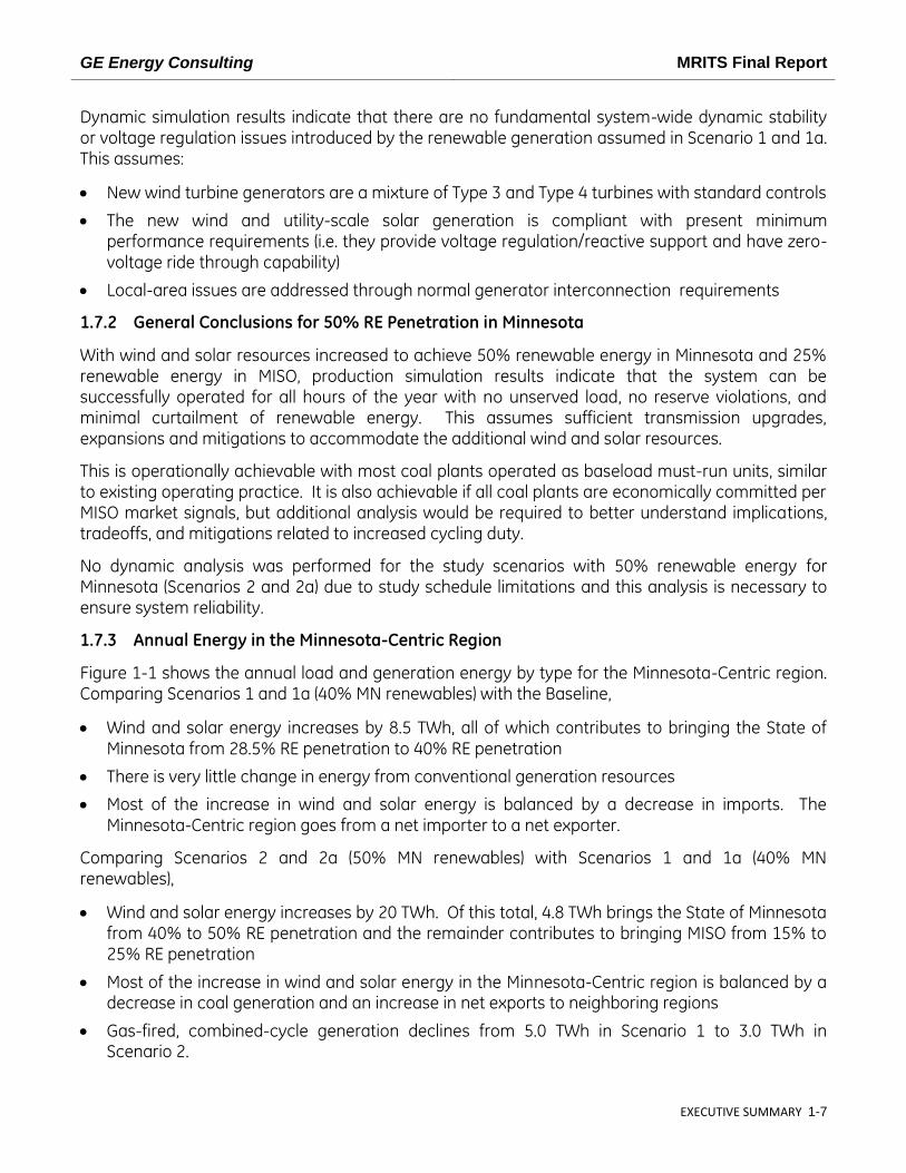


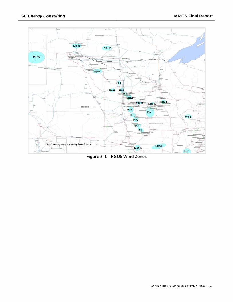


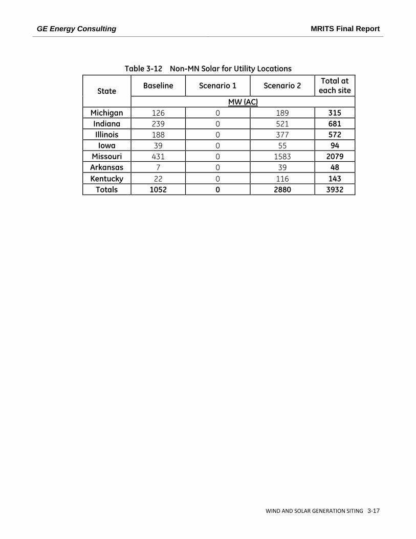


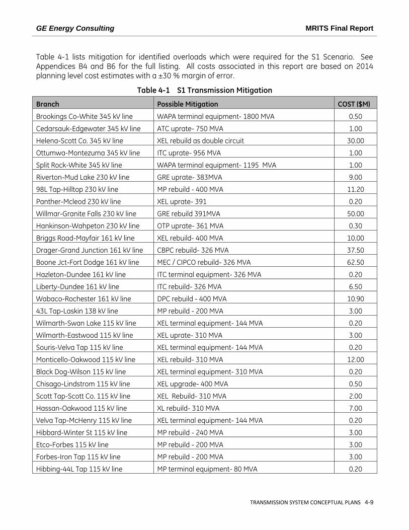


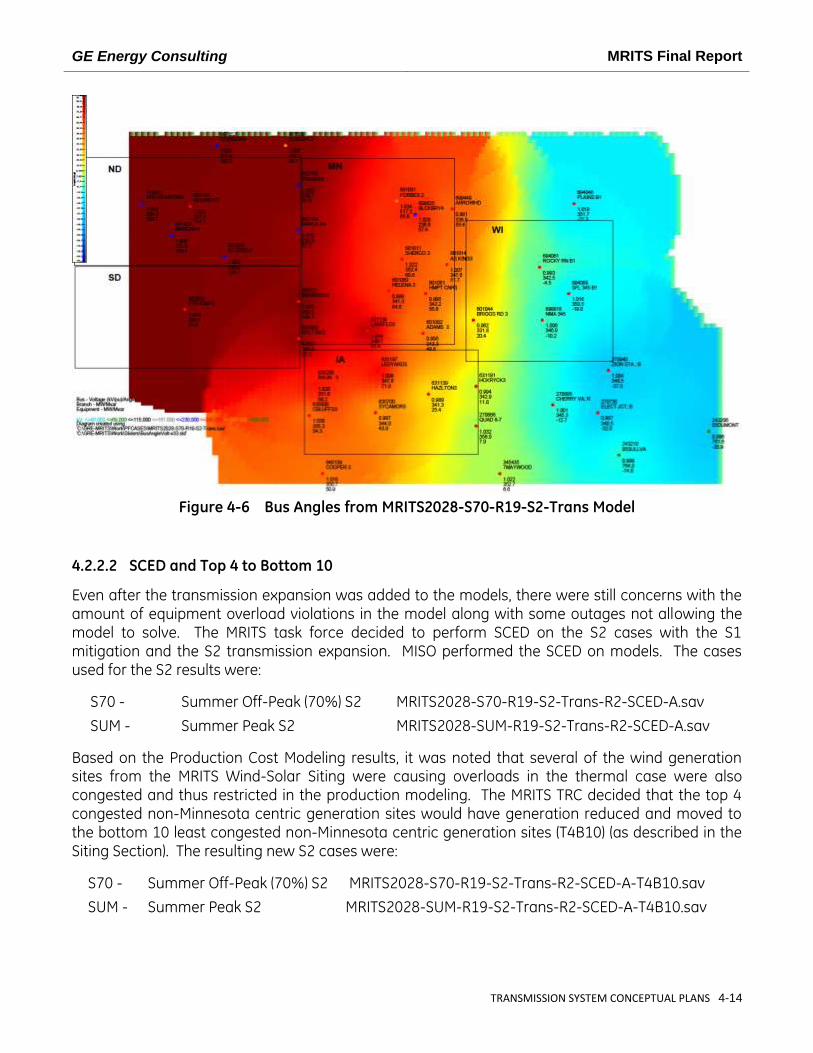


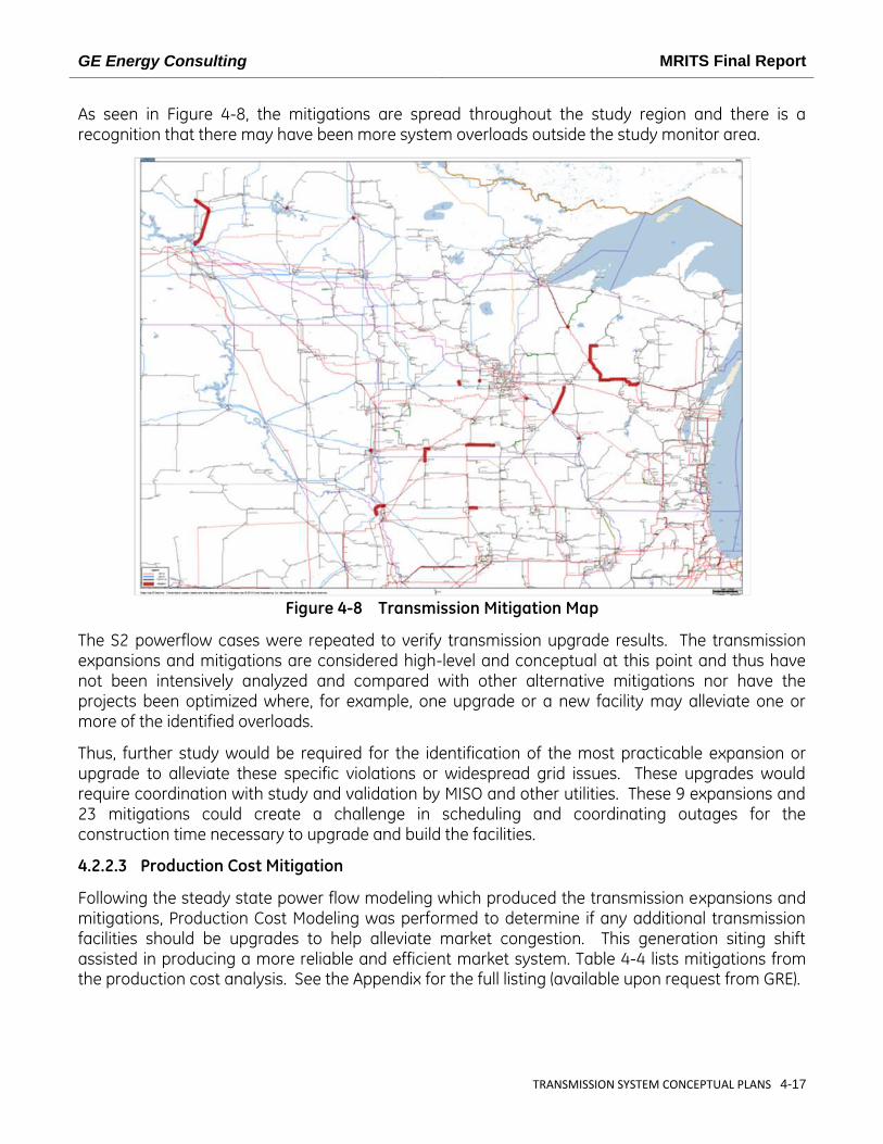


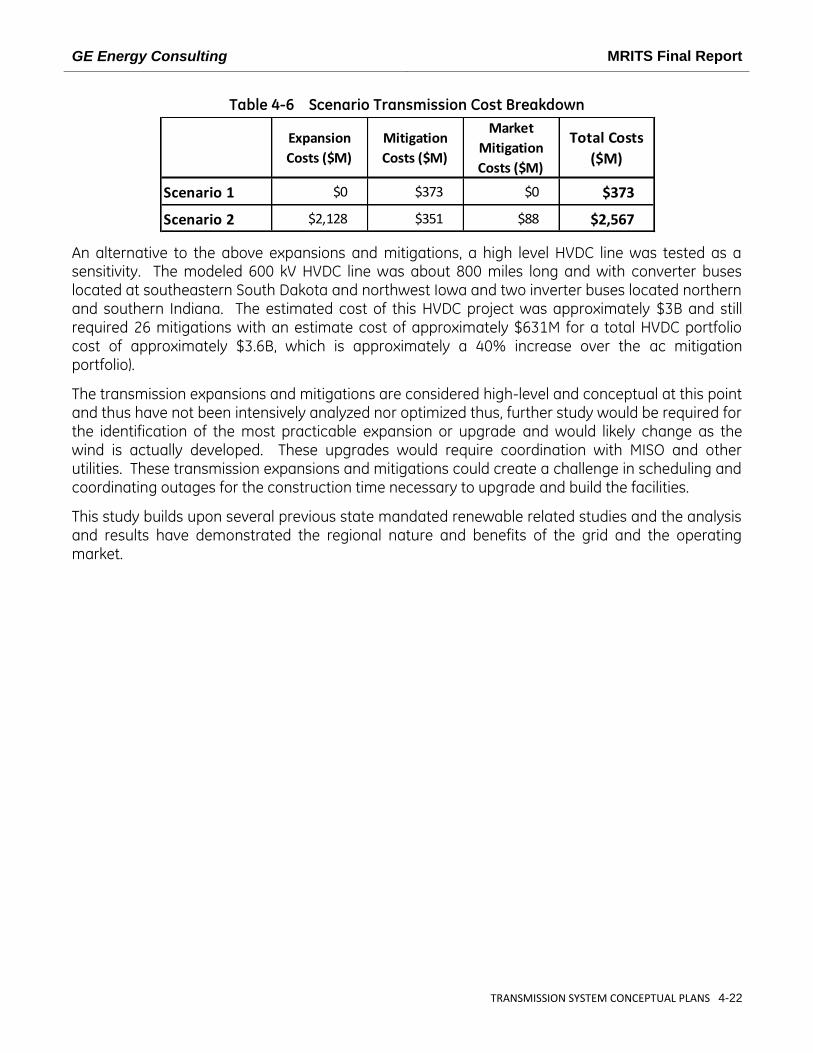


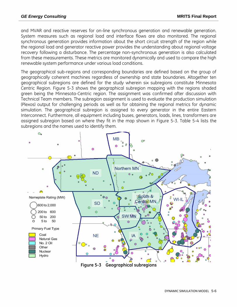


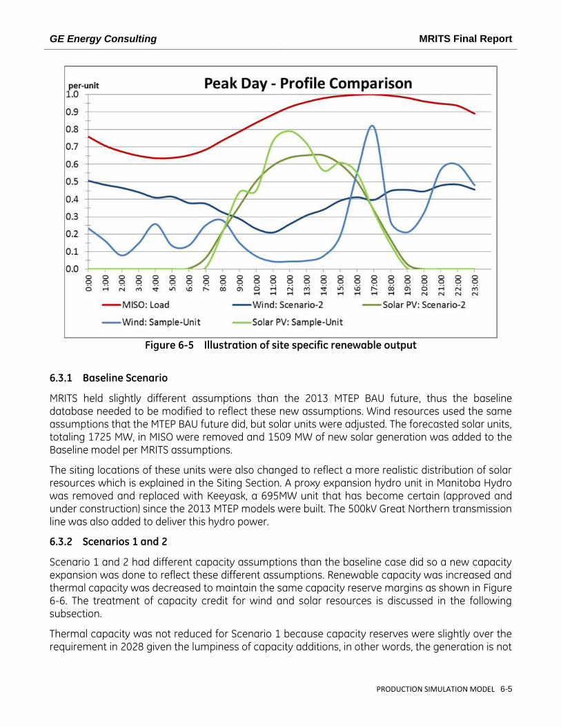
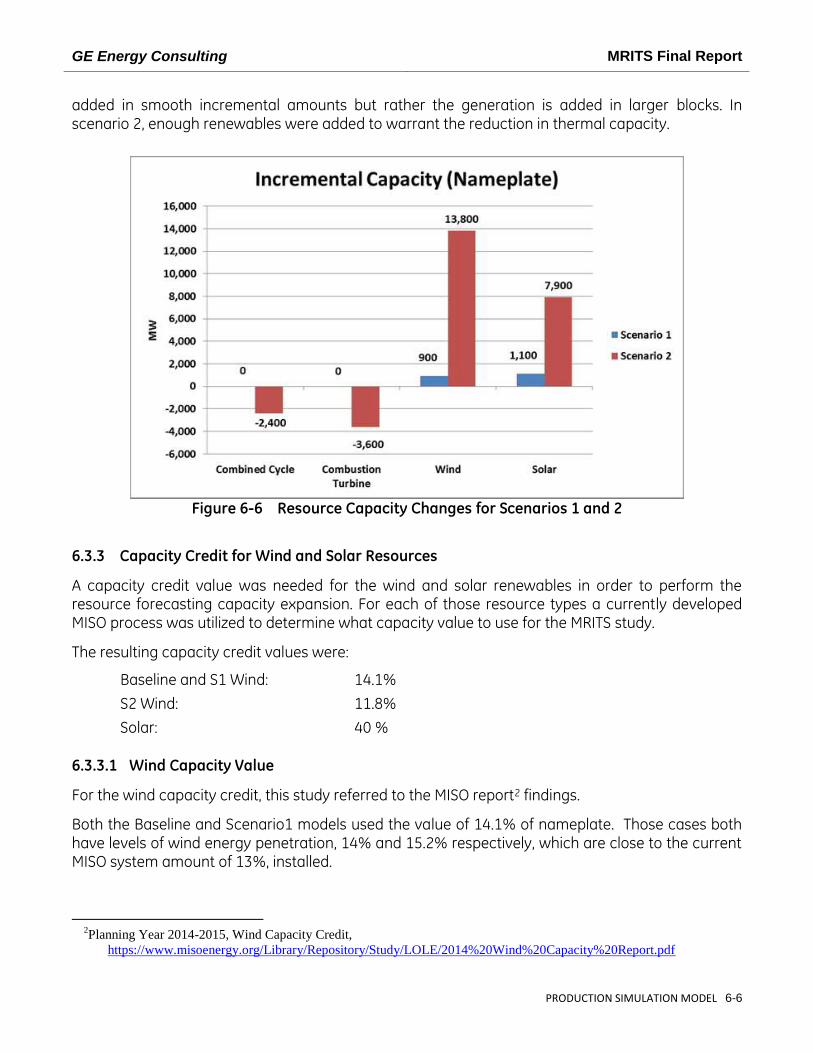


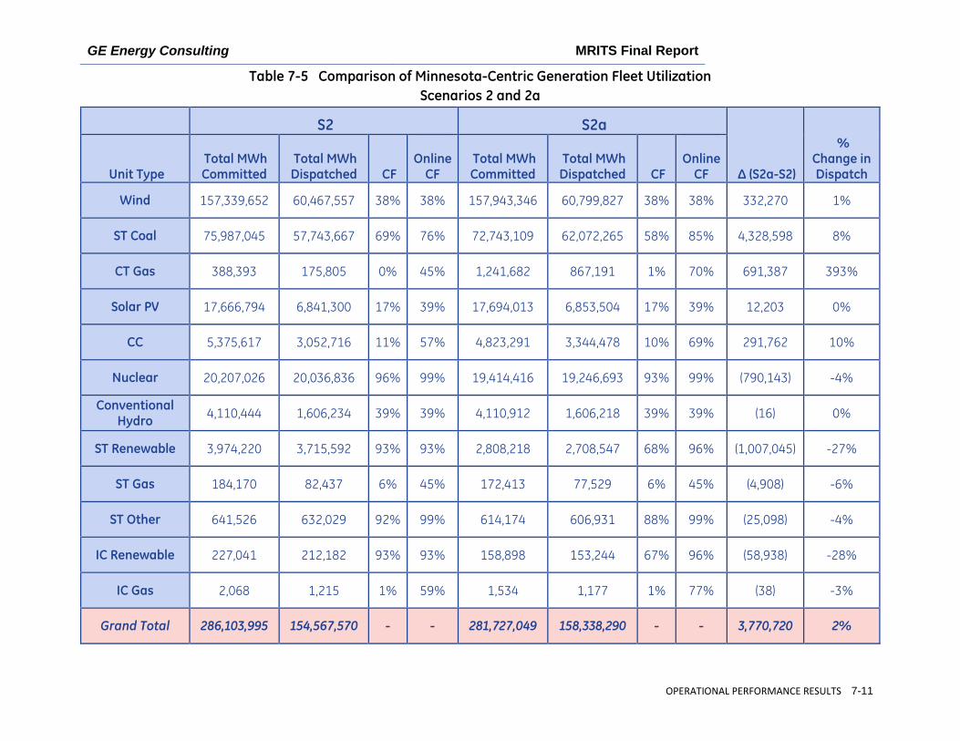


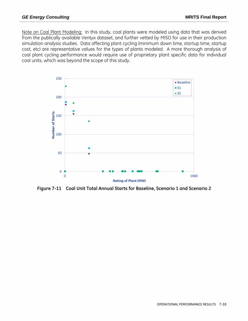


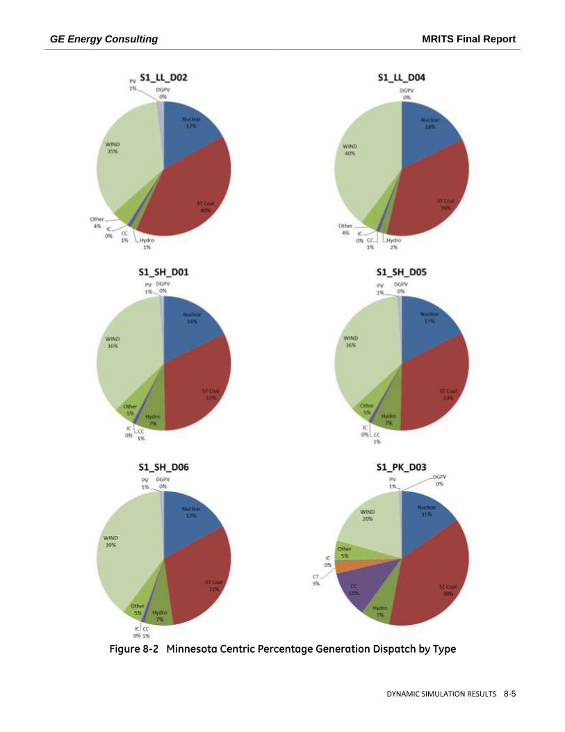


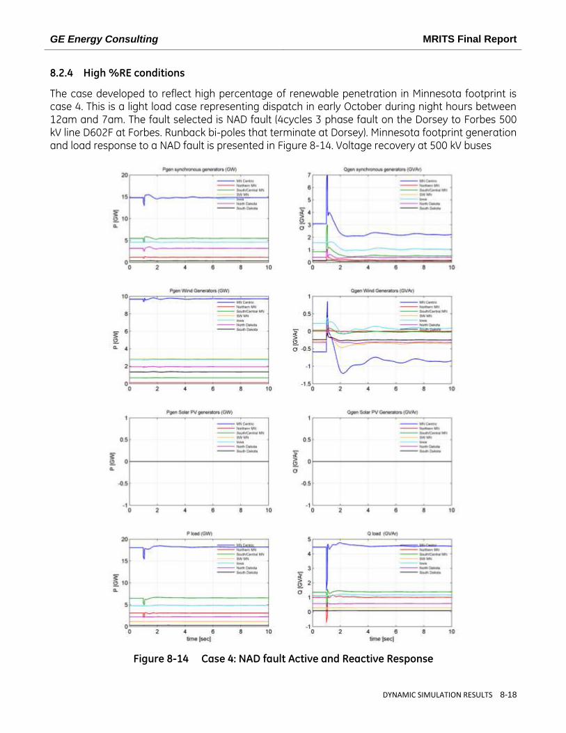


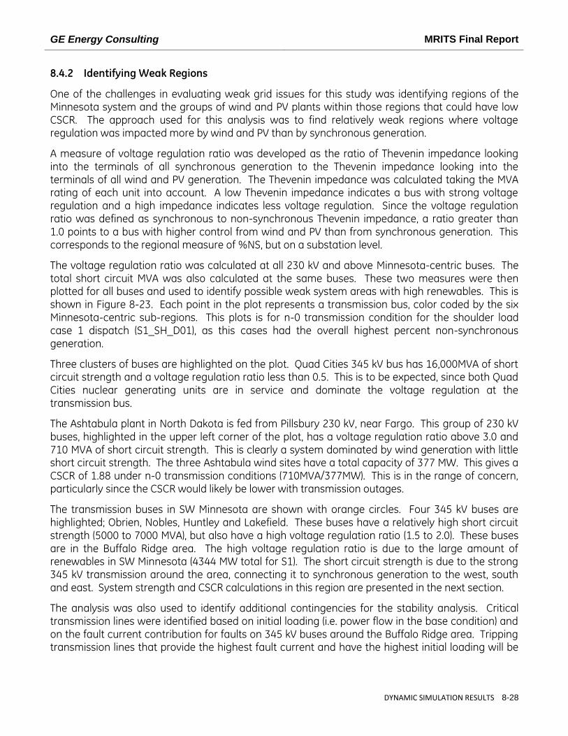


Related Documents