Mining the Social Web - Lecture 3 - T61.6020

Mining the Social Web

Aris%des Gionis Michael Mathioudakis

[email protected] Aalto University

Spring 2015

Mining the Social Web -‐ Aalto -‐ 2015 2

T-61.6020: Mining the social web — lecture #2

structure of social networks

social networks and social-media data can berepresented as graphs (or networks)

how these graphs look like?

what is their structure

data contain additional information

(actions, interactions, dynamics, attributes,…)

mining this additional information as part ofthe network structure

6

T-61.6020: Mining the social web — lecture #2

community structure in social networks

12

dolphins network and its NPC

Community structure

dolphins network and its NCP(source [Leskovec et al., 2009])

Frieze, Gionis, Tsourakakis Algorithmic Techniques for Modeling and Mining Large Graphs 34 / 277

Previously on T.61-‐6020

structure and dynamics of social networks

what does a social network look like? how do social networks evolve over Hme?

how does informaHon spread? do users influence each other?

Figure 4: Top 50 threads in the news cycle with highest volume for the period Aug. 1 – Oct. 31, 2008. Each thread consists of all newsarticles and blog posts containing a textual variant of a particular quoted phrases. (Phrase variants for the two largest threads ineach week are shown as labels pointing to the corresponding thread.) The data is drawn as a stacked plot in which the thickness of thestrand corresponding to each thread indicates its volume over time. Interactive visualization is available at http://memetracker.org.

Figure 5: Temporal dynamics of top threads as generated by our model. Only two ingredients, namely imitation and a preference torecent threads, are enough to qualitatively reproduce the observed dynamics of the news cycle.

3. GLOBALANALYSIS: TEMPORALVARI-ATIONANDAPROBABILISTICMODEL

Having produced phrase clusters, we now construct the individ-ual elements of the news cycle. We define a thread associated witha given phrase cluster to be the set of all items (news articles orblog posts) containing some phrase from the cluster, and we thentrack all threads over time, considering both their individual tem-poral dynamics as well as their interactions with one another.Using our approach we completely automatically created and

also automatically labeled the plot in Figure 4, which depicts the50 largest threads for the three-month period Aug. 1 – Oct. 31. Itis drawn as a stacked plot, a style of visualization (see e.g. [16])in which the thickness of each strand corresponds to the volume ofthe corresponding thread over time, with the total area equal to thetotal volume. We see that the rising and falling pattern does in facttell us about the patterns by which blogs and the media successivelyfocus and defocus on common story lines.An important point to note at the outset is that the total number

of articles and posts, as well as the total number of quotes, is ap-proximately constant over all weekdays in our dataset. (Refer to [1]for the plots.) As a result, the temporal variation exhibited in Fig-ure 4 is not the result of variations in the overall amount of globalnews and blogging activity from one day to the next. Rather, the

periods when the upper envelope of the curve are high correspondto times when there is a greater degree of convergence on key sto-ries, while the low periods indicate that attention is more diffuse,spread out over many stories. There is a clear weekly pattern inthis (again, despite the relatively constant overall volume), withthe five large peaks between late August and late September corre-sponding, respectively, to the Democratic and Republican NationalConventions, the overwhelming volume of the “lipstick on a pig”thread, the beginning of peak public attention to the financial crisis,and the negotiations over the financial bailout plan. Notice how theplot captures the dynamics of the presidential campaign coverageat a very fine resolution. Spikes and the phrases pinpoint the exactevents and moments that triggered large amounts of attention.Moreover, we have evaluated competing baselines in which we

produce topic clusters using standard methods based on probabilis-tic term mixtures (e.g. [7, 8]).2 The clusters produced for this timeperiod correspond to much coarser divisions of the content (poli-tics, technology, movies, and a number of essentially unrecogniz-able clusters). This is consistent with our initial observation in Sec-tion 1 that topical clusters are working at a level of granularity dif-ferent from what is needed to talk about the news cycle. Similarly,producing clusters from the most linked-to documents [23] in the2As these do not scale to the size of the data we have here, we couldonly use a subset of 10,000 most highly linked-to articles.

threads dynamics

Today

poliHcs does network structure reflect poliHcal divisions?

can we infer poliHcal affiliaHon?

financial senHment

can twiLer predict the stock market? urban compuHng

what does online acHvity say about how we live in ciHes?


PoliHcs Online

www & ‘democraHzaHon’ of informaHon

ciHzen journalism (e.g. HaiH earthquake, Arab spring)

poliHcians and tradiHonal media

parHcipate, too


US PoliHcs & the Web

Websites -‐ 1996

(Email) -‐ 1998

Online Fund raising -‐ 2000

Blogs -‐ 2004

TwiLer & FB -‐ 2008

Jesse Ventura - MN governor



social media mining vs

tradiHonal poliHcal polls

new content & biases

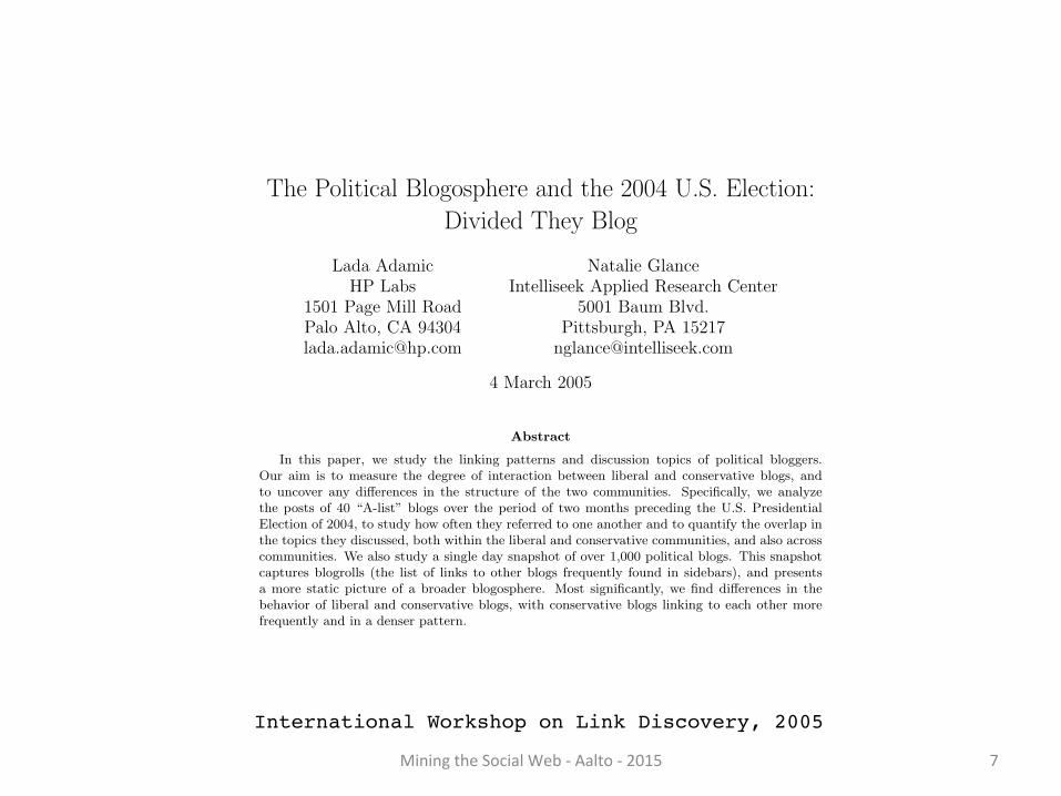
International Workshop on Link Discovery, 2005

The Political Blogosphere and the 2004 U.S. Election:

Divided They Blog

Lada AdamicHP Labs

1501 Page Mill RoadPalo Alto, CA [email protected]

Natalie GlanceIntelliseek Applied Research Center

5001 Baum Blvd.Pittsburgh, PA 15217

[email protected]

4 March 2005

Abstract

In this paper, we study the linking patterns and discussion topics of political bloggers.Our aim is to measure the degree of interaction between liberal and conservative blogs, andto uncover any differences in the structure of the two communities. Specifically, we analyzethe posts of 40 “A-list” blogs over the period of two months preceding the U.S. PresidentialElection of 2004, to study how often they referred to one another and to quantify the overlap inthe topics they discussed, both within the liberal and conservative communities, and also acrosscommunities. We also study a single day snapshot of over 1,000 political blogs. This snapshotcaptures blogrolls (the list of links to other blogs frequently found in sidebars), and presentsa more static picture of a broader blogosphere. Most significantly, we find differences in thebehavior of liberal and conservative blogs, with conservative blogs linking to each other morefrequently and in a denser pattern.

1 Introduction

The 2004 U.S. Presidential Election was the first Presidential Election in the United States in whichblogging played an important role. Although the term weblog was coined in 1997, it was not untilafter 9/11 that blogs gained readership and influence in the U.S. The next major trend in politicalblogging was “warblogging”: blogs centered around discussion of the invasion of Iraq by the U.S.1

The year 2004 saw a rapid rise in the popularity and proliferation of blogs. According to areport from the Pew Internet & American Life Project published in January 2005, 32 million U.S.citizens now read weblogs. However, 62% of online Americans still do not know what a weblogis.2 Another report from the same project showed that Americans are turning to the Internet inincreasing numbers to stay informed about politics: 63 million in mid-2004 vs. 30 million in March2000.3

A significant fraction of that traffic was directed specifically to blogs, with 9% of Internet userssaying they read political blogs “frequently” or “sometimes” during the campaign.4 Indeed, politicalblogs showed a large growth in traffic in the months preceding the election.5

Recognizing the importance of blogs, several candidates and political parties set up weblogsduring the 2004 U.S. Presidential campaign. Notably, Howard Dean’s campaign was particularly

1http://en.wikipedia.org/wiki/Weblog2http://www.pewinternet.org/PPF/r/144/report\ display.asp3http://www.pewinternet.org/PPF/r/141/report\ display.asp4http://www.pewinternet.org/pdfs/PIP blogging data.pdf5http://techcentralstation.com/011105B.html

1


Some History

before facebook and twiLer, there were blogs

rise a^er 9/11 ‘war-‐blogging’

2004

32 million US ciHzens read blogs 62% of US ciHzens do not know them


Jan 25, 2004


everyone talks with everyone?... or ‘echo chambers’?

In This Work...

task: extract network structure of poliHcal interacHons quesHon: one or separate communiHes? ...previous evidence on two blogs (Instapundit and Atrios) show ‘neighborhoods’ have no overlap in cited urls ...same with book purchases on amazon.com

on the other hand... ... it is now easier to interact


used blog directories for lists of poliHcal blogs parsed front page for links to discover more blogs

labeled them manually

only liberal & conservaHve

759 liberal & 735 conservaHve blogs


Data

Findings

Figure 1: Community structure of political blogs (expanded set), shown using utilizing a GEMlayout [11] in the GUESS[3] visualization and analysis tool. The colors reflect political orientation,red for conservative, and blue for liberal. Orange links go from liberal to conservative, and purpleones from conservative to liberal. The size of each blog reflects the number of other blogs that linkto it.

longer existed, or had moved to a different location. When looking at the front page of a blog we didnot make a distinction between blog references made in blogrolls (blogroll links) from those madein posts (post citations). This had the disadvantage of not differentiating between blogs that wereactively mentioned in a post on that day, from blogroll links that remain static over many weeks [10].Since posts usually contain sparse references to other blogs, and blogrolls usually contain dozens ofblogs, we assumed that the network obtained by crawling the front page of each blog would stronglyreflect blogroll links. 479 blogs had blogrolls through blogrolling.com, while many others simplymaintained a list of links to their favorite blogs. We did not include blogrolls placed on a secondarypage.

We constructed a citation network by identifying whether a URL present on the page of one blogreferences another political blog. We called a link found anywhere on a blog’s page, a “page link” todistinguish it from a “post citation”, a link to another blog that occurs strictly within a post. Figure 1shows the unmistakable division between the liberal and conservative political (blogo)spheres. Infact, 91% of the links originating within either the conservative or liberal communities stay withinthat community. An effect that may not be as apparent from the visualization is that even thoughwe started with a balanced set of blogs, conservative blogs show a greater tendency to link. 84%of conservative blogs link to at least one other blog, and 82% receive a link. In contrast, 74% ofliberal blogs link to another blog, while only 67% are linked to by another blog. So overall, we see aslightly higher tendency for conservative blogs to link. Liberal blogs linked to 13.6 blogs on average,while conservative blogs linked to an average of 15.1, and this difference is almost entirely due tothe higher proportion of liberal blogs with no links at all.

Although liberal blogs may not link as generously on average, the most popular liberal blogs,Daily Kos and Eschaton (atrios.blogspot.com), had 338 and 264 links from our single-day snapshot

4


Findings

100 101 102

10−2

10−1

100

incoming links (k)

fract

ion

of b

logs

with

at l

ast k

link

s

conservativeliberal

Lognormal fit

k−036 e−k/57

Figure 2: Cumulative distribution of incoming links for political blogs, separated by category. Asin [5] we find a lognormal, shown as a dashed line, to be a fairly good fit. A power-law with anexponential cutoff, shown as a solid line, is an even better fit.

of political blogs. This is on par with the 277 links received by the most linked to conservativeblog Instapundit. Figure 2 shows that, as is common in nearly every large subset of sites on theweb [1, 8, 12], the distribution of inlinks is highly uneven, with a few blogs of either persuasionhaving over a hundred incoming links, while hundreds of blogs have just one or two.

A small handful of blogs command a significant fraction of the attention, and it is these blogsthat we will be analyzing in more detail in the following sections. We will return to a descriptiveanalysis of the larger set of blogs in 3.5.

2.2 Weblog selection

In order to perform both an in-depth analysis and minimize bias, we decided to work with the top20 conservative leaning and top 20 liberal leaning blogs, which we identified as follows. First we usedpage link counts to cull the top 100 or so conservative blogs and the top 100 liberal blogs from thelarger list of 1494 political weblogs. Next, we used BlogPulse’s index (www.blogpulse.com/search)of weblog posts to count up citations to this list of approximately 200 weblogs during the monthsof October and November 2004. Tables 1 and 2 show the citation count and overall rank among allweblogs for the top 20 lists.

It is interesting to note that the top 20 conservative leaning weblogs fall within the overall top44 most cited weblogs for this time period. In contrast, the top 20 liberal leaning blogs fall withinthe overall top 77. This is evidence that bloggers in general link to conservative blogs more than toliberal blogs. Might bloggers “en masse” have predicted the outcome of the election after all?

These lists have some notable omissions. For example, we chose not to include drudgereport.com,which had received 7813 blog post citations during Sep. - Oct. 2004, because of its unusual formatand primary function as a mainstream news filter. We also omitted democraticunderground.com,which is principally a message board and secondarily a weblog.

In Tables 1 and 2 we have also included the number of page links from the larger set of liberaland conservative blogs in February of 2005 to the top ranked blogs. The page link counts serve bothto validate the popularity of the blogs and to show that the writings of a few bloggers, like AndrewSullivan and Wonkette have across the board appeal, while most others are read almost exclusively byeither the right or the left. It is immediately apparent that page link counts do not produce exactly

5

1 2

3

456

78

910

11

1213

1415

16

1718

19

20

21

22 2324

2526

27

2829 30

3132

3334 35 36

37 38 39

40

1 Digbys Blog2 James Walcott3 Pandagon4 blog.johnkerry.com5 Oliver Willis6 America Blog7 Crooked Timber8 Daily Kos9 American Prospect10 Eschaton11 Wonkette12 Talk Left13 Political Wire14 Talking Points Memo15 Matthew Yglesias16 Washington Monthly17 MyDD18 Juan Cole19 Left Coaster20 Bradford DeLong

21 JawaReport22 Voka Pundit23 Roger L Simon24 Tim Blair25 Andrew Sullivan26 Instapundit27 Blogs for Bush28 Little Green Footballs29 Belmont Club30 Captain’s Quarters31 Powerline32 Hugh Hewitt33 INDC Journal34 Real Clear Politics35 Winds of Change36 Allahpundit37 Michelle Malkin38 WizBang39 Dean’s World40 Volokh

(C)

(B)

(A)

Figure 3: Aggregate citation behavior prior to the 2004 election. Blogs are colored according topolitical orientation, and the size of the circle reflects how many citations from the top 40 the bloghas received. The thickness of the line reflects the number of citations between two blogs. (A) Alldirected edges are shown. (B) Edges having fewer than 5 citations in either or both directions areremoved. (C) Edges having fewer than 25 combined citations are removed.

9


similar picture for top 20 blogs

small number of blogs aLract most links

0 200 400 600 800 1000 1200 1400 1600

nytimes.comwashingtonpost.com

news.yahoo.commsnbc.msn.com

nationalreview.comcnn.com

latimes.comboston.com

usatoday.comwashingtontimes.comapnews.myway.com

guardian.co.ukfoxnews.comcbsnews.comslate.msn.com

nypost.comnews.bbc.co.uk

tnr.comopinionjournal.com

online.wsj.comsalon.com

# citations from weblog posts

Left

Right

Figure 4: Most linked to news sources by the top 20 conservative and top 20 liberal blogs during8/29/2004 - 11/15/2004.

1. CBS News poll of uncommitted voters shows Kerry winning 43% to 28%

2. Sun Times article: Bob Novak predicts that George Bush will retreat from Iraq if reelected

3. CBS News article on forged memos

4. New York Daily News article on Osama Bin Laden videotope, “gift” for the President

5. Time Magazine poll: Bush opens double-digit lead on post convention bounce

In contrast, the top news articles cited by right leaning bloggers are:



3. National Review article refuting the case about missing explosives

4. ABC News article refuting the case about missing explosives

5. Washington Post article reporting on Kerry’s proposal to allow Iran to keep its nuclear powerplants in exchange for giving up the right to retain the nuclear fuel that could be used forbomb-making

A time series chart further shows how quickly and strongly conservative bloggers responded toforged CBS documents (Figure 5). The conservative bloggers saw Dan Rather’s report as an attemptby the left to discredit President Bush. They acted quickly to debunk the report, with the chargeled by PowerLine and seconded by Wizbangblog and others. In contrast, the pick-up among liberalbloggers occurred later, with lower volume. The most vocal left leaning bloggers on the subject wereTalkLeft and AMERICAblog.

11

0 200 400 600 800 1000 1200 1400 1600











Left

Right














11


Findings 0 200 400 600 800 1000 1200 1400 1600











Left

Right














11

top 20 blogs news links

0 20 40 60 80 100 120 140

buzzflash.comcursor.org

mediamatters.orgcommondreams.org

alternet.orgairamericaradio.co

salon.comthenation.comtheonion.com

guardian.co.uknytimes.com

news.google.comwashingtonpost.com

cnn.comfoxnews.com

weeklystandard.comcommand-post.org

townhall.comopinionjournal.comnationalreview.com

number of blogs linking

Left

Right

Figure 7: Most linked to news sources (online and off), showing proportionally how many liberaland conservative blogs link to them.

and Rush Limbuagh (3,29). They link to the GOP site (0,37) and are influenced by conservativethink-tanks: the Heritage Foundation (1,33) and the Cato Institute (3,25).

4 Conclusions and Future Work

In our study we witnessed a divided blogosphere: liberals and conservatives linking primarily withintheir separate communities, with far fewer cross-links exchanged between them. This division ex-tended into their discussions, with liberal and conservative blogs focusing on different news articles,topics, and political figures. An interesting pattern that emerged was that conservative bloggerswere more likely to link to other blogs: primarily other conservative blogs, but also some liberalones. But while the conservative blogosphere was more densely linked, we did not detect a greateruniformity in the news and topics discussed by conservatives.

There are still many questions that we would like to explore regarding the political bloggingcommunity. Some would involve extending our current methods, and others would take us furtherinto the intricate behavior of the blogosphere. As a refinement of our current approach, we wouldlike to differentiate between blogs written by a single author and those written by multiple con-tributors. Our experiments treated individual blogs as if they were each written by one authorwith a single voice, point of view and patterns of language use and linking behavior. However,while single author weblogs are more common than collaborative blogs, a number of the blogs inour two top 20 lists have (or had) multiple authors, for example: blog.johnkerry.com, crookedtim-ber.org, pandagon.net, deanesmay.com, powerlineblog.com, blogsforbush.com, dailykos.com, wiz-

14


Findings all blogs

links to other websites

Summary

quesHon: one or separate communiHes? data: 1.5k blogs, manually labeled methodology: simple link analysis impact: showed divide in ‘online’ world reproducibility: ?


Political Polarization on Twitter

M. D. Conover, J. Ratkiewicz, M. Francisco, B. Goncalves, A. Flammini, F. MenczerCenter for Complex Networks and Systems Research

School of Informatics and ComputingIndiana University, Bloomington, IN, USA

Abstract

In this study we investigate how social media shape thenetworked public sphere and facilitate communication be-tween communities with different political orientations. Weexamine two networks of political communication on Twit-ter, comprised of more than 250,000 tweets from the sixweeks leading up to the 2010 U.S. congressional midtermelections. Using a combination of network clustering algo-rithms and manually-annotated data we demonstrate that thenetwork of political retweets exhibits a highly segregated par-tisan structure, with extremely limited connectivity betweenleft- and right-leaning users. Surprisingly this is not the casefor the user-to-user mention network, which is dominated bya single politically heterogeneous cluster of users in whichideologically-opposed individuals interact at a much higherrate compared to the network of retweets. To explain the dis-tinct topologies of the retweet and mention networks we con-jecture that politically motivated individuals provoke inter-action by injecting partisan content into information streamswhose primary audience consists of ideologically-opposedusers. We conclude with statistical evidence in support of thishypothesis.

1 IntroductionSocial media play an important role in shaping political dis-course in the U.S. and around the world (Bennett 2003;Benkler 2006; Sunstein 2007; Farrell and Drezner 2008;Aday et al. 2010; Tumasjan et al. 2010; O’Connor et al.2010). According to the Pew Internet and American LifeProject, six in ten U.S. internet users, nearly 44% of Amer-ican adults, went online to get news or information aboutpolitics in 2008. Additionally, Americans are taking an ac-tive role in online political discourse, with 20% of internetusers contributing comments or questions about the politi-cal process to social networking sites, blogs or other onlineforums (Pew Internet and American Life Project 2008).

Despite this, some empirical evidence suggests that politi-cally active web users tend to organize into insular, homoge-nous communities segregated along partisan lines. Adamicand Glance (2005) famously demonstrated that politicalblogs preferentially link to other blogs of the same politi-cal ideology, a finding supported by the work of Hargittai,

Copyright c⃝ 2011, Association for the Advancement of ArtificialIntelligence (www.aaai.org). All rights reserved.

Gallo, and Kane (2007). Consumers of online political in-formation tend to behave similarly, choosing to read blogsthat share their political beliefs, with 26% more users do-ing so in 2008 than 2004 (Pew Internet and American LifeProject 2008).

In its own right, the formation of online communities isnot necessarily a serious problem. The concern is that whenpolitically active individuals can avoid people and informa-tion they would not have chosen in advance, their opinionsare likely to become increasingly extreme as a result of beingexposed to more homogeneous viewpoints and fewer credi-ble opposing opinions. The implications for the political pro-cess in this case are clear. A deliberative democracy relies ona broadly informed public and a healthy ecosystem of com-peting ideas. If individuals are exposed exclusively to peopleor facts that reinforce their pre-existing beliefs, democracysuffers (Sunstein 2002; 2007).

In this study we examine networks of political commu-nication on the Twitter microblogging service during thesix weeks prior to the 2010 U.S. midterm elections. Sam-pling data from the Twitter ‘gardenhose’ API, we identi-fied 250,000 politically relevant messages (tweets) producedby more than 45,000 users. From these tweets we isolatedtwo networks of political communication — the retweetnetwork, in which users are connected if one has rebroad-cast content produced by another, and the mention network,where users are connected if one has mentioned another in apost, including the case of tweet replies.

We demonstrate that the retweet network exhibits a highlymodular structure, segregating users into two homogenouscommunities corresponding to the political left and right. Incontrast, we find that the mention network does not exhibitthis kind of political segregation, resulting in users being ex-posed to individuals and information they would not havebeen likely to choose in advance.

Finally, we provide evidence that these network structuresresult in part from politically motivated individuals annotat-ing tweets with multiple hashtags whose primary audiencesconsist of ideologically-opposed users, a behavior also doc-umented in the work of Yardi and boyd (2010). We arguethat this process results in users being exposed to contentthey are not likely to rebroadcast, but to which they mayrespond using mentions, and provide statistical evidence insupport of this hypothesis.

89

Proceedings of the Fifth International AAAI Conference on Weblogs and Social Media


International Conference on Weblogs and Social Media (ICWSM) 2011

In This Work...

quesHon check if same paLern holds in twiLer

however

retweets and men8ons instead of links


Data


6 weeks of tweets before US 2010 elecHons

to disHnguish poliHcal tweets 1.  parse all tweets (355 million) 2.  select subset with hashtags #p2 and #tcot 3.  find frequently co-‐occuring hashtags (66) 4.  keep tweets that contain those hashtags >> 250k tweets

The major contributions of this work are:• Creation and release of a network and text dataset derived

from more than 250,000 politically-related Twitter postsauthored in the weeks preceeding the 2010 U.S. midtermelections (§ 2).

• Cluster analysis of networks derived from this corpusshowing that the network of retweet exhibits clear seg-regation, while the mention network is dominated by asingle large community (§ 3.1).

• Manual classification of Twitter users by political align-ment, demonstrating that the retweet network clusters cor-respond to the political left and right. These data alsoshow the mention network to be politically heteroge-neous, with users of opposing political views interactingat a much higher rate than in the retweet network (§ 3.3).

• An interpretation of the observed community structuresbased on injection of partisan content into ideologicallyopposed hashtag information streams (§ 4).

2 Data and Methods2.1 The Twitter PlatformTwitter is a popular social networking and microbloggingsite where users can post 140-character messages, or tweets.Apart from broadcasting tweets to an audience of followers,Twitter users can interact with one another in two primarypublic ways: retweets and mentions. Retweets act as a formof endorsement, allowing individuals to rebroadcast contentgenerated by other users, thereby raising the content’s vis-ibility (boyd, Golder, and Lotan 2008). Mentions functiondifferently, allowing someone to address a specific user di-rectly through the public feed, or, to a lesser extent, referto an individual in the third person (Honeycutt and Herring2008). These two means of communication —retweets andmentions— serve distinct and complementary purposes, to-gether acting as the primary mechanisms for explicit, publicuser-user interaction on Twitter.

Hashtags are another important feature of the Twitter plat-form. They allow users to annotate tweets with metadataspecifying the topic or intended audience of a communica-tion. For example, #dadt stands for “Don’t Ask Don’t Tell”and #jlot for “Jewish Libertarians on Twitter.” Each hash-tag identifies a stream of content, with users’ tag choices de-noting participation in different information channels.

The present analysis leverages data collected from theTwitter ‘gardenhose’ API (dev.twitter.com/pages/streaming_api) between September 14th and Novem-ber 1st, 2010 — the run-up to the November 4th U.S.congressional midterm elections. During the six weeks ofdata collection we observed approximately 355 milliontweets. Our analysis utilizes an infrastructure and website(truthy.indiana.edu) designed to analyze the spreadof information on Twitter, with special focus on politicalcontent (Ratkiewicz et al. 2011).

2.2 Identifying Political ContentLet us define a political communication as any tweet con-taining at least one politically relevant hashtag. To identify

Table 1: Hashtags related to #p2, #tcot, or both. Tweetscontaining any of these were included in our sample.

Just #p2 #casen #dadt #dc10210 #democrats #du1

#fem2 #gotv #kysen #lgf #ofa #onenation

#p2b #pledge #rebelleft #truthout #vote

#vote2010 #whyimvotingdemocrat #youcut

Both #cspj #dem #dems #desen #gop #hcr

#nvsen #obama #ocra #p2 #p21 #phnm

#politics #sgp #tcot #teaparty #tlot

#topprog #tpp #twisters #votedem

Just #tcot #912 #ampat #ftrs #glennbeck #hhrs

#iamthemob #ma04 #mapoli #palin

#palin12 #spwbt #tsot #tweetcongress

#ucot #wethepeople

Table 2: Hashtags excluded from the analysis due to ambigu-ous or overly broad meaning.

Excl. from #p2 #economy #gay #glbt #us #wc #lgbt

Excl. from both #israel #rs

Excl. from #tcot #news #qsn #politicalhumor

an appropriate set of political hashtags and to avoid intro-ducing bias into the sample, we performed a simple tagco-occurrence discovery procedure. We began by seedingour sample with the two most popular political hashtags,#p2 (“Progressives 2.0”) and #tcot (“Top Conservativeson Twitter”). For each seed we identified the set of hashtagswith which it co-occurred in at least one tweet, and rankedthe results using the Jaccard coefficient. For a set of tweets Scontaining a seed hashtag, and a set of tweets T containinganother hashtag, the Jaccard coefficient between S and T is

σ(S, T ) =|S ∩ T ||S ∪ T | . (1)

Thus, when the tweets in which both seed and hashtag oc-cur make up a large portion of the tweets in which eitheroccurs, the two are deemed to be related. Using a similar-ity threshold of 0.005 we identified 66 unique hashtags (Ta-ble 1), eleven of which we excluded due to overly-broad orambiguous meaning (Table 2). This process resulted in a cor-pus of 252,300 politically relevant tweets. There is substan-tial overlap between streams associated with different po-litical hashtags because many tweets contain multiple hash-tags. As a result, lowering the similarity threshold leads toonly modest increases in the number of political tweets inour sample — which do not substantially affect the resultsof our analysis — while introducing unrelated hashtags.

2.3 Political Communication NetworksFrom the tweets containing any of the politically rele-vant hashtags we constructed networks representing politicalcommunication among Twitter users. Focusing on the twoprimary modes of public user-user interaction, mentions andretweets, we define communication links in the followingways. In the retweet network an edge runs from a node rep-resenting user A to a node representing user B if B retweets

90

Extract Networks


node u node v

v retweets u

u menHons v

two networks

clustering 1. max modularity for two clusters

to assign iniHal labels to nodes (a and b) 2. label propagaHon

re-‐assign nodes to label of most neighbors unHl no change

Findings

Figure 1: The political retweet (left) and mention (right) networks, laid out using a force-directed algorithm. Node colors reflectcluster assignments (see § 3.1). Community structure is evident in the retweet network, but less so in the mention network. Weshow in § 3.3 that in the retweet network, the red cluster A is made of 93% right-leaning users, while the blue cluster B is madeof 80% left-leaning users.

tive Twitter users. This structural difference is of particularimportance with respect to political communication, as wenow have statistical evidence to suggest that mentions andreplies may serve as a conduit through which users are ex-posed to information and opinions they might not choose inadvance. Despite this promising finding, the work of Yardiand boyd (2010) suggests that cross-ideological interactionsmay reinforce pre-existing in-group/out-group identities, ex-acerbating the problem of political polarization.

3.2 Content HomogeneityThe clustering described above was based only on the net-work properties of the retweet and mention graphs. An inter-esting question, therefore, is whether it has any significancein terms of the actual content of the discussions involved.To address this issue we associate each user with a profilevector containing all the hashtags in her tweets, weighted bytheir frequencies. We can then compute the cosine similari-ties between each pair of user profiles, separately for usersin the same cluster and users in different clusters. Figure 2shows that in the mention network, users placed in the samecluster are not likely to be much more similar to each otherthan users in different clusters. On the other hand, in theretweet network, users in cluster A are more likely to havevery similar profiles than users in cluster B, and users in dif-ferent clusters are the least similar to each other. As a resultthe average similarity within retweet clusters is higher thanacross clusters. Further, we note that in both mention andretweet networks, one of the clusters is more cohesive thanthe other — meaning the tag usage within one community ismore homogeneous.

Retweet MentionA↔A 0.31 0.31B↔B 0.20 0.22A↔B 0.13 0.26 10-1

100

101

0 0.2 0.4 0.6 0.8 1

P(c

os(

a, b))

cos(a, b)

Clusters ACluster B

Different clusters

Figure 2: Cosine similarities among user profiles. The tableon the left shows the average similarities in the retweet andmention networks for pairs of users both in cluster A, both incluster B, and for users in different clusters. All differencesare significant at the 95% confidence level. The plot on theright displays the actual distributions of cosine similaritiesfor the retweet network.

3.3 Political PolarizationGiven the communities of the retweet network identified in§ 3.1, their content homogeneity uncovered in § 3.2, andthe findings of previous studies, it is natural to investigatewhether the clusters in the retweet network correspond togroups of users of similar political alignment.

To accomplish this in a systematic, reproducible way weused a set of techniques from the social sciences knownas qualitative content analysis (Krippendorff 2004; Kolbe1991). Similar to assigning class labels to training data in su-pervised machine learning, content analysis defines a set ofpractices that enable social scientists to define reproduciblecategories for qualitative features of text. Next we outlineour annotation categories, and then explain the procedures

92

retweets men%ons


separate clusters for retweets one big cluster for men8ons

Summary

quesHon: does network structure reflect poliHcal divisions data: 250k poliHcal tweets before US 2010 elecHons methodology: clustering & label propagaHon impact: showed different modes of interacHon between

individuals in same & different sides reproducibility: data are online -‐-‐

http://truthy.indiana.edu/projects/data-and-software.html



This network graph details the landscape of Twi=er handles responding to the UNWRA school bombing.

Source: https://medium.com/i-data/israel-gaza-war-data-a54969aeb23e


Instagram co-‐tag graph, highligh8ng three dis8nct topical communi8es: 1) pro-‐Israeli (Orange), 2) pro-‐Pales8nian

(Yellow), and 3) Religious / muslim (Purple)

Source: https://medium.com/i-data/israel-gaza-war-data-a54969aeb23e



Classifying Political Orientation on Twitter: It’s Not Easy!

Raviv Cohen and Derek RuthsSchool of Computer Science

McGill [email protected], [email protected]

AbstractNumerous papers have reported great success at infer-ring the political orientation of Twitter users. This paperhas some unfortunate news to deliver: while past workhas been sound and often methodologically novel, wehave discovered that reported accuracies have been sys-temically overoptimistic due to the way in which vali-dation datasets have been collected, reporting accuracylevels nearly 30% higher than can be expected in popu-lations of general Twitter users.Using careful and novel data collection and annotationtechniques, we collected three different sets of Twitterusers, each characterizing a different degree of politicalengagement on Twitter — from politicians (highly po-litically vocal) to “normal” users (those who rarely dis-cuss politics). Applying standard techniques for infer-ring political orientation, we show that methods whichpreviously reported greater than 90% inference accu-racy, actually achieve barely 65% accuracy on normalusers. We also show that classifiers cannot be used toclassify users outside the narrow range of political ori-entation on which they were trained.While a sobering finding, our results quantify and callattention to overlooked problems in the latent attributeinference literature that, no doubt, extend beyond polit-ical orientation inference: the way in which datasets areassembled and the transferability of classifiers.

IntroductionMuch of the promise of online social media studies, analyt-ics, and commerce depends on knowing various attributesof individual and groups of users. For a variety of reasons,few intrinsic attributes of individuals are explicitly revealedin their user account profiles. As a result, latent attribute in-ference, the computational discovery of “hidden” attributes,has become a topic of significant interest among social me-dia researchers and to industries built around utilizing andmonetizing online social content. Most existing work hasfocused around the Twitter platform due to the widespreadadoption of the service and the tendency of its users to keeptheir accounts public.

Existing work on latent attribute inference in the Twit-ter context has made progress on a number of attributes

Copyright c� 2013, Association for the Advancement of ArtificialIntelligence (www.aaai.org). All rights reserved.

including gender, age, education, political orientation, andeven coffee preferences (Zamal, Liu, and Ruths 2012;Conover et al. 2011b; 2011a; Rao and Yarowsky 2010;Pennacchiotti and Popescu 2011; Wong et al. 2013; Liu andRuths 2013; Golbeck and Hansen 2011; Burger, Henderson,and Zarrella 2011). In general, inference algorithms haveachieved accuracy rates in the range of 85%, but have strug-gled to improve beyond this point. To date, the great suc-cess story of this area is political orientation inference forwhich a number of papers have boasted inference accuracyreaching and even surpassing 90% (Conover et al. 2011b;Zamal, Liu, and Ruths 2012).

By any reasonable measure, the existing work on politicalorientation is sound and represents a sincere and successfuleffort to advance the technology of latent attribute inference.Furthermore, a number of the works have yielded notableinsights into the nature of political orientation in online en-vironments (Conover et al. 2011b; 2011a). In this paper, weexamine the question of whether existing political orienta-tion inference systems actual perform as well as reported onthe general Twitter population. Our findings indicate that,without exception, they do not, even when the general pop-ulation consider is restricted only to those who discuss pol-itics (since inferring the political orientation of a user whonever speaks about politics is, certainly, very hard if not im-possible).

We consider this an important question and finding fortwo reasons. Foremost, nearly all applications of latent at-tribute inference involve its use on large populations of un-known users. As a result, quantifying its performance on thegeneral Twitter population is arguably the best way of eval-uating its practical utility. Second, the existing literature onthis topic reports its accuracy in inferring political orienta-tion without qualification or caveats (author’s note: includ-ing our own past work on the topic (Zamal, Liu, and Ruths2012)). To the reader uninitiated in latent attribute inference,these performance claims can easily be taken to be an asser-tion about the performance of the system under general con-ditions. In fact, we suspect that most authors of these workshad similar assumptions in mind (author’s note: we did!).Regardless of intentions, as we will show, past systems werenot evaluated under general conditions and, therefore, theperformance reported is not representative of the general usecase for the systems.

Proceedings of the Seventh International AAAI Conference on Weblogs and Social Media

91

In This Work...

task: classify poliHcal orientaHon on twiLer goal: invesHgate claims of previous work

previous work

high classificaHon accuracy but was the task too easy? heavily poliHcal user accounts

what about ‘modestly poliHcal’ users?


Data

3 datasets PoliHcal Figures PoliHcally AcHve PoliHcally Modest


collecting the k most discriminating items of that type (e.g.hashtags) for each label (e.g., Republicans and Democrats).Thus, k-top words is actually 2k features: k words fromRepublicans and k words from Democrats. For furtherdetails on these features, we refer the reader to the originalpaper (Zamal, Liu, and Ruths 2012).

For the purposes of this study, we primarily employedan SVM classifier based on (Zamal, Liu, and Ruths 2012).While this method did not achieve the best performance todate (93% vs. 95%), it was benchmarked on a less restric-tive dataset than (Conover et al. 2011b) which likely con-tributed to the small different in performance. Furthermore,because it incorporates nearly all features from work thatpreceded it, we considered it a more fair representation ofall existing systems proposed to date. Following prior work,a radial basis function was used as the SVM kernel. The costand � parameters were chosen using a grid search technique.The SVM itself was implemented using the library libSVM(Chang and Lin 2011).

We also evaluated the accuracy of a Labeled-LDA-basedclassifier, following work that shows how the LDA can beused on labeled data (Ramage et al. 2009; Ramage, Dumais,and Liebling 2010). Note that little work in latent attributeinference has used LDA-based classifiers alone. We appliedit here primarily as a way of characterizing the lexical di-versity of different datasets. We used a Labeled-LDA imple-mentation available in Scala as part of the Stanford Mod-eling Toolbox1. In evaluating the accuracy the LLDA, wefound it to be extremely similar to the SVM and, due tospace limitations, we do not report results for this classifierexcept as a means of characterizing the difference in topicspresent across the three datasets we considered. It is worthnoting that the similar accuracy achieved by both the LDAand the SVM methods allayed a concern we had about theSVM’s use of only top-discriminating features. The LDA,by construction, employs all words present in the corpus.Thus, if additional accuracy could be gained by incorporat-ing less discriminating words, presumably this would havemanifested as significant improvement in the LDA perfor-mance. This was not observed under any of the conditionsconsidered in this study.

Construction of Testing DatasetsAs mentioned earlier, the goal of this study was to evaluatethe extent to which the dataset selection criteria influencedthe performance of political orientation classifiers. In partic-ular, our concern was to determine the performance of clas-sifiers on “ordinary” Twitter users.

Our definition of “ordinary” primarily concerned the ex-tent to which users employed political language in tweets.Our intuition was that very few Twitter users generate po-litically overt tweets. This intuition was proven out by thefraction of randomly sampled users who had even a singletweet with political content. Given this bias towards little, ifany, political commentary in Twitter, benchmarks based on

1http://nlp.stanford.edu/software/tmt/tmt-0.4

Table 1: Basic statistics on the different datasets used. Total sizeof the Figures dataset was limited by the number of federal levelpoliticians; size of the Modest dataset was limited by the numberof users that satisfied our stringent conditions - these were culledfrom a dataset of 10,000 random individuals.

Dataset Republicans Democrats TotalFigures 203 194 397Active 860 977 1837Modest 105 157 262Conover 107 89 196

politically verbose users would not properly gauge the per-formance of classifiers on the general population. Of course,the discovery that the political orientation of ordinary usersis harder to discern than that of political figures is hardlynews. How much harder it is, however, is quite important:this is the difference between the problem still being rathereasy and the problem of political orientation inference sud-denly being largely unsolved. As we have already indicated,our findings suggest the latter to a profound degree.

To conduct this study, we built three datasets which actedas proxies for populations with different degrees of overt po-litical orientation. Each dataset consisted of a set of Twitterusers whose political orientation was known with high con-fidence. The basic statistics for these datasets are shown inTable 1.

Political Figures Dataset (PFD). This dataset was in-tended to act as a baseline for the study. In many ways it alsoserved to proxy for datasets that were used in other paperssince, with the exception of the Conover 2011 dataset de-scribed below, we were unable to obtain or recreate datasetsdescribed and used in other papers (Conover et al. 2011b). Inprior work, the primary way for labeled political orientationdatasets to be built was by compiling a list of self-declaredRepublicans and Democrats. In surveying such lists, we ob-served that a (super)majority of the Twitter users were, infact, politicians. To mimic this design, we populated thisdataset entirely with state governors, federal-level senators,and federal-level representatives.

We created this dataset by scraping the official websitesof the US governors2, senators3, and representatives4. Thisprovided us a complete list of their individual websites andpolitical orientation. From the individual websites, we ob-tained their Twitter username and used the Twitter searchAPI to obtain their latest 1000 tweets.

Once this dataset was constructed, we derived two ag-gregate statistics from it in order to generate the PoliticallyModest Dataset (described later): the politically discrimina-tive hashtag set, H�, and the politically neutral hashtag set,H

N

. These are mutually exclusive hashtag sets that are asubset of all abundant hashtags, H

A

, in the PFD. By abun-dant hashtags, we refer to all those that are used at least

2http://www.nga.org/cms/governors/bios

3http://www.senate.gov

4http://www.house.gov/representatives

93

Data

Poli%cal Figures

twiLer accounts for US governors & congressmen latest 1000 tweets

also...

parHHoned used hashtags into poliHcally discriminaHve & neutral


Data

Poli%cally Ac%ve self-‐declared, according to profile

democrats/liberals, conservaHves/republicans manual inspecHon only US residents

poliHcal topics not dominaHng their tweets


Data Poli%cally Modest >> 10000 random users

filter ones that use poliHcally neutral hashtag

>> 1500 users

use amazon turk to classify based on 10 tweets with hashtags

democrats/liberals vs republicans/conserva8ves >> 327 classified users


ClassificaHon

SVM with 10-‐fold cross validaHon Features (from previous work): –  tweet/rt/hashtag/link/menHon frequencies, –  number of friends, followers –  usage of top-‐k Rep/Dem 1-‐2-‐3-‐grams, hashtags


Findings


Table 2: Top hashtags in the Political Figures dataset compared totheir new ranking in the other datasets. Taking ranking as a roughproxy for the importance of political discussion in user tweeting be-haviors, differences in the user groups become immediately clear.

Hashtag Figures Active ModestRanking Ranking Ranking

#obama 1 147 568#tcot 2 312 26#gop 3 448 482#jobs 4 35 502#obamacare 5 128 4113#budget 6 67 2848#medicare 7 415 4113#healthcare 8 440 1436#debt 9 510 3370#jobsact 10 613 2458

To underscore, at the outset, the differences present withinthe three datasets, Table 2 shows the rankings of the tophashtags present in the PFD across the other two hashtags.Taking rank simply as a rough proxy for the relative impor-tance of political discourse in these different datasets, wecan see how the different sets of users engage differentlywith political topics.

Classifiers on the DatasetsTo evaluate the performance of the SVM and LLDA clas-sifiers on each dataset, we ran 10-fold cross validation andreport average accuracy achieved in the individual folds. Theresults are shown in Table 3. Note that while accuracy gen-erally is an insufficient statistic to characterize a classifier’sperformance, here we are considering a binary classificationproblem. In this special case, accuracy ( TPDem+TPRep

TotalDem+TotalRep)

correctly reports the overall performance of the classifier.What we lose is detailed knowledge about how much mem-bers of each label contributed more to the overall error. In thepresent study, we do not consider the classifier performanceat this level and, therefore, omit these details.

Due to space limitations, we only report the SVM clas-sifier performance here. The LLDA performance was effec-tively the same in values and trends to the SVM values re-ported.

Table 3: The average of ten 10-fold cross-validation SVM itera-tions. The test was performed on each one of our datasets respec-tively.

Dataset SVM AccuracyFigures 91%Active 84%Modest 68%Conover 87%

Table 4: Percentage of tweets that used highly discriminatinghashtags vs. those that did not. Highly discriminating hashtagswere those that had a discriminating value greater than 75% of allhashtags in the dataset.

Dataset High Disc. Low Disc.Figures 44% 56%Active 32% 68%Modest 24% 76%

In the results given in Table 3, two trends are apparent.First, we find that the Conover dataset falls somewhere be-tween the Political Figures and Politically Active Datasets.Recall that we were only able to obtain a heavily pre-processed version of the dataset which made a number ofuser-level features impossible to compute. In prior workthese features have been identified as significant contribu-tors to overall classifier accuracy. As a result, we suspectthat the classification accuracy would have been substan-tially higher on the original dataset - bringing it in line withthe Political Figures Dataset, which it is most similar to. Re-gardless of exactly how classifiers would fair on the original,its reported accuracy is substantially higher than both PADand PMD, indicating that our approximation of past datasetswith highly politically active and politician accounts wasfair.

A second, and more central, observation is that the accu-racy implications of different dataset selection policies areevident: politically modest users are dramatically more dif-ficult to classify than political figures. Surprisingly, politi-cally active users also are markedly more difficult to clas-sify. At the outset, we had expected these users would bemore like the political figures, assuming that a willingnessto self-identify with a particular political orientation wouldtranslate into tweets that clearly convey that political orien-tation. Evidently this is true for many active users, but isnotably less ubiquitous than is the case for politicians.

In order to better understand the nature of this loss in ac-curacy, we evaluated how lexical diversity, a major source ofnoise to both SVM and LLDA classifiers, varied across thedatasets. Fundamentally, by lexical diversity, we refer to theextent to which users in a particular dataset simply employa larger, less uniform vocabulary. A more diverse vocabu-lary could mean that individuals are talking about the samepolitical topics, but using a broader lexicon, or that individ-uals are actually discussing a wider range of topics. In eithercase, a less controlled vocabulary can make a class difficultto summarize or difficult to discern from another class (whenthe vocabularies overlap).

We evaluated this diversity in two different ways. First,we looked at the percent of tweets that used highly discrim-inating hashtags in each dataset, shown in Table 4. The nullmodel of interest in this case is one in which Democrats andRepublicans have different lexicons but do not favor any par-ticular word out of that lexicon. This is equivalent to usersfrom both groups draw a hashtag from the set of availableDemocrat/Republican discriminating hashtags with uniform

96

Table 5: Jaccard Similarity between the topics used by Republi-cans and Democrats.

Dataset Jaccard SimilarityFigures 37%Active 48%Modest 61%

probability. In this case, no hashtag would be statistically fa-vored over another. As a result, the hashtags that have a dis-criminating value greater than or equal to X% of all hash-tags would occur in no more than (1 � X)% of tweets —if a particular hashtag were favored (more discriminating),then it would be chosen more often than the other hashtagsin the hashtag set and appear in more tweets. This is ex-actly what we find is true for the Politically Modest users— the top 25% of discriminating hashtags occur in almostexactly 25% of the tweets. Politically active users exhibita high degree of affinity for particular discriminating hash-tags and Political figures deviating the most from the nullmodel. In other words, politically modest users show no col-lective preference for a particular political (or non-politicalsince a discriminating hashtag must not be, itself, politicalin nature) hashtag set. As a result, in the modest datasetneither Democrat or Republican groups of users are distin-guishing themselves by focusing around a particular set ofhashtags. This gives the classifier little within-label consis-tency to hold onto.

Another way of quantifying lexical diversity is by con-sidering the cross-label lexical similarities within a datasetusing the topic models constructed by the LLDA classi-fier. Briefly, the LLDA classifier builds a set of topics forthe documents it encounters and attempts to associate someprobability distribution over those topics with each label(in this case Republicans and Democrats). Individual top-ics are probability distributions over the complete vocabu-lary encountered in the document set (e.g., a sports-like topicwould assign high probabilities to “baseball” and “player”,low probabilities to “Vatican” and “economy” since theseare rarely associated with sports).

In Table 5, we show the average percent overlap in thetopics associated with Republicans and Democrats. Underideal classification conditions, labels would be associatedwith topics distinctive to that category. Here we see that formodest users, there is extensive overlap between the topicsthat characterize each label. Thus, not only is the within-label vocabulary diffuse (as evidenced by the hashtag anal-ysis above), but the across-label vocabulary is highly simi-lar (giving rise to similar categories being used to character-ize each label). This combination of lexical features makethe Politically Modest dataset exceedingly challenging forlexicon-based classifier.

Cross-Dataset ClassificationBeyond the raw accuracy of political orientation classifiers,a question of significant practical and theoretical interest isthe extent to which a classifier trained on one dataset can

Table 6: Performance results of training our SVM on one datasetand inferring on another, italicized are the averaged 10-fold cross-validation results

Table 7: Jaccard Similarity between the features across datasets.

Figures Active ModestFigures 100% 18% 9%Active 18% 100% 23%Modest 9% 23% 100%

be used to classify another dataset. Such a property wouldbe highly desirable in the political orientation case: as wehave seen, political figures are easy to find and easy to labelwhereas ordinary users are quite difficult to label properly.Thus, building a classifier on political figures is a much eas-ier endeavor. Can such a classifier be used to obtain mean-ingful labels on arbitrary users?

From the outset, the degree of classifier transferabilityacross datasets is not clear. While, certainly, the PFD, PAD,and PMD are different, if the features that correlate withDemocrat/Republican labels in the PFD also correlate in thePAD and PMD, then the classifier might maintain a moder-ate degree of accuracy. To evaluate this, we built a classifierfor each dataset using all labeled users. This classifier wasthen used to classify the political orientation of users in theother datasets.

The results of this experiment, shown in Table 6 revealthat the classifiers not only lose accuracy, but perform pro-foundly worse than even a random classifier, which wouldachieve ⇠50% accuracy on each dataset. Interestingly, thePFD-based classifier performs just as badly on PAD users asit does on PMD users. The same phenomenon is observedfor the PAD and PMD classifiers as well.

This trend also emerges by considering the overlap in fea-tures employed by the classifiers for the different datasets,shown in Figure 7. Here we find that the chasm betweenclassifiers is somewhat exacerbated. On one hand, this issomewhat to be expected since the classifiers are only able toincorporate the k-top items of each feature of interest (hash-tags, words, etc...). However, by comparing the k-top fea-tures, we obtain a stronger sense of the extent to which thesedatasets differ: no two datasets share more than 20% of theirmost discriminative features in common.

Taken together, these results strongly suggests that, whilepolitician and politically active users are substantially eas-ier to classify than politically modest users, their actual use-ful, politically-discriminating features are utterly different.This is both a remarkable and concerning result. For twocollections of users who share the same designations (Re-publican/Democrat) and similar classify-ability to be so dif-

97

Dataset Figures Active ModestFigures 91% 72% 66%Active 62% 84% 69%Modest 54% 57% 68%

cross-‐dataset classifica%on

Summary

goal: study classificaHon accuracy for poliHcal leaning data: targeted twiLer sample methodology: parHHoned subsets of data, AMT, SVM impact: showed difficulty of task reproducibility: data available per request -‐

http://www.icwsm.org/2015/datasets/datasets/



1

Twitter mood predicts the stock market.Johan Bollen1,?,Huina Mao1,?,Xiao-Jun Zeng2.

?: authors made equal contributions.

Abstract—Behavioral economics tells us that emotions canprofoundly affect individual behavior and decision-making. Doesthis also apply to societies at large, i.e. can societies experiencemood states that affect their collective decision making? Byextension is the public mood correlated or even predictive ofeconomic indicators? Here we investigate whether measurementsof collective mood states derived from large-scale Twitter feedsare correlated to the value of the Dow Jones Industrial Average(DJIA) over time. We analyze the text content of daily Twitterfeeds by two mood tracking tools, namely OpinionFinder thatmeasures positive vs. negative mood and Google-Profile of MoodStates (GPOMS) that measures mood in terms of 6 dimensions(Calm, Alert, Sure, Vital, Kind, and Happy). We cross-validatethe resulting mood time series by comparing their ability todetect the public’s response to the presidential election andThanksgiving day in 2008. A Granger causality analysis anda Self-Organizing Fuzzy Neural Network are then used toinvestigate the hypothesis that public mood states, as measured bythe OpinionFinder and GPOMS mood time series, are predictiveof changes in DJIA closing values. Our results indicate that theaccuracy of DJIA predictions can be significantly improved bythe inclusion of specific public mood dimensions but not others.We find an accuracy of 87.6% in predicting the daily up anddown changes in the closing values of the DJIA and a reductionof the Mean Average Percentage Error by more than 6%.

Index Terms—stock market prediction — twitter — moodanalysis.

I. INTRODUCTION

STOCK market prediction has attracted much attentionfrom academia as well as business. But can the stock

market really be predicted? Early research on stock marketprediction [1], [2], [3] was based on random walk theoryand the Efficient Market Hypothesis (EMH) [4]. Accordingto the EMH stock market prices are largely driven by newinformation, i.e. news, rather than present and past prices.Since news is unpredictable, stock market prices will follow arandom walk pattern and cannot be predicted with more than50 percent accuracy [5].

There are two problems with EMH. First, numerous studiesshow that stock market prices do not follow a random walkand can indeed to some degree be predicted [5], [6], [7], [8]thereby calling into question EMH’s basic assumptions. Sec-ond, recent research suggests that news may be unpredictablebut that very early indicators can be extracted from onlinesocial media (blogs, Twitter feeds, etc) to predict changesin various economic and commercial indicators. This mayconceivably also be the case for the stock market. For example,[11] shows how online chat activity predicts book sales. [12]uses assessments of blog sentiment to predict movie sales.[15] predict future product sales using a Probabilistic LatentSemantic Analysis (PLSA) model to extract indicators of

sentiment from blogs. In addition, Google search queries havebeen shown to provide early indicators of disease infectionrates and consumer spending [14]. [9] investigates the relationsbetween breaking financial news and stock price changes.Most recently [13] provide a ground-breaking demonstrationof how public sentiment related to movies, as expressed onTwitter, can actually predict box office receipts.

Although news most certainly influences stock marketprices, public mood states or sentiment may play an equallyimportant role. We know from psychological research thatemotions, in addition to information, play an significant rolein human decision-making [16], [18], [39]. Behavioral financehas provided further proof that financial decisions are sig-nificantly driven by emotion and mood [19]. It is thereforereasonable to assume that the public mood and sentiment candrive stock market values as much as news. This is supportedby recent research by [10] who extract an indicator of publicanxiety from LiveJournal posts and investigate whether itsvariations can predict S&P500 values.

However, if it is our goal to study how public moodinfluences the stock markets, we need reliable, scalable andearly assessments of the public mood at a time-scale andresolution appropriate for practical stock market prediction.Large surveys of public mood over representative samples ofthe population are generally expensive and time-consumingto conduct, cf. Gallup’s opinion polls and various consumerand well-being indices. Some have therefore proposed indirectassessment of public mood or sentiment from the results ofsoccer games [20] and from weather conditions [21]. Theaccuracy of these methods is however limited by the lowdegree to which the chosen indicators are expected to becorrelated with public mood.

Over the past 5 years significant progress has been madein sentiment tracking techniques that extract indicators ofpublic mood directly from social media content such as blogcontent [10], [12], [15], [17] and in particular large-scaleTwitter feeds [22]. Although each so-called tweet, i.e. anindividual user post, is limited to only 140 characters, theaggregate of millions of tweets submitted to Twitter at anygiven time may provide an accurate representation of publicmood and sentiment. This has led to the development of real-time sentiment-tracking indicators such as [17] and “Pulse ofNation”1.

In this paper we investigate whether public sentiment, asexpressed in large-scale collections of daily Twitter posts, canbe used to predict the stock market. We use two tools tomeasure variations in the public mood from tweets submitted

1http://www.ccs.neu.edu/home/amislove/twittermood/

arX

iv:1

010.

3003

v1 [

cs.C

E] 1

4 O

ct 2

010

Journal of Computational Science - 2011

In This Work...

Efficient Market Hypothesis ‘you can’t beat the market’ all informaHon is already taken into account

But maybe twiLer can? measure the people’s mood as reflected on twiLer use for predicHon


Data

about 10M tweets, February to December 2008 Hme-‐series of senHment scores OpinionFinder: posiHve -‐ negaHve scale POMS: lexicon-‐based mood score

> calm, alert, sure, vital, kind, happy

Hme-‐series of DJIA from Yahoo! Finance Dow Jones Industrial Average


5

TABLE IISTATISTICAL SIGNIFICANCE (P-VALUES) OF BIVARIATE GRANGER-CAUSALITY CORRELATION BETWEEN MOODS AND DJIA IN PERIOD FEBRUARY 28,

2008 TO NOVEMBER 3, 2008.

Lag OF Calm Alert Sure Vital Kind Happy1 day 0.085? 0.272 0.952 0.648 0.120 0.848 0.3882 days 0.268 0.013?? 0.973 0.811 0.369 0.991 0.70613 days 0.436 0.022?? 0.981 0.349 0.418 0.991 0.7234 days 0.218 0.030?? 0.998 0.415 0.475 0.989 0.7505 days 0.300 0.036?? 0.989 0.544 0.553 0.996 0.1736 days 0.446 0.065? 0.996 0.691 0.682 0.994 0.081?

7 days 0.620 0.157 0.999 0.381 0.713 0.999 0.150(p-value < 0.05: ??, p-value < 0.1: ?)

0. The Calm mood dimension thus has predictive value withregards to the DJIA. In fact the p-value for this shorter period,i.e. August 1, 2008 to October 30 2008, is significantly lower(lag n = 3, p = 0.009) than that listed in Table II for theperiod February 28, 2008 to November 3, 2008.

The cases in which the t � 3 mood time series fails totrack changes in the DJIA are nearly equally informativeas where it doesn’t. In particular we point to a significantdeviation between the two graphs on October 13th where theDJIA surges by more than 3 standard deviations trough-to-peak. The Calm curve however remains relatively flat at thattime after which it starts to again track changes in the DJIAagain. This discrepancy may be the result of the the FederalReserve’s announcement on October 13th of a major bankbailout initiative which unexpectedly increase DJIA values thatday. The deviation between Calm values and the DJIA on thatday illustrates that unexpected news is not anticipated by thepublic mood yet remains a significant factor in modeling thestock market.

E. Non-linear models for emotion-based stock predictionOur Granger causality analysis suggests a predictive re-

lation between certain mood dimensions and DJIA. How-ever, Granger causality analysis is based on linear regressionwhereas the relation between public mood and stock marketvalues is almost certainly non-linear. To better address thesenon-linear effects and assess the contribution that public moodassessments can make in predictive models of DJIA values, wecompare the performance of a Self-organizing Fuzzy NeuralNetwork (SOFNN) model [30] that predicts DJIA values onthe basis of two sets of inputs: (1) the past 3 days of DJIAvalues, and (2) the same combined with various permutationsof our mood time series (explained below). Statistically signif-icant performance differences will allow us to either confirmor reject the null hypothesis that public mood measurementdo not improve predictive models of DJIA values.

We use a SOFNN as our prediction model since they havepreviously been used to decode nonlinear time series datawhich describe the characteristics of the stock market [28]and predict its values [29]. Our SOFNN in particular is a five-layer hybrid neural network with the ability to self-organizeits own neurons in the learning process. A similar organizationhas been successfully used for electricial load forecasting inour previous work [31].

To predict the DJIA value on day t, the input attributesof our SOFNN include combinations of DJIA values and

mood values of the past n days. We choose n = 3 sincethe results shown in Table II indicate that past n = 4 theGranger causal relation between Calm and DJIA decreasessignificantly. All historical load values are linearly scaled to[0,1]. This procedure causes every input variable be treatedwith similar importance since they are processed within auniform range.

SOFNN models require the tuning of a number of pa-rameters that can influence the performance of the model.We maintain the same parameter values across our vari-ous input combinations to allow an unbiased comparison ofmodel performance, namely � = 0.04,� = 0.01, krmse =0.05, kd(i), (i = 1, ..., r) = 0.1 where r is the dimension ofinput variables and krmse is the expected training root meansquared error which is a predefined value.

To properly evaluate the SOFNN model’s ability to predictdaily DJIA prices, we extend the period under considerationto February 28, 2008 to December 19, 2008 for trainingand testing. February 28, 2008 to November 28, 2008 ischosen as the longest possible training period while Dec1 to Dec 19, 2008 was chosen as the test period becauseit was characterized by stabilization of DJIA values afterconsiderable volatility in previous months and the absence ofany unusual or significant socio-cultural events. Fig. 4 showsthat the Fall of 2008 is an unusual period for the DJIA dueto a sudden dramatic decline of stock prices. This variabilitymay in fact render stock market prediction more difficult thanin other periods.

DJIA daily closing value (March 2008−December 2008

Mar Apr May Jun Jul Aug Sep Oct Nov Dec 2008

8000

9000

10000

11000

12000

13000

Fig. 4. Daily Dow Jones Industrial Average values between February 28,2008 and December 19, 2008.

The Granger causality analysis indicates that only Calm(and to some degree Happy) is Granger-causative of DJIAvalues. However, the other mood dimensions could still con-tain predictive information of DJIA values when combined



3

mood dimensions and lexicon are derived from an existingand well-vetted psychometric instrument, namely the Profileof Mood States (POMS-bi)[32], [33]. To make it applicableto Twitter mood analysis we expanded the original 72 termsof the POMS questionnaire to a lexicon of 964 associatedterms by analyzing word co-occurrences in a collection of2.5 billion 4- and 5-grams5 computed by Google in 2006from approximately 1 trillion word tokens observed in publiclyaccessible Webpages [35], [36]. The enlarged lexicon of 964terms thus allows GPOMS to capture a much wider variety ofnaturally occurring mood terms in Tweets and map them totheir respective POMS mood dimensions. We match the termsused in each tweet against this lexicon. Each tweet term thatmatches an n-gram term is mapped back to its original POMSterms (in accordance with its co-occurence weight) and via thePOMS scoring table to its respective POMS dimension. Thescore of each POMS mood dimension is thus determined as theweighted sum of the co-occurence weights of each tweet termthat matched the GPOMS lexicon. All data sets and methodsare available on our project web site6.

To enable the comparison of OF and GPOMS time series wenormalize them to z-scores on the basis of a local mean andstandard deviation within a sliding window of k days beforeand after the particular date. For example, the z-score of timeseries Xt, denoted ZXt , is defined as:

ZXt =Xt � x(Xt±k)

�(Xt±k)(1)

where x(Xt±k) and �(Dt±k) represent the mean and stan-dard deviation of the time series within the period [t�k, t+k].This normalization causes all time series to fluctuate around azero mean and be expressed on a scale of 1 standard deviation.

C. Cross-validating OF and GPOMS time series against largesocio-cultural events

We first validate the ability of OF and GPOMS to capturevarious aspects of public mood. To do so we apply themto tweets posted in a 3-month period from October 5, 2008to December 5, 2008. This period was chosen specificallybecause it includes several socio-cultural events that may havehad a unique, significant and complex effect on public moodnamely the U.S presidential election (November 4, 2008) andThanksgiving (November 27, 2008). The OF and GPOMSmeasurements can therefore be cross-validated against theexpected emotional responses to these events. The resultingmood time series are shown in Fig. 2 and are expressed inz-scores as given by in Eq. 1.

Fig. 2 shows that the OF successfully identifies the public’semotional response to the Presidential election on November4th and Thanksgiving on November 27th. In both cases OFmarks a significant, but short-lived uptick in positive sentimentspecific to those days.

The GPOMS results reveal a more differentiated publicmood response to the events in the three-day period surround-ing the election day (November 4, 2008). November 3, 2008 is

5n-grams are frequently occurring sequences of terms in text of length n,for example “we are the robots” could be a frequent 4-gram.

6http://terramood.informatics.indiana.edu/data

characterized by a significant drop in Calm indicating highlyelevated levels of public anxiety. Election Day itself is char-acterized by a reversal of Calm scores indicating a significantreduction in public anxiety, in conjunction with a significantincreases of Vital, Happy as well as Kind scores. The latterindicates a public that is energized, happy and friendly onelection day. On November 5, these GPOMS dimensions con-tinue to indicate positive mood levels, in particular high levelsof Calm, Sure, Vital and Happy. After November 5, all mooddimensions gradually return to the baseline. The public moodresponse to Thanksgiving on November 27, 2008 provides acounterpart to the differentiated response to the Presidentialelection. On Thanksgiving day we find a spike in Happyvalues, indicating high levels of public happiness. However,no other mood dimensions are elevated on November 27.Furthermore, the spike in Happy values is limited to the oneday, i.e. we find no significant mood response the day beforeor after Thanksgiving.

1.25

1.75

OpinionFinder day afterelection

Thanksgiving

-1

1

pre- electionanxiety

CALM

-1

1

ALERT

-1

1

electionresults

SURE

1

1

pre! electionenergy

VITAL

-1

-1 KIND

-1

1

Thanksgivinghappiness

HAPPY

Oct 22 Oct 29 Nov 05 Nov 12 Nov 19 Nov 26

z-s

core

s

Fig. 2. Tracking public mood states from tweets posted between October2008 to December 2008 shows public responses to presidential election andthanksgiving.

A visual comparison of Fig. 2 suggests that GPOMS’Happy dimension best approximates the mood trend providedby OpinionFinder. To quantitatively determine the relationsbetween GPOMS’s mood dimensions and the OF mood trends,we test the correlation between the trend obtained from OFlexicon and the six dimensions of GPOMS using multipleregression. The regression model is shown in Eq. 2.

YOF = ↵+nX

i

�iXi + ✏t (2)

where X1, X2, X3, X4, X5 and X6 represent the mood timeseries obtained from the 6 GPOMS dimensions, respectively


4

TABLE IMULTIPLE REGRESSION RESULTS FOR OPINIONFINDER VS. 6 GPOMS

MOOD DIMENSIONS.

Parameters Coeff. Std.Err. t pCalm (X1) 1.731 1.348 1.284 0.20460Alert (X2) 0.199 2.319 0.086 0.932Sure (X3) 3.897 0.613 6.356 4.25e-08 ? ? ?Vital (X4) 1.763 0.595 2.965 0.004??Kind (X5) 1.687 1.377 1.226 0.226

Happy (X6) 2.770 0.578 4.790 1.30e-05 ??Summary Residual Std.Err Adj.R2 F6,55 p

0.078 0.683 22.93 2.382e-13(p-value < 0.001: ? ? ?, p-value < 0.05: ??, p-value < 0.1: ?)

Calm, Alert, Sure, Vital, Kind and Happy.The multiple linear regression results are provided in

Table I (coefficient and p-values), and indicate that YOF

is significantly correlated with X3 (Sure), X4 (Vital) andX6 (Happy), but not with X1 (Calm), X2 (Alert) and X5

(Kind). We therefore conclude that certain GPOMS mooddimension partially overlap with the mood values provided byOpinionFinder, but not necessarily all mood dimensions thatmay be important in describing the various components ofpublic mood e.g. the varied mood response to the Presidentialelection. The GPOMS thus provides a unique perspective onpublic mood states not captured by uni-dimensional tools suchas OpinionFinder.

D. Bivariate Granger Causality Analysis of Mood vs. DJIAprices

After establishing that our mood time series responds tosignificant socio-cultural events such as the Presidential elec-tion and Thanksgiving, we are concerned with the questionwhether other variations of the public’s mood state correlatewith changes in the stock market, in particular DJIA closingvalues. To answer this question, we apply the econometrictechnique of Granger causality analysis to the daily timeseries produced by GPOMS and OpinionFinder vs. the DJIA.Granger causality analysis rests on the assumption that if avariable X causes Y then changes in X will systematicallyoccur before changes in Y . We will thus find that the laggedvalues of X will exhibit a statistically significant correlationwith Y . Correlation however does not prove causation. Wetherefore use Granger causality analysis in a similar fashionto [10]; we are not testing actual causation but whether onetime series has predictive information about the other or not7.

Our DJIA time series, denoted Dt, is defined to reflect dailychanges in stock market value, i.e. its values are the deltabetween day t and day t� 1: Dt = DJIAt �DJIAt�1. Totest whether our mood time series predicts changes in stockmarket values we compare the variance explained by two linearmodels as shown in Eq. 3 and Eq. 4. The first model (L1)uses only n lagged values of Dt, i.e. (Dt�1, · · · , Dt�n) forprediction, while the second model L2 uses the n lagged valuesof both Dt and the GPOMS plus the OpinionFinder mood timeseries denoted Xt�1, · · · , Xt�n.

7[10] uses only one mood index, namely Anxiety, but we investigate therelation between DJIA values and all Twitter mood dimensions measured byGPOMS and OpinionFinder

We perform the Granger causality analysis according tomodel L1 and L2 shown in Eq. 3 and 4 for the period oftime between February 28 to November 3, 2008 to excludethe exceptional public mood response to the PresidentialElection and Thanksgiving from the comparison. GPOMS andOpinionFinder time series were produced for 342,255 tweetsin that period, and the daily Dow Jones Industrial Average(DJIA) was retrieved from Yahoo! Finance for each day8.

L1 : Dt = ↵+nX

i=1

�iDt�i + ✏t (3)

L2 : Dt = ↵+nX

i=1

�iDt�i +nX

i=1

�iXt�i + ✏t (4)

Based on the results of our Granger causality (shown inTable II), we can reject the null hypothesis that the mood timeseries do not predict DJIA values, i.e. �{1,2,··· ,n} 6= 0 with ahigh level of confidence. However, this result only applies to1 GPOMS mood dimension. We observe that X1 (i.e. Calm)has the highest Granger causality relation with DJIA for lagsranging from 2 to 6 days (p-values < 0.05). The other fourmood dimensions of GPOMS do not have significant causalrelations with changes in the stock market, and neither doesthe OpinionFinder time series.

To visualize the correlation between X1 and the DJIA inmore detail, we plot both time series in Fig. 3. To maintainthe same scale, we convert the DJIA delta values Dt and moodindex value Xt to z-scores as shown in Eq. 1.

-2

-1

0

1

2

DJIA

z-s

co

re

Aug 09 Aug 29 Sep 18 Oct 08 Oct 28

-2

-1

0

1

2

-2

-1

0

1

2

-2

-1

0

1

2

DJIA

z-s

co

reC

alm

z-s

co

re

Ca

lm z

-sco

re

bank

bail-out

Fig. 3. A panel of three graphs. The top graph shows the overlap of theday-to-day difference of DJIA values (blue: ZDt ) with the GPOMS’ Calmtime series (red: ZXt ) that has been lagged by 3 days. Where the two graphsoverlap the Calm time series predict changes in the DJIA closing values thatoccur 3 days later. Areas of significant congruence are marked by gray areas.The middle and bottom graphs show the separate DJIA and GPOMS’ Calmtime series.

As can be seen in Fig. 3 both time series frequently overlapor point in the same direction. Changes in past values of Calm(t � 3 ) predicts a similar rise or fall in DJIA values (t =

8Our DJIA time series has no values for weekends and holidays becausetrading is suspended during those days. We do not linearly extropolate to fillthe gaps. This results in a time series of 64 days.

Linear CorrelaHon


4

TABLE IMULTIPLE REGRESSION RESULTS FOR OPINIONFINDER VS. 6 GPOMS

MOOD DIMENSIONS.

Parameters Coeff. Std.Err. t pCalm (X1) 1.731 1.348 1.284 0.20460Alert (X2) 0.199 2.319 0.086 0.932Sure (X3) 3.897 0.613 6.356 4.25e-08 ? ? ?Vital (X4) 1.763 0.595 2.965 0.004??Kind (X5) 1.687 1.377 1.226 0.226

Happy (X6) 2.770 0.578 4.790 1.30e-05 ??Summary Residual Std.Err Adj.R2 F6,55 p

0.078 0.683 22.93 2.382e-13(p-value < 0.001: ? ? ?, p-value < 0.05: ??, p-value < 0.1: ?)

Calm, Alert, Sure, Vital, Kind and Happy.The multiple linear regression results are provided in

Table I (coefficient and p-values), and indicate that YOF

is significantly correlated with X3 (Sure), X4 (Vital) andX6 (Happy), but not with X1 (Calm), X2 (Alert) and X5

(Kind). We therefore conclude that certain GPOMS mooddimension partially overlap with the mood values provided byOpinionFinder, but not necessarily all mood dimensions thatmay be important in describing the various components ofpublic mood e.g. the varied mood response to the Presidentialelection. The GPOMS thus provides a unique perspective onpublic mood states not captured by uni-dimensional tools suchas OpinionFinder.

D. Bivariate Granger Causality Analysis of Mood vs. DJIAprices

After establishing that our mood time series responds tosignificant socio-cultural events such as the Presidential elec-tion and Thanksgiving, we are concerned with the questionwhether other variations of the public’s mood state correlatewith changes in the stock market, in particular DJIA closingvalues. To answer this question, we apply the econometrictechnique of Granger causality analysis to the daily timeseries produced by GPOMS and OpinionFinder vs. the DJIA.Granger causality analysis rests on the assumption that if avariable X causes Y then changes in X will systematicallyoccur before changes in Y . We will thus find that the laggedvalues of X will exhibit a statistically significant correlationwith Y . Correlation however does not prove causation. Wetherefore use Granger causality analysis in a similar fashionto [10]; we are not testing actual causation but whether onetime series has predictive information about the other or not7.

Our DJIA time series, denoted Dt, is defined to reflect dailychanges in stock market value, i.e. its values are the deltabetween day t and day t� 1: Dt = DJIAt �DJIAt�1. Totest whether our mood time series predicts changes in stockmarket values we compare the variance explained by two linearmodels as shown in Eq. 3 and Eq. 4. The first model (L1)uses only n lagged values of Dt, i.e. (Dt�1, · · · , Dt�n) forprediction, while the second model L2 uses the n lagged valuesof both Dt and the GPOMS plus the OpinionFinder mood timeseries denoted Xt�1, · · · , Xt�n.

7[10] uses only one mood index, namely Anxiety, but we investigate therelation between DJIA values and all Twitter mood dimensions measured byGPOMS and OpinionFinder

We perform the Granger causality analysis according tomodel L1 and L2 shown in Eq. 3 and 4 for the period oftime between February 28 to November 3, 2008 to excludethe exceptional public mood response to the PresidentialElection and Thanksgiving from the comparison. GPOMS andOpinionFinder time series were produced for 342,255 tweetsin that period, and the daily Dow Jones Industrial Average(DJIA) was retrieved from Yahoo! Finance for each day8.

L1 : Dt = ↵+nX

i=1

�iDt�i + ✏t (3)

L2 : Dt = ↵+nX

i=1

�iDt�i +nX

i=1

�iXt�i + ✏t (4)

Based on the results of our Granger causality (shown inTable II), we can reject the null hypothesis that the mood timeseries do not predict DJIA values, i.e. �{1,2,··· ,n} 6= 0 with ahigh level of confidence. However, this result only applies to1 GPOMS mood dimension. We observe that X1 (i.e. Calm)has the highest Granger causality relation with DJIA for lagsranging from 2 to 6 days (p-values < 0.05). The other fourmood dimensions of GPOMS do not have significant causalrelations with changes in the stock market, and neither doesthe OpinionFinder time series.

To visualize the correlation between X1 and the DJIA inmore detail, we plot both time series in Fig. 3. To maintainthe same scale, we convert the DJIA delta values Dt and moodindex value Xt to z-scores as shown in Eq. 1.

-2

-1

0

1

2

DJIA

z-s

core

Aug 09 Aug 29 Sep 18 Oct 08 Oct 28

-2

-1

0

1

2

-2

-1

0

1

2

-2

-1

0

1

2

DJIA

z-s

core

Calm

z-s

core

Calm

z-s

core

bank

bail-out

Fig. 3. A panel of three graphs. The top graph shows the overlap of theday-to-day difference of DJIA values (blue: ZDt ) with the GPOMS’ Calmtime series (red: ZXt ) that has been lagged by 3 days. Where the two graphsoverlap the Calm time series predict changes in the DJIA closing values thatoccur 3 days later. Areas of significant congruence are marked by gray areas.The middle and bottom graphs show the separate DJIA and GPOMS’ Calmtime series.

As can be seen in Fig. 3 both time series frequently overlapor point in the same direction. Changes in past values of Calm(t � 3 ) predicts a similar rise or fall in DJIA values (t =

8Our DJIA time series has no values for weekends and holidays becausetrading is suspended during those days. We do not linearly extropolate to fillthe gaps. This results in a time series of 64 days.

Basic Model

DJIA daily change

Mood Variables

Enhanced Model

two models, with and without senHment scores

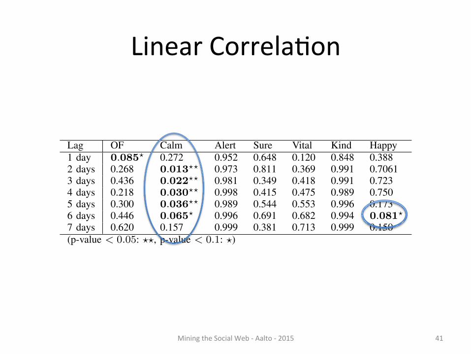
Linear CorrelaHon


5

TABLE IISTATISTICAL SIGNIFICANCE (P-VALUES) OF BIVARIATE GRANGER-CAUSALITY CORRELATION BETWEEN MOODS AND DJIA IN PERIOD FEBRUARY 28,

2008 TO NOVEMBER 3, 2008.

Lag OF Calm Alert Sure Vital Kind Happy1 day 0.085? 0.272 0.952 0.648 0.120 0.848 0.3882 days 0.268 0.013?? 0.973 0.811 0.369 0.991 0.70613 days 0.436 0.022?? 0.981 0.349 0.418 0.991 0.7234 days 0.218 0.030?? 0.998 0.415 0.475 0.989 0.7505 days 0.300 0.036?? 0.989 0.544 0.553 0.996 0.1736 days 0.446 0.065? 0.996 0.691 0.682 0.994 0.081?

7 days 0.620 0.157 0.999 0.381 0.713 0.999 0.150(p-value < 0.05: ??, p-value < 0.1: ?)

0. The Calm mood dimension thus has predictive value withregards to the DJIA. In fact the p-value for this shorter period,i.e. August 1, 2008 to October 30 2008, is significantly lower(lag n = 3, p = 0.009) than that listed in Table II for theperiod February 28, 2008 to November 3, 2008.

The cases in which the t � 3 mood time series fails totrack changes in the DJIA are nearly equally informativeas where it doesn’t. In particular we point to a significantdeviation between the two graphs on October 13th where theDJIA surges by more than 3 standard deviations trough-to-peak. The Calm curve however remains relatively flat at thattime after which it starts to again track changes in the DJIAagain. This discrepancy may be the result of the the FederalReserve’s announcement on October 13th of a major bankbailout initiative which unexpectedly increase DJIA values thatday. The deviation between Calm values and the DJIA on thatday illustrates that unexpected news is not anticipated by thepublic mood yet remains a significant factor in modeling thestock market.

E. Non-linear models for emotion-based stock predictionOur Granger causality analysis suggests a predictive re-

lation between certain mood dimensions and DJIA. How-ever, Granger causality analysis is based on linear regressionwhereas the relation between public mood and stock marketvalues is almost certainly non-linear. To better address thesenon-linear effects and assess the contribution that public moodassessments can make in predictive models of DJIA values, wecompare the performance of a Self-organizing Fuzzy NeuralNetwork (SOFNN) model [30] that predicts DJIA values onthe basis of two sets of inputs: (1) the past 3 days of DJIAvalues, and (2) the same combined with various permutationsof our mood time series (explained below). Statistically signif-icant performance differences will allow us to either confirmor reject the null hypothesis that public mood measurementdo not improve predictive models of DJIA values.

We use a SOFNN as our prediction model since they havepreviously been used to decode nonlinear time series datawhich describe the characteristics of the stock market [28]and predict its values [29]. Our SOFNN in particular is a five-layer hybrid neural network with the ability to self-organizeits own neurons in the learning process. A similar organizationhas been successfully used for electricial load forecasting inour previous work [31].

To predict the DJIA value on day t, the input attributesof our SOFNN include combinations of DJIA values and

mood values of the past n days. We choose n = 3 sincethe results shown in Table II indicate that past n = 4 theGranger causal relation between Calm and DJIA decreasessignificantly. All historical load values are linearly scaled to[0,1]. This procedure causes every input variable be treatedwith similar importance since they are processed within auniform range.

SOFNN models require the tuning of a number of pa-rameters that can influence the performance of the model.We maintain the same parameter values across our vari-ous input combinations to allow an unbiased comparison ofmodel performance, namely � = 0.04,� = 0.01, krmse =0.05, kd(i), (i = 1, ..., r) = 0.1 where r is the dimension ofinput variables and krmse is the expected training root meansquared error which is a predefined value.

To properly evaluate the SOFNN model’s ability to predictdaily DJIA prices, we extend the period under considerationto February 28, 2008 to December 19, 2008 for trainingand testing. February 28, 2008 to November 28, 2008 ischosen as the longest possible training period while Dec1 to Dec 19, 2008 was chosen as the test period becauseit was characterized by stabilization of DJIA values afterconsiderable volatility in previous months and the absence ofany unusual or significant socio-cultural events. Fig. 4 showsthat the Fall of 2008 is an unusual period for the DJIA dueto a sudden dramatic decline of stock prices. This variabilitymay in fact render stock market prediction more difficult thanin other periods.

DJIA daily closing value (March 2008−December 2008

Mar Apr May Jun Jul Aug Sep Oct Nov Dec 2008

8000

9000

10000

11000

12000

13000

Fig. 4. Daily Dow Jones Industrial Average values between February 28,2008 and December 19, 2008.

The Granger causality analysis indicates that only Calm(and to some degree Happy) is Granger-causative of DJIAvalues. However, the other mood dimensions could still con-tain predictive information of DJIA values when combined

Neural Network

7

TABLE IIIDJIA DAILY PREDICTION USING SOFNN

Evaluation IOF I0 I1 I1,2 I1,3 I1,4 I1,5 I1,6MAPE (%) 1.95 1.94 1.83 2.03 2.13 2.05 1.85 1.79?

Direction (%) 73.3 73.3 86.7? 60.0 46.7 60.0 73.3 80.0

sources, and a variety of relevant economic indicators. Theseresults have implications for existing sentiment tracking toolsas well as surveys of “self-reported subjective well-being” inwhich individuals evaluate the extent to which they experiencepositive and negative affect, happiness, or satisfaction withlife [40]. Such surveys are relatively expensive and time-consuming, and may nevertheless not allow the measurementof public mood along mood dimensions that are relevantto assess particular socio-economic indicators. Public moodanalysis from Twitter feeds on the other hand offers anautomatic, fast, free and large-scale addition to this toolkitthat may in addition be optimized to measure a variety ofdimensions of the public mood state.

Our analysis does not acknowledge a number of importantfactors that will form the basis of future research. First, wenote that our analysis is not designed to be limited to anyparticular geographical location nor subset of the world’spopulation. This approach may be appropriate since the USstock markets are affected by individuals worldwide, but forthe particular period under observation Twitter.com users werede facto predominantly English speaking and located in theUS. As Twitter.com’s user base becomes increasingly interna-tional and the use of smartphones equipped with geo-locationincreases, future analysis will have to factor in location andlanguage to avoid geographical and cultural sampling errors.Second, although we have cross-validated the results of 2different tools to assess public mood states, we have noknowledge of the “ground truth” for public mood states nor infact for the particular subsample of the population representedby the community of Twitter.com users. This problem can onlybe addressed by increased research into direct assessments ofpublic mood states vs. those derived from online communitiessuch as Twitter. Third, these results are strongly indicative ofa predictive correlation between measurements of the publicmood states from Twitter feeds, but offer no information onthe causative mechanisms that may connect public mood stateswith DJIA values in this manner. One could speculate that thegeneral public is presently as strongly invested in the DJIAas financial experts, and that therefore their mood states willdirectly affect their investment decisions and thus stock marketvalues, but this too remains an area of future research.

ACKNOWLEDGMENT

This research was supported by NSF Grant BCS #1032101.We thank David Crandell and Michael Nelson for their helpfulcomments on earlier versions of this manuscript. We are alsograteful to Daniel Kahneman for his early comments on ourwork.

REFERENCES

[1] Fama, Eugene F, e. a. (1969) International Economic Review 10, 1–21.

[2] Fama, E. F. (1991) Journal of Finance 46, 1575–617.[3] H.Cootner, P. (1964) The random character of stock market prices.

(MIT).[4] Fama, E. F. (1965) The Journal of Business 38, 34–105.[5] Qian, Bo, Rasheed, & Khaled. (2007) Applied Intelligence 26, 25–33.[6] Gallagher, L. A & Taylor, M. P. (2002) Southern Economic Journal 69,

345–362.[7] Kavussanos, M & Dockery, E. (2001) Applied Financial Economics 11,

573–79.[8] Butler, K. C & Malaikah, S. J. (1992) Journal of Banking and Finance

16, 197–210.[9] Schumaker, R. P & Chen, H. (2009) ACM Trans. Inf. Syst. 27, 12:1–

12:19.[10] Gilbert, E & Karahalios, K. (2010) Widespread worry and the stock

market.[11] Gruhl, D, Guha, R, Kumar, R, Novak, J, & Tomkins, A. (2005) The

predictive power of online chatter. (ACM, New York, NY, USA), pp.78–87.

[12] Mishne, G & Glance, N. (2006) Predicting Movie Sales from BloggerSentiment. AAAI 2006 Spring Symposium on Computational Ap-proaches to Analysing Weblogs

[13] S. Asur and B. A. Huberman 2010 Predicting the Future with SocialMedia arXiv:1003.5699v1

[14] Choi, H & Varian, H. (2009) Predicting the present with google trends.,(Google), Technical report.

[15] Liu, Y, Huang, X, An, A, & Yu, X. (2007) ARSA: a sentiment-awaremodel for predicting sales performance using blogs. (ACM, New York,NY, USA), pp. 607–614.

[16] Dolan, R. J. (2002) Science 298, 1191–1194.[17] Dodds, Peter. (2009) Journal of Happiness July, doi: 10.1007/s10902-

009-9150-9[18] Damasio, A. R. (1994) Descartes’ error : emotion, reason, and the

human brain. (Putnam), pp. xix, 312 p.+.[19] Nofsinger, J. (2005) Journal of Behaviour Finance. 6, 144–160.[20] Edmans, A, Garca, D, & Norli, . (2007) Journal of Finance 62, 1967–

1998.[21] Hirshleifer, D & Shumway, T. (2003) Journal of Finance 58, 1009–1032.[22] Pak, A & Paroubek, P. (2010) Twitter as a Corpus for Sentiment Analysis

and Opinion Mining. (European Language Resources Association(ELRA), Valletta, Malta).

[23] Pang, B & Lee, L. (2008) Foundations and Trends in InformationRetrieval 2, 1–135.

[24] Wilson, T, Wiebe, J, & Hoffmann, P. (2005) Recognizing ContextualPolarity in Phrase-Level Sentiment Analysis. (Vancouver, CA).

[25] Wilson, T, Hoffmann, P, Somasundaran, S, Kessler, J, Wiebe, J, Choi, Y,Cardie, C, Riloff, E, & Patwardhan, S. (2005) OpinionFinder: A systemfor subjectivity analysis. pp. 34–35.

[26] O’Connor, B, Balasubramanyan, R, Routledge, B. R, & Smith, N. A.(2010) From Tweets to Polls: Linking Text Sentiment to Public OpinionTime Series.

[27] Diener E, Diener M & Diener D (2009) Factors Predicting the SubjectiveWell-Being of Nations. Social Indicators Research Series 38:43-70

[28] Lapedes, A & Farber, R. (1987) Nonlinear signal processing using neuralnetwork: Prediction and system modeling, (Los Alamos National LabTechnical Report), Technical report.

[29] Zhu, X, Wang, H, Xu, L, & Li, H. (2008) Expert Syst. Appl. 34, 3043–3054.

[30] Leng, G, Prasad, G, & McGinnity, T. M. (2004) Neural Netw. 17, 1477–1493.

[31] Mao, H, Zeng, X.-J, Leng, G, Zhai, Y, & Keane, A. J. (2009) IEEETransaction on Power System. 24, 1080–1090.

[32] Norcross, J. C, Guadagnoli, E, & Prochaska, J. O. (2006) Journal ofClinical Psychology 40, 1270 – 1277.

[33] McNair, D, Heuchert, J. P, & Shilony, E. (2003) Profile of mood states.Bibliography 1964–2002. (Multi-Health Systems).

[34] Pepe, A & Bollen, J. (2008) Between conjecture and memento: shapinga collective emotional perception of the future.


calm calm + happy

values of 3 previous days

Mean Average PredicHon Error

less is beLer

PredicHon of DJIA direc%on

Summary

quesHon: does twiLer mood predict the stock market data: 8 months of tweets methodology: lexicon-‐based senHment scores, LR, NN impact: showed a case that twiLer mood can predict

the stock market reproducibility: data on website, website not working

https://terramood.soic.indiana.edu/data


Discussion

what do you think? what would you do differently?


Baseline Scenarios invest 10k $ on DJIA on Jan 1st 1976 sell everything at end of day if index is down buy everything back at end of first day that index is up cash in on Dec 31st 1985 >> 25k $ before transacHon costs >> 1.1k $ a^er transacHon costs (0.25% commission) invest 10k $ on Jan 1st 1976, cash in on Dec 31st 1985 >> 18k $ repeat during the 2000s >> 4k $ before commissions


source: “The Signal and the Noise”, N. Silver, 2012, page 344

Do Investors Mine TwiLer?



The Livehoods Project:Utilizing Social Media to Understand the Dynamics of a City

Justin Cranshaw Raz Schwartz Jason I. Hong Norman [email protected] [email protected] [email protected] [email protected]

School of Computer ScienceCarnegie Mellon University

Pittsburgh, PA 15213

Abstract

Studying the social dynamics of a city on a large scale has tra-ditionally been a challenging endeavor, often requiring longhours of observation and interviews, usually resulting in onlya partial depiction of reality. To address this difficulty, weintroduce a clustering model and research methodology forstudying the structure and composition of a city on a largescale based on the social media its residents generate. We ap-ply this new methodology to data from approximately 18 mil-lion check-ins collected from users of a location-based onlinesocial network. Unlike the boundaries of traditional munici-pal organizational units such as neighborhoods, which do notalways reflect the character of life in these areas, our clusters,which we call Livehoods, are representations of the dynamicareas that comprise the city. We take a qualitative approach tovalidating these clusters, interviewing 27 residents of Pitts-burgh, PA, to see how their perceptions of the city projectonto our findings there. Our results provide strong supportfor the discovered clusters, showing how Livehoods revealthe distinctly characterized areas of the city and the forcesthat shape them.

IntroductionThe forces that shape the dynamics of a city are multifariousand complex. Cultural perceptions, economic factors, mu-nicipal borders, demography, geography, and resources—allshape and constrain the texture and character of local urbanlife. It can be extremely difficult to convey these intricaciesto an outsider; one may call them well-kept secrets, some-times only even partially known to the locals. When out-siders, such as researchers, journalists, or city planners, dowant to learn about a city, it often requires hundreds of hoursof observation and interviews. And although such methodsoffer a way to gather deep insights about certain aspects ofcity life, they simply do not scale, and so can ever only un-cover a partial image of the inner workings of the city.

This work presents a new methodology for studying thedynamics, structure, and character of a city on a large scale.Our approach is fundamentally data-driven. Given geospa-tial social media data from hundreds of thousands of people,we developed an algorithm that maps the distinct geographicareas of the city depicting a snap-shot of the ever-changing

Copyright c� 2012, Association for the Advancement of ArtificialIntelligence (www.aaai.org). All rights reserved.

activity patterns of its people. Contrary to traditional organi-zational units such as neighborhoods that are often stagnantand may portray old realities, our clusters reflect current col-lective activity patterns of people in the city, thus revealingthe dynamic nature of local urban areas, exposing their indi-vidual characters, and highlighting various forces that formthe urban habitat.

Our work is made possible by the rapid proliferation ofsmartphones in recent years and the subsequent emergenceof location-based services and applications. Location-basedsocial networks such as foursquare have created new meansfor online interactions based on the physical location of theirusers. In these systems, users can “check-in” to a location byselecting it from a list of named nearby venues. Their check-in is then broadcast to other users of the system.

To algorithmically explore the dynamics of cities, we usedata from millions of check-ins gathered from foursquare.Using well studied techniques in spectral clustering, we in-troduce a model for the structure of local urban areas thatgroups nearby foursquare venues into clusters. Our modeltakes into account both the spatial proximity between venuesas given by their geographic coordinates, as well as the so-cial proximity which we derive from the distribution of peo-ple that check-in to them. The underlying hypothesis of ourmodel is that the “character” of an urban area is defined notjust by the types of places found there, but also by the peo-ple that choose to make that area part of their daily life. Wecall these clusters Livehoods, reflecting the dynamic natureof activity patterns in the lives of city inhabitants.

We take a qualatative approach to evaluating this hypoth-esis. In a true urban studies tradition, we conducted in-terviews with 27 residents of different areas of Pittsburgh,Pennsylvania to see how well their mental maps (Milgram1977) of the city projected onto the Livehood clusters our al-gorithms discovered. In addition to validating our algorithm,these interviews shed light onto the forces that shape the city,and the ways in which Livehoods can help untangle them.We present these results through a series of case studies ex-ploring the relationships between our Livehood clusters andthe municipal neighborhoods.

Our results provide a promising step for the emergingfield urban computing,1 which seeks to provide a compu-

1Urban computing, like many new fields, has several semi-

58

Proceedings of the Sixth International AAAI Conference on Weblogs and Social Media


In This Work...

goal: discover city structure using online acHvity use 4sq data to uncover ‘livehoods’ in PiLsburgh how do they differ from official boundaries? evaluate findings with interviews


Data

43k check-‐ins in PiLsburgh 4k users, 5k venues (restaurants, cafeterias, etc) newly collected & from previous work who (user id) visited what venue (venue-‐id, geo-‐locaHon)


Clustering

For each pair of venues –  geographic distance –  social similarity s (in terms of visiHng users)

For each venue –  maintain m nearest geographic neighbors –  connect them with an edge with weight s

Apply spectral clustering –  number of clusters at largest eigenvalue gap

Clusters è ‘Livehoods’


Findings

Figure 1: The municipal borders (black) and Livehoods for Shadyside/East Liberty (Left) and Lawrenceville/Polish Hill (Right).

Lawrenceville and Polish Hill: Lawrenceville, one ofPittsburgh’s largest neighborhoods, had been going throughmassive changes and development in recent years. Our inter-viewees were conflicted about the cohesiveness of the area.For some, it is one big neighborhood encompassing morethan 20 blocks whereas others notice distinct subsectionscarrying different characteristics.

The city itself subdivides Lawrenceville into three differ-ent municipal neighborhoods: Upper Lawrenceville, Cen-tral Lawrenceville, and Lower Lawrenceville. And althoughthese areas are all connected by Butler street, the characterof each of them is different. As Daniel, a 43 year old residentof Lawrenceville, explains:

The look isn’t different, but the vibe and the feel arevery different. Middle Lawrenceville from 40th un-til the cemetery that is where the first people weremoving in and fixing up the area... And then, LowerLawrenceville, is kind of picking up right now and thenUpper Lawrenceville it’s been like the really rough areawith gangs and drugs.

Our algorithm found similar divisions, breaking the areainto three Livehoods with boundaries closely correspond-ing to those of the municipal map (see Figure 1 Right). Theborder between LH3 and LH4 was situated exactly on the40th St. Bridge, the border between Lower and Cental Law-erenceville. The division between LH4 and LH5 was placedon 48th street, three blocks away from the municipal borderbetween Central an Upper Lawrenceville on 51st street.

We found strong evidence from our interviews supportingthe Livehood clusters based on factors such as property val-

ues, crime rates, business types, and general feel. As Clau-dia, a 54 year old journalist, notes:

I think middle [Central] Lawrenceville is the most de-sirable or well rooted. Where the better housing stockis. LH3 is definately newer. LH5 pretty much was leftalone... There are parking lots and convenience storesaround 40th that when you hit those you think ‘I haveleft something behind.’ And then you are in anotherpart of Lawrencevile because you passed a bridge andthere’s not a lot of connective tissue at some of theseintersections.Several of the interviewees did not agree with the sep-

aration of Lower and Central Lawrenceville. For them,the separation is arbitrary and it is based mainly on lo-cal businesses’ interests. Since Lawrenceville was perceivedas a dangerous area, a group of business owners in LowerLawrenceville decided to brand the area as “LoLa” and mar-ket it as a stand alone destination for unique shops andrestaurants.

Another point of interest is in the spilling of LowerLawrenceville into the adjacent neighborhood of Polish Hillin LH3. At first glance, this grouping seems odd and not fea-sible. Polish Hill is a very small neighborhood that is sepa-rated from Lower Lawrenceville by train tracks and a busway in addition to geographic barrier of being located on anhill. But this grouping seemed natural to Roger, a 47 yearold resident of Polish Hill who said:

I think it’s pretty accurate... I think that’s how someof our residents identify with Lower Lawrenceville be-cause of their activities and their perception. Where

62


EvaluaHon

Found livehoods that split, spilled, or corresponded with municipal areas

Interviews with 27 residents –  IdenHfied and drew their neighborhood –  Shown a map with municipal boundaries, asked if they could idenHfy borders that were not accurate (‘in flux’)

–  Shown algorithm’s results, asked for feedback


EvaluaHon Results

•  Not very rigorous, but interesHng... •  Most discovered livehoods matched boundaries •  When not, the interviewees usually agree & offered explanaHons

•  One controversial case •  Poor area missing (no smartphones?)


livehoods.org


Summary

goal: discover livehoods in ciHes data: 43k Foursquare check-‐ins methodology: combined geographic & social clustering impact: showed a case where we can use online data to

understand offline acHvity reproducibility: some data are online, results are online


Discussion

What do you think? What would you do differently?


Schedule

•  Today: overview •  February 2nd : discuss literature (Aris) •  February 9th : discuss literature (Michael) •  February 23rd : students present project proposals •  March 30th : students submit progress report •  March 30th & April 6th: intermediate presentaHons •  May 4th & May 11th : final presentaHons •  May 15th : final report due

57 Mining the Social Web -‐ Aalto -‐ 2015

Proposals

•  5 min presentaHons •  what do you intend to do? •  why? •  what data will you use? •  what techniques? •  how will you evaluate? •  do you plan to publish your code and data?


The End


Mining the Social Web - Lecture 3 - T61.6020

Education