Mining Sequential Patterns from Probabilistic Databases

Mining Sequential Patterns from Probabilistic

Databases

Muhammad Muzammal and Rajeev Raman

Department of Computer Science, University of Leicester, UK.{mm386,r.raman}@mcs.le.ac.uk

Abstract. We consider sequential pattern mining in situations wherethere is uncertainty about which source an event is associated with.We model this in the probabilistic database framework and consider theproblem of enumerating all sequences whose expected support is suffi-ciently large. Unlike frequent itemset mining in probabilistic databases[C. Aggarwal et al. KDD’09; Chui et al., PAKDD’07; Chui and Kao,PAKDD’08], we use dynamic programming (DP) to compute the prob-ability that a source supports a sequence, and show that this sufficesto compute the expected support of a sequential pattern. Next, we em-bed this DP algorithm into candidate generate-and-test approaches, andexplore the pattern lattice both in a breadth-first (similar to GSP) anda depth-first (similar to SPAM) manner. We propose optimizations forefficiently computing the frequent 1-sequences, for re-using previously-computed results through incremental support computation, and for elmim-inating candidate sequences without computing their support via prob-

abilistic pruning. Preliminary experiments show that our optimizationsare effective in improving the CPU cost.

Key words: Mining Uncertain Data, Mining complex sequential data,Probabilistic Databases, Novel models and algorithms.

1 Introduction

The problem of sequential pattern mining (SPM), or finding frequent sequencesof events in data with a temporal component, has been studied extensively [23,17, 4] since its introduction in [18, 3]. In classical SPM, the data to be mined isdeterministic, but it is recognized that data obtained from a wide range of datasources is inherently uncertain [1]. This paper is concerned with SPM in proba-bilistic databases [19], a popular framework for modelling uncertainty. Recentlyseveral data mining and ranking problems have been studied in this framework,including top-k [24, 8] and frequent itemset mining (FIM) [2, 5–7]. In classicalSPM, the event database consists of tuples 〈eid, e, σ〉, where e is an event, σ isa source and eid is an event-id which incorporates a time-stamp. A tuple mayrecord a retail transaction (event) by a customer (source), or an observation of anobject/person (event) by a sensor/camera (source). Since event-ids have a time-stamp, the event database can be viewed as a collection of source sequences, one

2 M. Muzammal and R. Raman

per source, containing a sequence of events (ordered by time-stamp) associatedwith that source, and classical SPM problem is to find patterns of events thathave a temporal order that occur in a significant number of source sequences.

Uncertainty in SPM can occur in three different places: the source, the eventand the time-stamp may all be uncertain (in contrast, in FIM, only the eventcan be uncertain). In a companion paper [16] the first two kinds of uncertaintyin SPM were formalized as source-level uncertainty (SLU) and event-level un-certainty (ELU), which we now summarize.

In SLU, the “source” attribute of each tuple is uncertain: each tuple containsa probability distribution over possible sources (attribute-level uncertainty [19]).As noted in [16], this formulation applies to scenarios such as the ambiguityarising when a customer makes a retail transaction, but the customer is eithernot identified exactly, or the customer database itself is probabilistic as a resultof “deduplication” or cleaning [11]. In ELU, the source of the tuple is certain,but the events are uncertain. For example, the PEEX system [13] aggregatesunreliable observations of employees using RFID antennae at fixed locationsinto uncertain higher-level events such as “with probability 0.4, at time 103,Alice and Bob had a meeting in room 435”. Here, the source (Room 435) isdeterministic, but the event ({Alice, Bob}) only occurred with probability 0.4.

Furthermore, in [16] two measures of “frequentness”, namely expected supportand probabilistic frequentness, used for FIM in probabilistic databases [5, 7], wereadapted to SPM, and the four possible combinations of models and measureswere studied from a computational complexity viewpoint. This paper is focussedon efficient algorithms for the SPM problem in SLU probabilistic databases,under the expected support measure, and the contributions are as follows:

1. We give a dynamic-programming (DP) algorithm to determine efficiently theprobability that a given source supports a sequence (source support proba-bility), and show that this is enough to compute the expected support of asequence in an SLU event database.

2. We give depth-first and breadth-first methods to find all frequent sequencesin an SLU event database according to the expected support criterion.

3. To speed up the computation, we give subroutines for:(a) highly efficient computation of frequent 1-sequences,(b) incremental computation of the DP matrix, which allows us to minimize

the amount of time spent on the expensive DP computation, and(c) probabilistic pruning, where we show how to rapidly compute an upper

bound on the probability that a source supports a candidate sequence.4. We empirically evaluate our algorithms, demonstrating their efficiency and

scalability, as well as the effectiveness of the above optimizations.

Significance of Results. The source support probability algorithm ((1) above)shows that in probabilistic databases, FIM and SPM are very different – thereis no need to use DP for FIM under the expected support measure [2, 6, 7].

Although the proof that source support probability allows the computationof the expected support of a sequence in an SLU database is simple, it is unex-pected, since in SLU databases, there are dependencies between different sources

Mining Sequential Patterns from Probabilistic Databases 3

– in any possible world, a given event can only belong to one source. In contrast,determining if a given sequence is probabilistically frequent in an SLU eventdatabase is #P-complete because of the dependencies between sources [16].

Also, as noted in [16], (1) can be used to determine if a sequence is frequentin an ELU database using both expected support and probabilistic frequentness.This implies efficient algorithms for enumerating frequent sequences under bothfrequentness criteria for ELU databases, and by using the framework of [10], wecan also find maximal frequent sequential patterns in ELU databases.

The breadth-first and depth-first algorithms (2) have a high-level similarityto GSP [18] and SPADE/SPAM [23, 4], but checking the extent to which asequence is supported by a source requires an expensive DP computation, andmajor modifications are needed to achieve good performance. It is unclear howto use either the projected database idea of PrefixSpan [17], or bitmaps as inSPAM); we instead use the ideas ((3) above) of incremental computation, andprobabilistic pruning. Although there is a high-level similiarity between thispruning and a technique of [6] for FIM in probabilistic databases, the SPMproblem is more complex, and our pruning rule is harder to obtain.

Related Work. Classical SPM has been studied extensively [18, 23, 17, 4]. Mod-elling uncertain data as probabilistic databases [19, 1] has led to several rank-ing/mining problems being studied in this context. The top-k problem (a rank-ing problem) has been studied intensively (see [12, 24, 8] and references therein).FIM in probabilistic databases was studied under the expected support measurein [2, 7, 6] and under the probabilistic frequentness measure in [5]. To the bestof our knowledge, apart from [16], the SPM problem in probabilistic databaseshas not been studied. Uncertainty in the time-stamp attribute was considered in[20] – we do not consider time to be uncertain. Also [22] studies SPM in “noisy”sequences, but the model proposed there is very different to ours and does notfit in the probabilistic database framework.

2 Problem Statement

Classical SPM [18, 3]. Let I = {i1, i2, . . . , iq} be a set of items and S ={1, . . . ,m} be a set of sources. An event e ⊆ I is a collection of items. A databaseD = 〈r1, r2, . . . , rn〉 is an ordered list of records such that each ri ∈ D is of theform (eid i, ei, σi), where eid i is a unique event-id, including a time-stamp (eventsare ordered by this time-stamp), ei is an event and σi is a source.

A sequence s = 〈s1, s2, . . . , sa〉 is an ordered list of events. The events si in thesequence are called its elements. The length of a sequence s is the total number ofitems in it, i.e.

∑a

j=1 |sj |; for any integer k, a k-sequence is a sequence of length k.Let s = 〈s1, s2, . . . , sq〉 and t = 〈t1, t2, . . . , tr〉 be two sequences. We say that s is asubsequence of t, denoted s � t, if there exist integers 1 ≤ i1 < i2 < · · · < iq ≤ r

such that sk ⊆ tij , for k = 1, . . . , q. The source sequence corresponding to asource i is just the multiset {e|(eid, e, i) ∈ D}, ordered by eid. For a sequences and source i, let Xi(s,D) be an indicator variable, whose value is 1 if s is

4 M. Muzammal and R. Raman

a subsequence of the source sequence for source i, and 0 otherwise. For anysequence s, define its support in D, denoted Sup(s,D) =

∑m

i=1 Xi(s,D). Theobjective is to find all sequences s such that Sup(s,D) ≥ θm for some user-defined threshold 0 ≤ θ ≤ 1.

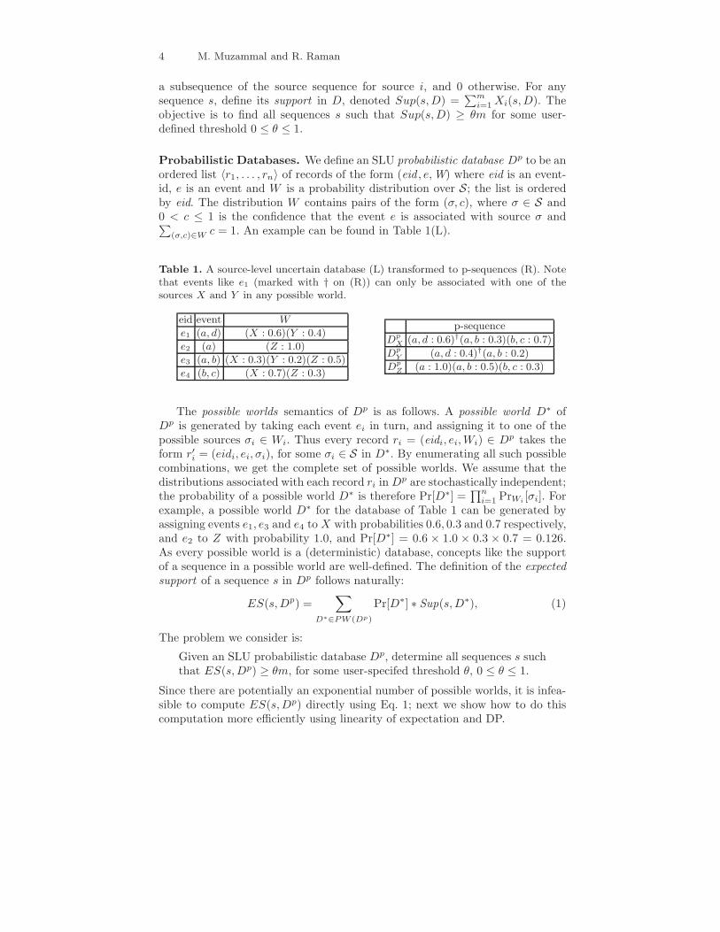
Probabilistic Databases. We define an SLU probabilistic database Dp to be anordered list 〈r1, . . . , rn〉 of records of the form (eid , e,W) where eid is an event-id, e is an event and W is a probability distribution over S; the list is orderedby eid. The distribution W contains pairs of the form (σ, c), where σ ∈ S and0 < c ≤ 1 is the confidence that the event e is associated with source σ and∑

(σ,c)∈W c = 1. An example can be found in Table 1(L).

Table 1. A source-level uncertain database (L) transformed to p-sequences (R). Notethat events like e1 (marked with † on (R)) can only be associated with one of thesources X and Y in any possible world.

eid event W

e1 (a, d) (X : 0.6)(Y : 0.4)

e2 (a) (Z : 1.0)

e3 (a, b) (X : 0.3)(Y : 0.2)(Z : 0.5)

e4 (b, c) (X : 0.7)(Z : 0.3)

p-sequence

Dp

X (a, d : 0.6)†(a, b : 0.3)(b, c : 0.7)

Dp

Y (a, d : 0.4)†(a, b : 0.2)

Dp

Z (a : 1.0)(a, b : 0.5)(b, c : 0.3)

The possible worlds semantics of Dp is as follows. A possible world D∗ ofDp is generated by taking each event ei in turn, and assigning it to one of thepossible sources σi ∈ Wi. Thus every record ri = (eidi, ei,Wi) ∈ Dp takes theform r′i = (eidi, ei, σi), for some σi ∈ S in D∗. By enumerating all such possiblecombinations, we get the complete set of possible worlds. We assume that thedistributions associated with each record ri in Dp are stochastically independent;the probability of a possible world D∗ is therefore Pr[D∗] =

∏n

i=1 PrWi[σi]. For

example, a possible world D∗ for the database of Table 1 can be generated byassigning events e1, e3 and e4 toX with probabilities 0.6, 0.3 and 0.7 respectively,and e2 to Z with probability 1.0, and Pr[D∗] = 0.6 × 1.0 × 0.3 × 0.7 = 0.126.As every possible world is a (deterministic) database, concepts like the supportof a sequence in a possible world are well-defined. The definition of the expectedsupport of a sequence s in Dp follows naturally:

ES(s,Dp) =∑

D∗∈PW (Dp)

Pr[D∗] ∗ Sup(s,D∗), (1)

The problem we consider is:

Given an SLU probabilistic database Dp, determine all sequences s suchthat ES(s,Dp) ≥ θm, for some user-specifed threshold θ, 0 ≤ θ ≤ 1.

Since there are potentially an exponential number of possible worlds, it is infea-sible to compute ES(s,Dp) directly using Eq. 1; next we show how to do thiscomputation more efficiently using linearity of expectation and DP.

Mining Sequential Patterns from Probabilistic Databases 5

3 Computing Expected Support

p-sequences. A p-sequence is analogous to a source sequence in classical SPM,and is a sequence of the form 〈(e1, c1) . . . (ek, ck)〉, where ej is an event and cj isa confidence value. In examples, we write a p-sequence 〈({a, d}, 0.4), ({a, b}, 0.2)〉as (a, d : 0.4)(a, b : 0.2). An SLU database Dp can be viewed as a collection of p-sequencesDp

1 , . . . , Dpm, whereDp

i is the p-sequence of source i, and contains a listof those events in Dp that have non-zero confidence of being assigned to source i,ordered by eid, together with the associated confidence (see Table 1(R)). How-ever, the p-sequences corresponding to different sources are not independent,as illustrated in Table 1(R). Thus, one may view an SLU event database as acollection of p-sequences with dependencies in the form of x-tuples [8]. Never-theless, we show that we can still process the p-sequences independently for thepurposes of expected suppport computation:

ES(s,Dp) =∑

D∗∈PW (Dp) Pr[D∗] ∗ Sup(s,D∗) =

∑

D∗ Pr[D∗] ∗∑m

i=1 Xi(s,D∗)

=∑m

i=1

∑

D∗ Pr[D∗] ∗Xi(s,D∗) =

∑m

i=1 E[Xi(s,Dp)], (2)

where E denotes the expected value of a random variable. Since Xi is a 0-1variable, E[Xi(s,D

p)] = Pr[s � Dpi ], and we calculate the right-hand quantity,

which we refer to as the source support probability. This cannot be done naively:e.g., if Dp

i = (a, b : c1)(a, b : c2) . . . (a, b : cq), then there are O(q2k) ways inwhich (a)(a, b) . . . (a)(a, b)

︸ ︷︷ ︸

k times

could be supported by source i, and so we use DP.

Computing the Source Support Probability. Given a p-sequence Dpi =

〈(e1, c1), . . . , (er, cr)〉 and a sequence s = 〈s1, . . . , sq〉, we create a (q+1)×(r+1)matrix Ai,s[0..q][0..r] (we omit the subscripts on A when the source and sequenceare clear from the context). For 1 ≤ k ≤ q and 1 ≤ ` ≤ r, A[k, `] will containPr[〈s1, . . . , sk〉 � 〈(e1, c1), . . . , (e`, c`)〉]. We set A[0, `] = 1 for all `, 0 ≤ ` ≤ r

and A[k, 0] = 0 for all 1 ≤ k ≤ q, and compute the other values row-by-row. For1 ≤ k ≤ q and 1 ≤ ` ≤ r, define:

c∗k` =

{c` if sk ⊆ e`0 otherwise

(3)

The interpretation of Eq. 3 is that c∗k` is the probability that e` allows the elementsk to be matched in source i; this is 0 if sk 6⊆ e`, and is otherwise equal to theprobability that e` is associated with source i. Now we use the equation:

A[k, `] = (1− c∗k`) ∗A[k, `− 1] + c∗k` ∗A[k − 1, `− 1]. (4)

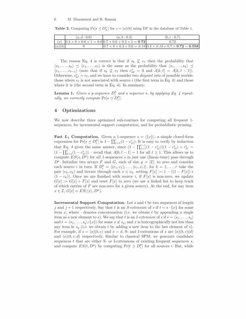
Table 2 shows the computation of the source support probability of an examplesequence s = (a)(b) for source X in the probabilistic database of Table 1. Simi-larly, we can compute Pr[s � D

pY ] = 0.08 and Pr[s � D

pZ ] = 0.35, so the expected

support of (a)(b) in the database of Table 1 is 0.558 + 0.08 + 0.35 = 1.288.

6 M. Muzammal and R. Raman

Table 2. Computing Pr[s � Dp

X ] for s = (a)(b) using DP in the database of Table 1.

(a, d : 0.6) (a, b : 0.3) (b, c : 0.7)

(a) 0.4× 0 + 0.6× 1 = 0.6 0.7 × 0.6 + 0.3× 1 = 0.72 0.72

(a)(b) 0 0.7× 0 + 0.3× 0.6 = 0.18 0.3× 0.18+ 0.7× 0.72 = 0.558

The reason Eq. 4 is correct is that if sk 6⊆ e` then the probability that〈s1, . . . , sk〉 � 〈e1, . . . , e`〉 is the same as the probability that 〈s1, . . . , sk〉 �〈e1, . . . , e`−1〉 (note that if sk 6⊆ e` then c∗k` = 0 and A[k, `] = A[k, ` − 1]).Otherwise, c∗k` = c`, and we have to consider two disjoint sets of possible worlds:those where e` is not associated with source i (the first term in Eq. 4) and thosewhere it is (the second term in Eq. 4). In summary:

Lemma 1. Given a p-sequence Dpi and a sequence s, by applying Eq. 4 repeat-

edly, we correctly compute Pr[s � Dpi ].

4 Optimizations

We now describe three optimized sub-routines for computing all frequent 1-sequences, for incremental support computation, and for probabilistic pruning.

Fast L1 Computation. Given a 1-sequence s = 〈{x}〉, a simple closed-formexpression for Pr[s � D

pi ] is 1−

∏r

`=1(1− c∗1`). It is easy to verify by induction

that Eq. 4 gives the same answer, since (1 −∏t−1

`=1(1 − c∗1`))(1 − c∗1t) + c∗1t =

(1 −∏t

`=1(1 − c∗1`)) – recall that A[0, `− 1] = 1 for all ` ≥ 1. This allows us tocompute ES(s,Dp) for all 1-sequences s in just one (linear-time) pass throughDp. Initialize two arrays F and G, each of size q = |I|, to zero and considereach source i in turn. If Dp

i = 〈(e1, c1), . . . , (er, cr)〉, for k = 1, . . . , r take thepair (ek, ck) and iterate through each x ∈ ek, setting F [x] := 1 − ((1 − F [x]) ∗(1 − ck)). Once we are finished with source i, if F [x] is non-zero, we updateG[x] := G[x] + F [x] and reset F [x] to zero (we use a linked list to keep trackof which entries of F are non-zero for a given source). At the end, for any itemx ∈ I, G[x] = ES(〈x〉, Dp).

Incremental Support Computation. Let s and t be two sequences of lengthj and j + 1 respectively. Say that t is an S-extension of s if t = s · {x} for someitem x, where · denotes concatenation (i.e. we obtain t by appending a singleitem as a new element to s). We say that t is an I-extension of s if s = 〈s1, . . . , sq〉and t = 〈s1, . . . , sq∪{x}〉 for some x 6∈ sq, and x is lexicographically not less thanany item in sq (i.e. we obtain t by adding a new item to the last element of s).For example, if s = (a)(b, c) and x = d, S- and I-extensions of s are (a)(b, c)(d)and (a)(b, c, d) respectively. Similar to classical SPM, we generate candidatesequences t that are either S- or I-extensions of existing frequent sequences s,and compute ES(t,Dp) by computing Pr[t � D

pi ] for all sources i. But, while

Mining Sequential Patterns from Probabilistic Databases 7

computing Pr[t � Dpi ], we will exploit the similarity between s and t to compute

Pr[t � Dpi ] more rapidly.

Let i be a source, Dpi = 〈(e1, c1), . . . , (er, cr)〉, and s = 〈s1, . . . , sq〉 be any

sequence. Now let Ai,s be the (q + 1) × (r + 1) DP matrix used to computePr[s � D

pi ], and let Bi,s denote the last row of Ai,s, that is, Bi,s[`] = Ai,s[q, `]

for ` = 0, . . . , r. We now show that if t is an extension of s, then we can quicklycompute Bi,t from Bi,s, and thereby obtain Pr[t � D

pi ] = Bi,t[r]:

Lemma 2. Let s and t be sequences such that t is an extension of s, and let ibe a source whose p-sequence has r elements in it. Then, given Bi,s and D

pi , we

can compute Bi,t in O(r) time.

Proof. We only discuss the case where t is an I-extension of s, i.e. t = 〈s1, . . . , sq∪{x}〉 for some x 6∈ sq. Firstly, observe that since the first q − 1 elements of sand t are pairwise equal, the first q− 1 rows of Ai,s and Ai,t are also equal. The(q−1)-st row of Ai,s is enough to compute the q-th row of Ai,t, but we only haveBi,s, the q-th row of Ai,s. If tq = sq ∪ {x} 6⊆ e`, then Ai,t[q, `] = Ai,t[q, ` − 1],and we can move on to the next value of `. If tq ⊆ e`, then sq ⊆ e` and so:

Ai,s[q, `] = (1− c`) ∗Ai,s[q, `− 1] + c` ∗Ai,s[q − 1, `− 1]

Since we know Bi,s[`] = Ai,s[q, `], Bi,s[` − 1] = Ai,s[q, ` − 1] and c`, we cancompute Ai,s[q − 1, ` − 1]. But this value is equal to Ai,t[q − 1, ` − 1], whichis the value from the (q − 1)-st row of Ai,t that we need to compute Ai,t[q, `].Specifically, we compute:

Bi,t[`] = (1 − c`) ∗Bi,t[`− 1] + (Bi,s[`]−Bi,s[`− 1] ∗ (1− c`))

if tq ⊆ e` (otherwise Bi,t[`] = Bi,t[` − 1]). The (easier) case of S-extensions andan example illustrating incremental computation can be found in [15].

Probabilistic Pruning. We now describe a technique that allows us to prunenon-frequent sequences s without fully computing ES(s,Dp). For each source i,we obtain an upper bound on Pr[s � D

pi ] and add up all the upper bounds; if

the sum is below the threshold, s can be pruned. We first show (proof in [15]):

Lemma 3. Let s = 〈s1, . . . , sq〉 be a sequence, and let Dpi be a p-sequence. Then:

Pr[s � Dpi ] ≤ Pr[〈s1, . . . , sq−1〉 � D

pi ] ∗ Pr[〈sq〉 � D

pi ].

We now indicate how Lemma 3 is used. Suppose, for example, that we have acandidate sequence s = (a)(b, c)(a), and a source X . By Lemma 3:

Pr[(a)(b, c)(a) � DpX ] ≤ Pr[(a)(b, c) � D

pX ] ∗ Pr[(a) � D

pX ]

≤ Pr[(a) � DpX ] ∗ Pr[(b, c) � D

pX ] ∗ Pr[(a) � D

pX ]

≤ (Pr[(a) � DpX ])2 ∗min{Pr[(b) � D

pX ],Pr[(c) � D

pX ]}

Note that the quantities on the RHS are computed for each source by the fastL1 computation, and can be stored in a small data structure. However, the lastline is the least accurate upper bound bound: if Pr[(a)(b, c) � D

pX ] is available

when pruning, an tighter bound is Pr[(a)(b, c) � DpX ] ∗ Pr[(a) � D

pX ].

8 M. Muzammal and R. Raman

5 Candidate Generation

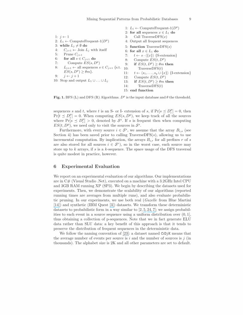
We now describe two candidate generation methods for enumerating all frequentsequences, one each based on breadth-first and depth-first exploration of thesequence lattice, which are similar to GSP [18, 3] and SPAM [4] respectively. Wefirst note that an “Apriori” property holds in our setting:

Lemma 4. Given two sequences s and t, and a probabilistic database Dp, if sis a subsequence of t, then ERS(s,Dp) ≥ ERS(t,Dp).

Proof. In Eq. 1 note that for all D∗ ∈ PW (Dp), Sup(s,D∗) ≥ Sup(t,D∗).

Breadth-First Exploration. An overview of our BFS approach is in Fig. 1(L).We now describe some details. Each execution of lines (6)-(10) is called a phase.Line 2 is done using the fast L1 computation (see Section 4). Line 4 is done asin [18, 3]: two sequences s and s′ in Lj are joined iff deleting the first item in s

and the last item in s′ results in the same sequence, and the result t comprisess extended with the last item in s′. This item is added the way it was in s′ i.e.either a separate element (t is an S-extension of s) or to the last element of s (tis an I-extension of s). We apply apriori pruning to the set of candidates in the(j + 1)-st phase, Cj+1, and probabilistic pruning can additionally be applied toCj+1 (note that for C2, probabilistic pruning is the only possibility).

In Lines 6-7, the loop iterates over all sources, and for the i-th source, firstconsider only those sequences from Cj+1 that could potentially be supportedby source i, Ni,j+1, (narrowing). For the purpose of narrowing, we put all thesequences in Cj+1 in a hashtree, similar to [18]. A candidate sequence t ∈ Cj+1

is stored in the hashtree by hashing on each item in t upto the j-th item, and theleaf node contains the (j + 1)-st item. In the (j + 1)-st phase, when consideringsource i, we recursively traverse the hashtree by hashing on every item in Li,1

until we have traversed all the leaf nodes, thus obtaining Ni,j+1 for source i.Given Ni,j+1 we compute the support of t in source i as follows. Consider

s = 〈s1, . . . , sq〉 and t = 〈t1, . . . , tr〉 be two sequences, then if s and t have acommon prefix, i.e. for k = 1, 2, . . . , z, sk = tk, then we start the computationof Pr[t � D

pi ] from tz+1. Observe that our narrowing method naturally tends to

place sequences with common prefixes in consecutive positions of Ni,j+1.

Depth-First Exploration. An overview of our depth-first approach is in Fig. 1(R). We first compute the set of frequent 1-sequences, L1 (Line 1) (assume L1

is in ascending order). We then explore the pattern sub-lattice as follows.Consider a call of TraverseDFS(s), where s is some k-sequence. We first check

that all lexicographically smaller k-subsequences of t are frequent, and reject t

as infrequent if this test fails (Line 7). We can then apply probabilistic pruningto t, and if t is still not pruned we compute its support (Line 8). If at any staget is found to be infrequent, we do not consider x, the item used to extend s to t,as a possible alternative in the recursive tree under s (as in [4]). Observe that for

Mining Sequential Patterns from Probabilistic Databases 9

1: j ← 12: L1 ← ComputeFrequent-1(Dp)3: while Lj 6= ∅ do4: Cj+1 ← Join Lj with itself5: Prune Cj+1

6: for all s ∈ Cj+1 do

7: Compute ES(s,Dp)8: Lj+1 ← all sequences s ∈ Cj+1 {s.t.

ES(s,Dp) ≥ θm}.9: j ← j + 110: Stop and output L1 ∪ . . . ∪ Lj

1: L1 ← ComputeFrequent-1(Dp)2: for all sequences x ∈ L1 do

3: Call TraverseDFS(x)4: Output all frequent sequences

5: function TraverseDFS(s)6: for all x ∈ L1 do

7: t← s · 〈{x}〉 {S-extension}8: Compute ES(t,Dp)9: if ES(t,Dp) ≥ θm then

10: TraverseDFS(t)11: t← 〈s1, . . . , sq ∪ {x}〉 {I-extension}12: Compute ES(t,Dp)13: if ES(t,Dp) ≥ θm then

14: TraverseDFS(t)15: end function

Fig. 1. BFS (L) and DFS (R) Algorithms. Dp is the input database and θ the threshold.

sequences s and t, where t is an S- or I- extension of s, if Pr[s � Dpi ] = 0, then

Pr[t � Dpi ] = 0. When computing ES(s,Dp), we keep track of all the sources

where Pr[s � Dpi ] > 0, denoted by Ss. If s is frequent then when computing

ES(t,Dp), we need only to visit the sources in Ss.Furthermore, with every source i ∈ Ss, we assume that the array Bi,s (see

Section 4) has been saved prior to calling TraverseDFS(s), allowing us to useincremental computation. By implication, the arrays Bi,r for all prefixes r of sare also stored for all sources i ∈ Sr), so in the worst case, each source maystore up to k arrays, if s is a k-sequence. The space usage of the DFS traversalis quite modest in practice, however.

6 Experimental Evaluation

We report on an experimental evaluation of our algorithms. Our implementationsare in C# (Visual Studio .Net), executed on a machine with a 3.2GHz Intel CPUand 3GB RAM running XP (SP3). We begin by describing the datasets used forexperiments. Then, we demonstrate the scalability of our algorithms (reportedrunning times are averages from multiple runs), and also evaluate probabilis-tic pruning. In our experiments, we use both real (Gazelle from Blue Martini[14]) and synthetic (IBM Quest [3]) datasets. We transform these deterministicdatasets to probabilistic form in a way similar to [2, 5, 24, 7]; we assign probabil-ities to each event in a source sequence using a uniform distribution over (0, 1],thus obtaining a collection of p-sequences. Note that we in fact generate ELUdata rather than SLU data: a key benefit of this approach is that it tends topreserve the distribution of frequent sequences in the deterministic data.

We follow the naming convention of [23]: a dataset named CiDjK means thatthe average number of events per source is i and the number of sources is j (inthousands). The alphabet size is 2K and all other parameters are set to default.

10 M. Muzammal and R. Raman

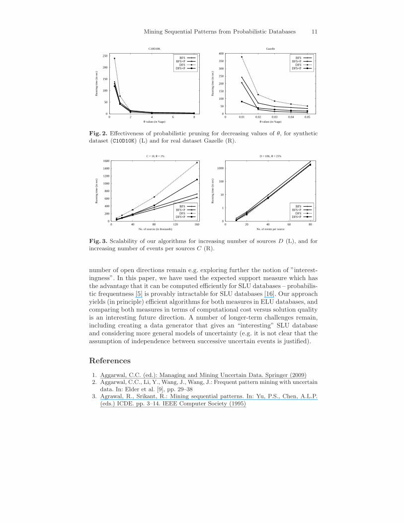
We study three parameters in our experiments: the number of sources D, theaverage number of events per source C, and the threshold θ. We test our algo-rithms for one of the three parameters by keeping the other two fixed. Evidently,all other parameters being fixed, increasing D and C, or decreasing θ, all makean instance harder. We choose our algorithm variants according to two “axes”:

– Lattice traversal could be done using BFS or DFS.– Probabilistic Pruning (P) could be ON or OFF.

We thus report on four variants in all, for example “BFS+P” represents thevariant with BFS lattice traversal and with probabilistic pruning ON.

Probabilistic Pruning. To show the effectiveness of probabilistic pruning, wekept statistics on the number of candidates both for BFS and for DFS. Due tospace limitations, we report statistics only for the dataset C10D20K here. Formore details, see [15]. Table 3 shows that probabilistic pruning is highly effectiveat eliminating infrequent candidates in phase 2 — for example, in both BFSand DFS, over 95% of infrequent candidates were eliminated without supportcomputation. However, probabilistic pruning was less effective in BFS comparedto DFS in the later phases. This is because we compute a coarser upper boundin BFS than in DFS, as we only store Li,1 probabilities in BFS, whereas westore both Li,1 and Li,j probabilities in DFS. We therefore, turn probabilisticpruning OFF after Phase 2 in BFS in our experiments. If we could also storeLi,j probabilities in BFS, a more refined upper bound could be attained (asmentioned after Lemma 3 and shown in (Section 6) [15]).

Table 3. Effectiveness of probabilistic pruning at θ = 2%, for dataset C10D20K in BFS(L) and in DFS (R). The columns from L to R indicate the numbers of candidates cre-ated by joining, remaining after apriori pruning, remaining after probabilistic pruning,and deemed as frequent, respectively.

Phase Joining Apriori Prob. prun. Frequent2 15555 15555 246 393 237 223 208 91

Phase Joining Apriori Prob. prun. Frequent2 15555 15555 246 393 334 234 175 91

In Fig. 2, we show the effect of probabilistic pruning on overall running timeas θ decreases, for both synthetic (C10D10K) and real (Gazelle) datasets. It canbe seen that pruning is effective particularly for low θ, for both datasets.

Scalability Testing. We test the scalability of our algorithms by fixing C = 10and θ = 1%, for increasing values of D (Fig. 3(L)), and by fixing D = 10Kand θ = 25%, for increasing values of C (Fig. 3(R)). We observe that all ouralgorithms scale essentially linearly in both sets of experiments.

7 Conclusions and Future Work

We have considered the problem of finding all frequent sequences in SLU databases.This is a first study on efficient algorithms for this problem, and naturally a

Mining Sequential Patterns from Probabilistic Databases 11

0

50

100

150

200

250

0 2 4 6 8

Run

ning

tim

e (i

n se

c)

θ values (in %age)

C10D10K

BFSBFS+P

DFSDFS+P

0

50

100

150

200

250

300

350

400

0 0.01 0.02 0.03 0.04 0.05

Run

ning

tim

e (i

n se

c)

θ values (in %age)

Gazelle

BFSBFS+P

DFSDFS+P

Fig. 2. Effectiveness of probabilistic pruning for decreasing values of θ, for syntheticdataset (C10D10K) (L) and for real dataset Gazelle (R).

0

200

400

600

800

1000

1200

1400

1600

0 40 80 120 160

Run

ning

tim

e (i

n se

c)

No. of sources (in thousands)

C = 10, θ = 1%

BFSBFS+P

DFSDFS+P

0

1

10

100

1000

0 20 40 60 80

Run

ning

tim

e (i

n se

c)

No. of events per source

D = 10K, θ = 25%

BFSBFS+P

DFSDFS+P

Fig. 3. Scalability of our algorithms for increasing number of sources D (L), and forincreasing number of events per sources C (R).

number of open directions remain e.g. exploring further the notion of ”interest-ingness”. In this paper, we have used the expected support measure which hasthe advantage that it can be computed efficiently for SLU databases – probabilis-tic frequentness [5] is provably intractable for SLU databases [16]. Our approachyields (in principle) efficient algorithms for both measures in ELU databases, andcomparing both measures in terms of computational cost versus solution qualityis an interesting future direction. A number of longer-term challenges remain,including creating a data generator that gives an “interesting” SLU databaseand considering more general models of uncertainty (e.g. it is not clear that theassumption of independence between successive uncertain events is justified).

References

1. Aggarwal, C.C. (ed.): Managing and Mining Uncertain Data. Springer (2009)2. Aggarwal, C.C., Li, Y., Wang, J., Wang, J.: Frequent pattern mining with uncertain

data. In: Elder et al. [9], pp. 29–383. Agrawal, R., Srikant, R.: Mining sequential patterns. In: Yu, P.S., Chen, A.L.P.

(eds.) ICDE. pp. 3–14. IEEE Computer Society (1995)

12 M. Muzammal and R. Raman

4. Ayres, J., Flannick, J., Gehrke, J., Yiu, T.: Sequential pattern mining using abitmap representation. In: KDD. pp. 429–435 (2002)

5. Bernecker, T., Kriegel, H.P., Renz, M., Verhein, F., Zufle, A.: Probabilistic frequentitemset mining in uncertain databases. In: Elder et al. [9], pp. 119–128

6. Chui, C.K., Kao, B.: A decremental approach for mining frequent itemsets fromuncertain data. In: PAKDD. pp. 64–75 (2008)

7. Chui, C.K., Kao, B., Hung, E.: Mining frequent itemsets from uncertain data. In:Zhou, Z.H., Li, H., Yang, Q. (eds.) PAKDD. LNCS, vol. 4426, pp. 47–58. Springer(2007)

8. Cormode, G., Li, F., Yi, K.: Semantics of ranking queries for probabilistic dataand expected ranks. In: ICDE. pp. 305–316. IEEE (2009)

9. Elder, J.F., Fogelman-Soulie, F., Flach, P.A., Zaki, M.J. (eds.): Proceedings of the15th ACM SIGKDD International Conference on Knowledge Discovery and DataMining, Paris, France, June 28 - July 1, 2009. ACM (2009)

10. Gunopulos, D., Khardon, R., Mannila, H., Saluja, S., Toivonen, H., Sharm, R.S.:Discovering all most specific sentences. ACMTrans. DB Syst. 28(2), 140–174 (2003)

11. Hassanzadeh, O., Miller, R.J.: Creating probabilistic databases from duplicateddata. The VLDB Journal 18(5), 1141–1166 (2009)

12. Hua, M., Pei, J., Zhang, W., Lin, X.: Ranking queries on uncertain data: a prob-abilistic threshold approach. In: Wang [21], pp. 673–686

13. Khoussainova, N., Balazinska, M., Suciu, D.: Probabilistic event extraction fromRFID data. In: ICDE. pp. 1480–1482. IEEE (2008)

14. Kohavi, R., Brodley, C., Frasca, B., Mason, L., Zheng, Z.: KDD-Cup 2000 orga-nizers’ report: Peeling the onion. SIGKDD Explorations 2(2), 86–98 (2000)

15. Muzammal, M., Raman, R.: Mining sequential patterns from probabilisticdatabases. Tech. Rep. CS-10-002, Dept. of Comp. Sci., Univ. of Leicester, UK.(2010), http://www.cs.le.ac.uk/people/mm386/pSPM.pdf

16. Muzammal, M., Raman, R.: On probabilistic models for uncertain sequential pat-tern mining. In: Cao, L., Feng, Y., Zhong, J. (eds.) ADMA (1). LNCS, vol. 6440,pp. 60–72. Springer (2010)

17. Pei, J., Han, J., Mortazavi-Asl, B., Wang, J., Pinto, H., Chen, Q., Dayal, U., Hsu,M.: Mining sequential patterns by pattern-growth: The PrefixSpan approach. IEEETrans. Knowl. Data Eng. 16(11), 1424–1440 (2004)

18. Srikant, R., Agrawal, R.: Mining sequential patterns: Generalizations and perfor-mance improvements. In: Apers, P.M.G., Bouzeghoub, M., Gardarin, G. (eds.)EDBT. LNCS, vol. 1057, pp. 3–17. Springer (1996)

19. Suciu, D., Dalvi, N.N.: Foundations of probabilistic answers to queries. In: Ozcan,F. (ed.) SIGMOD Conference. p. 963. ACM (2005)

20. Sun, X., Orlowska, M.E., Li, X.: Introducing uncertainty into pattern discovery intemporal event sequences. In: ICDM. pp. 299–306. IEEE Computer Society (2003)

21. Wang, J.T.L. (ed.): Proceedings of the ACM SIGMOD International Conferenceon Management of Data, SIGMOD 2008, Vancouver, BC, Canada, June 10-12,2008. ACM (2008)

22. Yang, J., Wang, W., Yu, P.S., Han, J.: Mining long sequential patterns in a noisyenvironment. In: Franklin, M.J., Moon, B., Ailamaki, A. (eds.) SIGMOD Confer-ence. pp. 406–417. ACM (2002)

23. Zaki, M.J.: SPADE: An efficient algorithm for mining frequent sequences. MachineLearning 42(1/2), 31–60 (2001)

24. Zhang, Q., Li, F., Yi, K.: Finding frequent items in probabilistic data. In: Wang[21], pp. 819–832