Mining, Pollution and Agricultural Productivity: Evidence from Ghana * Fernando M. Arag´ on † Juan Pablo Rud ‡ PRELIMINARY VERSION: September 2012 Abstract Most modern mines in the developing world are located in rural areas, where agriculture is the main source of livelihood. This creates the potential of negative spillovers to farmers through competition for key inputs (such as land and labor) and environmental pollution. To explore this issue, we examine the case of gold mining in Ghana. Through the estimation of an agricultural production function using household level data, we find that mining has reduced agricultural productivity by almost 40%. This result is driven by polluting mines, not by input availability. Additionally, we find that the mining activity is associated with an increase in poverty, child malnutrition and respiratory diseases. A simple cost-benefit analysis shows that the actual fiscal contribution of mining would not have been enough to compensate affected populations. Keywords: Natural resources, mining, pollution. 1 Introduction The economic effects of extractive industries, such as mining and oil extraction, are usu- ally thought in terms of a “Dutch disease”: a boon of natural resources may change rela- tive prices and crowd out industries with more growth potential -like manufacturing (van der * We thank the International Growth Centre for financial support under grant RA-2010-12-005. † Department of Economics, Simon Fraser University, Burnaby, British Columbia, V5A 1S6, Canada; Tel: +1 778 782 9107; Fax: +44-(0)20-7955-6951; Email: [email protected] ‡ Department of Economics, Royal Holloway, University of London, Egham, Surrey, TW20 0EX, United King- dom; Tel: +44 (0)1784 27 6392; Email: [email protected] 1

Welcome message from author
This document is posted to help you gain knowledge. Please leave a comment to let me know what you think about it! Share it to your friends and learn new things together.
Transcript
Mining, Pollution and Agricultural Productivity:
Evidence from Ghana∗
Fernando M. Aragon† Juan Pablo Rud‡
PRELIMINARY VERSION: September 2012
Abstract
Most modern mines in the developing world are located in rural areas, where agriculture
is the main source of livelihood. This creates the potential of negative spillovers to farmers
through competition for key inputs (such as land and labor) and environmental pollution.
To explore this issue, we examine the case of gold mining in Ghana. Through the estimation
of an agricultural production function using household level data, we find that mining has
reduced agricultural productivity by almost 40%. This result is driven by polluting mines,
not by input availability. Additionally, we find that the mining activity is associated with
an increase in poverty, child malnutrition and respiratory diseases. A simple cost-benefit
analysis shows that the actual fiscal contribution of mining would not have been enough to
compensate affected populations.
Keywords: Natural resources, mining, pollution.
1 Introduction
The economic effects of extractive industries, such as mining and oil extraction, are usu-
ally thought in terms of a “Dutch disease”: a boon of natural resources may change rela-
tive prices and crowd out industries with more growth potential -like manufacturing (van der
∗We thank the International Growth Centre for financial support under grant RA-2010-12-005.†Department of Economics, Simon Fraser University, Burnaby, British Columbia, V5A 1S6, Canada; Tel: +1
778 782 9107; Fax: +44-(0)20-7955-6951; Email: [email protected]‡Department of Economics, Royal Holloway, University of London, Egham, Surrey, TW20 0EX, United King-
dom; Tel: +44 (0)1784 27 6392; Email: [email protected]
1
Ploeg, 2011; Sachs and Warner, 2001; Corden and Neary, 1982). Less prominent in the aca-
demic and policy debate, however, are other crowding out mechanisms such as environmental
degradation and loss of agricultural output. This dimension has been neglected despite the
existing biological evidence linking pollution to reduction in crop yields, and the fact that most
extractive operations are located in rural areas where agriculture, more than manufacturing, is
the main economic activity.
To the best of our knowledge, this paper is the first in the economic literature to explore this
possible negative spillover effect of extractive industries. To do so, we examine empirically the
effect of mining on agricultural output and productivity in Ghana. We focus on gold mining,
the most important extractive industry in Ghana in terms of export value and fiscal revenue.
The industry has experienced a boom since the late 1990s, mostly driven by the expansion and
opening of large-scale operations. This has placed Ghana among the top 10 producers of gold
in the world. More importantly for our purposes, most gold mines are located in the vicinity of
fertile agricultural lands. They also have had little economic interactions with the local economy
(in terms of employment or purchases of local goods) and a poor environmental record.
To examine the effect of mining on agriculture, and its potential channels, we estimate an
agricultural production function. We use household survey data available for years 1998/99
and 2005 and we also collected detailed information on the geographical location of gold mines
and households. Then, we compare the evolution of total factor productivity in areas in the
proximity of mines to areas farther away. The main identification assumption is that the
change in productivity in both areas would be similar in the absence of mines. Using a less
rich dataset from 1989, we show that indeed agricultural output in areas close and far from
mines followed similar trends before the expansion of mining. This is a necessary, though not
sufficient, condition for the validity of our strategy.
An additional non-trivial empirical challenge relates to the endogeneity of input use. This
problem has long been recognized in the empirical literature on production functions (Blundell
and Bond, 2000; Olley and Pakes, 1996; Levinsohn and Petrin, 2003). We are limited, however,
by the lack of panel data to implement the standard solutions. Instead, we address this issue
controlling for farmer’s observable characteristics and district fixed effects. We complement
this strategy with an instrumental variables approach. As instruments, we use farmer’s input
2
endowments such as land holdings and households size. We show that under the assumption of
imperfect input markets, there is a positive correlation between input use and endowments.
The validity of these instruments might be, however, questioned. To address this concern, we
use a new partial identification approach developed by Nevo and Rosen (2012). This approach
uses imperfect instrumental variables (i.e. instruments that may be correlated to the error
term) to identify analytical bounds in the parameters. The validity of this method relies on two
assumptions: (i) the instrument and the endogenous variables should have the same direction
of correlation with the error term and (ii) the instrument has to be less correlated to the error
term than the endogenous variable. These assumptions are weaker than the exclusion restriction
required in a standard IV, and, as we discuss below, are more likely to be met in the case we
study.
We find evidence of a significant reduction in agricultural productivity. Our estimates
suggest that, between 1998/99 and 2005, productivity decreased by almost 40% in areas closer
to mines, relative to areas farther away. The reduction in productivity is paralleled by a similar
decline in agricultural output. The negative effects extend to areas within 20 km from mines,
decline with distance, and are mostly present around polluting mines. We also document
reduction in yields of cacao and maize, the two main crops in south west Ghana.
We interpret these results as evidence that pollution, from mining activities, has decreased
agricultural productivity. To further explore this interpretation, we would ideally need measures
of key water and air pollutants. These data, however, is unavailable in the Ghanaian case.
Instead, we rely on a novel approach using satellite imagery to obtain local measures of nitrogen
dioxide (NO2), a key indicator of air pollution. We find that concentrations of NO2 are higher
in mining areas, and that the concentration also declines with distance in a similar fashion as
the reduction in agricultural productivity.
These results relate to recent evidence showing that air pollution reduces health and produc-
tivity of agricultural workers in the U.S. (Graff Zivin and Neidell, 2011). We, however, examine
total factor productivity and find much larger effects. The effects we uncover are closer in
magnitude to the reduction in crop yields due to pollution documented in the natural sciences
literature. This evidence suggests that pollution may have important effects on productivity
through channels different than workers’ health such as quality of inputs and crops’ health.
3
Mining could also be crowding out agriculture through competition for key inputs. This is
particularly relevant since mining has been linked to land grabbings and increases in the cost
of living in mining areas. Either phenomenon could lead to an increase in agricultural input
prices and production costs. To further explore this alternative mechanism, we explore changes
in local input prices and find that, if anything, input prices have decreased. These findings are
consistent with the reduction of agricultural productivity, and weaken the case for mining to be
crowding out agriculture through market channels.
Our second set of results move beyond agricultural productivity and focus instead on local
living standards. This is a natural extension given the importance of agriculture in the local
economy. We find that rural poverty in mining areas shows a relative increase of almost 18%.
The effects are present not only among agricultural producers, but extend to other residents in
rural areas.
We also explore other markers of living conditions such as children malnutrition and health.
To do so, we use data from the Demographic Health Survey. We document deterioration in
indicators of children nutritional status such as weight for age, as well as increase in incidence
of respiratory diseases. We do not find, however, evidence of changes in indicators of chronic
malnutrition, such as height for age or in the incidence of diarrhea. Together, these findings are
consistent with lower local incomes and airborne pollution associated to mining.
These results highlight the importance of considering potential loss of agricultural produc-
tivity and rural income, as part of the social costs of extractive industries. So far, this dimension
is absent in the policy debate. Instead, both environmental regulators and opponents of the
industry have focused mostly on other aspects such as risk of environmental degradation, health
hazards, and social change. This omission may overestimate the contribution of extractive in-
dustries to local economies and lead to insufficient compensation and mitigation policies. To
illustrate this point, we do a simple back-of-the-envelope calculation and show that in 2005 the
annual loss to affected households amounted to US$ 150 million. In contrast, the contribution
of mining to the Ghanaian government’s revenue, one of the most important domestic benefits
from mining, was less than half this amount. Additionally, mining taxes’ redistribution rules
imply that only a small fraction of tax receipts might reach local communities.
This paper contributes to the economic literature studying the effect of environmental degra-
4
dation on living standards. This literature has focused mostly on examining the effect of pollu-
tion on health outcomes. For example, Chay and Greenstone (2003) find that reduction in air
pollution, associated with an economic slump in early 1980s in the US, has reduced infant mor-
tality. Currie et al. (2009) use U.S. school level data and find that air pollution increases school
absence, a proxy for worse children health. In the context of developing countries, Jayachandran
(2009) shows that exposure to pre-natal air pollution generated by wildfires in Indonesia in 1997
has increased child mortality. In contrast, Greenstone and Hanna (2011) find that air regulation
in India were effective on reducing air pollution, but did not have significant knock-on effects
on infant mortality.
Others have explored the long-term effects of environmental disasters such as soil erosion
(Hornbeck, 2012) and climate change (Dell et al., 2008; Guiteras, 2009). Recent papers have
also started to explore the link between pollution, workers’ health, and labor market outcomes.
In a closely related paper, Graff Zivin and Neidell (2011) find a negative effect of air pollution
on productivity of piece-rate farm workers in California’s central valley. They, however, cannot
estimate the effect of pollution on total factor productivity that may occur, for instance, if land
becomes less productive or if crop yields decline. Hanna and Oliva (2011) use the closure of a
refinery in Mexico as a natural experiment and document an increase in labor supply associated
to reductions in air pollution in the vicinity of the emissions source. Our paper contributes
to this literature by documenting another, non-health related, channel through which pollution
may affect living standards in rural setups: reduction in agricultural productivity and household
consumption.
This paper also contributes to the literature studying the effect of natural resources on devel-
opment. Using country level data, this literature finds that resource abundance may hinder eco-
nomic performance, specially in the presence of bad institutions (Sachs and Warner, 1995; Sachs
and Warner, 2001; Mehlum et al., 2006). Departing from these cross-country comparisons, a
growing literature is exploiting within-country variation to study other complementary channels
which may be more relevant at local level. For example using the Brazilian case, Caselli and
Michaels (2009) find that the revenue windfall from oil wells has not improved local income. In
the same setup, Brollo et al. (2010) document a political resource curse: the revenue windfall has
increased corruption and deteriorated political selection. Vicente (2010) also finds an increase
5

in corruption in Sao Tome and Principe in anticipation to oil production. On a more positive
side, Aragon and Rud (n.d.) document how the expansion of a mine’s backward linkages can
improve the income of local populations.
The next section provides an overview of mining in Ghana and discusses the link between
mining, pollution and agricultural productivity. Section 3 describes the empirical strategy and
the data. Section 4 presents the main results, while section 5 present a simple cost-benefit
analysis of the mining sector in Ghana. Section 6 concludes.
2 Background
2.1 Context
The importance of the mining sector in the economy of Ghana has increased substantially in the
last 20 years. According to the Ghana Chamber of Mines, in 2008 mining activities generated
around 45% of total export revenue, 12% of government’s fiscal revenue and attracted almost
half of foreign direct investment. The contribution to gross domestic product stands around
6%. This mining expansion has been attributed to the structural reforms in the 1980s that
encouraged foreign investment in large-scale mines, especially in gold (Aryeetey et al., 2007).
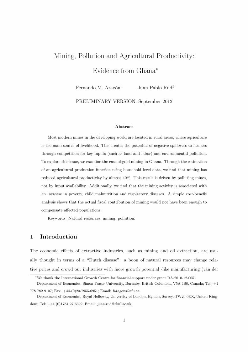
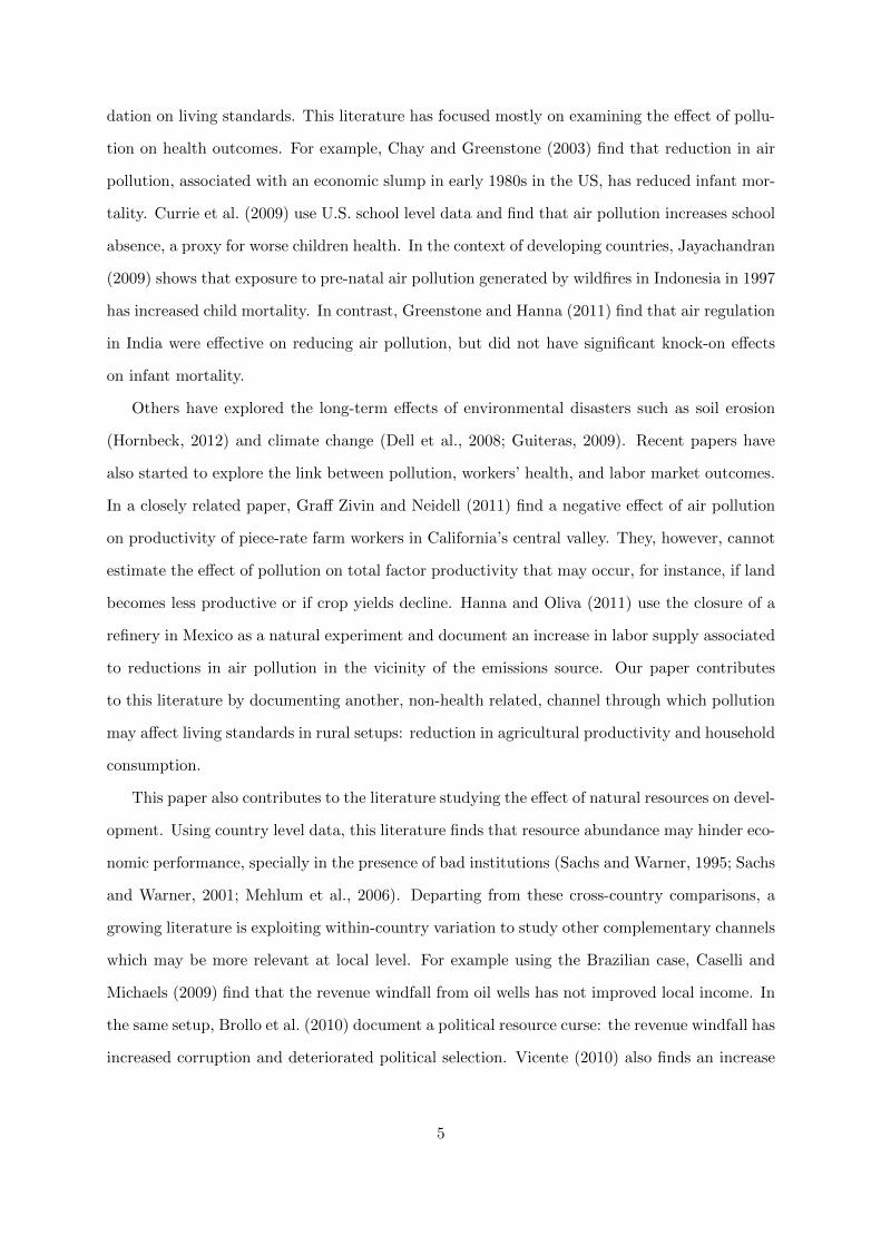
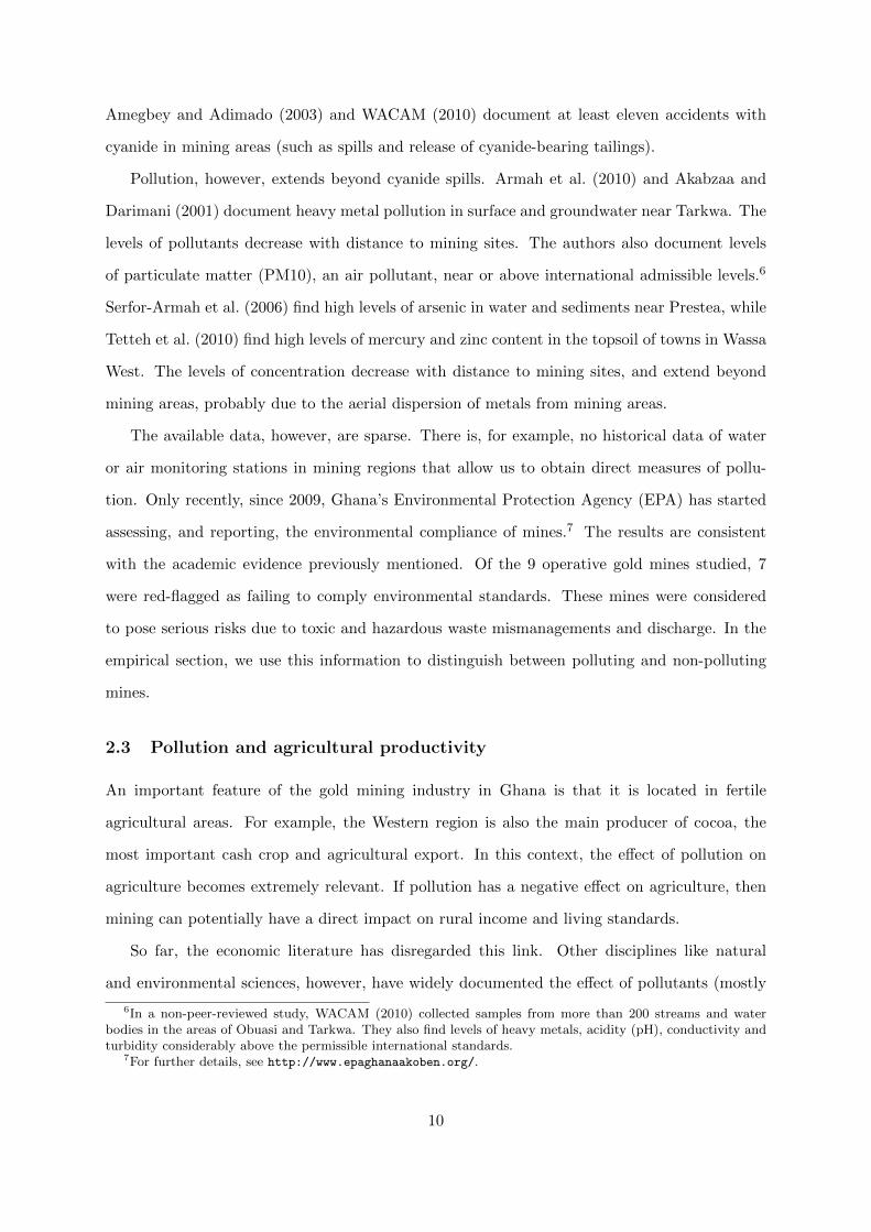
Gold production accelerated in late 1990s due to the opening of new mines and the expansion
of existing operations (see Figure 1). Gold has become the most important export product,
ahead of more traditional commodities such as cocoa, diamond, manganese and bauxite and
represents around of 97% of the country’s mineral revenue. This expansion has placed Ghana
among the top 10 gold producers in the world. In the empirical analysis, we exploit this increase
in mining activities as a source of variation to identify potential spillovers of mining on other
sectors, such as agriculture.
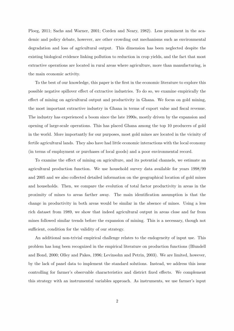
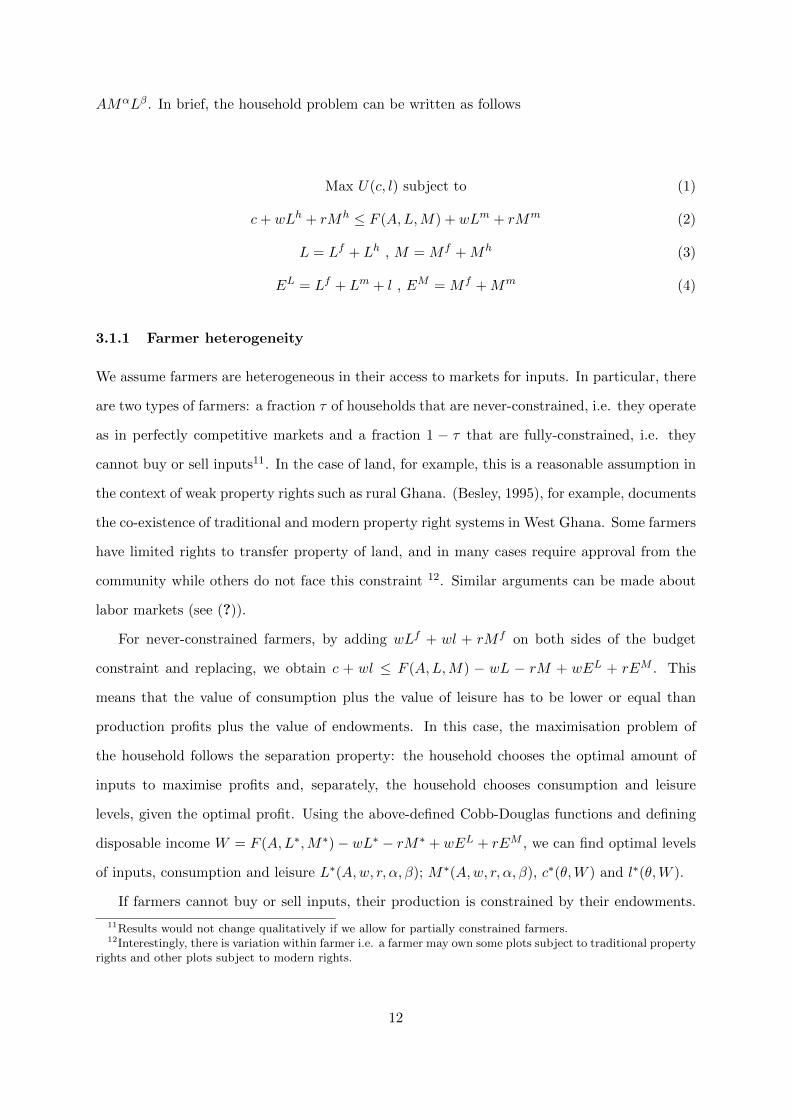
Traditionally, gold mines have been located in the Ashanti gold belt, in the south-west of
Ghana. The gold belt extends over three regions: Western, Ashanti and Central. Recently, new
mines have opened in the south of Brong-Ahafo, and there are several explorations and mine
developments in the Eastern and Northern regions (see Figure 2).1
Gold is produced by large-scale capital-intensive mines, that generate around 96% of to-
tal gold production, and by small-scale artisanal operations called galamseys that are labor-
1A mine cycle consists of several stages: exploration, mine development, production, and closure.
6
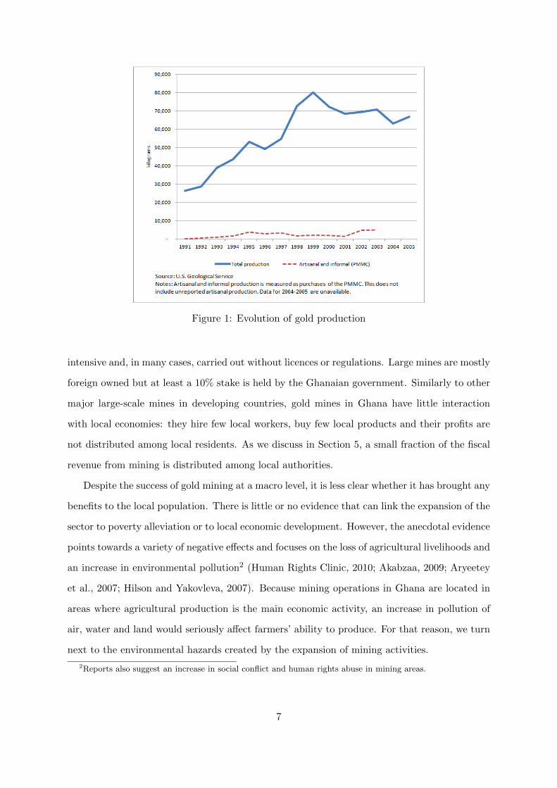
Figure 1: Evolution of gold production
intensive and, in many cases, carried out without licences or regulations. Large mines are mostly
foreign owned but at least a 10% stake is held by the Ghanaian government. Similarly to other
major large-scale mines in developing countries, gold mines in Ghana have little interaction
with local economies: they hire few local workers, buy few local products and their profits are
not distributed among local residents. As we discuss in Section 5, a small fraction of the fiscal
revenue from mining is distributed among local authorities.
Despite the success of gold mining at a macro level, it is less clear whether it has brought any
benefits to the local population. There is little or no evidence that can link the expansion of the
sector to poverty alleviation or to local economic development. However, the anecdotal evidence
points towards a variety of negative effects and focuses on the loss of agricultural livelihoods and
an increase in environmental pollution2 (Human Rights Clinic, 2010; Akabzaa, 2009; Aryeetey
et al., 2007; Hilson and Yakovleva, 2007). Because mining operations in Ghana are located in
areas where agricultural production is the main economic activity, an increase in pollution of
air, water and land would seriously affect farmers’ ability to produce. For that reason, we turn
next to the environmental hazards created by the expansion of mining activities.
2Reports also suggest an increase in social conflict and human rights abuse in mining areas.
7
Figure 2: Gold mines in Ghana
8
2.2 Mining and pollution
The production process that modern mining entails has the potential to affect the environment
in several ways, e.g. through acid rock drainage, contamination of ground and surface water,
and emission of air pollutants.3
Acid rock drainage (ARD) occurs when sulphide minerals are exposed to air and water, for
example during soil removal in mining operations.4 Sulphides oxidize and form an acid effluent
(sulfuric acid) which in turn leaches other metals from existing rocks. The resulting drainage
can become very acidic and contain a number of harmful metals. In turn, this can have severe
impacts on surrounding water bodies. ARD is considered as the most serious environmental
problem for the mining industry (U.S. Environmental Protection Agency, 2000, section 3-2).
Mining operations can also affect water quality when waters (natural or wastewater) infil-
trate through surface materials into the groundwater and pollutes it with contaminants such as
metals, sulphates and nitrates. Wastewater may also contain sediments that increase surface
water turbidity and reduces oxygen and light availability for aquatic life. In the case of gold,
the use of cyanide and mercury creates an additional hazard. Cyanide is used in large-scale
mining and re-processed, but some is discarded in tailings and there is a risk of spillages into
surface waters. Mercury is used in artisanal mining and it is usually released into surface water
or vaporized during the refining process.
Finally, mining activities produce several air pollutants such as nitrogen oxides, sulphur
oxides and particulate matter.5 These emissions are akin to any fuel-intensive technology and
similar to the ones associated to industrial sites, power plants, and motor vehicles. The main
direct sources of air emissions are diesel engines for haulage, drilling, heating and cooling, among
others. Additionally, the process of blasting, crushing and fragmenting the rocks, followed by
smelting and refining generate substantial aerial emissions in large-scale open pit mining.
In the case of Ghana, there is substantial evidence, ranging from anecdotal to scientific,
that gold mining is associated with high levels of pollution. Most studies focus on gold mining
areas in the Western Region such as Tarkwa, Obuasi, Wassa West and Prestea. For example,
3This section is based on U.S. Environmental Protection Agency (2000) , Environment Canada (2009) andNatural Resources Canada (2010).
4Sulphide minerals, such as pyrites, are associated to ores of base metals such as copper, lead, zinc and gold.5These pollutants are contributors to smog and acid rain. Smelters and refineries may also release more
dangerous particles of zinc, arsenic and lead into the air. In the area of analysis, however, there are no smeltingactivities.
9
Amegbey and Adimado (2003) and WACAM (2010) document at least eleven accidents with
cyanide in mining areas (such as spills and release of cyanide-bearing tailings).
Pollution, however, extends beyond cyanide spills. Armah et al. (2010) and Akabzaa and
Darimani (2001) document heavy metal pollution in surface and groundwater near Tarkwa. The
levels of pollutants decrease with distance to mining sites. The authors also document levels
of particulate matter (PM10), an air pollutant, near or above international admissible levels.6
Serfor-Armah et al. (2006) find high levels of arsenic in water and sediments near Prestea, while
Tetteh et al. (2010) find high levels of mercury and zinc content in the topsoil of towns in Wassa
West. The levels of concentration decrease with distance to mining sites, and extend beyond
mining areas, probably due to the aerial dispersion of metals from mining areas.
The available data, however, are sparse. There is, for example, no historical data of water
or air monitoring stations in mining regions that allow us to obtain direct measures of pollu-
tion. Only recently, since 2009, Ghana’s Environmental Protection Agency (EPA) has started
assessing, and reporting, the environmental compliance of mines.7 The results are consistent
with the academic evidence previously mentioned. Of the 9 operative gold mines studied, 7
were red-flagged as failing to comply environmental standards. These mines were considered
to pose serious risks due to toxic and hazardous waste mismanagements and discharge. In the
empirical section, we use this information to distinguish between polluting and non-polluting
mines.
2.3 Pollution and agricultural productivity
An important feature of the gold mining industry in Ghana is that it is located in fertile
agricultural areas. For example, the Western region is also the main producer of cocoa, the
most important cash crop and agricultural export. In this context, the effect of pollution on
agriculture becomes extremely relevant. If pollution has a negative effect on agriculture, then
mining can potentially have a direct impact on rural income and living standards.
So far, the economic literature has disregarded this link. Other disciplines like natural
and environmental sciences, however, have widely documented the effect of pollutants (mostly
6In a non-peer-reviewed study, WACAM (2010) collected samples from more than 200 streams and waterbodies in the areas of Obuasi and Tarkwa. They also find levels of heavy metals, acidity (pH), conductivity andturbidity considerably above the permissible international standards.
7For further details, see http://www.epaghanaakoben.org/.
10

airborne) on crop yields (Emberson et al., 2001; Maggs et al., 1995; Marshall et al., 1997).8
These studies, mostly in controlled environments, find drastic reductions in yields of main crops
-e.g. rice, wheat, and beans- coming from the exposure to air pollutants associated to the
burning of fossil fuels, such as nitrogen oxides and ozone.9 Depending of the type of crop, the
yield reductions can be as high as 30 to 60%.
The potential for mining to affect plants is also acknowledged by environmental agencies.
For example, Environment Canada states that “Mining activity may also contaminate terrestrial
plants. Metals may be transported into terrestrial ecosystems adjacent to mine sites as a result
of releases of airborne particulate matter and seepage of groundwater or surface water. In some
cases, the uptake of contaminants from the soil in mining areas can lead to stressed vegetation.
In such cases, the vegetation could be stunted or dwarfed” (Environment Canada, 2009, p. 39).
3 Methods
3.1 A consumer-producer household
In this section we provide a simple analytical framework that guides the empirical strategy. As
it is standard in the literature10, we assume households are both consumers and producers of
an agricultural good with price p = 1. They maximize utility U(c, l) over consumption c and
leisure l, subject to a budget constraint that accounts for household’s production and income
generated by market activities.
Households use labor (L) and land (M) to produce the agricultural good and have an
idiosyncratic productivity A, i.e. Q = F (A,L,M). A household’s labor endowments EL can
be split between agricultural production (Lf ), leisure (l) and market work (Lm) at a wage
w. Additionally, households can hire labor at the market wage (Lh). A household’s land
endowments EM can be used for agricultural production (Mf ) or supplied to the land market
( Mm), at a price r. Additionally, households can rent land (Mh).
We assume Cobb-Douglas utility and production functions: U(c, l) = cθl1−θ and F (L,M) =
8Most of the available evidence comes from experiments in developed countries. The above mentioned studies,however, document the effect of pollution in developing countries such as India, Pakistan and Mexico.
9Tropospheric ozone is generated at low altitude by a combination of nitrogen oxides, hydrocarbons andsunlight, and can be spread to ground level several kilometers around polluting sources. In contrast, the ozonelayer is located in the stratosphere and plays a vital role filtering ultraviolet rays.
10See (?) for a review.
11
AMαLβ. In brief, the household problem can be written as follows
Max U(c, l) subject to (1)
c+ wLh + rMh ≤ F (A,L,M) + wLm + rMm (2)
L = Lf + Lh , M = Mf +Mh (3)
EL = Lf + Lm + l , EM = Mf +Mm (4)
3.1.1 Farmer heterogeneity
We assume farmers are heterogeneous in their access to markets for inputs. In particular, there
are two types of farmers: a fraction τ of households that are never-constrained, i.e. they operate
as in perfectly competitive markets and a fraction 1 − τ that are fully-constrained, i.e. they
cannot buy or sell inputs11. In the case of land, for example, this is a reasonable assumption in
the context of weak property rights such as rural Ghana. (Besley, 1995), for example, documents
the co-existence of traditional and modern property right systems in West Ghana. Some farmers
have limited rights to transfer property of land, and in many cases require approval from the
community while others do not face this constraint 12. Similar arguments can be made about
labor markets (see (?)).
For never-constrained farmers, by adding wLf + wl + rMf on both sides of the budget
constraint and replacing, we obtain c + wl ≤ F (A,L,M) − wL − rM + wEL + rEM . This
means that the value of consumption plus the value of leisure has to be lower or equal than
production profits plus the value of endowments. In this case, the maximisation problem of
the household follows the separation property: the household chooses the optimal amount of
inputs to maximise profits and, separately, the household chooses consumption and leisure
levels, given the optimal profit. Using the above-defined Cobb-Douglas functions and defining
disposable income W = F (A,L∗,M∗)− wL∗ − rM∗ + wEL + rEM , we can find optimal levels
of inputs, consumption and leisure L∗(A,w, r, α, β); M∗(A,w, r, α, β), c∗(θ,W ) and l∗(θ,W ).
If farmers cannot buy or sell inputs, their production is constrained by their endowments.
11Results would not change qualitatively if we allow for partially constrained farmers.12Interestingly, there is variation within farmer i.e. a farmer may own some plots subject to traditional property
rights and other plots subject to modern rights.
12
In the case of land, this is straightforward: because the marginal cost of land is zero, this type
of farmers uses it all. In the case of labor, now farmers face a trade-off between leisure and
income. The binding budget constraint now becomes c = F (EL − l, EM ) and the optimisation
problem is reduced to the choice of leisure that maximizes the expression U(c, l) = cθl1−θ =
[A(EM )α(EL − l)β]θl1−θ.
Solving, we obtain optimal leisure l∗ = 1−θ1−θ(1−β)E
L that results in optimal in-farm labor use
L∗ = θβ1−θ(1−β)E
L. Note that for constrained farmers, endowments are good predictors of input
use. In particular, land endowment is equal to land use and labor endowments correlation with
labor use depends on farmers’ preference for leisure and technical labor needs in farming.
3.1.2 Expansion of mining activities: channels
In this simple framework, there are two main channel through which the expansion of mining
activities can affect farmers: pollution and competition for inputs. Pollution would imply a
reduction in agricultural productivity A. Note that because pollution affects the health of crops
either directly (e.g. leaf tissue injury or plant growth) or indirectly (e.g. reducing resistance to
pests and diseases), in the presence of pollution agricultural product would fall even if there is
no change in input use.
Output could also decline due to a reduction in input use, for example, if prices for L and M
increase because of a greater demand from mines or a reduction in endowments, following land
grabbings and population displacement. This mechanism is similar in flavor to the Dutch disease
and, as discussed in the previous section, has been flagged as a concern in the case of Ghana13.
The second of the arguments has been favored as an explanation for the perceived reduction
in agricultural activity, and an increase in poverty, in mining areas (Akabzaa, 2009; Aryeetey
et al., 2007). Either way, the competition for inputs would reduce agricultural output, even if
productivity remains unchanged.
Because the two proposed channels have different empirical implications, we can separate
them by estimating the agricultural production function. Furthermore, the analytical framework
presented above informs how consumer-producer farmers choose inputs in a way that can be
13For example, Duncan et al. (2009) quantify at around 15% the reduction of agricultural land use associatedwith the expansion of mining in the Bogoso-Prestea area. The conflict over resources seems to have exacerbateddue to weak property rights (i.e. customary property rights) and poor compensation schemes for displacedfarmers (Human Rights Clinic, 2010).
13
used to guide the estimation of the production function. Additionally, because agricultural
output affects the budget constraint of farmers, the anaytical framework shows that if the
mining sector is reducing farmer productivity, agricultural incomes should decrease and affect
negatively consumption and poverty levels (which is simply consumption relative to a threshold)
3.2 Empirical implementation
A farmer’s agricultural production function can be written as
Qivt = AivtMαitL
βit, (5)
where Q is expected output, M and L are land and labor, and A is total factor productivity.
All these variables vary for farmer i in locality v at time t. We define locality as the survey’s
enumeration area. This is the smallest recognizable jurisdiction and roughly corresponds to a
village or neighborhood.
We assume that A is composed of 3 factors: farmers’ heterogeneity (ηi), time-invariant local
economic and environmental conditions (ρv) and time-varying factors, potentially related to the
presence of local mining activity (Svt). In particular, we assume:
Aivt = exp(ηi + ρv + γSvt). (6)
In addition, note that we do not observe Q but only actual output Y :
Yivt = Qivteεit , (7)
where εit captures unanticipated shocks and is, by definition, uncorrelated to input decisions.
With these assumptions in mind, we can write the following relation:
yivt = αmit + βlit + ηi + ρv + γSvt + εit, (8)
where y, l and m represent the logs of observed output, labor and land, respectively.
Note that the effects of mining on input availability would affect output through change
in prices and the optimal choice of land and labor, but not through changes in A. As a
14
consequence, if the pollution mechanism is at play we should obtain that γ < 0. Also, in the
absence of direct measures of pollution, we use as a proxy the presence of local mining activities
Svt. A caveat with using this proxy, however, is that it may also capture other non-market
negative spillovers associated to mining activity such as decline in quality of inputs, change in
public good provision, and increase in social conflict. In the results section we examine these
alternative mechanisms in more detail.
There are two main empirical challenges to estimate specification (8). The first one is related
to the fact that mining and non-mining areas may have systematic differences in productivity.
In terms of equation (8), this means that E(Svtρv) 6= 0 and ρv is unobservable. This omitted
variable problem may lead to endogeneity issues when estimating the coefficients of interest. To
address this issue, we exploit the time variation in the repeated cross section to compare the
evolution of productivity in mining areas relative to non-mining areas. In particular, we replace
Svt by minev × Tt where minev is an indicator of being close to a mine and Tt is a time trend.
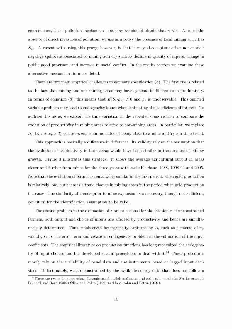
This approach is basically a difference in difference. Its validity rely on the assumption that
the evolution of productivity in both areas would have been similar in the absence of mining
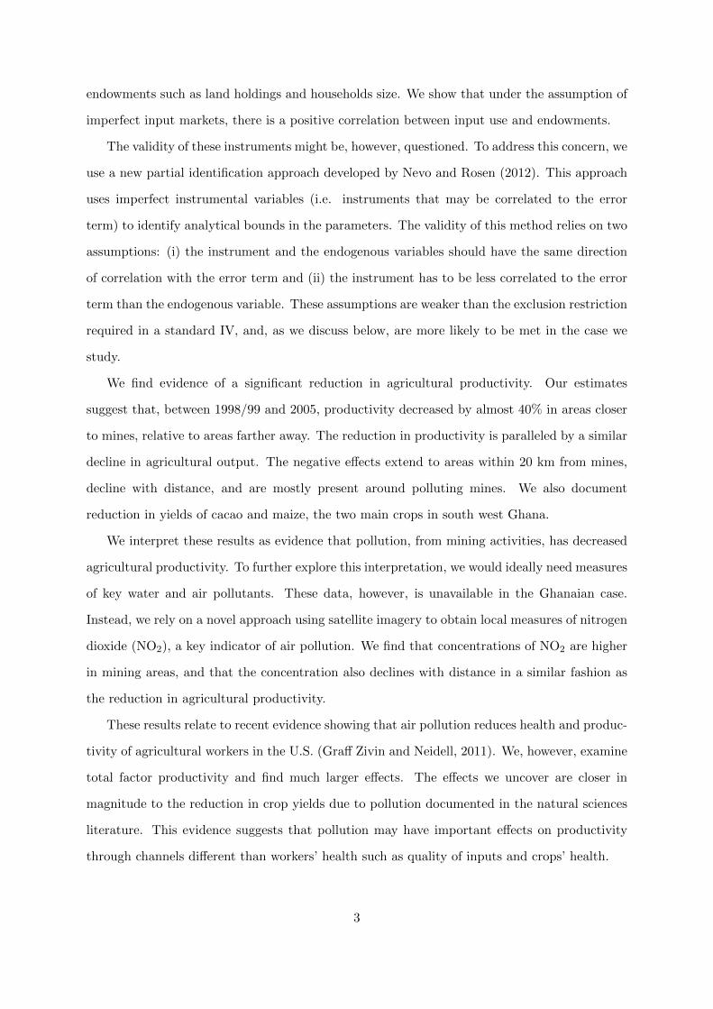
growth. Figure 3 illustrates this strategy. It shows the average agricultural output in areas
closer and farther from mines for the three years with available data: 1988, 1998-99 and 2005.
Note that the evolution of output is remarkably similar in the first period, when gold production
is relatively low, but there is a trend change in mining areas in the period when gold production
increases. The similarity of trends prior to mine expansion is a necessary, though not sufficient,
condition for the identification assumption to be valid.
The second problem in the estimation of 8 arises because for the fraction τ of unconstrained
farmers, both output and choice of inputs are affected by productivity and hence are simulta-
neously determined. Thus, unobserved heterogeneity captured by A, such as elements of ηi,
would go into the error term and create an endogeneity problem in the estimation of the input
coefficients. The empirical literature on production functions has long recognized the endogene-
ity of input choices and has developed several procedures to deal with it.14 These procedures
mostly rely on the availability of panel data and use instruments based on lagged input deci-
sions. Unfortunately, we are constrained by the available survey data that does not follow a
14There are two main approaches: dynamic panel models and structural estimation methods. See for exampleBlundell and Bond (2000) Olley and Pakes (1996) and Levinsohn and Petrin (2003).
15
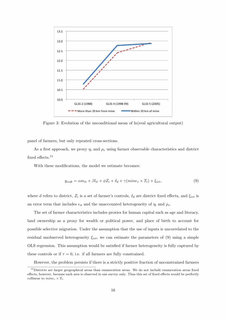
Figure 3: Evolution of the unconditional mean of ln(real agricultural output)
panel of farmers, but only repeated cross-sections.
As a first approach, we proxy ηi and ρv using farmer observable characteristics and district
fixed effects.15
With these modifications, the model we estimate becomes:
yivdt = αmit + βlit + φZi + δd + γ(minev × Tt) + ξivt, (9)
where d refers to district, Zi is a set of farmer’s controls, δd are district fixed effects, and ξivt is
an error term that includes εit and the unaccounted heterogeneity of ηi and ρv.
The set of farmer characteristics includes proxies for human capital such as age and literacy,
land ownership as a proxy for wealth or political power, and place of birth to account for
possible selective migration. Under the assumption that the use of inputs is uncorrelated to the
residual unobserved heterogeneity ξivt, we can estimate the parameters of (9) using a simple
OLS regression. This assumption would be satisfied if farmer heterogeneity is fully captured by
these controls or if τ = 0, i.e. if all farmers are fully constrained.
However, the problem persists if there is a strictly positive fraction of unconstrained farmers
15Districts are larger geographical areas than enumeration areas. We do not include enumeration areas fixedeffects, however, because each ares is observed in one survey only. Thus this set of fixed effects would be perfectlycollinear to minev × Tt.
16
and the set of controls does not capture fully farmers’ characteristics that affect the choice of
inputs. Assuming τ < 116, we can use the presence of fully-constrained farmers to deal with
input estimates. In particular, we can use endowments in an IV strategy. This works under
what we consider a more plausible assumption, i.e. that endowments are not conditionally
correlated to idiosyncratic productivity shocks or to an omitted variable, i.e. the (unobserved)
heterogeneity not captured by our controls17.
In the presense of a correlation between the error term and endowments that would invalidate
the exclusion restriction in the IV strategy, we can make further progress by using a partial
identification strategy proposed by Nevo and Rosen (2012). This approach uses imperfect
instrumental variables (IIV) to identify parameter bounds.18 An IIV is an instrument that may
be correlated with the error term. Nevo and Rosen (2012) show that if (i) the correlation between
the instrument and the error term has the same sign as the correlation between the endogenous
variable and the error term, and (ii) the instrument is less correlated to the error than the
endogenous variable, then it is possible to derive analytical bounds for the parameters.19
These (set) identification assumptions are weaker than the exogeneity assumption in the
standard IV approach. The analytical framework presented above again provides the rationale
for using this approach under less restrictive assumptions. First, there is a positive correlation
between endowments and input use that comes from the subset of constrained farmers. There
is no correlation between inputs and endowments for farmers operating in an unconstrained
environment, unless it comes from an omitted variable that affects both. We only need that
this omitted variable is such that higher productivity increases endowments20. Second, because
the input is a share of endowments, for the subset of constrained farmers the correlation with the
error term is the same. However, for unconstrained farmers there is a direct positive correlation
16Data shows that inputs markets are thin: in the area of study around 8% of available land is rented, andonly 1.4% of the total farm labor (in number of hours) is hired.
17The interpretation of this IV strategy would be as a local average treatment effect, since the coefficientswould be identified from constrained farmers only.
18In contrast, the standard IV approach focuses on point identification.19The parameter set could be a two- or one-sided bound depending on the observable correlation between
endogenous variables and instruments. In particular, denoting X as the endogenous variable, Z as the imperfectinstrument, and W other additional regressors, there is a two-sided bound if, in addition to the (set) identificationassumptions, (σxxσz −σxσxz)σxz < 0, where x is the projection of X on W . In the complementary case, there isa one-sided bound. In the empirical section we do check that this expression has a negative value. We refer thereader to Nevo and Rosen (2012) for a detailed exposition of the estimation method.
20One might argue that higher productivity might be negatively correlated with household size. In that case,we only need the fraction of constrained farmers to be high enough. In the case of land, the sign of the correlationslooks less controversial, but the same logic would apply.
17
between unobserved productivity and input use. We only need to assume that the correlation
between endowments and productivity is more tenuous for this group to use IIV. In brief, point
(i) above is obtained thanks to the group of constrained farmers, while point (ii) is obtained
thanks to the group of unconstrained farmers.
We have laid out thre alternative ways of estimating input coefficients in the agricultural
production function. However, our main interest is to test whether residual productivity has
changed in mining areas, as the smoking gun for the presence of pollution-related reduction in
production. A reduction in productivity should alse be reflected in lower consumption levels (and
greater levels of poverty) for consumer-producer households. Crowding out of farming through
other channels, such as an increase in the price of inputs, might increase household income for
unconstrained households selling inputs. In that case, the average effects on consumption could
even be positive.
3.3 Data
Our main results use household data from the rounds 4 and 5 of the Ghana Living Standards
Survey (GLSS) These surveys were collected by the Ghana Statistical Service (GSS) in 1998-99
and 2005, respectively. 21
The survey contains several levels of geographical information of the interviewees. The higher
levels are district and region. The district is the lower sub-national administrative jurisdiction,
while the region is the highest.22 The survey also distinguishes between urban and rural areas,
as well as ecological zones (i.e. coastal, savannah and forest). The finer level is the enumeration
area, which roughly corresponds to villages (in rural areas) and neighborhoods (in urban areas).
For each enumeration area we obtain its geographical coordinates from the GSS.23
We are mainly interested on two set of variables: measures of proximity to gold mines, and
measures of argicultural inputs and output.
21We also use the GLSS 2, taken in 1989, for evaluating pre-trends in agricultural output between mining andnon-mining areas. We do not use this data, however, in the estimation of the production function since it doesnot contain comparable information on input use. In addition, we do not use the GLSS 3 (1993-94) because thereis not available information on the geographical location of the interviewees.
22In 2005, there were 10 regions and 138 districts.23The GSS does not have location of enumeration areas for the GLSS 2. In this case, we extracted the location
using printed maps of enumeration areas in previous survey reports.
18
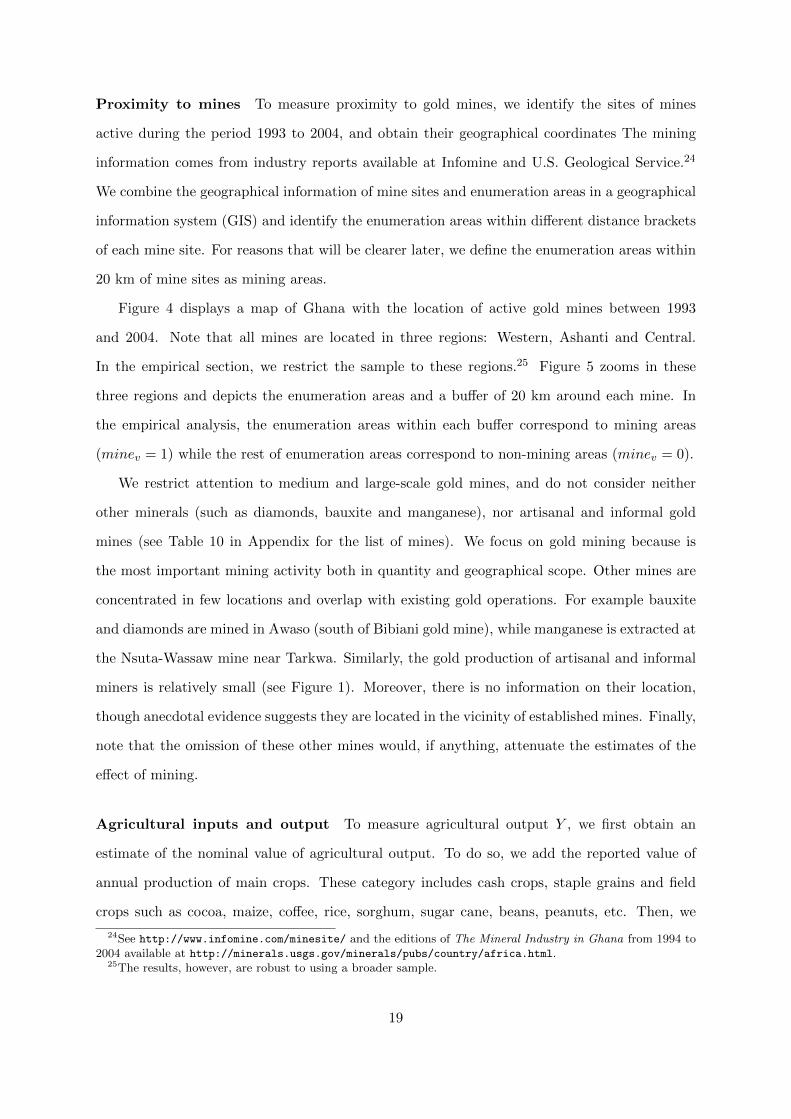
Proximity to mines To measure proximity to gold mines, we identify the sites of mines
active during the period 1993 to 2004, and obtain their geographical coordinates The mining
information comes from industry reports available at Infomine and U.S. Geological Service.24
We combine the geographical information of mine sites and enumeration areas in a geographical
information system (GIS) and identify the enumeration areas within different distance brackets
of each mine site. For reasons that will be clearer later, we define the enumeration areas within
20 km of mine sites as mining areas.
Figure 4 displays a map of Ghana with the location of active gold mines between 1993
and 2004. Note that all mines are located in three regions: Western, Ashanti and Central.
In the empirical section, we restrict the sample to these regions.25 Figure 5 zooms in these
three regions and depicts the enumeration areas and a buffer of 20 km around each mine. In
the empirical analysis, the enumeration areas within each buffer correspond to mining areas
(minev = 1) while the rest of enumeration areas correspond to non-mining areas (minev = 0).
We restrict attention to medium and large-scale gold mines, and do not consider neither
other minerals (such as diamonds, bauxite and manganese), nor artisanal and informal gold
mines (see Table 10 in Appendix for the list of mines). We focus on gold mining because is
the most important mining activity both in quantity and geographical scope. Other mines are
concentrated in few locations and overlap with existing gold operations. For example bauxite
and diamonds are mined in Awaso (south of Bibiani gold mine), while manganese is extracted at
the Nsuta-Wassaw mine near Tarkwa. Similarly, the gold production of artisanal and informal
miners is relatively small (see Figure 1). Moreover, there is no information on their location,
though anecdotal evidence suggests they are located in the vicinity of established mines. Finally,
note that the omission of these other mines would, if anything, attenuate the estimates of the
effect of mining.
Agricultural inputs and output To measure agricultural output Y , we first obtain an
estimate of the nominal value of agricultural output. To do so, we add the reported value of
annual production of main crops. These category includes cash crops, staple grains and field
crops such as cocoa, maize, coffee, rice, sorghum, sugar cane, beans, peanuts, etc. Then, we
24See http://www.infomine.com/minesite/ and the editions of The Mineral Industry in Ghana from 1994 to2004 available at http://minerals.usgs.gov/minerals/pubs/country/africa.html.
25The results, however, are robust to using a broader sample.
19
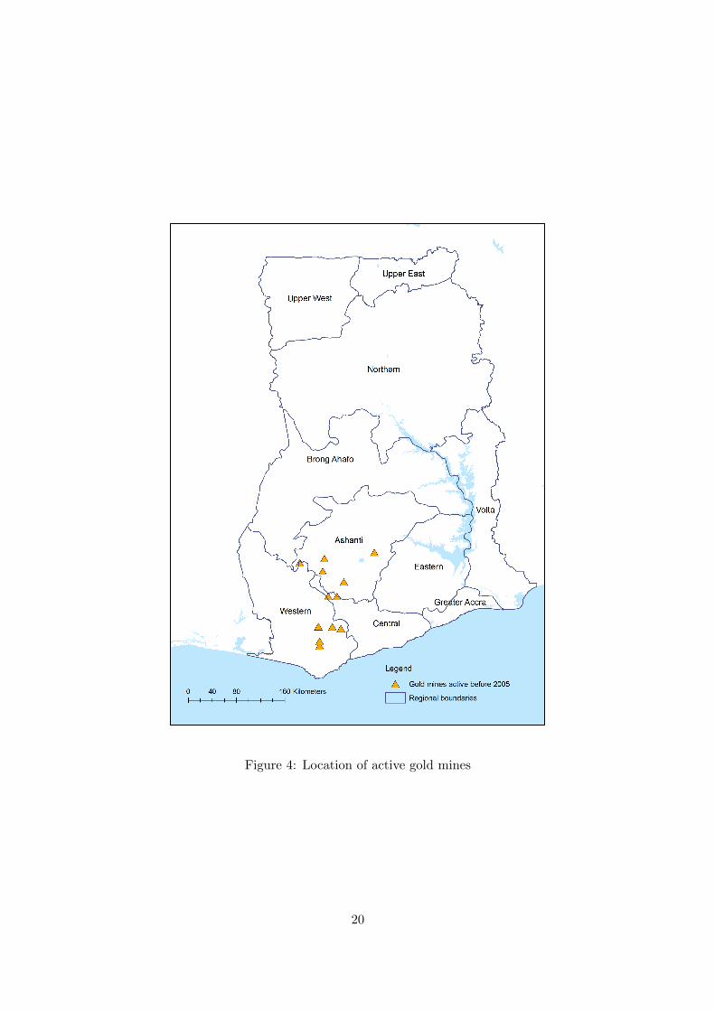
Figure 4: Location of active gold mines
20
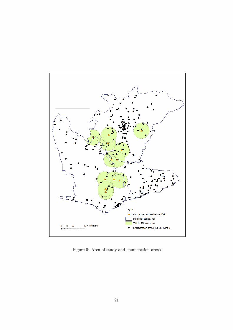
Figure 5: Area of study and enumeration areas
21
divide the nominal value of agricultural output by the value of the poverty line.The poverty
line is estimated by the GSS and measures the value of a minimum consumption basket, mostly
composed of food. This variable is available for Accra, rest of urban areas, and rural areas in
each ecological zone.
In addition, we construct estimates of yields of the two main crops in the area of study:
cocoa and maize. These measures provide us with alternative ways to explore the effect of
mining on agricultural productivity.
We construct estimates of the two most important agricultural inputs: land and labor. The
measure of land simply adds the area of plots cultivated with major crops in the previous 12
months. To measure labor we add the number of hired worker-days to the number of days each
household member spends working in the household farm. Finally, we measure land endowment
as the area of the land owned by the farmer, while the labor endowment is the number of
equivalent adults in the household.
The resulting dataset contains information on agricultural inputs and output for 1,627 farm-
ers in years 1998-99 and 2005. The farmers are located in 42 districts in 3 regions of south west
Ghana: Western, Ashanti and Central. Table 1 presents some summary statistics.
22
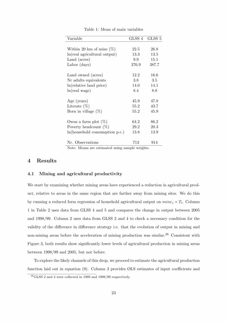
Table 1: Mean of main variables
Variable GLSS 4 GLSS 5
Within 20 km of mine (%) 22.5 26.8ln(real agricultural output) 13.3 13.5Land (acres) 9.9 15.1Labor (days) 376.9 387.7
Land owned (acres) 12.2 16.6Nr adults equivalents 3.8 3.5ln(relative land price) 14.0 14.1ln(real wage) 8.4 8.8
Age (years) 45.9 47.8Literate (%) 55.2 43.7Born in village (%) 55.2 45.9
Owns a farm plot (%) 64.2 86.2Poverty headcount (%) 29.2 20.3ln(household consumption p.c.) 13.8 13.9
Nr. Observations 713 914
Note: Means are estimated using sample weights.
4 Results
4.1 Mining and agricultural productivity
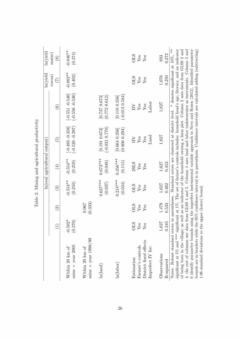
We start by examining whether mining areas have experienced a reduction in agricultural prod-
uct, relative to areas in the same region that are farther away from mining sites. We do this
by running a reduced form regression of household agricultural output on minev × Tt. Column
1 in Table 2 uses data from GLSS 4 and 5 and compares the change in output between 2005
and 1998/99. Column 2 uses data from GLSS 2 and 4 to check a necessary condition for the
validity of the difference in difference strategy i.e. that the evolution of output in mining and
non-mining areas before the acceleration of mining production was similar.26 Consistent with
Figure 3, both results show significantly lower levels of agricultural production in mining areas
between 1998/99 and 2005, but not before.
To explore the likely channels of this drop, we proceed to estimate the agricultural production
function laid out in equation (9). Column 3 provides OLS estimates of input coefficients and
26GLSS 2 and 4 were collected in 1989 and 1998/99 respectively.
23

explores whether exposure to mining has reduced residual productivity, under the assumption
that the identifying conditions discussed above hold. In column 4, we estimate a 2SLS using
input endowments (such as area of land owned and the number of adults equivalents living
in the household) as instruments for actual input use. All regressions include farmer controls
and district fixed effects to account for the endogeneity in input use. The estimates use sample
weights and cluster errors at district level to account for the sampling design and geographically
correlated shocks, respectively.
The main observation is that both OLS and 2SLS estimates suggest a drastic reduction in
agricultural productivity.27. The estimate of the interaction term “within 20 km × year 2005”
for the whole sample is around -0.55. This implies that, between 1998-99 and 2005, the average
agricultural productivity of farmers in the vicinity of mines declined by around 40%, relative
to farmers located farther away. The reduction in productivity is high, and consistent with the
results documented in biological literature (see Section 2.3).
Columns 5 and 6 use the imperfect instrumental variable approach developed by Nevo and
Rosen (2012). As previously discussed, this approach uses instrumental variables that may be
correlated to the error term to identify parameters bounds instead of point estimates. The key
identification assumptions are that (i) the instrument and the endogenous regressor have the
same direction of correlation with the error term and (ii) the instrument is less correlated to the
error term than the endogenous variable. These are weaker assumptions than the exogeneity
required in standard IV. We allow one instrument at a time to be imperfect.28 We include
similar controls as in the OLS and 2SLS estimates and also use sample weights.
We report the estimated lower and upper parameter bounds and also the confidence interval
of the identified set.29 Note that the identified parameter sets of α and β remain mostly positive,
though the range is quite broad. Despite this, the estimated effect of mining on agricultural
productivity (γ) remains negative with values ranging between -0.551 and -0.358.30
27The first stage of the 2SLS reveals a positive and significant correlation between input endowments and inputuse. This is consistent with imperfect input markets as discussed in Section X. The F-test statistic of excludedinstruments is 59.41. See Table 11 in the appendix for further details.
28Nevo and Rosen (2012) obtain analytical bounds only in the case when there is one endogenous regressorwith imperfect instruments. In the case of multiple endogenous variables, the parameter set can be, however,obtained by simulations. The estimates of γ in this more flexible case are similar (see Table 12 in the Appendix).
29In columns 5 and 6, the values of the expression (σxxσz − σxσxz)σxz are, respectively, -0.059 and -0.229.Recall that when this expression is negative there is a two-sided bound of the parameters. The 95% confidenceintervals of the identified sets are obtained by adding (subtracting) 1.96 standard deviations to the upper (lower)bounds.
30A sensitivity analysis confirm that the results are very robust to alternative assumptions in the values of α
24
These results suggest that the negative effect on total factor productivity is robust to a
series of specifications and estimation methods to (partially) identify input coefficients in the
production function. What is reassuring for our purposes is that even allowing for production
function coefficients to vary within a wide range of combinations (within the expected set where
α+β ≤ 1) does not affect the finding that residual productivity has deteriorated over time near
mining areas.
Finally, columns 7 and 8 examine the effect of mining on crop yields. Crop yields have been
used as a proxy for agricultural productivity in the empirical literature and are an output of
interest by themselves (see for example Duflo and Pande (2007) and Banerjee et al. (2002)). We
focus on the yields of cocoa and maize, the two most important crops in south west Ghana. In
both cases, we estimate an OLS regression including farmer’s controls and district fixed effects,
but without input use. Note that the sample size is smaller, since we only use data of farmers
engaged in cocoa or maize production. Consistent with the results on productivity, we find a
significant reduction (around 58%) in crops yields.
The role of distance So far, we have assumed that areas within 20 km of mines experience
most of the negative effect. Implicitly, this approach assumes that the effect of mining declines
with distance. To explore this issue further, we estimate equation (9) replacing “minev” by a
linear spline of distance to a mine,∑
c γcdistancecv where distancecv = 1 if enumeration area v
is in distance bracket c. This specification treats distance more flexibly and allow us to compare
the evolution of farmers’ productivity at different distance brackets from the mine relative to
farmers farther way (the comparison group is farmers beyond 50 km).
Figure 6 presents the estimates of γc. First, the effect of mining on productivity is (weakly)
decreasing in distance. Second, the loss of productivity is significant (at 10% confidence) within
20 km of mines, but becomes insignificant in farther locations. This result provides the rationale
for concentrating in a 20 km buffer around mines, as in the main results.
4.1.1 Is this driven by pollution?
We interpret the previous findings as evidence that agricultural productivity has decreased in
the vicinity of mines. We argue that a plausible channel is through the presence of mining-
and β. See Appendix A.1.
25
Tab
le2:
Min
ing
and
agri
cult
ura
lp
rod
uct
ivit
y
ln(r
eal
agri
cult
ura
lou
tpu
t)ln
(yie
ldln
(yie
ldco
coa)
mai
ze)
(1)
(2)
(3)
(4)
(5)
(6)
(7)
(8)
Wit
hin
20
km
of-0
.502*
-0.5
54**
-0.5
54**
[-0.
493
-0.3
58]
[-0.
551
-0.5
40]
-0.8
82**
-0.8
46**
min
e×
year
200
5(0
.270)
(0.2
50)
(0.2
59)
(-0.
520
-0.2
97)
(-0.
556
-0.5
30)
(0.4
02)
(0.3
74)
Wit
hin
20
km
of0.
067
min
e×
year
199
8/99
(0.3
33)
ln(l
and
)0.
627*
**0.
673*
**[0
.191
0.67
3][0
.737
0.67
3](0
.037
)(0
.048
)(-
0.03
10.
770)
(0.7
720.
612)
ln(l
abor)
0.21
8***
0.35
6***
[0.6
640.
356]
[0.1
180.
356]
(0.0
34)
(0.1
15)
(0.8
060.
294)
(-0.
013
0.58
4)
Est
imat
ion
OL
SO
LS
OL
S2S
LS
IIV
IIV
OL
SO
LS
Farm
er’s
contr
ols
Yes
Yes
Yes
Yes
Yes
Yes
Yes
Yes
Dis
tric
tfi
xed
effec
tsY
esY
esY
esY
esY
esY
esY
esY
esIm
per
fect
IVfo
r:L
and
Lab
or
Ob
serv
ati
on
s1,
627
1,47
91,
627
1,62
71,
627
1,62
71,
076
933
R-s
qu
are
d0.2
450.
533
0.46
20.
453
0.25
00.
272
Not
es:
Rob
ust
stan
dar
der
rors
inp
aren
thes
es.
Sta
nd
ard
erro
rsare
clu
ster
edat
dis
tric
tle
vel.
*d
enote
ssi
gn
ifica
nt
at
10%
,**
sign
ifica
nt
at5%
and
***
sign
ifica
nt
at1%
.T
he
set
of
farm
er’s
contr
ols
incl
ud
es:
hou
sehold
hea
d’s
age,
lite
racy
,an
dan
ind
icato
rof
bei
ng
bor
nin
the
vil
lage
;as
wel
las
anin
dic
ato
rof
the
hou
seh
old
own
ing
afa
rmp
lot.
Colu
mn
2u
ses
data
from
GL
SS
2and
4,th
ere
stof
colu
mn
su
sed
ata
from
GL
SS
4an
d5.
Colu
mn
4u
ses
lan
dan
dla
bor
endow
men
tes
as
inst
rum
ents
.C
olu
mn
5an
d6
iden
tify
par
amet
erb
oun
ds
usi
ng
the
imp
erfe
ctin
stru
men
tal
vari
ab
leap
pro
ach
inN
evo
an
dR
ose
n(2
012).
Iden
tifi
edp
ara
met
erb
oun
ds
are
inb
rack
ets
wh
ile
the
95%
con
fid
ence
inte
rval
isin
pare
nth
esis
.C
on
fid
ence
inte
rvals
are
calc
ula
ted
ad
din
g(s
ub
tract
ing)
1.96
stan
dar
dd
evia
tion
sto
the
up
per
(low
er)
bou
nd
.
26

Figure 6: The effect of mining on agricultural productivity, by distance to a mine
related pollution. As we discussed before, several studies show that water and soil in mining
areas have higher than normal levels of pollutants (see section 2.2).
To further explore this issue we would need measures of water and air pollutants at local
level. Then, we could examine whether mining areas are indeed more polluted. Unfortunately,
these data are unavailable in the Ghanaian case.31 Instead, we rely on three indirect ways to
assess the role of pollution.
First, we explore heterogeneous effects between areas located downstream and upstream
of mine sites. This is a crude way to assess the importance of pollutants that could be carry
by surface water. Second, we examine heterogeneous effects in areas near polluting and non-
polluting mines. This classification is based on Ghana EPA’s environmental assessments.32
Finally, we obtain indicators of air pollution using satellite imagery, and examine the relative
levels of pollution in mining and non-mining areas.
Column 1 and 2 in Table 3 estimates the baseline regression allowing for heterogeneous
effects between between areas upstream and downstream of a mine, as well as between polluting
31There are, for example, air monitoring stations only in the proximity of Accra. There are some indepen-dent measures of soil and water quality in mining areas. These measures, however, are sparse, not collectedsystematically, and unavailable for non-mining areas. This precludes a more formal regression analysis.
32See http://www.epaghanaakoben.org/rating/listmines2 for details. The earliest environmental assess-ments were published in year 2009. We classify a mine as polluting if it is red-flagged by EPA as failing tocomply environmental standards. As previously mentioned, these mines are considered to pose serious environ-mental risks.
27
and non-polluting mines. To do so, we include an interaction of “within 20 km × year 2005”
with an indicator of being downstream of a mine, or being near a polluting mine. The results
suggest that there is no heterogeneous effect of mining in areas downstream and upstream of
a mine. The coefficient of the triple interaction is negative but insignificant. Though this may
be due to lack of statistical power, a conservative interpretation is that pollution of superficial
waters may not be driving the main results. In contrast, column 1 shows that most of the
decline in productivity occurs in the proximity of mines red-flagged by the Ghana EPA as
having poor environmental practices. There are, however, two important caveats. First, the
environmental assessments are based on information collected since 2007, and hence may not
accurately reflect the mine environmental status during the period of analysis. Second, there
are no environmental assessments for all mines that were active before 2005. For that reason, we
impute a non-polluting status to mines with missing data. These issues may create measurement
errors and lead to an attenuation bias of the estimates.
Taken together these results are suggestive that environmental pollution may play a role.
To get more conclusive evidence, we examine indicators of air pollution obtained from satellite
imagery. The satellite imagery is obtained from the Ozone Monitoring Instrument (OMI) avail-
able at NASA.33 This satellite instrument provides daily measures of tropospheric air conditions
since October 2004.
We focus on a particular air pollutant: nitrogen dioxide (NO2). NO2 is a toxic gas by
itself and also an important precursor of tropospheric ozone -a gas harmful to both human and
crops’ health.34 The main source of NO2 is the combustion of hydrocarbons such as biomass
burning, smelters and combustion engines.35 Thus, it is likely to occur near highly mechanized
operations, such as large-scale mining.
There are three important caveats relevant for the empirical analysis. First, the data pro-
vides only a proxy of the cross sectional distribution of NO2 at ground level. Note that the
satellite data reflect air conditions in the troposphere (from ground level up to 12 km). Tropo-
spheric and ground-level NO2 are correlated, but to obtain accurate measures at ground level
we need to calibrate existing atmospheric models.36 This requires ground-based air pollution
33For additional details, see http://aura.gsfc.nasa.gov/instruments/omi.html. Data are available at http://mirador.gsfc.nasa.gov/cgi-bin/mirador/presentNavigation.pl?tree=project&project=OMI.
34NO2 gives the brownish coloration to smog seen above many polluted cities.35There are also natural sources of NO2 such as lightning and forest fires.36The correlation between these two measures is typically above 0.6. OMI tropospheric measures tend, however,
28

Table 3: Mining and pollution
ln(real agricultural ouput)Upstream vs Ghana EPA Average NO2 ln(real agric.downstream assessment output)
(1) (2) (3) (4) (5)
Within 20 km of mine × -0.498* -0.391year 2005 (0.274) (0.279)
Within 20 km of mine × -0.115year 2005 × downstream (0.421)
Within 20 km of mine × -0.773**year 2005 × polluting mine (0.318)
ln(land) 0.626*** 0.633*** 0.718***(0.036) (0.037) (0.066)
ln(labor) 0.218*** 0.215*** 0.136**(0.034) (0.034) (0.056)
Within 20 km of mine 0.342** 0.439***(0.137) (0.123)
Average NO2 -0.759*(0.407)
Farmer’s controls Yes Yes No No NoDistrict fixed effects Yes Yes No No NoRegion fixed effects No No No Yes Yes
Observations 1,627 1,627 399 399 918R-squared 0.462 0.464 0.063 0.209 0.265
Notes: Robust standard errors in parentheses. * denotes significant at 10%, ** significant at 5% and*** significant at 1%. Column 1 and 2 includes input use, district fixed effects and farmer’s controlvariables as in the baseline regression (see notes of Table 2). Columns 1, 2 and 4 reports standarderrors clustered at district level. Columns 3 to 4 uses the sample of enumeration areas and satellitedata for 2005. They include ecological zone fixed effects and indicators of urban areas. Columns 4also include region fixed effects. Column 5 presents 2SLS estimates of the agricultural productionfunction using only the sample of farmers in GLSS 5. It uses‘’ Within 20 km of mine” as instrumentfor NO2. The control variables are fixed effects for region and ecological zone.
29
measures from monitoring stations in some of the dates and locations covered by the satellite.37
Second, the data is available only from late 2004. Hence, we cannot study levels of air pollution
during the period of analysis (1998 to 2005), but only at the end. While this approach does not
allow us to study the change in air pollutants associated to mining, it can still be informative
of the relative levels of pollution at local level. Finally, the measures of NO2 are highly affected
by atmospheric conditions such as tropical thunderstorms, cloud coverage, and rain.38. These
disturbances are particularly important from November to March, and during the peak of the
rainy season.39 For that reason, we aggregate the daily data taking the average over the period
April-May 2005. These months are at the beginning of the rainy season. This period also
corresponds to the beginning of the main agricultural season in southern Ghana.
To compare the relative levels of NO2 in mining and non-mining areas, we match the satellite
data to each enumeration area and estimate the following regression:40
NO2v = φ1minev + φ2Wv + ωv, (10)
where NO2v is the average value of tropospheric NO2 in enumeration area v during the period
April-May 2005, minev is an indicator of being within 20 km of a mine, and Wv is a vector of
controls variables.41 Note that the unit of observation is the enumeration area, and that, in
contrast to the baseline results, this regression exploits cross-sectional variation only.
Columns 3 and 4 in Table 3 present the empirical results. Column 3 estimates (10) including
only indicators of ecological zones and urban areas. Column 4 populates the model with region
fixed effects. Finally, we replace the dummy minev by a distance spline with breaks at 10, 20, 30
and 40 km and plot the resulting estimates in Figure 7. Note that in this figure the comparison
group is farmers beyond 40 km of a mine.
The satellite evidence suggests that mining areas have a significantly greater concentration
of NO2.42 Moreover, the concentration of NO2 decreases with distance to the mine in a similar
to underestimate ground levels of NO2 by 15-30 % (Celarier et al., 2008).37Similar data would be necessary to estimate tropospheric ozone.38Lighting tends to increase NO2 while rain reduces it.39In southern Ghana, the rainy season runs from early April to mid-November.40The satellite data are binned to 13 km x 24 km grids. The value of NO2 of each enumeration area corresponds
to the value of NO2 in the bin where the enumeration area lies.41NO2 is measured as 1015 molecules per cm2. The average NO2 is 8.9 while its standard deviation is 1.2.42We also find a negative correlation between NO2 and agricultural productivity. These results, not reported,
exploit only cross sectional variation.
30
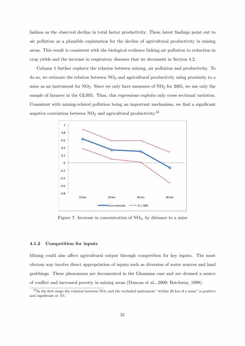
fashion as the observed decline in total factor productivity. These latest findings point out to
air pollution as a plausible explanation for the decline of agricultural productivity in mining
areas. This result is consistent with the biological evidence linking air pollution to reduction in
crop yields and the increase in respiratory diseases that we document in Section 4.2.
Column 5 further explores the relation between mining, air pollution and productivity. To
do so, we estimate the relation between NO2 and agricultural productivity using proximity to a
mine as an instrument for NO2. Since we only have measures of NO2 for 2005, we use only the
sample of farmers in the GLSS5. Thus, this regressions exploits only cross sectional variation.
Consistent with mining-related pollution being an important mechanism, we find a significant
negative correlation between NO2 and agricultural productivity.43
Figure 7: Increase in concentration of NO2, by distance to a mine
4.1.2 Competition for inputs
Mining could also affect agricultural output through competition for key inputs. The most
obvious way involve direct appropriation of inputs such as diversion of water sources and land
grabbings. These phenomena are documented in the Ghanaian case and are deemed a source
of conflict and increased poverty in mining areas (Duncan et al., 2009; Botchway, 1998).
43In the first stage the relation between NO2 and the excluded instrument ‘’within 20 km of a mine” is positiveand significant at 5%.
31

A possibility is that the loss in productivity reflects the reduction in quality of inputs
associated with farmers’ displacement. For example, farmers may have been relocated to less
productive lands or to isolated locations.44
It is unlikely, however, that this factor fully accounts for the observed reduction in pro-
ductivity. Population displacement, if required, is usually confined to the mine operating sites
i.e. areas containing mineral deposits, processing units and tailings. These areas comprise, at
most, few kilometers around the mine site. For example, Bibiani mine has a license over 19
km2; Iduapriem mine has a mining lease of 33 km2 while Tarkwa leases cover 260 km2. Note
that not all lands in mining concessions are inhabited nor all its population is displaced. In
contrast, we document drops in productivity in a much larger area i.e. within 20 km of a mine,
this represents an area of more than 1,200 km2 around a mine.45
Mines may also compete with farmers for scarce local inputs, such as unskilled labor. Simi-
larly, the mine’s demand for local goods and services may increase price of non-tradables (such
as housing). In either case, mining activities would increase input prices, and farmer’s pro-
duction costs. In turn, this may lead to a decline in output, and demand of inputs.46 This
phenomena cannot be studied by equation (9) since it already controls for input use and thus
it is only informative of the effect of mining on total factor productivity.
To explore this issue further, we study the effect of mining on input prices. As measure
of input prices, we use the daily agricultural wage from the GLSS community module and the
price of land per acre self-reported by farmers.47 We take the average of these variables by
enumeration area, and divide them by the poverty line to obtain relative input prices. Then, we
regress the log of the relative input price on the interaction term “within 20 km × year 2005”.
We also include geographical controls (such as region fixed effects, ecological zone fixed effects,
and indicators of proximity to the coast or a region’s capital) and their interaction with a time
trend to account for unobserved market conditions.
Table 4 display the results. Columns 1 and 3 start by estimating a parsimonious model
44Note that our previous results are conditional on being a farmer, hence they underestimate the loss ofagricultural output due to change of land use from agriculture to mining, or farmer’s leaving the industry.
45Another possibility is that the drop in productivity is driven by migrants with either lower human capital oroccupying poorer lands. We discuss this alternative explanation in the robustness checks.
46This effect could be offset if mines’ demand for local inputs has a positive effect on local income. The incomeeffect may increase demand for, and price of, local agricultural goods. In that case, agricultural output andfarmer’s income would actually increase (Aragon and Rud, n.d.).
47The results using the rental price of land are similar, though the sample size is much smaller and the estimates,less precise.
32
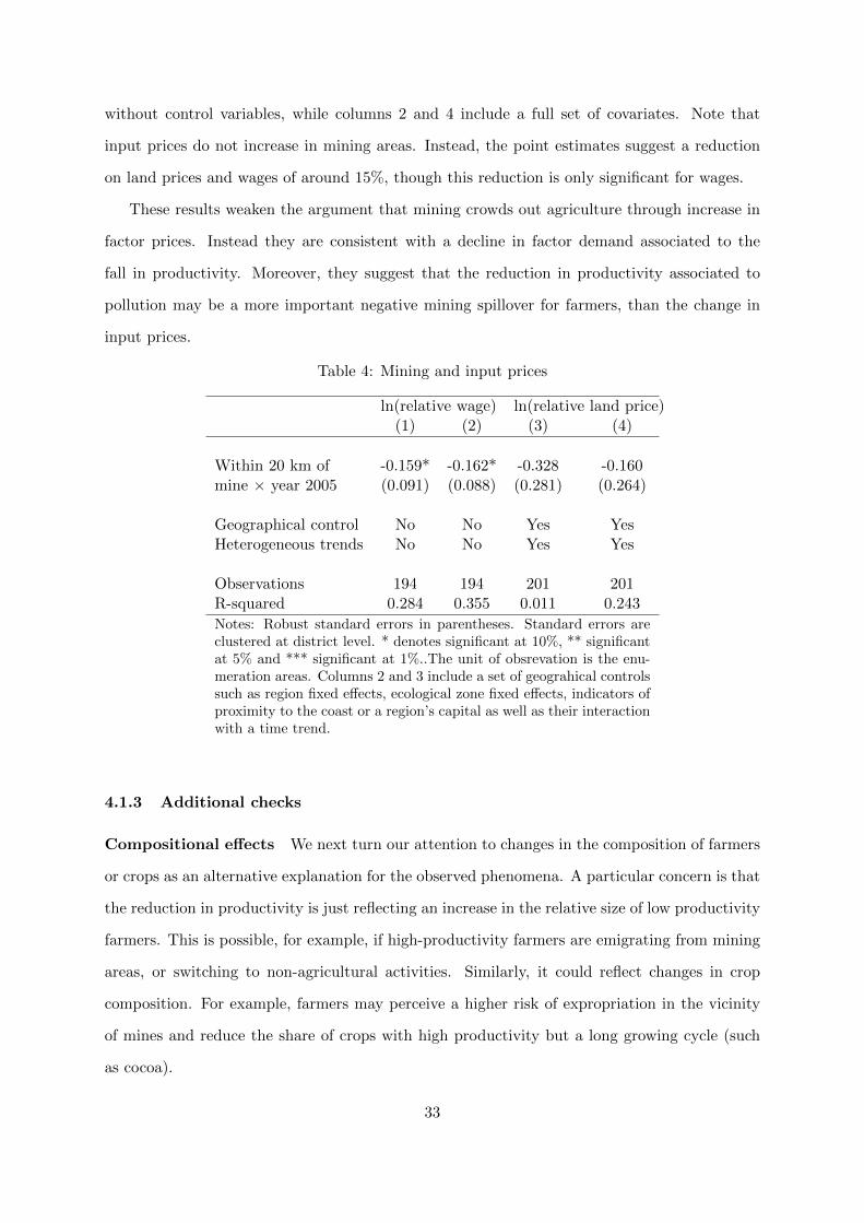
without control variables, while columns 2 and 4 include a full set of covariates. Note that
input prices do not increase in mining areas. Instead, the point estimates suggest a reduction
on land prices and wages of around 15%, though this reduction is only significant for wages.
These results weaken the argument that mining crowds out agriculture through increase in
factor prices. Instead they are consistent with a decline in factor demand associated to the
fall in productivity. Moreover, they suggest that the reduction in productivity associated to
pollution may be a more important negative mining spillover for farmers, than the change in
input prices.
Table 4: Mining and input prices
ln(relative wage) ln(relative land price)(1) (2) (3) (4)
Within 20 km of -0.159* -0.162* -0.328 -0.160mine × year 2005 (0.091) (0.088) (0.281) (0.264)
Geographical control No No Yes YesHeterogeneous trends No No Yes Yes
Observations 194 194 201 201R-squared 0.284 0.355 0.011 0.243
Notes: Robust standard errors in parentheses. Standard errors areclustered at district level. * denotes significant at 10%, ** significantat 5% and *** significant at 1%..The unit of obsrevation is the enu-meration areas. Columns 2 and 3 include a set of geograhical controlssuch as region fixed effects, ecological zone fixed effects, indicators ofproximity to the coast or a region’s capital as well as their interactionwith a time trend.
4.1.3 Additional checks
Compositional effects We next turn our attention to changes in the composition of farmers
or crops as an alternative explanation for the observed phenomena. A particular concern is that
the reduction in productivity is just reflecting an increase in the relative size of low productivity
farmers. This is possible, for example, if high-productivity farmers are emigrating from mining
areas, or switching to non-agricultural activities. Similarly, it could reflect changes in crop
composition. For example, farmers may perceive a higher risk of expropriation in the vicinity
of mines and reduce the share of crops with high productivity but a long growing cycle (such
as cocoa).
33
As a first check, we investigate whether workers in mining areas are changing occupation
relative to control households. Columns 1 and 2 in Table 5 estimate the probability that a
worker is engaged in the agricultural sector (as a producer or laborer). Column 1 focuses on all
workers, while column 2 focuses on household heads only. In both cases, there is no significant
change in the likelihood of working in agriculture. If anything, point estimates are slightly
positive.48
Second, we look at measures of farmer’s education. This result is informative, however,
under the assumption that farming ability is positively correlated with educational attainment.
This sounds a plausible assumption, given that in our baseline regression the measure of literacy
is associated with an increase in agricultural product and productivity. Columns 3 and 4 look
at the sample of producers only and check whether literacy levels and a measure of educational
attainment (e.g. secondary school completed) have dropped49. The results do not suggest that
mining areas have a relative decrease in measures of farmer’s education.
Finally, we examine whether farmer’s have changed crop composition. We focus on the share
of cocoa in total agricultural value. Note that cocoa is the main cash crop, but it also has a
long maturity cycle. In addition, we use a Herfindhal concentration index of all main crops.
Columns 5 and 6 suggest that there is no significant change in either variable in mining areas.50
Taken together, these results weaken the argument that the reduction in productivity is
driven by changes in occupational choice, farmer’s ability or crop choice.
Alternative specifications In table 6, we check that our results are robust to alternative
specifications. Column 1 estimates a parsimonious model without farmer characteristics and
district fixed effects. In contrast, column 2 saturates the baseline regression with an array of
heterogeneous trends. We include the interaction of time trends with indicators of ecological
zone, region, proximity to coast and to region capitals. This specification addresses concerns
that the interaction term “within 20 km × year 2005” may be just picking up other confounding
trends. Columns 3 and 4 split the sample between local and non-local farmers. We define a
48These results are robust to a series of specifications, with and without controls, and using other measures offarming activity, such as proportion of farmers in the household.
49Levels of completion of primary school are really high, i.e. around 88%, while literacy levels (47.7%) andsecondary school completed (37.2%) show greater variation. Results hold when using data on completed primaryschool.
50Additionally, we did not find any evidence of a reduction in the shares of maize, the second most importantcrop.
34
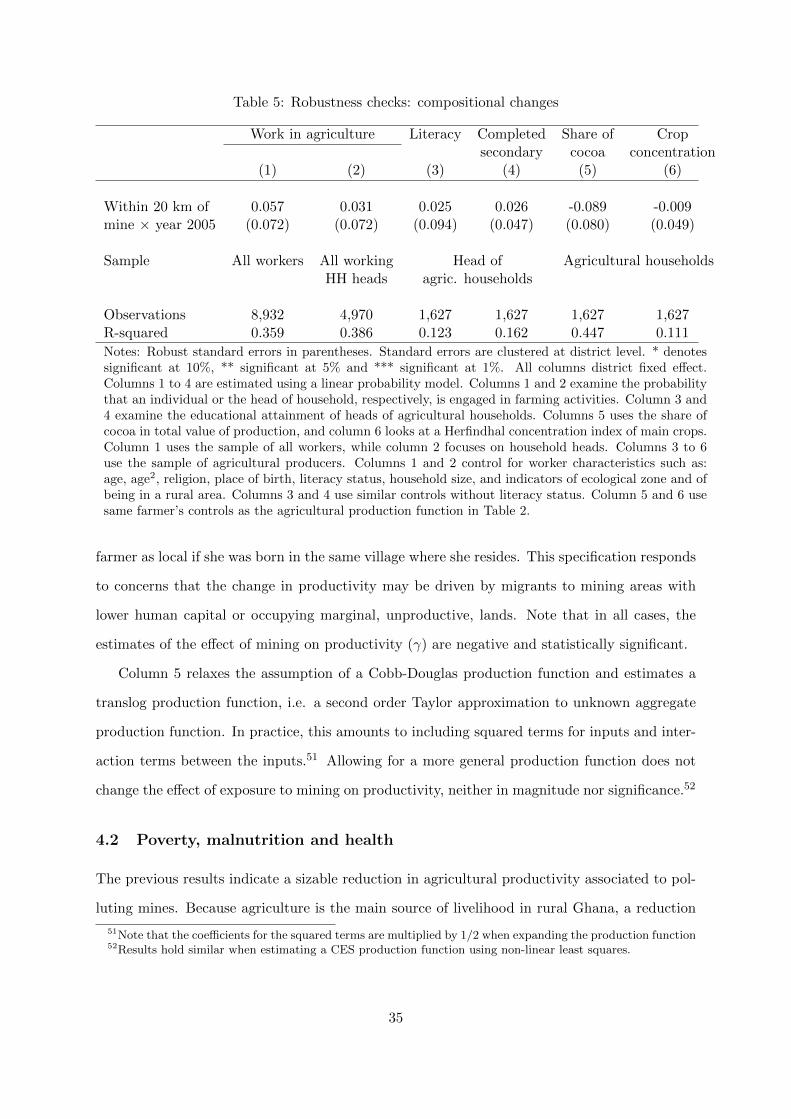
Table 5: Robustness checks: compositional changes
Work in agriculture Literacy Completed Share of Cropsecondary cocoa concentration
(1) (2) (3) (4) (5) (6)
Within 20 km of 0.057 0.031 0.025 0.026 -0.089 -0.009mine × year 2005 (0.072) (0.072) (0.094) (0.047) (0.080) (0.049)
Sample All workers All working Head of Agricultural householdsHH heads agric. households
Observations 8,932 4,970 1,627 1,627 1,627 1,627R-squared 0.359 0.386 0.123 0.162 0.447 0.111
Notes: Robust standard errors in parentheses. Standard errors are clustered at district level. * denotessignificant at 10%, ** significant at 5% and *** significant at 1%. All columns district fixed effect.Columns 1 to 4 are estimated using a linear probability model. Columns 1 and 2 examine the probabilitythat an individual or the head of household, respectively, is engaged in farming activities. Column 3 and4 examine the educational attainment of heads of agricultural households. Columns 5 uses the share ofcocoa in total value of production, and column 6 looks at a Herfindhal concentration index of main crops.Column 1 uses the sample of all workers, while column 2 focuses on household heads. Columns 3 to 6use the sample of agricultural producers. Columns 1 and 2 control for worker characteristics such as:age, age2, religion, place of birth, literacy status, household size, and indicators of ecological zone and ofbeing in a rural area. Columns 3 and 4 use similar controls without literacy status. Column 5 and 6 usesame farmer’s controls as the agricultural production function in Table 2.
farmer as local if she was born in the same village where she resides. This specification responds
to concerns that the change in productivity may be driven by migrants to mining areas with
lower human capital or occupying marginal, unproductive, lands. Note that in all cases, the
estimates of the effect of mining on productivity (γ) are negative and statistically significant.
Column 5 relaxes the assumption of a Cobb-Douglas production function and estimates a
translog production function, i.e. a second order Taylor approximation to unknown aggregate
production function. In practice, this amounts to including squared terms for inputs and inter-
action terms between the inputs.51 Allowing for a more general production function does not
change the effect of exposure to mining on productivity, neither in magnitude nor significance.52
4.2 Poverty, malnutrition and health
The previous results indicate a sizable reduction in agricultural productivity associated to pol-
luting mines. Because agriculture is the main source of livelihood in rural Ghana, a reduction
51Note that the coefficients for the squared terms are multiplied by 1/2 when expanding the production function52Results hold similar when estimating a CES production function using non-linear least squares.
35
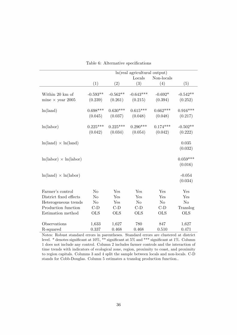
Table 6: Alternative specifications
ln(real agricultural output)Locals Non-locals
(1) (2) (3) (4) (5)
Within 20 km of -0.593** -0.562** -0.643*** -0.692* -0.542**mine × year 2005 (0.239) (0.261) (0.215) (0.394) (0.252)
ln(land) 0.698*** 0.630*** 0.615*** 0.662*** 0.916***(0.045) (0.037) (0.048) (0.048) (0.217)
ln(labor) 0.225*** 0.225*** 0.290*** 0.174*** -0.502**(0.042) (0.034) (0.054) (0.042) (0.222)
ln(land) × ln(land) 0.035(0.032)
ln(labor) × ln(labor) 0.059***(0.016)
ln(land) × ln(labor) -0.054(0.034)
Farmer’s control No Yes Yes Yes YesDistrict fixed effects No Yes Yes Yes YesHeterogeneous trends No Yes No No NoProduction function C-D C-D C-D C-D TranslogEstimation method OLS OLS OLS OLS OLS
Observations 1,633 1,627 780 847 1,627R-squared 0.337 0.468 0.468 0.510 0.471
Notes: Robust standard errors in parentheses. Standard errors are clustered at districtlevel. * denotes significant at 10%, ** significant at 5% and *** significant at 1%. Column1 does not include any control. Column 2 includes farmer controls and the interaction oftime trends with indicators of ecological zone, region, proximity to coast, and proximityto region capitals. Columns 3 and 4 split the sample between locals and non-locals. C-Dstands for Cobb-Douglas. Column 5 estimates a translog production function..
36
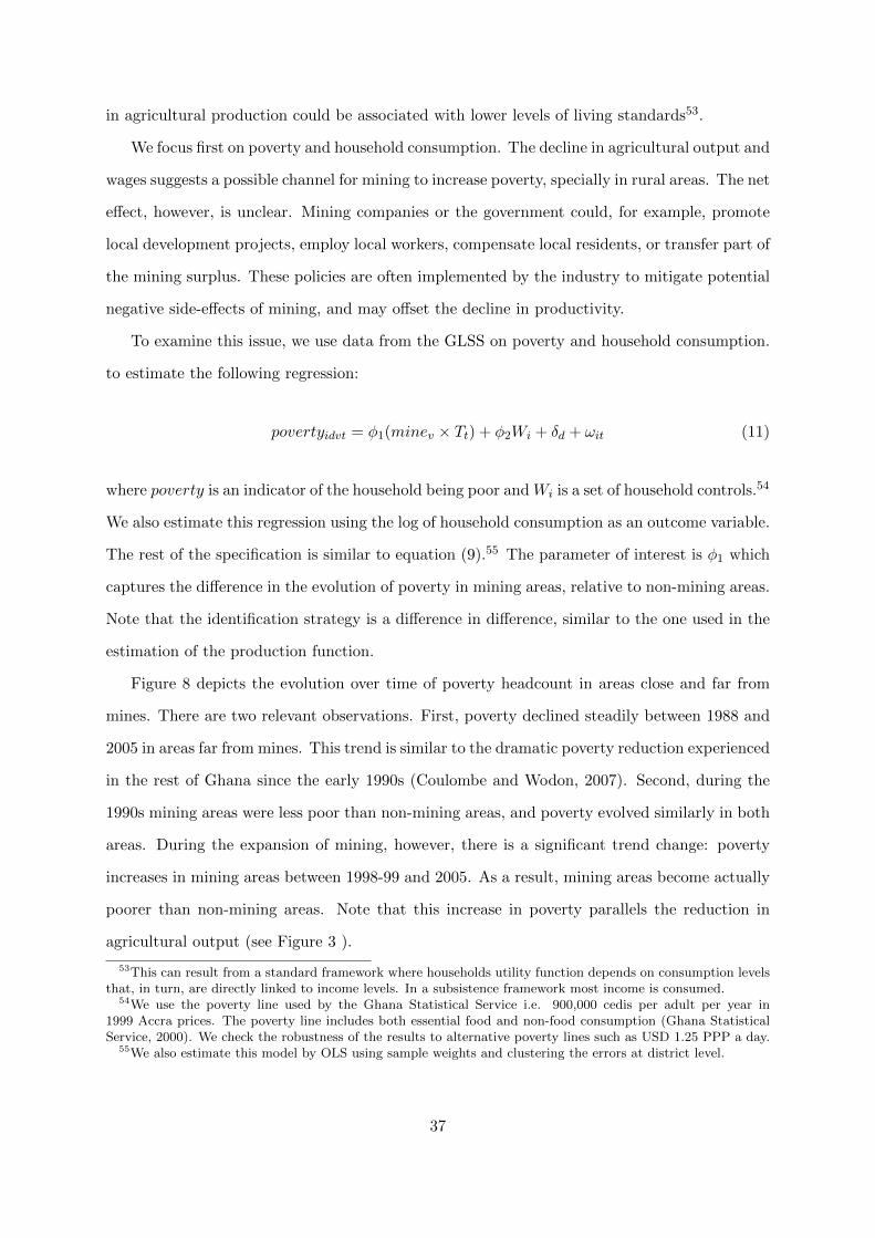
in agricultural production could be associated with lower levels of living standards53.
We focus first on poverty and household consumption. The decline in agricultural output and
wages suggests a possible channel for mining to increase poverty, specially in rural areas. The net
effect, however, is unclear. Mining companies or the government could, for example, promote
local development projects, employ local workers, compensate local residents, or transfer part of
the mining surplus. These policies are often implemented by the industry to mitigate potential
negative side-effects of mining, and may offset the decline in productivity.
To examine this issue, we use data from the GLSS on poverty and household consumption.
to estimate the following regression:
povertyidvt = φ1(minev × Tt) + φ2Wi + δd + ωit (11)
where poverty is an indicator of the household being poor and Wi is a set of household controls.54
We also estimate this regression using the log of household consumption as an outcome variable.
The rest of the specification is similar to equation (9).55 The parameter of interest is φ1 which
captures the difference in the evolution of poverty in mining areas, relative to non-mining areas.
Note that the identification strategy is a difference in difference, similar to the one used in the
estimation of the production function.
Figure 8 depicts the evolution over time of poverty headcount in areas close and far from
mines. There are two relevant observations. First, poverty declined steadily between 1988 and
2005 in areas far from mines. This trend is similar to the dramatic poverty reduction experienced
in the rest of Ghana since the early 1990s (Coulombe and Wodon, 2007). Second, during the
1990s mining areas were less poor than non-mining areas, and poverty evolved similarly in both
areas. During the expansion of mining, however, there is a significant trend change: poverty
increases in mining areas between 1998-99 and 2005. As a result, mining areas become actually
poorer than non-mining areas. Note that this increase in poverty parallels the reduction in
agricultural output (see Figure 3 ).
53This can result from a standard framework where households utility function depends on consumption levelsthat, in turn, are directly linked to income levels. In a subsistence framework most income is consumed.
54We use the poverty line used by the Ghana Statistical Service i.e. 900,000 cedis per adult per year in1999 Accra prices. The poverty line includes both essential food and non-food consumption (Ghana StatisticalService, 2000). We check the robustness of the results to alternative poverty lines such as USD 1.25 PPP a day.
55We also estimate this model by OLS using sample weights and clustering the errors at district level.
37
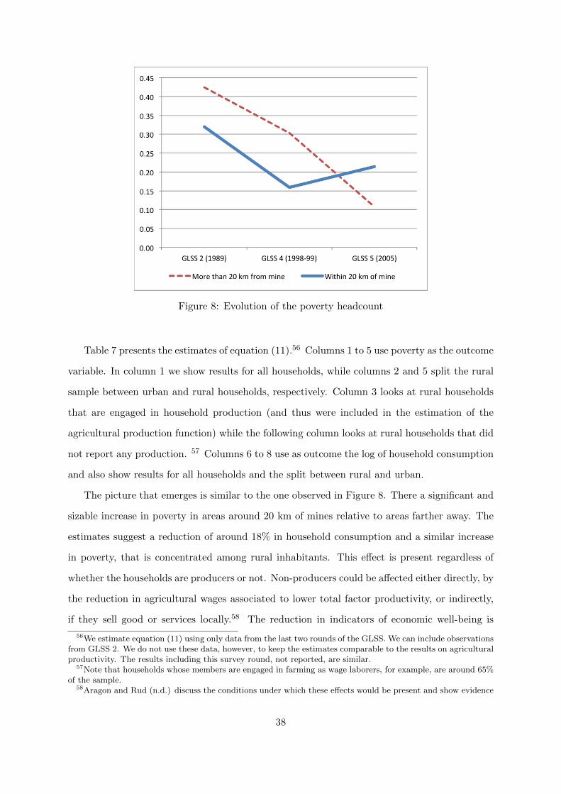
Figure 8: Evolution of the poverty headcount
Table 7 presents the estimates of equation (11).56 Columns 1 to 5 use poverty as the outcome
variable. In column 1 we show results for all households, while columns 2 and 5 split the rural
sample between urban and rural households, respectively. Column 3 looks at rural households
that are engaged in household production (and thus were included in the estimation of the
agricultural production function) while the following column looks at rural households that did
not report any production. 57 Columns 6 to 8 use as outcome the log of household consumption
and also show results for all households and the split between rural and urban.
The picture that emerges is similar to the one observed in Figure 8. There a significant and
sizable increase in poverty in areas around 20 km of mines relative to areas farther away. The
estimates suggest a reduction of around 18% in household consumption and a similar increase
in poverty, that is concentrated among rural inhabitants. This effect is present regardless of
whether the households are producers or not. Non-producers could be affected either directly, by
the reduction in agricultural wages associated to lower total factor productivity, or indirectly,
if they sell good or services locally.58 The reduction in indicators of economic well-being is
56We estimate equation (11) using only data from the last two rounds of the GLSS. We can include observationsfrom GLSS 2. We do not use these data, however, to keep the estimates comparable to the results on agriculturalproductivity. The results including this survey round, not reported, are similar.
57Note that households whose members are engaged in farming as wage laborers, for example, are around 65%of the sample.
58Aragon and Rud (n.d.) discuss the conditions under which these effects would be present and show evidence
38
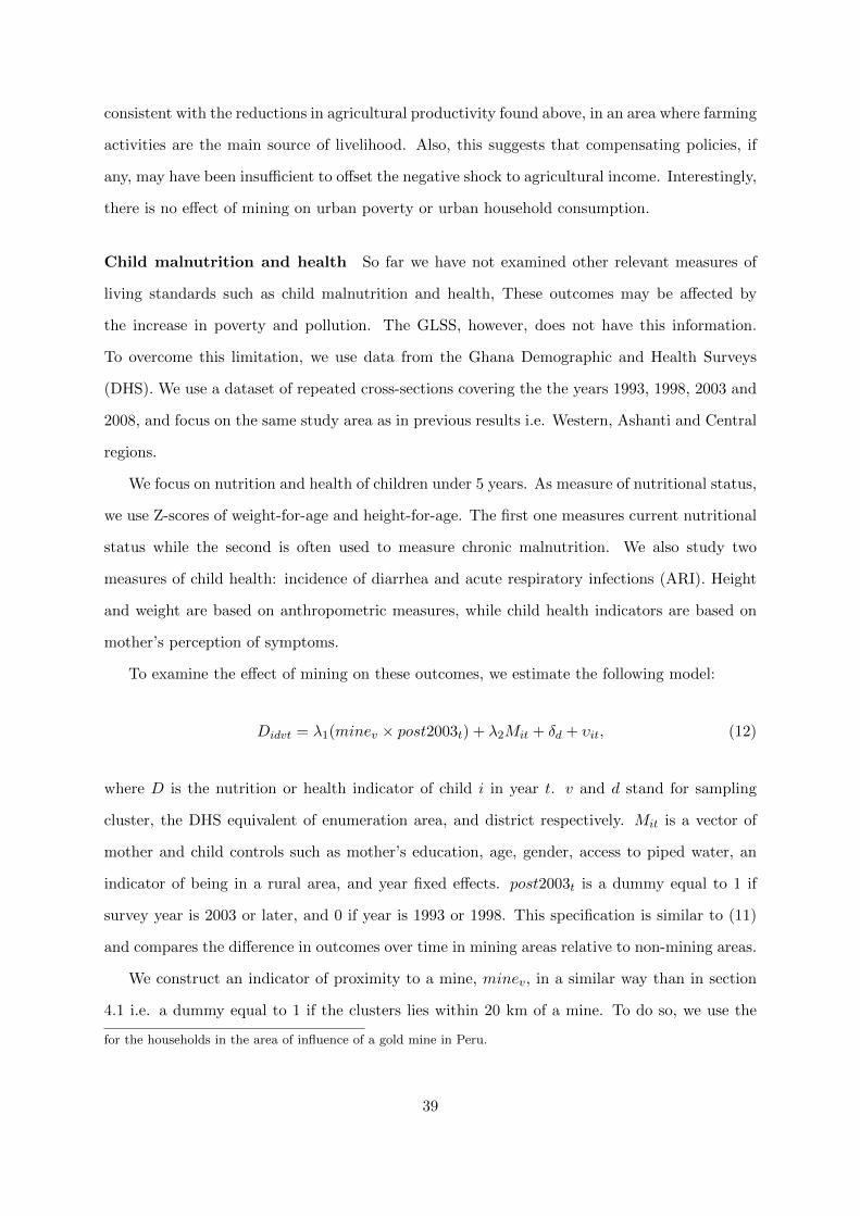
consistent with the reductions in agricultural productivity found above, in an area where farming
activities are the main source of livelihood. Also, this suggests that compensating policies, if
any, may have been insufficient to offset the negative shock to agricultural income. Interestingly,
there is no effect of mining on urban poverty or urban household consumption.
Child malnutrition and health So far we have not examined other relevant measures of
living standards such as child malnutrition and health, These outcomes may be affected by
the increase in poverty and pollution. The GLSS, however, does not have this information.
To overcome this limitation, we use data from the Ghana Demographic and Health Surveys
(DHS). We use a dataset of repeated cross-sections covering the the years 1993, 1998, 2003 and
2008, and focus on the same study area as in previous results i.e. Western, Ashanti and Central
regions.
We focus on nutrition and health of children under 5 years. As measure of nutritional status,
we use Z-scores of weight-for-age and height-for-age. The first one measures current nutritional
status while the second is often used to measure chronic malnutrition. We also study two
measures of child health: incidence of diarrhea and acute respiratory infections (ARI). Height
and weight are based on anthropometric measures, while child health indicators are based on
mother’s perception of symptoms.
To examine the effect of mining on these outcomes, we estimate the following model:
Didvt = λ1(minev × post2003t) + λ2Mit + δd + υit, (12)
where D is the nutrition or health indicator of child i in year t. v and d stand for sampling
cluster, the DHS equivalent of enumeration area, and district respectively. Mit is a vector of
mother and child controls such as mother’s education, age, gender, access to piped water, an
indicator of being in a rural area, and year fixed effects. post2003t is a dummy equal to 1 if
survey year is 2003 or later, and 0 if year is 1993 or 1998. This specification is similar to (11)
and compares the difference in outcomes over time in mining areas relative to non-mining areas.
We construct an indicator of proximity to a mine, minev, in a similar way than in section
4.1 i.e. a dummy equal to 1 if the clusters lies within 20 km of a mine. To do so, we use the
for the households in the area of influence of a gold mine in Peru.
39
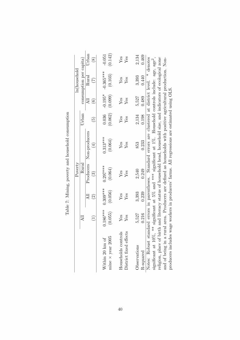
Tab
le7:
Min
ing,
pov
erty
and
hou
sehol
dco
nsu
mp
tion
Pov
erty
ln(h
ouse
hol
dA
llR
ura
lU
rban
con
sum
pti
onp
erca
pit
a)A
llP
rod
uce
rsN
on-p
rod
uce
rsA
llR
ura
lU
rban
(1)
(2)
(3)
(4)
(5)
(6)
(7)
(8)
Wit
hin
20
km
of0.
186**
*0.
309*
**0.
297*
**0.
313*
**0.
036
-0.1
95*
-0.3
65**
*-0
.051
min
e×
year
200
5(0
.055
)(0
.056
)(0
.064
)(0
.064
)(0
.062
)(0
.099
)(0
.103
)(0
.142
)
Hou
seh
old
sco
ntr
ols
Yes
Yes
Yes
Yes
Yes
Yes
Yes
Yes
Dis
tric
tfi
xed
effec
tsY
esY
esY
esY
esY
esY
esY
esY
es
Ob
serv
ati
on
s5,
527
3,39
32,
540
853
2,13
45,
527
3,39
32,
134
R-s
qu
are
d0.2
16
0.23
90.
249
0.23
30.
198
0.48
90.
440
0.46
9
Note
s:R
ob
ust
stan
dar
der
rors
inpar
enth
eses
.S
tan
dar
der
rors
are
clu
ster
edat
dis
tric
tle
vel.
*d
enot
essi
gn
ifica
nt
at10
%,
**
sign
ifica
nt
at5%
and
***
sign
ifica
nt
at1%
.H
ouse
hol
dco
ntr
ols
incl
ud
e:ag
e,ag
e2,
reli
gio
n,
pla
ceof
bir
than
dli
tera
cyst
atu
sof
hou
seh
old
hea
d,
hou
seh
old
size
,an
din
dic
ator
sof
ecol
ogic
alzo
ne
and
ofb
ein
gin
aru
ral
area
.P
rod
uce
rsar
ed
efin
edas
hou
seh
old
sw
ith
pos
itiv
eag
ricu
ltu
ral
pro
du
ctio
n.
Non
-p
rod
uce
rsin
clu
des
wage
work
ers
inp
rod
uce
rs’
farm
s.A
llre
gres
sion
sar
ees
tim
ated
usi
ng
OL
S.
40
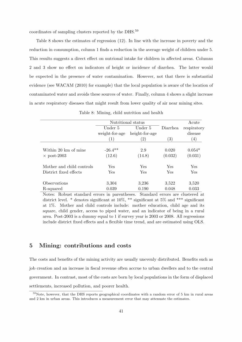
coordinates of sampling clusters reported by the DHS.59
Table 8 shows the estimates of regression (12). In line with the increase in poverty and the
reduction in consumption, column 1 finds a reduction in the average weight of children under 5.
This results suggests a direct effect on nutrional intake for children in affected areas. Columns
2 and 3 show no effect on indicators of height or incidence of diarrhea. The latter would
be expected in the presence of water contamination. However, not that there is substantial
evidence (see WACAM (2010) for example) that the local population is aware of the location of
contaminated water and avoids these sources of water. Finally, column 4 shows a slight increase
in acute respiratory diseases that might result from lower quality of air near mining sites.
Table 8: Mining, child nutrition and health
Nutritional status AcuteUnder 5 Under 5 Diarrhea respiratory
weight-for-age height-for-age disease(1) (2) (3) (4)
Within 20 km of mine -26.4** 2.9 0.020 0.054*× post-2003 (12.6) (14.8) (0.032) (0.031)
Mother and child controls Yes Yes Yes YesDistrict fixed effects Yes Yes Yes Yes
Observations 3,304 3,236 3,522 3,520R-squared 0.039 0.190 0.048 0.033
Notes: Robust standard errors in parentheses. Standard errors are clustered atdistrict level. * denotes significant at 10%, ** significant at 5% and *** significantat 1%. Mother and child controls include: mother education, child age and itssquare, child gender, access to piped water, and an indicator of being in a ruralarea. Post-2003 is a dummy equal to 1 if survey year is 2003 or 2008. All regressionsinclude district fixed effects and a flexible time trend, and are estimated using OLS.
5 Mining: contributions and costs
The costs and benefits of the mining activity are usually unevenly distributed. Benefits such as
job creation and an increase in fiscal revenue often accrue to urban dwellers and to the central
government. In contrast, most of the costs are born by local populations in the form of displaced
settlements, increased pollution, and poorer health.
59Note, however, that the DHS reports geographical coordinates with a random error of 5 km in rural areasand 2 km in urban areas. This introduces a measurement error that may attenuate the estimates.
41

This is clearly the case in Ghana. As we have shown in the previous section, mining is
associated to a reduction in agricultural product and productivity, and an increase in poverty.
These negative effects are suffered by rural households in the proximity of mines. The benefits
of mining, however, are perceived to be concentrated in urban centers, such as Accra, due to
the paucity of local backward linkages and a scheme of centralized revenue collection (Aryeetey
et al., 2007).
The increase in poverty suggests that existing policies and institutions have not offset the
adverse distributional impact of mining.60 A remaining policy question, however, is whether
the benefits, accrued to the Ghanaian government, exceed farmers’ losses.61 This question is
important because a positive answer is a necessary, though not sufficient, condition for the
success of any governmental compensation scheme. There is also an efficiency rationale: if
mines’ tax bills are smaller than farmer losses, mining companies would not fully internalize the
negative spillovers of their activities.
Mining contributes to the Ghanaian government’s revenue in three ways: corporate taxes
and royalties, dividends from government-owned mining shares, and mining workers’ income
tax. Table 9 shows a breakdown of mining-related revenue. In 2005, mining-related revenues
amounted to US$ 75 millions, which represent around 2-3% of total government revenue.62
Note that this figure includes contribution of all mining companies, not only gold mines. Most
of these revenue is channeled to the central government. Local authorities (such as District
Assemblies, Stools and Traditional Authorities) receive only 9% of mining royalties. Between
1999 and 2005, this represented in total around US$ 8 million.63
How does the contribution of mining to government revenue compare to the loss faced by the
local population? To answer this question, we estimate the aggregate loss imposed on farmers
by gold mines. We use the actual household consumption in 2005 in mining areas and the
60A similar finding is documented by Duflo and Pande (2007) in the context of Indian dams.61There may be, of course, other benefits of mining to a domestic economy. We focus, however, on rents
captured by the government since they are the ones available to fund the additional cost of a compensationscheme without further changes in fiscal policies.
62The low contribution of mining to fiscal revenue has been attributed to relatively low royalties (Akabzaa,2009). For example, in the period of analysis, royalties were fixed at 3% of profits, even thought the regulatoryframework set by the Minerals Royalties regulations allowed for rates of up to 12%.
63Mining taxes (corporate and personal) and dividends accrue directly to the central government. Mineralroyalties are distributed as follows: 80% goes to central government, 10% to a Mineral Development Fund, 1%to the Office of Stool Lands (OASL) and the remaining 9% distributed among local authorities. In turn, thisis distributed between District Assemblies (4.95%), Stools (2.25%) and Traditional Authorities (1.8%) (WorldBank, 2006, p. 91).
42

coefficient obtained in column 6 in Table 7 to estimate the counter-factual consumption, i.e.
what the household would have consumed in the absence of exposure to mining. We obtain the
total loss by multiplying the average loss times the number of households in mining areas. The
results are shown in table 9.
This back-of-the-envelope calculation suggests that farmer losses, associated to mining ac-
tivities, are sizable. We calculate that the average household consumption dropped by US$400
per year (or US$ 0.29 per person per day). In aggregate, this represents a loss of almost US$
158 million, more than double the revenue received by the government from the mining sector
as a whole64.
64If we only use results for rural households in column 7, their individual loss is around US$818 per year. Since69% of households within mining areas are rural in our sample, the aggregate loss would amount to US$ 221million.
43
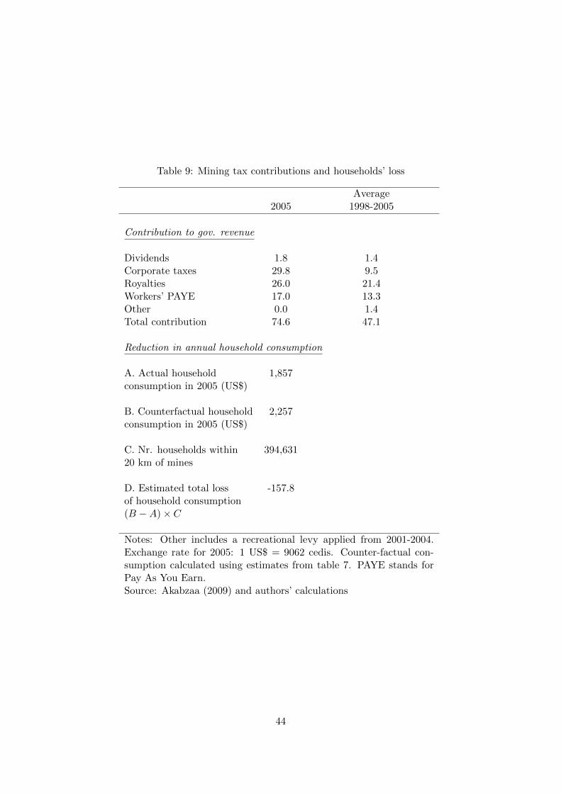
Table 9: Mining tax contributions and households’ loss
Average2005 1998-2005
Contribution to gov. revenue
Dividends 1.8 1.4Corporate taxes 29.8 9.5Royalties 26.0 21.4Workers’ PAYE 17.0 13.3Other 0.0 1.4Total contribution 74.6 47.1
Reduction in annual household consumption
A. Actual household 1,857consumption in 2005 (US$)
B. Counterfactual household 2,257consumption in 2005 (US$)
C. Nr. households within 394,63120 km of mines
D. Estimated total loss -157.8of household consumption(B −A)× C
Notes: Other includes a recreational levy applied from 2001-2004.Exchange rate for 2005: 1 US$ = 9062 cedis. Counter-factual con-sumption calculated using estimates from table 7. PAYE stands forPay As You Earn.Source: Akabzaa (2009) and authors’ calculations
44
6 Conclusion
Modern mines in many developing countries are located in rural areas, where agriculture is
an important economic activity and the main source of livelihood for a large proportion of
the population. Most importantly, mines have the potential to generate significant negative
spillovers to farmers such as pollution and competition for key inputs like land and labor. We
use the case of gold mining in Ghana to investigate how mining affects agricultural product and
productivity and, subsequently, local living standards in rural areas.
We find that total factor productivity, and crop yields have decreased in mining areas.
Our estimates suggest a reduction of up to 40% in agricultural productivity between 1998 and
2005. The negative effect is associated to polluting mines and decreases with distance. The
reduction in agricultural productivity is associated to an increase in rural poverty. During
the analyzed period, measures of living standards have improved all across Ghana. However,
households engaged in agricultural activities (whether as producers or workers) in areas closer
to mining sites have been excluded from this process. As a consequence, measures of household
consumption and poverty levels have deteriorated for them.
We also find that mitigation and compensation policies may be insufficient to offset local
negative effects. In the case of Ghana, this is due mainly because the level of taxation was lower
than the losses generated to farmers and because the distribution of mining taxes has favored
the central government. Even though the costs are exclusively born locally, less than 10% of the
receipts are received by district governments and traditional authorities in the affected areas.
The results of this paper suggest that in cases where mining occurs in the proximity of
agricultural areas, environmental policy should consider the possible impact of mine-related
pollution on crop yields and local income. In particular, the loss of agricultural productivity,
and farmers’ income should be an important part of the policy debate on the costs and benefits
of mining. Usually this policy debate focuses on the benefits mining could bring in the form of
jobs, taxes or foreign currency. These benefits are weighted against environmental costs such
as loss of biodiversity or health risks. However, local living standards may be also directly
affected by the reduction in agricultural productivity. In fertile rural environments, such as
Ghana, these costs may offset the country’s benefits from mining. It also means that the
scope of mitigation and compensation policies should be much broader. Usually mitigation and
45

compensation policies focus on populations directly displaced by mining. The negative effects
of air and water pollution, however, can extend to a broader population, beyond the boundaries
of mining licenses. These groups should also be considered in the area of influence of a mine.
As a consequence, activities such as mining may introduce substantial redistributive effects
on the economic activity and wealth of a country. Mining can bring broader benefits to a
country at the expense of localized costs (such as loss of agricultural output), some of them
born by already poor disadvantaged groups. This redistribution should be considered to better
understand local opposition to mining projects and demands for better compensation. Failing
to recognize this social cost would grossly overestimate the net contribution of mining to an
economy.
46

References
Akabzaa, Thomas, “Mining in Ghana: Implications for National Economic Development and
Poverty Reduction,” in Bonnie Campbell, ed., Mining in Africa: Regulation and Develop-
ment, International Development Research Group, 2009, chapter 1.
and Abdulai Darimani, “Impact of mining sector investment in Ghana: A study of
the Tarkwa mining region,” http://www.saprin.org/ghana/research/gha_mining.pdf
2001.
Amegbey, N. A. and A. A. Adimado, “Incidents of cyanide spillage in Ghana,” Mineral
Processing and Extractive Metallurgy, 2003, 112 (2), 126–130.
Aragon, Fernando M. and Juan Pablo Rud, “Natural resources and local communities:
evidence from a Peruvian gold mine,” American Economic Journal: Economic Policy.
Armah, F. A., S. Obiri, D. O. Yawson, A. N. M. Pappoe, and A. Bismark, “Mining
and Heavy Metal Pollution: Assessment of Aquatic Environments in Tarkwa (Ghana) using
Multivariate Statistical Analysis,” Journal of Environmental Statistics, 2010, 1 (4).
Aryeetey, Ernest, Osei Bafour, and Daniel K. Twerefou, “Impact of Mining Sector
Reforms on Output, Employment and Incomes in Ghana, 1980-2002,” Technical Publica-
tion 75, Institute of Statistical, Social and Economic Research (ISSER), November 2007.
Banerjee, Abhijit V., Paul J. Gertler, and Maitreesh Ghatak, “Empowerment and
Efficiency: Tenancy Reform in West Bengal,” Journal of Political Economy, April 2002,
110 (2), 239–280.
Besley, Timothy, “Property Rights and Investment Incentives: Theory and Evidence from
Ghana,” The Journal of Political Economy, October 1995, 103 (5), 903–937.
Blundell, Richard and Stephen Bond, “GMM Estimation with Persistent Panel Data: An
Application to Production Functions,” Econometric Reviews, 2000, 19 (3), 321–340.
Botchway, F. Nii, “Land Ownership and Responsibility for the Mining Environment in
Ghana,” Natural Resources Journal, Fall 1998, 38, 509–536.
Brollo, Fernanda, Tommaso Nannicini, Roberto Perotti, and Guido Tabellini, “The
Political Resource Curse,” NBER Working Paper No. 15705 January 2010.
Caselli, Francesco and Guy Michaels, “Do Oil Windfalls Improve Living Standards? Ev-
idence from Brazil,” http://personal.lse.ac.uk/casellif/papers/brazil.pdf, June
2009.
47
Celarier, E. A., E. J. Brinksma, J. F. Gleason, J. P. Veefkind, A. Cede, J. R. Her-
man, D. Ionov, F. Goutail, J.-P. Pommereau, J.-C. Lambert, M. van Roozen-
dael, G. Pinardi, F. Wittrock, A. Schonhardt, A. Richter, O. W. Ibrahim,
T. Wagner, B. Bojkov, G. Mount, E. Spinei, C. M. Chen, T. J. Pongetti, S. P.
Sander, E. J. Bucsela, M. O. Wenig, D. P. J. Swart, H. Volten, M. Kroon, and
P. F. Levelt, “Validation of Ozone Monitoring Instrument nitrogen dioxide columns,”
Journal of Geophysical Research (Atmospheres), May 2008, 113, 15.
Chay, Kenneth Y. and Michael Greenstone, “The Impact of Air Pollution on Infant Mor-
tality: Evidence From Geographic Variation In Pollution Shocks Induced By A Recession,”
The Quarterly Journal of Economics, August 2003, 118 (3), 1121–1167.
Corden, W. Max and J. Peter Neary, “Booming Sector and De-Industrialisation in a Small
Open Economy,” The Economic Journal, 1982, 92 (368), 825–848.
Coulombe, Harold and Quentin Wodon, “Poverty, livelihoods, and access to basic
services in Ghana,” http://siteresources.worldbank.org/INTGHANA/Resources/CEM_
poverty.pdf 2007.
Currie, Janet, Eric A. Hanushek, Matthew Kahn E. Megana nd Neidell, and
Steven G. Rivkin, “Does Pollution Increase School Absences,” The Review of Economics
and Statistics, November 2009, 91 (4), 682–694.
Dell, Melissa, Benjamin F. Jones, and Benjamin A. Olken, “Climate Change and
Economic Growth: Evidence from the Last Half Century,” NBER Working Papers 14132,
National Bureau of Economic Research, Inc 2008.
Duflo, Esther and Rohini Pande, “Dams,” The Quarterly Journal of Economics, 2007, 122
(2), 601–646.
Duncan, Edward E., Jerry S. Kuma, and Seth Frimpong, “Open Pit Mining and Land
Use Changes: An Example from Bogosu-Prestea Area, South West Ghana,” The Electronic
Journal of Information Systems in Developing Countries, 2009, 36, 1–10.
Emberson, L.D., M.R. Ashmore, F. Murray, J.C.I. Kuylenstierna, K.E. Percy,
T. Izuta, Y. Zheng, H. Shimizu, B.H. Sheu, C.P. Liu, M. Agrawal, A. Wahid,
N.M. Abdel-Latif, M. van Tienhoven, L.I. de Bauer, and M. Domingos, “Impacts
of Air Pollutants on Vegetation in Developing Countries,” Water, Air, & Soil Pollution,
2001, 130, 107–118.
Environment Canada, “Enviromental code of practice for metal mines,” http:
//www.ec.gc.ca/Publications/0B566B84-FBCC-4C75-81EA-ABCF62942A19/
Environmental-Code-of-Practice-for-Metal-Mines-2009.pdf 2009.
48
Ghana Statistical Service, “Poverty Trends in Ghana in the 1990s,” http:
//siteresources.worldbank.org/INTLSMS/Resources/3358986-1181743055198/
3877319-1190217341170/PovProf.pdf 2000.
Graff Zivin, Joshua S. and Matthew J. Neidell, “The Impact of Pollution on Worker
Productivity,” NBER Working Paper No. 17004 2011.
Greenstone, Michael and Rema Hanna, “Environmental regulations, air and water pollu-
tion, and infant mortality in India,” NBER Working Paper No. 17210 2011.
Guiteras, Raymond, “The Impact of Climate Change on Indian Agriculture,” http://www.
econ.umd.edu/research/papers/34 2009.
Hanna, Rema and Paulina Oliva, “The Effect of Pollution on Labor Supply: Evidence from
a Natural Experiment in Mexico City,” NBER Working Paper No. 17302 2011.
Hilson, Gavin and Natalia Yakovleva, “Strained relations: A critical analysis of the mining
conflict in Prestea, Ghana,” Political Geography, 2007, 26, 98–119.
Hornbeck, Richard, “The Enduring Impact of the American Dust Bowl: Short- and Long-
Run Adjustments to Environmental Catastrophe,” American Economic Review, June 2012,
102 (4).
Human Rights Clinic, “The Cost of Gold: Communities Affected by Mining in the Tarkwa
Region of Ghana,” 2010.
Jayachandran, Seema, “Air Quality and Early-Life Mortality: Evidence from Indonesias
Wildfires,” Journal of Human Resources, 2009, 44 (4), 916–954.
Levinsohn, James and Amil Petrin, “Estimating Production Functions Using Inputs to
Control for Unobservables,” Review of Economic Studies, 2003, 70, 317–342.
Maggs, R., A. Wahid, S. R. A. Shamsi, and M. R. Ashmore, “Effects of ambient
air pollution on wheat and rice yield in Pakistan,” Water, Air, Soil Pollution, 1995, 85,
1311–1316. 10.1007/BF00477163.
Marshall, Fiona, Mike ashmore, and Fiona Hinchcliffe, “A hidden threat to food pro-
duction: Air pollution and agriculture in the developing world,” Gatekeeper Series SA73,
International Institute for Environment and Development (IIED) 1997.
Mehlum, Halvor, Karl Moene, and Ragnar Torvik, “Institutions and the Resource
Curse,” The Economic Journal, 2006, 116 (508), 1–20.
Natural Resources Canada, “Mining sector performance report,” http://www.nrcan.gc.
ca/minerals-metals/publications-reports/3398#env-per 2010.
49
Nevo, Aviv and Adam Rosen, “Inference with Imperfect Instrumental Variables,” Review
of Economics and Statistics, 2012.
Olley, G. Steven and Ariel Pakes, “The Dynamics of Productivity in the Telecommunica-
tions Equipment Industry,” Econometrica, 1996, 64 (6), 1263–1297.
Sachs, Jeffrey D. and Andrew M. Warner, “Natural Resource Abundance and Economic
Growth,” NBER Working Papers 5398, National Bureau of Economic Research, December
1995.
and , “The Curse of Natural Resources,” European Economic Review, May 2001, 45
(4-6), 827–838.
Serfor-Armah, Y., B. Nyarko, S. Dampare, and D. Adomako, “Levels of Arsenic and
Antimony in Water and Sediment from Prestea, A Gold Mining Town in Ghana and its
Environs,” Water, Air, & Soil Pollution, 2006, 175, 181–192. 10.1007/s11270-006-9127-9.
Tetteh, Samuel, Adem A. Golow, David K. Essumang, and Ruphino Zugle, “Levels
of Mercury, Cadmium, and Zinc in the Topsoil of Some Selected Towns in the Wassa
West District of the Western Region of Ghana,” Soil and Sediment Contamination: An
International Journal, 2010, 19 (6), 635–643.
U.S. Environmental Protection Agency, “Abandoned mine site: characterization
and cleanup handbook,” http://water.epa.gov/polwaste/nps/upload/2000_08_pdfs_
amscch.pdf 2000.
van der Ploeg, Frederick, “Natural Resources: Curse or Blessing?,” Journal of Economic
Literature, May 2011, 49 (2), 366–420.
Vicente, Pedro C., “Does oil corrupt? Evidence from a natural experiment in West Africa,”
Journal of Development Economics, May 2010, 92 (1), 28–38.
WACAM, “Water report: impact of gold mining on water quality in Western Ghana,” http:
//www.wacamghana.com/app/webroot/img/documents/4accc8ce1913a.pdf 2010.
World Bank, “Ghana Country Environmental Analysis,” Report 36985-GH, The World Bank
2006.
50
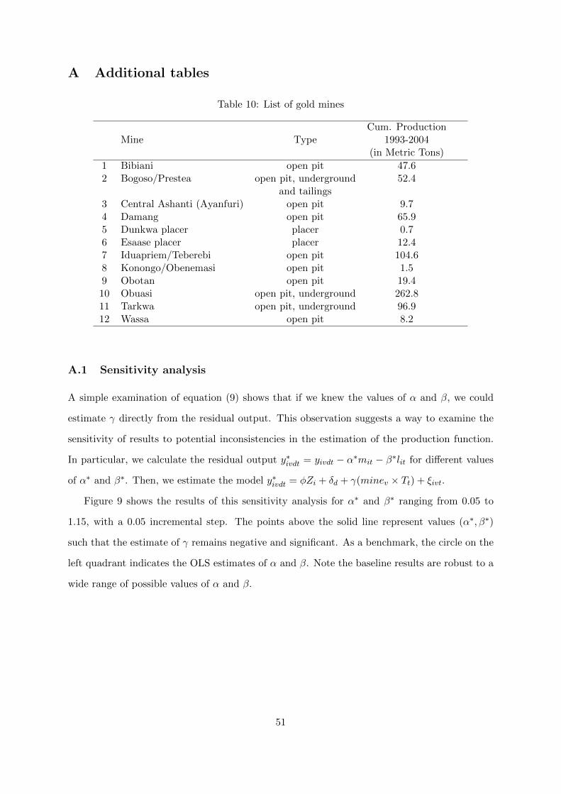
A Additional tables
Table 10: List of gold mines
Cum. ProductionMine Type 1993-2004
(in Metric Tons)
1 Bibiani open pit 47.62 Bogoso/Prestea open pit, underground 52.4
and tailings3 Central Ashanti (Ayanfuri) open pit 9.74 Damang open pit 65.95 Dunkwa placer placer 0.76 Esaase placer placer 12.47 Iduapriem/Teberebi open pit 104.68 Konongo/Obenemasi open pit 1.59 Obotan open pit 19.410 Obuasi open pit, underground 262.811 Tarkwa open pit, underground 96.912 Wassa open pit 8.2
A.1 Sensitivity analysis
A simple examination of equation (9) shows that if we knew the values of α and β, we could
estimate γ directly from the residual output. This observation suggests a way to examine the
sensitivity of results to potential inconsistencies in the estimation of the production function.
In particular, we calculate the residual output y∗ivdt = yivdt − α∗mit − β∗lit for different values
of α∗ and β∗. Then, we estimate the model y∗ivdt = φZi + δd + γ(minev × Tt) + ξivt.
Figure 9 shows the results of this sensitivity analysis for α∗ and β∗ ranging from 0.05 to
1.15, with a 0.05 incremental step. The points above the solid line represent values (α∗, β∗)
such that the estimate of γ remains negative and significant. As a benchmark, the circle on the
left quadrant indicates the OLS estimates of α and β. Note the baseline results are robust to a
wide range of possible values of α and β.
51
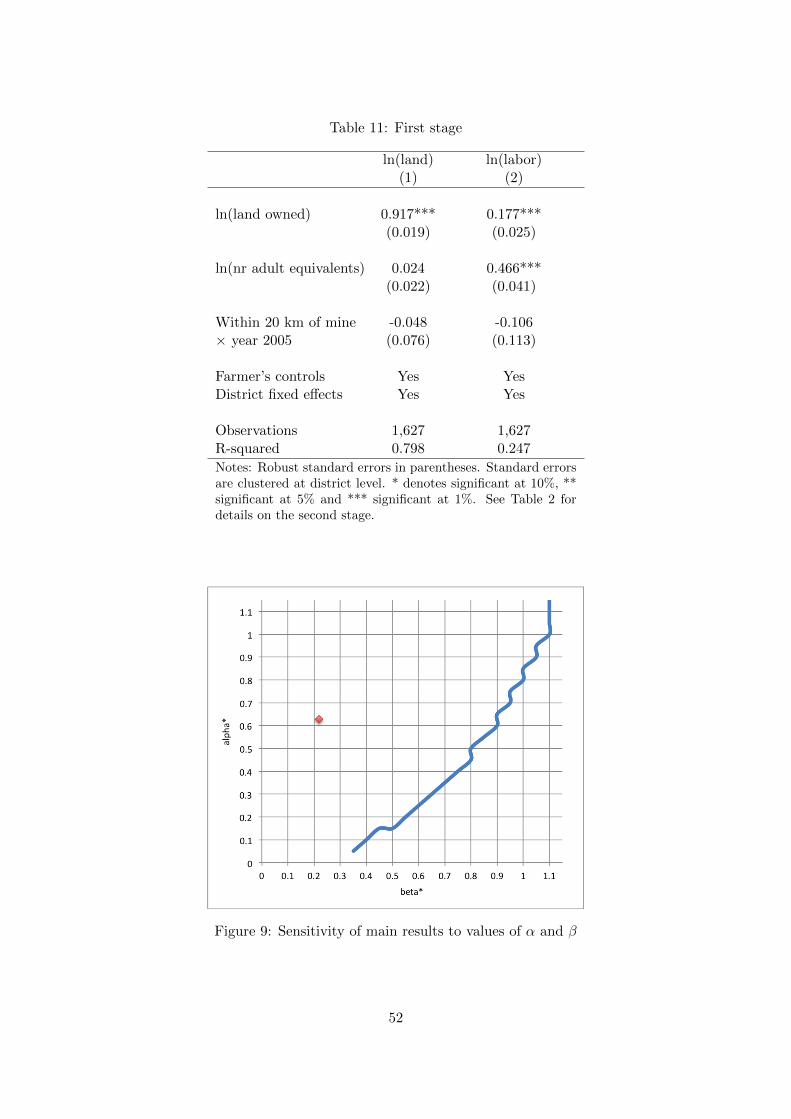
Table 11: First stage
ln(land) ln(labor)(1) (2)
ln(land owned) 0.917*** 0.177***(0.019) (0.025)
ln(nr adult equivalents) 0.024 0.466***(0.022) (0.041)
Within 20 km of mine -0.048 -0.106× year 2005 (0.076) (0.113)
Farmer’s controls Yes YesDistrict fixed effects Yes Yes
Observations 1,627 1,627R-squared 0.798 0.247
Notes: Robust standard errors in parentheses. Standard errorsare clustered at district level. * denotes significant at 10%, **significant at 5% and *** significant at 1%. See Table 2 fordetails on the second stage.
Figure 9: Sensitivity of main results to values of α and β
52
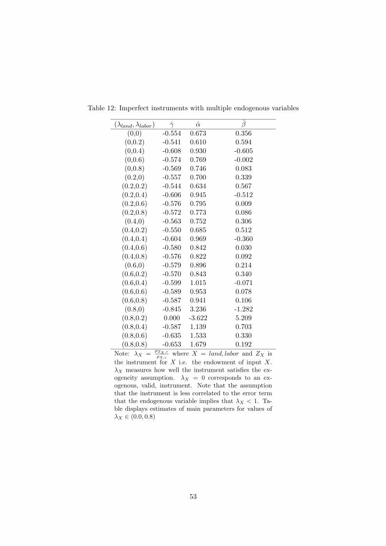
Table 12: Imperfect instruments with multiple endogenous variables
(λland, λlabor) γ α β
(0,0) -0.554 0.673 0.356(0,0.2) -0.541 0.610 0.594(0,0.4) -0.608 0.930 -0.605(0,0.6) -0.574 0.769 -0.002(0,0.8) -0.569 0.746 0.083(0.2,0) -0.557 0.700 0.339
(0.2,0.2) -0.544 0.634 0.567(0.2,0.4) -0.606 0.945 -0.512(0.2,0.6) -0.576 0.795 0.009(0.2,0.8) -0.572 0.773 0.086(0.4,0) -0.563 0.752 0.306
(0.4,0.2) -0.550 0.685 0.512(0.4,0.4) -0.604 0.969 -0.360(0.4,0.6) -0.580 0.842 0.030(0.4,0.8) -0.576 0.822 0.092(0.6,0) -0.579 0.896 0.214
(0.6,0.2) -0.570 0.843 0.340(0.6,0.4) -0.599 1.015 -0.071(0.6,0.6) -0.589 0.953 0.078(0.6,0.8) -0.587 0.941 0.106(0.8,0) -0.845 3.236 -1.282
(0.8,0.2) 0.000 -3.622 5.209(0.8,0.4) -0.587 1.139 0.703(0.8,0.6) -0.635 1.533 0.330(0.8,0.8) -0.653 1.679 0.192
Note: λX =ρZX,ερX,ε
where X = land, labor and ZX is
the instrument for X i.e. the endowment of input X.λX measures how well the instrument satisfies the ex-ogeneity assumption. λX = 0 corresponds to an ex-ogenous, valid, instrument. Note that the assumptionthat the instrument is less correlated to the error termthat the endogenous variable implies that λX < 1. Ta-ble displays estimates of main parameters for values ofλX ∈ (0.0, 0.8)
53
Related Documents