Mining moving flock patterns in large spatio-temporal datasets ...

Mining moving flock patterns in large

spatio-temporal datasets using a frequent pattern

mining approach

Andres Oswaldo Calderon Romero

March 2011

Course Title: Geo-Information Science and Earth Observation forEnvironmental Modelling and Management

Level: Master of Science (MSc.)

Course Duration: September 2009 – March 2011

Consortium partners: University of Southampton (UK)Lund University (Sweden)University of Warsaw (Poland)University of Twente,Faculty ITC (The Netherlands)

GEM thesis number: 2011–

Mining moving flock patterns in large spatio-temporal datasets using a frequentpattern mining approach

by

Andres Oswaldo Calderon Romero

Thesis submitted to the University of Twente, faculty ITC, in partial fulfilment ofthe requirements for the degree of Master of Science in Geo-information Scienceand Earth Observation for Environmental Modelling and Management.

Thesis Assessment Board

Chairman: Prof. Dr. Menno-Jan KraakExternal Examiner: Dr. Jadu DashFirst Supervisor: Dr. Otto HuismanSecond Supervisor: Dr. Ulanbek Turdukulov

Disclaimer

This document describes work undertaken as part of a programme of study

at the University of Twente, Faculty ITC. All views and opinions expressed

therein remain the sole responsibility of the author, and do not necessarily

represent those of the university.

Abstract

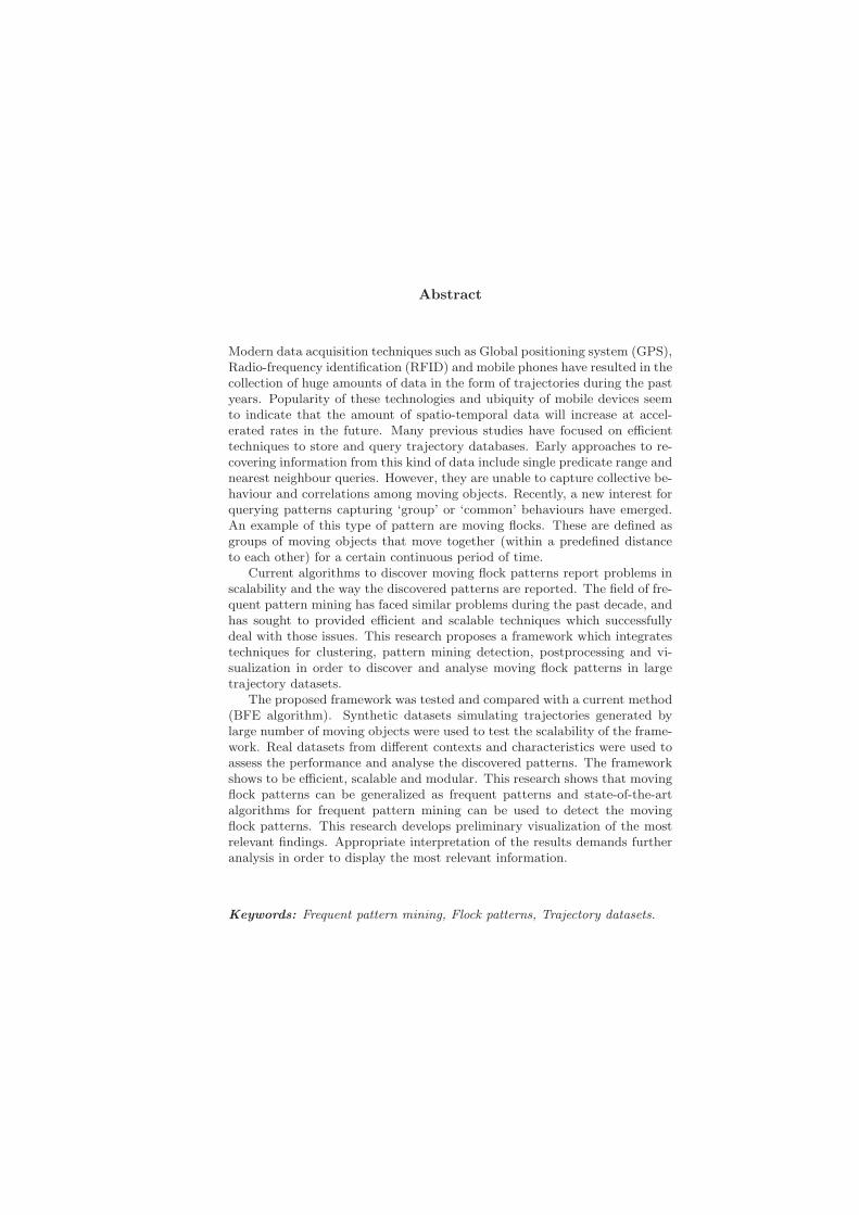
Modern data acquisition techniques such as Global positioning system (GPS),Radio-frequency identification (RFID) and mobile phones have resulted in thecollection of huge amounts of data in the form of trajectories during the pastyears. Popularity of these technologies and ubiquity of mobile devices seemto indicate that the amount of spatio-temporal data will increase at accel-erated rates in the future. Many previous studies have focused on efficienttechniques to store and query trajectory databases. Early approaches to re-covering information from this kind of data include single predicate range andnearest neighbour queries. However, they are unable to capture collective be-haviour and correlations among moving objects. Recently, a new interest forquerying patterns capturing ‘group’ or ‘common’ behaviours have emerged.An example of this type of pattern are moving flocks. These are defined asgroups of moving objects that move together (within a predefined distanceto each other) for a certain continuous period of time.

Current algorithms to discover moving flock patterns report problems inscalability and the way the discovered patterns are reported. The field of fre-quent pattern mining has faced similar problems during the past decade, andhas sought to provided efficient and scalable techniques which successfullydeal with those issues. This research proposes a framework which integratestechniques for clustering, pattern mining detection, postprocessing and vi-sualization in order to discover and analyse moving flock patterns in largetrajectory datasets.

The proposed framework was tested and compared with a current method(BFE algorithm). Synthetic datasets simulating trajectories generated bylarge number of moving objects were used to test the scalability of the frame-work. Real datasets from different contexts and characteristics were used toassess the performance and analyse the discovered patterns. The frameworkshows to be efficient, scalable and modular. This research shows that movingflock patterns can be generalized as frequent patterns and state-of-the-artalgorithms for frequent pattern mining can be used to detect the movingflock patterns. This research develops preliminary visualization of the mostrelevant findings. Appropriate interpretation of the results demands furtheranalysis in order to display the most relevant information.

Keywords: Frequent pattern mining, Flock patterns, Trajectory datasets.

Acknowledgements

I would like to express my sincere gratitude to my first supervisor, Dr.Otto Huisman, and second supervisor, Dr. Ulanbek Turdukulov, for theirgreat support and guidance during this research. I think I was the mostfortunate student for having the chance to work with such great scientists. Ivery appreciate your support, critical comments and suggestions. Thank youso much!!!

I would also like to thank Petter Pilesjo, Malgorzata Roge-Wisniewska,Andre Kooiman and Louise van Leeuwen for their valuable help at differentstages of my studies.

A special “Thank you!!!” goes to all my GEM friends for the wonderfultime we had together. You were my second family during the past monthsand I never will forget you. I will miss you a lot.

I would like to dedicate this thesis to my parents, Marcelo and Esperanza,my brother and sisters, Carlos, Paola and Carolina, and my little nephew andniece, Chris and Gabi. Thank you for believing in me even when I found itdifficult to believe in myself. I owe you much more than this.

Finally, I want to thank my fiancee. Nancy, you are the love of my life.Thank you for all your infinite love, support and patience during all this time.I love you!!!

Contents

1 Introduction 1

1.1 Background . . . . . . . . . . . . . . . . . . . . . . . . . . . . . . . . . . . 1

1.2 Problem statement . . . . . . . . . . . . . . . . . . . . . . . . . . . . . . . 2

1.3 Research identification . . . . . . . . . . . . . . . . . . . . . . . . . . . . . 2

1.3.1 Research objectives . . . . . . . . . . . . . . . . . . . . . . . . . . . 3

1.3.2 Research questions . . . . . . . . . . . . . . . . . . . . . . . . . . . 3

1.3.3 Innovation aimed at . . . . . . . . . . . . . . . . . . . . . . . . . . 3

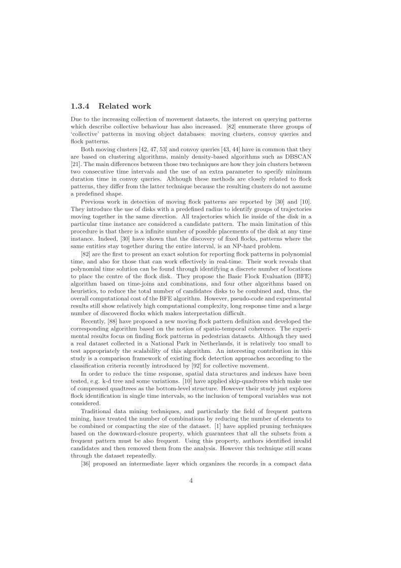
1.3.4 Related work . . . . . . . . . . . . . . . . . . . . . . . . . . . . . . 4

1.4 Thesis structure . . . . . . . . . . . . . . . . . . . . . . . . . . . . . . . . . 5

2 Framework Definition 7

2.1 Identifying patterns in moving objects . . . . . . . . . . . . . . . . . . . . 7

2.2 Basic Flock Pattern algorithm . . . . . . . . . . . . . . . . . . . . . . . . . 8

2.3 Finding frequent patterns in traditionaldatabases . . . . . . . . . . . . . . . . . . . . . . . . . . . . . . . . . . . . 9

2.3.1 Shopping basket analysis: an example . . . . . . . . . . . . . . . . 10

2.3.2 Maximal and Closed frequent patterns . . . . . . . . . . . . . . . . 11

2.4 Proposed Framework . . . . . . . . . . . . . . . . . . . . . . . . . . . . . . 12

2.4.1 Getting a final set of disks per timestamp . . . . . . . . . . . . . . 13

2.4.2 From trajectories to transactions . . . . . . . . . . . . . . . . . . . 13

2.4.3 Frequent Pattern Mining Algorithms . . . . . . . . . . . . . . . . . 14

2.4.4 Postprocessing Stage . . . . . . . . . . . . . . . . . . . . . . . . . . 15

2.5 Flock Interpretation . . . . . . . . . . . . . . . . . . . . . . . . . . . . . . 15

3 Implementation 17

3.1 BFE Implementation . . . . . . . . . . . . . . . . . . . . . . . . . . . . . . 17

3.2 Synthetic Generators . . . . . . . . . . . . . . . . . . . . . . . . . . . . . . 18

3.3 Synthetic Datasets . . . . . . . . . . . . . . . . . . . . . . . . . . . . . . . 18

3.4 Internal Comparison . . . . . . . . . . . . . . . . . . . . . . . . . . . . . . 18

3.5 Framework Implementation . . . . . . . . . . . . . . . . . . . . . . . . . . 22

3.6 Computational Experiments . . . . . . . . . . . . . . . . . . . . . . . . . . 26

3.7 Validation . . . . . . . . . . . . . . . . . . . . . . . . . . . . . . . . . . . . 26

i

4 Study Cases 294.1 Tracking Icebergs in Antarctica . . . . . . . . . . . . . . . . . . . . . . . . 29

4.1.1 Implications and possible applications . . . . . . . . . . . . . . . . 304.1.2 Data cleaning and preparation . . . . . . . . . . . . . . . . . . . . 314.1.3 Computational experiments . . . . . . . . . . . . . . . . . . . . . . 324.1.4 Results . . . . . . . . . . . . . . . . . . . . . . . . . . . . . . . . . 344.1.5 Findings in iceberg tracking . . . . . . . . . . . . . . . . . . . . . . 34

4.2 Pedestrian movement in Beijing . . . . . . . . . . . . . . . . . . . . . . . . 374.2.1 Implications and possible applications . . . . . . . . . . . . . . . . 374.2.2 Data cleaning and preparation . . . . . . . . . . . . . . . . . . . . 374.2.3 Computational experiments . . . . . . . . . . . . . . . . . . . . . . 384.2.4 Results . . . . . . . . . . . . . . . . . . . . . . . . . . . . . . . . . 394.2.5 Findings in pedestrian movement . . . . . . . . . . . . . . . . . . . 39

5 Discussion 455.1 Implementation and Performance Issues . . . . . . . . . . . . . . . . . . . 45

5.1.1 Impact of size trajectory . . . . . . . . . . . . . . . . . . . . . . . . 455.1.2 Possible solutions . . . . . . . . . . . . . . . . . . . . . . . . . . . . 46

5.2 Interpretation Issues . . . . . . . . . . . . . . . . . . . . . . . . . . . . . . 465.2.1 Number of patterns and quality of the results . . . . . . . . . . . . 465.2.2 Overlapping problem and alternatives . . . . . . . . . . . . . . . . 47

6 Conclusions and Recommendations 496.1 Summary of the Research . . . . . . . . . . . . . . . . . . . . . . . . . . . 496.2 Recommendation . . . . . . . . . . . . . . . . . . . . . . . . . . . . . . . . 50

References 51

Appendices 59

A Main source code of the framework implementation 59

ii

List of Figures

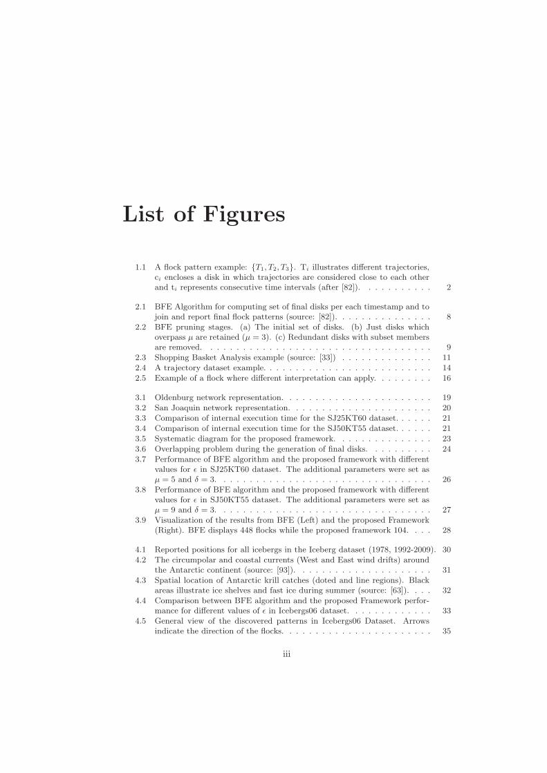
1.1 A flock pattern example: {T1, T2, T3}. Ti illustrates different trajectories,ci encloses a disk in which trajectories are considered close to each otherand ti represents consecutive time intervals (after [82]). . . . . . . . . . . 2

2.1 BFE Algorithm for computing set of final disks per each timestamp and tojoin and report final flock patterns (source: [82]). . . . . . . . . . . . . . . 8

2.2 BFE pruning stages. (a) The initial set of disks. (b) Just disks whichoverpass μ are retained (μ = 3). (c) Redundant disks with subset membersare removed. . . . . . . . . . . . . . . . . . . . . . . . . . . . . . . . . . . 9

2.3 Shopping Basket Analysis example (source: [33]) . . . . . . . . . . . . . . 112.4 A trajectory dataset example. . . . . . . . . . . . . . . . . . . . . . . . . . 142.5 Example of a flock where different interpretation can apply. . . . . . . . . 16

3.1 Oldenburg network representation. . . . . . . . . . . . . . . . . . . . . . . 193.2 San Joaquin network representation. . . . . . . . . . . . . . . . . . . . . . 203.3 Comparison of internal execution time for the SJ25KT60 dataset. . . . . . 213.4 Comparison of internal execution time for the SJ50KT55 dataset. . . . . . 213.5 Systematic diagram for the proposed framework. . . . . . . . . . . . . . . 233.6 Overlapping problem during the generation of final disks. . . . . . . . . . 243.7 Performance of BFE algorithm and the proposed framework with different

values for ε in SJ25KT60 dataset. The additional parameters were set asμ = 5 and δ = 3. . . . . . . . . . . . . . . . . . . . . . . . . . . . . . . . . 26

3.8 Performance of BFE algorithm and the proposed framework with differentvalues for ε in SJ50KT55 dataset. The additional parameters were set asμ = 9 and δ = 3. . . . . . . . . . . . . . . . . . . . . . . . . . . . . . . . . 27

3.9 Visualization of the results from BFE (Left) and the proposed Framework(Right). BFE displays 448 flocks while the proposed framework 104. . . . 28

4.1 Reported positions for all icebergs in the Iceberg dataset (1978, 1992-2009). 304.2 The circumpolar and coastal currents (West and East wind drifts) around

the Antarctic continent (source: [93]). . . . . . . . . . . . . . . . . . . . . 314.3 Spatial location of Antarctic krill catches (doted and line regions). Black

areas illustrate ice shelves and fast ice during summer (source: [63]). . . . 324.4 Comparison between BFE algorithm and the proposed Framework perfor-

mance for different values of ε in Icebergs06 dataset. . . . . . . . . . . . . 334.5 General view of the discovered patterns in Icebergs06 Dataset. Arrows

indicate the direction of the flocks. . . . . . . . . . . . . . . . . . . . . . . 35

iii

4.6 Detail of discovered flocks in Icebergs06 Dataset. Arrows indicate the di-rection of the flocks. . . . . . . . . . . . . . . . . . . . . . . . . . . . . . . 35

4.7 General view of the discovered patterns from January 01 to February 15. 364.8 General view of the discovered patterns from June 03 to August 17. . . . 364.9 Distribution points in study area. Left shows the sparse distribution around

China. Right focuses on 5th Ring Road area in Beijing (source: [98]). . . 384.10 Comparison of both methods with different values for ε in Beijing dataset. 394.11 General view of the discovered flocks in the Beijing Dataset. . . . . . . . . 404.12 Close-up around the region which concentrates the major number of flocks.

Some universities and IT institutions are highlighted. . . . . . . . . . . . . 404.13 Patterns shorter than 5 Km during workdays. Circle encloses the major

concentration around TSP region. Arrows highlight other locations. . . . 414.14 Patterns showing different routes to connect TSP area with the South.

Yellow patterns go from TSP to South, green patterns show the return. . 42

5.1 Example of reported flocks with different values of ε. . . . . . . . . . . . . 47

iv

List of Tables

2.1 Transactional version of the dataset from Figure 2.4. . . . . . . . . . . . . 14

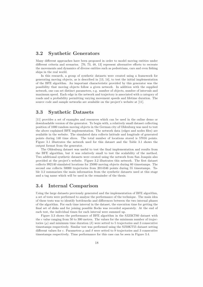
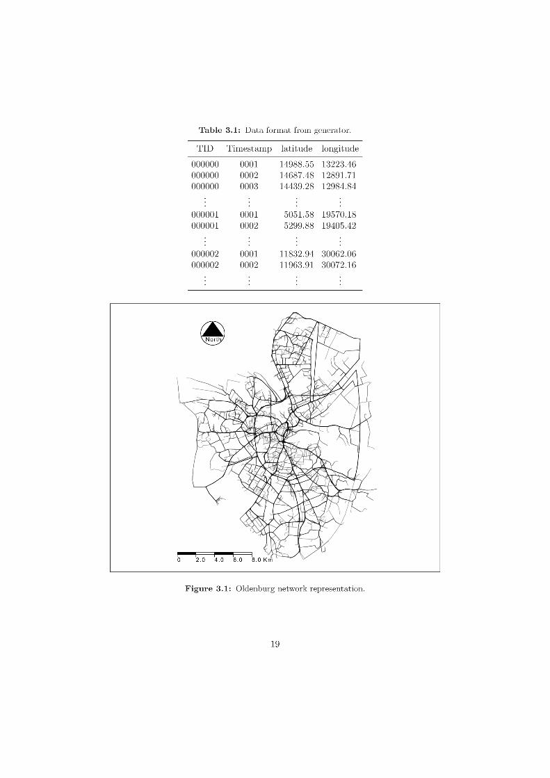
3.1 Data format from generator. . . . . . . . . . . . . . . . . . . . . . . . . . . 193.2 Synthetic Datasets. . . . . . . . . . . . . . . . . . . . . . . . . . . . . . . . 203.3 Number of combinations required for specific time intervals in SJ50KT55

dataset. . . . . . . . . . . . . . . . . . . . . . . . . . . . . . . . . . . . . . 223.4 Number of flocks generated before and after postprocessing phase for BFE

and the proposed framework in SJ25KT60 dataset. . . . . . . . . . . . . . 273.5 Number of flocks generated before and after postprocessing phase for BFE

and the proposed framework in SJ50KT55 dataset. . . . . . . . . . . . . . 28

4.1 Iceberg trajectories during 2006 in Antarctica. . . . . . . . . . . . . . . . 324.2 Number of flocks generated before and after postprocessing in Icebergs06

dataset. . . . . . . . . . . . . . . . . . . . . . . . . . . . . . . . . . . . . . 334.3 Description of the discovered flock patterns in Icebergs06 dataset. The first

column corresponds to tags in Figures 4.5 and 4.6. . . . . . . . . . . . . . 344.4 GPS log trajectories in Beijing. . . . . . . . . . . . . . . . . . . . . . . . . 384.5 Number of flocks generated before and after postprocessing in Beijing dataset. 384.6 Description of the discovered flock patterns in Beijing dataset. . . . . . . 43

v

vi

Chapter 1

Introduction

1.1 Background

Modern data acquisition techniques such as Global positioning system (GPS), Radio-frequency identification (RFID), mobile phones, wireless sensor networks, and generalsurveys have resulted in the collection of huge amounts of geographic data during thepast years. The popularity of these technologies and ubiquity of mobile devices seem toindicate that the amount of georeferenced data will increase at accelerated rates in thefuture.

However, and despite the growing demand, there are few tools available to apply aproper analysis of spatio-temporal datasets. The natural complexities in data handling,accuracy, privacy and its huge volume have become the analysis of spatial data into achallenging task. Traditional spatial analysis is not an effective solution. They were de-veloped in at time when access and quality of geodata was poor, as a result, they can notoffer scalability conditions to manage the increasing dimensionality of data. Therefore,there is an urgent need for new and efficient techniques to support the analysis and po-tential extraction of valuable information from voluminous and complex spatio-temporaldatasets.

Trajectory data associated with moving objects is one of the fields which has increasedin volume considerably. Early approaches to recovery of information from this kind ofdata include single predicate range and nearest neighbour queries, for instance, “find allthe moving objects inside area A between 10:00 AM and 2:00 PM” or “how many carsdrove between Main Square and the Airport on Friday”. Recently, diverse studies havefocused in querying patterns capturing group behaviour in moving object databases, forinstance: moving clusters, convoy queries and flock patterns [42, 47, 43, 82, 54].

Flock pattern detection is particularly relevant due to the characteristics of the objectof study (animals, pedestrians, vehicles or natural phenomena), how they interact eachother and how they move together [50, 31]. [82] define moving flock patterns as groups ofentities moving in the same direction while being close to each other for the duration of agiven time interval (Figure 1.1). They consider group of trajectories to be close togetherif there exists a disk with a given radius that encloses all of them. The current approachto discover moving flock patterns consists in finding a suitable set of disks in each timeinstance and then merging the results from one time instance to another. As consequence,

1

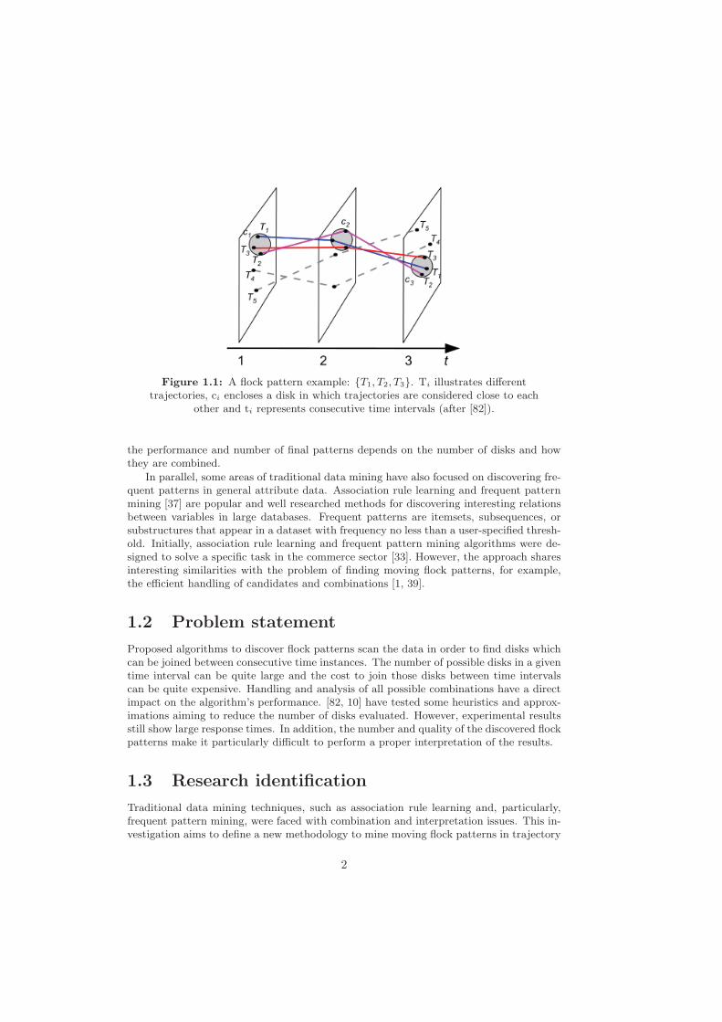
Figure 1.1: A flock pattern example: {T1, T2, T3}. Ti illustrates differenttrajectories, ci encloses a disk in which trajectories are considered close to each

other and ti represents consecutive time intervals (after [82]).

the performance and number of final patterns depends on the number of disks and howthey are combined.

In parallel, some areas of traditional data mining have also focused on discovering fre-quent patterns in general attribute data. Association rule learning and frequent patternmining [37] are popular and well researched methods for discovering interesting relationsbetween variables in large databases. Frequent patterns are itemsets, subsequences, orsubstructures that appear in a dataset with frequency no less than a user-specified thresh-old. Initially, association rule learning and frequent pattern mining algorithms were de-signed to solve a specific task in the commerce sector [33]. However, the approach sharesinteresting similarities with the problem of finding moving flock patterns, for example,the efficient handling of candidates and combinations [1, 39].

1.2 Problem statement

Proposed algorithms to discover flock patterns scan the data in order to find disks whichcan be joined between consecutive time instances. The number of possible disks in a giventime interval can be quite large and the cost to join those disks between time intervalscan be quite expensive. Handling and analysis of all possible combinations have a directimpact on the algorithm’s performance. [82, 10] have tested some heuristics and approx-imations aiming to reduce the number of disks evaluated. However, experimental resultsstill show large response times. In addition, the number and quality of the discovered flockpatterns make it particularly difficult to perform a proper interpretation of the results.

1.3 Research identification

Traditional data mining techniques, such as association rule learning and, particularly,frequent pattern mining, were faced with combination and interpretation issues. This in-vestigation aims to define a new methodology to mine moving flock patterns in trajectory

2

datasets based on the frequent pattern mining approach, aiming to tackle the aforemen-tioned drawbacks. Procedures and conceptualization will be outlined together with itsvalidity and usefulness using synthetic and real study cases.

1.3.1 Research objectives

In order to accomplish this purpose there are three main objectives:

1. To conceptualise an appropriate procedure to fit the concept of moving flock pat-terns into the frequent pattern mining methodology.

2. To implement a framework for pattern recognition in moving object datasets basedon the methodology proposed.

3. To test the performance of the resulting framework using study cases with real andsynthetic datasets.

1.3.2 Research questions

1. For design:

(a) How to apply the basic concepts of the frequent pattern mining approach inspatio-temporal datasets?

(b) How to adapt existing methods and data structures to fit the specific require-ments of frequent pattern mining algorithms?

(c) What would be an appropriate method to visualize and interpret the results?

2. For testing:

(a) How does the proposed framework perform in datasets with different charac-teristics?

(b) Which parameters and characteristics are the most important in determiningthe algorithm’s performance?

(c) Is the proposed framework applicable to different context and phenomena?

(d) Are the results from the framework useful and interpretable?

1.3.3 Innovation aimed at

Innovation in this research will be aimed towards the implementation of a novel movingflock pattern framework which adapts traditional frequent pattern mining techniques inorder to reduce the number of combinations and to improve the understanding of theresults. The scalability and performance of the proposed framework will be tested withsynthetic and real datasets in the context of human movement (pedestrians) and naturalphenomena (icebergs). Generation and visualization of the most relevant results will bealso explored.

3

1.3.4 Related work

Due to the increasing collection of movement datasets, the interest on querying patternswhich describe collective behaviour has also increased. [82] enumerate three groups of‘collective’ patterns in moving object databases: moving clusters, convoy queries andflock patterns.

Both moving clusters [42, 47, 53] and convoy queries [43, 44] have in common that theyare based on clustering algorithms, mainly density-based algorithms such as DBSCAN[21]. The main differences between those two techniques are how they join clusters betweentwo consecutive time intervals and the use of an extra parameter to specify minimumduration time in convoy queries. Although these methods are closely related to flockpatterns, they differ from the latter technique because the resulting clusters do not assumea predefined shape.

Previous work in detection of moving flock patterns are reported by [30] and [10].They introduce the use of disks with a predefined radius to identify groups of trajectoriesmoving together in the same direction. All trajectories which lie inside of the disk in aparticular time instance are considered a candidate pattern. The main limitation of thisprocedure is that there is a infinite number of possible placements of the disk at any timeinstance. Indeed, [30] have shown that the discovery of fixed flocks, patterns where thesame entities stay together during the entire interval, is an NP-hard problem.

[82] are the first to present an exact solution for reporting flock patterns in polynomialtime, and also for those that can work effectively in real-time. Their work reveals thatpolynomial time solution can be found through identifying a discrete number of locationsto place the centre of the flock disk. They propose the Basic Flock Evaluation (BFE)algorithm based on time-joins and combinations, and four other algorithms based onheuristics, to reduce the total number of candidates disks to be combined and, thus, theoverall computational cost of the BFE algorithm. However, pseudo-code and experimentalresults still show relatively high computational complexity, long response time and a largenumber of discovered flocks which makes interpretation difficult.

Recently, [88] have proposed a new moving flock pattern definition and developed thecorresponding algorithm based on the notion of spatio-temporal coherence. The experi-mental results focus on finding flock patterns in pedestrian datasets. Although they useda real dataset collected in a National Park in Netherlands, it is relatively too small totest appropriately the scalability of this algorithm. An interesting contribution in thisstudy is a comparison framework of existing flock detection approaches according to theclassification criteria recently introduced by [92] for collective movement.

In order to reduce the time response, spatial data structures and indexes have beentested, e.g. k-d tree and some variations. [10] have applied skip-quadtrees which make useof compressed quadtrees as the bottom-level structure. However their study just exploresflock identification in single time intervals, so the inclusion of temporal variables was notconsidered.

Traditional data mining techniques, and particularly the field of frequent patternmining, have treated the number of combinations by reducing the number of elements tobe combined or compacting the size of the dataset. [1] have applied pruning techniquesbased on the downward-closure property, which guarantees that all the subsets from afrequent pattern must be also frequent. Using this property, authors identified invalidcandidates and then removed them from the analysis. However this technique still scansthrough the dataset repeatedly.

[36] proposed an intermediate layer which organizes the records in a compact data

4

structure called frequent-pattern tree (FP-Tree). Main advantages of this methodologyare compression of datasets, minimization of scans and detection of patterns withoutcandidate generation [36, 12]. Recently, [39] have proposed a novel and improved FP-treestructure applied in different contexts, for instance: market basket, association rules andsequential patterns. [75] have applied this methodology successfully to find co-orientationpatterns from satellite imagery. The empirical results show an improvement around onedegree of magnitude respect to the traditional approach.

Recently, the Linear time Closed itemset Miner (LCM) [81] have demonstrated a re-markable performance in dense databases using Binary Decision Diagrams, a compactgraph-based data structure. Frequent patterns can be efficiently processed by using al-gebraic operations. LCM requires linear time to mine frequent patterns when the datacompression works well. A comparison performance of LCM and other state-of-the-arttechniques can be consulted in [9, 28].

However, [33] show how frequent pattern mining may generate a huge number offrequent patterns. It is even worse when there exist long patterns in the data. Thisis because if a pattern is frequent, each of its subpatterns is frequent as well. It clearlyincreases the complexity of analysis and understanding. To overcome this problem, Closedand Maximal pattern mining were proposed [7, 69]. The general idea is to report just thelongest patterns avoiding its subpatterns.

The aforementioned techniques have been applied successfully to diverse scenarios suchas bioinformatics [17, 16], GIS [60, 35] and marketing [96, 24]. Interested reader shouldrefer to [37] for a complete survey in the current status of the frequent pattern miningapproach. Additionally, the Frequent Itemset Mining Implementation repository (FIMI)[26] have gathered a collection of open source implementations for the most efficient andscalable Frequent/Closed/Maximal pattern mining algorithms.

Overall, the frequent pattern mining approach has made a tremendous progress in thelast decade and it is thought that this can contribute adequately to solve the drawbacksof finding moving flock patterns in trajectory datasets.

1.4 Thesis structure

The remainder of the thesis is outlined as follows:

Chapter 2 explains the basic concepts to identify patterns in moving objects. TheBasic Flock Pattern algorithm is introduced together with the formal definition of amoving flock pattern. Afterwards, frequent pattern mining in traditional databases isbriefly discussed in order to explain deeper relevant concepts used in following chapters.Then, the general steps of the proposed framework are explained. Finally, a discussionabout possible flock interpretations is presented.

Chapter 3 concentrates basically in implementation and technical issues. The first partexplains the methods and technologies used in the development of the BFE algorithm.Then it explains the generation and main characteristic of synthetic datasets used to testthe implementation. Later, it focus on the internal comparison between the two phases ofthe BFE algorithm. Afterwards, the main issues in the implementation of the proposedframework are described. The final part of the chapter present a performance comparisonbetween BFE and the proposed framework using the aforementioned synthetic datasets.

Chapter 4 focuses on study cases with real datasets. Two different moving entitiesare studied: pedestrians and icebergs. The chapter presents similar tests evaluated withsynthetic datasets, together with justification, possible applications and results discussion.

5

Chapter 5 deals with a more detailed discussion about the framework implementation.The main point of discussion are the impact of the size of trajectories in the framework’sperformance. Then, the discussion focus on the limitations and alternatives of the tech-niques used in the framework in the understanding and interpretation of the results.Finally, chapter 6 shares the conclusions and recommendations.

6

Chapter 2

Framework Definition

2.1 Identifying patterns in moving objects

Due to the increasing availability of spatial databases different methodologies have beenexplored in order to find meaningful information hidden in this kind of data. New under-standing in how diverse entities move in a spatial context have demonstrated to be usefulin topics as diverse as sports [41], socio-economic geography [23], animal migration [20]and security and surveillance [58, 71].

Early approaches to recovery information from spatio-temporal datasets include ad-hoc queries aimed to answer single predicate range or nearest neighbour queries, forinstance, “find all the moving objects inside area A between 10:00 AM and 2:00 PM”or “how many cars drove between Main Square and the Airport on Friday”. Spatialquery extensions in common GIS software packages and DBMS are able to run this typeof queries, however these techniques try to find the best solution exploring each spatialobject at a time according to some metric distance (usually Euclidean). As results, it isdifficult to capture collective behaviour and correlations among the involved entities usingthis type of queries.

Recently, a new interest for querying patterns capturing ‘group’ or ‘common’ be-haviour among moving entities have emerged. Of particular interest is the developmentof approaches to identify groups of moving objects whose share a strong relationshipand interaction in a defined spatial region during a given time duration. Some examplesof these kinds of approaches are moving cluster [47] [42], convoy queries [43] and flockpatterns [30] [10] [82].

Although different interpretations can be taken, a flock pattern refers to a predefinednumber of entities which stay close enough during at least a given time interval. Thechallenge to identify this kind of movement patterns is particularly relevant due to theintrinsic interactions among the members of the flock, specially in the context of animals,pedestrian or vehicles. In this research an alternative framework for discovering movingflock patterns is proposed. Part of this framework is based on an existing state-of-the-artalgorithm, extended to take advantage of well-known and tested frequent pattern miningalgorithms in the area of association rule learning. The details of these concepts andthe methodology used to build the proposed framework will be discussed in the followingsections.

7

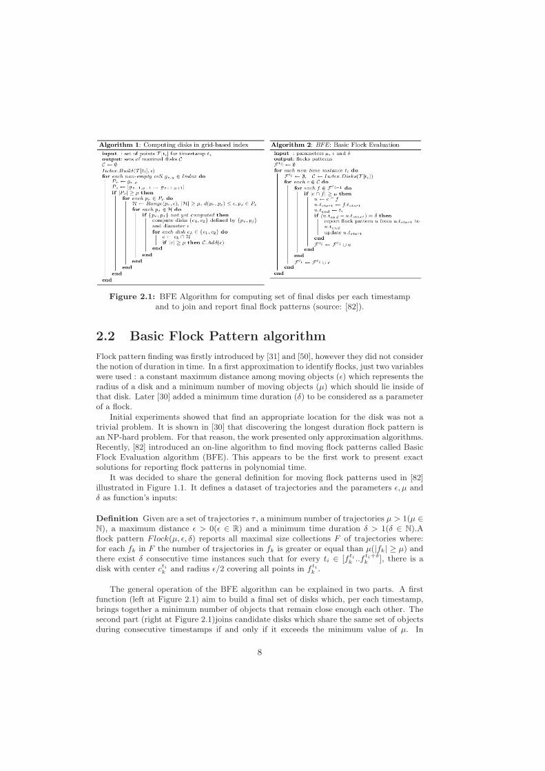
Figure 2.1: BFE Algorithm for computing set of final disks per each timestampand to join and report final flock patterns (source: [82]).

2.2 Basic Flock Pattern algorithm

Flock pattern finding was firstly introduced by [31] and [50], however they did not considerthe notion of duration in time. In a first approximation to identify flocks, just two variableswere used : a constant maximum distance among moving objects (ε) which represents theradius of a disk and a minimum number of moving objects (μ) which should lie inside ofthat disk. Later [30] added a minimum time duration (δ) to be considered as a parameterof a flock.

Initial experiments showed that find an appropriate location for the disk was not atrivial problem. It is shown in [30] that discovering the longest duration flock pattern isan NP-hard problem. For that reason, the work presented only approximation algorithms.Recently, [82] introduced an on-line algorithm to find moving flock patterns called BasicFlock Evaluation algorithm (BFE). This appears to be the first work to present exactsolutions for reporting flock patterns in polynomial time.

It was decided to share the general definition for moving flock patterns used in [82]illustrated in Figure 1.1. It defines a dataset of trajectories and the parameters ε, μ andδ as function’s inputs:

Definition Given are a set of trajectories τ , a minimum number of trajectories μ > 1(μ ∈N), a maximum distance ε > 0(ε ∈ R) and a minimum time duration δ > 1(δ ∈ N).Aflock pattern Flock(μ, ε, δ) reports all maximal size collections F of trajectories where:for each fk in F the number of trajectories in fk is greater or equal than μ(|fk| ≥ μ) andthere exist δ consecutive time instances such that for every ti ∈ [f ti

k ..f ti+δk ], there is a

disk with center ctik and radius ε/2 covering all points in f tik .

The general operation of the BFE algorithm can be explained in two parts. A firstfunction (left at Figure 2.1) aim to build a final set of disks which, per each timestamp,brings together a minimum number of objects that remain close enough each other. Thesecond part (right at Figure 2.1)joins candidate disks which share the same set of objectsduring consecutive timestamps if and only if it exceeds the minimum value of μ. In

8

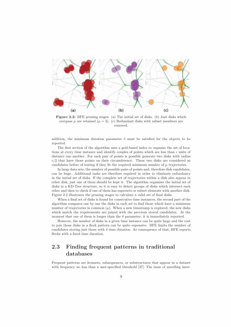
Figure 2.2: BFE pruning stages. (a) The initial set of disks. (b) Just disks whichoverpass μ are retained (μ = 3). (c) Redundant disks with subset members are

removed.

addition, the minimum duration parameter δ must be satisfied for the objects to bereported.

The first section of the algorithm uses a grid-based index to organize the set of loca-tions at every time instance and identify couples of points which are less than ε units ofdistance one another. For each pair of points is possible generate two disks with radiusε/2 that have those points on their circumference. These two disks are considered ascandidates before of testing if they fit the required minimum number of μ trajectories.

In large data sets, the number of possible pairs of points and, therefore disk candidates,can be huge. Additional tasks are therefore required in order to eliminate redundancyin the initial set of disks. If the complete set of trajectories within a disk also appear inother disk, just one of them should be kept it. The algorithm organizes the initial set ofdisks in a KD-Tree structure, so it is easy to detect groups of disks which intersect eachother and then to check if one of them has supersets or subset elements with another disk.Figure 2.2 illustrates the pruning stages to calculate a valid set of final disks.

When a final set of disks is found for consecutive time instances, the second part of thealgorithm compares one by one the disks in each set to find those which have a minimumnumber of trajectories in common (μ). When a new timestamp is explored, the new diskswhich match the requirements are joined with the previous stored candidates. At themoment that one of them is longer than the δ parameter, it is immediately reported.

However, the number of disks in a given time instance can be quite large and the costto join those disks in a flock pattern can be quite expensive. BFE limits the number ofcandidates storing just those with δ time duration. As consequence of that, BFE reportsflocks with a fixed time duration.

2.3 Finding frequent patterns in traditionaldatabases

Frequent patterns are itemsets, subsequences, or substructures that appear in a datasetwith frequency no less than a user-specified threshold [37]. The issue of unveiling inter-

9

esting patterns in databases under different contexts has been a recurrent research topicduring the last 15 years. General data mining has become widely recognized as a criticalfield by companies of all types. As a part of the data mining methods, the task of associ-ations rule learning have studied different frequent pattern mining algorithms to identifyrelevant trends in datasets in different disciplines [17, 60, 96].

One of the areas where the techniques of association rule learning and frequent patternmining algorithms have been more often applied is in analysing data and market trends intransactions of costumers of large supermarkets and stores [1]. Usually this technique hasbeen called ‘the shopping basket problem’ even though the methods derived to solve itcan be applied under different contexts [33]. During this chapter these techniques will bereferred to as ‘Shopping Basket Algorithms’ to facilitate their explanation and reference.

The shopping basket problem represents an attempt by a retailer to discover whichitems its costumers frequently purchased together [79]. The goal is an understanding of thebehaviour of a typical customer and the identification of valuable items and relationshipsamong them. For this kind of problem the input is a given database with informationabout the items purchased. When a customer pays for its products at the cashier, a recordwith the bought items is inserted into the database. In a general view, it is enough tocapture just the transaction ID and the product ID (one record per each item purchased).It is known as {TID:itemset} schema. As the records in the database usually refer totransactions, these databases are called transactional databases. The goal of shoppingbasket analysis is to find sets of items (itemsets) that are “associated” and the fact oftheir association is often called an association rule [79].

For instance, if we know that a high percentage of customers are buying milk and breadat the same time in their visits to a supermarket, this relationship represents an associationrule. It can be used to formulate new marketing strategies, promotions, introduction ofnew products, catalog design, cross-marketing or shelf space planning [33]. It is usual tolocate associated items in different aisles and high-profit or new products between them toensure they are exposed to more customers [79]. [24] discussed other case studies applied incommerce and marketing where different association rules methods are explored. Duringthe last years many improvements and new techniques have been developed and proposedin order to enhance and take advantage of the benefits of association rules analysis.

2.3.1 Shopping basket analysis: an example

Given the small example illustrated by Figure 2.3, we can take as input a database of 4transactions. Visually, it is easy to identify that Milk is present in 3 out of 4 transactions.It is also easy to see that Bread appear in all of the transaction where Milk is. Therefore,we can report the pair Milk and Bread as a frequent pattern and, for example, infer anassociation rule as:

Milk ⇒ Bread [support : 0.75, confidence : 1]

where support and confidence are two measure of the rule interestingness. A supportcount threshold of 0.75 means than the number of transactions involving Milk is equalto 75% (3 out of 4) of the total number of transactions in the database. A confidence of1 means that all (100%) transactions where Milk appears, also Bread appears. This twomeasures are used to assess the quality of the obtained rules, which in large databases canbe significant and they are defined as the parameters minimum support and minimumconfidence in most of the association rules algorithms.

10

Figure 2.3: Shopping Basket Analysis example (source: [33])

The process to retrieve a complete set of association rules from large databases can bedivided in two parts. First, all of possible itemsets which get over the support thresholdare found. This group is called frequent itemsets and refer to the most frequent patterns inthe database. The techniques used to discover the set of frequent itemsets are also calledfrequent pattern mining algorithms. Then, from the frequent itemsets, strong associationsare generated among the members of each itemset. Depending on the size of a itemset,all possible combination among its members are computed to obtain pairs of antecedentand consequence statements which will define a rule. The confidence value is used in thisstage to report just the most significant rules.

2.3.2 Maximal and Closed frequent patterns

Although the first generation of algorithms designed to mine associated rules aim to findthe complete group of frequent itemsets, in large databases using low values for minimumsupport threshold this number can be huge [33]. This is because if an itemset is frequent,each of its subsets is frequent as well. Long itemsets will contain large number of shorterfrequent subsets. For instance, let a long itemset I = {a1, a2, ..., a100} with 100 items.It is usually called type 100 or 100-itemset (for its number of members). It will contain(1001

)1-itemsets,

(1002

)2-itemsets, and so on. The total number of frequent itemsets that

it would contain would be:

(1001

)+

(1002

)+ ...+

(100100

)= 2100 − 1 ≈ 1.27 ∗ 1030

This magnitude of values is obviously too large to handle even for computer applica-tions. To overcome this drawback the concepts of closed frequent pattern and maximumfrequent pattern are used. A pattern α is a closed frequent pattern if α is frequent and

11

there exists no other pattern, with the same support, whose contains α. On the otherhand, a pattern α is a maximal frequent pattern if α is frequent and there exists no otherpattern, with any support, whose contains α. For example:

α = {a1, a2, a3, a4 : 2} α is maximal

β = {a1, a2, a3 : 4} β is closed but not maximal

The set of maximal frequent patterns is important because it contains the set of longestpatterns such that any kind of frequent pattern which exceeds the minimum support canbe generated. [33] provides a detailed and theoretical definition. For clarification, thesetwo concepts can be illustrated with an additional example:

Suppose a database D contains 4 transactions:

D = {〈a1, a2, ...a100〉; 〈a1, a2, ...a100〉; 〈a20, a21, ...a80〉; 〈a40, a41, ...a60〉}Note that the first transaction is repeated twice. The minimum support min sup = 2.

A complete search for all itemsets will generate a vast number of combinations. However,the closed frequent itemset approach will find only 3 frequent itemsets:

C = {{a1, a2, ...a100 : 2}; {a20, a21, ...a80 : 3}; {a40, a41, ...a60 : 4}}The set of closed frequent itemsets contains complete information to generate the rest

frequent itemsets with their corresponding support. It is possible to derive, for example,{a50, a51 : 4} from {a40, a41, ...a60 : 4} or {a90, a91, a92 : 2} from {a1, a2, ...a100 : 2}.

On the other hand, we just obtain one maximal frequent pattern, in this case:

M = {{a1, a2, ...a100 : 2}}From the results it is known that {a50, a51} and {a90, a91, a92} are frequent patterns,

although it is not possible to assert their actual support counts.

2.4 Proposed Framework

It is thought that current frequent patterns mining algorithms developed in the area ofassociation rule learning have made a tremendous progress bringing efficient and scalablealgorithms for discovering frequent itemsets in transactional databases which can be ap-plied on numerous research frontiers. Therefore the main aim of the remainder of thisthesis is to explore a methodology which allow the identification of moving flock patternsusing traditional and powerful algorithms for association rule mining.

In order to accomplish this goal, a framework including 4 steps is proposed:

1. Obtain a final set of valid clusters in each timestamp.

2. Construct a transactional version of the trajectory dataset based on the disks visitedby each trajectory.

3. Apply a frequent pattern mining algorithm in the generated database.

4. Perform postprocessing procedures to check consecutiveness, prune duplicates andreport patterns.

Each of the steps of the proposed framework are explained in the remainder of thischapter.

12

2.4.1 Getting a final set of disks per timestamp

The first step of the framework is to identify a final set of clusters in each timestamp.Although the first step of the BFE algorithm is affected by the number of trajectories, theinitial implementation showed acceptable time responses in preliminary testing on largesynthetically generated datasets (See Section 3.4). This fact promoted its use as a firststep in the proposed framework. The main objective with this is the generation of a finalset of disks which cluster the number of trajectories in groups according to proximity.This step still uses the parameter ε to define the diameter of the disks and μ for pruningprocedures to reduce the number of valid disks.

For simplicity, BFE algorithm and the proposed framework uses a fix disk shape; acircumference with a predefined radius and the Euclidean distance metric. However dif-ferent shapes and metrics could be used. Indeed, alternative spatial clustering techniques,such as DBSCAN or grid-based methods, which allow the identification of dense regionswith a minimum number of trajectories, could be used at this stage. These issues arediscussed further in Section 5.2.2.

2.4.2 From trajectories to transactions

In a general sense, spatio-temporal datasets are comprised of information for the locationof an entity at a specific time. Each entry in the dataset reflects an observation of a point,which in turn describes a specific trajectory. To be able to analyse trends in the data, weassume that spatio-temporal datasets contain at least 4 fields: a trajectory ID to whichbelongs a point, the time when it was measured and the X, Y coordinates of the location.

In order to use frequent pattern mining algorithms, the input database should followthe {TID:itemset} schema (see Section 2.3). The ID of the trajectory can be used toidentify its corresponding transaction, but it is necessary to define an Item ID whichcollects information for the time and location for each point. An unique ID is tagged toeach disk generated in the first step of the framework. In addition, information aboutwhich trajectories visited a disk in a particular time interval is stored in a separate table,so it is possible to get a transactional version of the trajectory if we match the time andlocation of a point with the ID of the corresponding disk. A specific disk will representa particular region in space and time and each trajectory can be translated according tothe disks which this visits during its lifetime. This concept is illustrated in the followingexample:

At Figure 2.4 we can see a dataset of 7 trajectories (Ti). From that, 5 disks can beidentified throughout the dataset lifetime (ci). Table 2.1 is created from the disks whichare visited for each trajectory at a specific timestamp (ti). If Table 2.1 is treated as atransactional databases, it is possible to apply any frequent pattern mining algorithm tofind the frequent patterns. For instance, let set the minimum support count (min sup) atthe same value that the minimum number of trajectories μ. If we use μ = 3 the patterns{C1, C2, C4 : 3} and {C3, C5 : 3} should be found. These patterns contain the informationabout the trajectory members and duration of the possible moving flock patterns.

It is no necessary a complete set of all frequent patterns. The set of maximal frequentpatterns will retrieve the required information. The main advantage of using this approachis that the longest flock patterns are reported. The maximal or closed sets of frequentpatterns avoids the need to set a parameter δ to limit the duration of the patterns. In theproposed framework, the parameter δ is only used to set the minimum duration allowed,but flocks with any duration will be reported. By contrast, BFE used δ to report flocks

13

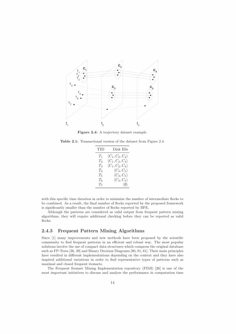
Figure 2.4: A trajectory dataset example.

Table 2.1: Transactional version of the dataset from Figure 2.4.

TID Disk IDs

T1 〈C1, C2, C4〉T2 〈C1, C2, C4〉T3 〈C1, C2, C4〉T4 〈C3, C5〉T5 〈C3, C5〉T6 〈C3, C5〉T7 〈∅〉

with this specific time duration in order to minimize the number of intermediate flocks tobe combined. As a result, the final number of flocks reported by the proposed frameworkis significantly smaller than the number of flocks reported by BFE.

Although the patterns are considered as valid output from frequent pattern miningalgorithms, they will require additional checking before they can be reported as validflocks.

2.4.3 Frequent Pattern Mining Algorithms

Since [1] many improvements and new methods have been proposed by the scientificcommunity to find frequent patterns in an efficient and robust way. The most popularsolutions involve the use of compact data structures which compress the original databasesuch as FP-Trees [36, 39] and Binary Decision Diagrams [80, 81, 61]. Their main principleshave resulted in different implementations depending on the context and they have alsoinspired additional variations in order to find representative types of patterns such asmaximal and closed frequent itemsets.

The Frequent Itemset Mining Implementation repository (FIMI) [26] is one of themost important initiatives to discuss and analyse the performance in computation time

14

and memory of the most relevant algorithms in this topic. In addition, it collects opensource code and sample datasets from the original authors. [25, 27] gave an introductorysurvey of the state-of-the-art methods and techniques as well as their performance withdifferent types of datasets and parameters.

According to the needs of the proposed framework, the technique which shows betterresults with preliminary datasets was the Linear time Closed itemset Miner (LCM)[81].LCM demonstrated an remarkable efficiency using extremely low values of support indense datasets, two characteristics present in mining moving flock patterns. LCM is abacktracking (or depth-first) algorithm based on recursive calls. The algorithm inputs afrequent itemset P and generate new itemsets by adding unused item to P . Then, foreach new frequent itemset, it computes recursive call with respect to P . The process endswhen new items cannot be added. Here, we omit the detailed description of the algorithmwhich is described in [80, 81].

2.4.4 Postprocessing Stage

As discussed above, information about time and location for each point of the trajectorieswas encoded into unique IDs for the disks. Once the LCM algorithm retrieves the set offrequent patterns, it is necessary to decode this information and check the quality andvalidity of the flocks. It is possible that the members of a valid frequent pattern belongto disks in non-consecutive times, so it is necessary to check this requirement, in additionto the minimum duration (δ), before reporting it as a valid flock.

As in the BFE algorithm it is required to prune possible duplicate patterns. Due tothe fact that a fixed diameter is used to define the disks, it is inevitable that some disksoverlap others. Points belonging to different disks at the same time interval lead to thegeneration of redundant patterns. An additional scan is needed in order to identify andremove repeated flocks. Alternatives to avoid this behaviour are discussed in Section 5.2.2.

2.5 Flock Interpretation

Although a formal definition was stated previously in this document different interpreta-tions of a flock are possible depending on the application. Figure 2.5 illustrates a casewhere according to the context and nature of the moving objects diverse set of patternscan be derived. The different interpretations are supported by the concepts of maximaland closed frequent patterns in the implementation of the proposed framework.

Let set μ = 3. If a maximal frequent pattern approach is implemented using aminimum support count equal than μ (min sup = 3), a moving flock pattern with member{T1, T2, T3} from time t1 to t6 would be identified. It is the general scenario used in thetests to measure the performance of the framework.

A second alternative will use the closed frequent pattern approach. In this case, fourflock patterns could be identified with different start times and number of members. Theyare: {T1, T2, T3} from time t1 to t6, {T1, T2, T3, T4} from time t2 to t4, {T1, T2, T3, T5} fromtime t3 to t5 and {T1, T2, T3, T4, T5} from time t3 to t4. It will bring more details aboutthe interaction among moving objects but it will increase considerably the number of finalflocks. However, it was useful during the validation stage because it generated a set ofpatterns similar to that generated by the BFE algorithm.

Finally, based on the maximal frequent pattern approach, a third alternative is pro-posed doing a further analysis over the additional trajectories. After identification of the

15

Figure 2.5: Example of a flock where different interpretation can apply.

core members of the flock (leaders), the additional points will be treated as followers ofthe core trajectories. In this fashion, just one flock will be reported from the example,where {T1, T2, T3} from t1 to t6, will be the leader trajectories. T4, joining the flock attime t2 until t4, and T5, joining it from t3 to t5, will be tagged as the correspondingfollowers.

The last interpretation is semantically more appropriate because reflects the intrinsicattraction and repulsion forces present, especially, in social entities such as animals orpedestrians. For instance, it is able to represent how a person joins a crowd, interactswith its members for a moment and then he leaves it. However, this approach needsadditional processing and the format of the results require a more suitable representation.This interpretation was implemented in the visualization of the patterns generated withthe real datasets.

16

Chapter 3

Implementation

3.1 BFE Implementation

An implementation of the BFE algorithm was developed keeping two goals in mind. First,to understand the bottlenecks processes during the execution of the method. Experimen-tal results in [82] showed high time responses dealing with large datasets but it does notclarify which parts of the algorithm are the most affected. Second, an available imple-mentation of the BFE algorithm would be useful so parts of the code could be re-used inthe development of the proposed framework and testing of the results.

Based on the pseudo-code published in [82], a version of the BFE algorithm wasdeveloped using several open source libraries and utilities. An initial attempt used Java 1.6programming language connected to spatial functions provided by PostGIS [72]. Spatialqueries were used to calculate the optimal location of the final set of disks at the firststage of BFE algorithm. However, this approach showed low performance due to multipleread/write operations and indexing. Together with this, difficult integration of SQLresults and efficient spatial data structures (e.g. KD-Tree) was also a limitation.

An alternative was an application written in 100% pure Java which allows to workwith the data in main memory avoiding multiple read/write operations. JTS TopologySuite (JTS) [85] was used for this purpose. It is an API for processing linear geometrywhich provides a complete, simple and robust implementation of distance and topologicalfunctions on the 2-dimensional plane. JTS implements the geometry model defined inthe Simple Features Specification for SQL by OpenGIS Consortium [65]. The software ispublished under the GNU Lesser General Public License (LGPL).

Although JTS supports almost all the spatial functions offered by PostGIS, it requiresefficient data structures to manage attribute data. Fastutils [78] is a fast and compactimplementation which extends the Java Collections Framework offered by default. Itprovides type-specific maps, lists, sets and trees with a small memory footprint and fastaccess and insertion, minimizing the number of write/read operations. It was developedby the Laboratory for Web Algorithmics (LAW) at the University of Milan. The sourcecode and API are released as free software under the Apache License 2.0.

Additional data management (specially for storing the resulting patterns) and somequery verification was performed using PostGIS and OpenJump GIS [86].

17

3.2 Synthetic Generators

Many different approaches have been proposed in order to model moving entities underdifferent criteria and scenarios. [70, 73, 48, 13] represent alternative efforts to recreatethe movements and dynamics of diverse entities such as pedestrians, cars and even fishingships in the real world.

In this research, a group of synthetic datasets were created using a framework forgenerating moving objects, as is described in [13, 14], to test the initial implementationof the BFE algorithm. An important characteristic provided by this generator was thepossibility that moving objects follow a given network. In addition with the suppliednetwork, one can set distinct parameters, e.g. number of objects, number of intervals andmaximum speed. Each edge in the network and trajectory is associated with a category ofroads and a probability permitting varying movement speeds and lifetime duration. Thesource code and sample networks are available on the project’s website at [11].

3.3 Synthetic Datasets

[11] provides a set of examples and resources which can be used in the online demo ordownloadable version of the generator. To begin with, a relatively small dataset collectingposition of 1000 random moving objects in the German city of Oldenburg was used to testthe above explained BFE implementation. The network data (edges and nodes files) areavailable in the website. The simulated data collects latitude and longitude of generatedpoints during 140 time slices. The total number of locations stored is 57016 points.Figure 3.1 illustrates the network used for this dataset and the Table 3.1 shows theoutput format from the generator.

The Oldenburg dataset was useful to test the final implementation and results fromthe BFE algorithm, but it was relatively small to test the scalability of the method.Two additional synthetic datasets were created using the network from San Joaquin alsoprovided at the project’s website. Figure 3.2 illustrates this network. The first datasetcollects 992140 simulated locations for 25000 moving objects during 60 timestamps. Thesecond one collects 50000 trajectories from 2014346 points during 55 timestamps. Ta-ble 3.2 summarizes the main information from the synthetic datasets used at this stageand a tag name which will be used in the remainder of the thesis.

3.4 Internal Comparison

Using the large datasets previously generated and the implementation of BFE algorithm,a set of tests were performed to analyse the performance of the technique. The main ideaof these tests was to identify bottlenecks and differences between the two internal phasesof the algorithm. For each time interval in the dataset, the execution time for getting thefinal set of disks and for joining possible flocks was recorded separately. At the end ofeach test, the individual times for each interval were summed up.

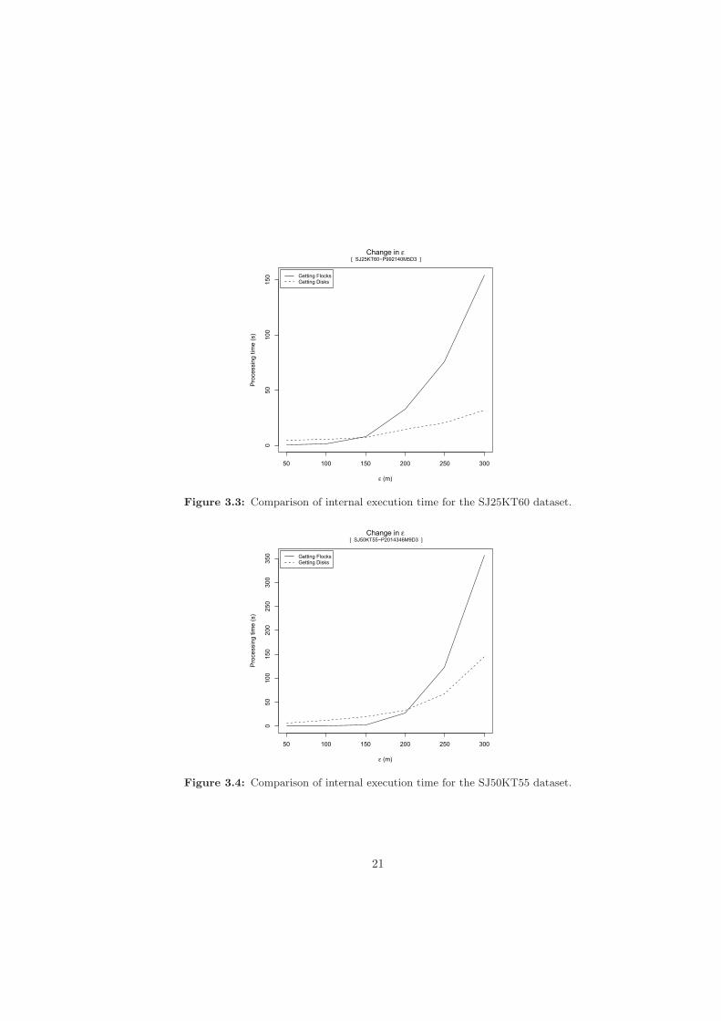
Figure 3.3 shows the performance of BFE algorithm in the SJ25KT60 dataset withthe ε value ranging from 50 to 300 metres. The values for the minimum number of trajec-tories (μ) and minimum time duration (δ) were setted to 5 trajectories and 3 consecutivetimestamps respectively. Similar test was performed using the SJ50KT55 dataset settingdifferent values for ε. Parameters μ and δ were setted to 9 trajectories and 3 consecutivetimestamps respectively. Time performance for this case can be seen in Figure 3.4.

18

50 100 150 200 250 300

050

100

150

Change in ε

ε (m)

Pro

cess

ing

time

(s)

[ SJ25KT60−P992140M5D3 ]

Getting FlocksGetting Disks

Figure 3.3: Comparison of internal execution time for the SJ25KT60 dataset.

50 100 150 200 250 300

050

100

150

200

250

300

350

Change in ε

ε (m)

Pro

cess

ing

time

(s)

[ SJ50KT55−P2014346M9D3 ]

Getting FlocksGetting Disks

Figure 3.4: Comparison of internal execution time for the SJ50KT55 dataset.

21

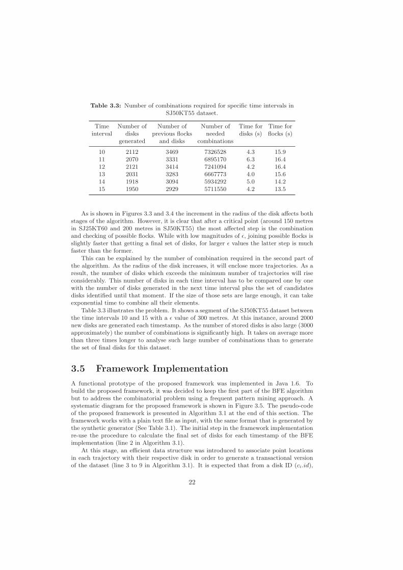
Table 3.3: Number of combinations required for specific time intervals inSJ50KT55 dataset.

Time Number of Number of Number of Time for Time forinterval disks previous flocks needed disks (s) flocks (s)

generated and disks combinations

10 2112 3469 7326528 4.3 15.911 2070 3331 6895170 6.3 16.412 2121 3414 7241094 4.2 16.413 2031 3283 6667773 4.0 15.614 1918 3094 5934292 5.0 14.215 1950 2929 5711550 4.2 13.5

As is shown in Figures 3.3 and 3.4 the increment in the radius of the disk affects bothstages of the algorithm. However, it is clear that after a critical point (around 150 metresin SJ25KT60 and 200 metres in SJ50KT55) the most affected step is the combinationand checking of possible flocks. While with low magnitudes of ε, joining possible flocks isslightly faster that getting a final set of disks, for larger ε values the latter step is muchfaster than the former.

This can be explained by the number of combination required in the second part ofthe algorithm. As the radius of the disk increases, it will enclose more trajectories. As aresult, the number of disks which exceeds the minimum number of trajectories will riseconsiderably. This number of disks in each time interval has to be compared one by onewith the number of disks generated in the next time interval plus the set of candidatesdisks identified until that moment. If the size of those sets are large enough, it can takeexponential time to combine all their elements.

Table 3.3 illustrates the problem. It shows a segment of the SJ50KT55 dataset betweenthe time intervals 10 and 15 with a ε value of 300 metres. At this instance, around 2000new disks are generated each timestamp. As the number of stored disks is also large (3000approximately) the number of combinations is significantly high. It takes on average morethan three times longer to analyse such large number of combinations than to generatethe set of final disks for this dataset.

3.5 Framework Implementation

A functional prototype of the proposed framework was implemented in Java 1.6. Tobuild the proposed framework, it was decided to keep the first part of the BFE algorithmbut to address the combinatorial problem using a frequent pattern mining approach. Asystematic diagram for the proposed framework is shown in Figure 3.5. The pseudo-codeof the proposed framework is presented in Algorithm 3.1 at the end of this section. Theframework works with a plain text file as input, with the same format that is generated bythe synthetic generator (See Table 3.1). The initial step in the framework implementationre-use the procedure to calculate the final set of disks for each timestamp of the BFEimplementation (line 2 in Algorithm 3.1).

At this stage, an efficient data structure was introduced to associate point locationsin each trajectory with their respective disk in order to generate a transactional versionof the dataset (line 3 to 9 in Algorithm 3.1). It is expected that from a disk ID (ci.id),

22

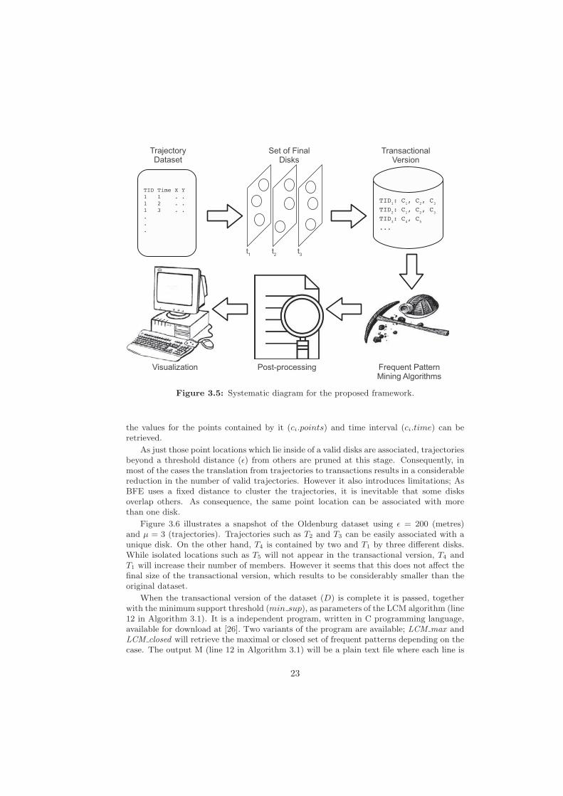
Figure 3.5: Systematic diagram for the proposed framework.

the values for the points contained by it (ci.points) and time interval (ci.time) can beretrieved.

As just those point locations which lie inside of a valid disks are associated, trajectoriesbeyond a threshold distance (ε) from others are pruned at this stage. Consequently, inmost of the cases the translation from trajectories to transactions results in a considerablereduction in the number of valid trajectories. However it also introduces limitations; AsBFE uses a fixed distance to cluster the trajectories, it is inevitable that some disksoverlap others. As consequence, the same point location can be associated with morethan one disk.

Figure 3.6 illustrates a snapshot of the Oldenburg dataset using ε = 200 (metres)and μ = 3 (trajectories). Trajectories such as T2 and T3 can be easily associated with aunique disk. On the other hand, T4 is contained by two and T1 by three different disks.While isolated locations such as T5 will not appear in the transactional version, T4 andT1 will increase their number of members. However it seems that this does not affect thefinal size of the transactional version, which results to be considerably smaller than theoriginal dataset.

When the transactional version of the dataset (D) is complete it is passed, togetherwith the minimum support threshold (min sup), as parameters of the LCM algorithm (line12 in Algorithm 3.1). It is a independent program, written in C programming language,available for download at [26]. Two variants of the program are available; LCM max andLCM closed will retrieve the maximal or closed set of frequent patterns depending on thecase. The output M (line 12 in Algorithm 3.1) will be a plain text file where each line is

23

Figure 3.6: Overlapping problem during the generation of final disks.

a maximal pattern which contains a set of Disk IDs separated by spaces.

The set of core trajectories and consecutiveness is checked in the post-processing stage.Lines 14 to 18 in Algorithm 3.1 declare initial values to iterate through the maximalpattern. Afterwards, information for time intervals and trajectory members is retrievedfor each disk contained in the pattern (lines 20 and 21 in Algorithm 3.1). The start andend for each flock pattern is set after checking time consecutiveness. The set of trajectoriescommon to all the disks in a maximal pattern are considered as the leader trajectories(line 23 in Algorithm 3.1).

In many cases, each frequent pattern can be associated with a unique flock pattern.However, it is possible that long frequent patterns contain disks from non-consecutivetime intervals. It will report various flock patterns from the same maximal pattern if eachsegment is greater than the minimum time duration (δ) (lines 26 to 29 and 32 to 34 inAlgorithm 3.1).

As in the BFE algorithm, the overlapping problem required the pruning of duplicatesand redundant patterns. Using a tree structure, the set of suitable flocks patterns arestored. In this way, patterns with the same members (and the same start and end times-tamps) will be easily detected and excluded (additional validation in lines 26 and 32 inAlgorithm 3.1). Redundant patterns occur when two patterns share exactly the samemembers but the time duration of one of them is contained by the longest one. Using thesame data structure, this kind of pattern can be also detected, keeping just the longestone. Once the postprocessing stage finishes, the final flock patterns are saved to a file.

The last phase of the framework covers the visualization of the resulting flock pat-terns. Key information about a specific flock pattern are its start and end timestampsand the trajectory IDs of their members. From this information the location (latitudeand longitude position) of the members along its lifetime can be queried from the originaldataset. However in large spatio-temporal datasets this could be costly. The implementa-tion stores a line representation of the flock, together with its key information when a flockpasses the postprocessing stage. Two variants were used as representations depending onthe context and application: firstly, a line generated from the centroids of the trajectory

24

members at each time interval, and secondly, the longest trajectory belonging to any ofthe members of the flock.

The flock representation follows the Simple Features Specification for SQL publishedby the Open GIS Consortium, so it can be visualized by several vector-based GIS softwaresuch as OpenJump or Google Earth. While OpenJump was useful to display the spatialextension of a flock, it was difficult to represent changes in time. Last updates of the KMLspecification [91] introduces additional elements (<TimeSpan> and <TimeStamp>) fordescription of spatio-temporal data. They allow the animation of vector georeferencedfeatures, such as trajectories, on Google Earth.

For simplicity, many of the final visualizations were performed separately from themain code. Python 3.1 were used to create KML files which represented the final flocksreported from the postprocessing stage (See Chapter 4). The main source code of theimplementation is shown in Appendix A.

Algorithm 3.1 Computing flocks using a frequent pattern mining algorithm

Input: parameters μ, ε and δ, set of points TOutput: flock patterns F1: for each new time instance ti ∈ T do2: C ← call Index.Disks(T [ti], ε) // call Algorithm 1 in Figure 2.13: for each ci ∈ C do4: P ← ci.points // points enclosed by ci5: for each pi ∈ P do6: ci.time ← ti7: D[pi] ← add ci.id8: end for9: end for10: end for11: min sup ← μ12: M ← call LCM max(D,min sup) // call LCM Algorithm [81]13: for each max pattern ∈ M do14: id0 ← max pattern[0]15: c0 ← C[id0]16: u ← c0.points17: u.tstart ← c0.time18: n ← max pattern.size // number of items in max pattern19: for i = 1 to n do20: idi ← max pattern[i]21: ci ← C[idi]22: if ci.time = ci−1.time+ 1 then // are disks consecutive?23: u ← u ∩ ci.points24: u.tend ← ci.time25: else26: if u.tend − u.tstart δ and u /∈ F then27: F ← add u28: u.tstart ← ci.time29: end if30: end if31: end for32: if u.tend − u.tstart δ and u /∈ F then33: F ← add u34: end if35: end for36: return F

25

50 100 150 200 250 300

050

100

150

Change in ε

ε (m)

Pro

cess

ing

time

(s)

●●

●

●

●

●

[ SJ25KT60 ]

●

BFEProposed Framework

Figure 3.7: Performance of BFE algorithm and the proposed framework withdifferent values for ε in SJ25KT60 dataset. The additional parameters were set as

μ = 5 and δ = 3.

3.6 Computational Experiments

Using the prototype implementation of the framework and the BFE algorithm, a set ofcomputational experiments were performed in order to evaluate the quality of the gener-ated patterns and the execution performance of the proposed approach. The SJ25KT60and SJ50KT55 datasets were evaluated using different parameter values. Although di-rect comparison between the two methods is not completely fair because of the differentcharacteristics of the output, it is useful to measure whether the proposal is feasible andcapable.

The results were produced on an AMD Athlon 64 X2 dual processor with 3 gigabytesof RAM and a 120GB 7200 RPM hard disk, running Ubuntu Linux 2.6.32. In all cases,experiments ran Java configured with 2048 megabytes of memory. For the two datasets thediameter of the flock was changed in intervals ranging from 50 to 300 metres. Figures 3.7and 3.8 show the final results.

3.7 Validation

As mentioned in Section 2.4.2 the proposed framework, unlike BFE, is able to identify thelongest flock patterns. In addition, depending on the definition of a flock, results could bereported in several ways. This makes it difficult to compare directly the output from thetwo methods; A long pattern reported by the proposed framework could be representedby several flocks from the BFE algorithm, since it reports flocks with fixed time duration.

26

50 100 150 200 250 300

010

020

030

040

050

0

Change in ε

ε (m)

Pro

cess

ing

time

(s)

● ●●

●

●

●

[ SJ50KT55 ]

●

BFEProposed Framework

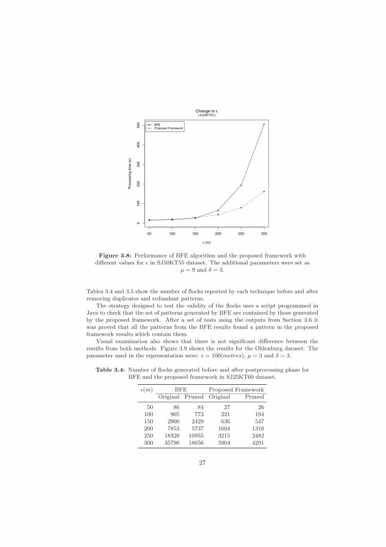
Figure 3.8: Performance of BFE algorithm and the proposed framework withdifferent values for ε in SJ50KT55 dataset. The additional parameters were set as

μ = 9 and δ = 3.

Tables 3.4 and 3.5 show the number of flocks reported by each technique before and afterremoving duplicates and redundant patterns.

The strategy designed to test the validity of the flocks uses a script programmed inJava to check that the set of patterns generated by BFE are contained by those generatedby the proposed framework. After a set of tests using the outputs from Section 3.6 itwas proved that all the patterns from the BFE results found a pattern in the proposedframework results which contain them.

Visual examination also shows that there is not significant difference between theresults from both methods. Figure 3.9 shows the results for the Oldenburg dataset. Theparameter used in the representation were: ε = 100(metres), μ = 3 and δ = 3.

Table 3.4: Number of flocks generated before and after postprocessing phase forBFE and the proposed framework in SJ25KT60 dataset.

ε(m) BFE Proposed FrameworkOriginal Pruned Original Pruned

50 86 84 27 26100 905 773 221 194150 2900 2429 636 547200 7853 5737 1604 1316250 18320 10955 3215 2482300 35796 18656 5904 4291

27

Chapter 4

Study Cases

Besides the synthetic datasets, the proposed framework was evaluated with trajectoriescollected from real case scenarios. Although synthetic datasets are a good approximationto reality, real datasets provide genuine characteristics and information about trajectorydata. However, for technical reasons, it is very complicated to track large number ofmoving entities in real life. Limitations in equipment, access or privacy concerns are somefactors which constrain the sources of data.

After some preliminary evaluation, two real datasets from different contexts wereselected to test the proposed framework. The first dataset tracks iceberg movementin Antarctica using a variety of satellite sensors since 1978. The second one collectsmovement information from a group of people around the metropolitan area of Beijing,China.

4.1 Tracking Icebergs in Antarctica

Antarctic icebergs are formed by the separation of massive sections of ice from ice shelvesand glaciers. Several researches have studied and monitored iceberg movement in Antarc-tic during the past 3 decades using diverse technologies and purposes [6, 77, 57, 84].

The National Ice Centre (NIC) and Brigham Young University Microwave Earth Re-mote Sensing Laboratory (BYU) have used a variety of satellite sensors to manually tracklarge Antarctic icebergs and collects their positions. [6] presented a long term analysis ofthe Antarctic iceberg activity based on scatterometer and radiometer data. They claimthat although the increasing in the number of icebergs reported could be explained byadvance in the tracking technologies, recent calving events (icebergs or glacier split onsmaller mass of ice) may represent a natural variability in iceberg activity.

NIC and BYU have produced an Antarctic iceberg tracking database which includesicebergs identified during 1978 and from 1992 to 2009 period. On average, each icebergis reported every 1 to 5 days using five different satellite instruments. The high temporalresolution of the dataset gives valuable information about the ocean currents in the studyarea. It is used for mariners to provide more accurate positional information to operatein the Antarctic region.

The Iceberg database gathers latitude, longitude, date and identification of 217 ice-bergs with more than 15100 point locations during the study period. In addition to the

29

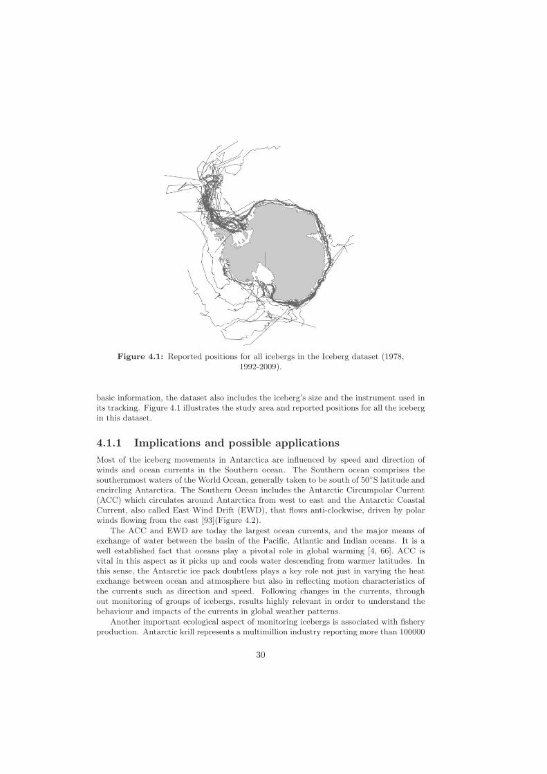
Figure 4.1: Reported positions for all icebergs in the Iceberg dataset (1978,1992-2009).

basic information, the dataset also includes the iceberg’s size and the instrument used inits tracking. Figure 4.1 illustrates the study area and reported positions for all the icebergin this dataset.

4.1.1 Implications and possible applications

Most of the iceberg movements in Antarctica are influenced by speed and direction ofwinds and ocean currents in the Southern ocean. The Southern ocean comprises thesouthernmost waters of the World Ocean, generally taken to be south of 50◦S latitude andencircling Antarctica. The Southern Ocean includes the Antarctic Circumpolar Current(ACC) which circulates around Antarctica from west to east and the Antarctic CoastalCurrent, also called East Wind Drift (EWD), that flows anti-clockwise, driven by polarwinds flowing from the east [93](Figure 4.2).

The ACC and EWD are today the largest ocean currents, and the major means ofexchange of water between the basin of the Pacific, Atlantic and Indian oceans. It is awell established fact that oceans play a pivotal role in global warming [4, 66]. ACC isvital in this aspect as it picks up and cools water descending from warmer latitudes. Inthis sense, the Antarctic ice pack doubtless plays a key role not just in varying the heatexchange between ocean and atmosphere but also in reflecting motion characteristics ofthe currents such as direction and speed. Following changes in the currents, throughout monitoring of groups of icebergs, results highly relevant in order to understand thebehaviour and impacts of the currents in global weather patterns.

Another important ecological aspect of monitoring icebergs is associated with fisheryproduction. Antarctic krill represents a multimillion industry reporting more than 100000

30

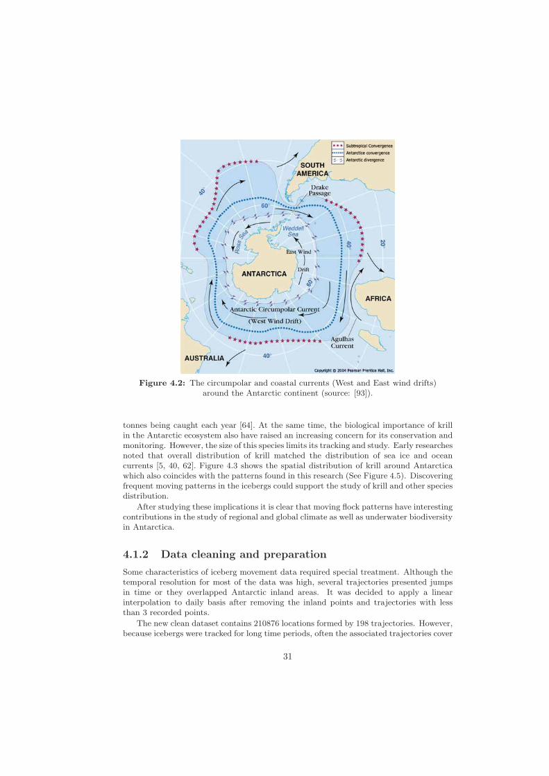
Figure 4.2: The circumpolar and coastal currents (West and East wind drifts)around the Antarctic continent (source: [93]).

tonnes being caught each year [64]. At the same time, the biological importance of krillin the Antarctic ecosystem also have raised an increasing concern for its conservation andmonitoring. However, the size of this species limits its tracking and study. Early researchesnoted that overall distribution of krill matched the distribution of sea ice and oceancurrents [5, 40, 62]. Figure 4.3 shows the spatial distribution of krill around Antarcticawhich also coincides with the patterns found in this research (See Figure 4.5). Discoveringfrequent moving patterns in the icebergs could support the study of krill and other speciesdistribution.

After studying these implications it is clear that moving flock patterns have interestingcontributions in the study of regional and global climate as well as underwater biodiversityin Antarctica.

4.1.2 Data cleaning and preparation

Some characteristics of iceberg movement data required special treatment. Although thetemporal resolution for most of the data was high, several trajectories presented jumpsin time or they overlapped Antarctic inland areas. It was decided to apply a linearinterpolation to daily basis after removing the inland points and trajectories with lessthan 3 recorded points.

The new clean dataset contains 210876 locations formed by 198 trajectories. However,because icebergs were tracked for long time periods, often the associated trajectories cover

31

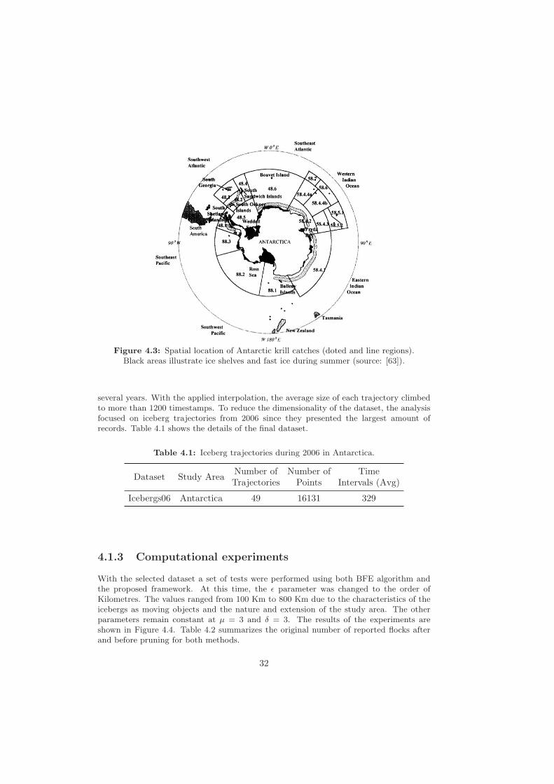
Figure 4.3: Spatial location of Antarctic krill catches (doted and line regions).Black areas illustrate ice shelves and fast ice during summer (source: [63]).

several years. With the applied interpolation, the average size of each trajectory climbedto more than 1200 timestamps. To reduce the dimensionality of the dataset, the analysisfocused on iceberg trajectories from 2006 since they presented the largest amount ofrecords. Table 4.1 shows the details of the final dataset.

Table 4.1: Iceberg trajectories during 2006 in Antarctica.

Dataset Study AreaNumber of Number of TimeTrajectories Points Intervals (Avg)

Icebergs06 Antarctica 49 16131 329

4.1.3 Computational experiments

With the selected dataset a set of tests were performed using both BFE algorithm andthe proposed framework. At this time, the ε parameter was changed to the order ofKilometres. The values ranged from 100 Km to 800 Km due to the characteristics of theicebergs as moving objects and the nature and extension of the study area. The otherparameters remain constant at μ = 3 and δ = 3. The results of the experiments areshown in Figure 4.4. Table 4.2 summarizes the original number of reported flocks afterand before pruning for both methods.

32

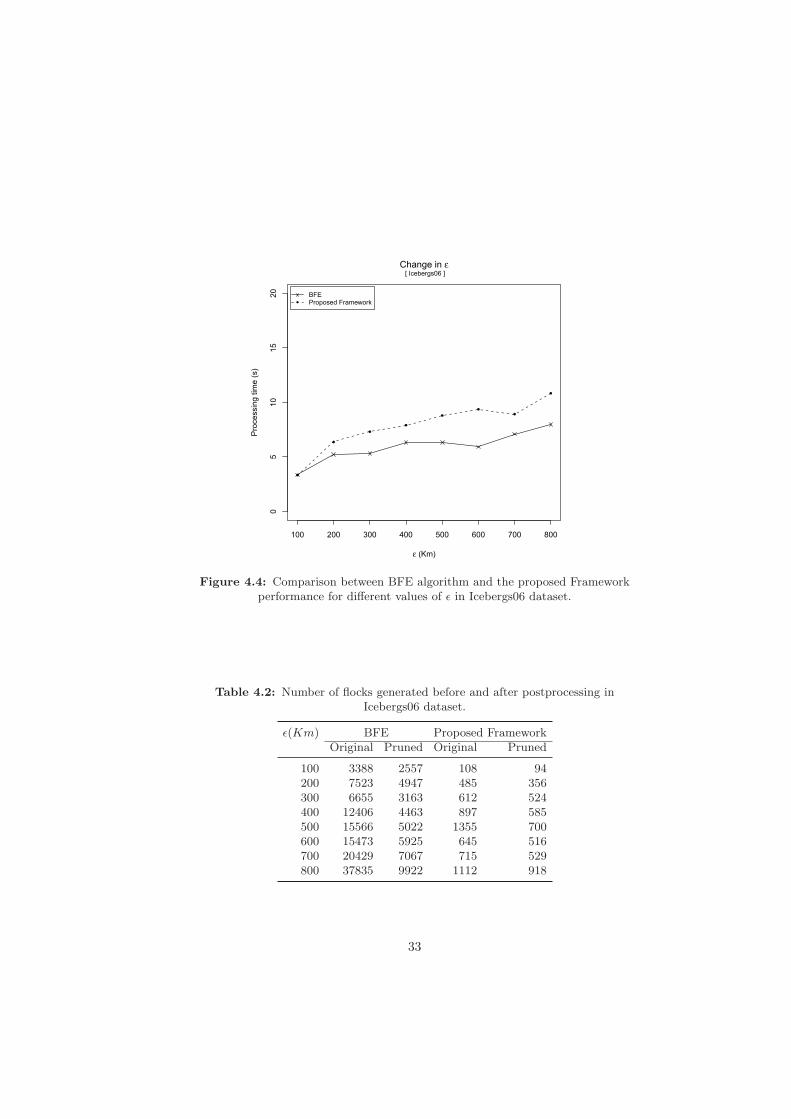
100 200 300 400 500 600 700 800

05

1015

20Change in ε

ε (Km)

Pro

cess

ing

time

(s)

●

●

●

●

●

●

●

●

●

BFEProposed Framework

[ Icebergs06 ]

Figure 4.4: Comparison between BFE algorithm and the proposed Frameworkperformance for different values of ε in Icebergs06 dataset.

Table 4.2: Number of flocks generated before and after postprocessing inIcebergs06 dataset.

ε(Km) BFE Proposed FrameworkOriginal Pruned Original Pruned

100 3388 2557 108 94200 7523 4947 485 356300 6655 3163 612 524400 12406 4463 897 585500 15566 5022 1355 700600 15473 5925 645 516700 20429 7067 715 529800 37835 9922 1112 918

33

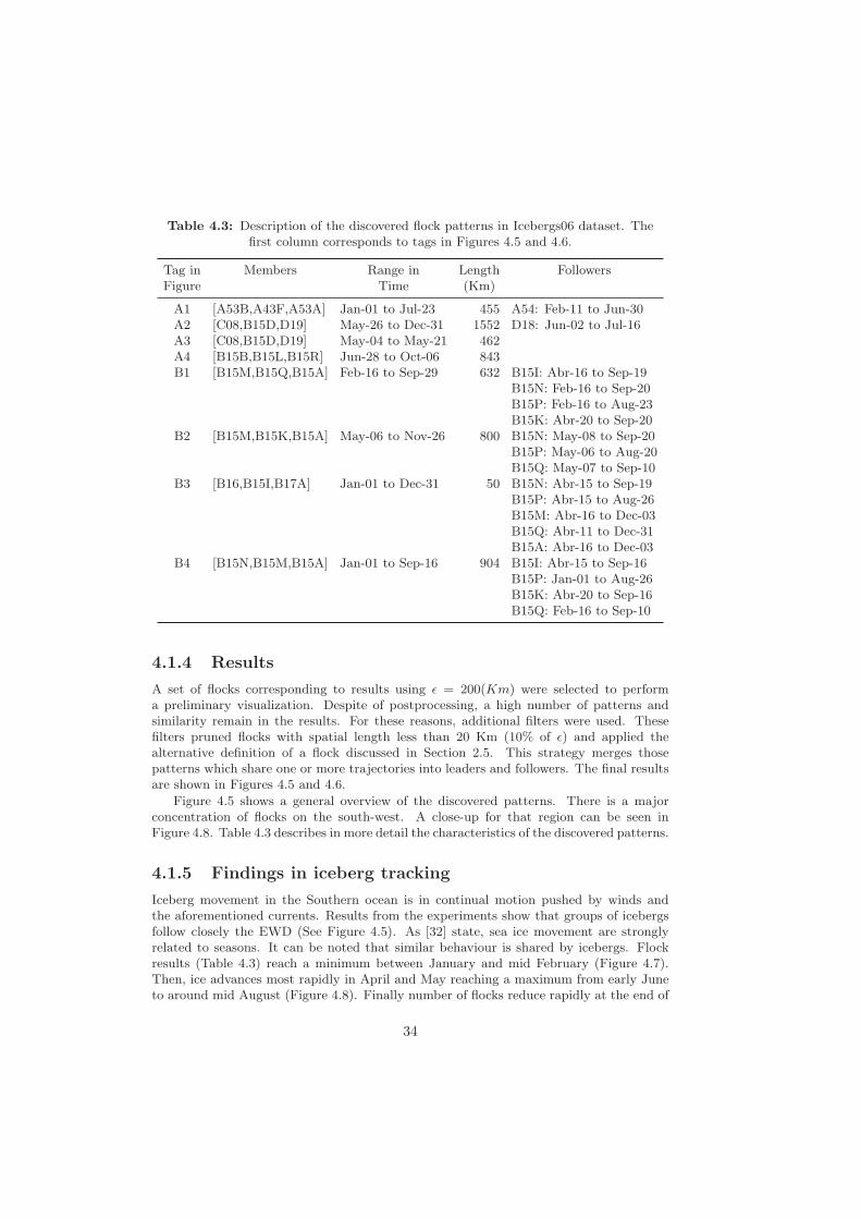
Table 4.3: Description of the discovered flock patterns in Icebergs06 dataset. Thefirst column corresponds to tags in Figures 4.5 and 4.6.

Tag in Members Range in Length FollowersFigure Time (Km)

A1 [A53B,A43F,A53A] Jan-01 to Jul-23 455 A54: Feb-11 to Jun-30A2 [C08,B15D,D19] May-26 to Dec-31 1552 D18: Jun-02 to Jul-16A3 [C08,B15D,D19] May-04 to May-21 462A4 [B15B,B15L,B15R] Jun-28 to Oct-06 843B1 [B15M,B15Q,B15A] Feb-16 to Sep-29 632 B15I: Abr-16 to Sep-19

B15N: Feb-16 to Sep-20B15P: Feb-16 to Aug-23B15K: Abr-20 to Sep-20

B2 [B15M,B15K,B15A] May-06 to Nov-26 800 B15N: May-08 to Sep-20B15P: May-06 to Aug-20B15Q: May-07 to Sep-10

B3 [B16,B15I,B17A] Jan-01 to Dec-31 50 B15N: Abr-15 to Sep-19B15P: Abr-15 to Aug-26B15M: Abr-16 to Dec-03B15Q: Abr-11 to Dec-31B15A: Abr-16 to Dec-03

B4 [B15N,B15M,B15A] Jan-01 to Sep-16 904 B15I: Abr-15 to Sep-16B15P: Jan-01 to Aug-26B15K: Abr-20 to Sep-16B15Q: Feb-16 to Sep-10

4.1.4 Results

A set of flocks corresponding to results using ε = 200(Km) were selected to performa preliminary visualization. Despite of postprocessing, a high number of patterns andsimilarity remain in the results. For these reasons, additional filters were used. Thesefilters pruned flocks with spatial length less than 20 Km (10% of ε) and applied thealternative definition of a flock discussed in Section 2.5. This strategy merges thosepatterns which share one or more trajectories into leaders and followers. The final resultsare shown in Figures 4.5 and 4.6.

Figure 4.5 shows a general overview of the discovered patterns. There is a majorconcentration of flocks on the south-west. A close-up for that region can be seen inFigure 4.8. Table 4.3 describes in more detail the characteristics of the discovered patterns.

4.1.5 Findings in iceberg tracking

Iceberg movement in the Southern ocean is in continual motion pushed by winds andthe aforementioned currents. Results from the experiments show that groups of icebergsfollow closely the EWD (See Figure 4.5). As [32] state, sea ice movement are stronglyrelated to seasons. It can be noted that similar behaviour is shared by icebergs. Flockresults (Table 4.3) reach a minimum between January and mid February (Figure 4.7).Then, ice advances most rapidly in April and May reaching a maximum from early Juneto around mid August (Figure 4.8). Finally number of flocks reduce rapidly at the end of

34

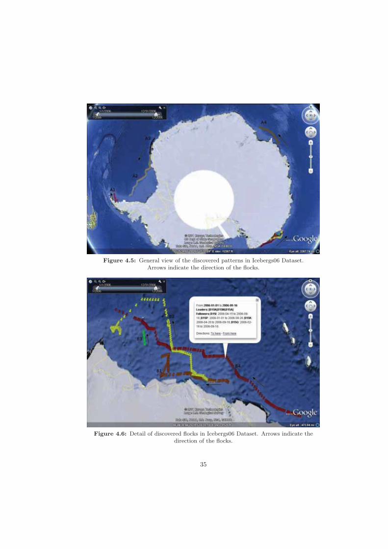
Figure 4.5: General view of the discovered patterns in Icebergs06 Dataset.Arrows indicate the direction of the flocks.

Figure 4.6: Detail of discovered flocks in Icebergs06 Dataset. Arrows indicate thedirection of the flocks.

35

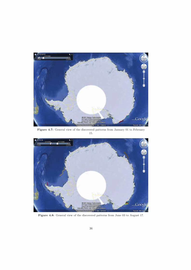
Figure 4.7: General view of the discovered patterns from January 01 to February15.

Figure 4.8: General view of the discovered patterns from June 03 to August 17.

36

September and November. These findings results are consistent with observations madeby [19] (cited in [32]) about sea ice movement.

4.2 Pedestrian movement in Beijing

This study case is based on Beijing using a GPS trajectory dataset provided by MicrosoftAsia Research. The dataset was collected during the Geolife project [59] by 165 anony-mous users in a period of two years from April 2007 to August 2009. Locations wererecorded by different GPS loggers or Smart-phones and most of them present a high sam-pling rate. 95% of the tracks were logged every 2 to 5 seconds or every 5 to 10 metres perpoint.

Although some locations in the dataset are distributed in over 30 cities in China andeven America and Europe, the majority of the data was created in Beijing. The datasetcollects information about latitude, longitude, altitude, date and time recording a broadrange of users movements, not just routines such as go work and back to home but alsosome amusement and sport activities. It is important to mention that users could use anykind of transportation during the tracking, so the trajectories could refer to movementby foot, car or public transport.

Previous researches have explored interesting locations, travel sequences and mobilitypatterns from this collection [98, 99]. The dataset and further information are freelyavailable at the project’s website [59].

4.2.1 Implications and possible applications

Applications of moving patterns in urban movement have been widely discussed in recentstudies [97, 99, 52, 83]. They could bring to light hidden and relevant information abouttrends and interaction among people. By mining people’s movement history, it is possibleto measure the similarity between users and perform personalized recommendation for anindividual. Furthermore, they can be used to detect problems in mobility and supportdecision makers in fields such as urban planning and public transport systems.

Predictions and forecasting [49, 76, 87] are interesting topics which can be supportedby this kind of knowledge. Indeed, as itemsets in association rule learning, moving flockpatterns are the first step towards discovery of trends in movement. Finding correlationsbetween places that people visit will be relevant and useful in fields such as location-basedservices and ubiquitous computing.

4.2.2 Data cleaning and preparation

The dataset groups the trajectories of each user in a separated folder. Each folder containsone or more GPS log files. In turn, each GPS log file could store one or more trajectories.From each trajectory, it was extracted timestamp and location and coupled to an sequen-tial identifier. After merging all the log files, a total of 15450 trajectories were obtained.However, this collection presented a sparse distribution in space and time.

The region around the 5th Ring Road in the metropolitan area of Beijing and thetime period between January and April of 2009 showed the major concentration of tra-jectories. These two constrains were selected to generate a sample dataset. The resultwas interpolated every minute to obtain a final dataset which contains 2562 trajectories

37

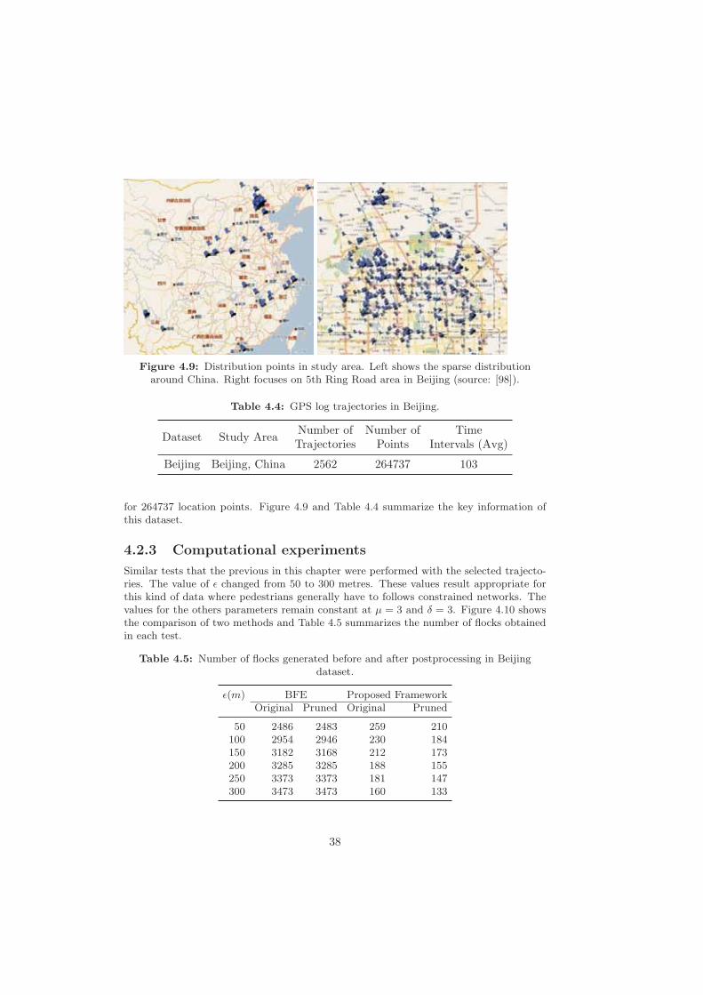
Figure 4.9: Distribution points in study area. Left shows the sparse distributionaround China. Right focuses on 5th Ring Road area in Beijing (source: [98]).

Table 4.4: GPS log trajectories in Beijing.

Dataset Study AreaNumber of Number of TimeTrajectories Points Intervals (Avg)

Beijing Beijing, China 2562 264737 103

for 264737 location points. Figure 4.9 and Table 4.4 summarize the key information ofthis dataset.

4.2.3 Computational experiments

Similar tests that the previous in this chapter were performed with the selected trajecto-ries. The value of ε changed from 50 to 300 metres. These values result appropriate forthis kind of data where pedestrians generally have to follows constrained networks. Thevalues for the others parameters remain constant at μ = 3 and δ = 3. Figure 4.10 showsthe comparison of two methods and Table 4.5 summarizes the number of flocks obtainedin each test.

Table 4.5: Number of flocks generated before and after postprocessing in Beijingdataset.

ε(m) BFE Proposed FrameworkOriginal Pruned Original Pruned

50 2486 2483 259 210100 2954 2946 230 184150 3182 3168 212 173200 3285 3285 188 155250 3373 3373 181 147300 3473 3473 160 133

38

50 100 150 200 250 300

01

23

45

6

Change in ε

ε (m)

Pro

cess

ing

time

(s)

●

●

●

●

●

●

●

BFEProposed Framework

[ Beijing ]

Figure 4.10: Comparison of both methods with different values for ε in Beijingdataset.

4.2.4 Results

Similar filters used in the last study case were also used for this dataset, especially toreduce similarity among data. Flocks corresponding to results for ε = 100(metres) wereselected for the visualization. In general, users travel to suburbs at south, north andeast with the city centre (Figure 4.11). The major concentration of patterns focus onthe north-west area between the 4th and 5th Ring Roads. Around the area, severaluniversities and IT business are located (Figure 4.12). This area is referred to as TSP(Tshingua Science Park) during this discussion. Table 4.6 describes a subset of the resultswith flock patterns larger than 5 Km and lasting 20 or more minutes.

4.2.5 Findings in pedestrian movement

Results were equally distributed during workdays (51%) and weekends (49%). From flockshappening in workdays, 83.5% were shorter than 5 Km and happened between 9 AM and7 PM. A vast majority of them concentrated in the TSP region. It is plausible that manyof the users carrying the GPS loggers were academics or researchers and their workingplace is located there (See Figure 4.13).

Focus on large distance in flocks, patterns larger than 5 Km represented 20% of thedata. Most of them (74%) happened during Fridays and the weekend. This could explainthe diversity in the time occurrence. Larger patterns connected areas at north and southof the city with the TSP region and the city centre with East at different hours duringthe day, especially late evening.

It is interesting that many of the longest flocks follows well defined expressways and

39

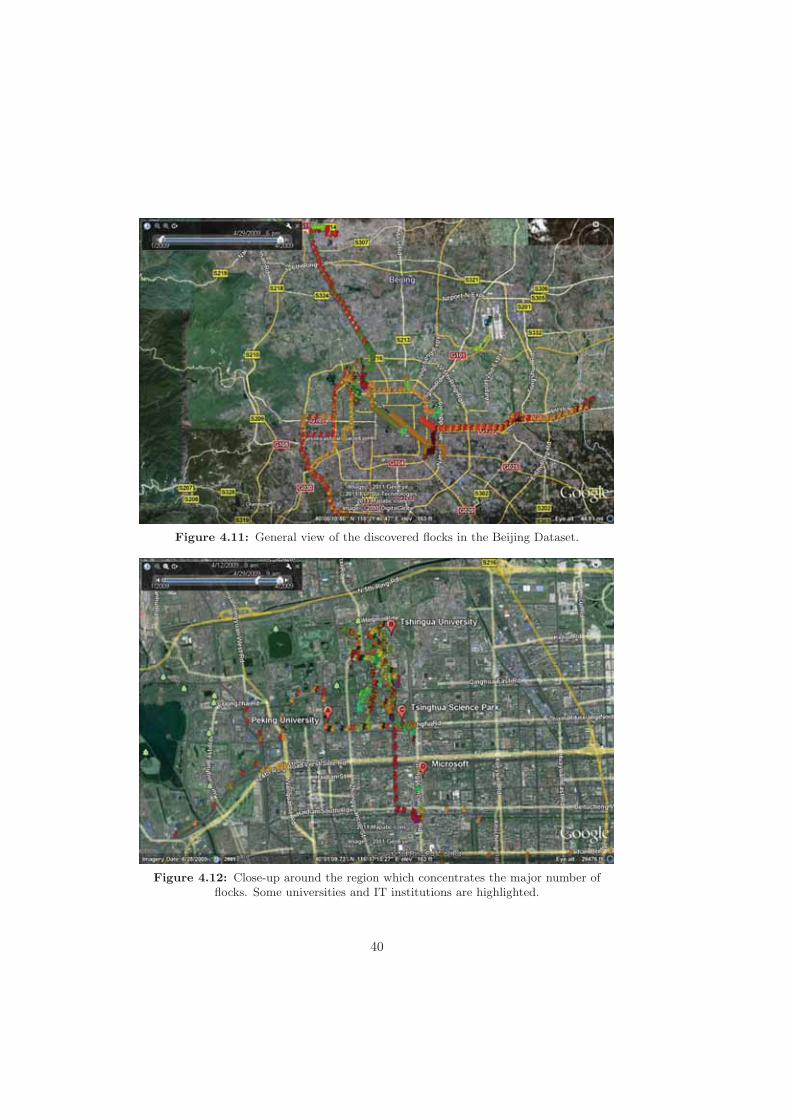
Figure 4.11: General view of the discovered flocks in the Beijing Dataset.

Figure 4.12: Close-up around the region which concentrates the major number offlocks. Some universities and IT institutions are highlighted.

40

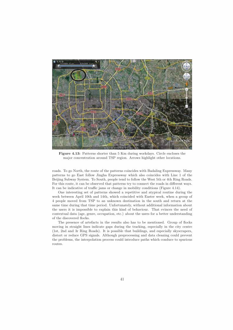
Figure 4.13: Patterns shorter than 5 Km during workdays. Circle encloses themajor concentration around TSP region. Arrows highlight other locations.

roads. To go North, the route of the patterns coincides with Badaling Expressway. Manypatterns to go East follow Jingha Expressway which also coincides with Line 1 of theBeijing Subway System. To South, people tend to follow the West 5th or 4th Ring Roads.For this route, it can be observed that patterns try to connect the roads in different ways.It can be indicative of traffic jams or change in mobility conditions (Figure 4.14).

One interesting set of patterns showed a repetitive and atypical routine during theweek between April 10th and 14th, which coincided with Easter week, when a group of4 people moved from TSP to an unknown destination in the south and return at thesame time during that time period. Unfortunately, without additional information aboutthe users it is impossible to explain this kind of behaviour. That evinces the need ofcontextual data (age, genre, occupation, etc.) about the users for a better understandingof the discovered flocks.

The presence of artefacts in the results also has to be mentioned. Group of flocksmoving in straight lines indicate gaps during the tracking, especially in the city centre(1st, 2nd and 3r Ring Roads). It is possible that buildings, and especially skyscrapers,distort or reduce GPS signals. Although preprocessing and data cleaning could preventthe problems, the interpolation process could introduce paths which conduce to spuriousroutes.

41

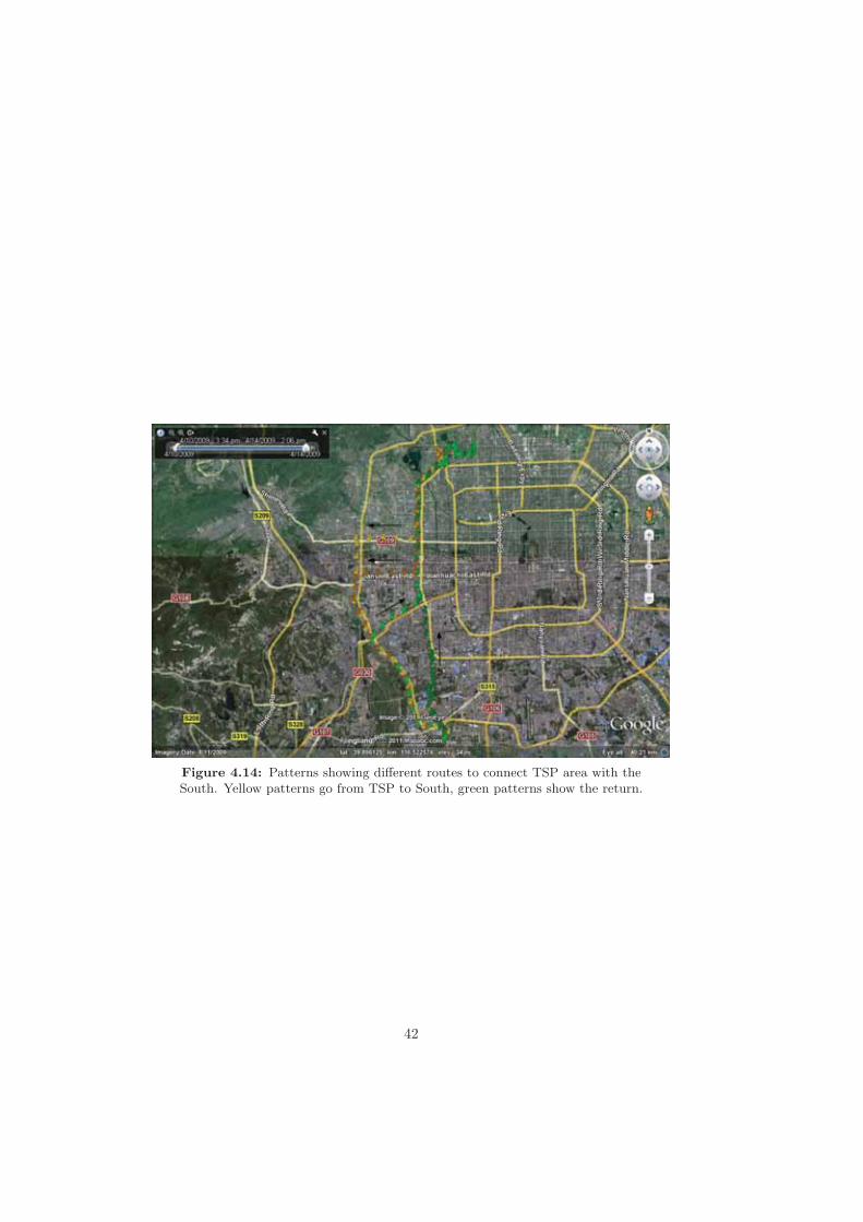
Figure 4.14: Patterns showing different routes to connect TSP area with theSouth. Yellow patterns go from TSP to South, green patterns show the return.

42

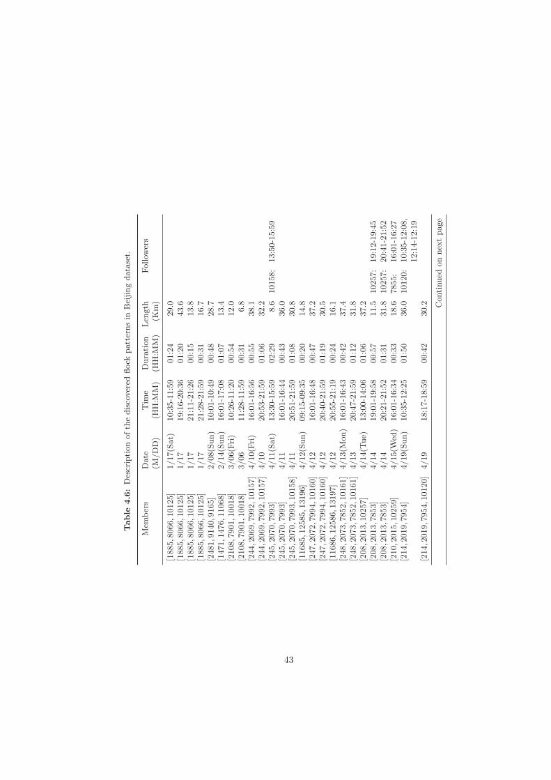
Table

4.6:Descriptionofthediscovered

flock

patternsin

Beijingdataset.

Mem

bers

Date

Tim

eDuration

Len

gth

Follow

ers

(M/DD)

(HH:M

M)

(HH:M

M)

(Km)

[1885,8066,10125]

1/17(Sat)

10:35-11:59

01:24

29.0

[1885,8066,10125]

1/17

19:16-20:36

01:20

43.6

[1885,8066,10125]

1/17

21:11-21:26

00:15

13.8

[1885,8066,10125]

1/17

21:28-21:59

00:31

16.7

[2481,9140,9165]

2/08(Sun)

10:01-10:49

00:48

28.7

[1471,1476,11068]

2/14(Sun)

16:01-17:08

01:07

13.4

[2108,7901,10018]

3/06(Fri)

10:26-11:20

00:54

12.0

[2108,7901,10018]

3/06

11:28-11:59

00:31

6.8

[244,2069,7992,10157]

4/10(Fri)

16:01-16:56

00:55

38.1

[244,2069,7992,10157]

4/10

20:53-21:59

01:06

32.2

[245,2070,7993]

4/11(Sat)

13:30-15:59

02:29

8.6

10158:

13:50-15:59

[245,2070,7993]

4/11

16:01-16:44

00:43

36.0

[245,2070,7993,10158]

4/11

20:51-21:59

01:08

30.8

[11685,12585,13196]

4/12(Sun)

09:15-09:35

00:20

14.8

[247,2072,7994,10160]

4/12

16:01-16:48

00:47

37.2

[247,2072,7994,10160]

4/12

20:40-21:59

01:19

30.5

[11686,12586,13197]

4/12

20:55-21:19

00:24

16.1

[248,2073,7852, 10161]

4/13(M

on)

16:01-16:43

00:42

37.4

[248,2073,7852,10161]

4/13

20:47-21:59

01:12

31.8

[208,2013,10257]

4/14(T

ue)

13:00-14:06

01:06

37.2

[208,2013,7853]

4/14

19:01-19:58

00:57

11.5

10257:

19:12-19:45

[208,2013,7853]

4/14

20:21-21:52

01:31

31.8

10257:

20:41-21:52

[210,2015,10259]

4/15(W

ed)

16:01-16:34

00:33

18.6

7855:

16:01-16:27

[214,2019,7954]

4/19(Sun)

10:35-12:25

01:50

36.0

10120:

10:35-12:08,

12:14-12:19

[214,2019,7954,10120]

4/19

18:17-18:59

00:42

30.2 Continued

onnex

tpage

43

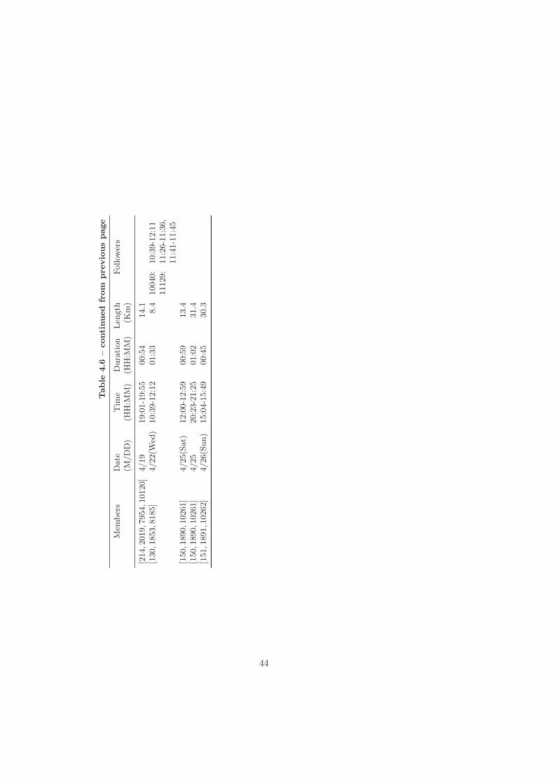
Table

4.6

–continued

from

pre

viouspage

Mem

bers

Date

Tim

eDuration

Len

gth

Follow

ers

(M/DD)

(HH:M

M)

(HH:M

M)

(Km)

[214,2019,7954,10120]

4/19

19:01-19:55

00:54

14.1

[130,1853,8185]

4/22(W

ed)

10:39-12:12

01:33

8.4

10040:

10:39-12:11

11129:

11:26-11:36,

11:41-11:45

[150,1890,10261]

4/25(Sat)

12:00-12:59

00:59

13.4

[150,1890,10261]

4/25

20:23-21:25

01:02

31.4

[151,1891,10262]

4/26(Sun)

15:04-15:49

00:45

30.3

44

Chapter 5

Discussion

One of the main concerns of this research is understanding the performance implications ofthe proposed framework. For this reason it was evaluated with synthetic and real datasetswith different characteristics. Although the overall size of the dataset was expected tomark a trend in the performance, it is clear that this is not the only one important factor.

Additionally, the number of reported flocks is a critical issue that affect the properinterpretation of the final results. Although the problem of duplicates and redundantpatterns is tackled in the postprocessing stage, high similarity among the patterns stillremain. Causes and some strategies to reduce the number of reported flocks and enhancetheir understanding are discussed.

5.1 Implementation and Performance Issues

5.1.1 Impact of size trajectory

Initial tests with synthetic datasets showed a high performance of the proposed approachwith respect to the traditional method. However under tests with real datasets thatdifference disappeared. In addition to the number of trajectories, the individual size ofeach segment also affects significantly the performance of traditional frequent patternsalgorithms used in the proposed approach. It is important to clarify that size of thetrajectory refers to number of point locations rather than to spatial length.

It is noted by [7, 29, 38] that not just the length of the involved transactions butalso the length of the resulting patterns have a direct impact in the performance offrequent pattern techniques. The results from the experiments unveil that the shorter thetrajectory size the better performance to find flock patterns.

As can be seen in the Table 3.2, for the two synthetic datasets the average trajectorysize is low (40 and 37 points for datasets SJ25KT60 and SJ50KT55 respectively). On theother hand average size in real datasets depend on the interpolation rate and range oftime selected by the study. For Icebergs06, it was decided to study a complete year witha daily interpolation. In this case the average size per trajectory is around 329 points.

For Beijing dataset previous preprocessing tasks were performed by the original au-thors. They separated the trajectory of the users daily. In addition, time periods greaterthan 20 minutes without position reports were used to mark a new trajectory. As con-

45

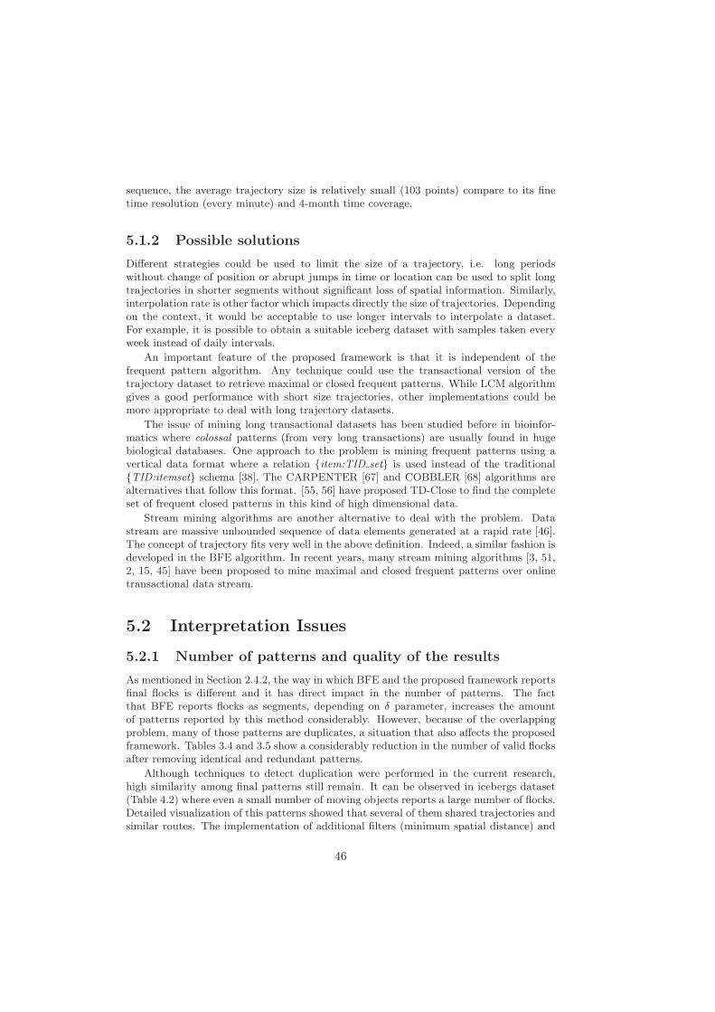
sequence, the average trajectory size is relatively small (103 points) compare to its finetime resolution (every minute) and 4-month time coverage.

5.1.2 Possible solutions

Different strategies could be used to limit the size of a trajectory, i.e. long periodswithout change of position or abrupt jumps in time or location can be used to split longtrajectories in shorter segments without significant loss of spatial information. Similarly,interpolation rate is other factor which impacts directly the size of trajectories. Dependingon the context, it would be acceptable to use longer intervals to interpolate a dataset.For example, it is possible to obtain a suitable iceberg dataset with samples taken everyweek instead of daily intervals.

An important feature of the proposed framework is that it is independent of thefrequent pattern algorithm. Any technique could use the transactional version of thetrajectory dataset to retrieve maximal or closed frequent patterns. While LCM algorithmgives a good performance with short size trajectories, other implementations could bemore appropriate to deal with long trajectory datasets.

The issue of mining long transactional datasets has been studied before in bioinfor-matics where colossal patterns (from very long transactions) are usually found in hugebiological databases. One approach to the problem is mining frequent patterns using avertical data format where a relation {item:TID set} is used instead of the traditional{TID:itemset} schema [38]. The CARPENTER [67] and COBBLER [68] algorithms arealternatives that follow this format. [55, 56] have proposed TD-Close to find the completeset of frequent closed patterns in this kind of high dimensional data.

Stream mining algorithms are another alternative to deal with the problem. Datastream are massive unbounded sequence of data elements generated at a rapid rate [46].The concept of trajectory fits very well in the above definition. Indeed, a similar fashion isdeveloped in the BFE algorithm. In recent years, many stream mining algorithms [3, 51,2, 15, 45] have been proposed to mine maximal and closed frequent patterns over onlinetransactional data stream.

5.2 Interpretation Issues

5.2.1 Number of patterns and quality of the results

As mentioned in Section 2.4.2, the way in which BFE and the proposed framework reportsfinal flocks is different and it has direct impact in the number of patterns. The factthat BFE reports flocks as segments, depending on δ parameter, increases the amountof patterns reported by this method considerably. However, because of the overlappingproblem, many of those patterns are duplicates, a situation that also affects the proposedframework. Tables 3.4 and 3.5 show a considerably reduction in the number of valid flocksafter removing identical and redundant patterns.

Although techniques to detect duplication were performed in the current research,high similarity among final patterns still remain. It can be observed in icebergs dataset(Table 4.2) where even a small number of moving objects reports a large number of flocks.Detailed visualization of this patterns showed that several of them shared trajectories andsimilar routes. The implementation of additional filters (minimum spatial distance) and

46

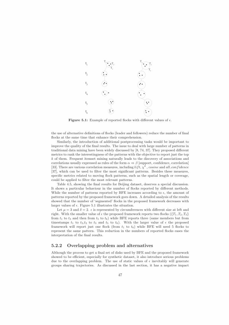
Figure 5.1: Example of reported flocks with different values of ε.

the use of alternative definitions of flocks (leader and followers) reduce the number of finalflocks at the same time that enhance their comprehension.

Similarly, the introduction of additional postprocessing tasks would be important toimprove the quality of the final results. The issue to deal with large number of patterns intraditional data mining have been widely discussed by [8, 74, 37]. They proposed differentmetrics to rank the interestingness of the patterns with the objective to report just the topk of them. Frequent itemset mining naturally leads to the discovery of associations andcorrelations usually expressed as rules of the form α ⇒ β [support, confidence, correlation][33]. There are various correlation measures, including lift, χ2 , cosine and all confidence[37], which can be used to filter the most significant patterns. Besides these measures,specific metrics related to moving flock patterns, such as the spatial length or coverage,could be applied to filter the most relevant patterns.

Table 4.5, showing the final results for Beijing dataset, deserves a special discussion.It shows a particular behaviour in the number of flocks reported by different methods.While the number of patterns reported by BFE increases according to ε, the amount ofpatterns reported by the proposed framework goes down. A detailed analysis of the resultsshowed that the number of ‘segmented’ flocks in the proposed framework decreases withlarger values of ε. Figure 5.1 illustrates the situation.

Let μ = 3 and δ = 2. ε is represented by circumferences with different size at left andright. With the smaller value of ε the proposed framework reports two flocks ({T1, T2, T3}from t1 to t3 and then from t5 to t6) while BFE reports three (same members but fromtimestamps t1 to t2,t2 to t3 and t5 to t6). With the larger value of ε the proposedframework will report just one flock (from t1 to t6) while BFE will need 5 flocks torepresent the same pattern. This reduction in the numbers of reported flocks eases theinterpretation of the final results.

5.2.2 Overlapping problem and alternatives

Although the process to get a final set of disks used by BFE and the proposed frameworkshowed to be efficient, especially for synthetic dataset, it also introduce serious problemsdue to the overlapping problem. The use of static values of ε inevitably will generategroups sharing trajectories. As discussed in the last section, it has a negative impact

47

introducing duplicate patterns. In addition, overlapped disks lead to generate flocks whichshare many of their trajectories. As result, many of the reported flocks are semanticallysimilar.

Formal definitions of flocks set ε as a fixed parameter [82, 10, 30]. However, naturalbehaviour of moving objects lead groups increase and decrease their members, and thespace which they occupy, according to time. For example, people and vehicles have tomove in constrained space which affect the size and shape of the flocks. It seems reasonableto think that flexible shapes and values for ε will model in a better way the interactionamong moving entities.

Spatial clustering algorithms are an option to discover set of clusters, instead of disks,of arbitrary shape and size. Furthermore, the use of arbitrary shapes will ensure thattrajectories belong to only one cluster per time interval. There are several methods inthis topic which can be classified into partitioning, hierarchical, density-based or grid-based methods [34]. Recent and well-known algorithms in this area could be applied asalternative to avoid the overlapping problem.

DBScan is one of the most popular density-based spatial clustering algorithm [21].Clusters are defined as a set of dense connected regions with irregular shape. It hassimilar parameters for minimum number of points (MinPts) and given radius (Eps) easilyassociated to μ and ε respectively. However, DBScan has problems with handling largedatabases and in worst case its complexity reaches to O(n2).

Recently, parallel spatial clustering algorithms based on the use of Swarm Intelligence(SI) techniques [90] have been proposed. [22] propose SPARROW, an algorithm whichcombines an exploratory strategy based on biologically inspired agents with a density-based cluster algorithm to discover adaptive clusters in spatial data. This approachextends DBScan to deal with large spatial databases using a decentralized approach

Grid and spatial index methods are another alternative to be considered. Spatialindexes have proved to be highly efficient to sort and manage point-set data. [18] presentTrajStore, an adaptive storage system to manage very large trajectory datasets. Theyintroduce spatial indexes based on adaptive quadtrees as clusterer and determine optimalsize cell using cost functions.

Grid-based methods have been also studied to face spatial clustering in presence ofobstacles or constrains. This approach is important in the case of pedestrians or vehicleswhich usually have to follow networks. [94] present a grid-based hierarchical spatialclustering algorithm which uses an obstacle-grid and a hierarchical strategy to reduce thecomplexity of clustering in presence of obstacles and constraints. [89] and [95] deal withthe problem following a density-based approach.

48

Chapter 6

Conclusions andRecommendations

6.1 Summary of the Research

This research has defined an appropriate methodology to apply the frequent pattern min-ing approach in order to discover moving flock patterns in large spatio-temporal datasets.A new framework which integrates techniques to identify groups of moving entities andlongest duration flocks patterns has been proposed and tested with synthetic and realdatasets.

The framework assumes that a moving flock patterns can be generalized as a typi-cal frequent pattern. The framework converts a trajectory dataset into a transactionaldatabase based on the locations visited by each trajectory. Once a transactional ver-sion of the dataset is available, frequent pattern mining algorithms can be applied on it(Objective 1).

Overall, the implementation of the proposed framework consists of four steps: iden-tification of groups of moving objects per time interval, construction of a transactionalversion of the trajectory dataset, application of a frequent pattern mining algorithm andperforming of postprocessing tasks (Objective 2).

The proposed framework was tested and compared with a current method (BFE algo-rithm). Synthetic datasets simulating trajectories generated by large number of movingobjects were used to test the scalability of the framework. Real datasets from differentcontexts and with different characteristics were used to assess the performance and anal-yse the discovered patterns. Compared with the current method (BFE), the proposedframework shows high performance with the characteristics of synthetic datasets. Withreal datasets, the time response was still efficient and quite similar to BFE (Objective 3).

The use of synthetic and real datasets provided valuable insights to understandingwhich parameters and dataset characteristics are the most relevant in order to find movingflock patterns. The size of the dataset had a high influence in the performance as expected,the length of the transactions also represented a relevant impact in the response of theproposed framework.

The frequent pattern mining approach showed to be useful to deal with the problemsfound in the BFE algorithm for datasets with large number of trajectories. The proposed

49

framework handle the disk combination efficiently by using scalable frequent pattern al-gorithms. Additionally, maximal pattern mining techniques are able to detect longestduration flocks.

Preliminary strategies to visualize the results were explored during this research.These include different interpretation of moving flock patterns and filters to retrieve themost relevant information. However, the large number of discovered patterns in manycases show that this task require additional treatment. A correct visualization of theresults is still an open issue.

The proposed framework is modular and different techniques can be applied to improvethe performance depending on a particular case. Although a specific frequent patternalgorithm was implemented in this framework, once a set of transactions are derived fromthe original trajectories, any frequent pattern algorithm can be used. Coupled with that,the initial stage to identify the most visited sites could be changed for other methods.

One important finding from this research was that the method is applicable to dif-ferent types of phenomena. The framework proved to be useful to find moving flockpatterns in diverse contexts such as human and iceberg movement. Results from studycases reflected useful information and trends which coincided with previous literature andexpected behaviour.

6.2 Recommendation

Some recommendations for improvement and further research are proposed as follows:

1. A fixed shape and distance was used to identify clusters in the first step of theframework. This introduces serious problems of overlapping and redundant results.The use of flexible shapes might define flocks which represent reality better. Meth-ods for spatial clustering, especially density and grid-based methods, could be usedto define flocks with different shapes.

2. Depending on the dimensionality of datasets and specific parameter settings, thenumber of discovered patterns can be significantly large. Appropriate analysis ofthe results demands special techniques to be developed. Further research in visual-ization is required to extract and display the most valuable patterns. Aggregation,summarisation and simplification techniques based on spatial and temporal statis-tics could be used for this purpose.

3. In contrast to the BFE algorithm, the proposed framework is not real-time. Itrequires a time window to build the transactional version of the dataset. A viablealternative is stream mining algorithms which deal with massive unbounded se-quence of continuous data. Application of this algorithms are usually found in thefield of bioinformatics and computer network traffic. The analysis and integrationof such algorithms in the framework is an interesting further research area.

4. The current research has shown the similarities between itemsets and moving flockpatterns. A logical next step would be to mine association rules based on the discov-ered patterns. In a similar way in which traditional association rules find correlationbetween items, association rule learning applied to spatio-temporal datasets mightfind interesting correlations among the places which are visited by moving objects.

In general, analysis of large spatio-temporal datasets has raised a lot of challeng-ing problems. Frequent pattern mining techniques have been shown to have importantcontributions to make in this area.

50

References

[1] R. Agrawal and R. Srikant. “Fast algorithms for mining association rules”.In: Proc. 20th Int. Conf. Very Large Data Bases, VLDB. Vol. 1215. Citeseer.1994, pp. 487–499.

[2] F. Ao, J. Du, Y. Yan, B. Liu, and K. Huang. “An efficient algorithm for min-ing closed frequent itemsets in data streams”. In: Computer and InformationTechnology Workshops, 2008. CIT Workshops 2008. IEEE 8th InternationalConference on. IEEE. 2008, pp. 37–42.

[3] F. Ao, Y. Yan, J. Huang, and K. Huang. “Mining Maximal Frequent Itemsetsin Data Streams Based on FP-Tree”. In: Machine Learning and Data Miningin Pattern Recognition (2007), pp. 479–489.

[4] K.R. Arrigo, G.L. van Dijken, D.G. Ainley, M.A. Fahnestock, and T. Markus.“Ecological impact of a large Antarctic iceberg”. In: Geophysical ResearchLetters 29.7 (2002), p. 1104. issn: 0094-8276.

[5] A. Atkinson, V. Siegel, E. Pakhomov, and P. Rothery. “Long-term declinein krill stock and increase in salps within the Southern Ocean”. In: Nature432.7013 (2004), pp. 100–103. issn: 0028-0836.

[6] J. Ballantyne and DG Long. “A Multidecadal Study of the Number of Antarc-tic Icebergs using Scatterometer Data”. In: International Geoscience and Re-mote Sensing Symposium. Vol. 5. 2002, pp. 3029–3031.

[7] R.J. Bayardo Jr. “Efficiently mining long patterns from databases”. In: ACMSigmod Record 27.2 (1998), pp. 85–93. issn: 0163-5808.

[8] R.J. Bayardo Jr and R. Agrawal. “Mining the most interesting rules”. In:Proceedings of the fifth ACM SIGKDD international conference on Knowl-edge discovery and data mining. ACM. 1999, p. 154. isbn: 1581131437.

[9] R.J. Bayardo Jr, B. Goethals, and M.J. Zaki. “FIMI 04, Proceedings of theIEEE ICDM Workshop on Frequent Itemset Mining Implementations”. In:vol. 126. 2004.

[10] M. Benkert, J. Gudmundsson, F. Hubner, and T. Wolle. “Reporting flockpatterns”. In: Computational Geometry 41.3 (2008), pp. 111–125.

[11] T. Birkhoff. Network-based Generator of Moving Objects. 2010. url: http://www.fh-oow.de/institute/iapg/personen/brinkhoff/generator/.

51

[12] C. Borgelt. “An Implementation of the FP-growth Algorithm”. In: Proceed-ings of the 1st international workshop on open source data mining: frequentpattern mining implementations. ACM. 2005, p. 5.

[13] T. Brinkhoff. “A framework for generating network-based moving objects”.In: GeoInformatica 6.2 (2002), pp. 153–180.

[14] T. Brinkhoff. “Generating traffic data”. In: IEEE Data Engineering Bulletin26.2 (2003), pp. 19–25.

[15] H. Chen. “Efficiently Mining the Recent Frequent Patterns over Online DataStreams”. In: Intelligent Systems and Applications (ISA), 2010 2nd Interna-tional Workshop on. IEEE. 2010, pp. 1–4.

[16] R. Chen, Q. Jiang, H. Yuan, and L. Gruenwald. “Mining association rules inanalysis of transcription factors essential to gene expressions”. In: AtlanticSymposium on Computational Biology, and Genome Information Systems &Technology. Citeseer. 2001.

[17] C. Creighton and S. Hanash. “Mining gene expression databases for associa-tion rules”. In: Bioinformatics 19.1 (2003), p. 79. issn: 1367-4803.

[18] P. Cudre-Mauroux, E. Wu, and S. Madden. “TrajStore: An adaptive storagesystem for very large trajectory data sets”. In: Data Engineering (ICDE),2010 IEEE 26th International Conference on. IEEE. 2010, pp. 109–120.

[19] G. Deacon. The Antarctic circumpolar ocean. Vol. 180. Cambridge UniversityPress Cambridge, 1984.

[20] H. Dettki, G. Ericsson, and L. Edenius. “Real-time moose tracking: an in-ternet based mapping application using GPS/GSM-collars in Sweden”. In:Alces 40 (2004), pp. 13–21.

[21] M. Ester, H.P. Kriegel, J. Sander, and X. Xu. “A density-based algorithm fordiscovering clusters in large spatial databases with noise”. In: Proc. KDD.Vol. 96. 1996, pp. 226–231.

[22] G. Folino and G. Spezzano. “An adaptive flocking algorithm for spatial clus-tering”. In: Parallel Problem Solving from Nature PPSN VII (2002), pp. 924–933.

[23] A.U. Frank, J. Raper, and J.P. Cheylan. Life and motion of socio-economicunits. CRC, 2001.

[24] P. Giudici and Ebooks Corporation. Applied data mining: Statistical methodsfor business and industry. Wiley New York, 2003. isbn: 047084678.

[25] B. Goethals. “Survey on frequent pattern mining”. In: Manuscript (2003),pp. 1–43.

[26] B. Goethals. The FIMI’04 Homepage. 2004. url: http : / / fimi . cs .

helsinki.fi/.

[27] B. Goethals and M.J. Zaki. “Advances in frequent itemset mining implemen-tations: report on FIMI’03”. In: ACM SIGKDD Explorations Newsletter 6.1(2004), pp. 109–117. issn: 1931-0145.

52

[28] B. Goethals and M.J. Zaki. “FIMI 03: Proceedings of the ICDM 2003 Work-shop on Frequent Itemset Mining Implementations”. In: vol. 90. 2003.

[29] G. Grahne and J. Zhu. “High performance mining of maximal frequent item-sets”. In: 6th International Workshop on High Performance Data Mining.Citeseer. 2003.

[30] J. Gudmundsson and M. van Kreveld. “Computing longest duration flocks intrajectory data”. In: Proceedings of the 14th annual ACM international sym-posium on Advances in geographic information systems. ACM. 2006, p. 42.

[31] J. Gudmundsson, M. van Kreveld, and B. Speckmann. “Efficient detection ofmotion patterns in spatio-temporal data sets”. In: Proceedings of the 12th an-nual ACM international workshop on Geographic information systems. ACM.2004, pp. 250–257.

[32] J. Gyory, J. Cangialosi, I. Jo, A. Mariano, and E. Ryan. Surface Currentsin the Southern Ocean: The Antarctic Coastal Current. 2003. url: http://oceancurrents.rsmas.miami.edu/southern/antarctic-coastal.html.

[33] J. Han and M. Kamber. Data mining: concepts and techniques. Morgan Kauf-mann, 2006. isbn: 1558609016.

[34] J. Han, M. Kamber, and A.K.H. Tung. “Spatial clustering methods in datamining: A survey”. In: Geographic Data Mining and Knowledge Discovery.Taylor and Francis 21 (2001).

[35] J. Han, K. Koperski, and N. Stefanovic. “GeoMiner: a system prototype forspatial data mining”. In: Proceedings of the 1997 ACM SIGMOD interna-tional conference on Management of data. ACM. 1997, pp. 553–556. isbn:0897919114.

[36] J. Han and J. Pei. “Mining frequent patterns by pattern-growth: methodologyand implications”. In: ACM SIGKDD Explorations Newsletter 2.2 (2000),pp. 14–20. issn: 1931-0145.

[37] J. Han, H. Cheng, D. Xin, and X. Yan. “Frequent pattern mining: currentstatus and future directions”. In: Data Mining and Knowledge Discovery 15.1(2007), pp. 55–86. issn: 1384-5810.

[38] J. Han, H. Cheng, D. Xin, and X. Yan. “Frequent pattern mining: currentstatus and future directions”. In: Data Mining and Knowledge Discovery 15.1(2007), pp. 55–86. issn: 1384-5810.

[39] J. Han, J. Pei, Y. Yin, and R. Mao. “Mining frequent patterns without can-didate generation: A frequent-pattern tree approach”. In: Data mining andknowledge discovery 8.1 (2004), pp. 53–87.

[40] R.P. Hewitt, D.A. Demer, and J.H. Emery. “An 8-year cycle in krill biomassdensity inferred from acoustic surveys conducted in the vicinity of the SouthShetland Islands during the austral summers of 1991-1992 through 2001-2002”. In: Aquatic Living Resources 16.3 (2003), pp. 205–213. issn: 0990-7440.

53

[41] S. Iwase and H. Saito. “Tracking soccer player using multiple views”. In: Pro-ceedings of the IAPR Workshop on Machine Vision Applications (MVA02).Citeseer. 2002, pp. 102–105.

[42] C.S. Jensen, D. Lin, and B.C. Ooi. “Continuous clustering of moving objects”.In: IEEE Transactions on Knowledge and Data Engineering (2007), pp. 1161–1174. issn: 1041-4347.

[43] H. Jeung, M.L. Yiu, X. Zhou, C.S. Jensen, and H.T. Shen. “Discovery ofconvoys in trajectory databases”. In: Proceedings of the VLDB Endowment1.1 (2008), pp. 1068–1080.

[44] Hoyoung Jeung, Heng Tao Shen, and Xiaofang Zhou. “Convoy Queries inSpatio-Temporal Databases”. In: Data Engineering, 2008. ICDE 2008. IEEE24th International Conference on. 2008, pp. 1457–1459. doi: 10.1109/ICDE.2008.4497588.

[45] N. Jiang and L. Gruenwald. “CFI-Stream: mining closed frequent itemsetsin data streams”. In: Proceedings of the 12th ACM SIGKDD internationalconference on Knowledge discovery and data mining. ACM. 2006, pp. 592–597. isbn: 1595933395.

[46] N. Jiang and L. Gruenwald. “Research issues in data stream association rulemining”. In: ACM Sigmod Record 35.1 (2006), pp. 14–19. issn: 0163-5808.

[47] P. Kalnis, N. Mamoulis, and S. Bakiras. “On discovering moving clustersin spatio-temporal data”. In: Advances in Spatial and Temporal Databases(2005), pp. 364–381.

[48] J. Kaufman, J. Myllymaki, and J. Jackson. “City Simulator V2. 0”. In: IBMalphaWorks, December (2001).

[49] J. Krumm and E. Horvitz. “Predestination: Where do you want to go today?”In: Computer 40.4 (2007), pp. 105–107. issn: 0018-9162.

[50] P. Laube, M. Kreveld, and S. Imfeld. “Finding REMO - detecting relativemotion patterns in geospatial lifelines”. In: Developments in Spatial DataHandling (2005), pp. 201–215.

[51] H.F. Li, S.Y. Lee, and M.K. Shan. “Online mining (recently) maximal fre-quent itemsets over data streams”. In: (2005). issn: 1097-8585.

[52] Q. Li, Y. Zheng, X. Xie, Y. Chen, W. Liu, and W.Y. Ma. “Mining user simi-larity based on location history”. In: Proceedings of the 16th ACM SIGSPA-TIAL international conference on Advances in geographic information sys-tems. ACM. 2008, pp. 1–10.

[53] Y. Li, J. Han, and J. Yang. “Clustering moving objects”. In: Proceedings ofthe tenth ACM SIGKDD international conference on Knowledge discoveryand data mining. ACM. 2004, pp. 617–622. isbn: 1581138881.

[54] Z. Li, M. Ji, J.G. Lee, L.A. Tang, Y. Yu, J. Han, and R. Kays. “MoveMine:mining moving object databases”. In: Proceedings of the 2010 internationalconference on Management of data. ACM. 2010, pp. 1203–1206.

54

[55] H. Liu, J. Han, D. Xin, and Z. Shao. “Mining Frequent Patterns from VeryHigh Dimensional Data: A Top-Down Row Enumeration Approach”. In: Pro-ceeding of the 2006 SIAM international conference on data mining (SDM 06),Bethesda, MD. Citeseer. 2006, pp. 280–291.

[56] H. Liu, J. Han, D. Xin, and Z. Shao. “Top-down mining of interesting patternsfrom very high dimensional data”. In: Data Engineering, 2006. ICDE’06.Proceedings of the 22nd International Conference on. IEEE. 2006, p. 114.isbn: 0769525709.

[57] DG Long, J. Ballantyne, and C. Bertoia. “Is the number of Antarctic icebergsreally increasing?” In: EOS Transactions 83 (2002), p. 469.

[58] D. Makris and T. Ellis. “Path detection in video surveillance”. In: Image andVision Computing 20.12 (2002), pp. 895–903. issn: 0262-8856.

[59] Microsoft Research Asia. GeoLife GPS Trajectories. 2010. url: http://research.microsoft.com/en-us/downloads/b16d359d-d164-469e-9fd4

-daa38f2b2e13/default.aspx.

[60] H.J. Miller and J. Han. Geographic data mining and knowledge discovery.Vol. 338. Wiley Online Library, 2001.

[61] S.I. Minato, T. Uno, and H. Arimura. “LCM over ZBDDS: fast generationof very large-scale frequent itemsets using a compact graph-based repre-sentation”. In: Advances in Knowledge Discovery and Data Mining (2008),pp. 234–246.

[62] S. Nicol. “Krill, currents, and sea ice: Euphausia superba and its changingenvironment”. In: BioScience 56.2 (2006), pp. 111–120.

[63] S. Nicol and Y. Endo. “Krill fisheries: development, management and ecosys-tem implications”. In: Aquatic Living Resources 12.2 (1999), pp. 105–120.issn: 0990-7440.

[64] S. Nicol and J. Foster. “Recent trends in the fishery for Antarctic krill”. In:Aquating Living Resources 16.1 (2003), pp. 42–45. issn: 0990-7440.

[65] Open GIS Consortium (OGC). Standards and Specifications. 2010. url:http://www.opengeospatial.org/standards.

[66] M. Oppenheimer and R.B. Alley. “The West Antarctic ice sheet and longterm climate policy”. In: Climatic Change 64.1 (2004), pp. 1–10. issn: 0165-0009.

[67] F. Pan, G. Cong, A.K.H. Tung, J. Yang, and M.J. Zaki. “CARPENTER:Finding closed patterns in long biological datasets”. In: Proceedings of theninth ACM SIGKDD international conference on Knowledge discovery anddata mining. ACM. 2003, pp. 637–642. isbn: 1581137370.

[68] F. Pan, A.K.H. Tung, G. Cong, and X. Xu. “COBBLER: combining columnand row enumeration for closed pattern discovery”. In: Scientific and Statisti-cal Database Management, 2004. Proceedings. 16th International Conferenceon. IEEE. 2004, pp. 21–30. isbn: 0769521460.

55

[69] N. Pasquier, Y. Bastide, R. Taouil, and L. Lakhal. “Discovering frequentclosed itemsets for association rules”. In: Database Theory ICDT 99 (1999),pp. 398–416.

[70] D. Pfoser and Y. Theodoridis. “Generating semantics-based trajectoriesof moving objects”. In: Computers, Environment and Urban Systems 27.3(2003), pp. 243–263. issn: 0198-9715.

[71] C. Piciarelli, GL Foresti, and L. Snidara. “Trajectory clustering and its appli-cations for video surveillance”. In: Advanced Video and Signal Based Surveil-lance, 2005. AVSS 2005. IEEE Conference on. IEEE. 2006, pp. 40–45. isbn:0780393856.

[72] Refractions Research. PostGIS (version 1.5.2). 2010. url: http://postgis.refractions.net/.

[73] J.M. Saglio and J. Moreira. “Oporto: A realistic scenario generator for movingobjects”. In: GeoInformatica 5.1 (2001), pp. 71–93. issn: 1384-6175.

[74] T. Scheffer and S. Wrobel. “Finding the most interesting patterns in adatabase quickly by using sequential sampling”. In: The Journal of MachineLearning Research 3 (2003), pp. 833–862. issn: 1532-4435.

[75] M.K. Shan and L.Y. Wei. “Algorithms for discovery of spatial co-orientationpatterns from images”. In: Expert Systems with Applications (2010).

[76] A. Stathopoulos, L. Dimitriou, and T. Tsekeris. “Fuzzy modeling approachfor combined forecasting of urban traffic flow”. In: Computer-Aided Civil andInfrastructure Engineering 23.7 (2008), pp. 521–535. issn: 1467-8667.

[77] C. Swithinbank, P. McClain, and P. Little. “Drift tracks of Antarctic ice-bergs”. In: Polar Record 18.116 (1977), pp. 495–501. issn: 0032-2474.

[78] The Laboratory for Web Algorithmics - University of Milan. fastutils: Fast& compact type-specific collections for Java (version 6.0). 2010. url: http://fastutil.dsi.unimi.it/.

[79] D. Tsur, J.D. Ullman, S. Abiteboul, C. Clifton, R. Motwani, S. Nestorov,and A. Rosenthal. “Query flocks: a generalization of association-rule min-ing”. In: Proceedings of the 1998 ACM SIGMOD international conference onManagement of data. ACM. 1998, pp. 1–12. isbn: 0897919955.

[80] T. Uno, M. Kiyomi, and H. Arimura. “LCM ver. 2: Efficient mining algo-rithms for frequent/closed/maximal itemsets”. In: IEEE ICDM04 WorkshopFIMI04 (International Conference on Data Mining, Frequent Itemset MiningImplementations). Citeseer. 2004.

[81] T. Uno, M. Kiyomi, and H. Arimura. “Lcm ver. 3: Collaboration of array,bitmap and prefix tree for frequent itemset mining”. In: Proceedings of the 1stinternational workshop on open source data mining: frequent pattern miningimplementations. ACM. 2005, pp. 77–86. isbn: 1595932100.

56

[82] M.R. Vieira, P. Bakalov, and V.J. Tsotras. “On-line discovery of flock pat-terns in spatio-temporal data”. In: Proceedings of the 17th ACM SIGSPA-TIAL International Conference on Advances in Geographic Information Sys-tems. ACM. 2009, pp. 286–295.

[83] M.R. Vieira, E. Frıas-Martınez, P. Bakalov, V. Frıas-Martınez, and V.J. Tso-tras. “Querying Spatio-Temporal Patterns in Mobile Phone-Call Databases”.In: Mobile Data Management (MDM), 2010 Eleventh International Confer-ence on. IEEE. 2010, pp. 239–248.

[84] T.E. Vinje. “Some satellite-tracked iceberg drifts in the Antarctic”. In: Annalsof Glaciology 1 (1980), pp. 83–87.

[85] Vivid Solution Inc. JTS Topology Suite (version 1.8). 2010. url: http://www.vividsolutions.com/jts/jtshome.htm.

[86] Vivid Solution Inc. Open JUMP GIS (version 1.3.1). 2010. url: http://www.openjump.org/.

[87] E.I. Vlahogianni, M.G. Karlaftis, and J.C. Golias. “Optimized and meta-optimized neural networks for short-term traffic flow prediction: A geneticapproach”. In: Transportation Research Part C: Emerging Technologies 13.3(2005), pp. 211–234. issn: 0968-090X.

[88] M. Wachowicz, R. Ong, C. Renso, and M. Nanni. Discovering Moving FlockPatterns Among Pedestrians Through Spatio-Temporal Coherence. Tech. rep.Istituto di Scienza e Tecnologie dell’Informazione, 2010. url: http://puma.isti.cnr.it/publichtml/section_cnr_isti/cnr_isti_2010-TR-027.

html.

[89] X. Wang, C. Rostoker, and H.J. Hamilton. “Density-based spatial clusteringin the presence of obstacles and facilitators”. In: Knowledge Discovery inDatabases: PKDD 2004 (2004), pp. 446–458.

[90] B. Webb. “Swarm Intelligence: From Natural to Artificial Systems”. In: Con-nection Science 14.2 (2002), pp. 163–164. issn: 0954-0091.

[91] T. Wilson. OGC KML. Tech. rep. OGC Standard 07-147r2, 2008-04-14, 251pp, 2008.

[92] Z. Wood and A. Galton. “A taxonomy of collective phenomena”. In: AppliedOntology 4.3 (2009), pp. 267–292.

[93] Woods Hole Oceanographic Institution. Antarctica’s Ocean Circulation. 2006.url: http://polardiscovery.whoi.edu/antarctica/circulation.html.

[94] Y. Yang, J. Zhang, and J. Yang. “Grid-Based Hierarchical Spatial ClusteringAlgorithm in Presence of Obstacle and Constraints”. In: 2008 InternationalConference on Internet Computing in Science and Engineering. IEEE. 2008,pp. 383–388.

57

[95] OR Zaiane and C.H. Lee. “Clustering spatial data in the presence of obsta-cles: a density-based approach”. In: Database Engineering and ApplicationsSymposium, 2002. Proceedings. International. IEEE. 2002, pp. 214–223. isbn:0769516386.

[96] C. Zhang and S. Zhang. Association rule mining: models and algorithms.2002. isbn: 3540435336.

[97] Y. Zheng, X. Xie, andW.Y. Ma. “GeoLife: A Collaborative Social NetworkingService among User, Location and Trajectory”. In: Data Engineering (2010),p. 32.

[98] Y. Zheng, L. Zhang, X. Xie, and W.Y. Ma. “Mining interesting locations andtravel sequences from GPS trajectories”. In: Proceedings of the 18th interna-tional conference on World wide web. ACM. 2009, pp. 791–800.

[99] Y. Zheng, Q. Li, Y. Chen, X. Xie, and W.Y. Ma. “Understanding mobilitybased on GPS data”. In: Proceedings of the 10th international conference onUbiquitous computing. ACM. 2008, pp. 312–321.

58

Appendix A

Main source code of the framework implementation

import com . v i v i d s o l u t i o n s . j t s . geom . ∗ ;import edu . wlu . cs . l evy .CG.KDTree ;import edu . wlu . cs . l evy .CG. ∗ ;import i t . unimi . d s i . f a s t u t i l . ∗ ;

5 import java . i o . ∗ ;import java . u t i l . ∗ ;

public class LCMFlock {private GeometryFactory f a c t o ry ;

10 public stat ic double ep s i l o n ;private stat ic double r2 ;private stat ic double r ;public stat ic int time ;public stat ic int mu;

15 public stat ic int de l t a ;private stat ic f ina l double p r e c i s i o n = 0 . 0 0 1 ;int numFlock = 0 ;Int2ObjectAVLTreeMap<ArrayList<ArrayList>> database ;private int ntime = 0 ;

20 Int2ObjectAVLTreeMap<DiskInfo> dbdisks = newInt2ObjectAVLTreeMap<DiskInfo >() ;

public LCMFlock(double eps i l on , int mu, int de l t a ) {LCMFlock . e p s i l o n = ep s i l o n ;LCMFlock .mu = mu;

25 LCMFlock . d e l t a = de l t a ;f a c t o r y = new GeometryFactory ( ) ;LCMFlock . r = ( ep s i l o n / 2) + LCMFlock . p r e c i s i o n ;LCMFlock . r2 = Math . pow( ep s i l o n / 2 , 2) ;database = new Int2ObjectAVLTreeMap<ArrayList<ArrayList>>() ;

30 }

public Object2ObjectAVLTreeMap<Index , ObjectArrayList<Point>>getGrid ( Po in t s e t po in t s ) {

Objec t I t e ra to r<Point> i t e r a t o r = po in t s . po in t s . i t e r a t o r ( ) ;Object2ObjectAVLTreeMap<Index , ObjectArrayList<Point>> g r id ;

59

35 g r id = new Object2ObjectAVLTreeMap<Index , ObjectArrayList<Point>>() ;

while ( i t e r a t o r . hasNext ( ) ) {Point po int = i t e r a t o r . next ( ) ;int i = ( int ) ( po int . getX ( ) / LCMFlock . e p s i l o n ) ;int j = ( int ) ( po int . getY ( ) / LCMFlock . e p s i l o n ) ;

40 Index index = new Index ( i , j ) ;i f ( g r i d . containsKey ( index ) ) {

g r id . get ( index ) . add ( po int ) ;} else {

ObjectArrayList<Point> aux = new ObjectArrayList<Point>() ;45 aux . add ( po int ) ;

g r i d . put ( index , aux ) ;}

}return g r id ;

50 }

public ObjectAVLTreeSet<Disk> getDisks (Object2ObjectAVLTreeMap<Index , ObjectArrayList<Point>> g r id ) {

ObjectAVLTreeSet<Disk> maximalDisks = new ObjectAVLTreeSet<Disk>() ;

Ob j e c t I t e ra to r<Index> i tKeys = gr id . keySet ( ) . i t e r a t o r ( ) ;55 Objec t I t e ra to r<ObjectArrayList<Point>> i tVa lue s = gr id . va lue s

( ) . i t e r a t o r ( ) ;ObjectAVLTreeSet<Pair> computedPairs = new ObjectAVLTreeSet<

Pair >() ;KDTree<Disk> kdtree = new KDTree<Disk>(2) ;ArrayList<double [ ]> d i skCoord inate s = new ArrayList<double

[ ] > ( ) ;while ( i tKeys . hasNext ( ) ) {

60 Index index = itKeys . next ( ) ;ObjectArrayList<Point> po i n t s I nCe l l = i tVa lue s . next ( ) ;Ob j e c t I t e ra to r<Point> i t P o i n t s I nCe l l = po i n t s I nCe l l . i t e r a t o r

( ) ;ObjectArrayList<Point> po int s InSubgr id ;po int s InSubgr id = new ObjectArrayList<Point>() ;

65 for ( int x = index . getX ( ) − 1 ; x <= index . getX ( ) + 1 ; x++) {for ( int y = index . getY ( ) − 1 ; y <= index . getY ( ) + 1 ; y++)

{Index newindex = new Index (x , y ) ;ObjectArrayList<Point> get = gr id . get ( newindex ) ;i f ( get != null ) {

70 po int s InSubgr id . addAll ( get ) ;}

}}//Line 6 BFE Pseudocode

75 i f ( po int s InSubgr id . s i z e ( ) < LCMFlock .mu) {continue ;

}while ( i tP o i n t s I nCe l l . hasNext ( ) ) {

Point po in t InCe l l = i tPo i n t s I nCe l l . next ( ) ;

60

80 Objec t I t e ra to r<Point> i tPo in t s InSubgr id = po int s InSubgr id .i t e r a t o r ( ) ;

ObjectArrayList<Point> range = new ObjectArrayList<Point>() ;

while ( i tPo in t s InSubgr id . hasNext ( ) ) {Point po int InSubgr id = i tPo in t s InSubgr id . next ( ) ;//Do not compare with the same po in t

85 // po in t InCe l l w i l l not be par t o f rangei f ( po i n t InCe l l . getUserData ( ) == point InSubgr id .

getUserData ( ) ) {continue ;

}i f ( po i n t InCe l l . i sWith inDis tance ( pointInSubgr id , e p s i l o n

) ) {90 range . add ( po int InSubgr id ) ;

}}//Points in range p lu s po in t InCe l li f ( range . s i z e ( ) + 1 >= LCMFlock .mu) {

95 Objec t I t e ra to r<Point> i tRange = range . i t e r a t o r ( ) ;int p1 = ( In t eg e r ) po in t InCe l l . getUserData ( ) ;int p2 ;while ( itRange . hasNext ( ) ) {

Point po int InSubgr id = itRange . next ( ) ;100 p2 = ( In t eg e r ) po int InSubgr id . getUserData ( ) ;

Pair pa i r = new Pair (p1 , p2 ) ;i f ( computedPairs . add ( pa i r ) ) {

Point c en t r e s [ ] = this . c a l c u l a t eD i s k s ( po in t InCe l l ,po int InSubgr id ) ;

i f ( c en t r e s == null ) {105 continue ;

}//Counting po in t s in each d i s kObjec t I t e ra to r<Point> i tCount = range . i t e r a t o r ( ) ;Disk d i sk1 = new Disk ( c en t r e s [ 0 ] ) ;

110 d i sk1 . addPoint ( po in t InCe l l ) ;Disk d i sk2 = new Disk ( c en t r e s [ 1 ] ) ;d i sk2 . addPoint ( po in t InCe l l ) ;while ( itCount . hasNext ( ) ) {

Point pointInRange = itCount . next ( ) ;115 i f ( d i sk1 . i sWith inDis tance ( pointInRange , LCMFlock .

r ) ) {di sk1 . addPoint ( pointInRange ) ;

}i f ( d i sk2 . i sWith inDis tance ( pointInRange , LCMFlock .

r ) ) {di sk2 . addPoint ( pointInRange ) ;

120 }}i f ( d i sk1 . count >= LCMFlock .mu) {

try {double [ ] key = { di sk1 . getX ( ) , d i sk1 . getY ( ) } ;

125 kdtree . i n s e r t ( key , d i sk1 ) ;d i skCoord inate s . add ( key ) ;

61

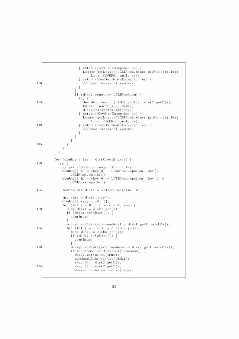
} catch ( KeySizeException ex ) {Logger . getLogger (LCMFlock . class . getName ( ) ) . l og (

Leve l .SEVERE, null , ex ) ;} catch ( KeyDuplicateException ex ) {

130 //Prune i d e n t i c a l c en t r e s}

}i f ( d i sk2 . count >= LCMFlock .mu) {

try {135 double [ ] key = { di sk2 . getX ( ) , d i sk2 . getY ( ) } ;

kdtree . i n s e r t ( key , d i sk2 ) ;d i skCoord inate s . add ( key ) ;

} catch ( KeySizeException ex ) {Logger . getLogger (LCMFlock . class . getName ( ) ) . l og (

Leve l .SEVERE, null , ex ) ;140 } catch ( KeyDuplicateException ex ) {

//Prune i d e n t i c a l c en t r e s}

}}

145 }}

}}for (double [ ] key : d i skCoord inate s ) {

150 try {// ge t Points in range o f each keydouble [ ] l o = {key [ 0 ] − LCMFlock . ep s i l on , key [ 1 ] −

LCMFlock . e p s i l o n } ;double [ ] h i = {key [ 0 ] + LCMFlock . ep s i l on , key [ 1 ] +

LCMFlock . e p s i l o n } ;

155 Lis t<Disk> d i s k s = kdtree . range ( lo , h i ) ;

int s i z e = d i s k s . s i z e ( ) ;double [ ] rkey = {0 , 0} ;for ( int i = 0 ; i < s i z e − 1 ; i++) {

160 Disk d i sk1 = d i s k s . get ( i ) ;i f ( d i sk1 . i s Subs e t ( ) ) {

continue ;}ArrayList<Integer> members1 = disk1 . getPo ints IDs ( ) ;

165 for ( int j = i + 1 ; j < s i z e ; j++) {Disk d i sk2 = d i s k s . get ( j ) ;i f ( d i sk2 . i s Subs e t ( ) ) {

continue ;}

170 ArrayList<Integer> members2 = disk2 . getPo ints IDs ( ) ;i f (members1 . c on ta i n sA l l (members2 ) ) {

d i sk2 . s e tSubse t ( true ) ;maximalDisks . remove ( d i sk2 ) ;rkey [ 0 ] = di sk2 . getX ( ) ;

175 rkey [ 1 ] = di sk2 . getY ( ) ;d i skCoord inate s . remove ( rkey ) ;

62

try {kdtree . d e l e t e ( rkey ) ;

} catch ( KeyMissingException ex ) {180 }

} else i f (members2 . c on ta i n sA l l (members1 ) ) {d i sk1 . s e tSubse t ( true ) ;maximalDisks . remove ( d i sk1 ) ;rkey [ 0 ] = di sk1 . getX ( ) ;

185 rkey [ 1 ] = di sk1 . getY ( ) ;d i skCoord inate s . remove ( rkey ) ;try {

kdtree . d e l e t e ( rkey ) ;} catch ( KeyMissingException ex ) {

190 }break ;

}}

}195 for ( Disk d i sk : d i s k s ) {

i f ( ! d i sk . i s Subs e t ( ) ) {maximalDisks . add ( d i sk ) ;

}}

200 } catch ( KeySizeException ex ) {Logger . getLogger (LCMFlock . class . getName ( ) ) . l og ( Leve l .

SEVERE, null , ex ) ;}

}for ( Disk d i sk : maximalDisks ) {

205 DiskIn fo d i = new DiskIn fo ( ) ;d i . setTime ( time ) ;d i . s e tPo in t s ( d i sk . po in t s ) ;dbdisks . put ( cid , d i ) ;for ( Point po int : d i sk . po in t s ) {

210 int id = ( In t eg e r ) po int . getUserData ( ) ;i f ( database . containsKey ( id ) ) {

ArrayList<ArrayList> aux = database . get ( id ) ;aux . get ( aux . s i z e ( ) − 1) . add ( c id ) ;

215 } else {ArrayList<ArrayList> aux = new ArrayList<ArrayList >() ;ArrayList tag = new ArrayList ( ) ;tag . add ( c id ) ;aux . add ( tag ) ;

220 database . put ( id , aux ) ;}

}c id++;

}225 return maximalDisks ;

}

public void mineMIF ( ) {Buf feredWriter wr i t e r = null ;

63

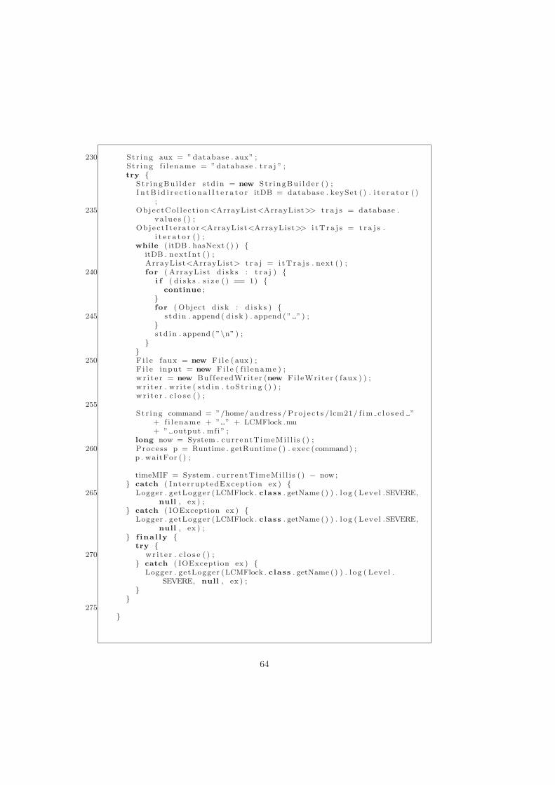
230 St r ing aux = ”database . aux” ;S t r ing f i l ename = ”database . t r a j ” ;try {

St r i ngBu i l d e r s td in = new St r i ngBu i l d e r ( ) ;I n tB i d i r e c t i o n a l I t e r a t o r itDB = database . keySet ( ) . i t e r a t o r ( )

;235 Objec tCo l l e c t i on<ArrayList<ArrayList>> t r a j s = database .

va lue s ( ) ;Ob j e c t I t e ra to r<ArrayList<ArrayList>> i tT r a j s = t r a j s .

i t e r a t o r ( ) ;while ( itDB . hasNext ( ) ) {

itDB . next Int ( ) ;ArrayList<ArrayList> t r a j = i tT r a j s . next ( ) ;

240 for ( ArrayList d i s k s : t r a j ) {i f ( d i s k s . s i z e ( ) == 1) {

continue ;}for ( Object d i sk : d i s k s ) {

245 s td in . append ( d i sk ) . append ( ” ” ) ;}s td in . append ( ”\n” ) ;

}}

250 F i l e faux = new F i l e ( aux ) ;F i l e input = new F i l e ( f i l ename ) ;w r i t e r = new Buf feredWriter (new Fi l eWr i t e r ( faux ) ) ;w r i t e r . wr i t e ( s td in . t oS t r i ng ( ) ) ;w r i t e r . c l o s e ( ) ;

255St r ing command = ”/home/ andress / Pro j e c t s / lcm21/ f im c l o s ed ”

+ f i l ename + ” ” + LCMFlock .mu+ ” output . mfi ” ;

long now = System . cur r entT imeMi l l i s ( ) ;260 Process p = Runtime . getRuntime ( ) . exec (command) ;

p . waitFor ( ) ;

timeMIF = System . cur r entT imeMi l l i s ( ) − now ;} catch ( Inte r ruptedExcept ion ex ) {

265 Logger . getLogger (LCMFlock . class . getName ( ) ) . l og ( Leve l .SEVERE,null , ex ) ;

} catch ( IOException ex ) {Logger . getLogger (LCMFlock . class . getName ( ) ) . l og ( Leve l .SEVERE,

null , ex ) ;} f ina l ly {

try {270 wr i t e r . c l o s e ( ) ;

} catch ( IOException ex ) {Logger . getLogger (LCMFlock . class . getName ( ) ) . l og ( Leve l .

SEVERE, null , ex ) ;}

}275

}

64

public void checkFlocks ( ) {BufferedReader reader = null ;

280 S t r i ngBu i l d e r s t d i o = new St r i ngBu i l d e r ( ) ;S t r i ngBu i l d e r s t r f l o c k s = new St r i ngBu i l d e r ( ) ;S t r ingToken i ze r s t ;try {

St r ing l i n e ;285 St r ing s c i d ;

int f i d = 1 ;int c id2 = 0 ;F i l e input = new F i l e ( ” output . mfi ” ) ;r eader = new BufferedReader (new Fi leReader ( input ) ) ;

290 int f r e cuency = LCMFlock .mu;while ( ( l i n e = reader . readLine ( ) ) != null ) {

s t = new Str ingToken i ze r ( l i n e , ” ” ) ;i f ( s t . countTokens ( ) < 4) {

295 continue ;}ArrayList<DiskInfo> aux = new ArrayList<DiskInfo>( s t .

countTokens ( ) − 1) ;while ( s t . hasMoreElements ( ) ) {

s c i d = s t . nextToken ( ) ;300 i f ( s c i d . charAt (0 ) == ’ ( ’ ) {

f r e cuency = In t eg e r . pa r s e In t ( s c i d . sub s t r i ng (1 , s c i d .l ength ( ) − 1) ) ;

} else {c id2 = In t eg e r . pa r s e In t ( s c i d ) ;Di sk In fo d i = dbdisks . get ( c id2 ) ;

305 aux . add ( d i ) ;}

}Co l l e c t i o n s . s o r t ( aux ) ;ArrayList<Integer> f i n a l P o i n t s = new ArrayList<Integer >() ;

310 f i n a lP o i n t s = aux . get (0 ) . getPointIDs ( ) ;int begin = aux . get (0 ) . getTime ( ) ;int end = begin ;int now ;int l im i t = aux . s i z e ( ) ;

315 for ( int i = 1 ; i < l im i t ; i++) {now = aux . get ( i ) . getTime ( ) ;i f (now == end + 1 | | now == end ) {

end = now ;i f ( f i n a lP o i n t s . s i z e ( ) != f r ecuency ) {

320 f i n a lP o i n t s . r e t a i nA l l ( aux . get ( i ) . getPointIDs ( ) ) ;}

} else i f ( end − begin >= LCMFlock . d e l t a − 1) {System . out . p r i n t l n ( ”\n” + f i d + ” ( ” + f i n a lP o i n t s . s i z e

( ) + ” ) : ” ) ;System . out . p r i n t l n ( ”From time ” + begin + ” to ” + end

) ;325 System . out . p r i n t l n ( ”Members : ” + f i n a lP o i n t s ) ;

numFlock++;begin = end = now ;

65

f i n a lP o i n t s = aux . get ( i ) . getPointIDs ( ) ;} else {

330 begin = end = now ;f i n a lP o i n t s = aux . get ( i ) . getPointIDs ( ) ;

}}i f ( end − begin >= LCMFlock . d e l t a − 1) {

335 System . out . p r i n t l n ( ”\n” + f i d + ” ( ” + f i n a lP o i n t s . s i z e ( )+ ” ) : ” ) ;

System . out . p r i n t l n ( ”From time ” + begin + ” to ” + end ) ;System . out . p r i n t l n ( ”Members : ” + f i n a lP o i n t s ) ;numFlock++;

}340 f i d++;

}} catch ( IOException ex ) {

Logger . getLogger (LCMFlock . class . getName ( ) ) . l og ( Leve l .SEVERE,null , ex ) ;

} f ina l ly {345 try {

r eader . c l o s e ( ) ;} catch ( IOException ex ) {

Logger . getLogger (LCMFlock . class . getName ( ) ) . l og ( Leve l .SEVERE, null , ex ) ;

}350 }

}

private Point [ ] c a l c u l a t eD i s k s ( Point p1 , Point p2 ) {355 Point d i s k s [ ] = new Point [ 2 ] ;

double p1 x = p1 . getX ( ) ;double p1 y = p1 . getY ( ) ;double p2 x = p2 . getX ( ) ;double p2 y = p2 . getY ( ) ;

360 double k 1 , k 2 , h 1 , h 2 ;double X, Y;double D2 ;

X = p1 x − p2 x ;365 Y = p1 y − p2 y ;

D2 = Math . pow(X, 2) + Math . pow(Y, 2) ;//The two po in t s are the same (Measure or resample e r ror s )i f (D2 == 0) {

return null ;370 }

double exp r e s s i on = 4 ∗ ( r2 / D2) − 1 ;double root = Math . pow( expres s ion , 0 . 5 ) ;h 1 = ( (X + Y ∗ root ) / 2) + p2 x ;

375 h 2 = ( (X − Y ∗ root ) / 2) + p2 x ;k 1 = ( (Y − X ∗ root ) / 2) + p2 y ;k 2 = ( (Y + X ∗ root ) / 2) + p2 y ;

66

d i s k s [ 0 ] = f a c t o r y . c r ea t ePo in t (new Coordinate ( h 1 , k 1 ) ) ;380 d i s k s [ 1 ] = f a c t o ry . c r ea t ePo in t (new Coordinate ( h 2 , k 2 ) ) ;

return d i s k s ;}

385 public void f l o ckF inde r ( S t r ing f i l ename ) {try {

Loader l oade r ;l oade r = new Loader ( f i l ename ) ;int po in t s = loade r . readPoints ( ) ;

390 numFlock = 0 ;Int2ObjectAVLTreeMap<Pointset> timestamps = loade r .

getTimestamps ( ) ;In tSe t t imes = timestamps . keySet ( ) ;Objec tCo l l e c t i on<Pointset> po i n t s e t s = timestamps . va lue s ( ) ;Ob j e c t I t e ra to r<Pointset> i t P o i n t s e t s = po i n t s e t s . i t e r a t o r ( ) ;

395 I n t I t e r a t o r itTimes = times . i t e r a t o r ( ) ;while ( itTimes . hasNext ( ) ) {

LCMFlock . time = itTimes . next ( ) ;Po in t s e t po i n t s e t = i tP o i n t s e t s . next ( ) ;Object2ObjectAVLTreeMap gr id = this . getGrid ( po i n t s e t ) ;

400 ObjectAVLTreeSet<Disk> maximalDisks = this . ge tDisks ( g r id ) ;ntime++;

}this . mineMIF ( ) ;this . checkFlocks ( ) ;

405 } catch ( IOException ex ) {Logger . getLogger (LCMFlock . class . getName ( ) ) . l og ( Leve l .SEVERE,

null , ex ) ;}

}

410 public stat ic void main ( S t r ing [ ] arg ) {LCMFlock main = new LCMFlock (100 , 3 , 3) ;main . f l o ckF inde r ( ” Iceberg06 . dat” ) ;

}}

67