Mining Behavioral Specifications of Distributed Systems

MINING BEHAVIORAL SPECIFICATIONS

OF DISTRIBUTED SYSTEMS

SANDEEP KUMAR

NATIONAL UNIVERSITY OF SINGAPORE

2012

Mining Behavioral Specifications

of Distributed Systems

Sandeep Kumar

A THESIS SUBMITTED

FOR THE DEGREE OF DOCTOR OF PHILOSOPHY

DEPARTMENT OF COMPUTER SCIENCE

NATIONAL UNIVERSITY OF SINGAPORE

2012

DECLARATION

I hereby declare that this thesis is my original work and it

has been written by me in its entirety. I have duly

acknowledged all the sources of information which have

been used in the thesis. This thesis has also not been

submitted for any degree in any university previously.

Sandeep Kumar

24 August 2012

Acknowledgements

I am indebted to my advisors Associate Professors Khoo Siau-Cheng and Abhik

Roychoudhury for their patience, support, and most of all, their guidance. Much

gratitude is also owed to Assistant Professor David Lo of the Singapore Manage-

ment University for his active collaboration in this work and for being a mentor

since my early days as a graduate student. My advisors and the internal members

of the thesis committee – Associate Professors Stanislaw Jarzabek and Chin Wei

Ngan, have through their comments and suggestions helped to bring this docu-

ment to its present state and I thank them sincerely. I am thankful to Professor

Mauro Pezze, University of Lugano, for his help as the external examiner in the

thesis committee.

The committee and fellow participants of the doctoral symposium at ICSE

2011, have through their valuable criticism helped to improve this dissertation. My

thanks also to anonymous reviewers and conference delegates from the software

engineering research community who have strengthened my research through their

comments and reviews. The members of the specmine and e-savvy research groups

at NUS have helped this research through numerous discussions and meetings.

I also thank the courteous inmates of the Programing Languages and Software

Engineering Lab for providing an environment most conducive to research. The

administrative staff at the School of Computing have also been extremely generous

with their time and assistance.

Contents

Acknowledgements iv

Contents v

Summary x

List of Tables xii

List of Figures xiii

1 Introduction 1

1.1 Distributed System Specifications . . . . . . . . . . . . . . . . . . . 2

1.2 Specification Mining . . . . . . . . . . . . . . . . . . . . . . . . . . 3

1.3 Thesis Statement . . . . . . . . . . . . . . . . . . . . . . . . . . . . 5

1.4 The Research Problem and Contributions . . . . . . . . . . . . . . . 5

1.5 Outline . . . . . . . . . . . . . . . . . . . . . . . . . . . . . . . . . . 8

2 Background 10

2.1 Distributed System Characteristics . . . . . . . . . . . . . . . . . . 10

2.2 Modelling and Specifying Distributed Systems . . . . . . . . . . . . 12

2.3 Message Sequence Charts . . . . . . . . . . . . . . . . . . . . . . . 14

2.3.1 MSC Syntax . . . . . . . . . . . . . . . . . . . . . . . . . . . 14

2.3.2 MSC Semantics . . . . . . . . . . . . . . . . . . . . . . . . . 15

vi CONTENTS

2.4 Message Sequence Graphs . . . . . . . . . . . . . . . . . . . . . . . 17

2.4.1 MSG Semantics . . . . . . . . . . . . . . . . . . . . . . . . . 18

2.5 Symbolic Message Sequence Charts . . . . . . . . . . . . . . . . . . 18

2.6 Symbolic Message Sequence Graphs . . . . . . . . . . . . . . . . . . 19

2.7 Example of SMSG Specification . . . . . . . . . . . . . . . . . . . . 19

2.8 Trace Collection . . . . . . . . . . . . . . . . . . . . . . . . . . . . . 21

3 Mining Message Sequence Graphs 23

3.1 Dependency Graphs . . . . . . . . . . . . . . . . . . . . . . . . . . 26

3.2 MSC Mining . . . . . . . . . . . . . . . . . . . . . . . . . . . . . . . 33

3.2.1 Event Tail . . . . . . . . . . . . . . . . . . . . . . . . . . . . 34

3.2.2 Combining Event tails . . . . . . . . . . . . . . . . . . . . . 37

3.2.3 Converting trace to sequence of MSCs . . . . . . . . . . . . 41

3.3 Constructing Message Sequence Graphs . . . . . . . . . . . . . . . . 42

3.4 Evaluation . . . . . . . . . . . . . . . . . . . . . . . . . . . . . . . . 44

3.5 Comparing MSGs with Per-process Automata . . . . . . . . . . . . 45

3.6 Case Studies . . . . . . . . . . . . . . . . . . . . . . . . . . . . . . . 46

3.6.1 CTAS . . . . . . . . . . . . . . . . . . . . . . . . . . . . . . 46

3.6.2 Session Initiation Protocol . . . . . . . . . . . . . . . . . . . 47

3.6.3 XMPP . . . . . . . . . . . . . . . . . . . . . . . . . . . . . . 47

3.7 Extensions . . . . . . . . . . . . . . . . . . . . . . . . . . . . . . . . 50

3.8 Parallel Composition in MSCs . . . . . . . . . . . . . . . . . . . . . 50

3.9 Message Loss . . . . . . . . . . . . . . . . . . . . . . . . . . . . . . 58

4 Inferring Class Level Specifications 60

4.1 Introduction . . . . . . . . . . . . . . . . . . . . . . . . . . . . . . . 60

4.2 Class Level Behavior . . . . . . . . . . . . . . . . . . . . . . . . . . 61

4.3 Formal Specifications . . . . . . . . . . . . . . . . . . . . . . . . . . 63

CONTENTS vii

4.3.1 Concrete Events . . . . . . . . . . . . . . . . . . . . . . . . . 64

4.3.2 Process Classes . . . . . . . . . . . . . . . . . . . . . . . . . 65

4.3.3 Symbolic Events . . . . . . . . . . . . . . . . . . . . . . . . 65

4.3.4 Process Class Constraints . . . . . . . . . . . . . . . . . . . 67

4.4 Discovering Class-Level Specification . . . . . . . . . . . . . . . . . 67

4.4.1 Transforming Traces . . . . . . . . . . . . . . . . . . . . . . 68

4.4.2 Mining Abstract State-based Model . . . . . . . . . . . . . . 70

4.4.3 Generating Aggregate Model . . . . . . . . . . . . . . . . . . 70

4.4.4 Inferring Symbolic Events . . . . . . . . . . . . . . . . . . . 71

4.5 Mining SMSGs . . . . . . . . . . . . . . . . . . . . . . . . . . . . . 77

4.5.1 Mining Abstract Behavior . . . . . . . . . . . . . . . . . . . 78

4.5.2 Conversion to Symbolic MSG . . . . . . . . . . . . . . . . . 78

4.6 Evaluation . . . . . . . . . . . . . . . . . . . . . . . . . . . . . . . . 80

4.7 Case Studies . . . . . . . . . . . . . . . . . . . . . . . . . . . . . . . 81

5 Mining Difference Specifications 84

5.1 Overview of Approach . . . . . . . . . . . . . . . . . . . . . . . . . 86

5.2 Problem Formulation . . . . . . . . . . . . . . . . . . . . . . . . . . 87

5.2.1 Difference Specifications . . . . . . . . . . . . . . . . . . . . 87

5.3 Mining Technique . . . . . . . . . . . . . . . . . . . . . . . . . . . . 90

5.3.1 Mining Difference Specification . . . . . . . . . . . . . . . . 90

5.4 Difference Mining for MSGs . . . . . . . . . . . . . . . . . . . . . . 92

5.4.1 Difference MSGs . . . . . . . . . . . . . . . . . . . . . . . . 92

5.4.2 Mining DMSGs . . . . . . . . . . . . . . . . . . . . . . . . . 94

5.5 Evaluation and Results . . . . . . . . . . . . . . . . . . . . . . . . . 96

6 Adapting Specifications to Changes 102

6.1 Overview . . . . . . . . . . . . . . . . . . . . . . . . . . . . . . . . . 103

viii CONTENTS

6.2 Technique . . . . . . . . . . . . . . . . . . . . . . . . . . . . . . . . 103

6.2.1 Edits and their Contexts . . . . . . . . . . . . . . . . . . . . 106

6.2.2 Applying Edits . . . . . . . . . . . . . . . . . . . . . . . . . 108

6.2.3 The ω-measure . . . . . . . . . . . . . . . . . . . . . . . . . 108

6.3 Propagating changes from DMSGs . . . . . . . . . . . . . . . . . . 110

6.3.1 MSG Event Records . . . . . . . . . . . . . . . . . . . . . . 110

6.3.2 Splitting Basic MSCs . . . . . . . . . . . . . . . . . . . . . . 111

6.4 Accuracy of Updated Specifications . . . . . . . . . . . . . . . . . . 111

7 Threats to validity 113

7.1 Trace Collection . . . . . . . . . . . . . . . . . . . . . . . . . . . . . 113

7.2 Comparison with Correct Specifications . . . . . . . . . . . . . . . . 114

7.3 Templates for Guards . . . . . . . . . . . . . . . . . . . . . . . . . . 115

7.4 Language of Difference Specifications . . . . . . . . . . . . . . . . . 115

7.5 Subject Selection . . . . . . . . . . . . . . . . . . . . . . . . . . . . 116

8 Related Work 118

8.1 Mining Finite State Machines (FSM) . . . . . . . . . . . . . . . . . 118

8.2 Frequent Patterns and Rules . . . . . . . . . . . . . . . . . . . . . . 122

8.3 Sequence Diagrams . . . . . . . . . . . . . . . . . . . . . . . . . . . 124

8.4 Invariant Detection . . . . . . . . . . . . . . . . . . . . . . . . . . . 124

8.5 Semantic Differencing . . . . . . . . . . . . . . . . . . . . . . . . . . 125

8.6 Structural Differencing . . . . . . . . . . . . . . . . . . . . . . . . . 126

8.7 Language Comparison . . . . . . . . . . . . . . . . . . . . . . . . . 127

8.8 Discriminative Pattern Based Rules . . . . . . . . . . . . . . . . . . 127

9 Future Work 129

9.1 Expansion of Specification Language . . . . . . . . . . . . . . . . . 129

9.2 Traceability to Informal Specifications . . . . . . . . . . . . . . . . 133

CONTENTS ix

9.3 Test-Suite Augmentation . . . . . . . . . . . . . . . . . . . . . . . . 134

9.4 Multi-threaded Systems . . . . . . . . . . . . . . . . . . . . . . . . 135

9.5 Usability Evaluation . . . . . . . . . . . . . . . . . . . . . . . . . . 136

10 Conclusion 138

Bibliography 140

Summary

Software specifications provide explicit and high-level descriptions of a program

ensuring a clear and consistent understanding of expected behavior. The impor-

tance of specifications and their neglect in real life software engineering processes

have motivated research into automated techniques to recover specifications af-

ter software has been implemented and tested. A relatively recent, yet promising

direction in this research is that of dynamic specification mining in which specifi-

cations of various types are mined from traces collected during actual executions

of a software system.

Current specification mining methods are largely limited to the analysis of

sequential interactions between software components. This dissertation presents

problems and methodologies in an attempt to advance the application of specifica-

tion mining in two directions. First, it proposes methodologies and algorithms for

mining specifications that account for concurrency and asynchronicity of processes

in a distributed system. These methods are then coupled with a process class ab-

straction technique to produce simpler and more accurate specifications. Together,

these methods make it possible to perform mining on execution traces for a larger

class of systems and produce models that can be expressed in the visual format

of sequence diagrams or Message Sequence Charts that have been popular ways

of representing and picturing distributed system behavior and telecommunication

protocols.

0. SUMMARY xi

The second advancement proposed in this thesis is towards better comprehen-

sion of evolving software. It discusses an approach to elicit behavioral changes of a

program at the specification level by directly mining program traces from two ver-

sions. As formal specifications need not be manually created, such a method can

be frequently used on successive versions of evolving software by those who have

limited familiarity with the actual program. Mined difference specifications can

be used to comprehend changes in evolving software and to automatically adapt

existing specifications of earlier versions to changes in the system implementation.

List of Tables

3.1 Table comparing accuracy of mining for MSG and Automata spec-

ifications . . . . . . . . . . . . . . . . . . . . . . . . . . . . . . . . . 50

4.1 Accuracy of mined concrete MSG and SMSG . . . . . . . . . . . . . 83

5.1 Evaluation Results for MSG based models . . . . . . . . . . . . . . 100

5.2 Accuracy of Mined Models . . . . . . . . . . . . . . . . . . . . . . . 101

6.1 Accuracy of Mind and Adapted Specifications . . . . . . . . . . . . 112

List of Figures

1.1 Overview of proposed mining and evaluation frameworks . . . . . . 9

2.1 A schematic MSC and its partial order. . . . . . . . . . . . . . . . . 15

2.2 A schematic Message Sequence Graph . . . . . . . . . . . . . . . . . 17

2.3 Class-level specification of centralized bus arbitration protocol . . . 20

3.1 Stages in the proposed mining framework. . . . . . . . . . . . . . . 23

3.2 Dependency graphs for MSCs in Figure 3.3 . . . . . . . . . . . . . . 24

3.3 Banking System Example . . . . . . . . . . . . . . . . . . . . . . . 25

3.4 Concatenated graph (g1 ◦ g3) ◦ g2, and some of its sub-graphs . . . . 30

3.5 Sample traces and event tails for some events . . . . . . . . . . . . 36

3.6 MCDs obtained by combining tails . . . . . . . . . . . . . . . . . . 40

3.7 The Mined MSG for CTAS (top) and the learnt automata for indi-

vidual processes . . . . . . . . . . . . . . . . . . . . . . . . . . . . . 51

3.8 MSC and dependency graph describing broadcast message in CTAS

system. . . . . . . . . . . . . . . . . . . . . . . . . . . . . . . . . . 54

3.9 Message areas in the CTAS system example. . . . . . . . . . . . . . 56

4.1 Concrete and Symbolic Message Sequence Charts describing inter-

actions in a computer bus . . . . . . . . . . . . . . . . . . . . . . . 64

4.2 Overview of proposed mining procedure . . . . . . . . . . . . . . . . 68

xiv LIST OF FIGURES

4.3 Plot showing impact of ec min sup on mining accuracy for the

XMPP core protocol . . . . . . . . . . . . . . . . . . . . . . . . . . 82

5.1 Difference mining example of the java.awt.Dialog class . . . . . . . 87

5.2 Converting probabilistic model to difference specification . . . . . . 91

5.3 Syntax and Semantics of DMSC . . . . . . . . . . . . . . . . . . . . 92

6.1 Difference mining example of the java.awt.Dialog class . . . . . . . 105

6.2 Matching of states using event records . . . . . . . . . . . . . . . . 107

8.1 LSCs for the CTAS System . . . . . . . . . . . . . . . . . . . . . . 124

9.1 Hierarchical Specification of the CTAS system . . . . . . . . . . . . 130

9.2 Class-Level Specification of the CTAS system . . . . . . . . . . . . 132

Chapter 1

Introduction

Technological developments in the field of computer networks have resulted in a

widespread adoption of distributed computing models. Distributed systems con-

tain several autonomous processes that collaborate through message passing to

perform the desired computational tasks. While most of these systems are de-

signed to hide such collaboration and communication from end users, the protocol

of communication is an important consideration in their design and development.

Specifications of interaction protocols are a common way to communicate the in-

tended behavior of processes in such systems and they act as standards using which

implementations can be verified. This dissertation discusses a set of methodologies

to automate the process of creating and maintaining specifications of interaction

protocols for distributed systems. This chapter will discuss the nature of dis-

tributed software specifications and their importance (Section 1.1) and introduce

the approach of specification mining (Section 1.2). In Sections 1.3 and 1.4 the

thesis statement, research problems and main contributions made in this research

will be presented.

2 1.1. DISTRIBUTED SYSTEM SPECIFICATIONS

1.1 Distributed System Specifications

Software specifications can take both a static (or architectural) view as well as

a dynamic (or behavioral) view of systems. The architectural view depicts how

the processes or components in the system are interconnected. The behavioral

view describes how the state of the system or of its components (and therefore

their response to inputs) changes over time. Both these aspects are important for

comprehending software systems. However, as the separation of components in

distributed systems and connections between them are explicit, we have focussed

our research on behavioral specifications of distributed systems.

For each use-case scenario, processes in a distributed system interact through

a pre-defined pattern of message exchanges. For example, when a person sends

an email, his or her email application communicates with a server application re-

siding at a remote machine in a precise manner to ensure accurate delivery. If

the client applications of the sender and recipient as well as their server applica-

tions are considered to be processes of a distributed system, then the sequence

of messages exchanged by these applications describe one execution scenario or

simply scenario of that system. Execution scenarios can be abstract and refer only

to the type of messages exchanged and not their actual payload. Traditionally,

distributed systems have been specified by describing important execution scenar-

ios. For example, the SMTP protocol [11] specifies the order of commands and

acknowledgements exchanged between an email client and server to successfully

send an email. Such descriptions of interactions between two or more components

are important to understanding distributed system behavior.

Message Sequence Charts (MSCs) are visual formalisms used to specify execu-

tion scenarios [6]. They are also part of UML standards in the form of sequence

diagrams. While MSCs and sequence diagrams are intended to precisely prescribe

the nature of interactions, they are also descriptive and directly provide a visual

1. INTRODUCTION 3

image of how processes interact. As scenarios involve multiple processes, they

carry a ‘broad picture’ of the system as opposed to the narrow view provided

by the specifications of individual components. The MSC formalism has been

used to specify various telecommunication protocols and embedded systems [2, 7].

However, for a large number of distributed systems, the protocol of interaction

is specified in informal and vague terms. In open source systems, specifications

often have to be parsed from source code comments, bug repositories, changelogs

and release notes. In brief, the following factors justify our research into scenario

based specifications:

• Scenario based specification languages are visual and informal in nature.

• Scenario based specifications such as MSCs and sequence diagrams provide

a broad perspective that is not easily provided by specifications of individual

processes.

• Formal specifications (and in many cases informal ones) are not documented

and readily available for a large number of real life distributed systems.

In Chapter 2, we shall formally define the specification language that is used

to represent scenarios in this thesis.

1.2 Specification Mining

Specification mining [17] is a program analysis method to automatically infer the

specification of a program based on examples of correct usage. Here, ’usage’ refers

to the manner in which a program or its exposed methods are invoked. For ex-

ample, the correct usage of resources such as a file or network connection follows

an acceptable invocation sequence: acquisition, access and then release. Similarly

to use individual methods correctly, the parameters passed to it should meet the

4 1.2. SPECIFICATION MINING

necessary preconditions. These are the implicit rules, followed by most programs

but not explicitly stated, that mining techniques attempt to uncover. The min-

ing of various specification formats such as automata [17, 53, 60], and temporal

rules [86, 55] has been studied. In general, specification mining techniques employ

data mining or machine learning on execution traces to generate models that are

useful in program verification. These techniques work under the assumption that

by observing sufficient executions of a good software implementation, inferences

regarding the specification (or expected behavior) of the software can be made.

There have been both dynamic and static approaches for specification mining.

These techniques are discussed in detail in Chapter 8. Broadly, dynamic specifica-

tion mining techniques rely on actual executions of programs. In contrast, static

approaches look to extract the specification by reasoning on the control flow of a

subject program or of other ’client’ programs that invoke the subject. Static spec-

ification mining can be performed if program source code is available. However,

to obtain precise specifications, expensive analysis may have to be performed to

eliminate infeasible paths. This obstacle is more overwhelming in the distributed

case, where feasible scenarios (the number of processes and how they will interact)

have to inferred based on the a static view provided by the program source code

executed by each process.

Dynamic approaches are chosen to recover behavioral specifications for dis-

tributed systems as they provide the following advantages:

• A dynamic approach is capable of basing inferences upon actual global in-

teractions whereas static approaches have to speculate upon what the actual

interactions are likely to be.

• Dynamic approaches witness the global synchronization patterns during the

execution of the distributed system.

1. INTRODUCTION 5

• A potential user of dynamic analysis tools can determine the set of test inputs

thereby controlling the use case scenarios to be analyzed. By doing so, the

user can first study behavior under the most common use case scenarios and

subsequently expand upon this knowledge through additional testing and

trace generation.

• Dynamic approaches can infer behavioral specifications even in cases where

the program source code is not available.

This thesis is a result of research that attempts to advance the state of the art in

dynamic specification mining techniques. The thesis statement, research problems

and contributions are described in following sections.

1.3 Thesis Statement

The thesis of this research is as follows:

“Directed and domain specific dynamic analysis of distributed system behav-

ior can synthesize and maintain accurate high-level scenario based specifications

thereby enhancing the comprehension of distributed system behavior as well as

the evolution of these systems over program versions”.

1.4 The Research Problem and Contributions

The chief focus of this dissertation is the problem of automated discovery of global

behavioral specifications for distributed systems. The discovery process is directed

in that it seeks to represent the behavior of systems in a specific language. The

methods are also tailored to the distributed domain as they take in to account and

exploit the prior knowledge about the set of processes the system is composed of

and the behavioral similarities, if any, that exist between those processes. Char-

6 1.4. THE RESEARCH PROBLEM AND CONTRIBUTIONS

acteristics such as concurrency and scalability that should be common to most

distributed systems pose the following research problems:

1. Concurrency and Asynchronicity: The processes in a distributed system

are usually required to honour only a weak set of ordering constraints in

order to achieve high levels of concurrency and therefore the best utilization

of resources. However, the distributed system as a whole can function as

desired only when certain global ordering rules are obeyed by its processes.

An important problem in mining specifications is to describe these essential

constraints and how they achieve global state transitions.

2. Parameterized Systems: As specification mining observes interactions

between a configuration of active processes executing in a real distributed

system, it is susceptible to inferring properties that are peculiar to that par-

ticular configuration. However, most distributed systems need not stick to a

single configuration and may contain a varying number of constituent pro-

cesses. A good specification of distributed systems, should not be particular

to a specific configuration, but rather like distributed system implementa-

tions themselves, are a parameterized definition of generic behavior that can

be instantiated in multiple ways.

3. Evolution: Like most other software systems, distributed systems evolve

due to reasons such as the addition of new features or resolution of bugs.

Some of these changes impact the scenario based specification of the system.

Changes to a single component may have intended or unintended conse-

quences to the global specification. To comprehend the evolution of systems,

it is important to understand the changes in global behaviors. Most exist-

ing specification mining techniques have sought to mine specifications for a

single version, suggesting that change comprehension should be achieved by

1. INTRODUCTION 7

visually comparing multiple mined specifications or employing model match-

ing techniques. Such comparisons are particularly difficult between models

that describe a collection of possible execution scenarios involving several

parties.

4. Human Assistance: As mining processes produce specifications that are

at best an approximation of the actual behavior, mined specifications end

up having to be verified and corrected through user inputs. However, when

mining is repeated in subsequent versions of an evolving program these cor-

rections are not remembered. Ideally, an automated process should be able

to remember and maintain these corrections, while at the same time update

the specification with crucial changes to the behavior of the program.

To address limitations of existing methods and solve the problems listed above,

we propose a specification mining framework that takes, as input, execution traces

from the subject program(s) and produces scenario based specifications in a high-

level version of the MSC specification language called Message Sequence Graphs

(MSG). Figure 1.1 provides an overview of the proposed research including mining

and evaluation. The mined specifications are evaluated by comparison against

benchmark specifications of the subjects.

At a conceptual level, this research makes the following contributions:

• A fundamental shift from analyzing and inferring specifications of the behav-

ior of individual processes to inferring scenario-based specifications of global

behaviors.

• The inference of an abstract state-based model of distributed systems that

specifies a collection of valid behaviors based on traces collected by executing

a test suite that provides good coverage of global behaviors.

8 1.5. OUTLINE

• The inference of class-level specifications for more accurate specification of

parameterized systems.

• The analysis of execution traces from different program versions, using spec-

ification mining as a means, to identify important differences between those

versions.

More specifically, the technical contributions of this dissertation are as follows:

• A technique to summarize multiple execution scenarios involving two or more

processes as a single high-level MSC specification.

• A techniques for inferring class-level specifications which specify constrained

symbolic interactions between various system processes.

• A technique to mine difference specifications based on the MSC language.

The difference specification highlights changes between program versions.

• A technique to update existing specifications to reflect changes in software

implementation.

• Mechanisms to evaluate the quality of mining by measuring the accuracy of

mined results.

Many of the techniques and results presented in this dissertation also appear

in conference proceedings [46, 45, 47].

1.5 Outline

Chapter 2 describes the basic language of mined specifications and some concepts

utilized in the paper. In Chapter 3 the desired patterns to be mined are formally

defined and the mining algorithm for high-level scenario based specifications is

introduced. Chapter 4 discusses specification techniques for describing class level

1. INTRODUCTION 9

Figure 1.1: Overview of proposed mining and evaluation frameworks

behavior in distributed systems and proposes mining techniques to discover such

specifications. In Chapter 5, a procedure for directly mining difference specifica-

tions is presented, and in Chapter 6 this technique is extended to update existing

specifications to reflect the inferred differences. Chapter 8 compares the research

to other work in specification mining. Chapter 9 looks at possible extensions to

the proposed work. The concluding remarks can be found in Chapter 10.

Chapter 2

Background

This chapter provides a brief background on the scope of systems and specifications

that this dissertation shall be concerned with. The basic characteristics of software

systems of interest are described and a formal definition of the language used

to represent their specifications are also provided. Section 2.8 contains a brief

discussion on possible methods of collecting execution traces for analyses of such

systems.

2.1 Distributed System Characteristics

Distributed systems are usually composed of several physically separate computers

connected by a network. In a general sense, the distributed computing model

includes any system containing separate autonomous processes that communicate

by message passing. These logically separate entities have been referred to as

components or nodes of the distributed system. In the modeling of distributed

systems that is used here, each logical node is viewed as containing exactly one

process that is capable of executing external actions/events such as send or receive

of messages to or from other nodes. The following are some physical and logical

characteristics of distributed systems [50]. They:

2. BACKGROUND 11

• Include an arbitrary number of system and user processes (Multiplicity of

general-purpose resource components).

• Have modular architecture, consisting of varying number of processing ele-

ments.

• Have mechanisms for processes to communicate via message passing.

• Contain dynamic interprocess cooperation and runtime management.

• Accommodate interprocess message transit delays.

This research caters to distributed systems that possess such characteristics, while

making the following assumptions:

• Each process in the system can be uniquely identified.

• The following information regarding interprocess communication can be recorded:

– The identity of the process participating in the action.

– The identity of the counterpart to or from which it sends or receives

the message.

– A (possibly abstract) representation of the message being exchanged.

• In the case of asynchronous message passing, two events, one at the time of

dispatch and another at the time of receipt can be recorded.

• For every event denoting the send/dispatch of a message its corresponding

receipt can be recorded.

We believe that these assumptions are valid in a large class of distributed systems.

Many systems, in which processes communicate over a reliable transport layer such

as TCP, satisfy a stronger restriction that messages are delivered in the order they

are sent and that every message that is sent is also received.

122.2. MODELLING AND SPECIFYING DISTRIBUTED SYSTEMS

As other classes of systems such as embedded systems and object oriented

systems comply with these assumptions, our techniques can in general be extended

to derive similar specifications for such systems.

2.2 Modelling and Specifying Distributed Sys-

tems

As distributed systems typically bring together several processes that may be pro-

grammed by different individuals and based on varying interests, there has been

considerable interest in ensuring compatibility and safe inter-operation. This has

led to several ways to precisely specify and verify communication patterns. The

semantics of distributed programming and specification languages are typically

formalized using concurrency models such as Petri nets, Automata, Mazurkiewicz

traces or process calculi such as π-calculus. Some of the specification methods

used for distributed systems are as follows:

• Communicating Finite State Machines (CFSM): CFSMs is an early

method developed to model distributed system protocols [27]. Protocols

are specified by defining how processes can send or receive messages over

FIFO channels. The CFSM model is important as it specifies how individ-

ual processes should be implemented. These models have been used as an

intermediate model to realize scenario based specifications like Message Se-

quence Charts (MSC) [24]. However it is challenging to mentally translate

design intentions which are typically based on a global view of the system

into a protocol specification using CFSMs. It is similarly challenging to com-

prehend intended behaviors based on individual automata without a global

context.

2. BACKGROUND 13

• Session Types: Session types are a type theoretic approach of specifying

the valid manners of interaction or “conversations” between two processes.

Session types allow the specification of how individual processes may respond

to messages that it receives. This has been extended to multi-party session

types to specify global behavior in distributed systems [42]. Session types

potentially form a powerful component of programming languages targeted

for programming client-server systems and web services.

• Language of Temporal Ordering Specification (LOTOS): LOTOS is

a language for formally specifying distributed system behavior and structure

by combining process algebra and abstract data types [25]. Systems are spec-

ified in LOTOS as processes whose behaviors are defined using expressions.

Process interaction is modelled through the concept of gates by which other

processes can observe certain (external) actions of a process. LOTOS also

permits an architectural specification and allows the definition of a hierarchy

of processes and sub-processes.

• Live Sequence Charts (LSC): LSCs are a scenario based specification that

can be used to define global system properties with the ability to differentiate

between necessary and optional behavior [32]. This enables the specification

of important global temporal properties in the form of a scenario based

specification. LSCs were proposed as an extension to Message Sequence

Charts and shall be discussed in Chapter 8 as one of the alternatives for

inferring distributed system specifications.

Message Sequence Charts (MSCs) are distinct from these approaches as they

have a visual syntax that is naturally suited for expressing behaviors of multiple

processes. While some of the other techniques like communicating automata have

better expressive power [39], MSCs and sequence diagrams have found a greater

14 2.3. MESSAGE SEQUENCE CHARTS

interest and popularity outside the research community. The formal semantics

of the MSC language is defined in [76] using a process algebra approach. In

subsequent sections we shall describe the basic syntax of MSCs and its partial

order semantics.

2.3 Message Sequence Charts

Message Sequence Charts (MSCs), a recommendation from the International Telecom-

munication Union - Telecommunications Standardization Sector (ITU-T) [6], have

traditionally played an important role in software development and been incorpo-

rated into modelling languages such as ROOM [26], SDL [12] and UML [83]. MSCs

describe scenarios by depicting the interaction between different components (ob-

jects) of a system, as well as the interaction of components of reactive systems

with their environment. Over the years, the MSC standard has been expanded to

include several features. This dissertation shall consider a basic version of MSCs

along with a few non-standard variations that shall be introduced and detailed in

subsequent chapters.

2.3.1 MSC Syntax

The basic MSC syntax consists of a set of vertical lines-each denoting a process

or a system component, internal events representing intraprocess execution and

annotated uni-directional arrows denoting inter processes communication. Figure

2.1 shows a simple MSC with two processes; m1 and m2 are messages sent from p

to q.

2. BACKGROUND 15

Figure 2.1: A schematic MSC and its partial order.

2.3.2 MSC Semantics

Semantically, an MSC denotes a set of events (message send, message receive and

internal events corresponding to computation) and prescribes a partial order over

these events. This partial order is the transitive closure of (a) the total order

of the events in each process1 and (b) the ordering imposed by the send-receive

of each message.2. It is also understood that arrows depicting the inter process

communication is either a horizontal line or one that is slanting downwards. The

events are described using the following notation. A send of message m from

process p to process q is denoted as 〈p!q,m〉. The receipt by process q of a message

m sent by process p is denoted as 〈q?p,m〉.

Consider the chart in Figure 2.1. The total order for process p is 〈p!q,m1〉 ≤

〈p!q,m2〉 where e1 ≤ e2 denotes that event e1 “happens-before” event e2. Similarly

for process q we have 〈q?p,m1〉 ≤ 〈q?p,m2〉. For the messages we have 〈p!q,m1〉 ≤

〈q?p,m1〉 and 〈p!q,m2〉 ≤ 〈q?p,m2〉. The transitive closure of these four ordering

relations defines the partial order of the chart. Note that it is not a total order

since from the transitive closure one cannot infer that 〈p!q,m2〉 ≤ 〈q?p,m1〉 or

〈q?p,m1〉 ≤ 〈p!q,m2〉. Thus, in this example chart, the send of m2 and the receive

of m1 can occur in any order. The partial order suggested by the MSC in this

example is also shown in Figure 2.1.

The vertical lines representing the independent processes or threads whose

1Time flows from top to bottom in each process.2The send event of a message must happen before its receive event.

16 2.3. MESSAGE SEQUENCE CHARTS

interactions are captured are also referred to as lifelines. MSCs can be formally

defined as follows.

Definition 2.3.1 (MSC) An MSC M can be viewed as a partially ordered set of

events M = (L, {El}l∈L,≤, γ,Σ), where L is the set of lifelines in m, El is the set

of events in which lifeline l takes part in M . Σ is the alphabet of send and receive

event labels 1 and γ : {El}l∈L → Σ is a function assigning each send or receive

event a label. ≤ is the partial order over the occurrences of events in {El}l∈L such

that

• ≤l is the linear ordering of events in El, which are ordered top-down along

the lifeline l,

• ≤sm is an ordering on message send/receive events in {El}l∈L. If γ(es) =

〈p!q,m〉 and the corresponding receive event is er, withγ(er) = 〈q?p,m〉, we

have es ≤sm er.

• ≤ is the transitive closure of ≤L=⋃

l∈L ≤l and ≤sm, that is, ≤= (≤L

⋃

≤sm

)⋆

Concatenation of MSGs can be defined in two different manners. For a con-

catenation of two MSCs say M1 ◦M2, all events in M1 must happen before any

event in M2. In other words, it is as if the participating processes synchronize

or hand-shake at the end of an MSC. In MSC literature, it is popularly known

as synchronous concatenation. On the other hand, asynchronous concatenation

performs the concatenation at the level of lifelines (or processes). Thus, for a con-

catenation of two MSCs, say M1 ◦M2, any participating process (say Interface)

must finish all its events in M1 prior to executing any event in M2. For the rest of

this dissertation the latter definition of concatenation shall be used.

1Internal events are ignored for simplicity

2. BACKGROUND 17

Figure 2.2: A schematic Message Sequence Graph

2.4 Message Sequence Graphs

An MSC as defined above is suited to specify a single execution scenario. A com-

plete specification of a system would therefore require multiple MSCs. A large

number of MSCs will be required to describe most non-trivial systems. For this

reason, MSC standards include High Level Message Sequence Charts (HMSCs)

that make it easy to define and visualize large collections of MSCs. HMSCs are

hierarchical graphs that have as nodes either a basic MSC or a lower level HMSC

chart. Mining exercises are limited to a simpler yet semantically equivalent repre-

sentation of Message Sequence Graphs [62].

Formally an MSC-graph or MSG is a directed graph (V,E, Vs, Vf , λ), in which

V is the set of vertices, E a set of edges, Vs a set of entry vertices, Vf a set of

accepting vertices and λ a labelling function that assigns an MSC to every vertex.

Figure 2.2 shows a simple MSG specification containing two basic MSCs M1

and M2 which are vertices of the graph represented using rectangular boxes. The

entry vertices are represented by incoming arrows that do not have a source vertex.

The accepting vertices are represented using double-lined boxes. The transitions

in the MSG are described using arrows from one vertex to another.

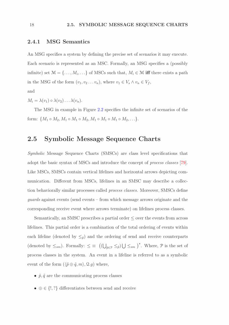
18 2.5. SYMBOLIC MESSAGE SEQUENCE CHARTS

2.4.1 MSG Semantics

An MSG specifies a system by defining the precise set of scenarios it may execute.

Each scenario is represented as an MSC. Formally, an MSG specifies a (possibly

infinite) set M = {. . . ,Mi, . . .} of MSCs such that, Mi ∈M iff there exists a path

in the MSG of the form (v1, v2 . . . vn), where v1 ∈ Vs ∧ vn ∈ Vf ,

and

Mi = λ(v1) ◦ λ(v2) . . . λ(vn).

The MSG in example in Figure 2.2 specifies the infinite set of scenarios of the

form: {M1 ◦M2,M1 ◦M1 ◦M2,M1 ◦M1 ◦M1 ◦M2, . . .}.

2.5 Symbolic Message Sequence Charts

Symbolic Message Sequence Charts (SMSCs) are class level specifications that

adopt the basic syntax of MSCs and introduce the concept of process classes [79].

Like MSCs, SMSCs contain vertical lifelines and horizontal arrows depicting com-

munication. Different from MSCs, lifelines in an SMSC may describe a collec-

tion behaviorally similar processes called process classes. Moreover, SMSCs define

guards against events (send events – from which message arrows originate and the

corresponding receive event where arrows terminate) on lifelines process classes.

Semantically, an SMSC prescribes a partial order ≤ over the events from across

lifelines. This partial order is a combination of the total ordering of events within

each lifeline (denoted by ≤p) and the ordering of send and receive counterparts

(denoted by ≤sm). Formally: ≤ ≡(

(⋃

p∈P ≤p)⋃

≤sm

)⋆. Where, P is the set of

process classes in the system. An event in a lifeline is referred to as a symbolic

event of the form (〈p⊕ q, m〉,Q.g) where,

• p, q are the communicating process classes

• ⊕ ∈ {!, ?} differentiates between send and receive

2. BACKGROUND 19

• Q is one of ∃, ∃k, ∀, ∀k – a universal or existential quantifier.

• g is a predicate on the state of a concrete process of process class p.

The concept of process classes and the semantic interpretation of quantifiers

and predicates in guards are further expanded in Chapter 4.

2.6 Symbolic Message Sequence Graphs

A Symbolic Message Sequence Graphs (SMSG) is a high-level SMSC, which rep-

resents a collection of SMSCs in graph form. It is a directed graph with basic

SMSCs as its vertices. Every path in the SMSG prescribes a valid scenario, which

is specified by “concatenating” basic SMSCs located at vertices along the path.

A concatenation of two basic MSCs M1 and M2 yields a bigger SMSC in which

events from each process class p in M1 have to occur before the occurrence of

any event of the same process class p in M2. The nature of such concatenation

is ‘asynchronous’ because no ordering between events from across distinct process

classes is explicitly enforced as a result of concatenation.

Furthermore, a process class constraint can be attached to an edge in an SMSG

to assert the condition of (the state of) the process class for the source SMSC to

be concatenated to the target SMSC.

2.7 Example of SMSG Specification

Figure 2.3 shows an example of an SMSG specification of a bus arbitration proto-

col. In such a system, there is a single centralized bus arbiter (BA), one or more

master devices and several slave or target devices. This specification contains five

basic SMSCs. M1 denotes the request phase when control of bus is requested. In

M2, the bus arbiter grants access to a single master, which then places the address

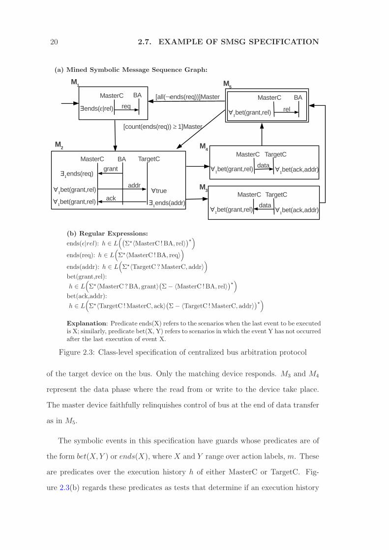
20 2.7. EXAMPLE OF SMSG SPECIFICATION

(a) Mined Symbolic Message Sequence Graph:

(b) Regular Expressions:

ends(ǫ|rel): h ∈ L(

(

Σ⋆〈MasterC !BA, rel〉)

⋆

)

ends(req): h ∈ L(

Σ⋆〈MasterC !BA, req〉)

ends(addr): h ∈ L(

Σ⋆〈TargetC ?MasterC, addr〉)

bet(grant,rel):

h ∈ L(

Σ⋆〈MasterC ?BA, grant〉(

Σ− 〈MasterC !BA, rel〉)

⋆

)

bet(ack,addr):

h ∈ L(

Σ⋆〈TargetC !MasterC, ack〉(

Σ− 〈TargetC !MasterC, addr〉)

⋆

)

Explanation: Predicate ends(X) refers to the scenarios when the last event to be executedis X; similarly, predicate bet(X, Y) refers to scenarios in which the event Y has not occurredafter the last execution of event X.

Figure 2.3: Class-level specification of centralized bus arbitration protocol

of the target device on the bus. Only the matching device responds. M3 and M4

represent the data phase where the read from or write to the device take place.

The master device faithfully relinquishes control of bus at the end of data transfer

as in M5.

The symbolic events in this specification have guards whose predicates are of

the form bet(X, Y ) or ends(X), where X and Y range over action labels, m. These

are predicates over the execution history h of either MasterC or TargetC. Fig-

ure 2.3(b) regards these predicates as tests that determine if an execution history

2. BACKGROUND 21

h, treated as a sentence, belongs to the language of a regular expression. The SMSC

M1 contains an event at the MasterC process class with guard ∃ ends (ǫ | rel). The

guard ensures that either the master device is making a request for the first time, or

it has released control over its previous request. Consider the SMSC M2 in Figure

2.3, the addr message is received by process class TargetC having a guard ∀true.

Here the predicate g = true ensures that every concrete process belonging to class

TargetC will receive the address placed by master. The guard ∀1ends(grant) im-

plies that exactly one master device has been granted control, and that device

sends address. The guard ∃1ends(addr) accepts any selection in which exactly

one of the processes that receive the address responds with ack. The SMSG has

two edges with process class constraints. One of them is count(ends(req)) ≥ 1. It

refers to the scenario when there are one or more master devices whose requests for

bus have not been granted. The other constraint is all(¬ends(req)). This refers

to the complementary scenario when there is no process still waiting to be granted

control to the bus. Together, these two constraints ensure that after M5, M2 is

executed if there are more requests to be processed and M1 is executed only after

all requests have been processed.

2.8 Trace Collection

As discussed in Section 2.1, certain assumptions have been made regarding the

nature of systems that can be analyzed using the proposed approaches. Many

of the assumptions are made to ensure that system interactions can be observed

and duly recorded. Traces used for subsequent analyses are obtained by executing

instrumented distributed systems. Traces are sequences of events recording the

dispatch or receipt of messages by the processes of a distributed system. In most

distributed systems that communicate over TCP/IP, processes can be uniquely

22 2.8. TRACE COLLECTION

identified using the combination of IP and port addresses. Connection mechanisms

such as sockets also provide information regarding the port and IP address of

the other party in the connection. An advantage in distributed systems is that

traces can be collected without any instrumentation of the application, but rather

by capture and filter of its communication packets. This ability of converting

captured packet logs into scenarios has been available as part of visualization and

debugging tools [13, 1]. Our techniques can be applied to any input data set that

can be represented as multiple scenarios (in formats such as sequence diagrams or

message sequence charts).

Message labels can be obtained by inspecting the messages exchanged between

processes. The message may have to be abstracted to obtain small and meaningful

specifications. In our analyses, we assume such assistance can be provided to select

the level of abstraction at which messages should be represented. For example,

in our experiments, messages in the form of XML packets are represented by

certain attributes extracted from those packets. In evaluating our technique on

mining program evolution, we shall use example subjects that are object oriented

programs rather than real distributed systems. In some of these examples the

objects represent behavior of processes in distributed or embedded systems. In

such systems the instrumentation framework ensures that interactions between

objects in the form of method invocations are recorded in the trace file.

Specific tracing mechanisms used in experiments shall be discussed along with

case studies and experiments performed to evaluate the proposed mining methods

in subsequent chapters.

Chapter 3

Mining Message Sequence Graphs

As described in Chapter 2, Sequence diagrams and Message Sequence Charts

(MSCs) are commonly used to express specifications of distributed systems. Mes-

sage Sequence Graphs (MSGs) are used to represent a collection of MSCs to allow

for choice and iteration. Using MSGs, a large collection of system behavior can be

represented in a concise manner. This chapter describes a technique to construct

an MSG specification from execution traces and its implementation as a framework

called MSGMiner.

Consider a hypotheitcal banking system containing three processes, a user

client, an internet portal and a back-end database. Figure 3.3(a) shows three

sample traces collected from executions of such a system. Figure 3.3(b) shows

Input Traces

Dependency Graphs Mined Basic MSCs

MSG

IdentifyBasic MSCs

Automaton LearningConvert to

Partial Order

Figure 3.1: Stages in the proposed mining framework.

24

Figure 3.2: Dependency graphs for MSCs in Figure 3.3

what an MSG mined from traces would appear like. The MSC indicates that the

actions described in M1 where a withdrawal is initiated, the system faces three

global choices. The database may return with a success or a failure. Additionally,

the user may make an additional withdrawal request before the processing is com-

plete. The MSG shows that the system may iterate over multiple requests from

the user before the inital request is fully processed.

The mined MSG is not an exact representation of the set of traces but instead

a generalized model of the system suggesting additional scenarios inferred based

on the input sample of scenarios. This model describes events within basic MSCs,

provide the precise partial order among them and uses the graphical format of

MSG to represent the collection of scenarios that are inferred to be valid.

Figure 3.1 describes the transformations performed by MSGMiner to construct

an MSG. Each execution trace is converted to a partial order (or dependency

graph) by (i) considering the individual control flows across different processes and

3. MINING MESSAGE SEQUENCE GRAPHS 25

(a) Sample execution traces (inputs to our MSGMiner)

(b) Mined MSG (output from our MSGMiner)

Figure 3.3: Banking System Example

26 3.1. DEPENDENCY GRAPHS

(ii) marking the dependencies between a send event and its corresponding receive.

These dependency graphs are then analyzed to find recurring portions — which

then appear as the basic MSCs in the mined model. The basic MSCs constitute

the nodes of the mined MSG model. These nodes are then connected up using

automata learning techniques. The approach used thus involves a combination of

automata learning and mining of partial orders.

The main challenge in this process lies in the task of discovering snippets of

concurrent behavior from traces and specifying them using MSCs. MSCs are

represented using data structures called dependency graphs that fully capture the

partial order relationship among events in the MSC. Furthermore, we introduce

a novel idea of maximal connected dependency graph (MCD) for a given trace set

to capture basic MSCs that can be used as the building blocks for constructing

an MSG. The entire mining process is thus divided into three stages, which are

elaborated in following sections.

1. Trace processing (Convert to Partial Order): At this stage each trace is

transformed into a corresponding dependency graph.

2. MSC mining (Identify Basic MSCs) : In this phase, basic MSCs (in MCD

representation) are identified from dependency graphs, and each dependency

graph is transformed into a chain of MSCs.

3. MSG construction (Automaton Learning) : The chains of MSCs are merged

into a single MSG specification at this final stage.

3.1 Dependency Graphs

Traces are collected by instrumenting and executing a system implementation with

various inputs. In a distributed system the trace points are chosen to be at program


locations where processes send or receive messages. A trace event is either a send

or receive message of the form 〈p ! q,m〉 or 〈q ? p,m〉 respectively, where m is

the message being exchanged between a sender named p and a receiver named

q. Furthermore every event must contain a time stamp to determine the global

ordering of events.

For presentation clarity, it is assumed that traces are strings of events, which are

drawn from a trace alphabet Σ. The collected traces record some linear temporal

order in which events occur during the execution of the system. Our first task is

to eliminate temporal ordering of events from different lifelines, when they are not

explicitly imposed through message passing. With this, we will have converted the

total ordering of events implied by the traces into a partial ordering that captures

concurrent behavior.

Recall from 2.3.1 that an MSC M = (L, {El}l∈L,≤, γ,Σ) prescribes the partial

ordering ≤ among a set of events. ≤ was defined to be a transitive closure of the

union of an ordering relationship between events within each lifeline (≤l) and the

ordering of send and receive events of a message (≤sm). It is observed that only

the ordering imposed by ≤l and ≤sm are sufficient to specify a scenario, and define

a dependency graph to capture its behavior. Specifically, a dependency graph is a

graph data structure g = (L, {Vl}l∈L, R, γ′,Σ) where:

• each vi ∈ Vl corresponds to an event ei ∈ El,

• there is a directed edge v1Rv2 iff for their corresponding events e1 and e2,

(e1, e2) ∈ (∪l∈L ≤l)∪ ≤sm

• γ′(vi) = γ(ei) for every event ei and its corresponding vertex vi in the de-

pendence graph.

(V,R, γ) is used as a shorter representation for dependency graphs whenever the

lifelines and event alphabet is not relevant to the analysis. Note that depen-


dency graphs are a graphical representation that is equivalent to the concept of

Mazurkiewicz traces in trace theory [33]. Figure 3.2 shows the corresponding de-

pendency graphs g1 and g2, for basic MSCs M1 and M2 respectively.

Some of the properties of dependence graphs used by the mining algorithm are

as follows.

Definition 3.1.1 (Equivalence ≡) If dependence graph g1 = (V1, R1, γ1) and

graph g2 = (V2, R2, γ2), g1 ≡ g2 iff there exists a bijection f : V1 → V2 such that,

∀v1 ∈ V1(γ1(v1) = γ2(f(v1))) and

∀v1, v2 ∈ V1(v1R1v2 ⇔ f(v1)R2f(v2)).

Definition 3.1.2 (Concatenation ◦) For two graphs,

g1 = (L1, {V1l}l∈L1, R1, γ1,Σ) and g2 = (L2, {V2l}l∈L2

, R2, γ2,Σ) the concatenation

g1 ◦ g2 = (L, {Vl}l∈L, R, γ,Σ) such that

L = L1 ∪ L2

Vl =

V1l ∪ V2l if l ∈ L1 ∩ L2

V1l if l ∈ L1 − L2

V2l if l ∈ L2 − L1

γ = γ1 ∪ γ2

R = R1 ∪R2 ∪RL ∪Rsr

The concatenated graph contains the following new sets of edges:

1. RL: This enforces the ordering that for a lifeline l, the events in V1l occur

before those in V2l. Let function f irst(Vil) return vertex v ∈ Vil such that

∀v′ ∈ Vil, vRiv′. Similarly let last(Vil) return the last event in lifeline l.

RL = {(last(V1l), first(V2l))|∀l ∈ L1 ∩ L2}


2. Rsr: This pairs an unmatched send event in g1 with an unmatched receive

event in g2. Since a graph may contain repetitions of the same send/receive

event, ambiguity is resolved by defining a function ϕl : Vl → N0 to differen-

tiate between identical events within the same lifeline. For a vertex v ∈ Vl,

ϕl(v) = |{v′|v′ ∈ Vl ∧ (v′, v) ∈ (RL ∪R1 ∪R2)

+ ∧ γ(v′) = γ(v)}|.

Rsr = {(vp, vq)|vp ∈ V1p ∧ vq ∈ V2q ∧ ∃〈p!q,m〉, 〈q?p,m〉 ∈ Σ : γ(vp) =

〈p!q,m〉 ∧ γ(vq) = 〈q?p,m〉 ∧ ϕp(vp) = ϕq(vq)}

Figure 3.4 shows the result of concatenation of dependency graphs g1, g3 and

g2 of Figure 3.2. The dotted lines show newly added edges.

Definition 3.1.3 (Sub-Graph) A sub-graph relationship among dependency graphs

is as follows: g′ ⊆ g if and only if there exist graphs x and y such that g ≡ (x◦g′)◦y.

Definition 3.1.4 (Prefix and Suffix) A subgraph g′ ⊆ g is a prefix of g iff for

some graph y, g ≡ g′ ◦ y. Similarly g′ is a suffix iff for some graph x, g ≡ x ◦ g′.

Our definition of sub-graph for dependency graphs is stricter than and not to

be confused with the definition commonly used in graph theory. In Figure 3.4, gx,

gy and gz are sub-graphs of the concatenated dependency graph. The sub-graph

gx is a prefix and gz a suffix.

Definition 3.1.5 (Frequency) The frequency of sub-graph g′ in dependency graph

g is n, if there exist dependency graphs g0, g1, . . . gn such that g ≡ ((((g0 ◦g′)◦g1)◦

g′) . . .) ◦ gn and g′ * g0, g1 . . . gn for some n ≥ 0. Note that g0, g1 . . . gn may be

empty.

Informally, the frequency of a sub-graph g′ in g is the number of distinct oc-

currences of the g′ in g. Figure 3.4 also shows the frequency of gx, gy and gz in

(g1 ◦ g3) ◦ g2.


Figure 3.4: Concatenated graph (g1 ◦ g3) ◦ g2, and some of its sub-graphs


A function dgraph(t) is defined, that accepts a trace t as parameter and con-

structs a dependency graph. The dependency graph is constructed by creating a

unique vertex for each occurrence of an event. After this, edges are added to link

up events within a lifeline into a chain. Subsequently, the send and receive events

are linked up starting from the bottom of the trace. For example the last occur-

rence of event 〈q?p,m〉 is linked to the last occurrence of event 〈p!q,m〉 and so on.

The resulting dependency graph captures the “happened before” relationship be-

tween events as defined by Lamport [48]. Algorithm 1 details how the dependency

graph is constructed from trace.

For construction of dependency graphs from traces, two assumptions have to

be made about the system:

1. No messages are lost in the message channels.

2. The message communication occurs through FIFO channels.

Function dgraph, by its design has the property that given a trace t, for any of its

suffixes ts, dgraph(ts) is a suffix of dgraph(t). For example if trace t = (〈p!q,m〉,

〈p!q,m〉, 〈q?p,m〉, 〈q?p,m〉 ), then dgraph(t) is a dependency graph (V,R, γ),

having

V = {v〈p!q,m〉1 , v

〈p!q,m〉2 , v

〈q?p,m〉3 , v

〈q?p,m〉4 }

R = { (v1, v2), (v3, v4), (v1, v3), (v2, v4) }.

If instead of the full trace t one of its suffixes, say ts = (〈p!q,m〉, 〈p?q,m〉,

〈p?q,m〉) is supplied, dgraph(ts) would contain,

V = {v〈p!q,m〉1 , v

〈q?p,m〉2 , v

〈q?p,m〉3 }

R = { (v2, v3), (v1, v3)}.


Algorithm 1 dgraph(t = (e1, e2 . . . en))

1: let L← V ← R← γ ← Σ← ∅2: /*Create Vertices */3: for i← 1 . . . n do4: if ei is a send event then5: p!q,m← ei6: else7: p?q,m← ei8: end if9: create new vertex vi10: Σ← Σ ∪ ei; V ← V ∪ vi11: if p /∈ L then12: L← L ∪ {p}13: /*tp stores projection of trace t on to process p*/14: tp ← ()15: end if16: tp.append(vi); γ ← γ ∪ (vi, ei)17: end for18: /*Add ordering within lifelines to R */19: for all l ∈ L do20: let (v1, v2...vm)← tl21: for i← 1 . . . m− 1 do22: R← R ∪ (vi, vi+1)23: end for24: end for25: /* Add send receive pairs to R */26: for all p, q ∈ L ∧ p 6= q do27: let i← |tp|; j ← |tq|28: while j > 0 do29: if tq[j] is a receive event then30: let q?p,m← γ(tq[j])31: while i > 0 ∧ γ(tp[i]) 6= p!q,m do32: i← i− 133: end while34: if i > 0 then35: R← R ∪ (tp[i], tq[j])36: end if37: end if38: j ← j − 139: end while40: end for41: return (L, V,R, γ,Σ)


3.2 MSC Mining

Using the function dgraph, the available trace set T = {t1, t2, . . . tn} is converted

to a set of dependency graphs G = {g1, g2, . . . gn}, where each dependency graph

gi ∈ G corresponds to a scenario of system execution. Our next step is to identify

basic sections within these graphs, that recur at several places within the same

graph or across the graphs in G. Intuitively, these fundamental blocks are likely

to capture the basic MSCs in an MSG describing the system. There are many

possible ways to break down a graph into fundamental blocks. Our method aims to

discover MSCs which are as big as possible and yet recurring frequently enough in

the input execution traces (or their corresponding dependency graphs). Therefore,

the notion of Maximal Connected Dependency Graphs (MCDs) to signify MSCs is

introduced. Formally,

Definition 3.2.1 (MCD) For a given trace set T = {t1, t2, . . . tn}, gmcd = (V,R, γ)

is an MCD iff

1. There is a trace t ∈ T such that gmcd ⊆ dgraph(t).

2. The total frequency of the MCD - freq(gmcd) with respect to the trace set T

is equal to the frequency of all its proper sub-graphs.1

3. For every distinct v1, v2 ∈ V , (v1, v2) ∈ (R ∪R−1)∗ .

4. There is no graph g′ that satisfies conditions 1-3 such that gmcd ⊂ g′.

Criterion 2 guarantees that no part of an MCD (and thus its corresponding

MSC) appears in some context in which the rest of the MCD does not also appear.

Criterion 4 enforces the maximality of MSCs. Criterion 3 requires that events in

1Given a trace set T = {t1, t2, . . . tn}, freq(g) is the sum of the frequency of g in dgraph(t1),dgraph(t2), .. dgraph(tn).

34 3.2. MSC MINING

MCDs be connected with each other. This additional constraint is introduced to

simplify the mining task.

An exhaustive search for graph structures that meet the conditions specified

above could turn out to be expensive. Instead, a graph structure termed event tail

is identified for each event, and then successively merged to arrive at dependency

graphs that will satisfy the frequency, connectedness and maximality criteria of

MCDs. Event tails and the method of merging graphs are described in the following

sub-sections.

3.2.1 Event Tail

For an event e ∈ Σ, when given a trace set T ⊆ Σ∗, its tail, tail[e], is the largest

dependency graph that contains a single minimal vertex (which is a vertex in the

graph without any associated incident edges) labelled e and satisfies conditions 1-3

of definition 3.2.1. Apart from the minimal vertex, it therefore contains all events

that immediately follows every occurrence of e in a consistent partial order.

Algorithm 3 outputs an associative array - tail, that maps every event in Σ to

its tail. For an event e and trace set T , Te is the set of trace suffixes that start with

e. Te can be easily derived from a suffix tree[82] constructed from the trace set.

From Te we obtain a collection of suffix graphs, by identifying dgraph(ts) for every

ts ∈ Te. In such a graph, let ve be the vertex corresponding to the first occurrence

of event e. All vertices v in the graph for which (ve, v) 6∈ R∗ are removed as they

do not belong to the tail. After this, the function getCommonPrefix is invoked to

identify the largest prefix common to all suffix graphs in the collection for event

e. This common prefix is the desired event tail tail[e].

Operationally, function getCommonPrefix identifies the largest common prefix

in a pair of dependency graphs g1 and g2 through a simultaneous breadth-first

traversal over these two graphs. During the traversal, vertices and edges are grad-


ually added to the largest common prefix g. A vertex v with label e is added to g

if and only if 1) there are vertices v1 in g1 and v2 in g2 having a common label e,

and 2) v1 and v2 have identical incident edges and all vertices from which there are

edges incident to v1, v2 have already been added to g. In addition, getCommonPre-

fix ensures that all events added to the common graph have identical frequencies.

All these operations ensure that conditions 1,2 and 3 of definition 3.2.1 are satis-

fied. Moreover, since the event tail is the maximal graph common to all suffixes

with ve as its minimal vertex, it has been ensured that 1) tail[e] contains at least

one vertex ve, and 2) tail[e] cannot be extended without violating conditions 1,2

or 3. Algorithm 2 presents the details of getCommonPrefix .

Algorithm 2 getCommonPrefix((V1, R1, γ1), (V2, R2, γ2))

Input: Two dependency graphs — (V1, R1, γ1), (V2, R2, γ2)Output: The largest common prefix of the input dependency graphs — (V,R, γ).

1: let vs1 ∈ V1 s.t. ∀v ∈ V1 ⇒ (vs1, v) ∈ R∗1

2: let vs2 ∈ V2 s.t. ∀v ∈ V2 ⇒ (vs2, v) ∈ R∗2

3: Initialise (V,R, γ), V ← R← γ ← ∅4: queue1.add([v

s1]); queue2.add([v

s2])

5: while queue1 6= ∅ ∧ queue2 6= ∅ do6: v1 ← queue1.remove(); v2 ← queue2.remove()7: if ∀v′1 ∈ V1, (v

′1, v1) ∈ R1 ⇒ v′1 ∈ V ∧

freq(γ1(v1)) = freq(γ1(vs1)) ∧ ∀v ∈ V1, γ1(v) 6= γ1(v1) then

8: V ← V ∪ {v1}, γ ← γ ∪ {(v1, γ1(v1)}9: R← R ∪ {(v′1, v1)|(v

′1, v1) ∈ R1}

10: for all v′′1 , v′′2 s.t. (v1, v

′′1) ∈ V1, (v2, v

′′2) ∈ V2 and γ1(v

′′1) = γ2(v

′′2) do

11: queue1.add(v′′1); queue2.add(v

′′2);

12: end for13: end if14: end while15: return (V,R, γ)

Figure 3.5 shows event tails derived from two sample traces from the banking

system.

36 3.2. MSC MINING

Algorithm 3 Find Event Tails

Input: T - The trace set, Σ - set of events appearing in T .Output: tail[e] that maps every event e ∈ Σ to its tail.1: for all e ∈ Σ do2: Find Te: the set of all suffixes(of traces in T ) starting with e3: let Te = {ts1 , ts2 , . . . tsne

}4: tail[e] ← ∅5: for i = 1 . . . ne do6: (V,R, γ)← dgraph(tsi)7: let ve be the vertex corresponding to event e8: for all v ∈ V s.t. (ve, v) /∈ R

∗ do9: V ← V − {v}10: end for11: if tail[e] = ∅ then12: tail[e] ← (V,R, γ)13: else14: tail[e] ← getCommonPrefix(tail[e] , (V,R, γ))15: end if16: end for17: end for

Figure 3.5: Sample traces and event tails for some events


3.2.2 Combining Event tails

Algorithm 4 uses the mapping from events to tails (tail[e]) to derive a mapping

from events to MCDs - MCD[e]. The algorithm starts with g1 = tail[e]. We

know that tail e cannot be extended at the end as it is already maximal. Hence

we attempt to grow g1 by prefixing it with other graphs. For every event e′ we

verify if tail[e′] can be merged into g1. Let tail[e′] be the graph g2. Without loss

of generality we can express the two tails as,

g1 ≡ gpref1 ◦ gcomm and

g2 ≡ (gpref2 ◦ gcomm) ◦ gsuff2

where gcomm is the largest possible such graph. If gcomm is empty, we do not perform

any merging. If gcomm is not empty, we obtain gpref2 ◦ g1 as the merged graph. To

satisfy the frequency criterion, we chose to accept the merged graph only when

freq(gpref2 ◦ g1) = freq(g1). When more than one prefix of g2 satisfy the conditions

on gpref2 , we select the largest one.

The dependency graph g1 is an MCD if no more event tails can be merged into

it.

Theorem 1 For every event e, the dependency graph MCD[e] assigned by Algo-

rithm 4 is an MCD.

Proof: We have established that tail[e1] satisfies criteria 1-3 of definition 3.2.1. In

line 3 of Algorithm 4, we initialize g1 to tail[e1]. To prove that dependency graph

g1 assigned to event e1 in line 8 is an MCD, it is sufficient to prove the following:

1. If g1 satisfies criteria 1-3 and g2 is an event tail, then merge(g1, g2) also

satisfies 1-3.

In line 5 of Algorithm 5, we ensure that freq(merge(g1, g2)) = freq(g1).

Therefore merge(g1, g2) must satisfy criterion 1. Since gcomm ⊆ g2 and

38 3.2. MSC MINING

g2 satisfies criterion 2, it follows that freq(gpref2 ) = freq(gcomm) = freq(g1).

merge(g1, g2) satisfies criterion 2 as its frequency is equal to the frequency

of its sub-parts.

Since g2 is an event tail, either gpref2 is empty or contains the minimal ver-

tex. In both cases, gpref2 ◦ gcomm is a connected graph. Since g1 is already

a connected graph, merge(g1, g2) will remain a connected graph satisfying

criterion 3.

2. If there are no more events e′ ∈ W such that tail[e′] can be merged into g1,

then g1 satisfies criterion 4.

If there is graph g′1 such that g1 ( g′1 and g′1 satisfies criteria 1-3, then it

follows that there is at least one event e in g′1 and not in g1 for which,

(a) ge ◦ g1 satisfies criteria 1-3 OR

(b) g1 ◦ ge satisfies criteria 1-3.

Where ge is a graph containing a single vertex ve labelled with event e.

Case a: Assume that g′′1 ≡ ge ◦ g1 = (V1, R1, γ) satisfies criteria 1-3.

Criterion 2 enforces that no two vertices have the same label. Therefore g1

will not contain a vertex labelled with event e. Consider a graph gsuff1 such

that, g′′1 ≡ gpre1 ◦ ge ◦ gsuff1 and for every vertex vingsuff1 , veR

+1 v. Clearly,gsuff1

is not empty (g′′1 is a connected graph) and ge ◦ gsuff1 is a prefix of tail[e]

(freq(ge ◦ gsuff1 ) = freq(ge)). For some gs, we therefore have:

g1 ≡ gpre1 ◦ gsuff1

tail[e] ≡ (ge ◦ gsuff1 ) ◦ gs

freq(ge ◦ g1) = freq(g1)

The implies that merge(g1, tail[e]) 6= ǫ and contrary to our assumption, ge

should already have been merged into g1.


Case b: Assume that g′′1 ≡ g1 ◦ ge = (V1, R1, γ) satisfies criteria 1-3. Since

g′′1 is a connected graph, there is a ve′ ∈ V1 s.t, ve′ 6= ve and ve′R1ve. This

implies that ve is part of tail[e′]. Let g (where g ⊆ g1) be the value of g1

when tail[e′] is merged into g1. The merged graph will be gpref2 ◦ g, for the

largest gcomm, such that

g ≡ gpref ◦ gcomm and

tail[e′]= g2 ≡ (gpref2 ◦ gcomm) ◦ gsuff2

If ve was part of gpref2 or gcomm then ve is already part of the merged graph.

If ve is part of gsuff2 it was discarded as it did not satisfy one of conditions

1-3. Both possibilities are contrary to our assumptions about g′′1 .

Since we have ruled out the possibilities of a larger graph g′1, g1 at the end

of each iteration of the outer loop is maximal, and hence satisfies criterion

4.

✷

Algorithm 4 Combine Event Tails

Input: tail[e] for all events e ∈ ΣOutput: MCD[e] for all events e ∈ Σ1: for all e1 ∈ Σ do2: W ← Σ− {e1}3: g1 ← tail[e1]4: while ∃e2 ∈ W s.t. merge(g1, tail[e2]) 6= ǫ do5: g1 ← merge(g1, tail[e2])6: W ← W − {e2}7: end while8: MCD[e1] ← g19: end for

Figure 3.6 shows the set of MCDs that are obtained by merging event tails

obtained from traces in Figure 3.5.

40 3.2. MSC MINING

Algorithm 5 merge(g1, g2)

Input: Candidates for merging g1, g2Output: The merged graph. (ǫ if merge is not possible).1: Let gcomm be the largest suffix of g1 that is a sub-graph of g2.2: if (gcomm is empty) then3: return ǫ4: else5: Find largest gpref2 that satisfies:

g2 ≡ (gpref2 ◦ gcomm) ◦ gsuff2 ∧ freq(gpref2 ◦ g1) = freq(g1)6: if no such gpref2 is found then7: return ǫ8: else9: return gpref2 ◦ g110: end if11: end if

Figure 3.6: MCDs obtained by combining tails


3.2.3 Converting trace to sequence of MSCs

Algorithm 4 associates each event with an MCD. Utilizing this association, we

transform each trace from the given trace set into a sequence of dependency graphs.

In order to achieve this transformation, we group events in a trace based on their

associated MCDs. In a trace t, we represent each group of events by a depen-

dency graph gi and derive a sequence of the form (g1, g2, . . . gi . . . gm) such that

dgraph(t) ≡ (g1 ◦ g2 . . .) ◦ gm. Therefore the ordering of two dependency graphs

is constrained by dependency relationships between events from one graph and

events from the other.

Certain cases warrant special handling. Firstly, we may have derived two MCDs

that share a common sub graph. For example, we may have MCD[e1] ≡ gx ◦ g

and MCD[e2] ≡ g ◦gy. Since MCDs are maximal, we know that the merged graph

(gx ◦ g) ◦ gy must have a lower frequency that its sub graphs. In such scenarios, we

will drop the common sub graph g from one of the MCDs. Secondly, two MCDs

may not co-exist in a sequence as the dependency relationships constrain each

other in a way that they can not be ordered. To resolve such cases, we split one

of the MCDs into smaller parts whenever necessary. For example, consider two

MCDs

gx = ({v1, v2}, {(v1, v2)}, {(v1, 〈p!q,m〉), (v2, 〈q?p,m〉)}),

which represents a single message m from p to q, and

gy = ({v1, v2}, {(v1, v2)}, {(v1, 〈q!p,m〉), (v2, 〈p?q,m〉)})

which represents message m from q to p.

For a trace t = (〈p!q,m〉, 〈q!p,m〉, 〈p?q,m〉, 〈q?p,m〉), it is clear that gx ⊂

dgraph(t) and gy ⊂ dgraph(t). However, we cannot represent trace t as a sequence

of the two MCDs because dgraph(t) 6≡ gx ◦ gy and dgraph(t) 6≡ gy ◦ gx. In such

cases we represent t by splitting either gx or gy into smaller dependency graphs.

While we have defined MCDs as dependency graphs, we do not require them

42 3.3. CONSTRUCTING MESSAGE SEQUENCE GRAPHS

to correspond to ‘complete MSCs’; ie., there may exist a send event in an MCD

which does not contain the matching receive event and vice versa. In order to

guarantee that all vertices of an MSG denote complete MSCs, we concatenate

successive partial graphs in a post-processing step to ensure that each dependency

graph in the final sequence of MSCs will represent a complete MSC. Algorithm

6 performs this transformation. This step effectively relaxes the second criterion

for MCDs that each MCD must be as frequent as every event occurring within it.

This relaxation is applied only at instances where the MCDs are incomplete MSC

specifications.

Algorithm 6 Convert to full MSCs

Input: gList - A sequence of dependency graphsInput: ψ - Input from UserOutput: outputList - Corresponding sequence of MSCs1: outputList ← [ ]2: temp ← gList[0]3: for i← 1 . . . gList.size() do4: if temp has an unmatched send event then5: temp ← temp ◦ gList[i]6: else7: outputList.add(temp)8: temp ← gList[i]9: end if10: end for11: return outputList

At the end of this stage we have defined an alphabet of basic MSCs and pro-

duced strings from this alphabet for the construction of MSGs.

3.3 Constructing Message Sequence Graphs

There exists a choice of algorithms to learn a finite state machine (FSM) from a

training set of strings [74, 22]. For experiments a variant of the k-tails algorithm

described in [29] is implemented. A shared prefix tree is initially constructed from


the set of MSC strings. The algorithm then identifies a set of nodes that are

equivalent. Two nodes are considered equivalent if their k-futures match. The

k-future of a node is simply the set of all valid paths of length k or less (if the end

node is reached) starting from that node. Several possible heuristics have been

suggested to match two sets of k-futures. For better precision one could insist on

the match being exact. Other methods involve matching two sets of strings if they

meet a certain probabilistic threshold. Equivalent nodes are merged to get a more

general and compact model. During the merging process loops are introduced to

the model. For a prefix tree with n nodes, since every pair of nodes are compared,

the algorithm has a worse case execution time of O(n2mk), where m is the size of

the trace alphabet. For an operation comparing the k-futures of any two nodes,

the maximum number of nodes to be compared is never greater than the total

number of nodes in the tree. As a result, the algorithm has an execution time

not worse than O(n3) for any value k. Note that n is shorter than the number of

events in the initial traces as each frequent co-occurring maximal series of events

has been identified and is represented using single nodes.

Once an MSG has been mined from traces using the FSM learner, it is refined

through a series of state reduction steps. An FSM learner usually produces a

Mealy model state machine which then has to be transformed into a minimal

Moore model. In the latter state machine each state corresponds to a basic MSC.

The final MSG is a structure-preserving homeomorphic embedding of the Moore

model state machine. The general rule for reduction is that if any state s is

reachable from one and only one state s’ and s is the only state reachable from

state s’, then the MSC in state s can be concatenated to the MSC in state s’. This

concatenation yields new basic MSCs. The reduced directed graph of basic MSCs

is the final output. The MSG can be exported as image files for visualization.

44 3.4. EVALUATION

3.4 Evaluation

We propose an evaluation technique to validate the mined model against a known

correct model. The correct model is used only for evaluation and never part of the

mining process. Given correct and mined models, we derive a precision and recall

score by performing language comparison. As discussed before, concatenating

basic MSCs along any path from a starting vertex to an accepting vertex in the

MSG produces an MSC that represents a valid execution scenario. We say that

such an MSC is generated by the MSG. Precision is defined as the number of MSCs

generated by the mined model that are accepted by the correct model divided by

the total number of MSCs generated by the mined model. Similarly recall is

the ratio of the number of MSCs from the correct model that are accepted by

the mined model to the total number of MSCs generated by the correct model.

However, MSGs could generate an infinite number of such MSCs that themselves

are of infinite length and it is not possible to enumerate all from one MSG and

then verify them on the other. Instead we use only a finite sample from the

MSG’s language for evaluation. Our sample consists of all accepting paths in

the MSG with a finite bound on loops. This bound is enforced by limiting the

number of times any vertex is revisited in a path. For the dependency graph g

corresponding to each MSC from the generating MSG, we verify if there is a path

in the accepting MSG that forms a dependency graph identical to g. This is done

by an efficient depth first search in the accepting graph. Due to the exponential

nature of the number of paths, exploration of all paths within a loop bound of 3

was found to produce a substantial number of paths. On some specifications, the

exploration could not be completed even with such a low bound. The experiments

are performed with loop bound 3 whenever possible and bound 2 otherwise.


3.5 Comparing MSGs with Per-process Automata

Past studies have recommended automaton learning algorithms to discover speci-

fications of system protocols in the form of state machines. These approaches have

been shown to be successful in learning behavioral protocols for Application Pro-

gramming Interfaces. In a distributed setting containing concurrently executing

processes , automaton learning can not be applied directly to interleaved traces.

This is because the mined model will not include all other possible interleavings

that are also valid resulting in poor recall. Instead, automaton learning could be

used to infer the state machine at each process. This can be done by separating

the original traces into traces local to each of the constituent processes. The au-

tomaton for each process gives an idea about its interactions with the rest of the

system components, thus providing a localized view of the system specification.

In contrast, an MSG captures the collective behavioral specification of the system

and presents a global view.

We compare the accuracy of our proposed approach with the accuracy of mining

this alternative model from the same collection of traces. To do this, we derive a

similar precision and recall score of the learnt automata with respect to the same

correct MSG specification that was used to score the mined MSG. The algorithm

used to learn automata is identical to the method used in the automaton learning

phase of MSG mining (Section 3.3). Precision and recall for automata is measured

as the ratio of the number of traces (rather than MSCs) generated from one model

that is accepted by the other model to the total number of traces generated. We

generate random sample of traces from the collection of automata. The parallel

composition of the automata, may contain accepting paths that create invalid

traces(eg: Receive event may appear before the message is sent). To generate

only ‘correct’ traces we simulate the FIFO message channels between processes.

While exploring a path in the composed automaton, if an edge outputting a send

46 3.6. CASE STUDIES

event 〈p!q,m〉 is chosen, the message m placed in the buffer corresponding to the

channel [p→ q]. An edge outputting a receive event 〈q?p,m〉 can be explored only

if message m can be removed from the front of buffer [p → q]. A path explored

in the composed automaton signifies a valid trace only when an accepting state is

reached and all the message buffers are empty. We impose a bound on the number

of loops as before.

3.6 Case Studies

The MSGMiner framework is evaluated through case studies involving real dis-

tributed systems. The following distributed systems were studied: (a) “Center

TRACON Automation System” [67] an air traffic control system from NASA, (b)

a system of server and VOiP clients communicating based on the Session Initia-

tion Protocol (SIP) and (c) a system of Server and Clients that follow the XMPP

Instant messaging and Chat protocol. In each of these systems, multiple processes

perform asynchronous communication over TCP socket connections. Timestamped

traces were collected by inserting instrumentation source code at points where mes-

sages are written to or read from a socket. The traces were filtered and the message

names abstracted with the help of text processing scripts.

3.6.1 CTAS

CTAS is an Air Traffic Control system from NASA. The CTAS weather control

logic specification [68] was one of the case studies recommended by the 3rd In-

ternational Workshop on Scenarios and State Machines (SCESM04). CTAS is

a distributed system having a central Communications Manager (CM) process

to which client processes connect. The weather control specification details how

clients should connect to CM and how a graphical user interface referred to as the


weather control panel (WCP) ought to communicate with CM to update weather

status. As access to the CTAS system is limited, we procure execution traces

by implementing and executing a simulation of this system in Java. Our imple-

mentation is based on a formal specification of the system in Promela and high

level HMSC that was developed by a fellow researcher. The process classes in this

systems are CM, WCP and Client. CM and WCP are singleton classes.

3.6.2 Session Initiation Protocol

SIP is a signalling protocol used to establish, manage and terminate VoIP calls

and multimedia sessions in general [10]. SIP clients interact with servers that

perform the necessary call routing and function as gateways to the Public Switched

Telephone Network(PSTN). We attempt to specify how clients should interact with

their proxy server to achieve some of the basic call features. For this, we set up a

system having three SIP clients connected to a single server. We use instrumented

versions of KPhone [5] - a SIP client implementation and the Opensips server [8]

both of which are available with source code under a GPL license. We execute

a set of test cases involving features such as basic call setup, call screening and

call forwarding. A set of test cases for each feature are identified and a trace set

is prepared by executing them on the system. The system contains two process

classes - Server and Client. The specifications were derived for cases involving just

a single server.

3.6.3 XMPP

Extensible Message and Presence Protocol is an open Instant Messaging standard

originally developed by the Jabber open source community. The core function-

ality of the protocol is specified in RFCs 3920 and 3921. XMPP is the protocol

for exchange of instant chat messages and presence information between various


entities in a network that are addressed by unique jabber ID. The clients com-

municate to the server through structured XML messages. The protocol defines

how XML nodes known as stanzas are to be exchanged between various entities.

A client connecting to a server is authenticated through TLS or SASL through

special XML stanzas. We attempt to discover the client server interaction proto-

col from a system having two jabber clients that are brokered by a single server.

In the specification, the server and client processes are the lifelines and the mes-

sage arrows represent the XML stanzas. The Openfire XMPP server [4] and Jeti

[3]/Pidgin [9] client implementations were instrumented and executed for trace

collection. For discovering the core specification as an MSG, we only record stan-

zas used for authentication or those having a message or presence tag and ignore

rest of the message exchanges.

In addition to the core specification, XMPP Standards Foundation (XSF) has

standardized several additional chat features. We attempt to mine behavioral

specification for the Multi User Chat(MUC) functionality [14]. For this we use a

separate set of test cases involving features such as service discovery, multi-party

chat and creation and administration chat rooms.

In the XMPP system the process classes are Server and Client. Configurations

involving a single server and multiple clients are studied.

The mining framework is evaluated by comparing various specifications against

a correct hand derived specification. To evaluate the proposed technique for min-

ing MSGs against techniques that mine FSM based models (per-process automata)

we compare both specifications against a specification that is considered to be ac-

curate. The correct specifications are also represented as MSGs. For mining MSG

specifications we obtain traces from a pre-defined configuration of the system. The

number of processes involved in every execution is fixed and behavioral similarity

is avoided. This is done by restricting the system to contain only one process from


each process class or by defining different roles for processes from the same process

class. The restrictions enforced for trace collection in this evaluation is as follows:

• CTAS: The execution traces and correct specifications assume that there is

only a single client in the system.

• SIP: The test cases involve three clients or SIP user agents labelled as Alice,

Bob and Carol whose roles were restricted in the following manner. In all

test cases, Alice initiates calls and Bob is the intended recipient. Features

such as call screening or forwarding are enabled at the client Bob. Carol is

the recipient of diverted calls.

• XMPP: The order of client login is the same in all executions. Only the

client labelled Client1 can initiate chat rooms thereby acquiring the role of

chatroom administrator.

The subjects were made to execute random test scenarios with these restric-

tions. It was ensured that all the interactions appearing in the correct specification

were also executed in at least one of the test cases. In each case a specification(that

reflects allotted client names and roles) was manually derived by the author for

quantitative analysis and comparison. In each case, both types of mined models

are derived from the same set of input traces and compared against the same cor-

rect specification. Table 3.1 tabulates the results from the case studies. It shows

the precision, recall and F1 measure(harmonic mean of precision and recall) of the

mined models obtained from the two alternatives (automaton learning and MSG

Mining) for each case study. The mining was performed on a JVM running on an

Intel duo core CPU with 1GB of available memory. The results from the systems

considered for case study suggest that the proposed MSG mining method provides

better mining accuracy.

50 3.7. EXTENSIONS

SystemNo:ofevents

Mined Automata Mined MSGPrec Rec F1

ScoreTime(s)

Prec Rec F1

ScoreTime(s)

SIP 1870 0.50 1 0.67 1.0 0.78 0.87 0.82 3.14

XMPP-Core

3212 0.72 0.44 0.55 8.3 1 0.71 0.83 10.2

XMPP-MUC

5736 1 1 1 22.0 1 1 1 28.7

CTAS 6418 0.95 1 0.97 48.1 1 1 1 45.8

Table 3.1: Table comparing accuracy of mining for MSG and Automata specifica-tions

The MSG mined from the traces collected from the CTAS system is shown in

Figure 3.7.

Our mining on the CTAS system succeeds in identifying the states of the system

that are mentioned in the informal requirements documents [68]. The narrative

in sub-sections of the document matches neatly with the visual representation

provided by the basic MSCs.

3.7 Extensions

The semantics of MSCs as per definition 2.3.1 accounts for only a basic subset of

the standardized MSC syntax. The framework described in this chapter discovers

specifications in this restricted language. The following sections describe how some

of these restrictions in the specification language can be removed through minor

modifications to the mining framework.

3.8 Parallel Composition in MSCs

In Definition 2.3.1, it is assumed that events within a lifeline follow a strict total

order. In specifying certain systems, it may be simpler to prescribe partial order

on events even if they belong to the same lifeline. For example, a process may


Figure 3.7: The Mined MSG for CTAS (top) and the learnt automata for individualprocesses

52 3.8. PARALLEL COMPOSITION IN MSCS

broadcast messages to multiple processes and await responses from its audience.

We refer to such instances as “message broadcasts”. During message broadcasts,

the order in which the messages are dispatched to individual recipients or that in

which responses are received at the broadcasting lifeline is usually inconsequential.

Furthermore, the actual order of events seen in traces may be different for each

realization of such broadcasts. Without knowledge of “message broadcasts”, the

mining procedure presented thus far fails to produce a succinct and comprehensible

MSG. Instead it will interpret different ordering of events as distinct interactions

and depict them using distinct basic MSCs.

MSC semantics [6] provide features such as coregions or the par inline expres-

sion to capture situations where there may be no specific logical ordering between

some events within a lifeline. The par expression allow us to list a group of MSCs

and imply that they are to be executed in parallel. With these constructs, a single

basic MSC can explain all valid interactions during the message broadcast scenario.

Since situations like message broadcasts are specific to certain systems, the

framework is extended to accept an additional input that declares specific behavior.

This additional input is termed as an oracle. By designing the mining framework in

this manner, the core mining methodology remains generic while domain specific

information regarding the system being mined can be provided as input. The

oracle for instance can inform the framework that certain events within a lifeline

need not be ordered. Based on this information, the framework will construct

customized dependency graphs and identify MCDs that capture such scenarios;

the MSGs produced by the extended system become less cluttered and much more

comprehensible.

While constructing a dependency graph, the framework can consult the oracle

on whether a dependency edge must be created between a given pair of events

from a lifeline. An oracle that returns true for all queries causes MSGMiner


to behave as per our original description. To handle special cases like message

broadcasts, the oracle can be customized based on the domain knowledge of users

or automatically created based on external static or dynamic analyses. Algorithm

7 is a modified version of Algorithm 1 that converts traces to dependency graphs

based on an oracle ψ : Σ × Σ → {true, false} that answers queries regarding

dependency between pairs of event labels. Algorithm 1, in lines 19 - 24 creates a

total order of events in each lifeline. In Algorithm 7, edges between events within

a lifeline are added only if the oracle answer with true.

Algorithm 7 dgraph(t = (e1, e2 . . . en), ψ)

let L← V ← R← γ ← Σ← ∅/*Create Vertices */. . ./*Add ordering within lifelines to R */for all l ∈ L dolet (v1, v2...vm)← tlfor i← 2 . . . m doj ← iwhile j > 0 doif ψ(vj, vi) = true ∧ ∀vk ∈ V : (vj, vk) /∈ R

+ ∨ (vk, vi) /∈ R+ then

R← R ∪ (vj, vi)end if

end whileend for

end for/* Add send receive pairs to R */. . .return (L, V,R, γ,Σ)

Figure 3.8 shows an example of broadcasts in the CTAS system (Section 3.6.1)

with two clients connected to the CM. The CM, requests and receives responses

from the two clients simultaneously. The figure also shows the dependence graph

corresponding to this MSC. Although events

〈CM!Client1.get new wthr〉 and 〈CM!Client2.get new wthr〉 belong to the same life-

line, there is no edge between their corresponding vertices in the dependency graph.

It can be tedious for the user to define the oracle by specifying the depen-


Figure 3.8: MSC and dependency graph describing broadcast message in CTASsystem.

dency between every pair of events. It is easier to indicate event pairs which are

exceptions to the default rule and for the oracle to be constructed automatically.

For broadcast messages, it is sufficient for the user to specify a pair of the form

(mreq,Mresp), where mreq is a broadcast message and Mresp is the set of response

messages that mreq evokes (Mresp = ∅ when there are no responses). With this

information, an oracle is constructed, to return true for all pairs (e1, e2) with the

following exceptions:

1. γ(e1) = 〈p!q1,mreq〉 ∧ γ(e2) = 〈p!q2,mreq〉 ∧ q1 6= q2

2. γ(e1) = 〈p?q1,m1〉 ∧ γ(e2) = 〈p?q2,m2〉 ∧ q1 6= q2 ∧m1,m2 ∈Mresp

3. γ(e1) = 〈p!q1,mreq〉 ∧ γ(e2) = 〈p?q2,m2〉 ∧ q1 6= q2 ∧m2 ∈Mresp

The first exception states that there is no dependency between two send events

from the same lifeline p, if the message being sent is mreq and it is being sent to

different lifelines. The second exception states that two receive events at a lifeline

have no dependency if they arrive from different process and are both responses

to a broadcast. The third exception enforces there be no dependency between a

send of a broadcast message to a process and the receipt of one of its responses

from some other process.

Using the dependency graphs created based on these rules and exceptions,


MCDs are identified. Before automaton learning, it should be ensured that for

each scenario given by G = (V,R, γ), if two adjacent events e1, e2 belong to the

same lifeline l, and they are not dependent i.e. (e1, e2) /∈ R+, then e1 and e2 must

be grouped under the same basic MSC. This is because the definition of MSC

concatenation dictates that every event in a lifeline from the first MSC should

occur before the events of the same lifeline in the next MSC. Algorithm 6 can be

modified to Algorithm 8 (in line 5 to account for user defined dependency relations.

Lastl(g) refers to the set of events in lifeline l that have no outgoing edges in

dependency graph g. Similarly Firstl(g) refers to the set of events in lifeline l that

have no incoming edges in dependency graph g. Note that besides Algorithms 1

and 6, none of the remaining algorithms for mining MSG Specifications need to

be modified.

Algorithm 8 Convert to full MSCs

Input: gList - A sequence of dependency graphsInput: ψ - User defined oracle1: Let L - Set of lifelines appearing in gList

Output: outputList - Corresponding sequence of MSCs2: outputList ← [ ]3: temp ← gList[0]4: for i← 1 . . . gList.size() do5: if temp has an unmatched send event ∨

∃l ∈ L, v1 ∈ Lastl(temp), v2 ∈ Firstl(gList[i]) s.t.ψ(γtemp(v1), γgList[i](v2)) = false then

6: temp ← temp ◦ gList[i]7: else8: outputList.add(temp)9: temp ← gList[i]

10: end if11: end for12: return outputList

After automaton learning, the dependency graphs at the nodes of the MSG

have to be converted to the visual formalism of MSCs. The ITU MSC standards

documentation specifies the syntax of the ”par” expression. Support for a simpli-


Figure 3.9: Message areas in the CTAS system example.

fied version of this has been implemented in the mining framework.

Let 〈message area〉 represent a visual region of the MSC that does not contain

any par expressions. We can define an MSC containing par expressions 〈msc area〉

in the following manner.

〈msc area〉 ::= 〈message area〉

| ( 〈msc area〉 )

| 〈msc area〉〈msc area〉

| 〈msc area〉 || 〈msc area〉

〈msc area〉〈msc area〉 represents one region above the other and 〈msc area〉 ||

〈msc area〉 shows two regions that are in parallel. For example, the MSC in Fig-

ure 3.8 is syntactically equivalent to

(〈message area〉1 〈message area〉2) || (〈message area〉3 〈message area〉4)

where 〈message area〉1, 〈message area〉2, 〈message area〉3 and 〈message area〉4 are

the regions shown in Figure 3.9.

Let us assume that for a dependency graph g that has total ordering within its

lifelines, we have function msc(g) to determine the corresponding 〈message area〉


in a straightforward manner. The function getEventArea() in Algorithm 9 converts

a dependence graph g to an 〈msc area〉 containing parallel regions. The algorithm

identifies Emax, a set of events that have to be placed in distinct parallel regions

as they are from the same lifeline but not dependent. If the set is a singleton,

then there are no parallel regions and the graph is converted to 〈message area〉

as before. If there are non-dependent events in the same lifeline, then vertices of

g are partitioned into sets. Each parallel block 〈message area〉pari is formed from

the events in the partition V pari . In the implementation of the algorithm, it is also

ensured that if a send event belongs to a message area, then its corresponding

receive event is also contained within the same message area.

Algorithm 9 getMSCArea(g)

Input: (V,R, γ)← g1: let Emax = {e1, e2 . . . en} be the largest set of events from the same lifeline s.t.ei ∈ Emax ∧ ej ∈ Emax ⇒ (ei, ej) /∈ R

∗ ∨ ei = ej.2: if n < 2 then3: /*g has no parallel blocks */4: return msc(g)5: else6: /* Split V into n+ 2 blocks*/7: let V pre = {e|e ∈ V ∧ ∀ei ∈ Emax, (ei, e) /∈ R

∗}8: 〈msc area〉pre ← getMSCArea((V pre, R, γ))9: for all ei ∈ Emax do

10: let V pari = {e|e ∈ V ∧ (ei, e) ∈ R

∗ ∧ ∀ej ∈ Emax(ej = ei ∨ (ej, e) /∈ R∗)}

11: 〈msc area〉pari ← getEventArea((V pari , R, γ))

12: end for13: let V post = V − V pre − (V par

1 ∪ V par2 . . . V par

n )14: 〈msc area〉post ← getMSCArea(V post, R, γ)15: return 〈msc area〉pre (〈msc area〉par1 || 〈msc area〉par2 || ... 〈msc area〉parn )

〈msc area〉post

16: end if

This method can be used to convert dependency graph to basic MSCs for the

case of message broadcasts. For the CTAS system with two connecting clients,

it was found that providing the list of broadcast messages reduced the number of

states in the MSG from 60 to 36. There was no loss in precision or accuracy of

58 3.9. MESSAGE LOSS

the mined specification.

A formal grammar is envisioned in which users can contribute domain specific

information about the system being studied. The information, can then be auto-

matically passed on to the Mining framework as the oracle. The user may enter

this information based on the results from one cycle of mining. Such an interface

also entertains the possibility of feeding discoveries from other automated analyses

into the MSG mining framework to improve overall comprehension.

3.9 Message Loss

MSC specifications also permit depiction of lost messages. Presently our algorithm

requires perfectly matched send or receive events in traces. However it may be

unreasonable to have this restriction in some systems, where system behavior in

the case of message loss has to be specified. It is possible to encounter execution

traces where a send message event occurs but the corresponding receive is not

encountered. The existing framework can be made to tackle lost messages by

preprocessing the traces and identifying scenarios where a send event does not

have a corresponding receive event. In general, a send and receive pair from

process p to process q can be modelled as an interaction between three processes

p, q and cpq, where cpq is an imaginary intermediate process depicting the FIFO

channel or buffer between p and q. A message event pair 〈p!q.m〉 and 〈q?p.m〉 can

be represented by four events, 〈p!cpq.m〉, 〈cpq?p.m〉, 〈cpq!q.m〉 and 〈q?cpq〉. Once

traces are represented in this way, a lost message can be depicted by the presence

of the pair 〈p!cpq.m〉, 〈cpq?p.m〉 without the latter pair of events. The mining

framework can proceed as before on the enlarged traces by taking the additional

precaution to make sure all four message events derived from a message passed

between two processes should be contained within a basic MSC. At the end, when


the output is presented, the imaginary processes can be hidden and lost messages

can be depicted using special symbols prescribed by the MSC syntax.

The frawework proposed in this chapter analyzes interactions between a set

of processes and infers the full set of behaviors that those processes are likely to

exhibit. This set of behaviors is presented in the form of an MSG. An important

limitation of this approach is the restrictions places on the test executions and

output model, such the number of processes present in the system and the role

that each process plays. Chapter 4 discusses these limitations in greater detail and

offers a solution this is based on the MSGMiner framework that is described here.

Chapter 4

Inferring Class Level

Specifications

4.1 Introduction

Many real distributed systems contain a large number of processes running on sev-

eral computers. Each process in such systems has its independent flow of control,

thereby being programmed as an active object. Typically, these processes belong

to one of a finite number of classes. As an example, consider a telecommunication

system with many phones and switches. Depending on the level of sophistication

of the telecommunications software - the phone and switch objects could exhibit

many snippets of behavior such as three way calling, call forwarding and call wait-

ing. However, the exact identities of the phone/switch objects participating in

such behavior are not important for comprehending the overall system behavior.

Instead, the system behavior can be understood at the class level - the behav-

ior of the class of phones, and the class of switches. The processes belonging to

the same class execute the same code or are various implementations of a generic

object specification. In application domains such as telecommunications, when

4. INFERRING CLASS LEVEL SPECIFICATIONS 61

system behavior in the form of inter-process interaction is expressed using MSCs

or sequence diagrams, class-level specifications are used [63, 40, 64].

In a class-level specification a lifeline may represent a single process or the

“collective” behavior of an entire class of objects. Class level interaction is ab-

stracted by describing them using symbolic actions. While concrete actions are

performed by a specific concrete process, a symbolic action is performed by a pro-

cess class. Here, an action involving a process class is specified using a symbolic

formula that constraints the exact manner in which processes of that class partici-

pate. Abstracting specifications in this manner simplifies the global specifications

significantly thereby making them more comprehendable. This is because a be-

havior specified at the class level summarizes a large set of corresponding concrete

behaviors. Class level specifications are also easier to verify as it allows a large set

of execution paths to be simultaneously explored in a symbolic manner.

4.2 Class Level Behavior

The inference of class level specifications requires a process of grouping observed

concrete behavior based on behavioral similarity and then describing the behavior

of these groups using symbolic actions. Ideally, the inferred symbolic specification

will also accept additional concrete behavior that is similar to the observed behav-

ior but not exactly the same. To appreciate how the presence of process classes

entails similarity of concrete behavior, consider a simple system consisting of a

server s and clients c1, c2, . . . cn. Consider the following informal description of the

system:

“when client c1 sends message update to server the server shall respond to c1

with message ack”.

If this were true of any client then n concrete specifications could be replaced

62 4.2. CLASS LEVEL BEHAVIOR

with a single class level specification:

“when any client sends message update to server, the same client shall receive

the response ack from server”.

This statement specifies the class level behavior of the class of clients in the

system. The term any is used to suggest that it applies to any client and same to

suggest the exchange involves just one client at a time.

We can also have a class level specification even when more than one processes

of the same process class are part of an interaction. For instance assume client c2

presently controls a resource that client c1 requests. We can envisage a concrete

interaction of the form : “when client c1 sends message request to server it shall

forward request to c2. When c2 sends release to server, it shall send grant to c1”.

As any two clients may be involved in such an interaction, there are n2 concrete

behaviors that are similar to the one described above 1. We can represent the

interaction using the following class level specification: “when any client sends

request to server, it shall forward request to the client that controls resource.

When the client controlling resource sends release to server, it shall send grant

to the client that sent request”. This class level specification specifies exactly the

set of n2 concrete interactions. Class level specification can therefore precisely

describe large number of concrete behaviors in a simple manner. As can been seen

in the example above, the class level specification contextualizes interactions using

conditions such as client that controls resource and client that requested resource

making it resemble informal descriptions.

Finally, symbolic actions can also be used to represent group actions performed

by multiple members with a process class. Concrete behaviors of the form “If the

client c1 sends change to server, it shall send message update to c2, c3, . . . and cn”,

can be replaced with the class level specification: “If any clients sends change to

1For simplicity we assume a client can request even if it already has control


server, it shall broadcast update to all other clients”. The term broadcast suggests

that the same action is repeated with respect to multiple clients in the process

class. In all the class level specifications above, the number of clients in a class

(n), is not explicitly specified. This is an important advantage as the specification

is equally valid for a system with any number of clients.

4.3 Formal Specifications

In this chapter, the inference of class-level specifications in the formal language of

Symbolic Message Sequence Graphs, a graph of symbolic Message Sequence Charts

[79] is considered. As an example, Figure 5.1(a) shows a Message Sequence Chart

(MSC) that describes interactions between multiple devices having a shared bus

as is typical in a bus architecture like PCI (Peripheral Component Interconnect).

The bus master broadcasts the address (addr) of the intended target device by

placing it in the bus and all connected devices decode it. Only one of the devices

responds by asserting a control signal (ack). This MSC description is specific

in that it addresses a unique scenario in which there are exactly three connected

devices and when the intended target device is Target2. The specification in Figure

5.1(b) stands for a generic interaction between a Master device and the class of

target devices and therefore is a parameterized version of the original specification.

In this Symbolic Message Sequence Chart (SMSC) [79], message communication

events are symbolic actions that have annotations specifying the exact nature of

the interaction. The guard ∀true signifies that the message “addr” is intended for

all target devices. The guard ∃1ends(addr) makes it a requirement that exactly

one of the devices that have received “addr” will respond with “ack”.

The major technical difficulty in the mining process is to infer the guards of

the events involving several behaviorally similar processes (or active objects) in

64 4.3. FORMAL SPECIFICATIONS

(a) (b)

Figure 4.1: Concrete and Symbolic Message Sequence Charts describing interac-tions in a computer bus

a class. Such guards can be seen as “object selectors” — they select a subset

of objects from the set of objects in a class of processes. Instead of specifying

such an object selector (as one would do in distributed system modeling), object

selectors are automatically inferred from the system execution traces. Mined object

selectors are less general, easy to comprehend and accurately match the positive

and negative observations as seen in the system execution traces.

The following subsections define the distinction between object-level concrete

events and class-level symbolic events. The characteristics of symbolic events are

also defined.

4.3.1 Concrete Events

It is assumed that the real system being analyzed has a finite set of processes –

P . We shall refer to these processes as concrete processes of the system. The

term Concrete Event is used to refer to an atomic action executed by any concrete

process in the system. A concrete event is either an internal action (〈p,m〉, sp) or

an external action (〈p⊕ q,m〉, sp) where,

• p ∈ P is the main concrete process to which this event is associated.

• ⊕ ∈ {!, ?} is an action type: send (!) or receive (?).

• m is an action label,


• q ∈ P is a counterpart process.

• sp, the current state of process p,

In a message passing context, 〈p!q,m〉 can be used to depict the event in which

p sends message m to q and 〈q?p,m〉 for the event in which q receives message m

from p. The current state sp is captured using {. . . , (p.xj, vj), . . .}⋃

{(hp, vh)}.

Here, p.xj refers to a process variable and vj refers to its corresponding value.

The variable hp refers to the local execution history or simply history of p when

it is at state sp. It is the sequence of actions executed by p prior to reaching sp.

For example, the sequence of events(

(〈p,m1〉, s1p), (〈p!q,m2〉, s

2p), (〈p?q,m3〉, s

3p))

represents an execution history of the concrete process p at state sp.

4.3.2 Process Classes

The mining of class-level specifications relies on a classification of processes in the

system being analyzed. Formally, process classification is a surjective function

Γ : P → P, from a set of concrete processes to P which is a set of process class

labels. For p ∈ P, we shall use the notation Γ−1(p) to refer to the set of concrete

processes having class label p. We assume that our analysis has prior knowledge

of the classification of concrete processes. It is of the case that the same source

code is executed by behaviorally similar processes in a distributed system. Even

in other cases it is usually possible to group processes in a system into classes of

behaviorally similar processes such as group of clients or the group of devices.

4.3.3 Symbolic Events

Class level specifications contain actions that are attached to a process class with-

out being specific about the concrete processes that perform it. We refer to such

66 4.3. FORMAL SPECIFICATIONS

class level actions as symbolic events , and these are the subjects which we shall

infer.

A symbolic event is of the form (〈p ⊕ q, m〉,Q.g) ((〈p,m〉,Q.g) for internal

events). Here, p ∈ P is the process class to which the action is associated and

q ∈ P its counterpart. A symbolic event signifies the abstraction of a set of

concrete events at one or more concrete processes belonging to the same process

class. The set of concrete events share the same label m and (external) action

type ⊕. The manner in which concrete processes may collectively participate in a

symbolic event is specified through a quantified predicate Q.g that is referred to as

its guard. For a concrete process p ∈ Γ−1(p), g : Sp → {true, false} is a predicate

on Sp, the set of all states of a process in p.

Definition 4.3.1 (Process Selection) For a process class p, a process selection

is a predicate σ : Γ−1(p)→ {true, false} on the set of its concrete members.

Definition 4.3.2 (Process Class Context) The context of a process class p is

a function θ : Γ−1(p)→ Sp that returns the state of each concrete member of that

class.

The quantifier Q in Q.g specifies the number of concrete processes satisfying

the predicate g that may participate in the symbolic action. It takes the form of

one of the following: ∃, ∀, ∃k or ∀k. The interpretation of the guard, denoted by

Q.g(σ, θ), is as follows.

1. ∃.g(σ, θ)⇔ ∀p ∈ Γ−1(p) : σ(p)⇒ g(θ(p))∧ |σ−1(true)| ≥ 1

2. ∀.g(σ, θ)⇔ ∀p ∈ Γ−1(p) : σ(p)⇔ g(θ(p))

3. ∃k.g(σ, θ)⇔ ∀p ∈ Γ−1(p) : σ(p)⇒ g(θ(p)) ∧ |σ−1(true)| = k

4. ∀k.g(σ, θ)⇔ ∀p ∈ Γ−1(p) : σ(p)⇔ g(θ(p)) ∧ |σ−1(true)| = k


The number of processes selected by σ is given by |σ−1(true)|. Informally, the

guard ∃.g permits any combination of one or more processes in the class that satisfy

g to participate in the action. The guard ∃k.g allows combinations of exactly k

processes that satisfy g to participate. The guard ∀.g requires the participation of

all processes satisfying g. Finally, ∀k.g, requires that exactly k processes satisfy g

and that all of them be involved in the action. In this work, we opt for selecting

processes for participation in the action based on the histories of the processes.

The format of g thus characterizes the histories of the selected processes. We defer

the details to Section 2.7.

4.3.4 Process Class Constraints

In addition to using symbolic actions, class level specifications may assert how

a process class should behave as a whole. We identify two such process class

constraints: “all(g)” and “count(g) op k”, where op can be either ”=” or ”≥”.

We consider the following process class constraints: “all(g)” and “count(g) op k”.

These predicates over the set of contexts of a process class p are interpreted as

follows as follows:

1. Jall(g)K(θ)⇔ ∀p ∈ Γ−1(p) : g(θ(p))

2. Jcount(g) op kK(θ)⇔ ∃P ′ ⊆Γ−1(p), ∀p∈Γ−1(p) : |P′| op k ∧ g(θ(p)) ⇔ p ∈ P ′

4.4 Discovering Class-Level Specification

The syntax of mined class level specifications closely resemble concrete specifica-

tions. The main difference lies in the primitive actions involved in both specifi-

cations (concrete events in concrete specifications, symbolic events in class-level

specifications). The principles and heuristics that are used to discover state based

68 4.4. DISCOVERING CLASS-LEVEL SPECIFICATION

Figure 4.2: Overview of proposed mining procedure

specifications with object level events are reused to discover similar models contain-

ing class level events. This section describes how an existing state-based model

miner can be combined with a guard inference mechanism to obtain class-level

specifications. The entire process is depicted in Figure 4.2. The first step involves

incorporating class-level information into concrete events of the trace. The trans-

formed traces will be used to mine an abstract model via a state-based model

miner. The transformed traces, together with the abstract model are then used to

generate an aggregate model. Lastly, guard inference is performed for each event

in the aggregate model to generate the class level specification.

4.4.1 Transforming Traces

The purpose of trace transformation is to incorporate process class information

into the trace, and prepare it for eventual extraction of class-level information. To

this end, the trace transformation performs the following tasks:

1. It translates concrete process labels to their corresponding class process la-

bels.

2. It combines consecutive concrete events having identical action label and

type into a single concrete-class event when those concrete events are part


of different processes of the same process class.

3. For each concrete-class event thus created it records the process selection (σ)

and the state information of the entire process class (θ).

Specifically, for each trace t consisting of concrete events of the form (ep, sp)

where ep = 〈p ⊕ q,m〉1, the trace transformer produces an embellished trace t

consisting of concrete-class events of the form (e, θ, σ), such that:

1. e = 〈p(np) ⊕ q(nq),m〉, where p = Γ(p), and q = Γ(q) and np, nq ∈ {1, ⋆}.

Here, p(1) indicates that only one concrete process participates in this event,

whereas p(⋆) indicates the participation of more than one concrete processes.

2. σ identifies the process selection corresponding to this class-level action.

(Definition 4.3.1)

3. θ Is the context of p prior to this class-level action. (Definition 4.3.2)

For example, if there is a sequence of adjacent actions (〈p1 ⊕ q1,m〉, sp1),

(〈p2 ⊕ q1,m〉, sp2), . . . , (〈pl ⊕ q1,m〉, spl), such that p1, p2, . . . , pl(, . . . pn) ∈ Γ−1(p)

are distinct concrete processes and q1 ∈ Γ−1(q), these concrete events will be

transformed into the following concrete-class event: (〈p(⋆) ⊕ q(1),m〉, θ, σ), where

∀p∈Γ−1(p) : θ(p) = sp (sp is the state of p, just prior to execution of the con-

crete events being combined) and σ−1(true) = {p1, . . . , pl}. The corresponding se-

quence of actions in q1 – (〈q1⊕p1,m〉, s1q1), (〈q1⊕p2,m〉, s

2q1), . . . , (〈q1⊕pl,m〉, s

lq1)

will also be combined into a single class level action (〈q(1) ⊕ p(⋆),m〉, θ, σ), where

∀q∈Γ−1(q) : θ(q) = sq (sq is the state of q, just prior to execution of the first concrete

event being combined).

1The presence of internal action is ignored for ease of presentation. Traces containing internalactions can be processed in a similar manner


4.4.2 Mining Abstract State-based Model

The concrete-class trace set {t1, . . . , tk} is then used by an off-the-shelf miner to

produce a state-based model. Such a model describes the system behavior in

terms of abstract, class-level events. Section (4.5.1) discusses the specific mining

approach used to generate the desired abstract MSC model.

Only an abstract view of the traces is presented to the mining tool. The process

selection σ and context information θ are stripped from the concrete-class events

in traces before using them to build the state-based model. The simplified abstract

events are of the form 〈p(np) ⊕ q(nq),m〉. The resulting model will contain states

and/or transitions attached with abstract events.

4.4.3 Generating Aggregate Model

Creation of a state-based model typically requires merging similar concrete-class

events occurring at different traces and “folding” several concrete-class events oc-

curring at different time stamps within a trace into one. Consequently, an action

in the state-based model will correspond to multiple concrete-class events in the

traces. The generation of an aggregate model first determines these correspon-

dences. It then aggregates the process selections (σj) and process class context

(θj) from all these concrete-class events. Lastly, it replaces the abstract events in

the abstract model by the aggregated information. Specifically, an abstract event

e will be replaced by an aggregate event (e,C) where C = ∪i{(σi, θi)} and σi and

θi are retrieved from the corresponding concrete-class events. We refer to C as a

configuration of the process class p.

Most techniques that mine for state based models can be easily adapted to

record the mapping of actions in the model to corresponding concrete-class events

in the trace that support it. Alternatively the correspondences may be recovered

by “executing” the state based model according to the sequence of concrete-class


events in the trace and thereafter mapping each instance in the trace to the cor-

responding action executed by the model.

4.4.4 Inferring Symbolic Events

The last step of the discovery process is to derive symbolic events, of the form

(〈p ⊕ q, m〉,Q.g), from the aggregate events, of the form (〈p ⊕ q, m〉,Cp), in the

aggregate model. This section describes how to infer the quantified guard Q.g from

the configuration Cp.

As we opt for guards that can characterize the history patterns of the par-

ticipating processes, the inference algorithm aims to solve the following problem:

“Find the most appropriate regular expression re that characterizes the history

hp of each participating process p belonging to the class p.” The corresponding

quantified guard is of the form Q.gre. The predicate obtained from re, denoted by

gre(p), evaluates to True only when hp ∈ L(re) for all p ∈ p. The inference algo-

rithm requires several inputs: The configuration Cp; a library of regular expression

templates from which the candidate regular expressions are constructed; and a

threshold min sup defining the mandatory minimum number of histories required

to support a candidate regular expression.

Algorithm 10 describes how a regular-expression based guard can be inferred

from an aggregate event of class p..

In line 1 the function extractData is used to extract relevant information from

the configuration Cp. Specifically, given that Cp = {(σ1, θ1), (σ2, θ2), . . . (σl, θl)}

and Γ−1(p) = {p1, p2, . . . pn}, we have extractData(Cp) = (H+, H−, k), where

H+ = {θi(pj)(hpj )|i ∈ {1, . . . , l} ∧ j ∈ {1, . . . , n} ∧ σi(pj)}

H− = {θi(pj)(hpj )|i ∈ {1, . . . , l} ∧ j ∈ {1, . . . , n} ∧ ¬σi(pj)}


k =

r if ∃r ∀i∈{1,...,l}(r = |σ−1i (true)|),

−1 otherwise.

H+/H− refers to the set of execution histories of concrete processes when they

had participated/not-participated in the action captured by the aggregate event.

Moreover, k stores a positive constant r only if for every (σ, θ) ∈ Cp, the number

of concrete processes which σ selects is r.

Line 2 in Algorithm 10 obtains R+ and R−, which are the sets of regular

expressions accepting all histories in H+ and H− respectively, by invoking the

function getAccREs. If there is no regular expression obtained in R+, the algorithm

will return ∃.true (line 14).

Among the regular expressions in R+, we select the most suitable one re,

based on certain ranking heuristics (line 5) that will be discussed later. Lines

6 to 12 specify how the right quantifier to this re is chosen. The final output

is the quantified expression Q.gre. The method used to obtain accepting regular

expressions as well as the ranking heuristics are discussed below.

Finding Candidate Regular Expressions

A finite set of regular expression templates are chosen for guard inference. This set

of templates may be modified as neither the inference technique nor the proposed

algorithm rely on any feature of these templates. For all p ∈ Γ−1(p), let Σ denote

the alphabet from which execution histories for a process class p are formed. The

following set of regular expression templates are selected as they are found to be

intuitive and sufficiently expressive.

1. ǫ: The process is in its initial state

2. Σ∗A: The last action taken by the process is A.


Algorithm 10 Guard Inference

Input: Configuration: Cp for aggregate event at process class p; Threshold:min sup

Output: Q.g - Inferred Guard1: (H+, H−, k)← extractData(Cp)2: R+ ← getAccREs(H+, p)3: R− ← getAccREs(H−, p)4: if R+ 6= ∅ then5: Select re ∈ R+ such that rank(re) is maximal.6: if supp(re,H+) > min sup ∧ ∃re′∈R− : L(re) = L(re′) then7: if k > 0 then Q← ∀k else Q← ∀ end if8: else9: if k > 0 then Q← ∃k else Q← ∃ end if

10: end if11: Let gre(p) represent the proposition hp ∈ L(re) for any p ∈ Γ−1(p)12: return Q.gre13: else14: return ∃.true15: end if

3. Σ∗AB: The last two actions taken by the process is AB.

4. Σ∗A(Σ − B)∗: The action B has not occurred after the last execution of

action A.

By substituting all pairs of events e1, e2 ∈ Σ for variables A and B in these

templates a library of basic regular expressions referred to as RELibp is generated.

The method, getAccREs(H, p) in Algorithm 11 returns a set of regular ex-

pressions accepting all elements of H. Here, every element of H has to be tested

against each expression in RELibp. In addition, more complex regular expressions

obtained by combining the basic ones are also considered.

Algorithm 11 is designed to efficiently find all the accepting regular expressions

through a single pass of each string h ∈ H. The approach used is adapted from the

one used by Yang et. al. to detect temporal rules based on some fixed templates

[86]. A method in which the process histories are tested for acceptance against an

arbitrary library of regular expressions is described here. Each regular expression is


represented by an automaton Ai (line 5). The current state of each Ai is maintained

in state[i]. The algorithm traverses through (in line 10) each event ej in the history

h and apply the corresponding transition ej to the current state of all automata.

As modList(ej) maintains the set of relevant automata where state change must

happen, the remaining automata need not be updated. When an automata is

moved to a new state (line 12), modList is updated as required in lines 15 and 17.

On reaching the end of string h, those regular expressions that are at their

accepting states are added to the set Rh in line 23. The set of expressions is

expanded to the set R′h, which contains regular expressions formed by combining

one or more regular expressions (line 25). For example for a pair re1, re2 ∈ RELibp,

if re1 ∈ Rh but re2 /∈ Rh, the function combineREs will include the regular

expressions re′, re′′ and re′′′ in the expanded set R′h, for which L(re′) = L(re2),

L(re′′) = L(re1) ∪ L(re2) and L(re′′′) = L(re1) ∩ L(re2).

Ranking Guard Conditions

Given a set of regular expressions R+ we have to select the most appropriate re

that can be applied as a guard for the symbolic event. For trace set T , let HTp

denote the set of all execution histories of class p which the entire trace set T

has witnessed. The following heuristics are employed to rank the list of potential

guards.

1. Ranking based on rejection: If re1 and re2 accept all positive sam-

ples, but re1 rejects more negative samples than re2 then rankrej(re1) >

rankrej(re2). This ranking criterion evidently prefers regular expressions

that accept all positive samples and rejects all negative samples. When such

a regular expression is not found, one that rejects the largest number of

negative samples is preferred.


Algorithm 11 getAccREs(H, p)

Input: p: Process classInput: H: Set of execution histories of concrete processes from pInput: RELibp ← {re1, re2 . . . rei . . . ren}: Regular expression libraryOutput: R: Set of regular expressions accepting history h, ∀h ∈ H1: Let Σ represent set of all events of the form 〈p⊕ , 〉2: for all h ∈ H do3: Let h = (e1, e2, . . . ej . . . em)4: //Create automaton for each regular expression5: Let Ai ← (Qi,Σ, δi, qi0, Qif ) s.t. L(Ai) = L(rei)6: // state[i] stores current state of Ai (initialize to qi0)7: state[i]← qi0 (for i = 1 . . . n)8: // modeList(e): set of regexes for which event e effects a state change9: modList(e)← RELibp (for all e ∈ Σ)

10: for j = 1 . . . m do11: for all rei ∈ modList(ej) do12: state[i]← δi(state[i], ej)13: for all e ∈ Σ do14: if δi(state[i], e) 6= state[i] then15: modList(e)← modList(e) ∪ {rei}16: else17: modList(e)← modList(e)− {rei}18: end if19: end for20: end for21: end for22: //Form Rh, the set of basic regexes accepting h23: Rh ← {rei|rei ∈ RELibp ∧ state[i] ∈ Qif}24: //Form R′

h, the set of basic and complex regular expressions accepting h25: Let R′

h ← combineREs(Rh)26: end for27: R←

⋂

h∈H R′h

28: return R


2. Ranking based on implication: If re1 and re2 are candidate guards for

an event belonging to process class p, if ∀h∈HTph ∈ L(re1)⇒ h ∈ L(re2) then

rankimpl(re2) > rankimpl(re1). If for every execution history h witnessed in

the traces, if h is included in the language of re1, then it is also included

in the language of re2 then re2 is preferred. These heuristics are based on

the intuition that in the given process class, when an execution history of

an object belongs to L(re1) then it is also known to belong L(re2) then

the regular expression re2 enforces a weaker constraint on execution histo-

ries. As we rely only on histories found in HTp , it should be noted that the

assumption of implication is not sound. It was found that when two expres-

sions are equally powerful in separating positive from the negative samples

(have equal rankrej), then the weaker constraint is more intuitive. This is

because in several cases, the set of actions that differentiate the role of pro-

cesses within the same class are selected. For example, in the basic MSC

M1 of Figure 5.1(a), the send event 〈MasterC!TargetC, addr〉, the regular

expression ends(grant) and bet(grant, rel) will have equal rankrej. However,

bet(grant, rel) will accept more execution histories in any trace set from the

system. For the same result, the regular expression bet(grant, rel) will also

be chosen at M3, M4 and M5. Therefore specification consistently uses the

expression bet(grant, rel) to refer to the master divide that has presently

been granted control.

3. Ranking based on likelihood: If |L(re1) ∩ HTp | > |L(re2) ∩ H

Tp | then

ranklkl(re1) > ranklkl(re2). Here |L(re1)∩HTp | refers to the number of strings

in HTp that are also part of language L(re1). If strings in HT

p , the set of all

execution histories witnessed in the trace, are more likely to be accepted by

guard re1 than by guard re2 then re1 is preferred. This a generalized version

that includes rankimpl. The intuition is similar, but is able to rank guards


even when one does not appear to imply the other.

4. Ranking based on simplicity of guards: If re1 is a guard formed directly

from one of the templates and re2 is a composite guard then, rankspl(re1) >

rankspl(re2).

These heuristics aim at an accurate regular expression that is also simple and easy

to understand. By considering traces that are beyond the current historical data,

the ranking criteria rankimpl and ranklkl encourage the reuse of regular expressions

across multiple events in the mined specification. This in turn improves the overall

comprehensibility of class level behavior. We select the highest overall ranking

guard as the inferred guard (line 5 in Algorithm 10). From our empirical studies

the best results are obtained by finding overall ranking after applying the ranking

methods in the following precedence order: rankrej > rankimpl > ranklkl > rankspl,

where a ranking criterion is used only to break a tie resulting from the application

of higher ranking criteria. The rankrej is given highest preference as it selects the

guard that has the most distinguishing power (rejects most number of negative

samples) and therefore likely to impact precision of mining. Apart from such

automatic methods to discover guards, user assistance may be sought at this point

to determine ideal guards from a shortlist. The user may also be able to assist

in narrowing down the alphabet used for obtaining the basic regular expression

library.

4.5 Mining SMSGs

The proposed class level specification mining approach can be used to mine SMSGs.

The method described here is based on the method used to mine to mine concrete

models in the MSG representation. The MSGMiner framework is used to mine

78 4.5. MINING SMSGS

abstract behavior and combine it with our method to infer symbolic events to

produce an SMSG.

4.5.1 Mining Abstract Behavior

MSGMiner converts each trace in the trace set into a dependency graph whose

vertices contain the events in the trace. The dependency graph captures the par-

tial order of events from across processes. The cronological order of events within

each process is maintained by a minimal set of directed edges. There is also a

set of edges from send events to their respective receive events. The trace trans-

formation operation discussed in Section 4.4.1, is performed to the dependency

graphs (partially ordered set of events) instead of traces (fully ordered sequence

of events). When a group of concrete events from different concrete processes can

be combined into a concrete-class event, the corresponding vertices are merged

and labelled with that concrete-class event. We use the dependency graphs with

concrete-class events to discover class level behavior. The MSGMiner framework

breaks down the dependency graphs obtained from the set of traces into sequences

of smaller dependency graphs called basic MSCs. It then mines for an MSG using

a variant of the k-tails algorithm [29]. From a finite set of sample strings of a

language, the k-tails algorithm mines an automaton that approximately defines

the full language. We feed the sequence of basic MSCs to this process to obtain

an automaton whose transitions contain basic MSCs. This automaton, when con-

verted to a Moore machine having basic MSCs as output at its states is an MSG

representing the abstract behavior of the system.

4.5.2 Conversion to Symbolic MSG

The MSGMiner framework maintains the set of trace locations which support each

action in the mined MSG. Using this information, the configuration for abstract


actions can be derived and transformed into to aggregate events. Using the guard

inference technique discussed in Section 4.4.4 a symbolic event is inferred from

every aggregate event.

Process class constraints are also attached to edges of the output SMSG. An

edge from a basic SMSC, say MA, to another basic SMSC MB is labelled with a

set of contexts Θp = {θ1, θ2, . . . θn} for each process class p. Here, Θp is the set of

contexts of p from the trace set, in which, it has just finished execution of events

in MA and is about to execute of events in MB.

A set of process class constraints, Gp, is inferred on p at edges of the SMSG by

first initializing it to a set of potential constraints of the form [all(gre)], [count(gre) ≥

k] and [count(gre) = k] (defined in Section 4.3.4) with each gre from the set of reg-

ular expression templates (RELibp). The value of k is initially chosen based on

any one θ ∈ Θ. We then iterate over remaining θi ∈ Θp and discard or modify the

constraints in Gp as necessary so that the final set of constraints are satisfied by

all elements of Θp.

Having identified a set of constraints G = ∪p∈PGp at edges in an SMSG, we now

discuss how it can be further reduced to a smaller set of important constraints. If

a basic SMSC has l outgoing edges, having set of constraints G1, G2 . . . Gl respec-

tively, let G = G1 ∩G2 ∩ . . . Gl represent the set of conditions that are common to

all edges. As constraints in G are valid at every outgoing edge and not critical to

the choice of an edge, they are discarded from G1, G2, . . . Gl. A set of constraints

G can be further reduced to contain only those constraints that are not implied by

any other constraint in G. In the mined SMSG, the conjunction of all constraints

in G is imposed at the respective edge. To reduce the risk of over-fitting data, an

edge constraint is imposed only if it has been inferred from a set of contexts Θp

such that its size (|Θp|) is greater than a specified threshold. This threshold is

referred to as ec min sup and make it a parameter to the mining technique.

80 4.6. EVALUATION

4.6 Evaluation

The mined models (both concrete and symbolic) are compared against the correct

specification of the system expressed as an SMSG. An MSG generates partially

ordered sets (rather than totally ordered sequences) of events, each expressed as an

MSC, which are tested against the accepting model. In Chapter 3, we have tested

if a generated MSC is accepted by an MSG. In order to test SMSCs (generated

by an SMSG) against the accepting model in a similar fashion, we will have to

quantify what portion of the behaviors expressed by each SMSC is valid according

to the accepting model. This is challenging because guards in symbolic events may

refer to an unbounded number of configurations. This challenge is overcome by

transforming each generated SMSC to a finite number of concrete MSCs. This is

done by producing all concrete realizations of the SMSC with each process class

mapped to a finite set of concrete processes.

In practice, process classification (Γ) that is part of the input to the mining

process is also used to generate concrete realizations. This ensures a fair compari-

son with the mined concrete model as the number of concrete processes and their

labels are consistent with what is present in the trace set. The concrete realizations

must also honor the edge constrains in the SMSG. For example consider the set

of SMSCs formed by concatenation of basic SMSCs beginning with the following

path (M1,M2,M3,M5,M2, . . . ) from the SMSG in Figure 2.3. Any concrete MSC

derived from these SMSCs, must be able to satisfy the constraint on edge from

M5 to M2, i.e., the concrete realizations of this SMSC must involve simultaneous

requests from two or more master devices. As the number of concretizations of an

SMSC can be exponentially high, we use a combination of a loop and path bound

to generate the SMSCs. A path bound of 10 basic MSCSs and a loop bound of 2

is used for precision and recall calculations.

To test if a concrete MSCMconc is accepted by an SMSG, we search the SMSG


for a path that forms an SMSC Msym, such that Mconc is one of the valid concrete

realizations of Msym. For evaluation in this chapter, precision and recall are rede-

fined as follows.

precision = # of MSCs generated by MM and accepted by CMTotal # of MSCs generated by MM

recall = # of MSCs generated by CM and accepted by MMTotal # of MSCs generated by CM

Here CM refers to the SMSG specification that is correct and MM the mined

model is either the mined SMSG (evaluating the proposed approach) or the mined

concrete MSG (evaluation of existing mining approach). The F1 score (the har-

monic mean of precision and recall) that is typically used by the information

retrieval community to measure accuracy is also computed.

4.7 Case Studies

We evaluate class-level mining on the same set of subjects considered in Chapter

4. In Chapter 4, the analysis is performed on traces collected from a specific

instantiation of each system. For instance, we ensured that only a fixed number

of processes would participate in any scenario. We also ensured that each process

operated within the constraints of a specific ’role’. The benchmark specifications

used for evaluation are also specific to the chosen instantiation of the systems. By

assigning such roles to processes (roles such as administrator of a multi user chat

conversation or call originator of a VoIP call), the person performing mining is

able to ensure a simple and more meaningful output specification. However, the

main disadvantage of this approach is that it assumes there is prior knowledge as

the the set of roles that processes of a type may assume.

To evaluate class-level specifications we consider more realistic configurations


0

0.2

0.4

0.6

0.8

1

0 20 40 60 80 100

Acc

urac

y

min_ec_supp

PrecisionRecall

F1 Measure

Figure 4.3: Plot showing impact of ec min sup on mining accuracy for the XMPPcore protocol

of the system. In each of the examples, processes are permitted to assume any

role that other processes in the same process class can assume under similar cir-

cumstances. For example, in a multi user chat scenario, any user may acquire the

role of the chat administrator. The results discussed in this section are based on

traces collected without instantiating the number of processes or roles of processes

within certain process class.

Both symbolic and concrete methods employ a variant of the k-tails algorithm

to mine finite state machines. The k parameter is set to 2 in both cases as is

commonly used in most applications of the algorithm. It was observed that uni-

versally quantified guards can be accurately inferred even with a low minimum

support (min sup in Section 4.4.4). The threshold ec min sup was found to play a

critical role in determining whether the constraints on edges are correctly effected.

The core XMPP protocol example was found to benefit most in terms of precision

from the presence of edge constraints. Figure 4.3 shows the impact of change in

ec min sup to the accuracy measures.

Table 4.1 tabulates the results from the case studies. It shows the precision,


System#eventsintraceset

Mined Concrete MSG Mined SMSGPrec Rec F1

Score#eventsinMSG

Time(s)

Prec Rec F1

Score#eventsinSMSG

Time(s)

SIP 3326 0.8 0.05 0.09 222 97.7 0.64 0.66 0.65 54 55.7XMPP-Core

5522 1 0.19 0.32 288 94.6 1 0.66 0.79 46 44.3

XMPP-MUC

7938 0.61 0.36 0.45 186 131.7 0.67 0.63 0.65 82 83.6

CTAS 11814 0.25 0.43 0.31 752 466.15 0.88 0.9 0.89 134 338.5

Table 4.1: Accuracy of mined concrete MSG and SMSG

recall and F1 measure of the mined concrete MSGs and the mined SMSGs for

each of these systems that were studied. The column, “# events in trace set”

indicates the total size of the trace set in each case. The columns “# events in

MSG/SMSG” reflect the size of mined specifications in terms of the number of

primitive actions they contain. It is seen that mined symbolic specifications have

better accuracy when compared to the mined concrete specifications. The concrete

specification mining approach gives poor recall as it does not consider similarity

between processes. Concrete MSGs reflect only those process selections that were

captured by the traces. In reality, the traces only capture a small fraction of all the

possible configurations of the system. In certain cases, the mined SMSG has better

precision. This can be attributed to the presence of guards and edge constraints

due to which the set of actions a process is allowed to perform is determined by its

full execution history. The selected set of regular expression templates were found

to be sufficient to infer meaningful guards and edge constraints for the subjects

that were considered.

Chapter 5

Mining Difference Specifications

Most state based specification mining techniques have focused on inferring the

behavior of a single software system. In reality, software systems are not written

from scratch — rather they gradually evolve over time. Software systems undergo

an evolutionary process during which they adapt to changes in requirements, addi-

tion of features, bug fixes, performance enhancements or re-factoring of code. The

evolution of software due to these factors is reflected in a series of incremental re-

visions made to the source code. These incremental revisions are often the root of

difficulty in understanding program behavior. Understanding the software system

is not simply understanding the current version - but also the major revisions it

went through, and the main functionalities that were added. Usually not all code

revisions get accurately described in the commit logs checked in by programmers,

when they check in a new version. Thus, when a new developer takes over the

maintenance of a large code-base, understanding the major differences between

certain program versions can greatly enhance his/her understanding of the pro-

gram behavior and its evolution. It can also help in understanding how bugs were

introduced and possibly subsequently fixed in the evolution of a software system.

Current methods for mining high-level state based specifications, including FSM

5. MINING DIFFERENCE SPECIFICATIONS 85

based specifications do not seek to mine for specifications that highlight differences

between program versions.

To infer the differences between program versions via model mining, one could

envision a rather simple strategy. One could employ specification mining to obtain

models for the individual program versions, and then subsequently perform model

differencing [69] on the mined models. However, note that such an approach

is open to several sources of loss of information. Since specification mining is

an inherently lossy process (subject to generalizations for inferring loops in the

mined model from the linear execution traces) — it is preferable to avoid repeated

specification mining on the individual program versions.

In this chapter, we discuss a directed mining technique that infers differences

between a given pair of program versions and presents them neatly in an extension

of MSG notation. Thus, the output of the mining method can be used to under-

stand, at a high level, the difference in the inter-object and inter-class behaviors

across two versions of a program.

Since the mining method precisely seeks to summarize the differences across two

versions, it can be useful for understanding the differences between two versions of

a legacy software system. This can be particularly helpful for a new inexperienced

developer taking over the maintenance of a software system. A difference mining

method can be used by such an inexperienced developer to understand the changes

between major versions checked-in in the past. Furthermore, if such a developer

makes some changes to the software which leads to regressions (breaking some

previously working functionality) - a summary of the differences with a previously

working program version can give a hint of what went wrong.

86 5.1. OVERVIEW OF APPROACH

5.1 Overview of Approach

This chapter describes a generic mining based technique to highlight program dif-

ferences on high-level state based behavioral specifications such as object usage

specifications, statecharts and Message Sequence Graphs. Later, we shall look at

specifics pertaining to the mining difference specifications based on MSGs. Con-

sider the java.awt.Dialog class, a Java UI container, as an example to describe

the general approach. Objects of the Dialog class are typically used to create UI

windows to collect user input. Figure 5.1(a) shows a specification of correct usage

of Dialog in Java version 1.4. Accessor methods and inherited methods are omit-

ted for simplicity. All constructors create an invisible window and methods show

or setVisible(true) have to be used to make the window visible. The proposed

difference mining technique can be used to comprehend changes to the usage of

Dialog class since Java 1.4 by observing how programs using dialogs that are writ-

ten for Java 1.4 have been adapted for use with Java 1.5. Assuming such programs

can be executed with test inputs providing reasonable coverage, one can generate

two sets of execution traces (containing usage of Dialog objects) — T1.4 and T1.5

corresponding to each version. These trace sets are used to produce a difference

specification of the form shown in Figure 5.1(b). In this specification, the method

calls show and hide are shown as deprecated and only the setVisible method is

now used for transitions between the visible and invisible states. Note that as the

mining technique is imperfect, certain transitions are incorrectly left out (eg: from

state 2 to state 0, and state 0 to itself). However, as the mined specification draws

the user’s attention to the changes between the two versions it serves a useful

purpose in program comprehension. Figure, 5.1 (c) is the difference between java

versions 1.5 and 1.6, which shows the introduction of new methods.


(a) Correct specification for v1.4

(b) Diff between v1.4 and v1.5 (c) Diff between between v1.5 and v1.6

Figure 5.1: Difference mining example of the java.awt.Dialog class

5.2 Problem Formulation

This section defines difference specifications and formalize the problem of mining

such specifications. For simplicity of presentation, we shall define difference speci-

fication on automata and then extend those principles to mining Message Sequence

Graphs.

5.2.1 Difference Specifications

In the remaining chapters, by difference FSA or DFSA, we shall refer to a tuple

of the form D = (Q, γv0, γv1, q0, Qf ,Σ) where,

• Q is a set of states,

• v0 is the original version label, v1 is the changed version label.

• γv0 , γv1 ⊆ Q × Q × Σ are transition functions for versions v0 and v1 respec-

88 5.2. PROBLEM FORMULATION

tively,

• Qf the set of accepting states,

• Σ the trace alphabet.

Semantically, the difference specification refers to two FSA specifications -

D[v0] = (Qv0 , γv0 , q0, Qfv0,Σ) and

D[v1] = (Qv1 , γv1 , q0, Qfv1,Σ).

Where,

• Qv0 = {q : q ∈ Q ∧ q0γ⋆v0q}: the set of states in D, reachable from q0 by γv0 .

• Qv1 = {q : q ∈ Q ∧ q0γ⋆v1q}: the set of states in D, reachable from q0 by γv1 .

• Qfv0

= Qf ∩Qv0 , Qfv1

= Qf ∩Qv1

The language L(D[v0]) contains the set of correct behaviors executed by pro-

gram with version v0 and L(D[v1]) contains the set of behaviors executed by pro-

gram with version v1.

DFSAs are directed graphs with the following syntax:

• Regular vertices denoted by labelled circles, and labelled arrows denoting

regular edges.

• Novel edges denoted by bold arrows and bold labelled text, can be executed

only in version v1 (γv1 − γv0).

• Novel vertices denoted by bold circles and bold labelled text, which are

visited only in version v1 (Qv1 −Qv0).

• Obsolete edges denoted by dotted arrows and strike-through text, can be

executed only in version v0 (γv0 − γv1).


• Obsolete vertices denoted by dotted circles which are visited only in version

v0 (Qv0 −Qv1).

The difference specifications in our motivating examples of Section 5.1 were de-

picted as DFSAs in Figure 5.1 (Note: State q0 is not depicted in the specifications).

Let P0 be the reference program or the older software version and the P1 the

changed or new software version. Let I be a set of inputs or test cases that can be

inputed to P0 and P1 to produce two execution trace sets, T0 and T1 respectively.

We state the difference specification mining problem as follows:

Given trace sets T0 and T1 as inputs obtained from a set of test cases I, infer

a DFSA D such that D[0] is a specification of P0 and D[1] a specification of P1.

In reality, it is impractical to infer a DFSA D that captures precisely the

specification of P0, that of P1 and their differences, because of the following two

reasons:

1. It is not feasible to obtain the set of test cases (I) that achieves full coverage

for black box testing.

2. The mining technology is not advanced enough to generate perfect specifi-

cation from a set of non-trivial traces.

Thus, our technical challenge is to infer a difference specification that enables

the derivation of specifications for P0 and P1 respectively, as precise as possible.

This naturally requires that the test cases used to generate T0 and T1 provide a

good coverage of behaviors exhibited by the programs.

90 5.3. MINING TECHNIQUE

5.3 Mining Technique

A methodology for mining difference specifications based on Finite-State Au-

tomata(FSA) is proposed in theis section. A description of the technique on a

simple specification languages will help the reader to better appreciate the basic

principles that we use to mine differences in MSG based languages.

5.3.1 Mining Difference Specification

Mining is performed on execution data from both program versions, T0 and T1.

An automaton learning algorithm can be adapted to directly mine a difference

specification from the two such sets of traces.

As discussed in earlier chapters, the sk-string algorithm has been popularly

used to learn automata from a sample set of input strings [74]. The algorithm

begins with a canonical automaton which accepts exactly the set of input strings.

States in this automaton are merged iteratively based on certain heuristics to

obtain a more general automaton that accepts additional strings which are not

in the sample set, but likely to belong to the language from which the sample

is derived. These heuristics are based on the probabilistic distribution of words

that are generated by transitions originating from a given state. Retaining these

heuristics, the algorithm is adapted to accept two trace sets (set of sample strings)

T0 and T1 as input.

An initial automaton is formed to accept all strings occurring in T0∪T1. During

the merging steps, the transition probabilities for each version are maintained

separately. At the end, we output a probabilistic automaton (Q, ρ, q0, Qf ,Σ) with

both T0 and T1 as the input trace sets. Here ρ ⊆ Q × Q × Σ × P × P, is a

probabilistic transition function, where P is the interval [0, 1] denoting the range

of a probability. A transition from one state to another is labelled (e, p0, p1), where


(a) Probabilistic model (b) Difference model

Figure 5.2: Converting probabilistic model to difference specification

e is the event executed by the transition, p0 ∈ P represents the probability that

the transition is taken in version 0 of the software and p1 the probability that

the transition is taken in version 1. From this output probabilistic automata, we

derive a difference automaton (Q, γv0, γv1, q0, Qf ,Σ) where,

• γv0 = {(q, q′, e) : (q, q′, e, p0, p1) ∈ ρ∧ (p0 6= 0 ∨ p1 ≤ τ)}

• γv1 = {(q, q′, e) : (q, q′, e, p0, p1) ∈ ρ∧ (p1 6= 0 ∨ p0 ≤ τ)}

Intuitively, we include a transition (q, q′, e) in γv0 if either there is at least

one trace in T0, that has executed a sequence of events to reach state q and then

executes event e to reach state q′. Alternatively, the probability that it is taken

by traces in T1 is less than a fixed threshold τ (indicating that we have insufficient

evidence to conclude that the transition does not exist in version 0). Similarly

for transitions included in γv1. The threshold τ is an additional parameter to the

mining algorithm. When τ = 0, transitions are excluded from a version when the

transition probability in that version is 0. For higher values of τ , a transition is

excluded from a version only if the other version has a high probability of executing

the same action. When τ = 1 transitions are never excluded from either versions.

Figure 5.2 describes how outgoing transitions from state 0 of a learnt proba-

bilistic automaton is transformed into corresponding transitions in the difference

model with τ = 0.2. The transition setResizable is preserved, but the transi-

92 5.4. DIFFERENCE MINING FOR MSGS

(a) Example of DMSC (b) M0,M1 and µ

Figure 5.3: Syntax and Semantics of DMSC

tion show is marked as removed in version 1.5. The differences between program

versions may involve a previously accepting state now becoming a non-accepting

state. Such changes can be easily handled by the difference automaton mining

algorithm if each input trace is marked with a special end of line character.

5.4 Difference Mining for MSGs

Automata learning techniques have been adopted to mine state based specifications

of various kinds. In this section, we shall discuss how the skeletal approach used

for FSAs can be combined with MSG learning to produce scenario-based difference

specifications.

5.4.1 Difference MSGs

A DMSC D represents a triplet 〈M0,M1, µ〉 in whichM0 represents a full or partial

execution scenario in program P0, and M1 represents a full or partial execution

scenario in P1. Visually, the MSC M0 can be derived from the syntax of D, by

dropping message arrows in bold and reverting dotted arrows to regular lines.

Similarly, dropping dotted arrows and reverting bold arrows give us the MSC M1.

Formally, MSCs M0 and M1 are represented by dependency graphs that record


the permissible partial order in which events may be executed. If vertex v in the

dependency graph represents a regular event (neither novel nor obsolete) in M0,

then µ(v) is the corresponding regular event in the dependency graph forM1 which

represents the same event.

Concatenation: An MSC MB can be concatenated to another MSC MA to

form a new MSC M ≡ MA ◦MB which contains events from both MSCs. The

order of events from within each MSC have the same partial order in M as in

MA or MB. However for any given lifeline, the events from MB must strictly

follow events of the same lifeline that come from MA. The concatenation (D ◦D′)

of two DMSCs D = 〈M0,M1, µ〉 and D′ = 〈M ′0,M

′1, µ

′〉 results in a new DMSC

D′′ = 〈M ′′0 ,M

′′1 , µ

′′〉, where

M ′′0 =M0 ◦M

′0, M

′′1 =M1 ◦M

′1, µ

′′ = µ ∪ µ′

Figure 5.3(b) describes the semantic interpretation of the DMSC in Figure

5.3(a).

A Message Sequence Graph (MSG) is a high-level version of the MSC formalism

that allows the specification of a collection of scenarios. An MSG’s vertices are la-

belled with basic MSCs that represent fundamental interaction snippets. Directed

arrows connecting the vertices represent valid transitions. An MSG represents

the set of scenarios obtained by concatenating basic MSCs along its paths. We

extend the syntax and semantics of Message Sequence Graphs (MSGs) and define

Difference Message Sequence Graphs (DMSGs) for easily describing changes in a

collection of system behaviors. DMSGs are directed graphs whose vertices are

labelled with basic DMSCs. The edges in the DMSG are either a regular arrow,

dotted lined arrow or bold arrow. As in the convention used within DFSAs, dotted

arrows represent obsolete transitions in the specification and bold arrows represent

novel transitions.

94 5.4. DIFFERENCE MINING FOR MSGS

5.4.2 Mining DMSGs

Chapter 3 defined the concept of Maximal Connected Dependency Graphs (MCDs)

to represent likely basic MSCs for a given trace set. An MCD is a dependency graph

that represents a partially ordered set of events occurring in execution scenarios

recorded by the traces. MCDs are maximal dependency graphs that occur in the

trace set with the same frequency as all its constituent events. We also developed

an algorithm to determine a set of weakly connected dependency graphs that are

sufficient to describe (by concatenation) all the scenarios witnessed in the trace

set.

A DMSG can be considered as a DFSA whose alphabet is a set of basic DMSCs.

We can represent trace sets T0 and T1 as a two sets of sentences or strings formed

out an alphabet of basic MSCs (represented by MCDs identified from T0 ∪ T1).

However, mining a DMSG in this manner limits our ability to represent minor

changes within basic DMSCs of the output specification. Furthermore, as our

learning algorithm relies on heuristics based on strings emitted after a state, minor

changes can prevent the detection of similarity between identical states of different

program versions which are reached immediately prior to the point of change. To

avoid these disadvantages we propose to identify a set of basic DMSCs prior to

applying the DFSA learning process.

Identifying Basic DMSCs

The set of basic DMSCs is constructed by first identifying the set of MCDs for T0

and T1 separately from M0 and M1 respectively. Algorithm 12, describes how the

set of basic DMSCs are derived. In the initial for-loop, if an MCD from one trace

set is a perfect prefix of an MCD from the other trace set, then the larger MCD

is split into two. The second for-loop identifies the best match for each MCD in

M0 from M1. Finally, when an MCD has no mapping to an MCD in the other


program version, DMSCs of the form (m, , ∅) or ( ,m′, ∅) are added.

Algorithm 12 Algorithm to identify basic DMSCs

Input: M0, M1

Output: D - The set of basic DMSCsD← ∅W ←M0

for all m ∈M0 ∧ m′ ∈M1 do

if For some m′′, m ≡ m′ ◦m′′ thenM1 ←M1 − {m}; M1 ←M1 ∪ {m

′}; M1 ←M1 ∪ {m′′}

else if For some m′′, m′ ≡ m′′ ◦m′′ thenM0 ←M0 − {m}; M0 ←M0 ∪ {m

′}; M0 ←M0 ∪ {m′′}

end ifend forfor all m ∈M0 ∧ m

′ ∈M1 s.t. m and m′ share a common event doif ∀m′′ ∈M1: dist(m,m

′) < dist(m,m′′) thenD← (m,m′, µm,m′)M0 ←M0 − {m}; M1 ←M1 − {m

′}end if

end forfor all m ∈M0: D← D ∪ {(m, , ∅)}for all m′ ∈M1: D← D ∪ {( ,m′, ∅)}

Here, dist(m,m′) refers to the minimum edit distance required to convert MSC

m into m′. The edit distance between two graphs for a given mapping between

vertices from one graph to the other, is the total cost of adding/removing the re-

maining vertices and edges to make one graph identical to the other. The minimum

edit distance for two MSCs is defined as a smallest edit distance of all possible

mappings. We use µm,m′ to represent a mapping between vertices of m and m′

such that the edit distance is minimal. The problem of calculating the minimum

edit distance between graphs is in NP-Hard. We adopt a solution which searches

the space of all possible mappings to identify the mapping with the least edit

distance. The search algorithm is bounded by pruning paths which exceed the

minimum distance from mappings that have already been considered [36]. The

search space is further pruned for dependency graphs corresponding to MSCs by

only considering mappings between events from the same lifeline.

96 5.5. EVALUATION AND RESULTS

Once the set of basic DMSCs have been established, the trace set is represented

as sequences from a unified alphabet of DMSCs. Each (m,m′, µ) ∈ D, replaces

occurrences of m in T0 and occurrences of m′ in T1 . We eliminate some mappings,

if dist(m,m′) > τdist for some configurable threshold τdist.

With strings formed from DMSCs, the approach to obtain a DMSG specifica-

tion is identical to the technique described for learning difference specifications in

the form of automata. The Mealy model machine that is created is converted to

a Moore model machine to be output as a DMSG.

5.5 Evaluation and Results

This section details experiments that employ our approach on various subject pro-

grams. For each pair of subject programs (P0 and P1) we derive a single difference

specification D using our approach. In addition, we also derive two separate MSG

specifications for each version. Subsequently, the mined models are compared

using a structural model matching technique.

To the best of our knowledge, there is no existing method to structurally com-

pare two MSG specifications. The work in [69] is a popular approach to compare

statechart models and is representative of related techniques to compare state

based models. Although this technique does not directly cater to the MSG syn-

tax, it permits non-exact matching of labels on states. We use this feature to

compare MSG models by modeling them as state machines with MSCs as state

labels. We implement the same model comparison technique at a lower level to

match MSCs (modelled as dependency graphs).

Two aspects are considered in evaluating difference models: (1) The accuracy

with which the models describe correct behaviors of their respective program ver-

sions. (2) the relative quantity of editing performed to describe changes. These


two aspects are discussed in greater detail:

Accuracy: The accuracy of mined FSAs have been evaluated by comparing the

language they describe with that of a manually constructed correct specification.

Precision and recall are derived by generating a bounded set of behaviors from

one model and testing their acceptance on another model. All paths in the MSGs

having a length of up to 20 vertices, with a loop bound of 2 are explored to generate

MSCs to identify precision and recall by the language comparison method used

previously. The accuracy of a difference specification D is expressed as precision

and recall, (p0, r0), ofD[0] with respect to a correct specification of program version

P0 and (p1, r1) of D[1] with respect to a correct specification of P1.

Edit Ratio: The size of edits is quantified based on past attempts to quantify

structural similarity between models [72, 23]. Intuitively, if according to a differ-

ence specification D, 2 out 10 edges in a specification S0 have been deleted and 2

new edges added to form a new specification S1, the similarity, sim between the

two, as described by this edit, is 0.8 (as both models share 80% of their edges).

We define edit ratio as the value 1− sim to measure the relative amount of struc-

tural editing performed in a difference specification. In DMSG specifications, we

also take into account the amount of edits needed within the basic DMSCs. Note

that two difference specifications that effect the same semantic change may have

different edit ratios. Although it is conceivable for a difference specification with

a larger edit ratio to be more comprehensible, it is typically desirable to express

the change in the simplest possible manner.

As subjects, the following systems described in [41] are considered:

• MOST – an embedded system for automobiles, Shuttle – an automated shut-

tle system that receives offers from and serves passengers.

• RailCar – an automated rail car system.


• Weather a part of NASA’s CTAS air traffic control system.

We perform our analysis on Java code that is automatically generated from UML

models of these systems. The experimental setup in [41] also uses a set of test

inputs as well as multiple buggy versions of these systems, defined as mutations

to the correct model. By executing the correct version we obtain trace set T0 and

and executing buggy versions gives us multiple sets of T1. As each state of system

components were implemented as a unique Java class in model generated code, we

employ simple trace preprocessing to reflect the appropriate component names in

trace events. We also considered three medium sized parsers/parser generator tools

in Java: JLex 1, NanoXML 2 and JTidy 3. Traces were generated from successive

versions by using a set of documents as input to these programs. The bytecode of

subjects are instrumented by load time weaving of tracing aspects using AspectJ

[21]. In each case, only invocations of public methods of one class by another are

recorded in the traces.

The results from quantitative evaluation of MSG specifications are tabulated

in Tables 5.1 and 5.2. Correct specifications used for evaluation were manu-

ally constructed. The parameters for difference mining used were as follows:

τ = 0.1, τdist = 4. The experiments demonstrate that changes between program

versions could be accurately captured in a mined difference specification. In certain

cases, in which changes do not affect the abstract behavioral specification and no

corresponding change is reported. In most cases, the mined difference specifications

have equal or better accuracy than individually mined specifications. The mined

difference specifications were consistently found to have a lower edit distance. As

fewer edits are made to effect the same semantic change, these specifications are

easier to comprehend. Directly mining single difference specification was found to

1http://www.cs.princeton.edu/ appel/modern/java/JLex/2http://nanoxml.sourceforge.net/3http://sourceforge.net/projects/jtidy/


be faster as, in early stages of mining, identical traces from the two trace sets are

combined thereby reducing the number of pairwise comparisons performed in the

MSG construction phase. Such comparisons are performed twice when separate

models are mined. In these experiments we were able to identify major changes in

the mined global DMSG specification and confirm these changes by observing code

level differences. The mined specification reveals only those changes where a new

method invocation is introduced between objects of different classes. It was ob-

served that only small changes result in the mined specification despite large code

level differences. This enables faster comprehension of the change and a better

understanding of the context of the change.

In NanoXML, a library in Java for parsing XML files, we were able to observe

the behavioral impact of changes to the class architecture between versions 2.0

and 2.2. The XMLElement is modified in the same version to implement the

IXMLElement. Existing code to build the document tree — StdXMLBuilder and

write the tree to file — XMLWriter are also modified to support the newly defined

interface. Our technique to mine for difference specifications allow us to determine

what the collective impact of these changes are to the behavior of the program.

In the difference specification, the transitions to the basic MSC which initializes

an new XMLElement are removed and new transitions from the same set of basic

MSCs now point to a new basic MSC that in which the createElementmethod, that

is defined in IXMLElement and newly implemented by XMLElement, is invoked.

The behavior of the XMLWriter class is also seen to be modified to invoke the

new methods exposed by the IXMLElement interface getFullName and getNameS-

pace before writing tree elements into the output file.

As these programs are small scale opensource projects, the documentation and

change logs included limited information regarding the changes. By performing

model level mining, it was possible to detect changes that were not documented.


Table 5.1: Evaluation Results for MSG based models

Prog LOC VersionsStructural Matching Mined DMSGEdit Time(s) Edit Time(s)

RailCar 3144

Bug1 0.0 10.1 0.0 5.2Bug2 0.0 9.6 0.0 5.5Bug3 0.780 9.5 0.071 5.7Bug4 0.613 9.8 0.184 5.4

MOST 3989

Bug1 0.046 6.0 0.046 3.8Bug2 0.100 6.9 0.100 4.5Bug3 0.700 7.0 0.150 5.4Bug4 0.050 6.7 0.050 5.8Bug5 0.0 6.7 0.0 5.4

Shuttle 1854


Weather 3114


JLex 5449 v1.1.1 - v1.1.2 0.119 26.4 0.119 26.9

NanoXML 5069v2.0 - v2.1 0.938 6.5 0.348 4.4v2.1 - v 2.2 0.0 7.0 0.0 3.8

JTidy 18946 r820 - r918 0.351 19.6 0.282 15.6r918 - r938 0.048 19.1 0.048 16.7

Average 0.234 13.5 0.074 9.5


Table 5.2: Accuracy of Mined Models

Prog ProgStructural Matching Mined DMSG

(p0, r0) (p1, r1) (p0, r0) (p1, r1)

RailCar

Bug1 (1.00,1.00) (1.00,1.00) (1.00,1.00) (1.00,1.00)Bug2 (1.00,1.00) (1.00,1.00) (1.00,1.00) (1.00,1.00)Bug3 (1.00,1.00) (1.00,1.00) (1.00,1.00) (1.00,1.00)Bug4 (1.00, 1.00) (1.00, 0.75) (1.00,1.00) (1.00, 1.00)

MOST

Bug1 (1.00,1.00) (1.00,1.00) (1.00,1.00) (1.00,1.00)Bug2 (1.00,1.00) (1.00,1.00) (1.00,1.00) (1.00,1.00)Bug3 (1.00,1.00) (1.00,0.22) (1.00,1.00) (1.00,1.00)Bug4 (1.00,1.00) (1.00,1.00) (1.00,1.00) (1.00,1.00)Bug5 (1.00,1.00) (1.00,1.00) (1.00,1.00) (1.00,1.00)

Shuttle

Bug1 (1.00, 0.41) (1,0.41) (1.00,0.48) (1.00,0.48)Bug2 (1.00, 0.41) (1.00,0.57) (1.00,0.48) (1.00, 0.89)Bug3 (1.00,0.41) (1.00,0.57) (1.00, 0.41) (1.00,0.89)Bug4 (1.00,0.41) (1.00,0.41) (1.00,0.41) (1.00, 0.86)Bug5 (1.00,0.41) (1.00,0.41) (1.00,0.41) (1.00, 0.41)

Weather

Bug1 (0.21, 0.29) (0.18,0.29) (0.21, 0.29) (0.18, 0.29)Bug2 (0.21, 0.29) (0.39, 0.16) (0.21,0.29) (0.42,0.41)Bug3 (0.21, 0.29) (0.21, 0.33) (0.24, 0.29) (0.20, 0.33)Bug4 (0.21, 0.29) (0.36,0.31) (0.21,0.29) (0.36, 0.41)Bug5 (0.21, 0.29) (0.24,0.25) (0.21,0.29) (0.24,0.25)

JLex v1.1.1 - v1.1.2 (1.00,0.13) (1.00,0.13) (1.00,0.19) (1.00,0.13)

NanoXMLv2.0 - v2.1 (1.00,1.00) (0.84,0.50) (1.00, 1.00) (1.00,0.82)v2.1 - v 2.2 (0.84,0.50) (0.84,0.50) (0.84,0.50) (0.84,0.50)

JTidy r820 - r918 (1.00,1.00) (1.00,0.50) (1.00,1.00) (1.00,0.50)r918 - r938 (1.00,0.50) (1.00, 0.50) (1.00, 0.50) (1.00, 0.50)

Average (0.83,0.65) (0.84, 0.58) (0.83,0.66) (0.84,0.68)

Chapter 6

Adapting Specifications to

Changes

Specification mining is a lossy and imprecise process and can only partially auto-

mate and assist the creation and maintenance of bona fide specifications through-

out the software life cycle. Errors in the mining process are unavoidable, and

mined specifications for each version will have to be subjected to human review

and correction. Ideally, such corrections made on the specification of the previ-

ous software version should not have to be repeated over each program version.

With this ideal case as motivation, this chapter processes an approach for man-

aging and maintaining up-to-date specifications of programs. One of the common

problems in software development comes from constant changes in the code-base

(possibly due to demands of new functionality from various stake holders), and

these changes not being reflected in the informal/formal specification document

even if such a document exists. Exploiting the difference specification mining

approached, a technique to update a existing correct specification of the earlier

program version is proposed. Using the correct specification as a reference enables

us to better understand changes and also obtain a more accurate specification of

6. ADAPTING SPECIFICATIONS TO CHANGES 103

the new software version.

6.1 Overview

Revisiting the example of Java Dialog in 5, Figure 6.1(a) shows the correct speci-

fication for version 1.4 of Java. Let us assume that this version is available to the

user, perhaps crafted manually or through semi-automatic means. The method

proposed here propagates changes in the mined difference specification to the cor-

rect specification. Figure 6.1 (c) shows changes in the mined difference specification

(Figure 6.1(b)) ported to correct specification of 1.4 (Figure 6.1(a)). Now, as the

reference specification is the familiar and correct specification of version 1.4, the

changes are easier to comprehend and verify. The meaningful labels attached to the

states can be retained after propagation of changes. Moreover, when the changes

are applied, i.e. deprecated transitions removed, we arrive at the correct specifi-

cation for version 1.5. Figure 6.1(e) shows both difference specifications ported to

the known correct specification, thereby allowing us to visualize the evolution of

the Dialog class over three versions.

6.2 Technique

The approach for adapting difference specifications makes use of the difference

specification identified from trace inputs from the previous software version and

the current software version. Given such a difference specification D, derived

through the methodology described in Chapter 5 we can define the problem of

adapting specifications as follows:

Given an approximated difference specification D for P0 and P1, and a correct

specification A0 of P0, derive an upgraded difference specification D′ such that

D′[0] ≡ A0 and D′[1] a more precise specification of P1 than D[1].

104 6.2. TECHNIQUE

When a correct specification of P0 is known, the difference specification D′ is

often easier to understand because it uses A0 as its basis, i.e. edits (such as add

and delete of transitions) are made on A0 — a representation of P0 that the user

is already familiar with. Moreover, due to incompleteness in the test input set,

certain behaviors common to P0 and P1 will be missing in both D[0] and D[1].

Similarly, inaccuracies of the mining process, can lead to new behaviors to be

added in the mined specifications. However, if such errors are not present in A0,

they will not be included in D′[0] and may be avoided in D′[1]. It should be noted

here, that the specification D′[1] remains an approximation of program P1 and as

D′ may not contain the full set of changes.

As seen in our motivating example of Figure 5.1, the mined specification pro-

vides an incomplete view of the system and incorrectly leaves out certain behaviors

(eg: setTitle may be invoked after setModal, without changing to the visible state).

These inaccuracies lead to a fragmented (and possibly inaccurate) understanding

of the overall specification, as well the detected changes. After a specification is

automatically generated it may have to be subjected to a review process whereby

such errors are corrected. Unless the mining procedure and the set of test inputs

are augmented to address these inaccuracies, they are bound to reappear in mined

specifications of subsequent software versions.

The proposed solution to this problem is as follows. We extract each change

in D, identify the corresponding contexts in A0 where it may apply and finally

superimpose those changes onto A0. At the end of this procedure, A0, with changes

superimposed is output as specification D′. The following sections will define

changes in a difference specification as a set of edits and the concept of “contexts”

in state based specificationsD and A0, with respect to a trace set T0. Subsequently,

the process of applying changes to a specification is discussed.


(a) Correct specification for v1.4 (b) Diff between v1.4 and v1.5

(c) Updated specification for v1.5 (d) Diff between v1.5 and v1.6

(e) All changes between v1.4 and v1.6

Figure 6.1: Difference mining example of the java.awt.Dialog class

106 6.2. TECHNIQUE

6.2.1 Edits and their Contexts

As in the previous chapter, we first discuss the process for automata based spec-

ifications before describing the additional steps required for adapting MSG based

specifications. The DFSA syntax allows us to specify changes using novel and ob-

solete edges or states. We can extract the changes in a mined DFSA specification

and represent them as a set of edits E. An edit represents a fundamental opera-

tion, to be performed in order to transform a specification of P0 to a specification

of P1. For FSAs, the addition or removal of transitions can be represented as

edits of the form 〈e,⊕, ψs, ψt〉, where e is a transition label, ⊕ ∈ {+,−} specifies

whether it is the addition or removal of the edge and ψs and ψt together form the

context of the edit by specifying the pair of source and destination states where it

was derived from.

Ideally, the context specified in the edits should also be recognizable in specifi-

cation A0 to which we intend to propagate the edits. Since A0 may hold an entirely

different view of the system, with its own set of states, specifying edits that are

applicable to both specifications is non-trivial. We assign a unique integer value to

each occurrence of events in the trace set T0 to symbolize the actual internal state

of a program (shown in parentheses in Figure 6.2(a)). Thereafter, by executing T0

against the deterministic FSA A0, we can accumulate a dynamic event record at

each state of A0. For example, when trace t1 from Figure 6.2(a) is executed on

the correct specification, the state invisible is reached by executing the first event

init (0). We therefore add 0 to the event record of the state. On executing the

next event setModal (1), we return to state invisible and add 1 to the same event

record. Similarly, each state in the mined specification D can be associated with a

corresponding event record. In practice we construct event records for states in D

during the difference mining stages and assign unique event records to novel states

in D to differentiate them from regular and obsolete states. Note that we have


(a) Trace set T0

(b) Correct spec with event records (c) Mined spec with event records

Figure 6.2: Matching of states using event records

made two assumptions regarding the specification A0. That it should faithfully

execute traces from T0 and that it should be deterministic. We believe that these

are reasonable restrictions and likely to hold true for most specifications.

The changes in the difference specification example of Figure 6.2(c), can be

expressed using the following set of edits:

δ1: 〈show,−, {0, 5, 6, 10, 11, 13, 14}, {2, 3, 4, 7, 8, 9, 12, 16}〉

δ2: 〈show,−, {1, 15}, {2, 3, 4, 7, 8, 9, 12, 16}〉

δ3: 〈setV isible,+, {1, 15}, {2, 3, 4, 7, 8, 9, 12, 16}〉

δ4: 〈hide,−, {2, 3, 4, 7, 8, 9, 12, 16}, {0, 5, 6, 10, 11, 13, 14}〉

108 6.2. TECHNIQUE

6.2.2 Applying Edits

We take the list of edits from the difference specification D and apply them to the

correct specification A0. For every novel state in D, we update A0 by introducing a

corresponding new state having an identical event record. For two states qu, qv, in

the updated A0 having event records ψu and ψv, we apply a change transition (e) of

type (⊕) between qu and qv if there exists a non-empty set of edits {. . . δi . . .} ⊆ E,

such that

• δi = 〈e,⊕, ψiqs, ψi

qt〉 and,

• ω(ψu,⋃

i ψiqs) ≤ τω ∧ ω(ψv,

⋃

i ψiqt) ≤ τω.

Where ω(ψ, ψ′) is a measure of the improbability that a change affecting a state

with event record ψ′ in D also affects a state with event record ψ in A0. A change is

effected, when the ω-measure is less than τω — a customizable maximum threshold

parameter.

In our example, state invisible has event record ψinv = {0, 1, 5, 6, 10, 11, 13, 14, 15}

and state visible has event record ψvis = {2, 3, 4, 7, 8, 9, 12, 16}. Based on δ1 and δ2,

we infer a deletion of transition show as there is an exact correspondence between

the event records at source and terminal vertices. Similarly, δ4 is propagated by to

delete the edge hide between states visible and invisible. The edit δ3 is not propa-

gated as there already exists an transition setVisible from state invisible to visible.

When there are new states in the mined difference specification, corresponding

new states are added to the correct specification.

6.2.3 The ω-measure

As event records in D[0] and A0 are sub-sets of the same internal state identifiers

assigned to T0, we can view them as two different models for clustering the same set


of event identifiers in trace set T0. Such comparison of multiple clustering meth-

ods have been performed, outside the field of software engineering research, using

the concept of conditional entropy in information theory [49]. In particular, two

clusters — c1 and c2 from different clustering methods C1 and C2 respectively are

considered proximate if there is a high conditional probability (or low conditional

entropy) that an event occurs in c1 when it is known to occur in c2. We calculate

conditional entropy as follows. Let N be the total number of event identifiers in

trace T0. Let X (or Y ) denote a random variable which takes value 1 in the event

that a randomly chosen event belongs to ψx from A0 (or ψy from D0) and has

value 0 otherwise. The entropy of variable X is given as:

H(X) = −P (X = 1)log(P (X = 1))− P (X = 0)log(P (X = 0))

The joint entropy H(X, Y ) is given by

H(X, Y ) =∑

a=0,1;b=0,1

−P (X = a, Y = b)log(P (Y = a, Y = b))

where the probability values are obtained based on the event records as follows,

P (X = 0) =|ψx|

NP (X = 0, Y = 0) =

N − |ψx ∪ ψy|

N

P (X = 1) =|N − ψx|

NP (X = 1, Y = 0) =

|ψx| − |ψx ∩ ψy|

N

P (X = 1, Y = 1) =|ψx ∩ ψy|

NP (X = 0, Y = 1) =

|ψy| − |ψx ∩ ψy|

N

The conditional entropy, i.e. the number of additional bits required to convey

information about X given the value of Y is given as, H(X|Y ) = H(X, Y )−H(Y ).

Typically, if ψx and ψy are similar event records the conditional entropy will be

low. We normalize the conditional entropy to obtain our ω-measure — ω(ψx, ψy) =

H(X|Y )H(X)

.

If ω(ψx, ψy) = 0, then there is an exact match between the two records. Values

close to 1 signify complete mismatch.

110 6.3. PROPAGATING CHANGES FROM DMSGS

When the changes in the mined difference specification D is applied to A0, the

syntax of DFSAs can be maintained. An edit of type (−) is marked as an obsolete

transition and an edit of type (+) is marked as a novel transition. States without

an incoming transition can also be marked as obsolete. The resulting difference

specification D′ is the final output. The specification D′[1] is likely to be a more

accurate representation of the behavior of P1 than the initially mined D[1] as only

portions of A0 which are impacted by edits are modified. For our running example,

after all the edits have been considered, the resulting D′ is as shown in Figure 5.1.

6.3 Propagating changes from DMSGs

The process of propagating changes from a mined DMSG D to a correct MSG S0

of P0 is fundamentally similar to the process used for DFSA. The peculiarities of

change propagation from mined DMSGs are described below.

6.3.1 MSG Event Records

While event records are associated with states of a DFSA, each send/receive event

(at two ends of a message arrow) in a DMSG or MSG has its associated event

record. For example, when a message ack is marked obsolete in a DMSC within

D, it is represented as an edit whose context is provided by the event records of

the send and receive events corresponding to the message. For a novel message,

the edit context is provided by adjacent event records on the lifelines connected by

the message arrow. The context for an edit involving the addition and removal of

edges in the graph is set by event records of maximal events (which must precede

all other events) of the source basic MSC and the event records of minimal events

(which must follow all other events) of the destination basic MSC. As for DFSAs,

each edit is propagated to all locations on S0 that have a low ω-measures with


respect to the event records in the edit.

6.3.2 Splitting Basic MSCs

A basic MSC in S0 may be cut into two basic MSCs that are connected by an edge

in order to accommodate a new incoming or outgoing transition. If the context

in an edit specifying the source of a novel edge matches the event records of non-

maximal events in a basic MSC in S0, that MSC is then split to make the matching

events maximal. Similarly a basic MSC is also split when the destination of a novel

edge matches event records of non-minimal events.

After performing the necessary splitting, internal edits within basic MSCs and

external edits between basic MSCs are imposed on S0 to produce the difference

specification D′. The specification D[1] is the correct specification that is output.

6.4 Accuracy of Updated Specifications

For the set of test subjects used in Chapter 5, we migrate the changes on the the

correct specification of program P0 that is used for evaluation. A threshold of τω =

0.5 is used for propagating changes. The precision and recall obtained for D′[1]

that is output as a result is compared with the correct specification of program P1

and is shown in column (p′1, r′1). Since by design, D′[0] = S0, the specification of P0

therefore this portion of the specification need not be evaluated. The accuracy of

mined specifications D[0] and D[1] are shown against these values for comparison.

Our experiments show that precision and recall is substantially improved after

changes are ported to the correct specification of program P0, indicating that

mined models convey sufficient information about the actual change.

112 6.4. ACCURACY OF UPDATED SPECIFICATIONS

Table 6.1: Accuracy of Mind and Adapted SpecificationsProg LOC Versions (p0, r0) (p1, r1) (p′1, r

′1)

RailCar 3144

Bug1 (1.00,1.00) (1.00,1.00) (1.00,1.00)Bug2 (1.00,1.00) (1.00,1.00) (1.00,1.00)Bug3 (1.00,1.00) (1.00,1.00) (1.00,1.00)Bug4 (1.00,1.00) (1.00, 1.00) (1.00,1.00)

MOST 3989

Bug1 (1.00,1.00) (1.00,1.00) (1.00,1.00)Bug2 (1.00,1.00) (1.00,1.00) (1.00,1.00)Bug3 (1.00,1.00) (1.00,1.00) (1.00,1.00)Bug4 (1.00,1.00) (1.00,1.00) (1.00,1.00)Bug5 (1.00,1.00) (1.00,1.00) (1.00,1.00)

Shuttle 1854

Bug1 (1.00,0.48) (1.00,0.48) (1.00,1.00)Bug2 (1.00,0.48) (1.00, 0.89) (1.00,1.00)Bug3 (1.00, 0.41) (1.00,0.89) (1.00,1.00)Bug4 (1.00,0.41) (1.00, 0.86) (1.00,1.00)Bug5 (1.00,0.41) (1.00, 0.41) (1.00,1.00)

Weather 3114

Bug1 (0.21, 0.29) (0.18, 0.29) (0.92, 1.00)Bug2 (0.21,0.29) (0.42,0.41) (0.647,1.00)Bug3 (0.24, 0.29) (0.20, 0.33) (0.45, 0.81)Bug4 (0.21,0.29) (0.36, 0.41) (0.53, 0.28)Bug5 (0.21,0.29) (0.24,0.25) (0.75,1.00)

JLex 5449 v1.1.1 - v1.1.2 (1.00,0.19) (1.00,0.13) (1.00,1.00)

NanoXML 5069v2.0 - v2.1 (1.00, 1.00) (1.00,0.82) (1.00,0.82)v2.1 - v 2.2 (0.84,0.50) (0.84,0.50) (1.00,1.00)

JTidy 18946 r820 - r918 (1.00,1.00) (1.00,0.50) (1.00,0.50)r918 - r938 (1.00, 0.50) (1.00, 0.50) (1.00,1.00)

Average (0.83,0.66) (0.84,0.68) (0.93,0.93)

Chapter 7

Threats to validity

In this chapter we discuss some of the threats to the validity of the research

described in this dissertation. Several of these threats are common to related work

in specification mining.

7.1 Trace Collection

Specification mining is a dynamic analysis technique that infers the general behav-

ior of a system based on an input set of observed samples. The size of the sample

has a significant impact on the accuracy of the mined result. The availability of

comprehensive test inputs to generate execution traces poses a threat to validity.

In our experiments, test execution of subject programs for trace generation was

performed in different ways. The traces were obtained for the CTAS system using

several executions in which the clients behave in a random and non-deterministic

manner. In the SIP and XMPP systems, the traces were collected from several

executions involving the usage of the graphical user interfaces of the clients in the

system. During usage we actively tried to cover the use-cases that are part of

the specifications. We rely on already available test drivers for trace generation

from model-generated code for the embedded system examples (RailCar, Shuttle,

114 7.2. COMPARISON WITH CORRECT SPECIFICATIONS

Weather and MOST). While a good test suite is required to obtain sufficient data

to mine a more accurate specification, trace collection from a limited test input

set can also help to improve the understanding of system behavior. In future, the

threat can be partially addressed by combining specification mining with test gen-

eration to generate new test inputs based on mined specifications [30]. The new

test inputs can produce new test executions that can be used to enrich the mined

specification. Another threat to validity is the availability of a message abstraction

method that records observed communication using meaningful message names.

In experiments involving implementations of SIP and XMPP protocols, we imple-

mented simple regular expressions to parse the packets being exchanged between

processes and automatically transform them into an abstract message labels. The

parsers were written based on information available in informal documentations

of these systems. We note that in practice, the mining process may have to be

repeated multiple times during which the message abstraction method may be

tweaked to refine or coarsen the model as desired.

7.2 Comparison with Correct Specifications

An internal threat to the validity is posed by the assessment method where the

benchmark specifications have been derived by hand based on informal specifica-

tions. For most systems considered, the specifications were derived by the author

to specify the configuration of the system that executes a pre-determined set of

use-cases. To partly address the threat, the results have been presented in the

context of corresponding results obtained from a baseline method. Both methods

use the same set of input traces and their outputs are compared against the same

benchmark specification. In addition, we inspect the set of behaviors specified by

mined concrete and symbolic models but rejected by the correct model to ensure

7. THREATS TO VALIDITY 115

they are in fact incorrect behaviors.

7.3 Templates for Guards

In experiments to evaluate the mining of class-level specifications, we have only

considered a small set of regular expression based templates. The selection of

templates and may not result in accurate specifications in other kinds of distributed

and embedded systems . We found that the selected set of templates were sufficient

to specify the subjects considered. In these systems, the processes participating in

a class-level interaction could be differentiated using an action it performed in the

past and/or the most recent operation it performed. Another common factor of

the systems considered in our experiments is that internal state changes affecting

global behavior were explicitly communicated to other processes. For example,

clients connect or disconnect through messages sent to the server. Additionally,

many of the communication in these systems followed a request-response format in

which the response messages are sent only by processes that have recently received

a request. In general, regular expression based guards may not be sufficient to

precisely define class-level behaviors in all systems.

7.4 Language of Difference Specifications

The difference specifications describe changes using a pre-defined set of edit oper-

ations that can be performed on MSG specifications. The evaluation is performed

against the correct specifications of two versions of the program at the same level

of abstraction. If the two correct specifications are different, we measure if the

difference has been sufficiently captured using the set of edit operations. However,

if two different versions of a program have the same correct MSG specification,

then the difference specifications are not expected to describe any changes. In

116 7.5. SUBJECT SELECTION

practice, difference MSGs may be insufficient to specify changes in a wide variety

of cases. While such instances were observed in the subjects considered, most

changes involved addition/removal of transitions or actions in the specification.

7.5 Subject Selection

The selection of subjects used in experiments raises an external threat to validity.

We have considered Java programs emulating embedded systems, open source

client-server programs and object-oriented programs as subjects for our evaluation.

The subjects were chosen based availability of traces sets, the ease of constructing

correct specifications and (for difference specifications) the availability of multiple

versions. Although, our approach does not make assumptions regarding the nature

of the systems, in practice, execution, instrumentation and dynamic analysis is

challenging in many real life applications. We have considered significantly large

subject programs in our evaluation (XMPP – 230KLOC, SIP –240KLOC). In

practice, comprehending complex distributed systems by mining a single state-

based specification can be challenging. We have evaluated our method on these

complex subjects by limiting the scope of the analysis to specific features and

system configurations.

The MSG and SMSG mining approach was seen to perform best in the CTAS

system where processes collectively shift from one global state to another. As

these global state changes were performed using broadcast messages, the class-

level mining approach significantly reduces the size of the mined specifications. In

the chat and VoIP systems, the class-level specification mining approaches were

able to exploit redundancies among scenarios involving multiple processes of the

same class. For example, a scenario in which client A calls client B is equivalent to

the scenario in which client B calls client A. Another factor common to the subjects

7. THREATS TO VALIDITY 117

considered is that there are no pre-defined ordering or distinctions among these

processes within a process classes. As a result, the class-level specification mining

was able to exploit symmetries in the behaviors of processes within a process

class and summarize scenarios effectively. As such features are common to a wide

variety of Internet protocols, the approaches proposed in our method can help

mine meaningful specifications for a large class of systems.

Chapter 8

Related Work

Existing work in specification mining involves both static and dynamic approaches

and the discovery of specifications that are tailored to specific applications. Signif-

icant amount of research has also looked into methods for comprehending program

evolution. These methods are organized based on the format or the language in

which mined specifications are expressed.

8.1 Mining Finite State Machines (FSM)

Multiple techniques have independently emerged to discover common specifications

in the form of finite state machines [17, 53, 60, 65, 31, 84, 71, 38, 15]. Many of

these techniques are built upon the k-tails learner [22]. In mined state machines,

the transition edges between program states are usually labelled with method calls.

Ammons et al. propose the use of automaton mining on execution traces to infer

state machine specifications for Application Programming Interfaces (API) [17].

The precision and recall of automaton mining is improved by a trace filtering and

clustering method proposed by Lo and Khoo [53]. Lorenzoli et al. combine the

work of Daikon[35] with mining finite state models [60]. Boolean invariants are

attached to transitions among the nodes in the finite state machines to express

8. RELATED WORK 119

guards. Walkinshaw et. al. in [84] use an alternative grammar inference algorithm

to mine state machines that is interactive and need not rely on positive sample

alone. The approach proposed here uses a similar automaton mining algorithm,

but performs additional steps so as to mine state machines having MSCs at each

node. It is possible to apply the techniques proposed in the past work on top of

the method proposed here to improve the mining accuracy (e.g., by performing

trace filtering and clustering) and enhance the expressiveness of the mined model

(e.g., by the addition of guards).

Component Interaction: In [65], component interactions are analyzed so

that compatibility can be tested when they are reused in new environments.

Method invocations from one component to another constitute component interac-

tions and they are characterized using two types of invariants; interaction invari-

ants and I/O invariants. Interaction invariants capture, in the form of an FSM,

valid interaction patterns between components. I/O invariants capture properties

of the data being exchanged between components, for example the parameter frac

being passed during the interaction must satisfy 0 ≤ x ≤ 1. Based on interaction

characteristics learnt during the learning phase, conformance is verified when com-

ponents are modified. The proposed mining of MSC based specifications can be

adopted in capturing interaction invariants. The proposed MSC mining solution

can be especially useful when the interacting components are autonomous units

having independent control. The approach proposed here does not identify I/O

invariants but can be easily extended using Daikon like invariant detection tools

to infer properties regarding the messages being exchanged.

Object Behavior: Dallmeier et. al. in [31] discover state machines that

model object behavior in Java. In this work object behavior is described in terms

of state changes that result from the invocation of its methods. This requires

classifying methods as those that modify the state of the object (modifiers) and

120 8.1. MINING FINITE STATE MACHINES (FSM)

those that keeps the state of objects intact (inspectors). For instance, the method

isEmpty() and size() are inspectors of a V ector object whereas add(), remove()

or clear() are modifiers. The mined behavioral model of the V ector object is then

an FSM with the modifier methods describing transitions. The states of the FSM

also capture the state of the object in terms of inspector methods. For instance

the initial state in the FSM is labelled with isEmpty() as this inspector returns

true when the V ector object is empty. As the object behavior model is derived

for a class, based upon multiple instances of that class it can be considered to

be specifying the behavior of the class. However, this kind of behavior model is

akin to the per-process view of a distributed system. As argued, the mined MSC

based specifications that are argued for in this thesis are global specifications of

the system and capture global state transitions. When the global specification is

raised to the class level it specifies the “collective” behavior of a class of objects

using symbolic actions. This is different from specifying all possible behaviors

that an individual object of the class can exhibit. This fundamental shift from

capturing individual behavior to collective or group behavior is an important step

towards the comprehension of distributed systems through specification mining.

Unlike in the work of Dallmeier et. al., our mining of MSC based specifications

does not recover object states using inspector methods and therefore can be used

in systems having processes with autonomous control and other types of message

passing.

Pradel and Gross in [71] also confront the problem of discovering object be-

havior models. The specification mined is similar to the object behavior model

discussed above. Their focus is to achieve scalability by identifying small sets of

related objects that can be analyzed separately. This paper adopts a different

course where the problem being studied is “how to characterize the complete be-

havior of a system based on observations in a given trace set from a system having

8. RELATED WORK 121

multiple autonomous components”. The solutions proposed here involve, a) use

of a specification language suited for concurrent systems, b) abstraction to class

level. The class level behavioral specification mined is parameterized and therefore

can be instantiated to a finite number of objects to define the complete behav-

ior of a system having those many objects. In contrast, the object interaction

specifications concentrate on a small set of objects. The methods that are used

narrow down the candidate components and the set of interactions that should be

analyzed from can be adopted to the MSG mining scenario.

Partial Order: In [15], Archaya et al. extract relevant API interaction sce-

narios out of static traces generated from program code. The scenarios are then

summarized as compacted partial orders. A collection of work that attempts to

infer frequent partial order from string databases is discussed in [34]. The generic

partial order representation that is identified can be used to explain multiple se-

quences occurring in the database. Lou et al. in [61] construct workflow models

from traces of concurrent systems by identifying dependency relationships between

pairs of events in interleaved traces. Different from the above studies, the method

proposed here expresses partial orders in the semantics of Message Sequence Charts

(MSCs). MSC is a popular specification language and formally specifies the par-

tial order constraints among messages sent between lifelines. At a technical level,

the problem addressed here is substantially different. In distributed systems the

partial ordering of events can easily be inferred based on the association of events

to processes and the causal links between send and receipt of the same message.

The particular problem addressed here is to analyze multiple partially ordered

scenario specifications and identify a simple MSG specification for those scenarios

that also includes additional scenarios which are likely to be executed by the same

system.

Global Automata: In [73], a library for automata learning is presented that

122 8.2. FREQUENT PATTERNS AND RULES

uses domain specific properties of distributed systems to optimize the learning

algorithm. Although some of the properties exploited are the ones identified for

the symbolic mining approach, the L∗ learning algorithm used is fundamentally

different. For the L∗ approach to identify the language, a series of membership

and equivalence queries must be adequately answered. As the approach proposed

here is based on the sk-string algorithm, it is sufficient to have execution traces

from the system and active experimentation (to answer queries) is not required.

Furthermore, the final model mined is a single global automaton containing con-

crete events, as opposed to the hierarchical and symbolic MSG model mined by

the approach proposed here.

Automata Inference based on Templates: Yang et. al. in [86] propose

an efficient algorithm to to detect temporal rules in API usage. This method is

capable of checking long execution traces for a set of properties based on prede-

fined regular expression templates. In contrast, we use regular expression based

templates to identify quantified guards that can be applied for process selections

or edge conditions within a behavioral specification. In our application, we found

it fruitful to form more complex guards by combining those from the basic tem-

plate using intersection, union and complement operations. Gabel and Su in [37]

improves the performance of mining templates having three or more characters

using a BDD based symbolic mining technique. It should be noted that the word

“symbolic” applies to the mining technique rather than the mined class-level spec-

ifications which we have also referred to as being symbolic.

8.2 Frequent Patterns and Rules

Approaches that mine frequent patterns highlight statistically significant patterns

in the execution of the system which can be interpreted as temporal rules [54, 80,

8. RELATED WORK 123

15, 86, 55]. While the mined set of rules and properties are valuable to processes

like model checking, they provide a limited understanding of the system as a

whole. We mine for MCDs based on a frequency criterion and use them along with

automaton learning methods to provide a complete specification of the system.

Live Sequence Charts: The work of [59, 56] mine Live Sequence Charts

(LSC) that represent rules of the format “If the execution described by the pre-

chart occurs, the execution prescribed by the main chart must follow”. These

charts are derived by discovering statistically significant sequential patterns in

execution traces and depicting them as rules in the LSC form. Figure 8.1 shows

LSCs for the CTAS example considered in case studies. For example, if a client

connects to the CM, then CM disables the weather control panel and at a later

stage of execution re-enables it. These rules must be followed by all execution

scenarios. The focus on mining for MSGs (a global system model) in the proposed

research involves a fundamental conceptual shift from mining of LSCs (a collection

of temporal properties). This is because LSCs are simply a visual description of

temporal properties which must hold in every system execution. In contrast, MSGs

can be a complete description of the global system behavior, that provides the full

set of scenarios that the executing system can take. The mined MSG accounts for

all execution scenarios witnessed in the traces and includes additional execution

scenarios inferred by the mining approach based on the given trace set whereas

mined LSCs provide a set of rules that hold for ‘most’ execution traces. Through

the mined MSG model we highlight the interaction snippets or commonly executed

protocols across the processes and these get captured as the nodes or basic MSCs

in the mined MSG model.

In [57] Lo et. al. mine for LSCs that contain symbolic lifelines representing a

class. However, the mined LSCs have very limited symbolic power - in rough terms,

existential quantification of objects within a class can be mined, but universal

124 8.3. SEQUENCE DIAGRAMS

Figure 8.1: LSCs for the CTAS System

quantification involving all objects in a certain class satisfying a certain guard

is not mined for. It is the combination of the existential/universal quantification,

along with the inference of the guards which makes our mining method challenging.

8.3 Sequence Diagrams

Efforts have been made in program visualization by constructing UML sequence

diagrams from dynamic executions [28, 70]. Such work constructs a sequence di-

agram from dynamic traces traces but does not produce graph-based models like

MSG that include loops and branches. Rountev et. al. [77], perform a static inter-

procedural analysis to reverse engineer UML Sequence Diagrams from programs.

Such an analysis requires the program source code, whereas the techniques pro-

posed here, being dynamic, only needs execution traces. The proposed framework

supports mining with synchronous/asynchronous message passing(within MSCs)

and synchronous/asynchronous concatenation(across MSCs) — making it a fully

general framework for mining MSC-based system models.

8.4 Invariant Detection

Property inferencing in a fixed logical language have been studied earlier, as evi-

denced by the work on Daikon [35]. However, Daikon attempts to infer potential

invariants — properties that may hold in a certain control location of a program

8. RELATED WORK 125

— via dynamic analysis. The Daikon method has been has been combined with

behavioral specification mining in [60, 58]. Boolean invariants regarding object

variables or parameters are attached to transitions between states or to method

calls to express guards. The conception of guards used in our class-level specifica-

tions is fundamentally different as it is a quantified expression that constrains the

selection of processes from a process class. In our work, we are inferring guards or

logical formulae which capture the set of processes/objects (each with their own

independent flow of control) which execute a common action. Furthermore, our

inferred guards involve reasoning about execution histories, as opposed to Daikon

which only infers state-based potential invariants. While execution history is used

to indirectly represent the state, it is easier to record only the history of actions

in traces rather than state variables and their respective values. Alternatively,

the guards on the execution history may in certain cases be easier to comprehend

that constraints on state variables. A possible extension to our work is to con-

sider a combination of both history based and state based dynamic analysis can

help to infer a more accurate class-level specification. It should be noted that

the method used to infer guards in class-level specifications was inspired by the

dynamic analysis approach taken by Daikon.

8.5 Semantic Differencing

Potential applications in program debugging have inspired research into techniques

for identifying differences between program versions. As syntactic differencing

techniques have limited ability to capture the scope and impact of changes, tech-

niques to identify semantic differences between program versions are proposed in

[43, 44, 19]. These techniques perform a static comparison between the source code

of two programs. Zhang et. al in [87] propose a dynamic technique for matching

126 8.6. STRUCTURAL DIFFERENCING

execution histories from program versions having dissimilar control flow graphs.

The matching technique outputs relationships between instructions from the two

versions using data recorded in the execution traces. These techniques highlight,

in addition to syntactic differences, differences between program control flow or

characterize the difference in the effect (output) of the program. Although they

can differentiate the more interesting semantic differences from minor syntactic dif-

ferences, the difference is described at the source-code level and therefore requires

a good understanding of the program. Moreover, semantic differencing techniques

are limited to the analysis of two versions of a single procedure or the program

dependence graphs of two programs. Our difference specification mining method

can describe version differences for distributed systems realized through multiple

communicating processes.

8.6 Structural Differencing

Xing et. al. in [85] propose a technique to compare UML specifications such as class

models through structural matching. Nejati et. al. propose a structural matching

and merging technique for behavioral models such as statecharts [69]. Both these

techniques presuppose that reliable specifications of two versions are already avail-

able. They match models using heuristics to identify structural similarity between

nodes or states in the input models. The result of such differencing techniques are

very similar to the output produced in the difference mining technique proposed

here. They try to address the same need for change comprehension at the model

level. However our technique is different in that it automatically infers a high-

level model through specification mining and therefore does not require models

for both versions as input. Instead we require that the two program versions have

been implemented and can be executed with a comprehensive test suite. Secondly

8. RELATED WORK 127

to identify similarities between models, we utilize actual dynamic execution data

rather than only structural similarities and features of a static model.

8.7 Language Comparison

Several techniques have been proposed to automatically synthesize behavioral spec-

ifications [18, 61, 31, 60]. Subsequently, approaches have been proposed to compare

and difference mined specifications. Lo et. al. propose a language based com-

parison between two models [52] to measure the proximity between two models.

Although, this approach can provide a set a of sample sentences that are accepted

by one model and rejected by the other, it can be difficult to comprehend change

and assess its impact by looking at a set of such samples. Structural approaches

to compare mined specifications have also been proposed [72, 23]. However, these

techniques first use dynamic data to separately derive the models and then per-

form comparisons, purely based on structural matching heuristics, to obtain a

structural difference model. In our approach, we utilize the dynamic execution

data to directly infer a difference model. Here, matching between program states

from the same version and from across program versions are both performed using

dynamic trace data.

8.8 Discriminative Pattern Based Rules

Discriminative pattern mining, identifies patterns that discriminate the traces of

one program version from traces of another version [51]. These patterns or rules

point to the core differences (potential cause of bugs) between the two versions.

Let us take the example of the Java Dialog class that we considered in Chapter 5

where methods show and hide were deprecated after version 1.4 (in version 1.5).

A discriminative pattern mining approach will report the simplest discriminating

128 8.8. DISCRIMINATIVE PATTERN BASED RULES

pattern to distinguish traces from each version which in this case are sequences

containing single events: < hide > and < show >. These two sequences occur

only in traces from version 1.4 and not in traces from version 1.5. A potential user

who is not familiar with the Dialog class may gain only a limited understanding

about the change. Specifically, it is not evident as to (a) what the function of

these methods are (b) what are they replaced with. Difference specifications,

in contrast, describe the removal of these methods within a complete behavioral

specification (such as state machine or Message Sequence Graph), enabling better

comprehension. One could argue that discriminative rules can be subsequently

used to modify an existing specification. However, as rules are minimal, they

are often insufficient to identify where they must be applied. In our approach for

adapting specifications, we extract changes by identifying the full dynamic context

in the form of event records as to where the changes must be applied.

Mileva et. al. in [66] introduce the LAMARCK tool to identify evolution of API

usage patterns. The patterns identified are temporal rules on the invocation of API

methods within a single function in the client programs. We identify evolution in

terms of modifications required on the high-level state based specifications through

a dynamic method based on execution traces that does not require program source

code. The LAMARCK tool is also used to identify other client code which may

have to be adapted in the wake of API changes. This points us towards future

work, in which mined difference specifications can be utilized to automatically

detect and adapt other code that utilize the evolving components.

Chapter 9

Future Work

There are multiple avenues by which the specification mining approach proposed

here can be extended. We explore directions for future research in the following

sections.

9.1 Expansion of Specification Language

The mining techniques studied here have targeted the discovery of specifications

in formally defined specification languages. These languages are variants of the

standardized MSC language. The mining tool can be extended to utilize the

expressive power of other features defined by the MSC standards. One manner in

which the readability of complete specifications can be improved is by representing

them in a hierarchical fashion. The node of a High-level MSC is either a basic MSC

or a nested HMSC. Figure 9.1 shows as an example a hierarchical specification

of the CTAS system. The HMSC in Figure 9.1(a) contains two nested HMSCs

(Figures 9.1(c) and (d)).

The automated or assisted discovery of such specifications faces interesting

challenges. As there are several ways in which a flat graph can be transformed

into a hierarchical graph, the properties that are desirable in hierarchical specifica-

130 9.1. EXPANSION OF SPECIFICATION LANGUAGE

(a) Highlevel MSC

(b) No Update

(c) Connect (d) Update

Figure 9.1: Hierarchical Specification of the CTAS system

9. FUTURE WORK 131

tions have to be identified and formally defined. From a program comprehension

standpoint, the specification at the higher level should provide a broad overview

of system behaviors and reveal details at lower levels of hierarchy. The mining

procedure must therefore be able to determine the relative “interestingness” of

nodes and transitions in the mined model so that less interesting characteristics

can be suppressed.

The language of guards used in mined class level specifications can also be ex-

panded. The guard language has already been defined to include constraints on the

execution histories and states of processes. Figure 9.2 shows basic SMSCs contain-

ing both state and history based constraints are depicted. Figure 9.2(a) shows how

a client initiates connection with the CM process. Figure 9.2(b) shows the sequence

of interactions at the end of a successful connection. Figure 9.2(c) shows the se-

quence of interactions if connection failed and CM has decided to close the connect-

ing client. The process history constraint ends(ǫ|close) refers to a client connecting

for the very first time or one that has been closed. The condition (isConnect ==

true) is used to refer to the unique object that is presently connecting (isConnect

here is a variable of the client process). The specification also enforces the postcon-

dition (isConnect = true) immediately after connect and resets it to (isConnect =

false) at the end of a successful (after receiving pgui alt setting) or failed (after

close) connection. The use of such a state based constraint is likely to be viewed

as being a less tedious description than the use of an equivalent regular expression

constraint such bet(connect, close) ∧ bet(connect, pgui alt setting), which refers

to execution histories in which the last occurrence of 〈Client!CM, connect〉 have

not been followed by the 〈Client?CM, pgui alt setting〉 or 〈Client?CM, close〉

actions.

Constraints over process states can be derived from mined regular expres-

sions. For example, for the regular expression bet(connect, close) we can specify

132 9.1. EXPANSION OF SPECIFICATION LANGUAGE

(a) SMSC using regular expressions

(b) SMSC using state variable - Connect

(c) SMSC using state variable - Close

Figure 9.2: Class-Level Specification of the CTAS system

9. FUTURE WORK 133

a boolean variable isBetConnectClose at client processes. The variable has to

be set to true whenever 〈Client!CM, connect〉 is executed and set to false after

〈Client?CM, close〉 is executed (enforced through post-conditions). In effect, the

variable at any state of a concrete process keeps track of whether the execution his-

tory of that process satisfies bet(connect, close). Occurrences of bet(connect, close)

can therefore be replaced with the equivalent constraint (isBetConnectClose ==

true).

Apart from improving readability, state based constraints may be important to

characterize class level behavior. This is because history based guard inferencing

can fail when the set of histories for participating and non-participating concrete

processes are indistinguishable or if their difference can not be characterized using

regular languages alone. To account for such scenarios, constraints over process

states (values of state variables) can be inferred directly from trace events. For

this, the values of variables that are common to all processes within a process class

must also be recorded in the traces events of those processes. As invariant detec-

tion based on program state can potentially produce a large number of invariants

a method to rank and select invariants has to be developed. State based con-

straints can be discovered by adopting existing techniques for invariant detection

(eg: Daikon [35]).

9.2 Traceability to Informal Specifications

MSC based specifications resemble the communication of system behavior in nat-

ural languages. This provides an opportunity to infer and maintain traceability

links from mined specifications to existing informal documentation. Traceability

links are mappings from requirements in documentations to code/design artifacts

(or vice versa) that enable requirements traceability. These links from informal

134 9.3. TEST-SUITE AUGMENTATION

specifications to methods and snippets in code can play an important role in pro-

gram understanding and maintenance.

The following excerpt is taken from requirements documentation in English for

the CTAS weather control logic [68].

2.6.2 The CM should perform the following actions when a weatheraware client attempts to es-

tablish a socket connection to the CM:

a) it should set the weatheraware clients weather status to ”preinitializing” (i.e., Socket.wthr status

= WTHR CLIENT STATUS PREINITIALIZING)

b) it should set the Weather Cycle status to “preinitializing”(i.e., Weather cycle.status =

WTHR STATUS PREINITIALIZING)

c) it should disable the F2 Weather Control panel ”update” button so no manual changes can be

made by the use

The external actions described in this section: set client status to “pre-initializing”

and WCP to “disable” closely matches up with the interactions described in the

basic SMSC considered in Figure 9.2(a). Automatic methods to establish trace-

ability links from mined specifications which contain message names used by the

system implementation to informal documentation will have to rely on techniques

from areas such as natural language processing and information retrieval. The

matching may be based on key-words (eg: “pre-initializing”, “disable” etc.) or

semantic similarities (eg: “first send message to Client and then send message to

WCP”).

9.3 Test-Suite Augmentation

The mined specifications reflect the set of behaviors that have been observed in

traces. It also contains the set of additional behaviors that were inferred based

on what is observed in traces. Additional behaviors may be a result of generaliza-

tions performed during the mining of state based models or guard inference for the

9. FUTURE WORK 135

creation of class-level specifications. If traces were generated during the execution

of a test suite, then the test suite can be augmented to include test cases where

the inferred behaviors are also tested. Furthermore, the mined MSGs can be uti-

lized to identify likely failure points in each process of a system. For example,

the mined specification of the CTAS system show that when CM broadcasts mes-

sage get new wthr two alternative responses (yes or no) are anticipated from the

clients. New tests, which ensure graceful handling by CM of incorrect responses

(other than yes or no) or delayed responses, can be constructed. The MSG also

reveals that the WCP component is indirectly impacted by the behavior of the

clients and therefore these new behaviors should be included in tests of WCP as

well.

9.4 Multi-threaded Systems

The proposed techniques have been targeted at systems in which there is a clear

and known separation of processes and modes of interactions. Behavior in multi-

threaded systems involving shared variables can also be specified in MSC like

specifications. In such specifications, threads and shared memory are represented

as lifelines and causal relationships between events from different threads (aris-

ing from synchronization operations or access shared memory) represented using

message arrows [16, 78]. A significant challenge here is the recording of execu-

tion traces without impacting system behavior and subsequent reconstruction of

a dependency graph from execution traces . Once dependency graphs are recov-

ered from execution traces, techniques proposed in this paper for the identification

of basic MSCs (Maximal Connected Dependency Graphs), construction of global

state transition models (MSG) and the inference of class level specifications can

be utilized to discover global models of multi-threaded systems.

136 9.5. USABILITY EVALUATION

9.5 Usability Evaluation

The importance of documented specifications in various software development

phases is widely appreciated. Among these, UML sequence diagrams are rec-

ommended in the process of translating requirements to design. MSC based spec-

ifications have been used in the industry to specify embedded systems or telecom-

munication protocols. This is a good indicator that the proposed automated spec-

ification discovery methods can become a powerful tool for creating specifications

that are useful during software engineering processes. User studies to evaluate the

impact of UML based specifications (including sequence diagrams) have been per-

formed in the past [20, 81]. A user study performed along similar lines could help

to verify the usability of mined specifications in software engineering processes.

The user study could also be set up to compare comprehensibility of two kinds

of specifications [75]. In our case, mined class level MSG specifications can be

compared to object level specifications mined using automata learning method.

Some of the factors involved in the design of such a study are considered below:

• Experimental Hypothesis: Mined global behavioral specifications aid in

the comprehension of overall design and properties of distributed systems as

compared to per-process automata views of the same system.

• Subject Selection: Ideal subjects for user study on program comprehen-

sibility are developers who have both a basic familiarity with concurrent

programming as well as specification languages such as sequence diagrams.

The competence of the subjects can be ensured through a basic screening

test containing questions regarding these two topics.

• Methodology: A distributed system is to be selected for case study and

MSG specifications as well as per-process specifications be mined from the

execution of that system. Simple tasks involving global behavioral changes

9. FUTURE WORK 137

to the system have to be identified. In addition to such tasks, a set of

questions regarding the architecture of the system can be designed and a quiz

formulated in a multiple choice format. The subjects are divided into two

groups A and B. Group A is provided with the source code 1, a compilation

kit and mined MSG specifications. Group B which is the control, should be

provided with the identical source code and compilation kit but specifications

in the form of per-process automata.

• Measured Variables: The relative comprehensibility of different software

specifications should be measured through by evaluating and scoring the

quality of completed tasks, time taken to complete tasks as well as a quiz

pertaining to the case studies. The completion times can be accurately

measured if the tasks and quizes are administered through an automated

mechanism online.

1It should be ensured that subjects have experience with the programming language as wellas the message passing mechanisms used in the implementation

Chapter 10

Conclusion

In this thesis, a dynamic specification mining framework to mine Message Sequence

Graphs from execution traces of distributed programs has been presented. The fo-

cus on Message Sequence Graphs is driven by the view that the mined specification

will be used for program comprehension. Thus, the mining framework exploits the

ease-of-use of MSCs/MSGs for understanding interactions in distributed software.

As demonstrated by experiments, an MSG being a global graph of interaction snip-

pets — provides a higher-level view of system behavior (and its interactions), as

compared to mining the behavior of individual processes of a concurrent program

as state machines.

The case studies show that the mining framework can be used to discover MSG

specifications with good accuracy. The global picture presented by the mined MSG

provides an intuitive way to understand system behavior when compared to local

process automata. While the local view is important for implementing the indi-

vidual components, the global view is desirable for understanding communication

protocols and the distributed system as a whole. The evaluation techniques show

that the mined MSG were found to provide precision and recall that is on par with

or better than the model obtained by mining automata for each process separately.

10. CONCLUSION 139

Class level mining is particularly important for distributed systems having

many behaviorally similar processes - as object-level specifications (with concrete

processes/objects) are hard to comprehend. Since specification mining aims for

behavior comprehension - arguably this makes for a strong case to mine succinct

class level specifications. The specification depicts inter-class interactions and

guards that behave as object selectors and allow for state-based as well as his-

tory based constraints, along with universal/existential quantification (capturing

whether all or any one process satisfying the guard executes the event in question).

The evaluation performed shows that such guards allow us to mine specifications

for distributed systems that are more accurate than concrete models.

We have also extended the specification mining approach used to mine MSG

based specifications to identify differences across program versions. Existing tech-

niques for model-level comparison of program versions require independent cre-

ation (manually or automatically) of specifications of each version which are then

subjected to structural matching techniques. By implicitly fusing the model cre-

ation/mining and difference identification processes into a single difference mining

step, we have made it possible to control the mined specifications specifications

using a single set of parameters. Furthermore, we have proposed a change porting

technique, which in effect makes it possible to remember and retain human inputs

and corrections to the mined specifications as the system evolves. Our experiments

show that difference mining to identify high-level behavioral differences reveal im-

portant, undocumented program changes which are useful to understand software

evolution.

Bibliography

[1] Callflow sequence diagram generator. http://sourceforge.net/projects/callflow/.

22

[2] Event Helix, Telecom Specifications. http://www.eventhelix.com/RealtimeMantra/Telecom/

#GSM Circuit Switched Call Flows. 3

[3] Jeti. Version 0.7.6 (Oct. 2006). //jeti.sourceforge.net/. 48

[4] Jive software. //www.igniterealtime.org/projects/openfire/. 48

[5] KPhone. //sourceforge.net/projects/kphone. 47

[6] Message sequence charts. ITU-TS Recommendation Z.120, 1996. 2, 14, 52

[7] MOST Cooperation - Specifications. http://www.mostcooperation.com/publications/

Specifications Organizational Procedures/index.html. 3

[8] Opensips. //www.opensips.org/. 47

[9] Pidgin. //www.pidgin.im/. 48

[10] RFC 3261 - Session Inititation Protocol. //www.ietf.org/rfc/rfc3261.txt/. 47

[11] RFC 5321 - Simple Mail Transfer Protocol.

http://tools.ietf.org/html/rfc5321. 2

[12] Specification and description language. ITU-T Recommendation Z.100. 14

BIBLIOGRAPHY 141

[13] VisualEther. //http://www.eventhelix.com/VisualEther/. 22

[14] XEP-0045: Multi-User Chat. //xmpp.org/extensions/xep-0045.html. 48

[15] M. Acharya, T. Xie, J. Pei, and J. Xu. Mining API patterns as partial orders

from source code: from usage scenarios to specifications. In ESEC/SIGSOFT

FSE, 2007. 118, 121, 123

[16] R. Alur. Shared variable interaction diagrams. In In International Conference

on Automated Software Engineering (ASE), pages 281–289. IEEE Press, 2001.

135

[17] G. Ammons, R. Bodik, and J. R. Larus. Mining Specification. In POPL,

2002. 3, 4, 118

[18] G. Ammons, R. Bodik, and J. R. Larus. Mining specifications. In In Proc. 29th

ACM SIGPLAN-SIGACT Symposium on Principles of Programming Lan-

guages (POPL’02), pages 4–16, 2002. 127

[19] T. Apiwattanapong, A. Orso, and M. J. Harrold. A differencing algorithm

for object-oriented programs. In Proceedings of the 19th IEEE international

conference on Automated software engineering, ASE ’04, 2004. 125

[20] E. Arisholm, L. C. Briand, S. E. Hove, and Y. Labiche. The impact of uml

documentation on software maintenance: An experimental evaluation. IEEE

Transactions on Software Engineering, 32:365–381, June 2006. 136

[21] The aspectj project. eclipse.org/aspectj. 98

[22] A. Biermann and J. Feldman. On the synthesis of finite-state machines from

samples of their behaviour. IEEE TOC, 21:591–597, 1972. 42, 118

142 BIBLIOGRAPHY

[23] K. Bogdanov and N. Walkinshaw. Computing the structural difference be-

tween state-based models. WCRE ’09, Washington, DC, USA, 2009. 97,

127

[24] B. Bollig, J.-P. Katoen, C. Kern, and M. Leucker. Learning communicating

automata from mscs. IEEE Trans. Softw. Eng., 2010. 12

[25] T. Bolognesi and E. Brinksma. Introduction to the iso specification language

lotos. Comput. Netw. ISDN Syst., 14(1):25–59, Mar. 1987. 13

[26] G. G. Bran Selic and P. T. Ward. Real-Time Object-Oriented Modeling. John

Wiley & Sons, Inc., 1994. 14

[27] D. Brand and P. Zafiropulo. On communicating finite-state machines. J.

ACM, 2008. 12

[28] L. C. Briand, Y. Labiche, and J. Leduc. Toward the Reverse Engineer-

ing of UML Sequence Diagrams for Distributed Java Software. IEEE TSE,

32(9):642–663, 2006. 124

[29] J. E. Cook and A. L. Wolf. Discovering models of software processes from

event-based data. TOSEM, 7(3), 1998. 42, 78

[30] V. Dallmeier, N. Knopp, C. Mallon, S. Hack, and A. Zeller. Generating

test cases for specification mining. In Proceedings of the 19th international

symposium on Software testing and analysis, ISSTA ’10, pages 85–96, New

York, NY, USA, 2010. ACM. 114

[31] V. Dallmeier, C. Lindig, A. Wasylkowski, and A. Zeller. Mining Object Be-

havior with ADABU. In WODA, 2006. 118, 119, 127

[32] W. Damm and D. Harel. LSCs: Breathing Life into Message Sequence Charts.

J. on Formal Methods in System Design, 19(1):45–80, 2001. 13

BIBLIOGRAPHY 143

[33] V. Diekert. The Book of Traces. World Scientific Publishing Co., Inc., River

Edge, NJ, USA, 1995. 28

[34] G. Dong and J. Pei. Mining partial orders from sequences. In Sequence Data

Mining, volume 33 of Advances in Database Systems, pages 89–112. Springer

US, 2007. 121

[35] M. Ernst, J. Cockrell, W. Griswold, and D. Notkin. Dynamically Discovering

Likely Program Invariants to Support Program Evolution. IEEE Transactions

on Software Engineering, 27(2):99–123, 2001. 118, 124, 133

[36] S. Fankhauser, K. Riesen, and H. Bunke. Speeding up graph edit distance

computation through fast bipartite matching. 2011. 95

[37] M. Gabel and Z. Su. Symbolic mining of temporal specifications. In ICSE,

2008. 122

[38] M. Gabel and Z. Su. Online inference and enforcement of temporal properties.

In ICSE, pages 15–24, 2010. 118

[39] B. Genest, A. Muscholl, and D. Peled. Message sequence charts. In Lectures

on Concurrency and Petri Nets, volume LNCS 3098, pages 537–558, 2003. 13

[40] A. Goel, A. Roychoudhury, and P. Thiagarajan. Interacting process classes.

TOSEM, 18(4), 2009. 61

[41] L. Guo and A. Roychoudhury. Debugging statecharts via model-code trace-

ability. In ISoLA, pages 292–306, 2008. 97, 98

[42] K. Honda, N. Yoshida, and M. Carbone. Multiparty asynchronous session

types. In Proceedings of the 35th annual ACM SIGPLAN-SIGACT symposium

on Principles of programming languages, POPL ’08, 2008. 13

144 BIBLIOGRAPHY

[43] S. Horwitz. Identifying the semantic and textual differences between two

versions of a program. In Proceedings of the ACM SIGPLAN 1990 conference

on Programming language design and implementation, PLDI ’90. 125

[44] D. Jackson and D. A. Ladd. Semantic diff: A tool for summarizing the effects

of modifications. In Proceedings of the International Conference on Software

Maintenance, ICSM ’94. 125

[45] S. Kumar. Specification mining in concurrent and distributed systems. In

ICSE Doctoral Symposium, 2011. 8

[46] S. Kumar, S.-C. Khoo, A. Roychoudhury, and D. Lo. Mining message sequence

graphs. In ICSE, 2011. 8

[47] S. Kumar, S.-C. Khoo, A. Roychoudhury, and D. Lo. Inferring class level

specifications for distributed systems. In ICSE, 2012. 8

[48] L. Lamport. Time, Clocks and the Ordering of Events in a Distributed System.

Communications of the ACM, 21(7):558–565, 1978. 31

[49] A. Lancichinetti, S. Fortunato, and J. Kertsz. Detecting the overlapping

and hierarchical community structure in complex networks. New Journal of

Physics, 11(3):033015, 2009. 109

[50] G. L. Lann. Motivations, objectives and characterization of distributed sys-

tems. In Distributed Systems - Architecture and Implementation, An Advanced

Course, pages 1–9, London, UK, 1981. Springer-Verlag. 10

[51] D. Lo, H. Cheng, J. Han, S.-C. Khoo, and C. Sun. Classification of software

behaviors for failure detection: a discriminative pattern mining approach. In

Proceedings of the 15th ACM SIGKDD international conference on Knowledge

discovery and data mining, KDD ’09, 2009. 127

BIBLIOGRAPHY 145

[52] D. Lo and S.-C. Khoo. QUARK: Empirical assessment of automaton-based

specification miners. In WCRE, 2006. 127

[53] D. Lo and S.-C. Khoo. SMArTIC: Towards building an accurate, robust and

scalable specification miner. In SIGSOFT FSE, 2006. 4, 118

[54] D. Lo, S.-C. Khoo, and C. Liu. Efficient mining of iterative patterns for

software specification discovery. KDD, 2007. 123

[55] D. Lo, S.-C. Khoo, and C. Liu. Mining temporal rules for software mainte-

nance. JSME, 20(4):227–247, 2008. 4, 123

[56] D. Lo and S. Maoz. Mining Scenario Based Triggers and Effects. In ASE,

2008. 123

[57] D. Lo and S. Maoz. Mining Symbolic Scenario-Based Specifications. In

PASTE, 2008. 123

[58] D. Lo and S. Maoz. Scenario-based and value-based specification mining:

better together. In ASE ’10, 2010. 125

[59] D. Lo, S. Maoz, and S.-C. Khoo. Mining Modal Scenario-Based Specifications

from Execution Traces of Reactive Systems. In ASE, 2007. 123

[60] D. Lorenzoli, L. Mariani, and M. Pezze. Automatic Generation of Software

Behavioral Models. In ICSE, 2008. 4, 118, 125, 127

[61] J.-G. Lou, Q. Fu, S. Yang, J. Li, and B. Wu. Mining program workflow from

interleaved traces. In KDD, 2010. 121, 127

[62] P. Madhusudan and B. Meenakshi. Beyond message sequence graphs. In

FSTTCS, 2001. 17

146 BIBLIOGRAPHY

[63] R. Marelly, D. Harel, and H. Kugler. Multiple instances and symbolic variables

in executable sequence charts. In OOPSLA’ 2001, pages 83–100, 2001. 61

[64] R. Marelly, D. Harel, and H. Kugler. Multiple Instances and Symbolic Vari-

ables in Executable Sequence Charts. In OOPSLA, 2002. 61

[65] L. Mariani, F. Pastore, and M. Pezze. Dynamic analysis for diagnosing in-

tegration faults. IEEE Transactions on Software Engineering, 37(4):486–508,

2011. 118, 119

[66] Y. M. Mileva, A. Wasylkowski, and A. Zeller. Mining evolution of object

usage. ECOOP’11, 2011. 128

[67] NASA. Center TRACON Automation System (CTAS).

//www.aviationsystemsdivision.arc.nasa.gov/

research/foundations/sw overview.shtml. 46

[68] NASA. CTAS Weather Control Requirements. //scesm04.upb.de/case-study-

2/requirements.pdf. 46, 50, 134

[69] S. Nejati, M. Sabetzadeh, M. Chechik, S. Easterbrook, and P. Zave. Matching

and merging of statecharts specifications. In In 29th International Conference

on Software Engineering (ICSE ’07), 2007. 85, 96, 126

[70] R. Oechsle and T. Schmitt. Javavis: Automatic program visualization with

object and sequence diagrams using the java debug interface (jdi). In Revised

Lectures on Software Visualization, International Seminar, pages 176–190,

2002. 124

[71] M. Pradel and T. R. Gross. Automatic generation of object usage specifica-

tions from large method traces. In ASE, 2009. 118, 120

BIBLIOGRAPHY 147

[72] J. Quante and R. Koschke. Dynamic protocol recovery. In Proceedings of the

14th Working Conference on Reverse Engineering, WCRE ’07, 2007. 97, 127

[73] H. Raffelt, B. Steffen, and T. Berg. Learnlib: a library for automata learning

and experimentation. In Proceedings of the 10th international workshop on

Formal methods for industrial critical systems, FMICS ’05, pages 62–71, 2005.

121

[74] A. V. Raman and J. D. Patrick. The sk-strings method for inferring PFSA.

In Proc. of the workshop on automata induction, grammatical inference and

language acquisition, 1997. 42, 90

[75] I. Reinhartz-Berger and D. Dori. Opm vs. uml–experimenting with compre-

hension and construction of web application models. Empirical Softw. Engg.,

10:57–80, January 2005. 136

[76] D. M. A. Reniers. Message sequence chart: Syntax and semantics. Technical

report, Faculty of Mathematics and Computing, 1998. 14

[77] A. Rountev and B. Connell. Object naming analysis for reverse-engineered

sequence diagrams. In ICSE, 2005. 124

[78] A. Roychoudhury. Depiction and playout of multi-threaded program execu-

tions. In ASE, pages 331–336, 2003. 135

[79] A. Roychoudhury, A. Goel, and B. Sengupta. Symbolic message sequence

charts. ACM Trans. Softw. Eng. Methodol., 21(2):12:1–12:44, Mar. 2012. 18,

63

[80] H. Safyallah and K. Sartipi. Dynamic Analysis of Software Systems using

Execution Pattern Mining. In ICPC, 2006. 123

148 BIBLIOGRAPHY

[81] S. Tilley and S. Huang. A qualitative assessment of the efficacy of uml dia-

grams as a form of graphical documentation in aiding program understanding.

In Proceedings of the 21st annual international conference on Documentation,

SIGDOC ’03, pages 184–191, New York, NY, USA, 2003. ACM. 136

[82] E. Ukkonen. On-line construction of suffix-trees. Algorithmica 14, pages 249–

260, 1995. 34

[83] UML. The Unified Modeling Language. Available from //www.omg.org. 14

[84] N. Walkinshaw, K. Bogdanov, M. Holcombe, and S. Salahuddin. Reverse

engineering state machines by interactive grammar inference. InWCRE, 2007.

118, 119

[85] Z. Xing and E. Stroulia. Umldiff: an algorithm for object-oriented design

differencing. In Proceedings of the 20th IEEE/ACM international Conference

on Automated software engineering, ASE ’05, 2005. 126

[86] J. Yang, D. Evans, D. Bhardwaj, T. Bhat, and M.Das. Perracotta: Mining

temporal API rules from imperfect traces. In ICSE, 2006. 4, 73, 122, 123

[87] X. Zhang and R. Gupta. Matching execution histories of program versions.

ESEC/FSE-13, 2005. 125

Mining Behavioral Specifications of Distributed Systems

Documents