Computers & Operations Research 36 (2009) 1249 – 1267 www.elsevier.com/locate/cor Minimizing makespan in permutation flow shop scheduling problems using a hybrid metaheuristic algorithm G.I. Zobolas ∗ , C.D. Tarantilis, G. Ioannou Management Science Laboratory, Department of Management Science and Technology, Athens University of Economics and Business, Evelpidon 47A and Leukados 33, 11369 Athens, Greece Available online 8 February 2008 Abstract This paper proposes a hybrid metaheuristic for the minimization of makespan in permutation flow shop scheduling problems. The solution approach is robust, fast, and simply structured, and comprises three components: an initial population generation method based on a greedy randomized constructive heuristic, a genetic algorithm (GA) for solution evolution, and a variable neighbourhood search (VNS) to improve the population. The hybridization of a GA with VNS, combining the advantages of these two individual components, is the key innovative aspect of the approach. Computational experiments on benchmark data sets demonstrate that the proposed hybrid metaheuristic reaches high-quality solutions in short computational times. Furthermore, it requires very few user-defined parameters, rendering it applicable to real-life flow shop scheduling problems. 2008 Elsevier Ltd. All rights reserved. Keywords: Production scheduling; Permutation flow shop; Variable neighbourhood search 1. Introduction The flow shop scheduling problem (FSSP) is a well-known and complex combinatorial optimization problem with many variations. In the permutation FSSP (PFSP), all jobs must enter the machines in the same order and the goal is to find a job permutation that minimizes a specific performance measure (usually makespan or total flowtime). The makespan minimization PFSP is commonly referred to as F m |prmu|C max , where m is the number of machines, prmu denotes that only permutation schedules are allowed, and C max denotes the makespan minimization as the optimization criterion. In the general FSSP, for n jobs and m machines, there are (n!) m different alternatives for sequencing jobs on machines, while in permutation problems, the search space is reduced to n! For the FSSP, Johnson [1] proposed an O(n log n) algorithm, which optimally solves the F 2 C max problem. Under the special circumstance that the middle machine is dominated by the other two, Johnson’s algorithm solves to optimality the F 3 C max problem as well. In the general case though, Garey et al. [2] proved that the F 3 |prmu|C max is strongly NP-hard. Due to the complexity of the problem, approximate algorithms for the general FSSP failed to achieve high- quality solutions for problems of large size in reasonable computational time and, thus, academic research focused on heuristic methods [3–9]. However, even the NEH heuristic developed by Nawaz et al. [6], which is the most powerful construction heuristic to date [10], fails to reach solutions even within 7% from the optimum, in some difficult problem ∗ Corresponding author. E-mail address: [email protected] (G.I. Zobolas). 0305-0548/$ - see front matter 2008 Elsevier Ltd. All rights reserved. doi:10.1016/j.cor.2008.01.007

Welcome message from author
This document is posted to help you gain knowledge. Please leave a comment to let me know what you think about it! Share it to your friends and learn new things together.
Transcript
Computers & Operations Research 36 (2009) 1249–1267www.elsevier.com/locate/cor
Minimizing makespan in permutation flow shop schedulingproblems using a hybrid metaheuristic algorithm
G.I. Zobolas∗, C.D. Tarantilis, G. IoannouManagement Science Laboratory, Department of Management Science and Technology, Athens University of Economics and Business, Evelpidon
47A and Leukados 33, 11369 Athens, Greece
Available online 8 February 2008
Abstract
This paper proposes a hybrid metaheuristic for the minimization of makespan in permutation flow shop scheduling problems. Thesolution approach is robust, fast, and simply structured, and comprises three components: an initial population generation methodbased on a greedy randomized constructive heuristic, a genetic algorithm (GA) for solution evolution, and a variable neighbourhoodsearch (VNS) to improve the population. The hybridization of a GA with VNS, combining the advantages of these two individualcomponents, is the key innovative aspect of the approach. Computational experiments on benchmark data sets demonstrate thatthe proposed hybrid metaheuristic reaches high-quality solutions in short computational times. Furthermore, it requires very fewuser-defined parameters, rendering it applicable to real-life flow shop scheduling problems.� 2008 Elsevier Ltd. All rights reserved.
Keywords: Production scheduling; Permutation flow shop; Variable neighbourhood search
1. Introduction
The flow shop scheduling problem (FSSP) is a well-known and complex combinatorial optimization problem withmany variations. In the permutation FSSP (PFSP), all jobs must enter the machines in the same order and the goal isto find a job permutation that minimizes a specific performance measure (usually makespan or total flowtime). Themakespan minimization PFSP is commonly referred to as Fm|prmu|Cmax, where m is the number of machines, prmudenotes that only permutation schedules are allowed, and Cmax denotes the makespan minimization as the optimizationcriterion. In the general FSSP, for n jobs and m machines, there are (n!)m different alternatives for sequencing jobs onmachines, while in permutation problems, the search space is reduced to n!
For the FSSP, Johnson [1] proposed an O(n log n) algorithm, which optimally solves the F2‖Cmax problem. Under thespecial circumstance that the middle machine is dominated by the other two, Johnson’s algorithm solves to optimalitythe F3‖Cmax problem as well. In the general case though, Garey et al. [2] proved that the F3|prmu|Cmax is stronglyNP-hard. Due to the complexity of the problem, approximate algorithms for the general FSSP failed to achieve high-quality solutions for problems of large size in reasonable computational time and, thus, academic research focused onheuristic methods [3–9]. However, even the NEH heuristic developed by Nawaz et al. [6], which is the most powerfulconstruction heuristic to date [10], fails to reach solutions even within 7% from the optimum, in some difficult problem
∗ Corresponding author.E-mail address: [email protected] (G.I. Zobolas).
0305-0548/$ - see front matter � 2008 Elsevier Ltd. All rights reserved.doi:10.1016/j.cor.2008.01.007
1250 G.I. Zobolas et al. / Computers & Operations Research 36 (2009) 1249–1267
instances. Thus, it became evident that new solution approaches should be followed for larger instances, and academicinterest switched to artificial intelligence optimization methods known as metaheuristics; these include simulatedannealing [11,12], tabu search [13,14], genetic algorithms (GAs) [15–18], ant colony optimization [19,20], particleswarm optimization [21], iterated local search (ILS) [22], and differential evolution [23].
The wealth of metaheuristics offered in the literature generated recently a new trend, i.e., the development of hybridapproaches, which combine different concepts or components of more than one metaheuristic [24]. Hybridization,when properly applied, may further enhance the effectiveness of the solution space search, and may overcome anyinherent limitations of single metaheuristic algorithms. Therefore, new opportunities emerge, which may lead to evenmore powerful and flexible solution methods for combinatorial optimization problems.
This paper presents an efficient and effective hybrid metaheuristic algorithm for the PFSP, which innovativelycombines four construction heuristics and two metaheuristic algorithms: the NEH heuristic of Nawaz et al. [6], theCDS heuristic of Campbell et al. [4], Palmer’s [3] heuristic, Gupta’s [5] heuristic, and the well-established GA [25]and variable neighbourhood search (VNS) [26] metaheuristic algorithms. GAs have been proved to be effective for avariety of scheduling and combinatorial optimization problems including flow shop [16–18], job shop [27,28] and openshop [29]. Moreover, a typical VNS algorithm performs a systematic change of neighbourhood in conjunction with aset of typical local search moves, and it has been successfully applied to scheduling problems either as a part of a hybridmethod or as a standalone component [30–34]. The proposed approach, referred to as NEGAVNS, is robust, fast, andsimply structured, and manages to find high-quality solutions in short computational times by efficiently alternatingsearch diversification and intensification. To our knowledge, NEGAVNS is the first to hybridize a GA with VNS for thePSFP, combining the strong characteristics of these two individual metaheuristic components. Furthermore, NEGAVNSrequires a very low number of user-defined parameters, an extremely important feature especially for a potentialimplementation in real-life Decision Support Tools and Enterprise Resource Planning Systems.
The remainder of the paper is organized as follows: Section 2 defines and formulates the PFSP. Section 3 developsthe proposed hybrid algorithm. Section 4 presents the computational results acquired and, finally, Section 5 providesconclusions and suggestions for further research. Additional experimental results are displayed in the Appendix section.
2. PFSP definition and formulation
The PFSP consists of a finite set J of n jobs {Ji}ni=1 to be processed on a finite set M of m machines {Mk}mk=1. Eachjob Ji consists of m operations (Oi1, Oi2, . . . , Oim) and all jobs Ji must be processed on every machine in the samesequence, given by the indexing of the machines. Oik is the kth operation of job Ji , which has to be processed onmachine Mk for an uninterrupted and fixed processing time period pik , while no operation can be pre-empted. In ourstudy, the goal is to find the permutation of jobs that minimizes the makespan. In the general PFSP, each machine canprocess only one job and each job can be processed by only one machine at a time (capacity constraints). According tothe number of jobs (n) and machines (m), the dimensionality of a flow shop instance is designated as n×m; the totalnumber of operations is, therefore, N = n×m.
Let C(k, Ji) denote the completion time of job Ji on machine k and let �= {�1, �2, . . . , �n} denote a permutationof jobs. The completion time for an n-job, m-machine flow shop problem is calculated as follows:
C(1, �1)= p1,�1 , (1)
C(1, �j )= C(1, �j−1, )+ p1,�j, j = 2, . . . , n, (2)
C(k, �1)= C(k − 1, �1)+ pk,�1 , k = 2, . . . , m, (3)
C(k, �j )=max{C(k, �j−1), C(k − 1, �j )+ pk,�j}, j = 2, . . . , n; k = 2, . . . , m. (4)
The makespan is then given by
Cmax(�)= C(m, �n). (5)
So, the PFSP with the makespan criterion is to find a permutation �∗ in the set of all permutations � such that
Cmax(�∗)�C(m, �n) ∀� ∈ �. (6)
G.I. Zobolas et al. / Computers & Operations Research 36 (2009) 1249–1267 1251
3. The proposed hybrid metaheuristic
3.1. Overview
To effectively solve the problem of (1)–(6), it is imperative that, apart from an efficient solution scheme, a propersolution representation is selected. The reason is that the solution representation of a combinatorial optimization problemgreatly influences the final outcome of any solution scheme, and should not only depend on the special characteristics ofthe problem itself but on the solution method as well. The PSFP representation is much simpler than that of the job shopscheduling problem [35], since a simple job permutation always represents a feasible and legal solution. Furthermore,in evolutionary-based solution approaches, this job permutation representation has full Lamarkian property [36]; i.e.,the ‘merits’ of the chromosomes can be inherited from one generation to another. Some alternative representations havebeen proposed (see, e.g., [23]), mainly to cope with the illegality that some crossover methods induce. In our work, thegenetic crossover methods are chosen in such a way to ensure the feasibility and legality of all solutions encoded withthe job-based representation (see Section 3.3).
Denoting the population size as i_pop, the solution index as y(y = 1, 2, . . . , i_pop), and the maximum allowedcomputational time as t_max, the steps of the proposed hybrid metaheuristic algorithm (referred to as NEGAVNS) areas follows:
Step 1: Initial population generation. Generate the initial population, which includes the job permutations of fourwell-known constructive heuristics for the PFSP: (a) NEH [6], (b) CDS [4], (c) Palmer [3] and (d) Gupta [5]. Apartfrom these four initial solutions, the initial population includes: (a) (i_pop ∗ a − 4) solutions provided by a greedyrandomized procedure based on the NEH heuristic (referred to as GRNEH) and (b) i_pop∗ (1− a) solutions generatedrandomly. All initial solutions are denoted as Sy_INI. Note that parameter a defines the relative contribution to the initialpopulation of GRNEH; to set this parameter, a series of tests was conducted (see Section 4.1.2).
do{Step 2: Population improvement via a GA. A GA is applied to improve the population. The GA parents are chosen
based on a tournament selection [25]. The two-point crossover (version I) of Murata et al. [15] and the shift mutationoperators [18] are used. Solutions Sy_INI are replaced if better solutions are found (denoted as Sy). At this step, i_pop/2couples are created which in turn mate to generate i_pop offsprings. Thereafter, Steps 3 and 4 are executed and theloop restarts (i_pop/2 couples generating i_pop new individuals) until the termination criterion is met (t = t_max).
Step 3: Intensification phase using VNS. The intensification phase is applied to a subset of the population. Each timea solution is selected for intensification, a different neighbourhood is chosen (total four neighbourhoods). If no betteror better but non-unique solutions are found in these neighbourhoods, the whole procedure restarts with the additionof a shaking function, inherent to generic VNS implementations, in an attempt to escape from local optima; i.e., foreach solution Sy , a solution S′y in another neighbourhood is found (through shaking), and Sy is replaced with the bestsolution within the neighbourhood of S′y (Sy_VNS), if f (Sy_VNS)�f (Sy), and if Sy_VNS represents a unique solution,not included in the current population.
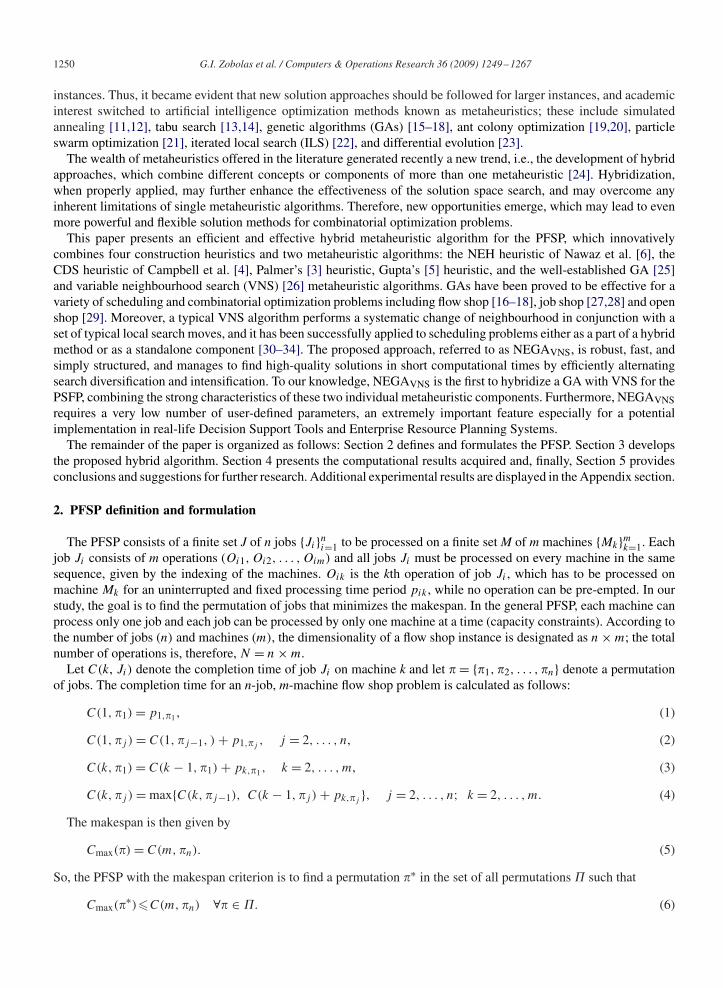
Step 4: Population renewal. Update the population to avoid entrapment in local optima and algorithm stall. Underspecific conditions (see Section 3.5), ‘aged’ solutions are replaced by new ones, which are generated similarly to Step1’s procedure, i.e., with a% probability by the GRNEH component and with (100− a)% probability randomly.}while (t < t_max) (where t is the total elapsed computational time).The proposed hybrid metaheuristic mechanics is schematically presented in Fig. 1.
3.2. Initial population generation
When generating initial solutions, the goal is to acquire a population of diversified, yet of adequate quality solutions.In our implementation, four well-known heuristics (NEH, Gupta, CDS, and Palmer) are initially employed to generate
Initial population Generation
Intensification Phase
Genetic Algorithm
NEGAVNSInitialization
PopulationRenewal End
Fig. 1. The NEGAVNS mechanics.
1252 G.I. Zobolas et al. / Computers & Operations Research 36 (2009) 1249–1267
solutions. A GRNEH is then employed to generate (i_pop ∗ a− 4) solutions. According to the original NEH heuristic,the job sequence is determined by initially arranging jobs in a descending order of their total processing time. Then,based on this order, an increasingly larger partial sequence is generated at each step by introducing one job from theunscheduled ones into the partial sequence (until all jobs are scheduled). At each step, a new job is scheduled in allpossible positions (k + 1 positions, where k is the size of last step’s partial sequence), and after choosing the bestplace for this job, regarding the makespan, the new partial sequence is fixed for the remaining procedure [6]. WithinGRNEH, at each step of the NEH method, instead of getting the best partial solution as the original NEH dictates, oneout of the best five partial solutions is randomly chosen with equal probabilities. This way, high-quality individuals,yet different from each other, can be generated. The remaining i_pop(1 − a) solutions of the initial population aregenerated randomly. If y denotes the solution index, k the size of the partial sequence, and n the number of jobs of aparticular problem instance, the pseudo-code of the GRNEH procedure is
y = 5 (the first four solutions are acquired by the classic constructive heuristic methods)Rank jobs in descending order of total processing timeDo {
Remove the first job for the ranked list and insert it as the first element of the partial sequencek = 1Do {
Evaluate k + 1 partial schedules by choosing the first unscheduled job of the ranked list and placing itin the k + 1 possible positionsStore best five (5) partial schedulesSelect randomly a partial schedule out of the five with equal probabilitiesk← k + 1
} while (k�n)
Store complete solutiony ← y + 1
} while (y < i_pop ∗ a).
3.3. Population improvement via a GA
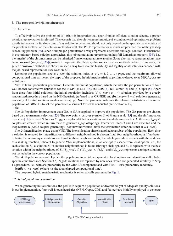
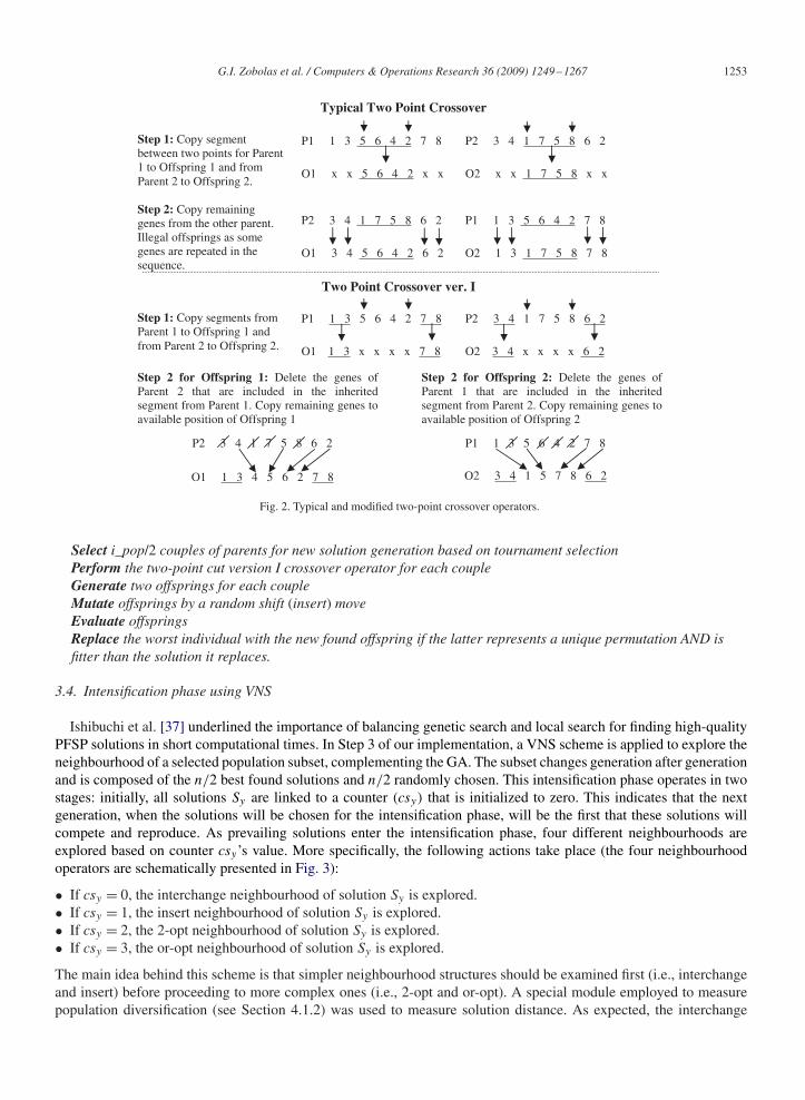
In Step 2 of NEGAVNS, a GA is employed to improve the initial population. In our implementation, the selectionof parents is based on a classic tournament selection scheme where i_pop/2 random couples of parents are selected.For the selection of each couple, a random number of solutions is selected at first, ranging from 3 to 10. There-after, the two fitter parents are selected and they mate to generate two new offsprings. This procedure is repeatedi_pop/2 times at each step (i.e., before every execution of the VNS and population renewal schemes). Concerningchromosome recombination, the latter is performed on a two-point crossover basis. It should be mentioned that di-rectly applying a two-point crossover operator most likely leads to illegal chromosomes, where some jobs are repeatedmore than once within a permutation. To overcome the chromosome illegality, a special variation of the operatoris applied herein, which according to Murata et al. [15], achieves the best performance for PFSP problems; this isthe two-point crossover version I, based on which genes before the first and after the second crossover points aredirectly copied from one parent to the offspring, while the rest of the offspring’s chromosome is filled up by le-gitimate genes from the second parent. The typical and the modified two point crossover operators are illustratedin Fig. 2.
Murata et al. [15] and Ruiz et al. [18] also showed that the best performing mutation operator for PFSP problems isthe shift mutation operation, i.e., a simple insert move (see Fig. 3 for the insert operator). In the final steps of our GA,the offsprings are evaluated (makespan calculation) and the best performing ones are included in the new population,while the worst performing solutions are deleted. According to Ruiz et al. [18] this selection mechanism performsbetter than the direct replacement of parents by their offsprings. To avoid premature convergence, each new found fitoffspring is accepted not only if it yields a better makespan than the worst solution of the current population, but alsoif it represents a unique sequence, not repeated in the population. The pseudo-code of the GA is (for one generation orone loop of Steps 2–4).
G.I. Zobolas et al. / Computers & Operations Research 36 (2009) 1249–1267 1253
Typical Two Point Crossover
Two Point Crossover ver. I
P1 1 3 5 6 4 2 7 8 P2 3 4 1 7 5 8 6 2
O1 1 3 x x x x 7 8
Step 1: Copy segments from Parent 1 to Offspring 1 and from Parent 2 to Offspring 2. O2 3 4 x x x x 6 2
Step 2 for Offspring 1: Delete the genes of Parent 2 that are included in the inherited segment from Parent 1. Copy remaining genes to available position of Offspring 1
P2 3 4 1 7 5 8 6 2
O1 1 3 4 5 6 2 7 8
Step 2 for Offspring 2: Delete the genes of Parent 1 that are included in the inherited segment from Parent 2. Copy remaining genes to available position of Offspring 2
P1 1 3 5 6 4 2 7 8
O2 3 4 1 5 7 8 6 2
P1 1 3 5 6 4 2 7 8 P2 3 4 1 7 5 8 6 2
O1 x x 5 6 4 2 x x O2 x x 1 7 5 8 x x
Step 2: Copy remaining genes from the other parent. Illegal offsprings as some genes are repeated in the sequence.
P2 3 4 1 7 5 8 6 2
O1 3 4 5 6 4 2 6 2
P1 1 3 5 6 4 2 7 8
O2 1 3 1 7 5 8 7 8
Step 1: Copy segment between two points for Parent 1 to Offspring 1 and from Parent 2 to Offspring 2.
Fig. 2. Typical and modified two-point crossover operators.
Select i_pop/2 couples of parents for new solution generation based on tournament selectionPerform the two-point cut version I crossover operator for each coupleGenerate two offsprings for each coupleMutate offsprings by a random shift (insert) moveEvaluate offspringsReplace the worst individual with the new found offspring if the latter represents a unique permutation AND isfitter than the solution it replaces.
3.4. Intensification phase using VNS
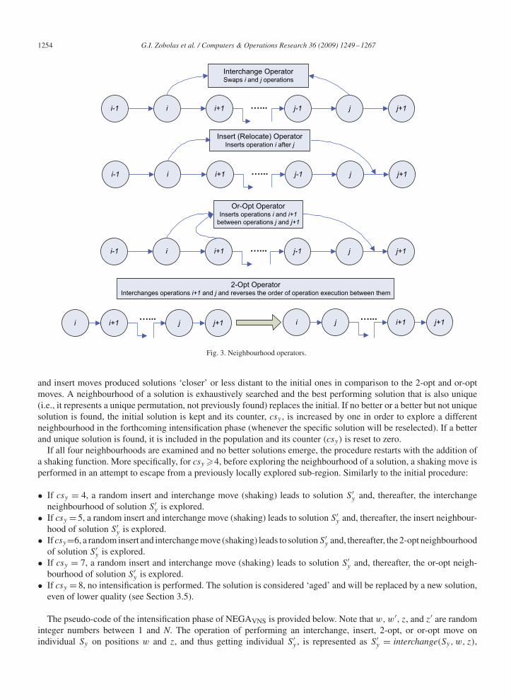
Ishibuchi et al. [37] underlined the importance of balancing genetic search and local search for finding high-qualityPFSP solutions in short computational times. In Step 3 of our implementation, a VNS scheme is applied to explore theneighbourhood of a selected population subset, complementing the GA. The subset changes generation after generationand is composed of the n/2 best found solutions and n/2 randomly chosen. This intensification phase operates in twostages: initially, all solutions Sy are linked to a counter (csy) that is initialized to zero. This indicates that the nextgeneration, when the solutions will be chosen for the intensification phase, will be the first that these solutions willcompete and reproduce. As prevailing solutions enter the intensification phase, four different neighbourhoods areexplored based on counter csy’s value. More specifically, the following actions take place (the four neighbourhoodoperators are schematically presented in Fig. 3):
• If csy = 0, the interchange neighbourhood of solution Sy is explored.• If csy = 1, the insert neighbourhood of solution Sy is explored.• If csy = 2, the 2-opt neighbourhood of solution Sy is explored.• If csy = 3, the or-opt neighbourhood of solution Sy is explored.
The main idea behind this scheme is that simpler neighbourhood structures should be examined first (i.e., interchangeand insert) before proceeding to more complex ones (i.e., 2-opt and or-opt). A special module employed to measurepopulation diversification (see Section 4.1.2) was used to measure solution distance. As expected, the interchange
1254 G.I. Zobolas et al. / Computers & Operations Research 36 (2009) 1249–1267
Interchange OperatorSwaps i and j operations
i-1 j+1jj-1i+1i …...
Insert (Relocate) OperatorInserts operation i after j
i-1 j+1jj-1i+1i …...
2-Opt OperatorInterchanges operations i+1 and j and reverses the order of operation execution between them
j+1ji+1i…...
j+1i+1ji…...
Or-Opt OperatorInserts operations i and i+1
between operations j and j+1
i-1 j+1jj-1i+1i …...
Fig. 3. Neighbourhood operators.
and insert moves produced solutions ‘closer’ or less distant to the initial ones in comparison to the 2-opt and or-optmoves. A neighbourhood of a solution is exhaustively searched and the best performing solution that is also unique(i.e., it represents a unique permutation, not previously found) replaces the initial. If no better or a better but not uniquesolution is found, the initial solution is kept and its counter, csy , is increased by one in order to explore a differentneighbourhood in the forthcoming intensification phase (whenever the specific solution will be reselected). If a betterand unique solution is found, it is included in the population and its counter (csy) is reset to zero.
If all four neighbourhoods are examined and no better solutions emerge, the procedure restarts with the addition ofa shaking function. More specifically, for csy �4, before exploring the neighbourhood of a solution, a shaking move isperformed in an attempt to escape from a previously locally explored sub-region. Similarly to the initial procedure:
• If csy = 4, a random insert and interchange move (shaking) leads to solution S′y and, thereafter, the interchangeneighbourhood of solution S′y is explored.• If csy = 5, a random insert and interchange move (shaking) leads to solution S′y and, thereafter, the insert neighbour-
hood of solution S′y is explored.• If csy=6, a random insert and interchange move (shaking) leads to solutionS′y and, thereafter, the 2-opt neighbourhood
of solution S′y is explored.• If csy = 7, a random insert and interchange move (shaking) leads to solution S′y and, thereafter, the or-opt neigh-
bourhood of solution S′y is explored.• If csy = 8, no intensification is performed. The solution is considered ‘aged’ and will be replaced by a new solution,
even of lower quality (see Section 3.5).
The pseudo-code of the intensification phase of NEGAVNS is provided below. Note that w, w′, z, and z′ are randominteger numbers between 1 and N. The operation of performing an interchange, insert, 2-opt, or or-opt move onindividual Sy on positions w and z, and thus getting individual S′y , is represented as S′y = interchange(Sy, w, z),
G.I. Zobolas et al. / Computers & Operations Research 36 (2009) 1249–1267 1255
S′y = insert(Sy, w, z), S′y = 2-opt(Sy, w, z), and S′y = or-opt(Sy, w, z), respectively. Finally, f (Sy) is equal to themakespan of individual Sy, B is a temporary vector to store a local optimum, and the VNS loop is conducted n(n− 1)
times where n is the number of jobs of a specific problem (chromosome size).
For all individuals Sy , y = 1, 2, . . . , n, where 1�y�n/2 corresponds to the n/2 best solutions andn/2�y�n corresponds ton/2 random solutions
w = rnd(1, N); z= rnd(1, N); w′ = rnd(1, N); z′ = rnd(1, N), w < z, w �= w′, z �= z′if csy �8 then brake and move to next Sy
if 8 > csy �4 then S′y = interchange(Sy, w, z); S′y = insert(S′y, w′, z′)if csy < 4 thenS′y ← Sy
loop= 0; B ← S′yDo { w = rnd(1, N); z= rnd(1, N) w < z
if (csy = 0 or csy = 4) then S′′y = interchange(B, w, z)
if (csy = 1 or csy = 5) then S′′y = insert(B, w, z)
if (csy = 2 or csy = 6) then S′′y = 2-opt(B, w, z)
if (csy = 3 or csy = 7) then S′′y = or-opt(B, w, z)
if (f (S′′y )�f (B) then B ← S′′yloop++
} while (loop < n(n− 1))
if (f (B)�f (Sy) and B represents a unique sequence then {csy = 0; Sy ← B}else csy ← csy + 1
EndFor.
3.5. Population renewal
It was observed that NEGAVNS would get stalled after a number of generations with most solutions having theircsy index equal to or higher than eight. As a result, a module was developed (Step 4) to renew the population. Morespecifically, every solution with csy �8 is considered ‘aged’ and is consequently replaced by a new one that is generatedsimilarly to Step 1’ s procedure, i.e., with a% probability by the GRNEH component and with (100− a)% probabilitycompletely randomly. The only exception is the best solution found so far, which even if it belongs to the ‘aged’solutions subgroup, it is not replaced by the population renewal module.
4. Computational results
The NEGAVNS algorithm was coded in C++ and all tests were conducted on a Pentium� IV PC at 2.4 GHz with1.0 GB of RAM. The proposed hybrid metaheuristic was tested on 120 benchmark problems developed by Taillard [38]which were downloaded from the OR bibliography [39,40]. More specifically, the algorithm was tested on 12 sets ofbenchmark problems (each set consisting of 10 instances) with sizes (n×m) ranging from 20× 5 to 500× 20 denotedas Ta001 to Ta120.
4.1. Parameter settings and sensitivity analysis
Typically, optimization algorithms are measured against two criteria: accuracy (i.e., solution quality) and speed.However, simplicity and flexibility are also essential attributes of good metaheuristics [41]. Limiting the number ofparameters and using fixed parameter settings enhance both the simplicity and flexibility of an algorithm. In ourimplementation, a total of three parameters are required to set up the hybrid algorithm: the initial population size(i_pop), the GRNEH initial population percentage (a), and the maximum running time (t_max). The values of theseparameters greatly affect the algorithm’s performance and thus an extensive series of tests was conducted to investigatetheir impact. The particularly difficult instances Ta051–Ta060, Ta081–090, and Ta101–Ta110 were mainly used forparameter sensitivity analysis. The results of these tests led to the adaptation of fixed or problem size-dependantparameter values, which are presented in Table 1.
1256 G.I. Zobolas et al. / Computers & Operations Research 36 (2009) 1249–1267
Table 1Parameter settings for NEGAVNS
Initial population size (i_pop) GRNEH initial solutions (a) (%) Max. running time (t_max) (s)
10n 30 n×m/10
Best Makespan
3940
3960
3980
4000
4020
4040
4060
4080
4100
0Computational time (s) Computational time (s)
Bes
t Mak
espa
n
Average Makespan
3980
4080
4180
4280
4380
4480
4580
4680
4780
4880
Mak
espa
n
i_pop=50 i_pop=100 i_pop=250 i_pop=500 i_pop=1000
302010 0 302010
Fig. 4. Analysis of initial population size effect (Ta051).
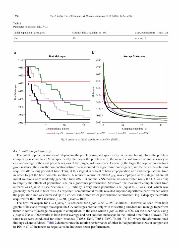
4.1.1. Initial population sizeThe initial population size should depend on the problem size, and specifically on the number of jobs as the problem
complexity is equal to n! More specifically, the larger the problem size, the more the solutions that are necessary toensure coverage of the most possible regions of the (larger) solution space. Generally, the larger the population size for agiven instance, the more the computational time that is required for algorithmic convergence, and the better the solutionsacquired after a long period of time. Thus, at this stage it is critical to balance population size and computational timein order to get the best possible solutions. A reduced version of NEGAVNS was employed at this stage, where allinitial solutions were randomly generated (no GRNEH) and the VNS module was deactivated (only the GA was run)to amplify the effects of population size on algorithm’s performance. Moreover, the maximum computational timeallowed was t_max/3 s (see Section 4.1.3). Initially, a very small population size (equal to n) was used, which wasgradually increased in later tests. As expected, computational results revealed superior algorithmic performance whenthe population size was increased up to a critical value after which performance deteriorated. Fig. 4 displays the resultsacquired for the Ta051 instance (n= 50, t_max= 100 s).
The best makespan for t = t_max/3 is achieved for i_pop = 5n = 250 solutions. However, as seen from bothgraphs of best and average makespan, the GA converges prematurely with this setting and does not manage to performbetter in terms of average makespan in comparison to the case where i_pop = 10n = 500. On the other hand, usingi_pop= 20n= 1000 results in both lower average and best solution makespan in the limited time frame allowed. Thesame tests were conducted for other instances (Ta052–Ta60, Ta081–Ta90, Ta101–Ta110) where the aforementionedfindings where validated. Table 2 demonstrates the relative performance of other initial population sizes in comparisonto 10n in all 30 instances (a negative value indicates better performance).
G.I. Zobolas et al. / Computers & Operations Research 36 (2009) 1249–1267 1257
Table 2Relative performance of i_pop values in comparison to 10n
i_pop= n (%) i_pop= 2n (%) i_pop= 5n (%) i_pop= 20n (%)
Average makespan 6.36 4.34 0.87 1.32Best makespan 2.65 1.22 −0.25 0.79
4400
4500
4600
4700
4800
4900
0% 10% 20% 30% 40% 50% 60% 70% 80% 90%
Percentage of GRNEH solutions
Ave
rage
Mak
espa
n
750
760
770
780
790
800
810
820
830
840
Div
ersi
ty I
ndex
Average Makespan Diversity Index
100%
Fig. 5. Parameter a’s effect on initial solution quality and initial population diversity (Ta051).
It should be mentioned that increasing the computational time available should lead to an increase of the populationsize so as to avoid premature convergence and, conversely, decreasing the computational time available should lead toa decrease of the population size to speed up convergence within the time limit imposed.
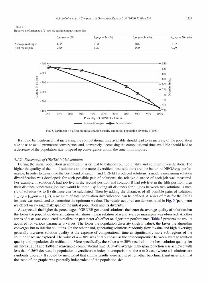
4.1.2. Percentage of GRNEH initial solutionsDuring the initial population generation, it is critical to balance solution quality and solution diversification. The
higher the quality of the initial solutions and the more diversified these solutions are, the better the NEGAVNS perfor-mance. In order to determine the best blend of random and GRNEH produced solutions, a module measuring solutiondiversification was developed: for each possible pair of solutions, the relative distance of each job was measured.For example, if solution A had job five in the second position and solution B had job five in the fifth position, thentheir distance concerning job five would be three. By adding all distances for all jobs between two solutions, a met-ric of solution (A to B) distance can be calculated. Then by adding the distances of all possible pairs of solutions(i_pop ∗ [i_pop − 1]/2), a measure of total population diversification can be defined. A series of tests for the Ta051instance was conducted to determine the optimum a value. The results acquired are demonstrated in Fig. 5 (parametera’s effect on average makespan of the initial population and its diversity).
As expected, the higher the percentage of GRNEH generated solutions, the better the average quality of solutions butthe lower the population diversification. An almost linear relation of a and average makespan was observed. Anotherseries of tests was conducted to realize the parameter a’s effect on algorithm performance. Table 3 presents the resultsacquired for various parameter a values. The lower the population diversity (high a value), the faster the algorithmconverges but to inferior solutions. On the other hand, generating solutions randomly (low a value and high diversity)generally increases solution quality at the expense of computational time as significantly more sub-regions of thesolution space are explored. The value of a=30% was finally chosen as the best compromise between average solutionquality and population diversification. More specifically, the value a = 30% resulted in the best solution quality forinstances Ta051 and Ta081 in reasonable computational time. A 0.94% average makespan reduction was achieved withless than 0.36% decrease in population diversification index in comparison to the a = 0 case (where all solutions arerandomly chosen). It should be mentioned that similar results were acquired for other benchmark instances and thatthe trend of the graphs was generally independent of the population size.
1258 G.I. Zobolas et al. / Computers & Operations Research 36 (2009) 1249–1267
Table 3Effect of parameter a on NEGAVNS performance
a Value (%) Ta051 Ta081
�avr tavr �avr tavr
10 0.78 41 1.71 10520 0.77 34 1.69 9530 0.77 31 1.69 9240 0.78 30 1.70 8650 0.78 30 1.71 8060 0.79 26 1.75 7470 0.81 22 1.82 69
Table 4Computational results with (NEGAVNS) and without (NEGAVNS′ ) the four heuristic solutions
Instance �avr tavr
NEGAVNS NEGAVNS′a NEGAVNS NEGAVNS′
a
Ta051 0.77 0.77 35 36Ta081 1.69 1.69 95 96Ta101 1.52 1.52 225 229
aNEGAVNS′ does not include the four heuristic solutions in the initial population.
0.00%
5.00%
10.00%
15.00%
20.00%
25.00%
30.00%
35.00%
40.00%
45.00%
50.00%
Interchange
Perc
enta
ge o
f new
bes
t fou
nd s
olut
ions
Or-OptInsert 2-Opt
Fig. 6. The contribution of each VNS move to finding a new best solution.
4.1.3. Maximum running timeExtensive testing revealed that using the ‘number of iterations with no recorded improvement’ for convergence
control was not suitable for NEGAVNS, as in many cases the algorithm managed to escape from a local optimumafter a quite large number of iterations. As a result, the ‘maximum running time convergence control’ was adopted.Generally, the larger the number of jobs and machines, the more difficult the instance, and computational time toachieve high-quality solutions increases. Thus, maximum allowed computation time should depend on each instance’sdimensionality and was arbitrarily given the value of N = n×m/10 s, which results in practical computational timesfor all Taillard instances.
4.2. Performance analysis of individual components
In this section, the effect of specific NEGAVNS components is analysed. Firstly, the contribution of the four construc-tion heuristics (initial solution generation) is evaluated followed by an analysis of the performance increase resulting
G.I. Zobolas et al. / Computers & Operations Research 36 (2009) 1249–1267 1259
Table 5Computational results with (NEGAVNS) and without (NEGAVNS′′ ) the 2-opt and or-opt moves
Instance �avr tavr
NEGAVNS NEGAVNS′′a NEGAVNS NEGAVNS′′
a
Ta051 0.77 0.78 31 39Ta081 1.69 1.69 92 95Ta101 1.52 1.53 223 234
aNEGAVNS′′ does not include the 2-opt and or-opt neighbourhood operators.
Table 6Computational results for different levels of GA-VNS interconnection
Instance �avr tavr
NEGA.VNS NEGAVNS NEVNS NEGAGA.VNS NEGAVNS NEVNS
Ta051 0.78 0.77 0.82 36 31 35Ta081 1.71 1.69 1.74 101 92 98Ta101 1.54 1.52 1.59 238 223 242
Table 7Additional performance measures for Taillard instances
Problems �min (%) �max (%) �avr (%) �NEH (%)
20× 5 0.00 0.00 0.00 3.2620× 10 0.00 0.01 0.01 4.6020× 20 0.00 0.03 0.02 3.7350× 5 0.00 0.00 0.00 0.7350× 10 0.77 0.87 0.82 5.0750× 20 0.96 1.19 1.08 6.66100× 5 0.00 0.01 0.00 0.53100× 10 0.08 0.17 0.14 2.21100× 20 1.31 1.51 1.40 5.34200× 10 0.11 0.21 0.16 1.26200× 20 1.17 1.33 1.25 4.41500× 20 0.63 0.77 0.71 2.07
from the 2-opt and or-opt moves. Finally, the strong wrapping of GA and VNS is tested by a series of tests with threedifferent levels of GA and VNS interconnection.
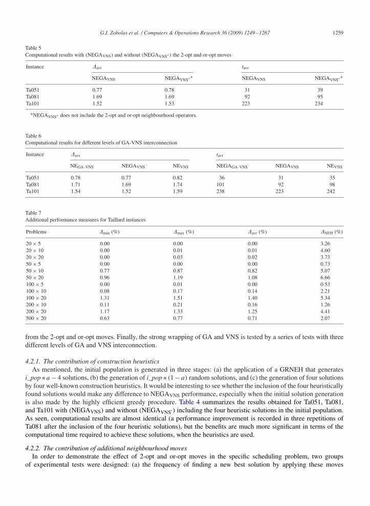
4.2.1. The contribution of construction heuristicsAs mentioned, the initial population is generated in three stages: (a) the application of a GRNEH that generates
i_pop ∗ a− 4 solutions, (b) the generation of i_pop ∗ (1− a) random solutions, and (c) the generation of four solutionsby four well-known construction heuristics. It would be interesting to see whether the inclusion of the four heuristicallyfound solutions would make any difference to NEGAVNS performance, especially when the initial solution generationis also made by the highly efficient greedy procedure. Table 4 summarizes the results obtained for Ta051, Ta081,and Ta101 with (NEGAVNS) and without (NEGAVNS′) including the four heuristic solutions in the initial population.As seen, computational results are almost identical (a performance improvement is recorded in three repetitions ofTa081 after the inclusion of the four heuristic solutions), but the benefits are much more significant in terms of thecomputational time required to achieve these solutions, when the heuristics are used.
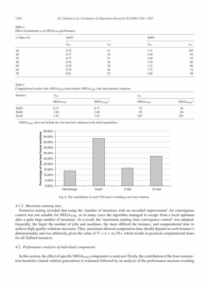
4.2.2. The contribution of additional neighbourhood movesIn order to demonstrate the effect of 2-opt and or-opt moves in the specific scheduling problem, two groups
of experimental tests were designed: (a) the frequency of finding a new best solution by applying these moves
1260 G.I. Zobolas et al. / Computers & Operations Research 36 (2009) 1249–1267
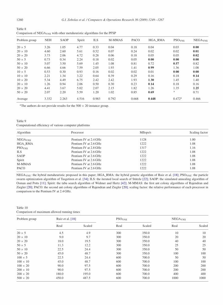
Table 8Comparison of NEGAVNS with other metaheuristic algorithms for the PFSP
Problem group NEH SAOP Spirit ILS M-MMAS PACO HGA_RMA PSOVNS NEGAVNS
20× 5 3.26 1.05 4.77 0.33 0.04 0.18 0.04 0.03 0.0020× 10 4.60 2.60 5.61 0.52 0.07 0.24 0.02 0.02 0.0120× 20 3.73 2.06 4.72 0.28 0.06 0.18 0.05 0.05 0.0250× 5 0.73 0.34 2.24 0.18 0.02 0.05 0.00 0.00 0.0050× 10 5.07 3.50 5.69 1.45 1.08 0.81 0.72 0.57 0.8250× 20 6.66 4.66 7.59 2.05 1.93 1.41 0.99 1.36 1.0810× 5 0.53 0.30 0.93 0.16 0.02 0.02 0.01 0.00 0.0010× 10 2.21 1.34 3.22 0.64 0.39 0.29 0.16 0.18 0.1410× 20 5.34 4.49 6.75 2.42 2.42 1.93 1.30 1.45 1.4020× 10 1.26 0.94 2.06 0.50 0.30 0.23 0.14 0.18 0.1620× 20 4.41 3.67 5.02 2.07 2.15 1.82 1.26 1.35 1.2550× 20 2.07 2.20 5.59 1.20 1.02 0.85 0.69 a 0.71
Average 3.332 2.263 4.516 0.983 0.792 0.668 0.448 0.472a 0.466
aThe authors do not provide results for the 500× 20 instance group.
Table 9Computational efficiency of various computer platforms
Algorithm Processor Mflops/s Scaling factor
NEGAVNS Pentium IV at 2.4 GHz 1128 1.00HGA_RMA Pentium IV at 2.6 GHz 1222 1.08PSOVNS Pentium IV at 2.8 GHz 1317 1.16ILS Pentium IV at 2.6 GHz 1222 1.08SAOP Pentium IV at 2.6 GHz 1222 1.08Spirit Pentium IV at 2.6 GHz 1222 1.08M-MMAS Pentium IV at 2.6 GHz 1222 1.08PACO Pentium IV at 2.6 GHz 1222 1.08
NEGAVNS: the hybrid metaheuristic proposed in this paper; HGA_RMA: the hybrid genetic algorithm of Ruiz et al. [18]; PSOVNS: the particleswarm optimization algorithm of Tasgetiren et al. [34]; ILS: the iterated local search of Stützle [22]; SAOP: the simulated annealing algorithm ofOsman and Potts [11]; Spirit: the tabu search algorithm of Widmer and Hertz [42]; M-MMAS: the first ant colony algorithms of Rajendran andZiegler [20]; PACO: the second ant colony algorithms of Rajendran and Ziegler [20]; scaling factor: the relative performance of each processor incomparison to the Pentium IV at 2.4 GHz.
Table 10Comparison of maximum allowed running times
Problem group Ruiz et al. [18] PSOVNS NEGAVNS
Real Scaled Real Scaled Real Scaled
20× 5 4.5 4.9 300 350.0 10 1020× 10 9.0 9.7 300 350.0 20 2020× 20 18.0 19.5 300 350.0 40 4050× 5 11.3 12.2 300 350.0 25 2550× 10 22.5 24.4 300 350.0 50 5050× 20 45.0 48.7 300 350.0 100 100100× 5 22.5 24.4 600 700.0 50 50100× 10 45.0 48.7 600 700.0 100 100100× 20 90.0 97.5 600 700.0 200 200200× 10 90.0 97.5 600 700.0 200 200200× 20 180.0 195.0 600 700.0 400 400500× 20 450.0 487.5 600 700.0 1000 1000
G.I. Zobolas et al. / Computers & Operations Research 36 (2009) 1249–1267 1261
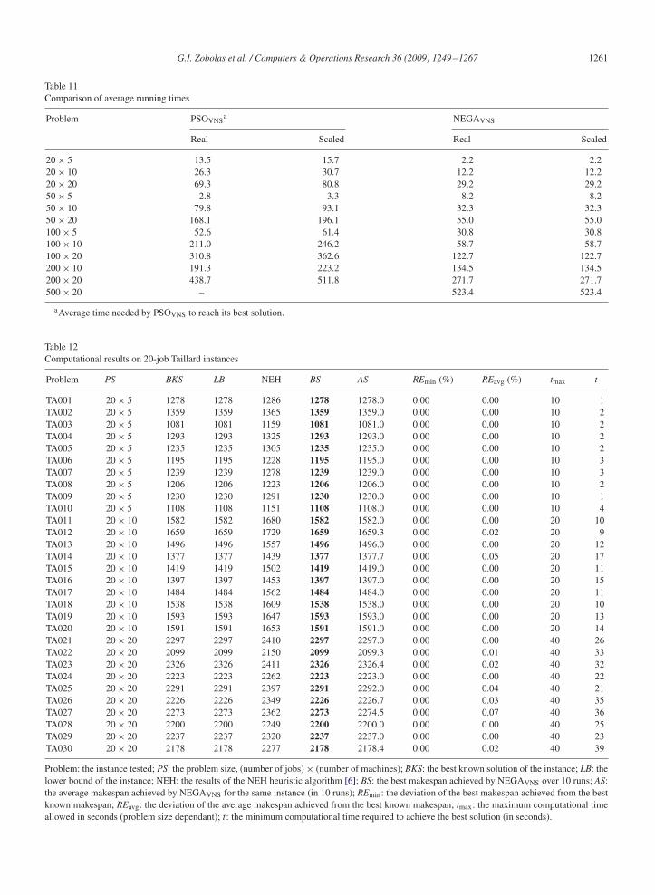
Table 11Comparison of average running times
Problem PSOVNSa NEGAVNS
Real Scaled Real Scaled
20× 5 13.5 15.7 2.2 2.220× 10 26.3 30.7 12.2 12.220× 20 69.3 80.8 29.2 29.250× 5 2.8 3.3 8.2 8.250× 10 79.8 93.1 32.3 32.350× 20 168.1 196.1 55.0 55.0100× 5 52.6 61.4 30.8 30.8100× 10 211.0 246.2 58.7 58.7100× 20 310.8 362.6 122.7 122.7200× 10 191.3 223.2 134.5 134.5200× 20 438.7 511.8 271.7 271.7500× 20 – 523.4 523.4
aAverage time needed by PSOVNS to reach its best solution.
Table 12Computational results on 20-job Taillard instances
Problem PS BKS LB NEH BS AS REmin (%) REavg (%) tmax t
TA001 20× 5 1278 1278 1286 1278 1278.0 0.00 0.00 10 1TA002 20× 5 1359 1359 1365 1359 1359.0 0.00 0.00 10 2TA003 20× 5 1081 1081 1159 1081 1081.0 0.00 0.00 10 2TA004 20× 5 1293 1293 1325 1293 1293.0 0.00 0.00 10 2TA005 20× 5 1235 1235 1305 1235 1235.0 0.00 0.00 10 2TA006 20× 5 1195 1195 1228 1195 1195.0 0.00 0.00 10 3TA007 20× 5 1239 1239 1278 1239 1239.0 0.00 0.00 10 3TA008 20× 5 1206 1206 1223 1206 1206.0 0.00 0.00 10 2TA009 20× 5 1230 1230 1291 1230 1230.0 0.00 0.00 10 1TA010 20× 5 1108 1108 1151 1108 1108.0 0.00 0.00 10 4TA011 20× 10 1582 1582 1680 1582 1582.0 0.00 0.00 20 10TA012 20× 10 1659 1659 1729 1659 1659.3 0.00 0.02 20 9TA013 20× 10 1496 1496 1557 1496 1496.0 0.00 0.00 20 12TA014 20× 10 1377 1377 1439 1377 1377.7 0.00 0.05 20 17TA015 20× 10 1419 1419 1502 1419 1419.0 0.00 0.00 20 11TA016 20× 10 1397 1397 1453 1397 1397.0 0.00 0.00 20 15TA017 20× 10 1484 1484 1562 1484 1484.0 0.00 0.00 20 11TA018 20× 10 1538 1538 1609 1538 1538.0 0.00 0.00 20 10TA019 20× 10 1593 1593 1647 1593 1593.0 0.00 0.00 20 13TA020 20× 10 1591 1591 1653 1591 1591.0 0.00 0.00 20 14TA021 20× 20 2297 2297 2410 2297 2297.0 0.00 0.00 40 26TA022 20× 20 2099 2099 2150 2099 2099.3 0.00 0.01 40 33TA023 20× 20 2326 2326 2411 2326 2326.4 0.00 0.02 40 32TA024 20× 20 2223 2223 2262 2223 2223.0 0.00 0.00 40 22TA025 20× 20 2291 2291 2397 2291 2292.0 0.00 0.04 40 21TA026 20× 20 2226 2226 2349 2226 2226.7 0.00 0.03 40 35TA027 20× 20 2273 2273 2362 2273 2274.5 0.00 0.07 40 36TA028 20× 20 2200 2200 2249 2200 2200.0 0.00 0.00 40 25TA029 20× 20 2237 2237 2320 2237 2237.0 0.00 0.00 40 23TA030 20× 20 2178 2178 2277 2178 2178.4 0.00 0.02 40 39
Problem: the instance tested; PS: the problem size, (number of jobs)× (number of machines); BKS: the best known solution of the instance; LB: thelower bound of the instance; NEH: the results of the NEH heuristic algorithm [6]; BS: the best makespan achieved by NEGAVNS over 10 runs; AS:the average makespan achieved by NEGAVNS for the same instance (in 10 runs); REmin: the deviation of the best makespan achieved from the bestknown makespan; REavg: the deviation of the average makespan achieved from the best known makespan; tmax: the maximum computational timeallowed in seconds (problem size dependant); t : the minimum computational time required to achieve the best solution (in seconds).
1262 G.I. Zobolas et al. / Computers & Operations Research 36 (2009) 1249–1267
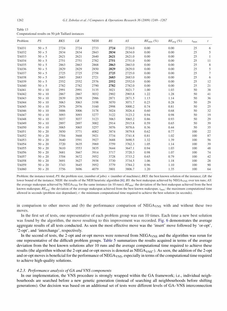
Table 13Computational results on 50-job Taillard instances
Problem PS BKS LB NEH BS AS REmin (%) REavg (%) tmax t
TA031 50× 5 2724 2724 2733 2724 2724.0 0.00 0.00 25 6TA032 50× 5 2834 2834 2843 2834 2834.0 0.00 0.00 25 5TA033 50× 5 2621 2621 2640 2621 2621.0 0.00 0.00 25 1TA034 50× 5 2751 2751 2782 2751 2751.0 0.00 0.00 25 11TA035 50× 5 2863 2863 2868 2863 2863.0 0.00 0.00 25 8TA036 50× 5 2829 2829 2850 2829 2829.0 0.00 0.00 25 5TA037 50× 5 2725 2725 2758 2725 2725.0 0.00 0.00 25 7TA038 50× 5 2683 2683 2721 2683 2683.0 0.00 0.00 25 6TA039 50× 5 2552 2552 2576 2552 2552.0 0.00 0.00 25 12TA040 50× 5 2782 2782 2790 2782 2782.0 0.00 0.00 25 21TA041 50× 10 2991 2991 3135 3021 3021.7 1.00 1.03 50 38TA042 50× 10 2867 2867 3032 2902 2903.8 1.22 1.28 50 41TA043 50× 10 2839 2839 2986 2871 2871.5 1.13 1.14 50 36TA044 50× 10 3063 3063 3198 3070 3071.7 0.23 0.28 50 29TA045 50× 10 2976 2976 3160 2998 3000.2 0.74 0.81 50 25TA046 50× 10 3006 3006 3178 3024 3026.4 0.60 0.68 50 32TA047 50× 10 3093 3093 3277 3122 3123.2 0.94 0.98 50 19TA048 50× 10 3037 3037 3123 3063 3065.2 0.86 0.93 50 29TA049 50× 10 2897 2897 3002 2914 2915.8 0.59 0.65 50 39TA050 50× 10 3065 3065 3257 3076 3078.6 0.36 0.44 50 35TA051 50× 20 3850 3771 4082 3874 3879.8 0.62 0.77 100 22TA052 50× 20 3704 3668 3921 3734 3741.8 0.81 1.02 100 87TA053 50× 20 3640 3591 3927 3688 3690.5 1.32 1.39 100 56TA054 50× 20 3720 3635 3969 3759 3762.3 1.05 1.14 100 39TA055 50× 20 3610 3553 3835 3644 3647.1 0.94 1.03 100 48TA056 50× 20 3681 3667 3914 3717 3720.3 0.98 1.07 100 74TA057 50× 20 3704 3672 3952 3728 3733.2 0.65 0.79 100 42TA058 50× 20 3691 3627 3938 3730 3734.5 1.06 1.18 100 28TA059 50× 20 3743 3645 3952 3779 3784.2 0.96 1.10 100 90TA060 50× 20 3756 3696 4079 3801 3806.7 1.20 1.35 100 64
Problem: the instance tested; PS: the problem size, (number of jobs)× (number of machines); BKS: the best known solution of the instance; LB: thelower bound of the instance; NEH: the results of the NEH heuristic algorithm [6]; BS: the best makespan achieved by NEGAVNS over ten runs; AS:the average makespan achieved by NEGAVNS for the same instance (in 10 runs); REmin: the deviation of the best makespan achieved from the bestknown makespan; REavg: the deviation of the average makespan achieved from the best known makespan; tmax: the maximum computational timeallowed in seconds (problem size dependant); t : the minimum computational time required to achieve the best solution (in seconds).
in comparison to other moves and (b) the performance comparison of NEGAVNS with and without these twomoves.
In the first set of tests, one representative of each problem group was run 10 times. Each time a new best solutionwas found by the algorithm, the move resulting to this improvement was recorded. Fig. 6 demonstrates the averageaggregate results of all tests conducted. As seen the most effective move was the ‘insert’ move followed by ‘or-opt’,‘2-opt’, and ‘interchange’, respectively.
In the second of tests, the 2-opt and or-opt moves were removed from NEGAVNS and the algorithm was rerun forone representative of the difficult problem groups. Table 5 summarizes the results acquired in terms of the averagedeviation from the best known solutions after 10 runs and the average computational time required to achieve theseresults (the algorithm without the 2-opt and or-opt moves is denoted as NEGAVNS′′). As seen, the addition of the 2-optand or-opt moves is beneficial for the performance of NEGAVNS, especially in terms of the computational time requiredto achieve high-quality solutions.
4.2.3. Performance analysis of GA and VNS componentsIn our implementation, the VNS procedure is strongly wrapped within the GA framework; i.e., individual neigh-
bourhoods are searched before a new genetic generation (instead of searching all neighbourhoods before shiftinggenerations). Our decision was based on an additional set of tests were different levels of GA–VNS interconnection
G.I. Zobolas et al. / Computers & Operations Research 36 (2009) 1249–1267 1263
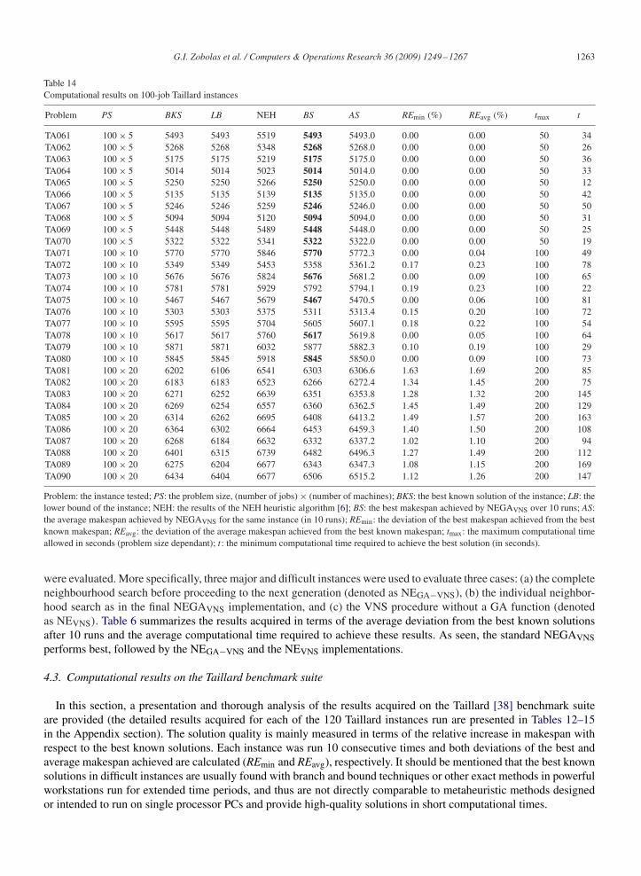
Table 14Computational results on 100-job Taillard instances
Problem PS BKS LB NEH BS AS REmin (%) REavg (%) tmax t
TA061 100× 5 5493 5493 5519 5493 5493.0 0.00 0.00 50 34TA062 100× 5 5268 5268 5348 5268 5268.0 0.00 0.00 50 26TA063 100× 5 5175 5175 5219 5175 5175.0 0.00 0.00 50 36TA064 100× 5 5014 5014 5023 5014 5014.0 0.00 0.00 50 33TA065 100× 5 5250 5250 5266 5250 5250.0 0.00 0.00 50 12TA066 100× 5 5135 5135 5139 5135 5135.0 0.00 0.00 50 42TA067 100× 5 5246 5246 5259 5246 5246.0 0.00 0.00 50 50TA068 100× 5 5094 5094 5120 5094 5094.0 0.00 0.00 50 31TA069 100× 5 5448 5448 5489 5448 5448.0 0.00 0.00 50 25TA070 100× 5 5322 5322 5341 5322 5322.0 0.00 0.00 50 19TA071 100× 10 5770 5770 5846 5770 5772.3 0.00 0.04 100 49TA072 100× 10 5349 5349 5453 5358 5361.2 0.17 0.23 100 78TA073 100× 10 5676 5676 5824 5676 5681.2 0.00 0.09 100 65TA074 100× 10 5781 5781 5929 5792 5794.1 0.19 0.23 100 22TA075 100× 10 5467 5467 5679 5467 5470.5 0.00 0.06 100 81TA076 100× 10 5303 5303 5375 5311 5313.4 0.15 0.20 100 72TA077 100× 10 5595 5595 5704 5605 5607.1 0.18 0.22 100 54TA078 100× 10 5617 5617 5760 5617 5619.8 0.00 0.05 100 64TA079 100× 10 5871 5871 6032 5877 5882.3 0.10 0.19 100 29TA080 100× 10 5845 5845 5918 5845 5850.0 0.00 0.09 100 73TA081 100× 20 6202 6106 6541 6303 6306.6 1.63 1.69 200 85TA082 100× 20 6183 6183 6523 6266 6272.4 1.34 1.45 200 75TA083 100× 20 6271 6252 6639 6351 6353.8 1.28 1.32 200 145TA084 100× 20 6269 6254 6557 6360 6362.5 1.45 1.49 200 129TA085 100× 20 6314 6262 6695 6408 6413.2 1.49 1.57 200 163TA086 100× 20 6364 6302 6664 6453 6459.3 1.40 1.50 200 108TA087 100× 20 6268 6184 6632 6332 6337.2 1.02 1.10 200 94TA088 100× 20 6401 6315 6739 6482 6496.3 1.27 1.49 200 112TA089 100× 20 6275 6204 6677 6343 6347.3 1.08 1.15 200 169TA090 100× 20 6434 6404 6677 6506 6515.2 1.12 1.26 200 147
Problem: the instance tested; PS: the problem size, (number of jobs)× (number of machines); BKS: the best known solution of the instance; LB: thelower bound of the instance; NEH: the results of the NEH heuristic algorithm [6]; BS: the best makespan achieved by NEGAVNS over 10 runs; AS:the average makespan achieved by NEGAVNS for the same instance (in 10 runs); REmin: the deviation of the best makespan achieved from the bestknown makespan; REavg: the deviation of the average makespan achieved from the best known makespan; tmax: the maximum computational timeallowed in seconds (problem size dependant); t : the minimum computational time required to achieve the best solution (in seconds).
were evaluated. More specifically, three major and difficult instances were used to evaluate three cases: (a) the completeneighbourhood search before proceeding to the next generation (denoted as NEGA−VNS), (b) the individual neighbor-hood search as in the final NEGAVNS implementation, and (c) the VNS procedure without a GA function (denotedas NEVNS). Table 6 summarizes the results acquired in terms of the average deviation from the best known solutionsafter 10 runs and the average computational time required to achieve these results. As seen, the standard NEGAVNSperforms best, followed by the NEGA−VNS and the NEVNS implementations.
4.3. Computational results on the Taillard benchmark suite
In this section, a presentation and thorough analysis of the results acquired on the Taillard [38] benchmark suiteare provided (the detailed results acquired for each of the 120 Taillard instances run are presented in Tables 12–15in the Appendix section). The solution quality is mainly measured in terms of the relative increase in makespan withrespect to the best known solutions. Each instance was run 10 consecutive times and both deviations of the best andaverage makespan achieved are calculated (REmin and REavg), respectively. It should be mentioned that the best knownsolutions in difficult instances are usually found with branch and bound techniques or other exact methods in powerfulworkstations run for extended time periods, and thus are not directly comparable to metaheuristic methods designedor intended to run on single processor PCs and provide high-quality solutions in short computational times.
1264 G.I. Zobolas et al. / Computers & Operations Research 36 (2009) 1249–1267
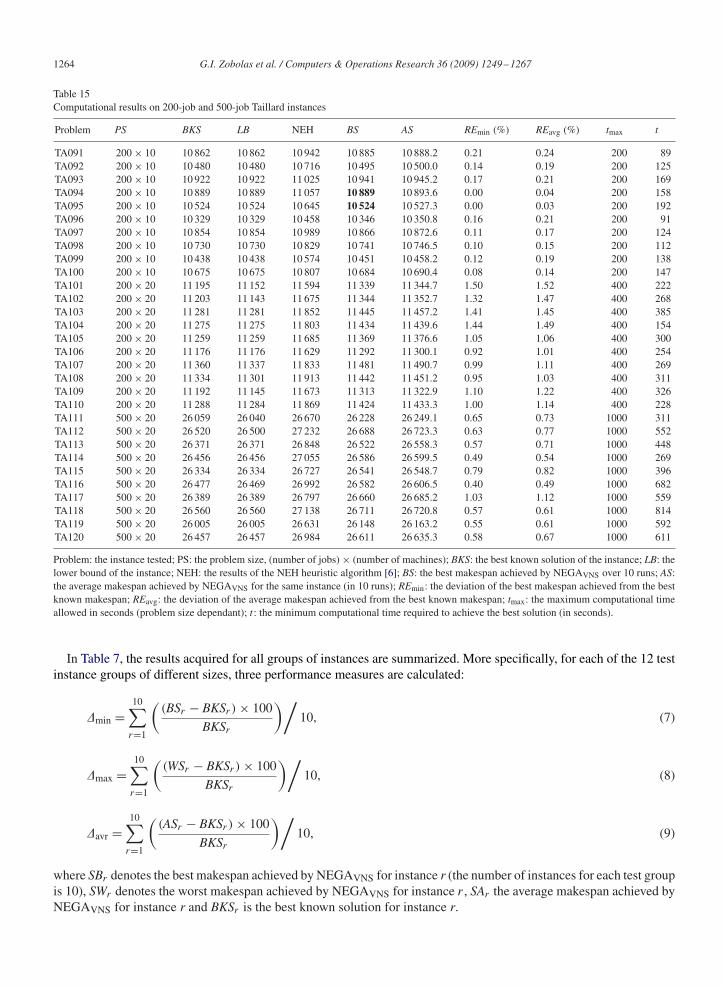
Table 15Computational results on 200-job and 500-job Taillard instances
Problem PS BKS LB NEH BS AS REmin (%) REavg (%) tmax t
TA091 200× 10 10 862 10 862 10 942 10 885 10 888.2 0.21 0.24 200 89TA092 200× 10 10 480 10 480 10 716 10 495 10 500.0 0.14 0.19 200 125TA093 200× 10 10 922 10 922 11 025 10 941 10 945.2 0.17 0.21 200 169TA094 200× 10 10 889 10 889 11 057 10 889 10 893.6 0.00 0.04 200 158TA095 200× 10 10 524 10 524 10 645 10 524 10 527.3 0.00 0.03 200 192TA096 200× 10 10 329 10 329 10 458 10 346 10 350.8 0.16 0.21 200 91TA097 200× 10 10 854 10 854 10 989 10 866 10 872.6 0.11 0.17 200 124TA098 200× 10 10 730 10 730 10 829 10 741 10 746.5 0.10 0.15 200 112TA099 200× 10 10 438 10 438 10 574 10 451 10 458.2 0.12 0.19 200 138TA100 200× 10 10 675 10 675 10 807 10 684 10 690.4 0.08 0.14 200 147TA101 200× 20 11 195 11 152 11 594 11 339 11 344.7 1.50 1.52 400 222TA102 200× 20 11 203 11 143 11 675 11 344 11 352.7 1.32 1.47 400 268TA103 200× 20 11 281 11 281 11 852 11 445 11 457.2 1.41 1.45 400 385TA104 200× 20 11 275 11 275 11 803 11 434 11 439.6 1.44 1.49 400 154TA105 200× 20 11 259 11 259 11 685 11 369 11 376.6 1.05 1.06 400 300TA106 200× 20 11 176 11 176 11 629 11 292 11 300.1 0.92 1.01 400 254TA107 200× 20 11 360 11 337 11 833 11 481 11 490.7 0.99 1.11 400 269TA108 200× 20 11 334 11 301 11 913 11 442 11 451.2 0.95 1.03 400 311TA109 200× 20 11 192 11 145 11 673 11 313 11 322.9 1.10 1.22 400 326TA110 200× 20 11 288 11 284 11 869 11 424 11 433.3 1.00 1.14 400 228TA111 500× 20 26 059 26 040 26 670 26 228 26 249.1 0.65 0.73 1000 311TA112 500× 20 26 520 26 500 27 232 26 688 26 723.3 0.63 0.77 1000 552TA113 500× 20 26 371 26 371 26 848 26 522 26 558.3 0.57 0.71 1000 448TA114 500× 20 26 456 26 456 27 055 26 586 26 599.5 0.49 0.54 1000 269TA115 500× 20 26 334 26 334 26 727 26 541 26 548.7 0.79 0.82 1000 396TA116 500× 20 26 477 26 469 26 992 26 582 26 606.5 0.40 0.49 1000 682TA117 500× 20 26 389 26 389 26 797 26 660 26 685.2 1.03 1.12 1000 559TA118 500× 20 26 560 26 560 27 138 26 711 26 720.8 0.57 0.61 1000 814TA119 500× 20 26 005 26 005 26 631 26 148 26 163.2 0.55 0.61 1000 592TA120 500× 20 26 457 26 457 26 984 26 611 26 635.3 0.58 0.67 1000 611
Problem: the instance tested; PS: the problem size, (number of jobs)× (number of machines); BKS: the best known solution of the instance; LB: thelower bound of the instance; NEH: the results of the NEH heuristic algorithm [6]; BS: the best makespan achieved by NEGAVNS over 10 runs; AS:the average makespan achieved by NEGAVNS for the same instance (in 10 runs); REmin: the deviation of the best makespan achieved from the bestknown makespan; REavg: the deviation of the average makespan achieved from the best known makespan; tmax: the maximum computational timeallowed in seconds (problem size dependant); t : the minimum computational time required to achieve the best solution (in seconds).
In Table 7, the results acquired for all groups of instances are summarized. More specifically, for each of the 12 testinstance groups of different sizes, three performance measures are calculated:
�min =10∑
r=1
((BSr − BKSr )× 100
BKSr
)/10, (7)
�max =10∑
r=1
((WSr − BKSr )× 100
BKSr
)/10, (8)
�avr =10∑
r=1
((ASr − BKSr )× 100
BKSr
)/10, (9)
where SBr denotes the best makespan achieved by NEGAVNS for instance r (the number of instances for each test groupis 10), SWr denotes the worst makespan achieved by NEGAVNS for instance r , SAr the average makespan achieved byNEGAVNS for instance r and BKSr is the best known solution for instance r.
G.I. Zobolas et al. / Computers & Operations Research 36 (2009) 1249–1267 1265
From Table 7, it is apparent that NEGAVNS was able to find the best solutions for all the instances with n = 20,and for the 50 × 5 and 100 × 5 instances. Most importantly, NEGAVNS produced consistent results in the multipleruns per instance as �max − �min was on average 0.09% for all instance groups, with a highest value of 0.20% on theTa051–Ta060 group. In addition, Table 7 also allows the comparison of the NEGAVNS average deviation with the one(�NEH) produced by the NEH heuristic.
4.4. Comparison with other metaheuristic algorithms
In this section, a comparison of NEGAVNS with state-of-the-art metaheuristics for the PFSP with makespan criterionis performed. More specifically, NEGAVNS is compared to the simulated annealing algorithm (SAOP) of Osman andPotts [11], the tabu search algorithm (Spirit) of Widmer and Hertz [42], the ILS of [22], the two ant colony algorithmsof Rajendran and Ziegler [20] named M-MMAS and PACO, the HGA_RMA of Ruiz et al. [18], and the particleswarm optimization algorithm (PSOVNS) of [34]. It should be mentioned that [18] recoded all implementations (exceptPSOVNS and NEGAVNS) to compare them more faithfully. The comparison results are provided in Table 6 (averagedeviation from best known solutions after 10 runs for each instance):
As seen in Table 8, the HGA_RMA, PSOVNS, and NEGAVNS perform very well in Taillard instances with mostlyminor differences between them. These three algorithms manage to generate much better results than their rivals,with only the PACO algorithm of [20] being close. More specifically, HGA_RMA has the lowest average deviationfrom the best known solutions and produces the best results in 50 × 20, 100 × 20, 200 × 10 and 500 × 20 instances.PSOVNS demonstrates the best results in the 50 × 10 group while NEGAVNS performs better than all its rivals in20 × 5, 20 × 10, 20 × 20, 100 × 10, and 200 × 20 instances. PSOVNS and NEGAVNS find the optimum solutionsof 100 × 5 instances in all iterations and all three algorithms find the optimum solutions in all iterations of 50 × 5instances.
Computational time comparison when different computer platforms are used is rather difficult as processor speedin modern PCs is not the sole indicator of computational power (e.g., dual core processors, CPU architecture, etc.).However, Dongarra [43] has conducted a thorough research concerning the computational power of various computerconfigurations ranging from home PCs to modern supercomputers. Although computational times are also affectedby other parameters such as the programming skills of the developer, the compiler, the programming language, andthe precision used during the execution of the runs, a scaling factor is calculated (see Table 9) to conduct a more faircomparison. Maximum computational times are then compared in Table 10, with and without the scaling factor. Itshould be mentioned that average computational times for individual instances are not reported by Ruiz et al. [18].Tasgetiren et al. [34] on the other hand report average computational times for groups of instances which are comparedto NEGAVNS in Table 11.
5. Conclusions
This paper presented a hybrid method for the PFSP. The algorithm comprises three main components: an initialpopulation generation scheme based on construction heuristics, a GA, and VNS. To our knowledge, this is the firsthybrid implementation of GAs and VNS for the PFSP with the makespan criterion. Throughout the algorithm execution,all solutions are encoded according to the job-based representation (job permutation). The NEGAVNS was tested on a setof 120 benchmark instances and the results demonstrate the efficiency and effectiveness of the method, which providescompetitive results in short computational times. More importantly, the proposed scheme has a simple structure andfew user-defined tuning parameters, which are given fixed or problem size-dependant values after a thorough sensitivityanalysis procedure.
It is suggested that a more sophisticated diversification scheme should be used in future research. More specifically,worse offsprings could be accepted to enter the population and replace fitter parents under some conditions. Thisdecision could be based on their ‘distance’ from current solutions in an attempt to further diversify the population.Moreover, the incorporation of memory in intensification phase (to form a hybrid VNS–tabu search algorithm) woulddecrease the number of unnecessary VNS moves, thus saving computational time in difficult instances and increasingthe chances of obtaining higher quality solutions.
1266 G.I. Zobolas et al. / Computers & Operations Research 36 (2009) 1249–1267
Acknowledgements
This work was supported by the General Secretariat for Research and Technology under contract GSRT-05-�AB-71.The authors would also like to thank the anonymous referee for his/her constructive comments and contribution to thecompletion of this work.
6. Appendix
Computational results on 20-, 50-, 100-, and 200- and 500-job. Taillard instances are given in Tables 12–15,respectively.
References
[1] Johnson SM. Optimal two- and three-stage production schedules with setup times included. Novel Research Logistics Quarterly 1954;1:61–8.[2] Garey MRD, Johnson DS, Sethi R. The complexity of flowshop and job shop scheduling. Mathematics of Operations Research 1976;1:
117–29.[3] Palmer DS. Sequencing jobs through a multistage process in the minimum total time: a quick method of obtaining a near optimum. Operations
Research Quarterly 1965;16:101–7.[4] Campbell HG, Dudek RA, Smith ML. A heuristic algorithm for the n-job, m-machine problem. Management Science 1970;16:B630–7.[5] Gupta JND. A functional heuristic algorithm for the flow-shop scheduling problem. Operations Research 1971;22:39–47.[6] Nawaz M, Enscore Jr E, Ham I. A heuristic algorithm for the m-machine, n-job flow-shop sequencing problem. Omega—International Journal
of Management Science 1983;11:91–5.[7] Rajendran C. Heuristic for scheduling in flowshop with multiple objectives. European Journal of Operational Research 1995;82:540–55.[8] Framinan JM, Ruiz-Usano R, Leisten R. Sequencing CONWIP flow-shops: analysis and heuristic. International Journal of Production Research
2001;39:2735–49.[9] Lee GC, Kim YD, Choi SW. Bottleneck-focused scheduling for a hybrid flow-shop. International Journal of Production Research 2004;42:
165–81.[10] Taillard E. Some efficient heuristic methods for the flow shop sequencing problem. European Journal of Operational Research 1990;47:65–74.[11] Osman I, Potts C. Simulated annealing for permutation flow shop scheduling. OMEGA 1989;17:551–7.[12] Ogbu FA, Smith DK. The application of the simulated annealing algorithm to the solution of the n/m/Cmax flowshop problem. Comput
Operations Research 1990;17:243–53.[13] Nowicki E, Smutnicki C. A fast tabu search algorithm for the permutation flowshop problem. European Journal of Operational Research
1996;91:160–75.[14] Grabowski J, Wodecki M. A very fast tabu search algorithm for the permutation flowshop problem with makespan criterion. Computers and
Operations Research 2004;31:1891–909.[15] Murata T, Ishibuchi H, Tanaka H. Genetic algorithms for flowshop scheduling problems. Computers and Industrial Engineering 1996;30:
1061–71.[16] Reeves C, Yamada T. Genetic algorithms, path relinking and the flowshop sequencing problem. Evolutionary Computation 1998;6:45–60.[17] Etiler O, Toklu B, Atak M, Wilson J. A genetic algorithm for flow shop scheduling problems. Journal of the Operations Research Society
2004;55:830–5.[18] Ruiz R, Maroto C, Alcaraz J. Two new robust genetic algorithms for the flowshop scheduling problem. Omega—International Journal of
Management Science 2006;34:461–76.[19] Ying KC, Liao CJ. An ant colony system for permutation flow-shop sequencing. Computers and Operations Research 2004;31:791–801.[20] Rajendran C, Ziegler H. Ant-colony algorithms for permutation flowshop scheduling to minimize makespan/total flowtime of jobs. European
Journal of Operational Research 2004;155:426–38.[21] Liu B, Wang L, Jin Y-H. An effective PSO-based memetic algorithm for flow shop scheduling. IEEE Transactions on Systems Man and
Cybernetics B 2007;37:18–27.[22] Stützle T. Applying iterated local search to the permutation flowshop problem. Technical Report, AIDA-98-04, TU Darmstadt, FG Intellektik;
1998.[23] Onwubolu GC, Davendra D. Scheduling flow-shops using differential evolution algorithm. European Journal of Operational Research
2006;171:674–92.[24] Blum C, Roli A. Metaheuristics in combinatorial optimization: overview and conceptual comparison. ACM Computing Surveys 2003;35:
268–308.[25] Holland JH. Genetic algorithms. New York: Scientific American; 1992.[26] Hansen P, Mladenovic N. Variable neighbourhood search: principles and applications. European Journal of Operational Research 2001;130:
449–67.[27] Groce FD, Tadei R, Volta G. A genetic algorithm for the job shop problem. Computers and Operations Research 1995;22:15–24.[28] Gonçalves JF, Mendes JJDM, Resende MGC. A hybrid genetic algorithm for the job shop scheduling problem. European Journal of Operational
Research 2005;167:77–95.[29] Liaw C-F. A hybrid genetic algorithm for the open shop scheduling problem. European Journal of Operational Research 2000;124:28–42.
G.I. Zobolas et al. / Computers & Operations Research 36 (2009) 1249–1267 1267
[30] Hindi KS, Fleszar K, Charalambous C. An effective heuristic for the CLSP with set-up times. Journal of the Operations Research Society2003;54:490–8.
[31] Fleszar K, Hindi KS. Solving the resource-constrained project scheduling problem by a variable neighbourhood search. European Journal ofOperational Research 2004;155:402–13.
[32] Gagné C, Gravel M, Price WL. Using metaheuristic compromise programming for the solution of multiple-objective scheduling problems.Journal of the Operations Research Society 2005;56:687–98.
[33] Anghinolfi D, Paolucci M. Parallel machine total tardiness scheduling with a new hybrid metaheuristic approach. Computers and OperationsResearch 2007;34:3471–90.
[34] Tasgetiren MF, Liang YC, Sevkli M, Gencyilmaz G. A particle swarm optimization algorithm for makespan and total flowtime minimizationin the permutation flowshop sequencing problem. European Journal of Operational Research 2007;177:1390–947.
[35] Tarantilis CD, Kiranoudis CT. A list-based threshold accepting method for job shop scheduling problems. International Journal of ProductionEconomics 2002;77(2):159–71.
[36] Cheng R, Gen M, Tsujimura Y. A tutorial survey of job-shop scheduling problems using genetic algorithms, part I: representation. Computersand Industrial Engineering 1996;30:983–97.
[37] Ishibuchi H, Yoshida T, Murata T. Balance between genetic search and local Search in memetic algorithms for multiobjective permutationflowshop scheduling. IEEE Transactions on Evolutionary Computation 2003;7:204–23.
[38] Taillard E. Benchmarks for basic scheduling problems. European Journal of Operational Research 1993;64:278–85.[39] Beasley JE. 〈http://ina2.eivd.ch/Collaborateurs/etd/problemes.dir/ordonnancement.dir/flowshop.dir/best_lb_up.txt〉, accessed 10 December
2006.[40] Beasley JE. 〈http://people.brunel.ac.uk/∼mastjjb/jeb/orlib/jobshopinfo.html〉, accessed 10 December 2006.[41] Cordeau J-F, Gendreau M, Laporte G, Potvin J-Y, Semet F. A guide to vehicle routing heuristics. Journal of the Operations Research Society
2002;53:512–22.[42] Widmer M, Hertz A. A new heuristic method for the flow shop sequencing problem. European Journal of Operational Research 1989;41:
186–93.[43] Dongarra JJ. Performance of various computers using standard linear equations software. Report CS-89-85, Computer Science Department,
University of Tennessee, Knoxville, TN; 2006.
Related Documents