Minimizing loss probability bounds for portfolio selection

Minimizing Loss Probability Bounds for Portfolio Selection 1

Jun-ya Gotoha 2 Akiko Takedab

aDepartment of Industrial and Systems Engineering, Chuo University2-13-27 Kasuga, Bunkyo-ku, Tokyo 112-8551, Japan.

E-mail address: [email protected]

bDepartment of Administration Engineering, Keio University3-14-1 Hiyoshi, Kohoku, Yokohama, Kangawa 223-8522, Japan

E-mail address: [email protected]

Abstract

In this paper, we derive a portfolio optimization model by minimizing upper and lowerbounds of loss probability. These bounds are obtained under a nonparametric assumption ofunderlying return distribution by modifying the so-called generalization error bounds for thesupport vector machine, which has been developed in the field of statistical learning. Basedon the bounds, two fractional programs are derived for constructing portfolios, where thenumerator of the ratio in the objective includes the value-at-risk (VaR) or conditional value-at-risk (CVaR) while the denominator is any norm of portfolio vector. Depending on theparameter values in the model, the derived formulations can result in a nonconvex constrainedoptimization, and an algorithm for dealing with such a case is proposed. Some computationalexperiments are conducted on real stock market data, demonstrating that the CVaR-basedfractional programming model outperforms the empirical probability minimization.

Keywords: Finance; Portfolio optimization; CVaR (Conditional Value-at-Risk); SVM(Support Vector Machine); Fractional programming.

1 Introduction

Portfolio Selection Models. The problem of allocating funds into a given set of investableassets is known as portfolio selection. Typical (single period) portfolio selection models deter-mine the distribution of a random return of the form

R(π) :=n∑

j=1

Rjπj ,

where Rj represents the random rate of return of asset j, and π represents a portfolio vector,each component representing the investment ratio into each asset. In practice, the criterion fordetermining a portfolio π is formulated as an optimization problem of the form:

minF [R(π)] : π ∈ Π ⊂ IRn , (1)

where the objective is a functional F of the random vector R := (R1, ...,Rn)⊤ on a probabilityspace (Ω, P,F) which is independent of π, and Π ⊂ IRn is a feasible region of the portfoliovector π. By definition of π, Π is supposed to include a constraint of the form e⊤

n π = 1 whereen := (1, ..., 1)⊤ is the n-dimensional vector of ones.

For example, the expected utility maximization criterion with some utility function U canbe formulated by adopting −E[U(R(x))] as the objective of (1), where E[·] denotes the mathe-matical expectation. More practically, a risk measure such as variance V[R(π)] or a compositeobjective considering return as well as risk, e.g., V[R(π)]−aE[R(π)] with a positive constant a,is preferred due to the ease in controlling the characteristics of the distribution of R(π), where

1This manuscript is the revised version of the authors’ paper entitled: “Portfolio Learning via VaR/CVaRMinimization.” The title is changed along with the major revision.

2Corresponding Author. Tel/fax: +81-3-3817-1928. E-mail address: [email protected]

(J.Gotoh).

1

V[·] denotes the variance operator. Alternative deviation type risk measures such as absolutedeviation, E[|R(π) − E[R(π)]|], have also been used (Konno and Yamazaki, 1991).

Although variance has been the most basic risk measure since the seminal work of Markowitz(1952), drawbacks of such deviation type measures have been pointed out in the literature,and both theoretical and practical attentions have recently cast a spot light on downside riskmeasures such as the class of coherent risk measures rather than deviation measures. A classicaldownside risk measure is Roy (1952)’s safety first criterion which minimizes the probability ofportfolio loss being greater than a threshold. More recently, Value-at-Risk (VaR) has gainedpopularity in 1990s in practice so as to grasp a large loss with a small probability. Although itis intuitive and easy to understand its implication, it faces critiques due to the lack of convexityand, accordingly, coherence (see, e.g., Artzner et al., 1999). In contrast with VaR, ConditionalValue-at-Risk (CVaR) has recently been obtaining a growing popularity due to nice propertiessuch as the coherence and the consistency with the second order stochastic dominance (see, e.g.,Ogryczak and Ruszczynski, 2002) as well as tractability in its optimization (Rockafellar andUryasev, 2002).

Limitation of Existing Approaches. In a typical situation of portfolio selection, historicalreturn data are given as in Figure 1 (left), where the rate of return of n assets has been observedin a market for last T months. For example, in order to adopt the variance as the objectiveof (1), we first estimate a covariance matrix Σ in place of the true covariance matrix Σ byusing the data, and next minimize the estimated portfolio variance π⊤Σπ over Π in place ofthe true objective V[R(π)] = π⊤Σπ, which is never known. This framework can be validatedby the law of large numbers, i.e., a large number of samples lead to the true optimal value. Infinancial practice, however, the number of available samples, T , is often limited due to the limitedfrequency of the observations, and a significant estimation error may occur in estimating theparameters and, accordingly, the optimal portfolio π. Besides, the number of assets, n, is oftenlarger than that of the samples, T . For example, T is 120 for ten-year monthly observations,while n can be more than one thousand, and in such a case, estimation error can be much larger.

Numerous papers address estimation error in the estimates of the mean and variance (e.g.,Chopra and Ziemba, 1993). According to those, estimation error in the mean estimate is muchseverer than that in variance. Therefore, recent papers focus on the minimum variance modelrather than the mean-variance model (e.g., Jagannathan and Ma, 2003; DeMiguel et al., 2009).Also, there exist papers comparing criteria proposed by various researchers. For example, Simaan(1997) points out that the use of absolute deviation instead of variance may cause larger esti-mation error when return follows a normal distribution.

Limitation of such arguments, however, is that only estimation error from a certain supposeddistribution can be evaluated. More specifically, since we cannot know the true distribution inusual financial practice, we cannot evaluate the true estimation error. In addition, althoughmany researchers assume the normal distribution so as to validate those criteria, it is knownthat return does not follow a normal distribution, but follows more fat-tailed and/or skeweddistribution. Thus, it can be said that the traditional models have little theoretical underpinningfor the out-of-sample performance of their optimal portfolio in the real world, or in the absenceof a specific parametric distribution assumption.

Recent Developments. In contrast to those traditional approaches, several recent researchesfocus on the out-of-sample performance of the “optimal” portfolio by introducing the idea devel-oped in the area of statistics into the portfolio selection models (1). For example, Jagannathanand Ma (2003) show that imposing the short-sale constraint, π ≥ 0, which is usually imposed inpractice, on the minimum variance model is equivalent to a shrinkage of the covariance matrixand the out-of-sample performance will be improved. DeMiguel et al. (2009) impose a norm-

2

asset

1 · · · n

1 R11 · · · R1n

date...

.

.....

T RT1 · · · RTn

attribute

1 · · · d

1 a11 · · · a1d

case...

.

.....

m am1 · · · amd

Figure 1: Typical data formats for portfolio selection (left) and unsupervised statistical model(right)

constraint on the variance minimization criterion by extending the idea of shrinkage methodsin statistics (see, e.g., Hastie et al., 2001). They reveal that the problem formulation with the2-norm (Euclidean norm) constraint contains the equally weighted portfolio, i.e., πj = 1/n, as aspecial case while that with the 1-norm constraint contains the minimum variance model withthe short-sale constraint. All of these researches incorporate shrinkage techniques in the samplecovariance matrix so as to improve the out-of-sample performance of the minimum variancemodel.

Similarity between Portfolio Selection and Statistical Learning. Apart from the port-folio selection context stated above, many statistical models also seek a linear combination ofrandom variables. For example, an outlier (or novelty) detection model called the one-classν-support vector machine (OC-νSVM), which is known as an unsupervised statistical learningmodel, determines a linear function of d-dimensional random vector a = (A1, ...,Ad)⊤:

A(w) :=d∑

k=1

wkAk

whose factor loadings wi are estimated by solving a convex program:

min 12∥w∥2

2 − ρ +1

νm

m∑i=1

[ρ − a⊤i w]+ : w ∈ IRd, ρ ∈ IR , (2)

where ∥x∥2 is 2-norm of a vector x, [x]+ := maxx, 0, ν ∈ (0, 1] is a constant to be tuned,and a1, ...,am are observed data of random vector a, given as in Figure 1 (right) where ai :=(ai1, ..., aid)⊤, i = 1, ...,m, follow an unknown distribution in IRd. The outliers are then definedby points ai satisfying a⊤

i w∗ < ρ∗ where (w∗, ρ∗) is an optimal solution to (2). The out-of-sample performance of OC-νSVM as well as the other types of SVMs is underpinned by an errorbound which is known as the generalization error bound (see, e.g., Theorem 8.6 of Scholkopfand Smola, 2002). It gives, for example, an upper bound of PA(w∗) < ρ∗−γ for γ > 0, whichmeans the probability that the linear function (w∗)⊤a takes less than ρ∗ − γ for a new datasample am+1.

As easily seen from Figure 1 and the procedures mentioned above, portfolio selection andunsupervised statistical learning have the same structure in the sense that both estimate alinear model (R(π) or A(w)) from the batch data as Figure 1 via optimization. In fact, theauthors (Gotoh and Takeda, 2005) propose a classification model, which is also a well-studiedsubject in statistical learning, by incorporating the concept of CVaR, which has been used inthe financial context as stated above, and point out that the two-class ν-SVM (Scholkopf et al.,2000) and its extension (Perez-Cruz et al., 2003) can be interpreted as a CVaR minimizationwith a loss associated with the (geometric) margin (see, e.g., Scholkopf and Smola, 2002, for theclassification problem and the definition of ‘margin’). Also, one of the authors (Takeda, 2009)shows stronger generalization error bounds for a couple of ν-SVMs by employing the notions of

3

VaR and CVaR. These facts indicate that VaR and CVaR can play an important role not onlyin portfolio selection but also in statistical learning.

This paper aims to discuss the interaction in the reverse direction. By employing the resultsexplored for statistical learning, we provide a new sight for the use of VaR and CVaR. Moreprecisely, contributions of this paper are summarized as follows:

Under a nonparametric assumption, upper and lower bounds of the probability of a portfolioloss being greater than a threshold are presented by using (empirical) VaR or CVaR on thebasis of the generalization error bound for SVMs. This indicates that empirical VaR or CVaRoptimization can work for lowering out-of-sample loss in a probabilistic sense and, thus, thebounds yield a theoretical underpinning for the use of VaR or CVaR.

Fractional programming portfolio models are posed so as to minimize those bounds of lossprobability, where the numerator of the objective function to be minimized includes VaR orCVaR whereas the denominator is any norm. Besides, the formulation contains the normalloss probability minimization as a special case, which indicates that the normal probabilityminimization can achieve a good out-of-sample performance even for nonnormal distribu-tion. Also, tractability of the fractional optimization formulation depends on the sign ofthe optimal value. To cope with the variable tractability, we develop a two-step algorithm,which yields a local optimizer when the problem is intractable while a global optimizer whentractable.

The generalization bounds also indicate a theoretical underpinning for the ordinary VaRor CVaR minimizing portfolio when the short-sale constraint is imposed. In other words,the short-sale constraint plays a role in improving out-of-sample performance of the VaRand CVaR minimization as in the variance minimization discussed in Jagannathan and Ma(2003).

In addition to the theoretical achievement, we conduct numerical experiments on actualstock market data. The results show that the CVaR-based fractional programming modeloutperforms the empirical loss probability minimization, and is comparable to the minimumvariance model.

The structure of this paper is as follows: In the next section, a few bounds of portfolio lossprobability are given after briefly reviewing existing approach for the probability minimizingportfolio and introducing notions of (empirical) VaR and CVaR. Section 3 is devoted to analgorithm for solving the fractional programs. In Section 4, the optimization models will beapplied to real stock market data. Finally, Section 5 concludes the paper with some remarks.Proofs of the propositions are given in the end of the paper.

2 Nonparametric Error Bounds of the Loss Probability

2.1 Loss Probability Minimizations

Let f(π, R) denote a random portfolio loss which is preferable to be as small as possible. Inthis paper, we adopt

f(π, R) = −R(π) (= −R⊤π)

for the loss variate in portfolio selection since the return R(= −f) is a prominent objective to beas large as possible. In order to determine a portfolio π, we consider a criterion of minimizingthe probability of the portfolio loss f being larger than a threshold θ, i.e., Pf(π, R) > θ. Forexample, if one sets θ = 0, it indicates the probability of the portfolio return being negative. Thisis known as Roy’s safety first criterion (Roy, 1952). Noting that minimizing Pf(π, R) > θ is

4

equal to maximizing PR(π, R) ≥ −θ, we can consider this criterion as the return probabilitymaximization.

When one knows that the return R follows a normal distribution N(µ,Σ), but does notknow the true parameters µ and Σ, he/she is likely to estimate the parameters and solve thefollowing fractional program in order to obtain the safety first portfolio:

min −µ⊤π − θ√π⊤Σπ

: π ∈ Π , (3)

where µ and Σ are the estimated return vector and covariance matrix, respectively. Typically,

the parameters are estimated as µ :=T∑

t=1Rt/T and Σ :=

T∑t=1

(Rt − µ)(Rt − µ)⊤/(T − 1) where

R1, ...,RT are T historical observations of R. In particular, when −θ is set equal to the risk-freerate, (3) is equivalent to the so-called Sharpe ratio maximization.

In contrast with the normal distribution case, we suppose in the remaining part of the paperthat the return R follows an unknown (n-dimensional) distribution, and that R1, ...,RT areindependently drawn from it. Note that most of traditional models have been constructed onthe i.i.d. assumption.

Noting that under the above nonparametric assumption, the empirical counterpart of theloss probability is represented by

1T|t : f(π, Rt) > θ, t = 1, ..., T|

a straightforward formulation for obtaining the smallest empirical loss probability portfolio isthen given by

min 1T

e⊤T z : −R⊤

t π − θ ≤ Mzt, (t = 1, ..., T ), z ∈ 0, 1T , π ∈ Π , (4)

where M is a sufficiently large constant and eT is the T -dimensional column vector of ones. Thisproblem is a 0-1 mixed integer linear program (MILP), which can be efficiently solved by state-of-the-art optimization softwares, e.g., IBM-ILOG CPLEX12, when the size of the problem, Tand n, is not huge and Π is represented by a system of linear or convex quadratic inequalities.

In addition, we assume throughout the paper that random return R has an implicit boundedsupport. Although this assumption excludes the normal distribution, it does not weaken itsapplicability. In fact, the total amount of financial contracts in the world is bounded, andtherefore, the return must be bounded.

2.2 Loss Probability Bounds and VaR/CVaR Minimization

Under the above nonparametric distribution assumptions, we below derive upper and lowerbounds of Pf(π, R) > θ. In order to describe those bounds, let us first introduce the β-value-at-risk (β-VaR) and β-conditional value-at-risk (β-CVaR).

Given T observed return vectors R1, ...,RT , the (empirical) β-VaR associated with lossf(π,R) is the β-quantile defined by

αβ(π) := minα : ΦT (α|π) ≥ β

where ΦT (α|π) := 1T |t ∈ 1, ..., T : f(π, Rt) ≤ α| is the empirical distribution function of

the loss f . β ∈ (0, 1) is a user-defined parameter for representing a confidence level and usuallytakes a value close to 1, say, 0.95 or 0.99, for capturing a large loss with a small probability.The β-VaR minimizing portfolio is thus given by a solution to

min αβ(π) : π ∈ Π , (5)

5

which can be reformulated as an MILP when Π is given by a system of linear inequalities.On the other hand, the (empirical) β-CVaR associated with loss f(π, R) is defined by

ϕβ(π) := minα

Fβ(π, α),

where β ∈ [0, 1) and Fβ is a convex function on IRn × IR, defined by

Fβ(π, α) := α +1

(1 − β)T

T∑t=1

[f(π, Rt) − α]+.

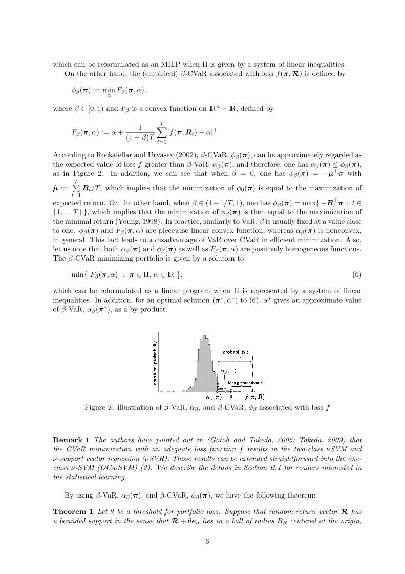
According to Rockafellar and Uryasev (2002), β-CVaR, ϕβ(π), can be approximately regarded asthe expected value of loss f greater than β-VaR, αβ(π), and therefore, one has αβ(π) ≤ ϕβ(π),as in Figure 2. In addition, we can see that when β = 0, one has ϕβ(π) = −µ⊤π with

µ :=T∑

t=1Rt/T , which implies that the minimization of ϕ0(π) is equal to the maximization of

expected return. On the other hand, when β ∈ (1−1/T, 1), one has ϕβ(π) = max−R⊤t π : t ∈

1, ..., T , which implies that the minimization of ϕβ(π) is then equal to the maximization ofthe minimal return (Young, 1998). In practice, similarly to VaR, β is usually fixed at a value closeto one. ϕβ(π) and Fβ(π, α) are piecewise linear convex function, whereas αβ(π) is nonconvex,in general. This fact leads to a disadvantage of VaR over CVaR in efficient minimization. Also,let us note that both αβ(π) and ϕβ(π) as well as Fβ(π, α) are positively homogeneous functions.The β-CVaR minimizing portfolio is given by a solution to

min Fβ(π, α) : π ∈ Π, α ∈ IR , (6)

which can be reformulated as a linear program when Π is represented by a system of linearinequalities. In addition, for an optimal solution (π∗, α∗) to (6), α∗ gives an approximate valueof β-VaR, αβ(π∗), as a by-product.

Figure 2: Illustration of β-VaR, αβ , and β-CVaR, ϕβ associated with loss f

Remark 1 The authors have pointed out in (Gotoh and Takeda, 2005; Takeda, 2009) thatthe CVaR minimization with an adequate loss function f results in the two-class νSVM andν-support vector regression (νSVR). Those results can be extended straightforward into the one-class ν-SVM (OC-νSVM) (2). We describe the details in Section B.1 for readers interested inthe statistical learning.

By using β-VaR, αβ(π), and β-CVaR, ϕβ(π), we have the following theorem:

Theorem 1 Let θ be a threshold for portfolio loss. Suppose that random return vector R hasa bounded support in the sense that R + θen lies in a ball of radius BR centered at the origin,

6

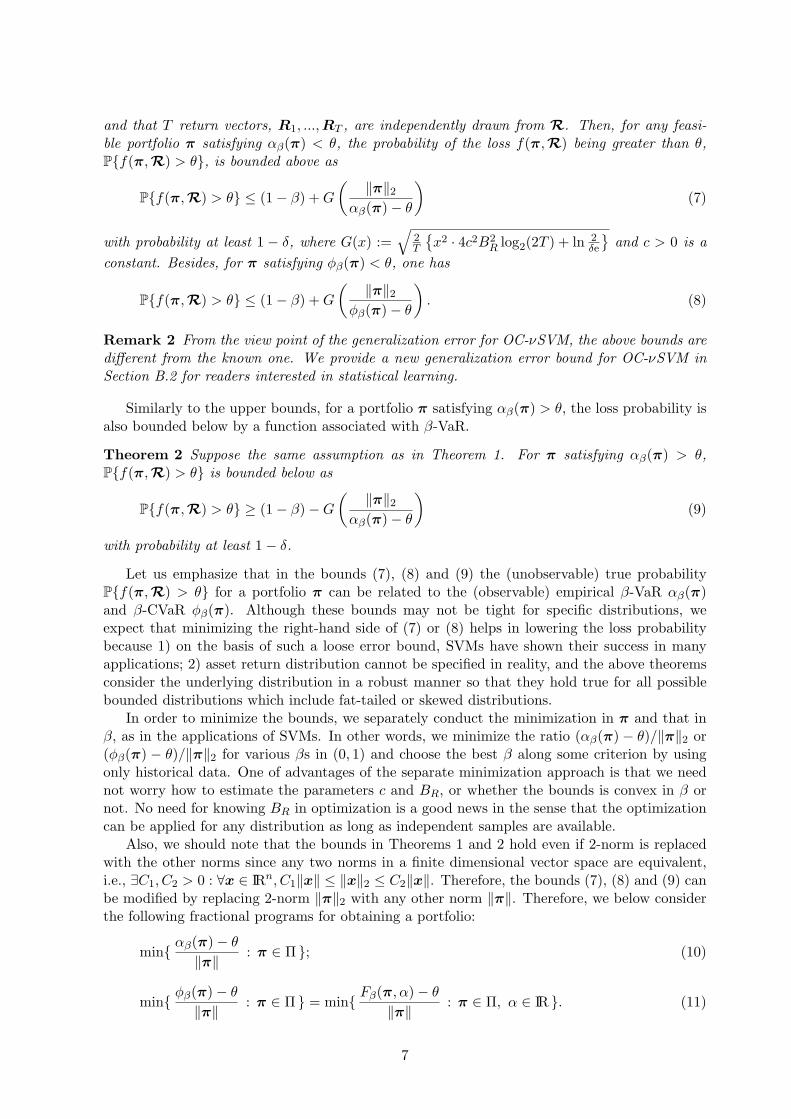
and that T return vectors, R1, ...,RT , are independently drawn from R. Then, for any feasi-ble portfolio π satisfying αβ(π) < θ, the probability of the loss f(π, R) being greater than θ,Pf(π, R) > θ, is bounded above as

Pf(π, R) > θ ≤ (1 − β) + G

(∥π∥2

αβ(π) − θ

)(7)

with probability at least 1 − δ, where G(x) :=√

2T

x2 · 4c2B2

R log2(2T ) + ln 2δe

and c > 0 is a

constant. Besides, for π satisfying ϕβ(π) < θ, one has

Pf(π, R) > θ ≤ (1 − β) + G

(∥π∥2

ϕβ(π) − θ

). (8)

Remark 2 From the view point of the generalization error for OC-νSVM, the above bounds aredifferent from the known one. We provide a new generalization error bound for OC-νSVM inSection B.2 for readers interested in statistical learning.

Similarly to the upper bounds, for a portfolio π satisfying αβ(π) > θ, the loss probability isalso bounded below by a function associated with β-VaR.

Theorem 2 Suppose the same assumption as in Theorem 1. For π satisfying αβ(π) > θ,Pf(π, R) > θ is bounded below as

Pf(π, R) > θ ≥ (1 − β) − G

(∥π∥2

αβ(π) − θ

)(9)

with probability at least 1 − δ.

Let us emphasize that in the bounds (7), (8) and (9) the (unobservable) true probabilityPf(π, R) > θ for a portfolio π can be related to the (observable) empirical β-VaR αβ(π)and β-CVaR ϕβ(π). Although these bounds may not be tight for specific distributions, weexpect that minimizing the right-hand side of (7) or (8) helps in lowering the loss probabilitybecause 1) on the basis of such a loose error bound, SVMs have shown their success in manyapplications; 2) asset return distribution cannot be specified in reality, and the above theoremsconsider the underlying distribution in a robust manner so that they hold true for all possiblebounded distributions which include fat-tailed or skewed distributions.

In order to minimize the bounds, we separately conduct the minimization in π and that inβ, as in the applications of SVMs. In other words, we minimize the ratio (αβ(π) − θ)/∥π∥2 or(ϕβ(π) − θ)/∥π∥2 for various βs in (0, 1) and choose the best β along some criterion by usingonly historical data. One of advantages of the separate minimization approach is that we neednot worry how to estimate the parameters c and BR, or whether the bounds is convex in β ornot. No need for knowing BR in optimization is a good news in the sense that the optimizationcan be applied for any distribution as long as independent samples are available.

Also, we should note that the bounds in Theorems 1 and 2 hold even if 2-norm is replacedwith the other norms since any two norms in a finite dimensional vector space are equivalent,i.e., ∃C1, C2 > 0 : ∀x ∈ IRn, C1∥x∥ ≤ ∥x∥2 ≤ C2∥x∥. Therefore, the bounds (7), (8) and (9) canbe modified by replacing 2-norm ∥π∥2 with any other norm ∥π∥. Therefore, we below considerthe following fractional programs for obtaining a portfolio:

minαβ(π) − θ

∥π∥: π ∈ Π ; (10)

minϕβ(π) − θ

∥π∥: π ∈ Π = min

Fβ(π, α) − θ

∥π∥: π ∈ Π, α ∈ IR . (11)

7

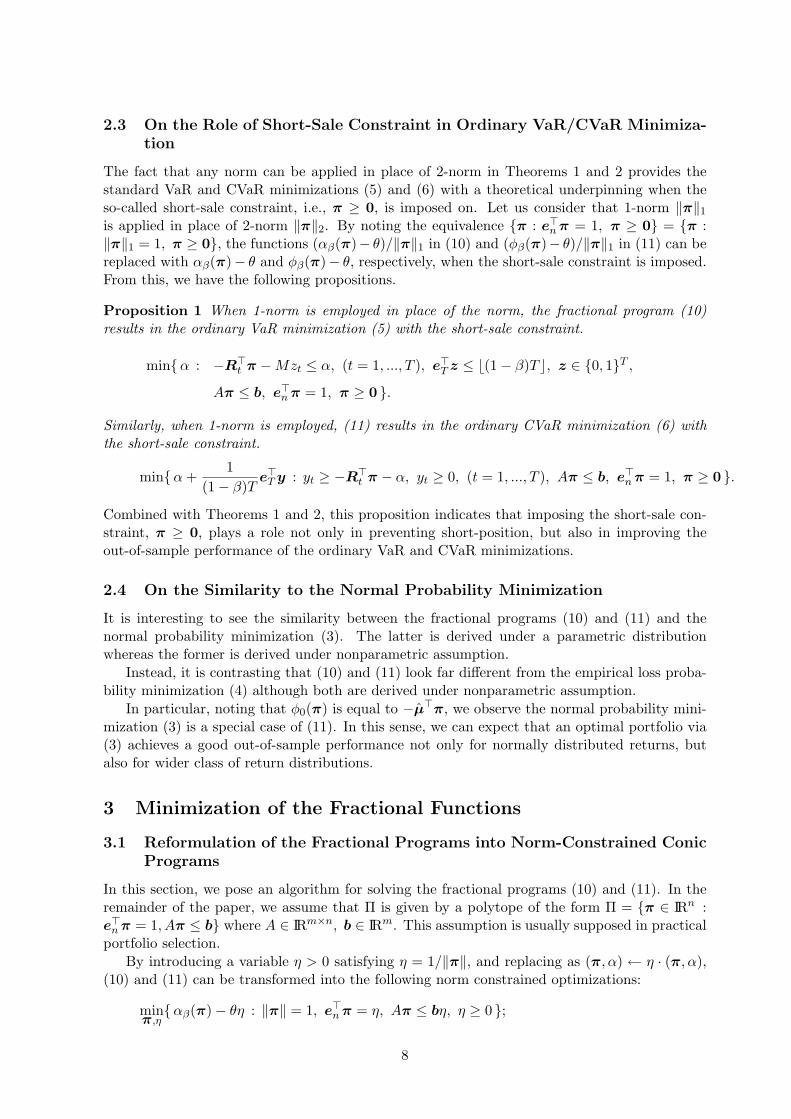
2.3 On the Role of Short-Sale Constraint in Ordinary VaR/CVaR Minimiza-tion

The fact that any norm can be applied in place of 2-norm in Theorems 1 and 2 provides thestandard VaR and CVaR minimizations (5) and (6) with a theoretical underpinning when theso-called short-sale constraint, i.e., π ≥ 0, is imposed on. Let us consider that 1-norm ∥π∥1

is applied in place of 2-norm ∥π∥2. By noting the equivalence π : e⊤n π = 1, π ≥ 0 = π :

∥π∥1 = 1, π ≥ 0, the functions (αβ(π)− θ)/∥π∥1 in (10) and (ϕβ(π)− θ)/∥π∥1 in (11) can bereplaced with αβ(π)− θ and ϕβ(π)− θ, respectively, when the short-sale constraint is imposed.From this, we have the following propositions.

Proposition 1 When 1-norm is employed in place of the norm, the fractional program (10)results in the ordinary VaR minimization (5) with the short-sale constraint.

minα : −R⊤t π − Mzt ≤ α, (t = 1, ..., T ), e⊤

T z ≤ ⌊(1 − β)T ⌋, z ∈ 0, 1T ,

Aπ ≤ b, e⊤n π = 1, π ≥ 0 .

Similarly, when 1-norm is employed, (11) results in the ordinary CVaR minimization (6) withthe short-sale constraint.

minα +1

(1 − β)Te⊤

T y : yt ≥ −R⊤t π − α, yt ≥ 0, (t = 1, ..., T ), Aπ ≤ b, e⊤

n π = 1, π ≥ 0 .

Combined with Theorems 1 and 2, this proposition indicates that imposing the short-sale con-straint, π ≥ 0, plays a role not only in preventing short-position, but also in improving theout-of-sample performance of the ordinary VaR and CVaR minimizations.

2.4 On the Similarity to the Normal Probability Minimization

It is interesting to see the similarity between the fractional programs (10) and (11) and thenormal probability minimization (3). The latter is derived under a parametric distributionwhereas the former is derived under nonparametric assumption.

Instead, it is contrasting that (10) and (11) look far different from the empirical loss proba-bility minimization (4) although both are derived under nonparametric assumption.

In particular, noting that ϕ0(π) is equal to −µ⊤π, we observe the normal probability mini-mization (3) is a special case of (11). In this sense, we can expect that an optimal portfolio via(3) achieves a good out-of-sample performance not only for normally distributed returns, butalso for wider class of return distributions.

3 Minimization of the Fractional Functions

3.1 Reformulation of the Fractional Programs into Norm-Constrained ConicPrograms

In this section, we pose an algorithm for solving the fractional programs (10) and (11). In theremainder of the paper, we assume that Π is given by a polytope of the form Π = π ∈ IRn :e⊤

n π = 1, Aπ ≤ b where A ∈ IRm×n, b ∈ IRm. This assumption is usually supposed in practicalportfolio selection.

By introducing a variable η > 0 satisfying η = 1/∥π∥, and replacing as (π, α) ← η · (π, α),(10) and (11) can be transformed into the following norm constrained optimizations:

minπ,η

αβ(π) − θη : ∥π∥ = 1, e⊤n π = η, Aπ ≤ bη, η ≥ 0 ;

8

minπ,α,η

Fβ(π, α) − θη : ∥π∥ = 1, e⊤n π = η, Aπ ≤ bη, η ≥ 0,

respectively, where η can be deleted as follows:

minπ

αβ(π) − θe⊤n π : ∥π∥ = 1, (A − be⊤

n )π ≤ 0, e⊤n π ≥ 0 ; (12)

minπ,α

Fβ(π, α) − θe⊤n π : ∥π∥ = 1, (A − be⊤

n )π ≤ 0, e⊤n π ≥ 0 . (13)

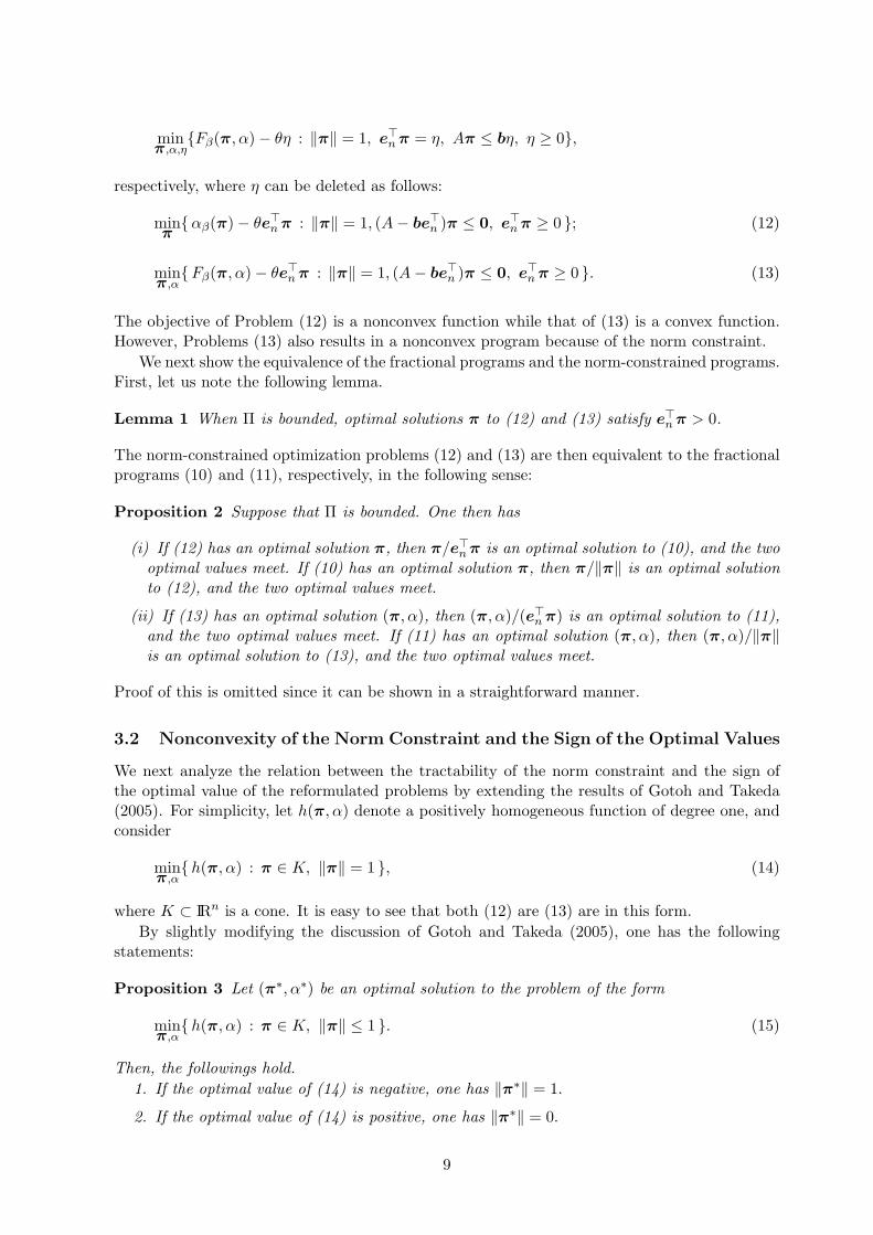
The objective of Problem (12) is a nonconvex function while that of (13) is a convex function.However, Problems (13) also results in a nonconvex program because of the norm constraint.

We next show the equivalence of the fractional programs and the norm-constrained programs.First, let us note the following lemma.

Lemma 1 When Π is bounded, optimal solutions π to (12) and (13) satisfy e⊤n π > 0.

The norm-constrained optimization problems (12) and (13) are then equivalent to the fractionalprograms (10) and (11), respectively, in the following sense:

Proposition 2 Suppose that Π is bounded. One then has

(i) If (12) has an optimal solution π, then π/e⊤n π is an optimal solution to (10), and the two

optimal values meet. If (10) has an optimal solution π, then π/∥π∥ is an optimal solutionto (12), and the two optimal values meet.

(ii) If (13) has an optimal solution (π, α), then (π, α)/(e⊤n π) is an optimal solution to (11),

and the two optimal values meet. If (11) has an optimal solution (π, α), then (π, α)/∥π∥is an optimal solution to (13), and the two optimal values meet.

Proof of this is omitted since it can be shown in a straightforward manner.

3.2 Nonconvexity of the Norm Constraint and the Sign of the Optimal Values

We next analyze the relation between the tractability of the norm constraint and the sign ofthe optimal value of the reformulated problems by extending the results of Gotoh and Takeda(2005). For simplicity, let h(π, α) denote a positively homogeneous function of degree one, andconsider

minπ,α

h(π, α) : π ∈ K, ∥π∥ = 1 , (14)

where K ⊂ IRn is a cone. It is easy to see that both (12) are (13) are in this form.By slightly modifying the discussion of Gotoh and Takeda (2005), one has the following

statements:

Proposition 3 Let (π∗, α∗) be an optimal solution to the problem of the form

minπ,α

h(π, α) : π ∈ K, ∥π∥ ≤ 1 . (15)

Then, the followings hold.1. If the optimal value of (14) is negative, one has ∥π∗∥ = 1.

2. If the optimal value of (14) is positive, one has ∥π∗∥ = 0.

9

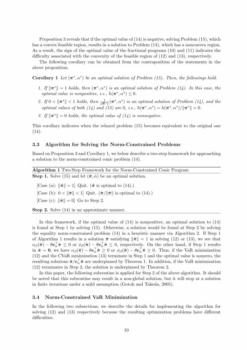
Proposition 3 reveals that if the optimal value of (14) is negative, solving Problem (15), whichhas a convex feasible region, results in a solution to Problem (14), which has a nonconvex region.As a result, the sign of the optimal value of the fractional programs (10) and (11) indicates thedifficulty associated with the convexity of the feasible region of (12) and (13), respectively.

The following corollary can be obtained from the contraposition of the statements in theabove proposition.

Corollary 1 Let (π∗, α∗) be an optimal solution of Problem (15). Then, the followings hold.

1. If ∥π∗∥ = 1 holds, then (π∗, α∗) is an optimal solution of Problem (14). In this case, theoptimal value is nonpositive, i.e., h(π∗, α∗) ≤ 0.

2. If 0 < ∥π∗∥ < 1 holds, then 1∥π∗∥(π

∗, α∗) is an optimal solution of Problem (14), and theoptimal values of both (14) and (15) are 0, i.e., h(π∗, α∗) = h(π∗, α∗)/∥π∗∥ = 0.

3. If ∥π∗∥ = 0 holds, the optimal value of (14) is nonnegative.

This corollary indicates when the relaxed problem (15) becomes equivalent to the original one(14).

3.3 Algorithm for Solving the Norm-Constrained Problems

Based on Proposition 3 and Corollary 1, we below describe a two-step framework for approachinga solution to the norm-constrained conic problem (14).

Algorithm 1 Two-Step Framework for the Norm-Constrained Conic ProgramStep 1. Solve (15) and let (π, α) be an optimal solution.

[Case (a): ∥π∥ = 1] Quit. (π is optimal to (14).)

[Case (b): 0 < ∥π∥ < 1] Quit. (π/∥π∥ is optimal to (14).)

[Case (c): ∥π∥ = 0] Go to Step 2.

Step 2. Solve (14) in an approximate manner.

In this framework, if the optimal value of (14) is nonpositive, an optimal solution to (14)is found at Step 1 by solving (15). Otherwise, a solution would be found at Step 2 by solvingthe equality norm-constrained problem (14) in a heuristic manner via Algorithm 2. If Step 1of Algorithm 1 results in a solution π satisfying ∥π∥ = 1 in solving (12) or (13), we see thatαβ(π) − θe⊤

n π ≤ 0 or ϕβ(π) − θe⊤n π ≤ 0, respectively. On the other hand, if Step 1 results

in π = 0, we have αβ(π) − θe⊤n π ≥ 0 or ϕβ(π) − θe⊤

n π ≥ 0. Thus, if the VaR minimization(12) and the CVaR minimization (13) terminate in Step 1 and the optimal value is nonzero, theresulting solutions π/e⊤

n π are underpinned by Theorem 1. In addition, if the VaR minimization(12) terminates in Step 2, the solution is underpinned by Theorem 2.

In this paper, the following subroutine is applied for Step 2 of the above algorithm. It shouldbe noted that this subroutine may result in a non-global solution, but it will stop at a solutionin finite iterations under a mild assumption (Gotoh and Takeda, 2005).

3.4 Norm-Constrained VaR Minimization

In the following two subsections, we describe the details for implementing the algorithm forsolving (12) and (13) respectively because the resulting optimization problems have differentdifficulties.

10

Algorithm 2 Subroutine for Step 2.Step 2.0. Obtain a nontrivial feasible solution π = 0, by, for example, solving a tractableproblem:

minh(π, α) : Aπ ≤ b, e⊤n π = 1 . (16)

Let (π0, α0) be an optimal solution to (16). Replacing as π0 ← π0/∥π0∥2 and k ← 1.

Step 2.k. With πk−1, solve a linearly constrained problem:

minh(π, α) : (A − be⊤n )π ≤ 0, e⊤

n π ≥ 0, (πk−1)⊤π = 1 . (17)

Let πk be an optimal solution to (17). If ∥πk∥2 = 1, terminate the algorithm with a solutionπk. Otherwise, replace as πk ← πk/∥πk∥2 and k ← k + 1, and repeat Step 2.k.

Upper Bound Minimization at Step 1. When the norm-constrained VaR minimization(12) is considered, the relaxed problem in Step 1 results in the following mixed integer quadrat-ically constrained program (MIQCP):

minα − θe⊤n π : −R⊤

t π − Mzt ≤ α, (t = 1, ..., T ), e⊤T z ≤ ⌊(1 − β)T ⌋, z ∈ 0, 1T ,

(A − be⊤n )π ≤ 0, e⊤

n π ≥ 0, π⊤π ≤ 1 ,(18)

where ⌊x⌋ denotes the maximum integer less than or equal to x, and M is a sufficiently largeconstant. Not-so-large MIQCPs can be solved in a practical time by employing the state-of-the-art optimization software. For example, it took about 170 seconds on average for solvinga problem of size n = 20 and T = 120 on a workstation environment used in the numericalexperiment in Section 4. However, computation time will exponentially grow as the problem sizeincreases. Besides, when iterative computations are required for parameter tuning, computationtime for solving single problem should be smaller. Considering such a heavy computationalburden, we only solve the CVaR-based model (11) in the next section.

Lower Bound Minimization at Step 2. When Step 1 of Algorithm 1 results in a mean-ingless solution satisfying π = 0, we have to solve MILPs iteratively in Step 2. This can still bea hard task, but it is much better than directly solving the equality-constrained problem of theform (14). In addition, the number of iterations in Step 2 is expected to be small according toGotoh and Takeda (2005).

3.5 Norm-Constrained CVaR Minimization

Upper Bound Minimization at Step 1. When the norm-constrained CVaR minimization(13) is considered, the relaxed problem (15) with h(π, α) = Fβ(π, α) in Step 1 results in thefollowing quadratically constrained program (QCP):

minα + 1(1−β)T e⊤

T y − θe⊤n π : yt ≥ −R⊤

t π − α, yt ≥ 0, (t = 1, ..., T ),

(A − be⊤n )π ≤ 0, e⊤

n π ≥ 0, π⊤π ≤ 1 ,(19)

which can be solved in an efficient manner by employing a standard optimization software.

CVaR Minimization at Step 2. Although no theoretical support has been obtained fromTheorem 1 or 2 for the CVaR minimization in the case of ϕβ(π) ≥ θ, we expect to attain a lowerloss probability even in that case because 1) β-CVaR is a tight upper bound of β-VaR especially

11

when β is large; 2) the nonconvex case which is to be solved in Step 2 sometimes ended up withbetter out-of-sample results in the classification problem (Gotoh and Takeda, 2005). The CVaRminimizations which are to be repeatedly solved in Step 2 are linear programs, and are moretractable than QCP which appears in Step 1.

4 Numerical Example

In this section, we apply the methods we discussed to real stock market data which consistof 256 monthly returns of stocks listed on the NIKKEI225 index at the end of August 2008.The investable stock set of size n is randomly chosen from 225 stocks listed on the index,n = 20, 40, 60, 80, 100, 120.

In order to evaluate the out-of-sample performance of each portfolio optimization model alongthe time series, we adopt a rolling horizon scheme as follows. At the τ -th time window, τ =T +1, ..., 256, a portfolio π∗

τ is determined by using T = 120 return observations Rτ−T , ...,Rτ−1

and is applied to the next month return Rτ . We repeat this 136 (= 256−T ) times for the wholegiven data by sliding the time window.

We solved the CVaR-based fractional program (11) with 2-norm via the algorithm describedin Section 3. The parameter β was dynamically chosen as follows. Each time a portfolio isdetermined by using historical data of size T , the first 5

6T is used for computing a portfolio withsome β and the obtained portfolio is applied to the remaining 1

6T for testing its performance.This is repeated for β = 0.5, 0.6, ..., 0.9, and one β is chosen among the five so that the portfolioachieves the highest (modified) Sharpe ratio (see, e.g., DeMiguel et al., 2009) for the test data.With the chosen β, we afresh compute a portfolio π∗

τ by using the data of size T and apply itto the next return Rτ .

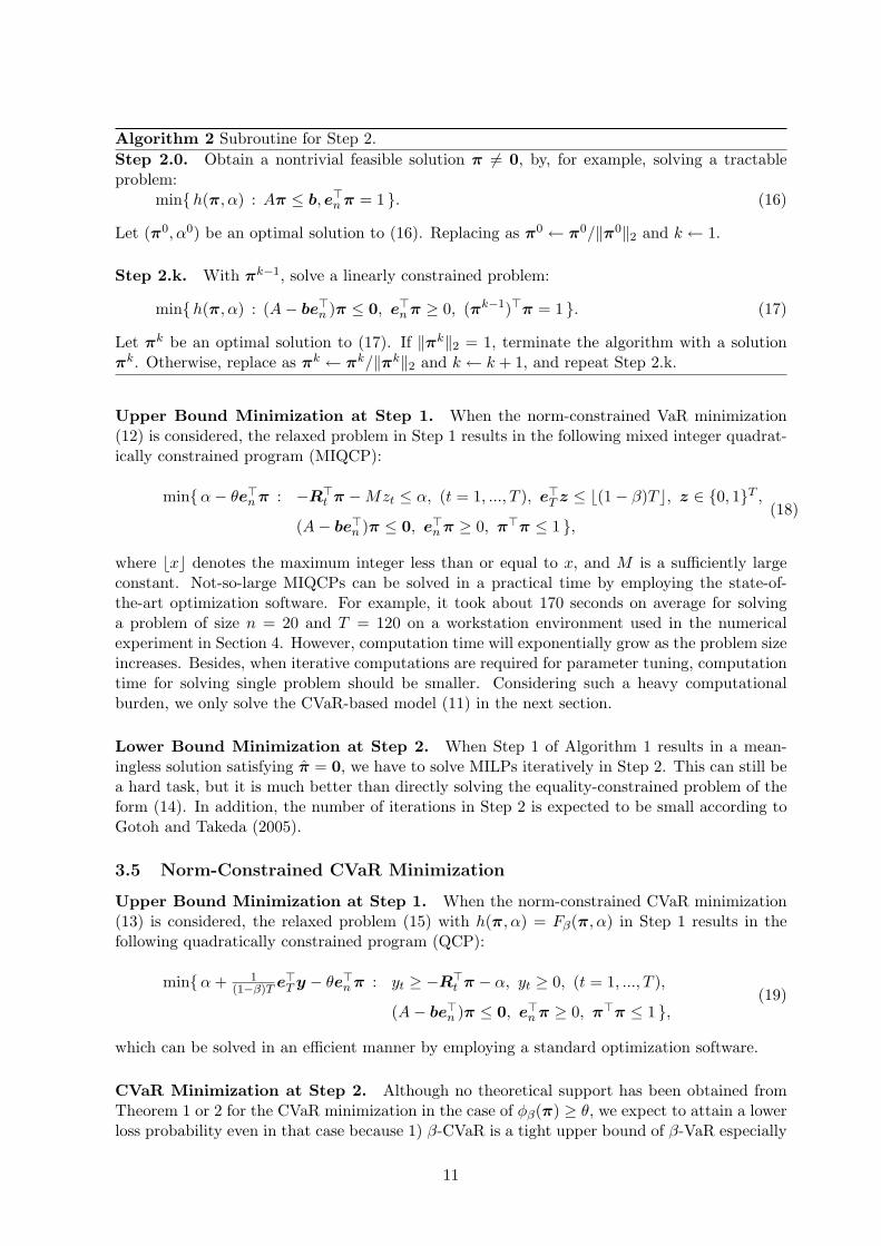
Loss Probability. First of all, we compare the empirical probability minimization (4) and theCVaR-based bound minimization (11) in terms of loss probability Pf(π, R) > θ. As stated inSection 2, the former minimizes the empirical version of the probability whereas the latter doesa (seemingly loose) bound of the probability. The thresholds θ in (4) and (11) are set equal tothe 95-percentiles of the realized distributions R⊤

τ−T π∗τ−1, ...,R

⊤τ−1π

∗τ−1 with previous portfolios

π∗τ−1 of (4) and (11), respectively. This is expected to reduce the frequency of large loss which

exceeds the 95-percentile.Figures 3 (a) to (c) show the out-of-sample loss distributions |τ = 121, ..., 256 : f(π∗

τ , Rτ ) >θ|/136 for n = 20, 60, 100. Note that these can be regarded as a realization of the loss prob-ability Pf(π∗, R) > θ with an optimal portfolio π∗. We see from these figures that moreor less, the CVaR-based bound minimization (11) achieves smaller loss probability than theempirical probability minimization (4). Especially, the former dominates the latter in Figure3 (b). Although there is no longer dominance relation in Figure 3 (c), the dispersion becomeslarger except for middle θ. Besides, for every n, the CVaR minimization (11) achieves smallerloss probability at big θs.

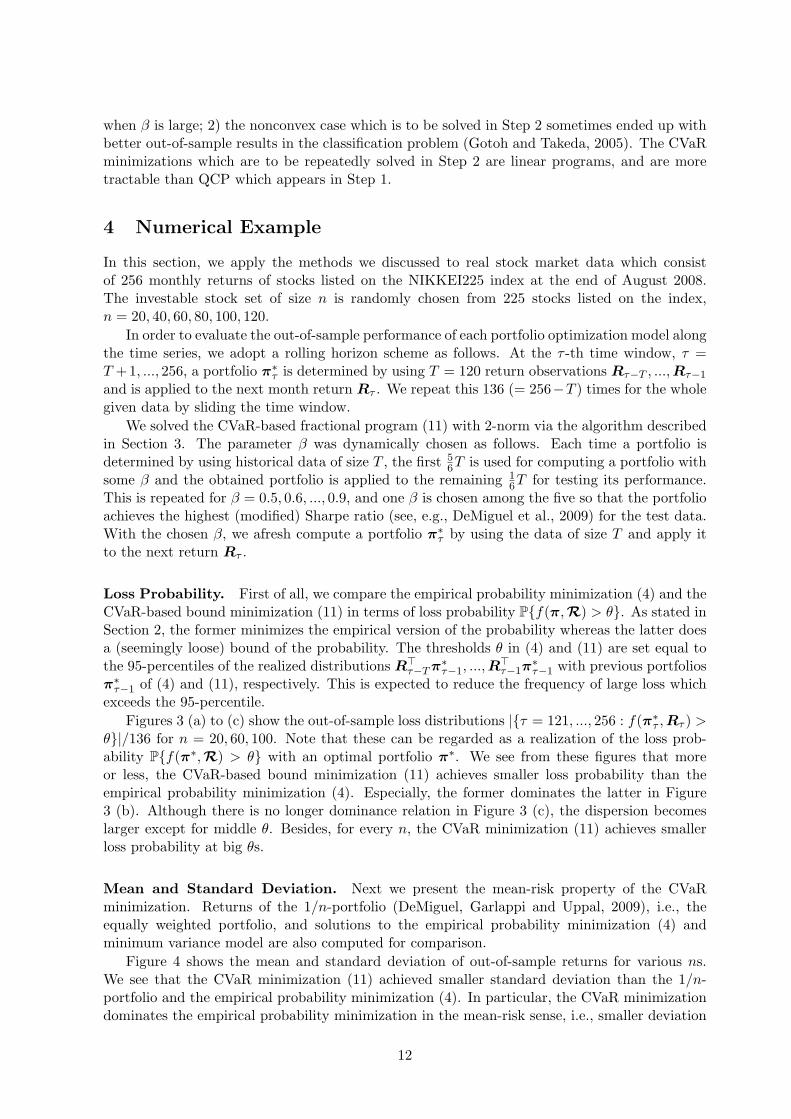
Mean and Standard Deviation. Next we present the mean-risk property of the CVaRminimization. Returns of the 1/n-portfolio (DeMiguel, Garlappi and Uppal, 2009), i.e., theequally weighted portfolio, and solutions to the empirical probability minimization (4) andminimum variance model are also computed for comparison.

Figure 4 shows the mean and standard deviation of out-of-sample returns for various ns.We see that the CVaR minimization (11) achieved smaller standard deviation than the 1/n-portfolio and the empirical probability minimization (4). In particular, the CVaR minimizationdominates the empirical probability minimization in the mean-risk sense, i.e., smaller deviation

12

0 2 4 6 8 10 12 14

0.0

0.1

0.2

0.3

0.4

θ

prob

abili

ty

CVaR min.(11) empirical prob.min.(4)

0 2 4 6 8 10 12 14

0.0

0.1

0.2

0.3

0.4

θ

prob

abili

ty

CVaR min.(11) empirical prob.min.(4)

0 2 4 6 8 10 12 14

0.0

0.1

0.2

0.3

0.4

θ

prob

abili

ty

CVaR min.(11) empirical prob.min.(4)

(a) n = 20 (b) n = 60 (c) n = 100

Figure 3: Realized Loss Probability

and larger mean. Although it has no dominating or dominated relation to the minimum variancemodel, its higher return behavior (under relatively low risk) is promising since in the literaturethe minimum variance model has been shown to perform as well as the mean-variance model.

3.5 4.0 4.5 5.0 5.5

0.1

0.2

0.3

0.4

0.5

0.6

0.7

risk (sd)

retu

rn

3.5 4.0 4.5 5.0 5.5

0.1

0.2

0.3

0.4

0.5

0.6

0.7

3.5 4.0 4.5 5.0 5.5

0.1

0.2

0.3

0.4

0.5

0.6

0.7

3.5 4.0 4.5 5.0 5.5

0.1

0.2

0.3

0.4

0.5

0.6

0.7

CVaR min.(11) empirical prob.min.(4) min.variance 1/n−portfolio

20

40

60

80

100

120

20

40

60

80100

120

20

4060

80

120

2040

60

80

100

120

20

4060

80

120

Figure 4: Out-of-Sample Mean and Standard DeviationThe number appended to each mark indicates the number of assets, n.

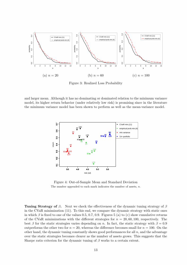
Tuning Strategy of β. Next we check the effectiveness of the dynamic tuning strategy of βin the CVaR minimization (11). To this end, we compare the dynamic strategy with static onesin which β is fixed to one of the values 0.5, 0.7, 0.9. Figures 5 (a) to (c) show cumulative returnsof the CVaR minimizations with the different strategies for n = 20, 60, 100, respectively. Thebest β for the static strategies varies depending on n. In fact, the static strategy with β = 0.9outperforms the other two for n = 20, whereas the difference becomes small for n = 100. On theother hand, the dynamic tuning constantly shows good performances for all n, and the advantageover the static strategies becomes clearer as the number of assets grows. This suggests that theSharpe ratio criterion for the dynamic tuning of β works to a certain extent.

13

0 20 40 60 80 100 120 140

0.98

1.00

1.02

1.04

1.06

1.08

1.10

term

accu

mul

ated

ret

urn

tuning ββ=0.9β=0.7β=0.5

0 20 40 60 80 100 120 140

0.98

1.00

1.02

1.04

1.06

1.08

1.10

term

accu

mul

ated

ret

urn

tuning ββ=0.9β=0.7β=0.5

0 20 40 60 80 100 120 140

0.98

1.00

1.02

1.04

1.06

1.08

1.10

term

accu

mul

ated

ret

urn

tuning ββ=0.9β=0.7β=0.5

(a) n = 20 (b) n = 60 (c) n = 100

Figure 5: Cumulative Returns of the CVaR minimizations (11) with Different βs

Behavior of the Two-step Algorithm. Finally let us mention the behavior of the two-stepalgorithm. Table 1 reports how many times the algorithm terminated in Step 1 or Step 2 amongthe 136 trials of obtaining portfolios for the out-of-sample evaluations. The rows “total wrt. β”show the numbers of βs chosen by the dynamic tuning in the rolling horizon scheme. The numberof problems whose solutions were found at Step 2 indicates how often the problem resulted in thenonconvex optimization discussed in Section 3. We see from the table that the dynamic tuningoften attained large βs with which we have to deal with the nonconvex structure. Consideringthe good performance of the dynamic tuning strategy relies in part on large βs, the nonconvexcases are also worth solving as in the classification problem (Gotoh and Takeda, 2005).

5 Concluding Remarks

In this paper, we have posed general portfolio optimization models, which are formulated asfractional programs whose objective is a ratio where the numerator includes VaR or CVaR whilethe denominator is any norm of portfolio vector. The fractional programming formulation is con-sidered as a generalization of traditional approaches in the following sense: 1) the CVaR-basedformulation includes the classical safety first criterion under normal distribution assumption as aspecial case (β = 0, ∥π∥ =

√π⊤Σπ); 2) It includes the ordinary VaR and CVaR minimizations

when the short-sale constraint is imposed and ∥π∥ = ∥π∥1. The formulation is derived so as toreduce upper and lower bounds of loss probability, which are obtained by modifying the gener-alization error bound for an SVM. In this sense, those bounds bring a theoretical underpinningto the criterion and the use of VaR and CVaR in portfolio selection.

The numerical results show that the CVaR-based probability bound minimization outper-forms the empirical probability minimization in terms of realized loss probability and mean-riskperformance. Also, the CVaR-based minimization achieves a promising portfolio performance,yielding relatively small risk and higher return than the benchmarks. This may be in part due toemploying the Sharpe ratio criterion for the dynamic tuning of β. In fact, the dynamic strategyachieved better performance than the static strategies.

On the other hand, we did not conduct experiments on the VaR-based formulation. Thisis because prohibitively large computation are required for solving hundreds of problems ofpractical size. Therefore, efficient solution to the VaR-based model is also to be developed.

14

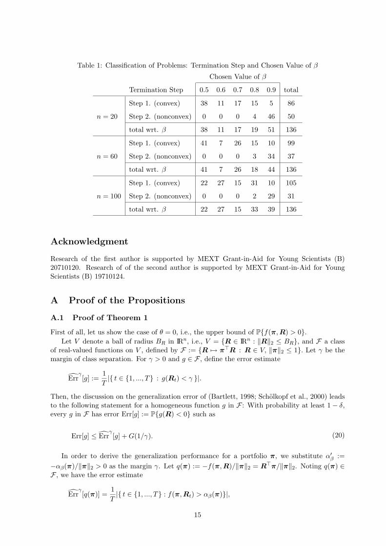
Table 1: Classification of Problems: Termination Step and Chosen Value of β

Chosen Value of β

Termination Step 0.5 0.6 0.7 0.8 0.9 total

Step 1. (convex) 38 11 17 15 5 86

n = 20 Step 2. (nonconvex) 0 0 0 4 46 50

total wrt. β 38 11 17 19 51 136

Step 1. (convex) 41 7 26 15 10 99

n = 60 Step 2. (nonconvex) 0 0 0 3 34 37

total wrt. β 41 7 26 18 44 136

Step 1. (convex) 22 27 15 31 10 105

n = 100 Step 2. (nonconvex) 0 0 0 2 29 31

total wrt. β 22 27 15 33 39 136

Acknowledgment

Research of the first author is supported by MEXT Grant-in-Aid for Young Scientists (B)20710120. Research of of the second author is supported by MEXT Grant-in-Aid for YoungScientists (B) 19710124.

A Proof of the Propositions

A.1 Proof of Theorem 1

First of all, let us show the case of θ = 0, i.e., the upper bound of Pf(π, R) > 0.Let V denote a ball of radius BR in IRn, i.e., V = R ∈ IRn : ∥R∥2 ≤ BR, and F a class

of real-valued functions on V , defined by F := R 7→ π⊤R : R ∈ V, ∥π∥2 ≤ 1. Let γ be themargin of class separation. For γ > 0 and g ∈ F , define the error estimate

Errγ[g] :=

1T| t ∈ 1, ..., T : g(Rt) < γ |.

Then, the discussion on the generalization error of (Bartlett, 1998; Scholkopf et al., 2000) leadsto the following statement for a homogeneous function g in F : With probability at least 1 − δ,every g in F has error Err[g] := Pg(R) < 0 such as

Err[g] ≤ Errγ[g] + G(1/γ). (20)

In order to derive the generalization performance for a portfolio π, we substitute α′β :=

−αβ(π)/∥π∥2 > 0 as the margin γ. Let q(π) := −f(π,R)/∥π∥2 = R⊤π/∥π∥2. Noting q(π) ∈F , we have the error estimate

Errγ[q(π)] =

1T| t ∈ 1, ..., T : f(π, Rt) > αβ(π)|,

15

which is bounded above by (1−β) by definition of αβ(π). Therefore, Err[q(π)] = Pf(π,R) > 0is bounded above by (1−β)+G(∥π∥2/αβ(π)). If ϕβ(π) < 0, the bound is, furthermore, boundedabove by (1 − β) + G(∥π∥2/ϕβ(π)) because of αβ(π) ≤ ϕβ(π).

As for the case of θ = 0, by noting e⊤n π = 1, one has

P−R⊤π > θ = P−(R + θen)⊤π > 0.

Replacing R with R + θen, the upper bounds are obtained. 2

A.2 Proof of Theorem 2

As in the proof of Theorem 1, we first consider the case of θ = 0. In this case we re-gard αβ(π)/∥π∥2 as the margin γ, and obtain Err[−q(π)] = 1 − Err[q(π)] ≤ Err

γ[−q(π)] +

G(∥π∥2/αβ(π)). Then, 1 − Errγ[−q(π)] = 1

T |t : f(π, Rt) ≥ αβ(π)| is bounded below by(1 − β) by definition. By considering e⊤

n π = 1, we establish the theorem for the case of θ = 0as in the proof of Theorem 1. 2

A.3 Proof of Lemma 1

Suppose that Π is bounded. Then, adding a set of box constraints of the form −Men ≤ π ≤ Men

to Problems (10) and (11) does not alter their feasible regions, where M > 0 is a large constant.The feasible regions of Problems (12) and (13) then satisfy −M(e⊤

n π)en ≤ π ≤ M(e⊤n π)en.

From this, if one has e⊤n π = 0 at optimality, any optimal solution π should satisfy π = 0, which

contradicts the norm constraint ∥π∥2 = 1 of (12) and (13). 2

A.4 Proof of Proposition 3

Let (π∗, α∗) be an optimal solution to (14). Then for any feasible solution (π, α) of (14), onehas h(π∗, α∗) ≤ h(π, α). Noting that any feasible solution to (15) is expressed as η · (π, α) forη ∈ [0, 1], the followings are easily obtained: when h(π∗, α∗) < 0, (π∗, α∗) achieves the minimumvalue in (15), i.e., π∗ = π∗, and when h(π∗, α∗) > 0, 0 · (π∗, α∗) is the unique minimum solutionin (15), i.e., π∗ = 0. 2

B Connection of the β-CVaR Minimization to OC-νSVM

In this part, we describe a connection of the β-CVaR Minimization to OC-νSVM and general-ization bound for OC-νSVM which is different from that in Scholkopf and Smola (2002).

B.1 Interpretation of OC-νSVM as a CVaR Minimization

Extending the discussion in (Gotoh and Takeda, 2005; Takeda, 2009), we can provide an inter-pretation of the formulation (2) for OC-νSVM in terms of CVaR minimization.

Proposition 4 The minimization of the CVaR associated with the loss −a⊤w∥w∥2

:

min α +1

(1 − β)m

m∑i=1

[−a⊤i w

∥w∥2− α]+ : w ∈ IRd, α ∈ IR (21)

is equivalent to OC-νSVM (2) with change of variable and parameter as α = −ρ/∥w∥2 and1 − β = ν if the optimal value of (21) is negative.

16

Proof. In order to prove this statement, we first observe that (21) is equivalent to the followingnorm-constrained optimization via changing variable and parameter:

min − ρ +1

νm

m∑i=1

[ρ − a⊤i w]+ : ∥w∥2 = 1, w ∈ IRd, ρ ∈ IR . (22)

Thus, what we would like to prove is that as long as the optimal value of (22) is negative,OC-νSVM (2) provides the same linear function as that of (22) except the scaling. Next, notethe following lemma:

Lemma 2 Let (w∗, ρ∗) be an optimal solution to (2). Then, (i) the optimal value of (22) isnegative if and only if (ii) ∥w∗∥2 > 0 .

Proof of the lemma

((i)⇒(ii)) Let (w, ρ) be an optimal solution to (22). Suppose that ∥w∗∥2 = 0 as well as (i),

i.e., −ρ + 1νm

m∑i=1

[ρ − a⊤i w]+ < 0. On the other hand, one observes that the optimal value of

(2) is zero since 12 · 0 − ρ∗ + 1

νm

m∑i=1

[ρ∗]+ = 1ν max(1 − ν)ρ∗,−νρ∗ ≥ 0. Note that (kw, kρ) is

feasible to (2) for any k > 0, and its objective value is 12∥kw∥2

2 − kρ + 1νm

m∑i=1

[kρ− ⟨ai, kw⟩]+ =

12k2∥w∥2

2 + k(−ρ + 1νm

m∑i=1

[ρ − ⟨ai, w⟩]+). However, this can be negative for sufficiently small

k > 0, contradicting the optimality of (w∗, ρ∗).

((ii)⇒(i)) Suppose that the objective value of (22) is nonnegative as well as ∥w∗∥2 > 0. One then

has 0 ≤ −ρ+ 1νm

m∑i=1

[ρ−a⊤i w]+ < 1

2∥w∗∥2

2−ρ∗+ 1νm

m∑i=1

[ρ∗−⟨ai, w∗⟩]+. (kw, kρ) is feasible to (2)

for any k > 0, and the corresponding objective value is 12k2∥w∥2

2 +k(−ρ+ 1νm

m∑i=1

[ρ−⟨ai, w⟩]+),

which can be smaller than the optimal value of (2) for sufficiently small k > 0, which contradictsthe optimality of (w∗, ρ∗). [end of the lemma]

Based on this lemma, we can see that ( w∗

∥w∗∥2, ρ∗

∥w∗∥2) is an optimal solution to (22) when the

optimal value of (22) is negative. On the contrary, when the optimal value of (22) is positive,(2) results in a meaningless solution, w∗ = 0, while (22) returns a solution with w = 0. 2

B.2 A Generalization Error Bound for OC-νSVM

From the view point of the generalization error for OC-νSVM, the bounds (7) and (8) aredifferent from the known one. Indeed, the bound given in Scholkopf and Smola (2002) are heldonly at the optimal solution of the problem (2). On the other hand, (7) and (8) bound theloss probability at any vector satisfying e⊤

n π = 1. Therefore, by slightly modifying the proof ofTheorem 1, we can obtain the following bounds for OC-νSVM.

Proposition 5 (Generalization bounds for OC-νSVM) Let θA be a threshold. Let α1−ν(w)be the (1 − ν)-VaR associated with the loss −A(w) = −a⊤w. Suppose that the n-dimensional

random vector a has a bounded support in the sense that the (n + 1)-dimensional vector(

aθA

)lies in a ball of radius BA centered at the origin, and that m vectors, a1, ...,am, are indepen-dently observed. Then, for any weight vector w satisfying α1−ν(w) < θA, the probability of thefunction A(w) being smaller than −θA, PA(w) < −θA, is bounded above as

PA(w) < −θA ≤ ν + G

(∥w∥2 + 1

α1−ν(w) − θA

)(23)

17

with probability at least 1 − δ, where G(x) :=√

2m

x2 · 4c2B2

A log2(2m) + ln 2δe

and c > 0 is a

constant. Besides, let ϕ1−ν(w) be the (1 − ν)-CVaR associated with the loss −A(w). Then, forw satisfying ϕ1−ν(w) < θA, one has

PA(w) < −θA ≤ ν + G

(∥w∥2 + 1

ϕ1−ν(w) − θA

). (24)

When one sets θA = −ρ∗ and w = w∗, the bound (24) is equal to that of Scholkopf et al.(2000).

Proof. Using w =(

w1

)and a =

(aθA

), we regard a homogeneous function a⊤w/∥w∥2 as

g in (20) and set a margin as γ = (θA − α1−ν(w))/∥w∥2 > 0. Noticing that 1m | i ∈ 1, ..., m :

−a⊤i w > α1−ν(w)| ≤ ν, we have a bound (23) of the generalization error Err[g] = Pg(R) < 0

as shown in the proof of Theorem 1. The bound (24) is also achieved when ϕ1−ν(w) < θA. 2

References

Artzner P, Delbaen F, Eber JM, Heath D. Coherent Measures of Risk. Mathematical Finance 1999; 9;203–228.

Bartlett PL. The Sample Complexity of Pattern Classification with Neural Networks: The Size of theWeights is More Important than the Size of the Network. IEEE Transactions on Information Theory1998; 44; 525–536.

Chopra VK, Ziemba WT. The Effect of Errors in Means, Variance, and Covariance on Optimal PortfolioChoice. Journal of Portfolio Management 1993; 19; 6–11.

DeMiguel V, Garlappi L, Nogales FJ, Uppal R. A Generalized Approach to Portfolio Optimization:Improving Performance By Constraining Portfolio Norms. Management Science 2009; 55; 798–812.

DeMiguel V, Garlappi L, Uppal R. Optimal versus Naive Diversification: How Inefficient Is the 1/NPortfolio Strategy? Review of Financial Studies 2009; 22; 1915–1953.

Gotoh J, Takeda A. A Linear Classification Model Based on Conditional Geometric Score. Pacific Journalon Optimization 2005; 1; 277–296.

Hastie T, Tibshirani R, Friedman J. The Elements of Statistical Learning –Data Mining, Inference, andPrediction. Springer-Verlag: New York; 2001.

Jagannathan R, Ma T. Risk Reduction in Large Portfolios: Why Imposing the Wrong Constraints Helps.The Journal of Finance 2003; 4; 1651–1683.

Konno H, Yamazaki H. Mean-Absolute Deviation Portfolio Optimization Model and Its Applications toTokyo Stock Market. Management Science 1991; 37; 519–531.

Markowitz H. Portfolio Selection. Journal of Finance 1952; 7; 77–91.

Ogryczak W, Ruszczynski A. Dual stochastic dominance and related mean–risk models. SIAM Journalon Optimization 2002; 13; 60–78.

Perez-Crus F, Weston J, Hermann DJL, Scholkopf B 2003. Extension of the ν-SVM Range for Classifi-cation. In: Suykens JAK, Horvath G, Basu S, Micchelli C, Vandewalle J (Eds), Advances in LearningTheory: Methods, Models and Applications 190. IOS Press: Amsterdam; 2003. p.179–196.

Rockafellar TR, Uryasev S. Conditional Value-at-Risk for General Loss Distributions. Journal of Bankingand Finance 2002; 26; 1443–1471.

18

Roy AD. Safety-First and the Holding of Assets. Econometrics 1952; 20; 431–449.

Scholkopf B, Smola AJ. Learning with Kernels –Support Vector Machines, Regularization, Optimization,and Beyond. The MIT Press: Massachusetts; 2002.

Scholkopf B, Smola AJ, Williamson RC, Bartlett PL. New support vector algorithms. Neural Computation2000; 12; 1207–1245.

Simaan Y. Estimation risk in portfolio selection: The mean variance model versus the mean absolutedeviation model. Management Science 1997; 43; 1437–1446.

Takeda A. Generalization Performance of ν-Support Vector Classifier Based on Conditional Value-at-RiskMinimization. Neurocomputing 2009; 72; 2351–2358.

Young MR. A Minimax Portfolio Selection Rule with Linear Programming Solution. Management Science1998; 44; 673–683.

19