Minimal HaemodynaIllic Modelling of the Heart & Circulation for Clinical Application Bram W. Smith A thesis presented for the degree of Doctor of Philosophy In Mechanical Engineering at the University of Canterbury, Christchurch, New Zealand. 19 January 2004

Welcome message from author
This document is posted to help you gain knowledge. Please leave a comment to let me know what you think about it! Share it to your friends and learn new things together.
Transcript

Minimal HaemodynaIllic Modelling of the Heart &
Circulation for Clinical Application
Bram W. Smith
A thesis presented for the degree of
Doctor of Philosophy
In
Mechanical Engineering
at the
University of Canterbury,
Christchurch, New Zealand.
19 January 2004

iii
To:
Sheena E. Smith
my best friend and wife
1 .3 FEB 2004
Acknowledgements
There have been lnany people that have helped me along the way with this
research. I would first like to thank my supervisors; Geoff Chase, Geoff Shaw
and Roger Nokes for their contributions. I mn very lucky to have a great group
of supervisors that have all been happy to help me when I needed it.
In particular I would like to thank Geoff Chase, my main supervisor. Geoff
was always available to discuss issues, particularly when I was having difficulties.
He included n1e in a nun1ber of different research areas outside my main topic,
which I found very interesting, and spent a lot of time helping me with my writing.
His contributions and guidance have been greatly appreciated.
I would also like to thank the following people who alllnade contributions:
Geoff Shaw, my contact at Christchurch hospital and the person who first
proposed the research topic. His help and enthusiasm for the research were in
valuable, especially when I was trying to figure out all the medical textbooks. No
wonder it takes years of training to be a doctor when the medical textbooks are
so difficult to read.
Roger Nokes; who I first contacted to help me with the fluids aspects of my
research. He has always been happy to talk and I found my discussions with him
to be very useful and enjoyable.
Ian Coope, who always enthusiastically helped me, and developed the opti
misation routine I use when Matlab's optimisation routines wouldn't work, using
his extensive knowledge and enthusiasm for optimisation.
Tim David, who made valuable contributions helping me understand the
fluids problen1s. His positive feedback when I initially showed hin1 my work was
very motivating.
Graeme Wake, who has always been ready to help when I needed it since my
undergraduate.
Garage (Gary Wake), who helped with the final proof reading of this thesis
vi
and was able to pick up on a number of errors that the rest of us missed. Also,
for the many enjoyable hours of kayaking we did every week that helped me get
over the days when I didn't seem to be getting anywhere.
Andrew Rudge, for doing the initial proof reading of each chapter and making
some valuable contributions.
Mum, Dad and the rest of my family for their encouragement and support
all the way through university, and also Sheena's family for their support and
interest.
Most importantly, I would like to thank Sheena, for her support and under
standing, and for always being enthusiastic about the research, even though she
didn't always understand it.

Contents
Abstract
1 Introduction 1.1 Applications of a CVS Model 1.2 Cardiovascular System Physiology .
1.2.1 The Heart ....... . 1.2.2 The Circulatory System 1.2.3 Cardiac Function .....
1.3 Cardiovascular Systelll Modelling 1.3.1 Finite Element Approach. 1.3.2 The Pressure-Volume (PV) Approach .
1.4 Minimal Modelling Approach 1.4.1 Model Specifications
1.5 Summary . . . . . . . . . .
2 Minimal Model 2.1 Single Ventricle Model .... .
2.1.1 The PV Diagram ... . 2.1.2 2.1.3 2.1.4
Cardiac Driver Function Blood Flow ...... . Summary of Single Chamber Model .
2.2 Ventricular Interaction .. . 2.2.1 Volume Definitions ....... .
2.2.2 Pressure Definitions ....... .
2.3 Peripheral Circulation, Closing the Loop 2.3.1 Pulmonary Circulation ..... . 2.3.2 Systemic Circulation . . . . . . .
2.4 Summary of Minimal Model Construction
3 Blood Flow in the Heart 3.1 Equations Governing Flow Rate ............ .
3.1.1 Poiseuille's Equation with Constant Resistance
xxiii
1 1 3 3 5
8 12 12 13 19 19 20
23 25 26 28 30 31 31 32 34 36 37 38
39
41 42 44
viii
3.1.2 Including Inertial Effects 3.2 The Womersley Number . . . . 3.3 Time Varying Resistance . . . .
3.3.1 Non-dimensionalisation. 3.4 Summary . . . . . . . . . . . .
4 Numerical Simulation Methods 4.1 Basic Model . . . . . . . . . . . 4.2 Inertia and Time Varying Resistance . .
4.2.1 Inertia with Constant Resistance 4.2.2 Valve Simulation . . . . . 4.2.3 Time Varying Resistance .
4.3 Ventricular Interaction . 4.4 Full Closed Loop Model 4.5 Initial Conditions ...
4.5.1 Zero Flow ICs . 4.5.2 Dynamic ICs
4.6 Summary . . . . . . .
5 Model Simulation & Verification 5.1 Single Chamber & Cardiac Dynamics
5.1.1 Passive Cardiac Chamber 5.1.2 Active Cardiac Chamber .. . 5.1.3 Time Varying Resistance .. .
5.2 Two Chambers & Ventricular Interaction. 5.3 Closed Loop Results, Physiological Verification. 5.4 Summary .. . . . . . . . . . . . . . . . . . . .
6 Optimisation of Model Parameters 6.1 The Optimisation Routine .....
6.1.1 Optimisation Variables . . . 6.1.2 The Objective Function Array.
6.2 Restructuring the CVS Model for Optimisation 6.2.1 Gradient Estimation ..... 6.2.2 6.2.3 6.2.4
Convergence . . . . . . . . . . . . . . . . Checking for Corrupt Results ..... . Finding a Steady State CVS Model Solution
6.3 Summary ., . . .
7 Optimisation Results 7.1 Convergence..........
7.1.1 Continuous Simulation
CONTENTS
45 48 52 52 55
57 57 59 59 59 61 63 66 67 67 68
70
73 74 75 76 78 81 81 85
87 88
89 91
96 97 99
101 101 102
105 105 106

CONTENTS
7.1.2 Gradient Estimation 7.2 Optimisation ....... .
7.2.1 Sensitivity Analysis. 7.3 Summary ......... .
8 Dynamic Response Verification 8.1 Ventricular Interaction . . . . . . . . . .
8.1.1 Static Ventricular Interaction . . 8.1.2 Dynamic Ventricular Interaction. 8.1.3 Ventricular Interaction Summary
8.2 Cardiopulmonary Interaction .. . 8.2.1 Respiratory FUnction .. . 8.2.2 8.2.3 8.2.4 8.2.5
Measuring Effects on CVS Other Models . . . . . . . Shnulation of Cardiopulmonary Interaction . Cardiopulmonary Interactions Summary
8.3 SUllllnary ....... .
9 Simulating Disease State 9.1 Heart Failure ..... .
9.1.1 Myocardial Dysfunction 9.1.2 Valvular Disorders ... 9.1.3
9.2 Shock 9.2.1 9.2.2 9.2.3 9.2.4 9.2.5
SUlnmary of Heart Failure Simulation .
Reflex actions . . . Hypovolemic Shock Distributive Shock Cardiogenic Shock . Extracardiac Obstructive Shock
9.2.6 Shock Discussion 9.3 Summary . . . . . . . .
10 Conclusions
11 Future Work 11.1 Model Structure . 11.2 Cardiac Driver FUnction 11.3 Optimisation ..... . 11.4 Application as a Diagnostic Aid 11.5 SUllllnary ........... .
A ODE Calculations
ix
106 108 112 115
117 118 118 120 130 131 131 133 134 134 144 145
147 148 148 151 155 156 158 160 163 164 166 168 169
171
175 175 177 178 179 179
181

List of Figures
1.1 Diagram of heart showing directions of blood flow. ........ 4
1.2 A cOlnputer reconstruction of a heart showing the right ventricle
as appearing to be attached to the side of the left ventricle [Weber
et aI., 1981]. ............................. 4
1.3 NIodified sketch of the circulation system originally drawn by Ver-
salius (1514-1564) in his Tabulae Anatomicae [Opie, 1998]. 6
1.4 Simplified diagram of the human heart and circulation system
[Guyton, 1991]. . . . . . . . . . . . . . . . . . . . . . . . . . . .. 7
1.5 Diagram showing the heart located between the lungs and the rela-
tive variations in intrapulmonary pressure, thoracic cavity pressure
and volume of breath (modified from [Ganong, 1979]).
1.6 An example of a pressure volume diagram. . .....
1.7 Variations in the ESPVR (labelled systolic failure) and the ED
PVR (labelled diastolic failure) during heart failure [Opie, 1998].
1.8 Illustration of aorta (top), the hydraulic representation of the aorta
(middle) and the electrical analogy representation (bottom). . ..
8
9
10
13
1.9 Comparing two CVS model representation of roughly equal size,
electrical circuit analogy (a) and hydraulic representation (b). .. 15
1.10 Electrical analogy of cardiopulmonary system by Sun et.al. (1997). 17
2.1 The presented closed loop model of the cardiovascular system. 24
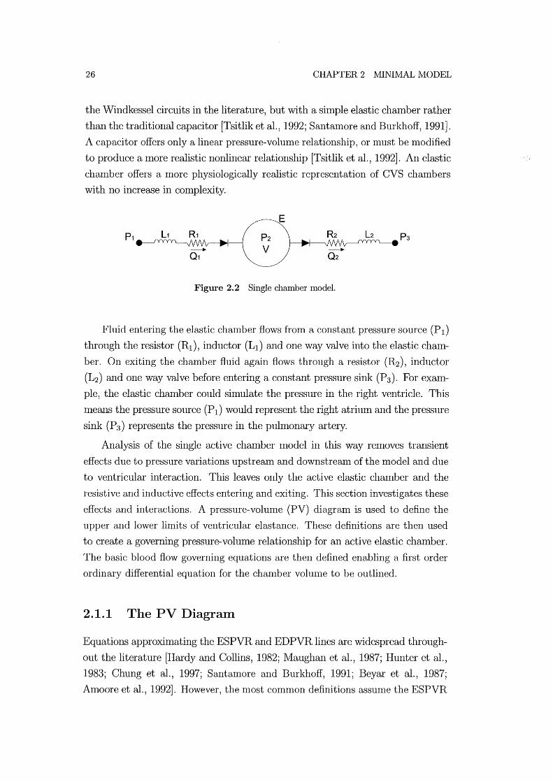
2.2 Single chamber model. . . . . . . . . . . . . . . . . . . . . . . 26
2.3 Pressure-volume diagram of the cardiac cycle and the variations
in end-diastolic and end-systolic pressure-volume relationships. 27
2.4 The model cardiac driver (e( t)). 29
2.5 Normalised time-varying resistance curve [Segers et aI., 2000a]. 29

XII LIST OF FIGURES
2.6 Two ventricle open loop model with ventricular interaction. 32
2.7 Sectioned view of the heart with left and right ventricles and left
and right ventricle and septum free walls.
2.8 Sectioned view of heart enclosed in the pericardium labelling cham-
ber pressures and pressures across walls. . .....
3.1 Flow through a rigid pipe of constant cross section.
3.2 Inductor and a resistor in series.
3.3 The velocity profile at zero flow rate.
3.4 Sinusoidally varying pressure gradient driving flow (top), varia-
33
35
44
46
48
tions in fJu/fJr(ro) and Q for small Womersley number flow, a = 0.009,
(middle) and large Womersley nunlber flow, a = 55 (bottom). .. 51
4.1 The 3 states of a single ventricle system during the cardiac cycle. 60
4.2 The 3 states of a single ventricle system during the cardiac cycle
on a PV diagram. 61
4.3 Percentage error of stroke volmne versus number of nodes on ra-
dius. . . . . . . . . . . . . . . . . . . . . . . . . . . . . . . . . .. 64
4.4 Pressure-volume diagram showing ED pressure as a function of ED
vohnne and ED pressure as a function of both ED volume and ES
volume. .............................. 69
5.1 Model settling from initial conditions with driver deactivated. 76
5.2 Results from single chamber model with driver function included
(e(t)). ................................. 77
5.3 Model settling from different initial conditions to the same solu-
tion. . . . . . . . . . . . . . . . . . . . . . . . . . . . . . . . . .. 78
5.4 Volume and pressure outputs showing long term stability in the
single chamber model with inertia. 79
5.5 Velocity profile method (VProf) and constant resistance method
(CR) results overlaid with inertial effects assumed to be negligible. 80
5.6 Velocity profile nlethod (VProf) and constant resistance (CR) re-
sults overlaid with density = 1050kg/m3• .•........•.. 80
5.7 Velocity profile method results (VProf) overlaid on constant resis-
tance results (CR) on a PV diagram. . . . . . . . . . . . . . . .. 81

LIST OF FIGURES xiii
5.8 Conlparing the variations in left and right ventricle volumes (V1v
and V rv) with the septunl deflection (Vspt ) and the pericardium
deflection (V pcd). . . . . . . . . . . . . . . . . . . . . . . . . . .. 82
5.9 Shnulation results froln the closed loop model with inertia and
ventricular interaction. 83
5.10 The Wiggers diagranl showing pressure and volume variations in
the left ventricle [Guyton, 1991]. ....... 84
5.11 The effect of varying ventricular contractility. 84
5.12 Shnulation for changes in systelnic resistance. 85
5.13 Response of aortic pressure to changes in systemic resistance. 85
5.14 Change in stroke volunle and PV diagram for a change in thoracic
pressure. 86
6.1 Flow chart showing the sequential steps of the opthnisation rou-
tine. . . . . . . . . . . . . . . . . . . . . . . . . . . . . . . . . .. 90
6.2 DiagraIn showing technique for Inaking a linear approxhnation of
the gradient of the puhnonary vein volume. ............ 98
6.3 Diagram illustrating on iteration of the gradient esthnation Inethod.
6.4 Steps taken by CVS 1110del to find steady state solution.
7.1 Peripheral chamber volume profiles resulting from continuous sim-
100
102
ulation to convergence. ....................... 106
7.2 Plot of puhnonary vohune converging to steady state solution from
different initial conditions. 107
7.3 Gradient estimation plots overlaid on continuous shnulation. 108
7.4 Profiles of the optiIl1isation variables and objective functions for
the first 20 sample steps. ...................... 109
7.5 Variations in opthnisation variables and objective function values
over an optimisation run plotting only iterations. 111
7.6 The CVS Il10del outputs run using the model parameters deter-
lnined by opthnisation. 112
7.7 Plot of Jacobian Inatrix showing the sensitivity of each opthnisa-
tion variable. 114
xiv LIST OF FIGURES
7.8 Plot of Jacobian matrix showing which optilnisation variables sig-
nificantly affect each objective function. 114
8.1 Diagram of the circulation system showing the location of the con-
strictions. . . . . . . . . . . . . . . . . . . . . . 121
8.2 Sectioned heart view showing crystal locations. 122
8.3 Haelnodynrumc CVS responses to sequential constrictions and re
leases of the pulmonary artery ruld vena-cava [Slinker and Glantz,
1986]. ................................. 124
8.4 Haemodynrunic CVS responses silnulated using the presented model.
..................................... 125
8.5 Comparing experilnental and sinlulated changes for prilnary ex-
perilnent. 126
8.6 Comparing experinlental and simulated changes for secondary ex-
perilnent. 127
8.7 Left ventricle volume variations with both series ruld direct in
teraction (top), with direct interaction only (middle) and series
interaction only (bottOln). . . . . . . . . . . . . . . . . . . . . . . 129
8.8 Changes in thoracic cavity pressure (Pth ) and puhnonary vascular
resistance (Rpul (t)) during positive pressure respiration. ..... 136
8.9 Experimental data Ineasured during positive pressure respiration
[Scharf et aI., 1980]. ......................... 138
8.10 Silnulated changes in CVS dynrunics during positive pressure res
piration with time varying pulmonary resistance (In=inspiration,
Out=expiration). .......................... 138
8.11 Scaled view the Qpv and Qav plots from Figure 8.10 showing Qav
lags Qpv by approximately 0.75 seconds. .............. 139
8.12 Simulated changes in CVS dynrunics during positive pressure respi-
ration with constant pulmonary resistance (In=inspiration, Out=expiration) .
. . . . . . . . . . . . . . . . . . . . . . . . . . . . . . . . . . . . . 140
8.13 Experilnental data measured during laboured spontaneous respi-
ration [Scharf et aI., 1979]. ..................... 142
8.14 Simulated changes in CVS dynrunics during laboured spontaneous
respiration with time varying puhnonary resistrulce (In=inspiration,
Out=expiration). .......................... 143
LIST OF FIGURES
8.15 SiInulated changes in CVS dynamics during laboured spontaneous
respiration with constant puhnonary resistance (In=inspiration,
xv
Out=expiration). .......................... 144
9.1 Comparison of diastolic dysfunction schematic with simulated re-
Slllts. . . . . . . . . . . . . . . . . . . . . . . . . . . . . . . . . . . 149
9.2 COlnparison of systolic dysfunction schelnatic with siInulated results. 150
9.3 Effect of decreased contractility and adnlinistration of a vasodilator
(hatched) [Parrillo and Bone, 1995]. ................ 151
9.4 Minimal model simulated effect of decreased left ventricle contrac
tility (dashed line) and decreased resistance sinlulating adnlinis-
tration of a vasodilator ( shaded area). ............... 152
9.5 Left ventricle pressure (solid line) and aortic pressure (dashed line)
schematic profiles for a nornlal heart, one with aortic stenosis, and
one with aortic regurgitation [Opie, 1998]. ............. 153
9.6 MiniInallnodel siInulations of left ventricle pressures for a healthy
heart valve (top), aortic stenosis (nliddle) and aortic insufficiency
(bottOln). ............................... 154
9.7 Mininlallnodel simulated changes in peripheral pressures due to
COlllrllon reflex response changes in resistance, heartbeat and stressed
blood volume. ............................ 159
9.8 Variations in stroke volulne and cardiac output with heartrate dur
ing exercise (Ex), supraventricular tachycardia (SVT) and left ven-
tricle failure (LVF) [Opie, 1998]. .................. 161
9.9 Variations in cardiac output versus heart rate for the lninimal
nlodel with two different sets of paranleters. . . . . . . . . . . . . 161
9.10 SiInulation of hypovolelnic shock, before blood loss (-), after
blood loss (- - -), after blood loss and increased Rsys due to re-
flex action (- .. ) . 162
9.11 Simulation of distributive septic shock, before drop in systenlic
resistance (-) and after (- - -). . . . . . . . . . . . . . . . . . . . 163
9.12 Minimallnodel simulation before (-) and after (- - -) left ventricle
infarction, and after increased stressed blood volurne (- .. ). 165

xvi LIST OF FIGURES
9.13 Minimal model silnulation before (-) and after (- - -) right ven
tricle infarction, and after increased stressed blood volume ( ... ).
9.14 Silnulation of pulmonary elnbolism, before (-) and after (- - -).
9.15 Minimal nlodel simulation of pericardial tamponade before (-),
166
168
after (- - -) and after potential reflex actions (- .. ). . . . . . . . . 169
11.1 Potential Inodel structure for capturing more subtle CVS dynam-
ics. 176
11.2 Left ventricle and ascending aorta pressures in a dog [Noble, 1968J. 177
List of Tables
2.1 Flow rate variables froln the full closed loop n10del of Figure 2.1. 31
2.2 Vohllne Variables. . 33
2.3 Pressure Variables. 35
2.4 Peripheral circulation systeln elastic chamber volume definitions. 38
3.1 Constants used in single-chamber silnulation. .
4.1 Pressure Variables. . ............. .
5.1 Mechanical properties of the heart and circulation system.
5.2 Hydraulic properties for flow between chan1bers.
5.3 Constants used in single-chalnber silnulation ..
6.1 Values of optilnisation routine paran1eters.
50
67
74
75
75
89
6.2 Model Paralneters to be optilnised. . . . . 91
6.3 Target Model Outputs frOln Guyton 1991. 93
6.4 Target Model Outputs as averages and amplitudes froln Guyton
1991. . . . . . . . . . . . . . . . . . . . . . . . . . . . . . . . . .. 94
7.1 Data comparing the rate of convergence of continuous simulation
versus gradient estilnation. . . . . . . . . . .
7.2 Model Paralneter values after optimisation ..
7.3 Objective Function Values. . . . . . . . . . .
109
110
113
8.1 Correlation between model variables and the experimental mea
surements taken by Scharf et.al. (1979; 1980). . . . . . . . . . . . 137
9.1 Correlation between measured physiological data and Inodel vari-
ables. . . . . . . . . . . . . . . . . . . . . . . . . . . . . . . . . . . 157

xviii LIST OF TABLES
9.2 Known physiological response of CVS variables during diff'erent
shock states, reproduced from Parrillo and Bone (1995).. . . . . . 158
9.3 Summary of the CVS response to diff'erent common reflex actions,
as plotted in Figure 9.7. ....................... 158
Nomenclature
a WOluersley nUluber
£ length of tube or vessel
A parmueter in EDPVR
J-l blood viscosity
v blood kinematic viscosity
w heart rate (beats/sec)
p density
e angle
ao aorta
av aortic valve
BPM beats per minute, heart rate
CO cardiac output
CR constant resistance
CVS cardiovascular systen1
e( t) cardiac driver function
ED end-diastolic
Ees end-systolic elastance
EDPVR end-diastolic pressure volun1e relationship
ES end-systolic
ESPVR end-diastolic pressure vohuue relationship
F objective function array
El part of E relating to target function values
E2 part of E relating to alTIount model paralTIeters are changed
HR heart rate, (beats/min)
L inertm1ce

xx
la
Iv
lvf
Int
M
ODE
E P
left atrium
left ventricle
left ventricle free wall
lnitral valve
objective function array
ordinary differential equation
model parameters array
pressure
NOMENCLATURE
Po
Ped
parmneter in EDPVR relating to end-diastolic elastance
end-diastolic pressure
Pes
Pth
pa
PAC
pcd
pu
pul
pv
PV
end-systolic pressure
thoracic cavity pressure
pulmonary artery
pulmonary artery constriction
pericardium
puhnonary vein
puhnonary circulation systeln
pulmonary valve
pressure-vohnne
Q flow rate (litres/nlin)
r radius
ro nlaxilnlnn radius
R resistance
Rpul (t) tilne varying puhnonary resistance, due to respiration
ra right atrhnn
RPAC release pulmonary artery constriction
rv right ventricle
RVCC release vena-cava constriction
rvf right ventricle free wall
spt septum
SV stroke volume
sys systemic circulation systeln

NOIVIENCLATURE
tc tricuspid valve
11 velocity profile vector
y optinnsation variables array
V volume
vc vena-cava
vee vena-cava constriction
V d relaxed end-systolic volume
Vo relaxed end-diastolic volume
VProf velocity profile n1ethod
Vtot stressed blood volume
x position along length of vessel or tube
xxi
Abstract
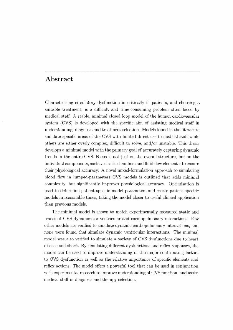
Characterising circulatory dysfunction in critically ill patients, and choosing a
suitable treatInent, is a difficult and tinle-consunling problenl often faced by
Inedical staff. A stable, Ininimal closed loop nlodel of the human cardiovascular
system (CVS) is developed with the specific aim of assisting nledical staff in
understanding, diagnosis and treatlnent selection. Models found in the literature
silnulate specific areas of the CVS with limited direct use to medical staff while
others are either overly complex, difficult to solve, and/or unstable. This thesis
develops a minhnallnodel with the prhnary goal of accurately capturing dynmnic
trends in the entire CVS. Focus is not just on the overall structure, but on the
individual components, such as elastic chambers and fluid flow elements, to ensure
their physiological accuracy. A novel Inixed-formulation approach to shnulating
blood flow in lunlped-parameters CVS Inodels is outlined that adds nlinilnal
complexity, but significantly improves physiological accuracy. Optinlisation is
used to determine patient specific nl0del paranleters and create patient specific
nl0dels in reasonable times, taking the nlodel closer to useful clinical application
than previous Inodels.
The nlinhnal Inodel is shown to Inatch experimentally Ineasured static and
transient CVS dynamics for ventricular and cardiopuhnonary interactions. Few
other nlodels are verified to sinlulate dynanlic cardiopulnl0nary interactions, and
none were found that simulate dynmnic ventricular interactions. The minimal
Inodel was also verified to simulate a variety of CVS dysfunctions due to heart
disease and shock. By sinlulating different dysfunctions and reflex responses, the
Inodel can be used to improve understanding of the major contributing factors
to CVS dysfunction as well as the relative importance of specific elelnents and
reflex actions. The nlodel offers a powerful tool that can be used in conjunction
with experimental research to hnprove understanding of CVS function, and assist
Inedical staff in diagnosis and therapy selection.

Chapter 1
Introduction
Cardiovascular disease is the largest cause of death in western countries [Wester
hof, 2003]. Cardiovascular dysfunction can occur in lnany areas of the cardiovas
cular systmn (CVS) as a result of a wide range of causes, such as age, birth defects
or illness. While a great deal of research has been carried out investigating CVS
function, nluch is still unknown about the causes and treatlnent of cardiovascular
disease. The CVS is an extrmnely cOlnplex systenl involving a cOlnbination of
hydraulic interactions, nervous systeln responses and other biological influences.
These cOlnplex interactions lnean that although extensive experimental research
has been carried out into CVS function, a great deal relnains unknown about the
cause and effect of these interactions and dysfunctions.
This chapter discusses how a working miniInal nlodel of the CVS would be
useful to nledical staff in patient diagnosis and treatInent. The physiology of the
circulation systeln is also discussed, elnphasising the dynamics that this lnodel
ainlS to reproduce. Different approaches to modelling the CVS found in the
literature are discussed and cOlnpared with the aiIns of this work. Fronl this
discussion a IniniInal model design philosophy is outlined in detail.
1.1 Applications of a CVS Model
While extensive experimental research has been carried out, there is still lnuch
to be learned about the function of the CVS system in healthy and dysfunctional
circulation systelllS. ExperiInental work is mostly carried out on aniInals and
often involves invasive surgery that itself significantly affects CVS function. In
addition, data measured from patients with various CVS diseases is not only
influenced by the cause of the dysfunction, but by the reflex actions that are
activated to lnaintain blood pressure and cardiac output.
2 CHAPTER 1 INTRODUCTION
Pin-pointing CVS dysfunction is often difficult because the clinical signs, or
the availability and interpretation of physiological measurelnents, are unreliable,
noisy or contradictory. Health professionals must often rely on intuition and
experience to make a "clinical" diagnosis in order to decide upon treatment op
tions. Sometimes this approach results in Inultiple therapies being applied until
a suitable treatment is found. Poor outcomes or death can result from failure to
correctly diagnose and treat the underlying condition.
A suitable CVS nl0del could be used to assist nledical staff in a variety of
applications ranging from improving understanding of CVS function to assisting
in diagnosing the cause of dysfunctions. Unlike most experilnental research, a
Inodel can isolate the function of particular areas of the CVS and identify their
contribution to the overall haeInodynalnics. A model could also be used to iden
tify the ilnpact of particular dysfunctions on overall CVS function while ignoring
the effects of reflex actions .
. This research ailns to create a Ininimal Inathematical Inodel of the cardio
vascular system to directly assist health professionals in the key areas of under
standing, diagnosis and therapy. Medical staff will be able to easily investigate
the cause and effect of various types of cardiac dysfunctions. A nl0del that cap
tures many of the essential dynamics of the CVS can also be used as a teaching
aid to ilnprove understanding of CVS function. An appropriate cOInputer Inodel
of the CVS system could be used to process patient data including blood pres
Slues, respiratory pressures, blood flow rates, ECG signals and heart rate. The
Inodel can be used to identify inconsistencies and irregularities in recorded pa
tient data to aid rnedical staff in choosing suitable fluid, drug, or mechanical
interventions to inlprove patient condition. 1\I10re specifically, the known effects
of treatments such as drug therapies, or Inechanical assist devices can be applied
to a model that has been customised to silnulate a particular patients condition
[Frazier et al., 2001; Westabyet al., 2000].
A specific example of modelling particular treatnlents is the VentT Assist car
diac assist device currently being tested in New South Wales, Australia [Ven
trAssist, 2003]. This small electronic centrifugal pUInp bypasses the aortic valve,
pUInping blood directly froln the ventricle into the aorta helping to increase cir
culation and blood pressure [Skatssoon, 2003]. The impact on CVS dynamics of
ilnplanting the VentT Assist pump could, for example, be tested on the proposed
model to detennine the feasibility of implants.

1.2 CARDIOVASCULAR SYSTEM PHYSIOLOGY 3
1.2 Cardiovascular System Physiology
The CVS can be divided into two key areas: the heart, which PUIUPS the blood,
and the circulation systelU, which channels the blood to every part of the body
[Guyton, 1991; Hurst, 1966]. The heart and CVS form an extremely complex
system with Iuany books dedicated to explaining all of the hydraulic, nervous and
biological interactions. This research focuses on simulating hydraulic function,
which nleans that although the effects of different reflex actions can be simulated,
the physiological activation of these actions is not modelled.
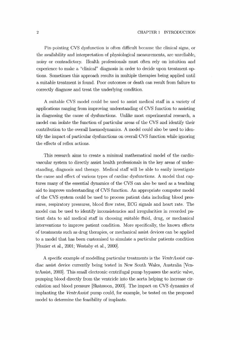
1.2.1 The Heart
The heart is Iuade up of two distinct PUIUPS known as the left and the right
heart. The right heart pumps deoxygenated blood returning from the body into
the lungs where carbon dioxide is removed and oxygen is absorbed into the blood.
The left heart pU111pS oxygenated blood frolu the lungs to all the tissues in the
peripheral circulation, supplying thelu with oxygen and nutrients. The layout of
the heart and the flow of blood through it is shown in Figure 1.1. Each pump
consists of an atrilllU and a ventricle in series. Both are active elastic chambers
that contract by increasing wall tension to plUUp blood. The ventricle provides
IUOSt of the pUIuping function and the atrium acts as a booster to suppleluent
ventricle perfornlance. In fact, the heart can operate effectively under resting
conditions without the atria functioning, relying solely on the ventricles [Guyton,
1991].
Both ventricles and atria are contained within the pericardiluu, a relatively
stiff walled passive elastic chanlber that encapsulates the heart [Glantz and ParIU
ley, 1978]. During contraction, the walls of the cardiac chalubers thicken, swelling
both inwards to reduce challlber volume, and outwards. The pericardium acts as
an outer constraint to this expansion, meaning the myocardiulu mostly expands
inwards, forcing blood out of the ventricle. Without this outer constraint of the
pericardiuIu, ventricle performance is reduced [Hoit et al., 1993].
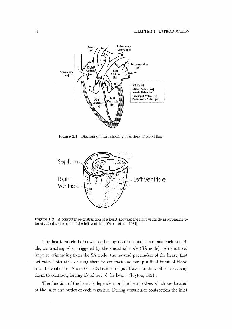
As shown in Figure 1.2 the right ventricle appears attached to the wall of
the left ventricle and they share a COillluon section of cardiac muscle wall called
the septum. It is because of this comnl0n wall, as well as the influence of the
pericardiun1, that the ventricles interact with each other. For eXalllple, right
ventricle overload is widely investigated, where right ventricle swelling pushes on
the left ventricle and impedes its function [Marcus et al., 2001; Lazar et al., 1993].
4
Yena-CaY3 lye]
CHAPTER 1 INTRODUCTION
VALVES Mitral Valve (mt] Aortic Valve la,'] TJicuspid ValYe ftc] Pulmonary Valve [Py]
Figure 1.1 Diagram of heart showing directions of blood flow.
" ':.' .
Septum ', __
Right :;):J:' l l Ventricle"- ,',:,.' ~ ..
Figure 1.2 A computer reconstruction of a heart showing the right ventricle as appearing to be attached to the side of the left ventricle [Weber et al., 1981].
The heart muscle is known as the Inyocardium and surrounds each ventri
cle, contracting when triggered by the sinoatrial node (SA node). An electrical
impulse originating from the SA node, the natural pacenlaker of the heart, first
activates both atria causing them to contract and pump a final burst of blood
into the ventricles. About 0.1-0.2s later the signal travels to the ventricles causing
theln to contract, forcing blood out of the heart [Guyton, 1991].
The function of the heart is dependent on the heart valves which are located
at the inlet and outlet of each ventricle. During ventricular contraction the inlet
1.2 CARDIOVASCULAR SYSTEM PHYSIOLOGY 5
heart valves close and the outlet valves open, pushing blood into the arterial
circulation system. During ventricle expansion, the outlet valves close and the
inlet valves open to allow blood to flow into the ventricles fron1 the venous systenl.
Thus, the heart valves ensure blood only flows in a forward direction through the
ventricles and are essential for heart function. This dependence means valvular
dysfunctions, such as nlitral stenosis or aortic insufficiency, can significantly affect
heart function causing life threatening consequences [Braunwald, 1997; Parrillo
and Bone, 1995].
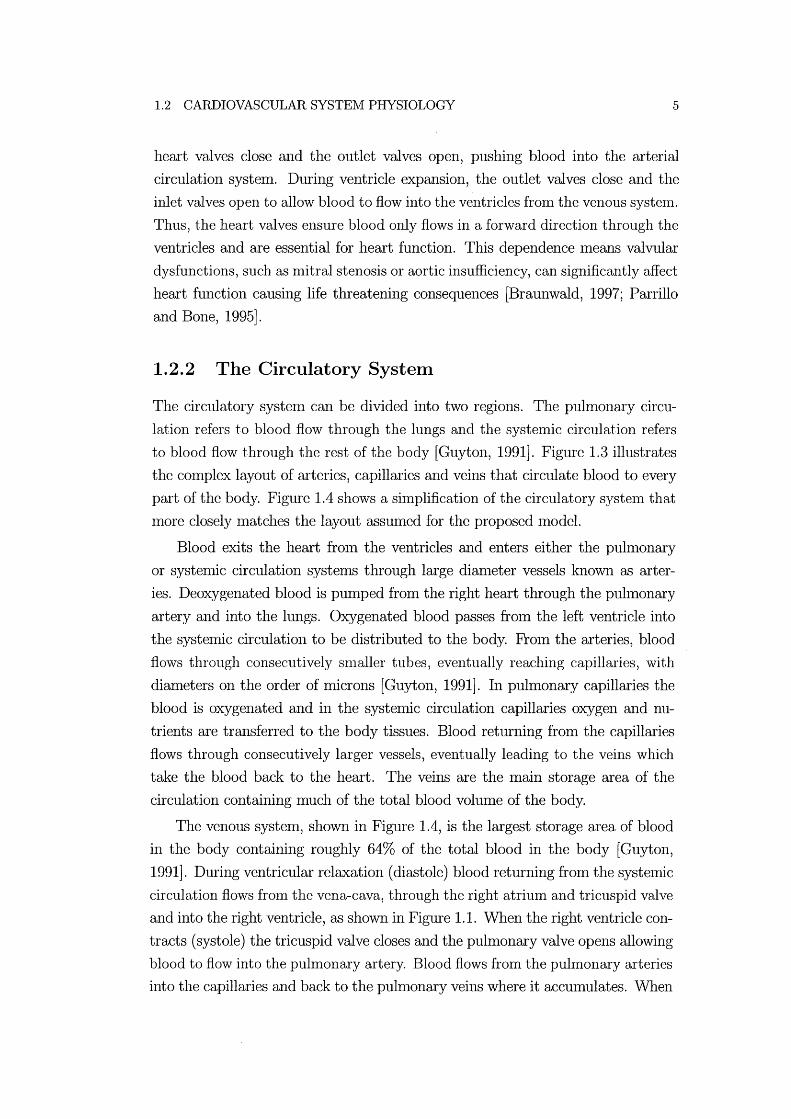
1.2.2 The Circulatory System
The circulatory system can be divided into two regions. The puhnonary circu
lation refers to blood flow through the lungs and the systel11ic circulation refers
to blood flow through the rest of the body [Guyton, 1991]. Figure 1.3 illustrates
the conlplex layout of arteries, capillaries and veins that circulate blood to every
part of the body. Figure 1.4 shows a sinlplification of the circulatory systel11 that
Inore closely Inatches the layout assluned for the proposed Inodel.
Blood exits the heart fron1 the ventricles and enters either the puhnonary
or systenlic circulation systelllS through large dimneter vessels known as arter
ies. Deoxygenated blood is pUInped from the right heart through the puhnonary
artery and into the lungs. Oxygenated blood passes froln the left ventricle into
the systenlic circulation to be distributed to the body. Froln the arteries, blood
flows through consecutively snlaller tubes, eventually reaching capillaries, with
dian1eters on the order of Imcrons [Guyton, 1991]. In pulmonary capillaries the
blood is oxygenated and in the systemic circulation capillaries oxygen and nu
trients are transferred to the body tissues. Blood returning fron1 the capillaries
flows through consecutively larger vessels, eventually leading to the veins which
take the blood back to the heart. The veins are the Inain storage area of the
circulation containing much of the total blood volume of the body.
The venous system, shown in Figure 1.4, is the largest storage area of blood
in the body containing roughly 64% of the total blood in the body [Guyton,
1991]. During ventricular relaxation (diastole) blood returning from the systelnic
circulation flows frOl11 the vena-cava, through the right atrium and tricuspid valve
and into the right ventricle, as shown in Figure 1.1. When the right ventricle con
tracts (systole) the tricuspid valve closes and the pulmonary valve opens allowing
blood to flow into the pulmonary artery. Blood flows from the pulmonary arteries
into the capillaries and back to the pulmonary veins where it accumulates. When
6 CHAPTER 1 INTRODUCTION
Figure 1.3 Nlodified sketch of the circulation system originally drawn by Versalius (1514-1564) in his Tabulae Anatomicae [Opie, 1998].
the left ventricle relaxes, the mitral valve opens and blood flows through the left
atriuln into the left ventricle. ArB the left ventricular pressure increases during
systole, the mitral valve closes and the aortic valve opens, forcing blood into
the aorta. Blood enters the aorta and flows into the capillaries of the systenlic
circulation until finally returning to the vena-cava.
The heart is located, along with the pulmonary circulation, within the tho
racic cavity. The pressure in the thoracic cavity varies as the pressure in the lungs
varies during respiration. As shown in Figure 1.5, the thoracic cavity pressure
is defined as the pressure around the outside of the heart. The intrapulmonary
pressure is the pressure inside the lungs. The plot in Figure 1.5 shows the relation
ship between the variation in the thoracic cavity pressure and the intrapulmonary

1.2 CARDIOVASCULAR SYSTEM PHYSIOLOGY
Pulmonary Circulation (Lungs) [pull
Pulmonary Vein __ [pv]
Aorta [ao]
Systemic Circulation (Body) [sys]
Figure 1.4 Simplified diagram of the human heart and circulation system [Guyton, 1991].
pressure.
7
Pressure variations in the lungs alter the pressure acting on the outside of
the heart, having an impact on its performance. During an intake of breath
(inspiration) the diaphragnl deflects downwards causing negative thoracic cavity
and intrapuhnonary pressures as air is sucked into the lungs. When breathing
out (expiration) the diaphragm deflects upwards increasing the intrapulnlonary
pressure to become positive and forcing air out of the lungs, while the thoracic
cavity pressure becOlnes less negative. This variation in intrapulmonary pressure
during respiration results in variations in thoracic cavity pressure as shown in
Figure 1.5 and influences the function of the heart.
Inspiration causes a negative pressure in the thoracic cavity (about -8mmHg
for a nornlal person) and results in a build-up of blood in the pulmonary cir
culation systeln. The opposite effect occurs during expiration when the intra
pulmonary pressure is positive and the thoracic cavity pressure is higher (about
-5lIllnHg for a normal person). Air is forced out of the lungs and the higher pres
sure causes the vohune of blood in the pulmonary circulation system to decrease
[Scharf and Cassidy, 1989; Guyton, 1991].

8 CHAPTER 1 INTRODUCTION
+1
0
-1 Pressure (mmHg)
-2
-3
-4
-5
-6
0.6
0.4 Volume
0.2 (L)
0 0 2 3 4
Time (sees)
Figure 1.5 Diagram showing the heart located between the lungs and the relative variations in intrapulmonary pressure, thoracic cavity pressure and volume of breath (modified from [Ganong, 1979]).
These cardiopulrnonary interactions can have a significant effect on cardiac
perforn1ance, particularly on cardiac output. During positive pressure breathing,
where a patient is n1echanically ventilated, the thoracic cavity pressure signifi
cantly affects cardiac output [Scharf and Cassidy, 1989]. The positive pressure
generated in the lungs by mechanical ventilation causes a significant drop in car
diac output, which can be detrimental to the health of a ventilated critically ill
patient, although it does protect the lungs.
1.2.3 Cardiac Function
Indices of cardiac function are used by health professionals to identify the per
formance of the heart. Three of the most common indicators of cardiac function
include the pressure-volume (PV) diagram, cardiac output, preload and afterload.
These measures are often used by health professionals to study patient condition.

1.2 CARDIOVASCULAR SYSTEIvr PHYSIOLOGY 9
The PV Diagram
PV diagrams for elastic chanlbers, as schematically shown in Figure 1.6, are
used extensively by lnedical professionals to explain the pumping lnechanics of
the ventricle. A lot of infonnation can be interpreted from a PV diagranl and it is
the method of choice for both medical staff and engineers for analysing ventricle
function. Two main characteristics of the PV diagram are the lines plotting
the End Systolic Pressure-Volunle Relationship (ESPVR) and the End Diastolic
Pressure-Vohune Relationship (EDPVR) which define the upper and lower linlits,
respectively, of the cardiac cycle.
opens
Outlet valve opens
Inlet valve closes
Ventricle Volume
Figure 1.6 An example of a pressure volume diagram.
The cardiac cycle, lnarked on Figure 1.6 by the triangular arrows, is divided
into four parts: filling, contraction, ejection and relaxation. Filling occurs when
the upstreaIn pressure in the atriunl is greater than the pressure in the ventri
cle. During contraction, the pressure in the ventricle becomes greater thaIl the
pressure upstreanl, the inlet flow goes to zero, and the valve closes. ~Tith both
inlet and outlet valves closed a period of isovolumetric ventricular contraction is
induced by the cardiac muscle. When the ventricle pressure is above the down
strealn pressure in the arteries the outlet valve opens and blood is ejected. The
ejection phase continues until the flow out of the ventricle stops, the outlet valve
closes, and the ventricle relaxes. The ventricle expands isovolulnetrically during
relaxation until its pressure is again below the upstream pressure and the inlet
valve opens to repeat the cycle. Note that the open on pressure, close on flow
valve law is clearly evident in these fundaInental definitions [Opie, 1998; Little,
1978].
10 CHAPTER 1 INTRODUCTION
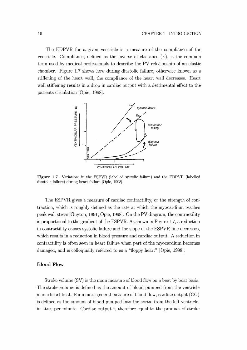
The EDPVR for a given ventricle is a Ineasure of the compliance of the
ventricle. Con1pliance, defined as the inverse of elastance (E), is the common
tenn used by Inedical professionals to describe the PV relationship of an elastic
chamber. Figure 1. 7 shows how during diastolic failure, otherwise known as a
stiffening of the heart wall, the compliance of the heart wall decreases. Heart
wall stiffening results in a drop in cardiac output with a detrimental effect to the
patients circulation [Opie, 1998J.
8 ill a: ::> CI) (f) LIJ a: a.. a: 5 ::> o 0: IZ ill >
-----VENTRICULAR VOLUME
systolic failure
/'
dilated and failing
t diastolic faifure
; /'
".../
Figure 1.7 Variations in the ESPVR (labelled systolic failure) and the EDPVR (labelled diastolic failure) during heart failure [Opie, 1998].
The ESPVR gives a Ineasure of cardiac contractility, or the strength of con
traction, which is roughly defined as the rate at which the myocardium reaches
peak wall stress [Guyton, 1991; Opie, 1998J. On the PV diagrmn, the contractility
is proportional to the gradient of the ESPVR. As shown in Figure 1.7, a reduction
in contractility causes systolic failure and the slope of the ESPVR line decreases,
which results in a reduction in blood pressure and cardiac output. A reduction in
contractility is often seen in heart failure when part of the myocardium becomes
d an1 aged , and is colloquially referred to as a "floppy heart" [Opie, 1998J.
Blood Flow
Stroke volume (SV) is the Inain measure of blood flow on a beat by beat basis.
The stroke volume is defined as the amount of blood pumped fron1 the ventricle
in one heart beat. For a more general measure of blood flow, cardiac output (CO)
is defined as the amount of blood pumped into the aorta, fron1 the left ventricle,
in litres per minute. Cardiac output is therefore equal to the product of stroke
1.2 CARDIOVASCULAR SYSTEM PHYSIOLOGY 11
volume and heart rate (HR) [Opie, 1998].
CO=SVxHR (1.1 )
Cardiac output is an inlportant nleasure of cardiac function, defining the
ability of the heart to plUllp oxygen and nutrient rich blood to the peripheral
tissues. Equation (1.1) highlights the ilnportant dependence of the cardiac out
put on both stroke volulne and heart rate. While heart rate is driven by the
sympathetic nervous systeIn, the stroke vohune is dependent on the function of
the Inyocardilun as well as ventricle preloads and afterloads. Ventricle preloads
and afterloads give nleasures of the boundary conditions around the heart, which
are influenced by the cardiovascular systenl as a whole.
Preload & Afterload
The definitions of cardiac preload and afterload used in the literature vary
depending on their application. Definitions include ventricle wall stress or strain,
end-diastolic and end-systolic pressures, and peripheral resistances, as well as
nlany Inore cOInbinations [Norton, 2001]. Preload and afterload are generally
intended to be Ineasures of ventricular boundary conditions, indicating the state
of the ventricle before and after contraction respectively. Preload is a measure
of the nluscle fibre length, or the anl0unt that the cardiac muscles are stretched,
immediately prior to contraction. Afterload is a measure of the cardiac muscle
stress required to eject blood froln a ventricle, or the pressure the ventricle must
pump against. However, outside influences can affect the preload and afterload
pressures such as thoracic pressure variations due to breathing.
A more suitable means of measuring preload and afterload is the wall stress
of the ventricle, or the pressure across the ventricle wall [Norton, 2001]. How
ever, these transnlural pressures are difficult to nleasure in a patient, while the
pressures at inlet and exit froln the heart are relatively easier to measure using
COmInon invasive sensors. For this reason, venous and arterial pressures around
the heart are the most common surrogate Ineasures of ventricle preload and af
terload, respectively.

12 CHAPTER 1 INTRODUCTION
1.3 Cardiovascular System Modelling
Most approaches to nlodelling the human CVS can be divided into either finite
element (FE) or pressure-volunle (PV) approaches. The finite element approach
involves breaking down each part of the CVS in great detail and utilising finite
element calculations to silnulate function. The PV approach is a simpler method,
grouping parameters and Inaking assumptions to sinlplify the model as much as
possible, while still attenlPting to silnulate the essential dynamics. This section
discusses both nlethods and investigates which approach is best suited to the
application of diagnostic assistance and therapy selection.
1.3.1 Finite Element Approach
FE techniques offer micro-scale results that can theoretically be very accurate
both in Inagnitude and in trends. To simulate a section of the CVS, very detailed
lnicro-scale Ineasurelnents Inust be taken of its mechanical properties such as
elastic properties, dinlensions and fibre directions. This information is then used
in detailed finite elenlent equations that simulate the dynamics of the component
being Inodelled on a Inicroscale. A great deal of research has been done in this
area with significant results helping to illlprove understanding.
The Bioengineering institute at Auckland University has carried out extensive
lnicro-scale research into the structure of the heart. Work has been carried out
both nleasuring and nlodelling nlyocardial structure, coronary blood flow that
supplies blood to the heart nluscle, and the excitation of the cardiac muscles.
This group has Inapped the structure of the cardiac muscle, including Inuscle
fibre directions, and created a finite elelllent nlodel of the heart [Nielsen et al.,
1991; Legrice et al., 1997; Stevens and Hunter, 2003]. The model is used to give
detailed insight into cardiac excitation during contraction [Hunter et al., 1991;
Buist et al., 1999].
Other 1110dels such as that of Peskin et.al. (1992) attempt to model the com
plex fluid flow dynamics in the heart, particularly around the heart valves. Glass
et.al. (1991) reviews Inany of the current finite element approaches to investi
gating cardiac function. Methods are outlined for measuring and simulating the
structure, excitation and fluid flow in the heart to varying degrees of precision.
While FE silnulation research has nlade significant contributions to the un
derstanding of cardiac function, its lack of flexibility makes it unsuitable for
patient-specific, rapid diagnostic feedback. It is not feasible to obtain the detailed
1.3 CARDIOVASCULAR SYSTEM IVIODELLING 13
patient specific nleasurements of cardiac structure required to create a patient
specific nlodel from a living patient. FE nlodels require significant computational
tilne to solve even on the most powerful cOlnputers Inaking them unsuitable for
immediate feedback. These models focus primarily on the function of the heart
and either do not simulate the closed loop function, or silnulate it using lumped
parmneter models.
1.3.2 The Pressure-Volume (PV) Approach
PV methods are lumped parmneter modelling methods where the CVS is divided
into a series of elements silnulating elastic chmnbers and other elen1ents simulat
ing blood flow. Elastic chmnber elenlents Inodel the pressure-vohllne relationship
in a section of the CVS, such as a ventricle, an atritlln, or a peripheral section
of the circulation system such as the arteries or veins. The fluid flow elenlents
connecting these chambers sinlulate blood flow through different parts of the
circulation systen1. Lumped parmneter CVS Inodels are usually illustrated using
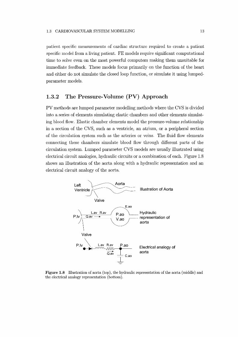
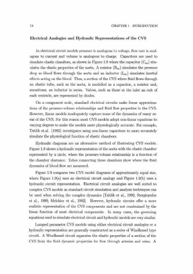
electrical circuit analogies, hydraulic circuits or a con1bination of each. Figure 1.8
shows an illustration of the aorta along with a hydraulic representation and an
electrical circuit analogy of the aorta.
Left
Ventricle \
Valve
L.av R.av P.lv Q.av -------..
\ Valve
E.ao
P.!v \ L.av R.av P.ao
c I·ao
Illustration of Aorta
Hydraulic representation of aorta
Electrical analogy of aorta
Figure 1.8 Illustration of aorta (top), the hydraulic representation of the aorta (middle) and the electrical analogy representation (bottom).
14 CHAPTER 1 INTRODUCTION
Electrical Analogies and Hydraulic Representations of the CVS
In electrical circuit Illodels pressure is analogous to voltage, flow rate is anal
ogous to current and volulne is analogous to charge. Capacitors are used to
simulate elastic chambers, as shown in Figure 1.8 where the capacitor (Cao ) sim
ulates the elastic properties of the aorta. A resistor (Rav) simulates the pressure
drop as blood flows through the aorta and an inductor (Lav) simulates inertial
effects acting on the blood. Thus, a section of the CVS where fluid flows through
an elastic tube, such as the aorta, is Inodelled as a capacitor, a resistor and,
somethnes, an inductor in series. Valves, such as those at the inlet an exit of
each ventricle, are represented by diodes.
On a component scale, standard electrical circuits Inake linear approxima
tions of the pressure-volume relationships and fluid flow properties in the CVS.
However, linear models inadequately capture some of the dynamics of Inany ar
eas of the CVS. For this reason Inost CVS Inodels adopt non-linear equations to
varying degrees to Inake the Inodels more physiologically accurate. For example,
Tsitlik et.al. (1992) investigates using non-linear capacitors to Inore accurately
simulate the physiological function of elastic chmnbers.
Hydraulic diagrmllS are an alternative Inethod of illustrating CVS n10dels.
Figure 1.8 shows a hydraulic representation of the aorta with the elastic chamber
represented by a circle, where the pressure-volume relationship is a function of
the chamber elastance. Tubes connecting these chambers show where the fluid
dynan1ics of blood flow are n1easured.
Figure 1.9 compares two CVS n10del diagralllS of approxilnately equal size,
where Figure 1.9(a) uses an electrical circuit analogy and Figure 1.9(b) uses a
hydraulic circuit representation. Electrical circuit analogies are well suited to
cOlnplex CVS models as standard circuit shnulation and analysis techniques can
be used when solving the cOlnplex dynmnics [Tsitlik et al., 1992; Stergiopulos
et al., 1999; Melchior et al., 1992]. However, hydraulic circuits offer a more
realistic representation of the CVS cOlnponents and are not constrained by the
linear function of Inost electrical components. In many cases, the governing
equations used to simulate electrical circuit and hydraulic models are very shnilar.
Lumped parameter CVS n10dels using either electrical circuit analogies or a
hydraulic representation are generally constructed as a series of Windkessel type
circuit. A Windkessel circuit separates the elastic properties of a section of the
CVS from the fluid dynaInic properties for flow through arteries and veins. A

1.3 CARDIOVASCULAR SYSTEM MODELLING
PULMONARY CIRCULA TION
1- - - - - - - - -'Nr"ERDEPENDEiic-E - -- -I
: PV '~_:~I~ __ j MV : I A1-' I I'TV Elf' EI rf' AoV, I HEART ~ rv,: T v. I I ~-----------------------
Res
l'C V$ l' Cas
SYSTEMIC C/RCULA TlON
( a) Layout of circulation system used by Santamore et.al. (1991).
PERIPHERAL UNPRESSURIZED COMPARTMENT
(b) Layout of circulation system used by Beyar et.al. (1987).
15
Figure 1.9 Comparing two CVS model representation of roughly equal size, electrical circuit analogy (a) and hydraulic representation (b).
rigid tube sinlulates the fluid dynamic effects and an elastic chamber silnulates
the compliance of the vessel [Tsitlik et al., 1992; Melchior et al., 1992]. This
approach avoids the conlplex, often unstable, equations that govern fluid flow
through an elastic vessel such as the aorta.
For exrunple, the elastic properties of the aorta are simulated using an elastic
chamber and the pressure in the chrunber is calculated using a relatively simple

16 CHAPTER 1 INTRODUCTION
pressure-volunle relationship. The fluid dynalnic properties are simulated as flow
through a rigid tube, which has much sinlpler governing equations than a flex
ible tube. Similarly, the entire CVS is divided into a series of elastic chambers
connected by rigid tubes. In Figure 1.8 the elastic properties are simulated using
either the elastic chamber or the capacitor labelled with the subscript ao. The
fluid dynanlics of blood flow through the aorta are simulated through the sections
labelled with the subscript avo
CVS models also come in varying degrees of complexity and focus, with a large
range of models that simulate only Slnall areas of the CVS. For example, some
authors focus on simulating the function of the left ventricle only [A vanzolini
et al., 1985; Hunter et al., 1983; Carnpbell et al., 1990; Wijkstra and Boom,
1991]. Others investigate the haenlodynamic effects of ventricular interaction or
interdependence with a nUlnber of different approaches used [Chung et al., 1997;
Beyar et al., 1987; Amoore et al., 1992; Santarnore and Burkhoff, 1991; Sun et al.,
1997]. Finally, some researchers attelnpt to Inodel the entire circuit as a series of
passive and active elastic charnbers in a closed circuit [Sun et al., 1997; Santamore
and Burkhoff, 1991; Beyar et al., 1987; Burkhoff and Tyberg, 1993; Ursino, 1999;
Chung et al., 1997; Olansen et al., 2000; Lu et al., 2001]. This research focuses
primarily on closed loop Inodels, although SOlne of the theory from smaller Inodels
is applied in specific areas of larger closed loop simulations.
Current Closed Loop CVS Models
Figure 1.10 illustrates the lunlped pararneter closed loop electrical circuit
analogy CVS Inodel proposed by Sun et.al. (1997). This model illustrates a com
Inon teInptation with electrical circuit analogies to build larger complex circuits
in the hope of capturing as InarlY of the CVS dynamics as possible. Complex
circuits Inay have the capability for more physiologically accurate simulations,
but understanding the individual contributions of each component and choosing
suitable parameter values is extremely difficult.
Santamore et.al. (1991) presents an electrical circuit analogy model, shown
in Figure 1.9(a), that includes the dynanlics of ventricular interaction. However,
the model is only verified against static experimental data that shows how one
ventricle reacts when the volume of the other is charlged. The model is not
shown to simulate transient haemodynamic response of ventricular interaction
due to sudden variations in the volume of one ventricle.

1.3 CARDIOVASCULAR SYSTEIVI MODELLING
Venous R",turn Righi Heart Pulmonary Circulation ~ ,,.--_.....111.\....---.\ , __ ---JA\----.
Laft Heart ,..--_-'''1-__ --,
OM jl)
Ea. tS,10
O,b ,Ul
1 l}~~
lid. J.1\)
Figure 1.10 Electrical analogy of cardiopulmonary system by Sun et.al. (1997).
17
t1a ,~l
k. u
E. ,1,1{J
Beyar et.al. (1987) presents the closed loop, 10 chmnber Inodel shown in
Figure 1. 9(b) that includes the effects of ventricular interaction and thoracic
cavity pressure variations. Limited results show the nl0del captures SOlne of the
transient response of the CVS due to dynmnic thoracic cavity pressure variations.
However, ventricular interaction is verified only against static experinlental data.
Burkhoff and Tyberg (1993) present a closed loop nl0del specifically designed
for simulating the effects of left ventricle dysfunction. Using this model they
are able to conlnlent on the contribution of nervous systeln reflexes involved in
left ventricle dysfunction in CVS dynmnics. SiInilarly, Ursino (1999) presents a
lllodel specifically designed for siIllulating the effects of the baroregulation on CVS
function. Nether 11l0del accounts for the affects of ventricular or cardiopulnl0nary
interactions. Although both Inodels Inake contributions to understanding the
mechanisms involved in these specific cases, the models are not shown to be
general enough to capture other types of dysfunction.
Chung et.al. (1997) present an open loop Inodel of the heart including ven
tricular interaction due to the septum and the pericardium. The model provides
good short term results, however these results are very dependent on accurate
calculation of initial conditions. Additionally, accumulation of numerical error
causes this model to diverge when simulated over longer periods on the order of
40secs. This problem is caused by too nlany governing equations over-defining the

18 CHAPTER 1 INTRODUCTION
model. In spite of this problmn, the Inodel was able to produce results for static
ventricular interaction that match experiInental results. Olansen et.al. (2000)
built on this work to create a much nl0re cOlnplex closed loop model that once
again Inatched static experiInental results for ventricular interaction.
Lu et.al. (2001) also extended this work to include the influence of barorecep
tor control of heart rate, nlyocardial contractility and vasomotor tone. They also
added a detailed lumped parameter nl0del of lung function and it's influence on
cardiac function. Results show the model roughly captures trends in some CVS
hamnodynaInics. It is also shown to capture the transient hamnodynaInic re
sponse of the CVS due to significant variations in thoracic cavity pressure during
forced breathing. However, the examples used for nl0del verification are limited
and the model is not shown to be flexible enough to capture a variety of dysfunc
tion. It is also worth noting that this research appears to be still built on the
over-defined ventricular interaction 1l10del presented by Chung et.al. (1997).
Although all the presented models Inake contributions to the understanding
of various types of dysfunctions, most are not shown to be capable of simulating a
range of CVS function and dysfunction. Additionally, it is not shown how any of
these nl0dels can be of direct use to nledical staff for diagnostic assistance. How
ever, these lumped parameter Inodels show how it nught be possible to capture
various CVS dynaInics using a nunimal ntunber of equations, parameters and
variables such as chaInber elastances and arterial resistances. Governing equa
tions are developed in this research that can be siInulated on modern, commonly
available desktop computers in very reasonable tiInes suitable for iImnediate feed
back.
CVS Models Summary
PV models can rapidly silnulate patient-specific CVS dynamics on a stan
dard desktop computer offering the potential for real-tinle patient specific mod
els. However, the simplicity of these nl0dels comes at the expense of accuracy
and a PV modellnay be too simple to capture all of the critical dynaInics. Where
lumped paraIneter methods sOlnetiInes do not capture enough detail there is a
need to include some of the cOlnplexity and physiologically accurate equations of
the finite element approach. Complexity costs conlputational power and time,
and should therefore only be added where significant benefits are obtained over
a simpler method. Hence, the addition of cOlnplexity to make a IUlnped pa-
1.4 IVIINIMAL MODELLING APPROACH 19
ranleter nl0del more physiologically accurate nlust be justified by deillonstrating
significant improvenlents in physiological accuracy.
The development of the lninimal lIlodel used in this research is based on a
lninimalist approach where the model is kept as simple as possible unless the
addition of complexity will result in a significant improvelnent in physiological
accuracy. The basic building blocks of the model are the passive and active elastic
chanlbers, and the governing equations for flow between these chanlbers. The
function of the basic model building blocks are investigated individually before
assembling these components to create a full closed-loop nlodel. This approach
ensures that the individual contributions of each cOIIlponent are known when
analysing the perfornlance of the cOIIlplete lIlodel.
1.4 Minimal Modelling Approach
As discussed, there are lIlany exalIlples in the literature of nlodels that silIlulate
and aid in the understanding of specific types of cardiac function. However, these
lIlodels are not shown to be of direct use to medical staff to assist in diagnosis and
therapy selection. In addition, many lIlodels in the literature focus on silIlulating
only particular types of dysfunction and not on a general silIlulation of the CVS. This research ainlS to not only create a lIlodel of the entire CVS to silIlulate a wide
variety of dysfunction, but also to structure the lIlodel so that it can be easily
applied for use by 111edical staff. This section outlines a list of specifications that
the final Inodel must achieve, followed by an outline of the general philosophy
behind this minimal lIlodel approach.
1.4.1 Model Specifications
The approach used involves combining the lumped parameter and finite elenlent
Inodelling techniques discussed previously with the requirements of Inedical staff
to create a useful, rapid-feedback, diagnostic assistance systelIl. It is intended
that the model will fulfil the following goals:
• A full closed-loop, stable model is required with lninilIlal cOIIlplexity and
physiologically realistic inertia and valve effects.
• Model parameters can be relatively easily deternlined or approxinlated for
a specific patient using standard, commonly used techniques.
20 CHAPTER 1 INTRODUCTION
• The Inodel can be run on a standard desktop computer in reasonable time,
(eg. on the order of 1-5 minutes)
• Although quantitatively exact results are not necessary, accurate prediction
of trends is required.
These goals are set to restrict the Inodel froln becoming too complex while en
suring its practicality. The lin1itations on the patient-specific information, cmn
putational power, and solution time n1eans the PV modelling method offers the
greatest potential for fulfilling the intended requiren1ents.
In SUIllillary, a "Minimal Model" approach to CVS nl0delling means using
a minimal nunlber of governing equations and parmneters where other similar
Inodels in the literature have been found to use Inany variables and cmnplex
formulae. Using Ininimal, siInple governing equations avoids the instability and
non-uniqueness of solution found in the Inodel developed by Chung et.al. (1996)
and further used by Olansen et.al. (2000) mld Lu et.al. (2001). Using minimal
variables avoids problmllS associated with large cOInplex Inodels such as the one
presented by Sun et.al. (1997). Less variables means less parameters that must
be defined, and an easier model to analyse and understand.
The general approach of this research is to Inake the Inodel IniniInal, stable
and easily solved. The CVS is an inherently stable systeln and therefore stability
in the Inodel must be a key feature. Straight forward solution is iInportant,
emphasising that the model must be solvable in a reasonable time on a standard
cOIDlnonly available cOInputer. The nuniInal CVS Inodel will be a closed loop
Inodel that is capable of capturing a variety of CVS interactions and dysfunction,
and not just focus on special cases.
1.5 Summary
An overall approach to nl0delling the hunlan CVS is proposed that will create
models to help medical staff in the key areas of understanding, diagnosis and
treatment of CVS dysfunction. A detailed design philosophy is outlined to create
an easily solved, stable, Ininimal Inodel. Prior CVS models and methods are
presented and discussed in detail. LUInped parmneter pressure-volulne modelling
methods are identified as the most suitable method for achieving the target model
perfonnance.
1.5 SUrv'lIVIARY 21
This thesis focuses first on the construction of the proposed CVS model start
ing with a silnple model of a single cardiac chamber and concluding with a full
closed loop nl0del. Two basic building block of the CVS nl0del are identified,
the governing equations for the elastic chambers and the fluid flow between these
chambers. The next chapter examines the governing equations for the active and
passive elastic chambers. The mathematics and assumptions of the fluid flow be
tween the chambers are then discussed in the following chapter. The method of
silnulating these dynamics is then discussed followed by sinlple Inodel verification
eXalnples. Subsequent chapters show n1ethods of identifying Inodel paralneters
to create patient specific models, and simulating CVS function in both healthy
and diseased cal'diovasculal' systen1S.

Chapter 2
Minimal Model
Ulthnately, the Inodel presented is intended to sinlulate the essential haelnody
nanncs of the cardiovascular systeln including the heart, and the pulnl0nary and
systelnic circulation systmllS. Figure 2.1 shows the model used for this research
Inade up of elastic chalnbers connected by resistors and inductors in series. The
layout of Figure 2.1 can be con1pared with the sin1plified representation of the
CVS shown in Figure 1.4. The atria have not been added as they contribute only
slightly to the main cardiac trends and can be easily added for Inore specific cases
[Guyton, 1991].
The Inodel is divided into blocks of Windkessel like circuits. Windkessel
circuits separate the pressure-volume properties and the fluid flow properties
of each section of the CVS into different Inodel con1ponents [Tsitlik et al., 1992;
Melchior et al., 1992]. This n1ethod avoids the con1plex formulae that govern fluid
flow through an elastic tube such as the aorta. An elastic chalnber, labelled Eao in
Figure 2.1, shnulates the elastic properties of the aorta, detennining the pressure
as a function of volume. The resistor (RllN ) and inductor (Lav) shnulate the
pressure drop and inertial effects, respectively, acting on blood flowing through
the aorta.
Each elastic chamber, labelled E in Figure 2.1, simulates the pressure-volulne
relationship in a particular area of the circulation system. Often this means that
an elastic challlber will be simulating a series of physiological chmnbers. The
Inodel presented in Figure 2.1 divides the circulation systeln into 6 Inain blood
storage areas simulated using elastic chambers.
Two active elastic chmnbers are used to simulate the left and right ventri
cles (Iv mld rv). The ventricles are coupled, via the septuln and pericardiuln,
to account for the important ventricular interaction dynmnics. The remaining
chambers are passive, with constant elastance and simulate the remainder of
24
Eve
Eao
Systemic Circulation
I I
I I
E.pcd I I
Elv I
I
IP.peri L _____ .1
CHAPTER 2 MINIMAL IvlODEL
"~- I
Epa
~ - - - - -" P.th Thoracic Cavity
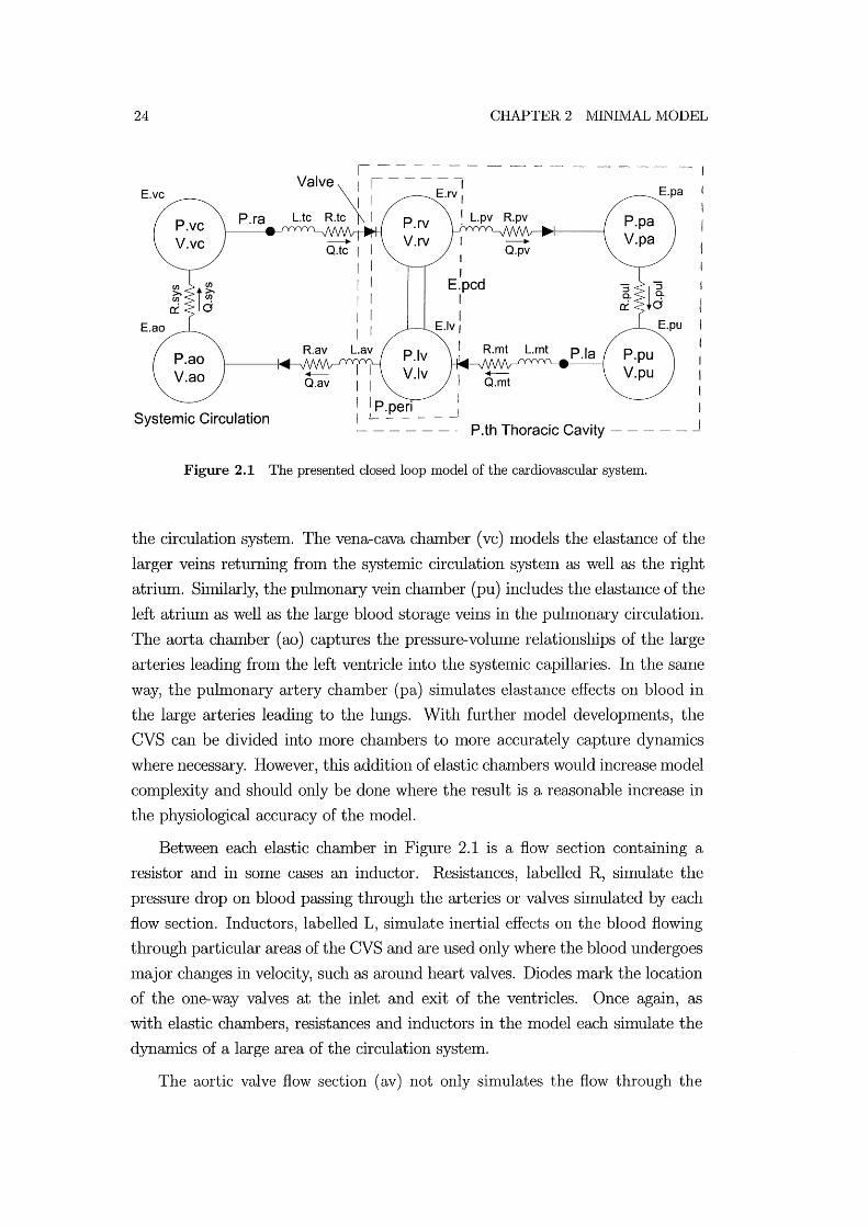
Figure 2.1 The presented closed loop model of the cardiovascular system.
the circulation system. The vena-cava chalnber (vc) Inodels the elastance of the
larger veins returning froln the systelnic circulation systen1 as well as the right
atrium. Shnilarly, the pulmonary vein chalnber (pu) includes the elastance of the
left atrium as well as the large blood storage veins in the puln10nary circulation.
The aorta chalnber (ao) captures the pressure-volume relationships of the large
arteries leading from the left ventricle into the systmnic capillal'ies. In the Salne
way, the pulnlonary artery chamber (pa) sirnulates elastance effects on blood in
the large arteries leading to the lungs. With further Inodel developments, the
CVS can be divided into more chalnbers to Inore accurately capture dynamics
where necessary. However, this addition of elastic challlbers would increase Inodel
complexity and should only be done where the result is a reasonable increase in
the physiological accuracy of the model.
Between each elastic chamber in Figure 2.1 is a flow section containing a
resistor and in some cases an inductor. Resistances, labelled R, simulate the
pressure drop on blood passing through the arteries or valves simulated by each
flow section. Inductors, labelled L, silnulate inertial effects on the blood flowing
through particular areas of the CVS and are used only where the blood undergoes
major changes in velocity, such as around heart valves. Diodes Inark the location
of the one-way valves at the inlet and exit of the ventricles. Once again, as
with elastic chambers, resistances and inductors in the model each simulate the
dynamics of a large area of the circulation system.
The aortic valve flow section (av) not only simulates the flow through the

2.1 SINGLE VENTRICLE MODEL 25
aortic valve, but also blood flowing through the .aorta. Much like the aortic valve
flow section, the pulmonary valve flow section (pv) silnulates flow through the
pulmonary valve and the arteries before entering the capillaries in the lungs. The
tricuspid valve flow section (tc) represents blood flowing through the vena-cava,
the right atrium (ra), the tricuspid valve and into the right ventricle. Similarly,
the nlitral valve flow section (nlt) sinlulates flow through the pulmonary vein, the
left atriunl (la) and the Initral valve into the left ventricle. The systemic (sys)
and puhnonary (pul) flow sections sinlulate the pressure drops through the small
dimneter arterioles, capillaries and venules in the body and the lungs respectively.
The dashed line around the ventricles in Figure 2.1 signifies the pericardiunl
that encapsulates both ventricles. The pericardhnn pressure, labelled P peri, de
fines the pressure in the pericardiunl chanlber acting on the outside of the ventri
cles. A further dashed line around the pericardium and the puhnonary circulation
systeln in Figure 2.1 represents the thoracic cavity. The thoracic cavity simulates
the rib cage and diaphragIn that expmlds and contracts during respiration to
inflate and deflate the lungs. The thoracic cavity pressure (P th) can be either set
to a constant to allow focus directly on ventricular function, or varied cyclically
to simulate respiration.
The following sections outline the basic concepts and Inathematics of the
nl0del, including the PV relationships and cardiac driver function. This chap
ter focuses prilnarily on the elastic chambers used in the CVS Inodel. Resistive
effects, inertial effects and other issues relating to blood flow between the chanl
bers are discussed in subsequent chapters. A single chmnber arrangelnent with
constant boundary pressures is investigated first to capture and understand the
essential dynanlics of a single active cardiac chamber. Ventricular interaction is
then included, before developing the full closed loop model with passive elastic
chambers. This construction is in accordance with the start out simple and de
velop complexity with understanding philosophy discussed earlier. In subsequent
chapters, the Inodel dynanlics at each step are checked against known physiolog
ical function and well accepted medical references, such as Guyton (1991) mld
Scharf (1989).
2.1 Single Ventricle Model
A single elastic chamber, as shown in Figure 2.2, was analysed first to exanline the
dynamics of a single active chamber such as a ventricle. This Inodel is similar to
26 CHAPTER 2 NIINIMAL MODEL
the Windkessel circuits in the literature, but with a siInple elastic chmnber rather
than the traditional capacitor [Tsitlik et al., 1992; Santamore and Burkhoff, 1991].
A capacitor offers only a linear pressure-volunle relationship, or nlust be nlodified
to produce a more realistic nonlinear relationship [Tsitlik et al., 1992]. An elastic
chanlber offers a more physiologically realistic representation of CVS chambers
with no increase in complexity.
E
Figure 2.2 Single chamber model.
Fluid entering the elastic chanlber flows from a constant pressure source (PI)
through the resistor (RI), inductor (LI) and one way valve into the elastic chaln
ber. On exiting the chamber fluid again flows through a resistor (R2), inductor
(L2 ) mld one way valve before entering a constant pressure sink (P3). For exaln
pIe, the elastic chamber could simulate the pressure in the right ventricle. This
InemlS the pressure source (PI) would represent the right atrium and the pressure
sink (P3) represents the pressure in the pulmonary artery.
Analysis of the single active chamber Inodel in this way removes trmlSient
effects due to pressure variations upstream and downstream of the model and due
to ventricular interaction. This leaves only the active elastic chmnber and the
resistive and inductive effects entering and exiting. This section investigates these
effects and interactions. A pressure-volunle (PV) diagram is used to define the
upper and lower lilnits of ventricular elastance. These definitions are then used
to create a governing pressure-volume relationship for an active elastic chmnber.
The basic blood flow governing equations are then defined enabling a first order
ordinary differential equation for the chanlber volulne to be outlined.
2.1.1 The PV Diagram
Equations approximating the ESPVR and EDPVR lines are widespread through
out the literature [Hardy and Collins, 1982; Maughan et al., 1987; Hunter et al.,
1983; Chung et al., 1997; Santamore and Burkhoff, 1991; Beyar et al., 1987;
Amoore et al., 1992]. However, the nl0st common definitions assunle the ESPVR

2.1 SINGLE VENTRICLE IVIODEL 27
to be a linear function and the EDPVR to be an exponential function of vol
Ulne [Suga et al., 1973; Weber et al., 1982; Amoore et al., 1992; Campbell et al.,
1990]. The most commonly used relationships are defined [Chung et al., 1997;
Santamore and BurkhofI, 1991; Beyar et al., 1987]:
(2.1)
(2.2)
where Equation (2.1) is the linear relationship between the end-systolic pressure
(Pes) and volulne (V) with elastance (Ees) and the volunle at zero pressure (V d).
Equation (2.2) represents the nonlinear relationship between end diastolic pres
sure (Ped) and volume (V). The additional constant paraIneters Po, A, aIld Vo
define gradient, curvature and volume at zero pressure of the EDPVR curve. The
ESPVR aIld EDPVR lines are plotted in Figure 2.3 along with the cardiac cycle.
~ ::J CI) CI)
~ a.. Q)
13 ·c +-' c: Q)
>
/:::::-. ~ \f!!
~«:- Pes(V) = Ees(V-Vd)
4 «)
c o ~ x co
Q) 0::
Vo = Volume at zero pressure Vct= Unstressed chamber volume
c o ts .§ c o o
Q2>0
o\}R ,9,'1.):::0) 'eOr
Pect(V) = Po(exp(A,(V-Vo))-1)
Ventricle Volume
Figure 2.3 Pressure-volume diagram of the cardiac cycle and the variations in end-diastolic and end-systolic pressure-volume relationships.
The ESPVR parameter Ees used in Equation (2.1), is widely seen as a mea
sure of the contractility of the ventricle. Suga et.al. (1973) refers to Ees as the
Inaxinlum ,elastance (Elnax) and enlpirically determines both Ees and Vd for a
range of canine hearts. The variation in Ees is investigated using Epinephrine, a
drug that increases the contractile strength of the cardiac muscle. The EDPVR
is more conlplex with 3 variables defining the profile of the curve, as shown in
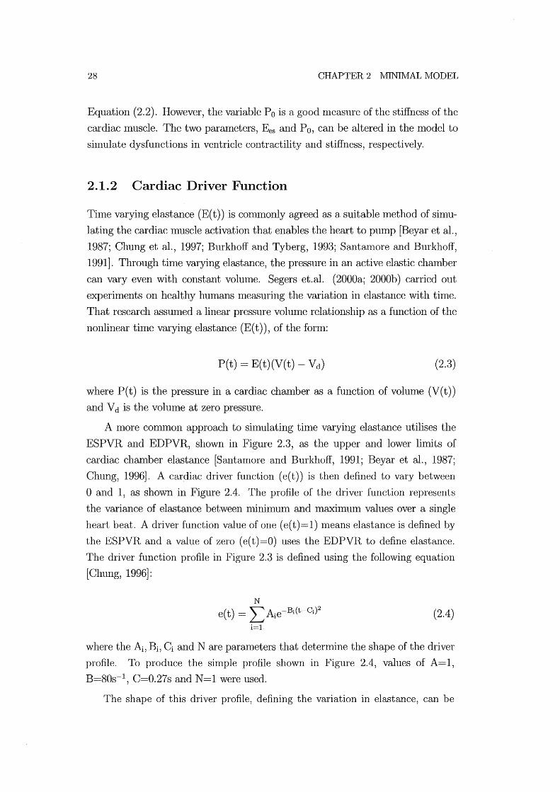
28 CHAPTER 2 IVlINIMAL MODEL
Equation (2.2). However, the variable Po is a good nleasure of the stiffness of the
cardiac Inuscle. The two parameters, Ees and Po, can be altered in the model to
silnulate dysfunctions in ventricle contractility and stiffness, respectively.
2.1.2 Cardiac Driver Function
Tilne varying elastance (E( t)) is commonly agreed as a suitable method of silnu
lating the cardiac muscle activation that enables the heart to pump [Beyar et al.,
1987; Chung et al., 1997; Burkhoff and Tyberg, 1993; Santanl0re and Burkhoff,
1991]. Through time varying elastance, the pressure in an active elastic chamber
can vary even with constant volulne. Segers et.al. (2000a; 2000b) carried out
experiments on healthy humans measuring the variation in elastance with tilne.
That research assumed a linear pressure volmne relationship as a function of the
nonlinear time varying elastance (E( t ) ), of the form:
P(t) = E(t)(V(t) - Vd ) (2.3)
where P(t) is the pressure in a cardiac chamber as a function of volume (V(t))
and V d is the volume at zero pressure.
A n10re COlmnon approach to silnulating time varying elastance utilises the
ESPVR and EDPVR, shown in Figure 2.3, as the upper and lower lilnits of
cardiac chrunber elastance [Santamore and Burkhoff, 1991; Beyar et al., 1987;
Chung, 1996]. A cardiac driver function (e( t)) is then defined to vary between
o and 1, as shown in Figure 2.4. The profile of the driver function represents
the variance of elastance between nlinimum and Inaximum values over a single
heart beat. A driver function value of one (e( t )=1) means elastance is defined by
the ESPVR and a value of zero (e( t )=0) uses the EDPVR to define elastance.
The driver function profile in Figure 2.3 is defined using the following equation
[Chung, 1996]:
N
e(t) = LAie-Bi(t-Ci)2 (2.4) i=l
where the Ai, Bi, Ci and N are parameters that determine the shape of the driver
profile. To produce the simple profile shown in Figure 2.4, values of A=l,
B=80s-\ C=O.27s and N=l were used.
The shape of this driver profile, defining the variation in elastance, can be
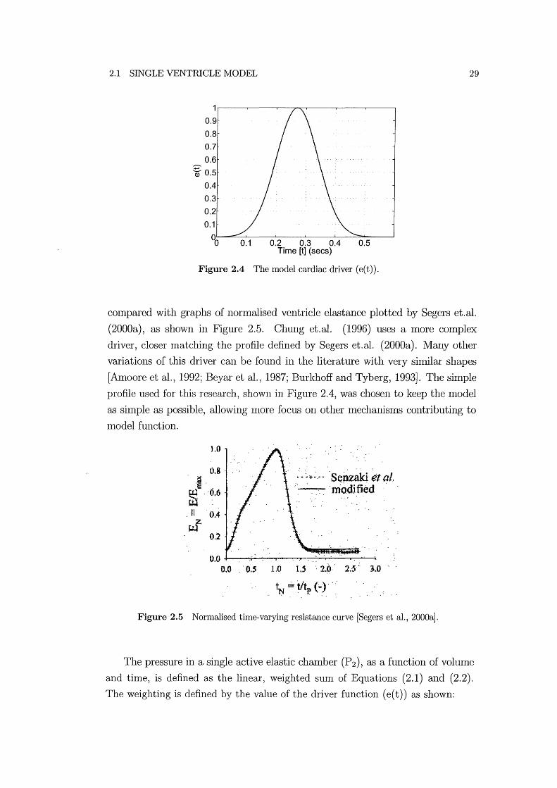
2.1 SINGLE VENTRICLE MODEL
0.9
0.8
0.7
0.6
~ 0.5
0.4
0.3
0.2
0.1
00 0.1 0.2 0.3 0.4 Time [t] (sees)
0.5
Figure 2.4 The model cardiac driver (e(t)).
29
cOlnpared with graphs of norn1alised ventricle elastance plotted by Segers et.al.
(2000a), as shown in Figure 2.5. Chung et.al. (1996) uses a more cOlnplex
driver, closer Inatching the profile defined by Segers et. al. (2000a). Many other
variations of this driver can be found in the literature with very similar shapes
[Amoore et al., 1992; Beyar et al., 1987; Burkhoff and Tyberg, 1993]. The simple
profile used for this research, shown in Figure 2.4, was chosen to keep the Inodel
as shnple as possible, allowing Inore focus on other Inechanisn1S contributing to
Inodel function.
1.0
0.8 .. ~.
e . ~ "0.6
It . 0.4
~
.: .'~'t-;.-. 'SenUid ~t aI, . ... ~ ·m'o.d;ti~d .'
0.2 .
0.0 ........... -:..:;.-.....~..,.--~......;.:..,.......,....;..---.-:------;
0.0 . 0.5 1.0 1,5'· 2-9" 25" 3.0
1N ::: tit (.)., : . . p ' ..
Figure 2.5 Normalised time-varying resistance curve [Segers et al., 2000a].
The pressure in a single active elastic chamber (P2), as a function of vohune
and time, is defined as the linear, weighted Slun of Equations (2.1) and (2.2).
The weighting is defined by the value of the driver function (e( t)) as shown:

30 CHAPTER 2 MINIMAL MODEL
P 2 (V, t) = e(t)Pes(V) + (1 - e(t))Ped(V) o ::; e(t) ::; 1 (2.5)
Equation (2.6) is now the governing equation for the time dependent pressure
volulne relationship in an active elastic chamber, such as a ventricle.
2.1.3 Blood Flow
The blood flow rate through the resistors in Figure 2.2 is primarily dependent on
the pressure gradient across the resistor. If the effects of inertia are either ignored
or negligible, the equation for the flow rate can be calculated using Poiseuille's
equation [Fung, 1990; Beyar et al., 1987; Chung, 1996; Olansen et al., 2000;
Guyton, 1991].
(2.7)
where the resistance (R) is defined by the Poiseuille's equation as R=1fr6/8p,l,
with the variables: radius, ro, fluid viscosity, p" and artery length, l. Poiseuille's
equation assumes incolnpressible, Newtonian, lmninar, axi-symlnetric, fully de
veloped flow through a rigid tube of constant cross-section. These assumptions
are reasonable in order to create a simple quasi-static model and are discussed
in Inore detail in Chapter 3. Note, the use of Windkessel circuit conlponents
in the nl0del allows the rigid tube assumption, as the elastic properties of each
component are silnulated in a subsequent elastic chamber.
Valves are modelled sinlply by nlaintaining flow rates that are either greater
than or equal to zero. If the flow rate calculated using Equation (2.7) is negative,
then that flow rate is set to zero. With the flow rate known, the rate of change of
volunle in the chanlber is sinlply calculated as the net flow through the chanlber.
dV cit = Qin - Qout (2.8)
Equation (2.8) defines a first order ordinary differential equation governing the
volunle of the elastic chambers in the model. All flow variables used in the model
shown in Figure 2.1 are defined in Table 2.1.

2.2 VENTRICULAR INTERACTION
Symbol Qtc Qpv
Qrnt Qtc QpuI
Qsys
Description Flow through the tricuspid valve Flow through the puhnonary valve Flow through the Initral valve Flow through the aortic valve Flow through the pulmonary circulation systeln Flow through the systemic circulation systeln
Table 2.1 Flow rate variables from the full closed loop model of Figure 2.1.
2.1.4 Summary of Single Chamber Model
31
To sUInmarize, for any given vohllne (V) and thne (t), the pressure in the chmn
ber (P2 (V,t)) can be calculated using Equation (2.6). The flow rates are then
calculated using Equation (2.7) and from the flow rate, the rate of change of
vohllne is calculated using Equation (2.8). These equations define the dynan1ics
of a single ventricle model with resistances at the inlet and outlet. The next step
in developing the full closed loop n10del is to capture the effect of ventricular in
teraction, using a two chmnber n10del representing both ventricles with constm1t
pressure bOlmdary conditions.
2.2 Ventricular Interaction
Ventricular interaction has a significant in1pact on cardiovascular dynamics, and is
caused by both the septuIll and the pericardiun1. The septum is an active, flexible
COlllinon wall between the left and right ventricle. The pericardiuln is a relatively
rigid, passive wall that encapsulates the entire heart [Hancock, 1995]. Beyar et.al.
(1987) use two constant parmneters to control the amount that the right ventricle
pressure affects the left ventricle pressure and visa-versa. Santan10re et.al. (1991)
use pressure-vohllne equations very sin1ilar to Equation (2.6), however it is not
clear how the elastances of the septuln and ventricle walls are calculated from
the non-linear PV equations. The presented method of modelling ventricular
interaction divides the ventricles into three separate free wall volumes [Chung
et al., 1997; Maughan et al., 1987].
Figure 2.6 shows the layout for a two ventricle Inodel including ventricular
interaction using an open loop n10del with constant inlet and outlet pressures.
Note that the ventricle interaction model is simply two single chmnber lnodels
coupled by the septuln and pericardiun1. The double lines between the left and
right ventricles indicate the coupling due to the common septal wall. The dashed

32 CHAPTER 2 IVIINIMAL MODEL
line around the left and right ventricles represents the pericardium.
P.vc
P.pu
I P.peri
Figure 2.6 Two ventricle open loop model with ventricular interaction.
This model is similar to that shown in Figure 2.1, but with the peripheral
chamber pressures held constant. This layout allows focus on the ventricle inter
action dynmnics without the influence of dynan1ics in the peripheral circulation.
The pressure variations in the peripheral chmnbers can also be defined as tin1e
varying functions, creating n10re realistic boundary conditions for the ventricles.
2.2.1 Volume Definitions
The volume variables required for this model are defined in Figure 2.7 and Ta
ble 2.2. Figure 2.7 shows the left and right ventricle volUlnes and the three
different free walls of the ventricles and the septum. The free wall volumes, Vlvf,
Vrvf and Vspt , are not actual physical volumes, but represent fractions of the
overall ventricle vohunes (V1v and V rv ). The volumes are separated to capture
the deflection of the cardiac free walls relative to the ventricle volumes.
The left ventricle free wall volume (Vlvf), using Figure 2.7, is simply the left
ventricle volume (V1v ) less the septal volume (Vspt)'
(2.9)
Similarly, the right ventricle free wall volume (V rvf) is the sum of the right ven
tricle volume (Vrv ) and the septum volume (Vspt )'

2.2 VENTRICULAR INTERACTION 33
Left Ventricle Septum Right Ventricle Right Ventricle Free free wall free wall free wall Septum Free wall volume (Vrvf)
wall volume (Vspt) ~
Figure 2.7 Sectioned view of the heart with left and right ventricles and left and right ventricle and septum free walls.
Vrvf = Vrv + V spt (2.10)
Finally, the pericardilllll voluille (V pcd) is the sum of the ventricle volumes, or
the sunl of the ventricle free wall volunles where the septal voluille drops out of
the definition.
(2.11)
The total volulne of the pericardiul11 defined in this lllodel excludes the volunle
of the atria and the myocardilllll, although the lllodelillay be readily augnlented
to include these details. Note that the septlllll vohlllle can be negative or positive
depending on the relative pressures in the ventricle chambers. Positive septal
deflectiol1 is into the right ventricle, as shown in Figure 2.7. The relaxed state of
the septunl is a small anlount of deflection into the right ventricle.
Symbol Description Vlv Left ventricle voluille Vrv Right ventricle vohlllle Vlvf Left ventricular free wall volume V rvf Right ventricular free wall volume V spt Septulll free wall vohlllle V pcd Pericardium volume
Table 2.2 Volume Variables.

34 CHAPTER 2 lVIINIMAL MODEL
2.2.2 Pressure Definitions
Given the volumes of the chaIllbers, the governing PV relationships can then
be used to calculate the pressures, as defined in Equation (2.6). The pressures
defined for the two ventricle nlodel are schenlatically shown in Figure 2.8 and
listed in Table 2.3. All pressures are measured relative to atmospheric pressure.
The specific pressure relations are defined using Figure 2.8 for the left and right
ventricle, and the pericardiulll using the variables in Table 2.3.
Ply = Plvf + P peri (2.12)
Pry = Prvf + Pperi (2.13)
Pperi = Ppcd + Pth (2.14)
where P lvf , P rvf and P pcd are the pressure difference across the wall of the left
ventricle, right ventricle and pericardiulll respectively. The pressure difference
across the septulll free wall (Pspt ) is therefore defined using Equations (2.12) and
(2.13).
(2.15)
The pressures across the free walls (Plvf , Prvf , Pspt and Ppcd) are represen
tations of the stretching force applied to each free wall. These pressures are
calculated fronl the free wall volunles (Vlvf' Vrvf , Vspt and Vpcd) , which define the
deflections, and hence the volullles of the free walls. The relative contributions
of each free wall volume to the overall ventricle volullles (Vlv and V rv) are cal
culated using Equations (2.9) aIld (2.10). The left and right ventricle and septal
free wall pressures are a function of the driver, e( t), and the end systolic aIld end
diastolic pressures, Ped and Pes respectively, in the same fonll as Equations (2.5)
and (2.6).
P lvf = eP es,lvf + (1 - e)Ped,lvf Prvf = eP es,rvf + (1 - e)Ped,rvf (2.16)
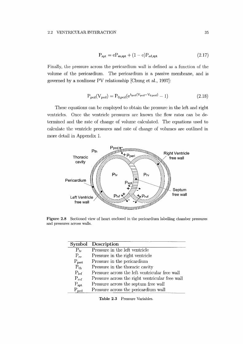
2.2 VENTRICULAR INTERACTION 35
Pspt = ePes,spt + (1 - e)Ped,spt (2.17)
Finally, the pressure across the pericardium wall is defined as a function of the
volume of the pericardium. The pericardium is a passive membrane, and is
governed by a nonlinear PV relationship [Chung et al., 1997]:
(2.18)
These equations can be eluployed to obtain the pressure in the left and right
ventricles. Once the ventricle pressures are known the flow rates can be de
tenmned and the rate of change of vohllue calculated. The equations used to
calculate the ventricle pressures and rate of change of volunles are outlined in
more detail in Appendix 1.
Thoracic cavity
Pericardium
Pth
Left Ventricle free wall
Septum free wall
Figure 2.8 Sectioned view of heart enclosed in the pericardium labelling chamber pressures and pressures across walls.
Symbol Description Ply Pressure in the left ventricle P rv Pressure in the right ventricle
P peri Pressure in the pericardiunl Pth Pressure in the thoracic cavity Plvf Pressure across the left ventricular free wall P rvf Pressure across the right ventricular free wall P spt Pressure across the septum free wall P pcd Pressure across the pericardiulu wall
Table 2.3 Pressure Variables.
36 CHAPTER 2 rvIINHvlAL MODEL
2.3 Peripheral Circulation, Closing the Loop
To capture more of the major governing haelnodynalnics, the circuit in Figure 2.6
Inust be closed so that blood can flow around the entire loop, as in Figure 2.1.
With the output of each cardiac chalnber connected to the inlet of the other,
the dynamics of the systeln will now be affected by peripheral elastances and
resistances, capturing the essential dynalnics of the pulmonary and systemic cir
culations.
Although the non-linear PV relation defined in Equation (2.2) Inay be more
suitable to define peripheral elastances, it requires knowledge of three parame
ters, Po, A, and Vo [Alnoore et al., 1992; Ursino, 1999]. To miniInise complexity,
this research employs the linear PV relationship in Equation (2.1) for the pe
ripheral chalnbers in Figure 2.1. Equation (2.1) requires knowledge of only two
paralneters, E and V d, although V d is set to zero for this work.
Dividing the peripheral circulation systems into elastic chambers separated
by resistances requires a trade-off between complexity and capturing the required
fundamental dynalnics. SOlne CVS lnodels in the literature are highly complex
attelnpting to modellnany of the circulation systmn chambers. An extreme ex
alnple of this approach is the lnodel proposed by Sun et. al. (1997) which uses
approximately 15 capacitors siInulating elastic chalnbers in the CVS. While com
plex lnodels may be more capable of capturing some of the complex dynalnics
than simpler alternatives, separating the individual contribution of each com
ponent is very difficult. Other nl0dels take a more Inininlal approach using a
similar layout to that shown in Figure 1.9(b) [Beyar et al., 1987; Santalnore alld
Burkhoff, 1991].
The minimal approach presented here divides both the puhnonary and sys
temic circulation systmllS into two chalnbers separated by a resistor. The impact
of the thoracic chalnber pressure variations resulting from respiration must also
be considered. As discussed earlier, the location of the heart in the thoracic
cavity between the lungs means that the thoracic cavity pressure (P th) can have
a significant effect on cardiac perfonnance. These cardiopulmonary interactions
are the subject of many publications, pal,ticularly on positive pressure ventilation
[Scharf and Cassidy, 1989; Parry-Jones and Pittlnan, 2003]. For eXalnple, posi
tive pressure ventilation through a respirator causes a significant rise in thoracic
cavity pressure. The location of the heart means increased thoracic cavity pres
sure impedes cardiac function and results in reduced cardiac output. Thoracic

2.3 PERIPHERAL CIRCULATION, CLOSING THE LOOP 37
pressure is included in the calculations for cardiac pressures in Equation (2.14),
however, as shown in Figure 2.1, it will also have an effect on the pressures in
the pulmonary chambers.
2.3.1 Pulmonary Circulation
The puhnonary circulation model includes a single elastic chamber to silnulate
the pulmonary artery (pa) and another to silnulate the pulnl0nary vein (pu) and
left atrium, as shown in Figures (1.4) and (2.1). Puhnonary circulation elastic
chanlber volumes are defined in Table 2.4. Each elastic chanlber siInulates the
pressure vohune relationship in these vessels using the following equations:
Ppa(Vpa) = Epa(Vpa .- Vpa,d) + Pth (2.19)
(2.20)
where P pa and P pu define the pressures in the pulmonary artery and pulnl0nary
vein respectively, and V pa and V pu define the volumes. The elastances of each
chanlber are defined Epa and Epu. The volunle at zero pressure is defined V pa,d
and V pu,d for the puhnonary artery and pulnl0nary vein respectively.
Between the chalnbers a resistor siInulates the pressure drop due to resis
tance acting on blood flowing through the small dianleter capillaries in the lungs
(Rpul). The resistance and pressure difference between the two chanlbers is used
to calculate the flow rate through the puhnonary circulation.
Q _ Ppa - Ppu
pul-Rpul
(2.21)
It is important to note that, Equation (2.21) offers only an approxinlation to fluid
flow through the capillaries. Particularly since at the extremely slnall scale of the
capillaries, Inany of the assulnptions associated with Poiseuille's equation are no
longer valid. For example, in slnall vessels, blood behaves in a non-Newtonian
manner, which is significantly more cOlnplex to silnulate. However, at the macro
scale Inodelled, these assulnptions are a reasonable approxiInation.
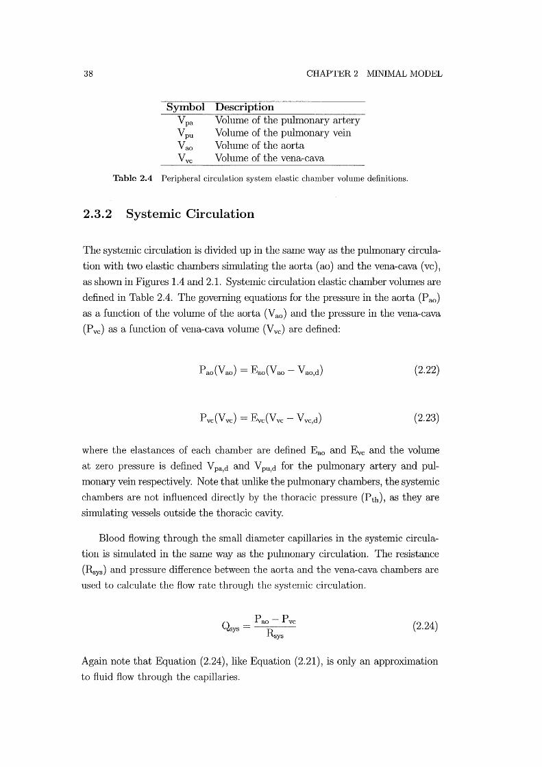
38 CHAPTER 2 IVIINIMAL IVIODEL
Symbol Description V pa Volulne of the pulmonary artery Vpu Volulne of the pulmonary vein Vao Volume of the aorta Vvc Volulne of the vena-cava
Table 2.4 Peripheral circulation system elastic chamber volume definitions.
2.3.2 Systemic Circulation
The systemic circulation is divided up in the same way as the puhnonary circula
tion with two elastic chalnbers silnulating the aorta (ao) and the vena-cava (vc) ,
as shown in Figures 1.4 and 2.1. Systennc circulation elastic chamber vohnnes are
defined in Table 2.4. The governing equations for the pressure in the aorta (P ao)
as a function of the volume of the aorta (Vao) and the pressure in the vena-cava
(Pvc) as a function of vena-cava volunle (V vc) are defined:
(2.22)
(2.23)
where the elastances of each chanlber are defined Eao and Eve and the volulne
at zero pressure is defined V pa,d and V pu,d for the pulmonary artery and pul
monary vein respectively. Note that unlike the pulnl0nary chambers, the systelnic
chanlbers are not influenced directly by the thoracic pressure (Pth), as they are
simulating vessels outside the thoracic cavity.
Blood flowing through the snlall dianleter capillaries in the systenlic circula
tion is simulated in the Salne way as the pulmonary circulation. The resistance
(Rsys) and pressure difference between the aorta and the vena-cava chambers are
used to calculate the flow rate through the systenlic circulation.
Q _ Paa - Pvc
sys -Rsys
(2.24)
Again note that Equation (2.24), like Equation (2.21), is only an approximation
to fluid flow through the capillaries.

2.4 SUMMARY OF NIINIMAL IVIODEL CONSTRUCTION 39
2.4 Summary of Minimal Model Construction
This chapter focuses mainly on the pressure-volulne relationships in the passive
and elastic chambers of the CVS. Thne varying elastance is introduced as the
method of simulating cardiac function and the Inathematical principles involved
have been outlined. A description of the entire CVS model is introduced as shown
in Figure 2.1, discussing all of the interactions involved.
Initially, a single chmnber Inodel is introduced with constant pressure bound
ary conditions to capture the dynalrucs of a single ventricle. The single chanlber
Inodel is then expanded into a two active chmnber systeln to simulate ventricu
lar interaction. The boundary pressures remain constmlt to once again highlight
the function of the ventricles, however these pressures can be varied with thne
to more accurately shnulate ventricle function. Finally, peripheral chmnbers are
added to shnulate the pulmonary mld systelruc circulation systelllS. This closed
loop model cml simulate direct ventricular interactions due to the septunl and
pericardium, as well as series interactions as blood flows frOln one ventricle to the
other through the peripheral circulation systelllS.
The Inain overall assumption of this Inodel is the lunlped parmneter approach
which divides the CVS into a series of elastic chmllbers and blocks shnulating
blood flow. Nunlerous assunlptions are also made in constructing each of these
blocks. This chapter focuses on the elastic chmnbers and the pressure volume
relationships in each chanlber. Important assumptions include the profile of the
driver function, a structure that excludes both atria, and attelnpting to nlodel
large sections of the CVS, such as the aorta, using only a single challlber. Also,
a linear PV relationship is asslllned for the chmnbers shnulating the peripheral
circulation. It is important to relnain aware of these asslllnptions when using the
Inodel as they will restrict the physiological accuracy of the resulting shnulations.
The elastic chambers described are one of the two Inain building blocks of this
model. The second key area is blood flow between the elastic chambers, through
the resistors, inductors and valves in Figure 2.1. This chapter used Poiseuille's
equation, which is only a sinlple approximation of this fluid flow. The next
chapter exanlines the nlathenlatical lnodelling of blood flow between the elastic
chambers in more detail.
Chapter 3
Blood Flow in the Heart
Typical lumped parameter nl0del equations governing arterial flow rate found in
the literature either include, or do not include, inertial effects. In both cases,
resistance to blood flow is typically assunled constant under varying flow velocity
and acceleration. Realistically, resistance varies with tinle for the pulsatile flow
around the heart and its valves, and the alnount of this variation is investigated.
If the variation in resistance is negligible the well-accepted asslunption of constant
resistance is valid. However, if the variation in resistance is not negligible, the
addition of time varying resistallCe to the model will produce nlore physiologically
accurate nlodel outputs.
The sinlplest and nl0st conlnl0n nlethod of nl0delling blood flow in the CVS
is to calculate flow rate as a function of pressure gradient and constant resistance
[Hoppensteadt and Peskin, 2002; Chung et al., 1997; Burkhoff and Tyberg, 1993;
Vis et al., 1997; Santanlore and Burkhoff, 1991]. To account for the effects of
inertia on accelerating blood, Inany models include inertial effects as well as
a constant resistance [Olansen et al., 2000; Beyar et al., 1987; Ursino, 1999;
Tsitlik et al., 1992; Hardyet al., 1982; Sun et al., 1997; Avanzolini et al., 1989;
Melchior et al., 1992]. Often these models are based on well-accepted electrical
circuit analogies with the advantage that electrical circuit analysis techniques
can be used to model the CVS [Ursino, 1999; Tsitlik et al., 1992; Santalnore
and Burkhoff, 1991; Lu et al., 2001; Olansen et al., 2000]. These methods offer
the benefit of being well suited to conlplex circuits such as the CVS, but on a
cOlnponent scale they are only approxiInations that are not necessarily based on
the fundamental mechanical and fluid dynamic principles involved.
This chapter derives the equations governing arterial blood flow near the
heart and notes the key assumptions Inade. The Womersley nUlnber is used
to investigate where it is necessary to model inertial and tinle varying resistance

42 CHAPTER 3 BLOOD FLOW IN THE HEART
effects and where they can be ignored. A method is developed that uses equations
derived from the Navier-Stokes equation to incorporate thne varying resistance
in lumped parmneter CVS models. The method is applied to a simple single
chamber model designed to simulate a single ventricular chamber. Models with
time varying resistance are then compared with nl0dels that assume constant
resistance to investigate the differences in performance.
3.1 Equations Governing Flow Rate
This section investigates the equations of fluid motion regularly used in lumped
parameter models, how they are derived, and their associated assumptions. Blood
flow in parts of the circulation system is approxhnated as flow through a tube.
Figure 3.1 shows an example where the longitudinal position along the tube (x),
the tube radius (ro) and the tube length (f) are labelled. The flow rate equations
are derived directly froln the Navier-Stokes equation in polar co-ordinates, the
form best suited to cylindrical tubes or simple approxinlations of arteries.
(3.1)
where Ux , Ur and Ue are the longitudinal, radial and angular velocities respectively,
P is the nlodified pressure relative to hydrostatic, p is the density and v is the
kinmnatic viscosity.
The following assumptions are applied to all equations governing fluid flow
used in this thesis and are referred to as the standard assUlnptions.
• Blood is assumed incompressible (p=constmlt) [White, 1991].
• Although in sInaller capillaries blood cannot be Inodelled using continuous
equations, in larger arteries the fluid is assunled to behave in a continuous,
Newtonian manner with constant viscosity (IL=constant ) [Fung, 1993].
• The arteries through which blood flows are assunled to be rigid with con
stant cross-sectional area (: = 0). This assumption fits with standard
Windkessel circuit design involving a rigid pipe m1d an elastic chamber in
3.1 EQUATIONS GOVERNING FLOW RATE 43
series. The rigid tube simulates the fluid dynaInics while the elastic chamber
simulates the compliance of the artery walls [Tsitlik et al., 1992; Melchior
et al., 1992].
• Lanlinar uni-directional axi-synulletric flow is assunled (ur = 0, Ue = 0,
a:rr = 0). Although turbulence can occur around the valves, it takes tilne
to develop, and is assumed not to affect the flow profile significantly.
• The flow is assumed fully developed along the length of the tube meaning
the velocity profile is constant with respect to x (~ = 0) [Fung, 1993].
• Pressure is assumed constant across the cross-sectional area and the pres
sure gradient is constant along the length of each section so that the pressure
gradient is a function of tilne only (a;: (t ) ) .
These aSslllnptions enable Equation (3.1) to be reduced to the following siln
plified version of the N avier-Stokes equation:
p &(r, t) = _ ap (t) + ~~ (r au(r, t)) at ax rar ar
(3.2)
where p is the viscosity (p=vp) and u(r,t) is the velocity in the x-direction
(ux(r, t)) as a function of radius and tilne only. Equation (3.2) can be divided
into the following 3 forces per unit volume that are applied to the fluid [Fung,
1997].
Transient inertial force = Pressure force + Viscous force (3.3)
The relative Inagnitudes of the transient inertial force and the viscous force are
important when choosing a suitable governing equation for flow in a section of
the CVS.
The two nlost commonly used equations governing flow rate in lunlped
parameter CVS models can be derived from Equation (3.2). When using equa
tions derived from Equation (3.2), all the assulnptions listed above are applied,
as well as equation specific assunlptions that nlay also apply. The first equation
exalnined is Poiseuille's equation for flow rate, assuming constant resistance and
no inertial effects. The second equation exanlined includes inertial effects, but
again asslllnes constant resistance.

44 CHAPTER 3 BLOOD FLOW IN THE HEART
3.1.1 Poiseuille's Equation with Constant Resistance
If the additional assun1ption of steady fully-developed flow is applied to Equa
tion (3.2), the acceleration term (0;, = 0) is ren10ved, leaving a further simplified
form of the equation.
0= _ oP (t) + ~~ (r ou(r, t)) Ox r or Or
(3.4)
All the density tenns have been divided out leaving an equation that is not
dependent on density and therefore ignores inertial effects. This equation can be
solved to obtain the velocity as a function of radius for flow through a pipe of
radius (TO), as shown in Figure 3.1, under a pressure gradient (oF/ox) [White,
1991; Fung, 1990].
u(r) = (3.5)
Figure 3.1 Flow through a rigid pipe of constant cross section.
Using Equation (3.5), an equation for the flow rate through a tube can be
found by integration.
fro 1Tr6 dp Q = 21T io urdr = - 8M dx (3.6)
where the pressure gradient (:) is replaced by the pressure drop along the pipe
with upstream pressure (PI (t ) ), downstrealll pressure (P 2 (t )) and artery length
(£) ..
(3.7)

3.1 EQUATIONS GOVERNING FLOW RATE 45
By grouping the constants an equation for resistance is derived.
(3.8)
Equation (3.7) can then be siInplified to the electrical analogy conlnlonly used
in the literature to calculate the flow rate of blood through arteries and valves
[Chung et al., 1997; Beyar et al., 1987; Burkhoff and Tyberg, 1993; Ursino, 1999;
Olansen et al., 2000; Slnith et al., 2003a,b].
(3.9)
Thus, in addition to the listed standard assumptions, Poiseuille's equation
aSSlUlles steady fully developed flow, meaning the flow has a fully developed
velocity profile and a constant flow rate. Hence, Equation (3.9) does not include
inertial effects or the effects of tiIne varying resistance that significantly influence
pulsatile flow.
In Inany parts of the arterial tree, such as the capillaries and the vena-cava,
the variation in velocity Inay be minimal. However, significant changes in velocity
will occur around the heart valves and the flow can not be assumed steady during
the course of a heart beat. As the ventricle is filling, blood is rushing into the
ventricle, however as the ventricle contracts, the inlet valve will shut due to
reversing flow rate. Hence, blood p~ssing through the heart valves is periodically
stopping during each cardiac cycle and inertial forces must be affecting blood
flow [Little, 1978].
3.1.2 Including Inertial Effects
A dynalnic equation for flow rate can be found by integrating Equation (3.2)
across the cross-sectional area and along the length.
lX2 la21f laro ou( r, t)
P at rdrdedx Xl 0 0
= rX2 r21f rro [_ oP (t) + ~~ (r ou(r, t))] rdrdedx JXl Jo Jo Ox r or Or
(3.10)

46 CHAPTER 3 BLOOD FLOW IN THE HEART
where the integration results in the following relation.
(3.11)
The vessel length (£) is substituted for (X2 - Xl) and Equation (3.11) is divided
by the cross-sectional area (1fr6).
(3.12)
where auJ;o) is the boundary velocity gradient at the wall of the tube. Equa
tion (3.12) can be compared with the equation for flow rate with inertial effects
commonly found in the literature [Olansen et al., 2000; Beyar et al., 1987; Ursino,
1999]:
dQ L- = PI - P 2 - QR
dt
with the constants inertia (L) and resistance (R).
(3.13)
The derivation of Equation (3.13) can be found frol11 electrical circuit analo
gies for an inductor and a resistor in series, as shown in Figure 3.2. The flow rate
of blood through an artery (Q) is analogous to the current (i), or the flow rate of
electrons in a wire in an electrical circuit. Likewise, the voltage (V) is analogous
to pressure drop (PI - P2) in a fluid flowing through a section of tube. A resistor
accounts for the drop in fluid pressure across a section of artery or tube. An
inductor in an electrical system limits the rate of change of current and is used
to simulate inertial effects on a fluid.
R VRi
VT ---------'
Figure 3.2 Inductor and a resistor in series.
In Figure 3.2 the voltages are labelled across the inductor (VL ), resistor (VR )
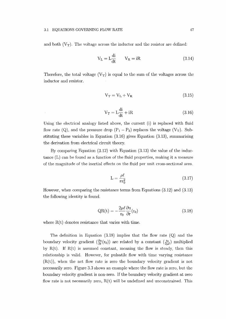
3.1 EQUATIONS GOVERNING FLOW RATE 47
and both (V T)' The voltage across the inductor and the resistor are defined:
V =L di L dt (3.14)
Therefore, the total voltage (VT ) is equal to the sum of the voltages across the
inductor and resistor.
(3.15)
(3.16)
Using the electrical analogy listed above, the current (i) is replaced with fluid
flow rate (Q), and the pressure drop (PI - P2) replaces the voltage (VT)' Sub
stituting these variables in Equation (3.16) gives Equation (3.13), sUlll1narising
the derivation froln electrical circuit theory.
By conlparing Equation (3.12) with Equation (3.13) the value of the induc
tance (L) can be found as a function of the fluid properties, nlaking it a nleasure
of the magnitude of the inertial effects on the fluid per unit cross-sectional area.
(3.17)
However, when conlparing the resistance terms frOln Equations (3.12) and (3.13)
the following identity is found.
QR(t) = _ 2/_d oU(ro) ro or
where R( t) denotes resistance that varies with time.
(3.18)
The definition in Equation (3.18) implies that the flow rate (Q) and the
boundary velocity gradient (aa: (ro)) are related by a constant (1fJ) multiplied
by R( t). If R( t) is assunled constant, nleaning the flow is steady, then this
relationship is valid. However, for pulsatile flow with tinle varying resistance
(R( t) ), when the net flow rate is zero the boundary velocity gradient is not
necessarily zero. Figure 3.3 shows an example where the flow rate is zero, but the
boundary velocity gradient is non-zero. If the boundary velocity gradient at zero
flow rate is not necessarily zero, R( t) will be undefined and unconstrained. This

48 CHAPTER 3 BLOOD FLOW IN THE HEART
inconsistency shows that Equation (3.13), which is used to sinlulate inertial effects
in many cases of prior research, is not a suitable governing equation for pulsatile
fluid flow with tinle varying resistance [Olansen et al., 2000; Beyar et al., 1987;
Ursino, 1999; Sun et al., 1997]. A more suitable alternative is Equation (3.12)
which is derived directly frOln the equations of Inotion rather than electrical
circuit approxilnations.
,?10 5-5 :s 0 en ~
'"0 5 co 0:: 10
-ve 0 +ve Fluid Velocity [u]
Figure 3.3 The velocity profile at zero flow rate.
3.2 The Womersley Number
The previous two sections have shown the derivation of three different nlethods
of nlodelling arterial flow, using either of Equations (2.7), (3.12) or (3.13). Equa
tion (2.7) would be the preferred choice where possible as it is silnple and easy
to implelnent. However, if including inertial effects by using Equations (3.12) or
(3.13) is going to produce significantly nlore accurate results, then the increase
in cOlllplexity is justified.
To investigate which of Equations (3.12) and (3.13) should be used to model
different types of flow, the Womersley nunlber (a) is used, along with a solution
to Equation (3.2) derived by Womersley. The 'iVomersley number is defined as
the ratio of the inertial force to the viscous forces in Equation (3.2) [Fung, 1990].
2 transient inertial force wd2 a - --
- viscous force - l/ (3.19)
where w is a characteristic frequency, defined as the heart rate (HR) and d is a
characteristic length, defined as the radius of an artery (ro). Transient inertial
forces represent body forces acting on the fluid limiting its rate of acceleration.
Viscous forces represent the effects of wall friction acting to slow the flow of the
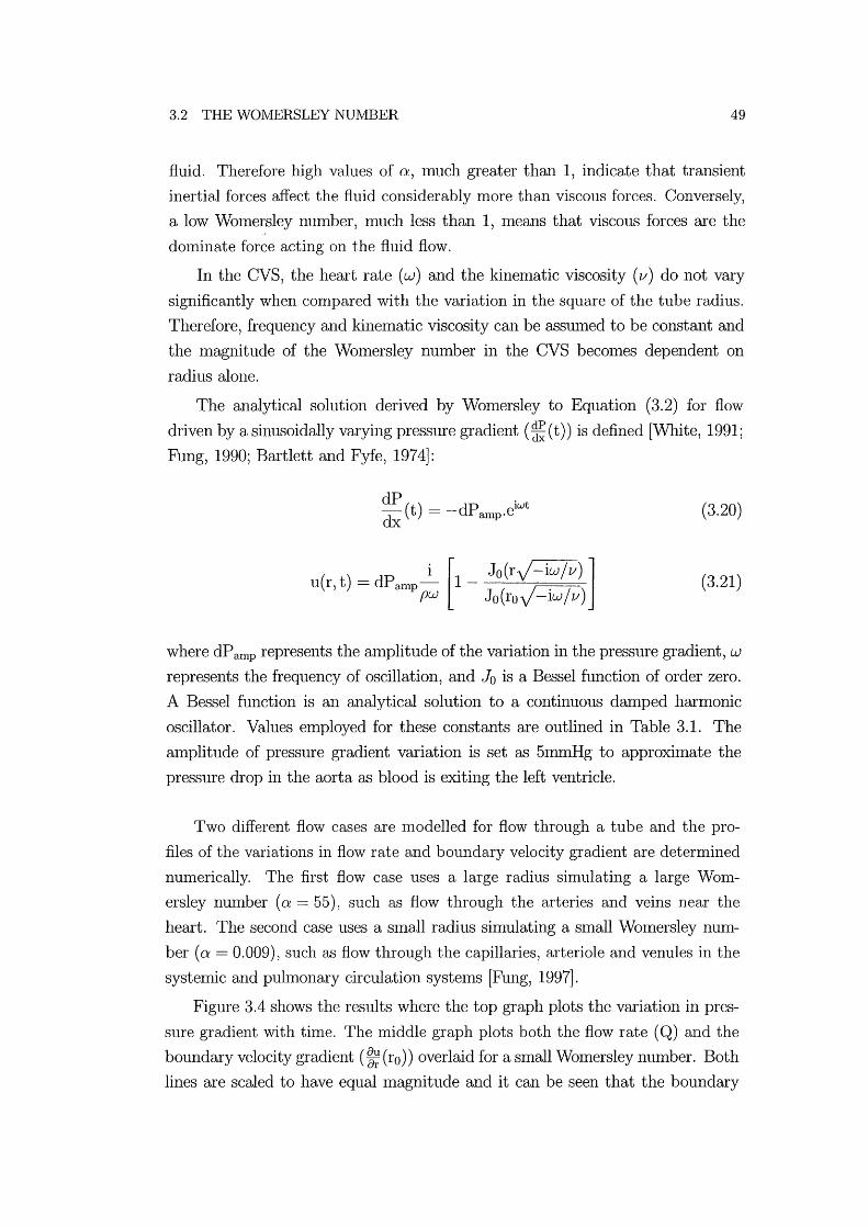
3.2 THE WOMERSLEY NUIvIBER 49
fluid. Therefore high values of 0', nluch greater than 1, indicate that transient
inertial forces affect the fluid considerably more than viscous forces. Conversely,
a low Womersley number, much less than 1, means that viscous forces are the
donlinate force acting on the fluid flow.
In the CVS, the heart rate (w) and the kinematic viscosity (v) do not vary
significantly when compared with the variation in the square of the tube radius.
Therefore, frequency and kinematic viscosity can be assumed to be constant and
the magnitude of the WOlnersley number in the CVS beCOlnes dependent on
radius alone.
The analytical solution derived by WOlnersley to Equation (3.2) for flow
driven by a sinusoidally varying pressure gradient (~~ (t)) is defined [White, 1991;
Fung, 1990; Bartlett and Fyfe, 1974]:
dP( ) dP iwt dx t = - amp·e (3.20)
( . ) - dP ~ [1- Jo(ryl-iWjV)] u I, t - amp PW Jo(royl-iwjv)
(3.21)
where dP amp represents the alnplitude of the variation in the pressure gradient, W
represents the frequency of oscillation, and Jo is a Bessel function of order zero.
A Bessel function is an analytical solution to a continuous dalnped harnl0nic
oscillator. Values eInployed for these constants are outlined in Table 3.1. The
alnplitude of pressure gradient variation is set as 5mmHg to approxiInate the
pressure drop in the aorta as blood is exiting the left ventricle.
Two different flow cases are nl0delled for flow through a tube and the pro
files of the variations in flow rate and boundary velocity gradient are detennined
numerically. The first flow case uses a large radius simulating a large WOln
ersley number (0' = 55): such as flow through the arteries and veins near the
heart. The second case uses a slnall radius simulating a small Womersley num
ber (0' = 0.009), such as flow through the capillaries, arteriole and venules in the
systemic and puhnonary circulation systelllS [Fung, 1997].
Figure 3.4 shows the results where the top graph plots the variation in pres
sure gradient with time. The Iniddle graph plots both the flow rate (Q) and the
boundary velocity gradient (~~ (ro)) overlaid for a small WOlnersley number. Both
lines are scaled to have equal Inagnitude and it can be seen that the boundary

50 CHAPTER 3 BLOOD FLOW IN THE HEART
Description Symbol Value Blood properties:
Blood density p 1050 kg/m::S Blood Viscosity 11 0.004 Ns/m2
Blood Kinematic Viscosity v 3.8xl0-6 m2/s Artery Properties:
Internal Artery Radius TO 0.0125 m Artery Length £ 0.2 In
Chamber properties: Chamber Elastance Ees IN/ln5
EDPVR Volume Cross-over Vo Om3
ESPVR Volume Cross-over Vd o m3
Constant A 23000 m-3
Heart Rate w 1.33 beats/sec Constant A 15 N/m2
Table 3.1 Constants used in single-chamber simulation.
velocity gradient is directly in phase with the flow rate for small WOlnersley nUln
ber flow. The bottom graph shows the sanle infornlation for a large Womersley
number, where the flow rate and the boundary velocity gradient are considerably
out of phase.
The results in Figure 3.4 show that for high \iVomersley number flow, the flow
rate lags the pressure gradient. This result is contrasted with the low Wonlersley
nlunber flow where there is no visible lag. Equation (3.19) shows that slnall Wom
ersley numbers lnean inertial forces are small relative to viscous forces, meaning
inertial effects can be ignored. The middle plot in Figure 3.4 reinforces this
conclusion showing no lag between the driving pressure, the flow rate and the
boundary velocity gradient. Therefore, small radius tubes imply low Womers
ley number flow and thus minilnal inertial effects. Hence, Equation (2.7) with
constant resistance can be used as the governing equation for fluid flow in the
systemic and pulmonary circulation systems where vessel diameters are small and
variations in flow rates are minhnal.
In the arteries and veins near the heart the Wonlersley number is large, in
ertial forces are significant, and therefore they must be included in fluid flow
calculations. For large Womersley number flow, inertial effects on the fluid cause
the flow rate to significantly lag behind the pressure gradient, as shown in Fig
ure 3.4. Additionally, the boundary velocity gradient is shown to be out of phase
with the flow rate. By relating this phase lag to Equation (3.18), it can be seen
that resistance lnust vary with time to accommodate the out of phase variations
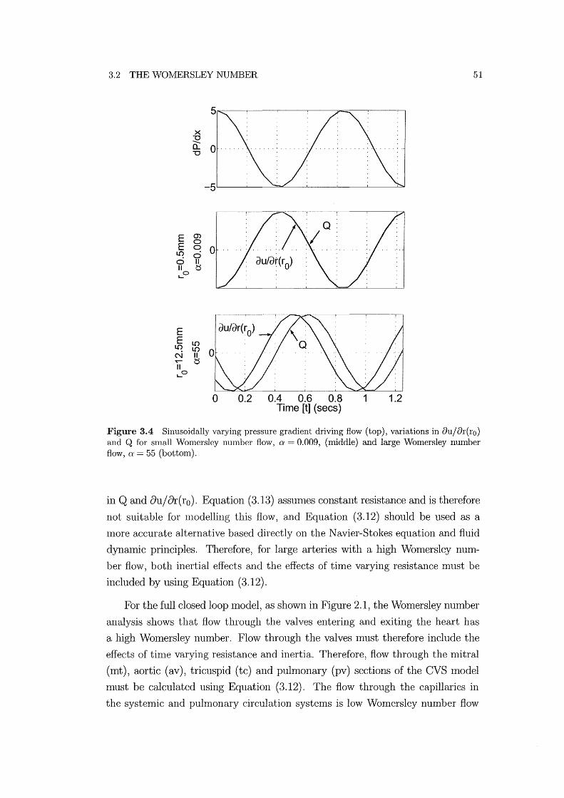
3.2 THE WOMERSLEY NUIVIBER
X "0 -0.. "0
E ~ E ~ 0
I.C) 0 o II II t$ ,-0
o 0.2 0.4 0.6 0.8 Time [t] (sees)
51
1 1.2
Figure 3.4 Sinusoidally varying pressure gradient driving flow (top), variations in 8u/&:(ro) and Q for small Womersley number flow, (}' = 0.009, (middle) and large Womersley number flow, IT = 55 (bottom).
in Q and 8uj8r(ro). Equation (3.13) aSSlunes constant resistance and is therefore
not suitable for Illodelling this flow, and Equation (3.12) should be used as a
III are accurate alternative based directly on the N avier-Stokes equation and fluid
dynamic principles. Therefore, for large arteries with a high Womersley nlllll
ber flow, both inertial effects and the effects of time varying resistance Illust be
included by using Equation (3.12).
For the full closed loop lllodel, as shown in Figure 2.1, the Womersley number
analysis shows that flow through the valves entering and exiting the heart has
a high Womersley number. Flow through the valves lllUSt therefore include the
effects of tin1e varying resistance and inertia. Therefore, flow through the n1itral
(mt) , aortic (av) , tricuspid (tc) and pulmonary (pv) sections of the CVS lllodel
must be calculated using Equation (3.12). The flow through the capillaries in
the systemic and pulmonary circulation systems is low Womersley number flow

52 CHAPTER 3 BLOOD FLOW IN THE HEART
and therefore inertial effects and the influence of time varying resistance can
be assun1ed negligible. Thus, flow through the resistors marked Rsys and Rpul on
Figure 2.1 can be governed by Equation (2.7). The result is a more physiologically
accurate model mixing lUlnped parameter equations, such as Equation (2.7), with
continuous systeln equations, such as Equation (3.12).
3.3 Time Varying Resistance
It has been shown that Equation (3.12) should be used when trying to model
the effects of til11e varying resistance and inertial effects. Equation (3.12) gives
a first order governing equation for flow rate, but it is posed as a function of
the boundary velocity gradient, which is unknown. Equation (3.2), the equation
from which Equation (3.12) is derived, is a function of velocity profile and pressure
gradient only. When the developl11ent of the velocity profile is simulated using
Equation (3.2), the velocity profile will be deten11ined at each time step. The flow
rate at any til11e can then be determined numerically by integrating the velocity
profile at that tin1e.
Q = 12
" 10'0 u(r, t)rdrdO (3.22)
where u(r,t) is the velocity gradient as a function of radius (r) and tilne (t).
Therefore, Equation (3.2) is used in this research as a more suitable governing
equation for the fluid flow in the arteries near the heart as it can be used to
detern1ine the variations in the velocity profile. Although not explicitly defined,
the effects of tinle varying resistance (R( t)) and inertia (L) are implicitly defined
in Equation (3.2).
3.3.1 Non-dimensionalisation
The magnitude of the variables used in Equation (3.2) can vary significantly,
which will contribute to an accumulation of computational error. For example,
the n1agnitude of the volume is on the order of millilitres (lO-6m3) and pres
sure is on the order of lnillimeters of mercury (102N/m2). The magnitudes of
these nUl11bers differs by a factor of 108 which is significant enough contribute
to excessive computational error. To avoid accumulation of machine error and
better pose the problelll for the numerical solution method, all equations are
non-dimensionalised.
3.3 TIME VARYING RESISTANCE 53
Non-dilnensional values are labelled with a star (*) so the non-dimensional
fonn of a dimensional variable x is x*, which is related to x by it's characteristic
value labelled x.
* x x =-X
The following characteristic values are used:
(3.23)
• The characteristic radius (r) is set to 12.51mn to roughly approximate the
diameter of human heart values [Bellhouse and Talbot, 1969J. The charac
teristic length (R) is set to 200nnll to approxinlate the effective length and
scale of the human aorta.
• The characteristic pressure drop along an artery is set to -10mmHg, to ap
proximate the pressure drop in the arteries around the heart (P 2 - PI = 101mnHg).
• These definitions allow the definition of a characteristic pressure gradient:
(3.24)
• The characteristic flow rate is obtained fronl Poiseuille's equation.
(3.25)
• The characteristic velocity is set as the characteristic flow rate divided by
the cross sectional area.
(3.26)
• The characteristic volume (V) is defined as the amount of flow per unit
time. - Q V=-=-
t (3.27)
• The characteristic tillle is defined as the period of one heartbeat in seconds.
- 1 t=HR (3.28)

54 CHAPTER 3 BLOOD FLOW IN THE HEART
• A characteristic value of resistance (R) is determined using Equation (2.7)
(3.29)
• If only the inertances are used, the characteristic inertance (L) is taken as
the average of all inertances (1 = Average L). If the radius and length of
the arteries are known the characteristic inertance is defined from Equa
tion (3.17). - pR L = -2
7fr (3.30)
• The characteristic elastance (E) is defined as the relationship between the
characteristic pressure and volume.
- P E==
V (3.31)
The characteristic variables are substituted into Equation (3.22) to obtain
the equation for the non-din1ensional value of the flow rate (Q*).
Q* ~ {27r fro u*(r*,t*)r*dr*dO 7f io io (3.32)
Equation (3.13) is non-dilnensionalised to produce the dilnensionless fonn of the
constant resistance equation governing fluid flow.
L* dQ*(t*) = 480v (_ oP* (t*) - Q(t*)R*) dt* f2HR Ox
(3.33)
The dimensionless fonn of the equation for the rate of change of the velocity
vector can also be found froln Equation (3.2).
ou*(r*, t*) = 480v (_ oP* t* ~ (02u*(r*, t*) + ~ ou*(r*, t*))) ot* f2HR Ox ( ) + 8 or*2 r* Or*
(3.34)
Note that the tenn v / (f2HR), found in both Equations (3.33) and (3.34), is equal
to the inverse of the WOlnersley nUInber squared (1/ ( 2). This result further
highlights the significance of the WOlnersley number in these calculations for
relating inertial effects to viscous effects.
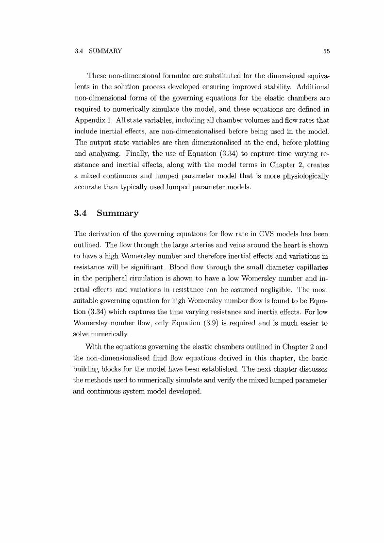
3.4 SUMIVIARY 55
These non-dilnensional formulae are substituted for the dimensional equiva
lents in the solution process developed ensuring improved stability. Additional
non-dinlensional fOflns of the governing equations for the elastic chambers are
required to numerically simulate the model, and these equations are defined in
Appendix 1. All state variables, including all chanlber volumes and flow rates that
include inertial effects, are non-dimensionalised before being used in the model.
The output state variables are then dinlensionalised at the end, before plotting
and analysing. Finally, the use of Equation (3.34) to capture time varying re
sistance and inertial effects, along with the nl0del ternlS in Chapter 2, creates
a mixed continuous and lUlnped paralneter model that is Inore physiologically
accurate than typically used hunped paranleter Inodels.
3.4 Summary
The derivation of the governing equations for flow rate in CVS nl0dels has been
outlined. The flow through the large arteries and veins around the heart is shown
to have a high Womersley number and therefore inertial effects and variations in
resistance will be significant. Blood flow through the slnall diameter capillaries
in the peripheral circulation is shown to have a low WOlnersley number and in
ertial effects and variations in resistance can be assumed negligible. The 1110st
suitable governing equation for high Wonlersley number flow is found to be Equa
tion (3.34) which captures the tilne varying resistance and inertia effects. For low
Womersley number flow, only Equation (3.9) is required and is much easier to
solve numerically.
With the equations governing the elastic chalnbers outlined in Chapter 2 and
the non-dimensionalised fluid flow equations derived in this chapter, the basic
building blocks for the model have been established. The next chapter discusses
the methods used to nUlnerically simulate and verify the mixed lumped parameter
and continuous system model developed.
Chapter 4
Numerical Simulation Methods
The construction of a mixed formulation, nrinin1allllodel including the governing
equations for the passive and active elastic chanlbers and the fluid flow between
them has been outlined in Chapters 2 and 3. This chapter investigates how
to nUlllerically shllulate these n10dels with their cOlllbined lumped parallleter
and continuous elements. Methods of detenllining accurate initial conditions to
improve COlllputational thlle are also discussed.
The nlixed model is primarily governed by ordinary differential equations
(ODEs) such as the rate of change of ventricle vohulle fonllula of Equation (2.8). The numerical ODE solver ode15s in the mathelllatical software package MAT
LAB is used to nlullerically integrate the 1110del equations. The ode15s function
is a variable step-size solver for solving stiff problellls of the fornl:
d~ = f(x) dt - (4.1)
where ~ is a vector of state variables, referred to as the state vector, f(~) is a
function of the state vector that yields the state derivative (d~/ dt ), or the rate
of change of each state variable.
Equation (4.1) easily adlnits the mixed 1110del elen1ents developed, including
the dynamics of the elastic chan1bers and fluid flow conlponents. This chapter
will bring together all the elelllents of Chapters 2 and 3 in defining the solution
method. The models and methods are developed from a single chamber model
and then sequentially expanded to the full closed loop system, as in Chapter 2.
4.1 Basic Model
For the single challlber model of Figure 2.2 with no inertia and constant pressure
boundary conditions (PI and P 3 constant), the minhllal l110del is governed by

58 CHAPTER 4 NUMERlCAL SIMULATION METHODS
only one ODE:
dV cit = f(V, t) (4.2)
where the rate of change of volume (V) is expressed as a function of volulne and
time (t). The following steps are taken at each iteration of the ODE solver to
obtain the overall solution.
• The chamber vohllne (V) is passed to the ODE function as the only state
variable in the state vector (~= [V] ) .
• The chamber pressure (P2 ) is calculated from the volulne using Equa
tion (2.6):
P 2 (V, t) = e(t)Ees(V - Vd ) + (1- e(t))Po(eA(V-Vo) - 1) (4.3)
• Equation (2.7) is used to calculate the flow rates in (Qin) and out (Qout) of
the chamber from the pressure differences:
(4.4)
• Any flow rates that are negative are set to zero to simulate valve function.
• The rate of change of chmnber vohllne (dV / dt) is calculated from the dif
ference between the inlet and outlet flow rates using Equation (2.8):
(4.5)
• The derivative of the state vector is passed back to the ODE solver as
the state derivative (~/dt = [dV/dtD. The ODE solver then estimates a
new volume based on the current volulne, the volume derivative and the
nUlnerical step size in time.
Models with greater nUlnbers of chmnbers and complexity are solved in the same
way by simply adding the volulne of every elastic chamber to the state vector.
This silnple method sUllllnarises the nlodelling of systelllS where there are no
continuous system elements because inertial effects are assumed to be negligible
and variations in resistance are ignored. Valve function is simulated by simply

4.2 INERTIA AND TIlVIE VARYING RESISTANCE 59
constraining the flow rate to be greater than or equal to zero. The next section
shows how inertial effects and time varying resistance can be added to the model.
4.2 Inertia and Time Varying Resistance
As discussed in Chapter 3, there are three different governing equations for flow
rate that can be used to simulate the blood flow in the arteries. Poiseuille's
equation, Equation (2.7), allows the calculation of flow rate directly from the
pressure gradient. However, Equations (3.2) and (3.13) are first order equations
governing the velocity profile and flow rate respectively, and variations in each
must be numerically silnulated. The following sections discuss the inclusion of
inertia with constant resistance, valves, and time varying resistance into hllnped
paraIneter CVS Inodels. As discussed in Chapter 3, Equations (3.2) aI1d (3.13)
are used in their non-dilnensional forn1 as shown in Equations (3.34) aI1d (3.33)
4.2.1 Inertia with Constant Resistance
Equation (3.33) is included as the governing equation for flow rate by sinlply
adding flow rate (Q) to the state vector. For exanlple, a single chanlber lllodel
that includes inertial effects at the inlet and outlet uses a state vector of the fonn:
~ = [V, Qin, Qout]T (4.6)
where Qin and Qout are the flow rates in and out respectively. Each iteration
of the ODE solver calculates the rate of change of the flow rate as a function of
pressure gradient using Equation (3.33). The flow rate is now tracked numerically
at each tilne step in the same way as the volume.
4.2.2 Valve Simulation
In nl0dels where inertia is not included and the governing flow equation is defined
by Equation (2.7), the valves are simulated simply by setting the flow rate to
zero when it is calculated to be zero or negative [Santamore and Burkhoff, 1991].
However, when inertial effects are included in the lllodel, the flow rate (Q) is
governed by a first order ODE and setting the flow rate to zero will create a
discontinuity, which will cause an unstable nun1erical solution.
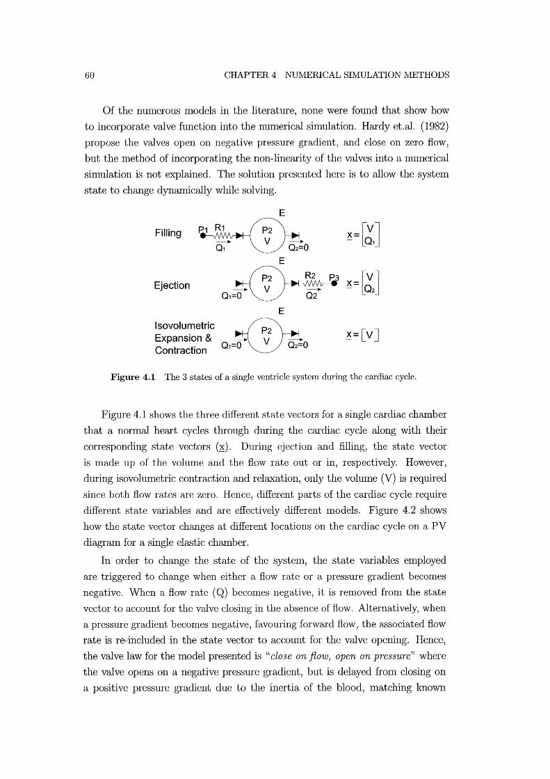
60 CHAPTER 4 NU1VIERlCAL SIMULATION METHODS
Of the nUlnerous models in the literature, none were found that show how
to incorporate valve function into the nUlnerical siInulation. Hardyet.al. (1982)
propose the valves open on negative pressure gradient, and close on zero flow,
but the n1ethod of incorporating the non-linearity of the valves into a numerical
simulation is not explained. The solution presented here is to allow the system
state to change dynamically while solving.
Filling
Ejection
Isovolumetric Expansion & Contraction
E
~=[vJ
Figure 4.1 The 3 states of a single ventricle system during the cardiac cycle.
Figure 4.1 shows the three different state vectors for a single cardiac chamber
that a normal heart cycles through during the cardiac cycle along with their
corresponding state vectors (~). During ejection and filling, the state vector
is made up of the volume and the flow rate out or in, respectively. However,
during isovohllnetric contraction and relaxation, only the volume (V) is required
since both flow rates are zero. Hence, different parts of the cardiac cycle require
different state variables and are effectively different Inodels. Figure 4.2 shows
how the state vector changes at different locations on the cardiac cycle on a PV
diagraln for a single elastic chamber.
In order to change the state of the systeln, the state variables employed
are triggered to change when either a flow rate or a pressure gradient becomes
negative. When a flow rate (Q) becon1es negative, it is removed fron1 the state
vector to account for the valve closing in the absence of flow. Alternatively, when
a pressure gradient becOInes negative, favouring forward flow, the associated flow
rate is re-included in the state vector to account for the valve opening. Hence,
the valve law for the model presented is "close on flow, open on pressure" where
the valve opens on a negative pressure gradient, but is delayed from closing on
a positive pressure gradient due to the inertia of the blood, matching known
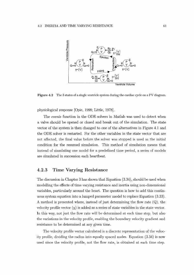
4.2 INERTIA AND TIME VARYING RESISTANCE 61
Ventricle Volume
Figure 4.2 The 3 states of a single ventricle system during the cardiac cycle on a PV diagram.
physiological response [Opie, 1998; Little, 1978].
The events function in the ODE solvers in Matlab was used to detect when
a valve should be opened or closed and break out of the sinll11ation. The state
vector of the systmn is then changed to one of the alternatives in Figure 4.1 and
the ODE solver is restarted. For the other variables in the state vector that are
not affected, the final value before the solver was stopped is used as the initial
condition for the resumed silnulation. This method of simulation nleans that
instead of sinllllating one nlodel for a predefined tinle period, a series of models
are sinlulated in succession each heartbeat.
4.2.3 Time Varying Resistance
The discussion in Chapter 3 has shown that Equation (3.34), should be used when
Inodelling the effects of time varying resistance and inertia using non-dilnensional
variables, particularly around the heart. The question is how to add this contin
uous system equation into a lumped parmneter model to replace Equation (3.33).
A method is presented where, instead of just determining the flow rate (Q), the
velocity profile vector (!!) is added as a series of state variables in the state vector.
In this way, not just the flow rate will be deternlined at each tilne step, but also
the variations in the velocity profile, enabling the boundary velocity gradient and
resistance to be determined at any given tilne.
The velocity profile vector calculated is a discrete representation of the veloc
ity profile, dividing the radius into equally spaced nodes. Equation (3.34) is now
used since the velocity profile, not the flow rate, is obtained at each tinle step.

62 CHAPTER 4 NUlvlERlCAL SIlVIULATION METHODS
At each iteration of the ODE solver the rate of change of velocity is calculated
at each node using Equation (3.34). A no-slip boundary condition is applied so
that the velocity at the boundary is always zero. Thus, where Equation (3.33)
is often used to calculate the rate of change of flow rate, Equation (3.34) is now
used to calculate the rate of change of the velocity profile vector.
Using this method, the state vector for a single chamber system is of the
form:
(4.7)
where .!!in.i and 1..lout.i are the velocity profile in and out of the chamber at node
location i, respectively. The following steps are taken at each iteration of the
ODE solver using the non-dimensionalised variables:
• The chanlber volunle (V) and the velocity profiles (:!lin and '!!out) are passed
to the ODE function as state variables.
(4.8)
• The chamber pressure (P2 ) is calculated froln the volume using the non
dimensional parmneters in Equation (2.6).
• Equation (3.34) is used to find the rate of change of the velocity profiles
( d.!!inl dt and d'!!outl dt).
&(r, t) = 480v (_ 8P() ~ (82u(r, t) ~ 8u(r, t)))
at f2HR &x t + 8 8r2 + r 8r (4.10)
• The velocity profiles are nUlnerically integrated to calculate the flow rates
in (Qin) and out (Qout) using Equation (3.32).
1 i21f i ro Q* = - u(r, t)rdrdB
'if 0 0 (4.11)
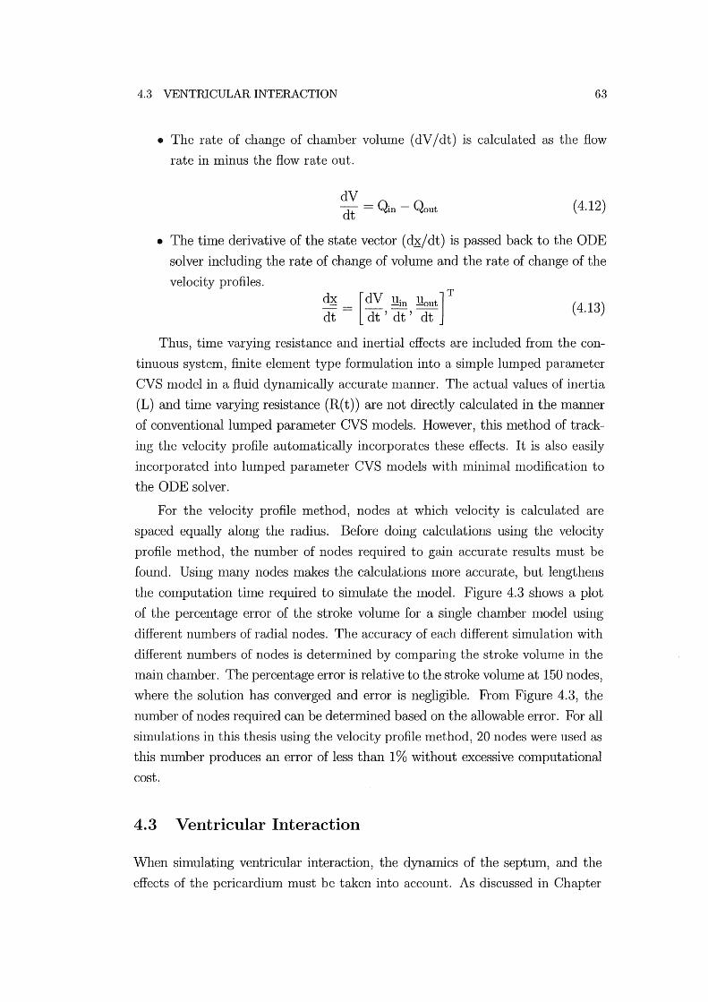
4.3 VENTRICULAR INTERACTION 63
.. The rate of change of chanlber vohune (dV / dt) is calculated as the flow
rate in minus the flow rate out.
( 4.12)
.. The time derivative of the state vector (~/ dt) is passed back to the ODE
solver including the rate of change of volume and the rate of change of the
velocity profiles.
~ _ [dV .1!in .1!out] T
dt - cit' dt' dt ( 4.13)
Thus, time varying resistance and inertial effects are included from the con
tinuous system, finite elenlent type fornlulation into a sinlple lumped paranleter
CVS nlodel in a fluid dynaInically accurate nlanner. The actual values of inertia
(L) and time varying resistance (R( t)) are not directly calculated in the lllanner
of conventional hllllped parmlleter CVS lllodels. However, this lllethod of track
ing the velocity profile autonlatically incorporates these effects. It is also easily
incorporated into hllnped parameter CVS models with nlininlal nl0dification to
the ODE solver.
For the velocity profile nlethod, nodes at which velocity is calculated are
spaced equally along the radius. Before doing calculations using the velocity
profile Inethod, the number of nodes required to gain accurate results nlllst be
found. Using n1any nodes makes the calculations Inore accurate, but lengthens
the computation time required to simulate the model. Figure 4.3 shows a plot
of the percentage error of the stroke volume for a single chmnber Inodel using
different nunlbers of radial nodes. The accuracy of each different simulation with
different numbers of nodes is determined by COln paring the stroke vohune in the
Inain chmnber. The percentage error is relative to the stroke volume at 150 nodes,
where the solution has converged and error is negligible. From Figure 4.3, the
number of nodes required can be determined based on the allowable error. For all
silnulations in this thesis using the velocity profile method, 20 nodes were used as
this number produces an error of less than 1 % without excessive computational
cost.
4.3 Ventricular Interaction
vVhen simulating ventricular interaction, the dynamics of the septum, and the
effects of the pericardium must be taken into account. As discussed in Chapter

64 CHAPTER 4 NUMERICAL SI1VIULATION METHODS
1~----~----~----~ l-
e 0 I-
w -1 (])
g> -2 ...... c (]) -3 e ~ -4 -5L-----~----~----~ o 50 100 150
Number of Nodes
Figure 4.3 Percentage error of stroke volume versus number of nodes on radius.
2, there are many eXalnples in the literature dividing the ventricle vohunes to
account for the displacelnent of the septuln. However, the author was unable to
find methods for detennining the displacenlent of the septum (V spt) given the
non-linear PV relationship of the myocardium defined in Equation (2.6):
P(V, t) = e(t)Ees(V - Vd) + (1 - e(t))Po(eA(V-Vo) - 1) (4.14)
By cOlnbining Equations (2.15), (2.16), (2.17) and (2.6), an equation that
relates Vlv , Vrv and Vspt can be found.
eE (V - Vd ) + (1 - e)P (eASpt.(Vspt-Vo,spt.) - 1) es,spt spt ,spt o,spt
= eEes,lvf(Vlv - Vspt - Vd,lvf) + (1- e)Po,lvf(eA!Vr(v!V-Vspt-VO,!vr) - 1) ( 4.15)
-eEes,rvf(Vrv + Vspt - Vd,rvf) - (1- e)Po,rvf(eArVf(VrV+Vspt-Vo,rvr) - 1)
where the subscript denotes to which cardiac free wall the properties apply. Equa
tion (4.15) can be numerically solved to detennine Vspt given Vlv and Vrv via zero
finding solutions such as a Gauss-Newton method. The function fsolve was used
frOln the Matlab toolbox to solve this equation and find Vspt ' Note that when
simulating the Inodel in the non-dimensional form, Equation (4.15) is of the same
form, but with all dimensional variables and paralneters substituted with their
non-dimensional equivalents.
This Inethod of calculating Vspt fron1 the two ventricle volumes means that
only Vlv and V rv need to be used as state variables. This result is in contrast
to the equations used by Chung et.al. (1997) which uses 6 state variables in the
state vector. That model included all 3 free wall volulnes (Vlvf' Vrvf and Vspt )
the left and right free wall pressures (Plvf and P rvf) and the pericardium pressure

4.3 VENTRICULAR INTERACTION 65
(Pperi ).
(4.16)
where Xc denotes the state vector used by Chung et.al. (1996). The three pres
sures are not necessary in the state vector as they can be calculated at any time
fronl the volumes. Also, it has been shown that the septuln volume deflection
is not required in the state vector. The inclusion of these variables nleans the
model is over-defined which results in it being numerically unstable and over
constrained. This research uses state vectors with the Ininimum number of ele
Inents required to create a Ininilnal model.
The following steps outline the sequence used in the nUInerical silnulation
for Inodelling ventricular interaction. The state derivative, dVlv/dt and dVrv/dt,
is calculated fronl the state variables, Vlv and Vrv , at each tilne step of the
silnulation:
1. The two state variables Vlv and Vrv are passed to the ODE function as
state variables.
( 4.17)
2. Calculate the pressure in the pericardiuln (P peri) using Equation (2.14) frOln
the pressure across the pericardium wall (Ppcd) using Equation (2.18) and
the total volume (Vpcd) froln Equation (2.11):
P . - Po d(eApCd(V!v+Vrv-VO,Pcd) - 1) + Ph pen - ,pc t (4.18)
3. Determine the septal wall deflection (Vspt) by solving Equation (4.15).
4. Given Vspt and Equations (2.9) and (2.10), Vlvf and Vrvf can be detennined
and used in Equation (2.16) to calculate Plvf and Prvf .
P lvf = ePes,lvf + (1 - e)Ped,lvf Prvf = ePes,rvf + (1 - e)Ped,rvf (4.19)
5. The values of P lvf , Prvf and Pperi are used in Equations (2.12) and (2.13) to
find Ply and Pry'
66 CHAPTER 4 NUwIERlCAL SIIvIULATION wIETHODS
Ply = P lvf + P peri Pry = Prvf + P peri (4.20)
6. The ventricle pressures are then used to calculate the flow rates, and thus,
the rate of change of ventricle volulnes:
(4.21)
These six steps are repeated at each tiIne step to account for ventricular inter
action. These steps also show how all of the ventricular interaction equations in
Chapter 2 are combined in the nUlnerical simulation.
4.4 Full Closed Loop Model
The full closed loop Inodel simply requires the addition of four additional state
variables to the model to account for the four additional peripheral elastic chmn
bers. The resulting state vector, used for sinlulations that nlodel inertial effects
with constant resistance, is constructed as follows:
( 4.22)
Alternatively, if each valve incorporates tinle varying resistance, then each flow
rate (Q) in the state vector is substituted with the 20 node velocity profile (!!)
for that value.
(4.23)
All the state variables are defined in Table 4.l.
The choice of using time varying resistance, or constant resistance with inertia
is dependent on the available cOlnputational time. The time varying resistance
Inethod takes approxilnately twice as long to solve as the constant resistance
method for 20 nodes. The constant resistance method is often used to produce
approximate results quickly and the tiIne varying resistance model is used to
achieve Inore accurate results.
The flow rate through the pulnlonary and systelnic circulation systenls is
assumed to be low Womersley number flow and is therefore governed by Equa
tion (2.7). Thus, by putting all of the above equations together and using an
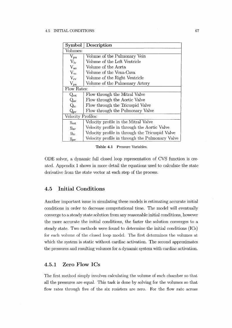
4.5 INITIAL CONDITIONS 67
Symbol Description Vohllnes:
Vpu Vollllne of the Puln10nary Vein Vlv Volume of the Left Ventricle Vao Volume of the Aorta Vvc Volulne of the Vena-Cava Vrv Volulne of the Right Ventricle Vpa Volume of the Puhnonary Artery
Flow Rates: Qrnt Flow through the Mitral Valve Qav Flow through the Aortic Valve Qtc Flow through the Tricuspid Valve Qpv Flow through the Puhnonary Valve
Velocity Profiles:
l!rnt Velocity profile in the ]VIitral Valve
l!av Velocity profile in through the Aortic Valve
l!tc Velocity profile in through the Tricuspid Valve
l!pv Velocity profile in through the Puln10nary Valve
Table 4.1 Pressure Variables.
ODE solver, a dynaInic full closed loop representation of CVS function is cre
ated. Appendix 1 shows in more detail the equations used to calculate the state
derivative fron1 the state vector at each step of the process.
4.5 Initial Conditions
Another ilnportant issue in simulating these models is estin1ating accurate initial
conditions in order to decrease computational tilne. The model will eventually
converge to a steady state solution from any reasonable initial conditions, however
the lnore accurate the initial conditions, the faster the solution converges to a
steady state. Two methods were found to determine the initial conditions (lCs)
for each volull1e of the closed loop lnodel. The first detern1ines the volullles at
which the systeln is static without cardiac activation. The second approximates
the pressures aI1d resulting volulnes for a dynamic system with cardiac activation.
4.5.1 Zero Flow ICs
The first method sinlply involves calculating the volume of each chmnber so that
all the pressures are equal. This task is done by solving for the volulnes so that
flow rates through five of the six resisters are zero. For the flow rate across
68 CHAPTER 4 NUMERICAL SIMULATION METHODS
a resistor to be zero, the pressures on either side of the resistor Inust be equal.
Consideration must also be Inade for the total volume of the system (Vtot ), which
Inust remain constant. The resulting probleln involves lninimising the following
function of the volumes vector.
Qrnt Vpu
Qav Vlv
Qtc =1
Va~
Qpv Vvc (4.24)
Qsys Vrv
L Vs - Vtot Vpa
where L: V s is the sum of all the volulnes and the relnaining variables are outlined
in Table 4.1. Thus, five of the flow rates must be set to zero, meaning the sixth
flow rate will also be zero, while making the sunl of the volumes equal to Vtot .
Calculating the volumes to Inake all the flow rates zero and consequently
all pressures equal, simulates the state of the systenl in a person whose car
diac function has ceased. Instances where there is no cardiac function occur
when attelnpting to shnulate cardio-puhnonary resuscitation (CPR). However,
this Inethod does not take into account the build-up of volume in chmnbers that
precede high resistances in the Inodel. For example, typical pressures in the vena
cava (Pvc) are on the order of ImmHg while a typical pressures in the aorta (P ao) is approxhnately lOOmlnHg. This Inethod is therefore not suitable for general
solutions, but is useful for simulating CPR.
4.5.2 Dynamic ICs
A Inore accurate method of capturing the ICs involves determining the end
systolic (ES) and end-diastolic (ED) pressures in the ventricles. As discussed,
the zero flow lCs defined previously do not account for the danlnling effect the
resistors have on blood flow. The significant difference in pressure between the
aorta and vena-cava is caused by blood build-up in the aorta before flowing
through the systemic resistance into the vena-cava. The zero flow lCs would
calculate these pressures to be equal, which is not an accurate approximation.
A good approximation for the pressure in the veins upstream of the ventricles,
such as the vena-cava, is the end-diastolic pressure in the ventricle (PED (V ED) ).

4.5 INITIAL CONDITIONS 69
PED(VED) can be calculated using the EDPVR as a flulction of end-diastolic vol
ume (VED)' The value of PED(VED) is therefore determined using Equation (2.6)
with the driver set to zero (e(t)=O). The end-systolic pressure (PES) is a good
approximation to the pressure downstream of the ventricle, such as in the aorta
or the pulmonary artery. PES is a function of end-systolic volume (PES (VES)),
however this volulne is unknown. The end-systolic pressure can be calculated as
a function of the end-diastolic volume (PES(VED)) using Equation (2.6) with the
driver set to one (e(t)=l). However, Figure 4.4 shows that PES(VED) is not a
good approxilnation to PES (V ES). A better approxilnation is found by using a
driver value (e(t)) of 0.5 in Equation (2.6) to roughly approximate PES(VES).
PES(VED)
Q) Q) - '-.S:2 ::J '- en +-' en C Q) Q) '->0..
e(t)=1
e(t)=O.S -r PES(VES)
E.O?\lR PED(VED) _-~a::--
e(t)=O
VED
Figure 4.4 Pressure-volume diagram showing ED pressure as a function of ED volume and ED pressure as a function of both ED volume and ES volume.
There are six vohnnes that must be determined to calculate the best initial
conditions for the CVS model, requiring the following six variables and equations
to be lnininlised.
• minimise Plv-Ppu for e(t)=O (across mitral valve)
• minimise PrY-Pvc for e(t)=O (across tricuspid valve)
• minimise Pao-Plv for e(t)=l (across aortic valve)
• millimise Ppa-Prv for e(t)=l (across pulmonary valve)
70 CHAPTER 4 NUMERICAL SIMULATION METHODS
• lIunhnise Qsys-Qpul
• Ininhnise L: V s - Vtot
The first two conditions require minimising the pressure difference across the
Initral valve (Plv-Ppu) and tricuspid valve (Prv-Pvc) using ventricle pressures cal
culated with the driver set to zero (e(t)=O). The second two conditions require
the pressure difference across the aortic valve (P ao-P lv) and the pulmonary valve
(P pa-P rv) to be nlinimised while using ventricle pressures calculated with the
driver set to 0.5 (e(t)=0.5). The fifth condition states that the flow rate through
the systelnic circulation (Qsys) must be equal to the flow rate through the pul
Inonary circulation (Qpul). This fifth condition implies a steady state solution
with no net flow rate being transferred frOln one part of the CVS to another. For
exan1ple, if Qpul was higher than Qsys it would hnply that blood is acculnulating
in the left ventricle. Finally, the sixth condition defines that the sum of all the
chan1ber volumes must be equal to Vtot .
4.6 Summary
The presented method used to numerically simulate the different CVS models
has been defined in tern1S of the pressure, volun1e and flow rate definitions in
Chapters 2 and 3. First, the solution method for the single chamber Inodel is
defined and then built up to include ventricular interaction and the full closed
loop n10del. A n1ethod of incorporating inertial effects into the model by using
flow rate (Q) in the state vector is also outlined. It is shown that this rnethod can
be Inodified so that instead of using Q, the velocity profile (1!) is used in the state
vector to obtain Inore physiologically accurate results. The results will include
both inertia and tin1e varying resistance in siInulating flow near the heart.
It can be seen that the presented method of numerically tracking the veloc
ity profile instead of the flow rate can be easily adapted into lumped paran1eter
Inodels. This approach creates a more physiologically accurate nlixed lumped pa
rarneter and continuous system model. However, the constant resistance method
of including inertial effects is also outlined as this method is often used to pro
duce approxin1ate results quickly. Once appropriate results are gained using
this quicker method, the more computationally intensive time varying resistance
Inodel is used to achieve Inore accurate results.

4.6 SUMlvIARY 71
Two methods of detennining accurate initial conditions are defined depend
ing on the type of lllodel being run. Although the lllodel does not require accu
rate initial conditions they are advantageous in achieving rapid convergence to a
steady state solution. This result is in contrast with other models presented in
the literature that require accurate initial conditions in order to find a reasonable
and/ or stable solution. The next chapter looks at model verification, sinlulating
each model and investigating their performance relative to each other and well
known trends to verify the lllodel elements and solution lllethods.
Chapter 5
Model Simulation & Verification
The previous chapters have shown the construction, governing equations and nu
merical techniques used to develop and siIl1ulate the l11odel. The fundaIl1ental
model elements and dynamics nlust be verified through comparison with known
physiological function and trends. This chapter investigates the results obtained
fronl simulation of the nl0del at different levels of conlplexity. In addition to
checking the hydraulic function and physiological accuracy of the l11odel, a par
ticular focus is ensuring that the l110del is stable, robust and easy to solve.
The single chamber nl0del is tested first, focusing on verifying the function of
the active elastic chanlbers, valve function and the fluid flow entering and exiting
the chanlber. VentriculaI' interaction is tested using the coupled two chal11ber
l110del with constant boundary conditions. Finally, the full closed loop l110del
including all of these elenlents is tested and the final results compared with phys
iological function. The patient specific model parameters used in the nunlerical
siIl1ulations in this chapter are extrapolated fronl those found over several refer
ences, producing model results comparable to an average human [Burkhoff and
Tyberg, 1993; Chung, 1996; Ursino, 1999]. Most of the data found in the lit
erature is adapted fr0111 aninlal studies as these values are difficult to measure
directly in humans.
Table 5.1 lists the mechanical properties of the heart and circulation systenl.
The top three lines define the mechanical properties of the ventricle free walls and
septum (VIvf, Vrvf and Vspt ) , used in Equation (2.6) to define the PV relationships
of these free walls. Only the nonlinear paI'aIl1eters are required for the pericardiul11
properties (Vpcd), used in the nonlinear PV relationship of Equation (2.18). The
last 4 lines in Table 5.1 give the mechanical properties of the peripheral elastic
chambers. Only the linear PV relationship paraIl1eters Ees and V d are required
to determine the PV relationship in these chambers, as seen in Equations (2.19),
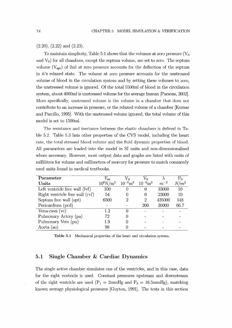
74 CHAPTER 5 MODEL SIMULATION & VERIFICATION
(2.20), (2.22) and (2.23).
To maintain simplicity, Table 5.1 shows that the volumes at zero pressure (Vd
and Vo) for all chambers, except the septum volume, are set to zero. The septum
vohllne (Vspt ) of 21nl at zero pressure accounts for the deflection of the septuln
in it's relaxed state. The volume at zero pressure accounts for the unstressed
vohllne of blood in the circulation system and by setting these volumes to zero,
the unstressed volulne is ignored. Of the total 5500Inl of blood in the circulation
system, about 4000ml is unstressed volume for the average human [Parsons, 2002].
More specifically, unstressed volume is the volume in a chamber that does not
contribute to an increase in pressure, or the relaxed volume of a chalnber [Kulnar
and Parrillo, 1995]. With the unstressed vohllne ignored, the total volume of this
model is set to 15001nl.
The resistance and inertance between the elastic chambers is defined in Ta
ble 5.2. Table 5.3 lists other properties of the CV8 model, including the heart
rate, the total stressed blood volunle and the fluid dynmnic properties of blood.
All paralneters are loaded into the Inodel in 81 units and non-dimensionalised
where necessary. However, 1110st output data and graphs are listed with units of
millilitres for volume and millimetres of mercury for pressure to match commonly
used units found in Inedical textbooks.
Parameter Ees Vd Vo A Po Units 106N/In5 10-61n3 10-6m3 m-3 N/m2
Left ventricle free wall (lvf) 100 0 0 33000 10 Right ventricle free wall (rvf) 54 0 0 23000 10 8eptllln free wall (spt) 6500 2 2 435000 148 Pericardium (pcd) 200 30000 66.7 Vena-cava (vc) 1.3 0 Pulmonary Artery (pa) 72 0 Pulmonary Vein (pu) 1.9 0 Aorta (ao) 98 0
Table 5.1 ]\I{echanical properties of the heart and circulation system.
5.1 Single Chamber & Cardiac Dynamics
The single active chamber silnulates one of the ventricles, and in this case, data
for the right ventricle is used. Constant pressures upstream alld downstream
of the right ventricle are used (PI = 2InmHg and P 3 = 16.5InmHg), matching
known average physiological pressures [Guyton, 1991]. The tests in this section
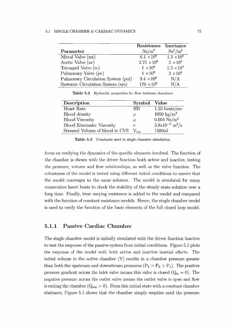
5.1 SINGLE CHAMBER & CARDIAC DYNAMICS
Parameter Mitral Valve (mt) Aortic Valve (av) Tricuspid Valve (tc) Pulmonary Valve (pv) Puhnonary Circulation Systeln (pul) Systelnic Circulation Systenl (sys)
Resistance Ns/m5
6.1 X 10⁶
2.75 X 10⁶
1 x10⁶
1 x10⁶
9.4 X 10⁶
170 x106
Inertance Ns2/m5
1.3 X 10⁴
5 x10⁴
1.3 X 10⁴
2 x10⁴
N/A N/A
Table 5.2 Hydraulic properties for flow between chambers.
Description Heart Rate Blood density Blood Viscosity Blood Kinematic Viscosity Stressed Volulne of blood in CVS
Symbol HR p
fl'
1/
Vtot
Value 1.33 beats/sec 1050 kg/In3
0.004 NS/In2
3.8x10⁻⁶ m2/s 1500ml
Table 5.3 Constants used in single-chamber simulation.
75
focus on verifying the dynamics of the specific elements involved. The function of
the chamber is shown with the driver function both active and inactive, testing
the pressure, vohune and flow relationships, as well as the valve function. The
robustness of the nl0del is tested using different initial conditions to ensure that
the nl0del converges to the SaIne solution. The Inodel is silnulated for InaI1Y
consecutive heart beats to check the stability of the steady state solution over a
long tilne. Finally, tilne varying resistance is added to the Inodel and cOlnpared
with the function of constant resistance Il1odels. Hence, the single chaIllber Il10del
is used to verify the function of the basic elelllents of the full closed loop Inodel.
5.1.1 Passive Cardiac Chamber
The single chaIllber Il10del is initially simulated with the driver function inactive
to test the response of the passive systeIll froln initial conditions. Figure 5.1 plots
the response of the nl0del with both active and inactive inertial effects. The
initial volullle in the active chaIllber (V) results in a chamber pressure greater
than both the upstream and downstreaIll pressures (P2 > P 3 > PI)' The positive
pressure gradient across the inlet valve means this valve is closed (Qin = 0). The
negative pressure across the outlet valve 111eans the outlet valve is open and flow
is exiting the chamber (Qout > 0). From this initial state with a constant chamber
elastance, Figure 5.1 shows that the chaIllber simply empties until the pressure
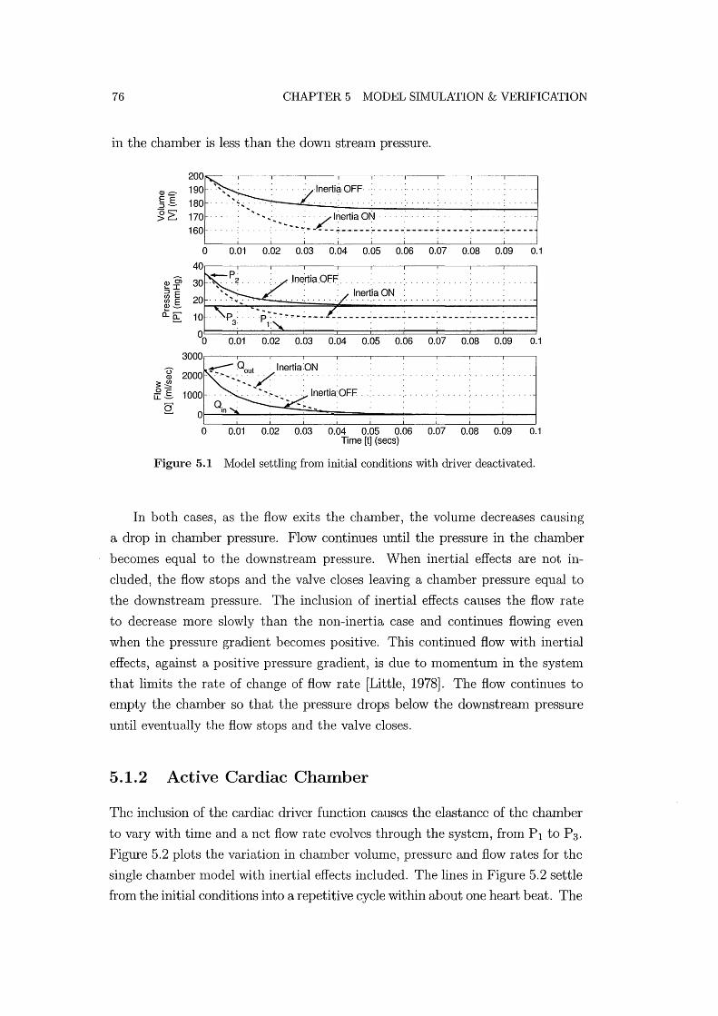
76 CHAPTER 5 MODEL SIMULATION & VERIFICATION
in the chaInber is less than the down stream pressure.
~ .. , . .. .:. ·lnertia·OFF .: .. 180· ~.;.. . . ....... .
~~~ .:::.': :""';":'~~~;~~Z_I:~~i~~~~~~_~;~~:_:_:~~~~~ __ :~~ __ :_:_._~~~~ o 0.01 0.02 0.03 0.04 0.05 0.06 0.07 0.08 0.09 0.1
Inertia ON
00 0.01 0.02 0.03 0.04 0.05 0.06 0.07 0.08 0.09 0.1
3000~--~--~--~~--~--~--~----~--~--~----.
U ~ Qout : Inertia:ON Q) 2000 . ""',' .. / ........ .
~ i 1000 . :' ' , " : : lnertia: OFF .
o 0.01 0.02 0.03 0.04 0.05 0.06 0.07 0.08 0.09 0.1 Time [t] (secs)
Figure 5.1 Model settling from initial conditions with driver deactivated.
In both cases, as the flow exits the chamber, the volun1e decreases causing
a drop in chamber pressure. Flow continues until the pressure in the chan1ber
becon1es equal to the downstremn pressure. yVhen inertial effects are not in
cluded, the flow stops and the valve closes leaving a chamber pressure equal to
the downstrean1 pressure. The inclusion of inertial effects causes the flow rate
to decrease n10re slowly than the non-inertia case and continues flowing even
when the pressure gradient becon1es positive. This continued flow with inertial
effects, against a positive pressure gradient, is due to momentum in the systen1
that lin1its the rate of change of flow rate [Little, 1978]. The flow continues to
empty the chamber so that the pressure drops below the downstream pressure
until eventually the flow stops and the valve closes.
5.1.2 Active Cardiac Chamber
The inclusion of the cardiac driver function causes the elastance of the chamber
to vary with time and a net flow rate evolves through the system, from PI to P3'
Figure 5.2 plots the variation in chmnber volume, pressure and flow rates for the
single chamber n10del with inertial effects included. The lines in Figure 5.2 settle
froln the initial conditions into a repetitive cycle within about one heart beat. The

5.1 SINGLE CHAMBER & CARDIAC DYNAIVlICS 77
developnlent of flow entering and exiting the chanlbers as the pressures change
can be seen on the bottom axis. Flow enters the chamber when the chamber
pressure is less than the upstreanl pressure, and exiting flow develops when the
chalnber pressure is greater than the downstream pressure.
0)0> '-I ~ E If) E ~o...e;: :~te(t)~2 P3 \ .~ ......... A~. __ .. ~ 1 1Ot·····z::s:· .; P, . "" L~~ 0
°o;::pt 0.5 irt:z 1 1.5
1000~------------~--------------~------------~
800 -600 - - - .~~ . -
I \ 400 - -. - -. - ... - - 1_ -,-I ,
200 - . - - - .1. -., -
o -------. ' ,
. - - - - - - Qo~; _~/\:. _ .. _ ....
- - - .: - . '. -I ' - __ -, _. _.t._
- I ' ------------ -----~--~--- -----.---200
0 0.5 1.5 Time [t] (secs)
Figure 5.2 Results from single chamber model with driver function included (e(t)).
The driver function (e( t)) is also plotted on the SaIne axes as the pressure
variations in Figure 5.2. The hnpact of variations in chalnber elastance (E(t)),
as a result of the driver function, can be seen in the chamber pressure variations.
The stroke volunle (SV) is also labelled on the graph as the difference between
the Inaximum and lninhnum volulnes.
The robustness of the Inodel is tested by running the model from different,
relatively extreme, initial conditions and detennining if it converges to the same
steady state results. Figure 5.3 shows two simulations starting at initial volumes
of 10m! and 80m!. These values are set well outside the normal steady state max
imum and lninhnum volumes, as shown in Figure 5.3. The solutions converge to
the same steady-state cycle within one heart beat. The stability of the numerical
procedure is tested by running the simulation for a long period. Figure 5.4 shows
a plot of the pressure and volunle profiles over a 40 second period, showing no
signs of divergence and emphasising steady state stability. Thus, Figures (5.3)
and (5.4) prove the single chalnber model is stable, robust and has only one
unique steady state solution.
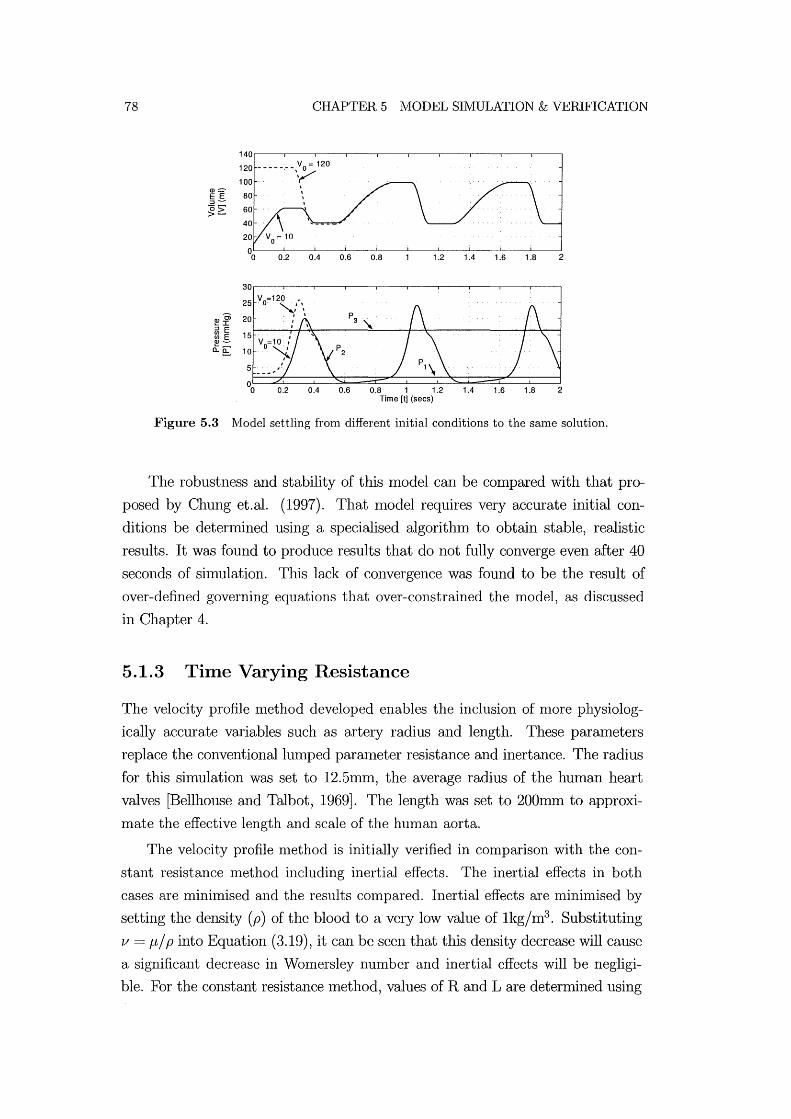
78 CHAPTER 5 JVIODEL SIMULATION & VERIFICATION
Figure 5.3 IVlodel settling from different initial conditions to the same solution.
The robustness and stability of this model can be compared with that pro
posed by Chung et.al. (1997). That nlodel requires very accurate initial con
ditions be detennined using a specialised algorithm to obtain stable, realistic
results. It was found to produce results that do not fully converge even after 40
seconds of siInulation. This lack of convergence was found to be the result of
over-defined governing equations that over-constrained the model, as discussed
in Chapter 4.
5.1.3 Time Varying Resistance
The velocity profile nlethod developed enables the inclusion of n10re physiolog
ically accurate variables such as artery radius and length. These parameters
replace the conventional lumped parmneter resistance and inertance. The radius
for this simulation was set to 12.51llID, the average radius of the human heart
valves [Bellhouse and Talbot, 1969]. The length was set to 200mm to approxi
mate the effective length and scale of the human aorta.
The velocity profile n1ethod is initially verified in comparison with the con
stant resistance method including inertial effects. The inertial effects in both
cases are minimised and the results compared. Inertial effects are nlinin1ised by
setting the density (p) of the blood to a very low value of 1kg/m3 . Substituting
v = p/ p into Equation (3.19), it can be seen that this density decrease will cause
a significant decrease in Womersley number and inertial effects will be negligi
ble. For the constant resistance Inethod, values of Rand L are detennined using

5.1 SINGLE CHAMBER & CARDIAC DYNAMICS
120~--~----~--~~--~----~--~----~----~---'
::::::-100 .s > 80 Q)
E 60 :::J (5 > 40
5 10 15 20 25 30 35 40 45
30~--~----~--~----~----~--~----~----~---.
'Ci I E .s20
e::. Q)
::; 10 (/) (/) Q)
0= 5 10 15 20 25 30 35 40 45
Time [t] (sees)
79
Figure 5.4 Volume and pressure outputs showing long term stability in the single chamber model with inertia.
Equation (3.8) and Equation (3.17) respectively. In both cases, 111aking the in
ertial effects negligible ll1eans that there is now l11uch less restriction on the rate
of change of velocity and the velocity profile develops alnl0st instantly to that
defined by the Poiseuille solution [White, 1991].
Figure 5.5 shows the results of each 111ethod in a PV diagrall1. There is vir
tually no difference in performance between the two. This result verifies that
the velocity profile method perfon11s in the sanle way as the constant resistance
method under very low inertia conditions, as expected, since density and conse
quently inertial effects, have been nlade negligible.
The models are simulated again with the density reset to a normal blood
density of 1050kg/m3 , from Table 5.3. Figure 5.6 compares the resulting varia
tions in pressure, volume and flow rates of the two nl0dels. Figure 5.7 plots the
same simulation results as Figure 5.6 but in a PV diagram, 1110re clearly high
lighting the differences in nl0del performance. The velocity profile ll1ethod results
in an approximately 17.5% decrease in stroke vohul1e, and thus cardiac output,
in comparison to the constant resistance and inertance case. This decrease is a
significant change in the cardiac performance of the nl0del j resulting from using
the more physiologically accurate velocity profile nlethod over the widely used
constant resistance assull1ption.
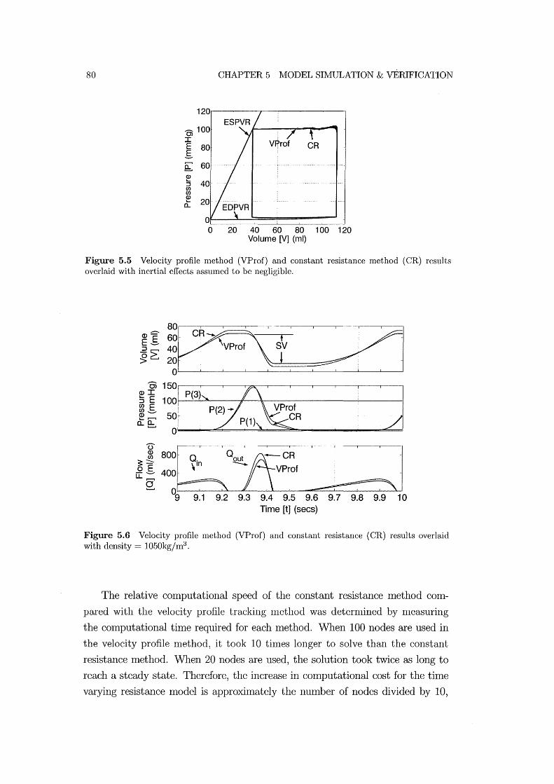
80
0> 100 I E 80 g ~ 60 ())
:s 40 C/) C/) ())
0::
CHAPTER 5 MODEL SIMULATION & vERIFICATION
20 40 60 80 100 120 Volume [V] (ml)
Figure 5.5 Velocity profile method (VProf) and constant resistance method (CR) results overlaid with inertial effects assumed to be negligible.
j ~ !j~,--_C-,-R __ -----L\V_P_ro_fL---------,--=s=(~==~-,--:::::::J/1_---'-----------1._--'--' Oi
(])I 100 P(3) :J E rn E ~ -- 50 o:e;:
800[hQ~CR 400 ' VProf
o ' 9 9.1 9.2 9.3 9.4 9.5 9.6 9.7 9.8 9.9
Time [t] (sees) 10
Figure 5.6 Velocity profile method (VProf) and constant resistance (CR) results overlaid with density = 1050kg/m3 .
The relative computational speed of the constant resistance method com
pared with the velocity profile tracking nlethod was deternlined by llleasuring
the cOlnputational tilne required for each Inethod. When 100 nodes are used in
the velocity profile method, it took 10 times longer to solve than the constant
resistance Inethod. When 20 nodes are used, the solution took twice as long to
reach a steady state. Therefore, the increase in computational cost for the time
varying resistance model is approximately the number of nodes divided by 10,
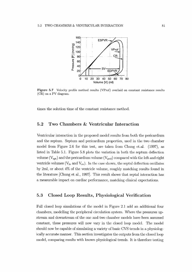
5.2 TWO CHAIVIBERS & VENTRICULAR INTERACTION
140 0; ~ 120
g 100
(b 80 Q)
:; 60 C/)
~ 40 a..
10 20 30 40 50 60 70 80 Volume [V] (ml)
81
Figure 5.7 Velocity profile method results (VProf) overlaid on constant resistance results (CR) on a PV diagram.
tilnes the solution tilne of the constant resistance lnethod.
5.2 Two Chambers & Ventricular Interaction
Ventricular interaction in the proposed model results frOln both the pericardillln
and the septun1. Septllln and pericardium properties, used in the two chamber
lnodel fron1 Figure 2.6 for this test, are taken froln Chung et.al. (1997), as
listed in Table 5.1. Figure 5.8 plots the variation in both the septlun deflection
volulne (Vspt ) and the pericardium volume (Vpcd ) con1pared with the left and right
ventricle volumes (Vlv and V rv). In the case shown, the septal deflection oscillates
by 2ml, or about 4% of the ventricle volulne, roughly n1atching results found in
the literature [Chung et al., 1997]. This result shows that septal interaction has
a measurable ilnpact on cardiac perfonnance, matching clinical expectations.
5.3 Closed Loop Results, Physiological Verification
Full closed loop simulations of the model in Figure 2.1 add an additional four
chmnbers, modelling the peripheral circulation system. Where the pressures up
stream and downstream of the one and two chmnber lnodels have been assumed
constant, these pressures will now vary in the closed loop n10del. The model
should now be capable of silnulating a variety of basic CVS trends in a physiolog
ically accurate manner. This section investigates the outputs from the closed loop
lnodel, comparing results with known physiological trends. It is therefore testing

82 CHAPTER 5 Iv:IODEL SIMULATION & VERIFICATION
~ 60f--
U~: ~~rl--·-----"~ ,~ G- 100~--------~~--------~----------~
0.5 1 1.5
4.5 _§~ 4 . ro .- E .• .... V . .
! I~~ ::~. . .... ~ 'pt .m ••• · •
2· o 0.5 1 1.5
i EE ~~ . ··V ..• . ......•• ro.2r-:t;, 70 . pcd .~ 0 [ CD >G 60· . . .... ~ 50~--------~----------~----------~
o 0.5 Time [t] (sees) 1 1.5
Figure 5.8 Comparing the variations in left and right ventricle volumes (Vlv and Vrv ) with the septum deflection (Vspt ) and the pericardium deflection (V pcd).
the aggregation of elelnents tested individually in the one and two chamber model
tests.
One of the key constraints in the closed loop model is that the total volume
of the system must remain constant. If the total vohllne of the systeln varies over
the course of a simulation, then the model is unstable. It was found that after
long shnulations over 100 seconds that the nlodellnaintained a constant volume
of 15001nl, verifying the stability of the nlllnerical procedure. Where previous
tests proved the stability of the numerical procedure for shnulating the single
chamber Inodel, this test proves the stability of the cOlnplete closed loop CVS
model.
Figure 5.9 plots the left and right ventricle pressure and volume variations for
the closed loop model after it has reached a steady state solution. This plot can
be compared with the Wiggers diagram shown in Figure 5.10 [Guyton, 1991]. The
model is seen to capture the major dynmnics of the CVS including the variations
in left ventricle pressure, aortic pressure and ventricle volume.
Since the ultimate goal is shnulation of human heart function, particularly
in response to changes in therapy, tests to validate shnple trends are carried out
comparing model outputs with known physiological trends. Figure 5.11 shows
the effect of varying ventricle contractility, a measure of cardiac pump function
[Maughan and Kass, 1988]. Contractility is varied in the model by changing the
end systolic elastance (Ees) [Burkhoff and Tyberg, 1993]. Typically, an increase

5.3 CLOSED LOOP RESULTS, PHYSIOLOGICAL VERIFICATION
Q)
E :::J (5 >
Left Ventricle [Iv] 160
1000 0.25 0.5 0.75
E 80
a.~ 60 Q)
:s 40 en en Q) a: 20
1.25
o 0.25 0.5 0.75 1 1.25 Time [t] (sees)
E
>~
110
~ 80 :::J
(5 70 >
30
E "'2: 20 Q:..
~ ~ 10 en Q) a:
Right Ventricle [rv]
0.25 0.5 0.75
rv'
00 0.25 0.5 0.75 Time [t] (sees)
83
1.25
1.25
Figure 5.9 Simulation results from the closed loop model with inertia and ventricular interaction.
in contractility results in an increase in cardiac output which correlates with an
increase in stroke volume (SV) , assunring heart rate relnains constant. Figure 5.11
plots a PV diagranl for 3 different contractilities showing the desired increase in
stroke volume as contractility increases.
A second test shows the effect of changing the systemic circulatory resistance.
Readily available clinical data shows that an acute increase in resistance results
in reduced cardiac output that varies with the magnitude of the change [Slinker
and Glantz, 1989J. Figure 5.12 shows the closed loop nlodel output, as systelnic
resistance is increased, and decreased. As systenric resistance decreases, stroke
vohnne increases, meaning an increase in cardiac output. The opposite trend
occurs as the resistance is increased. Figure 5.13 shows the rise in pressure in the
aorta as a result of increased peripheral resistance and the resulting decreased
cardiac output (CO), which illustrates the increase in blood pressure (BP) often
seen in patients with narrowed or blocked arteries, and the resulting increased
systemic resistance. Hence, both figures illustrate that the nlodel captures well
known, basic clinical behaviour in response to changes in systenric resistance.
Finally, the average thoracic cavity pressure in humans is nonnally about
-4mmHg, however if this pressure is increased, as occurs during positive pressure
Inechanical ventilation, cardiac output is decreased [Guyton, 1991J. Figure 5.14

84
Ejectionl Isovolumic contraction \
120 Aortic r 160 valve '/
I 0; .... opens I
-- J :c 80 ---E E- 60 ~ :::J
40 ~
Cl.. 20
0
i130j ~ 90
::J (5 :> 50
Systole
CHAPTER 5 MODEL SIMULATION & VERIFICATION
[
ISOVOlumiC relaxation
rRaPid inflow
r DiastasiS rAtnal systole
I Aortic valve ~ ~
~~~t--- --- ' -----Aortic pressure
A-V valve
","" __ Atrial pressure Ventricular pressure
Ventricular volume
'r--- Electrocardiogram
1II\r----nnu---- Phonocardiogram
Diastole
Figure 5.10 The Wiggers diagram showing pressure and volume variations in the left ventricle
[Guyton, 1991].
200
180 .
160 · .
OJ 140 · . I E 120 . E-~ 100 · .
~ 80 . ::J en en ~ 60 . Cl..
40 .
20 · .
o· 40
0~5xE : . . ef;i.
60 80 100 120 140 Volume ~) (ml)
200
180 .
160 .
OJ 140 . I E 120 .. E-~~ 100 . e:. ~ 80 . :J en en ~ 60 ..
Cl..
40 60 80 100 120 140 Volume [V rv] (ml)
Figure 5.11 The effect of varying ventricular contractility.
shows the model output for both a normal (-4nnnHg) and an increased (OmmHg)
thoracic pressure where the stroke vohune, and thus the cardiac output, is de
creased by 9%. This decrease in cardiac output is in good agreelnent with readily
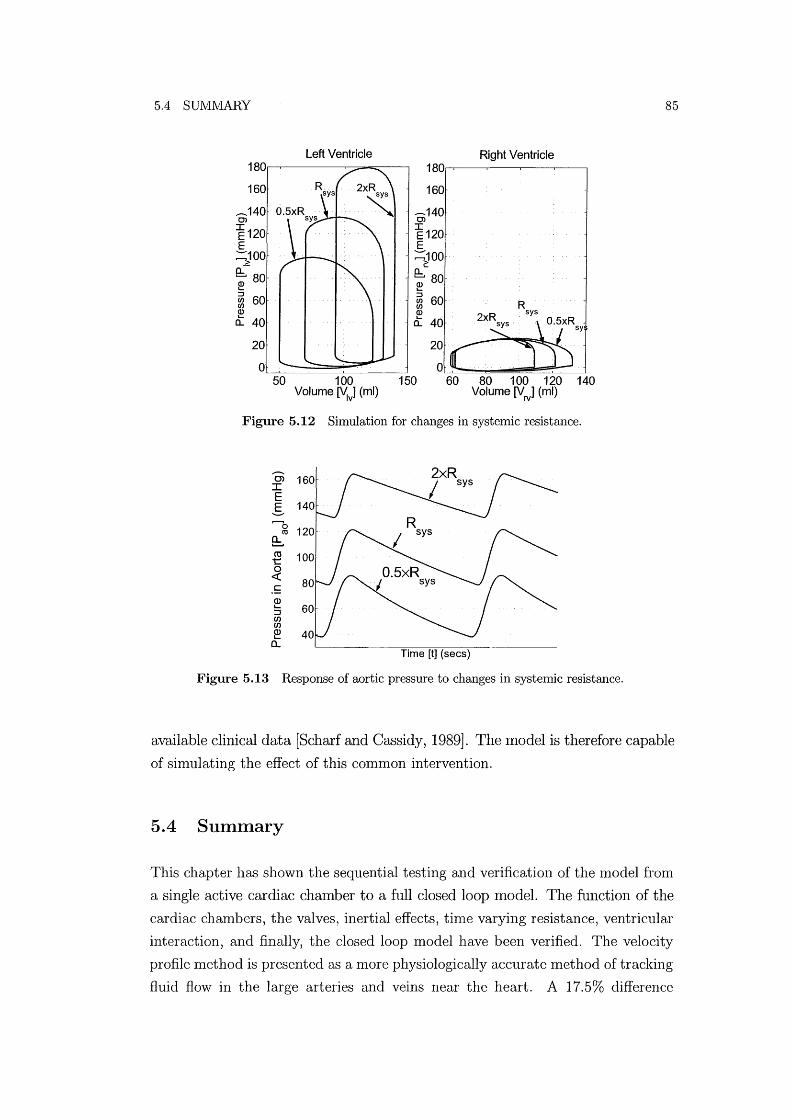
5.4 SUIVIMARY
Left Ventricle Right Ventricle 1S0 1S0
160 160
.-140 .-140 0> 0>
~120 I E120
E E :::;JOO :=:100
2: e;SO Q:.. SO ~ ~ :::J
60 ~ 60 CI)
R CI) CI)
~ ~ sys
a.. 40 a.. 40
20
0 50 100 150 SO 100 120 140
Volume ~) (ml) Volume [Vrv] (ml)
Figure 5.12 Simulation for changes in systemic resistance .
........... 0> :c E g
Time [t] (sees)
Figure 5.13 Response of aortic pressure to changes in systemic resistance.
85
available clinical data [Scharf and Cassidy, 1989]. The 1110del is therefore capable
of simulating the effect of this common intervention.
5.4 Summary
This chapter has shown the sequential testing and verification of the n10del fron1
a single active cardiac chamber to a full closed loop model. The function of the
cardiac chanlbers, the valves, inertial effects, tinle varying resistance, ventricular
interaction, and finally, the closed loop model have been verified. The velocity
profile Inethod is presented as a more physiologically accurate method of tracking
fluid flow in the large arteries and veins near the heart. A 17.5% difference

86 CHAPTER 5 MODEL SIlVIULATION & VERIFICATION
120 .
0>100 . I E S 80·
~ Q) 60 .. L-
::J en en Q) 40 . L-
a...
20 ..
Left Ventricle
g.
50 70 90 110 130 150 Volume M (ml)
120 ..
0>100 . : I E S 80':
~
Right Ventricle
~ 60 ::J : : p: = -4mmHg en : : tn : :
£ :: P fhVmmH9 I o·
40 60 80 100 120 Volume M (ml)
Figure 5.14 Change in stroke volume and PV diagram for a change in thoracic pressure.
in cardiac output for pulsatile flow in larger arteries is found, when conlparing
this nlethod with the constant resistance nlethod. This significant difference
justifies the inclusion of the more physiologically accurate velocity profile tracking
Inethod.
The Inodel is shown to be stable on both a cOlnponent scale, tested using
both a single and a two chmnber Inodel, and an overall scale, showing a constmlt
total volume throughout simulation. The full closed loop model is silnulated
producing results that are seen to correlate well with well-known, fundamental
physiological function and trends. The good agreenlent of these results with
known clinical data shows the potential of this nlodel in simulating trends in
the cardiovascular system in response to physiological changes or intervention.
However, even with the minimal model approach, there are still a large number of
parameters in the Inodel. This large number of patient specific parameters means
the model is still too complex to adjust nlanually to produce patient specific
Inodels. An automated method of determining patient specific parameters is
therefore required.
Chapter 6
Optimisation of Model Parameters
It has been shown that the model is capable of capturing major dynamics in the
CVS. However, one of the key goals of this research is to model the dynmIDcs of
a specific patient. Therefore, the model nlust be capable of matching a specific
patient's CVS dynmIDcs. For example, the model should be equally able to siln
ulate the Inagnitude of pressure variations in the aorta for a nonnal hUlnan of
120 over 80nunHg, or an abnormal pressure of 180 over 120 nllnHg. The dynmn
ics of the Inodel are a function of the model parameters such as elastance and
resistance. Thus, creating a nlodel to match a specific patient involves adjusting
the parmneters until the Inodel dynmIDcs Inatch the dynamics measured frOln a
patient. This task is well suited to structured optilnisation.
The cOlnplex interaction between the parmneters ll1eans that it is impossible
to manually adjust the model to produce target outputs. Instead, optilnisation
techniques are used to numerically adjust the parmneters to Ineet target perfor
ll1ance outputs. Before using the CVS Inodel in conjunction with the optimisa
tion routine, the implementation of the CVS model must be adjusted to suit the
optilnisation routine. Target performance dynmllics must be identified and the
lllodel parmlleters to be adjusted by the optimisation routine must be defined in
a nUlnerically robust fashion, similar to non-dilnensionalising variables, to avoid
cOlnputational error.
This chapter first explains the optimisation routine used in this research. The
target CVS nl0del perfornlance metrics are identified and suitable optilllisation
parallleters are chosen. The lllodifications required to enable an optimisation
routine to be used are discussed. In particular, a method of accelerating the
model to a steady state solution, satisfying predefined convergence criteria, is
outlined. Accelerating the nl0del will significantly enhance the conlputation speed
of the optimisation approach. Finally, the steps used to find a steady state

88 CHAPTER 6 OPTI:rvrrSATION OF IVIODEL PARAMETERS
solution to the CVS lnodel as quickly as possible, while maintaining robustness,
are described.
6.1 The Optimisation Routine
A particular feature of this optimisation problem is that the optilnisation routine
lnust be able to deal with imprecise function evaluations. Although the CVS
lnodel will converge to only one unique solution for a particular set of paralne
ters, finding this solution to a high level of accuracy can take considerable time
for SOlne parameter and IC combinations. However, it is not desirable to use
excessive conlputational time to find an accurate CVS model solution and less
accurate results lnustbe used. The optinusation routine lnust therefore be capa
ble of dealing with the ilnprecise values that result from error in the CVS lnodel
solutions.
Inaccurate solutions will be particularly important as the optimisation rou
tine converges to a steady state solution. Initially, the optimisation routine will
Inake large steps which will cause significant changes in nlodel dynamics. How
ever, as the routine converges the alnount the lnodel paralneters are adjusted,
and the resulting variations in CVS model dynamics, will significantly decrease.
Eventually, inaccuracies in the CVS model solutions will become significant com
pared to the magnitude of variations in the Inodel outputs at each optilnisation
step. At this point the optimisation routine will be unable to converge further.
It was found that the standard MATLAB nonlineal' least squares optilnisa
tion routine perfonned badly when optilnising the CVS nlodel parameters. The
reason for this poor performance is unclear, but a cOlnbination of noisy func
tion values and a lack of direct control over step size appeared to contribute.
The optimisation routine used is a derivative-free, trust-region, Gauss-Newton
method for nonlinear least squares problems. This optimisation routine is specif
ically designed for imprecise function evaluations, using a trust-region nlethod
of constraining the step size of each iteration [Conn et al., 2000]. The optimisa
tion routine was designed and written by Dr Iall Coope from the mathematics
department at the University of Canterbury.
Table 6.1 lists the optimisation paranleters used in this research. Note that
although a target precision of 1 would achieve an acceptable error of 1 %, a target
precision of 10-3 is used. This target precision is set significantly higher than
required in order to test the capabilities of the optilnisation routine.
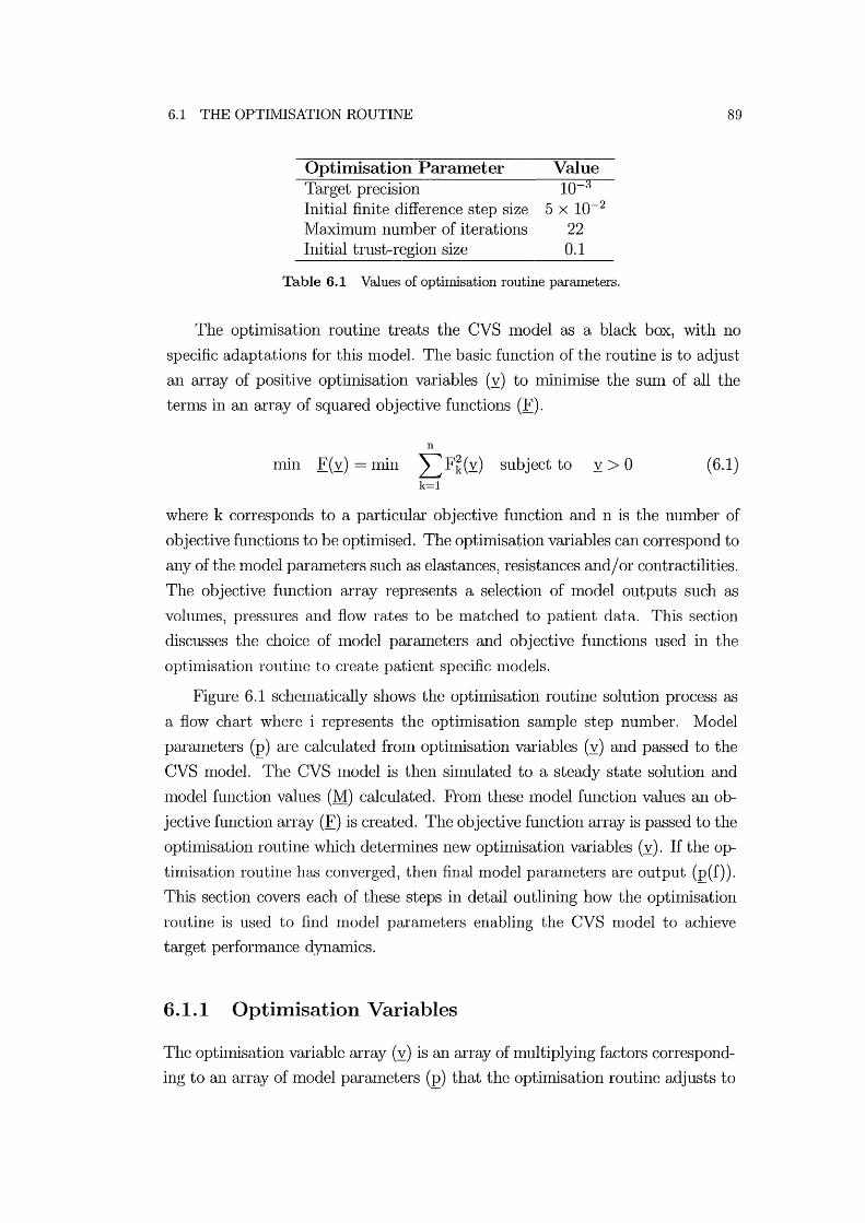
6.1 THE OPTIMISATION ROUTINE
Optimisation Parameter Target precision Initial finite difference step size Maximulll number of iterations Initial trust-region size
Value 10-3
5 X 10⁻²
22 0.1
Table 6.1 Values of optimisation routine parameters.
89
The optimisation routine treats the CVS model as a black box, with no
specific adaptations for this nl0del. The basic function of the routine is to adjust
an array of positive optinnsation variables (y) to minimise the SlUll of all the
teflns in an array of squared objective functions (E).
n
n11n E(y) = lnin LF~(Y) subject to y> 0 (6.1) k=l
where k corresponds to a particular objective function and n is the number of
objective functions to be optilnised. The optilnisation variables can correspond to
any of the 1110del parmlleters such as elastances, resistances and/or contractilities.
The objective function array represents a selection of model outputs such as
vohunes, pressures and flow rates to be nlatched to patient data. This section
discusses the choice of nl0del parmlleters and objective functions used in the
optilnisation routine to create patient specific Inodels.
Figure 6.1 schenlatically shows the optilnisation routine solution process as
a flow chart where i represents the optimisation salnple step nunlber. IVlodel
parmlleters (r) are calculated frolll optilnisation variables (y) and passed to the
CVS model. The CVS 1110del is then silllulated to a steady state solution and
1110del function values (M) calculated. FrOlll these 1110del function values an ob
jective function array (E) is created. The objective function array is passed to the
optilnisation routine which determines new optimisation variables (y). If the op
timisation routine has converged, then final model parameters are output (r(f)).
This section covers each of these steps in detail outlining how the optimisation
routine is used to find model parmneters enabling the CVS nl0del to achieve
target perfoflnance dynmnics.
6.1.1 Optimisation Variables
The optimisation variable array (y) is an array of multiplying factors correspond
ing to an array of model parmlleters (r) that the optimisation routine adjusts to
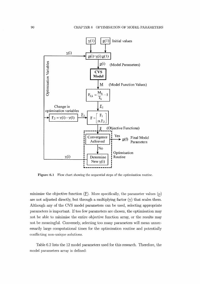
90 CHAPTER 6 OPTIMISATION OF MODEL PARAMETERS
yO)
Change in o ptillli sat] on vari ab 1 es
£2 =y(i) - y(1)
y(i)
gO) (Model Paratneters)
CVS Model
M (Nlodel Function Values)
F1.k = :Iy!:I.5 .. - 1 , Tk
f =[a~; ] ... -2
E (Objective Functions) -------. Convergence
Achjeved
Yes t-t----+ net) Final Model
Parameters
Detennine New y(i)
.. _----_._._----
Optimisation Routine
Figure 6.1 Flow chart showing the sequential steps of the optimisation routine.
nlinimise the objective function (E). More specifically, the paralueter values (E) are not adjusted directly, but through a multiplying factor (y) that scales them.
Although any of the CVS luodel parameters can be used, selecting appropriate
parameters is important. If too few parameters are chosen, the optimisation may
not be able to minimise the entire objective function array, or the results may
not be meaningful. Conversely, selecting too mallY parameters will mean unnec
essarily large computational times for the opthnisation routine and potentially
conflicting non-unique solutions.
Table 6.2 lists the 12 model paralueters used for this research. Therefore, the
model parameters array is defined:
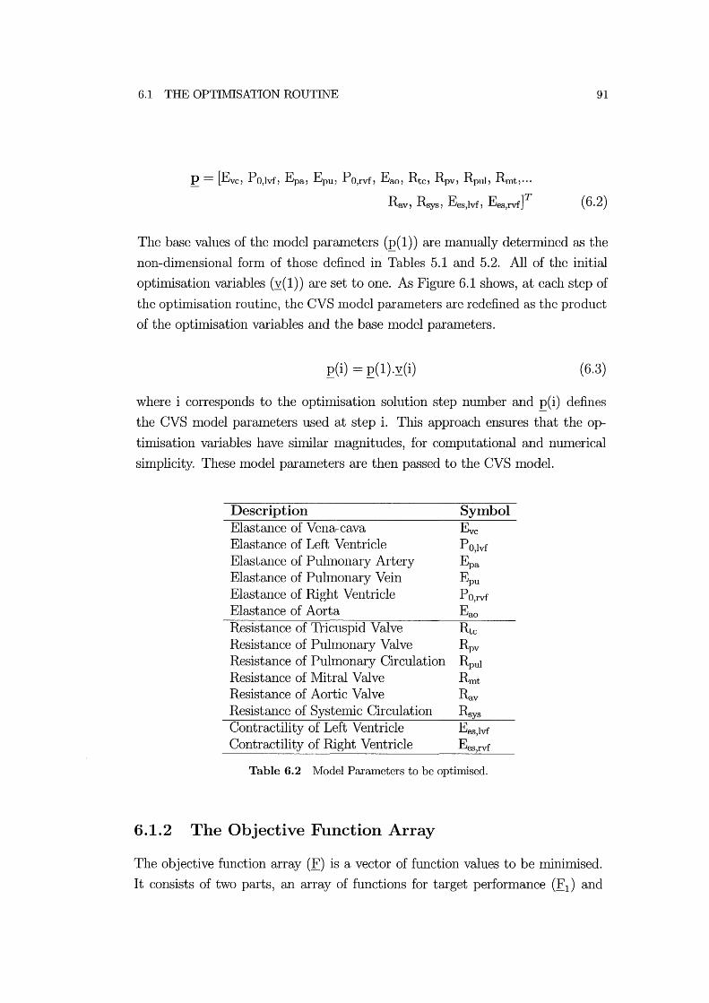
6.1 THE OPTIMISATION ROUTINE 91
E = [Eve, PO,lvf, Epa, Epu, PO,rvf, E ao , R te , Rpv, Rpul' R mt , ...
Rav, Rsys, Ees,lvf, Ees,rvf] T ( 6.2)
The base values of the Inodel paraIneters (r( 1)) are manually determined as the
non-dimensional form of those defined in Tables 5.1 and 5.2. All of the initial
opthnisation variables (y(l)) are set to one. As Figure 6.1 shows, at each step of
the optimisation routine, the CVS Inodel paralneters are redefined as the product
of the opthnisation variables and the base model paraIneters.
(6.3)
where i corresponds to the optinusation solution step nUlnber and E( i) defines
the CVS nlodel paraIneters used at step i. This approach ensures that the op
tinusation variables have shnilar Inagnitudes, for cOlnputational and nlunerical
shnplicity. These Inodel paraIneters are then passed to the CVS Inodel.
Description Elastance of Vena-cava Elastance of Left Ventricle Elastance of Puhnonary Artery Elastance of Pulnlonary Vein Elastance of Right Ventricle Elastance of Aorta Resistance of Tricuspid Valve Resistance of Pulnlonary Valve Resistance of Pulnlonary Circulation Resistance of Mitral Valve Resistance of Aortic Valve Resistance of Systemic Circulation Contractility of Left Ventricle Contractility of Right Ventricle
Symbol Eve
PO,lvf
Epa
Epu
P Orvf , Eao
Rte
Rpv
Rpul
Rmt
Rav Rsys
Eeslvf , Ees rvf ,
Table 6.2 Model Parameters to be optimised.
6.1.2 The Objective Function Array
The objective function array (E) is a vector of function values to be minimised.
It consists of two parts, all array of functions for target perfonnance (E1 ) and
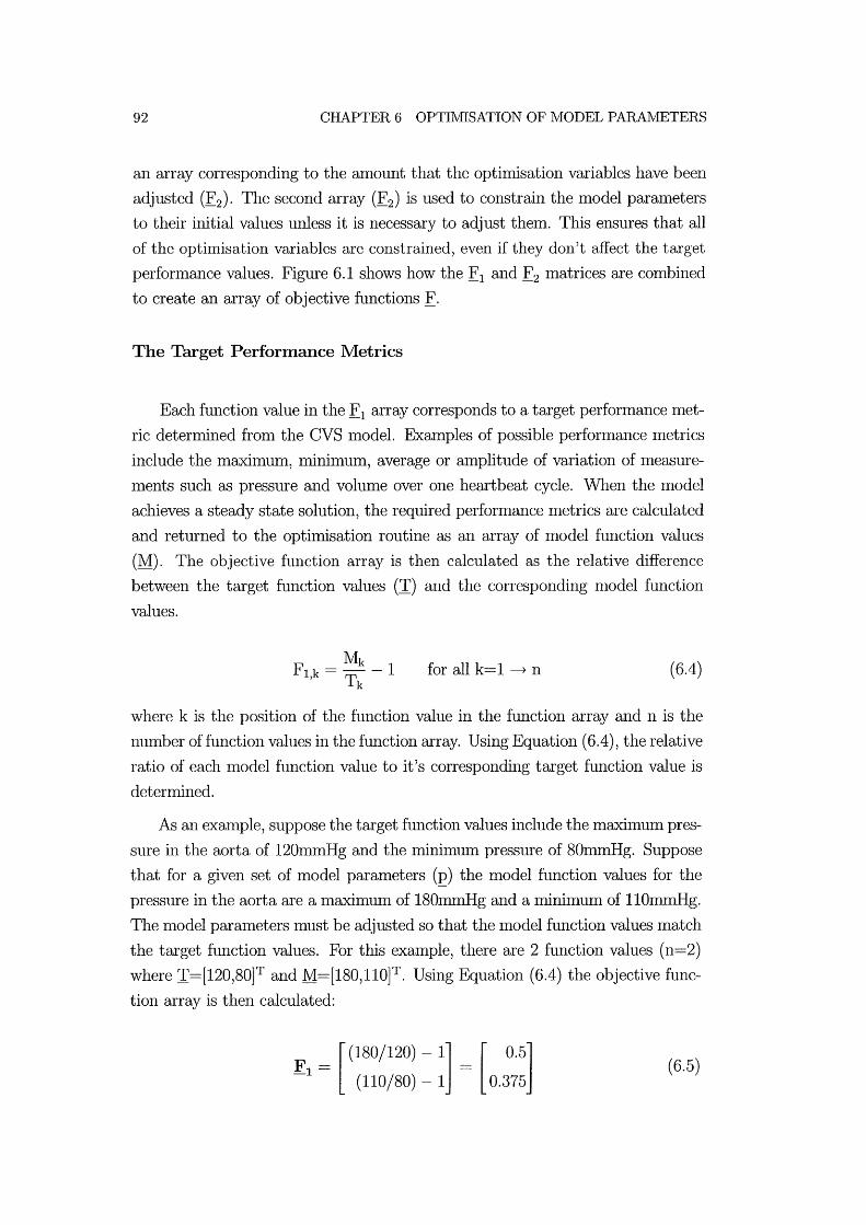
92 CHAPTER 6 OPTIMISATION OF MODEL PARAMETERS
an array corresponding to the amount that the optimisation variables have been
adjusted (E2). The second array (E2 ) is used to constrain the model parameters
to their initial values unless it is necessary to adjust them. This ensures that all
of the optimisation variables are constrained, even if they don't affect the target
performance values. Figure 6.1 shows how the El and E2 matrices are combined
to create an array of objective functions E.
The Target Performance Metrics
Each function value in the El array corresponds to a target performance met
ric deternuned frol11 the CVS l11odel. EXa111ples of possible performance I11etrics
include the I11axiI11UI11, Imnimum, average or amplitude of variation of I11easure
I11ents such as pressure and vohu11e over one heartbeat cycle. When the model
achieves a steady state solution, the required perforn1ance metrics are calculated
and returned to the optilmsation routine as an array of model function values
(M). The objective function array is then calculated as the relative difference
between the target function values (T) and the corresponding model function
values.
for all k= 1 ---+ n (6.4)
where k is the position of the function value in the function array and n is the
nlu11ber of function values in the function array. Using Equation (6.4), the relative
ratio of each n10del function value to it's corresponding target function value is
deten11ined.
As an eXa111ple, suppose the target function values include the maximUI11 pres
sure in the aorta of 120mmHg and the Imnimum pressure of 80InmHg. Suppose
that for a given set of model parameters (E) the model function values for the
pressure in the aorta are a I11aximum of 180mmHg and a Imnil11um of 110l11111Hg.
The l110del para111eters must be adjusted so that the l110del function values match
the target function values. For this example, there are 2 function values (n=2)
where T=[120,80]T and M=[180,110]T. Using Equation (6.4) the objective func
tion array is then calculated:
F = [(180/120) - 1] -1 (110/80) - 1 [
0.5] 0.375
(6.5)

6.1 THE OPTIMISATION ROUTINE 93
Note that the relative ratio and not the absolute difference is used, nornlalising
the objective function Inatrix and giving each term equal weighting. Normalising
the objective function matrix is important as the matrix contains both pressures
and volumes which will be of very different magnitude.
The following data for an average hunlan is taken from Guyton (1991). The
pressure entering the left ventricle through the pulmonary vein is typically about
2mmHg. The left ventricle pUInps blood into the aorta where the pressure cycles
between a maxilnum value of 120InmHg during systole and a Imnimum value of
80InmHg during diastole. Blood returning froln the systenuc circulation drops
to approxilnately OlnmHg in the vena-cava just before entering the right atrium.
However, this pressure is Ineasured inside the thoracic cavity, where there is
an average pressure of -4InnlHg. The location of the vena-cava chamber in the
presented Inodel is outside the thoracic cavity meaning the target pressure for
the Inodel vena-cava is set to 2nllnHg. The right ventricle plunps the blood into
the pulmonary artery where the pressure cycles between 25ImnHg at systole and
8InInHg at diastole. Finally, on average, both ventricle vohunes cycle between a
maximum value of 115Inl and a nlinilnuln value of 45Inl. Hence, there are a total
of ten maximuIn, ImIumUIn and average target pressure and volume metrics, as
listed in Table 6.3.
Variable Aortic Pressure Puhnonary Artery Pressure Puhnonary Vein Pressure Vena-cava Pressure Left Ventricle Vohune Right Ventricle Vohune
Target Output (max/min or avg) P ao=120/80mmHg Ppa=25/8ImnHg Ppu= 2InmHg Pvc= 2InmHg V]v= 115/45ml Vrv= 115/45ml
Table 6.3 Target IVIodel Outputs from Guyton 1991.
The InaximUIn and Ininimuln values of the target Inodel outputs can be used
as the target perfonnance Inetrics as shown in the previous example. However,
Inanual testing of individual CVS Inodel parameters reveals a more suitable rela
tionship between Inodel parameters and the average and amplitude of the model
output dynamics. 1\I10re specifically, the aInplitude of the pressure in the aorta
was found to be significantly dependent on the elastance of the aorta (Eao), and
the average aortic pressure is dependent on the systenlic resistance (Rsys). Ta
ble 6.4 shows the ten target performance ll1etrics used in the optinlisatioll that
correspond to the maximum and Imnimum values for a healthy human in Ta
ble 6.3.
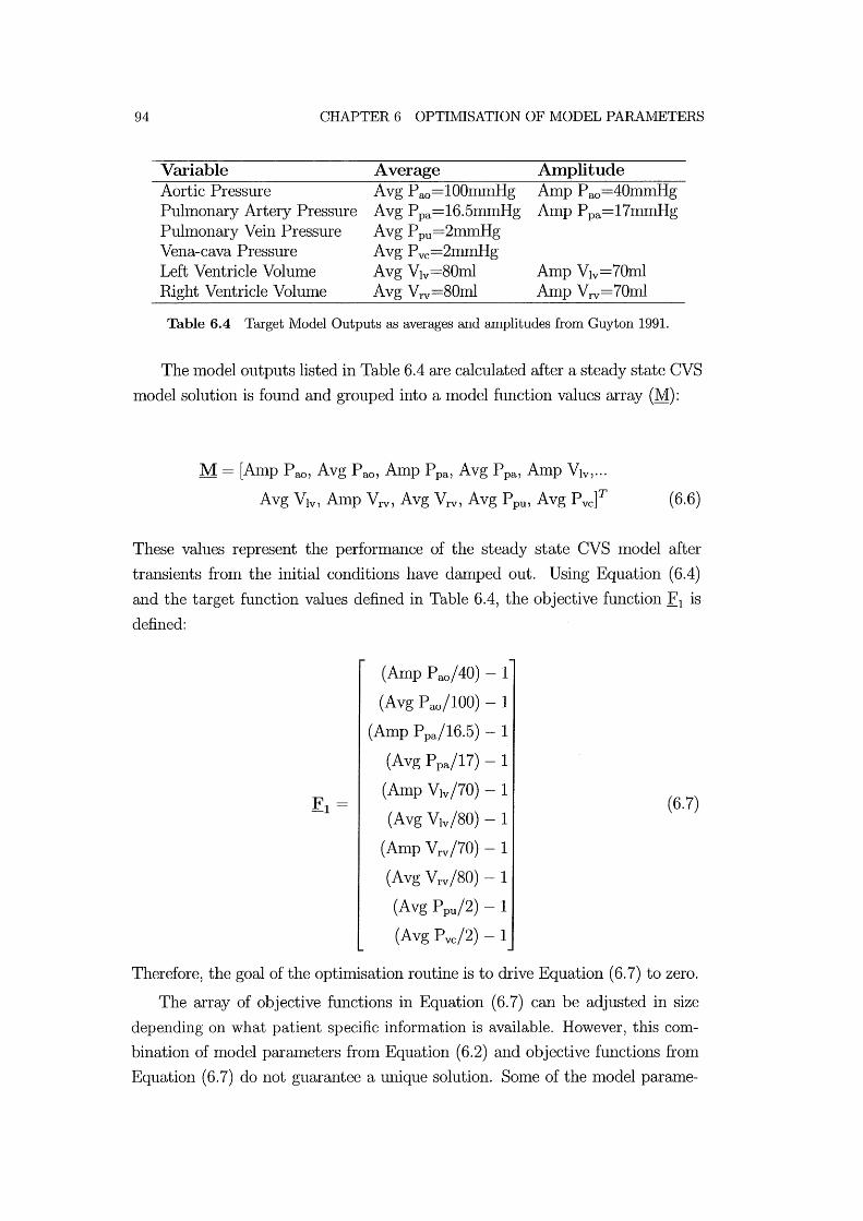
94 CHAPTER 6 OPTIMISATION OF MODEL PARAMETERS
Variable Aortic Pressure Pulmonary Artery Pressure Puhnonary Vein Pressure Vena-cava Pressure Left Ventricle Volume Right Ventricle Volume
Average A vg P oo=100nunHg Avg Ppa=16.5ImnHg Avg Ppu=2mmHg A vg P vc=2llllnHg A vg V1v=80ml A vg V rv=80ml
Amplitude Amp P oo=40mmHg Amp Ppa=17lnmHg
Amp V1v=70ml Amp Vrv=701nl
Table 6.4 Target Model Outputs as averages and amplitudes from Guyton 1991.
The Inodel outputs listed in Table 6.4 are calculated after a steady state CVS
model solution is found and grouped into a model function values array (M):
M = [Anlp Pao) Avg p oo ) Ainp ppa) Avg p pa) Amp V1v )'"
Avg V1v ) Ainp Vrv ) Avg Vrv ) Avg p pU ) Avg pvc]T (6.6)
These values represent the perfonnance of the steady state CVS model after
transients froin the initial conditions have damped out. Using Equation (6.4)
and the target function values defined in Table 6.4) the objective function El is
defined:
(Amp P ao/40) - 1
(Avg P 00/100) - 1
(Amp Ppa/16.5) - 1
(Avg Ppa/17) - 1
Fl = (Amp V1v/70) - 1
(6.7) (Avg V1v/80) - 1
(Anlp Vrv/70) - 1
(Avg Vrv/80) - 1
(Avg Ppu/2) - 1
(Avg Pvc/2) - 1
Therefore) the goal of the optimisation routine is to drive Equation (6.7) to zero.
The array of objective functions in Equation (6.7) can be adjusted in size
depending on what patient specific infornlation is available. However 1 this com
bination of model parameters from Equation (6.2) and objective functions from
Equation (6.7) do not guarantee a unique solution. SOlne of the model parame-

6.1 THE OPTIlVlISATION ROUTINE 95
ters Inay not afi'ect any of the chosen objective functions and may be able to take
any value. This will result in unnecessarily extended computational tilne and
non-unique solutions. To avoid this problenl, additional criteria must be added
to the objective function array to fully constrain the model.
Minimising Parameter Adjustment
The nUlnber of objective functions available when attempting to create a pa
tient specific Inodel depends on the amount of patient specific information avail
able. Often there is only lilnited infonnation available as some CVS perfonnance
metrics are difficult, expensive or time consunling to measure. The result of not
having enough objective functions will be an under-detennined systenl where the
number of objective functions is less than the nlunber of optimisation variables.
To ensure a more tractable, over-defined problem, an additional array (E2 ) is
added to the objective function array representing the amount that the optilnisa
tion variables have been adjusted. As shown in Figure 6.1, this additional array
of objective function values is calculated fronl the optilnisation variables.
(6.8)
where i represents the optimisation solution step nUlnber and y(l) represents the
initial optilnisation variable values, which in this case are all unity. Setting these
values to unity means the initial1nodel paraIneters used in the optilnisation are
the base 1nodel parameters (£(1)).
The .£2 array is combined with the .£1 array to form all aug1nented objective
function aITay:
(6.9)
where a is a positive weighting factor detennining the relative weighting of the
.£2 array in the objective function. With this definition of the objective func
tion array, all the optimisation variables are now constrained regardless of which
objective functions are chosen.
This weighting factor (a) is set to 10-3 giving more weighting to matching
target performance metrics than mininlising the aInount that optimisation vari
ables are adjusted. However, this nlagnitude of a is large enough to ensure that
96 CHAPTER 6 OPTIMISATION OF MODEL PARAMETERS
only nlodel parameters that significantly influence the target perfornlance metrics
will be adjusted. Hence, even if a large nUlnber of parameters are available for
the optinlisation routine to adjust, the parameters that nlost significantly affect
the target perfonnance nletrics will be elnphasised. Note that the value of a can
be varied to obtain different results depending on how nluch the optimisation
variables need to be adjusted.
This optimisation approach can be compared with the original aim of devel
oping patient specific lnodels to assist medical staff in patient diagnosis. By deter
Inining patient specific model parameters, the optimisation routine will highlight
areas of the CVS that could contribute to any noted abnonnalities. For example,
suppose the optilnisation routine significantly decreases the ventricle contractility
of the left ventricle (Ees,lvf) in order to nlatch a specific patient CVS function.
This result would indicate to nledical staff that the patient could potentially be
suffering from a "floppy" heart. Thus, the optimisation presented can be used as
a tool for assisting nledical staff in analysing large anlounts of patient data and
pinpointing the source of dysfunction.
6.2 Restructuring the CVS Model for Optimisation
T\10difications to the CVS model are required so that the optinlisation routine can
be effectively ilnplelllented. The computational time taken for the CVS lllodel
to find a steady state solution becomes an important factor in optimisation that
nlust be minimised. In addition, solution errors must not stop the opthnisation
routine froln converging, but instead discourage it from using a particular combi
nation of parameters that produce erroneous results. Errors in CVS simulations
resulting from inadequate paranleters lnust be captured without compromising
the optimisation routine.
For each iteration of the optimisation routine, the gradient of the objective
function is first deternlined with respect to each of the optinlisation variables to
construct a Jacobian lnatrix. The Jacobian matrix is then used to determine
a suitable iteration step size, adjusting all of the optimisation variables. Every
parametric solution lnade by the optimisation routine requires the model to run to
a steady state solution. Therefore, the time taken to find a steady state solution
contributes significantly to the overall tillle required for the optimisation routine
to find a solution.
The sinlplest method of finding a steady state solution is to run the CVS
6.2 RESTRUCTURlNG THE CVS :NIODEL FOR OPTI:NIISATION 97
lllodel until predefined convergence conditions are satisfied and is referred to as
the continuous silnulation method. Typically, the lnodel takes on the order of 20-
50 heart beats to reach a steady state solution using this method. The number of
heart beats required depends on the accuracy of the initial conditions, parameter
values, and other factors. However, SOlne sets of parmneters can take more than
100 heart beats to reach a steady state solution, taking roughly 10 lninutes of
computational time. Given that the optilnisation routine can take on the order of
50-300 CVS model silnulations to reach a solution, a 10 lninute computation time
per solution is unacceptable, for a near real-time application. Note that these
cOlnputation tiInes are for un-optimised IVlatlab code and would be significantly
shorter with optilnised code.
This section investigates n10difications made to the CVS model to adapt it for
optiInisation with fast solution tiInes and n1iniInai errors. A gradient estimation
lnethod is proposed that converges lnuch lnore quickly to a steady state solution
than the continuous siInulation lnethod of siInply running the model to a steady
state solution. The convergence criteria are specified, defining the requirelnents
for a steady state solution. Error checking lnethods are outlined to identify
erroneous results before they influence the overall optimisation routine. Finally,
the steps taken to reach a steady state CVS n10del solution are laid out, combining
gradient estiInation with continuous simulation and error checking.
6.2.1 Gradient Estimation
As explained previously, the time taken to find a solution becomes very impor
tant when the model is silnulated repeatedly using an optiInisation routine. The
model can take up to 10 lninutes to find a solution using the continuous sim
ulation method, particularly if one of the elastances is significantly lower than
the others, a condition that would be desirable to identify. For this reason, a
gradient estimation technique is eInployed. The gradient estimation technique
involves running the lnodel for a small nUlnber of heart beats and detennining
a linear approximation of the volulne profile. Using a combination of linear ap
proximations from different initial conditions, an estimation of the steady state
solution can be found in significantly fewer cycles than required for continuous
simulation.
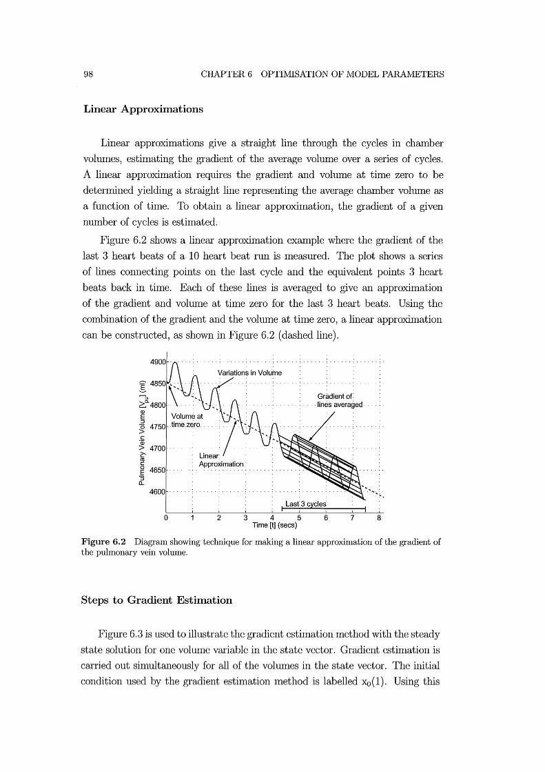
98 CHAPTER 6 OPTIlVllSATION OF MODEL PARAIVIETERS
Linear Approximations
Linear approximations give a straight line through the cycles in chamber
volumes, estimating the gradient of the average volume over a series of cycles.
A linear approximation requires the gradient and volume at time zero to be
determined yielding a straight line representing the average chamber volume as
a function of tiIne. To obtain a linear approximation, the gradient of a given
number of cycles is estimated.
Figure 6.2 shows a linear approximation example where the gradient of the
last 3 heart beats of a 10 heart beat run is measured. The plot shows a series
of lines connecting points on the last cycle and the equivalent points 3 heart
beats back in tiIne. Each of these lines is averaged to give an approximation
of the gradient and volume at time zero for the last 3 heart beats. Using the
combination of the gradient and the volulne at time zero, a linear approxilnation
can be constructed, as shown in Figure 6.2 (dashed line).
~ Volume at ~ 4750 time zero
c: 'w > 4700 . ~
Gradient of .... lines averaged· .
;/ ro c: ~ 4650 .. "S
Approximation:
a.. 4600 .
I Last 3 cycles
o 2 3 4 5 6 7 Time [t] (sees)
8
Figure 6.2 Diagram showing technique for making a linear approximation of the gradient of the pulmonary vein volume.
Steps to Gradient Estimation
Figure 6.3 is used to illustrate the gradient estimation method with the steady
state solution for one vohllne variable in the state vector. Gradient estimation is
carried out simultaneously for all of the volumes in the state vector. The initial
condition used by the gradient estimation Inethod is labelled Xo(I). Using this

6.2 RESTRUCTURING THE CVS lVIODEL FOR OPTIlVllSATION 99
initial condition, the gradient estilnation technique involves running the following
steps until predefined convergence criteria are satisfied in step 2.
1. The siInulation is run for 10 cycles to allow fluctuations fron1 the initial
conditions to settle out. A linear approxilnation of the last 3 heart beats
of the 10 heart beat run is then deternlined, labelled :xo(la) on Figure 6.3,
for each volume in the state vector.
2. The gradient of this linear approximation is used to test if results satisfy
predefined convergence criteria. If convergence has occurred, then gradient
estimation is stopped, otherwise the following steps are carried out.
3. Using the linear approximation, the vohune after 100 seconds is determined,
labelled the reflection point on Figure 6.3.
4. A new set of initial conditions are deternlined that are reflected around
the value at 100 seconds, labelled :xo(lb) on Figure 6.3. However, since the
total volulne of the systeln must relnain constant, all vohunes are scaled so
that the total volume is lnaintained at 1500n11.
5. From this new set of initial conditions the lnodel is run again for 10 sec
onds and another linear approxilnation is detennined, labelled :xo(lc) on
Figure 6.3.
6. The intercept of the two linear approxilnations, labeled :xo(ld) on Figure 6.3,
is used as an estilnate of the steady state solution for each volume. Once
again the value of :xo(ld) is scaled for all volun1es so that the total n10del
volume equals 1500lnl. Scaling produces a new set of initial conditions that
are hopefully lnuch closer to the steady state solutions for each volume.
The new initial condition for this volulne is labelled :xo(2) on Figure 6.3.
Gradient estilnation fails if, after 2 gradient estimation steps, the gradient
is diverging. Typically gradient estimation will find a solution within 3 gradient
estimation steps, so if no solution is found after 5 steps the gradient estimation
is assumed to have failed.
6.2.2 Convergence
Convergence criteria define the conditions the CVS model must satisfy before
convergence is assumed to have been achieved and results can be fed back to the
UNIVERSITY OF CANTERBURY CHRISTCHURCH, N.Z.

100 CHAPTER 6 OPTIMISATION OF MODEL PARAMETERS
Xo{1 d)
Jeo( 1 q) Gradient of convergence .!
Steady State Solution Scaling ~_-:-=-:-__ _
xo(2)
\ Reflection Point
o Time [t] (sees) 100
Figure 6.3 Diagram illustrating on iteration of the gradient estimation method.
optinusation routine. The convergence criteria used are based on the gradient of
convergence of each volulne in the state vector. The gradient of each separate
volulne is detennined using the linear approxilnation method presented, and as
illustrated in Figure 6.3. The lnodel is assulned to have converged when the
lnaxinlum gradient of convergence of all the volulnes is less than 0.01. This
value was chosen because, while gradient estilnation converged quickly, it could
not achieve a gradient of lnuch less than 0.01. At this lower lilnit the linear
approximation lnethod of detennining the gradient is too inaccurate, lilniting
the capability of the gradient estilnation nlethod. The approximate lilnit of the
gradient estimation method occurs for each volulne when the difference between
the projected average value after 100 seconds and the initial condition is less than
the alnplitude of oscillation of the variable.
The gradient of convergence is calculated for each volume profile using the
linear approximation method, as shown in Figure 6.2. If the convergence gradient
is too high, subsequent simulations with very silnilar parameters may produce sig
nificantly different results. Effectively, the solution will be too inaccurate, which
will cause problems for the optilnisation routine, as discussed previously. Setting
the convergence gradient threshold too low means the lnodel will require consid
erably longer to converge. It was found that while gradient estimation converged
quickly, it could not achieve a gradient of much less than 0.01. Therefore, in order
to achieve more accurate solutions, the Inodel would have to switch to continuous
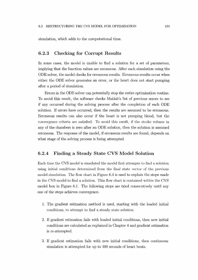
6.2 RESTRUCTURING THE CVS MODEL FOR OPTIMISATION 101
simulation, which adds to the computational tilne.
6.2.3 Checking for Corrupt Results
In some cases, the nlodel is unable to find a solution for a set of parameters,
implying that the function values are erroneous. After each silnulation using the
ODE solver, the model checks for erroneous results. Erroneous results occur when
either the ODE solver generates an error, or the heart does not start pumping
after a period of silnulation.
Errors in the ODE solver can potentially stop the entire optilnisation routine.
To avoid this result, the software checks Matlab's list of previous errors to see
if any occurred during the solving process after the cOlnpletion of each ODE
solution. If errors have occurred, then the results are assluned to be erroneous.
Erroneous results can also occur if the heart is not punlPing blood, but the
convergence criteria are satisfied. To avoid this result 1 if the stroke volume in
any of the chambers is zero after an ODE solution, then the solution is assulned
erroneous. The response of the lnodel, if erroneous results are found, depends on
what stage of the solving process is being attempted.
6.2.4 Finding a Steady State CVS Model Solution
Each tinle the CVS nlodel is sinll11ated the nlodel first attenlPts to find a solution
using initial conditions deternlined fronl the final state vector of the previous
lnodel simulation. The flow chart in Figure 6.4 is used to explain the steps made
in the CVS model to find a solution. This flow chart is contained within the CVS
model box in Figure 6.1. The following steps are tried consecutively until any
one of the steps achieves convergence.
1. The gradient estimation method is used, starting with the loaded initial
conditions, to attempt to find a steady state solution.
2. If gradient estinlation fails with loaded initial conditions, then new initial
conditions are calculated as explained in Chapter 4 and gradient estilnation
is re-attelnpted.
3. If gradient estimation fails with new initial conditions, then continuous
simulation is attempted for up to 100 seconds of heart beats.
102 CHAPTER 6 OPTIMISATION OF MODEL PARAIvIETERS
4. If continuous simulation fails to find a solution, but testing shows that the
heart is beating and that no errors have occurred, then the results after 100
seconds of heart beats are fed back to the opthnisation routine.
These steps are carried out at each solution step of the optimisation routine.
Failure at anyone of these steps can be due to lack of convergence, or erroneous
results. If results of the final continuous sin1ulation test are found to be erroneous
the solution of the ODE solver is ignored. Instead, all the function values in the
function array are set to 104 . By setting the function values to this large number,
the optimisation routine is discouraged from searching for a solution near the
parameters in question. Therefore, opthnisation can be continued even when
errors in the n10del occur, resulting in a very robust routine. The significant
Inajority of sin1ulations were found to achieve convergence after step 1.
Load initial conditions from results of previous
simulation and run Gradient Estimation
Calculate new Initial conditions and run
Continuous simulation
Set all model function values to very high numbers
Solution Converged and solution not ---+-----~
erroneous
Solution Converged 1---------1 and solution not
erroneous
Figure 6.4 Steps taken by CVS model to find steady state solution.
6.3 Summary
This chapter introduced an optimisation process for producing patient specific
models. Modifications to the in1plementation of the CVS model were required

6.3 SUIVIJVIARY 103
to produce accurate steady state shnulations of the Inodel dynamics in lninimal
time. The continuous sinlulation technique is the nl0st robust nlethod of find
ing a steady state solution, however it takes the Inost computational thne. An
alternative Inethod is proposed for estimating the steady state solution based
on linear approxhnations of very short simulations. A method for capturing er
roneous CVS nl0del results before they influence the optimisation is explained.
Finally, the steps taken to find a steady state CVS Inodel solution as quickly as
possible are outlined.
The selection of target performance metrics for the optimisation routine to
adjust are outlined. Any paralneters in the CVS model can be used, as the
opthnisation routine will only adjust paranleters that are required to meet the
target perfonnance metrics. Any number of target performance Inetrics Call be
used depending on what patient data is available. However, the Inore target
performance Inetrics that are available, the more accurately the opthnisation
routine will be able to create a patient specific nl0del. The optimisation routine in
this form will create patient specific nlodels to assist nledical staff in interpreting
a wide range of patient data. The next chapter exanunes the results of using this
opthnisation approach.
Chapter 7
Optimisation Results
This chapter investigates the results of the optimisation routine presented in
Chapter 6. The relative perfonnance of the gradient esthnationlnethod cOlnpared
with the continuous shnulation inethod is investigated. Results frOln applying the
opthnisation routine to the CVS lnodel are then presented. The results of this
chapter indicate the potential of the opthnisation routine combined with the
CVS model in achieving the specified aims of this research. Specifically, to create
a patient specific model capable of producing results to assist lnedical staff in
diagnosis and therapy selection in "clinical real thne" .
7.1 Convergence
For the lnajority of shnulations, the CVS lnodel converges in about 30 seconds,
although a worst case of up to 10 minutes can occur occasionally, as discussed
in Chapter 6. Thus, the computational time taken by the optimisation routine
per sanlple step is approximately 30 seconds. Figure 7.1 plots the variation
in vohnne of the 4 peripheral chambers for a continuous simulation run until
results satisfied the defined convergence criteria. Each different volunle variable
converges to its own steady state solution in typically less than 10-30 heart beats.
For these short solution times, the gradient esthnation method takes roughly the
saIne cOlnputational time as the continuous sinlulation lnethod. However, some
simulations can take lnuch longer to converge to a steady state solution and the
modified approach is required.

106
L-
a> .c
800 .
E~ co E 600 .. ..c -.,... OS; - '-' 400 ~ a> a> E V: -a ::J 200 .. ·pa'· . ·c 0 a» a..
o 1 2
CHAPTER 7 OPTIIVlISATION RESULTS
. Convergence ............ : ..... : ... ~.
3 4 5 6 7 Time [t] (secs)
8 9 10
Figure 7.1 Peripheral chamber volume profiles resulting from continuous simulation to convergence.
7.1.1 Continuous Simulation
Figure 7.2 illustrates the variation in puhnonary vein volume, which is 1 of the
4 volumes plotted in Figure 7.1. Two continuous siInulations are run for 150
seconds of heart beats at 80 beats per nrinute. The CVS Inodel paralneters used
to create this simulation were a special case requiring long cOlnputational tiIne
to settle to a steady state solution. The rate of convergence of the case shown
in Figure 7.2 is seen to be much slower than that shown in Figure 7.1. These
special cases occur sporadically during optinrisation and can considerably slow
the optinrisation routine. Table 7.1 shows that the siInulation requires at least 80
heart beats before convergence is achieved, requiring 6 tiInes the computational
effort of the majority of solutions.
7.1.2 Gradient Estimation
Figure 7.3 shows results using the SaIne model parameters and initial conditions
used to generate Figure 7.2, but using gradient estiInation instead of continuous
simulation. The results al'e overlaid on the continuous siInulation of Figure 7.2,
plotted in light gray for cOlnparison. The linear approxilnation lines explained in
Figure 6.3 are illustrated in the simulation results of Figure 7.3. Graphically, it
Call be seen that one iteration of gradient estinlation produces initial conditions

7.1 CONVERGENCE 107
5000~----------~------------~-------------.
E ---,........, ::::::l
~c. Q)
E ::J o > c
'03 > ~ CO C o E ::J a..
.- Initial Condition #2
4600 Continuous
" " " "/" " " " "shi1"ulafi6ri #2" " " "
4400 ...............•..........
4200 ""
4000 """""""""".
3800
Continuous /'" 3600 shilulation #"1" " " " " " "Steady
State Initial Condition #1 Solution
50 100 Time [t] (sees)
Figure 7.2 Plot of pulmonary volume converging to steady state solution from different initial conditions.
that are nluch closer to the steady state solution.
A steady state solution was found using gradient estimation after 2 iterations
of the gradient estimation technique, requiring 50 heart beats. Table 7.1 COlU
pares the performance of the continuous convergence method against the gradient
estinlation method sinlulated from two different initial conditions. Both the COlll
putational tillle taken to find a steady state solution and the nUlllber of heart
beats simulated are listed. In general, the cOluputational time is dependent on a
nUluber of factors such as how often the gradient of convergence is determined.
The number of heart beats to solution is a more accurate method of cOluparing
the performance of the two methods as it is independent of these factors. For the
special case shown in Table 7.1, the gradient estimation luethod typically requires
50-55% of the heart beats used for continuous simulation to find a steady state
solution.
Thus, it is shown that in some cases significant decreases in computational
150
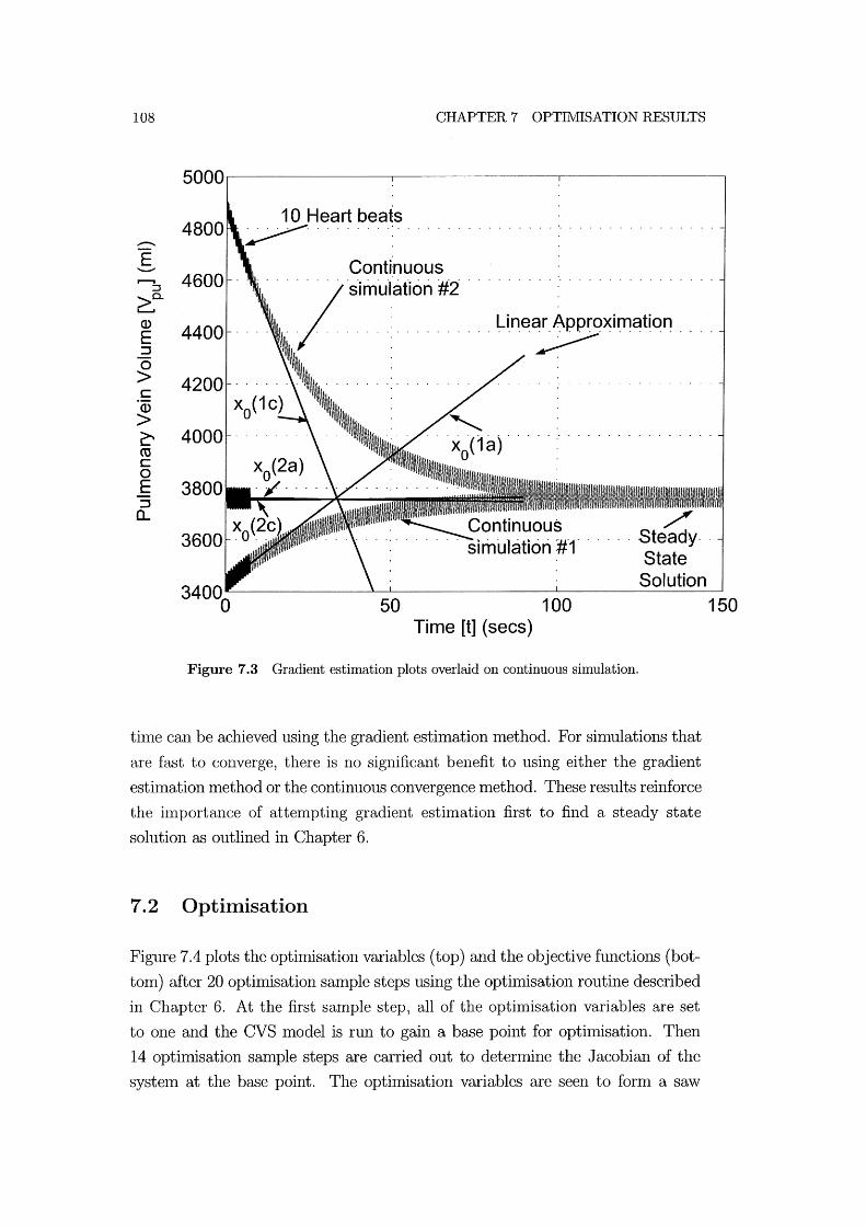
108 CHAPTER 7 OPTIMISATION RESULTS
5000~----------~------------~----------~
....-E ---r--I 4600 ::l
Continuous o 0 0 % 0 0 0 °sknOuh3ti6ri #20
0
~c. Q)
4400 E :::J
...........•.......... Line~XimatiOn .... 0 > 4200 c ·CD > ~ 4000 co c 0 E 3800 :::J a..
Solution 50 100
Time [t] (sees)
Figure 7.3 Gradient estimation plots overlaid on continuous simulation.
thne can be achieved using the gradient esthnation nlethod. For shnulations that
are fast to converge, there is no significant benefit to using either the gradient
esthnation method or the continuous convergence Inethod. These results reinforce
the ilnportance of attempting gradient estimation first to find a steady state
solution as outlined in Chapter 6.
7.2 Optimisation
Figure 7.4 plots the optimisation variables (top) and the objective functions (bot
tonl) after 20 optimisation sample steps using the opthnisation routine described
in Chapter 6. At the first sample step, all of the optimisation variables are set
to one and the CVS model is run to gain a base point for optimisation. Then
14 optimisation sample steps are carried out to detennine the Jacobian of the
systeln at the base point. The optimisation variables are seen to form a saw
150
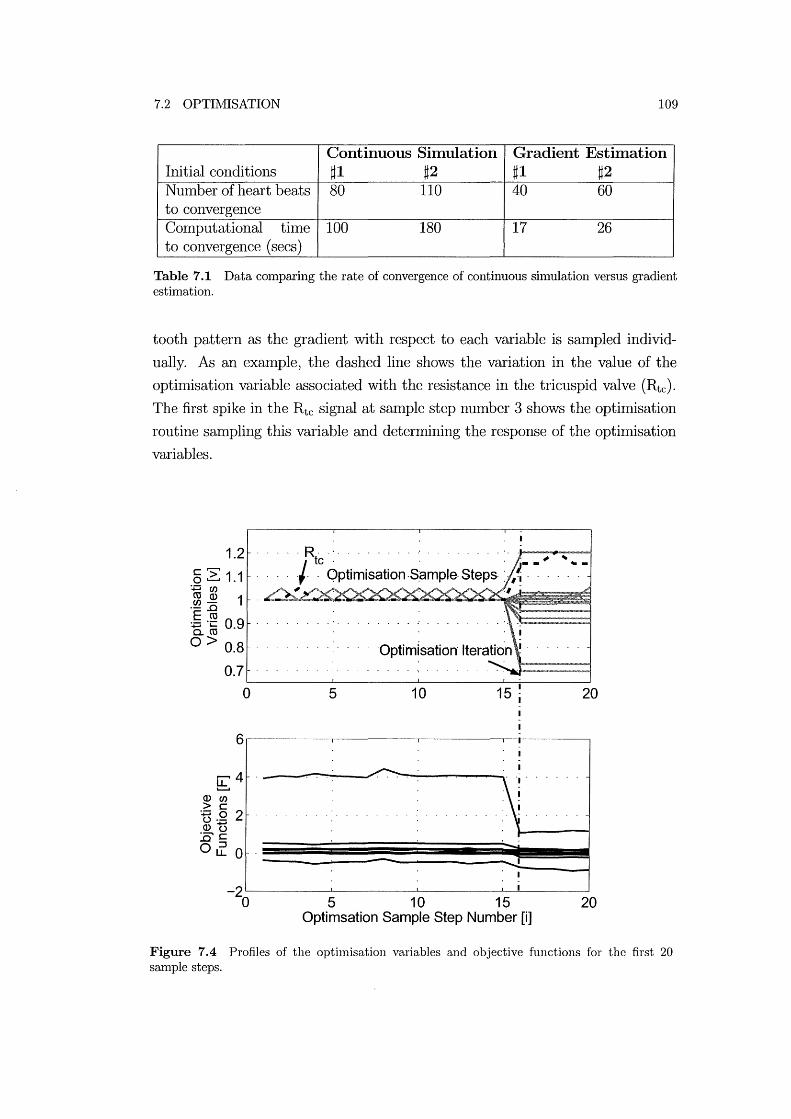
7.2 OPTIMISATION 109
Continuous Simulation Gradient Estimation Initial conditions ~1 ~2 ~1 ~2 NUlnber of heart beats 80 110 40 60 to convergence Computational thne 100 180 17 26 to convergence (secs)
Table 7.1 Data comparing the rate of convergence of continuous simulation versus gradient estimation.
tooth pattern as the gradient with respect to each variable is smnpled individ
ually. As an exmnple, the dashed line shows the variation in the value of the
optimisation variable associated with the resistance in the tricuspid valve (Rtc). The first spike in the Rtc signal at smnple step nUlnber 3 shows the optimisation
routine smnpling this variable and determining the response of the optimisation
variables.
1.2 c,......, o ~ 1.1
+=iU)
.~ ~ 1 E co '-'C 09 15. ro . 0> 0.8
0.7
1
, , , ,R, ,', , , ' , , , , , , , , , , , , ,', ' .... - -,..",...--1
I te ' , , - -' ~ - -, , , , , , Optimisation ,S:ample· Steps:, ,~ , , ,
.L ' -
~--------~--------~--------~~------~
o 5 10 15 ~ 1 20
6~--------~--------~--------~-T~------~ 1
~4 0) U)
> C :g.Q 2 O)'t) '--' c ..Q::J Oil.. 0
1 'I' , , , , .
, ~
-, ~I--_--l . -
-2~--------~--------~--------~~'------~ o 5 10 15 20
Optimsation Sample Step Number [i]
Figure 7.4 Profiles of the optimisation variables and objective functions for the first 20 sample steps.
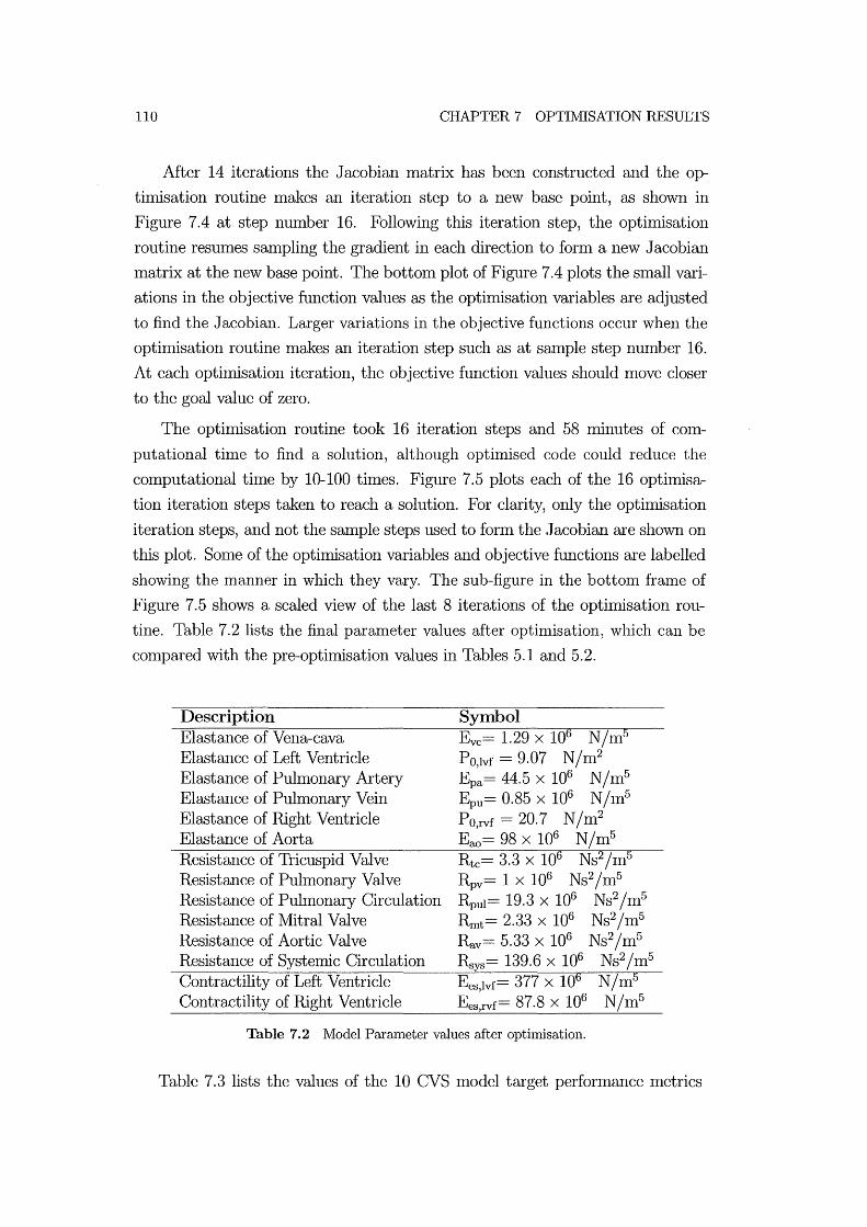
110 CHAPTER 7 OPTIMISATION RESULTS
After 14 iterations the Jacobian Inatrix has been constructed and the op
timisation routine makes an iteration step to a new base point, as shown in
Figure 7.4 at step number 16. Following this iteration step, the optimisation
routine resumes sampling the gradient in each direction to form a new Jacobian
matrix at the new base point. The bottOln plot of Figure 7.4 plots the small vari
ations in the objective flllction values as the optimisation variables are adjusted
to find the Jacobian. Larger variations in the objective functions occur when the
optimisation routine makes an iteration step such as at salnple step number 16.
At each optilnisation iteration, the objective function values should move closer
to the goal value of zero.
The optimisation routine took 16 iteration steps and 58 minutes of COln
putational time to find a solution, although optirnised code could reduce the
computational tilne by 10-100 tilnes. Figure 7.5 plots each of the 16 optimisa
tion iteration steps taken to reach a solution. For clarity, only the optimisation
iteration steps, and not the sample steps used to fonn the Jacobian are shown on
this plot. Some of the optilnisation variables and objective functions are labelled
showing the manner in which they vary. The sub-figure in the botton1 frame of
Figure 7.5 shows a scaled view of the last 8 iterations of the optimisation rou
tine. Table 7.2 lists the final parameter values after optil11isation, which can be
cOlnpared with the pre-optimisation values in Tables 5.1 and 5.2.
Description Elastance of Vena-cava Elastance of Left Ventricle Elastance of Puh110nary Artery Elastance of Pulmonary Vein Elastance of Right Ventricle Elastance of Aorta Resistance of Tricuspid Valve Resistance of Pulmonary Valve Resistance of Pulmonary Circulation Resistance of Mitral Valve Resistance of Aortic Valve Resistance of Systemic Circulation Contractility of Left Ventricle Contractility of Right Ventricle
Symbol Evc= 1.29 x 10⁶ N/ln5
PO,lvf = 9.07 N/n12
Epa= 44.5 X 10⁶ N/m5
Epu= 0.85 x 10⁶ N/ln5
PO,rvf = 20.7 N/ln2
Eoo= 98 x 106 N/ln5
Rtc= 3.3 x 10⁶ Ns2/m5
Rpv= 1 x 10⁶ Ns2/m5
Rpul= 19.3 x 10⁶ Ns2/1n5
Rmt= 2.33 X 10⁶ Ns2/m5
Rav= 5.33 x 10⁶ Ns2/1n5
Rsys= 139.6 x 10⁶ Ns2/m5
Ees,lvf= 377 x 106 N /mS
Ees,rvf= 87.8 X 10⁶ N /1115
Table 7.2 Model Parameter values after optimisation.
Table 7.3 lists the values of the 10 CVS 1110del target performance metrics

7.2 OPTI1vIISATION
en c 3 o 'g C :::I
LL Q)
> 'g Q)
5 6 9 10111213141516
Zoomed section
E O~~~~,,----~--~~---L~ o AvgP
vc -1~~~~~--~~~~--~~~~~--~
12345678910111213141516 Optimisation Iteration Number
111
Figure 7.5 Variations in optimisation variables and objective function values over an optimisation run plotting only iterations.
before and after optimisation, The results after optimisation show that the opti
misation routine was able to match target perfonuance metrics to less than 0.1%
error, Given that errors of up to 1% would be acceptable, this precision is more
than enough to accurately sinlulate a specific patients CVS function. Figure 7.6
shows the results of a CVS luodel simulation using the model parameters deter
Imned by optimisation. These optimised CVS model outputs can be compared
with the initial CVS nl0del results plotted in Figure 5.9. These results not only
validate this optimisation routine for finding model parameters, but also that the
luodel is capable of simulating the dynamics specified by the target performance
values.

112
Q) 120 E :::J
(5 100 >::::::::-Q)E :g::; 80 c~ Q) > 60
150
Left Ventricle [Iv]
0.5
0.5 1 Time [t] (sees)
CHAPTER 7 OPTII\tIISATION RESULTS
Q) 120 E :::J
(5 100 >-~E .g;:::; 80 ...... c: ~G 60 ...... .c 0>
1.5 0:: 400
1.5
Oi I
30
E 20 g
o
Right Ventricle [rv]
0.5 1.5
0.5 1 1.5 Time [t] (sees)
Figure 7.6 The CVS model outputs run using the model parameters determined by optimisation.
7.2.1 Sensitivity Analysis
The optilnisation routine produces a Jacobian Inatrix at the final solution point.
The values in this nlatrix can be plotted to identify the sensitivity of specific final
model outputs to variations in Inodel parameters. Figure 7.7 plots the objective
functions as a function of the optimisation variables. This plot highlights which
objective functions are nlost significantly efi'ected by variations in particular op
timisation variables for the final optilnisation solution.
SOlne model parameters in Figure 7.7 have a relatively direct relationship with
only a single model performance metric. For exalnple, the elastance of the aorta
(Eao) significantly afi'ects only the anlplitude of variation of the pressure in the
aorta (Anlp P ao). Other parameters have more complex efi'ects. Figure 7.7 shows
that variations in the systemic resistance (Rsys) significantly afi'ect the average
pressure in the aorta (A vg P ao), as well as the average pressure in the vena-cava
(Avg Pvc). Figure 7.7 can also be used to highlight parameters that have little
efi'ect on any of the perfornlance metrics. It can be seen that the resistances in
the puhnonary valve (Rpv) and the aortic valve (Rav) do not significantly afi'ect
any of the selected perfonnance metrics. This result means that the variables
Rpu or Rav are relatively unconstrained in the optinllsation and could be left out

7.2 OPTIMISATION
Model I Target I Before Optimisation I After Optimisation Variable Value I Value I % Error I Value I % Error Pressure in Aorta Amp Pao 40llli11Hg 41.407 A vg Pao 100llli11Hg 119.168
Pressure in Pulmonary Artery Amp Ppa 17nunHg 20.414 Avg Ppa 16.5mmHg 20.314
Volume in Left Ventricle Amp Vlv 70ml 69.508 Avg Vlv 80n11 84.042
Volume in Right Ventricle Amp Vrv 701m 69.569 Avg Vrv 80nli 121.185
Pressure in Pulmonary Vein Avg Ppu 2nll11Hg 10.112
Pressure in Vena-cava Avg Pvc 2mmHg 1.050
3.5% 39.992 19.2% 99.971
20.1% 17.004 23.1% 16.498
-0.7% 70.003 5.1% 79.998
-0.6% 69.993 51.5% 79.991
405.6% 2.001
-47.5% 2.000
Table 7.3 Objective Function Values.
for this particular set of perfoIl11ance l11etrics.
-0.021% -0.029%
0.022% -0.010%
0.004% -0.002%
-0.011% -0.011%
0.040%
-0.025%
113
An alternative to Figure 7.7 using the sal11e Jacobian data is shown in Fig
ure 7.8, where the optil11isation variables are instead plotted as a function of the
objective functions. This plot shows much of the sal11e data, such as the de
pendence of the pressure in the aorta (P ao) on the elastance of the aorta (Eao). However, the' alternative layout in Figure 7.8 can be a nl0re useful means of
finding which parameters must be adjusted to alter specific performance metrics.
For example, the difficultly in adjusting the amplitude of variation of the right
ventricle volume (Amp V rv) is clearly highlighted in Figure 7.8 where no variable
has a particularly large affect on this value.
It should be noted that Figure 7.7 plots the Jacobian at the final solution point
of the optimisation routine. The l11agnitudes of the individual components of the
Jacobian matrix Inay change and different cOlnponents may be more significant at
different stages in the optimisation process. However, assuming the optimisation
routine has found a solution nlatching a specific patients CVS dynamics, the final
Jacobian will be the most useful for that particular patient. It can also shed light
on how best to treat any abnoIl11ality found in the parameters of the patient

114 CHAPTER 7 OPTIMISATION RESULTS
: Avg Ppu
Evc Rtc Ervf Rpv Epa Rpul Epu Rmt Elvf Rav Eao Rsys Alvf Arvf
Optimisation Variables [v]
Figure 7.7 Plot of Jacobian matrix showing the sensitivity of each optimisation variable.
E
lao : E :
:; pa ~sys
: J
Amp-Pao Amp-Pap Avg-Pao Avg-Ppa Amp-Vlv Amp-Vrv Avg-Ppu Avg-Pvc Avg-Vlv Avg-Vrv
Objective Functions [F]
Figure 7.8 Plot of Jacobian matrix showing which optimisation variables significantly affect each objective function.
specific model.

7.3 SUMMARY 115
7.3 Summary
Tests using the gradient estimation n1ethod show it converges to a steady state
solution in roughly the SaIne cOlnputational time as the continuous shnulation
method. However, some special case sin1ulations were found that take signifi
cantly longer to converge. For these special case solutions, gradient esthnation
found a steady state solution in ahnost half the time of continuous shnulation.
These tests justify using gradient estimation first, followed by continuous simula
tion if convergence is not achieved, when opthnising the CVS Inodel paraIneters.
The results of the opthnisation routine carried out on the CVS Inodel show
the significant potential of this n1ethod. The optilnisation routine was found to
Ineet target perfoIlnance metrics to within 0.1% error. This considerable level of
precision shows not only the potential of the optimisation, but also the capability
of the CVS Inodel to l11eet target CVS perfonnance specifications. Loosening this
tolerance would significantly ease con1putational time.
The opthnisation routine required on the order of one hour to converge to
a solution offering a proof of concept for the optin1isation approach. However,
with n10difications to the sin1ulation software, considerable cOlnputational tin1e
reductions could be achieved, easily reducing the thne to solution to a matter of
a few nunutes. A further reduction in con1putational time could be achieved by
running the algOrithl11 in a lower level prograInnung environl11ent, such as C++. Additionally, developl11ents in the nun1erical hnplementation, such as relaxing the
optimisation target precision, could potentially halve the number of optimisation
paraIlleters required to reach a solution. A solution thne of 2-5 lninutes should
be readily achievable on a C++ platfoIln and target error toleraI1ces of greater
than 0.1%.
The initial ain1 of this research is to create a patient specific model for real
time feedback to assist medical staff in diagnosis and treatment. The results
of this chapter show the capability of the presented approach to create patient
specific models. It is also shown that modifications to the routine could reduce
the cOlllputational time to the matter of Ininutes necessary for real time, clinical
feedback. Thus, these results offer a proof of concept for the presented n1ethod
in achieving the specified goals.

Chapter 8
Dynamic Response Verification
The Ininilnal CVS model presented has been shown to silnulate the static response
of the cardiovascular systeln to changes in state, but the transient dynamic re
sponse of the model to these changes has not yet been verified. Tests were carried
out in Chapter 5 verifying the change in steady state solution of the systenl with
variations in resistance and thoracic pressure. These tests show that the static
response, or the change in steady state solution, of the model to changes in state
matches known physiological response. This chapter investigates the dynamic
response of the CVS systenl to changes in state, such as arterial constrictions
and changes in thoracic pressure due to respiration.
This dynalnic response verification focuses on ventricular interactions and
cardiopuhnonary interactions, which are inlportant CVS interactions that con
tribute significantly to CVS dynalnics. A review article by Weber et.al. (1981)
justifies the intensive research into cardiopulmonary interaction by stating: An
understanding of the physiological behaviour of the cardiopulmonary unit will pro
vide critical insight into the clinical recognition and management of the patient
with respiratory failure. The Salne justification applies to ventricular interaction,
as gaining more understanding of the physiological interactions will improve the
capability of medical staff to diagnose and treat CVS dysfunction.
This chapter is divided into two sections, the first focusing on ventricular
interaction and the second investigating cardiopuhnonary interaction. Each sec
tion contains a brief overview of the research carried out to date in measuring
and modelling each interaction. The CVS model is then verified by sinlulating
experilnental studies in the literature and cOlnparing the results.

118 CHAPTER 8 DYNAMIC RESPONSE VERIFICATION
8.1 Ventricular Interaction
There are two types of ventricular interaction, direct and series. Direct interaction
occurs as a result of the septunl and the pericardiunl. The deflection of the
septum depends on the relative difference in pressures between the ventricles,
while the pericardium essentially constrains the maximmn total volume of the
ventricles. Thus, if the volume of one ventricle increases, the other ventricle will
become compressed. Series interactions occur when the dynamics of one ventricle
propagate through the peripheral circulation system and into the other ventricle.
The relative contributions of each type of interaction are difficult to nleasure
[Beyar et al., 1987; Slinker and Glantz, 1986; Scharf and Cassidy, 1989].
There is extensive literature on the subject of ventricular interactions, dis
cussing the mechanisnls and nlagnitudes of how each ventricle affects the function
of the other. Experilnentally detennining the contribution of ventricular interac
tion to human heart function poses nlany problenls due to the tlifficulty in taking
accurate measurenlents. Accurately nleasuring pressures, volumes and flow rates
in and around the heart often requires invasive procedures which Inay affect the
dynamics of the CVS, which is what is intended to be Ineasured. For example,
the pericardium is often renloved to insert probes into the heart, significantly
affecting the dynalnics of the heart itself.
This section summarizes research that has been carried out to measure both
the static and dynalnic response of the CVS due to ventricular interaction. The
capability of the minilnal CVS nl0del presented to capture the dynamics of ven
tricular interaction is verified against experimental results in the literature. The
Inodel can then be used to delineate the relative contributions of direct and series
interaction to the CVS dynalnics as well as the inlpact of the specific physiological
elements modelled.
8.1.1 Static Ventricular Interaction
Measuring Static Ventricular Interaction
Experilnents are Inost often carried out on anaesthetized dogs and usually
involve surgically relnoving the heart frOln the circulation system and carrying out
static tests [Maughan et al., 1987; Weber et al., 1981; Glantz and Parmley, 1978;
Santamore and Dell'Italia, 1998]. Static tests involve disconnecting the heart from

8.1 VENTRICULAR INTERACTION 119
the circulation systeIn, isolating it froln series interactions. A known quantity of
blood is then injected into one ventricle of the isovolulnetrically beating heart,
while Ineasuring the pressure changes in both ventricles. These tests quantify the
amount of static interaction that occurs between the ventricles. However, they
do not measure the transient ventricular interaction dynamics that occur when
the operating conditions of one ventricle are altered.
For exaInple, when a person breathes in, the pressure in the puhnonary cir
culation drops and significantly affects the function of both ventricles, but in
different ways. The flow rate through the right ventricle will be initially higher
than the flow rate through the left ventricle. However, this transient effect is
only ten1porary before the CVS settles to a new steady state. Static tests will
determine the change in steady state vohllne of the systeIn, but give no indication
of the transient response of the system. It is during this transient response that
ventricular interaction may Inake a considerable contribution to CVS dynamics.
The miniInal n10del must be able to capture these dynamics and Inatch the trends
in experimental results.
A sunnnary of experiments to quantify ventricular interaction begins with
a review article by Glantz and Parnlley (1978) sun1n1arising the understanding
to that date. The article references a wide variety of publications outlining ex
periInental tests, n10stly carried out on dogs. The septun1 and the pericardiun1
are identified as n1aking significant contributions to the beat-to-beat changes in
ventricle dynamics.
Weber et.al. (1982) published a review article on their well referenced work
in ventricular interaction, including a sun1Inary of their extensive experimental
work with isolated canine hearts [Janicki and Weber, 1980; Weber et al., 1981].
This work clearly quantifies static ventricular interaction during isovolumetric
contraction of an isolated heart. Their work involves removing the heart from
the circulation systeln of an anaesthetized dog and holding one ventricle volume
constant while measuring the volume of the other. This arrangement means series
interactions are relnoved and only direct interactions are measured.
The results of this work showed that increasing the volUlne of one ventricle
will decrease the volun1e of the other ventricle due to direct interaction. As the
volume of one ventricle is increased, because the ventricles are contained within
the pericardiun1, the other ventricle will be con1pressed and the septum will de
flect away from the inflated ventricle. The work of'iVeber et.al. (1982) Inade an
iInportant contribution to understanding of the static properties of ventricle in-
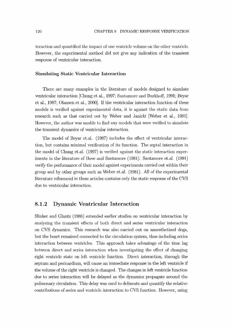
120 CHAPTER 8 DYNAMIC RESPONSE VERIFICATION
teraction and quantified the in1pact of one ventricle volume on the other ventricle.
However, the experimental n1ethod did not give any indication of the transient
response of ventricular interaction.
Simulating Static Ventricular Interaction
There are many eXaIllples in the literature of models designed to simulate
ventricular interaction [Chung et al., 1997; Santan10re and Burkhoff, 1991; Beyar
et al., 1987; Olansen et al., 2000]. If the ventricular interaction function of these
lllodels is verified against experimental data, it is against the static data fron1
research such as that carried out by Weber and Janicki [Weber et al., 1981].
However, the author was unable to find any Inodels that were verified to silnulate
the transient dynaInics of ventricular interaction.
The lllodel of Beyar et.al. (1987) includes the effect of ventricular interac
tion, but contains minimal verification of its function. The septal interaction in
the model of Chung et.al. (1997) is verified against the static interaction exper
iments in the literature of Bove and SantaIllOre (1981). SantaIllOre et.al. (1991)
verify the performance of their model against experiments carried out within their
group and by other groups such as Weber et.al. (1981). All of the experimental
literature referenced in these articles contains only the static response of the CVS
due to ventricular interaction.
8.1.2 Dynamic Ventricular Interaction
Slinker and Glantz (1986) extended earlier studies on ventricular interaction by
analysing the transient effects of both direct and series ventricular interaction
on CVS dynaIllics. This research was also caITied out on anaesthetized dogs,
but the heart remained connected to the circulation system, thus including series
interaction between ventricles. This approach takes advantage of the time lag
between direct and series interaction when investigating the effect of changing
right ventricle state on left ventricle function. Direct interaction, through the
septum and pericardium, will cause an iilllnediate response in the left ventricle if
the volun1e of the right ventricle is chaI1ged. The changes in left ventricle function
due to series interaction will be delayed as the dynaInics propagate around the
pulmonary circulation. This delay was used to delineate and quantify the relative
contributions of series and ventricle interaction to CVS function. However, using

8.1 VENTRICULAR INTERACTION 121
the minimal model developed it IS possible to directly separate each type of
interaction.
Measuring Dynamic Ventricular Interaction
The experiInent carried out by Slinker and Glantz (1986) involved sequen
tially constricting and releasing the puhnonary artery and vena-cava, as labelled
on Figure 8.1. Puhnonary artery constriction (PAC) causes an increase in resis
tance downstreaIn of the right ventricle, increasing the afterload against which
the right ventricle must pUlnp. Applying vena-cava constriction (VCC) decreases
the pressure upstream of the right ventricle, decreasing the right ventricle preload
as a result of reduced filling pressure. When the constrictions are subsequently
released the CVS responds again, settling to its original state. These constric
tions and their subsequent releases significantly inlpact the function of the right
ventricle. Volulnes, pressures and flow rates around both the right and left ven
tricles were Ineasured to detenmne the response of the CVS to these changes in
state.
Pulmonary artery constriction (PAC)
Right Heart
Pulmonary Circulation (Lungs) [pul]
[ao]
Left Heart
Figure 8.1 Diagram of the circulation system showing the location of the constrictions.
Pressure transducers were used to Ineasure ventricle and arterial pressures,
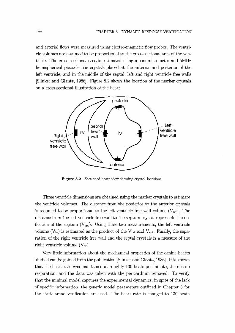
122 CHAPTER 8 DYNAlVlIC RESPONSE VERIFICATION
and arterial flows were nleasured using electro-magnetic flow probes. The ventri
cle volumes are assumed to be proportional to the cross-sectional area of the ven
tricle. The cross-sectional area is estimated using a sonomicrometer and 5MHz
hemispherical piezoelectric crystals placed at the anterior and posterior of the
left ventricle, and in the middle of the septal, left and right ventricle free walls
[Slinker and Glantz, 1986]. Figure 8.2 shows the location of the marker crystals
on a cross-sectional illustration of the heart.
Right, //' ventricle free wall
/'" Left ventricle free wall
Figure 8.2 Sectioned heart view showing crystal locations.
Three ventricle dhnensions are obtained using the Inarker crystals to estimate
the ventricle volumes. The distance froln the posterior to the anterior crystals
is assumed to be proportional to the left ventricle free wall volume (Vlvf). The
distance from the left ventricle free wall to the septuln crystal represents the de
flection of the septum (Vspt )' Using these two Ineasurements, the left ventricle
volume (Vlv) is estimated as the product of the Vlvf and Vspt ' Finally, the sepa
ration of the right ventricle free wall and the septal crystals is a measure of the
right ventricle volume (V rv ).
Very little information about the nlechanical properties of the canine hearts
studied can be gained frOln the publication [Slinker and Glantz, 1986]. It is known
that the heart rate was Inaintained at roughly 130 beats per minute, there is no
respiration, and the data was taken with the pericardium relnoved. To verify
that the minimal model captures the experimental dynamics, in spite of the lack
of specific information, the generic model paralneters outlined in Chapter 5 for
the static trend verification are used. The heart rate is changed to 130 beats
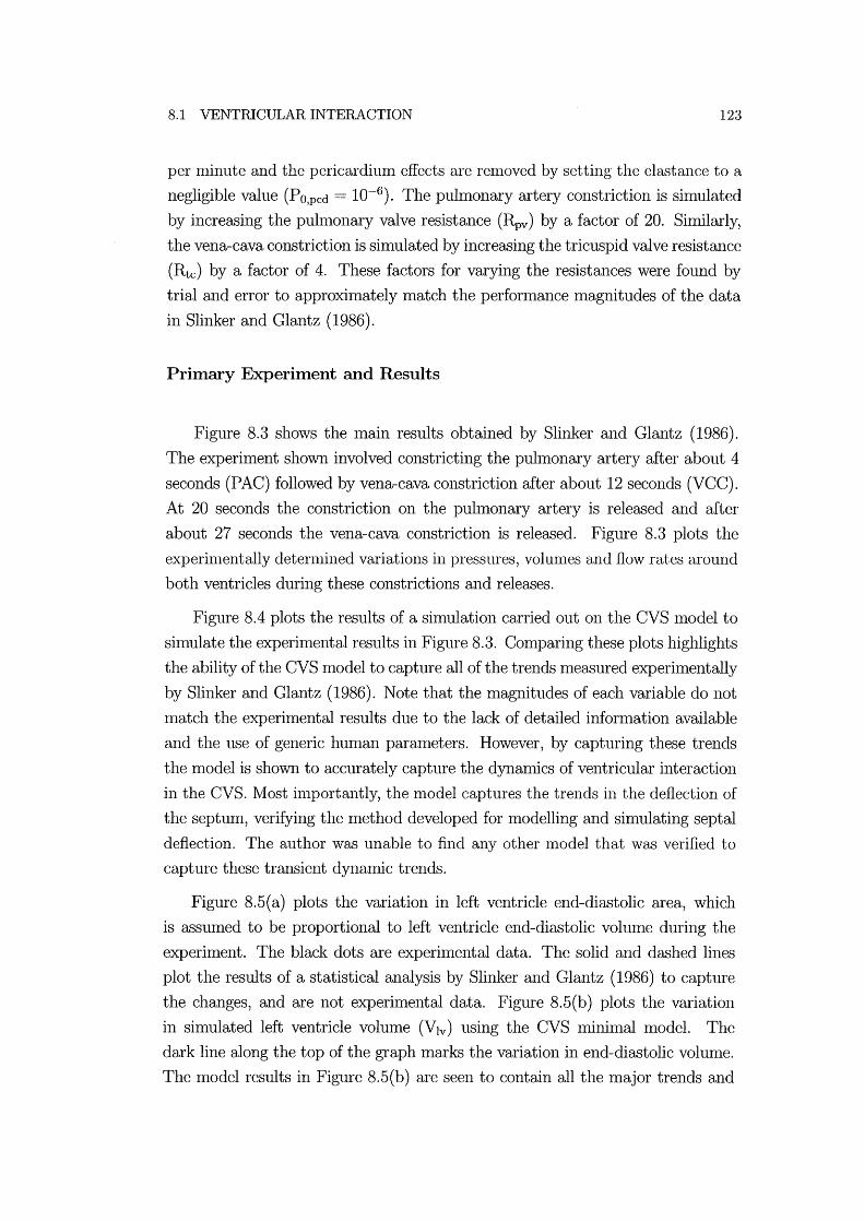
8.1 VENTRICULAR INTERACTION 123
per minute and the pericardium effects are reInoved by setting the elastance to a
negligible value (PO,pcd = 10-6). The puhnonary artery constriction is simulated
by increasing the pulnlonary valve resistance (Rpv) by a factor of 20. Shnilarly,
the vena-cava constriction is simulated by increasing the tricuspid valve resistance
(Rtc) by a factor of 4. These factors for varying the resistances were found by
trial and error to approximately match the perfonnance Inagnitudes of the data
in Slinker and Glantz (1986).
Primary Experiment and Results
Figure 8.3 shows the nlain results obtained by Slinker and Glantz (1986).
The experiment shown involved constricting the pulmonary artery after about 4
seconds (PAC) followed by vena-cava constriction after about 12 seconds (VCC).
At 20 seconds the constriction on the pulmonary artery is released and after
about 27 seconds the vena-cava constriction is released. Figure 8.3 plots the
experinlentally detennined variations in pressures, volulnes and flow rates around
both ventricles during these constrictions and releases.
Figure 8.4 plots the results of a shnulation carried out on the CVS nlodel to
shnulate the experhnental results in Figure 8.3. COlnparing these plots highlights
the ability of the CVS Inodel to capture all of the trends Ineasured experhnentally
by Slinker and Glantz (1986). Note that the Inagnitudes of each variable do not
match the experhnental results due to the lack of detailed infonnation available
and the use of generic hUlnan paralneters. However, by capturing these trends
the model is shown to accurately capture the dynalllics of ventricular interaction
in the CVS. IvIost inlportantly, the model captures the trends in the deflection of
the septum, verifying the method developed for 1110delling alld shllulating septal
deflection. The author was unable to find any other l110del that was verified to
capture these transient dynamic trends.
Figure 8.5(a) plots the variation in left ventricle end-diastolic area, which
is assumed to be proportional to left ventricle end-diastolic volume during the
experiment. The black dots are experhnental data. The solid and dashed lines
plot the results of a statistical analysis by Slinker and Glantz (1986) to capture
the changes, and are not experimental data. Figure 8.5(b) plots the variation
in shnulated left ventricle volullle (Vlv) using the CVS lnininlal nlodel. The
dark line along the top of the graph marks the variation in end-diastolic volume.
The model results in Figure 8.5(b) are seen to contain all the major trends and

124
Heart Rate (beats/min) 135]
2000 125
Left Ventricular dP/dt ] (mm Hg/sec)
·2000 150J Left Ventricular Pressure
(mm Hg)
10J 0 Aortic Flow (liters/min) 0
. 58] left Ventricular Arterior· Posterior Dimension (mm)
52] 50 Left Ventricular Septal. Free Wall Oimension (mm)
44 33J Right Ventricular Septal-Free Wall Dimension (mm)
lOJ 23 Pulmonary Artery Flow (liters/min) 0
50] Righi VentriculQr Pressure (mm Hg)
o
CHAPTER 8 DYNAlVilC RESPONSE VERlFICATION
Figure 8.3 Haemodynamic CVS responses to sequential constrictions and releases of the pulmonary artery and vena-cava [Slinker and Glantz, 1986].
transient dynaJnics in the experimental results of Figure 8.5(a).
Second Experiment and Results
A second experiment by Slinker and GlaJltZ (1986) involved applying a dif
ferent combination of the same constrictions. The puhnonary artery constriction
is again applied after 4 seconds, but released after about 23 seconds. At about
37 seconds a subsequent vena-cava constriction is applied until the end of the ex
periment. The experimentally measured variations in left ventricle end-diastolic
area are plotted in Figure 8.6(a). This experiment was also simulated using the
minimal model, and the trends shown in Figure 8.6(b) are seen to accurately
match experhnental results.
8.1 VENTRICULAR INTERACTION
Left ventricle volume [Plv] (mmHg)
100.' - - - . - - -50 - - ' . - . .
o - . - - . -
125
Aortic flow [Qav] (ml/sec) ~~~ 111111111111111111111111111 111111111111111 fl 11111111111 [11111111111111111111
80· Left ventricle ' , , , free wall volume 60 ' - - - - - - - -: - - - - - - - -: - - - -
[Vlvf] (ml) 40, , 20~--~--------~--------~------~--------~
30
Septal deflection 20 , - - -,' ,- - - --[Vspt] (ml) 10 - - - -: - - - - - : - - - - - - - -: - - - -
o - - - - - - - - - - _. - - - , - - . - - . - - - - - - . - - - - - - - -
100· , "
Right ventricle 50 _ _ : . _ . _ _ _ . . _ . _ . _ . . _ _: . _ _ . . _ _ .: _ vo~me~r~(mQ 0
~;:i(~~;ec) ~ ~~! 1" IIIII i:::::J 11111111111111 illlllllllllllilli Right ventricle pressure [Prv] (mmHg)
40~.------'--"---'--"'-'-'---'
20 .. '. ' . . '. - - - - - - -' .
o . 4 (PAC) 12 (VCC) 20 (RPAC) 27 (RVCC)
Time [t] (secs)
Figure 8.4 Haemodynarnic CVS responses simulated using the presented model.
Left Ventricle Volume Response
As discussed, the experimental research carried out by Slinker and Glantz
(1986) investigates the relative contributions of direct and series interaction on
CVS dynan1ics. However, it is very difficult to experin1entally separate and isolate
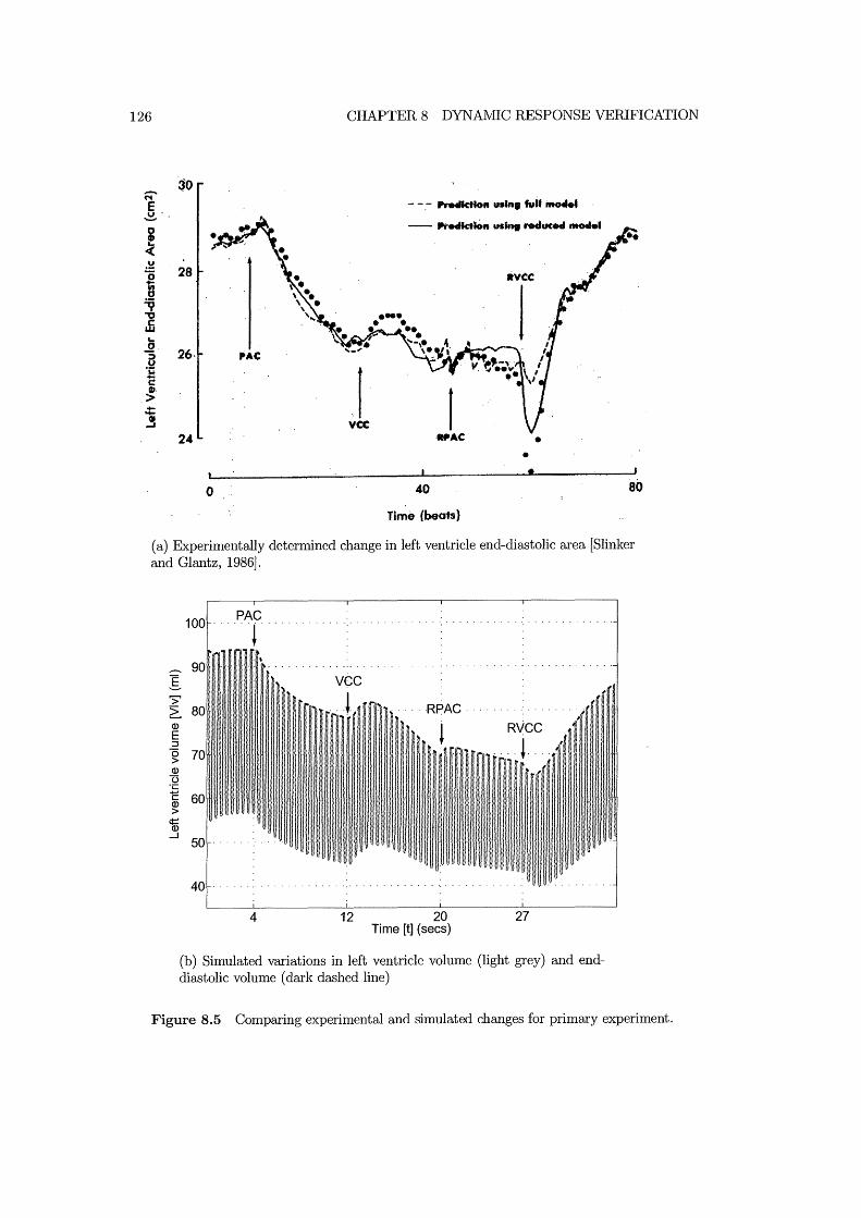
126 CHAPTER 8 DYNAMIC RESPONSE VERIFICATION
- -.- Pretlktloft Ullin, tvil iIto4M4
-- .-retlkt.on "' ... r.ducM nt04e1
I vee
24 WAC • • •
o 40 80
Time (beots)
(a) Experimentally determined change in left ventricle end-diastolic area [Slinker and Glantz, 1986].
100 PAC . . .. ~ ..
......... 90 I >' ~ 80 .... HPAC· Q)
E ::J 0 70 > Q)
13 .;::
C 60 Q)
> 'm ....J
50
40
4 12 20 27 Time [t] (sees)
(b) Simulated variations in left ventricle volume (light grey) and enddiastolic volume (dark dashed line)
Figure 8.5 Comparing experimental and simulated changes for primary experiment.

8.1 VENTRICULAR INTERACTION
~ 30 !' 0
·CD « v
I: 'V "
·28 vcc c: w .. 0 :;' ".C u
i > ..... - - - ,It of full moclef ''i 26 ..... - fit 0' ~ MCHIe •
0 70
Time (beats)
(a) Experimentally determined change in left ventricle end-diastolic area [Slinker and Glantz, 1986].
.-
I >' ~ Q)
E ::J o > Q)
13 ·c C Q)
> ¢:: Q)
.....J
PAC 100 .................. , . ... vec···
4 23 37 Time [t] (sees)
(b) Simulated variations in left ventricle volume (light grey) and enddiastolic volume (dark dashed line)
Figure 8.6 Comparing experimental and simulated changes for secondary experiment.
127
the different contributions of each interaction mechanis111, and determine how
they affect CVS dynamics. The CVS minimal model presented is capable of
analysing these effects by si111ply excluding certain interactions without changing
the relnainder of the system.

128 CHAPTER 8 DYNAIVIIC RESPONSE VERIFICATION
The top panel of Figure 8.7 plots the variations in left ventricle volume de
termined by simulation of the primary experiment. The individual contributions
of direct and series interaction can be seen in the lniddle and bottom panels re
spectively. The direct interaction plot is created by removing series interactions
from the simulation by setting constant pressure boundary conditions around the
ventricles. The series interaction plot is created by setting the elastance of the
septum to a high number (Po,sPt= 106), making it effectively rigid to eliminate
direct interaction through the septum.
Both the puhnonary artery constriction and the vena-cava constriction impact
directly on the function of the right ventricle. For this reason, the variations in
left ventricle volunle are investigated as this offers the best representation of the
effects of ventricular interaction. Increases in right ventricle volume will cause
decreases in left ventricle volulne, and vice-versa, due to direct interaction.
The direct interaction only response of the systeln, shown in the centre panel
of Figure 8.7, highlights the iInmediate impact of right ventricle parameter ad
justments on left ventricle function. The left ventricle vohune is seen to respond
to direct interaction and settle to a steady state solution within 5 heart beats in
each case. Conversely, the series interaction only results show a delayed response
to the paraIneter ChaIlges around the right ventricle. Series interactions occur
due to the changes in cardiac output aIld ventricle preloads as resistances are
increased and decreased.
Figure 8.4 shows that increasing the puhnonary valve resistance to simulate
PAC causes all increase in right ventricle afterload and results in a build-up of
right ventricle volume and pressure. This build-up causes an iImnediate drop in
left ventricle volume, which the middle panel of Figure 8.7 shows is due to direct
interaction, as the septum deflects into the left ventricle. The continued long
term drop in left ventricle volume is then attributed to series interactions. The
increase in resistance in the pulmonary artery decreases left ventricular preload,
and reduces cardiac output and left ventricular volume.
Subsequently constricting the vena-cava (VCC) causes a transient sudden by
small rise in left ventricle volume, followed by a gradual continued reduction.
The middle panel of Figure 8.7 shows that this initial transient is attributed to
direct interaction. Constricting the vena-cava causes a reduction in right ventricle
preload and the right ventricle volume decreases causing the septum to deflect
towards the right ventricle. This septal deflection causes a sudden rise in the
volume of the left ventricle. The continued long tenn reduction in left ventricle
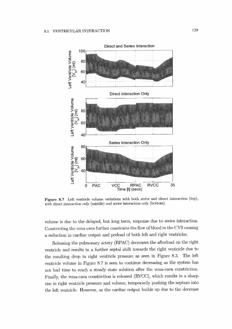
8.1 VENTRICULAR INTERACTION
Q)
E :::J "0 >::::-~S u,........., ·c > c~ Q)
> ¢:: Q)
.....J
Q)
E :::J "0 >::::- 80 ~S u,........., ·c > c~60 Q)
> ¢::
Direct and Series Interaction
Direct Interaction Only
~ 40L---~------~------~------~----~
Q)
E :::J "0 >::::- 60 ~S u,........., ·c > c~ 40 Q)
> ¢:: Q)
.....J o PAC
Series Interaction Only
VCC RPAC RVCC 35 Time [t] (secs)
129
Figure 8.7 Left ventricle volume variations with both series and direct interaction (top), with direct interaction only (middle) and series interaction only (bottom).
volume is due to the delayed, but long term, response due to series interaction.
Constricting the vena-cava further constrains the flow of blood in the CVS causing
a reduction in cardiac output and preload of both left and right ventricles.
Releasing the puhnonary artery (RP AC) decreases the afterload on the right
ventricle and results in a further septal shift towards the right ventricle due to
the resulting drop in right ventricle pressure as seen in Figure 8.3. The left
ventricle volulne in Figure 8.7 is seen to continue decreasing as the system has
not had tin1e to reach a steady state solution after the vena-cava constriction.
Finally, the vena-cava constriction is released (RVCC), which results in a sharp
rise in right ventricle pressure and volume, temporarily pushing the septum into
the left ventricle. However, as the cardiac output builds up due to the decrease

130 CHAPTER 8 DYNAMIC RESPONSE VERIFICATION
in resistance, the left ventricle volume increases and the septum returns to its
steady-state position.
Thus, Figure 8.7 shows how the CVS nunimal model developed can separate
the relative contributions of series and direct interaction. The model allows de
tailed analysis of the relative contributions of each interaction type by silnply
deactivating a particular CVS function without affecting other parts of the CVS.
This capability offers a considerable advantage over current, heavily invasive,
surgical techniques of lneasuring ventricular interaction.
8.1.3 Ventricular Interaction Summary
The different experilllental results that attenlpt to quantify ventricular interac
tion are reviewed. In particular, results that measure the transient response of
the CVS due to ventricular interactions are outlined. The nlinimal CVS lnodel
presented is verified to accurately capture the major trends in experimentally
lneasured CVS dynanlics. These results verify that the model is capable of cap
turing the transient dynmnic response of the CVS due to both direct and series
ventricular interaction. No other model found in the literature was verified to
capture these transient responses in CVS dynalnics due to ventricular interaction.
Following this verification, the model is used to delineate the relative con
tributions of the different contributing factors of ventricular interaction. Results
are shown that show both the ilnmediate response of the systelll due to direct in
teraction and the delayed response due to series interaction. The nunimallnodel
enables lnuch more detailed analysis, such as that presented, without needing
to resort to experimental lnethods, and allows the individual contributions and
dynanlics to be fully studied.
8.2 CARDIOPULMONARY INTERACTION 131
8.2 Cardiopulmonary Interaction
As discussed in Chapter 1, the location of the heart between the lungs in the
thoracic cavity lTIeanS that its function is significantly influenced by pressure
variations in the lungs and lung movement during respiration. As the pressure
in the lungs changes during respiration, the pressure around the heart and pul
lTIOnary circulation varies, influencing cardiac function. This section investigates
the ability of the IniniInal CVS model to siInulate experiInentally reported haemo
dynalmc trends due to cardiopulnlonary interactions.
8.2.1 Respiratory Function
Different types of respiration can have' different effects on CVS haelTIodynamics
depending on the anlount of change in thoracic pressure. Spontaneous respiration
typically involves thoracic pressure variations from a maxilnunl of about -4ffilnHg
during expiration to a nlinimUln of about -81mnHg during inspiration [Guyton,
1991]. During positive pressure ventilation of normal individuals, the average
thoracic pressure rises and typically may vary from a InaxilTIUm of 31nmHg at
end inspiration to a IniniInlun of -31nmHg at end expiration [Scharf et al., 1980].
More severe pressure variations can occur in ventilated patients with lung injury
or disease.
Respiratory nlanoeuvres such as the Mueller and the Valsalva manoeuvre can
be used by medical staff to evaluate cardiopulmonary function. During a IVlueller
Inanoeuvre the patient attelnpts to forcibly inspire against a blocked airway which
results in a drop in thoracic pressure on the order of -70ffilnHg [Schwartz et al.,
1999]. The Valsalva nlanoeuvre involves forcibly attempting to exhale with the
airway blocked, and results in significantly elevated thoracic pressures on the
order of 10-401mnHg [Lu et al., 2001].
Spontaneous respiration typically has only a minimal impact on CVS haemo
dynanlics due to the Ininimal variations in thoracic cavity pressure [Scharf and
Cassidy, 1989]. Positive pressure respiration results in an increase in the aver
age pressure in the thoracic cavity, placing a higher pressure on the heart and
results in decreased cardiac output. However, the transient changes in haenlody
namics during the respiratory cycle are dependent on the amplitude of variation
in pressure. The large variations in pressure caused by the Mueller and Val
salva manoeuvres, and used to investigate cardiopulmonary interactions, have
a significant impact upon CVS haemodynanlics. The changes in CVS function

132 CHAPTER 8 DYNAMIC RESPONSE VERIFICATION
during these manoeuvres are large enough to be easily detected using cormnonly
available medical equipment. For this reason these manoeuvres are also used
by nledical staff to evaluate cardiopulmonary function, such as diagnosing heart
failure [Braunwald, 1997].
The body will often react quickly to the catastrophic impact of the Mueller
and Valsalva manoeuvres on CVS function by activating reflex responses. For ex
ample, during the Valsalva manoeuvre the considerable positive pressure acting
on the heart causes a significant drop in cardiac output. The body will respond by
activating the baroreceptor reflex that, amongst other things, increases the heart
rate to improve cardiac output [Lu et al., 2001]. The minimallnodel developed
does not include the autonomous activation of baroreceptor reflexes. However,
the impact of the body's reflex response on haemodynalnics is less significant dur
ing lesser variations in thoracic cavity pressure. Thus, both the spontaneous and
positive pressure respiration cases are sinlulated, as they involve only slnall tho
racic pressure variations, to further validate the dynamic response of the lninhnal
Inodel.
Mechanisms for Cardiopulmonary Interaction
Variations in thoracic pressure lead directly to imlnediate changes to the
boundary pressures acting on the heart. For example, if thoracic pressure drops,
such as during spontaneous inspiration, it reduces the pressure acting on all of the
chalnbers within the thoracic cavity in Figure 2.1. The pressures in the puhnonary
artery, pulmonary vein and in the heart will therefore decrease. Equations (2.12-
2.14), (2.19) and (2.20) show how the minhnallnodel incorporates the thoracic
pressure in detennining chamber pressures.
During inspiration in spontaneous breathing, the pressures in the heart and
pulmonary circulation drop relative to the pressure outside the body. However,
the pressures in the systemic circulation, outside the thoracic cavity, are not af
fected. Thus, the right ventricle preload, or the pressure in the vena-cava relative
to the right ventricle pressure, increases. In the same way, the left ventricle af
terload, or the pressure in the aorta relative to the left ventricle, increases. The
overall result of these changes is an increase in stroke volume and output of the
right ventricle, and a decrease in stroke volume of the left ventricle. Therefore,
these changes in pressure mean the blood is redistributed from the systemic cir
culation to the pulmonary circulation.

8.2 CARDIOPULMONARY INTERACTION 133
The result of this redistribution of blood is a net blood volume increase in
the puhnonary circulatory system until a new steady state equilibrium is reached.
The opposite effect occurs during spontaneous expiration when the pressure in
the thoracic cavity increases, resulting in a net increase in blood volulne in the
systemic circulation. It is shown in Chapter 5 that the model captures these static
variations in cardiac output as a result of changes in thoracic cavity pressure.
However, a more important test is the ability of the lnodel to capture these same
trends in the transient haelnodynmnic response of the CVS during respiration.
Cyclic variations in thoracic pressure during respiration cause transient fluc
tuations in the haemodynamics that must be captured in a dynamic simulation.
This section first summarises the experimental research carried out to nleasure
the hnpact of respiration on hamnodynmnic function. A brief SUlnlnary of pre
vious attelnpts to shnulate cardiopuhnonary interactions is then outlined. Pub
lished experimental data is used to test the ability of the presented CVS model
to capture the transient haemodynamic response of the CVS due to variations in
thoracic cavity pressure. Both spontaneous and positive pressure respiration case
studies are used in this dynanlic nl0del verification. It is shown that the nl0del
can be used to identify the contributions of particular cardiopulmonm'y functions
that are currently hnpossible to isolate exp erhnent ally.
8.2.2 Measuring Effects on CVS
As with ventricular interaction, there have been many lnajor contributors to re
search on cardiopulnl0nary interactions. Buda et.al. (1979) reviewed previous
publications that discussed the effect of respiration and respiratory manoeuvres
on cardiac function. They elnphasised the "controversy" surrounding the lnecha
niSlllS by which left ventricle function is depressed during respiratory dysfunction.
Scharf and Cassidy (1989) published a comprehensive review of cardiopulmonary
interactions in both healthy and diseased patients. This review covers lnany of
the Inain contributors to the field including experimental research carried out by
thelllSel ves.
The nlinimal model is verified against results nleasured by Scharf et.al. (1979;
1980) on cardiopulmonary interaction during both spontaneous and positive pres
sure respiration. Many sinlilar experiments have been carried out that also plot
the dynamic response of the CVS during respiration, including lnore recent re
search by Denault et.al. (1999; 2001). However, other work does not contain the
detailed nleasurements of pressures and flow rates taken by Scharf et.al. (1979;

134 CHAPTER 8 DYNAlvlIC RESPONSE VER1FICATION
19S0). The intention here is to verify the ability of the model to simulate the
transient dynamic response of the CVS due to variations in pulmonary resistance.
The 111easure111ents taken by Scharf et.al. (1979; 19S0) are ideal for this task.
8.2.3 Other Models
Few of the closed loop CVS models investigated include the effects of thoracic
pressure changes. Beyar et.al. (19S7) and Chung et.al. (1997) include thoracic
pressure in their 1110del descriptions, but investigate only static response of the
1110dels due to thoracic pressure changes. Others have taken a more detailed
approach, attenlpting to sil11ulate the dranlatic effect of the valsalva 111anoeuvre
on CVS dynamics [Sun et al., 1997; Lu et al., 2001].
Sun et.al. (1997) Sil11ply adds the thoracic cavity pressure to their very C0111-
plex CVS 1110 del , shown in Figure 1.10, in a shnilar way to the 111ethod used in
the 1110del presented in this thesis. The thoracic cavity pressure is added to the
pressure of the puh110nary circulation. The nlodel also clahns to include barore
flex effects. The effects of normal respiration and valsalva 111anoeuvre on aortic
pressure (P ao) are simulated. However, the results are not directly c0111pared with
experinlental results and do not delineate the contribution of the baroreceptor
reflexes [Lu et al., 2001].
Lu et.al. (2001) proposes a 1110del which includes a detailed description of
airway and lung function, and the effect of the baroreceptor control on heart rate.
This model is built on the closed loop ventricular interaction model of Chung
et.al. (1997) and Olansen et.al. (2000). The resulting impact of the Valsalva
111anoeuvre on aortic pressure and heart rate are 111easured. Their results are
shown to 111atch experimental trends. However, only the dynalnic response of
the aortic pressure is reported, the variations in pulmonary artery pressure and
blood flow through the pulnlonary circulation are absent.
8.2.4 Simulation of Cardiopulmonary Interaction
All lllodel verification of cardiopulmonary dynanlics is tested against the exper
h11ental work by Scharf et.al. (1979; 19S0). AB with sh11ulations of ventricular
interaction, there is only 111inimal information available on the nlechanical prop
erties of the canine cardiovascular SyStel11S employed. For this reason, the generic
human parameters used in the static verification in Chapter 5 are used.

8.2 CARDIOPULMONARY INTERACTION 135
A significant contributor to cardiopuhnonary interaction is the tinle varying
nature of the pulmonary vascular resistance. This resistance is represented in
the Inodel by the pulmonary resistance (Rpul) , as shown in Figure 2.1. During
mechanical ventilation puhnonary vascular resistance increases as lung volume
increases due to stretching of the lung walls and the resulting effect on the intra
alveolar vessels [Scharf and Cassidy, 1989]. However, the exact relationship be
tween pulmonary vascular resistance and lung volume is non-linear [West, 1985;
Lu et al., 2001]. To Inaintain simplicity in the nlodel while obtaining the basic
trends for verification, a linear relationship between time varying pulnlonary re
sistance (Rpul (t)) and lung volume (Vlungs) is assumed for mechanical ventilation.
Rpul (t) <X Vlungs(t) (8.1)
During mechanical ventilation the thoracic pressure can be assumed to be
proportional to the lung vohune, for normal changes in volume [West, 1985].
(8.2)
Therefore, by cOlnbining Equations (8.1) and (8.2), a linear relationship between
Rpul (t) and the thoracic cavity pressure (P th) is assumed.
The following definition is used to approxilnate the pulmonary vascular re
sistance (Rpul (t )) as a function of P th.
[ { .} {Pth - Pth(relaxed) }] RpuI(t) = Rpul(relaxed) 1 + Rpul(nlultI) - 1 ~Pth (8.3)
where Rpul (relaxed) and P th (relaxed) is the puhnonary vascular resistance and
thoracic cavity pressure when the lungs are relaxed at end-expiration, Rpul (lnulti)
is a factor representing the nlaxinlum variation in resistance and ~P th is the
InaxilnUln variation in thoracic cavity pressure. The factor RpuI(multi) defines
the nlaxilnUln amount that the base resistance will be multiplied by at end in
spiration. Figure 8.8 shows an exmnple of variations in Pth and RpuI(t) during
positive pressure respiration. For these examples, the base value of RpuI is set to
1, defining the pulnlonary vascular resistance when the lungs are relaxed.
The value of RpuI(multi) is set to 2.5 for positive pressure respiration, indi
cating the proportional changes in resistance modelled. This value was found by
adjusting the value of RpuI until the percentage changes in the simulated out-

136 CHAPTER 8 DYNAMIC RESPONSE VERIFICATION
puts approximately Inatched the experilnental results. This result shows how
the model can be used to estimate the Inagnitude of changes of physiological
paralneters, such as the pulmonary resistance during ventilation.
2 Inspiration:
C» 1 .... \. I E -S 0 r--:c a..+-' -1
Expirati~n -2
0 5 10
3
2.5 ,........, ---+-'
"--""5 2 0-cr:
........ 1.5
1
0.50 5 10
Time [t] (secs)
Figure 8.8 Changes in thoracic cavity pressure (Pth ) and pulmonary vascular resistance (Rpul (t)) during positive pressure respiration.
Experilnents by Scharf et.al. (1979; 1980) n1easured variations in arterial flow
rates and pressures, and the pleural pressure during ventilation. Table 8.1 outlines
which Inodel variables are used to represent each experimental variable. The
pleural pressure (PPL) is represented in the model as the thoracic cavity pressure
(Pth ). The experilnentally measured variation in pulmonary artery pressure (P pa) correlates to the pulmonary artery pressure in the model (P pa). The measured
systemic artery pressure (Part) is simulated in the model as the pressure in the
aorta (P ao). The blood flow rates through the pulmonary artery (Qpa) and the
aorta (Qao) are simulated in the model as flow through the pulmonary valve (Qpv)
and the aortic valve (Qav) respectively. The right and left atrial pressures (P ra al1d PIa) are not included in the basic minimal model.

8.2 CARDIOPULMONARY INTERACTION
Description
Thoracic cavity pressure Pulmonary artery pressure Pressure in aorta Pulmonary artery flow Flow through aorta Atrial pressures
Scharf et.al. (1979; 1980) PPL
Ppa Part or Paa Qpa or Qpa Qaa or Qaa Pra and PIa
Model Equivalent
Pth Ppa Paa Qpv Qav
Not simulated
137
Table 8.1 Correlation between model variables and the experimental measurements taken by Scharf et.al. (1979; 1980).
Positive Pressure Respiration
Research carried out by Scharf et.al. (1980) on positive pressure ventilation in
anaesthetized dogs was investigated first. Various arterial pressures and flow rates
were measured on anaesthetized dogs during positive pressure ventilation. During
spontaneous respiration, air flows into the lungs as the pressure in the lungs drops
below atInospheric pressure. However, during positive pressure respiration air is
forced into the lungs and inspiration is Inarked by an increase in thoracic cavity
pressure above atInospheric.
Systen1 parameters for the CVS Inodel for these experiments include a respi
ratory rate of 10 breaths per nunute, and a heart rate of roughly 160 beats per
Ininute [Scharf et al., 1980]. Tilne varying pulmonary resistance is set propor
tional to the thoracic cavity pressure. The thoracic cavity pressure varies between
-lmn1Hg at end-expiration and 1nllnHg at end-inspiration. Rpul (multi) is set to
2.5 meaning the pulmonary resistance increases by a factor of 2.5 as the pressure
increases fron1 -bmnHg to 1mn1Hg.
Figure 8.9 reproduces experilnental results from Scharf et.al. (1980). These
results can be cOInpared with the results froln simulation of positive pressure
respiration shown in Figure 8.10. Note that the model captures all of the major
trends in the transient response of the CVS during positive pressure respiration.
The main trends reported by Scharf et.al. (1980) include the immediate drop
in Qpv and rise in P pa with inspiration, and the illllnediate opposite response with
expiration. The initial, temporary rise in P ao followed by a significant drop during
inspiration is also reported. The Ininilnal n10del results in Figure 8.10 capture
all of these trends. Of particular note is the delayed drop of Qav experimentally
measured to be about 0.75 seconds after the drop of Qpv. Figure 8.11 plots the
variations in Qpv and Qav from Figure 8.10, which are scaled to highlight the
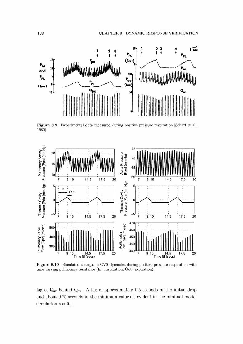
138
-5
CHAPTER 8 DYNAMIC RESPONSE VERIFICATION
1 t
2 3 + •
~~
o
10 1
• 2 3 + •
Figure 8.9 Experimental data measured during positive pressure respiration [Scharf et al., 1980].
OJ 75 ~~ Q) E 20 ~-t_ :::JC>
70 «~ CJ)I ~[ ~ E (lja.. 15 "- E c .......... 0.._ OQ) (lj~ 65 E "- to _:::J o (lj :::J CJ)
10 «e:. a..CJ) Q) 60 a: 7 9 10 14.5 17.5 20 7 9 10 14.5 17.5 20
OJ OJ 5 I 5 I In E E ~OiJt ~E
~E ~
.~ :::: .~ :::: 0-5 0-5 0 ue:. 0 ue:. '0 Q)
'0 Q) (lj "-"- :::J (lj"- o CJ)
"- :::J ..J::CJ) o CJ) I-~ ..J::CJ)
-5 -5 I-~ a.. a.. 7 9 10 14.5 17.5 20 7 9 10 14.5 17.5 20
0- 0- 470 Q)Q) 500 Q)
~ ~~ Q)E
460 ........
(ljE >- >-~'> 400 CU'> 450 > (lj (ljQ.
In III :eQ. III ·111 cO 440 0 .......... E ;: 300 o ;: 'S.9 «.9 a..u. u. 430
7 9 10 14.5 17.5 20 7 9 10 14.5 17.5 20 Time [t] (sees) Time [t] (sees)
Figure 8.10 Simulated changes in CVS dynamics during positive pressure respiration with time varying pulmonary resistance (In=inspiration, Out=expiration).
lag of Qav behind Qpv. A lag of approximately 0.5 seconds in the initial drop
and about 0.75 seconds in the Imnimum values is evident in the lninimal model
simulation results.
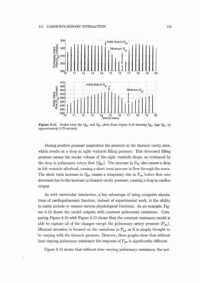
8.2 CARDIOPULMONARY INTERACTION
500
u ~ ~ 450 ca:::::' >.s ~400 cO 0 ........
E 3: 350 'S.Q a.. LL
470
U 465 ~ 460
~E 455 ca->'io 450 :eQ. 445
~ ~ 440 [[ 435
11 12 13 14
'l initlal'drop'in 'd~v':' ,
.. Minimum Q' , . 'pv
. ·111 15 16 17
............
18
: ' , : ,:: : : : : :' : ,Initial drop in: Qav r: ' , : , , , , Minimum ,Q,
av
<1 11 12 13 14 15 16 17 18
Time [t] (sees)
139
19 20
19 20
Figure 8.11 Scaled view the Qpv and Qav plots from Figure 8.10 showing Qav lags Qpv by approximately 0.75 seconds.
During positive pressure inspiration the pressure in the thoracic cavity rises,
which results in a drop in right ventricle filling pressure. This decreased filling
pressure Ineans the stroke volunle of the right ventricle drops, as evidenced by
the drop in pulrnonary artery flow (Qpv). The increase in P th also causes a drop
in left ventricle afterload, causing a short ternl increase in flow through the aorta.
The short tenn increase in Qav causes a telnporary rise in P ao before flow rate
decreases due to the increase in thoracic cavity pressure, causing a drop in cardiac
output.
As with ventricular interaction, a key advantage of using cOlnputer simula
tions of cardiopulmonary function, instead of experhnental work, is the ability
to easily include or renlove various physiological functions. As an eXalnple, Fig
ure 8.12 shows the model outputs with constant pulmonary resistance. Com
paring Figure 8.10 with Figure 8.12 shows that the constant resistance model is
able to capture all of the changes except the pulmonary artery pressure (P pa).
Minimal attention is focused on the variations in P pa as it is shnply thought to
be varying with the thoracic pressure. However, these graphs show that without
time varying puhnonary resistance the response of P pa is significantly different.
Figure 8.12 shows that without time varying puhnonary resistance, the pul-

140 CHAPTER 8 DYNAlVilC RESPONSE VERlFICATION
0> I
€,E 20 .. ' ... ' ... ~--Q)E ::JO>
t- enI «(U ~E ~~ 15 .... E 0.._ ro '--" ro ........ c Q) to 0"" oro E ~ 10 «f!::. "5~ 60 0.. ....
a.. 7 910 14.5 17.5 20 7 910 14.5 17.5 20
0> 5 0> 5 I In . I E ...... E
.~g .: :·Out ~E
~--.~ ::::
0-5 0 0-5 0 of!::. of!::. '0 Q) '0 Q)
ro .... ro .... .... ::J .... ::J oen oen .J::en .J::en -5 f-Q) -5 f-~ ....
a.. 7 910 14.5 17.5 20 a.. 7 910 14.5 17.5 20
0 470 0 Q) Q)Q) 500 en >~ :::::: 460 (ij"E Q)E >- >-~> 400 ~ ~ 450 roa.
1111 illl cO .QO 0'--" "5 'i' 440 E ~ 300 "5.2 «.2 o..LL LL 430
7 910 14.5 17.5 20 7 910 14.5 17.5 20 Time [t] (secs) Time [t] (secs)
Figure 8.12 Simulated changes in CVS dynamics during positive pressure respiration with constant pulmonary resistance (In=inspiration, Out=expiration).
monary artery pressure does not respond in a physiologically accurate manner.
With constant Rpul the rise in thoracic pressure causes a drop in puhnonary artery
pressure due to the drop in cardiac output of the right ventricle, as evidenced by
the drop in Qpv. This drop continues through inspiration and rises again during
expiration to the original value. The inclusion of thne varying pulmonary resis
tance (Rpul (t )) causes the pulmonary resistance to rise during positive pressure
inspiration. Figure 8.10 shows that this rise results in a rise in P pa as the increased
resistance further restricts flow through the pulrnonary circulation SysteIll, and
blood builds up in the puhnonary artery. Thus, it is shown that the pressure in
the pulmonary artery is not shnply caused by the increase in thoracic pressure,
but more likely by the increase in pulmonary resistance.
Spontaneous Respiration
A second verification of nl0del function is a simulation of experimental re
sults measured by Scharf et.al. (1979) on spontaneous respiration in anaesthetized

8.2 CARDIOPULIVIONARY INTERACTION 141
dogs. The experilnental procedure involved carrying out a bilateral cervical vago
tomy on the dogs, which involves renloving the effect of the vagal reflex on the
heartrate. This procedure produces conditions that Inore accurately match the
model, which does not directly simulate the activation of these reflex responses.
The airway is restricted, resulting in laboured breathing and slightly higher tho
racic pressure changes froln a minimlun of -8lmnHg to a nlaximum of OmmHg.
The respiration rate was set to 10 breaths per minute and the heart rate is set
to 150 beats per Ininute to match the experimental conditions.
During spontaneous respiration air is sucked into the lungs and lung vohune
is now assumed to be inversely proportional to thoracic pressure.
1 Vlungs(t) ex: Pth(t) (8.4)
It is expected that pulmonary vascular resistance (Rpul) will still be proportional
to lung volunle, as defined in Equation (8.1), due to lung wall stretching. How
ever, in order to Inatch experimental results, it was found that Rpul(multi) Inust
be reduced to 0.4 for spontaneous respiration. Interestingly, setting Rpul (multi)
to a value of less than 1 simulated a decrease in puhnonary vascular resistance
during spontaneous inspiration as the lung vohune is increasing. This implies
that during spontaneous respiration, there is an inverse relationship between lung
volulne and the value of Rpul '
During positive pressure ventilation the puhnonary vascular resistance in
creases when air is forced into the lungs during inspiration causing axial stretch
ing or cOInpression of alveolar capillaries [West, 1985; Lu et al., 2001]. This
ilnplies that puhnonary vascular resistance is proportional to lung volume during
mechanical ventilation. However, it is unclear froln the literature how Rpul varies
during spontaneous ventilation where air is sucked into the lungs. To match
experimental data, it is found that Rpul nlust be decreased during spontaneous
ventilation. A potential explanation for the inverse relationship between lung
vohune and Rpul is that during spontaneous ventilation the alveolar vessels are
not compressed because lung expansion is driven by expansion of the surrounding
cavity. In addition, there may be radial stretching of extra-alveolar causing an
increase in vessel diameter, and a corresponding decrease in Rpul.
The experilnental data Ineasured by Scharf et.al. (1979) is reproduced in
Figure 8.13. Figure 8.14 plots the simulated response of the CVS due to equivalent
changes in thoracic cavity pressure. By comparing Figure 8.13 with Figure 8.14

142 CHAPTER 8 DYNAMIC RESPONSE VERIFICATION
it can be seen that the shnulated results capture all of the major trends in the
experimental results.
~ ha.~
Figure 8.13 Experimental data measured during laboured spontaneous respiration [Scharf et al., 1979].
Scharf et.al. (1979) divides the changes in aortic pressure into four stages
during the respiratory cycle. Stage I occurs at the onset of inspiration and is
characterised by a tenlporary decrease in flow rate through the aorta. Stage II
labels the subsequent rise in aortic flow rate. Stage III occurs at the beginning
of expiration and involves a temporary rise in aortic flow rate. Finally, stage IV
labels the return of the aortic flow to a steady state value. The model results in
Figure 8.14 are seen to capture all of these stages, as labelled in the graph of Qav.
During early inspiration the thoracic cavity pressure drops significantly, caus
ing an increase in right ventricle filling pressure. This increase in filling pressure
results in an increase in right ventricle stroke volume, which is shown by the
increase in flow rate through the pulmonary artery (Qpv) in Figure 8.14. The
drop in thoracic pressure also means the left ventricle afterload increases and the
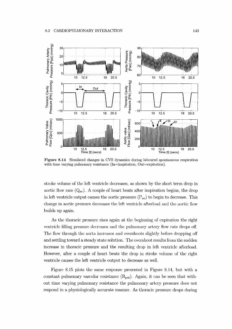
8.2 CARDIOPULMONARY INTERACTION 143
0> >.I 30 t:: E Q) .......... Q) E .... 01 t:: __ ::JI «,........, 20 ~ E ~[ ~ E coo.. 0..--c .........
10 coo o Q) E .... tco 'S~ 00.. « ......... o..cn 0 ~
0.. 10 12.5 18 20.5 10 12.5 18 20.5 0> 5
0> 5 I I
~E Out ~E .:; E .:; E co-- 0 co-- 0 0 .......... 0 ..........
.c .c 0 ...... 0 ...... '0 e:. .- 0.. o ......... ~ Q) -5 ~ ~ -5 o .... o ::J .c::J .ccn r-~ r-cn
Q) -10 ~ -10 ....
0.. 10 12.5 18 20.5 0.. 10 12.5 18 20.5
Q)u 1000 U
> Q) Q) 600 ... '-\ ./.I:./"'ylV .. co~ .!!2 >E Q)E
~;:::: > -- 400 co > 500 co>, co.. > co 00 :e g
200 E ......... -~ o ~ ::J 0 «.2 o..u::
0 LL 0 10 12.5 18 20.5 10 12.5 18 20.5
Time [t] (sees) Time [t] (sees)
Figure 8.14 Simulated changes in CVS dynamics during laboured spontaneous respiration with time varying pulmonary resistance (In=inspiration, Out=expiration).
stroke volume of the left ventricle decreases, as shown by the short tenn drop in
aortic flow rate (Qav). A couple of heart beats after inspiration begins, the drop
in left ventricle output causes the aortic pressure (P ao) to begin to decrease. This
change in aortic pressure decreases the left ventricle afterload and the aortic flow
builds up again.
As the thoracic pressure rises again at the beginning of expiration the right
ventricle filling pressure decreases and the pulmonary artery flow rate drops off.
The flow through the aorta increases and overshoots slightly before dropping off
and settling toward a steady state solution. The overshoot results from the sudden
increase in thoracic pressure and the resulting drop in left ventricle afterload.
However, after a couple of heart beats the drop in stroke volume of the right
ventricle causes the left ventricle output to decrease as well.
Figure 8.15 plots the same response presented in Figure 8.14, but with a
constant pulmonary vascular resistance (Rpul)' Again, it can be seen that with
out time varying pulmonary resistance the pulmonary artery pressure does not
respond in a physiologically accurate lnanner. As thoracic pressure drops during

144 CHAPTER 8 DYNAlVilC RESPONSE VERlFICATION
early inspiration, Figure 8.15 shows that it causes an immediate drop in pul
monary artery pressure (P pa). However, this drop is short lived and the eventual
response is a significant rise in P pa. The drop causes a sudden increase in blood
flow into the pulmonary artery and pulmonary artery blood volume increases
as a result of the increased puhnonary resistance (Rpul)' With thne varying pul
monary resistance, this resistance drops during inspiration and limits the build-up
of blood in the pulmonary artery. Thus, the inclusion of time varying pulmonary
resistance produces much Inore physiologically accurate results, matching the
experimental results of Figure 8.13.
0> 90 ~I 30 .... E Q) .--... Q) E .... 0> t __ 20 ::JI
80 ~Cif ~ E e:-o. ~ E roo.. 0.. --c ........ 10 roO' 70 OQ) E .... tro _::J 00.. ::J W ~ ........ o..W 0
~ 60 0.. 10 12.5 18 20.5 10 12.5 18 20.5
0> 5 0> 5 I I ~E Out ~E 'S; E 'S; E ro -- 0 ro -- 0 0'--'" 0'--'" .c .c o+-' o+-' .- 0.. "[5 e::. 0 ........ ~Q) -5 ~ Q) -5 o .... 0 .... .c::J .c::J I-~ I-~
~ -10 0.. 10 12.5 18 20.5
~ -10 0.. 10 12.5 18 20.5
Q)u 1000 U > Q) Q) 600 (ij~ ~ >E Q)E e:-:=: >-- 400 ro > 500 (ij,> co. > ro 00 :f§Q. E ........ 200 -~ o ~ ::J 0 0..[[ ~..Q
0 LL 0 10 12.5 18 20.5 10 12.5 18 20.5
Time [t] (secs) Time [t] (secs)
Figure 8.15 Simulated changes in CVS dynamics during laboured spontaneous respiration with constant pulmonary resistance (In=inspiration, Out=expiration) .
8.2.5 Cardiopulmonary Interactions Summary
The minimallnodel developed shows very good correlation with experimentally
measured data investigating the haen10dynan1ic effects of cardiopuln10nary inter
actions. The model captures all of the Inajor trends, but the limited availability
of patient specific parameters restricts its ability to match the explicit magnitudes
of changes. These two examples show the capability of the model to explicitly

8.3 SUMIVIARY 145
delineate the contribution of time varying pulmonary resistance to CVS haemody
naImcs. It is found that the changes in pulmonary vascular resistance contributes
significantly to the changes seen in experinlentally nleasured pulmonary artery
pressure, but only minimally to other areas of the CVS. Removal of time varying
resistance in the pulmonary circulation from experimental nleasurements is inl
possible, but removing it from the CVS Inodel is simple. These results explicitly
defined the contributions and impact of pulmonary vascular resistance (Rpul).
8.3 Summary
The dynamic verification exanlples in this chapter have shown the capability of
the nlininlal CVS nl0del presented to capture significant and cOlnplex transient
changes in CVS dynanlics. The transient effects of both ventricular and car
diopuhnonary interactions on CVS haelnodynaInics have been investigated and
compared with experimental data. Most other full CVS nlodels found in the lit
erature are verified only against the static responses of the CVS and none capture
the transient dynamics of ventricular interaction. The minimal model is the first
known exalnple of a full closed loop model that is robust enough to shnulate the
dynanlics of many areas of the CVS. Therefore i these results represent a signifi
CaIlt advance over previous Inodels that focus on shnulating the static responses
of a particular CVS function. Now that the nlininlal model is verified to simulate
both static and traIlSient CVS function, the next step involves testing its ability
to capture specific types of CVS dysfunction.

Chapter 9
Simulating Disease State
Studying the causes of heart disease and the resulting effects on CVS dynamics
can be a conlplex task of differentiating mechanical interactions and adaptive
reflex responses. NIedical staff faced with measured patient data, such as pres
sures and cardiac output, must attempt to identify the cause of CVS dysfunction.
However, nleasured patient data also includes the effect of various autononlic re
flex actions that act to change CVS properties, such as peripheral resistances,
heart rate and the stressed blood volume. If the minilnallnodel can be used to
sinlulate different types of CVS dysfunction, then it can also be used to gain a
1110re detailed understanding of the relative contributions of different nlechanical
and reflex actions to CVS function.
This chapter investigates the ability of the nlodel to sinlulate different types
of CVS dysfunction commonly encountered in critically ill patients where quick,
accurate diagnosis can be essential to patient survival. The first section focuses on
dysfunction directly associated with the heart and how it can be simulated using
the lninimal model. In particular, myocardial dysfunction and valvular disorders
are simulated, and compared with known physiological responses. The second
section investigates shock states, their impact on CVS function, and the impact
of different reflex actions. Each different dysfunction is simulated by adjusting
the appropriate minimal model parameters, however the complex interactions
prevent exact knowledge of the physiological changes. Therefore, these paraIn
eters are adjusted well beyond physiologically realistic limitations, to highlight
the resulting impact on CVS haemodynamics and to clearly illustrate the trends
in dynmnic response.

148 CHAPTER 9 SIMULATING DISEASE STATE
9.1 Heart Failure
Heart failure can be caused by inadequate ventricle filling, classified as diastolic
dysfunction, and/or inadequate ejection of blood, classified as systolic dysfunc
tion. This section investigates lnyocardial and valvular disorders that are the
most common causes of these two basic types of cardiac dysfunction. The focus
is primarily on left ventricle failure, as it is lnore common than right heart failure
and has a much more catastrophic impact on CVS function [Katz, 2002]. Minimal
lnodel function is compared with known CVS trends and schematic illustrations
frOIll nledical references showing the effects of various types of heart dysfunction
on ventricle pressures and volumes.
9.1.1 Myocardial Dysfunction
Myocardial dysfunction relates to abnonllalities in the cardiac muscle that impact
on the hearts ability to pump. Diastolic dysfunction caused by lnyocardial dis
orders, such as nlyocardial ischemia and hypertrophy, affect the elastance of the
ventricle during diastole. Systolic dysfunction due to cardiac nluscle disorders,
such as acute myocardial infarction, prilnarily result in a drop in left ventricle
contractility or the strength of contraction of the heart. In lnany cases myocardial
dysfunction affects both systolic and diastolic function sinlultaneously, however
this research investigates the independent contributions [Braunwald, 1997].
Diastolic Dysfunction
Diastolic dysfunction caused by lnyocardial disorders, such as ischemia or
hypertrophy, limits the ability of the heart to relax so blood can enter the ventricle
during diastole. Ischemia occurs when the myocardiulll is not supplied with
enough oxygen, perhaps due to a blocked artery or SOlne other cause of diminished
cardiac output. Myocardial hypertrophy is an expansion of the ventricle walls,
usually as a long term result of increased ventricle loading, such as in aortic
stenosis where the aortic valve fails to open properly. Both myocardial ischemia
and hypertrophy impede diastolic function by lilniting the ability of the ventricle
to expand during diastole. The effect of this dysfunction can be simulated by
increasing the ventricle elastance at end-diastole, represented in the model by
the paraIlleter Po in Equation (2.2), and changing the EDPVR. A heart with a
high diastolic elastance is often referred to as a "stiff" heart.

9.1 HEART FAILURE 149
Figure 9.1(a) shows a PV diagram illustrating the impact of increased end
diastolic elastance on the cardiac cycle where the gradient of the ESPVR line
has increased [Braunwald, 1997]. Increased end-diastolic elastance is simulated
by significantly increasing P O,lvf by a factor of 10, as shown in Figure 9.1 (b) .
Both figures show the cardiac cycle moving to the left on a PV diagram due
to the lllodified ESPVR. Diastolic dysfunction is characterised by an increase
in ventricle filling pressure, a decrease in ventricle volume, dilninished cardiac
output, and in the absence of reflex responses, a drop in end-systolic pressure.
The minimal nl0del results in Figure 9.1 (b) show that the model captures all
of these trends. Figure 9.1(a) is a schematic illustration specifically focused on
end-diastolic function and does not show changes in end-systolic pressure.
'Ci 120 I
E ·s . i.u. 80 0: :::> C/) C/)
~ 40 Q.
?j
Diastolic. .. dysfunction
c 100.
LV·VOLUME (mll;,,2 BSA)
(a.) Effect of diastolic dysfunction ca.using an increase in ventricle elastance on a PV diagram of the left ventricle [Braunwald, 1997].
150
~ ~
'4 Normal' ,,'-' -- -------\.,,'\
\ \
20 40 60 80 100 120 140
Left Ventricle Free Wall Volume ~vf] (ml)
(b) Minimal model simulated drop in left ventricle diastolic elastance.
Figure 9.1 Comparison of diastolic dysfunction schematic with simulated results.
Systolic Dysfunction
Myocardial infarction occurs where Inyocardium tissue has died due to lack of
oxygen and can lead to catastrophic heart failure. The Inain ilnpact of myocardial
infarction is a drop in ventricle contractility because the weakened heart is no
longer able to eject an adequate amount of blood. Decreased contractility is sim
ulated in the minilnal model by decreasing the paralneter Ees in Equation (2.1),
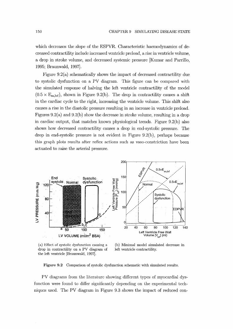
150 CHAPTER 9 SIMULATING DISEASE STATE
which decreases the slope of the ESPVR. Characteristic haemodynaInics of de
creased contractility include increased ventricle preload, a rise in ventricle volume,
a drop in stroke volume, and decreased systemic pressure [Kumar and Parrillo,
1995; Braunwald, 1997].
Figure 9.2(a) schelnatically shows the impact of decreased contractility due
to systolic dysfunction on a PV diagram. This figure can be cOlnpared with
the simulated response of halving the left ventricle contractility of the model
(0.5 x Ees,lvf), shown in Figure 9.2(b). The drop in contractility causes a shift
in the cardiac cycle to the right, increasing the ventricle volume. This shift also
causes a rise in the diastolic pressure resulting in an increase in ventricle preload.
Figures 9.2(a) and 9.2(b) show the decrease in stroke volulne, resulting in a drop
in cardiac output, that Inatches known physiological trends. Figure 9.2(b) also
shows how decreased contractility causes a drop in end-systolic pressure. The
drop in end-systolic pressure is not evident in Figure 9.2(b), perhaps because
this graph plots results after reflex actions such as vaso-constriction have been
actuated to raise the arterial pressure.
B> + E g w a; :;) CIJ en w il: a.. > -'
·120
80
40
Sys~olic: . dysfunction
150
LV VOLUME (mi/m~ eSA)
(a) Efi'ect of systolic dysfunction causing a drop in contractility on a PV diagram of the left ventricle [Braunwald, 1997].
150
~5XEes'.II.f ",
~~""", -,-~--------_ ,,' 0.5xE Normal '''''~'' eS,lvf
:/ ,./"',,1 """, \
: ", ,~'
" I " I
,.,.,." ; I I I I
0~--~1~'-=-~~~~~----~1
20 40 60 80 100
Left Ventricle Free Wall Volume ~v~ (ml)
120 140
(b) Minimal model simulated decrease in left ventricle contractility.
Figure 9.2 Comparison of systolic dysfunction schematic with simulated results.
PV diagranls from the literature showing different types of myocardial dys
function were found to differ significantly depending on the experimental tech
niques used. The PV diagraIn in Figure 9.3 shows the impact of reduced con-

9.1 HEART FAILURE 151
tractility [Parrillo and Bone, 1995]. Where a patient is found to have symptolllS
of reduced contractility, a vasodilator is often adlninistered to reduce peripheral
resistance. This reduction causes a recovery in cardiac output, but at the ex
pense of a drop in blood pressure. The hatched region in Figure 9.3 shows how
administering the vasodilator causes an increase in stroke volume that is directly
related to cardiac output and a drop in end-systolic pressure, which accolnpanies
a drop in Inean arterial pressure. Figure 9.4 repeats Figure 9.2(b) and shows
the silnulated lninimal model response of the CVS due to decreased contractility,
as well as results from halving the systemic resistance (0.5 x Rsys) to model the
effect of a vaso-dilator. The nlodel is seen to capture the increase in stroke vol
tune and decrease in end-systolic pressure that occurs as a result of vasodilator
administration. This eXalnple highlights the ability of the model to assist medical
staff in choosing suitable therapies for different types of cardiac dysfunction by
sinlulating the known effect of a drug and identifying its inlpact on the CVS .
VENTRIGl)LAR / PRES~UFlE
. ; DEPRESSl:D CQNTRACTILITY
VENTRICUI..AR VOLUME
Figure 9.3 Effect of decreased contractility and administration of a vasodilator (hatched) [Parrillo and Bone, 1995].
9.1.2 Valvular Disorders
Heart valves playa critical role in the pumping function of the heart, so valvular
disorders can often be life threatening. There are two main types of valvular
disorders, valvular stenosis and valvular insufficiency. Valvular stenosis occurs
when a heart valve doesn't open properly, causing a much higher resistance to
blood flow passing through the valve and decreasing flow rate. Valvular insuffi-
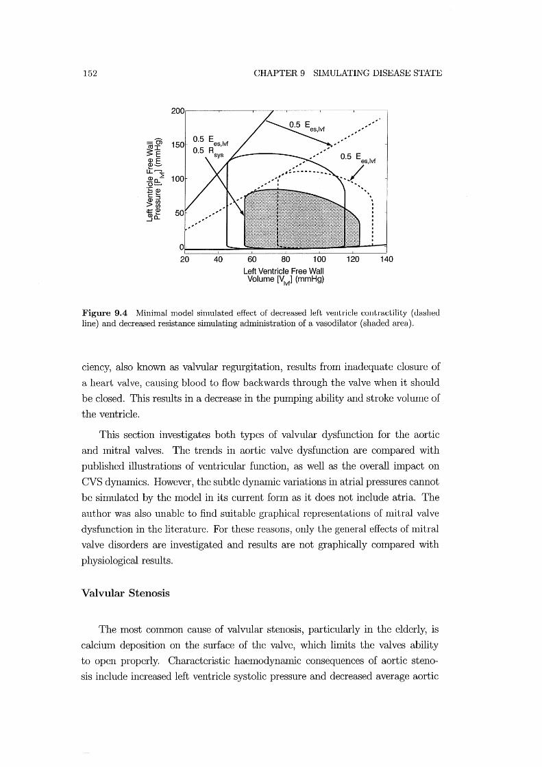
152 CHAPTER 9 SIMULATING DISEASE STATE
200~----~----~--~~----~----~-----'
150
40 60 80 100
Left Ventricle Free Wall Volume [V
1vf] (mmHg)
0.5 E Ivf .)S . ............
120
.. \
140
Figure 9.4 "Minimal model simulated effect of decreased left ventricle contractility (dashed line) and decreased resistance simulating administration of a vasodilator (shaded area).
ciency, also known as valvular regurgitation, results from inadequate closure of
a heart valve, causing blood to flow backwards through the valve when it should
be closed. This results in a decrease in the punlping ability and stroke volunle of
the ventricle.
This section investigates both types of valvular dysfunction for the aortic
and Initral valves. The trends in aortic valve dysfunction are conlpared with
published illustrations of ventricular function, as well as the overall ilnpact on
CVS dynmnics. However, the subtle dynmnic variations in atrial pressures cannot
be simulated by the model in its current fonn as it does not include atria. The
author was also unable to find suitable graphical representations of nlitral valve
dysfunction in the literature. For these reasons, only the general effects of Initral
valve disorders are investigated and results are not graphically compared with
physiological results.
Valvular Stenosis
The Inost common cause of valvular stenosis, particularly in the elderly, is
calcium deposition on the surface of the valve, which limits the valves ability
to open properly. Characteristic haemodynamic consequences of aortic steno
sis include increased left ventricle systolic pressure and decreased average aortic

9.1 HEART FAILURE 153
pressure [Braunwald, 1997J. The middle panel in Figure 9.5 illustrates the impact
of aortic stenosis resulting in an increase in the difference between the maxin1um
left ventricle pressure and the Iuaximum aortic pressure (max P lv- max P 80)' This
increased difference is caused by the larger pressure drop across the aortic valve
as a result of the higher resistance.
NORMAL AORTIC STENOSIS AORTIC REGURGITATION
Figure 9.5 Left ventricle pressure (solid line) and aortic pressure (dashed line) schematic profiles for a normal heart, one with aortic stenosis, and one with aortic regurgitation [Opie, 1998].
Aortic stenosis is simulated in the model by increasing the aortic valve resis
tance (Rav) by a factor of 5. The Iuiddle panel of Figure 9.6 shows the simulated
response fron1 the n1inilual 1110 del , which is seen to capture the increase in pres
sure drop across the aorta. The luaxilUUIU left ventricle pressure (Plv ) increases
significantly along with a drop in the average pressure in the aorta.
The characteristic haeluodynamic response during Initral stenosis is an in
crease in pulmonary venous pressure, and a decrease in left ventricle volume and
stroke volume [Braunwald, 1997J. Mitral stenosis is simulated in the minimal
Iuodel by multiplying the Initral valve resistance (Rmt) by 2. This produces a rise
in pulmonary venous pressure frolu Ppu=2mmHg to Ppu= 4.2mmHg, a reduction
in average left ventricle volume from 80ml to 66ml, and the stroke volume de
creases from 70ml to 58IUl. As discussed, the model is unable to exactly match
measured physiological trends because the Iuodel does not include the atria.
Valvular Insufficiency
Aortic insufficiency is characterised by an increase in left ventricle volume
and stroke volulue, and reduced aortic diastolic pressure [Braunwald, 1997J. Al
though ventricle stroke volulue increases, cardiac output decreases, as n1uch of the

154 CHAPTER 9 SIMULATING DISEASE STATE
0> I
E E_ -0 ,......., I-a..+" ,--,c Q) 0 I-() ::J f/) f/)
~ a..
0> If/)
E'E ~ -c ,......., Q)
Q:.U5
100
50
0 0
p .. ""
.80"
' , ,
0.2 0.4 0.6 0.8 1.2 1.4
Q) c.> :; t 50 f/) 0
~<{ a..
0.2 0.4 0.6 0.8 1.2 1.4
, \
" ,\, \
\ '
"
OL-__ ~ __ ~~~ __ ~ __ ~ __ ~~~ o 0.2 0.4 0.6 0.8 1.2 1.4
Time [t] (secs)
Figure 9.6 Minimal model simulations of left ventricle pressures for a healthy heart valve (top), aortic stenosis (middle) and aortic insufficiency (bottom).
blood pUlnped into the aorta during diastole can return to the ventricle during
diastole. The panel on the right side of Figure 9.5 schematically illustrates the
effect of aortic regurgitation on ventricle and aortic pressures. The main trend is
a significant increase in the amplitude of variation of the aortic pressure (Amp
p ao) as the diastolic aortic pressure decreases.
Valvular insufficiency is sinlulated in the nlinilllal Inodel by nl0difying the
way the Inodel responds to a change in model state when valves open and close.
As discussed in Chapter 4, when the flow rate beconles negative in a normally
functioning heart, that flow rate variable is removed frOlll the state vector. To
simulate aortic insufficiency, the flow rate variable is not removed from the state
vector. Instead, the resistance to the regurgitating flow through that valve is
9.1 HEART FAILURE 155
significantly increased. Therefore, reversing flow has a nluch higher resistive force
acting on it but blood can still return to the ventricle during diastole, which is
a physiologically accurate nlethod of simulating valvular insufficiency. When the
flow rate becomes positive, the resistance is restored to it's original value.
Aortic insufficiency is simulated by increasing the aortic valve resistance by a
factor of 20 when the valve would nornlally close. The silnulated response, plotted
on the bottom panel of Figure 9.6, captures most of the haemodynamic trends
on the right side panel of Figure 9.5. The average left ventricle volume increased
from 80ml to 941m and the stroke vohune increased from 701m to 1201m. This
latter result silnulates the swelling of the left ventricle, characteristic of aortic
insufficiency. The increase in stroke volunle does not indicate an increase in net
cardiac output as a significant aInount of blood is regurgitating. Figure 9.6 also
shows a drop in aortic pressure, Inatching known physiological response.
Mitral insufficiency is sinlulated by increasing the mitral valve resistance
(Rmt) by a factor of 10 when the flow is reversing. The characteristic haemo
dynamic response due to nlitral insufficiency is an increased pulmonary venous
pressure (P pu) and an increase in ventricle stroke volume [Braunwald, 1997]. Dur
ing sinll11ation of aortic insufficiency, P pu increases froln a base value of 2l1llnHg
to 3. 21nmHg. The stroke volunle increases froln 701nl to 120ml, although as with
aortic insufficiency, this result does not represent a net increase in cardiac output.
Once again these trends Inatch known physiological function.
9.1.3 Summary of Heart Failure Simulation
The minimal CVS model presented is used to simulate a variety of different
fonns of heart disease and the results compared with known physiological trends.
Examples include different types of ventricular and valvular dysfunction. The PV
diagram is the most COl1llnon Inethod of investigating ventricular function during
heart disease and the minimal model is clearly shown to capture most variations
in CVS state that occur during dysfunction. The known effects of a vasodilator
are also silnulated and the results found to match known response, giving an
eXaInple of the potential usefulness of the model in predicting CVS response to
therapy. These specific cases focus prilnarily on the function of the heart. The
next section investigates shock which, although it is still based heavily on heart
function, is also dependent on the state of the peripheral vascular systeln.

156 CHAPTER 9 SIMULATING DISEASE STATE
9.2 Shock
Shock is a serious condition, often encountered in intensive care units (ICUs)
that frequently leads to progressively worsening patient condition and eventually
death. A general definition of shock is tissue damage due to lack of oxygen and
other nutrients, which can be caused by low cardiac output. Cardiac muscle
tissue damage, due to low blood flow, results in a further drop in cardiac output
and continued, cyclic worsening of patient condition. For this reason the time
taken to diagnose the cause of shock in a patient can be an important factor in
patient survival.
Understanding the cause and effect of different types of shock can be difficult
as powerful nervous reflex actions in the body are activated to n1aintain blood
pressure and cardiac output [Guyton, 1991]. These reflex actions cause other
significant variations in CVS haen10dynml1ics ll1aking it difficult to detern1ine
the source of dysfunction. This section investigates the ability of the minimal
CVS lnodel to capture the haemodynamic trends that occur due to changes in
CVS state that result in shock.
Silnulations of shock using the minilnal CVS model will only capture the
CVS dynamics resulting froln n1echanical interactions, and do not silnulate the
autonOlnous activation of reflex actions. However, once the initial response of the
CVS due to a particular dysfunction has been identified, the effects of different
reflex actions can be lnanually simulated to detennine their relative contribution
to CVS response. For example, systolic dysfunction causes a drop in mean arterial
pressure. The body typically responds by increasing systelmc resistance through
vasoconstriction which leads to a recovery in the blood pressure. Thus, reflex
actions in the body n1ay hide the effect of a particular dysfunction, confounding
atten1pts to identify or diagnose it.
The shock states simulated are divided into four groups, hypovolemic shock,
cardiogenic shock, extracardiac obstructive shock and distributive shock. Hypo
volelmc shock results from a decrease in circulating blood volume, such as during
severe haen10rrhage. Cardiogenic shock occurs due to failure of the heart as a
pump, such as systolic or diastolic dysfunction. Extracardiac obstructive shock is
caused by an obstruction to flow in the CVS. Finally, distributive shock is caused
by inflan1matory lnediators in the blood stream.
Simulations of each different shock state are carried out using the minimal
CVS n10del by changing model parmneters to silnulate the known causes of each
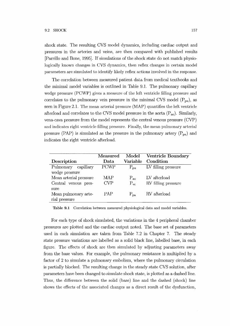
9.2 SHOCK 157
shock state. The resulting CVS Inodel dynalnics, including cardiac output and
pressures in the arteries and veins, are then compared with published results
[Parrillo and Bone, 1995]. If silnulations of the shock state do not Inatch physio
logically known changes in CVS dynanlics, then reflex changes in certain model
paralneters are simulated to identify likely reflex actions involved in the response.
The correlation between measured patient data from medical textbooks and
the minimal model variables is outlined in Table 9.1. The pulmonary capillary
wedge pressure (PC-VVP) gives a measure of the left ventricle filling pressure and
correlates to the puhnonary vein pressure in the lninimal CVS model (P pu), as
seen in Figure 2.1. The mean arterial pressure (IVIAP) quantifies the left ventricle
afterload and correlates to the CVS Inodel pressure in the aorta (P ao). Similarly,
vena-cava pressure fron1 the Inodel represents the central venous pressure (CVP)
and indicates right ventricle filling pressure. Finally, the nlean pulnl0nary arterial
pressure (PAP) is silnulated as the pressure in the puhnonary artery (P pa) and
indicates the right ventricle afterload.
Measured Model Ventricle Boundary Description Data Variable Condition Pulmonary capillary PCWP Ppu LV filling pressure wedge pressure Mean arterial pressure MAP Pao LV afterload Central venous pres- CVP Pvc RV filling pressure sure Mean puhnonary arte- PAP Ppa RV afterload rial pressure
Table 9.1 Correlation between measured physiological data and model variables.
For each type of shock silnulated, the variations in the 4 peripheral chamber
pressures are plotted and the cardiac output noted. The base set of parameters
used in each simulation are taken froln Table 7.2 in Chapter 7. The steady
state pressure variations are labelled as a solid black line, labelled base, in each
figure. The effects of shock are then si1nulated by adjusting paranleters away
froln the base values. For exan1ple, the puln10nary resistance is multiplied by a
factor of 2 to simulate a puln10nary elnbolism, where the pulmonary circulation
is partially blocked. The resulting change in the steady state CVS solution, after
paralneters have been changed to silnulate shock state, is plotted as a dashed line.
Thus, the difference between the solid (base) line and the dashed (shock) line
shows the effects of the associated changes as a direct result of the dysfunction,
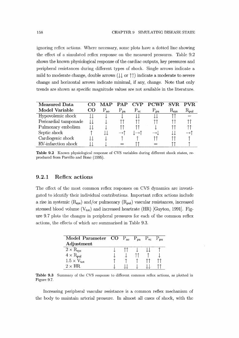
158 CHAPTER 9 SIlVIULATING DISEASE STATE
ignoring reflex actions. Where necessary, sonle plots have a dotted line showing
the effect of a sinlulated reflex response on the measured pressures. Table 9.2
shows the lmown physiological response of the cardiac outputs, key pressures and
peripheral resistances during different types of shock. Single arrows indicate a
mild to moderate change, double arrows (11 or II) indicate a moderate to severe
change and horizontal arrows indicate minimal, if any, change. Note that only
trends are shown as specific Inagnitude values are not available in the literature.
Measured Data CO MAP PAP CVP PCWP SVR PVR Model Variable CO P ao P pa Pvc Ppu Rsys Rpul Hypovolemic shock 11 1 1 11 11 II Pericardial tmnponade 11 1 II II II II II Pulmonary elnbolism 11 1 II II 1 II II Septic shock I 11 -+1 1-+1 -+1 11 -+1 Cardiogenic shock 11 1 I I II II I RV-infarction shock 11 1 II II I
Thble 9.2 Known physiological response of CVS variables during different shock states, reproduced from Parrillo and Bone (1995).
9.2.1 Reflex actions
The effect of the nl0st COlnlnon reflex responses on CVS dynamics are investi
gated to identify their individual contributions. IInportant reflex actions include
a rise in systelnic (Rsys) and/or pulmonary (Hpul) vascular resistances, increased
stressed blood vohune (Vtot ) and increased heartrate (HR) [Guyton, 1991]. Fig
ure 9.7 plots the changes in peripheral pressures for each of the common reflex
actions, the effects of which are summarised in Table 9.3.
Model Parameter CO P ao Ppa Pvc Ppu Adjustment 2 x Rsys 1 II 1 11 I 4 x Rpul 1 1 II I 1 1.5 x Vtot I I I II II 2x HR 1 11 1 11 II
Thble 9.3 Summary of the CVS response to different common reflex actions, as plotted in Figure 9.7.
Increasing peripheral vascular resistance is a common reflex mechanism of
the body to Inaintain arterial pressure. In almost all cases of shock, with the
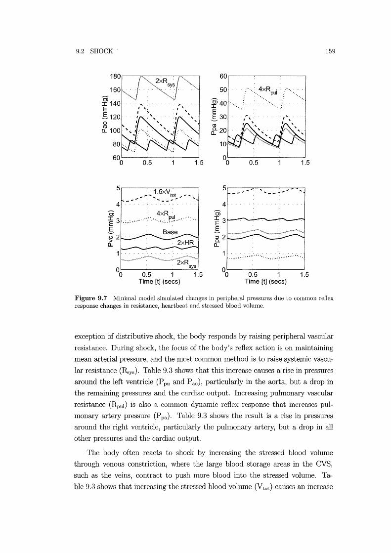
9.2 SHOCK
5~----~~~~----~ , 1.5xV
t t _ ........... ,. ......... _ ... 3"'''' .........
4 Oi '4xR ' ~ 3,.;.:,.;· ,,' , ! • :.' ': • ',., ; , .-, • p.~! ,,' ' " ' '.' . :' " ,
S u2 > (L
0.5 1 1.5 Time [t] (sees)
60~----~----~----~
50 '" f"",:,,~xRpui :' /"'';'': f 40 "' ... j . : .. :.,., . ./ .. S30 co ~20
...-0> I3 E S ~ 2 Q. (L
0.5 1 1.5
1 ' , " , , , , , " , ...... , .. , .......... ".,.".,', ....... , .... , , ,
0.5 1 1.5 Time [t] (sees)
159
Figure 9.7 Minimal model simulated changes in peripheral pressures due to common reflex response changes in resistance, heartbeat and stressed blood volume.
exception of distributive shock, the body responds by raising peripheral vascular
resistance. During shock, the focus of the body's reflex action is on Inaintaining
mean arterial pressure, and the Inost conllnon method is to raise systelruc vascu
lar resistance (Rsys). Table 9.3 shows that this increase causes a rise in pressures
around the left ventricle (P pu and P ao), particularly in the aorta, but a drop in
the relnaining pressures and the cardiac output. Increasing pulmonary vascular
resistance (Rpul) is also a con1n10n dynan1ic reflex response that increases pul
monary artery pressure (P pa). Table 9.3 shows the result is a rise in pressures
around the right ventricle, particularly the puhnonary artery, but a drop in all
other pressures and the cardiac output.
The body often reacts to shock by increasing the stressed blood volume
through venous constriction, where the large blood storage areas in the CVS,
such as the veins, contract to push Inore blood into the stressed volume. Ta
ble 9.3 shows that increasing the stressed blood volume (Vtot ) causes an increase

160 CHAPTER 9 SIMULATING DISEASE STATE
in cardiac output and all other pressures.
In most cases, the body will increase heartrate to increase cardiac output,
however Table 9.3 shows a drop in cardiac output when the heartrate is dou
bled, in this case from 80 beats per minute to 160 beats per minute. Figure 9.8
plots the typical changes in cardiac output that occur with changes in heartrate
during exercise, labelled Ex, and a relatively normal state, labelled SVT [Opie,
1998]. The plots show that the peak cardiac output typically occurs at about 160
beats/min, for the case labelled SVT.
The results in Figure 9.8 can be cOInpared with the simulated changes in car
diac output at different heartrates from the IniniInal model shown in Figure 9.9.
The line labelled Params A is plotted using the optimised parruneters in Ta
ble 7.2. The peak cardiac output using ParrullS A occurs at a heartrate of about
90 beats/min. The line labelled Paran1S B is the result of the pre-optimisation
generic parameters listed in Chapter 5 and reaches a maximum cardiac output at
about 140 beats/Inin. This result shows that the combination of parameters used
for the simulations in this chapter, Params A, will not show an increase in car
diac output with increased heartrate as is nonnally the case. However, the model
Inore accurately sin1ulates the curve shown in Figure 9.8 using an alternative
cOInbination of parruneters (ParalllS B).
The miniInal model uses only a siInple method of siInulating heartrate that
does not account for physiological changes that occur in the heart as the heartrate
changes. For example, it is known that the shape of the driver function, shown
in Figure 2.4, changes with different heartrates, but how it changes is not well
understood [Olansen et al., 2000]. Alternatively, the continued rise in cardiac
output could be attributed to the autonOlnous activation of reflex actions. For
example, as heart rate increases the systelnic vascular resistance may decrease to
further increase cardiac output. Thus, it is difficult to account for large changes
in heartrate without knowing the changes in driver function and reflex actions.
The model could be used in an inverse fashion to determine these changes and
the optimiser can also include such perfonnance metrics as additional objective
functions.
9.2.2 Hypovolemic Shock
Hypovolemic shock is the leading cause of death for trauma patients under the
age of 45 years [Kumar and Parrillo, 1995]. Hypovolemic shock is caused by a

9.2 SHOCK
2.5
2.0
1 STROKE VOLUME
....... -'" LVF
CARDIAC OUTPUT
Ex
SVT
1.0~;---r ___ --r_b_e_ats_/_m--,in
80 100 150 200
161
Figure 9.8 Variations in stroke volume and cardiac output with heartrate during exercise (Ex), supraventricular tachycardia (SVT) and left ventricle failure (LVF) [Opie, 1998].
6000~~--~----~--~----~--~----~----
60 80
Params B:
100 120 140 Time [t] (sees)
160 180 200
Figure 9.9 Variations in cardiac output versus heart rate for the minimal model with two different sets of parameters.
drop in blood volume, and primarily results in a drop in cardiac output and mean
arterial pressure along with a decrease in ventricle filling pressures. To conlbat
the drop in mean arterial pressure, arterioles in the systenric circulation constrict
to increase systenric arterial pressure.
Hypovolenric shock is simulated by decreasing the total volume of blood in
the nrinimallllodel, which represents only the stressed volume in the hmllan CVS,
as discussed in Chapter 5. However, the physiological response of the CVS to
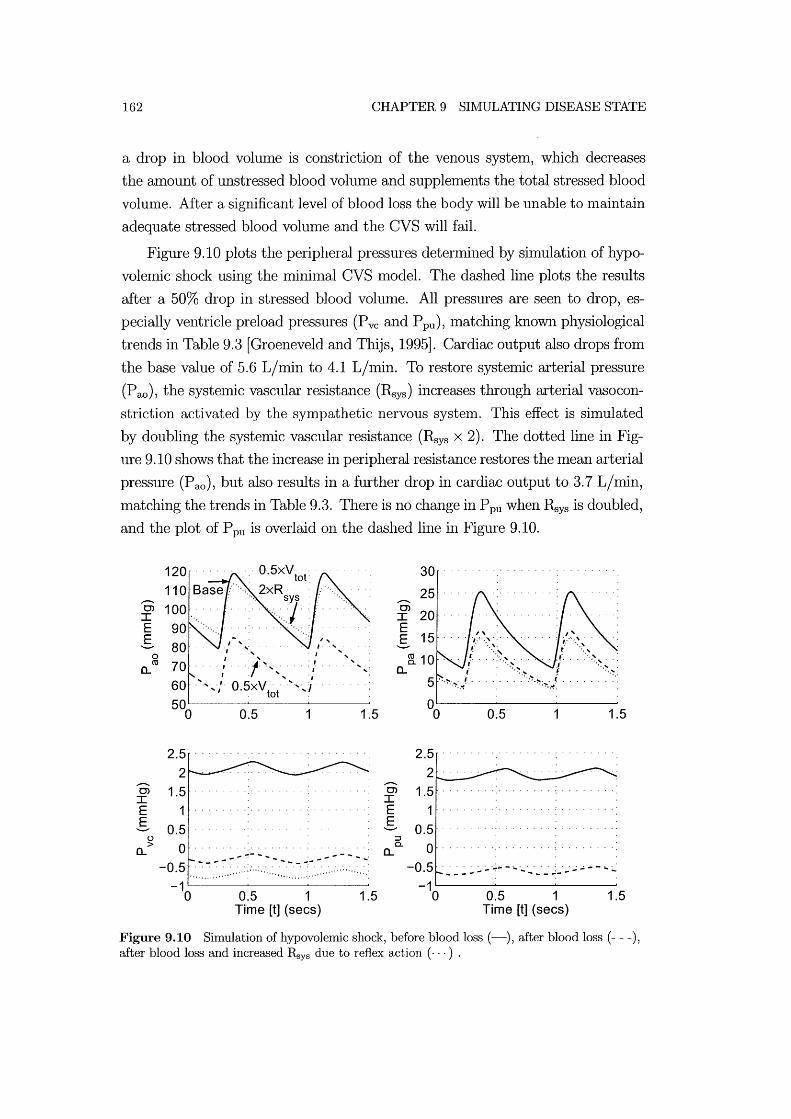
162 CHAPTER 9 SI:NIULATING DISEASE STATE
a drop in blood volume is constriction of the venous system, which decreases
the amount of unstressed blood volume and supplements the total stressed blood
volunle. After a significant level of blood loss the body will be unable to nlaintain
adequate stressed blood volume and the CVS will fail.
Figure 9.10 plots the peripheral pressures detennined by simulation of hypo
volemic shock using the minilnal CVS model. The dashed line plots the results
after a 50% drop in stressed blood volume. All pressures are seen to drop, es
pecially ventricle preload pressures (Pvc and P pu), Inatching known physiological
trends in Table 9.3 [Groeneveld and Thijs, 1995]. Cardiac output also drops from
the base value of 5.6 L/min to 4.1 L/lnin. To restore systelnic arterial pressure
(P ao), the systelnic vascular resistance (Rsys) increases through arterial vasocon
striction activated by the sympathetic nervous system. This effect is simulated
by doubling the systemic vascular resistance (Rsys x 2). The dotted line in Fig
ure 9.10 shows that the increase in peripheral resistance restores the mean arterial
pressure (Pao) , but also results in a further drop in cardiac output to 3.7 L/min,
matching the trends in Table 9.3. There is no change in Ppu when Rsys is doubled,
and the plot of P pu is overlaid on the dashed line in Figure 9.10.
Oi I E E-a..
--. 0> I E E-
o ro
o > a..
120
80 ". .',:~. , .' 70 .... , ... :1" ~ ,. ,. .. : '
" " .' 60 . ·'·,·,'·0.5xV .......... "/ . tot
2.5 2
1.5 1
0.5 o
-0.5
0.5
... - .....
1.5
....-- ...
-1~----~------~----~
o 0.5 1 1.5 Time [t] (sees)
--.
30
25
~ 20 E E- 15
~10 a..
2.5
0.5
2 ____ _
1.5 1
0.5 o
-0.5 --------:--- ...
1
.... .; ... -- .. ... - -..:- ...
1.5
-1~----~----~~----~
o 0.5 1 1.5 Time [t] (sees)
Figure 9.10 Simulation of hypovolemic shock, before blood loss (-), after blood loss (- - -), after blood loss and increased Rsys due to reflex action ( ... ) .

9.2 SHOCK 163
9.2.3 Distributive Shock
The mechanislTIS associated with distributive shock are not well known and it is
one of the leading causes of death in intensive care units [Natanson et al., 1995].
Septic shock, alternatively referred to as blood poisoning, is a common type of
distributive shock that is characterised by a drop in systelIDc vascular resistance.
This drop is thought to occur due to a drop in vascular auto-regulatory control
[Parrillo and Bone, 1995].
Septic shock is shllulated in the lllinimal CVS lllodel by halving the SyStelIDC
resistance (0.5 x Rys). Figure 9.11 shows the resulting variation in pressures.
Cardiac output increases from 5.6 L/lnin to 6.2 L/nlin with the drop in sys
temic resistance. Overall, the lllodel captures the n1ain published physiological
responses during septic shock outlined in Table 9.2, including a drop in mean
arterial pressure (P ao) and a rise in cardiac output.
150 30 Base
~100 ~20 E E g g 0 ... ... " ro ' . ! "
a.. ... ... 1.
0.5xR sys
00 0.5 1 1.5 00 0.5 1 1.5
3.5
3 ... ;. .,. ...... , . . . ., .... . C> ., , , , , , , . , , ,
I , ........ -~.; E
.......... g () ~ > 0-a.. a.. , , .. ...
'" ..
1.50 0.5 1 1.5 0 0.5 1.5
Time [t] (sees) Time [t] (sees)
Figure 9.11 Simulation of distributive septic shock, before drop in systemic resistance (-) and after (- - -).

164 CHAPTER 9 SIMULATING DISEASE STATE
9.2.4 Cardiogenic Shock
Cardiogenic shock results from failure of the heart to pump an adequate amount
of blood as a result of damage to the Inyocardium. Myocardial dysfunction
usually results from an infarction, where part of the myocardium dies due to
lack of oxygen. The main result of myocardial infarction is a drop in ventricle
contractility, represented in the lninilnal nlodel by the parameter Ees.
Cardiogenic shock is generally characterised by an increase in ventricle filling
pressures and ventricle volumes, and reductions in both cardiac output and sys
tenuc arterial pressure. Hence, less blood is distributed to the tissues, including
the Inyocardium. As a result, further myocardial daInage can occur aIld if this
sequence continues, death will rapidly ensue.
Left Ventricle Infarction
Figure 9.12 shows the simulated effects of reduced left ventricle contractility
on the peripheral pressures. Contractility is reduced to only 50% of the base
value (0.5 x Ees,lvf) to enlphasise the effects of left ventricle infarction on CVS
dynamics. The key results are a drop in both systelnic arterial pressure and
cardiac output. The cardiac output drops fronl 5.6 l/min to 2.6 l/min and Fig
ure 9.12 shows a drop in Pao. The literature also refers to a rise in Ppa, Pvc
and Ppu during left ventricle infarction [Parrillo and Bone, 1995]. The simulated
results are shown to capture the rise in puhnonary venous pressure (P pu), which
raises the left ventricle filling pressure and causes the characteristic increase in
left ventricle volume. However, the silnulated pressures around the right ventricle
(Pvc and P pa) decrease.
A common reflex action to cardiogenic shock is a rise in both pulmonary
and systemic vascular resistance (Rpul and R,ys). Increasing R,ys produces an
increase in P ao and P pu, but causes a further drop in Pvc and P pa. Increasing
RpuI causes a recovery in both P pa aIld Pvc. More specifically, P pa increases to
greater than the base value, Inatching published results, but the increase in Pvc
is not enough to recover the base value. An alternative reflex action is venous
constriction which increases the stressed volume of blood in the CVS. Figure 9.12
shows that increasing the stressed blood vohllne by a factor of 1. 5 will cause all
of the pressures, except P ao, to increase above base values to match physiological
response. Thus, a cOlnbination of these reflex actions would cause the simulated
model to match the responses outlined in Table 9.2, and may all be involved in

9.2 SHOCK
the actual physiological response.
140 .................. .
0> 0> I I E E E- E-
g 60 ........ : ........ . a..
0> I E E-
u > a..
40 ... ·O.-5xE· .... . eS,lvf
0.5
3 ........ . . . . . . . .
00 0.5 Time [t] (sees)
1.5
1.5
35
30
8
0.5 1.5
6 .. :.: ..... : .. :.:.: ..... : .. : ..... : .. : ... : .. :.:.: .. : ..... : ..... : ..... :.: .. : . .
4 .................. .
-------------------,
0.5 1.5
Time [t] (sees)
165
Figure 9.12 Minimal model simulation before (-) and after (- - -) left ventricle infarction, and after increased stressed blood volume ( ... ).
Right Ventricle Infarction
Right ventricle infarction is simulated by reducing the right ventricle con
tractility (Ees,rvf) to 50% of the base value (0.5 x Ees,rvf). Once again, the model
captures the main trends including a drop in mean arterial pressure (P ao), as
shown in Figure 9.13 and a drop in cardiac output from 5.6 l/lnin to 4.8 l/min.
The central venous pressure (P ve) increases, Inatching the response outlined in
Table 9.2 of an increase in ventricle preload, and the consequent increase in right
ventricle volume. However, the model shows a significant drop in pulnl0nary
venous pressure (P pu) where normal physiological response shows no significant
variation in Ppu [Parrillo and Bone, 1995J.
Figure 9.13 shows that increasing the stressed blood volume of the model
(Vtot ) by a factor of 1.2 causes an increase in P ve, a recovery in P ao and minimal
change in the other pressures, matching the responses in Table 9.2. Therefore,
it is likely that reflex changes that increase stressed blood volume are a major

166 CHAPTER 9 SINIULATING DISEASE STATE
contributing factor in the physiological response to right ventricle infarction.
140 ..... . Base
120 0> I E E-~ a.
0> I E E-
u > a.
60 ..... ·O.-sxE····· . e5,rvf
0.5
5 ................... .
0.5 Time [t] (sees)
1.5
1.5
30 ................... .
0> I E E-
4
0.5 1 1.5
: 0.5xE f 3 ...... ·/1.2XV:~'M .
E:::J 2 .. · .. : .. · .... ···,··· D
o.
o
----"* --- .... ..... - ........ ..... __ :..... ......
0.5 1 1.5 Time [t] (sees)
Figure 9.13 Minimal model simulation before (-) and after (- - -) right ventricle infarction, and after increased stressed blood volume (- .. ).
To summarise, the Inodel is found to shnulate the Inain trends characteristic
of cardiogenic shock, including decreases in systelnic arterial pressure and cardiac
output. Sin1ulation of known reflex changes in systemic and pulmonary vascular
resistance and stressed blood vohune produced model results that more closely
match the physiological responses outlined in Table 9.2. Hence, the model may
serve as a framework for determining the relative importance and contribution of
different reflex actions in the body's response to cardiogenic shock.
9.2.5 Extracardiac Obstructive Shock
Extracardiac obstructive shock results fron1 an obstruction to flow in the cardio
vascular systen1. Examples of obstructions to flow include a pulmonary embolism
or pericardial tamponade. Pulmonary eInboliSln is most often caused by a blood
clot that has broken free froln the veins in the systelnic circulation and become
lodged in the pulmonary circulation. Pericardial tamponade occurs when blood
fills the pericardial chamber and limits the expansion of the ventricles. Different
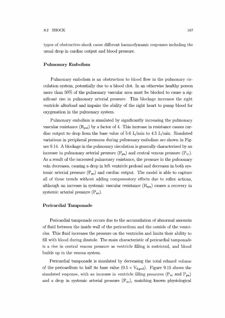
9.2 SHOCK 167
types of obstructive shock cause different haenl0dynamic responses including the
usual drop in cardiac output and blood pressure.
Pulmonary Embolism
Pulmonary enlbolism is an obstruction to blood flow in the pulmonary cir
culation system, potentially due to a blood clot. In an otherwise healthy person
1110re than 50% of the pulmonary vascular area must be blocked to cause a sig
nificant rise in pulnl0nary arterial pressure. This blockage increases the right
ventricle afterload and impairs the ability of the right heart to pUll1P blood for
oxygenation in the pulmonary systell1.
Puhnonary embolisnl is sinlulated by significantly increasing the puhnonary
vascular resistance (Rpul) by a factor of 4. This increase in resistance causes car
diac output to drop frOll1 the base value of 5.6 L/nlin to 4.5 L/nlin. Simulated
variations in peripheral pressures during pulmonary ell1bolisll1 are shown in Fig
ure 9.14. A blockage in the puhl10nary circulation is generally characterised by an
increase in pulmonary arterial pressure (Ppa) and central venous pressure (Pvc).
As a result of the increased puhl10nary resistance, the pressure in the puhl10nary
vein decreases, causing a drop in left ventricle preload and decreases in both sys
tenlic arterial pressure (P ao) and cardiac output. The Inodel is able to capture
all of these trends without adding compensatory effects due to reflex actions,
although an increase in systelIDc vascular resistance (R,ys) causes a recovery in
systenlic arterial pressure (P ao).
Pericardia! Tamponade
Pericardial tamponade occurs due to the accumulation of abnoflnal amounts
of fluid between the inside wall of the pericardiunl and the outside of the ventri
cles. This fluid increases the pressure on the ventricles and linlits their ability to
fill with blood during diastole. The main characteristic of pericardial tamponade
is a rise in central venous pressure as ventricle filling is restricted, and blood
builds up in the venous system.
Pericardial tamponade is simulated by decreasing the total relaxed vohllne
of the pericardium to half its base value (0.5 x VO,pcd). Figure 9.15 shows the
simulated response, with an increase in ventricle filling pressures (Pvc and P pu)
and a drop in systelnic arterial pressure (P ao), matching known physiological
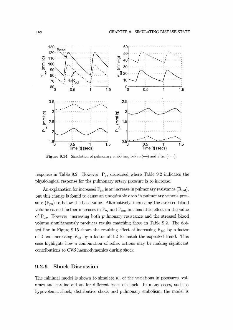
168 CHAPTER 9 SHvIULATING DISEASE STATE
130 60 ................. . Base
...-0> I
50 ..... /- ..... ,,~ ....... ~ . , ......... ,. / . I
. I :/ ...... .
'''-I
I . / .
"" E E-
o C\l
a.. , , 70 . ", ~,. . ......
600
3.5
0) 3 I E E- 2.5
C,) > a..
0.5 1
......
0.5 1 Time [t] (sees)
1.5
1.5
0.5 1
2.5 ................. .
...-0> I E E- 1.5
::J c..
a.. 1
0.5 1 Time [t] (sees)
Figure 9.14 Simulation of pulmonary embolism, before (-) and after (- - -).
1.5
1.5
response in Table 9.2. However, P pa decreased where Table 9.2 indicates the
physiological response for the pulmonary artery pressure is to increase.
An explanation for increased P pa is an increase in puhnonary resistance (Rpul)'
but this change is found to cause an undesirable drop in pulmonary venous pres
sure (P pu) to below the base value. Alternatively, increasing the stressed blood
volume caused further increases in Pvc and P pu, but has little effect on the value
of P pa' However, increasing both pulmonary resistance and the stressed blood
vohune simultaneously produces results Inatching those in Table 9.2. The dot
ted line in Figure 9.15 shows the resulting effect of increasing Rpul by a factor
of 2 and increasing Vtot by a factor of 1.2 to Inatch the expected trend. This
case highlights how a conlbination of reflex actions nlay be nlaking significant
contributions to CVS haemodynamics during shock.
9.2.6 Shock Discussion
The minimal model is shown to simulate all of the variations in pressures, vol
Ulnes and cardiac output for different cases of shock. In many cases, such as
hypovolemic shock, distributive shock and pulmonary embolism, the model is
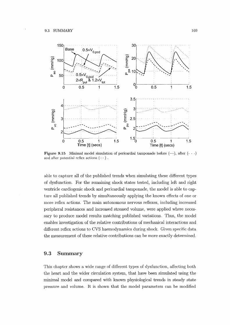
9.3 SUIVIMARY 169
1S0 30 O.SxVO d ,pc
...-... ...-... 0> 0> I
I E E
' .. ,., .. ,./~.~.>.~.~ .'. """"V""'" g g 0 ro
SO ... 0,S0Vd,pcd .. ' ....... -: a... .. " 2xR I & 1.2x'vt t . pu 0
00 0 O.S 1 1.S O.S 1 1.S
3.S
4 ...-... ...-... 0> 0>
I I E 3
E g ..... , . g
u .............. .. .... .. ::I > a.
a... .. -- .... __ .... - ..... a... 2
0 O.S 1 1.S 1.S
0 O.S 1 1.S Time [t] (sees) Time [t] (sees)
Figure 9.15 Minimal model simulation of pericardial tamponade before (-), after (- - -) and after potential reflex actions ( ... ) .
able to capture all of the published trends when sinlulating these different types
of dysfunction. For the relllaining shock states tested, including left and right
ventricle cardiogenic shock and pericardial talllponade, the lllodel is able to cap
ture all published trends by simultaneously applying the known effects of one or
lllore reflex actions. The main autonOlllOUS nervous reflexes, including increased
peripheral resistances and increased stressed volume, were applied where neces
sary to produce lllodel results matching published variations. Thus, the lllodel
enables investigation of the relative contributions of lllechanical interactions and
different reflex actions to CVS haenl0dynanlics during shock. Given specific data
the measurelllent of these relative contributions Call be more exactly determined.
9.3 Summary
This chapter shows a wide range of different types of dysfunction, affecting both
the heart and the wider circulation systelll, that have been simulated using the
lninimal lllodel alld compared with known physiological trends in steady state
pressure and volume. It is shown that the model parameters can be modified

170 CHAPTER 9 SIMULATING DISEASE STATE
to sinlulate various types of CVS dysfunction and reflex actions. In many cases,
the model accurately captures the changes in pressures, volumes and cardiac
output in and around the heart during CVS dysfunction. During severe shock,
the body's autonomic nervous system responds to decreased cardiac output and
blood pressure by initiating powerful reflex actions that significantly affect CVS
function. In these cases, it is necessary to include the effects of reflex action in
model simulations to match reported physiological trends. Hence, the minimal
model can be used to identify the relative contributions of CVS functions and
reflex actions. This capability offers a powerful new tool that can be used in
conjunction with experimental investigations into CVS function during health
and disease.
Chapter 10
Conclusions
Cardiovascular systel11 function involves a cOlllplex interaction of mechanical, hy
draulic and autonomous reflex effects that can nlake diagnosis of CVS dysfunction
difficult and tinle consuming. This thesis presents a model of the human CVS
that can be used to assist medical staff in understanding, diagnosis and treat
l11ent selection for patients with CVS dysfunction. A l110del is developed using a
nrininlal philosophy leading to a nrinimum nUl11ber of parallleters, variables and
governing equations. The resulting model is both stable and simple to solve, with
a silllpler structure than most closed loop l110dels in the literature.
The initial focus is on creating a physiologically and fluid dynamically accu
rate nlodel that is nUl11erically stable. Therefore, the individual function of the
separate cOlllponents including the active and passive elastic chambers, ventric
ular interaction and conlponents sinlulating blood flow are developed first. A
l11ethod of l110delling the active cardiac challlbers based on the PV diagralll is
outlined because PV diagralllS are commonly used and understood by l11edical
staff. Equations governing fluid flow are included along with a novel approach of
tracking velocity profile variations that uses a mixed finite-elelllent and lumped
parallleter fornlulation, and includes time varying resistance and inertial effects.
This approach is cOl11bined with a physiologically accurate method of simulating
heart valve function.
The basic components, such as elastic chambers and elements simulating fluid
flow, are verified separately before cOlllbining them to create the full closed loop
lllodel. The advantages in numerical stability, model robustness and uniqueness
of solution of the lninilllal l110del approach to CVS modelling are presented. In
contrast, other lllodels in the literature were found to be overly c0111plex, unstable,
physiologically inaccurate, or too focused on specific aspects of the CVS.
Optinrisation is used to achieve one of the key ailllS of this research, to create

172 CHAPTER 10 CONCLUSIONS
patient specific nl0dels by nlatching specific patient CVS perfornlance. A set of
model panuneters are adjusted using an opthnisation routine until the minhnal
Inodel output dynamics satisfy a set of objective functions. The optimisation
technique presented can be used to make the minimal model Inatch the general
CVS function of any animal or hlunan in reasonable time to within 0.1 % of target
values. lVledical staff will be able to investigate irregularities in the optinlised
parameters to assist in identifying areas of dysfunction. The optimised Inodel
can also be used to simulate the known effects of different therapies to assist in
choosing a suitable intervention. Thus, patient specific models created using the
optimisation approach developed will directly assist medical staff in diagnosis and
treatlnent selection.
Static and dynamic experhnents investigating the response of the CVS due
to ventricular and cardiopuhnonary interactions are used to verify the function
of the CVS model. Static responses are cOlmnonly used to verify the function of
models in the literature, however few other closed loop models accurately shnu
late the transient dynamics of cardiopuhnonary interactions and none shnulate
the transient dynamics of ventricular interaction. The minimal nl0del is shown
to capture the dynamics of both types of interactions accurately. Experimentally
quantifying the relative effects of series and direct ventricular interactions is nor
mally a difficult task, however it is shown to be easy using the presented model.
In addition, the model also enables the relative inlportance of different physio
logical elenlents in these interactions to be investigated. For eXalnple, pulnl0nary
resistance variations during respiration are found to be an important contributor
to the dynamics of the puhnonary artery pressure.
The ability of the model to shnulate dysfunction is also investigated. Particu
lar cases of heart disease and shock are shnulated to COlnpare the minhnal model
outputs with the known physiological response of the human CVS to various
types of dysfunction. Heart disease and shock can cause severe states of dysfunc
tion in the CVS and the body responds with powerful reflex actions. It is shown
how the model can be used to not only investigate the effects of dysfunction, but
also investigate the most likely reflex responses that contribute to the character
istic CVS measurements. The increased systemic vascular resistance required to
maintain mean arterial pressure is an example of a conlnlon reflex action that is
simulated.
The case studies on ventricular and cardiopulmonary interaction, and cardiac
dysfunction, highlight the Inodel's capability to delineate the relative contribu-

173
tions of different interactions and/or dysfunction to particular CVS responses.
Normally, isolating these individual contributions using experimentallnethods is
difficult, if not illlpossible, however different contributions can be easily included
or excluded using the minimal model developed. Thus, the l11ininlal model offers
a powerful tool that can be used as a teaching aid, in a research environment to
improve understanding of experilnentally measured CVS function.
The ability of the Imnimal nlodel developed to silnulate a wide range of CVS dynmmcs and dysfunction memlS it can be of direct use in teaching, research and
clinical environlllents. As a teaching aid, the Imnilnal Inodel will help medical
students learn 1110re about CVS function through silnulation. The minilnallllodel
would help researchers develop experimental methods and increase understanding
of the results. Clinically, the nlininlal model can create patient specific Inodels
and silllulate a variety of dysfunction to assist clinical staff in diagnosis and
treatment selection.
The author believes the following areas SUlllmarize the novel and significant
contribution to knowledge in the area of CVS 1110delling made in this thesis:
• The nlininlal l110del offers a stable, flexible nlodel of the entire CVS that
can be used to siInulate a variety of dysfunctions. It uses significantly fewer
state variables and an event driven solver to account for the changes in
state as the valves open and close during the cardiac cycle.
• More physiologically realistic and numerically stable 111ethods of sinlulating
ventricular interaction and valve functions, including a reasonable valve
law.
• A physiologically accurate nlethod of simulating pulsatile flow through large
arteries for use with lunlped-parameter models.
• A novel Inethod of deternnning initial conditions to improve the rate of
convergence, which is particularly useful in parameter identification.
• A method of creating patient specific models using optimisation of model
parameters.
• Model verification against experinlentally nleasured transient changes in
CVS dynmnics due to ventricular and cardiopulmonary interaction. TIns
verification shows the full capability of the model and is unique in the CVS
modelling literature.

174 CHAPTER 10 CONCLUSIONS
• Simulation of disease state and the delineation of the relative contributions
of autonomous reflex actions on CVS dynamics.
Chapter 11
Future Work
The minhnal model developed can shnulate many of the Inajor trends in CVS
function due to interactions and disease. Further modifications could enable it to
Inore accurately shnulate nlore subtle variations in CVS pressures and volumes,
and a wider range of CVS dysfunction. However, as Inentioned earlier, care
should be taken to only included additional cOInplexity where it will nlake a sig
nificant, and necessary, contribution to the models performance and physiological
accuracy.
This section investigates changes to the Inodel structure that would enable it
to Inore accurately simulate sonle aspects of CVS function, such as the addition of
nl0re elastic chmnbers. The cardiac driver function is also identified as a key area
where further work would inlprove nl0del functional. Potential modifications
to the opthnisation routine that would produce Inore accurate results are also
discussed. Finally, further work is now needed to specifically investigate how the
Inodel can be best used in the clinical envirolunent by nledical staff.
11.1 Model Structure
The Ininimal model presented captures nlany of the Inajor CVS haemodynamics,
which was the initial intention of the model. Many nl0difications could be carried
out using cOInponents already developed for the minimal Inodel. This section
investigates examples of adding cOlnplexity to capture specific dynalnics that
would hnprove function and accuracy.
Figure 11.1 shows a potential modification to the model structure where three
additional elastic chmnbers have been added to shnulate the left and right atria
(la and ra) and divide the systelnic artery into two elastic challlbers (ao and ar).
The addition of atria would enable the model to capture Inore subtle variations
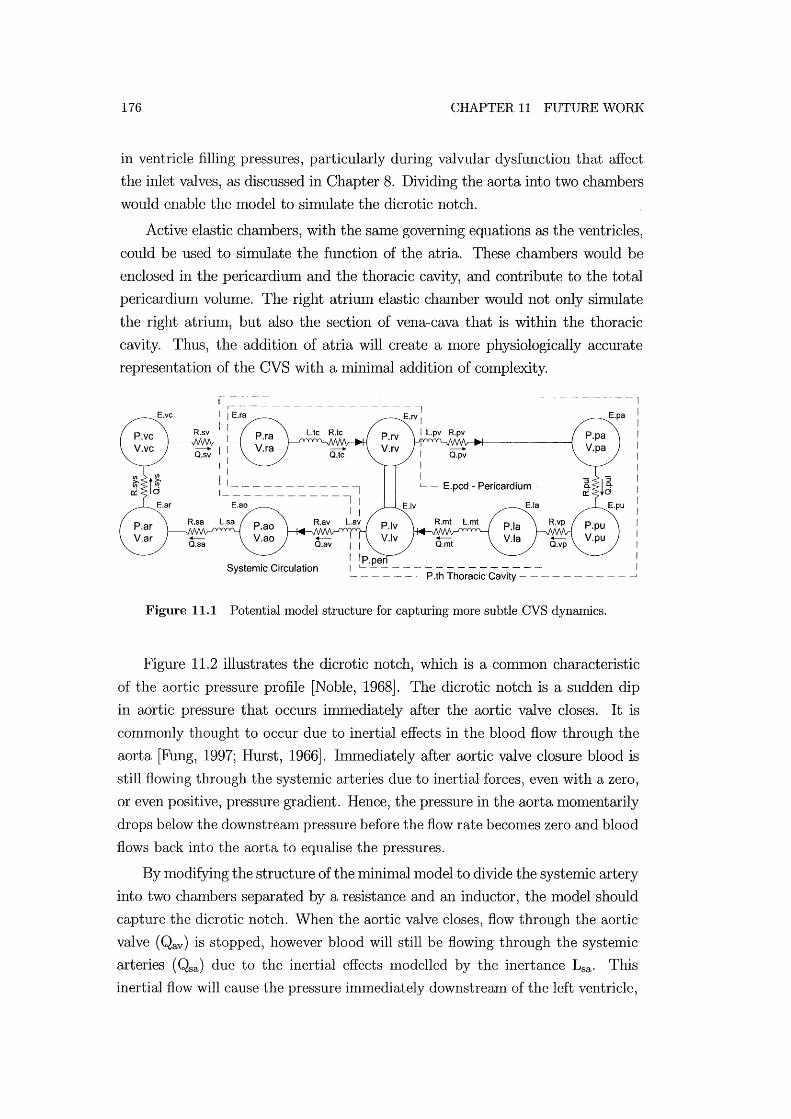
176 CHAPTER 11 FUTURE WORK
in ventricle filling pressures, particularly during valvular dysfunction that affect
the inlet valves, as discussed in Chapter 8. Dividing the aorta into two chambers
would enable the model to simulate the dicrotic notch.
Active elastic chambers, with the same governing equations as the ventricles,
could be used to simulate the function of the atria. These chambers would be
enclosed in the pericardium and the thoracic cavity, and contribute to the total
pericardium volume. The right atrium elastic chmnber would not only simulate
the right atrium, but also the section of vena-cava that is within the thoracic
cavity. Thus, the addition of atria will create a nl0re physiologically accurate
representation of the CVS with a minhnal addition of complexity.
E.vc
Systemic Circulation
I I I I
I I I L - E.pcd - Pericardium
I IP.peri I ~- - -----------~ - - - -. P.th Thoracic Cavity --
Figure 11.1 Potential model structure for capturing more subtle CVS dynamics.
-I
E.pa 1
I I I I I I I I I I I I I I
Figure 11.2 illustrates the dicrotic notch, which is a COIlllnon characteristic
of the aortic pressure profile [Noble, 1968]. The dicrotic notch is a sudden dip
in aortic pressure that occurs hnmediately after the aortic valve closes. It is
commonly thought to occur due to inertial effects in the blood flow through the
aorta [Fung, 1997; Hurst, 1966]. IIlllnediately after aortic valve closure blood is
still flowing through the systemic arteries due to inertial forces, even with a zero,
or even positive, pressure gradient. Hence, the pressure in the aorta momentarily
drops below the downstream pressure before the flow rate beconles zero and blood
flows back into the aorta to equalise the pressures.
By modifying the structure of the minimal model to divide the systemic artery
into two chambers separated by a resistmlce and an inductor, the model should
capture the dicrotic notch. When the aortic valve closes, flow through the aortic
valve (Qav) is stopped, however blood will still be flowing through the systemic
arteries (Qsa) due to the inertial effects lllodelled by the inertance Lsa. This
inertial flow will cause the pressure immediately downstream of the left ventricle,

11.2 CARDIAC DRIVER FUNCTION
150
Cl I
E E
o
pressure in ascending aorta
pressure in left ventricle
Dicrotic notch
~ ....... ,I -----0·1 s
Figure 11.2 Left ventricle and ascending aorta pressures in a dog [Noble, 1968].
177
in the aorta (P ao), to drop below the pressure in the arterioles (Par). However,
once the Qsa drops to zero, the lower P ao will cause blood to flow back into the
aorta. Thus, the pressure in the aorta will dip after valve closer before rising
again as blood flows back into the aorta, silnulating the dicrotic notch.
These eXalnples of adding chalnbers to the nlinimal model illustrate how the
structure of the model can be easily extended and modified to capture nl0re
subtle CVS dynalllics. However, the addition of chambers adds conlplexity to
the model and should only be done where it is necessary. For example, if the
only benefit of splitting the systenlic artery into two chambers is to capture the
dicrotic notch, then this change should only be done when it is necessary to
silnulate this particular dynanlic. The current structure of the Imnilnal model
has been shown to capture a wide range of Inajor CVS dynalmcs in its current
state and additional cOlnplexity should only be added where it is necessary.
11.2 Cardiac Driver Function
As discussed in Chapter 2, a simple cardiac driver function (e( t)) profile is used to
leave the focus on the CVS model function of the components and avoid possible
contributions to CVS dynamics fronl nlore conlplex driver profiles. However,
further developlnent to Inake the driver function more physiologically accurate
could produce better simulation results. The parameters used to define the shape
of the driver profile in Equation (2.4) could also be used as variables in the
optinlisation routine.
178 CHAPTER 11 FUTURE WORK
11.3 Optimisation
Chapters 6 and 7 show how optimisation can be used to Inanipulate the minimal
Inodel parameters to achieve target model perfornlrulce dynamics and create a
patient specific nl0del. The application of optimisation techniques to the mini
Inal model can be further extended by modifying the optimisation routine and
by adding additional parruneters and more objective functions. Examples of po
tential modifications to the optinlisation routine include:
• The inlportance of the difference between the nlaximum ventricle pressure
and the maximum afterload pressure is illustrated in Chapter 9, relating to
valvular dysfunction. The difference in these two nlaxinlunl values could
be added as an objective function in the optimisation routine. Thus, the
optimisation of the minimallnodel nlay show a significant increase in aortic
resistance, which is characteristic of aortic stenosis.
• When plotting cardiac output as a function of heart rate in Chapter 9, the
plot of optimised parruneters was found to reach a peak at a heartrate that
is too low. If the peak heartrate value is known, or estimated, it could be
used as an objective function in the optimisation.
• Only the average ventricle filling pressures (A vg Pvc and A vg P pu) were
used, and no restraint was placed on the runplitude of the variation in these
variables. If this pressure infonnation was available it could be added as
additional objective functions.
• Model parruneters such as the elastance and relaxed volume of the peri
cardium and the septum could be added as additional optimisation vari
ables, particularly if the focus is on ventricular interaction.
However, care should be taken when choosing appropriate parruneters to be used
as optimisation vru'iables. Too many parameters will cause large computation
time and potentially non-unique solutions. Conversely, if not enough parameters
are used, the optimisation routine may not be able to satisfy all of the objective
functions.
The optinlisation settings and routine could also be modified to accelerate
the time taken to find a solution. Many of the optimisation routine settings
could be adjusted to produce faster results. For example, Chapter 7 discusses
how relaxing the target error to 1 % would still produce accurate results, but

11.4 APPLICATION AS A DIAGNOSTIC AID 179
take significantly less con1putational tin1e. Additionally, the generic optimisation
routine used could be modified to be n10re specifically suited to this application.
11.4 Application as a Diagnostic Aid
One of the key initial aims of this research is to create a model that is of direct
use to n1edical staff to help in understanding, diagnosis and treatn1ent selection.
This thesis offers a proof of concept of the n1inin1al model to simulate specific
patient CVS function. Further developlnent should be focused on the application
of the minimal model as a teaching and diagnostic aid. The next stage should
involve two areas of developlnent to Inake the model more useful to nledical
staff. One area involves investigating the application of the model, how n1edical
staff will use it, and clinical verification. The other area is in decreasing the
computational tin1e to find a solution, n10st directly achieved by converting the
nlodel to a faster language, such as C\ C++. The result would be increases in
the speed of the shnulations by an order of 10 to 100 times, and a reduction in
the tin1e required for patient specific optilnisation to a n1atter of n1inutes.
11.5 Summary
The nuninlallnodel has been shown to capture a wide range of CVS dynaInics.
However, further developlnents in the Inodel structure aIld governing equations
could enable 1110re specific and subtle dY11al11ics to be captured. In particular,
the driver function profile could be investigated to 111ake it n10re physiologically
accurate. The opthnisation routine could also be further developed by adding
l110re objective functions to create more accurate patient specific l11odels. Finally,
further investigation is needed into how the Inodel can be of direct use to Inedical
staff, perhaps by carrying out specific clinical verification and accelerating the
cOlnputational solution thne.
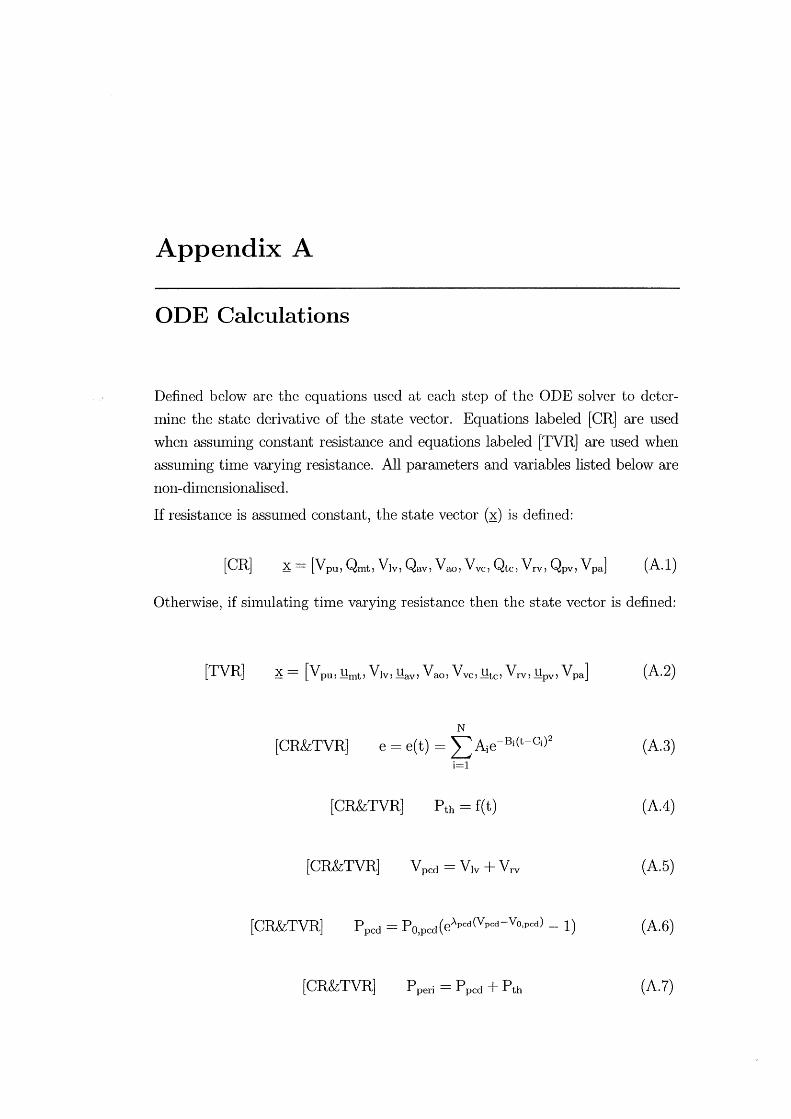
Appendix A
ODE Calculations
Defined below are the equations used at each step of the ODE solver to deter
Imne the state derivative of the state vector. Equations labeled [CR] are used
when asslumng constant resistance and equations labeled [TVR] are used when
assuming time varying resistance. All parruneters and variables listed below are
non-dhnensionalised.
If resistance is assunled constant, the state vector (~) is defined:
[CR] (A.I)
Otherwise, if simulating tilne varying resistance then the state vector is defined:
[TVR] (A.2)
N
[CR&TVR] e = e(t) = LAie-Bi(t-Ci)2 (A.3) i=l
[CR&TVR] Pth = f(t) (A.4)
[CR&TVR] Vpcd = Vlv + Vrv (A.5)
[CR&TVR] P pcd = P O,pcd ( eApcd (V pcd - VO,pcd) - 1) (A.6)
[CR&TVR] Pperi = Ppcd + Pth (A.7)
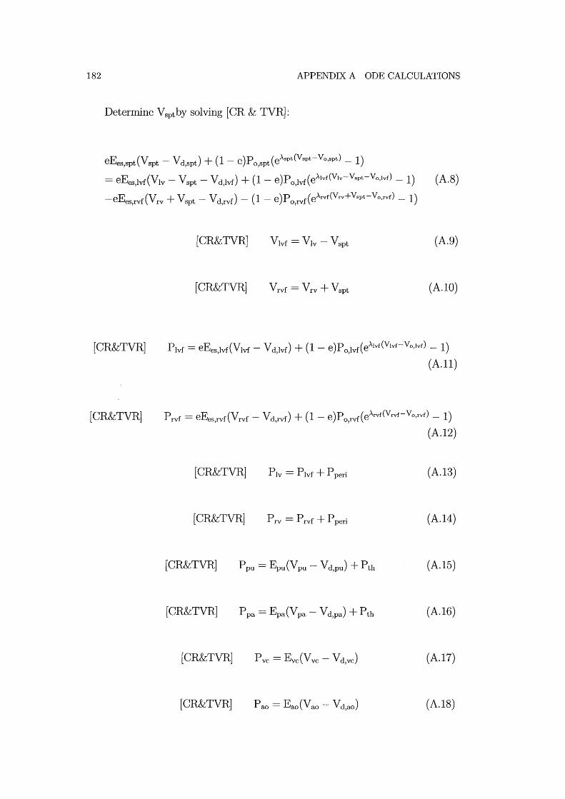
182 APPENDIX A ODE CALCULATIONS
Determine Vsptby solving [CR & TVR]:
eE (V V ) + (1 e)P (eAspt(Vspt-Vo,spt) 1) es,spt spt - d,spt - o,spt -
= eEes,lvf(V1v - Vspt - Vd,lvf) + (1 - e)Po,lvf(eAlvf(Vlv-VsPt-Vo,lvr) - 1) (A.8)
-eE vf(V + V - Vd f) - (1 - e)P rvf(eArvf(Vrv+Vspt-Vo,rvf) - 1) eS,r rv spt ,rv 0,
[CR&TVR] (A.9)
[CR&TVR] Vrvf = Vrv + Vspt (A.I0)
[CR&TVR] Plvf = eEes,lvf(Vlvf - Vd,lvf) + (1- e)Po,lvf(eAlvf(Vlvf-VO,IVf) - 1)
(A. 11)
[CR&TVR] Prvf = eEes,rvf(Vrvf - Vd,rvf) + (1 - e)Po,rvf(eArvf(Vrvf-Vo,rvf) - 1)
(A.12)
[CR&TVR] Ply = Plvf + P peri (A.13)
[CR&TVR] Pry = Prvf + Pperi (A.14)
[CR&TVR] P pu = Epu (V pu - V d,pu) + P th (A.15)
(A.16)
(A.17)
[CR&TVR] P ao = Eao (Vao V d,ao) (A.18)

183
[CR&TVR] Qsys = Pao - Pvc
(A.19) Rsys
[CR&TVR] Q _Ppa-Ppu pul-
Rpul (A.20)
[CR] Q _ 480v P pu - Ply - QmtRmt
mt - f2HR X Lmt (A.21)
[CR] Q _ 480v Ply - Pao - QavRav
av - f2HR X Lav (A.22)
[CR] Q _ 480v Pvc - Pry - QtcRtc
tc - f2HR X Ltc (A.23)
[CR] Q _ 480v Pry - Pao - QpvRpv
pv - f2HR X Lpv (A.24)
[CR&TVR] Vpv = Qpul - Qmt (A.25)
[CR&TVR] Vlv = Qmt - Qav (A.26)
[CR&TVR] Vao = Qav - Qsys (A.27)
[CR&TVR] Vvc = Qsys - Qtc (A.28)
[CR&TVR] Vrv = Qtc - Qpv (A.29)
[CR&TVR] Vpa = Qpv - Qpul (A.30)

References
Amoore, J., Santamore, W., Corin, W., and George, D. (1992). Computer simu
lation of the effects of ventricular interdependence on indices of left ventrilcular
systolic function. J. Biomed. Eng, 14:257-262. [P-V relations].
Avanzolini, G., Barbini, P., Cappello, A., Cevenini, G., Pohl, V., and Sikora, T.
(March 1989). Tracking time-varying properties of the systemic vascular bed.
IEEE Trans. Biomed. Eng., 3(3) :373-381.
Avanzolini, G., Barbini, P., Cappello, A., and Cevese, A. (Oct 1985). Time
varying mechanical properties of the left ventricle - a computer simulation.
IEEE Trans. Bio. Eng., BME-32(10):756-763. Time-varying mechanical prop
erties, good paper.
Bartlett, B. and Fyfe, D. (1974). Handbook of mathematical formulae for engi
neers and scientists. Denny publications ltd, London.
Bellhouse, B. J. and Talbot, L. (1969). The fluid mechanics of the aortic valve.
J. Fluid Mech., 35(4):721-735.
Beyar, R., Hausknecht, M. J., Halperin, H. R., Yin, F. C., and Weisfeldt, M. L.
(1987). Interaction between cardiac chambers and thoracic pressure in intact
circulation. Am. J. Physiol., 22(253):H124G-H1252.
Bove, A. A. and Santamore, W. P. (Marl Apr 1981). Ventricular interdependence.
Prog. Cardio. Disease, 265(5):365-387.
Braunwald, E. (1997). Heart Disease, A text book of cardiovascular medicine, 5th
edition. W.B. Saunders Company, Philadelphia.
Buda, A. J., Pinsky, M. R., Ingels, N. B., J., Daughters, G. T., n., Stinson, E. B.,
and Alderman, E. L. (1979). Effect of intrathoracic pressure on left ventricular
performance. N Engl J Med, 301(9):453-9.
186 REFERENCES
Buist, M., Pullan, A., and Hunter, P. (1999). Modelling electrical activity from
cell to body surface. In IEEE: Proceedings of the first joint BMES/EMBS
Conference, page 1174, Atlanta, GA, USA.
Burkhoff, D. and Tyberg, J. V. (1993). Why does pulnl0nary venous pressure
rise after onset of Iv dysfunction: a theoretical analysis. Am. J. Physiol.,
265:H1819-H1828.
Campbell, K. B., Kirkpatrick, R. D., Knowlen, G. G., and Ringo, J. A. (Jan
1990). Late-systolic pumping properties of the left ventricle. Circ. Res.,
66(1):218-233. time-varying properties such as elactance and resistance.
Chung, D. (1996). Ventricular Interaction in a Closed-Loop model of the canine
circulation. Master of science, Rice University.
Chung, D., Niranjan, S., Clark, J., Bidani, A., and Johnston, W. (1997). A
dynamic model of ventricular interaction and pericardial influence. Am. J.
Physiol., 14(272):H2924-H2962.
Conn, A. R., Gould, N. 1. M., and Toint, P. L. (2000). Trust-Region Methods.
Society for Industrial and Applied Mathematics, Philadelphia, PA.
Denault, A. Y., Gasior, T. A., Gorcsan, J., L, Mandarino, W. A., Deneault,
L. G., and Pinsky, M. R. (1999). Detenninants of aortic pressure variation
during positive-pressure ventilation in man. Chest, 116(1):176-86. 0012-3692
Journal Article.
Denault, A. Y., Gorcsan, J., r., and Pinsky, M. R. (2001). Dynamic effects of
positive-pressure ventilation on canine left ventricular pressure-volume rela
tions. J Appl Physiol, 91(1):298-308. 8750-7587 Journal Article.
Frazier, O. H., Myers, T. J., Jarvik, R. K., Westaby, S., Pigott, D. W., Gre
goric, 1. D., Khan, T., Tamez, D. W., Conger, J. L., and Macris, M. P. (2001).
Research and developnlent of an implantable, axial-flow left ventricular assist
device: the jarvik 2000 heart. Ann Thorac Burg, 71(3 Suppl):S125-32; discus
sion S144-6.
Fung, Y. (1990). Biomechanics: Motion, flow, stress, and growth. Springer
Verlag, San Deigo.
Fung, Y. (1993). Biomechanics: Mechanical properties of Living Tissues, 2nd
Edition. Springer-Verlag, San Deigo.
REFERENCES 187
Fung, Y. (1997). Biomechanics: Circulation. Springer-Verlag, New York.
Funk and Wagnalls (1960). Funk and Wagnalls Standard Dictionary of the En
glish Language. Funk and Wagnalls Co., New York.
Ganong, W. F. (1979). Review of Medical Physiology, 9th Edition. Lange Medical
Publications, Los Altos, California.
Glantz, S. A. and Parn1ley, W. W. (1978). Factors which affect the diastolic
pressure-volume curve. Circ Res, 42(2):171-80.
Glass, L., Hunter, P., and McCulloch, A. (1991). Theory of Heart, Biomechanics,
Biophysics, and Nonlinear Dynamics of Cardiac Function. Springer-Verlag
New York, Inc.
Groeneveld, A. and Thijs, L. (1995). Hypovolemic shock. In Parrillo, J. E.
and Bone, R. C., editors, Critical Care Medicine, Principles of diagnosis and
management. Mosby, St. Louis, Missouri.
Guyton, A. C. (1991). Textbook of medical physiology. W.B. Saunders Company,
Philadelphia, 8 edition.
Hancock, E. W. (1995). Pericardial tamponade. In Parrillo, J. E. and Bone,
R. C., editors, Critical Care Medicine, Principles of diagnosis and manage
ment. Mosby, St. Louis, Missouri.
Hardy, H. H. and Collins, R. E. (1982). On the pressure-volulne relationship in
circulatory elements. Med Biol Eng Comput, 20(5):565-70.
Hardy, H. H., Collins, R. E., and Calvert, R. E. (1982). A digital computer Inodel
of the human circulatory system. Med Biol Eng Comput, 20(5):550-64.
Hoit, B. D., Shao, Y., Gabel, M., and Walsh, R. A. (1993). Influence of peri
cardium on left atrial compliance and pulmonary venous flow. Am J Physiol,
264(6 Pt 2):H1781-7.
Hoppensteadt, F. C. and Peskin, C. S. (2002). Modeling and Simulation in
Medicine and the Life Sciences. Springer-Verlag, New York.
Hunter, P., Hookings, A., LeGrice, I., and Smaill, B. (1991). Activation of the
heart with a 3d finite element model. In Annual International Conference of
the IEEE Engineering in Medicine and Biology Society, volume 13, 2, pages
681-983.
188 REFERENCES
Hunter, W. C., Janicki, J. S., Weber, K. T., and Noordergraff, A. (1983). Systolic
mechnical properties of the left ventricle. Circulation Research, 52(3):319-327.
Hurst, J. W. (1966). The heart, arteries and veins (3rd edition). McGraw-Hill,
Kogakusha Ltd, Tokyo.
Janicki, J. S. and Weber, K. T. (1980). The pericardium and ventricular inter
action, distensibility, and function. Am J Physiol, 238(4):H494-503.
Katz, A. M. (2002). A modern view of heart failure: practical applications of
cardiovascular physiology. In Page, E., Fozzard, H. A., and Solaro, R. J.,
editors, Handbook of medical physiology, Section 2: The cardiovascular system,
Volume 1: The heart. Oxford university press, New York, USA.
Kumar, A. and Parrillo, J. E. (1995). Shock: Classification, pathophysiology,
and approach to management. In Parrillo, J. E. and Bone, R. C., editors,
Critical Care Medicine, Principles of diagnosis and management. Mosby, St.
Louis, Missouri.
Lazar, J. M., Flores, A. R., Grandis, D. J., Orie, J. E., and Schulman, D. S.
(1993). Effects of chronic right ventricular pressure overload on left ventricular
diastolic function. Am J Cardiol, 72(15):1179-82. 0002-9149 Journal Article.
Legrice, I., Hunter, P., and Smaill, B. (1997). Laminar structure of the heart: a
mathematical model. Am J Physiol, 272:H2466-76.
Little, R. C. (1978). Physiology of the Heart and Circulation. Year book medical
publishers, Inc., New York.
Lu, K., Clark, J., Ghorbel, F., Ware, D., and Bidani, A. (2001). A human car
diopulomonary system model applied to the analysis of the valsalva maneuver.
Am. J. Physiol., 281:H2661-H2679.
Marcus, J. T., Vonk Noordegraaf, A., Roeleveld, R. J., Postmus, P. E., Heethaar,
R. M., Van Rossum, A. C., and Boonstra, A. (2001). Impaired left ventric
ular filling due to right ventricular pressure overload in primary pulnlonary
hypertension: noninvasive monitoring using mri. Chest, 119(6):1761-5.
Maughan, W. and Kass, D. A. (1988). The use of the pressure-volume diagram
for measuring ventricular pump function. Automedica, 11:317-342.

REFERENCES 189
Maughan, W. L., Sunagawa, K., and Sagawa, K. (1987). Ventricular systolic
interdependence: volume elastance model in isolated canine hearts. Am. J.
Physiol., 253:H1381-H1390. [Ventricular interaction].
Melchior, F. M., Sriniwasan, R. S., and Charles, J. B. (1992). Mathematical mod
eling of human cardiovascular system for simulation of orthostatic response.
Am. J. Physiol., 262:H1920-H1933.
Natanson, C., Hoffnlan, W. D., and Parrillo, J. E. (1995). Septic shock and
multiple organ failure. In Parrillo, J. E. and Bone, R. C., editors, Critical Care
Medicine, Principles of diagnosis and management. Mosby, St. Louis, Missouri.
Nielsen, P. M., Le Grice, 1. J., Smaill, B. H., and Hunter, P. J. (1991). Mathe
nlatical model of geonletry and fibrous structure of the heart. Am J Physiol,
260( 4 Pt 2):H1365-78.
Noble, M. 1. (1968). The contribution of blood momentum to left ventricular
ejection in the dog. Circ Res, 23(5):663-70. 0009-7330 Journal Article.
Norton, J. M. (2001). Toward consistent definitions for preload and afterload.
Adv Physiol Educ, 25(1-4):53-61. 1043-4046 Journal Article Review Review
Literature.
Olansen, J., Clark, J., Khoury, D., Ghorbel, F., and Bidani, A. (2000). A closed
loop model of the canine cardiovascular system that includes ventricular inter
action. Compo Biomed. Res., 33:260-295.
Opie, L. H. (1998). The heart: physiology, from cell to circulation, 3rd ed.
Lippincott-Raven, Philadelphia.
Parrillo, J. E. and Bone, R. C. (1995). Critical Care Medicine, Principles of
diagnosis and management. Mosby, St. Louis, Missouri.
Parry-Jones, A. and Pittman, J. (2003). Arterial pressure and stroke volume vari
ability as measurements for cardiovascular optimisation. International Journal
of Intensive Care.
Parsons, R. H. (2002). Human parameters. http://bio.bio.rpi.edu /Parsons /Uni
versal/2Hemor Volume%20Lab /HemPar2.html.
Peskin, C. S. and McQueen, D. M. (1992). Cardiac fluid dynamics. Crit Rev
Biomed Eng, 20(5-6):451-9.
190 REFERENCES
Santamore, W. P. and Burkhoff, D. (1991). Hemodynamic consequences of ven
tricular interaction as assessed by model analysis. Am. J. Physiol., 260:H146-
H157.
S ant amore , W. P. and Dell'Italia, L. J. (Jan/Feb 1998). Vantricular interde
pendence: Significant left ventricular contributions to right ventricular systolic
function. Prog. Cardiovascular Diseases, 40(4):289-308.
Scharf, S. M., Brown, R., Saunders, N., and Green, L. H. (1979). Effects of
normal and loaded spontaneous inspiration on cardiovascular function. J Appl
Physiol, 47(3):582-90.
Scharf, S. M., Brown, R., Saunders, N., and Green, L. H. (1980). Hemodynamic
effects of positive-pressure inflation. J Appl Physiol, 49(1):124-31.
Scharf, S. M. and Cassidy, S. S. (1989). Heart-lung interactions in health and
disease. Marcel Dekker Inc, New York.
Schwartz, D. R., Maroo, A., Malhotra, A., and Kesselman, H. (1999). Negative
pressure pulmonary hemorrhage. Chest, 115(4):1194-7. 0012-3692 Journal
Article.
Segers, P., Stergiopulos, N., Schreuder, J. J., Westerhof, B. E., and Wester
hof, N. (2000a). Left ventricular wall stress normalization in chronic pressure
overloaded heart: a mathematical model study. Am J Physiol Heart Circ
Physiol, 279(3):Hl120-7.
Segers, P., Stergiopulos, N., and Westerhof, N. (2000b). Quantification of the
contribution of cardiac and arterial remodeling to hypertension. Hypertension,
36(5):760-5.
Skatssoon, J. (2003). Patient given new type of heart pump. The Courier-Mail,
Queensland Newspapers.
Slinker, B. K. and Glantz, S. A. (1986). End-systolic and end-diastolic ventricular
interaction. Am J Physiol, 251(5 Pt 2):H1062-75.
Slinker, B. K. and Glantz, S. A. (1989). Beat-to-beat regulation of left ventricular
function in the intact cardiovascular system. Am J Physiol, 256(4 Pt 2):R962-
75.

REFERENCES 191
Smith, B. W., Chase, J. G., Nokes, R. I., Shaw, G. M., and Wake, G. (2003a). A
minimal cardiovascular system haemodynamic model for rapid diagnostic assis
tance. In 5th IFAC 2003 Symposium on Modelling and Control in Biomedical
Systems, pages 427-432, Melbourne, Australia.
Smith, B. W., Chase, J. G., Nokes, R. 1., Shaw, G. M., and Wake, G. (2003b).
Minimal haemodynamic system model including ventricular interaction and
valve dynamics. Medical Engineering and Physics, (Accepted, to be published).
Stergiopulos, N., Segers, P., and Westerhof, N. (1999). Use of pulse pressure
method for estimating total arterial compliance in vivo. Am J Physiol, 276(2
Pt 2):H424-8.
Stevens, C. and Hunter, P. J. (2003). Sarcomere length changes in a 3d math
elnatical model of the pig ventricles. Prog Biophys Mol Biol, 82(1-3):229-4l.
0079-6107 Journal Article Review Review, Tutorial.
Suga, H., Sagawa, K., and Shoukas, A. A. (March 1973). Load independence of
the instantaneous pressure-volume ratio of the canine left ventricle and effects
of epinephrine and heart rate on the ratio. Circulation Res., 32:314-322.
Sun, Y., Beshara, M., Lucariello, R. J., and Chiaramida, S. A. (1997). A compre
hensive model for right-left heart interaction under the influence of pericardium
and baroreflex. Am J Physiol, 272(3 Pt 2):H1499-515.
Tsitlik, J. E., Halperin, H. R., Popel, A. S., Shoukas, A. A., Yin, F. C., and
Westerhof, N. (1992). Modeling the circulation with three-terminal electrical
networks containing special nonlinear capacitors. Ann Biomed Eng, 20(6):595-
616.
Ursino, M. (1999). A mathematical model of the carotid baroregulation in pul
sating conditions. IEEE Trans Biomed Eng, 46(4):382-92.
Ventr Assist (2003). http://www.ventrassist.com/.
Vis, M. A., Sipkenla, P., and 'Vesterhof, N. (1997). Modeling pressure-flow re
lations in cardiac muscle in diastole and sysole. Am. J. Physiol., 272:H1516-
H1526.
Weber, K. T., Janicker, J. S., Hunter, W. C., Shroff, S., Pearlman, E. S., and
Fishman, A. P. (Marchi April 1982). The contractile behaviour of the heart
192 REFERENCES
and its functional coupling to the circulation. Prog. Card. Dis., 24(5):375-400.
Good general summary of heart stuff.
Weber, K. T., Janicki, J. S., Shroff, S., and Fishman, A. P. (1981). Contrac
tile mechanics and interaction of the right and left ventricles. Am J Cardiol,
47(3):686-95.
West, J. B. (1985). Respiratory Physiology - the essentials, 3rd Edition. Waverly
Press, Inc., Baltimore.
Westaby, S., Banning, A. P., Jarvik, R., Frazier, O. H., Pigott, D. W., Jin, X. Y.,
Catarino, P. A., Saito, S., Robson, D., Freeland, A., Myers, T. J., and Poole
Wilson, P. A. (2000). First permanent implant of the j arvik 2000 heart. Lancet,
356( 9233) :900-3.
Westerhof, N. (2003). Special issue on mechanics of the cardiovascular system.
J. Biomech., 36(5):621-622.
White, F. M. (1991). Viscous Fluid Flow, Second Edition. McGraw-Hill, Inc,
USA.
Wijkstra, H. and Boom, H. B. (Dec 1991). Left-ventricular dynamic model based
on constant ejection flow periods. IEEE Trans. Biomed. Eng., 38(12):1204-
1212. [Time varying mechanical properties].
Related Documents